Three Essays on Agricultural Prices, Markets, and Trade by Li Gong A dissertation submitted to the Graduate Faculty of Auburn University in partial fulfillment of the requirements for the Degree of Doctor of Philosophy Auburn, Alabama May 10, 2015 Keywords: Agricultural demand system, price transmission, marketing margin, trade balance Copyright 2014 by Li Gong Approved by Henry Kinnucan, Chair, Professor of Agricultural Economics and Rural Sociology Robert Taylor, Professor of Agricultural Economics and Rural Sociology Hyeongwoo Kim, Associate Professor of Agricultural Economics and Rural Sociology Norbert Wilson, Associate Professor of Agricultural Economics and Rural Sociology
Transcript
Three Essays on Agricultural Prices, Markets, and Trade
by
Li Gong
A dissertation submitted to the Graduate Faculty of
Henry Kinnucan, Chair, Professor of Agricultural Economics and Rural Sociology
Robert Taylor, Professor of Agricultural Economics and Rural Sociology
Hyeongwoo Kim, Associate Professor of Agricultural Economics and Rural Sociology
Norbert Wilson, Associate Professor of Agricultural Economics and Rural Sociology
ii
Abstract
This dissertation includes three essays to address price analysis, market response as well
as trade effects of the agricultural commodities, in both China and U.S. The first chapter
examines the demand impacts following a food contamination with focus on the case of Sanlu
melamine contamination of dairy products in 2008, China. Evidence is presented on media
coverage effects, seasonal factors, time trends, and contemporaneous own- and cross-price
effects with respect to dairy food consumptions. The average demand response of powdered milk
to media reports was small, especially in comparison to price effects, and to previous estimates
of related issues. This average small impact on dairy demand can be attributed to the average
amount of adverse news information concerning dairy safety being small as well as short lasting,
and furthermore, the media coverage had no significant lagged effect on demand.
The second chapter analyzes the farm-retail price transmission for U.S. whole milk
according to the conventional Houck approach and to the von Cramon Taubadel and Loy error
correction model (ECM) approach by using monthly data over the period from January 1996 to
December 2011. Also, to accommodate to Gardner’s (1975) model including demand and supply
shifters, the study is examining for marketing margin model and price transmission model.
Though the tests agrees to the previous examples that increases in the farm price of milk are
passed through to the retail level more fully than were decreases in the farm price of milk, there
ii
is no clear-cut conclusions that can be drawn regarding the effects of market power on the degree
of price transmission for U.S. whole milk.
The third chapter focuses on the U.S. agricultural trade against the remaining of the world.
The dynamic ARDL model of error correction version is applied, not only investigating if there
is J-curve effect in the short-run or not, but also taking a deep analysis for U.S. recession effects
and exchange rate as well as income growth effects in the long run on the U.S. trade balance of
agricultural commodities which mainly consists of bulk products and high-value products. Our
results indicate that there is no significant J-curve effect for three cases, while the long-run effect
demonstrates that the domestic currency devaluation is positively related with U.S. agricultural
trade balance for bulk, high-value and combined agricultural products, though the high-value
products appear the more modest effects compared to the other two. In sum, the real trade-
weighted exchange rate is found to be the key determinant of U.S. agricultural trade balance in
the long-term, rather than domestic or foreign income. We find that the three categories of
agricultural products do indeed respond differently to exchange rate and income. For bulk and
high-value products, U.S. exports are highly sensitive to exchange rate and foreign income,
while U.S. imports barely respond. For combined agricultural products, on the other hand, U.S.
exports respond greatly to exchange rate, and U.S. imports behave significantly with respect to
both of changes in exchange rate and foreign income; besides, the 1980s recession had
significant effects on U.S. trade balance while the most recent recession had great impact on U.S.
imports, showing the U.S. trade with ROW partners was mainly influenced by the two times
economic crisis during our sample period.
iii
Acknowledgments
I would like to express my deepest gratitude to my major advisor and committee chair, Dr.
Henry Kinnucan, for his excellent guidance, caring, patience, and providing me with a
comfortable atmosphere for doing my research. He let me experience the research of market
analysis and demand system as well as practical issues beyond the textbooks, patiently corrected
my writing and financially supported my research. Other than that, he encouraged me to
challenge the new and interesting research topics and showed me how to develop my passion to
the research career, how to explore the problems independently, and last but not the least, how to
pursue scholarly work strict and cautious.
I would like to thank Dr. Robert Taylor for his inspiration and professional guidance on
my second chapter about farm-retail price transmission; and I would like to thank Dr.
Hyeongwoo Kim for his patience and help on any econometric issues of my dissertation. I
would also love to thank Dr. Norbert Wilson for his excellent suggestions on the part of food
safety analysis. Special thanks goes to Dr. Henry Thompson, who was willing to be the
university reader for my dissertation and his professional comments on the trade analysis part.
Other appreciation goes to Dr. Diane Hite and Dr.Valentina Hartarska for their excellent
teaching and research guidance. My research would not have been possible without their helps.
iv
I owe my parents a big debt of appreciation for their love, support, and patience in all
these years. And I would love to thank my husband, Shaomao Li, who was always there cheering
me up and stood by through the good times and bad.
Finally, I appreciate for my one year-old baby girl Mia, who is the most precious gift and
the greatest motivation of keeping me to strive for my research career and life as well.
v
Table of Content
Abstract ........................................................................................................................................... ii
Acknowledgments.......................................................................................................................... iii
List of Tables ................................................................................................................................ vii
List of Figures ................................................................................................................................ ix
Chapter I. Does melamine incident impact Chinese dairy demand? .............................................. 1
and the 1999 Dioxin crisis; and the empirical results showed little relevance of the Dioxin crisis
in light of the preference shift, while not excluding the more relevant price effect.
Chang and Kinnucan (1991) examined the impact of cholesterol information and
advertising, representing the positive and negative information respectively, on consumption of
fats and oils (while focusing on butter) in Canada. They concluded that consumers’ response to
negative information appeared to outweigh their responses to positive information and
particularly, the increased consumer awareness concerning health effects might have contributed
to the secular decline in butter consumption.
Kinnucan et al. (1997) did research on the effects of health information on U.S. meat
demand and suggested that the contemporaneous effects of health information in general are
larger than the lagged effects, indicating a relatively rapid decay in health information effects,
coupled with the insignificance of many of the lagged terms. Furthermore, their study showed
the health information elasticities in general are larger in absolute value than price elasticities,
showing that small percentage changes in health information have larger impacts on meat
consumption than equivalently small percentage changes in relative prices.
Piggott and Marsh (2004) developed the expanded GAIDS (Generalized AIDS) model
accounting for a media index specifically built for the contamination impact on meat demand
about Bovine Spongiform Encephalopathy (BSE); they constructed food safety indices
separately for beef, pork and poultry allowing for the investigation of separate own- and cross-
commodity impacts from food safety concerns and lead to the conclusion that the impact of food
safety information on demand was determined to be limited to a contemporaneous effect.
8
1.4 The Model
Swartz and Strand (1981) developed a model of how consumers respond to a contamination
incident in the case of kepone in 1981 and argued that consumer’s utility function can be
expressed as U (Xi (Zi (N))).1 In their study of demand for oysters in Baltimore they found that
the measure of negative media coverage of the ban was statistically significant in explaining
declines of purchases of oysters. Later in 1982, Smith et al. also applied such a model in the case
of heptachlor contamination of fresh milk in Oahu and their focus was to find how a consumer
allocated income among goods when information about the quality of one of those goods has
changed; in the end, they found that media coverage following the incident had a significant
impact on milk purchases.
The dairy category of this article represents a weakly separable food grouping 2 and
variable of income should be replaced by total expenditure (TEXP) assigned for the group. P1, P2,
and P3, denote respective prices for each product within the group. The demand for Xi is a
function of expenditure, prices, and information:
(1) Xi = Xi (P1, P2, P3, TEXP, N)
As Smith et al. (1982) noted, information can be classified into favorable versus
unfavorable, or positive versus negative, and the unfavorable information may have a greater
impact because it is less common in an individual’s social environment than the positive cues of
favorable information (Kanouse and Hanson, 1971). However, Kahneman (2011) argued, by
citing a number of experimental examples, that the boundary between good and bad is a
reference point that changes over time and depends on the immediate circumstances. That means
1 It stands for consumer’s perception of the quality (Zi) of a good (Xi) affects that consumer’s level of utility and the perception of product quality will depend on
information index (N). 2 The utility function mentioned above can be partitioned into separate subsets or branches, such as food or, at a more disaggregated level, dairy products; which
means that consumers decide first on their total consumption of food, then on the budget allocation among food groups, and finally on the allocation among individual
commodities within a specific food grouping. (Pollak, 1971).
9
at any given moment present condition and past reference both determine the utility function.
Consequently, the unfavorable information provided either by the factual performance or vested
interest (Mizerski, 1982) would possibly turn into less unfavorable taking the reference point into
account, or rather, may be getting worse given the situation that loss-aversion outweighs other
positive elements. This two-sided distribution cannot be identified exactly and if ignoring the
reference point, the measurement of difference between favorable and unfavorable information
would be not accurate.
A couple of related hypotheses accordingly suggest that the melamine incident can be
considered as a bad event in the study and therefore, media coverage on such an incident would
be the bad (unfavorable) information that was absorbed by consumers and may influence their
purchasing behavior as well as demand for dairy food. The extent of dairy demand shift should
depend on whether unfavorable information concerning the melamine incident was available to
consumers, how likely they received that bad information, and to what degree would their
subsequent evaluation be about the tradeoff between loss and net gains of consumption. Further,
the Internet news reports are assumed to be the only source of information about melamine
contamination based on the availability of data selection, although milk quality can be
communicated to consumers from numerous other sources including in-store information and
information sent from directly to buyers and the word of mouth (Smith et al., 1988).
Media Coverage Index
Following earlier case of the Hawaii milk contamination incident (Smith et al., 1988), media
coverage indices were constructed based on newspaper articles from the popular press. Different
from the above study, the electronic news or articles related to the incident were searched by the
author from portal websites of China as the Internet-browsing technology has been widely
popular in urban cities, rather than the traditional habit of newspaper reading. Thus, data for the
series were obtained by searching in each news page of the three major portal websites of Sina,
Sohu and Fenghuang, which rank top three with regard to the number of visits over the sample
period in all of China. Keywords searched were narrowed to Sanlu milk melamine incident or
Sanlu milk contamination, because this can make selections constrained to barely favorable or
the unfavorable information from the websites. The media coverage index was first measured by
scaling probability of influencing consumer judgments of milk safety and then weighted by
attention score from each news page concerned. Specifically speaking, the media index was
constructed by coding articles from the three web portals during the post-incident period, since
each website had released a certain number of articles or news each month, and the average
scores of 0, .25, .75 or 1 were assigned to articles/news of each website in each month depending
on the author’s judgment of probability 3 that the reported articles would negatively affect
consumers’ confidence of consuming milk (Swartz and Strand); then these codes were assigned a
scaling weighted number of 0 to 1 by the prominence of monthly website articles using the
attention score.4 The weighted codes collected from the three biggest Chinese websites were
finally summed for each month for media coverage index. The larger the number is, the more
negative the effect would be. The effective single index of unfavorable information variable for
all the three dairy products was then built up as a running total applying the expression
(2) Xi, t = ∑ 𝜌j, t ω j, t
3 The judgment was based on the website visits and appearance frequency of key words. For example, if the Sanlu Company or government issued public statements
such as the problem eliminated or all of the contaminated products recalled, the assigned score would be zero. 4 This method was imitated by Budd (1964) and the weighted scale ranged from 0 to 5 for newspaper articles, but in this paper, the weighted number is scaling by 0,
0.2, 0.4, 0.6, 0.8 and 1 for electronic news which differentiates from traditional ones. For example, the article appearing in news section of Sina website in late year
2009 would be assigned a weight of 0.6.
11
where Xi, t is the negative information datum collected from each website (i = 1, 2, 3) in each
month (t = 36, . . . ,75), 𝜌 j, t is the scaling scores of influencing consumer judgments ranging
from 0 to 1 and ωj, t is the weighted attention score ranging from 0 to 1, (j is representing each
selected reported article of each website)
(3) Nt=∑ 𝑋𝑡𝑡=1 1, t + ∑ 𝑋𝑡
𝑡=1 2, t + ∑ 𝑋𝑡𝑡=1 3, t
where Nt is the sum of negative information data collected from three websites in each month.
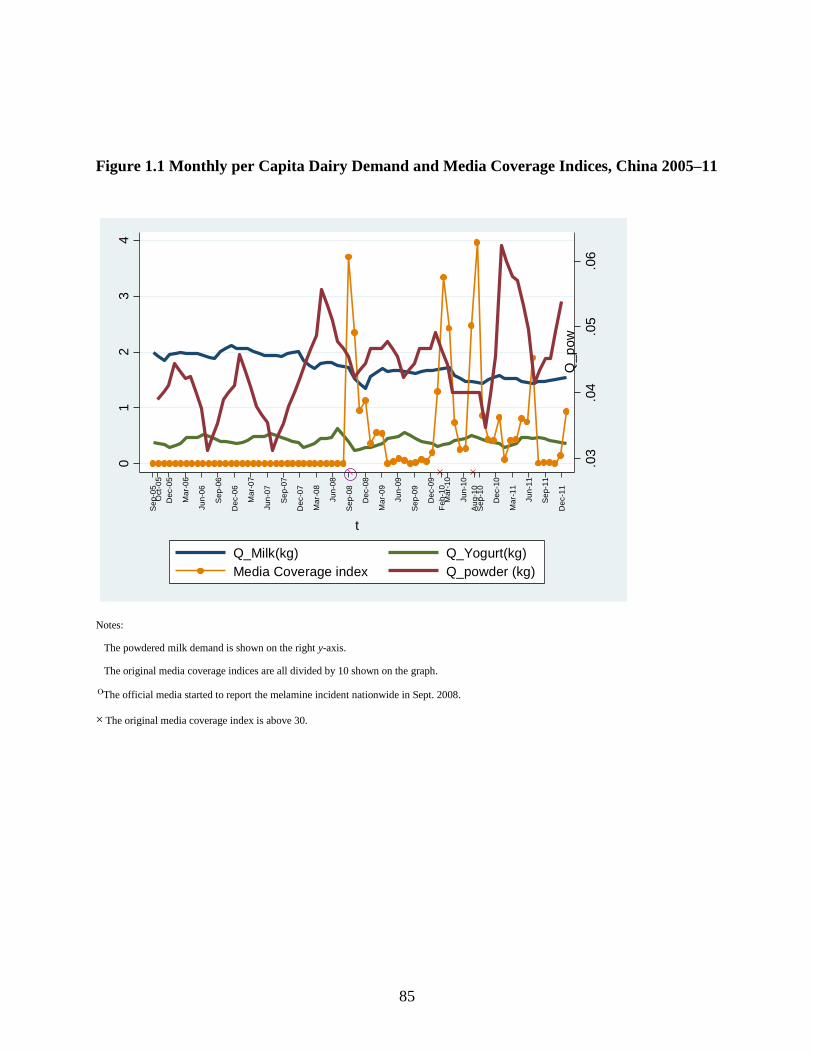
Overall, the media coverage of the melamine incident reveals higher concerns for
powdered milk than liquid milk or yogurt over the sample period. Figure 1.1 plots the media
coverage indices. During the period of ex ante incident the news indices remained zero; from
Sept. 2008, the media series increased significantly but was starting to wane by the end of 2009,
when the indices reached a new, historic high in February and August of 2010 respectively in
that the dairy safety issue became the national focus of attention again, pertaining to some
similar important events.5 The sales of dairy products were all greatly affected in Sept. 2008 but
only powdered milk was highly related with media index change for each time, showing that as
the adverse media reports increased (indices increased), the per capita consumption of powdered
milk went down immediately.
Empirical Specification
For the weakly separable grouping of dairy food, the conditional demand equations (Edgerton,
1997; Pollak, 1971) are specified for liquid milk, powdered milk and yogurt; thus following
Chang and Kinnucan (1991), a semilogarithmic form was selected in that the utility
5 In February and August 2010, respective media reported that the Shengyuan powered milk contained contents that could cause precocious puberty and the Mengniu
milk added some subsistence which might invoke cancer problems. These articles mentioned Sanlu incident again, contributing to the increased media indices in those
two months.
12
maximization can be satisfied (Hanemann, 1982) and in accordance with Smith, et al. (1988) the
Almon polynomial lag model is estimated without log form6. The demand model for the three
dairy products (fresh milk, powdered milk and yogurt) is set up here7. Thus, the estimated
where t stands for monthly observation and t = 1, . . . ,75 from October 2005 to December 2011;
Qi is monthly per capita consumption of dairy product i (i = 1, 2, 3); Pj is the real price of good
j8; TEXP is the consumers’ total group expenditure on dairy deflated by the Stone price index,
Pt* = wj,t ln Pjt (Deaton and Muellbauer, 1908, p. 62), where wj is the consumer’s expenditure
share of good j of the dairy products; DV is the dummy variable that is zero before the
September 2008 contamination and 1.0 thereafter; Nt measures the negative media coverage
which was defined earlier and A(L) is a polynomial lag structure of the media variable; Sk’s are
seasonal dummy variables (month of December is the omitted category); and εi’s are random
error terms.
1.5 Data
Dairy data used in this article are monthly consumption over the period from 2005 to 2011,9
providing a total of 75 observations.10 The basic quantity data are per capita consumption data
from the Dairy Association of China (DAC) published in both the China Dairy Yearbook and
updated publications available online. The real price of liquid milk is the average monthly retail
fresh milk price; and the prices for both powdered milk and yogurt were calculated by their
6 The level variable of media indices is used here because there are too many zeros during ex-ante incident. 7 Originally a generalized ideal demand system (GAIDS) was specified. However, preliminary analysis with this system provided unsatisfactory results, e.g., positive
own-price elasticities for powdered-milk products. The purpose of this article is to study melamine impacts on different dairy food and not to test demand theory per
se, thus the GAIDS model was replaced by a semilog model. 8 The prices are interpolated from quarterly to monthly by CPI deflator. 9 Data source is based on the representative sample of the 36 big and medium-sized cities of China. 10 A data appendix, containing sources, is available upon request from the author.
13
monthly consumer’s expenditure divided by monthly per capita consumption, respectively. All
of the expenditure variables were published in the same DAC source and China Statistical
yearbook Database Report. Media coverage index variables for the melamine incident used in the
analysis were also monthly data over the same period, constructed as discussed previously.
Besides, the effects of seasonality using monthly demand binary variables and a linear time
trending were incorporated in the model as well. Table 1 provides descriptive summary of the
non-binary variables.
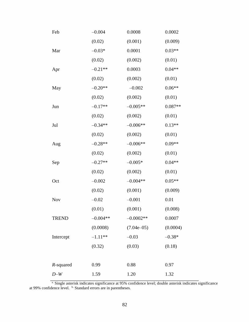
1.6 Empirical Results
In the empirical analysis, “dairy” is treated as a weakly separable group including liquid milk,
powdered milk and yogurt in which consumption of an individual dairy item depends only on the
expenditure of the group, the prices of the goods within the group, and certain introduced
demand shifters. The preliminary tests demonstrate that there is no heteroscedasticity or
autocorrelation in any of the equations. The demand equations were measured as a system by
using Seemingly Unrelated Regression (SUR) under the assumption that error terms are
correlated across equations but not over time. The results of the estimation are shown in Table
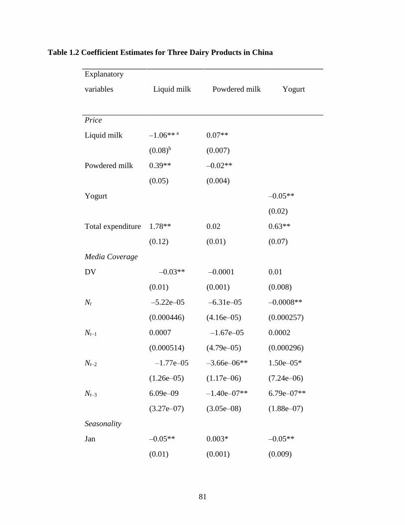
1.2.
Price and Expenditure Effect
The expenditure estimates of each milk type are all positive as expected (Table 1.2) and
meanwhile, consistent with the law of demand, the own-price estimates are all negative and
significant, among which liquid milk displays the greatest price sensitivity in the group.
14
As seen from Table 1.3, the expenditure elasticities for liquid milk, powdered milk and
yogurt are 1.08, 0.50 and 1.71, respectively; except for powdered milk, two other products both
generate statistically significant expenditure effects. Every one percent growth of yogurt
consumption will lead to the greatest expenditure increase of dairy group. The most recent
studies by Zheng et al. (2009) reported an average expenditure elasticity of 1.37 for dairy
products in Jiangsu province, China that falls well within the reported range of 1.08 to 1.71.
The estimated own-price elasticities are –0.63 for liquid milk, –0.43 for powdered milk and
–0.15 for yogurt, and apparently the own-price effect of liquid milk is the largest among dairy
grouping. This figure is very close to the range of estimated fluid milk price elasticities of –0.66
to –0.73 reported by Kinnucan (1983) and the figure of –0.70 estimated by Smith et al. (1988).
tabl(2010), milk was the most studied category aside from meat in United States. Thirteen
studies provided elasticity estimates for specific milk fat levels. Mean elasticities for skim, 1%,
and whole milk ranged from –0.75 to –0.79, whereas the mean elasticity for 2% milk was –1.22.
Also, Bai et al. (2008) applied the Tobit model drawing on individual consumer survey data
collected in urban Qingdao of China in 2005 and found that the own-price effect of fluid milk is
–0.44, implying that fluid milk in Qingdao is a normal good but is price inelastic. However,
unlike the previous studies that were based on either regional data or earlier time periods, the
present analysis draws a recent national monthly dataset with respect to the melamine incident,
therefore, allowing for the different estimated own-price effects.
The cross-price elasticity of liquid milk with respect to powdered milk price is 1.71, while
the cross-price elasticity of powdered milk with respect to liquid milk price is only 0.23; which
suggests that liquid milk is a very strong substitute for powdered milk, but powdered milk is
15
quite a weak substitute for liquid milk.11 This result, however, is consistent with the fact that
much less powdered milk than liquid milk is consumed in urban China (Figure 1.1). And a
plausible explanation for the asymmetry is that the dried milk price is ten times more than that
for fresh milk given the same quantity, resulting in a larger income effect when the price of
powdered milk increases, ceteris paribus, than when the price of liquid milk increases; also, it
might be due in part to the melamine incident that made consumers instead turn to purchase the
cheaper substitute of fresh milk.
Media Coverage Effect
The results show that incremental increases in current media coverage indices elicit small but
negative impacts on the demand across the three products, but only powdered milk estimates
support the theory that coefficients on both of current and lagged media indices should be
negative. Similar to the Hawaii case, the estimated lagged effect of media indices for powdered
milk exhibits a geometrically declining shape with the greatest impact occurring in the month of
melamine news release, though the magnitude is far smaller than in the previous example. This
yields the implication that within dairy grouping, direct demand response of powdered milk was
most adversely affected, compared to that of fresh milk or yogurt, by the same media reports.
Likewise, the dummy variable estimate that distinguishes the ex ante and ex post incidence
is negative for liquid and powdered milk, but not for yogurt, confirming the time trend of
declined consumption of both liquid and powdered milk in the ex post period. The positive
coefficients of three lags for yogurt indicate that the melamine crisis had no negative carryover
effect on consumption of yogurt. Compared to the heptacholor incident in Hawaii decades ago,
11 The cross-price effects for dairy products other than liquid milk and powdered milk were insignificant and therefore were dropped from the demand equations.
16
the melamine case occurring in China had much less impact on dairy demand. There might be
several reasons; firstly, dairy products are a normal good as examined in the previous section and
urban consumers of China can find very few suitable substitutes outside the dairy group,
particularly those for infant food. In addition, the negative media coverage should be downward
biased to some extent since in PR China the censorship mechanism for mass media is extremely
restrictive in order to prevent public fears growing nationally; besides, even if the news media
were reliably measured, temporary media coverage would be expected to have a weaker effect
than the continuing warning (Schucker et al., 1983). Since the Sanlu dairy company was shutting
down at the end of 2008, the credence value of milk might be regained from the
“uncontaminated” or “qualified” milk produced by other dairy companies, including imported
brands.
Seasonality Effect
The results also illustrate seasonality dummy and time-trending effects for the dairy
consumptions; the yogurt demand had been increasing within the second quarter of the year and
peaking in each August, while sales of both liquid milk and powdered milk were reducing in the
summer time (third quarter) of year. But over the whole sample period, there was a gradually
declining demand for both liquid and powdered milk, corresponding to the estimated effects of
dummy variable mentioned above.
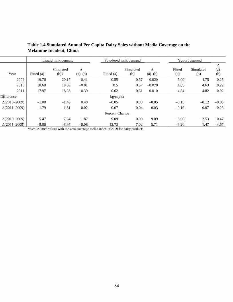
Demand Response Simulations
To further investigate the magnitudes of the media coverage impacts on each dairy demand,
separate simulations for each of the own-demand responses were carried out using the estimated
demand model while keeping media indices constantly zero over the ex post period; the results of
17
the simulation shown in Table 1.4 indicate that in the period of 2009–10, the decline in annual
demand of per capita powdered milk and yogurt would have been 9.09 and 0.47% less
respectively without news coverage on the incident (holding all else equal), coinciding with
significant increase of media indices during period of 2010; however, the decline in annual per
capita liquid milk demand would have been 1.87% more. By contrast, the situation is different
for the period of 2009 and 2011: without media coverage effects, the decline for liquid milk and
yogurt consumption would be 0.08 and 4.67% less whereas the increase for powdered milk
demand would be 5.71% less. These results, on the one hand, corroborate the empirical result
mentioned earlier that liquid milk and powdered milk are substitutes and on the other, imply that
the lagged effects of bad information on consumers’ demand for dairy food were not sustained in
the long term.
Meanwhile, the immediate demand response of specific month can be significantly larger
than the reported averages over the sample period. For example, the difference in actual and
projected own-demand response of powdered milk to media release was around –0.005 kg per
person (a 9.14% decline) in Feb.2010 and –0.004 kg per person (a 9.10% decline) in Aug.2010,
coinciding with the most largest effects of the media coverage indices in the two months. The
average difference of actual and projected own-demand responses of powdered milk to media
reports over the sample was only as much as –0.001 kg person per month. In sum, these
deviations illustrate that the reported average demand response for powdered milk might be
economically smaller than the immediate demand response to the influential (above 30) media
indices; also, the empirical results suggest that as news coverage becomes sharply intense, the
response to media effects would be larger, yet the apparent significant impacts are short-lived
past the large increase in media coverage indices concerning dairy safety.
18
1.7 Concluding remarks
The focus and interest of this chapter is to investigate whether the news information concerning
the Sanlu melamine incident has impacted the weakly separate grouping of dairy consumption in
urban China over the recent years. The melamine incident exposed the government’s lack of
related legislation and supervision of dairy food safety, so that the powerful implementation of
the Chinese Food Safety Law should be called for.
The economic and empirical framework reveals coefficients measuring the own- and cross-
price effects of the dairy products in the case of melamine incident. The current media coverage
effect indicated that publicized news information of melamine incident was detrimental toward
demand for each of the studied products, while only powdered milk was showing consistent
results with the hypothesis that the estimated lagged media effects were declining geometrically.
The positive cross-price elasticity of liquid milk and powdered milk explains the reciprocal
substitution effect and the asymmetric demand response to adverse media news.
The current estimated demand response to the melamine contamination incident over the
study period was found to be economically small; there was also no significant evidence of
negative cumulative effects (or lagged effects) on demand, especially in comparison to price
effects and to previous estimates of unfavorable information effects regarding milk incidents.
That the news media reports had no apparent significant impact on dairy sales, insofar as the
statistical analysis was concerned, is not altogether unexpected. The sample of news indices was
not national in scope covering urban China, whereas the monthly sales observations were. In
contrast to the isolated island of Hawaii (the heptachlor case 1982) that was dominated by the
domestic produced milk, the Chinese dairy industry has been seriously affected by the substantial
19
increase of imports in last few years. The aggregate dataset did not distinguish domestic
suppliers from imported producers, which otherwise might have yielded a different conclusion
on the demand response to the incident.
Therefore, the media coverage of the melamine incident can be characterized as having a
minor long-run impact on dairy demand accompanied with temporary but important shocks to
demand.
Finally, the robustness of the results is subject to further scrutiny across alternative model
specifications; and a series of extensions including using more refined data that measure media
coverage indices or disaggregated cross-sectional household data on per capita consumption
remains a topic for further investigations.
20
Chapter II. Examination of Asymmetry in Farm-Retail Price Transmission for U.S. Whole
Milk
21
2.1 Background
In the recent decades, testing for Asymmetric Price Transmission (APT) and analyzing the APT
elasticity are of importance in applied economics. However, a wide variety often conflicting
theories of, and empirical tests for, APT co-exist in the literature. Economists who study market
processes are therefore interested in price transmission processes. Of special interest are those
processes that are referred to as asymmetric, i.e. for which transmission differs according to
whether prices are increasing or decreasing (Meyer et al., 2004), versus others holding that retail
prices would respond in the same manner for both increases and decreases in farm prices (Aguiar
and Santana, 2002). In an extensive study of 282 products and product categories, including 120
agricultural and food products, Peltzman (2000) found asymmetric price transmission to be the
rule rather than the exception, leading to the strong conclusion that the standard economic theory
of markets is wrong, because it does not predict or explain the prevalence of asymmetric price
adjustment; while others indicated that standard tests (such as the test applied by Peltzman) can
result in excessive rejection of the null hypothesis of symmetry under common conditions.
2.2 Literature Review
Ward (1982) suggested that market power can lead to negative APT if oligopolists are reluctant
to risk losing market share by increasing output prices. In a similar vein, Bailey and Brorsen
(1989) considered firms facing a kinked demand curve that was either convex or concave to the
origin. Otherwise if the firm conjectures that all firms will match an increase but none will match
a price cut (convex), positive asymmetry will result.
22
Damania and Yang (1998) in a paper on imperfect information in a competitive duopoly
stressed potential punishment as a cause of asymmetry. In their model demand was assumed to
fluctuate randomly between high and low states. Punishment occured if a firm believes that its
competitor is undermining a collusive price.
Besides, McCorriston et al. (2001) also showed that if an industry is characterized by
non-constant marginal costs, there can be a significant impact on price transmission. The most
important conclusion was that under certain conditions, price transmission may be greater in
industries with increasing returns to scale (IRS) than in markets characterized by perfect
competition and constant returns to scale (CRS).
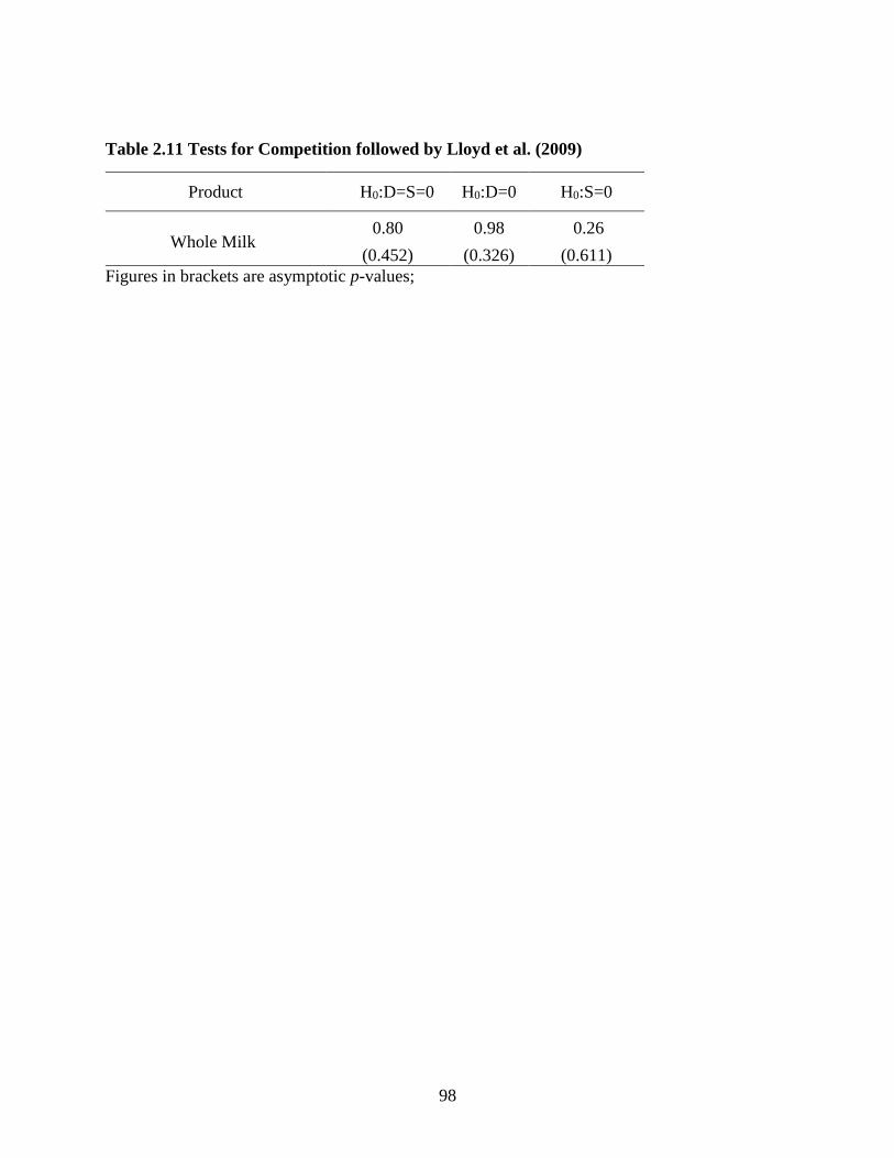
Lloyd et al. (2009) investigated the buyer power in U.K. food retailing by a ‘first-pass’ test
using a cointegrated vector autoregression and identified the null of perfect competition can be
rejected in seven out of the nine food products, except for milk product no evidence can be found
for the exercise of buyer power. Their proposed test, at the very least, offered a means via which
the behavior of the retail-producer price spread is consistent with the buyer power.
However, some other economic analyses were focusing on price transmission elasticites
and even on the demand/supply shifter impacts on dairy food. Kinnucan and Forker (1987)
discussed the farm-retail price transmission effects and the work of distinguishing retail demand
from farm supply shifts original derived by Gardener model. They identified that farm-retail
price transmission process in the dairy sector was asymmetric using Houck procedure with data
covering from 1971-1981 and tested the role in pricing asymmetry of retail demand versus farm
supply shifts via a Chow-type test. Results suggested the major impact on retail prices of a
change in the farm price of milk was felt sooner when farm prices are increasing than when farm
prices are decreasing. Later Lass et al. (2000) estimated for Boston and Hartford retail dairy
23
prices by using an econometric model, concluding that asymmetric speeds of adjustment to farm
price increases and decreases were found and retail prices do return to the same level following
equal farm price increases and decreases.
Recently Capps and Sherwell (2007) analyzed the behavior of tests for asymmetry by both
of the conventional Houck approach and the error correction model (ECM) approach, employing
monthly data over period from January 1994 to October 2002 for whole milk and 2% milk for
seven typical U.S. cities. Their study was consistent with Kinnucan and Forker that price
transmission elasticities were generally larger than corresponding elasticities associated with
falling farm prices though they all were inelastic. By contrast, very few empirical tests yielded
the opposite results that retail prices were more sensitive to decreases in farm prices than to
increases in farm prices (Ward 1982, Punyawadee et al. 1991).
In this study, application of markup model and computation for the natural by-product of
price transmission elasticities will be extended; meanwhile, testing the differences between
demand as well as supply shifters will also be yielded with the ad hoc econometric procedures.
2.3 Theoretical Model
There are two alternative approaches in detecting asymmetric price transmission in this article
and the emphasis is put on price transmission between the farm and retail levels of the vertical
market system. But different from some previous analyses centered on spatial considerations by
regional investigations (Bailey and Brorsen 1989, Frigon et al.1999, and Capps and Sherwell
2007), this paper is mainly based on asymmetric responses at the national aggregate level which
might not lose any generality.
24
The “Houck” Approach
Houck (1977) developed a test for asymmetric price transmission in terms of the segmentation of
price variables into increasing and decreasing phases. Till today, there are many analysts that
have followed suit. The static asymmetric model can be written as:
(1) 𝛥𝑃𝑟𝑡 = α0 + α1 𝛥𝑃𝑓𝑡+
+ α2 𝛥𝑃𝑓𝑡
−
+ 𝜀𝑡
where 𝑃𝑟𝑡 and 𝑃𝑓𝑡 are retail and farm prices of the marketing chain, respectively, t=1,2,…,T, 𝛥 is
the first difference operator and following Houck procedure, 𝛥𝑃𝑓𝑡+
= 𝑃𝑓𝑡 – 𝑃𝑓𝑡−1 if 𝑃𝑓𝑡 > 𝑃𝑓𝑡−1
and 0 otherwise, and 𝛥𝑃𝑓𝑡−
= 𝑃𝑓𝑡 – 𝑃𝑓𝑡−1 if 𝑃𝑓𝑡 < 𝑃𝑓𝑡−1 and 0 otherwise. An example of the
segmentation procedure is presented in table 2.112.
According to Houck (1977), Ward (1982) and Kinnucan and Forker (1987), the theoretical
model including both asymmetry and lags is specified as follows:
(2) 𝛥𝑃𝑟𝑡 = π0 𝑇𝑅 + ∑ π1i 𝛥𝑃𝑓𝑡+
m1
i=0 + ∑ π2i 𝛥𝑃𝑓𝑡−
m2i=0 + π3 𝑀𝐷𝑡 + 𝜀𝑡
where 𝛥𝑃𝑟𝑡 is the dependent variable; 𝑀𝐷𝑡 is the marketing cost difference variable, expressed
as deviations from its initial value and TR is a trend term; at meanwhile π1i and π2i are
coefficients in Equation 2 indicating the impact of rising and falling phases of farm whole milk
prices on retail prices respectively; m1 and m2 represent the length of the lags with regards to
rising farm prices and falling farm prices; 𝜀𝑡 is a random disturbance term.
𝐹𝑅𝑡 = 𝐹1 + ∑ max ( 𝛥𝑃𝑓𝑡+
, 0)
t−2
i=0
12 Note that it makes no difference whether the variable is lagged and then segmented or segmented and then lagged.
25
measures the accumulated increases in farm prices up to period t,
𝐹𝐹𝑡 = 𝐹1 + ∑ min (𝛥𝑃𝑓𝑡− , 0)
t−2
i=0
measures the accumulated decreases in farm prices up to period t. Theory provides no guidance
for the number of lags to include. The model presented in the equation above is completely
general, allowing for different lag lengths for rising and falling farm prices. Here I evaluated a
number of different lag structures during the analysis and found that short-run price (period t)
and two lagged prices (for periods t-1 and t-2) best fit the data for the Houck procedure.
Besides, the coefficients of π1 and π2 in equation (2) are representing the net effect of
rising / falling farm prices on retail prices respectively. A formal test of linear restriction for the
asymmetry hypothesis is below, which would be measured by t-test (Johnston, 1972).
HN: πi + = πi
−, for lags i=0, 1, 2;
and: HN: ∑ π1i m1i=0 = ∑ π2i
m2i=0
The alternative hypotheses in each case are that the parameters or sums of parameters are
not equal. The first hypothesis is a test of the speeds of adjustment of rising versus falling farm
prices, sometimes referred to as a test for short-run price transmission asymmetry. For example,
suppose the estimated parameter for current rising farm price is statistically greater than the
estimated parameter for current falling farm price. Then processors will have a greater response
to an increase in the current farm price than they will to a decrease in the current farm price. This
result will demonstrate that upward adjustments in retail prices due to rising farm prices occur
more rapidly than do downward adjustments due to falling farm prices (Lass et al., 2001).
Correspondingly, the second hypothesis will test for long-run price transmission asymmetry
26
which constitutes a linear combination of coefficients. A rejection of HN is evidence of
asymmetry or non-reversibility in price transmission. If one fails to reject HN, then there exists
evidence to support the notion of symmetry (or reversibility) in price transmission
(Capps&Sherwell, 2007).
Meanwhile, I also computed mean lags for rising and falling farm price effects. And the
formula is (Rao and Miller1971):
(3) ͞L =∑ |πi
+/−|∗i2i=0
∑ |πi +/−|2
i=0
where ͞L is the mean lag for rising (falling) farm prices and the maximum lag length is two
months. A mean lag for rising farm prices that is smaller than the mean lag for falling farm
prices will identify that the upward speed of adjustment is rapid than the downward speed of
adjustment.
The final set of measures of short-run and long-run elasticites are computed as follows:
(4) εSR=π0+/−
∗𝑃 𝑓𝑡(mean)
𝑃 𝑟𝑡(mean)
(5) εLR=∑ πl+/−
∗𝑃 𝑓𝑡−𝑙(mean)
𝑃 𝑟𝑡−𝑙(mean)
2l=0
where all the estimated elasticities are all based on mean values of retail prices and farm prices.
The short-run and long-run elasticities differ in that the latter incorporate all lagged farm price
effects on the retail price. In this study, the current (short-run) period and one-month as well as
two-month lags are used to calculate long-run elasticities.
The “Error Correction Model” Approach
27
The recent literature dealing with the price transmission has paid attentions to the time-series
properties of the data, considering the inherent nonstationarity of prices or long-run stationary
equilibria (cointegration) relationships among prices. Cramon-Taubel (1998) studied asymmetric
price behavior in German producer and wholesale hog markets. Goodwin and Harper (2000)
investigated linkages among farm, wholesale, and retail markets utilizing cointegration
techniques in analyzing price transmission and asymmetric adjustment in the U.S. pork sector.
Also, Goodwin and Piggott (2001) evaluated linkages among four corn and four soybean markets
in North Carolina using cointegration methods. Till lately, Capps and Sherwell (2007) evaluated
the behavior of price asymmetry for fluid milk according to both Houck procedure and error
correction model for seven U.S. cities. Following Capps and Sherwell, this study is updated by
the most recent monthly data and extended up to the national aggregate level.
Since the asymmetric ECM approach is motivated by the fact that none of the variants of
the aforementioned Houck approach is consistent with cointegration between the retail and farm
price series (Cramon-Taubadel, 1998; Cramon-Taubadel &Loy, 1999), the tests and discussion
for ECM procedure is particularly of importance. If 𝑃 𝑓𝑡 and 𝑃 𝑟𝑡
are cointegrated, and the ECT
can be developed into positive and negative components (Granger and Lee, 1989), consequently,
the asymmetric error correction model in this analysis can be replicated from equation (7) by
Capps and Sherwell (op cit) and written as:
(6) 𝛥𝑃𝑟𝑡 = β 0 𝑇𝑅 + ∑ β1i 𝛥𝑃𝑓𝑡+
p1i=0 + ∑ β2i 𝛥𝑃𝑓𝑡
−
p2i=0 + ∑ β3i 𝛥𝑃𝑟𝑡−𝑖
+ p3i=1 β4 𝐸𝐶𝑇𝑡−1
+ +
β5 𝐸𝐶𝑇𝑡−1− + β6 𝑀𝐷𝑡 + 𝜀𝑡
Compared with Houck approach given by Equation (2), Equation (6) has three additional
terms:∑ β3i 𝛥𝑃𝑟𝑡−𝑖
p3i=1 , β4 𝐸𝐶𝑇𝑡−1
+ and β5 𝐸𝐶𝑇𝑡−1− . Thus, the asymmetric ECM nests the Houck
28
model when the lag lengths m1 and p1 or m2 and p2 are the same. Here in this paper, the lag
structure of rising farm prices for ECM is set up differently with Houck procedure in terms of
best-fitness principle. Therefore, to determine whether one model is superior to the other, the
Akaike Information Criterion (AIC) (Akaike, 1974) or the Schwarz Information Criterion (SIC)
(Schwarz, 1978) can be appealed in choosing between Houck and ECM specifications13.
Absolute Marketing Margin vs. Relative Marketing Margin14
Revisited from Gardener’s (1975) analysis, the summarized concluding was quoted as follows:
“one implication of the results is that no simple markup pricing rule-a fixed percentage margin,
a fixed absolute margin, or a combination of the two can in general accurately depict the
relationship between the farm and retail price. This is so because these prices move together in
different ways depending on whether the events that cause the movement arise from a shift in
retail demand, farm supply, or the supply of marketing inputs.” The three analytical expressions
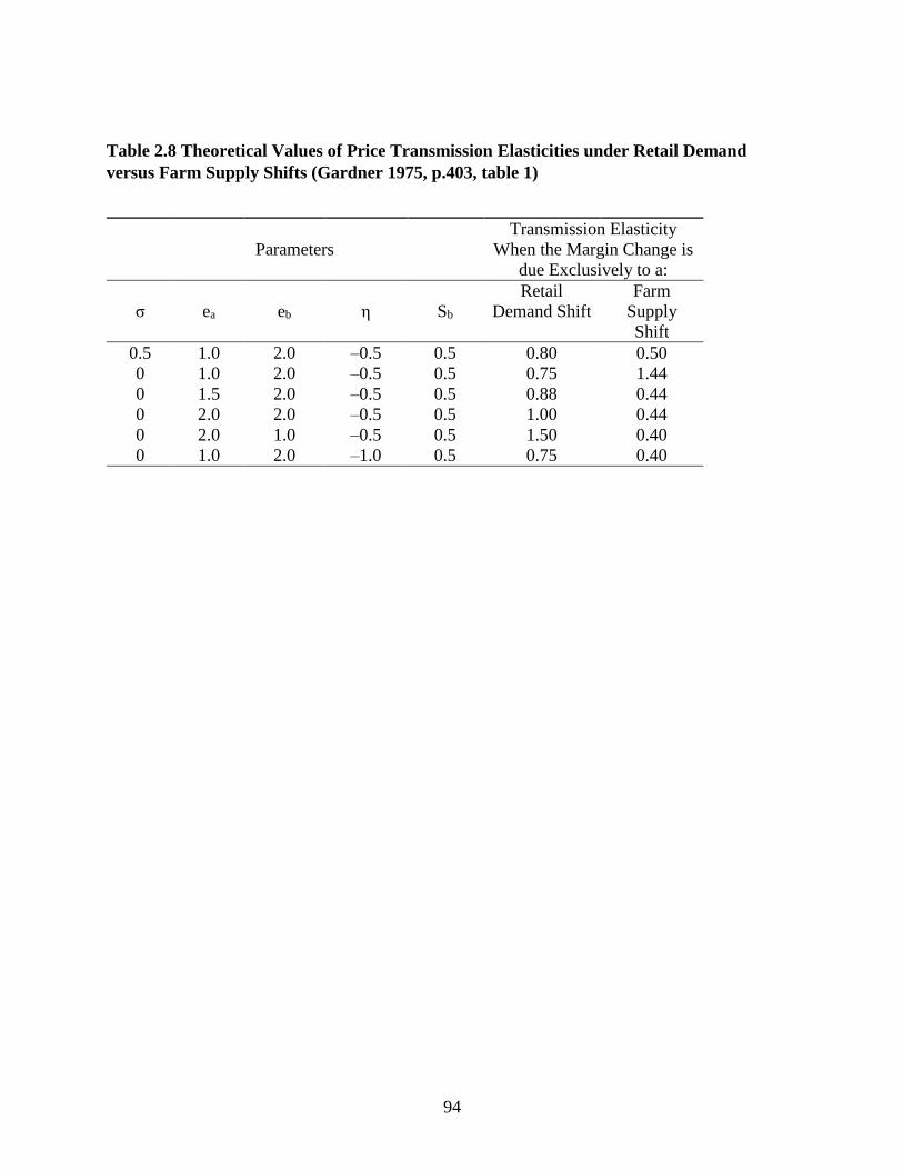
for the price transmission elasticites drawn from Gardner are as follows15:
(7) τRD=𝜎+𝑆𝑎𝑒𝑏+𝑆𝑏𝑒𝑎
𝜎+𝑒𝑏
(8) τFS=𝑆𝑎(𝜎+𝑒𝑏)
𝑒𝑏+𝑆𝑎𝜎−𝑆𝑏𝜂
(9) τMS=𝜎+𝑒𝑎
𝜎+𝜂
13 Choice of model selection rests on the lowest values of the AIC or SIC (Capps and Sherwell, 2007) 14 Most of this part was replicated by the previous work of Kinnucan and Tadjion (2013). 15 τi represents the percentage change in retail price over percentage change in farm price; η is the own-price of demand for the retail product x; 𝜎 is the elasticity of substitution between the farm-based input a and the bundle of marketing inputs b; 𝑒𝑎 is the own-price elasticity of supply input a while 𝑒𝑏 is the own-price elasticity of supply for input b; Sa the cost share for input a and Sb is the cost share for input b (Sb=1-Sa). The determinants of τi for isolated shifts in retail demand (RD), farm supply (FS) and marketing inputs’ supply (MS).
29
To accommodate Gardner’s analysis that the farm-retail price transmission elasticity in
general will differ depending on the source of the supply or demand shock, we extend two
equations from Gardener and Lloyd et al. (2009) testing for marketing margin stickiness with
respect to farm price and price transmission effect that allows changes in whole milk quality to
where t=1, 2, 3…T indicates the time period of the observation; the delta terms represent first
difference (e.g. 𝛥ln𝑀𝑡=ln 𝑀𝑡–ln 𝑀𝑡−1), and 𝑀𝑡 stands for the marketing margin, measured as
the difference between the retail price and the retail farm price; here it is meaningful to
distinguish between the relative marketing margin 𝑀𝑅 = 𝑃𝑟𝑡/ 𝑃𝑓𝑡 and the absolute marketing
margin MA=𝑃𝑟𝑡 − 𝜃𝑃𝑓𝑡 16 since Gardner analyzed the relative margin, but not the absolute
margin. D stands for the dummy variable that equals 1 while Farm price is falling, otherwise
equals 0; 𝐹𝑀𝐶 is the original food marketing cost index; 𝐼𝑁𝐶 is per capita real disposable
personal income as proxy for retail demand shifters while 𝐶𝑃𝑅𝐼𝐶𝐸 is corn price which is a proxy
for supply shifters17. The model is expressed in logarithmic first-difference form18, with these
16 It is based on the retail-equivalent farm price M=Px–θ Pa (Px is the retail price and Pa is farm price) in terms of
USDA’s definition of the marketing margin and in the special case θ is a fixed constant (Gardener 1975, p.405; Reed et al.2002, p.2) where in this article, θ is assumed to be 1 in the dairy market. For absolute marketing margin, the logarithmic first difference may be approximated as: ΔlnMt≈ ((𝑙𝑛𝑃𝑟𝑡 − 𝑙𝑛𝑃𝑟𝑡−1)-S1t (𝑙𝑛𝑃𝑓𝑡 − 𝑙𝑛𝑃𝑓𝑡−1)), where
S1t= ((S1t+ S1t-1)/2 is the average farmers’ share of the retail dollar between adjacent time periods. 17 The supply shifter variable can also be represented by price index rather than corn price, such as cow slaughter price, manufacturing production costs etc., depending on the data access or availability.
30
variables of marketing cost, retail demand shifters and farm supply shifters all considered as
exogenous 19 . And simply put, when it is legitimate to treat the price of marketing inputs
exogenous, theory indicates that shifts in retail demand and farm supply have no effect on the
absolute marketing margin; however, the both of demand and supply shifters should have
statistically significant impact on the relative marketing margin. An intercept is included in the
equation (10) to capture movements in the margin due to autonomous factors such as technical
change in the marketers’ production function.
According to Lloyd et al.’s test, when equations (7) and (8) are reduced to τRD =τFS =Sa, it can be
implied farm supply and retail demand shifters have no effect on the marketing margin and price
transmission elasticity in either case equals to the farmer’s share of the consumer dollar. The two
hypotheses tests are conducted with respect to equation (10) and (11):
Weak Form Hypothesis:
HN:𝛼4 = 𝛼5 = 0
HA: HN not true.
Strong Form Hypothesis:
HN:𝛼1 = 𝛼4 = 𝛼5 = 0 and β1 = average Farmers′share20
HA: HN not true.
In this instance, these combined zero-restrictions can be tested with a standard Wald and F-
statistic.21
18 The logarithmic first differences are apt to be stationary. 19 The Hausman test for marketing cost will be shown later. 20 The average farmers’ share of the retail dollar over the sample period.
31
2.4 Data and Estimation Procedures
Monthly undeflated (nominal) retail price of U.S. city average for whole milk, the undeflated
farm price measured by announced cooperative price for whole milk, and monthly total food-
marketing cost indices during the period January 1996—December 2011 from the national level
were used in this study. The main Data source comes from Agricultural Marketing Service, U.S.
Department of Agriculture (USDA) and Bureau of Labor Statistics (BLS)22. However, since the
BLS does not appear to have retail price data for whole milk per gallon prior to 1995, and instead
has price data per half gallon for 1980-95, changes occur over the years in how people buy milk
(Half gallons used to be the most popular form. It is now gallons.) Thus, I select the time period
for monthly and it lasts from January 1996 to December 2011, including 192 observations (the
statistical summary is shown in table 2.2); and the farm and retail prices are expressed in terms
of dollars per gallon.
I tested the hypothesis that farm prices Granger cause retail prices and vice versa. If farm
prices Granger cause retail prices, then in the case where retail price is the dependent variable,
the F-test corresponding to all coefficients associated with lagged farm prices should be
statistically significant. Vice versa, if retail prices fail to Granger cause farm price, the F-test
corresponding to all coefficients associated with lagged retail prices should not be statistically
significant where farm price in the dependent variable (Granger, 1969). As shown in Table 2.3,
21 As emphasized by Lloyd et al. (2009, pp.4-5), although rejection of the zero restrictions constitutes evidence against perfect competition, failure to reject does not constitute evidence in favor of imperfect competition. Thus, failure to reject the null should not be taken as evidence that antitrust action is warranted. It is only when the null is rejected that such action might be appropriate. The qualification is necessary because other factors, such as non-constant returns to scale, could account for the rejection. In this sense, the tests are appropriately regarded as “first pass”, i.e., a signal that more in-depth (and costly) analysis is necessary to establish probable cause. 22 Original data is available from the author upon request.
32
the Granger causality tests regards to the farm and retail prices of whole milk in this study
support the underlying assumption that farm price precede or Granger cause retail prices, which
means the retail price should be set up as the dependent variable, rather than farm price. This
result hence coincides with the unidirectional-upward causal relationship assumption by
Kinnucan and Forker (op cit) as well as with the same Granger causality test by Capps and
Sherwell (op cit).
The next step was to test cointegration between the respective farm price and retail price
series. The Augmented Dickey-Fuller (ADF) test was used to check on the stationarity of the
retail and farm price series. And the Johansen test is also presented here to check for
cointegration (see Table 2.4). Based on both the trace test and maximal eigenvalue test statistics,
farm and retail prices of whole milk were cointegrated. Consequently, the asymmetric ECM can
be applied to the respective cointegrated series compared with the traditional Houck model.
About 40% of the observations in the sample were months of farm price decline. And in
terms of Kinnucan and Forker (op cit), this provided a sufficient number of price declines to
reliably assess the asymmetry issue by the statistical procedures used here.
Besides, the changes in farm milk prices may not be matched by changes in retail prices
for whole milk. Generally speaking, the changes between vertical prices became tend to track
relatively closely over the sample period and seen from Figure 2.1, the retail prices do move
when farm milk prices drop while it takes time for the shocks to pass through the firms that
manufacture and distribute whole milk, which may contribute to the consideration of lag
structures of equation (2) and (6). In short, differences in farm and retail prices as well as in
farm-retail price spreads (market margin) in States are likely the results of government policy
33
and the cost of transporting fluid milk from surplus to deficit areas concluded by Capps and
Sherwell (2007).
Finite distributed lag structure in the farm price variable is assumed and in this article, the
lag length for whole milk is two month except that only one month period for rising farm price
by ECM procedure.
The length of lag distribution was based on Almon procedure (Almon, 1965), set up as a
second order polynomial. Endpoint restrictions were used in conjunction with the Almon
procedure. And the length of the distributed lag process was determined based on the Akaike
Information Criterion (AIC) (Akaike, 1974) or the Schwarz Information Criterion (SIC)
(Schwarz, 1978).
Ordinary Least Squares estimates are presented for both of Houck procedure and ECM
approach since the serial correlation was not evident in those equations.
Furthermore, Seemingly Unrelated Regression (SUR) is applied for equation (10) and (11).
And the quarterly data are estimated for the marketing margin model and price transmission
model respectively, in that the demand and supply shifters will be paid more attentions, rather
than focus on the length of lag distribution.
2.5 Empirical Results
The estimated coefficients and their standard errors generated by equation (2) and (6) are
exhibited in Table 2.5-2.6. For the equations corresponding to the Houck approach, the
goodness-of-fit statistics ranged from 0.60 to 0.64, and for the equations corresponding to the
ECM approach, the goodness-of-fit statistics ranged from 0.70 to 0.71 which both suggest that
34
the variation in retail price provided a reasonably good explanation, with or without the variables
of total food-marketing costs and the trend term.
With the Houck approach, the number of lags associated with both rising and falling farm
price variables was two, meaning the time for milk prices at the retail level to adjust to either
increases or decrease in milk prices at the farm level was roughly the same, consistent with the
result derived by Capps and Sherwell (2007). As observed in table 5, the direction of the price
change matters for both the current period effect and the one-period lag effect. The positive
calculated t-statistic indicated the current period rising coefficient was statistically greater than
the current period falling coefficient, while the negative t-statistic for the one-period lag
indicated the opposite. The two-period lag coefficients were not statistically significant23.
Nevertheless, with the ECM approach(see table 2.6), the number of lags associated with
rising farm prices was only one, relative to the lag number for falling-farm prices of two, which
represents milk prices at the retail level might adjust faster to increases in milk prices at the farm
level than to decreases; the positive calculated t-statistic also indicated that current period rising
coefficient was statistically greater than the current period falling coefficient, and the negative t-
statistic for the one-period lag was not statistically different.
With the Houck approach and the ECM approach, there is empirical evidence for all
models that retail whole milk series adjustments to rising farm milk prices were much more rapid
than adjustments to falling farm milk prices, implying the estimated coefficients in general were
significant and agreed with a priori expectations. At the meantime, the cumulative (long-run)
23 Specifically, for Houck procedure, the estimated coefficients of cumulative (long-run) effect indicate that Model IV yielded a smaller number for rising-farm prices but a larger one for falling-farm prices; while for ECM, it did not show such a variance among different models.
35
effect on retail milk prices attributable to increases in farm milk prices exceeded the cumulative
effect attributable to decreases in farm milk prices. The F-test associated with the null hypothesis
that retail prices responded symmetrically to increases and decreases in farm prices was rejected
with both approaches in all models.
Besides, to decide whether the error correction model is statistically superior to the
Houck procedure, one may use either the Akaike Information Criterion (AIC) (Akaike, 1974) or
the Schwarz Information Criterion (SIC) (Schwarz, 1978) to make comparison since the lag
structures are not the same. Basically, each model of ECM approach provided a lower value of
either AIC or SIC than Houck approach did and it might suggest the ECM be preferred over the
Houck model based on model selection criteria, and statistically speaking, cointegration played a
relatively vital role.
Furthermore, the computed Farm-Retail price transmission elasticities of short-run and
long-run are displayed for both Houck approach and ECM approach24 (Table 2.7), illustrating the
unequal retail response to changes in the farm price of whole milk. All estimated elasticities of
price transmission were quite inelastic. For rising-farm price transmission the long-run
elasticities were similar while for falling-farm price transmission the long-run effects were
almost twice as large as the corresponding short-run effects. On the other hand, the long-run
rising price elasticity was more than the corresponding falling-price elasticity by 10.9 times for
Houck model and 13.5 times for ECM procedure which demonstrates that increases in the farm
price of whole milk were passed through to the retail level more completely than were farm price
decreases; moreover, the mean lags associated with the rising farm price variables were
uniformly smaller than the corresponding mean lags of the falling farm price variables, stating
24 The elasticites are computed based on the estimated coefficients of Model III by both approaches, in order to compare with the estimates derived by Capps and Sherwell (2007).
36
that retail dairy product prices adjust much faster to increases in the farm price than to decreases.
To compare the empirical results with those addressed by previous studies e.g. Kinnucan and
Forker (1987)25, who reported the elasticity of price transmission for rising farm prices of milk to
be 0.274 in the short run and 0.462 in the long run, and for falling farm prices of milk the short-
run estimate to be 0.184 versus 0.330 for long run, it can be perceived in a clearer fashion that
our elasticities for falling-farm prices were much smaller than theirs but the long-run estimates
for rising-farm prices were more close to theirs.
Lass et al. (2001) estimated northeast dairy compact impacts for Boston and Hartford retail
prices and figured out that the immediate effect of a farm price increase was greater than the
immediate effect of a farm price decrease while over time the aggregate effects of increases and
decreases were approximately the same. Their estimates for rising-farm prices varied around
from 0.30 to 0.46 and from 0.14 to 0.35 for falling-farm prices; though our results seemed
outside their intervals (the rising prices are larger while the falling prices are smaller), there is
one thing in common: that in our study the ECM approach derived the long-run rising elasticity
of 0.429 which was a bit smaller than the short-run rising elasticity of 0.433; likewise, Lass et al.
found for Boston market the long-run rising estimate reached 0.351 which was also smaller
relative to its current (short-run) effect of 0.45726. Thus, it cannot be inferred that the retail
response to long-run farm prices be slower to short-run prices.
Capps and Sherwell (2007), applying the same two procedures as this study did, illustrated
the elasticities of price transmission for seven U.S. cities respectively. The numbers for rising
farm prices of milk ranged from 0.037 to 0.263 in the short run and from 0.187 to 0.527 in the
25 The long-run rising price elasticities exceed corresponding its counterpart by 40% for fluid milk, covering from 1971-1981. 26 The short-run rising elasticity exceeds the long-run effect around 30% for Boston (Lass et al. 2001).
37
long run; and for falling farm prices of milk the elasticities varied from 0.005 to 0.166 in the
short run and from 0.031 to 0.553 in the long run. Accordingly, with the same two approaches
mentioned above, our results were more consistent with those of Capps and Sherwell, and agreed
to the estimation evidence that increases in the farm price of milk were passed through to the
retail level more fully than were decreases in the farm price of milk.
Potential importance for price transmission work of distinguishing retail demand from
farm supply shifts was focused by some numerical results derived from the Gardener model
(Table 2.8). And the relevance between Gardener model and equation (2) or (6) is due to the
aforementioned Granger causality test that only farm prices have unidirectional impact on retail
prices, rather than vice versa.
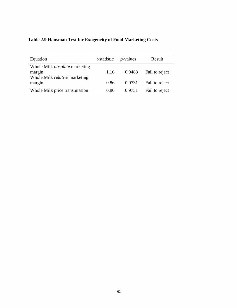
According to Hausman test results from table 2.9, t-tests were both failed to reject on 10%
level for either equation (10) or (11)27, indicating that the null hypothesis of exogeneity was
compatible with the data with almost no probability of a type II error, which means the price of
marketing inputs is exogenous (eb=∞), as was commonly assumed in empirical studies (e.g.,
Heien 1980, Kinnucan and Forker 1987, Wohlgenant and Mullen 1987).
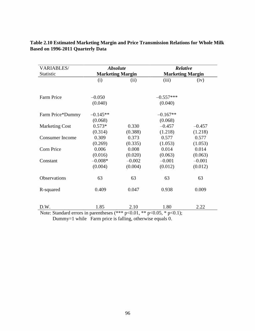
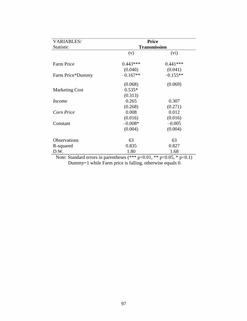
Estimated results were derived by SUR from Table 2.10. For U.S. whole milk in the
sample period, and none of the equations showed signs of serial correlation (see D.W. test); one
per cent increase of farm price for whole milk would yield to around 0.56% decreases for
relative marketing margin and 0.44% increases for retail price, which identified the estimated
price transmission elasticity for rising-farm prices was around 0.44 (t-ratio=11.10); and this
27 The exogeneigty test was performed on FMC using per capita personal income, Producer Production Index, and Real Retail and Food Services Sales (millions of dollars), data available upon request.
38
result highly agreed to the long-run price transmission elasticity for rising-farm prices28 of 0.43
with the ECM procedure. The demand and supply shifters had no any significant effect on
neither of absolute marketing margin nor relative marketing margin, which satisfied one of a
priori expectations that shifts in retail demand and farm supply have no effect on the absolute
marketing margin, but did not agree to the other one that shifts should significantly influence on
the relative marketing margin. Thus, it is hardly to detect if the non-competitive market prevails
or not at this stage. Additionally, the marketing cost variable was statistically significant for the
full absolute marketing margin model (i) as well as for the full price transmission model (v),
where their estimated coefficients were close to each other (0.57 vs. 0.54). The technical change
variable (constant in table 10), however, yielded the minus results across all the models which
can be inferred the marketing margin be negatively affected by the technical change but limited
to a minor extent.
Of key interest are the results relating to the demand and supply shifters, and test statistics
were distributed as χ2 under the null hypothesis of no buyer power (i.e. perfect competition).
However, following Lloyd et al.’s (2009) methodology, the U.S. whole milk was found not to
reject the perfectly competitive nulls, and seen from table 2.11, there was no evidence for the
exercise of buyer power in milk. The two big players, Dallas-based Dean Foods Co. and the
Dairy Farmers of America, a cooperative out of Kansas City, Missouri, were the target of
pending federal class actions, one filed in 2008, and the other in 2010, in which they were
accused of colluding to control market access and suppress milk prices (USDA, 2010)29. Thus if
28 The estimated marketing margin and price transmission regression are both based on the quarterly data, which test only for the long-run effects. 29 The source can be found by this link: http://www.bloomberg.com/news/2010-05-27/obama-regulators-to-review-dairy-farmers-complaints-of-market-dominance.html
the milk price spread was being maintained by collusion rather than competition, as the
regulatory authorities have found to be the case, it is little wonder that our simple test was unable
to detect what amounts to relatively sophisticated strategic pricing behavior.
Note also from Figure 2.2, either for the absolute market margin or for the relative margin,
there was no overall trend in the retail-farm spread. And given the raw data, it is not surprising
that the null hypothesis in this case cannot be rejected. There could of course be some other
aspect of buyer/seller power that exists in this market and that the concerns about collusion
between retailers and processors did not negatively impact on milk producers taken over the
period for which our data applies (Lloyd et al.2009).
More specifically, for absolute marketing margin, the Wald statistic test regarding to both
Weak-Form and Strong-Form hypothesis was too small to reject the null at any confidence level
(Table 2.12). Thus, it resulted in the conclusion that retail demand and farm supply shifters for
absolute marketing margin had no effect on the marketing margins for whole milk. Nevertheless,
for relative marketing margin the Strong-Form of whole milk appeared quite differently, and the
Wald statistic test rejected the null at any confidence level (Table 2.13). The computed chi-
square value for the Wald test was 6880.97 and large enough to reject null hypothesis at any p
value. This, corroborated with the relative marketing margin elasticity of –0.557% (t-ratio= –
13.96) (An isolated 1% increase in the farm price of whole milk is likely to narrow the marketing
margin by 0.56%). From this point, it is difficult to reveal any clear-cut information regarding
the effects of market power on the degree of price transmission in the U.S. marketing channel for
whole milk.
40
2.6 Concluding Comments
This study rests on the assumption that the aggregate technology for food processing and
marketing is characterized by CRTS (Wohlgenant 1989, hold for all commodities except fresh
fruits).
The larger size of rising farm price elasticities compared to decreasing price elasticities
demonstrates that the retail whole milk prices adjust faster to rising farm prices than to decreases.
And the slower response of retail prices to downward movements in farm prices stays consistent
with the commonly held belief that consumers do not benefit from decreases in farm prices in
dairy market.
Meanwhile, though it is inherently likely to constitute the evidence of non-competitive
pricing (market power at the retail level) in the U.S. dairy/whole milk marketing channel driven
by the presence of asymmetric price transmission mentioned earlier, the acceptance of the
perfectly competitive null is apparently contradicting to the evidence for the exercise of buyer
power in milk. In combination with the results provided by both absolute marketing margin and
relative marketing margin, no meaningful conclusions can be drawn regarding the effects of
market power on the degree of price transmission for U.S. whole milk30.
It is probably that competitive market clearing does not require that the elasticity of farm-
retail price transmission equal 1, in that Gardner (1975) pointed out situations in which this
would occur are rare to the point of irrelevance. By the same token, price transmission
30 Weldegebriel H.T. (2004) casted doubt on the validity of empirical estimates of the price transmission coefficient obtained from regressions using retail and farm level price information, quoted as “without knowledge of the functional forms of retail demand and farm input supply, little can be inferred… in particular, it is not generally possible to attribute low (or high) values of the price transmission coefficient to market power.”
41
elasticities close to zero might represent non-competitive pricing, or they simply might represent
consumers’ preference for food products that intensive in the marketing input. From an
econometric perspective, a price transmission elasticity close to zero in models that exclude
marketing costs (Model III) perhaps is to be expected, as such models are subject to attenuation
bias whenever consumers can substitute more easily than intermediaries, i.e., whenever |η| >σ.
The main contribution of this paper is to examine the asymmetric price transmission from
multiple perspectives. Houck and ECM approaches are both employed and compared for this
analysis, which corroborates the previous assumed unidirectional-upward causal relationship
from farm to retail prices and updated Capps and Sherwell (2007) ’s analysis from regional areas
to the entire nation with more recent data. Besides, the comparison between absolute marketing
margin and relative marketing margin are also shedding a new light that it is not generally
possible to attribute low (or high) values of the price transmission coefficient to market power, or
if the collusion rather than competition exists in U.S. dairy market, what amounts to relatively
sophisticated strategic pricing behavior would be unable to detect.
There may be other necessary factors affecting marketing margin that include price risk,
technical change and other structural change, product quality and seasonality (Wohlgenant,
2001). Since it is not accessible to Four-firm concentration ratios (CR4) in the milk processing
sector, measuring the market power with approximated proxy variables remains a further topic.
42
Chapter III. Effects of Recession and Dollar Weakening on the U.S. Agricultural Trade Balance
43
44
3.1 Introduction
The J-curve hypothesis generated a series of empirical research that investigated the existence of
J-curve both in US data and other countries’ data. Earlier studies like Krugman and Baldwin
(1987) found evidence of a J-curve in the US data, and Carter and Pick (1989) indicated the first
segment of the J-curve did exist for the U.S. agricultural trade balance, based on the empirical
evidence that a 10 percent depreciation of the U.S. dollar was estimated to lead a deterioration of
the agricultural trade balance that would last for about nine months. However in a series of
papers Rose and Yellen (1989), Rose (1990) and (1991), not only the J-curve hypothesis was
rejected, but also it is argued that there was no significant effect of the real exchange rate on the
trade balance for both the developing and the developed countries, including the U.S.
By the same token, Bahmani-Oskoee and Brooks (1999) used the ARDL approach to
analyze the US data and found that short-run results supported Rose and Yen (1989) that there
was no effect of real exchange rate on the trade balance in the short run, but in the long-run the
real depreciation of the US dollar was found to have a favorable effect on the trade balance.
Wilson and Tat (2001) on the other hand again by using the Rose and Yellen’s model found
similar results for Singapore. However Singh (2002) by using a trade balance model a la Rose
(1991) and an error correction model implied that trade balance of India was sensitive to the real
exchange rate changes as opposed to Rose (1990) and (1991). Akbostanci (2002) investigated the
existence of a J-curve in the Turkish data in the period of 1987-2000 and suggested the results
did not exactly support the J-curve hypothesis in the short-run, yet the short-run behavior of the
trade balance in response to real exchange rate shocks showed an S-pattern reminiscent of the
Backus et al (1994) rather than the J-curve pattern.
45
The most recent work of Baek et al. (2009) analyzed the dynamic effects of changes in
change rates on bilateral trade of agricultural products between the U.S. and its 15 major trading
partners, by applying the ARDL model of the error correction version, which, in the empirical
specification is ad hoc; they concluded the exchange rate plays a crucial role in determining the
short- and long-run behavior of U.S. agricultural trade, but there was no evidence of the J-curve
phenomenon for U.S. agricultural products with its major trading partners. However, Baek et al.
applied the bilateral trade balance model between U.S. and its 15 major trading partners, which
did not specialize the difference among them, since these trading partners include developing as
well as developed countries and their historical trading pattern with U.S. could be restricted to
internal circumstances such as macroeconomic environment, political changes and national
productions etc. Meanwhile, the exchange rate effects on U.S. agricultural trade should be
distinguished between these selected countries because different countries have different policies
for adjusting exchange rates. Therefore, in our study, we will do the aggregation analysis for U.S.
trade balance and select exchange rate index based on world US agricultural trade weighted real
rate (where year 2005=100), rather than on the real annual country exchange rates of Baek et al.;
and our article will take the recession effects into account, the trade issue becomes different from
the macro-economic perspective.
There have been numerous theoretical arguments and empirical analyses in the past decades,
and exchange rate and the income growth particularly draw the most attention, yet there is no
consistent conclusions to the dynamic effects on U.S. agricultural trade. The general objective of
this article is to determine the U.S. agricultural trade pattern during the past decades. The two
specific objectives: (a) determine if the exchange rate dominates the factors that impact on
46
agricultural trade balance, and (b) determine if there is any recession effects on U.S. agricultural
trade.
Unlike the previous work by Baek and Koo (2011), we divide U.S. agricultural products
into two categories: bulk and high-value goods31; in addition, the four times decennial recessions
from 1970s to date will be included and examined if each recession had different impacts on U.S.
trade of agricultural products. Hence, the two individual commodities plus the combined
products will be analyzed for their trade balance between United States and the Rest of World
(ROW). Within our sample period, the U.S. trade balance of high-value and combined
agricultural goods showed similar pattern especially after 1990s, and both were almost flat since
2008; while the balance of high-valued commodities had been in deficit mostly 32 . Bulk
commodities, on the other hand, fluctuated greatly with ups and downs through each time of
recession (see Figure 3.1).
During our sample period, the major oil shock occurred in the early 1980s which is also
referred to as a “double-dip” or “W-shaped” recession led to a rising real U.S. interest rate, a
decline in import demand, and stagnant growth in many external debt impacted developing
countries (see Table 3.1). And prior to the early 1990s recession, both a devalued dollar and
GDP growth helped to rise the U.S. agricultural trade balance, including individual bulk and
high-value goods. The Economic Research Service (ERS) reported that since 1995, the exchange
rate for U.S. bulk exports was up by nearly twenty percent. The Asian financial crisis that began
in July 1997 led to depreciated currencies, decreased economic growth, and depressing global
commodity prices, which decreased U.S. agricultural exports. And U.S. agricultural exports
31 Instead of the three groups of bulk, intermediate and consumer-oriented products categorized by Baek and Koo (2011). 32 Except in the period from 1992 to 1996, the trade balance of HVP exceeded than 1.
47
value experienced a 23 percent decrease in real terms for the period from fiscal 1997 to fiscal
1999. USDA analysis blamed oversupplies for this decrease, however, the U.S. as a non-crisis
exporter experienced a four percent increase in economic growth, decreased producer prices,
increased production, increased consumption, decreased exports and increased imports due to the
Asian crisis, which included significant depreciations of crisis countries’ currencies.
Over 2000–07, the per capita GDP of U.S. grew by around 1.5% a year, falling below the
annual growth of 2.3% during the 1990s; meanwhile, the per capita GDP of the rest of world
grew by 2.37% yearly from 2000-07, which was far more than the percentage of 0.88% since
1990s. The spread of the crisis beyond the United States is impacting economic growth
throughout the world; the world GDP in 2009 dropped by 4.3%, compared to about 2.5% growth
in 2008 and 3% yearly average growth since 1970 (see Figure 3.2). Our question is how might
the decennial economic crisis and ensuing economic downturn affect U.S. agriculture goods over
the four decades, especially given how important exports and imports are to the sector?
The economic crisis can have direct and indirect effects on U.S. agriculture. The direct
effects come from changes within the U.S. economy alone. The indirect effects will occur from
how the crisis impacts foreign income and trade and world energy prices (Liefert and Shane
2009). Seen from Figure 3.2, before each economic recession mounted there went through a
devaluation of U.S. dollar, no matter how long it lasts; between 2002 and 2008 the dollar fell in
real terms against all foreign currencies by 18%, 22% and 21% for bulk, high-value and
combined agricultural products respectively. However, the crisis’ short-run (current) effect on
the U.S. dollar has been, perhaps ironically to appreciate rather than depreciate, yet the
appreciation did not last long and reappeared in 2011 again. According to Liefert and Shane
48
(2009), the dollar was appreciating against the currencies of most other countries, developed as
well as developing, which means the appreciation could hurt U.S. agricultural exports by making
them less price competitive compared to output produced not only by importing countries but
also by export competitors, such as Canada, Australia, and Brazil.
The remainder of the article is organized as follows: the next section introduces the
theoretical foundation for the J-curve pattern of U.S. agricultural trade balance. Then, the
empirical model will be described and the data set used will be discussed, followed by results
analysis for both short- and long-run effects on U.S. agricultural trade. And the final section
concludes the paper.
3.2 Theoretical Framework33
The basic economics of the agricultural trade balance in a partial-equilibrium setting can be
illustrated with the aid of the following structural model. In this model, agricultural products are
assumed to be undifferentiated in international trade, and we abstract from complicating factors
such as price wedges due to subsidies and tariffs, transportation costs, and farm programs. Prices
are assumed to be determined under competitive conditions so that the Law of One Price (LOP)
holds. Exports and imports are a function of local currency prices, which adjust in response to
changes in the exogenously-determined exchange rate and income levels in the importing and
exporting countries. Other exogenous variables that shift supply and demand curves are
suppressed. With these assumptions, the structural model consists of seven equations:
(1) 𝑄𝑑 = 𝐷(𝑃𝑑, 𝑌𝑑)
33 This section was mainly written by Henry W. Kinnucan.
49
(2) 𝑄𝑥 = 𝑋(𝑃𝑓 , 𝑌𝑓)
(3) 𝑄𝑠 = 𝑆(𝑃𝑑)
(4) 𝑄𝑚 = 𝑀(𝑃𝑓)
(5) 𝑃𝑑 = 𝑃𝑓 ∙ 𝑒
(6) 𝑄𝑠 + 𝑄𝑚 = 𝑄𝑑 + 𝑄𝑥
(7) 𝑇𝐵 =𝑃𝑓𝑄𝑥
𝑃𝑑𝑄𝑚=
𝑃𝑑𝑄𝑥
𝑃𝑑𝑄𝑚𝑒 .
Quantities of agricultural products produced and consumed in the home market in the initial
equilibrium are given by 𝑄𝑠 and 𝑄𝑑; quantities imported into and exported from the home market
are given by 𝑄𝑚 and 𝑄𝑥; the price of the agricultural products in foreign currency units (FCU) in
the initial equilibrium is given by 𝑃𝑓, and the corresponding price in domestic currency units
(DCU) is given by 𝑃𝑑; income levels in the domestic and export (foreign) markets in the initial
equilibrium are given by 𝑌𝑑 and 𝑌𝑓; the exchange rate in the initial equilibrium is given by 𝑒 =
𝐷𝐶𝑈 𝐹𝐶𝑈⁄ ; and the trade balance in the initial equilibrium is given by TB. Because 𝑒 tells how
many units of domestic currency can be purchased per unit of foreign currency, an increase 𝑒
implies currency weakening (devaluation) from the domestic buyers’ perspective.
The model consists of seven endogenous variables (𝑄𝑑, 𝑄𝑥, 𝑄𝑠, 𝑄𝑚, 𝑃𝑑, 𝑃𝑓, 𝑇𝐵) and three
exogenous variables (𝑌𝑑 , 𝑌𝑓 , 𝑒). At issue are the hypotheses that can be deduced given the
structure defined by equations (1) – (7). Specifically, do the reduced-form elasticities of trade
balance with respect to income and exchange rate have determinate signs?
To determine that, the model is first expressed in proportionate change form as follows
50
(8) 𝑄𝑑∗ = 𝜂𝑑𝑃𝑑
∗ + 𝛾𝑑𝑌𝑑∗
(9) 𝑄𝑥∗ = 𝜂𝑥𝑃𝑓
∗ + 𝛾𝑥𝑌𝑓∗
(10) 𝑄𝑠∗ = 𝜀𝑑𝑃𝑑
∗
(11) 𝑄𝑚∗ = 𝜀𝑚𝑃𝑓
∗
(12) 𝑃𝑑∗ = 𝑃𝑓
∗ + 𝑒∗
(13) 𝑘𝑠𝑄𝑠∗ + 𝑘𝑚𝑄𝑚
∗ = 𝑘𝑑𝑄𝑑∗ + 𝑘𝑥𝑄𝑥
∗
(14) 𝑇𝐵∗ = 𝑄𝑥∗ − 𝑄𝑚
∗ − 𝑒∗.
The asterisk (*) indicates proportionate change (e.g., 𝑄𝑑∗ = 𝑑𝑄𝑑 𝑄𝑑⁄ ); the Greek symbols
indicate elasticities; and the k terms indicate quantity shares. Specifically, 𝜂𝑑 (< 0) and 𝜂𝑥 (<
0) are price elasticities of domestic and export demand; 𝛾𝑑 (> 0) and 𝛾𝑥 (> 0) are income
elasticities of domestic and export demand; 𝜀𝑑 (> 0) and 𝜀𝑚 > 0 are price elasticities of
domestic and import supply; 𝑘𝑠 = 𝑄𝑠 (𝑄𝑠 + 𝑄𝑚)⁄ is the share of domestic supply that comes
from domestic production; 𝑘𝑚 = 𝑄𝑚 (𝑄𝑠 + 𝑄𝑚)⁄ is the share of domestic supply that is imported;
𝑘𝑑 = 𝑄𝑑 (𝑄𝑠 + 𝑄𝑚)⁄ is the share of domestic supply that is consumed in the home market; and
𝑘𝑥 = 𝑄𝑥 (𝑄𝑠 + 𝑄𝑚)⁄ is the share of domestic supply that is exported.
Reduced Form
The reduced-form equations for proportionate changes in domestic price, exports, imports, and
trade balance implied by the structural model are as follows:
(15) 𝑃𝑑∗ = (
𝑘𝑚𝜀𝑚−𝑘𝑥𝜂𝑥
𝜀−𝜂) 𝑒∗ + (
𝑘𝑑𝛾𝑑
𝜀−𝜂) 𝑌𝑑
∗ + (𝑘𝑥𝛾𝑥
𝜀−𝜂) 𝑌𝑓
∗
51
(16) 𝑄𝑥∗ = (
−𝜂𝑥(𝑘𝑠𝜀𝑑−𝑘𝑑𝜂𝑑)
𝜀−𝜂) 𝑒∗ + (
𝜂𝑥𝑘𝑑𝛾𝑑
𝜀−𝜂) 𝑌𝑑
∗ + ((𝜀−𝑘𝑑𝜂𝑑)𝛾𝑥
𝜀−𝜂) 𝑌𝑓
∗
(17) 𝑄𝑚∗ = (
−𝜀𝑚(𝑘𝑠𝜀𝑑−𝑘𝑑𝜂𝑑)
𝜀−𝜂) 𝑒∗ + (
𝜀𝑚𝑘𝑑𝛾𝑑
𝜀−𝜂) 𝑌𝑑
∗ + (𝜀𝑚𝑘𝑥𝛾𝑥
𝜀−𝜂) 𝑌𝑓
∗
(18) 𝑇𝐵∗ = ((𝜀𝑚−𝜂𝑥)(𝑘𝑠𝜀𝑑−𝑘𝑑𝜂𝑑)
𝜀−𝜂− 1) 𝑒∗ + (
(𝜂𝑥−𝜀𝑚)𝑘𝑑𝛾𝑑
𝜀−𝜂) 𝑌𝑑
∗ + (𝜀𝑚(𝑘𝑚−𝑘𝑥)+𝑘𝑠𝜀𝑑−𝑘𝑑𝜂𝑑
𝜀−𝜂) 𝑌𝑓
∗
where 𝜀 = (𝑘𝑠𝜀𝑑 + 𝑘𝑚𝜀𝑚) > 0 is the overall supply elasticity and 𝜂 = (𝑘𝑑𝜂𝑑 + 𝑘𝑥𝜂𝑥) < 0 is
the overall demand elasticity. The reduced-form elasticities in equations (15) – (18) shed light
on empirical estimates in the literature. For example, the only variable to have a determinant
effect on trade balance is domestic income. Specifically, market theory predicts that an isolated
increase in domestic income will reduce the trade balance, i.e., cause import value to rise in
relation to export value. No such predictions are forthcoming about isolated movements in either
the exchange rate or foreign income. Thus, one should not be surprised to find mixed signs (or a
zero effect) for these variables in an empirical trade balance relation.
Exports are positively related to domestic currency devaluation and foreign income, and
negatively related to domestic income. Imports are negatively related to domestic currency
devaluation, and positively related to domestic and foreign income. In the trade balance literature
these relations are typically estimated with the dependent variable defined as trade value (e.g.,
Baek and Koo, 2011). The relevant reduced-form equations in this instance are obtained by
combining equation (15) and with equations (16) and (17) to yield:
(19) 𝑉𝑥∗ = (
−𝜂𝑥(𝑘𝑠𝜀𝑑−𝑘𝑑𝜂𝑑+𝑘𝑥)+𝑘𝑚𝜀𝑚
𝜀−𝜂) 𝑒∗ + (
(1+𝜂𝑥)𝑘𝑑𝛾𝑑
𝜀−𝜂) 𝑌𝑑
∗ + ((𝜀−𝑘𝑑𝜂𝑑+𝑘𝑥)𝛾𝑥
𝜀−𝜂) 𝑌𝑓
∗
(20) 𝑉𝑚∗ = (
−𝜀𝑚(𝑘𝑠𝜀𝑑−𝑘𝑑𝜂𝑑−𝑘𝑚)−𝑘𝑥𝜂𝑥
𝜀−𝜂) 𝑒∗ + (
(1+𝜀𝑚)𝑘𝑑𝛾𝑑
𝜀−𝜂) 𝑌𝑑
∗ + ((1+𝜀𝑚)𝑘𝑥𝛾𝑥
𝜀−𝜂) 𝑌𝑓
∗
52
Switching from quantity to value renders the domestic income effect in the export equation and
the exchange rate effect in the import equation indeterminate. An increase in domestic income
will reduce export value only if export demand must be price elastic. Similarly, domestic
currency devaluation will reduce import value only if the negative quantity effect of the
devaluation outweighs the positive price effect. That is, referring to the coefficient of 𝑒∗ in
equation (20), only if |−𝜀𝑚(𝑘𝑠𝜀𝑑 − 𝑘𝑑𝜂𝑑)| > (𝑘𝑚𝜀𝑚 − 𝑘𝑥𝜂𝑥).
Small Trader Effects
The analysis thus far indicates that the only variable to have a determinant effect on trade
balance is domestic income. This suggests restrictions need to be placed on model parameters if
market theory is to have predictive content with respect to exchange rate and foreign income.
One such restriction is that the country in question is too small a buyer or seller in the world
market to affect prices. A small seller in world markets implies the country faces a perfectly
elastic export demand curve. In this instance, the equations (15) – (20) reduce to:
Reduced form when 𝜂𝑥 = −∞ (small exporter):
(21) 𝑃𝑑∗ = 𝑉𝑚
∗ = 𝑒∗
(22) 𝑄𝑚∗ = 0
(23) 𝑉𝑥∗ = (
𝑘𝑠𝜀𝑑−𝑘𝑑𝜂𝑑+𝑘𝑥
𝑘𝑥) 𝑒∗ − (
𝑘𝑑𝛾𝑑
𝑘𝑥) 𝑌𝑑
∗
(24) 𝑇𝐵∗ = 𝑄𝑥∗ = (
𝑘𝑠𝜀𝑑−𝑘𝑑𝜂𝑑
𝑘𝑥) 𝑒∗ − (
𝑘𝑑𝛾𝑑
𝑘𝑥) 𝑌𝑑
∗
Imposing the small exporter assumption eliminates the ambiguity about the effects of exchange
rate and foreign income on trade balance. Specifically, theory now predicts that changes in
53
foreign income will have no effect on trade balance, and that domestic currency devaluation will
improve the trade balance. The reason for the latter is that although devaluation causes import
value (cost) to increase (since the full burden of the exchange rate adjustment falls on domestic
price), export value rises faster. Specifically, (𝑉𝑥∗ 𝑒∗⁄ / 𝑉𝑚
∗ 𝑒∗⁄ ) = (𝑘𝑠𝜀𝑑−𝑘𝑑𝜂𝑑+𝑘𝑥
𝑘𝑥) > 1.
A small buyer in world markets faces a perfectly elastic import supply curve. In this
instance, equations (15) – (20) reduce to:
Reduced form when 𝜀𝑚 = ∞ (small importer):
(25) 𝑃𝑑∗ = 𝑒∗
(26) 𝑄𝑥∗ = 0
(27) 𝑄𝑚∗ = − (
𝑘𝑠𝜀𝑑−𝑘𝑑𝜂𝑑
𝑘𝑚) 𝑒∗ + (
𝑘𝑑𝛾𝑑
𝑘𝑚) 𝑌𝑑
∗ + (𝑘𝑥𝛾𝑥
𝑘𝑚) 𝑌𝑓
∗
(28) 𝑉𝑥∗ = 𝑒∗ + 𝛾𝑥𝑌𝑓
∗
(29) 𝑉𝑚∗ = − (
𝑘𝑠𝜀𝑑−𝑘𝑑𝜂𝑑−𝑘𝑚
𝑘𝑚) 𝑒∗ + (
𝑘𝑑𝛾𝑑
𝑘𝑚) 𝑌𝑑
∗ + (𝑘𝑥𝛾𝑥
𝑘𝑚) 𝑌𝑓
∗
(30) 𝑇𝐵∗ = (𝑘𝑠𝜀𝑑−𝑘𝑑𝜂𝑑
𝑘𝑚) 𝑒∗ − (
𝑘𝑑𝛾𝑑
𝑘𝑚) 𝑌𝑑
∗ + (𝑘𝑚−𝑘𝑥
𝑘𝑚) 𝑌𝑓
∗
Imposing the small importer assumption eliminates the ambiguity about the effects of exchange
rate on trade balance, but not the ambiguity about the effects of changes in foreign income. The
latter effect is positive only if the import share exceeds the export share. As for the exchange
rate effect, domestic currency devaluation causes the trade balance to improve, the same result
obtained for the small exporter case.
The J-Curve
54
The J-curve describes a situation where the trade balance initially deteriorates following
devaluation before it improves. The Marshall-Lerner Condition attributes this phenomenon to
differences in short- and long-run elasticities of demand (e.g., Rose and Yellen 1989; Rose 1991).
The MLC in terms of the present model can be derived by dividing the trade-balance relation
(equation (14)) through by 𝑒∗ to yield
(31) 𝑇𝐵∗
𝑒∗ =𝑄𝑥
∗
𝑃𝑓∗
𝑃𝑓∗
𝑒∗ −𝑄𝑚
∗
𝑃𝑑∗
𝑃𝑑∗
𝑒∗ − 1
where 𝑄𝑥
∗
𝑃𝑓∗ = 𝜂𝑥 is the export demand elasticity;
𝑄𝑚∗
𝑃𝑑∗ = 𝜂𝑚 the import demand elasticity;
𝑃𝑑∗
𝑒∗ = 𝑃𝑇𝐸
is the pass-through elasticity into the domestic price; and 𝑃𝑓
∗
𝑒∗ = (𝑃𝑇𝐸 − 1) is the pass-through
elasticity into the foreign price. Substituting these parameters into equation (21), for the trade
balance to improve following devaluation the following condition must hold
(32) 𝑃𝑇𝐸 |𝜂𝑚| + (1 − 𝑃𝑇𝐸)|𝜂𝑥| > 1.
where
(33) 0 < 𝑃𝑇𝐸 = (𝑘𝑚𝜀𝑚−𝑘𝑥𝜂𝑥
𝜀−𝜂) ≤ 1.
Equation (32) is the MLC modified to include the pass-through elasticity. If the sum of the
import and export demand elasticities (in absolute value) is less than one, as might be true in a
short-run situation, the trade balance deteriorates following devaluation. This explains the
downward-sloping portion of the J-curve. If pass-through is complete (𝑃𝑇𝐸 = 1), as would be
true if export demand or import supply were perfectly elastic (the small-trader situation), the
MLC reduces to |𝜂𝑚| > 1. In this instance, the trade balance improves following devaluation
provided import demand is price elastic. The reason is that with elastic import demand, the
55
proportionate increase in price associated with devaluation is more than offset by a proportionate
decrease in import quantity, implying a decrease in import value. Because foreign price and
export revenue are unaffected when pass-through into the domestic price is complete, the trade
balance necessarily improves.34
In summary, our structural model yields only one hypothesis, namely that domestic income
growth will cause the agricultural trade balance to deteriorate. The trade balance deteriorates
because an increase in domestic income causes a simultaneous increase in imports and decrease
in exports (and price effects cancel owing to LOP). The effect of an increase in foreign income
on the trade balance is indeterminate, as is the effect of domestic currency devaluation. Thus,
the effect of these variables on the trade balance is an empirical issue.
3.3 Empirical Model
To test the hypothesis that the domestic income growth has a negative effect on the U.S.
agricultural trade balance, we follow Baek et al. (2009) and replicate their work with employing
an autoregressive distributed lag (ARDL) modeling approach. The ARDL approach avoids
spurious regression associated with non-stationary time series, and permits distinguishing short-
run from long-run effects. The ARDL approach lends itself to the present problem in that the
equation to be estimated, namely 𝑇𝐵 = 𝑇𝐵(𝑌𝑑, 𝑌𝑓 , 𝑒) , is in reduced form, thereby avoiding
problems associated with endogenous right-hand-side variables (Pesaran and Shin 1999).
34 In our model, the import demand elasticity is |𝜂𝑚| =
|𝜂|+𝑘𝑠𝜀𝑑
𝑘𝑚 , where 𝜂 = 𝑘𝑑𝜂𝑑 + 𝑘𝑥𝜂𝑥 is the overall demand
elasticity for domestic consumption and exports. For import demand to be price inelastic (|𝜂𝑚| < 1), overall demand must be sufficiently price inelastic to satisfy |𝜂| < (𝑘𝑚 − 𝑘𝑠𝜀𝑑). This condition would seem difficult satisfy, even in the short-run situation where 𝜀𝑑 = 0. Thus, in instances where LOP and the other assumptions underlying our model hold, one would expect the MLC to hold as well.
56
The first step is to specify the long-run equilibrium relationship. For this purpose, we adopt
the constant elasticity specification
(34) ln 𝑇𝐵𝑖,𝑡 = 𝛼 + 𝛽1 ln 𝑌𝑡𝑈𝑆 + 𝛽2 ln 𝑌𝑡
𝑅𝑂𝑊 + 𝛽3 ln 𝐸𝑅𝑖,𝑡 + 𝜀𝑖,𝑡,
where i indexes the type of agricultural product (1 = bulk, 2 = high value, and 3 = combined bulk
and high value); t indexes the year (1976-2012); 𝑇𝐵𝑖𝑡 is the U.S. trade balance defined as the real
value of U.S. exports divided by the real value of U.S. imports; 𝑌𝑡𝑈𝑆 is real U.S. per capita GDP;
𝑌𝑡𝑅𝑂𝑊 is real per capita GDP for world less US (in U.S. dollars); 𝐸𝑅𝑖𝑡 is the real trade weighted
exchange rates between the United States and the currency of foreign trading partners for U.S.
bulk products, U.S. high-value products, and combined bulk and high-value products,
respectively35; and 𝜀𝑖𝑡 is the error term. The exchange-rate variables are defined as U.S. dollar
divided by Foreign Currency Unit (ER = DCU/FCU). Hence, an increase in ER implies domestic
currency devaluation.
The betas are long-run elasticities. Theory predicts 𝛽1 < 0 (a rise in domestic income will
increase imports and reduce exports, causing TB to decline). Intuitively, a rise in foreign income
and a weaker domestic currency should each improve the trade balance, implying positive signs
for 𝛽2 and 𝛽3. However, as we saw in the theoretical analysis, intuition is correct only under
certain conditions. The signs of 𝛽2 and 𝛽3 are an empirical issue.
The second step is to write the long-run equilibrium relation in ARDL form
35 According to the Economic Research Service (2001), nominal exchange rates are those observed and are a result of the market and other forces out of our control. Real exchange rates are nominal rates adjusted for inflation. Trade weighted exchange rates are calculated with a trade-weight index. These indices are constructed by multiplying the average trade weight of a country in U.S. exports, exports to the world, and U.S. imports. These weights are average dollar shares of U.S. exports, exports to the world, and U.S. imports for the relevant commodity. The current exchange rate for each country (in units per dollar) is then adjusted by taking the ratio of the same period CPI in the U.S. to the country in question. The percent change from the base period is then multiplied by the weight. These weighted changes are summed into a total, which is the “real” index.
investments and because of the high rates of return available because of high interest rates in the
U.S. compared to the rest of the world. Thus, devaluing the dollar did not change that
significantly (Pool and Stamos, 1990). Beyond that, during the period of 1980s, while the dollar
did fall against some U.S. trading partners, e.g. Japan and West Germany, it did not fall against
others, such as the newly industrialized countries of Taiwan and South Korea and the Pacific
Rim countries37. Before the first recession within our sample period, the exchange rate line
reached peak for all the three groups, which means the dollar against ROW currency was
devalued to the most extent, and the U.S. trade surplus of bulk and combined goods hit the
highest point in the following year. However, till the last year of the sample period, the trade
surplus of combined agricultural products fell by 34 percent compared to its initial value, and the
value of bulk goods even decreased about 70 percent though going through ups and downs. Only
the trade deficit of U.S. high-value products improved by 36 percent over the past four decades
(See Figure 3.1).
It should also be pointed out that the coefficients of the error-correction terms are all
negative for bulk products, high-value products and the combined agricultural products, and all
are statistically significant at least at the level of 10 percent. For the U.S. bulk and combined
agricultural products, the speed of adjustment towards equilibrium would both be around 80
percent, and for high value products, the speed towards equilibrium is about 30 percent, which
further provides evidence of the existence of the long-run relationship among variables (Kremers,
Ericson, and Dolado 1992, Banerjee, Dolado and Mestre 1998, and Baek et al.2009). The
37 Since 2000, U.S. goods imports from developing countries have exhibited higher growth (almost 4 times as much) than that from industrial countries, 130 percent compared with 36 percent. On the other hand, U.S. goods exports to developing countries have grown almost three times as fast as U.S. goods exports to industrial countries, 135 percent compared to 54 percent. Due to this long-term higher-growth difference, the share of U.S. goods exports to developing countries have grown from 45 percent in 2000 to 55 percent in 2011. For example, the percentage change of U.S. exports to China reached 554% versus that of U.S. imports from China was 300.2% from 2000-11.
62
findings further justify the ARDL modeling of U.S. agricultural trade of all the three categories
with ROW, in which the F-statistics results are cointegration (See Table 3.2).
Table 3.4 yields the estimated results from the full model before any F-tests for recession
effects, and the coefficient estimates of trade weighted real exchange rate carry the positive
relationship with the U.S. trade balance for all the three products; at meanwhile, high-value and
combined agricultural products are statistically significant at the 5 percent level (Table 3.4). It
states that the depreciating domestic currency (U.S. dollars) lead to an improvement of U.S. trade
balance in the long term, meaning with each one percent of U.S. dollar depreciation, U.S. trade
balance of high-value commodities and total agricultural products would enhance by 1.62
percent and 1.88 percent respectively. Besides, for both of high value and combined products,
the U.S. trade balance displays the positive relationship with domestic income and negative with
foreign income, where only trade balance of combined goods with foreign income shows
statistical significance at the level of 5 percent. According to Baek et al. (2009), it demonstrates
that a rise of real domestic income increases the domestic demand for U.S. exports while
decreases the demand for foreign imports, thereby improving the U.S. trade balance; and vice
versa, for the foreign income, it has adverse relationship with the U.S. trade balance and a
deteriorating effect accordingly. One of the possible explanations for the finding is that, since
imports are defined as the difference between domestic consumption and production, an increase
in domestic income could increase the domestic production of import-substitute commodities
faster than a rise in domestic consumption, thereby leading to the reduction of domestic
imports38; meanwhile, records show HVP exports exceeded exports of bulk products at the
beginning of year 1990 for the first time and kept the trend until today, then the income effects of
38 See Magee (1973), Bahmani-Oskooee (1985), and Bahmani-Oskooee and Ratha (2004)
63
HVP could be the major contributor and thus one percent increase of foreign GDP, ceteris
paribus, would decrease the U.S. trade surplus of combined agricultural goods by around 1.32
percent39. Furthermore, our results found that growth in incomes has a larger effect on exports of
bulk commodities than on high-value exports, which is opposite to the finding drawn by Shane et
al. (2009).
Compared to the recent work by Baek and Koo (2011), our results indicate the similar
results on the U.S. import side but different on the export side in the long run. That is, the U.S.
exports are very responsive to exchange rate changes for bulk, high-value (consumer-oriented
products) and the combined commodities but do not seem to respond much to income; And for
U.S. imports, both of bulk and high-value products are relatively insensitive to exchange rate
changes.
As for dummy variables of recessions, F-test indicates that only trade balance model and
import model of U.S. combined agricultural products reject the null hypothesis that the four
dummy variable coefficients are zero, which means the U.S. recessions occurred in the past forty
years have had different effects on trade balance as well as imports of U.S. combined products.
And the dummy variable effects imply that the U.S. trade balance would decrease by 0.21
percent during the 1980s crisis compared with other years, while the U.S. imports would increase
by 0.15 percent within the recent great recession from 2008 to 2009. This might suggest that
when the first economic recession of our sample period occurred, the U.S. trade balance of
combined agricultural goods decreased, meaning U.S. exports declined or U.S. imports increased
39 Stephen (ERS, USDA, 2013) introduced the market share of middle-income and high-income countries that import from U.S. Agricultural products, and they now account for the largest share of U.S. agricultural exports of both bulk products and semi-processed high-value products (e.g. wheat, soybeans, and soybean meal); while for the other categories of high-value products---raw products and processed products, high-income countries remain the largest U.S. markets, followed by the upper middle-income countries.
64
or both. One possible reason should be correlated with decreasing U.S. GDP declining: Table 3.4
demonstrates the U.S. income is positively related with its trade balance and negatively related
with its imports for combined products, therefore U.S. trade balance would be hurt and U.S.
imports would increase under such a circumstance. Another reason could be the U.S. dollar was
getting strong instead of weakening (or devaluation) in both recession periods, the 1980s
recession and the most recent recession, during which the exchange rate curve of combined
agricultural goods started to slump seen from Figure 3.2, thus, the U.S. exports became
decreasing and imports increasing correspondingly. Besides, the most recent recession was
verified to positively impact on U.S. imports, which further states that the recession could
increase the imports. And our results agree to the previous work by Liefert and Shane (2009)
mentioned earlier. For individual agricultural goods such as bulk or high-value products, F-tests
indicate that none of the recessions has any significant impact on U.S. trade balance. This might
imply that global trade partners have tended to constrain exports/imports to the U.S. combined
agricultural products rather than to individual ones in response to recessions, and basically the
U.S. recession effects for agricultural trade in the last forty years were less than expected and the
U.S. monetary policy or financial tools for mitigating the recession downturns should have
worked to certain extent.
Specifically, the export and import equations are estimated separately for further analysis.
The results suggest that the U.S. exports have a positive relationship with the exchange rate in
long-run for three cases, and all of the estimates are statistically significant at least at level of 5
percent, highly suggesting that the devaluing domestic currency (U.S. dollars) would increase the
domestic (U.S.) exports; meanwhile, in the long term, the real exchange rate is passed through to
the U.S. exports of combined agricultural products to the largest degree, compared with
65
individual bulk and high-value goods. Besides, for bulk commodities the relationship between
U.S. exports and foreign income appears positive and statistically significant at the level of 10
percent, rather than the other two cases; and one percent increase of foreign per capita GDP
would enhance U.S. bulk exports by around 3.57 percent, while one percent of increase of traded
weighted real exchange rate would improve U.S. exports by 1.19 percent, which corroborates the
conclusion drawn by Shane et al. (2009) that the net effect on total agricultural exports depends
on the magnitude of growth in income compared to the magnitude of change in the trade-
weighted exchange rate.
By contrast, the reduced import model implies that the real exchange rates of all the three
categories are negatively related with the U.S. imports, but only the coefficient of combined
agricultural goods shows significance at 10 percent level, corroborating the common-held belief
that the devalued U.S. dollar would cause U.S. imports to decline, which is consistent with our
hypothetical expectations. The decomposed export model and import model demonstrate the
depreciation effects of exchange rate on U.S. trade outweigh the inconclusive effects of either
domestic or foreign income in the long run.
As beginning with the pioneering studies of Bahmani-Oskooee and Ardalani (2006, 2007),
there has been a growing body of literature that argues that trade balance study could suffer from
aggregation bias of data due to the fact that a country tends to export and import different
commodities to/from different trading partners, thus in this article we did the Wald tests to
determine whether or not bulk and high-value commodities can be aggregated across three
models (See table 3.5). The results show that all the three null hypotheses are rejected at 5%
probability level, which means there might not exist any aggregation bias between bulk and
high-value in our study.
66
As for the F-tests for determining whether recession effects are jointly significant, only
combined agricultural goods receive some support in that two of the nine tests show a significant
relationship between U.S. import value or trade balance and the recession effects during the past
decades. However, the remaining tests show no significance (See Table 3.6).
Though not all the estimated coefficients for the three cases are statistically significant, the
signs between exchange rates and U.S. trade balance are the same; according to the earlier
mentioned theoretical deductions, the relationship between foreign income and U.S. trade
balance is ambiguous and cannot be inferred. Thus, our results might provide empirical evidence,
if any, for the previous theoretical argument. Generally speaking, the estimates of real exchange
rates present positive relationship with U.S. trade balance not only for individual agricultural
commodities of bulk and high-value goods but also for the combined agricultural products within
the sample period since late 1970s.
Finally, to test if the estimated coefficients are stable or not over time, we use the
cumulative sum (CUSUM) and cumulative sum of squares (CUSUMSQ) tests to the residuals of
ECMs (Eqs. (35). For stability of all estimated coefficients, the plot of these two statistics should
stay within the 5% significance level. The overall results of stability test suggest that the
estimated coefficients of all models are generally stable over the sample period40.
3.6 Conclusions
The article applies the dynamic ARDL model of error correction version, not only investigating
if there is J-curve effect in the short-run or not, but also taking a deep analysis for U.S. recession
effects and exchange rate as well as income growth effects in the long run on the U.S. trade
40 According to Baek and Koo (2011), these tests are known to have low power and could miss important breaks.
67
balance of agricultural commodities which mainly consists of bulk products and high-value
products. Our results indicate that there is no significant J-curve effect for three cases, while the
long-run effect demonstrates that the domestic currency devaluation is positively related with
U.S. agricultural trade balance for bulk, high-value and combined agricultural products, though
the high-value products appear the more modest effects compared to the other two.
In sum, the real trade-weighted exchange rate is found to be the key determinant of U.S.
agricultural trade balance in the long-term, rather than domestic or foreign income. We find that
the three categories of agricultural products do indeed respond differently to exchange rate and
income. For bulk and high-value products, U.S. exports are highly sensitive to exchange rate and
foreign income, while U.S. imports barely respond. For combined agricultural products, on the
other hand, U.S. exports respond greatly to exchange rate, and U.S. imports behave significantly
with respect to both of changes in exchange rate and foreign income; besides, the 1980s
recession had significant effects on U.S. trade balance while the most recent recession had great
impact on U.S. imports, showing the U.S. trade with ROW partners was mainly influenced by
the two times economic crisis during our sample period.
To our knowledge, it is the first time that the ARDL model is applied for the recession
effects on individual groups of U.S. total agricultural commodities: Bulk and High-Value
products. Different from the previous work by Baek and Koo (2011), this paper analyzes both of
dollar devaluation impacts and the decennial U.S. economic recession effects on U.S. trade
balance by employing the aggregated data and explores the reasons that the J-curve effect did not
show up during the past decades; also, the test shows that there is no any aggregation bias
between bulk and high-value in our study, making both of the dynamic short-run effect and
68
stable long-run effect estimated from the reduced model at linkage with the theoretical structure
equations more solid and convincing.
References
Adelaja, Adesoji O., 1991. “Price Changes, Supply Elastic Ties, Industry Organization, and Dairy
Output Distribution.” American Journal of Agricultural Economics, pp. 89–102.
Aguiar, D. and J.A.Santana, 2002. "Asymmetry in Farm to Retail Price Transmission: Evidence for
Brazil." Agribusiness, Vol.18:pp. 37-48.
Almon, S., 1965. "The distributed lag between capital appropriations and expenditures.”
Econometrica, Vol.33:pp. 178-196.
Alston, Julian; James Chalfant and Nicholas Piggott, 2002. “Estimating and Testing the Compensated
Double-Log Demand Model.” Applied Economics, Vol. 34, pp. 1177–1186.
Table 2.3 Granger Causality Test from 1996:01 to 2011:12 based on Monthly Data of Farm
and Retail prices for national Whole Milk
Effect Hypothesized
cause
F-
statistic p-value
Farm price Retail price 2.20 0.1138
Retail price Farm price 5.18 0.0065* Note: The null hypothesis is that one series does not Granger cause another. The Granger
causality tests use a lag length of two months. *indicates statistical significance at the 0.05 level. EVIEWS 7.0 was
the statistical package employed to conduct the Granger tests.
90
Table 2.4 Empirical Results of the Johansen Cointegration Tests for Farm prices and
Retail Prices of Whole Milk.
Hypothesized No. of Trace test Maximal
eigenvalue
cointegrated equations Statistic p-value test Statistic p-value
None * 19.82 0.0104* 17.30 0.0161*
At most 1 2.53 0.1118 2.53 0.1118 Note: The intercept (no trend) option with three lags was used in conjunction with these tests. The level of
significance chosen for this analysis was 0.05. *indicates statistical significance. EVIEWS 7.0 was the statistical
package employed to conduct the cointegration tests.
91
Table 2.5 Empirical Results of the Houck Procedure for U.S. Whole Milk Based on 1996-
2011 Monthly Data
Model I Model II Model III Model IV
Trend –0.0006
–0.0003
(0.0004)
(5.73E-05)
ΔPft+ (SR+ ) a 0.9099 b 0.8982 0.9056 0.8472
(0.0582) c (0.0580) (0.0580) (0.0586)
ΔPft-1+ 0.2272 0.2129 0.2217 0.1571
(0.0433) (0.0427) (0.0429) (0.0426)
ΔPft-2+ –0.0762 –0.0865 –0.0802 –0.1253
(0.0425) (0.0421) (0.0422) (0.0418)
LR+ 1.0609 1.0245 1.0471 0.8790
(0.1038) (0.1023) (0.1028) (0.1027)
ΔPft– (SR– ) a 0.0568 0.0583 0.0574 0.0647
(0.0180) (0.0181) (0.0180) (0.0186)
ΔPft-1– 0.0279 0.0299 0.0288 0.0362
(0.0126) (0.0127) (0.0126) (0.0136)
ΔPft-2– 0.0089 0.0105 0.0096 0.0146
(0.0129) (0.0129) (0.0129) (0.0134)
LR– 0.0936 0.0987 0.0958 0.1155
(0.0298) (0.0300) (0.0298) (0.0328)
MDta 0.0003 –0.0002
(0.0003) (5.75E-05)
AR(1) 0.2329 0.2445 0.2361 0.3264
(0.0757) (0.0755) (0.0755) (0.0753)
AR(2) 0.0761 0.0855 0.0788 0.1452
(0.0754) (0.0751) (0.0751) (0.0757)
R square
0.6434 0.6380 0.6417 0.6040
D.W. 1.99 1.99 1.99 2.01
AIC –3.1680 –3.1637 –3.1741 –3.0848
SIC –3.0277 –3.0410 –3.0514 –2.9796 Note: a. ΔPft
+ and ΔPft– are identified above, where ft-i and rt-i implies lag lengths (i=0, 1, 2, 3); where MDt is marketing cost
variables, expressed as deviations from its initial value. The dependent value is expressed as the first difference of retail price. b. Parameter estimate
c. Standard errors in parentheses
92
Table 2.6 Error Correction Model Results for U.S. Whole Milk Based on 1996-2011
Monthly Data
Model I Model II Model III
Model IV
Trend –
0.0005
–2.59E-05
(0.0002)
(4.95E-05)
ΔPft+ (SR+ ) a 0.9316b 0.9191 0.9250 0.9178
(0.0573) c (0.0576) (0.0577) (0.0559)
ΔPft-1+ –0.0151 –0.0391 –0.0275 –0.0418
(0.0889) (0.0891) (0.0895) (0.0851)
LR+ 0.9165 0.8800 0.8975 0.8760
(0.0944) (0.0938) (0.0948) (0.0853)
ΔPft– (SR– ) a 0.0469 0.0453 0.0453 0.0454
(0.0167) (0.0169) (0.0169) (0.0169)
ΔPft-1– 0.0176 0.0183 0.0182 0.0183
(0.0103) (0.0104) (0.0104) (0.0104)
ΔPft-2– 0.0020 0.0031 0.0031 0.0031
(0.0116) (0.0117) (0.0117) (0.0117)
LR– 0.0665 0.0667 0.0666 0.0668
(0.0237) (0.0240) (0.0239) (0.0239)
ECT t-1+ –0.2467 –0.2476 –0.2377 –0.2501
(0.0400) (0.0404) (0.0401) (0.0323)
ECT t-1 – 0.0004 0.0263 0.0248 0.0264
(0.0338) (0.0318) (0.0320) (0.0318)
ΔPrt-1 0.1087 0.1266 0.1237 0.1271
(0.0722) (0.0725) (0.0725) (0.0721)
ΔPrt-2 –0.0551 –0.0542 –0.0519 –0.0548
(0.0481) (0.0486) (0.0485) (0.0481)
ΔPrt-3 –0.1370 –0.1373 –0.1335 –0.1383
(0.0459) (0.0463) (0.0463) (0.0453)
MDta 0.0005 –5.09E-06
(0.0002) (4.86E-05)
R square 0.7117 0.7043
0.7048
0.7043
D.W. 1.98 2.00 1.99 2.00
AIC –3.3343 –3.3198 –3.3212 –3.3304
SIC –3.1443 –3.1470 –3.1485 –3.1749 Note: a. ΔPft+ and ΔPft– are identified above, where ft-i and rt-i implies lag lengths (i=0, 1, 2, 3); where MDt is marketing
cost variables, expressed as deviations from its initial value. The dependent value is expressed as the first difference of retail
price.
b. Parameter estimate
c. Standard errors in parentheses
93
Table 2.7 Elasticites of Farm-Retail Price Transmission for Whole Milk under Rising and
Falling Farm Prices, United States, Based on Data Covering January 1996-December 2011
Elasticity When Farm Prices Are:
Rising
Falling
LR SR LR SR
Houck
approach
0.5006
0.4422
0.0458
0.0217
ECM
approach
0.4291
0.4329
0.0318
0.0274
Note: The elasticites are evaluated on the mean value.
94
Table 2.8 Theoretical Values of Price Transmission Elasticities under Retail Demand
versus Farm Supply Shifts (Gardner 1975, p.403, table 1)
Parameters
Transmission Elasticity
When the Margin Change is
due Exclusively to a:
σ ea eb η Sb
Retail
Demand Shift
Farm
Supply
Shift
0.5 1.0 2.0 –0.5 0.5 0.80 0.50
0 1.0 2.0 –0.5 0.5 0.75 1.44
0 1.5 2.0 –0.5 0.5 0.88 0.44
0 2.0 2.0 –0.5 0.5 1.00 0.44
0 2.0 1.0 –0.5 0.5 1.50 0.40
0 1.0 2.0 –1.0 0.5 0.75 0.40
95
Table 2.9 Hausman Test for Exogeneity of Food Marketing Costs
Equation t-statistic p-values Result
Whole Milk absolute marketing
margin 1.16 0.9483 Fail to reject
Whole Milk relative marketing
margin 0.86 0.9731 Fail to reject
Whole Milk price transmission 0.86 0.9731 Fail to reject
96
Table 2.10 Estimated Marketing Margin and Price Transmission Relations for Whole Milk
Based on 1996-2011 Quarterly Data
VARIABLES/
Statistic Absolute
Marketing Margin
Relative
Marketing Margin
(i) (ii) (iii) (iv)
Farm Price
–0.050
–0.557***
(0.040) (0.040)
Farm Price*Dummy
–0.145**
–0.167**
(0.068) (0.068)
Marketing Cost 0.573* 0.330 –0.457 –0.457
(0.314) (0.388) (1.218) (1.218)
Consumer Income 0.309 0.373 0.577 0.577
(0.269) (0.335) (1.053) (1.053)
Corn Price 0.006 0.008 0.014 0.014
(0.016) (0.020) (0.063) (0.063)
Constant –0.008* –0.002 –0.001 –0.001
(0.004) (0.004) (0.012) (0.012)
Observations 63 63 63 63
R-squared
0.409
0.047
0.938
0.009
D.W. 1.85 2.10 1.80 2.22
Note: Standard errors in parentheses (*** p<0.01, ** p<0.05, * p<0.1);
Dummy=1 while Farm price is falling, otherwise equals 0.
97
VARIABLES/
Statistic Price
Transmission
(v) (vi)
Farm Price
0.443***
0.441***
(0.040) (0.041)
Farm Price*Dummy –0.167** –0.155**
(0.068) (0.069)
Marketing Cost 0.535*
(0.313)
Income 0.265 0.307
(0.268) (0.271)
Corn Price 0.008 0.012
(0.016) (0.016)
Constant –0.008* –0.005
(0.004) (0.004)
Observations 63 63
R-squared
D.W.
0.835
1.80
0.827
1.68
Note: Standard errors in parentheses (*** p<0.01, ** p<0.05, * p<0.1)
Dummy=1 while Farm price is falling, otherwise equals 0.
98
Table 2.11 Tests for Competition followed by Lloyd et al. (2009)
Product H0:D=S=0 H0:D=0 H0:S=0
Whole Milk 0.80 0.98 0.26
(0.452) (0.326) (0.611)
Figures in brackets are asymptotic p-values;
99
Table 2.12 Wald Tests for Competitive Market Clearing in the U.S. Whole Milk Marketing
Channels
Testa Chi Square p-values Result
Weak-Form 0.83 0.6596 Fail to reject
Strong-Form 4.15 0.3855 Fail to reject a The weak-form test imposes the restriction that the absolute marketing margin be invariant to shifts in retail
demand and farm supply. The strong-form imposes the additional restrictions that the absolute marketing margin be
invariant to farm price, and the elasticity of farm-retail price transmission be equal to the farmers’ share of the food
dollar. The farmers’ share of the consumer dollar for whole milk was set to 0.48 according to USDA estimates
(Jones, Dunham).
100
Table 2.13 Wald Tests for Competitive Market Clearing in the U.S. Whole Milk Marketing
Channels
Testa Chi Square p-values Result
Weak-Form 0.05 0.9759 Fail to reject
Strong-Form 6880.97 0.0000 Reject a The weak-form test imposes the restriction that the relative marketing margin be invariant to shifts in retail demand
and farm supply. The strong-form imposes the additional restrictions that the relative marketing margin be invariant
to farm price, and the elasticity of farm-retail price transmission be equal to the farmers’ share of the food dollar.
The farmers’ share of the consumer dollar for whole milk was set to 0.48 according to USDA estimates (Jones,
Dunham).
101
Figure 2.1 Whole milk, farm and retail prices (U.S. city average)
102
Figure 2.2 The Whole Milk Retail-Producer Price Spread (gallon per dollar)
Note: The graphs are generated by statistical package Stata 12.0.
103
Appendix 3: Tables and Figures for Chapter III
104
Table 3.1 The Descriptive Summary of Economic Recession from 1976 to 2012.
Table 3.2 Results of F-Test for Cointegration among Variables of Reduced Trade Balance
Model.
Variable AIC Lags F-statistic Decision
Bulk 5 5.03 Cointegration
High-Value 4 4.11 Cointegration
Combined 3 10.66 Cointegration Note: A lag order is chosen based on Akaike Info Criterion (AIC). F-statistic for 10 percent critical value bounds is
(2.72, 3.77), which is taken from Table CI in Pesaran et al. (2001).
107
Table 3.3 Coefficient Estimates of Exchange Rate and Error-Correction Terms of the
Reduced Trade Balance Model.
Products
Lag Order of Exchange Rate
0
1
2
3
4
5
ECt-1
Bulk
−0.56
−0.58
−0.63
−1.60
−1.47**
−1.57
*
−0.81**
(−0.64
) (-0.67) (−0.78) (−0.77)
(−2.22)
(−1.95
) (−3.15)
High-
Value
0.37
0.06
0.60
−0.57
0.98**
−0.29*
(1.00) (0.14) (1.37) (−1.45) (2.75) (−2.05)
Combined
0.25
−0.24
−0.40
0.69
−0.80**
(0.53) (−0.59) (−1.27) (1.86) (−3.91) Note: ** and * denote significance at the 5 percent and 10 percent levels, respectively. Parentheses are t-statistics.
ECt–1 refers to the error correction term.
108
Table 3.4 Estimated Reduced-Form Equations for U.S. Agricultural Exports, Imports, and Trade
SIC −1.13 −2.24 −1.84 0.15 −2.93 −3.43 0.12 −2.23 −2.18 a Number in parenthesis is asymptotic t-ratio. ** and * denote significance at the 5 percent and 10 percent levels,
respectively. Since the model is estimated in double-log form, the coefficients of the exchange-rate and income
variables are elasticities.
109
Table 3.5 Wald tests to determine whether bulk and high-value products can be aggregated
Model Null Hypothesis Computed
Chi-square
Probability Result
Export
Value
Coefficients of Bulk and High
Value Equations are Equal
127.4
0.00
Reject at 5% probability
level
Import
Value
Coefficients of Bulk and High
Value Equations are Equal
101.9
0.00
Reject at 5% probability
level
Trade
Balance
Coefficients of Bulk and High
Value Equations are Equal
165.7
0.00
Reject at 5% probability
level
110
Table 3.6 F-tests to determine whether recession effects are jointly significant
Item Computed F-
Statistica
Probability Result
Export Value:
Model Ab 0.32 0.86 Fail to reject
Model B 1.39 0.29 Fail to reject
Model C 1.74 0.19 Fail to reject
Import Value:
Model A 1.81 0.20 Fail to reject
Model B 1.28 0.35 Fail to reject
Model C 3.30 0.08 Reject at 10% probability level
Trade Balance:
Model A 0.96 0.47 Fail to reject
Model B 1.40 0.30 Fail to reject
Model C 3.56 0.03 Reject at 5% probability level aThe F-statistic is computed under null hypothesis that the coefficients of the dummy variables for the four
recessionary periods are jointly zero. bModels A, B, and C refer to bulk, high value, and combined bulk and high-value products, respectively.
111
Figure 3.1 Trade Balance Ratio for U.S. Bulk products and Real Trade Weighted
Exchanges Rates for U.S. Bulk products, HVP and Combined agricultural goods.
(2005=100)
Source: FAS, USDA
112
Figure 3.2 Domestic Income, Foreign Income and Real Trade Weighted Exchanges Rates
for U.S. Bulk, High Value and the combined products respectively from 1976 to 2012
(1976=1).
Source: FAS, USDA, and ERS International Macroeconomic Data Set