276

Three Essays on Bayesian Claims
Reserving Methods in General Insurance
Guangyuan Gao
April 2016
A thesis submitted for the degree of Doctor of Philosophy of
The Australian National University
c© Copyright by Guangyuan Gao 2016


For six years (2010-2015) in Australia
For my girlfriend
For my mother, father and sister


Statement of Originality
To the best of my knowledge, the content of this thesis is my own work. I certify
that the intellectual content of this thesis is the product of my own work and
that all the sources used have been properly acknowledged.
Guangyuan Gao
14 April 2016


Acknowledgements
I am very grateful to my supervisor, Borek Puza. We worked together intensively
in the rst year on the examples in Chapter 2 and Chapter 3 and he allowed me
the exibility to inspire me to explore areas of interest to me. I am very grateful
to Richard Cumpston, with whose help I obtained the WorkSafe Victoria data
set. He also greatly helped me in understanding the data set and the associated
actuarial concepts.
I am grateful to Chong It Tan, who gave me lots of suggestions on the thesis
and on job opportunities. I would like to thank Hanlin Shang, who helped me
with Chapter 6. Tim Higgins, Bridget Browne and Anton Westveld provided
helpful and enlightening feedback on my two presentations. I appreciate the
proofreading from Bronwen Whiting, Steven Roberts and Xu Shi. Professional
editor Matthew Sidebotham provided copyediting and proofreading in accordance
with the national Guidelines for editing research theses. I also would like thank
my school for providing a generous scholarship, comfortable oces and fantastic
facilities.
My family has supported me as usual and I think it is time I started doing
something for them. My girlfriend has displayed her usual patience as the writing
of this thesis became a major consumer of time.
vii


Abstract
This thesis investigates the usefulness of Bayesian modelling to claims reserving
in general insurance. It can be divided into two parts: Bayesian methodology
and Bayesian claims reserving methods.
In the rst part, we review Bayesian inference and computational methods.
Several examples are provided to demonstrate key concepts. Deriving the pre-
dictive distribution and incorporating prior information are focused on as two
important facets of Bayesian modelling for claims reserving.
In the second part, we make the following contributions:
• Propose a compound model as a stochastic version of the payments per
claim incurred method.
• Introduce the Bayesian basis expansion models and Hamiltonian Monte
Carlo method to the claims reserving problem.
• Use copulas to aggregate the doctor benet and the hospital benet in the
WorkSafe Victoria scheme.
All the Bayesian models proposed are rst checked by applying them to simulated
data. We estimate the liabilities of outstanding claims arising from the weekly
benet, the doctor benet and the hospital benet in the WorkSafe Victoria
scheme. We compare our results with those from the PwC report.
Except for several Markov chain Monte Carlo algorithms written for the pur-
pose in R and WinBUGS, we largely rely on Stan, a specialized software environ-
ment which applies Hamiltonian Monte Carlo method and variational Bayes.
ix


Contents
Acknowledgements vii
Abstract ix
1 Introduction 1
1.1 Bayesian inference and MCMC . . . . . . . . . . . . . . . . . . . 2
1.2 Bayesian claims reserving methods . . . . . . . . . . . . . . . . . 3
1.3 Thesis structure . . . . . . . . . . . . . . . . . . . . . . . . . . . . 5
1.4 The general notation used in this thesis . . . . . . . . . . . . . . . 8
2 Bayesian Fundamentals 11
2.1 Bayesian inference . . . . . . . . . . . . . . . . . . . . . . . . . . 12
2.1.1 The single-parameter case . . . . . . . . . . . . . . . . . . 12
2.1.2 The multi-parameter case . . . . . . . . . . . . . . . . . . 18
2.1.3 Choice of prior distribution . . . . . . . . . . . . . . . . . 19
2.1.4 Asymptotic normality of the posterior distribution . . . . . 23
2.2 Model assessment and selection . . . . . . . . . . . . . . . . . . . 24
2.2.1 Posterior predictive checking . . . . . . . . . . . . . . . . . 24
2.2.2 Residuals, deviance and deviance residuals . . . . . . . . . 28
2.2.3 Bayesian model selection methods . . . . . . . . . . . . . . 30
2.2.4 Overtting in the Bayesian framework . . . . . . . . . . . 35
2.3 Bibliographic notes . . . . . . . . . . . . . . . . . . . . . . . . . . 36
xi
xii CONTENTS
3 Advanced Bayesian Computation 43
3.1 Markov chain Monte Carlo (MCMC) methods . . . . . . . . . . . 44
3.1.1 Markov chain and its stationary distribution . . . . . . . . 45
3.1.2 Single-component Metropolis-Hastings (M-H) algorithm . . 46
3.1.3 Gibbs sampler . . . . . . . . . . . . . . . . . . . . . . . . . 49
3.1.4 Hamiltonian Monte Carlo (HMC) . . . . . . . . . . . . . . 51
3.2 Convergence and eciency . . . . . . . . . . . . . . . . . . . . . . 55
3.2.1 Convergence . . . . . . . . . . . . . . . . . . . . . . . . . . 55
3.2.2 Eciency . . . . . . . . . . . . . . . . . . . . . . . . . . . 57
3.3 OpenBUGS and Stan . . . . . . . . . . . . . . . . . . . . . . . . . 60
3.3.1 OpenBUGS . . . . . . . . . . . . . . . . . . . . . . . . . . 61
3.3.2 Stan . . . . . . . . . . . . . . . . . . . . . . . . . . . . . . 62
3.4 Modal and distributional approximations . . . . . . . . . . . . . . 65
3.4.1 Laplace approximation . . . . . . . . . . . . . . . . . . . . 65
3.4.2 Variational inference . . . . . . . . . . . . . . . . . . . . . 66
3.5 A Bayesian hierarchical model for rats data . . . . . . . . . . . . 68
3.5.1 Classical regression models . . . . . . . . . . . . . . . . . . 68
3.5.2 A Bayesian bivariate normal hierarchical model . . . . . . 70
3.5.3 A Bayesian univariate normal hierarchical model . . . . . . 71
3.5.4 Reparameterization in the Gibbs sampler . . . . . . . . . . 71
3.6 Bibliographic notes . . . . . . . . . . . . . . . . . . . . . . . . . . 72
4 Bayesian Chain Ladder Models 85
4.1 General insurance claims reserving background . . . . . . . . . . . 86
4.1.1 Terminology . . . . . . . . . . . . . . . . . . . . . . . . . . 87
4.1.2 Run-o triangles . . . . . . . . . . . . . . . . . . . . . . . 89
4.1.3 Widely-used methods in the insurance industry . . . . . . 90
4.2 Stochastic chain ladder models . . . . . . . . . . . . . . . . . . . . 92
4.2.1 Frequentist chain ladder models . . . . . . . . . . . . . . . 92
4.2.2 A Bayesian over-dispersed Poisson (ODP) model . . . . . . 99
CONTENTS xiii
4.3 A Bayesian ODP model with tail factor . . . . . . . . . . . . . . . 103
4.3.1 Reversible jump Markov chain Monte Carlo . . . . . . . . 104
4.3.2 RJMCMC for model (4.7) . . . . . . . . . . . . . . . . . . 106
4.4 Estimation of claims liability in WorkSafe VIC . . . . . . . . . . . 110
4.4.1 Background of WorkSafe Victoria . . . . . . . . . . . . . . 110
4.4.2 Estimation of the weekly benet liability using models (4.1)
and (4.7) . . . . . . . . . . . . . . . . . . . . . . . . . . . . 111
4.4.3 Estimation of the doctor benet liability using a compound
model . . . . . . . . . . . . . . . . . . . . . . . . . . . . . 112
4.5 Discussion . . . . . . . . . . . . . . . . . . . . . . . . . . . . . . . 117
4.6 Bibliographic notes . . . . . . . . . . . . . . . . . . . . . . . . . . 118
5 Bayesian Basis Expansion Models 139
5.1 Aspects of splines . . . . . . . . . . . . . . . . . . . . . . . . . . . 140
5.1.1 Basis functions of splines . . . . . . . . . . . . . . . . . . . 141
5.1.2 Smoothing splines . . . . . . . . . . . . . . . . . . . . . . . 143
5.1.3 Low rank thin plate splines . . . . . . . . . . . . . . . . . 146
5.1.4 Bayesian splines . . . . . . . . . . . . . . . . . . . . . . . . 149
5.2 Two simulated examples . . . . . . . . . . . . . . . . . . . . . . . 150
5.2.1 A model with a trigonometric mean function and normal
errors . . . . . . . . . . . . . . . . . . . . . . . . . . . . . 151
5.2.2 A gamma response variable with a log-logistic growth curve
mean function . . . . . . . . . . . . . . . . . . . . . . . . . 154
5.3 Application to the doctor benet . . . . . . . . . . . . . . . . . . 159
5.3.1 Claims numbers . . . . . . . . . . . . . . . . . . . . . . . . 159
5.3.2 PPCI . . . . . . . . . . . . . . . . . . . . . . . . . . . . . . 160
5.3.3 Combining the ultimate claims numbers with the outstand-
ing PPCI . . . . . . . . . . . . . . . . . . . . . . . . . . . 160
5.3.4 Computing time . . . . . . . . . . . . . . . . . . . . . . . . 161
5.4 Discussion . . . . . . . . . . . . . . . . . . . . . . . . . . . . . . . 161

xiv CONTENTS
5.5 Bibliographic notes . . . . . . . . . . . . . . . . . . . . . . . . . . 162
6 Multivariate Modelling Using Copulas 179
6.1 Overview of copulas . . . . . . . . . . . . . . . . . . . . . . . . . . 180
6.1.1 Sklar's theorem . . . . . . . . . . . . . . . . . . . . . . . . 180
6.1.2 Parametric copulas . . . . . . . . . . . . . . . . . . . . . . 182
6.1.3 Measures of bivariate association . . . . . . . . . . . . . . 183
6.1.4 Inference methods for copulas . . . . . . . . . . . . . . . . 185
6.2 Copulas in modelling risk dependence . . . . . . . . . . . . . . . . 190
6.2.1 Structural and empirical dependence between risks . . . . 191
6.2.2 The eects of empirical dependence on risk measures . . . 192
6.3 Application to the doctor and hospital benets . . . . . . . . . . . 194
6.3.1 Preliminary GLM analysis using a Gaussian copula . . . . 194
6.3.2 A Gaussian copula with marginal Bayesian splines . . . . . 195
6.4 Discussion . . . . . . . . . . . . . . . . . . . . . . . . . . . . . . . 197
6.5 Bibliographic notes . . . . . . . . . . . . . . . . . . . . . . . . . . 198
7 Summary and Discussion 217
7.1 The three most useful models . . . . . . . . . . . . . . . . . . . . 218
7.1.1 A compound model . . . . . . . . . . . . . . . . . . . . . . 218
7.1.2 A Bayesian natural cubic spline basis expansion model . . 219
7.1.3 A copula model with Bayesian margins . . . . . . . . . . . 220
7.2 A suggested Bayesian modelling procedure . . . . . . . . . . . . . 221
7.3 Limitations and further research topics . . . . . . . . . . . . . . . 222
7.3.1 Bayesian methodology . . . . . . . . . . . . . . . . . . . . 222
7.3.2 Actuarial applications . . . . . . . . . . . . . . . . . . . . 223
A Derivations 225
A.1 Example 2.3 . . . . . . . . . . . . . . . . . . . . . . . . . . . . . . 225
A.1.1 The joint posterior distribution . . . . . . . . . . . . . . . 225
A.1.2 Two marginal posterior distributions . . . . . . . . . . . . 226

CONTENTS xv
A.1.3 Full conditional distribution of λ . . . . . . . . . . . . . . 227
A.2 Example 2.5 . . . . . . . . . . . . . . . . . . . . . . . . . . . . . . 227
A.2.1 CLR and GLR . . . . . . . . . . . . . . . . . . . . . . . . 228
A.2.2 pB using CLR . . . . . . . . . . . . . . . . . . . . . . . . . 228
A.2.3 pB using GLR . . . . . . . . . . . . . . . . . . . . . . . . . 229
A.3 Calculation of equation (2.5) . . . . . . . . . . . . . . . . . . . . . 230
B Other Sampling Methods 233
B.1 A simple proof of the M-H algorithm . . . . . . . . . . . . . . . . 233
B.2 Adaptive rejection sampling . . . . . . . . . . . . . . . . . . . . . 234
B.3 Slice sampling . . . . . . . . . . . . . . . . . . . . . . . . . . . . . 236
Bibliography 238


List of Figures
2.1 The prior, posterior and likelihood of θ. . . . . . . . . . . . . . . . 37
2.2 The posterior predictive distribution of∑10
j=1 y′j/10. . . . . . . . . 37
2.3 The prior, posterior and likelihood of θ. . . . . . . . . . . . . . . . 38
2.4 The joint posterior distribution of α and λ. . . . . . . . . . . . . . 38
2.5 The marginal posterior distributions of α and λ. . . . . . . . . . . 39
2.6 The eect of two non-informative priors, Beta(1, 1) and Beta(0.5, 0.5),
on the posterior distribution. . . . . . . . . . . . . . . . . . . . . . 40
2.7 The deviance residual plots of the three models. . . . . . . . . . . 41
3.1 The trace plots of α and λ. . . . . . . . . . . . . . . . . . . . . . . 74
3.2 The MC estimates of α and λ using M-H. . . . . . . . . . . . . . 75
3.3 The Rao-Blackwell estimates of λ and x21. . . . . . . . . . . . . . 76
3.4 The graphical model for AR(1). . . . . . . . . . . . . . . . . . . . 77
3.5 The BGR plots and the trace plots of α and λ from OpenBUGS. . 78
3.6 The MC estimates of α, λ and log posterior density from Stan. . . 79
3.7 Two regression lines for the control and treatment groups. . . . . 80
3.8 Residuals from the xed eects model and the random eects model. 80
3.9 Fitted lines in the random eects model. . . . . . . . . . . . . . . 81
3.10 The deviance residual plots of the Bayesian bivariate model. . . . 81
3.11 The posterior density plots of interested parameters in the Bayesian
bivariate model. . . . . . . . . . . . . . . . . . . . . . . . . . . . . 82
4.1 Time line of a claim. . . . . . . . . . . . . . . . . . . . . . . . . . 119
xvii

xviii LIST OF FIGURES
4.2 The histogram of the total outstanding claims liability via the
bootstrap. . . . . . . . . . . . . . . . . . . . . . . . . . . . . . . . 119
4.3 The trace plots of the rst 10, 000 iterations. . . . . . . . . . . . . 120
4.4 The MC estimates of the ultimate claims µ∗ and the incremental
claims percentages γ∗. . . . . . . . . . . . . . . . . . . . . . . . . 121
4.5 The predictive distributions of outstanding claims liability for each
accident year and the predictive distribution of the total outstand-
ing claims liability. . . . . . . . . . . . . . . . . . . . . . . . . . . 122
4.6 DIC's and pD's for the simulated data with respect to k. . . . . . 123
4.7 The trace plot and the histogram of k. . . . . . . . . . . . . . . . 123
4.8 DIC's and pD's for Verrall and Wüthrich (2012) data with respect
to k. . . . . . . . . . . . . . . . . . . . . . . . . . . . . . . . . . . 124
4.9 The Logarithm of development parameters γ's including the tail
factor. . . . . . . . . . . . . . . . . . . . . . . . . . . . . . . . . . 124
4.10 The trace plot and the histogram of k for Verrall and Wüthrich
(2012) data. . . . . . . . . . . . . . . . . . . . . . . . . . . . . . . 125
4.11 The diagnostic plots for the distribution-free model applied to the
weekly benet. . . . . . . . . . . . . . . . . . . . . . . . . . . . . 126
4.12 The trace plot and the histogram of k for the weekly benet data. 127
4.13 The scaled Pearson residuals of the ODP model. . . . . . . . . . . 128
4.14 The scaled Pearson residuals of the GLM with a gamma error and
a log link function. . . . . . . . . . . . . . . . . . . . . . . . . . . 129
4.15 The residual plot and the histogram of total outstanding claims
number. . . . . . . . . . . . . . . . . . . . . . . . . . . . . . . . . 130
4.16 The residual plot and the histogram of total outstanding PPCI. . 131
4.17 The predictive distribution of total outstanding liability of the doc-
tor benet. . . . . . . . . . . . . . . . . . . . . . . . . . . . . . . . 132

LIST OF FIGURES xix
5.1 Three polynomial basis functions in the interval [0, 1]: a raw poly-
nomial basis of 4 degrees, an orthogonal polynomial basis of 4
degrees and an orthogonal polynomial basis of 11 degrees. . . . . 163
5.2 The tted lines of three polynomial models with df=5, 8, 12. . . . 164
5.3 A cubic B-spline basis and a natural cubic B-spline basis. . . . . 164
5.4 The tted lines of two spline regressions and the smoothing spline. 165
5.5 A Bayesian mixed eects model using radial basis functions. . . . 165
5.6 A Bayesian natural cubic spline model using Cauchy(0, 0.01) prior. 166
5.7 Simulated incremental and cumulative claims. . . . . . . . . . . . 166
5.8 AIC vs. H ′ of polynomial basis expansion models. . . . . . . . . . 167
5.9 Prediction of future claims from a polynomial basis expansion model.168
5.10 Prediction of future claims from a natural cubic spline regression
model. . . . . . . . . . . . . . . . . . . . . . . . . . . . . . . . . . 168
5.11 Comparison of tail development predictions by three models: a
polynomial regression, a natural cubic spline regression and a GAM.169
5.12 The residual plot of a Bayesian natural cubic spline model. . . . . 170
5.13 Proportions of the incremental claims to the ultimate claims. . . . 170
5.14 The predictive distributions of cumulative claims for 9 accident
years. . . . . . . . . . . . . . . . . . . . . . . . . . . . . . . . . . . 171
5.15 The predictive distribution of the total outstanding liability using
dierent shrinkage priors. . . . . . . . . . . . . . . . . . . . . . . . 172
5.16 Proportions of incremental claims numbers to ultimate claims num-
bers. . . . . . . . . . . . . . . . . . . . . . . . . . . . . . . . . . . 173
5.17 Proportions of the incremental PPCI's to the ultimate PPCI's. . . 173
5.18 The predictive distributions of cumulative claims numbers for 9
accident years. . . . . . . . . . . . . . . . . . . . . . . . . . . . . . 174
5.19 The predictive distributions of cumulative PPCI's for 9 accident
years. . . . . . . . . . . . . . . . . . . . . . . . . . . . . . . . . . . 175
5.20 The predictive distribution of total outstanding claims liability of
the doctor benet. . . . . . . . . . . . . . . . . . . . . . . . . . . 176
xx LIST OF FIGURES
6.1 The surfaces and contour plots of the independent, minimum, and
maximum copulas. . . . . . . . . . . . . . . . . . . . . . . . . . . 200
6.2 A bivariate Gaussian copula and t-copulas with df=1, 10, which
have the same Pearson correlation of 0.8 and Kendall's tau of 0.5903.201
6.3 Clayton, Gumbel and Frank copulas with the same Kendall's tau
of 0.5903. . . . . . . . . . . . . . . . . . . . . . . . . . . . . . . . 202
6.4 The scatter plots of the simulated data. . . . . . . . . . . . . . . . 203
6.5 ui1 vs. ui2. . . . . . . . . . . . . . . . . . . . . . . . . . . . . . . . 204
6.6 y101,1 vs. y101,2 and the predictive distribution of y101,1 + y101,2 via
the bootstrap methods. . . . . . . . . . . . . . . . . . . . . . . . . 204
6.7 ui1 vs. ui2 and the posterior distribution of θc via the MCMC. . . 205
6.8 y101,1 vs. y101,2 and the predictive distribution of y101,1 + y101,2
via the MCMC. The rst row is from the desirable copula model.
The second row is from the inappropriate independent model for
the purpose of comparison. VaR and TVaR will be discussed in
Section 6.2.2. . . . . . . . . . . . . . . . . . . . . . . . . . . . . . 206
6.9 The marginal distributions of x1 and x2, obtained via simulation. 207
6.10 x1 vs. x2 and the distribution of x1 +x2. The rst row is for θc = 1.
The second row is for θc = 2. . . . . . . . . . . . . . . . . . . . . . 208
6.11 The top two: the residual plots of two marginal regressions. The
bottom two: the scatter plot of residuals and the scatter plot of
uij vs. vij. . . . . . . . . . . . . . . . . . . . . . . . . . . . . . . . 209
6.12 The top two: the prediction of claims liability of two benets made
from the desirable copula model. The bottom two: the prediction
of claims liability of two benets made from the inappropriate in-
dependent model. The simulation is performed using bootstrap
methods . . . . . . . . . . . . . . . . . . . . . . . . . . . . . . . . 210
6.13 Proportions of the incremental claims to the ultimate claims under
non-informative priors. . . . . . . . . . . . . . . . . . . . . . . . . 211

LIST OF FIGURES xxi
6.14 Proportions of the incremental claims to the ultimate claims under
strong priors. . . . . . . . . . . . . . . . . . . . . . . . . . . . . . 212
6.15 The top two: the prediction of claims liability of two benets made
from the desirable copula model. The bottom two: the prediction
of claims liability of two benets made from the inappropriate inde-
pendent model. The simulation is performed using MCMC methods.213
6.16 The top two: the prediction of next year claims payment of two
benets made from the desirable copula model. The bottom two:
the prediction of next year claims payment of two benets made
from the inappropriate independent model. The simulation is per-
formed using MCMC methods. . . . . . . . . . . . . . . . . . . . 214


List of Tables
2.1 Special cases for the probability of R(n1, n2). . . . . . . . . . . . . 42
2.2 pB's for other observations. . . . . . . . . . . . . . . . . . . . . . . 42
2.3 lppdloo-cv, DIC and WAIC for the three models. . . . . . . . . . . 42
3.1 The MC, BM, TS estimates of the posterior means and the asso-
ciated 95% CIs using the M-H algorithm. . . . . . . . . . . . . . . 83
3.2 The MC, BM, TS estimates of the posterior means and the asso-
ciated 95% CIs using a Gibbs sampler. . . . . . . . . . . . . . . . 83
3.3 Comparison of the least-squared estimates with the MC estimates
using dierent Gibbs samplers. . . . . . . . . . . . . . . . . . . . . 83
3.4 The rats' weights measured at the end of each week (Gelfand et al.,
1990). . . . . . . . . . . . . . . . . . . . . . . . . . . . . . . . . . 83
3.5 The MC estimates made by Stan. . . . . . . . . . . . . . . . . . . 84
3.6 Information criteria of models (3.4) and (3.5). . . . . . . . . . . . 84
3.7 Comparison of the MC estimates of scale parameters via dierent
sampling methods. . . . . . . . . . . . . . . . . . . . . . . . . . . 84
4.1 An incremental claims run-o triangle. . . . . . . . . . . . . . . . 133
4.2 An age-to-age factors triangle. . . . . . . . . . . . . . . . . . . . . 133
4.3 The total outstanding liability estimates from models (4.1) and (4.2).133
4.4 The proportions of the 95% CPDRs containing the true values. . . 134
4.5 The outstanding liability estimates under dierent priors. . . . . . 134
xxiii

xxiv LIST OF TABLES
4.6 Comparison of the total outstanding liability estimates from four
dierent models. . . . . . . . . . . . . . . . . . . . . . . . . . . . 134
4.7 Summary of the PwC report. . . . . . . . . . . . . . . . . . . . . 135
4.8 The outstanding claims liability estimates of the weekly benet
from dierent models. . . . . . . . . . . . . . . . . . . . . . . . . 137
4.9 Summary of the predictions made from the compound model. . . 137
5.1 Comparison of Bayesian spline models using dierent shrinkage
priors in the rst simulated example. . . . . . . . . . . . . . . . . 177
5.2 Comparison of Bayesian spline models using dierent shrinkage
priors in the second simulated example. . . . . . . . . . . . . . . . 177
5.3 The predictions made from the compound model for the doctor
benet. . . . . . . . . . . . . . . . . . . . . . . . . . . . . . . . . . 177
5.4 The outstanding claims liability estimates of the doctor benet
from dierent models. . . . . . . . . . . . . . . . . . . . . . . . . 178
5.5 Comparison of the computing times for the Bayesian chain ladder
model and the Bayesian spline model. . . . . . . . . . . . . . . . . 178
6.1 The generators, Kendall's tau and tail dependence for two elliptical
copulas and three Archimedean copulas. . . . . . . . . . . . . . . 215
6.2 The inferences made for two marginal linear regressions in Example
6.1. . . . . . . . . . . . . . . . . . . . . . . . . . . . . . . . . . . . 215
6.3 The tail-based risk measures under dierent copula paramters in
Example 6.2. . . . . . . . . . . . . . . . . . . . . . . . . . . . . . 215
6.4 The tail-based risk measures of the aggregated liability via boot-
strap methods. . . . . . . . . . . . . . . . . . . . . . . . . . . . . 215
6.5 The tail-based risk measures of the aggregated liability via MCMC
methods. . . . . . . . . . . . . . . . . . . . . . . . . . . . . . . . . 216
6.6 The tail-based risk measures of the aggregated claims payments in
the next calendar year via MCMC methods. . . . . . . . . . . . . 216

Chapter 1
Introduction
The foundation of Bayesian data analysis is Bayes' theorem, which derives from
Bayes (1763). Although Bayes' theorem is very useful in principle, Bayesian
statistics developed more slowly in the 18th and 19th centuries than in the 20th
century. Statistical analysis based on Bayes' theorem was often daunting because
of the extensive calculations, such as numerical integrations, required. Perhaps
the most signicant advances to Bayesian statistics in the period just after Bayes'
death were made by Laplace (1785, 1810).
In the 20th century, the development of Bayesian statistics continued, charac-
terised by Jereys (1961), Lindley (1965) and Box and Tiao (1973). At the time
these books were written, computer simulation methods were much less conve-
nient than they are now, so they restricted their attention to conjugate families
and devoted much eort to deriving analytic forms of marginal posterior densities.
Thanks to advances in computing, millions of calculations can now be per-
formed easily in a single second. This removes the prohibitive computational
burden involved in much Bayesian data analysis. At the same time, computer-
intensive sampling methods have revolutionized statistical computing and hence
the application of Bayesian methods. They have profoundly impacted the prac-
tice of Bayesian statistics by allowing intricate models to be posited and used in
disciplines as diverse as biostatistics and economics.
1

2 CHAPTER 1. INTRODUCTION
1.1 Bayesian inference and MCMC
Compared with the frequentist approach, the Bayesian paradigm has the advan-
tages of intuitive interpretation of condence interval, fully dened predictive
distributions and a formal mathematical way to incorporate the expert's prior
knowledge of the parameters. For example, a Bayesian interval for an unknown
quantity of interest can be directly regarded as having a high probability of con-
taining the unknown quantity. In contrast, a frequentist condence interval may
strictly be interpreted only in relation to a sequence of similar inferences that
might be made in repeated practice.
The central feature of Bayesian inference, the direct quantication of uncer-
tainty, means that there is no impediment in principle to tting models with
many parameters and complicated multi-layered probability specications. The
freedom to set up complex models arises in large part from the fact that the
Bayesian paradigm provides a conceptually simple method for dealing with mul-
tiple parameters. In practice, the problems that do exist are ones of setting up
and computing with such large models and we devote a large part of this thesis to
recently developed, and still developing, techniques for handling these modelling
and computational challenges.
Among Bayesian computational tools, Markov chain Monte Carlo (MCMC)
methods (Metropolis et al., 1953; Hastings, 1970) are the most popular. The
Metropolis algorithm (Metropolis et al., 1953) was rst used to simulate a liquid
in equilibrium with its gas phase. Hastings (1970) generalized the Metropolis
algorithm, and simulations following his scheme are said to use the Metropolis-
Hastings (M-H) algorithm. A special case of the Metropolis-Hastings algorithm
was introduced by Geman and Geman (1984). Simulations following their scheme
are said to use the Gibbs sampler. Gelfand and Smith (1990) made the wider
Bayesian community aware of the Gibbs sampler, which up to that time had been
known only in the spatial statistics community. It was rapidly realized that most
Bayesian inference could be done by MCMC. Green (1995) generalized the M-H

1.2. BAYESIAN CLAIMS RESERVING METHODS 3
algorithm, as much as it can be generalized.
In the context of a Bayesian model, MCMC methods can be used to generate
a Markov chain whose stationary distribution is the posterior distribution of
the quantity of interest. Statisticians and computer scientists have developed
software packages such as BUGS (Lunn et al., 2012) and Stan (Gelman et al.,
2014) to implement MCMC methods for user-dened Bayesian models. Hence,
practitioners from other areas without much knowledge of MCMC can create
Bayesian models and perform Bayesian inference with relative ease.
The BUGS project started in 1989 at the MRC Biostatistics Unit in Cam-
bridge, parallel to and independent of the classic MCMC work of Gelfand and
Smith (1990). Nowadays there are two versions of BUGS: WinBUGS and Open-
BUGS. WinBUGS is an older version and will not be further developed. Open-
BUGS represents the future of the BUGS project.
Stan is a relatively new computing environment which applies Hamiltonian
Monte Carlo (Duane et al., 1987; Neal, 1994) and variational Bayes (Jordan et al.,
1999). Stan was rst introduced in Gelman et al. (2014). The BUGS examples
(volume 1 to 3) are translated into Stan as shown in the Stan GitHub Wiki. In
this thesis, we largely rely on Stan for doing Bayesian inference.
1.2 Bayesian claims reserving methods
Recent attempts to apply enterprise risk management (ERM) principles to insur-
ance have placed a high degree of importance on quantifying the uncertainty in
the various necessary estimates, using stochastic models. For general insurers, the
most important liability is the reserve for unpaid claims. Over the years a number
of stochastic models have been developed to address this problem (Taylor, 2000;
Wüthrich and Merz, 2008).
In many countries, loss reserves are the single largest liability on the insurance
industry's balance sheet. The delayed and stochastic nature of the timing and
amount of loss payments makes the insurance industry unique, and it eectively

4 CHAPTER 1. INTRODUCTION
dominates or denes much of the nancial management and risk and opportu-
nity management of an insurance company. For example, insurers are typically
hesitant to utilize a signicant amount of debt in their capital structure, as their
capital is already leveraged by reserves. Also, the characteristics of unpaid loss
liabilities heavily inuence insurer investment policy.
The claims reserving problem is not only about the expected value of claims
liability, but also the distribution of claims liability (Taylor, 2000; Wüthrich and
Merz, 2008). The predictive distribution of unpaid claims is vital for risk man-
agement, risk capital allocation and meeting the requirements of Solvency II
(Christiansen and Niemeyer, 2014) etc.
A feature of most loss reserve models is that they are complex, in the sense that
they have a relatively large number of parameters. It takes a fair amount of eort
to derive a formula for the predictive distribution of future claims from a complex
model with many parameters (Mack, 1993, 1999, 2008). Taking advantage of
ever-increasing computer speeds, England and Verrall (2002) pass the work on to
computers using a bootstrapping methodology with the over-dispersed Poisson
model. With the relatively recent introduction of MCMC methods (Gelfand and
Smith, 1990), complex Bayesian stochastic loss reserve models are now practical
in the current computing environment.
Bayesian inference can often be viewed in terms of credibility theory, where
the posterior distribution is a weighted average of the prior and likelihood. The
idea of credibility was widely used in actuarial science a long time ago (Whitney,
1918; Longley-Cook, 1962; Bühlmann, 1967). Often reasonable judgements by
experienced actuaries can override the signals in unstable data. Also, an insur-
ance company may not have enough direct data available to do a credible
analysis. Bayesian credibility theory provides a coherent framework for combin-
ing the direct data with either subjective judgements or collateral data so as to
produce a useful credibility estimate (Mayerson, 1964).
Setting a median reserve will lead to a half chance of insolvency, which def-
initely violates the policyholders' interest and will not meet the regulators' re-

1.3. THESIS STRUCTURE 5
quirements. The insurers care more about the tail behaviour of future claims.
Normally they hold the economic capital dened as a remote quantile of future
claims distribution so as to ensure a low probability of insolvency.
Furthermore, the insurers may have several lines of business, such as auto-
mobile, commercial general liability, commercial property, homeowners etc. It is
good for such multi-line insurers to know not only which lines have higher net
prot but also which are riskier so they can compare the risk-adjusted return
between lines. The risk cannot be characterised just by standard errors, since the
claims amounts are always heavy-tailed. We are more interested in the tail-based
risk measures such as value-at-risk (Brehm et al., 2007), which can be estimated
from the predictive distribution of future claims.
Each line of insurance is typically modelled with its own parameters, but ulti-
mately the distribution of the sum of the lines is needed. To get the distribution
of the sum, the dependencies among the lines must be taken into account. For ex-
ample, if there are catastrophic events, all of the property damage lines could be
hit at the same time. Legislation changes could hit all of the liability lines. When
there is the possibility of correlated large losses across lines, the distribution of
the sum of the lines gets more probability in the right tail.
Unfortunately, even though the univariate distribution of the sum is the core
requirement, with dependent losses the multivariate distribution of the individual
lines is necessary to obtain the distribution of the sum. That quickly leads to
the realm of copulas (Joe, 2014), which provide a convenient way to combine
individual distributions into a single multivariate distribution.
1.3 Thesis structure
Two chapters of this thesis focus on Bayesian methodology and three chapters on
the application of Bayesian methods to claims reserving in general insurance.
In Chapter 2, we provide a broad overview of Bayesian inference, making
comparisons with the frequentist approach where necessary. Model assessment

6 CHAPTER 1. INTRODUCTION
and selection in the Bayesian framework are reviewed. Some toy examples are
used to illustrate the main concepts.
In Chapter 3, Bayesian computational methods are reviewed. These compu-
tational methods will be employed later in the thesis. As we mentioned before, the
popularity of Bayesian modelling is largely due to the development of Bayesian
computational methods and advances in computing. A knowledge of Bayesian
computational methods lets us feel more condent with using a black box such
as OpenBUGS or Stan. Moreover, with the computational methods at our dis-
posal, we may develop our own algorithm for some special models which cannot
be solved by any available package. To end this chapter, we do a full Bayesian
analysis of a hierarchical model for biology data in Gelfand et al. (1990). This
model has a connection with random eects models discussed in Chapter 4.
The next three chapters constitute an application of Bayesian methods to a
data set from WorkSafe Victoria which provides the compulsory workers compen-
sation insurance for all companies in Victoria except the self-insured ones. The
data set includes claims histories of various benet types from June 1987 to June
2012.
In Chapter 4, the parametric Bayesian models for the run-o triangle are in-
vestigated. We rst review the time-honoured Mack's chain ladder models (Mack,
1993,1999) and Bornhuetter-Ferguson models (Bornhuetter and Ferguson, 1972),
which have been widely used in actuarial science for decades. Then the more re-
cent Bayesian chain ladder models with an over-dispersed Poisson error structure
(England et al., 2012) are studied. Reversible jump Markov chain Monte Carlo
(RJMCMC) is discussed in this chapter for the purpose of dealing with the tail
development component in the models. Finally, we apply the models discussed
above to estimate the claims liabilities for the weekly benet and the doctor ben-
et in WorkSafe Victoria. For the doctor benet, we propose a compound model
as a stochastic version of the payments per claim incurred (PPCI) method.
Chapter 5 investigates Bayesian basis expansion models with shrinkage priors
and their applications to claims reserving. We rst summarize some aspects of

1.3. THESIS STRUCTURE 7
basis expansion models (Hastie et al., 2009). Among all the basis expansion
models, the Bayesian natural cubic spline basis expansion model with shrinkage
priors is our favourite. Two simulated examples are studied to illustrate two
advantages of this model: the shorter computational time and the better tail
extrapolation. The second simulated example is designed to mimic the mechanism
of claims payments. Finally, we reanalyze the doctor benet using the proposed
Bayesian basis expansion model and compare the results with those in Chapter
4 and the PwC report (Simpson and McCourt, 2012).
In Chapter 6, Bayesian copula models are used to aggregate the estimated
claims liabilities from two correlated run-o triangles. In the rst section, we
review Sklar's theorem, several parametric copulas, and inferential methods. A
simulated example is used to demonstrate the inference functions for margins
(IFM) method (Joe and Xu, 1996). In the second section, we discuss the useful-
ness of copulas in modelling risk dependence. Ignorance of risk dependence does
not aect the aggregated mean too much, but it will aect the more interesting
tail-based risk measures signicantly. In the third section, we aggregate two cor-
related benets in WorkSafe Victoria: the doctor benet and the hospital benet.
The marginal regression for each benet is the same as in Chapter 5.
Chapter 7 provides a summary of the thesis and discusses limitations and
further research topics. It includes remarks about the three most useful stochastic
claims reserving models in the thesis and suggests alternative Bayesian modelling
procedures.
There are two appendices. Appendix A supplies the technical complements
to support the examples in Chapter 2 and Chapter 3. Appendix B lists some
Bayesian computational methods not included in Chapter 3 and relevant proofs.
In each chapter, all gures and tables appear together at the end, in that
order.

8 CHAPTER 1. INTRODUCTION
1.4 The general notation used in this thesis
By default, vectors are column vectors. If we write θ = (α, β), we mean θ is a
column vector with two elements. A lower case letter is a column vector or a
scalar. A matrix is denoted by a bold upper case letter.
Data. Bold and lower case Roman letters represent the observed data vector.
For example, y might be an n-vector of observed response values. A bold and
upper case Roman letter could represent a design matrix. For example, X might
represent an n× p matrix of observed predictors.
Parameters. Non-bold and lower case Greek letters represent the parameters.
For example, θ can be a vector containing p parameters. Bold and upper case
Greek letters might represent a covariance matrix. Σ can be a p × p covariance
matrix.
Functions. Unless stated otherwise, all the probability density (or mass) func-
tions are represented by p and all the cumulative distribution functions are rep-
resented by F . Other generic functions are typically represented by f, g, h, π.
Conditional distributions. The distribution of data is conditional on the
parameters and the prior of parameters is conditional on the hyperparameters.
For example, a normal-normal-gamma model with unknown mean and variance
is formally written as follows:
y|µ, σ2 ∼ N(µ, σ2)
µ|σ2 ∼ N(µ0, σ20)
σ2 ∼ Inv-Gamma(α, β).
For compactness, we will typically assume an implicit conditioning on the param-
eters going down the page. For example the normal-normal-gamma model above

1.4. THE GENERAL NOTATION USED IN THIS THESIS 9
could also be written as follows:
y ∼ N(µ, σ2)
µ ∼ N(µ0, σ20)
σ2 ∼ Inv-Gamma(α, β).
For the posterior distributions, we always include the conditioning parts to em-
phasize the meaning of posterior. For example, the posterior distribution of µ
is denoted by p(µ|y), the full conditional posterior distribution of µ is denoted by
p(µ|y, σ) or p(µ|·), and the posterior predictive distribution is denoted by p(y′|y).

Chapter 2
Bayesian Fundamentals
Bayesian statistics is a eld of study with a long history (Bayes, 1763). It has the
features of straightforward interpretation and simple underlying theory, at least in
principle. Analogous to the maximum likelihood estimates and condence inter-
vals in the frequentist framework, we have point estimates and interval estimates
based on posterior distributions in the Bayesian framework. We also have similar
diagnostic tools for model assessment and selections such as residual plots and
information criteria.
In Section 2.1, we review Bayesian inference including the posterior distribu-
tion, the posterior predictive distribution and the associated point estimates and
interval estimates. We also summarize the usefulness of dierent priors and state
the asymptotic normality of the posterior distribution for large samples.
In Section 2.2, Bayesian model assessment and selections are discussed. For
the model assessment, the posterior predictive p-value is an alternative to the fre-
quentist p-value. For model selection, we turn to the several information criteria
including DIC, WAIC and LOO cross-validation.
We use several examples to illustrate the main concepts and methods. Ex-
amples 2.1 and 2.2 discuss a Bayesian Bernoulli-Beta model. Example 2.3 is a
simulated example using AR(1). This example will be used several times through-
out this and the next chapter. Example 2.5 comes from Meng (1994). Example
11

12 CHAPTER 2. BAYESIAN FUNDAMENTALS
2.6 comes from Gelman et al. (2014) and is studied via a new approach. Example
2.7 studies a well-known data set, the stack loss data. Example 2.8 comes from
Spiegelhalter et al. (2002).
2.1 Bayesian inference
In contrast to frequentist statistics, where parameters are treated as unknown
constants, Bayesian statistics treats parameters as random variables with speci-
ed prior distributions that reect prior knowledge (information and subjective
beliefs) about the parameters before the observation of data. Given the observed
data, the prior distribution of the parameters is updated to the posterior dis-
tribution from which Bayesian inference is made. In the following, the model
with a single parameter is considered rst, and then extensions are made to the
multi-parameter case.
2.1.1 The single-parameter case
Denote an observed sample of size n as y = (y1, y2, . . . , yn), the parameter as θ
(assumed to be a scalar), the prior density function of θ as p(θ), the parameter
space as Θ, the likelihood function (sometimes called sampling distribution) as
p(y|θ), and the posterior density function of θ as p(θ|y). According to Bayes'
theorem, the three functions p(θ|y), p(y|θ) and p(θ) have the following relation-
ship:
p(θ|y) =p(θ,y)
p(y)=
p(y|θ)p(θ)∫Θp(y|θ)p(θ)dθ
∝ p(y|θ)p(θ), (2.1)
where p(θ,y) is the unconditional joint density function of parameters and obser-
vations, and p(y) is the unconditional density function (sometimes calledmarginal
distribution) of y which averages the likelihood function over the prior.
An important concept associated with the posterior distribution is conjugacy.
If the prior and posterior distributions are in the same family, we call them
conjugate distributions and the prior is called a conjugate prior for the likelihood.

2.1. BAYESIAN INFERENCE 13
We will see in Example 2.1 that the Beta distribution is the conjugate prior for
the Bernoulli likelihood.
An aim of frequentist inference is to seek the best estimates of xed unknown
parameters; for Bayesian statistics, the counterpart aim is to seek the exact
distribution for parameters and equation (2.1) has realized this aim.
Point estimation
The fundamental assumption of Bayesian statistics is that parameters are random
variables, but we are still eager to nd a single value or an interval to summa-
rize the posterior distribution in equation (2.1). Intuitively, we want to use the
mean, median or mode of the posterior distribution to indicate an estimate of the
parameter. We dene the posterior mean of θ as
θ := E(θ|y) =
∫Θ
θp(θ|y)dθ,
where Θ is the domain of θ determined by the prior p(θ). The posterior median
of θ is dened as
θ := median(θ|y) = t : Pr(θ ≥ t|y) ≥ 0.5 and Pr(θ ≤ t|y) ≥ 0.5.
The posterior mode of θ is dened as
θ := mode(θ|y) = argmaxθ∈Θ
p(θ|y).
Interval estimation
An interval covering the most likely values is called the highest posterior density
region (HPDR). It is dened as
HPDR(θ|y) := the shortest interval in S,

14 CHAPTER 2. BAYESIAN FUNDAMENTALS
where
S = S : Pr(θ ∈ S|y) ≥ 1−α and p(θ = s|y) ≥ p(θ = t|y) for any s ∈ S, t ∈ Sc.
Another interval, called the central posterior density region (CPDR), covers
the central values of a distribution. It is dened as
CPDR(θ|y) := (supz : Pr(θ < z|y) ≤ α/2, infz : Pr(θ > z|y) ≤ α/2) ,
where α is the signicance level. Note that when θ is continuous, the above is
simplied as CPDR(θ|y) =(F−1θ|y(α/2), F−1
θ|y(1− α/2)), where F−1
θ|y is the inverse
of the cumulative posterior distribution function of θ.
Decision analysis/theory
When selecting a point estimate, it is of interest and value to quantify the con-
sequences of that estimate being wrong to a certain degree. To this end, we may
consider a specied loss function L(θ∗, θ) as a measure of the information cost
due to using an estimate θ∗ of the true value θ. We want θ∗ to minimize the
overall cost, E(L(θ∗, θ)), namely the Bayes risk. According to the law of total
expectation, we have the following relationship:
E(L(θ∗, θ)) = EyEθ|y (L (θ∗, θ) |y) = EθEy|θ(L(θ∗, θ)|θ).
We dene the posterior expected loss (PEL) and the risk function respectively
as follows:
PEL(θ∗) := Eθ|y(L(θ∗, θ)|y) =
∫Θ
L(θ∗, θ)p(θ|y)dθ
R(θ∗, θ) := Ey|θ(L(θ∗, θ)|θ) =
∫L(θ∗, θ)p(y|θ)dy.
Hence E(L(θ∗, θ)) = Ey(PEL(θ∗)) = Eθ(R(θ∗, θ)). If θ∗ minimizes PEL(θ∗) for all
data y, then it also minimizes the Bayesian risk. Such θ∗ is called the Bayesian

2.1. BAYESIAN INFERENCE 15
estimate with respect to the loss function L(θ∗, θ). Consider the following three
loss functions:
• Quadratic error loss function: Lq(θ∗, θ) = (θ∗ − θ)2.
• Absolute error loss function: La(θ∗, θ) = |θ∗ − θ|.
• Zero-one error loss function: Lz = 10c(θ∗ − θ).
It can be proved that the posterior mean θ minimizes the quadratic error loss
function, the posterior median θ minimizes the absolute error loss function, and
the posterior mode θ minimizes the zero-one error loss function. Hence, the point
estimates discussed before are the Bayesian estimates with respect to these loss
functions.
Prediction
Before the data y is observed, the distribution of the unknown but observable y
is
p(y) =
∫Θ
p(y, θ)dθ =
∫Θ
p(y|θ)p(θ)dθ.
This is called the marginal distribution, the prior predictive distribution or the
unconditional distribution of y since it is not conditional on a previous observa-
tion.
After the data y has been observed, we can predict an unknown observable
y′. The distribution of y′ is called the posterior predictive distribution, since it is
conditional on the data y:
p(y′|y) =
∫Θ
p(y′, θ|y)dθ =
∫Θ
p(y′|θ)p(θ|y)dθ.
Example 2.1 (A single-parameter Bernoulli-Beta model). Consider the following
Bayesian Bernoulli-Beta model:
yi ∼ Bern(θ), i = 1, . . . , n
θ ∼ Beta(α, β).

16 CHAPTER 2. BAYESIAN FUNDAMENTALS
According to Bayes' theorem, the posterior distribution of θ is
p(θ|y) ∝ θα−1+∑n
i=1 yi(1− θ)β−1+n−∑n
i=1 yi , (2.2)
which implies the posterior distribution of θ is Beta(α+∑n
i=1 yi, β+n−∑n
i=1 yi).
The posterior mean of θ is θ = (α+∑n
i=1 yi)/(α+β+n), and it can be interpreted
as an upgrade from the prior mean of α/α+ β due to observation y. And we can
continually upgrade θ as more observations become available.
If we choose α = 1, β = 1, i.e., the prior of θ is an uniform distribution
on [0, 1] reecting no favourite of a particular value of θ, then the posterior
mean θ = (1 +∑n
i=1 yi)/(2 + n). In the case when α = 0, β = 0, the prior
is improper (discussed later). However, the resulting posterior is still proper and
θ = n−1∑n
i=1 yi, which is equal to the MLE.
To illustrate the point estimates and interval estimates in the Bayesian frame-
work, we assume the true underlying parameter as θTrue = 0.3, then simulate a
data set y = (0, 0, 0, 1, 0, 0, 1, 0, 1, 1, 0, 1, 0, 0, 1, 0, 0, 0, 1, 0). The prior of θ is as-
sumed to be Beta(2, 5), because suppose we had previously observed 2 successes in
7 trials before our y was observed. In Figure 2.11, we show the prior distribution,
the likelihood, the posterior distribution, three point estimates, the 95% CPDR,
the MLE and the 95% condence interval. The posterior distribution is a kind of
weighting between the prior distribution and the likelihood. The predictive distri-
bution of the proportion of successes in the next 10 trials,∑10
j=1 y′j/10, is given
in Figure 2.2, together with the predictive mean, mode and median.
Example 2.2 (Number of positive lymph nodes). This example is adjusted from
Berry and Stangl (1996). About 75% of the lymph from the breasts drains into the
axillary lymph nodes, making them important in the diagnosis of breast cancer.
A doctor will usually refer a patient to a surgeon to have an axillary lymph node
dissection to see if cancer cells have been trapped in the nodes. The presence of
cancer cells in the nodes increases the risk of metastatic breast cancer.
1In each chapter, all gures appear together at the end, before all the tables.

2.1. BAYESIAN INFERENCE 17
Suppose a surgeon removes four axillary lymph nodes from a woman with
breast cancer and none tests positive (i.e., no cancer cells). Suppose also that the
probability of a node testing positive has a distribution of Beta(0.14, 4.56) (Berry
and Stangl, 1996). The question is, what is the probability that the next four
nodes are all negative?
Denote a random variable by y with the sample space of 0, 1, where 0 repre-
sents negative and 1 represents positive for a tested node. We know y ∼ Bern(θ).
Now we have a data set y = (0, 0, 0, 0), so according to equation (2.2) our knowl-
edge of θ is upgraded as the posterior distribution of Beta(0.14 +∑4
i=1 yi, 4.56 +
4−∑4
i=1 yi) = Beta(0.14, 8.56). Figure 2.3 shows how the observation shifts the
prior to the posterior. In this example, the number of successes is zero, so the
95% CI is not well dened while the 95% CPDR still exists. The posterior mean
is θ = 0.01609, the posterior median is θ = 0.0005460, the posterior mode is
θ = 0 and the 95% CPDR of θ is (0, 0.14).
The posterior predictive distribution of y′ is given by:
Pr(y′ = 1|y) =
∫ 1
0
θp(θ|y)dθ = θ = 0.016
Pr(y′ = 0|y) =
∫ 1
0
(1− θ)p(θ|y)dθ = 1− θ = 0.984,
where p(θ|y) is the density function of Beta(0.14, 8.56). Hence y′|y ∼ Bern(0.016).
Now denote the status of next four nodes by y5, y6, y7, y8. The probability that the
next four nodes are all negative is
Pr(y5, y6, y7, y8 = 0|y)
= Pr(y8 = 0|y5, y6, y7 = 0,y) Pr(y7 = 0|y5, y6 = 0,y) Pr(y6 = 0|y5 = 0,y)
Pr(y5 = 0|y)
=0.946.
Note that Pr(y5 = 0|y) = 0.984 and the other terms are obtained from the updat-

18 CHAPTER 2. BAYESIAN FUNDAMENTALS
ing procedure just described in two previous paragraphs.
2.1.2 The multi-parameter case
We extend a single parameter θ to multiple parameters θ and assume the pa-
rameter vector θ = (θ1, . . . , θm) distributed as a joint prior p(θ) with parameter
space θ ⊆ Rm. The left hand side of equation (2.1) becomes a joint posterior
distribution of θ = (θ1, . . . , θm).
Unlike the single parameter case, we cannot make inferences about a param-
eter directly from equation (2.1). We need to further nd the marginal posterior
distribution by integrating the joint posterior distribution p(θ|y) over all the pa-
rameters except the parameter of interest, θk, as follows:
p(θk|y) =
∫p(θ|y)dθ−k, (2.3)
where θ−k = (θ1, . . . , θk−1, θk+1, . . . , θm). Now the denitions of posterior mean,
median, mode, HPDR and CPDR from the previous section can be applied to
p(θk|y). For the posterior predictive distribution, multiple integration is required
since p(θ|y) is a joint distribution. We also dene the full conditional posterior
distribution of θk as p(θk|y, θ−k) ∝ p(θ|y) for 1 ≤ k ≤ m.
Example 2.3 (An autoregressive process of order one2). Consider the following
Bayesian model for an autoregressive process of order one:
xt = αxt−1 + et, t = 1, . . . , n
et ∼ N(0, λ−1)
α ∼ U(−1, 1)
p(λ) ∝ 1/λ,
where λ is the precision parameter. We simulate a sample of size n, assuming
2See details in Appendix A on page 225.
2.1. BAYESIAN INFERENCE 19
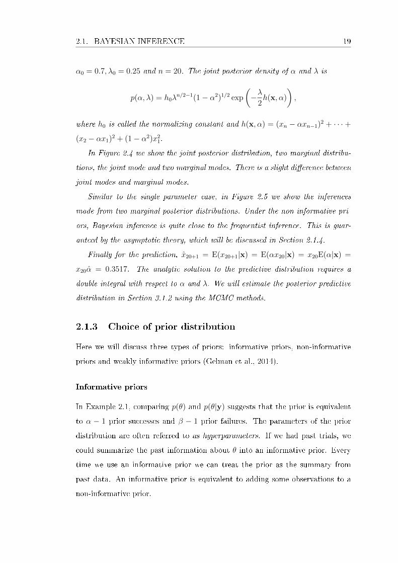
α0 = 0.7, λ0 = 0.25 and n = 20. The joint posterior density of α and λ is
p(α, λ) = h0λn/2−1(1− α2)1/2 exp
(−λ
2h(x, α)
),
where h0 is called the normalizing constant and h(x, α) = (xn − αxn−1)2 + · · · +
(x2 − αx1)2 + (1− α2)x21.
In Figure 2.4 we show the joint posterior distribution, two marginal distribu-
tions, the joint mode and two marginal modes. There is a slight dierence between
joint modes and marginal modes.
Similar to the single parameter case, in Figure 2.5 we show the inferences
made from two marginal posterior distributions. Under the non-informative pri-
ors, Bayesian inference is quite close to the frequentist inference. This is guar-
anteed by the asymptotic theory, which will be discussed in Section 2.1.4.
Finally for the prediction, x20+1 = E(x20+1|x) = E(αx20|x) = x20E(α|x) =
x20α = 0.3517. The analytic solution to the predictive distribution requires a
double integral with respect to α and λ. We will estimate the posterior predictive
distribution in Section 3.1.2 using the MCMC methods.
2.1.3 Choice of prior distribution
Here we will discuss three types of priors: informative priors, non-informative
priors and weakly informative priors (Gelman et al., 2014).
Informative priors
In Example 2.1, comparing p(θ) and p(θ|y) suggests that the prior is equivalent
to α − 1 prior successes and β − 1 prior failures. The parameters of the prior
distribution are often referred to as hyperparameters. If we had past trials, we
could summarize the past information about θ into an informative prior. Every
time we use an informative prior we can treat the prior as the summary from
past data. An informative prior is equivalent to adding some observations to a
non-informative prior.
20 CHAPTER 2. BAYESIAN FUNDAMENTALS
Sometimes informative priors are called strong priors, in the sense that they
aect the posterior distribution more strongly, relative to the data, than other
priors. The distinction between strong priors and weak priors is vague, and a
strong prior may become a weak prior as more data comes in to counterbalance
the strong prior. It is better to look at the prior together with the likelihood of
data.
Non-informative priors
There has been a desire for priors that can be guaranteed to play a minimal
role, ideally no role at all, in the posterior distribution. Such priors are vari-
ously called non-informative priors, uninformative priors, reference priors (Berger
et al., 2009), vague priors, at priors, or diuse priors. The rationale for using a
non-informative prior is often given as letting the data speak for themselves.
The Bernoulli-Beta model. In Example 2.1, Beta(1, 1) is a non-informative
prior, since it assumes that θ is distributed uniformly on [0, 1]. The posterior
distribution under this prior is the same as the likelihood. The posterior mode
will be equal to the maximum likelihood estimate∑n
i=1 yi/n. Note that the
posterior mean is not equal to the posterior mode.
If we want the posterior mean equal to the MLE, we need to specify α, β = 0.
This prior is called a improper non-informative prior since the integral of this
prior's pdf is not 1. When we use an improper non-informative prior, we need to
check whether the resulting posterior is proper. Fortunately, the posterior here
is proper.
The normal-normal model with known variance. Another example is the
normal model with unknown mean but known variance, shown as follows:
yi ∼ N(µ, σ2), i = 1, . . . , n
µ ∼ N(µ0, τ20 ).

2.1. BAYESIAN INFERENCE 21
If τ 20 → ∞, the prior is proportional to a constant, and is improper. But the
posterior is still proper, p(µ|y) ≈ N(µ|y, σ2/n). Here N(µ|y, σ2/n) is used to
represent the probability density function for variable µ, a normal distribution
with mean of y and variance of σ2/n.
The normal-normal model with known mean. Now assume the mean is
known and variance is unknown. We know that the conjugate prior for variance is
inverse-gamma distribution, i.e., σ−2 follows a gamma distribution, Gamma(α, β).
The non-informative prior is obtained as α, β → 0.
Here we parameterize it as a scaled inverse−χ2 distribution with scale σ20
and ν0 degrees of freedom; i.e., the prior distribution of σ2 is taken to be the
distribution of σ20ν0/X, where X is a χ2
ν0random variable. The model can be
written as follows:
yi ∼ N(µ, σ2), i = 1, . . . , n
σ2 ∼ Inv-χ2(ν0, σ20).
The resulting posterior distribution of σ2 can be shown as
σ2|y ∼ Inv-χ2
(ν0 + n,
ν0σ20 + nν
ν0 + n
),
where ν = 1/n∑n
i=1(yi − µ)2.
The non-informative prior is obtained as ν0 → 0, which is improper and
proportional to the inverse of the variance parameter. This non-informative prior
is sometimes written as p(log σ2) ∝ 1. The resulting posterior distribution is
proper, with the density function of p(σ2|y) ≈ Inv-χ2(σ2|n, ν). The uniform
prior distribution on σ2, i.e., p(σ2) ∝ 1, will lead to an improper posterior.
Jereys' priors. Finally, there is a family of non-informative priors called
Jereys' priors. The idea is that the non-informative priors should have the same
inuence as likelihood on the parameters. It can be shown that the Jereys' prior

22 CHAPTER 2. BAYESIAN FUNDAMENTALS
of θ is proportional to the squared root of Fisher information; i.e., p(θ) ∝ J(θ)1/2,
where
J(θ) = E
((d log p(y|θ)
dθ
)2∣∣∣∣∣θ)
= −E
(d2 log p(y|θ)
dθ2
∣∣∣∣θ) . (2.4)
As a simple justication, the Fisher information measures the curvature of the
log-likelihood, and high curvature occurs wherever small changes in parameter
values are associated with large changes in the likelihood. So the proportional
relationship ensures that Jereys' prior gives more weight to these parameters.
In Example 2.1, the Fisher information is J(θ) = n/(θ(1 − θ)). Hence, Jereys'
prior is p(θ) ∝ θ−1/2(1− θ)−1/2, which is Beta(0.5, 0.5).
Weakly informative priors
A weakly informative prior lies between informative priors and non-informative
priors. It is proper, but is set up so that the information it provides is intentionally
weaker than whatever actual prior knowledge is available. We do not use weakly
informative priors here. For more discussion, please refer to Gelman et al. (2014)
on page 55.
Example 2.4 (A single-parameter Bernoulli-Beta model). We continue with
Example 2.1 and consider the eects of two non-informative priors, Beta(1, 1)
and Beta(0.5, 0.5), on the posterior distributions. Under the uniform distribu-
tion Beta(1, 1), the posterior distribution is equal to the scaled likelihood, so the
posterior mode is equal to the MLE. Under the Jereys' prior Beta(0.5, 0.5), the
posterior distribution is quite close to the scaled likelihood. In both cases, the
eect of the priors on the posterior distribution is negligible.
In Figure 2.6, we plot the likelihood, the prior, and the posterior distribution.
As we expect, under the two non-informative priors the scaled likelihood is quite
close to the posterior distribution.

2.1. BAYESIAN INFERENCE 23
2.1.4 Asymptotic normality of the posterior distribution
Suppose y1, . . . , yn are outcomes sampled from a distribution f(y). We model
the data by a parametric family p(y|θ) : θ ∈ Θ, where θ is distributed as p(θ).
The result of large-sample Bayesian inference is that as more and more data
arrive, i.e., n→∞, the posterior distribution of the parameter vector approaches
multivariate normal distribution.
We label θ0 as the value of θ that minimizes the Kullback-Leibler diver-
gence KL(θ) of the likelihood p(y|θ) relative to the true distribution f(y). The
Kullback-Leibler divergence is dened as a function of θ as follows:
KL(θ) := Ef
(log
(f(y)
p (y|θ)
))= −
∫log
(f(y)
p (y|θ)
)f(y)dy.
When the true distribution is in the parametric family
If the true data distribution is included in the parametric family, i.e., f(y) =
p(y|θTrue) for some θTrue, then θ0 will approach θTrue as n → ∞. The posterior
distribution of θ approaches normality with mean θ0 and variance nJ(θ0)−1, where
J(θ0) is the Fisher information dened in equation (2.4).
The proof of asymptotic normality is based on the Taylor series expansion
of log posterior distribution, log p(θ|y), centred at the posterior mode up to the
quadratic term. As n → ∞, the likelihood dominates the prior, so we can just
use the likelihood to obtain the mean and variance of the normal approximation.
When the true distribution is not in the parametric family
The above discussion is based on the assumption that the true distribution is
included in the parametric family, i.e., f(y) ∈ p(y|θ) : θ ∈ Θ. When this as-
sumption fails, there is no true value θTrue ∈ Θ, and its role in the theoretical
result is replaced by the value θ0 which minimizes the Kullback-Leibler diver-
gence. Hence, we still have the similar asymptotic normality that the posterior
distribution of θ approaches normality with mean θ0 and variance nJ(θ0)−1. But

24 CHAPTER 2. BAYESIAN FUNDAMENTALS
now p(y|θ0) is no longer the true distribution f(y).
2.2 Model assessment and selection
In this section, we review the model diagnostic tools including posterior predictive
checking and residual plots. We also discuss the model selection criteria including
several information criteria and cross-validation.
2.2.1 Posterior predictive checking
In the classical framework, the testing error is preferred since it is calculated on a
testing data set which is not used to train the model. In the Bayesian framework,
ideally we want to split the data into a training set and a testing set and do
the posterior predictive checking on the testing data set. Alternatively, we can
choose a test statistic whose predictive distribution does not depend on unknown
parameters in the model but primarily on the assumption being checked. Then
there is no need to have a separate testing data set. Nevertheless, when the same
data are used for both tting and checking the model, this needs to be carried
out with caution, as the procedure can be conservative.
In frequentist statistics, p-value is typically dened as
p := Pr(T (y′) ≥ T (y)|H0),
where T is the function of data that generates the test statistic. T (y) is regarded
as a constant. The probability is calculated over the sampling distribution of y
under the null hypothesis. It is well known that p can be calculated exactly only
in the sense that T (y) is a pivotal quantity.
Meng (1994) explored the posterior predictive p-value (pB), a Bayesian version
of the classical p-value. pB is dened as the probability
pB := PrT (y′, θ) ≥ T (y, θ)|y, H0,

2.2. MODEL ASSESSMENT AND SELECTION 25
where y′ is the future data, and T (y, θ) is a discrepancy measure that possibly
depends on θ. This probability is calculated over the following distribution:
p(y′, θ|y, H0) = p(y′|θ)p(θ|y, H0),
where the form of p(θ|y, H0) depends on the nature of the null hypothesis. Fol-
lowing Meng (1994), we consider the two null hypotheses: a point hypothesis and
a composite hypothesis. For the completion of discussion, please refer to Robins
et al. (2000). They mentioned some problems associated with the posterior pre-
dictive p-value under a composite hypothesis.
When the null hypothesis is a point hypothesis
Suppose the null hypothesis is θk = a and the prior under the null hypothesis is
p(θ−k|θk = a) with the parameter space Θ ⊂ Rm−1. Then the posterior density
of θ under the null hypothesis is
p (θ|y, H0) =p (y|θ−k, θk = a) p (θ−k|θk = a)∫
Θp (y|θ−k, θk = a) p (θ−k|θk = a) dθ−k
.
The posterior predictive p-value is calculated as
pB = Pr T (y′, θ) ≥ T (y, θ) |y,H0
=
∫Θ
Pr T (y′, θ) ≥ T (y, θ) |θ p (θ|y, H0) dθ−k.
When the null hypothesis is a composite hypothesis
Suppose the null hypothesis is θk ∈ A and the prior under the null hypothesis is
p(θ−k|θk)p(θk). Then the posterior density of θ under the null hypothesis is
p (θ|y, H0) = p (θ−k|y, θk) p (θk) =p (y|θ) p (θ−k|θk)∫
Θp (y|θ) p (θ−k|θk) dθ−k
p (θk) .

26 CHAPTER 2. BAYESIAN FUNDAMENTALS
The posterior predictive p-value is calculated as
pB = Pr T (y′, θ) ≥ T (y, θ) |y, H0
=
∫Θ
∫A
Pr T (y′, θ) ≥ T (y, θ) |θ p (θ−k|y, θk) p (θk) dθkdθ−k.
Choice of T (y, θ)
Recall that in the frequentist theory, the most powerful test in a composite test,
H0 : θk ∈ A vs. H1 : θk /∈ A, is based on the generalized likelihood ratio dened
as follows:
Λg (y) :=supθk /∈Ap(y|θk)supθk∈Ap(y|θk)
.
Meng (1994) suggested using the conditional likelihood ratio and the generalized
likelihood ratio, dened respectively as follows:
CLR (y, θ) = TC (y, θ) :=supθk /∈Ap (y|θ)supθk∈Ap (y|θ)
GLR (y) = TG (y) :=supθk /∈Asupθ−k
p (y|θ)supθk∈Asupθ−k
p (y|θ).
Because a probability model can fail to reect the process that generated the
data in any number of ways, pB can be computed for a variety of discrepancy
measures T in order to evaluate more than one possible model failure.
Example 2.5 (A one-sample normal mean test using pB). This example is ex-
tracted from Meng (1994). Suppose we have a sample of size n from N(µ, σ2), and
we test the null hypothesis that µ = µ0 with σ2 unknown. Recall that in classical
testing, the pivotal test statistic is√n(x−µ0)/s, where x is the sample mean and
s2 is the sample variance. We know this test statistic follows a tn−1 distribution.
So p = Pr(tn−1 ≥√n(x− µ0)/s).
In the Bayesian framework, we assume µ and σ2 are independent and σ2 has

2.2. MODEL ASSESSMENT AND SELECTION 27
a non-informative prior (i.e., p(σ2) ∝ 1/σ2). We can nd CLR and GLR as
CLR(x, σ2
)= TC
(x, σ2
)=n(x− µ0)2
σ2
GLR (x) = TG (x) =n(x− µ0)2
s2.
Using the two discrepancy measures, we calculate pB as
pCB = PrTC(x′, σ2
)> TC
(x, σ2
)|x, µ0 = Pr
(F1, n >
n(x− µ0)2
s20
)pGB = PrTG (x′) > TG (x) |x, µ0 = PrF1, n−1 > TG (x),
where s20 =
∑ni=1(xi − µ0)2. Note that p = pGB 6= pCB; pB is equal to the classical
p-value when using GLR. See details in Appendix A on page 227.
Example 2.6 (Number of runs). Suppose we have a data set x = (x1, x2, . . . , x10) =
(1, 1, 1, 0, 0, 0, 0, 0, 1, 1), resulting from n = 10 Bernoulli trials with success prob-
ability θ which has an non-informative improper prior, Beta (0, 0). Now we want
to test the null hypothesis that the trials are independent of each other.
We use the number of runs in x as the test statistic, denoted by r(x). Note that
a run is dened as a subsequence of elements of one kind immediately preceded and
succeeded by elements of the other kind. So in this example we have r(x) = 3,
and θ is treated as a nuisance parameter. It is easy to nd that the posterior
distribution of θ is Beta(6, 6) under H0. To calculate pB = Prr(x′) ≤ 3|H0, we
apply the exact density of r(x′).
According to Kendall and Stuart (1961), assuming n1 1's and n2 0's are ran-
domly placed in a row, the number of runs, denoted by R (n1, n2), has the following
probability mass functions for 0 ≤ n2 ≤ n1 and 2 ≤ R ≤ n1 + n2 :
Pr R = 2s =2(n1−1s
)(n2−1s−1
)(n2−1s−1
) , for s = 1, . . . , n2
Pr R = 2s− 1 =
(n1−1s−2
)(n2−1s−1
)+(n1−1s−1
)(n2−1s−2
)(n2−1s−1
) , for s = 2, 3, . . . , n2.

28 CHAPTER 2. BAYESIAN FUNDAMENTALS
However, this probability mass function is not complete, missing the case when
R = 2n2 + 1 (i.e., R is odd and s = n2 + 1). For completeness, we add the two
special cases and their associated probabilities as in Table 2.13.
Applying the exact density of R (n1, n2), pB is calculated as
pB =
∫ 1
0
(10∑i=0
3∑j=1
PrR (i, 10− i) = jPr (n1 = i|θ)
)p(θ|x)dθ = 0.1630, (2.5)
which implies that under H0 the number of runs of a future observed sample would
be smaller than 3 with probability of 0.163. See details in Appendix A on page
230.
Furthermore, we list pB's calculated for other observations in Table 2.2. Note
that the sample test statistics in cases iv and vii reach the maximum number of
runs, so pB is denitely 1. However, we cannot conclude that x's are denitely
independent of each other, as these observations indicate that 1's are most likely
followed by 0's. We consider any pB smaller than 0.1 or larger than 0.9 as indi-
cating the violation of H0.
2.2.2 Residuals, deviance and deviance residuals
In the Bayesian framework, we can generate a set of residuals for one realization
of posterior parameters. So there are four choices of residuals:
• Choose the posterior mean of parameters and nd one set of residuals.
• Randomly choose a realization of parameters and nd one set of the resid-
uals.
• Get the posterior mean of residuals.
• Get the posterior distribution of residuals.
3In each chapter, all tables appear together at the end, after all the gures.

2.2. MODEL ASSESSMENT AND SELECTION 29
In the following, we will review Pearson residuals, deviance and deviance residu-
als. A Pearson residual is dened as
ri (θ) :=yi − E(yi|θ)√Var(yi|θ)
.
The deviance is dened as
D (θ) := −2 log p(y|θ) = −2n∑i=1
log p (yi|θ) , (2.6)
and the contribution of each data point to the deviance is Di (θ) = −2 log p (yi|θ) .
We will dene and use D(θ) and D (θ) in the next section.
The deviance residuals are based on a standardized or saturated version of
the deviance, dened as
DS (θ) := −2n∑i=1
log p (yi|θ) + 2n∑i=1
log p(yi
∣∣∣θS (y)),
where θS (y) are appropriate saturated estimates, e.g., we set θS (y) = y. The
contribution of each data point to the standardized deviance is
DSi(θ) = −2 log p (yi|θ) + 2 log p
(yi
∣∣∣θS (y)).
The deviance residual is dened as
dri := signi√DSi
(θ),
where signi is the sign of yi − E(y′i|θ).
Example 2.7 (Three error structures for stack-loss data). The data set con-
tains 21 daily responses of stack loss y, the amount of ammonia escaping, with
covariates being air ow x1, temperature x2 and acid concentration x3. We as-
sume a linear regression on the expectation of y, i.e., E (yi) = µi = β0 + β1zi1 +
β2zi2 + β3zi3, i = 1, . . . , 21. We consider three error structures: normal, double

30 CHAPTER 2. BAYESIAN FUNDAMENTALS
exponential and t4, as follows:
yi ∼ N(µi, τ−1)
yi ∼ DoubleExp(µi, τ−1)
yi ∼ t4(µi, τ−1),
where zij = (xij − xj) /sd (xj) for j = 1, 2, 3 are covariates standardized to
have zero mean and unit variance, and β0, β1, β2, β3 are given independent non-
informative priors.
The deviance residuals of the three models have the following forms respec-
tively:
DSi=√τ (yi − µi)
DSi= signi
√2τ |yi − µi|
DSi= signi
√√√√5 log
(1 +
(yi − µi)2
4
).
We plot the posterior distributions of deviance residuals for each model in Figure
2.7. The three residual plots agree on four outliers: 1, 3, 4 and 21.
2.2.3 Bayesian model selection methods
The model selection problem is a trade-o between a simple model and good
tting. Ideally, we want to choose the simplest model with best tting. However
good tting models tend to be more complicated while simpler models tend to be
undert. The model selection methods used in frequentist statistics are typically
cross-validation and information criteria, which are the modied residual sum of
squares with respect to the model complexity and overtting.
Cross-validation measures the t of a model on the testing data set, which is
not used to t the model, while the information criteria adjust the measure of t
on the training data set by adding a penalty for model complexity.

2.2. MODEL ASSESSMENT AND SELECTION 31
The predictive accuracy of a model
In the Bayesian framework, the t of a model is sometimes called the predictive
accuracy of a model (Gelman et al., 2014). We measure the predictive accuracy
of a model to a data set y′ by log point wise predictive density (lppd), calculated
as follows:
lppd:= logn′∏i=1
Eθ|yp (y′i|θ) =n′∑i=1
log(Eθ|yp (y′i|θ)
)=
n′∑i=1
log
(∫p(y′i|θ)p(θ|y)dθ
).
Ideally, y′ should not be used to t the model. If we choose y′ = y, we get
the within-sample lppd (denoted by lppdtrain), which is typically larger than the
out-of-sample lppd (denoted by lppdtest). To compute lppd in practice, we can
evaluate the expectation using draws from the posterior distribution p(θ|y), which
we label as θt, t = 1, . . . , T . The computed lppd is dened as follows:
computed lppd:=n′∑i=1
log
(1
T
n′∑i=1
p(y′i|θt)
).
Cross-validation
In Bayesian cross-validation, the data are repeatedly partitioned into a training
set ytrain and a testing set ytest. For simplicity, we restrict our attention to leave-
one-out cross-validation (LOO-CV), where ytest only contains a data point. The
Bayesian LOO-CV estimate of out-of-sample lppd is dened as follows:
lppdloo-cv :=n∑i=1
log
(∫p (yi|θ) p (θ|y−i) dθ
), (2.7)
where y−i is the data set without the ith point. The lppdloo-cv can be computed
as
computed lppdloo-cv =n∑i=1
log
(1
T
T∑t=1
p(yi|θit
)),
where θit, t = 1, . . . , T are the simulations from the posterior distribution p (θ|y−i) .

32 CHAPTER 2. BAYESIAN FUNDAMENTALS
Deviance information criterion (DIC)
AIC and BIC. Before describing the DIC, we review another two information
criteria employed in frequentist statistics. The Akaike information criterion (AIC)
by Akaike (1973) is dened as
AIC:=− 2n∑i=1
log p (yi|θMLE) + 2p.
The Bayesian information criterion (BIC) by Schwarz (1978) is dened as
BIC:=− 2n∑i=1
log p (yi|θMLE) + p log n,
where p is the number of parameters. The rst common term−2∑n
i=1 log p(yi|θMLE)
measures the discrepancy between the tted model and the data. The second term
measures the model complexity.
DIC. In the Bayesian framework, we dene a similar quantity to measure the
discrepancy, −2∑n
i=1 log p(yi|θ), where θ is the posterior mean. Spiegelhalter
et al. (2002) proposed a measure of number of eective parameters, which is
dened as the dierence between the posterior mean of the deviance and the
deviance at the posterior means, as follows:
pD := D (θ)−D(θ) = −2Eθ|y
(n∑i=1
log p (yi|θ)
)+ 2
n∑i=1
log p(yi
∣∣∣θ) ,where D is the deviance dened in equation (2.6).
Furthermore, they proposed a deviance information criterion (DIC), dened as
the deviance at the posterior means plus twice the eective number of parameters,
to give
DIC:=D(θ) + 2pD.
DIC is viewed as a Bayesian analogue of AIC. We prefer the model with smaller

2.2. MODEL ASSESSMENT AND SELECTION 33
DIC. Note that DIC and pD are sensitive to the level of a hierarchical model.
They are appropriate when we are interested in the parameters directly related
to the data. DIC and pD can be calculated using OpenBUGS, which will be
discussed in Section 3.3.
Watanabe-Akaike or widely available information criterion (WAIC)
Watanabe (2010) proposed another measure of number of eective parameters as
follows:
pWAIC := D(θ) + 2lppdtrain = −2Eθ|y
(n∑i=1
log p (yi|θ)
)+ 2
n∑i=1
log(Eθ|yp (yi|θ)
),
where −2lppdtrain plays a role as D(θ) as in pD. As with AIC and DIC, the
Watanabe-Akaike information criterion (WAIC) is dened as
WAIC:=− 2lppdtrain + 2pWAIC.
Leave-one-out information criterion (LOOIC)
Dierent from the denition of number of eective parameters in AIC, DIC, and
WAIC, we dene
ploo := lppdtrain − lppdloo-cv,
where lppdloo-cv comes from equation (2.7). The leave-one-out information crite-
rion (LOOIC) is dened as
LOOIC:=− 2lppdtrain + 2ploo = −2lppdloo-cv,
which is reasonable since lppdloo-cv already penalizes the overtting (or equiva-
lently the model complexity).
Example 2.8 (pD in a random eects model). This example follows Spiegelhalter

34 CHAPTER 2. BAYESIAN FUNDAMENTALS
et al. (2002). Consider the following random eects Bayesian model:
yij ∼ N(θi, τ−1i ), i = 1, . . . ,m, j = 1, . . . , n
θi ∼ N(µ, λ−1)
µ ∼ N(0,∞)
where τi, i = 1, . . . ,m, and λ are known precision parameters. τi is termed as the
within-group precision, and λ is termed as the between-group precision. It can be
shown that the posterior distribution of population mean is
µ|y ∼ N
y,
(λ
m∑i=1
ρi
)−1 ,
where
y =
∑mi=1 ρiyi∑mi=1 ρi
, ρi =τi
τi + λ, yi =
∑nj=1 yij
n.
Assuming θ = (θ1, . . . , θm), we will have the following equations:
D (θ) =∑
ρi + λ∑
ρi (1− ρi) (yi − y)2 +
∑ρi (1− ρi)∑
ρi
D(θ) = λ∑
ρi (1− ρi) (yi − y)2
pD =∑
ρi +
∑ρi (1− ρi)∑
ρi.
Consider the number of eective parameters pD under the following three cases:
• If λ→∞, then ρi → 0, and pD = 1. All the groups have the same mean µ,
which is the only eective parameter. The model is equivalent to:
yij ∼ N(µ, τ−1
i
), i = 1, . . . ,m, j = 1, . . . , n
µ ∼ N (0,∞) .
• If λ → 0, then ρi → 1, and pD = m. All the groups are independent and
2.2. MODEL ASSESSMENT AND SELECTION 35
have dierent means. The model is equivalent to:
yij ∼ N(θi, τ
−1i
), i = 1, . . . ,m, j = 1, . . . , n
θi ∼ N (0,∞) .
• If τi are equal, then ρ1 = . . . = ρm = ρ and pD = 1 + (m− 1) ρ.
In summary, if we assign the majority of variation in y to the within-group vari-
ation rather than between-group variation (i.e., λ is much larger than τi), then
the group means θi tend to converge to the population mean µ, and we have only
one parameter (i.e., θi cannot be eectively estimated distinguishably).
On the other hand, if we assign the majority of variation in y to the between-
group variation (i.e., τi is much larger than λ), then there is no accurate estimate
of µ, and every θi tends to escape from the trap distribution θi ∼ N (µ, λ−1).
Every θi can be eectively estimated by its group mean, and there are m eective
parameters.
Example 2.9 (Three error structures for stack-loss data). We continue with
Example 2.7 and calculate lppdloo-cv, DIC, pD, WAIC and pWAIC for the three
models discussed on page 29. As shown in Table 2.3, lppdloo-cv, DIC, and WAIC
agree on the model with double exponential error distribution.
2.2.4 Overtting in the Bayesian framework
Suppose that we have a sample of size n from a common normal distribution
with unknown mean and known precision, yi ∼ N (µ, τ−1) , i = 1, . . . ,m. In the
Bayesian framework we can assume m parameters, each of which is for one data
value. Such a Bayesian model can be written as follows:
yi ∼ N(µi, τ
−1), i = 1, . . . ,m
µi ∼ N(µ0, τ
−10
),

36 CHAPTER 2. BAYESIAN FUNDAMENTALS
where τ is known and p(µ0, τ−10 ) ∝ τ0 is a non-informative improper hyperprior.
This is a special case when n = 1 in Example 2.8.
This random eects model can also be viewed as a hierarchical model with
three levels. We refer to the top level distribution related to the data as the
sampling distribution or likelihood, the second level distribution as the prior
and the third level distribution as the hyperprior. Accordingly, µi, τ are called
parameters and µ0, τ0 are called hyperparameters.
The model has m data values and m+ 2 parameters, which presents an over-
tting issue in the frequentist framework on account of parameters treated as
unknown xed constants. However, it is quite common for the number of pa-
rameters to be larger than the number of data values in the Bayesian framework,
where the number of eective parameters would be smaller than m as shown in
Example 2.8.
2.3 Bibliographic notes
Bayesian statistics derives from Bayes' famous 1763 essay, which has been reprinted
as Bayes (1763). For other early contributions, see also Laplace (1785, 1810). Gel-
man et al. (2014) contains most of the current developments in Bayesian statistics.
Jereys' priors and the invariance principles for non-informative priors are
studied in Jereys (1961). The asymptotic normality of the posterior distribution
was known by Laplace (1810).
The method of posterior predictive checking was proposed by Rubin (1981,
1984). The posterior predictive p-value was studied by Meng (1994). Akaike
(1973) introduced the expected predictive deviance and AIC. Schwarz (1978)
introduced BIC. Spiegelhalter et al. (2002) introduced the DIC. Watanabe (2010,
2013) presented WAIC. RJMCMC was introduced by Green (1995). A recent
work summarizing criteria for evaluation of Bayesian model selection procedures
is Bayarri et al. (2012).

FIGURES 37
0.0 0.2 0.4 0.6 0.8 1.0
01
23
4
θ
Den
sity
0.0 0.1 0.2 0.3 0.4 0.5 0.6 0.7 0.8 0.9 1.0
Posterior densityPrior densityLikelihoodθ0
Posterior meanPosterior modePosterior median95% CPDRPrior meanMLE95% CI
Figure 2.1: The prior, posterior and likelihood of θ.
0.0 0.2 0.4 0.6 0.8 1.0
0.00
0.05
0.10
0.15
0.20
∑y m
pmf
0.0 0.1 0.2 0.3 0.4 0.5 0.6 0.7 0.8 0.9 1.0
0.033
0.111
0.191
0.225
0.197
0.133
0.071
0.029
0.0090.002 0
Predictive meanPredictive mode/median
Figure 2.2: The posterior predictive distribution of∑10
j=1 y′j/10.

38 CHAPTER 2. BAYESIAN FUNDAMENTALS
0.0 0.1 0.2 0.3 0.4
01
23
45
6
θ
Den
sity
Posterior densityPrior densityLikelihoodPosterior mean95% CPDRPrior meanMLE
Figure 2.3: The prior, posterior and likelihood of θ.
alpha
0.0
0.2
0.4
0.6
0.81.0lam
bda
0.0
0.2
0.4
0.6
0.8
1.0
Joint density
0
2
4
6
Joint mode (0.493, 0.389)Marginal mode 0.496
Marginal mode 0.370
Figure 2.4: The joint posterior distribution of α and λ.

FIGURES 39
0.0 0.2 0.4 0.6 0.8 1.0
0.0
0.5
1.0
1.5
2.0
α
Den
sity
Posterior meanPosterior modePosterior median95% CPDRα0
MLE95% CI
0.0 0.2 0.4 0.6 0.8 1.0
0.0
0.5
1.0
1.5
2.0
2.5
3.0
λ
Den
sity
Posterior meanPosterior modePosterior median95% CPDRλ0
MLE95% CI
Figure 2.5: The marginal posterior distributions of α and λ.

40 CHAPTER 2. BAYESIAN FUNDAMENTALS
0.0 0.2 0.4 0.6 0.8 1.0
01
23
4
θ
Den
sity
0.0 0.1 0.2 0.3 0.4 0.5 0.6 0.7 0.8 0.9 1.0
Posterior densityPrior densityLikelihoodθ0
Posterior meanPosterior modePosterior median95% CPDRPrior meanMLE95% CI
0.0 0.2 0.4 0.6 0.8 1.0
01
23
4
θ
Den
sity
0.0 0.1 0.2 0.3 0.4 0.5 0.6 0.7 0.8 0.9 1.0
Posterior densityPrior densityLikelihoodθ0
Posterior meanPosterior modePosterior median95% CPDRPrior meanMLE95% CI
Figure 2.6: The eect of two non-informative priors, Beta(1, 1) and Beta(0.5, 0.5),on the posterior distribution.

FIGURES 41
1 2 3 4 5 6 7 8 9 10 11 12 13 14 15 16 17 18 19 20 21
−4
−2
02
4
Nor
mal
1 2 3 4 5 6 7 8 9 10 11 12 13 14 15 16 17 18 19 20 21
−4
−2
02
4
Dou
ble
Exp
1 2 3 4 5 6 7 8 9 10 11 12 13 14 15 16 17 18 19 20 21
−4
−2
02
4
t(4)
Figure 2.7: The deviance residual plots of the three models.

42 CHAPTER 2. BAYESIAN FUNDAMENTALS
Table 2.1: Special cases for the probability of R(n1, n2).
n1 n2 s Pr(R(n1, n2) = 2s− 1)≥1 0 1 1
≥ n2 + 1 n2 ≥ 1 n2 + 1(n1−1n2
)/(n1+n2
n1
)
Table 2.2: pB's for other observations.
Case Sample x n r(x) pBi (1, 1, 1, 1, 1, 1, 1, 1, 1, 1) 10 1 0.5293ii (0,0,0,0,0, 1,1,1,1,1) 10 2 0.0462iii (0,1,1,0,1, 1,0,1,1,1) 10 6 0.6066iv (0,1,0,1,0, 1,0,1,0,1) 10 10 1v (1,0,1,1,1, 0,0,1,1,0, 1,0,1,1,0) 15 10 0.9354vi (1,1,1,1,1, 0,0,0,0,0, 1,1,1,1,1, 1,1,1,1,1, 1,1,1,0,0) 25 4 0.0248vii (1,0,1,0,1, 0,1,0,1,0, 1,0,1,0,1, 0,1,0,1,0, 1,0,1,0,1) 25 25 1
Table 2.3: lppdloo-cv, DIC and WAIC for the three models.
Error structures lppdloo-cv DIC pD WAIC pWAIC
Normal -59.0 115.5 5.23 116.5 4.8DoubleExp -57.3 113.3 5.53 114.5 5.7
t4 -57.8 114.2 5.53 115.6 5.8
Chapter 3
Advanced Bayesian Computation
The popularity of Bayesian statistics is largely due to advances in computing
and developments in computational methods. Currently, there are two types of
Bayesian computational methods. The rst type involves iterative Monte Carlo
simulation and includes the Gibbs sampler, the Metropolis-Hastings algorithm,
Hamiltonian sampling etc. These methods (of the rst type) typically generate
a Markov chain whose stationary distribution is the target distribution (i.e., the
posterior distribution of parameters in the context of Bayesian inference). The
second type involves distributional approximation and includes Laplace approxi-
mation (Laplace, 1785, 1810), variational Bayes (Jordan et al., 1999) etc. These
methods (of the second type) follow a dierent philosophy. They try to nd a
distribution with the analytical form that best approximates the target distribu-
tion.
In Section 3.1, we review Markov chain Monte Carlo (MCMC) methods in-
cluding the general Metropolis-Hastings algorithm (M-H), Gibbs sampler with
conjugacy, and Hamiltonian Monte Carlo (HMC) algorithm (Neal, 1994). Sec-
tion 3.2 discusses the convergence and eciency of the above sampling methods.
We then show how to specify a Bayesian model and draw model inferences us-
ing OpenBUGS and Stan in Section 3.3. Section 3.4 provides a brief summary
on the mode-based approximation methods including Laplace approximation and
43

44 CHAPTER 3. ADVANCED BAYESIAN COMPUTATION
Bayesian variational inference. Finally, in Section 3.5, a full Bayesian analysis is
performed on a biological data set from Gelfand et al. (1990). The key concepts in
Chapter 2 and the computational tools discussed in this chapter are demonstrated
in this section.
3.1 Markov chain Monte Carlo (MCMC) methods
In Section 2.1, we discussed how to make inferences about parameters from the
posterior distribution. When the posterior distribution is complicated, it is te-
dious to make any inferences analytically. We have seen that in Example 2.3
the marginal posterior distribution p(λ|y) contains a complicated integral. Even
if p(λ|y) can be found analytically, it still requires some eort to get the exact
posterior mean and the CPDR of λ. This motivates us to explore other methods.
Monte Carlo simulation is a sampling process from a target distribution. Once
sucient samples are obtained, the inferences of target distribution can be ap-
proximated by sample statistics, such as sample mean, sample standard error,
sample percentile etc. The traditional Monte Carlo simulation methods involve
inversing the cumulative distribution function, the rejection sampling method,
etc. These methods generate independent samples. In contrast, Markov chain
Monte Carlo (MCMC) methods generate a Markov chain whose stationary dis-
tribution is equivalent to the target distribution. In MCMC, the next sampled
value typically depends on the previous sampled value.
In this section, we rst briey state some properties of a Markov chain with
a stationary distribution. Then the Metropolis-Hastings (M-H) algorithm, Gibbs
sampler and Hamiltonian Monte Carlo (HMC) are reviewed. Throughout this
section, we continue with Example 2.3. We compare the MC-based inferences to
analytical inferences.

3.1. MARKOV CHAIN MONTE CARLO (MCMC) METHODS 45
3.1.1 Markov chain and its stationary distribution
Let X be a nite set. A Markov chain is characterized by a transition matrix
K (x, y) with K (x, y) ≥ 0 for any x, y ∈ X , and∑
y K (x, y) = 1 for any x ∈ X .
Note that the nth power of K (x, y) has (x, y) entry of Pr(Xn = y|X0 = x). All of
the Markov chains considered in this chapter have a stationary distribution π (x)
which satises the equation
∑x∈X
π (x) K (x, y) = π (y) .
The stationary theorem of Markov chains says, under a simple connectedness
condition, π is unique, and high powers of K converge to a rank one matrix with
all rows equal to π. That is
Kn (x, y)→ π (y) for each x, y ∈ X .
The probabilistic content of the theorem is that from any starting state x, the
nth step of a run of the Markov chain has a chance close to π (y) of being at y
if n is large. In computational settings, when the cardinality of X is large, it is
easy to move from x to y according to K (x, y), but it is hard to sample from π
directly.
Example 3.1 (The stationary distribution of a Markov chain process). Suppose
a Markov chain with the sample space S = 0, 1, 2, 3, and a transition matrix as
follows:
K =
0.9 0.1 0 0
0.9 0 0.1 0
0.9 0 0 0.1
0.9 0 0 0.1
.

46 CHAPTER 3. ADVANCED BAYESIAN COMPUTATION
A little more calculation shows that
K4 =
0.9 0.09 0.009 0.001
0.9 0.09 0.009 0.001
0.9 0.09 0.009 0.001
0.9 0.09 0.009 0.001
,
so that for some m ≥ 4, Km (x1, y) = Km (x2, y) for all x1, x2 ∈ S. It follows
that Km+1 = Km, since
Km+1 (x, y) =∑z∈S
K (x, z) Km (z, y) = Km (x, y)∑z∈S
K (x, z) = Km (x, y) .
Therefore, limn→∞Kn (x, y) = Km (x, y) = π (y), where we write the nal equality
without reference to x since all the rows of Km (x, y) are identical. π (y) is the
stationary distribution.
3.1.2 Single-component Metropolis-Hastings (M-H) algo-
rithm
When x contains multiple variables, instead of sampling the whole x at a time, it is
often more convenient and computationally ecient to divide x into components
as x1, x2, .., xh, and sample these components one by one, i.e., using single-
component Metropolis-Hastings.
An iteration of the single-component Metropolis-Hastings algorithm comprises
h updating processes. Suppose x is updated sequentially according to the com-
ponent index and the target multivariate distribution as π. The ith updating
process for xi at the tth iteration in the M-H algorithm works as follows:
1. Draw a value from a proposal distribution of xi, gi(x∗i |xt−1
i , xt−i), where
xt−i =xt+1
1 , . . . , xt+1i−1, x
ti+1, . . . , x
th
, and xt−1
i denotes the value of xi at the
end of iteration t− 1 or denotes the initial value when t = 1.

3.1. MARKOV CHAIN MONTE CARLO (MCMC) METHODS 47
2. Calculate the acceptance ratio
Ai(x∗i , x
t−1i
)=
π(x∗i |xt−i
)gi(x
t−1i |x∗i , xt−i)
π(xt−1i |xt−i
)gi(x∗i |xt−1
i , xt−i),
where π(·|xt−i
)is the full conditional distribution of xi.
3. Accept x∗i and set xti = x∗i with probability Ai(x∗i , x
t−1i
). Otherwise, reject
x∗i and set xti = xt−1i .
Note that the parameters in the proposal distribution gi are called tuning pa-
rameters ; these are specied in advance and will aect the acceptance rates and
the convergence. In Section 3.3, we will see that OpenBUGS has a phase called
adapting, when the program automatically chooses the appropriate tuning pa-
rameters. In the M-H algorithm, we need to discard the rst few iterations,
which are called burn-in. We judge the length of burn-in by looking at trace
plots, BGR plots (Gelman and Rubin, 1992) or potential scale reduction factor
(Gelman et al., 2014), which will be discussed in Section 3.2.1.
Example 3.2 (An autoregressive process of order one). We continue with Ex-
ample 2.3 on page 18. Now we complete the following tasks:
1. Write a M-H algorithm to generate a sample of size T = 1000 from the joint
posterior distribution p (α, λ|x), and produce trace plots for α and λ. Also
calculate the acceptance rates for both parameters.
2. Draw histograms for the sampled values in (1) and superimpose density
estimates of marginal posterior distributions, p (α|x) and p (λ|x). Estimate
the posterior means α and λ and give the 95% condence intervals for them.
Also report the 95% CPDR estimates for α and λ.
Solutions to (1): Instead of using p (α, λ|x) directly, we take the logarithm of
it, denoted by l (α, λ|x), and calculate the acceptance ratio on a logarithm scale.
The tth iteration in the M-H algorithm is as follows:

48 CHAPTER 3. ADVANCED BAYESIAN COMPUTATION
1. Draw a proposed value α∗ ∼ U (α− c, α + c) . If α∗ /∈ [−1, 1] , reject it and
redraw. Otherwise, calculate the acceptance ratio:
Aα(α∗, αt−1
)= exp
[l(α∗|x, λt−1
)− l(αt−1|x, λt−1
)],
where αt−1 and λt−1 are the values at the end of the (t − 1)th iteration
or the initial values when t = 1. If Aα (α∗, αt−1) ≥ 1, accept α∗ and set
αt = α∗. If Aα (α∗, αt−1) ≤ 1, accept α∗ and set αt = α∗ with probability of
Aα (α∗, αt−1); otherwise, set αt = αt−1.
2. Draw a proposed value λ∗ ∼ U (α− d, α + d). If λ∗ < 0, reject it and
redraw. Otherwise, calculate the acceptance ratio:
Aλ(λ∗, λt−1
)= exp
[l(λ∗|x, αt
)− l(λt−1|x, αt
)],
where αt comes from step 1. If Aλ (λ∗, λt−1) ≥ 1, accept λ∗ and set λt =
λ∗. If Aλ (λ∗, λt−1) ≤ 1, accept λ∗ and set λt = λ∗ with probability of
Aλ (λ∗, λt−1); otherwise, set λt = λt−1.
With c = 0.3, d = 0.2, α0 = 0, λ0 = 1, the M-H algorithm converges within 100
iterations with acceptance rate of 71% for α and 69% for λ over a total of 10, 000
iterations. The trace plots for α and λ are shown in Figure 3.1.
Solutions to (2): The last 9, 900 sampled values are used for inference. The
MC estimate of posterior mean α is α = (∑10000
t=101 αt)/9900 = 0.4721, with the
95% CI (α− 1.96
√Var (α)
9900, α + 1.96
√Var (α)
9900
)= (0.4683, 0.4759) ,
where Var (α) is the MC sample variance (i.e., the sample variance of αt, t =
101, . . . , 10000). The MC estimate of 95% CPDR for α is (0.0726, 0.8188).
Similarly, the MC estimate of posterior mean λ is λ = (∑10000
t=101 λt)/9900 =

3.1. MARKOV CHAIN MONTE CARLO (MCMC) METHODS 49
0.4101, with the 95% CI (0.4075, 0.4126). The MC estimate of 95% CPDR for λ
is (0.1947, 0.6959). We show the MC histograms and the MC density estimates
comparing with the exact densities in Figure 3.2. We can see the MC estimates
are quite close to the exact values.
Since there is strong series dependence in a Markov chain, it is not good to
make inferences directly from the original MCMC sample. Two methods can be
applied to reduce the dependence: the batch means (BM) method and the thinning
sample (TS) method. We will discuss these two methods in more detail in Section
3.2.2. In the batch means method we place 20 bins and in the thinning sample
method we extract one value from every 20 successive samples. Table 3.1 lists the
inferences made from the two methods. Note that * indicates the exact posterior
mean is in the 95% CI.
3.1.3 Gibbs sampler
The Gibbs sampler is another MCMC method which simulates the joint distri-
bution via full conditional distributions. In fact, if we choose the full conditional
distribution of each component in single-component M-H algorithm as the pro-
posal distribution for this component, i.e., gi(x∗i∣∣xt−1i , xt−i
)= π
(x∗i∣∣xt−i) , the
acceptance ratio will be
Ai(x∗i , x
t−1i
)=π(x∗i∣∣xt−i) π (xt−1
i
∣∣xt−i)π(xt−1i
∣∣xt−i) π (x∗i ∣∣xt−i) = 1,
which guarantees the proposed value x∗i being accepted. So the Gibbs sampler is
a special case of the M-H algorithm.
Compared with the M-H algorithm, the Gibbs sampler does not have the
accept-reject step and tuning parameters. However, the main diculty with the
Gibbs sampler is simulating from the full conditional distribution which some-
times does not have a recognizable form. In that case, we may turn to other
sampling methods such as adaptive rejection sampling1 (Gilks and Wild, 1992).
1See details in Appendix B on page 234.

50 CHAPTER 3. ADVANCED BAYESIAN COMPUTATION
Adaptive rejection sampling is a generalized rejection sampling method that
can be used to simulate for any univariate log-concave probability density func-
tion. As sampling proceeds, the rejection envelope and the squeezing function
converge to the target function. The adaptive rejection sampling and the M-H
algorithm are both intended for the situation where there is non-conjugacy of the
Gibbs sampler in a Bayesian model.
Example 3.3 (An autoregressive process of order one). We continue with Exam-
ple 2.3. The Gibbs sampler is applied to the joint posterior distribution of α and λ.
The full conditional distributions are
p (α|x, λ) ∝(1− α2
) 12 exp
[−λ
2h (x, α)
]
λ|x, α ∼ Gamma
(n
2,h (x, α)
2
).
The full conditional distribution of α is unrecognisable. We can write a Gibbs
sampler for λ and keep the M-H algorithm for α.
To simulate x21, we add an extra step to every iteration: draw a value from
N(αtx20, 1/λj
t), where αj
t, λjt are the ending values at the tth iteration. Similar
to Table 3.1, we can obtain the new MC estimates based on the Gibbs sampler as
shown in Table 3.2.
The Rao-Blackwell method. Another way to nd the posterior mean and the
posterior marginal density is to apply the Rao-Blackwell (RB) method. We can
estimate the marginal posterior distribution of λ as
p (λ|x) =1
T
T∑t=1
Gamma
(λ
∣∣∣∣n2 , h (x, αt)
2
),

3.1. MARKOV CHAIN MONTE CARLO (MCMC) METHODS 51
where αt is the tth sampled value from the posterior distribution p (α|x). The
posterior mean is estimated as
λ =1
T
T∑t=1
n
h (x, αt).
The 95% CI for posterior mean is calculated as (λ ± 1.96s/√T ), where s is the
sample standard deviation of n/h (x, αt) , t = 1, . . . , T.
Similarly, we can estimate the posterior predictive distribution of x21 as
p (x21|x) =1
T
T∑t=1
p(x20
∣∣x, αt, λt) =1
T
T∑t=1
N
(x21
∣∣∣∣αtx20,1
λt
).
The posterior mean of x21 is estimated as
x21 =1
T
T∑t=1
αtx20.
The 95% CI for the posterior mean is calculated as(x21 ± 1.96s/
√T), where s
is the sample standard deviation of αtx20, t = 1, . . . , T. We summarize the Rao-
Blackwell estimates in Figure 3.3. We see that the 95% RB CIs cover the exact
posterior means, and the RB density estimate of λ is almost equal to its exact
density.
3.1.4 Hamiltonian Monte Carlo (HMC)
HMC was introduced to physics by Duane et al. (1987) and to statistical problems
by Neal (1994, 2011). In contrast to the random-walk Metropolis algorithm where
the proposed value is not related to the target distribution, HMC proposes a value
by computing a trajectory according to Hamiltonian dynamics that takes account
of the target distribution.

52 CHAPTER 3. ADVANCED BAYESIAN COMPUTATION
Hamiltonian dynamics
Suppose we have a Hamiltonian dynamics scenario in which a frictionless ball
slides over a surface of varying height. The state of the ball at any time consists
of the position and the momentum. Denote the position by a h vector θ and the
momentum by a same length vector φ.
Hamiltonian functions can be written as
H(θ, φ) = U(θ) +K(φ),
where U(θ) is called the potential energy and will be dened to be minus the log
probability density of the distribution of θ we wish to simulate, K(φ) is called
the kinetic energy and is usually dened as
K(φ) = φTΣ−1φ/2,
where Σ−1 is a symmetric positive-denite mass matrix which is typically di-
agonal and is often a scalar multiple of the identity matrix. This form of K(φ)
corresponds to the minus log probability density of the zero-mean Gaussian dis-
tribution with covariance matrix Σ.
The state of the ball in the next innitesimal time is determined by Hamilton's
equations of motion:
dθidt
=∂H
∂φi= [Σ−1φ]i
dφidt
= −∂H∂θi
= −∂U∂θi
.
For computer implementation, Hamilton's equation must be approximated by
discretizing time, using some small step size, ε. The most straightforward method
is Euler's method. The solution to the above system of dierential equations can
3.1. MARKOV CHAIN MONTE CARLO (MCMC) METHODS 53
be approximated by Euler's method as follows:
φi(t+ ε) = φi(t) + εdφidt
(t) = φi(t)− ε∂U
∂θi(θi(t))
θi(t+ ε) = θi(t) + εdθidt
(t) = θi(t) + ε[Σ−1φ]i.
However, Euler's method does not preserve the volume and the resulting trajec-
tory would diverge from the exact trajectory to innity. A better trajectory may
be generated by using the leapfrog method as follows:
φi(t+ ε/2) = φi(t)− (ε/2)∂U
∂θi(θi(t))
θi(t+ ε) = θi(t) + ε[Σ−1φ(t+ ε/2)]i
φi(t+ ε) = φi(t+ ε/2)− (ε/2)∂U
∂θi(θi(t+ ε)).
The leapfrog method preserves volume exactly.
MCMC from Hamiltonian dynamics
Suppose we want to simulate a sample from the target density p(θ). HMC intro-
duces auxiliary momentum variables φ and draws from a joint density p(θ, φ). We
assume the auxiliary density is a multivariate Gaussian distribution, independent
of the parameter θ. The covariance matrix Σ acts as a Euclidean metric to rotate
and scale the target distribution. The joint density p(θ, φ) denes a Hamiltonian
function as follows:
H(θ, φ) = − log p(θ, φ) = − log p(θ)− log p(φ) = U(θ) +K(φ).
Starting from the value of the parameters at the end of the t−1th iteration, θt−1,
a new value θ∗ is proposed by two steps before being subjected to a Metropolis
accept step.
First, a value φt−1 for the momentum is drawn from the multivariate Gaus-
sian distribution, N(0,Σ). Next the joint system (θt−1, φt−1) is evolved via the
54 CHAPTER 3. ADVANCED BAYESIAN COMPUTATION
following leapfrog method for L steps to get the proposed value (θ∗, φ∗):
φt−1+ε/2i = φt−1
i + (ε/2)∂ log p(θt−1)
∂θi
θt−1+εi = θt−1
i + ε[Σ−1φt−1+ε/2]i
φt−1+εi = φ
t−1+ε/2i + (ε/2)
∂ log p(θt−1+ε)
∂θi.
Note that θ∗ = θt−1+εL, φ∗ = φt−1+εL. If there were no numerical errors in the
leapfrog step (i.e., the leapfrog trajectory followed the exact trajectory), we would
accept (θ∗, φ∗) denitely. However, there are always errors given the non-zero step
size. Hence, we conduct a Metropolis accept step with the acceptance rate as
min1, exp[H(θt−1, φt−1)−H(θ∗, φ∗)].
Neal (1994) suggests that HMC is optimally ecient when its acceptance rate is
approximately 65% while the multi-dimensional M-H algorithm is optimal at an
acceptance rate of around 23%.
The no-U-turn sampler (NUTS)
There are three tuning parameters in HMC: the mass matrix Σ, the step size ε and
the number of steps L. If ε is too large, the resulting trajectory will be inaccurate
and too many proposals will be rejected. If ε is too small, too many steps will be
taken by the leapfrog method, leading to long simulation times per iteration. If L
is too small, the trajectory traced out will be too short and sampling will devolve
to a random walk. If L is too large, the algorithm will spend too much time in
one iteration. The mass matrix Σ needs to be comparable with the covariance of
the posterior.
In MCMC, all the tuning parameters should be xed during the simulation
that will be used for inference; otherwise the algorithm may converge to the
wrong distribution. BUGS has an adaptive period during which suitable tuning
parameters are selected.

3.2. CONVERGENCE AND EFFICIENCY 55
NUTS (Homan and Gelman, 2014) can dynamically adjust the number of
leapfrog steps at each iteration to send the trajectory as far as it can go during
that iteration. If such a rule is applied alone, the simulation will not converge
to the desired target distribution. The full NUTS is more complicated, going
backward and forward along the trajectory in a way that satises detailed balance
(Gelman et al., 2014).
The programming of NUTS is much more complicated than a M-H algorithm.
We rely on Stan to implement NUTS inferential engine. More details of Stan
are provided in Section 3.3. Along with this algorithm, Stan can automatically
optimize ε to match an acceptance rate target and estimate Σ based on warm up
iterations. Hence we do not need to specify any tuning parameters in Stan.
3.2 Convergence and eciency
Two concerns in MCMC methods are checking the convergence of sampled values
and designing an ecient algorithm.
3.2.1 Convergence
We can detect the convergence by eye, relying on the trace plots such as Figure
3.1. Informally speaking, a fat hairy caterpillar appearance indicates the con-
vergence. For numerical diagnosis, we use the Brooks-Gelman-Rubin (BGR) ratio
and potential scale reduction factor, both of which are based on the mixture and
stationarity of simulated multiple chains starting from diversied initial values.
The Brooks-Gelman-Rubin (BGR) ratio
The numerical diagnosis for convergence in OpenBUGS is based on comparing
within- and between- chain variability (Gelman and Rubin, 1992). Suppose we
simulate I chains, each of length J , with a view to assessing the degree of sta-
tionarity in the nal J/2 iterations. We take the width of 100 (1− α) % credible
56 CHAPTER 3. ADVANCED BAYESIAN COMPUTATION
interval for the parameter of interest as a measure of posterior variability.
From the nal J/2 iterations we calculate the width of empirical 100 (1− α) %
credible interval for each chain as Wi, i = 1, . . . , I, then nd the average width
across these chains as W =∑I
i=1Wi/m. We also pool IJ iterations together and
nd the pooled width B.
The BGR ratio is dened as the ratio of pooled interval widths to average
interval widths, RBGR = B/W. It should be larger than 1 if the starting values
are suitably diversied and will tend to be 1 as convergence is approached. So
we can assume convergence for practical purposes if RBGR < 1.05.
Brooks and Gelman (1998) further suggested splitting the total iteration range
of each chain intoM batches of length a = J/M and calculating B(m),W (m) and
RBGR(m) based on the latter halves of iterations (1, . . . ,ma) for m = 1, . . . ,M .
The potential scale reduction factor
Gelman et al. (2014) propose a similar quantity to monitor the convergence,
namely potential scale reduction factor. This factor is automatically monitored
in Stan. Again, suppose we simulate I chains, each of length J (this is all after
discarding the burn-in iterations). We split each chain into two parts to get 2I
batches, each of length J/2. We label the simulations as θi,j, i = 1, .., 2I, j =
1, . . . , J/2 and calculate the between- and within- batch variances as a measure
of posterior variability rather than the width of credible interval as in BGR.
The average within-batch variance is WVar =∑2I
i=1 s2i , where s
2i is the sample
variance of the ith batch. The between-batch variance is
BVar =J/2
2I − 1
2I∑i=1
(θi· − θ
)2,
where θi· is the sample mean of ith batch and θ is the pooled sample mean. The
reason for containing a factor of J/2 is that BVar is based on the sample variance
of batch means θi· Note that WVar and BVar are both estimates of the posterior
variance Var (θ|y). Later we will show that√BVar/IJ is the MC standard error

3.2. CONVERGENCE AND EFFICIENCY 57
of the posterior mean estimate using batch-mean method.
Gelman et al. (2014) proposes an estimate of Var (θ|y) as a weighted average
of WVar and BVar:
Var (θ|y) =J/2− 1
JWVar +
1
JBVar,
which is also an unbiased estimate under stationarity, but an overestimate if
involving the burn-in iterations. On the other hand, WVar always underestimates
Var (θ|y) due to limited sample size J/2 and dependent iterations. So we monitor
convergence by estimating the potential scale reduction factor by
R =
√Var (θ|y)
WVar
, (3.1)
which declines to 1 as J → ∞. If R is high, we believe that more iterations are
needed to guarantee the convergence.
3.2.2 Eciency
For a given sample size, the accuracy of our inferences is dependent on the e-
ciency of the posterior sample, which decreases with an increasing level of auto-
correlation. We can improve the eciency by rening the algorithm or resampling
from the MC sample to reduce the correlation.
Reparameterization, thinning and adding auxiliary variables
One way of increasing eciency is to reparameterize the model so that the pos-
terior correlation among parameters is reduced, as shown in Example 3.4 and
Section 3.5.4.
Another way to improve eciency is to perform a process known as thinning,
whereby only every vth value from the MC sample is actually retained for infer-
ence. In Section 3.3, we will see there is an option of thin in the OpenBUGS
Update Tool window.

58 CHAPTER 3. ADVANCED BAYESIAN COMPUTATION
Finally, the Gibbs sampler can often be simplied or the convergence can be
accelerated by adding an auxiliary variable (Gelman et al., 2014).
The batch means method
In Example 2.3 we are interested in the 95% CI of the posterior mean. The
standard error of the posterior mean estimate (i.e., the MC sample mean) is
calculated by the sample standard deviation over the squared root of sample size.
This follows the central limit theorem (CLT) under the condition of independent
samples. However, the MC sample is from a Markov chain and each sampled
value depends on the previous sampled value. The MC sample variance is not an
accurate estimate of the posterior variance Var (θ|y). We will turn to the batch
means method to get a more accurate estimate.
Suppose we have I chains, each of length J , and split every chain into M
batches, each of length J/M , and J/M is suciently large that CLT holds for
each batch. We label the simulations as θij, i = 1, .., IM, j = 1, . . . , J/M .
We calculate the batch means θi·, which are roughly independent and iden-
tically distributed with a mean of posterior mean and a variance of posterior
variance over J/M . Then we can use the sample variance of batch means to
estimate the posterior variance as
Var (θ|y) =J/M
IM − 1
IM∑i=1
(θi· − θ
)2.
The standard error of the posterior mean estimate θ =∑
ij θij/(IJ) can be ap-
proximated more accurately by
√Var (θ|y)
IJ=
√√√√ 1
IM (IM − 1)
IM∑i=1
(θi· − θ
)2, (3.2)
which is also called the Monte Carlo standard error given in the MC_error
column in OpenBUGS output and the se_mean column in Stan. Using the

3.2. CONVERGENCE AND EFFICIENCY 59
batch means method, the 95% CI of θ is modied as
(θ ± 1.96
√Var (θ|y)/(IJ)
).
Eective sample size
Gelman et al. (2014) dened an estimate of eective sample size as
ne =IJ
1 + 2∑∞
t=1 ρt, (3.3)
where I, J follow the notation in batch means method and ρt is the autocorrelation
of the MC sample at lag t. Stan automatically monitors ne for each parameter
of interest and gives them in the column of neect.
Example 3.4 (Reparameterize a simple linear regression model). Consider the
simple linear regression model: yi ∼ N (a+ bxi, σ2) , i = 1, . . . , 30, with true pa-
rameters a = 17, b = 3, σ2 = 16. Assume x = (0.5, 1.0, . . . , 15) and generate a
response vector y = (y1, y2, . . . , y30) . We assume a non-informative prior, i.e.,
p (a, b, σ2) ∝ 1/σ2.
Gibbs sampler (1). A Gibbs sampler which could be applied here is based on
the following full conditional distributions:
a|· ∼ N
(1
n
n∑i=1
(yi − bxi) ,σ2
n
)
b|· ∼ N
(∑ni=1 xi (yi − a)∑n
i=1 xi2
,σ2∑ni=1 xi
2
)σ2|· ∼ Inv-Gamma
(n
2,
∑ni=1 (yi − a− bxi)2
2
).
The dependence of p (a|·) on b makes the Gibbs sampler (1) ineective, especially
for σ2. We reparameterize the simple linear regression model as
yi ∼ N(c+ b (xi − x) , σ2
),
60 CHAPTER 3. ADVANCED BAYESIAN COMPUTATION
where c = a + bx. The prior for c can be shown as N (a+ bx,∞). So c also has
a non-informative at prior.
Gibbs sampler (2). An alternative Gibbs sampler is based on the following
full conditional distributions:
c|· ∼ N
(1
n
n∑i=1
yi,σ2
n
)
b|· ∼ N
(∑ni=1 (xi − x) yi∑ni=1 (xi − x)2 ,
σ2∑ni=1 (xi − x)2
)
σ2|· ∼ Inv-Gamma
(n
2,
∑ni=1 (yi − c− bxi + bx)2
2
),
where p (c|·) does not depend on b and p(b|·) is not dependent on c. The inde-
pendence between full conditional distributions will make Gibbs sampler (2) more
eective than Gibbs sampler (1).
We compare the MC estimates and the least-squares estimates in Table 3.3.
Gibbs sampler (2) improves the MC estimates of posterior means σ2, y′, while
performing equally well for a and b as Gibbs sampler (1).
3.3 OpenBUGS and Stan
The MCMC methods are useful Bayesian model computation tools, especially
when the posterior distribution does not have a closed form. The programming
of MCMC requires a lot of eort, even for a simple linear regression model as
in Example 3.4. Moreover, we need to customize a MCMC algorithm for every
model. To relieve the burden of programming MCMC, several packages have
been developed. The two main statistical packages are BUGS and Stan. We will
see in this section how to use these two packages to do a Bayesian analysis.

3.3. OPENBUGS AND STAN 61
3.3.1 OpenBUGS
BUGS stands for Bayesian inference Using Gibbs Sampler. The BUGS project
began in 1989 and has developed into two versions: WinBUGS and OpenBUGS.
Currently all development is focused on OpenBUGS. As its name suggests, Open-
BUGS uses a Gibbs sampler which updates unknown quantities one by one, based
on their full conditional distribution.
The MCMC building blocks include the conjugacy Gibbs sampler, the M-H
algorithm, various types of rejection sampling and slice sampling2. Such methods
are used only as a means of updating full conditional distributions within a Gibbs
sampler. OpenBUGS has an expert system, which determines an appropriate
MCMC method for analysing a specied model.
Directed graphical models
Suppose we have a set of quantities G arranged as a direct acyclic graph, in which
each quantity υ ∈ G represents a node in the graph. The intermediate nodes
always have parents and descendants. The relationship between parent and
child can be logical or stochastic. If it is a logical relationship, the value of the
node is determined exactly by its parents. If it is a stochastic relationship, the
value of the node is generated by a distribution which is determined only by its
parents.
Conditional on its parents, denoted by pa [υ], υ is independent of all the other
nodes except its descendants, denoted by ch [υ]. This conditional independence
assumption implies the joint distribution of all the quantities G has a simple
factorization in terms of the conditional distribution p(υ|pa [υ]), as follows:
p (G) =∏υ∈G
p(υ|pa [υ]),
where the conditional distribution may degenerate to a logical function of its
2See details in Appendix B on page 236.

62 CHAPTER 3. ADVANCED BAYESIAN COMPUTATION
parents if the relationship is logical. The full joint distribution p (G) can be fully
specied by the parent-child relationships.
The crucial idea behind BUGS is that this factorization forms the basis for
both the model description and the computational methods. The Gibbs sampler
for each unknown quantity θi, is based on the following full conditional distribu-
tion:
p (θi|θ−i, y) ∝ p (θi|pa [θi])×∏
υ∈ch[θi]
p (υ|pa [υ]) .
Note that θi can be any unknown quantities, not just unknown parameters. An
important implication of directed graphical models is that every node should
appear in the left side of an assignment sign only once. This implication can be
used as a debugging tool of the BUGS language.
The BUGS language
For a complex model, it is better to use the BUGS language to specify the model
rather than using a graphical model. It takes time for R users to get used to
BUGS. The fundamental dierence is the declarative language in BUGS, so it
does not matter in which order the statements come in BUGS.
3.3.2 Stan
Stan stands for Sampling Through Adaptive Neighbourhoods, which applies the
no-U-turn sampler (NUTS). Besides the no-U-turn sampler, Stan can also ap-
proximate Bayesian inference using variational Bayes, which will be discussed in
Section 3.4.2, and do penalized maximum likelihood estimation if we specify the
priors as the penalized term.
The key steps of the algorithm include data and model input, computation of
the log posterior density (up to an arbitrary constant that cannot depend on the
parameters in the model) and its gradients, a warm-up phase in which the tuning
parameters, ε and M , are set, an implementation of NUTS to move through the
parameter space, convergence monitoring, and inferential summaries at the end.

3.3. OPENBUGS AND STAN 63
Compared with OpenBUGS, Stan works seamlessly with R. Stan is installed
as a package in R. The output from Stan is stored in R automatically and can be
analyzed and plotted in R directly. Instead, BUGS works by itself. BUGS has its
own graph tools and output form. The output from BUGS needs to be transferred
into another package such as R before it can be used for further analysis.
Stan can analyze all the BUGS examples. It provides more instructive error
messages than BUGS. This is particularly helpful when we work with a black
box inferential engine. Stan can solve the multi-level models with unknown
covariance matrices which BUGS can not easily deal with. Moreover, it is easier
to specify the constraints of parameters in Stan.
Example 3.5 (An autoregressive process of order one). We continue with Ex-
ample 3.2. Rather than programming the MCMC, we rely on BUGS and Stan to
make inference.
BUGS. A graphical model (also called a Doodle) representation is shown in
Figure 3.4. For the simplicity, we only assume 6 observations. The single arrows
imply stochastic relationship, while double arrows imply logical relationship. A
parent constant is denoted by a squared plate, while other nodes are denoted
by ellipse plates. The BUGS can generate codes from graphical model by using
pretty print under model menu.
The modelling procedure using BUGS language typically includes the following
steps:
1. Check the syntax of the model specication by Specication Tool; if the
model is correctly specied, the message model is syntactically correct will
appear on the bottom left of the screen.
2. Read in the following data by clicking load data:
list(K=20,x=
c( -0.58196581 , -1.70339058 , -4.29434356 , -2.00495593 ,
-0.09234224 , -1.56433489 , -0.49151508 , -1.55912920 ,
-0.90546327 , -1.31576285 , -1.12240668 , 0.50931757 ,

64 CHAPTER 3. ADVANCED BAYESIAN COMPUTATION
0.54899741 , -1.87582922 , -4.54187225 , -0.41553845 ,
0.31656492 , -0.32832899 , 1.69457825 , 0.73050020)).
The message data loaded will appear.
3. Specify the number of chains as 2 and compile the model. The message
model compiled will appear.
4. Load the following initial values:
list(alpha =-0.99, lambda =100)
list(alpha =0.99 , lambda =0.001).
The message model initialised or initial values loaded but chain contains
uninitialised variables will appear. In the second case, we need to click gen
inits, which will generate initial values from priors.
After compiling and loading data, BUGS will choose an appropriate MCMC
method for each unknown quantity, which is shown under the menu In-
fo/Updater types.
5. Start the simulation using Update Tool. We have the following options:
• Thin: Every kth iteration will be used for inference.
• Adapting: This will be ticked while the M-H or slice sampling is in its
initial tuning phase where some optimization parameters are tuned.
• Over relax: This generates multiple samples at each iteration and then
selects one that is negatively correlated with the current value. The
within-chain correlations should be reduced.
6. Monitor the interested unknown quantities using Sample Monitor Tool.
Typing * into the node box means all monitored nodes.
7. Diagnose the convergence via bgr diag plots and trace plots shown in Figure
3.5. MCMC converges after 750 iterations, so we can rely on the subsequent
iterations to make inferences.
8. Report the inferences. We can get the inference by clicking stats in Sam-
ple Monitor Tool window. OpenBUGS also automatically reports DIC, pD,
D (θ) (shown as Dbar), and D(θ) (shown as Dhat). In this example, pD

3.4. MODAL AND DISTRIBUTIONAL APPROXIMATIONS 65
is close to the number of parameters. See the following output:
Dbar Dhat DIC pD
x 75.83 73.86 77.81 1.975
total 75.83 73.86 77.81 1.975
Stan. Programming in Stan is more exible and easier than in BUGS. For
example, there is no need to specify at priors, logical operators are allowed in
stochastic expressions, constraints are easily incorporated, and there are more
instructive error messages.
When applying Stan, we run 1, 000 iterations for each of four chains. By
default, Stan discards the rst half of each chain as burn-in. In the output, the
last row is normalized log posterior density. The se_mean column contains the
MC errors dened in equation (3.2). The last two columns correspond to ne and
R, which we dened in equation (3.3) and equation (3.1). The posterior densities
of α, λ, x21 and log posterior density are shown in Figure 3.6, which are similar
to Figure 3.2 and 3.3.
3.4 Modal and distributional approximations
The joint posterior modes can be found using the optimizing( ) function in Stan,
which applies the Broyden-Fletcher-Goldfarb-Shanno (BFGS) algorithm (No-
cedal and Wright, 2006). Conditional maximization Newton's method can also
nd the posterior joint modes. For the marginal modes, a well-known method is
the expectation-maximization (EM) algorithm.
3.4.1 Laplace approximation
Once the posterior mode is found, we can approximate the target distribution by a
multivariate Gaussian distribution with the same mode and covariance matrix as
the inverse of the log posterior density curvature at the mode. This approximation

66 CHAPTER 3. ADVANCED BAYESIAN COMPUTATION
works well for large sample sizes following the asymptotic theory discussed in
Section 2.1.4.
3.4.2 Variational inference
When facing a dicult problem for which we cannot give an exact solution, we
typically have two alternatives. One is to stick to this problem and give an
approximation to the exact answer. That is what the MCMC methods do. We
approximate the exact posterior distribution using a Markov chain. The other
is to introduce a closely similar problem for which we can give an exact answer.
That is what the variational inference tries to do.
We introduce an approximate distribution family q that is easier to deal with
than p(θ|y). The log model evidence log p(y) can be written as follows:
log p(y) = logp(y, θ)
p(θ|y)
=
∫q(θ) log
p(y, θ)
p(θ|y)dθ
=
∫q(θ)
(log
q(θ)
p(θ|y)+ log
p(y, θ)
q(θ)
)dθ
=
∫q(θ) log
q(θ)
p(θ|y)dθ +
∫q(θ) log
p(y, θ)
q(θ)dθ
= KL[q||p] + F (q,y),
where the rst term in the last line is called the Kullback-Leibler divergence be-
tween q(θ) and p(θ|y), and the second term is called free energy. If we want to
nd an approximate distribution q to minimize KL[q||p], we can just maximize
the free energy since the model evidence is a constant given the sample.

3.4. MODAL AND DISTRIBUTIONAL APPROXIMATIONS 67
Mean eld variational inference
A common choice of q(θ) is to assume it can be factorized into independent
partitions:
q(θ) =h∏i=1
qi(θi).
This assumption is called mean eld assumption. Under this assumption, if we
dissect out the dependence on qk(θk), then the free energy can be written as
F (q,y) =
∫q(θ) log
p(y, θ)
q(θ)dθ
=
∫ h∏i=1
qi(θi)×
(log p(y, θ)−
h∑i=1
log qi(θi)
)dθ
=
∫qk(θk)
∏i 6=k
qi(θi)× [log p(y, θ)− log qk(θk)] dθ
−∫qk(θk)
∏i 6=k
qi(θi)∑i 6=k
log qi(θi)dθ
=
∫qk(θk)
(∫ ∏i 6=k
qi(θi) log p(y, θ)dθ−k − log qk(θk)
)dθk
−∫qk(θk)
(∫ ∏i 6=k
qi(θi)∑i 6=k
log qi(θi)dθ−k
)dθk
=
∫qk(θk) log
expEθ−klog p(y, θ)
qk(θk)dθk + C
= −KL[qk(θk)|| expEθ−k
log p(y, θ)]
+ C.
Then the approximate distribution qk(θk) that maximizes the free energy is given
by
q∗k = argmaxqk
F (q,y) =expEθ−k
log p(y, θ)Z
.
This implies a straightforward algorithm for variational inference. Assume the
parameters in distribution qk are φk. The algorithm consists of the following two
steps:
1. Determine the form of the approximating distribution. Average log p (y, θ)

68 CHAPTER 3. ADVANCED BAYESIAN COMPUTATION
over q−k (θ−k) to nd the marginal approximate distribution q∗k, whose pa-
rameters are some function of parameters in q−k, φ−k.
2. Iterative update φ. The rst step establishes the a circular dependence
among φi. We iterate φ until there are no more visible changes and use the
last update q (θ|φ) as an approximation to p (θ|y).
3.5 A Bayesian hierarchical model for rats data
We have seen a hierarchical model in Example 2.8. A hierarchical model is often
used when considering the variations on dierent levels. For most hierarchical
models, the posterior distribution does not have a closed form. We compute
Bayesian inference via programming a MCMC algorithm or using BUGS/Stan.
In this section, we reanalyze the rats' weights data set shown in Table 3.4,
and extend the work by Gelfand et al. (1990) and Lunn et al. (2000). The data
set contains the weights of 60 rats measured weekly for 5 weeks. The rst 30 rats
are under control while the rest are under treatment. Our interest is the eect of
treatment on the growth rates and on the growth volatility.
In Section 3.5.1, a classical xed eects model and a random eects model
are considered. In Section 3.5.2 and 3.5.3, two Bayesian hierarchical models are
used. The advantages of Bayesian models are the accommodation of parameters
uncertainties and the inherent hierarchical structure. We turn to Stan to do
model inference in this section. In Section 3.5.4, we reparameterize the univariate
normal hierarchical model to propose a more ecient Gibbs sampler as we did in
Example 3.4.
3.5.1 Classical regression models
We rst t a xed eects model, then a random eects model with rat IDs as
group levels. We will see that the random eects model is better at capturing the
two levels of variation: between-rat variation and within-rat variation.
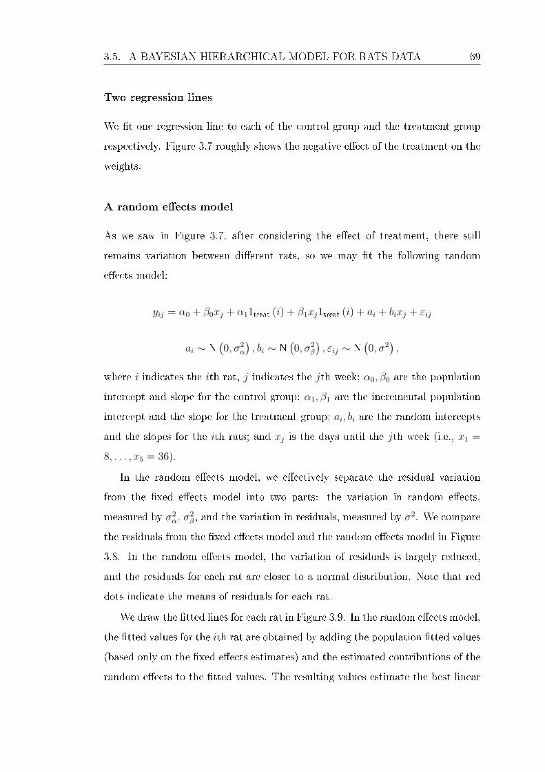
3.5. A BAYESIAN HIERARCHICAL MODEL FOR RATS DATA 69
Two regression lines
We t one regression line to each of the control group and the treatment group
respectively. Figure 3.7 roughly shows the negative eect of the treatment on the
weights.
A random eects model
As we saw in Figure 3.7, after considering the eect of treatment, there still
remains variation between dierent rats, so we may t the following random
eects model:
yij = α0 + β0xj + α11treat (i) + β1xj1treat (i) + ai + bixj + εij
ai ∼ N(0, σ2
α
), bi ∼ N
(0, σ2
β
), εij ∼ N
(0, σ2
),
where i indicates the ith rat, j indicates the jth week; α0, β0 are the population
intercept and slope for the control group; α1, β1 are the incremental population
intercept and the slope for the treatment group; ai, bi are the random intercepts
and the slopes for the ith rats; and xj is the days until the jth week (i.e., x1 =
8, . . . , x5 = 36).
In the random eects model, we eectively separate the residual variation
from the xed eects model into two parts: the variation in random eects,
measured by σ2α, σ
2β, and the variation in residuals, measured by σ2. We compare
the residuals from the xed eects model and the random eects model in Figure
3.8. In the random eects model, the variation of residuals is largely reduced,
and the residuals for each rat are closer to a normal distribution. Note that red
dots indicate the means of residuals for each rat.
We draw the tted lines for each rat in Figure 3.9. In the random eects model,
the tted values for the ith rat are obtained by adding the population tted values
(based only on the xed eects estimates) and the estimated contributions of the
random eects to the tted values. The resulting values estimate the best linear

70 CHAPTER 3. ADVANCED BAYESIAN COMPUTATION
unbiased predictions (BLUPs) for the ith rat.
One interest is the eect of treatment on the growth rate, measured by β1. The
summary output shows the signicant negative eect of treatment on the growth
rate. Another interest is whether a rat with higher birth weight will grow faster.
A Pearson correlation test of intercepts and slopes shows there is no signicant
relationship between birth weights and growth rates.
3.5.2 A Bayesian bivariate normal hierarchical model
A Bayesian bivariate normal hierarchical model is used to t both control and
treatment groups as follows:
yij ∼ N(αi + βixj, σ
2c
), i = 1, . . . , 30
yij ∼ N(αi + βixj, σ
2t
), i = 31, . . . , 60αi
βi
∼ N
αβ
,Σc
, i = 1, . . . , 30
αiβi
∼ N
α + ∆α
β + ∆β
,Σt
, i = 31, . . . , 60
Σc,Σt ∼ Inv-Wishart
200 0
0 0.2
−1
, 2
,
(3.4)
where α, β,∆α,∆β, σ2c , σ
2t have non-informative priors.
We are interested in the eect of treatment on the growth rate, ∆β, the
variation ratio of treatment group to control group, σt/σc, and the correlation
between growth rates and born weights (for either control group, i.e., ρc, or
treatment group, i.e., ρt), ρc/t = Σc/t [1, 2] /√
Σc/t [1, 1] Σc/t [2, 2].
In Stan, we simulate four chains, each of 400 iterations, and discard the rst
halves. The MC estimates are shown in Table 3.5. The MC estimated posterior
densities of interested quantities are drawn in Figure 3.11. According to Table
3.5 and Figure 3.11, we make the following conclusion: the eect of treatment

3.5. A BAYESIAN HIERARCHICAL MODEL FOR RATS DATA 71
on the growth rates is negative, i.e., the CPDR of ∆β = βt − βc is negative;
the treatment group is less volatile, i.e., the CPDR of σt/σc is less than 1; there
is no signicant relationship between born weights and growth rates for either
group, i.e., the CPDRs of ρc and ρt contain 0. Finally, Figure 3.10 validates the
assumption of normal error distribution.
3.5.3 A Bayesian univariate normal hierarchical model
In the previous section, ρ is not signicantly dierent from 0. If we can assume
that ρ = 0, the bivariate normal hierarchical model (3.4) can be simplied to a
univariate normal hierarchical model, as follows:
yij ∼ N(αi + βixj, σ
2c
), i = 1, . . . , 30
yij ∼ N(αi + βixj, σ
2t
), i = 31, . . . , 60
αi ∼ N(α, σ2
αc
), i = 1, . . . , 30
βi ∼ N(β, σ2
βc
), i = 1, . . . , 30
αi ∼ N(α + ∆α, σ2
αt
), i = 31, . . . , 60
βi ∼ N(β + ∆β, σ2
βt
), i = 31, . . . , 60,
(3.5)
where α, β,∆α,∆β, σ2αc, σ
2αt, σ
2βc, σ
2βt, σ
2c , σ
2t are assumed to have non-informative
priors. We get similar estimates of ∆β and σt/σc as in model (3.4). We display
the model selection criteria in Table 3.6. Both DIC and WAIC agree on the best
model (3.5).
3.5.4 Reparameterization in the Gibbs sampler
An issue arises when R is used to reproduce the results from the Stan analysis.
Table 3.7 shows the posterior mean estimates of scale parameters in model (3.5)
using a Gibbs sampler coded in R, compared with the estimates from Stan. The
estimates of σc and σt using the R Gibbs sampler are unduly large.
The eectiveness of the Gibbs sampler crucially depends on the choice of

72 CHAPTER 3. ADVANCED BAYESIAN COMPUTATION
parameters to be simulated. Gelman et al. (2014) suggested parameterization
in terms of independent components as an approach to constructing an ecient
simulation algorithm. Following the suggestion, model (3.5) is reparameterized
as follows:
yij ∼ N(γi + βi (xij − xi) , σ
2c
), i = 1, . . . , 30
yij ∼ N(γi + βi (xij − xi) , σ
2t
), i = 31, . . . , 60
γi ∼ N(α + βxi, σ
2αc + σ2
βcxi2), i = 1, . . . , 30
βi ∼ N(β, σ2
βc
), i = 1, . . . , 30
γi ∼ N(α + ∆α + (β + ∆β) xi, σ
2αt + σ2
βtxi2), i = 31, . . . , 60
βi ∼ N(β + ∆β, σ2
βt
), i = 31, . . . , 60,
where the prior of γi is derived based on the relationship γi = αi + βixi.
For i = 1, . . . , 30, the full conditional distributions of γi and βi are
γi|· ∼ N
(∑5j=1 yij
(σ2αc + σ2
βcxi2)
+ (α + βxi)σ2c
5(σ2αc + σ2
βcxi2)
+ σ2c
,
(σ2αc + σ2
βcxi2)σ2c
5(σ2αc + σ2
βcxi2)
+ σ2c
)
βi|· ∼ N
(∑5j=1 yij (xij − xi)σ
2βc + βσ2
c∑5j=1 (xij − xi)
2σ2βc + σ2
c
,σ2βcσ
2c∑5
j=1 (xij − xi)2σ2
βc + σ2c
),
where p(γi| ·) does not depend on βi and p(βi|·) does not depend on γi. We
use these full conditional distributions to update γi, βi, and then recover αi as
γi − βixi. This new Gibbs sampler gives more accurate posterior mean estimates
of scale parameters, as shown in Table 3.7.
3.6 Bibliographic notes
Metropolis et al. (1953) were the rst to describe the Metropolis algorithm. This
was generalized by Hastings (1970). The Gibbs sampler was rst so-named by
Geman and Geman (1984). HMC was introduced by Duane et al. (1987) in the
physics literature and Neal (1994) for statistics problems.

3.6. BIBLIOGRAPHIC NOTES 73
Gelman and Rubin (1992) and Brooks and Gelman (1998) provided a the-
oretical justication of the convergence checking methods presented in Section
3.2.1 and 3.2.2. For improving the eciency of MCMC, Tanner and Wong (1987)
discussed data augmentation and auxiliary variables. Hills and Smith (1992)
and Roberts and Sahu (1997) discussed dierent parameterizations for the Gibbs
sampler.
Lunn et al. (2012) is the rst book about the BUGS project. Other references
to BUGS include Lunn et al. (2000) and Spiegelhalter et al. (2003). The references
to Stan include Stan Development Team (2012), Carpenter et al. (2015), Gelman
et al. (2015), Homan and Gelman (2014) and Kucukelbir et al. (2015). Vehtari
et al. (2015) demonstrated the calculation of WAIC and LOO cross-validation in
Stan.
The EM algorithm was rst presented in full generality by Dempster et al.
(1977). Some references on variational Bayes include Jordan et al. (1999), Jaakkola
and Jordan (2000), Blei et al. (2003) and Gershman et al. (2012). Homan et al.
(2013) presented a stochastic variational algorithm that is computable for large
datasets.
Gilks et al. (1996) is a book full of examples and applications of MCMC
methods. The data and model investigated in Section 3.5 are from Gelfand et al.
(1990).
For other sampling methods, Neal (2003) discussed slice sampling, and Gilks
and Wild (1992) introduced adaptive rejection sampling.
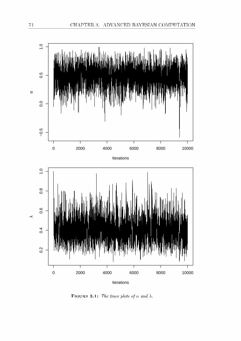
74 CHAPTER 3. ADVANCED BAYESIAN COMPUTATION
0 2000 4000 6000 8000 10000
−0.
50.
00.
51.
0
Iterations
α
0 2000 4000 6000 8000 10000
0.2
0.4
0.6
0.8
1.0
Iterations
λ
Figure 3.1: The trace plots of α and λ.
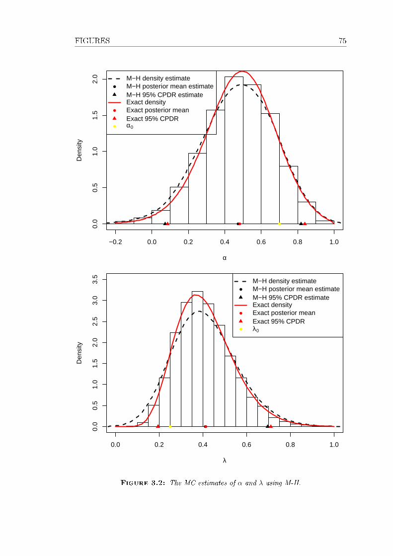
FIGURES 75
α
Den
sity
−0.2 0.0 0.2 0.4 0.6 0.8 1.0
0.0
0.5
1.0
1.5
2.0
M−H density estimateM−H posterior mean estimateM−H 95% CPDR estimateExact densityExact posterior meanExact 95% CPDRα0
λ
Den
sity
0.0 0.2 0.4 0.6 0.8 1.0
0.0
0.5
1.0
1.5
2.0
2.5
3.0
3.5
M−H density estimateM−H posterior mean estimateM−H 95% CPDR estimateExact densityExact posterior meanExact 95% CPDRλ0
Figure 3.2: The MC estimates of α and λ using M-H.

76 CHAPTER 3. ADVANCED BAYESIAN COMPUTATION
λ
Den
sity
0.2 0.4 0.6 0.8 1.0
0.0
0.5
1.0
1.5
2.0
2.5
3.0
RB density estimateRB posterior mean estimateRB 95% CIExact densityExact posterior meanλ0
x21
Den
sity
−4 −2 0 2 4 6
0.00
0.05
0.10
0.15
0.20
0.25
RB density estimateRB posterior mean estimateRB 95% CIExact posterior mean
Figure 3.3: The Rao-Blackwell estimates of λ and x21.
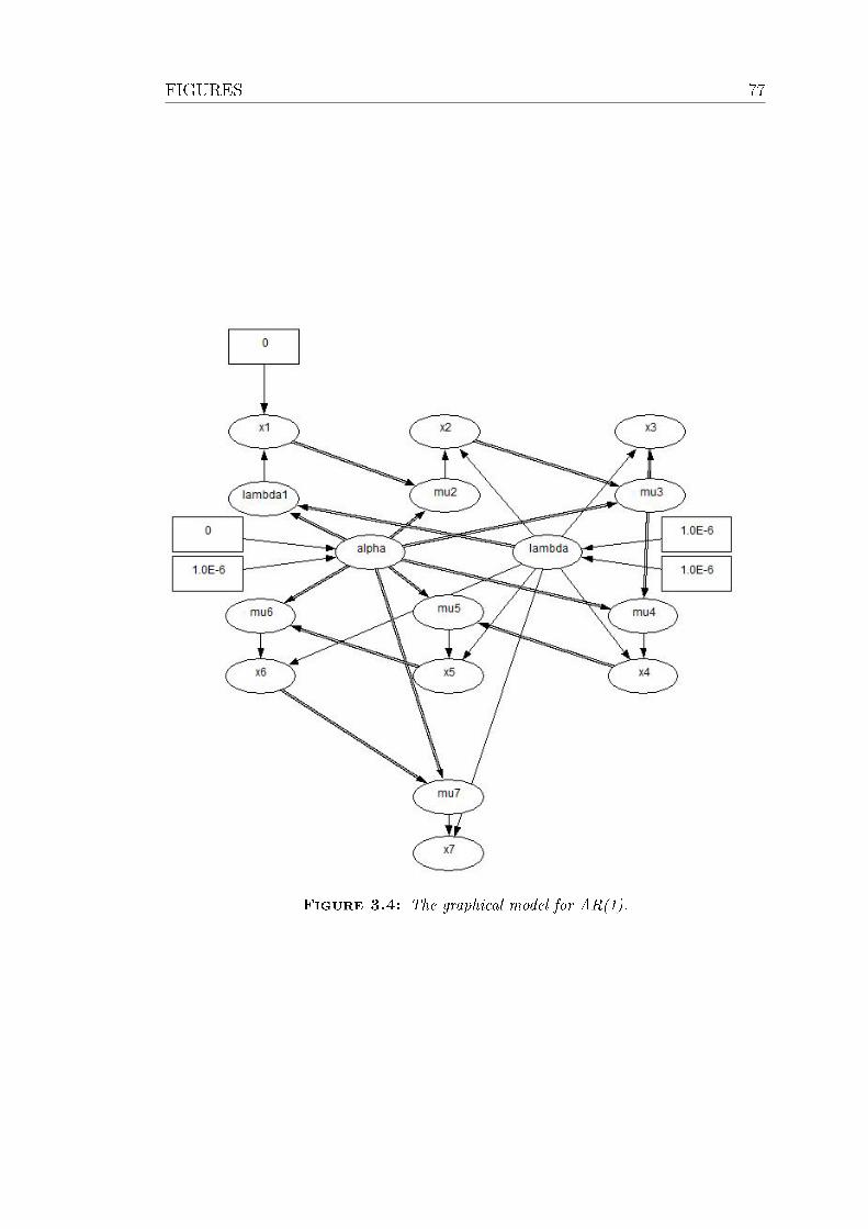
FIGURES 77
Figure 3.4: The graphical model for AR(1).
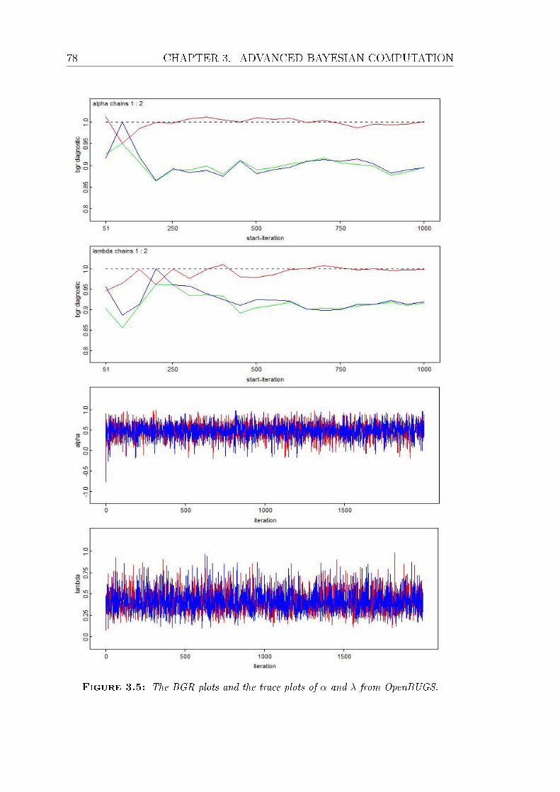
78 CHAPTER 3. ADVANCED BAYESIAN COMPUTATION
Figure 3.5: The BGR plots and the trace plots of α and λ from OpenBUGS.

FIGURES 79
α
Den
sity
−0.4 −0.2 0.0 0.2 0.4 0.6 0.8 1.0
0.0
0.5
1.0
1.5
2.0
Posterior mean estimate
λ
Den
sity
0.0 0.2 0.4 0.6 0.8 1.0
0.0
0.5
1.0
1.5
2.0
2.5
3.0
Posterior mean estimate
x21
Den
sity
−4 −2 0 2 4
0.00
0.05
0.10
0.15
0.20
0.25
Posterior mean estimate
log posterior density
Den
sity
−26 −24 −22 −20 −18
0.0
0.1
0.2
0.3
0.4
Figure 3.6: The MC estimates of α, λ and log posterior density from Stan.

80 CHAPTER 3. ADVANCED BAYESIAN COMPUTATION
10 15 20 25 30 35
100
150
200
250
300
350
Days
Wei
ghts
ControlTreatment
Figure 3.7: Two regression lines for the control and treatment groups.
−40 0 20 40 60
010
2030
4050
60
Residuals from fixed effects model
Rat
ID
−15 −5 0 5 10 15
010
2030
4050
60
Residuals from random effects model
Rat
ID
Figure 3.8: Residuals from the xed eects model and the random eects model.

FIGURES 81
10 15 20 25 30 35
100
150
200
250
300
350
Days
Wei
ghts
ControlTreatment
Figure 3.9: Fitted lines in the random eects model.
100 200 300
−2
−1
01
2
Scatter plot of residuals
Fitted posterior mean
Pos
terio
r re
sidu
als
mea
n
−3 −2 −1 0 1 2 3
−2
−1
01
2
Normal Q−Q plot
Theoretical Quantiles
Sam
ple
Qua
ntile
s
Figure 3.10: The deviance residual plots of the Bayesian bivariate model.

82 CHAPTER 3. ADVANCED BAYESIAN COMPUTATION
βt − βc
Den
sity
−1.8 −1.6 −1.4 −1.2 −1.0 −0.8
0.0
0.5
1.0
1.5
2.0
2.5
ρc
Den
sity
−1.0 −0.5 0.0 0.5 1.0
0.0
0.5
1.0
1.5
σt/σc
Den
sity
0.5 0.6 0.7 0.8 0.9
01
23
45
ρt
Den
sity
−1.0 −0.5 0.0 0.5 1.0
0.0
0.5
1.0
1.5
2.0
Figure 3.11: The posterior density plots of interested parameters in the Bayesian
bivariate model.
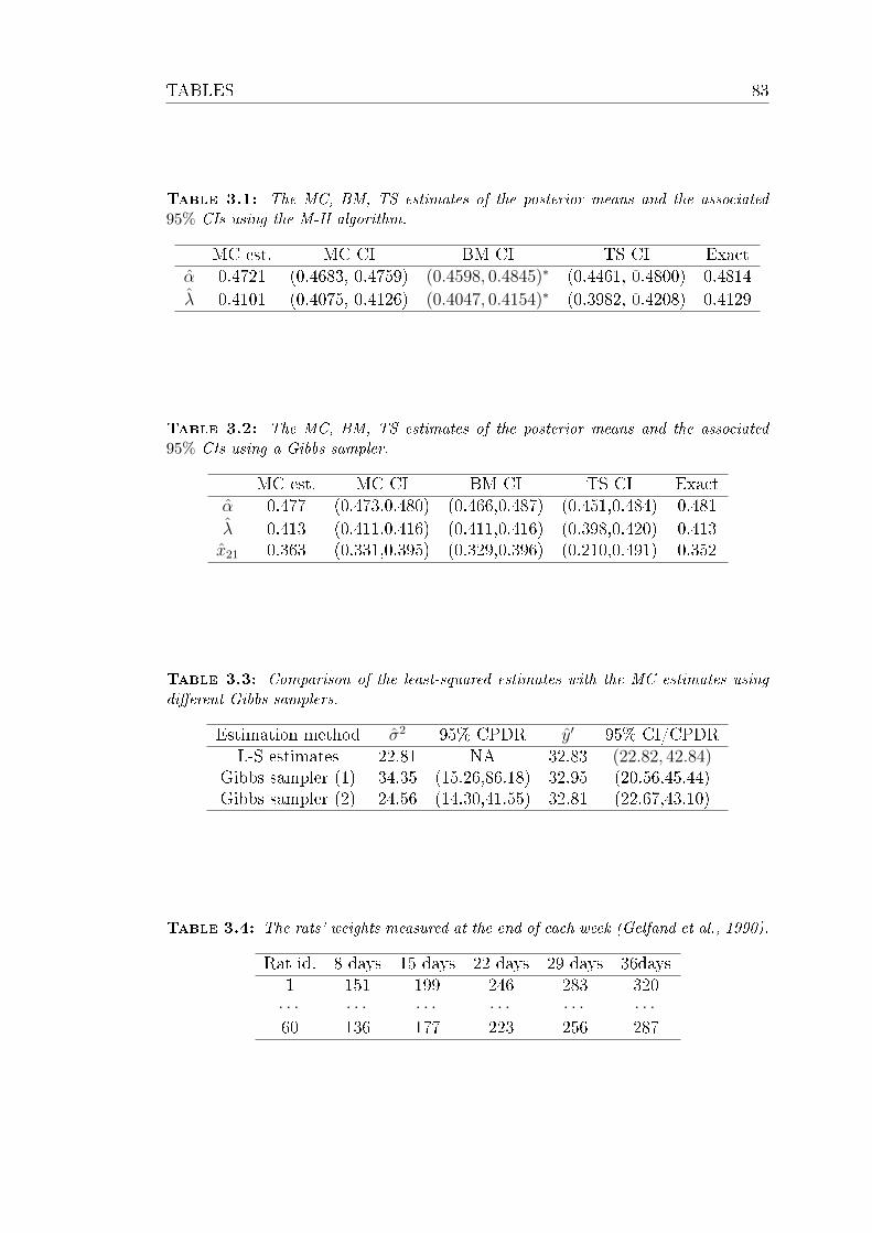
TABLES 83
Table 3.1: The MC, BM, TS estimates of the posterior means and the associated
95% CIs using the M-H algorithm.
MC est. MC CI BM CI TS CI Exactα 0.4721 (0.4683, 0.4759) (0.4598, 0.4845)∗ (0.4461, 0.4800) 0.4814
λ 0.4101 (0.4075, 0.4126) (0.4047, 0.4154)∗ (0.3982, 0.4208) 0.4129
Table 3.2: The MC, BM, TS estimates of the posterior means and the associated
95% CIs using a Gibbs sampler.
MC est. MC CI BM CI TS CI Exactα 0.477 (0.473,0.480) (0.466,0.487) (0.451,0.484) 0.481
λ 0.413 (0.411,0.416) (0.411,0.416) (0.398,0.420) 0.413x21 0.363 (0.331,0.395) (0.329,0.396) (0.210,0.491) 0.352
Table 3.3: Comparison of the least-squared estimates with the MC estimates using
dierent Gibbs samplers.
Estimation method σ2 95% CPDR y′ 95% CI/CPDRL-S estimates 22.81 NA 32.83 (22.82, 42.84)
Gibbs sampler (1) 34.35 (15.26,86.18) 32.95 (20.56,45.44)Gibbs sampler (2) 24.56 (14.30,41.55) 32.81 (22.67,43.10)
Table 3.4: The rats' weights measured at the end of each week (Gelfand et al., 1990).
Rat id. 8 days 15 days 22 days 29 days 36days1 151 199 246 283 320· · · · · · · · · · · · · · · · · ·60 136 177 223 256 287
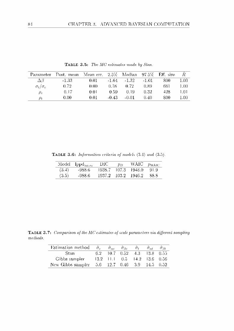
84 CHAPTER 3. ADVANCED BAYESIAN COMPUTATION
Table 3.5: The MC estimates made by Stan.
Parameter Post. mean Mean err. 2.5% Median 97.5% E. size R∆β -1.33 0.01 -1.64 -1.32 -1.01 800 1.00σt/σc 0.72 0.00 0.58 0.72 0.89 661 1.00ρc -0.17 0.01 -0.59 -0.19 0.32 428 1.01ρt 0.00 0.01 -0.43 -0.01 0.40 800 1.00
Table 3.6: Information criteria of models (3.4) and (3.5).
Model lppdloo-cv DIC pD WAIC pWAIC
(3.4) -988.6 1938.7 107.3 1948.0 91.9(3.5) -988.6 1937.2 103.2 1946.2 88.8
Table 3.7: Comparison of the MC estimates of scale parameters via dierent sampling
methods.
Estimation method σc σαc σβc σt σαt σβtStan 6.2 10.7 0.52 4.3 13.8 0.55
Gibbs sampler 13.2 11.1 0.5 14.2 13.6 0.56New Gibbs sampler 5.6 12.7 0.46 3.9 14.5 0.52

Chapter 4
Bayesian Chain Ladder Models
In this and the next two chapters, the Bayesian methods introduced previously
are applied to general insurance claims reserving. This chapter has three topics
of discussion: the background of general insurance claims reserving, a summary
of the widely used reserving models, and the payments per claim incurred (PPCI)
method in a Bayesian framework.
Wüthrich and Merz (2008) commented on claim reserving methods that, Re-
serving actuaries now have to not only estimate reserves for the outstanding loss
liabilities but also to quantify possible shortfalls in these reserves that may lead
to potential losses. Such an analysis requires stochastic modelling of loss liability
cash ows and it can only be done within a stochastic framework.
There have been much stochastic reserving literature proposed in recent decades.
England and Verrall (2002) is a good summary of stochastic models up to 2002.
Wüthrich and Merz (2008) is very much mathematically driven. The literature
using Bayesian methods include Taylor (2000), England et al. (2012), Verrall and
Wüthrich (2012), Zhang et al. (2012) and Meyers (2015). Most of these focus
on the payments triangle and base the claims liability estimation on a stochastic
model induced from the chain ladder method.
In Australia, the PPCI method (Taylor, 2000) is widely used. However, there
is little research on the stochastic model based on the PPCI method. This chapter
85
86 CHAPTER 4. BAYESIAN CHAIN LADDER MODELS
tries to ll this gap. As a stochastic version of PPCI, a generalized linear model
is tted to the claims counts triangle and the PPCI triangle respectively, and
then a compound model is tted to aggregate the estimates of ultimate claims
counts and outstanding PPCI. The generalized linear models are in the Bayesian
framework and we use MCMC inferential tools to solve them.
In Section 4.1, the general insurance claims reserving background is reviewed.
There are two parts in this section. The rst part is claims reserving terminology,
mainly following the Exam 5 syllabus provided by the Casualty Actuarial Society.
The second part summarizes widely used traditional reserving methods, including
the chain ladder (CL) method and the Bornhuetter-Ferguson (BF) method.
Stochastic models are discussed in Section 4.2 and 4.3. We focus on a Bayesian
over-dispersed Poisson (ODP) model with an exponential decay curve component
(Verrall et al., 2012). Reversible jump MCMC is used to simulate a sample from
this model.
In Section 4.4, we propose a compound model based on the PPCI method. The
model contains three sub-models, each of which ts the claim counts triangle, ts
the PPCI triangle, and aggregates them. A fully Bayesian analysis blending with
preliminary classical model checking is performed on the weekly benet data set
and the doctor benet data set from WorkSafe Victoria, a workers compensation
scheme in Victoria state of Australia. We compare our results with the PwC
evaluation (Simpson and McCourt, 2012).
4.1 General insurance claims reserving background
General insurance is also known as property and casualty (P&C) insurance in
the United States and non-life insurance in continental Europe. We follow Tay-
lor (2000) to review the claims reserving terminology and the traditional claims
reserving methods.

4.1. GENERAL INSURANCE CLAIMS RESERVING BACKGROUND 87
4.1.1 Terminology
A general insurance policy is a contract between two parties, the insurer and the
insured, providing for the insurer to pay an amount of money to the insured on
the occurrence of specied events.
A claim is the right of the insured to these amounts and the aggregate of
facts establishing that right and the insurer's fullment of it. These facts are
also called trigger events. For a personal automobile policy, the trigger event is
usually a car accident. For a workers compensation policy, the trigger event is
usually a work-place accident. For a homeowners policy, it can be a re or storm.
The date on which the events generating the claim took place is called date
of occurrence. Most general insurance policies are occurrence policies, which
limit the insurer's liability to the trigger events within the policy period. In
contrast, claims-made policies cover the claims made during the policy period
even if these claims arise from an event that happened before policy inception.
Most malpractice insurance policies are belong to this type. Claim amount is the
amount which the insurer is obliged to pay with respect to a claim. It is also
called loss amount, claim payment, loss payment, paid claim, paid loss etc.
The claims process
Figure 4.1 shows the time line of a claim. The period A to B is the policy eective
period, during which accidents fullling other policy conditions will be covered.
t1 is the date of occurrence. The claim is not notied to the insurer until t2, when
the policy is already expired.
Typically, the claim will not be paid immediately. At the very least there will
be administrative delays. For more complicated claims, investigation, dispute,
litigation or other processes are needed before determination of any payments.
It may be in the nature of the policy that the payments extend over years, e.g.,
when the benets are income replacement under workers compensation. At time
t5, the insurer considered the action on the claim was complete and closed it. At

88 CHAPTER 4. BAYESIAN CHAIN LADDER MODELS
time t6, the early closure decision was found to be wrong and claim was reopened,
further payments made, and it was closed again at t8.
The components of unpaid claims
Unpaid claims as of a particular time are dened as the outstanding loss liability
with regarding to the past exposure period. For the claim in Figure 4.1, the
unpaid claims as of time B are called the incurred but not reported claim (IBNR),
since there is no notication of the claim.
At t2, when the claim is notied, the unpaid claims consist of case estimates,
future development of case estimates and estimates for reopened claim. Case
estimate is established by the claim department or independent adjusters. The
sum of future development of case estimates and estimates of the re-opened claim
are called incurred but not enough reported (IBNER).
Aggregately, at any particular time point, the unpaid claims of an insurer con-
sist of IBNR, case estimates for reported claims, and IBNER. The case estimates
and IBNER are set up individually according to the characteristics of a particular
claim, while IBNR must be estimated aggregately since it comes from the existing
claims not yet reported to the insurer. Actuaries rely on the historical aggregate
claims data to estimate IBNR, which is also one of the main tasks of this
thesis.
Loss reserving
The outstanding loss liability is distinct from loss reserve. The outstanding loss
liability is an unknown random variable which would be recognized after all the
claims are paid. Before all the claims are closed, an unbiased estimate of unpaid
claims liability as of a valuation date is called expected outstanding loss liability.
A reserve set at this level would have a roughly 50% chance of ultimate ad-
equacy. Often an insurer will wish to reserve more strongly than this and will
add a margin to the expected liability. This margin is also referred to as the

4.1. GENERAL INSURANCE CLAIMS RESERVING BACKGROUND 89
prudential margin or provision for adverse deviation. To quantify the margin,
the uncertainty of outstanding loss liability or, ideally, its predictive distribution
needs to be estimated.
4.1.2 Run-o triangles
As mentioned before, the estimation of IBNR is impossible for a single claim. So
we need to rely on the aggregate claims history. The claims are usually cross-
aggregated by two factors: period of occurrence and period of development. We
treat all the claims with the same occurrence period as a group and track the
group's development in the future. This structure is analogous to the rats growth
data in Section 3.5. The only dierence is that the claims groups have varying
development periods at a particular time.
Notation for a run-o triangle
We denote the occurrence periods (or accident periods) by i = 1, . . . , I, and the
development periods by j = 1, . . . , J . The unit can be a quarter, half or full
year, but the occurrence periods and development periods should use the same
units and the intervals should be equal. The experience periods (or calendar
periods) are denoted by k = i + j, which contains a cross-section of experience
from various periods of occurrence lying on a diagonal line, and the incremental
claims of occurrence period i during the development period j as yi,j.
In the case of I > J , the run-o triangle becomes a trapezoid where the early
occurrence periods i = 1, .., J − I are assumed fully run-o by the development
period J . A trapezoid can be converted to a triangle by adding J−I development
periods and assuming yi,j = 0 for J < j ≤ I. So we always consider the case when
I = J .
Table 4.1 shows a typical structure of incremental claims run-o triangle,
where the upper triangle yi,j : i+ j ≤ I + 1 is available by the end of most
recent accident year I (or by the end of most recent experience period I+1). The

90 CHAPTER 4. BAYESIAN CHAIN LADDER MODELS
loss reserving problem is to predict the lower triangle yi,j : i+ j > I + 1, j ≤ I,
and tail development yi,j : j > I if not fully run-o by the end of development
period I. The nal reserve is not equal to the summation of predicted lower
triangle and possible tails development but depends on the uncertainty around
them.
We dene the cumulative claims for occurrence year i as of development period
j as ci,j =∑j
l=1 yi,l, and the ultimate claims of occurrence year i as ci,∞ or ui,
which is equal to ci,I when the claims are fully run-o by the development period I.
The unpaid claims of accident year i are dened as Ri =∑∞
j=I−i+2 yi,j. In the
case of no development after I, Ri = ci,I − ci,I−i+1. The total unpaid claims are
dened as R =∑I
i=1Ri.
4.1.3 Widely-used methods in the insurance industry
Here we list two methods: the chain ladder (CL) method and the Bornhuetter-
Ferguson (BF) method. Friedland (2010) discusses other popular methods such
as the Cape Cod method, frequency-severity method, case development method
etc. But the CL and BF methods are the building blocks of all the other methods.
The chain ladder method
The CL method is the most popular and basic technique. The key assumption
is that the future claims development is similar to prior years' development. An
implicit assumption is that, for an immature accident year, the claims observed so
far tell something about the claims yet to be observed. This is in contrast to the
assumption underlying the BF method. Other important assumptions include a
consistent claim processing and a stable mix of claim types.
The CL method rst calculates the observed age-to-age factor (also called
the development factor) triangle as in Table 4.2. The CL method requires the
judgementally selected age-to-age factors among the candidates including all-year
average, last three-year average, volume-weighted average etc. We dene the CL

4.1. GENERAL INSURANCE CLAIMS RESERVING BACKGROUND 91
estimate of development factor of j to j + 1 as the volume-weighted average:
fj =
∑I−ji=1 ci,j+1∑I−ji=1 ci,j
for j = 1, . . . , I − 1.
Assume the tail factor as fI . In the case of no development after I, fI = 1. The
CL estimate of ultimate claim of occurrence period i is
ui = ci,∞ = ci,I+1−ifI+1−i · · · fI .
The expected outstanding liability of occurrence period i is
Ri = ci,I+1−i
(fI+1−i · · · fI − 1
).
The Bornhuetter-Ferguson method
The Bornhuetter-Ferguson (BF) method (Bornhuetter and Ferguson, 1972) as-
sumes that unpaid claims will develop based on a prior ultimate claim estimate.
In other words, the claims reported to date contain no informational value as to
the amount of claim yet to be reported. The BF method is rather robust against
the unreliable immature claim in the recent accident years.
The BF method applies the same estimate of development pattern as the CL
method, but uses a prior estimate of ultimate claims ui. The BF reserve is Ri =
ui (1− zI+1−i) , where zI+1−i is the estimated percentage of the ultimate claims
amount that is expected to be known by the end of the most recent development
period I + 1 − i for the occurrence period i (i.e. by the end of the most recent
experience period I + 1). The BF method simply uses the CL estimates fj to
estimate z as follows:
z1 =(f1 · · · fI−1fI
)−1
, . . . , zI−1 =(fI−1fI
)−1
, zI = f−1I .

92 CHAPTER 4. BAYESIAN CHAIN LADDER MODELS
4.2 Stochastic chain ladder models
This section summarizes the recent literature on stochastic claims reserving mod-
els. They can be divided into two categories according to the mean functions:
multiplicative structure using occurrence period and development period as fac-
tor covariates, and parametric curve using development period as a continuous
variable.
The rst type of models can give the CL estimates when using over-dispersed
error structure but they cannot accommodate the tail development. The second
type of models have far fewer parameters and can accommodate the tail develop-
ment. We will turn to the bootstrap or the MCMC method to get the predictive
distribution of unpaid claims. RJMCMC is discussed in this section as a way of
combining the MCMC methods with the model selection.
4.2.1 Frequentist chain ladder models
The distribution-free model by Mack (1993) and the over-dispersed Poisson (ODP)
model by Renshaw and Verrall (1998) use the same mean function to t the in-
cremental claims. The mean function is the multiplication of two parameters,
which correspond to the occurrence periods and the development periods respec-
tively. Besides having the same response variable and mean function, they both
assume the variance of the response variable is proportional to its mean. It is not
surprising that both of them give the CL estimates.
The distribution-free model does not assume a distribution family and relies
on the unbiased estimators, while the ODP model assumes a Poisson distribu-
tion and relies on the MLE. They have dierent prediction errors and predictive
distributions which can be estimated via the bootstrap.
The distribution-free model
Mack (1993) proposed a distribution-free model assuming only the rst two mo-

4.2. STOCHASTIC CHAIN LADDER MODELS 93
ments, as follows:
E (ci,j|ci,j−1) = fj−1ci,j−1, i = 1, . . . , I, j = 2, . . . , I
Var (ci,j|ci,j−1) = σ2j−1ci,j−1, i = 1, . . . , I, j = 2, . . . , I.
(4.1)
It can be shown that the CL estimators fj are the unbiased estimator of fj. Using
the CL estimators fj, the unpaid claims estimate is the same as the CL estimate.
Furthermore, an unbiased estimator for σ2j is
σ2j =
1
I − j − 1
I−j∑i=1
ci,j
(ci,j+1
ci,j− fj
)2
, j = 1, . . . , I − 2
σ2I−1 = min
(σ2I−2/σ
2I−3,min
(σ2I−3, σ
2I−2
)).
The conditional mean squared error of prediction (MSEP) for Ri is
MSEPc
(Ri
∣∣∣y) = E
((Ri − Ri
)2∣∣∣∣y) = Var (Ri) +
(E (Ri)− Ri
)2
,
where y = yij : i = 1, . . . I, j = 1, . . . , I − i+ 1 is the upper triangle. In words,
the conditional prediction variance is equal to the sum of process variance and
estimation bias squared1. The analytical results of conditional MSEP of individ-
ual occurrence period reserve and total reserve are available. As a nal remark,
Mack (1999) extends this model to involve the tail factor.
The over-dispersed Poisson (ODP) model
One of the most popular generalized linear models in the claims reserving problem
is the ODP model which has the following form:
yi,jϕ∼ Poisson
(µiγjϕ
), i = 1, . . . , I, j = 1, . . . , I, (4.2)
1E (Ri) 6= R; see Mack (1993).

94 CHAPTER 4. BAYESIAN CHAIN LADDER MODELS
with the constraint∑J
j=1 γj = 1. Here µi is interpreted as the expected ultimate
claims of occurrence period i and γj as the expected proportion of incremental
claims to the ultimate claims during development period j. This model has been
intensively studied, including by Renshaw and Verrall (1998); Verrall (2000);
England and Verrall (2002); Verrall (2004); England and Verrall (2006); England
et al. (2012); Verrall et al. (2012); and Wüthrich (2013b).
An implicit assumption of this model is that the variance of the response vari-
able is proportional to its mean. We can check this assumption by inspecting the
residual plots. When it fails, other error structures such as a Tweedie distribution
can be used.
It can be shown that the MLEs for µi and γj are equal to the CL estimates
using the weighted averages of age-to-age factors. The ODP model can be ex-
tended to non-integer, and negative data (i.e., when recoveries are possible) via
the quasi-likelihood method (Faraway, 2015). The quasi-likelihood method is
easily applied in R by specifying the argument family as quasi in the function
glm().
We dene the unscaled Pearson residuals as
ri,j =yi,j − mi,j√
mi,j
,
where mi,j is the MLE for E (yi,j) (i.e., the tted value). The dispersion parameter
ϕ is estimated by
ϕ =
∑i+j≤I+1 ri,j
2
N − p,
where N = (I + 1)I/2 is the number of observations, and p = 2I − 1 is the
number of parameters. Fortunately, R can calculate all of these estimates in a
second. England and Verrall (2006) also consider the non-constant dispersion
for development periods, which is the assumption of the distribution-free model
(4.1).

4.2. STOCHASTIC CHAIN LADDER MODELS 95
The mean squared error of prediction for Ri is
MSEP(Ri) = E(Ri − Ri
)2
= Var(Ri − Ri
)+(
E (Ri)− E(Ri))2
.
The second term is approximately zero. Hence,
MSEP(Ri) ≈ Var(Ri − Ri
)= Var (Ri) + Var(Ri). (4.3)
In words, the prediction variance is roughly equal to the sum of process vari-
ance and estimation variance. R cannot provide the MSEP(Ri) directly since
it is a complicated function of parameters. From Renshaw and Verrall (1998),
MSEP(Ri) is estimated as
I∑j=I−i+2
ϕmi,j +I∑
j=I−i+2
m2i,jVar (ηi,j) + 2
∑k>l
mi,kmi,lCov (ηi,k, ηi,l) ,
where η is the linear predictor and its covariance matrix is available directly from
R. England and Verrall (2002) also give the MSEP of total reserve with an addi-
tional covariance term for dierent occurrence periods (i.e., Cov (ηm,k, ηn,l)). We
can rely on ChainLadder package to get MSEP(Ri). Later, we will use the boot-
strap or MCMC to simulate Ri and estimate its MSEP based on the simulated
sample.
The predictive distribution via the bootstrap
Bootstrapping (Efron and Tibshirani, 1994) is a powerful, yet simple, technique
for obtaining information from a single sample of data. In a standard applica-
tion of the bootstrap, where data are assumed to be independent and identically
distributed, resampling with replacement takes place of the data themselves.
In regression problems the data are usually assumed to be independent but not
identically distributed due to the existence of covariates. Therefore, with regres-
sion problems it is common to bootstrap residuals, rather than data themselves,
96 CHAPTER 4. BAYESIAN CHAIN LADDER MODELS
since the residuals are approximately independent and identically distributed.
For model (4.1) and model (4.2), we use the scaled Pearson residuals for boot-
strapping.
The bootstrap for model (4.1). Model (4.1) is in a recursive structure. Eng-
land and Verrall (2002) showed that an equivalent model can be obtained using
the observed factors fi,j as a response variable with the following mean and vari-
ance:
E (fi,j|ci,j) = fj
Var (fi,j|ci,j) =σ2j
ci,j.
The scaled Pearson residuals are dened as
rsi,j =fi,j − fjσj/√ci,j
.
The bootstrap algorithm for model (4.1) is as follows:
1. Sample with replacement, from the set of scaled Pearson residuals, to get a
sample of residuals for a single bootstrap iterationrBi,j : i+ j ≤ I
.
2. Back out the residual denition to obtain a pseudo run-o triangle of de-
velopment factor as follows:
fBi,j =rBi,jσj√ci,j
+ fj.
3. Obtain the new volume-weighted development factor
fj =
∑I−ji=1 f
Bi,j ci,j∑I−j
i=1 ci,j.
4. Simulate the future claims. Starting from the latest cumulative claims
ci,I+1−i, forecast the next cumulative claims by sampling a value from a

4.2. STOCHASTIC CHAIN LADDER MODELS 97
gamma distribution:
ci,I+2−i|ci,I+1−i ∼ Gamma
(f 2I+1−i ci,I+1−i
σ2I+1−i
,fI+1−i
σ2I+1−i
)for i = 2, . . . , I.
5. Recursively predict the future cumulative claims by sampling from
ci,j+1|ci,j ∼ Gamma
(f 2j ci,j
σ2j
,fjσ2j
)for i = 3, . . . , I and j = I − i+ 3, . . . , I.
6. Calculate each accident year future claims and total future claims as
Ri = ci,I − ci,I+1−i, for i = 2, . . . , I
R = R2 + R3 + · · ·+ RI .
7. Repeat steps 1 to 6 to get a sample of Ri and R.
The empirical distribution of the bootstrap sample approximates the predictive
distribution. The prediction variance of total liability can be estimated by the
sample variance of the bootstrap sample of total liability. Note that the boot-
strap sample variation consists of variation due to bootstrapping in step 1 (i.e.,
estimation variance) and variation due to forecasting in step 4 and 5 (i.e., process
variance), which correspond to the two terms on the right side of equation (4.3).
The bootstrap for model (4.2). The scaled Pearson residuals of model (4.2)
are
rsi,j =yi,j − mi,j√
ϕmi,j
.
The bootstrap algorithm for model (4.2) is as follows:
1. Sample with replacement from the set of scaled Pearson residuals to get a
sample of residuals for a single bootstrap iterationrBi,j : i+ j ≤ I
.
2. Back out the residual denition to obtain a pseudo run-o triangle of in-

98 CHAPTER 4. BAYESIAN CHAIN LADDER MODELS
cremental claims as follows:
yBi,j = rBi,j√ϕmi,j + mi,j.
3. Use the CL method to get the new estimate µi, γj based on the pseudo
incremental claims run-o triangle from step 2.
4. Simulate the future claims from the following ODP model:
Ri ∼ ϕPoisson
(µi∑I
j=I−i+2 γj
ϕ
)for i = 2, 3, . . . , I.
Calculate the total future claims as R = R2 + R3 + · · ·+ RI .
5. Repeat steps 1 to 4 to get a sample of Ri and R.
In the case when ϕ is large, e.g., ϕ = 1000, Ri will be sampled from 0, 1000, . . .,
which is undesirable. We can use an alternative gamma distribution with the
target mean and variance in step 4.
Example 4.1 (Liability insurance claims data). We use the liability claims run-
o data with 22 accident years and 22 development years from Verrall and Wüthrich
(2012). The R package ChainLadder by Gesmann et al. (2015) can estimate all the
quantities we have previously mentioned.The residual plots are needed to validate
the model assumptions.
Table 4.3 shows that models (4.1) and (4.2) both give the same point esti-
mate of total liability, which are also equal to the CL estimate. The numbers in
parentheses are from the bootstrap method. The distribution-free model (4.1) can
accommodate tail development, which consists of nearly 10% of total liability. The
conditional mean squared error is smaller than the unconditional mean squared
error since the latter involves the extra uncertainty induced by the historical claims
data (i.e., estimation error).
The function BootChainLadder in the R package ChainLadder performs the
bootstrap for model (4.2). Here we bootstrap 1, 000 times. We show the histogram
of the bootstrap sample of total outstanding liability in Figure 4.2, and we get the

4.2. STOCHASTIC CHAIN LADDER MODELS 99
bootstrap estimate of total outstanding liability and the standard error in Table
4.3 (stated in parentheses).
4.2.2 A Bayesian over-dispersed Poisson (ODP) model
The model (4.2) in a Bayesian framework has the following form:
yi,jϕ∼ Poisson
(µiγjϕ
)µi ∼ Gamma (ai, bi)
γj ∼ Gamma (cj, dj) ,
(4.4)
where µi is related to the ultimate claim of accident year i, γj is related to the
incremental claims percentage during development year j, and ai, bi, cj, dj are
constant hyperparameters whose values are adjusted according to prior knowl-
edge. In the case where there is no prior knowledge, we assume µi and γj follow
the same non-informative prior. ϕ is a plug-in estimate via GLM (see Section
4.2.1).
The joint posterior distribution of µ = (µ1, . . . , µI) and γ = (γ1, . . . , γI) is
p (µ, γ|y) =p (y|µ, γ) p (µ, γ)∫
µ,γp (y|µ, γ) p (µ, γ) dµdγ
∝ p (y|µ, γ) p (µ, γ)
∝∏
i+j≤I+1
exp
(−µiγj
ϕ
)(µiγjϕ
) yi,jϕ
I∏i=1
µiai−1 exp (−biµi)
I∏j=1
γjcj−1 exp (−djγj) .
Our interest is in not only the parameter µ, γ but also the future claims. We have
the following posterior predictive distribution of future claims:
p(y′|y) =
∫µ,γ
p (y′|µ, γ) p (µ, γ|y) dµdγ,
where y′ is the set of lower triangle. It is hard to solve p (y′|y) analytically. The

100 CHAPTER 4. BAYESIAN CHAIN LADDER MODELS
conditional mean squared error of prediction for a predictor R is
MSEPc(R) = E
((R−R
)2∣∣∣∣y) = Var (R|y) +
(R− E (R|y)
)2
.
We prefer the predictor R = E (R|y) (i.e., the posterior mean) which minimizes
MSEPc(R). The MSEP of the posterior mean is Var (R|y), which can be esti-
mated from a MC sample.
A Gibbs sampler for model (4.4)
The Gibbs sampler is a special case of the Metropolis-Hastings (M-H) algorithm.
In the M-H algorithm if we choose the full conditional distribution as the proposed
distribution, the acceptance rate will be 1. The use of the Gibbs sampler implicitly
requires that the full conditional distribution is recognisable; otherwise, we need
to turn to the general M-H algorithm or adaptive rejection sampling (Gilks and
Wild, 1992).
The full conditional distribution of µi is obtained from p (µ, γ|y), assuming
all the other parameters constant, as follows:
p (µi|y, γ, µ−i) ∝ exp
(−µi∑I+1−i
j=1 γj
ϕ
)µi
∑I+1−ij=1
yi,j
ϕ µiai−1 exp (−biµi) ,
where µ−i is the vector µ excluding µi. It can be recognized as a gamma distri-
bution
µi|y, γ ∼ Gamma
(ai +
∑I+1−ij=1 yi,j
ϕ, bi +
∑I+1−ij=1 γj
ϕ
). (4.5)
Symmetrically, the full conditional distribution of γj for j = 1, . . . , I is
γj|y, µ ∼ Gamma
(cj +
∑I+1−ji=1 yi,jϕ
, dj +
∑I+1−ji=1 µiϕ
). (4.6)
A Gibbs sampler based on the above full conditional distributions has the follow-
ing steps:

4.2. STOCHASTIC CHAIN LADDER MODELS 101
1. Initialize µ0, γ0. For t ≥ 1, repeat the steps 2 to 4.
2. For 1 ≤ i ≤ I, draw a value µti from distribution (4.5) with γ = γt−1, and
set µt = (µt1, . . . , µtI) .
3. For 1 ≤ j ≤ I, draw a value γtj from distribution (4.6) with µ = µt, and set
γt = (γt1, . . . , γtI) .
4. For 1 ≤ i ≤ I, draw a value Rti from the distribution
ϕPoisson
(µti∑I
j=I−i+1 γtj
ϕ
),
and set Rt = Rt2 + · · ·+Rt
I .
Steps 2 and 3 provide a Markov chain (µt, γt)t≥0 whose stationary distribution
is p (µ, γ|y). Step 4 provides a sample of the total outstanding liability. The
prediction error of future claims consists of estimation error via steps 2 and 3 and
process error via step 4, which correspond to the bootstrap resampling step and
forecasting step respectively.
Note that parameters µ and γ are not uniquely dened. In Example 4.2,
we will see that the multiplication µiγj is converged rather than µi,γj by them-
selves. In other words, µi, γj cannot be estimated accurately individually. For
interpretation purposes, we dene the normalized µi, γj as
µ*i = µi
I∑j=1
γj, γ*j =γj∑Ik=1 γk
.
Inferences under non-informative priors. Under the non-informative pri-
ors, i.e., a → 0, b → 0, c → 0, d → 0, distributions (4.5) and (4.6) dene the
following conditional expectations:
E (µi|y, γ) =
∑I+1−ij=1 yi,j∑I+1−ij=1 γj
, E (γj|y, µ) =
∑I+1−ji=1 yi,j∑I+1−ji=1 µi
.
102 CHAPTER 4. BAYESIAN CHAIN LADDER MODELS
If we substitute the left sides with µi and γj, the above equations dene a system
of equations whose solutions will be consistent with the CL estimates. Strictly,
the posterior mean of outstanding liability is close but not exactly equal to the
CL estimate.
In Example 4.1, we use the plug-in estimate ϕ = 631.8, and non-informative
prior for µ, γ, (i.e., a, b, c, d→ 0). We iterate for T = 1000 times and get the MC
estimate of posterior mean of total outstanding liability as 1,461,958 dollars, with
the standard error of 60,902 dollars. These values are quite close to the result in
Table 4.3.
Inferences under strong priors for µ. Assume the prior knowledge of µ
is some value around m with small variation, i.e., b/mi → ∞ and ai = mib.
Distributions (4.5) and (4.6) dene the following conditional expectations:
E (µi|y, γ) ≈ mi, E (γj|y, µ) ≈∑I+1−j
i=1 yi,j∑I+1−ji=1 mi
,
which follows the BF predictor proposed by Mack (2008). The estimation error
of µ is close to 0, and the standard error of claims liability will be largely reduced.
Example 4.2 (A Monte Carlo study of model (4.4) using simulated data). We as-
sume the parameters in model (4.4) as µ =(107, 1.02× 10⁷, . . . , 1.029 × 10⁷
), γ =
(0.30, 0.21, 0.15, 0.10, 0.08, 0.06, 0.04, 0.03, 0.02, 0.01) , ϕ = 25000, where the
sum of γ is 1 implying no claims development beyond age 10. We simulate a sam-
ple of incremental claims in the upper triangle.
Inferences under non-informative priors. We use the plug-in estimate ϕ =
23, 488, and choose a = 0, b = 0. We iterate for T = 1000 times. The trace plots
in Figure 4.3 show that µ*6, γ*6 converge rather than µ6, γ6.
The MC estimates of posterior means of µ*, γ* are close to the CL estimates
as shown in Figure 4.4. The predictive distributions of outstanding liability are
shown in Figure 4.5.
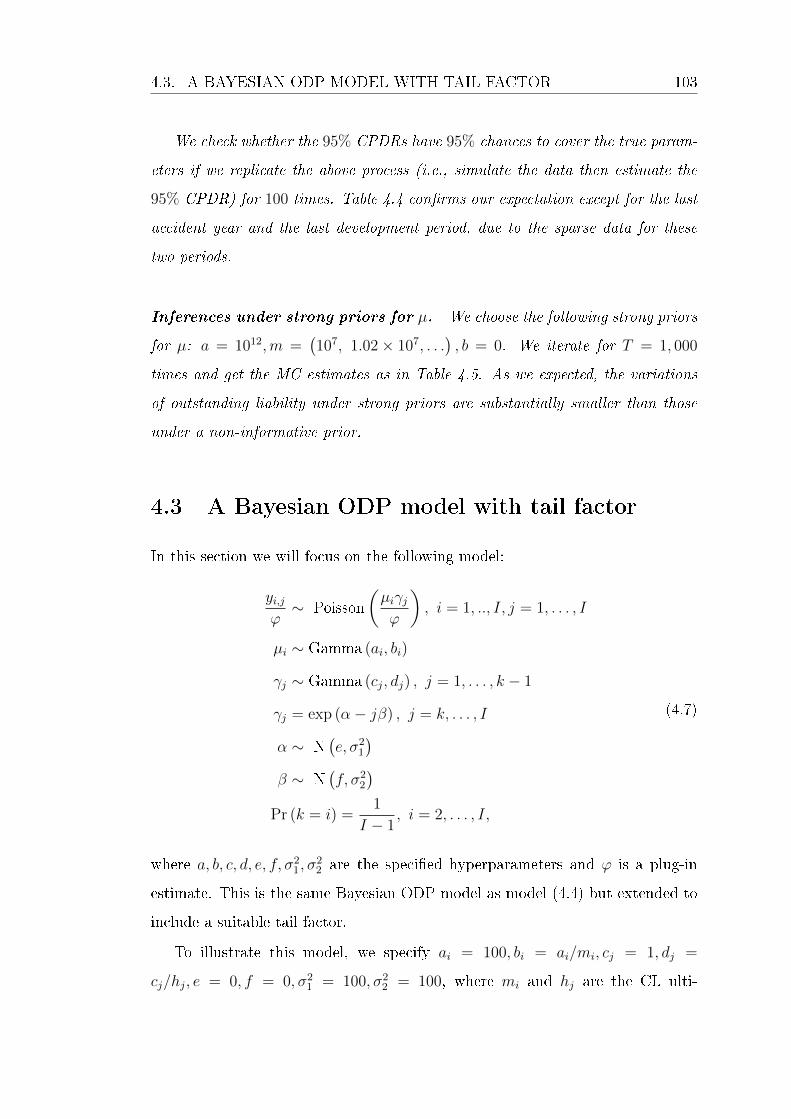
4.3. A BAYESIAN ODP MODEL WITH TAIL FACTOR 103
We check whether the 95% CPDRs have 95% chances to cover the true param-
eters if we replicate the above process (i.e., simulate the data then estimate the
95% CPDR) for 100 times. Table 4.4 conrms our expectation except for the last
accident year and the last development period, due to the sparse data for these
two periods.
Inferences under strong priors for µ. We choose the following strong priors
for µ: a = 1012,m =(107, 1.02× 10⁷, . . .
), b = 0. We iterate for T = 1, 000
times and get the MC estimates as in Table 4.5. As we expected, the variations
of outstanding liability under strong priors are substantially smaller than those
under a non-informative prior.
4.3 A Bayesian ODP model with tail factor
In this section we will focus on the following model:
yi,jϕ∼ Poisson
(µiγjϕ
), i = 1, .., I, j = 1, . . . , I
µi ∼ Gamma (ai, bi)
γj ∼ Gamma (cj, dj) , j = 1, . . . , k − 1
γj = exp (α− jβ) , j = k, . . . , I
α ∼ N(e, σ2
1
)β ∼ N
(f, σ2
2
)Pr (k = i) =
1
I − 1, i = 2, . . . , I,
(4.7)
where a, b, c, d, e, f, σ21, σ
22 are the specied hyperparameters and ϕ is a plug-in
estimate. This is the same Bayesian ODP model as model (4.4) but extended to
include a suitable tail factor.
To illustrate this model, we specify ai = 100, bi = ai/mi, cj = 1, dj =
cj/hj, e = 0, f = 0, σ21 = 100, σ2
2 = 100, where mi and hj are the CL ulti-

104 CHAPTER 4. BAYESIAN CHAIN LADDER MODELS
mate claims estimates and the CL incremental claims proportion estimates. The
choice of these hyperparameters ensures the convergence of the RJMCMC al-
gorithm while allowing sucient exibility. Denote θk = α, β, µ, γ1, . . . , γk−1.
This model reduces the number of parameters from 2I in model (4.4) to k + 2.
Note that k is usually much smaller than I.
Model (4.7) implicitly includes a tail factor
γJ =J∑
j=I+1
exp (α− jβ) ,
where J is chosen judgementally. J →∞ leads
γ∞ =exp (α− (I + 1) β)
1− exp (−β).
The main task of this section is to determine which k leads to the optimal
model t. Since dierent ks will lead to dierent parameter dimensions, this
problem is equivalent to model selection. Here we investigate two methods: de-
viance information criteria (DIC) (Spiegelhalter et al., 2002) and reversible jump
Markov chain Monte Carlo (RJMCMC) method (Green, 1995). There are other
methods to compare and evaluate Bayesian models such as BIC, cross-validation
and posterior predictive checking (see Section 2.2).
4.3.1 Reversible jump Markov chain Monte Carlo
RJMCMC generalizes the Metropolis-Hastings (M-H) algorithm to include a
model indicator. The joint state space (θl, l) is dened by both model parameters
θl and the model index l, where l ∈ 1, 2, . . . , L. The joint posterior distribution
of θl, l can be factorized as
p (l, θl|y) ∝ p (θl|y) p (l|y) ∝ p (y|θl, l) p (θl) p (l) ,
which is the product of the likelihood, the prior of θl and the prior of l.

4.3. A BAYESIAN ODP MODEL WITH TAIL FACTOR 105
Before turning to the RJMCMC algorithm, we review the M-H algorithm.
In the M-H algorithm, a proposal distribution from θ to θ∗ is q(θ∗|θ), and the
acceptance rate is
min
(1,p(θ*|y
)q(θ|θ*)
p (θ|y) q(θ*|θ)
).
For RJMCMC, we need a model index proposal distribution from l to l∗, q(l∗|l),
and a parameter proposal distribution from θl to θl∗ . Since θl and θl∗ may have
dierent dimensions, the parameter proposal process involves two steps: generate
u ∼ ql→l* , and then set(θl* , u
*)
:= Tl→l* (θl, u) , where Tl→l* is a one-to-one
mapping with Tl→l* = T−1l*→l.
Note that (θl, u) must have the same dimension as(θl* , u
*). It is possible that
u is zero-dimensional, e.g., θl has more parameters than θl* . Similar to the M-H
algorithm, the acceptance rate is calculated as
min
(1,p(l*, θl* |y
)p (l, θl|y)
q(l|l*)q(l*|l)
ql*→l(u*)
ql→l* (u)
∣∣∣∣∂Tl→l* (θl, u)
∂ (θl, u)
∣∣∣∣),
where the nal term is the determinant of the Jacobian matrix.
The RJMCMC algorithm typically has the following steps:
1. Initialize l0 and θ0l0 . In the following we use the shortened notation θtlt for
θt. For t ≥ 1, repeat the following steps.
2. Propose a new model index l∗ from the distribution q (l∗|lt) .
3. If l∗ = lt, do the following within-model update. Otherwise, jump to step
4.
(a) Update the current model lt by one iteration (i.e., via normal MCMC).
(b) Set lt+1 = l∗ and θt+1 as the updated parameters.
(c) Go to step 2.
4. If l* 6= lt, do the following between-model update.
(a) Generate ut ∼ qlt→l* .
(b) Set(θ*, u*
):= Tlt→l* (θt, ut ).

106 CHAPTER 4. BAYESIAN CHAIN LADDER MODELS
(c) Compute the acceptance rate as
min
(1,p(l*, θ*|y
)p (lt, θt|y)
q(lt|l*
)q (l*|lt)
ql*→lt(u*)
qlt→l* (ut)
∣∣∣∣∂Tlt→l* (θt, ut)
∂ (θt, ut)
∣∣∣∣).
(d) With this acceptance rate, set lt+1 = l∗ and θt+1 = θ∗. Otherwise keep
lt+1 = lt and θt+1 = θt.
(e) Go to step 2.
The RJMCMC algorithm provides a Markov chain (lt, θt)t≥0 whose stationary
distribution is p (l, θl|y). We can either choose the model l0 which has the highest
posterior probability p (l|y), or perform model averaging over p (l, θl|y).
4.3.2 RJMCMC for model (4.7)
In model (4.7), k is a model index variable whose value determines the param-
eter dimension. The joint posterior of k and θk is simplied as p (k, θk|y) ∝
p (y|θk) p (θk) . We use the following model index proposal distributions:q(k* = k|k
)= q
(k* = k + 1|k
)= q
(k* = k − 1|k
)= 1
3for k = 3, 4, . . . , I − 1
q(k* = k|k
)= 2
3and q
(k* = k + 1|k
)= 1
3for k = 2
q(k* = k|k
)= 2
3and q
(k* = k − 1|k
)= 1
3for k = I
(4.8)
which implies that k can equally jump to the nearest neighbourhood or stay in the
current state. The RJMCMC algorithm for model (4.7) consists of a within-model
update and a between-model update.
Within-model update
Suppose at the t+ 1th iteration we propose k∗ = kt from (4.8) . The parameters
at the end of tth iteration are denoted by θt =αt, βt, µt, γt1, . . . , γ
tkt−1
. The
following steps update θt to θt+1:
1. For µt+1, γt+11 , . . . , γt+1
kt−1, we apply the Gibbs sampler algorithm from Section

4.3. A BAYESIAN ODP MODEL WITH TAIL FACTOR 107
4.2.2.
2. For αt+1, βt+1, we apply the following M-H algorithm:
(a) Propose α* ∼ N(αt, 0.022
), β* ∼ N
(βt, 0.022
).
(b) Set θ* =α*, β*, µt+1, γt+1
1 , . . . , γt+1kt−1
.
(c) Calculate the acceptance as
min
(1,p(y|θ*
)N(αt|α*, 0.022
)N(βt|β*, 0.022
)p (y|θt)N
(α*|αt, 0.022
)N(β*|βt, 0.022
) ) ,where N (x|a, b) is the normal density at x with mean a and variance
b.
(d) With this acceptance rate, set αt+1 = α*, βt+1 = β*. Otherwise keep
αt+1 = αt, βt+1 = βt.
3. Set kt+1 = k*, θt+1 =αt+1, βt+1, µt+1, γt+1
1 , . . . , γt+1kt−1
. Note that the
within-model acceptance rate of k∗ is always 1.
Between-model update
Between-model update case 1: Suppose at the t+ 1th iteration, we propose
k∗ = kt+1 from (4.8). The parameters at the end of the tth iteration are denoted
by θt =αt, βt, µt, γt1, . . . , γ
tkt−1
. The following steps update θt to θt+1:
1. Propose a value ut from a gamma distribution with shape of 100 and mean
of exp (αt − ktβt) , as follows:
ut ∼ qkt→k* = Gamma
(100,
100
exp (αt − ktβt)
).
2. Set(θ*, u*
):= Tkt→k* (θt, ut) = (θt, ut), where u* has zero-dimension. Tkt→k*
is an identity mapping matrix with the Jacobian of 1.
3. Calculate the acceptance rate as
min
1,p(y|θ*
)p(θ*)
p (y|θt) p(θt)Gamma(ut∣∣∣100, 100
exp(αt−ktβt)
) .

108 CHAPTER 4. BAYESIAN CHAIN LADDER MODELS
4. With this acceptance rate, set (kt+1, θt+1) =(k*, θ*
). Otherwise keep
(kt+1, θt+1) = (kt, θt) .
Between-model update case 2: Suppose at the t+ 1th iteration, we propose
k∗ = kt−1 from (4.8). The parameters at the end of the tth iteration are denoted
by θt =αt, βt, µt, γt1, . . . , γ
tkt−1
. The following steps update θt to θt+1:
1. Set(θ*, u*
):= Tkt→k* (θt, ut) = (θt, ut), where ut has zero-dimension, u∗ =
γtkt−1. Tkt→k∗ is an identity mapping matrix with the Jacobian of 1.
2. Calculate the acceptance rate as
min
1,p(y|θ*
)p(θ*)Gamma
(u*∣∣∣100, 100
exp(αt−(kt−1)βt)
)p (y|θt) p(θt)
.
3. With this acceptance rate, set (kt+1, θt+1) =(k*, θ*
). Otherwise keep
(kt+1, θt+1) = (kt, θt) .
Example 4.3 (A Monte Carlo study of model (4.7)). We specify the true param-
eters as follows:
I = 10, k = 5, α = −1.4, β = 0.2, ϕ = 25000
µ =(107, 1.02× 10⁷, . . . , 1.029 × 10⁷
)γ = (0.159, 0.179, 0.179, 0.139) ,
and simulate a sample from model (4.7).
DIC method. We want to determine which k leads to the optimal model t.
Applying MCMC to dierent models indexed by k gives the corresponding DIC
and pD. We prefer the model with smaller DIC, thus k = 5 is preferred as shown
in Figure 4.6. Also note that pD is always less than the length of θk, since pD
depends on the strength of priors, the structure of the Bayesian model and the
data (Spiegelhalter et al., 2002).

4.3. A BAYESIAN ODP MODEL WITH TAIL FACTOR 109
RJMCMC method. We iterate for 105 times. The within-model acceptance
rate is 0.37 and the between-model acceptance rate is 0.11. We plot the trace plot
and the histogram of k in Figure 4.7.
In this example, DIC and RJMCMC suggest the same best model, k = 5.
However, the DIC method takes a much longer time than RJMCMC. The reason
is that the DIC method spends equal time on every model while RJMCMC always
tends to jump to a more accepted model. Hence, in term of running time,
RJMCMC is more ecient.
Example 4.4 (Liability insurance claims data). We continue with Example 4.1.
DIC method suggests that the models with k larger than 7 perform equally well as
shown in Figure 4.8. We choose k = 8 to keep pD as small as possible.
RJMCMC is then applied starting from k0 = 3 and iterating for 105 times.
The trace plot and histogram of k are shown in Figure 4.10. Again, the model
with k = 8 is preferred. RJMCMC outperforms DIC in terms of distinguishing
the best model from the other candidates.
We set k = 8 and estimate the posterior mean and the 95% CPDR of γ,
comparing with the CL estimates (in logarithm scale) shown in Figure 4.9. The
development pattern after age 8 is smoothed to a straight line due to an exponential
decay curve being used. The big jump at development period 23 represents a large
proportion of tail development to the ultimate claims. In fact, the last point is
valued as
log
(J∑
j=I+1
exp (α− jβ)
).
We close this section by summarizing the total outstanding liability estimates
from dierent models in Table 4.6. For model (4.1) and (4.2), R is an unbiased
estimate and equal to the CL estimate. For model (4.4) and (4.7), R is an
estimate of posterior mean.
110 CHAPTER 4. BAYESIAN CHAIN LADDER MODELS
4.4 Estimation of claims liability in WorkSafe VIC
In this section, we analyze WorkSafe Victoria claims data to estimate the claims
liabilities of the weekly benet and doctor benet. The data are from the actuarial
valuation reports of outstanding claims liability for the scheme as of 30 June 2012
by Pricewaterhouse Coopers (PwC) Actuarial Pty Ltd (Simpson and McCourt,
2012).
4.4.1 Background of WorkSafe Victoria
A company operating in Victoria must take out WorkSafe insurance if it pays
more than $7,500 a year in rateable remuneration. WorkSafe insurance covers
employee's work related claims, such as back-injury during work. The benets
include income replacement, medical costs, rehabilitation etc. The premiums
depend on the remuneration, the industry classication, industry claims history or
its own business claims history, capping etc. Most of the functions associated with
premium and claims management are performed by WorkSafe agents appointed
by WorkSafe, including Allianz Australia Workers' Compensation Ltd., CGU
Workers Compensation Ltd. etc.
Benets
Depending on the features of a claim, one benet or several benets may be paid.
A benet can be a stream of payments extending for years or a lump sum. In
the claims reserving problem, it is desirable to distinguish benets in terms of
payment period, settlement rate, average size etc. The PwC report divides claims
payments into ve benets shown in Table 4.7, each of which has several sub-
benets. The reserving method is chosen for each sub-benet depending on the
benet features and the data available. The last column in Table 4.7 provides
some key information about each sub-benet.

4.4. ESTIMATION OF CLAIMS LIABILITY IN WORKSAFE VIC 111
Reserving methods used by the PwC report
The methods used in the PwC report mainly include payments per active claim
(PPAC), payments per claim incurred (PPCI) and payments per claim resolved.
For example, it is suitable to use PPAC to model the weekly benet. The
weekly benet is to compensate the loss of salary. So PPAC during a development
year should be stably proportional to average weekly salary for that period. In
contrast, PPCI is not suitable for the weekly benet since PPCI does not take
account of the duration of a claim, a main factor determining the weekly benet.
4.4.2 Estimation of the weekly benet liability using mod-
els (4.1) and (4.7)
We analyze the weekly benet using the distribution-free model with tail factor
(4.1) and the Bayesian ODP model with tail factor (4.7). We will show that the
tail development consists of a large percentage of total outstanding liability.
The distribution-free model (4.1)
We apply this model to the incremental payments run-o triangle. The total
outstanding liability is estimated as 2,902,875,000 dollars with the standard error
of 172,396,900 dollars (CV=6.0%). The PwC estimate of 2,831,072,753 dollars is
within the 95% prediction interval (2,558,081,200, 3,247,668,800).
From the diagnostic plots in Figure 4.11, we can see an obvious pattern in the
standardized residuals vs. original years plot, which implies that the distribution-
free model does not t the data well (i.e. the model assumptions do not hold).
The PwC report mentioned that the scheme structure changed in 2010, 2006,
1999 and 1997. These changes aected the weekly benet, which more or less
explains the pattern observed.

112 CHAPTER 4. BAYESIAN CHAIN LADDER MODELS
The Bayesian over-dispersed Poisson model with tail factor (4.7)
First we apply the RJMCMC algorithm. The trace plot and the histogram of k are
plotted in Figure 4.12. Then we apply the M-H algorithm with k = 8 to estimate
the outstanding liability. The tail factor is considered and J is assumed to be 37.
The posterior mean of total outstanding liability is estimated as 3,127,649,615
dollars with the standard error of 145,385,671 dollars (CV=4.6%). The 95%
CPDR is (2,849,161,960, 3,417,721,458) as shown in Table 4.8.
Limitations
The above analysis demonstrates that real world problems are always more com-
plex than our models. In the actuarial area, we typically use a statistical model
to identify and quantify the independent risk. Other risks, such as event risk,
strategic risk, operational risk, legal risk etc, are dicult to be quantied by a
statistical model.
The models discussed in this chapter all assume that historical experience can
predict the future. When the assumption does not hold, actuarial judgement is
necessary to adjust the prediction inferred from the model. Nevertheless, a com-
prehensive understanding of model assumptions, historical events and possible
future events is required before making any judgements.
4.4.3 Estimation of the doctor benet liability using a com-
pound model
The doctor benet is not subject to changes in legislation as frequently as the
weekly benet, hence the historical claims data are much more instructive for
the future claims. The PPCI method is used to analyze the doctor benet.
Compared to the CL method applied to the claims amounts directly, the PPCI
method provides more information, such as the total incurred claims number and
the average claim size. There are three steps in the PPCI method:

4.4. ESTIMATION OF CLAIMS LIABILITY IN WORKSAFE VIC 113
1. Project the ultimate incurred claims number for each accident year.
2. Divide the incremental claims amounts by the ultimate claims number to
get the PPCI triangle, and project the PPCI triangle to get the outstanding
PPCI.
3. Combine the ultimate claims number with the outstanding PPCI to get the
outstanding liability.
Here we apply the Bayesian ODP model without tail factor model (4.4) to both
the claims number and PPCI triangles, since the doctor benet is not a long-tailed
benet. We then aggregate them using a compound model.
Preliminary GLM analysis
Before going to the Bayesian analysis, we apply a quasi-likelihood GLM to the
incremental claims number, in which a log link function and variance proportional
to mean are specied. It is equivalent to tting an ODP model (4.2). We get
the scaled Pearson residual plot in Figure 4.13. It displays heteroscedasticity,
implying the variance is proportional to the mean powered to more than one. We
then try a GLM with the same link function but with variance proportional to
mean squared, as follows:
ni,j ∼ Gamma
(α,
α
µiγj
), i = 1, . . . , 27, j = 1, . . . , 27.
A better residual plot is obtained as in Figure 4.14. The scaled Pearson residual
in this model is dened as
rij =eij√
φV (nij)=nij − nijnij
√α.
By dividing the incremental payments triangle by the ultimate claims number
predicted from the above model, we get the PPCI triangle. The same process is
applied to the PPCI triangle as to the claims number. Similarly, a gamma error
distribution does a better t than an ODP error structure.
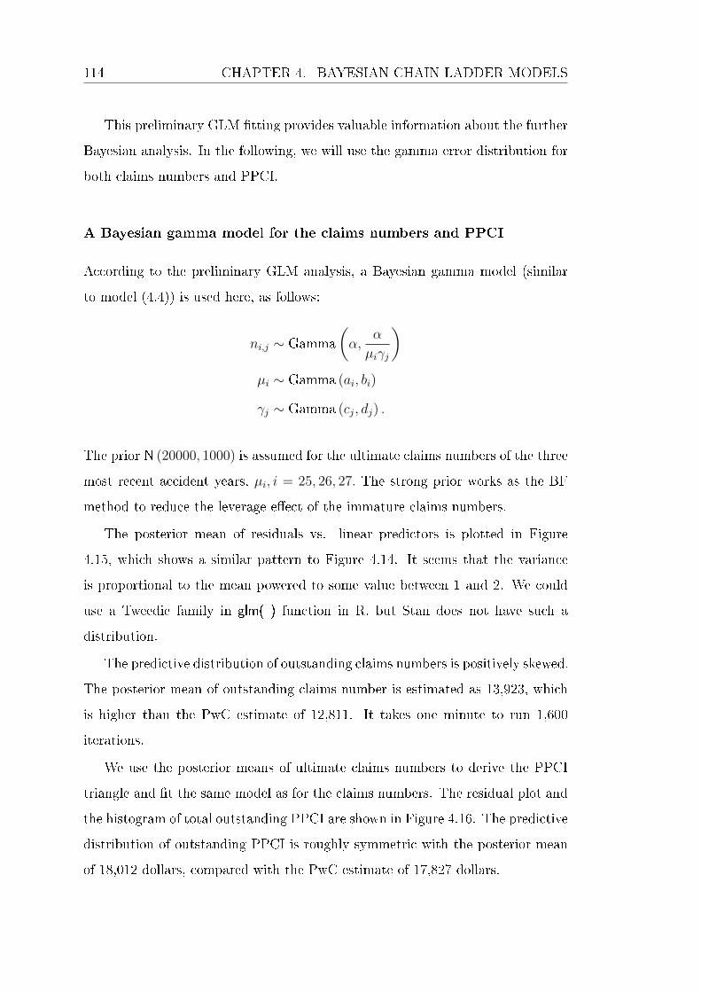
114 CHAPTER 4. BAYESIAN CHAIN LADDER MODELS
This preliminary GLM tting provides valuable information about the further
Bayesian analysis. In the following, we will use the gamma error distribution for
both claims numbers and PPCI.
A Bayesian gamma model for the claims numbers and PPCI
According to the preliminary GLM analysis, a Bayesian gamma model (similar
to model (4.4)) is used here, as follows:
ni,j ∼ Gamma
(α,
α
µiγj
)µi ∼ Gamma (ai, bi)
γj ∼ Gamma (cj, dj) .
The prior N (20000, 1000) is assumed for the ultimate claims numbers of the three
most recent accident years, µi, i = 25, 26, 27. The strong prior works as the BF
method to reduce the leverage eect of the immature claims numbers.
The posterior mean of residuals vs. linear predictors is plotted in Figure
4.15, which shows a similar pattern to Figure 4.14. It seems that the variance
is proportional to the mean powered to some value between 1 and 2. We could
use a Tweedie family in glm( ) function in R, but Stan does not have such a
distribution.
The predictive distribution of outstanding claims numbers is positively skewed.
The posterior mean of outstanding claims number is estimated as 13,923, which
is higher than the PwC estimate of 12,811. It takes one minute to run 1,600
iterations.
We use the posterior means of ultimate claims numbers to derive the PPCI
triangle and t the same model as for the claims numbers. The residual plot and
the histogram of total outstanding PPCI are shown in Figure 4.16. The predictive
distribution of outstanding PPCI is roughly symmetric with the posterior mean
of 18,012 dollars, compared with the PwC estimate of 17,827 dollars.

4.4. ESTIMATION OF CLAIMS LIABILITY IN WORKSAFE VIC 115
A compound model to combine the ultimate claims numbers and the
outstanding PPCI
Ideally, we should use the predictive distribution of ultimate claims numbers to
derive the PPCI triangle, then combine the predictive distribution of the out-
standing PPCI with the corresponding ultimate claims numbers to get the pre-
dictive distribution of outstanding liability. This method requires a large amount
of computing time.
Here we propose a compound model to get the predictive distribution of out-
standing liability. The model is specied as follows:
yij =
µi∑k=1
xijk, i = 1, . . . , 27, j = 1, . . . , 27
µi ∼ Distributioni
xijk ∼ Gamma (αij, βij) , k = 1, . . . , µi,
where µi is the ultimate claims number of accident year i whose distribution is
approximated by a Bayesian model, and xijk is the payment for the kth claim
during the development year j, with the distribution depending on both accident
year and development year.
The payments per claim incurred (PPCI) during the development period j of
accident year i is dened as
PPCIij := yij/E (µi).
Note that E(PPCIij) = E(xijk). The posterior mean of µi is an estimate of E (µi).
The relationship between the variance of PPCIij and the variance of xijk is as
follows:
Var (PPCIij) = Var
(∑µik=1 xijkE (µi)
)
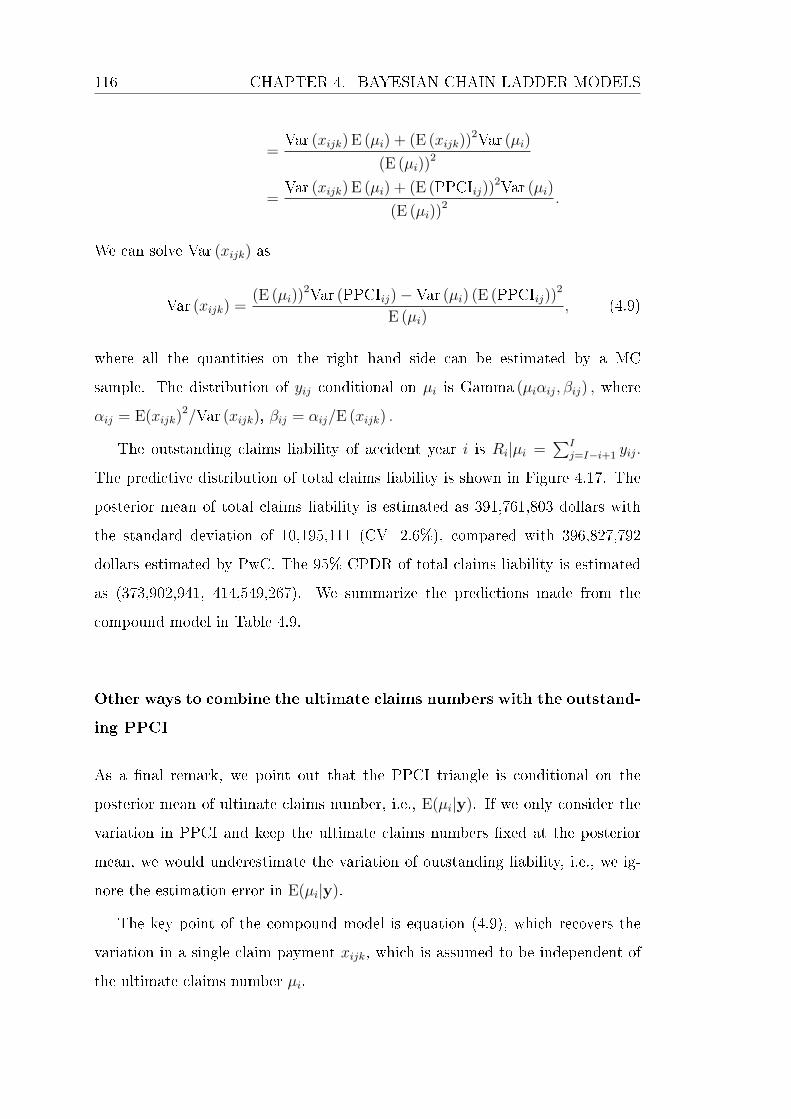
116 CHAPTER 4. BAYESIAN CHAIN LADDER MODELS
=Var (xijk) E (µi) + (E (xijk))
2Var (µi)
(E (µi))2
=Var (xijk) E (µi) + (E (PPCIij))
2Var (µi)
(E (µi))2 .
We can solve Var (xijk) as
Var (xijk) =(E (µi))
2Var (PPCIij)− Var (µi) (E (PPCIij))2
E (µi), (4.9)
where all the quantities on the right hand side can be estimated by a MC
sample. The distribution of yij conditional on µi is Gamma (µiαij, βij) , where
αij = E(xijk)2/Var (xijk), βij = αij/E (xijk) .
The outstanding claims liability of accident year i is Ri|µi =∑I
j=I−i+1 yij.
The predictive distribution of total claims liability is shown in Figure 4.17. The
posterior mean of total claims liability is estimated as 391,761,803 dollars with
the standard deviation of 10,195,111 (CV=2.6%), compared with 396,827,792
dollars estimated by PwC. The 95% CPDR of total claims liability is estimated
as (373,902,941, 414,549,267). We summarize the predictions made from the
compound model in Table 4.9.
Other ways to combine the ultimate claims numbers with the outstand-
ing PPCI
As a nal remark, we point out that the PPCI triangle is conditional on the
posterior mean of ultimate claims number, i.e., E(µi|y). If we only consider the
variation in PPCI and keep the ultimate claims numbers xed at the posterior
mean, we would underestimate the variation of outstanding liability, i.e., we ig-
nore the estimation error in E(µi|y).
The key point of the compound model is equation (4.9), which recovers the
variation in a single claim payment xijk, which is assumed to be independent of
the ultimate claims number µi.
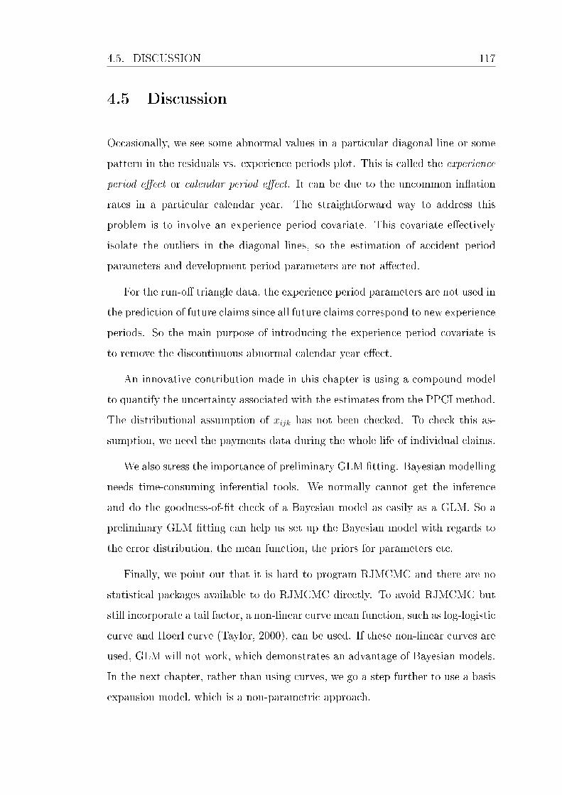
4.5. DISCUSSION 117
4.5 Discussion
Occasionally, we see some abnormal values in a particular diagonal line or some
pattern in the residuals vs. experience periods plot. This is called the experience
period eect or calendar period eect. It can be due to the uncommon ination
rates in a particular calendar year. The straightforward way to address this
problem is to involve an experience period covariate. This covariate eectively
isolate the outliers in the diagonal lines, so the estimation of accident period
parameters and development period parameters are not aected.
For the run-o triangle data, the experience period parameters are not used in
the prediction of future claims since all future claims correspond to new experience
periods. So the main purpose of introducing the experience period covariate is
to remove the discontinuous abnormal calendar year eect.
An innovative contribution made in this chapter is using a compound model
to quantify the uncertainty associated with the estimates from the PPCI method.
The distributional assumption of xijk has not been checked. To check this as-
sumption, we need the payments data during the whole life of individual claims.
We also stress the importance of preliminary GLM tting. Bayesian modelling
needs time-consuming inferential tools. We normally cannot get the inference
and do the goodness-of-t check of a Bayesian model as easily as a GLM. So a
preliminary GLM tting can help us set up the Bayesian model with regards to
the error distribution, the mean function, the priors for parameters etc.
Finally, we point out that it is hard to program RJMCMC and there are no
statistical packages available to do RJMCMC directly. To avoid RJMCMC but
still incorporate a tail factor, a non-linear curve mean function, such as log-logistic
curve and Hoerl curve (Taylor, 2000), can be used. If these non-linear curves are
used, GLM will not work, which demonstrates an advantage of Bayesian models.
In the next chapter, rather than using curves, we go a step further to use a basis
expansion model, which is a non-parametric approach.

118 CHAPTER 4. BAYESIAN CHAIN LADDER MODELS
4.6 Bibliographic notes
The Bornhuetter-Ferguson method derives from Bornhuetter and Ferguson (1972).
Friedland (2010) is the reading material of the CAS Exam 5 and provides an
overview of basic techniques of estimating unpaid claims. For the stochastic
claims reserving methods, Mack (1993, 1999, 2008) established the Mack's mod-
els. Australian actuaries are largely inuenced by Taylor (2000). England and
Verrall (2002, 2006) and Wüthrich and Merz (2008) are summaries of stochastic
reserving models.
An excellent GLM reference is McCullagh and Nelder (1989). The references
of ODP model in claims reserving problem include Renshaw and Verrall (1998),
Verrall (2000, 2004), Alai et al. (2009), Saluz et al. (2011), England et al. (2012),
Verrall and Wüthrich (2012) and Wüthrich (2013a),
Other papers using a Bayesian approach include Scollnik (2001), De Alba
(2002), Ntzoufras and Dellaportas (2002) and Meyers (2009, 2015).
Clark (2003) and Zhang et al. (2012) used the stochastic curve models. Brydon
and Verrall (2009) and Wüthrich (2013a) considered the calendar year eect.
Piwcewicz (2008) and Beens et al. (2010) are two presentations about Bayesian
claims reserving method in IAA's general insurance seminars.
Verrall et al. (2012) and Verrall and Wüthrich (2012) used RJMCMC. RJM-
CMC is proposed by Green (1995). The collective risk model (or aggregate risk
model) have been much studied in the standard risk modelling text books such
as Klugman et al. (2012) and Gray and Pitts (2012).

FIGURES 119
Figure 4.1: Time line of a claim.
Total outstanding liability (in millions)
Fre
quen
cy
1.3 1.4 1.5 1.6 1.7
01
23
45
6
CL estimateBootstrap meanBootstrap 90% CI
Figure 4.2: The histogram of the total outstanding claims liability via the bootstrap.

120 CHAPTER 4. BAYESIAN CHAIN LADDER MODELS
0 200 400 600 800 1000
4.0e
+06
8.0e
+06
1.2e
+07
Iterations
µ 6
0 200 400 600 800 1000
8500
000
1000
0000
1150
0000
Iterations
Nor
mal
ized
µ6
0 200 400 600 800 1000
0.04
0.08
0.12
0.16
Iterations
γ 6
0 200 400 600 800 1000
0.04
50.
055
0.06
50.
075
Iterations
Nor
mal
ized
γ6
Figure 4.3: The trace plots of the rst 10, 000 iterations.
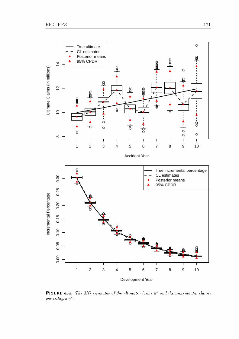
FIGURES 121
1 2 3 4 5 6 7 8 9 10
810
1214
Accident Year
Ulti
mat
e C
laim
s (in
mill
ions
)
True ultimateCL estimatesPosterior means95% CPDR
1 2 3 4 5 6 7 8 9 10
0.00
0.05
0.10
0.15
0.20
0.25
0.30
Development Year
Incr
emen
tal P
erce
ntag
e
True incremental percentageCL estimatesPosterior means95% CPDR
Figure 4.4: The MC estimates of the ultimate claims µ∗ and the incremental claims
percentages γ∗.

122 CHAPTER 4. BAYESIAN CHAIN LADDER MODELS
1 2 3 4 5 6 7 8 9 10
02
46
810
Accident Year
Unp
aid
clai
ms
(in m
illio
ns)
True liabilityCL estimatesPosterior means95% CPDR
Total outstanding liability in millions
Den
sity
20 22 24 26 28 30
0.00
0.05
0.10
0.15
0.20
0.25
True total outstanding liabilityCL estimatePosterior Mean95% CPDR
Figure 4.5: The predictive distributions of outstanding claims liability for each acci-
dent year and the predictive distribution of the total outstanding claims liability.
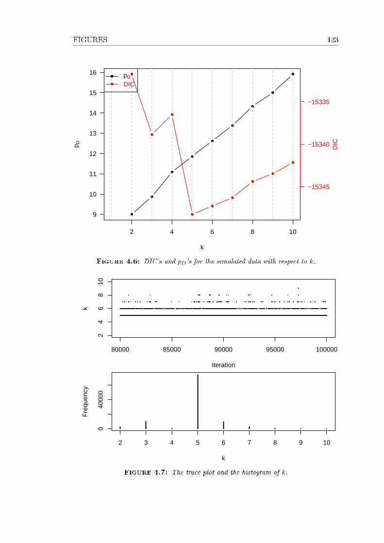
FIGURES 123
2 4 6 8 10
9
10
11
12
13
14
15
16
k
p D
−15345
−15340
−15335
DIC
pD
DIC
Figure 4.6: DIC's and pD's for the simulated data with respect to k.
80000 85000 90000 95000 100000
24
68
10
Iteration
k
040
000
k
Fre
quen
cy
2 3 4 5 6 7 8 9 10
Figure 4.7: The trace plot and the histogram of k.
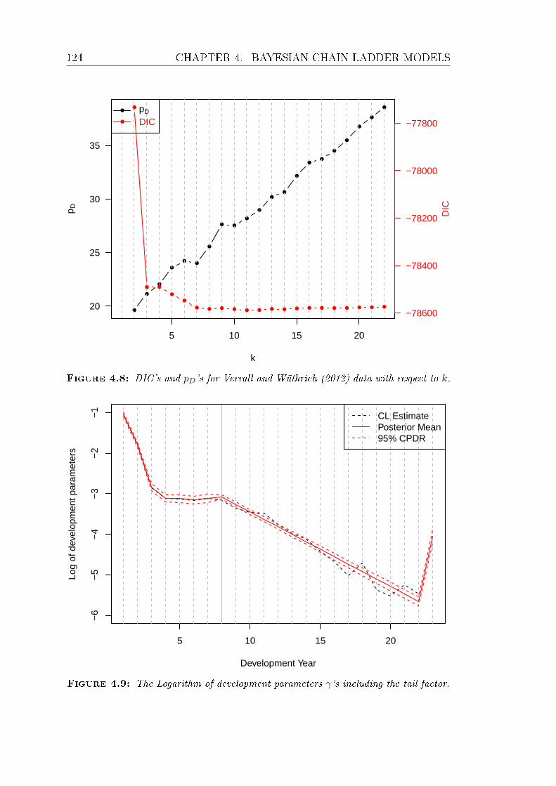
124 CHAPTER 4. BAYESIAN CHAIN LADDER MODELS
5 10 15 20
20
25
30
35
k
p D
−78600
−78400
−78200
−78000
−77800
DIC
pD
DIC
Figure 4.8: DIC's and pD's for Verrall and Wüthrich (2012) data with respect to k.
5 10 15 20
−6
−5
−4
−3
−2
−1
Development Year
Log
of d
evel
opm
ent p
aram
eter
s
CL EstimatePosterior Mean95% CPDR
Figure 4.9: The Logarithm of development parameters γ's including the tail factor.

FIGURES 125
80000 85000 90000 95000 100000
78
911
Iteration
k
020
000
5000
0
k
Fre
quen
cy
2 3 4 5 6 7 8 9 10 11 12 13 14 15 16
Figure 4.10: The trace plot and the histogram of k for Verrall and Wüthrich (2012)
data.
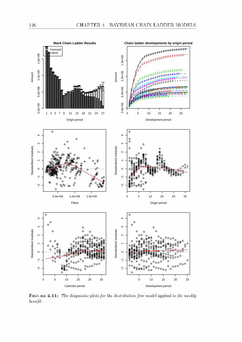
126 CHAPTER 4. BAYESIAN CHAIN LADDER MODELS
1 3 5 7 9 12 15 18 21 24 27
ForecastLatest
Mack Chain Ladder Results
Origin period
Am
ount
0.0e
+00
5.0e
+08
1.0e
+09
1.5e
+09
0 5 10 15 20 250.0e
+00
5.0e
+08
1.0e
+09
1.5e
+09
Chain ladder developments by origin period
Development period
Am
ount
1
1
1
1
11
11 1 1 1 1 1 1 1 1 1 1 1 1 1 1 1 1 1 1 1
2
2
2
2
22
2 2 2 2 2 2 2 2 2 2 2 2 2 2 2 2 2 2 2 2
3
3
33
33 3 3 3 3 3 3 3 3 3 3 3 3 3 3 3 3 3 3 3
4
4
44
4 4 4 4 4 4 4 4 4 4 4 4 4 4 4 4 4 4 4 4
5
5
55 5 5 5 5 5 5 5 5 5 5 5 5 5 5 5 5 5 5 5
6
6
66 6 6 6 6 6 6 6 6 6 6 6 6 6 6 6 6 6 6
7
77 7 7 7 7 7 7 7 7 7 7 7 7 7 7 7 7 7 7
88 8 8 8 8 8 8 8 8 8 8 8 8 8 8 8 8 8 8
99 9 9 9 9 9 9 9 9 9 9 9 9 9 9 9 9 9
00
0 0 0 0 0 0 0 0 0 0 0 0 0 0 0 0
aa
a a a a a a a a a a a a a a a
bb
b b b b b b b b b b b b b b
cc
c c c c c c c c c c c c c
dd
dd
d d d d d d d d d d
ee
ee
e e e e e e e e e
f
ff
ff f f f f f f f
gg
gg g g g g g g g
hh
h h h h h h h h
ii
i i i i i i i
jj
j j j j j j
kk
k k k k k
ll
l l l l
mm
mmm
nn
n n
oo
o
p
p
q
5.0e+08 1.0e+09 1.5e+09
−2
−1
01
23
4
Fitted
Sta
ndar
dise
d re
sidu
als
0 5 10 15 20 25
−2
−1
01
23
4
Origin period
Sta
ndar
dise
d re
sidu
als
0 5 10 15 20 25
−2
−1
01
23
4
Calendar period
Sta
ndar
dise
d re
sidu
als
5 10 15 20 25
−2
−1
01
23
4
Development period
Sta
ndar
dise
d re
sidu
als
Figure 4.11: The diagnostic plots for the distribution-free model applied to the weekly
benet.
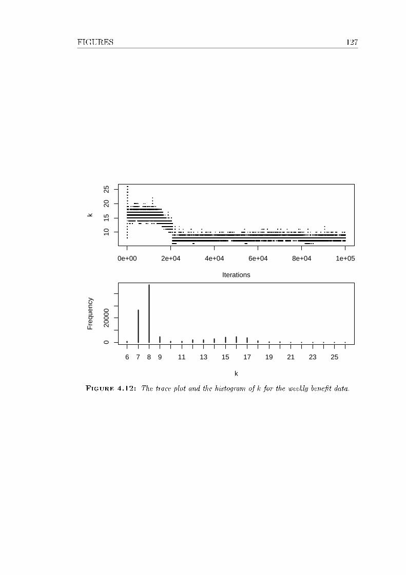
FIGURES 127
0e+00 2e+04 4e+04 6e+04 8e+04 1e+05
1015
2025
Iterations
k
020
000
k
Fre
quen
cy
6 7 8 9 11 13 15 17 19 21 23 25
Figure 4.12: The trace plot and the histogram of k for the weekly benet data.
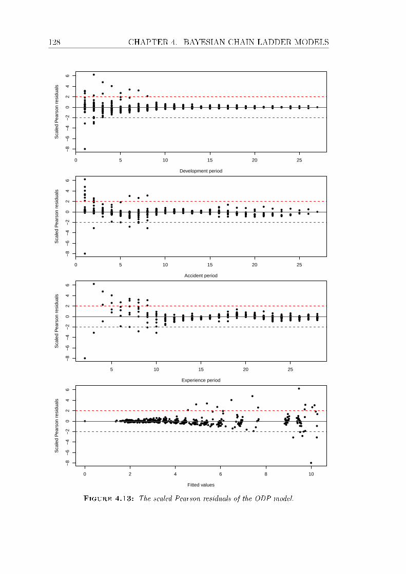
128 CHAPTER 4. BAYESIAN CHAIN LADDER MODELS
0 5 10 15 20 25
−8
−6
−4
−2
02
46
Development period
Sca
led
Pea
rson
res
idua
ls
0 5 10 15 20 25
−8
−6
−4
−2
02
46
Accident period
Sca
led
Pea
rson
res
idua
ls
5 10 15 20 25
−8
−6
−4
−2
02
46
Experience period
Sca
led
Pea
rson
res
idua
ls
0 2 4 6 8 10
−8
−6
−4
−2
02
46
Fitted values
Sca
led
Pea
rson
res
idua
ls
Figure 4.13: The scaled Pearson residuals of the ODP model.

FIGURES 129
0 5 10 15 20 25
−2
−1
01
23
Development period
Sca
led
Pea
rson
res
idua
ls
0 5 10 15 20 25
−2
−1
01
23
Accident period
Sca
led
Pea
rson
res
idua
ls
5 10 15 20 25
−2
−1
01
23
Experience period
Sca
led
Pea
rson
res
idua
ls
0 2 4 6 8 10
−2
−1
01
23
Fitted values
Sca
led
Pea
rson
res
idua
ls
Figure 4.14: The scaled Pearson residuals of the GLM with a gamma error and a
log link function.
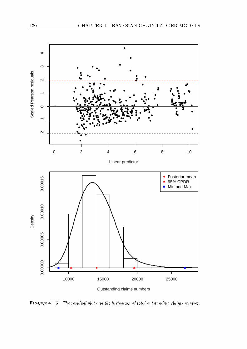
130 CHAPTER 4. BAYESIAN CHAIN LADDER MODELS
0 2 4 6 8 10
−2
−1
01
23
4
Linear predictor
Sca
led
Pea
rson
res
idua
ls
Outstanding claims numbers
Den
sity
10000 15000 20000 25000
0.00
000
0.00
005
0.00
010
0.00
015
Posterior mean95% CPDRMin and Max
Figure 4.15: The residual plot and the histogram of total outstanding claims number.

FIGURES 131
2 3 4 5 6 7
−2
02
4
Linear predictor
Sca
led
Pea
rson
res
idua
ls
Outstanding PPCI
Den
sity
16500 17000 17500 18000 18500 19000 19500
0e+
002e
−04
4e−
046e
−04
8e−
04
Posterior mean95% CPDRMin and Max
Figure 4.16: The residual plot and the histogram of total outstanding PPCI.

132 CHAPTER 4. BAYESIAN CHAIN LADDER MODELS
Total outstanding claims liability
Den
sity
380 400 420 440
0.00
0.01
0.02
0.03
0.04
Posterior mean95% CPDRMin and Max
Figure 4.17: The predictive distribution of total outstanding liability of the doctor
benet.

TABLES 133
Table 4.1: An incremental claims run-o triangle.
Occurrence Development periodperiod 1 2 · · · I
1 y1,1 y1,2 · · · y1,I
2 y2,1 y2,2 · · ·· · · · · ·I yI,1
Table 4.2: An age-to-age factors triangle.
Occurrence Age-to-age factorperiod 1 to 2 2 to 3 · · · I − 1 to I
1 f1,1 = c1,2/c1,1 f1,2 = c1,3/c1,2 · · · fI−1 = c1,I/c1,I−1
2 f2,1 = c2,2/c2,1 f2,2 = c2,3/c2,2
· · ·I fI−1,1 = cI−1,2/cI−1,1
Table 4.3: The total outstanding liability estimates from models (4.1) and (4.2).
Model Estimate No tail factor With tail factor
(4.1)R 1,463,076 1,599,558√
MSEPc(R) 55,300 58,528
(4.2)R 1,463,076 (1,471,906) NA√
MSEP(R) 60,444 (60,087) NA

134 CHAPTER 4. BAYESIAN CHAIN LADDER MODELS
Table 4.4: The proportions of the 95% CPDRs containing the true values.
µ1 µ2 µ3 µ4 µ5 µ6 µ7 µ8 µ9 µ10
0.93 0.91 0.95 0.92 0.93 0.89 0.91 0.96 0.95 0.89γ1 γ2 γ3 γ4 γ5 γ6 γ7 γ8 γ9 γ10
0.94 0.94 0.94 0.94 0.95 0.92 0.97 0.92 0.96 0.78R R2 R3 R4 R5 R6 R7 R8 R9 R10
0.94 0.90 0.94 0.98 0.95 0.98 0.97 0.97 0.95 0.88
Table 4.5: The outstanding liability estimates under dierent priors.
EstimateStrong prior case Non-informative prior case
Post. mean Sd. error CV Post. Mean Sd. error CVR 24,244,540 1,006,232 4.2% 23,867,671 1,524,567 6.4%R10 8,340,955 453,191 5.4% 8,206,132 857,982 10.5%R9 5,706,840 383,309 6.7% 5,189,284 528,886 10.2%R8 3,862,495 321,367 8.3% 4,040,881 422,256 10.5%
Table 4.6: Comparison of the total outstanding liability estimates from four dierent
models.
Model Estimate No tail With tail
(4.1)R 1,463,076 1,599,558
se(R) 55,300 58,528
(4.2)R 1,463,076 NA
se(R) 60,444 NA
(4.4)R 1,463,312 NA
se(R) 60,428 NA
(4.7)R 1,475,336 1,610,734
se(R) 54,060 56,746

TABLES 135
Table 4.7: Summary of the PwC report.
Benet Sub-benet Method Key note
Weekly
Weekly PPAC 34% of the total liability
Occupational
rehabilitation
Relate to
income
Help workers back to work
Medical
and like
Doctor PPCI Shorter tail than weekly benet
Hospital PPCI Correlated with doctor
Paramedical PPAC Generally ceases one year after
weekly benet
Hearing aids PPCI Missing data before experience year
1994
Personal &
household
services
PPAC Including attendant care, personal
services, home care, case manage-
ment, home and vehicle modication
payments
Community
integration
program
CL on
amounts
Personal & household services for
catastrophically injured workers
Medical
reports
PPCI Refers to independent medical ex-
aminations and treating health prac-
titioners' reports
Common
law
Common law
damages and
legal costs
PPCR Relates to damages and costs aris-
ing from common law claims with re-
spect to injuries occurring on or after
20 Oct 1999
Old common
law
PPCR Date of injury prior to 12 Nov 1997
Continued on next page

136 CHAPTER 4. BAYESIAN CHAIN LADDER MODELS
Table 4.7 Continued from previous page
Benet Sub-benet Method Key note
Impairment
and death
benets
Impairment PPCR Injured workers can access impair-
ment benet if their whole person
impairment is assessed as being 10%
or more
Maim PPCR The maim benet is in run-o, being
applicable only for injuries occurring
prior to 12 Nov 1997
Death lump
sum
PPCR Includes payments of statutory lump
sum and interest payments on it
Death pen-
sion
PPAC Payment pattern determines the
method used
Disputes,
recoveries
and others
Statutory le-
gal
PPCR All legal costs, other than those as-
sociated with common law cases,
arising from workers and employers
appealing decisions relating to eligi-
bility of payments or continuance of
benets
Investigation
costs
PPCI Can be incurred before any claims
payments
Recoveries PPCI Relates to recoveries from negli-
gent third parties or recoveries of
amounts where agents have paid in-
jured workers in excess of the re-
quired amount
Other PPCI Travel and accommodation costs

TABLES 137
Table 4.8: The outstanding claims liability estimates of the weekly benet from dif-
ferent models.
Model Expected value Standard deviation 95% PI/CPDR(4.1) 2,902,875,000 172,396,900 (2,558,081,200, 3,247,668,800)(4.7) 3,127,649,615 145,385,671 (2,849,161,960, 3,417,721,458)PwC 2,831,072,753 NA NA
Table 4.9: Summary of the predictions made from the compound model.
Post. mean Std. deviation 95% CPDRO/S2 Claims No. 13,9233 2,407 (9,742, 19,117)
O/S PPCI 18,0124 474 (17,056, 18,901)O/S Liability 391,761,8035 10,195,111 (373,902,941, 414,549,267)
2Stands for outstanding.3Compared with the PwC estimate of 12,811.4Compared with the PwC estimate of 17,827.5Compared with the PwC estimate of 396,827,792.


Chapter 5
Bayesian Basis Expansion Models
It is dicult to apply model (4.7), since it involves RJMCMC which is still un-
available in most Bayesian inferential packages such as WinBUGS and Stan. In
this chapter, Bayesian basis expansion models are used to t various development
patterns and accommodate the tail factor. A parametric model is typically char-
acterized by a parametric mean function and an error distribution. The shape
of the mean function is restricted by the space of parameters. Non-parametric
models such as basis expansion models are able to be automatically adjusted to
t any shape of data.
We should always bear in mind that there is a trade-o between exibility
and simplicity in model tting. Basis expansion models on one hand are more
exible, able to be adjusted to t various shapes of data, while on the other
hand, they are more complicated (i.e., involve more parameters). Before using a
non-parametric model, we should consider whether there is a capable parametric
model. The log-logistic curve and Hoerl curve together with the models in the
previous chapter can tackle most claims reserving problems.
Consider the following underlying true model:
yi ∼ f (xi) + εi, i = 1, . . . , n,
where εi are i.i.d N (0, σ2ε). A non-parametric approach is to approximate f by
139
140 CHAPTER 5. BAYESIAN BASIS EXPANSION MODELS
a non-parametric function m. Basis expansion is a way to express the form of
m. The core idea of basis expansion is to expand the input x with additional
variables, which are transformations of x, and then to apply linear models to this
newly expanded space of input x. In basis expansion models, m is written as a
linear combination of basis functions, as follows:
m (x) =H∑h=1
βhbh (x) ,
where bh is called a basis function. A common choice of bh is a polynomial. The
mechanism of dening bh determines the behaviour of m. Here we consider m as
splines, which use polynomials as basis functions with some constraints.
In Section 5.1, the aspects of splines are reviewed, including spline basis func-
tions, smoothing splines, low rank smoothing splines and Bayesian shrinkage
splines. In Section 5.2, we study two simulated examples. The rst simulated
example is based on a trigonometric mean function (Faraway, 2015), while the
second simulated example is based on the claims payments process. Both ex-
amples illustrate the usefulness of natural cubic spline basis in the extrapolation
beyond the range of data. Section 5.3 is the application of above methodology to
the doctor benet in WorkSafe Victoria. The basis expansion model used to t
the PPCI triangle induces a tail development.
5.1 Aspects of splines
Splines are a combination of polynomials and step functions. Before discussing
splines, we review the properties of polynomial models and step function models.
Our focus is the form of the mean function m rather than the error distribution.
In polynomial models, the basis functions have the form of bh (x) = xh. Polyno-
mial models tend to capture the shape of the data as long as there are high-degree
polynomials. A disadvantage of polynomial models is the global representation of
basis functions, which means all the data points can aect parameter estimation

5.1. ASPECTS OF SPLINES 141
and every parameter can aect the mean function.
A step function model partitions the data into H parts and ts the hth part
using a basis function bh (x) whose value is zero for the remaining parts of data.
Step function models have a disadvantage of discontinuity at the boundaries of
partition.
Spline models are a combination of polynomial models and step function mod-
els. For example, a cubic spline is a series of piecewise-cubic polynomials joined
continuously up to the second derivatives. The properties of continuity and being
piecewise are realised by using a particular set of basis functions.
5.1.1 Basis functions of splines
Truncated power basis
One intuitive choice is truncated power basis of degree p, which contains K+p+1
basis functions as follows:
1, x, . . . , xp, (x− κ1)p+ , . . . , (x− κK)p+ ,
where (x− κi)p+ = (x− κi)p for x > κi and 0 elsewhere, κi, i = 1, . . . , K are
called knots. The basis functions consist of two parts: the global polynomials
up to degree p, and the truncated degree p polynomials which have the local
representation property. It can be shown that any linear combination of these
basis functions has continuous derivatives up to order p− 1 at every knot.
The degrees of freedom of a spline is the number of parameters in the mean
function. Truncated power basis of degree p has K + p + 1 degrees of freedom,
which is intuitive to join K + 1 pieces of degree p polynomials smoothly (up
to p−1th derivatives at knots), Kp degrees of freedom are lost, leaving K+p+1
degrees of freedom, i.e., K + p+ 1 = (K + 1) (p+ 1)−Kp. In the GLM setting,

142 CHAPTER 5. BAYESIAN BASIS EXPANSION MODELS
we write the design matrix as
X =
1 x1 · · · xp1 (x1 − κ1)p+ · · · (x1 − κK)p+
1 · · · · · · · · · · · · · · · · · ·
1 xn · · · xpn (xn − κ1)p+ · · · (xn − κK)p+
.
At rst glance, it seems that spline models are more complicated than either
polynomial models or step function models. This is not true. Compared with
polynomial models, we do not need the higher degree polynomials to capture all
the curvatures of the data, since we have the local basis functions. Compared
with step function models, we overcome the problem of discontinuity via the
mechanism of basis functions. Spline models combine the advantages of both
polynomial and step functions models, and get rid of the aws of both models
when they are used alone.
A truncated power basis has a practical disadvantage in that it is far from
orthogonal, i.e., the columns of design matrix X are not orthogonal. It is better
to work with an equivalent basis1 with more stable numerical properties.
B-spline basis
The most common choice for spline basis is the B-spline basis of degree p, which
consists of piecewise continuous functions only non-zero over the intervals between
p+ 2 adjacent knots. The degrees of freedom of a K-knot degree p B-spline basis
is K−p+1, since the spline is to be evaluated only over the interval [κp+1, κK−p].
To span the same function space as truncated power basis of degree p with K
knots, we need to add p arbitrary knots to the ends of [κ1, κK ], i.e., we usually
choose the knots κ1, κ1, κ1, κ1, κ2, . . . , κK−1, κK , κK , κK , κK in a cubic B-spline
basis. A B-spline basis is an orthogonal set.
1Two bases are equivalent if they span the same set of functions.

5.1. ASPECTS OF SPLINES 143
Radial basis
Another set of basis functions equivalent to a truncated power basis of degree p
(odd) is a radial basis, as follows:
1, x, . . . , xp, |x− κ1|p, . . . , |x− κK |p.
We will come back to radial basis functions in smoothing splines and Bayesian
shrinkage splines.
5.1.2 Smoothing splines
Smoothing splines2 come from the solution to the optimal problem of nding a
function g to minimizes the residual sum of squares (RSS) plus a penalty on the
integral of the squared second derivatives of g. This penalized residual sum of
squares is
RSS (g, λ) =n∑i=1
[yi − g (xi)]2 + λ
∫[g′′ (t)]
2dt, (5.1)
where λ is a xed smoothing parameter. The rst term measures closeness to the
data, while the second term penalizes curvature in the function and λ establishes
a trade-o between the two. Two special cases are: λ→ 0, g can be any function
that interpolates the data (i.e., RSS=0); λ→∞, g is the simple linear regression
t since no second derivative can be tolerated.
Remarkably, even without the constraint of g as splines, it can be shown, for
0 < λ < ∞, that g is a natural cubic spline with knots placed at the unique
values of xi, i = 1, .., n (Hastie and Tibshirani, 1990). Natural cubic splines
are cubic splines with the constraint that they are linear beyond the boundary
knots. Hence, the degrees of freedom of a smoothing spline g are n (i.e., n =
n+ 3 + 1−2−2), since 4 degrees of freedom are lost due to the linear constraints
at two boundary knots.
2A smoothing spline is a one-dimensional thin plate spline.

144 CHAPTER 5. BAYESIAN BASIS EXPANSION MODELS
We can write this natural cubic spline as
g (x) =n∑h=1
βhbh (x) ,
where bh : h = 1, . . . , n is a set of n basis functions for representing this natural
cubic spline. We write the design matrix as
X =
b1 (x1) · · · bn (x1)
· · · · · · · · ·
b1 (xn) · · · bn (xn)
,
which is an n× n matrix. RSS in (5.1) can be written as
RSS (β, λ) = y −Xβ + λβTΩβ, (5.2)
where Ω [i, j] =∫bi′′ (t) bj
′′ (t) dt. The solution is β =(XTX + λΩ
)−1XTy, which
has a additional penalty term λΩ compared with the ordinary least squares so-
lution.
Rank of a smoother and eective degrees of freedom
The tted values of smoothing splines are
y = X(XTX + λΩ
)−1XTy = Sλy,
where Sλ is known as the smoother matrix or hat matrix. We list some features
of Sλ as follows:
1. Sλ is a symmetric positive semi-denite matrix with rank n.
2. Sλ has n eigenvectors and n non-zero eigenvalues.
3. λ cannot aect the eigenvectors of Sλ.
4. λ aects the eigenvalues of Sλ negatively, except the rst two which are
always 1 corresponding to the two-dimensional eigenspace of functions linear

5.1. ASPECTS OF SPLINES 145
in x. Other eigenvalues are between 0 and 1 depending on λ.
5. The degree of freedom of Sλ is dfλ = trace (Sλ) = sum of eigenvalues, which
is always between 2 and n.
6. When λ→ 0, all the eigenvalues are 1. dfλ = trace (Sλ) = sum of eigenval-
ues = n, corresponding to any functions interpolating the data.
7. When λ→∞, all the eigenvalues are 0 except the rst two. dfλ = trace (Sλ) = sum
of eigenvalues = 2, corresponding to a straight line.
Radial basis functions for smoothing splines
Smoothing splines have a natural representation in terms of radial basis functions.
For a given λ, a smoothing spline can be written as
g (x) = γ0 + γ1x+n∑k=1
δk|x− xk|3,
where θ =(γ0, γ1, δ1, . . . , δn
)minimizes the penalized residual sum of squares
n∑i=1
(yi − γ0 − γ1xi −
n∑k=1
δk|xi − xk|3)2
+ λn∑i=1
δi
n∑k=1
δk|xi − xk|3, (5.3)
subject to the constraints∑n
k=1 δk =∑n
k=1 δkxk = 0. The constraints make the
number of parameters n rather than n + 2 which is consistent with the degrees
of freedom of a smoothing spline.
The criterion (5.3) is connected with the criterion of best linear unbiased predi-
cation (BLUP) in a mixed eects model, which opens a gate for a Bayesian mixed
eects model representing a smoothing spline.
Choice of λ
The above discussion is based on a given λ. We can treat λ as a tuning parameter
which indexes dierent smoothing models. The choice of λ can be thought as a
model selection problem. The selection criterion relates to a model's prediction

146 CHAPTER 5. BAYESIAN BASIS EXPANSION MODELS
capability on an independent test data set. Typically, we use test error as a
measure of prediction capability, dened as the prediction squared error over
an independent test sample. The most widely used method for estimating the
test error is cross-validation (see Section 2.2). λ is chosen by minimizing CV or
generalized CV (Hastie et al., 2009).
5.1.3 Low rank thin plate splines
The rank of smoother Sλ is the number of distinct x. Sometimes it is called a full
rank smoother. Wood (2003, 2006) uses the truncated eigen-decomposition of X
to achieve a low rank smoother approximating the full rank smoother. A simpler
approximation is to set up a new natural cubic spline basis with specied knots
κi, i = 1, . . . , K, rather than at every distinctive x.
It can be shown that a natural cubic spline with specied knots tted by
minimizing (5.1) can approximate the full rank smoothing spline well (Ruppert
et al., 2003). A spline with xed knots is called a spline regression. If it is tted
by minimizing (5.1), it is called a penalized spline regression, or more generally a
low rank thin plate spline.
Rank of a xed-knot thin plate spline and eective degrees of freedom
Some features of a K-knot thin plate spline smoother Sλ are as follows:
1. Sλ is a symmetric positive semi-denite matrix with rank of K
2. Sλ has K eigenvectors and K non-zero eigenvalues.
3. λ cannot aect the eigenvectors of Sλ.
4. λ aects the eigenvalues of Sλ negatively, except the rst two which are
always 1 corresponding to the two-dimensional eigenspace of functions linear
in x. Other eigenvalues are between 0 and 1 depending on λ.
5. The degrees of freedom of Sλ is dfλ = trace (Sλ) = sum of eigenvalues,
which is always between 2 and K.

5.1. ASPECTS OF SPLINES 147
6. When λ→ 0, all the eigenvalues are 1, Sλ → I. dfλ = trace (Sλ) = sum of
eigenvalues = K, corresponding to any functions interpolating the K knots.
7. When λ → ∞, all the eigenvalues are 0 except the rst two. dfλ =
trace (Sλ) = sum of eigenvalues = 2, corresponding to a straight line.
Radial basis functions for a xed-knot thin plate spline
For a given λ and xed knots κi, i = 1, . . . , K, the xed-knot thin plate spline
can be written as
g (x) = γ0 + γ1x+K∑k=1
δk|x− κk|3,
where θ =(γ0, γ1, δ1, . . . , δK
)minimizes the following penalized residual sum of
squares,
n∑i=1
(yi − γ0 − γ1xi −
K∑k=1
δk|xi − κk|3)2
+ λK∑l=1
δl
K∑k=1
δk|κl − κk|3,
subject to the constraints∑K
k=1 δk =∑K
k=1 δkκk = 0. The constraint makes the
number of parameters K rather than K + 2 which is consistent with the degrees
of freedom of a natural cubic spline with K knots. For compact notation and
programming, we can write the above equation in terms of matrices, as follows:
RSS = ‖y −Xγ − Zδ‖+ λδTKδ, (5.4)
where X [i, ] = (1, xi)T ,Z [i, k] = |xi − κk|3, γ = (γ0, γ1) , δ =
(δ1, . . . , δK
)and
K [l, k] = |κl − κk|3, l = 1, . . . , K, k = 1, . . . , K.
Linkage to a mixed eects model
As already mentioned at the end of Section 5.1.2, the criterion of minimizing
(5.4) is related to the criterion for calculating the best linear unbiased predic-
tion(BLUP) in a mixed eects model. Suppose we have the following mixed

148 CHAPTER 5. BAYESIAN BASIS EXPANSION MODELS
eects model:
yi = γ0 + γ1xi +K∑k=1
δk|xi − κk|3 + εi
E (δk) = 0; Var (δ) = σ2δK−1
E (εi) = 0; Var(ε) = σ2εI.
BLUP of γ and δ is dened as follows:
γ, δ = argminγ′,δ′
E(sTXγ′ + tTZδ′
)−(sTXγ + tTZδ
)2,
for any arbitrary s and t, and subject to the unbiasedness constraint
E(sTXγ′ + tTZδ′
)= E
(sTXγ + tTZδ
).
It can be shown that γ and δ also minimize the following penalized RSS:
(y −Xγ′ − Zδ′)T (σ2εI)−1
(y −Xγ′ − Zδ′) + δT(σ2δK−1)−1
δ,
which is equivalent to minimizing (5.4) with λ = σ2ε/σ
2δ . γ and δ have the following
expression: γδ
=(CTC + λB
)−1CTy,
where
C = [X,Z] , B =
0 0
0 K
.The tted values are y = C
(CTC + λB
)−1CTy. Note that γ and δ depend on the
variance parameters σ2δ and σ
2ε , which can be estimated via maximum likelihood
or restricted maximum likelihood (REML).
The connection of a xed-knot thin plate spline with a mixed eects linear
model makes it possible to analyze a smoothing spline in the framework of a

5.1. ASPECTS OF SPLINES 149
Bayesian mixed eects linear model. Bayesian mixed eects linear models can
quantify the estimation uncertainties of variance parameters which are ignored
in the REML approach.
5.1.4 Bayesian splines
Rather than using the equivalence of a smoothing spline to a mixed eects linear
model, we can set up a mixed eects model structure directly on the basis expan-
sion functions. The core idea of a smoothing spline is to shrink the parameters
δi, i = 1, . . . , n towards 0 in equation (5.3), where the shrinkage force and style
are controlled by the smoothing parameter λ.
In the Bayesian framework, we can assume shrinkage priors, which perform
the role of the smoothing parameter. Generally, we use the following Bayesian
shrinkage spline model:
yi =H∑h=1
βhbh (xi) + εi
εi ∼ N(0, σ2
)βh ∼ Gh, h = 1, . . . , H,
where Gh is a shrinkage prior having high density at zero and heavy tails to
avoid over-shrinking. Gh can be a t distribution with small degrees of freedom,
or a double exponential distribution (Laplace distribution) which is related to
the lasso method. The Laplace prior induces sparsity in the posterior mode, in
that the posterior mode βh can be exactly equal to zero. The Laplace prior is
the prior having heaviest tails which still produces a computationally convenient
uni-modal posterior density.
An alternative is to use a generalized double Pareto prior distribution (Gelman
et al., 2014), which resembles the double exponential near the origin while having
arbitrarily heavy tails.
One can sample from a generalized double Pareto with scale parameter of

150 CHAPTER 5. BAYESIAN BASIS EXPANSION MODELS
ξ and shape parameter of α by instead drawing βh ∼ N (0, σ2τh), with τh ∼
Exp (λ2h/2) and λh ∼ Gamma (α, αξ). Placing the prior p (σ) ∝ 1/σ, we then
obtain a simple block Gibbs sampler having the following full conditional posterior
distributions:
β|· ∼ N((
XTX + T−1)−1
XTy, σ2(XTX + T−1
)−1)
σ2|· ∼ Inv-gamma
(n+ k
2,(y −Xβ)T (y −Xβ)
2+βTT−1β
2
)
λh|· ∼ Gamma
(α + 1,
|βh|σ
+ η
), h = 1, . . . , H
τ−1h |· ∼ Inv-Gaussian
(µ =
λhσ
βh, ρ = λ2
h
), h = 1, . . . , H,
where
X =
b1 (x1) · · · bH (x1)
· · · · · · · · ·
b1 (xn) · · · bH (xn)
,T = Diag (τ1, · · · , τH) .
5.2 Two simulated examples
Now we turn to two simulated examples. It is always good to rst check our
methods using some simulated data to see whether these methods work before we
go into the more complicated application. In these two examples, even though we
know the underlying true mean function, estimating the coecients in the mean
function is not straightforward. We use smoothing splines, low rank smoothing
splines and Bayesian shrinkage splines to estimate the mean function.
The rst simulated example uses a trigonometric mean function with normal
errors. It is an example used by Faraway (2015). Here we are more interested in
prediction beyond the boundary. Besides the methods used by Faraway (2015),
we also study this example in the Bayesian framework. The second simulated
example assumes the response variable following a gamma distribution with a
log-logistic curve mean function. We design the second example to mimic the

5.2. TWO SIMULATED EXAMPLES 151
claims payment process in general insurance. This prepares for application to
real claims data in Section 5.3.
5.2.1 A model with a trigonometric mean function and nor-
mal errors
We generate the data from the following model:
yi = sin3(2πx3i ) + εi, i = 1, . . . , 100
xi ∼ U (0, 1)
εi ∼ N (0, 0.01) .
Polynomial basis expansion regression models
The R function poly( ) generates an orthogonal polynomial basis matrix of spec-
ied degree at specied values. In Figure 5.1, the rst plot shows the raw poly-
nomial basis of degree 4 at values from 0 to 1, where each line corresponds to
a polynomial. The second plot shows the orthogonal polynomial basis of degree
4 at values from 0 to 1, where each line corresponds to a linear combination of
polynomials, x, x2, x3, x4. The third plot shows the orthogonal polynomial basis
of degree 11 at values from 0 to 1.
We use the orthogonal polynomial basis of degrees 4, 7, and 11 to t the
simulated data. The tted lines are shown in Figure 5.2. Note that the degrees
of freedom (df) shown in the legend box include the intercept term. None of the
tted lines can capture the shape of data adequately.
Spline regression models
The R function bs( ) works similarly to poly( ). It generates the B -spline basis
matrix of specied degree and knots. The number of rows of the B -spline basis
matrix is equal to the number of values to be calculated. The number of columns
of B -spline basis matrix is equal to the degrees of freedom of this spline. Here
152 CHAPTER 5. BAYESIAN BASIS EXPANSION MODELS
we use a cubic B -spline with 8 knots at (0.2, 0.4, 0.5, 0.6, 0.7, 0.8, 0.85, 0.9). So
the degrees of freedom (or equivalently the number of columns) is 12, including
the intercept term.
Using the R function ns( ), we generate a natural cubic B -spline with 8 interior
knots at (0.2, 0.4, 0.5, 0.6, 0.7, 0.8, 0.85, 0.9) and the boundary knots at the
ending points of x. A natural cubic B -spline has the property of orthogonality
and linearity beyond the boundary knots, so the degrees of freedom of this natural
cubic B -spline are 10 (i.e., 8+2+3+1-4), including the intercept term.
The comparison of a normal cubic B -spline basis with a natural cubic B -spline
basis is shown in Figure 5.3. There are 12 lines in the rst plot corresponding to
12 columns of a cubic B -spline basis matrix. Except the marginal lines, all the
lines are non-zero over the interval between 5 adjacent knots. There are 10 lines
in the second plot, corresponding to 10 columns of the natural cubic B -spline
basis matrix.
Figure 5.4 shows the tted lines from spline basis expansion regressions. The
cubic spline with 12 degrees of freedom is less wiggly than the polynomial regres-
sion with the same degrees of freedom. This is mainly due to the local represen-
tation of spline basis functions. However, the cubic spline spreads weirdly outside
the range of data, especially for x > 1.
The natural cubic spline regression with 10 degrees of freedom has similar
performance to the cubic spline within the range of data. Moreover, it has a
better extrapolation outside the range of data due to the linear constraints.
A full rank thin plate spline
The full rank smoothing spline is as good as the natural cubic spline since the
smoothing spline also puts linear constraints beyond the range of data. However,
the tting process of a smoothing spline is quite dierent.
A smoothing spline uses the natural basis functions with knots at every unique
x and shrink the coecients by a penalty matrix based on (5.2), while the natural
cubic spline regression does not shrink the coecients but uses the least squares

5.2. TWO SIMULATED EXAMPLES 153
estimates.
Low rank thin plate splines
Rather than using the full rank basis matrix as in a smoothing spline, Wood
(2003, 2006) uses the truncated eigen-decomposition of a full rank basis matrix
to achieve a low rank smoother approximating the full rank smoother. Package
mgcv can t a low rank smoothing spline by smoothing function s. A disadvantage
of this package is that we cannot specify the degrees of freedom or the location
of knots. They are chosen automatically by generalized cross-validation criteria.
Another approach to solving the low rank smoothing spline is using a set
of radial basis functions with specied knots as in Section 5.1.3. Due to the
equivalence of a low rank thin plate spline to a mixed eects model, we can set
up a low rank thin plate spline model as a Bayesian mixed eects model:
y = Xγ + Zδ + ε
δ ∼ N(0, σ2
δK−1)
ε ∼ N(0, σ2
εI),
(5.5)
where X [i, ] = (1, xi)T ,Z [i, k] = |xi − κk|3, γ = (γ0, γ1) , δ = (δ1, . . . , δK) and
K [l, k] = |κl − κk|3, l = 1, . . . , K, k = 1, . . . , K. Here we specify a set of 20
equally located knots spreading the range of x. We give non-informative priors
for γ, σ2δ , σ
2ε . The smoothing parameter λ = σ2
ε/σ2δ is not xed, and we can get
the posterior distribution of it.
We use Stan to simulate from the posterior distribution. It takes approxi-
mately 5 minutes to generate 1,600 iterations of which the rst half are discarded
as burn-in.
The posterior mean of λ is estimated as 0.000121 compared with 0.000102
from smoothing spline t. We also plot the posterior predictive distribution for
x ∈ (−0.05, 1.05) in Figure 5.5. The estimated number of eective parameters
is pD = 17.9, pWAIC = 16.5, ploo = 17.5, which indicates around 16 degrees of

154 CHAPTER 5. BAYESIAN BASIS EXPANSION MODELS
freedom for the smoothing line (i.e., 18 minus two scale parameters, σ2δ and σ
2ε).
A Bayesian spline model
We apply the method in Section 5.1.4. A natural cubic spline basis is used with 20
equally located interior knots spreading the range of x and the boundary knots at
the ending points of x. We compare the goodness-of-t of three shrinkage priors:
generalized double Pareto (gdP) prior, Laplace prior (double exponential prior)
and Cauchy prior.
The smoothness depends on the hyperparameters in the shrinkage priors,
which can be specied as xed constants or left to be estimated from the data.
We list several information criteria in Table 5.1. Generally, all the shrinkage
priors perform equally well. The tted line is not sensitive to shrinkage priors.
Hence we only give the posterior mean of the tted line with the 95% CPDR
under Cauchy(0, 0.1) shrinkage prior in Figure 5.6.
5.2.2 A gamma response variable with a log-logistic growth
curve mean function
We assume the cumulative claims following a log-logistic growth curve, and gen-
erate the incremental claims from a gamma distribution. More specically, we
use the following model to generate the incremental claims:
yij ∼ Gamma
(100,
100
µij
), i = 1, . . . , 30, j = 1, . . . , 40
µij = Pi × LRi × (G (j; θi, ωi)−G (j − 1; θi, ωi))
Pi = (1.00 + i× 0.01)× 106
LRi ∼ N(0.8, 0.12
)θi ∼ N
(7.5, 0.052
)ωi ∼ N
(2.5, 0.032
)G (l; θ, ω) =
lω
lω + θω, l = 0, . . . , 40,
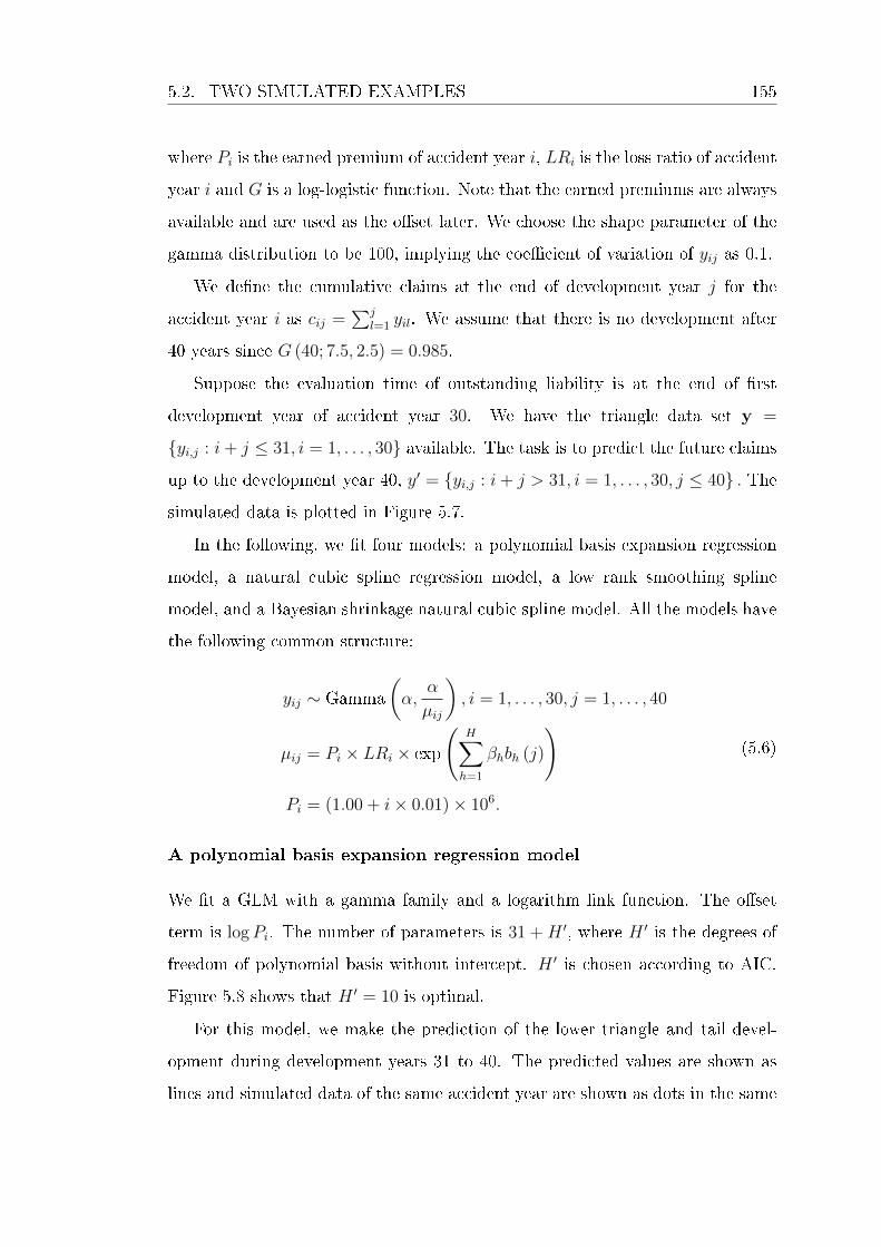
5.2. TWO SIMULATED EXAMPLES 155
where Pi is the earned premium of accident year i, LRi is the loss ratio of accident
year i and G is a log-logistic function. Note that the earned premiums are always
available and are used as the oset later. We choose the shape parameter of the
gamma distribution to be 100, implying the coecient of variation of yij as 0.1.
We dene the cumulative claims at the end of development year j for the
accident year i as cij =∑j
l=1 yil. We assume that there is no development after
40 years since G (40; 7.5, 2.5) = 0.985.
Suppose the evaluation time of outstanding liability is at the end of rst
development year of accident year 30. We have the triangle data set y =
yi,j : i+ j ≤ 31, i = 1, . . . , 30 available. The task is to predict the future claims
up to the development year 40, y′ = yi,j : i+ j > 31, i = 1, . . . , 30, j ≤ 40 . The
simulated data is plotted in Figure 5.7.
In the following, we t four models: a polynomial basis expansion regression
model, a natural cubic spline regression model, a low rank smoothing spline
model, and a Bayesian shrinkage natural cubic spline model. All the models have
the following common structure:
yij ∼ Gamma
(α,
α
µij
), i = 1, . . . , 30, j = 1, . . . , 40
µij = Pi × LRi × exp
(H∑h=1
βhbh (j)
)Pi = (1.00 + i× 0.01)× 106.
(5.6)
A polynomial basis expansion regression model
We t a GLM with a gamma family and a logarithm link function. The oset
term is logPi. The number of parameters is 31 + H ′, where H ′ is the degrees of
freedom of polynomial basis without intercept. H ′ is chosen according to AIC.
Figure 5.8 shows that H ′ = 10 is optimal.
For this model, we make the prediction of the lower triangle and tail devel-
opment during development years 31 to 40. The predicted values are shown as
lines and simulated data of the same accident year are shown as dots in the same
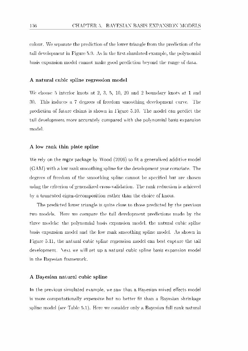
156 CHAPTER 5. BAYESIAN BASIS EXPANSION MODELS
colour. We separate the prediction of the lower triangle from the prediction of the
tail development in Figure 5.9. As in the rst simulated example, the polynomial
basis expansion model cannot make good prediction beyond the range of data.
A natural cubic spline regression model
We choose 5 interior knots at 2, 3, 5, 10, 20 and 2 boundary knots at 1 and
30. This induces a 7 degrees of freedom smoothing development curve. The
prediction of future claims is shown in Figure 5.10. The model can predict the
tail development more accurately compared with the polynomial basis expansion
model.
A low rank thin plate spline
We rely on the mgcv package by Wood (2006) to t a generalized additive model
(GAM) with a low rank smoothing spline for the development year covariate. The
degrees of freedom of the smoothing spline cannot be specied but are chosen
using the criterion of generalized cross-validation. The rank reduction is achieved
by a truncated eigen-decomposition rather than the choice of knots.
The predicted lower triangle is quite close to those predicted by the previous
two models. Here we compare the tail development predictions made by the
three models: the polynomial basis expansion model, the natural cubic spline
basis expansion model and the low rank smoothing spline model. As shown in
Figure 5.11, the natural cubic spline regression model can best capture the tail
development. Next we will set up a natural cubic spline basis expansion model
in the Bayesian framework.
A Bayesian natural cubic spline
In the previous simulated example, we saw that a Bayesian mixed eects model
is more computationally expensive but no better t than a Bayesian shrinkage
spline model (see Table 5.1). Here we consider only a Bayesian full rank natural

5.2. TWO SIMULATED EXAMPLES 157
cubic spline model with shrinkage priors. An alternative is to use a xed-knot
natural cubic spline model which leads to similar prediction given the knots are
chosen properly.
The Bayesian shrinkage spline model we will focus on is as follows:
yij ∼ Gamma
(α,
α
µij
), i = 1, . . . , 30, j = 1, . . . , 40
µij = Pi × LRi × exp
(30∑h=1
βhbh (j)
)βh ∼ DoubleExp
(0, σ2
), h = 1, . . . , 30
Pi = (1.00 + i× 0.01)× 106,
(5.7)
where bh : h = 1, . . . , 30 is a set of natural cubic spline basis functions with
interior knots placed at 2, . . . , 29 and boundary knots placed at 1 and 30.
Denote the natural cubic spline basis matrix (40× 30) by B. Hence
30∑h=1
βhbh (j) = (Bβ) [, j] ,
where β = (β1, . . . , β30). We use the double exponential (Laplace) shrinkage
priors with mean zero and unknown variance σ2. We assume non-informative
priors for LRi, α and σ.
Model inference. We use Stan to estimate parameters and predict future
claims. It takes 40 seconds for 1600 iterations. After checking convergence,
we plot the posterior mean of Pearson residuals vs. the posterior mean of t-
ted values in Figure 5.12. Not surprisingly, it shows a randomly spread, since
the gamma distribution assumption is the same as the underlying error structure
generating the data.
The posterior mean and the 95% CPDR of the proportion of the incremental
claims to the ultimate claims (i.e., the term exp(∑30
h=1 βhbh (j))in equation (5.7))
is shown in Figure 5.13. The posterior mean is close to the true underlying log-

158 CHAPTER 5. BAYESIAN BASIS EXPANSION MODELS
logistic curve. The 95% CPDR covers most of the true underlying curve. As we
expected, the 95% CPDR spreads out after development year 30, since there are
no data after development year 30.
We plot the posterior distribution of cumulative claims up to development year
40 for 9 accident years shown in Figure 5.14. The ultimate claims distributions
are positively skewed due to the assumption of gamma likelihood. The posterior
distribution of total outstanding unpaid claims liability is plotted in Figure 5.15.
We also plot the result using a Cauchy shrinkage prior for comparison. Both
models lead to similar posterior distributions that are positively skewed.
Advantages of using a Bayesian model. An important advantage of Bayesian
modelling is the ability to evaluate the uncertainty via simulation from the pos-
terior distribution. Frequentist models typically use the asymptotic property of
parameters under resampling to estimate the uncertainty associated with param-
eters and future values. This method becomes problematic for some complicated
functions of direct predictions.
For the claims reserving problem, the response variable is the incremental
claims, but our interest is the cumulative claims whose uncertainty is dicult to
estimate. The bootstrap method can tackle this task through resampling residuals
and generating the pseudo-data. In the Bayesian framework, we use MCMC or
HMC to simulate the joint posterior distribution of parameters and perform a
further step to generate the future claims. Essentially, the distribution of any
functions of response variable can be simulated through this process.
Model selection. Finally, we compare four models in terms of the three in-
formation criteria discussed in Section 2.2. As shown in Table 5.2, these four
models have similar goodness-of-t values. The dierences are mainly due to the
randomness.

5.3. APPLICATION TO THE DOCTOR BENEFIT 159
5.3 Application to the doctor benet
In the previous chapter, the analysis of doctor benet did not accommodate the
tail development. While all the claims seem to be reported by the development
year 27, the benet payments seem to continue beyond the development year 27.
So we need to consider the tail development of PPCI.
A basis expansion model is applied to extrapolate the tail development. The
natural cubic spline is at the top of our option list, since it comes from an optimal
problem and has the linear constraint beyond the boundary knots.
As in the previous chapter, we have three steps to t a compound model. The
rst step is to t a Bayesian natural cubic spline model to the claims numbers.
The posterior mean of ultimate claims number is used to calculate the PPCI
triangle. Next, we t a Bayesian natural cubic spline model to the PPCI triangle
to get the posterior distribution of outstanding PPCI. The payments are assumed
to continue up to the development year 30. Finally, we apply a compound model
to combine the ultimate claims numbers with the outstanding PPCI to get the
claims liability.
5.3.1 Claims numbers
A Bayesian natural cubic spline model with Cauchy shrinkage priors and a gamma
distribution is tted to the claims numbers triangle. The boundary knots are
placed at the rst and last available development years, i.e., the development
years 1 and 27. The development years 2 to 26 are interior knots. The basis
matrix for prediction must use the same knots.
The residual plot shows a quite similar pattern to Figure 4.14 so we did not
present it here. The posterior mean and the 95% CPDR for the proportion of
incremental reported claims to the ultimate claims numbers are plotted in Figure
5.16. It shows that nearly all the claims are reported by the development year
3, hence the assumption of no tail development after development year 27 is
reasonable.

160 CHAPTER 5. BAYESIAN BASIS EXPANSION MODELS
We plot the posterior distributions of cumulative claims numbers for the ac-
cident years 8, 10, 12, 14, 16, 18, 20, 22 and 24 in Figure 5.18. It shows that
the ultimate claims numbers for the older accident years can be estimated more
accurately. For the recent accident years, the large uncertainties in the rst three
development years are carried forward to the ultimate claims numbers. We use
the posterior mean of the ultimate claims number as a proxy to derive the PPCI
triangle.
5.3.2 PPCI
Similar to the claims numbers, we t a natural cubic spline model with Cauchy
shrinkage priors to the PPCI triangle. The choice of knots is the same as for the
claims numbers, and we assume the payments are nalized by the development
year 30. The posterior inference of the proportion of incremental PPCI to the
ultimate PPCI is shown in Figure 5.17. The 95% CPDR spreads out in the tail
area due to the lack of data. The development of PPCI for accident years 8, 10,
12, 14, 16, 18, 20, 22 and 24 is plotted in Figure 5.19. As expected, less developed
accident years show more variation.
Here we saw the advantage of the basis expansion model compared with model
(4.7). Model (4.7) separates the development curve into two parts: the rst few
development years, characterized by a factor covariate, and the last mature de-
velopment years, characterized by an exponential curve. The RJMCMC method
is used to simulate from the posterior distribution, which is a joint distribution
of the model index and parameters. By using a basis expansion model, only one
model is focused and non-signicant coecients are shrunk to zero.
5.3.3 Combining the ultimate claims numbers with the out-
standing PPCI
A compound model discussed in the previous chapter (see Section 4.4) is ap-
plied to calculate the posterior distribution of total outstanding claims liability

5.4. DISCUSSION 161
as shown in Figure 5.20. Table 5.3 lists the predictions made from the compound
model.
The posterior mean of total outstanding liability is 419,770,032 dollars (7%
higher than in the previous chapter) with standard variance of 10,492,327 dol-
lars. The 95% CPDR is (401,778,990, 442,281,893). These estimates should be
compared with those from the previous chapter in Table 5.4.
5.3.4 Computing time
Finally, we point out that the computing time for the Bayesian basis expansion
model is much less than for the Bayesian chain ladder model in the previous
chapter, since we use the orthogonal basis functions in the basis expansion model.
The computing times for the models used in this section and for those used in
Section 4.4.3 are displayed in Table 5.5.
5.4 Discussion
To the best of our knowledge of the actuarial science literature, the contribution
of this chapter is to introduce a Bayesian basis expansion model to the claims
reserving problem. Compared with a stochastic chain ladder model, a Bayesian
basis expansion model has the advantages of reducing the number of parameters
via shrinkage priors and incorporating the tail factor via interpolation. Due
to the orthogonality of basis functions, the running time of MCMC is largely
reduced. Unlike a non-linear curve model, a Bayesian basis expansion model can
accommodate all the shapes of data. Hence, the Bayesian basis expansion model
is one of the most powerful tools according to our research.
This chapter considers the basis expansion of the development year covariate,
and it is typically enough for the claims reserving problem. Further research can
consider the basis expansion of two or more covariates, which is more common in
the insurance rating problem.

162 CHAPTER 5. BAYESIAN BASIS EXPANSION MODELS
Finally, we point out a problem in Figure 5.17. From a statistical point of
view, since there is no data in the tail development, more variability is expected.
However, from an actuarial point of view, the claims paid in the tail development
period should be subjected to less variability since almost all the claims have
been closed by this period. We do expect less variation associated with the tail
development. To realize this expectation, a strong prior for the tail development
can be assumed to limit its posterior variability. This method will be applied in
the next chapter (see Figure 6.13 and Figure 6.14). This is a situation when the
actuarial judgements override the data.
5.5 Bibliographic notes
There are several books covering the topic of spline models: Hastie and Tibshirani
(1990), Ruppert et al. (2003), Wood (2006), Hastie et al. (2009) and James et al.
(2013).
Wood (2003) discusses low rank thin plate splines. Ruppert (2012) discusses
selecting the number of knots. DiMatteo et al. (2001) apply RJMCMC to allocate
the knots. Crainiceanu et al. (2005) t a penalized spline model via WinBUGS
and give several examples. Hall and Opsomer (2005) give some theoretical prop-
erties of penalized spline regression. Lay (2012) is an excellent reference book for
matrix concepts such as orthogonality, rank, basis etc.
Bishop (2006) provides a useful review of basis function models. Park and
Casella (2008) discuss inference using the Laplace prior distribution. References
on generalized double Pareto shrinkage include Armagan et al. (2013). Komaki
(2006) investigates the shrinkage predictive distributions based on vague priors.
There is little literature about non-parametric claims reserving models. Eng-
land and Verrall (2001) apply the generalized additive model. Zhang and Dukic
(2013) apply a semi-parametric Bayesian model proposed by Crainiceanu et al.
(2005).

FIGURES 163
0.0 0.2 0.4 0.6 0.8 1.0
0.0
0.2
0.4
0.6
0.8
1.0
x
Pol
ynom
ials
of x
0.0 0.2 0.4 0.6 0.8 1.0
−0.
2−
0.1
0.0
0.1
0.2
x
Pol
ynom
ials
of x
0.0 0.2 0.4 0.6 0.8 1.0
−0.
3−
0.2
−0.
10.
00.
10.
20.
3
x
Pol
ynom
ials
of x
Figure 5.1: Three polynomial basis functions in the interval [0, 1]: a raw polyno-
mial basis of 4 degrees, an orthogonal polynomial basis of 4 degrees and an orthogonal
polynomial basis of 11 degrees.

164 CHAPTER 5. BAYESIAN BASIS EXPANSION MODELS
0.0 0.2 0.4 0.6 0.8 1.0
−1.
0−
0.5
0.0
0.5
1.0
x
y
True y = sin3(2πx3)Polynomial fit with df=5Polynomial fit with df=8Polynomial fit with df=12
Figure 5.2: The tted lines of three polynomial models with df=5, 8, 12.
0.0 0.2 0.4 0.6 0.8 1.0
0.0
0.5
1.0
x
Cub
ic B
−sp
line
basi
s
Knots
0.0 0.2 0.4 0.6 0.8 1.0
−0.
40.
20.
6
x
Nat
ural
cub
ic s
plin
e ba
sis
Interior KnotsBoundary knots
Figure 5.3: A cubic B-spline basis and a natural cubic B-spline basis.

FIGURES 165
0.0 0.2 0.4 0.6 0.8 1.0
−1.
0−
0.5
0.0
0.5
1.0
x
yTrue y = sin3(2πx3)Cubic spline regression with df=12Natural cubic spline regression with df=10Smoothing spline with df=12(Interior) knots of (natural) cubic splineBoundary knots of natural cubic spline
Figure 5.4: The tted lines of two spline regressions and the smoothing spline.
0.0 0.2 0.4 0.6 0.8 1.0
−1.
0−
0.5
0.0
0.5
1.0
x
y
TruePosterior mean95% CPDRKnots
Figure 5.5: A Bayesian mixed eects model using radial basis functions.
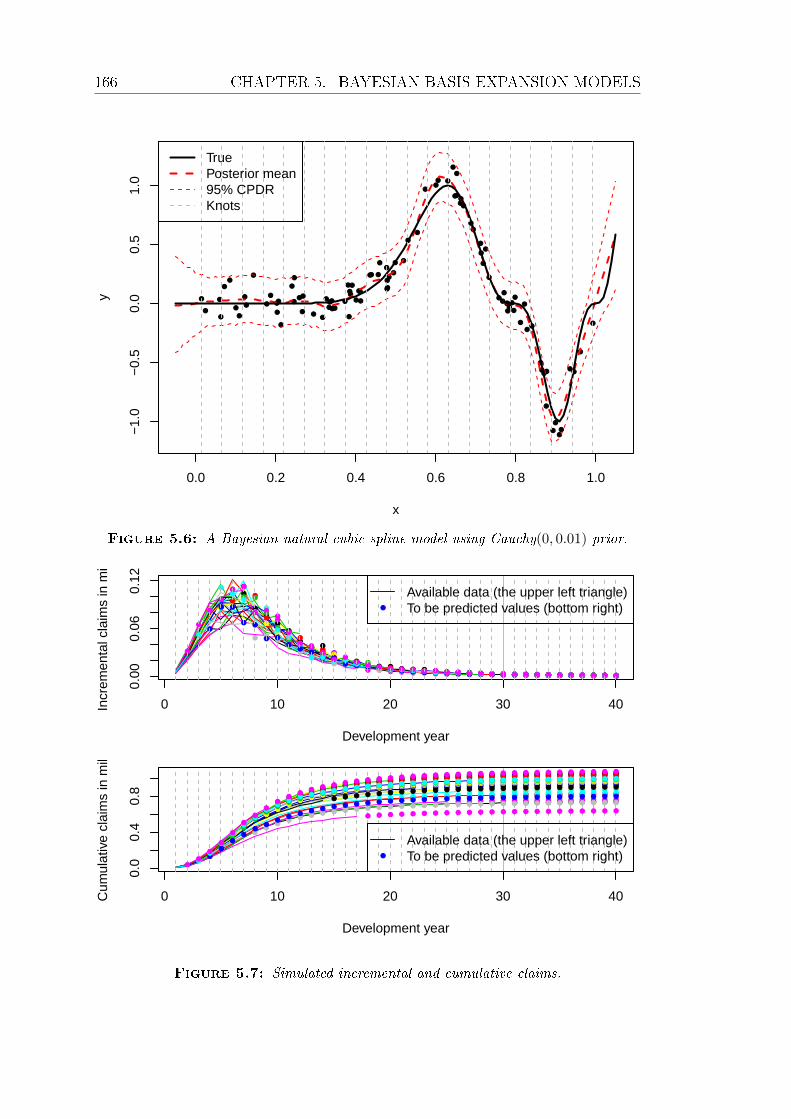
166 CHAPTER 5. BAYESIAN BASIS EXPANSION MODELS
0.0 0.2 0.4 0.6 0.8 1.0
−1.
0−
0.5
0.0
0.5
1.0
x
y
TruePosterior mean95% CPDRKnots
Figure 5.6: A Bayesian natural cubic spline model using Cauchy(0, 0.01) prior.
0 10 20 30 40
0.00
0.06
0.12
Development year
Incr
emen
tal c
laim
s in
mill
ion
Available data (the upper left triangle)To be predicted values (bottom right)
0 10 20 30 40
0.0
0.4
0.8
Development year
Cum
ulat
ive
clai
ms
in m
illio
n
Available data (the upper left triangle)To be predicted values (bottom right)
Figure 5.7: Simulated incremental and cumulative claims.

FIGURES 167
5 10 15 20
9000
9500
1000
010
500
H'
AIC
3035
4045
50
Equ
ival
ent d
egre
es o
f fre
edom
Figure 5.8: AIC vs. H ′ of polynomial basis expansion models.

168 CHAPTER 5. BAYESIAN BASIS EXPANSION MODELS
0 5 10 15 20 25 30
060
000
Development years
Incr
emen
tal c
laim
s
Simulated dataPredicted lower triangle
32 34 36 38 40
010
0025
00
Development years
Incr
emen
tal c
laim
s
Simulated dataPredicted tail development
Figure 5.9: Prediction of future claims from a polynomial basis expansion model.
0 5 10 15 20 25 30
060
000
Development years
Incr
emen
tal c
laim
s
Simulated dataPredicted lower triangle
32 34 36 38 40
010
0025
00
Development years
Incr
emen
tal c
laim
s
Simulated dataPredicted tail development
Figure 5.10: Prediction of future claims from a natural cubic spline regression model.

FIGURES 169
32 34 36 38 40
050
010
0015
0020
0025
00
Development years
Incr
emen
tal c
laim
s
Simulated dataPredicted tial development by polynomial expansion model
32 34 36 38 40
500
1000
1500
2000
2500
Development years
Incr
emen
tal c
laim
s
Simulated dataPredicted tial development by natural cubic spline
32 34 36 38 40
1000
2000
3000
4000
Development years
Incr
emen
tal c
laim
s
Simulated dataPredicted tial development by GAM using 'mgcv'
Figure 5.11: Comparison of tail development predictions by three models: a polyno-
mial regression, a natural cubic spline regression and a GAM.
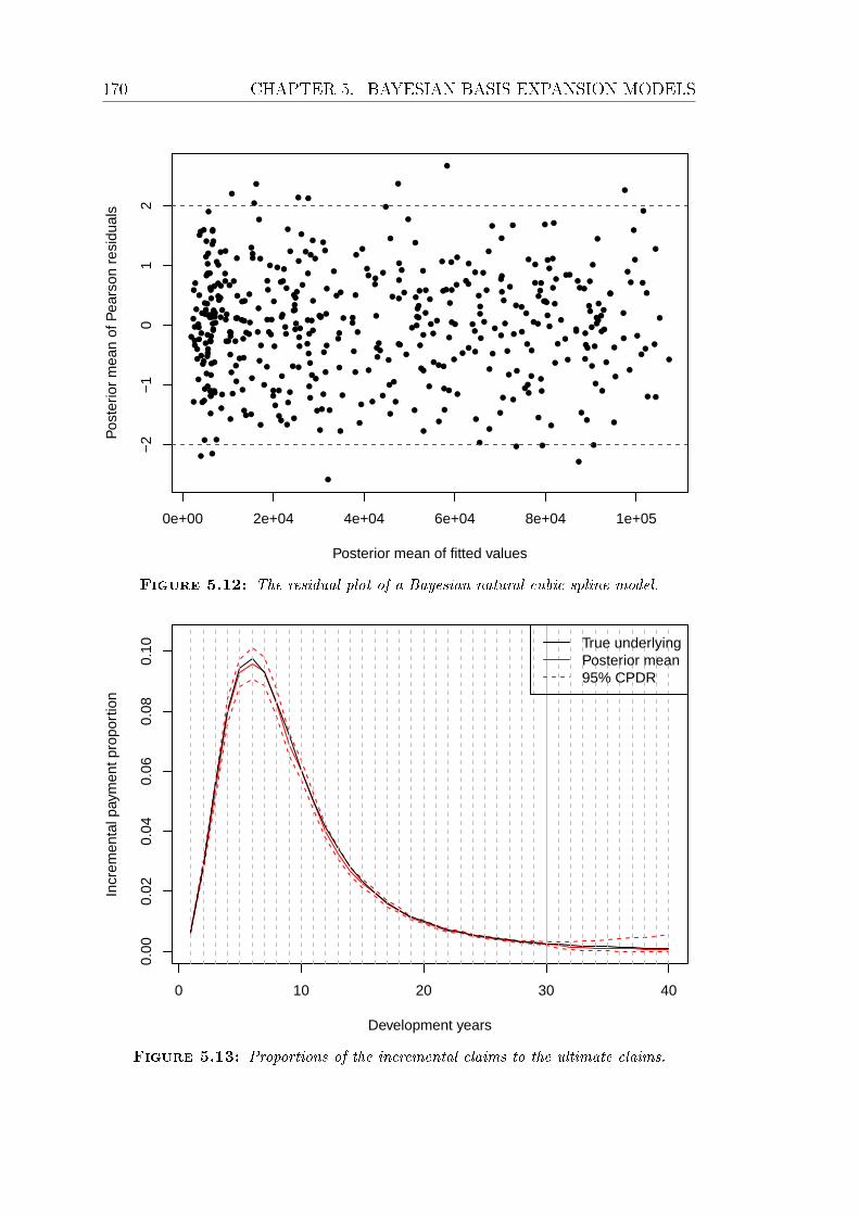
170 CHAPTER 5. BAYESIAN BASIS EXPANSION MODELS
0e+00 2e+04 4e+04 6e+04 8e+04 1e+05
−2
−1
01
2
Posterior mean of fitted values
Pos
terio
r m
ean
of P
ears
on r
esid
uals
Figure 5.12: The residual plot of a Bayesian natural cubic spline model.
0 10 20 30 40
0.00
0.02
0.04
0.06
0.08
0.10
Development years
Incr
emen
tal p
aym
ent p
ropo
rtio
n
True underlyingPosterior mean95% CPDR
Figure 5.13: Proportions of the incremental claims to the ultimate claims.
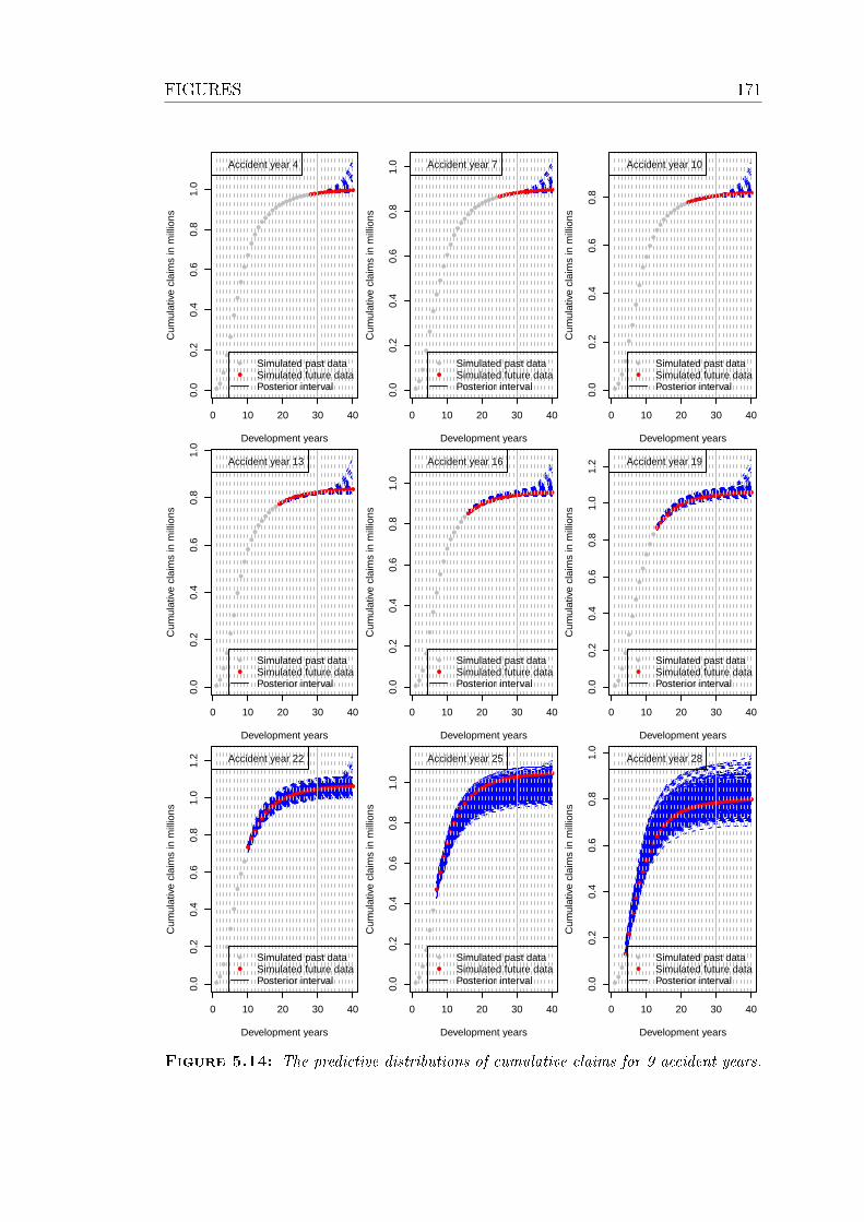
FIGURES 171
0 10 20 30 40
0.0
0.2
0.4
0.6
0.8
1.0
Development years
Cum
ulat
ive
clai
ms
in m
illio
ns
Accident year 4
Simulated past dataSimulated future dataPosterior interval
0 10 20 30 40
0.0
0.2
0.4
0.6
0.8
1.0
Development years
Cum
ulat
ive
clai
ms
in m
illio
ns
Accident year 7
Simulated past dataSimulated future dataPosterior interval
0 10 20 30 40
0.0
0.2
0.4
0.6
0.8
Development years
Cum
ulat
ive
clai
ms
in m
illio
ns
Accident year 10
Simulated past dataSimulated future dataPosterior interval
0 10 20 30 40
0.0
0.2
0.4
0.6
0.8
1.0
Development years
Cum
ulat
ive
clai
ms
in m
illio
ns
Accident year 13
Simulated past dataSimulated future dataPosterior interval
0 10 20 30 40
0.0
0.2
0.4
0.6
0.8
1.0
Development years
Cum
ulat
ive
clai
ms
in m
illio
ns
Accident year 16
Simulated past dataSimulated future dataPosterior interval
0 10 20 30 40
0.0
0.2
0.4
0.6
0.8
1.0
1.2
Development years
Cum
ulat
ive
clai
ms
in m
illio
ns
Accident year 19
Simulated past dataSimulated future dataPosterior interval
0 10 20 30 40
0.0
0.2
0.4
0.6
0.8
1.0
1.2
Development years
Cum
ulat
ive
clai
ms
in m
illio
ns
Accident year 22
Simulated past dataSimulated future dataPosterior interval
0 10 20 30 40
0.0
0.2
0.4
0.6
0.8
1.0
Development years
Cum
ulat
ive
clai
ms
in m
illio
ns
Accident year 25
Simulated past dataSimulated future dataPosterior interval
0 10 20 30 40
0.0
0.2
0.4
0.6
0.8
1.0
Development years
Cum
ulat
ive
clai
ms
in m
illio
ns
Accident year 28
Simulated past dataSimulated future dataPosterior interval
Figure 5.14: The predictive distributions of cumulative claims for 9 accident years.
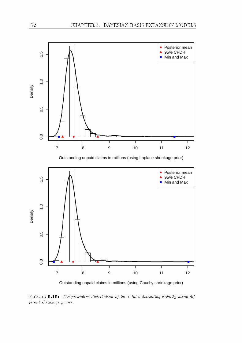
172 CHAPTER 5. BAYESIAN BASIS EXPANSION MODELS
Outstanding unpaid claims in millions (using Laplace shrinkage prior)
Den
sity
7 8 9 10 11 12
0.0
0.5
1.0
1.5
Posterior mean95% CPDRMin and Max
Outstanding unpaid claims in millions (using Cauchy shrinkage prior)
Den
sity
7 8 9 10 11 12
0.0
0.5
1.0
1.5
Posterior mean95% CPDRMin and Max
Figure 5.15: The predictive distribution of the total outstanding liability using dif-
ferent shrinkage priors.

FIGURES 173
0 5 10 15 20 25
0.0
0.1
0.2
0.3
0.4
0.5
0.6
Development years
Incr
emen
tal p
ropo
rtio
n of
num
ber
of r
epor
ted
clai
ms
Posterior mean95% CPDR
Figure 5.16: Proportions of incremental claims numbers to ultimate claims numbers.
0 5 10 15 20 25 30
0.00
0.05
0.10
0.15
0.20
0.25
Development years
Incr
emen
tal p
ropo
rtio
n of
PP
CI
Posterior mean95% CPDR
Figure 5.17: Proportions of the incremental PPCI's to the ultimate PPCI's.

174 CHAPTER 5. BAYESIAN BASIS EXPANSION MODELS
0 5 10 15 20 25
050
0010
000
1500
020
000
2500
030
000
Development years
Cum
ulat
ive
num
ber
of c
laim
s
Accident year 8
DataPosterior interval
0 5 10 15 20 25
050
0010
000
1500
020
000
2500
030
000
Development years
Cum
ulat
ive
num
ber
of c
laim
s
Accident year 10
DataPosterior interval
0 5 10 15 20 25
050
0010
000
1500
020
000
2500
030
000
Development years
Cum
ulat
ive
num
ber
of c
laim
s
Accident year 12
DataPosterior interval
0 5 10 15 20 25
050
0010
000
1500
020
000
2500
030
000
Development years
Cum
ulat
ive
num
ber
of c
laim
s
Accident year 16
DataPosterior interval
0 5 10 15 20 25
050
0010
000
1500
020
000
2500
030
000
Development years
Cum
ulat
ive
num
ber
of c
laim
s
Accident year 18
DataPosterior interval
0 5 10 15 20 25
050
0010
000
1500
020
000
2500
030
000
Development years
Cum
ulat
ive
num
ber
of c
laim
s
Accident year 20
DataPosterior interval
0 5 10 15 20 25
050
0010
000
1500
020
000
2500
030
000
Development years
Cum
ulat
ive
num
ber
of c
laim
s
Accident year 22
DataPosterior interval
0 5 10 15 20 25
050
0010
000
1500
020
000
2500
030
000
Development years
Cum
ulat
ive
num
ber
of c
laim
s
Accident year 24
DataPosterior interval
0 5 10 15 20 25
050
0010
000
1500
020
000
2500
030
000
Development years
Cum
ulat
ive
num
ber
of c
laim
s
Accident year 26
DataPosterior interval
Figure 5.18: The predictive distributions of cumulative claims numbers for 9 accident
years.

FIGURES 175
0 5 10 15 20 25 30
010
0020
0030
0040
0050
00
Development years
Cum
ulat
ive
PP
CI
Accident year 8
DataPosterior interval
0 5 10 15 20 25 30
010
0020
0030
0040
0050
00
Development years
Cum
ulat
ive
PP
CI
Accident year 10
DataPosterior interval
0 5 10 15 20 25 30
010
0020
0030
0040
0050
00
Development years
Cum
ulat
ive
PP
CI
Accident year 12
DataPosterior interval
0 5 10 15 20 25 30
010
0020
0030
0040
0050
00
Development years
Cum
ulat
ive
PP
CI
Accident year 16
DataPosterior interval
0 5 10 15 20 25 30
010
0020
0030
0040
0050
00
Development years
Cum
ulat
ive
PP
CI
Accident year 18
DataPosterior interval
0 5 10 15 20 25 30
010
0020
0030
0040
0050
00
Development years
Cum
ulat
ive
PP
CI
Accident year 20
DataPosterior interval
0 5 10 15 20 25 30
010
0020
0030
0040
0050
00
Development years
Cum
ulat
ive
PP
CI
Accident year 22
DataPosterior interval
0 5 10 15 20 25 30
010
0020
0030
0040
0050
00
Development years
Cum
ulat
ive
PP
CI
Accident year 24
DataPosterior interval
0 5 10 15 20 25 30
010
0020
0030
0040
0050
00
Development years
Cum
ulat
ive
PP
CI
Accident year 26
DataPosterior interval
Figure 5.19: The predictive distributions of cumulative PPCI's for 9 accident years.

176 CHAPTER 5. BAYESIAN BASIS EXPANSION MODELS
Outstanding liability in millions
Den
sity
400 420 440 460 480
0.00
00.
010
0.02
00.
030
Posterior mean95% CPDRMin and Max
Figure 5.20: The predictive distribution of total outstanding claims liability of the
doctor benet.
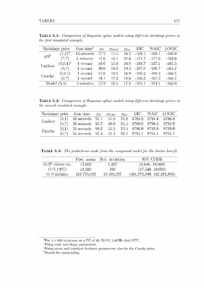
TABLES 177
Table 5.1: Comparison of Bayesian spline models using dierent shrinkage priors in
the rst simulated example.
Shrinkage prior Run time3 pD pWAIC ploo DIC WAIC LOOIC
gdP(1,1)4 13 seconds 17.5 15.5 16.5 -168.5 -168.1 -166.0(?,?) 5 minutes 17.6 16.1 22.6 -171.7 -171.0 -158.0
Laplace(0,0.1)5 1 second 16.6 15.6 16.5 -168.7 -167.1 -165.3(0,?) 1 second 20.0 18.0 19.3 -167.9 -166.7 -164.2
Cauchy(0,0.1) 1 second 17.6 16.0 16.9 -169.2 -168.2 -166.5(0,?) 1 second 19.1 17.3 18.6 -168.3 -167.2 -164.5
Model (5.5) 5 minutes 17.9 16.5 17.5 -165.4 -164.1 -162.0
Table 5.2: Comparison of Bayesian spline models using dierent shrinkage priors in
the second simulated example.
Shrinkage prior Run time pD pWAIC ploo DIC WAIC LOOIC
Laplace(0,1) 35 seconds 57.1 51.6 52.8 8783.8 8784.4 8786.8(0,?) 35 seconds 55.7 49.8 51.1 8780.5 8780.3 8782.9
Cauchy(0,1) 34 seconds 58.2 51.9 53.4 8786.0 8785.9 8789.0(0,?) 34 seconds 57.3 51.2 52.7 8784.1 8784.1 8787.1
Table 5.3: The predictions made from the compound model for the doctor benet.
Post. mean Std. deviation 95% CPDRO/S6 claims no. 13,693 2,397 (9,846, 19,060)
O/S PPCI 18,320 386 (17,548, 19,059)O/S liability 419,770,032 10,492,327 (401,778,990, 442,281,893)
3For 4× 800 iterations on a PC of 6G RAM, 2.8GHz dual CPU.4Using scale and shape parameters.5Using mean and standard deviance parameters; also for the Cauchy prior.6Stands for outstanding.
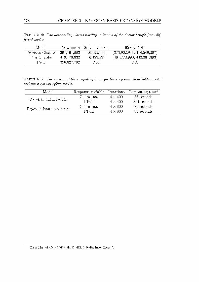
178 CHAPTER 5. BAYESIAN BASIS EXPANSION MODELS
Table 5.4: The outstanding claims liability estimates of the doctor benet from dif-
ferent models.
Model Post. mean Std. deviation 95% CPDRPrevious Chapter 391,761,803 10,195,111 (373,902,941, 414,549,267)This Chapter 419,770,032 10,492,327 (401,778,990, 442,281,893)
PwC 396,827,792 NA NA
Table 5.5: Comparison of the computing times for the Bayesian chain ladder model
and the Bayesian spline model.
Model Response variable Iterations Computing time7
Bayesian chain ladderClaims no. 4× 400 86 secondsPPCI 4× 400 364 seconds
Bayesian basis expansionClaims no. 4× 800 73 secondsPPCI 4× 800 65 seconds
7On a Mac of 4GB 1600MHz DDR3, 1.3GHz Intel Core i5.
Chapter 6
Multivariate Modelling Using
Copulas
All the models we discussed before are univariate models, i.e., there is one re-
sponse. However, for many applications, it is more appropriate to apply a multi-
variate model which captures important relationships. Typical multivariate dis-
tributions include multivariate Gaussian distribution, multivariate t-distribution,
Wishart distribution etc. These multivariate distributions also determine the
marginal distributions. Copulas are a family of multivariate distributions whose
marginal distributions are uniform.
At the end of reserving problems, we need to aggregate the outstanding lia-
bility distribution of each line of business or each type of benet to get the total
outstanding liability distribution. The dependence between them must be con-
sidered. Property damage lines could be positively correlated, e.g., homeowners
property damage insurance and personal auto damage insurance could be hit at
the same time in catastrophic events. Liability lines could be positively correlated
due to changes in litigation. These positive correlations are a kind of risk con-
centration, while independence is a kind of risk diversication. It is important to
consider the impacts of correlation between lines or benets on the distribution
of aggregated liability.
179

180 CHAPTER 6. MULTIVARIATE MODELLING USING COPULAS
In the Bayesian copulas framework, all the uncertainties are considered during
the inferential process which is an advantage compared with the likelihood-based
frequentist inference. Nevertheless, preliminary frequentist copula modelling can
quickly give us a partial picture of multivariate modelling, which importantly
guides the direction of the follow-up Bayesian analysis.
In Section 6.1, the elements of copulas are reviewed, including Sklar's theo-
rem, parametric copulas, inference methods etc. In Section 6.2, we discuss the
usefulness of copulas in risk modelling generally. We point out that the copula
is used to model the empirical dependence between risks while the marginal re-
gression model is used to model the structural dependence. In Section 6.3, a
bivariate Gaussian copula is used to aggregate the liabilities of the doctor benet
and the hospital benet in WorkSafe Victoria. These two benets are correlated
positively even after removing the structural eects of the development periods.
6.1 Overview of copulas
In this section, we summarize the elements of copulas in four parts: the mech-
anism of copulas to join arbitrary marginal distributions, two copula families,
measures of bivariate association, and the inferential methods.
6.1.1 Sklar's theorem
Sklar's theorem (Sklar, 1959) is perhaps the most important result regarding
copulas. It establishes the general connection between any multivariate distri-
bution and copulas and is used essentially in all copula applications. Sklar's
theorem states that for an m-dimensional multivariate distribution function F
with marginal distributions, F1, . . . , Fm, there always exists an m-dimensional
copula C such that
F (y1, . . . , ym) = C [F1 (y1) , . . . , Fm (ym)] .

6.1. OVERVIEW OF COPULAS 181
Conversely, if C is an m-dimensional copula and F1, . . . , Fm are distribution func-
tions, then the function F dened above is an m-dimensional multivariate distri-
bution function with marginal distribution functions, F1, . . . , Fm.
From Sklar's theorem, we see that for any multivariate distributions, the
marginal distributions can be separated from the multivariate dependence which
can then be represented by a copula. A direct implication of Sklar's theorem is
deriving a copula from a multivariate distribution as follows:
C (u1, . . . , um) = F[F−1
1 (u1) , . . . , F−1m (um)
],
where u1, . . . , um follow marginal uniform distributions on the interval [0, 1].
Invariance to monotone transformation
While a joint distribution is aected by the monotone transformation of vari-
ables, a copula is invariant to the monotone transformation of variables. Let
(y1, . . . , ym) be a vector of continuous random variables with a copula C. Dene
x1 = h1 (y1) , . . . , xm = hm (ym). If h1, . . . , hm are strictly increasing functions,
then (x1, . . . , xm) also has the same copula C.
The Fréchet-Hoeding bounds for bivariate copulas
Fréchet (1935) found that any bivariate copula C is bounded by the Fréchet-
Hoeding lower bound W and the Fréchet-Hoeding upper bound M , as follows:
W (u1, u2) ≤ C (u1, u2) ≤M (u1, u2) ,
where W (u1, u2) = max (u1 + u2 − 1, 0) ,M (u1, u2) = min (u1, u2) . Figure 6.1
shows the surfaces and contours of W and M compared with the independent
copula1.
1The variables in an independent copula are independent with each other.

182 CHAPTER 6. MULTIVARIATE MODELLING USING COPULAS
6.1.2 Parametric copulas
We will investigate two parametric copula families: elliptical copulas and Archimedean
copulas. Elliptical copulas are simply the copulas of elliptical distributions such
as multivariate Gaussian distribution and multivariate t-distribution.
Rather than deriving from multivariate distributions, Archimedean copulas
are functions of a convex generator and the dependence strength is governed by
only one parameter. Archimedean copulas include the Clayton, Gumbel, Frank,
and others.
Elliptical copulas
The copula of an m-dimensional normal distributed random vector z with mean
zero and correlation matrix Σ is
C (u) = Φm
[Φ−1 (u1) , . . . ,Φ−1 (um) ; Σ
],
where Φ−1 is the inverse of the standard normal distribution function and Φm is
the joint distribution function of z. The connection between elliptical copulas and
elliptical distributions provides an easy way to simulate from elliptical copulas:
rst simulate z ∼ Φm, then let ui = Φ−1 (zi) for i = 1, . . . ,m.
The copula of an m-dimensional t-distributed random vector x with mean
zero, degrees of freedom ν and correlation matrix Σ is
C (u) = tm,ν[t−1ν (u1) , . . . , t−1
ν (um) ; Σ],
where t−1ν is the inverse of the t-distribution function with ν degrees of freedom
and tm,ν is the joint distribution function of x.
Figure 6.2 shows a bivariate Gaussian copula and a bivariate t-copula, both
of which have the same Pearson correlation of 0.8 and Kendall's tau of 0.5903
(dened in Section 6.1.3). Kendall's tau of a t-copula does not depend on the
degrees of freedom. With the degrees of freedom increasing, a t-copula approaches

6.1. OVERVIEW OF COPULAS 183
a normal copula.
Archimedean copulas
A general denition of Archimedean copulas can be found in Nelsen (2013). An
Archimedean m-dimensional copula has the following form:
C (u) = ϕ[−1] [ϕ (u1; θ) + . . .+ ϕ (um; θ) ; θ] ,
where ϕ is called the generator of copula C and ϕ[−1] is the pseudo-inverse of ϕ.
The function ϕ is a continuous, strictly decreasing convex function mapping from
[0, 1] to [0,∞], such that ϕ (1) = 0.
Table 6.1 shows the generators of three popular Archimedean copulas. We
plot the cumulative distribution functions, the probability density functions and
the contours of probability density functions for the three Archimedean copulas
in Figure 6.3.
6.1.3 Measures of bivariate association
Copulas are invariant under monotone transformation, so we want the measures of
association to also be invariant to monotone transformation. Pearson correlation
(or linear correlation) is invariant under linear transformation but not invariant
under non-linear transformation.
In the following we will review two measures of association known as Kendall's
tau and Spearman's rho, both of which depend on the variable ranks rather than
their values (and hence are invariant under monotone transformations).
Moreover, we will discuss the tail dependence relating to the amount of depen-
dence in the upper-right-quadrant tail or lower-left-quadrant tail of a bivariate
distribution. It turns out that tail dependence is also a copula-based association
measure that is invariant under monotone transformations.
184 CHAPTER 6. MULTIVARIATE MODELLING USING COPULAS
Kendall's tau and Spearman's rho
Kendall's tau for two random variables is dened as the probability of concordance
minus the probability of discordance. Assuming the two variables y1, y2 have a
copula C, then Kendall's tau for y1, y2 is given by
τ (y1, y2) := 4
∫∫[0,1]2
C (u1, u2) dC (u1, u2)− 1 = 4E [C (u1, u2)]− 1.
Spearman's rho for y1, y2 is given by
ρS (y1, y2) = 12
∫∫[0,1]2
u1u2dC (u1, u2)− 3 = 12E (u1u2)− 3.
If the marginal distributions are F1 and F2, and u1 = F1 (y1) and u2 = F2 (y2),
then
ρS (y1, y2) =E (u1u2)− 1/4
1/12=
Cov (u1, u2)√Var (u1)
√Var (u2)
= ρ (F1 (y1) , F2 (y2)) .
Table 6.1 lists Kendall's tau for two elliptical copulas and three Archimedean
copulas discussed before. Figure 6.3 shows three Archimedean copulas, all of
which have the same Kendall's tau of 0.5903.
Tail dependence
The coecient of upper tail dependence of the two variables y1, y2 with the copula
C is dened as
λU := limu→1
Pr[y2 > F−1
2 (u) |y1 > F−11 (u)
].
It can be shown that λU is a copula property which has the following equivalent
form:
λU = limu→1
1− 2u+ C (u, u)
1− u.

6.1. OVERVIEW OF COPULAS 185
The coecient of lower tail dependence λL is dened in a similar way:
λL := limu→0
C (u, u)
u.
Table 6.1 lists the coecients of upper and lower tail dependence for bivariate
copulas. None of the copulas exhibit tail dependence except the Clayton copula
and the Gumbel copula. The Clayton copula has a lower tail dependence while
the Gumbel copula has an upper tail dependence.
6.1.4 Inference methods for copulas
In this section, we follow the model specication as in Pitt et al. (2006). Consider
an m-element response variable y = (y1, . . . , ym). It is observed for n times, so
the data is
y = (y1, . . . , yn) =(
(y11, . . . , y1m)T , . . . , (yn1, . . . , ynm)T)
= (y1, . . . ,ym)T ,
where yi is an m-row-vector of the ith observation, yj is an n-column-vector of
the jth response variable.
For the jth element in the ith observation yij, we have a k-vector covariate xij.
Marginally, we t a generalized linear model Fj to yj. We denote the associated
parameters as θj = (βj, ϕj), where βj is a k-vector of coecients of xij and ϕj is
a vector of all the other parameters in Fj.
The joint distribution of the ith observation yi = (yi1, . . . , yim) is modelled by
a copula with parameters θc as follows:
F (yi) = C [F1 (yi1) , . . . , Fm (yim) ; θc] , (6.1)
which can be seen as a joint distribution of residual ranks of response variables
(after removing the systematic eects of covariates). In a Gaussian copula setting,

186 CHAPTER 6. MULTIVARIATE MODELLING USING COPULAS
we can write the above copula as
ΦmΦ−1 [F1 (yi1)] , . . . ,Φ−1 [Fm (yim)] ; Σ,
where Φ−1 is the inverse of a standard normal distribution function and Φm is an
m-multivariate Gaussian distribution function with mean zero.
In the following, we discuss two likelihood-based estimations: the maximum
likelihood estimation (MLE) and the inference functions for margins estimator
(IFME). Bootstrap methods and MCMC methods can be applied to estimate the
estimation error and the prediction error in IFME.
Maximum likelihood estimation (MLE)
The density function of yi is the derivative of equation (6.1), as follows:
f (yi) =∂mC [F1 (yi1) , . . . , Fm (yim)]
∂yi1 . . . ∂yim
= c [F1 (yi1) , . . . , Fm (yim)] f1 (yi1) · · · fm (yim) ,
where c is the density function of C and fi is the density function of yi. The
likelihood function of y = (y1, . . . , yn) is
L (θ; y) =n∏i=1
c [F1 (yi1) , . . . , Fm (yim)]m∏j=1
n∏i=1
fj (yij) .
The MLE is then dened as
θMLE = argmaxθc
L (θ; y) .
Note that the optimization of global likelihood can be quite demanding since
the copula likelihood part also contains marginal regression parameters θj, j =
1, . . . ,m.

6.1. OVERVIEW OF COPULAS 187
Inference functions for margins estimator (IFME)
Joe (2014) suggested rst estimating θj for each jth marginal regression model,
and then estimating the copula parameter θc via
θIFMEc = argmax
θc
n∏i=1
c(F1
(yi1; θ1
), . . . , Fm
(yim; θm
); θc
),
where θj, j = 1, . . . ,m are the MLEs of the marginal models. IFME is always
easier to compute than the global MLE.
Predictive distributions via parametric bootstrap. Suppose we want to
get the predictive distribution of R = g (yn+1,1, . . . , yn+1,m) given the covariates
xn+1 = (xn+1,1, . . . , xn+1,m), where g is a generic function. The bootstrap algo-
rithm is as follows:
1. Fit a marginal regression to yj to get the estimated parameters θj for j =
1, . . .m.
2. Calculate the cdfs given the estimated parameters in step 1 as
uij = Fj
(yij; θj
)for i = 1, . . . n, j = 1 . . . ,m.
3. Calculate the IFME of θc:
θIFMEc = argmax
θc
n∏i=1
c(F1
(yi1; θ1
), . . . , Fm
(yim; θm
); θc
).
4. Generate a bootstrap sample usij, i = 1, . . . , n, j = 1, . . . ,m from the copula
C(u; θc).
5. Inverse the cdfs to get a bootstrap data sample ysij = F−1j
(usij; θj
), i =
1, . . . , n, j = 1, . . . ,m, where θj is from step 1.
6. Fit a marginal regression to ysj to get the estimated parameters θsj , j =
1, . . .m.
7. Calculate the prediction as Rs = g(ysn+1,1, . . . , y
sn+1,m
), where ysn+1,j =

188 CHAPTER 6. MULTIVARIATE MODELLING USING COPULAS
F−1j
(usn+1,j; θ
sj
). usn+1 is a realized sample from C(u; θc).
8. Redo steps 4 to 7 for S times to get a bootstrap sample Rs, s = 1, . . . , S.
The key steps are 4 and 7 which establish the correlation between the estimated
parameters and the correlation between the predicted values.
Predictive distributions via MCMC. Again, suppose we want to get the
predictive distribution of R = g (yn+1,1, . . . , yn+1,m) given the covariates xn+1 =
(xn+1,1, . . . , xn+1,m), where g is a generic function. The MCMC algorithm is as
follows:
1. Apply the MCMC methods to each marginal model to generate a Markov
chain whose stationary distribution is the posterior distribution of θj for j =
1, . . . ,m.
2. For the tth MC sampled parameters θtj, calculate the corresponding cumu-
lative probabilities utij = Fj(yij; θ
tj
), which will be used as the observed
data of the copula.
3. Calculate the MLE of copula parameter θtc, and generate a sample utn+1 ∼
C(u|θtc).
4. Calculate the prediction values as
Rt = g(F−1
1
(utn+1,1; θt1
), . . . , F−1
m
(utn+1,m; θtm
)).
5. Repeat steps 2 to 4 for T times to get a MC sample Rt, t = 1, . . . , T.
Example 6.1 (A simulated example using a Gumbel copula). Suppose the joint
distribution of two response variables have a Gumbel copula and each variable is
marginally modelled by a linear regression model:
yi1, yi2 ∼ C(F1 (yi1;α, β01, β11) , F2
(yi2;σ2, β02, β12
); θc)
yi1 ∼ Gamma
(α,
α
β01 + β11xi1
)log yi2 ∼ N
(β02 + β12xi2, σ
2).

6.1. OVERVIEW OF COPULAS 189
The following true parameters are specied: n = 100, β01 = 1, β11 = 2, α =
10, β02 = 0.1, β12 = 0.3, σ2 = 0.5, θc = 2 (Kendall's tau is 0.5). xi1, xi2 are
generated independently from a uniform distribution U [0, 10]. yi1 and yi2 are
associated via the same index i which can indicate the same time, the same place
or other common features.
Figure 6.4 shows the relationships between the variables. Due to the eects of
covariates, there is no signicant relationship between the two response variables.
Inference functions for margins estimator (IFME). Two linear regres-
sion models are tted to two response variables respectively. The estimated pa-
rameters of two models are shown in Table 6.2. We then calculate the cdfs of the
response variables given the estimated regression parameters as
F1
(yi1; β01, β11, α
), F2
(yi2; β02, β12, σ
),
which are denoted by ui1, ui2, i = 1, . . . , 100.
The scatter plot of (ui1, ui2) , i = 1, . . . , 100 is shown in Figure 6.5, indicating
a signicant positive relationship with an empirical Kendall's tau of 0.51. The
rugs indicate that the marginal distributions of ui1, ui2 are close to a uniform
distribution as expected.
The predictive distribution via bootstrap methods. Suppose we want to
predict the sum of y101,1 and y101,2, both of which have the same covariate of
5. The bootstrap algorithm discussed before is used to simulate the predictive
distribution of y101,1 + y101,2. Figure 6.6 shows a signicant positive correlation
between y101,1 and y101,2. The bootstrap estimate is 16.42 with the 95% PI of
(7.24, 32.23).
The predictive distribution via MCMC methods. We t two Bayesian
linear models separately to the two response variables. HMC is applied to simulate
from the posterior distribution. At the end of Bayesian inferential simulation, a

190 CHAPTER 6. MULTIVARIATE MODELLING USING COPULAS
sample of parameters is obtained.
Assuming the tth sampled parameters as βt01, βt11, α
t, βt02, βt12, σ
t, we can cal-
culate the corresponding uti1, uti2, i = 1, . . . , n. For the ease of copula parameter
estimation, a bivariate Gaussian copula is chosen. The MLE of a bivariate nor-
mal copula parameter is just the sample correlation of Φ−1 (uti1) and Φ−1 (uti2),
denoted by θtc.
Figure 6.7 shows the scatter plot of posterior means, ui1 vs. ui2, which is
quite similar to Figure 6.5 indicating the suitability of using a bivariate Gaussian
copula. The histogram of θc is shown in Figure 6.7, which also conrms the
signicant positive relationship between ui1 and ui2.
Again, suppose we want to predict the sum of y101,1 and y101,2, both of which
have the same covariate value of 5. We compare two approaches: the independent
prediction and the dependent prediction using a copula.
The independent prediction is the sum of posterior predictions yt101,1, ys101,2
without considering the permutation. For the dependent prediction using a copula,
rst a pair of(ut101,1, u
t101,2
)is generated from a bivariate Gaussian copula with
parameter θtc. Then we inverse two functions, ut101,1 = F1
(yt101,1; βt01, β
t11, α
t)
and ut101,2 = F2
(yt101,2; βt02, β
t12, σ
t), to get a pair of
(yt101,1, y
t101,2
). Figure 6.8
shows a positive correlation between y101,1, y101,2 under the dependent prediction
and this positive correlation aects the 97.5% percentile signicantly compared
with independent prediction. The posterior mean is 16.74 with the 95% CPDR of
(7.80, 33.20) under the dependent prediction.
6.2 Copulas in modelling risk dependence
We focus on the models for multiple run-o triangles. There are several papers
on this topic. Shi and Frees (2011) and Shi (2014) use the elliptical copulas to
address the dependencies introduced by various sources. They use the parametric
bootstrap method to simulate the predictive distribution of outstanding liabilities.
De Jong (2012) uses a Gaussian copula to model the dependence of payments from

6.2. COPULAS IN MODELLING RISK DEPENDENCE 191
dierent triangles in the same calendar year.
One of the most important works is Zhang et al. (2012) which was awarded
the ARIA prize by the Casualty Actuary Society. This annual prize, rst awarded
in 1997, is made to the author or authors of a paper published by the Journal
of Risk and Insurance that provides the most valuable contribution to casualty
actuarial science. This paper uses a Bayesian copula model to address the de-
pendence between the dierent triangle payments in the same accident year and
development year. This paper compares the goodness-of-t of Clayton, Gumbel,
Frank and Gaussian copulas and uses three dierent marginal regressions: a gen-
eralized linear regression, a non-linear growth curve model and a semi-parametric
model.
6.2.1 Structural and empirical dependence between risks
We distinguish the two types of dependence since two dierent approaches are
used to tackle them. In general, the risks an insurer faces often exhibit co-
movement or dependencies. This means that knowledge about results for one risk
can be used to better predict the results for another risk. Dependence between
two risks may be due to known relationships (structural dependence), or simply
due to the historically observed correlations (empirical dependence).
Structural dependence modelling The structural co-movements can be ac-
counted for in a regression modelling process. Structural dependencies include
situations where loss variables are driven by common variables: for example,
the cumulative claims of two benets are both increasing with the development
periods. This positive dependence can be modelled by using the covariate of
development periods.
Empirical dependence modelling The empirical co-movements are simply
observed without any known (or capable of being modelled) relationships, i.e.,
the positive relationship of residuals from two models. For many types of risks,
192 CHAPTER 6. MULTIVARIATE MODELLING USING COPULAS
particularly in property and liability areas, co-movements are observed, but may
not be easily explained. It is more likely necessary to construct dependency
models that reect observed and expected dependencies without formalising the
structure of those dependencies with cause-eect models. The theory of copulas
provides a comprehensive modelling tool that can reect dependencies in a very
exible way.
6.2.2 The eects of empirical dependence on risk measures
An insurer needs to hold much more than the expected value of unpaid claims
liability to ensure the company's solvency with a quite large probability. In
Australia, insurers typically add a risk margin to the mean of liability to get the
estimation of reserve amount.
A risk margin is set consistently with risk measures. A risk measure is not
calculated by summing up the contributions of dierent business lines, but more
likely from the distribution of all risks combined. So it is necessary to consider
the empirical dependence between dierent lines.
Risk measures
Most risk measures can be classied as moment-based, tail-based, or probability
transforms. The moment-based risk measures (including the standard deviation
and semi-standard deviation) are not often used since they are not directly related
to the solvency concept.
The most used risk measures are tail-based risk measures which emphasize
large losses. The four tail-based risk measures, value at risk (VaR), tail value at
risk (TVaR), excess tail value at risk (XTVaR), and expected policyholder decit
(EPD), are dened as follows:
• VaR is a percentile of a loss distribution.
• TVaR is the expected loss at a specied probability level and beyond.

6.2. COPULAS IN MODELLING RISK DEPENDENCE 193
• XTVaR is TVaR less the mean. When the mean is nanced by other fund-
ing, capital is needed for losses above the mean, so subtracting the mean
can capture this need.
• EPD is calculated by multiplying TVaR minus VaR by the probability level.
If the probability level is chosen so that capital is VaR at that level, then
TVaR minus VaR is the expected value of defaulted losses if there is default.
Multiplying this quantity by the complement of the probability level yields
the unconditional expected value of defaulted losses.
Probability transforms measure risk by shifting the probability towards the
unfavourable outcomes and then computing a risk measure from the transformed
probabilities. Most of the usual asset pricing formulas, like the capital asset
pricing model and the Black-Scholes options pricing formula, can be expressed as
transformed mean.
Example 6.2 (Empirical dependence). We illustrate the eects of empirical de-
pendence on the risk measures by a hypothetical example. Consider two correlated
loss variables x1 and x2 with the following distribution:
F (x1, x2) = C(FG (x1;α, µ1) , FLN
(x2;µ2, σ
2)
; θc)
x1 ∼ Gamma
(α,
α
µ1
)log x2 ∼ N
(µ2, σ
2),
where C is a Gumbel copula. The underlying parameters are specied as µ1 =
200, α = 5, µ2 = log 130 and σ2 = 0.25. Consider three cases: θc = 1 (i.e., the
two risks are independent), θc = 2 and θc = 4. The marginal distributions are
plotted in Figure 6.9. Both of them are positively skewed.
By doing simulation, we estimate the four tail-based risk measures for indi-
vidual loss and the aggregated loss. Table 6.3 shows the results, implying the
signicant eects of empirical dependence on the tail-based risk measures. Figure
6.10 shows that when θc = 2, larger x1 and x2 are more likely to be correlated with

194 CHAPTER 6. MULTIVARIATE MODELLING USING COPULAS
each other. This is because a Gumbel copula has a non-zero upper tail dependence
as shown in Table 6.1.
6.3 Application to the doctor and hospital bene-
ts
Recall that Table 4.7 lists all the benets in the WorkSafe Victoria. In medical
and like benet category, we have two sub-benets: doctor and hospital. Intu-
itively, these two sub-benets should be positively correlated. Here we focus on
the models applied to the claims amounts rather than the PPCI method as in
the previous two chapters.
6.3.1 Preliminary GLM analysis using a Gaussian copula
As a quick check of correlation between two triangles, we recommend starting
from the least complicated models. We t two chain ladder GLMs with a gamma
error and a log link to the doctor benet x and the hospital benet y. The model
is as follows:
F (xij, yij) = C (F1 (xij;α1, µ1i, γ1j) , F2 (yij;α2, µ2i, γ2j) ; θc)
xij ∼ Gamma
(α1,
α1
µ1iγ1j
), i = 1, . . . , 27, j = 1, . . . , 27
yij ∼ Gamma
(α2,
α2
µ2iγ2j
), i = 1, . . . , 27, j = 1, . . . , 27,
where F1, F2 are the cdfs of gamma distributions and C is a bivariate Gaussian
copula.
For model inference, the IFME method is applied. We calculate the em-
pirical cdfs, uij = F1 (xij; α1, µ1i, γ1j) and vij = F2 (yij; α2, µ2i, γ2j). Note that
α1,µ1i,γ1j,α2,µ2i,γ2j are the MLEs. We draw four Pearson residual plots: two
scatter plots of residuals from marginal GLMs, the plot showing the relationship

6.3. APPLICATION TO THE DOCTOR AND HOSPITAL BENEFITS 195
between two residuals, and the plot of uij vs. vij in Figure 6.11. It shows a
signicant positive empirical relationship.
The predictive distribution via a parametric bootstrap
The claims liability is simulated via the bootstrap method. The IFME of θc
is θc = cor [Φ−1 (u) ,Φ−1 (v)] = 0.5530. We compare the bootstrap sample from
the copula model (rst row in Figure 6.12) with the bootstrap sample from an
independent model (second row in Figure 6.12).
The 95% VaR from the copula model is larger than that from the independent
model. We also list other tail-based risk measures in Table 6.4. Note that the
estimated aggregated liability of both benets is 707,407,135 dollars in the PwC
report.
6.3.2 A Gaussian copula with marginal Bayesian splines
We apply a Gaussian copula model with two marginal Bayesian natural cubic
spline models to the two benets, as follows:
F (xij, yij) = C [F1 (xij;α1, θij) , F2 (yij;α2, ϕij) ; θc]
xij ∼ Gamma
(α1,
α1
θij
)yij ∼ Gamma
(α2,
α2
ϕij
)θij = Ai × exp
(27∑h=1
βhbh (j)
)
ϕij = Bi × exp
(27∑h=1
γhbh (j)
)βh ∼ DoubleExp
(0, σ2
1
), h = 1, . . . , 27
γh ∼ DoubleExp(0, σ2
2
), h = 1, . . . , 27
θc ∼ U (0, 1) ,
196 CHAPTER 6. MULTIVARIATE MODELLING USING COPULAS
where F1, F2 are the cdfs of gamma distributions and C is a bivariate Gaussian
copula. All the claims are assumed to be settled by the development year 30.
The IFME method is applied for the copula parameter estimation.
The inferences for the marginal Bayesian splines
We draw the posterior mean and the 95% CPDR of the proportions of incremental
payments to the ultimate claims payments for two benets in Figure 6.13. The in-
creasing uncertainty in the tail developments is due to the lack of data. However,
as stated in the discussion of previous chapter, we believe that the uncertainties
should not increase dramatically. One approach to solving this problem is to
assume strong priors for the tail developments.
Under the non-informative priors, the posterior mean of exp[∑27
h=1 βhbh (27)]
was 0.003 with posterior standard deviation of 0.0004 and the posterior mean of
exp[∑27
h=1 γhbh (27)]is 0.003 with posterior standard deviation of 0.0006. Ac-
cordingly, we assume the following strong priors for the tail developments in the
development years 28, 29, 30:
exp
(27∑h=1
βhbh (j)
)∼ N (0.003, 0.0003) , j = 28, . . . , 30
exp
(27∑h=1
γhbh (j)
)∼ N (0.003, 0.0006) , j = 28, . . . , 30.
The resulting posterior distributions of proportions of incremental claims for both
benets are plotted in Figure 6.14. Now the tail developments do not show as
much volatility as in the model with non-informative priors.
The predictive distribution via MCMC methods
We aggregate the liabilities of two benets via a bivariate Gaussian copula. Sur-
prisingly, there is no signicant dierence between simulations of total liability
from the copula model and from the independent model as shown in Figure 6.15.
There are two reasons for this: one is that the marginal Bayesian model uncer-

6.4. DISCUSSION 197
tainty overwhelms the dependence between them; the other is that the copula is
used to model the dependence of incremental claims and the sum of incremental
claims may display less dependence. We list the tail-based risk measures of the
aggregated liability in Table 6.5.
To end of this section, we point out that the copula model makes a dierence
if the claims payments in the next calendar year are predicted. As we did for the
total claims liability, we simulate the claims payments in the next calendar year
for both benets from the copula model and from the independent model. The
results are shown in Figure 6.16 and Table 6.6. The empirical positive correlation
is more obvious and it aects the XTVaR most signicantly.
6.4 Discussion
Copulas have a wide range of applications in nance, risk management, insurance
etc. This chapter uses copulas to model the contemporaneous correlation, i.e., the
dependence among dierent run-o triangles at the same development year and
the same accident year. There are several actuarial papers considering using
copulas to model other types of dependence, such as the common calendar years
dependence due to claims ination.
Another concern is the estimation method for the copula models. Here we
apply the IFME method involving two consecutive steps: rst make inference of
the marginal regressions, then x the parameters of the marginal regressions and
infer the copula parameters. We have done some experiments to compare the
Bayesian IFME method (applying MCMC to the marginal distribution and MLE
to the copula consecutively) and the full Bayesian method (applying MCMC to
the multivariate likelihood directly). They show that the Bayesian IFME method
takes much less time with better convergence and similar inferences compared
with the full Bayesian method. So we are condent with the Bayesian IFME
method. Nevertheless, several papers develop a MCMC algorithm for the full
Bayesian copula models (see the relevant literature in the next section).

198 CHAPTER 6. MULTIVARIATE MODELLING USING COPULAS
In this chapter, we do not consider the selection of the optimal copula family,
since a Gaussian copula ts well (at least visually) in all the problems consid-
ered. Genest and Rivest (1993) provide estimation and selection methods for
Archimedean copulas. The tail dependence can be used to select a copula if the
interest is in the tail behaviour.
6.5 Bibliographic notes
A thorough discussion of copulas can be found in Joe (2014). An introduction
to copulas is available in Nelsen (2013), which does not, however, contain the
inference methods. Sklar (1959) introduces Sklar's theorem. Trivedi and Zimmer
(2007) cover the main implementation and estimation of copulas. Genest and
Rivest (1993) provide estimation and selection methods for Archimedean copulas.
Embrechts and Hofert (2013) address the inference methods and goodness-of-
t tests for high-dimensional copulas.Kruskal (1958) discusses the measures of
association in detail.
Pitt et al. (2006), Ho (2007), Danaher and Smith (2011) and Smith (2011)
discuss the Bayesian copula models and design ecient MCMC methods accord-
ingly. All of them also consider the special case where there are discrete response
variables.
Frees and Valdez (1998) introduced copulas to actuarial science. A general
overview of copulas and their applications in actuarial science is provided by
Embrechts et al. (2001), Venter (2002), Brehm et al. (2007) and Feldblum (2010),.
Literature considering the dependence among run-o triangles includes Shi
and Frees (2011) and Zhang et al. (2012), both of which use copulas to model the
contemporaneous correlations among various lines of business: the former apply
the bootstrap to estimate the predictive distribution of unpaid claims, while the
latter apply the MCMC methods, which is closer to what we did in this chapter.
De Jong (2012) uses copulas to accommodate the common calendar eect between
triangles.

6.5. BIBLIOGRAPHIC NOTES 199
Shi et al. (2012) and Merz et al. (2013) model the contemporaneous depen-
dence between run-o triangles and the common calendar eect within a run-o
triangle via a Bayesian hierarchical log-normal model, which is equivalent to a
Gaussian copula model with marginal log-normal regressions. Shi (2014) relaxes
the marginal log-normal regression using elliptical copulas. Anas et al. (2015)
use a hierarchical Archimedean copula to analyze the data from Shi and Frees
(2011).
Czado et al. (2012) and Krämer et al. (2013) use copulas to model the depen-
dence between claims occurrences and claims sizes.
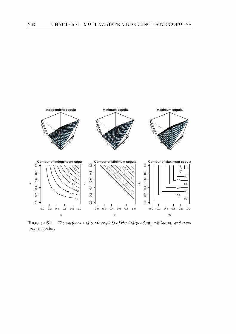
200 CHAPTER 6. MULTIVARIATE MODELLING USING COPULAS
u1 u2
C(u1,u2)
Independent copula
u1 u2
C(u1,u2)
Minimum copula
u1 u2
C(u1,u2)
Maximum copula
Contour of Independent copula
u1
u 2
0.1
0.2 0.3
0.4
0.5
0.6
0.7
0.8
0.0 0.2 0.4 0.6 0.8 1.0
0.0
0.2
0.4
0.6
0.8
1.0
Contour of Minimum copula
u1
u 2
0.1
0.2
0.2
0.2
0.3
0.4 0.5 0.6
0.7 0.8
0.0 0.2 0.4 0.6 0.8 1.0
0.0
0.2
0.4
0.6
0.8
1.0
Contour of Maximum copula
u1
u 2
0.1
0.2
0.3
0.4
0.5
0.6
0.7
0.8
0.0 0.2 0.4 0.6 0.8 1.0
0.0
0.2
0.4
0.6
0.8
1.0
Figure 6.1: The surfaces and contour plots of the independent, minimum, and max-
imum copulas.

FIGURES 201
u1 u2
C(u1,u2)
Normal copula
u1 u2
C(u1,u2)
t−copula with df=1
u1 u2
C(u1,u2)
t−copula with df=10
u1 u2
c(u1,u2)
Normal copula density
u1 u2
c(u1,u2)
t−copula density with df=1
u1 u2
c(u1,u2)
t−copula density with df=10
0.0 0.2 0.4 0.6 0.8 1.0
0.0
0.2
0.4
0.6
0.8
1.0 Contour of normal copula
u1
u 2
0.4
0.4
0.6
0.6
0.8
0.8
1
1
1.2 1.2
1.4
1.4
2
2
0.0 0.2 0.4 0.6 0.8 1.0
0.0
0.2
0.4
0.6
0.8
1.0
Contour of t−copula (df=1)
u1
u 2
0.5
0.5
1
1
1.5
1.5
2
2
2.5
2.5
0.0 0.2 0.4 0.6 0.8 1.0
0.0
0.2
0.4
0.6
0.8
1.0
Contour of t−copula(df=10)
u1
u 2
0.4
0.4
0.6
0.6
0.8
0.8
1
1
1.2 1.2
1.4
1.4
1.6
1.6
Figure 6.2: A bivariate Gaussian copula and t-copulas with df=1, 10, which have the
same Pearson correlation of 0.8 and Kendall's tau of 0.5903.

202 CHAPTER 6. MULTIVARIATE MODELLING USING COPULAS
u1 u2
C(u1,u2)
Clayton copula
u1 u2
C(u1,u2)
Gumbel copulau1 u2
C(u1,u2)
Frank copula
u1 u2
c(u1,u2)
Clayton copula densityu1 u2
c(u1,u2)
Gumbel copula density
u1 u2
c(u1,u2)
Frank copula density
0.0 0.2 0.4 0.6 0.8 1.0
0.0
0.2
0.4
0.6
0.8
1.0 Contour of Clayton density
u1
u 2
0.5
0.5
1
1
1.5
1.5
2
0.0 0.2 0.4 0.6 0.8 1.0
0.0
0.2
0.4
0.6
0.8
1.0
Contour of Gumbel density
u1
u 2
0.5
0.5
1
1 1.5
1.5
2
0.0 0.2 0.4 0.6 0.8 1.0
0.0
0.2
0.4
0.6
0.8
1.0
Contour of Frank density
u1
u 2
0.4
0.4
0.6
0.6
0.8
0.8 1
1 1.2
1.2
1.4
1.4
1.6
1.6
2
Figure 6.3: Clayton, Gumbel and Frank copulas with the same Kendall's tau of
0.5903.

FIGURES 203
0 2 4 6 8 10
05
1015
2025
30
x1
y 1
0 2 4 6 8 10
010
2030
4050
60
x2
y 2
0 2 4 6 8 10
02
46
810
x1
x 2
0 5 10 15 20 25 30
010
2030
4050
60
y1
y 2
Figure 6.4: The scatter plots of the simulated data.
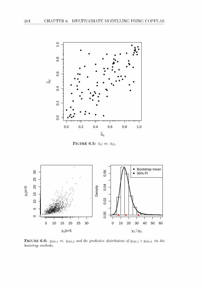
204 CHAPTER 6. MULTIVARIATE MODELLING USING COPULAS
0.0 0.2 0.4 0.6 0.8 1.0
0.0
0.2
0.4
0.6
0.8
1.0
ui1
u i2
Figure 6.5: ui1 vs. ui2.
5 10 15 20 25 30
05
1015
2025
30
yi1|x=5
y i2|
x=5
yi1 + yi2
Den
sity
0 10 20 30 40 50 60
0.00
0.02
0.04
0.06
Bootstrap mean95% PI
Figure 6.6: y101,1 vs. y101,2 and the predictive distribution of y101,1 + y101,2 via the
bootstrap methods.

FIGURES 205
0.0 0.2 0.4 0.6 0.8 1.0
0.0
0.2
0.4
0.6
0.8
1.0
Posterior mean of u1
Pos
terio
r m
ean
of u
2
θc
Den
sity
0.67 0.68 0.69 0.70 0.71
020
4060
Mean95% credible interval
Figure 6.7: ui1 vs. ui2 and the posterior distribution of θc via the MCMC.

206 CHAPTER 6. MULTIVARIATE MODELLING USING COPULAS
5 10 15 20 25
05
1015
2025
3035
y1
y 2
y1 + y2
Den
sity
0 10 20 30 40 50
0.00
0.01
0.02
0.03
0.04
0.05
0.06
Posterior meanVaRTVaR
5 10 15 20 25 30
05
1015
2025
y1
y 2
y1 + y2
Den
sity
0 10 20 30 40 50
0.00
0.02
0.04
0.06
Posterior meanVaRTVaR
Figure 6.8: y101,1 vs. y101,2 and the predictive distribution of y101,1 + y101,2 via the
MCMC. The rst row is from the desirable copula model. The second row is from the
inappropriate independent model for the purpose of comparison. VaR and TVaR will be
discussed in Section 6.2.2.

FIGURES 207
X1
Den
sity
0 100 200 300 400 500 600
0.00
00.
001
0.00
20.
003
0.00
40.
005
Mean95% VaR
X2
Den
sity
0 200 400 600 800
0.00
00.
002
0.00
40.
006
Mean95% VaR
Figure 6.9: The marginal distributions of x1 and x2, obtained via simulation.
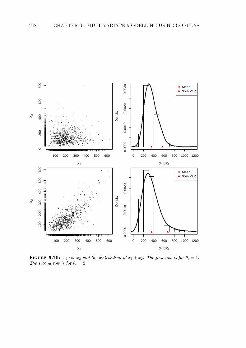
208 CHAPTER 6. MULTIVARIATE MODELLING USING COPULAS
100 200 300 400 500 600
020
040
060
080
0
X1
X2
X1 + X2
Den
sity
0 200 400 600 800 1000 1200
0.00
000.
0010
0.00
200.
0030
Mean95% VaR
100 200 300 400 500 600
100
200
300
400
500
600
X1
X2
X1 + X2
Den
sity
0 200 400 600 800 1000 1200
0.00
000.
0010
0.00
20
Mean95% VaR
Figure 6.10: x1 vs. x2 and the distribution of x1 + x2. The rst row is for θc = 1.The second row is for θc = 2.

FIGURES 209
13 14 15 16 17
−2
02
4
Linear predictors of doctor benefit
Pea
rson
res
idua
ls
13 14 15 16 17
−4
−2
02
4
Linear predictors of hospital benefit
Pea
rson
res
idua
ls
−2 0 2 4
−4
−2
02
4
Pearson residuals from doctor model
Pea
rson
res
idua
ls fr
om h
ospi
tal m
odel
0.0 0.2 0.4 0.6 0.8 1.0
0.0
0.2
0.4
0.6
0.8
1.0
u
v
Figure 6.11: The top two: the residual plots of two marginal regressions. The bottom
two: the scatter plot of residuals and the scatter plot of uij vs. vij.
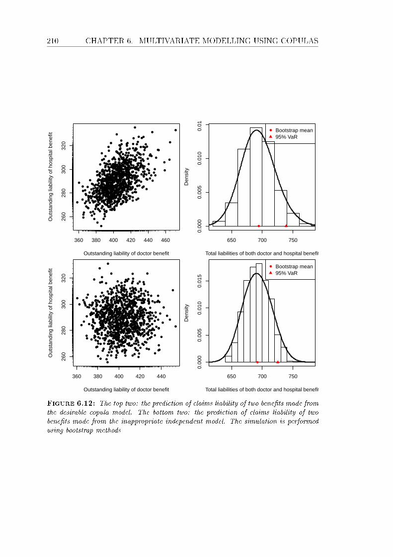
210 CHAPTER 6. MULTIVARIATE MODELLING USING COPULAS
360 380 400 420 440 460
260
280
300
320
Outstanding liability of doctor benefit
Out
stan
ding
liab
ility
of h
ospi
tal b
enef
it
Total liabilities of both doctor and hospital benefit
Den
sity
650 700 750
0.00
00.
005
0.01
00.
015
Bootstrap mean95% VaR
360 380 400 420 440
260
280
300
320
Outstanding liability of doctor benefit
Out
stan
ding
liab
ility
of h
ospi
tal b
enef
it
Total liabilities of both doctor and hospital benefit
Den
sity
650 700 750
0.00
00.
005
0.01
00.
015
Bootstrap mean95% VaR
Figure 6.12: The top two: the prediction of claims liability of two benets made from
the desirable copula model. The bottom two: the prediction of claims liability of two
benets made from the inappropriate independent model. The simulation is performed
using bootstrap methods

FIGURES 211
0 5 10 15 20 25 30
0.00
0.05
0.10
0.15
0.20
0.25
Development years
Incr
emen
tal p
ropo
rtio
n (d
octo
r)Posterior mean95% CPDR
0 5 10 15 20 25 30
0.0
0.1
0.2
0.3
0.4
Development years
Incr
emen
tal p
ropo
rtio
n (h
ospi
tal)
Posterior mean95% CPDR
Figure 6.13: Proportions of the incremental claims to the ultimate claims under
non-informative priors.
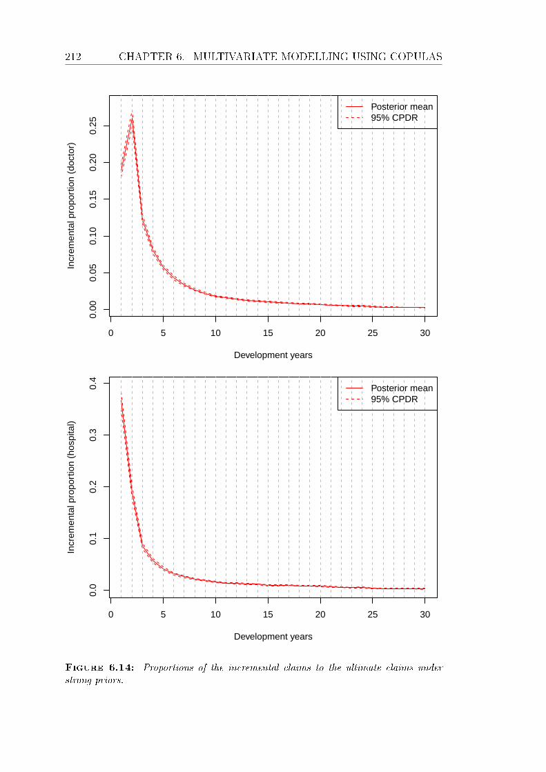
212 CHAPTER 6. MULTIVARIATE MODELLING USING COPULAS
0 5 10 15 20 25 30
0.00
0.05
0.10
0.15
0.20
0.25
Development years
Incr
emen
tal p
ropo
rtio
n (d
octo
r)
Posterior mean95% CPDR
0 5 10 15 20 25 30
0.0
0.1
0.2
0.3
0.4
Development years
Incr
emen
tal p
ropo
rtio
n (h
ospi
tal)
Posterior mean95% CPDR
Figure 6.14: Proportions of the incremental claims to the ultimate claims under
strong priors.

FIGURES 213
380 400 420 440 460
260
280
300
320
340
Outstanding liability of doctor benefit (copula)
Out
stan
ding
liab
ility
of h
ospi
tal b
enef
it
Total liabilities in millions (copula model)
Den
sity
650 700 750 800
0.00
00.
005
0.01
00.
015
Posterior mean95% VaR
380 400 420 440 460
260
280
300
320
340
Outstanding liability of doctor benefit (independent)
Out
stan
ding
liab
ility
of h
ospi
tal b
enef
it
Total liabilities in millions (independent model)
Den
sity
650 700 750
0.00
00.
005
0.01
00.
015
Posterior mean95% VaR
Figure 6.15: The top two: the prediction of claims liability of two benets made from
the desirable copula model. The bottom two: the prediction of claims liability of two
benets made from the inappropriate independent model. The simulation is performed
using MCMC methods.

214 CHAPTER 6. MULTIVARIATE MODELLING USING COPULAS
70 80 90 100
4045
5055
6065
70
Doctor benefit payment in the next year(copula)
Hos
pita
l ben
efit
paym
ent i
n th
e ne
xt y
ear
Total payments in the next year in millions (copula model)
Den
sity
110 120 130 140 150 160 170
0.00
0.01
0.02
0.03
0.04
Posterior mean95% VaR
70 80 90 100
4045
5055
6065
70
Doctor benefit payment in the next year (independent)
Hos
pita
l ben
efit
paym
ent i
n th
e ne
xt y
ear
Total payments in the next year in millions (independent model)
Den
sity
110 120 130 140 150 160
0.00
0.01
0.02
0.03
0.04
0.05
Posterior mean95% VaR
Figure 6.16: The top two: the prediction of next year claims payment of two benets
made from the desirable copula model. The bottom two: the prediction of next year
claims payment of two benets made from the inappropriate independent model. The
simulation is performed using MCMC methods.
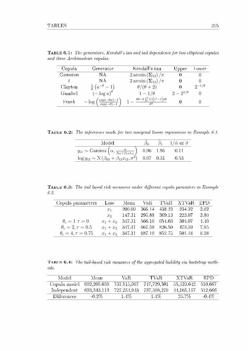
TABLES 215
Table 6.1: The generators, Kendall's tau and tail dependence for two elliptical copulas
and three Archimedean copulas.
Copula Generator Kendall's tau Upper LowerGaussian NA 2 arcsin (Σ12) /π 0 0
t NA 2 arcsin (Σ12) /π 0 0Clayton 1
θ
(u−θ − 1
)θ/(θ + 2) 0 2−1/θ
Gumbel (− log u)θ 1− 1/θ 2− 21/θ 0
Frank − log(
exp(−θu)−1exp(−θ)−1
)1− 4θ−4
∫ a0 t/(et−1)dtθ2
0 0
Table 6.2: The inferences made for two marginal linear regressions in Example 6.1.
Model β0· β1· 1/α or σ
yi1 ∼ Gamma(α, α
β01+β11xi1
)0.96 1.95 0.11
log yi2 ∼ N (β02 + β12xi2, σ2) 0.07 0.31 0.53
Table 6.3: The tail-based risk measures under dierent copula paramters in Example
6.2.
Copula parameters Loss Mean VaR TVaR XTVaR EPDx1 200.00 366.14 438.23 234.32 3.02x2 147.31 295.88 369.13 223.07 3.80
θc = 1 τ = 0 x1 + x2 347.31 566.10 654.03 304.07 4.40θc = 2, τ = 0.5 x1 + x2 347.31 667.59 826.50 473.59 7.95θc = 4, τ = 0.75 x1 + x2 347.31 687.10 852.75 501.18 8.28
Table 6.4: The tail-based risk measures of the aggregated liability via bootstrap meth-
ods.
Model Mean VaR TVaR XTVaR EPDCopula model 692,205,659 737,515,967 747,729,301 55,523,642 510,667Independent 693,343,113 727,254,943 737,508,270 44,165,157 512,666Dierences -0.2% 1.4% 1.4% 25.7% -0.4%

216 CHAPTER 6. MULTIVARIATE MODELLING USING COPULAS
Table 6.5: The tail-based risk measures of the aggregated liability via MCMC methods.
Model Mean VaR TVaR XTVaR EPDCopula model 706,344,7152 745,713,292 756,101,056 49,756,341 519,388Independent 706,302,106 742,610,194 753,119,350 46,817,244 525,458Dierences 0.01% 0.42% 0.40% 6.28% 1.16%
Table 6.6: The tail-based risk measures of the aggregated claims payments in the next
calendar year via MCMC methods.
Model Mean VaR TVaR XTVaR EPDCopula model 133,988,676 149,919,590 154,493,898 20,505,222 228,715Independent 133,956,740 147,246,196 151,426,112 17,469,373 208,996Dierences 0.02% 1.82% 2.03% 17.38% 9.44%
2Compared with the PwC estimate of 707,407,135.

Chapter 7
Summary and Discussion
This thesis presents several Bayesian models to tackle the claims reserving prob-
lem in general insurance. These models are used to analyze the WorkSafe Victoria
data set. In this nal chapter, we summarize the three most useful models in this
thesis. We also suggest a Bayesian modelling procedure for use when facing a
real problem. Finally, the limitations are discussed and further research topics
on both Bayesian methodology and actuarial applications are suggested.
Bayesian models provide a coherent way to incorporate the prior knowledge
and combine it with the evidence from the data. This property is particularly
useful when the actuarial judgements override the data. Another advantage of
Bayesian models is that the Bayesian inferential engine can simulate the posterior
distribution of parameters and the predictive distribution of the future value. This
property is very important for application to the claims reserving problem, since
claims reserving models are always complicated in terms of number of parameters
and insurers are more interested in the distribution of unpaid claims than the
point estimates.
A typical Bayesian modelling procedure includes: proposing a full probabil-
ity model, calculating the posterior inference conditional on the data, modelling
evaluation, and renement. We will discuss the Bayesian modelling procedure in
more detail shortly.
217

218 CHAPTER 7. SUMMARY AND DISCUSSION
7.1 The three most useful models
We point out that the three most useful models in this thesis are a compound
model, a Bayesian natural cubic spline basis expansion model and a copula model
with Bayesian margins.
For the model inference, we rely on Stan, which implements the HMC method.
Like MCMC, HMC simulates a Markov chain whose stationary distribution is
the same as the target distribution. Compared with MCMC, HMC has a higher
acceptance rate due to the Hamiltonian dynamics proposal.
7.1.1 A compound model
The PPCI method is used in the PwC report for the doctor benet in WorkSafe
Victoria, and we propose a compound model as a stochastic version of the PPCI
method. The key point is to establish the relationship between the variance in a
single claim payment and the variance in PPCI. The distributional assumption
of a single claim payment could be checked if we had the individual claims data.
The compound model discussed in Chapter 5 and 6 is as follows:
yij =
µi∑k=1
xijk
µi ∼ Distributioni
xijk ∼ Gamma (αij, βij) , k = 1, . . . , µi,
where µi is the ultimate claims number of accident year i whose distribution is
approximated by a Bayesian model, and xijk is the payment for the kth claim
during the development year j whose distribution depends on both accident year
and development year.
We dene the payments per claim incurred during the development period j
of accident year i as PPCIij := yij/E (µi). Note that E(PPCIij) = E(xijk). We
use the posterior mean of µi as an estimate of E (µi). The relationship between

7.1. THE THREE MOST USEFUL MODELS 219
the variance of PPCIij and the variance of xijk is
Var (xijk) =(E (µi))
2Var (PPCIij)− Var (µi) (E (PPCIij))2
E (µi),
where all the quantities on the right hand side can be estimated by a MC
sample. The distribution of yij conditional on µi is Gamma (µiαij, βij) , where
αij = E(xijk)2/Var (xijk) and βij = αij/E (xijk) .
7.1.2 A Bayesian natural cubic spline basis expansion model
In the claims reserving models, the two challenging tasks are the derivation of the
predictive distribution and the t to the various shapes of development patterns.
In the Bayesian framework, the rst task is easily tackled by either the MCMC
method or the HMC method. To deal with the second task, we rely on the chain
ladder model or the basis expansion model.
The stochastic chain ladder model treats the development year as a factor
variable, eectively introducing the same number of parameters as the number
of development periods. So it can accommodate all the shapes of development
patterns. However, the stochastic chain ladder model does not introduce the tail
development.
The basis expansion model treats the development year as a continuous vari-
able and expands the predictor space by including transformation of the predictor
variable. In the Bayesian framework, we can shrink the non-signicant parame-
ters and interpolate the tail development.
Consider the Bayesian basis expansion model as discussed in Chapter 5:
yij ∼ Gamma
(α,
α
µij
), i = 1, . . . , I, j = 1, . . . , J
µij = Pi × LRi × exp
(H∑h=1
βhbh (j)
)βh ∼ DoubleExp
(0, σ2
h
), h = 1, . . . , H.

220 CHAPTER 7. SUMMARY AND DISCUSSION
The key part of this model is the natural cubic spline basis functions bh : h =
1, . . . , H which expand the predictor space. We use the B-spline basis, an or-
thogonal set, generated by R function ns( ). We normally choose the knots at
every unique value of x, which is analogous to the full rank smoothing splines.
Here we choose a gamma error distribution which could be replaced by other
distributions such as a more general Tweedie distribution.
7.1.3 A copula model with Bayesian margins
The copula model is used to aggregate the outstanding claims liabilities estimated
from multiple triangles. We could assume any marginal regression for each tri-
angle in the copula framework. In this thesis, we use the Gaussian copula which
oers computational simplicity.
The copula model with Bayesian marginal regressions discussed in Chapter 6
is as follows:
F (xij, yij) = C [F1 (xij;α1, θij) , F2 (yij;α2, ϕij) ; θc]
xij ∼ Gamma
(α1,
α1
θij
)yij ∼ Gamma
(α2,
α2
ϕij
)θij = Ai × exp
(H∑h=1
βhbh (j)
)
ϕij = Bi × exp
(H∑h=1
γhbh (j)
)βh ∼ DoubleExp
(0, σ2
1
)γh ∼ DoubleExp
(0, σ2
2
)θc ∼ U (0, 1) ,
with non-informative priors for α1, α2, Ai, Bi, σ21, σ
22. We t the model using the
IFME method (Joe and Xu, 1996) which is not a full Bayesian analysis. It is

7.2. A SUGGESTED BAYESIAN MODELLING PROCEDURE 221
possible to do a full Bayesian analysis by using a user-dened MCMC algorithm.
7.2 A suggested Bayesian modelling procedure
From the experience and perspective of the author, a typical Bayesian modelling
procedure should involve the following steps:
1. Dene the problem. Dierent problems need dierent levels of eort. If we
just need to get a point estimate of unpaid claims, the deterministic CL
method or BF method may solve this problem well enough.
2. Visualize the data. We cannot change the data which is a reection of real
world, but we could change a model. Visualising the data helps us detect
abnormal observations and choose a suitable model to analyze the data.
3. Fit a classical model, usually a GLM. This includes choosing the covariates,
the mean function and the error distribution. It is good to try a simple
model rst, then go deeper into a more complicated model. In the GLM
setting, lots of diagnostic tools are available and easily accessed. The mean
function and the error distribution can be used in the next step.
4. Set up a Bayesian model and simulate from the posterior distribution. We
turn to Bayesian modelling software such as BUGS or Stan to simulate from
the posterior distributions. The detection of convergence was discussed in
Section 3.2.1 and strategies for improving the convergence and eciency
were discussed in Section 3.2.2.
5. Make inferences from the MCMC or HMC sample. If the predictive dis-
tribution is required, we need to perform one further step to simulate the
future values from the likelihood.
6. Model assessment and selection. We can compare dierent models using
several information criteria. LOO cross-validation and WAIC can be easily
derived using Stan, while DIC can be calculated automatically in BUGS.
We followed these six steps (though not strictly) in all the Bayesian modelling

222 CHAPTER 7. SUMMARY AND DISCUSSION
presented in this thesis. A variation to step 4 is to use a user-dened MCMC
or HMC algorithm. We did this in the early stage of research for the examples
discussed in Chapter 2 and 3. We also used a user-dened RJMCMC algorithm
in Section 4.3.1.
7.3 Limitations and further research topics
For the claims reserving problems, we cannot model all the uncertainty with a sta-
tistical model. The models we discussed only address the independent risk. Other
risks such as operation risk, strategy risk, and event risk are better addressed in
other ways. We list several limitations in this thesis, and further research can be
done on these limitations.
7.3.1 Bayesian methodology
ODP models and Tweedie models in Stan
ODP models can be specied in BUGS via the zero trick1. However, Stan does
not accept the zero trick and we have not yet worked out how to make a statement
of the ODP model in Stan. In addition, Tweedie distributions are not built-in
distributions in Stan.
Other non-parametric Bayesian models
We have seen the power of basis expansion models. Other Bayesian non-parametric
models include Gaussian process models, Dirichlet process models etc. Further
research could be done on these models and their applications.
Copulas comparison and selection
As we mentioned in Section 6.4, the comparison of dierent copulas is ignored in
that chapter. The selection of a suitable copula could be based on the information
1A trick used in BUGS to dene arbitrary likelihood function (Lunn et al., 2000).

7.3. LIMITATIONS AND FURTHER RESEARCH TOPICS 223
criteria or the tail dependence. The goodness-of-t for copulas is discussed in
Genest et al. (2009).
Distributional approximation
In Section 3.4, we have briey reviewed variational Bayes methods, which are
promising when dealing with large data sets. Other distributional approximation
methods, such as pragmatic expectation (Minka, 2001), are discussed in Bishop
(2006). These methods deserve more attention in future research.
7.3.2 Actuarial applications
Calendar year eect
The calendar year eect is not considered in this thesis. The obvious pattern in
Figure 4.14 indicates a signicant calendar year eect. A possible approach is to
incorporate a calendar year covariate (see Section 4.5).
Stochastic reserving methods for other benets in WorkSafe Victoria
Three benets in WorkSafe Victoria are investigated: the weekly benet, the
doctor benet and the hospital benet. These benets are chosen since they are
stable and less subject to changes in legislation than many others. It is desirable
to propose stochastic versions of other reserving methods in the PwC report
(Simpson and McCourt, 2012) such as PPAC and PPCR.
One-year reserve volatility
One key issue relating to the actual implementation of Solvency II is the estima-
tion of the one-year reserve volatility (or claims development results). This issue
is discussed in some recent literature, including Saluz et al. (2011), Christiansen
and Niemeyer (2014) and Saluz (2015).

224 CHAPTER 7. SUMMARY AND DISCUSSION
Applications to ratemaking
This thesis focuses on claims reserving problems and run-o triangle data. The
techniques explored could also be applied to other actuarial areas such as insur-
ance ratemaking, which normally involves more features (covariates). The basis
expansion model could be extended to incorporate several covariates. For exam-
ple, in automobile ratemaking, we could incorporate features such as driver age,
model and year of make, so as to determine the appropriate insurance policy price
specically for a subgroup of interest.

Appendix A
Derivations
A.1 Example 2.3
Since E (xt) = E (xt−1) and Var (xt) = Var (xt−1), we can easily get
E (x1) = 0 and Var (x1) =1
λ (1− α2).
Hence, this autoregressive process is uniquely determined by the following two
distributions:
x1|α, λ ∼ N
(0,
1
λ (1− α2)
)xt|xt−1, α, λ ∼ N
(αxt−1,
1
λ
), t = 2, 3, . . . , n.
A.1.1 The joint posterior distribution
The joint posterior distribution of α and λ is
p (α, λ|x) ∝ p (x|α, λ) p (α) p (λ)
∝ p(x|α, λ)1
λ
= p (xn|xn−1, xn−2, . . . , x1, α, λ) p(xn−1, xn−2, . . . , x1|α, λ)1
λ
225

226 APPENDIX A. DERIVATIONS
= p (xn|xn−1, α, λ) p (xn−1|xn−2, α, λ) · · · p (x1|α, λ)1
λ
∝√λ exp
[−λ
2(xn − xn−1)2
]· · ·√λ (1− α2) exp
[−λ (1− α2)
2x1
2
]1
λ
= λn2−1(1− α2
) 12
exp
−λ
2
[(xn − αxn−1)2 + · · ·+ (x2 − αx1)2 +
(1− α2
)x1
2]
.
Thus,
p (α, λ|x) = h0λn2−1(1− α2
) 12 exp
[−λ
2h (x, α)
],
where
h0 =1∫∞
0
∫ 1
−1λ
n2−1(1− α2)
12 exp
[−λ
2h (x, α)
]dαdλ
is called the normalizing constant and
h (x, α) = (xn − αxn−1)2 + (xn−1 − αxn−2)2 + · · ·+ (x2 − αx1)2 +(1− α2
)x1
2.
A.1.2 Two marginal posterior distributions
The marginal posterior distribution of α is
p (α|x) =
∫ ∞0
p (α, λ|x) dλ
∝∫ ∞
0
λn2−1(1− α2
) 12 exp
[−λ
2h (x, α)
]dλ
=(1− α2
) 12
Γ(n2
)(h(x,α)
2
)n2
∝ (1− α2)12
h(x, α)n2
.
Thus,
p (α|x) = h1(1− α2)
12
h(x, α)n2
,

A.2. EXAMPLE 2.5 227
where
h1 =
∫ 1
−1
h(x, α)n2
(1− α2)12
dα.
The marginal posterior distribution of λ is
p (λ|x) =
∫ 1
−1
p (α, λ|x) dα
∝∫ 1
−1
λn2−1(1− α2
) 12 exp
[−λ
2h (x, α)
]dα
∝ λn2−1
∫ 1
−1
exp
[−λ
2h (x, α)
]dα
≡ π (λ) .
Thus p (λ|x) = π0π (λ), where π0 = 1/∫∞
0π (λ) dλ.
A.1.3 Full conditional distribution of λ
It is easy to note that the full conditional distribution of λ is given by
λ|x, α ∼ Gamma
(n
2,h (x, α)
2
).
So
λ = E (λ|x) = E (E (λ|α,x) |x) = E
(n
h (x, α)
∣∣∣∣x) =
∫ 1
−1
n
h (x, α)p(α|x)dα.
In Section 3.1.3 we show that the Rao-Blackwell estimate of λ is just based on
the above argument.
A.2 Example 2.5
Consider a sample of size n from N (µ, σ2), denoted by x. We want to test
H0 : µ = µ0 vs. H1 : µ 6= µ0 with σ2 unspecied.

228 APPENDIX A. DERIVATIONS
A.2.1 CLR and GLR
The conditional likelihood ratio (CLR) is
TC (x, θ) =supµ6=µ0p(x|µ, σ
2)
supµ=µ0p(x|µ, σ2)=
p(x|µ = x, σ2)
p(x|µ = µ0, σ2)= exp
(n(x− µ0)2
−2σ2
).
Since the posterior predictive p-value, pB, is invariant under any strictly monotone
data-free transformation of a discrepancy variable, we can use n(x− µ0)2/σ2
as the CLR. Similarly, the generalized likelihood ratio (GLR), TG (x), can be
calculated as n(x− µ0)2/s2, where x and s2 are the sample mean and the sample
variance.
A.2.2 pB using CLR
The posterior predictive p-value, pB, conditional on σ2 is
pCB(σ2)
= Pr
(n(X − µ0
)2
σ2≥ n(x− µ0)2
σ2
∣∣∣∣∣H0, σ2
),
which depends on the choice of the conditional prior p(σ2). Under the non-
informative prior, p(σ2) ∝ 1/σ2, the posterior distribution of σ2 can be calculated
as
σ2|x ∼ ns20
χ2n
,
where s20 =
∑ni=1 (xi − µ0)2/n is the MLE of σ2 under the null hypothesis H0.
We have the following equation:
pCB = E(pCB(σ2)|x, H0
)= E
[Pr
(n(X − µ0
)2
σ2≥ n(x− µ0)2
σ2
∣∣∣∣∣µ0, σ2,x
)∣∣∣∣∣µ0,x
]
= E
Pr
n(X−µ0)2
σ2
ns20σ2 /n
≥ n(x− µ0)2
s20
∣∣∣∣∣∣µ0, σ2,x
∣∣∣∣∣∣µ0,x
.(A.1)

A.2. EXAMPLE 2.5 229
Let:
u =n(X − µ0
)2
σ2, v =
ns20
σ2, T0 (x) =
n(x− µ0)2
s20
.
Since u|µ0, σ2,x ∼ χ2
1 does not depend on σ or x, we have
u|µ0,x ∼ χ21 and (u|µ0,x)⊥
(σ2|µ0,x
).
Similarly we have
v|µ0,x ∼ χ2n, (v |µ0,x)⊥(u|µ0,x),
(uvn
∣∣∣∣µ0,x
)⊥(σ2|µ0,x).
It follows, by continuation of (A.1), that
pCB = E
[Pr
(uvn
≥ T0 (x)
∣∣∣∣µ0, σ2,x
)∣∣∣∣µ0,x
]
= E
Pr(uvn≥ T0 (x) , σ2|µ0,x
)p (σ2|µ0,x)
∣∣∣∣∣∣µ0,x
=
∫σ2
Pr(uvn≥ T0 (x) , σ2|µ0,x
)p (σ2|µ0,x)
p(σ2|µ0,x
)dσ2
=
∫σ2
Pr
(uvn
≥ T0 (x) , σ2
∣∣∣∣µ0,x
)dσ2
= Pr
(uvn
≥ T0 (x)
∣∣∣∣µ0,x
)∫σ2
p(σ2|µ0,x
)dσ2
= Pr (F1,n ≥ T0 (x) |x, µ0) .
A.2.3 pB using GLR
The posterior predictive p-value using GLR is
pGB = Pr
(n(X − µ0
)2
s2≥ n(x− µ0)2
s2
∣∣∣∣∣µ0,x
)
= Pr
(F1,n−1 ≥
n(x− µ0)2
s2
∣∣∣∣∣µ0,x
)= Pr
(F1,n−1 ≥ TG (x)
)

230 APPENDIX A. DERIVATIONS
= Pr(tn−1 >
√TG (x)
).
Notice that TG is a pivotal quantity, and pB based on GLR is identical to the
classical p-value based on the t-test.
A.3 Calculation of equation (2.5)
To calculate pB, we will rst verify that 1's are uniformly placed given n1. It can
be shown that Pr (xk = 1|∑n
i=1 xi = n1) = n1/n, as follows:
Pr
(xk = 1
∣∣∣∣∣n∑i=1
xi = n1
)
=
∫ 1
0
Pr
(xk = 1
∣∣∣∣∣n∑i=1
xi = n1, θ
)p
(θ
∣∣∣∣∣n∑i=1
xi = n1
)dθ
=
∫ 1
0
Pr (xk = 1, x−k = n1 − 1|θ)Pr (
∑ni=1 xi = n1|θ)
p
(θ
∣∣∣∣∣n∑i=1
xi = n1
)dθ
=
∫ 1
0
θ(n−1n1−1
)θn1−1(1− θ)(n−1)−(n1−1)(nn1
)θn1(1− θ)n−n1
p
(θ
∣∣∣∣∣n∑i=1
xi = n1
)dθ
=
∫ 1
0
n1
np
(θ
∣∣∣∣∣n∑i=1
xi = n1
)dθ =
n1
n,
where x−k =∑n
i=1 xi − xk.
Next,
pB =10∑i=0
Pr (R (i, 10− i) ≤ 3)Pr(n1 = i|x). (A.2)
It follows that
pB = Pr (r (x′) ≤ r (x)|x)
=
∫ 1
0
(10∑i=0
3∑j=1
Pr (R (i, 10− i) = j) Pr (n1 = i|θ)
)p(θ|x)dθ
=10∑i=0
∫ 1
0
Pr (R (i, 10− i) ≤ 3) p (n1 = i|θ) p (θ|x) dθ

A.3. CALCULATION OF EQUATION (2.5) 231
=10∑i=0
∫ 1
0
Pr (R (i, 10− i) ≤ 3) p (n1 = i, θ|x) dθ
=10∑i=0
Pr (R (i, 10− i) ≤ 3)Pr(n1 = i|x).
We next calculate p (n1|x) as follows:
p (n1|x) =
∫ 1
0
p(n1, θ|x)dθ
=
∫ 1
0
p (n1|θ,x) p(θ|x)dθ
=
∫ 1
0
p (n1|θ) p(θ|x)dθ
∝∫ 1
0
(n
n1
)θn1+5(1− θ)n−n1+5dθ
∝(n
n1
)Γ (n1 + 6) Γ (n+ 6− n1)
∝ (n1 + 5)! (n+ 5− n1)!
n1! (n− n1)!,
which implies that
p (n1|x) =
(n1+5)!(n+5−n1)!n1!(n−n1)!∑n
i=0(i+5)!(n+5−i)!
i!(n−i)!
.
Now the pmfs of R (i, 10− i) and n1|x are know. Finally, according to equation
(A.2), pB can be calculated as
pB =10∑i=0
Pr (R (i, 10− i) ≤ 3)Pr (n1 = i|x) = 0.1630.


Appendix B
Other Sampling Methods
B.1 A simple proof of the M-H algorithm
The Metropolis-Hastings (M-H) algorithm is used to simulate a Markov chain
whose stationary distribution is the target distribution. This Markov chain has
a certain transaction matrix determined by the target distribution and by a pro-
posal distribution.
Let X be a nite sample space and π (x) a probability of interest on X (perhaps
specied up to an unknown normalizing constant). The M-H algorithm at the
tth iteration works as follows:
1. Propose a value from a proposal distribution g(x∗|xt−1), where xt−1 is the
state of x at the end of t− 1 iteration or the initial value when t = 1.
2. Calculate the acceptance ratio
A(x∗, xt−1
)=
π (x∗) g(xt−1|x∗)π (xt−1) g(x∗|xt−1)
.
3. Accept x∗ and set xt = x∗ with probability A (x∗, xt−1) if A (x∗, xt−1) ≤ 1.
Otherwise, reject x∗ and set xt = xt−1.
The above M-H algorithm denes a Markov transaction matrix K, whose entry,
233

234 APPENDIX B. OTHER SAMPLING METHODS
K (xt−1, xt), has the following expression:g (xt|xt−1) , if xt 6= xt−1, A (xt−1, xt) ≥ 1
g (xt|xt−1)A (xt−1, xt) , if xt 6= xt−1, A (xt−1, xt) < 1
g (xt|xt−1) +∑g (xt|xt−1) (1− A (xt−1, xt)) , if xt = xt−1,
where A (xt−1, xt) is the acceptance ratio. Note that the normalizing constant of
π cancels out in all calculations. It is easy to show that the following equation
holds:
π(xt−1
)K(xt−1, xt
)= π
(xt)
K(xt, xt−1
).
Thus
∑xt−1
π(xt−1
)K(xt−1, xt
)=∑xt−1
π(xt)
K(xt, xt−1
)= π
(xt)∑xt−1
K(xt, xt−1
)= π
(xt).
The above equation says that no matter what the starting value is, after many
iterations, the chance of being at xt is approximately π (xt).
When X extends to the general space, many results are analogous to the
results for discrete state-space space chains as we have shown here (see Robert
and Casella (2013)). Hence the M-H algorithm can be applied to most target
distributions.
B.2 Adaptive rejection sampling
In adaptive rejection sampling, we assume π (x) is log-concavity and denote
h (x) = log (π (x)). Suppose that h (x) and h′ (x) have been evaluated at k ab-
scissae in X : x1 ≤ x2 ≤ . . . ≤ xk. Let Tk = xi : i = 1, 2, . . . , k.
Dene the envelope function on Tk as expuk (x) where uk (x) is a piecewise
linear upper hull formed from the tangents to h (x) at the abscissae in Tk. The

B.2. ADAPTIVE REJECTION SAMPLING 235
tangents at xi and xi+1 intersect at
zi =h (xi+1)− h (xi)− xi+1h
′ (xi+1) + xih′ (xi)
h′ (xi)− h′ (xi+1), for i = 1, . . . , k − 1.
We add z0 as the lower bound of X and zk as the upper bound of X . Then
uk (x) = h (xi) + (x− xi)h′ (xi) for x ∈ [zi−1, zi] , i = 1, . . . , k.
Dene the squeezing function on Tk as exp lk (x), where lk (x) is a piecewise
linear lower hull formed from the chords between adjacent abscissae in Tk. For
x ∈ [xj, xj+1] , j = 1, 2, . . . , k − 1,
lk (x) =(xj+1 − x)h (xj) + (x− xj)h (xj+1)
xj+1 − xj.
For x < x1 and x > xk, we dene lk (x) = −∞.
Note that the envelope and squeezing functions are piecewise exponential
functions. The concavity of h (x) ensures that lk (x) ≤ h (x) ≤ uk (x) for all x
in X . To independently simulate n values from π (x) by the adaptive rejection
sampling, we perform the following steps until n values are accepted:
1. Initialisation step. Initialize the abscissae in Tk. If X is unbounded, make
sure h′ (x1) > 0 and h′ (xk) < 0. Calculate the functions uk (x) and lk (x).
Also calculate
sk (x) =exp (uk (x))∫X exp (uk (x)) dx
.
2. Sampling step. Sample a value x∗ from sk (x) (a piecewise exponential dis-
tribution) and a value u from U (0, 1). Accept it if u ≤ exp [lk (x∗)− uk (x∗)].
Otherwise, calculate h (x∗) and h′ (x∗), accept it if u ≤ exp [h (x∗)− uk (x∗)].
3. Updating step. If h (x∗) and h′ (x∗) were evaluated at the sampling step,
include x∗ in Tk to form Tk+1, relabel the elements of Tk+1 in ascending
order, construct functions uk+1 (x) , lk+1 (x) and sk+1 (x) on the basis of
Tk+1. Return to the sampling step if n values have not yet been accepted.
In a Gibbs sampler, the full conditional distribution of a particular parameter θ
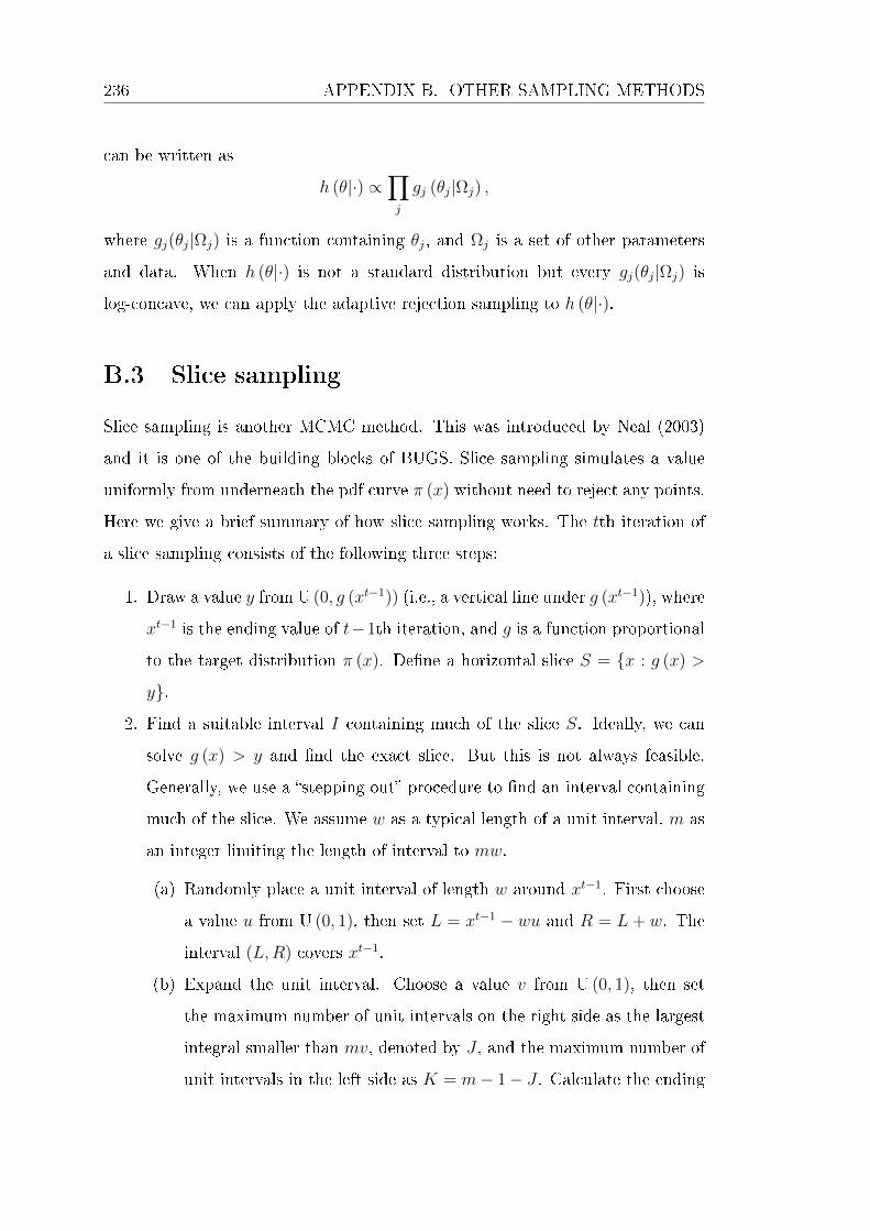
236 APPENDIX B. OTHER SAMPLING METHODS
can be written as
h (θ|·) ∝∏j
gj (θj|Ωj) ,
where gj(θj|Ωj) is a function containing θj, and Ωj is a set of other parameters
and data. When h (θ|·) is not a standard distribution but every gj(θj|Ωj) is
log-concave, we can apply the adaptive rejection sampling to h (θ|·).
B.3 Slice sampling
Slice sampling is another MCMC method. This was introduced by Neal (2003)
and it is one of the building blocks of BUGS. Slice sampling simulates a value
uniformly from underneath the pdf curve π (x) without need to reject any points.
Here we give a brief summary of how slice sampling works. The tth iteration of
a slice sampling consists of the following three steps:
1. Draw a value y from U (0, g (xt−1)) (i.e., a vertical line under g (xt−1)), where
xt−1 is the ending value of t−1th iteration, and g is a function proportional
to the target distribution π (x). Dene a horizontal slice S = x : g (x) >
y.
2. Find a suitable interval I containing much of the slice S. Ideally, we can
solve g (x) > y and nd the exact slice. But this is not always feasible.
Generally, we use a stepping out procedure to nd an interval containing
much of the slice. We assume w as a typical length of a unit interval, m as
an integer limiting the length of interval to mw.
(a) Randomly place a unit interval of length w around xt−1. First choose
a value u from U (0, 1), then set L = xt−1 − wu and R = L + w. The
interval (L,R) covers xt−1.
(b) Expand the unit interval. Choose a value v from U (0, 1), then set
the maximum number of unit intervals on the right side as the largest
integral smaller than mv, denoted by J , and the maximum number of
unit intervals in the left side as K = m− 1− J . Calculate the ending

B.3. SLICE SAMPLING 237
points of the expanded interval as follows:
L = xt−1 − wu− wJ, R = L+ w.
(c) Adjust the interval. If J > 0 and y < g (L), repeat set the new L as
L− w and the new J as J − 1 until J = 0 or y > g (L); if K > 0 and
y < g (R), repeat set the new R as R + w and the new K as K − 1
until K = 0 or y > g (R). Return the nal interval I = (L,R).
3. Draw a new value xt uniformly from S. Repeatedly draw a value uniformly
from an interval which is initially equal to I but shrinks each time when a
draw is not in the slice S, until a value is found within S ∩ I. Note that the
interval I found from stepping out procedure may overlap S.
Neal (2003) gave detailed proof of slice sampling which is not discussed here.


Bibliography
Akaike, H. (1973). Information theory and an extension of the maximum like-
lihood principle. In Second International Symposium on Information Theory,
pages 267281.
Alai, D. H., Merz, M., and Wüthrich, M. V. (2009). Mean square error of predic-
tion in the Bornhuetter-Ferguson claims reserving method. Annals of Actuarial
Science 4, 731.
Anas, A., Boucher, J. P., and Cossette, H. (2015). Modeling dependence between
loss triangles with hierarchical Archimedean copulas. ASTIN Bulletin .
Armagan, A., Dunson, D. B., and Lee, J. (2013). Generalized double Pareto
shrinkage. Statistica Sinica 23, 119143.
Bayarri, M. J., Berger, J. O., Forte, A., and Garcia-Donato, G. (2012). Criteria
for Bayesian model choice with application to variable selection. The Annals
of Statistics 40, 15501577.
Bayes, T. (1763). An essay towards solving a problem in the doctrine of chances.
Philosophical Transactions of the Royal Society, pages 330418.
Beens, F., Bui, L., Collings, S., and Gill, A. (2010). Stochastic reserving using
Bayesian models : Can it add value? In Institute of Actuaries of Australia
17th General Insurance Seminar.
Berger, J. O., Bernardo, J. M., and Sun, D. (2009). The formal denition of
reference priors. The Annals of Statistics 37, 905938.
239

240 BIBLIOGRAPHY
Berry, D. A. and Stangl, D. (1996). Bayesian Biostatistics. Marcel Dekker, New
York.
Bishop, C. M. (2006). Pattern Recognition and Machine Learning. Springer, New
York.
Blei, D. M., Ng, A. Y., and Jordan, M. I. (2003). Latent Dirichlet allocation.
Journal of Machine Learning Research 3, 9931022.
Bornhuetter, R. L. and Ferguson, R. (1972). The actuary and IBNR. Proceedings
of the Casualty Actuarial Society 59, 181195.
Box, G. E. and Tiao, G. C. (1973). Bayesian Inference in Statistical Analysis.
Wiley Classics, New York.
Brehm, P. J., Perry, G., Venter, G. G., and Witcraft, S. (2007). Enterprise Risk
Analysis for Property and Liability Insurance Companies: A Practical Guide
to Standard Models and Emerging Solutions. Guy Carpenter & Company, New
York.
Brooks, S. P. and Gelman, A. (1998). General methods for monitoring conver-
gence of iterative simulations. Journal of Computational and Graphical Statis-
tics 7, 434455.
Brydon, D. and Verrall, R. (2009). Calendar year eects, claims ination and the
chain-ladder technique. Annals of Actuarial Science 4, 287301.
Bühlmann, H. (1967). Experience rating and credibility. ASTIN Bulletin 4,
199207.
Carpenter, B., Gelman, A., Homan, M., Lee, D., Goodrich, B., Betancourt, M.,
Brubaker, M. A., Guo, J., Li, P., and Riddell, A. (2015). Stan: A probabilistic
programming language. Journal of Statistical Software (in press) .
Christiansen, M. and Niemeyer, A. (2014). The fundamental denition of the
solvency capital requirement in Solvency II. ASTIN Bulletin 44, 501533.

BIBLIOGRAPHY 241
Clark, D. R. (2003). LDF curve-tting and stochastic reserving: A maximum
likelihood approach. Casualty Actuarial Society Forum (Fall 2003) pages 41
92.
Crainiceanu, C. M., Ruppert, D., and Wand, M. P. (2005). Bayesian analysis
for penalized spline regression using WinBUGS. Journal of Statistical Software
14, 114.
Czado, C., Kastenmeier, R., Brechmann, E. C., and Min, A. (2012). A mixed
copula model for insurance claims and claim sizes. Scandinavian Actuarial
Journal 2012, 278305.
Danaher, P. J. and Smith, M. S. (2011). Modeling multivariate distributions
using copulas: Applications in marketing. Marketing Science 30, 421.
De Alba, E. (2002). Bayesian estimation of outstanding claim reserves. North
American Actuarial Journal 6, 120.
De Jong, P. (2012). Modeling dependence between loss triangles. North American
Actuarial Journal 16, 7486.
Dempster, A. P., Laird, N. M., and Rubin, D. B. (1977). Maximum likelihood
from incomplete data via the EM algorithm. Journal of the Royal Statistical
Society B 39, 138.
DiMatteo, I., Genovese, C. R., and Kass, R. E. (2001). Bayesian curve-tting
with free-knot splines. Biometrika 88, 10551071.
Duane, S., Kennedy, A. D., Pendleton, B. J., and Roweth, D. (1987). Hybrid
Monte Carlo. Physics Letters B 195, 216222.
Efron, B. and Tibshirani, R. J. (1994). An Introduction to the Bootstrap. Chap-
man & Hall, New York.
Embrechts, P. and Hofert, M. (2013). Statistical inference for copulas in high
dimensions: A simulation study. ASTIN Bulletin 43, 8195.

242 BIBLIOGRAPHY
Embrechts, P., Lindskog, F., and McNeil, A. (2001). Modelling dependence with
copulas and applications to risk management.
England, P. and Verrall, R. (2006). Predictive distributions of outstanding liabil-
ities in general insurance. Annals of Actuarial Science 1, 221270.
England, P. D. and Verrall, R. J. (2001). A exible framework for stochastic
claims reserving. Proceedings of the Casualty Actuarial Society 88, 138.
England, P. D. and Verrall, R. J. (2002). Stochastic claims reserving in general
insurance. British Actuarial Journal 8, 443518.
England, P. D., Verrall, R. J., and Wüthrich, M. V. (2012). Bayesian
over-dispersed poisson model and the Bornhuetter-Ferguson claims reserving
method. Annals of Actuarial Science 6, 258283.
Faraway, J. J. (2015). Linear Models with R. Chapman & Hall, Boca Raton,
second edition.
Feldblum, S. (2010). Dependency modeling. Casualty Actuarial Society Study
Notes .
Fréchet, M. (1935). Generalisations du theoreme des probabilites totales. Funda-
menta Mathematicae 25, 379387.
Frees, E. W. and Valdez, E. A. (1998). Understanding relationships using copulas.
North American Actuarial Journal 2, 125.
Friedland, J. (2010). Estimating unpaid claims using basic techniques. Casualty
Actuarial Society Study Notes .
Gelfand, A. E., Hills, S. E., Racinepoon, A., and Smith, A. F. M. (1990). Il-
lustration of Bayesian-inference in normal data models using Gibbs sampling.
Journal of the American Statistical Association 85, 972985.

BIBLIOGRAPHY 243
Gelfand, A. E. and Smith, A. F. (1990). Sampling-based approaches to calculating
marginal densities. Journal of the American Statistical Association 85, 398
409.
Gelman, A., Carlin, J. B., Stern, H. S., and Rubin, D. B. (2014). Bayesian Data
Analysis. Chapman & Hall, Boca Raton, third edition.
Gelman, A., Lee, D., and Guo, J. (2015). Stan: A probabilistic programming
language for Bayesian inference and optimization. Journal of Educational and
Behavioral Statistics (in press) .
Gelman, A. and Rubin, D. B. (1992). Inference from iterative simulation using
multiple sequences. Statistical Science 7, 457472.
Geman, S. and Geman, D. (1984). Stochastic relaxation, Gibbs distributions, and
the Bayesian restoration of images. IEEE Transactions on Pattern Analysis and
Machine Intelligence 6, 721741.
Genest, C., Rémillard, B., and Beaudoin, D. (2009). Goodness-of-t tests for
copulas: A review and a power study. Insurance: Mathematics and economics
44, 199213.
Genest, C. and Rivest, L.-P. (1993). Statistical inference procedures for bivari-
ate Archimedean copulas. Journal of the American statistical Association 88,
10341043.
Gershman, S., Homan, M., and Blei, D. (2012). Nonparametric variational
inference. In 29th International Conference on Machine Learning.
Gesmann, M., Murphy, D., Zhang, W., Carrato, A., Crupi, G., Wuthrich, M., and
Concina, F. (2015). ChainLadder: Statistical Methods and Models for Claims
Reserving in General Insurance. R package version 0.2.1.
Gilks, W. R., Richardson, S., and Spiegelhalter, D. J. (1996).Monte Carlo Markov
Chain in Practice. Chapman & Hall, New York.

244 BIBLIOGRAPHY
Gilks, W. R. andWild, P. (1992). Adaptive rejection sampling for Gibbs sampling.
Journal of the Royal Statistical Society C 41, 337348.
Gray, R. J. and Pitts, S. M. (2012). Risk Modelling in General Insurance: from
Principles to Practice. Cambridge University Press, Cambridge.
Green, P. J. (1995). Reversible jump Markov chain Monte Carlo computation
and Bayesian model determination. Biometrika 82, 711732.
Hall, P. and Opsomer, J. D. (2005). Theory for penalised spline regression.
Biometrika 92, 105118.
Hastie, T. J. and Tibshirani, R. J. (1990). Generalized Additive Models. Chapman
& Hall, New York.
Hastie, T. J., Tibshirani, R. J., and Friedman, J. H. (2009). The Elements of
Statistical Learning: Data Mining, Inference, and Prediction. Springer, New
York, second edition.
Hastings, W. K. (1970). Monte Carlo sampling methods using Markov chains
and their applications. Biometrika 57, 97109.
Hills, S. E. and Smith, A. F. (1992). Parameterization Issues in Bayesian Infer-
ence. Oxford University Press, London.
Ho, P. D. (2007). Extending the rank likelihood for semiparametric copula
estimation. The Annals of Applied Statistics 1, 265283.
Homan, M. D., Blei, D. M., Wang, C., and Paisley, J. (2013). Stochastic varia-
tional inference. Journal of Machine Learning Research 14, 13031347.
Homan, M. D. and Gelman, A. (2014). The no-u-turn sampler: Adaptively setting
path lengths in Hamiltonian Monte Carlo. The Journal of Machine Learning
Research 15, 15931623.
BIBLIOGRAPHY 245
Jaakkola, T. S. and Jordan, M. I. (2000). Bayesian parameter estimation via
variational methods. Statistics and Computing 10, 2537.
James, G., Witten, D., Hastie, T., and Tibshirani, R. (2013). An Introduction to
Statistical Learning. Springer, New York.
Jereys, H. (1961). Theory of Probability. Oxford University Press, London, third
edition.
Joe, H. (2014). Dependence Modeling with Copulas. Chapman & Hall, New York.
Joe, H. and Xu, J. J. (1996). The estimation method of inference functions for
margins for multivariate models.
Jordan, M. I., Ghahramani, Z., Jaakkola, T. S., and Saul, L. K. (1999). An
introduction to variational methods for graphical models. Machine Learning
37, 183233.
Kendall, M. G. and Stuart, A. (1961). The Advanced Theory of Statistics: Infer-
ence and Relationship. Charles Grin, London.
Klugman, S. A., Panjer, H. H., and Willmot, G. E. (2012). Loss Models: From
Data to Decisions. John Wiley & Sons, New York, fourth edition.
Komaki, F. (2006). Shrinkage priors for Bayesian prediction. The Annals of
Statistics 34, 808819.
Krämer, N., Brechmann, E. C., Silvestrini, D., and Czado, C. (2013). Total loss
estimation using copula-based regression models. Insurance: Mathematics and
Economics 53, 829839.
Kruskal, W. H. (1958). Ordinal measures of association. Journal of the American
Statistical Association 53, 814861.
Kucukelbir, A., Ranganath, R., Gelman, A., and Blei, D. M. (2015). Automatic
variational inference in Stan. arXiv preprint arXiv:1506.03431 .

246 BIBLIOGRAPHY
Laplace, P. S. (1785). Memoire sur les approximations des formules qui sont fonc-
tions de tres grands nombres. In Memoires de l'Academie Royale des Sciences.
Laplace, P. S. (1810). Memoire sur les approximations des formules qui sont
fonctions de tres grands nombres, et sur leur application aux probabilites. In
Memoires de l'Academie des Science de Paris.
Lay, D. C. (2012). Linear Algebra and Its Application. Addison Wesley, Boston,
fourth edition.
Lindley, D. V. (1965). Introduction to Probability and Statistics from Bayesian
Viewpoint, volume 2. Cambridge University Press, Cambridge.
Longley-Cook, L. H. (1962). An introduction to credibility theory. Proceedings
of the Casualty Actuarial Society 49, 194221.
Lunn, D., Jackson, C., Best, N., Thomas, A., and Spiegelhalter, D. (2012). The
BUGS Book: A Practical Introduction to Bayesian Analysis. Chapman & Hall,
Boca Raton.
Lunn, D. J., Thomas, A., Best, N., and Spiegelhalter, D. (2000). WinBUGS - a
Bayesian modelling framework: concepts, structure, and extensibility. Statistics
and Computing 10, 325337.
Mack, T. (1993). Distribution-free calculation of the standard error of chain
ladder reserve estimates. ASTIN Bulletin 23, 213225.
Mack, T. (1999). The standard error of chain-ladder reserve estimates, recursive
calculation and inclusion of a tail factor. ASTIN Bulletin 29, 361366.
Mack, T. (2008). The prediction error of Bornhuetter-Ferguson. ASTIN Bulletin
38, 87.
Mayerson, A. L. (1964). A Bayesian view of credibility. Proceedings of the Casualty
Actuarial Society 51, 723.

BIBLIOGRAPHY 247
McCullagh, P. and Nelder, J. A. (1989). Generalized Linear Models. Chapman
& Hall, New York, second edition.
Meng, X. L. (1994). Posterior predictive p-values. The Annals of Statistics 22,
11421160.
Merz, M., Wüthrich, M. V., and Hashorva, E. (2013). Dependence modelling in
multivariate claims run-o triangles. Annals of Actuarial Science 7, 325.
Metropolis, N., Rosenbluth, A. W., Rosenbluth, M. N., Teller, A. H., and Teller,
E. (1953). Equation of state calculations by fast computing machines. Journal
of Chemical Physics 21, 10871092.
Meyers, G. (2009). Stochastic loss reserving with the collective risk model. Vari-
ance 3, 239269.
Meyers, G. (2015). Stochastic loss reserving using Bayesian MCMC models. CAS
Monograph Series 1, 164.
Minka, T. P. (2001). Expectation propagation for approximate Bayesian infer-
ence. In Proceedings of the Seventeenth Conference on Uncertainty in Articial
Intelligence, pages 362369. Morgan Kaufmann Publishers Inc.
Neal, R. M. (1994). An improved acceptance procedure for the hybrid Monte
Carlo algorithm. Journal of Computational Physics 111, 194203.
Neal, R. M. (2003). Slice sampling. The Annals of Statistics 31, 705741.
Neal, R. M. (2011). MCMC using Hamiltonian dynamics. Handbook of Markov
Chain Monte Carlo .
Nelsen, R. B. (2013). An Introduction to Copulas. Springer, New York.
Nocedal, J. and Wright, S. (2006). Numerical Optimization. Springer Science &
Business Media, New York.

248 BIBLIOGRAPHY
Ntzoufras, I. and Dellaportas, P. (2002). Bayesian modelling of outstanding liabil-
ities incorporating claim count uncertainty. North American Actuarial Journal
6, 113125.
Park, T. and Casella, G. (2008). The Bayesian lasso. Journal of the American
Statistical Association 103, 681686.
Pitt, M., Chan, D., and Kohn, R. (2006). Ecient Bayesian inference for Gaussian
copula regression models. Biometrika 93, 537554.
Piwcewicz, B. (2008). Stochastic reserving: case study using a Bayesian approach.
In Institute of Actuaries of Australia 16th General Insurance Seminar.
Renshaw, A. E. and Verrall, R. J. (1998). A stochastic model underlying the
chain-ladder technique. British Actuarial Journal 4, 903923.
Robert, C. and Casella, G. (2013). Monte Carlo statistical methods. Springer
Science & Business Media, New York.
Roberts, G. O. and Sahu, S. K. (1997). Updating schemes, correlation structure,
blocking and parameterization for the Gibbs sampler. Journal of the Royal
Statistical Society B 59, 291317.
Robins, J. M., van der Vaart, A. W., and Ventura, V. (2000). Asymptotic distri-
bution of p-values in composite null models. Journal of the American Statistical
Association 95, 11431156.
Rubin, D. B. (1981). Estimation in parallel randomized experiments. Journal of
Educational and Behavioral Statistics 6, 377401.
Rubin, D. B. (1984). Bayesianly justiable and relevant frequency calculations
for the applied statistician. The Annals of Statistics 12, 11511172.
Ruppert, D. (2012). Selecting the number of knots for penalized splines. Journal
of Computational and Graphical Statistics 11, 735757.

BIBLIOGRAPHY 249
Ruppert, D., Wand, M. P., and Carroll, R. J. (2003). Semiparametric Regression.
Cambridge University Press, New York.
Saluz, A. (2015). Prediction uncertainties in the Cape Cod reserving method.
Annals of Actuarial Science 9, 239263.
Saluz, A., Gisler, A., and Wüthrich, M. V. (2011). Development pattern and pre-
diction error for the stochastic Bornhuetter-Ferguson claims reserving method.
ASTIN Bulletin 41, 279313.
Schwarz, G. (1978). Estimating the dimension of a model. The Annals of Statistics
6, 461464.
Scollnik, D. P. (2001). Actuarial modeling with MCMC and BUGS. North Amer-
ican Actuarial Journal 5, 96124.
Shi, P. (2014). A copula regression for modeling multivariate loss triangles and
quantifying reserving variability. Astin Bulletin 44, 85102.
Shi, P., Basu, S., and Meyers, G. G. (2012). A Bayesian log-normal model for
multivariate loss reserving. North American Actuarial Journal 16, 2951.
Shi, P. and Frees, E. W. (2011). Dependent loss reserving using copulas. ASTIN
Bulletin 41, 449486.
Simpson, L. and McCourt, P. (2012). Worksafe Victoria actuarial valuation of
outstanding claims liability for the scheme as at 30 June 2012. Technical report,
PricewaterhouseCoopers Actuarial Pty Ltd.
Sklar, M. (1959). Fonctions de répartition à n dimensions et leurs marges. Pub-
lications de l'Institut de Statistique de l'Université Paris 8, 229231.
Smith, M. S. (2011). Bayesian approaches to copula modelling. Available at
SSRN 1974297 .

250 BIBLIOGRAPHY
Spiegelhalter, D., Thomas, A., Best, N., and Lunn, D. (2003). WinBUGS user
manual.
Spiegelhalter, D. J., Best, N. G., Carlin, B. R., and van der Linde, A. (2002).
Bayesian measures of model complexity and t. Journal of the Royal Statistical
Society B 64, 583616.
Stan Development Team (2012). Stan modeling language.
Tanner, M. A. and Wong, W. H. (1987). The calculation of posterior distributions
by data augmentation. Journal of the American statistical Association 82, 528
540.
Taylor, G. (2000). Loss Reserving: An Actuarial Perspective. Huebner Inter-
national Series on Risk, Insurance and Economic Security. Kluwer Academic
Publishers, Boston.
Trivedi, P. K. and Zimmer, D. M. (2007). Copula Modeling: An Introduction for
Practitioners. Now Publishers, Boston.
Vehtari, A., Gelman, A., and Gabry, J. (2015). Ecient implementation of leave-
one-out cross-validation andWAIC for evaluating tted Bayesian models. arXiv
preprint arXiv:1507.04544 .
Venter, G. G. (2002). Tails of copulas. Proceedings of the Casualty Actuarial
Society 89, 68113.
Verrall, R., Hössjer, O., and Björkwall, S. (2012). Modelling claims run-o with
reversible jump Markov chain Monte Carlo methods. ASTIN Bulletin 42, 35
58.
Verrall, R. J. (2000). An investigation into stochastic claims reserving models
and the chain-ladder technique. Insurance: Mathematics and Economics 26,
9199.

BIBLIOGRAPHY 251
Verrall, R. J. (2004). A Bayesian generalized linear model for the Bornhuetter-
Ferguson method of claims reserving. North American Actuarial Journal 8,
6789.
Verrall, R. J. and Wüthrich, M. V. (2012). Reversible jump Markov chain Monte
Carlo method for parameter reduction in claims reserving. North American
Actuarial Journal 16, 240259.
Watanabe, S. (2010). Asymptotic equivalence of Bayes cross validation and widely
applicable information criterion in singular learning theory. Journal of Machine
Learning Research 11, 35713594.
Watanabe, S. (2013). A widely applicable bayesian information criterion. Journal
of Machine Learning Research 14, 867897.
Whitney, A. W. (1918). The theory of experience rating. Proceedings of the
Casualty Actuarial Society 4, 274292.
Wood, S. (2006). Generalized Additive Models: An Introduction with R. Chapman
& Hall, New York.
Wood, S. N. (2003). Thin plate regression splines. Journal of the Royal Statistical
Society B 65, 95114.
Wüthrich, M. V. (2013a). Calendar year dependence modeling in run-o triangles.
In ASTIN Colloquium, pages 2124.
Wüthrich, M. V. (2013b). Challenges with non-informative gamma priors in the
Bayesian over-dispersed Poisson reserving model. Insurance: Mathematics and
Economics 52, 352358.
Wüthrich, M. V. and Merz, M. (2008). Stochastic Claims Reserving Methods in
Insurance. John Wiley & Sons, Chichester.

252 BIBLIOGRAPHY
Zhang, Y., Dukic, V., and Guszcza, J. (2012). A Bayesian non-linear model for
forecasting insurance loss payments. Journal of the Royal Statistical Society A
175, 637656.
Zhang, Y. W. and Dukic, V. (2013). Predicting multivariate insurance loss pay-
ments under the Bayesian copula framework. Journal of Risk and Insurance
80, 891919.


