University of Calgary PRISM: University of Calgary's Digital Repository Graduate Studies The Vault: Electronic Theses and Dissertations 2019-07-02 Three Essays on Business Taxation Wei, Feng Wei. F. (2019). Three Essays on Business Taxation (Unpublished doctoral thesis). University of Calgary, Calgary, AB. http://hdl.handle.net/1880/110572 doctoral thesis University of Calgary graduate students retain copyright ownership and moral rights for their thesis. You may use this material in any way that is permitted by the Copyright Act or through licensing that has been assigned to the document. For uses that are not allowable under copyright legislation or licensing, you are required to seek permission. Downloaded from PRISM: https://prism.ucalgary.ca
Transcript
University of Calgary
PRISM: University of Calgary's Digital Repository
Graduate Studies The Vault: Electronic Theses and Dissertations
2019-07-02
Three Essays on Business Taxation
Wei, Feng
Wei. F. (2019). Three Essays on Business Taxation (Unpublished doctoral thesis). University of
Calgary, Calgary, AB.
http://hdl.handle.net/1880/110572
doctoral thesis
University of Calgary graduate students retain copyright ownership and moral rights for their
thesis. You may use this material in any way that is permitted by the Copyright Act or through
licensing that has been assigned to the document. For uses that are not allowable under
copyright legislation or licensing, you are required to seek permission.
Downloaded from PRISM: https://prism.ucalgary.ca
UNIVERSITY OF CALGARY
Three Essays on Business Taxation
by
Feng Wei
A THESIS
SUBMITTED TO THE FACULTY OF GRADUATE STUDIES
IN PARTIAL FULFILLMENT OF THE REQUIREMENTS FOR THE
3.1 Summary Statistics . . . . . . . . . . . . . . . . . . . . . . . . . . . . . . . . 983.2 Placebo Tests between the Service Sector and Manufacturing Sector . . . . . 1023.3 The Aggregate Effect: Wage Rate and Working Hours . . . . . . . . . . . . . 1043.4 The Heterogeneous Effects: Wage Rate and Working Hours . . . . . . . . . 1073.5 Different Size of Firms . . . . . . . . . . . . . . . . . . . . . . . . . . . . . . 1123.6 Selection on observations . . . . . . . . . . . . . . . . . . . . . . . . . . . . . 1143.7 Checks on the Exclusion Restriction Assumption . . . . . . . . . . . . . . . . 1163.8 Checks on the Anticipatory Effect of the Wage Rate . . . . . . . . . . . . . . 1193.9 Checks on the Anticipatory Effect of the Number of Working Hours . . . . . 1203.10 The Extended Heterogeneous Effects: Wage Rates and Working Hours . . . 121
viii
Chapter 1
Designing Presumptive Taxes in
Countries with Large Informal Sectors
1.1 Introduction
Informal sector activities are pervasive in developing countries.1 Medina and Schneider
(2017) estimate that the average size of the so-called shadow economy is 36.1% of official
GDP in Sub-Saharan Africa and 34.8% in Latin America and the Caribbean, compared to
18.4% in the OECD. The vast majority of informal businesses have fewer than five employees
and many have none, but there are also relatively large businesses operating without licenses
or tax identification numbers (see, e.g., Amin and Islam, 2015, and Benjamin and Mbaye,
2012). Bringing the larger and more profitable informal firms into the formal system would
widen the tax base and probably more than justify the additional administrative costs.2
There are also compelling reasons to try to tax micro-enterprises, in terms of improving
horizontal equity and elevating tax morale in the formal sector (Terkper, 2003, and Torgler,
1We adopt the common definition that a business is formal if it is registered for the relevant municipallicenses and with the tax department (Bruhn and McKenzie, 2013). However, see Kanbur and Keen (2014)for a more nuanced discussion of the meaning of informality.
2Andrade et al. (2013) suggest that inspecting informal firms earning an average of $1,000 a monthin profits in Brazil would formalize more than enough firms for the revenues to pay for the costs of suchenforcement.
1
2005). However, widespread evasion and limited taxation capacity constrain the feasible
designs of tax policy for mobilizing revenues in developing countries.
For many firms, the decision to operate in the informal economy rests on the relative costs
(for example, tax and regulatory costs) and benefits (for example, access to financial sector
and legal systems) of operating in the formal economy (Bird and Zolt, 2008). According to
an open-ended survey of informal enterprises in the third largest city in Brazil, firm owners
responded that the main disadvantages of formalizing were the initial costs of registration
(62 percent of respondents stated this), having to pay taxes (58 percent), having to pay for
an accountant (34 percent), and the process of registering taking too much time (32 percent)
(de Andrade et al., 2016). Similarly, in a World Bank survey of mainly micro-businesses
in Ethiopia (Yesegat, 2015), the single biggest disadvantage of registering for taxes was
identified by respondents as being: a higher tax burden or high tax rates (34 percent),
complicated tax compliance procedures (13 percent), harassment by government officials (8
percent), and frequent inspections (8 percent), with other factors accounting for the rest.
The fixed costs of registering and complying with taxation are evidently highly regressive
and thus can act as barriers to formalisation. Consequently, strategies for inducing formality
have focused on reducing the cost of registering a business and paying taxes. Examples of
initiatives to cut costs include the establishment in many countries of one-stop shops for
registering a business for tax and licensing and disseminating information about how to
formalize and file taxes (Joshi et al., 2014).
In a similar vein, presumptive tax regimes for small-, and medium-sized enterprises
(SMEs), which use turnover or some other simple proxy for profitability as the tax base,
can help deter informality by facilitating taxpayer compliance. For SMEs, complying with
the standard tax regime’s burdensome recordkeeping requirements not only is costly, but
often exceeds the capacity and skills of the small business operator (Engelschalk, 2007).
Turnover-based presumptive systems can ease the accounting requirements for filing taxes,
while still obliging small businesses to keep basic books and records, thereby facilitating an
2
eventual transition from the presumptive to the standard tax regime. Recent work has high-
lighted the importance of reducing taxpayer compliance costs in encouraging entrepreneurs
and small firms to voluntarily register for tax. Harju et al. (2019) show that registration for
VAT in Finland increased substantially in response to simplified reporting procedures (in-
cluding changing from monthly to annual VAT filing) for firms below a threshold of 25,000
euros. In Georgia, new tax regimes were introduced for micro and small businesses in 2010
to significantly lowered compliance and administrative costs of businesses and the revenue
service. Specifically, firms without employees and an annual turnover below GEL 30,000
($18,255) were excluded from taxation (but paid a patent prior to the reform) and busi-
nesses with turnover between GEL 30,000 and GEL 100,000 (US$ 60,850) qualified for a
turnover tax regime instead of regular income tax. Bruhn and Loeprick (2016) report an
18-30% increase in the number of newly registered formal firms below the eligibility threshold
of GEL 30,000 during the first year of the reform, though not in the following two years. The
authors also found no evidence that the newly registered micro firms were previously formal
firms producing just above the threshold. In the absence of such strategic sorting, the newly
registered micro firms plausibly were drawn in from an existing stock of informal firms that
decided to register when the reform was introduced. However, at the GEL 100,000 cutoff
for the new small business turnover tax regime, Bruhn and Loeprick did not find a robust
effect of the reform on formal firm creation in any year.
A threshold is required to limit the presumptive regime to smaller enterprises only. It
is standard to define the threshold itself in terms of turnover, while putting consolidation
rules into place to prevent entities from artificially splitting for tax purposes. In contrast,
using the number of employees to define the threshold makes it prone to outsourcing labor.3
In low-income countries, turnover taxes appear best suited for small companies, rather than
for self-employed workers operating informally and without employees.4 The latter group,
3However, even if they do not serve as the presumptive tax threshold, alternative size or profit indicators,such as the number of employees, the size of the business premises, or the value of assets, can be usefulinformation to collect for auditing a company’s reported turnover.
4The case is likely different in developed countries, where the education level of self-employed individuals
3
which characterizes a substantial portion of the informal sector, is unlikely to formalize, even
with simplified accounting and financial incentives to do so (La Porta and Shleifer, 2008, de
Mel et al., 2010, de Mel et al., 2013, and Loayza, 2016). Thus, a fixed fee (patent system)
may be a more realistic approach to taxing self-employed workers and microenterprises with
few employees. In Uzbekistan, for instance, as of 2019, unincorporated businesses with fewer
than 5 employees pay a fixed amount, rather than the 4% turnover tax applied to businesses
below a turnover threshold of $120,000. A more drastic approach is to leave untaxed mi-
croenterprises below a lower bound threshold level for the turnover tax, as described above
in the case of Georgia.
Despite the simplified accounting requirements under a turnover-based presumptive tax,
the experiences some countries have had with the tax are disappointing. In Tanzania, which
operates a presumptive tax that is a progressively increasing proportion of turnover, the level
of recordkeeping among Tanzanian SMEs has not increased much, despite a substantial tax
concession for SMEs who keep (simplified) records (Engelschalk, 2007). In Kenya, a tax of
3% on declared turnover (and 3% of the threshold if the business does not keep accounts) was
introduced in 2008 to curb the rapidly growing informal sector. Despite the simplification
in tax compliance and tax computation, the uptake and revenue yield were weaker than
expected (Wanyagathi Maina, 2017). A new presumptive tax of 15% percent of the amount
payable for a business permit or trade license was introduced in 2019 in the hope of widening
the tax base to include more informal firms and the small businesses into the tax ambit. Such
experiences reinforce the observation that simplified procedures and presumptive tax policies
by themselves are insufficient to induce enterprises to formalize.
In the case of Kenya, the need for the government to demonstrate to informal businesses
that non-compliance can be detected and punished was noted in IEA (2012). In a field exper-
iment in Brazil, de Andrade et al. (2014) estimated that receiving an inspection generated a
21 to 27 percentage point increase in the likelihood that an enterprise will of formalize. The
is likely to be higher.
4
probability of detection by tax or other government authorities, resulting in penalties, raises
the cost of operating a company informally. Thus, policies of simplifying taxation and tax-
payer education need to be supplemented with enhanced tax enforcement and verification.
Recent technological improvements may provide tax authorities with greater capabilities to
observe and monitor transactions and taxpayers and hence to estimate revenue and profits
(Bird and Zolt, 2008). Slemrod et al. (2019) report that innovative programs, using social
and psychological factors can serve to complement standard measures for deterring tax eva-
sion in developing countries. In Pakistan, for instance, public disclosures of tax payments
boosted the rate of tax filing and the amounts of declared tax liabilities from self-employment
earnings.
We construct a simple model where a turnover threshold separates firms paying stan-
dard corporate income tax from firms (below the threshold) who pay a tax on their sales
(turnover). We make two extreme assumptions to allow us to study, in the simplest pos-
sible way, the behavior of firms faced by the turnover tax regime. Thus, following Kanbur
and Keen (2014), we suppose that firms can costlessly adjust their output downward from
an exogenous maximum potential amount and that they can escape taxation altogether by
becoming ‘ghosts’ in the shadow economy.5 While crude, the assumptions highlight how the
option to produce informally constrains the turnover tax rate and how the turnover tax in-
teracts with the standard corporate income tax regime to create ‘notches’ in the production
levels of firms. The production inefficiencies associated with the presumptive regime and
with informal sector production are also modeled very simply, as exogenous additions to the
marginal cost of production.
The advantage of such a streamlined model is that it is easy to calibrate and generates
practical tax policy guidelines. Thus, closed-form solutions are derived for the optimal
5Waseem (2018) shows that the number of enterprises operating in the formal sector responds to taxpressures. When Pakistan increased the tax on unincorporated partnerships to a level comparable to thestandard corporate tax, within three years of the tax increase, the number of partnerships in Pakistan haddeclined to 36% of the baseline level. Very few of these companies became incorporated. It is plausible thata portion of them became informal.
5
threshold, in terms of the standard corporate income tax rate and the turnover tax rate;
and closed-form solutions are derived for the optimal turnover tax rate as a function of
the threshold. The solutions depend on whether bunching below the threshold occurs or
not; both types of equilibria are possible, depending on the parameter values of the model.
The formulas for the optimal threshold are relatively simple and intuitive. In contrast, the
formulas for the optimal tax rate are long and tedious, reflecting the complicated balancing
act between two behavioral margins. That is, if the tax rate is too low, some firms will
migrate away from the standard regime, but if it is too high then some firms will choose
to produce in the informal sector. Nevertheless, the model optimal threshold and turnover
tax rate can be computed with a spreadsheet. Numerical solutions of the model for different
scenarios and comparative statics analysis are used to provide further insights.
The numerical values for the optimal threshold and turnover tax rate are both lower
than the results of the more complicated model of Wei and Wen (2019), where production
is endogenous through the input choices of heterogeneous firms. It is not quite evident
why this is the case, but we note that the optimal threshold for VAT using Keen and
Mintz’s (2004) ‘simple rule,’ which has much in common with our simple model, is also
substantially lower than the optimal threshold in Keen and Mintz’s (2004) more general
model, characterized by heterogeneous production technologies. Furthermore, the restraint
on the optimal turnover tax rate, imposed by the option of firms disappearing into the
informal sector in the present model, reduces the relative benefit of the presumptive regime
over the regular regime, placing downward pressure on the optimal threshold. The main
parameters of interest in our current analysis are the (constant) marginal cost of production
in the informal sector and the fixed cost of taxpayer compliance in the presumptive regime.
Both of these parameters can be influenced by the tax enforcement policies of the authorities.
For example, the cost of operating in the shadow economy increases with the probability of
inspection. The cost of compliance is diminished by disseminating information to informal
enterprises on the processes of bookkeeping and filing taxes. Hence, the study contributes
6
to our understanding of how to design presumptive tax regimes for economies characterized
by high levels of informality.
Section 2 presents the model. Section 3 describes the optimal tax policy and provides
the comparative statics analysis. Section 4 calculates the optimal turnover threshold and
turnover tax rate for alternative calibrations of the economy. Section 6 concludes. Proofs of
lemmas and propositions are contained in an appendix.
1.2 A Simple Model of Firms’ Behavior
We suppose that there is a population of firms endowed with differing levels of maximum
potential sales, Z ∈ (0, ZM), where Z is exogenous and distributed according to a twice
differentiable distribution function H(Z) with strictly positive density h(Z). The upper-
support of the distribution, ZM , may be finite or infinite. To study the behavioral responses
of firms in the simplest way possible, we follow Kanbur and Keen (2014) in assuming that
firms can choose to adjust (costlessly) their output to any level below their maximum po-
tential, for instance, to reduce their tax burden. The marginal cost of production is assumed
to be a constant proportion of sales, C < 1, which is identical across the population. The
output price is normalized to one, so output is the same as sales. Hence, a firm producing
Z has a pre-tax profit of (1− C)Z.
The tax system is as follows. Firms with actual sales equal to or exceeding a threshold
Z face a corporate income tax rate of tc on their profits (henceforth, the ‘regular regime’),
while firms selling below the threshold are taxed on their sales, with no deduction for costs,
at the rate t (henceforth, the ‘presumptive regime’). The corporate income tax rate is taken
to be exogenous. The turnover tax rate t and the threshold Z are the policy choices in
the model. Firms face fixed compliance costs of Γ and Γ′, in the standard and presumptive
regimes, respectively. The government faces corresponding fixed administrative costs of A
and A′. Since sales are easier to record and audit than profit, let Γ > Γ′ > 0 and A > A′ > 0.
7
While the compliance costs are exogenous in the model, public initiatives, such as a one-stop
shop for registering a business with the various licensing and tax authorities, and educational
campaigns on bookkeeping and tax filing, can be regarded as efforts to reduce the size of Γ′
for SMEs. We shall also suppose that there is an extra marginal cost α, on top of C, incurred
by firms in the presumptive regime, possibly representing higher borrowing costs due to a
lack of verifiable information on profit (since the tax base is revenue) or, more generally, the
production inefficiencies caused by the non-deductibility of costs under presumptive taxation.
Finally, as in Kanbur and Keen (2014), we assume that firms can escape taxation altogether
by ‘disappearing’ into the informal sector. However, in this case, their marginal cost is
increased by an amount λ, on top of C, where λ is an exogenous parameter representing
the inefficiencies associated with the informal sector. For example, informal enterprises face
inconveniences in having to produce in ways that avoid detection by tax officials.6 Indeed,
advances in electronic technology has facilitated coordination between government agencies,
such that a taxpayer identification number (TIN) can be required to access government
services, such as obtaining passports or driver’s licenses, register cars and property, use
public schools or hospitals, or to subscribe to public utility services—thus further increasing
the costs of operating outside the tax system (Bird and Zolt, 2008).
We suppose that
(1− tc)(1− C) > 1− C − α− t > 1− C − λ > 0 (1.1)
Hence, so long as the tax rate of the presumptive regime is not too high, the net profit
margin is lowest in the informal sector and highest in the regular regime. The inequalities
are assured for any t by the assumption that λ > α > tc(1 − C). We also assume that the
fixed compliance costs, Γ and Γ′, are not so large as to preclude the possibility that large
producers (i.e., for Z in a neighborhood of ZM) can earn a strictly positive net profit in the
6For example, informal firms have less scope for marketing or they locate in obscure locations to avoidattracting the attention of the law (Bruhn and McKenzie, 2013).
8
regular regime (given tc) and in the presumptive regime (at t = 0), respectively.
We can summarize the structure of the economy by specifying the after-tax profit func-
tions of four types of firms: those producing at their maximum sales level in the regular
regime (regulars , earning πR); those who adjust their sales downward to just below the
threshold (adjusters , earning πA);7 those producing at their maximum sales in the presump-
tive regime (presumptive, earning πP ); and those producing at their maximum sales but
escaping taxation by remaining informal (informals , earning πI). Each firm chooses how to
behave to maximize its after-tax profits. The net profit functions are:8
πR(Z) = (1− tc)(1− C)Z − Γ
πA(Z) = (1− t− C − α)Z − Γ′
πP (Z) = (1− t− C − α)Z − Γ′
πI(Z) = (1− C − λ)Z
(1.2)
1.2.1 Partitioning the distribution of firms
1.2.1.1 Informal and formal sectors
Recall that firms have the option of becoming informal.9 There are three such pairwise com-
parisons to consider: informality versus presumptive taxation; informality versus adjusting;
and informality versus regular taxation. Firms prefer informality to presumption if and only
if
(1− C − λ)Z > (1− t− C − α)Z − Γ′ (1.3)
7Their sales are below, but arbitrarily close to, the threshold.8In the case of adjusters, since firms must produce below the threshold to be eligible for the presumptive
regime, their profit is below, but arbitrarily close to, πA.9We shall label all taxpaying firms (or, more precisely, firms registered with the tax authorities) as
‘formal,’ regardless of whether they are in the regular tax regime or the presumptive tax regime. In contrast,informal firms evade taxation altogether.
9
which defines a cutoff sales level,
ZIP =Γ′
λ− t− α(1.4)
All firms with Z < ZIP prefer informality over presumptive taxation. The expression for
ZIP shows how the proportion of firms in the informal sector is shaped by the taxpayer
compliance cost in the presumptive regime and the relative cost disadvantage of producing
informally. Similarly, firms prefer informality over adjusting if Z > ZIA where,
ZIA =(1− t− C − α)Z − Γ′
1− C − λ(1.5)
Finally, firms prefer informality over the regular regime if Z < ZIR where,
ZIR =Γ
λ− tc(1− C)(1.6)
1.2.1.2 Jumping and bunching
Firms with maximum sales of at least Z, that choose to remain in the formal sector, must
decide between producing at their maximum and being subjected to the regular regime, or
reducing their output to just below the threshold and paying the presumptive tax. Given a
threshold Z and tax rates tc and t, adjusting dominates the regular regime whenever
(1− t− C − α)Z − Γ′ > (1− tc)(1− C)Z − Γ (1.7)
which defines a cut-off sales level
Z =(1− t− C − α)Z − Γ′ + Γ
(1− tc)(1− C)(1.8)
All firms with sales below Z prefer adjusting over being regulars.
10
Adjusting gives rise to two distinct situations, depending on whether Z ≥ Z or Z < Z.10
Figure 1.1 illustrates Z < Z, which we shall refer to as the ‘jumping’ case. As the figure
shows, firms with potential sales inferior to the threshold produce their maximum output
and face the presumptive tax, earning πP (Z); then at the point Z = Z, profit ‘jumps’ up as
firms become regulars, earning πR(Z). Figure 1.2 shows the other possibility, where Z ≥ Z,
which is the ‘bunching’ case. All the firms in the segment [Z, Z) have πA(Z) > πR(Z) and
hence ‘the bunch of them’ choose to adjust their production to a level that is just below
the threshold, each earning the same profit, πA(Z). When bunching occurs, there will be a
notch between Z and Z where no production is observed.
Figure 1.1: The “Jumping” Case Figure 1.2: The “Bunching” Case
Using the cut-off levels defined above, we have two possible partitions of the distribution
of firms in (0, ZM), corresponding to jumping and bunching. We will examine the jumping
and bunching equilibria separately. It will turn out that either type of partition may feature
as a welfare optimum, depending on parameter values and the distribution of maximum
sales. Once the possible partitions have been established, we will turn to the question of
welfare maximization.
10The inequalities can be expressed in terms of the tax rates: from (1.8), Z ≥ Z when Z ≤ Γ−Γ′
t+α−tc(1−C) .
11
1.2.1.2.1 Jumping
We begin the analysis of the private sector equilibrium under policy choices that generate
the jumping case. The following lemma characterizes the different partitions that could arise
under jumping.
Lemma 1.1. If Z < Z (Jumping Case):
1. ∀Z ∈ [0, Z), firms choose between πI and πP :
1.a. If ZIP ≤ Z, then
i. ∀Z ∈ [0, ZIP ), firms locate in the informal sector
ii. ∀Z ∈ [ZIP , Z), firms locate in the presumptive regime
1.b. If ZIP > Z, then
i. ∀Z ∈ [0, Z), firms locate in the informal sector
2. ∀Z ∈ [Z,∞), firms choose between πI and πR:
2.a. If ZIR ≤ Z, then
i. ∀Z ∈ [Z,∞), firms locate in the regular regime
2.b. If ZIR > Z, then
i. ∀Z ∈ [Z, ZIR), firms locate in the informal sector
ii. ∀Z ∈ [ZIR,∞), firms locate in the regular regime
We have omitted discussing ZIA in the jumping case, as any sales above the threshold Z
must be greater than Z, implying that πR > πA for all Z > Z. Therefore, firms above the
threshold only need to compare πR with πI .
1.2.1.2.2 Bunching
Now we turn to the bunching case. The following partitions can arise under bunching.
12
Lemma 1.2. If Z ≥ Z (Bunching Case):
1. ∀Z ∈ [0, Z), firms choose between πI and πP :
1.a. If ZIP ≤ Z, then
i. ∀Z ∈ [0, ZIP ), firms locate in the informal sector
ii. ∀Z ∈ [ZIP , Z), firms locate in the presumptive regime
1.b. If ZIP > Z, then
i. ∀Z ∈ [0, Z), firms locate in the informal sector
2. ∀Z ∈ [Z, Z), firms choose between πI and πA:
2.a. If ZIA ≤ Z, then
i. ∀Z ∈ [Z, Z), firms locate in the informal sector
2.b. If ZIA ∈ (Z, Z), then
i. ∀Z ∈ [Z, ZIA), firms bunch just below the threshold
ii. ∀Z ∈ [ZIA, Z), firms locate in the informal sector
2.c. If ZIA ≥ Z, then
i. ∀Z ∈ [Z, Z), firms bunch just below the threshold
3. ∀Z ∈ [Z,∞), firms choose between πI and πR:
3.a. If ZIR ≤ Z, then
i. ∀Z ∈ [Z,∞), firms locate in the regular regime
3.b. If ZIR > Z, then
i. ∀Z ∈ [Z, ZIR), firms locate in the informal sector
ii. ∀Z ∈ [ZIR,∞), firms locate in the regular regime
13
Note that there cannot exist situations where both ZIA and ZIR are greater than Z,
since this would generate a contradiction: πR > πA, πA > πI and πI > πR. Thus, points 2.c
and 3.b are mutually exclusive conditions. Similarly, ZIA and ZIR cannot both be smaller
than Z and, hence, 2.a. (2.b) invokes 3.a. We now turn to constructing and analyzing the
social welfare function.
1.3 Social Welfare Analysis
Social welfare is the sum of aggregate private net incomes (Π) and net tax revenue (G), with
the latter weighted by a factor δ > 1, representing the marginal social value of tax revenues.
The choice variables in the social welfare function are the turnover threshold Z and the tax
rate t. Hence,
SW (Z, t) = Π(Z, t) + δG(Z, t) (1.9)
The welfare function will consist of a series of integrals with limits of integration determined
by the relevant partition of sales in (0, ZM), in accordance with lemma 1.1 or lemma 1.2. We
simplify the problem with some preliminary observations on the optimal policy. First, in both
the jumping case and the bunching case, it can never be optimal to set the threshold such
that Z < ZIP , as this would cause all firms eligible for the presumptive regime, including
those bunching just below the threshold, to prefer the informal sector (see part 1b of lemmas
1.1 and 1.2). Then, welfare would be at least as large (for a given t) if the threshold were
raised to the level ZIP . More formally,
Lemma 1.3. Any turnover threshold such that Z < ZIP , is (weakly) welfare-dominated by
a threshold satisfying Z ≥ ZIP .
Lemma 1.3 allows us to drop from further consideration any policy combination {t, Z}
such that Z < ZIP . Second, notice that 1 − t − C − α must be at least slightly greater
than 1−C − λ, as otherwise, given the fixed compliance costs, no firm would ever choose to
14
be subjected to the presumptive regime, since there is always the option of earning strictly
positive profits in the informal sector. More formally,
Lemma 1.4. Any turnover tax rate such that λ − t − α ≤ 0 is (weakly) welfare-dominated
by some tax rate satisfying λ− t− α > 0, which, in turn, implies 1− t− C − α > 0.
The inequality in lemma 1.3 is used to formulate limits of integration in the welfare
function, while lemma 1.4 will be useful later in the comparative statics analysis.
1.3.1 Welfare in the Jumping Case: Z > Z
Recall that all firms with Z < ZIR would prefer to be informal over producing in the regular
regime. Then, given ZIP ≤ Z from lemma 1.3, the set of partitions in lemma 1.1 yield two
possible cases for further consideration: ZIP ≤ Z < ZIR and ZIP ≤ ZIR ≤ Z.11 Then there
is
Lemma 1.5. The case ZIP ≤ ZIR ≤ Z welfare-dominates the case ZIP ≤ Z < ZIR.
Lemma 1.5 states that the optimal threshold should avoid firms with high-potential
maximum sales finding it more profitable in the informal sector rather than staying in the
regular regime.
Thus, we construct the social welfare function with ZIP < ZIR < Z < Z, which corre-
sponds to the partition defined by 1.a and 2.a in lemma 1.1. The total profit function can
be written as
Π(Z, t) =
∫ ZIP
0
πIh(Z)dZ +
∫ Z
ZIPπPh(Z)dZ +
∫ ZM
Z
πRh(Z)dZ (1.10)
and the total tax revenue can be written as
G(Z, t) =
∫ Z
ZIP(tZ − A′)h(Z)dZ +
∫ ZM
Z
[tc(1− C)Z − A]h(Z)dZ (1.11)
11We write ZIP < ZIR < Z for convenience; it is also possible to have ZIR < ZIP ≤ Z but it will notchange the argument.
15
Since the informal sector is an untaxed sector, there are no tax revenues collected from there.
Firms with sales below the threshold (including bunchers) pay tax based on their sales, while
firms with sales above the threshold pay tax based on their profit. The welfare function in
a jumping configuration is then given by
SW (Z, t) =
∫ ZIP
0
πIh(Z)dZ +
∫ Z
ZIPπPh(Z)dZ +
∫ ZM
Z
πRh(Z)dZ
+ δ{∫ Z
ZIP(tZ − A′)h(Z)dZ +
∫ ZM
Z
[tc(1− C)Z − A]h(Z)dZ}(1.12)
The first-order condition with respect to the threshold Z for an interior solution to the
welfare maximization problem can be rearranged to give the following result.
Proposition 1. For given tax rates t and tc, the optimal threshold in a jumping equilibrium
(i.e., when Z > Z) is given by
Z =(Γ + δA)− (Γ′ + δA′)
(δ − 1)[tc(1− C)− t] + α(1.13)
The expression for Z is intuitive and independent of the distribution function H(Z),
except through its effect from t.12 A small increase in the threshold causes the marginal
firm to be moved from the regular regime to the presumptive regime. Since there is no
bunching of firms in the jumping case, the marginal firm is unique. Thus the optimum
occurs when the net welfare gain from the new arrival in the presumptive regime (equal to
(1−C − t− α)Z − Γ′ + δ(tZ −A′)) balances with the net welfare loss from the firm exiting
the regular regime (equal to (1− tc)(1−C)Z−Γ + δ(tc(1−C)Z−A)). Proposition 1 gives a
convenient formula for the optimal threshold at fixed (but not necessarily optimal) tax rates, t
and tc. It offers a guide for setting the threshold when the market equilibrium is characterized
by ‘jumping,’ or, in practice, if no bunching is observed in the data and changing the tax rates
themselves is not up for discussion. The formula (1.13) is akin to the ‘benchmark’ closed-
12The proposition assumes the denominator of (1.13) is positive. If it is non-positive, then there is a cornersolution, where Z = 0.
16
form expression for the optimal VAT in Kanbur and Keen (2014) and Keen and Mintz (2004),
which is interpreted there as an optimality condition when compliance is perfect and there
are no behavioral responses (and the VAT tax rate is fixed). Along the same lines, (1.13)
may serve as a benchmark for the threshold of the presumptive income tax regime. However,
in the case of (1.13), behavioral responses of firms (by adjusting their sales downward) are
not precluded; instead, the formula arises as an equilibrium outcome of the model, under
parameterizations that result in ‘jumping’ at the optimal policy.13
From the first-order condition of welfare with respect to the tax rate t in the jumping
equilibrium, we obtain the following optimality condition.
Proposition 2.
(δ − 1)
∫ Z
ZIPZh(Z)dZ = δ(tZIP − A′)h(ZIP )
dZIP
dt(1.14)
The left-hand side of (1.14) is the social benefit of the increased tax revenues collected
from firms in the presumptive regime, as a result of raising the tax rate. On the right-hand
side is the social cost of the lost tax revenues, net of administrative costs, resulting from
firms now choosing to vanish from the formal sector into the informal sector (dZIP/dt > 0).
The latter amount is weighted by the density of firms at the margin of indifference between
informality and operating in the presumptive regime.
An insight on the role of the effect of the informal sector on optimal tax policy can be
obtained by examining the optimal turnover tax rate when the compliance cost is small.
Proposition 3. If Z is uniformly distributed and Z ≥ Z (the jumping case), then the
optimal presumptive tax rate approaches λ − α as the compliance cost, Γ′, goes to zero.
13If there are no behavioral responses of firms—equivalent in our model to removing the assumption thatfirms can strategically adjust their output—then (1.13) can serve as a benchmark even when there is bunchingobserved in the data, as in the interpretation of Keen and Mintz (2004), since a change in the thresholdwould mechanically reallocate some firms from one tax regime to the other. However, it begs the questionas to why bunching may be observed in the first place.
17
That is,
limΓ′→0
t∗ → λ− α (1.15)
Proposition 3 is interesting because it demonstrates how the existence of an informal
sector constrains the presumptive tax rate that the government can set. Since λ is the size
of the inefficiency from producing in the informal sector, the higher is λ the larger the tax
on turnover can be without causing firms to vanish from the view of the tax authorities.
Conversely, if firms can operate relatively efficiently in the informal sector, then the tax
rate in the presumptive regime must remain relatively low, as otherwise firms will prefer
informality.
In the special case of H(Z) uniformly distributed on (0, ZM), the first-order condition
for t given by (1.14) results in a cubic equation. The cubic can be written in general form as
at3 + bt2 + ct+ d = 0, where the coefficients a, b, c, and d are functions of the parameters of
the model and the threshold Z. The definitions of these coefficients is contained in the proof
of the following proposition. Defining the discriminant as ∆ = 18abcd− 4b3d+ b2c2− 4ac3−
27a2d2 (Irving, 2013, Theorem 5.6),14 we find that ∆ < 0 in the numerical calibrations
reported in Table 1 in section 1.4, when a uniform distribution is used for H(Z) and a
jumping equilibrium is observed. Whenever ∆ < 0 (Irving, 2013, Theorem 5.4), there is
necessarily a unique real root for the cubic. This observation enables us to write a solution
for the optimal turnover tax rate in terms of the threshold.
Proposition 4. If H(Z) is uniformly distributed and ∆ < 0, then there exist a unique real
root for the first-order condition for the turnover tax rate, given by
14In Theorem 5.6 from Irving (2013), the parameter a is set to 1.
18
where J = − (δ+1)Γ′2+2δΓ′A′
(δ−1)Z2 and K = [2δΓ′A′−(δ−1)Γ′2](λ−α)
(δ−1)Z2 .
The formula for the optimal t in (1.16) is a twin of the formula for the optimal Z in
(1.13). While somewhat unwieldy-looking, (1.16) can be easily calculated with a spreadsheet
to obtain the optimal tax at a given threshold and parameter values. The simultaneous
solutions for (1.16) and (1.13) can also be readily computed numerically.15 Although we
have assumed a uniform distribution for H(Z) in deriving (1.16), our numerical analysis
in section 1.4 shows that the optimal t and Z is similar whether we assume a log-normal
distribution or a uniform distribution with the same means. Furthermore, the optimal
policies under jumping are not very different from the optimal policies under bunching, at
the parameter values that replicate the features of developing countries. For these reasons,
(1.16) and (1.13) may be regarded as benchmarks for the optimal design of a turnover-based
presumptive income tax. We now turn to comparative statics analysis for further insights.
1.3.1.1 Comparative statics for a jumping equilibrium
We assume that the two first-order conditions necessary for an interior solution for t and Z
are satisfied and that the second-order sufficiency conditions are satisfied at the optimum.16
The parameters of interest in our comparative statics analysis are λ, Γ′, tc, α, and δ on
the optimal values of Z and t. We first provide the partial effects of parameter changes
on the optimal tax rate t, holding Z fixed, and the optimal threshold Z, holding t fixed.
These partial effects can be useful for understanding the direction of optimal policy reform
when only one policy variable is being considered for reform, such as a change in the desired
threshold when the tax rate is not up for discussion. Then we present the full comparative
statics, which can guide an overall reform in the presumptive tax regime.
15The equations (1.16) and (1.13) can be combined to eliminate Z, yielding another cubic equation in t.16Conditional on the first-order conditions being satisfied, the latter conditions require ∂2SW/∂Z
2< 0,
∂2SW/∂t2 < 0 and the Hessian to be negative definite ((∂2SW/∂Z
2)(∂2SW/∂t2
)−(∂2SW/∂Z∂t
)2> 0
at a locally optimal t and Z.
19
Lemma 1.6. In the case of a jumping equilibrium, the following are the partial effects of
parameter changes on the optimal threshold, if the derivative of the density function h′(Z)
is non-negative at the optimal threshold.
1. dZdλ |t
= −∂2SW∂Z∂λ
/∂2SW
∂Z2 = 0
2. dZdΓ′ |t
= − ∂2SW∂Z∂Γ′
/∂2SW
∂Z2 < 0
3. dZdtc |t
= −∂2SW∂Z∂tc
/∂2SW
∂Z2 < 0
4. dZdα |t
= −∂2SW∂Z∂α
/∂2SW
∂Z2 < 0
Note that the uniform distribution satisfies the requirement in the proposition, since
h′(Z) = 0 for all Z. It is a sufficient condition, but not a necessary one, for the comparative
statics analysis.
Lemma 1.6 says that, holding the tax rate constant, the optimal threshold is unaffected
by changes in the marginal cost of informality, and decreases in the cost of complying with
the presumptive regime, as well as with the tax rate in the regular regime and the marginal
cost of production in the presumptive regime.
Lemma 1.7. In the case of a jumping equilibrium, the following are the partial effects of
parameter changes on the optimal turnover tax rate, if the derivative of the density function
h′(Z) is non-negative at the point of indifference between informality and the presumptive
regime (ZIP ).
1. dtdλ |Z
= −∂2SW∂t∂λ
/∂2SW∂t2
> 0
2. dtdΓ′ |Z
= −∂2SW∂t∂Γ′
/∂2SW∂t2
< 0
3. dtdtc |Z
= −∂2SW∂t∂tc
/∂2SW∂t2
= 0
4. dtdα |Z
= −∂2SW∂t∂α
/∂2SW∂t2
< 0
20
Again, a uniform distribution for H(Z) is a sufficient condition to determine the signs
of the derivatives. Lemma 1.6 indicates that, holding the threshold constant, the optimal
turnover tax rate increases with the marginal cost of informal sector production; this high-
lights how the informal sector constrains the level of the presumptive tax. The optimal
threshold decreases with the cost of complying with the presumptive regime and with the
marginal cost of production in the presumptive regime, but is unaffected by the regular cor-
porate income tax rate. The latter point is interesting, because it suggests that any impact
of the regular tax rate on the presumptive tax rate occurs only indirectly via changes in
the threshold; for a fixed threshold, a change in the corporate tax rate has no effect on
the optimal turnover tax rate. The full comparative statics analysis is given next, where H
denotes the Hessian of second derivatives. It is assumed that H is negative definite at the
solutions to the first-order conditions, to satisfy the second-order sufficiency conditions for
a welfare maximum.17
Proposition 5. In the case of a jumping equilibrium, the following are the full effects of
parameter changes on the optimal threshold, if the derivative of the density function h′(Z)
is non-negative at the optimal threshold and at ZIP .
1. dZdλ
=−( ∂
2SW∂Z∂λ
∂2SW∂t2
)+( ∂2SW∂Z∂t
∂2SW∂t∂λ
)
|H| > 0
2. dZdΓ′
=−( ∂
2SW∂Z∂Γ′
∂2SW∂t2
)+( ∂2SW∂Z∂t
∂2SW∂t∂Γ′ )
|H| < 0
3. dZdtc
=−( ∂
2SW∂Z∂tc
∂2SW∂t2
)+( ∂2SW∂Z∂t
∂2SW∂t∂tc
)
|H| < 0
4. dZdα
=−( ∂
2SW∂Z∂α
∂2SW∂t2
)+( ∂2SW∂Z∂t
∂2SW∂t∂α
)
|H| < 0
Proposition 5 reveals that a higher marginal cost of informal production results in a higher
optimal threshold, while a a greater compliance cost in the presumptive regime, a higher
corporate income tax rate, and a higher marginal cost of production in the presumptive
regime, all translate into a lower optimal threshold.
17H is negative definite when |H| > 0 and ∂2SW∂Z2 < 0 and ∂2SW
∂t2 < 0. The latter two inequalities
are satisfied automatically with the condition stated in the proposition, that h′(Z) is non-negative at theoptimum. Hence, the additional assumption for an interior welfare maximum is that |H| > 0.
21
Proposition 6. In the case of a jumping equilibrium, the following are the full effects of
parameter changes on the optimal turnover tax, if the derivative of the density function
h′(Z) is non-negative at the optimal threshold and at ZIP .
1. dtdλ
=−( ∂
2SW∂Z2
∂2SW∂t∂λ
)+( ∂2SW∂Z∂λ
∂2SW∂t∂Z
)
|H| > 0
2. dtdΓ′
=−( ∂
2SW∂Z2
∂2SW∂t∂Γ′ )+( ∂
2SW∂Z∂Γ′
∂2SW∂t∂Z
)
|H| < 0
3. dtdtc
=−( ∂
2SW∂Z2
∂2SW∂t∂tc
)+( ∂2SW∂Z∂tc
∂2SW∂t∂Z
)
|H| < 0
4. dtdα
=−( ∂
2SW∂Z2
∂2SW∂t∂α
)+( ∂2SW∂Z∂α
∂2SW∂t∂Z
)
|H| < 0
Proposition 6 shows that the optimal turnover tax rate increases with the marginal
cost of informal production, but falls with the compliance cost of the presumptive regime,
the corporate tax rate, and the marginal cost of production in the presumptive regime.
Overall, then, countries with rampant informal sector activity—which can be interpreted in
the model as economies with a low λ and a high Γ′—should set a relatively low threshold and
a relatively low turnover tax rate, provided that the equilibrium continues to be characterized
by jumping.18 Countries with high corporate income tax rates should also set a lower t and
a lower Z. We consider now the optimal policy when firms bunch just below the threshold.
1.3.2 Welfare in the Bunching Case: Z ≤ Z
Together with lemma 1.3, lemma 1.2 leaves three cases for further analysis under the possible
bunching configurations: ZIP ≤ ZIA ≤ Z < Z < ZIR, ZIP ≤ Z ≤ ZIA ≤ Z < ZIR
and ZIP ≤ Z < ZIR ≤ Z < ZIA.19 Numerical simulations, which consider all possible
configurations, show that the case of ZIP ≤ Z < ZIR ≤ Z < ZIA generates the highest
social welfare. Moreover, we show with the next lemma that, in the case where H(Z) is the
18In our simulations, a significant reduction in λ causes the equilibrium to change from jumping to bunch-ing, which in turn impacts the optimal threshold.
19We write ZIR > Z for convenience, but it also possible that ZIR < Z. However, this alternative willnot change the argument, i.e. if ZIR < Z, any firms with sales level between ZIP and ZIR (ZIR and Z)would still choose πP over πI , since πR is not achievable for any sales below the presumptive tax threshold.
22
uniform distribution, this case must be welfare-dominant. Hence, we use it to construct the
social welfare function for analytical purposes below.
Lemma 1.8. The case of ZIP ≤ Z < ZIR ≤ Z < ZIA welfare-dominates the case of
ZIP ≤ ZIA ≤ Z < Z < ZIR and the case of ZIP ≤ Z ≤ ZIA < Z < ZIR, if H(Z) is
uniformly distributed.
According to lemma 1.8, in the bunching case, the government sets the threshold to incite
firms with high potential sales not to stay informal. Thus, firms with sales ranging from Z
to ZIA would choose to be formal and earn πR. Firms with sales at and above ZIA would
also choose to be regulars rather than informals, since ZIR < ZIA. Lemma 1.8 generates the
partition defined by 1.a, 2.c, and 3.a of the lemma 1.2. Total profit is then,
Π(Z, t) =
∫ ZIP
0
πIh(Z)dZ +
∫ Z
ZIPπPh(Z)dZ
+
∫ Z
Z
πAh(Z)dZ +
∫ ZM
Z
πRh(Z)dZ
(1.17)
while the total tax revenue is
G(Z, t) =
∫ Z
ZIP[tZ − A′]h(Z)dZ +
∫ Z
Z
[tZ − A′]h(Z)dZ
+
∫ ZM
Z
[tc(1− C)Z − A]h(Z)dZ
(1.18)
Social welfare in the bunching partition is then given by
SW (Z, t) =
∫ ZIP
0
πIh(Z)dZ +
∫ Z
ZIPπPh(Z)dZ +
∫ Z
Z
πAh(Z)dZ
+
∫ ∞Z
πRh(Z)dZ + δ{∫ Z
ZIP(tZ − A′)h(Z)dZ
+
∫ Z
Z
(tZ − A′)h(Z)dZ +
∫ ZM
Z
[tc(1− C)Z − A]h(Z)dZ}
(1.19)
The first-order condition with respect to Z can be rearranged to obtain the following
6.8),20 is negative at any of the parameter values used in our simulations (see section 4).
This implies that there are two distinct real roots (and two imaginary roots) (Irving, 2013,
Theorem 6.5). Since the real roots are solutions to a first-order condition, one root is welfare-
maximizing and the other is welfare-minimizing. There is, therefore, a unique real root for
t that maximizes social welfare, for any given threshold. The following proposition provides
an expression for the optimal tax rate, based on that root. The formula is long, but can be
readily calculated in a spreadsheet. Together with (1.21), they provide a complete solution
for the optimal policy in the case of bunching with a uniform distribution for potential
20In Theorem 6.5, a is set to 1. For simplicity, we don’t unify a in our case.
25
output. We provide the formulas for the optimal policy, despite the caveats, because they
may be useful in a practical setting.
Proposition 9. If H(Z) is uniformly distributed on (0, ZM) and bunching occurs in the
equilibrium (Z ≥ Z), then there is a unique turnover tax rate that maximizes social welfare,
for a given threshold Z. At the parameter values used to simulate the model (see table 1)
the optimal tax rate is given by
t = (1/4)(λ− α)3 + (3/4)(λ− α)− M
4Q+ J − 1
2
√−4J2 − 2j − k
J(1.23)
where
• M = − δ−12Z2 − δ(A−A′)Z
(1−tc)(1−C)+ (δ−1)Z[(1−C−α)Z+Γ−Γ′]
(1−tc)(1−C)+ δtc(1−C)Z[(1−C−α)Z+Γ−Γ′]
[(1−tc)(1−C)]2
• Q = − (2δ−1)Z2
(1−tc)(1−C)− δtc(1−C)Z2
[(1−tc)(1−C)]2
• j = 8ac−3b2
8a2 ; k = b3−4abc+8a2d8a3
• J = 12
√−2
3j + 1
3a(K + ∆0
K); K =
3
√∆1+√
∆12−4∆0
3
2
1.4 Numerical Solutions for the Optimal Threshold and
Tax Rate
Since both the “jumping” and “bunching” cases are theoretically possible, this section turns
to numerical simulations to explore the nature of these two cases. An important feature of the
calibration is the distribution of potential sales. The pertinent distribution to use depends
on the specific features of the informal sector we wish to model. In our view, a turnover
tax is less appropriate for self-employed workers without employees, which constitutes a
large segment of informal firms. As reported in La Porta and Shleifer (2014), in low-income
countries, these individuals are typically very poor and unlikely to be choosing informality
for tax purposes. Thus, the distribution of sales in our simulations should in principle reflect
26
only the segment of firms for which informality and formality are, arguably, both viable
options. La Porta and Shleifer (2008) provide statistics on average sales from different
surveys in low-income countries undertaken by the World Bank. One of these surveys (the
Micro survey) targets areas of a country where there is a high concentration of businesses
with fewer than five employees, but randomly selects all establishments in the area. In this
survey, which includes firms both unregistered and registered with the central government,
about 85% of the sample has two or more employees in addition to the entrepreneur. In
the Micro survey, the average value of sales is about $51,000 in 2006. At the same time,
another survey by the World Bank (the Enterprise survey) drops firms with fewer than five
employees and includes many large firms (more than 100 employees). The average size of
firms for the same countries and year as the Micro survey is about $1.1 million. Taking
into account the number of observations in the Micro survey and the Enterprise survey, the
overall average sales across the two surveys is about $815,000. In our main simulations, we
calibrate a lognormal distribution for sales to approximately this mean.
The cost of tax compliance in developing countries is subject to a wide range of estimates.
Sapiei et al. (2014) estimates corporate income tax compliance cost as between 0.05% and
15% of taxable turnover in developing and transition economies. Yesegat et al. (2015) report
that the total tax compliance cost (mainly bookkeeping) of businesses in Ethiopia is about
5% of turnover and that the bulk of it is attributable to business profit tax.21 Survey evidence
from East European transition economies in Engelschalk and Loeprick (2015) indicate that
corporate income tax compliance costs are around 2% at a turnover of $100,000, although
they note that even for businesses operating at more than $100,000 in turnover, measured
compliance costs can still surpass 3%. Harju et al. (2019) estimate VAT compliance costs at
1,300 euro (about $1,500) in Finland; however, the accounting costs of corporate income tax
are typically greater than for VAT.22 We set the fixed compliance cost in the regular regime
21Although the compliance costs are for all taxes, 61% of the formal businesses reported paying profit taxand 36% reported paying turnover tax, while only 12% submit VAT and 15% pay employment related taxes.
22Yesegat et al. (2015) find that, in Ethiopia, 50% of the outsourcing component of compliance costs isattributable to business profit tax, compared to 20% for VAT.
27
to $3, 000, which makes compliance costs equal to about 0.75% of average turnover in the
simulations. The fixed cost of tax administration is set to 20% of the compliance cost for
the presumptive tax, consistent with the evidence on VAT administration costs in Cnossen
(1994). However, the cost-side auditing issues relating to standard corporate income tax,
such as abusive transfer pricing, suggest a relatively higher ratio of administration cost to
compliance cost in the regular regime, which we set to 1/3.23 Given the fact that both
fixed costs are likely much lower in the presumptive regime, compared to the costs in the
regular regime, the compliance cost in the presumptive regime is set to one-third of the cost
in the regular regime. This is broadly consistent with Yesegat et al. (2015), which finds
that, in Ethiopia, 18% of the cost of outsourcing accounting tasks stems from the turnover
tax, compared to 50% for business profit tax, and 31% of in-house accounting costs relate
to the turnover tax, compared to 50% for business profit tax. The additional marginal cost
associated with producing informally, λ, is set at 0.15 to fix the relative size of the informal
sector at realistic values. The base case values of all the parameters of the model are in the
notes of Table 1.1. Table 1.1 shows the results for four exogenous tax rates in the standard
corporate income tax regime, ranging from 8% to 24%. The simulation process covers all
the possible partitions described in lemmas 1.1 and 1.2. A numerical grid search algorithm
is used to find globally optimal combination of the threshold Z and the tax rate t, given
tc. The table identifies the type of equilibrium—jumping or bunching—associated with the
policy optimum for each set of parameter values considered in Table 1.
In the base case, the optimal threshold is close to $40,000 and the turnover tax rate is
close to 3%.24 We observe jumping equilibria at lower values of the corporate tax rate tc and
bunching at higher values of tc. About 30% of businesses are in the informal sector. The
use of the presumptive regime reduces the amount of informality by between 6.7 and 20.8
percentage points, compared to the situation without the presumptive tax regime (equivalent
23There appears to be almost no estimates of the administrative costs of tax systems for developingcountries (Evans, 2003).
24The non-monotonic trend in the optimal threshold in the base case arises from the lognormal distributionassumed for sales.
28
Table 1.1: Simulation Results
Corporate income tax rate 8% 12% 16% 20% 24%
Base case
Optimal turnover threshold 40700 38900 37100 35700 36300Optimal turnover tax rate 2.54% 2.54% 2.54% 2.54% 3.02%Type of equilibrium Jumping Jumping Jumping Bunching BunchingProportion of informal firms 29.20% 29.20% 29.20% 29.20% 30.50%Percentage point reduction in informality 6.71% 10.43% 14.12% 18.21% 20.78%
Case 1. Smaller costs of compli-ance and administration in presump-tive regime
Optimal turnover threshold 50800 48100 46100 44400 44000Optimal turnover tax rate 3.32% 3.32% 3.32% 3.32% 3.93%Type of equilibrium Jumping Jumping Jumping Bunching BunchingProportion of informal firms 21.50% 21.50% 21.50% 21.50% 24.10%Percentage point reduction in informality 31.31% 34.05% 36.76% 39.78% 37.40%
Case 2. Less cost of Informality
Optimal turnover threshold 38900 37000 37900 43800 52900Optimal turnover tax rate 1.36% 1.30% 1.36% 1.77% 1.87%Type of equilibrium Jumping Jumping Bunching Bunching BunchingProportion of informal firms 32.90% 32.70% 32.90% 34.30% 34.80%Percentage point reduction in informality 3.24% 8.91% 14.99% 17.15% 23.19%
Case 3. Smaller Costs of Compli-ance and Administration in StandardRegime
Optimal turnover threshold 22600 21600 20500 22600 24900Optimal turnover tax rate 1.55% 1.55% 1.55% 1.72% 2.14%Type of equilibrium Jumping Jumping Bunching Bunching BunchingProportion of informal firms 26.90% 26.90% 26.90% 27.40% 28.50%Percentage point reduction in informality 0% 5.28% 9.43% 11.90% 12.84%
Case 4. Lower average sales
Optimal turnover threshold 41200 38300 36500 35500 34600Optimal turnover tax rate 2.83% 2.25% 2.25% 2.83% 2.83%Type of equilibrium Jumping Jumping Bunching Bunching BunchingProportion of informal firms 41.00% 39.40% 39.40% 41.00% 41.00%Percentage point reduction in informality 4.43% 11.66% 15.99% 15.98% 20.08%
Case 5. Sales uniformly distributed
Optimal turnover threshold 40900 38900 36800 35600 35000Optimal turnover tax rate 2.69% 2.50% 2.50% 2.78% 2.95%Type of equilibrium Jumping Jumping Bunching Bunching BunchingProportion of informal firms 2.60% 2.50% 2.50% 2.60% 2.70%Percentage point reduction in informality 13.33% 24.24% 32.43% 38.10% 43.75%
Notes: The following parameters were used in the simulations. Base case: λ = 0.15, α = 0.05, Γ= 3000, A = 1000, Γ′ = 1000 , A′ = 200, C = 0.7 , µ = 11.2, σ = 2.2. In each alternative case, theparameters are identical to the base case, except for the parameter indicated: Case 1: Γ′ = 500, A′
= 100; Case 2: λ = 0.125; Case 3: Γ = 2100, A = 700; Case 4: µ = 10.5; Case 5: H(Z) uniformlydistributed on (0, 800,000).
to forcing the threshold to be zero).
Cases 1 to 5 consider modifications of parameters values. When the costs of compliance
29
and administration in the presumptive regime are reduced (case 1), both the threshold
and the turnover tax rate tend to increase. If the cost of informality falls (case 2), the
optimal thresholds rise, while the optimal turnover tax rates fall. If the costs of compliance
and administration in the regular regime decrease (case 3), then this results in very low
thresholds. Case 4, where the mean of the distribution of H(Z) is lowered from around
$800,000 to around $400,000, perhaps corresponding to a lower income country, the optimal
threshold is very similar to the base case. Finally, case 5 examines the effect of assuming a
uniform distribution instead of a log-normal distribution, with close to the same expected
value for Z. Comparing case 5 with the base case, we observe that the results are very
similar. In all cases, jumping equilibria occur at lower values of tc, then bunching emerges.
1.5 Conclusions
The emphasis in this paper is on how the informal sector both motivates and constrains the
design of presumptive income tax regimes. We analyze the optimal design of a presumptive
income tax in the form of a tax on turnover applied to firms with sales below a thresh-
old, when firms can make strategic choices for tax purposes, regarding their sales level and
whether to produce formally or to evade taxes altogether by disappearing into the informal
sector. The main purpose of the study is to generate practical insights for authorities in
developing countries, seeking to reduce informal activities and to lighten the burden of tax-
payer compliance and the cost of tax administration. Our recommendation for designing
presumptive tax systems is to allow a fixed tax (patent) for micro enterprises with few em-
ployees, and a turnover tax for small enterprises in lieu of the standard corporate income tax
and VAT. The analysis of a simple model generates formulas for the optimal threshold and
the tax rate. Comparative statics and numerical simulations are provided to further guide
policy choices.
Several caveats apply. The simplifying assumptions adopted for the analysis suggests that
30
the results should be taken as suggestive but not definitive. The calibration of the model
requires some guesses on values for which reliable data is lacking. The analysis also omits two
important real world issues. The first is under-reporting of income by formal firms. In our
model, tax evasion only occurs by firms producing informally—that is, completely outside
of the view of the tax authorities. In reality, some formal firms may under-report their sales
in order to remain below the threshold separating the standard corporate income tax regime
and the presumptive tax regime. Second, we abstract from a co-existing VAT threshold. On
the one hand, it can be argued that economies of scope in taxpayer compliance exist when
the VAT registration threshold coincides with the turnover tax threshold. On the other hand,
Kanbur and Keen (2014) have argued that there are game-theoretic reasons for setting the
two thresholds far apart. Specifically, setting one threshold far above the other might induce
firms to profitably expand their sales until they are just below the higher threshold; hence
they have now crossed the lower threshold and pay more tax on that tax instrument. If the
thresholds were identical, the same firms might choose to produce just both thresholds to
avoid the higher tax burdens associated with crossing the common threshold for both tax
instruments. Future work could integrate these considerations into the model. Finally, as
the recent literature has stressed, tax policy is not a panacea for informality in low-income
countries. Reducing the cost of tax compliance through presumptive taxation may help
encourage formalization, but cannot be successful without accompanying improvements in
tax inspections and audits.
31
Bibliography
[1] Amin, M., & Islam, A. (2015). Are large informal firms more productive than the small
informal firms? Evidence from firm-level surveys in Africa. World Development, 74,
374-385.
[2] Benjamin, N. C., & Mbaye, A. A. (2012). The Informal Sector, Productivity, and En-
forcement in W est A frica: A Firm-level Analysis. Review of Development Economics,
16(4), 664-680.
[3] Best, M. C., Brockmeyer, A., Kleven, H. J., Spinnewijn, J., & Waseem, M. (2015).
Production versus revenue efficiency with limited tax capacity: theory and evidence
from Pakistan. Journal of political Economy, 123(6), 1311-1355.
[4] Bird, R. M., & Zolt, E. M. (2008). Technology and taxation in developing countries:
from hand to mouse. National Tax Journal, 791-821.
[5] Bruhn, M., & Loeprick, J. (2016). Small business tax policy and informality: evidence
from Georgia. International Tax and Public Finance, 23(5), 834-853.
[6] Bruhn, M., & McKenzie, D. (2014). Entry regulation and the formalization of microen-
terprises in developing countries. The World Bank Research Observer, 29(2), 186-201.
[7] Cnossen, S. (1994). Administrative and Compliance Costs of the VAT: A Review of the
Evidence. Erasmus University Rotterdam.
32
[8] Coolidge, J., & Yilmaz, F. (2016). Small business tax regimes. View point , note no. 349
(Washington DC: World Bank Group).
[9] Coolidge, J. (2012). Findings of tax compliance cost surveys in developing countries.
eJTR, 10, 250.
[10] De Andrade, G. H., Bruhn, M., & McKenzie, D. (2014). A helping hand or the long
arm of the law? Experimental evidence on what governments can do to formalize firms.
The World Bank Economic Review, 30(1), 24-54.
[11] De Mel, S., McKenzie, D., & Woodruff, C. (2013). The demand for, and consequences of,
formalization among informal firms in Sri Lanka. American Economic Journal: Applied
Economics, 5(2), 122-50.
[12] De Mel, S., McKenzie, D., & Woodruff, C. (2008). Who are the microenterprise owners?
Evidence from Sri Lanka on Tokman v. de Soto. pp.63-87 in J.Lerner and A. Schoar
(eds.) International Differences in Entrepreneurship, National Bureau of Economic Re-
search: Boston, MA.
[13] Engalschalk, M. (2007) Designing a tax system for micro and small busi-
nesses: guide for practitioners (English). Washington, DC: World Bank.
Turnover taxes are widely used as “presumptive” or “simplified” income tax regimes for
small and medium-sized enterprises (SMEs) to reduce the costs of tax compliance and ad-
ministration. The rationale for this approach is that sales (turnover) are relatively easier to
measure, record, and verify than profit. As the fixed costs of complying with and admin-
istrating regular business income taxation makes the costs regressive,1 presumptive regimes
are intended for firms with sales below a threshold. However, a tax on turnover distorts the
input choice of firms, unlike a well-designed tax on profits, thereby reducing productivity.
Countries with presumptive regimes include France, Italy, Portugal, but especially develop-
ing and transition economies. Table 1 shows the thresholds and turnover tax rates currently
in force in various countries.2 There is significant variation in the observed turnover tax
1For taxpayers, there is the time spent on bookkeeping tasks related to tax compliance and the cost ofpurchasing specialized accounting software. For the authorities, the cost of enforcing tax collection by visitsto the premises and audits is largely independent of the amount of tax due.
2There can be additional eligibility criteria for the presumptive regime and in many countries a companybelow the threshold can elect to be subjected to the regular regime. For example, in Belarus firms in thesimplified regime can have a maximum of 50 employees and can elect for the regular corporate income tax
49
rates and thresholds for SMEs. For example, in Kenya, firms with a turnover below $49,000
are subjected to a turnover tax rate of 3% in lieu of the regular corporate income tax rate of
30%; in Seychelles the threshold and turnover tax rate are $74,000 and 1.5%; in Mauritania
they are $84,000 and 3%; in Guinea the threshold is $16,500 with a turnover tax rate of 5%,
while in Belarus they are $625,000 and 5%.3
Table 2.1: International practices on turnover thresholds and tax rates
Country Threshold (USD) Turnover tax rate (%) Corporate income tax rate (%)
Austria 250,800 0.22 25France 94,400 1.7 (industrial/commercial), 2.2 (non-commercial) 28Italy 39,900 0.06 (food), 0.117 (professionals), etc. 27.9Portugal 228,000 0.15 21
Sources : Miscellaneous tax guides and IBFD library. Notes : US dollar exchange rate as ofDecember 2018.
Despite the prevalence of turnover taxes for SMEs, there is little theoretical guidance
for determining the optimal threshold separating the presumptive and regular tax regimes,
nor on the relationships between the threshold and the tax rates on turnover and corporate
regime. In some cases, only unincorporated businesses are eligible. For example, in France the simplifiedregime is available only to unincorporated sole proprietors and partnerships.
3See Engelschalk and Loeprick (2015) and International Tax Dialogue (2007) for more examples of pre-sumptive income taxes. See Logue and Vettori (2001) for a discussion of presumptive regimes in the contextof the tax compliance of SMEs in the United States.
50
income. A very commonly advocated rule of thumb for the threshold of the presumptive
income tax regime is to use the VAT threshold. The logic is that firms large enough to
comply with the bookkeeping requirements of the VAT ought also to be able to comply with
business income taxation. However, the optimal threshold for income taxation is driven
by various margins that are not the same as for the optimal VAT. One such consideration
is the gap between the regular corporate income tax rate and the presumptive tax rate
on sales. A “good practice” recommendation in reports by international organizations is
that the effective tax rate on income, implied by the turnover tax, should be more onerous
at the threshold than the burden under the regular tax, in order to encourage firms to
“graduate” to the regular system. But this advice neglects the cost of tax compliance, the
avoidance of which is the very purpose of the presumptive regime. Another common policy
recommendation is that the presumptive tax should be “neutral,” in the sense of equalizing
the after-tax profit margins across tax regimes. However, in any interior equilibrium there
will, by definition, be some firms that are indifferent between the two tax regimes, so that
the recommendation for setting the optimal policy is vacuous without a detailed model,
unless it is assumed that all firms have identical pre-tax profit margins. At the same time,
moreover, care must be taken in setting the turnover tax rate, so as not to push firms in the
presumptive system down into the untaxed but low-productivity informal sector, or, in some
cases, into a fixed tax regime (“patent system”) intended for subsistence self-employment
activities (Coolidge and Yilmaz, 2016). Thus, the optimal design of a presumptive tax regime
is a complex issue.
This paper is the first to study the optimal sales threshold separating the presumptive and
regular corporate income tax regimes and the corresponding optimal tax rates. We identify
the key margins determining the welfare optimum and show how the optimal policies vary
with the marginal cost of public funds, with administrative costs, and with productivity
shifts. Additionally, we show how the optimal threshold and turnover tax rate are affected
by changes in the corporate income tax rate. Our study is related to several strands of the
51
literature. First, our analysis of an optimal turnover threshold separating two tax regimes
is complementary to Keen and Mintz (2004) on the VAT threshold and Dharmapala et al.
(2011) on the threshold between a tax on sales and a fixed fee regime, while contributing to
our understanding of the behavior of firms confronted by “notches” in tax schedules (Kleven
and Waseem, 2013, Kanbur and Keen, 2014). Important differences with Kanbur and Keen
(2014) are our inclusion of an intensive margin and our characterization of not only the
optimal threshold, but also the optimal tax rates. While solutions for the optimal threshold
can be derived in the absence of behavioral responses, akin to the “benchmark” in Kanbur
and Keen (2014), marginal adjustments are crucial for interior solutions of optimal tax rates.4
The structure of our model resembles the model of Keen and Mintz (2004), except for
an important distinction. While the heterogeneity of firms in Keen and Mintz (2004) stems
from differences in productivity, in our model the heterogeneity is in terms of marginal
costs of production. This is crucial for studying turnover taxes, because it is precisely the
non-deductibility of costs that generates the inefficiencies associated with turnover taxation.
Thus, an interesting finding arising from adjustments along the intensive margin in our model
is that, depending on the tax rates and the size of compliance costs, both the higher-cost
firms and the lower-cost firms may locate in the presumptive regime, leaving only middle-cost
firms in the regular regime. Best et al. (2015) analyze a related tax system, whereby firms
are taxed on profits, provided the tax liability is greater than an alternative minimum tax
levied on turnover. The turnover tax in this case does not economize on compliance costs,
since every firm must calculate and report its liabilities under the regular regime.5 The
heterogeneity of firm’s marginal costs in our model also makes it suitable for considering the
effects of another approach used to simplify taxation for small businesses, in which a turnover
threshold is used to separate larger businesses subject to VAT and smaller businesses subject
to an alternative turnover tax system (Zu, 2018).
4However, unlike Kanbur and Keen (2014), we do not extend the analysis to consider multiple thresholdsand income concealment.
5The purpose of the minimum tax is to reduce the opportunity for evading the corporate income tax.
52
Our main findings are that the optimal threshold is generally between about $100,000
and $150,000, depending on the value added per firm of a country, and the optimal turnover
tax rate is close to 3% in our benchmark calculation, if a single tax rate is being applied to
all sectors of the economy. However, according to our estimates, the optimal turnover tax
rate is higher and the optimal threshold is lower for Sub-Saharan Africa. Comparing our
results with actual the practices described in Table 1, we find that, while many countries
have appropriate policies, others deviate substantially from our prescriptions for welfare
maximization.
The paper is structured as follows. Section 2 provides the basic description of the model.
Section 3 contrasts the theoretical properties of the corporate income tax and the turnover
tax by supposing that only one regime is used. Section 4 analyzes the choices of firms
when the presumptive and regular tax regimes coexist. Section 5 examines the first-order
conditions of the social welfare function with respect to the threshold and tax rates, given the
private sector equilibrium responses. Section 6 provides numerical simulations of the optimal
policies for a benchmark case and for countries at differing levels of economic development.
Section 7 concludes. Proofs are in Appendix 1 unless they follow directly from the discussion.
2.2 The general setup
We assume that every individual allocates one unit of labor time between an amount L
for production in the formal sector and 1 − L for production in the informal sector. Both
sectors produce final goods, but the production technologies differ. An individual’s output
in the formal sector is f(L), where f is increasing and strictly concave (with f(0) = 0
and derivatives indicated by f ′ > 0 and f ′′ < 0). In contrast, there is a constant rate of
productivity w in the informal sector. The informal-sector good serves as the numeraire and,
by definition of informality, the earnings w(1− L) are untaxable. Production in the formal
sector requires, in addition to labor supply, some amount λ > 0 of an imported intermediate
53
good, per unit of output. The country is small in world markets, with the price of the formal-
sector final good and the imported intermediate good fixed at p and pI , respectively. The
value of λ is individual-specific. Thus, for a given value of λ the cost of the intermediate good
per unit of output produced is c = pIλ and we can differentiate between the heterogeneous
abilities of individuals, or “firms” by assuming directly that c is distributed according to
a twice differentiable cumulative distribution function H(c), with density h(c) and support
c ∈ [0, 1].6
Two linear tax regimes are considered for the income earned in the formal sector. In
the regular regime, the cost of the intermediate input is tax deductible, with formal-sector
profits taxed at the rate tc < 1, while in the presumptive regime the tax rate is t < 1
and costs are not deductible. Thus, the regular regime represents a corporate income tax
and the presumptive regime corresponds to a tax on turnover. Firms with sales inferior to
a fixed threshold Z are placed in the presumptive regime. Finally, it is assumed that an
individual subjected to the regular regime faces a fixed compliance cost Γ ≥ 0 and imposes
a fixed administrative cost A > 0 on the tax authority. For simplicity, we assume that there
are no compliance or administration costs associated with the presumptive regime. We can
represent net profits by
π(L) ≡ ρf(L(ρ)) + w(1− L(ρ))− IRΓ (2.1)
where the “net price” is
ρ =
pP ≡ (1− t)p− c if in the presumptive regime
pR ≡ (1− tc)(p− c) if in the regular regime(2.2)
6Similarly to Keen and Mintz (2004), an alternative interpretation of the model makes the reference to“firms” more natural. The variable L can be thought of as the amount of capital a firm invests in thetaxed sector, subject to a fixed required rate of return, represented by w. Aside from an irrelevant constantstemming from the fixed time endowment, this interpretation gives the same formal structure as the self-employed labor model that we have described. In this case, however, no inferences can be drawn about theprevalence of informal activities, since 1− L is not constrained to be positive.
54
and IR is an indicator function, which equals 1 when the firm is subjected to the regular
regime and 0 if it is in the presumptive regime.
Ignore the sales threshold for the moment. The first-order condition for unconstrained
profit-maximization by a type-c firm in a given tax regime is
ρf ′(L∗)− w = 0 (2.3)
with the net price ρ being a function of c via (2). The second-order condition, ρf ′′(L∗) < 0,
requires ρ to be positive. Let L(ρ) ≡ L∗ and define the optimized profit function using (2.3)
and (2.1) as
π∗(ρ) = π(L(ρ)) (2.4)
and let
πR(c) ≡ π∗(pR(c)) (2.5)
πP (c) ≡ π∗(pP (c)) (2.6)
Since informal sector activities are untaxed, the minimum net profit of a firm in the regular
regime is πR = w − Γ (obtained by setting L = 0, which becomes optimal as tc approaches
unity).7 Similarly, a firm in the presumptive regime may encounter a tax rate t such that its
net price, pP , is negative. In this case, the solution for L∗ given by (2.3) would violate the
second-order condition. Such a firm would choose the corner solution of retreating entirely
to the informal sector with L∗ = 0 and earn w (recall there is no compliance cost for the
presumptive regime).
7An alternative assumption would be that the compliance cost is escaped when the firm chooses L = 0.This would introduce a kink in the profit function of firms in the regular regime. However, the alternativeassumption does not affect our findings on the optimal policies.
55
Observe that, at interior solutions for L∗,
dπ∗
dρ= f(L∗) > 0 (2.7)
d2π∗
dρ2= f ′(L∗)
dL∗
dρ> 0 (2.8)
where (2.7) uses the envelope theorem and the inequality in (2.8) is implied by the differential
of (2.3) and the strict concavity of the production function. Hence, the profit function is an
increasing and strictly convex function of the net price. However, the effect on ρ arising from
changes in c will generally differ between the two regimes, due to the lack of deductibility of
costs under presumptive taxation. To consider this relationship, rewrite the optimized profit
function directly as a function of c, π∗(c), and calculate its derivatives, as follows:
dπ∗
dc=dπ∗
dρ
dρ
dc= f(L∗)
dρ
dc< 0 (2.9)
d2π∗
dc2=d2π∗
dρ2
(dρdc
)2> 0 (2.10)
where the linearity of the tax systems (d2ρ/dc2 = 0) is used in deriving (2.10) and the
relationship between cost and the net price (dρ/dc) is given by
dpP
dc= −1 in the presumptive regime (2.11)
dpR
dc= −(1− tc) in the regular regime (2.12)
The signs of the derivatives (2.9) and (2.10) follow from (2.7)–(2.8) and (2.11)–(2.12). Now
consider the effect of the sales threshold, whereby firms face the presumptive tax only if
their sales are below the threshold. It may cause some firms to achieve a constrained profit
maximum by producing just below the threshold (but arbitrarily close to Z) while facing
the presumptive tax, or producing exactly at the threshold while facing the regular tax. We
examine these situations later.
56
On the demand side, for simplicity, all individuals are assumed to have identical quasi-
linear preferences, defined over the two final goods, with all income effects attached to the
informal-sector good. Since p is fixed on world markets, individual demand for the formal-
sector good x(p) is independent of tax policy. Tax revenues, net of administrative costs in
the case of the regular regime, are used to pay for public expenditure G, which is assumed
to generate a constant marginal utility, δ > 1.8 An individual’s indirect utility is then of the
form v(p) + π + δG, where v(p) is a constant that is independent of tax policy. If the tax
payment of a type-c individual net of any administration cost is denoted by g(c), then the
objective function of a utilitarian government can be represented by an expectation on the
unit continuum for c:9
SW = E[v(p) + π(c) + δ(g(c))] (2.13)
The model delivers optimal values for t, tc and Z simultaneously. We shall also consider
how t and Z should vary with the regular regime tax rate tc, taking the latter variable as
exogenous. This will allow us to comment on optimal reforms to a presumptive regime when
the corporate income tax rate is taken as a given, but not necessarily at its optimal value;
such partial reforms appear common in practice. Before proceeding to an analysis of the
optimal threshold, it is interesting to contrast the presumptive and regular tax regimes, if
all firms were placed in a single tax regime.
2.3 Comparing the presumptive and regular regimes
We first consider the simple case in which all firms are placed in a single fiscal regime. The
comparison is useful for identifying the benefits and costs of each type of tax. Observe that,
if there were no variation in the unit cost c across firms (i.e., if H(c) were a degenerate
distribution), then, for any value of tc, there would be an equivalent value of t, such that
8In equilibrium, the marginal cost of public funds will be identical to the marginal utility of publicspending.
9The expectation will consist of sets of integrals, corresponding to segments of firms in the regular regimeand segments of firms in the presumptive regime.
57
pP = pR and LP∗
= LR∗. In that case, clearly the presumptive regime would dominate
the regular regime, because of the compliance and administrative costs associated with the
regular regime. However, when there is dispersion in the unit costs, there can be no value of t
that is equivalent to tc for every firm. Thus, as a result of the nondeductibility of costs in the
presumptive regime, the output of many firms in the presumptive regime will be distorted,
which results in a loss of social welfare.10 These observations are illustrated with the square
root production function f(L) = L1/2, which allows us to solve explicitly for the optimal
tax rate in each regime and to show how welfare in the presumptive regime is a decreasing
function of the variance of unit costs.
2.3.1 All firms are in the regular regime
With a square root production function and all firms placed in the regular regime, individual
firms’ profits and net tax payments, along with social welfare, are given by the expressions:
πR(c) = (1
4w)(pR)2 + w − Γ (2.14)
gR(c) = tc(p− c)( 1
2w)(pR)2 − A (2.15)
SWR = v(p) +1
4wE([(1− tc)(p− c)]2) (2.16)
+ δ1
2wtcE[(p− c)(1− tc)(p− c)] + w − (Γ + δA)
From the first- and second-order conditions for welfare maximization, we obtain the optimal
tax rate in the regular regime, tc∗.
Lemma 2.1. The optimal tax rate in the regular regime is an increasing function of the
marginal value of public funds and is independent of the distribution of unit costs. It is given
by
tc∗ =δ − 1
2δ − 110This distortion compounds the distortion already present in either regime, due to the nondeductibility
of the opportunity cost w of L supplied to the formal sector.
58
2.3.2 All firms in the presumptive regime
When all firms are placed in the presumptive regime, the solutions for the same variables as
above are:
πP (c) = (1
4w)(pP )2 + w (2.17)
gP (c) =( tp
2w
)((1− t)p− c
)(2.18)
SW P = v(p) +1
4wE([(1− t)p− c]2) + δ
tp
2wE[(1− t)p− c] + w (2.19)
Maximizing SW P with respect to t yields the optimal presumptive tax rate, t∗.
Lemma 2.2. The optimal tax rate in the presumptive regime is an increasing function of
the average profit margin of the sector and is smaller than the optimal tax rate in the regular
regime. It is given by
t? =( δ − 1
2δ − 1
)(p− E(c)
p
)= tc∗
(1− E(c)
p
)
The average profit margin is (p − E(c))/p. The last equation implies that 0 < t∗ < tc∗,
since p > E(c).11
2.3.3 Comparison of welfare between the assigned regimes
Substituting the optimal tax rates tc∗ and t∗ into (2.16) and (2.19), respectively, yields the
maximized social welfare functions. The difference between the maximized values of SWR
and SW P is given by following proposition.
Proposition 10. With a square root production function, the difference between social
11We are assuming here interior solutions for L for all firms, which is readily satisfied if p is large enough,so that no firm faces a negative net price at t∗.
59
welfare in the regular regime and the presumptive regime is increasing in the variance of
the unit costs σ2, but decreasing in both the fixed compliance and administrative costs.
Depending on these two forces, either regime could be optimal, if only one regime is possible
and tax rates are linear. The welfare difference is given by
SWR − SW P = −(Γ + δA) +1
4w
(δ − 1)2
(2δ − 1)σ2 (2.20)
Hence, the presumptive regime works best when there is little dispersion in the unit costs
of firms in the presumptive regime, or, more generally speaking, in their profit margins.
This observation can justify the common practice of categorizing firms in the presumptive
regime by their types of economic activities and applying different tax rates to each category.
Doing so reduces the variance of costs in each category, but it also makes the tax system
more complex and may increase the cost of administering it.12
2.4 Presumptive regime with a sales threshold
We now analyze the tax structure in which only firms with sales below some threshold Z
are subjected to the presumptive regime, while firms with sales at or above Z are obliged
to be in the regular regime. We proceed by characterizing the private sector equilibrium for
an arbitrary policy triplet {t, tc, Z}, including which regime each firm faces, subject to the
constraint imposed by the threshold. This is accomplished in several steps. We calculate
the desired sales levels of firms at each tax rate, tc and t, and compare these outcomes
with the turnover threshold, Z, to characterize the choices effectively available to each firm.
Comparisons of profit under the alternatives then determine each firm’s optimal production
decision. Thus, given the tax policy and the resulting market equilibrium, social welfare can
12It is worth noting that the Keen and Mintz (2004) model of the optimal VAT, where all firms have thesame input cost but differ in terms of productivity, is unsuitable for analyzing the questions addressed inour paper. Since every firm in their model has an identical unit cost, pP will be the same for every firm.Given tc, a unique value of t exists that makes pP = pR for every firm. Thus the presumptive regime mustdominate the regular regime, due to the fixed costs associated with the regular regime.
60
be computed and the government, proceeding in this manner, searches for a global optimum.
Of particular interest in the characterization of the behavior of firms is the possibility that
some will “bunch” at, or just below, the sales threshold.
2.4.1 Partitioning the distribution of firms
To analyze the effect of the threshold on the behavior of firms, according to their unit costs,
it is convenient to transform the profit function to express it in terms of sales. That is,
maximizing (2.1) by choosing L is equivalent to choosing Z to maximize
π(Z, ρ) ≡ ρZ
p+ w[1− f−1(
Z
p)]− IRΓ (2.21)
in which Z = pf(L) and f−1(Z/p) = L is the inverse of the production function. The desired
sales level Z(ρ) ≡ Z∗ solves the first-order condition
dπ(Z, ρ)
dZ=ρ
p− w
pf ′(f−1(Z∗/p))= 0 (2.22)
Differentiating (2.22) and using the properties of inverse functions, the desired sales function
is decreasing in the unit cost c:
dZ(ρ)
dc=dZ
dρ
dρ
dc= − p
w
(f ′)3
f ′′dρ
dc< 0 (2.23)
since dρdc< 0 and f ′′ < 0. A simple illustration of the desired sales curves and profit functions
is provided by the square root production function f(L) = L1/2:
Z(ρ) =p
2wρ (2.24)
and
π(ρ) =ρ2
4w+ w − IRΓ (2.25)
61
Since ρ is a linear function of c and from (2.24) Z(ρ) is itself linear in ρ, desired sales Z(c)
is linear in c:
ZR(c) =p
2w[(1− tc)(p− c)] (2.26)
ZP (c) =p
2w[(1− t)p− c] (2.27)
The desired sales functions characterized by (2.22) and illustrated with (2.26)–(2.27) can
be used to construct four mutually exclusive sets of unit costs that exhaust the domain of
H(c). These sets are determined by whether the desired sales level of a given firm with unit
cost c is below or above the threshold Z. We will say that a firm is “constrained” by the
threshold, if its desired turnover, when facing the presumptive tax, exceeds the threshold
permitted for firms in the presumptive regime; or, if its desired turnover, when facing the
regular tax regime, is below the threshold. Given any policy {t, tc, Z}, the four sets are
1. ZP (c) ≥ Z and ZR(c) ≥ Z
(Only firms in the presumptive regime are constrained)
Define the set S1(c) = {c|ZP (c) ≥ Z andZR(c) ≥ Z}
2. ZP (c) ≥ Z and ZR(c) < Z
(Firms are constrained in both regimes)
Define the set S2(c) = {c|ZP (c) ≥ Z andZR(c) < Z}
3. ZP (c) < Z and ZR(c) ≥ Z
(Firms are unconstrained in both regimes)
Define the set S3(c) = {c|ZP (c) < Z andZR(c) ≥ Z}
4. ZP (c) < Z and ZR(c) < Z
(Only firms in the regular regime are constrained)
Define the set S4(c) = {c|ZP (c) < Z andZR(c) < Z}
62
2.4.2 Constructing the sets using sales diagrams
The two curves described by (2.22) for ZR and ZP can be depicted on the same diagram,
together with an arbitrary sales threshold Z, with c on the horizontal axis, in order to
determine which firms are constrained by the threshold. The slopes and intercepts of ZR
and ZP will depend on the (arbitrary) values of tc and t. The sales threshold is a horizontal
line. We illustrate the procedure in Figure 2.1 using the linear case of (2.26) and (2.27),
which cross where pR(c) = pP (c), i.e., at c = (tc−t)ptc
. Let Z = ZR(c) = ZP (c). Figure 2.1
depicts a situation where ZR has a lower intercept than ZP (corresponding to tc > t) and
the lines cross in the interior at c > 0 with the threshold Z > Z (Case A). ZR is necessarily
shallower than ZP in the linear case since tc < 1. In contrast, Figure 2.2 shows Z < Z
(Case B). In both figures, define c′ by ZP (c′) = Z and c′′ by ZR(c′′) = Z. Similarly, the
values of c′ and c′′ can be constructed for the cases where ZR has a higher intercept than
ZP (corresponding to tc < t) or the lines do not intersect in the interior of the space. We
omit these analyses for the sake of brevity.
Figure 2.1: Case A Figure 2.2: Case B
In Figure 2.1, it can be seen that firms in the segment [0, c′′) would, if they are in the
regular regime with the given tax rate tc, desire a level of sales exceeding the threshold Z.
63
Hence, their optimal sales in the regular regime is unconstrained by the threshold. However,
firms [c′′, 1] are constrained in the regular regime, in that their preferred sales level is below
the threshold. In the presumptive regime, the segment [0, c′] is constrained by the threshold,
because the threshold level of sales is inferior to their preferred sales level when facing the
given presumptive tax rate t; firms in [c′, 1] are unconstrained in the presumptive regime,
because their preferred level of sales is below the threshold. In Figure 2.2, the situation is
slightly different, because c′′ lies to the right of c′. We have
• Case A: shown in Figure 2.1 ⇒ if Z ≥ Z, there is 0 < c′′ ≤ c′ ≤ c
• Case B: shown in Figure 2.2 ⇒ if Z < Z, there is 0 < c < c′ < c′′
From the discussion of Figure 2.1, the sets S1 to S4 corresponding to Case A are given by
1. S1(c) = {c : c ∈ [0, c′′)}
2. S2(c) = {c : c ∈ [c′′, c′)}
3. S3(c) = ∅
4. S4(c) = {c : c ∈ [c′, 1]}
Similarly, from Figure 2.2, the sets in Case B are given by
1. S1(c) = {c : c ∈ [0, c′)}
2. S2(c) = ∅
3. S3(c) = {c : c ∈ [c′, c′′]}
4. S4(c) = {c : c ∈ (c′′, 1]}
Note that, in each case, the union of the four sets equals [0, 1]. With a given sales threshold,
there are four types of profit functions associated with a firm’s choice of tax regime:
2. Constrained in presumptive regime: πB(pP ) = pP Zp
+ w(1− µ(Z))
3. Unconstrained in regular regime: πR(pR) = pRZ(pR)p
+ w[1− f−1(Z(pR)p
)]− Γ
4. Constrained in regular regime: πA(pR) = pR Zp
+ w(1− µ(Z))− Γ
where µ = f−1( Zp) is the labor supply that makes sales just equal to the threshold. The
profit πB(pP ) corresponds to firms that “bunch” just below the threshold. If their sales were
any higher, they would have to switch to the regular regime. Similarly, πA(pR) is the profit
of firms in the regular regime, who bunch at the threshold. If their sales were any lower, they
would be obliged to face the presumptive tax regime.13 Each firm compares the profits it can
earn from alternative choices of regime and sales level. This is done with profit-difference
functions, as follows.
1. For firms in S1: D1(c) = πR(c)− πB(c)
Assume that firms choose the regular regime if and only if D1(c) > 0.
2. For firms in S2: D2(c) = πA(c)− πB(c)
Assume that firms bunch at the threshold if and only if D2(c) > 0.
3. For firms in S3: D3(c) = πR(c)− πP (c)
Assume that firms choose the regular regime if and only if D3(c) > 0.
4. For firms in S4: D4(c) = πA(c)− πP (c)
Assume that firms bunch at the threshold if and only if D4(c) > 0.
13All firms that are restricted from achieving their desired sales level by the threshold would choose thethreshold level of sales as their constrained optimum—hence the notion of bunching.
65
The roots of the profit-difference curves partition the cost space into firms that are better off
under one one tax regime or the other. Thus the roots identify every firm’s optimal choice
of sales and hence the fiscal regime each is subjected to, given the tax policies {t, tc, Z} and
the compliance cost Γ.
Proposition 11. The profit-difference curves have the following characteristics.
1. The graph of D1(c) is strictly convex and has at most two real roots. If the roots are
imaginary, then all firms in S1 choose the regular regime.
2. The graph of D2(c) is linear and is positively sloped for any tc > 0. Let c∗ denote its
single root. Firms in S2 with c∗ ≤ c ≤ 1 choose to bunch at the threshold. If c∗ > 1,
then all firms in S2 choose to bunch just below the threshold.
3. The graph of D3(c) is strictly quasi-concave and has at most two real roots, if 3(f ′′)2−
f ′f ′′′ is positive for all L > 0. If the roots are imaginary, then all firms in S3 choose
the presumptive regime.14
4. The graph of D4(c) is strictly quasi-concave and has at most two real roots. If the
roots are imaginary, then all firms in S4 choose the presumptive regime.
The quasi-concavity or convexity of the profit-difference curves (except for D2) can give
rise to situations where the curves have a hump-shape or an inverted hump-shape, respec-
tively. Take, for example, the case of D3(c) = πR(c) − πP (c). It is an increasing function
at low values of c if dD3(0)/dc > 0.15 However, it eventually starts decreasing, because πP
flattens as pP approaches 0; meanwhile, πR continues to decline with c, since pR > 0 and
dpR/dc < 0 for all c. Thus, D3 would initially rise, reach a peak, and then fall, yielding two
possible real roots for D3(c) = 0.
14The sufficiency condition is weaker than requiring f(L(ρ)) to be strictly concave in ρ (i.e., 2(f ′′)2−f ′f ′′′ >0), which is satisfied by standard production functions, such as the exponential, the logarithmic, and thequadratic forms of f(L).
15 When f(L) = Lα, the parametric condition for dD3(0)/dc > 0 is (1− tc) < (1− t)α.
66
Each of the profit-difference curves can be superimposed on the sets S1, S2, S3, and
S4, with the roots of the functions used to characterize the equilibrium choice of each firm
c ∈ [0, 1]. To illustrate the approach, consider again the case of D3 = πR − πP and assume
it has a hump-shape. Define cl and ch as the lower and upper roots of D(c), respectively.
Proposition 12. If the profit-difference curve πR(c)−πP (c) is hump-shaped with real roots
cl and ch, then
1. ∀c ∈ [0, cl), πP > πR ⇒ firms are better off in the presumptive regime
2. ∀c ∈ [cl, ch], πR ≥ πP ⇒ firms are better off in the regular regime
3. ∀c ∈ (ch, 1], πP > πR ⇒ firms are better off in the presumptive regime
To ensure that the roots are confined to the unit interval, in the statements above, for
i = {l, h}, if ci < 0, replace ci with ci = 0, while if ci > 1, replace it with ci = 1.
The following lemma shows how to apply these observations.
Lemma 2.3. Define c′ by ZP (c′) = Z and c′′ by ZR(c′′) = Z and suppose that tax policy
{t, tc, Z} generates Case B in Figure 2.2. Then the behavior of the firms in the interval
S3 = [c′, c′′] is characterized by the intersection of S3 and each of the three intervals described
in Proposition 12.
The proposition records an interesting and novel observation: both the relatively low-cost
and the relatively high-cost firms can prefer the presumptive regime, with only the middle-
cost firms preferring the regular regime. Intuitively, non-deductibility is unimportant for low-
cost firms and hence they will favor the presumptive regime, either to avoid the compliance
cost of the regular regime or because tc > t. At the other end of the cost spectrum, high-cost
firms have relatively small operating profits and so they will tend to prefer the presumptive
regime to avoid the compliance cost. It is the middle cost firms that are confronted with
an important tradeoff between the nondeductibility of costs in the presumptive regime and
67
the cost of compliance in the regular regime. If, instead of having a hump-shape, the profit-
difference curve is monotonically decreasing, then there will be a single root, which will
again partition the firms in an obvious way. In general, it will be clear from the graphs of
the various profit-difference curves how firms in each of the different segments of [0, 1] behave
(in terms of labor supply and hence of sales) for any given tax policy.
To illustrate further, consider the case of f(L) = L1/2. The profit-difference D3(c) is then
a quadratic function, over the interval of costs for which pP (c) ≥ 0:
πR−πP =1
4w[(1− tc)2−1]c2 +
p
2w[(1− t)− (1− tc)2]c+{ p
2
4w[(1− tc)2− (1− t)2]−Γ} (2.28)
For the interval of costs for which pP (c) < 0 and hence πP = w, the profit-difference curve
in that case is simply
πR − πP =1
4w[(1− tc)(p− c)]2 − Γ (2.29)
The roots of (2.28) are
c =p[(1− t)− (1− tc)2]± p
√t2(1− tc)2 − 4w
p2 [1− (1− tc)2]Γ
1− (1− tc)2(2.30)
Real roots exist if and only if Γ ≤ Γ′, where
Γ′ =p2
4w
( t2(1− tc)2
1− (1− tc)2
)(2.31)
Suppose the compliance cost is Γ = 0. The two roots in (2.30) become:
cl =(tc − t)p
tc; ch =
(2− tc − t)p2− tc
(2.32)
The upper root ch is inadmissible because pP (ch) < 0.16 If t < tc, then cl > 0 and firms with
c ∈ [0, cl) prefer the presumptive regime, while firms with c ∈ [cl, 1] prefer the regular regime
16In that case, the admissible upper root is obtained from (2.29), which is ch = p− 2(wΓ)1/2/(1− tc).
68
(a) Case with Γ ∈ [0,Γ′′) (b) Case with Γ ∈ [Γ′′,Γ′]
(c) Case with Γ ∈ (Γ′,∞)
Figure 2.3: D3(c) = πR(c)− πP (c) with different scales of Γ
(firm-cl is indifferent). If t < tc but cl > 1, then all firms prefer the presumptive regime.
Finally, if t ≥ tc, then cl ≤ 0 and all firms (weakly) prefer the regular regime. For larger
values of Γ, both cl and ch can be admissible roots of the profit-difference curve. Figure
2.3 (panels a to c) provides graphs of the profit-difference curve D3(c) = πR(c)− πP (c) for
different values of Γ. The inflexion point in each graph corresponds to the point at which
pP (c) becomes negative, so the profit-difference curve equation switches from (2.28) to (2.29).
In panel a, Γ is small, so the only root for (2.28) is cl; firms with unit costs exceeding (1− t)p
will switch to a corner solution, in which L∗ = 0 and πP becomes a constant equal to w. For
larger values of Γ, both roots of (2.28) become admissible, as illustrated in panel b. Finally,
in panel c, Γ is so large that there are no real roots for D3(c)—every firm prefers to be
subjected to the presumptive regime instead of the regular regime.
Figures 2.4 and 2.5 illustrate how the four S sets and the profit-difference curves are
combined to determine the market equilibrium. The sets S1 to S4 partition the cost space
[0, 1] and the corresponding profit-difference curves D1 to D4 determine the behaviors of
69
the firms in each segment, depending on the values of the roots. Figure 2.4 shows the
Case A configuration of ZP (c), ZR(c) and Z such that Z ≥ Z and 0 < c′′ ≤ c′ ≤ c,
as previously illustrated in Figure 2.1. Figure 2.5 shows the Case B configuration, where
Z < Z and 0 < c < c′ < c′′, as previously illustrated in Figure 2.2. The bottom portions
of Figure 2.4 and Figure 2.5 provide graphs of the profit-difference curves for the sets S1(c),
S2(c), S3(c), and S4(c), associated with Case A and Case B, respectively. Observe that the
profit-difference curves corresponding to each segment can be “stitched” together to form a
continuous curve. To see this, recall that S3 is empty in Case A, so D3 becomes irrelevant.
The curves D1 and D2 are therefore joined, using the fact that πR = πA at the unique cost at
which the desired sales curve equals the threshold, ZR(c′′) = Z. Similarly, D2 is joined to D4
at the cost level at which πP = πB (c′). In Case B, S2 is empty and D2 becomes irrelevant.
Then, D1 is joined to D3 where πP = πB (c′) and D3 is joined to D4 where πR = πA (c′′).
Thus, we can speak of an overall profit-difference curve as the outcome of joining the specific
profit-difference curves over the S1, S2, S3 and S4 segments of the unit interval.
Figure 2.4 exhibits a unique root for D1(c) within the set of costs S1 = [0, c′′), indicated
as c1. In the segment S2 = [c′′, c′), there are no real roots. In the segment [c′, 1], there are
two admissible roots, labelled c4 and c5; hence, only the firms with unit costs c4 < c < c5
prefer a sales level that puts them at the threshold for the regular regime, rather than
in the presumptive regime. in Figure 5, there are two admissible roots in the segment
S1 = [0, c′), shown as c1 and c2; thus, among these firms, the ones in the subintervals [0, c1)
and [c2, c′) prefer the regular regime, while the “intermediate” firms prefer to bunch just
below the threshold. Figure 2.5 also shows that all firms in the set S3 = [c′, c′′] choose the
regular regime over the presumptive regime, while firms in the set S4 = (c′′, 1] bunch at the
threshold. Thus, Figures 2.4 and 2.5 illustrate how, for a given tax policy, we can characterize
the behavior of all of the firms to determine which tax regime each firm is subjected to in
equilibrium. It is then straightforward to compute the social welfare value corresponding
to the given tax policy. A global welfare optimum can be determined by performing a grid
70
search across all combinations of {tc, t, Z}.
Figure 2.4: Case A Figure 2.5: Case B
2.5 Social welfare optimization
Due to the discontinuous nature of the private sector equilibria—i.e., the number of admis-
sible roots can change as tax rates or the sales threshold change—using calculus to optimize
the global value of social welfare is infeasible. However, it is possible to characterize the first-
order conditions for welfare maximization at an interior local optimum. From our numerical
simulations, it turns out that the globally optimal tax policy generates the configuration
shown in Figure 2.6, which is analogous to Figure 2.5 in the previous section, except that
there is now a single root, denoted by c1, for the overall profit-difference curve. The welfare
function in the neighborhood of this optimal policy can then be constructed using the vari-
ables c′ and c1 from Figure 2.6 as limits of integration.17 The aggregate net profit function
17Note that c1 is the lower root of πR−πB = 0, which determines which firms in the set S1 for Case B willchoose the regular regime versus bunching below the threshold. In Figure 2.6, S1 ≡ [0, c′] = [0, c1) ∪ [c1, c
′]
71
Figure 2.6: Figure from Simulation Results
is given by
Π(Z, t, tc) =
∫ c1
0
{pRf(L(pR)) + w[1− L(pR)]− Γ}h(c)dc
+
∫ c′
c1
{pP Zp
+ w[1− µ(Z)]}h(c)dc
+
∫ 1
c′{pPf(L(pP )) + w[1− L(pP )]}h(c)dc
(2.33)
where µ(Z) is the labor supply at which a firm’s sales equals the threshold. The first term
on the right-hand side of (2.33) is the net profit of firms in the regular regime; the second
term is the net profit of firms just below the threshold; the third term is the net profit of
and firms in [0, c1) are unconstrained in the regular regime, while those in [c1, c′] choose to be constrained
just below the threshold; the set S2 is empty, while in S3 ≡ [c′, c′′] and S4 ≡ (c′′, 1] all the firms prefer to beunconstrained by the threshold in the presumptive regime over any alternative behavior. The equilibriumdepicted in Figure 2.6 can be referred to as R-B-P, meaning that relatively low-cost firms (c ∈ [0, c1)) areunconstrained in the regular regime (R), mid-cost firms (c ∈ [c1, c
′]) bunch just below the threshold (B),while higher-cost firms (c ∈ (c′, 1]) are unconstrained in the presumptive regime (P).
72
firms unconstrained in the presumptive regime. Government spending is given by
G(Z, t, tc) =
∫ c1
0
[tc(p− c)f(L(pR))− A]h(c)dc
+
∫ c′
c1
tZh(c)dc
+
∫ 1
c′tpf(L(pP ))h(c)dc
(2.34)
The first term on the right-hand side of (2.34) is the tax revenues in the regular regime, net
of administrative costs; the second term is the tax revenues collected from the firms just
below the threshold; the third term is the revenue generated by firms in the presumptive
regime that are unconstrained by the threshold. Social welfare can be written in terms of
these aggregates as,
SW = Π(Z, t, tc) + δG(Z, t, tc) + V (p) (2.35)
where V (p) is the aggregate consumer surplus from sales in the formal sector, which is a
constant and hence of no consequence for the welfare optimization. The first-order condition
for welfare-maximization with respect to the threshold Z can be rearranged to obtain the
following result.
Proposition 13. The optimal threshold is characterized by:
δ[(tc(p− c1)f(L(pR(c1)))− A− tZ)]h(c1)dc1
dZ×(−1)
=
∫ c′
c1
[pP
p− wµZ ]h(c)dc+ δt[H(c′)−H(c1)]
(2.36)
where µZ ≡ dµ/dZ. The left-hand side of (2.36) (in absolute value) is the net effect along
the extensive margin (EM) that results from raising the threshold by $1, while the right-
hand side is the net effect along the intensive margin (IM) of raising the threshold by $1.
At the optimum, the extensive and intensive margins are balanced.18 The extensive margin
refers to the change in welfare arising from the relocation of some firms from the regular
18Letting dSW/dZ = EM + IM = 0, the optimum requires −EM = IM .
73
regime toward bunching just below the threshold in the presumptive regime. In contrast,
the intensive margin refers to the change in welfare from the increased threshold, holding
the mass of firms in each regime constant. Beginning with the extensive margin, on the
left side of (2.36), the mass of firms moving from the regular regime to now bunching below
the threshold is h(c1)(dc1/dZ), where dc1/dZ is the leftward shift of c1 in Figure 2.6 and
h(c1) is the density of firms at c1.19 This shift in mass is multiplied by the total tax revenue
change per affected firm: tc(p − c1)f(L(pR(c1))) − A is the tax revenue loss in the regular
regime, net of savings of administrative costs, while tZ is the gain from the presumptive tax
on each new “buncher.” Turning to the intensive margin, the first term on the right side
of (2.36) is positive and represents the gain in production efficiency: when the threshold is
increased, firms that used to bunch below the threshold would expand their output.20 The
second term is the extra tax revenue in the presumptive regime directly due to the higher
threshold: every firm previously bunching in the presumptive regime (i.e., the mass of firms
with unit costs between c1 and c′) pay an additional t× $1, with the increased tax revenues
weighted by the marginal utility of public spending.21
The first-order condition for welfare with respect to the presumptive tax rate t gives the
following result.22
19Since firms constrained below the threshold desire to expand sales, their profits rise as Z is raised. Atthe same time, the profits of firms unconstrained in the regular regime are unaffected by the threshold.Consequently, πR(c) − πB(c), which has an inverted hump-shape (i.e., a parabola that opens upward inthe square root production function case), must sink at every c, as Z increases. c1 is the lower root of theprofit-difference curve D1; hence, dc1/dZ < 0.
20Recall that Z = pf(µ(Z)) and hence µZ = 1pf ′ . In equation (2.36), all firms with cost between c1 and c′
are constrained by the threshold and would choose, in its absence, to produce more. So, for them,
pP f ′ − w > 0
and it follows, after substituting in the expression for µZ , that pP
p − wµZ > 0.21Note that the compliance cost, Γ, does not explicitly enter the social welfare first-order conditions,
because the marginal firm, c1, already balances the discontinuous gain in net profit in moving to the regularregime with the compliance cost incurred.
22For brevity, we omit from the discussion the first-order condition with respect to the regular tax rate tc.Thus, the results can be interpreted as optimizing welfare by choosing Z and t for a given value of tc. Thefirst-order condition with respect to tc is given in the appendix.
74
Proposition 14. The optimal t is characterized as:
δ[tc(p− c1)f(L(pR(c1)))− A− tZ]h(c1)dc1
dt×(−1)
=(δ − 1)Z[H(c′)−H(c1)] + (δ − 1)
∫ 1
c′pf(L(pP ))h(c)dc
−δ∫ 1
c′tp2f ′
dL
dpPh(c)dc
(2.37)
The left side of (2.37) (in absolute value) is the effect along the extensive margin of in-
creasing the presumptive tax rate t and the right side is the effect along the intensive margin.
When t increases by 1%, the mass h(c1)dc1dt
of firms with cost c1, who previously stayed just
below the threshold, would now move to the regular regime,23 resulting in a welfare change
equal to δ times the net revenue gain in the regular regime, tc(p−c1)f(L(pR(c1)))−A, minus
the revenue loss from the former “bunchers,” tZ. As for intensive margin, the first pair of
terms on the right-hand side of (2.37) gives the welfare change due to the increased revenues
from both the bunchers and unconstrained firms in the presumptive regime, respectively,
while the last term is the welfare loss from the lower tax revenues caused by the reduction
in the output of the firms in the presumptive regime,24 as a result of the increased tax rate.
In summary, Propositions 13 and 14 can provide guidance on tax reforms. Consider the
impacts of slightly raising t from a given level. The following effects must be considered.
1. The net revenue change from the firms switching to the regular regime.
2. The greater administrative costs generated by the firms switching to the regular regime.
3. The tax revenue gain from firms that remain in the presumptive regime.
4. The reduction in the output of firms in the presumptive regime.
23πR(c) − πB(c) has an inverted hump shape and πR is independent of t, while πB is decreasing in t.Consequently, an increase in t lifts the graph of the profit-difference curve, making c1 shift to the right.Hence, dc1/dt > 0.
24The term, −tp2f ′ dLdpP
, stems from tp(f ′ dLdpP
dpP
dt ) with dpP
dt = −p. It can also be written as the product
of sales and the elasticity of output with respect to the presumptive tax rate: ZP (dfdt )(tf ) where ZP =
pf(L(pP )).
75
The weight δ is applied to the net change in tax revenues arising from shifts in the equilibrium
allocation of firms or from changes in their output, while the weight (δ− 1) is applied when
firms pay more of their current profits as tax revenues. The proportion of firms switching
from bunching just below the threshold to entering the regular regime (point 1) and the
efficiency loss from raising the presumptive tax rate (point 4) are empirical matters.
2.6 Numerical simulations
For quantitative insights, we calibrate a numerical simulation model to replicate the broad
characteristics of an economy with both regular and presumptive regimes. The production
function is f(L) = βLα and parameter values are selected such that: the average value
added of a firm is about $120,000;25 there is some bunching of firms just below the optimal
threshold;26 and the compliance cost is about 0.4% of the average turnover of firms in the
regular regime.27 The formal sector output price is 1 USD and the informal sector good’s
price is normalized to 1. The distribution of firms’ unit costs is H(c) = 0.2c2 + 0.8c3, with
c ∈ [0, 1], capturing the preponderance of relatively high cost firms in most economies and
generating a ratio of average value-added to sales equal to 26%. The marginal value of public
funds is set to 1.3. A summary of the baseline parameterizations is in lower-left cell of Table
2.2.
Table 2.2 reports the optimal turnover tax rate and the optimal threshold at corporate
tax rates ranging (exogenously) from 11% to 29%. The row entitled “Placement of firms”
shows the tax regimes firms choose (implicitly through their sales level) starting from the
25The figure corresponds, e.g., to the value added per firm in Latvia, of 106,369 euro in 2017 (see EuropeanCommission, 2018).
26Bruhn and Loeprick (2016) provide evidence of bunching below the thresholds of the turnover tax regimesin Georgia.
27Corporate income tax compliance cost is between 0.05% and 15% of taxable turnover in developing andtransition economies (Sapiei et al., 2014). Surveys of companies in Armenia and Ukraine suggest compliancecosts comparable to our calibration for turnovers in the range of $150,000 to $1 million (Engelschalk andLoeprick, 2015). To fix A, we used the ratio of administrative cost to taxpayer compliance cost, based onestimates for VAT reported in Keen and Mintz (2004).
76
lowest cost segment of firms to the highest cost segment.28 When the corporate tax rate is
low (tc = 11%), the regular regime is not worth the compliance/administrative costs and the
optimal threshold is very high, with all firms allocated to the presumptive regime. If tc is
raised to 14%, there is bunching at the threshold in the regular regime, whereas at higher
corporate tax rates there is bunching just below the threshold. Increasing the corporate tax
rate in steps from 17% to 26%, the optimal threshold falls and the optimal turnover tax
rate rises.29 Eventually, when tc is high enough (tc = 29%), the distortion induced by the
corporate income tax makes it optimal to again have all firms in the presumptive regime by
setting an elevated threshold.
The last set of rows in Table 2.2 provide the global optimum at the baseline parameter
values and the comparative statics analysis. The overall optimal policy occurs when the
corporate income tax rate is 20.9% and the optimal turnover tax rate is 2.7%, while the
optimal threshold is $113,000 and about 7% of firms bunch just below the threshold.30
A slight increase in the cost of compliance and administration (Case 1: Γ = $1300 and
A = $260) leads to a decrease in the optimal threshold, as well as an increase in both the
corporate tax rate and the presumptive tax rate. A slight increase in the marginal value of
public funds (Case 2: δ = 1.35) leads to a decrease in the threshold, accompanied by an
increase in both the corporate tax rate and the turnover tax rate. A slight increase in the
productivity parameter β (Case 3: β = 810) leads to an increase in the threshold and in the
tax rates.
Going beyond comparative statics, in Table 2.3 we fix the corporate income tax rate at
20% and consider how the optimal threshold and turnover tax rates vary at significantly
different levels of economic development. However, such an exercise can only be taken
28At the calibration used for Table 2.2, there is no case of multiple equilibria at the optimal policy.29Raising the corporate tax rate makes bunching more attractive, resulting in lost revenue. Lowering
the threshold and increasing the turnover tax rate both serve to counter the incentive to bunch below thethreshold.
30Though not shown in Table 2.2, the gross profit margins of firms bunching just below the threshold variesfrom 9% to 12% at the equilibrium. This shows the difficulty of applying the conventional wisdom, that thetax rates should be chosen to equalize the net returns of the marginal firm across tax regimes. When firmsare heterogeneous, there is no unique profit margin on which to base the calculation of net returns.
77
as suggestive, rather than definitive, as we do not recalibrate the whole model for each
country. Instead, we simply adjust the production function’s shift parameter, β, to control
the level of productivity in the economy. In reality, richer or poorer countries, relative to the
baseline, likely have quite different distributions of firms in terms of marginal costs and their
governments will have different marginal values of public funds. But there is insufficient data
on most developing countries to calibrate individually and, moreover, attempting to do so
could obscure the impacts of the different parameter configurations on the country-specific
optimal tax policies. We take the following approach instead. The parameter β is adjusted
to achieve a target level of average value added per firm. As we do not have systematic data
on the value added per firm for countries outside of the EU, we use data on GDP per person
employed from the ILOSTAT database of the International Labour Organization to shift
the value added per firm proportionately, relative to our benchmark simulation. We do this
for three categories of countries, based on their group average, as reported in the ILOSTAT
data: Sub-Saharan Africa, Latin America, and the Euro area, in ascending order of GDP per
person employed. As Table 2.3 shows, the lower the average value added per firm, the lower
is the optimal threshold and the higher is the turnover tax rate. The result for Sub-Saharan
Africa stands out, as the optimal turnover tax rate is high, at 6.8%, and a large proportion of
firms are in the presumptive regime (including those bunching below the threshold), despite
a relatively low threshold. These results are not unrealistic. For example, in Madagascar,
firms with sales below $56,000 face a turnover tax rate of 5%, while the corporate income
tax rate is 20%.
78
Tab
le2.
2:Sim
ula
tion
Res
ult
s
Tax
rate
inth
ere
gula
rre
gim
e11.0
%14.0
%17.0
%20.0
%23.0
%26.0
%29.0
%
Opti
mal
tax
rate
inth
epre
sum
pti
ve
regim
e6.0
0%
4.4
0%
2.4
0%
2.6
0%
2.8
0%
3.1
0%
6.0
0%
Opti
mal
sale
sth
resh
old
($th
ousa
nd)
924
339
141
120
97
86
924
Pla
cem
ent
of
firm
sP
R-
A-
PR
-B
-P
R-
B-
PR
-B
-P
R-
B-
PP
Pro
port
ion
of
firm
s100%
42%
-14%
-44%
65%
-9%
-26%
68%
-8%
-24%
73%
-6%
-21%
75%
-4%
-21%
100%
Avera
ge
valu
e-a
dded
per
firm
1.2
6E
+05
1.2
7E
+05
1.2
3E
+05
1.2
3E
+05
1.1
6E
+05
1.1
2E
+05
1.2
6E
+05
Avera
ge
com
pliance
cost
/tu
rnover
n.a
.0.3
9%
0.3
9%
0.4
1%
0.4
2%
0.4
3%
n.a
.C
om
pliance
cost
/tu
rnover
at
the
thre
shold
n.a
.0.3
5%
0.8
5%
1.0
0%
1.2
4%
1.4
0%
n.a
.Socia
lW
elf
are
82185.2
282185.6
882476.4
982626.6
482611.0
282419.2
082185.2
2
Com
para
tive
stati
stic
stc∗
t∗Z∗
($th
ousa
nd)
Pla
ce
of
firm
sP
rop
ort
ion
of
firm
sA
vera
ge
valu
e-
added
per
firm
Avera
ge
com
-pliance
cost
/tu
rnover
Com
pliance
cost
/tu
rnover
at
the
thre
shold
Base
line:
Γ=
1200,A
=240,δ
=1.3
,α
=0.4
5andβ
=800
20.9
%2.7
%113
R-
B-
P70%
-7%
-23%
1.1
8E
+05
0.4
1%
1.0
6%
Case
1.
Γ=
1300,A
=260
21.1
%2.8
%112
R-
B-
P70%
-7%
-23%
1.1
8E
+05
0.4
5%
1.1
6%
Case
2.δ
=1.3
523.1
%2.8
%99
R-
B-
P72%
-7%
-21%
1.1
6E
+05
0.4
2%
1.2
1%
Case
3.β
=810
21.3
%2.7
%114
R-
B-
P70%
-8%
-22%
1.2
0E
+05
0.4
0%
1.0
5%
79
Tab
le2.
3:Sel
ecte
dR
egim
esC
ompar
ison
Sele
cte
deconom
yt∗
Z∗
($th
ousa
nd)
Pla
ce
of
firm
sP
rop
ort
ion
of
firm
sA
vera
ge
com
pliance
cost
/tu
rnover
Com
pliance
cost
/tu
rnover
at
the
thre
shold
Sub-S
ahara
nA
fric
a6.8
%46
R-
B-
P34%
-14%
-52%
2.5
5%
2.6
1%
Lati
nA
meri
ca
3.6
%92
R-
B-
P57%
-11%
-32%
0.7
2%
1.3
0%
Euro
Are
a2.0
%150
R-
B-
P76%
-6%
-18%
0.2
5%
0.8
0%
80
2.7 Conclusions
Turnover-based presumptive business income tax systems are very common in developing and
transition economies, where the compliance and administrative costs associated with corpo-
rate income taxation are highly regressive. In several OECD countries, including France,
Italy, and Portugal, turnover taxes are applied to sole proprietorships meeting the sales
threshold. This paper is the first to provide a theoretical analysis of the optimal turnover
threshold and tax rate. The analysis provides insights on the key margins for setting the
turnover threshold and tax rate, in relation to the corporate income rate, the importance
of revenues for the government, and the size of compliance and administrative costs. A
calibrated model suggests an optimal turnover tax rate of between 2 and 3 percent, with
a threshold of around $115,000, with some variation for countries at different levels of eco-
nomic development. While the threshold value resembles the rule-of-thumb often used to
recommend the VAT threshold, the margins of behavior between the VAT and a turnover
tax are very different. A potentially important omission from our model is the economies of
scope for taxpayer compliance and tax administration that may arise from using the same
threshold for the presumptive tax on turnover as the VAT threshold. The joint determi-
nation of the thresholds for VAT and presumptive income taxation is an area for future
research.31 The model assumes full compliance but allows for firms to restrict their output
to remain below the threshold (bunching). Concerns frequently expressed, that presumptive
tax regimes discourage small firms from growing, because they prefer not to be subjected
to the regular corporate income tax, attest to the relevance of this form of adjustment of
production. Future work can consider the additional possibility that firms remain below the
threshold by concealing their actual sales (Waseem, 2018).
31Kanbur and Keen (2014) show some of the complexities arising from the interplay of the thresholds ofdifferent instruments.
81
Bibliography
[1] Best, M. C., Brockmeyer, A., Kleven, H. J., Spinnewijn, J., & Waseem, M. (2015).
Production versus revenue efficiency with limited tax capacity: theory and evidence
from Pakistan. Journal of political Economy, 123(6), 1311-1355.
[2] Slemrod, J. B., & Blumenthal, M. (1996). The income tax compliance cost of big busi-
ness. Public finance quarterly, 24(4), 411-438.
[3] Bruhn, M., & Loeprick, J. (2016). Small business tax policy and informality: evidence
from Georgia. International Tax and Public Finance, 23(5), 834-853.
[4] Coolidge, J., & Yilmaz, F. (2016) Small business tax regimes . View point, note no. 349
(Washington DC: World Bank Group).
[5] Coolidge, J. (2012) Findings of tax compliance cost surveys in developing countries.
eJournal of Tax Research 10 (January): 250–287.
[6] Dharmapala, D., Slemrod, J., & Wilson, J. D. (2011) Tax policy and the missing mid-
dle: Optimal tax remittance with firm-level administrative costs. Journal of Public
Economics, 95 (9-10): 1036–1047.
[7] Engelschalk, M., & Loeprick, J. (2015) MSME taxation in transition economies country
experience on the costs and benefits of introducing special tax regimes . Policy Research
Working Paper 7449, World Bank Group.
82
[8] International Monetary Fund (2007) Taxing small- and medium-sized enterprises . Back-
grounder paper for the International Tax Dialog conference, Buenos Aires, October
2007.
[9] European Commission (2018) 2018 SBA fact sheet–Latvia.
[10] Kanbur, R., & Keen, M. (2014) Thresholds, informality, and partitions of compliance.
International Tax and Public Finance 21 (4): 536–559.
[11] Keen, M., & Mintz, J. (2004) The optimal threshold for a value-added tax. Journal of
Public Economics. 88 (3-4): 559–576.
[12] Kleven, H. J., & Waseem, M. (2013) Using notches to uncover optimizing frictions
and structural elasticities: theory and evidence from Pakistan. Quarterly Journal of
Economics 128 (2): 669–723.
[13] Logue, K. D., & Vettori, G. G. (2011) Narrowing the Tax Gap Through Presumptive
Taxation. Columbia Journal of Tax Law 2 (1): 100–149.
[14] Sapiei, N. S., Abdullah, M., & Sulaiman, N. A. (2014) Regressivity of the corporate
taxpayers’ compliance costs. Procedia - Social and Behavioral Sciences 164: 26–31.
[15] Waseem, M. (2018) Taxes, informality and income shifting: evidence from a recent
Pakistani tax reform. Journal of Public Economics 157 (January): 41–77.
[16] Zu, Y. (2018) VAT/GST thresholds and small businesses: Where to draw the line?
Canadian Tax 66(2): 309–347.
83
Appendix
Proof of Proposition 11
1. We have
D1(c) = πR − πB
= [pRf(L(pR(c))) + w(1− L(pR(c)))− Γ]− [pP (Z
p) + w(1− µ(Z))]
(2.38)
d(πR − πB)
dc= −(1− tc)f(L(pR)) +
Z
p(2.39)
d2(πR − πB)
dc2= (1− tc)2f ′
dL∗
dpR> 0 (2.40)
where µ(Z) is the labor supply needed to generate the sales level Z. Since d2(πR −
πB)/dc2 > 0, the function is strictly convex. It can therefore have at most two real
roots.
2. We have
D2(c) = πA − πB
= pRZ
p+ w(1− µ(Z))− Γ− [pP
Z
p+ w(1− µ(Z))]
= [(t− tc)p+ tcc]Z
p− Γ
(2.41)
d(πA − πB)
dc= tc
Z
p> 0 (∀tc > 0) (2.42)
Hence, D2 is linear and its unique real root is c∗ = (pΓ/Z)+(tc−t)ptc
. Consequently, πA >
πB for all c ∈ [c∗, 1].
3. For strict quasi-concavity, we will establish that D3(c) is increasing over an interval
[0, c∗) and then decreasing over the remaining interval [c∗, 1], or it is either decreasing
84
or increasing throughout. Suppose, first, that pP (c) ≥ 0 for all firms. We have
Using the definitions of c1 and c′ to cancel terms, the expression simplifies to
dSW
dtc= (δ − 1)
∫ c1
0
(p− c)f(L(pR))h(c)dc
− δ∫ c1
0
[tc(p− c)f ′ dLdpR
(p− c)]h(c)dc
+ [tc(p− c1)f(L(pR(c1)))− A− tpZp
]h(c1)dc1
dtc
= 0
(2.56)
90
Chapter 3
Corporate Tax Reform and the Labor
Market in Canada
3.1 Introduction
The corporate income tax (CIT) is an important source of revenue for many governments.
However, its distributional impacts—the incidence of the tax—is widely debated. Most of the
empirical studies on the labor market effects of corporate taxation rely on variations in tax
policy across jurisdictions for identification. However, potentially omitted variables relating
to non-tax differences and trends between countries or states could confound the measured
effects of tax policies on wages (Fuest, Peichl, and Siegloch, 2018). In contrast, this paper
takes advantage of a unique tax reform in Canada, which excluded manufacturing industries
from a seven-point general CIT rate reduction over the 2001 to 2004 period. Prior to 2001,
manufacturing and processing industries benefited from a federal tax credit that effectively
reduced the federal tax rate from the generally applicable rate of 28 percent to 21 percent.
The tax reform extended the same treatment to services-producing industries and by 2004
the effective statutory rate was identical, at 21 percent, in services and manufacturing. We
exploit the selective nature of the tax reform and the large size of the tax rate change to
91
estimate the effects of lower taxes on wages and employment using a difference-in-differences
(DiD) approach.
Previous studies have elaborated on two channels for corporate tax incidence. The so-
called direct effect assumes quasi-rents earned by firms in imperfectly competitive industries
are bargained over between owners and workers. Under this hypothesis, a change in the
corporate tax burden can affect wages directly by altering the after-tax quasi-rents available
for distribution. The direct effect was introduced by Arulampalam, Devereux, and Maffini,
2012. Related papers estimating a direct effect include Felix and Hines Jr, 2009; Dwenger,
Rattenhuber, and Steiner, 2011, Liu and Altshuler, 2011. The distinguishing feature of this
approach is the inclusion of an explanatory variable that controls for tax-induced capital
investments, such as the capital-labor ratio or the value added per worker. In contrast,
the indirect effect of CIT on wages arises from tax-induced changes in capital investments
in competitive industries. In a small open economy, but with limited international labor
mobility, the marginal product of labor would respond to the investments and national
changes in the CIT rate would thereby pass through to workers’ wages in competitive labor
markets. The indirect effect is associated with the seminal theoretical work of Harberger
(1962), which was extended to small open economies by Harberger (1995, 2008), Mutti
and Grubert (1985), Gravelle and Smetters (2006). In open economy general equilibrium
models, when there is perfect capital mobility and perfect product substitution, the share
of the corporate tax burden falling on workers is inversely related to the size of the country.
The relative capital intensity of manufacturing industries and the internationally tradeable
nature of manufactured goods would also contribute to domestic labor bearing the CIT
burden in small economies. Gravelle (2014) provides a survey of studies on the direct effect
of the literature on the indirect effect of CIT on tax incidence.
A study by the federal Department of Finance of Canada (Parsons, 2008) used a DiD
estimation strategy to examine changes in the real capital stock among 22 service industries
that saw large reductions in their tax burden in the 2001-2004 tax cut period against 21
92
manufacturing industries that saw little or no change. His finding, that a 10 per cent
reduction in the user cost of capital arising from changes in the tax parameters resulted in a
7 per cent increase in the capital stock, provides support for using the tax reform episode to
identify the indirect effect of CIT on wages. We use the individual-level monthly Canadian
Labor Force Survey (LFS) to explore labor market effects of the tax reform. This microdata
not only provides the key variables of interest—the hourly wage rate and weekly working
hours—but also the characteristics of individuals and the industry in which they work.
We test the capital-skill complementarity hypothesis (Griliches, 1969) by examining the
wage effects of the CIT reforms across educational categories. Under this hypothesis, capital
is more complementary with skilled labor than with unskilled labor. Consequently, the
wage rate of skilled labor should fall (rise) more compared to unskilled labor, when there
is an increase (decrease) in the CIT rate. Given the existence of a gender wage gap (Blau
and Kahn, 2017), we also conduct an analysis for males and female earners separately. In
addition, we disaggregate the labor market effects of CIT by size of firm. As noted by
McKenzie (2017), small open economy models of tax incidence presume that corporations
are large enough to access international capital markets, which is less likely in the case of
small corporations. Furthermore, large firms may pay differently than smaller firms to deter
shirking and raise productivity (Oi and Idson, 1999).
Most of the existing empirical estimates of the wage effects of CIT are based on cross-
country tax variations. These include Hassett, Mathur, et al., 2006 and 2015; Felix, 2007;
Clausing, 2012. See Fuest, Peichl, and Siegloch (2018) for a broad critique of this cross-
jurisdiction approach.1 McKenzie and Ferede (2017) used aggregate provincial data for
Canada to examine, simultaneously, the effects of provincial variations of CIT rates on
capital-labor ratios, and the effects of capital-labor ratios on wages. In this way, they
established the link between provincial CIT and wages via the indirect effect. However,
the CIT rates are weighted averages across industries and hence abstract from tax variations
1See also Gravelle and Hungerford (2008) and Clausing (2012) for specific criticisms of the empiricalspecifications of some of the papers in this stream of the literature.
93
between industries. Clausing (2012) had applied a similar strategy to OECD countries from
1981 to 2009. In a first-stage regressions relating the capital-to-labor ratio to the CIT,
she found no impact, casting doubt on previous estimates of the indirect channel for tax
incidence in small open economies. Recently, Fuest, Peichl, and Siegloch (2018) exploited the
substantial tax variation in the German local business tax across municipalities to estimate
DiD models of wages paid by firms in different locations, using administrative employer-
employee micro data. They found that on average workers bear approximately 51 percent
of the total tax burden.
Our main results are that the seven percentage point in the CIT rate in service industries
increased the real hourly wage rate by 1.4% and the number of weekly working hours by
0.7%. Since the combined federal-provincial CIT rate in the service sector fell by about
20% between 2000 and 2004 (the combined CIT rate being 43.4% in 2000), the elasticity of
the wage rate with respect to the CIT rate is estimated from the DiD at about −0.7. The
value is very similar to the result obtained from a continuous DiD regression in which the
event dummy variable is replaced by the actual CIT rate. A back-of-the-envelope calculation
based on the elasticity estimates suggests that annual wages increase by 118 cents per dollar
of reduced corporate tax revenue collection in Canada. Furthermore, highly-educated work-
ers benefited the most from the reform, compared with medium-educated or low-educated
workers. The wage increases resulting from the reform are 2.9%, 1.6%, and 1.1% for high-
educated, medium-educated, and low-educated male workers, respectively. For females, only
the high-educated group saw wage increases (5.3%) during the reform period. The only sig-
nificant change in the number of working hours was for medium-educated female workers (an
increase of 1.1%). Medium-sized firms are found to increase the wage rate by 1.1%, while
large-sized firms increased both the wage rate and the working hours by 1.2% and 0.7%,
respectively. No wage effects of CIT were found for small firms, defined as having fewer than
20 employees. The findings are robust by including a comprehensive set of individual and
aggregate-level variables.
94
A caveat on the DiD estimates is the comment by Fuest, Peichl, and Siegloch (2018), that
service sector products are generally less tradeable than manufactured goods, making services
relatively more susceptible to forward-shifting of the tax burden onto their customers. As a
result, the wage and employment effects of changes in the CIT rate applied to services may be
expected to be smaller than in a case where the CIT rate changes for manufacturing, making
our DiD estimates a lower bound for the tax incidence effects in manufacturing industries.
The rest of the paper is organized as follows. Section 2 describes the structure of the
Canadian corporate tax system and the 2001-2004 federal tax reform and the labor force
data. Sections 3 describes the identification methods. Section 4 gives the empirical results.
Section 5 provides a series of checks on the validity of the identification assumptions required
for the DiD estimation strategy. Section 6 concludes.
3.2 Canadian CIT and description of the data
3.2.1 Corporate income tax in Canada
The CIT system in Canada consists of both federal and provincial taxes. At the federal level,
there are three main elements: the basic federal CIT rate, the federal corporate surtax rate,
and the federal abatement rate (Cahill et al., 2007). In addition, there is a manufacturing and
processing (M&P) profit tax credit to encourage investment in these activities. The February
2000 federal budget announced a five-year, seven percentage point CIT rate reduction plan,
beginning with a one-percentage point reduction in the CIT rate, effective January 1, 2001;
the October 2000 federal budget update confirmed the additional six percentage point CIT
reductions to be phased in by 2 percentage points per year from January 1, 2002 to January
1, 2004. These reductions were implemented as a “general tax reduction,” deducted in the
same manner as used for manufacturing and processing (Cahill et al., 2007). Importantly,
the general tax reduction only applied to income not already benefiting from preferential
corporate tax treatment. Hence, the manufacturing, processing, and resource sectors, which
95
were already beneficiaries of special tax reductions, were excluded from the reform. Each
province also imposes its own CIT. Provincial corporate taxes are about one-third of the in-
come taxes on Canadian corporations. The provincial CIT rates were unchanged or changed
by little during the reform period in all but two provinces.2 The total effective CIT rate is
the sum of the federal and provincial rates, where the latter were aggregated using capital
weights from the Department of Finance.3 In 2000, the federal CIT rate inclusive of the
surtax was 29.12% for services and 22.12% for manufacturing, while the weighted-average
provincial CIT rate was 14.2% for services and 12.8% for manufacturing. In 2004 the federal
rate was 22.12% in both services and manufacturing, while the weighted-average provincial
rates were 12.8% and 11.7%, respectively.
3.2.2 Data description
The main data source is the public-use Canadian Labor Force Survey (LFS) (January 1997 to
December 2007.4) The Canadian LFS is a monthly survey including approximately 56,000
households with 100,000 individuals in total. The LFS is used by Statistics Canada to
evaluate the current state of the Canadian labor market and the related results are used by
governments to make important economic decisions.
The data set contains rich information at the individual level including demographic
information (such as age, gender, the highest level of educational attainment, marital status,
etc.) and social-economic status (such as employment status, earnings and working hours).
The employment status includes several key features, i.e., labor force status, industry of main
2British Columbia reduced the CIT rate by 3 percentage points in 2002; New Brunswick decreased itsrate by 4 percentage points between 2000 and 2003.
3For example, the combined federal-provincial CIT tax rate = (basic federal CIT rate - federal abatementrate) × (1 + federal surtax rate) - M&P credit rate + provincial CIT. Note that corporations that payprovincial/territorial corporate income tax receive a 10-percentage-point federal abatement and the federalsurtax rate is constant at 1.12% across the period covered in the study. The federal CIT statutory ratethat we describe in the paper is the “basic federal rate” minus the federal abatement rate, which exists forpolitical historical reasons. Thus, in 2000, the federal CIT rate of 28 percent is given by the basic federalrate of 38 percent, net of the 10 percent federal abatement.
4Due to the global financial crisis and a new tax reduction policy implemented in 2008, the years after2008 are excluded.
96
job, class of worker and firm size. Labor force status tells whether an individual is employed,
unemployed or not in the labor force. Industry of main job links each individual’s main
job with the North American Industry Classification System (NAICS) code, showing which
sector an individual belongs to. Class of worker divides all workers into three categories:
wage and salary worker, self-employed worker and unpaid family workers. For wage and
salary workers, class of worker also provides information about whether a worker is in the
public or private sector and firm size indicates how many employees there are in the same
firm. Earnings are defined as usual hourly wages and the working hours are the usual working
hours at main job.
We restrict the sample to workers aged 25-54 because it is standard in the labor economics
literature to study the age group corresponding to workers’ prime years of work. Only
workers in the private sector are studied because wage and salary for employees in public
sector are partially affected by governments’ budget as Mueller (2000) discussed.5 The range
of years for the main results is from 1997 to 2004 because the wage data becomes available
in the data set starting from 1997 and the manufacturing sector starts to experience a
general downturn after 2004;6 moreover, the federal government introduced a tax policy of
significant accelerated depreciation for manufacturing in 2007. These various factors are
likely to confound the DiD analysis. However, the years 2005 to 2007 are added to the DiD
as a robustness check in subsection 5.5. The results show that restricting the post-reform
period to 2001-2004 understates the incidence of the corporate tax cut on wages, making the
main estimates a lower bound.
Table 3.1 reports summary statistics of wage rates, number of working hours, and other
5The services-producing sector includes wholesale and retail trade, transportation and warehousing, pro-fessional, scientific and technical services, business, building and other support services, information, cultureand recreation and other services. Accommodation and food service is excluded because it is most likely tobe affected by the Law of Minimum Wage. Public or quasi-public industries, such as public administration,education services, healthcare services and utilities are excluded. Finance, insurance, real estate, rental andleasing which qualify for other special tax provisions are also excluded.
6Although Bernard (2009) argues that more than one in seven manufacturing jobs (322,000) disappearedin Canada between 2004 and 2008, Baldwin and Macdonald (2009) finds that the growth rate of productivityin manufacturing sector stayed close to constant at 1.1% since the 1960s until 2009.
97
Table 3.1: Summary Statistics
All Service Manufacturing Difference-in-Differences
Pre Post Pre Post Pre Post% of Female Workers 41.09% 42.18% 46.94% 47.53% 25.72% 27.19% -0.88%% of Married Workers 86.45% 72.77% 86.04% 71.64% 87.55% 75.96% -2.81%
# of Observations 727,776 728,406 527,284 536,741 200,492 191,665 18284
Notes: This table reports summary statistics using data from the Canadian LFS 1997 - 2004. Samples areseparated by sectors and time periods. Service sector is the treated sector and manufacturing sector is thecontrol sector. The pre-policy period is from 1997 to 2000 and the post-policy period is from 2001 to 2004.
individual-level observable variables, separately for the service and manufacturing sectors,
using the manufacturing industries which pass the placebo test for parallel trends with the
service sector (see section 3).7 The statistics show that workers in the manufacturing sector
have higher wage rates on average than those in the service sector; the average wage rate
increases by 43 cents in service sector but only by 1 cent in the manufacturing sector after
the tax reform. On the other hand, the number of working hours rose by 0.07 hours in
the service sector but declined by 0.05 hours in the manufacturing sector. The proportion
of female workers is higher in the services than in manufacturing, while the proportion of
married workers is lower. The workers have lower level of education, higher percentages of
the mid-age and older-age groups in the manufacturing sector compared with those in the
service sector.
7Five industries are excluded: wood product, computer & electronics, transportation equipment, textilemills & product and clothing & leather, as these industries do not satisfy the common trend assumption.
98
3.3 Identification methods
3.3.1 Identification methods
A multivariate regression analysis is used to isolate the effects of demographic factors. In
particular, a difference-in-differences (DiD) approach is used to evaluate the causal effect of
the five-year tax reduction plan. Since the tax rate reduction is applied to the service sector,
the treatment group is defined as workers in private service sector. The definition of the
comparison group is crucial, as it should not be affected by the tax policy and should be
able to capture the counterfactual economic trends in the absence of the tax reform. Specific
industries within the manufacturing sector are tested for a parallel trend with the services
sector, in order to determine the best comparison group for the DiD analysis. More details
regarding the comparison group will be discussed later. The DiD analysis is implemented
where i denotes individual (worker), j industry, t time, and Yijt is the outcome variable of
interest (wage rate, number of working hours). The variable Servicej is a dummy variable
for the industries in service sector (1 if in service sector, 0 otherwise). Postt is a time dummy
which takes on the value of 0 from 1997 to 2000, and 1 in 2001 and in the following years.8
γj captures the industry fixed effect and λt controls the Year×Month time fixed effect, i.e.,
the monthly trend for each year will be captured. XTijt is a matrix of individual-specific
characteristics to control for any observable differences that might confound the analysis,
including indicator variables for age, gender, highest educational attachment, marital status,
and province that a worker lives in. The coefficient β is the primary interest which captures
8The tax reduction is effective on Jan. 1st, 2001. Since there is a gap between the date of announcementand the date of implementation, the anticipatory effects of treatment will be checked in Section 5.4.
99
the average treatment effect of the tax cut on services. In an alternative specification, in
order to estimate the average effect of a change in the CIT rate on the dependent variable,
the term Servicej × Postt in Equation 3.1 is replaced by ln(Taxjt), where Taxjt stands
for the tax rate in either service or manufacturing sector in a given year. Recall that the
weighted average tax rate in the service sector across all provinces is reduced from 43.63%
in 1997 to 34.90% in 2004, while there is only 1.19% reduction in the manufacturing sector
from 1997 to 2004. Hence, the variation over time in Taxjt is primarily driven by changes
in the CIT rate applicable to services. Then the regression equation is given by
Service Sector B. Non-Metallic Mineral -0.384 -0.0445 -0.327C. Primary Metal Manufact. -0.0778 0.0799 -0.130D. Fabricated Metal 0.303* 0.302* -0.0684E. Machinery Manufacture -0.122 0.0720 -0.138F. Computer & Electronics -0.552 -0.667** -0.333G. Elec. Equip & Appliance -0.380 0.545 0.513H. Transport Equipment 0.173 0.369*** 0.335***I. Furniture and Related -0.0587 -0.00267 -0.241J. Food & Bev. & Tobacco Prod. 0.274* 0.230* 0.0712K. Textile Mills & Product 0.668** 0.741*** 0.709**L. Clothing & Leather 0.457** 0.394** 0.393*M. Paper Manufacturing 0.218 0.236 0.0547N. Printing and Related 0.275 0.213 -0.0711O. Petro. & Coal Products 0.0224 0.175 -0.286P. Chemical Manufacturing 0.0196 -0.383 -0.0194Q. Plastics and Rubber 0.0207 -0.188 0.414*R. Misc Manufacturing 0.424 0.212 -0.263
Notes: A placebo test is conducted to examine whether the common trend assumption is satisfied bycomparing each industry within manufacturing sector with the whole service sector. The null hypothesis ofthe placebo test is β = 0, as described in the content. If the null hypothesis is not rejected, the commontrend assumption before the policy changes is valid. The industries covered by green are the ones havingparallel trends with the service sector before the policy. The outcome variable used is the wage rate perhour. Significance levels: ∗ ∗ ∗ = 1%, ∗∗ = 5%, ∗ = 10%. The null hypothesis is rejected if p-value < 5%.
assumption will be discussed in section 3.5.1. Assumption (3) is tested by another type of
placebo test among the above 13 potential control groups which have the common trend with
the service sector. The test is conducted by using each industry within the manufacturing
sector as a pseudo-treatment group to compare with the remaining manufacturing industries
in the pool across all sample years. The detailed discussion of this test is in section 3.5.3.
Assumption (4) rules out the anticipatory effect. Since the tax reduction policy is first
announced on Feb. 28th, 2000, there may exist a case that some firms in the service sector
decide to expand production and increase the wage rate for hiring more labor during the
period of announcement, then the estimates of the policy becomes the lower bound of the
102
actual effect. The tests of the anticipatory effect is discussed in section 3.5.4.
3.4 Results
3.4.1 The aggregate effects of the tax reduction
Table 3.3 presents the regression results for the aggregate effects of the tax-reduction policy
using equations (3.1) and (3.2). The outcome variables are the hourly wage rate and weekly
working hours (both in logarithm). Before the tax policy is implemented, the average wage
rate is $16.03 and the average working hours is 37.39 in the service sector. The variable Tax
in Table 3.3 refers to the log value of the tax rate. The estimation is a simple fixed-effects
estimation with only two periods and two groups. Columns (1) and (3) include only industry
and month×year fixed effects, and Columns (2) and (4) also include the dummies for gender,
age, education level, marital status, and provinces.
Panel A gives the results of the wage regressions. The estimates in Column (1) and (2)
suggest that the tax cut increased the wage rate in the service sector by 0.9%-1.4%. The
elasticity of the wage rate with respect to the CIT rate in (4), which has the full set of
controls, is negative with a magnitude of 0.077, which means that a 1 percent decrease in
the CIT rate for the service sector is associated with a 0.077 percent increase in the wage
rate in that sector. These results are statistically significant at the one percent level. As the
weighted average tax rate in service sector was reduced from 43.63% to 34.90%, accounting
for a 20-percent decrease, using the elasticity of the CIT rate on wage rate of−0.077, the wage
rate should increase by 1.54%, which is close to the estimated coefficient of Service×Post in
Column (2).
Panel B reveals the positive effect of the policy on the intensive margin of the employment.
The estimates in Columns (1) and (2) indicate that the average working hours in service
sector is lifted up by 0.7%. The estimates in Columns (3) and (4) imply that the elasticity
of the CIT rate on the number of working hours is between −0.044 and −0.055 and are
103
Table 3.3: The Aggregate Effect: Wage Rate and Working Hours
Notes: All specifications includes the industry and the month×year fixed effects. In column (2) and (4), thedummies for gender, age, education level, marital status and provinces are also included in the specifications.All samples are restricted to the employed in private sectors. Service sector is the treatment group andselected industries within manufacturing sector are in the control group. Data come from the Canadian LFS1997-2004. The post-policy period is from 2001 to 2004. * indicates significance at the 10 percent level, **significance at the 5 percent level, and *** significance at the 1 percent level.
statistically significant at the one percent level.
In summary, the tax-reduction policy aiming at the service sector increased both the
wage rate and the number of working hours, relative to the control group of manufacturing
industries, suggesting that the burden of the corporate tax does fall on labor in Canada,
which is eased as the the CIT rates are reduced. The findings on the elasticity of CIT rate
on wage rate are supported by the existing literature which studied the indirect transmission
mechanism with the estimated range of the elasticity from 0 to 0.5 percent.11 On the other
11Clausing (2012) only finds a significant positive relationship between capital labor ratio and wage rate,but insignificant relationship between CIT rates and capital labor ratio. However, Hassett and Mathur(2015) expand their study by incorporating the spatial effects and find the elasticity of CIT rate on wagerate is 0.5. Fuest et al. (2018) finds that labor bears about half of the corporate tax incidence.
104
side, there are few studies which have looked at the effect of CIT on working hours, among
which Mertens and Ravn (2013) finds no impact of a CIT cut on working hours. One possible
source of the increase in working hours is that some part-time jobs switch to full-time jobs,
which is supported by our results shown later.
To evaluate the labor share of the corporate tax burden, we use year 2002 as an example
calculation. In 2002, the total federal and provincial tax revenue from the private service
sector was $11.07 billion.12 Thus, a 1 percent reduced in the CIT rate would be expected
to have a $110.7 million less tax collection from the private service sector (in the absence of
behavioral changes). The estimated elasticities imply that such a decline in corporate tax
collections would have lifted the average hourly wage in services by 0.077 percent. Using the
average wage rate in services, which was $16.48 in the same year, the annual wage would
have risen by about $24.73 per worker.13 Aggregating over the 5.26 millions workers in the
private services sector,14, this adds up to an increase of about $130.08 millions in wages.
That implies that the annual wage increases by 118 cents for every dollar less collected from
the corporate tax.
3.4.2 The heterogeneous effects of the tax reduction
The heterogeneous effects of the policy are investigated across gender and education levels
in this subsection. This enables us to uncover how the corporate tax burden is distributed
among different types of labor. Table 3.4 presents the empirical results using equation (3.1).
The models are estimated by including industries and month×year fixed effect and dummies
for age, marital status, and province. Genders and education levels are separated by columns
and rows, respectively. High-educated workers are those who achieve bachelor’s degree or
above, medium educated are those who have post some secondary degree or diploma and
12This figure is the aggregated corporate income taxes paid by the service industries and is obtained usingthe Financial and Taxation Statistics for Enterprises, 2002.
13Given the average wage rate of $16.48 and the average working hours of 37.48 in 2002, the amount ofthe increase in the annual income per worker equals to 16.48× 0.00077× 37.48× 52, which is $27.43.
14The figure is the sum across private service industries. The source of the data is Survey of Employment,Payrolls and Hours, 2002.
105
low educated are those with 13-year education or below. Panel A uses the interaction term
of Serv × Postt to look at the overall effect of the tax policy and Panel B investigates the
elasticity of CIT rate on the outcome variables with the term ln(Tax).
While estimates from Table 3.4 are a bit noisier on gender/education level due to the
smaller size of observations, some important points emerge from each sub-sample estimates.
First, the coefficients for working hours in Panels A and B become insignificant or marginally
significant, implying that the effect of the policy has a limited impact on the number of
working hours across gender or education level. Second, the treatment effect on the wage
rate is statistically significant across education levels for males in Panel A but only significant
for high-educated female.
Third, the results in Table 3.4 support the capital-skill complementarity hypothesis. In
fact, the tax reduction is estimated to increase the wage rate of high-educated males by
2.9% and medium-educated males by 1.6%, which in dollar values are 69.2 cents and 29.4
cents, respectively.15 For females, only the high-educated workers benefit from the policy
significantly, as there is a larger increase in the wage rate which is 5.3 percents and accounts
for 97.5 cents, compared to the high-educated males. The finding that the CIT incidence is
relatively largest for workers with high levels of education is opposite to the results in Fuest
et al. (2018).
In summary, the increase in the wage rate is mainly from the males across all education
levels and the high-educated females. Within the group of the medium-educated and low-
educated workers, the gender premium between males and females would increase as a result
of a reduction of the CIT rate.
3.4.3 The annual effects of the tax reduction
This subsection examines the annual trend between the service and manufacturing sector
before and after the tax reduction policy. Since the tax reform was implemented in four
15Average wage rates in the service sector for high-educated, medium-educated and low-educated malesare $23.85, $18.36 and $16.06.
106
Table 3.4: The Heterogeneous Effects: Wage Rate and Working Hours
Difference-in-Differences Analysis
(1) (2) (3) (4)
Dependent Variable ln(Real Wage Rate) ln(Weekly Working Hours)Gender M F M F
Panel A
High - Educated
Serv × Post 0.029** 0.053*** -0.004 0.010(0.012) (0.018) (0.004) (0.011)
Notes: All specifications includes the industry and the month×year fixed effects and the dummies forgender, age, education level, marital status and provinces. All samples are restricted to the employed inprivate sectors. Service sector is the treatment group and selected industries within manufacturing sectorare in the control group. Data come from the Canadian LFS 1997-2004. The post-policy period is from2001 to 2004. * indicates significance at the 10 percent level, ** significance at the 5 percent level, and ***significance at the 1 percent level.
years starting from 2001 and the level of tax rate reduction is different across years, the
study of the annual effect can provide more information going beyond the study of the
aggregate effect, including whether there was a lead or lagged effect of the policy. It also
107
serves as an internal validity check for the common trend assumption: before the policy is
implemented, the outcome variables in the service sector should have a similar trend as in
the manufacturing sector. By replacing Servicej ×Postt from Equation (3.1) with a full set
of treatment × year interaction terms, the following equation is used to explore the dynamic
where dt is a year dummy, equal to 1 if a respondent is observed in year t and 0 otherwise. Us-
ing Equation (3.3), the coefficient βt of the interaction term Servicej×dt captures the annual
effect, which is the difference of the outcome variable between the service and manufacturing
sector in year t, relative to the reference year 2000. The industries and year ×month fixed
effects and the dummies for gender, age and provinces are controlled for in all regressions
and the dummy of education levels are controlled for in the general regression (all workers).
The leads of Equation (3.3) are the estimated βts with year t prior to the reference year
2000. If the common trend assumption is satisfied, one should expect that these βts are
not significantly different from zero. The βts with year t greater than or equal to 2000 are
the lags of Equation (3.3). As the results shown in the previous subsections indicate that
the CIT reduction increases the wage rate, the annual effect is expected to rise in each
additional post-reform year, due to two reasons: first, CIT affects the wage rate through
capital investment, which could take time to be respond to the tax rate changes; second, the
rate of the reduction becomes 2 percentage points following the 1 percentage point in 2001,
and the larger is the tax reduction, the larger expected impact.
Figures 3.1 and 3.2 plot the estimated coefficients of the interaction term Service × dt
over the period from 1997 to 2004 for the wage rate and the number of working hours,
respectively. Each dot represents the coefficient of the interaction term and the blue dashed
lines give the 95 percent confidence interval. The β in the year 2000, which is one year before
the first year of reform, is normalized to 0 as the base year used to compare with the other
108
years, and the vertical black dashed line represents the first year that the tax reduction is
implemented.
Looking at the dots before the year 2000 from Figures 3.1 and 3.2 using the whole sample,
all of them are not significantly different from zero. These sub-figures on the upper left of
each figure indicate that the outcome variables are parallel between the service and the
manufacturing sector before the policy is implemented, which provides strong support to the
satisfaction of the common trend assumption required for the validity of the difference-in-
differences method.
Figure 3.1: The Annual Effects on the Wage Rate
-.05
-.01
.03
.07
.11
.15
DID
Est
imat
es
1997 1999 2001 2003 2005Year
Sample: All Workers
-.05
-.01
.03
.07
.11
.15
DID
Est
imat
es
1997 1999 2001 2003 2005Year
Sample: High-Educated Workers
-.05
-.01
.03
.07
.11
.15
DID
Est
imat
es
1997 1999 2001 2003 2005Year
Sample: Medium-Educated Workers
-.05
-.01
.03
.07
.11
.15
DID
Est
imat
es
1997 1999 2001 2003 2005Year
Sample: Low-Educated Workers
Notes: This table presents estimated coefficients from a linear model for wage rate. The dependent variableis log transformed and CPI adjusted. The time periods are 1997-2004. Each dot is the estimated coefficientsof the interaction terms in Equation (3.3). A 95-percent confidence interval is shown by the blue dashedlines. Service sector is the treatment group and selected industries within manufacturing sector is the controlgroup.
109
Figure 3.2: The Annual Effects on the Number of Working Hours
-.04
-.02
0.0
2.0
4D
ID E
stim
ates
1997 1999 2001 2003 2005Year
Sample: All Workers
-.04
-.02
0.0
2.0
4D
ID E
stim
ates
1997 1999 2001 2003 2005Year
Sample: High-Educated Workers
-.04
-.02
0.0
2.0
4D
ID E
stim
ates
1997 1999 2001 2003 2005Year
Sample: Medium-Educated Workers
-.04
-.02
0.0
2.0
4D
ID E
stim
ates
1997 1999 2001 2003 2005Year
Sample: Low-Educated Workers
Notes: This table presents estimated coefficients from a linear model for number of working hours. Thedependent variable is log transformed. The time periods are 1997-2004. Each dot is the estimated coefficientsof the interaction terms in Equation (3.3). A 95-percent confidence interval is shown by the blue dashedlines. Service sector is the treatment group and selected industries within manufacturing sector is the controlgroup.
The impact of the tax reduction on the wage rate increases in dollar values gradually, as
shown in Figure 3.1. Although the growth rate of the wage rate across all samples retreats a
bit between the year 2001 and 2002, it is still positive. There is a significant and consecutive
rise in the wage rate for the high-educated from the year 2003 to 2004, implying that the wage
rate of the high-educated workers responded most strongly to the tax cut toward the end of
the reform period. The medium-educated workers experience non-significant increase in the
wage rate across most of the sample years. However, the low-educated workers experienced
110
a modest but consistent gain in each year of the reform period.
The number of working hours does not change significantly following the implementation
of the tax reduction, as shown in Figure 3.2. The results indicate that the tax reduction has
limited impact on the intensive margin.
In summary, looking at the impact on either the wage rate or the number of working
hours, the results suggest that the common trend assumption is satisfied. Medium-educated
workers experience no increase in either the wage rate or number of working hours, high-
educated and low-educated workers only benefit from an increase in the wage rate, but not
in the working hours.
3.4.4 Who offers more: small-, medium- or large-sized firms?
A CIT reduction in the tax burdens of firms may have different effects across firm sizes,
perhaps dues to financial constraints on smaller firms and different exposures to the labor
market. This subsection investigates the wage and working hours effects of tax cuts on
different sizes of firms.
Table 3.5 presents both the wage and working-hour effect on workers from firms of dif-
ferent sizes using equation (3.1). Samples are restricted to workers in small-, medium-,
and large-sized firms. Small-sized firms are defined as those with less than 20 employees,
medium-sized firms are defined as those with 21-500 workers and large-sized firms are defined
as those with more than 500 employees.
The results suggest that the wage and working-hour effects on workers for small-sized
firms are negligible with insignificant estimates. One possible reason for this result is that
Canadian controlled private corporations with active incomes below $200,000 already ben-
efited from a tax deduction prior to the 2001 tax reform and hence were precluded from
a further reduction on this portion of their income. Another possible explanation is that
smaller firms are less capital intensive than larger firms and hence are less affected by the
CIT rate. The estimates on medium-sized firms indicate that the average wage in the service
111
sector increases by 1.1% but the average weekly working hours are not significantly changed.
The estimates on large-sized firms suggest that the wage and working-hour effects are statis-
tically significant, as there are 1.2% and 0.6% increases in the average wage rate and working
hours, respectively. The last column combines the medium- and large-sized firms. It shows
that the wage rate increases by 1%, while working hours is not significantly affected.
Table 3.5: Different Size of Firms
Difference - in - Difference Analysis
Small Firms Medium Firms Large Firms Medium & Large Firms
Adjusted R2 0.292 0.325 0.407 0.363Dependent Variable: ln(Weekly Working Hours)
Serv × Post 0.003 0.000 0.006** 0.002(0.007) (0.003) (0.003) (0.002)
Observations 303,373 432,978 539,856 972,834
Adjusted R2 0.12 0.099 0.15 0.121
Notes: All specifications includes the industry, the year and the months fixed effect, the dummies for gender,age, marital status, provinces. Samples are restricted to the workers who are employed in the private sector.Service sector is the treatment group and selected industries within manufacturing sector are in the controlgroup. Data come from the Canadian LFS 1997-2004. The post-policy period is from 2001 to 2004. *indicates significance at the 10 percent level, ** significance at the 5 percent level, and *** significance atthe 1 percent level.
3.5 Discussions
3.5.1 Assessing the stable unit treatment value assumption
To make sure that the stable unit treatment value assumption is satisfied, i.e., there is no
significant change in the manufacturing sector as the control group after the tax policy is
implemented on the service sector as the treated group, the policy effects on other indicators
are checked as follows:
First, the tax reduction policy does not cause important changes in the labor market
structure for either the service or the manufacturing sector. The employment ratio and
the average number of education levels are the two indicators which are used as proxies
to check whether the CIT reform induced a labor movement from the service sector to the
112
manufacturing sector.16 The employment ratio for the service sector is always between 34.1%
and 35.1%, and for the selected manufacturing sector it is around 8.1% - 8.8%. The stable
employment share in both sectors suggest that there is no significant change in the extensive
margin due to the tax reduction. On the other hand, the average number of education levels,
which captures the level of workers’ skill, increases from 4.08 to 4.26 in the service sector
and from 3.7 to 3.97 in the manufacturing sector. Furthermore, the summary results for the
percentage of workers in the different education groups in Table 3.1 show that changes in
the proportion in each educational category changes in the same direction for manufacturing
and services between the pre- and post-reform periods. These structural parallels between
the two sectors suggest that there is no obvious transformation in the skill distribution in
the economy in 2001-2004 as a result of the tax reform.
Second, a more precise method is used to check whether the policy reform changes the
demographic variables by running a difference-in-differences regression on the demographic
variable as the outcome variable. Table 3.6 suggests that the tax cut had no effects on the
composition of gender, age and education level, the results provide extra evidence that there
is no change in the characteristics of the workers which are relevant to the labor market
outcomes.17
In summary, little evidence is found that the tax policy changes the structure of the labor
market. Both the employment ratio and the education level are stable between the service
and manufacturing sector. The results from using the DiD approach on the demographic
variables such as gender, age and education level provide extra evidence that the structure
of the labor market has not changed as a result of the tax reduction in the service sector.
However, if it is the case that manufacturing wages are impacted by the tax cut in services,
then the main results should be interpreted as a lower bound of the CIT incidence on wages.
16The education levels are divided into 7 categories: 1. 0-8 years; 2. some secondary; 3. Grade 11-13, graduate; 4. some post secondary; 5. post secondary certificate or diploma; 6. bachelor’s degree; 7.postgraduates.
17Although the policy effect on marital status is significant, it is less important for the validity of the DiD,compared to gender, age or education level.
113
Table 3.6: Selection on observations
Difference-in-Differences Analysis
Dependent Variable Female Marriage Age Education
Serv × Post -0.003 -0.029*** -0.013 -0.008(0.004) (0.008) (0.011) (0.007)
Notes: All specifications includes the industry and the month×year fixed effects. Service sector is thetreatment group and selected industries within manufacturing sector are in the control group. Data comefrom the Canadian LFS 1997-2004. The post-policy period is from 2001 to 2004. * indicates significance atthe 10 percent level, ** significance at the 5 percent level, and *** significance at the 1 percent level.
3.5.2 Assessing the exclusion restriction assumption
One concern in the DiD approach is that the change in the wage rate or the number of
working hours may occur not only because of the tax reduction, but also due to other
factors. For example, it could be that the service sector became more unionized after 2001.
For the indirect transmission mechanism to be valid, the tax reduction must affect the wage
rate or the number of working hours only through their effects on capital investment. The
validity of the exclusion restriction assumption is addressed in the following two ways.
First, a direct way to rule out the effect of greater unionization in services (or less
uninionization in manufacturing) over the sample period is to include a variable in the
regression that captures the rate of unionization. The LFS data provides the information on
whether a worker is a union member or covered by some collective agreement; in each case
we treat the worker as a union member. Unionization may be a key factor in determining the
bargaining power of workers (Felix and Hines Jr, 2009). Thus, controlling for unionization
is also a device for controlling for the direct effect of the corporate tax burden on wages.
Columns (1) and (4) in Table 3.7 show that the estimated results of the tax reduction on
the wage rate and the number of working hours are significant and robust after controlling
for unionization, respectively. The magnitudes and signs of the coefficients of Serv x Post
114
and Serv x Tax are very similar to the values reported in Columns (1) and (4) in Table 3,
suggesting that the indirect effect is the principal channel for the tax incidence in Canada,
and perhaps for small open economies more generally.
Second, whether the tax reduction decreases the ratio of the number of part-time jobs
over the number of employment is another potential policy concern. As a business in the
service sector receives more investment as its tax burden is reduced, some of the part-time
positions in this business are likely to become the full-time positions. As most of the part-
time jobs are low-paid and vulnerable, the wage rate and the number of working hours are
likely affected by the ratio of part-time employment in the overall employment (Aaronson
and French, 2004). The results of the CIT cut on the wage rate in Columns (2) and (5) of
Table 3.7 show that the dummy variable indicating a part-time job has a limited impact on
changing the parameter of interest and its significance level. However, the results for the
number of working hours become insignificant after controlling for the dummy variable of
the part-time job, which indicates that the change in the number of working hours appears
to be mainly through the channel of switching from the part-time into full-time positions.
In summary, the exclusion restriction assumption is satisfied for both the wage rate and
the number of working hours. The results are robust and significant when controlling for
the effect of unionization. The impact on the wage rate is also robust and significant when
including a dummy variable for part-time jobs. The insignificance of the tax reform on hours
of work after controlling for part-time jobs suggests that the channel through which the tax
reduction increases the number of working hours is through part-time work.
3.5.3 Assessing the common trend assumption among the com-
parison industries
Identification of causal effects requires common trends between the treatment and control
groups in the pre-treatment period, in order to render credible the assumption that the
outcome variables in the treatment group would have been parallel with the same outcome
115
Table 3.7: Checks on the Exclusion Restriction Assumption
Difference-in-Difference Analysis
(1) (2) (3) (4) (5) (6)
A. Dependent Variable: ln(Real Wage Rate)
Serv × Post 0.013*** 0.012*** 0.012***(0.004) (0.004) (0.004)
Notes: All specifications includes the industry, the month×year fixed effects, the dummies for gender, age,education level, marital status and provinces. In column (1) and (4), the dummy for unionization is includedin the specifications. In column (2) and (5), the dummy for part-time jobs is included. Column (3) and (6)include all the variables. All samples are restricted to the employed in private sectors. Service sector is thetreatment group and selected industries within manufacturing sector are in the control group. Data comefrom the Canadian LFS 1997-2004. The post-policy period is from 2001 to 2004. * indicates significance atthe 10 percent level, ** significance at the 5 percent level, and *** significance at the 1 percent level.
variables in the control group during the post-treatment period in the counter-factual case
that the tax reduction had not been implemented. However, it is also necessary to check
that the common trend assumption is satisfied using each industry within the manufacturing
sector as a pseudo-treatment industry, compared with the rest within the manufacturing
sector. This is needed to support the assumption that there are no significant changes in
the outcome variables among the control industries. The wage and working-hour effect are
examined by using Equation (3.3) separately and the analysis is repeated for each of the 13
industries used in the control group in the empirical analysis.
Figures A1-A3 plot the estimated results of wage rates from Equation (3.3). These
figures suggest that most of the industries within the manufacturing sectors share the same
116
trends with the rest of the manufacturing industries, except for machinery manufacture and
electronic equipment & appliance, which experienced some shocks after and before the year
2001, respectively. To carefully address this issue, Equation (3.1) is re-estimated by excluding
the industries of machinery manufacture and electronic equipment & appliance. Table A.1
shows that the results are robust after restricting the sample.
Figures A4-A6 illustrate the estimated results of working hours from Equation (3.3).
The trends of the number of working hours are parallel for most of the industries within
the manufacturing sector, except furniture & related and petro & coal products which have
some slight changes after the year 2001. Similarly, Equation (3.1) is estimated by excluding
these two industries. Compared with the results in Table 3.3, the results shown in Table A.2
are also robust.
3.5.4 Assessing the anticipatory effect
The existence of the anticipatory effect can make the results biased. Since there is a 10-month
gap between the date of the announcement and the implementation of the tax reduction,
whether companies in the service sector responded to the policy before it took effect should
be checked, as the previous analysis based on the assumption of non-anticipatory effect.
The policy was initially announced on February 28, 2000 and the first tax cut was im-
plemented on January 1, 2001. Therefore, the pre-announcement period can be defined as
January and February, and the post-announcement period is defined as the months between
March and December in 2000. Therefore, the first difference captures the difference in the
outcome variables between the pre- and post-announcement periods. The second difference
takes seasonality into account by using the observations in 1998 and 1999 to control for it.
The last difference is used to control for the permanent heterogeneity across sectors using
117
dummy variables for the sector. The estimation function can be written as follows:
Notes: Dependent variable is ln(wage rate). All specifications includes the industry, the year and the monthsfixed effects, the dummies for gender, age, marital status, provinces, the dummies of unionization and part-time jobs. Samples are restricted to the workers who are employed in the private sector and divided by threeeducation levels and two genders. The service sector between March and December in 2000 is the treatmentgroup. The selected industries within manufacturing sector between March and December in 2000 and theservice sector between March and December for 1998-1999 are the two control groups. Data come fromthe Canadian LFS 1998-2000. The post-treatment period is from March to December in 2000. * indicatessignificance at the 10 percent level, ** significance at the 5 percent level, and *** significance at the 1 percentlevel.
same trends as shown in the main results, which imply the anticipatory effect is absent.
3.5.5 The years after the tax implementation period
As the manufacturing sector experienced a significant downtown after 2004, this paper uses
2004 as a cut-off point for the main result. Between 2005 and 2007, the CIT rate at the federal
level for the service and manufacturing sector remains the same after the tax reduction policy,
although the federal government did introduce accelerated depreciation for machinery and
equipment, as well as buildings, used in manufacturing and processing. These factors risk
confounding the analysis. Nevertheless, Table 3.10 presents the effects of the tax reduction
on the estimation of equation 3.1 by extending the post-treatment year to 2007. Similar
to Table 3.4, male (female) samples are examined in columns of odd (even) numbers and
samples of high-, medium-, and low-educated workers are examined in different rows. All
119
Table 3.9: Checks on the Anticipatory Effect of the Number of Working Hours
Notes: Dependent variable is ln(working hours). All specifications includes the industry, the year and themonths fixed effects, the dummies for gender, age, marital status, provinces, the dummies of unionizationand part-time jobs. Samples are restricted to the workers who are employed in the private sector and dividedby three education levels and two genders. The service sector between March and December in 2000 is thetreatment group. The selected industries within manufacturing sector between March and December in2000 and the service sector between March and December for 1998-1999 are the two control groups. Datacome from the Canadian LFS 1998-2000. The post-treatment period is from March to December in 2000. *indicates significance at the 10 percent level, ** significance at the 5 percent level, and *** significance atthe 1 percent level.
specification include the industry and the Year × Month fixed effects and the dummies for
age, marital status and provinces.
Compared with the main results in Table 3.4, the male workers experience a further
increase in the wage rate across different education levels but their working hours have not
increased. The high-educated males still show the largest increase in the wage rate at 3.5%,
compared with the medium or low-educated workers. The hourly wage rate increases by
1.8% among the low-educated males, which is more than 1.7% among the medium-educated
workers. For the female workers, the size of increase in the wage rate among the high-
educated workers shrinks to 4.7% and the wage rate does not rise for the medium- and low-
educated female workers. For the number of working hours, the medium- and low-educated
female workers show increases of 1.8% and 1.4%, respectively.
Because of the presumably exogenous negative shock to manufacturing, the resulting fall
120
Table 3.10: The Extended Heterogeneous Effects: Wage Rates and Working Hours
Difference-in-Differences Analysis
(1) (2) (3) (4)
Dependent Variables ln(Real Wage Rate) ln(Weekly Working Hours)Gender M F M F
High-Educated
Serv × Post 0.035*** 0.047*** -0.004 0.015(0.011) (0.017) (0.004) (0.010)
Serv × Post 0.017*** 0.002 0.003 0.018***(0.005) (0.008) (0.002) (0.006)
Observations 543,094 384,106 542,636 384,017
Adjusted R2 0.224 0.213 0.032 0.045Low-Educated
Serv × Post 0.018*** -0.002 0.002 0.014**(0.006) (0.008) (0.003) (0.006)
Observations 448,488 334,482 447,963 334,414
Adjusted R2 0.2 0.197 0.048 0.053
Notes: All specifications includes the industry and the month×year fixed effects and the dummies forgender, age, education level, marital status and provinces. All samples are restricted to the employed inprivate sectors. Service sector is the treatment group and selected industries within manufacturing sectorare in the control group. Data come from the Canadian LFS 1997-2007. The post-policy period is from2001 to 2007. * indicates significance at the 10 percent level, ** significance at the 5 percent level, and ***significance at the 1 percent level.
in the labor demand in manufacturing could cause a downward trend of the wage rate and the
working hours across different educational levels in the manufacturing sector. Therefore, the
estimated results when including the years from 2005 to 2007 are likely to be overestimated,
making our tax incidence results for the restricted period ending in 2004 likely lower bound
estimates. Combined with the main results, the “true” estimates might lie between the
estimates from Table 3.4 and Table 3.10; i.e., the gain in the wage rate for the high-educated
male workers as a result of the CIT rate cut is bounded between 2.9% and 3.5%.
3.6 Conclusion
This paper exploits the selective nature and the large size of the 2001-2004 CIT reform in
Canada to identify the impact of corporate tax rate on the outcomes of the labor market.
121
Using the individual-level data from 1997 to 2004, and then extended to 2007, this study
is able to estimate the causal effect of corporate taxation using the difference-in-differences
method under the satisfaction of the required assumptions, such as the common trend and
non-anticipatory assumptions. Through studying the tax reduction, the results support the
notion that workers benefited from the 2001 tax reduction. The estimates are a 1.4% and
0.7% increase in the overall wage rate and working hours in the service sector over the period
of the tax implementation.
This paper also investigates the heterogeneous effects across different groups. The results
strongly confirm the capital-skill hypothesis among the male workers, as the high-educated
male workers top the percentage gain in the wage rate compared with the medium- and
low-educated male workers. For the female workers, the high-educated workers experience
an increase in the wage rate leaving the medium and low-educated workers unchanged. The
increase in working hours only appears in the group of the medium-educated females workers,
as more part-time positions become full-time positions. Furthermore, examining the labor
outcome impacts across different firm sizes, we find that the larger a firm is, the more it
increases the wage rate and working hours for its employees in response to the tax cut.
One challenge of the paper is the length of the period covered in the study, as the
manufacturing sector starts to face a downturn after 2004. Since the potential downward
trend of the wage rate and working hours would widen the gain in service sector wages
relative to manufacturing wages for reasons not having to do with the tax cut in services,
including the years 2005-2007 in the post reform period risks overestimating the impact of
the reform on wages and hours of work. Indeed, when the study extends the sample period
to 2007, we find mainly some modest increases in the impacts. The results for the sample
period ending in the last year of the reform, 2004, may be interpreted as a lower bound
of the estimated effects. Based on the estimates, we find that the incidence of the CIT
falls on labor and that CIT rate cuts increase wages significantly. A back-of-the-envelope
calculation based on our main DiD estimate suggests that workers gain 118 cents per dollar
122
of CIT revenue forgone through a tax rate cut. CIT tax incidence estimates can be used
to inform income distribution analysis. For example, if wage earnings are relatively more
important for below-average income households than is capital income, then the finding that
the incidence of the CIT burden falling on workers would suggest the CIT may be a regressive
tax.
123
Bibliography
[1] Aaronson, D., & French, E. (2004). The effect of part-time work on wages: Evidence
from the social security rules. Journal of Labor Economics, 22(2), 329-252.
[2] Angrist, J. D., & Pischke, J. S. (2008). Mostly harmless econometrics: An empiricist’s
companion. Princeton university press.
[3] Arulampalam, W., Devereux, M. P., & Maffini, G. (2012). The direct incidence of
corporate income tax on wages. European Economic Review, 56(6), 1038-1054.
[4] Baldwin, J. R., & Macdonald, R. (2009). The Canadian manufacturing sector: Adapting
to challenges. Available at SSRN 1444021.
[5] Bernard, A. (2009). Trends in manufacturing employment. Change, 5, 6.
[6] Bertrand, M., Duflo, E., & Mullainathan, S. (2004). How much should we trust
differences-in-differences estimates?. The Quarterly journal of economics, 119(1), 249-
275.
[7] Blau, F. D., & Kahn, L. M. (2017). The gender wage gap: Extent, trends, and expla-
nations. Journal of Economic Literature, 55(3), 789-865.
[8] Cahill, S. A. (2007). Corporate Income Tax Rate Database-Canada and the Provinces,
1960-2005 (No. 361-2016-18722).
124
[9] Cameron, A. C., Gelbach, J. B., & Miller, D. L. (2008). Bootstrap-based improvements
for inference with clustered errors. The Review of Economics and Statistics, 90(3), 414-
427.
[10] Clausing, K. A. (2013). Who pays the corporate tax in a global economy?. National Tax
Journal, 66(1).
[11] Dwenger, N., Rattenhuber, P., & Steiner, V. (2011). Sharing the burden? Empirical
evidence on corporate tax incidence. German Economic Review.
[12] Felix, R. A. (2007). Passing the burden: Corporate tax incidence in open economies (No.
468). LIS Working Paper Series.
[13] Felix, R. A., & Hines Jr, J. R. (2009). Corporate taxes and union wages in the United
States (No. w15263). National Bureau of Economic Research.
[14] Fuest, C., Peichl, A., & Siegloch, S. (2018). Do higher corporate taxes reduce wages?
Micro evidence from Germany. American Economic Review, 108(2), 393-418.
[15] Gravelle, J. G. (2014). International corporate tax rate comparisons and policy impli-
cations.
[16] Gravelle, J. G., & Smetters, K. A. (2006). Does the open economy assumption really
mean that labor bears the burden of a capital income tax?. Advances in Economic
Analysis & Policy, 6(1).
[17] Gravelle, J., & Hungerford, T. L. (2008). Corporate Tax Reform: Should We Really
Believe the Research?. Tax Notes, 121(4).
[18] Griliches, Z. (1969). Capital-skill complementarity. The review of Economics and Statis-
tics, 465-468.
[19] Harberger, A. C. (1995). The ABCs of Corporation Tax Incidence: Insights into the
Open-Economy Case. Tax policy and economic growth, 51, 51-73.
125
[20] Harberger, A. C. (1962). The incidence of the corporation income tax. Journal of Po-
litical economy, 70(3), 215-240.
[21] Harberger, A. C. (2008). The incidence of the corporation income tax revisited. National
Tax Journal, 61(2), 303-312.
[22] Hassett, K. A., & Mathur, A. (2015). A spatial model of corporate tax incidence. Applied
Economics, 47(13), 1350-1365.
[23] Hassett, K. A., & Mathur, A. (2006). Taxes and wages. American Enterprise Institute
Working Paper, 128.
[24] Helliwell, J. F., & McKitrick, R. (1999). Comparing Interprovincial and International
Capital Mobility. Canadian Journal of Economics, 32(5), 1164-73.
[25] Clausing, K. A. (2011). In search of corporate tax incidence. Tax L. Rev., 65, 433.
[26] LaLonde, R. J. (1986). Evaluating the econometric evaluations of training programs
with experimental data. The American economic review, 604-620.
[27] Liu, L., & Altshuler, R. (2011). Measuring the burden of the corporate income tax under
imperfect competition.
[28] McKenzie, K. J., & Ferede, E. (2017). The Incidence of the Corporate Income Tax on
Wages: Evidence from Canadian Provinces.
[29] Mertens, K., & Ravn, M. O. (2013). The dynamic effects of personal and corporate
income tax changes in the United States. American Economic Review, 103(4), 1212-47.
[30] Mueller, R. E. (2000). Public-and Private-Sector Wage Differentials in Canada Revis-
ited. Industrial Relations: A Journal of Economy and Society, 39(3), 375-400.
126
[31] Mutti, J., & Grubert, H. (1985). The taxation of capital income in an open economy:
the importance of resident-nonresident tax treatment. Journal of Public Economics,
27(3), 291-309.
[32] Oi, W. Y., & Idson, T. L. (1999). Firm size and wages. Handbook of labor economics,
3, 2165-2214.
[33] Parsons, M. (2008). The Effect of Corporate Taxes on Canadian Investment: An Em-
pirical Investigation. Department of Finance.
[34] Piketty, T., & Saez, E. (2007). How progressive is the US federal tax system? A historical
and international perspective. Journal of Economic perspectives, 21(1), 3-24.
127
Appendix
Appendix A: Trends among the Comparison Industries
Figure A.1: Placebo Test: Trends in Wage Rate among the Comparison Industries
-.05
-.01
.03
.07
.11
.15
DID
Est
imat
es
1997 1999 2001 2003 2005Year
Sample: Non-metallic Mineral
-.05
-.01
.03
.07
.11
.15
DID
Est
imat
es
1997 1999 2001 2003 2005Year
Sample: Primary Metal Mineral
-.05
-.01
.03
.07
.11
.15
DID
Est
imat
es
1997 1999 2001 2003 2005Year
Sample: Fabricated Metal
-.05
-.01
.03
.07
.11
.15
DID
Est
imat
es
1997 1999 2001 2003 2005Year
Sample: Machinery Manufacture
Notes: This table presents estimated coefficients from a linear model for wage rate. The dependent variableis log transformed and CPI adjusted. The time periods are 1997-2004. Each dot is the estimated coefficientsof the interaction terms in Equation (3.3). A 95-percent confidence interval is shown by the blue dashedlines.
128
Figure A.2: Placebo Test: Trends in Wage Rate among the Comparison Industries
-.05
-.01
.03
.07
.11
.15
DID
Est
imat
es
1997 1999 2001 2003 2005Year
Sample: Electronic Equipment & Appliance
-.05
-.01
.03
.07
.11
.15
DID
Est
imat
es
1997 1999 2001 2003 2005Year
Sample: Furniture & Related
-.05
-.01
.03
.07
.11
.15
DID
Est
imat
es
1997 1999 2001 2003 2005Year
Sample: Food & Beverage & Tobacco Product
-.05
-.01
.03
.07
.11
.15
DID
Est
imat
es
1997 1999 2001 2003 2005Year
Sample: Paper Manufacturing
Notes: This table presents estimated coefficients from a linear model for wage rate. The dependent variableis log transformed and CPI adjusted. The time periods are 1997-2004. Each dot is the estimated coefficientsof the interaction terms in Equation (3.3). A 95-percent confidence interval is shown by the blue dashedlines.
129
Figure A.3: Placebo Test: Trends in Wage Rate among the Comparison Industries
-.05-.0
1.03.0
7.11.1
5D
ID E
stim
ates
1997 1999 2001 2003 2005Year
Sample: Printing & Related
-.05-.0
1.03.0
7.11.1
5D
ID E
stim
ates
1997 1999 2001 2003 2005Year
Sample: Petro & Coal Products
-.05-.
01.0
3.07
.11.
15D
ID E
stim
ates
1997 1999 2001 2003 2005Year
Sample: Chemical Manufacturing-.0
5-.01
.03.
07.1
1.15
DID
Est
imat
es
1997 1999 2001 2003 2005Year
Sample: Plastics & Rubber
-.05-.0
1.03.0
7.11.1
5D
ID E
stim
ates
1997 1999 2001 2003 2005Year
Sample: Misc Manufacturing
Notes: this table presents estimated coefficients from a linear model for wage rate. The dependent variableis log transformed and CPI adjusted. The time periods are 1997-2006. Each dot is the estimated coefficientsof the interaction terms in Equation (3.3). A 95-percent confidence interval is shown by the blue dashedlines.
130
Figure A.4: Placebo Test: Trends in Number of Working Hours among the ComparisonIndustries
-.05
-.01
.03
.07
.11
.15
DID
Est
imat
es
1997 1999 2001 2003 2005Year
Sample: Non-metallic Mineral
-.05
-.01
.03
.07
.11
.15
DID
Est
imat
es
1997 1999 2001 2003 2005Year
Sample: Primary Metal Mineral
-.05
-.01
.03
.07
.11
.15
DID
Est
imat
es
1997 1999 2001 2003 2005Year
Sample: Fabricated Metal
-.05
-.01
.03
.07
.11
.15
DID
Est
imat
es
1997 1999 2001 2003 2005Year
Sample: Machinery Manufacture
Notes: This table presents estimated coefficients from a linear model for number of working hours. Thedependent variable is log transformed. The time periods are 1997-2004. Each dot is the estimated coefficientsof the interaction terms in Equation (3.3). A 95-percent confidence interval is shown by the blue dashedlines.
131
Figure A.5: Placebo Test: Trends in Number of Working Hours among the ComparisonIndustries
-.05
-.01
.03
.07
.11
.15
DID
Est
imat
es
1997 1999 2001 2003 2005Year
Sample: Electronic Equipment & Appliance
-.05
-.01
.03
.07
.11
.15
DID
Est
imat
es
1997 1999 2001 2003 2005Year
Sample: Furniture & Related
-.05
-.01
.03
.07
.11
.15
DID
Est
imat
es
1997 1999 2001 2003 2005Year
Sample: Food & Beverage & Tobacco Product
-.05
-.01
.03
.07
.11
.15
DID
Est
imat
es
1997 1999 2001 2003 2005Year
Sample: Paper Manufacturing
Notes: This table presents estimated coefficients from a linear model for number of working hours. Thedependent variable is log transformed. The time periods are 1997-2004. Each dot is the estimated coefficientsof the interaction terms in Equation (3.3). A 95-percent confidence interval is shown by the blue dashedlines.
132
Figure A.6: Placebo Test: Trends in Number of Working Hours among the ComparisonIndustries
-.05-.
01.0
3.07
.11.
15D
ID E
stim
ates
1997 1999 2001 2003 2005Year
Sample: Printing & Related
-.05-.
01.0
3.07
.11.
15D
ID E
stim
ates
1997 1999 2001 2003 2005Year
Sample: Petro & Coal Products
-.05-.
01.0
3.07
.11.
15D
ID E
stim
ates
1997 1999 2001 2003 2005Year
Sample: Chemical Manufacturing-.0
5-.01
.03.
07.1
1.15
DID
Est
imat
es1997 1999 2001 2003 2005
YearSample: Plastics & Rubber
-.05-.
01.0
3.07
.11.
15D
ID E
stim
ates
1997 1999 2001 2003 2005Year
Sample: Misc Manufacturing
Notes: This table presents estimated coefficients from a linear model for number of working hours. Thedependent variable is log transformed. The time periods are 1997-2004. Each dot is the estimated coefficientsof the interaction terms in Equation (3.3). A 95-percent confidence interval is shown by the blue dashedlines.
133
Table A.1: Difference-in-Difference Analysis
Difference-in-Differences Analysis
Serv × Post 0.016*** 0.014*** 0.015***(0.004) (0.004) (0.004)
Sample E G E & G E G E & GRestriction Excluded Excluded Excluded Excluded Excluded Excluded
Notes: E is machinery manufacture industry and G is the electronic equipment & appliance industry.All specifications includes the industry and the month×year fixed effects. The dummies for gender, age,education level, marital status and provinces are also included in the specifications. All samples are restrictedto the employed in private sectors. Service sector is the treatment group and selected industries withinmanufacturing sector are in the control group. Data come from the Canadian LFS 1997-2004. The post-policy period is from 2001 to 2004. * indicates significance at the 10 percent level, ** significance at the 5percent level, and *** significance at the 1 percent level.
Table A.2: Difference-in-Difference Analysis
Difference-in-Differences Analysis
Serv × Post 0.007*** 0.007*** 0.007***(0.002) (0.002) (0.002)
Sample I O I & O I O I & ORestriction Excluded Excluded Excluded Excluded Excluded Excluded
Notes: I is the furniture and related industry and O is the petro & coal products industry. All specificationsincludes the industry and the month×year fixed effects. The dummies for gender, age, education level, maritalstatus and provinces are also included in the specifications. All samples are restricted to the employed inprivate sectors. Service sector is the treatment group and selected industries within manufacturing sectorare in the control group. Data come from the Canadian LFS 1997-2004. The post-policy period is from2001 to 2004. * indicates significance at the 10 percent level, ** significance at the 5 percent level, and ***significance at the 1 percent level.
134
Appendix B: Robustness Check for Anticipatory Effect
Table B.1: The Anticipatory Effect across Education Levels
All Samples High-Educated Medium-Educated Low-Educated
Notes: All specifications includes the industry, the year and the months fixed effects, the dummies for gender,age, marital status, provinces, the dummies of unionization and part-time jobs. Samples are restricted tothe workers who are employed in the private sector and divided by three education levels and two genders.The service sector between March and December in 2000 is the treatment group. The selected industrieswithin manufacturing sector between March and December in 2000 and the service sector between Marchand December for 1998-1999 are the two control groups. Data come from the Canadian LFS 1998-2000. Thepost-treatment period is from March to December in 2000. * indicates significance at the 10 percent level,** significance at the 5 percent level, and *** significance at the 1 percent level.
135
Table B.2: The Aggregate Effect excluding 2000: Wage Rate and Working Hours
Notes: All specifications includes the industry and the month×year fixed effects. In column (2) and (4), thedummies for gender, age, education level, marital status and provinces are also included in the specifications.All samples are restricted to the employed in private sectors. Service sector is the treatment group andselected industries within manufacturing sector are in the control group. Data come from the Canadian LFS1997-2004. The pre-policy period is from 1997 to 1999. The post-policy period is from 2001 to 2004. *indicates significance at the 10 percent level, ** significance at the 5 percent level, and *** significance atthe 1 percent level.
136
Table B.3: The Heterogeneous Effects excluding 2000: Wage Rate and Working Hours
Difference-in-Differences Analysis
(1) (2) (3) (4)
Dependent Variable ln(Wage Rate) ln(Working Hours)Gender M F M F
Panel A
High - Educated
Serv × Post 0.030** 0.038* -0.003 0.019(0.014) (0.020) (0.005) (0.012)
Notes: All specifications includes the industry and the month×year fixed effects and the dummies forgender, age, education level, marital status and provinces. All samples are restricted to the employed inprivate sectors. Service sector is the treatment group and selected industries within manufacturing sectorare in the control group. Data come from the Canadian LFS 1997-2004. The pre-policy period is from 1997to 1999 The post-policy period is from 2001 to 2004. * indicates significance at the 10 percent level, **significance at the 5 percent level, and *** significance at the 1 percent level.
137
Appendix C: Including all Industries in the Manufacturing Sector
Although there is strong evidence showing that some industries in the manufacturing sector
have experienced downturn before the tax reduction policy, the following regression results
by including all industries in the manufacturing sector using equation 3.1 provide additional
supports for the robustness of the main results.
Table C.1: the Aggregate Effect including all Industries in the Manufacturing Sector: WageRate and Working Hours
Notes: All specifications includes the industry and the month×year fixed effects. In column (2) and (4), thedummies for gender, age, education level, marital status and provinces are also included in the specifications.All samples are restricted to the employed in private sectors. Service sector is the treatment group and themanufacturing sector is the control group. Data come from the Canadian LFS 1997-2004. The post-policyperiod is from 2001 to 2004. * indicates significance at the 10 percent level, ** significance at the 5 percentlevel, and *** significance at the 1 percent level.
138
Faculty of Graduate Studies
University of Calgary
2500 University Dr., NW
Calgary, AB T2N 1N4
To Whom It May Concern,
I allow Feng Wei to use the materials from working papers “Designing Presumptive Taxes in Countries with Large Informal Sector” and “The Optimal Turnover Threshold and Tax Rate for SMEs” for his dissertation.


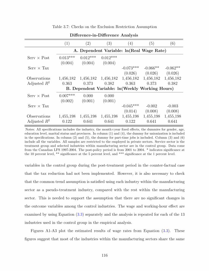


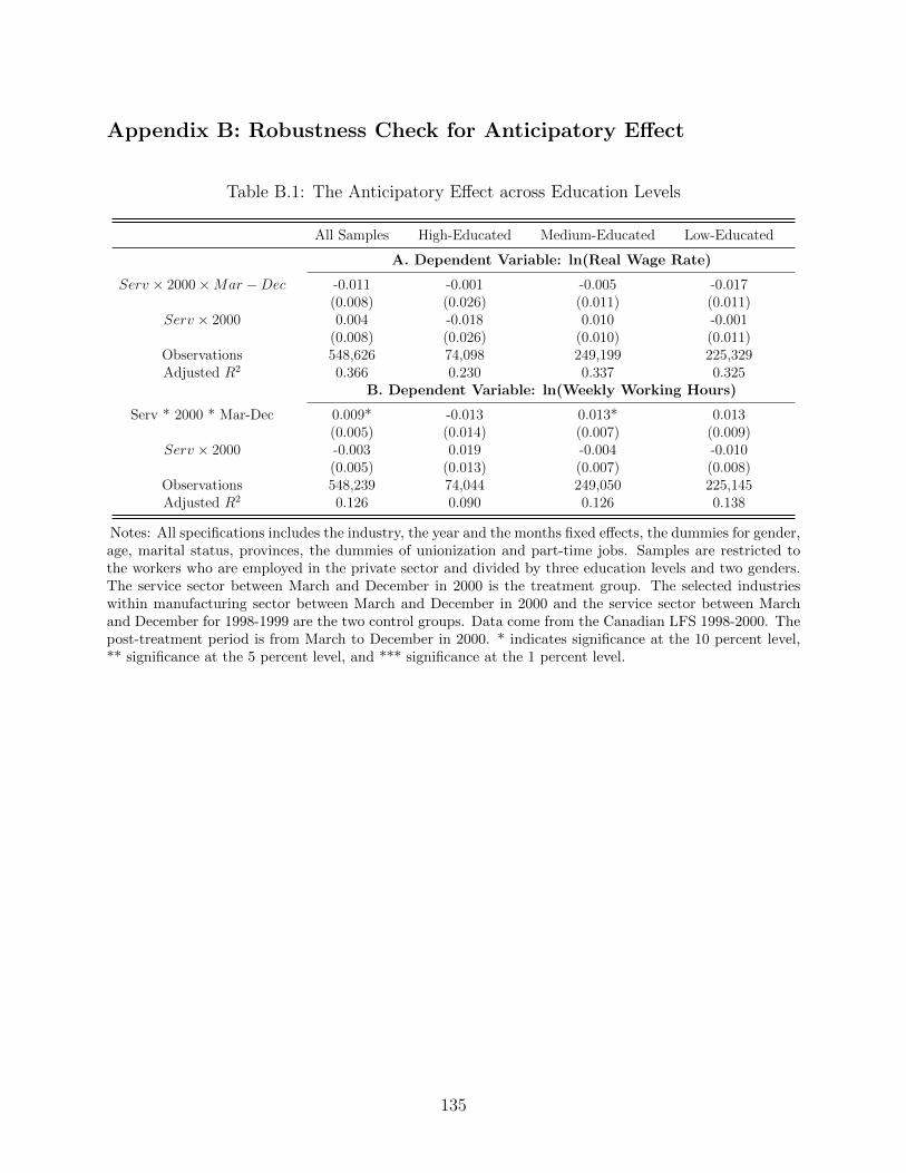


![[2005] Three Essays in International Finance](https://static.documents.pub/doc/80x56/577d34e81a28ab3a6b8f2476/2005-three-essays-in-international-finance.jpg)


