Three Essays on Income Growth, Poverty and Inequality Dissertation to obtain the Doctoral Degree at the Faculty of Economics and Business Studies Justus-Liebig-University Giessen Submitted by Hosnieh Mahoozi First Supervisor: Prof. Dr. Jürgen Meckl Second Supervisor: Prof. Dr. Dr. Armin Bohnet Giessen, July 2017
Transcript
Three Essays on Income Growth, Poverty and Inequality
Dissertation to obtain the Doctoral Degree
at the Faculty of Economics and Business Studies
Justus-Liebig-University Giessen
Submitted by
Hosnieh Mahoozi
First Supervisor: Prof. Dr. Jürgen Meckl
Second Supervisor: Prof. Dr. Dr. Armin Bohnet
Giessen, July 2017
I highly appreciate all who encouraged, trusted and supported,
who made it possible to complete this work.
i
Table of Contents
Introduction and Executive Summary 1
Chapter 1 Literature Review 6
1.1. The Discussion on Poverty Measurement with Emphasis on the Capability
Approach 7
1.2. Empirical Approaches to the Multidimensional Poverty Measurement 9
1.2.1. Selecting Dimensions 9
1.2.2. Methods to Measure Multidimensional Poverty 11
1.3. The Alkire-Foster Methodology 13
1.3.1. Rational for Using a Composite Index 14
1.3.2. Rational for Aggregation 15
1.3.3. Axioms (or Properties) of the Methodology 16
Chapter 2 Multiple Dimensions of Impoverishment in Iran 18
2.1. Introduction 20
2.2. Methodology of Measuring Poverty 23
2.2.1. One-Dimensional Poverty Measurement 24
2.2.2. Multidimensional Poverty Measurement 24
2.2.3. Data 26
2.3. Criteria for Selecting Dimensions 26
ii
2.4. Multidimensional Poverty versus One-Dimensional Monetary Poverty
Measurement 30
2.5. Conclusion 36
Chapter 3 Gender and Spatial Disparity of Multidimensional Poverty in Iran
38
3.1. Introduction 40
3.2. Methodology of Measuring Poverty 42
3.2.1. Criteria of Selecting Dimensions 42
3.2.2. Identification of the Poor 46
3.2.3. Measurement of Poverty 46
3.3. Multilevel Regression Models 47
3.3.1. Multilevel Logit Model 49
3.3.2. Multilevel Linear Model 50
3.4. Results of Measuring Poverty 51
3.5. Results of Regression Analyses 57
3.6. Concluding Remarks 64
3.7. Appendix: Robustness Analysis 66
iii
Chapter 4 Growth Elasticity of Poverty: with Application to the Iran Case Study
67
4.1. Introduction 69
4.2. Economic Methods for Estimating Growth Elasticity of Poverty 72
4.3. Growth Elasticity of Deprivation for Non-income Dimensions 74
4.4. Empirical Results 76
4.4.1. A Case Study of Iran 76
4.4.2. Growth Elasticity of Monetary Poverty 81
4.4.3. Growth Elasticity of Multidimensional Poverty 83
4.5. Concluding Remarks 87
Conclusion and Thoughts on Future Research 89
Complete List of References 93
iv
List of Figures
Figure 2.1. Multidimensional Poverty Headcount, H 32
In the paper of chapter 2, we stress the demands of Sen’s (1984) capabilities approach to assessment
of human well-being. We estimate both the values of frequency and breadth of multidimensional
poverty, and the traditional income poverty, compare the results of different measurements and
demonstrate the overlaps between the results of different methods. We investigate poverty in Iran
for the time-period 1999-2007, we distinguish three regions in Iran (Tehran, other urban areas and
rural areas), and we estimate the poverty values for three snapshots over the time-period. The study
works out significant differences in the poverty as well as the pace of poverty reduction in the three
regions. The comparison of changes in poverty over the time-period also shows which
measurement records faster progress or in which form of measurement economic growth has
greater impact on poverty reduction. We also elaborate on the contribution of each dimension in
the adjusted poverty headcount measure of each region, showing which dimensions contribute
more in making the poor people to fall in poverty that can be a useful property for policy-making.
Inequalities in the distribution of welfare among individuals and special groups are another issue
highlighted in this dissertation. In the second essay of this cumulative work, chapter 3, we tried to
Introduction and Executive Summary
4
highlight inequalities in the distribution of welfare among the population and show how special
groups are marginalized by their demographic and spatial circumstances. Measuring the
multidimensional poverty ratio and the adjusted headcount ratio do not reflect the effect of the
household’s characteristics or region’s features on incidence or intensity of poverty, besides they
do not distinct poverty variation between provinces and within provinces. Hence, after identifying
the poor by applying the Alkire-Foster method instead of using the counting approach, we develop
multilevel regression models with the premise that households nested within the provinces. The
multilevel regressions show how much the inequality in distribution of welfare relates to the
province level and how much relates to the differences in the level of households. Besides,
conducting a logit multilevel model we predict the probability of falling in poverty for a typical
household with certain circumstances and in each province in Iran. The results show that most of
the poverty incidence variation relates to within-province variation (94.5%), and only 5.5% of the
poverty incidence variation relates to between-province variation. The results also indicate a
remarkable disparity among the population in Iran in which female-headed households and rural
households are heavily disadvantaged compared to their peers of male-headed and urban
households. According to our results, the most disadvantaged households are female-headed rural
households in the poorest southeast provinces, while the most fortunate households are (married,
middle aged) male-headed urban households in Tehran, Bushehr and Mazandaran. The study
concludes that certain households are marginalized based on their demographic and spatial
circumstances.
The sensitivity of the frequency of poverty to economic growth is another central issue of the
poverty and inequality discourse. The discussion on this issue has been going on for about two
decades (Ravallion and Chen, 1997; Ravallion and Datt, 1998; Adams, 2000; Bhalla, 2002;
Bourguignon, 2003; Kraay, 2006; Bresson, 2009). However, the more tools at our disposal, the
more demand comes up for further constructive studies. In the third essay, chapter 4 of this
dissertation, we made our individual contribution by measuring the sensitivity of monetary and
non-monetary deprivations to income growth. In this paper, we estimate the income growth
elasticity of poverty and the income inequality elasticity of poverty using the Ravallion and Chen
(1997) regression model for a panel of 28 provinces of Iran from 1999 to 2009. We also for the
first time estimate the growth elasticity of multidimensional poverty (estimated using the Alkire-
Foster method). We find a low income growth elasticity of poverty, and strong and significant
income inequality elasticity of poverty. The results of our estimation of growth elasticity of non-
monetary deprivations and multidimensional poverty also indicate rather similar results. Hence,
inequality (both the initial level and its increase over time) has a negative effect on both monetary
Introduction and Executive Summary
5
and non-monetary poverty reduction. Furthermore, high income-inequality diminishes the positive
effect of income growth, especially for lower poverty lines. The results also indicate that the smaller
the monetary poverty threshold, the higher is the sensitivity of poverty for changes in mean income
and for changes in income inequality. The sensitivity of multidimensional poverty for changes in
mean income and the sensitivity of multidimensional poverty for changes in income inequality are
more than the sensitivities of monetary poverty (with upper threshold) and less than the sensitivities
of monetary poverty (the lower threshold).
Chapter 1 Literature Review
6
Chapter 1
Literature Review
Chapter 1 Literature Review
7
1.1. The Discussion on Poverty Measurement with Emphasis on the Capability
Approach
Measuring individual (or household) welfare is the basic input to all inequality and poverty analyses.
Although there is agreement in economics and other social sciences that measurement of individual
welfare is essential, no consensus exists for how to conceptualize welfare theoretically or how to
measure it empirically (Kuklys, 2005). In economics, there are three general arguments in terms of
conceptualizing and measuring welfare. The first is some notion of opulence. The second is to see
the living standard as some notion of utility, the third to see the standard of living as one type of
freedom (see Sen, 1985). The first approach goes back at least to Adam Smith and the modern
literature on real income indicators, and the indexing of commodity bundles is the inheritor of this
tradition of evaluating opulence. It is sometimes discussed as an approach with the utility approach
in disguise. However, as Sen argues, there is an important difference between the two approaches
even when the evaluation of real income is done in terms of an indifference map preference, since
what is being evaluated is not utility as such (in the form either of desirability or of satisfaction),
but the commodity basis of utility (Sen, 1985). The second argument is the dominant view that
conceptualizes welfare as utility, and measures it empirically by one-dimensional indicators such as
income or expenditure (Sen, 1973; Atkinson and Bourguignon, 2000). These two arguments, which
are supported by “welfarists”, however, are challenged by alternative views that conceptualize
welfare as standard of living, quality of life, or subjective well-being, and measure welfare by
multidimensional indictors (Sen, 1985, 1992; Kolm, 1977). That is known as capability approach.
The most common empirical welfare measure in economics is income. The advantage of using
one-dimensional measures is their simplicity and clarity, although they can never tell the whole
story (Goodman and Shepard, 2002). The income measure has been criticized for some sources of
measurement error. First, individuals often underreport their income. The second source of
measurement error is that, even if reported correctly, current income might not reflect
appropriately the long-run level of individual welfare. This is the case when the household has a
temporarily higher or lower income than usual during the period of reporting. Moreover, an income
measure of welfare neglects important issues such as welfare derived from home production, non-
market goods and services, and in-kind transfers (Kuklys, 2005). Employing expenditure data can
be a simple solution for this problem, under the assumptions that households report expenditure
more truthfully than income, and that they smooth their expenditures over time when making
consumption decisions, expenditure is a better proxy of long-run welfare levels than current
Chapter 1 Literature Review
8
income (Deaton, 1997). Nevertheless, some problems remain. With respect to measurement
errors, for instance, it cannot still fully reflect the long-run welfare situation of the households or
individuals, when income or expenditure increase or decrease temporarily.
Moreover, the well-being of a population and hence its poverty which is a manifestation of
insufficient well-being, depends on both monetary and non-monetary variables. It is certainly true
that with a higher income or consumption budget, a person may be able to improve the position
of some of his/her monetary and non-monetary attributes. Nevertheless, at the same time it may
be the case that markets for some non-monetary attributes (e.g. some public goods) do not exist.
It may also happen that markets are imperfect. Therefore, income as the sole indicator of well-
being is inappropriate and it should be supplemented by other attributes or variables (Bourguignon
and Chakravarty, 2003).
Sen challenges the welfare or utility approach, which concentrates on happiness, pleasure and desire
fulfillment. He indicates that neither opulence (income, commodity command) nor utility
(happiness, desire fulfillment) constitute or adequately represent human well-being and deprivation
(see Sen, 1985, p. 670). Hence, Sen advocates a multidimensional assessment of individual welfare
in the space of standard of living measures such as health, nutrition, education, or shelter. His
approach is known as the capability approach (Kuklys, 2005) which its roots basically going back
to Smith, Marx, and Mill, among others (see Sen, 1984), or back even to Aristotle’s theory of
“political distribution” and his analysis of Eudaimonia - “human flourishing” (Sen, 1993).
The capability approach is primarily and mainly a framework of thought, a mode of thinking about
normative issues, hence a paradigm – loosely defined – that can be used for a wide range of
evaluative purposes. The approach focuses on the information that we need in order to make
judgments about individual well-being, social policies, and so forth, and consequently rejects
alternative approaches those are considered normatively inadequate, like an evaluation based on
monetary terms (Robeyns, 2005).
In its most basic form the capability approach conceptualizes welfare as standard of living, and
measures it as function(ing)s (or dimensions). Function(ing)s are defined as the achieved states of
being and activities of an individual, e.g., being healthy, being well-sheltered, moving about freely,
or being well-nourished. Welfare measurement in the function(ing)s space takes into account the
presence of non-market goods and services in an economy, home production, and adjusts for non-
monetary constraints in decision making, because function(ing)s are outcome-based (as opposed
to resource-based) welfare measures. Capability is a derived notion and reflects the various
function(ing)s he or she can potentially achieve, and involves the person’s freedom to choose
Chapter 1 Literature Review
9
between different ways of living (Kuklys, 2005). A series of approaches to multidimensional
poverty have formed based on the capability approach.
1.2. Empirical Approaches to the Multidimensional Poverty Measurement
Sen's approach is theoretically attractive. However, to operationalize it empirically several issues
arise. First of all it is not at all clear which function(ing)s or dimensions should be selected for the
measurement of welfare. Additionally, it is not obvious how the dimensions should be measured.
The third issue is a missing natural aggregator to summarize different dimensions in a composite
standard of living measure, and finally measurement error problems.
In this section, at first we discuss about selecting dimensions, then we indicate the different
methods to measure multidimensional poverty.
1.2.1. Selecting Dimensions
In practical applications of the capability approach and related multidimensional approaches, it
seems that the methods for identifying capabilities or dimensions of poverty are surprisingly
straightforward. Although, as mentioned initially, the discussion of the basis of choice is rarely
explicit, it seems that most researchers draw implicitly on five selection methods, either alone or in
combination. The five selection methods are:
Existing Data or Convention – select dimensions (or capabilities) mostly because of convenience
or a convention that is taken to be authoritative, or because these are the only data available that
have the required characteristics.
Assumptions – to select dimensions based on implicit or explicit assumptions about what people
do value or should value. These are commonly the informed guesses of the researcher; they may
also draw on convention, social or psychological theory, philosophy, religion, and so on.
Public ‘Consensus’ – to select dimensions that relate to a list that has achieved a degree of legitimacy
due to public consensus. Examples of such lists at the international level are universal human rights,
the MDGs (Millennium Development Goals); these will vary at the national and local levels.
Ongoing Deliberative Participatory Processes – to select dimensions based on ongoing purposive
participatory exercises that periodically elicit the values and perspectives of stakeholders.
Empirical Evidence regarding people’s Values – to select dimensions on the basis of expert analyses
of people’s values based on empirical data on values, or data on consumer preferences and
Chapter 1 Literature Review
10
behaviors, or studies of which values are most conducive to mental health or social benefit (Alkire,
2008).
Robeyns (2003) has proposed that authors use four procedures when identifying the relevant
domains and capabilities. These are:
1. Explicit formulation: the list (of domains and/or capabilities) should be made explicit, discussed
and defended: why it is claimed to be something people value and have reason to value.
2. Methodological justification: The method that has generated the list should be clarified and
defended (and open to critique or modification), if this domain was chosen on the basis of a
participatory exercise, or through consultation of empirical studies of human values.
3. Two stage processes, Ideal-Feasible: If a set of domains aims at an empirical application or at
implementable policy proposals, then the list should be set in at least two stages. Each stage will
generate a list at a different level, ranging from the level of ideal theory to the lists, which are more
pragmatic. Distinguishing between the ideal and the second-best level is important, because these
second best constraints might change over time, for example as knowledge expands, empirical
research methods become more refined, or the reality of political or economic feasibility changes.
4. Exhaustion and non-reduction: the capabilities on the (ideal) list should include important
elements: no relevant dimension should be dismissed. For example, those capabilities related to the
non-market economy should also be included in economic assessments.
An example of multidimensional measure of wellbeing in terms of functioning achievements is the
Human Development Index suggested by UN Development Programme (UNDP) (Streeten, 1981).
It aggregates at the country level functioning achievements in terms of the attributes life
expectancy, real gross domestic product (GDP) per capita and educational attainment rate. Another
example suggested by Ravallion (1996) in a paper that four sets of indicators considered as
ingredients for a sensible approach to poverty measurement. These are real expenditure per single
adult on market goods, non-income indicators as access to non-market goods, indicators of
personal characteristics, which impose constraints on the ability of an individual, such as child
nutritional status, and indicators of personal characteristics, which impose constraints on the ability
of an individual, such as physical handicap. A very well-known example of multidimensional index
of wellbeing in terms of functioning achievements is the Multidimensional Poverty Index (MPI),
developed by the Oxford Poverty & Human Development Initiative (OPHI) with the UNDP. The
MPI includes three dimensions and ten indicators; Health (nutrition, child mortality), Education
Chapter 1 Literature Review
11
(years of schooling, school attendance), Living Standard (cooking fuel, sanitation, water, electricity,
floor, assets).
Regarding the aforementioned discussion there is not a fixed list of capabilities in the literature as
Sen (2004) mentioned “Pure theory cannot freeze a list of capabilities for all societies for all time
to come, irrespective of what the citizens come to understand and value. That would be not only
a denial of the reach of democracy, but also a misunderstanding of what pure theory can do.” (Sen,
2004, p. 78) Or “To insist on a fixed forever list of capabilities would deny the possibility of
progress in social understanding and also go against the productive role of public discussion, social
agitation, and open debates” (Sen, 2004, p. 80).
In sum, Sen argues that key capabilities must be selected, but argues consistently against the
specification of only one authoritative ‘canonical’ list of capabilities that is expected to apply at all
times and all places. Hence, as the relevant literature addressed, although generally there is an
agreement on some dimensions, in many cases the set of dimensions (and indicators) should be
designed according to the certain time and place.
1.2.2. Methods to Measure Multidimensional Poverty
After selecting the dimensions and the threshold of deprivation, it comes to the aggregation of
deprivation. There are some different methods in terms of aggregation process, namely counting,
scaling, fuzzy sets theory, factor and principal component analysis, which formed different
methodologies of measuring multidimensional poverty.
The “Counting” approach concentrates on counting the number of dimensions in which people
suffer deprivation (Atkinson, 2003). People have scores corresponding to the number of
dimensions on which they fall below some threshold specified in advance. An example that applied
this approach is the human poverty index based on three sub-indices, which was provided by
Anand and Sen (1997).
The method of scaling as employed by the UNDP (since 1990) in the calculation of the Human
Development Index (HDI) is a technique, which is mainly targeted at solving the unit of
measurement problem. Each of the variables indicating a dimension is projected linearly onto a 0-
1 interval. Then the problem of aggregating several dimensions to a composite welfare measure is
solved by combining the different dimensions with a weighted sum of indicators. The weights are
chosen in accordance to the analyst's values. In case of the HDI each of the dimensions, health,
education, and material wealth, receive the same weight of 1/3. This procedure assumes perfect
substitutability between the dimensions: an individual can trade off her welfare in terms of, say,
Chapter 1 Literature Review
12
health and education with an infinite elasticity of substitution. The difficulty of the method is
determining the maximum achievable level and ignoring a potential different anchoring of the
scales by each individual.
Fuzzy sets theory, as applied in the empirical capability literature, is an extension of the previously
described method of scaling. It was pioneered in this area by Chiappero (2000) and by Qizilbash
(2002). It extends the method of scaling in two respects. First, it introduces flexibility in projecting
the indicator variable onto a 0-1 interval by allowing for nonlinear projection functions, then by
allowing for different weighting schemes. The analysts do not choose the weights arbitrarily, but
they do based on the data.
Time Series Clustering developed as a method for measuring and aggregating dimensions, building
on contributions by McGee and Carlton (1970), Piccolo (1970), and Hobijn and Franses (2000),
Hirschberg et al. (2001). This method may be interpreted as a generalization of the exploratory
factor analysis (EFA). As with EFA, the aim is to explore the data to find clusters of function(ing)s
indicators which represent the same dimension; it extends EFA in the sense that it uses the
statistical information contained in the entire distribution, not only the covariance or correlation
matrices of the data. The focal point of their analysis is the identification of dimensions in the data
set that have statistically similar distributions. They do this by (i) applying ARIMA models1 to time
series of 15 separate indicators; (ii) estimating non-parametric kernel densities of the residuals of
these ARIMA models; and (iii) estimating the distance between the 15 densities with an entropy
measure. Subsequently, those indicators that have statistically similar distributions are combined to
a new variable representing a dimension. Hirschberg et al. (2001) used exclusively cardinal
indicators in their application that were standardized to have unit variance and zero mean. In this
way, the unit of measurement is not a problem. If ordinal indicators were used, they would have
to be given a cardinal interpretation. Although measurement errors are not treated explicitly, we
can interpret the combination of similar indicators as an implicit treatment of possible
measurement error.
There is a variety of methods for poverty measure in the multidimensional approach as well as in
the capability approach, like some we above mentioned. Researchers in this era adapt and adjust
some method, and sometimes they mix two or more methods or introduce a method according
1 An autoregressive integrated moving average (ARIMA) model is a generalization of an autoregressive moving average (ARMA) model. Both of these models are fitted to time series data either to better understand the data or to predict future points in the series (forecasting). ARIMA models are applied in some cases where data show evidence of non-stationarity, where an initial differencing step (corresponding to the "integrated" part of the model) can be applied to reduce the non-stationarity.
Chapter 1 Literature Review
13
their special cases. For instance, Alkire and Foster (2011b) in a well-known study use a ‘counting’
based method to identify the poor, and propose adjusted Foster–Greer–Thorbecke (FGT)1
measures that is decomposable with population-share weights as well as reflect the breadth, depth
and severity of multidimensional poverty, and which were introduced by Foster et al. (1984).
Alkire and Foster (2011b) introduce an approach to identify the poor that uses two forms of
cutoffs. The first is the dimension-specific deprivation cutoff, which identifies whether a person is
deprived with respect to that dimension. The second determines how widely deprived a person
must be in order to be considered poor. Their approach uses a counting methodology after
identifying the poor over the ‘dual cutoff’ procedure. This ‘dual cutoff’ identification system gives
clear priority to those suffering multiple deprivations and works well in situations with many
dimensions. The overall methodology satisfies a range of useful properties. A key property for
policy is its decomposability, which allows the index to be broken down by population subgroups
(such as region or ethnicity) to show the characteristics of multidimensional poverty for each group.
Furthermore, it can be unpacked to reveal the dimensional deprivations contributing most to
poverty for any given group (this property is not available to the standard headcount ratio and is
particularly useful for policy). It embodies Sen’s (1993) view of poverty as capability deprivation
and is motivated by Atkinson's (2003) discussion of counting methods for measuring deprivations.
To sum up: there are several methods in this field, which can be adapted, adjusted or mixed.
However, an important consideration in developing a new methodology for measuring poverty is
that it can be employed using real data to obtain meaningful results.
1.3. Alkire-Foster Methodology
In this work, we mainly adapt the Alkire-Foster method for its range of advantages, some of which
have been listed above. Since in the second chapter of this dissertation (first paper) we review the
methodology thoroughly, we do not intend to explain the methodology in this section. However,
conducting the Alkire-Foster method may rise several questions, which we usually face by
presenting the results extracting by the Alkire-Foster method. Hence, in the following subsections
we try to answer some of these most common questions. Then we sum up this section by
numerating the properties (axioms) of the Alkire-Foster methodology.
1 The Foster–Greer–Thorbecke indices are a family of poverty metrics. The most commonly used index from the family, FGT2, puts higher weight on the poverty of the poorest individuals, making it a combined measure of poverty and income inequality and a popular choice within development economics. The indices were introduced in a 1984 paper by economists Erik Thorbecke, Joel Greer, and James Foster.
Chapter 1 Literature Review
14
One of the common challenging questions are: Why do we use a composite index? Composite
indices do compress information on individual trends, so we may lose some information. Why do
we not use indices together in a dashboard approach (making a matrix of people’s achievement in
different dimension without aggregation)? Why do we aggregate if we break the index down again?
1.3.1. The Reasons Behind Using a Composite Index
In order to answer the first two questions and clear the motives behind using a composite
multidimensional index (Alkire-Foster method), we propose the four following reasons.
First, designing an index should serve a specific purpose. A poverty measure is designed to help
realizing who is poor actually, how many poor people are there, how poor are they, and how overall
poverty has changed. They provide information that gives us some principal hints to design better
poverty alleviation policies. A dashboard approach identifies who is deprived in each dimension,
for example who is deprived in education, or deprived in health dimension. However, it does not
identify who is actually poor. For example, consider a well-educated, wealthy person who suffers a
chronic disease and identifies deprived in health dimension, while he is not actually poor. The same
problem emerges with the one-dimensional method as well. As Alkire and Foster declare “when
poor people describe their situation, as has been found repeatedly in participatory discussions, part
of their description often narrates the multiplicity of disadvantages that batter their lives at once.
Malnutrition is coupled with a lack of work, water has to be fetched from an area with regular
violence, or there are poor services and low incomes. In such cases, part of the experience and
problem of poverty itself is that several deprivations are coupled – experienced together.” (Alkire,
and Foster 2011a, p. 13).
Hence, we need a method based on a concept of poverty as multiple deprivations those are
simultaneously experienced. The fact is, only the aggregate index fully bears the concept of poverty
and gives a coherent summary statistical convey of how overall poverty has changed. A dashboard
of marginal measures can indeed be useful for some purposes. The advantages of a dashboard
approach are that it is transparent and every trend is monitored. However, it is not particularly well
suited to answer aforementioned questions.
The second, practical problem with a dashboard approach is its heterogeneity. At some point, we
need to use data reduction techniques to reduce the number of indicators. Hence, the dashboard’s
appeal has an inverse proportion to the number of poverty indicators. As the Stigliz, Sen, Fitoussi
report puts it: “Dashboards… suffer because of their heterogeneity, at least in the case of very large
and eclectic ones, and most lack indications about … hierarchies amongst the indicators used.
Further, as communications instruments, one frequent criticism is that they lack what has made
Chapter 1 Literature Review
15
GDP a success: the powerful attraction of a single headline figure allowing single comparisons of
socioeconomic performance …” (Stiglitz et al 2009, p. 63). A single indicator that conveys the
concept of poverty as the joint distribution of deprivations particularly is useful for the politicians
when they report the progress of pro-poor policies or comparing socioeconomic performance.
Third, dashboard approaches also toss out information. They are insensitive to the joint
distribution of deprivations. That means they are useless for measuring extreme forms of poverty
and indigence. A dashboard approach reflects population deprivations within dimensions, but does
not look across dimensions for the same person. For example, consider the two following matrices,
when they show deprivations (denoted with 1) in four dimensions (four columns) for four persons
(four rows)
𝑔0 = [
0 00 0
0 00 0
0 01 1
0 01 1
]… [
0004
], and 𝑔0 = [
1 00 1
0 00 0
0 00 0
1 00 1
]… [
1111
]
In a dashboard approach, both matrices have identical marginal headcount ratios for each
dimension (25%). However, they indicate two different situations; in the first matrix, one person
is deprived in all dimensions while the second matrix demonstrated each of the four persons are
deprived in one dimension. The disability of dashboard approach to distinguish these situations is
politically important, particularly to target multiply deprived families first.
Forth, using the Alkire-foster method does not mean we deny usefulness of the other methods.
However, we try to analyze additional indicators as Alkire and Foster state “our measure aims to
complement income poverty measure” (Alkire, and Foster, 2011 a). We believe AF method carries
some additional information. The method, using the FGT (Foster- Greer- Thorbeck) technology
in a multidimensional approach, creates the opportunity to measure breadth and depth of poverty,
which add the properties of the measurement.
1.3.2. The Reasons of Aggregating
The adjusted poverty headcount M0 is an index, which benefits the decomposability axiom. After
Estimating M0 we break it down by population subgroups and dimensions to understand the
relationship between dimensional policies and overall poverty impacts. It may seem we aggregate
the indices and break it down to get the same indices. However, that is just a misunderstanding.
M0 is resulted of an identification process, while equals the aggregate deprivations experienced by
the poor as a share of the maximum possible range of deprivations across society. As Alkire and
Santos express the sub-indices are not independent, but instead rely on the joint distribution
Chapter 1 Literature Review
16
through the identification step (Alkire and Santos, 2010). Therefore, sub-indices after breaking
down M0 are showing the share of each dimension in making poor the population of each group.
We believe that is a virtue of this methodology, which helps for policy targeting.
1.3.3. Axioms (or Properties) of the Methodology
The dual cutoff method enjoys a range of properties, for any given weighing vector and cutoffs,
the methodology Mkα=(ρk, Mα) satisfies: decomposability, replication invariance, symmetry,
poverty and deprivation focus, weak and dimensional monotonicity, nontriviality, normalization,
and weak rearrangement for α≥0; monotonicity for α>0; and weak transfer for α≥1 (Alkire and
Foster, 2011b). The axioms that the methodology satisfies are as below:
Decomposability: a key property for AF method is decomposability, which requires overall poverty
to be the weighted average of subgroup poverty levels, where weights are subgroup population
shares. This characteristic allows the index to be broken down by population subgroups to show
the specifications of multidimensional poverty for each group. This axiom is an extremely useful
property for generating profiles of poverty and targeting high poverty populations.
Replication invariance: this property ensures that poverty is evaluated relative to the population
size, and allows for meaningful comparisons across different sized populations.
Symmetry: according to symmetry, if two or more persons switch achievements, measured poverty
is unaffected. This ensures that the measurement does not place greater emphasis on any person
or group of persons.
Focus (poverty focus and deprivation focus): that means that the poverty measure is independent
of the data of the non-poor. In a multidimensional setting, a non-poor person could be deprived
in several dimensions while a poor person might not be deprived in all dimensions. There are two
forms of multidimensional focus axioms, one concerning the poor, and the other pertaining to
deprived dimensions. This is a basic requirement that ensures that the measurement measures
poverty in a way that is consistent with the identification method (Alkire and Foster, 2011b). That
is that the property is absent in a number of other methodologies. For example, the methodologies
with non-composite indices may satisfy the deprivation focus, but they do not satisfy the poverty
focus.
Monotonicity (weak and dimensional monotonicity): it means if poor become poorer, the measure
has the ability to reflect it. Weak monotonicity ensures that poverty does not increase when there
is an unambiguous improvement in achievements. Monotonicity additionally requires poverty to
fall if the improvement occurs in a deprived dimension of a poor person. Dimensional
Chapter 1 Literature Review
17
monotonicity specifies that poverty should fall when the improvement removes the deprivation
entirely; it is clearly implied by monotonicity (Alkire and Foster, 2011b).
Non-triviality: it ensures the indicator achieves a unique maximum value (in which all achievements
are 0 and hence each person is maximally deprived) and a distinct minimum value (where all
achievements reach or exceed the respective deprivation cutoffs and hence no one is deprived).
Normalization: that means that the methodology regards changes in inequality among the poor.
This axiom goes further than weak monotonicity and reflects the depth of poverty, which is
satisfied in Alkire-Foster Methodology by index M11.
Transfer: This axiom ensures that an averaging of achievements among the poor generates a
poverty level that is less than or equal to the original poverty level. This axiom alongside the
Rearrangement regards changes in inequality among the poor.
Rearrangement: rearrangement among the poor reallocates the achievements of the tow poor
persons but leaves the achievements of
In this chapter, we mainly discussed the literature on multidimensional poverty measurement, and
particularly on the capability approach as the theory basis of multidimensional poverty
measurement, regarding the particular role of multidimensional poverty in all three essays of this
cumulative work. In addition to, we tried to introduce and briefly discuss the characteristics and
axioms of the Alkire-Foster method, as the main technique for measuring the multidimensional
poverty in this dissertation.
1 The adjusted poverty gap M1 is the product of the adjusted headcount ratio M0 and the average poverty gap G. In the other words, it is the sum of the normalised gaps of the poor divided by the highest possible sum of normalised gaps. The poverty measure M1 ranges in value from 0 to 1.
Chapter 2 Multiple Dimension of Impoverishment in Iran
18
Chapter 2
Multiple Dimensions of Impoverishment in Iran
Chapter 2 Multiple Dimension of Impoverishment in Iran
19
ABSTRACT
Concerning the demands of Sen’s (1987) Capabilities Approach to assessment of human well-
being, the paper estimates the values of frequency and breadth of multidimensional poverty in Iran,
while compares those results with the results of traditional income poverty measurement. The
paper detects poverty over the period 1999-2007, whilst it distinguishes specific regions as Tehran,
other urban areas, and rural areas. The study reveals that over the period, with relatively high rate
of GDP, the pace of income poverty reduction was much faster than the multidimensional poverty
alleviation. The study also detects the pace of poverty reduction in rural areas is much slower than
urban areas and the capital city, Tehran, which increases the inequality between rural and urban
areas over the time. Furthermore, the paper detects the specific socio-economic group’s
deprivation type, which is invaluable information for an effective policy targeting.
Chapter 2 Multiple Dimension of Impoverishment in Iran
20
2.1. Introduction
Poverty is a major problem for many less developed countries and continues serious challenges for
the governments of the involved states. Not surprisingly, poverty reduction in general as well as
specific approaches to overcome that problem played a significant role in the political debates
during the recent decades in Iran. The Islamic revolution claimed that the social base of Iran is
primarily formed by the poor. The Iranian government implemented different policies over the last
three decades, ranging from extensive nationalization of central industries and heavy subsidization
of a wide range of basic goods in the first decade (1980-90) to the more market-oriented reforms
launched in the second and third decades. Although all these policies were explicitly designed to
reduce poverty they seem to have been only partially successful. As a result, poverty is still the
central issue of political debates in Iran.
Existing studies providing reliable measures about the size and the development of poverty in Iran
are relatively sparse and deliver quite mixed results. Assadzadeh and Paul (2004) disentangle the
effects of macroeconomic growth and redistributive policy measures on poverty for the time span
of 1983 to 1993. In order to measure poverty, they apply the Foster-Greer-Thorbacke (FGT)
method (cf. Foster et al., 1984) that specifies a threshold value of monetary income to identify the
poor in the society4. To substantiate that monetary poverty line, the authors consider the cost of a
balanced diet propagated by the Iranian Institute of Nutrition Science and Food Industry satisfying
normal nutritional requirement at 1989 prices and augment that pure food-cost component by
adding a non-food component calculated from the ratio of average non-food expenditure to
average food expenditure in the country. Their results indicate that the deterioration of income
inequality contributed to the worsening of poverty, while the economic growth contributed to a
reduction in poverty in rural areas and an increase in urban areas. They find that poverty declined
slightly in the rural sector while increasing significantly in the urban sector over that time period.
Salehi-Isfahani (2009) examined the trends in poverty and inequality for the time-period 1984-2005
and compares them to the published survey results of the pre-revolution years (1970-1979). He
takes per capita expenditure as a measure for individual welfare and uses the Assadzadeh and Paul
(2004) poverty line to identify the poor for the time-period 1984-2005. However, since the data are
not available for 1970s, he relied on the published survey results for the pre-revolution years. His
study reveals that poverty declined substantially over the considered time span while inequality
almost remained stable. More recently, Maasoumi and Mahmoudi (2013) also decompose the
change in poverty into a growth and an inequality component. They set monetary poverty lines for
4 The FGT method can specify frequency, breadth and depth of poverty. In the other word, FGT method besides of demonstrating poverty is able to show the income distribution among poor.
Chapter 2 Multiple Dimension of Impoverishment in Iran
21
each year (2000, 2004 and 2009) based on the adjusted consumption expenditure, while they
applied FGT method for measuring poverty. They found a reduction in poverty both in urban and
rural areas primarily driven by economic growth for their evaluation period of 2000 to 2009.
On the background of these rather positive results on the extent of poverty reduction it rather
comes as a surprise that poverty is a central issue in actual debates. In our view the positive results
derived by the studies cited above are misleading since they fail to perfectly measure the actual
extent of poverty by concentrating on a one-dimensional monetary concept such as real income or
real consumption expenditures. Basically poor people typically go beyond income in evaluating
their experience of poverty, and refer to a set of variables containing malnutrition, lack of safe
water, health issues, and children out of school … in assessing their situation. As a result, a single
indicator such as income or consumption is not able to capture the multiple aspects that contribute
to poverty in a comprehensive way, and the pursued strategy of narrowing down the diagnosis of
poverty to a pure monetary measurement falls short of covering the phenomenon adequately. The
current study substantiates this critique by confronting results of the traditional one-dimensional
approach with those derived from a multidimensional approach. Specifically with respect to the
pace of poverty reduction our multidimensional approach clearly qualifies the results from the one-
dimensional approach and thus gives good reason for the high awareness of poverty in the political
agenda.
The theoretical reasons that support measuring welfare as a multidimensional phenomenon were
brought forward by Kolm (1977) and Sen (1984). Both authors criticized the use of income as the
sole measure of poverty on the grounds of individuals’ self-assessment of being poor. Building on
Kolm’s and Sen’s contributions, two strands of literature on multidimensional welfare
measurement have emerged: the first in the theoretical literature on inequality and poverty
(Atkinson and Bourguignon, 1982; Maasoumi, 1999; Bourguignon and Chakravarty, 2003); and the
second in the realm of applied welfare and development economics (e.g., Klasen, 2000; Qizilbash,
2002; Kuklys, 2005). The discussion about multidimensionality of poverty has also been reflected
in the United Nations Millennium Declaration and Millennium Development Goals [MDGs] (UN,
2000) which have highlighted multiple dimensions of poverty since 2000, as well as in the Human
Development Reports by UNDP since 2010 (United Nations Development, 2010).
In the current paper, we calculate the changes in poverty over the time period 1999-2007 using
both a traditional one-dimensional poverty measurement and a multi-dimensional approach. We
find that the traditional monetary measurement delivers faster reduction in poverty than the
multidimensional measurement. We also identify significant differences in poverty values and the
Chapter 2 Multiple Dimension of Impoverishment in Iran
22
pace of poverty reduction between three regions that we distinguish: rural areas, urban areas, and
Tehran. Although Iran experienced relatively high growth rates of its real gross domestic product
(GDP) and subsequent poverty reduction from 1999 to 2007, the uneven pace of poverty reduction
in different areas contributed to an increase in the rural-urban gap. Since the rural-urban gap is an
important source of overall inequality and affects the improvement of welfare negatively, this result
can be interpreted as another reason why poverty is still a central issue in political debates in Iran.
Before developing our multidimensional framework of poverty measurement, we shortly
recapitulate the political evolution of Iran over the last decades. In 1979, the Islamic revolution
happened, where the former Monarchy Regime was replaced by the Islamic Republic Regime. The
political changes quickly triggered economic changes including a large-scale nationalization, putting
about 80% of total industrial production under the control of the government. Soon after the
revolution, Iran’s economy was heavily hit by the prolonged, eight-year Iran-Iraq War (1980-1988).
During the 1980s, the oil production plummeted as the consequence of that war and the associated
lack of investment, and consequently national income declined dramatically. During the war,
however, the Islamic republic government tried to protect especially the poor against wartime
inflation by rationing of basic goods and extensive price controls that intensified the government’s
role in the economy.
After the end of the war in 1989, production of oil recovered and the Iranian government started
economic reforms by five-year plans that gradually dismantled rationing and price controls,
increased the role of markets in distribution of goods and services, and began the move away from
state ownership of productive assets. The reform plans gave priority to growth-based policies
creating opportunities for the poor through rising income. In the first five-year plan the average
growth of GDP was high, about 7.4% annually, but mainly the result of filling the already existent
free capacities of the economy after the war. In the second five-year plan, however, the average
growth of GDP decreased to 3.2% annually, primarily because of the decline of oil prices on the
world market (Maroofkhani, 2009).
With the oil price increasing again in 1999, Iran’s economy experienced a rise in growth of real
GDP during almost a decade until 2007. Part of this growth has been due to increases in oil
production and in oil prices on the world market improving Iran’s terms of trade. Between 1999
and 2006, oil production increased by 13.3 percent, a little more than one-fourth of the increase in
GDP. Export prices for Iranian oil have risen much more rapidly, from an average of $16.81 a
barrel in 1999 to $59.82 in 2006. As a result, revenues from oil exports more than tripled between
1999 and 2006. According to the IMF report (IMF, 2007), between 1999 and 2006 the average rate
Chapter 2 Multiple Dimension of Impoverishment in Iran
23
of GDP growth was 5.8 percent per year. This economic growth was attributed largely to rising
international oil prices, but it was also associated with an agricultural recovery as well as with
expansionary monetary and fiscal policy reforms (IMF, 2007). After 2007, however, by the crippling
international economic sanctions against Iran, GDP growth became volatile again. Table1
summarizes the GDP growth rate of the economy of Iran during 1992-2012.
Table 2.1. Real GDP Growth of Iran 1992-2012
year 1992 1993 1994 1995 1996 1997 1998
GDP growth rate -1.9 5.6 -3.7 2.7 -1.4 -5.4 -2.8
year 1999 2000 2001 2002 2003 2004 2005
GDP growth rate 1.9 5.1 3.7 7.5 7.1 5.1 4.6
year 2006 2007 2008 2009 2010 2011 2012
GDP growth rate 5.9 7.8 -3.7 -8 4.5 4.5 -5.7
Source: Central Bank of Iran, 2013
We investigate poverty in Iran for the time-period of 1999-2007, because we intend to study
poverty over a time period when Iran’s economy experienced a steadily increasing trend of rate of
real GDP growth on the one hand, and since we have access to sufficient information for
measuring multidimensional poverty over this time-period on the other hand. This study is an
attempt to give a new image of poverty in Iran by measuring multidimensional poverty over 8-
years of growing economy in rural and urban Iran, and comparing the trend of multidimensional
poverty changes to the trend of income poverty changes. Indeed, we try to highlight the importance
of poverty measurement for targeting the poverty reduction policies.
The structure of the paper is as follows. Section 2 introduces the methodology of measuring
multidimensional poverty, and section 3 gives an overview of selecting dimensions of our poverty
indicator. The results from our empirical analysis are presented in section 4. Section 5 offers some
concluding remarks.
2.2. Methodology of Measuring Poverty
We develop a measure of multidimensional poverty and compare it with the one-dimensional
income poverty measurement. In order to measure income poverty, we follow the appropriate
literature and apply the Foster-Greer-Thorbecke (FGT) methodology that also measures how
income is distributed below the poverty line and incorporates inequality aspects (breadth of
poverty). In order to measure multidimensional poverty, we use the Alkire-Foster method (2011b).
This is a well-known method in multidimensional poverty measurement, with the virtues of being
intuitive and flexible, as it can be adapted to many contexts. We discuss the two approaches in the
following.
Chapter 2 Multiple Dimension of Impoverishment in Iran
24
2.2.1. One-dimensional Poverty Measurement
In order to measure the traditional one-dimensional income poverty we apply FGT method (Foster
et al., 1984). The FGT approach first defines a poverty line z and derives gi as the relative deviation
of individual i’s income yi from that threshold: gi ≡(z-yi)/z. We then obtain giα as a measure of
individual poverty with α≥0 as a parameter that measures poverty aversion. Aggregating over
individuals we get a poverty index Pα according to
𝑃∝ =1
𝑛∑ (
𝑧 − 𝑦𝑖𝑧
)∝𝑞
𝑖=1
where n denotes the total population, and q is the number of poor individuals. Obviously, the case
α=0 yields a distribution of individual poverty levels in which each poor person has poverty level
equal to unity; the average across the entire population then is simply the headcount ratio P0. The
case α=1 uses the normalized gap gi as a poor person’s poverty level, thereby differentiating among
the poor, the average becomes the poverty gap measure P1. The case α=2 squares the normalized
gap and thus weights the gap by the gaps, this yields the squared gap measure P2. As α tends to
identify, the condition of the poorest poor is all that matters (Foster et al., 1984). The parameter α
has an interpretation as an indicator of “poverty aversion” in that a person whose normalized gap
is twice as large has 2α times the level of individual poverty. Alternatively, α is the elasticity of
individual poverty with respect to the normalized gap, so that a 1% increase in the gap of a poor
person leads to α% increase in the individual’s poverty level. The parametric class of measures gave
analysts and policymakers an instrument to evaluate poverty under different magnifying glasses
with varying sensitivity to distributional issues (Foster et al., 2010).
We use households as the units of measurement in this study, since our data gives the income of
families not of individuals. As income poverty line, we use two worldwide income deprivation
threshold values of 1,25 $ and 2 $ per day, and apply both of them respectively.
2.2.2. Multidimensional Poverty Measurement
We apply the Alkire-Foster method as the multidimensional poverty measurement. That method
encompasses two parts: the process of identifying poor and the aggregation process for measuring
poverty. The process of identifying poor involves of two cutoffs: the deprivation cutoff and the
poverty cutoff. The method in the first stage defines deprivation cutoffs zi for j different
dimensions of deprivation. A person i with an individual achievement of yij in dimension j is then
characterized as deprived if yij<zj. Individual i can then be characterized by its total number
deprivations ci diagnosed by that procedure. At the second stage, we identify some individual as
Chapter 2 Multiple Dimension of Impoverishment in Iran
25
poor if its total number of diagnosed deprivations ci exceeds some threshold value k. Thus we have
ci>k for the poor, and ci<k for the non-poor.
In order to implement the aggregation process for measuring poverty, we make use of a set of
definitions (cf. Alkire and Foster, 2011b). However, first we present a progression of matrices for
transition between the identification step and the aggregation step. The achievement matrix y
contains the single achievements yij of n persons in d dimensions. We then obtain the deprivation
matrix gij0 by replacing each element of y that is below its respective deprivation cutoff zj by 1, and
each entry that is not below its deprivation cutoff by zero. Therefore, the deprivation matrix
censors the value of non-deprived items, i.e. it focuses only on the deprived items. The gij0 matrix
provides a snapshot of frequency and breadth of deprivation among the population. Obviously,
there is no deprivation at all if the gij0 matrix contains only zeros. We observe a concentration of
deprivation on any of dimensions, if columns of that matrix contain less zeros (frequency of
deprivation). On the other hand, we have a concentration of deprivation on specific persons, if
rows of that matrix contain rather any zeros (breadth of poverty).
[
𝑦11 … 𝑦1𝑑⋮ ⋮ ⋮𝑦𝑛1 … 𝑦𝑛𝑑
]⏟
𝑌
→ 𝑀𝑖𝑛{0, 1 × 𝑤𝑖 𝑖𝑓 𝑦𝑖𝑗 < 𝑧𝑗}⏟ 𝑔𝑖𝑗0
→ 𝑀𝑖𝑛 {0, (𝑦𝑖𝑗 − 𝑧𝑗
𝑧𝑗)𝑤𝑖 𝑖𝑓𝑦𝑖𝑗 < 𝑧𝑗 }
⏟ 𝑔𝑖𝑗1
The normalized gap matrix gij1 replaces each deprived item in Y with the respective normalized gap
(i.e. the difference between the deprivation cutoff and the person’s achievement divided by the
deprivation cutoff) multiplied by the deprivation weight, wi. And it replaces each item that is not
below its deprivation cutoff with zero. The normalized gap is only valid for achievements, which
are cardinally measured. The gij1 matrix represents a snapshot of the depth of deprivation of each
poor person in each deprived dimension, while weighted by its relative importance.
In aggregation process, the AF method uses the so called headcount ratio H to measure frequency
of poverty. That variable is defined as the ratio of the number of the poor persons, which are
estimated by the dual cutoff method, q, and the number of persons of the complete population, n.
The measure H has the virtue of being easy both to compute and to understand. But the headcount
ration H is a purely static concept and does not reflect changes in deprivation over time.
Specifically, H does not reflect that some poor persons become deprived in a new dimension, or
that a person initially deprived in some dimension now passes that threshold. In addition to that,
H cannot be broken down and cannot show the contribution of each dimension to poverty.
Chapter 2 Multiple Dimension of Impoverishment in Iran
26
In order to overcome those deficits of the headcount ratio, the AF method introduces the adjusted
headcount ratio M0 that reflects the concerns mentioned above. M0 is obtained by multiplying the
headcount ratio by H by the average deprivation share across the poor given by A=|ci(k)|/(qd).
M0 is sensitive both to the frequency and the breadth of multidimensional poverty. M0 also is
defined as the mean of the censored deprivation matrix;
M0= HA = µ(gij0(k))
If a poor person becomes deprived in a new dimension, M0 reflects that change. Furthermore, M0
can be broken down to show how much each dimension contributes to poverty. M0 has also the
virtue of using pure ordinal data, which appear frequently in multidimensional approaches based
on capabilities.
2.2.3. Data
The data used in this study are taken from the Household Expenditure and Income Surveys (HEIS)
conducted annually by the statistical center of Iran (SCI). These surveys are nationally
representative household surveys. They consist of separate rural and urban surveys and are
stratified at the provincial level. The number of households e surveyed in each province is
determined based on the province population and variance of the variables in the province. The
number of Primary Sampling Units (PSU) in each province is determined by dividing the sample
size for the province by 5. PSUs correspond to census tracts that are chosen randomly, and from
each of which five households are randomly selected. Sample sizes vary from 5,759 households in
1986 to 31,283 in 2007.
The survey includes the basic demographic and economic characteristics of the households
including self-reported income and expenditures collected for some 600 items (expenditure
includes the self-produced and self-consumed items by the households). Similar to most household
surveys, expenditures are based on a 30- or 365-days recall period, depending on the frequency of
purchase. The recall period for food, fuel, and clothing, for example, is for the last 30 days, while
the recall period for expenditures on durables, travel, school tuition, etc., is annual.
2.3. Criteria for Selecting Dimensions
Applying our multidimensional poverty measurement based on the capability approach brings
forward the challenge of selecting dimensions. It is important to select dimensions that are
convincingly meaningful in the poverty discourse. However, there is not a well-established list of
dimensions or capabilities in the literature, nor there is a process to develop such a fixed list meeting
Sen’s pretentions: “Pure theory cannot freeze a list of capabilities for all societies for all time to
Chapter 2 Multiple Dimension of Impoverishment in Iran
27
come, irrespective of what the citizens come to understand and value. That would be not only a
denial of the reach of democracy, but also a misunderstanding of what pure theory can do.” (Sen,
2004, p. 78) Or “To insist on a fixed forever list of capabilities would deny the possibility of
progress in social understanding and also go against the productive role of public discussion, social
agitation, and open debates” (Sen, 2004, p. 80). Indeed, Sen argues that key capabilities must be
selected, but argues consistently against the specification of only one authoritative standard list of
capabilities with the expectation of applying it at all times and places.
There are different lists of dimensions in the literature. Although the discussion of the basis of
choice is rarely explicit, it seems, as Alkire (2008) argues, that most researchers draw implicitly on
either one or more of the following five selection procedures: 1. Use existing data; 2. Make
assumptions – perhaps based on a theory; 3. Draw on an approved existing list of dimensions; 4.
Use an ongoing deliberative participatory process; and 5. Propose dimensions based on empirical
studies of people’s values and/or behaviors.
An example of multidimensional index of wellbeing in terms of functioning achievements is the
Multidimensional Poverty Index (MPI), developed by the Oxford Poverty & Human Development
Initiative (OPHI) with the UN Development Programme (UNDP) for inclusion in UNDP’s
flagship Human Development Report in 2010. The MPI includes ten indicators in three
dimensions; Health (nutrition, child mortality), Education (years of schooling, school attendance),
Living Standard (cooking fuel, sanitation, water, electricity, floor, assets).
For this study we tried to adopt the MPI list of dimensions and adapt it according to our available
data. Since our data does not contain the health information, we tried to find proxies. Eventually,
due to the availability of reliable data, in the present study we draw on the following three variables:
(1) nutrition, (2) education, (3) living standard. We choose identical weights for all three
dimensions.
Nutrition: Regarding the available data we considered two indicators as the proxies for the
nutrition: percentage of expenditures on food, and expenditure of daily minimum calorie intake for
each individual. The poorest households in the world spend more than 75 percent of their income
on food, while households in the richest countries such as the United States and Canada - on
average spend less than 15 percent of their expenditures on food (Smith and Subandoro, 2007).
Since the households who spend more than 75 percent of their expenditures on food are presumed
very vulnerable to food insecurity, we use that threshold value for the indicator of the percentage
of expenditures on food.
Chapter 2 Multiple Dimension of Impoverishment in Iran
28
Expenditure of the minimum of daily required calories is another indicator of dimension of
nutrition. For determining the threshold for this indicator we use the estimated nutrition
deprivation threshold by Iran Statistical Research Center (Kashi et al. 2003; Bagheri et al. 2005;
Haidari et al 2015). In these studies, the minimum daily-required calories for each individual are
taken from nutrition experts’ opinion. Then the minimum essential amount of (different types of)
food and the value of minimum required food (based on the poorest percentile food habitation)
for rural and urban household in Iran were estimated.
Education: The literacy situation can be considered as an index that indicates extreme education
deprivation. This dimension consists of two indicators: household head literacy situation and
school attendance of 6 to 16 years old children. The household head literacy situation is not only
important because data about it are available, but also because of a number of other reasons: The
head of the household has a very important role in the Iranian culture. She or he typically is the
person that not only earns the major part of household income, but that also decides about how
income is spent. Moreover, the head of the household also decides about the cultural issues and
social issues of the household. Therefore, the household’s welfare may be affected significantly, if
the head of the household is completely illiterate or if he or she cannot read, write or count.
School attendance of school-aged children is another indicator of this dimension. If in a household
there is a child between six to 16 years old that is not attending school, the household is regarded
as deprived in the school attendance indicator.
Living standard: We measure the standard of living by five indicators: accessing electricity and safe
water (piped water), enough living space for each individual, fuel for cooking and asset ownership.
Access to electricity and to safe water, are the primary prerequisite of living standards in most
references in the literature (e.g. in the MPI index mentioned above). Another dimension of living
standard considered here is sufficient living space for each individual. A low value of living space
per person is a sign of overcrowding. Overcrowded housing may have a negative impact on physical
and mental health, relations with others as well as children’s development. The indicator includes
all living space, along with bathrooms, internal corridors and closets. Covered semi-private spaces
such as corridors, inner courtyard or verandas should be included in the calculation, if used for
cooking, eating, sleeping, or other domestic activities. The living space per person is defined as the
median floor area (in square meter) of a housing unit divided by the average household size. This
indicator measures the adequacy of living space in dwelling. Living space per person does not by
itself give a complete picture of living conditions. Cultural values affect sensitivity to crowding as
well. According to UNCHS (1996), however, this indicator is more precise and policy sensitive
Chapter 2 Multiple Dimension of Impoverishment in Iran
29
than related indicators, such as persons per room or households per dwelling unit. Specifying a
threshold for the living space per person is not an easy task, because there is no fixed standard and
it is also affected by cultural values. Hence, regarding its self-realization of the cultural
circumstances of the case, we choose a threshold of 10m2 per capita. That means that each
household living in a house with a per capita living space of less than 10m2 is deprived in the
housing dimension.
To implement the AF methodology, tow general forms of cutoffs should be chosen; the
deprivation cutoffs zj and the poverty cutoff k. The deprivation cutoffs zj have been introduced in
the previous section. For the poverty cutoff the study uses the equal weight of the dimensions and
k = 0.333.
Table 2.2. Dimensions, Weights and Deprivation Cut-off the Multidimensional Poverty
Dimension
Indicator
The deprivation threshold Relative
weight
Nutrition
Daily required calories
Percentage of expenditures on food
2300 calories per day
Spend more than 75% of expenditures on food
16.7%
16.7%
Education
Literacy situation of the household
head
School attendance
Illiterate household head
Household member ( 6 to 16 years old ) out of school
16.7%
16.7%
Living standard
Electricity
Safe water
Overcrowding
Fuel of cooking
Asset ownership
No access to electricity
No access to safe water
No enough (10qm) living space of housing per capita
Coking fuel is wood, charcoal or dung.
Household does not own more than one of these items
(radio, TV, telephone, bike, motorbike or refrigerators)
and does not own a car.
6.66%
6.66%
6.66%
6.66%
6.66%
Chapter 2 Multiple Dimension of Impoverishment in Iran
30
2.4. Multidimensional Poverty Versus One-dimensional Monetary Poverty
In this section, we provided a comparison between results of the traditional one-dimensional
approach and those of the multi-dimensional approach over time that comprise changes of income
poverty, frequency of multidimensional poverty and breadth of multidimensional poverty in two
four-year periods 1999-2003 and 2003-2007.
Table 2.3 gives the values of one-dimensional poverty headcount, multi-dimensional poverty
headcount and adjusted multi-dimensional poverty headcount by region in Iran in the years 2007,
2003 and 1999. As it can be seen, by income poverty measurement more households are identified
as poor than by multidimensional poverty measurement, for instance in 1999 75.9% of total
population are income poor with applying old poverty line, 1.25$ per day, and 89.7% of the total
population are income poor with applying new poverty line, 2$ per day, while only 16.1% of the
total population are multidimensional poor. The same trend is also observed in 2003 and 2007, as
well as, in in different regional areas. Indeed, multidimensional poverty measurement is a more
appropriate approach for measuring extreme poverty, while income poverty measure, particularly
with new poverty line, covers more proportion of population as poor people.
The results also show that poverty (both frequency and breadth) has declined in total and in each
region over the time period. However, the income-poverty alleviation trend was significantly faster
than the multidimensional-poverty alleviation. The trend of poverty reduction is also uneven in
different regional areas. The pace of poverty reduction in rural areas is much slower than in urban
areas and in the capital city Tehran. It can be seen from the percentage contribution of poverty in
different areas that the percentage contribution of rural areas increased over the time, thus
confirming the uneven poverty reduction in different regional areas in Iran. This uneven poverty
reduction in favor of urban areas amplifies the welfare inequality between rural and urban areas,
which causes many social as well as political issues, like growing emigration from rural to urban
areas, or fortifies the populist political parties in rural areas.
Chapter 2 Multiple Dimension of Impoverishment in Iran
31
Table 2.3. Poverty Profile of Iran 1999,2003 and 2007
30 Tehran 0.153 0.283 0.052 0.102 0.059 0.104 0.019 0.037
Total 0.280 0.611 0.107 0.297 0.109 0.229 0.039 0.105
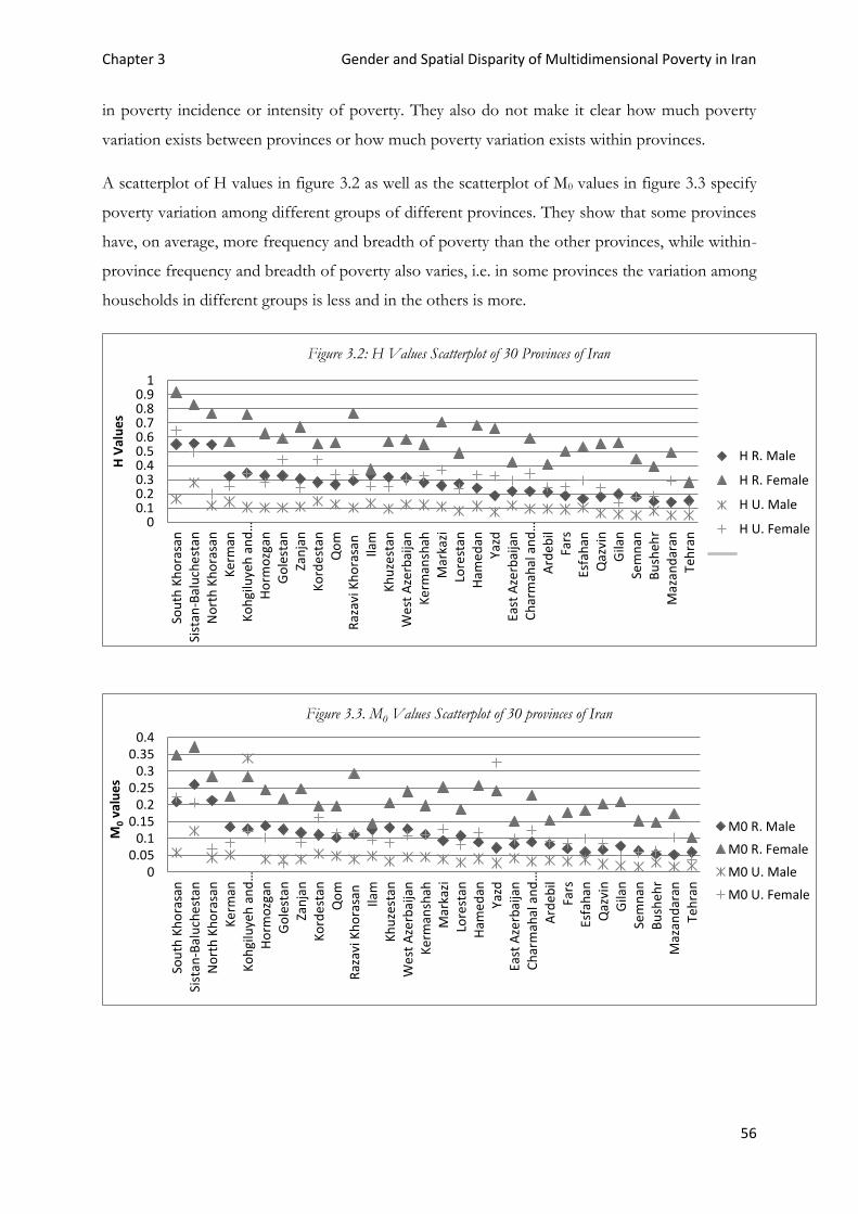
Nevertheless, table 3.3 depicts another aspect of multidimensional poverty in Iran by displaying
the frequency (via H headcount) and breadth (via M0 headcount) of poverty for four different
groups (rural households with a male head, rural households with a female head, urban households
with a male head, and urban households with a female head) for each of the 30 provinces in Iran.
A glance at the table 3 shows the disparity of poverty within provinces and among different groups
in each province. It can be seen by looking carefully at the table that the poorest groups in each
province are rural households and mostly the rural female-headed households. However, the bunch
of values in table 3.2 and table 3.3 does not reflect the role of each feature of households or region
Chapter 3 Gender and Spatial Disparity of Multidimensional Poverty in Iran
56
in poverty incidence or intensity of poverty. They also do not make it clear how much poverty
variation exists between provinces or how much poverty variation exists within provinces.
A scatterplot of H values in figure 3.2 as well as the scatterplot of M0 values in figure 3.3 specify
poverty variation among different groups of different provinces. They show that some provinces
have, on average, more frequency and breadth of poverty than the other provinces, while within-
province frequency and breadth of poverty also varies, i.e. in some provinces the variation among
households in different groups is less and in the others is more.
00.10.20.30.40.50.60.70.80.9
1
Sou
th K
ho
rasa
nSi
stan
-Bal
uch
est
anN
ort
h K
ho
rasa
nK
erm
anK
oh
gilu
yeh
an
d…
Ho
rmo
zgan
Go
lest
anZa
nja
nK
ord
est
anQ
om
Raz
avi K
ho
rasa
nIla
mK
hu
zest
anW
est
Aze
rbai
jan
Ke
rman
shah
Mar
kazi
Lore
stan
Ham
ed
anYa
zdEa
st A
zerb
aija
nC
har
mah
al a
nd
…A
rde
bil
Fars
Esfa
han
Qaz
vin
Gila
nSe
mn
anB
ush
ehr
Maz
and
aran
Teh
ran
H V
alu
es
Figure 3.2: H Values Scatterplot of 30 Provinces of Iran
H R. Male
H R. Female
H U. Male
H U. Female
00.05
0.10.15
0.20.25
0.30.35
0.4
Sou
th K
ho
rasa
nSi
stan
-Bal
uch
est
anN
ort
h K
ho
rasa
nK
erm
anK
oh
gilu
yeh
an
d…
Ho
rmo
zgan
Go
lest
anZa
nja
nK
ord
est
anQ
om
Raz
avi K
ho
rasa
nIla
mK
hu
zest
anW
est
Aze
rbai
jan
Ke
rman
shah
Mar
kazi
Lore
stan
Ham
ed
anYa
zdEa
st A
zerb
aija
nC
har
mah
al a
nd
…A
rde
bil
Fars
Esfa
han
Qaz
vin
Gila
nSe
mn
anB
ush
ehr
Maz
and
aran
Teh
ran
M0
valu
es
Figure 3.3. M0 Values Scatterplot of 30 provinces of Iran
M0 R. Male
M0 R. Female
M0 U. Male
M0 U. Female
Chapter 3 Gender and Spatial Disparity of Multidimensional Poverty in Iran
57
3.5. Results of Regressions Analysis
As data are available on two levels, i.e. households are nested within provinces and the response is
binary, we applied a multilevel regression model. The model helps to answer questions such as,
what is the extent of between-province variation in poverty. What amount of poverty variation can
be attributed to either between-province variation or within-province (among households)
variation? To what extent the poverty variation can be explained by the household-level variables
(i.e. the demographic features of households). Do household-level variables such as age or gender
have different effects in different provinces? Can between-province differences in poverty be
explained by differences in the province level variables?
Table 3.4 shows the results of multilevel mixed effect regression, when the dependent variable is
incidence of poverty and the responses are binary. The results of the empty model, which is
sometimes referred to as a variance components model, are shown at the first rows of the table.
The empty model helps us to extract the information of how much the variation at the dependent
variable is attributable to the second level if none of the household’s characteristics is included to
the regression. The variance of the intercepts across the groups (provinces) or group-level residual
variance in the empty model was estimated as σ2=0.191, which is significant by the Wald test in
P<0.001. The between-group variance helps to estimate the VPC, because in analyzing multilevel
data, we are interested for variation that can be attributed to the different levels in the data structure
and the extent to which variation at a given level can be explained by explanatory variables. Thus,
the VPC for our two-level logit model is VPC= σ2/σ2+3.29= 0.055, i.e. 5.5% of variance in the
incidence of poverty is due to between-province variation, and 94.5% of variance in the incidence
of poverty occurs within provinces or between households.
In model 1.1, we considered hierarchical regression models for the relationship between the binary
response variable (ρ) and a set of explanatory variables of level 1. However, a particular advantage
of multilevel modelling is the ability to explore the effects of group-level (level 2) predictors or
contextual effects while simultaneously including random effects to allow the effects of unobserved
group-level variables. Hence, the model 1.2 is the logit mixed effect model with an added dummy
variable for the province level.
In order to prove that the multilevel model provides a significantly better fit to the data than the
single-level model, we use a likelihood ratio (LR) test, which is equivalent to the reduction in the
deviance. We compare LR to a chi-squared distribution with 1 degree of freedom. The critical value
for testing at 5% level is 3.84. The LR test statistic values in all three regressions greatly exceed 3.84
(p < 0.001).
Chapter 3 Gender and Spatial Disparity of Multidimensional Poverty in Iran
58
β0 = -3.898 is interpreted as the log-odds that ρ=1 when xij=0 and u=0, and is referred to as the
overall intercept. The probability of β0 is estimated by Logit-1(-3.898) = 0.0198, that means, when
we ignore the state variation, the probability of multidimensional poverty incidence for an urban
household with four members and with a married middle-aged male head is 2 %. If we hold u=0,
the probability of poverty for a female-headed household with the same circumstances would be
Logit-1(-3.898 +0.859) = 0.045, i.e. about twice more than the male peer. Furthermore, the
probability of poverty incidence for a rural male-headed household with the similar above-
mentioned factors is 6%, while the probability of poverty incidence for the peer rural female-
headed household is approximately 13%. Controlling for province differences, we would expect
the odds of being poor to increase by a factor of exp (0.254) =1.3 for each one-unit increase in the
number of household members. The dummies for age (of head of household) show a strong
positive and significant correlation between being aged and possibility of falling in poverty. When
it comes to marital status variables, the dummy of never married (head of household) is not
significant, while there is a positive dummy for divorced (head of household) and a strong positive
and significant dummy for the widow (head of household). The results, however, does not
demonstrate significant dummy for the province-level variable, rural proportion. The dummy of
the other province-level variable, distance to capital city is positive, though it is not strong.
Chapter 3 Gender and Spatial Disparity of Multidimensional Poverty in Iran
59
Table 3.4. Mixed Effects REML Regression for the Total Population with Response ρ ϵ [0, 1].
Empty Model
Parameter Estimate Std. Err. Z P>|Z|
Intercept β0 -1.298 0.081 -16.05 0.000
Between state variance σ2 0.191 0.050 3.82 0.000
LR test: χ2 (01) = 1303.92 (p <0.001)
Individual level Model (1.1)
Intercept β0 -3.57 0.112 -31.70 0.000
Rural HH β1 1.167 0.029 39.59 0.000
Female head β2 0.861 0.067 12.88 0.000
N of H members c β3 0.254 0.008 32.52 0.000
Age Parameters
Young head H β4 -0.771 0.140 -5.49 0.000
Old head H β5 1.497 0.32 46.6 0.000
Marital status of household’s head H Parameters
Widow β6 0.825 0.068 12.07 0.000
Divorced β7 0.583 0.161 3.63 0.000
Never married β8 0.167 0.139 1.20 0.229
Random effect Parameters
Between state variance σ2 0.208 0.055 3.78 0.000
LR test: χ2 (01) = 1124.90 (p <0.001)
Individual- and Province-level Model (1.2)
Intercept β0 -3.898 0.54 -7.22 0.000
Rural HH β1 1.167 0.029 39.57 0.000
Female head β2 0.859 0.067 12.86 0.000
N of H members c β3 0.254 0.008 32.45 0.000
Age Parameters
Young head H β4 -0.772 0.140 -5.50 0.000
Old head H β5 1.497 0.032 46.61 0.000
Marital status of household’s head H Parameters
Widow β6 0.825 0.068 12.07 0.000
Divorced β7 0.582 0.161 3.62 0.000
Never married β8 0.166 0.139 1.19 0.233
Level 2 variables
Rural prop. β9 -0.214 1.058 -0.20 0.840
distance β10 0.0007 0.0002 3.61 0.000
Random effect Parameters
Between state variance σ2 0.142 0.038 3.74 0.000
LR test: χ2 (01) = 681.71 (p <0.001)
Chapter 3 Gender and Spatial Disparity of Multidimensional Poverty in Iran
60
Table 3.5. Profile of Residuals for the 30 Provinces.
State uj ujstd. Err. uj rank Random(provincial)
intercept
Logit1(β0+u30)
0 Markazi 0.286 0.071 23 -3.612 0.026
1 Gilan -0.161 0.083 12 -4.059 0.017
2 Mazandaran -0.275 0.09 7 -4.173 0.015
3 East Azerbaijan -0.185 0.077 11 -4.083 0.017
4 West Azerbaijan -0.006 0.076 18 -3.904 0.020
5 Kermanshah 0.17 0.067 21 -3.728 0.023
6 Khuzestan -0.283 0.076 5 -4.181 0.015
7 Fars -0.546 0.08 2 -4.444 0.012
8 Kerman -0.011 0.063 17 -3.909 0.020
9 Razavi Khorasan 0.047 0.066 19 -3.851 0.021
10 Esfahan -0.153 0.076 13 -4.051 0.017
11 Sistan-Baluchestan 0.557 0.06 28 -3.341 0.035
12 Kordestan 0.362 0.077 24 -3.536 0.029
13 Hamedan 0.203 0.070 22 -3.695 0.025
14 Charmahal and Bakhtiari -0.120 0.086 14 -4.018 0.018
15 Lorestan -0.206 0.081 10 -4.104 0.016
16 Ilam -0.055 0.081 16 -3.953 0.019
17 Kohgiluyeh and Buyer Ahmad 0.152 0.062 20 -3.746 0.024
18 Bushehr -0.929 0.091 1 -4.827 0.008
19 Zanjan 0.4 0.073 26 -3.498 0.030
20 Semnan -0.231 0.097 9 -4.129 0.016
21 Yazd -0.28 0.075 6 -4.178 0.015
22 Hormozgan -0.313 0.066 4 -4.211 0.015
23 Tehran -0.343 0.08 3 -4.241 0.014
24 Ardebil -0.247 0.082 8 -4.145 0.016
25 Qom 0.385 0.076 25 -3.513 0.03
26 Qazvin -0.096 0.086 15 -3.994 0.018
27 Golestan 0.442 0.069 27 -3.456 0.031
28 North Korasan 0.709 0.063 29 -3.189 0.041
29 South Khorasan 0.763 0.060 30 -3.135 0.043
However, the advantage of a hierarchical model is that it enables us to look at the effect of variables
for units within the same group, which is known as the cluster-specific effect. Hence, β0 is the
overall intercept, the intercept for a given group (state) j is β0+uj, which will be higher or lower
Chapter 3 Gender and Spatial Disparity of Multidimensional Poverty in Iran
61
than the overall intercept depending on whether uj is greater or less than zero. We can estimate the
probability of falling in poverty for any typical household in each province like 𝑃 𝑟(𝜌 = 1) =
𝑙𝑜𝑔𝑖𝑡−1(𝛽0 + 𝛽1 𝑥𝑖𝑗 + 𝑢𝑗) , when we estimate uj.
Table 3.5 depicts the estimated uj and u rank for 30 provinces. As we have already calculated the
predicted probability for an average province is uj=0 and, assuming that uj follows a normal
distribution, we would expect approximately 95% of provinces to have a value of uj within 2
standard deviations of the mean of zero, i.e. between approximately -2σu=-0.754 and 0.754. Table
3.5 also shows the predicted random intercept for each province, while the column titled by Logit1
(β0+u30) shows the probability of falling in poverty for a typical urban male headed household (with
four members) in each province.
In similar fashion, the probability of poverty for each typical household with certain circumstances
can be estimated. As the focus of this study is on the gender and spatial poverty, table 3.6 only
categorizes and depicts the probability of poverty for the urban and rural households with a male
head or female head in three provinces at the top and three at the bottom, when the other
demographic variables are supposed to be constant. The number of household members is
assumed four and the age and marital status of the head are considered married and middle-aged.
Table 3.6. Probability of Poverty for Four Typical Households in the Least Poor and the Poorest Provinces.
Provinces Urban male h. Urban female h. Rural male h. Rural female h.
The least poor
Tehran 1.4% 3.3% 4.4 % 9.8 %
Bushehr 0.8% 2 % 2.5 % 5.7 %
Mazandaran 1.5% 3.5% 4.7 % 10.5%
The most poor
South Khorasan 4.3% 9.3% 12.3% 25 %
North Korasan 4.1% 8.8% 11.7% 24 %
Sistan-Baluchestan 3.5% 7.7% 10.2% 21 %
Average in country with
controlling states difference
2 % 4.5% 6 % 13 %
The values, which are shown in table 3.6, reflect two main ideas; first, the probability of poverty
increases by some household characteristics (Like having female head or being rural), second, the
effect of household characteristics are different in different provinces.
Chapter 3 Gender and Spatial Disparity of Multidimensional Poverty in Iran
62
Table 3.7. Mixed Effects Regression for the Poor Population with Response ci.
Fixed effect Model
Parameter Estimate Std. Err. Z P>|Z|
Intercept β0 0.352 0.004 83.22 0.000
Rural HH β1 0.026 0.002 14.48 0.000
Female head β2 0.008 0.003 2.19 0.028
N of H members c β3 0.008 0.0004 20.74 0.000
Age Parameters
Young head H β4 0.012 0.01 1.22 0.223
Old head H β5 -0.013 0.002 -7.10 0.000
Marital status of household’s head Parameters
Widow β6 0.003 0.003 0.85 0.396
Divorced β7 0.011 0.01 1.16 0.248
Never married β8 0.031 0.01 3.30 0.001
Multilevel Empty Model
Intercept β0 0.376 0.003 104.62 0.000
Between state variance σu2 0.0003 - - -
Within state variance σe2 0.005 - - -
LR test: χ2 (2) = 631.20 (p <0.001)
Individual level Model
Intercept β0 0.349 0.005 69.06 0.000
Rural HH β1 0.029 0.002 16.04 0.000
Female head β2 0.006 0.003 1.67 0.095
N of H members c β3 0.007 0.0004 18.24 0.000
Age Parameters
Young head H β4 0.003 0.009 0.36 0.721
Old head H β5 -0.011 0.002 -5.87 0.000
Marital status of household’s head H Parameters
Widow β6 0.002 0.003 0.69 0.489
Divorced β7 0.010 0.009 1.11 0.266
Never married β8 0.029 0.009 3.25 0.001
Random effect Parameters
Between state variance σu2 0.00025
Within state variance σe2 0.005
LR test: χ2 (2) = 492.60 (p <0.001)
Individual- and Province-level Model
Intercept β0 0.369 0.02 19.53 0.000
Rural HH β1 0.029 0.002 16.06 0.000
Female head β2 0.005 0.003 1.65 0.099
N of H members c β3 0.007 0.0004 18.17 0.000
Age Parameters
Young head H β4 0.0032 0.01 0.33 0.739
Old head H β5 -0.011 0.002 -5.88 0.000
Marital status of household’s head H Parameters
Widow β6 0.002 .003 0.70 0.483
Divorced β7 0.010 0.009 1.08 0.278
Never married β8 0.029 0.009 3.23 0.001
Level 2 variables
Rural prop. β9 -0.073 0.036 -2.00 0.046
distance β10 0.00003 6.57e-06 4.16 0.000
Random effect Parameters
Between state variance σu2 0.00015
Within state variance σe2 0.00069
LR test: χ2 (2) = 196.69 (p <0.001)
Chapter 3 Gender and Spatial Disparity of Multidimensional Poverty in Iran
63
Table 3.7 shows the results of mixed effect regression when response is ci, when 0<ci<1 and the
number of observations= the number of poor people (= 8039). We also estimated fixed effect
regression to compare it with the results of multilevel models, which show no significant
distinction. However, the LR test shows that the mixed effect regression is the preferable regression
model to conduct in this case. The empty model again was conducted to show how much the
variation at the dependent variable is attributable to the second level if none of the household’s
characteristics is included to the regression.
The results imply that the average deprivation value for a poor urban male-headed household in
the whole country is β0=0.369, while the threshold of falling in multidimensional poverty is 0.34.
Other factors such as being rural or a female-headed household added only β1=0.029 and β2=0.005
to the value of poverty intensity, whereas having an old head of household has a negative effect of
β5 = -0.011on the intensity of poverty. And the marital states parameters and level 2 parameter of
rural proportion are insignificant with a p value of <0.001. Therefore, controlling between-
provinces variation, the intensity of poverty varies from 0.37 for an urban household with a young
male head to 0.445 for a rural household with single female head. On the other hand, as the
VPCu=σu2/σu
2+σe2=0.18, approximately 18% of the variation in the intensity of poverty lies among
provinces variation, and 82 % embedded within provinces variation (or the characteristics of the
households).
To sum up, while inequality among the subgroups of the household population of the provinces is
significant with respect to the incidence of poverty, the difference in the intensity of poverty among
the poor is not remarkable.
To sum up results of the analysis above, we point out the following items. The variance of poverty
incidence mostly related to within-province variation (94.5%), while only 5.5% of variance in
poverty incidence lays between-province variation. The demographic factors of head of household
(gender, age and marital status) have significant correlation with poverty incidence. Female, aged,
divorced or widow head of households are significantly disadvantaged to their male, middle age,
married counterparts. The other characteristics of household like being rural and the number of
members also have positive and significant relation with the incidence of poverty. Being rural puts
the household twice more in danger of falling in poverty than their urban counterparts, while each
member extra than 4 centric number of members increase 0.5% to the possibility of falling in
poverty for a household. And eventually the effect of household characteristics is some provinces
are stronger than the others are.
Chapter 3 Gender and Spatial Disparity of Multidimensional Poverty in Iran
64
Indeed, the analysis above confirms that certain individuals and groups are marginalized based on
their gender and location of residence. In fact, the opportunities that people should have to avoid
extreme poverty are vastly different depending on these factors.
3.6. Concluding Remarks
This paper focuses on two phenomena at the same time; multidimensional poverty in different
areas in Iran; and inequality in the matter of distribution of welfare among the households and
specific groups within the population of Iran.
The study, in the first place expands the monetary concept of poverty, which only captures income
or sometimes expenditure, to a more comprehensive concept of multidimensional poverty and
applies the Alkire-Foster method to measure the multidimensional poverty of households in 30
provinces of Iran. The results of multidimensional poverty ratio (H) and the adjusted headcount
ratio (M0) estimation show that the southeast and northeast provinces in particular and remote
areas near the eastern and western borders in general experience higher incidence of poverty, while
welfare tends to concentrate in capital province (Teharan) and in some of its neighbor provinces
in the center and north of Iran.
However, measuring multidimensional poverty ratio (H) and the adjusted headcount ratio (M0) do
not reflect the effect of household’s characteristics or region’s features in incidence or intensity of
poverty; also they do not distinct poverty variation between provinces and within provinces.
Therefore, to find out the extent of the disparity between subgroups and to measure and compare
the likelihood of certain typical units falling into poverty and to capture inequality among the poor,
the study employs a multilevel regression analysis.
The results imply that most of the poverty incidence variation related to within-province variation
(94.5%), and only 5.5% of the poverty incidence variation related to between-province variation.
The results also indicate that having a female, aged, and divorced or widow head, as well as being
rural are characteristics, which increase the likelihood of falling in poverty for a household. The
probability of poverty for a rural family is, on average, four times greater than an urban family with
the same circumstances, while the probability of poverty for a female-headed family is, on average,
twice that of a male-headed family with the same circumstances. According to the results, the most
disadvantaged households are female-headed rural households in the poorest southeast provinces,
while the most fortunate households are male (married, middle aged)-headed urban households in
Tehran, Bushehr and Mazandaran. The study concludes that certain households are marginalized
based on their demographic and spatial circumstances.
Chapter 3 Gender and Spatial Disparity of Multidimensional Poverty in Iran
65
The study focuses on estimating poverty and inequality of welfare in Iran in a way that is beneficial
for policy makers, helping them to optimize poverty mitigation policies by targeting the most
marginalized communities, as well as addressing inequalities, and social exclusion, which are deeply
embedded in the social and economic processes of Iranian society. It is our hope that this study
has prepared a base for future projects to design effective policies to alleviate poverty and
inequality.
3.7. Appendix: Robustness Analysis
Using a rank robustness analysis, we evaluated how changes in the parameters affect relative
multidimensional poverty values. A series of rank robustness tests was applied in order to assess
how sensitive the relative values of multidimensional poverty across provinces are to changes in
indicators’ weights.
To test whether multidimensional poverty results are robust to a plausible range of weights, the
multidimensional poverty has been estimated with three other alternative weighting structures -
giving 50% of the relative weight to one of three dimensions and 25% to each of the other two in
turn. Changing the indicators’ weights affects the poverty estimates. However, the provinces
rankings are robust to such changes. Table 3.8 presents the correlation between the province
rankings obtained with the baseline of equal weights and those obtained with the other three
alternatives. The correlation is 0.862 or higher using Kendall Tau and 0.955 or higher with the
Spearman correlation. Interestingly, the rank correlation between the three alternative weighting
systems is also relatively high – none lower than 0.829 with the Kendall correlation.
Chapter 3 Gender and Spatial Disparity of Multidimensional Poverty in Iran
66
Table 3.8. Correlation Coefficients between Multidimensional Poverty Values Using Alternative Weighting Structures (in 30 Provinces of Iran) Equal Weights
33% each
50% Expenditure
25% Education
25% LS
50% Education
25% Expenditure
25% LS
50% Expenditure
25% Education
25% LS
Spearman 0.968
Kendall 0.956
50% Education
25% Expenditure
25% LS
Spearman 0.966 0.918
Kendall 0.903 0.834
50% LS
25% Expenditure
25% Education
Spearman 0.995 0.971 0.969
Kendall 0.981 0.917 0.903
Note: LS: Living Standard. The Spearman rank correlation coefficients are 0.95 and higher
Acknowledgment
I thank Armin Bohnet and Jürgen Meckl for valuable suggestions and comments. I also thank
Sabina Alkire and Bouba Housseini for their useful comments. I thank Ali Asgar Salem for his help
to find and access complementary data. I am grateful for the support of the department of
development and environmental studies of Justus-Liebig University (ZEU). I also appreciate
participants in the 2014 MAGKS Doctoral Colloquium for critical comments. Financial support
from DAAD (Grant No. 57076385) is gratefully acknowledged.
Chapter 4 Growth Elasticity of Poverty: with Application to Iran Case Study
67
Chapter 4
Growth Elasticity of Poverty: with Application to Iran
Case Study
Chapter 4 Growth Elasticity of Poverty: with Application to Iran Case Study
68
Abstract
The sensitivity of the frequency of poverty to economic growth is one of the central issues of
poverty and development discourse. In this paper, we estimate the income growth elasticity of
poverty and income inequality elasticity of poverty for a panel of 28 provinces of Iran from 1998
to 2009. We also, for the first time, estimate the growth elasticity of multidimensional poverty
(estimated via Alkire-Foster method). The results demonstrate the low income growth elasticity of
poverty while the income inequality elasticity of poverty is stronger and significant. Similar results
are obtained for elasticities of multidimensional poverty. The results suggest that changes in
inequality are more important for poverty reduction than changes in income growth.
Key words: Growth elasticity of poverty, income inequality, monetary poverty, Multidimensional poverty.
Chapter 4 Growth Elasticity of Poverty: with Application to Iran Case Study
69
4.1. Introduction
In the welfare-economic discourse there is a strong argument stating that economic growth in
terms of increasing per capita incomes or expenditures reduces poverty in the developing world.
However, there is no agreement on the exact extent that economic growth reduces poverty. In
other words, the growth elasticity of poverty has become a subject of controversy.
The discussion about the sensitivity of the frequency of poverty to economic growth has been
going on for about two decades (Ravallion and Chen, 1997; Bruno et al., 1998; Bhalla, 2002;
Bourguignon, 2003; Adams, 2004; Kraay, 2006; Bresson, 2009). However, while the extent of
poverty reduction by economic growth is a key concept for policy, the size of that sensitivity has
been on debate. Whereas Ravallion and Chen (1997), and Bruno et al. (1998) estimated the value
of the growth elasticity of poverty for the cross section countries to be between -2.0 and -3.0,
Bhalla (2002) calculated the growth elasticity of poverty for a large selection of developing countries
to be about -5.01. Richard and Adams (2004) admitted that the growth elasticity of poverty is within
the range of -2.0 and -3.0, and argued that Bhalla’s suggestion (that the growth elasticity of poverty
should be about -5.0) is only correct when the full sample of intervals for a large selection of
developing countries is used and growth is defined by changes in the survey mean.
Parallel to the study on the growth-poverty relationship it was also largely debated that the impact
of economic growth on poverty can be enforced or reduced by changes in the income distribution
over time (Bourguignon, 2003; Datt and Ravallion, 1992). Hence, the changes in poverty headcount
can be decomposed into a growth effect and a distributional effect. Figure 4.1 (adapted from
Bourguignon 2003, p. 32) qualitatively illustrates the decomposition of change in poverty into a
growth and a distributional effect. The initial distribution is taken as given and illustrated by the fat
lined density function. The growth effect is illustrated by a pure rightward shift of that distribution
without affecting the shape of the curve. The pure growth effect on poverty is illustrated by the
light shadowed area. The distribution effect corresponds to a change in the shape of the density
function. When the initial distribution transforms to the new distribution as shown in Figure 4.1,
we can illustrate the distributional effect on poverty by the dark shadowed area. In contrast to
Bourguignon (2003, p. 32) who emphasizes the growth effect on poverty, figure 4.1 emphasizes
the inequality effect on poverty, since we find this effect to be stronger in our data. As will be
shown, the size of the growth effect relative to the size of the inequality effect depends on particular
country circumstances such as initial income inequality or growth scenarios.
1 An elasticity value of – x means that an income growth of 1% leads to a reduction of poverty of x%.
Chapter 4 Growth Elasticity of Poverty: with Application to Iran Case Study
70
As mentioned above, many of the former studies estimated the elasticity of poverty for a cross
section of countries. However, addressing this issue by regressing the rate of poverty on mean
income for a range of countries suffers from numerous shortcomings; cross-country data often
have a limited number of data points for each country so that the results are largely driven by cross-
country differences (Meng et al., 2005). It could also potentially be misleading due to some
conceptual and practical problems arising from currency conversions, different survey-based
measures of living standards, different levels of development and omitted country-specific fixed
effects correlated with income (Ravallion, 1995; Ravallion and Chen, 1997). Hence assessing
growth and inequality elasticities of poverty, depending on particular country circumstances and
growth scenarios could improve our insight and prospect about the impact of growth and
distributional change on poverty reduction.
In this paper, we study the income growth-poverty-inequality nexus in a particular country – Iran.
Therefore, we avoid the conceptual and practical problems of similar studies with cross-country
comparisons, such as currency exchange or surveys diversity. In this study, we utilize data from the
Household Expenditure and Income Survey (HEIS) for the whole country, i.e. 28 provinces, and
for the period 1998 to 2009. These data present a more general picture of the poverty and the
changes in inequality about the twelve-year period in Iran.
Figure4.1. Decomposition of Change in Poverty into Growth and Distributional Effects
Chapter 4 Growth Elasticity of Poverty: with Application to Iran Case Study
71
The main contribution of this study to the literature, however, is that in the current study we
measure the growth elasticity of multidimensional poverty as well as growth elasticity of one-
dimensional monetary poverty.
The studies on the growth elasticity of poverty have mainly focused on the traditional income
poverty. However, considering poverty as a multidimensional concept as Sen (1984) argued in his
capability approach leads us to study the relationship of growth and multidimensional poverty.
Such a study is also particularly essential, since a reduction in income poverty does not necessarily
reduce non-income dimensions of poverty. “Measuring Pro-Poor Growth in Non-Income
Dimensions” (Grosse et al., 2008) is one of the few studies on the growth-poverty relationship
which extend the toolbox of pro-poor growth measurement to non-income dimensions and
composite measures of well-being (using the human development index, HDI, as a composite
measure). They applied the growth incidence curve (GIC) of Ravallion and Chen (2003) for the
case study of Bolivia during 1989-98 for measuring pro-poor growth. The GIC is a visual tool for
the assessment of the distributional pattern of growth, and shows the mean growth rate in
achievements (e.g. incomes) at each centile of the distribution between two points in time.
Although GIC is a nice visual tool, which shows the absolute changes of achievement for each
centile, and successfully was applied by Grosse et al (2008) to investigate pro-poor growth in non-
income dimensions, it can barely be considered as a substitute for growth elasticity of poverty for
assessing the impact of growth on poverty. The growth elasticity of poverty gives us a digit, which
is easier to interpret and does not have the limitation of GIC in the matter of estimating it for each
centile separately. Hence, in the current paper we estimate the growth elasticity of (income and
non-income) poverty for the case study of Iran over 1998-2009. In order to estimate growth
elasticity of poverty, we applied the method of Ravallion and Chen (1997), while for extending the
method to estimate growth elasticity of non-income poverty we have been inspired by the way
Grosse et al. (2008) in the way they extend the toolbox of pro-poor growth measurement to non-
income dimensions and multidimensional poverty measures. Given that we estimate growth and
inequality elasticities of non-income deprivation as well as elasticities of multidimensional poverty,
our study may also contribute to the understanding of growth, poverty, and inequality beyond Iran.
The paper proceeds as follows. Section 2 reviews the econometric methods for estimating the
growth elasticity of poverty. Section 3 describes how we extend the method to estimate the growth
and inequality elasticities of poverty for non-income dimensions. Section 4 derives the results for
the case study of Iran. Finally, section 5 offers the concluding remarks.
Chapter 4 Growth Elasticity of Poverty: with Application to Iran Case Study
72
4.2. Econometric Methods for Estimating Growth Elasticity of Poverty
Changing poverty due to income growth and income inequality has been strongly discussed in the
literature. Kakwani (1993), Ravallion and Chen (1997), Bourguignon (2003), Klasen and Misselhorn
(2008) are some of the most outstanding studies which worked in this area.
Kakwani (1993) estimated the pure growth effect on poverty and the effect of inequality on
poverty. Since both mean income and income inequality affects poverty, he argued that
proportionate changes in poverty could be decomposed into an effect from mean income on
poverty and an effect from a change in the Gini index. Denoting the poverty variable by θ, mean
income by µ, and the Gini coefficient by G, this decomposition can be written as:
𝑑𝜃
𝜃= 𝜂𝜃
𝑑𝜇
𝜇+ 𝜀𝜃
𝑑𝐺
𝐺 ,
Where 𝜂𝜃 denotes the growth elasticity of poverty, while 𝜀𝜃 is the effect of change in the Gini index
on the total poverty. Then he introduced marginal proportional rate of substitution (MPRS)
between mean income and income inequality which can be computed for each poverty measure:
=𝜕𝜇
𝜕𝐺
𝐺
𝜇= −
𝜀𝜃
𝜂𝜃 .
Ravallion and Chen (1997) suggested the following regression to show the relation between
poverty, mean income and inequality for a cross-country analysis
P represents the poverty index, Y is the mean income, G is the Gini coefficient, and µ is a vector
of time-invariant provincial dummy variables, while ɛit is a random error term. The subscripts t and
i index provinces and time.
Chapter 4 Growth Elasticity of Poverty: with Application to Iran Case Study
74
4.3. Growth Elasticity of Deprivation for Non-Income Dimensions
In addition to measure the growth elasticity of monetary poverty, we are interested to measure the
growth elasticity of multidimensional poverty and study the progress in multidimensional
achievements. Apart from few attempts of demonstrating the growth-(non-income and
multidimensional) poverty relationship such as Grosse et al. (2008), this approach has been rarely
applied in the literature. Partly because non-monetary and multidimensional poverty discussion in
comparison with income poverty still is young, partly because most of the former studies were
cross-countries studies using different surveys, which usually do not contain enough or compatible
information of multidimensional poverty. In addition to, some difficulties are brought out and
should be dealt with by estimating growth and inequality elasticities of non-monetary and
multidimensional poverty, such as compromising on an aggregated digit as the multidimensional
poverty index or non-income deprivation, or the way we should choose to demonstrate the
inequality.
In order to solve the first difficulty, we decided on measuring multidimensional poverty index by
applying Alkire-Foster (2011b) method, which gives us a single digit to signify experiencing
multiple deprivations simultaneously. The Alkire-Foster methodology also gives us the facility of
decomposing multidimensional poverty index to the dimensions, hence we can estimate the growth
and inequality elasticities of (each dimension) deprivation.
Hereupon, we consider poverty as a set of dimensions containing as three main dimensions:
nutrition, education and a non-monetary standard of living that is illustrated in detail in table 4.1.
Chapter 4 Growth Elasticity of Poverty: with Application to Iran Case Study
75
Table 4.1. Dimensions, Weights and Deprivation Cut-off of the Multidimensional Poverty
Dimension Indicator The deprivation cutoff zj
Nutrition (1/3)
Daily food Expenditure (1/6) 1.08 $ in urban area and 0.69 $ in rural area
Percentage of expenditures on food (1/6) Spend more than 75% of expenditures on food
Education (1/3)
Literacy situation of the household head (1/6) Illiterate household head
School attendance (1/6) Household member (6 to 16 years old ) out of school
Living standard (1/3)
Electricity (1/15) No access to electricity
Safe water (1/15) No access to safe water
Overcrowding (1/15) No enough (10qm) floor area of housing per capita
Fuel of cooking (1/15) Coking fuel is wood, charcoal or dung.
Asset ownership (1/15) Household does not own more than one of these items (radio, TV, telephone, bike, motorbike or refrigerators) and does not own a car.
The amount of deprivation is 0 < Ci < 1, and the poverty cutoff is Ci > 0.333.
The second difficulty in estimating the growth elasticity of multidimensional poverty using the
conventional regression model is the inequality index. Grosse et al. (2008) tried to solve this
problem in two different ways: in the first approach which they rank the individuals by each
respective non-income variable and generate the population centiles based on this ranking; in the
second approach they rank the individuals by income and calculate the growth of non-income
achievements for these income percentiles. The advantage of first approach is that it answers the
questions such as how the education poor benefited disproportionately from improvements in
education. The advantage of the second way is that it analyzes the impact of income growth on the
income poorest centile, while providing an instrument to assess if public social spending programs
have reached the targeted income poorest population groups and if the public resources are
effectively allocated.
In our case, we apply the second way, rank the individuals by income, and calculate the growth of
non-income achievements for these income percentiles. We cannot apply the first approach to
index the inequality, because the identity of most of our indicators makes the ranking impossible
as the households either deprived in them or not. There is another idea to rank the individuals by
the intense of their deprivation Ci. However, the Gini index, which is calculated in this way, suffers
from a limitation. Actually, this generates the problem that some households have reached the
upper limit and upper level of welfare is not measurable. It generates the further problem that
inequality in such indicator is typically low when a significant share of households has reached the
Chapter 4 Growth Elasticity of Poverty: with Application to Iran Case Study
76
upper limit. Hence, by computing the regression model with income Gini index, we estimate the
relation of growth in non-income achievements to the distribution of income, while this provides
insights about how far the income poor have benefited by improvements in non-income
dimensions of well-being.
4.4. Empirical Results
We present the empirical results of the study in three orders in this section. First, we present the
trend of mean income, poverty and inequality for our particular time in the case study of Iran,
which we estimated from our available survey data. Second, we represent the results of our
estimation of growth elasticity of monetary poverty. The third sub-section is dedicated to display
the results of the estimation of growth elasticity of multidimensional poverty.
4.4.1. The Case Study of Iran
The period we consider for our study on growth elasticity of poverty in Iran is from 1998 to 2009,
concerning we have the survey data available for that particular time. Over the certain time period
Iran experienced both a reformist administration and a conservative government, and recorded 4.5
average growth rate of real GDP (Iran Central Bank, 2012), while the population in 1998 to 2009
changed from 62.103 million to 73.196 million people (Iran Statistical center, 2011).
Table 4.2 shows that the mean income per person calculated from the household expenditure and
income survey (HEIS) of Iran statistical center (ISC) constantly increased at the rural, urban and
national levels over the time span under consideration. The mean income per person at the national
level increased from 366.94$ per year in 1998 to 1617.51$ per year in 2009. However, our
estimations of income per person in rural and urban areas show a large disparity of income
distribution between rural and urban areas that echoes an important feature of Iran’s economy. At
the same time, the urban population share in Iran changed from 39.06 in 1998 to 51.41 in 2009.
This high pace of urbanization is probably the result of migration from rural to urban areas, which
does not sound surprising against the background of the large income disparity between rural and
urban areas. However, we do not have complete information about how much this development
is related to urban expansion into rural areas or to actual migration from rural to urban areas.
Over the period 1998-2009, the expenditure poverty that we estimated from the HEIS data by
applying the Foster-Greer-Thorbecke method is summarized in table 4.3 and is illustrated in figure
4.2 and figure 4.3, decreased alongside the mean income increasing, although the progress is not
uniform. Table 4.3 shows that monetary poverty with the old poverty line decreased from 0.649 in
1998 to 0.056 in 2009, while the monetary poverty with the new poverty line decreased from 0.829
Chapter 4 Growth Elasticity of Poverty: with Application to Iran Case Study
77
in 1998 to 0.172 in 2009, which record a noticeable progress in monetary poverty reduction.
However, our estimation of Gini indices demonstrated in table 4.4 shows that inequality has been
increased over the particular time. As can be seen in table 4.4, the Gini index at the national level
increased from 0.441 in 1998 to 0.7 in 2009. The interesting point is that the Gini index over the
same period decreased slightly in both rural and urban areas (from 0.463 to 0.402 in rural areas,
and from 0.386 to 0.362 in urban areas). This observation suggests that the inequality between rural
and urban areas is the main source of inequality at the national level.
Likewise, the one-dimensional monetary poverty as our estimator of multidimensional poverty
indicates a decreasing pace during the period 1998-2009, though this progress is uneven.
Eventually, table 4.5 shows the multidimensional poverty in Iran from 1998 to 2009, which we
estimated by Alkire-Foster method.
The estimated results presented in this subsection can be sum up as follows: over the time period
1998-2009 we observe a steady increasing income per capita trend in Iran, as well as a decreasing
poverty (monetary and multidimensional) trend, while the Gini index at national level constantly
increases. The results are tempting enough to lead us to the further investigation of the relationship
between income growth, poverty and inequality. Hence, we conduct a regression model with
poverty as the response and income growth and inequality as the independent variable to show the
relationship between poverty, income growth and inequality and demonstrate the growth elasticity
of poverty and elasticity of poverty respecting to inequality.
Chapter 4 Growth Elasticity of Poverty: with Application to Iran Case Study
78
Table 4.2. Summary Statistics: Mean Income per Person in Iran 1998-2009
Urban pop.
Share (%)
Mean income per person ($)
Rural Urban National
1998 39.1 267.02 495.55 366.94
1999 40.2 284.80 512.01 383.36
2000 41.4 329.98 636.15 458.43
2001 42.5 360.36 681.39 495.62
2002 43.7 454.41 855.57 629.19
2003 44.8 574.97 1026.18 776.04
2004 46.0 640.54 1197.82 887.13
2005 47.1 787.29 1342.25 1036.98
2006 48.3 903.08 1609.62 1205.95
2007 49.3 1069.45 1901.17 1447.45
2008 50.3 1112.47 2021.63 1548.14
2009 51.4 1206.95 2037.30 1617.51
Table 4.3. Monetary Poverty in Iran, 1998-2009
Poverty measures
Old poverty line (1.25 $ per day) New poverty line (2$ per day)
Rural Urban National Rural Urban National
1998 0.792 0.491 0.649 0.919 0.729 0.829
1999 0.806 0.549 0.687 0.926 0.777 0.857
2000 0.717 0.416 0.579 0.889 0.671 0.789
2001 0.642 0.311 0.491 0.839 0.572 0.717
2002 0.512 0.217 0.374 0.756 0.452 0.613
2003 0.396 0.142 0.276 0.671 0.358 0.523
2004 0.302 0.100 0.206 0.570 0.273 0.429
2005 0.255 0.078 0.170 0.514 0.228 0.376
2006 0.218 0.065 0.148 0.468 0.197 0.344
2007 0.145 0.042 0.096 0.372 0.131 0.256
2008 0.096 0.024 0.060 0.286 0.085 0.186
2009 0.086 0.027 0.056 0.256 0.091 0.172
Chapter 4 Growth Elasticity of Poverty: with Application to Iran Case Study
79
Table 4.4. Gini Indices of Income Inequality
Rural Urban National
1998 0.463 0.386 0.441
1999 0.461 0.405 0.451
2000 0.459 0.402 0.363
2001 0.435 0.389 0.43
2002 0.435 0.396 0.432
2003 0.426 0.383 0.587
2004 0.441 0.345 0.595
2005 0.425 0.376 0.586
2006 0.413 0.389 0.592
2007 0.417 0.381 0.584
2008 0.401 0.37 0.569
2009 0.403 0.362 0.70
Table 4.5. Multidimensional Poverty in Iran, 1999-2009
Poverty measures
Rural Urban National
(MD)H MD Gini (MD)H MD Gini (MD)H MD Gini
1998 0. 919 0.178 0.506 0.327 0.724 0.263
1999 0.680 0.228 0.453 0.369 0.575 0.302
2000 0.655 0.248 0.299 0.435 0.492 0.343
2001 0.632 0.255 0.282 0.464 0.472 0.358
2002 0.573 0.299 0.449 0.410 0.515 0.360
2003 0.487 0.363 0.196 0.618 0.349 0.488
2004 0.423 0.417 0.142 0.680 0.289 0.546
2005 0.381 0.447 0.124 0.711 0.257 0.577
2006 0.346 0.469 0.105 0.736 0.236 0.595
2007 0.284 0.523 0.077 0.767 0.185 0.644
2008 0.217 0.565 0.053 0.783 0.136 0.678
2009 0.192 0.575 0.054 0.765 0.122 0.675
Chapter 4 Growth Elasticity of Poverty: with Application to Iran Case Study