THREE ESSAYS ON MARKET ANOMALIES AND EFFICIENT MARKET HYPOTHESIS by EHAB YAMANI Presented to the Faculty of the Graduate School of The University of Texas at Arlington in Partial Fulfillment of the Requirements for the Degree of DOCTOR OF PHILOSOPHY THE UNIVERSITY OF TEXAS AT ARLINGTON December 2012
Transcript
THREE ESSAYS ON MARKET ANOMALIES
AND EFFICIENT MARKET HYPOTHESIS
by
EHAB YAMANI
Presented to the Faculty of the Graduate School of
The University of Texas at Arlington in Partial Fulfillment
I would like to express my gratitude to my supervisor, Dr. Darren Hayunga, whose expertise,
understanding, and patience, added considerably to my graduate experience. I appreciate his vast
knowledge and skill in many areas.
A very special thanks goes out to Dr. Peggy Swanson, without whose motivation and
encouragement I would not have considered a graduate career in Finance research. Dr. Swanson is the
one professor/teacher who truly made a difference in my life. She provided me with direction, and
became more of a mentor and friend, than a professor.
I must also acknowledge Dr. Peter Lung for his suggestions and provision of the SAS program
and SAS codes required to accomplish my first essay. He provided me with statistical advice at times of
critical need.
I would like also to thank Dr. Mahmut Yasar from the Economics department for taking time out
from his busy schedule to serve as my external member.
Finally, I would like to dedicate this thesis to my mother’s soul whom I know would have been
so proud of me. I would also like to thank my father, Abdel-Tawab Yamani, for the constant wisdom,
support and encouragement he provided me through my entire life. I must also acknowledge my wife
Samar and my beloved daughter Judy without whose love, I would not have finished this thesis.
September 19th, 2012
iv
ABSTRACT
THREE ESSAYS ON MARKET ANOMALIES
AND EFFICIENT MARKET HYPOTHESIS
EHAB YAMANI, PhD
The University of Texas at Arlington, 2012
Supervising Professor: Darren Hayunga
This dissertation consists of three distinct essays. The first essay investigates the risk
interpretation of the investment premium by empirically examining the fundamental view versus the
sentimental view. Overall, the results show that financial factors are the dominant driver of investment
returns and they control the negative relation between investment and stock return.
In the second essay, I examine the impact of financial contagion resulting from four global
financial crises based on analyses of the global value premium. Results show that equity markets become
more integrated after financial crises that exhibit global effects but less integrated after crises that exhibit
regional effects. Overall findings support the risk story of the global value premium.
The third essay examines the joint dynamics of volume and volatility in the junk bond market
during the 2007-2008 financial crisis. Using trading volume information as a proxy for changes in the
information set available to investors when financial crises occur, I investigate the impact of the subprime
crisis on the informational efficiency of the junk bond market. The overall results show that the crisis
does not have an impact on the market efficiency of the junk bond market.
v
TABLE OF CONTENTS
ACKNOWLEDGEMENTS ..................................................................................................... ……………..iii ABSTRACT ................................................................................................................................................... iv LIST OF TABLES ....................................................................................................................................... viii LIST OF ILLUSTRATIONS .......................................................................................................................... x Chapter Page
3.4.1 FF Model versus GJR-GARCH-FF Model ............................................... 35
3.4.2 Fundamental Riskiness of the Global Value Premium .............................. 41 3.4.3 Financial Crises and Integration ................................................................ 43
3.5.1 International Debt Crisis ........................................................................... 47
3.5.2 ERM Crisis ................................................................................................ 47 3.5.3 Asian Crisis ............................................................................................... 49 3.5.4 September 11, 2001 Attack ....................................................................... 51
4. THE SUBPRIME CRISIS AND THE EFFICIENCY OF
THE JUNK BOND MARKET: EVIDENCE FROM THE MICROSTRUCTURE THEORY ............................................................................ 54 4.1 Introduction ................................................................................................................ 54 4.2 Literature Review ....................................................................................................... 56
4.2.1 Trading and Financial Crises ..................................................................... 56
vii
4.2.2 Price-Volume Models and Efficient Market Hypothesis........................... 57 4.2.3 Financial Crises and Efficient Market Hypothesis .................................... 58
VAR and 2SLS .................................................................................... 62 4.3.3.1 Vector Autoregressive (VAR) Model .................................... 62 4.3.3.2 Two Stage Least Square (2SLS) Model ................................. 63
4.4 Data and Variables Measurement ............................................................................... 63
4.4.1 Data Requirements and Sample ................................................................ 63 4.4.2 Sample Period ........................................................................................... 64 4.4.3 Variables Measurement ............................................................................. 66
4.4.3.1 Bond Return ........................................................................... 66 4.4.3.2 Bond Trading Volume and its Determinants .......................... 66
REFERENCES ............................................................................................................................................. 78 BIOGRAPHICAL INFORMATION ............................................................................................................ 86
viii
LIST OF TABLES
Table Page 2.1 Descriptive Statistics of the VAR Variables ........................................................................................... 22 2.2 Composite VAR Parameter Estimates .................................................................................................... 23 2.3 Variance Decomposition of Firm-Level Investment Returns.................................................................. 24 2.4 Orthogonal Impulse Response Function ................................................................................................. 25 2.5 Fundamental and Financial Betas for Decile Portfolios .......................................................................... 27 3.1 Sample Period Description ...................................................................................................................... 31 3.2 Maximum Likelihood Estimates of GJR-GARCH (3, 1, 1) Model - Without Risk Factors (Entire Sample Period: January 1975 – December 2007) .................................. 37 3.3 Comparison of Different International Asset Pricing Models ................................................................. 38 3.4 Maximum Likelihood Estimates of GJR-GARCH-FF (3, 1, 1) Model: (Entire Sample Period: January 1975 – December 2007) ....................................................................... 39 3.5 ARCH-LM Test of the GJR-GARCH-FF Model .................................................................................... 40 3.6 Global Value Premium Coefficient Estimates of GJR-GARCH-FF Model: International Debt Crisis (1982-83) ........................................................................................................ 42 3.7 Global Value Premium Coefficient Estimates of GJR-GARCH-FF Model: Asian Crisis (1997-99) .......................................................................................................................... 43 3.8 Global Market Portfolio Coefficient Estimates of GJR-GARCH-FF Model: International Debt Crisis (1982-83) ...................................................................................................... 44 3.9 Global Market Portfolio Coefficient Estimates of GJR-GARCH-FF Model: Asian Crisis (1997-99) .......................................................................................................................... 45 3.10 Month-by-Month Returns during the International Debt Crisis (August 1982 – December 1983): Value - Growth ............................................................................... 48 3.11 Month-by-Month Returns during the ERM Crisis (September 1992 – December 1993): Value - Growth .......................................................................... 50 3.12 Month-by-Month Returns during the Asian Crisis (July 1997 – March 1999): Value - Growth .......................................................................................... 52
ix
3.13 Month-by-Month Returns around the September 11, 2001 Attack (April 2001 – February 2002): Value - Growth .................................................................................... 53 4.1 Sample Description: Top Publicly Traded Junk Bonds by Number of Trades in 2008 ................................................................................................................. 65 4.2 Volume and Volatility Measurement Issues: Survey .............................................................................. 67 4.3 Summary Statistics for Return and Volume before and during the Crisis Period ................................... 69 4.4 Determinants of Trading Volume (Entire Sample Period): Censored Regression Model .................................................................................................................. 70 4.5 Estimates of Volatility before and during the Crisis Period: GJR-GARCH Estimates .......................................................................................................................... 71 4.6 Estimates of Volume-Volatility Relation before and during the Crisis Period: VAR Model Results ............................................................................................................................... 73 4.7 Estimates of Volume-Volatility Relation before and during the Crisis Period: 2SLS Model Results ............................................................................................................................... 74
x
LIST OF ILLUSTRATIONS
Figure Page 2.1 Investment Return – Stock Return Relation: Fundamental and Financial Factors .......................................................................................................... 5 2.2 Impulse Responses for 5 lag VAR of IGR CF DR .................................................................................. 26 4.1 The Linkage among the three Strands of the Literature ......................................................................... 56 4.2 Closing Price of CBOE VIX .................................................................................................................. 69
1
CHAPTER 1
INTRODUCTION
For many decades, there has been a battle between mainstream finance and behavioral finance,
and the Efficient Market Hypothesis (EMH) is considered the main weapon in this battle. Fama (1970)
defined efficiency in terms of the speed and completeness with which capital markets incorporate
relevant information into security prices. This means that there are two main implications of the EMH:
(1) security prices are rational in the sense that they reflect risk rather than sentiment, and (2) no one can
systematically beat the market (Statman, 1999).
Based on these two implications, researchers have formulated two main groups of tests of the
efficiency of financial markets. The first group of tests is based on testing the asset pricing models
Fama(1991) states that “market efficiency per se is not testable”. This means that the EMH must be
tested jointly with an asset pricing model such as the Capital Asset Pricing Model (CAPM). The EMH
and CAPM are connected in the sense that the former implies the rationality of the prices of capital assets
since capital markets allocate resources efficiently, and the latter describes the pricing mechanism of
these capital assets. Therefore, the CAPM provides a mean for testing the EMH and at the same time
serves to show that markets are efficient since the central prediction of CAPM is that market beta is
sufficient to describe the cross sectional expected returns.
However, many empirical studies agree on the fact that there are other effects or anomalies that can
describe expected returns. The list of these anomalies is large but I will mention only two of them –
‘investment effect’ and ‘value effect’. Chen and Zhang (2010), for example, find that low-investment
stocks earn higher expected returns than high-investment stock. In addition, Fama and French (1992) find
security returns to be positively related to book-to-market. The problem with these anomalies is that they
cannot be explained by the single-factor CAPM, and they are also inconsistent with the idea of the EMH
since security prices did not appear to reflect all available information. In general, there are two common
2
explanations for these effects – risk (rational) explanation and behavioral (irrational) explanation.
According to the risk explanation, the capital asset prices are rational that reflect only utilitarian
characteristics, such as risk. Therefore, the rational explanation interprets the effects as a risk premium
for a state-variable risk. Alternatively, the behavioral explanation views the effects as anomalies rather
than risk factors, since asset prices are irrational in the sense that they reflect value-expressive
characteristics, such as sentiment. Like most hypotheses in finance and economics, the evidence on these
two explanations is mixed.
The second group of the empirical tests of the EMH is the autocorrelation test of independence
that measures the significance of any correlation in return overtime. In its weak form, the EMH says that
security prices adjust rapidly to the arrival of new information and, therefore, the current price of security
fully reflects all historical information. Those who believe that capital markets are efficient would not
expect to profit by trading on the information contained in the security’s return or trading history.
One would expect insignificant correlations in return overtime if market is efficient.
The above two groups of tests of the EMH motivates my research interests in this dissertation.
I raise three main research questions in three distinct essays that will contribute to the understanding of
market anomalies and the efficiency of financial markets. The first essay “What Explains the Investment
Puzzle: Fundamental Beta or Financial Beta?” examines the risk explanation versus the behavioral story of
the investment effect. In particular, I empirically test two hypotheses. The first hypothesis tests the
determinants of investment return, using Vector Auto Regression (VAR) model and impulse response (IRF)
function. The findings show that the firm-level investment returns is attributed mainly to the variability in
discount rate news. The second hypothesis examines the determinants of the negative relation between stock
return and investment return using the beta decomposition approach. The results show that the value of the
financial betas is greater than the value of fundamental betas for decile portfolios based on one-dimensional
(two-dimensional) classification by investment return (size and investment return). Overall, the results
show that financial factors are main driver of investment returns, and they are also the dominant driver of
the negative relation between investment return and stock return.
3
In the second essay “Financial Crises and the Global Value Premium: Revisiting Fama-French”,
I investigate the rational versus irrational explanation of the global value premium documented by Fama
and French (1998), using international data from thirteen countries during four selected financial crises.
The main idea of this essay is that if global value stocks are fundamentally riskier than global growth
stocks, one would expect value stocks to perform more poorly than growth stocks during financial crises.
This is because risk-averse investors rush to get rid of high-risk securities and replace them with low-risk
liquid securities during the bad states of the economy. To this end, I propose a new international asset
pricing model that is a composite of the asymmetric Sign GARCH model developed by Glosten,
Jagannathan and Runkle (1993) (GJR-GARCH model) and the international version of the Fama and
French model (1998). The results show that value stocks consistently perform more poorly than growth
stocks during the four financial crises. These findings support the risk story for a global value premium.
The third essay “The Subprime Crisis and the Efficiency of the Junk Bond Market: Evidence
from the Microstructure Theory” investigates the impact of the recent financial crisis on the Junk bond
market, along three dimensions: First, I examine the impact of the subprime crisis on the high yield bond
return volatility using GJR-GARCH model. Second, I investigate the trading volume impact of the crisis
using censored regression model. Finally, I explore the impact of the financial crisis on the junk bond
Market Efficiency using the volume-volatility relation. The overall results of VAR and 2SLS estimates
show that the financial crisis does not have an impact on the efficiency of the junk bond market.
This dissertation consists of five chapters with one chapter per essay. Chapter two and three cover
the first and the second essay, respectively. Both essays focus on the first group of the EMH tests (i.e., the
risk interpretation of anomalies). Chapter four presents the third essay, which examines the second group of
tests (i.e., independence tests). In each chapter, I review the relevant literature, identify the contributions of
my study, cover the data and methods used, and then I present the results. Finally, I conclude my
dissertation in chapter five.
4
CHAPTER 2
WHAT EXPLAINS INVESTMENT PUZZLE:
FUNDAMENTAL BETA OR FINANCIAL BETA?
2.1 Introduction
Why do low-investment stocks earn higher expected returns than high-investment stocks?
This appears to be a critical but difficult question that attracted the attention of scholars and investment
professionals for many decades. The production-based models and the real option theory imply two
explanations for such investment puzzle (i.e., negative relation between real investment and expected
returns) – a fundamental story and a behavioral story. The fundamental story (or the cash flow channel)
interprets the investment premium as a common risk factor of stock returns such that high-investment
firms and low-investment firms are exposed to different cash flow risks. Controlling for discount rates,
the higher the current investment, the lower the marginal productivity of capital under diminishing returns
to scale, the lower the expected returns as firms exploit investment opportunities. Alternatively,
the behavioral view (or the discount rate channel) reinterprets the high returns of low-investment firms as
one of the stock return anomalies that are due to error by some investors. Specifically, changes in the
investor sentiment affect the investment policy through changes in discount rates that investors apply
to cash flows. Controlling for expected cash flows, the lower the discount rate, the higher the current
investment, the lower the future returns.
Though the cash flow and discount rate channels may successfully describe variation in
securities’ expected return by their covariance with investment’s return, but they never explain such
variation. This leaves an open question: What real risks cause variations in investment returns that cause
expected stock returns to vary? The literature based on the Q-theory of investment developed by Tobin
(1969) emphasizes two determinants of the cyclical variability of investment – investment and financial
variables. The investment return, therefore, may increase either because there is good news about future
5
cash flows (investment channel), or because there is a decline in the cost of capital that investors apply to
these cash flows (financial channel).
The two channels (i.e., fundamental and financial) that determine investment returns, as well as
the two explanations of the investment puzzle (i.e., fundamental and behavioral), motivate my research
interest. Specifically, my goal in this study is to test two hypotheses empirically. First, I empirically
examine the determinants of the variability of investment returns. I use the vector autoregression (VAR)
approach to break firm-level investment returns into fundamental (i.e., marginal productivity of capital
‘MPK’) and financial (i.e., cost of capital) components. Second, I examine the fundamental versus the
behavioral story of the ‘investment puzzle’, by breaking the sensitivity of stock returns to the investment
returns (i.e., investment beta) into two betas – fundamental (or cash flow) beta and financial (or discount
rate) beta. The main idea of this study can be summarized in figure 2.1.
Figure 2.1 Investment Return – Stock Return Relation: Fundamental and Financial Factors
I believe this study contributes to the existing theoretical and empirical investment literature in
two ways. First, my theoretical work in section three bridges a gap between the Tobin’s q-theory of real
investment and production based models to provide a model that can explain the real risks that determine
the ‘investment puzzle’. Specifically, I show theoretically that both the investment and financial channels
that determine the optimal investment level from the Q-theory of investment literature are the same real
risk factors that govern the negative relation between real investment and expected returns inspired by the
production-based models and the real option theory. Second, to the best of my knowledge, this study is
the first one that empirically investigates the determinants of the investment-return relation, by running
a horse race between the cash flow and discount rate channel without the need to control one while
examining the other. Thanks to the beta decomposition approach (e.g., Campbell and Vuolteenaho, 2004),
Cost of Capital Financial Beta
MPK Fundamental Beta Fundamental Factors
Financial Factors
Stock Return
Investment Return
6
I am able in section four to isolate the sensitivity of the stocks’ expected return to the investment
component (fundamental beta) from the financial component (financial beta) of investment returns1.
The organization of the rest of this chapter is as follows: Section two presents study hypotheses
and literature review. Section three develops a theoretical model. Section four presents the econometric
methodology. Section five describes the data. Section six shows the empirical results.
2.2 Testable Hypotheses
My work is related to two strands of literature. The first one is based on the present value
version of the Q-theory of investment that focuses on examining the determinants of the optimal
investment level by separating the response of investment to shocks from fundamental factors than those
from financial factors (e.g., Abel and Blanchard, 1986; Gilchrist and Himmelberg, 1995; and Love and
Zicchino, 2006). The second strand includes the production-based models and the real option theory that
predict two channels (i.e., cash flow and discount rate channels) that govern the investment-return
relation (e.g., Li, Livdan, and Zhang 2009). In this study, I test two hypotheses inspired by these two
strands of literature.
2.2.1 Hypothesis 1
The first hypothesis is that investment return is positively related to the marginal productivity of
capital and negatively related to the discount rate. This hypothesis follows from the early literature on the
determinants of the variability of manufacturing investment. Early research led by Franco Modigliani and
Merton Miller (M&M) capital structure irrelevance proposition, emphasized that the financial structure of
any firm will not affect its market value in perfect capital markets. This proposition provides the
theoretical foundation for the neoclassical theory of investment that implies that firm’s financial structure
is irrelevant to investment decisions (i.e., classical dichotomy) since internal and external funds are
1 The reason for such gap in literature is that valuation equation is used to be the workhorse for explaining the investment-return relation (i.e., investment is high when future marginal cash flow (numerator) is high or when the discount rate (denominator) is low). Fama and French (2006) show that tests based solely on the valuation equation cannot split between the cash flow effects and the discount rate effects.
7
perfect substitutes. This means that fundamental factors, measured by the expected present value of future
profits, are the only determinants of the investment decisions.
The neoclassical theory of investment, however, does not provide a complete description of the
determinants of the investment level, since M&M’s perfect capital assumption is not satisfied in real life.
There are many factors that make external finance more costly than internal finance such as agency costs,
financial distress costs and transaction costs (Fazzari et al., 1988). With these frictions, classical
dichotomy no longer holds and ‘financial factors’ can affect firm-level investment through the capital
adjustment cost: the higher the investment costs, the lower the elasticity of the firm’s investment with
respect to changes in discount rate. These frictions are usually viewed as an evidence of financing
constraints (e.g., Love and Zicchino, 2006).
An alternative approach to examining the investment determinants is the Q-theory of investment
originated in Tobin and Brainard (1963) and Tobin (1969). According to the Tobin's q-theory, the firm's
investment return (defined as the marginal rate at which a firm can transfer resources through time by
increasing investment today and decreasing at a future date) should rise with its Q (defined as the ratio of
market value of new additional investment goods to their replacement cost of capital). The present value
version of the theory states that the marginal cost of investment equals the marginal benefits of
investment defined as the present value of the expected future profit (e.g., Abel and Blanchard, 1986; and
Shapiro, 1986). A more recent literature introduces financing constraints as a proxy for investment
frictions into the Q-theory (e.g., Li and Zhang, 2010). Unlike the neoclassical theory of investment,
therefore, the q-theory emphasizes the importance of financial factors (such as debt leverage, and
dividend payments) and the investment factors as two determinants of investment.
2.2.2 Hypothesis 2
The second hypothesis in this study is that capital investment is negatively correlated with future
equity returns through two channels – fundamental and financial channels. This hypothesis stems from
two related strands of literature that explain the negative relation between current investment return and
future stock return –production-based models and real option models – through cash flow channel and
8
discount rate channel. The production-based models link market performance to aggregate investment,
while the real option models link stock return to firm-specific investment.
Much of the work on the production-based models is built upon the q-theory, and Cochrane
(1991) is the first one who reinterprets the q-theory of investment as a production-based model to show
that investment return and stock return are equal. According to the q-theory, the discount rate channel
controls for expected cash flows, and predicts that the lower the discount rate, the higher the current
investment, the lower the future returns (e.g., Cochrane (1996); Li, Vassalou, and Xing (2006); and Liu,
Whited, and Zhang (2009)). Alternatively, the cash flow channel says that, controlling for the discount
rates, the higher the future marginal productivity, the higher the current investment, the lower the
marginal productivity of capital under diminishing returns to scale, the lower the expected returns as the
firms exploit investment opportunities (e.g., Li, Livdan, and Zhang (2009)).
More recently, the real option models have been developed which focus on the link between the
firm-specific investment patterns and the cross section of stock returns. These models view the firm value
as a sum of the value of the existing assets (measured by summing the present value of future cash flows
from all ongoing projects) and the value of the growth options (measured by the present value of all
future positive NPV projects). In the real option models, the cash flow channel holds project revenue
risks constant and focuses on the numerator of the present value formula through decomposing the cash
flow among revenues from the existing assets and growth options (e.g., Berk, Green and Naik (1999) and
Gomes, Kogen, and Zhang (2003)). In contrast, the discount rate channel holds expected cash flow
constant and focuses on the denominator of the valuation equation through examining the cross-sectional
dispersion in new project betas (e.g., Carlson, Fisher and Giammarino (2004)).
An intuitive way to summarize this section is to say that hypothesis 2 complements hypothesis 1.
In particular, hypothesis 1 explains variation in investment returns through two channels – cash flow and
discount rate channel, and hypothesis 2 states that these two channels are responsible for describing
variation in stock expected return by its covariance with investment return.
9
2.3 The Theoretical Model
In this section, I develop a model that serves as a mathematical formulation for the hypotheses
developed in the previous section. In my model, I assume that there are heterogeneous firms in the
economy indexed by ‘i'. Each firm uses capital stock ( )itK and other costless inputs
to produce
homogenous output. The major production constraint facing the firm is capital accumulation, since the
level of capital stock next period ( )1+itK depends on three factors: the current capital stock ( )itK ,
investment level( )itI , and depreciation rate of existing capital( )δ . The capital accumulation, therefore,
can be represented mathematically as follows: ( ) ititit IKK +−=+ δ11 . The firm’s production function is
Cobb-Douglas given by ( ) αitit KKf = where ''α is the capital share. The production function exhibits
diminishing returns to scale( ),10.,. <<αei which means that more investments lead to lower marginal
product of capital. Production is subject to aggregate productivity shocks( )tX that serve as a source of
systematic risk as well as firm-specific productivity shocks( )itZ that act as a source of firm heterogeneity.
Let ( )ittit ZXK ,,π denote the firm’s operating profits that is function of capital( )itk , aggregate
shocks( )tX , and firm-specific shocks( )itZ , as follows:
( ) )1()(,, , απ itZX
itZX
ittit KeKfeZXK itttit ++ ==
Firms’ opportunity cost is reflected in the adjustment cost ( )itit KI ,φ that represents the firms’
foregone operating profit since they have to reduce sales to increase investment. Following the literature
(e.g., Li, Livdan and Zhang, 2009; and Liu, Whited and Zhang, 2009), I assume that the adjustment cost
function is quadratic in capital growth( )itit KI , as follows:
( ) )2(2
,2
itit
ititit K
K
IKI
=γ
φ
If the total cost of investment ( )),( ititit KII φ+ exceeds the existing capital level, firms will resort to issue
stocks assuming that new equity is the only source of external financing. The firm’s cash flow( )itFCF ,
10
therefore, equals the operating profits minus the total cost of investment:
( ) ( ) )3(,,, itititittitit KIIZXKFCF φπ −−=
Since my focus is on investment, I assume that firms take operating profits as given and they
choose the optimal capital investment to maximize its market value of equity( )itV given by the
discounted value of future free cash flows, subject to the capital accumulation condition. Based on the
above framework, the firm’s optimization problem can be stated as follows:
( )( ) ( )( )
( ))4(
1:
,,,max
1
11
,
+−=
−−=
+
∞
=+∑
ititit
itititittitt
tKI
it
IKKtoSubject
KIIZXKEVitit
δ
φπβ
In this section, I will use the optimization problem as approximated by equation 4 to provide
mathematical justification for my two testable hypotheses in this study. First, I solve equation 4 to
decompose the real factors that cause variations in investment return into two channels - fundamental
channel (marginal productivity of future capital) and financial channel (cost of capital). Second, I use
these two channels to explain variations in equity return in response to variations in investment returns,
as production-based models and real option models predict.
2.3.1 Mathematical Formulation of Hypothesis 1: Theoretical Determinants of Investment Return
By setting the Lagrangian multiplier for the firm’s optimization problem (equation 4) and taking
the first-order condition with respect to( )1+itK , I get '' itq (or what is called marginal q) that reflects the
shadow price of capital, as follows:
( ) ( ) ( ) )5(1,,,
11
11
1
111
01
−+
∂
∂−
∂
∂= +
+
++
+
+++∞
=+∑ it
it
itit
it
ittit
ttit q
K
KI
K
ZXKq δ
φπβ
Equation 5 shows the relation between investment and the expected present value of marginal
profits, as the Q-theory predicts (e.g., Abel and Blanchard, 1986, and Gilchrist and Himmelberg, 1995).
The marginal product of capital is given by( )( )111111 ,, −+++++ =∂∂ ααπ ititittit KKZXK , the marginal reduction in
adjustment costs generated by an extra unit of capital is given by ( ) [ ]( )( )211111 2, +++++ =∂∂ ittititt KIKKI γφ ,
11
and the marginal liquidation value of capital net of depreciation is given by( )1)1( +− itqδ . For clarity,
I define ( ) ( )[ ]211
11 2)( ++−+ += ititit KIKKL γα α , so that I can rewrite equation 5, as follows:
[ ] )6()1()()1(20
10
11
2
1
1111∑ ∑
∞
=+
∞
=++
+
+−++ −+=
−+
+=
tit
ttit
it
itittit qKLq
K
IKq δβδ
γαβ α
The optimality condition states that the shadow price of capital is equal to the discounted infinite
stream of marginal products of depreciating capital at all future dates. In other words, equation 6 breaks
the determinants of the cyclical variability of investment down into two components: discount rate risk
(variations in the cost of capital( )1+tβ ), and cash flow risk (variations in the marginal productivity of
capital).
In spite of the attractiveness of the q-theory, its empirical performance has not been satisfactory
due to the difficulty in computing marginal q, since it requires computing the expectation of a present
value of a stream of marginal profits as in equation 6. Therefore, I re-express the q-theory as a relation
between returns, as in Cochrane (1991), instead of modeling it as a fundamental present value relation.
By setting the first order derivative of the objective function in the firm’s optimization problem in
equation 4 with respect to( )1+itI , I get:
( ))7(1
,1
+=
∂
∂+=
it
it
it
ititit K
I
I
KIq γ
φ
The first-order condition says that a firm should invest up to the point where the expected
present value of marginal benefits of investment '' itq
marginal benefit of investment (equation 6) to the marginal cost of investment (equation 7):
( )( )
( ) ( )( )
)8(1
1
1
)1(2
Investment of Costs Marginal
Investment of Benefits Marginal 112
1111
1,itit
it
itit
ititititInvestmentti KI
qKL
KI
qKIKR
γδ
γδγα α
+−+
≡+
−++≡= ++++
−+
+
Equation 8 implies that there are two major channels affecting investment returns: fundamental
factors (numerator) that work through the marginal productivity of capital, and financial factors
12
(denominator) that work through the investment adjustment costs. Taken together, equations 6 and 8 are
analogous to stock price and return equations, respectively. Specifically, equation 6 measures the shadow
price of capital as the present value of marginal products of depreciating capital, and equation 8 measures
investment returns as a ratio of marginal benefits to marginal cost of investment. If I substitute
( ) ititit qKI =+γ1 from equation 7, I can approximate a relation between investment price ( )itq and
investment return( )InvestmenttiR 1, + as follows:
)9()1()( 1
1,
−
+
≡ ++
it
it
it
Investmentti q
q
q
KLR
δ
Equation 9 expresses the investment return as a sum of two ratios: the first ratio is proportional
to the marginal productivity of capital (analogous to the dividend yield), and the second ratio is function
of the investment growth (analogous to the capital yield). The major problem in computing investment
returns, as in equation 9, is the assumption that returns are time-varying. Such assumption makes it much
more difficult to work with present value relations because the shadow price of capital ( )itq and marginal
productivity of capital ( ))(KL appear to grow exponentially over time rather than linearly like many
other macroeconomic time series. This means that price-return becomes nonlinear (Campbell, Lo and
MacKinlay 1997).
Following Campbell and Shiller (1988)2, I achieve linearity by estimating a log-linear present
value relation between capital prices and marginal productivity of capital, through two steps. First, I take
the logarithm of equation 9 and define ( )Investmenttir 1, + as the log investment return:
( )( ) ( ) [ ]( ) )10(1loglog1(log
log)()1(log
11 )1log()(log1
111,
++ −−+
+++
++−−≡
−+−≡
itt qKLitit
ittitInvestmentti
eqq
qKLqrδδ
δ
2 Campbell and Shiller (1988) develop a log-linear present value relation between prices and dividends, based on an accounting framework: high prices must be followed by high future dividends, or low future returns or some combination of both. Analogous to their intuition, the log-linear present value relation between marginal productivity of capital and capital prices can also provide an accounting framework. Specifically, equation (6) says that high capital prices must be followed by high expected future marginal productivity( ))(KL , or low future returns( )β , or some combination of both.
13
Second, I achieve linearity between ( )1, +tiq and ( )1)( +tKL by using a first-order Taylor expansion to
approximate ( )Investmenttir 1, + around its mean. If I substitute the first-order Taylor approximation
( )))(()()( 11 xxxfxfxf tt −′+≈ ++ into equation 10, I get:
since marginal q is unobservable) and discount rate investment news '' 1,Investment
tDRN + (the predictable or the
expected investment returns).
14
2.3.2. Mathematical Formulation of Hypothesis 2: Theoretical Determinants of Investment Return-Stock
Return Relation
In order to provide a mathematical formulation for hypothesis 1, as in equation 13, I use present
value relations to distinguish between cash flow and discount rate channels that explain variations in
investment returns, while controlling for stock return process. Now, I want to explain the variation in
stock returns while holding investment return constant, in order to formulate hypothesis 2
mathematically. Following Cochrane (1991), I set investment return( )InvestmenttiR 1, +
, estimated by equation 8,
equal to the stock return( )StocktiR 1, +
as follows:
( )( )
)14(1
)1(2 12
1111
1,1,
itit
ititititInvestmentti
Stock
KI
qKIKRR
ti γδγα α
+−++
≡= +++−+
++
If I take the derivative of ( )StocktiR 1, +
in equation 14 with respect to( )itI , as in Li, Livdan, and Zhang (2009),
I get:
( )( )
( ))15(0
)(11
)1(2
11
211, <
+−
+
−=
∂
∂ −+
−++
ititit
it
itit
it
it
Stockti
KKI
K
KI
K
I
R
γ
αγγαα αα
Equation 15 is the mathematical counterpart of hypothesis 2, since it says that there are two
channels that drive the negative relation between stock returns and investment returns: cash flow channel
(the first term) that works through diminishing returns to scale (since the first term will equal zero if the
production function exhibits constant returns to scale( )1.,. =αei , and discount rate channel (the second
term) that works through the adjustment costs. The cash flow channel says that the higher the future
marginal productivity, the higher the current investment, the lower the marginal productivity of capital
under diminishing returns to scale, the lower the expected returns as firms exploit investment
opportunities. The discount rate channel predicts that the lower the discount rate, the higher the current
investment, the lower the future returns.
15
2.4 The Empirical Model
In this section, I set up the empirical tests of the two hypotheses discussed in section two and
formulated mathematically in section three. First, I examine hypothesis 1 empirically in order to split
between the effects of the cash flows and the effects of the discount rate on the investment return. Next,
I aggregate these two components of investment return in order to estimate a common factor that serves
as a state variable that describe investment returns. These two aggregated channels allow me to test
hypothesis 2 empirically by breaking investment beta (i.e., stock returns’ sensitivity to the investment
returns) into two betas – fundamental (or cash flow) beta and financial (or discount rate) beta.
2.4.1 Empirical Design for Testing Hypothesis 1: Impulse Response Function
Hypothesis 1 states that investment return is driven by two major factors: fundamental factors
(that work through the marginal productivity of capital), and financial factors (that work through the
investment adjustment costs). However, there are three major challenges in testing this hypothesis
empirically. My first problem is the difficulty of measuring the fundamental channel, since marginal q is
unobservable. In order to solve this problem, I use equation 13 as my framework to decompose the
unexpected investment return into unpredictable (fundamental) and predictable (financial) components.
In particular, I will focus on measuring the ‘predictable financial factors’, while leaving the
‘unpredictable fundamental factors’ in the error term of the investment return equation. In other words, I
assume that the unpredictable fundamental channel equal the difference between actual and expected
investment return, as in equation 13.
The second problem is finding an appropriate measure of the observable discount rate channel or the
financial factors. I will use book-to-market and asset size to proxy for the discount rate and the financing
constraints, respectively. The rationale for using the ‘book-to-market’ variable is that it serves as a state
variable that describe the state of discount rate (systematic risk), while controlling for the expected cash
flow (Berk, Green and Naik 1999). Zhang (2005) shows that value firms exhibit lower capital investment
than growth firms since they have more unproductive capital stock. One might expect, therefore, that
growth firms (low BEME) invest the most since a greater fraction of their value consists of growth
16
options. Furthermore, growth firm invest the most since they have lower cost of capital and less risky
compared to value firms. Since the least risky firms have the lowest cost of capital, one might expect
again that growth firms invest the most. Additionally, I follow Gilchrist and Himmelberg (1995) and
Li and Zhang (2010) in using ‘asset size’ as a firm-level proxy of financing constraints, since young and
less well-known firms typically have small assets and consequently more financially constrained than
well-known firms with big assets.
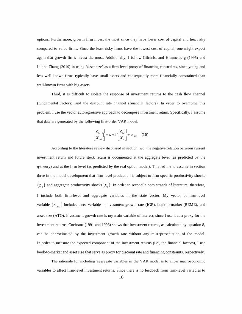
Third, it is difficult to isolate the response of investment returns to the cash flow channel
(fundamental factors), and the discount rate channel (financial factors). In order to overcome this
problem, I use the vector autoregressive approach to decompose investment return. Specifically, I assume
that data are generated by the following first-order VAR model:
)16(1,,
1
1,+
+
+ +
Γ+=
ti
t
ti
t
tiu
X
Za
X
Z
According to the literature review discussed in section two, the negative relation between current
investment return and future stock return is documented at the aggregate level (as predicted by the
q-theory) and at the firm level (as predicted by the real option model). This led me to assume in section
three in the model development that firm-level production is subject to firm-specific productivity shocks
( )itZ and aggregate productivity shocks( )tX . In order to reconcile both strands of literature, therefore,
I include both firm-level
and aggregate
variables in the state vector. My vector of firm-level
variables( )1, +tiZ includes three variables - investment growth rate (IGR), book-to-market (BEME), and
asset size (ATQ). Investment growth rate is my main variable of interest, since I use it as a proxy for the
investment returns. Cochrane (1991 and 1996) shows that investment returns, as calculated by equation 8,
can be approximated by the investment growth rate without any misrepresentation of the model.
In order to measure the expected component of the investment returns (i.e., the financial factors), I use
book-to-market and asset size that serve as proxy for discount rate and financing constraints, respectively.
The rationale for including aggregate variables in the VAR model is to allow macroeconomic
variables to affect firm-level investment returns. Since there is no feedback from firm-level variables to
17
aggregate variables, I constrain the lower left corner of Γ matrix to zero. In this context, I use a four-
aggregate variable vector ( )1+tX that includes variables that have a common “business cycle” component
that forecasts aggregate investment returns. Similar to Cochrane (1991 and 1996), these variables include
aggregate investment growth rate, term premium (defined as the ten-year government bond return minus
Treasury bill return), corporate premium (measured as the difference between corporate bond return and
Treasury bill return), and the lagged real value weighted stock return.
After estimating the VAR model in equation 16, my next step is to use these parameter estimates
to decompose investment returns into two components, as in equation 13. Since discount rate news reflect
the predictable component of investment returns, the expected investment return news( )InvestmenttiDRN 1,, +
can be
expressed using the following function:
)17(1 1,1,, ++ ′= tiInvestment
tiDR ueN λ
Where ( ) 1−Γ−Γ≡ ρρλ I , 1′e is a vector with the first element equal to one and the remaining elements
equal to zero [ ]( )00000011 ≡′e , ''Γ is the estimated VAR transition matrix, and ''ρ is set equal to
0.937. Equation 17 models the discount rate news as a linear function of the t+1 shock vector, so that the
greater the ability of the VAR state variables (in the first row of the VAR matrix) to predict investment
return, the higher the predictable component in investment return, and consequently, the greater the
discount rate news.
Once I calculate discount rate news using equation 17, cash flow news( )InvestmenttiCFN 1,, +
can be
computed directly as residuals. Specifically, I can restate equation 13 to define cash flow news as the sum
of unexpected investment return and expected (discount rate) news:
[ ] - Return Investment Unexpected Investment1,,
Investment1,,1,1, ++++ =−= tiDRtiCF
Investmenttit
Investmentti NNrErQ
( )
( ) )18( 11
1e 1
NReturn Expected Return Investment Unexpected
1,
1,1,
1ti,DR,1,,
+
++
++
′+′=
′+′=
+=∴
ti
titi
InvestmentInvestmenttiCF
uee
uue
N
λ
λ
18
Equation 18 says that if all of the firm-level and aggregate variables’ coefficients in the first row
of the estimated VAR transition matrix( )Γ have zero values (i.e., the investment returns are completely
unpredictable), the expected return news ( )1,'
1,, ++ = tiInvestment
tiDR uN λ will have zero value and the investment
return will be driven only by the cash flow news( )1,1,, 1 ++ ′= tiInvestment
tiCF ueN .
I use the above extracted news terms to empirically test the first hypothesis that examines how
much of the variability in investment returns is due to variability in the marginal product of capital
(proxied by the cash flow news in equation 18) and how much is due to variability in the cost of capital
(proxied by the discount rate news in equation 17). To this end, I calculate the variance-covariance matrix
for the cash flow news and discount rate news. The magnitude of the variance of the cash flow news
relative to the discount rate news can tell us whether the fundamental or financial factors are the major
driver of the firm-level investment returns.
The problem with the variance-covariance matrix, however, is that errors are unlikely to be
diagonal. This means that it is difficult to shock one variable while holding other variables constant.
Therefore, I use the impulse response function (IRF) to measure the response of investment return to a
lagged unit impulse in financial variables, while holding the fundamental factors constant. One of the
major drawbacks of using IRF is its sensitivity to variables ordering since the underlying assumption is
that variables that appear earlier in the system have contemporaneous and lagged effect on variables that
appear later in the ordering, while the variables that come later in the model have only lagged effect on
the previous variables in the ordering. Love and Zicchino (2006), for example, adopt a particular ordering
– the fundamental factor (proxied by sales-to-capital) followed by the financial factor (proxied by cash
flow scaled by capital) and the investment level. The problem with adopting a particular ordering is that it
is based on assumptions which might not be plausible, and, consequently, leads to major distortions in
IRF. To overcome the problem of order dependence, I use the orthogonalized or the generalized IRF3.
3 Pesaran and Shin (1998) show that the orthogonalized or the generalized IRF are the same only when examining the impulse responses of the shocks to the first equation in VAR (the first equation in the VAR matrix as estimated by equation (16) is the one of our particular interest in this paper).
19
2.4.2 Empirical Design for Testing Hypothesis 2: Beta Decomposition Approach
There is a wealth of empirical evidence for the cross-sectional negative relation between stock and
investment return. For example, Chen and Zhang (2010) develop a new three factor model
( )iROAROAi
InvestmentInvestmenti
InvestmentMarketifi urrrrr ++++=− βββϕ
that says that excess return on
a security is described by its sensitivity to three factors: the traditional market factor ( )Marketiβ
in addition
to two common factors formed on investment ( )Investmentiβ
and return on assets( ).ROA
iβ In order to
empirically test the second hypothesis, I need an econometric methodology in the manner of Campbell
and Vuolteenaho (2004) who decompose market return into cash flow and discount rate news in order to
break market beta( )Marketiβ into cash flow (bad) and discount rate (good) betas. My goal is to decompose
investment returns (rather than market returns) into cash flow and discount rate news in order to split
investment beta( )Investmentiβ (rather than market beta) into fundamental and financial betas. In order to
estimate these two betas, I use a two-step procedure. First, I need to estimate a common factor that serves
as a state variable that describe investment returns. Therefore, I approximate two equal weighted
portfolios for discount rate news and cash flow news, in the manner of Vuolteenaho (2002), as follows:
)19(11
1,1 1
1,,1, += =
++ ∑ ∑=≈ ti
n
i
n
i
InvestmenttiDR
InvestmenttDR u
nN
nN λ
( ) )20(1
111,
'
111,,1, +
==++ +=≈ ∑∑ ti
n
i
n
i
InvestmenttiDR
InvestmenttCF ue
nN
nN λ
)21( 1,1,1
InvestmenttCF
InvestmenttDR
Investmentt NNN +++ +=
Second, these two approximated aggregated channels allow me to break investment beta( )Investmentiβ
(i.e., the sensitivity of stock returns to the investment returns) into two betas – discount rate (financial)
beta and cash flow (fundamental) beta:
( )( ) )22(
, :Beta Financial
1
1,1,, Investment
t
InvestmenttDR
StocktitInvestment
iDR rVar
NrCov
+
++ −≡β
20
( )( ) )23(
, :Beta lFundamenta
1
1,1,, Investment
t
InvestmenttCF
StocktitInvestment
iCF rVar
NrCov
+
++ −≡β
The cash flow investment beta ( )InvestmentiCF ,β is defined as the covariance between stock returns
and cash flow investment returns, and I call it fundamental beta because it measures the sensitivity of
stock returns to the shocks from the fundamental marginal productivity of capital. In addition, the
discount rate investment beta ( )InvestmentiDR,β
is defined as the covariance between the stock returns and
discount rate component of investment returns, and I call it financial beta since it measures the sensitivity
of stock returns to financial factors.
These two betas are the ones of the interest since they are the empirical counterparts of both
channels that derive the negative relation between investment return and stock return, as estimated by
equation 15. In particular, fundamental beta reflects the cash flow channel (assuming a constant discount
rate, the higher the current level of investment, the lower the marginal product of capital, the lower the
expected stock returns) as predicted by Li, Livdan, and Zhang (2009). Alternatively, financial beta
reflects the discount rate channel (assuming constant returns to scale, the lower the discount rate, the
higher the current investment, the lower the future stock return). Past research had to control one channel
in order to examine the other, but using beta decomposition approach allows me to run a horse race
between both channels.
2.5 Data Description and Experimental Design
2.5.1 Basic Data
My data set consists of quarterly firm-level data as well as aggregate data from the first quarter
in 1963 to the second quarter in 2011. I start my sample period in 1963 to make my results more
comparable to those in literature. I obtain financial statement and balance sheet data from quarterly
COMPUSTAT, and stock return data from the Center for Research in Security Prices (CRSP).
I consider all domestic, primary stocks listed on the New York Stock Exchange (NYSE), American Stock
Exchange (AMEX), and NASDAQ stock markets.
21
2.5.2 Data Requirements
To be included in the tests, a firm must meet two criteria that have been used in the literature: First,
I exclude financial firms (i.e., firms in finance, insurance and real estate) such as closed-end funds, trusts,
ADRs, and REITs, due to the difficulty of interpreting their capital investment – which is our major focus
in this study. Since investment literature focuses mostly on manufacturing firm, I include only firms in
the manufacturing sector defined as those with primary standard industrial classifications (SIC) between
2000 and 3999. Second, I include only firms whose fiscal year end in December in order to align the
timing of firm-level and aggregate data across firms. Other studies, such as Vuolteenaho (2002), Liu,
Whited and Zhang (2009), and Xing (2008), use this requirement and they find that it does not affect the
representatives of the sample since the fiscal year of most firms ends in December.
2.5.3. Variables Definition
I use three firm-level variables – investment growth rate (IGR), Book-to-Market (BE/ME), and
asset size (ATQ). ‘IGR’ is measured as the growth rate in the firm’s capital expenditures( )11−−tt II , where
( )tI is defined as the sum of the firm’s quarterly gross property, plant, and equipment (PPEGTQ)
(investment in long-term assets) and the firm’s quarterly inventories (INVTQ) (investment in the short-
term assets). ‘BE’ is the quarterly book value of the equity defined as the sum of the COMPUSTAT book
value of common equity (CEQQ) and balance sheet deferred taxes and investment tax credit (TXDITCQ)
less the book value of preferred stock (PSTKQ). ‘ME’ is the market value of equity measured as the
quarterly closing price of common equity (PRCCQ) multiplied by the number of quarterly common
shares outstanding (CSHOQ). ‘ATQ’ is the quarterly book value of total assets.
In addition, I use four aggregate variables: aggregate real value weighted stock return (MKT),
default premium (default), term premium (term), and Aggregate investment growth rate (AIGR).
‘MKT’ is the excess returns on the S&P composite index over the consumer price index inflation.
‘Default’ is calculated as the difference between Moody’s seasoned yields on Baa and Aaa corporate
bonds. ‘Term’ is defined as the difference between 10-year government bond return and three-month
Treasury bill return. ‘AIGR’ is the quarterly change in the gross private domestic investment (GPDI).
22
‘MKT’ data is downloaded directly from French’s website, while ‘default’, ‘term’, and ‘AIGR’ are
obtained from the Federal Reserve Economic Data (FRED).
2.6 Empirical Results
Table 2.1 reports descriptive statistics that include means, standard deviations, minimums, and
maximums for firm-level (Panel ‘A’) and aggregate variables (Panel ‘B’) used in the composite VAR as
in equation 16. From Panel ‘A’, the investment growth rate has a mean of 0.26, and standard deviation of
95.76. The book-to-market ratio and quarterly asset size have a mean of -1.86 and 2885.52, respectively.
From Panel ‘B’, the aggregate investment growth rate has a mean of 0.85 and a standard deviation of
4.18. The market premium, default premium, and term premium have a mean of 1.49, 1.08, and 1.88,
respectively.
Table 2.1 Descriptive Statistics of the VAR Variables
Variable N Mean St. Deviation Min Max Panel (A): Descriptive Statistics – Firm-level variables
Table 2.2 presents the parameter estimates of the composite VAR in equation 16, using all the
forecasting variables that include firm-level variables ( )1, +tiZ and aggregate variables( ).1+tX The firm-level
variables include the growth rate in the firm’s capital expenditures (IGR), book-to-market ratio (BEME),
and the book value of total assets (ATQ). The aggregate variables include the aggregate real value
weighted stock return (MKT), the default premium (default), the term premium (term), and the growth
rate in the aggregate investment (AIGR). Each row of table 2.2 corresponds to a different equation of the
composite VAR. The first row in the table is the one of major interest since it implies that two out of
three firm-level variables have some ability to predict quarterly firm investment returns. In particular,
investment returns are high when past one-quarter book-to-market ratio and asset size are high.
23
In addition, the coefficient of firm investment returns on the term premium is significant at 10%. This
result is consistent with the findings of Cochrane (1991), and it means that term premium has a ‘business
cycle’ component that can predict the investment returns at the firm-level.
Table 2.2 Composite VAR Parameter Estimates
1−tIGR 1−tATQ 1−tBEME
1−tMKT 1−tDefault
1−tTerm 1−tAIGR 2R
tIGR -0.01 (0.08)
0.01** (0.01)
0.02* (0.01)
0.00 (0.02)
-0.25 (0.33)
-0.31** (0.15)
-0.01 (0.04)
6.48%
tATQ 35.57** (15.99)
0.91*** (0.03)
-7.95*** (2.57)
0.35 (4.23)
142.53*** (63.62)
36.36 (29.28)
-10.24 (7.95)
74.96%
tBEME -0.34 (0.49)
-0.01 (0.01)
0.30*** (0.08)
-0.17 (0.13)
2.84 (1.98)
-0.05 (0.91)
-0.37 (0.24)
17.59%
tMKT -0.05 (0.32)
-0.01 (0.01)
-0.01 (0.05)
0.06 (0.08)
0.67 (1.30)
0.80 (0.60)
-0.16 (0.16)
1.37%
tDefault -0.01 (0.01)
0.01*** (0.01)
0.01 (0.00)
-0.00 (0.00)
0.94*** (0.03)
-0.03 (0.01)
0.01 (0.00)
71.10%
tTerm -0.01 (0.02)
0.01 (0.01)
0.02 (0.02)
-0.01* (0.00)
0.16 (0.10)
0.84*** (0.04)
-0.01 (0.01)
72.50%
tAIGR 0.08 (0.15)
-0.01 (0.01)
-0.02 (0.02)
0.13*** (0.04)
-0.09 (0.61)
0.79*** (0.28)
0.29*** (0.07)
22.76%
Table 2.3 translates the VAR parameter estimates from table 2.2 into a function of( )λ'1e
where )00000001(1' ≡e , ( ) 1−Γ−Γ≡ ρρλ I , ,937.0≡ρ and Γ is the estimated VAR matrix.
The shock vector ( )iu
from each equation in the VAR system is linearly modeled as a function of( )λ'1e
to decompose the firm-level investment returns into investment cash flow news
( )( )1,'
1,, 11 ++ ′+= tiInvestment
tiCF ueeN λ and investment discount rate news( ).1 1,'
1,, ++ = tiInvestment
tiDR ueN λ I use these
extracted news terms to empirically test the first hypothesis that examines how much of the variability in
the investment returns is due to variability in the marginal product of capital (proxied by the cash flow
news) and how much is due to variability in the cost of capital (proxied by the discount rate news).
Panel (A) show the descriptive statistics of both news terms. The cash flow news has a mean of -0.82, and
standard deviation of 4.85, while the discount rate news has a mean of -0.86 and standard deviation of
2.93. These preliminary results show that the standard deviation of the firm-level cash flow news is
approximately twice the standard deviation of the discount rate news. Panel (B) shows the results of the
24
variance decomposition investment returns since it reports the covariance matrix of the news terms.
The results show that the variance of the cash flow news is 23.53 and the variance of the discount rate
news is 8.60. This means that 73% of the firm-level investment returns is attributed to variability in
marginal productivity of capital and only 27% is attributed to variability in cost of capital.
Table 2.3 Variance Decomposition of Firm-level Investment Returns
Panel (A): Descriptive Statistics Investment
tiDRN 1,, + Investment
tiCFN 1,, + Mean -0.8616 -0.8205
Standard Deviation 2.9330 4.8508 Minimum -17.0691 -34.4021 Maximum 6.0826 16.6046
Panel (B): The Covariance Matrix of the News Terms News Covariance Investment
tiDRN 1,, + Investment
tiCFN 1,, +
InvestmenttiDRN 1,, +
8.6029 13.5912
InvestmenttiCFN 1,, +
13.5912 23.5307
Although the above results from the variance decomposition might lead me to conclude that
fundamental factors are the dominant determinant of investment, these results show suspect because the
errors of the variance-covariance matrix are unlikely to be diagonal. Therefore, I proceed to the second
empirical test of hypothesis one which is the orthogonal impulse response function. Table 2.4 presents the
results of the orthogonal impulse response function that show the response of the system to an impulse,
and figure 2.2 reports graphs of impulse responses for the VAR model with three variables estimated –
.,, DRCF NNIGR The result of my particular interest is the response of investment return (IGR) to
the fundamental and financial variables (i.e., IGR is the response while DRCF NN and are the
impulses). In contrast to the results of the variance decomposition, I find that the impact of the lagged
financial news on investment return is much larger than the impact of the lagged fundamental news.
In particular, the long-run responses of IGR to an impulse in CF are -0.0615, -0.0153, -0.0181, -0.0177,
-0.0165 for lag 1, 2, 3, 4, and 5 respectively, while the long-run responses of IGR to an impulse in DR are
25
-0.2101, -0.2051, -0.1871, -0.1687, -0.1510 for lag 1, 2, 3, 4, and 5 respectively. These results, therefore,
indicate that discount rate news is the main driver of the firm-level investment returns.
Table 2.4 Orthogonal Impulse Response Function
Response\Impulse Lag CF DR IGR
CF
1 -0.0305 (0.5856)
0.7229 (0.5052)
0.2484 (1.3520)
2 0.0737 (0.3904)
0.6263 (0.4263)
0.2271 (1.2230)
3 0.0635 (0.3515)
0.5576 (0.3929)
0.2075 (1.0826)
4 0.0566 (0.3147)
0.4958 (0.3582)
0.1871 (0.9623)
5 0.0504 (0.2808)
0.4408 (0.3256)
0.1675 (0.8558)
DR
1 0.0257 (0.4656)
0.7760 (0.3806)
0.2019 (1.4608)
2 0.0774 (0.4010)
0.6842 (0.3891)
0.2171 (1.3256)
3 0.0687 (0.3725)
0.6100 (0.3846)
0.2123 (1.1814)
4 0.0617 (0.3388)
0.5430 (0.3631)
0.1979 (1.0524)
5 0.0551 (0.3048)
0.4830 (0.3362)
0.1802 (0.9367)
IGR
1 -0.0615 (0.2106)
-0.2101 (0.4017)
0.2019 (0.4658)
2 -0.0153 (0.0337)
-0.2051 (0.1329)
0.0560 (0.3986)
3 -0.0181 (0.0692)
-0.1871 (0.0734)
-0.0077 (0.3622)
4 -0.0177 (0.0837)
-0.1687 (0.0890)
-0.0341 (0.3265)
5 -0.0165 (0.0851)
-0.1510 (0.0979)
-0.0434 (0.2928)
Now, I turn to the empirical testing of the second hypothesis. To this end, I aggregate firm-level
news series by forming two equal weighted portfolios for cash flow and discount rate news using
formulas (19) and (20). After that, I sort the NYSE, AMEX, and NASDAQ stocks into five quintiles
based on investment growth rate (IGR). The portfolio “LOW” is the lowest IGR portfolio (quintile 1)
while the portfolio “HIGH” is the highest IGR portfolio (quintile 5). I then regress the returns of
investment growth rate (IGR) sorted portfolios on the aggregated cash flow and discount rate news, in
26
order to estimate the fundamental and financial beta, using equations (20) and (21), which add up to
investment beta.
Figure 2.2 Impulse Responses for 5 lag VAR of IGR CF DR
Table 2.5 puts such procedure to work. In particular, Panel (A) reports the value of fundamental
and financial betas for one-dimensional sorting by investment return proxied by IGR. Panel (B) shows the
results of those estimated betas for two-dimensional sorting by IGR and size. Taken together, the results
27
from both panels are consistent and show that the value of the financial betas is greater than the value of
fundamental betas for all decile portfolios whether based on one-dimensional and two-dimensional
classification. This means that financial factors rather than fundamental factors are the dominant driver of
the negative relation between investment and stock return.
Table 2.5 Fundamental and Financial Betas for Decile Portfolios
Panel (A): One-Dimensional Sorting by Investment Growth Rate (IGR) LOW 2 3 4 HIGH
InvestmentiCF , :Beta lFundamenta β -0.14772
(0.04183) -0.10044 (0.02638)
0.16529 (0.11775)
0.77371 (0.98806)
0.00670 (0.01761)
InvestmentiDR , :Beta Financial β 0.31199
(0.05047) 1.31838
(0.04871) 0.76478
(0.01794) 0.33666
(0.04054) 1.18781
(0.02846) Panel (B): Two-Dimensional Sorting by Investment Growth Rate (IGR) and Size (ATQ)
InvestmentiCF , :Beta lFundamenta β LOW 2 3 4 HIGH
Small -0.06692 (0.02292)
-0.21557 (0.11985)
-0.00907 0.00848
-0.00756 0.05655
0.00096 0.01030
2 -0.01217 (0.09470)
-2.76084 (1.23719)
0.35025 0.56244
-0.23083 0.49501
-0.02687 0.16659
3 0.07457 (1.19861)
-0.26303 (0.27965)
-0.45188 0.43491
0.27255 2.39302
-0.08907 0.09529
4 -0.000152 (0.00521)
0.82251 (0.60943)
0.35720 0.44032
0.07729 0.33695
1.51682 0.72185
Large -0.02648 (0.06557)
-0.00130 (0.00505)
-0.47260 0.53269
-0.19448 0.67965
0.33866 0.60685
InvestmentiDR, :Beta Financial β LOW 2 3 4 HIGH
Small 0.99645 (0.06943)
1.00918 (0.00600)
1.03531 0.00414
1.05704 0.00874
1.18341 0.02092
2 1.05882 (0.00919)
1.15174 (0.01114)
0.86616 0.00667
0.92090 0.00553
1.16572 0.01814
3 0.96569 (0.02577)
-0.26303 (0.27965)
0.40594 0.04997
0.08973 0.02492
0.21425 0.03294
4 0.92525 (0.03289)
0.94365 (0.02181)
0.95361 0.01683
0.91167 0.02445
0.83487 0.05281
Large 0.00201 (0.00574)
-0.04060 (0.01996)
0.09610 0.02811
0.31705 0.04348
0.36721 0.04212
28
CHAPTER 3
FINANCIAL CRISES AND THE GLOBAL VALUE PREMIUM:
REVISITING FAMA-FRENCH
3.1 Introduction
Financial crises occur with recurring patterns as evidenced by at least one severe global financial
crisis per recent decade – the 1987 stock market crash, the 1997 Asian financial crisis, and the 2007 credit
meltdown. A common feature of the crises of the last few decades has been the rapid spread from one
country to others in a process that has come to be known as “contagion”. Starting with the 1987 stock
market crisis that began in Hong Kong, global stock markets plummeted one after another in Europe and
in the United States. The 1997-1998 Asian crisis began in Thailand with the collapse of the Thai Baht and
spread rapidly into neighboring countries. The 2007-2008 financial crisis that hit the world as a result of
the implosion of the US mortgage market was followed by a series of collapses in major world markets.
The surprising frequency has stimulated extensive research related to crises.
This study investigates effects of financial market crises from two perspectives – the global
value premium and equity market integration. The primary purpose is to investigate whether or not the
global value premium is a risk factor affecting equity market integration. When a financial crisis occurs in
any region in the world with fears of contagion, risk-averse investors rush to quality and liquidity by
trying to get rid of high-risk, illiquid securities and replacing them with low-risk liquid securities.
Therefore, if global value stocks are fundamentally riskier than global growth stocks, one would expect
value stocks to perform more poorly than growth stocks during financial crises (Lakonishok et al., 1994).
The permanence of the effects evident during crises can be investigated by viewing pre-crisis and
post-crisis relationships. The study makes contributions to both integration literature and asset pricing
29
literature. It is the first attempt I found to investigate the impact of financial crises along two dimensions:
global value premium and financial integration. Financial integration can be defined in terms of either
a global market portfolio or Purchasing Power Parity (PPP). The global market portfolio argues that
international markets are integrated if all financial assets yield the same risk-adjusted expected returns to
investors the world over (assuming that investors do not hedge exchange rate risks and the single relevant
source of risk is the market portfolio). According to PPP, two financial markets are integrated if securities
are priced identically and the exchange risk premium is zero. My initial results indicate that countries
share “distress risk factors” (proxied by the global value premium) during four crisis periods.
The findings of distress risk motivate adding the global value premium as a third dimension for
measuring financial market integration. According to the new measure, financial markets are integrated if
value stocks underperform growth stocks in bad states of the world as proxied by financial crises.
This chapter proposes a new international asset pricing model that takes into account market
risk, foreign exchange risk, value premium, time-varying risk premium, and leverage effect, well-known
phenomena in the literature that refer to asymmetric responses of return volatility series to bad news and
good news. The model is named GJR-GARCH-FF because it is a composite of the asymmetric Sign
GARCH model developed by Glosten, Jagannathan and Runkle (1993) (GJR-GARCH model) and the
international version of the Fama and French model (1998). The original FF model is based on two
crucial assumptions – that purchasing power parity holds and that the price of risk is constant. The merit
of my newly introduced model is that it relaxes these two assumptions by adding the exchange risk
premium to the FF model and then incorporating it as the mean equation in the GJR-GARCH model.
The results show that the new model provides an attractive representation of countries’ returns since the
average intercept of the model is significantly lower than the FF two factor model.
The remainder of the chapter is organized as follows: data and crisis periods are explained in
section two, methodology is set forth in section three, empirical results are reported in section four, and
robustness tests are in section five.
30
3.2 Data and Crisis Periods
Data from January 1975 to December 2007 for thirteen countries – Australia, Belgium, France,
Germany, Hong Kong, Italy, Japan, Netherlands, Singapore, Sweden, Switzerland, the UK and the US –
is used to test the risk explanation for the global value premium, before, after and within crisis periods,
allowing for both long-run effects and shorter-run effects. Pre-crisis and post-crisis periods each require
a long data span to provide an adequate number of meaningful observations. Thus, for the pre-crisis and
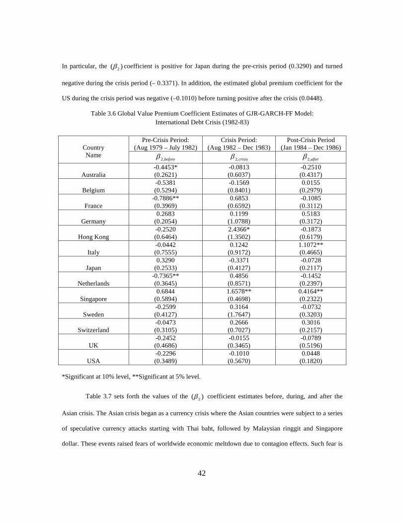
post-crisis analysis, I can include only two crises – the international debt crisis in 1982-1983 and the
Asian crisis in 1997-1998 – in order to ensure no overlapping observations. However, studying within
crisis periods allows for inclusion of four crises: the international debt crisis in 1982-1983, the ERM
crisis in 1992-1993, the Asian crisis in 1997-1998 and the September 11, 2001 attack.
Three important currencies—the British pound, German mark4 and Japanese yen proxy for
foreign exchange risk while the monthly market return is the value weighted average of returns for firms
in each country. The return on one-month US Treasury Bills is used as the risk-free rate, because the
analysis is from the perspective of a US investor. All of the exchange rate data is obtained from
Compustat, while the returns on individual countries’ portfolios, the global market portfolio, value and
growth portfolio, and the risk-free rate are obtained from Kenneth French’s homepage5.
A challenge in examining financial crises is to identify the precise beginning and ending of
a crisis, that is to pinpoint the source of the crisis (identify the major triggering event). According to the
Federal Deposit Insurance Corporation (FDIC) (1997), the international debt crisis officially started on
August 15, 1982 when Mexico declared its inability to pay its debt obligations. By the end of 1983, the
crisis management efforts could be called successful, since Mexico had fulfilled its interest payments and
the large international banks did not collapse. Therefore, I define the ‘debt crisis period’ from August
1982 to December 1983. According to the International Monetary Fund (1998), the Asian crisis began
4 On January 1, 1999, the euro was adopted by eleven countries – including Germany – as their official currency. Therefore, I use DM during the first part of the period and I then use the Euro as a proxy for the DM during the latter part of the study. 5 http://mba.tuck.dartmouth.edu/pages/faculty/ken.french/data_library.html.
31
July 2, 1997 when the bank of Thailand devalued the baht by roughly 20%. On March, 1999, the Asian
crisis had ended when the IMF approved a $1 billion increase in its emergency loan package for
Indonesia, and the DJIA closed above the 10,000 level for the first time in its history. Therefore, I define
the ‘Asian crisis period’ from July 1997 to March 1999. Table 3.1 shows the decomposition of the sample
period of the study for each crisis.
Table 3.1 Sample Period Description
Crisis Pre-Crisis Period Crisis Period Post-Crisis Period
International Debt Crisis Aug 1979 – July 1982 Aug 1982 – Dec 1983 Jan 1984 – Dec 1986
Asian Crisis July 1994 – June 1997 July 1997– Mar 1999 April 1999 – Mar 2002
3.3 Methodology
The goal is to test whether the global value premium is a risk premium rather than a behavioral
factor and whether the international equity markets become more integrated after financial crises.
3.3.1 Supporting Rationale
Two primary approaches for measuring financial market integration are market beta and
purchasing power parity (PPP). The more popular is beta as measured by the CAPM that assumes
investors do not hedge against exchange rate risks and the single relevant source of risk is the market
portfolio. However, studies differ in terms of the definition of the market portfolio as to whether it is
a global, local or hybrid portfolio. The global CAPM (the integration model) is based on the logic that the
international markets are perfectly integrated, such that all financial assets yield the same risk-adjusted
expected returns to investors the world over. In this case, the global portfolio risk is the only risk
considered. The domestic CAPM (the segmentation model) assumes that the local market is perfectly
segmented from the world market and, therefore, the capital markets may demonstrate substantially
different risk-return trade-offs. In this case, the local market portfolio will be the source of risk and
should replace the returns for the global index in the CAPM formulation. Many studies find evidence of
market segmentation (e.g., You et al., 2006; Bruner et al., 2008; Koedijk et al., 2002; Harris et al., 2003).
32
A more realistic approach than the two above versions is a two-factor Hybrid CAPM (Mid-Segmentation
Model) that assumes capital markets are neither perfectly integrated nor perfectly segmented, so that
global and domestic risk factors should be priced separately. This approach was originally launched by
Erunza and Losq (1985) and Erunza, Losq, and Padmanabhan (1992), and empirically supported by
Bruner et al. (2008). Finally, the Fama-French two factor model (1998) is an alternative version of CAPM
that says that international returns are explained by the value premium and the global market premium.
They empirically test their model and find that for thirteen countries the model fits the data well.
Rather than being defined in terms of the market portfolio, financial integration can also be
defined in terms of PPP based on the ‘Law of One Price’. The idea behind PPP is simple: once converted
to a common currency at current exchange rates, national prices should be equal. According to PPP,
therefore, two financial markets are integrated if securities are priced identically and the exchange risk
premium is zero. Any deviations from PPP cause national investors to perceive different exchange rate
adjusted returns from the same security and thus the exchange risk premium should be considered. Solnik
(1983) was the first to explore this issue by arguing that CAPM should contain an exchange risk premium
in addition to the market risk premium when PPP is violated. Wu (2008) finds that the international
version of the FF model does not fit the data well, and he documents that the international CAPM with
exchange risk is the best international model for forecasting compared to the CAPM and the FF model.
3.3.2. Model Development
The cited literature reveals two primary weaknesses in modeling the first and second moments.
First: there is no clear-cut determination of the best international asset pricing model in explaining
international returns. Asset pricing models that use beta as an integration measure differ in many regards
such as whether to include the home country or the global index as the mean-variance efficient portfolio
in the regression; whether to include exchange rate risk as an additional source of risk; and whether to
incorporate the value premium as captured by Fama and French (1998) in the CAPM regression.
Second: a common weakness in studies that apply CAPM in the international setting is that they are based
on the constant price of risk (CRP) assumption inherent in CAPM. However, a time-varying risk
33
premium on equities is widely documented in the literature. This means that investors’ expectations about
future security returns are conditional on all available information, and that modeling integration of
financial markets without taking into account this time variation will yield imprecise results.
Therefore, the CRP assumption should be relaxed to allow the price of market risk to vary over time.
In light of these two methodological observations in the international CAPM literature, I propose
a new model that takes into account market risk, foreign exchange rate risk, the value premium, and a
time-varying risk premium. In particular, the FF two factor model assumes that there is no deviation from
PPP and the price of risk is constant. This study relaxes these two assumptions. To this end, I add two
modifications to the original FF two-factor model: first, I assume that PPP does not hold by adding the
foreign exchange risk premium as another risk factor in addition to the market risk premium and the value
premium. Second, in order to relax the constant risk price (CRP) assumption, I incorporate the new model
as the mean equation in the asymmetric GJR-GARCH model. Although conditional heteroskedasticity
models appear to be among the best that are currently available, there is a major drawback of using first
generation of GARCH models because they are said to be symmetrical, due to the quadratic specification
used for the conditional variance (i.e., the error term is squared). Therefore, volatility will be a function
only of the innovation’s magnitude, since the lagged shock will have the same effect on the present
volatility whether the lagged shock is positive or negative (i.e., neutral impact). This symmetrical nature
of the traditional GARCH models makes them not well suited for capturing a well-known phenomenon of
asymmetric volatility in stock returns series or what is called asymmetric or leverage effects (e.g., French,
Schwert and Stambaugh, 1987; Glosten, Jagannathan and Runkle, 1993). The asymmetric volatility
phenomenon (AVP) is a market dynamic that shows that periods of crisis (when residual is negative)
cause the level of market volatility to increase more than in periods of relative calm (when residual is
positive). To handle the asymmetries in the conditional variance, I use the asymmetric Sign-GARCH
model of Glosten, Jagannathan and Runkle (1993) (GJR-GARCH model) that allows for different
reactions of volatility to the sign of past innovations. I call the newly created model GJR-GARCH-FF,
34
because it is a composite of both the GJR-GARCH model with the FF model. Mathematically, it can be
represented as follows:
( ) ( )( ) ( ) ( )
( )
(1) otherwise ,0
0 if ,1 :Where
),0(~ .,........,
1-ti,1,
21,1,
11
21,
11
21,
110
2,
2,2,1-ti,ti,
,543
2,,10,,
<
=
+++=
++++
−+−+=−
−
−−=
−=
−=
−
∑∑∑ε
ελσδεαασ
σεεε
εβββ
βββ
ti
titi
r
iti
p
iti
q
iti
titi
ti
tftgtfti
S
S
YenMarkPound
LHrrrr
The model consists of two equations: the mean equation and the variance equation. In the mean
equation, the excess monthly market return for a country is computed by subtracting the risk-free rate
)( fr from the monthly market return for that country )( ,tcr . The excess return of a country is a function of
three risk factors: global market risk premium )( , ftg rr − where )( ,tgr is the return on the global equity
market portfolio, the value premium (H–L) measured by the return difference between the high and low
BE/ME portfolio for each country, representing the international version of the distress factor in the FF
two-factor model, and the exchange risk premium proxied by three selected important currencies that are
the British Pound, German Mark, and Japanese Yen, with the US dollar as the reference currency.
The intercept )( 0β examines to what extent the new model can explain international returns, the )( 1β
coefficient measures integration, the )( 2β coefficient explores the risk explanation of the global value
premium, and the )( 3β ,
)( 4β and
)( 5β coefficients are exchange risk premiums and are used as control
variables. Following Fama and French (1998), I do not include size premium (small minus big- the
difference between the returns on diversified portfolios of small and big stocks) because the data for the
twelve countries (other than US) is from Morgan Stanley’s Capital International (MSCI) which primarily
includes large firms that represents 80 percent of a market’s invested wealth. It is clear from the above
formulation that the mean equation is the international Fama and French two-factor model with currency
risk. By incorporating such equation into the GJR-GARCH model, the new model becomes the
time-varying empirical counterpart to the FF model (with currency risk).
35
The variance equation expresses the current volatility (measured by variance )( 2,tiσ ) as a
function of four factors: the mean volatility )(a , news about volatility from the previous period measured
as the lag of the squared residual from the mean equation )( 21, −tiε (the ARCH term), the last period's
variance )( 21, −tiσ (the GARCH term) to control for volatility clustering, and the asymmetric volatility term
)( 21,1, −− titiS ε to account for the leverage effect. A model with ‘q’ lags of )( 2
1, −tiε , ‘p’ lags of )( 21, −tiσ and
‘r’ lags of )( 21,1, −− titiS ε is labeled GJR (p, q, r), and I determine the lag structure in the conditional
variance equation based on Akaike (AIC) and Bayesian (BIC) information criteria. The central feature of
the above specification is that the dummy variable (S) allows the conditional variance to differ on crash
days, since the effect of lagged shock on current volatility now is a function of its magnitude and its sign
rather than its magnitude only, as in the original GARCH models. Specifically, volatility is affected by
one term )( iα when the residual is negative (i.e., good news), while it is affected by two terms
)( ii λα + when the residual is negative (i.e., bad news).
3.4 Empirical Results
3.4.1 FF Model versus GJR-GARCH-FF Model
My goal in this section is to evaluate the ability of the GJR-GARCH-FF model to explain
international returns. To this end, I perform three different tests. As a preliminary test, I use the standard
GJR-GARCH (p, q, r) model (under the restriction that )054321 ===== βββββ to model the
monthly excess return for individual countries. I test several GARCH (p) terms, ARCH (q), and
asymmetric (r) terms and find that the most appropriate model is GJR-GARCH (3, 1, 1):
( )
(2) otherwise ,0
0 if ,1 :Where
),0(~ .,........, ;
1-ti,1,
21,1,1
23,3
22,2
21,1
21,10
2,
2,2,1-ti,ti,,0,,
<
=
+++++=
+=−
−
−−−−−−
−
ε
ελσδσδσδεαασ
σεεεεβ
ti
tititititititi
titititfti
S
S
Nrr
36
Table 3.2 sets forth results of estimating equation 2 and shows that most of the estimated
coefficients of the ARCH term )( 1α and the three GARCH terms ),,( 321 δδδ are highly significant at
1% for almost all of the countries. Moreover, the asymmetry parameters are statistical significant for most
of the countries, indicating the presence of the leverage effect. This indicates that GJR-GARCH
is an acceptable representation of international returns and shows the existence of changing conditional
variance in return series in international markets.
In the second test, the following three international asset pricing models are investigated relative
to my model in order to examine which model best describes international returns data:
One factor global CAPM: ( ) (3) r ti,,tg,10,, εββ +−+=− tftfti rrr
Table 3.3 sets forth the intercepts obtained from each model. They should be insignificantly
different from zero if the model fits the data well. The average intercept of the GJR–GARCH–FF model
is lower than that of the other three models. Specifically, the average intercept of the GJR-GARCH-FF
model is lower in magnitude and significance than the intercept of the one factor global CAPM and the
global CAPM with foreign exchange risk. More importantly, the average mean in the GJR-GARCH-FF
model is lower than the FF model in nine out of thirteen countries, particularly important because three of
these nine countries are G5 countries – USA, France, and Italy.
Additional evidence comes from Table 3.4 that presents results of the remaining estimated
coefficients of the mean equation ( ),,,, 54321 βββββ and in the GJR-GARCH-FF model. The FF
two-factor model and the GJR-GARCH-FF model produce similar market and value slopes with similar
levels of significance. This indicates that adding the exchange risk premium and the conditional volatility
equation yields better results in describing international returns.
37
Table 3.2 Maximum Likelihood Estimates of GJR-GARCH (3, 1, 1) Model – Without Risk Factors (Entire Sample Period: January 1975 – December 2007)
*Significant at 10% level, **Significant at 5% level, ***Significant at 1% level.
Country Name 1α 1δ 2δ
3δ 1λ
Australia 0.0404***
(0.0114)
2.3619***
(0.0404)
-2.2783***
(0.0706)
0.8838***
(0.0417)
-0.0356***
(0.0110)
Belgium 0.1913***
(0.0506)
0.0942**
(0.0446)
-0.0830**
(0.0448)
0.7013***
(0.0826)
0.0703
(0.0693)
France 0.0426***
(0.0184)
2.0433***
(0.0443)
-1.8961***
(0.0770)
0.7690***
(0.0498)
0.0630**
(0.0259)
Germany 0.1621**
(0.0688)
0.2898
(0.2432)
0.4931*
(0.2876)
-0.0511
(0.3052)
-0.0107
(0.0674)
Hong Kong 0.2192***
(0.0662)
0.5077***
(0.1672)
0.8461***
(0.0373)
-0.5112***
(0.1542)
-0.1616***
(0.0595)
Italy 0.0177***
(0.0002)
-0.7249***
(0.0107)
1.0052***
(0.0017)
0.7341***
(0.1086)
0.0035
(0.0077)
Japan 0.03112*
(0.0192)
1.1706***
(0.0375)
-1.1580**
(0.0525)
0.8761***
(0.0453)
0.0768**
(0.0309)
Netherlands -0.0379
(0.0255)
0.7928***
(0.0800)
-0.8175***
(0.1008)
0.6258***
(0.0898)
0.1665***
(0.0555)
Singapore 0.0844***
(0.0177)
0.8196***
(0.0261)
0.8737***
(0.0261)
-0.7652***
(0.0143)
-0.0597***
(0.0186)
Sweden 0.1602***
(0.0552)
0.7983***
(0.0995)
-0.7519***
(0.1049)
0.5746***
(0.1133)
0.0931
(0.0791)
Switzerland 0.3084***
(0.0938)
-0.3907***
(0.1207)
0.6247***
(0.0701)
0.3168**
(0.1677)
-0.1953**
(0.0852)
UK 0.0788***
(0.0247)
1.7593***
(0.046262)
-1.6134***
(0.0951)
0.7090***
(0.0550)
0.0400
(0.0288)
USA -0.0620
(0.0637)
0.0852
(0.1927)
0.3766**
(0.1690)
0.1134
(0.1802)
0.3508***
(0.1300)
38
Table 3.3 Comparison of Different International Asset Pricing Models:
Country Name
One Factor Global CAPM
Global CAPM with FX Risk
FF Model
GJR-GARCH-FF Model
Australia
0.328853 (0.282700)
0.321424 (0.286223)
0.120349 (0.286348)
0.0780 (0.25665)
Belgium
0.405651** (0.206155)
0.394714* (0.207974)
0.356302* (0.211370)
0.3583* (0.1942)
France
0.228604 (0.240311)
0.185902 (0.240505)
0.319353 (0.245871)
0.1062 (0.1509)
Germany
0.271052 (0.208022)
0.268132 (0.205090)
0.183952 (0.212662)
0.2472 (0.1981)
Hong Kong
0.677500* (0.376465)
0.640320* (0.380580)
0.523385 (0.384936)
0.3869 (0.3411)
Italy
0.116628 (0.313361)
0.170572 (0.317154)
0.059972 (0.321484)
0.0329 (0.2709)
Japan
-0.246033 (0.165586)
-0.296351* (0.157472)
-0.199058 (0.169678)
-0.2254 (0.1673)
Netherlands
0.432684* (0.175061)
0.456496*** (0.173707)
0.408708** (0.179660)
0.2165 (0.1616)
Singapore
0.323239 (0.308772)
0.259758 (0.308973)
0.044425 (0.310601)
0.1539 (0.2690)
Sweden
0.442448* (0.265767)
0.421945 (0.265129)
0.464788* (0.272828)
0.3766 (0.2439)
Switzerland
0.342963* (0.723976)
0.339132* (0.193750)
0.291839 (0.197005)
0.1671 (0.1895)
UK
0.361359* (0.217785)
0.442408** (0.190551)
0.309597 (0.223299)
0.0661 (0.1289)
USA
0.336955* (0.183803)
0.292019 (0.181723)
0.340052* (0.188718)
0.2332 (0.1799)
*Significant at 10% level, **Significant at 5% level
The final diagnostic test is the ARCH LM Test, which is a Lagrange multiplier (LM) test for
autoregressive conditional heteroskedasticity (ARCH) in the residuals since ignoring ARCH effects may
result in a loss of efficiency. To test the null hypothesis that there is no ARCH up to order q in the
residuals, a regression of the squared residuals )( 2tε on constant and lagged squared residuals up to order
q is run, as follows:
t
q
sstst µεββε +
+= ∑
=−
1
20
2
This particular specification of heteroskedasticity is motivated by the observation that in many
financial time series, the magnitude of residuals appears to be related to the magnitude of recent residuals.
39
Table 3.4 Maximum Likelihood Estimates of the GJR-GARCH-FF (3, 1, 1) Model: (Entire Sample Period: January 1975 – December 2007)
*Significant at 10% level, **Significant at 5% level
If the variance equation is correctly specified, there should be no ARCH remaining in the standardized
residuals. Table 3.5 reports the results of the F-statistics for the Lagrange Multiplier test. The values of
Country Name
1β 2β 3β 4β
5β
Australia 0.9643***
(0.0475)
0.3035***
(0.0874)
-13.2677
(14.9505)
12.1657
(9.4389)
-8.4258
(10.0956)
Belgium 0.7842***
(0.0354)
0.1209**
(0.0605)
11.4240
(8.8093)
4.4949
(2.9505)
-7.1480
(6.2745)
France 1.0488***
(0.0369)
-0.0085
(0.0487)
-15.8766
(10.6198)
12.7131***
(2.2681)
-18.6552***
(6.4500)
Germany 0.8841***
(0.0394)
0.1217**
(0.0605)
-2.7082
(8.2640)
14.4222***
(2.0880)
-18.0845**
(7.2382)
Hong Kong 0.9744***
(0.0684)
0.1623
(0.1124)
-2.7809
(16.6076)
-9.9128
(15.0074)
8.6519
(15.6419)
Italy 0.9720***
(0.0645)
0.0887
(0.0882)
-0.7660
(13.1864)
2.9652
(9.6852)
-4.0444
(10.7835)
Japan 1.1148***
(0.0302)
-0.0484
(0.0486)
-26.408***
(9.2015)
-6.0782*
(3.4905)
32.1272***
(6.5921)
Netherlands 0.8727***
(0.0339)
0.0550
(0.0428)
1.9586
(6.6565)
-4.0104
(3.6234)
-20.3498***
(5.9884)
Singapore 0.7769***
(0.0535)
0.4051***
(0.1007)
-11.3974
(15.1652)
-8.1434
(13.2926)
7.9714
(10.9933)
Sweden 0.9607***
(0.0521)
0.0879
(0.0786)
-24.3429*
(12.7325)
13.6049
(11.4274)
-25.6233***
(10.0470)
Switzerland 0.6878***
(0.0336)
0.1009*
(0.0619)
6.6354
(8.6565)
5.4241**
(2.7425)
-0.5114
(7.0024)
UK 0.8400***
(0.0307)
0.1142***
(0.0411)
38.8402***
(8.9922)
1.2024
(5.1374)
-13.7862**
(5.4624)
USA 0.6063***
(0.0345)
-0.0324
(0.0404))
-21.8383**
(10.5614)
5.2890
(8.4082)
-22.2785***
(8.4195)
40
LM are insignificant for all countries (except France). This result leads to the rejection of the null
hypothesis (i.e., the residuals are homoscedastictic), meaning that the variance equation in the GJR-
GARCH model has been correctly formulated.
Table 3.5 ARCH-LM Test of the GJR-GARCH-FF model
Country Name
ARCH-LM
Lag (1) Lag (2) Lag (3) Lag (4) Lag (5)
Australia
0.0032
(0.0510)
-0.0126
(0.0509)
0.0264
(0.0508)
0.0930
(0.0555)
0.0036
(0.0557)
Belgium
-0.0250
(0.0509)
0.0297
(0.0512)
-0.0148
(0.0512)
-0.0280
(0.0511)
0.0261
(0.0511)
France
0.1184*
(0.0510)
0.0576
(0.0514)
-0.0443
(0.0514)
0.0324
(0.0514)
0.0072
(0.0510)
Germany
-0.0511
(0.0508)
0.0423
(0.0508)
0.0382
(0.0508)
-0.0364
(0.0507)
0.0299
(0.0508)
Hong Kong
-0.0398
(0.0508)
0.0266
(0.0508)
0.0191
(0.0506)
-0.0265
(0.0506)
0.1024
(0.0505)
Italy
0.0415
(0.0511)
0.0071
(0.0512)
0.0085
(0.0511)
-0.0029
(0.0512)
0.0081
(0.0511)
Japan
0.0008
(0.0506)
-0.0016
(0.0506)
0.0009
(0.0505)
0.0752
(0.0505)
0.0276
(0.0506)
Netherlands
-0.0013
(0.0508)
-0.0251
(0.0508)
0.0312
(0.0507)
0.0572
(0.0507)
-0.0040
(0.0508)
Singapore
-0.0007
(0.0510)
-0.0213
(0.0510)
-0.0288
(0.0510)
0.0436
(0.0513)
0.0008
(0.0514)
Sweden
-0.0085
(0.0507)
0.0397
(0.0507)
-0.0039
(0.0509)
-0.0146
(0.0509)
-0.0411
(0.0509)
Switzerland
0.0305
(0.0516)
0.0192
(0.0516)
0.0547
(0.0515)
-0.0175
(0.0516)
0.0303
(0.0514)
UK
0.0351
(0.0510)
0.0074
(0.0510)
0.0060
(0.0514)
0.0078
(0.0514)
-0.0422
(0.0514)
USA
-0.0288
(0.0508)
0.0780
(0.0507)
-0.0017
(0.0509)
0.0213
(0.0508)
0.0082
(0.0508)
41
3.4.2 Fundamental Riskiness of the Global Value Premium
Following the approach of Lakonishok et al. (1994) where a fear of market breakdown causes
risk-averse investors to rush to quality and liquidity, I examine the performance of global value strategies
(high BE/ME – low BE/ME) for the thirteen countries in the sample during financial crises. The rationale
is that if value stocks are fundamentally riskier than glamour stocks, then risk-averse investors should
replace risky value stocks with less risky glamour stocks during economic recessions when the marginal
utility of consumption is especially high6. Therefore, one would expect the global premium coefficient
)( 2β from equation (1) during crisis period to be lower than that of pre-crisis and post crisis period.
Table 3.6 reports results of the estimated coefficients of the global value premium )( 2β from
equation (1) for pre-crisis, crisis, and post-crisis periods for the international debt crisis. Although several
of the world’s largest banks faced the prospect of major loan defaults as a consequence of the crisis, the
fear of a widespread banking collapse in creditor countries was concentrated primarily in the USA and
Japan7. It is easy to understand, therefore, that Japan is the only country in table 3.6 whose
global premium coefficient is lower during crisis period than during pre-crisis and post-crisis periods.
6 A striking example that supports the rationale of such an approach is the collapse of Long-Term Capital Management (LTCM). In January 1998, the spread between high-yield corporate bonds and US treasuries was 4 percentage points. LTCM believed that such spread was excessively wide as a consequence of the Asian crisis, and that this spread would narrow when the crisis ended. Consequently, LTCM engaged in ‘market neutral arbitrage’ by longing high-yielding, less liquid bonds and shorting low-yielding, more liquid bonds. By August 1998, the crisis continued and fear spread over the world because of the collapse of the Russian market. Consequently, the spread between US B-rated bonds and high-rated corporate bonds rose from 2 percentage points before the crisis to 5.7 percentage points. This wide spread led to the collapse of the LTCM by September 1998 (Edwards, 1999). 7 The US banks’ exposure was the highest because the major debtors were concentrated in Latin America. The largest Latin American countries (Mexico, Brazil, Venezuela, and Argentina) owed the eight largest US banks $37 billion that constituted 147% of their capital and reserves at the end of 1983. The size of such debt coupled with the overexposure (lending in excess of capital assets) gave rise to a fear of financial collapse to the largest American banks such as Citibank, Bank of America, Chase Manhattan, and Morgan Guaranty (FDIC, 1997). The Japanese banks also had a similar rate of debt exposure. the exposure level of the Bank of Tokyo (that handled $753 million as the leading international bank in forming syndicate loans by 1981 in Mexico) was 83% of its capital, and the exposure of Long-Term Credit Bank of Japan and Mitsui Bank was 53.6% and 28.3%, respectively (Katada, 2001).
42
In particular, the )( 2β coefficient is positive for Japan during the pre-crisis period (0.3290) and turned
negative during the crisis period (– 0.3371). In addition, the estimated global premium coefficient for the
US during the crisis period was negative (–0.1010) before turning positive after the crisis (0.0448).
Table 3.6 Global Value Premium Coefficient Estimates of GJR-GARCH-FF Model: International Debt Crisis (1982-83)
Country Name
Pre-Crisis Period: (Aug 1979 – July 1982)
Crisis Period: (Aug 1982 – Dec 1983)
Post-Crisis Period (Jan 1984 – Dec 1986)
before,2β crisis,2β after,2β
Australia
-0.4453* (0.2621)
-0.0813 (0.6037)
-0.2510 (0.4317)
Belgium
-0.5381 (0.5294)
-0.1569 (0.8401)
0.0155 (0.2979)
France
-0.7886** (0.3969)
0.6853 (0.6592)
-0.1085 (0.3112)
Germany
0.2683 (0.2054)
0.1199 (1.0788)
0.5183 (0.3172)
Hong Kong
-0.2520 (0.6464)
2.4366* (1.3502)
-0.1873 (0.6179)
Italy
-0.0442 (0.7555)
0.1242 (0.9172)
1.1072** (0.4665)
Japan
0.3290 (0.2533)
-0.3371 (0.4127)
-0.0728 (0.2117)
Netherlands
-0.7365** (0.3645)
0.4856 (0.8571)
-0.1452 (0.2397)
Singapore
0.6844 (0.5894)
1.6578** (0.4698)
0.4164** (0.2322)
Sweden
-0.2599 (0.4127)
0.3164 (1.7647)
-0.0732 (0.3203)
Switzerland
-0.0473 (0.3105)
0.2666 (0.7027)
0.3016 (0.2157)
UK
-0.2452 (0.4686)
-0.0155 (0.3465)
-0.0789 (0.5196)
USA
-0.2296 (0.3489)
-0.1010 (0.5670)
0.0448 (0.1820)
*Significant at 10% level, **Significant at 5% level.
Table 3.7 sets forth the values of the )( 2β coefficient estimates before, during, and after the
Asian crisis. The Asian crisis began as a currency crisis where the Asian countries were subject to a series
of speculative currency attacks starting with Thai baht, followed by Malaysian ringgit and Singapore
dollar. These events raised fears of worldwide economic meltdown due to contagion effects. Such fear is
43
in line with the results in table 3.7 that indicate that )( 2β coefficients during the crisis period are lower
than those during the pre-crisis period for nine out of thirteen countries. The results from Tables 3.6 and
3.7 support the risk explanation of the global risk premium, although the results are weak since most of
the estimated coefficients are insignificant.
Table 3.7 Global Value Premium Coefficient Estimates of GJR-GARCH-FF Model: Asian Crisis (1997-99)
Country Name
Pre-Crisis Period: (July 1994-June 1997)
Crisis Period: (July 1997- Mar 1999)
Post-Crisis Period (April 1999 – Mar 2002)
before,2β crisis,2β after,2β
Australia
0.1805 (0.4098)
0.1108 (0.4847)
0.3172** (0.1339)
Belgium
0.4891*** (0.3244)
-0.5747* (0.3172)
0.3030* (0.1872)
France
0.4811 (0.4432)
-0.0526 (0.2416)
0.0456 (0.0741)
Germany
0.8470** (0.4286)
-0.1182 (0.3106)
-0.1212 (0.1306)
Hong Kong
0.5641 (1.0583)
-0.4689 (0.8817)
-0.0110 (0.1842)
Italy
0.9196 (0.9246)
-0.0107 (0.4164)
-0.2834** (0.1229)
Japan
-0.8629*** (0.3077)
-0.0874 (0.4965)
-0.1214*** (0.1030)
Netherlands
0.7653** (0.3350)
-0.4296 (0.3171)
0.1409** (0.0830)
Singapore
1.8167*** (0.4452)
-0.2188 (0.7141)
0.2307 (0.3108)
Sweden
0.3529 (0.7445)
0.4417 (0.4403)
-0.3953 (0.3260)
Switzerland
-0.9893** (0.4824)
-0.1612 (0.2379)
0.1940** (0.1079)
UK
0.2333 (0.2988)
0.1233 (0.1884)
0.0853* (0.0503)
USA
0.1535 (0.4239)
0.1593 (0.4444)
0.0118 (0.1581)
*Significant at 10% level, **Significant at 5% level, ***Significant at 1% level.
3.4.3 Financial Crises and Integration
This section investigates the impact of financial crises – via contagion – on the integration of
international financial markets. By comparing the coefficients from regressing each country’s portfolio
44
return on the global market premium )( 1β from equation (1) for each of the pre-crisis, crisis, and
post-crisis periods, I can measure the impact of the financial crises on the integration of financial markets.
Table 3.8 presents the values of )( 1β from equation (1) covering the three sub-periods of
the international debt crisis. Comparison of results from the pre-crisis period and crisis period reveals that
the size of )( 1β is greater in the pre-crisis period for ten out of thirteen countries – Australia, France,
Hong Kong, Italy, Netherlands, Singapore, Sweden, Switzerland, the UK, and the USA. Surprisingly,
Hong Kong and Australia were positively correlated with the global market portfolio before the crisis but
become negatively correlated during the crisis. Comparison of the )( 1β coefficient from the pre-crisis
Table 3.8 Global Market Portfolio Coefficient Estimates of GJR-GARCH-FF Model: International Debt Crisis (1982-83)
Country Name
Pre-Crisis Period: (Aug 1979 – July 1982)
Crisis Period: (Aug 1982 – Dec 1983)
Post-Crisis Period (Jan 1984 – Dec 1986)
before,1β crisis,1β after,1β
Australia
1.1118*** (0.1645)
-0.8127** (0.6037)
0.9756*** (0.2682)
Belgium
0.7081*** (0.1977)
1.2394** (0.5000)
0.7800*** (0.2083)
France
1.4178*** (0.1582)
0.3092*** (0.2866)
0.8442*** (0.1412)
Germany
0.6757*** (0.1207)
0.9942** (0.5261)
0.8924*** (0.2111)
Hong Kong
1.7771*** (0.3810)
-0.0610 (0.9762)
0.4731 (0.4257)
Italy
0.8516** (0.3708)
-0.1291 (0.3584)
0.8011*** (0.2779)
Japan
0.8794** (0.1042)
1.5407*** (0.2443)
1.2304*** (0.1254)
Netherlands
0.9569*** (0.2528)
0.7272 (0.6111)
0.8119*** (0.1915)
Singapore
0.9028*** (0.3008)
0.7586 (0.5511)
0.3864** (0.1693)
Sweden
0.5523* (0.2107)
0.2716 (1.1124)
0.6633*** (0.1918)
Switzerland
0.9842*** (0.1539)
0.8704** (0.4140)
0.6158*** (0.1450)
UK
1.1464*** (0.2078)
0.6680*** (0.2245)
0.7515*** (0.2333)
USA
0.6064*** (0.1236)
0.4640 (0.3973)
0.2636 (0.1943)
45
period and the post-crisis period leads to similar conclusions. Except for Belgium, Germany, Japan, and
Sweden, the coefficient )( 1β is higher in the pre-crisis period than the post crisis-period. Thus, it
appears that international financial markets became less integrated after the debt crisis.
Table 3.9 sets forth the values of )( 1β coefficient for the Asian crisis. Its contents are
contradictory to those in Table 3.8 since twelve out of thirteen countries became more integrated (reveal
greater )( 1β coefficients) during the Asian crisis relative to the pre-crisis period. Comparison of the
pre-crisis period and the post crisis period confirms the results since )( 1β coefficients estimated using the
post crisis period are higher than those calculated in the pre-crisis period for all of the sample countries
except Japan. Thus international financial markets became more integrated after the Asian crisis.
Table 3.9 Global Market Portfolio Coefficient Estimates of GJR-GARCH-FF Model: Asian Crisis (1997-99)
Country Name
Pre-Crisis Period: (July 1994-June 1997)
Crisis Period: (July 1997- Mar 1999)
Post-Crisis Period (April 1999 – Mar 2002)
before,1β crisis,1β after,1β
Australia
0.8989*** (0.1553)
0.9518*** (0.2587)
1.0722*** (0.1907)
Belgium
0.4622*** (0.1150)
0.7729*** (0.2746)
0.6847*** (0.1642)
France
0.7650*** (0.2547)
1.2847*** (0.2119)
1.3981*** (0.1167)
Germany
0.4787*** (0.1880)
1.1914*** (0.1613)
1.1999*** (0.1302)
Hong Kong
0.9859*** (0.2522)
1.0754** (0.5796)
1.1230*** (0.1627)
Italy
0.6643** (0.3455)
1.3755*** (0.3069)
0.9783*** (0.1523)
Japan
1.5024*** (0.1284)
0.9548** (0.5770)
1.1388*** (0.1487)
Netherlands
0.7934*** (0.1282)
1.1156*** (0.2226)
1.0179*** (0.0728)
Singapore
0.4034** (0.2047)
1.1090 (0.7783)
0.8577*** (0.2638)
Sweden
0.6191** (0.3642)
1.5156*** (0.2108)
1.7028*** (0.2346)
Switzerland
0.5049** (0.2189)
0.7889*** (0.2141)
0.5832*** (0.1156)
UK
0.6108*** (0.1374)
0.7577*** (0.1011)
0.7841*** (0.0573)
USA
0.4899*** (0.1415)
0.9140*** (0.2371)
0.9726*** (0.1816)
46
For the selected sample period, the above results indicate that if the international debt crisis is
considered regional while the Asian crisis is considered global, effects of crises are dependent upon the
geographic impact of the individual crisis. In other words, financial crises with regional effects (such as
the less developed debt crisis that affected primarily Latin American countries) decrease financial
integration, while crises with global effects (such as the Asian crisis) increase integration. This new
evidence raises the issue of appropriate economic explanation. I believe the international debt crisis
reflects intra-regional contagion effects, while the Asian crisis reflects global herding behavior8.
During regional crises (such as the international debt crisis), investors pay little attention to
international news and focus primarily on regional news. In particular, when Mexico declared its inability
to pay its debt obligations in 1982, intra-regional contagion took place since difficulties in interest
payments were evident in most of the Latin American countries (e.g., Argentina, Brazil, Bolivia, Ecuador
and Venezuela). Consequently, investors began to withdraw their investments from the Latin American
market for safer markets. As a result, the Latin American countries adopted restrictive capital controls for
self-protection, further segmenting their markets. This implies an increase in gains from global market
portfolio diversification, since the Latin American countries become less integrated with the world.
In contrast to regional crises, global crises (such as the Asian crisis) affect the remainder of the
world. Investors’ decisions are affected not only by their local countries’ situation, but also by other
countries’ markets. This is evident in the Asian crisis when the Asian markets, with their vast global
capital flows, rode out their crises with increased cooperation not only with each other but with the
remainder of the world. As the Asian crisis continued and the global stock markets plummeted one after
another in Europe and in the United State and fear spread over the world, the herding behavior prevails
(i.e., investors start to follow the crowd leading to a uniform behavior among international investors).
This leads to a higher integration among international markets and, consequently, to lower diversification
benefits since equity markets are exposed to common systematic risk.
8 Chiang et al. (2007) differentiates between ‘contagion’ and ‘herding’ in the sense that the former reflects the spread of one shock from one market to another, while the latter describes the mechanism of a behavioral convergence among investors’ sentiments.
47
3.5 Robustness Tests: Short-term Effects (Within Crisis Period Analysis)
A common problem in empirical research of financial crises is that results might be affected by
the choice of window length. That is, my choice of duration of three years before and three years after the
crises may have an impact on the results. Therefore, I need another test that is not sensitive to period
duration to verify whether my period definition affects the central results. Therefore, I report month-by-
month returns on the highest BE/ME (value) relative to the lowest BE/ME (growth) portfolios for four
crises: the Latin American debt crisis (1982-1983), the European Monetary System (ERM) crisis (1992-
1993), the Asian crisis (1998-1999), and the September 11, 2001 attack. If global value stocks are
fundamentally riskier, one would expect a negative return for the value strategies during financial crises.
3.5.1 International Debt Crisis
As mentioned earlier, US and Japanese banks’ exposure was the greatest and they faced the
prospect of major loan defaults and failure as a consequence of the crisis. Table 3.10 reveals that monthly
returns on the US value strategy are negative in the three months following August 1982, the starting
month of the crisis. In addition, the average value premium during the entire crisis period (August 1982 –
December 1983) in the USA and Japan is zero and -0.68%, respectively. The value premium of -1.15 for
Hong Kong may relate to Hong Kong’s close relationship to Japan. Although the European banks had
less exposure to third world lending than did the U.S. and Japanese banks, the value strategy in August
and September of 1982 yielded negative returns in the UK, Germany, and Italy where the major European
banks are located.
3.5.2 ERM Crisis9
Table 3.11 shows the month-by-month returns of the value strategy during the ERM crisis from
September, 1992 until December, 1993, and reflects the fear of investors during the period.
9 The ERM crisis of 1992-1993 is a crisis of the exchange rate system. A primary reason for the crisis is the difference in economic strength of members of ERM. Germany witnessed a strong economy and was concerned about domestic inflation and raised its interest rate to 8.7%. The UK and Italy, however, were suffering from recession and severe budget deficits, forcing them to adopt stimulative policies by reducing interest rates. Such contradiction dramatically widened the interest rate differentials between Germany and other ERM members.
48
Table 3.10 Month-by-Month Returns during the International Debt Crisis Period (August 1982 – December 1983): Value – Growth
Australia Belgium France Germany HK Italy Japan Neth. Sing. Sweden Switz. UK USA Australia
THE SUBPRIME CRISIS AND THE EFFICIENCY OF THE JUNK BOND MARKET:
EVIDENCE FROM THE MICROSTRUCTURE THEORY
4.1 Introduction
Financial crises occur frequently as evidenced by at least one severe global financial crisis per
recent decade – the 1987 stock market crash, the 1997 Asian financial crisis, and the 2007 credit
meltdown. The recurring occurrence of financial crises during the last few decades motivated three
strands of literature on financial crises. One strand investigates crisis transmission in terms of how
financial crises lead to comovements among the international stock markets (e.g., Gerlach et al., 2006).
The second strand examines the reasons behind the occurrence of financial crises (e.g., Summers, 2000).
The third category focuses on the relation between crises and market efficiency (e.g., Lim et al., 2008).
My research interests in this study fall in the latter category. After the onset of the 2007-2008
financial crisis, there has been a debate in the finance circles on the role of the efficient market hypothesis
(EMH) in the occurrences of financial crises. On one hand, financial crises can be viewed as an evidence
of the failure of the efficient market hypothesis, since market should have predicted the crisis if it is
efficient. On the other hand, others defend the EMH based on the argument that bubbles were present in
the economic history before the evolution of the market efficiency concept in 1970s, such as the 1637
Dutch tulip, the Railway Mania in the 1840s, and the Florida Land bubble in 1926 (e.g., Ball 2009).
This debate motivates my research question in this study. In particular, my goal is to better understand
this debate by examining the impact of the recent financial crisis on the market efficiency of the high-
yield (Junk) corporate bond market, an issue that is understudied in the literature.
The contribution of this study is twofold. First, to the best of my knowledge, this study fills
a gap in the literature since it is the first one that examines the impact of financial crises on the
informational efficiency of financial markets using data from the fixed income market. The importance of
55
investigating the junk bond market stems from the unique association between trading in the high-yield
corporate bond market and financial crises. Risk-averse investors rush for quality and liquidity during the
bad states of economy. As a result, they tend to replace risky securities with less risky securities during
financial crises. A striking example that supports the association between crises and trading in junk bonds
is the collapse of Long-Term Capital Management (LTCM). When the fear spread all over the world in
August 1998 because of the Asian crisis, the spread between US B-rated bonds and high-rated corporate
bonds rose from 2 percentage points before the crisis to 5.7 percentage points. The second contribution is
the empirical methodology that I propose in this study. My objective is to examine the impact of the
financial crisis on market efficiency within the context of the market microstructure theory (price-volume
models). However, the empirical examination of the volume-volatility relation suffers from three major
methodological problems – truncation of volume data10, heteroskedasticity of return data, and endogenity
between volume and return variables. I propose a three-step procedure that is free from these three
problems. First, I examine the reaction of the average daily trading volume of the junk bonds to the
financial crisis, using the censored regression model that is well suited for truncated data. Second,
I investigate the impact the crisis had on the junk bond return volatility, using asymmetric Sign-GARCH
model of Glosten, Jagannathan and Runkle (1993) (GJR-GARCH model) to account for the leverage
effect, a well-known phenomenon in the literature which refers to the asymmetric response of the return
volatility series to bad and good news. Finally, I use the fitted values of volume and volatility from the
estimated censored regression model and GJR-GARCH, respectively, to estimate the volume-volatility
relation using two-stage least square (2SLS) methodology. By comparing the estimated volume
coefficients before and during the crisis, I can examine the impact of the crisis on the market efficiency of
the junk bond market. If lagged volume has no power in forecasting volatility during the crisis, but had
such predictive power before the crisis, this would suggest that the crisis increased the efficiency of the
junk bond market, and vice versa.
10 The problem with using TRACE data is that trade size information is not reported completely, since the volume information reported by TRACE for junk bonds is truncated at one million dollars (1MM+). As a result, bond trading volume data is censored and has a truncated distribution.
56
The rest of the chapter is organized as follows: literature review is discussed in section two.
Section three presents methodology. Section four discusses data. Section five presents empirical results.
4.2 Literature Review
My work links three strands of literature – financial crises, market microstructure, and market
efficiency. Figure 4.1 shows my intuition for linking the three strands of literature.
Figure 4.1 The Linkage among the three Strands of the Literature
The market microstructure theory examines how information is incorporated into security
market prices through trading activities. The bid-ask spread models and price-volume models are among
the major categories of literature on the market microstructure theory11. I use the former models to link
microstructure models to financial crises literature, while I use the latter models to connect microstructure
theory to the efficient market hypothesis.
4.2.1 Trading and Financial Crises
The quoted bid-ask spread includes three-components: order processing costs, inventory control,
and adverse selection. I can understand the role of trading volume information in financial markets from
the adverse selection component that is designed to compensate ‘uninformed’ market participants for the
risk of trading with better ‘informed’ investors. The adverse selection theory introduces two components
of trading volume information – informational and liquidity components. Equilibrium in financial market
looks like a game between informed traders and liquidity suppliers (Kyle, 1985). Under ‘informational
trading’ view, information is the primary motive for trading in financial securities, and any increase in
trading volume is a signal of informational trading that means that there is new information reached the
market. In most of the time, ‘uniformed’ traders as a group will lose money by trading against the
informed investors’ private information. Consequently, uniformed investors will widen the bid-ask spread
11 Other categories include price formation models, market structure models, non-stock market microstructure models, and optimal security market regulation models.
57
to make some money (Easely and O’hara, 1992). Alternatively, the primary trading motive for ‘liquidity
or non-informational trading’ is demand for liquidity (Harris and Raviv, 1993).
In a normal market, investors are interested mainly in gathering fundamental information such as
future investment opportunities and dividends. As financial markets shift from normal environment to
crash environment, investors’ trading motive also shifts from informational trading to liquidity trading.
One of the major troubling aspects of financial crashes is the drying up of supply (Bookstaber, 1999).
This can be seen during the 1987 equity market crash, the 1991 junk bond crisis, the LTCM collapse, and
the 2008 subprime crisis, since illiquidity was an extremely key feature in all of these crises (Ball, 2009).
In addition, Dick-Nielsen et al. (2011) find that illiquidity in corporate bond market had little contribution
to the corporate bond spread before the subprime crisis, but the lack of liquidity was the key factor in
widening the spreads during the crisis period compared to the credit risk component of the spread.
4.2.2 Price-Volume Models and Efficient Market Hypothesis
One of the major categories of the market microstructure theory is price-volume models,
inspired by the market axiom that says “it makes volume to make prices move”. The literature on
price-volume relation can be categorized into information theories (such as the sequential information
arrival hypothesis ‘SEQ’), and noise theories (such as the dispersion of beliefs theory). The main
assumption of SEQ models (e.g. Copeland, 1976; Jennings et al., 1981; and Jennings and Barry, 1983)
is the gradual arrival of new information to the market. Such sequential flow of information resulting
from asymmetric information among investors leads to a bi-directional causality between trading volume
and return volatility of securities.
The Dispersion of Beliefs Theory represents another strand of literature that examines the
implication of noise trading models (e.g., Delong et al., 1990) for the volume-volatility relation. The
theory assumes that traders' behavior in the market is heterogeneous, given that such disagreement
among traders can arise either because traders simply interpret commonly known data differently (Harris
and Raviv, 1993) or because they have different private information (Shalen, 1993). The key prediction
of the dispersion of beliefs theory is that current trading volume data can predict future return volatility.
58
This evidence is in line with the technical approach to investment, since technicians expect a gradual
price adjustment to reflect gradual flow of information that causes trends in security price movements.
This philosophy is in sharp contrast to the EMH that contends that past performance has no
influence on future performance. In its weak form, the EMH implies that security prices adjust rapidly
to the arrival of new information and the current security price fully reflects all historical information.
If market is efficient, therefore, it should not be possible to profit by trading on the information contained
in the asset’s price history.
4.2.3 Financial Crises and Efficient Market Hypothesis
After the onset of the subprime crisis, the EMH has come under attack based on the claim that it
is responsible for the occurrence of the housing bubble because if market is efficient, it should have
predicted the crisis. Moreover, people believe in the validity of market efficiency and, consequently,
do not verify the fair value of securities since the market price reflects all available information.
Theoretically, it is difficult to examine the above argument, because one of the major limitations
of the EMH is that it assumes continuous trading and, consequently, ignores liquidity trading (Ball,
2009). However, several studies (e.g., Chen et al., 2007) find that liquidity is priced in corporate yield
spreads. As I mentioned earlier, investors’ trading motive shifts from informational trading to liquidity
trading as the financial market shifts from normal environment to crisis environment. This limitation
might explain the lack of theoretical research on the impact of financial crises on the efficiency of
financial markets. Given such gap in the theoretical literature, few studies empirically examined the
impact of financial crises on market efficiency and the evidence is mixed. For example, Hoque et al.
(2007) examine the impact of the Asian financial crisis on the market efficiency of eight Asian markets,
using variance ratio tests for the pre-crisis and post-crisis periods. Their findings show that the Asian
crisis does not significantly affect the market efficiency of six Asian markets. On the other hand, Lim et
al. (2008) use a rolling bi-correlation test statistic as a proxy for market efficiency and they find that the
Asian crisis adversely affect the market efficiency of the same eight Asian markets.
59
4.3 Methodology
My goal is to investigate the impact of the subprime financial crisis on the junk bond market,
along three dimensions. First, I investigate the trading volume impact of the financial crisis. Second,
I examine the impact of the crisis on the junk bond return volatility. Finally, I explore the impact of the
In modeling the determinants of junk bond trading volume, it is important to bear in mind the
limitations of TRACE data set that the pooled OLS regression might suffer. The problem with using
TRACE data is that trade size information is not reported completely, since volume information reported
by TRACE for junk bonds is truncated at one million dollars (1MM+). As a result, bond volume data (my
dependent variable) is censored and has a truncated distribution. Therefore, using OLS to estimate the
impact of independent variables on trading volume will produce biased parameter estimates, since one of
the OLS assumptions (i.e., the independence between OLS errors and explanatory variables) is violated.
To handle this truncation problem, I use a limited dependent variable approach that is the
censored regression model since it is specifically suited for estimation where the dependent variable is
only partially observed over some range. The censored regression models use MLE estimation to produce
unbiased estimates when the dependent variable is truncated, and can be driven from an underlying latent
variable model, as follows:
(1) it*
itititVB ξα +Χ=
Where )( itΧ is a vector of the determinants of trading volume of junk bonds, such as bond age, price
volatility, equity volume, equity return, market return, autocorrelation in volume, and VIX CBOE.
The literature promotes these variables as the key determinants of trading in junk bond market
(e.g., Alexander et al., 2000; and Hotchkiss and Jostava, 2007)12. )( *itVB is an unobserved (latent)
variable, but I only observe )( itVB which is an indicator function as follows:
12 Other volume determinants that have been used in the literature include bond rating and issue size.
60
(2) million 1 if million 1
million 1 if *
**
>
<=
it
itit
v
vVBVB
In this case, the data is right censored or top coded. This means that I know the actual value of
a variable only up to a certain threshold (i.e., 1 million), but for values greater than this threshold
I know only that the variable is at least as the threshold. The indicator function in equation (2) is of
particular interest because large trades (with par value size above $1million) are typically institutional
trades13 carried out by well-informed institutional traders with high bargaining power, given that the junk
bond market is largely institutional.
4.3.2 Modeling Return Volatility: GJR-GARCH
After examining the impact of financial crisis on the trading volume of high yield corporate
bond market, the next step is to investigate the volatility impact of the crisis. The evidence of the excess
volatility of corporate bonds documented by Bao and Pan (2010) show that OLS assumptions are
violated. The common practice to capture the heteroskedasticity of return volatility is to use the
autoregressive conditional heteroskedasticity (ARCH) and generalized ARCH (GARCH) models
proposed originally by Engle (1982) and Bollerslev (1986) respectively. The first generation of the
GARCH model have allowed the magnitude of volatility to be predicted from past news and lagged
conditional variance, as:
(4)
(3) ),0(~,2
122
112
2,
−− ++=
+=
ititoit
ittiititr
σβεββσ
σεεµ
Although it appears from literature that conditional heteroskedasticity models are among the best
that are currently available, there is a major drawback of using the first generation of GARCH models in
examining financial crises. The GARCH models are said to be symmetrical, due to the quadratic
specification used for the conditional variance (i.e., the error term is squared). Therefore, volatility will be
a function only of the innovation’s magnitude, since the lagged shock will have the same effect on the
present volatility whether the lagged shock is positive or negative (i.e., neutral impact).
61
This symmetrical nature of the traditional GARCH model makes them not well suited for
capturing a well-known phenomenon in the literature which is the asymmetric volatility in stock returns
series or what is called asymmetric or leverage effect (e.g., French et al. 1987). The asymmetric volatility
phenomenon (AVP) is a market dynamic that shows that periods of crash environment (when residual is
negative) cause the level of market volatility to increase more than in periods of relative calm (when
residual is positive).
In order to handle the asymmetries in the conditional variance, I use the asymmetric
Sign-GARCH model of Glosten, Jagannathan and Runkle (1993) (GJR-GARCH model) that allows for
different reactions of volatility to the sign of past innovations. The GJR-GARCH model can be
formulated as follows:
(7) otherwise ,0
0 if ,1 :Where
(6)
(5) ),0(~ ;
1-ti,1,
21,13
21,2
21,10
2
2,,,,
<
=
+++=
+=
−
−−−−
ε
εβσβεββσ
σεεµ
ti
tittitiit
titititi
S
S
r
Like any traditional GARCH model, the above model consists of two equations. The mean
equation specifies returns as a constant plus an error term that has a mean of zero and a variance of)( 2itσ .
The variance equation expresses the current volatility (measured by variance )( 2itσ ) as a function of four
factors: the mean volatility )(a , news about volatility from the previous period measured as the lag of the
squared residual from the mean equation )( 21−itε (the ARCH term), the last period's variance )( 2
1−itσ (the
GARCH term) to control for volatility clustering, and the asymmetric volatility term )( 211 −− ittS ε to
account for the leverage effect. A model with ‘q’ lags of )( 21−itε , ‘p’ lags of )( 2
1−itσ and ‘r’ lags of
)( 211 −− ittS ε is labeled GJR (p, q, r), and I determine the lag structure in the conditional variance equation
based on Akaike (AIC) and Bayesian (BIC) information criteria. The central feature of the above
13 Institutional trades are defined as trade with par value size above $100,000.
62
specification is that the dummy variable (S) allows the conditional variance to differ on crash days, since
the effect of lagged shock on current volatility now is a function of its magnitude and its sign rather than
its magnitude only, as in the original GARCH models. In particular, volatility is affected by one
term )( 1β when the residual is negative (i.e., good news), while it is affected by two
terms )( 31 ββ + when the residual is negative (i.e., bad news).
4.3.3 Modeling Volume-Volatility relation (EMH Test): VAR and 2SLS
After modeling volume and volatility, I turn now to the relation of particular interest in this
study that is examining the impact of the global financial crisis on the informational efficiency of the junk
bond market within the context of the volatility-volume relation. In undertaking this exercise, it is
important to account for endogenity problem (since the SEQ hypothesis implies that there is a
bidirectional causal relation between trading volume and return volatility). In order to handle such
endogenity problem, I use vector autoregression (VAR) and two-stage least squares (2SLS).
4.3.3.1 Vector Autoregressive (VAR) Model
The VAR system treats all the variables in the model as endogenous variables. Therefore, the
relation between bond return volatility and trading volume can be examined by estimating the following
vector autoregressive (VAR) system:
)8( 1
,1
2
1,0
2
, ∑∑=
−=
−
∧∧
+++=J
jtjtij
I
i
tiiti VB εβσαασ
∑∑=
−
∧
=− +++=
J
jtjitj
I
itiiti eVBVB
1
2
11,0, (9) σδλλ
Where )(2
it
∧
σ represents the fitted values of volatility from equations (6); )( itVB is the average daily
bond volume; )( iα and )( iλ are the coefficients for the lagged regressor of the dependent variable;
)( jβ and )( jδ are the coefficients for the lagged explanatory variable. I estimate such VAR system for
two subsamples – before and during the financial crisis. I am interested mainly in the value of the
estimated )( jβ since any evidence of volatility predictability contradicts the implications of the EMH.
63
4.3.3.2 Two Stage-Least Square (2SLS) Model
Another way to account for endogenity (or simultaneity) bias and still get unbiased estimates
is to estimate a simultaneous equation model using two stage least square (2SLS). The first step is to use
the seven determinants of bond trading volume (i.e., bond age, price volatility, equity volume, equity
return, market return, lagged bond trading volume, and VIX) as instruments to predict the endogenous
bond trading volume ),( itVB as follows:
( ) ( ) ( )( ) ( ) ( ) ( ) (10) 71654
3210
ititititit
itititit
VIXVBRMRE
VEpricevolAgeVB
ξαααα
αααα
++++
++++=
−
The next step is to run simple regression between fitted values of volatility )( 1, −
∧
tiσ from equation (6) and
lagged fitted values of volume )( 1, −
∧
tiVB from equation (10), as follows:
(11) ˆ it1,102 εθθσ ++= −
∧
tiit VB
As a robustness test, I use alternative 2SLS specification. Instead of running a simple regression
between the fitted values of volatility and volume, I incorporate the lagged fitted trading volume series
)( 1, −
∧
tiVB into the GJR-GARCH model directly to examine the effect of bond trading volume on bond
return volatility, as follows:
(14) otherwise ,0
0 if ,1 :Where
(13) VB
(12) ),0(~ ;
1-ti,1,
1-ti,42
1,132
1,22
1,102
2,,,,
<
=
++++=
+=
−
∧
−−−−
ε
βεβσβεββσ
σεεµ
ti
tittitiit
titititi
S
S
r
4.4 Data and Variables Measurement
4.4.1 Data Requirements and Sample
The bond market in general is less transparent than equity and futures market in terms of the
availability of basic information on trading activity. This led the SEC to encourage the National
Association of Securities Dealers (NASD) in April 1994 to initiate the fixed income pricing system
(FIPS) that is an electronic quotation system for the junk bonds as a source of trading volume in corporate
64
bonds. In July 2002, FINRA, formerly NASD, launched another source of data that is TRACE
(Transaction Reporting and Compliance Engine) to increase transparency in the corporate bond markets.
My data set is obtained from TRACE and consists of hourly prices and hourly trading volume
for 19 junk bonds. Table 4.1 summarizes the major bond characteristics of these sample bonds.
To be included in the sample, a bond must meet two criteria: First, the bond has to be actively traded in
terms of number of trades so that they were included in TRACE 50 during 200814. Second, the bond must
be publicly traded since I am using data from the equity market.
4.4.2 Sample Period
My sample runs from July 2005 till July 2009. In order to address the impact of the subprime
crisis on the US high yield corporate bond market, I further subdivide the sample into two subsamples –
pre crisis and crisis period. Based on the above analysis of the chronology of the subprime crisis, I divide
the sample period into two sub-periods:
(1) Pre-Crisis Period: from May 15, 2006 to July 17, 200715.
(2) Crisis Period: from July 18, 2007 to September 15, 200816.
My definition of the crisis period is similar to Santos (2011) and Longstaff (2010). I subdivide the crisis
period into two phases to ensure a fair comparison, such that each period has roughly equal number of
observations.
14 TRACE 50 bonds are chosen by the NASD advisory committee and updated continuously overtime such that small trading volume were replaced with more active bonds. 15 The first indications of a credit crunch appeared on July 17, 2007 when the credit spreads soar as a result of Bear Sterns announcement that two if its hedge funds with subprime exposure has released losses of $1.5 billion (more than 90% of their value). Two weeks later after the announcement, on July 31 2007, these two hedge funds filed for Chapter 15 bankruptcy. 16 September 2008 is considered a historic month and a new phase of the crisis since it witnessed the bankruptcy of Lehman Brothers that is considered the largest bankruptcy filing in the US history. Lehman’s bankruptcy in September 2008 led to profound effects on the equity and bond market. On September 15 2008 – the day the Lehman Brothers filed for bankruptcy, the DJIA witnessed the largest drop in a single day since the September 11, 2001 attack (-4.4%). Also, the price volatility of investment grade bonds reached unprecedented levels during September 2008 (Longstaff, 2010; Cox and Glapa, 2009).
65
Table 4.1 Sample Description: Top Publicly Traded Junk Bonds by Number of Trades in 2008
Symbol
Issuer
Name
Offering
Dates
Coupon
Maturity
Rating
Trades
Total
Observations
WM.IE
WASHINGTON
MUTUAL, INC. 10/27/2003 4.000 1/15/2009 D 18,497 1222
WM.HE
WASHINGTON
MUTUAL, INC. 3/30/2000 8.250 4/1/2010 D 10,774 654
GM.GM
GENERAL MOTORS
CORPORATION 1/4/2001 7.200 1/15/2011 C 10,551 1740
GM.HB
GENERAL MOTORS
CORPORATION 6/26/2003 8.375 7/15/2033 C 10,248 1489
F.GY
FORD MOTOR
COMPANY 7/9/1999 7.450 7/16/2031 CC 6,887 2137
WM.IL
WASHINGTON
MUTUAL, INC. 12/13/2004 4.200 1/15/2010 D 6,152 899
Table 4.4 Determinants of Trading Volume (Entire Sample Period): Censored Regression Model
*Significant at 10% level, **Significant at 5% level, ***Significant at 1% level.
Table 4.5 sets out the results of the estimated parameters of the GJR-GARCH model for the two
sub-periods – before and during the financial crisis. Before the crisis, most of the estimated ARCH,
GARCH and the asymmetry (GJR) parameters are small and not statistically significantly different from
zero. During the crisis, most of the ARCH and GARCH estimates are statistically significant at 1% level.
Bond Age Volatility VE RE RM AC VIX
WM.IE -0.00***
(0.00) -2.33 (1.61)
0.76*** (0.03)
-0.18 (0.90)
0.21 (4.94)
0.18 (0.03)
-0.06*** (0.01)
WM.HE -0.01***
(0.00) 0.57
(2.09) 0.85*** (0.06)
0.19 (1.17)
1.31 (7.56)
0.20*** (0.04)
-0.11*** (0.02)
GM.GM -0.00** (0.00)
-0.22 (0.60)
0.55*** (0.02)
1.69*** (0.59)
-1.12 (1.78)
0.35*** (0.02)
0.00** (0.00)
GM.HB -0.00***
(0.00) -0.28 (0.36)
0.38*** (0.02)
-0.43 (0.43)
1.94 (1.43)
0.58*** (0.02)
0.00* (0.00)
F.GY -0.00***
(0.00) 0.49
(0.43) 0.52
(0.02) -0.55 (0.61)
3.77** (1.47)
0.46*** (0.02)
0.00*** (0.00)
WM.IL -0.00***
(0.00) 1.56
(1.87) 0.75*** (0.03)
-0.48 (1.05)
8.60 (6.24)
0.17*** (0.03)
-0.06*** (0.02)
RAD.GA 0.00*** (0.00)
0.88 (0.85)
0.63*** (0.03)
-0.78 (0.79)
3.85 (2.65)
0.21*** (0.02)
-0.00 (0.00)
GT.GF -0.00***
(0.00) 0.27
(0.80) 1.46*** (0.05)
-0.50** (0.89)
0.20 (2.31)
0.22*** (0.02)
-0.01*** (0.00)
LEH.HF -0.00***
(0.00) 1.88* (1.08)
0.83*** (0.03)
2.31*** (0.91)
-8.22* (4.50)
0.15*** (0.03)
-0.07*** (0.01)
GM.HC 0.00*** (0.00)
-0.25 (0.52)
0.60*** (0.02)
0.99 (0.62)
2.25 (2.02)
0.29*** (0.02)
0.01** (0.00)
LEH.GZJ -0.01*** (0.00)
1.70 (1.69)
0.79*** (0.05)
0.46 (1.21)
-2.27 (7.07)
0.14*** (0.05)
-0.06*** (0.02)
GM.HA 0.00*** (0.00)
0.12 (0.58)
0.51*** (0.02)
0.06 (0.60)
-0.81 (1.97)
0.38*** (0.02)
0.00*** (0.00)
LEH.HQ -0.00*** (0.00)
-0.72** (0.31)
0.83*** (0.03)
0.40 (0.93)
-1.77 (4.95)
0.12*** (0.03)
-0.06*** (0.01)
LEH.TZ -0.00*** (0.00)
-1.27 (1.58)
0.88*** (0.03)
0.31 (1.41)
5.13 (7.55)
0.11*** (0.03)
-0.09*** (0.02)
WM.HV -0.00*** (0.00)
-0.52 (1.37)
0.88*** (0.04)
-0.60 (1.16)
3.93 (6.52)
0.18*** (0.03)
-0.12*** (0.01)
CHK.HE -0.00*** (0.00)
-0.78 (1.34)
0.60*** (0.02)
-0.22 (1.37)
-1.08 (3.06)
0.26*** (0.03)
-0.02*** (0.00)
LEH.XS -0.00*** (0.00)
-1.71 (1.91)
0.83*** (0.04)
-0.71 (1.42)
5.36 (7.40)
0.16*** (0.03)
-0.06*** (0.02)
SFD.GG -0.00*** (0.00)
0.39 (1.28)
0.77*** (0.03)
0.38 (1.26)
-3.87 (2.91)
0.21*** (0.03)
-0.01*** (0.03)
DJTE.GA -0.00** (0.00)
0.16 (0.28)
0.59*** (0.03)
-1.16 (0.81)
6.28** (2.97)
0.45*** (0.03)
-0.00 (0.01)
71
The magnitude of the ARCH term increases during the crisis period, and this proves that the volatility
dynamics become more ‘reactive’. Moreover, the magnitude of the asymmetry parameters becomes large
and highly statistical significant at 1% level, indicating the presence of the leverage effect during the
financial crisis. It seems, therefore, that the GJR-GARCH model provides a better description of volatility
dynamics during the crisis period compared to the before crisis period.
Table 4.5 Estimates of Volatility before and during the Crisis Period: GJR-GARCH Estimates
During Crisis Period Crisis Period
0β 1β 2β 3β 0β 1β 2β 3β
WM.IE 0.00
(0.00) 0.04
(2.35) 0.58
(0.37) -0.05 (2.35)
0.00** (0.00)
4.81*** (0.88)
0.18*** (0.03)
4.83*** (1.10)
WM.HE 0.00
(0.00) 0.04
(0.55) 0.58* (0.34)
-0.06 (0.55)
0.00 (0.00)
-0.01*** (0.00)
0.99*** (0.00)
0.01*** (0.00)
GM.GM 0.00
(0.00) 0.02
(0.21) 0.58
(0.42) -0.03 (0.21)
0.00 (0.41)
0.84*** (0.16)
-0.05 (0.43)
-0.84*** (0.16)
GM.HB 0.00
(0.00) 0.04** (0.02)
0.59 (0.41)
-0.05** (0.02)
0.00 (0.00)
0.08* (0.04)
0.59 (0.56)
-0.08*** (0.03)
F.GY 0.00
(0.00) 0.03*** (0.00)
0.59 (0.39)
-0.05*** (0.00)
0.00 (0.00)
-0.12*** (0.01)
1.00*** (0.00)
0.12*** (0.01)
WM.IL 0.00
(0.00) 0.05
(0.22) 0.94*** (0.01)
-0.06 (0.21)
0.00** (0.00)
4.02*** (0.45)
0.21*** (0.02)
2.56*** (0.68)
RAD.GA 0.00
(0.00) -0.07***
(0.01) 0.98*** (0.00)
0.06*** (0.01)
0.00 (0.00)
0.45* (0.27)
0.75*** (0.10)
-0.45* (0.27)
GT.GF 0.00
(0.00) 0.04
(0.36) 0.82*** (0.13)
-0.05 (0.35)
0.00 (0.00)
0.03*** (0.00)
0.89*** (0.01)
-0.04*** (0.00)
LEH.HF 0.00
(0.00) -0.97***
(1.33) -0.02 (0.02)
1.67 (1.06)
0.00 (0.00)
11.09*** (0.91)
-0.00* (0.00)
-9.49*** (1.43)
GM.HC 0.00
(0.00) 0.03
(1.48) 0.59
(0.47) -0.04 (1.48)
0.00 (0.00)
-0.03 (0.38)
0.70* (0.36)
0.02 (0.38)
LEH.GZJ 0.00 (0.00)
0.05 (0.32)
0.58 (0.62)
-0.06 (0.34)
0.00 (0.00)
7.46*** (0.37)
-0.01 (0.01)
-6.92*** (0.43)
GM.HA 0.00 (0.00)
0.02*** (0.00)
0.93*** (0.01)
-0.02*** (0.00)
0.00 (0.00)
-0.06*** (0.00)
1.02*** (0.00)
0.05*** (0.00)
LEH.HQ 0.00 (0.00)
0.87 (0.85)
-0.02 (0.03)
-1.24 (0.86)
0.00 (0.00)
0.58* (0.55)
-0.01 (0.69)
-1.53 (1.63)
LEH.TZ 0.00 (0.00)
0.04 (0.27)
0.57 (0.37)
-0.05 (0.26)
0.00 (0.00)
-0.15 (0.11)
0.54*** (0.01)
6.81*** (0.43)
WM.HV 0.00 (0.00)
0.04 (0.22)
0.57 (0.38)
-0.06 (0.22)
0.00 (0.00)
47.73*** (2.93)
0.02*** (0.00)
-46.61*** (2.96)
40CHK.HE 0.00 (0.00)
-0.08*** (0.00)
1.01*** (0.00)
0.08*** (0.00)
0.00 (0.00)
0.04*** (0.00)
0.58* (0.32)
-0.05*** (0.00)
LEH.XS 0.00 (0.00)
0.04 (0.87)
0.89*** (0.04)
-0.05 (0.87)
0.00 (0.00)
-0.40** (0.20)
-0.22** (0.08)
10.25** (4.05)
SFD.GG 0.00 (0.00)
0.03 (0.22)
0.94 (0.01)
-0.04 (0.20)
0.00 (0.00)
-0.02*** (0.00)
0.93*** (0.01)
0.00*** (0.00)
DJTE.GA 0.00 (0.00)
0.02 (0.49)
0.89*** (0.01)
-0.03 (4.89)
0.00 (0.00)
0.17 (0.13)
0.58 (0.42)
-0.18 (0.13)
72
After examining the impact of the financial crisis on the trading volume and return volatility of
the junk bond market, I turn to VAR and 2SLS estimates to examine the impact of the recent financial
crisis on the efficiency of the junk bond market, through examining bi-directional relation between
volume and volatility. Table 4.6 presents the results from the two VAR specifications running from
volume to volatility and from volatility to volume, as implied by equations (11) and (12), respectively.
In each of these two specifications, the lagged dependent regressor estimated coefficients are not
statistically different from zero in both sub-periods. These results indicate that historical trading volume
data does not have any impact on the junk bond return volatility whether before or during crisis period.
Table 4.7 sets out the results of estimating the volume-volatility relation using 2SLS as
an alternative methodological procedure to solve the endogenity problem. Panel (A) and (B) show the
results the estimated volume coefficient from equation (11) and (13), respectively. The results from both
panels are consistent. Unlike the results from the VAR estimates, the estimated 2SLS parameters support
the notion that trading volume data has some predictability power of the bond return volatility.
In particular, most of the lagged volume coefficients, with some exceptions, are positive and highly
significant at 1% level. This gives some evidence that greater trading on the prior day increases the return
volatility. The magnitudes of the lagged volume coefficients, however, are small indicating that there are
other factors that help in predicting bond return volatility. Moreover, the magnitude and significance of
the lagged volume regressor are similar in both subsample periods. This proves that the crisis does not
have an impact on the informational efficiency of the junk bond market, at least from the price-volume
relation perspective.
73
Table 4.6 Estimates of Volume-Volatility relation before and during the Crisis Period: VAR Model Results
*Significant at 10% level, **Significant at 5% level, ***Significant at 1% level.
Crisis Period During Crisis Period
1β 2β 1δ 2δ 1β 2β 1δ 2δ
WM.IE 4.06E-05 (8.4E-05)
6.27E-05 (8.4E-05)
100.17** (50.68)
-32.29 (50.96)
-1.11E-05 (0.00)
-4.00E-05 (0.00)
19.76 (20.16)
-35.94 (-1.7)
WM.HE -1.57E-06 (5.7E-06)
-2.55E-06 (5.7E-06)
884.6670 (933.485)
-573.36 (934.92)
-6.84E-06 (7.2E-06)
5.35E-06 (7.1E-06)
-450.69 (563.96)
-284.72 (561.95)
GM.GM -0.01 (0.00)
-0.01 (0.00)
-0.25 (0.57)
0.35 (0.57)
0.01 (0.00)
-0.01 (0.01)
0.22 (0.35)
0.01 (0.35)
GM.HB 3.15E-06 (3.7E-06)
-6.19E-07 (3.7E-06)
-592.79 (1100)
664.66 (1098)
3.35E-06 (5.6E-06)
3.76E-06 (5.6E-06)
-375.93 (582.57)
468.52 (583.73)
F.GY 8.14E-06** (4.7E-06)
-4.88E-06 (4.8E-06)
377.9976 (860.87)
-1287 (857.9)
-8.84E-07 (5.6E-06)
4.11E-06 (5.6E-06)
519.96 (574.462)
596.75 (577.834)
WM.IL 0.01
(0.00) 0.01
(0.00) 1.15
(2.96) 1.07
(2.96) 0.00
(0.00) 0.00
(0.00) -1.78 (1.61)
0.05 (1.61)
RAD.GA -1.37E-05 (9.8E-05)
-0.01 (9.8E-05)
-0.86 (35.00)
-7.14 (35.00)
-0.00 (0.00)
8.78E-05 (0.00)
35.19** (14.82)
-18.23 (14.96)
GT.GF 5.23E-07 (4.4E-06)
9.46E-07 (4.4E-06)
-359.29 (779.508)
499.68 (781.66)
5.23E-07 (4.4E-06)
9.46E-07 (4.4E-06)
-359.29 (779.5)
499.68 (781.6)
LEH.HF 0.01** (0.00)
-0.00 (0.00)
-11.98 (11.43)
-4.54 (11.43)
0.00 (0.00)
-0.00 (0.00)
-2.95 (2.59)
0.84 (2.61)
GM.HC -3.14E-06 (2.17E-06)
-4.16E-06 (2.7E-06)
-1737.9 (1490)
-585.00 (1492.17)
3.07E-06 (3.9E-06)
-4.06E-06 (3.8E-06)
75.88 (879.68)
-903.12 (880.78)
LEH.GZJ 0.00 (0.00)
0.00 (0.00)
-12.90 (11.15)
19.69** (11.16)
-0.00 (0.00)
0.00 (0.00)
10.96** (4.48)
-5.21 (4.57)
GM.HA -4.05E-06 (0.00)
0.00 (0.00)
0.28 (3.51)
-1.09 (3.51)
-0.00 (0.00)
0.00 (0.00)
0.48 (2.10)
2.69 (2.10)
LEH.HQ 7.32E-05 (0.00)
-0.00 (0.00)
-20.86 (35.09)
-2.06 (35.09)
-0.00 (0.00)
0.00 (0.00)
-3.21 (3.15)
4.04 (3.12)
LEH.TZ -0.00 (0.00)
-0.00 (0.00)
-5.69** (2.86)
6.75** (2.86)
0.00 (0.00)
0.00 (0.00)
0.47* (1.86)
1.25 (2.03)
WM.HV -0.00 (0.00)
-0.00 (0.00)
-0.91 (0.65)
-0.47 (0.65)
-0.00 (0.00)
-0.00 (0.00)
-0.15 (1.67)
-0.06 (1.67)
CHK.HE 2.14E-06 (2.5E-06)
-3.77E-06 (2.5E-06)
-291.21 (1474.48)
174.32 (1474.52)
2.05E-05** (8.4E-06)
-1.84E-06 (8.5E-06)
93.63 (410.42)
35.25 (48.58)
LEH.XS 0.00 (0.00)
0.00 (0.00)
9.79 (8.05)
-3.07 (8.07)
-0.00 (0.00)
0.00 (0.00)
3.99 (5.96)
5.97 (6.11)
SFD.GG 6.59E-07 (3.0E-06)
-1.50E-06 (3.0E-06)
-58.71 (1308.33)
-321.10 (1308.67)
-3.61E-06 (4.8E-06)
-3.60E-06 (4.8E-06)
-27.74 (790.37)
-108.85 (788.88)
DJTE.GA -2.69E-05 (0.00)
-0.00 (0.00)
2.57 (15.93)
13.43 (15.93)
0.00 (0.00)
-0.00 (0.00)
1.99 (3.87)
1.07 (3.86)
74
Table 4.7 Estimates of Volume-Volatility relation before and during the Crisis Period: 2SLS Model Results
*Significant at 10% level, **Significant at 5% level, ***Significant at 1% level
Panel (A) Panel (B) Before Crisis During Crisis Before Crisis During Crisis
WM.IE 6.71E-05***
(0.00) 7.34E-05
(1.24E-05) -1.08E-05 (2.60E-05)
0.01*** (2.08E-06)
WM.HE 0.0002*** (1.39E-06)
0.0002*** (1.07E-06)
-1.82E-05 (0.00)
-5.60E-05*** (3.31E-06)
GM.GM 0.0009**
(0.00) 0.0009 (0.00)
-4.72E-05*** (1.36E-05)
-1.57E-05 (0.00)
GM.HB 0.0003*** (6.75E-07)
0.0002*** (7.57E-07)
-1.90E-05 (0.00)
-4.33E-05 (0.00)
F.GY 0.0002*** (5.05E-07)
0.0002*** (5.99E-07)
8.30E-06 (0.00)
-9.16E-05*** (9.72E-07)
WM.IL 0.0004**
(0.00) 0.0002**
(0.00) -1.42E-05***
(1.50E-07) 0.00***
(1.92E-06)
RAD.GA 0.0002*** (1.57E-05)
0.0004*** (4.33E-05)
-9.30E-05*** (1.69E-05)
-0.00*** (1.70E-08)
GT.GF 6.72E-05***
(1.18E-06) 7.34E-05*** (1.24E-06)
-1.87E-05 (3.20E-05)
2.24E-05 (3.66E-
LEH.HF 0.0001*** (4.86E-05)
0.0002*** (5.30E-05)
0.00** (0.00)
-0.00*** (5.56E-05)
GM.HC 0.0003*** (7.28E-07)
0.0003*** (8.79E-07)
-2.01E-05 (0.00)
-1.40E-05 (0.00)
LEH.GZJ 0.0001** (8.53E-05)
0.0004*** (9.17E-05)
-1.48E-06 (0.00)
0.00*** (3.00E-05)
GM.HA 0.0002*** (8.36E-05)
0.0003*** (0.00)
-1.89E-05 (1.75E-05)
0.00*** (2.06E-05)
LEH.HQ 0.0002*** (3.58E-05)
0.0027*** (0.00)
-0.00** (0.00)
-0.00 (0.00)
LEH.TZ 0.0005** (0.00)
0.0007*** (0.00)
-2.52E-06 (7.59E-06)
-6.78E-05*** (1.06E-05)
WM.HV 0.0006** (0.00)
0.0005** (0.00)
-3.92E-05 (3.08E-05)
3.86E-05*** (7.40E-06)
CHK.HE 7.47E-05*** (7.89E-07)
7.89E-05*** (7.55E-07)
-2.11E-05** (8.45E-06)
-4.68E-05 (8.23E-05)
LEH.XS 0.0001** (6.64E-05)
0.0002** (8.01E-05)
-1.13E-05 (1.31E-05)
-0.01*** (1.05E-05)
SFD.GG 9.51E-05*** (9.79E-07)
9.26E-05*** (1.23E-06)
-1.38E-05 (0.00)
-6.83E-06 (8.20E-05)
DJTE.GA 0.0001*** (1.85E-05)
0.0004*** (7.67E-05)
-0.00*** (1.91E-05)
-1.22E-05 (0.00)
75
CHAPTER 5
CONCLUSION
For many decades, the Efficient Market Hypothesis (EMH) is considered the main weapon in the
battle between mainstream finance and behavioral finance. Researchers have formulated two main groups
of tests of the efficiency of financial markets. The first group of tests is based on investigating the risk
versus the behavioral explanation of effects or market anomalies that can describe expected returns, and
they are inconsistent with the idea of the EMH since security prices did not appear to reflect all available
information. The second group of the empirical tests of the EMH is the autocorrelation test of
independence that measures the significance of any correlation in return overtime. Those who believe that
capital markets are efficient would expect insignificant correlations in return overtime. My work in
chapter two and three is related to the first group of the EMH tests by examining the risk interpretation of
investment premium and global value premium respectively, and chapter four focuses on the second
group of tests (i.e., independence tests) by investigating the market efficiency of the junk bond market
during the subprime crisis within the context of the price-volume relation.
Chapter two investigates the theoretical and empirical explanation for the investment effect
(i.e., low-investment stocks earn higher expected returns than high-investment stocks). To this end,
I empirically investigate two hypotheses. The first hypothesis investigates whether the marginal
productivity of capital (fundamental factors) or the cost of capital (financial factors) is the main driver of
the variability of firm-level investment returns. The second hypothesis examines the fundamental versus
the behavioral explanation for the negative relation between stock returns and investment returns. The
estimation of the orthogonal impulse response function gives direct empirical test of the first hypothesis,
while I use the beta decomposition approach to test the second hypothesis. I conclude from the findings
that (1) most of the firm-level investment returns are attributed to the variability in discount rate news
76
compared to the variability in cash flow news, and (2) the value of the financial betas is greater than the
value of fundamental betas for decile portfolios based on one-dimensional (two-dimensional)
classification by investment return (size and investment return). Overall, I conclude that financial factors
are main driver of investment returns, and they are also the dominant driver of the negative relation
between investment and stock return.
Chapter three investigates the impact of financial crises along two dimensions: the global value
premium and financial market integration. For risk aversion effects of the crises on the global value
premium, the estimated coefficients of regressing the monthly excess return for the country’s portfolio on
the dollar global value premium during the Asian crisis period are lower than those during the pre-crisis
period for nine of the thirteen countries in my sample. In addition, the month-to-month performance of
value stocks relative to growth stocks is examined. Results show that value stocks consistently perform
more poorly than growth stocks during four selected financial crises – the international debt crisis, the
ERM crisis, the Asian crisis, and the terrorist attack on September 11, 2001. These findings support the
risk story for a global value premium, because they indicate that international investors tend to rush to
quality and liquidity by getting rid of high risk (high BE/ME) stocks and replacing them with low risk
(low BE/ME) stocks during financial crises.
For the effects of the financial crises on the integration of financial markets, investigation of the
impact of the international debt crisis (1982-1983) and the Asian crisis (1997-1998) indicates that
international financial markets became less integrated during and after the Latin American debt crisis
relative to before the crisis, while financial markets became more integrated during and after the Asian
crisis relative to the period before the crisis. Therefore, financial crises with regional effects (such as the
less developed debt crisis in 1982-1983 that affected primarily Latin American countries) decrease
financial integration, while crises with global effects (such as the Asian crisis in 1997 and 1998) increase
integration. This suggests that the Latin American countries adopted restrictive capital controls for self-
protection, further segmenting their markets. However, the Asian markets, with their vast global capital
flows, rode out their crises with increased cooperation not only with each other but with the remainder of
77
the world. In summary, I conclude that (1) the proposed GJR-GARCH-FF model is superior to popular
existing models for explaining international returns data, (2) the global value premium is a risk factor and
not an anomaly, (3) value premiums change as a result of financial market crises, and (4) the global value
premium contributes to measuring integration.
Chapter four examines the impact of the subprime crisis on the market efficiency of the junk
bond market. The result of such examination reveals three main conclusions: (1) the estimates of the
GJR-GARCH model provides a better description of volatility dynamics during the crisis period
compared to the before crisis period, indicating the presence of leverage effect. (2) The results of VAR
and 2SLS estimates show that crisis does not have an impact on the efficiency of the junk bond market.
(3) It seems that my empirical three-step procedure gives better results than previous studies. Instead of
using VAR to account for endogenity problem in the volume-volatility relation, I use the fitted values of
volume and volatility from censored regression and GJR-GARCH to run 2SLS model. The results from
VAR (2SLS) estimation show that volume is insignificant (significant) predictor of bond return volatility.
Findings in the three essays open directions for further research. First, my theoretical model in
the first essay bridges a historical gap in the literature between Tobin’s q-theory of real investment and
production-based models, by providing a theoretical model that links the two theories. Such theoretical
model open directions for more empirical testing in the future research. Second, identifying links between
the global value premium and integration in the second essay allows creation of new and better
methodologies to incorporate the global value premium. In addition, the results support use of the new
GJR-GARCH-FF model in future studies because the average intercept of the GJR-GARCH-FF model is
lower than that of competing models. Therefore, incorporating cross-sectional asset pricing models (e.g.,
CAPM; Fama-French three factor model, 1996; Carhart four-factor model, 1997) as the mean equation in
GARCH models could yield improved empirical results. Finally, the three-step empirical procedure,
proposed in the third essay, may open directions for future research on the volume-volatility relation.
The overall results support use of the new procedure to overcome truncation and endogenity problem.
78
REFERENCES
Abel, A. B., and Blanchard, O. J., 1986. The Present Value of Profits and Cyclical Movements in Investment. Econometrica 54 (2), 249-273.
Alexander, G., Edwards, A., and Ferri, M., 2000. The Determinants of Trading Volume of High-Yield
Corporate Bonds. The Journal of Financial Markets 3, 177-204. Anderson, T. G., 1996. Return Volatility and Trading Volume: An Information Flow Interpretation of
Stochastic Volatility. Journal of Finance 5, 169-204. Arrif, M., and Lee, D., 1993. Share-Price-Changes-Volume Relation on the Singapore Equity Markets.
Applied Financial Economics 3, 339-348. Ball, R., 1999. The Global Financial Crisis and the Efficient Market Hypothesis: What Have We
Learned? Journal of Applied Corporate Finance 21 (4), 8-16. Bao, J., and Pan, J., 2010. Excess Volatility of Corporate Bonds. Working Paper, Massachusetts Institute
of Technology (MIT). Berk, J. B, Green, R. C., and Naik, V., 1999. Optimal Investment, Growth Options, and Security Returns.
Journal of Finance 54, 1153-1607. Bodnar, G.M., Dumas, B., Marston, R.C., 2003. Cross-Border Valuation: The International Cost of
Equity Capital. NPER Working Paper 10115. Bollerslev, T., 1986. Generalized Autoregressive Conditional Heteroskedasticity. Journal of
Econometrics 31, 307-327. Bookstaber, R.M., 1999. A Framework for Understanding Market Crisis. Risk Management: Principles
and Practices. The Association for Investment Management and Research. Breeden, D.T., 1979. An Intertemporal Asset Pricing Model with Stochastic Consumption and Investment
Opportunities. Journal of Financial Economics 7, 265-96. Brooks, C., 1998. Predicting Stock Index Volatility: Can Market Volume Help? Journal of Forecasting
17, 59-80. Bruner, R.F., Li, W., Kritzman, M., Myrgren, S., and Page, S., 2008. Market Integration in Developed
and Emerging Markets: Evidence from CAPM. Emerging Markets Review 9, 89 -103. Campbell, J.Y., Grossman, S.J., and Wang, J., 1993. Trading Volume and Serial Correlation in Stock
Returns. Quarterly Journal of Economics 108, 905-939. Campbell, J.Y., Lo, A.W., MacKinlay, A.C., 1997. The Econometrics of Financial Markets. Princeton,
NJ, Princeton University Press.
79
Campbell, J.Y., and Shiller, R.J., 1988. The Dividend-Price Ratio and Expectations of Future Dividends and Discount Factors. Review of Financial Studies 1, 195–228.
Campbell, J.Y. and Vuolteenaho, T., 2004. Bad beta, Good beta. American Economic Review 94,
1249-1275. Carhart, M., 1997. On Persistence in Mutual Fund Performance. Journal of Finance 52, 57-82. Carlson, M., Fisher, A., and Giammarino, R., 2004. Corporate Investment and Asset Price Dynamics:
Implications for the Cross Section of Returns. Journal of Finance 59, 2577-2603. Chan, K.C., Fong, W., Kho, B., and Stulz, R., 1996. Information, Trading and Stock Returns: Lessons
from Dually-Listed Securities. Journal of Banking and Finance 20, 1161-1187. Chang, E. C., Pinegar, J. M., and Schachter, B., 1997. Intraday Variations in Volume, Variance and
Participation of Large Speculators. Journal of Banking and Finance 21, 797-810. Chen, L., Lesmond, D.A., and Wei, J., 2007. Corporate Yield Spreads and Bond Liquidity. Journal of
Finance 1, 119-149. Chen, L., and Zhang, L., 2010. A better Three-Factor Model that Explains More Anomalies. Journal of
from the Asian Markets. Journal of International Money and Finance 26, 1206-1228. Chordia, T., Roll, R., and Subrahmanyam, A., 2000. Commonality in Liquidity. Journal of Financial
Economics 56, 3-28. Chordia, T., and Swaminathan, B., 2000. Trading Volume and Cross-Autocorrelations in Stock Returns.
Journal of Finance 55, 913-935. Clark, P. K., 1973. A Subordinated Stochastic Process Model with Finite Variance for Speculative Prices.
Econometrica 41, 135-155. Cochrane, J. H., 1991. Production-based Asset Pricing and the Link between Stock Returns and
Economic Fluctuations. Journal of Finance 46, 209-237. Cochrane, J. H., 1996. A Cross-Sectional Test of an Investment-Based Asset Pricing Model. Journal of
Political Economy 104, 572-621. Conrad, J.S., Hameed, A., and Niden, C., 1994. Volume and Autocovariances in Short-Horizon
Individual Security Returns. Journal of Finance, 49, 1305-1329. Copeland, T.E., 1976. A Model of Asset Trading under the Assumption of Sequential Information
Arrival. Journal of Finance 31, 1149-1168. Cox, J., and Glapa, L., 2009. Credit Crisis Timeline. The University of Iowa Center For International
Finance and Development. Daigler, R., and Wiley, M., 1999. The Impact of Trader Type on the Futures Volatility-Volume Relation.
Journal of Finance 54, 2297-2316.
80
Day, Z., and Gaoz, P., 2009. Clientele Change, Persistent Liquidity Shock, and Bond Return Reversal After Rating Downgrades. Working Paper.
DeBondt, W., and Thaler, R., 1985. Does the Stock Market Overreact? The Journal of Finance 40 (3),
793-805. Delong, J.B., Bradford, J., Shleifer, A., Summers, L.H., and Waldman R.J., 1990. Positive Feedback
Investment Strategies and Destabilizing Rational Speculation. Journal of Finance 45, 379-395. Dick-Nielsen, J., Feldhutter, P., and Lando, D., 2011. Corporate Bond Liquidity before and after the
Onset of the Subprime Crisis, Working Paper. Downing, C., Underwood, S., and Xing, Y., 2009. An Intraday Analysis of the Relative Informational
Efficiency of Stocks and Bonds. Journal of Financial and Quantitative Analysis 44, 1081-1102. Downing, C, and Zhang, F., 2004. Trading Activity and Price Volatility in the Municipal Bond Market.
Journal of Finance, 899-931. Easley, D., and O'Hara, M., 1992. Time and the Process of Security Price Adjustment. The Journal of
Finance 47(2), 577-605 Edison, H., and Kole, L., 1995. European Monetary Arrangements: Implications for the Dollar, Exchange
Rate Variability and Credibility. European Financial Management 1, 61-86. Edwards, F., 1999. Hedge Funds and the Collapse of Long-Term Capital Management. Journal of
Economic Perspectives 13, 189–210. Engle, R., 1982. Autoregressive Conditional Heteroscedasticity with Estimates of the Variance of United
Kingdom Inflation. Econometrica 50, 987-1008. Epps, T.W., and Epps, M.L., 1976. The Stochastic Dependence of Security Price Changes and
Transaction Volumes: Implications for the Mixture of Distributions Hypothesis. Econometrica 44, 305-321.
Errunza, V., and Losq, E., 1985. International Asset Pricing under Mild Segmentation: Theory and Test.
Journal of Finance 40, 105-24. Errunza, V.R., Losq, E., and Padmanabhan, P., 1992. Tests of Integration, Mild Segmentation and
Segmentation Hypotheses. Journal of Banking and Finance 16, 949–972. Fama, E. F., 1970. Efficient Capital Markets: A Review of Theory and Empirical Work. Journal of
Finance 25, 383-417. Fama, E. F., 1991. Efficient Capital Markets: II. Journal of Finance 46 (5), 1575-1617. Fama, E.F., and French, K.R., 1992. The Cross-Section of Expected Stock Returns. Journal of Finance
47, 427-465. Fama, E.F., and French, K.R., 1993. Common Risk Factors in the Returns on Stocks and Bonds. Journal
of Financial Economics 33, 3-56.
81
Fama, E.F., and French, K.R., 1995. Size and Book-to-Market Factors in Earnings and Returns, Journal of Finance 50, 131-155.
Fama, E.F., and French, K.R., 1998. Value versus Growth: The International Evidence. Journal of
Finance 1, 1975-1999. Fama, E. F. and French, K. R., 2006. Profitability, Investment, and Average Returns. Journal of Financial
Constraints and Corporate Investment. Brookings Papers on Economic Activity 1, 141-206. Federal Deposit Insurance Corporation (FDIC), 1997. An Examination of the Banking Crises of the
1980s and Early 1990s. Volume I, Chapter 5, 191-210. Federal Financial Institutions Examination Council (FFIEC), 1982. Country Exposure Report. Fleming, J., and Kirby, C., 2011. Long Memory in Volatility and Trading Volume. Journal of Banking
and Finance 35, 1714-1726. Foster, F. D., and Viswanathan, S., 1993. Variations in Trading Volume, Return Volatility, and Trading
Costs: Evidence on Recent Price Formation Models. Journal of Finance 48, 187-211. French, K., Schwert, G. and Stambaugh, R., 1987. Expected Stock Returns and Volatility. Journal of
Financial Economics 19(1), 3-29. Gallant, R., Rossi, P., and Tauchen, G., 1992. Stock Prices and Volume. Review of Financial Studies 5,
199-242. Gerlach, R., Wilson, P., and Zurbruegg, R., 2006. Structural Breaks and Diversification: The impact of
the 1997 Asian Financial Crisis on the Integration of Asia-Pacific Real Estate Markets. Journal of International Money and Finance 25, 974-991.
Gervais, S., Kaniel, R., and Mingelgrin, D.H., 2001. The High-Volume Return Premium. Journal of
Finance 56, 877-919. Giavazzi, F., and Giovannini, A., 1989. Limiting Exchange Rate Flexibility: The European Monetary
System. MIT Press: Cambridge, Mass. Gilchrist, S., and Himmelberg, C.P., 1995. Evidence on the Role of Cash Flow for Investment. Journal of
Monetary Economics 36, 541-572. Glosten, L.R., Jaganathan, R., and Runkle, D.E., 1993. On The Relation between the Expected Value and
the Volatility of the Nominal Excess Return on Stocks. Journal of Finance 48(5), 1779-1801. Gome J., Kogen L., and Zhang L., 2003. Equilibrium Cross Section of Returns. Journal of Political
Economy 111, 693-732. Grammatikos, T., and Saunders, A., 1988. Futures Price Variability: A Test of Maturity and Volume
Effects. Journal of Business 59, 319-330.
82
Hakansson, N.H., 1999. The Role of a Corporate Bond Market in an Economy and in Avoiding Crises. Working Paper.
Hanna, M., 1978. Security Price Changes and Transaction Volumes: Additional Evidence. The American
Economic Review 68 (4), 692-695. Harris, S., Marston, F., Mishra, D., and O’Brien, T., 2003. Ex ante Cost of Equity Estimates of S&P 500
Firms: the Choice between Global and Domestic CAPM. Financial Management, 51- 66. Harris, M., and Raviv, A., 1993. Differences of Opinion Make a Horse Race. Review of Financial Studies
6, 473-506. Hiemstra, C., and Jones, J.D., 1994. Testing for Linear and Nonlinear Granger Causality in the Stock
Price Volume Relation. Journal of Finance 49, 1639-1664. Hoque, H.A., Kim, J. K., and Pyun, C.S., 2007. A Comparison of Variance Ratio Tests of Random Walk:
A Case of Asian Emerging Stock Markets. International Review of Economics and Finance 16, 488-502.
Hotchkiss, E., and Jostava, G., 2007. Determinants of Corporate Bond Trading: A Comprehensive
Analysis, Working Paper. Hotchkiss, E., and Ronen, T., 2002. The Informational Efficiency of the Corporate Bond Market:
An Intraday Analysis. Review of Financial Studies 15, 1325-1354. Hsu, C., 1998. Volume and the Nonlinear Dynamics of Stock Returns. Lecture Notes in Economics and
Mathematical Systems. Jain, P.C., and Joh, G., 1988. The Dependence between Hourly Prices and Trading Volume. Journal of
Financial and Quantitative Analysis 23, 269-283. Jennings, R.H., and Barry, C., 1983. Information Dissemination and Portfolio Choice. Journal of
Financial and Quantitative Analysis 18, 1-19. Jennings, R.H., Starks, L.T., and Fellingham, J.C., 1981. An Equilibrium Model of Asset Trading with
Sequential Information Arrival. Journal of Finance 19, 143-161. International Monetary Fund (1998). World Economic and Financial Surveys: International Capital
Markets Developments, Prospects and Key Policy Issues. Washington, D.C.: International Monetary Fund.
Kaminsky, G., and Schmukler, S., 1999. What Triggers Market Jitters? A Chronicle of the Asian Crisis.
Journal of International Money and Finance 18, 537-560. Katada, S., 2001. Japan and the Latin American Debt Crisis, in: Banking on Stability: Japan and the
Cross-Pacific Dynamics of International Financial Crisis Management. University of Michigan Press, 123-144.
Koedijk, C., Kool, C., Schotman, P., and Van Dijk, M., 2002. The Cost of Capital in International
Financial Markets: Local or Global? Journal of International Money and Finance 21 (6), 905-929.
83
Kyle, A.S., 1985. Continuous Auctions and Insider Trading. Econometrica 53, 1315-1335. Lakonishok, J., Shleifer, A., and Vishny, W., 1994. Contrarian Investment, Extrapolation, and Risk.
Journal of Finance 49 (5), 1541-1578. Lamont, O.A., 2000. Investment Plans and Stock Returns. Journal of Finance 55 (6), 2719-2745. Lamoureux, C.G. and Lastrapes, W.D., 1990. Heteroskedasticity in Stock Return Data: Volume versus
GARCH Effects. Journal of Finance 45, 221-229. Li, E.X., Livdan, D., and Zhang L., 2009. Anomalies. Review of Financial Studies 22, 4302-4334. Li, Q., Vassalou, M., and Xing, Y., 2006. Sector Investment Growth Rates and the Cross Section of
Equity Returns. Journal of Business 79, 1637-1665. Li, D., and Zhang, L., 2010. Does q-theory with Investment Frictions Explain Anomalies in the Cross
Section of Returns? Journal of Financial Economics 98, 297-314. Liu, L.X., Whited, T.M., and Zhang, L., 2009. Investment-based Expected Stock Returns. The Journal of
Political Economy 117, 1105-1139. Love, I., and Zicchino, L., 2006. Financial Development and Dynamic Investment Behavior: Evidence
from Panel VAR. The Quarterly Review of Economics and Finance 46, 190-210. Lee, B.S., and Rui, O.M., 2002. The Dynamic Relationship between Stock Returns and Trading Volume.
Journal of Banking and Finance 26, 51-78. Lee, C.M., and Swaminathan, B., 2000. Price Momentum and Trading Volume. Journal of Finance 55,
2017-2069. Leeves, G., 2007. Asymmetric Volatility of Stock Returns during the Asian Crisis: Evidence from
Indonesia. International Review of Economics and Finance 16, 272–286. Lim, K., Brooks, R.D., and Kim, J.H., 2008. Financial Crisis and Stock Market Efficiency: Empirical
Evidence from Asian Countries. International Review of Financial Analysis 17, 571-591. Longstaff, F.A., 2010. The Subprime Credit Crisis and Contagion in Financial Markets. Journal of
Financial Economics 97, 436-450. Martikainen, T., Puttonen, V, Luoma, M., and Rothovius, T., 1994. Linear and Nonlinear Dependence of
Stock Returns and Trading Volume in the Finnish Stock Market. Applied Financial Economics 4, 159-169.
McKenzie, M., Dungey, M., and Frino, A., 2008. Public Information, Price Volatility, and Trading
Volume in U.S. Bond Markets. Review of Future Markets 17(1), 17-41. Morgan, I.G., 1976. Stock Prices and Heteroscedasticity. Journal of Business 49, 407-422. Pesaran, H., and Shin, Y., 1998. Generalized Impulse Response Analysis in Linear Multivariate Models.
Economic Letter 58 (1), 17-29.
84
Rogalski, R.T., 1978. The Dependence of Prices and Volume. The Review of Economics and Statistics 36, 268-274.
Safvenblad, P., 2000. Trading Volume and Autocorrelation: Empirical Evidence from the Stockholm
Stock Exchange. Journal of Banking and Finance 24, 1275-1287. Santos, J., 2011. Bank Corporate Loan Pricing Following the Subprime Crisis. Review of Financial
Studies 24 (6), 1916-1943. Sevilla, C., 1995. Explaining the September 1992 ERM Crisis: The Maastricht Bargain and Domestic
Politics in Germany, France, and Britain. Working Paper, Harvard University. Shalen, C.T., 1993. Volume, Volatility and the Dispersion of Opinion. Review of Financial Studies 6,
405-434. Shapiro, M.D., 1986. The Dynamic Demand for Capital and Labor. The Quarterly Journal of Economics
101 (3), 513-542. Smirlock, M., and Starks, L., 1988. An Empirical Analysis of the Stock Price-Volume Relationship.
Journal of Banking and Finance 12, 31-41. Smith, B. F., White, R., Robinson, M., and Nason, R., 1997. Intraday Volatility and Trading Volume after
Takeover Announcements. Journal of Banking and Finance 21, 337-368. Solnik, B., 1983. International Arbitrage Pricing Theory. Journal of Finance 38, 449-457. Statman, M., 1999. Behavioral Finance: Past Battles and Future Engagements. Financial Analysts Journal
55, 18-27. Summers, L,H, 2000. International Financial Crises: Causes, Prevention, and Cures. The American
Economic Review 90, 1-16. Tauchen, G., and Pitts, M., 1983. The Price Variability-Volume Relationship on Speculative Markets.
Econometrica 51, 485-505. Titman, S., Wei, K.C., and Xie, F., 2004. Capital Investments and Stock Returns. Journal of Financial and
Quantitative Analysis 39, 677-700. Tobin, J., 1969. A General Equilibrium Approach to Monetary Theory. Journal of Money, Credit, and
Banking, 15-29. Tobin, J. and Brainard, W.C., 1963. Financial Intermediaries and the Effectiveness of Monetary
Controls. American Economic Review 53 (2), 383-400. Vuolteenaho, T., 2002. What Drives Firm-level Stock Returns? Journal of Finance LVII (1), 233-263. World Bank, 1992. World Development Report, Washington, DC. Wu, H., 2008. International Asset Pricing Models: A Forecasting Evaluation. International Research
Journal of Finance and Economics 15, 175-184.
85
Xing, Y., 2008. Interpreting the Value Effect Through the Q-theory: An Empirical Investigation. Review of Financial Studies 21 (4), 1767-1795.
Yan, H., and Xiong, W., 2010. Heterogeneous Expectations and Bond Markets. Review of Financial
Studies 23(4), 1433-1466. Ying, C.C., 1966. Stock Market Prices and Volumes of Sales. Econometrica 34, 676-686. You L., Ghai, G., and Welch, W., 2006. Estimation of Global Beta and Tests of Capital Asset pricing
Models. The International Journal of Finance 18, 4161-4182. Yunus, N., 2009. Increasing Convergence Between U.S. and International Securitized Property Markets:
Evidence Based on Cointegration Tests. Real Estate Economics 37, 383-411. Zhang, L., 2005. The Value Premium. Journal of Finance 1, 67-103.
86
BIOGRAPHICAL INFORMATION
Ehab Abdel-Tawab Yamani was born on June, 28 1978 in Alexandria, Egypt. In 1999,
he received a Bachelor degree majoring in Business Administration from Tanta University in Egypt.
In 2006, he received his Master in Business Administration degree with a concentration in Finance from
Tanta University in Egypt. He enrolled in the PhD program in Finance at the University of Texas at
Arlington in 2009. He served as a finance lecturer in the college of business at Tanta University (Egypt)
from 2000 till 2009. In addition, he had the opportunity to serve as a visiting assistant professor at the
University of South Dakota (USD) for one academic year (2011/2012). His current research interests
include investment, international finance, and asset pricing.