Three Essays on the Search for Economic Efficiency

Georgia State UniversityScholarWorks @ Georgia State University

Economics Dissertations Department of Economics

Fall 12-15-2010

Three Essays on the Search for Economic EfficiencyJason J. DelaneyGeorgia State University

Follow this and additional works at: https://scholarworks.gsu.edu/econ_diss

Part of the Economics Commons

This Dissertation is brought to you for free and open access by the Department of Economics at ScholarWorks @ Georgia State University. It has beenaccepted for inclusion in Economics Dissertations by an authorized administrator of ScholarWorks @ Georgia State University. For more information,please contact [email protected].

Recommended CitationDelaney, Jason J., "Three Essays on the Search for Economic Efficiency." Dissertation, Georgia State University, 2010.https://scholarworks.gsu.edu/econ_diss/73

https://scholarworks.gsu.edu?utm_source=scholarworks.gsu.edu%2Fecon_diss%2F73&utm_medium=PDF&utm_campaign=PDFCoverPages

https://scholarworks.gsu.edu/econ_diss?utm_source=scholarworks.gsu.edu%2Fecon_diss%2F73&utm_medium=PDF&utm_campaign=PDFCoverPages

https://scholarworks.gsu.edu/econ?utm_source=scholarworks.gsu.edu%2Fecon_diss%2F73&utm_medium=PDF&utm_campaign=PDFCoverPages

https://scholarworks.gsu.edu/econ_diss?utm_source=scholarworks.gsu.edu%2Fecon_diss%2F73&utm_medium=PDF&utm_campaign=PDFCoverPages

http://network.bepress.com/hgg/discipline/340?utm_source=scholarworks.gsu.edu%2Fecon_diss%2F73&utm_medium=PDF&utm_campaign=PDFCoverPages

mailto:[email protected]

PERMISSION TO BORROW

In presenting this dissertation as a partial fulfillment of the requirements for an advanced

degree from Georgia State University, I agree that the Library of the University shall

make it available for inspection and circulation in accordance with its regulations

governing materials of this type.

I agree that permission to quote from, to copy from, or to publish this dissertation may be

granted by the author or, in his or her absence, the professor under whose direction it was

written or, in his or her absence, by the Dean of the Andrew Young School of Policy

Studies. Such quoting, copying, or publishing must be solely for scholarly purposes and

must not involve potential financial gain. It is understood that any copying from or

publication of this dissertation which involves potential gain will not be allowed without

written permission of the author.

____________________________________

Signature of the Author

NOTICE TO BORROWERS

All dissertations deposited in the Georgia State University Library must be used only in

accordance with the stipulations prescribed by the author in the preceding statement.

The author of this dissertation is:

Jason J. Delaney

1686 Glencove Ave SE

Atlanta, GA 30317

The director of this dissertation is:

James C. Cox

Experimental Economics Center

Andrew Young School of Policy Studies

Georgia State University

14 Marietta Street, NW

Atlanta, GA 30303

Users of this dissertation not regularly enrolled as students at Georgia State University

are required to attest acceptance of the preceding stipulations by signing below. Libraries

borrowing this dissertation for the use of their patrons are required to see that each user

records here the information requested.

Type of use

Name of User Address Date (Examination only or copying)

THREE ESSAYS ON THE SEARCH

FOR ECONOMIC EFFICIENCY

By

JASON JAMES DELANEY

A Dissertation Submitted in Partial Fulfillment

of the Requirements for the Degree

of

Doctor of Philosophy

in the


of


GEORGIA STATE UNIVERSITY

2010

Copyright by

Jason James Delaney

2010

ACCEPTANCE

This dissertation was prepared under the direction of the candidate’s Dissertation

Committee. It has been approved and accepted by all members of that committee, and it

has been accepted in partial fulfillment of the requirements for the degree of Doctor of

Philosophy in Economics in the Andrew Young School of Policy Studies of Georgia

State University.

Dissertation Chair: James C. Cox

Committee: Jane G. Gravelle

Jorge Martinez-Vazquez

Vjollca Sadiraj

Electronic Version Approved:

Mary Beth Walker, Dean



August 2010

iv

ACKNOWLEDGMENTS

As I completed the following dissertation, I had the unique and irreproducible

pleasure of working with some of my favorite people; my only regret is that the solitary

work of a graduate student did not afford me more opportunities to work more closely

with them. It is my hope that the luxurious existence of the tenure-track assistant

professor will give me some opportunities to work with them again—if not then, well,

there’s always tenure.

First, I wish to thank Jim Cox. His example, as a scholar, a scientist, and an ardent

pursuer of truth, is one I hope to follow. His passion for the field deserves credit for

bringing me into the experimental fold, and his advice and encouragement have improved

the nascent ideas with which he was presented and pushed me to become a better and

more rigorous researcher. There’s no place quite like the lab, and I owe Jim a debt of

gratitude for getting me in there.

The second paper would never have been written if not for Jane Gravelle’s

insistence that I do the thing right. She pushed me to concern myself not with the feasible

but with the ideal, and then find a way to make it happen—and that lesson will improve

all the work I ever do. Jorge Martinez-Vazquez pushed me to improve the dissertation as

a whole, and the second essay in particular. His policy focus and his expertise are an

inspiration, and his sense of humor is one I always find refreshing.

Vjollca Sadiraj made the third paper possible. Her intellectual rigor and curiosity,

her willingness to entertain almost any idea for the sake of argument, and her shared

inability to let a good discussion die—all of these make her one of my favorite

colleagues, and a true pleasure to work with.

v

I would be remiss if I did not extend gratitude also to those who have helped me

through this process. Todd Swarthout and Kevin Ackaramongkolrotn have been essential

in my development as an experimentalist. Sarah Jacobson has been a peerless

collaborator, and William Holmes and Daniel Hall, my co-sufferers through the

wonderful, terrible dissertation process. Thank you also to the participants in the

workshops and seminars upon whom I have inflicted less than finished versions of the

essays within. Financial support for the research in Chapter I came from Georgia State

University.

Finally, there is the way one envisions completing a dissertation, and the way it

actually happens. Thank you to my wife, Cheryl, for helping to make it actually happen.

Thank you to my daughter, Violet, who slept as an infant in my arms when I came up

with some of my best ideas. I love you both so very much.

vi

CONTENTS

TABLES .......................................................................................................................... viii

FIGURES ........................................................................................................................... ix

ABSTRACT ........................................................................................................................ x

Chapter I: An Experimental Test of the Pigovian Hypothesis ............................................ 1

Introduction ..................................................................................................................... 1

Theory ............................................................................................................................. 5

Protocol ........................................................................................................................... 9

Hypotheses .................................................................................................................... 14

Results ........................................................................................................................... 16

Conclusion .................................................................................................................... 26

Chapter II: Apples to Apples to Oranges .......................................................................... 29

Introduction ................................................................................................................... 29

Cost and Comparability in States and Cities................................................................. 35

Several Methods............................................................................................................ 39

What Determines Public Expenditures? ....................................................................... 44

Comparing Apples to Apples to Oranges ..................................................................... 48

Conclusion .................................................................................................................... 60

Chapter III: Evading Nash Traps in Two-Player Simultaneous Games: .......................... 62

Introduction ................................................................................................................... 62

Theory of Mind, the Categorical Imperative, and Agents ............................................ 66

Modeling agents ........................................................................................................ 69

Properties of strategic concepts ................................................................................ 70

Détente and No-Initiative Strategic Concepts............................................................... 72

Détente and No-Initiative in Two-Player Games.......................................................... 77

Conflict games .......................................................................................................... 77

Social dilemmas ........................................................................................................ 78

Constant-sum games ................................................................................................. 80

Concluding Remarks ..................................................................................................... 80

vii

Appendix A. Subject Instructions for the Pigovian Subsidy Experiment ......................... 83

Appendix B. Tutorial Screenshots .................................................................................... 91

Appendix C. Estimates of Per-Capita Expenditure Need by State ................................. 100

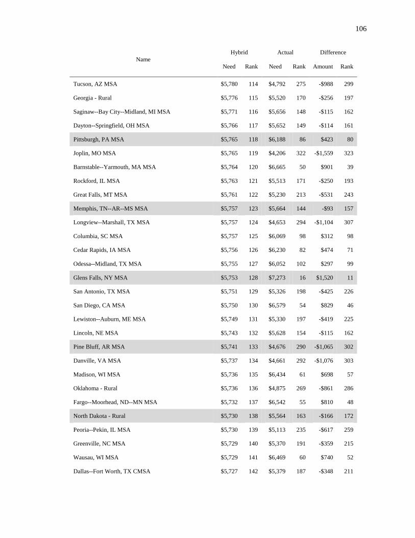
Appendix D. Estimates of Per-Capita Expenditure Need by Sub-State Area ................. 102

Appendix E. Workload and Expenditure Need Calculations Under the ACIR Approach

......................................................................................................................................... 114

Appendix F: Proofs of Results in ―Evading Nash Traps in Two-Player Simultaneous

Games‖ ............................................................................................................................ 117

Sources ............................................................................... Error! Bookmark not defined.

Vita .................................................................................................................................. 129

viii

LIST OF TABLES

Table Page

1. Statistical tests of hypotheses and robustness checks ................................................... 17

2. Tests of the effect of the Decrease treatment ................................................................ 22

3. Regression results under different specifications ......................................................... 24

4. Seven approaches to estimating fiscal need in the United States ................................. 41

5. Regression results from pooled MSA-level SUR ......................................................... 49

6. Top 5, Median, and Bottom 5 States and sub-state areas by fiscal need ...................... 51

7. Correlation coefficients for different measures of expenditure need ............................ 52

8. The difference in regression-based expenditure need estimates dependent on land area

and population density .......................................................................................... 57

9. Subject behavior in the Traveler’s Dilemma ................................................................ 79

ix

LIST OF FIGURES

Figure Page

1. Information treatment ................................................................................................... 12

2. Tutorial screenshot ........................................................................................................ 13

3. Payoff calculator ........................................................................................................... 14

4. Mean BLUE investment by period by session .............................................................. 18

5. Investment decisions by period, Subsidy Session......................................................... 18

6. Investment decisions by period, Information Session .................................................. 20

7. Absolute deviation from best-response by period by session ....................................... 26

8. Per-capita state-and-local direct expenditure by state in 2002 ($1,000) ....................... 35

9. Measures of state expenditure need by state population density .................................. 38

10. Kernel density estimates of hybrid, state-based, and traditional RES estimates against

actual expenditures................................................................................................ 54

11. Measures of sub-state-level expenditure need by sub-state population density ......... 55

12. Hybrid-regression RES results across States .............................................................. 56

13. State-based regression vs. Hybrid-regression ............................................................. 56

14. Traditional estimates of fiscal need vs. Hybrid estimates ........................................... 58

15. Hybrid estimate of fiscal need vs. Actual per-capita expenditure .............................. 59

16. Four-stage centipede game ......................................................................................... 64

17. Traveler’s Dilemma .................................................................................................... 64

18. Nash equilibrium, détente strategic, and no-initiative strategic profiles in a two-player

game ...................................................................................................................... 74

19. Purely ordinal conflict games with different NE and NIS profiles ............................. 77

20. The Prisoner’s Dilemma and an abbreviated Traveler’s Dilemma ............................. 79

21. General normal-form 2x2 game. ............................................................................... 120

x

ABSTRACT

ESSAYS ON THE SEARCH FOR ECONOMIC EFFICIENCY

By

Jason James Delaney

July 2010

Committee Chair: Dr. James C. Cox

Major Department: Economics

The chapters of this dissertation examine efficiency failures in three areas of

applied microeconomics: experimental economics, public finance, and game theory. In

each case, we look at ways to resolve these failures to promote the public good.

The first chapter, ―An Experimental Test of the Pigovian Hypothesis,‖ looks at

two different policies designed to reduce congestion in a common-pool resource (CPR).

The predictive power of game-theoretic results with respect to an optimal subsidy in a

common-pool resource game remains an open question. We present an experiment with

training and a simplified decision task, allowing more tractable computerized CPR

experiments. We find that subject behavior converges to the Nash prediction over a

number of periods. A Pigovian subsidy effectively moves subject behavior to the pre-

subsidy social optimum. Finally, we find a significant but non-persistent effect of

information provision in moving subjects toward the social optimum.

The second chapter, ―Apples to Apples to Oranges,‖ looks at efficiency and

equity failures across states resulting from public expenditure. The literature on fiscal

equalization and horizontal equity has established that measures of fiscal capacity should

be complemented by measures of fiscal need: the ability of a sub-national government to

xi

provide services given an average level of revenue. This chapter introduces an extension

of the Representative Expenditure System that uses regression methods and both state

and metropolitan statistical area (MSA) level data, allowing for comparability of input

costs, service requirements, and levels of need. The regression-based results are robust

across state- and MSA-level formulations, although state-level approaches overestimate

need for larger, less populous states. All regression-based results diverge from previous

workload-based approaches.

The third chapter, ―Evading Nash Traps in Two-Player Simultaneous Games,‖

looks at efficiency failures in two-player simultaneous games. In some important games,

Nash equilibrium selects Pareto-inferior equilibrium profiles. Empirically, Nash

equilibrium sometimes performs poorly when predicting actual behavior. Previous

approaches rely on repetition or external correlation to support efficient outcomes in

simultaneous games. This chapter presents two new concepts: ―détente‖ and ―no-

initiative,‖ in which players consider their own strategies and other-best-responses. We

discuss their efficiency and descriptive properties across a set of simultaneous games.

1

Chapter I: An Experimental Test of the Pigovian Hypothesis

Introduction

Many of the most important policy questions of our time relate not to privately

consumed goods, but to the unintended consequences of consumption of goods, broadly

referred to as externalities. Carbon emissions, obesity, and the stability of financial

firms—they all have consequences that extend beyond those involved in making the

economic decisions. A classic model to describe externalities is that of the common-pool

resource (CPR), and a classic solution to the problem of externalities is a Pigovian tax or

subsidy. The theoretical implications of consumption of a CPR by self-interested agents

are straightforward, but the robustness of those results is less clear. This paper addresses

several related issues: first, the literature has presented mixed results with respect to the

performance of the self-interested Nash equilibrium in predicting subject behavior.

Second, this paper presents an experimental test of the use of a Pigovian subsidy to

induce socially optimal behavior. Finally, we ask whether, given the economic and

political costs of introducing such a policy, there are other, nonmonetary ways to induce

socially preferred behavior.

This paper introduces a laboratory limited-access CPR experiment designed to

test the theory and examine potential policies to achieve improvements in governing

common-pool resources. Our experiment offers important contributions to: the public

finance literature by testing the theory of Pigovian taxation; the social preferences

literature by presenting data on the comparative results of two different policy tools—

price-based incentives and informational appeals; and the field of experimental design, in

2

that it presents a simple design making common-pool resources more tractable for future

experimental analysis.

In general, the literature has had a mixed response with respect to an important

question: does self-interested Nash equilibrium predict subject behavior toward an open-

or limited-access CPR? In their baseline experiment, Ostrom et al. (1994) (OGW) find

that subjects appropriate from a CPR at a suboptimal level—there is congestion—but that

subjects’ observed choices do not achieve a stable equilibrium. Walker et al. (1990) find

that the subjects over-consume by more than the Nash prediction, while Budescu et al.

(1995) also find that subjects over-consume, but by less than the Nash prediction. Bru et

al. (2003) find that even strategically irrelevant factors affect behavior. Rodriguez-Sickert

et al. (2008) present a CPR game with fines and find that even low fines have high

deterrence power, and that a fine which is voted down nonetheless establishes a norm.

Velez et al. (2009) find that subjects balance self-interest with conformity when selecting

strategies. Cox et al. (2009) find that first movers’ choices in a common property version

of the investment game are more likely to increase the size of the pie—and efficiency—

than in the private property version; neither version accords with the Nash prediction.

This lack of consensus in the previous literature is perhaps unsurprising. In

environments with pure private goods and institutions of impersonal exchange, Nash

equilibrium under the assumption of self-interested agents does an excellent—but not

perfect—job of predicting behavior. This is in contrast to the line of research concerning

pure public goods, following, among others, Isaac and Walker (1988), and Marwell and

Ames (1979). The deviations from the self-interested Nash equilibrium have been so

ubiquitous and persistent in public goods games and games of personal exchange that it

3

has led to the flourishing of the other-regarding preferences literature (Isaac and Walker

2003).

Perhaps theory and behavior diverge due to other-regarding preferences. The

effects of these preferences on both predicted behavior and optimal policy depend greatly

upon how the utility or consumption of others is incorporated into one’s own preferences.

In the cases of pure and impure (or ―warm-glow‖) altruism, for example, the optimal

Pigovian tax will be the same as in the self-regarding case, but the level of consumption

of the CPR will differ from the Nash prediction. Paternalistic altruism, however, implies

a higher optimal tax than the one under self-interest, because the social optimum requires

less consumption than under the presumption of self-interest (Johansson 1997)1.

Another reason equilibrium predictions might fail could be the difficulties present

in modeling the situation experimentally. In practice, creating congestion in an

experimental setting presents a formidable task, particularly in a framework that allows

simple testing of a Pigovian subsidy. This problem derives from the fact that congestion

requires a nonlinearity in payoffs such that total social payoff peaks and declines at an

overcongested—and privately optimal—level of consumption. This has the side effect of

reducing the incentive to think very hard about it at the margin, because the marginal

return to social payoff is closest to zero at the social optimum and the marginal private

return is closest to zero at the overcongested level of consumption. Because of the payoff

structure, determining the optimal strategy can be difficult, which may cause Nash

1 Briefly, the intuition for pure altruism derives from the assumption that the utility from own-consumption

is ―larger‖ than the external utility effect through altruism, and for large populations, the difference in the

tax approaches zero. For impure altruism, there is merely an additional utility advantage to reducing own-

consumption, but the difference between private and social impact is unchanged. In the case of paternalistic

altruism, marginal damages are increased by the extent of the paternalism, and the tax should thus be

higher.

4

predictions to perform poorly. If subjects are confused or frustrated, they may simply

(and rationally) decide not to think too hard about it. In one treatment, OGW allow (and

record) communication, and note that in some of their experiments, this lack of

dominance appears to be a problem. When CPR consumption increased in one period, the

group members tried to determine whether greed or error was to blame, and one member

noted that a defector would have earned ―Just a few darn cents above the rest of us.‖

The predictive power of Nash equilibria with respect to CPR games directly

affects the theoretical efficacy of Pigovian taxation or subsidies as a means to achieving

efficiency. One of the earliest and simplest solutions to congestion under an open- or

limited-access property regime, the Pigovian hypothesis has, to our knowledge, never

been tested experimentally. Pigou (1920) hypothesized that, to offset congestion, an

optimal tax or subsidy could be applied to internalize the congestion externality—

essentially altering the game so that the socially optimal outcome of the CPR is the Nash

equilibrium outcome of the modified system. If the Nash equilibrium strategy profile fails

to predict behavior in a CPR game, it is unclear what to expect from a Pigovian subsidy.

Finally, the costs of monitoring and enforcement—be they technical or political—

required to implement and maintain a Pigovian scheme are often prohibitive. To the

extent that people are motivated by non-monetary factors—other-regarding preferences,

conformity and other social norms, or merely cognitive difficulty—it may be possible to

reduce deadweight welfare loss through non-monetary means.

In order to try to minimize dominance effects, the present experiment reduces the

complexity of the payoff function, provides an intuitive interface and response mode, and

provides training and software-assisted payoff calculation. The aim is to reduce the

5

cognitive costs of decision-making to allow a sharper test of the Nash equilibrium

prediction in this CPR game. This experiment provides evidence that subjects’ choices

converge, but that it takes some time to reach the predicted outcome.

To date, there has been incidental evidence with respect to the performance of a

Pigovian subsidy in achieving the intended outcome, but there has been no direct test of

the theory. This experiment presents an experimental test of the Pigovian hypothesis; the

experimental results fit well with the theoretical prediction—Pigou was correct. A second

treatment in this paper presents subjects with information on the social optimum as a test

for the effect of such information on subjects’ behavior. We find a small and non-

persistent effect, but further experimental study is warranted to determine the feasibility

of information provision as a means of improving efficiency.

The paper is set up as follows: The next section presents the basic model of a

limited-access CPR that we use in this experiment. Section 2 presents the experimental

design, the hypotheses, and the statistical approach. Section 3 presents the results and a

discussion and Section 4 presents some concluding comments.

Theory

The theory of limited-access common-pool resources is a standard in public

finance, and environmental, urban and regional economics. The intuition derives from a

difference between the marginal private benefit (MPB) or cost (MPC) from consumption,

and the marginal social benefit (MSB) or cost (MSC) of consumption—an externality.

Assuming MPB > MSB and MPC = MSC, for example, the marginal social cost at

equilibrium will be greater than the marginal social benefit, and the socially optimal

6

quantity will be less than the equilibrium quantity. Pigou asserted that there exists a

subsidy (or tax), t*, that will induce the socially optimal quantity choice, and that t* is

simply the difference between the net MSB and net MPB at the optimal quantity.

The theory itself is relatively straightforward, but the design of an experimental

framework to represent congestion has proven complicated. In general, CPR games,

including OGW, represent the CPR using a production function approach with an

―outside option,‖ which is a pure private good. A test of the Pigovian hypothesis can be

implemented by increasing the opportunity cost of expenditure on the CPR, by increasing

the private return to the outside option. In order to avoid potential subjective

considerations surrounding subjects’ concept of taxation, as well as to avoid negative

returns and potential effects due to prospective losses, we test the theory using a subsidy,

rather than a tax.

Formally, let index individual agents. Let represent individual i's

endowment, , represent i's expenditure on the CPR, and represent total (combined)

expenditure on CPR (including i). Let represent the payoff from an outside

option, , the payoff from the CPR, and an individual’s total payoff.

Specify the payoff to the common pool resource by defining

where β is a per-token payoff to the CPR that declines with increasing consumption of

the CPR with the γ parameter (for γ = 0, there is no congestion). Under standard

economic assumptions, each individual is maximizing with respect to . In

general, with appropriation games, there is an incentive to consume the CPR and an

7

incentive to consume the outside option. The game played in the present experiment has

the following payoff function2:

To help subjects determine their payoffs, the software provides a payoff calculator

that allows subjects to examine hypothetical situations before making a decision. The

calculator is discussed further in section 2.

This payoff function presents subjects with a fixed per-token return to the outside

option and a declining per-token return to the CPR. In order to introduce a subsidy, we

add an additional fixed per-token amount to the return to the outside option.

Proposition. Define the payoff function for individual i as:

Without a subsidy , the Nash equilibrium is symmetrical with each

player choosing

.

For , the social optimum occurs when each player chooses

.

The socially optimal level of consumption and the Nash equilibrium level of consumption

are only identical for n = 1 or β = α.3

For , the strategy at the Nash equilibrium becomes

, and the

optimal Pigovian subsidy is

.

4

2 This is similar, but not identical, to the payoff function used in OGW (although the solutions are the

same). In particular, OGW use an approach where each subject earns a share of quasi-linear production in

the CPR, in which the framing and the functional form are presented to the subjects. We use a per-token

approach, explained as such, which seems more transparent, and requires no facility with exponents to

figure out one’s own payoff. 3 These represent two trivial cases: the case of individual use, in which there is no externality, and the case

of an outside option that dominates the CPR.

8

The incentives governing the marginal decision to consume the CPR warrant a

brief discussion. Unlike linear VCM games, the marginal per-capita return (MPCR) is not

constant in this game. Consider a unit increase in the consumption of the CPR (implying

a unit decrease in consumption of the outside option), and where represents the current

level of CPR consumption. The MPCR to oneself (which is the previously discussed

MPB) from consuming an additional unit of the CPR is –

– . The MPCR to others varies across individuals, proportional with their level of

consumption of the CPR, and is equal to – for each individual, where indexes other

individuals. This is straightforward: each unit of CPR consumption carries a variable

benefit, which is for the th unit, carries an opportunity cost in the

form of a forgone return to the outside option, , and reduces the value of all

previous consumption of the CPR by , which decreases own-payoff by (fishing or

driving congests own-consumption as well), and decreases other payoffs by for each

k in the group. Except for the case where no one else is currently consuming the CPR,

one’s own consumption of the CPR unambiguously reduces others’ payoffs: MSB <

MPB for .

4 For the purposes of this experiment, we are abstracting away from the source of the subsidy and possible

distortionary effects in raising the required revenue. It should be noted that the theory postulated by Pigou

is not complete in this respect, as it does not posit a budget balancing constraint—the taxes go nowhere and

the subsidies come from nowhere. This is typical in tax theory in a partial equilibrium framework, and in

practice, it seems unlikely that people are aware of the total effect of every dollar they receive as a subsidy

or dollar they pay in taxes. In addition, a number of other mechanisms for achieving efficiency rely on

abandonment of budget balancing; the Clarke tax and the Groves-Ledyard mechanism are two important

examples

9

Protocol

Because the impact of social norms and framing seems non-trivial, we avoid

terminology like ―common-pool resource,‖ ―extraction,‖ ―appropriation,‖ ―tax,‖

―subsidy,‖ etc. We follow Andreoni and Petrie (2004) in presenting the decision they face

as an ―investment‖ decision in which they will decide how to invest a number of tokens

in each period. Subjects are given the choice to invest their tokens in the outside option or

the CPR, which are referred to in the experiment as the ―RED investment‖ and the

―BLUE investment,‖ respectively.

We implement this model using the following parameterization: (α: per-token

baseline RED payoff; β: per-token starting BLUE payoff; γ: per-token BLUE congestion

parameter; δ: per-token RED subsidy; z: period endowment; n: group size) = ($0.00,

$0.36, $0.01, $0.12, 10, 3). These parameters were chosen for a number of reasons. In

particular, they guarantee a unique (and symmetric) interior Nash equilibrium in both the

baseline and the subsidy treatments ( and , respectively). They also provide

enough distance between the two equilibria for statistical inference. In addition, the

differences are economically significant. Under the socially optimal outcome, subjects

would earn $26.88; the per-subject payment under the Nash equilibrium outcome is

$22.26. The minimum possible payoff is $0.00 for the information treatment and $4.20

for the subsidy treatment. The maximum possible payoff is $54.60 under both conditions.

Finally, the group size is such that off-Nash behavior might reasonably be sustained, as

implicit collusion is easier with smaller groups. If Nash cannot be rejected, it seems likely

that it would predict well for larger groups.

10

This analysis has relied on continuity and differentiability to determine Nash

results. In practice, it is not generally true that a unique Nash equilibrium in the

continuous case implies a unique equilibrium in a discrete implementation (Swarthout

and Walker 2009). In order to ensure that these continuous results hold for the

implementation we use in the experiment, we tested every strategy profile under the

parameters and find that there is indeed a unique (and symmetric) interior Nash

equilibrium in both the baseline case and the subsidy case

.

The experiment was conducted in two sessions at Georgia State University’s

Experimental Economics Center (ExCEN). In each session there were 24 subjects,

randomly separated into 8 groups of 3.5 Each session lasted about an hour and a half.

Individual earnings, including a $5 show-up payment, ranged from $17.98 to $40.60.

The sessions were run with a double-blind protocol. Our primary research

questions concern individual behavior under induced preferences, as well as those

preferences they might have regarding the welfare of anonymous members of their group.

In addition, the information treatment looks at information provision without a direct

appeal to social norms. There is some experimental evidence that with less than strict

anonymity, the domain of other-regarding preferences may expand beyond the group

(see, for example, Hoffman et al. (1994), Cox and Deck (2006), and Andreoni and Petrie

(2004)). Relaxing anonymity to observe CPR consumption decisions in the presence of

external subjective norms is another straightforward extension of the present experiment.

5 In the first session, a student asked to leave after subjects had been signed in and placed in groups, but

before the experiment began. A graduate student took his place to satisfy the requirements of the software

and to allow the other students in his group to participate. We exclude data from that group; inclusion does

not affect the qualitative results.

11

Strict anonymity was maintained, but in each round, all subjects were aware of

the sum of the decisions made by the other members of their group in each previous

round. Groups were randomly assigned, but fixed throughout the experiment. The

experiment was computerized, and was run in an experimental lab with dividers in place

so that subjects could not easily see one another. Each subject participated in two

baseline treatments and one of two experimental treatments: either the Pigovian subsidy

treatment or the information treatment. All subjects in a given session participated in the

same treatments. For each treatment, each individual was asked to make seven

―investment‖ decisions.

In each period, each token invested in the RED investment paid a fixed per-token

amount. Each token invested in the BLUE investment paid a per-token amount that

depended upon the total number of tokens invested in the BLUE investment by the group.

Each session consisted of two treatments, administered in B-A-B format, so that each

session consisted of a baseline treatment, an experimental treatment, and a second

baseline treatment. Subjects knew the number of periods, but were not made aware ahead

of time when treatments would begin or end. Because of the relative complexity of the

payoff structure as well as an established downward trend, or ―decay,‖ in group

contributions, widely documented in public goods games (Isaac and Walker 1988, for

example), providing a second baseline allows us to observe, and perhaps account for, any

such trends when trying to discern a treatment effect.

In the baseline periods in both sessions, tokens invested in the RED investment

provided a per-token payoff of $0.00. Tokens invested in the BLUE investment provided

a per-token payoff of $0.35 for a single token. The per-token value of tokens invested in

12

the BLUE investment declined by $0.01 per token invested in BLUE under all

experimental conditions, down to a minimum of $0.00 per token. After each period,

subjects were informed of the total group investment in the BLUE investment, as well as

their period payoff and their total profit.

In the first session, the experimental treatment was the administration of a

Pigovian subsidy. During periods 8-14, the RED token payoff was increased to $0.12.

In the second session, the experimental treatment was the provision of

information regarding the common pool resource. During periods 8-14, subjects were

given the total group payoff in the previous period, the hypothetical group payoff at the

social optimum, and an explanation of how to achieve the social optimum in the event

that the two are unequal (Figure 1).

Figure 1. Information treatment

Each session proceeded as follows: subjects were allowed to read the instructions

privately; the instructions were then read aloud, verbatim. (Appendix A) After the

instructions were completed, an example was drawn from the instructions and

demonstrated by the experimenter on a projection of the computer interface. Subjects

then were given a walk-through tutorial of the computer interface (Figure 2), in which

they were allowed to select from several sets of parameters and then given the

opportunity to practice using the software with a computer playing deterministically as

the ―rest of the group,‖ selecting 0 tokens in the BLUE investment in the first round,

13

followed by 1 token in the second round, continuing up through 20 tokens, before

restarting at 0 tokens. Subjects were allowed to practice this way as long as they liked.

They chose to participate in between 0 and 42 practice rounds.

Figure 2. Tutorial screenshot

See Appendix B for screenshots of the full tutorial.

In addition to the practice rounds, subjects had access to a payoff calculator

throughout the tutorial and the experiment. The payoff calculator (Figure 3) allows

subjects to choose a hypothetical decision for themselves, a hypothetical combined

investment in the BLUE investment for the rest of the group, and provides information on

their payoffs under the current parameters, as well as the own-payoff consequences of

single-token changes in either direction for themselves or for the group. The practice

periods and tutorial were intended to introduce subjects to the decision task, familiarize

them with both the task and the interface, and provide them with an opportunity to use

14

the calculator and the interface before making decisions for real payoffs. We collected

data on the number of practice rounds each subject chose to use.

Figure 3. Payoff calculator

Once the experiment concluded, subjects were asked to fill out a questionnaire

while payments were prepared. This questionnaire included basic demographic data, as

well as data on education and measures of outlook regarding trust, justice, and human

nature.

Hypotheses

The primary hypotheses of interest are as follows ( indicates mean):

1. The Nash equilibrium outcome is a good predictor of subjects’ choices:

.

2. The Pigovian subsidy has the theoretically predicted effect:

, where is the mean investment in the CPR at the pre-subsidy social

optimum.

15

3. The presentation of information has no effect: .

If subjects express other-regarding preferences—particularly pure, impure, or

paternalistic altruism—we should expect 1 and 2 to fail. In particular, if other-payoff

enters positively into the utility function, we should expect and

.

If subjects are intending to express other-regarding preferences, but making errors

in the attempt, the provision of information on the group payoff in addition to

information on their own payoff would allow them to change their investment decisions

to more accurately represent their preferences. If they possess an external norm that

indicates that, given an opportunity to make the group better off at one’s own expense,

one ought to take such an opportunity, provision of information on the group’s total

payoff provides both a reminder of the relevance of the choice task to group welfare and

information on how to improve group welfare at one’s own expense. Finally, if

information acts as a coordination point, even self-interested agents might strategically

coordinate on a point that would give them higher payoffs with the hope of either

sustaining a higher level of earnings or reneging in the future. Consequently, if subjects

are either prone to errors, have norms that are not fully internalized, or are prone to

strategic coordination, we should expect to see .

In addition, we test a number of other hypotheses regarding subsets of the data to

try to get a more accurate picture of subject behavior. We also consider other questions,

including the source and causes of deviations from Nash strategy, as well as concerns

regarding censoring, using more parametric estimation techniques.

16

Results

As previously mentioned, in both treatments the first seven rounds were baseline

rounds, as were the last seven rounds, with the intervening seven rounds presenting

experimental treatments. We report the results discursively; statistical test results are

presented in Table 1 and indexed by hypothesis being tested (e.g. H1, H2, …). In the

table, ―Baseline 1‖ refers to periods 1-7, ―Baseline 2‖ refers to periods 15-21, and

―Baseline‖ without a number refers to the combined results from Baseline 1 and Baseline

2. In addition, unless otherwise specified, the variable of interest in this section is the

across-period mean CPR investment decision by a given subject, paired when

appropriate. This approach accounts for both individual and group fixed effects.

The sessions differ significantly (H1: p = 0.000, Figure 4). The mean baseline

investment in the CPR in Session 1 was 8.803 tokens, while the mean baseline

investment in Session 2 was 7.964 tokens. The null that these are equal can be rejected.

In addition, there is evidence of either learning or a ―decay‖-type trend (probably both).

In the first session, baseline 1 mean investment in the CPR was 8.517 (SE = 0.126)

tokens while the baseline 2 mean investment was 9.088 (SE = 0.063) tokens. Again, we

can reject the null of equality (H2: p = 0.010). In the second session, the baseline 1 mean

investment was 7.452 (SE = 0.200) tokens, while the baseline 2 mean investment was

8.476 (SE = 0.125) tokens. Once again, we can reject the null that these observations are

drawn from the same distribution. (H3: p = 0.003).

Figure 5 presents the mean decision by period in the first session. In the first

session baseline periods, we cannot reject the null that subjects’ behavior accorded with

the Nash prediction, on average (H4: p = 0.388). The subsidy, in addition, seems to have

17

Table 1. Statistical tests of hypotheses and robustness checks

Hypothesis Reject? Wilcoxon test K-S Test6

H1: Session 1 Baseline =

Session 2 Baseline

Reject rank-sum

Z = 3.665, p = 0.002

D = 0.4464,

p = 0.017

H2: Session 1 Baseline 1 =

Session 1 Baseline 2

Reject matched-pairs sign-rank

Z = -2.575, p = 0.010

D = 0.5238,

p = 0.006


Session 2 Baseline 2


Z = -3.002, p = 0.003

D = 0.3333,

p = 0.093

H4: Session 1 Baseline = 9 Cannot reject sign-rank

Z=-0.863, p =0.388

H5: Session 1 Treatment = 6 Cannot reject sign-rank

Z=-0.233, p =0.816


Session 1 Treatment


Z = -3.002, p = 0.000

D = 0.857,

p = 0.000

H7: Session 2 Baseline = 9 Reject sign-rank

Z=-6.714, p =0.000


Session 2 Treatment

Cannot reject matched-pairs sign-rank

Z = 0.729, p = 0.466

D = 0.125,

p = 0.975


Session 2 Treatment


Z = 3.211, p = 0.001

D = 0.25,

p = 0.347

H10: Session 2 Mid-Baseline =

Session 2 Treatment

Marginal rejection matched-pairs sign-rank

Z = 1.416, p = 0.157

D = 0.1667,

p = 0.815


Session 2 Treatment

(detrended)


Z = 0.743, p = 0.458

D = 0.1667,

p = 0.820


Session 2 Treatment

(detrended)


Z = 0.972, p = 0.331

D = 0.1667,

p = 0.834


Session 2 Period 8


Z = 2.258, p = 0.024

D = 0.375,

p = 0.047


Session 2 Period 8


Z = 2.733, p = 0.006

D = 0.417,

p = 0.020

H15: Session 2 Baseline = 9

(random-effect tobit

model)

Cannot reject Wald test

= 0.02, p = 0.896

6 Where appropriate, we use a boot-strapped (10,000 iteration) Kolmogorov-Smirnov test of equality of

distributions for distribution tests, which does not incorporate matching, but has the nice property of being

able to test against discrete distributions. (See Sekhon, forthcoming) We use this test as a robustness check.

18

Figure 4. Mean BLUE investment by period by session

(NE line indicates Nash equilibrium prediction without subsidy)

Figure 5. Investment decisions by period, Subsidy Session

treatment

01

23

45

67

89

10

1 7 14 21Period

decision (no tax) decision (tax)

mean decision by period

De

cis

ion

19

the effect posited by Pigou (H5: p = 0.816). Subjects’ mean investment in the CPR was

5.946 (SE = 0.154) tokens, which is not significantly different from the Pigovian

prediction of 6 tokens. We can reject the null of no treatment effect; this is robust to using

the first, the second, or the combined baseline treatment as a basis for comparison (H6: p

= 0.000).

Because of the existence of an underlying time trend, two approaches were used

to try to separate the effects of learning and decay from the treatment effect. The first is

to use as a basis of comparison only those periods which are most like those of the

treatment group in terms of learning and decay—namely, the last three of the first

baseline and the first four of the second baseline, which we will refer to as the ―mid-

baseline.‖ Using the mid-baseline has a few advantages: we expect some of the noise of

experimentation and learning has dissipated by period 5, while these periods do not

contain the same level of decay as the last three periods.

The second attempt requires the assumption of a linear trend that is stationary

throughout the session. Elimination of this trend was done by simple OLS regression of

the subjects’ investment decisions on the period, and then subtraction of this period-based

component to produce a de-trended decision. For the subsidy treatment session, neither

method has a qualitative effect on the magnitude or significance of this treatment effect.

For the second session, we can reject the null that pooled baseline behavior is

equal to the Nash prediction (H7: p = 0.000), and subjects’ investment decisions appear to

be noisier and converge later than do those in the first session (Figure 6). The effect of

the information they receive is more difficult to discern. The mean contribution decision

during the information treatment was 7.833 (SE = 0.163) tokens, and indeed, we cannot

20

reject the null of equality with the baseline mean (H8: p = 0.466). Considering the

dispersion of decisions in the first several periods of this session, however, other tests

seem appropriate. Comparing the treatment periods only to the second baseline, for

example, produces a paired test that recommends rejecting the null of equality (H9).

Because the treatment precedes this second baseline, it appears that the underlying time-

trend may confound the result. Both methods to account for the time-trend in the first

session were also used for the second session.

Figure 6. Investment decisions by period, Information Session

The mean contribution in the mid-baseline periods was 8.125 (SE = 0.162), which

is marginally different than that of the treatment group (H10). The mean de-trended

decision in the session was 7.127 (SE = 0.117) tokens in the CPR. Use of the de-trended

version removes any significant difference between the second baseline and the treated

group or the mid-baseline and the treated group (H11, H12).

01

23

45

67

98

10

1 7 14 21Period

decision (no info) decision (info)

mean decision by period

De

cis

ion

treatment

21

A sharp decline in contributions is visible in Figure 6 during period 8, the first

period of the treatment (mean contribution to the CPR = 6.750, SE = 0.494).

Nonparametric tests indicate that this is indeed significantly different from the full

baseline, as well as the mid-baseline, and that these results persist even in the de-trended

data (H13, H14).

It is unclear that an assumption of a linear trend is a legitimate one, so while the

tests for the de-trended data are illustrative, they may not be conclusive. A more

sophisticated test for an effect of information can be developed by considering the nature

of the treatment: in particular, subjects may see one of three different types of message.

For subjects in groups that under-invest in the CPR, they are informed that an increase in

their level of investment would increase the payoff to the group. For those in groups at

the social optimum, they are informed that their current level of investment is optimal.

Finally, for those in groups suffering from overcongestion in the CPR, subjects are

informed that a reduction in investment would lead to an increase in group payoff. It may

be the case that the information is having an effect, but that offsetting behavior leads to

an inability to reject the null of no effect, because the changes preserve the mean level of

investment within subjects.

In practice, of the 168 messages subjects received during the information

treatment, 147 informed subjects that a decrease would improve group payoff, 9 informed

subjects that an increase would improve group payoff, and 12 informed subjects that they

were at the maximum group payoff. Consequently, 12.5% of the messages sent to

subjects would not be expected to induce a reduction in CPR investment. Considering the

subset of subjects who received a message related to a decrease in CPR investment

22

should allow a better test of a treatment effect. Consider this ―sub-treatment‖ the

―Decrease‖ treatment.

Selection of the counterfactual is important in this case. Those who received the

Decrease treatment are similar in known ways. First, these are subjects in the Information

session. Second, the decisions under the treatment occur during the middle seven periods.

Finally, only those who were members of groups whose combined investment in the

previous period exceeded the socially optimal level of investment received advice to

decrease their investment. For a basis of comparison, we can consider decisions that meet

the first and third criteria as ―candidates for treatment.‖

Considering all periods in session 2, we cannot reject the null of no effect of the

Decrease treatment (Table 2). When comparing against the mid-baseline, we can reject

the null of no effect at the 10% level. In both cases, these hypothesis tests are

unconditional and, as we are using mean levels of investment by subject, we have 24

observations. Using regression methods, we may be able to account for censoring and

improve statistical power.

Table 2. Tests of the effect of the Decrease treatment

Matched-pair

sign-rank test Session 2 only Session 2 mid-

baseline Treatment

Mean (SD)

8.070 (1.508)

8.178 (1.638)

7.846 (1.657)

Z 1.001 1.753

p 0.317 0.080

In this case, again, selection of the counterfactual is important. In order to

increase the power of the test, some of the regressions include data from both sessions.

23

Table 3 presents the results for selected regressions. Those observations that are

considered ―candidates‖ from session 1, under the ―Full‖ subset of the data, are those

investment decisions for which the group decision in the previous period exceeded the

social optimum and the price level was the same as in the information treatment in both

the preceding period and the period in which the decision was made. The reported results

are robust to modifications in the chosen counterfactual set of observations.

In addition to tests of the average effect of the Decrease treatment over the seven-

period treatment, the regressions include specifications using only the first 8 periods of

session 2 (the results labeled ―One-shot‖ in the ―Data subset‖ row), which provides a test

of the effect of the Decrease treatment on first sight. This ―first-sight‖ effect is always

significant at the 10% level. Subjects’ observed choices declined significantly the first

time they received the Decrease treatment.

The effect of the Decrease treatment is always negative and generally significant,

so this particular form of information provision appears to have a small negative effect on

investment in the CPR that spikes in subjects’ first exposure, reducing investment levels

on average by a little over a single token, but which does not persist through subsequent

periods. It is smaller than the effect of the Pigovian subsidy, but is perhaps surprisingly

large, given that there is no direct appeal to social norms nor any communication allowed

among subjects. These results represent a roughly 9% increase in subjects’ single-period

earnings as a result of the first exposure to the Decrease treatment, indicating that there

may be greater efficiency gains possible without requiring a costly intervention such as a

tax or subsidy.

24

Table 3. Regression results under different specifications

Dependent variable is number of tokens invested in the CPR

informationa -0.247* -0.277* -0.891* -0.188 -0.178 -1.303*** -0.249* -0.231 -1.186** -1.257* -0.422*

(0.089) (0.080) (0.083) (0.234) (0.321) (0.010) (0.087) (0.135) (0.044) (0.090) (0.057)

candidate 0.654** 0.916** 0.402 0.426** 0.416* 0.326 0.720** 0.667* 0.68 0.654 1.080***

(0.020) (0.013) (0.205) (0.027) (0.077) (0.234) (0.018) (0.080) (0.331) (0.487) (0.000)

subsidy -2.323***

-2.494***

-2.477***

-2.551***

(0.000)

(0.000)

(0.000)

(0.000)

period

0.0570*** 0.0713*** 0.121 0.0554*** 0.0683*** 0.0562

0.0590***

(0.000) (0.004) (0.191) (0.000) (0.000) (0.604)

(0.000)

Constant 7.830*** 7.224*** 7.163*** 7.367*** 6.817*** 6.672*** 8.021*** 7.374*** 6.869*** 7.725*** 8.369***

(0.000) (0.000) (0.000) (0.000) (0.000) (0.000) (0.000) (0.000) (0.003) (0.000) (0.000)

Lags? N N N N N N Y Y Y N Y

σu

2.636*** 1.186***

(0.000) (0.000)

σe

2.274*** 1.500***

(0.000) (0.000)

Specification Fixed-effects OLS, standard errors clustered on group Fixed-effects OLS, heteroskedasticity-

robust standard errors

Panel Tobit with

bootstrapped standard

errors

Data subsetb Full Session 2 One-shot Full Session 2 One-shot Full Session 2 One-shot One-shot Full

Observations 900 480 168 900 480 168 855 456 144 168 855

R-squared 0.346 0.03 0.036 0.384 0.097 0.052 0.501 0.228 0.132

Number of id 45 24 24 45 24 24 45 24 24 24 45 a Significance of the coefficient on ―information‖ represents a test of the null hypothesis that information about a decrease in CPR investment had no effect.

b ―Full‖ indicates both sessions are included with the first period omitted, as candidacy for treatment depends on lagged group decisions. ―Session 2‖ indicates

only session 2 data is included. ―One-shot‖ indicates that data is drawn from periods 1 – 8 only.

p-values in parentheses. *p < 0.10 **p < 0.05 ***p < 0.01

25

The observed difference between sessions may be correlated with use of practice

rounds. During the tutorial phase of the experiment, subjects had the opportunity to play

with a deterministic computerized ―rest of the group‖ as many times as they liked. The

median number of practice rounds for subjects in Session 1 was 3.5, while the median for

session 2 was 1.5 (the corresponding means are 9.04 and 5.583). The two distributions

are marginally significantly different (the Mann-Whitney test gives a p-value of 0.1215,

but the total number of subjects is only 45), but in other observable ways, the two

sessions appear to draw from the same population.7

This seems to be borne out by the progress of subjects’ behavior over the course

of the experiment. The mean absolute deviation from best response is, in a sense, a

measure of the deviation from self-interested behavior, as payoffs are decreasing with

this deviation. Figure 7 presents the mean absolute deviation from the best response over

time: it is clear that both samples are converging over the course of the experiment—in

the limit, to the Nash prediction—but that 21 periods are not enough to ultimately

converge within the second session.

If learning is a concern, we might expect the practice rounds to help subjects

converge, and indeed there is a marginally significant effect of the number of practice

rounds played on the mean absolute deviation from best response (p=0.058, n = 45). For

the average subject, in terms of mean absolute deviation from best response, the effect of

practice rounds reduces the mean absolute deviation from best response by 0.0354 tokens

7 An early hypothesis for the difference in baseline behavior was a ―Friday effect,‖ as the second session

was run on a Friday, the first on a Tuesday. This could either be due to a hypothetical change of behavior

among subjects on Fridays or to drawing from different sets of students not in class at the time of the

experiment— different types of classes might be held on a Tuesday/Thursday schedule, others on

Monday/Wednesday/Friday. This second hypothetical cause of a ―Friday effect‖ does not appear to be

detectable among observable covariates.

26

per round. With an average number of tutorial trials of 7.18 across the full sample, the

mean effect of practice rounds reduces the mean absolute deviation from best response by

.25 tokens, or a 15% reduction in average absolute deviation.

Figure 7. Absolute deviation from best-response by period by session

(with population means and lines of best fit)

Conclusion

As population continues to rise, the impact of congestion externalities continues

to increase. Common-pool resources are increasingly policy-relevant, and while there is a

growing literature on common-pool resource experiments, these goods still have not

received the research attention that private and pure public goods have received. The

reasons for this are both technical and theoretical—these goods are complicated by their

very nature, and the institutions that govern them vary widely. This experiment presents a

simplified common-pool resource experiment to subjects and the results indicate that

02

46

810

abs(d

elta b

r)

0 5 10 15 20Period

Session 1 Session 2

S1 mean S2 mean

Fitted values Fitted values

27

subjects do indeed converge to the Nash prediction under these conditions, but that

convergence can take quite a while.

One of the simplest (theoretically, if not practically) policy tools to correct for the

congestion externality inherent in common-pool resources is the introduction of a

Pigovian tax or subsidy to internalize the externality. We show that such an intervention,

if feasible, should have the effect hypothesized by Pigou. Bearing in mind the

impracticality or high cost of introducing such a direct intervention, we find a smaller,

but significant effect from an information provision treatment. Further study on similar

approaches to appeals to social norms should provide more insights into how effective

such appeals can be at reducing congestion in common-pool resources. Ferraro (2009),

for example, reports a large-scale randomized policy field experiment and finds that ―pro-

social‖ messages have an effect on water use. The information treatment used here

primarily provides information, rather than appealing directly to social norms. Future

research should look at the effect of specific appeals to social norms in reducing

congestion in the lab.

In addition, extending the experiment to incorporate taxes directly, allowing

subjects to see marginal changes in both own- and other-payoff, changing group size, and

directly modifying marginal per-capita return on investment would provide useful

information on the sensitivity of CPR consumption decisions to these conditions. In

particular, experiments using very large groups could be useful in extending external

validity to more closely represent naturally occurring common-pool-resources.

Finally, we find that subjects’ participation in practice rounds has a positive and

significant effect on the rate of convergence to the Nash prediction. This, as well as the

28

evidence on the rate of subjects’ convergence to equilibrium, confirms that common-pool

resource experiments are complicated, and our inference with respect to subject behavior

should allow for a nontrivial amount of time for convergence to equilibrium.

29

Chapter II: Apples to Apples to Oranges

Fiscal Need in the United States in a Regression-Based

Representative Expenditure Approach

Introduction

Fiscal need is a measure of the ability of a sub-national government (SNG) to

provide an average level of services with an average level of revenue. The level of

services required of U.S. states has grown over the last fifty years, without reference to

the differing abilities of the states to keep up with these requirements.8 The latter half of

the twentieth century witnessed the steady advance of minimum standards of public

service provision, motivated both by local public choice and by federal legislation.

Such laws, in general, have the potential to create efficiency gains. The federal

government has the unique ability to internalize externalities at the national level,

circumventing difficult public choice quandaries that can lead to pollution havens or

interstate competition over fair labor standards, for example. While many programs have

been designed and mandated at the national level, the fiscal apparatus required to

implement them, including the primary source of funding, remains primarily a state and

local phenomenon: national standards are not generally funded by the Federal

Government (e.g. No Child Left Behind and the Clean Air Act). States face different

challenges in complying with these standards. A state with a stiff wind blowing in off the

coast may find it easier to comply with clean air standards, while a state with entrenched

8 Since 1960, the share of GDP devoted to state and local public expenditure has nearly doubled from

11.6% of GDP in 1960 to 22.2% in 2010.

30

poverty and low levels of adult education may have a difficult time improving eighth-

grade test scores.

A common standard with heterogeneous costs and needs leads to spending

different amounts of money to provide a mandated level of public services. Implicitly,

this results in redistribution of net fiscal burden (NFB) across states. The fiscal

equalization literature notes that redistribution represents an opportunity to advance both

equity and efficiency through equalization. By the same token, service provision

standards without consideration of fiscal need can reduce both efficiency and equity.

The implications for policy have an upside: policy that accounts for this burden-

shifting can improve efficiency and equity by eliminating the incentive to move for fiscal

reasons. In principle, this means equalizing the NFB for each individual across SNGs. In

practice, the policy goal has been to provide SNGs with the ability to do so by equalizing

―fiscal comfort,‖ or the ability of a SNG to provide an average level of services with an

average level of tax effort, not revenue.

Measuring fiscal comfort involves measuring two dimensions: revenue-raising

ability, or ―fiscal capacity,‖ and service-provision ability. Measuring fiscal capacity has

proven to be more straightforward than measuring fiscal need for practical, theoretical,

and analytical reasons, and as a result most equalization schemes are based on tax

equalization.9 This adjusts revenue as though per-capita expenditure need were constant

within a country. When only tax treatment is accounted for in an equalization program,

the equalization program may increase efficiency, but there remains an incentive to move

to reduce one’s NFB, and thus allocative inefficiencies remain (Boadway and Flatters

1982). Tax-based equalization leaves money on the table.

9 Bird and Vaillancourt (2007) provide a good overview of the types of exceptions found in practice.

31

Empirical evidence indicates that ignoring fiscal need is economically significant.

Wilson (2003) looks at Canadian migration data in response to Canada’s capacity-based

equalization program and finds significant efficiency gains in addition to the more

straightforward equity improvements. Shah (1996) provides evidence on the size of the

disparity that arises from excluding fiscal need in Canada’s equalization program and

finds that incorporating expenditure need in the measure of fiscal comfort leads to

significant changes in the existing entitlements, nearly halving the net transfer out of

Ontario and nearly doubling the net transfer out of British Columbia.

Given the potential gains from a fiscal-comfort approach, why do existing policies

generally ignore fiscal need? There are several reasons. First, the concept of fiscal need

can be politically unpalatable. As controversial as property value assessments can be, the

idea of measuring a tax base is relatively straightforward. Asserting that higher levels of

per-capita expenditure in one area are ―necessary‖ or ―just,‖ while it advances equity in

practice, may appear to violate the principle of equity.10

In addition, this policy approach,

like others, creates winners and losers relative to the status quo. Any change is likely to

be met with resistance from those who lose from the policy change, even if net social

welfare is improved.

Second, while the size of the tax base does not directly depend on preferences, the

size and structure of public expenditures does, and so differentiating between

idiosyncratic preferences for public goods and fiscal need must be done by assumption or

10

For example, providing higher per-capita funds for schooling to a city with more children in poverty or

higher teacher salaries may effectively provide the same level of service, but when making cross-

jurisdictional comparisons, funding levels are easier to compare than service levels, and the inequality of

funding levels may appear to be inequitable.

32

by government definition. As is often the case, our estimates must be qualified by these

assumptions, or by the adequacy of government guidelines.

Finally, measurement of fiscal capacity runs into problems typical of

measurement of stocks and flows of capital, while fiscal need measurement requires a

more diverse set of variables: people and their possessions, the stock of existing public

infrastructure, crime rates, public health measures—any major determinants of public

expenditure.

Despite these challenges, the literature has sought to develop some good measures

of fiscal need. The primary approaches to measuring both fiscal capacity and fiscal need

were developed by the Advisory Committee on Intergovernmental Relations (ACIR).

Mushkin and Rivlin (1962) developed the Representative Tax System (RTS) to measure

fiscal capacity, and Rafuse (1990) introduced the complementary Representative

Expenditure System (RES) to measure fiscal need. In both cases, the approach uses mean

values across SNGs as the benchmark to which all SNGs are compared, and produces

absolute levels of capacity or need as well as an index for comparison across SNGs.

The RTS approach has become well-established, but the RES approach has seen

less use. Most noteworthy is the contribution of Robert Tannenwald, who produced a

series of papers continuing and improving on Rafuse’s RES approach (Tannenwald 1999;

Tannenwald and Cowan 1997; Tannenwald and Turner 2004; Yilmaz, Hoo, Nagowski,

Rueben and Tannenwald 2006). The existing work using the RES method has relied on

Rafuse’s original workload-based approach which, while informative and parsimonious

with respect to data, relies heavily on assumptions in generating its estimates of fiscal

need. Delaney (2007) looks at some of the difficulties faced when using workloads and

33

states as the unit of analysis and finds that the estimates are sensitive to variables selected

for inclusion. Boex and Martinez-Vazquez (2007) note that ―the technically most

sophisticated techniques (notably local expenditure needs computed using a regression-

based [RES])…quite possibly provide the best possible measures.‖ (p. 329). If this is the

best measure, why is it not more widely implemented? Bird and Vaillancourt (2007)

provide some insight:

Almost all who have studied the RTS-RES approach agree on two points: first, it

is formally the most satisfactory way to meet the normative objectives of the

theoretical equalization model, and, second, that it is difficult and costly to obtain

the necessary data…, especially for expenditures. (284)

This is certainly the case in many of the countries Bird and Vaillancourt consider.

Data in the United States is readily accessible, however, and these data make it possible

to explore the differences between workload- and regression-based approaches, as well as

the practical data requirements for improving regression-based estimates.

In addition, these representative approaches rely on the assumption that observed

patterns of revenue and expenditure accurately capture decisions made by autonomous

local governments in raising revenue and providing services to meet the needs of their

constituents. To the extent that observed patterns instead represent structural

inefficiencies from central control, discrimination across segments of society, or factor

immobility, for example, both the RTS and RES would fail to correct for these historical

problems. This is unlikely to be the case in the United States, but any implementation of

an RTS-RES approach should consider these possible problems.

This paper represents several contributions to the literature. First, we introduce a

―hybrid-regression‖ method of determining fiscal need. Using this method, we make use

of data from U.S. economic sub-national units, which we define as MSAs (or CMSAs,

34

where relevant) or the surrounding rural areas (hereafter referred to as a group as ―sub-

state areas‖). We produce per-capita need measures by sub-state area. Next we use this

data to generate measures of fiscal need for SNGs, which include the fifty states and the

District of Columbia. We thus contribute to the public finance and urban and regional

economic literatures by producing the first MSA-level and sub-state-level measures of

fiscal need for the United States as well as the first regression-based measures of fiscal

need for states (including D.C.).11

Finally, we produce estimates using other regression-

based methods with different levels of data aggregation and different levels of data

availability for comparison.

We find that estimates of need depend on the approach used to estimate need

levels. These estimates differ greatly from previous workload-based approaches,

consistent with previous comparisons of regression- and workload-based estimates (Boex

and Martinez-Vazquez 2007). The preferred estimates are relatively robust across

regression-based approaches, maintain a U-shaped trend with respect to population

density, and accord more closely with actual expenditure than previous estimates.

Sub-state-level estimates also indicate that while the District of Columbia is an

outlier among states, it is not unique among cities (Delaney 2007). Comparing measures

developed with state- and sub-state-level data reveal high correlation. However, the use

of state-level data significantly and systematically overestimates need in larger, less

populated states, relative to the more disaggregated approach.

11

Previous regression-based RES estimates exist for the provinces of Canada (Shah 1996) as well as the

local governments within the state of Georgia, USA, in 1960 (Boex and Martinez-Vazquez 2007).

35

Cost and Comparability in States and Cities

The RES method runs into several complications, which we refer to as

comparability and cost. Figure 8 presents actual per-capita direct expenditures in the

United States and illustrates the comparability issue: when developing relative measures

and transforming them into absolutes, one must establish comparable jurisdictional units.

The District of Columbia, Alaska and Hawaii provide obvious examples of idiosyncratic

SNGs, although the same critique applies to many interstate comparisons. Looking at

data from the 2002 Census of State and Local Government Finances, public expenditure

varies across states, with direct per-capita expenditures in 2002 ranging from $4,746 in

Arkansas to $10,802 in Alaska (Figure 8). In principle, actual expenditures should be

positively correlated with expenditure need, but measuring disparity is difficult without

accounting for heterogeneity.

Figure 8. Per-capita state-and-local direct expenditure by state in 2002 ($1,000)

States vary widely across a number of dimensions, including land area,

population, urbanization, land rents, industrial characteristics, input costs, prices of final

goods, and age distribution. To the extent that expenditure need might vary in ways

36

correlated with these characteristics, treating the state as the unit of observation may lead

to problems in the measurement of fiscal need.

The use of aggregated data reduces the cost of data acquisition but systematically

changes inference. First, aggregation of data reduces information in an important way: if

there are two areas, one with high wage or wealth inequality and the other with the same

mean and median wage and wealth but a lower level of inequality, aggregation could

make these two look similar and understate variation in fiscal need. In addition, to the

extent that data availability exists at smaller units of observation, we can use more

observations of disaggregated data to improve our estimation of fiscal need.

Most importantly, however, there is a sound theoretical reason in this case, in

particular, to prefer MSA-level data. Labor markets tend to be urban labor markets, and

as Arnott and McMillan (2006) note:

Although well-known studies of local labor markets have used US states as their

unit of analysis, few believe that Los Angeles and San Francisco are in the same

labor market, let alone the agricultural areas of the San Joaquin Valley. Indeed,

the San Francisco labor market may be more similar and more closely tied to

labor markets in Boston and Seattle than to rural areas in northern California.

(386)

To the extent that this is the case, the use of state wage levels may fail to account for

input costs.

The large literature on human capital externalities confirms a concern with

explicitly accounting for labor costs. Recent results indicate that labor cost differences

may, in fact, be driven by differences in productivity (Glaeser and Maré 2001), especially

for white-collar workers (Gould 2007), for whom voluntary mobility may be highest.

Comparing cities that are similar to one another (or part of the same national labor

37

market) rather than state-level wage data may better account for input costs in the

provision of public goods.

In addition, the determinants of need for public services may differ across

heterogeneous areas, both in type and in quantity. Rural police expenditures, for example,

might depend more on land area that police forces must cover than on the incidence of

crime, while in urban areas, population density and poverty might be primary

determinants of police expenditures. Similarly, transportation costs in education and

hospital provision would likely be much greater in rural areas than in towns or cities. We

can use data to try to account for this. Using the sub-state-level as the unit of analysis and

allowing the effect of a given determinant on expenditure need to vary across ―types‖ of

places provides comparability of input costs and of the basket of public goods required in

an area.

As is visible in Figure 9, actual public expenditures have a pronounced U-shape

with respect to population density (here and elsewhere, the traditional RES results are

taken from Yilmaz et al. 2006 ). This relationship is robust to the exclusion of outliers

and to the scale under consideration—it holds for both states and sub-state areas. The

optimal jurisdiction size literature provides some insight as to why this might be the case.

Because of this robust and pronounced relationship, we categorize types of places

(―clusters‖) by using an index of urbanization in our preferred approach. This allows for

flexibility in the determinants of need across clusters. While this has intuitive and

theoretical appeal, the soundness of this approach is ultimately an empirical question. If

there is no systematic effect, a Chow test will prevent rejection of the null of equality of

coefficients across clusters. In addition, we present results in which this flexibility is

38

removed in case favoring density over other factors in this way negatively affects our

results.

Figure 9. Measures of state expenditure need by state population density

Traditional RES data taken from Yilmaz et al. 2006.

A recurring critique of regression-based estimates of net fiscal benefit is that they

suffer relative to other approaches because they are less transparent (McLarty 1997). It is

not entirely clear that this is a disadvantage. In any case, as Shah (1997) notes, the

potential for abuse is no greater than that of a RTS-based equalization program, in which

assessment of tax bases and selection of tax rates are both explicitly determined by SNGs

in many cases.

39

Several Methods

We look at seven different approaches; 4 at the state level and 3 at the sub-state

level. This paper advocates for a ―hybrid-regression‖ method, a method that shares

features with two other sub-state-level-based regression approaches, the MSA-regression

and the cluster-regression, both of which we will detail further below. The hybrid-

regression method provides flexibility in both baskets of public services and input costs

and makes it possible to correct for systematic revenue constraints in some areas. This

preference over a pooled approach is supported by the data—using a Chow test, we can

reject the null that public expenditure determination is homogenous across clusters at the

p < 0.001 level—and the estimates are systematically different from those using state-

level data.

Before looking at the relationship between estimates generated by the different

methods, their theoretical differences warrant a brief discussion. In all regression-based

approaches, we use data to separate expenditures into those parts determined by revenue-

raising capacity, by idiosyncratic preference (by constituents or their government), and

by fiscal need. We can then hold revenue and preference constant across economic units

to come up with a measure of fiscal need by isolating expenditure related to need

determinants.

Previous literature has used different approaches to account for heterogeneity.

Shah (1996) fixes revenue measures at the national average (across Canadian provinces)

and fixes coefficients across all provinces. Our state-based regression method essentially

replicates this approach for the United States, using states and the District as units of

analysis. Using states as the unit of analysis produces regression-based measures of

40

expenditure need directly comparable to workload-based measures outlined in Rafuse

(1990) and succeeding papers, including a previous analysis of 2002 expenditure data

(Yilmaz et al. 2006). The MSA-regression method uses sub-state areas as units of

analysis, but replicates Shah’s approach as well, with revenue measures and need

coefficients fixed across provinces.

The cluster-regression and hybrid-regression methods rely on an index of

urbanization to sort sub-state areas into clusters, but treat these clusters differently. The

cluster-regression method treats each cluster as a separate population of data, allowing

coefficients to vary across clusters and setting the average level of revenue at the within-

cluster mean. The hybrid-regression method allows coefficients to vary across clusters,

providing flexibility in the baskets of services and input costs across sub-state areas, but

sets the average level of revenue at the national mean revenue.

These methods vary by the unit of analysis, by the constraints placed upon the

basket of services and the scope of potential implied redistribution. The state-regression

method relies on political place definitions, while the MSA-, cluster-, and hybrid-

regression methods all use sub-state areas, which are perhaps more defensible economic

units of analysis. The state- and MSA-regression methods hold the basket of services and

input costs fixed across all sub-state areas, while the cluster- and hybrid-regression

methods allow places that are substantially different in urbanization to have substantially

different determinants of need. Finally, all methods use some average level of revenue as

a baseline, and so the measures involve some implicit ―redistribution.‖ Total expenditure

is the same, but the RES approach redistributes expenditure based on need. The cluster-

based approach constrains redistribution to happen within clusters, while the state-,

41

MSA-, and hybrid-regression methods all allow redistribution to happen across the entire

population, which would be preferable if cities or rural areas are needier than average in

systematic ways, but are constrained in their ability to raise revenue. Table 4 illustrates

the relevant differences across all the different approaches.

Table 4. Seven approaches to estimating fiscal need in the United States

Approach

Workload-

based Regression-based

Traditional State MSA Cluster Hybrid Single Barebones

Regressor selection

process Structural

State-

level Sub-state-level

State-

level

Population

and land

area only

Capacity/preference

indicator means

national

mean state

value

national

mean

state

value

national

mean

sub-state

value

Within-

cluster

mean

sub-state

value

national

mean

sub-state

value

national

mean

state

value

national

mean state

value

Regression

coefficients

restricted to

equality

N/A Across

all states

Across

all

sub-

states

Within

cluster

Within

cluster

Across all

states

Across all

states

Expenditure broken

down by category? Y Y Y Y Y N N

Total units of

observation 51 51 323 323 323 51 51

Total number of

regressions 0 7 7 63 63 1 1

Two other regression-based methods are presented. Throughout the RES

literature, expenditure is broken down by major category before it is analyzed. In

practice, this means that a system of at least seven equations (seven by nine clusters for

sixty-three, sometimes) is estimated for the regression-based methods. The single-

regression method replicates the state-regression method, but instead of using spending

by category, it relies on a single regression of expenditure on capacity and determinants

42

of need to produce its results.12

The barebones-regression method replicates the single-

regression method, but uses only population and land area as determinants of need, to

provide a true minimum performance improvement from a regression-based approach.

In addition to these four regression-based methods, we compare regression-based

results to those generated by the traditional workload-based approach, in which

determinants of need are selected beforehand and the index is constructed ex ante (here

and elsewhere, traditional results are taken from Yilmaz et al. 2006). Some other data

about the ―correct‖ percentage of expenditure on elementary and secondary education, for

example, is used, and a structural formula is determined with pre-assigned weights. This

is a much less data-intensive but much more constrained approach and is sensitive to

incorrect specification. In practice, this may be particularly useful for establishing a

prescriptive expenditure norm, and its relationship with the regression-based approach

may indicate the distance between the standards of service that are currently observed

and those embodied in the structural formula.

In all cases, expenditure and capacity data is taken from the 2002 Census of State

and Local Government Finances. Determinants of expenditure need and political

preference are taken from the 2000 Census, from the 2000 FBI Uniform Crime Reports,

and from the 1997 Economic Census.

While the approaches differ somewhat, the process itself is straightforward. We

use a modified version of that laid out in Shah (1996) for the regression-based methods:

Step 1. Disaggregate expenditures into major functional categories.

12

This may introduce aggregation problems, but represents the simplest case in terms of expenditure data

collection, and illustrates the scope of such aggregation problems.

43

Step 2. For each expenditure category, select determinants of expenditure from

several categories: those that determine fiscal capacity, those that exhibit

an idiosyncratic preference for public services, and those that indicate a

need for public services.

Step 3. Estimate influence on spending levels of both capacity/preference and

need/cost indicators through regression analysis.

Step 4. Holding capacity/preference indicators constant at the mean, evaluate

regression results for individual need/cost levels to construct per-capita

expenditure need.

For the cluster-based approaches (cluster- and hybrid-regression methods), we modify the

procedure as follows:

Step 2a′. Using an index of urbanization, sort sub-state areas into subgroups, or

―clusters.‖

Step 3′. For each cluster, estimate influence on spending levels of both

capacity/preference and need/cost indicators through regression analysis.

Step 4′. Holding capacity/preference indicators constant at an average level

(cluster-level mean for cluster-regression, national sub-state-area mean for

hybrid-regression), evaluate regression results for individual need/cost

levels to construct per-capita expenditure need.

Step 5. Disaggregate expenditure need down to the county level, and aggregate

back up to the state level.

44

What Determines Public Expenditures?

Following Rafuse (1990), total direct expenditure is broken down into seven

categories:

• Elementary & Secondary Education (29.8% of total direct expenditure)

• Public Welfare (16.9% of total direct expenditure)

• Higher Education (10.1% of total direct expenditure)

• Health & Hospitals (8.9% of total direct expenditure)

• Highways (7.5% of total direct expenditure)

• Police (3.2% of total direct expenditure)

• and All Other Expenditures (29.7% of total direct expenditure)

For each expenditure category, determinants of need and of capacity are selected.

We will report those selected for the cluster, MSA, and hybrid estimates; the set

considered is large and available upon request. For the state regression-based estimates,

the same procedure was used to select variables, as if more disaggregated data were

unavailable and information on the relevance of a particular variable could only be

inferred from state-level data. All variables are in per-capita terms (or percentages of the

population) unless otherwise specified. In addition, all capacity measures are combined

state and local unless otherwise specified. For sub-state areas, state and local measures

are combined on a per-capita basis.

When constructing these indices, endogeneity bears particular consideration. The

most important form of endogeneity derives from the fact that a number of the regressors

might be justly considered either determinants of need or measures of idiosyncratic

45

preference.13

While this may be a concern, we can examine the potential effect of the

difficulty. Using the subset of disputable variables, we can consider them as purely

determinants of need or purely elements of political preference. While these variables

describe some of the variance, they do not seem to be driving the main results: the

correlation between the sub-state-level regression-based expenditure need with and

without the assumption that these variables represent preferences is .9838.

In light of the small magnitude of the likely effect, except for the case of the

political party affiliation of the state Governor, all variables considered in these models

are treated as determinants of either capacity or need.14

In practice, it would fall to

policymakers to decide on a case-by-case basis which variables are indicators of need and

which indicate preference before doing any such analysis with the end goal of

implementing a regression-based equalization scheme.

In addition to the problem of discriminating between need and preference

variables, public expenditures and tax revenue are highly endogenous—most SNGs are

required by law to maintain balanced budgets, and the data support revenues as the

primary determinant of expenditures. Fortunately, for our purposes, the RES method for

measuring fiscal need has the advantage of relying little on specific variable-by-variable

causal arguments for its results. This reduced-form approach means that causal inference

relying on the coefficients is inadvisable, but that the indices constructed will satisfy the

13

For example, migrants from the Midwest may place a demand on highway expenditures because they are

acclimated to an area with readily accessible highways, bring cars when they move, and thus demand

highway expenditures in order to enjoy the use of their cars. Alternatively, they may be more likely than

most to move to areas where manufacturing is an important sector of the economy. Manufacturing

generally occurs in relatively diffuse places, and so the distribution of housing relative to the workplace

may require longer commutes. Whether this is a ―desire‖ for longer commutes or a ―need‖ for longer

commutes can be debated. 14

The set of variables considered does not include many that clearly reflect idiosyncratic preferences. The

inclusion of more elaborate measures of voter preference, including, for example, religious affiliation or

outcomes of referenda, would be a useful avenue for future research on public expenditure determination.

46

goals of the method: providing a measure of the amount of public funds required to

provide an average level of services within an area that is characterized by a particular set

of observable variables.

For elementary and secondary education, the determinants of capacity are general

own-source revenue, property taxes, individual income taxes, and state debt at the end of

the year.15

Determinants of need include the population between 5 and 17 years of age,

the population attending private high school, the population with at least a bachelor’s

degree, and the number of households receiving some form of public assistance.

For public welfare expenditures, determinants of capacity include general own-

source revenue, long-term debt outstanding, and federal intergovernmental revenue for

public welfare. The determinants of need are the number of households receiving some

form of public assistance, the native population born in the state of current residence, the

population living with total income below the poverty line, the percentage of married

families, and the population under 18 years of age.

For higher education, the capacity variables include charges for higher education,

federal intergovernmental revenue for education, and total cash securities. The political

party of the governor is included as a measure of preference for education expenditure.

The determinants of need are the population with no schooling and the population that

commutes to work via carpool.

Health and hospital capacity is determined by federal intergovernmental revenue

for health and hospitals and total hospital charges. Need determinants include the log of

the median rent in a given area and full-time government employment in 1997.

15

Here and elsewhere, it is possible that ―double-counting‖ might occur. The method attempts to use these

variables as proxies for overall capacity, so if including both own-source revenue and individual income

taxes improves explanatory power without introducing multicollinearity problems, we include both.

47

The capacity variables for highway expenditure are federal intergovernmental

revenue for highways, and interest earnings on investments. The determinants of need

include land area and population density (defined as log (population/land area)), as well

as the following per-capita measures: high school graduates, rural population living on

farmland, and the population that migrated from the Midwest.

The sole capacity variable for expenditure on police and protection is general

own-source revenue. The determinants of need include population, population density,

and land area, as well as the percentage of families that are married, the percentage of

households with less than $15,000/year in income, and a standardized index of crime

calculated using the number of reported assaults, armed robberies, auto thefts, burglaries,

larcenies, murders, rapes, and robberies in the year 2000. Per-capita need determinants

for police expenditure include the native population born in state of current residence, the

over-65 population in poverty, the population commuting to work via bicycle, and the

urban population.

―Other Expenditures‖ have four measures of capacity: general own-source

revenue, federal intergovernmental revenue for other expenditures, tobacco tax revenue

and general debt interest. Determinants of expenditure include land area, per-capita

income, the population commuting to work by bike or on foot, the number of households

in urban areas and the number of households receiving public assistance.

Given the potential effects of unobservable characteristics within each area, these

regressions are run as a system of equations using a seemingly-unrelated regression

(SUR) framework. Table 5 shows regression equations for the pooled MSA-level model.

The regression equations have quite a good fit, with a system adjusted R2 of .83. While

48

not our preferred model, this regression equation is reported to provide a sense of the

magnitude and direction of the effects of the determinants of need and measures of fiscal

capacity.

Because of its flexibility with respect to entrenched revenue constraints and

baskets of services across clusters, the preferred model is the hybrid-regression model.

Using a Chow test, we can reject the null hypothesis that the coefficients are equal across

clusters at the p < 0.000 level, which is to say that our intuition that public expenditures

are indeed determined differently across areas with different levels of ―urbanization‖

turns out to be well-founded, and thus that a cluster-based regression approach is

preferable to the pooled approach. Regression equations for all regression-based

approaches are available on request.

Comparing Apples to Apples to Oranges

As previously discussed, we consider a number of approaches to measuring fiscal

need. Table 6 presents the top five, median, and bottom five states and sub-state areas by

estimate of fiscal need. As our primary focus is on the relative performance of different

approaches to estimating expenditure need, we relegate the full reporting of point

estimates of expenditure need to Appendices C (by state) and D (by sub-state area). In

this section, we will discuss the ways in which estimates differ across states, and how

these results vary by approach.

49

Table 5. Regression results from pooled MSA-level SUR

System’s adjusted R2 = 0.8318. p-values <0.001 unless listed in parentheses below coefficient

PUBWELF = CONST + HHPA + LT18 + MARRIED + NATIVE + POOR + OSREV + LTD + FIPW

R2 = 0.76

0.688

7.567

-1.823

0.688

0.183

-1.506

0.028

0.019

0.844

(0.008)

POLICE = CONST + AREA + BIKE + CRIME + MARRIED + NATIVE + POORHH + POOR>65 + POP + POPDEN + URBAN + OSREV

R2 = 0.68 2.841 0 3.918 0.013 -0.227 -0.057 -0.367 2.841 0.005 -0.011 0.108 0.029

(0.035) (0.002)

HIGHWAY = CONST + AREA + FARM + HS + MIGMW + FIHW + INTREV + POPDEN

R2 = 0.67

0.091

-0.001

1.041

0.547

0.321

0.645

0.438

-0.033

(0.001)

(0.005)

HIEDUC = CONST + RGOV + CARPOOL + NOSCHOOL + CASHSEC + FIHE + HIEDCHG

R2 = 0.71 0.12 -0.018 2.159 1.319 0.004 0.547 1.327

(0.019) (0.040)

HEALTH = CONST + GOVEMP + RENT + FIHH + HHCHG

R2 = 0.94

-2.485

3.97

0.303

0.445

0.975

(0.041)

ESEDUC = CONST + COLLEGE + HHPA + POP517 + PRIV + OSREV + PROPTAX + STDEBT + YTAX

R2 = 0.74 -0.567 -0.567 3.834 6.2 -21.872 0.102 0.226 0.715 0.119

(0.028)

OTHER = CONST + AREA + BIKEWALK + HHPA + HURBAN + INCOME + DEBTINT + FIOTHER + OSREV + TOBACCO

R2 = 0.85

-1.382

0.003

7.552

9.787

1.076

0

1.461

1.425

0.299

17.345

(0.008)

50

Table 5 continued. Variable Definitions

Variable Name Description

AREA Land Area (1,000 sq miles)

BIKE Population that bikes to work (%)

BIKEWALK Population commuting to work via bike or on foot (%)

CARPOOL Population commuting to work via carpool (%)

CASHSEC Total cash securities held ($ per capita)

COLLEGE Population with college degree or higher (%)

CRIME Crime index

DEBTINT General debt interest ($ per capita)

FARM Population living on a farm (%)

FIHE Federal Intergovernmental Transfers for higher education ($ per capita)

FIHH Federal Intergovernmental Transfers for health and hospitals ($ per capita)

FIHW Federal Intergovernmental Transfers for highways ($ per capita)

FIOTHER Federal Intergovernmental Transfers for other categories ($ per capita)

FIPW Federal intergovernmental transfers for public welfare ($ per-capita)

GOVEMP Population employed full-time by the government in 1997 (%)

HHCHG Total charges received for hospitals ($ per capita)

HHPA Households receiving public assistance (per-capita)

HIEDCHG Total charges received for Higher Education ($ per capita)

HS Population with a high-school diploma (%)

HURBAN Housing stock in urban areas (per-capita)

INCOME Per-capita income

INTREV Total State & Local Interest Revenue ($ per capita)

LT18 Population below age 18 (%)

LTD Long term debt outstanding ($ per capita)

MARRIED Families that are married (%)

MIGMW Population that migrated from the Midwest (%)

NATIVE Population that is native-born living in state of birth (%)

NOSCHOOL Population with no schooling (%)

OSREV General own-source revenue ($ per capita)

POOR Population living below poverty line (%)

POOR>65 Population below poverty line over age 65 (% of total population)

POORHH Households with income less than $15,000 (%)

POP Population (millions)

POP517 Population between 5 and 17 years of age (%)

POPDEN Population density (log(Population/Land Area))

PRIV Population attending private high school (%)

PROPTAX Revenue from property taxes ($ per capita)

RENT Log Rent (=log(median earnings * median rent as % of income))

RGOV 1 if State Governor is Republican

STDEBT State Debt outstanding at end of year ($ per capita)

TOBACCO Revenue from tobacco taxes ($ per capita)

URBAN Population living in Urbanized Areas or Urban Clusters (%)

YTAX Revenue from State & Local Income Tax ($ per capita)

51

Table 6. Top 5, Median, and Bottom 5 States and sub-state areas by fiscal need

State Hybrid State Traditional Actual Difference

Need Rank Need Rank Need Rank Need Rank Need Rank

Alaska $8,177 1 $9,226 1 $5,995 21 $13,418 1 $5,241 1

Hawaii $6,767 2 $6,938 3 $5,216 50 $6,828 7 $61 15

Wyoming $6,564 3 $6,534 4 $5,894 23 $7,677 4 $1,113 4

Minnesota $6,560 4 $6,274 11 $5,553 45 $7,052 5 $492 8

Connecticut $6,448 5 $6,199 15 $5,772 31 $6,789 9 $341 10

Oklahoma $6,012 26 $6,163 17 $6,059 19 $5,109 45 -$903 47

South Carolina $5,682 47 $5,747 48 $5,745 33 $5,903 21 $221 13

Arkansas $5,631 48 $5,689 49 $6,539 3 $4,746 51 -$885 46

Louisiana $5,548 49 $5,781 45 $6,631 2 $5,287 40 -$261 28

Alabama $5,448 50 $5,558 51 $6,492 4 $5,308 38 -$140 21

Mississippi $5,442 51 $5,672 50 $6,800 1 $5,296 39 -$146 22

Sub-State Area Hybrid Actual Difference

Need Rank Need Rank Amount Rank

Alaska - Rural $7,857 1 $13,694 1 $5,837 1

Anchorage, AK MSA $7,768 2 $13,029 2 $5,261 2

Massachusetts - Rural $7,096 3 $10,010 3 $2,914 3

Fresno, CA MSA $6,983 4 $6,821 37 -$162 170

Visalia--Tulare--Porterville, CA MSA $6,925 5 $7,850 7 $925 36

Wilmington, NC MSA $5,692 162 $7,795 8 $2,103 5

Mississippi - Rural $5,042 319 $5,104 238 $62 131

Houma, LA MSA $5,024 320 $6,132 91 $1,108 26

Lafayette, LA MSA $4,991 321 $4,693 283 -$298 201

Bryan--College Station, TX MSA $4,963 322 $4,388 313 -$575 250

Auburn--Opelika, AL MSA $4,682 323 $4,686 285 $4 137

Following Boex and Martinez-Vazquez (2007), we present correlation

coefficients across measures of need in Table 7. Our results are similar to those of Boex

and Martinez-Vazquez, who also find a correlation of -0.11 between actual expenditure

and the traditional RES approach, and positive correlations between actual expenditure

and their regression RES results. In addition, the estimates generated by our preferred

52

approach, the hybrid-regression method, are highly correlated with the other regression-

based approaches, implying that these results are relatively robust to different

specifications. We also find a high correlation between the hybrid- and state-regression

estimates, despite the loss of information from aggregation and the use of a different set

of regressors.

Table 7. Correlation coefficients for different measures of expenditure need

Actual

Expenditure Hybrid MSA Cluster State Single Trad. Adj. R

2

Hybrid 0.7860

.8600

MSA 0.7892 0.9667

.8318

Cluster 0.7529 0.9059 0.9406

.8600

State 0.9088 0.8811 0.9128 0.8222

.9356

Single 0.4586 0.6995 0.7556 0.7149 0.7021

.9740

Traditional -0.1192 -0.2845 -0.2583 -0.2067 -0.1975 0.0864

---

Barebones 0.5036 0.6394 0.6594 0.5529 0.6819 0.6672 0.0196 .7329

The traditional RES approach is negatively correlated or uncorrelated with all the

regression-based approaches. The barebones approach (which uses only area and

population) displays a surprisingly high correlation with our preferred approach, the

hybrid-regression method—which bodes well for our ability to account for expenditure

need with poor data: at least in the United States, population and area are important

53

determinants of public expenditure. Using units of observation less varied in size and

population may change these results, although the similarity between state-based and sub-

state estimates indicates that the results are robust to scale.

Figure 10 presents kernel density estimates of the distributions of the most

important measures of expenditure need: the hybrid results, the state-based results, and

the traditional RES method. All three approaches reduce the variance of the expenditure

estimates, which both accords well with theory and should occur of necessity; recall not

only that the goal is to isolate the difference in expenditure that derives from differences

in need across areas, but also that much of this effect is attained by holding capacity

measures constant at the national or cluster-based average level. In addition, the variance

in estimates among the hybrid approach is lower than that of the state-based approach

(p<0.02 using an F-test). The finer data resolution available without aggregation allows

us to account for more expenditure heterogeneity across states, and more finely isolate

that portion of expenditure which is related to need.

Figure 9 (page 38) plots the same measures of expenditure need against state

population density. The marked U-shape of actual expenditures with respect to

population density is greatly muted in the regression-based approaches, but is still

present. While Alaska and the District of Columbia appear to be outliers, the underlying

U-shape is robust to their exclusion. The traditional RES approach, however, appears to

show no meaningful relationship between expenditure need and population density.

Figure 11 presents hybrid regression and MSA regression estimates of

expenditure need, along with actual expenditure, against sub-state area population

54

Figure 10. Kernel density estimates of hybrid, state-based, and traditional RES estimates

against actual expenditures

density. The U-shape of actual expenditure and expenditure need with respect to

population density is again robust to the exclusion of outliers. One point of note is that

while the District of Columbia is an outlier when compared to states across a number of

dimensions, it is no longer an outlier when considering sub-state-level data, either in

terms of actual expenditure or expenditure need. The outliers in the sub-state-level

analysis are rural Alaska, the Anchorage MSA, and rural Massachusetts, all of which

spend more than $10,000 per capita.16

16

This is likely due to Alaska’s oil-revenue redistribution policies and rural Massachusetts’ citizens’ high

income, which may increase both the demand for and the cost of public services.

55

Figure 11. Measures of sub-state-level expenditure need by sub-state population density

Figure 12 presents the geographical distribution of expenditure need under the

hybrid approach. Figure 13 illustrates the comparative results of the state-based approach

and the hybrid approach. Due to an aggregation effect, we hypothesize that the state-

based approach would be expected to overestimate expenditure need for areas that are

relatively large and less populous. Table 8 presents a simple OLS regression of the

difference between the state and hybrid results on land area and population density and

confirms that there is a systematic difference in the estimates generated by these two

regression-based methods. This difference is economically significant: our results imply

that aggregation at the state level represents a 15% overestimate of expenditure need for

the District of Columbia and a 4% underestimate of need for Minnesota, with the rest of

the states arrayed in between.

56

Figure 12. Hybrid-regression RES results across States

(darker implies greater expenditure need)

Figure 13. State-based regression vs. Hybrid-regression

(Dark implies State-based expenditure need estimate is higher than Hybrid)

57

Table 8. The difference in regression-based expenditure need estimates dependent on

land area and population density

Difference between State & Hybrid

regression RES estimates (State – Hybrid)

land area 9.52e-07

(0.033)

log(population) -0.109

(0.004)

Constant 1.645

(0.004)

Observations 51

R2

0.24

p-values in parentheses

Figure 14 shows the difference between the traditional RES results and the hybrid

regression estimates, and the traditional RES results clearly overestimate expenditure

need for the South. There are a number of possible reasons for this, but the most likely

seems to be the approach to adjusting for input costs. With no input cost adjustment, for

example, estimates would tend to be much higher wherever wages were lower, because

the poverty rate would tend to be higher in those areas—expenditure need and input costs

are both correlated with the prevailing wage.

Accounting for input costs should mitigate that effect to some extent, but if we

consider two areas with similar median wages, one of which has high wage inequality,

and one of which has low wage inequality, then accounting for median wages will not

account for the higher cost of providing public services (from the relatively higher wage

half of the population) and the higher need for public services (for the lower wage half) in

the area with greater wage inequality. Comparing expenditures using a regression-based

approach—particularly one that attempts to compare areas with similar labor markets to

one another—should account for not only a median-wage effect, but to some extent for a

58

Figure 14. Traditional estimates of fiscal need vs. Hybrid estimates

(Dark implies Traditional projects higher required per-capita expenditure)

full distributional wage effect. We hypothesize that the difference between the traditional

approach and our regression-based results is linked to wage-inequality across states.

Another possible source of the difference between the sub-state approaches and

any state-based approach could arise from within-state heterogeneity. Heterogeneity

should increase the effect of aggregation on a state’s expenditure need estimates. Because

size may be a proxy for heterogeneity, an alternative hypothesis to account for the

disparity between our results and previous results might be an aggregation effect,

although the similarity between regression results across different scales indicates that

this does not fully explain the disparity.

Figure 15 presents the difference between the hybrid regression estimates and

actual expenditure. When compared to overall hybrid estimates (see the final column in

Table 6), it becomes clear that states with actual expenditures higher than estimated

expenditure need are states with high estimates of expenditure need to begin with, in

59

general. In other words, states with high levels of need overspend, and states with low

levels of need do not spend enough.

Figure 15. Hybrid estimate of fiscal need vs. Actual per-capita expenditure

(Dark implies over-expenditure, Light implies under-expenditure)

In general we should expect places that spend more to have a higher level of

expenditure need, both based on the principle that policymakers are doing their jobs and

on some insight from basic political economy. The fact that actual expenditure might not

only be correlated with our estimates of need, but that policymakers might overshoot in

both directions makes sense as well. States with the highest levels of expenditure need

might have the largest percentage of constituents who might directly benefit from greater

public expenditure, while those with the lowest levels of expenditure need are more likely

to have net contributors to the public good outnumbering net beneficiaries. We

hypothesize then that the population receiving a NFB greater than 0 is larger in those

states with higher levels of public spending.

60

Conclusion

We have presented a data-intensive approach to estimating expenditure need in

the United States in the hope of producing a benchmark to which other approaches might

be compared. Our findings echo those of Boex and Martinez-Vazquez (2002) in that the

regression-based approaches appear to be (very slightly) negatively correlated with those

achieved by traditional representative expenditure approaches.

The evidence appears to suggest that these regression-based approaches are

preferable in a few different dimensions. First, these estimates are less sensitive to

specification in both unit of analysis and selection of regressors than are more traditional

methods that rely on structural assumptions. Second, regression-based estimates accord

more closely with actual expenditure, both in relation to population density and to

geographical distribution. As previously discussed, this represents an advantage for

regression-based approaches, as both the RTS and RES approaches rely on the

assumption that, on average, sub-national government tax and expenditure packages do

not raise problems in and of themselves. Finally, the use of data to decide upon the

determinants of need seems consistent with this assumption as well, as regression-based

approaches use underlying relationships within actual expenditure, demographic, and

characteristic data to apportion expenditure need.

In addition to presenting a comparison of traditional and regression-based

approaches to estimating expenditure need, we have presented a comparison of the

effects of using state-level data relative to sub-state-level data. Sub-state-level data

provide the advantage of allowing determinants of need to differ across clusters of places,

which allows for better estimation of expenditure need. In addition, it allows for better

61

comparison across similar labor markets, so that the need to explicitly account for input

costs is mitigated or eliminated. While the estimates are relatively robust to the choice

between state-based and sub-state-level approaches, the state-based approaches provide

less variance in estimates, and thus capture less of the expenditure need variation across

places, and systematically overestimate need in larger, less densely populated places.

This last insight confirms the intuition that more heavily urbanized areas, with greater

wage and wealth inequality, are likely to have systematic underestimation of expenditure

need under a state-based approach.

62

Chapter III: Evading Nash Traps in Two-Player Simultaneous Games:

Two New Concepts

Introduction

When people play strategic games with strangers, the problem they face is not a

simple one—this is fundamentally different from mere constrained optimization. As von

Neumann and Morgenstern argue:

This is certainly no maximum problem, but a peculiar and disconcerting mix of

several conflicting maximum problems…. [Other players’ actions] cannot, from

[the player’s] point of view be described by statistical assumptions. This is

because the others are guided, just as he himself, by rational principles—whatever

that may mean—and no modus procedendi can be correct which does not attempt

to understand those principles and the interactions of the conflicting interests of

all participants. (Von Neumann and Morgenstern 1947)

Under such conditions, how can we expect people to behave? Nash equilibrium is

perhaps the most widely applied tool of analysis in attempting to understand and address

this question. In many cases, it performs quite well; the existence results presented in

Nash’s original paper recommend it highly, and its refinements make up the foundation

for study in both strategic- and extensive-form games (1951). Sometimes, however, the

Nash prediction is Pareto-inferior to another strategy profile—perhaps the clearest case of

this is the Prisoner’s Dilemma. If mutually preferable profiles can be supported, all

players will be made better off. Previous literature has relied on external coordinating

devices or repetition to achieve efficiency (Aumann 1974, Friedman 1971). This paper

introduces strategic concepts that are at least as efficient as Nash predictions.

Under certain institutions, Nash equilibrium performs well in predicting behavior.

This is an important result: if Nash equilibrium predicts behavior, then we may be able to

design an institution to achieve a particular outcome that has desirable properties. In one-

63

shot simultaneous games, however, the experimental evidence on the predictive power of

the Nash concept has been mixed. Frank et al. (1993) find that participants in a Prisoners’

Dilemma game with nonbinding communication chose dominated strategies between

39% (economics undergraduates) and 60% (other majors) of the time. Stahl and Wilson

(1995) find that 42.8% of responses in one-shot 3x3 games with pure-strategy NE are

non-NE. Cooper et al. (1996) find that 22% of subjects’ responses are dominated in one-

shot Prisoner’s Dilemma games.

In some games—particularly those in which strategic interactions can lead to

Pareto improvements—subjects systematically deviate from game-theoretic predictions,

with a non-trivial proportion playing dominated strategies. The centipede game (Figure

16) is perhaps the most oft-cited extensive-form game of this kind—McKelvey and

Palfrey (1992) find that 85-99% of first movers in their centipede games choose the non-

Nash strategy and 15-31% of last movers play the dominated strategy. The Traveler’s

Dilemma (Figure 17) is an important illustrative example among the class of

simultaneous games (Basu 1994). Capra et al. (1999) report on a set of repeated

Traveler’s Dilemma games and find that only under extreme conditions do decisions

approach the Nash prediction. Becker et al. (2005) report that 20% of their respondents

choose the dominated strategy in a one-shot Traveler’s Dilemma.

While Nash equilibrium may not always predict behavior well, the desirability,

simplicity, and plausibility of axiomatic representations of Nash equilibrium attest to its

normative power. In equilibrium, by definition, one’s decisions are robust to a unilateral

deviation: the strategy played is the strategy one ought to play, given others’ strategies.

The Nash prediction is also the strategy one ought to play to maintain consistency with

64

Figure 16. Four-stage centipede game

2 3 4 5 97 98 99 100

2 2, 2 4, 0 4, 0 4, 0

4, 0 4, 0 4, 0 4, 0

3 0, 4 3, 3 5, 1 5, 1 5, 1 5, 1 5, 1 5, 1

4 0, 4 1, 5 4, 4 6, 2 6, 2 6, 2 6, 2 6, 2

5 0, 4 1, 5 2, 6 5, 5 7, 3 7, 3 7, 3 7, 3

97 0, 4 1, 5 2, 6 3, 7

97, 97 99, 95 99, 95 99, 95

98 0, 4 1, 5 2, 6 3, 7 95, 99 98, 98 100, 96 100, 96

99 0, 4 1, 5 2, 6 3, 7 95, 99 96, 100 99, 99 101,97

100 0, 4 1, 5 2, 6 3, 7 95, 99 96, 100 97, 101 100, 100

Figure 17. Traveler’s Dilemma

apparently plausible axioms of rationality: a long line of research has sought an internally

consistent generalized set of predictions by transforming the problem into a Bayesian

decision problem. This approach has yielded advances in our understanding of, among

other things, the relationship between belief and equilibrium, the epistemic conditions for

Nash equilibrium, and rationalizability and admissibility (Harsanyi 1976, Aumann and

1 1 2 2 R R r r

D D d d

1, 0 3, 1 0, 2 2, 4

3, 3

65

Brandenburger 1995, Tan and Werlang 1988, Asheim and Dufwenberg 2003, Pearce

1984, Bernheim 1984).

In practice, however, it is unclear that Nash predictions recommend those

strategies one ought to play, except in two cases: in the first, other agents’ actions are

given, in which case the problem becomes one of constrained optimization, begging the

question posed by von Neumann and Morgenstern. In the second, one highly values

consistency with the set of axioms of rationality upon which the equilibrium hinges. In

these games, however, consistency with a particular set of axioms provides no utility.

Following Vernon Smith’s taxonomy of a microeconomic system (1982), Nash

predictions and agents’ choices might differ because of a divergence in the workings of

the environment, the institution, or of subject behavior. In light of the simplicity of the

institution in many strategic-form games, the most likely culprits—and the avenues of

approach taken by researchers—are the other two. In the environment, subjects’

preferences may differ from those the experimenter intended to induce. The ways in

which they differ may vary, from a concern for others’ payoffs to other (perhaps exotic)

utility functions that account for the sign of a payoff or order statistics (Becker 1974,

Rabin 1993, Cox et al. 2008, Kahneman and Tversky 1979, Quiggin 1982). Apparent

failures of Nash predictions under these circumstances might instead be a result of poor

tests of the theory—if preferences are misspecified or unknown by researchers, then the

predictive power of a theory that requires preferences to make its predictions becomes

very difficult to test.

On the other hand, preferences may be correctly specified and induced, in the

sense that subjects rank outcomes in the intended fashion. Even under these conditions, a

66

long line of research posits (and confirms) that people diverge from rational behavior in a

number of ways. Subjects may, for example, iterate toward a maximum, but not achieve

the limit; they may systematically edit information to reduce cognitive costs; they may

misapprehend probability, minimize regret, or choose with error (Hey and Orme 1994,

Stahl and Wilson 1995, Nagel 1995, McKelvey and Palfrey 1995, Holt and Laury 2002,

Halpern and Pass 2008).

The present paper follows in the behavior-focused line in the introduction of two

new strategic concepts—the détente concept and the no-initiative concept—in

simultaneous games. We will argue that détente and no-initiative are often preferable on

grounds both normative, in that agents can improve efficiency, and positive, in that these

concepts describe observed behavior.

The paper is organized as follows: Section 2 presents a discussion of internal

correlation, and some possible psychological and normative bases for these concepts, as

well as some properties of strategic concepts. Section 3 presents the definitions of two

strategic concepts that satisfy these properties, Section 4 discusses some implications in

commonly studied two-player simultaneous games, and Section 5 concludes with a

discussion of these concepts and some thoughts on future developments.

Theory of Mind, the Categorical Imperative, and Agents

From the outset, game theory has relied on the intuition that the player faced with

a game is aware that there is another player in similar circumstances; there is another

person playing the game. This separates choice in a game from choice under uncertainty.

It is a unique, albeit ordinary, situation, as people have well-developed faculties for

67

constructing propositions about others’ inferences when in circumstances similar to our

own: we predict how people will act.

In many cases, a unilateral deviation undermines the justification for the Nash

strategy for other players in the game. Under any of a number of deviations, agents may

be better off playing a different strategy, and where no unilateral deviation may be

profitable for the deviator, multilateral deviations may lead to economically significant

efficiency improvements. While external correlation devices or repetition may offer one

means of increasing efficiency, the similarity between agents—and resulting self-

reflection—may itself provide a source of strategic correlation of reasoning. Considering

the evolution of humans within groups, it may be ecologically rational to take advantage

of this correlation, even if the underlying presumptions are not themselves traditionally

rational. Consider two examples: agents’ reasoning may be correlated due to common

internal models of the other, or it may be correlated due to common internalized social

norms.

The philosophical and psychological literature has developed the concept of

―theory of mind‖ (Baron-Cohen 1997, Carruthers and Smith 1996). In essence,

individuals possess a model of others which allows them to postulate behavior.17

In

practice, this modeling process usually includes quite a bit of sensory evidence about a

specific other; in the absence of other evidence, agents may regard their own thought

process as a good predictor of others’ thought processes, using this as a coordinating

device. As Aumann (1987) argues, ―The player is not really conditioning on his choice,

17

The question of whether this process is the result of a simulation module or a working internal theory of

mind—which might matter in a more comprehensive model of strategic behavior—is the topic of no small

debate with the psychological literature, although a number of people, including Carruthers (1996) and

Mitchell (2005) have argued for a synthesis of the two. For more, see Carruthers and Smith (1996).

68

but on the substantive information that leads him to make this choice.‖ This ―substantive

information‖ should include not only a description of the game, but also a working model

of other players. Nash equilibrium relies on models of others as myopically self-

interested and individually rational to establish its results. Rationalizability relies on

models of others as plausible—dominated strategies are never played or posited to be

played. In analyzing a game, agents may realize that the Nash equilibrium solution is

inferior, and that a mutual deviation provides mutual benefit. Alternatively, they may not

be aware of the Nash equilibrium concept, and may instead search under some other

criterion. If this process itself is correlated, then agents may make a separate but

correlated decision to approach the problem differently.18

Another rationale for not playing a Nash strategy profile is the belief that one

should abandon that behavior. Ethicists throughout history—Kant, Jesus, Bentham—have

argued that self-interest should be replaced with something: other-regarding preferences

or even merely ―enlightened‖ self-interest, wherein we escape traps by moving past

myopic self-interest and trusting that others will do the same—particularly if it is to our

mutual benefit. This trust may be innate—subjects have been selected from a social

species—or acquired—subjects are active, living members of a complex, functioning

society of interdependent people.19

18

This is clearly different from an external device used to select particular strategies, but it changes

expected payoffs to particular strategies. Instead, agents may use their model of the other’s mind to provide

sufficient belief for abandoning a particularly inferior Nash equilibrium profile in favor of another

approach. A different approach than the one taken in this paper might examine the ways in which prior

belief might be shifted due to internal correlation. 19

Widespread rejection in ultimatum games, such as is visible in Henrich et al. 2001, is consistent with the

hypothesis that pro-social norms are reinforced with varying degrees of severity across cultures. It may be

the case that Pareto-inferior Nash deviations serve as costly signals to support a norm that encourages

Pareto-improving Nash deviations in other simultaneous games.

69

In some games, people should violate Nash predictions, as groups of violators can

sometimes be made better off, and in practice, people do violate such predictions. These

types of agents are not classically rational, but a population of such agents might achieve

higher levels of utility. We turn now to a proposal of what such agents might look like.

Modeling agents

When evaluating a profile, agents consider only counterfactual profiles that

satisfy ―feasibility under opponent rationality.‖ When considering deviations from a

given strategy profile, agents presume that other agents are at least as insightful and

flexible as they are. They consider only those strategy profiles resulting from bi- or

multilateral strategic changes, rather than considering a strategy profile involving a

unilateral strategic change. Consequently, agents only consider those counterfactual

profiles in which opponents are playing best response strategies. In this paper, we

constrain players’ consideration to bilateral strategic changes.

Agents are limited in their depth of reasoning—they engage in finite (but

nonzero) steps of inference when evaluating alternative strategies.20

These agents, then,

are boundedly rational. The experimental evidence recommends the number of iterations

to be 1-2 (Nagel 1995). In this paper, we constrain agents to consider two iterations—

their own strategic change and their opponent’s best response to the strategic change.

Stemming from the limited depth of reasoning, agents use a neighborhood

heuristic—if iteration leads to inferior outcomes, agents cut off the iteration process and

―settle.‖ The possible existence of search costs implies that strategy profiles that offer

20

Nagel (1995) estimates that the optimal and model level of steps is about 2: best reply to best reply to a

uniform distribution. Stahl and Wilson (1995) consider a number of levels of inference and reject a ―perfect

foresight‖ type model.

70

local maxima when compared to 1-2 iterations might be preferred to an uncertain,

perhaps nonexistent, improvement requiring further iteration. One way to consider Nash

equilibrium is that it represents a maximal neighborhood heuristic (as many iterations as

necessary to achieve a steady state). This particular heuristic lies at the heart of the

strategic concepts contained herein. Détente strategic profiles and no-initiative strategic

profiles are in equilibrium with respect to a ―move-countermove‖ neighborhood heuristic.

The distinction between the détente concept and the no-initiative concept is

related to a distinction between two potential properties of the agents. The first is ―best

response focus,‖ in which agents consider only best responses to opponents’ strategies

when evaluating a strategy profile. This carries intuitive appeal as potentially satisfying

ecological rationality. It seems likely that naturally occurring payoffs accruing to a

particular strategy might be positively correlated, which is to say: some actions in life are

―good ideas‖ and others are ―bad ideas‖ across large subsets of other players’ actions.

Détente profiles satisfy best response focus.

The alternative property is ―flexibility.‖ Under flexibility, agents are not bound to

play best response if another strategy would yield a higher payoff, given previous

assumptions; agents compare all possible strategies when assessing a strategy profile.

This is satisfying with respect to profile selection, as a profile that is robust to flexibility

passes a particularly strict robustness test. It also reduces the multiplicity of predicted

outcomes. No-initiative profiles satisfy flexibility.

Properties of strategic concepts

A useful strategic concept, for both descriptive and normative purposes, should

allow dominated strategies to be played if efficiency gains can be achieved. Evidence

71

from experiments indicates that any concept that eliminates all dominant strategies is

going to eliminate played strategies: Becker et al. (2005) present evidence that

experienced players selected dominated strategies 20% of the time in the Traveler’s

Dilemma. As discussed earlier, Frank et al. (1993) find that participants in a Prisoners’

Dilemma game with nonbinding communication chose dominated strategies between

39% (economics undergraduates) and 60% (other majors) of the time. Both the détente

concept and the no-initiative concept allow dominated strategies.

The efficiency of strategic concepts is also of primary interest. If the concept is to

be supported on normative grounds, it should offer agents a chance to improve on Nash

equilibrium. In the next section, we show that in 2x2 normal-form games that contain

both a pure-strategy Nash equilibrium and a détente strategic profile, a détente strategic

profile is always weakly preferred by some player to a pure-strategy Nash equilibrium.

We also show that any two-player game that contains both a pure-strategy Nash

equilibrium and a no-initiative strategic profile, all players will weakly prefer all no-

initiative strategic profiles to all pure-strategy Nash equilibria.

Finally, one of the goals of the introduction of these strategic concepts is their

descriptive power. A descriptive strategic concept should coincide with subject behavior,

particularly in cases where Nash equilibrium fails. After dealing with the formal

definitions of the concepts and some of their properties, we provide some evidence of

their descriptive power from existing experimental results.

72

Détente and No-Initiative Strategic Concepts

Let us be given a strategic form game . For our purposes, we will

confine ourselves to the two-player case. N is the set of all players , is

player i's strategy, is the strategy set for player , is the set of strategy

profiles , the other player’s strategy, and is the set of

payoff functions , player i's payoff to profile s. Let or

represent

player i's best response to the strategy chosen by the other player, that is:

Define the détente alternative profile for player i to the strategy profile s, as

the strategy profile consisting of i's best response to and the counter-response:

Define i's initiative-response set of strategy profiles with respect to a given

strategy profile as the set of profiles in which i’s opponent is playing a best-response to

i’s strategy:

Definition 1. A strategy profile is a Nash equilibrium (NE) if no

unilateral deviation in strategy by any single player is profitable for that player, that is:

Definition 2. A strategy profile is a strict Nash equilibrium

(SNE) if any unilateral deviation in strategy by any single player would reduce the payoff

for that player, that is:

73

Definition 3. A strategy profile is détente strategic (DS) if the

payoff to each player from s is greater or equal to that of the détente alternative profile:

Definition 4. A strategy profile is no-initiative strategic21

(NIS) if

the payoff to each player from the strategy profile is greater than or equal to that from

each profile in his initiative-response set for the strategy profile:

To illustrate these concepts, let us consider the 3x3 game in Figure 18. This game

has a unique pure-strategy Nash equilibrium profile: . In addition it

has four détente strategic profiles and three no-initiative strategic profiles. Looking at

, we can see that it does indeed satisfy the détente strategic definition: The row

player gets a payoff of 3 from the strategy profile: . If he considers his best

response, , and the counter-response,

, we can see that

his utility from the détente alternative profile is , so he has no

incentive to deviate. This is a symmetric game, so the reasoning for the column player is

identical, and thus is détente strategic.

21

The intuition behind the nomenclature I’m using here is that détente equilibrium assumes something akin

to a Mexican standoff—players can only respond by employing a best reply (firing the pistol in the

Mexican standoff), but because the consequences thereafter would be utility-reducing for all parties

involved, no one wants to pull the trigger first. If both sides are aware of the tension, the détente concept

―solves‖ this problem by easing the tension, achieving a détente.

In the case of no-initiative equilibria, players can choose not only (to continue the metaphor) to

unilaterally fire, but also to unilaterally put down their guns (or do a little dance, sing ―The Yellow Rose of

Texas,‖ or anything else in their action set if they think they can win their opponents over), and so a profile

is no-initiative when no player has an incentive to take the initiative in any sense, not just in the ―shooting

first‖ sense.

74

The strategy profile (4,4) is also no-initiative strategic. The profile (3,3) on the

other hand, while it is DS, is not no-initiative strategic. We can see this by looking at a

posited change from s = 3 for the row player to s = 4. For both players, the best response

2 3 4

2 1,1#*

4,0 3,0

3 0,4 1,1# 4,2

#!

4 0,3 2,4#!

3,3#!

*: Nash equilibrium, #: Détente profile, !: No-initiative profile

Figure 18. Nash equilibrium, détente strategic, and no-initiative strategic profiles in a

two-player game

to a strategy of 3 is to choose a strategy of 2, but by allowing the players to be flexible,

we can see that the row player’s payoff to (3,3) is 1. If the row player considers a change

to , and he predicts that the column player will foresee this and play a best

response: , then we can see that his utility from the new profile is

, and so the row player has an incentive to deviate from the strategy profile

(3,3): this profile is not NIS. There is no strategic change from (4,3), however, that will

provide an improved payoff for either player, if they believe their opponent will play a

best response to their altered strategy: this is a NIS profile.

Nash equilibrium, the détente concept, and the no-initiative concept all rely on the

idea that a given strategy profile provides at least as great a payoff to each individual than

that of any other profile in a particular subset of S. In particular, a NE profile provides at

least as great a payoff than all those strategy profiles in which i’s strategy varies, but the

other player’s strategy is held constant. A DS profile provides at least as great a payoff to

each player i than that strategy profile in which i’s strategy is a best response to his

75

opponent’s strategy, and his opponent’s modified strategy represents the posited counter-

response to i’s best response. A NIS profile provides at least as great a payoff as all those

strategy profiles in which i’s strategy is varied, and his opponent’s strategy is the posited

counter-response to the modified strategy profile.

The differences, then, stem from the counterfactuals that players consider when

making a decision. The détente concept shares characteristics with k-step thinking

models, in that agents are posited to have insight into the behavior of their opponents

with limited powers of induction; in this case, agents are symmetric in that they possess

the same depth of inference. One possible way to consider agents is that they all believe

that their opponents have one additional level of inference.

These concepts are all similar in that they rely on agents seeking to make

themselves better off. The following results formally establish relationships between

these strategic concepts and Nash equilibrium. The results are presented here; the proofs

can be found in Appendix F.

Result 1: Every strict Nash equilibrium profile is détente strategic.

If the strategy profile is a strict Nash equilibrium, then the current strategy is

the unique best response to the set of other players’ strategies, , for each player i, so

clearly each player weakly prefers the profile to itself.

76

Result 2: Every no-initiative strategic profile is détente strategic.

A strategy profile is no-initiative strategic if there exists no alternative strategy

for any player such that the counter-response to the modified strategy profile

provides a greater payoff to the player. The détente concept requires that this be true only

of alternative strategies that are themselves best responses to a given set of opponents’

strategies.

Result 3(a): There are profiles that are DS but neither NE nor NIS.

3(b): There are profiles that are NE but not NIS, and NIS but not NE.

These results are visible in Figure 18.

Result 4: In any 2x2 game with both a pure-strategy Nash equilibrium profile and

a détente strategic profile, at least one player weakly prefers the détente

strategic profile to some pure-strategy Nash equilibrium profile.

If there is both a DS profile and a NE profile in a 2x2 game, there must be some

NE profile such that the NE profile does not represent an actual Pareto improvement over

the DS profile. The next result, however, illustrates the efficiency of NIS profiles relative

to NE profiles.

77

Result 5: In any game with both a pure-strategy Nash equilibrium profile and a

no-initiative strategic profile, both players weakly prefer all no-initiative

strategic profiles to all pure-strategy Nash equilibrium profiles.

This result has particular appeal, in that it indicates that in two-player games, NIS

profiles are at least as efficient as pure-strategy Nash equilibrium profiles.

Détente and No-Initiative in Two-Player Games

Conflict games

There are 57 2x2 purely ordinal ―conflict games‖ in which there is no mutually

preferred outcome and no indifference (Brams 1994). Of these games, 41 have a unique

pure-strategy Nash equilibrium. In 35 of these 41, the unique NE profile is both DS and

NIS. Figure 19 displays the three purely ordinal conflict games with a unique NE and a

unique NIS profile which diverge. Worth noting is that in all three cases, the NIS profile

requires that the row player play a dominated strategy, and that if players can

successfully coordinate in the face of domination, then a Pareto improvement can be

achieved—the Nash trap can be evaded.

L R L R L R

U 2,3#*

4,1 U 2,2#*

4,1 U 2,3#*

4,2

D 1,2 3,4#!

D 1,3 3,4#!

D 1,1 3,4#!


Figure 19. Purely ordinal conflict games with different NE and NIS profiles

78

Social dilemmas

Figure 20 presents results for the Prisoner’s Dilemma and an abbreviated version

of the Traveler’s Dilemma (Basu 1994). In both games, there is a unique pure-strategy

Nash equilibrium (indeed, these games are dominance solvable). In the Prisoner’s

Dilemma, both the Nash equilibrium profile of (Confess, Confess) and the Pareto optimal

profile, (Deny, Deny), are détente strategic and no-initiative strategic. One drawback of

détente is that it is, in some cases, not very restrictive. Much like Nash equilibrium,

détente suffers from multiplicity. In both the Prisoner’s and Traveler’s Dilemma’s, for

example, every available strategy falls into a détente strategy profile. One approach to

improve descriptive power is to refine the détente concept. No-initiative serves as a

restriction on détente in this fashion. As the Traveler’s Dilemma is expanded, the

distance between the NE and the set of NIS strategy profiles grows.22

In the full (99x99) Traveler’s Dilemma, the set of NIS profiles includes six

strategy profiles, four symmetric, and two asymmetric: {(97,97), (98,98), (99,99),

(99,100), (100,99), (100,100)}. Becker et al. (2005) present behavior of game theorists in

the Traveler’s Dilemma. Of the 51 entries they received, 45 played pure strategies; their

reported subject behavior is displayed in Table 9. While their procedure and sample

render the results perhaps illustrative at best, only ~6% of their subjects played the Nash

strategy, while nearly 20% played the dominated strategy s100, and 55% of their subjects

chose strategies within NIS profiles. Becker et al. choose to model s100 players as

―irrational cooperators,‖ but the concepts of détente and no-initiative support s100 players

in fully half the no-initiative profiles.

22

The characteristic shape remains the same: the NIS profiles make a ―kite‖ shape in the lower right corner,

while DS profiles represent a 7x7 swath along the diagonal from (4, 4) down to (smax, smax).

79

Confess Deny

Confess 2,2#!*

4,1

Deny 1,4 3,3#!


2 3 4 5 6 7 8 9 10 11

2 2,2#*

4,0 4,0 4,0 4,0 4,0 4,0 4,0 4,0 4,0

3 0,4 3,3# 5,1 5,1 5,1 5,1 5,1 5,1 5,1 5,1

4 0,4 1,5 4,4# 6,2

# 6,2

# 6,2

# 6,2

# 6,2

# 6,2

# 6,2

5 0,4 1,5 2,6# 5,5

# 7,3

# 7,3

# 7,3

# 7,3

# 7,3

# 7,3

#

6 0,4 1,5 2,6# 3,7

# 6,6

# 8,4

# 8,4

# 8,4

# 8,4

# 8,4

#

7 0,4 1,5 2,6# 3,7

# 4,8

# 7,7

# 9,5

# 9,5

# 9,5

# 9,5

#

8 0,4 1,5 2,6# 3,7

# 4,8

# 5,9

# 8,8

#! 10,6

# 10,6

# 10,6

#

9 0,4 1,5 2,6# 3,7

# 4,8

# 5,9

# 6,10

# 9,9

#! 11,7

# 11,7

#

10 0,4 1,5 2,6# 3,7

# 4,8

# 5,9

# 6,10

# 7,11

# 10,10

#! 12,8

#!

11 0,4 1,5 2,6 3,7# 4,8

# 5,9

# 6,10

# 7,11

# 8,12

#! 11,11

#!


Figure 20. The Prisoner’s Dilemma and an abbreviated Traveler’s Dilemma

Table 9. Subject behavior in the Traveler’s Dilemma

Taken from Becker et al. (2005), Table 1.

Strategy Entries Strategy Entries Strategy Entries

2 3 88 1 96 3

4 1 90 1 97 6

31 1 93 1 98 9

49 1 94 2 99 3

70 1 95 2 100 10

80

Furthermore, Becker et al. elicited beliefs and over 50% of the 47 belief

respondents believed (correctly) that subjects would play a strategy of 96 or greater. In

addition, game theorists exhibited a pronounced lack of classical rationality: only 36% of

subjects played a best response to their stated belief, and as mentioned above, nearly 20%

of subjects chose s100, the only dominated strategy.

Constant-sum games

In constant-sum games, the concepts of détente and no-initiative can offer no

efficiency gains. In some cases, they provide little predictive power, although in many of

these cases pure-strategy NE profiles are either multiple or nonexistent as well. In

Matching Pennies, for example, as well as the game presented to subjects in O’Neill

(1987), every strategy profile is both détente and no-initiative, while no pure-strategy

profile is a Nash equilibrium. In the 13 basic 2x2 constant-sum games, every game has at

least one profile that is NIS. In 3 cases, there is a unique profile that is DS and NIS—in

all three cases this is also the unique pure-strategy NE profile. In 5 cases, 2 of the 4

profiles are DS and NIS. As one of the primary benefits of these concepts is Pareto

improvement, and all strategy profiles are equally efficient in any zero-sum game, it is

perhaps unsurprising that the predictive power of these concepts is limited in these

games.

Concluding Remarks

This paper has introduced two strategic concepts, détente and no-initiative, that

characterize strategy profiles in normal-form games that might be reached by particular

types of agents. These concepts represent a formal justification for the consideration of

81

strategy profiles that improve on Nash equilibrium profiles in terms of efficiency, and,

we argue, predictive power. These concepts allow play of dominated strategies, which

excludes them from the set of ―solutions‖ as defined by von Neumann and Morgenstern,

but may more accurately represent observed behavior.

As Aumann (1974) showed, it is possible to achieve efficiency gains through

external correlation. By the similar nature of agents playing games, it may be possible to

coordinate on Nash deviations to achieve efficiency gains through either an internal

model of the other person, or shared external norms—including the willingness to play a

dominated strategy if it is possible to improve efficiency.

The détente concept is attractive in that it is roughly a generalization of Nash

equilibrium, allowing for the possibility of an additional level of sophistication on the

part of agents. As a consequence, however, it restricts the set of strategy profiles for

consideration even less than does the Nash concept. The no-initiative concept is a

refinement of détente that allows for more flexible fictional play, and consequently

reduces the set of strategy profiles considerably. In addition, in two-player games, the no-

initiative concept always recommends strategy profiles at least as efficient as any existing

pure-strategy Nash equilibrium profiles.

In social dilemmas, these concepts provide significant predictive power over Nash

equilibrium; in other games, the evidence is mixed. In many cases, the predictions align.

The predictive power of détente and no-initiative is diminished in some constant-sum

games, but the lack of the opportunity for efficiency gains limits their usefulness in

constant-sum games in any case.

82

This discussion has focused exclusively on pure strategies in two-player

simultaneous games. Further research should expand these concepts to mixed strategies,

n-player games, and sequential play. It may also be the case that some people play in

ways predicted by Nash while others play strategies that are détente or no-initiative.

Further analysis of experimental results may improve our ability to discriminate between

the two.

83

Appendix A. Subject Instructions for the Pigovian Subsidy Experiment

[The instructions, as viewed by subjects, were presented as part of the computer interface

and were formatted as a webpage. As a result, there were no page breaks and the spacing

and leading were slightly different than in the example below.]

This is an experiment about decision making. You will be paid for participating, and the

amount of money you earn depends on the decisions that you and the other participants

make. At the end of the session, you will be paid privately and in cash for your decisions.

Privacy and Anonymity

You will never be asked to reveal your identity to anyone during the course of the

experiment. Your name will never be associated with any of your decisions. In order to

keep your decisions private, please do not reveal your choices to any other participant.

Your Key and Your Payment

All the money that you earn will be yours to keep, and your earnings will be paid to you

IN CASH at the end of the experiment.

At this time, you will be given a key with a number on it. After you have finished

reading the instructions, you will be asked to enter the number on your key into the

computer.

84

IT IS VITALLY IMPORTANT THAT YOU ENTER YOUR KEY NUMBER

CORRECTLY,

AS THIS NUMBER WILL BE LINKED TO YOUR PAYMENT.

At the end of the experiment, we will place payment in a locked box which your key will

open. We will call you out of the room, one by one, to open your box anonymously,

retrieve your earnings, and deposit your key.

This Experiment

In this experiment you will be asked to make a series of decisions about how to invest a

set of tokens. You and the other subjects will be randomly assigned into groups and you

will not be told each others’ identities.

There will be three people in your group—you and two others.

In each period, each of you will have ten (10) tokens to invest. You can invest these in

either a RED investment or a BLUE investment. The amount of money you earn depends

upon how many tokens you decide to invest in the RED investment or the BLUE

investment, as well as how many tokens others decide to invest in the RED investment or

the BLUE investment.

In each decision you make, tokens in the RED investment will pay a fixed amount per

token, and tokens in the BLUE investment will pay an amount that depends on the

number of tokens invested in the BLUE investment by you and the other members of

group. The value of each token in the BLUE investment is high when people invest small

85

numbers of tokens in BLUE, and decreases as people invest more tokens in BLUE. For

example, if 1 token is invested in BLUE, that token might be worth $0.50. If 2 tokens are

invested in BLUE, each might be worth $0.47. If 3 tokens are invested in BLUE, each

might be worth $0.44. In this example, tokens in BLUE begin at a value of $0.50 per

token and decrease in value at a rate of $0.03 per token for every additional token

invested. No token ever pays less than $0.00, which is to say, you can never lose money

from a token. In this example, if more than 17 tokens are invested in BLUE, all tokens

invested in BLUE will have a value of $0.00.

To summarize:

• In each period, you will have ten (10) tokens.

• Your task, in each period, is to decide how many of your tokens to invest in the

RED investment and how many to invest in the BLUE investment.

• In each period, you will earn a fixed amount for each token you invest in the RED

investment.

• You may earn money for each token you invest in the BLUE investment—the

actual amount you earn for each token you invest depends on your and everyone

else in your group’s decision to invest in the BLUE investment.

Earning money in this experiment

You will be asked to make twenty-one (21) investment decisions like the example we

have just discussed. At the end of the experiment, whatever money you have earned will

be yours to keep.

86

As an example of how money is earned, assume that:

• Tokens invested the RED investment pay $0.05 per token.

• Tokens invested in the BLUE investment begin at a value of $0.50 per token and

decrease in value at a rate of $0.03 per token for every additional token invested.

You will make a decision about how to invest your ten tokens.

Example 1: If you invest 6 tokens in RED and 4 tokens in BLUE, and the other members

of your group combine to invest 3 tokens in BLUE, then your earnings will be calculated

as follows:

Each token in RED pays $0.05.

There are 7 tokens invested in BLUE in total, combining your decision with the

rest of the group’s decisions. Each token in BLUE begins at $0.50, and then for

each token invested after the first one, decreases by $0.03 per token. So each

token in BLUE pays $0.50 – 6 * ($0.03) = $0.50 - $0.18

In this case, each token in BLUE pays $0.32.

You earn $0.05 * 6 = $0.30 for your RED tokens, $0.32 * 4 = $1.28 for your

BLUE tokens, so your total earnings for the round are:

87

$0.30 + $1.28 = $1.58.

Example 2: If you decide to invest 2 tokens in RED and 8 tokens in BLUE, and the other

members of your group combine to invest 17 tokens in BLUE, then your earnings will be

calculated as follows:

Each token in RED pays $0.05.

There are 25 tokens invested in BLUE in total, combining your decision with the

rest of the group’s decisions. Each token in BLUE begins at $0.50, and then for

each token invested after the first one, decreases by $0.03 per token. So each

token in BLUE is worth $0.50 – 24 * ($0.03) = $0.50 - $0.72 = -$0.22.

Because this is less than zero, in this case, each token in BLUE pays = $0.00.

You would earn $0.05 * 2 = $0.10 for your RED tokens, $0.00 * 8 = $0.00 for

your BLUE tokens, so your total earnings for the round are:

$0.10 + $0.00 = $0.10

To figure out by hand how much each token will pay during the game can take a long

time. To help you with this, a calculator is provided as part of the computer program.

This calculator shows the amount you will earn, assuming that you invest a certain

number of tokens in the BLUE investment and assuming that your group combines to

invest a certain number of tokens in the BLUE investment. You will have an opportunity

88

to practice using the calculator before you make any decisions that will determine your

payment.

After each choice, the decision you have made and the decision the other members of

your group have made will be tallied, and your earnings will be determined. You will be

informed of your earnings for the round. You will then have an opportunity to review the

decision you made, the decision made by the other members of your group, and your

earnings for the round.

The Computer Interface

In the experiment, you will be making decisions on the computer screen. This section of

the instructions will briefly introduce and explain the parts of the program. After you

complete the instructions, you will have an opportunity to practice making decisions

before any of your decisions will be counted for payment.

The screen you will see will look like the one below.

89

You will use the slide-bar in the upper left to decide how to invest your tokens. As you

move the slider on the slide-bar, the tokens you see will change. In the image above, it

says ―I have decided to invest 6 tokens in RED and 4 tokens in BLUE.‖ Use the slider to

make your decision, and then click that button to submit your investment choice for the

period.

Below the decision slider is the Calculator. The Calculator will tell you what your

earnings for the period will be if you submit your decision, depending on what the other

members of your group decide. As you move the sliders or enter numbers in the text

boxes, the contents of the Calculator will change. In each case, the table will tell you

what your earnings for the period will be under different choices by your group members.

90

In the example above, the Calculator is being used to predict what the profit would be for

a decision of 4 tokens in BLUE, assuming that the rest of the group combines to invest 9

tokens in BLUE.

In the upper right corner, you will see messages that change depending on what you are

currently doing. While you are making your decision, the message will tell you what the

value of the tokens are. While you are reviewing your decision and earnings, the message

will tell you what you earned in the round and what your total earnings are.

The table at the right of the screen contains the decisions you’ve made in previous

rounds, your earnings for those rounds, as well as your total earnings.

Questions

If you have any questions, please raise your hand and the experimenter will come by to

answer your question privately.

When you are finished reading these instructions, click OK below. Once you have

finished reading the instructions, you will have an opportunity to practice using the

computer screen.

91

Appendix B. Tutorial Screenshots

92

93

94

95

96

97

98

99

100

Appendix C. Estimates of Per-Capita Expenditure Need by State

State

Hybrid State Barebones Traditional Actual


Alaska $8,177 1 $9,226 1 $7,305 1 $5,995 21 $13,418 1

Hawaii $6,767 2 $6,938 3 $6,079 33 $5,216 50 $6,828 7

Wyoming $6,564 3 $6,534 4 $6,313 6 $5,894 23 $7,677 4

Minnesota $6,560 4 $6,274 11 $6,130 17 $5,553 45 $7,052 5

Connecticut $6,448 5 $6,199 15 $5,906 42 $5,772 31 $6,789 9

California $6,434 6 $6,335 6 $5,998 51 $6,211 13 $6,933 6

New Mexico $6,364 7 $6,303 9 $6,257 3 $6,052 20 $6,225 14

Oregon $6,282 8 $6,277 10 $6,155 11 $5,605 40 $6,576 10

New Jersey $6,280 9 $6,043 30 $5,817 48 $5,797 29 $6,094 16

New York $6,247 10 $6,327 7 $5,877 50 $6,460 5 $8,486 3

District of Columbia $6,223 11 $7,880 2 $5,992 35 -- -- $10,802 2

Montana $6,212 12 $6,365 5 $6,414 2 $5,798 28 $5,550 32

Washington $6,211 13 $6,310 8 $6,091 23 $5,791 30 $6,468 12

Maryland $6,199 14 $6,123 23 $6,001 43 $5,688 35 $6,024 20

Illinois $6,193 15 $6,140 19 $6,014 44 $6,126 17 $5,887 22

Michigan $6,188 16 $6,125 22 $6,068 41 $6,255 10 $6,079 18

Nevada $6,174 17 $6,251 12 $6,206 5 $5,489 48 $5,732 27

Idaho $6,174 18 $6,096 26 $6,254 8 $5,880 24 $5,034 46

Iowa $6,102 19 $5,998 32 $6,168 18 $5,491 47 $5,683 29

Rhode Island $6,100 20 $6,152 18 $6,069 37 $5,603 41 $6,091 17

North Dakota $6,061 21 $6,179 16 $6,212 13 $6,113 18 $5,866 24

Virginia $6,049 22 $5,988 34 $6,066 40 $5,764 32 $5,400 35

Nebraska $6,041 23 $6,058 27 $6,206 14 $5,619 37 $5,631 30

Maine $6,037 24 $6,098 25 $6,108 22 $5,593 42 $5,734 26

Vermont $6,030 25 $6,227 14 $6,100 29 $5,493 46 $6,041 19

Oklahoma $6,012 26 $6,163 17 $6,157 16 $6,059 19 $5,109 45

Ohio $6,001 27 $5,945 37 $6,078 46 $5,814 27 $5,772 25

101

State

Hybrid State Barebones Traditional Actual


Delaware $5,999 28 $6,045 29 $6,032 34 $5,557 44 $6,797 8

South Dakota $5,994 29 $6,114 24 $6,252 10 $6,291 8 $4,990 48

Massachusetts $5,992 30 $6,134 21 $6,020 45 $5,709 34 $6,562 11

Utah $5,982 31 $6,021 31 $6,137 12 $6,181 14 $5,708 28

Arizona $5,981 32 $6,139 20 $6,114 7 $6,128 16 $5,004 47

Georgia $5,979 33 $5,885 41 $6,099 36 $6,297 7 $5,617 31

West Virginia $5,978 34 $5,820 44 $6,111 26 $6,227 12 $5,282 41

Kansas $5,971 35 $5,948 36 $6,195 15 $5,846 25 $5,498 34

Indiana $5,961 36 $5,891 39 $6,081 38 $5,908 22 $5,228 43

Colorado $5,958 37 $6,245 13 $6,126 9 $5,610 38 $6,159 15

Wisconsin $5,957 38 $5,886 40 $6,113 25 $5,566 43 $6,328 13

Missouri $5,953 39 $5,975 35 $6,132 20 $5,816 26 $4,985 50

New Hampshire $5,908 40 $5,997 33 $6,031 30 $5,282 49 $5,116 44

Florida $5,894 41 $6,053 28 $6,068 49 $5,666 36 $5,360 36

Pennsylvania $5,889 42 $5,892 38 $6,060 47 $5,609 39 $5,883 23

Texas $5,884 43 $5,766 47 $6,166 4 $6,456 6 $5,260 42

Tennessee $5,744 44 $5,865 43 $6,105 32 $6,271 9 $4,987 49

North Carolina $5,737 45 $5,774 46 $6,102 39 $6,248 11 $5,510 33

Kentucky $5,733 46 $5,882 42 $6,125 28 $6,141 15 $5,314 37

South Carolina $5,682 47 $5,747 48 $6,096 31 $5,745 33 $5,903 21

Arkansas $5,631 48 $5,689 49 $6,154 19 $6,539 3 $4,746 51

Louisiana $5,548 49 $5,781 45 $6,102 27 $6,631 2 $5,287 40

Alabama $5,448 50 $5,558 51 $6,115 24 $6,492 4 $5,308 38

Mississippi $5,442 51 $5,672 50 $6,162 21 $6,800 1 $5,296 39

102

Appendix D. Estimates of Per-Capita Expenditure Need by Sub-State Area

Name

Hybrid Actual Difference


Alaska - Rural $7,857 1 $13,694 1 $5,837 1

Anchorage, AK MSA $7,768 2 $13,029 2 $5,261 2

Massachusetts - Rural $7,096 3 $10,010 3 $2,914 3

Fresno, CA MSA $6,983 4 $6,821 37 -$162 170

Visalia--Tulare--Porterville, CA MSA $6,925 5 $7,850 7 $925 36

Merced, CA MSA $6,893 6 $7,042 24 $149 120

Bakersfield, CA MSA $6,783 7 $7,680 10 $897 40

McAllen--Edinburg--Mission, TX MSA $6,758 8 $5,343 195 -$1,415 320

Hawaii - Rural $6,751 9 $7,014 25 $263 101

Laredo, TX MSA $6,644 10 $5,894 118 -$750 271

Redding, CA MSA $6,604 11 $6,663 51 $59 132

California - Rural $6,558 12 $6,944 30 $386 89

Brownsville--Harlingen--San Benito, TX MSA $6,506 13 $5,234 211 -$1,272 314

Stockton--Lodi, CA MSA $6,477 14 $6,841 36 $364 92

Wyoming - Rural $6,435 15 $7,951 5 $1,516 12

Chico--Paradise, CA MSA $6,421 16 $6,338 71 -$83 154

Minneapolis--St. Paul, MN--WI MSA $6,412 17 $7,222 17 $810 48

Yuba City, CA MSA $6,389 18 $6,508 59 $119 123

Honolulu, HI MSA $6,364 19 $6,757 40 $393 87

Hartford, CT MSA $6,340 20 $6,427 66 $87 126

New Mexico - Rural $6,307 21 $6,265 78 -$42 147

Modesto, CA MSA $6,305 22 $6,712 47 $407 83

Yakima, WA MSA $6,304 23 $5,942 113 -$362 216

Sacramento--Yolo, CA CMSA $6,302 24 $7,012 26 $710 54

Rochester, MN MSA $6,225 25 $6,875 33 $650 60

Utah - Rural $6,219 26 $6,121 93 -$98 159

103

Name



Rochester, NY MSA $6,205 27 $7,374 14 $1,169 24

Richland--Kennewick--Pasco, WA MSA $6,190 28 $6,183 87 -$7 140

Colorado - Rural $6,185 29 $6,741 41 $556 65

El Paso, TX MSA $6,176 30 $5,248 208 -$928 294

Los Angeles--Riverside--Orange County, CA CMSA $6,149 31 $6,722 44 $573 63

Arizona - Rural $6,145 32 $4,672 291 -$1,473 321

Minnesota - Rural $6,131 33 $6,732 42 $601 61

New London--Norwich, CT--RI MSA $6,120 34 $7,533 11 $1,413 17

Flagstaff, AZ--UT MSA $6,117 35 $5,214 216 -$903 291

Eugene--Springfield, OR MSA $6,110 36 $6,521 57 $411 82

Duluth--Superior, MN--WI MSA $6,102 37 $7,138 20 $1,036 30

Santa Fe, NM MSA $6,090 38 $6,627 52 $537 66

Washington - Rural $6,083 39 $6,310 73 $227 107

Grand Forks, ND--MN MSA $6,058 40 $6,937 31 $879 42

Montana - Rural $6,055 41 $5,672 142 -$383 218

New York--Northern New Jersey--Long Island, NY--NJ-

-CT--PA CMSA $6,053 42 $7,963 4 $1,910 6

Rocky Mount, NC MSA $6,045 43 $6,423 67 $378 90

Portland--Salem, OR--WA CMSA $6,019 44 $6,689 48 $670 59

Detroit--Ann Arbor--Flint, MI CMSA $6,018 45 $6,420 68 $402 84

Fort Collins--Loveland, CO MSA $6,017 46 $5,436 178 -$581 252

Casper, WY MSA $6,006 47 $6,846 35 $840 45

Nevada - Rural $6,001 48 $4,679 288 -$1,322 317

Chicago--Gary--Kenosha, IL--IN--WI CMSA $5,992 49 $6,237 81 $245 105

San Francisco--Oakland--San Jose, CA CMSA $5,989 50 $7,480 13 $1,491 15

Springfield, MA MSA $5,980 51 $6,432 63 $452 75

Oregon - Rural $5,975 52 $6,291 74 $316 97

Miami--Fort Lauderdale, FL CMSA $5,959 53 $6,117 95 $158 116

Washington--Baltimore, DC--MD--VA--WV CMSA $5,951 54 $6,431 64 $480 70

Reno, NV MSA $5,951 55 $5,828 121 -$123 165

104

Name



Pueblo, CO MSA $5,950 56 $4,957 257 -$993 300

Spokane, WA MSA $5,949 57 $5,778 128 -$171 173

Bismarck, ND MSA $5,946 58 $5,741 132 -$205 181

San Luis Obispo--Atascadero--Paso Robles, CA MSA $5,944 59 $6,194 84 $250 103

Idaho - Rural $5,938 60 $4,969 254 -$969 298

Indianapolis, IN MSA $5,922 61 $5,716 135 -$206 182

Medford--Ashland, OR MSA $5,918 62 $5,911 116 -$7 140

Portland, ME MSA $5,909 63 $5,967 111 $58 133

Norfolk--Virginia Beach--Newport News, VA--NC

MSA $5,902 64 $5,784 126 -$118 164

Lawton, OK MSA $5,897 65 $5,469 175 -$428 227

Corvallis, OR MSA $5,897 66 $6,050 103 $153 118

Albuquerque, NM MSA $5,897 67 $6,151 88 $254 102

Bangor, ME MSA $5,895 68 $5,835 120 -$60 150

Green Bay, WI MSA $5,894 69 $6,964 28 $1,070 28

West Palm Beach--Boca Raton, FL MSA $5,891 70 $5,738 134 -$153 168

Cincinnati--Hamilton, OH--KY--IN CMSA $5,884 71 $5,744 131 -$140 167

Lima, OH MSA $5,881 72 $5,372 190 -$509 239

Omaha, NE--IA MSA $5,880 73 $5,628 155 -$252 195

Iowa - Rural $5,879 74 $5,496 173 -$383 218

Burlington, VT MSA $5,878 75 $6,065 99 $187 112

Mansfield, OH MSA $5,878 76 $5,309 200 -$569 249

Kalamazoo--Battle Creek, MI MSA $5,876 77 $5,652 150 -$224 187

Las Vegas, NV--AZ MSA $5,876 78 $5,741 133 -$135 166

Boise City, ID MSA $5,874 79 $5,059 242 -$815 281

Janesville--Beloit, WI MSA $5,873 80 $6,312 72 $439 77

Columbus, OH MSA $5,871 81 $6,191 85 $320 95

Salinas, CA MSA $5,870 82 $7,491 12 $1,621 10

Utica--Rome, NY MSA $5,865 83 $7,102 21 $1,237 22

Bellingham, WA MSA $5,861 84 $5,799 124 -$62 151

105

Name



Michigan - Rural $5,861 85 $5,609 160 -$252 195

Las Cruces, NM MSA $5,859 86 $6,010 107 $151 119

Binghamton, NY MSA $5,859 87 $6,975 27 $1,116 25

Kansas City, MO--KS MSA $5,858 88 $5,627 157 -$231 189

Seattle--Tacoma--Bremerton, WA CMSA $5,858 89 $6,714 46 $856 44

Jamestown, NY MSA $5,855 90 $7,714 9 $1,859 7

Des Moines, IA MSA $5,853 91 $6,058 100 $205 111

South Dakota - Rural $5,843 92 $4,923 262 -$920 293

Kokomo, IN MSA $5,840 93 $5,244 209 -$596 256

Davenport--Moline--Rock Island, IA--IL MSA $5,840 94 $5,506 172 -$334 206

Lansing--East Lansing, MI MSA $5,837 95 $5,977 110 $140 121

Elmira, NY MSA $5,833 96 $6,820 38 $987 34

Enid, OK MSA $5,830 97 $4,575 301 -$1,255 313

Yuma, AZ MSA $5,830 98 $4,642 295 -$1,188 311

Cheyenne, WY MSA $5,826 99 $7,193 19 $1,367 18

Florida - Rural $5,826 100 $4,431 311 -$1,395 319

Philadelphia--Wilmington--Atlantic City, PA--NJ--DE--

MD CMSA $5,825 101 $6,530 56 $705 56

Providence--Fall River--Warwick, RI--MA MSA $5,824 102 $6,864 34 $1,040 29

Springfield, IL MSA $5,819 103 $5,296 203 -$523 241

Tulsa, OK MSA $5,819 104 $5,256 205 -$563 246

St. Louis, MO--IL MSA $5,811 105 $5,209 217 -$602 257

Illinois - Rural $5,809 106 $4,997 252 -$812 280

Alexandria, LA MSA $5,808 107 $5,195 223 -$613 258

West Virginia - Rural $5,807 108 $5,310 199 -$497 238

Rapid City, SD MSA $5,807 109 $5,288 204 -$519 240

Sioux City, IA--NE MSA $5,806 110 $5,749 129 -$57 149

Cleveland--Akron, OH CMSA $5,805 111 $6,276 77 $471 72

Buffalo--Niagara Falls, NY MSA $5,804 112 $7,076 22 $1,272 20

Grand Junction, CO MSA $5,787 113 $5,195 222 -$592 254

106

Name



Tucson, AZ MSA $5,780 114 $4,792 275 -$988 299

Georgia - Rural $5,776 115 $5,520 170 -$256 197

Saginaw--Bay City--Midland, MI MSA $5,771 116 $5,656 148 -$115 162

Dayton--Springfield, OH MSA $5,766 117 $5,652 149 -$114 161

Pittsburgh, PA MSA $5,765 118 $6,188 86 $423 80

Joplin, MO MSA $5,765 119 $4,206 322 -$1,559 323

Barnstable--Yarmouth, MA MSA $5,764 120 $6,665 50 $901 39

Rockford, IL MSA $5,763 121 $5,513 171 -$250 193

Great Falls, MT MSA $5,761 122 $5,230 213 -$531 243

Memphis, TN--AR--MS MSA $5,757 123 $5,664 144 -$93 157

Longview--Marshall, TX MSA $5,757 124 $4,653 294 -$1,104 307

Columbia, SC MSA $5,757 125 $6,069 98 $312 98

Cedar Rapids, IA MSA $5,756 126 $6,230 82 $474 71

Odessa--Midland, TX MSA $5,755 127 $6,052 102 $297 99

Glens Falls, NY MSA $5,753 128 $7,273 16 $1,520 11

San Antonio, TX MSA $5,751 129 $5,326 198 -$425 226

San Diego, CA MSA $5,750 130 $6,579 54 $829 46

Lewiston--Auburn, ME MSA $5,749 131 $5,330 197 -$419 225

Lincoln, NE MSA $5,743 132 $5,628 154 -$115 162

Pine Bluff, AR MSA $5,741 133 $4,676 290 -$1,065 302

Danville, VA MSA $5,737 134 $4,661 292 -$1,076 303

Madison, WI MSA $5,736 135 $6,434 61 $698 57

Oklahoma - Rural $5,736 136 $4,875 269 -$861 286

Fargo--Moorhead, ND--MN MSA $5,732 137 $6,542 55 $810 48

North Dakota - Rural $5,730 138 $5,564 163 -$166 172

Peoria--Pekin, IL MSA $5,730 139 $5,113 235 -$617 259

Greenville, NC MSA $5,729 140 $5,370 191 -$359 215

Wausau, WI MSA $5,729 141 $6,469 60 $740 52

Dallas--Fort Worth, TX CMSA $5,727 142 $5,379 187 -$348 211

107

Name



Topeka, KS MSA $5,727 143 $5,405 183 -$322 204

Maryland - Rural $5,724 144 $5,806 123 $82 127

Atlanta, GA MSA $5,723 145 $5,660 147 -$63 152

Billings, MT MSA $5,722 146 $5,477 174 -$245 192

Pocatello, ID MSA $5,722 147 $5,563 165 -$159 169

Benton Harbor, MI MSA $5,719 148 $5,252 206 -$467 231

Toledo, OH MSA $5,718 149 $5,784 125 $66 130

Iowa City, IA MSA $5,713 150 $5,176 226 -$537 245

Vermont - Rural $5,712 151 $6,030 105 $318 96

Grand Rapids--Muskegon--Holland, MI MSA $5,708 152 $5,703 137 -$5 138

Syracuse, NY MSA $5,708 153 $7,202 18 $1,494 14

Macon, GA MSA $5,707 154 $6,718 45 $1,011 32

Nebraska - Rural $5,706 155 $5,701 138 -$5 138

Oklahoma City, OK MSA $5,706 156 $5,308 201 -$398 222

Augusta--Aiken, GA--SC MSA $5,705 157 $5,061 241 -$644 262

Panama City, FL MSA $5,700 158 $5,815 122 $115 124

Maine - Rural $5,699 159 $5,609 159 -$90 156

Wisconsin - Rural $5,698 160 $6,092 96 $394 86

Wichita, KS MSA $5,696 161 $5,202 220 -$494 237

Wilmington, NC MSA $5,692 162 $7,795 8 $2,103 5

Boston--Worcester--Lawrence, MA--NH--ME--CT

CMSA $5,690 163 $6,150 89 $460 73

Muncie, IN MSA $5,689 164 $4,560 303 -$1,129 309

Columbus, GA--AL MSA $5,689 165 $4,894 266 -$795 277

Richmond--Petersburg, VA MSA $5,688 166 $5,374 189 -$314 202

Abilene, TX MSA $5,686 167 $4,385 314 -$1,301 315

St. Cloud, MN MSA $5,684 168 $6,390 70 $706 55

Colorado Springs, CO MSA $5,678 169 $5,748 130 $70 128

South Bend, IN MSA $5,675 170 $5,402 184 -$273 199

Missoula, MT MSA $5,675 171 $5,152 230 -$523 241

108

Name



Cumberland, MD--WV MSA $5,675 172 $5,438 177 -$237 191

Elkhart--Goshen, IN MSA $5,667 173 $4,924 261 -$743 270

New York - Rural $5,665 174 $7,346 15 $1,681 9

Roanoke, VA MSA $5,660 175 $5,173 227 -$487 236

Wichita Falls, TX MSA $5,657 176 $4,309 318 -$1,348 318

Pittsfield, MA MSA $5,656 177 $6,433 62 $777 50

Kansas – Rural $5,654 178 $5,605 161 -$49 148

Albany--Schenectady--Troy, NY MSA $5,649 179 $6,916 32 $1,267 21

Albany, GA MSA $5,648 180 $6,023 106 $375 91

Champaign--Urbana, IL MSA $5,644 181 $5,302 202 -$342 208

Canton--Massillon, OH MSA $5,641 182 $5,047 245 -$594 255

Charleston, WV MSA $5,635 183 $5,384 186 -$251 194

Savannah, GA MSA $5,633 184 $5,663 145 $30 135

Sheboygan, WI MSA $5,632 185 $6,211 83 $579 62

Milwaukee--Racine, WI CMSA $5,630 186 $6,514 58 $884 41

Beaumont--Port Arthur, TX MSA $5,627 187 $4,788 276 -$839 284

Lakeland--Winter Haven, FL MSA $5,625 188 $4,431 310 -$1,194 312

Amarillo, TX MSA $5,622 189 $4,689 284 -$933 296

Decatur, IL MSA $5,620 190 $4,956 258 -$664 264

Salt Lake City--Ogden, UT MSA $5,619 191 $5,641 153 $22 136

Corpus Christi, TX MSA $5,618 192 $4,921 263 -$697 269

Pensacola, FL MSA $5,613 193 $4,684 287 -$929 295

Raleigh--Durham--Chapel Hill, NC MSA $5,613 194 $5,450 176 -$163 171

Eau Claire, WI MSA $5,609 195 $6,055 101 $446 76

Johnstown, PA MSA $5,605 196 $5,251 207 -$354 213

Waterloo--Cedar Falls, IA MSA $5,603 197 $5,564 164 -$39 146

Evansville--Henderson, IN--KY MSA $5,602 198 $4,958 256 -$644 262

Myrtle Beach, SC MSA $5,602 199 $6,686 49 $1,084 27

Virginia - Rural $5,601 200 $4,284 320 -$1,317 316

109

Name



Youngstown--Warren, OH MSA $5,599 201 $5,014 249 -$585 253

Dubuque, IA MSA $5,598 202 $5,379 188 -$219 186

Phoenix--Mesa, AZ MSA $5,597 203 $5,166 228 -$431 228

Biloxi--Gulfport--Pascagoula, MS MSA $5,597 204 $6,285 75 $688 58

Nashville, TN MSA $5,595 205 $5,122 233 -$473 233

Delaware - Rural $5,589 206 $6,588 53 $999 33

Shreveport--Bossier City, LA MSA $5,587 207 $5,192 224 -$395 221

Victoria, TX MSA $5,587 208 $6,075 97 $488 68

Terre Haute, IN MSA $5,584 209 $4,487 309 -$1,097 305

Huntington--Ashland, WV--KY--OH MSA $5,577 210 $5,231 212 -$346 209

Lynchburg, VA MSA $5,575 211 $4,678 289 -$897 290

Sharon, PA MSA $5,574 212 $5,134 231 -$440 229

San Angelo, TX MSA $5,569 213 $4,096 323 -$1,473 321

Dover, DE MSA $5,567 214 $6,765 39 $1,198 23

Charlotte--Gastonia--Rock Hill, NC--SC MSA $5,566 215 $6,281 76 $715 53

Fort Wayne, IN MSA $5,562 216 $4,869 270 -$693 268

Jacksonville, FL MSA $5,560 217 $5,086 239 -$474 234

Lake Charles, LA MSA $5,559 218 $5,680 140 $121 122

Indiana - Rural $5,551 219 $4,878 268 -$673 266

Bloomington--Normal, IL MSA $5,545 220 $5,521 169 -$24 143

Springfield, MO MSA $5,541 221 $4,777 277 -$764 273

New Hampshire - Rural $5,539 222 $5,347 193 -$192 177

St. Joseph, MO MSA $5,538 223 $4,686 286 -$852 285

Jackson, TN MSA $5,537 224 $7,947 6 $2,410 4

Santa Barbara--Santa Maria--Lompoc, CA MSA $5,530 225 $7,044 23 $1,514 13

Charleston--North Charleston, SC MSA $5,530 226 $5,932 114 $402 84

Pennsylvania - Rural $5,527 227 $4,960 255 -$567 248

Reading, PA MSA $5,522 228 $5,869 119 $347 93

Austin--San Marcos, TX MSA $5,522 229 $5,426 181 -$96 158

110

Name



Denver--Boulder--Greeley, CO CMSA $5,521 230 $6,265 79 $744 51

Clarksville--Hopkinsville, TN--KY MSA $5,518 231 $4,694 282 -$824 282

Ohio - Rural $5,518 232 $5,332 196 -$186 176

Killeen--Temple, TX MSA $5,514 233 $4,640 297 -$874 289

Melbourne--Titusville--Palm Bay, FL MSA $5,512 234 $4,744 278 -$768 274

Missouri - Rural $5,511 235 $4,390 312 -$1,121 308

Fort Walton Beach, FL MSA $5,509 236 $4,605 299 -$904 292

Sherman--Denison, TX MSA $5,507 237 $4,642 296 -$865 288

Chattanooga, TN--GA MSA $5,505 238 $5,661 146 $156 117

La Crosse, WI--MN MSA $5,503 239 $6,410 69 $907 38

Fort Pierce--Port St. Lucie, FL MSA $5,498 240 $4,823 273 -$675 267

Appleton--Oshkosh--Neenah, WI MSA $5,496 241 $5,979 108 $483 69

Williamsport, PA MSA $5,495 242 $5,428 180 -$67 153

Harrisburg--Lebanon--Carlisle, PA MSA $5,489 243 $5,922 115 $433 79

Fort Smith, AR--OK MSA $5,486 244 $4,816 274 -$670 265

Allentown--Bethlehem--Easton, PA MSA $5,483 245 $5,977 109 $494 67

Decatur, AL MSA $5,482 246 $5,551 167 $69 129

Louisville, KY--IN MSA $5,477 247 $5,650 151 $173 113

Johnson City--Kingsport--Bristol, TN--VA MSA $5,469 248 $4,370 316 -$1,099 306

Charlottesville, VA MSA $5,467 249 $4,712 280 -$755 272

Parkersburg--Marietta, WV--OH MSA $5,457 250 $5,070 240 -$387 220

Tampa--St. Petersburg--Clearwater, FL MSA $5,452 251 $4,993 253 -$459 230

Houston--Galveston--Brazoria, TX CMSA $5,451 252 $5,664 143 $213 110

Fayetteville, NC MSA $5,445 253 $5,902 117 $457 74

Naples, FL MSA $5,444 254 $5,244 210 -$200 180

State College, PA MSA $5,444 255 $4,489 308 -$955 297

Jacksonville, NC MSA $5,443 256 $4,357 317 -$1,086 304

Lubbock, TX MSA $5,439 257 $5,208 219 -$231 189

Erie, PA MSA $5,437 258 $5,548 168 $111 125

111

Name



Altoona, PA MSA $5,437 259 $4,655 293 -$782 276

Knoxville, TN MSA $5,437 260 $4,858 271 -$579 251

Kentucky - Rural $5,436 261 $5,122 232 -$314 202

Greensboro--Winston-Salem--High Point, NC MSA $5,427 262 $5,018 248 -$409 224

Orlando, FL MSA $5,424 263 $5,596 162 $172 114

Monroe, LA MSA $5,423 264 $5,700 139 $277 100

Asheville, NC MSA $5,421 265 $5,228 215 -$193 178

Lancaster, PA MSA $5,416 266 $5,209 218 -$207 183

Texarkana, TX--Texarkana, AR MSA $5,416 267 $4,583 300 -$833 283

Baton Rouge, LA MSA $5,415 268 $5,057 243 -$358 214

Sarasota--Bradenton, FL MSA $5,411 269 $5,627 156 $216 108

North Carolina - Rural $5,409 270 $5,200 221 -$209 184

Jackson, MI MSA $5,407 271 $5,643 152 $236 106

Columbia, MO MSA $5,406 272 $5,008 251 -$398 222

Birmingham, AL MSA $5,406 273 $5,966 112 $560 64

Tallahassee, FL MSA $5,398 274 $5,049 244 -$349 212

Arkansas - Rural $5,395 275 $4,532 305 -$863 287

Jackson, MS MSA $5,389 276 $5,110 237 -$279 200

Lawrence, KS MSA $5,376 277 $5,415 182 $39 134

Sioux Falls, SD MSA $5,374 278 $5,028 247 -$346 209

Owensboro, KY MSA $5,373 279 $5,622 158 $249 104

Provo--Orem, UT MSA $5,370 280 $5,350 192 -$20 142

Lexington, KY MSA $5,369 281 $5,345 194 -$24 143

Gainesville, FL MSA $5,361 282 $4,724 279 -$637 261

New Orleans, LA MSA $5,356 283 $5,677 141 $321 94

Ocala, FL MSA $5,351 284 $4,216 321 -$1,135 310

South Carolina - Rural $5,342 285 $5,779 127 $437 78

Fayetteville--Springdale--Rogers, AR MSA $5,330 286 $4,850 272 -$480 235

Waco, TX MSA $5,323 287 $5,713 136 $390 88

112

Name



Fort Myers--Cape Coral, FL MSA $5,321 288 $6,137 90 $816 47

Punta Gorda, FL MSA $5,318 289 $4,546 304 -$772 275

Texas - Rural $5,315 290 $4,698 281 -$617 259

Huntsville, AL MSA $5,311 291 $6,245 80 $934 35

Wheeling, WV--OH MSA $5,310 292 $5,111 236 -$199 179

Tennessee - Rural $5,303 293 $4,305 319 -$998 301

Steubenville--Weirton, OH--WV MSA $5,301 294 $4,935 259 -$366 217

Lafayette, IN MSA $5,300 295 $4,501 307 -$799 278

Hattiesburg, MS MSA $5,300 296 $6,723 43 $1,423 16

Little Rock--North Little Rock, AR MSA $5,292 297 $5,114 234 -$178 175

Jonesboro, AR MSA $5,266 298 $4,932 260 -$334 206

Daytona Beach, FL MSA $5,264 299 $5,178 225 -$86 155

Mobile, AL MSA $5,260 300 $5,229 214 -$31 145

Greenville--Spartanburg--Anderson, SC MSA $5,259 301 $6,121 94 $862 43

Tuscaloosa, AL MSA $5,259 302 $6,953 29 $1,694 8

Hickory--Morganton--Lenoir, NC MSA $5,258 303 $5,154 229 -$104 160

Sumter, SC MSA $5,232 304 $5,008 250 -$224 187

Florence, SC MSA $5,232 305 $5,394 185 $162 115

York, PA MSA $5,216 306 $5,430 179 $214 109

Bloomington, IN MSA $5,215 307 $4,885 267 -$330 205

Scranton--Wilkes-Barre--Hazleton, PA MSA $5,212 308 $5,038 246 -$174 174

Tyler, TX MSA $5,190 309 $4,382 315 -$808 279

Goldsboro, NC MSA $5,181 310 $4,916 265 -$265 198

Gadsden, AL MSA $5,165 311 $4,633 298 -$532 244

Anniston, AL MSA $5,147 312 $5,560 166 $413 81

Florence, AL MSA $5,130 313 $6,045 104 $915 37

Louisiana - Rural $5,128 314 $4,919 264 -$209 184

Athens, GA MSA $5,108 315 $6,126 92 $1,018 31

Alabama - Rural $5,094 316 $4,528 306 -$566 247

113

Name



Dothan, AL MSA $5,084 317 $6,428 65 $1,344 19

Montgomery, AL MSA $5,044 318 $4,575 302 -$469 232

Mississippi – Rural $5,042 319 $5,104 238 $62 131

Houma, LA MSA $5,024 320 $6,132 91 $1,108 26

Lafayette, LA MSA $4,991 321 $4,693 283 -$298 201

Bryan--College Station, TX MSA $4,963 322 $4,388 313 -$575 250

Auburn--Opelika, AL MSA $4,682 323 $4,686 285 $4 137

114

Appendix E. Workload and Expenditure Need Calculations Under the ACIR Approach

The ACIR method requires demographic data at the state level for all states. In

particular, the following data are required:

From the U.S. Census Bureau:

• Total population

• Population age cohorts:

o 5 and 13

o 14 - 17

o 18 - 24

o 25 - 34

o 34 and over

• Private school attendance

• K-8

• 9-12 (High School)

• Population living in poverty

• Population living below 1.5 times poverty line

• Population under 18 living in poverty

• Population between 16-64 with work disability

From the Federal Highway Administration:

• Vehicle miles traveled

• Lane-miles of streets and road

115

From the Federal Bureau of Investigation’s Uniform Crime Reports:

• Number of murders and non-negligent manslaughters

Because the workloads are the basic factor by which the RES apportions national

expenditures by expenditure category and state, these statistics provide the main variation

in expenditures. In particular, because expenditure need is presented in per-capita terms,

and because poverty, population by age, and crime make up such a large portion of the

workloads, the RES method largely provides a measure of poverty, youth, and the murder

rate. The workloads are determined for seven different categories of expenditure: (1)

elementary and secondary education, (2) higher education, (3) public welfare, (4) health

and hospitals, (5) highways, (6) police and corrections, and (7) all other expenditures.

The ACIR report places weights on demographic statistics in calculating the

workloads for each of these categories of expenditures, but does not present these weights

clearly. The following equations are adjusted so that in every case, the sum of workloads

across states equals one.23

23

Note: these workloads will not match exactly the ones used in either the ACIR study or the GAO study

(which are unreported), because neither study explicitly normalizes the workloads. Nonetheless, these

equations are just normalized versions of the ACIR workloads, and the results that arise are comparable to

those reported in the ACIR study.

In these equations, superscript ―i‖ indexes states, and ―US‖ refers to the national total. Numerical

subscripts refer to age ranges and the subscripts ―K-8‖ and ―HS‖ refer to school grade. the rest of the

abbreviations are as follows: ESeduc = Elementary and Secondary education workload; HIeduc = Higher

education workload; pubwelf = Public welfare workload; highways = Highways workload; police = Police

and Corrections workload; allother = All other expenditures workload; p = population; prvsch = private

school enrollment; ppvty (1.5*pvrty) = population living below (1.5 times) the poverty line; pwrkdsabl =

population with work disabilities; VMT = vehicle miles traveled; lanemiles = lane-miles of road and

highway; murders = # of murders.

116

In the ACIR and GAO studies, these workloads are adjusted for variations in the

cost of labor inputs across states and variations of the relative importance of labor inputs

across categories of expenditure. Thus, there is a matrix of input-cost indices across states

and categories of expenditure that modifies the representative expenditure level.24

The ACIR study combined data on the mean annual earnings of 45-64 year-old

males who worked 40 or more weeks in 1979, by years of educational attainment, across

states, with data on the portion of national expenditure by category attributable to payroll.

24

An example of such a matrix is available in Tannenwald and Turner (2004) pp. 87-90.

117

Appendix F: Proofs of Results in ―Evading Nash Traps in Two-Player Simultaneous

Games‖

Result 1: Every strict Nash equilibrium profile is détente strategic.

Given that is a SNE,

Def. of SNE

is unique Def. of best response

is unique Def. of counter-response

Substitution

Substitution

Def. of function

is DS Def. of DS

Result 2: Every no-initiative strategic profile is a détente strategic profile.

A strategy profile is no-initiative strategic if there exists no alternative strategy

for any player such that the counter-response to the modified strategy profile

provides a greater payoff to the player. The détente concept requires that this be true only

of alternative strategies that are themselves best-responses to a given set of opponents’

strategies:

118

Given that is NIS,

Def. of NIS

Def. of initiative-response set

Substitution

is a DE Def. of DS

Result 3a: There are profiles that are DS but neither NE nor NIS.

Given that is DS,

Def. of DS

Def. of DS

Assume

is not NE, but is DS.

Assume

119

is not NIS.

Result 3b: There are profiles that are NE but not NIS, and profiles that are NIS

but not NE.

Given that is NE,

Assume

is not NIS.

Given that is NIS,

Def. of NIS

Assume

is NIS, but not NE.

Result 4: In any 2x2 game with both a pure-strategy Nash equilibrium profile and

a détente strategic profile, at least one player weakly prefers the détente strategic profile

to some pure-strategy Nash equilibrium profile. For purposes of the proof, Figure 21

presents a general form for a 2x2 normal-form game.

120

L R

U D

Figure 21. General normal-form 2x2 game.

Assume (D, R) is a DE profile:

Assume there is a pure-strategy NE profile.

Case 1:

, meaning (D, R) is both DE and a NE. Clearly,

.

Case 2:

, making (D, L) a NE

Definition of Nash

Definition of DE

Substitution

Case 3:

, meaning (U, L) is a NE.

Definition of Nash

3a: (U, L) is a SNE (U, L) is a DE. Result 1

3b: (U, L) is a weak NE and not DE. Assume

and .

Either

3b1:

for some détente alternative profile

is false by identity

is false by assumption

3b1’:

OR

3b2:

for some détente alternative profile

121

is false by identity

3b2’:

Assumption, transitivity

But

=

Therefore .

Result 5: In any 2-player game with both a pure-strategy Nash equilibrium profile

and a no-initiative strategic profile, both players weakly prefer the no-initiative strategic

profile to all pure-strategy Nash equilibrium profiles.

Assume is a NIS profile, and assume there is a pure-strategy NE:

.

Player 1:

Def. of NIS

Substitution

Def. of best response

Player 2:

Def. of NIS

Substitution

Def. of best response

122

Reference List

Andreoni, James, and Ragan Petrie. 2004. Public goods experiments without

confidentiality: a glimpse into fund-raising. Journal of Public Economics 88,

1605-1623.

Arnott, Richard, and Daniel P. McMillen, eds. 2006. A Companion to Urban Economics.

Malden, Mass: Blackwell Publishing.

Asheim, Geir B., and Martin Dufwenberg. 2003. Admissibility and common belief.

Games and Economic Behavior 42, 208.

Aumann, Robert J. 1974. Subjectivity and correlation in randomized strategies. Journal

of Mathematical Economics 1, 67.

Aumann, Robert J. 1987. Correlated equilibrium as an expression of Bayesian rationality.

Econometrica 55, 1.

Aumann, Robert J., and Adam Brandenburger. 1995. Epistemic conditions for Nash

equilibrium. Econometrica 63, 1161.

Baron-Cohen, Simon. 1997. Mindblindness. The MIT Press.

Basu, Kaushik. 1994. The Traveler's Dilemma: Paradoxes of Rationality in Game

Theory. The American Economic Review 84, 391-395.

Becker, Gary S. 1974. A theory of social interactions. The Journal of Political Economy

82, 1063.

Becker, Tilman, Michael Carter, and Jörg Naeve. 2005. Experts Playing the Traveler's

Dilemma. Institut für Volkswirtschaftslehre (520), Universität Hohenheim,

Stuttgart.

Bernheim, B. Douglas. 1984. Rationalizable strategic behavior. Econometrica 52, 1007.

Bird, Richard, and François Vaillancourt. 2007. Expenditure-Based Equalization

Transfers. In Fiscal Equalization: Challenges in the Design of Intergovernmental

123

Transfers, ed. Jorge Martinez-Vazquez and Bob Searle. New York: New York:

Springer.

Boadway, Robin, and Frank Flatters. 1982. Efficiency and equalization payments in a

federal system of government: a synthesis and extension of recent results.

Canadian Journal of Economics 15, 613.

Boex, Jameson, and Jorge Martinez-Vazquez. 2007. Designing Intergovernmental

Equalization Transfers with Imperfect Data: Concepts, Practices, and Lessons. In

Fiscal Equalization: Challenges in the Design of Intergovernmental Transfers,

ed. Jorge Martinez-Vazquez and Bob Searle. New York: New York: Springer..

Brams, Steven J. 1994. Theory of moves.

Bru, Lluis, Susana Cabrera, C. Monica Capra, and Rosario Gomez. 2003. A Common

Pool Resource Game with Sequential Decisions and Experimental Evidence.

Experimental Economics 6, 91-114.

Budescu, David V., Ramzi Suleiman, and Amnon Rapoport. 1995. Positional Order and

Group Size Effects in Resource Dilemmas with Uncertain Resources.

Organizational Behavior and Human Decision Processes 61, 225-238.

Capra, C. Monica, Jacob K. Goeree, Rosario Gomez, and Charles A. Holt. 1999.

Anomalous Behavior in a Traveler's Dilemma? The American Economic Review

89, 678-690.

Carruthers, Peter. 1996. Simulation and self-knowledge: a defence of theory-theory.

Cambridge University Press.

Carruthers, Peter, and Peter K. Smith. 1996. Theories of theories of mind.

Cooper, Russell, Douglas V. DeJong, Robert Forsythe, and Thomas W. Ross. 1996.

Cooperation without Reputation: Experimental Evidence from Prisoner's

Dilemma Games. Games and Economic Behavior 12, 187-218.

Cox, James C., and Cary Deck. 2006. When are women more generous than men?

Economic Inquiry 44, 587-598.

124

Cox, James C., Daniel Friedman, and Vjollca Sadiraj. 2008. Revealed Altruism.

Econometrica 76, 31.

Cox, James C., Elinor Ostrom, James M. Walker, Antonio J. Castilio, Eric Coleman,

Robert Holahan, Michael Schoon, and Brian Steed. 2009. Trust in Private and

Common Property Experiments. Southern Economic Journal 75, 957-975.

Delaney, Jason J. 2007. The Representative Expenditure System and the District of

Columbia's Financial Need. State Tax Notes 46.

Ferraro, Paul J. 2009. Common Pool Management Without Prices: A large-scale

randomized experiment to test the effects of imperfect information and pro-social

preferences. Georgia State University, Atlanta, GA.

Frank, Robert H., Thomas Gilovich, and Dennis T. Regan. 1993. Does Studying

Economics Inhibit Cooperation? The Journal of Economic Perspectives 7, 159-

171.

Friedman, James. 1971. A Non-cooperative Equilibrium for Supergames. The Review of

Economic Studies 38, 1-12.

Glaeser, Edward L., and David C. Maré. 2001. Cities and Skills. Journal of Labor

Economics 19, 316-342.

Gould, Eric D. 2007. Cities, Workers, and Wages: A Structural Analysis of the Urban

Wage Premium. Review of Economic Studies 74, 477-506.

Halpern, Joseph Y., and Rafael Pass. 2008. Iterated Regret Minimization: A More

Realistic Solution Concept. Proceedings of the Twenty-First International Joint

Conference on Artificial Intelligence.

Harsanyi, John C. 1976. Essays on ethics, social behavior, and scientific explanation.

Henrich, Joseph, Robert Boyd, Samuel Bowles, Colin F. Camerer, Ernst Fehr, Herbert

Gintis, and Richard McElreath. 2001. In search of homo economicus: Behavioral

experiments in 15 small-scale societies. The American Economic Review 91, 73.

125

Hey, John D., and Chris Orme. 1994. Investigating generalizations of expected utility

theory using experimental data. Econometrica 62, 1291.

Hoffman, Elizabeth, Kevin McCabe, Kevin Shachat, and Vernon L. Smith. 1994.

Preferences, Property Rights, and Anonymity in Bargaining Games. Games and

Economic Behavior 7, 35.

Holt, Charles A., and Susan K. Laury. 2002. Risk aversion and incentive effects. The

American Economic Review 92, 1644.

Isaac, R. Mark, and James M. Walker. 1988. Group Size Effects in Public Goods

Provision: The Voluntary Contributions Mechanism. Quarterly Journal of

Economics 103 1, 179-199.

Isaac, R. Mark, and James M. Walker. 2003. Nash as an Organizing Principle in the

Voluntary Provision of Public Goods: Experimental Evidence. 269-284.

Johansson, Olof. 1997. Optimal Pigovian Taxes under Altruism. Land Economics 73 3,

297-308.

Kahneman, Daniel, and Amos Tversky. 1979. Prospect theory: An analysis of decision

under risk. Econometrica 47, 263.

Marwell, Gerald, and Ruth E. Ames. 1979. Experiments on the Provision of Public

Goods. I. Resources, Interest, Group Size, and the Free-Rider Problem. The

American Journal of Sociology 84, 1335-1360.

McKelvey, Richard D., and Thomas R. Palfrey. 1992. An experimental study of the

centipede game. Econometrica 60, 803.

McKelvey, Richard D., and Thomas R. Palfrey. 1995. Quantal response equilibria for

normal form games. Games and Economic Behavior 10, 6.

McLarty, Robert A. 1997. Econometric Analysis and Public Policy: The Case of Fiscal

Need Assessment. Canadian Public Policy / Analyse de Politiques 23, 203-208.

Mitchell, Jason P. 2005. The false dichotomy between simulation and theory-theory: the

argument's error. Cognitive Sciences 9, 363-364.

126

Mushkin, Selma, and Alice Rivlin. 1962. Measures of State and Local Fiscal Capacity

Advisory Committee on Intergovernmental Relations, Washington, DC.

Nagel, Rosemarie. 1995. Unraveling in guessing games: An experimental study. The


Nash, John. 1951. Non-cooperative games. Annals of Mathematics 54, 286.

O'Neill, Barry. 1987. Nonmetric test of the minimax theory of two-person zerosum

games. Proceedings of the National Academy of Sciences of the United States of

America 84, 2106-2109.

Ostrom, Elinor, Roy Gardner, and James Walker. 1994. Rules, games, and common-pool

resources Ann Arbor: University of Michigan Press.

Pearce, David G. 1984. Rationalizable strategic behavior and the problem of perfection.

Econometrica 52, 1029.

Pigou, Arthur. 1920. The Economics of Welfare.

Quiggin, John. 1982. A theory of anticipated utility. Journal of Economic Behavior &

Organization 3, 323.

Rabin, Matthew. 1993. Incorporating fairness into game theory and economics. The


Rafuse, Robert W. 1990. Representative expenditures: addressing the neglected

dimension of fiscal capacity. Advisory Committee on Intergovernmental

Relations, Washington, DC.

Rodriguez-Sickert, Carlos, Ricardo A. Guzman, and Juan C. Cardenas. 2008. Institutions

Influence Preferences: Evidence from a Common Pool Resource Experiment.

Journal of Economic Behavior and Organization 67 1, 215-227.

Sekhon, Jasjeet S. Forthcoming. Multivariate and Propensity Score Matching Software

with Automated Balance Optimization: The Matching package for R. Journal of

Statistical Software.

127

Shah, Anwar. 1996. A Fiscal Need Approach to Equalization. Canadian Public Policy /

Analyse de Politiques 22, 99-115.

Shah, Anwar. 1997. Econometric Analysis and Public Policy: The Case of Fiscal Need

Assessment: A Reply. Canadian Public Policy / Analyse de Politiques 23, 209-

211.

Smith, Vernon J. 1982. Microeconomic System as an Experimental Science. The

American Economic Review 72, 923-955.

Stahl, Dale O., and Paul W. Wilson. 1995. On Players' Models of Other Players: Theory

and Experimental Evidence. Games and Economic Behavior 10, 218.

Swarthout, J. Todd, and Mark Walker. 2009. Discrete Implementation of the Groves-

Ledyard Mechanism. Review of Economic Design 13 1-2, 101-114.

Tan, Tommy C. C., and Sergo R. d. Costa Werlang. 1988. The Bayesian foundations of

solution concepts of games. Journal of Economic Theory 45, 370.

Tannenwald, Robert. 1999. Interstate Fiscal Disparity in 1997. New England Economic

Review 1999, 17-33.

Tannenwald, Robert, and Jonathan Cowan. 1997. Fiscal Capacity, Fiscal Need, and

Fiscal Comfort among U.S. States: New Evidence. Publius: The Journal of

Federalism 27, 113-126.

Tannenwald, Robert, and Nicholas Turner. 2004. Interstate fiscal disparity in state fiscal

year 1999. Federal Reserve Bank of Boston.

Velez, Maria A., John K. Stranlund, and James J. Murphy. 2009. What motivates

common pool resource users? Experimental evidence from the field. Journal of

Economic Behavior & Organization 70, 485-497.

Von Neumann, John, and Oskar Morgenstern. 1947. Theory of games and economic

behavior.

128

Walker, James M., Roy Gardner, and Elinor Ostrom. 1990. Rent dissipation in a limited-

access common-pool resource: Experimental evidence. Journal of Environmental

Economics and Management 19, 203-211.

Wilson, Leonard S., 2003. Equalization, Efficiency and Migration: Watson Revisited.

Canadian Public Policy / Analyse de Politiques 29, 385-396.

Yilmaz, Yesim, Sonya Hoo, Matthew Nagowski, Kim Rueben, and Robert Tannenwald,

2006. Measuring fiscal disparities across the U. S. states: a representative revenue

system/representative expenditure system approach, fiscal year 2002. Federal

Reserve Bank of Boston.

129

Vita

Jason James Delaney was born November 2, 1980 in Allentown, Pennsylvania.

He received a Bachelor of Arts in English from The Pennsylvania State University in

2002. He worked as an Editorial Assistant and a Production Coordinator for Lippincott

Williams and Wilkins between 2003 and 2005. In 2005, he returned to school to begin his

graduate work. He received his Masters of Arts in 2010 from Georgia State University.

He expects to receive his Doctor of Philosophy degree in Economics from Georgia State

University in December 2010. He has accepted a tenure-track faculty position as an

Assistant Professor of Economics at the University of Arkansas at Little Rock in Little

Rock, Arkansas, to begin August 2010.

During his tenure at Georgia State University, Mr. Delaney served as a research

assistant to Professor Paul Ferraro, Professor Erdal Tekin, and Professor James Cox. As

an assistant to James Cox, he served as an affiliated graduate student in the Experimental

Economics Center (ExCEN). He served as a teaching assistant for Professor Shelby Frost

(for Principles of Microeconomics). In Spring 2010, he taught ―The Global Economy‖ as

sole instructor.

Mr. Delaney received several grants and awards while attending Georgia State

University: he received the Georgia State University Dissertation Grant in 2009, the Jack

Blicksilver Scholarship in Economics in 2008, the Harold Ball Award for Economics in

2007, and the Mark E. Schaefer Graduate Fellowship in 2007. In addition, he served as

an intern at the Congressional Research Service in Washington, D.C., between May and

130

August 2007. He also participated in a graduate workshop at the International Foundation

for Research in Experimental Economics (IFREE) in January 2009.

Mr. Delaney’s primary research interests are in applied microeconomics. His

areas of specialization are experimental economics, public economics, urban economics

and individual choice. His current research programs look at institutions and group

behavior, public expenditure policy, and preferences under risk and uncertainty. He

published a paper ―The Representative Expenditure System and the District of

Columbia's Fiscal Need‖ in the October 2007 issue of State Tax Notes. The research

funds for ―An Experimental Test of the Pigovian Hypothesis‖ were provided through a

Georgia State University Dissertation Grant.

Mr. Delaney has presented his research at seminars at Georgia State University, at

IFREE, and at conferences held by the American Economic Association and the Southern

Economic Association. He has served as a referee for the journal Public Finance Review.

Mr. Delaney’s permanent address is 1686 Glencove Ave SE, Atlanta, GA, 30317.

Date post:	11-Feb-2022
Category:	Documents
Upload:	others
View:	1 times
Download:	0 times

Three Essays on the Search for Economic Efficiency

Documents