19
•
| Date post: | 26-May-2018 |
| Category: |
Documents |
| Upload: | truongthien |
| View: | 215 times |
| Download: | 0 times |

Loughborough UniversityInstitutional Repository
Three-way couplingsimulation of a gas-liquid
stirred tank using amulti-compartment
population balance model
This item was submitted to Loughborough University's Institutional Repositoryby the/an author.
Citation: GIMBUN, J. ...et al., 2016. Three-way coupling simulation of agas-liquid stirred tank using a multi-compartment population balance model.Chemical Product and Process Modeling, 11(3), pp. 205-216.
Additional Information:
• This paper was accepted for publication in the journal Chemical Productand Process Modeling and the definitive published version is available athttp://dx.doi.org/10.1515/cppm-2015-0076
Metadata Record: https://dspace.lboro.ac.uk/2134/23100
Version: Accepted for publication
Publisher: c© Walter de Gruyter GmbH
Rights: This work is made available according to the conditions of the Cre-ative Commons Attribution-NonCommercial-NoDerivatives 4.0 International(CC BY-NC-ND 4.0) licence. Full details of this licence are available at:https://creativecommons.org/licenses/by-nc-nd/4.0/
Please cite the published version.

Three-Way Coupling Simulation of a Gas-Liquid Stirred Tank using a Multi-Compartment 1 Population Balance Model 2 3 Abstract 4 Modelling of gas-liquid stirred tanks is very challenging due to the presence of strong bubble-5 liquid interactions. Depending upon the needs and desired accuracy, the simulation may be 6 performed by considering one-way, two-way, three-way or four-way coupling between the 7 primary and secondary phase. Accuracy of the prediction on the two-phase flow generally 8 increases as the details of phase interactions increase but at the expense of higher computational 9 cost. This study deals with two-way and three-way coupling of gas-liquid flow in stirred tanks 10 which were then compared with results via four-way coupling. Population balance model (PBM) 11 based on quadrature method of moments (QMOM) was implemented in a multi-compartment 12 model of an aerated stirred tank to predict local bubble size. The multi-compartment model is 13 regarded as three-way coupling because the local turbulent dissipation rates and flow rates were 14 obtained from a two-way computational fluid dynamics (CFD) simulation. The predicted two-15 phase flows and local bubble size showed good agreement with experimental data. 16 17 Key words: Computational fluid dynamics, multi-compartment model, three-way coupling, 18 population balance model, gas-liquid 19 20 1 Introduction 21 Gas-liquid stirred tanks are widely employed in fine-chemical manufacturing, pharmaceutical 22 processes and biochemical fermentation. It is vital to have a good gas dispersion in gas-liquid 23 stirred tank to achieve the desired production output. The estimated lost due to poor stirred tank 24 design is over USD 600 million annually for pharmaceutical industry and over USD 1 billion 25 annually for chemical industry (Kresta et al., 2015). Industrial stirred vessels still rely on 26 empirical and semi-empirical correlations derived from laboratory experiments for scale-up and 27 design. Such methods are currently only limited to similar geometrical designs and are incapable 28 of providing detailed local flow phenomena. Hence, numerical simulation becomes an alternative 29 solution to provide in depth understanding on the hydrodynamics of gas-liquid system in the 30 stirred tank. 31 32 Numerous numerical efforts have been devoted to improve predictive accuracy of flow fields in 33 gas-liquid stirred tanks but are hindered by the complexity of the turbulent two-phase system. 34 One of the major challenges encountered when modelling gas-liquid system is poorly predicted 35 bubble size distribution (BSD). It is understood bubble sizes are not homogeneous in aerated 36 stirred tanks (as commonly assumed) due to breakage and coalescence events influenced by local 37 turbulent quantities and spatial position (Barigou and Greaves, 1992; Laakkonen et al., 2005; 38 2007; Montante et al., 2008). Moreover, the accuracy of predicted polydisperse bubbles will 39 affect the result of mass transfer rate as it concerns the interfacial area of contact between the gas 40 and liquid phase. Thus, it is crucial to predict BSD correctly, especially for chemical and 41 fermentation processes, where mass transfer of the two-phase system can potentially be the 42 overall limiting step of the reaction. The mainstream method of predicting BSD is usually done 43 by predicting gas-liquid turbulent flow via computational fluid dynamics (CFD) and employing 44 population balance model (PBM) to account for breakage and coalescence events. 45 46

47 Figure 1: Illustration of phase coupling in gas-liquid modelling. 48 49 Phase coupling represents the level of interaction between gas-liquid phases usually assumed in 50 two-phase modelling as shown in Figure 1. Earlier studies were carried out using one-way 51 coupling; an approach that assumes only gas phase motion is affected by liquid flow. Bakker and 52 Van den Akker (1994) and Venneker et al. (2002) have managed to obtain fair agreement with 53 experimental result on gas hold-up but their methods were deem unrealistic as it fails to consider 54 the effects of gas flow on liquid phase and liquid aeration height, limiting its application as a 55 design tool. Two-way coupling on the other hand, is an approach that accounts the flow 56 contribution from both phases on gas-liquid dispersion. It is widely applied in gas-liquid stirred 57 tank simulation studies (e.g. Morud and Hjertager, 1996; Deen et al., 2002; Khopkar and Ranade, 58 2006; Sun et al., 2006; Wang et al., 2006; Scargiali et al., 2007), assuming mono-disperse bubbles 59 throughout the tank. Mono-disperse bubbles however, indicate the absence of bubble interactions 60 caused by coalescence and breakage events which is deem inaccurate. 61 62 Alternatively, bubble dynamic may be considered in a separate PBM using flow field information 63 (e.g. flow rate, ε and αg) obtained from two-way coupling simulation. This method is called three-64 way coupling, which employs the multi-compartment model by dividing the tank into well-mixed 65 compartments, where turbulence dissipation rate, ε and gas hold-up, αg will be taken as a volume 66 average value in each compartment respectively. It was reported that, the local bubble size was 67 fairly predicted with the utilisation of PBM via method of classes (Laakkonen et al., 2006a; 68 2006b; 2007). However, the drawback of this method is the lack of consideration on the effect of 69 local bubble size on gas-liquid flow field. Meanwhile, four-way coupling considers all two-way 70 coupling, bubble dynamics and the effect of local bubble size on two-phase flow field. Fully 71 coupled CFD-PBM solution via various derivative of the quadrature methods of moment have 72 surfaced with satisfactory results on bubble size prediction in recent years (Gimbun et al., 2009; 73 Buffo et al., 2012; Petitti et al., 2013). This method is promising for its high accuracy due to the 74 implementation of PBM within CFD using user defined subroutines, but can be complicated to 75 execute (convergence issue) and computationally expensive. A four-way coupling solution may 76 take between several days to few weeks to simulate an aerated stirred tank, whereas the three-way 77 coupling solution can be performed within a few minutes. 78 79 A simpler approach in modelling gas-liquid system should be seek to provide important 80 interpretations on the two-phase as sufficiently needed without sacrificing computational cost and 81 time. Hence, this work focuses on three-way coupling method using multi-compartment model 82 where local conditions (i.e. local bubble size) in the tank are of interest at lower computational 83 expense. Previous three-way coupling simulations (e.g. Alopaeus et al., 1999; Zahradnik et al., 84 2001; Hristov et al., 2001; Alves et al., 2002) mostly obtain their flow field data from 85 experimental measurements or simple correlations rather than inter-compartment flow field 86 results through two-way coupled CFD simulations. Such approaches are not considered as proper 87 three-way coupling simulation as experimental flow field would have accounted the effects from 88 local bubble size and limit the flexibility over other stirred tank designs. In addition, there has yet 89 to be any three-way coupling stirred tank simulations performed using quadrature moment of 90 methods (QMOM) and this is one of the objectives of this study. 91

92 This paper concerns the development and validation of a multi-compartment model for the 93 simulation of a gas-liquid stirred tank. The exchange of inter-compartment flows, the local gas 94 hold-up and the local energy dissipation rates were estimated using flow field CFD calculations 95 conducted assuming constant initial bubble size. PBM based on QMOM was implemented to 96 accommodate the bubble break-up and coalescence phenomenon to predict local bubble size for 97 each compartment. In order to validate the QMOM system, a single compartment model was 98 initially carried out involving bubble break-up and coalescence. A sensitivity study concerning 99 the number of quadrature approximation points used for the QMOM and their effect on the 100 prediction accuracy were evaluated. The single compartment model is then extended into a multi-101 compartment model for the simulation of gas-liquid aerated stirred tank (refer to supplementary 102 data). Results from the multi-compartment model are then compared with experimental 103 measurements Laakkonen et al. (2007) and CFD-PBM results by Gimbun et al. (2009). 104 105 2 CFD approach for gas-liquid stirred tanks 106 2.1 CFD modelling of two-phase flow 107 Eulerian-Eulerian multiphase model was employed in this work, whereby the continuous and 108 disperse phases are considered as interpenetrating media, identified by their local volume 109 fractions. The liquid volume fraction sums to unity and is governed by the following continuity 110 equation: 111 112
( ) ( ) 0=⋅∇+∂∂
lllll ut
ραρα (1)
113 where lα is the liquid volume fraction, lρ is the density, and lu is the velocity of the liquid 114 phase. The mass transfer between phases is negligibly small and hence is not included in the RHS 115 of Eq. 1. A similar equation is solved for the volume fraction of the gas phase by replacing the 116 subscript l with g. The momentum balance for the liquid phase is: 117 118
( ) ( ) lvmlliftlllllllllll FFgFPuuut ,,lg
++++⋅∇+∇−=⋅∇+
∂∂ ραtαραρα (2)
119 where lt is the liquid phase stress-strain tensor, lliftF ,
is a lift force, g is the acceleration due to 120
gravity, lvmF ,
is the virtual mass force and a similar equation is solved for the gas phase as well. 121
lgF
on the other hand, accounts the interaction force per unit volume of mixture between phases, 122 mainly due to drag. An assessment conducted by Scargiali et al. (2007) concluded that the effect 123 of virtual mass and lift force in stirred tanks are relatively negligible in comparison to drag. By 124 adding the effects of virtual mass and lift force in their study, there was minimal increase of 125 overall gas hold-up by 0.24% and 0.31% respectively, aside from a significant increase of 126 unnecessary computational expense and convergence difficulties. Previous studies have also 127 resorted to similar practice (e.g. Bakker and Van Den Akker, 1994; Morud and Hjertager, 1996; 128 Lane et al., 2002; Kerdouss et al., 2006) and thus in this work they were omitted as well. lgF
is 129
represented by a simple interaction term for drag force given by: 130 131
( )b
lglgDllg
duuuuC
F4
3lg
−−
−=ραα
(3)

132 where CD is the drag coefficient and db is the Sauter mean bubble diameter. Drag models tend to 133 have a significant effect on aerated flow fields, as it relates directly to the bubble terminal rise 134 velocity. Schiller and Naumann (1935) standard FLUENT drag model is only best suited for 135 spherical bubbles which are by nature small in size (i.e. air-water for bubble with diameter lesser 136 than 3 mm). Thus, a modified drag model that considers non-spherical bubbles, especially those 137 with diameter more than 3 mm is appropriate for realistic interpretations of the flow field. The 138 drag model by Ishii and Zuber (1979) was selected in this work, as it takes into account the drag 139 of distorted bubbles: 140 141
( )
+= 38,
32min,Re15.01
Re24max 687.0
Obb
D EC (4)
142 where the µρ bslipb duRe = and σρ 2
bO dgE ∆= are the bubble Reynolds number and Eotvos 143 number, respectively. The slip velocity, uslip, is given by: 144 145
lgslip uuu −= (5)
146 The drag for ellipsoidal bubble regime is dependent on the bubble shape through the Eotvos 147 number, meanwhile for spherical cap regime the drag coefficient is 8/3. The cap regime is 148 negligible when the aeration rate is low in gas-liquid stirred tanks but should be accounted for 149 large bubbles. This setting is not a standard option in FLUENT and hence was implemented using 150 user-defined subroutine to activate the cap regime equation when bubble size becomes larger than 151 10.9 mm. The effect of the local bubble volume fraction on the drag coefficient was estimated 152 using Behzadi et al. (2004) correlation as follows: 153 154
( )864.064.3, αα += eCC DdenseD (6)
155 where DC is the drag coefficient for an isolated bubble estimated using Eq. 4, whereas denseDC , is 156 for the dense dispersion of bubbles. 157 158 It is also crucial that the formation of bubble cavity behind the impeller blade is considered as the 159 cavity behind the blade behaves in a manner similar to an isolated bubble rather than a dense 160 bubble at high void fractions. Modelling the gas cavity can be done using the Eulerian-Eulerian 161 multiphase model by modifying the interphase exchange; the drag coefficient is set to account the 162 case as isolated bubbles when the void fraction is greater than 0.7 (Lane et al., 2005). An attempt 163 to implement the dense drag model in cavity regions has resulted to the disappearances of the 164 bubble cavity behind the blade and an over-prediction of the relative gassed power number by 165 more than 20% from 0.45 of Smith (2006) correlation to 0.55. Significant increase in radial 166 velocity was also observed. However, this issue has been successfully overcome by disabling the 167 dense drag model around the cavity by setting the model to calculate the drag for isolated bubble 168 when the local volume fraction exceeded 0.7. 169 170 The effects of turbulent dispersion on bubble drag coefficient may affect the gas hold-up in 171 stirred tanks. However, Scargiali et al. (2007) found a minimal difference on gas hold-up in 172 stirred tank with turbulent dispersion of 4.36%, without turbulent dispersion of 4.35% compared 173 to the measurement by Bombac et al. (1997) of 4.20%. They concluded that, turbulent dispersion 174

of the gas phase seems to play a negligible role in gas distribution. Hence, the effect of turbulent 175 dispersion on drag model is omitted in this work. 176 177 2.2 Modelling of turbulence 178 This work implements two-phase realizable k-ε turbulence model for gas-liquid stirred tank 179 simulation, in which both the k and ε are allowed to have different values for each phase. The 180 transport equations for the model were described in the Fluent (2005) and the standard values of 181 the model parameters have been applied. The realizable k-ε model is designated to be superior to 182 standard k-ε model at predicting turbulent quantities for flow features inhibiting strong streamline 183 curvature, vortices and rotation (Gimbun, 2009). This is due to the introduction of a new turbulent 184 viscosity formulation and new transport equation for dissipation rate that incorporates different 185 model constants within the realizable k-ε turbulence model. 186 187 3 Modelling of bubble breakage and coalescence 188 PBM considers the birth and death of bubbles due to breakage and coalescence events. To 189 eliminate closure problem since integration cannot be written in terms of moment, transformed 190 QMOM equation for the kth moment of a single well-mixed system is given by: 191 192
( ) ( ) ( ) ( )
( ) ( ))))) ()))) ))())
)))))) ()))))) ))) ()))
ecoalescenctoduedeath
1 1
breakagetoduedeath
1
ecoalescenctoduebirth
1
3/33
1
breakagetoduebirth
1
,
,21,
dd
∑ ∑∑
∑∑∑
= ==
===
−−
++=
N
i
N
jjij
kii
N
i
kiii
N
jji
kjij
N
ii
N
iiii
k
LLwLwLLaw
LLLLwwLkbLawt
b
bµ
(7)
193 where ( )ji LL ,b , a(Li) and ( )iLkb , are the coalescence kernel, breakage kernel and daughter 194 bubble distribution function, respectively. The weights (w) and abscissas (L) from the moments 195 were solved using product difference algorithm (PD) by Gordon (1968). Prince and Blanch 196 (1990) breakage and coalescence kernel was employed in this work following the validation 197 performed earlier by Gimbun et al. (2009). 198 199 3.1 Coalescence kernel 200 The bubble coalescence kernel, ( )ji LL ,b , is given as a product of the collision frequency 201
( )ji LL ,ω and the bubble collision efficiency ( )ji LL ,L (Prince and Blanch, 1990): 202 203 ( ) ( ) ( )jijiji LLLLLL ,,, L=ωb (8)
204 Bubble coalescence in turbulent regime may occur due to collisions driven by turbulent and 205 buoyancy. In turbulent flow, bubble collision can occur due to random bubble movement and 206 large velocity gradient in the mean flow. Whereas, buoyancy driven collision can occur due 207 varying bubble sizes having different rise velocities. Thus, the bubble collision frequency for a 208 Newtonian fluid can be modelled following the approach proposed by Prince and Blanch (1990): 209 210

( ) [ ]))))) ())))) ))))) ()))))
bouyancy
jiji
turbulent
jtitji
ji LuLuLLLuLu
LLLL )()(22
)()(22
,2
5.0222
∞∞ −
+++
+= ππω (9)
211 where )( it Lu is the turbulent velocity in the inertial range of isotropic turbulence (Rotta, 1972): 212 213
3/13/14.1)( iit LLu ε= (10) 214 and )( iLu∞ is the rise velocity of bubble given as a function of bubble size (e.g. using the method 215 by Clift et al. (1978)): 216 217
5.0
505.014.2)(
+=∞ i
ili gL
LLu
ρσ (11)
218 Bubble collision efficiency, ( )ji LL ,L is the probability of coalescence likely to occur during a 219 bubble-bubble collision between sizes Li and Lj. Prince and Blanch (1990) describes the 220 occurrence of coalescence between two bubbles in turbulent flows in three steps, which are 221 collision, film draining and film rupture. Bubbles that successfully collide will entrap a thin film 222 of liquid in between bubble boundaries. For a sufficient period of time, the liquid film will drain 223 until a critical thickness is reached before rupturing, resulting to coalescence. Thus the bubble 224 collision efficiency is given as a function of film drainage and bubble-bubble contact times as 225 described in the following (Prince and Blanch, 1990): 226 227
( ) ( ) ( )( )
−=L
3/13/2
3
/2/
16/2/lnexp,
ε
σρ
ij
lijfoji L
LhhLL (12)
228 where ( ) 1112 −+= jiij LLL , oh is the initial film thickness and fh is the final thickness at 229
which the film rupture occurs. A value of 10-4 m for oh and a value of 10-8 m for fh from Prince 230 and Blanch (1990) was used throughout this work. 231 232 3.2 Breakage kernel 233 Prince and Blanch (1990) breakage kernel considers eddies with size larger than 0.2 times bubble 234 diameter and eddy velocities larger than critical velocity, ciu to be significantly affecting overall 235
break-up rate. The breakage kernel ( )iLa , is given as a product of the collision rate of bubbles 236
with turbulent eddies, ieθ , and the break-up efficiency, iκ (Prince and Blanch, 1990): 237 238 ( ) iieiLa κθ= (13)
239 The collision rate of bubbles with turbulent eddies is given by (Kennard, 1938): 240 241

( ) ( )( ) 5.022etitieeiie LuLuSnn +=θ (14)
242 where in , en and ieS are the number of bubbles per unit volume, number of eddies per unit 243
volume and collision cross-sectional area respectively. )( it Lu is the turbulent velocity in the 244
inertial range of isotropic turbulence given by Eq. 10 and the eddy velocity, )( et Lu of eddy size, 245
eL is also calculated analogously using the same Eq. 10. The eddy size is expressed using 246
Kolmogorov (1941) theory of isotropic turbulence as ( ) 4/13 εle vL = . 247 248 Meanwhile, the break-up efficiency, iκ is given by (Kennard, 1938; Prince and Blanch, 1990): 249 250
( )( )22 /exp etcii Luu=κ (15) 251 where the ciu is the critical eddy velocity necessary to break a bubble of diameter Li, given by 252 Shimizu et al. (2000): 253 254
5.0
=
lici L
uρσ (16)
255 In QMOM, the daughter BSD function, ( )iLkb , determines the corresponding moments of 256
daughter particles, iL formed from any breakage event. A uniform breakage function was 257 selection with binary breakage to form similar particle sizes: 258 259
( )3
6,+
=k
LLkb kii (17)
260 Although, the possibility of non-binary breakage for liquid-liquid systems may occur where 261 internal viscosity of the dispersed phase can produce multiple daughter drops, the assumption of 262 binary breakage is still valid as air viscosity is low and thus the bubbles cannot form an extremely 263 elongated shape (Andersson and Andersson, 2006). In addition, Andersson and Andersson (2006) 264 study has reported that 95% of bubble break-ups occur due to binary breakage. 265 266 4 Results and discussion 267 4.1 Validation of CFD simulation 268 Gas-liquid CFD simulation was conducted to obtain flow field results (i.e. local turbulence 269 dissipation rate and local gas hold-up) and inter-compartment fluxes across the stirred tank for 270 multi-compartment modelling. A study by Laakkonen et al. (2007) on a 14 L aerated stirred tank 271 agitated using a Rushton turbine was adopted for both the validation and multi-compartment 272 modelling. The stirred tank is considered to be operating in a fully dispersed regime (N > NCD) for 273 better gas dispersion. Gas was injected through a sparger ring at a flow rate of 0.7 VVM which is 274 treated as a continuous source of gas (velocity inlet) in the CFD simulation. The CFD simulation 275 was performed by assuming a uniform bubble diameter of d32 = 2 mm throughout the tank based 276 on Laakkonen et al. (2007) work. The bubble size of 2 mm was chosen based on Laakkonen et al. 277
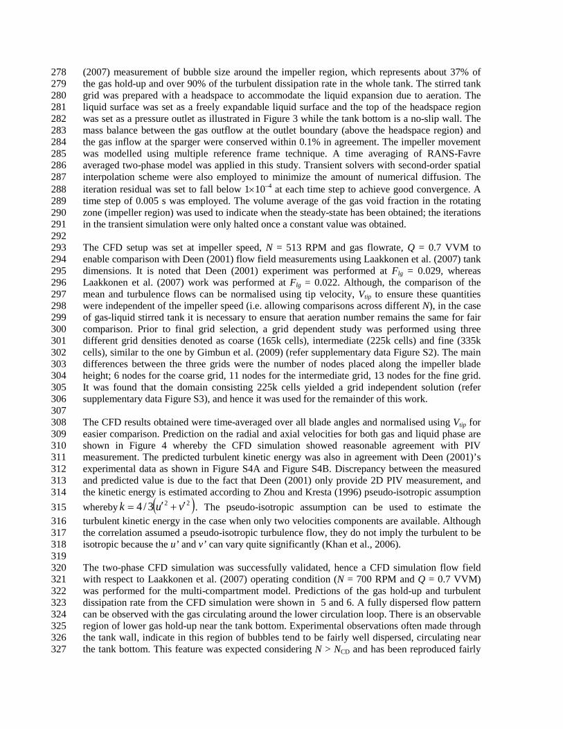
(2007) measurement of bubble size around the impeller region, which represents about 37% of 278 the gas hold-up and over 90% of the turbulent dissipation rate in the whole tank. The stirred tank 279 grid was prepared with a headspace to accommodate the liquid expansion due to aeration. The 280 liquid surface was set as a freely expandable liquid surface and the top of the headspace region 281 was set as a pressure outlet as illustrated in Figure 3 while the tank bottom is a no-slip wall. The 282 mass balance between the gas outflow at the outlet boundary (above the headspace region) and 283 the gas inflow at the sparger were conserved within 0.1% in agreement. The impeller movement 284 was modelled using multiple reference frame technique. A time averaging of RANS-Favre 285 averaged two-phase model was applied in this study. Transient solvers with second-order spatial 286 interpolation scheme were also employed to minimize the amount of numerical diffusion. The 287 iteration residual was set to fall below 1×10⁻⁴ at each time step to achieve good convergence. A 288 time step of 0.005 s was employed. The volume average of the gas void fraction in the rotating 289 zone (impeller region) was used to indicate when the steady-state has been obtained; the iterations 290 in the transient simulation were only halted once a constant value was obtained. 291 292 The CFD setup was set at impeller speed, N = 513 RPM and gas flowrate, Q = 0.7 VVM to 293 enable comparison with Deen (2001) flow field measurements using Laakkonen et al. (2007) tank 294 dimensions. It is noted that Deen (2001) experiment was performed at Flg = 0.029, whereas 295 Laakkonen et al. (2007) work was performed at Flg = 0.022. Although, the comparison of the 296 mean and turbulence flows can be normalised using tip velocity, Vtip to ensure these quantities 297 were independent of the impeller speed (i.e. allowing comparisons across different N), in the case 298 of gas-liquid stirred tank it is necessary to ensure that aeration number remains the same for fair 299 comparison. Prior to final grid selection, a grid dependent study was performed using three 300 different grid densities denoted as coarse (165k cells), intermediate (225k cells) and fine (335k 301 cells), similar to the one by Gimbun et al. (2009) (refer supplementary data Figure S2). The main 302 differences between the three grids were the number of nodes placed along the impeller blade 303 height; 6 nodes for the coarse grid, 11 nodes for the intermediate grid, 13 nodes for the fine grid. 304 It was found that the domain consisting 225k cells yielded a grid independent solution (refer 305 supplementary data Figure S3), and hence it was used for the remainder of this work. 306 307 The CFD results obtained were time-averaged over all blade angles and normalised using Vtip for 308 easier comparison. Prediction on the radial and axial velocities for both gas and liquid phase are 309 shown in Figure 4 whereby the CFD simulation showed reasonable agreement with PIV 310 measurement. The predicted turbulent kinetic energy was also in agreement with Deen (2001)’s 311 experimental data as shown in Figure S4A and Figure S4B. Discrepancy between the measured 312 and predicted value is due to the fact that Deen (2001) only provide 2D PIV measurement, and 313 the kinetic energy is estimated according to Zhou and Kresta (1996) pseudo-isotropic assumption 314 whereby ( )223/4 vuk ′+′= . The pseudo-isotropic assumption can be used to estimate the 315 turbulent kinetic energy in the case when only two velocities components are available. Although 316 the correlation assumed a pseudo-isotropic turbulence flow, they do not imply the turbulent to be 317 isotropic because the u’ and v’ can vary quite significantly (Khan et al., 2006). 318 319 The two-phase CFD simulation was successfully validated, hence a CFD simulation flow field 320 with respect to Laakkonen et al. (2007) operating condition (N = 700 RPM and Q = 0.7 VVM) 321 was performed for the multi-compartment model. Predictions of the gas hold-up and turbulent 322 dissipation rate from the CFD simulation were shown in 5 and 6. A fully dispersed flow pattern 323 can be observed with the gas circulating around the lower circulation loop. There is an observable 324 region of lower gas hold-up near the tank bottom. Experimental observations often made through 325 the tank wall, indicate in this region of bubbles tend to be fairly well dispersed, circulating near 326 the tank bottom. This feature was expected considering N > NCD and has been reproduced fairly 327

successfully by the CFD simulation. Flow field information obtained from the CFD simulation 328 was used to develop the multi-compartment model in this work. 329 330
331 Figure 2: Evolution of moments for bubble coalescence and breakage problem, (A) Coalescence 332 dominated case 1, ε = 1.18 m2/s3, lognormal distribution parameter (dmean initial = 2.2 mm), (B) 333 Breakage dominated case 2, ε = 1.18 m2/s3, lognormal distribution parameter (dmean initial = 5 334 mm). 335 336
337 Figure 3: Boundary condition of gas-liquid stirred tank simulation. Also shown is the 338 instantaneous contour of gas hold-up. 339 340
341 Figure 4: Prediction of liquid and gas phase axial (u) and radial velocity (v) at r/R = 0.37. 342 Experimental data is adopted from Deen (2001). 343 344 4.2 Multi-compartment model and comparison with CFD-PBM and experiment 345 Prior to the multi-compartment model, a single compartment simulation was carried out to test 346 the reliability of the PD-QMOM response on the bubble dynamics to changes in turbulence 347 dissipation rate, gas flow rate and initial bubble size. The simulation of the single compartment 348 (refer to supplementary data) is then extended to the multi-compartment simulation of aerated 349 stirred tank. Flow field data obtained from CFD results was used to divide the tank into a number 350 of homogeneous and well-mixed compartments. The connectivity between each compartment is 351 also determined by the flow direction obtained from two-way coupling CFD simulation. In order 352 to divide the tank, a new mesh of the vessel consisting 12 compartments was prepared based on 353 the CFD predicted flow patterns. The flow fields obtained from the gas-liquid CFD simulation 354 was interpolated into the new mesh for easier data interpretation as shown in Figure 5. The 355 compartments were split by taking into account the three major regions in a stirred tank, i.e. upper 356 recirculation loop, impeller discharge region and lower recirculation loop. 357 358 The compartments were prepared in a way that the flow was only allowed to move in one 359 direction at each interface responsible for separating the compartments. Figure 6A shows the 360 vector map of the gas flow extracted from the CFD simulation which is taken as a basis to 361 construct the compartments as shown in Figure 6B. The criteria of one direction flow for each 362 compartment interface were all satisfied except for compartments 2 and 3 thus, manual 363 adjustments were made on both the compartments to satisfy the inter-compartment mass balance. 364

The liquid turbulence dissipation rates and the inter-compartment gas flow rates were obtained 365 from averaging the detailed CFD results azimuthally over compartment volumes or areas, 366 respectively. The gas flow between the compartments are obtained by reporting the fluxes (mass 367 flow rate) through each interface in the CFD simulation. The exchanging gas flow rates of each 368 compartment do not exactly balance (with difference up to 10-6 kg/s), possibly due to 369 interpolation error and the fact that the CFD result was obtained from a transient simulation. 370 Therefore, the inter-compartment flows were adjusted (balanced) manually in order to make the 371 multi-compartment model satisfy the gas mass balance. A multi-compartment simulation with 372 imbalanced inter-compartment flow rates would result in a different distribution of third moments 373 (related to gas hold-up described in Eq. S6) to those obtained from the CFD simulation. It was 374 made clear from the supplementary data on a validation performed using single compartment 375 simulation that the third moment should be strictly preserved, unless there is a change in the local 376 gas-hold up. 377 378 The number density of bubbles in each compartment was determined by the volume averaged gas 379 hold-up. The initial BSD for each compartment were assumed to follow the lognormal 380 distribution with a geometric mean diameter of 2 mm and standard deviation of 0.2. The 381 calculation for the bubble number density in each compartment were performed following the 382 method described in the example as shown in Table S3, using the information of gas hold-up 383 from the CFD simulation. The turbulence dissipation rates and inter-compartment gas flow rates 384 were shown in Table 1. 385 386 Table 1: Parameter for the multi-compartment PBM. 387 Compartment
Volume
(cm3) αg
x 100 ε
(m2/s3) Gas flow direction
Gas flow rate (cm3/s)
Gas flow direction
Gas flow rate (cm3/s)
1 635.85 7.56 11.35 q11to12 28.08 q6to7 0.00 2 1502.22 1.16 2.57 q9to12 57.78 q2to8 108.48 3 552.35 1.56 0.40 q10to11 25.47 q2to9 46.36 4 394.21 0.07 0.05 q8to10 41.23 q8to9 67.25 5 863.14 0.02 0.12 q9to11 55.83 q1to12 6.21 6 2425.29 0.00 0.05 q2to3 3.33 q1to2 154.84 7 1043.64 1.53 0.06 q4to2 3.33 q7to1 161.05 8 1370.65 1.44 0.29 q3to4 2.92 qout12 92.07 9 977.86 3.92 0.05 q3to5 0.41 qout11 53.22 10 1938.08 0.47 0.06 q4to7 0.00 qout10 15.76 11 1378.62 2.14 0.06 q6to4 0.41 qspr 161.05 12 2427.41 3.72 0.03 q5to6 0.41
388 The sparger is modelled as a constant source of bubbles (a nucleation term) with uniform 389 diameter of 5.5 mm, following the experimental measurements by Laakkonen et al. (2007). The 390 gas flow rate of 1.6 x 10⁻⁴ m3/s (0.7 VVM) was set to match Laakkonen et al. (2007)’s 391 experiment. Table 2 shows the rate of the moments introduction at the sparger (i.e. compartment 392 no. 7) which is calculated using the following equation: 393 394
7
3
,sparger V6π
−
=k
sprk
LqS
(18)
395 Table 2: Rate of moments introduction at sparger. 396 Ssparger, 0 (/m3s) 1771417.33 Ssparger, 1 (m/m3s) 9742.80
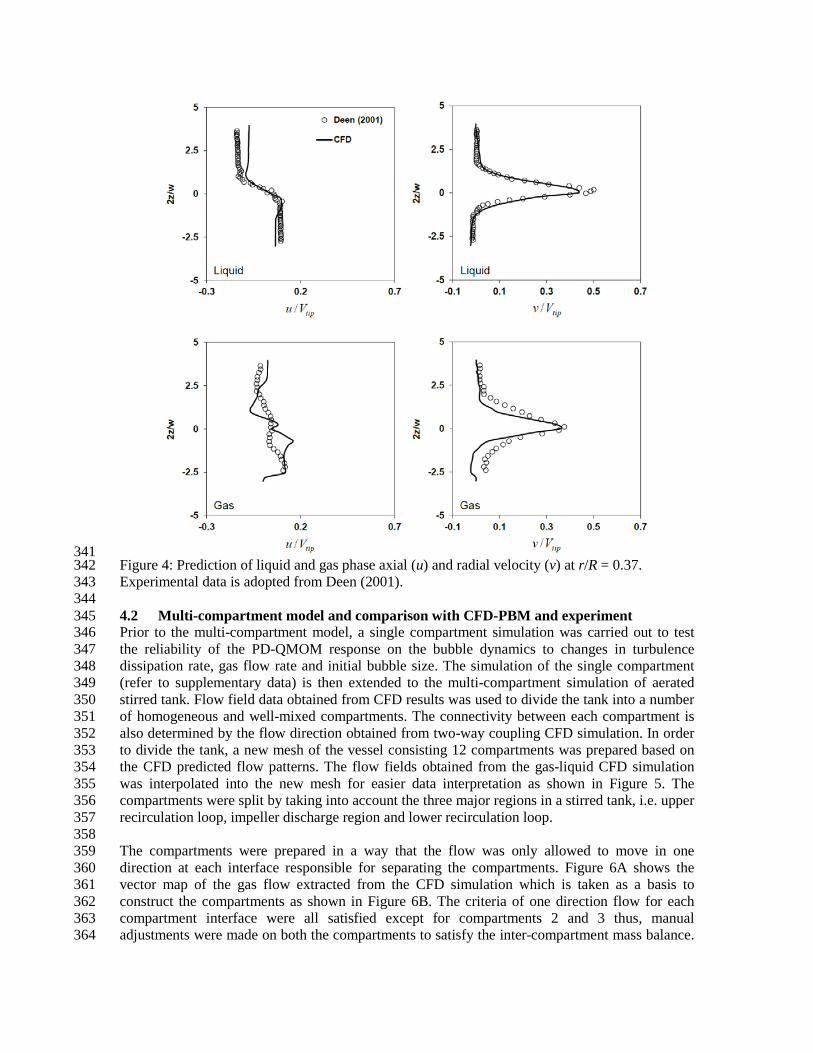
Ssparger, 2 (m2/m3s) 53.59 Ssparger, 3 (m3/m3s) 0.29
397
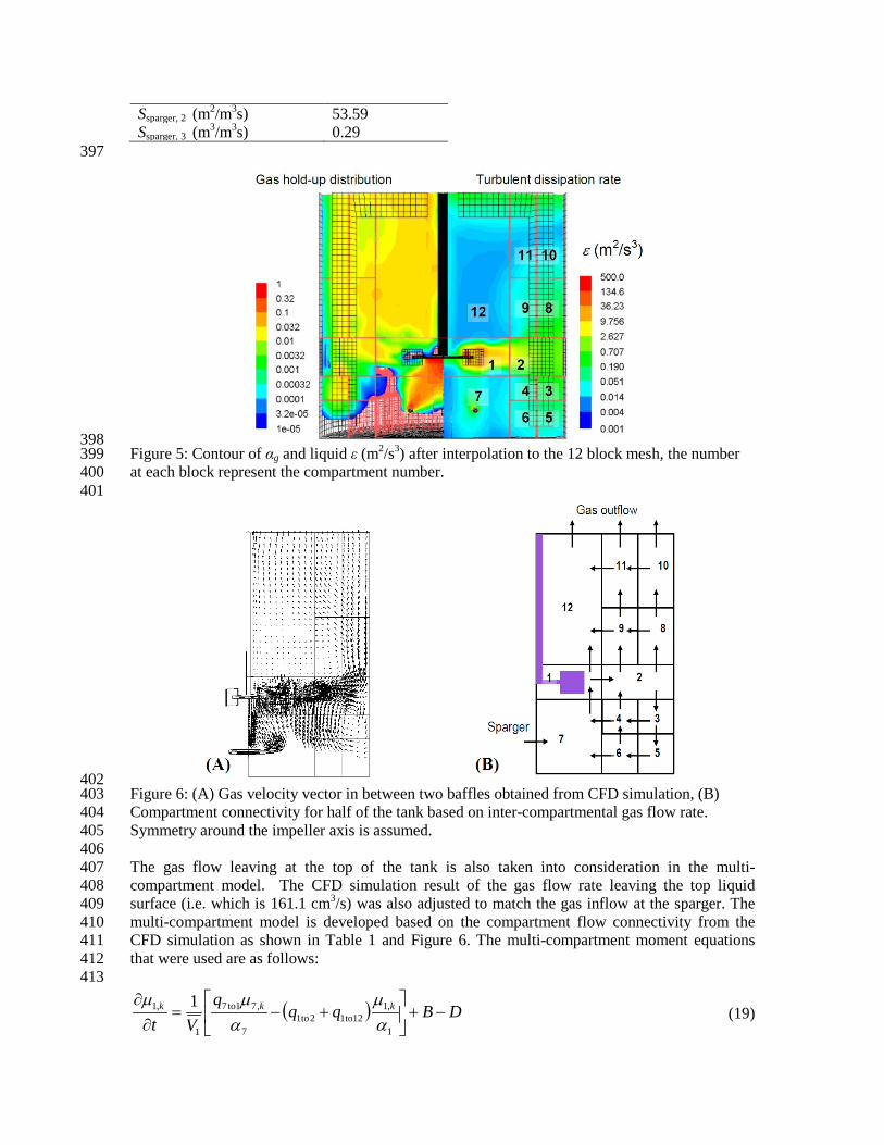
398 Figure 5: Contour of αg and liquid ε (m2/s3) after interpolation to the 12 block mesh, the number 399 at each block represent the compartment number. 400 401
402 Figure 6: (A) Gas velocity vector in between two baffles obtained from CFD simulation, (B) 403 Compartment connectivity for half of the tank based on inter-compartmental gas flow rate. 404 Symmetry around the impeller axis is assumed. 405 406 The gas flow leaving at the top of the tank is also taken into consideration in the multi-407 compartment model. The CFD simulation result of the gas flow rate leaving the top liquid 408 surface (i.e. which is 161.1 cm3/s) was also adjusted to match the gas inflow at the sparger. The 409 multi-compartment model is developed based on the compartment flow connectivity from the 410 CFD simulation as shown in Table 1 and Figure 6. The multi-compartment moment equations 411 that were used are as follows: 412 413
( ) DBqqq
Vtkkk −+
+−=
∂∂
1
,112to12to1
7
,71to7
1
,1 1αµ
αµµ
(19)

( ) DBqqqqq
Vtkkkk −+
++−+=
∂∂
2
,29to28to23to2
4
,4to24
1
,12to1
2
,2 1αµ
αµ
αµµ
(20)
( ) DBqqq
Vtkkk −+
+−=
∂∂
3
,35to34to3
2
,2to32
3
,3 1αµ
αµµ
(21)
( ) DBqqqq
Vtkkkk −+
+−+=
∂∂
4
,47to4to24
6
,6to46
3
,3to43
4
,4 1αµ
αµ
αµµ
(22)
DBqq
Vtkkk −+
−=
∂∂
5
,56to5
3
,3to53
5
,5 1αµ
αµµ
(23)
( ) DBqqq
Vtkkk −+
+−=
∂∂
6
,67to64to6
5
,5to65
6
,6 1αµ
αµµ
(24)
kkkkk SDB
qqqVt sparger,
7
,7to17
4
,4to74
6
,6to76
7
,7 1+−+
−+=
∂∂
αµ
αµ
αµµ
(25)
( ) DBqqq
Vtkkk −+
+−=
∂∂
8
,810to89to8
2
,2to82
8
,8 1αµ
αµµ
(26)
( ) DBqqqq
Vtkkkk −+
+−+=
∂∂
9
,9to11912to9
8
,8to98
2
,2to92
9
,9 1αµ
αµ
αµµ
(27)
( ) DBqqq
Vtkkk −+
+−=
∂∂
10
,10out1011to10
8
,8to108
10
,10 1αµ
αµµ
(28)
( ) DBqqqq
Vtkkkk −+
+−+=
∂∂
11
,11out1112to11
10
,100to111
9
,9to119
11
,11 1αµ
αµ
αµµ
(29)
( ) DBqqqq
Vtkkkkk −+
−++=
∂∂
12
,1212out
1
,1to121
9
,9to129
11
,111to121
12
,12 1αµ
αµ
αµ
αµµ
(30)
414 where B and D are the birth and death due to breakage and coalescence, similar to those in single 415 compartment model in the supplementary data; see Eq. 7. The multi-compartment population 416 balance was implemented using PD-QMOM in MATLAB; the ODE integrations were conducted 417 with absolute and relative tolerances set at 10-8 for all solutions. The multi-compartment model 418 represented by Eqs. 19 to 30 was solved using the ode113 solver in MATLAB. The simulations 419 took about 5 minutes (wall clock) to complete on a GENIE workstation fitted with two dual-core 420 3.8 GHz Xeon processors and 3 GB RAM. 421 422 Figure 7 shows the evolution of bubble size for each compartment where the inter-compartment 423 moment balances are calculated for this simulation. Unlike the single compartment where the 424 steady-state is obtained within a second, the multi-compartment requires up 5 seconds at most to 425 achieve steady-state bubble size. This is because the moment of evolution in neighbouring 426 compartments can affect the evolution of the moments in another compartment resulting to a 427 relatively longer time to approach steady-state. 428 429

430 Figure 7: Evolution of the Sauter mean bubble size d32 (m) at each compartment. 431 432 Meanwhile, Figure 8 displays the prediction of the local steady-state bubble size via multi-433 compartment PBM. The results show some qualitative agreement to Laakkonen et al. (2007)’s 434 experiment data and Gimbun et al. (2009)’s CFD-PBM simulation. There are discrepancies on 435 bubble size prediction in some compartments (e.g. compartment no. 3), where d32 is slightly 436 larger than the value measured by Laakkonen et al. (2007). Predictions of the multi-compartment 437 model in this work were also in fair agreement with the CFD-PBM predictions from Gimbun et 438 al. (2009). The discrepancy mainly occurs in the lower circulation loop where d32 is over-439 predicted by the current model. This may be due to the small uniform bubble size (i.e. 2 mm) 440 employed throughout the tank for the initial CFD simulation which led to a higher gas hold-up 441 around the lower circulation loop. It can be observed from Figure 8 that the assumptions of 442 bubble size around 2 mm is only valid around the impeller and to some extent in the upper 443 circulation loop but certainly not for lower circulation loop. It was concluded from the single 444 compartment study that higher gas hold-up led to larger bubble size especially in regions of lower 445 turbulence dissipation rate. Nevertheless the multi-compartment simulation has successfully 446 reproduced the correct distribution of bubble size inside the tank with the smallest bubble 447 harboring around the impeller region and the largest in the bulk flow of the upper circulation 448 loop. The former is due high turbulence dissipation rate around the impeller region (refer to Table 449 1). This finding is in agreement with experimental measurements by Barigou and Greaves (1992) 450 and Laakkonen et al. (2005) who also observed small bubble sizes around the impeller region. 451 452

453 Figure 8: Prediction of local bubble size (d32). The italic font (CFD-PBM from Gimbun et al. 454 (2009)), bold font (Laakkonen et al. (2007) experiment) and underlined font (this work). 455 456 There is also a growing concern regarding the use of constant bubble size assumption for gas-457 liquid CFD simulation. Such an assumption is certainly not valid in a stirred tank where the 458 turbulence dissipation rate gradient is high especially around the impeller region. The mean 459 bubble size should be significantly smaller around the impeller region compared to the bulk 460 region, as evidenced in the multi-compartment results. The bubble size can affect the prediction 461 of turbulent flows, gas void fraction and the gas flow rate which is required for the multi-462 compartment modelling. Thus it can be concluded that the error from the original CFD simulation 463 can severely affect the results of the multi-compartment modelling. It is best that a four-way 464 coupling is used to improve prediction accuracy in order to eliminate the assumption of uniform 465 bubble size. It cannot be deny that the multi-compartment model is not capable of providing as 466 high resolution as CFD, however they require less computational effort to simulate. Nevertheless, 467 the multi-compartment model is capable of yielding a reasonably accurate prediction of the local 468 bubble size, despite all its simplifications. 469 470 The gas hold-up is an important mass transfer parameter for gas-liquid stirred tanks. The gas 471 hold-up in each compartment is related to the third moment and is estimated using Eq. S6. The 472 gas hold-up obtained from the multi-compartment PBM is compared to the result from CFD 473 simulation in Table 6. The prediction shows an excellent agreement between the multi-474 compartment model and the CFD predictions, meaning that the third moment is perfectly 475 conserved during the simulation thus confirming the validity of the multi-compartment model. 476 477 Table 6: Comparison between the gas hold-up from CFD simulation and the value obtained from 478 multi-compartment simulation 479
Compartment Multi-compartment 6/3πµα =g x 100
CFD simulation
gα x 100 1 7.56 7.56 2 1.16 1.16 3 1.56 1.56 4 0.07 0.07 5 0.02 0.02 6 0.00 0.00

7 1.53 1.53 8 1.44 1.44 9 3.92 3.92 10 0.47 0.47 11 2.14 2.14 12 3.72 3.72
480 5 Conclusion 481 The PBM implementation in a single compartment model (refer to supplementary data) has 482 demonstrated the capability of the PD-QMOM algorithm, with realistic breakage and coalescence 483 kernels in predicting the evolution of bubble size in a homogeneous gas-liquid flow. The 484 prediction from the single compartment PBM shows a reasonable agreement with the Sauter 485 mean bubble sizes obtained from empirical correlations. The algorithm also responded well to 486 changes in the turbulence dissipation rate and the initial BSD. The results suggest that the final 487 bubble size is only affected by the turbulence dissipation rate and local gas hold-up, but is not 488 affected by the initial bubble size. The single compartment model was combined with gas-liquid 489 CFD simulation to form a multi-compartment model. The multi-compartment PBM yielded a 490 reasonable prediction of the local bubble size and compared with experimental measurements by 491 Laakkonen et al. (2007). The three-way coupling PBM requires less computational effort and 492 easier to converge than that of four-way coupling. Thus, the model developed and tested in this 493 work may be useful for a quick evaluation of local bubble size in an aerated stirred tank. 494 495 References 496 Alopaeus V, Koskinen J, Keskinen KI. Simulation of the population balances for liquid–liquid 497
systems in a nonideal stirred tank. Part 1: Description and qualitative validation of the 498 model. Chem. Eng. Sci. 1999;54(24):5887-5899. 499
Alves SS, Maia CI, Vasconcelos JMT. Experimental and modelling study of gas dispersion in a 500 double turbine stirred tank. Chem. Eng. Sci. 2002;57(3):487-496. 501
Andersson R, Andersson B. On the breakup of fluid particles in turbulent flows. AIChE J. 502 2006;52(6):2020-2030. 503
Bakker A, Van den Akker H. A computational model for the gas-liquid flow in stirred reactors. 504 Che. Eng. Res. Des. 1994;72(A4):594-606. 505
Barigou M, Greaves M. Bubble-size distributions in a mechanically agitated gas—liquid 506 contactor. Chem. Eng. Sci. 1992;47(8):2009-2025. 507
Behzadi A, Issa RI, Rusche H. Modelling of dispersed bubble and droplet flow at high phase 508 fractions. Chem. Eng. Sci. 2004;59(4):759-770. 509
Buffo A, Vanni M, Marchisio DL. Multidimensional population balance model for the simulation 510 of turbulent gas–liquid systems in stirred tank reactors. Chem. Eng. Sci. 2012;70:31-44. 511
Bombač, A, Žun, I, Filipič, B, Žumer, M. (1997). Gas-filled cavity structures and local void 512 fraction distribution in aerated stirred vessel. AIChE J. 1997;43(11):2922-2931. 513
Clift R, Grace JR, Weber ME. Bubbles, drops, and particles. New York: Academic Press; 1978. 514 Deen NG. An experimental and computational study of fluid dynamics in gas-liquid chemical 515
reactors (Doctoral dissertation). Esbjerg: Aalborg University;2001 516 Deen NG, Solberg T, Hjertager BH. Flow generated by an aerated rushton impeller: two-phase 517
PIV experiments and numerical simulations. Can. J. Chem. Eng. 2002;80(4):1-15. 518 Degaleesan S. Fluid dynamic measurements and modeling of liquid mixing in bubble columns 519
(Doctoral dissertation). St. Louis MO: Washington University; 1997. 520 Fluent Inc. User’s Guide. Lebanon, New Hampshire; 2005. 521 Gimbun J. Scale-up of gas-liquid stirred tanks using coupled computational fluid dynamics and 522
population balance modelling (Doctoral dissertation). Leicestershire: Loughborough 523 University;2009. 524

Gimbun J, Rielly CD, Nagy ZK. Modelling of mass transfer in gas–liquid stirred tanks agitated 525 by Rushton turbine and CD-6 impeller: A scale-up study. Chem. Eng. Res. Des. 526 2009;87(4):437-451. 527
Gordon RG. Error bounds in equilibrium statistical mechanics. J. Math Phys.1968;9:655-663. 528 Hristov H, Mann R, Lossev V, Vlaev SD, Seichter P. A 3-D analysis of gas-liquid mixing, mass 529
transfer and bioreaction in a stirred bio-reactor. Food Bioprod. Process. 2001;79(4):232-530 241. 531
Ishii M, Zuber N. Drag coefficient and relative velocity in bubbly, droplet or particulate flows. 532 AIChE J. 1979;25(5):843-855. 533
Kennard EH. Theory of gasses. New York: Mc Graw-Hill; 1938. 534 Kerdouss F, Bannari A, Proulx P. CFD modeling of gas dispersion and bubble size in a double 535
turbine stirred tank. Chem. Eng. Sci. 2006;61(10):3313-3322. 536 Khan, FR, Rielly, CD, Brown, DAR. Angle-resolved stereo-PIV measurements close to a down-537
pumping pitched-blade turbine. Chem. Eng. Sci. 2006;61(9):2799-2806. 538 Khopkar AR, Ranade VV. CFD simulation of gas–liquid stirred vessel: VC, S33, and L33 flow 539
regimes. AIChE J. 2006;52(5):1654-1672. 540 Kolmogorov AN. The local structure of turbulence in incompressible viscous fluid for very large 541
Reynolds numbers. Dokl. Akad. Nauk SSSR. 1941;30(4):301-305. 542 Kresta SM, Etchells III AW, Dickey DS, Atiemo-Obeng VA. Advances in industrial mixing: a 543
companion to the handbook of industrial mixing. New Jersey: John Wiley & Sons Inc; 544 2015. ISBN: 978-0-470-52382-7. 545
Laakkonen M, Moilanen P, Miettinen T, Saari K, Honkanen M, Saarenrinne P, Aittamaa J. Local 546 bubble size distributions in agitated vessel comparison of three experimental techniques. 547 Chem. Eng. Res. Des. 2005;83(1):50-58. 548
Laakkonen M, Moilanen P, Alopaeus V, Aittamaa J. Dynamic modeling of local reaction 549 conditions in an agitated aerobic fermenter. AIChE J. 2006;52(5):1673-1689. 550
Laakkonen M, Alopaeus V, Aittamaa J. Validation of bubble breakage, coalescence and mass 551 transfer models for gas–liquid dispersion in agitated vessel. Chem. Eng. Sci. 552 2006;61(1):218-228. 553
Laakkonen M, Moilanen P, Alopaeus V, Aittamaa J. Modelling local bubble size distributions in 554 agitated vessels. Chem. Eng. Sci. 2007;62(3):721-740. 555
Lane GL, Schwarz MP, Evans GM. Predicting gas–liquid flow in a mechanically stirred tank. 556 Appl. Math. Model. 2002;26(2):223-235. 557
Lane GL, Schwarz MP, Evans GM. Numerical modelling of gas-liquid flow in stirred tanks. 558 Chem. Eng. Sci. 2005;60(8-9):2203-2214 559
Marchisio DL, Vigil RD, Fox RO. Quadrature method of moments for aggregation–breakage 560 processes. J. Colloid Interface Sci. 2003;258(2):322-334. 561
Montante G, Horn D, Paglianti A. Gas–liquid flow and bubble size distribution in stirred tanks. 562 Chem. Eng. Sci. 2008;63(8):2107-2118. 563
Morud KE, Hjertager BH. LDA measurements and CFD modelling of gas-liquid flow in a stirred 564 vessel. Chem. Eng. Sci. 1996;51(2):233-249. 565
Petitti M, Vanni M, Marchisio DL, Buffo A, Podenzani F. Simulation of coalescence, break-up 566 and mass transfer in a gas-liquid stirred tank with CQMOM. Chem. Eng. J. 2013;228:1182-567 1194. 568
Pohorecki R, Moniuk W, Bielski P, Sobieszuk P. Diameter of bubbles in bubble column reactors 569 operating with organic liquids. Chem. Eng. Res. Des. 2005;83(7):827-832. 570
Prince MJ, Blanch HW. Bubble coalescence and break-up in air-sparged bubble columns. AIChE 571 J. 1990;36(10):1485-1499. 572
Rotta JC. Turbulent flows (Turbulente Stromungen). Stuttgart: Teubner-Verlag; 1972. 573 Scargiali F, D’Orazio A, Grisafi F, Brucato A. Modelling and simulation of gas-liquid 574
hydrodynamics in mechanically stirred tanks. Chem. Eng. Res. Des. 2007;85(5):637-646. 575
Schiller L, Naumann L. A drag coefficient correlation. Z. Ver. Deutsch. Ing. 1935;77:318. 576 Shimizu K, Takada S, Minekawa K, Kawase Y. Phenomenological model for bubble column 577
reactors: prediction of gas hold-ups and volumetric mass transfer coefficients. Chem. Eng. 578 J. 2000;78(1):21-28. 579
Smith, JM. Large multiphase reactors: some open questions. Chem. Eng. Res. Des. 580 2006;84(4):265-271. 581
Sun H, Mao Z, Yu G. Experimental and numerical study of gas hold-up in surface aerated stirred 582 tanks. Chem. Eng. Sci. 2006;61(12):4098-4110. 583
Venneker BCH, Derksen JJ, Van den Akker H. Population balance modeling of aerated stirred 584 vessels based on CFD. AIChE J. 2002;48(4):673-685. 585
Wang W, Mao Z, Yang C. Experimental and numerical investigation on gas holdup and flooding 586 in an aerated stirred tank with Rushton impeller. Ind. Eng. Chem. Res. 2006;45(3):1141-587 1151. 588
Wilkinson PM. Physical aspects and scale-up of high pressure bubble columns (Doctoral 589 dissertation). The Netherlands: University of Groningen; 1991. 590
Wu, H, Patterson, G.K. Laser-doppler measurements of turbulent-flow parameters in a stirred 591 mixer. Chem. Eng. Sci. 1989;44(10):2207-2221. 592
Zahradnı́k J, Mann R, Fialová M, Vlaev D, Vlaev SD, Lossev V, Seichter P. A networks-of-zones 593 analysis of mixing and mass transfer in three industrial bioreactors. Chem. Eng. Sci. 594 2001;56(2):485-492. 595
Zhou, G., & Kresta, S. M. (1996). Distribution of energy between convective and turbulent-flow 596 for 3 frequently used impellers. Chem. Eng. Res. Des. 1996;74(3):379-389. 597


![ResearchArticle Coupling Solvent Extraction Units to ...downloads.hindawi.com/journals/ijce/2018/1620218.pdfTreybal [] was followed. A stirred tank was used that ... said for the kinetic](https://static.documents.pub/doc/80x56/5e841b304e8a1861c70c2fa2/researcharticle-coupling-solvent-extraction-units-to-treybal-was-followed.jpg)


