Page 1
Kennedy Masunda
Student Number: 514285
[email protected]
Supervisor: Prof Fambirai Takawira
Submitted in fulfilment of the academic requirements for the Master of Science
in Engineering in Electrical and Information Engineering degree in the School
of Electrical and Information Engineering at the University of Witwatersrand,
Johannesburg, South Africa.
August 2017
School of Electrical and Information Engineering
University of the Witwatersrand
Private Bag 3, 2050, Johannesburg, South Africa
Threshold based multi-bit flipping
decoding of binary LDPC codes.
Page 2
ii
As the candidate’s supervisor, I have approved this dissertation for submission.
Signed: ___________________________
Date: ___________________________
Name: Prof. Fambirai Takawira.
Page 3
iii
Declaration
I, KENNEDY. T. F. MASUNDA declare that
i. The research reported in this dissertation, except where otherwise indicated, and is my
original work.
ii. This dissertation has not been submitted for any degree or examination at any other
university.
iii. This dissertation does not contain other persons’ data, pictures, graphs or other
information, unless specifically acknowledged as being sourced from other persons.
iv. This dissertation does not contain other persons’ writing, unless specifically
acknowledged as being sourced from other researchers. Where other written sources
have been quoted, then:
a. their words have been re-written but the general information attributed to them
has been referenced;
b. where their exact words have been used, their writing has been placed inside
quotation marks, and referenced.
v. Where I have reproduced a publication of which I am an author, co-author or editor, I
have indicated in detail which part of the publication was actually written by myself
alone and have fully referenced such publications.
vi. This dissertation does not contain text, graphics or tables copied and pasted from the
Internet, unless specifically acknowledged, and the source being detailed in the
dissertation and in the list of References sections.
Signed: _________________________
Date: _________________________
Name: Kennedy Masunda
Page 4
iv
Abstract
There has been a surge in the demand of high speed reliable communication infrastructure in
the last few decades. Advanced technology, namely the internet has transformed the way
people live and how they interact with their environment. The Internet of Things (IoT) has been
a very big phenomenon and continues to transform infrastructure in the home and work place.
All these developments are underpinned by the availability of cost-effective, reliable and error
free communication services.
A perfect and reliable communication channel through which to transmit information does not
exist. Telecommunication channels are often characterised by random noise and unpredictable
disturbances that distort information or result in the loss of information. The need for reliable
error-free communication has resulted in advanced research work in the field of Forward Error
Correction (FEC).
Low density parity check (LDPC) codes, discovered by Gallager in 1963 provide excellent
error correction performance which is close to the vaunted Shannon limit when used with long
block codes and decoded with the sum-product algorithm (SPA). However, long block code
lengths increase the decoding complexity exponentially and this problem is exacerbated by the
intrinsic complexity of the SPA and its approximate derivatives. This makes it impossible for
the SPA to be implemented in any practical communication device. Bit flipping LDPC
decoders, whose error correction performance pales in comparison to the SPA have been
devised to counter the disadvantages of the SPA. Even though, the bit flipping algorithms do
not perform as well as the SPA, their exceeding low complexity makes them attractive for
practical implementation in high speed communication devices. Thus, a lot of research has
gone into the design and development of improved bit flipping algorithms.
This research work analyses and focusses on the design of improved multi-bit flipping
algorithms which converge faster than single-bit flipping algorithms. The aim of the research
is to devise methods with which to obtain thresholds that can be used to determine erroneous
sections of a given codeword so that they can be corrected.
Two algorithms that use multi-thresholds are developed during the course of this research. The
first algorithm uses multiple adaptive thresholds while the second algorithm uses multiple near
optimal SNR dependant fixed thresholds to identify erroneous bits in a codeword. Both
algorithms use soft information modification to further improve the decoding performance.
Simulations show that the use of multiple adaptive or near optimal SNR dependant fixed
Page 5
v
thresholds improves the bit error rate (BER) and frame error rate (FER) correcting performance
and also decreases the average number of iterations (ANI) required for convergence.
The proposed algorithms are also investigated in terms of quantisation for practical applications
in communication devices. Simulations show that the bit length of the quantizer as well as the
quantization strategy (uniform or non-uniform quantization) is very important as it affects the
decoding performance of the algorithms significantly.
Page 6
vi
Acknowledgements
First of all I would like to thank the Lord and my saviour Jesus Christ for seeing me through
this very hectic but productive portion of my academic journey. I would also want to show
deep appreciation and gratitude to my irreplaceable supervisor Professor Fambirai Takawira
for being an unending source of invaluable guidance, information and support throughout the
course of this research. There where so many brick walls and pitfalls but you assisted in
navigating through them all.
Secondly I would like to show my gratitude to the Wits School of Electrical and Information
Engineering for all the support and coffee. It was not going to be easy to navigate through this
minefield without your companionship and camaraderie. I would also like to thank the Wits
CeTAS, Prof Takawira and the Wits Financial Aid Office for sponsoring this research. It would
not have been possible without these reliable sources of funds.
Last but not least, I would like to express my profound gratitude to my friends and family,
particularly Mr James K Masunda for constantly encouraging me and supporting me through
the good and bad times as this research progressed. All of you made this a bearable and
worthwhile experience.
Many Thanks.
Page 7
vii
Preface
This dissertation is a compilation of the research work completed by Mr Kennedy T. F.
Masunda under the supervision of Prof. Fambirai Takawira at the School of Electrical and
Information Engineering at the University of the Witwatersrand. The work involves the study
of multi-bit flipping algorithms for LDPC codes. The topic of discussion is the improvement
of these algorithms by attempting to optimise the way in which flipping thresholds are
determined.
Part of the results obtained in the research work have been submitted at the SATNAC 2016
conference held at George in South Africa. Some of the results will be submitted in an
upcoming journal.
The dissertation in its entirety is a product of the author’s work apart from the referenced
material.
Page 8
viii
Table of Contents
Declaration ............................................................................................................................................. iii
Abstract .................................................................................................................................................. iv
Acknowledgements ................................................................................................................................ vi
Preface .................................................................................................................................................. vii
Table of Contents ................................................................................................................................. viii
Table of Figures ..................................................................................................................................... xi
List of Acronyms .................................................................................................................................. xv
Glossary of Nomenclature .................................................................................................................. xvii
1. Introduction ..................................................................................................................................... 1
1.1 Forward Error Correction........................................................................................................ 1
1.2 Research Motivation ............................................................................................................... 3
1.3 Research Contributions ........................................................................................................... 4
1.4 Overview of Dissertation ........................................................................................................ 5
1.5 Publications ............................................................................................................................. 6
2. Low Density Parity Check Codes ................................................................................................... 7
2.1 Introduction ............................................................................................................................. 7
2.1.1 The Parity Check Matrix ................................................................................................. 7
2.1.2 The Tanner Graph ........................................................................................................... 8
2.1.3 The Generator Matrix ...................................................................................................... 9
2.1.4 Types of LDPC Codes .................................................................................................. 10
2.2 Encoding ............................................................................................................................... 14
2.2.1 Generator Matrix Encoder ............................................................................................ 14
2.2.2 Linear Time Encoding .................................................................................................. 15
2.3 Decoding ............................................................................................................................... 16
2.3.1 Belief Propagation......................................................................................................... 17
2.3.2 Approximate Belief Propagation................................................................................... 18
2.3.3 Bit flipping Algorithms ................................................................................................. 18
3. Bit Flipping decoding of LDPC Codes ......................................................................................... 20
3.1 Single Bit Flipping Algorithms ............................................................................................. 21
3.1.1 Gallager Bit Flipping Decoding Algorithm (GBF) (1962) ........................................... 21
3.1.2 Weighted Bit Flipping Decoding Algorithm (WBF) (2001) ......................................... 21
3.1.3 Bootstrapped Weighted Bit Flipping Decoding Algorithm (B-WBF) (2002) .............. 22
3.1.4 Modified Weighted Bit Flipping Decoding Algorithm (M-WBF) (2004) .................... 23
3.1.5 Improved Modified Weighted Bit Flipping Decoding Algorithm (IMWBF) (2005) ... 23
3.1.6 Reliability Ratio Based Weighted Bit Flipping Algorithm (RR-WBF) (2005) ............ 24
3.1.7 Channel Independent Weighted Bit Flipping Decoding Algorithm (CI-WBF) (2012) 24
Page 9
ix
3.1.8 Modified Channel Independent Weighted Bit Flipping Decoding Algorithm (MCI-
WBF) (2013) ................................................................................................................................. 25
3.1.9 An Iterative Bit Flipping based Decoding Algorithm (2015) ....................................... 25
3.1.10 A Self-Normalized Weighted Bit-Flipping Decoding Algorithm (2016) ..................... 26
3.1.11 Hybrid iterative Gradient Descent Bit-Flipping algorithm (HGDBF) algorithm (2016)
27
3.1.12 Weighted Bit-Flipping Decoding for Product LDPC Codes (2016) ............................. 28
3.2 Multi-bit Flipping Algorithms .............................................................................................. 29
3.2.1 Gradient Descent Bit Flipping Algorithm (2008) ......................................................... 29
3.2.2 Candidate bit based bit-flipping decoding algorithm (CBBF) (2009) .......................... 31
3.2.3 Modified I-WBF (MBF) (2009) .................................................................................... 32
3.2.4 Soft-Bit-Flipping (SBF) Decoder for Geometric LDPC Codes (2010) ........................ 33
3.2.5 Combined Modified Weighted Bit Flipping Algorithm (CM-WBF) (2012) ................ 34
3.2.6 An Adaptive Weighted Multi-bit Flipping Algorithm (AWMBF) (2013) .................... 34
3.2.7 Two-Staged Weighted Bit Flipping Decoding Algorithm (2015) ................................ 35
3.2.8 Mixed Modified Weighted Bit Flipping Decoding Algorithm (MM-WBF) (2015) ..... 36
3.2.9 Noise-Aided Gradient Descent Bit-Flipping Decoder (2016) ....................................... 37
3.3 Threshold Based decoding .................................................................................................... 37
3.4 Channel Information modification ........................................................................................ 38
4. Adaptive Multi-Threshold Multi-bit Flipping Algorithm (AMTMBF) ........................................ 41
4.1 Introduction ........................................................................................................................... 41
4.2 Adaptive Threshold Scheme ................................................................................................. 42
4.2.1 Convergence comparison – Single bit flipping vs Adaptive threshold multi-bit flipping
43
4.2.2 Convergence comparison – Existing and proposed adaptive threshold techniques ...... 44
4.2.3 Adaptive Multi Threshold ............................................................................................. 45
4.3 Channel Information Modification Scheme .......................................................................... 49
4.3.1 The proposed scheme .................................................................................................... 50
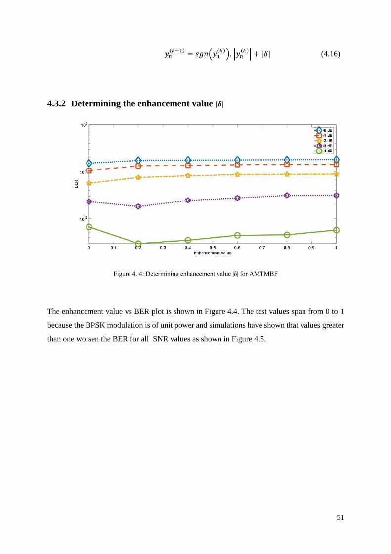
4.3.2 Determining the enhancement value |𝜹| ....................................................................... 51
4.4 Proposed Decoding Algorithm .............................................................................................. 52
4.5 Simulation Results ................................................................................................................ 54
4.6 Discussion ............................................................................................................................. 61
5. Near Optimal SNR Dependent Threshold Multi-bit Flipping Algorithm (NOSMBF) ................. 63
5.1 Introduction ........................................................................................................................... 63
5.2 SNR Dependent Threshold Scheme ...................................................................................... 64
5.2.1 Primary Flipping Thresholds ........................................................................................ 65
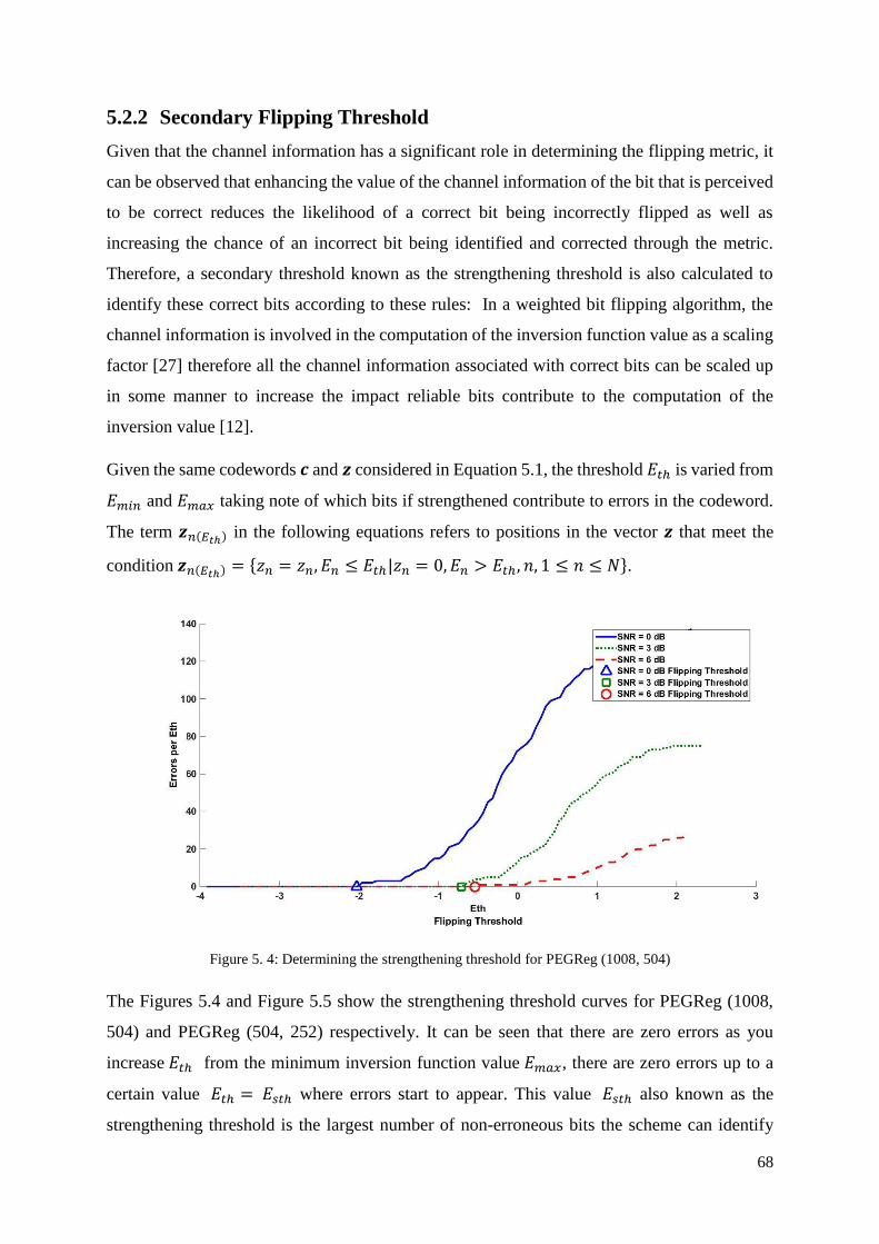
5.2.2 Secondary Flipping Threshold ...................................................................................... 68
5.2.3 Distribution of the inversion function values in a Random codeword .......................... 72
Page 10
x
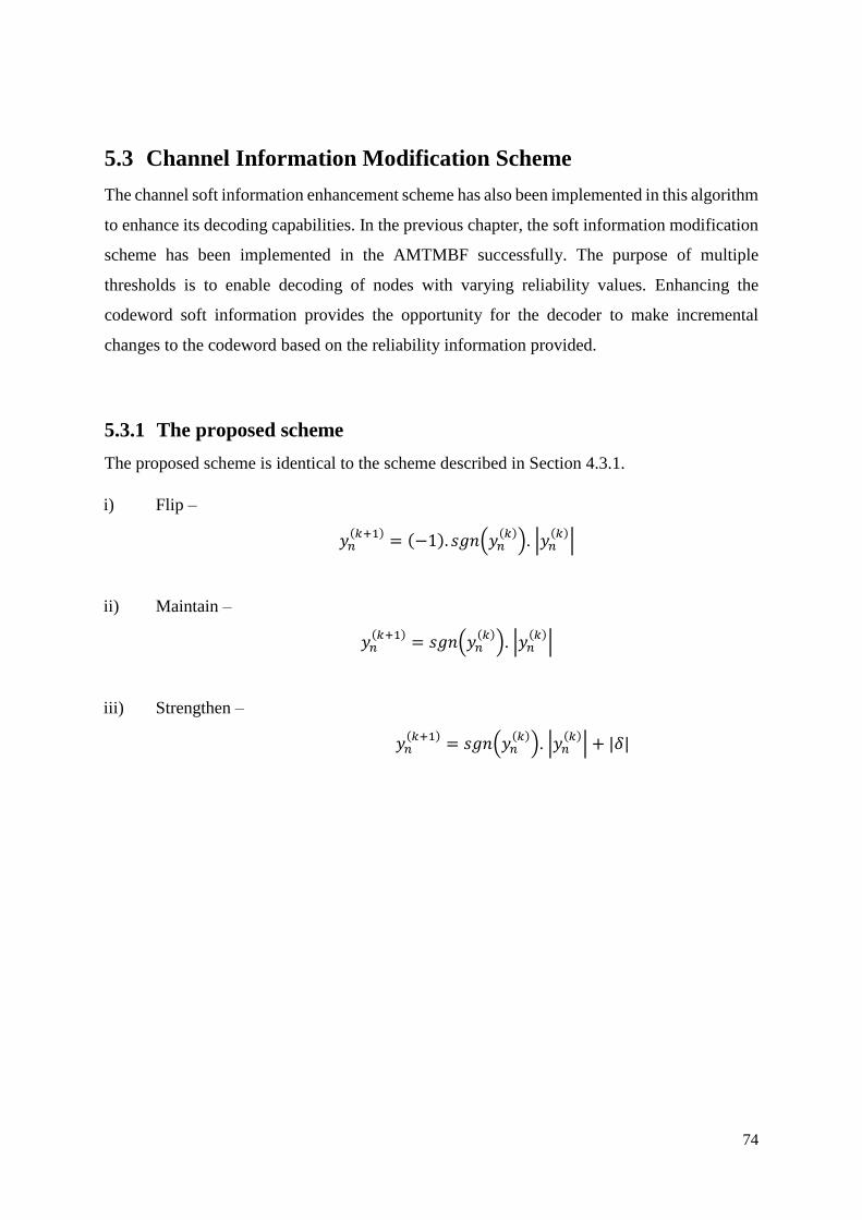
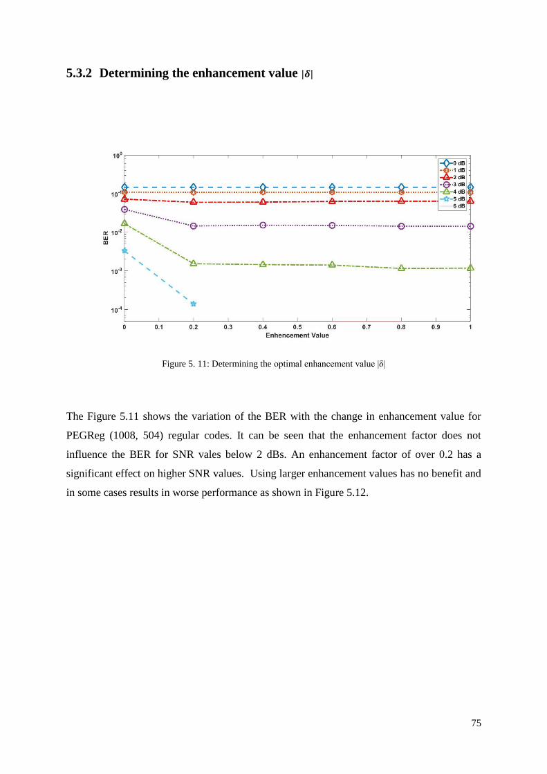
5.3 Channel Information Modification Scheme .......................................................................... 74
5.3.1 The proposed scheme .................................................................................................... 74
5.3.2 Determining the enhancement value |𝜹| ....................................................................... 75
5.4 Proposed Decoding Algorithm .............................................................................................. 76
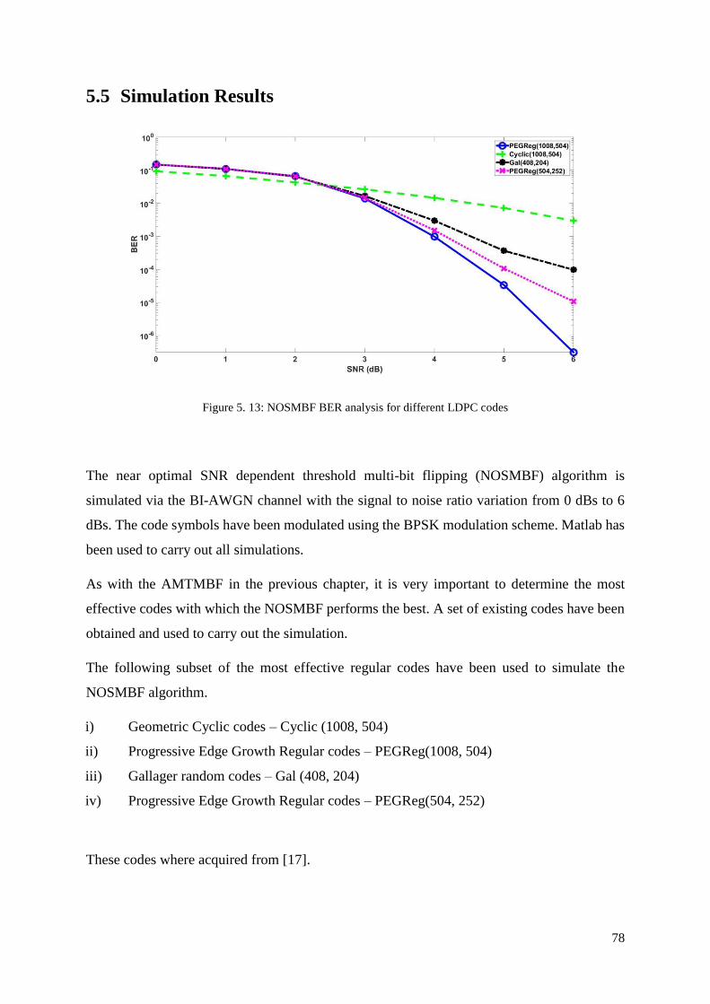
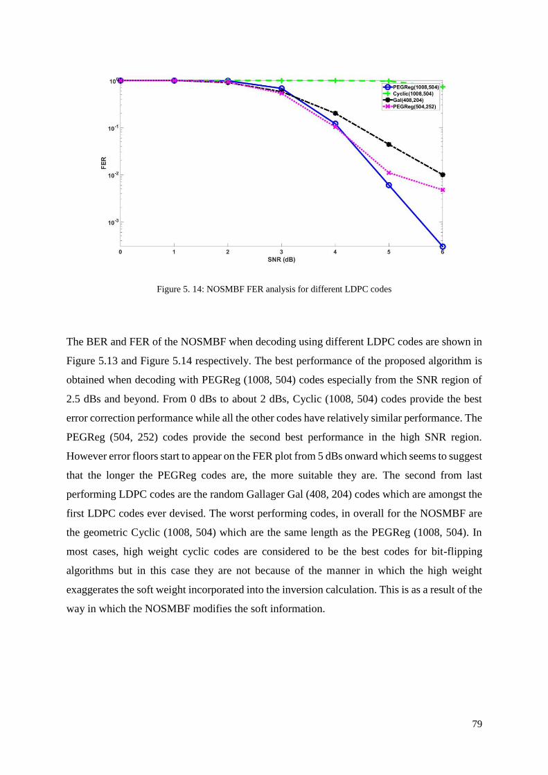
5.5 Simulation Results ................................................................................................................ 78
5.6 Discussion ............................................................................................................................. 85
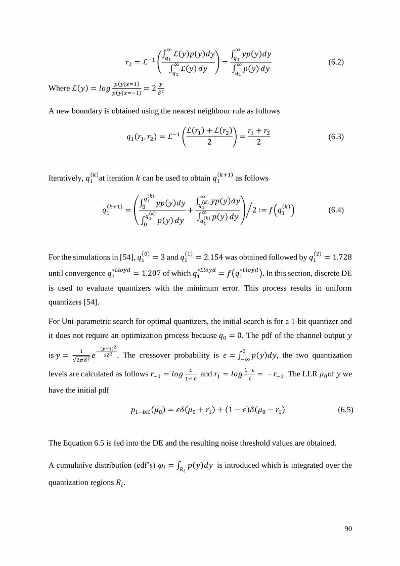
6. Quantisation of Bit Flipping algorithms ....................................................................................... 87
6.1 Introduction ........................................................................................................................... 87
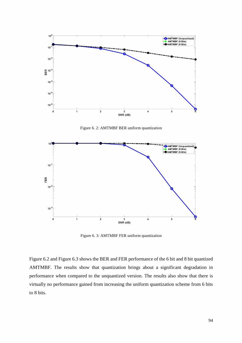
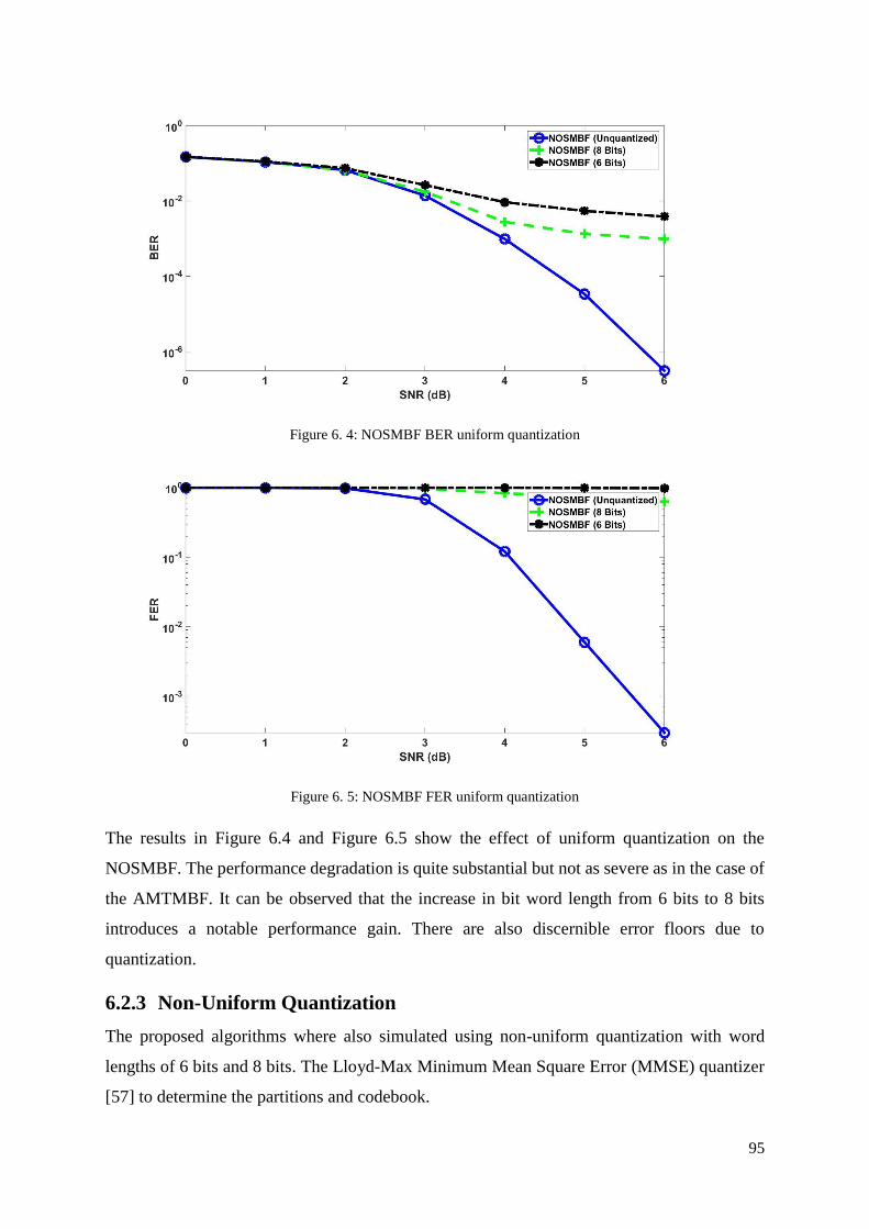
6.2 Simulation Results ................................................................................................................ 93
6.2.1 Quantisation Schemes ................................................................................................... 93
6.2.2 Uniform Quantization ................................................................................................... 93
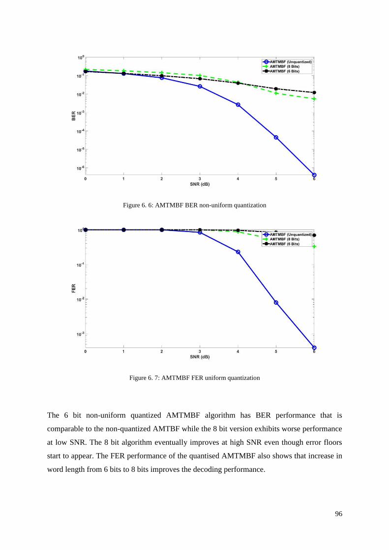
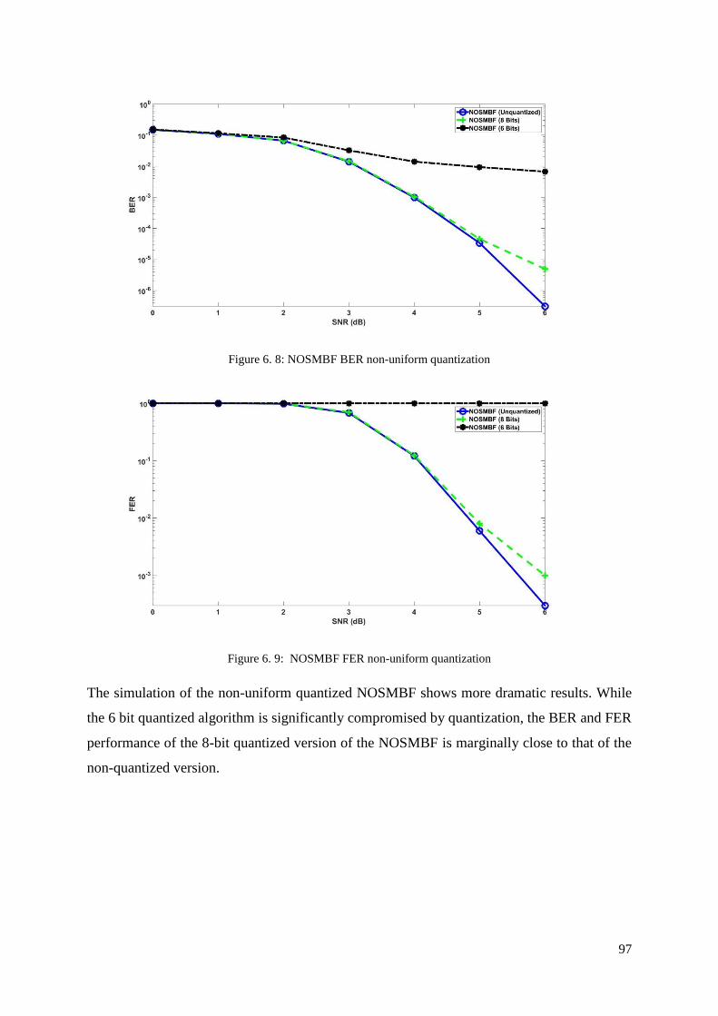
6.2.3 Non-Uniform Quantization ........................................................................................... 95
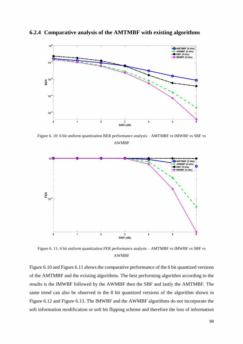
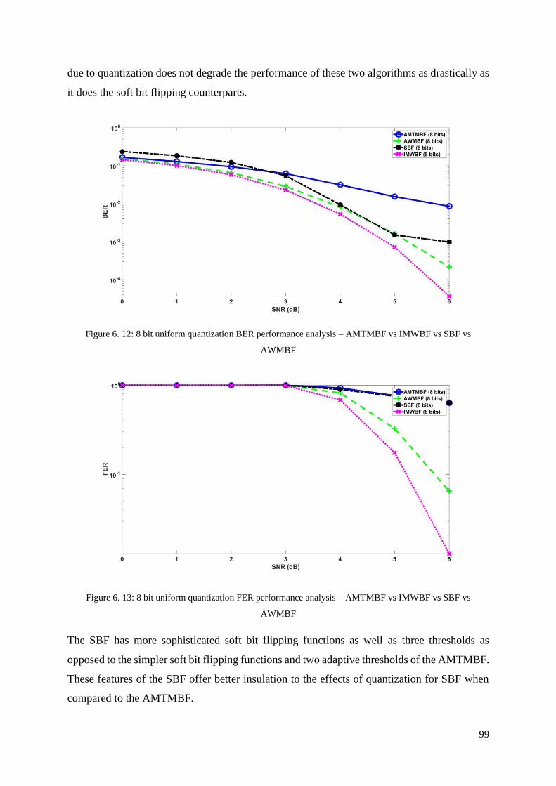
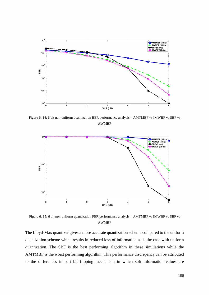
6.2.4 Comparative analysis of the AMTMBF with existing algorithms ................................ 98
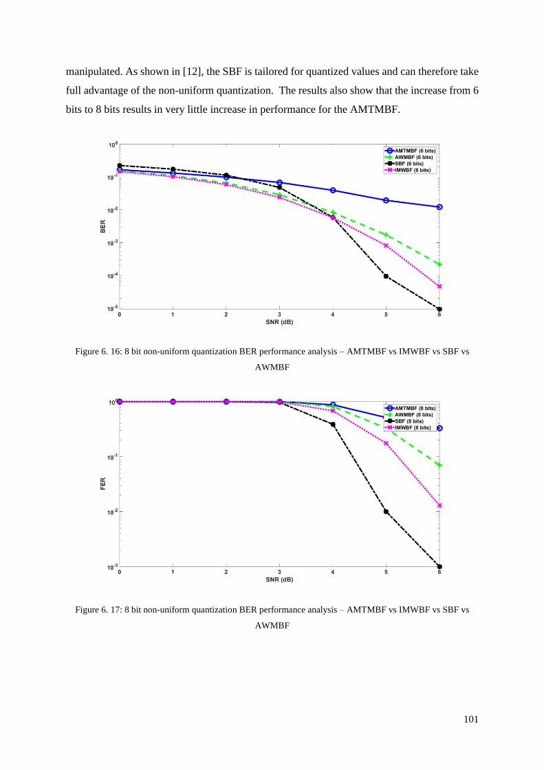
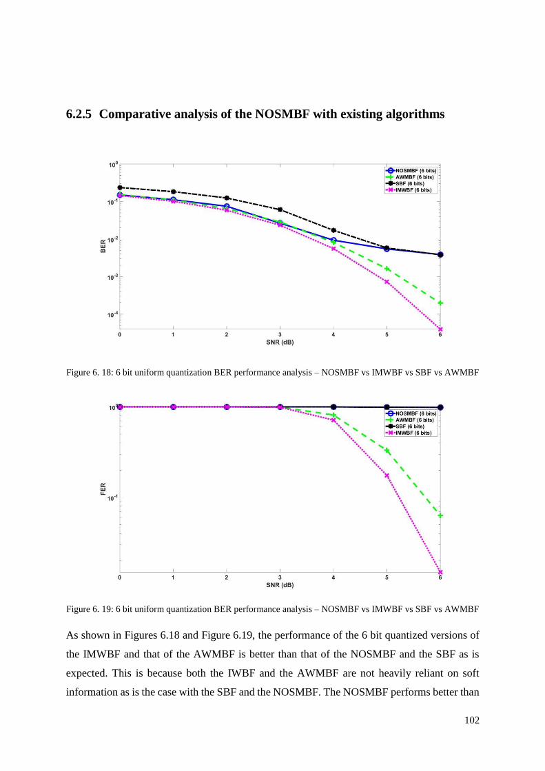
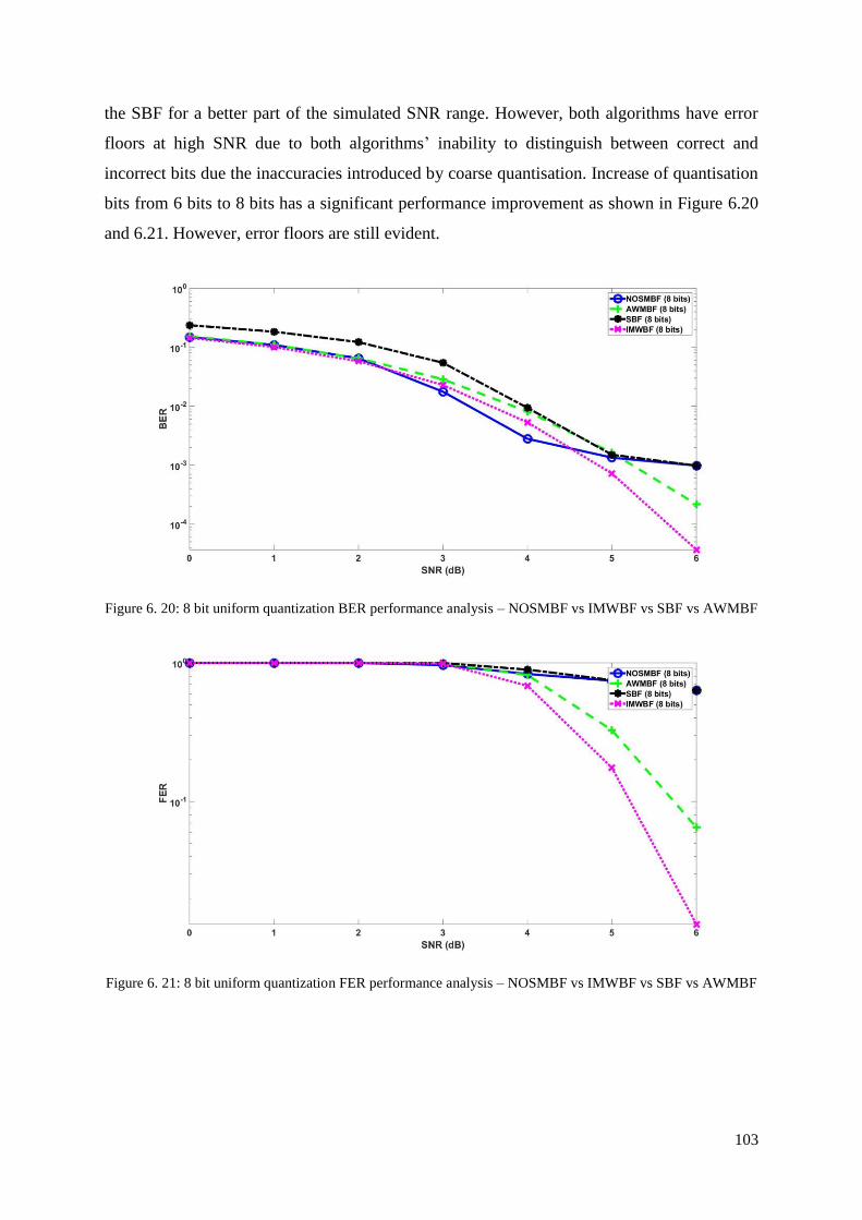
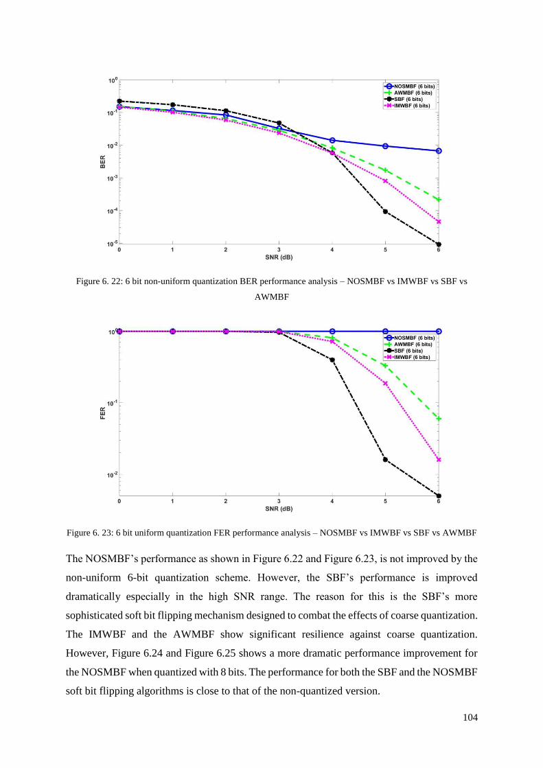
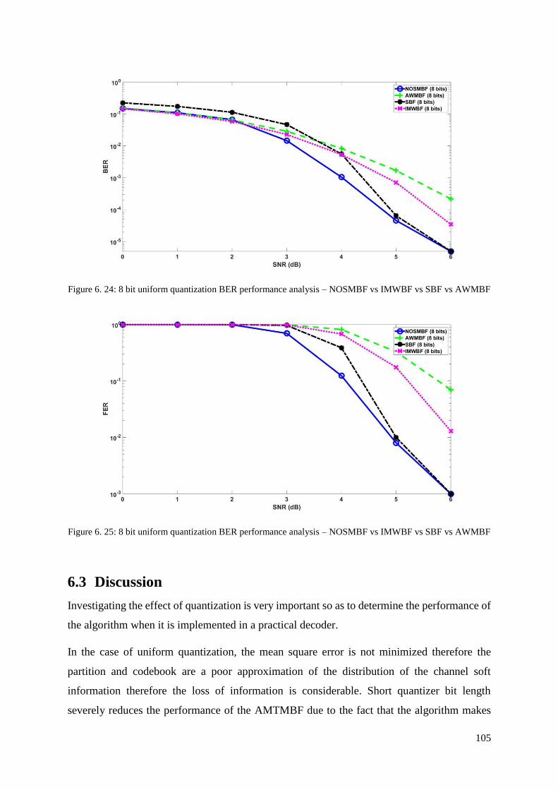
6.2.5 Comparative analysis of the NOSMBF with existing algorithms ............................... 102
6.3 Discussion ........................................................................................................................... 105
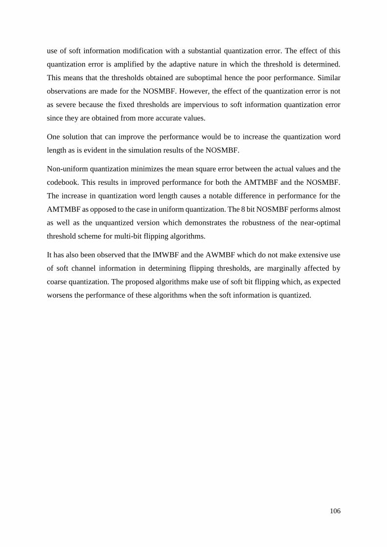
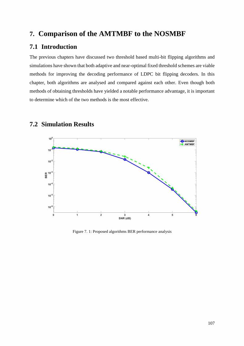
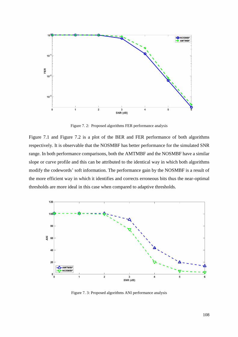
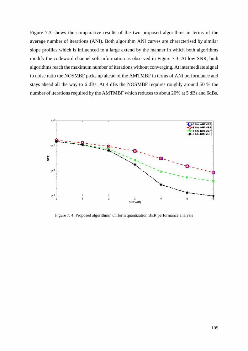
7. Comparison of the AMTMBF to the NOSMBF ......................................................................... 107
7.1 Introduction ......................................................................................................................... 107
7.2 Simulation Results .............................................................................................................. 107
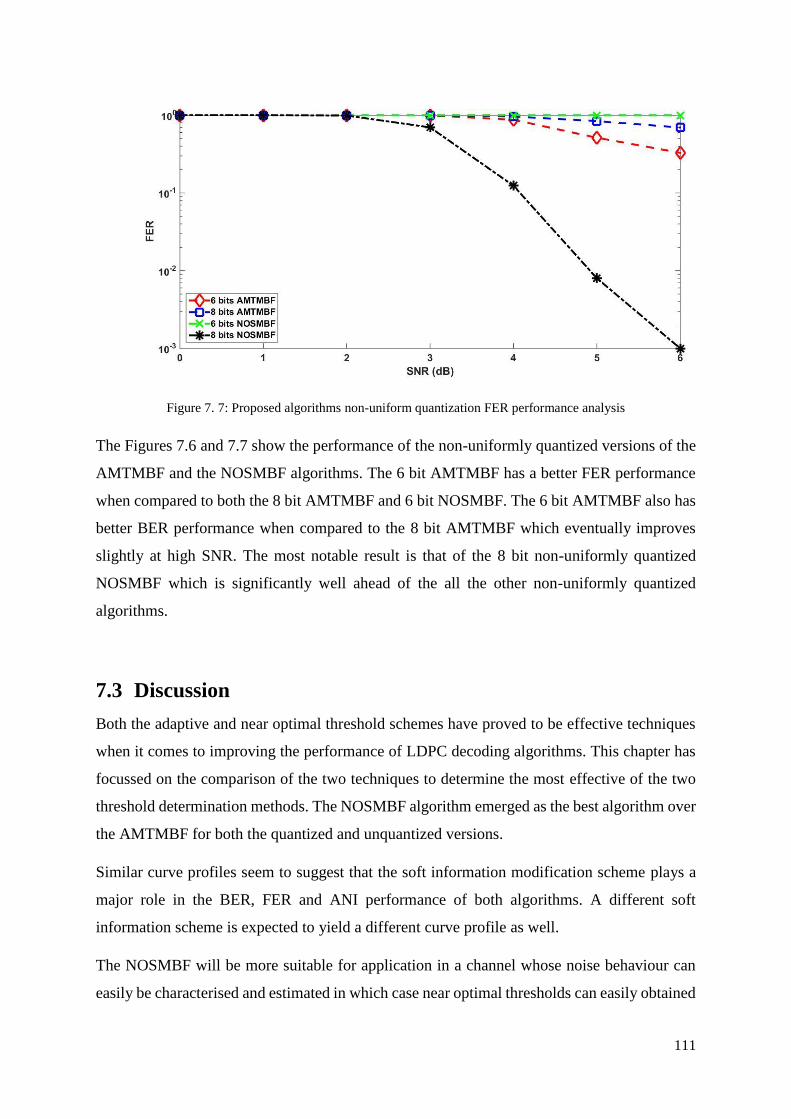
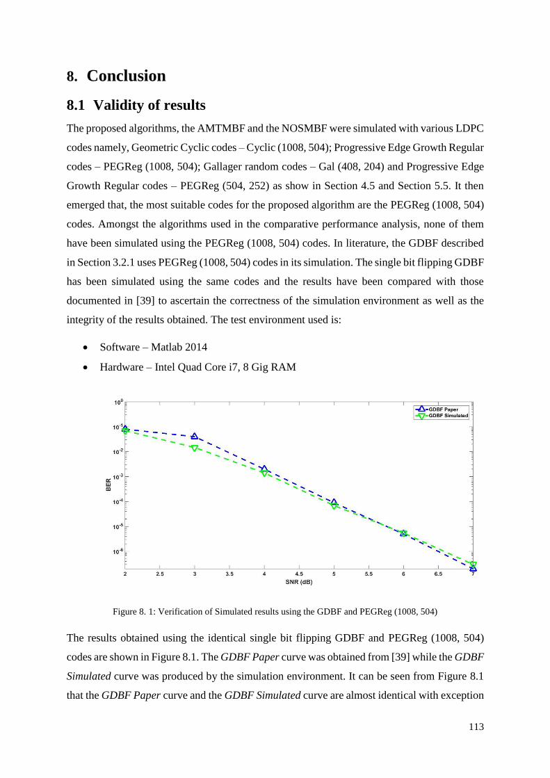
7.3 Discussion ........................................................................................................................... 111
8. Conclusion .................................................................................................................................. 113
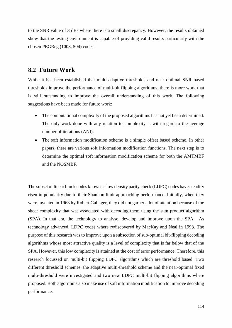
8.1 Validity of results ................................................................................................................ 113
8.2 Future Work ........................................................................................................................ 114
References ........................................................................................................................................... 117
Page 11
xi
Table of Figures
Figure 2. 1 The Tanner Graph.................................................................................................... 8
Figure 2. 2 Repeat-Accumulate (RA), irregular Repeat-Accumulate (IRA) and extended
irregular Repeat-Accumulate (eIRA) code encoders ............................................................... 14
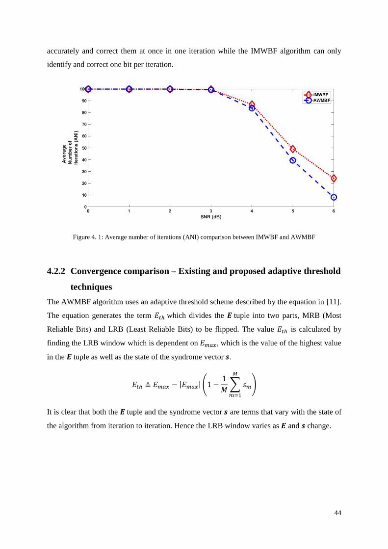
Figure 4. 1: Average number of iterations (ANI) comparison between IMWBF and AWMBF
.................................................................................................................................................. 44
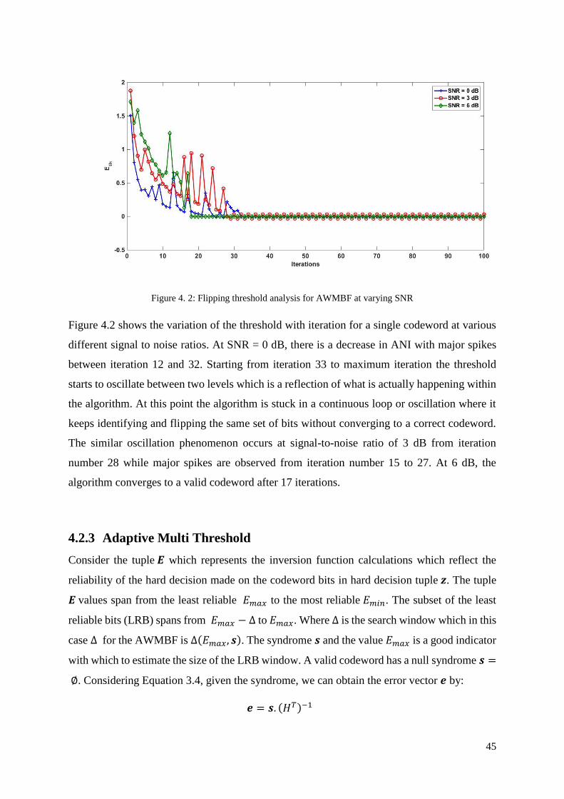
Figure 4. 2: Flipping threshold analysis for AWMBF at varying SNR ................................... 45
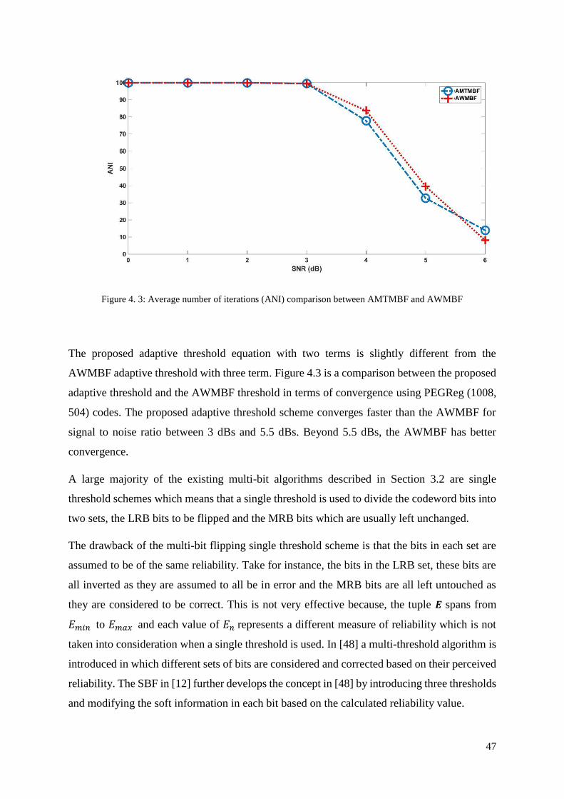
Figure 4. 3: Average number of iterations (ANI) comparison between AMTMBF and
AWMBF .................................................................................................................................. 47
Figure 4. 4: Determining enhancement value |δ| for AMTMBF.............................................. 51
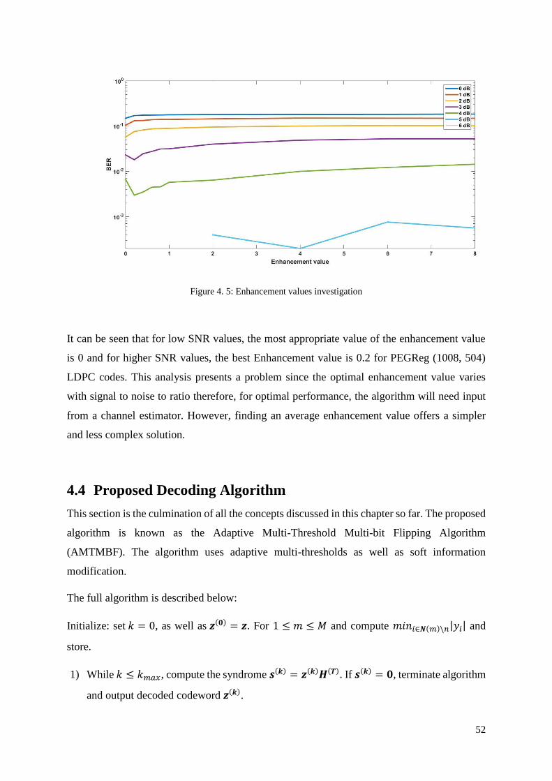
Figure 4. 5: Enhancement values investigation ....................................................................... 52
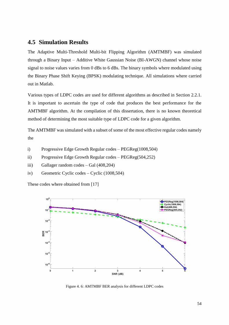
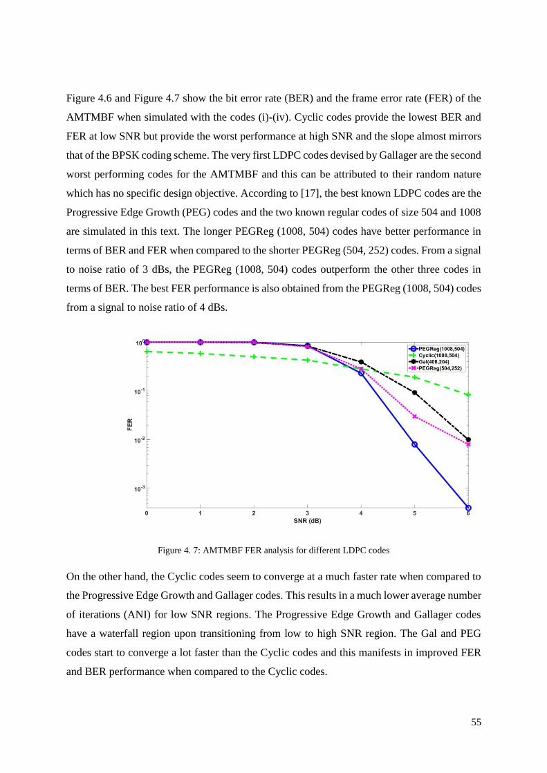
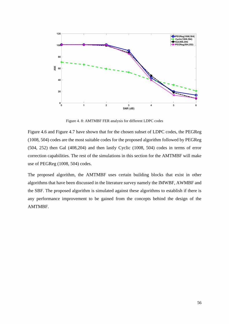
Figure 4. 6: AMTMBF BER analysis for different LDPC codes ............................................ 54
Figure 4. 7: AMTMBF FER analysis for different LDPC codes ............................................. 55
Figure 4. 8: AMTMBF FER analysis for different LDPC codes ............................................. 56
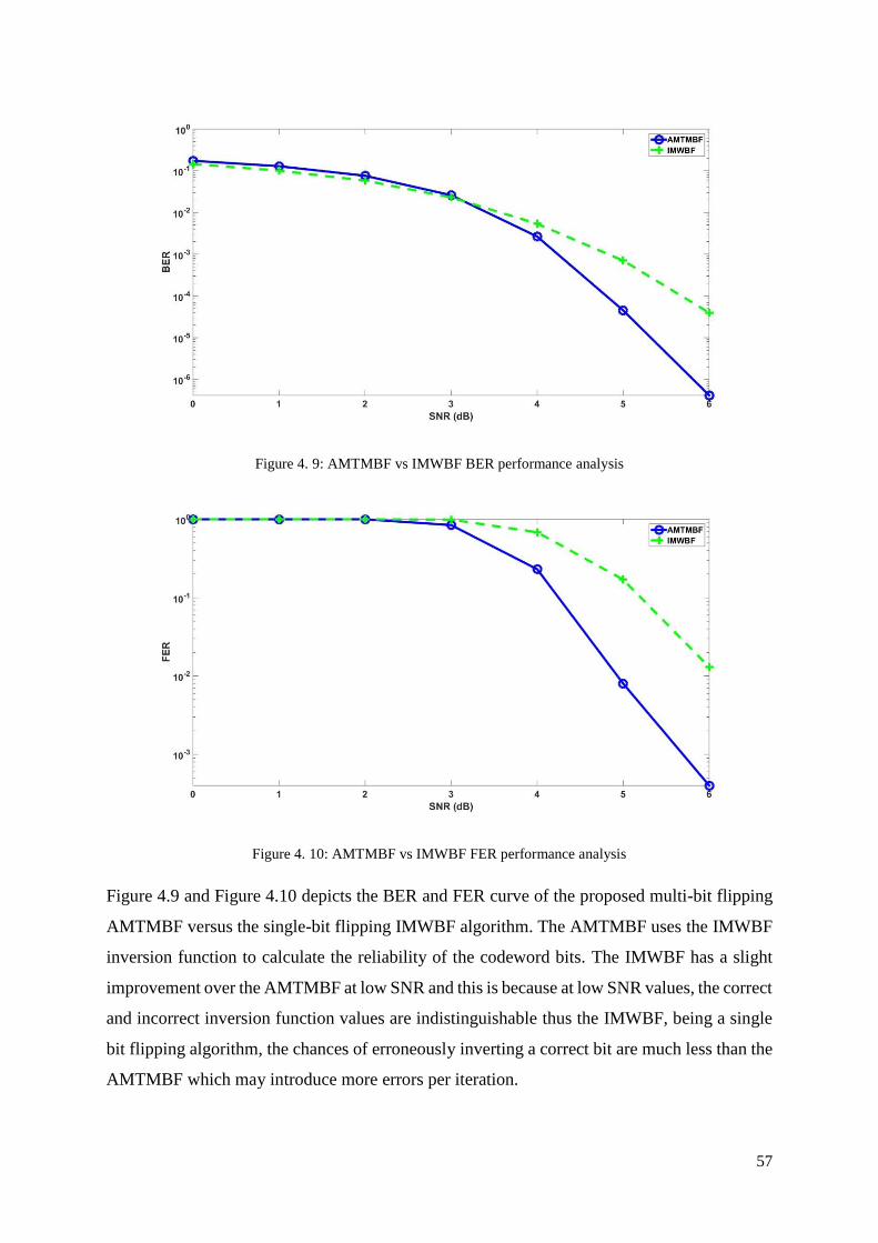
Figure 4. 9: AMTMBF vs IMWBF BER performance analysis .............................................. 57
Figure 4. 10: AMTMBF vs IMWBF FER performance analysis ............................................ 57
Figure 4. 11: AMTMBF vs AWMBF BER performance analysis .......................................... 58
Figure 4. 12: AMTMBF vs AMWBF FER performance analysis........................................... 58
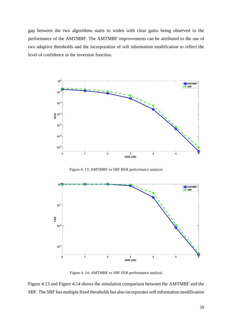
Figure 4. 13: AMTMBF vs SBF BER performance analysis .................................................. 59
Figure 4. 14: AMTMBF vs SBF FER performance analysis................................................... 59
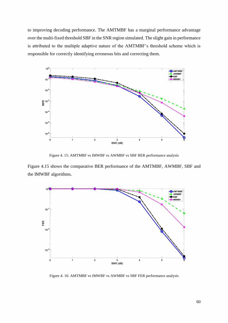
Figure 4. 15: AMTMBF vs IMWBF vs AWMBF vs SBF BER performance analysis .......... 60
Figure 4. 16: AMTMBF vs IMWBF vs AWMBF vs SBF FER performance analysis ........... 60
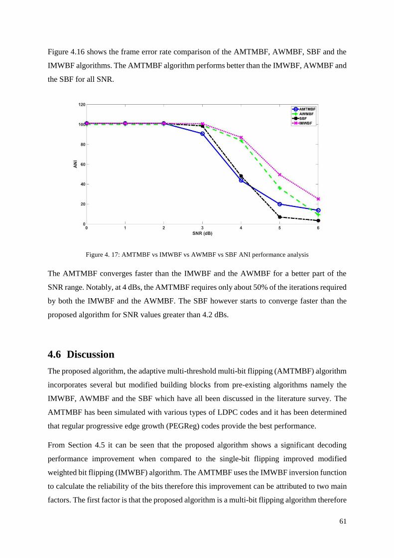
Figure 4. 17: AMTMBF vs IMWBF vs AWMBF vs SBF ANI performance analysis ........... 61
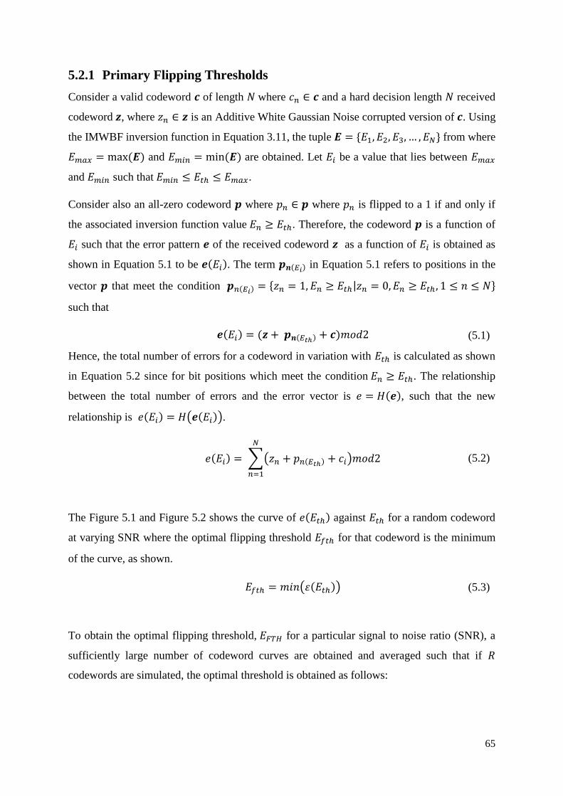
Figure 5. 1: Determining the flipping threshold at varying SNR values for PEGReg (1008,
504) .......................................................................................................................................... 66
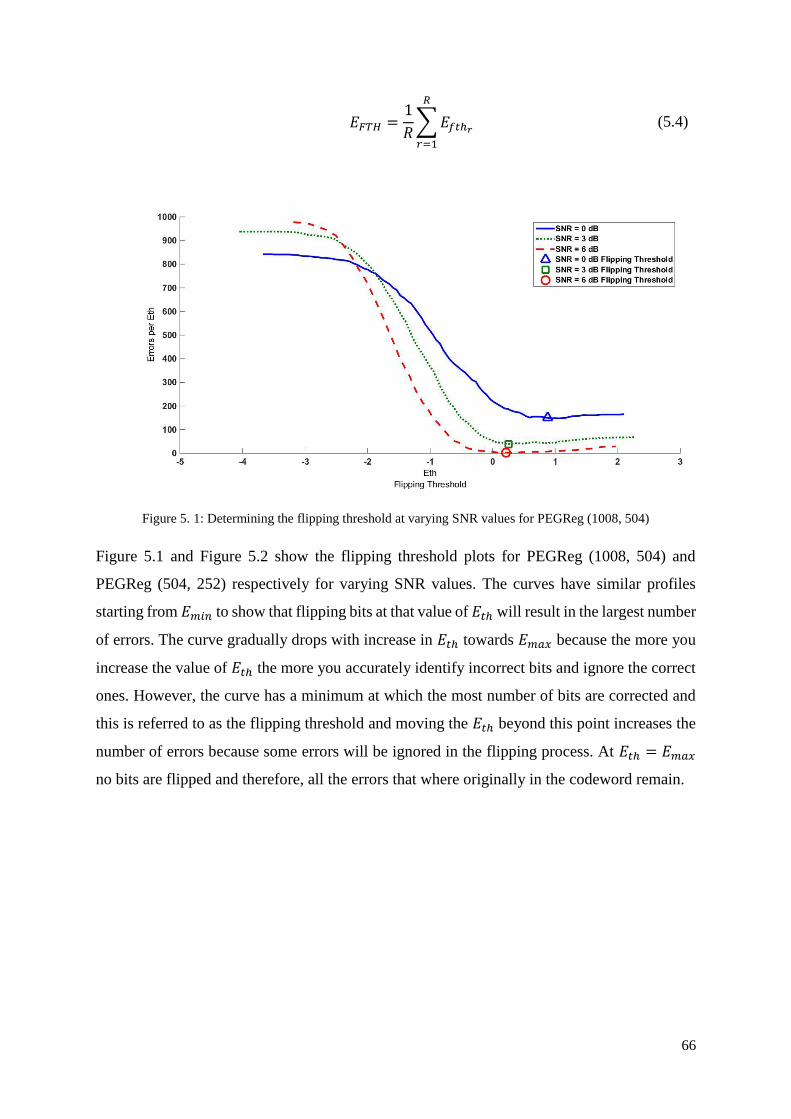
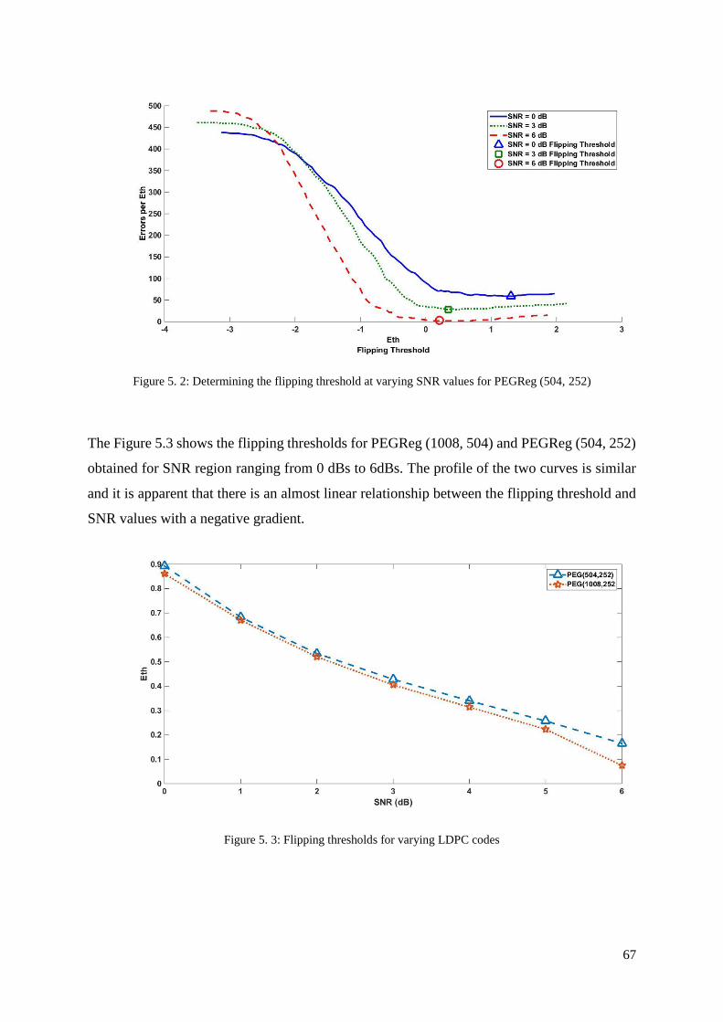
Figure 5. 2: Determining the flipping threshold at varying SNR values for PEGReg (504,252)
.................................................................................................................................................. 67
Figure 5. 3: Flipping thresholds for varying LDPC codes ....................................................... 67
Figure 5. 4: Determining the strengthening threshold for PEGReg (1008, 504) ..................... 68
Figure 5. 5: Determining the strengthening threshold for PEGReg (504, 252) ....................... 69
Page 12
xii
Figure 5. 6: Strengthening thresholds for varying LDPC codes ............................................. 69
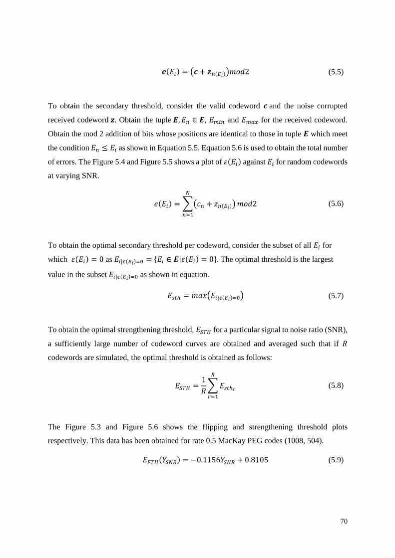
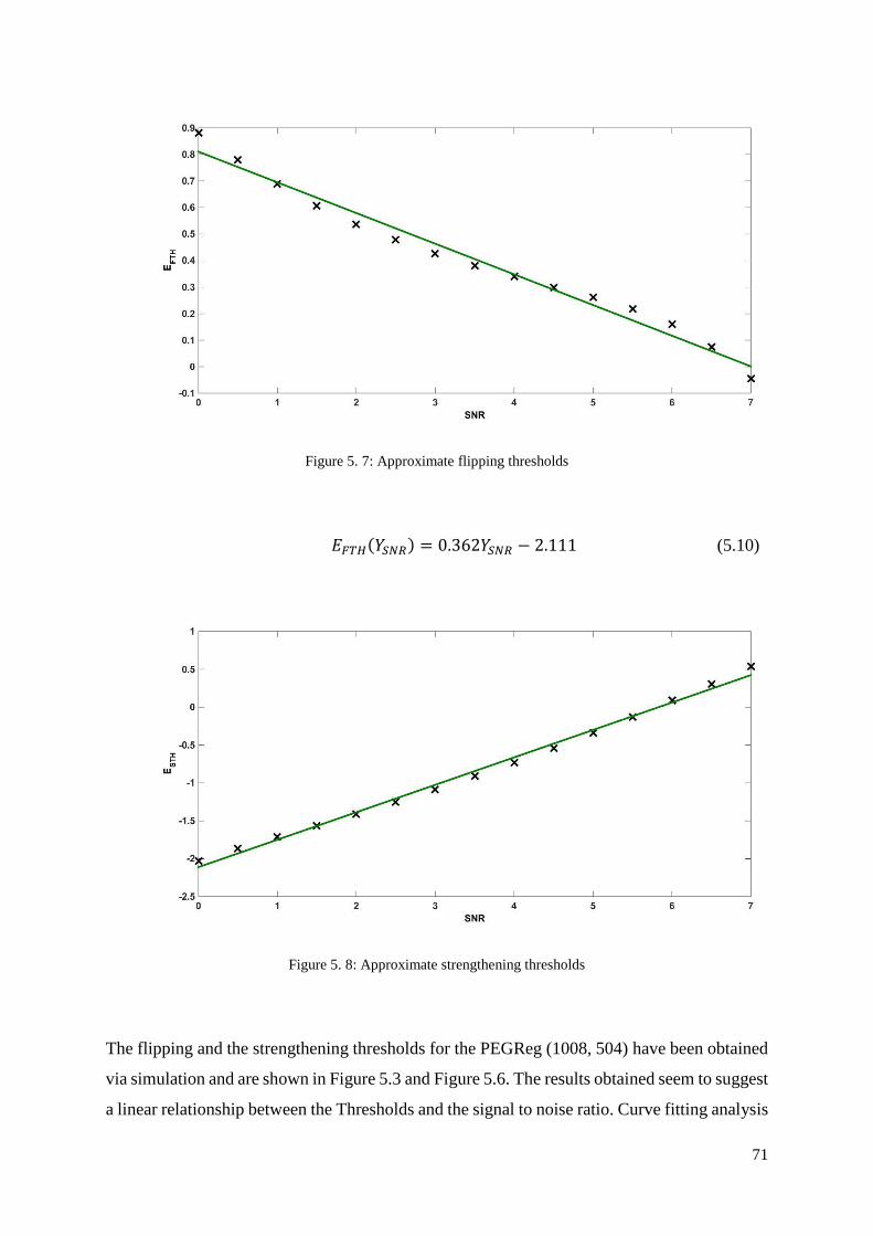
Figure 5. 7: Approximate flipping thresholds .......................................................................... 71
Figure 5. 8: Approximate strengthening thresholds ................................................................. 71
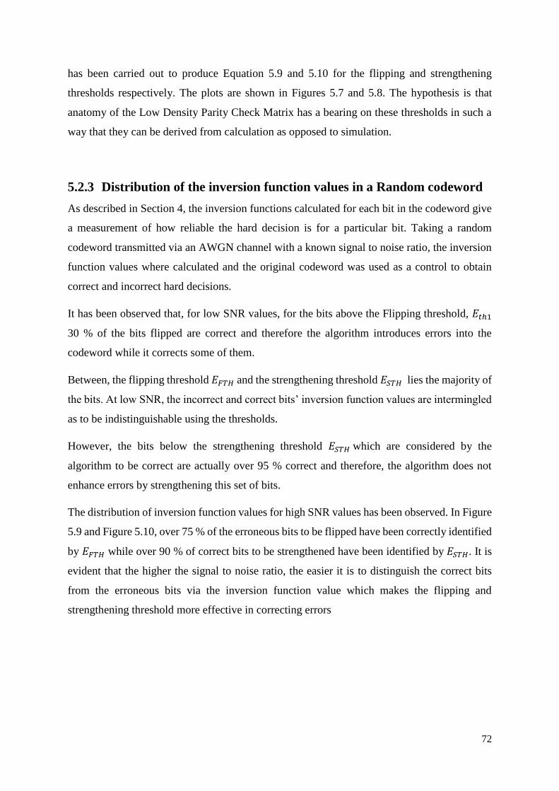
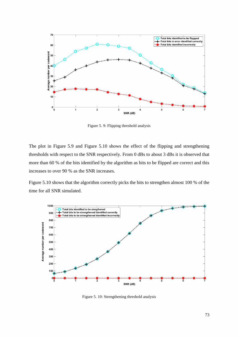
Figure 5. 9: Flipping threshold analysis ................................................................................... 73
Figure 5. 10: Strengthening threshold analysis ........................................................................ 73
Figure 5. 11: Determining the optimal enhancement value |δ| ................................................ 75
Figure 5. 12: Enhancement values investigation ..................................................................... 76
Figure 5. 13: NOSMBF BER analysis for different LDPC codes ........................................... 78
Figure 5. 14: NOSMBF FER analysis for different LDPC codes............................................ 79
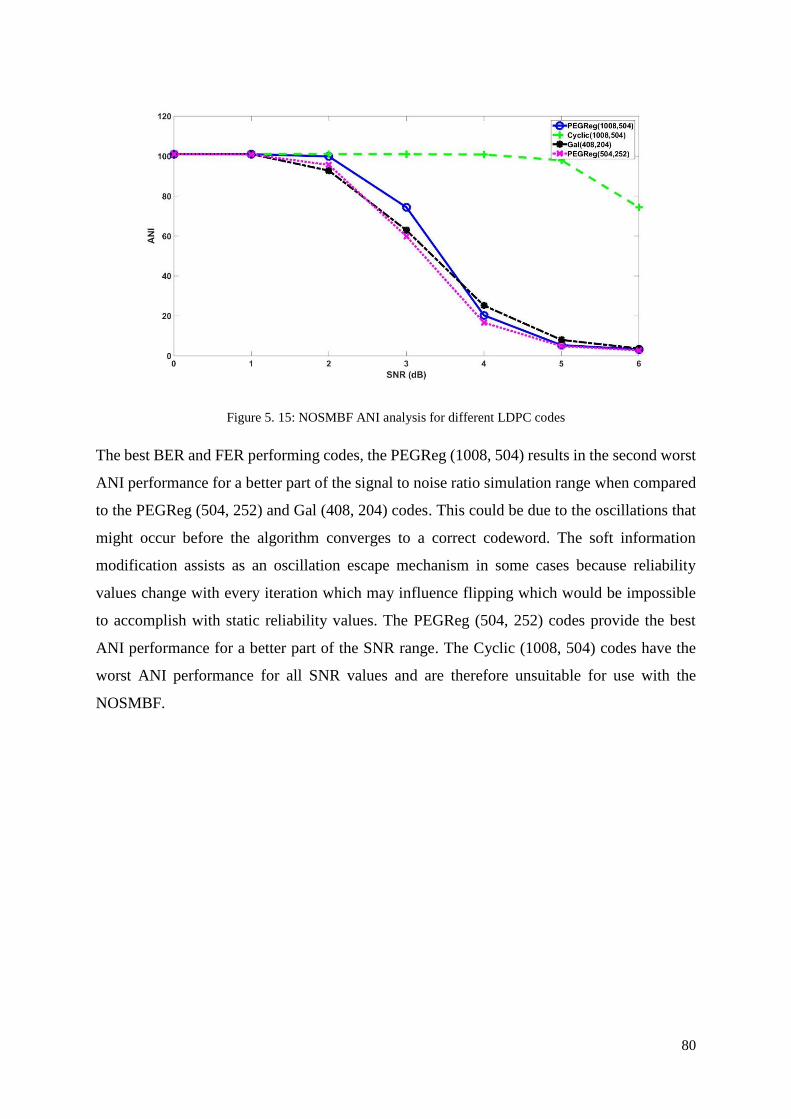
Figure 5. 15: NOSMBF ANI analysis for different LDPC codes ............................................ 80
Figure 5. 16: NOSMBF vs IMWBF BER performance analysis ............................................. 81
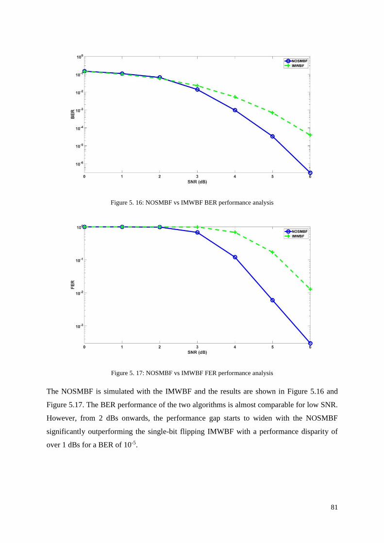
Figure 5. 17: NOSMBF vs IMWBF FER performance analysis ............................................. 81
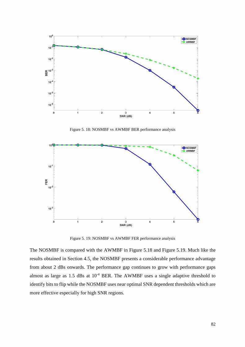
Figure 5. 18: NOSMBF vs AWMBF BER performance analysis ........................................... 82
Figure 5. 19: NOSMBF vs AWMBF FER performance analysis ........................................... 82
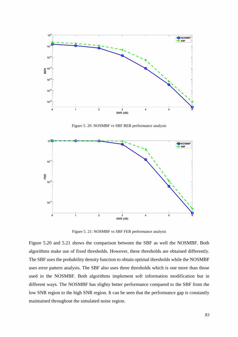
Figure 5. 20: NOSMBF vs SBF BER performance analysis ................................................... 83
Figure 5. 21: NOSMBF vs SBF FER performance analysis ................................................... 83
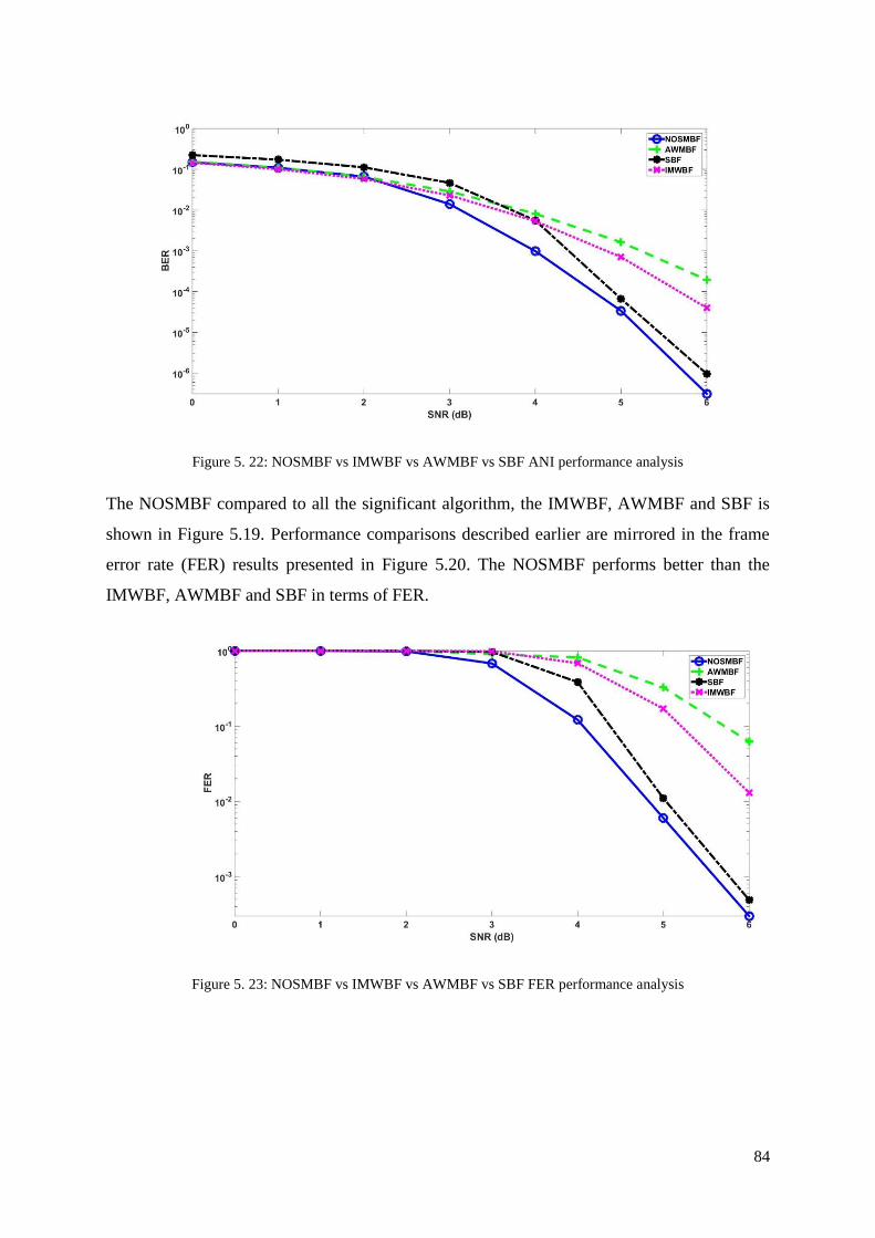
Figure 5. 22: NOSMBF vs IMWBF vs AWMBF vs SBF ANI performance analysis ............ 84
Figure 5. 23: NOSMBF vs IMWBF vs AWMBF vs SBF FER performance analysis ............ 84
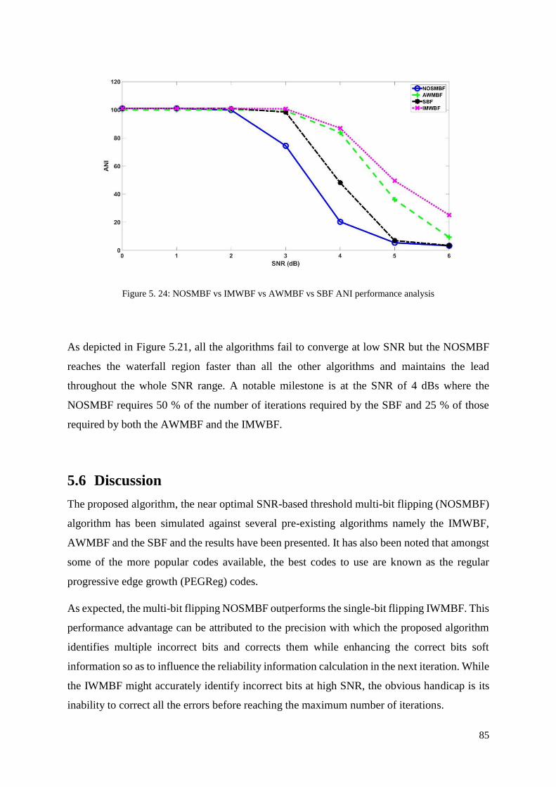
Figure 5. 24: NOSMBF vs IMWBF vs AWMBF vs SBF ANI performance analysis ............ 85
Figure 6. 1: Quantization boundaries (qi), levels (ri), and regions (Ri) for a symmetric 2-bit
quantizer ................................................................................................................................... 89
Figure 6. 2: AMTMBF BER uniform quantization ................................................................. 94
Figure 6. 3: AMTMBF FER uniform quantization .................................................................. 94
Figure 6. 4: NOSMBF BER uniform quantization .................................................................. 95
Figure 6. 5: NOSMBF FER uniform quantization................................................................... 95
Figure 6. 6: AMTMBF BER non-uniform quantization .......................................................... 96
Figure 6. 7: AMTMBF FER uniform quantization .................................................................. 96
Figure 6. 8: NOSMBF BER non-uniform quantization ........................................................... 97
Figure 6. 9: NOSMBF FER non-uniform quantization .......................................................... 97
Figure 6. 10: 6 bit uniform quantization BER performance analysis – AMTMBF vs IMWBF
vs SBF vs AWMBF ................................................................................................................. 98
Page 13
xiii
Figure 6. 11: 6 bit uniform quantization FER performance analysis – AMTMBF vs IMWBF
vs SBF vs AWMBF ................................................................................................................. 98
Figure 6. 12: 8 bit uniform quantization BER performance analysis – AMTMBF vs IMWBF
vs SBF vs AWMBF ................................................................................................................. 99
Figure 6. 13: 8 bit uniform quantization FER performance analysis – AMTMBF vs IMWBF
vs SBF vs AWMBF ................................................................................................................. 99
Figure 6. 14: 6 bit non-uniform quantization BER performance analysis – AMTMBF vs
IMWBF vs SBF vs AWMBF ................................................................................................. 100
Figure 6. 15: 6 bit non-uniform quantization FER performance analysis – AMTMBF vs
IMWBF vs SBF vs AWMBF ................................................................................................. 100
Figure 6. 16: 8 bit non-uniform quantization BER performance analysis – AMTMBF vs
IMWBF vs SBF vs AWMBF ................................................................................................. 101
Figure 6. 17: 8 bit non-uniform quantization BER performance analysis – AMTMBF vs
IMWBF vs SBF vs AWMBF ................................................................................................. 101
Figure 6. 18: 6 bit uniform quantization BER performance analysis – NOSMBF vs IMWBF
vs SBF vs AWMBF ............................................................................................................... 102
Figure 6. 19: 6 bit uniform quantization BER performance analysis – NOSMBF vs IMWBF
vs SBF vs AWMBF ............................................................................................................... 102
Figure 6. 20: 8 bit uniform quantization BER performance analysis – NOSMBF vs IMWBF
vs SBF vs AWMBF ............................................................................................................... 103
Figure 6. 21: 8 bit uniform quantization FER performance analysis – NOSMBF vs IMWBF
vs SBF vs AWMBF ............................................................................................................... 103
Figure 6. 22: 6 bit non-uniform quantization BER performance analysis – NOSMBF vs
IMWBF vs SBF vs AWMBF ................................................................................................. 104
Figure 6. 23: 6 bit uniform quantization FER performance analysis – NOSMBF vs IMWBF
vs SBF vs AWMBF ............................................................................................................... 104
Figure 6. 24: 8 bit uniform quantization BER performance analysis – NOSMBF vs IMWBF
vs SBF vs AWMBF ............................................................................................................... 105
Figure 6. 25: 8 bit uniform quantization BER performance analysis – NOSMBF vs IMWBF
vs SBF vs AWMBF ............................................................................................................... 105
Figure 7. 1: Proposed algorithms BER performance analysis ............................................... 107
Figure 7. 2: Proposed algorithms FER performance analysis ............................................... 108
Page 14
xiv
Figure 7. 3: Proposed algorithms ANI performance analysis ................................................ 108
Figure 7. 4: Proposed algorithms uniform quantization BER performance analysis ............ 109
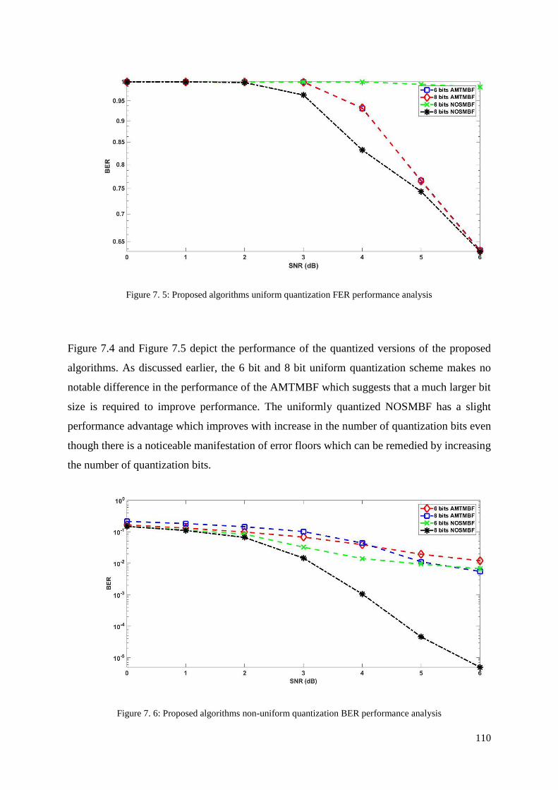
Figure 7. 5: Proposed algorithms uniform quantization FER performance analysis ............. 110
Figure 7. 6: Proposed algorithms non-uniform quantization BER performance analysis ..... 110
Figure 7. 7: Proposed algorithms uniform quantization FER performance analysis ............. 111
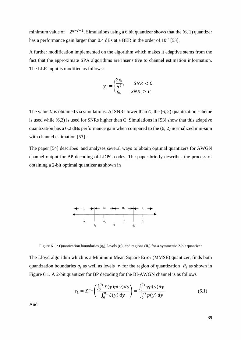
Figure 8. 1: Verification of Simulated results using the GDBF and PEGReg (1008, 504) ... 113
Page 15
xv
List of Acronyms
1G: First Generation
2G: Second Generation
3G: Third Generation
4G: Fourth Generation
5G: Fifth Generation
AMPS: Advanced Mobile Phone System
AMTMBF: Adaptive Multi-threshold Multi-bit Flipping
ANI: Average Number of Iterations
AWGN: Additive White Gaussian Noise
AWMBF: Adaptive Weighted Multi-bit Flipping
BEC: Binary Erasure Channel
BER: Bit Error Rate
BF: Bit Flipping
BP: Belief Propagation
BPSK Binary Phase Shift Keying
BSC: Binary Symmetric Channel
B-WBF: Bootstrapped - Weighted Bit Flipping
CDMA: Code Division Multiple Access
CI-WBF: Channel Independent - Weighted Bit Flipping
CM – WBF: Combined Modified - Weighted Bit Flipping
DVB-S2: Digital Video Broadcasting - Satellite - Second Generation
eIRA: Extended Irregular Repeat Accumulate
ETACS: European Total Access Communication Systems
FDMA: Frequency Division Multiple Access
FEC: Forward Error Channel
FER: Frame Error Rate
FG – LDPC: Finite Geometry - Low Density Parity Check Codes
FM: Frequency Modulation
GBF: Gallager Bit Flipping
GDBF: Gradient Descent Bit Flipping
GSM: Global System for Mobile Communications
HGDBF: Hybrid Gradient Descent Bit Flipping
Page 16
xvi
IMWBF: Improved Modified Weighted Bit Flipping
IoT: Internet of Things
IRA: Irregular Repeat Accumulate
LDPC: Low Density Parity Check Codes
LTE Long Term Evolution
MBF: Modified Weighted Bit Flipping
MCI-WBF: Modified Channel Independent - Weighted Bit Flipping
MLD: Maximum Likelihood Decoder
MM – WBF: Mixed Modified - Weighted Bit Flipping
MSA: Min Sum Algorithm
MWBF: Modified Weighted Bit Flipping
NOSMBF: Near Optimal SNR dependant threshold Multi-bit Flipping
RA: Repeat Accumulate
RR-WBF: Reliability Ratio - Based Weighted Bit Flipping
SBF: Soft Bit Flipping
SNR: Signal to Noise Ratio
SNWBF: Self-Normalized Weighted Bit-Flipping
SPA: Sum Product Algorithm
TDMA: Time Division Multiple Access
WBF: Weighted Bit Flipping
Page 17
xvii
Glossary of Nomenclature
AT Transverse of matrix A
c Valid codeword
cm Check node m
cn Valid codeword bit n
E Inversion function values vector
e Error vector
En Inversion function values vector element for codeword bit n
G Generator matrix
H Parity check matrix
H(x) Hamming weight of vector x
hm Parity check matrix row m
IK Size K identity matrix
m∈N(n) Check nodes converging on variable node n
n∈M(m) Variable nodes converging on check node m
P(cn=0\y) Probability of codeword bit = 0 given a received soft information
vector
P(cn=1\y) Probability of codeword bit = 1 given a received soft information
vector
s Syndrome vector
sm Syndrome bit m
u Message vector u
un Message bit n
vn Variable node n
wc Column weight
wr Row weight
y Soft information vector
yn Soft information vector element n
z Received hard decision codeword
zn Hard decision codeword bit n
α Weighting factor
γ Threshold coefficients
Page 18
xviii
e Total number of errors
Page 19
1
1. Introduction
1.1 Forward Error Correction
In information theory and telecommunications, Forward Error Correction (FEC) is a method
used to regulate the transmission of errors in unreliable noisy channels. The first error
correcting codes, the Hamming Codes where invented by Richard Hamming in the early 1950s
[1].
There are several FEC methods but they all essentially function by adding redundant
information to form what is called a codeword. This information, usually added to the message
via an algorithm, is used to identify and correct errors. Systematic codewords are a result of
redundant information being appended at the beginning or end of the message while the
message itself remains unchanged. When the message itself is modified, as is the case with
simple repetition code, the resulting codeword is non-systematic.
The two main types of Forward Error Correction codes in existence are linear block codes and
convolutional codes. Linear block codes such as BCH, LDPC and Reed Solomon codes use
fixed length symbol or bit patterns while convolutional codes are of arbitrary length.
Claude Shannon’s acclaimed A Mathematical Theory of Communication introduces the
channel coding theorem which states that reliable communication is possible in a noisy channel
provided that the rate does not exceed that channel’s capacity [2]. It also alludes to the existence
of error-correcting codes that can reduce error probability to any desired level without
specifying what the particular error codes are.
This research is carried out with low density parity check (LDPC) codes discovered by Robert
Gallager [3] in the early 1960s but were forgotten for nearly thirty years until interest was
rekindled by MacKay et al upon discovery that the performance of these codes approaches the
Shannon limit. Binary symbols are encoded into fixed frame size codewords, modulated via
the Binary Phase-shift keying (BPSK) scheme, transmitted through an additive white Gaussian
noise (AWGN) channel and then decoded at the receiver via an LDPC decoder. This research
work focusses on the decoding process with the aim to improve it and making it more efficient.
This aim can be achieved by improving the design of LDPC decoders.
FEC has increasingly found application in recent communication standards which has resulted
in massive improvements in communication. However, history shows that this has not always
Page 20
2
been the case. First generation (1G) mobile networks were deployed in the early 1980s [4].
These were analog networks which made use of FDMA and FM modulation. 1G standards
such as AMPS and ETACS have no documented FEC technologies incorporated [4].
As mobile wireless communication improved, second generation (2G) networks came to the
forefront in the late 1980s to remove the capacity limitations that were prevalent in the 1G
mobile system. 2G mobile systems used time division multiple access (TDMA) and code
division multiple access (CDMA) digital technologies. Standards such as the Global System
for Mobile Communications (GSM) used concatenated cyclic and convolution codes together
with an interleaver to protect frames against burst errors, for forward error correction [5]. This
made the 2G network more reliable than the precursor 1G network.
The evolution of 2G mobile networks resulted in 3G mobile networks. 3G networks are faster
and can handle more complex multimedia services seamlessly. 3G has found applications in
Video Conferencing, Telemedicine, Global Positioning Systems, Mobile TV and Video on
demand services. Forward error correction in standards such as the Multi-Carrier Code
Division Multiple Access (MC-CDMA) used in 3G use concatenated turbo and LDPC codes
to eliminate transmission errors [6].
4G technology was developed to meet the shortcomings of 3G. It is estimated that the customer
requirements will far outstrip the services available on 3G networks [7]. 4G has the ability to
handle high volumes of multimedia data seamlessly at speeds up to 100 Mbps [7]. While 4G is
a major improvement to 3G it is not a complete overhaul but a complement to 3G in which pre-
existing technology is amalgamated with new to improve performance [7]. The physical layer
of 4G systems in some cases, uses concatenated Reed-Solomon/LDPC codes for forward error
correction [8].
The evolution of wireless mobile technology and the rediscovery of LDPC codes have seen the
rise in popularity of LDPC codes as evidenced by its inclusion in major communication
standards that have been described above. LDPC codes have also been included in the FEC
schemes for Wi-Fi and Wi-Max standards such as the IEEE 802.16e [9].
The Digital Video Broadcasting - Satellite - Second Generation (DVB-S2) standard for video
broadcasting applications uses a concatenation of BCH and LDPC codes. This second
generation standard replaces the first DVB-S which used a Reed Solomon and Convolutional
code concatenation [10].
Page 21
3
1.2 Research Motivation
The world is rapidly becoming a global digital village due to rapid evolution of technology and
with the advent of the Internet-of-Things (IoT), connectivity has become of paramount
importance. That means the establishment of reliable and low-cost communication systems for
mobile devices and microsystems on larger mechanical machinery. A major aspect of a reliable
communication system is the requirement to transmit correct information which requires
effective error correction schemes. A second important aspect of a reliable communication
system is power consumption in the process of transmitting and receiving information. The
overall complexity of encoding and decoding algorithms plays a pivotal role in the amount of
energy consumed by a communications system. This means, the less complex the algorithm
the more desirable it is. A third critical aspect is the speed at which information is transmitted
and the less complex a decoder, the higher the throughput.
LDPC codes discovered by Gallager in 1960 [3] have some of the most effective error
correcting capabilities rivalling even those of Reed-Solomon codes. The biggest drawback of
using LDPC codes is that the most effective decoding algorithm, the Belief Propagation (BP)
Sum-product algorithm (SPA) is too complex to implement practically and therefore not
suitable for use in high-speed mobile devices.
Apart from the SPA and its approximations, there exists another set of LDPC decoders known
as bit flipping (BF) decoders. Within the family of BF decoders, there is a subset of sub-optimal
LDPC decoders which comprises of multi-bit flipping algorithms worthy of attention in the
goal to devise high-speed, low cost communication devices. The family of bit flipping decoders
generally performs worse than the family of BP-SPA algorithms but they offer the attractive
quality of low complexity.
This dissertation focusses on the design and development of low-complexity low-cost multi-
bit LDPC algorithms for the purpose of improving the existing decoders. The success of this
research points to improved understanding of multi-bit flipping LDPC decoders which will
improve future designs. The performance of the proposed decoder/algorithms will be based on
the following metrics, the bit error rate (BER), frame error rate (FER),average number of
iterations (ANI) which give an idea of complexity of the algorithms.
A study into the practical implementation of a real decoder is also important to investigate the
effects of approximating algorithm values by quantizing the input the same way a practical
decoder does.
Page 22
4
1.3 Research Contributions
The research compilation has made the following contributions:
In Chapter 4, the Adaptive Multi-Threshold Multi-bit Flipping (AMTMBF) is proposed
following the observation that there exists very few prominent algorithms with state-dependant
adaptive threshold multi-bit flipping algorithm namely the AWMBF discussed in [11]. This
chapter makes the following contributions in this regard:
1. The main contribution is the development of a scheme by which multiple decoding state
based adaptive thresholds can be incorporated into a multi-bit flipping algorithm. This
scheme makes use of the inversion function result vector as well as the syndrome to
determine the appropriate threshold for bit flipping. Simulation of this scheme shows
an improved performance over existing algorithms with similar characteristics.
2. The second contribution is the discovery of the role played by soft variable node
modification in the decoding of LDPC codes. It can be observed through simulations
that variable node (VN) soft information modification improves the decoding
performance of LDPC decoders.
In Chapter 5, the Near Optimal SNR Dependent Threshold Multi-bit Flipping (NOSMBF) is
proposed following the observation that, there is very little mention in literature on how optimal
flipping thresholds for a multi-bit flipping algorithm can be obtained. In this chapter, the
following contributions are made in this regard:
1. The main contribution is the development of SNR dependant threshold scheme for
LDPC multi-bit flipping algorithms. This scheme differs from [12] in which a multi-bit
flipping threshold scheme is devised based on the probability density function of the
inversion function in which the thresholds obtained are constant throughout the whole
SNR range. It is observed that the SNR dependant threshold scheme improves the
performance of multi-bit flipping algorithms.
2. The second contribution is the discovery that there exists a linear relationship between
the SNR and the near-optimal thresholds for LDPC multi-bit flipping algorithms. In
[12], there is no established relationship between flipping parameters and channel state.
3. Finally, the research provides an empirical approach for determining the near optimal
flipping thresholds while in [11] flipping thresholds are obtained from formulae and in
[12] they are obtained from statistical analysis of bit reliability information.
Page 23
5
In Chapter 6 is an analysis of the quantized versions of both algorithms. Both algorithms where
simulated using 6 and 8 bit uniform and non-uniform quantization. The following research
contributions where made:
1. The non-uniform quantization scheme provides better performance for adaptive and
near-optimal threshold algorithms.
2. Adaptive thresholds are highly susceptible to both uniform and non-uniform
quantization and therefore need larger word lengths to achieve performance close to the
unquantized version.
3. While the near optimal thresholds are susceptible to uniform quantization, they perform
very well with 8 bit non-uniform quantization.
In Chapter 7 is a comparison of both algorithms to determine the best performing threshold
scheme. In this chapter, both quantized and unquantized versions where compared and the
following research contribution was made:
1. The near optimal SNR dependant threshold scheme performs better than the adaptive
threshold scheme in all respects.
1.4 Overview of Dissertation
This section of the document introduces the work while the rest of the dissertation is organised
in this manner. The following chapter, Chapter 2 introduces the linear block codes known as
Low Density Parity Check (LDPC) codes. Therein lies a full discussion of various types of
LDPC codes including the encoding and the decoding process. Chapter 3 discusses the main
focus of this research which is the bit-flipping decoding of LDPC codes. Several single and
multi-bit flipping algorithms or decoders are discussed at length citing their strengths and
weaknesses.
Chapter 4 is a proposal for a new multi-bit flipping LDPC algorithm known as the Adaptive
Multi-Threshold Multi-bit Flipping (AMTMBF) algorithm. This algorithm uses multiple
thresholds that adapt to the state of the algorithm to choose bits to flip or enhance while offering
reduced complexity. The algorithm is analysed, simulated and the results are discussed.
Chapter 5 introduces a second multi-threshold multi-bit flipping algorithm known as the Near
Optimal SNR Dependent Threshold Multi-bit Flipping Algorithm (NOSMBF). The research
on this algorithm focusses on the determination of near optimal flipping thresholds based on
Page 24
6
the codeword error patterns, channel noise and inversion function values. The algorithm is also
simulated, analysed and the results are discussed.
Chapter 6 focusses on the issues surrounding the implementation of a practical decoder by
introducing the concept of quantization. The quantized versions of the AMTMBF and the
NOSMBF are simulated against their non-quantized versions. The results are analysed and
discussed.
Chapter 7 is a comparison of the performance of both algorithms. Both the quantized and
unquantized versions of the AMTMBF and the NOSMBF are compared to determine which
algorithm performs the best. The results of this simulation are presented and discussed.
The last section concludes the research dissertation.
1.5 Publications
Certain parts of this dissertation have been presented at the following publications and
conferences:
Kennedy Masunda, Fambirai Takawira, “A Multi Adaptive Threshold Weighted Multi-bit
Flipping Algorithm for LDPC codes”, In proceedings of SATNAC 2016, George, South
Africa, September 2016.
Kennedy Masunda, Fambirai Takawira, “A Near Optimal SNR Dependant Threshold Weighted
Multi-bit Flipping Algorithm for LDPC codes”, To be submitted, 2017.
Page 25
7
2. Low Density Parity Check Codes
2.1 Introduction
Low-density parity-check codes (LDPC) codes are a very important class of forward error-
correction codes with the ability to perform close to the Shannon limit on various storage and
data transmission channels. These codes can be implemented as both binary and non-binary
codes but this research focusses only on binary LDPC codes. There are various constructions
of LDPC codes such as Gallager Codes, MacKay Codes, Array Codes, Irregular Codes,
Combinatorial Codes, Finite Geometry Codes and Repeat Accumulate Codes.
LDPC codes are generally expressed as a large two dimensional sparse matrix and it is this
sparseness that gives rise to the codes’ exceptional error correcting capabilities [13]. These
codes can also be expressed in form of a bi-partite graph known as the Tanner Graph [14]. The
parity-check matrix elements are mostly zeros whilst the non-zero elements are ones [15].
Messages to be transmitted through a channel can be encoded using a generator matrix derived
from the parity-check matrix or by permuting the parity-check matrix in such a way that it can
be used for more efficient almost linear-time encoding.
Decoding a received message can be achieved in many ways ranging from the very effective
but highly complex belief propagation sum product algorithm to the less efficient but very low
complexity hard decision bit flipping algorithm.
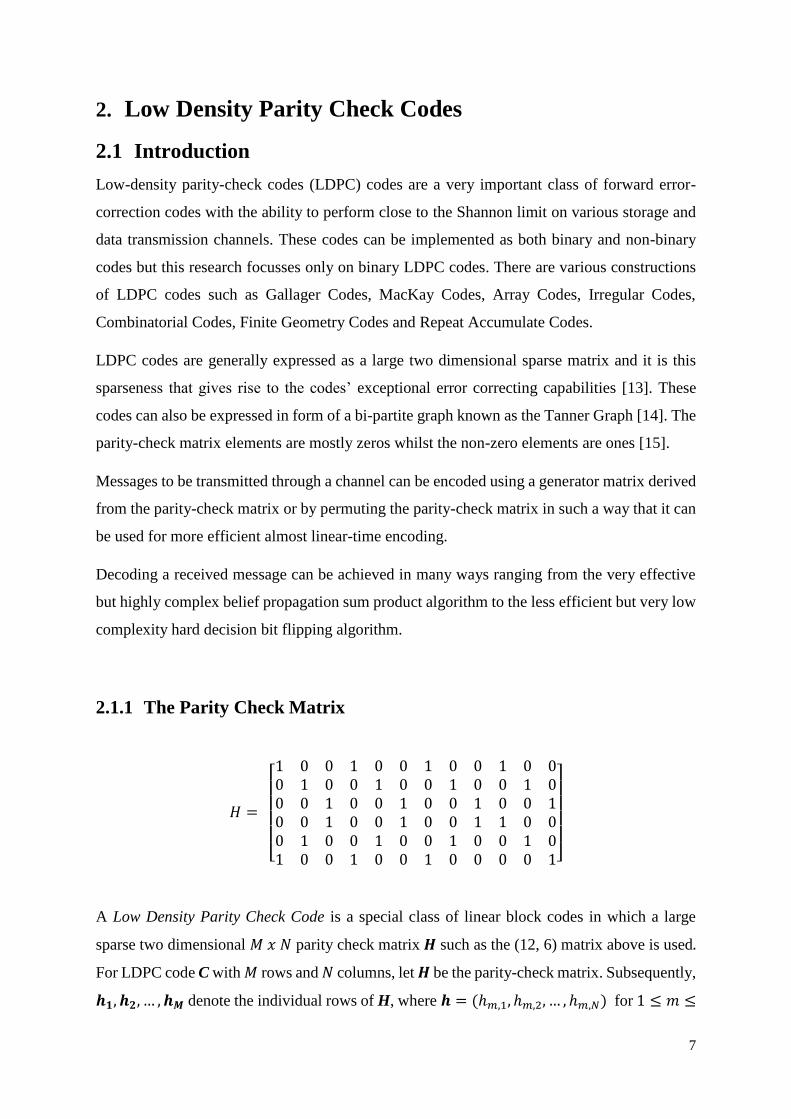
2.1.1 The Parity Check Matrix
𝐻 =
[ 1 0 0 1 0 0 1 0 0 1 0 00 1 0 0 1 0 0 1 0 0 1 00 0 1 0 0 1 0 0 1 0 0 10 0 1 0 0 1 0 0 1 1 0 00 1 0 0 1 0 0 1 0 0 1 01 0 0 1 0 0 1 0 0 0 0 1]
A Low Density Parity Check Code is a special class of linear block codes in which a large
sparse two dimensional 𝑀 𝑥 𝑁 parity check matrix 𝑯 such as the (12, 6) matrix above is used.
For LDPC code C with 𝑀 rows and 𝑁 columns, let 𝑯 be the parity-check matrix. Subsequently,
𝒉𝟏, 𝒉𝟐, … , 𝒉𝑴 denote the individual rows of H, where 𝒉 = (ℎ𝑚,1, ℎ𝑚,2, … , ℎ𝑚,𝑁) for 1 ≤ 𝑚 ≤
Page 26
8
𝑀. It is due to the sparsity of the matrices that the code has excellent error correcting
capabilities. An arbitrary data stream is split into 𝒖 = (𝑢1, 𝑢2, … , 𝑢𝐾) vectors of length 𝐾 bits.
The vector 𝒖 is encoded using code C into a codeword 𝒄 = (𝑐1, 𝑐2, … , 𝑐𝑁) 𝑁 bits long in a
systematic or non-systematic fashion in which 𝑀 = 𝑁 − 𝐾 redundant bits are added to 𝒖, for
error checking and correcting purposes. These extra 𝑀 bits are referred to as parity check bits.
The rate of the code is defined as 𝑅 = 𝐾 𝑁⁄ = 1 − 𝑤𝑐
𝑤𝑟⁄
Regular LDPC codes have a constant row weight 𝑤𝑟 and column weight 𝑤𝑐 for all rows and
columns in the matrix respectively. The row and column weights are related in this manner
𝑤𝑟 = 𝑤𝑐(𝑁/𝑀) and 𝑤𝑐 << 𝑚. However, irregular codes which are discussed in Section
2.1.4, have varying row and column weights throughout the matrix.
In the decoding phase, the validity of each received codeword is checked using the parity check
matrix 𝑯. Every bit is checked by the parity checksum in which it participates to
ascertain 𝒄𝒊𝒉𝒎𝒊 = 0. This check tests the zero-parity check constraint. In the event that this
check is not satisfied, it then follows that the given bit is most likely to be in error and the
opposite is true. The equation 𝒔 = 𝒄𝑯𝑻 produces 𝒔 which is known as the syndrome of the
received vector. The received vector can be confirmed a codeword if and only if the
syndrome 𝒔 = 0.
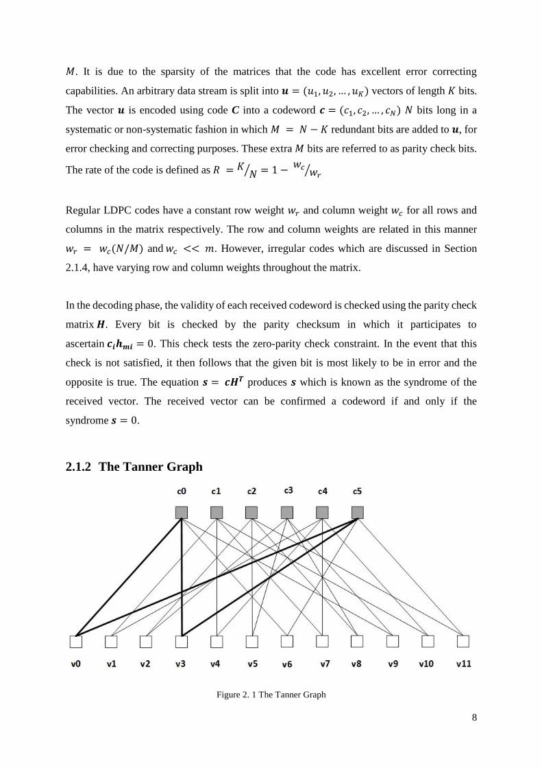
2.1.2 The Tanner Graph
Figure 2. 1 The Tanner Graph
Page 27
9
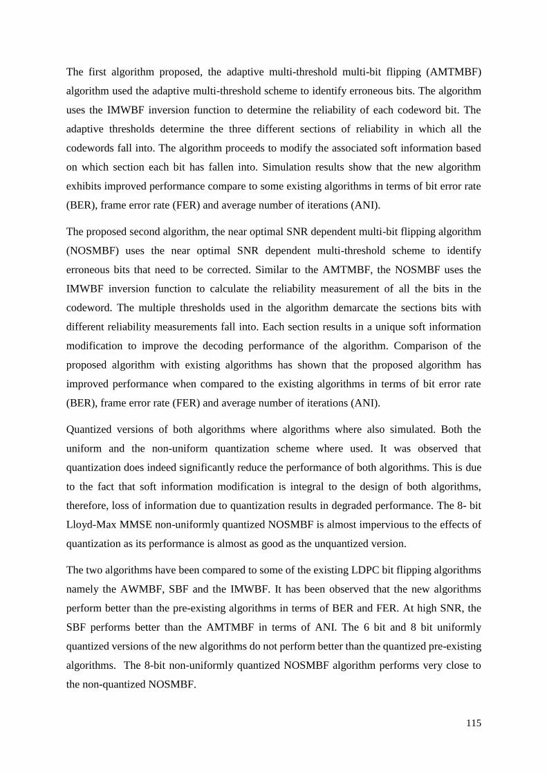
In 1981, Michael Tanner introduced the Tanner graph, shown in Figure 2.1, which is a bipartite
graph that is useful for graphically representing parity-check matrixes [14]. The Tanner graph
has two sets of nodes: check nodes, labelled c0 to c5 as well as variable nodes labelled v0 to
v11. The number of check nodes and variable nodes is equivalent to the number of rows and
columns of a given matrix respectively. The lines connecting the check nodes and variable
nodes are known as edges.
The Tanner graph became such a critical tool in the study of LDPC codes because it facilitates
the study of LDPC message passing decoders such as the sum-product algorithm [3]. It is also
very useful when analysing the potential weaknesses of the parity-check matrix that can result
in poor decoding performance. Figure 2.1 shows the Tanner graph for the matrix 𝑯 in Section
2.1.1. The bold four edges connecting v0, c0, v3 and c5 form what is known as a short cycle
which can also have six edges. Short cycles are not desirable because they degrade the decoding
performance of a code. It is evident that short cycles are difficult to detect without the Tanner
graph.
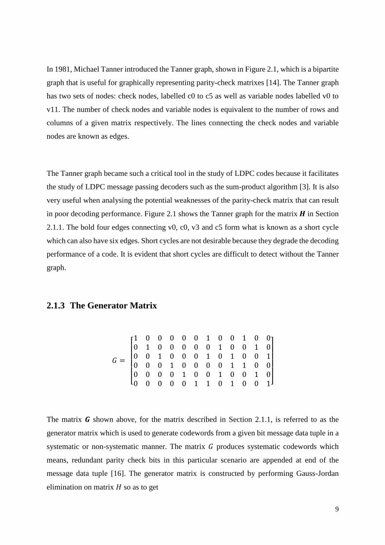
2.1.3 The Generator Matrix
𝐺 =
[ 1 0 0 0 0 0 1 0 0 1 0 00 1 0 0 0 0 0 1 0 0 1 00 0 1 0 0 0 1 0 1 0 0 10 0 0 1 0 0 0 0 1 1 0 00 0 0 0 1 0 0 1 0 0 1 00 0 0 0 0 1 1 0 1 0 0 1]
The matrix 𝑮 shown above, for the matrix described in Section 2.1.1, is referred to as the
generator matrix which is used to generate codewords from a given bit message data tuple in a
systematic or non-systematic manner. The matrix 𝐺 produces systematic codewords which
means, redundant parity check bits in this particular scenario are appended at end of the
message data tuple [16]. The generator matrix is constructed by performing Gauss-Jordan
elimination on matrix 𝐻 so as to get
Page 28
10
𝐻 = [𝐴, 𝐼𝑛−𝑘] (2.1)
in which case 𝑰𝒏−𝒌 is an (𝑛 − 𝑘) identity matrix whilst 𝑨 is a (𝑛 − 𝑘) × 𝑘 sub-matrix. It then
follows that, the matrix 𝐺 is obtained as
𝐺 = [𝐼𝑘, 𝐴𝑇] (2.2)
The process of encoding using the generator matrix is described in Section 2.2.1.
2.1.4 Types of LDPC Codes
The construction of LDPC codes is not merely random, there is a method in the way LDPC
codes are constructed and different methods produce codes with different properties.
I. Gallager Codes
In 1962, when Robert Gallager discovered LDPC codes, he also developed a
construction technique for pseudo-random codes that are now referred to as Gallager
codes [3]. This is the original LDPC code with a regular 𝐻 matrix made up of
𝐻𝑛 submatrices that are structured in this manner
𝐻 =
[ 𝐻1𝐻2𝐻3⋱𝐻𝑤𝑐]
(2.3)
Let 𝑤𝑐 and 𝛽 be two integers such that 𝑤𝑐 > 1 and 𝛽 > 1 such that the submatrix 𝐻𝑛
with column weight and row weight 1 and 𝑤𝑟 respectively, is of size 𝛽 × 𝛽𝑤𝑟 . The
primary submatrix 𝐻1 is in the form: for 𝑗 = 1,2,3, … , 𝛽 and all the 1’s are in the 𝑗-th
row in columns spanning from 1 + (𝑗 − 1)𝑤𝑟 to 𝑗𝑤𝑟. The remaining submatrices are
column permutations of the primary submatrix. This code design is not guaranteed to
be devoid of short cycles, however, these can be avoided by computer optimised design
of the parity-check matrix. In [3] it is shown that these codes have remarkable distance
properties given 𝑤𝑐 ≥ 3 and 𝑤𝑟 > 𝑤𝑐. These codes give rise to low complexity
encoders.
Page 29
11
II. MacKay Codes
Gallager codes were further extended by MacKay who also learned independently the
near capacity performance of these codes in [13]. A library of codes designed and
developed by McKay which includes Progressive Edge Growth (PEG) codes can be
found at [17]. MacKay developed algorithms to pseudo-randomly create sparse parity-
check matrices and these are shown in [13]. The least complex of the algorithms
involves, generating random weight 𝑤𝑐 columns and 𝑤𝑟 rows ensuring that no two
columns overlap more than once. The more complex algorithms involve actively
terminating short cycles and splitting the parity check as follows
𝐻 = [𝐻1 𝐻2] (2.4)
such that 𝐻2 is either invertible or in the very least full rank.
As with Gallager codes, Mackay codes do not facilitate the development of low-
complexity decoders [13]. The encoding process for these codes is mostly carried out
via the generator matrix and it is explained in Section 2.2.1 why this is a
computationally expensive process.
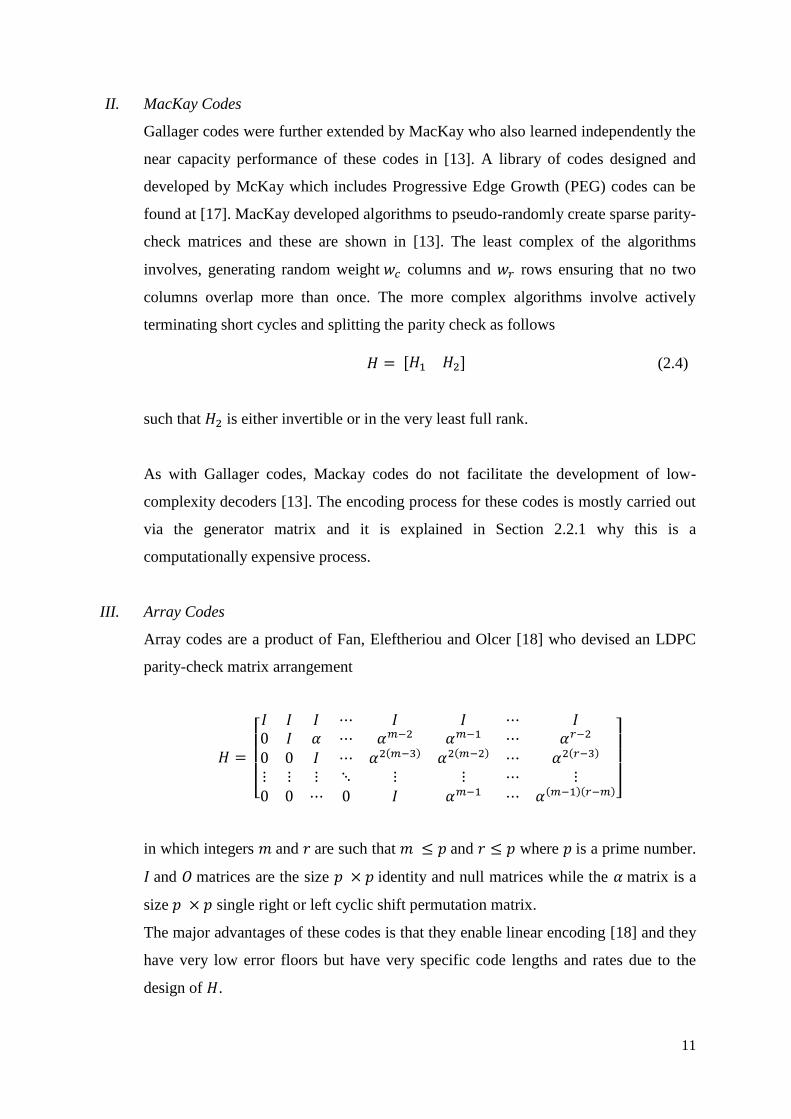
III. Array Codes
Array codes are a product of Fan, Eleftheriou and Olcer [18] who devised an LDPC
parity-check matrix arrangement
𝐻 =
[ 𝐼 𝐼 𝐼 ⋯ 𝐼 𝐼 ⋯ 𝐼0 𝐼 𝛼 ⋯ 𝛼𝑚−2 𝛼𝑚−1 ⋯ 𝛼𝑟−2
0 0 𝐼 ⋯ 𝛼2(𝑚−3) 𝛼2(𝑚−2) ⋯ 𝛼2(𝑟−3)
⋮ ⋮ ⋮ ⋱ ⋮ ⋮ ⋯ ⋮0 0 ⋯ 0 𝐼 𝛼𝑚−1 ⋯ 𝛼(𝑚−1)(𝑟−𝑚)]
in which integers 𝑚 and 𝑟 are such that 𝑚 ≤ 𝑝 and 𝑟 ≤ 𝑝 where 𝑝 is a prime number.
𝐼 and 𝑂 matrices are the size 𝑝 × 𝑝 identity and null matrices while the 𝛼 matrix is a
size 𝑝 × 𝑝 single right or left cyclic shift permutation matrix.
The major advantages of these codes is that they enable linear encoding [18] and they
have very low error floors but have very specific code lengths and rates due to the
design of 𝐻.
Page 30
12
IV. Irregular Codes
In contrast to regular codes, irregular codes defined by Richardson et al [15] and Luby
et al [19] have a non-constant variable and check node distributions. Irregular code
ensembles are characterized by degree distribution polynomials
𝜆(𝑥) = 𝜆1𝑥 + 𝜆2𝑥2 + 𝜆3𝑥
3 +⋯+ 𝜆𝑑𝑣𝑥𝑑𝑣 (2.1)
and
𝜌(𝑥) = 𝜌𝑑0𝑥𝑑0 + 𝜌𝑑0+1𝑥
𝑑0+1 + 𝜌𝑑0+2𝑥𝑑0+2 +⋯+ 𝜌𝑑𝑐𝑥
𝑑𝑐 (2.2)
for variable and check nodes respectively where 𝑑𝑣 is the maximum variable node
degree, 𝑑0 and 𝑑𝑐 is the minimum and maximum check node degree for a given
ensemble. The polynomials are optimised via density evolution [19]. Irregular codes
have been proven to outperform regular codes for very long codes but exhibit worse
performance for short to medium codes. This is due to the density evolution algorithm
being optimised for codes length 𝑁 → ∞.
V. Combinatorial Codes
Given that LDPC codes can be constructed using random methods, researchers have
produced Steiner and Kirkman triples based systems by successfully applying
combinatorial mathematics to the design of optimal codes given some specific design
constraints [20]. The problem can be expressed as a combinatorics problem of
designing a size (𝑁 − 𝐾) × 𝑁 𝑯 matrix with no short cycles of length four or six [20].
VI. Finite Geometry Codes
In [21] several codes have been designed using techniques based on finite geometries
(FG-LDPC codes). These codes fall into a category of block codes referred to as quasi-
cyclic or cyclic codes whose main advantage is apparent in the ease with which FG-
LDPC decoders can be implemented via shift registers. Short length FG-LDPC codes
generally outperform short length pseudo-random codes [21].
Page 31
13
A major drawback of FG-LDPC codes is high row and column weight of the 𝐻 matrices
which compromises the sparsity of these matrices and therefore increases the iterative
message passing decoder complexity. It is also not possible to construct FG-LDPC
codes of arbitrary length or rate. This requires puncturing and code shortening [21].
VII. Repeat Accumulate Codes
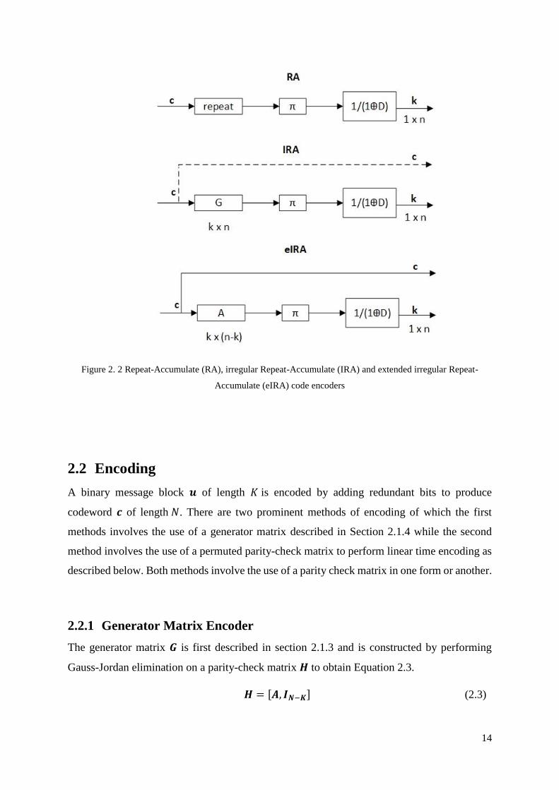
In [22] codes with serial turbo and low density parity-check code features were
proposed and these codes are referred to as repeat-accumulate (RA) codes because of
the way in which these codes are encoded as shown in Figure 2.2. In the RA encoder,
bits are repeated two or three times, permuted and then channelled through a differential
encoder or accumulator. Due to the repetition, these codes are characteristically low
rate but have been shown to perform very close to capacity [22].
In Irregular repeat-accumulate (IRA) codes the bits are repeated a variable number of
times. In this set up, the generator matrix is added. These codes outperform RA codes
and also facilitate higher rates [23]. The obvious drawback of IRA codes is that they
are non-systematic and making them systematic greatly lowers the code rate [23].
Extended Irregular repeat-accumulate (eIRA) codes can be encoded in a more efficient
manner giving rise to low and high rate codes which are also systematic [24].
Page 32
14
Figure 2. 2 Repeat-Accumulate (RA), irregular Repeat-Accumulate (IRA) and extended irregular Repeat-
Accumulate (eIRA) code encoders
2.2 Encoding
A binary message block 𝒖 of length 𝐾 is encoded by adding redundant bits to produce
codeword 𝒄 of length 𝑁. There are two prominent methods of encoding of which the first
methods involves the use of a generator matrix described in Section 2.1.4 while the second
method involves the use of a permuted parity-check matrix to perform linear time encoding as
described below. Both methods involve the use of a parity check matrix in one form or another.
2.2.1 Generator Matrix Encoder
The generator matrix 𝑮 is first described in section 2.1.3 and is constructed by performing
Gauss-Jordan elimination on a parity-check matrix 𝑯 to obtain Equation 2.3.
𝑯 = [𝑨, 𝑰𝑵−𝑲] (2.3)
Page 33
15
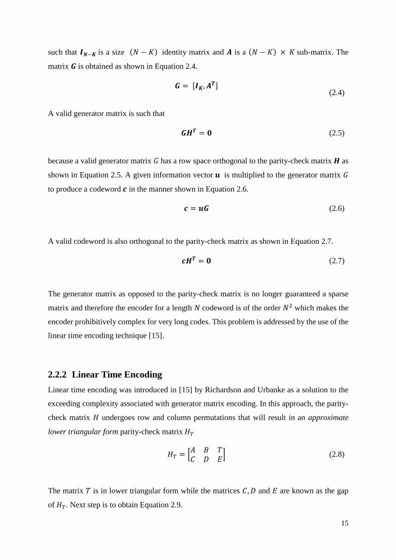
such that 𝑰𝑵−𝑲 is a size (𝑁 − 𝐾) identity matrix and 𝑨 is a (𝑁 − 𝐾) × 𝐾 sub-matrix. The
matrix 𝑮 is obtained as shown in Equation 2.4.
𝑮 = [𝑰𝑲, 𝑨𝑻]
(2.4)
A valid generator matrix is such that
𝑮𝑯𝑻 = 𝟎 (2.5)
because a valid generator matrix 𝐺 has a row space orthogonal to the parity-check matrix 𝑯 as
shown in Equation 2.5. A given information vector 𝒖 is multiplied to the generator matrix 𝐺
to produce a codeword 𝒄 in the manner shown in Equation 2.6.
𝒄 = 𝒖𝑮 (2.6)
A valid codeword is also orthogonal to the parity-check matrix as shown in Equation 2.7.
𝒄𝑯𝑻 = 𝟎 (2.7)
The generator matrix as opposed to the parity-check matrix is no longer guaranteed a sparse
matrix and therefore the encoder for a length 𝑁 codeword is of the order 𝑁2 which makes the
encoder prohibitively complex for very long codes. This problem is addressed by the use of the
linear time encoding technique [15].
2.2.2 Linear Time Encoding
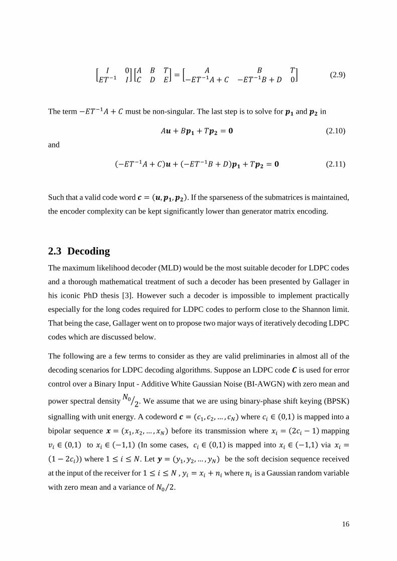
Linear time encoding was introduced in [15] by Richardson and Urbanke as a solution to the
exceeding complexity associated with generator matrix encoding. In this approach, the parity-
check matrix 𝐻 undergoes row and column permutations that will result in an approximate
lower triangular form parity-check matrix 𝐻𝑇
𝐻𝑇 = [𝐴 𝐵 𝑇𝐶 𝐷 𝐸
] (2.8)
The matrix 𝑇 is in lower triangular form while the matrices 𝐶, 𝐷 and 𝐸 are known as the gap
of 𝐻𝑇. Next step is to obtain Equation 2.9.
Page 34
16
[𝐼 0
𝐸𝑇−1 𝐼] [𝐴 𝐵 𝑇𝐶 𝐷 𝐸
] = [𝐴 𝐵 𝑇
−𝐸𝑇−1𝐴 + 𝐶 −𝐸𝑇−1𝐵 + 𝐷 0] (2.9)
The term −𝐸𝑇−1𝐴 + 𝐶 must be non-singular. The last step is to solve for 𝒑𝟏 and 𝒑𝟐 in
𝐴𝒖 + 𝐵𝒑𝟏 + 𝑇𝒑𝟐 = 𝟎 (2.10)
and
(−𝐸𝑇−1𝐴 + 𝐶)𝒖 + (−𝐸𝑇−1𝐵 + 𝐷)𝒑𝟏 + 𝑇𝒑𝟐 = 𝟎 (2.11)
Such that a valid code word 𝒄 = (𝒖, 𝒑𝟏, 𝒑𝟐). If the sparseness of the submatrices is maintained,
the encoder complexity can be kept significantly lower than generator matrix encoding.
2.3 Decoding
The maximum likelihood decoder (MLD) would be the most suitable decoder for LDPC codes
and a thorough mathematical treatment of such a decoder has been presented by Gallager in
his iconic PhD thesis [3]. However such a decoder is impossible to implement practically
especially for the long codes required for LDPC codes to perform close to the Shannon limit.
That being the case, Gallager went on to propose two major ways of iteratively decoding LDPC
codes which are discussed below.
The following are a few terms to consider as they are valid preliminaries in almost all of the
decoding scenarios for LDPC decoding algorithms. Suppose an LDPC code 𝑪 is used for error
control over a Binary Input - Additive White Gaussian Noise (BI-AWGN) with zero mean and
power spectral density 𝑁0
2⁄ . We assume that we are using binary-phase shift keying (BPSK)
signalling with unit energy. A codeword 𝒄 = (𝑐1, 𝑐2, … , 𝑐𝑁) where 𝑐𝑖 ∈ (0,1) is mapped into a
bipolar sequence 𝒙 = (𝑥1, 𝑥2, … , 𝑥𝑁) before its transmission where 𝑥𝑖 = (2𝑐𝑖 − 1) mapping
𝑣𝑖 ∈ (0,1) to 𝑥𝑖 ∈ (−1,1) (In some cases, 𝑐𝑖 ∈ (0,1) is mapped into 𝑥𝑖 ∈ (−1,1) via 𝑥𝑖 =
(1 − 2𝑐𝑖)) where 1 ≤ 𝑖 ≤ 𝑁. Let 𝒚 = (𝑦1, 𝑦2, … , 𝑦𝑁) be the soft decision sequence received
at the input of the receiver for 1 ≤ 𝑖 ≤ 𝑁 , 𝑦𝑖 = 𝑥𝑖 + 𝑛𝑖 where 𝑛𝑖 is a Gaussian random variable
with zero mean and a variance of 𝑁0 2⁄ .
Page 35
17
2.3.1 Belief Propagation
The most famous decoding algorithm is the iterative sum product algorithm (SPA) which is
also known as soft-decision decoding algorithm and makes use of received channel information
and the parity check matrix to calculate the probabilities of a received bit being correct based
on the information received from the channel via a process known as belief propagation. This
is the best known LDPC decoder whose performance nears the Shannon limit for long
codewords. Even though the SPA is a very effective decoder, it is very computationally
complex due to the numerous divisions and multiplications needed per iteration. This makes
the SPA very difficult to practically implement in hardware because multiplications and
divisions are expensive to implement on logic circuits [25]. A marginally less complex version
of the SPA has also been devised and is known as the log likelihood ratio version of the SPA.
The functions of log-likelihood version of the SPA are shown below.
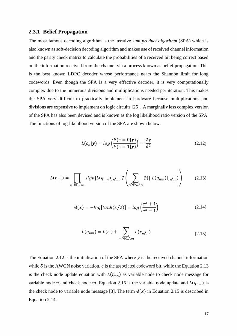
𝐿(𝑐𝑛|𝒚) = 𝑙𝑜𝑔 (
𝑃(𝑐 = 0|𝒚)
𝑃(𝑐 = 1|𝒚)) =
2𝑦
𝛿2 (2.12)
𝐿(𝑟𝑛𝑚) = ∏ 𝑠𝑖𝑔𝑛[𝐿(𝑞𝑚𝑛)]𝑛′𝑚. ∅( ∑ ∅([|𝐿(𝑞𝑛𝑚)|]𝑛′𝑚)
𝑛′∈𝑉𝑚\𝑛
)
𝑛′∈𝑉𝑚\𝑛
(2.13)
∅(𝑥) = −𝑙𝑜𝑔[𝑡𝑎𝑛ℎ(𝑥 2⁄ )] = 𝑙𝑜𝑔 (
𝑒𝑥 + 1
𝑒𝑥 − 1) (2.14)
𝐿(𝑞𝑛𝑚) = 𝐿(𝑐𝑖) + ∑ 𝐿(𝑟𝑚′𝑛)
𝑚′∈𝐶𝑛\𝑚
(2.15)
The Equation 2.12 is the initialisation of the SPA where 𝑦 is the received channel information
while 𝛿 is the AWGN noise variation. 𝑐 is the associated codeword bit, while the Equation 2.13
is the check node update equation with 𝐿(𝑟𝑚𝑛) as variable node to check node message for
variable node 𝑛 and check node 𝑚. Equation 2.15 is the variable node update and 𝐿(𝑞𝑛𝑚) is
the check node to variable node message [3]. The term ∅(𝑥) in Equation 2.15 is described in
Equation 2.14.
Page 36
18
2.3.2 Approximate Belief Propagation
Due to the very complex nature of the SPA and its log likelihood version, several algorithms
such as the Normalized BP-based Min-Sum algorithm (MSA) and the Offset BP-Based
algorithm which are approximate versions of the SPA were proposed. These algorithms are not
as complex to implement practically as the SPA but they have Bit Error Rate (BER)
performance which is close to that of the SPA [26].
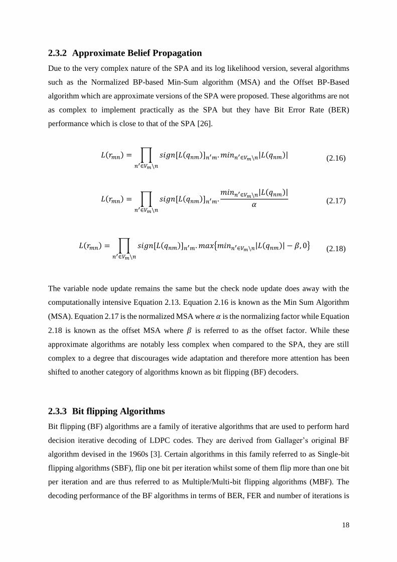
𝐿(𝑟𝑚𝑛) = ∏ 𝑠𝑖𝑔𝑛[𝐿(𝑞𝑛𝑚)]𝑛′𝑚. 𝑚𝑖𝑛𝑛′∈𝑉𝑚\𝑛|𝐿(𝑞𝑛𝑚)|
𝑛′∈𝑉𝑚\𝑛
(2.16)
𝐿(𝑟𝑚𝑛) = ∏ 𝑠𝑖𝑔𝑛[𝐿(𝑞𝑛𝑚)]𝑛′𝑚.
𝑚𝑖𝑛𝑛′∈𝑉𝑚\𝑛|𝐿(𝑞𝑛𝑚)|
𝛼𝑛′∈𝑉𝑚\𝑛
(2.17)
𝐿(𝑟𝑚𝑛) = ∏ 𝑠𝑖𝑔𝑛[𝐿(𝑞𝑛𝑚)]𝑛′𝑚. 𝑚𝑎𝑥{𝑚𝑖𝑛𝑛′∈𝑉𝑚\𝑛|𝐿(𝑞𝑛𝑚)| − 𝛽, 0}
𝑛′∈𝑉𝑚\𝑛
(2.18)
The variable node update remains the same but the check node update does away with the
computationally intensive Equation 2.13. Equation 2.16 is known as the Min Sum Algorithm
(MSA). Equation 2.17 is the normalized MSA where 𝛼 is the normalizing factor while Equation
2.18 is known as the offset MSA where 𝛽 is referred to as the offset factor. While these
approximate algorithms are notably less complex when compared to the SPA, they are still
complex to a degree that discourages wide adaptation and therefore more attention has been
shifted to another category of algorithms known as bit flipping (BF) decoders.
2.3.3 Bit flipping Algorithms
Bit flipping (BF) algorithms are a family of iterative algorithms that are used to perform hard
decision iterative decoding of LDPC codes. They are derived from Gallager’s original BF
algorithm devised in the 1960s [3]. Certain algorithms in this family referred to as Single-bit
flipping algorithms (SBF), flip one bit per iteration whilst some of them flip more than one bit
per iteration and are thus referred to as Multiple/Multi-bit flipping algorithms (MBF). The
decoding performance of the BF algorithms in terms of BER, FER and number of iterations is
Page 37
19
inferior to that of the soft decision Sum-Product Algorithm (SPA). The SPA and its
approximate versions are not used in many applications because of the complexity and
therefore much attention has been given to sub-optimal but significantly less complex decoding
algorithms based on the SPA such as the soft decision MSA algorithms [26] and several
variations of the hard decision BF algorithm.
Almost all bit flipping algorithms follow Gallager’s general BF algorithm which makes use of
the syndrome vector as described in the following steps [3]:
Step 1: Compute the syndrome for the received codeword of size N. If all the parity-
check equations are satisfied then decoding can stop otherwise proceed to step 2.
Step 2: For each bit in the codeword, compute the number of parity-check equations
that have not been satisfied and denote for each bit as 𝑓𝑖 , 𝑖 = 1,2, … ,𝑁 .
Step 3: Identify the set 𝝁 of bits that have the largest 𝑓𝑖 measured against some
predefined threshold 𝑓𝑥. (One for SPF and a set of bits for MBF).
Step 4: Flip the bits in set 𝝁.
Step 5: Repeat the steps 1 to 4 until all the parity check equations have been satisfied in
which case we stop at Step 1, or until a predetermined maximum iteration number
has been reached.
Most of the bit flipping algorithms discussed in literature follow Gallager’s general BF
algorithms as shown in the next chapter.
Page 38
20
3. Bit Flipping decoding of LDPC Codes
Various parts of the original bit flipping algorithm discussed in Section 2.3.3 have been
modified to come up with different versions of BF algorithms. Improvement in decoding
performance of BF algorithms is obtained by incorporating certain soft decision aspects such
as those of the SPA into the hard decision BF algorithm. This means that apart from hard
decision decoding, the algorithms also make use of soft channel information to establish a
metric by which the reliability of the hard decision is measured.
Consider H to be the parity-check matrix for LDPC code C with 𝑁 columns and 𝑀 rows. Let
𝒉𝟏, 𝒉𝟐, … , 𝒉𝑴 represent rows of H, in which 𝒉𝒎 = (ℎ𝑚,1, ℎ𝑚,2, … , ℎ𝑚,𝑁) for 1 ≤ 𝑚 ≤ 𝑀. It
can then be shown that the received hard decision codeword 𝒛 has the syndrome s where
𝒔 = (𝑠1, 𝑠2, … , 𝑠𝑀) = 𝒛.𝑯𝑻 (3.1)
The syndrome component 𝑠𝑚 is given by Equation 3.1
𝑠𝑚 = 𝒛. 𝒉𝒎 = ∑𝑧𝑙ℎ𝑚,𝑙
𝑁
𝑙=1
(3.2)
The vector 𝒛 received is a codeword if and only if 𝒔 = 𝟎. If 𝒔 ≠ 𝟎 then it means that errors
have been detected. The check nodes joining on a variable bit 𝑛 are signified by 𝑴(𝑛) =
{𝑚|ℎ𝑚,𝑛 = 1}, whereas the set of variable nodes joining on a check 𝑚 are noted as 𝑵(𝑚) =
{𝑛|ℎ𝑚,𝑛 = 1}.
Let
𝑒 = (𝑒1, 𝑒2, … , 𝑒𝑁) = (𝑐1, 𝑐2, … , 𝑐𝑁) + (𝑧1, 𝑧2, … , 𝑧𝑁) (3.3)
The vector 𝒆 is the error pattern that appears in 𝒛 when compared with the corresponding valid
codeword 𝒄. It follows then that the error pattern found in vector 𝒆 and the syndrome 𝒔 are
related as shown
𝒔 = 𝒆.𝑯𝑻 (3.4)
Page 39
21
where
𝑠𝑚 = 𝒆. 𝒉𝒎 = ∑ 𝑒𝑛ℎ𝑚,𝑛
𝑁
𝑛=1
(3.5)
for 1 ≤ 𝑚 ≤ 𝑀.
3.1 Single Bit Flipping Algorithms
There are numerous variations of the SBF decoding algorithms documented. However, they all
have a common feature, which is the use of the syndrome vector 𝒔 to obtain a metric by which
to flip a single perceived erroneous bit per single iteration. What differs in each algorithm is
how the metric is obtained as explained below.
3.1.1 Gallager Bit Flipping Decoding Algorithm (GBF) (1962)
This is the original SBF decoding algorithm on which most of the algorithms are based. The
algorithm is basically the exact one described in Section 2.3.3 [3].
3.1.2 Weighted Bit Flipping Decoding Algorithm (WBF) (2001)
In this algorithm [27] the hard decision vector 𝒛 is obtained from the soft information vector
𝒚 received from the communication channel. We define a reliability measure |𝑦𝑛| of the
received symbol 𝑦𝑛. The larger |𝑦𝑛| is, the more reliable the hard decision is considered to be.
From the parity check matrix H, where 𝒉𝒎 = (ℎ𝑚,1, ℎ𝑚,2, … , ℎ𝑚,𝑁) for 1 ≤ 𝑚 ≤ 𝑀. We
define
|𝑦𝑛|𝑚𝑖𝑛 ≜ {𝑚𝑖𝑛{|𝑦𝑛|}: 1 ≤ 𝑛 ≤ 𝑁, ℎ𝑚,𝑛 = 1} (3.6)
The metric, also known as the inversion function, with which to flip bits believed to be in error
is calculated as follows
𝐸𝑛 ≜ ∑ (2𝑠𝑚 − 1)
𝑚 ∈ 𝑀(𝑛)
|𝑦𝑛|𝑚𝑖𝑛 (3.7)
Page 40
22
Where the set of variable nodes sums orthogonal to the syndrome bit 𝑠𝑚 is 𝑚 ∈ 𝑀(𝑛). The
metric 𝐸𝑛 is a weighted checksum orthogonal on the codeword bit positioned at 𝑛.
The general algorithm is modified as follows:
Step 2: Find the bit position 𝑛 which has the largest 𝐸𝑛.
Step 3: Flip bit 𝑧𝑛 in position 𝑛 found in step 2.
3.1.3 Bootstrapped Weighted Bit Flipping Decoding Algorithm (B-WBF)
(2002)
Consider the received vector 𝒚. A value 𝑦𝑛 is considered unreliable if |𝑦𝑛| < 𝛼, for a
predetermined 𝛼 which is optimized by simulation. A check node connected to an unreliable
variable node is considered reliable if all the variable nodes adjacent to it are reliable.
Unreliable 𝑦𝑛 are replaced by improved values 𝑦𝑛′ as shown in Equation 3.8. This new value is
obtained from reliable check nodes which obtain information from reliable variable nodes [28].
𝑦𝑛′ = 𝑦𝑛 + ∑ ∏ 𝑠𝑔𝑛(𝑦𝑛 ).𝑚𝑖𝑛𝑛∈𝑀(𝑛)\𝑛|𝑦𝑛 |
𝑛∈𝑀(𝑛)\𝑛𝑚∈𝑁(𝑚)
(3.8)
The term 𝑚 ∈ 𝑁(𝑚) denotes the reliable check nodes adjacent to variable node 𝑛. The term
𝑛 ∈ 𝑀(𝑛)\𝑛 represents all the variable nodes connected to check node 𝑚 apart from 𝑛. All
reliable variable nodes or unreliable variable nodes with unreliable check nodes remain
unchanged such that 𝑦𝑛′ = 𝑦𝑛.
When vector 𝒚′ has been obtained, conventional WBF can commence as described in Section
3.1.2. The optimal value for 𝛼 is dependent on the SNR and the code as well as its tanner graph.
The BWBF shows a considerable BER improvement as well as reduced iterations when
compared to the WBF [29]. The number of iterations is halved and a performance improvement
of about 1.5 dB at a BER of 10-5.
Page 41
23
3.1.4 Modified Weighted Bit Flipping Decoding Algorithm (M-WBF)
(2004)
The basic framework for this algorithm is similar to Section 3.1.2 apart from the calculation of
the metric 𝐸𝑛 which is calculated as follows:
𝐸𝑛 ≜ ∑ (2𝑠𝑚 − 1)
𝑚 ∈ 𝑀(𝑛)
|𝑦𝑛∈𝑁(𝑚)|𝑚𝑖𝑛− 𝛼|𝑦𝑛| (3.9)
The first term on the right indicates to what extend the erroneous bit should be flipped while
the second term indicates to what extend the bit value should be maintained. The weighting
factor 𝛼 is obtained through simulation [30]. It is a real number 𝛼 ≥ 0. The term 𝛼 is SNR and
code dependant. It is shown in [30] that the MWBF performs considerably better than the WBF
at SNRs of particular interest. With an optimal 𝛼 the M-WBF requires about half the iterations
required for the standard WBF and offers about 0.5 dB improvement at a BER of 10-5.
3.1.5 Improved Modified Weighted Bit Flipping Decoding Algorithm
(IMWBF) (2005)
This algorithm is a slight modification of the algorithm in Section 3.1.4. The soft information
from the bit whose metric is being calculated is removed from the metric computation such
that in Equation 3.8 becomes:
|𝑦𝑛∈𝑁(𝑚)/𝑛|𝑚𝑖𝑛≜ {𝑚𝑖𝑛{|𝑦𝑖|}: 1 ≤ 𝑖 ≤ 𝑁, ℎ𝑗,𝑖 = 1, 𝑛 ≠ 𝑖} (3.10)
And (3.9) becomes:
𝐸𝑛 ≜ ∑ (2𝑠𝑚 − 1)
𝑚 ∈ 𝑀(𝑛)
|𝑦𝑛∈𝑁(𝑚)/𝑛|𝑚𝑖𝑛− 𝛼|𝑦𝑛| (3.11)
Analysis of the weighting also shows that 𝛼 decreases as the SNR increases and also increases
as the column weight of the codes increases. However, 𝛼 is unaffected by the length of the
codes. In [31] it is also demonstrated how to optimise 𝛼.
Page 42
24
Simulation BER curves show that the IMWBF with an optimised 𝛼 value performs better than
the MWBF for both Gallager and Finite Geometry codes [31].
3.1.6 Reliability Ratio Based Weighted Bit Flipping Algorithm (RR-WBF)
(2005)
This algorithm introduces a different way of calculating the bit flipping function by including
what is termed a reliability ratio [32].
𝑅𝑚𝑛 = 𝛽
|𝑦𝑛|
|𝑦𝑛∈𝑁(𝑚)𝑚𝑎𝑥 |
(3.4)
In this algorithm, |𝑦𝑛∈𝑁(𝑚)𝑚𝑎𝑥 | is the highest soft magnitude of the variable nodes adjacent to
check node 𝑚. The term 𝛽 is a normalization factor to ensure ∑ 𝑅𝑚𝑛 = 1𝑛∈𝑀(𝑛) . The new
function therefore becomes
𝐸𝑛 ≜
∑ (2𝑠𝑚 − 1)𝑚 ∈ 𝑀(𝑛) |𝑦𝑛∈𝑁(𝑚)/𝑛|𝑚𝑖𝑛𝑅𝑚𝑛
(3.5)
Simulations in [32] have shown that the RR-WBF has performance improvement of about 1 to
2 dB at a BER of 10-5 over the IMWBF. The algorithm has a complexity similar to that of the
IMWBF and there is no need for offline pre-processing.
3.1.7 Channel Independent Weighted Bit Flipping Decoding Algorithm
(CI-WBF) (2012)
The CI-WBF modifies the method of computing the weighting function and also does away
with the channel information term that is present in the IM-WBF. The weighting term is
calculated as shown in Equation 3.13.
𝑤𝑚𝑛 =
1
|𝑦𝑛|∑ |𝑦𝑛|
𝑛∈𝑀(𝑛)\𝑛
(3.14)
The weighting function is incorporated into the metric formula as shown
Page 43
25
𝐸𝑛 ≜ ∑ (2𝑠𝑚 − 1)
𝑚 ∈ 𝑀(𝑛)
𝑤𝑚𝑛 (3.15)
Simulations show that the CI-WBF algorithm has a 1.6 dB coding gain improvement at a BER
of 10-5 over the WBF and also reduces the number of iterations by 53% without increasing
complexity [33].
3.1.8 Modified Channel Independent Weighted Bit Flipping Decoding
Algorithm (MCI-WBF) (2013)
This algorithm is also known as the Offset Channel Independent Weighted Bit Flipping
Decoding Algorithm (OCIWBF). The basic structure of the CI-WBF is retained apart from the
weighting function in which an offset factor 𝛾 ≥ 0 is added to improve the accuracy of the CI-
WBF. The weighting factor becomes:
𝑤𝑚𝑛 =1
|𝑦𝑛|𝑚𝑎𝑥 ( ∑ |𝑦𝑛|
𝑛∈𝑀(𝑛)\𝑛
−𝑚𝑖𝑛(𝛾, 0)) (3.16)
The offset factor 𝛾 is found through Monte-Carlo simulation because theoretical determination
of this term is difficult to accomplish. The offset is either a 0 or 𝛾 depending on which one is
smaller. Computational complexity is only slightly increased at initialisation. Simulations in
[34] show that, the OCI-WBF has a 0.45 dB performance gain at a BER of 10-5 over the CI-
WBF.
3.1.9 An Iterative Bit Flipping based Decoding Algorithm (2015)
The algorithm presented in [35] is a modification of the original weighted bit flipping (WBF)
described in [35]. The algorithm is initialised in the exact same way as the WBF, however, the
difference, lies in the manner in which the inversion function is calculated.
The proposed algorithm, the recursive weighted bit flipping algorithm (RECWBF) exploits the
correlation between iteratively decoded and received channel vectors. The inversion function
is:
Page 44
26
𝐸𝑛,𝑘 = ∑ ø𝑚2(𝑠𝑚 − 1)
𝑚 ∈ 𝑀(𝑛)
+∑(𝜆)𝑘−𝑡𝑘−1
𝑡=1
𝑣𝑛𝑘−1𝑦𝑛 + (𝛾)
𝑘𝑣𝑛𝑘𝑦𝑛 (3.17)
Where
ø𝑖 = 𝑚𝑖𝑛𝑛∈𝑀(𝑛)|𝑦𝑛| (3.18)
and the terms 𝜆 and 𝛾 are known as the forgetting coefficients. The proposed algorithm
introduces a new term 𝑣𝑛𝑘𝑦𝑛 from the preceding iteration to prevent fluctuations in the inversion
function values which is a model for bits which are most likely to be flipped. This modification
is said to aid in the rapid convergence of the decoder subsequently improving the decoding
performance.
Simulations of the RECWBF with PEGReg (1008, 504) and Gallager (273,191) show that the
algorithm shows a performance improvement of at least 1.5 dB when compared to the WBF,
GDWBF and IERRWBF [35]. There is no theoretical determination of the forgetting factors
𝜆 and 𝛾 and therefore have been determined via exhaustive simulations.
3.1.10 A Self-Normalized Weighted Bit-Flipping Decoding Algorithm (2016)
The Weighted Bit-flipping (WBF) algorithm is the blue print for the algorithm proposed in
[36]. The so-called Self-Normalized Weighted Bit-Flipping Decoding Algorithm (SNWBF)
operates as an iterative single bit flipping algorithm for bits that have the highest inversion
function value defined as:
𝐸𝑛 = ∑ (2𝑠𝑚 − 1)∅𝑚,𝑛𝑚∈𝑀(𝑛)
(3.19)
Where
∅𝑚,𝑛 =
𝑚𝑖𝑛𝑖∈𝑁(𝑚)|𝑦𝑖||𝑦𝑛|⁄ (3.20)
Page 45
27
The main modification is the introduction of the normalizing absolute variable node channel
value |𝑦𝑛| in the weighting factor which represents the reliability of the received signal 𝑦𝑛 .
When compared to the IMWBF, the SNWBF does away with the weighting factor because the
optimal weighting factor cannot be determined theoretically and so needs extensive simulations
to obtain. This is inefficient and the weighting factor varies with changing conditions such as
SNR and code structure [36]. The normalization procedure is important so as to take into
account the influence of the reliability of the channel information and the hard decision bit. A
2-bit and 3-bit quantized version of the algorithm has also been developed. However, this
quantised algorithm does not provide any performance improvement, but it does reduce the
complexity.
The SNWBF is only marginally more complex than both the WBF and the IMWBF.
Simulations with finite geometry codes (FG-LDPC) codes reveals that both the quantized and
unquantized SNWBF algorithm outperforms both the WBF and IMWBF algorithm at high
SNR. The proposed algorithm also converges faster and therefore requires fewer iterations to
achieve better BER performance when compared to existing aforementioned algorithms.
3.1.11 Hybrid iterative Gradient Descent Bit-Flipping algorithm (HGDBF)
algorithm (2016)
The Hybrid iterative Gradient Descent Bit-Flipping algorithm (HGDBF) algorithm is a
modified version of the original GDBF. The paper considers the inversion function modified
by Li et al [37] in which a zero-mean Gaussian random term 𝑞𝑛 and a weighting factor 𝜔 to
improve performance are introduced:
𝐸𝑛 = �̂�𝑛𝑦𝑛 + 𝜔 ∑ (1 − 2𝑠𝑘) + 𝑞𝑛𝑛∈𝑀(𝑛)
(3.21)
However, the HGDBF is modified by introducing a weighting to the single bit GDBF. This is
done on the variable nodes by adding a weighted inversion function value so as to reflect the
check node transactions on the variable node in question. The weighting factor takes into
account the one-sided power spectral density of the additive white Gaussian Noise (AWGN)
associated with the codeword as shown
Page 46
28
𝛼 = 𝜂 ∙
𝑁0𝐸𝑏 (3.22)
The optimal value for the term 𝜂 is obtained by simulation and the term 𝑁0
𝐸𝑏 is the inverse of the
SNR. The term �̂�𝑛 is the hard decision bit term. The final variable node update equation looks
like:
𝑦𝑛𝑘+1 = 𝑦𝑛
𝑘 + �̂�𝑛 ∙ 𝛼 ∙ 𝐸𝑛𝑘 (3.23)
Simulations carried out in [37] reveal that the HGDBF has a 0.4 dB gain over the GDBF. It is
suggested that improved performance can also be obtained by applying [38] to the noisy GDBF
as well as the multi-bit GDBF.
3.1.12 Weighted Bit-Flipping Decoding for Product LDPC Codes (2016)
Unlike most algorithm described in this section, the Page-Based Weighted Bit-Flipping (P-
WBF) and its simplified version, the Row-Column Weighted Bit-Flipping (RC-WBF)
decoding algorithm are designed specifically for product LDPC codes for 2D codewords
described in [38].
The P-WBF has an inversion function for a 2D codeword described by:
𝐸𝑛𝑖,𝑗 =1
|𝑦𝑛𝑖,𝑗|[ ∑ (2𝑠𝑚𝑗
− 1)( ∑ |𝑦𝑖,𝑗|
𝑗∈𝑁𝑟𝑜𝑤(𝑚)
)
𝑚∈𝑀𝑟𝑜𝑤(𝑗)
+ ∑ (2𝑠𝑚𝑖− 1)( ∑ |𝑦𝑖,𝑗|
𝑖∈𝑁𝑐𝑜𝑙(𝑚)
)
𝑚∈𝑀𝑐𝑜𝑙(𝑖)
]
(3.24)
The algorithm flips the bit with the highest 𝐸𝑛𝑖,𝑗 for variable node 𝑦𝑛𝑖,𝑗 where 𝑖 and 𝑗 represents
the row and column position respectively. The biggest drawback of the P-WBF is that its
complexity increases quadratically as the codeword size increases. This gives rise to the Row-
Column Weighted Bit-Flipping (RC-WBF) decoding algorithm which has a linear complexity
because it decodes the 2D codeword on column and row directions separately. The RC-WBF
inversion function of the RC-WBF is
Page 47
29
𝐸𝑛 =1
|𝑦𝑛|[ ∑ (2𝑠𝑚 − 1)( ∑ |𝑦𝑛|
𝑗∈𝑁𝑟(𝑚)
)
𝑚∈𝑀𝑟(𝑗)
]
(3.25)
where 𝑟 is either row or column.
The RC-WBF exhibits what is known as the V-Shape property [38] in which the algorithm
reaches the lowest BER at some optimal iteration number but then the BER increases as the
iterations go beyond the optimal number of iterations. Thus, a threshold obtained from
exhaustive simulations, must be set to ensure optimum BER.
Simulations show that, the P-WBF performs better than the RC-WBF however, the RC-WBF
has a lower complexity. Both algorithms have a BER performance that is still inferior to the
Belief Propagation SPA decoder [38].
3.2 Multi-bit Flipping Algorithms
The bit-flipping algorithms in this category have the similar characteristics to the single-bit
flipping algorithms apart from the fact that they flip multiple bits as opposed to flipping one
bit per iteration. The general algorithm framework is the same as the one described in Section
2.3.3 with a few modifications to step 2 and step 3.
3.2.1 Gradient Descent Bit Flipping Algorithm (2008)
This algorithm will have a few different preliminaries defined as follows 𝐻 is the binary 𝑀 𝑥 𝑁
matrix and 𝑁 > 𝑀 ≥ 1. We have binary linear code 𝐶 ≜ {𝒄 ∈ 𝐹2𝑛: 𝐻𝒄 = 0}. Conversion is
through �̃� ≜ {(1 − 2𝑐1, 1 − 2𝑐2, … ,1 − 2𝑐𝑁: 𝒄 ∈ 𝐶)}, 𝐶 ∈ {0,1}, �̃� ∈ {+1,−1} . The AWGN
effects are as described in 1.1. We have the parity condition ∏ 𝑥𝑗 = 1, (∀𝑖 ∈ [1, 𝑁])𝑗∈𝑁(𝑖) is
equivalent to (𝑥1, 𝑥2, … , 𝑥𝑁) ∈ �̃�. The 𝑖 −th bipolar syndrome of 𝑥 is the value ∏ 𝑥𝑗 ∈𝑗∈𝑁(𝑖)
{+1,−1}.
Then we have 𝑁(𝑖) ≜ {𝑗 ∈ [1, 𝑁]: ℎ𝑖𝑗 = 1}, and 𝑀(𝑗) ≜ {𝑖 ∈ [1,𝑀]: ℎ𝑖𝑗 = 1} in which case
𝑁(𝑖) and 𝑀(𝑗)(𝑖 ∈ [1,𝑀], 𝑗 ∈ [1, 𝑁]).
We introduce the objective function which is based on the MLD correlation decoding rule:
Page 48
30
𝑓(𝑥) ≜∑𝑥𝑗𝑦𝑗 +∑ ∏ 𝑥𝑗𝑗∈𝑁(𝑖)
𝑀
𝑖=1
𝑁
𝑖=1
(3.26)
The first term is a correlation between the received word and the bipolar codeword which
requires maximisation. The sum of the bipolar syndrome of 𝑥. If and only if 𝒙 ∈ �̃�, the second
term has its maximum value.
The single BF algorithm based function is shown below:
∆𝑘(𝐺𝐷)
≜ 𝑥𝑘𝑦𝑘 + ∑ ∏ 𝑥𝑗𝑗∈𝑁(𝑖)𝑖∈𝑀(𝑘)
(3.27)
The GDBF is a variable size bit-flipping algorithm and uses Equation 3.26) and Equation 3.27
to decode by modifying the bit flipping step 3 and step 4 as shown below [39]. We introduce
new parameters 𝜃which is a negative real number named the inversion threshold. A secondary
parameter 𝜇 defined in step 3 is a binary variable called the mode flag responsible for selecting
the mode in which the algorithm is operating.
Step 3 – Evaluate the value of the objective function, and let 𝑓1 ∶= 𝑓(𝒙). If 𝜇 = 0, then
execute Sub-step 3-1 (multi-bit mode), else execute Sub-step 3-2 (single-bit mode).
Step 3.1 Flip all bits satisfying
∆𝑘(𝐺𝐷)
< 𝜃 (𝑘 ∈ [1, 𝑁]) (3.28)
Evaluate the value of the objective function again, and let𝑓2 ∶= 𝑓(𝒙). If 𝑓1 > 𝑓2then
make 𝜇 = 1.
Step 3.2 Flip a single bit at the 𝑗th position, where
𝑗 ≜ 𝑎𝑟𝑔𝑚𝑖𝑛𝑘∈[1,𝑛]∆𝑘(𝐺𝐷)
(3.29)
In some cases the algorithm can be trapped in a local maxima which is not a codeword. When
this occurs, there is a further modification which called the escape process described in [39].
Page 49
31
Simulations presented in [39] show that the Multi-GDBF algorithm has a 1.6 dB performance
improvement over the MWBF. The Multi-GDBF algorithm with the escape mechanism adds
another 1.5 dB improvement.
3.2.2 Candidate bit based bit-flipping decoding algorithm (CBBF) (2009)
The multi-bit flipping Candidate bit based bit-flipping (CBBF) decoding algorithm is proposed
and described at length in [40]. This algorithm works on the premise that an unreliable bit 𝑧𝑛
has 𝑢𝑛 number of unsatisfied parity check equations. If 𝑢𝑛 > 𝛿 where the term 𝛿 is some fixed
threshold, then is considered to have a high probability of being in error. The bits to be flipped
are those where 𝑢𝑛 = 𝑢𝑚𝑎𝑥 where the term 𝑢𝑚𝑎𝑥 = 𝑚𝑎𝑥(𝑢𝑛).
The 𝑚𝑡ℎ parity check may have a total 𝑐𝑚 number of candidate bits and the lower the number
of 𝑐𝑚 the more likely, the selected candidate bits are likely to be in error. A new term, the
flipping criterion or metric
𝑟𝑛 = ∑ 𝑐𝑚 − 1
𝑚∈𝑀(𝑛)
(3.30)
Equation 3.30 is introduced such that 𝑢𝑛 = 𝑢𝑚𝑎𝑥 and 𝑢𝑙 = 𝑚𝑖𝑛(𝑟𝑖) both contribute to
unsatisfied parity checks.
The initialisation of the algorithm is similar to prior algorithms apart from the computation of
𝑢𝑛 and 𝑟𝑛 . The flipping criteria however is such that, flip all the bits in which 𝑢𝑛 = 𝑢𝑚𝑎𝑥
and 𝑢𝑙 = 𝑚𝑖𝑛(𝑟𝑛).
The CBBF is seen to perform better than the Gallager BF and the soft information WBF.
Performance of the CBBF approaches that of the IMWBF but does not surpass it. In
comparison to the single bit flipping WBF and IMWBF algorithms, the CBBF is marginally
less complex and also converges a lot faster because it flips multiple bits at a time. While most
bit flipping algorithms oscillate, the CBBF has a terminating condition in which the algorithm
terminates if 𝑢𝑚𝑎𝑥 < 𝛿.
Page 50
32
3.2.3 Modified I-WBF (MBF) (2009)
In this algorithm, we receive the vector 𝒚 with soft information from the AWGN. For each
output 𝑦𝑛, 0 ≤ 𝑛 ≤ 𝑁 we define a log-likelihood ratio (LLR):
𝐿𝑛 ≜ 𝑙𝑛 (
𝑃(𝑐𝑛 = 1|𝑦𝑛)
𝑃(𝑐𝑛 = 0|𝑦𝑛)) (3.31)
The larger the reliability |𝐿𝑛| the higher the reliability of the hard decision of 𝑧𝑛(0)
at iteration 0.
For each parity check sum, i.e. the rows in 𝑯, 1 ≤ 𝑚 ≤ 𝑀 compute “lower check reliability”
value and the “upper check reliability value” as shown in (3.32)
𝑙𝑚 ≜ 𝑚𝑖𝑛𝑙∈𝑀(𝑚)|𝐿𝑚|, 𝑢𝑗 ≜ 𝑚𝑎𝑥𝑙∈𝑀(𝑚)|𝐿𝑚| (3.32)
The cumulative metric by which we flip a bit at position 𝑙 in iteration 𝑘 is obtained as follows:
∅𝑛(𝑘)≜ ∑ ∅𝑛,𝑚
(𝑘), 1 ≤ 𝑛 ≤ 𝑁
𝑚∈𝑀(𝑛)
(3.33)
For each check 𝑚 ∈ 𝑀(𝑛)
∅𝑛(𝑘) ≜ {
|𝐿𝑛| − 𝑙𝑚 2⁄ , 𝑖𝑓 𝑠𝑚(𝑘−1) = 0
|𝐿𝑛| − (𝑢𝑚 + 𝑙𝑚 2⁄ ), 𝑖𝑓 𝑠𝑚(𝑘−1) = 1
(3.34)
The bits to flip are the ones with the least cumulative metric. We therefore calculate the number
of bits 𝑝 to flip using as follows:
𝑝 = ⌊
𝑤𝐻(𝒔𝑘)𝑤𝐶⁄ ⌋ (3.35)
𝑤𝐻(𝒂) is the Hamming Weight of the vector 𝒂 while ⌊𝑥⌋ represents the largest integer that is
equal to or less than 𝑥. We then proceed to find the set of 𝑝 bits 𝐷𝑘 = {𝑣1(𝑘), 𝑣2
(𝑘), … , 𝑣𝑝
(𝑘)} with
the least value of ∅𝑛(𝑘)
.
The algorithm also has a loop detection feature. Consider a situation in which a decoded
vector 𝒛(𝒌𝟎)decoded at iteration 𝑘0and another 𝒛(𝑘) one decoded at iteration 𝑘, where 𝑘0 ≤ 𝑘.
Then 𝒛(𝑘0+1) = 𝒛(𝑘+1) because 𝑫(𝑘0+1) = 𝑫(𝑘+1)and this is a clear indication that an infinity
loop has occurred. The loop detection feature is discussed here [41].
Page 51
33
Simulations indicate that the MBF has a 0.25 dB performance improvement at a BER of 10-5
compared to the IMWBF. A few observations have been listed in [41] concerning the MBF:
• The standard algorithm is known to experience decoding failure due to infinite loop traps
• The MFB has fewer infinite traps due to its ability to flip multiple bits at the same time.
• Most bits flipped at each iteration correspond to actual errors. If new errors are introduced
they are subsequently corrected in preceding iterations.
• The number of bits flipped by the MBF decrease as the iterations increase.
3.2.4 Soft-Bit-Flipping (SBF) Decoder for Geometric LDPC Codes (2010)
The Soft-Bit-Flipping (SBF) decoder presented in [12] is a multi-bit flipping algorithm
designed specifically for geometric codes and VLSI high speed, high throughput applications.
The SBF uses a modified version of the IMWBF inversion function [31]. The SBF inversion
function does away with IMWBF marginalization which increases complexity and is not
suitable for high speed applications but rather employs pseudo-marginalization like the
MWBF.
𝐸𝑛 ≜ ∑ (2𝑠𝑚 − 1)
𝑚∈𝑴(𝑛)
𝑚𝑖𝑛𝑖∈𝑵(𝑚)|𝑦𝑖| − 𝛼. |𝑦𝑛| (3.36)
The SBF also uses a multi-threshold technique first developed in [12] to determine the flipping
strategy for each bit dependant on the associated inversion function value. The values 𝑏1, 𝑏2
and 𝑏3, which are the flipping thresholds are obtained by investigating the distribution of the
inversion function values probability density function and are such that 𝑏1 < 𝑏2 < 𝑏3. Instead
of performing a hard flip on the codeword, the SBF performs what are referred to as soft flips
on VN channel values as follows:
Strong flip:
If 𝑏3 ≤ 𝐸𝑛(𝑘)
, 𝑦𝑛(𝑘+1) = 𝑠𝑔𝑛 ((|𝑦𝑛
(𝑘)| − 2.5) . 𝑦𝑛(𝑘)) .𝑚𝑎𝑥 (1, |𝑦𝑛
(𝑘)| − 2)
Weak flip:
If 𝑏2 ≤ 𝐸𝑛(𝑘)< 𝑏3, 𝑦𝑛
(𝑘+1) = 𝑠𝑔𝑛 ((|𝑦𝑛(𝑘)| − 1.5) . 𝑦𝑛
(𝑘)) .max (1, |𝑦𝑛(𝑘)| − 1)
Maintain:
Page 52
34
If 𝑏1 ≤ 𝐸𝑛(𝑘) < 𝑏2 , 𝑦𝑛
(𝑘+1) = 𝑠𝑔𝑛(𝑦𝑛(𝑘)). |𝑦𝑛
(𝑘)|
Strengthen:
If 𝐸𝑛(𝑘) < 𝑏1 , 𝑦𝑛
(𝑘+1) = 𝑠𝑔𝑛(𝑦𝑛(𝑘)).𝑚𝑖𝑛 (2𝑞 , |𝑦𝑛
(𝑘)|)
where 𝑘 is the iteration number.
Simulation and implementation as presented in [12], shows that hardware complexity is
reduced significantly when compared to belief propagation algorithms. The algorithm also has
an improved BER performance and convergence speed when compared to the IMWBF [31].
3.2.5 Combined Modified Weighted Bit Flipping Algorithm (CM-WBF)
(2012)
This algorithm makes use of two algorithms to flip erroneous bits. Both algorithms
independently select perceived erroneous bits based on their inversion metric calculations. The
two algorithms to a large extend select different bits to flip per iteration. Simulations show that
the two algorithms select different bits at least 60 % of the time.
If both algorithms select different bits then both bits can be flipped otherwise flip the bit that
the first algorithm chose.
In [42] the first algorithm is the MWBF as explained in Section 3.1.4 while the second
algorithm is the as described in explained in [43].
In comparison to other WBF algorithms, the CM-WBF has a higher complexity per iteration.
The CM-WBF algorithm has also been observed to have fewer iterations, about a 50% fewer
iterations as well as a 0.2 dB and 0.1 dB improvement over the LC-WBF and M-WBF
respectively on irregular LDPC codes.
3.2.6 An Adaptive Weighted Multi-bit Flipping Algorithm (AWMBF)
(2013)
This algorithm makes use of the IMWBF as described in Section 3.1.5 as well as a bit-flipping
threshold 𝐸𝑡ℎto flip multiple bits per iteration. In this algorithm, the bipolar encoder is defined
as 𝑥𝑛 = 1 − 2𝑐𝑛. The inversion function 𝐸𝑛 of the IMWBF is also defined in Section 3.1.5.
Page 53
35
However, in this case, the bit with the highest 𝐸𝑛 is the one most likely to be incorrect.
Designate the highest 𝐸𝑛to 𝐸𝑚𝑎𝑥 . A set of the least reliable bits is identified using the following
criterion.
𝐿𝑅𝑃(𝐸) = {𝑛|𝐸𝑛 ≥ 𝐸𝑡ℎ, 𝑛 ∈ [1, 𝑁]} (3.37)
The flipping threshold is defined as follows
𝐸𝑡ℎ ≜ 𝐸𝑚𝑎𝑥 − |𝐸𝑚𝑎𝑥| (1 −1
𝑀∑ 𝑠𝑚
𝑀
𝑚=1
) (3.38)
The set of bits 𝑛∗ ∈ 𝐿𝑅𝑃(𝐸) are all flipped in parallel.
Simulation results presented in [11] show that, the AWMBF performs better than the IMWBF
with fewer iterations and achieves approximately 0.9 dB performance gain over the IMWBF
at a BER of 10-5 [11].
3.2.7 Two-Staged Weighted Bit Flipping Decoding Algorithm (2015)
In [44] is presented the Two-Staged Weighted Bit Flipping Decoding Algorithm (TSWBF)
aimed at mitigating the error floors prevalent in many bit flipping decoders. Achieving this
objective will enable the implementation of LDPC decoders in low power communication
devices.
The proposed algorithm is a hybrid of the parallel IMWBF (PWBF) [45] (which has an
inversion function identical to the IMWBF in [45]) and the Gallager Bit Flipping (BF)
algorithm. The hybrid system is meant to mitigate the high error floors that appear at the high
SNR regions of the PWBF decoder [45].
It has been investigated and been found out that the PWBF decoding fails when there is a bad
node and this happens when a variable 𝜔𝑆 is greater than a value 𝑇𝑆. The TSWBF algorithm is
designed such that it switches to the BF when 𝜔𝑆 < 𝑇𝑆 .The switching of the TSWBF is
described as follows:
Generate the syndrome 𝒔
If (𝒔 = Ø) or (𝑘 > 𝐾𝑀𝑎𝑥)
Page 54
36
Terminate TSWBF and output codeword;
Else If 0 < 𝜔𝑆 < 𝑇𝑆
Activate Bit Flipping (BF) Algorithm decoding
Else If 𝑇𝑆 ≤ 𝜔𝑆
Activate Two-Staged Weighted Bit Flipping (TSWBF) Algorithm decoding
End If
The computational complexity of the TSWBF is slightly more than that of the PWBF. The term
cannot be obtained by theoretical means and so can only be obtained by exhaustive simulations.
The TSWBF decoder is simulated against the PWBF and the BP algorithm for EG, PG, McKay
and PEG codes and is shown to reduce the error floors prevalent in the PWBF. As expected,
the TSWBF algorithm does not perform better than the BP algorithm, however it does reduce
the performance gap between the BP and the PWBF algorithm [44].
3.2.8 Mixed Modified Weighted Bit Flipping Decoding Algorithm (MM-
WBF) (2015)
This algorithm makes use of two algorithms to flip erroneous bits. One algorithm acts as the
main algorithm while the other acts as an auxiliary algorithm. The main algorithm has to be
the best performing algorithm available while the auxiliary algorithm is the second best and
this is determined by simulations. The two algorithms must also to a large extend select
different bits per iteration.
Certain rules apply when flipping bits. First, if both algorithms select different bits then both
bits can be flipped otherwise flip the bit that the main algorithm chose. Secondly, the auxiliary
algorithm may not flip bits that have already been flipped by the main algorithm.
In [32] the main algorithm is the RR-WBF as explained in Section 3.1.6 while the second
algorithm is the IMWBF as explained in Section 3.1.5.
In comparison to other WBF algorithms, the MM-WBF has a higher complexity per iteration.
The MM-WBF algorithm has also been observed to have fewer iterations and a 0.4 dB and 0.6
dB improvement over the RR-WBF and IM-WBF respectively on irregular LDPC codes.
Page 55
37
3.2.9 Noise-Aided Gradient Descent Bit-Flipping Decoder (2016)
In the literature [46], a Noise-Added Gradient Descent Bit-Flipping Decoder is proposed as a
further enhancement to the existing GDBF described in [39]. The algorithm has been designed
for both the BSC channel and the AWGN channel. Two important concepts intended to
improve GDBF decoding are presented namely the introduction of noise to VN flipping matric
calculation and iterative scheduling.
It is demonstrated in simulations that adding noise to GDBF decoders in form of random
perturbations enables the decoders to escape error prone structures of fixed points exhibited by
trapping sets that result in decoding failure.
The iterative scheduling modification of the noisy GDBF algorithms enhances the random
nature of the VN perturbations which further improves the performance of the decoder to
approach the performance of a typical MLD decoder when the algorithm runs for a large
number of iterations.
This novel noise addition to GDBF decoder design is expected to improve in performance to
match the decoding performance of soft decision belief propagation (BP) decoders [46].
3.3 Threshold Based decoding
The syndrome is an indication of the correctness of a received codeword. The parity check
equations converging on a codeword, in which the syndrome bits participate, also gives a
measure of the probability of the correctness of a variable node hard decision. This
characteristic of the LDPC codes has given rise to various bit flipping algorithms which make
use of parity check equation based inversion functions.
The simplest algorithms [29] only flip one bit per iteration. In the WBF [47] single bit flipping
algorithm, the inversion function is defined in Equation 3.7. The bit with the highest probability
of error has the highest value of 𝐸𝑛. The single bit flipping GDBF algorithm on the other hand
operates in the opposite manner. The objective function described in Equation 3.26 provides a
measure of the correctness of the hard decision. However, in this case, the variable node with
the smallest value of ∆𝑛 is considered to be the least reliable bit and should therefore be
corrected.
Page 56
38
The single bit flipping concept can be further enhanced and applied to multi-bit flipping
algorithms. Weighted Bit Flipping algorithms such as the WBF, MWBF and IMWBF operate
on the premise that the higher the value of 𝐸𝑛 of a particular bit, the more likely that bit is in
error. Gradient Descent Bit Flipping (GDBF) algorithms operate on the premise that the smaller
value of ∆𝑛, the higher the probability of error.
In order to correct multiple bits at the same time, it can be assumed that for WBF based
decoders, the higher values of 𝐸𝑛 contain a significant number of erroneous bits and the least
of the ∆𝑛 values are comprised of erroneous bits for GDBF based decoders. This reasoning
has brought about what are known as thresholds for multi-bit flipping decoders which are used
as a flipping criterion depending on the algorithm in question.
The Adaptive Weighted Multi-bit Flipping Algorithm (AMWBF) uses a non-fixed threshold
to correct erroneous bits. The threshold is calculated using Equation 3.38 and bits with
𝐸𝑛 above this threshold are flipped while those below it are left unchanged. The SBF in [12]
uses multiple fixed thresholds to determine how to modify the associated soft bit information.
The multi-bit flipping GDBF also uses a fixed threshold to determine which bits to flip. Almost
all the algorithms described in Section 3.2 of this document use some form of threshold to
determine which bits to flip.
This method of flipping is very effective in speeding up the convergence of a bit flipping
algorithm when it has a high chance of flipping erroneous bits correctly. However, this concept
of thresholds sometimes results in the flipping of correct bits in which case new errors are
introduced into the codeword.
3.4 Channel Information modification
The default operation of bit flipping algorithms is to obtain the hard decision from the received
channel values upon initialization. As the algorithm iteratively decodes, certain bits which meet
the flipping criterion get inverted with no modification to the associated soft channel
information.
In [12] and [46] the bit flipping algorithms perform the flipping function using a different
strategy which involves the modification of the soft channel information which in turn modifies
the hard decision. The purpose of modifying the soft channel information is to increase the
Page 57
39
transfer of information from variable nodes to check nodes and vice versa in the same way the
sum-product algorithm passes messages for more effective error correction [3].
The multiple-step majority logic decoder by Palinki et al [48] is the first known decoder to
make note of the difference in the distribution of the inversion function values and therefore
modify the bits with respect to the reliability as calculated by the inversion function. The
multiple-step majority logic decoder was a three stage decoder which worked as follows:
If any of the bits in a checksum calculation are erased, deactivate the check sum
If 𝑏1 ≤ 𝐸𝑛(𝑘)
, Flip the bit 𝑛
If 𝑏2 ≤ 𝐸𝑛(𝑘)< 𝑏1, Erase the bit 𝑛
If 𝐸𝑛(𝑘) < 𝑏2 , Maintain the bit 𝑛
The simulations with EG codes have shown that, the algorithm can operate at close to MLD of
intermediary length MSLMLD codes despite the presence of short cycles.
The BWBF described in Section 3.1.3 also incorporates soft bit flipping decoding by
initialising the variable node values according to the rule shown below
𝑦𝑛′ = 𝑦𝑛 + ∑ ∏ 𝑠𝑔𝑛(𝑦𝑛).𝑚𝑖𝑛𝑛∈𝑀(𝑛)\𝑛|𝑦𝑛|
𝑛∈𝑀(𝑛)\𝑛𝑚∈𝑁(𝑚)
The aptly named Soft bit flipping (SBF) algorithm decodes codewords by manipulating the
received codeword soft information as opposed to hard decision bit flipping [12]. The
algorithm uses a non-marginalized IMWBF inversion function to calculate the reliability of the
hard decision. While in the usual case, an LDPC decoding algorithm would flip bits that meet
a given flipping criterion, the SBF, has three different thresholds 𝑏1, 𝑏2 and 𝑏3 that are used to
modify soft channel information as follows:
Strong flip:
If 𝑏3 ≤ 𝐸𝑛(𝑘)
,
𝑦𝑛(𝑘+1) = 𝑠𝑔𝑛 ((|𝑦𝑛
(𝑘)| − 2.5) . 𝑦𝑛(𝑘)) .𝑚𝑎𝑥 (1, |𝑦𝑛
(𝑘)| − 2) (3.39)
Weak flip:
Page 58
40
If 𝑏2 ≤ 𝐸𝑛(𝑘)< 𝑏3,
𝑦𝑛(𝑘+1) = 𝑠𝑔𝑛 ((|𝑦𝑛
(𝑘)| − 1.5) . 𝑦𝑛(𝑘)) .max (1, |𝑦𝑛
(𝑘)| − 1) (3.40)
Maintain:
If 𝑏1 ≤ 𝐸𝑛(𝑘) < 𝑏2 ,
𝑦𝑛(𝑘+1) = 𝑠𝑔𝑛(𝑦𝑛
(𝑘)). |𝑦𝑛(𝑘)| (3.41)
Strengthen:
If 𝐸𝑛(𝑘) < 𝑏1 ,
𝑦𝑛(𝑘+1) = 𝑠𝑔𝑛(𝑦𝑛
(𝑘)).𝑚𝑖𝑛 (2𝑞 , |𝑦𝑛(𝑘)|) (3.42)
where 𝑘 is the iteration number.
The SBF decoder has been simulated with Geometric LDPC codes and has been observed to
have a higher throughput and better BER performance when compared to the regular IMWBF
[45].
The HGDBF algorithm presented in [46] is a hybrid iterative decoder for LDPC Codes. The
HGDBF uses the latest channel information and inversion function value to update the variable
node to increase the reliability of the hard decision. The inversion function for the HGDBF is
described in [46]. The variable node values are iteratively updated per iteration 𝑘 as follows:
𝑦𝑛𝑘+1 = 𝑦𝑛
𝑘 + �̂�𝑛 ∙ 𝜂 ∙𝑁0𝐸𝑏∙ 𝐸𝑛
𝑘 (3.43)
The variable node update is also used to reduce oscillations that are prevalent in many LDPC
bit flipping algorithms.
Page 59
41
4. Adaptive Multi-Threshold Multi-bit Flipping
Algorithm (AMTMBF)
4.1 Introduction
In this chapter, a new adaptive threshold based multi-bit flipping algorithm is devised. The
proposed algorithm known as the Adaptive Multi-Threshold Multi-bit Flipping Algorithm
(AMTMBF) is an investigation into the efficacy of the adaptive threshold strategy in the design
of multiple bit decoding LDPC algorithm in terms of bit error rate (BER), average number of
iterations (ANI) and complexity.
As discussed in literature, there has been extensive study into the design of single bit flipping
algorithms which span from Gallager’s original bit flipping algorithm [3] to the more recent
single bit flipping Gradient Descend bit flipping algorithms (GDBF [39]. The most obvious
drawback of single bit-flipping algorithm is the average time required for convergence which
increases the complexity of the algorithm mostly because the algorithm flips a perceived
incorrect bit per iteration. The second problem with single bit flipping algorithms occurs when
a codeword has more errors than the maximum number of iterations, then it is impossible to
correct that particular codeword even when the total number of errors is lower than the
minimum distance of that particular code. Thirdly, the algorithm may flip the wrong bits
thereby introducing new errors into the codeword or it may start oscillating about a set of bits
until it reaches maximum number of iterations in which case a decoding failure occurs.
The weaknesses detailed above that are associated with the single bit flipping algorithms have
motivated increased research into several variations of multi-bit flipping algorithms to facilitate
the design and development of low cost, low complexity and high speed communication
devices as shown in [12]. The major benefit of using multi-bit flipping algorithms is in the
average number of iterations (ANI) required for convergence which are reduced when
compared to the SBF ANI. This reduced ANI also manifests itself in the reduced complexity
of the decoder since multiple bits can be corrected in fewer iterations. However, the multi-bit
flipping strategy does not solve the issue of oscillations as this is also prevalent in all bit-
flipping algorithms. However, a technique to curb oscillations has been presented by Ngatched
et al in [41].
While, it is relatively simple to determine which bit to flip in single bit flipping algorithms
where the bit with the largest or smallest inversion matric is flipped, determining which bits to
Page 60
42
flip in multiple bit flipping algorithm is a more complex process. This process involves some
form of threshold with which to identify bits with high error probability.
The AWMBF presented in [11] uses an adaptive threshold determined by the state of the
algorithm as it iteratively decodes. This is very effective in curbing oscillations as the threshold
is not fixed but changes as the errors are corrected in the codeword.
The SBF implemented on VLSI chips and presented in [12] makes use of multiple fixed
thresholds to modify the associated soft bit information in its decoding iterations. The reason
for this is so that the algorithm can take note of various degrees of reliability of all the inversion
function values and adjusts each of the associated soft bit values in each individual iteration.
Weighted bit flipping algorithms incorporate weighted soft bit information to aid in the
calculation of the reliability factor or inversion function which is the metric by which the
reliability of the bit hard decision is measured. A bit is then flipped or left unchanged based on
this metric. In a majority of these algorithms, only the hard decision bits are modified with no
corresponding modification to the associated soft bit information. In the paper [12], the SBF
makes use of soft information modification to enhance the effect of the weight by adjusting the
signs and magnitude of the soft information to reflect the confidence in reliability of the hard
decision in the calculation of the inversion function weight.
Application of this soft information modification scheme in the SBF coupled with a fixed
multi-threshold scheme has improved its decoding capabilities. The adaptive threshold scheme
presented in [11] has also improved the convergence and BER of the AWMBF. The AMTMBF
presented in this chapter combines the multi-threshold scheme; adaptive threshold scheme and
the soft information modification scheme with the aim to improve the decoding capabilities of
the existing threshold based multi-bit flipping algorithms.
4.2 Adaptive Threshold Scheme
Hard decision LDPC bit-flipping algorithms determine the reliability of a given codeword bit
by computing a reliability function also known as the inversion function. In single bit flipping
functions, the bit with the least reliable inversion function value is flipped while a group of bits
with the least reliable inversion function values are flipped in the multi-bit flipping algorithms.
The crux of the multi-bit flipping conundrum is determining which bits have the most
unreliable inversion function values such that amongst the ones selected, none have been
Page 61
43
selected in error such that the algorithm flips correct bits thereby introducing errors into the
codeword. This has to be accomplished while also ensuring rapid convergence.
The adaptive threshold scheme has received very little attention in favour of fixed threshold
algorithms. This is a scheme in which the threshold with which to determine bits to flip varies
according to the state of the decoding algorithm. The adaptive threshold scheme has been
introduced to the IMWBF to create the multi-bit flipping AWMBF [11] described in Section
3.2.6.
The AWMBF converts the reliability profile of a given codeword into two sections. The one
section contains the most reliable bits (MRB) while the other contains the least reliable bits
(LRB). The threshold is calculated as shown in Equation 3.38.
4.2.1 Convergence comparison – Single bit flipping vs Adaptive threshold
multi-bit flipping
An important performance metric for bit flipping algorithms is the average number of iterations
(ANI) required for convergence. In general, multi-bit flipping algorithms converge faster than
single bit flipping algorithms because they correct more bits per iteration as opposed to one bit.
However, many bit flipping algorithms are susceptible to oscillations which may take away the
low ANI advantage that the multi-bit flipping algorithms have.
Figure 4.1 shows the ANI performance comparison between the IMWBF and the AWMBF
using Projective Geometry Regular (PEGReg (1008, 504)) LDPC codes for an average 100
000 codewords at a maximum number of iterations equal to 100. At low SNR both algorithms
have the same performance in terms of convergence. Below an SNR of 3 dB, both algorithms
actually do not converge to a valid codeword therefore using up the maximum 100 iterations
without converging to a valid codeword. This can be attributed to both algorithms either
oscillating or introducing new errors due to flipping the wrong bits. A BER performance can
be used to determine which algorithm corrects more errors. However, the paper [11], Chen et
al shows that the AWMBF has better error correction performance when compared to the
IMWBF.
At high SNR, the ANI performance improves with the multi-bit AWMBF taking the lead. At
SNR higher than 3 dB, the inversion function value profile can clearly distinguish between the
correct and wrong bits and therefore the AWMBF can identify multiple erroneous bits
Page 62
44
accurately and correct them at once in one iteration while the IMWBF algorithm can only
identify and correct one bit per iteration.
Figure 4. 1: Average number of iterations (ANI) comparison between IMWBF and AWMBF
4.2.2 Convergence comparison – Existing and proposed adaptive threshold
techniques
The AWMBF algorithm uses an adaptive threshold scheme described by the equation in [11].
The equation generates the term 𝐸𝑡ℎ which divides the 𝑬 tuple into two parts, MRB (Most
Reliable Bits) and LRB (Least Reliable Bits) to be flipped. The value 𝐸𝑡ℎ is calculated by
finding the LRB window which is dependent on 𝐸𝑚𝑎𝑥, which is the value of the highest value
in the 𝑬 tuple as well as the state of the syndrome vector 𝒔.
𝐸𝑡ℎ ≜ 𝐸𝑚𝑎𝑥 − |𝐸𝑚𝑎𝑥| (1 −1
𝑀∑ 𝑠𝑚
𝑀
𝑚=1
)
It is clear that both the 𝑬 tuple and the syndrome vector 𝒔 are terms that vary with the state of
the algorithm from iteration to iteration. Hence the LRB window varies as 𝑬 and 𝒔 change.
Page 63
45
Figure 4. 2: Flipping threshold analysis for AWMBF at varying SNR
Figure 4.2 shows the variation of the threshold with iteration for a single codeword at various
different signal to noise ratios. At SNR = 0 dB, there is a decrease in ANI with major spikes
between iteration 12 and 32. Starting from iteration 33 to maximum iteration the threshold
starts to oscillate between two levels which is a reflection of what is actually happening within
the algorithm. At this point the algorithm is stuck in a continuous loop or oscillation where it
keeps identifying and flipping the same set of bits without converging to a correct codeword.
The similar oscillation phenomenon occurs at signal-to-noise ratio of 3 dB from iteration
number 28 while major spikes are observed from iteration number 15 to 27. At 6 dB, the
algorithm converges to a valid codeword after 17 iterations.
4.2.3 Adaptive Multi Threshold
Consider the tuple 𝑬 which represents the inversion function calculations which reflect the
reliability of the hard decision made on the codeword bits in hard decision tuple 𝒛. The tuple
𝑬 values span from the least reliable 𝐸𝑚𝑎𝑥 to the most reliable 𝐸𝑚𝑖𝑛. The subset of the least
reliable bits (LRB) spans from 𝐸𝑚𝑎𝑥 − ∆ to 𝐸𝑚𝑎𝑥. Where ∆ is the search window which in this
case ∆ for the AWMBF is ∆(𝐸𝑚𝑎𝑥, 𝒔). The syndrome 𝒔 and the value 𝐸𝑚𝑎𝑥 is a good indicator
with which to estimate the size of the LRB window. A valid codeword has a null syndrome 𝒔 =
∅. Considering Equation 3.4, given the syndrome, we can obtain the error vector 𝒆 by:
𝒆 = 𝒔. (𝐻𝑇)−1
Page 64
46
Therefore, it can be inferred that the larger the number of non-zero terms in the syndrome, the
larger the perceived number of errors 𝑒 = 𝐻(𝒆), such that 𝑒 ∝ 𝐻(𝒔) as a hypothesis stating
that the number of non-zero elements in the syndrome 𝒔 is directly proportional to the number
of errors in the codeword 𝒄. The term 𝐻(𝒙) is the hamming weight of a given vector 𝒙.
The maximum 𝐻(𝒔) = 𝑀 and therefore an estimation of the number of errors in a codeword
can be determined by
𝑒
𝑁≅𝐻(𝒔)
𝑀𝑚𝑎𝑥(𝑬) (4.1)
Which is an approximate size of the window
∆(𝐸𝑚𝑎𝑥, 𝒔) ≅
𝑒
𝑁≅𝐻(𝒔)
𝑀𝑚𝑎𝑥(𝑬) (4.2)
Therefore a new adaptive threshold is defined in Equation 4.3
𝐸𝑡ℎ ≜ 𝐸𝑚𝑎𝑥 − ∆(𝐸𝑚𝑎𝑥, 𝒔) (4.3)
For ease of computation as the algorithm executes, Equation 4.3 can be rewritten as
𝐸𝑡ℎ = 𝐸𝑚𝑎𝑥 − 𝛾. |𝐸𝑚𝑎𝑥| (1
𝑀∑ 𝑠𝑚
𝑀
𝑚=1
) (4.4)
where 𝛾 is a weight that can be optimised through simulations.
Page 65
47
Figure 4. 3: Average number of iterations (ANI) comparison between AMTMBF and AWMBF
The proposed adaptive threshold equation with two terms is slightly different from the
AWMBF adaptive threshold with three term. Figure 4.3 is a comparison between the proposed
adaptive threshold and the AWMBF threshold in terms of convergence using PEGReg (1008,
504) codes. The proposed adaptive threshold scheme converges faster than the AWMBF for
signal to noise ratio between 3 dBs and 5.5 dBs. Beyond 5.5 dBs, the AWMBF has better
convergence.
A large majority of the existing multi-bit algorithms described in Section 3.2 are single
threshold schemes which means that a single threshold is used to divide the codeword bits into
two sets, the LRB bits to be flipped and the MRB bits which are usually left unchanged.
The drawback of the multi-bit flipping single threshold scheme is that the bits in each set are
assumed to be of the same reliability. Take for instance, the bits in the LRB set, these bits are
all inverted as they are assumed to all be in error and the MRB bits are all left untouched as
they are considered to be correct. This is not very effective because, the tuple 𝑬 spans from
𝐸𝑚𝑖𝑛 to 𝐸𝑚𝑎𝑥 and each value of 𝐸𝑛 represents a different measure of reliability which is not
taken into consideration when a single threshold is used. In [48] a multi-threshold algorithm is
introduced in which different sets of bits are considered and corrected based on their perceived
reliability. The SBF in [12] further develops the concept in [48] by introducing three thresholds
and modifying the soft information in each bit based on the calculated reliability value.
Page 66
48
A more effective decoder design will take into consideration the different reliability measures
of all the values in 𝑬 and modify the bits or associated bit information accordingly. A multi-
threshold scheme is proposed as follows:
Consider an error vector 𝒆𝟏 that can be identified via the window ∆𝟏 such that:
∆1 = 𝑒1𝑁
(4.5)
Consider also an error vector 𝒆𝟐 which is a subset of 𝒆𝟏 such that 𝒆𝟐 can be extracted from 𝒆𝟏
by:
𝑒2 = 𝛽1𝑒1 (4.6)
The window ∆2 to identify 𝒆𝟐 can be obtained as:
∆2 =
𝑒2𝑁= 𝛽1
𝑒1𝑁
(4.7)
In the same way window ∆3 to identify 𝒆𝟑 can be obtained as:
∆3 = 𝑒
𝑁= 𝛽2
𝑒1𝑁
(4.8)
Therefore, the arbitrary window ∆𝑖 to identify 𝒆𝒊 can be obtained as:
∆𝑖 =
𝑒𝑖𝑁= 𝛽𝑖−1
𝑒1𝑁
(4.9)
All the possible windows for an error vector 𝒆𝑵 can be defined as follows
[∆1 , ∆2 , ∆3 , … , ∆𝑁 ] = [ 𝑒1𝑁, 𝛽1
𝑒1𝑁, 𝛽2
𝑒1𝑁,… , 𝛽𝑁−1
𝑒1𝑁] (4.10)
Page 67
49
Where the values [𝛽1, 𝛽2, … , 𝛽𝑁−1] have to be determined through simulation.
The error vector 𝒆𝒊 can be identified between two windows [∆𝑖 , ∆𝑖+1 ] such that [𝒆𝟏, 𝒆𝟐, … ]
can be identified from [(∆1 , ∆2), (∆2 , ∆3),… ]
It is practically impossible to devise a bit flipping algorithm that makes use of all the possible
thresholds without incurring prohibitive computational complexity. The AMTMBF makes use
of two thresholds 𝐸𝑡ℎ1 and 𝐸𝑡ℎ2 such that the error vectors in the codeword [𝒆𝟏, 𝒆𝟐, 𝒆𝟑] can be
identified from [𝐸𝑛 > 𝐸𝑡ℎ1, 𝐸𝑡ℎ1 ≥ 𝐸𝑛 > 𝐸𝑡ℎ2, 𝐸𝑡ℎ2 ≥ 𝐸𝑛].
The two thresholds are obtained from the window calculation
∆𝑖(𝐸𝑚𝑎𝑥, 𝒔) ≅
𝒆
𝑁=𝐻(𝒔)
𝑀𝑚𝑎𝑥(𝑬) (4.11)
The thresholds 𝐸𝑡ℎ1 and 𝐸𝑡ℎ2 uses a different scaling factor for the window. The thresholds
for the AMTBF are calculated as follows:
𝐸𝑡ℎ1 ≜ 𝐸𝑚𝑎𝑥 − ∆1(𝐸𝑚𝑎𝑥, 𝒔) = 𝐸𝑚𝑎𝑥 − 𝛾1. |𝐸𝑚𝑎𝑥| (1
𝑀∑ 𝑠𝑚
𝑀
𝑚=1
)
(4.12)
𝐸𝑡ℎ2 ≜ 𝐸𝑚𝑎𝑥 − ∆2(𝐸𝑚𝑎𝑥, 𝒔) = 𝐸𝑚𝑎𝑥 − 𝛾2. |𝐸𝑚𝑎𝑥| (1
𝑀∑ 𝑠𝑚
𝑀
𝑚=1
) (4.13)
where 𝛾1 and 𝛾2 are weighting factors that can be optimised through simulations.
4.3 Channel Information Modification Scheme
Weighted bit flipping algorithms depend on two sources of information to make decoding
decisions. These two sources of information are the soft information obtained from the channel
and the hard decision codeword derived from this soft information. Conventional bit flipping
algorithms simply flip the least reliable bits of the hard decision codeword by inverting them.
In literature, the SBF devised in [12] as well as the HGDBF in [46] enhance the decoding
capabilities of a conventional decoder by modifying the codeword soft information based on
Page 68
50
reliability values. This gives the algorithm more decoding states as opposed to binary states of
the codeword bits. This is also effective in decoding because soft information participates in
the calculation of the inversion function calculation, thus modifying it with respect to reliability
measurements will influence the value of the inversion function in the next iteration. The soft
information can be modified based on the various degrees of reliability in the vector 𝑬.
4.3.1 The proposed scheme
The scheme used in the proposed algorithm is described as follows:
i) Flip – The bits in this set are considered to be the most unreliable and should therefore
be inverted. However, these bits are inverted indirectly by inverting the actual soft
information which will manifest as a codeword bit flip in the next iteration. The bit flip
is described by:
𝑦𝑛(𝑘+1) = (−1). 𝑠𝑔𝑛(𝑦𝑛
(𝑘)). |𝑦𝑛(𝑘)| (4.14)
ii) Maintain – The bits in this set are considered to be correct to an acceptable degree and
should therefore remain untouched. The uncertainty of the correctness of these bits is
not 0 % and therefore, the soft information remains untouched as well so that incorrect
bits do not negatively affect the inversion function calculations in the next iterations.
The maintain procedure is described by:
𝑦𝑛(𝑘+1) = 𝑠𝑔𝑛(𝑦𝑛
(𝑘)). |𝑦𝑛(𝑘)| (4.15)
iii) Strengthen – The bits in this set are considered to be correct with the highest level of
confidence. Since these bits are correct, the related soft information can be used to
influence the inversion function calculations for other bits. Therefore, the value of the
soft information of these bits can be enhanced or strengthened to influence the next
iteration. The strengthening procedure is described by:
Page 69
51
𝑦𝑛(𝑘+1) = 𝑠𝑔𝑛(𝑦𝑛
(𝑘)). |𝑦𝑛(𝑘)| + |𝛿| (4.16)
4.3.2 Determining the enhancement value |𝜹|
Figure 4. 4: Determining enhancement value |δ| for AMTMBF
The enhancement value vs BER plot is shown in Figure 4.4. The test values span from 0 to 1
because the BPSK modulation is of unit power and simulations have shown that values greater
than one worsen the BER for all SNR values as shown in Figure 4.5.
Page 70
52
Figure 4. 5: Enhancement values investigation
It can be seen that for low SNR values, the most appropriate value of the enhancement value
is 0 and for higher SNR values, the best Enhancement value is 0.2 for PEGReg (1008, 504)
LDPC codes. This analysis presents a problem since the optimal enhancement value varies
with signal to noise to ratio therefore, for optimal performance, the algorithm will need input
from a channel estimator. However, finding an average enhancement value offers a simpler
and less complex solution.
4.4 Proposed Decoding Algorithm
This section is the culmination of all the concepts discussed in this chapter so far. The proposed
algorithm is known as the Adaptive Multi-Threshold Multi-bit Flipping Algorithm
(AMTMBF). The algorithm uses adaptive multi-thresholds as well as soft information
modification.
The full algorithm is described below:
Initialize: set 𝑘 = 0, as well as 𝒛(𝟎) = 𝒛. For 1 ≤ 𝑚 ≤ 𝑀 and compute 𝑚𝑖𝑛𝑖∈𝑵(𝑚)\𝑛|𝑦𝑖| and
store.
1) While 𝑘 ≤ 𝑘𝑚𝑎𝑥, compute the syndrome 𝒔(𝒌) = 𝒛(𝒌)𝑯(𝑻). If 𝒔(𝒌) = 𝟎, terminate algorithm
and output decoded codeword 𝒛(𝒌).
Page 71
53
2) Compute the vector 𝑬(𝒌) = (𝐸1(𝑘), 𝐸2
(𝑘), … , 𝐸𝑁
(𝑘) ) based on:
𝐸𝑛 ≜ ∑ (2𝑠𝑚 − 1)
𝑚∈𝑴(𝑛)
𝑚𝑖𝑛𝑖∈𝑵(𝑚)\𝑛|𝑦𝑖| − 𝛼. |𝑦𝑛|
𝛼 is the weighting factor obtained via simulations.
3) Compute the upper flipping and lower strengthening threshold 𝐸𝑡ℎ1 and 𝐸𝑡ℎ2 respectively
based on:
𝐸𝑡ℎ1 ≜ 𝐸𝑚𝑎𝑥 − 𝛾1. |𝐸𝑚𝑎𝑥| (1
𝑀∑ 𝑠𝑚
𝑀
𝑚=1
)
And
𝐸𝑡ℎ2 ≜ 𝐸𝑚𝑎𝑥 − 𝛾2. |𝐸𝑚𝑎𝑥| (1
𝑀∑ 𝑠𝑚
𝑀
𝑚=1
)
Where 𝛾1 and 𝛾2 are determined via simulation.
4) Obtain 𝒚(𝒌+𝟏) = (𝑦1(𝑘), 𝑦2
(𝑘), … , 𝑦𝑁
(𝑘) ) on the basis of the following:
(a) Flip:
If 𝐸𝑡ℎ1 < 𝐸𝑛(𝑘)
,
𝑦𝑛(𝑘+1) = (−1). 𝑠𝑔𝑛(𝑦𝑛
(𝑘)). |𝑦𝑛(𝑘)|
(b) Maintain:
If 𝐸𝑡ℎ2 < 𝐸𝑛(𝑘)≤ 𝐸𝑡ℎ1,
𝑦𝑛(𝑘+1) = 𝑠𝑔𝑛(𝑦𝑛
(𝑘)). |𝑦𝑛(𝑘)|
(c) Strengthen:
If 𝐸𝑡ℎ1 ≤ 𝐸𝑛(𝑘),
𝑦𝑛(𝑘+1) = 𝑠𝑔𝑛(𝑦𝑛
(𝑘)). |𝑦𝑛(𝑘)| + |𝛿|
5) 𝑘 ← 𝑘 + 1, if 𝑘 > 𝑘𝑚𝑎𝑥 terminate algorithm otherwise go to step 1.
Page 72
54
4.5 Simulation Results
The Adaptive Multi-Threshold Multi-bit Flipping Algorithm (AMTMBF) was simulated
through a Binary Input – Additive White Gaussian Noise (BI-AWGN) channel whose noise
signal to noise values varies from 0 dBs to 6 dBs. The binary symbols where modulated using
the Binary Phase Shift Keying (BPSK) modulating technique. All simulations where carried
out in Matlab.
Various types of LDPC codes are used for different algorithms as described in Section 2.2.1.
It is important to ascertain the type of code that produces the best performance for the
AMTMBF algorithm. At the compilation of this dissertation, there is no known theoretical
method of determining the most suitable type of LDPC code for a given algorithm.
The AMTMBF was simulated with a subset of some of the most effective regular codes namely
the
i) Progressive Edge Growth Regular codes – PEGReg(1008,504)
ii) Progressive Edge Growth Regular codes – PEGReg(504,252)
iii) Gallager random codes – Gal (408,204)
iv) Geometric Cyclic codes – Cyclic (1008,504)
These codes where obtained from [17]
Figure 4. 6: AMTMBF BER analysis for different LDPC codes
Page 73
55
Figure 4.6 and Figure 4.7 show the bit error rate (BER) and the frame error rate (FER) of the
AMTMBF when simulated with the codes (i)-(iv). Cyclic codes provide the lowest BER and
FER at low SNR but provide the worst performance at high SNR and the slope almost mirrors
that of the BPSK coding scheme. The very first LDPC codes devised by Gallager are the second
worst performing codes for the AMTMBF and this can be attributed to their random nature
which has no specific design objective. According to [17], the best known LDPC codes are the
Progressive Edge Growth (PEG) codes and the two known regular codes of size 504 and 1008
are simulated in this text. The longer PEGReg (1008, 504) codes have better performance in
terms of BER and FER when compared to the shorter PEGReg (504, 252) codes. From a signal
to noise ratio of 3 dBs, the PEGReg (1008, 504) codes outperform the other three codes in
terms of BER. The best FER performance is also obtained from the PEGReg (1008, 504) codes
from a signal to noise ratio of 4 dBs.
Figure 4. 7: AMTMBF FER analysis for different LDPC codes
On the other hand, the Cyclic codes seem to converge at a much faster rate when compared to
the Progressive Edge Growth and Gallager codes. This results in a much lower average number
of iterations (ANI) for low SNR regions. The Progressive Edge Growth and Gallager codes
have a waterfall region upon transitioning from low to high SNR region. The Gal and PEG
codes start to converge a lot faster than the Cyclic codes and this manifests in improved FER
and BER performance when compared to the Cyclic codes.
Page 74
56
Figure 4. 8: AMTMBF FER analysis for different LDPC codes
Figure 4.6 and Figure 4.7 have shown that for the chosen subset of LDPC codes, the PEGReg
(1008, 504) codes are the most suitable codes for the proposed algorithm followed by PEGReg
(504, 252) then Gal (408,204) and then lastly Cyclic (1008, 504) codes in terms of error
correction capabilities. The rest of the simulations in this section for the AMTMBF will make
use of PEGReg (1008, 504) codes.
The proposed algorithm, the AMTMBF uses certain building blocks that exist in other
algorithms that have been discussed in the literature survey namely the IMWBF, AWMBF and
the SBF. The proposed algorithm is simulated against these algorithms to establish if there is
any performance improvement to be gained from the concepts behind the design of the
AMTMBF.
Page 75
57
Figure 4. 9: AMTMBF vs IMWBF BER performance analysis
Figure 4. 10: AMTMBF vs IMWBF FER performance analysis
Figure 4.9 and Figure 4.10 depicts the BER and FER curve of the proposed multi-bit flipping
AMTMBF versus the single-bit flipping IMWBF algorithm. The AMTMBF uses the IMWBF
inversion function to calculate the reliability of the codeword bits. The IMWBF has a slight
improvement over the AMTMBF at low SNR and this is because at low SNR values, the correct
and incorrect inversion function values are indistinguishable thus the IMWBF, being a single
bit flipping algorithm, the chances of erroneously inverting a correct bit are much less than the
AMTMBF which may introduce more errors per iteration.
Page 76
58
At higher SNR values, the correct and incorrect inversion values are more separated. The set
of incorrect bits have a much higher probability of having the largest inversion function values
while the opposite is true for the correct bits. This enables the algorithm to accurately select
and correct the incorrect bits.
Figure 4. 11: AMTMBF vs AWMBF BER performance analysis
Figure 4. 12: AMTMBF vs AMWBF FER performance analysis
The AWMBF which forms the foundation of the adaptive threshold technique is simulated
against the proposed AMTMBF and the results are displayed in Figure 4.11 and Figure 4.12.
The AWMBF is a multi-bit, single adaptive threshold algorithm while the AMTMBF is a multi-
bit, multi-adaptive threshold algorithm. At SNR values greater than 2.5 dBs the performance
Page 77
59
gap between the two algorithms starts to widen with clear gains being observed in the
performance of the AMTMBF. The AMTMBF improvements can be attributed to the use of
two adaptive thresholds and the incorporation of soft information modification to reflect the
level of confidence in the inversion function.
Figure 4. 13: AMTMBF vs SBF BER performance analysis
Figure 4. 14: AMTMBF vs SBF FER performance analysis
Figure 4.13 and Figure 4.14 shows the simulation comparison between the AMTMBF and the
SBF. The SBF has multiple fixed thresholds but also incorporates soft information modification
Page 78
60
to improving decoding performance. The AMTMBF has a marginal performance advantage
over the multi-fixed threshold SBF in the SNR region simulated. The slight gain in performance
is attributed to the multiple adaptive nature of the AMTMBF’s threshold scheme which is
responsible for correctly identifying erroneous bits and correcting them.
Figure 4. 15: AMTMBF vs IMWBF vs AWMBF vs SBF BER performance analysis
Figure 4.15 shows the comparative BER performance of the AMTMBF, AWMBF, SBF and
the IMWBF algorithms.
Figure 4. 16: AMTMBF vs IMWBF vs AWMBF vs SBF FER performance analysis
Page 79
61
Figure 4.16 shows the frame error rate comparison of the AMTMBF, AWMBF, SBF and the
IMWBF algorithms. The AMTMBF algorithm performs better than the IMWBF, AWMBF and
the SBF for all SNR.
Figure 4. 17: AMTMBF vs IMWBF vs AWMBF vs SBF ANI performance analysis
The AMTMBF converges faster than the IMWBF and the AWMBF for a better part of the
SNR range. Notably, at 4 dBs, the AMTMBF requires only about 50% of the iterations required
by both the IMWBF and the AWMBF. The SBF however starts to converge faster than the
proposed algorithm for SNR values greater than 4.2 dBs.
4.6 Discussion
The proposed algorithm, the adaptive multi-threshold multi-bit flipping (AMTMBF) algorithm
incorporates several but modified building blocks from pre-existing algorithms namely the
IMWBF, AWMBF and the SBF which have all been discussed in the literature survey. The
AMTMBF has been simulated with various types of LDPC codes and it has been determined
that regular progressive edge growth (PEGReg) codes provide the best performance.
From Section 4.5 it can be seen that the proposed algorithm shows a significant decoding
performance improvement when compared to the single-bit flipping improved modified
weighted bit flipping (IMWBF) algorithm. The AMTMBF uses the IMWBF inversion function
to calculate the reliability of the bits therefore this improvement can be attributed to two main
factors. The first factor is that the proposed algorithm is a multi-bit flipping algorithm therefore
Page 80
62
it can correct multiple bits at the same time and therefore it converges at a much faster rate than
the IMWBF. The second factor is the modification of the way, the inversion function is
calculated. The inversion function of the AMTMBF incorporates modified soft information to
improve the calculation of the reliability values.
The proposed algorithm also presents a significant performance advantage when compared to
the adaptive weighted modified bit flipping (AWMBF) algorithm. The AMTMBF has multiple
adaptive thresholds while the AWMBF only has one threshold. The AMTMBF thresholds are
also determined differently from the AWMBF method. At a BER of 10-5 and FER of 10-3 the
proposed algorithm had over 1 dBs performance advantage. This performance advantage was
also realised in the algorithm complexity at high SNR where the AMTMBF needed about 50
% average number of iterations to converge.
The proposed algorithm has a slight performance advantage when compared to the SBF
algorithm. The SBF has fixed thresholds that determine the decoding of the codewords. The
SBF like the AMTMBF also incorporates soft information modification to improve decoding
performance. Beyond the signal to noise ratio of 3 dBs, the AMTMBF maintains a slight
performance gap ahead of the SBF. At high SNR the AMTMBF has a higher ANI because it
is difficult to distinguish the correct bits from the incorrect bits due to the very small noise
induced variations in the soft information. Therefore, the AMTMBF tends to “hunt” for
erroneous bits whose values are similar to those of the correct bits so in some cases it
erroneously flips correct bit thereby introducing errors which are later corrected in subsequent
iterations resulting in a higher ANI.
In conclusion, the AMTMBF presents a strong argument for adaptive thresholds. Multi-bit,
multi-adaptive threshold techniques do improve the decoding capabilities of LDPC decoding
algorithms as evidenced by the simulation results in which the proposed algorithm is compared
to existing algorithm whose building blocks are incorporated into the proposed algorithm.
Simulations show that, the proposed algorithm performs better than the existing algorithms in
terms of BER and FER. The SBF seems to be preferable in terms of ANI at high SNR.
Page 81
63
5. Near Optimal SNR Dependent Threshold Multi-bit
Flipping Algorithm (NOSMBF)
5.1 Introduction
In this chapter an SNR dependent multi-threshold, multi-bit flipping algorithm is proposed with
improved decoding capabilities algorithm in terms of bit error rate (BER), average number of
iterations (ANI) and complexity. The proposed algorithm is designated the Near Optimal SNR
Dependent Threshold Multi-bit Flipping Algorithm (NOSMBF). The algorithm is a study into
the relationship between multi-bit flipping thresholds and additive white Gaussian signal to
noise ratio.
The discussion in Section 3.2 shows that the majority of the multi-bit flipping algorithms make
use of fixed thresholds that are obtained from exhaustive simulation. The multi-GDBF in [39]
uses two predetermined thresholds to flip bits. The main threshold 𝜃1 is the primary threshold,
while the second threshold 𝜃2 is activated to extricate the algorithm from oscillations. The SBF
in [12] makes use of three different thresholds which divide the reliability measurements into
four sections such that the soft bit information is modified with respect to the section in which
the reliability measurement falls.
As explained at length in the previous chapter, multi-bit flipping algorithms make use of
thresholds to select the bits to flip or to maintain. There exist two main methods of setting
thresholds, namely the adaptive threshold and the fixed threshold. The NOSMBF uses a fixed
threshold for a given SNR value. This threshold is termed the near optimal threshold because
it is determined by finding the threshold with the least number of errors for a particular SNR.
The study of SNR dependant thresholds also provides a heuristic approach with which to
determine near optimal thresholds given for all SNR values given an LDPC parity check
matrix.
The NOSMBF has two thresholds and these are the primary and the secondary thresholds.
These thresholds serve different purposes in the decoding process. The primary threshold
determines the set of bits to flip while the secondary threshold determines the set of bits to
enhance. Both thresholds are used to determine the bits to maintain.
The NOSMBF also uses the channel soft information modification scheme since the inversion
function uses a weighting factor obtained from channel soft information. This scheme has been
Page 82
64
shown to be effective in [46] and [12]. A custom soft information modification scheme has
been introduced in Section 4 and this scheme is employed in the NOSMBF.
5.2 SNR Dependent Threshold Scheme
In the single bit flipping scheme, a flipping metric based on the parity check sum and received
channel information is calculated for each bit in the codeword. Depending on the manner in
which the metric is calculated, the bit with the largest or smallest metric is flipped iteratively
until a correct codeword is found or until the maximum number of iterations has been reached.
In a multi-bit flipping scheme, the flipping metric is also calculated but multiple bits are flipped
per iteration based on a given criterion. One criterion is to make use of thresholds such that a
set of bits can be flipped based on the value of their flipping metric with respect to that given
threshold. Therefore, bits can be flipped or have the soft information modified based on a given
threshold as shown in [12].
In [12] the high throughput soft bit flipping decoder makes use of three fixed thresholds whose
values are determined by analysing the statistical distribution of the inversion function values
obtained from the modified Improved Modified Weighted Bit-Flipping algorithm. In [12]
correct and incorrect bit inversion function values are obtained and the probability density
function (PDF) for these values is obtained. The three flipping thresholds which determine how
the soft bit information is flipped are obtained by analysing the PDF.
The rational for determining thresholds is the existence of a pattern or a characteristic
associated with each bit in the codeword that points to the likelihood of a bit being correct or
incorrect. Therefore, certain thresholds derived mostly through exhaustive simulations as
shown in [12] are derived and bits or associated channel information is modified with the aim
to correct any errors in the codeword.
The flipping thresholds in this text are a development from the algorithm in Section 4 which
makes use of two thresholds that are used to modify channel information. Instead of using
adaptive threshold equations, this new scheme makes use of predetermined fixed thresholds as
seen in [12]. These thresholds are obtained by simulating a large number of codewords with
known error patterns so as to get a distribution of the inversion function values.
Page 83
65
5.2.1 Primary Flipping Thresholds
Consider a valid codeword 𝒄 of length 𝑁 where 𝑐𝑛 ∈ 𝒄 and a hard decision length 𝑁 received
codeword 𝒛, where 𝑧𝑛 ∈ 𝒛 is an Additive White Gaussian Noise corrupted version of 𝒄. Using
the IMWBF inversion function in Equation 3.11, the tuple 𝑬 = {𝐸1, 𝐸2, 𝐸3, … , 𝐸𝑁} from where
𝐸𝑚𝑎𝑥 = max (𝑬) and 𝐸𝑚𝑖𝑛 = min (𝑬) are obtained. Let 𝐸𝑖 be a value that lies between 𝐸𝑚𝑎𝑥
and 𝐸𝑚𝑖𝑛 such that 𝐸𝑚𝑖𝑛 ≤ 𝐸𝑡ℎ ≤ 𝐸𝑚𝑎𝑥.
Consider also an all-zero codeword 𝒑 where 𝑝𝑛 ∈ 𝒑 where 𝑝𝑛 is flipped to a 1 if and only if
the associated inversion function value 𝐸𝑛 ≥ 𝐸𝑡ℎ. Therefore, the codeword 𝒑 is a function of
𝐸𝑖 such that the error pattern 𝒆 of the received codeword 𝒛 as a function of 𝐸𝑖 is obtained as
shown in Equation 5.1 to be 𝒆(𝐸𝑖). The term 𝒑𝒏(𝐸𝑖) in Equation 5.1 refers to positions in the
vector 𝒑 that meet the condition 𝒑𝑛(𝐸𝑖) = {𝑧𝑛 = 1, 𝐸𝑛 ≥ 𝐸𝑡ℎ|𝑧𝑛 = 0, 𝐸𝑛 ≥ 𝐸𝑡ℎ , 1 ≤ 𝑛 ≤ 𝑁}
such that
𝒆(𝐸𝑖) = (𝒛 + 𝒑𝒏(𝐸𝑡ℎ) + 𝒄)𝑚𝑜𝑑2 (5.1)
Hence, the total number of errors for a codeword in variation with 𝐸𝑡ℎ is calculated as shown
in Equation 5.2 since for bit positions which meet the condition 𝐸𝑛 ≥ 𝐸𝑡ℎ. The relationship
between the total number of errors and the error vector is 𝑒 = 𝐻(𝒆), such that the new
relationship is 𝑒(𝐸𝑖) = 𝐻(𝒆(𝐸𝑖)).
𝑒(𝐸𝑖) = ∑(𝑧𝑛 + 𝑝𝑛(𝐸𝑡ℎ) + 𝑐𝑖)𝑚𝑜𝑑2
𝑁
𝑛=1
(5.2)
The Figure 5.1 and Figure 5.2 shows the curve of 𝑒(𝐸𝑡ℎ) against 𝐸𝑡ℎ for a random codeword
at varying SNR where the optimal flipping threshold 𝐸𝑓𝑡ℎ for that codeword is the minimum
of the curve, as shown.
𝐸𝑓𝑡ℎ = 𝑚𝑖𝑛(휀(𝐸𝑡ℎ)) (5.3)
To obtain the optimal flipping threshold, 𝐸𝐹𝑇𝐻 for a particular signal to noise ratio (SNR), a
sufficiently large number of codeword curves are obtained and averaged such that if 𝑅
codewords are simulated, the optimal threshold is obtained as follows:
Page 84
66
𝐸𝐹𝑇𝐻 =1
𝑅∑𝐸𝑓𝑡ℎ𝑟
𝑅
𝑟=1
(5.4)
Figure 5. 1: Determining the flipping threshold at varying SNR values for PEGReg (1008, 504)
Figure 5.1 and Figure 5.2 show the flipping threshold plots for PEGReg (1008, 504) and
PEGReg (504, 252) respectively for varying SNR values. The curves have similar profiles
starting from 𝐸𝑚𝑖𝑛 to show that flipping bits at that value of 𝐸𝑡ℎ will result in the largest number
of errors. The curve gradually drops with increase in 𝐸𝑡ℎ towards 𝐸𝑚𝑎𝑥 because the more you
increase the value of 𝐸𝑡ℎ the more you accurately identify incorrect bits and ignore the correct
ones. However, the curve has a minimum at which the most number of bits are corrected and
this is referred to as the flipping threshold and moving the 𝐸𝑡ℎ beyond this point increases the
number of errors because some errors will be ignored in the flipping process. At 𝐸𝑡ℎ = 𝐸𝑚𝑎𝑥
no bits are flipped and therefore, all the errors that where originally in the codeword remain.
Page 85
67
Figure 5. 2: Determining the flipping threshold at varying SNR values for PEGReg (504, 252)
The Figure 5.3 shows the flipping thresholds for PEGReg (1008, 504) and PEGReg (504, 252)
obtained for SNR region ranging from 0 dBs to 6dBs. The profile of the two curves is similar
and it is apparent that there is an almost linear relationship between the flipping threshold and
SNR values with a negative gradient.
Figure 5. 3: Flipping thresholds for varying LDPC codes
Page 86
68
5.2.2 Secondary Flipping Threshold
Given that the channel information has a significant role in determining the flipping metric, it
can be observed that enhancing the value of the channel information of the bit that is perceived
to be correct reduces the likelihood of a correct bit being incorrectly flipped as well as
increasing the chance of an incorrect bit being identified and corrected through the metric.
Therefore, a secondary threshold known as the strengthening threshold is also calculated to
identify these correct bits according to these rules: In a weighted bit flipping algorithm, the
channel information is involved in the computation of the inversion function value as a scaling
factor [27] therefore all the channel information associated with correct bits can be scaled up
in some manner to increase the impact reliable bits contribute to the computation of the
inversion value [12].
Given the same codewords 𝒄 and 𝒛 considered in Equation 5.1, the threshold 𝐸𝑡ℎ is varied from
𝐸𝑚𝑖𝑛 and 𝐸𝑚𝑎𝑥 taking note of which bits if strengthened contribute to errors in the codeword.
The term 𝒛𝑛(𝐸𝑡ℎ) in the following equations refers to positions in the vector 𝒛 that meet the
condition 𝒛𝑛(𝐸𝑡ℎ) = {𝑧𝑛 = 𝑧𝑛, 𝐸𝑛 ≤ 𝐸𝑡ℎ|𝑧𝑛 = 0, 𝐸𝑛 > 𝐸𝑡ℎ, 𝑛, 1 ≤ 𝑛 ≤ 𝑁}.
Figure 5. 4: Determining the strengthening threshold for PEGReg (1008, 504)
The Figures 5.4 and Figure 5.5 show the strengthening threshold curves for PEGReg (1008,
504) and PEGReg (504, 252) respectively. It can be seen that there are zero errors as you
increase 𝐸𝑡ℎ from the minimum inversion function value 𝐸𝑚𝑎𝑥, there are zero errors up to a
certain value 𝐸𝑡ℎ = 𝐸𝑠𝑡ℎ where errors start to appear. This value 𝐸𝑠𝑡ℎ also known as the
strengthening threshold is the largest number of non-erroneous bits the scheme can identify
Page 87
69
using the 𝐸𝑡ℎ. These are the bits the algorithm has the highest confidence in their correctness.
These are the bits whose soft information the algorithm can enhance to influence the inversion
function calculations in subsequent iterations. In this case, the modification involves the
addition of a strengthening offset value hence the name strengthening threshold.
Figure 5. 5: Determining the strengthening threshold for PEGReg (504, 252)
The Figure 5.6 shows the strengthening thresholds for PEGReg (1008, 504) and PEGReg (504,
252) from 0 dBs to 6 dBs. It can be seen that the strengthening threshold has a positive gradient
linear relationship with the SNR.
Figure 5. 6: Strengthening thresholds for varying LDPC codes
Page 88
70
𝒆(𝐸𝑖) = (𝒄 + 𝒛𝑛(𝐸𝑖))𝑚𝑜𝑑2 (5.5)
To obtain the secondary threshold, consider the valid codeword 𝒄 and the noise corrupted
received codeword 𝒛. Obtain the tuple 𝑬, 𝐸𝑛 ∈ 𝑬, 𝐸𝑚𝑖𝑛 and 𝐸𝑚𝑎𝑥 for the received codeword.
Obtain the mod 2 addition of bits whose positions are identical to those in tuple 𝑬 which meet
the condition 𝐸𝑛 ≤ 𝐸𝑖 as shown in Equation 5.5. Equation 5.6 is used to obtain the total number
of errors. The Figure 5.4 and Figure 5.5 shows a plot of 휀(𝐸𝑖) against 𝐸𝑖 for random codewords
at varying SNR.
𝑒(𝐸𝑖) = ∑(𝑐𝑛 + 𝑧𝑛(𝐸𝑖))
𝑁
𝑛=1
𝑚𝑜𝑑2 (5.6)
To obtain the optimal secondary threshold per codeword, consider the subset of all 𝐸𝑖 for
which 휀(𝐸𝑖) = 0 as 𝐸𝑖| (𝐸𝑖)=0 = {𝐸𝑖 ∈ 𝑬|휀(𝐸𝑖) = 0}. The optimal threshold is the largest
value in the subset 𝐸𝑖| (𝐸𝑖)=0 as shown in equation.
𝐸𝑠𝑡ℎ = 𝑚𝑎𝑥(𝐸𝑖| (𝐸𝑖)=0) (5.7)
To obtain the optimal strengthening threshold, 𝐸𝑆𝑇𝐻 for a particular signal to noise ratio (SNR),
a sufficiently large number of codeword curves are obtained and averaged such that if 𝑅
codewords are simulated, the optimal threshold is obtained as follows:
𝐸𝑆𝑇𝐻 =1
𝑅∑𝐸𝑠𝑡ℎ𝑟
𝑅
𝑟=1
(5.8)
The Figure 5.3 and Figure 5.6 shows the flipping and strengthening threshold plots
respectively. This data has been obtained for rate 0.5 MacKay PEG codes (1008, 504).
𝐸𝐹𝑇𝐻(𝑌𝑆𝑁𝑅) = −0.1156𝑌𝑆𝑁𝑅 + 0.8105 (5.9)
Page 89
71
Figure 5. 7: Approximate flipping thresholds
𝐸𝐹𝑇𝐻(𝑌𝑆𝑁𝑅) = 0.362𝑌𝑆𝑁𝑅 − 2.111 (5.10)
Figure 5. 8: Approximate strengthening thresholds
The flipping and the strengthening thresholds for the PEGReg (1008, 504) have been obtained
via simulation and are shown in Figure 5.3 and Figure 5.6. The results obtained seem to suggest
a linear relationship between the Thresholds and the signal to noise ratio. Curve fitting analysis
Page 90
72
has been carried out to produce Equation 5.9 and 5.10 for the flipping and strengthening
thresholds respectively. The plots are shown in Figures 5.7 and 5.8. The hypothesis is that
anatomy of the Low Density Parity Check Matrix has a bearing on these thresholds in such a
way that they can be derived from calculation as opposed to simulation.
5.2.3 Distribution of the inversion function values in a Random codeword
As described in Section 4, the inversion functions calculated for each bit in the codeword give
a measurement of how reliable the hard decision is for a particular bit. Taking a random
codeword transmitted via an AWGN channel with a known signal to noise ratio, the inversion
function values where calculated and the original codeword was used as a control to obtain
correct and incorrect hard decisions.
It has been observed that, for low SNR values, for the bits above the Flipping threshold, 𝐸𝑡ℎ1
30 % of the bits flipped are correct and therefore the algorithm introduces errors into the
codeword while it corrects some of them.
Between, the flipping threshold 𝐸𝐹𝑇𝐻 and the strengthening threshold 𝐸𝑆𝑇𝐻 lies the majority of
the bits. At low SNR, the incorrect and correct bits’ inversion function values are intermingled
as to be indistinguishable using the thresholds.
However, the bits below the strengthening threshold 𝐸𝑆𝑇𝐻 which are considered by the
algorithm to be correct are actually over 95 % correct and therefore, the algorithm does not
enhance errors by strengthening this set of bits.
The distribution of inversion function values for high SNR values has been observed. In Figure
5.9 and Figure 5.10, over 75 % of the erroneous bits to be flipped have been correctly identified
by 𝐸𝐹𝑇𝐻 while over 90 % of correct bits to be strengthened have been identified by 𝐸𝑆𝑇𝐻. It is
evident that the higher the signal to noise ratio, the easier it is to distinguish the correct bits
from the erroneous bits via the inversion function value which makes the flipping and
strengthening threshold more effective in correcting errors
Page 91
73
Figure 5. 9: Flipping threshold analysis
The plot in Figure 5.9 and Figure 5.10 shows the effect of the flipping and strengthening
thresholds with respect to the SNR respectively. From 0 dBs to about 3 dBs it is observed that
more than 60 % of the bits identified by the algorithm as bits to be flipped are correct and this
increases to over 90 % as the SNR increases.
Figure 5.10 shows that the algorithm correctly picks the bits to strengthen almost 100 % of the
time for all SNR simulated.
Figure 5. 10: Strengthening threshold analysis
Page 92
74
5.3 Channel Information Modification Scheme
The channel soft information enhancement scheme has also been implemented in this algorithm
to enhance its decoding capabilities. In the previous chapter, the soft information modification
scheme has been implemented in the AMTMBF successfully. The purpose of multiple
thresholds is to enable decoding of nodes with varying reliability values. Enhancing the
codeword soft information provides the opportunity for the decoder to make incremental
changes to the codeword based on the reliability information provided.
5.3.1 The proposed scheme
The proposed scheme is identical to the scheme described in Section 4.3.1.
i) Flip –
𝑦𝑛(𝑘+1) = (−1). 𝑠𝑔𝑛(𝑦𝑛
(𝑘)). |𝑦𝑛(𝑘)|
ii) Maintain –
𝑦𝑛(𝑘+1) = 𝑠𝑔𝑛(𝑦𝑛
(𝑘)). |𝑦𝑛(𝑘)|
iii) Strengthen –
𝑦𝑛(𝑘+1) = 𝑠𝑔𝑛(𝑦𝑛
(𝑘)). |𝑦𝑛(𝑘)| + |𝛿|
Page 93
75
5.3.2 Determining the enhancement value |𝜹|
Figure 5. 11: Determining the optimal enhancement value |δ|
The Figure 5.11 shows the variation of the BER with the change in enhancement value for
PEGReg (1008, 504) regular codes. It can be seen that the enhancement factor does not
influence the BER for SNR vales below 2 dBs. An enhancement factor of over 0.2 has a
significant effect on higher SNR values. Using larger enhancement values has no benefit and
in some cases results in worse performance as shown in Figure 5.12.
Page 94
76
Figure 5. 12: Enhancement values investigation
5.4 Proposed Decoding Algorithm
This section is the conclusion of the design discussed in this chapter so far. The proposed
algorithm is known as the Near Optimal SNR Dependent Threshold Multi-bit Flipping
Algorithm (NOSMBF). The algorithm uses SNR dependant fixed multi-thresholds as well as
soft information modification.
The full algorithm is described below:
Initialize: set 𝑘 = 0, as well as 𝒛(𝟎) = 𝒛. For 1 ≤ 𝑚 ≤ 𝑀 and compute 𝑚𝑖𝑛𝑖∈𝑵(𝑚)\𝑛|𝑦𝑖| and
store.
1) While 𝑘 ≤ 𝑘𝑚𝑎𝑥, compute the syndrome 𝒔(𝒌) = 𝒛(𝒌)𝑯(𝑻). If 𝒔(𝒌) = 𝟎, terminate algorithm
and output decoded codeword 𝒛(𝒌).
2) Compute the vector 𝑬(𝒌) = (𝐸1(𝑘), 𝐸2
(𝑘), … , 𝐸𝑁
(𝑘) ) based on:
𝐸𝑛 ≜ ∑ (2𝑠𝑚 − 1)
𝑚∈𝑴(𝑛)
𝑚𝑖𝑛𝑖∈𝑵(𝑚)\𝑛|𝑦𝑖| − 𝛼. |𝑦𝑛|
3) Compute the upper flipping and lower strengthening threshold 𝐸𝑡ℎ1 and 𝐸𝑡ℎ2 respectively
based on:
Page 95
77
𝐸𝑡ℎ1 ≜ 𝐸𝐹𝑇𝐻(𝑌𝑆𝑁𝑅)
And
𝐸𝑡ℎ2 ≜ 𝐸𝑆𝑇𝐻(𝑌𝑆𝑁𝑅)
4) Obtain 𝒚(𝒌+𝟏) = (𝑦1(𝑘), 𝑦2
(𝑘), … , 𝑦𝑁
(𝑘) ) on the basis of the following:
(a) Flip:
If 𝐸𝐹𝑇𝐻 ≤ 𝐸𝑛(𝑘)
,
𝑦𝑛(𝑘+1) = (−1). 𝑠𝑔𝑛(𝑦𝑛
(𝑘)). |𝑦𝑛(𝑘)|
(b) Maintain:
If 𝐸𝑆𝑇𝐻 ≤ 𝐸𝑛(𝑘)< 𝐸𝐹𝑇𝐻,
𝑦𝑛(𝑘+1) = 𝑠𝑔𝑛(𝑦𝑛
(𝑘)). |𝑦𝑛(𝑘)|
(c) Strengthen:
If 𝐸𝑆𝑇𝐻 ≤ 𝐸𝑛(𝑘),
𝑦𝑛(𝑘+1) = 𝑠𝑔𝑛(𝑦𝑛
(𝑘)). |𝑦𝑛(𝑘)| + |𝛿|
5) 𝑘 ← 𝑘 + 1, if 𝑘 > 𝑘𝑚𝑎𝑥 terminate algorithm otherwise go to step 1.
Page 96
78
5.5 Simulation Results
Figure 5. 13: NOSMBF BER analysis for different LDPC codes
The near optimal SNR dependent threshold multi-bit flipping (NOSMBF) algorithm is
simulated via the BI-AWGN channel with the signal to noise ratio variation from 0 dBs to 6
dBs. The code symbols have been modulated using the BPSK modulation scheme. Matlab has
been used to carry out all simulations.
As with the AMTMBF in the previous chapter, it is very important to determine the most
effective codes with which the NOSMBF performs the best. A set of existing codes have been
obtained and used to carry out the simulation.
The following subset of the most effective regular codes have been used to simulate the
NOSMBF algorithm.
i) Geometric Cyclic codes – Cyclic (1008, 504)
ii) Progressive Edge Growth Regular codes – PEGReg(1008, 504)
iii) Gallager random codes – Gal (408, 204)
iv) Progressive Edge Growth Regular codes – PEGReg(504, 252)
These codes where acquired from [17].
Page 97
79
Figure 5. 14: NOSMBF FER analysis for different LDPC codes
The BER and FER of the NOSMBF when decoding using different LDPC codes are shown in
Figure 5.13 and Figure 5.14 respectively. The best performance of the proposed algorithm is
obtained when decoding with PEGReg (1008, 504) codes especially from the SNR region of
2.5 dBs and beyond. From 0 dBs to about 2 dBs, Cyclic (1008, 504) codes provide the best
error correction performance while all the other codes have relatively similar performance. The
PEGReg (504, 252) codes provide the second best performance in the high SNR region.
However error floors start to appear on the FER plot from 5 dBs onward which seems to suggest
that the longer the PEGReg codes are, the more suitable they are. The second from last
performing LDPC codes are the random Gallager Gal (408, 204) codes which are amongst the
first LDPC codes ever devised. The worst performing codes, in overall for the NOSMBF are
the geometric Cyclic (1008, 504) which are the same length as the PEGReg (1008, 504). In
most cases, high weight cyclic codes are considered to be the best codes for bit-flipping
algorithms but in this case they are not because of the manner in which the high weight
exaggerates the soft weight incorporated into the inversion calculation. This is as a result of the
way in which the NOSMBF modifies the soft information.
Page 98
80
Figure 5. 15: NOSMBF ANI analysis for different LDPC codes
The best BER and FER performing codes, the PEGReg (1008, 504) results in the second worst
ANI performance for a better part of the signal to noise ratio simulation range when compared
to the PEGReg (504, 252) and Gal (408, 204) codes. This could be due to the oscillations that
might occur before the algorithm converges to a correct codeword. The soft information
modification assists as an oscillation escape mechanism in some cases because reliability
values change with every iteration which may influence flipping which would be impossible
to accomplish with static reliability values. The PEGReg (504, 252) codes provide the best
ANI performance for a better part of the SNR range. The Cyclic (1008, 504) codes have the
worst ANI performance for all SNR values and are therefore unsuitable for use with the
NOSMBF.
Page 99
81
Figure 5. 16: NOSMBF vs IMWBF BER performance analysis
Figure 5. 17: NOSMBF vs IMWBF FER performance analysis
The NOSMBF is simulated with the IMWBF and the results are shown in Figure 5.16 and
Figure 5.17. The BER performance of the two algorithms is almost comparable for low SNR.
However, from 2 dBs onwards, the performance gap starts to widen with the NOSMBF
significantly outperforming the single-bit flipping IMWBF with a performance disparity of
over 1 dBs for a BER of 10-5.
Page 100
82
Figure 5. 18: NOSMBF vs AWMBF BER performance analysis
Figure 5. 19: NOSMBF vs AWMBF FER performance analysis
The NOSMBF is compared with the AWMBF in Figure 5.18 and Figure 5.19. Much like the
results obtained in Section 4.5, the NOSMBF presents a considerable performance advantage
from about 2 dBs onwards. The performance gap continues to grow with performance gaps
almost as large as 1.5 dBs at 10-4 BER. The AWMBF uses a single adaptive threshold to
identify bits to flip while the NOSMBF uses near optimal SNR dependent thresholds which are
more effective especially for high SNR regions.
Page 101
83
Figure 5. 20: NOSMBF vs SBF BER performance analysis
Figure 5. 21: NOSMBF vs SBF FER performance analysis
Figure 5.20 and 5.21 shows the comparison between the SBF as well the NOSMBF. Both
algorithms make use of fixed thresholds. However, these thresholds are obtained differently.
The SBF uses the probability density function to obtain optimal thresholds while the NOSMBF
uses error pattern analysis. The SBF also uses three thresholds which is one more than those
used in the NOSMBF. Both algorithms implement soft information modification but in
different ways. The NOSMBF has slighty better performance compared to the SBF from the
low SNR region to the high SNR region. It can be seen that the performance gap is constantly
maintained throughout the simulated noise region.
Page 102
84
Figure 5. 22: NOSMBF vs IMWBF vs AWMBF vs SBF ANI performance analysis
The NOSMBF compared to all the significant algorithm, the IMWBF, AWMBF and SBF is
shown in Figure 5.19. Performance comparisons described earlier are mirrored in the frame
error rate (FER) results presented in Figure 5.20. The NOSMBF performs better than the
IMWBF, AWMBF and SBF in terms of FER.
Figure 5. 23: NOSMBF vs IMWBF vs AWMBF vs SBF FER performance analysis
Page 103
85
Figure 5. 24: NOSMBF vs IMWBF vs AWMBF vs SBF ANI performance analysis
As depicted in Figure 5.21, all the algorithms fail to converge at low SNR but the NOSMBF
reaches the waterfall region faster than all the other algorithms and maintains the lead
throughout the whole SNR range. A notable milestone is at the SNR of 4 dBs where the
NOSMBF requires 50 % of the number of iterations required by the SBF and 25 % of those
required by both the AWMBF and the IMWBF.
5.6 Discussion
The proposed algorithm, the near optimal SNR-based threshold multi-bit flipping (NOSMBF)
algorithm has been simulated against several pre-existing algorithms namely the IMWBF,
AWMBF and the SBF and the results have been presented. It has also been noted that amongst
some of the more popular codes available, the best codes to use are known as the regular
progressive edge growth (PEGReg) codes.
As expected, the multi-bit flipping NOSMBF outperforms the single-bit flipping IWMBF. This
performance advantage can be attributed to the precision with which the proposed algorithm
identifies multiple incorrect bits and corrects them while enhancing the correct bits soft
information so as to influence the reliability information calculation in the next iteration. While
the IWMBF might accurately identify incorrect bits at high SNR, the obvious handicap is its
inability to correct all the errors before reaching the maximum number of iterations.
Page 104
86
Simulations in Section 4.5 suggested that the fixed threshold scheme may have superior
decoding performance when compared to single adaptive threshold scheme at high SNR. It
actually turns out that the NOSMBF has a significant performance advantage when compared
to the AWMBF for the SNR range investigated. The near optimisation of the fixed thresholds
has a greater probability of identifying incorrect bits as opposed to “hunting” for them as is the
case with the AWMBF. This is because the NOSMBF identifies the threshold at which most
errors will occur which results in better performance for the NOSMBF when compared to the
AWMBF for all SNR and not just high SNR.
The NOSMBF has a notable performance advantage over the soft bit flipping (SBF) algorithm
in the simulation region from 0 dBs to 6 dBs. There is a clear performance gap between the
NOSMBF and the SBF which is maintained throughout the simulated noise region. The curve
profiles are similar and this can be attributed to both algorithms making use of fixed thresholds
and soft information modification. Even though the two concepts are incorporated into both
algorithms, they are done differently which results in the NOSMBF performing better than the
SBF.
In conclusion, simulation results have been presented and analysed to show that the near
optimisation of fixed thresholds does indeed lead to LDPC decoding algorithms with improved
decoding capabilities. The results also show that the near optimal threshold scheme is more
efficient when compared to the probability density function threshold scheme.
Page 105
87
6. Quantisation of Bit Flipping algorithms
6.1 Introduction
A very important aspect in the decoding of LDPC codes is the process of quantizing channel
output to accurately reflect the information that is being transmitted by the sender. In most
cases, decoder designs do not take into account the effects of quantization. Most simulations
are carried out using infinite accuracy which is not practical in real life communication devices.
In practice, information will have to be quantized by a finite number of bits.
The quantization of channel information simplifies decoder implementation but presents a new
problem because it is a lossy process so the decoder makes use of approximate information
which degrades the performance of the decoder by enhancing the effects of error prone
structures such as trapping sets, short cycles and stopping sets which raises error floors,
produces less gentle waterfall regions and also increases the number of iterations required for
convergence [49] [50]particularly for the SPA. The problem listed in the last statement presents
a fundamental question which is how to optimally quantize information such that the
performance degradation due to quantization is mitigated.
In the paper [51], there is a comparative discussion of three methods of channel value
quantization. The main argument of this paper is that capacity maximization is the most
important criterion for quantizer design in the case of capacity approaching codes. A quantizer
for each of the methods is designed and compared in terms of mean-square error (MSE),
capacity maximization and cut-off rate. These quantizers are compared by examining the
convergence of LDPC codes over the equivalent quantized channels along the code-specific
convergence-optimizing quantizers.
The research paper [52] pays attention to code dependent error prone structures known as
absorbing sets as well as the effects of quantizing the SPA algorithm and its approximations
which are the normalized and offset conditional offset min-sum algorithms.
The notation for the quantization scheme is 𝑄𝑚. 𝑓 in which there are 𝑚 bits and 𝑓bits to the
left and right of the radix. Such a scheme produces an asymmetric quantizer in the
range [−2𝑚−1, 2𝑚−1 − 2−𝑓].
The codes are simulated by a sophisticated parallel processor to exhaustively simulate codes to
a BER of 10−10 for the SPA, 𝑄3.2, 𝑄3.3, 𝑄4.2 𝑎𝑛𝑑 𝑄5.2 [52].
Page 106
88
The paper also gives definitions for error prone structures known as absorbing sets and trapping
sets. These structures cause three kinds of errors to occur. These are fixed patterns, oscillatory
patterns and random-like patterns [52].
It is observed that low bit e.g. 5-bit Q3.2 quantizer results in clipping and low resolution which
leads to errors, mostly oscillatory behaviour.
The log-tahn function in the SPA algorithm has been observed to majorly operate in two
different sections which are the upper left corner and the lower right corner of the curve. To
accurately capture this profile, the algorithm makes use of a dual quantizer. The 𝑄𝑚. 𝑓
quantizer is configured as follows: For the upper left corner where range is important because
of high LLR values 𝑚 > 𝑓 in terms of number of bits, whereas 𝑚 < 𝑓 for the lower right corner
where there are much smaller LLR values thus resolution is much more important. Simulations
carried out with array-based LDPC codes show that the dual quantized SPA is more robust
against oscillation errors caused by absorbing sets and therefore has an improved waterfall
region and lower error floors [52].
The approximate sum-product algorithm has also been simulated with a fixed quantization
scheme and it is shown that it has a 0.2 dB performance degradation in the waterfall region but
is more robust in the error floor region [52].
In conclusion it has been established that sub-optimal resolution and range choices in
quantization schemes exacerbates error floor performance and oscillatory behaviour. It has also
been observed that absorbing sets dominate error floors in a high-range quantizer are as a result
of code construction [52].
Irregular LDPC codes are used in the Wireless MAN (IEEE 802.16e) and the paper [53]
describes a quantized normalized min-sum decoder for LDPC codes. The normalized algorithm
reduces the magnitude of extrinsic information to curb premature saturation states at the bit
nodes. Some forms of the decoder use down-scaled intrinsic information iteratively to cater for
quantization errors introduced by quantization at the bit-nodes. It is an established fact that the
approximate SPA algorithms’ performance is not affected by the scaling of a-posteriori
information therefore, the channel information is input to the algorithm without any scaling
[53].
The (𝑞, 𝑓) quantization scheme, which is uniform, uses 𝑞 bits in total and 𝑓 bits to represent
fractional values to a precision of 2−𝑓 while the maximum value is 2𝑞−𝑓−1 − 2−𝑓 and a
Page 107
89
minimum value of −2𝑞−𝑓−1. Simulations using a 6 bit quantizer shows that the (6, 1) quantizer
has a performance gain larger than 0.4 dBs at a BER in the order of 10-7 [53].
A further modification implemented on the algorithm which makes it adaptive stems from the
fact that the approximate SPA algorithms are insensitive to channel estimation information.
The LLR input is modified as follows:
𝑦𝑣 = {
2𝑟𝑣𝛿2, 𝑆𝑁𝑅 < 𝐶
𝑟𝑣, 𝑆𝑁𝑅 ≥ 𝐶
The value 𝐶 is obtained via simulations. At SNRs lower than 𝐶, the (6, 2) quantization scheme
is used while (6,3) is used for SNRs higher than C. Simulations in [53] show that this adaptive
quantization has a 0.2 dBs performance gain when compared to the (6, 2) normalized min-sum
with channel estimation [53].
The paper [54] describes and analyses several ways to obtain optimal quantizers for AWGN
channel output for BP decoding of LDPC codes. The paper briefly describes the process of
obtaining a 2-bit optimal quantizer as shown in
Figure 6. 1: Quantization boundaries (qi), levels (ri), and regions (Ri) for a symmetric 2-bit quantizer
The Lloyd algorithm which is a Minimum Mean Square Error (MMSE) quantizer, finds both
quantization boundaries 𝑞𝑖 as well as levels 𝑟𝑖 for the region of quantization 𝑅𝑖 as shown in
Figure 6.1. A 2-bit quantizer for BP decoding for the BI-AWGN channel is as follows
𝑟1 = ℒ
−1 (∫ ℒ(𝑦)𝑝(𝑦)𝑑𝑦𝑞10
∫ ℒ(𝑦)𝑞10
𝑑𝑦) =
∫ 𝑦𝑝(𝑦)𝑑𝑦𝑞10
∫ 𝑝(𝑦)𝑞10
𝑑𝑦 (6.1)
And
R1 R-1 R2 R
-2
r2 r
1 -r
1 -r
2
-q1 q
1 0
Page 108
90
𝑟2 = ℒ−1 (∫ ℒ(𝑦)𝑝(𝑦)𝑑𝑦∞
𝑞1
∫ ℒ(𝑦)∞
𝑞1𝑑𝑦
) =∫ 𝑦𝑝(𝑦)𝑑𝑦∞
𝑞1
∫ 𝑝(𝑦)∞
𝑞1𝑑𝑦
(6.2)
Where ℒ(𝑦) = 𝑙𝑜𝑔𝑝(𝑦|𝑥=1)
𝑝(𝑦|𝑥=−1)= 2
𝑦
𝛿2
A new boundary is obtained using the nearest neighbour rule as follows
𝑞1(𝑟1, 𝑟2) = ℒ−1 (
ℒ(𝑟1) + ℒ(𝑟2)
2) =
𝑟1 + 𝑟22
(6.3)
Iteratively, 𝑞1(𝑘)
at iteration 𝑘 can be used to obtain 𝑞1(𝑘+1)
as follows
𝑞1(𝑘+1) = (
∫ 𝑦𝑝(𝑦)𝑑𝑦𝑞1(𝑘)
0
∫ 𝑝(𝑦)𝑞1(𝑘)
0𝑑𝑦
+∫ 𝑦𝑝(𝑦)𝑑𝑦∞
𝑞1(𝑘)
∫ 𝑝(𝑦)∞
𝑞1(𝑘) 𝑑𝑦
) 2⁄ ∶= 𝑓(𝑞1(𝑘)) (6.4)
For the simulations in [54], 𝑞1(0) = 3 and 𝑞1
(1) = 2.154 was obtained followed by 𝑞1(2) = 1.728
until convergence 𝑞1∗𝐿𝑙𝑜𝑦𝑑
= 1.207 of which 𝑞1∗𝐿𝑙𝑜𝑦𝑑
= 𝑓(𝑞1∗𝐿𝑙𝑜𝑦𝑑
). In this section, discrete DE
is used to evaluate quantizers with the minimum error. This process results in uniform
quantizers [54].
For Uni-parametric search for optimal quantizers, the initial search is for a 1-bit quantizer and
it does not require an optimization process because 𝑞0 = 0. The pdf of the channel output 𝑦
is 𝑦 = 1
√2𝜋𝛿2𝑒−(𝑦−1)2
2𝛿2 . The crossover probability is 𝜖 = ∫ 𝑝(𝑦)𝑑𝑦,0
−∞ the two quantization
levels are calculated as follows 𝑟−1 = 𝑙𝑜𝑔𝜖
1− 𝜖 and 𝑟1 = 𝑙𝑜𝑔
1−𝜖
𝜖= −𝑟−1. The LLR 𝜇0of 𝑦 we
have the initial pdf
𝑝1−𝑏𝑖𝑡(𝜇0) = 𝜖𝛿(𝜇0 + 𝑟1) + (1 − 𝜖)𝛿(𝜇0 − 𝑟1) (6.5)
The Equation 6.5 is fed into the DE and the resulting noise threshold values are obtained.
A cumulative distribution (cdf’s) 𝜑𝑖 = ∫ 𝑝(𝑦)𝑑𝑦 𝑅𝑖
is introduced which is integrated over the
quantization regions 𝑅𝑖.
Page 109
91
In addition, a quantizer with an erasure region is considered. The quantization levels
𝑟−1, 𝑟0 𝑎𝑛𝑑 𝑟1 are separated by −𝑞𝑒 by symmetry such that 𝑟−1 = −𝑟1. The initial pdf of the
channel output LLR is shown in Equation 6.6.
𝑝𝑒𝑟𝑎𝑠𝑢𝑟𝑒(𝜇0) = 𝜑−1𝛿(𝜇0 − 𝑟−1) + 𝜑0𝛿(𝜇0) + 𝜑1𝛿(𝜇0 − 𝑟1) (6.6)
In which 𝑟−1 = 𝑙𝑜𝑔𝜑−1
𝜑1 and 𝑟1 = 𝑙𝑜𝑔
𝜑1
𝜑−1= −𝑟−1.
A 2-bit symmetric quantizer can also be found using (34) in which 𝑟𝑖 = 𝑙𝑜𝑔𝜑𝑖
𝜑−𝑖 for 𝑖 =
−2,−1,1,2 and 𝑞1 > 0 and the other boundary is at 0.
𝑝2−𝑏𝑖𝑡(𝜇0) = 𝜑−2𝛿(𝜇0 − 𝑟−2) + 𝜑−1𝛿(𝜇0 − 𝑟−1) + 𝜑1𝛿(𝜇0 − 𝑟1)
+ 𝜑2𝛿(𝜇0 − 𝑟2) (6.7)
It is demonstrated in [54] that the 2-bit symmetric quantization found by DE outperforms the
MMSE Lloyd quantizer by 0.42 dB.
A general 𝑛 (≥ 2) bit quantizer can be obtained using uni-parametric exhaustive search method
[54]. A single quantization step 𝑞∆ defines the quantizer and the boundaries are represented by
𝑞𝑖 = 𝑖 × 𝑞∆ for −2𝑛−1 + 1 ≤ 𝑖 ≤ 2𝑛−1 − 1. Optimizing the quantizer is done by tweaking 𝑞∆
and performing DE. The pdf of 𝜇0 is given by
𝑝𝑛−𝑏𝑖𝑡(𝜇0) = 𝜑−2𝑛−1𝛿(𝜇0 − 𝑟−2𝑛−1) + ⋯+ 𝜑−1𝛿(𝜇0 − 𝑟−1)
+ 𝜑1𝛿(𝜇0 − 𝑟1) + ⋯+ 𝜑2𝑛−1𝛿(𝜇0 − 𝑟2𝑛−1) (6.8)
Where 𝑟𝑖 = 𝑙𝑜𝑔𝜑𝑖
𝜑−𝑖 for 𝑖 = −2𝑛−1 + 1,… ,−1,1, … , 2𝑛−1 − 1. The integration regions for
partial cdf’s 𝜑𝑖 are 𝑅−2𝑛−1 = (−∞, 𝑞−2𝑛−1−1), 𝑅2𝑛−1 = [𝑞2𝑛−1−1, ∞) and 𝑅𝑖 = [𝑞𝑖−1, 𝑞𝑖) and
𝑅−𝑖 = [𝑞−𝑖, 𝑞−𝑖+1) for 𝑖 = 1,… , 2𝑛−1 − 1 and 𝑞 = 0 [54].
The simulation includes code rates varying from 0.25 to 0.95. For all code rates the difference
between 3-bit uniform and non-uniform quantizer is less than 0.01 dBs. The 1-bit erasure
quantizer has a 1 dBs gain over the simple 1-bit quantizer. The results also show that the 3-bit
Page 110
92
quantizers only have about a 0.1 dBs performance degradation as compared to floating point
precision for all code rates. A higher column weight and code rate results in finer quantization
about the origin [54].
The paper [55] describes how error floors are not just a result of a small girth or Error Prone
Structures (EPS) such as near codewords, trapping or absorbing sets. It is also known that error
floors are caused by the quantization of channel information [55]. The paper investigates the
causal effects of error floors in the binary LDPC codes from the perspective of the MP decoder
implementation, giving particular attention to limitations that reduce the accuracy of messages
during decoding [55].
The quantizer is motivated by the analysis of the decoding process occurring in the region of
an EPS such that a (𝑞 + 1)-bit quasi-uniform quantizer with an extremely high saturation level
is proposed. The decoding algorithm itself is unchanged [55].
The paper goes on to define an absolute trapping set, a k-iteration computation tree, the
separation assumption and an unsaturated decoder [55].
The 𝑞-bit uniform quantizer has a quantization step ∆ with one sign bit. Quantized values are
∆𝑙 for −𝑁 ≤ 𝑙 ≤ 𝑁 in which 𝑁 = 2𝑞−1 − 1.
A (𝑞 + 1)-bit quasi-uniform quantizer is introduced to attempt to capture exponentially
growing trapping set messages while still capturing small messages precisely. The quasi-
uniform quantization rule is given by
𝑄(𝐿) =
{
(0, 𝑙), 𝑖𝑓 𝑙∆ −
∆
2< 𝐿 < 𝑙∆ +
∆
2
(0, 𝑁), 𝑖𝑓 𝑁∆ −∆
2< 𝐿 < 𝑑𝑁∆
(0,−𝑁), 𝑖𝑓 − 𝑑𝑁∆< 𝐿 ≤ −𝑁∆ +∆
2(1, 𝑟), 𝑖𝑓 𝑑𝑟𝑁∆ ≤ 𝐿 < 𝑑𝑟+1𝑁∆
(1,−𝑟), 𝑖𝑓 −𝑑𝑟+1𝑁∆ ≤ 𝐿 < −𝑑𝑟𝑁∆
(1,𝑁 + 1), 𝑖𝑓 𝐿 ≥ 𝑑𝑁+1𝑁∆
(1,−𝑁 − 1), 𝑖𝑓 𝐿 ≤ 𝑑𝑁+1𝑁∆
(6.9)
Where 𝑁 = 2𝑞−1 − 1,−𝑁 − 1 ≤ 𝑙 ≤ 𝑁 + 1, 1 ≤ 𝑟 ≤ 𝑁 and 𝑑 is a in the range (1, 𝑑𝑣 − 1])
[55].
Page 111
93
Simulations were done using quasi-cyclic (QC) LDPC and Margulis codes on both the BSC
and AWGNC codes [55]. The quasi-uniform quantizer significantly reduces error floors and
the performance is much like that of an unsaturated decoder. It is also noted that when the BSC
crossover probability is low or when the AWGNC SNR is high, the error patterns do not
correspond to the support of small trapping sets but the decoding failures in the uniform
quantizers could be attributed to small trapping sets [50].
Significant research has gone into quantization of the SPA algorithm and its variants. Apart
from [12], there is very little research that has gone into understanding the quantization effects
on BF decoding algorithms.
6.2 Simulation Results
6.2.1 Quantisation Schemes
The quantizer of choice is the mid-tread algorithm [56] for uniform quantization and the
minimum mean square error (MMSE) Lloyd-Max algorithm [57] for non-uniform
quantization. Both schemes of quantization are important in order to ascertain the quantization
scheme that provides the best performance. The bit length that was used was 6-bits and the 8-
bit for both quantization schemes.
6.2.2 Uniform Quantization
The proposed AMTMBF and NOSMBF algorithms where simulated against their quantized
versions and the results obtained. The quantized versions processed quantized channel
information while reliability values themselves remain unquantized. The quantized versions
used 6 bit and 8 bit quantization schemes.
Page 112
94
Figure 6. 2: AMTMBF BER uniform quantization
Figure 6. 3: AMTMBF FER uniform quantization
Figure 6.2 and Figure 6.3 shows the BER and FER performance of the 6 bit and 8 bit quantized
AMTMBF. The results show that quantization brings about a significant degradation in
performance when compared to the unquantized version. The results also show that there is
virtually no performance gained from increasing the uniform quantization scheme from 6 bits
to 8 bits.
Page 113
95
Figure 6. 4: NOSMBF BER uniform quantization
Figure 6. 5: NOSMBF FER uniform quantization
The results in Figure 6.4 and Figure 6.5 show the effect of uniform quantization on the
NOSMBF. The performance degradation is quite substantial but not as severe as in the case of
the AMTMBF. It can be observed that the increase in bit word length from 6 bits to 8 bits
introduces a notable performance gain. There are also discernible error floors due to
quantization.
6.2.3 Non-Uniform Quantization
The proposed algorithms where also simulated using non-uniform quantization with word
lengths of 6 bits and 8 bits. The Lloyd-Max Minimum Mean Square Error (MMSE) quantizer
[57] to determine the partitions and codebook.
Page 114
96
Figure 6. 6: AMTMBF BER non-uniform quantization
Figure 6. 7: AMTMBF FER uniform quantization
The 6 bit non-uniform quantized AMTMBF algorithm has BER performance that is
comparable to the non-quantized AMTBF while the 8 bit version exhibits worse performance
at low SNR. The 8 bit algorithm eventually improves at high SNR even though error floors
start to appear. The FER performance of the quantised AMTMBF also shows that increase in
word length from 6 bits to 8 bits improves the decoding performance.
Page 115
97
Figure 6. 8: NOSMBF BER non-uniform quantization
Figure 6. 9: NOSMBF FER non-uniform quantization
The simulation of the non-uniform quantized NOSMBF shows more dramatic results. While
the 6 bit quantized algorithm is significantly compromised by quantization, the BER and FER
performance of the 8-bit quantized version of the NOSMBF is marginally close to that of the
non-quantized version.
Page 116
98
6.2.4 Comparative analysis of the AMTMBF with existing algorithms
Figure 6. 10: 6 bit uniform quantization BER performance analysis – AMTMBF vs IMWBF vs SBF vs
AWMBF
Figure 6. 11: 6 bit uniform quantization FER performance analysis – AMTMBF vs IMWBF vs SBF vs
AWMBF
Figure 6.10 and Figure 6.11 shows the comparative performance of the 6 bit quantized versions
of the AMTMBF and the existing algorithms. The best performing algorithm according to the
results is the IMWBF followed by the AWMBF then the SBF and lastly the AMTMBF. The
same trend can also be observed in the 8 bit quantized versions of the algorithm shown in
Figure 6.12 and Figure 6.13. The IMWBF and the AWMBF algorithms do not incorporate the
soft information modification or soft bit flipping scheme and therefore the loss of information
Page 117
99
due to quantization does not degrade the performance of these two algorithms as drastically as
it does the soft bit flipping counterparts.
Figure 6. 12: 8 bit uniform quantization BER performance analysis – AMTMBF vs IMWBF vs SBF vs
AWMBF
Figure 6. 13: 8 bit uniform quantization FER performance analysis – AMTMBF vs IMWBF vs SBF vs
AWMBF
The SBF has more sophisticated soft bit flipping functions as well as three thresholds as
opposed to the simpler soft bit flipping functions and two adaptive thresholds of the AMTMBF.
These features of the SBF offer better insulation to the effects of quantization for SBF when
compared to the AMTMBF.
Page 118
100
Figure 6. 14: 6 bit non-uniform quantization BER performance analysis – AMTMBF vs IMWBF vs SBF vs
AWMBF
Figure 6. 15: 6 bit non-uniform quantization FER performance analysis – AMTMBF vs IMWBF vs SBF vs
AWMBF
The Lloyd-Max quantizer gives a more accurate quantization scheme compared to the uniform
quantization scheme which results in reduced loss of information as is the case with uniform
quantization. The SBF is the best performing algorithm in these simulations while the
AMTMBF is the worst performing algorithm. This performance discrepancy can be attributed
to the differences in soft bit flipping mechanism in which soft information values are
Page 119
101
manipulated. As shown in [12], the SBF is tailored for quantized values and can therefore take
full advantage of the non-uniform quantization. The results also show that the increase from 6
bits to 8 bits results in very little increase in performance for the AMTMBF.
Figure 6. 16: 8 bit non-uniform quantization BER performance analysis – AMTMBF vs IMWBF vs SBF vs
AWMBF
Figure 6. 17: 8 bit non-uniform quantization BER performance analysis – AMTMBF vs IMWBF vs SBF vs
AWMBF
Page 120
102
6.2.5 Comparative analysis of the NOSMBF with existing algorithms
Figure 6. 18: 6 bit uniform quantization BER performance analysis – NOSMBF vs IMWBF vs SBF vs AWMBF
Figure 6. 19: 6 bit uniform quantization BER performance analysis – NOSMBF vs IMWBF vs SBF vs AWMBF
As shown in Figures 6.18 and Figure 6.19, the performance of the 6 bit quantized versions of
the IMWBF and that of the AWMBF is better than that of the NOSMBF and the SBF as is
expected. This is because both the IWBF and the AWMBF are not heavily reliant on soft
information as is the case with the SBF and the NOSMBF. The NOSMBF performs better than
Page 121
103
the SBF for a better part of the simulated SNR range. However, both algorithms have error
floors at high SNR due to both algorithms’ inability to distinguish between correct and
incorrect bits due the inaccuracies introduced by coarse quantisation. Increase of quantisation
bits from 6 bits to 8 bits has a significant performance improvement as shown in Figure 6.20
and 6.21. However, error floors are still evident.
Figure 6. 20: 8 bit uniform quantization BER performance analysis – NOSMBF vs IMWBF vs SBF vs AWMBF
Figure 6. 21: 8 bit uniform quantization FER performance analysis – NOSMBF vs IMWBF vs SBF vs AWMBF
Page 122
104
Figure 6. 22: 6 bit non-uniform quantization BER performance analysis – NOSMBF vs IMWBF vs SBF vs
AWMBF
Figure 6. 23: 6 bit uniform quantization FER performance analysis – NOSMBF vs IMWBF vs SBF vs AWMBF
The NOSMBF’s performance as shown in Figure 6.22 and Figure 6.23, is not improved by the
non-uniform 6-bit quantization scheme. However, the SBF’s performance is improved
dramatically especially in the high SNR range. The reason for this is the SBF’s more
sophisticated soft bit flipping mechanism designed to combat the effects of coarse quantization.
The IMWBF and the AWMBF show significant resilience against coarse quantization.
However, Figure 6.24 and Figure 6.25 shows a more dramatic performance improvement for
the NOSMBF when quantized with 8 bits. The performance for both the SBF and the NOSMBF
soft bit flipping algorithms is close to that of the non-quantized version.
Page 123
105
Figure 6. 24: 8 bit uniform quantization BER performance analysis – NOSMBF vs IMWBF vs SBF vs AWMBF
Figure 6. 25: 8 bit uniform quantization BER performance analysis – NOSMBF vs IMWBF vs SBF vs AWMBF
6.3 Discussion
Investigating the effect of quantization is very important so as to determine the performance of
the algorithm when it is implemented in a practical decoder.
In the case of uniform quantization, the mean square error is not minimized therefore the
partition and codebook are a poor approximation of the distribution of the channel soft
information therefore the loss of information is considerable. Short quantizer bit length
severely reduces the performance of the AMTMBF due to the fact that the algorithm makes
Page 124
106
use of soft information modification with a substantial quantization error. The effect of this
quantization error is amplified by the adaptive nature in which the threshold is determined.
This means that the thresholds obtained are suboptimal hence the poor performance. Similar
observations are made for the NOSMBF. However, the effect of the quantization error is not
as severe because the fixed thresholds are impervious to soft information quantization error
since they are obtained from more accurate values.
One solution that can improve the performance would be to increase the quantization word
length as is evident in the simulation results of the NOSMBF.
Non-uniform quantization minimizes the mean square error between the actual values and the
codebook. This results in improved performance for both the AMTMBF and the NOSMBF.
The increase in quantization word length causes a notable difference in performance for the
AMTMBF as opposed to the case in uniform quantization. The 8 bit NOSMBF performs almost
as well as the unquantized version which demonstrates the robustness of the near-optimal
threshold scheme for multi-bit flipping algorithms.
It has also been observed that the IMWBF and the AWMBF which do not make extensive use
of soft channel information in determining flipping thresholds, are marginally affected by
coarse quantization. The proposed algorithms make use of soft bit flipping which, as expected
worsens the performance of these algorithms when the soft information is quantized.
Page 125
107
7. Comparison of the AMTMBF to the NOSMBF
7.1 Introduction
The previous chapters have discussed two threshold based multi-bit flipping algorithms and
simulations have shown that both adaptive and near-optimal fixed threshold schemes are viable
methods for improving the decoding performance of LDPC bit flipping decoders. In this
chapter, both algorithms are analysed and compared against each other. Even though both
methods of obtaining thresholds have yielded a notable performance advantage, it is important
to determine which of the two methods is the most effective.
7.2 Simulation Results
Figure 7. 1: Proposed algorithms BER performance analysis
Page 126
108
Figure 7. 2: Proposed algorithms FER performance analysis
Figure 7.1 and Figure 7.2 is a plot of the BER and FER performance of both algorithms
respectively. It is observable that the NOSMBF has better performance for the simulated SNR
range. In both performance comparisons, both the AMTMBF and the NOSMBF have a similar
slope or curve profile and this can be attributed to the identical way in which both algorithms
modify the codewords’ soft information. The performance gain by the NOSMBF is a result of
the more efficient way in which it identifies and corrects erroneous bits thus the near-optimal
thresholds are more ideal in this case when compared to adaptive thresholds.
Figure 7. 3: Proposed algorithms ANI performance analysis
Page 127
109
Figure 7.3 shows the comparative results of the two proposed algorithms in terms of the
average number of iterations (ANI). Both algorithm ANI curves are characterised by similar
slope profiles which is influenced to a large extend by the manner in which both algorithms
modify the codeword channel soft information as observed in Figure 7.3. At low SNR, both
algorithms reach the maximum number of iterations without converging. At intermediate signal
to noise ratio the NOSMBF picks up ahead of the AMTMBF in terms of ANI performance and
stays ahead all the way to 6 dBs. At 4 dBs the NOSMBF requires roughly around 50 % the
number of iterations required by the AMTMBF which reduces to about 20% at 5 dBs and 6dBs.
Figure 7. 4: Proposed algorithms’ uniform quantization BER performance analysis
Page 128
110
Figure 7. 5: Proposed algorithms uniform quantization FER performance analysis
Figure 7.4 and Figure 7.5 depict the performance of the quantized versions of the proposed
algorithms. As discussed earlier, the 6 bit and 8 bit uniform quantization scheme makes no
notable difference in the performance of the AMTMBF which suggests that a much larger bit
size is required to improve performance. The uniformly quantized NOSMBF has a slight
performance advantage which improves with increase in the number of quantization bits even
though there is a noticeable manifestation of error floors which can be remedied by increasing
the number of quantization bits.
Figure 7. 6: Proposed algorithms non-uniform quantization BER performance analysis
Page 129
111
Figure 7. 7: Proposed algorithms non-uniform quantization FER performance analysis
The Figures 7.6 and 7.7 show the performance of the non-uniformly quantized versions of the
AMTMBF and the NOSMBF algorithms. The 6 bit AMTMBF has a better FER performance
when compared to both the 8 bit AMTMBF and 6 bit NOSMBF. The 6 bit AMTMBF also has
better BER performance when compared to the 8 bit AMTMBF which eventually improves
slightly at high SNR. The most notable result is that of the 8 bit non-uniformly quantized
NOSMBF which is significantly well ahead of the all the other non-uniformly quantized
algorithms.
7.3 Discussion
Both the adaptive and near optimal threshold schemes have proved to be effective techniques
when it comes to improving the performance of LDPC decoding algorithms. This chapter has
focussed on the comparison of the two techniques to determine the most effective of the two
threshold determination methods. The NOSMBF algorithm emerged as the best algorithm over
the AMTMBF for both the quantized and unquantized versions.
Similar curve profiles seem to suggest that the soft information modification scheme plays a
major role in the BER, FER and ANI performance of both algorithms. A different soft
information scheme is expected to yield a different curve profile as well.
The NOSMBF will be more suitable for application in a channel whose noise behaviour can
easily be characterised and estimated in which case near optimal thresholds can easily obtained
Page 130
112
via simulation for any given signal to noise ratio. The AMTMBF is more suitable for
application in a situation where the channel parameters are not known and cannot be
characterised, therefore, the flipping threshold is obtained on-the-go, depending on the state of
the channel and algorithm at that particular time.
Page 131
113
8. Conclusion
8.1 Validity of results
The proposed algorithms, the AMTMBF and the NOSMBF were simulated with various LDPC
codes namely, Geometric Cyclic codes – Cyclic (1008, 504); Progressive Edge Growth Regular
codes – PEGReg (1008, 504); Gallager random codes – Gal (408, 204) and Progressive Edge
Growth Regular codes – PEGReg (504, 252) as show in Section 4.5 and Section 5.5. It then
emerged that, the most suitable codes for the proposed algorithm are the PEGReg (1008, 504)
codes. Amongst the algorithms used in the comparative performance analysis, none of them
have been simulated using the PEGReg (1008, 504) codes. In literature, the GDBF described
in Section 3.2.1 uses PEGReg (1008, 504) codes in its simulation. The single bit flipping GDBF
has been simulated using the same codes and the results have been compared with those
documented in [39] to ascertain the correctness of the simulation environment as well as the
integrity of the results obtained. The test environment used is:
• Software – Matlab 2014
• Hardware – Intel Quad Core i7, 8 Gig RAM
Figure 8. 1: Verification of Simulated results using the GDBF and PEGReg (1008, 504)
The results obtained using the identical single bit flipping GDBF and PEGReg (1008, 504)
codes are shown in Figure 8.1. The GDBF Paper curve was obtained from [39] while the GDBF
Simulated curve was produced by the simulation environment. It can be seen from Figure 8.1
that the GDBF Paper curve and the GDBF Simulated curve are almost identical with exception
Page 132
114
to the SNR value of 3 dBs where there is a small discrepancy. However, the results obtained
show that the testing environment is capable of providing valid results particularly with the
chosen PEGReg (1008, 504) codes.
8.2 Future Work
While it has been established that multi-adaptive thresholds and near optimal SNR based
thresholds improve the performance of multi-bit flipping algorithms, there is more work that
is still outstanding to improve the overall understanding of this work. The following
suggestions have been made for future work:
• The computational complexity of the proposed algorithms has not yet been determined.
The only work done with any relation to complexity is with regard to the average
number of iterations (ANI).
• The soft information modification scheme is a simple offset based scheme. In other
papers, there are various soft information modification functions. The next step is to
determine the optimal soft information modification scheme for both the AMTMBF
and the NOSMBF.
The subset of linear block codes known as low density parity check (LDPC) codes have steadily
risen in popularity due to their Shannon limit approaching performance. Initially, when they
were invented in 1963 by Robert Gallager, they did not garner a lot of attention because of the
sheer complexity that was associated with decoding them using the sum-product algorithm
(SPA). In that era, the technology to analyse, develop and improve upon the SPA. As
technology advanced, LDPC codes where rediscovered by MacKay and Neal in 1993. The
purpose of this research was to improve upon a subsection of sub-optimal bit-flipping decoding
algorithms whose most attractive quality is a level of complexity that is far below that of the
SPA. However, this low complexity is attained at the cost of error performance. Therefore, this
research focussed on multi-bit flipping LDPC algorithms which are threshold based. Two
different threshold schemes, the adaptive multi-threshold scheme and the near-optimal fixed
multi-threshold were investigated and two new LDPC multi-bit flipping algorithms where
proposed. Both algorithms also make use of soft information modification to improve decoding
performance.
Page 133
115
The first algorithm proposed, the adaptive multi-threshold multi-bit flipping (AMTMBF)
algorithm used the adaptive multi-threshold scheme to identify erroneous bits. The algorithm
uses the IMWBF inversion function to determine the reliability of each codeword bit. The
adaptive thresholds determine the three different sections of reliability in which all the
codewords fall into. The algorithm proceeds to modify the associated soft information based
on which section each bit has fallen into. Simulation results show that the new algorithm
exhibits improved performance compare to some existing algorithms in terms of bit error rate
(BER), frame error rate (FER) and average number of iterations (ANI).
The proposed second algorithm, the near optimal SNR dependent multi-bit flipping algorithm
(NOSMBF) uses the near optimal SNR dependent multi-threshold scheme to identify
erroneous bits that need to be corrected. Similar to the AMTMBF, the NOSMBF uses the
IMWBF inversion function to calculate the reliability measurement of all the bits in the
codeword. The multiple thresholds used in the algorithm demarcate the sections bits with
different reliability measurements fall into. Each section results in a unique soft information
modification to improve the decoding performance of the algorithm. Comparison of the
proposed algorithm with existing algorithms has shown that the proposed algorithm has
improved performance when compared to the existing algorithms in terms of bit error rate
(BER), frame error rate (FER) and average number of iterations (ANI).
Quantized versions of both algorithms where algorithms where also simulated. Both the
uniform and the non-uniform quantization scheme where used. It was observed that
quantization does indeed significantly reduce the performance of both algorithms. This is due
to the fact that soft information modification is integral to the design of both algorithms,
therefore, loss of information due to quantization results in degraded performance. The 8- bit
Lloyd-Max MMSE non-uniformly quantized NOSMBF is almost impervious to the effects of
quantization as its performance is almost as good as the unquantized version.
The two algorithms have been compared to some of the existing LDPC bit flipping algorithms
namely the AWMBF, SBF and the IMWBF. It has been observed that the new algorithms
perform better than the pre-existing algorithms in terms of BER and FER. At high SNR, the
SBF performs better than the AMTMBF in terms of ANI. The 6 bit and 8 bit uniformly
quantized versions of the new algorithms do not perform better than the quantized pre-existing
algorithms. The 8-bit non-uniformly quantized NOSMBF algorithm performs very close to
the non-quantized NOSMBF.
Page 134
116
The two algorithms where compared against each and it emerged that even though the adaptive
threshold scheme AMTMBF had a notable improvement over the existing algorithms, the near-
optimal SNR dependent threshold scheme NOSMBF emerged as the best threshold best
algorithm of the two in all aspects. The NOSMBF is a suitable algorithm for channels that can
be characterised or estimated but for channels where this is impossible, the AMTMBF which
generates thresholds on the go is more suitable.
It has therefore been established that adaptive and near optimal SNR dependent multi-
threshold schemes improve the decoding performance of multi-bit flipping LDPC algorithms
in response to the main research question posed in the research proposal. It is also possible to
determine the near optimal thresholds heuristically given a parity check matrix and some
channel output to use as simulation training data. There are still opportunities for further work
to be carried out. Due to time constraints it was not possible to determine the effect of
increasing the number of thresholds for both algorithms. The analytical determination of the
NOSMBF thresholds is also still outstanding which may also lead to the discovery of optimal
thresholds for high SNR regions. There is also still opportunity to experiment with various soft
information modification schemes.
Page 135
117
References
[1] R. W. Hamming, “Error Detecting and Error Correcting Codes,” The Bell System Technical
Journal, vol. 29, no. 2, pp. 147-160, 1950.
[2] C. E. Shannon, “A Mathematical Theory of Communication,” The Bell System Technical
Journal, vol. 27, pp. 379-423, 623-656, 1948.
[3] R. G. Gallager, “Low Density Parity Check Codes,” IRE Trans. Inform. Theory vol. IT-8, pp.
21-28, 1962.
[4] D. Seo, The 1G (First Generation) Mobile Communications Technology Standards, 2013.
[5] J. Scourias, “Overview of the Global System for Mobile Communications,” University of
Waterloo, Ontario, Canada, 1996.
[6] P. Kumar, “LDPC Coding for Performance Enhancement of MC-CDMA System,” Department
of Information technology,Sri Venkateswara College of Engineering, Sriperumbudur – 602105,
Chennai, INDIA, 2013.
[7] E. Abboud , D. Gurram and J. Pearce , “4G - 4th Generation Mobile Communication
Networks,” University of Technology, Sydney.
[8] F. Mattoussi, B. Sayadi and V. Roca, “Good coupling between LDPC-Staircase and Reed-
Solomon for the design of GLDPC codes for the Erasure Channels,” Inria, Alcatel-Lucent Bell
Lab, France, 2013.
[9] S. H. Gupta and B. Virmani, “LDPC for Wi-Fi and WiMAX Technologies,” Deptt. of
Electronics and Communication, ASET, Amity University, Noida, India, 2009.
[10] W. S. Shaker, “DVB-S2 LDPC Finite-Precision Decoder,” DVB-S2 LDPC Finite-Precision
Decoder, Cairo, 2011.
[11] T. C. Chen and K. L. Lin, “An Adaptive Weighted Multibit-Flipping Algorithm for Decoding
LDPC Codes,” Hsinchu, Taiwan, 2013.
[12] J. Cho, J. Kim and W. Sung, “VLSI Implementation of a High-Throughput Soft-Bit-Flipping
Decoder for Geometric LDPC Codes,” IEEE Transactions on Circuits and Systems—I: Regular
Papers, vol. 57, no. 5, 2010.
[13] D. J. MacKay, “Good error-correcting codes based on very sparse matrices,” IEEE
Transactions, Information Theory, vol. 45, no. 3, pp. 399-431, 1999.
[14] R. M. Tanner, “A recurcive approach to low complexity codes,” Information Theory, vol. 27,
pp. 533-547, 1981.
[15] T. J. Richardson and R. L. Urbanke, “Efficient encoding of low-density parity check codes,”
IEEE Transactions on Information Theory, vol. 47, no. 2, pp. 1570-1579, 2001.
Page 136
118
[16] S. Johnson, “Introducing Low-Density Parity-Check Codes,” School of Electrical Engineering
and Computer Science, The University of Newcastle, Australia.
[17] D. MacKay, “Encyclopedia of Sparse Graph Codes - Inference Group,” [Online]. Available:
www.inference.phy.cam.ac.uk/mackay/codes/data.html. [Accessed 26 February 2017].
[18] E. Eleftheriou and S. Oelcer, “IEEE international conference on communications.,” Low-
Density Parity-Check Codes for Digital Subscriber Lines, vol. 3, pp. 1752-1757, 2002.
[19] M. G. Luby, M. Mitzenmacher,, A. Shokrollahi, and D. A. Spielman, “Improved Low-Density
Parity-Check Codes Using Irregular Graphs,” IEEE Transaction on Information Theory, vol. 47,
no. 2, pp. 585-598, 2001.
[20] S. J. Johnson and S. R. Weller, “Construction of low-density parity-check codes from Kirkman
triple systems,” in IEEE Globecom 2001, San Antonio, TX, 2001.
[21] M. P. Fossorier, “Quasi-Cyclic Low-Density Parity-Check Codes From Circulant Permutation
Matrices,” IEEE Transactions on Information Theory, vol. 50, no. 8, pp. 1788-1793, 2004.
[22] D. Divsalar, H. Jin and R. J. McEliece, “Coding theorems for ‘turbo-like’ codes,” in 36th
Allerton Conf. on Communication, Control, and Computing, Allerton, Illinois, 1998.
[23] H. Jin, R. McEliece and A. Khandekar, “Irregular Repeat–Accumulate Codes,” in Second
International, Brest, France, 2000.
[24] M. Yang, M. E. Ryan and Y. Li, “Design of efficiently encodable moderate-length high-rate
irregular LDPC codes,” IEEE Trans. on Communications, vol. 52, pp. 564-571, 2004.
[25] F. Zarkeshvar and A. H. Banihashemi, “On Implementation of Min-Sum Algorithm for
Decoding Low-Density Parity-Check (LDPC) Codes,” Global Telecommunications Conference,
2002. GLOBECOM '02. IEEE (Volume:2 ), 2002.
[26] J. Chen and M. P. Fossorier, “Density Evolution for Two Improved BP-Based Decoding
Algorithms of LDPC Codes,” IEEE Communication Letters, vol. 6, no. 5, pp. 208-210, 2002.
[27] Y. Kou and M. P. Fossorier, “Low-Density Parity-Check Codes Based on Finite Geometries: A
Rediscovery and New Results,” IEEE Transactions on Information Theory, Vol. 47, No 7, pp. 8-
9, 2001.
[28] A. Nouh and A. H. Banihashemi, “Bootstrap Decoding of Low-Density Parity-Check Codes,”
IEEE Communication Letters, Vol. 6, No.9, vol. 6, no. 9, pp. 391-393, 2002.
[29] Y. Kou and M. P. Fossorier, “Low-Density Parity-Check Codes Based on Finite Geometries: A
Rediscovery and New Results,” IEEE Transactions on Information Theory, vol. 47, no. 7, pp. 8-
9, 2001.
[30] J. Zhang and M. P. C. Fossorier, “A Modified Weighted Bit-Flipping Decoding of Low-Density
Parity-Check codes,” IEEE Communications Letters Vol. 8, No. 3, vol. 8, no. 3, pp. 165-167,
2004.
[31] M. Jiang, C. Zhao, Z. Shi and Y. Chen, “An Improvement on the Modified Weighted Bit
Flipping Decoding Algorithm for LDPC Codes,” IEEE Communications Letters, vol. 9, no. 9,
pp. 814-816, 2005.
Page 137
119
[32] F. Guo and L. Hanzo, “Reliability Ratio Based Weighted Bit-Flipping Decoding for LDPC
codes,” pp. 1-3, 2005.
[33] T. C. Chen, “Channel-Independent weighted bit-flipping decoding algorithm for low-density
parity-check codes,” IET Communications, vol. 6, no. 17, pp. 1-5, 2012.
[34] G. Zhang, L. Zhou and H. Wen, “Modified Channel-Independent Weighted Bit-Flipping
decoding algorithm for low-density-parity-check codes,” IET Communications, vol. 8, no. 6, pp.
1-4, 2013.
[35] S. Imani, R. Shahbazian and S. A. Ghorashi, “An Iterative Bit Flipping based Decoding
Algorithm for LDPC Codes,” in IEEE, Shahid Beheshti University, G. C, Tehran, Iran, 2015.
[36] C. Wang, X. Wu and W.-P. Zhu, “A Self-Normalized Weighted Bit-Flipping Decoding,” in
IEEE, Nanjing 210003, CHINA, 2016.
[37] H. Li, H. Ding and L. Zheng, “Hybrid Iterative Decoding for LDPC Codes Based on Gradient
Descent Bit-Flipping Algorithm,” School of Electronic Science and Engineering National
University of Defense Technology, Changsha, China, 2016.
[38] S. Khittiwitchayakul, W. Phakphisut and P. Supnithi, “Weighted Bit-Flipping Decoding for
Product LDPC Codes,” Faculty of Engineering, King Mongkut's Institute of Technology
Ladkrabang, Bangkok 10520, Thailand, 2016.
[39] T. Wadayama, K. Nakamura, M. Yagita, Y. Funahashi, S. Usami and I. Takumi, “Gradient
Descent Bit Flipping Algorithms for Decoding LDPC Codes,” 2008.
[40] G. Dong, Y. Li, N. Xie, T. Zhang and H. Liu, “Candidate Bit Based Bit-Flipping Decoding
Algorithm for LDPC Codes,” ECSE Department, Rensselaer Polytechnic Institute, NY, USA,
2009.
[41] T. M. N. Ngatched, F. Takawira and M. Bossert, “An Improved Decoding Algorithm for Finite-
Geometry LDPC Codes,” IEEE Transactions Communications, vol. 57, no. 2, pp. 1-5, 2009.
[42] H. Huang, Y. Wang and G. Wei, “Mixed modified weighted bit-flipping decoding of low-
density parity-check codes,” IET Communications, vol. 9, no. 2, pp. 283-290, 2015.
[43] Z. Liu and A. Pados, “Low Complexity Decoding of Finite Geometry LDPC Codes,” IEEE
Trans Communication, vol. 53, pp. 415-421, 2005.
[44] K. Ma, “Two-Staged Weighted Bit Flipping (WBF) Decoding Algorithm for LDPC Codes,”
Beijing Institute of Astronautical Systems Engineering, Xián, China, 2015.
[45] M. Jiang, C. Zhao and Y. Chen, “An Improvement on the Weighted Bit Flipping decoding
algorithm for LDPC codes,” IEEE Communication Letters, vol. 9, pp. 814-816, 2005.
[46] D. Declercq and C. Winstead, “Noise-Aided Gradient Descent Bit-Flipping Decoders
approaching Maximum Likelihood Decoding,” in 9th International Symposium on Turbo Codes
& Iterative Information Processing, 2016.
[47] M. Fossorier, M. Mihaljevic and H. Imai, “Reduced Complexity iterative decoding of low-
density parity check codes based on belief propagation,” IEEE Trans. Comm, vol. 47, no. 5, pp.
673-680, 1999.
Page 138
120
[48] R. Palinki, M. P. Fossorier and J. S. Yedidia, “Iterative decoding of multiple-step majority logic
decodable codes,” IEEE Trans Communication, vol. 55, no. 6, pp. 1099-1102, 2007.
[49] L. Ping and W. K. Leung, “Decoding Low Density Parity Check Codes with Finite Quantization
Bits,” IEEE Communications Letters, vol. 4, no. 2, 2000.
[50] T. Zhang, Z. Wang and K. K. Parhi, On Finite Precision Implementation of Low Density Parity
Check Codes Decoder, Minnesota, Minneapolis, USA: Dept of Electrical and Computer
Engineering, University of Minnesota, 2001.
[51] A. D. Liveris and C. N. Georghiades, “On Quantization of Low-Density Parity-Check Coded
Channel Measurements,” GLOBECOM 2003, 2003.
[52] Z. Zhang , L. Dolecek, B. Nikolic, V. Anantharam and M. J. Wainwright, “Design of LDPC
Decoders for Improved Low Error Rate Performance: Quantization and Algorithm Choices,”
IEEE Transactions on wireless communications, vol. 8, no. 11, 2009.
[53] S. Kim, G. Sobelman and H. Lee, “Adaptive Quantization in Min-Sum based Irregular LDPC
Decoder,” 2008.
[54] J. Cho, J. Kim and W. Sung, “Optimal Output Quantization of Binary Input AWGN Channel for
Belief-Propagation Decoding of LDPC Codes,” IEEE Workshop on Signal Processing, 2012.
[55] X. Zhang and S. H. Paul, “Quantized Min-Sum Decoders with Low Error Floor for LDPC
Codes,” in IEEE International Symposiumon Information Theory Proceedings, Carlifornia,
2012.
[56] “Characteristic of a Linear Uniform Quantizer,” DSP, [Online]. Available: http://dsp-
nbsphinx.readthedocs.io/en/nbsphinx-
experiment/quantization/linear_uniform_characteristic.html. [Accessed 27 02 2017].
[57] S. P. Lloyd, “Least squares quantization in PCM,” IEEE Transactions on Information Theory,
vol. 28, no. 2, pp. 129-137, 1982.
[58] J. Ming , C. Zhao, Z. Shi and C. Yu, “An Improvement on the Modified Weighted Bit Flipping
Decoding Algorithm for LDPC Codes,” IEEE Communications letters, Vol 9, No 9, pp. 1-3,
2005.
[59] P. Elias, “Coding for two noisy channels,” Department of Electrical Engineering and Research
Laboratory of Electronics, Massachusetts Insitute of Technology, Cambridge, Massachusetts,
1955.
[60] C. E. Shannon, “The zero error capacity of a noisy channel,” IRE Transactions on Information
Theory, vol. 2, no. 2, pp. 112-124, 1956.
[61] C. Wang, X. Wu and W.-P. Zhu, “A Self-Normalized Weighted Bit-Flipping Decoding
Algorithm for LDPC Codes,” Nanjing University of Posts and Telecommunications, Nanjing
210003, CHINA, 2016.
[62] H. Huang, Y. Wang and G. Wei, “Combined Modified Weighted Bit-Flipping Decoding of
Low-Density Parity-Check Codes,” in IEEE, Sydney, NSW, Australia, 2012.