Threshold Phenomena in Random Constraint Satisfaction - T-Space

Threshold Phenomena in Random Constraint SatisfactionProblems

by

Harold Scott Connamacher

A thesis submitted in conformity with the requirementsfor the degree of Doctor of Philosophy

Graduate Department of Computer ScienceUniversity of Toronto

Copyright c© 2008 by Harold Scott Connamacher

Abstract

Threshold Phenomena in Random Constraint Satisfaction Problems

Harold Scott Connamacher

Doctor of Philosophy

Graduate Department of Computer Science

University of Toronto

2008

Despite much work over the previous decade, the Satisfiability Threshold Conjecture re-

mains open. Random k-SAT, for constant k ≥ 3, is just one family of a large number of

constraint satisfaction problems that are conjectured to have exact satisfiability thresh-

olds, but for which the existence and location of these thresholds has yet to be proven.

Of those problems for which we are able to prove an exact satisfiability threshold, each

seems to be fundamentally different than random 3-SAT.

This thesis defines a new family of constraint satisfaction problems with constant

size constraints and domains and which contains problems that are NP-complete and

a.s. have exponential resolution complexity. All four of these properties hold for k-SAT,

k ≥ 3, and the exact satisfiability threshold is not known for any constraint satisfaction

problem that has all of these properties. For each problem in the family defined in this

thesis, we determine a value c such that c is an exact satisfiability threshold if a certain

multi-variable function has a unique maximum at a given point in a bounded domain.

We also give numerical evidence that this latter condition holds.

In addition to studying the satisfiability threshold, this thesis finds exact thresholds

for the efficient behavior of DPLL using the unit clause heuristic and a variation of the

generalized unit clause heuristic, and this thesis proves an analog of a conjecture on the

satisfiability of (2 + p)-SAT.

Besides having similar properties as k-SAT, this new family of constraint satisfaction

ii

problems is interesting to study in its own right because it generalizes the XOR-SAT

problem and it has close ties to quasigroups.

iii

Acknowledgements

First and foremost, I wish to acknowledge and thank my supervisor, Michael Molloy,

for his help and support. The many hours he spent guiding me through the subject,

listening to my ideas and providing constructive advice, and helping me revise my papers,

talks, and this thesis are invaluable. Through it all, he taught me a great deal about

mathematics, computer science, and how to do research. I am very fortunate to have

been his student.

I would like to thank Derek Corneil for being an informal mentor to me during my

time as a graduate student. I really appreciate the many times I sought his advice and

was warmly received.

I owe a debt of gratitude to the other members of my supervisory committee: Fahiem

Bacchus, Stephen Cook, and Toniann Pitassi. Their insightful comments and recommen-

dations helped me tremendously in preparing this thesis.

I would like to thank Nicholas Wormald for his very careful reading of the thesis and

excellent suggestions for improving it.

I wish to acknowledge many people who helped me throughout my work on this

thesis, from explaining details of various papers and mathematical techniques to provid-

ing suggestions for ways to attack the various problems: Christina Christara, Abraham

Flaxman, Travis Gagie, Hamed Hatami, Stephanie Horn, and Glenn Lilly. In particular,

Hamed Hatami was especially valuable in helping me prove some of the lemmas in this

thesis and simplify the matrices of Section 4.5.

Finally, I wish to thank my friends and fellow graduate students from the graph theory

group at the University of Toronto: Anna Bretscher, Babak Farzad, Richard Krueger,

Lap Chi Lau, Yiannis Papoutsakis, Natasa Przulj, Mohammad Salavatipour, and Frank

Van Bussel. The shared work we did in reading papers and the discussions we had made

my life as a graduate student more enjoyable.

iv

To Celeste, Nadine, and Charlotte.

v

Contents

1 Introduction and Definitions 1

1.1 Constraint Satisfaction Problems . . . . . . . . . . . . . . . . . . . . . . 8

1.2 Useful Tools . . . . . . . . . . . . . . . . . . . . . . . . . . . . . . . . . . 9

1.2.1 Probability Bounds . . . . . . . . . . . . . . . . . . . . . . . . . . 9

1.2.2 Some Facts on Random (Hyper)graphs . . . . . . . . . . . . . . . 10

2 Background 12

2.1 The Satisfiability Threshold Conjecture . . . . . . . . . . . . . . . . . . . 12

2.1.1 Lower Bounds and Algorithm Analysis . . . . . . . . . . . . . . . 14

2.1.2 Upper Bounds and Statistical Techniques . . . . . . . . . . . . . . 16

2.2 The (2 + p)-SAT Model . . . . . . . . . . . . . . . . . . . . . . . . . . . 19

2.3 Algorithm Behavior on Random SAT . . . . . . . . . . . . . . . . . . . . 21

2.3.1 The Davis Putnam Logemann Loveland (DPLL) Algorithm . . . . 21

2.3.2 Other Algorithms for Random SAT . . . . . . . . . . . . . . . . . 23

2.4 Contributions from Physics . . . . . . . . . . . . . . . . . . . . . . . . . 24

2.4.1 The Replica Method . . . . . . . . . . . . . . . . . . . . . . . . . 25

2.4.2 Order Parameters . . . . . . . . . . . . . . . . . . . . . . . . . . . 26

2.4.3 The Solution Space Topology . . . . . . . . . . . . . . . . . . . . 27

2.4.4 Survey Propagation . . . . . . . . . . . . . . . . . . . . . . . . . . 29

2.5 XOR-SAT . . . . . . . . . . . . . . . . . . . . . . . . . . . . . . . . . . . 31

vi

2.5.1 The Satisfiability Threshold for XOR-SAT . . . . . . . . . . . . . 31

2.5.2 Algorithm Behavior on XOR-SAT . . . . . . . . . . . . . . . . . . 35

3 Uniquely Extendible Constraint Satisfaction Problems 37

3.1 Defining Uniquely Extendible CSPs . . . . . . . . . . . . . . . . . . . . . 37

3.2 Links to Combinatoric Structures . . . . . . . . . . . . . . . . . . . . . . 39

3.3 Complexity Results . . . . . . . . . . . . . . . . . . . . . . . . . . . . . . 40

3.3.1 Polynomial Time Variations . . . . . . . . . . . . . . . . . . . . . 42

3.3.2 NP-Complete Variations . . . . . . . . . . . . . . . . . . . . . . . 46

3.4 The Random Model . . . . . . . . . . . . . . . . . . . . . . . . . . . . . . 58

3.5 Resolution Complexity . . . . . . . . . . . . . . . . . . . . . . . . . . . . 59

4 The Satisfiability Threshold for (k, d)-UE-CSP 62

4.1 Introduction . . . . . . . . . . . . . . . . . . . . . . . . . . . . . . . . . . 62

4.2 The Satisfiability Threshold for 2-UE-CSP . . . . . . . . . . . . . . . . . 63

4.3 The Maximum Hypothesis . . . . . . . . . . . . . . . . . . . . . . . . . . 64

4.4 The Satisfiability Threshold for (3, d)-UE-CSP . . . . . . . . . . . . . . . 65

4.4.1 The 2-Core of the Underlying Hypergraph . . . . . . . . . . . . . 66

4.4.2 A Second Moment Argument . . . . . . . . . . . . . . . . . . . . 68

4.4.3 Proof That K > 0 if x > 0. . . . . . . . . . . . . . . . . . . . . . 82

4.4.4 An Approximation for Generalized Stirling Numbers of the Second

Kind . . . . . . . . . . . . . . . . . . . . . . . . . . . . . . . . . . 83

4.5 Extending the Threshold Results to k > 3 . . . . . . . . . . . . . . . . . 84

4.6 Analyzing the Maximum Hypothesis . . . . . . . . . . . . . . . . . . . . 102

4.6.1 An Equation for All Stationary Points of f . . . . . . . . . . . . . 103

4.6.2 Numeric Evidence for k = 3 and d = 4 That There Is Only One

Maximum in the Interior of the Domain . . . . . . . . . . . . . . 107

vii

4.6.3 Evidence for k = 3 and d = 4 That There Is No Maximum on the

Boundary of the Domain . . . . . . . . . . . . . . . . . . . . . . . 109

5 DPLL Behavior on UE-CSP 117

5.1 Introduction and Main Results . . . . . . . . . . . . . . . . . . . . . . . . 117

5.1.1 The (2 + p)-UE-CSP Model . . . . . . . . . . . . . . . . . . . . . 123

5.2 Behavior of Various Non-Backtracking

Algorithms . . . . . . . . . . . . . . . . . . . . . . . . . . . . . . . . . . . 124

5.2.1 Unit Clause . . . . . . . . . . . . . . . . . . . . . . . . . . . . . . 125

5.2.2 Generalized Unit Clause . . . . . . . . . . . . . . . . . . . . . . . 135

5.2.3 Other Algorithms for Selecting the Next Variable

in DPLL . . . . . . . . . . . . . . . . . . . . . . . . . . . . . . . . 140

5.3 Resolving the (2 + p) Conjecture for UE-CSP . . . . . . . . . . . . . . . 140

5.4 Resolution Lower Bound for (2 + p)-UE-CSP . . . . . . . . . . . . . . . . 144

5.5 The Proof of Theorem 5.1 . . . . . . . . . . . . . . . . . . . . . . . . . . 151

6 The Size of the Core for Non-Uniform Hypergraphs 153

7 Conclusion 169

Bibliography 173

viii

List of Tables

1.1 Summary of threshold results for the NP-complete constraint satisfaction

problem (3, 4)-UE-CSP. . . . . . . . . . . . . . . . . . . . . . . . . . . . . 6

3.1 Three representations of the same constraint with k = 3 and d = 4.

The left example is a list of all legal ordered triples of three values. The

center example is a list of all legal unordered triples of three values. This

representation is possible only if the constraint is totally symmetric. The

right example is as a multiplication table. (x, y, z) is a legal tuple for the

constraint if the value at the xth row and yth column is z. . . . . . . . . 41

3.2 The constraints used in the proof of Theorem 3.11. Each row of a con-

straint lists the ordered triples of values that the constraint permits to be

assigned to the 3 variables. . . . . . . . . . . . . . . . . . . . . . . . . . . 47

3.3 The constraints used for the case d = 6 in Lemma 3.12. Each row of a

constraint lists the unordered triples of values that the constraint permits

to be assigned to a clause. . . . . . . . . . . . . . . . . . . . . . . . . . . 53

3.4 The constraints used for the case d = 9 in Lemma 3.12. Each row of a

constraint lists the unordered triples of values that the constraint permits

to be assigned to a clause. . . . . . . . . . . . . . . . . . . . . . . . . . . 53

ix

3.5 Two constraints with k = 3 and d = 6 that are totally symmetric, medial

and only share the tuple (0, 1, 2). The constraints are listed as multiplica-

tion tables. (x, y, z) is a legal tuple for the constraint if the value at the

xth row and yth column is z. . . . . . . . . . . . . . . . . . . . . . . . . 56

3.6 The constraints used for Theorem 3.18. Each row of a constraint lists the

unordered triples of values that the constraint permits to be assigned to a

clause. . . . . . . . . . . . . . . . . . . . . . . . . . . . . . . . . . . . . . 58

x

List of Figures

3.1 An example graph for the proof of Theorem 3.11. We convert the 3-

COLOR problem on this graph to a (3, 4)-UE-CSP problem by creating the

clauses (v1, v2, e1), (v2, v3, e2), (v3, v4, e3), (v4, v5, e4), (v5, v1, e5) and plac-

ing the three constraints of Table 3.2 onto each clause. . . . . . . . . . . 48

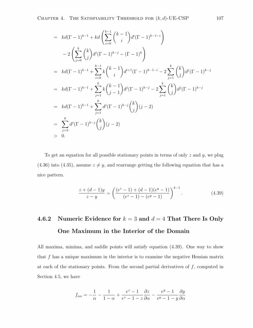
4.1 A plot of c as a function of y when k = 3 and d = 4. The largest solution

to equation (4.39) gives the corresponding value of z, and then equation

(4.40) gives the value of c. . . . . . . . . . . . . . . . . . . . . . . . . . . 110

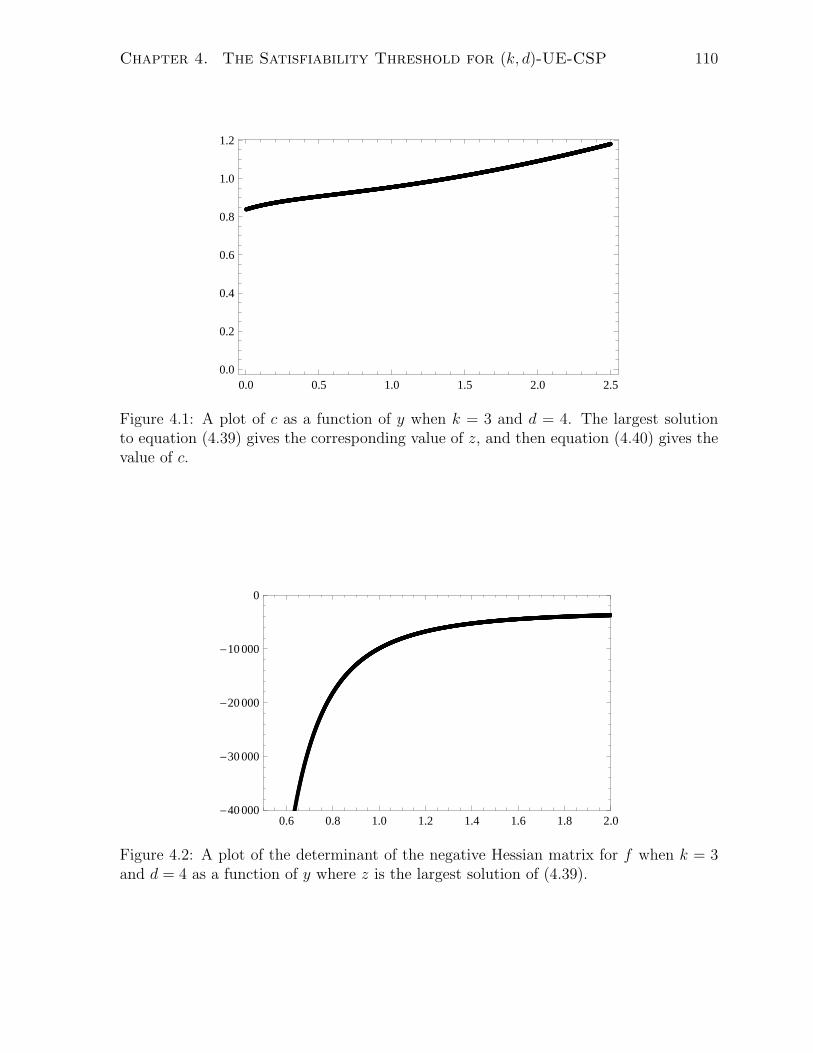
4.2 A plot of the determinant of the negative Hessian matrix for f when k = 3

and d = 4 as a function of y where z is the largest solution of (4.39). . . . 110

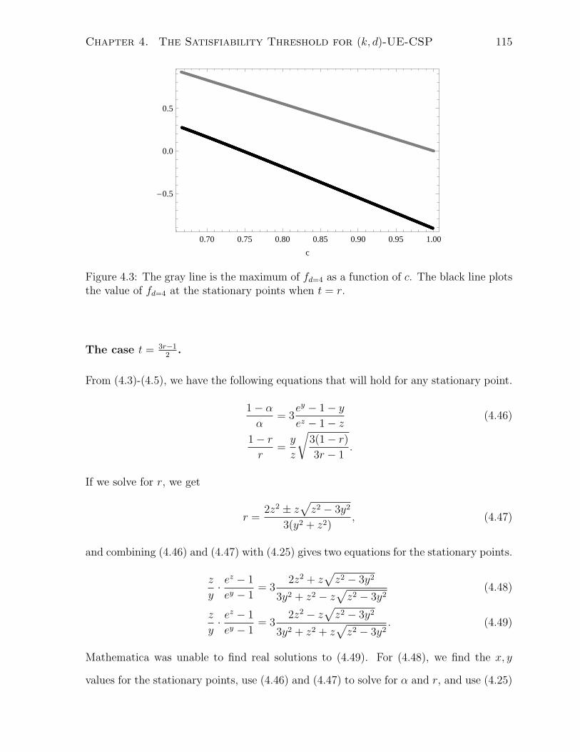
4.3 The gray line is the maximum of fd=4 as a function of c. The black line

plots the value of fd=4 at the stationary points when t = r. . . . . . . . . 115

4.4 The gray line is the maximum of fd=4 as a function of c. The black line

plots the value of fd=4 at the stationary points when 2t = 3r − 1. . . . . 116

5.1 A modification of GUC used in Lemma 5.11. . . . . . . . . . . . . . . . . 137

xi

Chapter 1

Introduction and Definitions

The study of threshold phenomena in random constraint satisfaction problems has grown

out of three different disciplines: mathematics, statistical physics, and computer science.

In mathematics, Erdos and Renyi began the study of random graphs in the 1950’s. A

graph is a finite set of vertices and a set of edges, each edge connecting a pair of vertices.

Erdos and Renyi explored two different models of random graphs. The first is to fix

integers n and m and choose a graph uniformly at random from all possible graphs

with n vertices and m edges. The second is to fix an integer n and a probability p and

each of the(n2

)possible edges is included in the graph with probability p. In [ER60]

they considered the model where the number of edges is fixed, and they studied many

properties such as being connected (studied in [ER59]), containing a cycle, complete

subgraph, or tree of fixed size, being planar, or containing a giant component. For each

of these properties, they discovered that if we consider the probability that a graph has

that property as n tends to infinity, there is a definite threshold m0 = m0(n) in the edge

density such that for a random graph with n vertices and m = m(n) edges, if m m0,

the graph almost surely does not have the property, and for m m0, the graph almost

surely has the property. By an equivalence theorem for random graphs, these results

also hold in the random graph model where each edge exists with probability p. In this

1

Chapter 1. Introduction and Definitions 2

model, there is a threshold p0 = p0(n) in the edge probability distinguishing the graphs

that almost surely have the property from those that do not. Formally, a sequence of

events En holds almost surely (a.s.) if limn→∞ Pr(En) = 1. Likewise, the sequence holds

with uniform positive probability (w.u.p.p.) if lim infn→∞ Pr(En) = α > 0.

Physicists have long been interested in understanding physical transitions in natural

processes such as when materials cool and crystallize. In statistical physics, models such

as the spin-glass like model (see [MPV87]) are used to study these physical transitions

and discover which conditions lead to threshold behavior in the transitions. Natural

systems are generally uniform in the sense that particles interact equally with all other

particles in their neighborhood, and the strength of the interaction is determined by the

distance separating the particles. However, if we generalize the model to allow for sparse,

random interactions, then we can represent the same random problems considered by the

mathematicians and computer scientists.

In computer science, it is well known that a large number of important problems

are NP-complete/hard, and so they appear to be very difficult to solve in the worst

case. However, less is known about the average case difficulty of these problems. Some

researchers (see, for example, [CKT91, SML96]) proposed studying uniformly random

problem instances as a way of determining average-case hardness. It was discovered in

these empirical studies that many random problems demonstrate threshold behavior in

some parameter of the problem. Namely, as the parameter value crosses some threshold,

the problems go from being almost surely solvable to being almost surely unsolvable. It

was also discovered that in many cases the random instances that require the most time

to solve are those that are drawn from near this threshold.

Of the open questions in the study of threshold phenomena of random problems, the

problem that attracts the most attention from all three communities is the Satisfiability

Threshold Conjecture for k-SAT. In k-SAT, we are given a formula that is a set of m

clauses over n variables. Each clause is a set of k literals where a literal is either a


positive or negative occurrence of a variable, and the problem is to assign the values

true or false to the variables so that each clause has at least one true literal. If there

exists such an assignment to the variables, the formula is satisfiable, and if there is not,

the formula is unsatisfiable. The k-SAT decision problem is NP-complete for k ≥ 3.

The random formula model is to fix n and m and to choose a uniformly random k-SAT

formula with n variables and m clauses. The interesting region, as far as satisfiability is

concerned, is when m is a linear function of n.

Conjecture 1.1 (Satisfiability Threshold Conjecture [CR92]) There exists a

value c∗k such that a uniformly random k-SAT formula on n variables and cn clauses, with

n tending to infinity, is almost surely unsatisfiable if c > c∗k and almost surely satisfiable

if c < c∗k.

Neither the existence nor the location of c∗k is known for any k ≥ 3. Much of the

work on the conjecture over the past decade has been in improving the upper and lower

bounds for the thresholds, if they exist.

Research on the satisfiability threshold has extended to generalizations of k-SAT

such as the Schaefer [Sch78] generalizations: 1-in-k SAT [ACIM01] (only one true literal

per clause), NAE-SAT [ACIM01, AM06] (at least one true and one false literal per

clause), and XOR-SAT [DM02, MRTZ03] (each clause is an exclusive-or rather than a

disjunction), and to more general random constraint satisfaction problems.

In a constraint satisfaction problem (CSP), we can allow variables to take on values

from a domain of size larger than 2, and we have more freedom as to the types of

constraints to apply to each clause. There have been various models proposed and studied

for random constraint satisfaction problems [AMK+01, CD03, Mit02, Mol02, Mol]. For

each such model and generalization of the satisfiability conjecture, the primary focus

of the research has been to determine the satisfiability threshold for the generalized

model. In addition, there has been a large body of experimental studies [GMP+01] to


find the approximate location of the satisfiability threshold and to study the difficulty

of solving random instances of the CSP models. Two reasons these generalizations are

studied are that some of these generalizations are interesting problems in their own

right, and some of these generalizations have led to a greater understanding of random 3-

SAT [AM06]. In addition, researchers have studied models where the domain size grows

with n [DFM03, FM03, Smi01, XL00, XL06] or where the constraint size grows with

n [FW01, Fla03].

The exact satisfiability threshold is known for very few SAT-like problems, and we

are not yet close to answering the Satisfiability Threshold Conjecture. In fact, each

problem for which we know the exact satisfiability threshold appears to be fundamentally

different from k-SAT, k ≥ 3. For example, we know the exact satisfiability threshold

for 2-SAT [CR92, FdlV92, Goe96] and 3-XOR-SAT [DM02, MRTZ03]), but neither of

these problems is NP-complete. Exact thresholds are known for some models where

the domain size grows with n [XL00, XL06] or where the constraint size grows with n

[FW01, Fla03], but the satisfiability threshold for these models occurs when the number of

clauses is superlinear in the number of variables, and the structure of a random constraint

satisfaction problem with a superlinear number of clauses is very different from one with

a linear number of clauses. Molloy [Mol02] shows that we can force the satisfiability

threshold to occur with a linear number of clauses if we restrict our problem model

to have constant sized constraints and domain. In addition, we know the satisfiability

threshold for a few NP-complete problems with constant sized domain and constraints:

1-in-k-SAT [ACIM01], a mixture of 2-SAT and 3-SAT when the number of clauses of

size 3 is kept small [MZK+99], and a model of [MS07]. However, in each of these cases

the proofs of the threshold demonstrate that, unlike k-SAT, k ≥ 3, the models are very

similar to random 2-SAT at the satisfiability threshold and thus easy to solve almost

surely.

This thesis identifies a new class of constraint satisfaction problems, and this class


contains a problem that has the following properties, all of which are known to hold for

k-SAT, k ≥ 3. The problem is NP-complete, has constant size constraints and domain,

and a uniformly random instance with a linear number of clauses a.s. has exponential

resolution complexity. None of the CSPs that have a known satisfiability threshold also

have all of these properties. We come very close to determining an exact satisfiability

threshold for the random model of the problem defined in this thesis, and if we can

find an exact satisfiability threshold, it will be the first NP-complete CSP that both

has an exact satisfiability threshold located when the number of clauses is linear in

the number of variables and also is not known to have a polynomial time algorithm

that correctly, with uniform positive probability, decides an instance drawn from close

to the satisfiability threshold. Because these properties suggest that problems in this

CSP model may be closer to random k-SAT than the other CSP’s for which we know

the satisfiability threshold, studying this new class of problems may lead to a better

understanding of random k-SAT. This thesis will examine several subclasses of CSPs

from this model, characterize their complexity, study their satisfiability thresholds, and

explore the behavior of several algorithms on these problems. The new class of problems

includes XOR-SAT. Therefore, many of the results proven about the general class of

CSPs will also be true for XOR-SAT.

The analysis of the satisfiability threshold for these problems involves a complicated

second moment analysis, and part of this analysis depends on a certain function having

a unique maximum in a specified domain. We are able to identify one local maximum

in this domain, and we provide numerical evidence that there are no other maxima in

the domain, but we can not prove non-existence of another maximum. We specify as the

Maximum Hypothesis this assumption that the function has one maximum in the domain,

and verifying the Maximum Hypothesis is the only obstacle preventing our determining

the exact satisfiability threshold for the CSP. Hypothesis 4.2 gives the precise description

of the Maximum Hypothesis. Section 4.4 discusses, in more detail, the function, its


known local maximum, and the domain for the Maximum Hypothesis. Section 4.6 gives

numerical evidence supporting the Maximum Hypothesis.

As a short summary of the main results of this thesis, Table 1.1 lists the threshold

behavior we prove for one NP-complete problem, called (3, 4)-UE-CSP, that is contained

in the class of constraints satisfaction problems defined in this thesis.

Threshold Type Threshold Value

Threshold for DPLL with the unit clause heuristic

running in polynomial vs. exponential time, w.u.p.p. .666666. . .

Maximum threshold at which any known solver will

find a satisfying assignment in polynomial time, a.s. .818469. . .

Threshold for satisfiability, a.s.,

conditional on the Maximum Hypothesis .917935. . .

Table 1.1: Summary of threshold results for the NP-complete constraint satisfactionproblem (3, 4)-UE-CSP.

If we consider the related problem of XOR-SAT, the first and third thresholds of

Table 1.1 still hold. The third threshold, without the condition, was originally proven

for XOR-SAT in [DM02], and the first is proven for XOR-SAT in this thesis. The second

threshold does not hold for XOR-SAT because XOR-SAT is in P, but we do get a similar

threshold for XOR-SAT at the same value if we restrict the analysis to greedy algorithms.

The outline of the thesis is as follows. In Section 1.1, we formally define what is meant

by a constraint satisfaction problem, and we give notations that we will use throughout

the thesis. In Section 1.2, we list some known probability bounds and some facts on

random hypergraphs that we will use to prove results in this thesis.

In Chapter 2, we survey the current state of research in resolving the Satisfiability

Threshold Conjecture. We also examine what is known about the behavior of DPLL


and other SAT-solving algorithms on random 3-SAT instances with a linear number of

clauses, how techniques from statistical mechanics give us a better understanding of the

properties of random k-SAT, and what is known about the satisfiability threshold and

algorithm behavior for random XOR-SAT.

In Chapter 3, we generalize XOR-SAT to a new family of CSPs that we denote UE-

CSP, and we identify NP-complete variations of the family. We show that for random

k-UE-CSP, similar to random k-SAT, k ≥ 3, a uniformly random instance of k-UE-CSP

with n variables and cn clauses, c > 0, a.s. has exponential resolution complexity.

In Chapter 4, we show that, under the Maximum Hypothesis, k-UE-CSP has an exact

satisfiability threshold and we identify the location for each k. We also give numerical

evidence supporting the Maximum Hypothesis.

In Chapter 5, we completely characterize the behavior of two DPLL variations on

UE-CSP, and we prove a theorem for random UE-CSP that is analogous to an open

question for random SAT.

In Chapter 6, we prove the size of cores of non-uniform hypergraphs building on

results for uniform hypergraphs of [PSW96, MWHC96, Mol05, Coo04, Kim06, CW06,

DN, Rio07]. This result is required for the main theorem of Chapter 5.

Since introducing the k-UE-CSP problem at the International Conference on Theory

and Applications of Satisfiability Testing (SAT 2004), the k-UE-CSP problem has been

used to test satisfiability solvers [BS04, LSB05, HvM06, HvM07]. Other work includes a

study of the clause structure that is created when transforming an instance of random

k-UE-CSP into a boolean formula in conjunctive normal form [Her06], and a study of how

the unit clause and generalized unit clause algorithms perform on an instance of random

k-UE-CSP [AMZ07]. The results of this latter study are non-rigorous and similar to the

results we achieve in Chapter 5 of this thesis.


1.1 Constraint Satisfaction Problems

First, we will formally define what is meant by a constraint satisfaction problem. A

constraint satisfaction problem is a set of n variables where each variable has a non-

empty domain of possible values and a set of m clauses where a clause both is an ordered

subset of variables and has one or more constraints applied to it. A constraint, applied

to a clause, restricts the values we may assign the variables of the clause. The goal

is to find an assignment to the variables such that every constraint is satisfied. One

common constraint satisfaction problem model is to use the same domain of values for

every variable. Typically, a domain of d values is represented by the set 0, . . . , d − 1,

and the domain is assumed to contain at least two values.

A constraint is usually represented as either a list of the value tuples permitted or

a list of the value tuples forbidden by the constraint. In the literature, each clause

typically has exactly one constraint that lists all the forbidden or permitted tuples for

that clause. As a result, the terms clause and constraint are often used interchangeably

in the literature. In this thesis, we will deviate from the standard notation slightly.

Definition 1.2 (Constraint) A constraint is a fixed relation on a canonical ordered set

of variables. A constraint lists the permitted (or forbidden) tuples of values that we may

assign to the variables.

We will usually assume each clause has exactly one constraint, but we will occasionally

apply more than one constraint to a clause. If a clause has multiple constraints, then we

can apply a tuple of values to the variables of the clause only if that tuple is permitted by

each of the constraints applied to the clause. This notation will simplify the presentation

in Chapter 3 .

In keeping with SAT notation, we will denote an instance of a constraint satisfaction

problem as a formula. A formula consists of the set of variables, the set of clauses, and

for each clause, the constraint or constraints applied to the clause.


For the remainder of this text, n will denote the number of variables andm the number

of clauses of a constraint satisfaction problem. Unless otherwise noted, m is always a

linear function of n, and c is used to denote the clause density m = cn. Likewise, k

will always refer to the clause or constraint size and d will denote the domain size. For

simplicity, clauses of size k will be denoted as k-clauses.

1.2 Useful Tools

Second we will list the probability bounds that we use in this thesis, and we will give

some basic facts on random hypergraphs.

1.2.1 Probability Bounds

Given a random variable X, the following are useful tools for bounding the probability

that X deviates from its expected value.

Markov’s inequality states that if X is non-negative, then

Pr(X ≥ t) ≤ E(X)

t.

If we set t = 1, we get Pr(X > 0) ≤ E(X). If Y1, Y2, . . . is a sequence of non-negative

random variables with E(Yn) = o(1), then Yn is a.s. 0. The technique of using Markov’s

inequality to bound the probability that X is larger than some value t is known as the

first moment method.

Chebychev’s inequality states

Pr(|X − E(X)| ≥ t) ≤ Var(X)

t2.

The technique of using Chebychev’s inequality to bound the probability that X differs

from its expected value is known as the second moment method.

If X is non-negative, a well known application of the Cauchy-Swartz inequality gives

Pr(X > 0) ≥ E(X)2

E(X2),


and using this inequality is also known as the second moment method.

The Chernoff bound has several forms. Sufficient for our purposes is the following

simple variation. Let X be a binomial random variable that counts the number of

successful trials from a set of n trials with probability of success p. Then,

Pr(|X − E(X)| ≥ t) ≤ e−2t2

n .

Similarly, Azuma’s inequality [Azu67] has more than one variation. The following

variation, sufficient for our purposes, is a corollary of the original Azuma’s inequality.

Lemma 1.3 Let X be determined by a series of random trials T1, . . . , Tn such that for

all i,

|E(X | T1, . . . , Ti−1)− E(X | T1, . . . , Ti)| ≤ ci.

Then

Pr(|X − E(X)| > t) < 2e− t2

2Pc2i .

1.2.2 Some Facts on Random (Hyper)graphs

A hypergraph is a finite set of vertices and a set of hyperedges. Each hyperedge is a subset

of the vertices. If every hyperedge has the same size, the hypergraph is called uniform,

and if every hyperedge has size 2, we have a graph.

A useful technique when analyzing the structure of an instance C of a constraint

satisfaction problem is to consider the underlying hypergraph H of C. Define H to

have as vertices the set of variables of C, and define the hyperedges of H to be exactly

the clauses of C. Usually, each clause is assumed to have one constraint. If a clause

has multiple constraints applied to it, we can model this by a multi-hyperedge in the

hypergraph. As with clauses, a hyperedge of size i will be denoted as an i-edge.

The two basic models of random graphs extend to uniform hypergraphs, and we will

use the same notation for the random uniform hypergraph models as is used for the


random graph models. For any fixed hyperedge size k, we will let Gn,m denote a random

hypergraph drawn from the model where we choose m random hyperedges uniformly at

random from all possible hyperedges of size k, and we will let Gn,p denote a random hyper-

graph drawn from the model where we consider each possible hyperedge of size k and in-

clude it with probability p. These two models are equivalent in the sense that if m =(nk

)p,

note that strict equality is not needed but is sufficient for our purposes, then for a prop-

erty Q if limn→∞ Pr(Gn,p has Q) = a then limn→∞ Pr(Gn,m has Q) = a. Likewise, for a

monotone property Q, if limn→∞ Pr(Gn,m has Q) = a then limn→∞ Pr(Gn,p has Q) = a

[Bol79, Luc90].

Here are a few useful facts on random hypergraphs when there is a linear number of

edges. These facts were first discovered by Erdos and Renyi [ER59, ER60] for random

graphs and extended by Schmidt and Shamir [SS85] and Karonski and Luczak [K L02]

for random uniform hypergraphs. Let k be the hyperedge size. The hypergraph a.s.

has a linear number of isolated vertices and isolated components that are trees. On a

random hypergraph with n vertices and cn edges, if c < 1k(k−1)

almost all components

are hypertrees with possibly a constant number of cycles. The largest such component

a.s. has size O(log n). If c > 1k(k−1)

, a.s. one component of the hypergraph will have size

Θ(n), and the number of cycles now grows unbounded as n tends to infinity. Most of

these cycles have length greater than log n, a.s., and for each constant j the number of

cycles of length j a.s. remain bounded by a constant.

Chapter 2

Background

2.1 The Satisfiability Threshold Conjecture

The Satisfiability Threshold Conjecture states that there exists a value c∗k such that a uni-

formly random k-SAT formula on n variables and cn clauses is almost surely unsatisfiable

if c > c∗k and almost surely satisfiable if c < c∗k.

For 2-SAT, c∗2 = 1, a result proven independently by Chvatal and Reed [CR92],

Fernandez de la Vega [FdlV92], and Goerdt [Goe96]. The proof uses the well-known

fact, first observed in Aspvall, Plass, and Tarjan [APT79], that we can model a 2-SAT

formula as a directed graph with the literals as the vertices. For each clause (l1, l2) there

are two directed edges l1l2 and l2l1. A 2-SAT formula is unsatisfiable if and only if a

variable and its complement both appear in the same strongly connected component of

the directed graph. The threshold proof then follows by showing that if c < 1, there

a.s. is no such strongly connected component and if c > 1 there a.s. is such a strongly

connected component.

The satisfiability threshold conjecture remains open for k ≥ 3. While neither the

existence nor the location of c∗k is known for any k ≥ 3, Friedgut [Fri99] proves that the

satisfiability threshold for k-SAT is sharp. However, the location of the threshold might

12

Chapter 2. Background 13

not be at the same clause density for each value of n. Specifically, for each k ≥ 2 there

exists a function c∗k(n) such that for a uniformly random k-SAT instance with n variables

and cn clauses, if c < c∗k(n) the formula is a.s. satisfiable and if c > c∗k(n) the formula is

a.s. unsatisfiable.

On the other hand, we say a constraint satisfaction problem has a coarse threshold

if there exists a function r(n), and for each δ > 0 there exists ε1, ε2 > 0 such that for a

uniformly random instance with n variables and cn clauses, if c = r(n), the probability

the instance is satisfiable is 12, if c = r(n)−ε1, the probability the instance is satisfiable is

12

+δ, and if c = r(n)+ε2, the probability the instance is satisfiable is 12−δ. In this thesis

we will only consider thresholds that occur when there is a linear number of clauses.

Friedgut proves that monotonic properties with coarse thresholds on hypergraphs can

be approximated by the property of the existence of a finite number of small subgraphs.

From Bourgain’s extension to Friedgut’s theorem, located in the appendix of [Fri99], to

prove that k-SAT has a sharp threshold, it is sufficient to show that for a formula F

on n variables drawn uniformly randomly from all formulae with clause density close

to the satisfiability threshold, neither of the following two cases hold: that F contains

w.u.p.p. an unsatisfiable subformula of constant size nor that there exists a satisfiable

formula φ of constant size such that the probability F is satisfiable conditional on φ

being a subformula of F is larger than the probability F is satisfiable, and the difference

in the two probabilities depends on the size of φ and not on n. Roughly speaking, we

can think of properties with coarse thresholds as being local in nature while properties

with sharp thresholds are not. Friedgut’s theorem provides a very useful corollary: if

we can prove a uniformly random formula with c′n clauses is w.u.p.p. satisfiable then a

uniformly random formula with cn clauses c < c′ is a.s. satisfiable.

We have a tight asymptotic bound for the conjectured c∗k. The observation, first

made by Franco and Paull [FP83], that the expected number of satisfying assignments

of a random formula is 2n(1− 2−k

)cnyields c∗k ≤ 2k log 2. Achlioptas and Peres [AP04]


proves this bound is asymptotically tight, as k tends to infinity, by proving c∗k ≥ 2k log 2−

O(k). The proof by Achlioptas and Peres is non-algorithmic and gives the best known

lower bounds for c∗k, k > 3, but the lower bound it gives for 3-SAT is weaker than

the bounds found by algorithmic analysis. From experimental evidence, the threshold

for 3-SAT is c∗3 ≈ 4.2 [KS94, SML96, CA96], and the current state of the research has

3.52 [HS03, KKL03] ≤ c∗3 ≤ 4.506 [DBM03].

2.1.1 Lower Bounds and Algorithm Analysis

The proof of the current lower bound for the 3-SAT satisfiability threshold uses algorithm

analysis. To prove a threshold bound with this method, one must develop both an

algorithm for 3-SAT and the techniques to analyze that algorithm. Then one must

identify the maximum density c of clauses for which the algorithm will w.u.p.p. find a

satisfying assignment on a uniformly random instance drawn from that clause density,

and Friedgut’s result [Fri99] implies c∗3 ≥ c. A survey of this technique is in [Ach01].

However, it is not clear that this technique will succeed in finding the exact threshold,

if it exists. The algorithms that are currently amenable to analysis only find solutions

on instances drawn from well below the conjectured satisfiability threshold, and it is not

known whether there even exists an algorithm that w.u.p.p. finds a satisfying assignment

of a random instance near the conjectured threshold. However, empirical results for a new

algorithm, survey propagation [BMZ05], suggest that the algorithm can find solutions to

random problems drawn from quite close to the conjectured threshold, but the algorithm

is too complicated for exact analysis by current techniques.

In general, the algorithms that can be analyzed are greedy, non-backtracking algo-

rithms. The reason for this restriction is that the analysis requires that after each step or

sequence of steps by the algorithm, the subformula induced by the unassigned variables

is still uniformly random, possibly conditional on some parameter such as the degree

sequence. Algorithms that have been considered for 3-SAT and that have led to incre-


mental improvements in the lower bound for the 3-SAT satisfiability threshold include

the following. The unit clause (UC) algorithm works by repeatedly setting the literal

of a clause of size 1 to true, and if there is no clause of size 1 then assigning a variable

at random. Chao and Franco [CF86] proves that UC succeeds w.u.p.p. when the clause

density is less than 83. Chao and Franco also proves that for each variable chosen at ran-

dom, if you assign the variable in such a way as to satisfy the majority of the 3-clauses in

which that variable appears, then the algorithm succeeds w.u.p.p. for densities less than

2.9. These results did not, at the time, give lower bounds on c∗3 because we did not have

the Friedgut result. The first lower bound for the 3-SAT satisfiability threshold was from

Broder, Frieze, and Upfal’s [BFU93] analysis of the pure literal rule. The pure-literal rule

is to iteratively set to true each literal whose complement does not occur in the formula,

and [BFU93] proves that this algorithm succeeds a.s. up to clause density 1.63. The next

improvement in the lower bound for the 3-SAT threshold came from Frieze and Suen’s

[FS96] study of generalized unit clause (GUC): choose a clause of shortest length from

the subformula induced by the unassigned variables and set to true a random literal from

that clause. GUC succeeds w.u.p.p. for clause densities less than 3.003 . . ., and by show-

ing that modifying GUC with a limited amount of backtracking succeeds a.s. for clause

densities less than 3.003 . . ., [FS96] establishes that c∗3 ≥ 3.003 . . . . Achlioptas [Ach00]

modifies UC such that if there is no unit clause and there is a 2-clause then set both its

literals in such a way as to minimize the number of 3-clauses that become 2-clauses, and

[Ach00] uses this algorithm to prove that c∗3 > 3.145.

Except for the Frieze and Suen modification to GUC, all the algorithms considered

do not change the assignment to a variable once it is made, and the Frieze and Suen

algorithm uses a very limited backtracking that leaves most of the formula uniformly

random. In addition, each algorithm considered, except the pure-literal rule, has the

property that the next variable to assign is either chosen uniformly at random or selected

from a random clause of a specific length. Once a variable is chosen, every literal on that


variable is exposed and a value for the variable is selected. Achlioptas and Sorkin [AS00]

gives the term myopic for such algorithms, and Achlioptas and Sorkin proves that the

maximum clause density at which a myopic algorithm that selects one variable at a time

will succeed a.s. is 3.22, and if the algorithm selects up to two variables at a time, the

maximum clause density is 3.26. This result establishes both that c∗3 > 3.26 and that

a myopic algorithm will not achieve additional improvements in the lower bound of the

satisfiability threshold without considering more than two variables at a time, and these

improvements will be insignificant and tedious.

Kaporis, Kirousis, and Lalas [KKL02] improves the lower bound to c∗3 ≥ 3.42 by

considering the algorithm that sets to true a literal that appears in as many clauses as

possible while also satisfying any unit clauses that appear. The current lower bound on

the 3-SAT threshold comes from an algorithm that selects and sets a literal to true based

on the degree of the literal and the degree of its complement. Both Kaporis, Kirousis,

and Lalas [KKL03] and Hajiaghayi and Sorkin [HS03] independently analyze slightly

different variations of this algorithm to get the lower bound of 3.52.

The upper bounds are proven using statistical counting techniques. Being non-

algorithmic, this method appears to hold more promise for finding the threshold if it

exists, but this method has its own challenges that are dealt with in the next section.

2.1.2 Upper Bounds and Statistical Techniques

The typical statistical tools used to find bounds for the satisfiability threshold are known

as the first moment method and the second moment method. If we let the random variable

X be the number of solutions to a uniformly random CSP, the first moment method yields

Pr(X > 0) ≤ E(X). Thus, the goal is to find the minimum constant c such that for

a random formula with n variables and cn clauses E(X) = o(1). To compute a lower

bound, we use the second moment method which involves computing E(X2). If we can

show E(X2) = (1+o(1))E(X)2, then, by an application of the Cauchy-Swartz inequality,


we have Pr(X > 0) ≥ E(X)2

E(X2)= 1− o(1).

The main challenge in using these techniques to find good bounds on the satisfiability

threshold is in dealing with what are known as “jackpot phenomena”. Namely, the prop-

erty that one solution yields an exponential number of other solutions by changing the

values of some of the variables. For the first moment method, this phenomenon hinders

computation of the threshold because even if formulae with solutions are exponentially

rare, one such formula with an exponential number of solutions is enough to give a high

expected number of solutions. For the second moment method, the existence of jackpots

means the random variable X will have a large variance. Because of this challenge, the

current best lower bounds for c∗3 found using the second moment method are weaker than

the lower bounds found using algorithmic analysis. However, the second moment method

has been more successful with c∗k, k ≥ 4 [AP04].

A well known observation, the first known citation is by Franco and Paull [FP83], is

that the expected number of satisfying assignments to a random 3-SAT formula with n

variables and cn clauses is

2n(

7

8

)cn.

Therefore, Markov’s inequality implies that a formula is a.s. unsatisfiable if c ≥ log8/7 2 ≈

5.191. The improvements in the upper bound for the threshold have come from methods

that reduce the jackpot phenomena.

The first improvement, due to Fernandez de la Vega and El Maftouhi [MdlV95],

reduces the upper bound to 5.081. Kamath, Motwani, Palem, and Spirakis [KMPS95]

improves the upper bound to 4.758 by computing the probability that a formula is satisfi-

able by dividing the expected number of satisfying assignments computed with Markov’s

inequality by a lower bound on the average number of satisfying assignments for all

formulae that are satisfied by a given assignment.

Dubois and Boufkhad [DB97] decreases the upper bound to 4.643 by roughly calcu-

lating the expected number of solutions that have the property that flipping any vari-


able value from false to true will yield an unsatisfying assignment. Kirousis, Kranakis,

Krizanc, and Stamatiou [KKKS98], independently of [DB97], introduces the generalized

technique of lexicographically ordering assignments as bit strings with true assigned 1

and false assigned 0. A satisfying assignment is l-maximal if switching the values of up

to l variables does not yield a lexicographically larger assignment that is also satisfying.

The technique of [DB97] is equivalent to counting the number of 1-maximal assignments.

By counting the number of 2-maximal assignments, [KKKS98] lowers the upper bound

for 3-SAT satisfiability to 4.6011. Janson, Stamatiou, and Vamvakari [JSV00] further

improves this bound to 4.596 by improving the estimate for the number of 2-maximal

assignments. By providing a better estimate of the probability that a satisfying assign-

ment is 1-maximal and combining this with the probability determined in [KKKS98] that

a satisfying assignment is maximal over double-flips in which one literal is flipped false

to true and another true to false, Kaporis, et al, [KKS+01] further improves the lower

bound to 4.571. We could get better upper bounds by calculating the expected number of

l-maximal assignments for l > 2, but the calculations quickly get complicated for larger

values of l.

The current upper bound for the 3-SAT satisfiability threshold, 4.506 by Dubois,

Boufkhad, and Mandler [DBM03], combines the idea of 1-maximal assignments with a

structural argument that considers only “typical” formulae, proving that the “atypical”

formulae occur almost never. Dubois, Boufkhad, and Mandler [DBM03] demonstrates

that typical formulae have the property that the number of occurrences of each variable

follows a Poisson distribution, and the number of positive and negative occurrences of the

variable follows a binomial distribution. Then, [DBM03] groups the typical formulae into

equivalence classes where two formulae are equivalent if one can be transformed into the

other by repeatedly selecting a vertex and flipping all its literals. The expected number

of satisfying assignments for an equivalence class is found by counting the number of 1-

maximal assignments for the representative that is assumed to have the fewest 1-maximal


assignments and multiplying that value by the number of formulae in the equivalence

class. The formula assumed to have the fewest assignments is the one for which every

variable has at least as many occurrences as a negative literal as it does as a positive

literal. Note, the authors are inverting the definition of 1-maximal.

In all of the cases for the upper bound of 3-SAT, the first moment method is used. One

variation of SAT for which the second moment method is useful is NAE-SAT [ACIM01,

AM06] (at least one true and one false literal per clause). NAE-SAT has a greatly

reduced jackpot phenomenon because there is less freedom on how to satisfy each clause.

Although an exact satisfiability threshold for NAE-SAT is not known, the bound is very

tight for large k. This tight bound is used in Achlioptas and Moore [AM06] to greatly

improve the asymptotic lower bound for k-SAT, and the k-SAT lower bound is further

improved in Achlioptas and Peres [AP04] for all k ≥ 4 by using the second moment

method on balanced assignments that are similar to NAE-SAT assignments.

2.2 The (2 + p)-SAT Model

With random 2-SAT and random 3-SAT behaving differently and in order to understand

what happens between k = 2 and k = 3, Monasson, et al, [MZK+96] introduces the

(2 + p)-SAT model which contains pcn clauses of size 3 and (1 − p)cn clauses of size 2.

The analogous conjecture to the satisfiability threshold conjecture is that (2 + p)-SAT

has an exact satisfiability threshold for each value of p. Clearly, the results for SAT give

us an exact satisfiability threshold for p = 0, and the threshold is not known to exist for

p = 1. Likewise, it is clear that the random (2+p)-SAT instance will be a.s. unsatisfiable

if the 2-clauses alone are a.s. unsatisfiable, when (1−p)c > 1, or when the 3-clauses alone

are a.s. unsatisfiable, when pc > 4.506.

The current bounds on the satisfiability threshold for random (2 + p)-SAT come

from Achlioptas, Kirousis, Kranakis and Krizanc [AKKK01]. The exact satisfiability


threshold exists for p ≤ 25, and the threshold is at the clause density 1

1−p . The proof of

the satisfiability threshold involves analyzing the unit clause heuristic to find the greatest

clause density for which UC will w.u.p.p. find a satisfying assignment, and the authors

prove that Friedgut’s [Fri99] result that k-SAT has a sharp threshold also applies to

(2 + p)-SAT. As the location of the satisfiability threshold indicates, when p ≤ 25

the

(2 + p)-SAT formula is a.s. satisfiable if the 2-SAT problem induced by the 2-clauses is

a.s. satisfiable. This result implies that if we have (1− ε)n random 2-clauses, we can add

up to 23n random 3-clauses and still be a.s. satisfiable. The conjecture is that this bound

on the behavior of (2 + p)-SAT is tight. That is, for p > 25, the satisfiability threshold

for (2 + p)-SAT, if it exists, will be at a clause density strictly less than 11−p . If true,

this conjecture implies that for every δ > 0 there exists an ε > 0 such that a uniformly

random instance of (2 + p)-SAT with (1 − ε)n 2-clauses and(

23

+ δ)n 3-clauses is a.s.

unsatisfiable. We denote this last conjecture the (2 + p)-SAT Conjecture.

For the case when p > 25, [AKKK01] gives a lower bound for the satisfiability thresh-

old, if it exists, by again analyzing the greatest clause density at which the unit clause

algorithm will find, w.u.p.p., a satisfying assignment. The upper bound is found by us-

ing the same technique of counting maximal satisfying assignments used in [KKKS98] for

the upper bound of 3-SAT. This upper bound is strictly less than 11−p when p > 0.695,

and from this upper bound, we know that there exists an ε > 0 such that a random

(2 + p)-SAT formula with (1− ε)n 2-clauses and 2.28n 3-clauses is a.s. unsatisfiable.

As a result, we have a gap where, at p ≤ 25, a random (2 + p)-SAT formula is a.s.

satisfiable if and only if the density of the 2-clauses lies below the satisfiability threshold

for 2-SAT, and when p > 0.695 the a.s. satisfiability of the formula depends on the

densities of both the 2-clauses and 3-clauses. Also, for any random 2-SAT instance

drawn from close to but below the satisfiability threshold, we can add up to 23n 3-clauses

to the formula and still be a.s. satisfiable, but once we add 2.28n 3-clauses, the formula

is a.s. unsatisfiable. We would like to close this gap, and the (2 + p)-SAT Conjecture


implies that the lower bound is tight.

2.3 Algorithm Behavior on Random SAT

2.3.1 The Davis Putnam Logemann Loveland (DPLL) Algo-

rithm

DPLL [DLL62, DP60] forms the basis of most current complete SAT solvers where a

complete solver is an algorithm that will find a solution if one exists. The DPLL algorithm

has a simple backtracking framework. At each step, an unassigned variable v is assigned

a value. Any clause that is satisfied by the assignment is removed, and v is removed from

any clause in which it occurs. DPLL then recurses on this reduced formula. If a conflict

occurs, DPLL backtracks and tries a different value for v. There are many variations

that can be made in choosing the next variable, choosing the appropriate value to try,

propagating the implications of variable assignments through the constraints, learning

new clauses, and restarting. Researchers have noticed experimentally, for example the

study by Selman, Mitchell, and Levesque [SML96], that DPLL works fast on random

problems drawn from well below or above the conjectured satisfiability threshold, but it

performs poorly on problems drawn from near the satisfiability threshold.

The idea that DPLL quickly proves unsatisfiable a problem drawn from well above

the satisfiability threshold is somewhat misleading and is an artifact of the small problem

sizes used in the studies. A resolution proof of unsatisfiability for a SAT instance is a

sequence of clauses, ending with the empty clause, and such that each clause is either

a clause of the instance or is derived from two previous clauses of the sequence, Ci and

Cj, by the following rule. Clause Ci contains the literal x, clause Cj contains the literal

x, and the derived clause contains all literals of Ci and Cj not involving the variable x.

Chvatal and Szemeredi [CS88] proves that an unsatisfiable random k-SAT instance with


a linear number of clauses will a.s. require a resolution proof with an exponential number

of clauses. We define the length of a resolution proof to be the number of clauses in

the proof. The length of the shortest resolution proof of unsatisfiability is the resolution

complexity, and a well known observation of Galil [Gal77] is that exponential resolution

complexity implies that DPLL will require an exponential amount of time to prove the

problem unsatisfiable.

The algorithm analysis used to find the lower bound on the satisfiability threshold also

gives a bound on the running time of DPLL. DPLL can use a variety of heuristics to guide

it in finding a solution to a problem instance. For example, to select the next variable

to assign a value, to choose the value to assign, and to trim the search space. If this

heuristic, running as a stand-alone greedy algorithm, can find a solution w.u.p.p., then

DPLL using that heuristic will w.u.p.p. not have to backtrack. In particular, DPLL using

unit clause (DPLL+UC) as its heuristic will run in linear time w.u.p.p. if c ≤ 2.66 [CF86],

and DPLL using generalized unit clause (DPLL+GUC) will run in linear time w.u.p.p.

if c ≤ 3.003 [FS96].

One might think that at a slightly higher clause density, DPLL will backtrack a few

times but still run in linear or polynomial time. However, if the (2 + p)-SAT Conjecture

is true, then the bounds listed in the preceding paragraph are in fact the border between

linear and exponential running times for the algorithms.

Instead, we currently have a gap between the greatest density at which DPLL w.u.p.p.

runs in linear time and the least density at which DPLL will require w.u.p.p. exponen-

tial time. To find the bound for exponential behavior, Achlioptas, Beame, and Mol-

loy [ABM04b] starts with a random (2+p)-SAT instance with 2.28n 3-clauses and (1−ε)n

2-clauses, for sufficiently small ε > 0. Such a random formula is proven a.s. unsatisfiable

in [AKKK01], and Achlioptas, Beame, and Molloy proves the formula a.s. has exponen-

tial resolution complexity. Results of Chao and Franco [CF90] for UC and Frieze and

Suen [FS96] for GUC, both of which are simplified in Achlioptas [Ach01], prove that we


can trace the behavior of UC and GUC using a system of differential equations. Using

these systems, [ABM04b] works backward to find the smallest clause density of a random

3-SAT instance on which UC and GUC will w.u.p.p. reach the unsatisfiable (2 + p)-SAT

instance without backtracking. As a result, DPLL+UC will require exponential time

w.u.p.p. to solve a random 3-SAT instance with n variables and cn clauses if c ≥ 3.81.

For DPLL+GUC, the exponential behavior occurs w.u.p.p. when c ≥ 3.98.

2.3.2 Other Algorithms for Random SAT

Two other classes of algorithms used on random SAT are local search and belief propaga-

tion. Local search is a very general framework where the algorithm starts at an arbitrary

assignment to the variables, and until a solution is found, the value to a selected variable

is flipped. The pure random walk algorithm starts with a random assignment to the vari-

ables. Then it repeatedly chooses at random an unsatisfied clause and a variable from

that clause, and the assignment to that variable is flipped. Alekhnovich and Ben-Sasson

[ABS03] proves that the pure random walk algorithm a.s. finds a satisfying assignment

in polynomial time if c < 1.63. The similarity of the bound with that of the pure-literal

rule is not coincidental and is due to the heavy reliance on pure literals in the proof.

However, experimental evidence in Parkes [Par02] suggests that the pure random walk

algorithm will succeed in polynomial time up to c < 2.65, and this value is supported

by non-rigorous analysis of Semerjian and Monasson [SM03]. Other variations of local

search include gradient descent: flip a randomly chosen variable only if it decreases the

number of unsatisfied clauses, and GSAT: a hill climbing procedure that chooses a ran-

dom variable from those variables that yield the maximum number of satisfied clauses

when their value is changed.

Roughly speaking, the standard belief propagation algorithm works by starting with

an arbitrary probability distribution on each variable where the probability distribution

is over possible assignments to the variable. At each iteration of the algorithm, a variable


v recomputes its marginal distribution as follows. For each neighbor u of v, v computes

a probability distribution for itself using the probability distributions, received in the

previous iteration, for each of its neighbors except u, and it sends this new probability

distribution to u. Once v receives a new probability distribution from each neighbor, it

uses these to recompute its own marginal distribution. This process repeats until either

the marginal distributions converge or until a set number of iterations is reached. At

that time, the variable, or set of variables, that has the strongest bias in its marginal

distribution is assigned the value with greatest bias, and then the whole process repeats.

These latter algorithms are too complicated for rigorous analysis, but none of them

are known, experimentally, to w.u.p.p. find a satisfying assignment in polynomial time

(in the case of a random walk algorithm), or to find a satisfying assignment at all (in the

case of gradient descent and belief propagation), at clause densities above 3.921. The

only algorithm that is known, experimentally, to find satisfying assignments above this

density in polynomial time is the survey propagation algorithm, a recent variation of

belief propagation, that is discussed in Section 2.4.4.

2.4 Contributions from Physics

Statistical mechanics is a branch of physics that attempts to derive the behavior of

large systems from an understanding of the behavior of individual particles within the

system. In the systems studied, the number of particles is enormous making an exact

calculation impossible. Instead, statistics are used to discover the almost sure behavior

of the system. For example, one family of models of statistical mechanics, called the spin-

glass-like models, is used to study physical transitions, such as when materials cool and

crystallize, but where the particles do not all align in the same direction. A large survey

of the model is in Mezard, Parisi, and Virisoro [MPV87]. In most natural processes

particles interact with all other particles in their neighborhood, and the strength of the


interaction is proportional to the distance between the particles. However, [MPV87]

notes that by allowing arbitrary particle interactions, the spin-glass models could model

any constraint satisfaction problem, and finding the expected behavior of the model at

zero temperature is equivalent to solving the CSP.

2.4.1 The Replica Method

Monasson and Zecchina [MZ96, MZ97] model k-SAT as a spin-glass problem and use the

statistical mechanics technique known as the replica method with symmetry breaking

to study the model. While Monasson and Zecchina conjecture that the replica method

should be able to find the 3-SAT satisfiability threshold, even if it does it will not be

a proof of the Satisfiability Threshold Conjecture. The replica method is not mathe-

matically sound. In particular, one step of the replica method involves determining,

or estimating, an expression for the integer nth moment of a random variable, and

then taking the limit as the real n goes to 0. There is some work, notably by Ta-

lagrand [Tal01, Tal03a, Tal03b], in determining when the assumptions implicit in the

replica method hold. Also, properly applying the needed symmetry breaking is as much

an art as a science. On its own, the replica method provides a (not sound) upper bound

of the threshold location, and symmetry breaking is used to tighten the bound. Through

iterative improvements in symmetry breaking, Biroli, Monasson, and Weight [BMW00]

gets the upper bound of 4.48 and Franz, Leone, Ricci-Tersenghi, and Zecchina [FLRTZ01]

gets the upper bound 4.396. Mezard and Zecchina [MZ02] achieves a non-rigorous up-

per bound of 4.267 by applying a technique known as the cavity method with one-step

replica symmetry breaking and introduces the survey propagation algorithm for random

SAT, inspired by this technique. In [MZ02] and [MMZ06], the authors conjecture that

this bound is very close to the satisfiability threshold because there is evidence that

applying additional symmetry breaking to the cavity method will only yield very small

improvements to the estimate. Additional evidence for the validity of the cavity method


comes from Mertens, Mezard, and Zecchina [MMZ06] where the authors apply the cavity

method to estimate the satisfiability threshold for larger values of k, and in each case,

the estimate provided by the cavity method falls between the current proven bounds for

the satisfiability threshold. The current best estimate of the threshold for 3-SAT using

the the cavity method is 4.26675± 0.00015 [MMZ06]. The replica method does correctly

predict the threshold for both 2-SAT [MZ97] and 3-XOR-SAT [FLRTZ01], and the cavity

method correctly finds the 3-XOR-SAT threshold [MRTZ03].

2.4.2 Order Parameters

When studying thresholds, physicists look for order parameters. An order parameter

is a value that is a.s. zero on one side of the threshold and a.s. non-zero on the other.

Monasson and Zecchina [MZ97] uses an order parameter called the backbone, and the

backbone is defined as the set of variables that must have the same value in all assignments

that minimize the number of unsatisfied clauses. The analysis of the replica technique

and empirical evidence of [MZ97] suggests a difference between 2-SAT and k-SAT, k ≥ 3.

In 2-SAT, the size of the backbone appears to increase continuously as the clause density

crosses the satisfiability threshold, but for k ≥ 3, the size of the backbone appears to

jump discontinuously to Ω(n).

Bollobas, et al, [BBC+01] uses a different order parameter called the spine in a study

of 2-SAT, and [BBC+01] defines the spine as the number of literals that, if added as a unit

clause to some satisfiable subformula of the formula, makes that subformula unsatisfiable.

Bollobas, et al, proves that the spine is an order parameter for 2-SAT, that 2-SAT has a

continuous spine size at the satisfiability threshold, and [BBC+01] completely character-

izes what is known as the finite size scaling window of random 2-SAT satisfiability. The

sharp threshold for k-SAT satisfiability is an asymptotic result. An interesting question

is to determine, for each n, the actual probability that a uniformly random instance of

k-SAT on n variables and cn clauses is satisfiable. In this case, we do not have a sharp


transition from 0 to 1 at the asymptotic threshold. Rather, the probability is close to 1

if we are well below the asymptotic threshold, gradually moves from near 1 to near 0 in

a region around the threshold, and is close to 0 if we are well above the threshold. This

“broadening” of the transition due to finite instances is the finite size scaling window.

Specifically, for each n and constant δ > 0, the window is defined to be the region in

which the probability of satisfiability lies between δ and 1− δ.

The spine is easier to manipulate analytically than the backbone because the spine

is monotone in the sense that adding clauses to a formula can not decrease the spine

size. Because of its nice properties, Boettcher, Istrate, and Percus [BIP05], generalizes

the notion of a spine to generic CSPs and proves that the size of the spine for XOR-SAT

jumps discontinuously to Ω(n) at the satisfiability threshold. [BIP05] also proves that

if a CSP has a sharp satisfiability threshold when the number of clauses is linear in the

number of variables and if the size of the spine jumps discontinuously to Ω(n) at that

threshold, then a uniformly random instance with any linear number of clauses a.s. has

exponential resolution complexity.

2.4.3 The Solution Space Topology

A further insight gained by the physical analysis is in understanding the topology of

the solution space for k-SAT. The analysis of the replica technique and empirical evi-

dence of Monasson and Zecchina [MZ97] suggests a clustering behavior of the solutions

to the k-SAT instance. Given a random instance of 3-SAT drawn from well below the

satisfiability threshold, all the satisfying assignments belong to a single cluster. Two sat-

isfying assignments belong to the same cluster if we can transform one assignment into

the other through a sequence of satisfying assignments where each intermediate assign-

ment is formed by flipping the value of O(1) variables. However, close to the satisfiability

threshold, the solution space appears to break into exponentially many clusters where two

assignments in different clusters are separated by Θ(n) variable flips. In [MZ97], the onset


of clustering is said to occur at a clause density of approximately 4. This estimated loca-

tion of this threshold was improved to 3.96 by Biroli, Monasson, and Weight [BMW00],

to 3.94 by Franz, Leone, Ricci-Tersenghi, and Zecchina [FLRTZ01], and finally to 3.921

by Mezard and Zecchina [MZ02].

Mezard and Zecchina [MZ02] conjectures that it is the existence of multiple clusters

that causes any algorithm that depends on local information, such as the algorithms of

Section 2.3, to fail. We consider an assignment to be minimal if changing the value of one

variable will not decrease the number of unsatisfied clauses and minimum if the assign-

ment leaves the minimum number of unsatisfied clauses, over all possible assignments.

[MZ02] conjectures that there are exponentially more clusters that contain minimal as-

signments than there are that contain minimum assignments. In addition, [MZ02] conjec-

tures that each cluster is distinguished by a subset of variables that have the same value

in all assignments in the cluster. Achlioptas and Ricci-Tersenghi [ART06] proves that,

for k ≥ 8, there is a clause density dk below the conjectured satisfiability threshold c∗k,

where the solution space a.s. breaks into an exponential number of clusters. Specifically,

if we define an assignment graph where each vertex is an assignment to the variables

and two assignments are adjacent if they differ in exactly one variable assignment, then

a solution graph is a subgraph of the assignment graph induced on those vertices that

correspond to a satisfying assignment. The clusters are the connected components of the

solution graph, and [ART06] proves that for k ≥ 8, there exist constants ak < bk <12

such that at a clause density dk < c∗k, a random k-SAT formula on n variables and dkn

clauses a.s. has clusters of diameter at most akn, there are no satisfying assignments at

distance more than akn and less than bkn from each other in the assignment graph, and

there are an exponential number of clusters at distance at least bkn from one another in

the assignment graph.

Two other papers, Mezard, Mora, and Zecchina [MMZ05] and Daude, Mezard, Mora,

and Zecchina [DMMZ05], also show that for k ≥ 8 there is a clause density below the


conjectured satisfiability threshold at which the solution space a.s. breaks into clusters.

Though the results in these papers are not rigorous.

2.4.4 Survey Propagation

As mentioned in Section 2.4.1, the use of the cavity method in [MZ02] led to the creation

of the survey propagation algorithm. The cavity method was first developed by Mezard,

Parisi, and Virasoro [MPV86] for analyzing spin-glass-like models, and the method is

the same as the belief propagation algorithm developed by Pearl [Pea82] for Bayesian

networks. The cavity method (and belief propagation) is a heuristic for solving a function

on a graph when the value of the function at a node depends on the value of the function

at the neighbors of the node. At each iteration of the algorithm, the function value

at each node is computed using the current values at the neighbors of the node. The

algorithm repeats until the values converge so that the change in the values after each

iteration is below some threshold. In belief propagation, the value that is sent from one

variable to another is called the message.

A series of three papers, Mezard and Zecchina [MZ02], Mezard, Parisi, and Zecchina

[MPZ02], and Braunstein, Mezard, and Zecchina [BMZ05], introduces the survey prop-

agation algorithm. Survey propagation is a variation of belief propagation, but it has a

more refined message. In traditional belief propagation, the messages indicate the prob-

ability that a variable is assigned true versus false. In survey propagation, the messages

indicate the probability that the variable is constrained to take a specific value or free to

take any value. The result is that in traditional belief propagation, variables that are far

apart in the formula can converge toward assignments that belong to different clusters

while survey propagation does a better job of converging toward a single cluster. More

specifically, the main assumption of survey propagation is that we can better estimate

the fraction of clusters in which a variable is true, false, or unconstrained than we can

estimate the fraction of solutions in which the variable is true versus false. Once all


constrained variables are found and set, a faster local algorithm will be able to assign

the remaining variables appropriately. Hsu and McIlraith [HM06] gives a modification to

the belief propagation and survey propagation algorithms that guarantees convergence.

The modification is based on the expectation maximation algorithm of Dempster, Laird,

and Rubin [DLR77], but it is not known how the modification affects the likelihood of

finding a solution.

Maneva, Mossel and Wainwright [MMW07] notes that survey propagation is essen-

tially calculating the core assignment of a cluster. The core assignment of a cluster is

found by taking any assignment from the cluster and repeatedly marking a variable as

unconstrained if all clauses in which it occurs have either a different true literal or an

unconstrained variable. The assignment to the constrained variables and the set of un-

constrained variables form the core assignment. Note that the core is the same for all

assignments in the same cluster and that the set of constrained variables in the core is a

subset of the constrained variables in the cluster. A core is called trivial if all variables

are unconstrained.

Achlioptas and Ricci-Tersenghi [ART06] proves that for k ≥ 9, there exists a clause

density dk < c∗k such that a.s. every cluster in a uniformly random instance of k-SAT

with n variables and dkn clauses has a non-trivial core and thus has constrained variables.

However, experimental evidence of [MMW07] and evidence of [ART06] suggest that 3-

SAT clusters a.s. have trivial cores. Therefore, [MMW07] suggests that the success

of survey propagation on 3-SAT is partly due to luck, and [MMW07] makes a slight

modification to survey propagation by changing the weights of the different messages in

order to deal with the trivial cores.


2.5 XOR-SAT

XOR-SAT is one of the variations of SAT discussed by Schaeffer [Sch78]. In XOR-SAT,

each clause is an exclusive-or of the literals, rather than a disjunction, and unlike SAT,

XOR-SAT is in P because it can be solved by Gaussian elimination modulo 2. The

statistical physics community studies XOR-SAT because it is exactly the p-spin model,

which is considered to be the simplest non-trivial spin-glass-like model on random graphs

at zero temperature [MRTZ03]. The importance of XOR-SAT and the p-spin model

is that it is easier to analyze than k-SAT, and physicists can use XOR-SAT to prove

predictions made by their non-rigorous techniques [CMMS03, MRTZ03], and these proofs

lend justification to the predictions made by the physicists for the behavior of k-SAT.

2.5.1 The Satisfiability Threshold for XOR-SAT

3-XOR-SAT is one of the few SAT-like problems which has constant size domain and

constraints for which the satisfiability threshold is known. The threshold occurs at clause

density .917935 . . ., and Franz, Leone, Ricci-Tersenghi, and Zecchina [FLRTZ01] correctly

predicts the threshold with the replica method before Dubois and Mandler [DM02] and

Mezard, Ricci-Tersenghi, and Zecchina [MRTZ03] prove it.

Although XOR-SAT is in P, unlike the NP-complete, constant size domain and con-

straint problems for which the satisfiability threshold is known, the proof of the 3-XOR-

SAT threshold is non-algorithmic. The proof uses the second moment method and does

not rely in any way on the Gaussian elimination algorithm. Also, unlike these NP-

complete problems, there is no known greedy algorithm that w.u.p.p. solves a random

instance of 3-XOR-SAT drawn from close to the satisfiability threshold. This property

as well as details in the threshold proofs support the notion that although XOR-SAT is

in P and 1-in-k SAT is NP-complete, in the random model, 3-XOR-SAT behaves more

like 3-SAT and 1-in-k SAT behaves more like 2-SAT.


The key property that makes the non-algorithmic proof of the satisfiability threshold

for 3-XOR-SAT possible is that the constraint on each clause in XOR-SAT is uniquely

extendible. That is, for each possible assignment to any k − 1 variables of a clause of

size k, there is a unique value for the kth variable that will satisfy the constraint. In

particular, the proof makes crucial use of the fact that the constraints are both “at

most one extendible” and “at least one extendible”. The technique used to calculate the

satisfiability threshold is to reduce the random formula to the 2-core, the unique maximal

subformula where each variable occurs in at least two clauses. Then, the first moment

and second moment methods are used to give coinciding upper and lower bounds on the

satisfiability threshold of the 2-core. Standard calculations translate the satisfiability

threshold of the 2-core into a satisfiability threshold for 3-XOR-SAT.

It is the property that the constraint on each clause is “at least one extendible” that

permits us to consider only the 2-core. Consider the following procedure to find the

2-core:

CORE: While the formula has any variable that occurs in at most one clause,

choose an arbitrary such variable and delete it along with any clause that

contains it.

The order in which variables are chosen to be deleted is easily seen to be irrelevant

in that it does not affect the final output of the procedure.

Lemma 2.1 Let F be an instance of a CSP with one constraint per clause, and let the

constraint on each clause have the property that if we assign values to all but one variable

of the clause, then there is at least one possible assignment to the unassigned variable

that will satisfy the constraint. F is satisfiable iff the 2-core of F is satisfiable.

Proof. Clearly, if the 2-core of F is unsatisfiable then so is F . Assume that the

2-core of F is satisfiable. Consider running CORE on F , and suppose that the deleted


variables are x1, x2, ..., xt in that order. Start with any satisfying assignment of the 2-

core. Now restore the deleted variables in reverse order, i.e. xt, xt−1, ..., x1, each time

adding the variable along with the at most one clause that was deleted when the variable

was deleted. Because the constraint on that clause is at least one extendible, there is a

value that can be assigned to the variable that does not violate the constraint. This will

result in a satisfying assignment for F .

Let N be the number of satisfying assignments of a random formula F . Suppose

that the dn possible assignments are σ1, . . . , σdn , and let Ni be the indicator variable

that σi is a satisfying assignment. Then N = N1 + · · · + Ndn and N2 =∑

i,j NiNj.

Therefore, E(N2) is the sum over all pairs of assignments of the probability that both

assignments satisfy the formula. Since the goal of the second moment method is to show

that E(N2) = E(N)2(1 + o(1)), for the second moment argument to work we must have

the sum for E(N2) dominated by the terms where the event one assignment is satisfying

is independent of the other. In particular, this sum must not be dominated by the terms

where the two assignments differ by the values of only a constant number of variables

because the indicator variables for these assignments are not independent.

It is the property that the constraint on each clause is “at most one extendible” that

enables the second moment method to give a tight bound on the satisfiability threshold

for the 2-core of a random 3-XOR-SAT formula. The second moment method fails to

do so for 3-SAT because of the “jackpot phenomena” that creates a strong correlation

between satisfying assignments. Here is one simple way we get a jackpot where the

existence of one satisfying assignment implies there are a.s. an exponential number of

satisfying assignments. Let F be a random 3-SAT formula, conditional on the event

that setting every variable to true satisfies the 2-core of F , and consider the 2-core.

Standard arguments show that the formula will a.s. contain Ω(n) variables that occur in

the formula as pure literals of the form x. The assignment to each of these variables can be

flipped independently to achieve another satisfying assignment. As a result, conditioning


on having one satisfying assignment for the 2-core implies that there will a.s. be 2Ω(n)

satisfying assignments. Other CSPs behave in a similar manner; more generally, rather

than Ω(n) variables that can be flipped independently, we may a.s. have Ω(n) subsets

of variables such that the assignment to the variables in one subset may be changed

independently of the assignments in any other subset. This also yields 2Ω(n) satisfying

assignments.

On the other hand, the “at most one extendible” property of an XOR-SAT clause

prevents this type of jackpot in the 2-core of a random 3-XOR-SAT formula. When

we change the assignment to a variable x in a satisfying assignment, we must change

the assignment to exactly one other variable in every clause containing x. Since each

variable lies in at least two clauses, we must repeat this process. The result will be a

chain of variables that must be flipped, and the chain will contain at least one cycle.

Now assume the random 3-XOR-SAT formula has a satisfying assignment and there are

Ω(n) subsets of variables such that the assignment to the variables in one subset can be

changed, independently of the other subsets, while maintaining satisfiability. A simple

counting argument shows that for at least n2

of the sets, the number of variables in the set

is bounded by some constant. This implies the underlying random hypergraph has Ω(n)

small cycles, and such a configuration a.s. does not occur in a random hypergraph with

a linear number of hyperedges. This idea can be summarized in the following remark.

Remark 2.2 Let F be a uniformly random instance of a CSP with one constraint per

clause, let each constraint have the property that if we assign values to all but one variable

of the clause, then there is at most one possible assignment to the unassigned variable

that will satisfy the constraint, and suppose we have a satisfying assignment for F . F

does not contain Ω(n) subsets of variables such that we can produce another satisfying

assignment by changing the assignments for any one subset of variables independently of

the assignments to the remaining subsets of variables.


As a result, there is at least one type of jackpot phenomena that occurs in random 3-

SAT and that does not occur in random 3-XOR-SAT. Note that reducing the formula to

the 2-core is critical to the success of the second moment method. In a uniformly random

hypergraph with a linear number of hyperedges and an edge density large enough that

there a.s. is a connected component of Ω(n) variables, there are a.s. Ω(n) clauses such

that each contains one variable that is in more than one clause of this giant component

and two variables that are in no other clause. If we have a satisfying assignment for the

formula, we could choose one such clause and flip the assignments to the two variables

that are in only that clause, and we would achieve another satisfying assignment. As

above, conditioning on having one satisfying assignment implies that there will a.s. be

2Ω(n) satisfying assignments for this giant component.

This proof, of course, requires a good understanding of the 2-core of random 3-XOR-

SAT. In fact, what we need to understand is the 2-core of the underlying hypergraph.

Both Dubois and Mandler [DM02] and Mezard, Ricci-Tersenghi, and Zecchina [MRTZ03]

give the threshold for the appearance of the 2-core in 3-XOR-SAT as .818469 . . ., and this

threshold is easily calculated for any k-XOR-SAT, or any k-uniform hypergraph for that

matter, using a theorem of either Molloy [Mol05] or Cain and Wormald [CW06] on cores

of random hypergraphs that extends the results of Pittel, Spencer, and Wormald [PSW96]

for cores of random graphs. There, arguments also yield the number of vertices and edges

in the 2-core.

2.5.2 Algorithm Behavior on XOR-SAT

XOR-SAT is in P because it can be solved by Gaussian elimination; however, no greedy

algorithm is known to work a.s. on a random instance of XOR-SAT. In fact, no greedy

algorithm is known to work at densities above .818469 . . ., the appearance of the 2-core.

In Section 5.2, we prove that unit clause fails at densities above 23, and a variation of

generalized unit clause fails at densities above .75087 . . . . The other algorithms used to


increase the lower bound of the conjectured satisfiability threshold of 3-SAT, discussed

in Section 2.1.1, do not apply to XOR-SAT because they exploit an asymmetry in the

literals of SAT. For example, because any true literal satisfies a clause, if a variable occurs

more often as a positive rather than as a negative literal, setting that variable to true will

satisfy more literals than setting it to false. This dichotomy does not hold for XOR-SAT.

For local search, Cocco, Monasson, Montanari, and Semerjian [CMMS03] shows that

gradient descent, and by extension GSAT, can get trapped in a simple configuration that

a.s. appears in a random formula with a linear number of clauses. Non-rigorous analysis

of the pure random walk algorithm on k-XOR-SAT by Semerjian and Monasson [SM03]

suggests that the algorithm a.s. finds assignments in satisfiable random instances in

polynomial time up to the density 1k.

It is straightforward to see that the standard belief propagation algorithm on XOR-

SAT is equivalent to unit clause. By the uniquely extendible property, a literal in a

clause has an equal probability of being assigned true or false until all the other literals

in the clause get assigned a value. Likewise, survey propagation does poorly on XOR-

SAT. Mezard, Ricci-Tersenghi, and Zecchina [MRTZ03] notes that the threshold for the

appearance of the 2-core corresponds to the threshold for the appearance of multiple

clusters in the solution space. By the same argument that the 2-core of XOR-SAT does

not suffer from the jackpot phenomena, we can argue that the fixed variables in the core

assignment corresponding to each cluster include all the variables that exist in the 2-

core. In an investigation of this phenomenon, Mora and Mezard [MM06] uses the cavity

method to estimate the size of and distance between solution clusters for XOR-SAT.

Chapter 3

Uniquely Extendible Constraint

Satisfaction Problems

3.1 Defining Uniquely Extendible CSPs

In this chapter, we will define a new class of constraint satisfaction problems with con-

stant sized domain and constraints. We focus on a particular subclass that we show

to be NP-complete. We also prove that, for each problem in our subclass, a uniformly

random instance with n variables and cn clauses, c > 0, a.s. has exponential resolution

complexity. In the next chapter, we prove that, for each problem in our subclass, the

random model has an exact satisfiability threshold, subject to the Maximum Hypoth-

esis. These problems are the first NP-complete problems that are proven to have all

these characteristics. Prior to this thesis, Xu and Li [XL00, XL06] defines two random

CSP models that have exact satisfiability thresholds, and [XL06] proves that both these

models contain many problems that a.s. have exponential tree resolution complexity. In

addition, [XL06] notes that the model of [FW01], which also has an exact satisfiability

threshold, contains problems that a.s. have exponential resolution complexity. However,

the model of [FW01] has a constraint size that grows with n, and the models of [XL00]

37

Chapter 3. Uniquely Extendible Constraint Satisfaction Problems 38

have a domain size that grows with n. In these cases, the satisfiability threshold occurs

when the number of clauses is superlinear in n, and the structure of such random for-

mulae is very different from the structure of random formulae with a linear number of

clauses.

The inspiration for the problem defined in this chapter is from the proof of the satis-

fiability threshold for random 3-XOR-SAT. The proof does not depend on the Gaussian

elimination algorithm, and this suggests that the computational complexity of 3-XOR-

SAT is not the property that yields the satisfiability threshold. Given the proof for

3-XOR-SAT, a natural question to ask is whether the same techniques can be applied

to prove the exact satisfiability threshold for an NP-complete problem. Our goal is to

generalize XOR-SAT to a NP-complete problem while maintaining the properties that

make XOR-SAT amenable to calculating the exact satisfiability threshold.

Recall, from Section 2.5.1, that the key property of 3-XOR-SAT that permits the

technique of [DM02] to determine its precise threshold of satisfiability is that each con-

straint is uniquely extendible. That is, for each possible assignment to any k−1 variables

of a clause, there is a unique legal value for the kth variable that satisfies the constraint

on the clause. The first step to finding the desired NP-complete problem is to general-

ize XOR-SAT to a universal uniquely extendible constraint satisfaction problem that we

denote UE-CSP.

Definition 3.1 (Uniquely Extendible Constraint) A uniquely extendible constraint

on a canonical ordered set of variables restricts the values we can assign to the variables

as follows. For any subset of k − 1 of these variables and for any assignment to those

k − 1 variables, there is exactly one value we can give to the unassigned variable such

that the constraint will permit that tuple.

Definition 3.2 (UE-CSP) A UE-CSP instance is a constraint satisfaction problem

where every variable is assigned a value from the same domain and every constraint


is uniquely extendible.

Definition 3.3 (k-UE-CSP) An instance of k-UE-CSP is an instance of UE-CSP

where we restrict every clause to have size k.

Definition 3.4 ((k, d)-UE-CSP) An instance of (k, d)-UE-CSP is an instance of k-

UE-CSP where we specify that the domain size is d.

In k-XOR-SAT, each clause is a parity constraint on the values of the variables in the

clause. The parity of the variables assigned to true (or 1) is the opposite parity of the

negative literals in the clause. For example, a clause with two negative literals requires

an odd number of variables to be assigned true. Similarly, a straightforward induction on

k yields that there are only two different uniquely extendible constraints of size k with

d = 2. This observation implies that k-XOR-SAT is exactly (k, 2)-UE-CSP.

3.2 Links to Combinatoric Structures

It turns out that uniquely extendible constraints correspond to well studied combinatorial

structures. For k = 2, each constraint corresponds to a permutation on d objects. For

k = 3, uniquely extendible constraints correspond to quasigroups and Latin squares, and

for k > 3, the constraints correspond to the somewhat less studied natural generalization

of quasigroups and Latin squares to higher dimensions.

A Latin square is a d×d matrix with elements from 0, . . . , d−1 such that no element

appears twice in a row or column. A quasigroup is a set Q with a binary operation defined

in Q such that for any two (not necessarily distinct) elements a, b of Q, the equations

ax = b and ya = b each have exactly one solution. This is equivalent to stating that

ab = c defines a triple of values of Q and for any assignment of elements of Q to two of

the values a, b, c, there is a unique element of Q to assign to the third. Equivalently, a

quasigroup is an algebraic group without the associative law. A well known result is that


the multiplication table of a quasigroup is a Latin square, and every Latin square is the

multiplication table of a quasigroup.

Two subsets of quasigroups are used in the proofs of this chapter. Using terminology

from [DK74], a totally symmetric quasigroup has the property that if xy = z, then we

must have all the symmetric relations:

xy = z yx = z xz = y zx = y yz = x zy = x.

A medial quasigroup has the property that

(ab)(cd) = (ac)(bd).

Finally, two quasigroups Q1, Q2 are called isomorphic if Q2 can be formed by permuting

the values of Q1.

As a result, there are different ways to represent a constraint. Table 3.1 demonstrates

each of these representations. We can think of a constraint as a list of ordered tuples

where each tuple represents a legal assignment to the variables of a clause. If the con-

straint is totally symmetric, then we can compact the representation by using unordered

tuples. Finally, we can think of the constraint on clause (v1, . . . , vk) as the mathemat-

ical operation v1 · · · vk−1 = vk. For k = 3, the permitted values for the variables can

be represented by the Latin square that corresponds to that constraint’s multiplication

table.

3.3 Complexity Results

In Section 3.3.1, we prove that (k, d)-UE-CSP is in P whenever k ≤ 2 or d ≤ 3. In

Section 3.3.2, we prove that (3, d)-UE-CSP is NP-complete for any d ≥ 4. We conjecture

that (k, d)-UE-CSP is NP-complete for all k ≥ 3 and d ≥ 4, but we cannot prove this.

Section 3.3.2.3 discusses the open conjectures.


0 0 00 1 20 2 10 3 31 0 21 1 3 (0, 0, 0) 0 1 2 31 2 0 (0, 1, 2) 0 0 2 1 31 3 1 (0, 3, 3) 1 2 3 0 12 0 1 (1, 1, 3) 2 1 0 3 22 1 0 (2, 2, 3) 3 3 1 2 02 2 32 3 23 0 33 1 13 2 23 3 0

Table 3.1: Three representations of the same constraint with k = 3 and d = 4. The leftexample is a list of all legal ordered triples of three values. The center example is a listof all legal unordered triples of three values. This representation is possible only if theconstraint is totally symmetric. The right example is as a multiplication table. (x, y, z)is a legal tuple for the constraint if the value at the xth row and yth column is z.


3.3.1 Polynomial Time Variations

In this section, we prove that (k, d)-UE-CSP ∈ P whenever k ≤ 2 or d ≤ 3.

Theorem 3.5 1-UE-CSP is in P.

Proof. Trivial.

Theorem 3.6 (k, 2)-UE-CSP is in P for all k ≥ 2.

Proof. Recall from Section 3.1 that (k, 2)-UE-CSP is exactly k-XOR-SAT, and it is

well known that XOR-SAT is in P because every uniquely extendible constraint must be

a parity constraint, and so the problem reduces to solving a system of linear equations

modulo 2.

Theorem 3.7 (2, d)-UE-CSP is in P for all d ≥ 2.

Proof. By the nature of (2, d)-UE-CSP, setting a variable v forces the value for each

variable that shares a clause with v. Therefore, assigning a value to v will force the value

for every other variable that, in the underlying graph of the formula, is in the connected

component containing v. Given an instance F of (2, d)-UE-CSP with n variables and m

clauses, consider the following algorithm to find a satisfying assignment:

Choose a variable v and assign it a value from 0, . . . , d−1. Then traverse the

connected component containing v in a systematic manner (for example, in a

breadth first traversal) setting each variable to its forced value. If every clause

of this component is satisfied, repeat the procedure with the next connected

component. Otherwise, try a new value for v.

Since each variable may be set at most d different times and each clause will be tested

at most d times for validity, the running time of the algorithm is O(d(n+m)).

Theorem 3.8 (k, 3)-UE-CSP is in P for all k ≥ 2.


The proof will rely on the following two lemmas. In the next lemma we will consider

a constraint to be a list of acceptable tuples.

Lemma 3.9 The number of constraints of (k, 3)-UE-CSP is twice the number of possible

constraints of (k − 1, 3)-UE-CSP, k ≥ 3.

Proof. We begin with a general observation on generating uniquely extendible con-

straints of size k from uniquely extendible constraints of size k−1. Let C be a constraint

of (k, d)-UE-CSP. For each i ∈ 0, . . . , d− 1, let Ci be the set of tuples defined by

Ci = (v1, . . . , vk−1) | (v1, . . . , vk) ∈ C and vk = i.

Note that Ci is a constraint of (k − 1, d)-UE-CSP because, in constraint C, for any

setting of v1, . . . , vk−2, there is a unique value for vk−1 that satisfies the constraint when

vk = i. With a slight abuse of notation, we can write C = (0, C0), . . . , (d− 1, Cd−1) for

C0, . . . , Cd−1 constraints of (k − 1, d)-UE-CSP where

(i, Ci) = (v1, . . . , vk) | (v1, . . . , vk−1) ∈ Ci and vk = i.

Also note that each pair of constraints in the set C0, . . . , Cd−1 cannot have the same

acceptable tuple. If two constraints Ci, Cj shared an acceptable tuple (a1, . . . , ak−1) then

(a1, . . . , ak−1, i) and (a1, . . . , ak−1, j) would both be acceptable tuples of C, and then C

would not be uniquely extendible.

Call a pair of uniquely extendible constraints of size k compatible if the constraints do

not contain the same acceptable tuple, and a set is called pairwise compatible if every pair

of constraints in that set is compatible. Given a maximal set C of pairwise compatible

uniquely extendible constraints of size k−1, we can form a uniquely extendible constraint

C of size k by taking any d constraints from C and piecing them together in the following

manner:

C = (0, Ci0), . . . , (d− 1, Cid−1) with Ci0 , . . . , Cid−1

∈ C.


A maximal set of pairwise compatible uniquely extendible constraints contains at least d

constraints, and for any uniquely extendible constraint C there is a simple construction

for creating a set of d pairwise compatible constraints containing C. Given

C = (0, Ci0), . . . , (d− 1, Cid−1),

create d− 1 uniquely extendible constraints by rotating the Ci’s. That is,

C = (0, Ci0), (1, Ci1), . . . , (d− 1, Cid−1)

C1 = (0, Ci1), (1, Ci2), . . . , (d− 1, Ci0)

C2 = (0, Ci2), (1, Ci3), . . . , (d− 1, Ci1)...

Cd1 = (0, Cid−1), (1, Ci0), . . . , (d− 1, Cid−2

),

and it is straightforward to verify that the set C,C1, C2, . . . , Cd−1 is pairwise compat-

ible.

The key observation for Lemma 3.9 is that for every constraint C of (k, 3)-UE-CSP,

k ≥ 2, there are exactly two constraints compatible with C and these three constraints

form a pairwise compatible set. We can prove this observation by induction. For k = 2

and constraint (0, α), (1, β), (2, γ), with (α, β, γ) a permutation of 0, 1, 2, the pairwise

compatible set of constraints containing (0, α), (1, β), (2, γ) is

(0, α), (1, β), (2, γ), (0, β), (1, γ), (2, α), (0, γ), (1, α), (2, β) .

For arbitrary k, let C be a constraint of size k. C is of the form (0, C0), (1, C1), (2, C2)

where C0, C1, C2 are pairwise compatible constraints of size k − 1. By the induction

hypothesis, this set contains the only compatible constraints for C0, C1, and C2. As a

result, the set of pairwise compatible constraints containing C is

C, (0, C1), (1, C2), (2, C0), (0, C3), (1, C0), (2, C1) .


To complete the proof, note that for each constraint C ′ of size k− 1 we can build two

constraints of size k using C ′ for C0. Namely,

(0, C ′), (1, C ′1), (2, C

′2) and (0, C ′), (1, C ′

2), (2, C′1)

where C ′1 and C ′

2 are the compatible constraints of C ′.

Lemma 3.10 For k ≥ 2 and p a prime, let the equation

xk + ak−1xk−1 + · · ·+ a1x1 + a0 = 0 (3.1)

define a constraint on x1, . . . , xk such that a0 ∈ 0, . . . , p− 1, a1, . . . , ak−1 ∈ 1, . . . , p−

1, and all operations are modulo p. Such a constraint is uniquely extendible and each

choice of a0, . . . , ak−1 defines a unique such constraint.

Proof. The constraint is obviously extendible. To show it is uniquely extendible

assume, w.l.o.g., (x1, x2, . . . , xk) and (y1, x2, . . . , xk) are both solutions to (3.1). Straight-

forward algebraic manipulation shows that x1 = y1.

Now, assume a0, . . . , ak−1 and b0, . . . , bk−1 are two different sets that define the

same constraint on x1, . . . , xk. Since the constraints are uniquely extendible, for any

setting of xk−1, . . . , x1, there is a unique setting of xk such that

xk + ak−1xk−1 + · · ·+ a1x1 + a0 = 0 and

xk + bk−1xk−1 + · · ·+ b1x1 + a0 = 0.

Thus, we must have

ak−1xn−1 + . . .+ a1x1 + a0 = bk−1xn−1 + . . .+ b1x1 + b0 (3.2)

for all choices of xk−1, . . . , x1 ∈ 0, . . . , p − 1. In particular, let every xi = 0, and we

have a0 = b0. Now let x1 be the only non-zero variable. Since p is prime, every element

of 0, . . . , p− 1 has a unique inverse modulo p, we get a1 = b1. Repeating this process

shows that ai = bi for all i = 0, . . . , k − 1.


Note that if p were not prime, the argument above fails because there will exist choices

of a0, . . . , ak−1 for which the constraint defined by (3.1) is not extendible. In particular

fix x2, . . . , xk, if xk+ak−1xk−1 + · · ·+a2x2 +a0 is a multiple of gcd(a1, p) then there exists

gcd(a1, p) values for x1 that satisfy (3.1) otherwise there are no values for x1 that satisfy

(3.1).

Proof. [Theorem 3.8] For (2, 3)-UE-CSP the number of possible constraints is the

number of permutations on 3 elements. From this observation and Lemma 3.9, there are

6(2k−2

)uniquely extendible constraints for (k, 3)-UE-CSP. Likewise, there are 3

(2k−1

)equations of the form (3.1), and from Lemma 3.10 each equation uniquely defines such a

constraint. As a result, there is a one-to-one correspondence between the linear equations

and the uniquely extendible constraints. Therefore, given an instance F of (k, 3)-UE-

CSP, we can replace each clause and its constraint by a corresponding linear equation

over the variables of the clause. Then we find a solution to F by solving the system of

linear equations modulo 3 using Gaussian elimination.

The proof of Theorem 3.8 fails to extend to d > 3 because, as d increases, the number

of possible constraints of (k, d)-UE-CSP grows faster than the number of equations of

the form (3.1).

3.3.2 NP-Complete Variations

3.3.2.1 The Basic Proof for NP-Completeness of (3, 4)-UE-CSP

Theorem 3.11 (3, 4)-UE-CSP is NP-complete.

This theorem appears in [CM04]. The proof is a straightforward reduction from 3-

coloring a graph. Recall that in a general CSP, multiple constraints may be applied to

a clause, and this proof makes use of that property. However, this proof forms the basis

of a more complicated extension, given in Section 3.3.2.2, to show that (3, d)-UE-CSP is

NP-complete for d ≥ 4 even when restricted to inputs where there is only one constraint


Constraint 1 Constraint 2 Constraint 3u v e u v e u v e0 0 0 0 0 3 0 0 30 1 2 0 1 2 0 1 20 2 1 0 2 1 0 2 10 3 3 0 3 0 0 3 01 0 2 1 0 2 1 0 21 1 3 1 1 1 1 1 31 2 0 1 2 0 1 2 01 3 1 1 3 3 1 3 12 0 1 2 0 1 2 0 12 1 0 2 1 0 2 1 02 2 3 2 2 3 2 2 22 3 2 2 3 2 2 3 33 0 3 3 0 0 3 0 03 1 1 3 1 3 3 1 13 2 2 3 2 2 3 2 33 3 0 3 3 1 3 3 2

Table 3.2: The constraints used in the proof of Theorem 3.11. Each row of a constraintlists the ordered triples of values that the constraint permits to be assigned to the 3variables.

per clause and no two clauses intersect on more than one variable.

Proof. Clearly the problem is in NP. We will prove it is NP-hard by showing 3-COLOR

≤p (3, 4)-UE-CSP. For 3-COLOR, we are given a graph G with n vertices and m edges,

and we wish to color G with three colors such that any two vertices joined by an edge

cannot receive the same color. Now given G, we will create an instance of (3, 4)-UE-CSP

with n + m variables, m clauses, and we apply 3 constraints to each clause so that G is

3-colorable if and only if there is a valid assignment to the variables of the CSP. We will

create one variable for each vertex of G and one variable for each edge of G. For each

edge e = uv of G, we will create a clause containing the three variables corresponding to

u, v, and e, and we will apply 3 uniquely extendible constraints to this clause (u, v, e).

These constraints are listed in Table 3.2.


BB

BB

BB

BB

ZZ

ZZ

ZZZ

t

tt

t

tv5

v1

v2

v3

v4

e1 e2

e3

e4

e5

Figure 3.1: An example graph for the proof of Theorem 3.11. We convert the3-COLOR problem on this graph to a (3, 4)-UE-CSP problem by creating theclauses (v1, v2, e1), (v2, v3, e2), (v3, v4, e3), (v4, v5, e4), (v5, v1, e5) and placing the threeconstraints of Table 3.2 onto each clause.

Note that the variables u, v, and e may be set any permutation of 0, 1, 2. However,

no variable can receive a value of 3 without violating one of the constraints. Likewise, u

and v cannot be assigned the same value without violating the constraints. If we let the

colors for G be 0, 1, 2, the proof follows.

For an example, consider the graph of Figure 3.1 with vertices v1, . . . , v5 and edges

labeled e1, . . . , e5. We convert this graph to an instance of (3, 4)-UE-CSP with variables

v1, . . . , v5, e1, . . . , e5. For edge e1 connecting vertices v1 and v2, we create the clause

(v1, v2, e1). Similarly, we create a clause for each of the other edges giving the following

set of clauses: (v1, v2, e1), (v2, v3, e2), (v3, v4, e3), (v4, v5, e4), (v5, v1, e5). Then on each

clause, we apply all three constraints from Table 3.2.

3.3.2.2 Extending the NP-Completeness Result

In this section we extend the proof of NP-completeness to the case for d ≥ 4 and with

only one constraint applied to each clause. In addition, we will use a restricted model

where no pair of variables appears in more than one clause. It is important to extend

the NP-completeness proof because the reduction of Theorem 3.11 is unsatisfactory for


our purposes. The random model described in Section 3.4 has one constraint per clause;

however, Theorem 3.11 only proves the problem is NP-complete if we have multiple

constraints per clause. At the least, we should extend the model to the case where

each clause has a single constraint. In addition, we should restrict the model further

because in a uniformly random instance with the number of clauses linear in the number

of variables, the expected number of clauses that share a pair of variables is Θ(1). Since

we expect there are at most a constant number of clauses that share a pair of variables,

it is not hard to show that w.u.p.p. a uniformly random formula will have no clauses

sharing a pair of variables.

As a first step, we restrict the problem to use only constraints that are totally sym-

metric and medial. Such constraints are defined in Section 3.2.

Lemma 3.12 (3, d)-UE-CSP is NP-complete for d ≥ 4 even if every constraint must be

totally symmetric and medial.

Proof. The key step of the proof of Theorem 3.11 for the reduction from 3-COLOR

is that we can find a set of constraints for (3, 4)-UE-CSP such that every permutation

of 0, 1, 2 is a legal tuple in each constraint and that no other tuple exists in every

constraint. To prove Lemma 3.12, we perform the same step by finding a set of constraints

that permit every permutation of 0, 1, 2 but forbid every other tuple.

Both [BPZ78] and [Bru44] discuss techniques for generating totally symmetric quasi-

groups. Let C∅ be the constraint that consists of every triple of values (a, b, c) such

that

(a+ b+ c− 3) mod d = 0.

From the associative and symmetric properties of addition, it is straightforward to verify

that the constraint is totally symmetric and medial. Note that in C∅, every permutation

of 0, 1, 2 is a legal tuple. Let σ be a permutation of 0, . . . , d − 1. Given constraint

C∅, define Cσ to be a constraint isomorphic to C∅ formed by permuting the values of C∅


by the permutation σ. For example, if we represent the constraint as a Latin square, we

permute the constraint by σ by permuting the rows, columns, and elements of the table

by σ. If we represent the constraint as a list of tuples, we apply the permutation σ to

each element in every tuple of the list.

We require two simple observations. First, every constraint isomorphic to C∅ is also

a totally symmetric and medial constraint. Second, if

(α + β + γ) mod d 6= (α′ + β′ + γ′) mod d

then α, β, γ and α′, β′, γ′ are different sets of values.

Define

φ(a, b, c) = (a+ b+ c− 3) mod d.

Given a permutation σ of 0, . . . , d− 1, let

φσ(a, b, c) = φ(σ(a), σ(b), σ(c)).

Note that a triple (a, b, c) belongs to C∅ if and only if φ(a, b, c) = 0.

To extend the NP-completeness proof of Theorem 3.11, we apply a finite set C of

totally symmetric, medial constraints to each clause. The set C will have the following

properties. For every constraint C ∈ C, (0, 1, 2) ∈ C; for any triple of values (a, b, c) that

is not (0, 1, 2), there is a constraint C ∈ C such that (a, b, c) /∈ C; and the cardinality of

C does not depend on the number of variables and clauses in the input formula.

If d = 4, let C = C∅, C(0,1,2), C(0,2,1), and C is exactly the set used in Theorem 3.11.

If d > 4, d 6= 6, 9, let C = C∅, C(0,1,2), C(3,...,d). Note that every permutation of

0, 1, 2 exists in both C(0,1,2) and C(3,...,d). Let X be the set of all tuples that contain an

element of 0, 1, 2 but are not a permutation of 0, 1, 2. We now prove that each such

tuple is absent in either C∅ or C(0,1,2). Let A = X ∩ C∅.

A = (0, 0, 3), (1, 1, 1), (2, 2, d− 1), (0, r, d+ 3− r), (1, s, d+ 2− s), (2, s, d+ 1− s)


where r > 3, s ≥ 3. Let

B = (σ(a), σ(b), σ(c)) | (a, b, c) ∈ A

where σ = (0, 1, 2). Note that B = X ∩ C(0,1,2).

To show X ∩C∅ ∩C(0,1,2) = ∅, it is sufficient to show A∩B = ∅. Since for each tuple

τ ∈ A, φ(τ) = 0, if for every tuple τ ∈ B, φ(τ) 6= 0, then A ∩B = ∅.

φ(0,1,2)(0, 0, 3) = φ(1, 1, 3) = 2 mod d

φ(0,1,2)(1, 1, 1) = φ(2, 2, 2) = 3 mod d

φ(0,1,2)(2, 2, d− 1) = φ(0, 0, d− 1) = −4 mod d

φ(0,1,2)(0, r, d+ 3− r) = φ(1, r, d+ 3− r) = 1 mod d

φ(0,1,2)(1, s, d+ 2− s) = φ(2, s, d+ 2− s) = 1 mod d

φ(0,1,2)(2, s, d+ 1− s) = φ(0, s, d+ 1− s) = −2 mod d

where r > 3, s ≥ 3. As a result, every triple of C∅ that contains an element of 0, 1, 2

except for the triple (0, 1, 2) does not exist in C(0,1,2) assuming d > 4.

Using the same reasoning, consider every triple of C∅ that does not contain an element

of 0, 1, 2, d−1, and we will show that such a triple does not exist in C(3,...,d−1). Following

similar steps to the above computation yields

φ(3,...,d−1)(a, b, c) = 3 mod d

for a, b, c ∈ 3, . . . , d− 2.

Finally, assume at least one element of the triple is d− 1. The possible triples of C∅

are:

(d− 1, d− 1, 5), (d− 1, r, d+ 4− r)

where r > 4. (d− 1, d− 1, d− 1) is not a valid tuple of C∅ since d 6= 6.

φ(3,...,d−1)(d− 1, d− 1, 5) = 9 mod d

φ(3,...,d−1)(d− 1, r, d+ 4− r) = 6 mod d


Therefore, every triple of C∅ that does not contain an element of 0, 1, 2 does not exist

in C(3,...,d−1) assuming d 6= 6, 9.

If d = 6, let C = C∅, C(0,1,2), C(0,3,1),(2,4,5). Table 3.3 lists the triples in each con-

straint. It is clear that only the triples that are a permutation of 0, 1, 2 occur in all

constraints.

If d = 9, let C = C∅, C(0,1,2), C(3,5,7),(4,6,8). Table 3.4 lists the triples in each con-

straint. Likewise, only the permutations of 0, 1, 2 occur in all constraints.

The rest of the proof follows exactly the same steps as the proof of Theorem 3.11

using C as the set of constraints to apply to each edge.

We need one more step before we can prove the main theorem of this section. The

following lemma describes a construction with which we can replace a constraint on a

clause by a gadget containing a constant number of variables and clauses and such that

the satisfiability of the formula is unchanged.

Construction 3.13 Given a (3, d)-UE-CSP formula F , let (a, b, c) be a clause of F and

let C be a constraint on (a, b, c). Add six new variables

x1, x2, x3, x4, x5, x6

and five new clauses

(a, x1, x2), (b, x3, x4), (c, x5, x6), (x1, x3, x5), (x2, x4, x6)

to F . Remove C from (a, b, c) and add C to each new clause.

Lemma 3.14 Given a (3, d)-UE-CSP formula F , we can form a new formula F ′ by

replacing any medial constraint C on a clause c using Construction 3.13. The substitution

will be such that no clause added by the construction will share a pair of variables with any

other clause of F and such that F is satisfiable if and only if F ′ is satisfiable. Moreover,

any assignment that satisfies F can be extended to an assignment satisfying F ′ by finding


C∅ C(0,1,2) C(0,3,1),(2,4,5)

(0, 0, 3) (0, 0, 5) (0, 0, 0)(0, 1, 2) (0, 1, 2) (0, 1, 2)(0, 4, 5) (0, 3, 4) (0, 3, 4)(1, 1, 1) (1, 1, 3) (0, 5, 5)(1, 3, 5) (1, 4, 5) (1, 1, 1)(1, 4, 4) (2, 2, 2) (1, 3, 3)(2, 2, 5) (2, 3, 5) (1, 4, 5)(2, 3, 4) (2, 4, 4) (2, 2, 2)(3, 3, 3) (3, 3, 3) (2, 3, 5)(5, 5, 5) (5, 5, 5) (2, 4, 4)

Table 3.3: The constraints used for the case d = 6 in Lemma 3.12. Each row of aconstraint lists the unordered triples of values that the constraint permits to be assignedto a clause.

C∅ C(0,1,2) C(3,5,7),(4,6,8)

(0, 0, 3) (0, 0, 8) (0, 0, 5)(0, 1, 2) (0, 1, 2) (0, 1, 2)(0, 4, 8) (0, 3, 7) (0, 3, 7)(0, 5, 7) (0, 4, 6) (0, 4, 6)(0, 6, 6) (0, 5, 5) (0, 8, 8)(1, 1, 1) (1, 1, 3) (1, 1, 1)(1, 3, 8) (1, 4, 8) (1, 3, 6)(1, 4, 7) (1, 5, 7) (1, 4, 5)(1, 5, 6) (1, 6, 6) (1, 7, 8)(2, 2, 8) (2, 2, 2) (2, 2, 4)(2, 3, 7) (2, 3, 8) (2, 3, 5)(2, 4, 6) (2, 4, 7) (2, 6, 8)(2, 5, 5) (2, 5, 6) (2, 7, 7)(3, 3, 6) (3, 3, 6) (3, 3, 3)(3, 4, 5) (3, 4, 5) (3, 4, 8)(4, 4, 4) (4, 4, 4) (4, 4, 7)(5, 8, 8) (5, 8, 8) (5, 5, 8)(6, 7, 8) (6, 7, 8) (5, 6, 7)(7, 7, 7) (7, 7, 7) (6, 6, 6)

Table 3.4: The constraints used for the case d = 9 in Lemma 3.12. Each row of aconstraint lists the unordered triples of values that the constraint permits to be assignedto a clause.


appropriate values for the new variables, and any assignment satisfying F ′, restricted to

the variables of F , will be a satisfying assignment for F .

Proof. Given a formula F , let C be a medial constraint on the clause (a, b, c). Create

a new formula F ′ by Construction 3.13 on clause (a, b, c) and constraint C. Since each

constraint is a quasigroup, the original constraint C on (a, b, c) is equivalent to the state-

ment ab = c where the operation is the quasigroup operator. This statement continues

to hold in F ′.

c = x5x6

= (x1x3)(x2x4)

= (x1x2)(x3x4) by medial property

= ab.

Therefore, if we have a solution to F ′, we can form a solution to F by giving every

variable in F the same value as in the solution to F ′. Similarly, if we have a solution to

F , we can form a solution to F ′ by assigning all original variables the same value as in

the solution to F , assigning x1 and x3 arbitrary values, and assigning to x2, x4, x5, and

x6 the values forced by the values of a, b, x1, and x3. The following calculation shows

that c = x5x6 and thus every constraint is satisfied.

x5x6 = (x1x3)(x2x4)

= (x1x2)(x3x4) by medial property

= ab

= c

We are now ready to prove the main theorem of this section.


Theorem 3.15 (3, d)-UE-CSP is NP-complete for d ≥ 4 even if there is only one con-

straint applied to each clause and even if no pair of variables appears in more than one

clause.

Proof. From Lemma 3.12, we have a reduction that converts a graph G into a (3, d)-

UE-CSP formula F such that F contains only totally symmetric, medial constraints.

However, F has three constraints on each clause. Note that if G is a simple graph, no

pair of variables appears in more than one clause. Iteratively apply Construction 3.13

to each clause that has multiple constraints until we are left with a formula F ′′ that

has only one constraint per clause. As each application of Construction 3.13 adds a

constant number of variables and constraints, the size of F ′′ will be a polynomial in the

size of F . From Lemma 3.14, each application of Construction 3.13 does not change the

satisfiability of the formula. Therefore F ′′ is satisfiable if and only if F is satisfiable, and

we have successfully modified the reduction of Lemma 3.12 into a reduction that converts

G to a (3, d)-UE-CSP formula F ′′ such that F ′′ has no pair of variables that appear in

more than one constraint.

3.3.2.3 Open Problems on the Complexity of UE-CSP

Note that the proofs of NP-completeness each require only three constraints from the

set of all possible uniquely extendible constraints. It should be possible to reduce that

number to two for most cases by a careful choice of the constraints. For the case of

d = 4, three constraints are required for the reduction from 3-COLOR of Theorem 3.11.

This can be proven by generating the uniquely extendible constraints that contain all

permutations of (0, 1, 2) and observing that any pair has an additional tuple of values in

common. However, it appears that if d ≥ 5, we can always find two constraints so the

reduction of Theorem 3.11 works. In addition, it seems that we can still find two such

constraints even if we restrict the constraints to be totally symmetric and medial.


0 1 2 3 4 5 0 1 2 3 4 50 4 2 1 5 0 3 0 3 2 1 0 4 51 2 1 0 4 3 5 1 2 3 0 1 5 42 1 0 3 2 5 4 2 1 0 4 5 2 33 5 4 2 3 1 0 3 0 1 5 4 3 24 0 3 5 1 4 2 4 4 5 2 3 0 15 3 5 4 0 2 1 5 5 4 3 2 1 0

Table 3.5: Two constraints with k = 3 and d = 6 that are totally symmetric, medial andonly share the tuple (0, 1, 2). The constraints are listed as multiplication tables. (x, y, z)is a legal tuple for the constraint if the value at the xth row and yth column is z.

Conjecture 3.16 (3, d)-UE-CSP is NP-complete for all d ≥ 5 even if restricted to only

two totally symmetric, medial constraints.

For example, if d = 5, the following two totally symmetric, medial constraints work:

C∅, C(0,1)(3,4). However, this pattern of using a constraint that is isomorphic to C∅ does

not always work. For d = 6, Table 3.3 lists the tuples of C∅. Notice that

(1, 1, 1), (3, 3, 3), (5, 5, 5) ∈ C∅.

This implies, for the isomorphic constraint, the permutation must map 1, 3, 5 onto

0, 2, 4. However,

(0, 1, 2), (0, 4, 5), (1, 3, 5), (2, 3, 4) ∈ C∅

are the only tuples with three distinct values. As a result the permutation must map

either 0, 1, 2, 0, 4, 5, 1, 3, 5, or 2, 3, 4 onto 0, 1, 2. The result is that the permu-

tation must map 5 values onto 4. Therefore, it is impossible to find a totally symmetric,

medial constraint isomorphic to C∅ and that violates every tuple of C∅ except (0, 1, 2).

Yet, it is possible to find two totally symmetric, medial constraints with d = 6 that only

share the tuple (0, 1, 2). Such a pairing is listed in Table 3.5.

Conjecture 3.17 (k, d)-UE-CSP is NP-complete for all k ≥ 3 and d ≥ 4.


It should be possible to extend the technique of Section 3.3.2.2 to the case where

d ≥ k by using a reduction from k-COLOR. One example is Theorem 3.18. However, it

is not clear how to extend the technique to the case where d < k.

Theorem 3.18 (4, 4)-UE-CSP is NP-complete even when restricted to the case that ex-

actly one constraint is applied to each clause and no pair of variables appears in more

than one clause.

Proof. The proof uses a reduction from 4-COLOR. Replace each edge uv of the graph

by a clause of size 4, (u, v, e1, e2), and apply the following three constraints to the clause:

C∅, C(1,2), C(2,3). Here we define C∅ to be the set of tuples (a, b, c, d) that satisfy the

function (a+ b+ c+ d− 6) mod 4 = 0. Table 3.6 lists these constraints, and it is clear

that the only assignment that satisfies all constraints is to set the variables of the clause

a permutation of 0, 1, 2, 3. The rest of the reduction from 4-COLOR follows the same

reasoning as Theorem 3.11.

To convert this formula to one in which there is only one constraint per clause and no

pair of variables appears in more than one clause, note that the constraints are totally

symmetric and medial. In the case of k = 4, the medial property is that

(abc)(pqr)(xyz) = (apx)(bqy)(crz).

Following the same logic as Lemma 3.15, assume (a, b, c, d) is a clause in the formula.

Let C be a constraint on (a, b, c, d) such that C is medial. Then remove C from (a, b, c, d)

and add 12 new variables:

x, x′, x′′, y, y′, y′′, z, z′, z′′, α, α′, α′′

and seven new clauses:

(a, x, y, z), (b, x′, y′, z′), (c, x′′, y′′, z′′), (x, x′, x′′, α), (y, y′, y′′, α′),

(z, z′, z′′, α′′), (α, α′, α′′, d).


C∅ C(1,2) C(2,3)

(0, 0, 0, 2) (0, 0, 0, 1) (0, 0, 0, 3)(0, 0, 1, 1) (0, 0, 2, 2) (0, 0, 1, 1)(0, 0, 3, 3) (0, 0, 3, 3) (0, 0, 2, 2)(0, 1, 2, 3) (0, 1, 1, 1) (0, 1, 2, 3)(0, 2, 2, 2) (0, 1, 2, 3) (0, 3, 3, 3)(1, 1, 1, 3) (1, 1, 2, 2) (1, 1, 1, 2)(1, 1, 2, 2) (1, 1, 3, 3) (1, 1, 3, 3)(1, 3, 3, 3) (2, 2, 2, 3) (1, 2, 2, 2)(2, 2, 3, 3) (2, 3, 3, 3) (2, 2, 3, 3)

Table 3.6: The constraints used for Theorem 3.18. Each row of a constraint lists theunordered triples of values that the constraint permits to be assigned to a clause.

Finally, to each new clause, add the constraint C.

The new formula preserves the relation abc = d,

d = αα′α′′

= (xx′x′′)(yy′y′′)(zz′z′′)

= (xyz)(x′y′z′)(x′′y′′z′′) by medial property

= abc,

and the rest of the proof uses the same steps as the proof of Theorem 3.15.

3.4 The Random Model

For each appropriate n,m, we define Ω(k,d)n,m to be the set of (k, d)-UE-CSP instances with

m clauses on variables v1, ..., vn and one uniquely extendible constraint on each clause.

We define U(k,d)n,m to be a uniformly random member of Ω

(k,d)n,m . When m is defined to be

some function g(n), we often write U(k,d)n,m=g(n). As is common in the study of random

problems of this sort, we will be most interested in the case where m = cn for some

constant c. This model is equivalent to first choosing a uniformly random hypergraph

on n vertices and m hyperedges to be the underlying hypergraph of the (k, d)-UE-CSP


instance, and then for each hyperedge, choosing a uniformly random uniquely extendible

constraint of size k and domain size d.

We can consider a second random model. Define U(k,d)n,p to be an instance of (k, d)-

UE-CSP on n variables where each of the(nk

)clauses occurs in U

(k,d)n,p with probability p

and a uniformly random constraint is applied to each clause.

From results of [Bol79, Luc90] on random structures, the two models are asymptoti-

cally equivalent in the sense that

limn→∞

Pr(U (k,d)n,m has property A

)= lim

n→∞Pr(U (k,d)n,p has property A

)if A is a monotone (increasing or decreasing) property and m and

(nk

)p are “close” to

each other. Formally, m is “close” to(nk

)p if

m =

(n

k

)p+ O

(√(n

k

)p(1− p)

),

and p is “close” to m

(nk)if

p =m(nk

) + O

√√√√m((nk

)−m

)(nk

)3 .

The ability to switch between the two models will be useful in some of the proofs of

this thesis.

3.5 Resolution Complexity

While the uncertainty of the P versus NP question means that we can not state defini-

tively whether an efficient algorithm exists to either solve an instance of (k, d)-UE-CSP

or prove no solution to the instance exists, we can state that there is no efficient reso-

lution based algorithm, such as DPLL, that will correctly handle unsatisfiable instances

of (k, d)-UE-CSP for k ≥ 3. The proof of a.s. exponential resolution complexity follows

along the same lines as the techniques of [Mit02] and [MS07].


Theorem 3.19 For any constant c > 0, and any k ≥ 3, d ≥ 2, the resolution complexity

of a uniformly random instance of (k, d)-UE-CSP with n variables and cn clauses is a.s.

2Θ(n).

Proof. From techniques developed in [BSW01, Mit02, MS07], a.s. the shortest res-

olution proof of unsatisfiability of a constraint satisfaction problem on n variables has

exponential size if there exists constants α, ζ > 0 such that a.s. the following three con-

ditions hold.

1. Every subformula on at most αn variables is satisfiable.

2. Every subproblem on v variables, where 12αn ≤ v ≤ αn, has at least ζn variables of

degree at most 1, where the degree of a variable is the number of clauses containing

that variable.

3. If x is a variable of degree at most 1 in a CSP F then, letting F ′ be the subproblem

obtained by removing x and its clause, any satisfying assignments of F ′ can be

extended to a satisfying assignment of F by assigning some value to x.

Because our random model for UE-CSP applies one uniquely extendible constraint to

each clause, the third condition is trivially true. The following lemma from [MS07]

states a useful property of random formulae with a linear number of clauses: a.s. every

subproblem on at most αn variables has a low clause density. A similar lemma is proven

in [Mit02] and several other papers.

Lemma 3.20 ([MS07]) Let c > 0 and k ≥ 2 and let H be a random k-uniform

hypergraph with n vertices and m = cn edges. Then for any δ > 0, there exists

α = α(c, k, δ) > 0 such that a.s. H has no subgraph with 0 < h ≤ bαnc vertices and

at least(

1+δk−1

)h edges.

Let F ′ be a minimally unsatisfiable subformula of F with at most h ≤ bαnc variables.

Then F ′ cannot have a variable of degree less than 2 because condition 3 above is trivially


true for UE-CSP. Thus, F ′ must have at least(

2k

)h edges. However, if k > 2, there exists

δ = δ(k) > 0 such that 2k> 1+δ

k−1. As a result, a.s. every subformula on h variables, and in

particular F ′, will be satisfiable. By the same argument, let ζ = 1− (1−δ)k2(k−1)

, and F ′ must

have at least ζn variables of degree at most 1.

Chapter 4

The Satisfiability Threshold for

(k, d)-UE-CSP

4.1 Introduction

This chapter studies the satisfiability thresholds for uniformly random instances of (k, d)-

UE-CSP. The random model considered is described in Section 3.4. Section 4.2 contains

a simple proof for the (2, d)-UE-CSP threshold. Section 4.3 contains the precise descrip-

tion of the Maximum Hypothesis. Section 4.4 contains a proof that if the Maximum

Hypothesis holds, then the satisfiability threshold for (3, d)-UE-CSP is at a specific con-

stant. Section 4.5 extends the analysis from Section 4.4 to all k ≥ 3. Section 4.6 presents

numerical evidence supporting the Maximum Hypothesis.

For d = 2, i.e. XOR-SAT, the threshold for the case k = 3 is proven in [DM02],

and the proof of Section 4.4 closely follows the technique from this paper. However, the

increased domain size leads to a more complicated calculation. Similarly, a formula for

the threshold of random k-XOR-SAT, k ≥ 2, is given in [MRTZ03], with some proof

details omitted, and the threshold values for k ≤ 6 are stated in that paper.

Section 4.4 is joint work with Michael Molloy and originally appeared in [CM04].

62

Chapter 4. The Satisfiability Threshold for (k, d)-UE-CSP 63

4.2 The Satisfiability Threshold for 2-UE-CSP

This section contains a proof that the satisfiability transition for random (2, d)-UE-CSP

is 12. Note that, unlike the case k ≥ 3, (2, d)-UE-CSP does not have a sharp satisfiability

threshold.

Lemma 4.1 For 0 < c < 12, a uniformly random instance C of (2, d)-UE-CSP, d ≥ 2

with n variables and cn clauses is w.u.p.p. satisfiable, and for c > 12, it is a.s. unsatisfiable.

Proof. Given c, let F be a uniformly random instance of (2, d)-UE-CSP on n variables

and cn clauses. As described in Section 1.1, consider the random graph G that is the

underlying hypergraph of F . The proof follows from the following well known properties

of random graphs on n vertices and cn edges. For any constant c, the number of cycles

of constant length in G is asymptotically equivalent to a Poisson random variable with a

mean that depends on c, not on n. If c < 12

then G a.s. has no cycles with a length that

tends to ∞ as n grows. If c > 12

then the number of cycles with length Ω(log n) grows

unbounded as n increases.

Choose an arbitrary variable v of F and assign it a value. We will then expose the

rest of the formula in rounds. We will start by exposing, one at a time, the clauses

that contain v. We will then expose, one at a time, the clauses containing a neighbor

of v, and then the clauses containing a variable at distance 2 from v, and so on. We

will continue this process until all clauses of the connected component containing v are

exposed, and then we will repeat the process with another component until the entire

formula is exposed.

In this exposure process, when we expose a clause, at least one of the variables in

that clause will have been assigned a value. If the other variable has not been assigned

a value, then we will assign it the value forced by the constraint on that clause from

the value of the already assigned variable. If the clause contains two variables that have

already been assigned values, then with probability 1d

the constraint on that clause will


permit the pair of assigned values. This probability is derived from the observation of

Section 3.2 that uniquely extendible constraints with k = 2 correspond to permutations.

There are d! possible constraints, and (d − 1)! will contain a particular ordered pair of

values.

We will only expose a clause with both variables already assigned values if the under-

lying hypergraph of F contains cycles. From the above properties of random graphs, if

c < 12, w.u.p.p. the underlying hypergraph of F has no cycles, and so the exposure pro-

cess will never expose a clause containing two variables that have already been assigned

a value. As a result, w.u.p.p. the formula can be satisfied given any initial assignment to

v. If c > 12, then the number of times the process exposes a clause between two already

assigned variables will grow as n grows and so the probability that the formula is satisfi-

able will tend to 0 as n tends to infinity. In particular, a well known property of random

graphs with c > 12

is that the giant component contains Ω(n) more edges than vertices.

This implies that when we try to assign a value to a variable in this component, we will

expose Ω(n) clauses with both variables already assigned. With probability(

1d

)Ω(n)we

will satisfy all the constraints on all of these clauses, and so any assignment will a.s. fail.

4.3 The Maximum Hypothesis

At this time, we can only prove the location of the satisfiability threshold for (3, d)-UE-

CSP under the assumption that the following technical hypothesis holds for the same

d.

Hypothesis 4.2 (Maximum Hypothesis) Consider any integer constant d ≥ 2 and


any real constant 0.8 < c ≤ 1. The function

f(α, r, t) = ln d− c ln d+ (1− α) ln(d− 1)− c(2 + t− 3r) ln(d− 1)

+ c(1− 3r + 2t) ln(d− 2)− α lnα− (1− α) ln(1− α)

− c(1− 3r + 2t) ln(1− 3r + 2t)− c(3r − 3t) ln(r − t)− ct ln t+ r3c ln r

+ (1− r)3c ln(1− r) + α ln(ez − 1− z)− r3c ln z + (1− α) ln(ey − 1− y)

− (1− r)3c ln y − ln(ex − 1− x) + 3c lnx,

where x, y, z > 0 are defined as

ex − 1− x

ex − 1− x

3c=ey − 1− y

ey − 1− y(1− α)

3c(1− r)=ez − 1− z

ez − 1− zα

3cr= 0,

has a unique maximum in the region bounded by 0 ≤ α, r, t ≤ 1. Furthermore, this

maximum is at the point α = 1d, r = 1

d, and t = 1

d2with f

(1d, 1d, 1d2

)= 2(1− c) ln d .

The Maximum Hypothesis is used in the proof of the lower bound for the satisfiability

threshold given in Section 4.4.2. To find the lower bound, we use a second moment

argument that gives a rather complicated formula. The equation f of the Maximum

Hypothesis represents the exponential terms of the second moment. We know that the

point α = 1d, r = 1

d, and t = 1

d2is a local maximum, and we need the Maximum

Hypothesis in order assume that it is also the unique global maximum so that we can

use the Laplace method to approximate the second moment. In Section 4.6, we provide

some evidence supporting this hypothesis.

4.4 The Satisfiability Threshold for (3, d)-UE-CSP

As described in Section 2.1.2, a major hurdle in studying the satisfiability threshold for

3-SAT is that 3-SAT suffers from “jackpot phenomena”. Namely, the property that even

if a random formula is a.s. unsatisfiable, one satisfiable formula will have an exponential

number of solutions. One way to reduce the jackpot phenomena for both 3-SAT and


3-UE-CSP is to first trim away any variables of degree 0 or 1 from the formula. Unlike

for 3-SAT, for 3-UE-CSP this trimming procedure is enough to remove the jackpots. As

a result, counting the expected number of satisfying assignments is sufficient to prove

the location of the satisfiability threshold, conditional on the Maximum Hypothesis.

Theorem 4.3 Under the Maximum Hypothesis, the satisfiability threshold for random

(3, d)-UE-CSP is c∗ = .917935... , where c∗ is the clause density at which a random (3, d)-

UE-CSP instance with n variables and c∗n clauses will a.s. contain a non-empty 2-core

with clause to variable ratio 1 + o(1).

This theorem, limited to d = 4, appears in [CM04]. The proof, on both sides of the

threshold, is non-algorithmic and closely follows the proof of [DM02] for 3-XOR-SAT.

The proof of Theorem 4.3 will proceed as follows: first the variables of degree 0

and 1 are stripped away to produce a 2-core. Then the satisfiability threshold on the

2-core is proven using the first and second moment methods, and this threshold on the

2-core yields the threshold for the original problem. The upper bound for satisfiability

is a simple use of the first moment method, but the lower bound is more challenging.

Applying the second moment method produces a complicated summation. Following the

example of [DM02], the summation is approximated by a multiple integral, and then the

Laplace Method is used to approximate the integral.

4.4.1 The 2-Core of the Underlying Hypergraph

Similar to the technique of Section 4.2, we will consider the underlying hypergraph of an

instance F of (k, d)-UE-CSP. The 2-core of a hypergraph is the largest (possibly empty)

subgraph that has no vertices of degree less than 2. The 2-core is unique, and from

Lemma 2.1 in Section 2.5.1, we know that if F is an instance of (k, d)-UE-CSP, then

F is satisfiable if and only if the 2-core of F is satisfiable because of the “at least one

extendibility” of (k, d)-UE-CSP.


Cores of random uniform hypergraphs are well-studied (see, for example, [PSW96,

MWHC96, Mol05, CW06, Kim06, Rio07, DN]). From [CW06], the 2-core of a k-uniform

random hypergraph on n vertices and cn edges has a.s. (1− e−x − xe−x)n+o(n) vertices

and a.s. (1− e−x)kcn + o(n) hyperedges where x is the largest solution to x = ck(1 −

e−x)k−1. As a result, letting

γ(c) =x(1− e−x)

3(1− e−x − xe−x),

[Mol05] implies the following fact:

Fact 4.4 Let U(3,d)n,m=cn be a uniformly random instance of (3, d)-UE-CSP with n variables

and m = cn clauses. A.s. the 2-core of U(3,4)n,m=cn has Θ(n) variables and γ(c) + o(1) times

as many constraints as variables.

Lemmas 4.6 and 4.7 and Fact 4.5 below prove that, under the Maximum Hypothesis,

the satisfiability threshold for the 2-cores of random (3, d)-UE-CSP is at clause density

1. Thus we define c∗ to be the solution to γ(c) = 1, and we obtain Theorem 4.3.

Let Ψn,m denote the subset of Ω(3,d)n,m in which every variable lies in at least 2 constraints,

and let U∗n,m denote a uniformly random member of Ψn,m.

Fact 4.5 For any n,m, n′,m′, if we condition on the event that the 2-core of U(3,d)n,m=cn

has n′ variables and m′ constraints, then that 2-core is a uniformly random member of

Ψn′,m′.

Proof. This is a straightforward variation of the proof of Claim 1 in the proof of

Lemma 4(b) from [Mol05], which is itself a very standard argument. Consider a hyper-

graph H and its 2-core Hc. Assume Hc has n′ variables and m′ edges. Replace Hc in H

by a arbitrary member of Ψn′,m′ , H ′c. Call this new hypergraph H ′. Note that H ′

c is the

2-core of H ′ and that H ′ and H have the same number of edges. Thus, the probability

a random hypergraph is equal to H is the same as the probability it is equal to H ′, and


this implies the probability that the 2-core of a random hypergraph is Hc is equal to the

probability that the 2-core is H ′c.

All this implies that Theorem 4.3 is equivalent to the following two lemmas:

Lemma 4.6 For every c > 1, U∗n,m=cn is a.s. unsatisfiable.

Proof. We apply what is, in this field, a very standard and straightforward first

moment argument. Consider a random instance F chosen from Ψn,m=cn, and let N

denote the number of satisfying assignments of F . We will show that E(N) = o(1); this

implies that a.s. N = 0; i.e., that a.s. F is unsatisfiable.

Consider any assignment σ of values to the variables of F . Since each constraint is

uniquely extendible, for each possible setting of k − 1 variables in a constraint, there is

exactly one possible value for the kth variable. Because the random model considered

includes all possible uniquely extendible constraints and because there are d possible

values for the kth variable, the probability that a particular constraint is satisfied by σ

is 1d. As there are dn choices for σ, we have

E(N) = dnd−m = d(1−c)n = o(1),

since c > 1.

Lemma 4.7 Under the Maximum Hypothesis, for every c < 1, U∗n,m=cn is a.s. satisfiable.

The proof of this lemma is much more involved, and the proof is presented in the

next subsection.

4.4.2 A Second Moment Argument

This section contains the proof of Lemma 4.7, the hardest part of Theorem 4.3. Inspired

by the proof of the corresponding theorem in [DM02], this proof applies the second mo-

ment argument. Unfortunately, the increased domain size yields a larger set of constraints

to choose from and more complicated calculations than those in [DM02].


Unique extendibility, and in particular “at most one extendibility”, is crucial to prov-

ing Lemma 4.7 by the second moment method, as described in Remark 2.2 in Sec-

tion 2.5.1.

Proof. As in the proof of Lemma 4.6, consider a random instance F chosen from

Ψn,m=cn, and let N denote the number of satisfying assignments of F . Again, we have

E(N) = d(1−c)n. The main step of this proof is to compute the second moment of N

obtaining:

Lemma 4.8 Under the Maximum Hypothesis, E(N2) = E(N)2(1 + o(1)).

Because N is non-negative, a well known application of the Cauchy-Swartz inequality

implies

Pr(N > 0) ≥ E(N)2

E(N2),

and so Lemma 4.8 implies Lemma 4.6.

Following the technique of [DM02], the proof will compute E(N2) by putting E(N2)E(N)2

into the form ∫ b1

a1

∫ b2

a2

∫ b3

a3

g(x1, x2, x3)enh(x1,x2,x3)dx1 dx2 dx3

where g is polynomial in n and h has a unique maximum in the range of the integrals.

Then we use the Laplace Method to approximate the triple integral.

As mentioned above, let the dn possible assignments be σ1, ..., σdn , and let Ni be the

indicator variable that σi is a satisfying assignment. Then N = N1 + ... + Ndn and

so N2 =∑

i,j NiNj. Since NiNj = 1 if and only if F is satisfied by both σi and σj,

this indicates that we must focus on counting the number of instances satisfied by two

assignments to the variables.

Similarly to [DM02], let σ and τ be arbitrary assignments to the variables, let #C be

the total number of instances in Ψn,m, and let #Cσ,τ be the total number of instances in


Ψn,m that are satisfied by both σ and τ . Then,

E(N2) =1

#C∑σ,τ

#Cσ,τ .

Let q be the number of possible uniquely extendible constraints of size 3. So for each

clause, we will have q choices for the constraint to apply to that clause. As is done in

[DM02], we can think of the m clauses as inducing a distribution of 3m “places” to the n

variables such that each variable receives at least 2 “places”. So, #C = qmS(3m,n, 2)n!

where S(i, j, 2), known as a generalized Stirling number of the second kind, counts the

number of ways to partition i elements into j sets such that each set has at least 2

elements, for i and j positive integers.

Consider a clause and a random constraint on that clause. We need to determine

the probability that both assignments σ and τ satisfy the constraint. Place an arbitrary

ordering on the variables of the clause, and let α, β, and γ be the values assigned to

those variables by σ, and let α′, β′, and γ′ be the values assigned to those variables by

τ . In addition, let zαβ be the value the constraint forces the third variable to be if the

first variable is assigned α and the second variable is assigned β.

If the values of the three variables are unchanged between σ and τ , i.e. if α = α′, β =

β′, and γ = γ′, then the probability that both assignments satisfy a random constraint

is the same as the probability that a random constraint assigns the third variable γ if

the first two are assigned α and β respectively. Every constraint of size 3 will permit a

tuple of the form (α, β, zαβ), and there are d possible choices for zαβ. Exactly 1d

of the

constraints will have zαβ = γ. As a result,

Pr(zαβ = γ) =1

d.

Thus, both assignments will satisfy a proportion of 1d

of the possible constraints.

Note that the uniquely extendible property means that if exactly one of the clause’s

variables changes value between σ and τ , for example if α = α′, β = β′, and γ 6= γ′, then

the constraint can not be satisfied by both σ and τ .


Suppose one variable, assume w.l.o.g. the first variable, is assigned the same value by

σ and τ and each of the other two variables is assigned a different value in τ from what

it is assigned in σ, i.e. α = α′, β 6= β′, and γ 6= γ′. In this case, we need to determine

Pr(zαβ = γ ∧ zαβ′ = γ′) = Pr(zαβ′ = γ′|zαβ = γ)Pr(zαβ = γ).

Every constraint of size 3 that permits the tuple (α, β, γ) will also permit a tuple of the

form (α, β′, zαβ′) with zαβ′ 6= γ. There are d− 1 choices for zαβ′ , and by symmetry, each

is equally likely. So exactly 1d−1

of the constraints will have zαβ′ = γ′. Thus,

Pr(zαβ′ = γ′|zαβ = γ)Pr(zαβ = γ) =1

d(d− 1).

As a result, both assignments will satisfy a proportion of 1d(d−1)

of the possible constraints.

Finally, if none of the variables of the clause receives the same value in τ as it does in

σ then we must have d > 2 because each constraint with d = 2 is a parity check, and it

is impossible for both τ and σ to satisfy the same parity check on the clause. If α 6= α′,

β 6= β′, and γ 6= γ′, then

Pr(zαβ = γ ∧ zα′β′ = γ′) = Pr(zαβ = γ ∧ zαβ′ 6= γ′ ∧ zα′β′ = γ′)

= Pr(zα′β′ = γ′ | zαβ = γ ∧ zαβ′ 6= γ′)

× Pr(zαβ′ 6= γ′|zαβ = γ)Pr(zαβ = γ)

Consider only the tuples (α, β, zαβ), (α, β′, zαβ′), and (α′, β′, zα′β′) permitted by the con-

straint. There are d choices for zαβ, and exactly 1d

of the constraints will have zαβ = γ.

For each constraint that contains the tuple (α, β, γ), there are exactly d − 1 choices for

zαβ′ , and d − 2 of these choices are not γ′. By a straightforward symmetry argument,

each is equally likely. As a result, d−2d−1

of the constraints that contain the tuple (α, β, γ)

will not contain the tuple (α, β′, γ′). Finally, for every choice of zαβ and zαβ′ there are

d − 1 equally likely choices for zα′β′ . The reason is that we fix the set of 3-tuples that

start with α, and then the number of ways we can choose the set of tuples that starts


with α′ is equal to the number of derangements on d elements, and by symmetry each

derangement is equally likely.

As a result, the expression above yields:

Pr(zαβ = γ ∧ zα′β′ = γ′) =1

d− 1· d− 2

d− 1· 1

d

=d− 2

d(d− 1)2.

So both assignments will simultaneously satisfy a proportion of d−2d(d−1)2

of the possible

constraints.

Using the same notation as [DM02], let Ik = 0, 1k, 2k, . . . , k−1

k, 1, and let α ∈ In be

the proportion of variables having the same value in both assignments. To enumerate all

pairs of assignments, we must count the number of choices for the αn variables and count

the possible assignments to the variables. This gives∑

α∈In

(nαn

)dn(d − 1)(1−α)n pairs of

assignments.

To enumerate all satisfied instances for one pair of assignments, let r ∈ I3m be the

proportion of 3m “places” in the second assignment that receive one of the αn variables,

and let Tk be the number of clauses with 3− k of these αn variables. Recall that T1 = 0.

For each choice of T0, T2, T3, we need to

(a) count the ways to choose the clauses for T0, T2, T3:(m

T0

)(m− T0

T2

);

(b) for each clause, count the number of ways we can choose a constraint for the clause

given the number of variables in the clause that receive the same value in τ as in σ:(q(d− 2)

d(d− 1)2

)T3(

q

d(d− 1)

)T2 (qd

)T0

;

(c) for each clause in T2, count the 3 positions for the αn variables:

3T2 ;


(d) finally, distribute the variables amongst the “places”:

S(r3m,αn, 2)(αn)!S((1− r)3m, (1− α)n, 2)((1− α)n)!.

Recall that S(i, j, 2) counts the number of ways to partition i elements into j sets such

that each set has at least 2 elements.

In total, we have

E(N2) =1

qmS(3m,n, 2)n!

∑α∈In

∑r∈I3m

∑T0+T2+T3=mT2+3T0=3rm

(n

αn

)dn(d− 1)(1−α)n

×(m

T0

)(m− T0

T2

)(q(d− 2)

d(d− 1)2

)T3(

q

d(d− 1)

)T2 (qd

)T0

3T2

×S(r3m,αn, 2)(αn)!S((1− r)3m, (1− α)n, 2)((1− α)n)!.

Let t ∈ Im = 0, 1m, 2m, . . . , m−1

m, 1 be the proportion of m clauses in which all 3

variables have the same assignment. Thus,

T0 = tm

T2 = 3rm− 3T0 = 3rm− 3tm

T3 = m− T0 − T2 = m− 3rm+ 2tm.

Note that T2 ≥ 0 implies r ≥ t and T3 ≥ 0 implies t ≥ 3r−12

. Substituting and factoring

out common terms gives

E(N2) =1

S(3m,n, 2)n!

∑α∈In

∑r∈I3m

∑t∈Im∩[ 3r−1

2,r]

(n

αn

)dn(d− 1)(1−α)n

×(

m!

(m− 3rm+ 2tm)!(3rm− 3tm)!(tm)!

)33rm−3tm

×(

1

d

)m(1

d− 1

)2m+tm−3rm

(d− 2)m−3rm+2tm

×S(r3m,αn, 2)(αn)!S((1− r)3m, (1− α)n, 2)((1− α)n)!.

Next, we use Lemma 4.11 which will be presented in Section 4.4.4. This lemma

appears in [DM02] but with a typographical error, and the lemma is a specific case of

the general results in [Hen94]. It states:

S(i, j, 2) ∼ 1

j!

(i

z0e

)i(ez0 − 1− z0)

jΦ(i, j)


where z0 is the positive real solution of the equation

j

iz0 =

ez0 − 1− z0

ez0 − 1

and where

Φ(i, j) =

√ij

z0j(i− j)− i(i− 2j).

Also note that

Φ(vi, vj) = Φ(i, j) for any value v. (4.1)

This gives

S(3m,n, 2)n! ∼ (ex − 1− x)nx−3me−3m(3m)3mΦ(3m,n)

S(r3m,αn, 2)(αn)! ∼ (ez − 1− z)αnz−r3me−r3m(r3m)r3mΦ(r3m,αn)

S((1− r)3m, (1− α)n, 2)((1− α)n)! ∼ (ey − 1− y)(1−α)ny−(1−r)3m

e−(1−r)3m((1− r)3m)(1−r)3m

Φ((1− r)3m, (1− α)n)

for some x, y, z > 0 such that

ex − 1− x

ex − 1− x

3c=ey − 1− y

ey − 1− y(1− α)

3c(1− r)=ez − 1− z

ez − 1− zα

3cr= 0. (4.2)

Substituting these terms and using Stirling’s Approximation that

i! ∼ iie−i√

2πi, gives

E(N2) ∼ 1

(ex − 1− x)nx−3me−3m(3m)3mΦ(3m,n)

∑α∈In

∑r∈I3m

∑t∈Im∩[ 3r−1

2,r]

dn

×(d− 1)(1−α)n(ne

)n (αne

)−αn(n− αn

e

)−(n−αn) √2πn√

2παn√

2π(n− αn)

×(me

)m(m− 3rm+ 2tm

e

)−(m−3rm+2tm)(3rm− 3tm

e

)−(3rm−3tm)

×(tm

e

)−tm √2πm√

2π(m− 3rm+ 2tm)√

2π(3rm− 3tm)√

2πtm

×33rm−3tm

(1

d

)m(1

d− 1

)2m+tm−3rm

(d− 2)m−3rm+2tm

×(ez − 1− z)αnz−r3me−r3m(r3m)r3mΦ(r3m,αn)(ey − 1− y)(1−α)n

×y−(1−r)3me−(1−r)3m((1− r)3m)(1−r)3mΦ((1− r)3m, (1− α)n).


Grouping the non-exponential and exponential terms and simplifying allows us to

write E(N2) in the form

E(N2) ∼∑α∈In

∑r∈I3m

∑t∈Im∩[ 3r−1

2,r]

g(α, r, t)enf(α,r,t)

where

g(α, r, t) = Φ(3m,n)−1Φ(r3m,αn)Φ((1− r)3m, (1− α)n)

× (2πnα(1− α))−12 (2πm)−1((1− 3r + 2t)(3r − 3t)t)−

12

f(α, r, t) =1

n[n ln d+ (1− α)n ln(d− 1)−m ln d−m(2 + t− 3r) ln(d− 1)

+m(1− 3r + 2t) ln(d− 2) +m(3r − 3t) ln 3− nα lnα

− n(1− α) ln(1− α)−m(1− 3r + 2t) ln(1− 3r + 2t)

−m(3r − 3t) ln(3r − 3t)−mt ln t+ αn ln(ez − 1− z)− r3m ln z

− r3m+ r3m ln(r3m) + (1− α) ln(ey − 1− y)− (1− r)3m ln y

− (1− r)3m+ (1− r)3m ln((1− r)3m)− n ln(ex − 1− x) + 3m lnx

+3m− 3m ln(3m)] .

We fix c and replace m with cn. Combining common terms, and dividing f through

by n gives

g(α, r, t) = Φ(3c, 1)−1Φ(r3c, α)Φ((1− r)3c, (1− α))

× (2πn)−32 c−1(α(1− α)(1− 3r + 2t)(3r − 3t)t)−

12 ,

f(α, r, t) = ln d− c ln d+ (1− α) ln(d− 1)− c(2 + t− 3r) ln(d− 1)

+ c(1− 3r + 2t) ln(d− 2)− α lnα− (1− α) ln(1− α)

− c(1− 3r + 2t) ln(1− 3r + 2t)− c(3r − 3t) ln(r − t)− ct ln t+ r3c ln r

+ (1− r)3c ln(1− r) + α ln(ez − 1− z)− r3c ln z + (1− α) ln(ey − 1− y)

− (1− r)3c ln y − ln(ex − 1− x) + 3c lnx,


and thus,

E(N2)

E(N)2∼∑α∈In

∑r∈I3cn

∑t∈Icn∩[ 3r−1

2,r]

g(α, r, t)en(f(α,r,t)−2(1−c) ln d).

Continuing with the technique of [DM02], we will use the Laplace Method to approx-

imate this sum. In order to apply the Laplace Method, we must find the maxima for

f and prove that f has only one maximum on the region defined by the bounds of α,

r, and t. Unfortunately, we are unable to prove that f has only one maximum on this

region, and so we need to condition these results with the assumption that the Maximum

Hypothesis holds.

If we differentiate f with respect to α, r, t, we get

∂f

∂α= Dα[(1− α) ln(d− 1)− α lnα− (1− α) ln(1− α) + α ln(ez − 1− z)

− r3c lnx+ (1− α) ln(ey − 1− y)− (1− r)3c ln y]

= − ln(d− 1)− lnα + ln(1− α) + ln(ez − 1− z)− ln(ey − 1− y)

+

[α(ez − 1)

ez − 1− z− 3rc

z

]∂z

∂α+

[(1− α)(ey − 1)

ey − 1− y− (1− r)3c

y

]∂y

∂α

= − ln(d− 1)− lnα + ln(1− α) + ln(ez − 1− z)− ln(ey − 1− y) by (4.2)

∂f

∂r= Dr[3rc ln(d− 1)− 3rc ln(d− 2)− c(1− 3r + 2t) ln(1− 3r + 2t)

− c(3r − 3t) ln(r − t) + r3c ln r + (1− r)3c ln(1− r) + α ln(ez − 1− z)

− r3c ln z + (1− α) ln(ey − 1− y)− (1− r)3c ln y]

= 3c ln(d− 1)− 3c ln(d− 2) + 3c ln(1− 3r + 2t)− 3c ln(r − t) + 3c ln r

− 3c ln(1− r)− 3c ln z + 3c ln y +

[α(ez − 1)

ez − 1− z− r3c

z

]∂z

∂r

+

[(1− α)(ey − 1)

ey − 1− y− (1− r)3c

y

]∂y

∂r

= 3c ln(d− 1)− 3c ln(d− 2) + 3c ln(1− 3r + 2t)− 3c ln(r − t) + 3c ln r

− 3c ln(1− r)− 3c ln z + 3c ln y by (4.2)


∂f

∂t= Dt[−ct ln(d− 1) + c2t ln(d− 2)− c(1− 3r + 2t) ln(1− 3r + 2t)

− c(3r − 3t) ln(r − t)− ct ln t]

= −c ln(d− 1) + 2c ln(d− 2)− 2c ln(1− 3r + 2t) + 3c ln(r − t)− c ln t.

Setting ∂f∂α

= ∂f∂r

= ∂f∂t

= 0 implies

1− α

α= (d− 1)

ey − 1− y

ez − 1− z(4.3)

1− r

r=d− 1

d− 2· yz· (1− 3r + 2t)

(r − t)(4.4)

(r − t)3

(1− 3r + 2t)2=

(d− 1)t

(d− 2)2. (4.5)

To find a maximum for f , we use the guess that x = y = z. The intuition for the

guess is that x, y, and z correspond to the parameter for the truncated Poisson random

variable used to model the degrees of all the variables in the 2-core, the variables in the

2-core that are not in the set of αn variables, and the variables in the 2-core that are the

set of αn variables, respectively. Since f is considering all possible sets of size αn, it is

reasonable to guess that the expected degrees for the variables in each set are the same

when f is maximized.

Plugging this guess into (4.3), (4.4) and (4.5) gives α = 1d, r = 1

d, t = 1

d2, and

f

(1

d,

1

d,

1

d2

)= 2(1− c) ln d.

Setting α = 1d

and r = 1d

in (4.2) confirms that that x = y = z at a stationary point

of f . Below we prove that x = y = z is a local maximum validating the guess.

Next, we replace the summations with integrals. The summations are essentially

a Riemann sum, and as n tends to infinity, the error term from approximating the


summations with integrals tends to 0.

E(N2)

E(N)2∼

∑α∈In

∑r∈I3cn

∑t∈Icn∩[ 3r−1

2,r]

g(α, r, t)en(f(α,r,t)−2(1−c) ln d)

∼ n · 3cn · cn ·∫ 1

0

∫ 1

0

∫ r

max0, 3r−12

g(α, r, t)en(f(α,r,t)−2(1−c) ln d)dt dr dα

= 3c2n3

∫ 1

0

∫ 1

0

∫ r

max0, 3r−12

g(α, r, t)en(f(α,r,t)−2(1−c) ln d)dt dr dα.

Continuing with the technique of [DM02], we will use the Laplace Method to ap-

proximate the value of the integrals, conditional on the Maximum Hypothesis. To apply

the Laplace Method, we require that f has a unique local maximum in the domain of

integration. We know that α = 1d, r = 1

d, t = 1

d2is a local maximum, and the Maximum

Hypothesis implies that it is the unique global maximum in the domain of integration.

See, for example, [BO78] and [dB70] for descriptions of the Laplace Method. The Laplace

Method for a triple integral can be stated as follows.

Lemma 4.9 ([dB70]) Let

F (n) =

∫ b1

a1

∫ b2

a2

∫ b3

a3

g(x1, x2, x3)enh(x1,x2,x3)dx1 dx2 dx3

where

(a) h is continuous in ai ≤ xi ≤ bi,

(b) h(c1, c2, c3) = 0 for some point (c1, c2, c3) with ai < ci < bi and h(x1, x2, x3) < 0 for

all other points in the range,

(c) h(x1, x2, x3) = −1

2

3∑i=1

3∑j=1

aijxixj + o(x21 + x2

2 + x23)

with (x21 + x2

2 + x23 → 0), and

(d) the quadratic form∑∑

aijxixj is positive definite.


Then,

F (n) ∼ (2π)32D− 1

2n−32 g(c1, c2, c3)

where D is the determinant of the matrix (aij).

Just as is done in [DM02], we apply the lemma by letting h(x1, x2, x3) = f(α, r, t)−

2(1 − c) ln d. By our choice of h, point (a) is satisfied, and point (b) is assumed true

in view of the value of f at the hypothesized maximum. Point (c) is satisfied if we

approximate h by the Taylor expansion about the point α = 1d, r = 1

d, t = 1

d2and take

the aij’s from the second partial derivatives of h. The second partial derivatives of f are:

fαα = − 1

α− 1

1− α+

ez − 1

ez − 1− z

∂z

∂α− ey − 1

ey − 1− y

∂y

∂α

fαr =ez − 1

ez − 1− z

∂z

∂r− ey − 1

ey − 1− y

∂y

∂r

fαt = 0

frα =−3c

z

∂z

∂α+

3c

y

∂y

∂α

frr = − 3c

r − t+

3c

r+

3c

1− r− 9c

1− 3r + 2t− 3c

z

∂z

∂r+

3c

y

∂y

∂r

frt =3c

r − t+

6c

1− 3r + 2t

ftα = 0

ftr =3c

r − t+

6c

1− 3r + 2t

ftt = − 3c

r − t− c

t− 4c

1− 3r + 2t

where, from (4.2),

∂z

∂α=

−z(ez − 1)2

α(ez − 1)2 + 3rc(ez(ez − 1− z)− (ez − 1)2)

∂z

∂r=

αz(ez − 1)2

r[α(ez − 1)2 + 3rc(ez(ez − 1− z)− (ez − 1)2)]

∂y

∂α=

y(ey − 1)2

(1− α)(ey − 1)2 + 3(1− r)c(ey(ey − 1− y)− (ey − 1)2)

∂y

∂r=

−(1− α)y(ey − 1)2

(1− r)[(1− α)(ey − 1)2 + 3(1− r)c(ey(ey − 1− y)− (ey − 1)2)].


Since x = y = z at the maximum and if we let K = c(ex−1)2

(ex−1)2+3c(ex−xex−1), we have

fαα(1

d,

1

d,

1

d2) = − d2

d− 1− 3d2

d− 1K

fαr(1

d,

1

d,

1

d2) = 3K

(d2

d− 1

)fαt(

1

d,

1

d,

1

d2) = 0

frα(1

d,

1

d,

1

d2) = 3K

(d2

d− 1

)frr(

1

d,

1

d,

1

d2) = − 9cd2

(d− 2)(d− 1)− 3K

d2

d− 1

frt(1

d,

1

d,

1

d2) =

3cd3

(d− 1)(d− 2)

ftα(1

d,

1

d,

1

d2) = 0

ftr(1

d,

1

d,

1

d2) =

3cd3

(d− 1)(d− 2)

ftt(1

d,

1

d,

1

d2) = −cd2

(1 +

3

d− 1+

4

(d− 1)(d− 2)

).

Thus,

(aij) =

d2

d−1(1 + 3K) − d2

d−1(3K) 0

− d2

d−1(3K) d2

d−2

(3cd−2

+ 3K)− d2

d−1

(3cdd−2

)0 − d2

d−1

(3cdd−2

)d2

d−1

(cd2

d−2

) .

The quadratic form is positive definite if the following determinates are all positive


(see, e.g., [Apo74] p. 152).

|a11| =d2

d− 1(1 + 3K)∣∣∣∣∣∣∣

a11 a12

a21 a22

∣∣∣∣∣∣∣ =

(d2

d− 1

)2((1 + 3K)

(9c

d− 2+ 3K

)− (3K)2

)

=

(d2

d− 1

)2(9c

d− 2+

27cK

d− 2+ 3K

)∣∣∣∣∣∣∣∣∣∣a11 a12 a13

a21 a22 a23

a31 a32 a33

∣∣∣∣∣∣∣∣∣∣=

(d2

d− 1

)3

(1 + 3K)

∣∣∣∣∣∣∣a22 a23

a32 a33

∣∣∣∣∣∣∣ −(

d2

d− 1

)3

(−3K)

∣∣∣∣∣∣∣a21 a23

a31 a33

∣∣∣∣∣∣∣=

(d2

d− 1

)3((1 + 3K)

[3K

(cd2

d− 2

)]− (3K)2

[cd2

d− 2

])=

3Kcd8

(d− 1)3(d− 2).

In Section 4.4.3, we will prove Lemma 4.10 which states that K > 0. Thus, the

quadratic form is positive definite, and the determinant D of (aij) is 3Kcd8

(d−1)3(d−2).

Now, we can apply the Laplace Method and get,

E(N2)

E(N)2∼ 3c2n3(2π)

32

(3Kcd8

(d− 1)3(d− 2)

)− 12

n−32 g

(1

d,

1

d,

1

d2

)∼ 3

12 (2cπn)

32K− 1

2d−4(d− 1)32 (d− 2)

12 g

(1

d,

1

d,

1

d2

).

g

(1

d,

1

d,

1

d2

)= Φ(3c, 1)−1Φ

(3c

d,

1

d

)Φ

((1− 1

d

)3c,

(1− 1

d

))(2πn)−

32 c−1

(1

d

(1− 1

d

)(1− 3

d+

2

d2

)(3

d− 3

d2

)1

d2

)− 12

= Φ(3c, 1)(2πn)−32 c−1

(3(d− 1)3(d− 2)

d8

)− 12

by (4.1)

= Φ(3c, 1)(2πn(d− 1))−32 c−1d4(3(d− 2))−

12 . (4.6)


From (4.2), ex = 1 + 3cx3c−x . Using this, we can simplify K.

K =c(ex − 1)2

(ex − 1) + 3c(ex − 1− xex)

=c(3cx)2

(3cx)2 + 3c(3cx)(3c− x)− 3cx(3c− x)2 − (3cx)2(3c− x)

=3c2

x(3c− 1)− 3c(3c− 2)

= c(Φ(3c, 1))2. (4.7)

Thus,

E(N2)

E(N)2∼ 3

12 (2cπn)

32K− 1

2d−4(d− 1)32 (d− 2)

12 g

(1

d,

1

d,

1

d2

)∼ 3

12 (2cπn)

32K− 1

2d−4(d− 1)32 (d− 2)

12 Φ(3c, 1)(2πn(d− 1))−

32 c−1d4(3(d− 2))−

12

by (4.6)

∼ c12K− 1

2 Φ(3c, 1)

∼ c12

(c(Φ(3c, 1))2

)− 12 Φ(3c, 1) by (4.7)

∼ 1

which completes the proof.

4.4.3 Proof That K > 0 if x > 0.

Lemma 4.10 If x > 0, c > 0, then K = c(ex−1)2

(ex−1)2+3c(ex−xex−1)> 0.

Proof. If K < 0, then the denominator of K must be less than 0. By (4.2), 3c =

x(ex−1)ex−1−x , so we can expand the denominator.

(ex − 1)2 + 3c(ex − 1− xex) = (ex − 1)2 +x(ex − 1)

ex − 1− x(ex − 1− xex)

=ex − 1

ex − 1− x((e2x + 1)− ex(x2 + 2)).

Since x > 0, we know ex−1ex−1−x > 0. Thus, if K < 0, we must have e2x + 1 < ex(x2 + 2),

and thus ex + e−x < x2 + 2, for some value of x > 0. However, ex + e−x = 2 cosh(x) =

2(

1 + x2

2!+ x4

4!+ . . .

)> x2 + 2.


4.4.4 An Approximation for Generalized Stirling Numbers of

the Second Kind

Lemma 4.11

S(n, k, 2) ∼ n

k!

(n

z0e

)n(ez0 − 1− z0)

k

√nk

z0k(n− k)− n(n− 2k)

where z0 is the positive real solution of the equation

k

nz0 =

ez0 − 1− z0

ez0 − 1.

Proof. Hennecart, in [Hen94], gives the following approximation for the generalized

Stirling number S(n, k, r).

S(n, k, r) ∼ n!

k!(n− kr)!

(n− kr

e

)n−krBk(z0, r)

zn+10

√kt0

φ′′(z0)

where B(z, r) = ez −∑r−1

l=0zl

l!, φ(z) = −n ln z + k lnB(z, r), t0 = n−kr

k, and z0 is the

positive real solution of the equation z0B′(z0,r)B(z0,r)

= nk.

If we let r = 2, then B(z, 2) = ez − 1− z, and

φ′′(z) =

n

z2+ k

ez(ez − 1− z)− (ez − 1)2

(ez − 1− z)2.

Since, z0ez0−1

ez0−1−z0 = nk, we have

ez0 =n+ nz0 − kz0

n− kz0

ez0 − 1 =nz0

n− kz0

ez0 − 1− z0 =kz2

0

n− kz0

,

and we can simplify φ′′(z0).

φ′′(z0) =

n

z20

+ k(n+ nz0 − kz0)kz

20 − (nz0)

2

(kz0)2

=1

kz20

(z0k(n− k)− n(n− 2k)).


Thus, using Stirling’s approximation that n! ∼(ne

)n√2πn, we get

S(n, k, 2) ∼ n!

k!(n− 2k)!

(n− 2k

e

)n−2k(ez0 − 1− z0)

k

zn+10

√kz2

0(n− 2k)

z0k(n− k)− n(n− 2k)

=

√n− 2k

k!

[n!

(n− 2k)!

](n− 2k

e

)n−2k(ez0 − 1− z0)

k

zn0√k

z0k(n− k)− n(n− 2k)

∼√n− 2k

k!

[(ne

)n( e

n− 2k

)n−2k √n√

n− 2k

](n− 2k

e

)n−2k

(ez0 − 1− z0)k

zn0

√k

z0k(n− k)− n(n− 2k)

=1

k!

(n

z0e

)n(ez0 − 1− z0)

k

√nk

z0k(n− k)− n(n− 2k)

which completes the proof.

4.5 Extending the Threshold Results to k > 3

This section will extend the proof of the satisfiability threshold for random (3, d)-UE-CSP

under the Maximum Hypothesis of Section 4.4 to all random (k, d)-UE-CSP with k ≥ 3.

The proof follows the exact same technique, but the resulting expressions are significantly

more complicated. To simplify the presentation, some notation will be abused, and

some steps will not be justified if the justification directly follows from similar steps in

Section 4.4.

To use the same technique of Section 4.4, we need to generalize the Maximum Hy-

pothesis to the case where k ≥ 3.

Hypothesis 4.12 (General Maximum Hypothesis) Let κk be the threshold for the

appearance of a 2-core in a k-uniform hypergraph. Consider any integer constants k ≥ 3


and d ≥ 2 and any real constant κk < c ≤ 1. The function

f(α, r, t0, . . . , tk) = ln d− c ln d+ (1− α) ln(1− d)− α lnα− (1− α) ln(1− α)

− t0c ln t0 −k∑i=2

tic ln ti +k−1∑i=2

tic

(k

i

)+

k∑i=2

tic ln

((d− 1)i−1 + (−1)i

d(d− 1)i−1

)+ α ln(ez − 1− z)− krc ln z + krc ln r − ln(ex − 1− x) + kc lnx

+ (1− α) ln(ey − 1− y)− k(1− r)c ln y + k(1− r)c ln(1− r),

where∑k

i=0 ti = 1,∑k−1

i=0 (k − i)ti = kr, and x, y, z > 0 are defined as

ex − 1− x

ex − 1− x

kc=ey − 1− y

ey − 1− y(1− α)

kc(1− r)=ez − 1− z

ez − 1− zα

kcr= 0,

has a unique maximum in the region bounded by 0 ≤ α, r, ti ≤ 1, for i = 0 . . . k. Further-

more, the maximum is at the point

α =1

d, r =

1

d, t0 =

1

dk−1, ti =

(k

i

)(d− 1)i + (d− 1)(−1)i

dk

for 0 ≤ i ≤ k.

The function f of the General Maximum Hypothesis contains the exponential terms from

the second moment calculation used to lower bound the satisfiability threshold, and if

we set k = 3, the General Maximum Hypothesis becomes the Maximum Hypothesis of

Section 4.3.

The results for random k-XOR-SAT in [MRTZ03] imply that the satisfiability thresh-

old for a random 2-core with n′ variables and c′n′ clauses is when c′ = 1 for all k ≥ 3.

This section will prove that, under the General Maximum Hypothesis, this is indeed the

case for all (k, d)-UE-CSP, k ≥ 2.

To find the satisfiability threshold for each k, we can use the results from [Mol05]

discussed in Section 4.4.1, and the result is the following theorem.

Theorem 4.13 Under the General Maximum Hypothesis, the satisfiability threshold for

random (k, d)-UE-CSP on n variables and cn clauses is at c = c∗k where x is the largest

solution to x = c∗kk(1− e−x)k−1 and x(1− e−x) = k(1− e−x − xe−x).


Extending Theorem 4.3 to Theorem 4.13 follows from the following two lemmas. Let

Ψn,m denote the subset of Ω(k,d)n,m in which every variable lies in at least 2 constraints, and

let U∗n,m denote a uniformly random member of Ψn,m.

Lemma 4.14 For every c > 1, U∗n,m=cn is a.s. unsatisfiable.

The proof of Lemma 4.14 is identical to the proof of Lemma 4.6.

Lemma 4.15 Under the General Maximum Hypothesis, for every c < 1, U∗n,m=cn is a.s.

satisfiable.

Proof. Similar to the method of Section 4.4.2, we first compute the probability a

constraint is satisfied by two different variable assignments σ and τ conditional on the

number of variables in the clause for which each such variable is assigned the same value

in τ as it is assigned in σ.

We begin with a general observation on the relation between uniquely extendible

constraints that are of different sizes but over the same domain. Let C be a constraint

of (k, d)-UE-CSP. For each i ∈ 0, . . . , d− 1, let Ci be the set of tuples defined by

Ci = (x2, . . . , xk) | (x1, . . . , xk) ∈ C and x1 = i.

Note that each Ci is a constraint of (k − 1, d)-UE-CSP because, in constraint C, for any

setting of x2, . . . , xk−1, there is a unique value for xk that satisfies the constraint when

x1 = i. More generally, let Cβ1,...,βj be the set of tuples defined by

Cβ1,...,βj = (xj+1, . . . , xk) | (x1, . . . , xk) ∈ C and x1 = β1, . . . , xj = βj, (4.8)

and by the same arguments, Cβ1,...,βj is a constraint of (k − j, d)-UE-CSP. Given a con-

straint C of (k, d)-UE-CSP and a constraint D of (k − j, d)-UE-CSP for 1 ≤ j ≤ k − 2,

we call D a subconstraint of C if there exists β1, . . . , βj such that (4.8) holds with

D = Cβ1,...,βj .


We will compute the probability a uniformly random (k, d)-UE-CSP constraint on

a k-clause permits two different particular variable assignments that do not agree on

exactly i variables of the clause. First, we fix 2 ≤ i ≤ k. For a k-clause (v1, . . . , vk), let

α1, . . . , αk be the values assigned by the first assignment to v1, . . . , vk, and let

β1, . . . , βi, αi+1, . . . , αk be the values assigned by the second assignment to v1, . . . , vk

where βj 6= αj for all j ≤ i.

Consider a constraint to be a list of acceptable k-tuples of values to the variables of

the clause. We will choose a uniformly random constraint, C, and expose the acceptable

tuples of C one at a time. Assume (α1, . . . , αk) is permitted by the constraint C. By

symmetry, exactly 1d

of the constraints will permit this tuple. Now let us consider the

subconstraints Cα1 and Cβ1 . By symmetry, Cα1 could be any (k−1, d)-UE-CSP constraint

that permits the tuple (α2, . . . , αk), and Cβ1 could be any (k − 1, d)-UE-CSP constraint

that does not permit the tuple (α2, . . . , αk). In particular, Cβ1 will permit the tuple

(α2, . . . , αk−1, γ1) for γ1 6= αk, and by symmetry, all d−1 choices for γ1 are equally likely.

Now, let us repeat this argument focusing on the subconstraint Cβ1 and consider

its subconstraints Cβ1,α2 and Cβ1,β2 . Without knowing anything else about the tuples

C permits, because Cβ1 can be any (k − 1, d)-UE-CSP constraint that does not permit

(α2, . . . , αk), by symmetry Cβ1,α2 can be any (k− 2, d)-UE-CSP constraint that does not

permit (α3, . . . , αk), and Cβ1,β2 can be any (k−2, d)-UE-CSP constraint. Now we expose

the fact that C permits the tuple (β1, α2, . . . , αk−1, γ1) where γ1 6= αk. By symmetry,

Cβ1,α2 can be any (k−2, d)-UE-CSP constraint that permits (α3, . . . , αk−1, γ1), and Cβ1,β2

can be any (k−2, d)-UE-CSP that does not permit (α3, . . . , αk−1, γ1). In particular, Cβ1,β2

will permit the tuple (α3, . . . , αk−1, γ2) for γ2 6= γ1, and by symmetry, all d − 1 choices

for γ2 are equally likely. Now we expose the fact that C permits (β1, β2, α3, . . . , αk−1, γ2),

and we can then repeat this argument for the subconstraints of Cβ1,β2 .

We continue this process of exposing acceptable tuples of C until, for j = 1 to i, we

have exposed the tuples (β1, . . . , βj, αj+1, . . . , αk−1, γj) in that order. For each j, let Rj be


the probability that γj = αk. To calculate Rj, by the symmetry argument above, immedi-

ately after we exposed (β1, . . . , βj−1, αj, . . . , αk−1, γj−1), the subconstraint Cβ1,...,βj could

be any (k− j, d)-UE-CSP constraint that did not permit the tuple (αj+1, . . . , αk−1, γj−1),

and in particular, Cβ1,...,βj will permit the tuple (αj+1, . . . , αk−1, γj) for γj 6= γj−1, and

all d− 1 choices for γj are equally likely. So the probability γj = αk is 1d−1

conditioning

on the event that γj−1 6= αk, and the probability of this latter event is 1 − Rj−1. That

gives us the following recurrence: Ri = 1d−1

(1 − Ri−1). Finally, to get the probability

both (α1, . . . , αk) and (β1, . . . , βi, αi+1, . . . , αk) are acceptable tuples, we have to multiply

Ri by the probability 1d

that our original assumption holds, i.e. that (α1, . . . , αk) is in

the constraint. Therefore the probability a uniformly random (k, d)-UE-CSP constraint

permits two different particular variable assignments that disagree on exactly i variables

of the clause is 1d

1d−1

(1 − Ri−1). To simplify the presentation below, we will denote this

probability Pid

. Note that Pi = Ri, and we have

P0

d=

1

dPid

=1

d

1

d− 1(1− Pi−1) .

As a result,

E(N2)

E(N)2=∑α

∑r

∑Ti

dn(d− 1)(1−α)n

(n

αn

)m!

T0!T2! . . . Tk!

(P0

d

)T0 k∏i=2

(Pid

)Ti k−1∏i=2

(k

i

)Ti× S(krm, αn, 2)(αn)!S(k(1− r)m, (1− α)n, 2)((1− α)n)!

S(km, n, 2)n!(4.9)

where α ∈ In and r ∈ Ikm and where the final sum is over all T0, . . . , Tk such that

T1 = 0,

T0 +k∑i=2

Ti = m, and (4.10)

kT0 +k∑i=2

(k − i)Ti = krm. (4.11)


Since∑k

i=0 Ti = m, we can simplify (4.9) slightly:

E(N2)

E(N)2=∑α

∑r

∑Ti

dn−m(d− 1)(1−α)n

(n

αn

)m!

T0!T2! . . . Tk!P T0

0

k∏i=2

(Pi)Ti

k−1∏i=2

(k

i

)Ti× S(krm, αn, 2)(αn)!S(k(1− r)m, (1− α)n, 2)((1− α)n)!

S(km, n, 2)n!. (4.12)

Let ti = Tim

. We can write (4.12) as

E(N2)

E(N)2=∑α

∑r

∑ti

g(α, r, t0, . . . , tk)enf(α,r,t0,...,tk)

where

g(α, r, t0, . . . , tk) = (2πn)−k2 c−

k−12 (α(1− α)t0t2t3 . . . tk)

− 12

× Φ(krm, αn)Φ(k(1− r)m, (1− α)n)Φ−1(km, n)

f(α, r, t0, . . . , tk) = ln d− c ln d+ (1− α) ln(d− 1)− α lnα− (1− α) ln(1− α)

− t0c ln t0 −k∑i=2


tic

(k

i

)+

k∑i=2

tic lnPi

+ α ln(ez − 1− z)− krc ln z + krc ln r − ln(ex − 1− x) + kc lnx

+ (1− α) ln(ey − 1− y)− k(1− r)c ln y + k(1− r)c ln(1− r)

such that, from Lemma 4.11, x, y, z > 0 and

ex − 1− x

ex − 1− x

kc=ey − 1− y

ey − 1− y(1− α)

kc(1− r)=ez − 1− z

ez − 1− zα

kcr= 0. (4.13)

Substitute tk−1 = kr−kt0−∑k−2

i=2 (k−i)ti and tk = 1−kr+(k−1)t0+∑k−2

i=2 (k−i−1)ti,


and find the partial derivatives as before:

∂f

∂α= − ln(d− 1)− lnα + ln(1− α) + ln(ez − 1− z)− ln(ey − 1− y),

∂f

∂r= Dr[krc ln r + k(1− r)c ln(1− r)α ln(ez − 1− z)− krc ln z + (1− α)(ey − 1− y)

− k(1− r)c ln y − tkc ln tk − tk−1c ln tk−1 + tk−1c ln k

− tkc lnPk + tk−1c lnPk−1]

= kc ln r − kc ln(1− r)− kc ln z + kc ln y + kc ln tk − kc ln tk−1 + kc ln k

− kc lnPk + kc lnPk−1,

∂f

∂t0= Dt0 [−t0c ln t0 − tk−1c ln tk−1 − tkc ln tk + tk−1c ln k + tk−1c lnPk−1 + tkc lnPk]

= −c ln t0 + kc ln tk−1 − (k − 1)c ln tk − kc ln k − kc lnPk−1 + (k − 1)c lnPk,

∂f

∂ti= Dti [−tic ln ti − tk−1c ln tk−1 − tkc ln tk + tk−1c ln k

+ tic lnPi + tk−1c lnPk−1 + tkc lnPk]

= −c ln ti + (k − i)c ln tk−1 − (k − i− 1)c ln tk + c ln

(k

k − i

)− (k − i)c ln k

+ c lnPi − (k − i)c lnPk−1 + (k − i− 1)c lnPk.

Setting the derivatives to 0 yields the following equations

1− α

α= (d− 1)

ey − 1− y

ez − 1− z(4.14)

1− r

r=y

z

tktk−1

Qk−1

Qk

(d− 1)k (4.15)

t0 =(tk−1)

k

(tk)k−1

(Qk)k−1

(Qk−1)k

1

(d− 1)kk(4.16)

ti =(tk−1)

k−i

(tk)k−i−1

Qi (Qk)k−i−1

(Qk−1)k−i

(kk−i

)kk−i

(4.17)

where (4.17) is for 2 ≤ i ≤ k− 2 and with Q2 = 1 and Qj = (d− 1)j−2−Qj−1, for j > 2.


Note that

Qi =(d− 1)i−1 + (−1)i

d. (4.18)

From the observation that applying (4.18) yields Q1 = 0 and Q0 = 1d−1

and the

observation that (4.17) holds when i = k and i = k− 1, we can replace (4.16) and (4.17)

by

ti =(tk−1)

k−i

(tk)k−i−1

Qi (Qk)k−i−1

(Qk−1)k−i

(kk−i

)kk−i

(4.19)

for all 0 ≤ i ≤ k.

Analyzing the equations and again guessing that x = y = z at the maximum of f

yields the following values

α =1

d, r =

1

d, t0 =

1

dk−1, ti =

(k

i

)(d− 1)Qi

1

dk−1(4.20)

for 2 ≤ i ≤ k − 2.

To complete the proof of Lemma 4.15, we need the following steps.

1. Verify (4.20) is a possible maximum of f and has the desired value.

2. Form the negative Hessian matrix of f at (4.20).

3. Verify that (4.20) is a local maximum of f by showing that the negative Hessian

matrix of f is positive definite, and get its determinate.

4. Calculate g at this maximum.

5. Assume from the General Maximum Hypothesis that (4.20) is the unique maximum

of f , and use the Laplace Method to approximate E(N2)E(N)2

.

Step 1: Verify (4.20) is a possible maximum of f and has the desired value.

Let tk = (d−1)Qkdk−1 and let tk−1 = k(d−1)Qk−1

dk−1 . Plugging these values and (4.20) into (4.14)-

(4.17) shows that each equation is satisfied and (4.20) is a maximum for f .


Let τ = (α = 1d, r = 1

d, t0 = 1

dk−1 , τi =(ki

)(d− 1)Qi

1dk−1 ) for i = 2, . . . , k.

f(τ) = 2 ln d− c ln d− kc ln d+(k − 1)c

dk−1ln d+

k(d− 1)c

dln(d− 1)

−k∑i=2

(k

i

)Qi(d− 1)c

dk−1ln

((d− 1)i

dk−1

).

We use the following claims.

Claim 4.16k∑i=2

(k

i

)(d− 1)Qi = dk−1 − 1.

Proof.

k∑i=2

(k

i

)(d− 1)Qi =

d− 1

d

k∑i=2

(k

i

)((d− 1)i−1 + (−1)i) by (4.18)

=1

d

(k∑i=0

(k

i

)(d− 1)i − k(d− 1)− 1

)

+d− 1

d

(k∑i=0

(k

i

)(−1)i + k − 1

)

=1

d(dk − k(d− 1)− 1) +

d− 1

d(k − 1)

= dk−1 − 1.

Claim 4.17k∑i=2

i

(k

i

)Qi

dk−1=k

d.

Proof.

k∑i=2

i

(k

i

)Qi

dk−1=

k

dk

(k∑i=2

(k − 1

i− 1

)(d− 1)i−1 +

k∑i=2

(k − 1

i− 1

)(−1)i

)by (4.18)

=k

dk

(k−1∑i=0

(k − 1

i

)(d− 1)i − 1−

k−1∑i=0

(k − 1

i

)(−1)i + 1

)

=k

dkdk−1

=k

d.


From Claim 4.16,

k∑i=2

(k

i

)Qi(d− 1)c

dk−1ln(dk−1

)=dk−1 − 1

dk(k − 1)c ln d,

and from Claim 4.17,

k∑i=2

(k

i

)Qi(d− 1)c

dk−1ln((d− 1)i

)=k(d− 1)c

dln(d− 1).

As a result, we have

f(τ) = 2 ln d− 2c ln d

as desired.

Step 2: Form the negative Hessian matrix of f at (4.20).

The second partial derivatives of f are:

fαα = − 1

α− 1

1− α+

ez − 1

ez − 1− z

∂z

∂α− ey − 1

ey − 1− y

∂y

∂α

fαr =ez − 1

ez − 1− z

∂z

∂r− ey − 1

ey − 1− y

∂y

∂r

fαt0 = 0

fαti = 0

frα =−kcz

∂z

∂α+kc

y

∂y

∂α

frr =kc

r+

kc

1− r− kc

z

∂z

∂r+kc

y

∂y

∂r− k2c

tk− k2c

tk−1

frt0 =k(k − 1)c

tk+k2c

tk−1

frti =k(k − i− 1)c

tk+k(k − i)c

tk−1

(4.21)


ft0α = 0

ft0r =k(k − 1)c

tk+k2c

tk−1

ft0t0 = − c

t0− (k − 1)2c

tk− k2c

tk−1

ft0ti = −(k − 1)(k − i− 1)c

tk− k(k − i)c

tk, for i 6= 0

ftiα = 0

ftir =k(k − i− 1)c

tk+k(k − i)c

tk−1

ftit0 = −(k − 1)(k − i− 1)c

tk− k(k − i)c

tkfor i 6= 0

ftiti = − c

ti− (k − i− 1)2c

tk− (k − i)2c

tk−1

ftitj = −(k − i− 1)(k − j − 1)c

tk− (k − i)(k − j)c

tk−1

for i 6= j

where, from (4.13),

∂z

∂α=

−z(ez − 1)2

α(ez − 1)2 + krc(ez(ez − 1− z)− (ez − 1)2)

∂z

∂r=

αz(ez − 1)2

r[α(ez − 1)2 + krc(ez(ez − 1− z)− (ez − 1)2)]

∂y

∂α=

y(ey − 1)2

(1− α)(ey − 1)2 + k(1− r)c(ey(ey − 1− y)− (ey − 1)2)

∂y

∂r=

−(1− α)y(ey − 1)2

(1− r)[(1− α)(ey − 1)2 + k(1− r)c(ey(ey − 1− y)− (ey − 1)2)].

Thus,

fαα(τ) = − d2

d− 1− kd2

d− 1K

fαr(τ) = kKd2

d− 1

fαt0(τ) = 0

fαti(τ) = 0

frα(τ) = kKd2

d− 1

frr(τ) = kcd2

d− 1− kK

d2

d− 1− dk−1c

d− 1

(k2

Qk

+k

Qk−1

)


frt0(τ) =dk−1c

d− 1

(k(k − 1)

Qk

+k

Qk−1

)frti(τ) =

dk−1c

d− 1

(k(k − i− 1)

Qk

+(k − i)

Qk−1

)ft0α(τ) = 0

ft0r(τ) =dk−1c

d− 1

(k(k − 1)

Qk

+k

Qk−1

)ft0t0(τ) = −cdk−1 − dk−1c

d− 1

((k − 1)2

Qk

+k

Qk−1

)ft0ti(τ) = −d

k−1c

d− 1

((k − 1)(k − i− 1)

Qk

+k − i

Qk−1

)for i 6= 0

ftiα(τ) = 0

ftir(τ) =dk−1c

d− 1

(k(k − i− 1)

Qk

+(k − i)

Qk−1

)ftit0(τ) = −d

k−1c

d− 1

((k − 1)(k − i− 1)

Qk

+k − i

Qk−1

)for i 6= 0

ftitj(τ) = −dk−1c

d− 1

((k − i− 1)(k − j − 1)

Qk

+(k − i)(k − j)

kQk−1

)for i 6= j

ftiti(τ) = −dk−1c

d− 1

(1(

ki

)Qi

+(k − i− 1)2

Qk

+(k − i)2

kQk−1

)where K = c(ex−1)2

(ex−1)2+kc(ex−xex−1), and thus the negative Hessian matrix is the matrix

(aij) =

d2

d−1(1 + kK) − d2

d−1kK 0 · · ·

− d2

d−1kK d2kd−1(K − c) + dk−1c

d−1

(k2

Qk+ k2

kQk−1

)−dk−1c

d−1

(k(k−1)Qk

+ k2

kQk−1

)· · ·

0 −dk−1cd−1

(k(k−1)Qk

+ k2

kQk−1

)cdk−1 + dk−1c

d−1

((k−1)2

Qk+ k2

kQk−1

)· · ·

0 −dk−1cd−1

(k(k−3)Qk

+ k(k−2)kQk−1

)dk−1cd−1

((k−1)(k−3)

Qk+ k(k−2)

kQk−1

)· · ·

0 −dk−1cd−1

(k(k−4)Qk

+ k(k−3)kQk−1

)dk−1cd−1

((k−1)(k−4)

Qk+ k(k−3)

kQk−1

)· · ·

0 −dk−1cd−1

(k(k−5)Qk

+ k(k−4)kQk−1

)dk−1cd−1

((k−1)(k−5)

Qk+ k(k−4)

kQk−1

)· · ·

......

.... . .

where

aii =dk−1c

d− 1

(k(

ki−2

)Qi−2

+(k − (i− 2)− 1)2

Qk

+(k − (i− 2))2

kQk−1

)


for 4 ≤ i ≤ k.

Step 3: Verify that (4.20) is a local maximum of f by showing that the

negative Hessian matrix of f is positive definite, and get its determinate.

To simplify (aij), multiply the ith row for i ≥ 4 by k and add the second row multiplied

by (k− i+ 2). Also, add the second row to the third row. This yields the matrix (bij) =

d2

d−1(1 + kK) − d2

d−1kK 0 · · ·

− d2

d−1kK d2k

d−1(K − c) + dk−1c

d−1

(k2

Qk+ k2

kQk−1

)−dk−1c

d−1

(k(k−1)Qk

+ k2

kQk−1

)· · ·

− d2

d−1(kK) d2

d−1(kK − kc) + dk−1c

d−1· kQk

cdk−1 − dk−1cd−1

· k−1Qk

· · ·

− d2

d−1(kK)(k − 2) d2

d−1(kK − kc)(k − 2) + dk−1c

d−1· k2

Qk−dk−1c

d−1· k(k−1)

Qk· · ·

− d2

d−1(kK)(k − 3) d2

d−1(kK − kc)(k − 3) + dk−1c

d−1· k2

Qk−dk−1c

d−1· k(k−1)

Qk· · ·

− d2

d−1(kK)(k − 4) d2

d−1(kK − kc)(k − 4) + dk−1c

d−1· k2

Qk−dk−1c

d−1· k(k−1)

Qk· · ·

......

.... . .

where

bii =dk−1c

d− 1

(k(

ki−2

)Qi−2

− k(k − (i− 2)− 1)

Qk

)

for 4 ≤ i ≤ k. Note that D = det ( (aij) ) = k−(k−3) det ( (bij) ).

Now, add the appropriate multiple of the first row to each other row to yield

d2

d−1(1 + kK) − d2

d−1kK 0 · · ·

d2

d−1d2

d−1(−kc) + dk−1c

d−1

(k2

Qk+ k2

kQk−1

)−dk−1c

d−1

(k(k−1)Qk

+ k2

kQk−1

)· · ·

d2

d−1d2

d−1(−kc) + dk−1c

d−1· kQk


· k−1Qk

· · ·d2

d−1(k − 2) d2

d−1(−kc)(k − 2) + dk−1c

d−1· k2

Qk−dk−1c

d−1· k(k−1)

Qk· · ·

d2

d−1(k − 3) d2

d−1(−kc)(k − 3) + dk−1c

d−1· k2

Qk−dk−1c

d−1· k(k−1)

Qk· · ·

d2

d−1(k − 4) d2

d−1(−kc)(k − 4) + dk−1c

d−1· k2

Qk−dk−1c

d−1· k(k−1)

Qk· · ·

......

.... . .

.


Subtracting k times the third row from each following row and the second row yields

d2

d−1(1 + kK) − d2

d−1kK 0 · · ·

d2

d−1(1− k) d2

d−1(−kc)(1− k) + dk−1c

d−1

(k2

kQk−1

)−kcdk−1 − dk−1c

d−1

(k2

kQk−1

)· · ·

d2

d−1d2

d−1(−kc) + dk−1c

d−1· kQk


· k−1Qk

· · ·

− d2

d−12 d2

d−1(2kc) −kcdk−1 · · ·

− d2

d−13 d2

d−1(3kc) −kcdk−1 · · ·

− d2

d−14 d2

d−1(4kc) −kcdk−1 · · ·

......

.... . .

where, for row and column i, j with 4 ≤ i, j ≤ k, the entries are 0 for i 6= j and

dk−1c

d− 1

(k(

ki−2

)Qi−2

)for i = j.

Adding kc times the first column to the second column yields

d2

d−1(1 + kK) d2

d−1(kc+ k2cK − kK) 0 · · ·

d2

d−1(1− k) dk−1c

d−1

(k2

kQk−1

)−kcdk−1 − dk−1c

d−1

(k2

kQk−1

)· · ·

d2

d−1dk−1cd−1

· kQk


· k−1Qk

· · ·

− d2

d−12 0 −kcdk−1 · · ·

− d2

d−13 0 −kcdk−1 · · ·

− d2

d−14 0 −kcdk−1 · · ·

......

.... . .

.

Finally, we add the appropriate multiple of each row after the third row to the second

and third rows and use the diagonal elements to eliminate the first and third columns

below the third row. The end result is the matrix (cij) of the form

(cij) =

L 0

0 M

where L is a 3× 3 matrix and M is a (k − 3)× (k − 3) diagonal matrix. Note that

D = det ( (aij) ) = k−(k−3) det(L) det(M).


The diagonal elements of M are

dk−1c

d− 1

(k(ki

)Qi

)

for 2 ≤ i ≤ k − 2. Thus

det(M) =

(k−2∏i=2

dk−1c

d− 1· k(

ki

)Qi

).

The elements of L are

L1,1 =d2

d− 1(1 + kK)

L1,2 =d2

d− 1(kc+ k2cK − kK)

L1,3 = 0

L2,1 =d2

d− 1(1− k)− d2

d− 1· 1

kQk−1

k−2∑i=2

Qi

(k

i

)i(k − 1)

L2,2 =dk−1c

d− 1

(k2

kQk−1

)L2,3 = −kcdk−1 − dk−1c

d− 1

(k2

kQk−1

)− cdk−1

Qk−1

k−2∑i=2

Qi

(k

i

)(k − 1)

L3,1 =d2

d− 1− d2

d− 1· 1

kQk

k−2∑i=2

Qi

(k

i

)(k − i− 1)

L3,2 =dk−1c

d− 1· kQk

L3,3 = cdk−1 − dk−1c

d− 1· k − 1

Qk

− cdk−1

Qk

k−2∑i=2

Qi

(k

i

)(k − i− 1).

To find the det(L), multiply out the terms, combine common terms, and simplify.

This yields

det(L) =d2

d− 1· d

k−1c

d− 1k

(cdk−1

QkQk−1

(1 + kK)

(B0 +Qk + kQk−1 +

1

d− 1

)+c+ ckK −K

QkQk−1

(−d2QkQk−1 −

kd2Qk

d− 1+

d2

k(d− 1)B3 −

d2

d− 1B1 + d2Qk−1(B3 −B1)

+d2Qk

kB3 − d2QkB2 − d2(k − 1)Qk−1(B2 −B0) +

d2

kQkQk−1

(B3B0 −B2B1)

))(4.22)


where

B0 =k−2∑i=2

(k

i

)Qi

B1 =k−2∑i=2

i

(k

i

)Qi

B2 =k−2∑i=2

(k − i)

(k

i

)Qi

B3 =k−2∑i=2

i(k − i)

(k

i

)Qi.

Using (4.18) for Qi and properties of the binomial gives

B0 =d

d− 1

(dk − (d− 1)k − k(d− 1)k−1 − k(d− 1)− 1)− d(k(−1)k−1 + (−1)k − k + 1

)B1 =

k

d

(dk−1 − (d− 1)k−1 − (k − 1)(d− 1)k−2 + (k − 1)(−1)k−2 + (−1)k−1

)B2 =

k

d(d− 1)

(dk−1 − (d− 1)k−1 − (k − 1)(d− 1)− 1) +

k

d(−1 + (k − 1)− (−1)k−1

)B3 =

k(k − 1)

d

(dk−2 − (d− 1)k−2 + (−1)k−2

).

Plugging these values for the Bi’s back into (4.22) and solving gives

det(L) =kKcd3k−1

(d− 1)3QkQk−1

,

and thus

D =(k−(k−3)

) kKcd3k−1

(d− 1)3QkQk−1

(k−2∏i=2

dk−1c

d− 1· k(

ki

)Qi

)

= k2ck−2dk2−k+2(d− 1)−kK

k∏i=2

1(ki

)Qi

. (4.23)

As in Section 4.4.2, to prove the negative Hessian matrix is positive definite one must

show the determinate of each of the leading principal minors of the matrix is positive.

In this case, it suffices to show the determinate of the second leading principal minor

is positive. A very simple generalization of Lemma 4.10, replacing every occurrence of

“3” in the statement of the lemma and the proof with “k”, proves that K > 0, and this


fact plus the calculation of the determinate D demonstrate that the rest of the leading

principal minors obviously have positive determinates.

∣∣∣∣∣∣∣a11 a12

a21 a22

∣∣∣∣∣∣∣ =

(d2

d− 1

)(1 + kK)

(−kc d2

d− 1+ kK

d2

d− 1+dk−1c

d− 1

(k2

Qk

+k

Qk−1

))

−(kK

d2

d− 1

)2

= kK

(d2

d− 1

)2

+

(d2

d− 1

)2

(1 + kK)

(dk−3

(k

Qk

+1

Qk−1

)− 1

)kc.

Thus, it is sufficient to show that dk−3(

kQk

+ 1Qk−1

)> 1, and this holds since by the

definition of Qi, dk−3 > Qk−1.

Step 4: Calculate g at this maximum.

g(τ) = (2πn)−k2 c−

k−12

(1

d

(1− 1

d

)( k∏i=0

(k

i

)d− 1

dk−1Qi

))− 12

× Φ(krm, αn)Φ(k(1− r)m, (1− α)n)Φ−1(km, n)

g(τ) = (2πn)−k2 c−

k−12

((d− 1)kd−(k2−k+2)

k∏i=2

(k

i

)Qi

)− 12

Φ(kc, 1). (4.24)

Step 5: Assume from the General Maximum Hypothesis that (4.20) is the

unique maximum of f , and use the Laplace Method to approximate E(N2)E(N)2

.

The general Laplace Method for a multiple integral can be stated as follows.

Lemma 4.18 ([dB70]) Let

F (n) =

∫ b1

a1

· · ·∫ bk

ak

g(x1, . . . , xk)enh(x1,...,xk)dx1 . . . dxk

where

(a) h is continuous in ai ≤ xi ≤ bi,


(b) h(c1, . . . , ck) = 0 for some point (c1, . . . , ck) with ai < ci < bi and h(x1, . . . , xk) < 0

for all other points in the range,

(c) h(x1, . . . , xk) = −1

2

k∑i=1

k∑j=1

aijxixj + o(x21 + · · ·+ x2

k)

with (x21 + · · ·+ x2

k → 0), and

(d) the quadratic form∑∑

aijxixj is positive definite.

Then,

F (n) ∼ (2π)k2D− 1

2n−k2 g(c1, . . . , ck)

where D is the determinant of the matrix (aij).

This yields,

E(N2)

E(N)2=∑α

∑r

∑ti

g(α, r, t0, . . . , tk)enf(α,r,t0,...,tk)

∼ kck−1nk∫· · ·∫g(α, r, t0, . . . , tk)e

nf(α,r,t0,...,tk)dtk−2 . . . dt2 dt0 dr dα

∼ kck−1nk(2π)k2D− 1

2n−k2 g(τ) by the Laplace Method

∼ kck−1nk2 (2π)

k2D− 1

2 g(τ)

∼ kck−1nk2 (2π)

k2 k−1c−

k−22 d−

k2−k+22 (d− 1)

k2

k∏i=2

((k

i

)Qi

) 12

Kg(τ) by (4.23)

∼ ck2n

k2 (2π)

k2 d−

k2−k+22 (d− 1)

k2

k∏i=2

((k

i

)Qi

) 12

Kg(τ)

∼ ck2n

k2 (2π)

k2 d−

k2−k+22 (d− 1)

k2

k∏i=2

((k

i

)Qi

) 12

K

× (2πn)−k2 c−

k−12 (d− 1)−

k2 d

k2−k+22

k∏i=2

((k

i

)Qi

)− 12

Φ(kc, 1) by (4.24)

∼ c12KΦ(kc, 1)

∼ 1 by an analogue of (4.7).


4.6 Analyzing the Maximum Hypothesis

In this section, we will explore the Maximum Hypothesis and give evidence to support it.

The Maximum and General Maximum Hypotheses each state that a certain function has

one unique maximum in its domain. We will start this analysis with the General Maxi-

mum Hypothesis, and we will find the location of all stationary points of the function.

The General Maximum Hypothesis concerns the following function where we consider

any integer constants k ≥ 3 and d ≥ 4 and any real constant c such that κk < c ≤ 1

where κk is the threshold for the appearance of a 2-core in a k-uniform hypergraph. Let

f(α, r, t0, . . . , tk) = ln d− c ln d+ (1− α) ln(d− 1)− α lnα− (1− α) ln(1− α)

− t0c ln t0 −k∑i=2


tic ln

(k

i

)+

k∑i=2

tic lnPi

+ α ln(ez − 1− z)− krc ln z + krc ln r − ln(ex − 1− x) + kc lnx

+ (1− α) ln(ey − 1− y)− k(1− r)c ln y + k(1− r)c ln(1− r)

where Pi = (d−1)i−1+(−1)i

d(d−1)i−1 ,∑k

i=0 ti = 1,∑k−1

i=0 (k − i)ti = kr, t1 = 0, and x, y, z > 0 are

defined as

ex − 1− x

ex − 1− x

kc=ey − 1− y

ey − 1− y(1− α)

kc(1− r)=ez − 1− z

ez − 1− zα

kcr= 0. (4.25)

The General Maximum Hypothesis states that this function has a unique maximum in

the region bounded by 0 ≤ α, r, ti ≤ 1, for i = 0 . . . k, and this maximum is at

α = r =1

d, ti =

(k

i

)d− 1

dk((d− 1)i−1 + (−1)i

)for 0 ≤ i ≤ k.

We can prove that if k is odd, for each y, there are at exactly two stationary points,

one with z = y, and one when z > y. We prove that the stationary point with z = y

is at our conjectured unique maximum. We then focus on the Maximum Hypothesis for

the case k = 3 and d = 4. This case corresponds to the first NP-complete variation of


UE-CSP, and we use Mathematica to give numerical evidence that the stationary point

with z > y is not a local maximum and that there are no maxima on the boundaries of

the domain.

To obtain a formal proof of the Maximum Hypothesis, we need to rigorously prove

these last two points. The more challenging will be proving that the stationary point with

z > y is not a local maximum. The technique used to prove that should be sufficient

to complete the proof that there are no maxima on the boundary. For the General

Maximum Hypothesis, we need to expand that proof to k > 3 as well as deal with the

possibility that there may be stationary points with z < y when k is even.

While the evidence below strongly suggests that the Maximum Hypothesis holds for

k = 3 and d = 4, it does not constitute a proof. The Mathematica results are not

rigorous, and the computations required are rather complicated. We can not rule out the

possibility that small error terms are accumulating to give a large error in Mathematica’s

result.

4.6.1 An Equation for All Stationary Points of f

To find all stationary points for f , we use the partial derivatives of f , calculated in

Section 4.5, and from these we know that any stationary point must satisfy all of the

following equations.

1− α

α= (d− 1)

ey − 1− y

ez − 1− z(4.26)

1− r

r=y

z

tktk−1

Qk−1

Qk

(d− 1)k (4.27)

ti =(tk−1)

k−i

(tk)k−i−1

Qi (Qk)k−i−1

(Qk−1)k−i

(kk−i

)kk−i

(4.28)

for 0 ≤ i ≤ k where

Qi =(d− 1)i−1 + (−1)i

d. (4.29)

Note that these equations are all independent of the constant c.


Let

Γ =tk−1Qk

ktkQk−1

. (4.30)

Then we rewrite (4.28) as

ti =tkQk

Γk−i(

k

k − i

)Qi. (4.31)

From the fact that∑k

i=0 ti = 1 and∑k−1

i=0 (k − i)ti = kr, we have

k∑i=0

ti =1

kr

k−1∑i=0

(k − i)ti.

and substituting in (4.31) gives

k∑i=0

tkQk

Γk−i(

k

k − i

)Qi =

1

kr

k−1∑i=0

(k − i)tkQk

Γk−i(

k

k − i

)Qi.

Applying (4.29) gives,

k∑i=0

(k

i

)Γk−iQi =

1

r

k−1∑i=0

k − i

k

(k

i

)Γk−iQi

k∑i=0

(k

i

)Γk−i

((d− 1)i−1 + (−1)i

d

)=

1

r

k−1∑i=0

k − i

k

(k

i

)Γk−i

((d− 1)i−1 + (−1)i

d

)k∑i=0

(k

i

)Γk−i

((d− 1)i

d− 1+ (−1)i

)=

Γ

r

k−1∑i=0

(k − 1

i

)Γk−1−i

((d− 1)i

d− 1+ (−1)i

)(d− 1 + Γ)k

d− 1+ (Γ− 1)k =

Γ

r

[(d− 1 + Γ)k−1

d− 1+ (Γ− 1)k−1

].

Since d ≥ 2 and Γ > 0, we have (d− 1 + Γ)k + (d− 1)(Γ− 1)k > 0, and

r = Γ

((d− 1 + Γ)k−1 + (d− 1)(Γ− 1)k−1

(d− 1 + Γ)k + (d− 1)(Γ− 1)k

),

1− r =(d− 1)(d− 1 + Γ)k−1 − (d− 1)(Γ− 1)k−1

(d− 1 + Γ)k + (d− 1)(Γ− 1)k,

and

1− r

r=d− 1

Γ

((d− 1 + Γ)k−1 − (Γ− 1)k−1

(d− 1 + Γ)k−1 + (d− 1)(Γ− 1)k−1

). (4.32)

Combining (4.27) and (4.30) yields

1− r

r=y(d− 1)

zΓ, (4.33)


and combining (4.32) and (4.33) gives

y

z=

(d− 1 + Γ)k−1 − (Γ− 1)k−1

(d− 1 + Γ)k−1 + (d− 1)(Γ− 1)k−1, (4.34)

or

z

y= 1 +

d(Γ− 1)k−1

(d+ Γ− 1)k−1 − (Γ− 1)k−1. (4.35)

Since all stationary points must satisfy (4.35), we will look at cases. First, we can

rule out the case when k is odd and z < y. If z < y then the left hand side of (4.35) is

smaller than 1, but since (d + Γ − 1)k−1 − (Γ − 1)k−1 > 0, the right hand side is larger

than 1. Thus, there are no solutions to (4.35) with k odd and z < y. We will prove below

that, for each y, there is exactly one stationary point with z > y.

First we prove that the stationary point with z = y is the maximum that is conjectured

to be unique. If z = y, then the only solution to (4.35) has Γ = 1. Plugging z = y into

(4.26) gives α = 1d, and plugging Γ = 1 into (4.33) gives r = 1

d. Since α = r, from (4.25)

we have x = y = z = kc(ez−1)kc+ez−1

. Plugging (4.31) into∑k

i=0 ti = 1 and setting Γ = 1 yields

tkQk

= d−1dk−1 , and plugging this back into (4.31) gives ti =

(ki

)d−1dk

((d− 1)i−1 + (−1)i).

Plugging these values into f gives the desired maximum of 2 ln d− 2c ln d.

Now we prove that for each y, there is exactly one stationary point with z > y. We

will do this by fixing y and determining how each side of the equation (4.35) changes as

z increases. We will calculate the first and second derivatives of the right hand side of

(4.35), and we will show that both are 0 when z = y and both are positive when z > y.

That implies the right hand side of (4.35) will cross zy

exactly once when z > y.

First we need an equation for Γ in terms of z. From (4.25),

ey − 1− y

ez − 1− z=y

z

(1− α)

α

r

(1− r)

(ey − 1)

(ez − 1).

From (4.26),

ey − 1− y

ez − 1− z=

1− α

α(d− 1),

and so

y

z

(1− α)

α

r

(1− r)

(ey − 1)

(ez − 1)=

1− α

α(d− 1),


and simplifying gives

y

z

r

(1− r)(d− 1) =

ez − 1

ey − 1.

From (4.33), we have

Γ =yr(d− 1)

z(1− r),

and so

Γ =ez − 1

ey − 1. (4.36)

Therefore, when Γ < 1, z < y, and when Γ > 1, z > y.

The first derivative of the right hand side of (4.35) with respect to z, with y fixed is

d2(k − 1)(Γ− 1)k−2(d+ Γ− 1)k−2

((d+ Γ− 1)k−1 − (Γ− 1)k−1)2 · ∂Γ

∂z, (4.37)

and the second derivative is

d2(k − 1)(d+ Γ− 1)k−3(Γ− 1)k−3

((d+ Γ− 1)k−1 − (Γ− 1)k−1)2

×

((d+ Γ− 1)(Γ− 1)

∂2Γ

∂z2+ (k − 2)(d+ 2(Γ− 1))

(∂Γ

∂z

)2

− 2(k − 1)(d+ Γ− 1)(Γ− 1)(d+ Γ− 1)k−2 − (Γ− 1)k−2

(d+ Γ− 1)k−1 − (Γ− 1)k−1

(∂Γ

∂z

)2)

(4.38)

where ∂Γ∂z

= ez

ey−1. It is straightforward to see that both (4.37) and (4.38) are 0 when

Γ = 1, and (4.37) is negative when Γ < 1 and positive when Γ > 1.

To show the second derivative is positive when Γ > 1, it is sufficient to show that

(k − 2)(d + 2(Γ − 1)) − 2(k − 1)(d + Γ − 1)(Γ − 1)(d+ Γ− 1)k−2 − (Γ− 1)k−2

(d+ Γ− 1)k−1 − (Γ− 1)k−1> 0

when k ≥ 3, d ≥ 2, and Γ > 1.

(k − 2)(d+ 2(Γ− 1))− 2(k − 1)(d+ Γ− 1)(Γ− 1)(d+ Γ− 1)k−2 − (Γ− 1)k−2

(d+ Γ− 1)k−1 − (Γ− 1)k−1

= ((k − 2)(d+ 2(Γ− 1))− 2(k − 1)(Γ− 1)) (d+ (Γ− 1))k−1

+ (2(k − 1)(d+ (Γ− 1))− (k − 2)(d+ 2(Γ− 1))) (Γ− 1)k−1

= kd(d+ (Γ− 1))k−1 + kd(Γ− 1)k−1 − 2((d+ (Γ− 1))k − (Γ− 1)k

)


= kd(Γ− 1)k−1 + kd

(k−1∑i=0

(k − 1

i

)di(Γ− 1)k−1−i

)

− 2

(k∑j=0

(k

j

)dj(Γ− 1)k−j − (Γ− 1)k

)

= kd(Γ− 1)k−1 +k−1∑i=0

k

(k − 1

i

)di+1(Γ− 1)k−1−i − 2

k∑j=1

(k

j

)dj(Γ− 1)k−j

= kd(Γ− 1)k−1 +k∑j=1

k

(k − 1

j − 1

)dj(Γ− 1)k−j − 2

k∑j=1

(k

j

)dj(Γ− 1)k−j

= kd(Γ− 1)k−1 +k∑j=1

dj(Γ− 1)k−j(k

j

)(j − 2)

=k∑j=3

dj(Γ− 1)k−j(k

j

)(j − 2)

> 0.

To get an equation for all possible stationary points in terms of only z and y, we plug

(4.36) into (4.35), assume z 6= y, and rearrange getting the following equation that has a

nice pattern.

z + (d− 1)y

z − y=

((ez − 1) + (d− 1)(ey − 1)

(ez − 1)− (ey − 1)

)k−1

. (4.39)

4.6.2 Numeric Evidence for k = 3 and d = 4 That There Is Only

One Maximum in the Interior of the Domain

All maxima, minima, and saddle points will satisfy equation (4.39). One way to show

that f has a unique maximum in the interior is to examine the negative Hessian matrix

at each of the stationary points. From the second partial derivatives of f , computed in

Section 4.5, we have

fαα = − 1

α− 1

1− α+

ez − 1

ez − 1− z

∂z

∂α− ey − 1

ey − 1− y

∂y

∂α


where

∂z

∂α=

−z(ez − 1)2

α(ez − 1)2 + krc(ez(ez − 1− z)− (ez − 1)2)

∂y

∂α=

y(ey − 1)2

(1− α)(ey − 1)2 + k(1− r)c(ey(ey − 1− y)− (ey − 1)2).

As a result, the top left value in the negative Hessian matrix will be

1

α+

1

1− α− ez − 1

ez − 1− z

∂z

∂α+

ey − 1

ey − 1− y

∂y

∂α.

Using the same analysis as in Section 4.4.3, we can prove that ∂z∂α

is always negative

when z > 0 and that ∂y∂α

is always positive when y > 0, and as a result the top left value

in the negative Hessian matrix will be positive.

Examining the case where k = 3 and d = 4, we know that (4.39) gives the location of

every stationary point, and because k is odd, for each y, there are exactly two solutions

of (4.39). One corresponds to the known local maximum, and the other is a stationary

point with z > y. If we show that the determinant of the 3× 3 negative Hessian matrix

is negative at this point, then that point can be not be a local maximum nor a local

minimum.

First we limit the domain of y to contain only values that admit a c < 1. From (4.25),

we have

c =1

3· αr· (ez − 1)z

ez − 1− z,

from (4.26), we have

α =ez − 1− z

3(ey − 1− y) + ez − 1− z,

and from (4.33) and (4.36), we have

r =(ez − 1)z

3(ey − 1)y + (ez − 1)z.

Combining these three equations gives

c =1

3· 3(ey − 1)y + (ez − 1)z

3(ey − 1− y) + ez − 1− z. (4.40)


From (4.25), it is straightforward to see that y < x < z, and we can initially bound y

with the upper bound for z. From (4.25), the maximum value x can have with c ≤ 1 is

the largest solution to

3 =x(ex − 1)

ex − 1− x,

or x = 2.1491 . . . .

Using Mathematica, we start y at 0.001 and increment y by 0.001 until it exceeds

2.500. For each value of y, we use Newton’s method to determine the value of z that is

the largest solution to (4.39) with k = 3 and d = 4, and we plug both this y and z value

into (4.40) and solve for c. Figure 4.1 plots c as a function of y. Notice that it appears

we can further restrict the domain for y because when y is greater than approximately

1.4, c looks to be greater than 1.

Next we compute the value of the determinant of the negative Hessian matrix for f

at each y and the corresponding computed z. We again start y at 0.001 and increment

y by 0.001 until it exceeds 2.000. Figure 4.2 plots this determinant. Note that the value

appears to be negative in the entire plot, supporting our claim that these (y, z) pairs are

not local maxima.

4.6.3 Evidence for k = 3 and d = 4 That There Is No Maximum

on the Boundary of the Domain

Our goal is to examine the boundary of the domain for f when k = 3 and d = 4. The

domain is 0 ≤ α, r, t ≤ 1, and we will restrict the domain further to the region where

x, y, z > 0 and f has a real value.


0.0 0.5 1.0 1.5 2.0 2.50.0

0.2

0.4

0.6

0.8

1.0

1.2

Figure 4.1: A plot of c as a function of y when k = 3 and d = 4. The largest solutionto equation (4.39) gives the corresponding value of z, and then equation (4.40) gives thevalue of c.

0.6 0.8 1.0 1.2 1.4 1.6 1.8 2.0-40 000

-30 000

-20 000

-10 000

0

Figure 4.2: A plot of the determinant of the negative Hessian matrix for f when k = 3and d = 4 as a function of y where z is the largest solution of (4.39).


From, Section 4.4, the function f restricted to d = 4 is

fd=4(α, r, t) = ln 4− c ln 4 + (1− α) ln(3)− α lnα− (1− α) ln(1− α)

− c(1− 3r + 2t) ln(1− 3r + 2t)− c(3r − 3t) ln(3r − 3t)− ct ln t

− c(1− 3r + 2t) ln 9 + c(1− 3r + 2t) ln 2

+ r3c ln r + (1− r)3c ln(1− r) + α ln(ez − 1− z)− r3c ln z

+ (1− α) ln(ey − 1− y)− (1− r)3c ln y − ln(ex − 1− x) + 3c lnx.

We will rewrite fd=4 slightly using the equalities

ex − 1− x

ex − 1− x

3c=ey − 1− y

ey − 1− y(1− α)

3c(1− r)=ez − 1− z

ez − 1− zα

3cr= 0. (4.41)

from (4.2).

fd=4(α, r, t) = ln 4− c ln 4 + (1− α) ln(3)− α lnα− (1− α) ln(1− α)

− c(1− 3r + 2t) ln(1− 3r + 2t)− c(3r − 3t) ln(3r − 3t)− ct ln t

− c(1− 3r + 2t) ln 9 + c(1− 3r + 2t) ln 2

+ r3c ln r + (1− r)3c ln(1− r)

+ α

(ln(ez − 1− z)− (ez − 1)z

ez − 1− zln z

)+ (1− α)

(ln(ey − 1− y)− (ey − 1)y

ey − 1− yln y

)− ln(ex − 1− x) +

(ex − 1)x

ex − 1− xlnx.

Let

Φ(x) = − ln(ex − 1− x) +(ex − 1)x

ex − 1− xlnx.

Observation 4.19 The function Φ(x) has the following form. When x→ 0, the function

approaches ln 2, the function has one minimum at x = 1 with value − ln(e− 2), and the

function grows unbounded as x→∞.


As a result,

Φ(x) = − ln(ex − 1− x) +(ex − 1)x

ex − 1− xlnx

is always positive, and

−αΦ(z) = α

(ln(ez − 1− z)− (ez − 1)z

ez − 1− zln z

),

−(1− α)Φ(y) = (1− α)

(ln(ey − 1− y)− (ey − 1)y

ey − 1− yln y

)are always negative. Since the maximum of

(1− α) ln(3)− α lnα− (1− α) ln(1− α)− c(1− 3r + 2t) ln(1− 3r + 2t)

− c(3r − 3t) ln(3r − 3t)− ct ln t− c(1− 3r + 2t) ln 9 + c(1− 3r + 2t) ln 2

+ r3c ln r + (1− r)3c ln(1− r)

occurs at the local maximum, the only way another point can be a local maximum is if

Φ(x) dominates the linear combination −(1− α)Φ(y)− αΦ(z) by a sufficient amount.

Observation 4.20 Because the maximum value x can have in fd=4 is the largest solution

to

3 =x(ex − 1)

ex − 1− x,

or x = 2.1491 . . ., the largest value of Φ(x) with x > 1 is .60355 . . ..

The first boundaries we will consider are α = 0 and α = 1.

The boundary with α = 0.

The terms

(1− α) ln 3− α lnα− (1− α) ln(1− α)

will all go to 0 as α goes to 0, and this will decrease the value of fd=4 by ln 4. From

Observations 4.19 and 4.20, the maximum value of Φ(x) is at most ln 2. As a result,

there can not be a maximum when α tends to 0.


The boundary with α = 1.

The terms

(1− α) ln 3− α lnα− (1− α) ln(1− α)

will decrease from ln 4 to ln 3 as α goes to 1. From Observation 4.19, the z and y terms

will reduce the value of fd=4 by at least − ln(2 − e). To have a local maximum, the x

terms must add back in at least

ln 4− ln 3− ln(2− e) ≈ 0.61857.

From Observation 4.20, Φ(x) can only achieve this amount with x < 1. However, as α

tends to 1, y tends to ∞, and so z < x. This means both Φ(z) and Φ(y) are larger than

Φ(x), and so Φ(x) − αΦ(z) − (1 − α)Φ(y) < 0, and there can not be a maximum when

α tends to 1.

The boundaries with r = 2α3c

and 1− r = 2(1−α)3c

.

The next boundaries to test are for r tending to 0 and 1. However, from (4.41), we have

ez − 1− z

z(ez − 1)=

α

3cr,

and as

limz→0

ez − 1− z

z(ez − 1)=

1

2,

for z > 0, we must have r > 2α3c

, and so we will examine the boundary when r tends to

2α3c

from above. The boundary when 1− r tends to 2(1−α)3c

is handled analogously.

We will take advantage of the fact that the threshold for the a.s. appearance of a 2-core

in a uniformly random hypergraph with edges of size 3 is at clause density 0.818469 . . .,

and the clause density in the 2-core will be greater than for the original hypergraph.

This is the reason for the technicality in the Maximum Hypothesis in Section 4.3 that

0.8 < c ≤ 1.


As 3rc approaches 2α, and as 0.8 < c ≤ 1, we know that r < α. That implies

1−α3c(1−r) <

13, and y, from (4.41), will be much larger than the maximum value for x. In

order to dominate the values Φ(y) and Φ(z), x would have to tend toward 0, but if x < 1

then c < 0.8, and so we do not have a maximum.

The case t = r.

For the boundary that depends on t, we note that, as specified in Section 4.4, we require

3r−12

≤ t ≤ r. Because the edges of this boundary are covered in the above sections, we

will search for stationary points and determine that these points are not global maxima.

From the derivatives of fd=4, (4.3)-(4.5), we have the following equations that will

hold for any stationary point.

1− α

α= 3

ey − 1− y

ez − 1− z(4.42)(

1− r

r

)2

=9

2

(yz

)3

. (4.43)

From (4.25),

z

y· e

z − 1

ey − 1· e

y − 1− y

ez − 1− z=

1− α

α· r

1− r. (4.44)

Combining (4.44) with (4.42) and (4.43) gives

ez − 1

ey − 1=

√2z

y. (4.45)

Using (4.45), we find the x, y values for the stationary points, use (4.42) and (4.43) to

solve for α and r, and use (4.25) to solve for c and x. We plug these values into fd=4

and plot the results in Figure 4.3. As the plot shows, these values appear to be less than

2(1− c) ln 4, the maximum for fd=4, and can not be maxima.


0.70 0.75 0.80 0.85 0.90 0.95 1.00

-0.5

0.0

0.5

c

Figure 4.3: The gray line is the maximum of fd=4 as a function of c. The black line plotsthe value of fd=4 at the stationary points when t = r.

The case t = 3r−12

.

From (4.3)-(4.5), we have the following equations that will hold for any stationary point.

1− α

α= 3

ey − 1− y

ez − 1− z(4.46)

1− r

r=y

z

√3(1− r)

3r − 1.

If we solve for r, we get

r =2z2 ± z

√z2 − 3y2

3(y2 + z2), (4.47)

and combining (4.46) and (4.47) with (4.25) gives two equations for the stationary points.

z

y· e

z − 1

ey − 1= 3

2z2 + z√z2 − 3y2

3y2 + z2 − z√z2 − 3y2

(4.48)

z

y· e

z − 1

ey − 1= 3

2z2 − z√z2 − 3y2

3y2 + z2 + z√z2 − 3y2

. (4.49)

Mathematica was unable to find real solutions to (4.49). For (4.48), we find the x, y

values for the stationary points, use (4.46) and (4.47) to solve for α and r, and use (4.25)


0.70 0.75 0.80 0.85 0.90 0.95 1.00

-0.5

0.0

0.5

c

Figure 4.4: The gray line is the maximum of fd=4 as a function of c. The black line plotsthe value of fd=4 at the stationary points when 2t = 3r − 1.

to solve for c and x. We plug these values into f and plot the results in Figure 4.4. The

values of fd=4 at these stationary points all appear to fall below the line 2(1− c) ln 4, the

maximum for fd=4.

This analysis supports the Maximum Hypothesis, but these results do not constitute

a proof. An important continuation of the work in this thesis is to rigorously prove the

statements of the Maximum and General Maximum Hypotheses.

Chapter 5

DPLL Behavior on UE-CSP

5.1 Introduction and Main Results

The Davis-Putnam-Logemann-Loveland (DPLL) algorithm [DP60, DLL62] forms the ba-

sis of most current complete SAT solvers. The algorithm is a simple backtracking frame-

work. At each step, an unassigned variable v is assigned a value. Any clause that is

satisfied by the assignment is removed, v is removed from any clauses in which it occurs,

and the constraint on those clauses is appropriately modified. DPLL then recurses on

this reduced formula. If a conflict occurs, DPLL backtracks and tries a different value

for v.

Because DPLL is a basic framework, there are many possible variations of the al-

gorithm. Current SAT solvers use complex heuristics for choosing the next variable to

assign a value, choosing the value to assign, and trimming the search space to prevent

DPLL from trying assignments that are known to fail. While the DPLL variations used in

practice are too complicated to analyze, we can study simplified variations. Two simple

variations discussed in this chapter are DPLL with the unit clause heuristic (DPLL+UC)

and DPLL with the generalized unit clause heuristic (DPLL+GUC). In DPLL+UC, if

a unit clause (a clause of size 1) exists, the variable from that clause is assigned the

117

Chapter 5. DPLL Behavior on UE-CSP 118

appropriate value in order to satisfy the clause. Otherwise, DPLL+UC chooses the next

variable that will be assigned a value uniformly randomly from all unassigned variables.

In DPLL+GUC, a clause is selected uniformly randomly from the shortest clauses in

the formula, and a variable is chosen uniformly randomly from that clause and, in SAT,

assigned the appropriate value in order to satisfy that clause. Note that in UE-CSP, we

can only choose an appropriate value if the clause is a unit clause, and for larger clauses,

the variable is assigned a random value.

As mentioned in Section 2.3.1, bounds on the behavior of both DPLL+UC and

DPLL+GUC on 3-SAT are known. Given a random 3-SAT instance with n variables and

cn clauses, the result of Chao and Franco [CF86] proves that DPLL+UC will w.u.p.p.

take linear time to find a satisfying assignment if c < 83, and Achlioptas, Beame, and

Molloy [ABM04b] proves that DPLL+UC will w.u.p.p. require exponential time either to

find a satisfying assignment or to verify that the formula is unsatisfiable if c ≥ 3.81. For

DPLL+GUC, from Frieze and Suen [FS96] we know that linear behavior occurs w.u.p.p.

when c ≤ 3.003, and from [ABM04b] we know that exponential behavior occurs w.u.p.p.

when c ≥ 3.98. Note that the upper bounds are below the conjectured satisfiability

threshold for 3-SAT. This implies that these DPLL variations are running in exponential

time, w.u.p.p., on formulae that are conjectured to be a.s. satisfiable. Applying the same

techniques of the above papers gives a similar gap for UE-CSP, and one of the main re-

sults of this chapter is that we can take advantage of the uniquely extendible property to

close this gap for DPLL+UC on UE-CSP. We can also close the gap for a slight variation

of DPLL+GUC.

Theorem 5.1 Given a random instance of 3-UE-CSP with n variables and cn clauses

and fixed d ≥ 2 as input, DPLL+UC will take, w.u.p.p., linear time if c < 23

and

exponential time if c > 23.

A variation of this theorem with the given lower bound but a weaker upper bound is


presented in [Con04]. The tight upper bound is implied by Theorem 5.4 which first

appears in [CM04]. Note that the bound is below the satisfiability threshold, assuming

the Maximum Hypothesis. Again, assuming the Maximum Hypothesis, there are formula

that are a.s. satisfiable but DPLL+UC will require exponential time, w.u.p.p., to find

a satisfying assignment. A recent paper, Altarelli, Monasson, and Zamponi [AMZ07]

also traces the behavior of UC and GUC on k-UE-CSP. That study is non-rigorous, but

reaches similar conclusions.

The proof will consist of four steps. From Lemma 5.9 presented in Section 5.2.1, if

c < 23, w.u.p.p. DPLL+UC will find a satisfying assignment without backtracking. From

Lemma 5.16, if c > 23, w.u.p.p. the unit clause heuristic will guide the algorithm to a

subformula on γn variables,(

12− ε)γn 2-clauses and (1+δ)γn 3-clauses where γ, ε, and δ

are positive constants, ε depends on δ, and the subformula is uniformly random on those

parameters. By Theorem 5.4 such a formula is a.s. unsatisfiable, and from Lemma 5.17

presented in Section 5.4, DPLL will require, w.u.p.p., 2Ω(γn) steps to backtrack out of

this configuration.

We perform a similar analysis for DPLL+GUC, but we do not quite show that

DPLL+GUC has a threshold separating exponential and linear time behavior. Instead,

we prove in Theorem 5.13 of Section 5.2.2 that a simple variation of DPLL+GUC, when

run on a random 3-UE-CSP instance with n variables and cn clauses, will w.u.p.p. find

a satisfying assignment in linear time if c < ∆ and will w.u.p.p. run in exponential time

if c > ∆, where ∆ = .75807 . . . is the solution of

3∆− 1

2ln ∆− 1

2− 1

2ln 2− 1

2ln 3 = 1.

This simple variation of DPLL+GUC adds a random coin flip to decide whether the

algorithm should look for unit clauses to satisfy or whether the algorithm should deal

with 2-clauses. In addition, we add δn random 2-clauses to the instance before running

the algorithm, δ > 0 arbitrarily small. These modifications aid the analysis because we

can now apply the Lazy Server Lemma of [Ach00] to bound the growth of unit clauses


during the execution of the algorithm.

The intuition is that these modifications do not significantly change the behavior of

GUC, but we do not have a rigorous proof of this. The additional 2-clauses and delaying

the satisfying of unit clauses would only seem to hurt the algorithm. So, we would expect

that if this modified DPLL+GUC can solve a problem in linear time w.u.p.p., then so

should the standard DPLL+GUC.

On the other hand, if the modifications to DPLL+GUC seem to hurt the algorithm,

then the standard DPLL+GUC might be able to find satisfying assignments w.u.p.p. in

linear time at a higher clause density than the modified algorithm. However, our intuition

suggests this will not be the case. Though we add δn 2-clauses, we can make δ arbitrarily

small, and we can make the probability the algorithm satisfies unit clauses arbitrarily

close to the expected rate at which unit clauses are generated. This suggests that as n

gets large, the behavior of our modified DPLL+GUC will tend toward the behavior of

the standard DPLL+GUC.

While these DPLL variations are much simpler than the DPLL algorithms used in

practice, studying these variations provides insight into the behavior of the more com-

plicated variants. In particular, most DPLL variations include either a unit clause or

generalized unit clause heuristic. Two other common additions to DPLL algorithms are

clause learning and restarts. In clause learning, the standard DPLL algorithm with unit

clause propagation (all unit clauses are satisfied before testing for a conflict) executes

until a conflict occurs. A new clause that identifies the cause of the conflict is added

to the set of clauses, and DPLL backtracks. If we allow restarting, DPLL may throw

away all variable assignments and start again, but if clause learning is implemented, all

learned clauses are retained. The running time of the DPLL algorithm without clause

learning is lower bounded by the size of the smallest tree-resolution proof. It is known

that tree-resolution can require proofs that are exponentially larger than those for reg-

ular resolution [BEGJ00, BSIW03], and regular resolution can require proofs that are


exponentially larger than those for general resolution [AJPU02]. Beame, Kautz, and

Sabharwal [BKS03] proves that adding clause learning to DPLL can lead to exponentially

smaller proofs of unsatisfiability than regular resolution, and adding unlimited restarts

and the assumption that an unknown clause is learned on every encountered conflict

gives general resolution. This result implies that adding clause learning and restarts

will not improve on the exponential bounds of Theorems 5.1 and 5.13. DPLL will not

learn a clause until a conflict occurs. From the proof of Theorem 5.1, and similarly

Theorem 5.13, when the first conflict occurs, w.u.p.p. the unassigned variables induce

a uniformly random subformula that both is a.s. unsatisfiable and w.u.p.p. requires an

exponentially long resolution proof of refutation. This implies the following remark.

Remark 5.2 Adding clause learning to DPLL can give an exponentially faster algorithm,

but the exponential lower bounds of Theorems 5.1 and 5.13 still hold even if we supplement

clause learning with unlimited restarts.

We note in Section 2.3.1 that one way to close the gap in the proven behaviors of

DPLL+UC and DPLL+GUC on SAT is to prove the (2 + p)-SAT Conjecture, stated

below as Conjecture 5.3. As mentioned in Section 2.2, it is known that for any ε > 0, a

uniformly random SAT formula with (1− ε)n 2-clauses and λn 3-clauses is a.s. satisfiable

if λ ≤ 23. On the other hand, there exists an ε > 0 such that a uniformly random

SAT formula with (1 − ε)n 2-clauses and λn 3-clauses is a.s. unsatisfiable if λ ≥ 2.28.

The (2 + p)-SAT Conjecture, stated formally below, is that the bound of 23

is tight. In

Section 5.3, we prove the third main result of this chapter, the UE-CSP version of the

(2 + p)-SAT Conjecture. The lower bound of the theorem is presented in [Con04], and

the upper bound is in [CM04].

Conjecture 5.3 ((2 + p)-SAT Conjecture [AKKK01, BMW00]) For every

constant δ > 0 there exists a constant ε > 0 such that a uniformly random instance of

SAT with (1− ε)n 2-clauses and(

23

+ δ)n 3-clauses is a.s. unsatisfiable.


Theorem 5.4 For any constant ε > 0 a uniformly random instance of UE-CSP with(12− ε)n 2-clauses, at most 1

6n 3-clauses, and no other clauses is w.u.p.p. satisfiable.

For any constant δ > 0 there exists a constant ε > 0 such that a uniformly random

instance of UE-CSP with(

12− ε)n 2-clauses and

(16


Section 5.1.1 will introduce the (2 + p)-UE-CSP model, similar to the (2 + p)-SAT

model. In Section 5.2, we apply the same techniques used in the study of SAT to study

the behavior of the greedy, non-backtracking algorithms unit clause and generalized unit

clause on UE-CSP, and we get analogous results to those known for SAT. In Section 5.3

we prove that, by taking advantage of the uniquely extendible nature of UE-CSP, we

can answer the (2 + p) Conjecture affirmatively for UE-CSP, and this result tightens the

bounds we get in Section 5.2. Finally, Section 5.4 will prove that, analogous to (2 + p)-

SAT, a uniformly random instance of (2+p)-UE-CSP w.u.p.p. has exponential resolution

complexity.

It is important to note that the proofs of this chapter hold for any constant domain

size d ≥ 2. As a result, all theorems proven here for UE-CSP also apply to XOR-SAT. In

particular, Theorems 5.1 and 5.13 give the first proven bounds for the behavior of DPLL

on XOR-SAT, and Theorem 5.4 answers the (2 + p)-SAT Conjecture for XOR-SAT.

This chapter also reveals important differences between SAT and UE-CSP. For one,

results that can be proven to hold a.s. in SAT can only be proven to hold w.u.p.p. in

UE-CSP. This difference is not a weakness of the techniques, but it is indicative of the

nature of UE-CSP and is a consequence of the fact that 2-SAT has a sharp satisfiability

threshold while 2-UE-CSP does not. Also, it should be noted that in SAT it is possible

to satisfy a clause without assigning values to all of its variables. As a result, DPLL on

SAT will remove clauses of various sizes. However, for UE-CSP only singleton clauses

will be removed.


5.1.1 The (2 + p)-UE-CSP Model

In order to model the subformulae produced during an execution of DPLL, we introduce

the random ((2+p), d)-UE-CSP model, similar to the (2+p)-SAT model. In this model, a

UE-CSP instance on n variables and m constraints has pm clauses of size 3 and (1−p)m

clauses of size 2. To generate a random instance, we first choose U(3,d)n,pm, a uniformly

random member of the set Ω(3,d)n,pm of all (3, d)-UE-CSP instances with pm 3-clauses on

the variables v1, . . . , vn. Then we choose U(2,d)n,(1−p)m, a uniformly random member of the

set Ω(2,d)n,(1−p)m of all (2, d)-UE-CSP instances with (1− p)m 2-clauses over the same set of

variables. The uniformly random member of ((2 + p), d)-UE-CSP is formed by merging

the two clause sets together. As with (k, d)-UE-CSP, when the domain size can be any

arbitrary value greater than 1, we drop the d from the notation.

Experiments by Cocco, Monasson, Montanari, and Semerjian [CMMS03] suggest that

for each value of p, 0 ≤ p ≤ 1, there is an exact satisfiability threshold for (2 + p)-SAT,

and there is also an exact threshold for DPLL algorithms on 3-SAT. If the input to

the algorithm is a random 3-SAT instance with clause density below the threshold for

that DPLL algorithm, the algorithm will find the satisfying assignment in linear time,

but if the input has clause density above the threshold, the algorithm will produce a

subformula with a clause density that falls on the unsatisfied side of the satisfiability

threshold for (2 + p)-SAT, and DPLL will take a long time to backtrack out of the

subformula. Achlioptas, Beame, and Molloy [ABM04b] proves this algorithm behavior

for DPLL+UC and DPLL+GUC using an upper bound on the conjectured (2 + p)-SAT

threshold, and this chapter will prove analogous behavior for UE-CSP.

Unlike with SAT, (2 + p)-UE-CSP will not have a sharp satisfiability threshold for

p < 1. The reason, similar to that for the 2-UE-CSP threshold of Lemma 4.1, is that

with a linear number of 2-clauses, w.u.p.p. the 2-clauses will contain a small number of

cycles, and w.u.p.p. each cycle can cause the formula to be unsatisfiable. As a result,

the threshold for (2 + p)-UE-CSP will distinguish the random formulae that are a.s.


unsatisfiable from the random formulae that are w.u.p.p. satisfiable.

Let cp be the non-sharp, satisfiability threshold for (2 + p)-UE-CSP, if it exists. That

is, let cp(n) be the least density at which a uniformly random (2 + p)-UE-CSP formula

on n variables is a.s. unsatisfiable, and assume cp = limn→∞ cp(n). To get a trivial

upper bound for cp, we note that both the subformula induced by the 3-clauses and the

subformula induced by the 2-clauses must be satisfiable. Thus,

cp ≤ min

c∗2

1− p,c∗3p

= min

1

1− p,.917935 . . .

p

.

To get a nontrivial upper bound for cp, we count the expected number of solutions to

a random instance of ((2 + p), d)-UE-CSP. For both (2, d)-UE-CSP and (3, d)-UE-CSP,

a random assignment satisfies each clause with probability 1d. Thus, if Sn is the set of

solutions for any ((2 + p), d)-UE-CSP formula on n variables, the expected number of

solutions is

E(|Sn|) = dn(

1

d

)cn,

and when c > 1, E(|Sn|) tends to 0 as n tends to infinity. Thus, from Markov’s inequality,

we get cp ≤ 1 and the following lemma.

Lemma 5.5 For any ε > 0, a uniformly random UE-CSP instance with(

12− ε)n 2-

clauses and βn 3-clauses with β >(

12

+ ε)

is a.s. unsatisfiable.

This bound on unsatisfiability is not tight, and it will be strengthened in Section 5.3.

5.2 Behavior of Various Non-Backtracking

Algorithms

To study the behavior of DPLL+UC and DPLL+GUC on 3-UE-CSP, we will consider

both unit clause and generalized unit clause as non-backtracking algorithms. An upper

bound on when a stand-alone algorithm that runs in linear time w.u.p.p. finds a satisfying


assignment implies that DPLL using that algorithm as a heuristic for choosing the next

variable to assign will w.u.p.p. find a satisfying assignment in linear time.

The algorithms considered in this section have the following structure. At each step of

the algorithm, a variable is selected and assigned a value. Either the variable is selected

uniformly at random from all unassigned variables or a particular clause is identified

and a variable is chosen uniformly at random from the variables in that clause. Such

algorithms are called “card games” by Achlioptas [Ach01] because we can represent a

random formula as a pack of cards with one card for each occurrence of a variable in the

formula. The card face records the variable, and the cards are placed face down in m

columns where column i gets the same number of cards as there are variables in clause

i. The algorithm may select a variable either by naming it or by pointing to a card,

and the variable selected is the variable on the card face. All cards that contain the

selected variable are turned face up. A key observation for SAT, see e.g. [Ach01], that

can be trivially extended to UE-CSP, or any CSP for that matter, is that the distribution

of the face down cards is still uniformly random over the unselected variables. This is

formalized in the following fact.

Fact 5.6 Until a card game algorithm backtracks, the subproblem produced at each step by

the algorithm is uniformly random. Specifically, the 2-clauses form a uniformly random

instance of 2-UE-CSP, and the 3-clauses form a uniformly random instance of 3-UE-

CSP.

5.2.1 Unit Clause

In this section we model the behavior of unit clause, without backtracking, by a system

of differential equations. Let Ci(t) be the number of i-clauses at step t of the algorithm.

Note that at each step of the algorithm, an unassigned variable is given a value. Since no

backtracking occurs, the number of steps is the same as the number of assigned variables.


From Fact 5.6, if we select a random variable to assign, we expect that variable to occur

in 3C3(t)n−t 3-clauses and 2C2(t)

n−t 2-clauses. As a result, we expect the number of 3-clauses

to decrease by 3C3(t)n−t , and since each 3-clause becomes a 2-clause, we expect the number

of 2-clauses to change by 3C3(t)n−t − 2C2(t)

n−t . To make the analysis more straightforward, we

will not stop the algorithm when a contradiction is reached. Instead, we will have the

algorithm continue until all variables are assigned a value, and then we will check for

contradictions in the form of null clauses.

To model this behavior as a system of differential equations, let x be the number of

variables assigned a value and ci(x) the number of i-clauses with ci and x normalized to

the range [0, 1], and we have

dc3dx

= − 3c3(x)

(1− x)

dc2dx

=3c3(x)

(1− x)− 2c2(x)

(1− x),

and solving the differential equations gives

c3(x) = c3(0)(1− x)3 (5.1)

c2(x) = (c2(0) + 3c3(0)x)(1− x)2. (5.2)

These equations are almost identical to the analogous equations for the behavior of UC on

SAT. The only difference is that, for 3-SAT, half of the 3c3(x)1−x 3-clauses will be satisfied by

the assignment to the variable and half will become 2-clauses while for UE-CSP, all will

become 2-clauses. Therefore, the justifications found in Achlioptas, Kirousis, Kranakis,

and Krizanc [AKKK01] and Achlioptas [Ach01] that use a theorem of Wormald [Wor95]

to prove the analogous differential equations describe the a.s. behavior of UC on SAT also

imply that the above equations describe the a.s. behavior of UC on UE-CSP. Specifically,

for any ε > 0 and for 0 ≤ t ≤ (1− ε)n, a.s.

Ci(t) = ci(t/n) · n+ o(n), (5.3)


and therefore,

C3(t) = c3(0)(1− t/n)3 · n+ o(n) (5.4)

C2(t) = (c2(0) + 3c3(0)(t/n))(1− t/n)2 · n+ o(n). (5.5)

The justifications of [AKKK01, Ach01] depend on three properties holding. One is a

technicality, that the functions 3c3(x)(1−x) and 3c3(x)

(1−x) −2c2(x)(1−x) satisfy a Lipschitz condition. The

second property is that as long as x and ci(x), 0 ≤ i ≤ 3, stay within some domain, the

change in the number of 3-clauses and 2-clauses at each step has constant expectation

and is highly concentrated. Specifically, the probability the change in the number of i-

clauses at step t is more than n1/5 is o(n−3). It is easy to see this property holds because

if we let Xi,v be number of i-clauses that contain the variable v, then Xi,v is a binomial

random variable, and we can use a straightforward application of the Chernoff bound.

The third property is that, while x and ci(x) are within some domain, changing the value

of t, C3(t), C2(t), and C1(t) by o(n) only affects the expected change in the value of C3

and C2 at step t by o(1).

Given (5.4) and (5.5), the important observation is that as long as no clause of length

0 is generated, no contradiction is reached, and a clause of length 0 can only be generated

if we have more than one clause of length 1. From Fact 5.6, the subformula at each step

is uniformly random, and so the probability that, if we satisfy a unit clause at step t, no

clause of length 0 is generated at step t is(1− 1

n−td−1d

)C1(t)−1. If we run the algorithm

for (1− ε)n steps, the probability that no contradiction is generated during all (1− ε)n

steps is

(1−ε)n∏t=1

(1− 1

n− t

d− 1

d

)a(t)where a(t) =

C1(t)− 1 if C1(t) > 0

1 otherwise,

and this probability is lower bounded by(1− 1

εn

d− 1

d

)P(1−ε)nt=1 a(t)

.


The expected number of clauses of length 1 generated at step t is 2C2(t)/(n − t). So if

this density is bounded by (1 − δ) for some δ > 0, the expected number of unit clauses

generated at each step will be less than the rate at which unit clauses are satisfied by the

algorithm, and a.s. the unit clauses will not accumulate. As noted in [Ach01] the number

of unit clauses behaves like the queue size in a stable server system. Therefore, the total

number of unit clauses generated during s steps of the algorithm is a.s. less than Ms

where M depends only on δ. As a result, we can lower bound the probability that no

clause of length 0 is generated during the first (1− ε)n steps by a constant independent

of n: (1− 1

εn

d− 1

d

)(M−1+ε)n

≥(

1− 1

εn

d− 1

d

)Mn

≥ e−Mεd−1d .

Therefore, w.u.p.p. there will be no contradictions. In addition, because the expected

number of unit clauses generated at each step is less than 1, we can lower bound the

probability that no unit clauses are generated at a specific step. These observations are

summarized in the following lemma which is a direct extension of a lemma for SAT in both

[AKKK01] and [Ach01], and this lemma of [AKKK01, Ach01] is a compilation of results

in Chao and Franco [CF90]. Because a straightforward application of the technique used

in [CF90] will prove Lemma 5.7, the proof is omitted.

Lemma 5.7 Fix δ, ε > 0 and let t0 = n − bεnc. If for all 0 ≤ t ≤ t0 a.s. C2(t) <

12(1− δ)(n− t) then w.u.p.p. C1(t0) + C0(t0) = 0.

We can use the differential equations (5.4) and (5.5) to a.s. trace the first t0 = n−bεnc

steps of UC. If we add the condition that C2(t) <12(1 − δ)(n − t), we can bound the

probability that UC fails because by Lemma 5.7, after step t0 we are left with a formula

with εn variables, w.u.p.p. no clauses of length 1, and a.s. C3(t0) clauses of length 3 and

C2(t0) clauses of length 2 where

C3(t0) = c3(0)ε3n+ o(n)

C2(t0) = (c2(0) + 3c3(0)(1− ε))ε2n+ o(n).


For Lemmas 5.8 and 5.9 below, we need to analyze the algorithm to termination, and so

we must deal with the final n − t0 steps. We will prove that if we pick ε small enough

w.u.p.p. the remaining subproblem will be simple enough that UC will always find a

satisfying assignment.

We define a cycle in the remaining clauses to be a sequence of l distinct variables

v1, . . . , vl and l distinct clauses e1, . . . , el, with l ≥ 2 such that each pair vi, v(i mod l)+1

is contained in clause ei. Because the subformula remaining after t0 steps is uniformly

random, we can switch to the model where we have εn vertices and each of the(εn3

)possible 3-clauses is added with probability p3 = C3(t0)

(εn3 )+ o(1) and each of the

(εn2

)possible 2-clauses is added with probability p2 = C2(t0)

(εn2 )+ o(1). Therefore, the probability

that a pair of variables exists in a clause is p2 + 1 − (1 − p3)εn−2. Given a sequence of

l variables, since we require each pair in the sequence to be in a different clause, the

probability that the sequence forms a cycle is the probability that each sequential pair

of variables exists in a clause. This latter probability is (p2 + 1− (1− p3)εn−2 − o(1))

l,

and hence the expected number of cycles of length l is

(εn

l

)l!

2l

(p2 + 1− (1− p3)

εn−2 + o(1))l.

Using the fact that p2 + 1− (1− p3)εn−2 = p2 + εnp3 + o(1), we can find an upper bound

on the expected number of cycles of length l, for any constant l, as follows.

(εn

l

)l!

2l

(p2 + 1− (1− p3)

εn−2)l

=

(εn

l

)l!

2l(p2 + εnp3 + o(1))l

=(εn)!

(εn− l)!

1

2l

×(

2 (c2(0) + 3c3(0)(1− ε)) ε2n

(εn)2+

6c3(0)ε4n2

(εn)3+ o(1)

)l


∼ (εn)εn+ 12 e−εn

(εn− l)εn−l+12 el−εn

1

2l

(2c2(0) + 6c3(0)(1− ε)

n+

6c3(0)ε

n

)l=

(εn− l

εn

)−(εn−l+ 12)

(εn)le−l1

2l

(2c2(0) + 6c3(0)

n

)l≤ el(εn)le−l

1

2l

(2c2(0) + 6c3(0)

n

)l=

(ε (2c2(0) + 6c3(0)))l

2l

The expected number of cycles of length l, for any constant l, is a constant that does

not depend on n. If we choose ε < 12c2(0)+6c3(0)

then the expected number of cycles of

length l vanishes as l grows large, and the expected total number tends to a constant.

Using a straightforward application of the method of moments technique (see [J LR00]),

we can show that if ε < 12c2(0)+6c3(0)

the total number of cycles in the formula is asymptotic

to a Poisson random variable with constant mean. Therefore, w.u.p.p. there will be no

such cycle in the formula.

Consider a formula where there are no such cycles and no unit clauses. UC will always

find a satisfying assignment for this formula because during the execution of UC, there

will never be more than one unit clause in each connected component of the subformula

induced by the unassigned variables. Consider, as a means of contradiction, the first time

that two unit clauses appear in the same connected component, and let uk be the variable

that was assigned a value during this step. Let v1 and v2 be the two variables that occur

in these unit clauses. Because v1 and v2 are in the same connected component, they

must be connected by a path P of 2- and 3-clauses. Let ui be the last variable that UC

assigned from a clause of size 2 or 3, and let U = ui, . . . , uk be the set of all variables

assigned by UC between the assignment to ui and the assignment to uk, including ui and

uk. Before ui was assigned a value, there were no unit clauses, and the assignments to

each ui+1, . . . , uk was forced by the unit clause rule. As a result, prior to the assignment

of ui, v1 and v2 must have been connected by a path of 2- and 3-clauses, containing

variables from U , and containing no clauses from P . This implies that we had a cycle in


the formula.

For the proofs below, we will use the differential equations (5.4) and (5.5) to a.s.

trace the first t0 = n − bεnc steps of UC, for ε sufficiently small. Assuming we do

not reach a contradiction during the first t0 steps, then the analysis above shows that

w.u.p.p. there will not be a cycle in the subformula induced by the unassigned variables,

Lemma 5.7 implies that w.u.p.p. there will also be no unit clauses, and UC will always

find a satisfying assignment for such a subformula.

Using this analysis, we can prove the following two key lemmas. Recall that cp is the

satisfiability threshold for (2 + p)-UE-CSP, if it exists.

Lemma 5.8 For p ≤ 14, cp = 1

2(1−p) .

Proof. From the observation that if the 2-clauses alone are unsatisfiable then the

(2 + p)-UE-CSP formula is unsatisfiable, we know that cp ≤ 12(1−p) . To prove that

cp = 12(1−p) for p ≤ 1

4, we will show that UC will succeed w.u.p.p. on random formulae

with clause density c < 12(1−p) .

Given p, we run UC on a random formula with cp 3-clauses and c(1− p)n 2-clauses.

By the justifications above for (5.3), we can plug c3(0) = cp and c2(0) = c(1 − p) into

(5.5) and a.s. after each step t there will be C2(t) =(c(1− p) + 3cp t

n

) (1− t

n

)2n+ o(n)

2-clauses. From Lemma 5.7, if we add the bound C2(t) <12(1 − δ)(n − t), w.u.p.p. UC

will reach step t0 without producing a contradiction and there will be no unit clauses.

From the above observation, w.u.p.p. there are no cycles in the remaining clauses, and

in this case, UC will find an assignment for the remaining n − t0 unassigned variables.

Substituting the value for C2(t) into the bound gives(c(1− p) + 3cp

t

n

)(1− t

n

)2

n <1

2(n− t).

Letting x = tn

and simplifying yields

2c(3px− p+ 1)(1− x) < 1, (5.6)


and UC will succeed w.u.p.p. if (5.6) holds for all x in the range [0, 1).

Following the same technique as [AKKK01], we note that if p ≤ 14, the l.h.s. of (5.6)

is a decreasing function of x, and thus the inequality holds iff it holds for x = 0, and

plugging in x = 0 gives

c <1

2(1− p).

Lemma 5.9 Let C be a uniformly random instance of 3-UE-CSP with n variables and

cn clauses with c < 23. Then w.u.p.p. DPLL+UC will find a satisfying assignment without

backtracking.

Proof. Plug c2(0) = 0 into (5.5), and a.s. after each step t of UC there will be

C2(t) =(3c3(0) t

n

) (1− t

n

)2n+o(n) 2-clauses. From Lemma 5.7, if C2(t) <

12(1−δ)(n−t)

after each step t ≤ t0, w.u.p.p. UC will reach step t0 without producing a conflict, and

there will be no unit clauses in the remaining subformula after step t0. In addition, from

the above observation, w.u.p.p. there will be no cycles in the remaining subformula, and

UC will always succeed in assigning values to a subformula with no cycles and no unit

clauses. Therefore, UC will succeed w.u.p.p. if 3c3(0)nt

(1− n

t

)< 1

2. Since the l.h.s. of

the inequality has its maximum when nt

= 12, UC will succeed w.u.p.p. if c3(0) < 2

3.

Finally, we use this technique to prove the following lemma.


(89

+ δ)n clauses for any δ > 0. Then there exists ε > 0 such that w.u.p.p. DPLL with

UC will reach a subproblem C ′ of C that has n′ > 34n variables,

(12− ε)n′ 2-clauses and

βn′ 3-clauses, β >(

12

+ ε), with all such subproblems equally likely.

Proof. Choose an arbitrary δ > 0, and trace the a.s. behavior of UC on a 3-UE-

CSP formula with ∆n 3-clauses where ∆ = 89

+ δ. We will show that there exist values

xc < xu < 14

with xu > 0 and such that for any x′ ∈ (maxxc, 0, xu), w.u.p.p. the


subformula remaining after t′ = x′n steps of UC will have(

12− ε)

(n − t′) 2-clauses for

some ε > 0 and β(n− t′) 3-clauses with β > 12

+ ε.

Plug c2(0) = 0 and c3(0) = ∆ into (5.1) and (5.2) to get

c3(x) = ∆(1− x)3 (5.7)

c2(x) = 3∆x(1− x)2. (5.8)

Solving the equation c3(x)+c2(x) = 1−x for x gives the points where, during the a.s.

trace of UC, the sum of the number of 2- and 3-clauses equals the number of variables.

Using (5.7) and (5.8) for c3(x) and c2(x) in this equation and simplifying gives

∆(1− x)(2x+ 1) = 1. (5.9)

It is straightforward to verify that (5.9) has two real solutions when ∆ > 89. Let xc be

the smaller solution,

xc =1

4−√

9∆2 − 8∆

4∆. (5.10)

Later we will use the fact x = 14

maximizes ∆(1− x)(2x+ 1).

Solving the equation c2(x)1−x = 1

2for x gives the points where, during the a.s. trace of

UC, the density of the number of 2-clauses is 12n. Plugging in (5.8) and simplifying yields

6∆x(1− x) = 1. (5.11)

It is straightforward to verify that (5.11) has two real solutions when ∆ > 23. Let xu be

the smaller solution,

xu =1

2−√

9∆2 − 6∆

6∆. (5.12)

If ∆ = 89

then xc = xu = 14. To prove that for ∆ = 8

9+ δ we have xc < xu, we will

take the derivatives of (5.9) and (5.11) with respect to ∆ and see how xc and xu change

as we perturb the value of ∆.

dxud∆

= − 1

2∆√

9∆2 − 6∆(5.13)

dxcd∆

= − 1

∆√

9∆2 − 8∆. (5.14)


It is clear that if ∆ > 89, both derivatives exist, both derivatives are negative, and

dxud∆

> dxcd∆

. Therefore, if ∆ = 89

+ δ, we have xc < xu <14, and since c2(0) = 0 we know

that xu > 0.

For any value x ∈ (0, xu), we have c2(x)1−x < 1

2. In addition, from the observation that

x = 14

is the location of the maximum of ∆(1 − x)(2x + 1), the interval(xc,

14

)is a

subinterval of the values x for which c3(x) + c2(x) > 1. Therefore, for any value x′ such

that maxxc, 0 < x′ < xu, we have c2(x′)1−x′ = 1

2− ε for some ε > 0 and c3(x

′) + c2(x′) > 1,

and this implies c3(x′) = β for some β > 1

2+ ε. Therefore, after t′ = x′n steps, the

subformula will a.s. have C2(t′) = c2(x

′)n + o(n) 2-clauses with C2(t′) =

(12− ε)

(n− t′)

and C3(t′) = c3(x

′)n+ o(n) 3-clauses with C3(t′) = β(n− t′).

Because C2(t) <12(n− t) for all 0 ≤ t ≤ t′, by Lemma 5.7 w.u.p.p. no conflict occurs,

and by Note 5.6 the subformula reached after t′ steps is uniformly random over all such

mixed formulae with the same clause densities.

Lemmas 5.5 and 5.10 as well as Lemma 5.17 presented in Section 5.4 imply that DPLL

on a uniformly random instance of 3-UE-CSP with n variables and cn clauses will take

linear time to find a solution w.u.p.p. if c < 23

and exponential time w.u.p.p. if c > 89. This

result is similar to the analogous result for 3-SAT of [ABM04b], but it is slightly stronger

in the sense that the lower bound for exponential behavior for 3-UE-CSP is below the

proven satisfiability threshold. The lower bound for exponential behavior for 3-SAT is

below the conjectured satisfiability threshold but above the proven lower bound for that

threshold, if it exists. On the other hand, Achlioptas, Beame, and Molloy [ABM04a]

gives a lower bound for exponential behavior of DPLL on k-SAT, k ≥ 4, that is below

the proven lower bound for the satisfiability threshold.

In addition, Lemmas 5.5 and 5.8 show that a random (2+p)-UE-CSP instance with n

variables,(

12− ε)n 2-clauses and βn 3-clauses is w.u.p.p. satisfiable if β ≤ 1

6and w.u.p.p.

unsatisfiable if β > 12

+ ε. Again, this result similar to the analogous result for 3-SAT of

[AKKK01], but it is slightly weaker in the sense that the (2 + p)-SAT behavior is proven


a.s. to hold.

The (2 + p)-SAT Conjecture states that the lower bound is actually tight. By taking

advantage of the unique extendibility of UE-CSP, we can prove the analogous conjecture

for (2 + p)-UE-CSP. The proof is in Section 5.3.

5.2.1.1 Extending Unit Clause to Large Clause Sizes

As noted in Achlioptas [Ach01], using differential equations to analyze the behavior of

UC on 3-SAT can easily be extended to general k-SAT. The same observation holds for

k-UE-CSP. The differential equations for k-UE-CSP are:

dckdx

= −kck(x)

1− x...

dcidx

=(i+ 1)ci+1(x)

1− x− ici(x)

1− x,

and solving yields

ci(x) = (1− x)i

[k∑j=i

(j

i

)xj−icj(0)

].

If we let ci(x) = 0 for all 2 ≤ i < k and add the bound that 2c2(x)1−x < 1, UC will

succeed w.u.p.p. on k-UE-CSP with n variables and cn clauses if c < 1k

(k−1k−2

)k−2.

5.2.2 Generalized Unit Clause

In this section, we prove an upper bound on the clause density at which DPLL with a

slightly modified variation of GUC will find a satisfying assignment without backtracking.

While the result for GUC on 3-SAT was first proven in [FS96], the proof of Lemma 5.11

follows a simplification, presented in [Ach01], using a technique developed in [Ach00],

and using a variation of GUC, called GUC*, based on the techniques of [Ach01].



cn clauses with c < ∆ where ∆ = .75807 . . . is the solution to

3∆− 1

2ln ∆− 1

2− 1

2ln 2− 1

2ln 3 = 1. (5.15)

Then if we add δn random 2-clauses to the problem instance, with δ > 0 arbitrarily small,

w.u.p.p. DPLL+GUC* will find a satisfying assignment without backtracking.

As discussed in Section 5.1, it seems intuitive that adding additional random 2-clauses

will not make the problem easier to solve, and GUC*, defined in Figure 5.1, appears to

be a slightly weaker solver than GUC because it does not deal with unit clauses as soon

as they appear. We argue, but do not prove, that these modifications only help the

analysis, but do not change the behavior of GUC on random 3-UE-CSP.

Proof. As mentioned in Section 5.2.1, one property of unit clause that permitted

[AKKK01, Ach01] to use the theorem of [Wor95] to model UC with differential equations

is the property that changing the value of t, C3(t), C2(t), and C1(t) by o(n) only affects

the expected change of C3 and C2 at time t by o(1). However, for GUC, this property no

longer holds because the expected change of C2 at time t depends on whether C1(t) = 0.

The solution used in [Ach01] is to analyze a modified version of the algorithm and apply

the Lazy-server Lemma of [Ach00]. In the variation GUC*, the algorithm will flip a coin,

and with probability q it will satisfy a unit clause or, if no unit clause exists, it will assign

a value to a random variable. As a result, the expected change in C2 at time t depends

on q and not on whether C1(t) = 0.

If n− t = Θ(n), in one round of GUC* the expected number of 3-clauses that become

2-clauses is 3C3(t)n−t . The change in 2-clauses depends on the coin flip. If U(t) = 1 or there

are no 2-clauses, the expected number of 2-clauses that become unit clauses is 2C2(t)n−t , and if

U(t) = 0 and there exist 2-clauses, the expected number is 2(C2(t)−1)n−t +1 = 2C2(t)

n−t +1+o(1).

We can simplify this expected number calculation by making the assumption that there

will always be 2-clauses present when the algorithm requires one. In fact, for the expected


GUC*

(1) for t = 1, . . . , n

(2) flip coin U(t) with probability q

(3) if U(t) = 1 or if there are no 2-clauses then

(5) if there are any unit clauses then

(6) choose one at random and satisfy it

(7) otherwise

(8) choose a random variable and assign a value to it

(9) otherwise

(10) choose a 2-clause at random, choose a random variable

from the clause, and assign a value to it

Figure 5.1: A modification of GUC used in Lemma 5.11.

change in 2-clauses to be well behaved, we need a linear number of 2-clauses at each step.

As in [Ach01], we will add the constraint that C2(t) ≥ δn for an arbitrarily small δ > 0.

Since the expected number of 2-clauses increases and then decreases, we can ensure this

constraint holds a.s. if we start with 2δn 2-clauses. Clearly, if the formula with the added

2-clauses is satisfiable, then so is the original formula.

As a result, we can describe the algorithm with the following system of differential

equations:

dc3dx

= −3c3(x)

1− x(5.16)

dc2dx

=3c3(x)

1− x− q

2c2(x)

1− x− (1− q)

(2c2(x)

1− x+ 1

)(5.17)

c2(0) = 2δ (5.18)


where x = tn

and ci(x) is the number of i-clauses at step t = xn normalized to [0, 1]. By

the same justifications as [Ach01] for GUC* on SAT, we have Ci(t) = ci(x)n + o(n) a.s.

for any ε > 0 and 0 ≤ t ≤ (1− ε)n.

Solving (5.16) with initial condition c3(0) = ∆ yields

c3(x) = 3∆(1− x)3, (5.19)

and using this to simplify (5.17) yields,

dc2dx

= 3∆(1− x)2 − 2c2(x)

1− x− 1 + q. (5.20)

Note that the rate unit clauses are generated is 2c2(x)1−x + 1− q, and the rate unit clauses

are satisfied is q.

The Lazy-server Lemma of Achlioptas [Ach00] states that if the rate at which the

algorithm satisfies unit clauses is greater than the rate unit clauses are generated, then a.s.

the number of unit clauses remains bounded throughout the execution of the algorithm.

As a result, we have the following lemma for UE-CSP that is analogous to the equivalent

lemma of [Ach01] for SAT.

Lemma 5.12 Let A be any algorithm expressible in the card game that in every step t

attempts to satisfy a unit clause with probability u = u(t, C2(t), C3(t)). If δ, ε > 0 and te

are such that te ≤ (1− ε)n and a.s. C2(t) <12(1− δ)(n− t)u for all 0 ≤ t ≤ te, then there

exists π = π(δ, ε) > 0 such that Pr[C0(te) + C1(te) = 0] > π.

To avoid contradictions, GUC* must attempt to satisfy a unit clause at a rate that

is faster than the rate at which they are generated. So, the number of unit clauses

will remain bounded if GUC* attempts to satisfy a unit clause with probability q =

min

(1 + θ)(c2(x)1−x + 1

2

), 1

for some θ > 0 and if c2(x)1−x + 1

2< 1. As a result, we can

substitute q = (1 + θ)(c2(x)1−x + 1

2

)into 5.20 to get

dc2dx

= 3∆(1− x)2 − (1− θ)

(c2(x)

1− x− 1

2

). (5.21)


To complete the lemma, we solve this differential equation and determine the maximum

∆ such that c2(x)1−x < 1

2.

Because we want θ and δ to be arbitrarily small, and because (5.21) is a simple, con-

tinuous function, we will use the same technique as [Ach01] and specialize the differential

equation by letting θ = δ = 0. Thus we need to solve the system

dc∗2dx

= 3∆(1− x)2 − c2(x)

1− x− 1

2(5.22)

c∗2(0) = 0, (5.23)

and solving yields

c∗2(x) =3

2∆x3 − 9

2∆x2 + 3∆x− 1

2x ln(1− x) +

1

2ln(1− x). (5.24)

We need to make certain that for all x in the range [0, (1 − ε)],2c∗2(x)

1−x < 1. The

derivative of2c∗2(x)

1−x is 6∆x2−12∆x+6∆−11−x . Thus the maximum occurs when x = 1± (6∆)−1/2.

We are interested in the maximum when x < 1.

Plugging this value for x into2c∗2(x)

1−x = 1 yields an equation for ∆:

3∆− 1

2ln ∆− 1

2− 1

2ln 2− 1

2ln 3 = 1. (5.25)

Thus, ∆ = .75087 . . . .

Similar to Theorem 5.1 that gives a threshold separating the linear time and expo-

nential behavior of DPLL+UC on 3-UE-CSP, we can do the same for DPLL+GUC*.

The proof exactly follows the proof for DPLL+UC and is sketched in Section 5.5.

Theorem 5.13 Given a random instance of 3-UE-CSP with n variables and cn clauses

as input, if we add δn random 2-clauses, for δ > 0 arbitrarily small, DPLL+GUC* will

take, w.u.p.p., linear time if c < ∆ and exponential time if c > ∆ where ∆ = .75807 . . .

is the solution to

3∆− 1

2ln ∆− 1

2− 1

2ln 2− 1

2ln 3 = 1.


5.2.3 Other Algorithms for Selecting the Next Variable

in DPLL

This chapter limits its analysis to UC and GUC*. Other algorithms have been used for

SAT such as the pure literal rule, setting a variable that will satisfy the most clauses, and

selecting and satisfying a literal based on its degree and the degree of its complement.

However, as mentioned in Section 2.5.2, these algorithms do not apply to XOR-SAT,

and by extension to UE-CSP. Implicit in these algorithms is the fact that in SAT, you

can satisfy a clause with an assignment to a subset of its variables. In particular, if you

set one literal to true, the assignment to the rest of the variables in the clause does not

matter. This property does not hold in a uniquely extendible CSP.

5.3 Resolving the (2 + p) Conjecture for UE-CSP

We now give a proof of Theorem 5.4 which states the UE-CSP version of the (2 + p)

SAT Conjecture. Namely, Theorem 5.4 states that for a UE-CSP formula with mixture

of clauses of size 2 and 3, the maximum clause density at which the unit clause algorithm

will w.u.p.p. find a solution is also the maximum clause density at which the formula is

w.u.p.p. solvable.

Similar to Section 4.4.1, we reduce a formula F with a mixture of clauses of size 2

and 3 to its 2-core. By the same arguments as the proof of Lemma 4.6, if the 2-core

has n′ vertices and cn′ constraints for c > 1, it is a.s. unsatisfiable, and thus F is a.s.

unsatisfiable. Cores of random graphs and uniform hypergraphs are well understood, and

we can extend these results to non-uniform hypergraphs.

Theorem 5.14 Let c2, c3 ≥ 0. Let x be the largest solution to

x = (1− e−x)23c3 + (1− e−x)2c2. (5.26)

If x > 0, then a uniformly random hypergraph with c2n 2-edges, c3n 3-edges and no


other edges a.s. has a 2-core with α(c2, c3)n+o(n) vertices, β2(c2, c3)n+o(n) 2-edges and

β3(c2, c3)n+ o(n) 3-edges where α(c2, c3) = 1− e−x− xe−x, β2(c2, c3) = c2(1− e−x)2, and

β3(c2, c3) = c3(1− e−x)3.

We will not give the proof of Theorem 5.14 here. Instead, we will prove a more

general version in Chapter 6. Theorem 6.1 gives the a.s. size of the r-core of a non-

uniform hypergraph for r ≥ 2, and Theorem 5.14 is a straightforward restriction to the

case when r = 2 and we only have edges of size 2 and 3.

We restate Theorem 5.4.

Theorem 5.4 For any constant ε > 0 a uniformly random instance of UE-CSP with(12− ε)n 2-clauses, at most 1

6n 3-clauses, and no other clauses is w.u.p.p. satisfiable.

For any constant δ > 0 there exists a constant ε > 0 such that a uniformly random

instance of UE-CSP with(

12− ε)n 2-clauses and

(16


Proof. From Lemma 5.8, if p ≤ 14, a uniformly random instance of (2 + p)-UE-CSP is

satisfiable w.u.p.p. if and only if the 2-clauses alone are satisfiable w.u.p.p.. If we have(12− ε)n 2-clauses, then p ≤ 1

4corresponds to adding up to 1

6n 3-clauses.

Now, consider a random UE-SAT formula F on n variables with(

12− ε)n constraints

of size 2 and(

16

+ δ)n constraints of size 3 for some δ, ε = ε(δ) > 0 where δ is arbitrary

and ε will be chosen later.

Take the underlying hypergraph H of F , and assume H has a 2-core H ′ with αn

vertices and βn hyperedges. Consider the subformula F ′ of F that corresponds to H ′.

By the same argument as Fact 4.5, F ′ is uniformly random conditional on the number of

variables, constraints of size 2 and constraints of size 3, and if we choose an assignment,

that assignment satisfies each constraint of F ′, regardless of the size of that constraint,

with probability 1d

where d is the domain size. Thus by the same argument as the proof


of Lemma 4.6,

E(# of satisfying assignments) = dαn(

1

d

)βn= o(1) if β > α.

Thus, if β > α, F ′ is a.s. unsatisfiable and so F is a.s. unsatisfiable.

Now we prove F a.s. has a 2-core with more edges than vertices by applying The-

orem 5.14 with c2 = 12− ε and c3 = 1

6+ δ. Lemma 5.15 below proves that for

all δ > 0 there exists an ε > 0 such that the x of Theorem 5.14 is positive and

β = β2(c2, c3) +β3(c2, c3) > α(c2, c3) = α. Thus, we pick an ε which satisfies Lemma 5.15

and complete the proof.

Lemma 5.15 For any δ > 0, there exists ε > 0 such that the largest solution to

x = (1− e−x)23

(1

6+ δ

)+ (1− e−x)2

(1

2− ε

)(5.27)

is greater than 0 and

1− e−x − xe−x <(1

2− ε

)(1− e−x)2 +

(1

6+ δ

)(1− e−x)3. (5.28)

Proof. We fix an arbitrary δ > 0, and the proof will have two steps. First, we find a

value xδ such that all x > xδ, if we plug δ and x into (5.27) and solve for ε, these values

will also satisfy (5.28). Second, we prove that there exists an ε > 0 such that plugging δ

and ε into (5.27) yields an x such that x > xδ.

Solving (5.27) for (1− 2ε) gives

(1− 2ε) =2x− (1− e−x)2(1 + 6δ)

2(1− e−x), (5.29)

and solving (5.28) for (1− 2ε) gives

(1− 2ε) >

6(1− e−x − xe−x)− (1− e−x)3(1 + 6δ)

3(1− e−x)2. (5.30)


To find xδ, set the r.h.s.’s of (5.29) and (5.30) equal to each other and solve for δ:

δ =x+ xe−x + 2e−x − 2

(1− e−x)3− 1

6. (5.31)

Consider the r.h.s. of (5.31). Its derivative is positive if x > 0, it tends to 0 as x tends

to 0, and it tends to infinity as x tends to infinity. Therefore, for any δ > 0, there is an

x > 0 such that (5.31) holds. For our fixed δ, we will denote as xδ the positive value of

x that satisfies (5.31).

Note that, for fixed δ, xδ is the point at which the r.h.s.’s of (5.29) and (5.30) are

equal. Also note that for all x > 0, the r.h.s. of (5.30) grows slower than the r.h.s. of

(5.29). Therefore for all x > xδ, the (1−2ε) value from the equality (5.29) always satisfies

the inequality (5.30). As a result, for any δ and x > xδ, both (5.27) and (5.28) hold.

Now prove that for any δ > 0, there exists ε > 0 such that x > xδ. From (5.27) we

have

δ =x− (1− e−x)(1− 2ε)

3(1− e−x)2− 1

6. (5.32)

Consider the δ of (5.31) as a function of x, denote this function δ5.31(x), and consider the δ

of (5.32) as a function of x and ε, denote this function δ5.32(x, ε). Note that xδ = δ−15.31(δ),

and let x0 = limε→0 δ−15.32(δ, ε). Examining derivatives and limits, we see that for any

x > 0, lime→0 δ5.32(x, ε) < δ5.31(x), and thus for any δ > 0, x0 > xδ. Therefore, for any

δ > 0, there exists ε > 0 such that x > xδ.

Finally, we can use this lemma along with the results of Section 5.2 to prove that

on random instances of 3-UE-CSP drawn from above the thresholds of Lemmas 5.9 and

5.11, UC will produce uniformly random subformulae with n′ variables,(

12− ε)

2-clauses,

and a linear number of 3-clauses, and the subformulae are a.s. unsatisfiable.


cn clauses. If c > 23, then executing the UC algorithm on C will w.u.p.p. produce a

uniformly random subformula on n′ variables with(

12− ε)n′ 2-clauses and

(16

+ δ)n′

3-clauses where δ and ε are positive constants that satisfy Lemma 5.15.


Proof. Let c3(x)1−x = 1

6+ δ, and let c2(x)

1−x = 12− ε. If we plug these values into (5.1) and

(5.2), set c2(0) = 0, and solve for c3(0), we get c3(0) = 23· (1+3δ−ε)2

1+6δ. As δ and ε tend to

0, c3(0) will tend to 23.

For any δ > 0, we set ε = ε(δ) > 0 so that δ and ε satisfy (5.27) and (5.28) of

Lemma 5.15, and for any c > 23, we can find an appropriate δ so that c = 2

3· (1+3δ−ε)2

1+6δ. As

a result, if we run UC on a uniformly random instance of 3-UE-CSP with n variables and

cn clauses, UC will reach a subformula with(

16

+ δ)n 3-clauses and

(12− ε)n 2-clauses

such that δ and ε satisfy (5.27) and (5.28). By Fact 5.6 such a formula is uniformly

random.

A similar lemma will hold for GUC* if we start with c > ∆, where ∆ is given by

(5.15), and we add δn 2-clauses for some arbitrarily small δ > 0. Then, if we plug

c3(x)1−x = 1

6+ δ and

c∗2(x)

1−x = 12− ε into (5.19) and (5.24) and solve for c3(0), we get

1− 2ε = 3∆− 1

2− 3δ − 1

2ln 2− 1

2ln 3 + ln

(√∆(1 + 6δ)

∆

),

and letting δ and ε approach 0 gives the desired result.

5.4 Resolution Lower Bound for (2 + p)-UE-CSP

The final step to prove Theorem 5.1 is the following lemma.

Lemma 5.17 For any ∆, ε > 0, DPLL will require 2Ω(n) steps w.u.p.p. to backtrack out

of a uniformly random UE-CSP instance with(

12− ε)n 2-clauses and ∆n 3-clauses, if

that instance is unsatisfiable.

The trace of an execution of DPLL on an unsatisfiable formula can be converted

into a tree-like resolution proof of the same size, and tree-like resolution proofs are at

least as large as general resolution proofs. In fact, Bonet, Esteban, Galesi, and Jo-

hansen [BEGJ01] and Ben-Sasson, Impagliazzo, and Wigderson [BSIW03] show that


tree-like resolution proofs can be exponentially larger. Therefore, Lemma 5.17 follows

from the following lemma.

Lemma 5.18 For any ∆, ε > 0, the resolution complexity of a uniformly random in-

stance of (2 + p)-UE-CSP with n variables,(

12− ε)n 2-clauses and ∆n 3-clauses, is

w.u.p.p. 2Θ(n).

Resolution complexity is the smallest size of a resolution proof of unsatisfiability.

From techniques developed in Ben-Sasson and Wigderson [BSW01] and Mitchell [Mit02],

the shortest resolution proof of unsatisfiability for a CSP has exponential size, a.s., if

there exists constants α, ζ > 0 such that a.s. the following three conditions hold.

1. Every subproblem on at most αn variables is satisfiable.

2. Every subproblem on v variables where 12αn ≤ v ≤ αn has at least ζn variables of

degree at most 1.

3. If x is a variable of degree at most 1 in a CSP f then, letting f ′ be the subproblem

obtained by removing x and its constraint, any satisfying assignment of f ′ can be

extended to a satisfying assignment of f by assigning some value to x.

Note that the third condition is trivially true for UE-CSP. However the first condition

does not hold a.s. for a random UE-CSP formula with(

12− ε)n 2-clauses because, as

first observed in [ER60], the number of constant length cycles induced by the 2-clauses

has a Poisson distribution with a constant mean. As a result, w.u.p.p. the formula will

have a small unsatisfiable cycle. On the other hand, w.u.p.p. the formula will have no

cycles in the 2-clauses and hence no unsatisfiable cycle. As a result, Lemma 5.18 reduces

to the following lemma.

Lemma 5.19 For any ∆, ε > 0, consider a random UE-CSP problem C on n variables

with ∆n 3-clauses and (12− ε)n 2-clauses where every such formula is equally likely. A.s.

either C has a cycle in the 2-clauses or the following two conditions hold:


(a) every subformula on at most αn variables is satisfiable, and

(b) every subformula on v variables where 12αn ≤ v ≤ αn has at least ζn variables of

degree at most 1.

The proof of this lemma closely follows a similar one from Molloy and Salavatipour

[MS07].

Proof. Consider any (2 + p)-UE-CSP problem C and its underlying hypergraph H. A

pendant path of H is a path of 2-edges whose internal vertices each have degree 2 and do

not lie in any 3-edge of H. Trivially, a single vertex is a pendant path of length 0.

For any r ≥ 1, a Yr configuration consists of:

• r pendant paths and

• a collection of t2 additional 2-edges and t3 additional 3-edges whose vertices are all

endpoints of the r pendant paths for some t2, t3 with

3

2t2 + 3t3 ≥

2

3r0 +

5

3r1 (5.33)

where r0 is the number of pendant paths of length 0 and r1 = r − r0.

Let P be a set of r pendant paths of H such that (i) every vertex of H appears

on exactly one path and (ii) P is minimal in the sense that it is impossible to form a

collection of r − 1 paths satisfying (i) by adding a 2-edge from H to P .

If C′

is a minimally unsatisfiable subformula of C, then C′

must be connected and

have no vertices of degree at most 1. In addition, the lemma statement assumes C, and

therefore C′, has no cycle in the 2-clauses. Lemma 5.20 says that such a C

′must have

a Yr configuration for some r ≥ 1. Lemma 5.21 says that there a.s. cannot be a Yr

configuration on at most αn variables for any r ≥ 1, and so C a.s. has no unsatisfiable

formula on at most αn variables.

Consider any subformula F on v variables where 12αn ≤ v ≤ αn. Consider a minimal

set of pendant paths of the underlying hypergraph of F such that every variable of F


appears on exactly one path. Let r be the number of paths in this set. The proof of

Lemma 5.20 below shows that if F has at most r3

variables of degree at most 1 then F

has a Yr configuration. Since a.s. every such formula does not have a Yr configuration,

a.s. for each such F , there exists an r ≥ 1 such that F has at least r3

variables of degree

at most 1 and a collection of r pendant paths that contain all its variables.

Now we show that r must be Θ(n). Let G be the underlying hypergraph of F . By

Lemma 5.22 below, for every constant θ > 0, G a.s. has at most 2ne2θ−θ pendant paths

of length θ. Since any path of length more than θ contains a path of length exactly θ, G

a.s. has at most 2ne2θ1−θ vertices on pendant paths of length at least θ. Pick θ so that

2e2θ1−θ < α4. Thus, at least α

4n variables of G lie on paths in P of length less than θ.

Therefore, r > α4θn, and so G has at least ζn vertices of degree at most 1 for ζ = α

12θ.

The following two lemmas closely follow lemmas from [MS07].

Lemma 5.20 For each H there exists an r ≥ 1 such that if H has at most r3

vertices of

degree at most 1 and no cycles in the 2-edges then H has a Yr configuration.

Proof. Let P be a minimal set of pendant paths of H such that every vertex of H

appears on exactly one path. Let r be the number of paths in P , let r0 be the number

of paths of length 0, and let r1 = r − r0.

We call the edges of P path edges and the other edges of H non-path edges. Note that

every non-path edge contains only vertices that are endpoints of the paths in P . Let t2

be the number of non-path 2-edges, and let t3 be the number of (non-path) 3-edges. We

will prove H has a Yr configuration by proving 32t2 + 3t3 ≥ 2

3r0 + 5

3r1.

We define a set X to contain exactly those vertices that are an endpoint of a path of

P . Thus, |X| = 2r1 + r0. We form a graph G with vertex set X, and the edges of G are

the 2-edges of H that do not lie on a path of P . Note that t2 = |E(G)|.

Let l1 be the number of components of G with exactly one vertex, and let l2 be

the number of components with exactly two vertices. The remaining components have


size at least 3, and thus these components contain |X| − l1 − 2l2 vertices and at least

23(|X| − l1 − 2l2) edges. Therefore, t2 ≥ l2 + 2

3(|X| − l1 − 2l2), and rearranging gives

32t2 + l1 + 1

2l2 ≥ |X| = r0 + 2r1.

Now note that every vertex that had degree 0 in G must either be in a 3-edge or have

degree at most 1 in H. Also note that every component of G that has size 2 must have

at least one vertex that is either in a 3-edge or has degree at most 1 in H. Otherwise,

the two vertices are either the two endpoints of the same path in P which would form a

cycle in the 2-edges of H, or endpoints of different paths in P which would violate the

minimality of P . This yields l1 + l2 ≤ 3t3 + s where s is the number of vertices of degree

at most 1 in H. Thus,

r0 + 2r1 ≤3

2t2 + l1 +

1

2l2 ≤

3

2t2 + l1 + l2 ≤

3

2t2 + 3t3 + s.

Since s ≤ r3, H has a Yr configuration.

Lemma 5.21 For any ∆, ε > 0, consider a random hypergraph H on n vertices with

∆n 3-edges and (12− ε)n 2-edges where every such graph is equally likely. There is some

constant α > 0 such that a.s. H has no Yr configuration for any r < αn.

Proof. Fix an r < αn and compute the expected number of Yr configurations. Con-

sider any list of 2-edges e1, . . . , ek. The probability that they all appear in H is( (n2)−k( 12−ε)n−k

)( (n2)( 12−ε)n

) =

((n2

)− k)!((

12− ε)n)!(

n2

)!((

12− ε)n− k

)!

=

((12− ε)n(

n2

) )· · ·

((12− ε)n− k(

n2

)− k

)

≤

((12− ε)n(

n2

) )k

=

(2(

12− ε)

n− 1

)k

<

(2(

12− ε′

)n

)k


for some 0 < ε′ < ε.

As before, we let X be the set of vertices that are endpoints of the pendant paths of

the Yr configuration. Let r0 be the number of paths of length 0, and let r1 = r− r0. We

will use t2 and t3 to represent the number of 2- and 3-edges that are not on a pendant

path of the Yr configuration but whose vertices are all endpoints of the r pendant paths.

There are at most(nr

)nr1 choices for the endpoints of the r paths. Suppose the number

of 2-edges in the paths are l1, . . . , lr, and let L = l1 + · · ·+ lr. Then there are nL−r choices

for the interior vertices of the paths. We multiply by the probability that all L of these

edges appear and that there are t2 other 2-edges and t3 3-edges on the endpoints. First,

assume that t2 and t3 are both at least r100

. This gives an upper bound of

∑l1,...,lr≥0

(n

r

)nr1nL−r

(2(1

2− ε′)

n

)L((1

2− ε)n

t2

)(∆n

t3

)(|X|n

)2t2+3t3

≤(ner

)rnr1−r

( 12ne

t2

)t2 (∆ne

t3

)t3 (2r

n

)2t2+3t3 ∑l1,...,lr

(1− 2ε′)L

≤( rn

)t2+2t3−r1et2+t3+r∆t32t2+3t3100t2+t3

(∑l≥0

(1− 2ε′)l

)r

(5.34)

≤( rn

)t2+2t3−r1ζ3t2+6t3+2r

≤(γ1r

n

)t2+2t3−r1(5.35)

≤(γ1r

n

)r1/9(5.36)

for some ζ, γ1 > 0. Inequality (5.34) follows because t2, t3 ≥ r100

. Multiplying (5.33) by

23

gives t2 + 2t3 − 49r0 − 10

9r1 ≥ 0, and (5.35) follows because

ζ3t2+6t3+2r ≤ ζ3t2+6t3+2r+45(t2+2t3− 49r0− 10

9r1) ≤

(ζ48)t2+2t3−r1 .

To get (5.36), we note that t2 + 2t3 − r1 = 23(3

2t2 + 3t3)− r1, and from (5.33),

2

3(3

2t2 + 3t3)− r1 ≥

2

3(2

3r0 +

5

3r1)− r1 ≥

2

3(5

3r1)− r1 =

r19.

If t2 ≤ r100

then from (5.33), t3 ≥ (29− 1

200)r0 + (5

9− 1

200)r1. For such a t2, compute

the expected number of collections of r pendant paths along with t3 3-clauses on their


endpoints. As above, the expected number is upper bounded with:

(ner

)rnr1−r

(e∆n

t3

)t3 ( |X|n

)3t3(∑

l≥0

(1− 2ε′)l

)r

<(γ2r

n

)r1/10for some γ2 > 0.

If t3 ≤ r100

then from (5.33), t2 ≥ (49− 2

100)r0 + (10

9− 2

100)r1. For such a t3, and similar

to above, the expected number of collections of r pendant paths and t2 2-edges on the

endpoints is upper bounded by:

(ner

)rnr1−r

( 12ne

t2

)t2 ( |X|n

)2t2(∑

l≥0

(1− 2ε′)l

)r

<(γ3r

n

)r1/11for some γ3 > 0.

Let γ = maxγ1, γ2, γ3. As there are O(r) choices for t2, t3, it suffices to show that

αn∑r=1

r(γrn

)r1/11= o(1).

The first log n terms of this sum add up to at most O(

lognn1/11

), and if α < 1

2γthen the rest

add up to at most∑

i≥logn i(

12

)i/11= o(1).

The proof of this final lemma is an exercise in the second moment method on random

graphs.

Lemma 5.22 For any constants ε > 0, ζ > 0, and θ > 0, a uniformly random graph

with n vertices and(

12− ε)n edges has a.s. at most (1+ζ)ne2θ−θ pendant paths of length

θ.

Proof. Using a well known property of random graphs, we can consider a model with

n vertices and each of the(n2

)edges existing independently with probability p < 1

n.

Let X be the number of pendant paths of length θ. The expected value of X is

bounded above by the number of choices for the θ vertices, the probability that each

edge on the path exists, the probability there is no edge from the interior path vertices


to the rest of the graph, and the probability the path is induced:

E(X) ≤(n

θ

)pθ−1(1− p)(n−θ)(θ−2)(1− p)(

θ−12 )

∼(neθ

)θ ( 1

n

)θ−1

e2−θ

= ne2θ−θ.

Using the second moment method, we show the expected number is highly concen-

trated about its mean by summing over all sets of θ vertices that intersect with a given

path multiplied by the probability that the intersecting set is also a pendant path. In the

calculations below, k is the number of the θ vertices that intersect with the given path.

E(X2) = E(X)

[1 +

θ−1∑k=1

2

(n− θ

k

)pk(1− p)(n−θ−k+1)k−1(1− p)(

k2)

+

(n− θ

θ

)pθ−1(1− p)(n−2θ+2)(θ−2)(1− p)(

θ−12 )]

∼ E(X)

[1 +

θ−1∑k=1

2(nek

)k ( 1

n

)ke−k + E(X)

]∼ E(X)2(1 + o(1)).

So by Chebyshev’s Inequality, the probability that for any ζ > 0, X > (1 + ζ)E(X)

is o(1).

5.5 The Proof of Theorem 5.1

Finally, we close this chapter with a proof of Theorem 5.1. The proof of Theorem 5.13

follows from the same analysis replacing the upper bound of UC with the upper bound

of GUC* sketched after the proof of Lemma 5.16.

Theorem 5.1 Given a random instance of 3-UE-CSP with n variables and cn clauses as

input, DPLL+UC will take, w.u.p.p., linear time if c < 23

and exponential time if c > 23.

Proof. The proof consists of four steps. From Lemma 5.9 presented in Section 5.2.1,


if C is a random instance of 3-UE-CSP with n variables and cn clauses with c < 23, then

w.u.p.p. DPLL+UC will find a satisfying assignment without backtracking.

From Lemma 5.16 if c > 23, executing the unit clause algorithm on C will w.u.p.p.

produce a uniformly random subformula on n′ variables with(

12− ε)n′ 2-clauses and(

16

+ δ)n′ 3-clauses where δ and ε are positive constants such that the largest solution to

x = (1− e−x)23

(1

6+ δ

)+ (1− e−x)2

(1

2− ε

)is greater than 0 and

1− e−x − xe−x <(1

2− ε

)(1− e−x)2 +

(1

6+ δ

)(1− e−x)3.

From the proof of Theorem 5.4, we know that such a subformula has more edges than

vertices and is a.s. unsatisfiable.

From Lemma 5.17 presented in Section 5.4, DPLL will require, w.u.p.p., 2Ω(γn) steps

to backtrack out of any random UE-CSP instance with(

12− ε)n′ 2-clauses and a linear

number of 3-clauses.

Chapter 6

The Size of the Core for

Non-Uniform Hypergraphs

In order to prove Theorem 5.4, we need to reduce a formula with a mixture of clauses

of size 2 and 3 to its 2-core. Cores of graphs, and therefore of formulae, are well un-

derstood for graphs and uniform hypergraphs. The first paper to identify the threshold

for the appearance of a k-core in a random graph and give its size was Pittel, Spencer

and Wormald [PSW96]. Since then many papers have extended these results to random

uniform hypergraphs and found alternative models and techniques for examining cores.

These papers include Molloy [Mol05], Kim [Kim06], Cain and Wormald [CW06], Rio-

dan [Rio07], and Darling and Norris [DN]. Still more papers examine cores for graphs

with a given degree sequence. This list includes Cooper [Coo04], Fernholz and Ramachan-

dran [FR03, FR04], and Jansen and Luczak [J L06]. In this chapter, we simply extend

the theorem of Molloy [Mol05] on r-cores of random uniform hypergraphs to random

non-uniform hypergraphs, r ≥ 2.

Theorem 6.1 Let r ≥ 2 and k ≥ 3, for each i such that 2 ≤ i ≤ k, let ci ≥ 0, and let x

153

Chapter 6. The Size of the Core for Non-Uniform Hypergraphs 154

be the largest solution to

x =k∑i=2

(1− e−x

r−2∑d=0

xd

d!

)i−1

ici. (6.1)

If x > 0 andk∑i=2

i(i− 1)

(1− e−x

r−2∑d=0

xd

d!

)i−2

cie−x xr−2

(r − 2)!< 1, (6.2)

then a uniformly random hypergraph with cin i-edges for each 2 ≤ i ≤ k and no other

edges a.s. has an r-core with α(c2, . . . , ck)n + o(n) vertices and βi(c2, . . . , ck)n + o(n)

i-edges for each 2 ≤ i ≤ k where

α(c2, . . . , ck) = 1− e−xr−1∑d=0

xd

d!,

and

βi(c2, . . . , ck) = ci

(1− e−x

r−2∑d=0

xd

d!

)i

.

Note that the left hand side of (6.2) is the derivative of the right hand side of (6.1),

and this derivative can never be greater than 1 at the largest solution to (6.1). So (6.2)

can only fail if the derivative equals 1. This corresponds to all the clause densities aligning

at exactly a threshold for the appearance of a core. In this case, the theorem does not

guarantee the existence of a core in a hypergraph with those edge densities c2, . . . , ck.

However, increasing any ci by an arbitrarily small positive ε will not change the sign

of the largest solution to (6.1), and it will force the largest solution to (6.1) to satisfy

inequality (6.2). So the theorem will guarantee that a random hypergraph, with this

small change to ci, a.s. has an r-core.

The proof of this theorem follows the same technique as the proof of the equivalent

theorem for r-cores of uniform hypergraphs in [Mol05]. The above theorem is slightly

weaker than the results of [Mol05] because [Mol05] actually proves the location of a

sharp threshold for the appearance of a 2-core. In our case, the existence of the linear

number of 2-edges implies that the appearance of a 2-core in mixed hypergraphs has a


coarse threshold. The proof will analyze the behavior of the CORE procedure, defined

in Section 2.5.1 for CSPs, on a non-uniform hypergraph.

Proof. The proof will give the a.s. size of an r-core by analyzing the behavior of a

function that takes a hypergraph H as input and outputs the r-core of H.

CORE: While the hypergraph has any vertices of degree less than r, choose

an arbitrary such vertex and delete it along with all hyperedges containing

it.

To simplify analysis, we will actually analyze two equivalent variations. The first

variation, CORE1, removes all vertices of degree at most r − 1 simultaneously in each

round of the algorithm. The second variation, CORE2, removes one vertex of degree at

most r−1 in each round, but it chooses that vertex uniformly at random from all vertices

of degree at most r− 1. Note that the order in which the vertices are removed in CORE

does not affect the output of the function, and as a result, CORE, CORE1, and CORE2

will produce identical outputs when run on the same input hypergraph H.

The proof idea is to first use CORE1 to reduce H until we are left with a subgraph of

H that has the desired size and only a small number of vertices of degree at most r − 1.

We then run CORE2 on this output to remove these last vertices of degree at most r−1.

We define the following recursion similar to a recursion in [Mol05]:

ρ0 = 1

ρj = Pr

(Z

(k∑i=2

iρi−1j−1ci

)≥ r − 1

),

and define

λj = Pr

(Z

(k∑i=2

iρi−1j−1ci

)≥ r

)where Z(x) is a Poisson random variable with mean x. We then use the following lemma.

Lemma 6.2 For any constant t, the probability that a vertex v survives after t rounds

of CORE1 is λt + o(1).


Proof. Let η be the set of vertices within distance t of v. Let E1 be the event that

|η| < log2 n and the vertices of η induce a hypertree.

Claim 6.3 Pr(E1) = 1− o(1).

Proof. Note that the expected number of i-edges incident to a vertex v is ici. As

a result, the expected number of neighbors of v is∑k

i=2 i(i − 1)ci. So, the expected

number of vertices at distance exactly t of v is at most(∑k

i=2 i(i− 1)ci

)t, and for all t

this expected number is at most log n. From Markov’s inequality, the probability that

there are at least log2 n vertices within distance t from v is o(1).

To prove that the vertices at distance at most t from v a.s. induce a hypertree, start

at v and do a breadth first traversal of the hypergraph exposing only those edges that

belong to this breadth first tree rooted at v. Continue the breadth first traversal until it

reaches a depth t from v. Now expose any additional edges between these vertices of the

breadth first tree. The probability that there is an edge between any two vertices is

k∑i=2

1−

(1− cin(

ni

))(n−2i−2) = Θ

(n−1).

As the total number of vertices in the breadth first tree is a.s. less than log2 n, the

expected number of edges between any pair of these vertices is upper bounded by(log2n

2

)Θ(n−1)

= o(1),

and by Markov’s inequality, the probability that there is at least one edge in addition to

the edges of the breadth first tree is o(1).

Therefore E1 holds with probability 1− o(1).

If E1 holds then η induces a hypertree in H that is rooted at v. For any vertex u

at distance j from v, define a child edge of u of size i to be a hyperedge of the form

(u, x1, . . . , xi−1) where each x1, . . . , xi−1 is at distance j+ 1 from v. Note that if E1 holds

and u 6= v then exactly one hyperedge containing u is not a child edge of u.


Now consider the variation of CORE, COREt, where in round j, for 1 ≤ j ≤ t − 1,

only vertices at distance t− j of v are considered, and a vertex is removed from H if it

has no remaining child edge in H. Note that COREt will not consider vertices at distance

at least t from H. If E1 holds, then v remains after t rounds of COREt if and only if it

remains after t rounds of CORE1.

Now we prove by induction on j, 0 ≤ j ≤ t− 1, that for any fixed α and β and any

set of vertices u1, . . . , uα, w1, . . . , wβ all at distance t− j from v, the probability that the

u’s all survive and the w’s all do not survive is ραj (1− ρj)β + o(1).

For j = 0, nothing is removed, and the assertion holds. For j ≥ 1, we will expose the

vertices at distance t− j from v by doing a breadth first traversal from v. Let ηj be the

number of vertices exposed by this search. We expose the child edges from each ui and

wi. We will say that a vertex wins if at least r − 1 of its child edges survive. Note that

if a vertex wins then it will survive, but the converse may not be true. However, if E1

holds, then a vertex wins if and only if it survives.

If |ηj| ≥ log2 n, we will set up the following experiment. The reason for the experiment

is to make the probability of winning roughly the same regardless of whether E1 holds.

Then can bound the probability a vertex survives with the probability the vertex wins

plus or minus the probability E1 fails. We create |ηj|− log2 n “special” vertices. For each

“special” vertex we flip a coin, and the vertex survives with probability ρj. We create a

set containing all vertices of H not in ηj and all of our “special” vertices. For each ui and

wi, we consider every subset of size i − 1 from this set such that the subset contains at

least 1 “special” vertex. Then we flip a coin and with probability cin

(ni)we add that subset

to the child edges of the vertex.

Let n′ be the number of vertices not in ηj, including any “special” vertices. If |ηj| <

log2 n, n′ = n− |ηj|, and otherwise n′ = n− log2 n.

Now, consider a vertex u from the set u1, . . . , uα, w1, . . . , wβ. Run COREt for j − 1

rounds, and let µ be the expected number of child edges of u that survived COREt. This


number is equal to the expected number of child edges containing u multiplied by the

probability those edges survive, and the probability an edge survives is the probability the

set of vertices, except u, in that edge survive. Assuming each edge survives independently,

applying the induction hypothesis gives,

µ =k∑i=2

(n′

i− 1

)cin(ni

)ρi−1j−1.

Because n′ = n− o(n), this yields

µ =k∑i=2

ni−1

(i− 1)!

cinni

i!

ρi−1j−1 + o(1)

=k∑i=2

iciρi−1j−1 + o(1).

However, each edge does not survive independently. One child vertex may appear in

more than one child edge, but the probability this happens is o(1). Also, the probability

a child vertex survives is not independent of whether the other child vertices survive.

However, the induction hypothesis implies that this dependence contributes only o(1)

to the probabilities. If we were to compute the probability stated in the induction

hypothesis, we would get a large sum over all possibilities and each term of this sum

will be of the same form as the induction hypothesis: this set of vertices survives and

that does not. In addition, by the same argument on the child vertices and the fact that

the probability one child vertex is in more than one child edge is o(1), we see that the

probability u wins affects the probability the other ui and wi vertices win by o(1).

Now we show that the distribution of the number of child edges of u that survive

after j rounds of COREt is asymptotic to a Poisson variable, and to do this we use the

following lemma from Janson, Luczak, and Rucinski [J LR00].

Lemma 6.4 (Corollary 6.8 of [J LR00]) Let Sn =∑

α∈An In,α be sums of indicator

variables In,α. If µ ≥ 0 is such that, as n→∞,∑α1,...,αl

Pr(In,α1 = · · · = In,αl = 1) → µl, (6.3)


for every l ≥ 1 where the sum is over distinct indices, then Sn is asymptotic to a Poisson

random variable with mean µ.

For each i, we will apply the lemma separately to the set of i-edges by defining An to

be the set of i-edges that are possible child edges of u. Since u is at distance j from v,

An is the set of all subsets of i vertices containing u but not containing a vertex from ηj.

Let In,α be an indicator variable that is 1 if and only if edge α is a child edge of u after

j iterations of COREt.

The total number of ordered subsets of size l of possible child i-edges is

l!

(( n′i−1

)l

),

and each i-edge exists in H with probability i!ci+o(1)ni−1 . From the argument above con-

cerning survival independence and overlapping edges, each i-edge survives j rounds of

COREt with probability ρi−1j−1 + o(1). Thus, the sum (6.3) tends to

(iciρ

i−1j−1 + o(1)

)l, and

by Lemma 6.4, the number of i-edges is asymptotic to a Poisson random variable with

mean iciρi−1j−1 + o(1).

Since the sum of k − 1 Poisson variables with means µ2, . . . , µk is a Poisson random

variable with mean µ2 + · · · + µk, the distribution of the number of child edges of u

that survive j rounds of COREt is asymptotic to a Poisson random variable with mean

µ =∑k

i=2 iciρi−1j−1 + o(1).

Because n′ = n − o(n), we can bound the probability that u has at least r − 1 child

edges by Pr(Z(µ) ≥ r − 1) + o(1) = ρj + o(1).

Finally, we note that

Pr(u wins)×Pr(E1 holds) ≤ Pr(u survives) ≤ Pr(u wins),

and so Pr(u survives) = ρj + o(1). A similar analysis for the rest of the vertices in the

set u1, . . . , uα, w1, . . . , wβ completes the induction.

Vertex v survives the final round of COREt if and only if at least 2 edges incident to

v remain after t−1 rounds. By the same analysis, the expected number of edges incident


to v that survive t− 1 rounds of COREt is

k∑i=2

(n− 1

i− 1

)cin(ni

)ρi−1t−1 =

k∑i=2

iciρi−1t−1 + o(1),

and the number of such edges is asymptotic to a Poisson random variable. Therefore,

conditional on E1 holding, the probability v survives t rounds of COREt is λt + o(1).

Since Pr(E1) = 1− o(1), v survives t rounds of CORE1 with probability λt + o(1).

For any integer t > 0, let Ht be the subhypergraph of H that remains after t rounds

of CORE1. Following the technique of [Mol05], we prove that the size of Ht is highly

concentrated about its expected size.

Lemma 6.5 For any constant t, a.s. ||Ht| − λtn| = o(n).

Proof. The proof will use the second moment method and closely follows the proof of

Goerdt and Molloy [GM03] for a similar result on random regular graphs.

For a vertex i, let Xi be the indicator variable that is 1 if vertex i survives t rounds

of CORE1 and 0 otherwise. Then |Ht| = X =∑n

i=1Xi.

Var(X) = E(X2)− (E(X))2

= E

(∑i,j

XiXj

)− (E(X))2

= E

(∑i

X2i +

∑i6=j

XiXj

)− (E(X))2

= E

(∑i

X2i

)+∑i6=j

E (XiXj)− (E(X))2 by linearity of expectation.

So,

Var(X) = E(X) +∑i6=j

E (XiXj)− (E(X))2

= E(X) + n(n− 1)E (XuXv)− (E(X))2 by symmetry

= E(X) + n(n− 1)Pr(XuXv = 1)− (E(X))2


where u and v are arbitrary vertices.

Let ηu and ηv be the set of vertices within t of u and v, respectively. Similar to event

E1 above, let Eu be the event that |ηu| < log2 n and the vertices of ηu induce a hypertree.

Likewise, define Ev similarly, and we will assume both Eu and Ev hold.

Pr(XuXv = 1) = Pr(XuXv = 1 | ηu ∩ ηv = ∅)Pr(ηu ∩ ηv = ∅)

+ Pr(XuXv = 1 | ηu ∩ ηv 6= ∅)Pr(ηu ∩ ηv 6= ∅).

Note that if ηu ∩ ηv = ∅ then the probability that u survives is independent from the

probability that v survives. To compute Pr(ηu ∩ ηv 6= ∅), expose ηu. Now expose each

vertex of ηv one at a time. The probability that we expose an element of ηu is at most

1−(

1− |ηu|n− |ηu| − |ηv|

)|ηv |.

If Eu and Ev hold, then |ηu|, |ηv| < log2 n, and thus this probability is o(1). By

Lemma 6.2, we have

Pr(XuXv = 1) = (λn + o(1))2(1− o(1)) + Pr(XuXv = 1 | ηu ∩ ηv 6= ∅)× o(1)

= λ2n + o(1).

This plus the fact that Eu and Ev fail to hold with probability o(1) gives

Var(X) ≤ E(X) + n(n− 1)(λ2n + o(1)

)− (E(X))2

≤ n(λn + o(1)) + n2(λ2n + o(1)

)− (n(λn + o(1)))2

= o(n2).

To complete the proof, we show that there exists a function f(n) = o(n) such that

Pr(|Ht| − λtn| ≥ f(n)) = o(1).

Since Var(X) = o (n2), we have√

Var(X) = nω(n)

where limn→∞ ω(n) = ∞. Let

f(n) =√

Var(X)ω(n).


By Chebychev’s Inequality,

Pr(|X − E(X)| ≥ f(n)) ≤ 1

ω(n)= o(1).

Recalling that X = |Ht| and E(X) = λtn completes the proof.

Lemma 6.6 For any δ > 0 and for x defined in (6.1), there exists I = I(δ, x) such that

if x > 0 then

(a) if we run CORE1 for I rounds, a.s. α(c2, . . . , ck)n < |HI | < α(c2, . . . , ck)n+ δn, and

(b) if after iteration I we run CORE2 until all vertices of degree at most r−1 are removed,

a.s. CORE2 will remove at most δn vertices after iteration I.

The proof again follows the technique of [Mol05].

Proof. First we show that the sequence ρ0, ρ1, . . . is non-increasing. Note that ρ1 ≤ ρ0

by definition, and if ρj ≤ ρj−1 then ρj+1 ≤ ρj because if the expected value of a Poisson

random variable does not increase then neither can the probability that the variable is

greater than r − 1. Let ρ = limt→∞ ρt. Since each ρt is non-negative and the sequence

ρ0, ρ1, . . . is non-increasing, this limit exists. Furthermore, it must satisfy the largest

solution to

ρ = Pr

(Z

(k∑i=2

iρi−1ci

)≥ r − 1

). (6.4)

Let x =∑k

i=2 iρi−1ci, and by substituting we get

x =k∑i=2

i (Pr(Z(x) ≥ r − 1))i−1 ci

=k∑i=2

i

(1− e−x

r−2∑d=0

xd

d!

)i−1

ci. (6.5)

Assume (6.5) has a positive solution for x. (6.5) may have more than one solution for

x; let x1 be the largest solution. Consider the function

τ(ρ) = Pr

(Z

(k∑i=2

iρi−1ci

)≥ r − 1

).


It is straightforward to see that increasing any ci will increase the value of τ(ρ) for

any ρ > 0. As a result, the largest solution to (6.4) will increase for any increase

in a ci. It is straightforward to see that x1 is the only solution to (6.5) that will in-

crease on any increase to a ci. Therefore, ρ satisfies x1 =∑k

i=2 iρi−1ci, and limt→∞ λt =

Pr (Z(x1) ≥ r) = α(c2, . . . , ck) > 0. Therefore, for I sufficiently large in terms of x and

δ, we have α(c2, . . . , ck) < λI < α(c2, . . . , ck) + δ. This plus Lemma 6.5 proves part (a).

To prove part (b), we follow the technique of [Mol05] and expose the vertices of HI

and their degrees.

Claim 6.7 Every hypergraph with that vertex set and degree sequence is equally likely to

be HI .

The proof of Claim 6.7 follows exactly the same logic as the proof of Fact 4.5 in Sec-

tion 4.4.1 and is omitted.

We will draw HI uniformly randomly from the configuration model. The configu-

ration model is defined by Bollobas [Bol80] and based on Bender and Canfield [BC78].

Independently, Wormald [Wor78, Wor81a, Wor81b] defines an equivalent model in a

slightly different form that is based on the more general model of Bekessy, Bekessy, and

Komlos [BBK72]. To generate a uniformly random element of this model, we make d(v)

copies of vertex v where d(v) is the degree of v. Then we take a uniformly random parti-

tion of all the copies into sets of sizes 2 through k, each set corresponding to a hyperedge

on the vertices whose copies are in the set. It is possible that this technique will form a

multigraph. For each i, using the techniques from [Bol80, Wor78, Wor81a, Wor81b] for

graphs and from [CFMR96] for hypergraphs, we know that we can lower bound with a

positive constant the probability the i-edges alone do not induce a multigraph. The only

other way to form a multigraph is if some j-edge is a subset of some i-edge with i > j.

However, there are(ij

)sets of variables of size j that are contained in each i-edge, and


the probability that none of the j-edges are one of these at most(ij

)cin sets is at least(

1−(ij

)cin(nj

) )cjn

,

and as n tends to infinity this probability tends to 1 if j > 2, and the probability

tends to e−j!(ij)c2c3 if j = 2. Therefore, we can bound the probability that the resulting

hypergraph is a simple hypergraph by a constant, and this yields that results holding a.s.

for the random configuration also hold a.s. for HI .

For each d, I ≥ 0, let γd,In be the number of vertices of degree d in HI . For any

vertex v, the probability that v ∈ HI and the degree of v in HI is less than r is equal

to the probability that v is in HI but not HI+1. By Lemma 6.2, a.s. the number of such

vertices is at most (λI − λI+1)n+ o(n). Since limi→∞ λi exists, we can make (γ0,I + γ1,I)

arbitrarily small by taking I sufficiently large. For any d ≥ r, since limi→∞ ρi = ρ, the

expected number of edges incident to a vertex in HI approaches∑k

i=2 iciρi−1 + o(1) and

since the number of incident edges is asymptotic to a Poisson random variable, a.s.

γd,I = Pr

(Z

(k∑i=2

iρi−1I ci

)= d

)+ o(1).

By taking I sufficiently large, we can make this value arbitrarily close to

γ′d = e−xxd

d!.

Now consider the procedure CORE2 that starts with the graph HI resulting from

I rounds of CORE1. CORE2 will then remove one vertex chosen uniformly at random

from all vertices of degree at most r − 1. We let X0 =(∑r−1

i=0 γi,I)n, i.e. the number of

vertices of degree less than r in HI , and for each j > 0, we let Xj be the number of such

vertices remaining after the jth iteration of CORE2. Similar to [Mol05], we will show

that there is some ψ such that 0 < ψ < δ and such that a.s. the sequence X0, X1, X2, . . .

will drift to Xj = 0 for some j ≤ ψn. This implies that CORE2 will halt at the jth

iteration and will have found a 2-core after removing at most ψn < δn vertices.


During the first iteration of CORE2, we delete at most r− 1 hyperedges. Expose the

vertices in those hyperedges. Each has degree exactly r with probabilityrγr,IPd≥1 dγd,I

+o(1).

By taking I sufficiently large so X0 will be arbitrarily small, we can make this probability

arbitrarily close to

rγ′r∑d≥r dγ

′d

=re−x x

r

r!∑d≥r de

−x xdd!

=

xr

(r−1)!∑d≥r

xd

(d−1)!

=

xr−1

(r−1)!∑d≥r−1

xd

d!

=

xr−1

(r−1)!

ex −∑r−2

d=0xd

d!

. (6.6)

The next step is to show that this probability multiplied by the expected number of

neighbors of a vertex v of degree less than r is less than 1. We can calculate the expected

number of neighbors of v as follows. Fix an edge of size i, for I sufficiently large and for

each vertex in that edge, the probability that vertex survives I rounds of CORE1 can be

made arbitrarily close to ρ = (1− e−x∑r−2

d=1xd

d!), and the probability the edge survives is

ρi, the probability each vertex of the edge survives. Therefore, after I rounds of CORE,

there are ρici + o(1) i-edges that have survived, for each i ∈ 2, . . . , k. By definition of

the configuration model, given a vertex v if we choose a uniformly random edge incident

to v, the probability that edge has size i is equal to

i× the number of i edgesthe sum of degrees in the graph

,

and the expected number of neighbors of v is

(degree of v)×

(k∑i=2

(i− 1)×Pr(v is in a i-edge)

).

If the degree of v is at most r − 1, the expected number of neighbors is at most

(r − 1)

∑ki=2(i− 1)iρici∑k

i=2 iρici

= (r − 1)

∑ki=2(i− 1)iρi−2ci∑k

i=2 iρi−2ci

= (r − 1)

∑ki=2(i− 1)i

(1− e−x

∑r−2d=0

xd

d!

)i−2

ci∑ki=2 i

(1− e−x

∑r−2d=0

xd

d!

)i−2

ci

. (6.7)


Expanding on the technique of [Mol05], from (6.2),

1 >k∑i=2

(i− 1)i

(1− e−x

r−2∑d=0

xd

d!

)i−2

cie−x xr−2

(r − 2)!

=

∑ki=2(i− 1)i

(1− e−x

∑r−2d=0

xd

d!

)i−2

ci∑ki=2 i

(1− e−x

∑r−2d=0

xd

d!

)i−2

ci

·xr−2

(r−2)!

∑ki=2 i

(1− e−x

∑r−2d=0

xd

d!

)i−2

ci

ex

=

∑ki=2(i− 1)i

(1− e−x

∑r−2d=0

xd

d!

)i−2

ci∑ki=2 i

(1− e−x

∑r−2d=0

xd

d!

)i−2

ci

·xr−2

(r−2)!

∑ki=2 i

(1− e−x

∑r−2d=0

xd

d!

)i−1

ci

ex(

1− e−x∑r−2

d=0xd

d!

)= (r − 1)

∑ki=2(i− 1)i

(1− e−x

∑r−2d=0

xd

d!

)i−2

ci∑ki=2 i

(1− e−x

∑r−2d=0

xd

d!

)i−2

ci

·xr−1

(r−1)!(ex −

∑r−2d=0

xd

d!

) . (6.8)

Note that (6.8) is exactly (6.7) multiplied by (6.6). As a result, there is some κ =

κ(x) > 0 such that for sufficiently large constant I, the expected number of vertices of

degree r that are adjacent to each vertex of degree less than r is at most (1− κ).

Even if an adversary can deterministically choose the degrees of the at most (k−1)(r−

1)j vertices whose degrees are altered during the first j iterations of CORE2, for each d

the number of vertices of degree d will be arbitrarily close to the range γ′dn±(k−1)(r−1)j.

In particular for I sufficiently large, the probability a vertex is degree r after j iterations

is arbitrarily close to

2γ2 ± 2 (k−1)(r−1)jn∑

d≥r dγ′d

=

xr−1

(r−1)!

ex −∑r−1

d=0xd

d!

± 2(k − 1)(r − 1)j(ex −

∑r−1d=0

xd

d!

)e−xxn

.

Therefore, if

ψ ≤ κx2

4(k − 1)(r − 1)2∑k

i=0(i− 1)i(

1− e−x∑r−2

d=0xd

d!

)i−2

ci

, (6.9)

then for each j < ψn, even if the adversary can deterministically choose the degrees of

the at most (k−1)(r−1)j vertices whose degrees are altered during the first j iterations,

the expected number of degree r vertices whose degree decreases during iteration j + 1

is at most(1− κ

2

).


When CORE2 deletes a vertex v, a.s. the degree of each neighbor of v will decrease by

1. For the degree of a neighbor y of v to decrease by more than 1, y must be contained in

more than one edge incident to x. Since the number of edges incident to v is asymptotic

to a Poisson distribution with constant expectation, the probability that some variable

y occurs more than once in this neighborhood is O(

1n

). Therefore E(X1−X0) ≤ −κ for

some κ > 0, and furthermore, for each j < ψn, if Xj > 0 then E(Xj+1 −Xj) ≤ −κ2. We

pick I large enough such that λI − λI+1 <ψκ8

, ψ < δ, and (6.9) hold.

By Lemma 6.5, a.s. X0 <(ψκ8

)n+o(n). In particular, we have a.s. X0 <

(ψκ4

)n. The

final step of the proof is to show that a.s. the sequence X0, X1, X2, . . . drifts to Xj = 0

for some j ≤ ψn. At this point CORE2 will halt and output a k-core, removing at most

ψn < δn vertices in the process. This proves part (b).

Following the ideas of [Mol05], we prove that X0, X1, . . . drifts to zero quickly by

coupling it to another random sequence: Y0, Y1, . . .. For each i ∈ 0, . . . , (r−1)(k−1)−1,

let

ξi = maxj<ψn

Xj+1 −Xj = i | Xj > 0,

and let

ξ−1 = 1−(r−1)(k−1)−1∑

i=0

ξi.

By the definition of ψ, we have ∑iξi ≤ −κ

2.

Define Y0 = X0, and for each i ∈ −1, . . . , (r − 1)(k − 1) − 1, Yj+1 = Yj + i with

probability ξi. We can couple the sequences so that for each j < ψn, if Xj > 0 and

Xj+1 −Xj 6= −1 then Yj+1 − Yj = Xj+1 −Xj. Thus for each j ≤ ψn, Xi ≤ maxYj, 0.

Note that

E(Yψn) ≤ Y0 −(κ

2

)ψn ≤ −

(ψκ

4

)n.


Since changing any one choice from the sequence Y0, Y1, . . . can affect Yψn by at most

(r − 1)(k − 1), Lemma 1.3, Azuma’s Inequality, implies that

Pr

(Yψn ≥ −ψκn

8

)≤ e−(ψκn8 )

2/2ψn(r−1)(k−1) = e−ψκ

2n/128(k−1)2(r−1)2 = o(1),

since ψ, κ, r− 1, and k − 1 are all positive constants. Thus a.s. Yψn ≤ −(ψκ8

)n and a.s.

Xψn = 0.

Therefore, the probability a vertex survives CORE is limt→∞ λt = α(c2, c3). Since

ρ = limt→∞ ρt is the probability a vertex in a given edge survives CORE, we have

β2(c2, c3) = c2ρ2 and β3(c2, c3) = c3ρ

3 as desired.

Chapter 7

Conclusion

This thesis studied several threshold phenomena in random constraint problems including

the satisfiability threshold and the thresholds for algorithm behavior. We defined a new

family of constraint satisfaction problems that appears to be very similar to SAT. If the

Maximum Hypothesis is proven, then (3, d)-UE-CSP will become the first problem that

is known to have all of the following properties: it is NP-complete, a uniformly random

instance with n variables and cn clauses, c > 0, a.s. has high resolution complexity, its

random model has a known exact satisfiability threshold, and the satisfiability threshold

occurs when the number of clauses is linear in the number of variables. Therefore, an

important task is to resolve the Maximum Hypothesis, Hypothesis 4.2, or to find an

alternative proof of the satisfiability threshold for (3, d)-UE-CSP.

The reasons for studying uniquely extendible constraints are many. First is that

uniquely extendible constraints have a nice connection to the well studied combinatorial

structures of quasigroups, Latin squares, and generalized Latin squares. Second is that

extending our knowledge of uniquely extendible constraints improves our understanding

of XOR-SAT. Third is that comparing the behavior of random UE-CSP with random

SAT improves our understanding of both problems. While this thesis does not improve

on any of the known results for random SAT, it does suggest areas for additional research.

169

Chapter 7. Conclusion 170

The first such area is resolving the Satisfiability Threshold Conjecture, Conjecture 1.1.

The differences between SAT and UE-CSP seem to relate to the differences between

directed and undirected graphs. For 2-SAT and 2-UE-CSP, the relation is obvious because

to find the 2-UE-CSP satisfiability threshold location, we translate a random 2-UE-

CSP instance into an undirected graph and find the threshold that indicates the a.s.

appearance of a cycle in the graph. For 2-SAT, we find the satisfiability threshold location

by translating a random problem instance into a directed graph, and we find the clause

density at which a strongly connected component a.s. appears in the directed graph. A

strongly connected component is a directed analog of an undirected cycle because both

are the minimum structures required for a vertex to be connected to itself by a non-empty

vertex disjoint path. For larger clause sizes, a similar relationship may hold. To find the

satisfiability threshold for k-UE-CSP, we translate a random k-UE-CSP instance into a

k-uniform hypergraph and the satisfiability threshold for k-UE-CSP occurs at the same

point as the threshold for when the 2-core of the k-uniform hypergraph a.s. has as many

hyperedges as vertices. It may be that a similar structure using some notion of directed

hyperedge also holds for k-SAT.

A second topic is to resolve the (2+p) Threshold Conjecture for SAT, Conjecture 5.3.

If the (2+p) Threshold Conjecture holds for SAT, this will lend strong evidence that SAT

and UE-CSP have very similar behavior in the random model. If the (2 + p) Threshold

Conjecture does not hold for SAT then the proof should illuminate key differences between

random SAT and random UE-CSP and lead to a better understanding of both problems.

However, it may be that we will not resolve the (2 + p) Threshold Conjecture for SAT

until we have a tight upper bound on the satisfiability threshold for 3-SAT.

A third area to explore concerns the behavior of survey propagation. While most of

the current research is focused on proving survey propagation behavior for SAT, studying

the behavior of survey propagation on XOR-SAT, or UE-CSP in general, may lead to

some important results. Survey propagation currently fails on XOR-SAT above the


threshold for the 2-core. The primary reason survey propagation behavior is different in

the two problems is that SAT has an asymmetry in its solutions that XOR-SAT does not:

exactly one variable in each clause must be set appropriately. However, another difference

in the two problems is that once a 2-core appears in XOR-SAT, a.s. every variable that

occurs in the 2-core is constrained in each solution cluster. On the other hand, for

SAT we expect a large number of variables from the 2-core to remain unconstrained

in a solution cluster. However, evidence for SAT suggests that as the clause density

approaches the satisfiability threshold, the size of a solution cluster decreases as the

number of variables from the 2-core that remain unconstrained in the cluster decreases.

In particular, it is proven for k-SAT, with large k, as the clause density approaches the

conjectured satisfiability threshold, the solution clusters become arbitrarily small and

maximally far apart [ART06]. This result suggests that if the number of constrained

versus unconstrained variables plays a role in the success of survey propagation, then

if we are unable to improve the behavior of survey propagation on XOR-SAT, we may

be unsuccessful in getting survey propagation to succeed w.u.p.p. on SAT up to the

satisfiability threshold. On the other hand, it may be that the asymmetry of SAT is

enough to find solutions even when the cluster sizes are arbitrarily small.

A fourth area for research is to prove a bound on the behavior of a random walk

algorithm on XOR-SAT. Such a proof may likely lead to a better bound for random walk

on SAT. The current SAT bound is based on the pure literal rule, and to improve it we

need some technique that does not depend on always finding pure literals.

A fifth topic is to explore the threshold behavior of UE-CSP when we restrict the

number of constraints or the properties of those constraints that may be assigned to

a clause. If we consider a k-SAT clause to induce a constraint on its k variables, the

number of possible constraints that can be placed on a set of k variables is exponential in

k while the number of possible (k, d)-UE-CSP constraints is exponential in both k and d.

The current random model has all possible uniquely extendible constraints occurring with


equal probability. However, only a small number of totally symmetric, medial constraints

are actually required to have an NP-complete problem. It may be interesting to see how

the threshold behavior changes as the number of constraints is restricted.

Bibliography

[ABM04a] Dimitris Achlioptas, Paul Beame, and Michael Molloy. Exponential bounds

for DPLL below the satisfiability threshold. In Proceedings of the Fifteenth

Annual ACM-SIAM Symposium on Discrete Algorithms, pages 132–133,

2004.

[ABM04b] Dimitris Achlioptas, Paul Beame, and Michael Molloy. A sharp threshold

in proof complexity yields lower bounds for satisfiability search. Journal of

Computer and System Sciences, 68:238–268, 2004.

[ABS03] Mikhail Alekhnovich and Eli Ben-Sasson. Linear upper bounds for ran-

dom walk on small density random 3-CNFs. In Proceedings of the 44th An-

nual IEEE Symposium on Foundations of Computer Science, pages 352–361,

2003.

[Ach00] Dimitris Achlioptas. Setting two variables at a time yields a new lower

bound for random 3-SAT. In Proceedings of the Thirty-Second Annual ACM

Symposium of Theory of Computing, pages 28–37, 2000.

[Ach01] Dimitris Achlioptas. A survey of lower bounds for random 3-SAT via differ-

ential equations. Theoretical Computer Science, 256(1–2):159–185, 2001.

[ACIM01] Dimitris Achlioptas, Arthur Chtcherba, Gabriel Istrate, and Cristopher

Moore. The phase transition in 1-in-k SAT and NAE 3-SAT. In Proceed-

173

Bibliography 174

ings of the Twelfth Annual ACM-SIAM Symposium on Discrete Algorithms,

pages 721–722, 2001.

[AJPU02] Michael Alekhnovich, Jan Johannsen, Toniann Pitassi, and Alasdair

Urquhart. An exponential separation between regular and general resolution.

In Proceedings of the Thirty-Fourth Annual ACM Symposium of Theory of

Computing, pages 448–456, 2002.

[AKKK01] Dimitris Achlioptas, Lefteris M. Kirousis, Evangelos Kranakis, and Danny

Krizanc. Rigorous results for random (2 + p)-SAT. Theoretical Computer

Science, 265(1–2):109–129, 2001.

[AKV04] Albert Atserias, Phokion G. Kolaitis, and Moshe Y. Vardi. Constraint prop-

agation as a proof system. In Proceedings of the Tenth International Con-

ference on Principles and Practice of Constraint Programming, 2004.

[AM06] Dimitris Achlioptas and Cristopher Moore. Random k-SAT: Two moments

suffice to cross a sharp threshold. SIAM Journal of Computing, 36(3):740–

762, 2006.

[AMK+01] Dimitris Achlioptas, Michael S. O. Molloy, Lefteris M. Kirousis, Yannis C.

Stamatious, Evangelos Kranakis, and Danny Krizanc. Random constraint

satisfaction: A more accurate picture. Constraints, 6(4):329–344, 2001.

[AMZ07] Fabrizio Altarelli, Remi Monasson, and Francesco Zamponi. Relation-

ship between clustering and algorithmic phase transitions in the random

k-XORSAT model and its NP-complete extensions. In Proceedings of

the International Workshop on Statistical-Mechanical Informatics, 2007.

arXiv:cs.CC:0709.0367v2 [cs.CC].

Bibliography 175

[AP04] Dimitris Achlioptas and Yuval Peres. The threshold for random k-SAT is

2k log 2 − O(k). Journal of the American Mathematical Society, 17(4):947–

973, 2004.

[Apo74] Tom M. Apostol. Mathematical Analysis: A Modern Approach to Advanced

Calculus. Addison-Wesley, 1957 and 1974.

[APT79] Bengt Aspvall, Michael F. Plass, and Robert Endre Tarjan. A linear-time

algorithm for testing the truth of certain quantified boolean formulas. In-

formation Processing Letters, 8(3):121–123, 1979.

[ART06] Dimitris Achlioptas and Federico Ricci-Tersenghi. On the solution-space

geometry of random constraint satisfaction problems. In Proceedings of the

38th Annual ACM Symposium on Theory of Computing, pages 130–139,

2006.

[AS00] Dimitris Achlioptas and Gregory B. Sorkin. Optimal myopic algorithms

for random 3-sat. In Proceedings of the 41th Annual IEEE Symposium on

Foundations of Computer Science, pages 590–600, 2000.

[Azu67] Kazuoki Azuma. Weighted sums of certain dependent random variables.

Tohoku Mathematical Journal, 19:357–367, 1967.

[BBC+01] Bela Bollobas, Christian Borgs, Jennifer T. Chayes, Jeong Han Kim, and

David B. Wilson. The scaling window of the 2-SAT transition. Random

Structures and Algorithms, 18(3):201–256, 2001.

[BBK72] A. Bekessy, P. Bekessy, and J. Komlos. Asymptotic enumeration of regular

matrices. Studia Scientiarium Mathematicarum Hungarica, 7:343–353, 1972.

Bibliography 176

[BC78] Edward A. Bender and E. Rodney Canfield. The asymptotic number of la-

beled graphs with given degree sequences. Journal of Combinatorial Theory,

Series A, 24(3):296–307, 1978.

[BEGJ00] Maria Luisa Bonet, Juan Luis Esteban, Nicola Galesi, and Jan Johanssen.

On the relative complexity of resolution refinements and cutting planes proof

systems. SIAM Journal on Computing, 30(5):1462–1484, 2000.

[BEGJ01] Maria Luisa Bonet, Juan Luis Esteban, Nicola Galesi, and Jan Johannsen.

On the relative complexity of resolution refinements and cutting planes proof

systems. SIAM Journal on Computing, 30(5):1462–1484, 2001.

[BFU93] Andrei Z. Broder, Alan M. Frieze, and Eli Upfal. On the satisfiability and

maximum satisfiability of random 3-CNF formulas. In Proceedings of the

Fourth Annual ACM-SIAM Symposium on Discrete Algorithms, pages 322–

330, 1993.

[BIP05] Stefan Boettcher, Gabriel Istrate, and Allon G. Percus. Spines of ran-

dom constraint satisfaction problems: Definition and connection with com-

putational complexity. Annals of Mathematics and Artificial Intelligence,

44(4):353–372, 2005.

[BKS03] Paul Beame, Henry Kautz, and Ashish Sabharwal. Understanding the power

of clause learning. In International Joint Conference of Artificial Intelligence

(IJCAI’03), pages 1194–1201, August 2003.

[BKW97] Johannes Blomer, Richard Karp, and Emo Welzl. The rank of sparce random

matrices over finite fields. Random Structures and Algorithms, 10:407–419,

1997.

Bibliography 177

[BMW00] Giulio Biroli, Remi Monasson, and Martin Weigt. A variational descrip-

tion of the ground state structure in random unsatisfiability problems. The

European Physical Journal B, 14:551–568, 2000.

[BMZ05] A. Braunstein, M. Mezard, and R. Zecchina. Survey propagation: An algo-

rithm for satisfiability. Random Structures and Algorithms, 27(2):201–226,

2005.

[BO78] C. Bender and S. Orsag. Advanced Mathematical Methods for Scientists and

Engineers. McGraw-Hill, 1978.

[Bol79] B. Bollobas. Graph Theory: An Introductory Course. Springer-Verlag, 1979.

[Bol80] B. Bollobas. A probabilistic proof of an asymptotic formula for the number

of labelled regular graphs. European Journal of Combinatorics, 1:311–316,

1980.

[BPZ78] R. A. Bailey, D. A. Preece, and P. J. Zemroch. Totally symmetric latin

squares and cubes. Utilitas Mathematical, 14:161–170, 1978.

[Bru44] Richard H. Bruck. Some results in the theory of quasigroups. Transactions

of the American Mathematical Society, 55:19–52, 1944.

[BS04] Daniel Le Berre and Laurent Simon. Fifty-five solvers in vancouver: The SAT

2004 competition. In Proceedings of the Seventh International Conference

on Theory and Applications of Satisfiability Testing, pages 231–344, 2004.

[BSIW03] Eli Ben-Sasson, Russell Impagliazzo, and Avi Wigderson. Near optimal

separation of tree-like and general resolution. Combinatorica, 24(4):585–

603, 2003.

[BSW01] Eli Ben-Sasson and Avi Wigderson. Short proofs are narrow - resolution

made simple. Journal of the ACM, 48(2):149–169, 2001.

Bibliography 178

[CA96] James M. Crawford and Larry D. Auton. Experimental results on the

crossover point in random 3-SAT. Artificial Intelligence, 81(1–2):31–57,

1996.

[Cal96] Neil J. Calkin. Dependent sets of constant weight vectors in GF(q). Random

Structures and Algorithms, 9(1–2):49–53, 1996.

[CD03] Nadia Creignou and Herve Daude. Generalized satisfiability problems: Min-

imal elements and phase transitions. Theoretical Computer Science, 302(1–

3):417–430, June 2003.

[CF86] Min-Te Chao and John Franco. Probabilistic analysis of two heuristics for

the 3-satisfiability problem. SIAM Journal of Computing, 15(4):1106–1118,

1986.

[CF90] Min-Te Chao and John Franco. Probabilistic analysis of a generalization

of the unit clause literal selection heuristic for the k-satisfiability problem.

Information Science, 51(3):289–314, 1990.

[CFMR96] Colin Cooper, Alan Frieze, Michael Molloy, and Bruce Reed. Perfect match-

ings in random r-regular, s-uniform hypergraphs. Combinatorics, Probabil-

ity, and Computing, 5:1–14, 1996.

[CKS01] Nadia Creignou, Sanjeev Khanna, and Madhu Sudan. Complexity Classifi-

cations of Boolean Constraint Satisfaction Problems. SIAM Monographs on

Discrete Mathematics and Applications. Society for Industrial and Applied

Mathematics, 2001.

[CKT91] Peter Cheeseman, Bob Kanefsky, and William M. Taylor. Where the RE-

ALLY hard problems are. In Proceedings of the Twelfth International Joint

Conference on Artificial Intelligence, pages 331–337, 1991.

Bibliography 179

[CM04] Harold Connamacher and Michael Molloy. The exact satisfiability threshold

for a potentially intractable random constraint satisfaction problem. In Pro-

ceedings of the 45th Annual IEEE Symposium on Foundations of Computer

Science, pages 590–599, 2004.

[CMMS03] S. Cocco, R. Monasson, A. Montanari, and G. Semerjian. Approximate

analysis of search algorithms with “physical” methods. arXiv:cs/0302003v1

[cs.CC], 2003.

[Con04] Harold Connamacher. A constraint satisfaction problem that seems hard for

DPLL. In Proceedings of the Seventh International Conference on Theory

and Applications of Satisfiability Testing, pages 3–11, 2004.

[Coo00] C. Cooper. On the rank of random matrices. Random Structures and Algo-

rithms, 16(2):209–232, 2000.

[Coo04] Colin Cooper. The cores of random hypergraphs with a given degree se-

quence. Random Structures and Algorithms, 25(4):353–375, 2004.

[CR92] V. Chvatal and B. Reed. Mick gets some (the odds are on his side). In Pro-

ceedings of the 33rd Annual IEEE Symposium on Foundations of Computer

Science, pages 620–627. IEEE, 1992.

[CS88] Vacek Chvatal and Endre Szemeredi. Many hard examples for resolution.

Journal of the ACM, 35(4):759–768, 1988.

[CW06] Julie Cain and Nicholas Wormald. Encores on cores. The Electronic Journal

of Combinatorics, 13(1), 2006. R81.

[dB70] N. G. de Bruijn. Asymptotic Methods in Analysis. North-Holland, 1958 and

1970. Dover reprint, 1981.

Bibliography 180

[DB97] O. Dubois and Y. Boufkhad. A general upper bound for the satisfiability

threshold of random r-SAT formulae. Journal of Algorithms, 24(2):395–420,

1997.

[DBM03] Olivier Dubois, Yacine Boufkhad, and Jacques Mandler. Typical random 3-

SAT formulae and the satisfiability threshold. Technical Report TR03-007,

Electronic Colloquium on Computational Complexity, 2003.

[DFM03] Martin Dyer, Alan Frieze, and Michael Molloy. A probabilistic analysis

of randomly generated binary constraint satisfaction problems. Theoretical

Computer Science, 290(3):1815–1828, January 2003.

[DK74] J. Denes and A. D. Keedwell. Latin Squares and their Applications. Aca-

demic Press, 1974.

[DLL62] Martin Davis, George Logemann, and Donald Loveland. A machine program

for theorem-proving. Communications of the ACM, 5(7):394–397, 1962.

[DLR77] Arthur Dempster, Nan Laird, and Donald Rubin. Maximum likelihood from

incomplete data via the EM algorithm. Journal of the Royal Statistical

Society, 39(1):1–39, 1977.

[DM02] Olivier Dubois and Jacques Mandler. The 3-XORSAT threshold. In Pro-

ceedings of the 43rd Annual IEEE Symposium on Foundations of Computer

Science, pages 769–778, 2002.

[DMMZ05] Herve Daude, Marc Mezard, Thierry Mora, and Riccardo Zecchina. Pairs of

SAT assignment in random boolean formulae. arXiv:cond-mat/0506053v3

[cond-mat.dis-nn], 2005.

[DN] R. Darling and J. R. Norris. Cores and cycles in random hypergraphs. In

preparation.

Bibliography 181

[DP60] Martin Davis and Hilary Putnam. A computing procedure for quantification

theory. Journal of the ACM, 7(3):201–215, 1960.

[ER59] Paul Erdos and Alfred Renyi. On random graphs, I. Publicationes Mathe-

maticae Debrecen, 6:290–297, 1959. Reprinted in Paul Erd os: The Art of

Counting. Joel Spencer, editor, The MIT Press, 1973.

[ER60] Paul Erdos and Alfred Renyi. On the evolution of random graphs. Publica-

tions of the Mathematical Institute of the Hungarian Academy of Sciences,

5:17–61, 1960. Reprinted in Paul Erd os: The Art of Counting. Joel Spencer,

editor, The MIT Press, 1973.

[FdlV92] W. Fernandez de la Vega. On random 2-SAT. Manuscript, 1992.

[Fla03] Abraham D. Flaxman. A sharp threshold for a random constraint satisfac-

tion problem. Discrete Mathematics, 285(1–3):301–305, August 2003.

[FLRTZ01] Silvio Franz, Michele Leone, Federico Ricci-Tersenghi, and Riccardo

Zecchina. Exact solutions for diluted spin glasses and optimization prob-

lems. Physical Review Letters, 87(12):127209, 2001.

[FM03] Alan M. Frieze and Michael Molloy. The satisfiability threshold for randomly

generated binary constraint satisfaction problems. In Proceedings of the 7th

International Workshop on Randomization and Approximation Techniques

in Computer Science, 2003.

[FP83] John Franco and Marvin Paull. Probabilistic analysis of the davis putnam

procedure for solving the satisfiability problem. Discrete Applied Mathemat-

ics, 5(1):77–87, 1983.

[FR03] Daniel Fernholz and Vijaya Ramachandran. The giant k-core of a random

graph with a specified degree sequence. Manuscript, 2003.

Bibliography 182

[FR04] Daniel Fernholz and Vijaya Ramachandran. Cores and connectivity in sparse

random graphs. Technical Report TR04-13, University of Texas Computer

Science, 2004.

[Fri99] Ehud Friedgut. Sharp thresholds of graph properties, and the k-SAT prob-

lem. Journal of the American Mathematical Society, 12(4):1017–1054, 1999.

[FS96] Alan Frieze and Stephen Suen. Analysis of two simple heuristics on a random

instance of k-SAT. Journal of Algorithms, 20(2):312–355, 1996.

[FW01] Alan Frieze and Nicholas C. Wormald. Random k-SAT: A tight threshold for

moderately growing k. In Proceedings of the Fifth International Symposium

on the Theory and Applications of Satisfiability Testing (SAT 2002), pages

1–6, 2001.

[Gal77] Zvi Galil. On the complexity of regular resolution and the Davis-Putnam

procedure. Theoretical Computer Science, 4(1):23–46, 1977.

[GFSB04] Carla P. Gomes, Cesar Fernandez, Bart Selman, and Christian Bessiere. Sta-

tistical regimes across constrainedness regions. In Proceedings of the Tenth

International Conference on Principles and Practice of Constraint Program-

ming, 2004.

[GJ79] Michael R. Garey and David S. Johnson. Computers and Intractability: A

Guide to the Theory of NP-Completeness. W. H. Freeman and Company,

1979.

[GM03] Andreas Goerdt and Mike Molloy. Analysis of edge deletion processes on

faulty random regular graphs. Theoretical Computer Science, 297(1–3):241–

260, 2003.

Bibliography 183

[GMP+01] Ian P. Gent, Ewan Macintyre, Patrick Prosser, Barbara M. Smith, and Toby

Walsh. Random constraint satisfaction: Flaws and structure. Constraints,

6(4):345–372, 2001.

[Goe96] Andreas Goerdt. A threshold for unsatisfiability. Journal of Computer and

System Sciences, 53(3):469–486, 1996.

[Hen94] F. Hennecart. Stirling distributions and stirling numbers of the second kind.

computational problems and statistics. Kybernetika, 30(3):279–288, 1994.

[Her06] P. R. Herwig. Decomposing satisfiability problems. Master’s thesis, Delft

University of Technology, 2006.

[HM06] Eric I. Hsu and Sheila A. McIlraith. Characterizing propagation methods for

boolean satisfiability. In Proceedings of the Ninth International Conference

on Theory and Applications of Satisfiability Testing, pages 325–338, 2006.

[HS03] Mohammad Taghi Hajiaghayi and Gregory B. Sorkin. The satisfiabil-

ity threshold of random 3-SAT is at least 3.52. arXiv:math/0310193v2

[math.CO], 2003.

[HvM06] Marijn J. H. Heule and Hans van Maaren. March dl: Adding adaptive

heuristics and a new branching strategy. Journal on Satisfiability, Boolean

Modeling, and Computation, 2:47–59, 2006.

[HvM07] Marijn Heule and Hans van Maaren. Effective incorporation of double look-

ahead procedures. In Proceedings of the Tenth International Conference on

Theory and Applications of Satisfiability Testing, pages 258–271, 2007.

[Int04] Yannet Interian. Approximation algorithm for random MAX-kSAT. In Pro-

ceedings of the Seventh International Conference on Theory and Applications

of Satisfiability Testing, pages 64–68, 2004.

Bibliography 184

[JK LP93] Svante Janson, Donald E. Knuth, Tomasz Luczak, and Boris Pittel. The

birth of the giant component. Random Structures and Algorithms, 4(3):231–

358, 1993.

[J L06] Svante Janson and Malwina J. Luczak. A simple solution to the k-core

problem. Random Structures and Algorithms, 30(1–2):50–62, 2006.

[J LR00] Svante Janson, Tomasz Luczak, and Andrzej Rucinski. Random Graphs.

Wiley-Interscience Series in Discrete Mathematics and Optimization. John

Wiley & Sons, 2000.

[JMS04] Haixia Jia, Cris Moore, and Bart Selman. From spin glasses to hard satis-

fiable formulas. In Proceedings of the Seventh International Conference on

Theory and Applications of Satisfiability Testing, pages 12–19, 2004.

[JSV00] Svante Janson, Yannis C. Stamatiou, and Malvina Vamvakari. Bounding

the unsatisfiability threshold of random 3-sat. Random Structures and Algo-

rithms, 17(2):103–116, 2000. Erratum in Random Structures and Algorithms,

18(1): 99–100, 2001.

[Kim06] Jeong Han Kim. The poisson cloning model for random graphs. re-

search.microsoft.com/theory/jehkim/papers/PCMRG.pdf, 2006.

[KK01] Jeff Kahn and Janos Komlos. Singularity probabilities for random matrices

over finite fields. Combinatorics, Probability and Computing, 10(2):137–157,

2001.

[KKKS98] Lefteris M. Kirousis, Evangelos Kranakis, Danny Krizanc, and Yannis C.

Stamatiou. Approximating the unsatisfiability threshold of random formulas.

Random Structures and Algorithms, 12:253–269, 1998.

Bibliography 185

[KKL02] Alexis C. Kaporis, Lefteris M. Kirousis, and Efthimios G. Lalas. The prob-

abilistic analysis of a greedy satisfiability algorithm. In Proceedings of the

10th Annual European Symposium on Algorithms, pages 574–585. Springer-

Verlag, 2002.

[KKL03] Alexis C. Kaporis, Lefteris M. Kirousis, and Efthimios G. Lalas. Selecting

complementary pairs of literals. In Electronic Notes in Discrete Mathematics,

volume 16. Elsevier, 2003.

[KKS+01] Alexis C. Kaporis, Lefteris M. Kirousis, Yannis C. Stamatious, Malvina

Vamvakari, and Michele Zito. Coupon collectors, q-binomial coefficients and

the unsatisfiability threshold. In Theoretical Computer Science, 7th Italian

Conference, ICTCS 2001, Lecture Notes in Computer Science, pages 328–

338. Springer, 2001.

[K L02] Michal Karonski and Tomasz Luczak. The phase transition in a random hy-

pergraph. Journal of Computational and Applied Mathematics, 142(1):125–

135, 2002.

[KMPS95] Anil Kamath, Rajeev Motwani, Krishna Palem, and Paul Spirakis. Tail

bounds for occupancy and the satisfiability threshold conjecture. Random

Structures and Algorithms, 7:59–80, 1995.

[KS94] Scott Kirkpatrick and Bart Selman. Critical behavior in the satisfiability of

random boolean expressions. Science, 264(5163):1297–1232, 1994.

[LSB05] Matthew D. T. Lewis, Tobias Schubert, and Bernd W. Becker. Speedup

techniques utilizes in modern SAT solvers: An analysis in the MIRA envi-

ronment. In Proceedings of the Eighth International Conference on Theory

and Applications of Satisfiability Testing, pages 437–443, 2005.

Bibliography 186

[ Luc90] Tomasz Luczak. On the equivalence of two basic models of random graphs. In

Michal Karonski, Jerzy Jaworski, and Andrzej Rucinski, editors, Proceedings

of Random Graphs ’87, pages 151–158. John Wiley & Sons, 1990.

[ Luc91] Tomasz Luczak. Size and connectivity of the k-core of a random graph.

Discrete Mathematics, 91(1):61–68, 1991.

[MdlV95] A. El Maftouhi and Wenceslas Fernandez de la Vega. On random 3-SAT.

Combinatorics, Probability & Computing, 4:189–195, 1995.

[Meh91] Madan Lal Mehta. Random Matrices. Academic Press, 2nd edition, 1991.

[Min02] Mark Minichiello. Solving MAX-XOR-SAT problems with stochastic local

search. Masters in Mathematics 3rd Year Project Report, 2002.

[Mit02] David G. Mitchell. Resolution complexity of random constraints. In Prin-

ciples and Practices of Constraint Programming – CP 2002, pages 295–309,

2002.

[MM06] Thierry Mora and Marc Mezard. Geometric organization of solutions to

random linear boolean equations. arXiv:cond-mat/0609099v1 [cond-mat.dis-

nn], 2006.

[MMW07] Eliza Maneva, Elchanan Mossel, and Martin J. Wainwright. A new look

at survey propagation and its generalizations. Journal of the ACM, 54(4),

2007.

[MMZ01] Olivier C. Martin, Remi Monasson, and Riccardo Zecchina. Statistical me-

chanics methods and phase transitions in optimization problems. Theoretical

Computer Science, 265(1–2):3–67, 2001.

Bibliography 187

[MMZ05] Marc Mezard, Thierry Mora, and Riccardo Zecchina. Clustering of solutions

in the random satisfiability problem. Physical Review Letters, 94(19):197205,

2005.

[MMZ06] Stephan Mertens, Marc M’ezard, and Riccardo Zecchina. Threshold values of

random k-SAT from the cavity method. Ramdom Structures and Algorithms,

28(3):340–373, 2006.

[Mol] Michael Molloy. When does the giant component bring unsatisfiability? To

appear in Combinatorica.

[Mol01] Michael Molloy. Thresholds for colourability and satisfiability for random

graphs and boolean formulae. In J. Hirschfield, editor, Surveys in Combina-

torics, pages 165–197. Cambridge University Press, 2001.

[Mol02] Michael Molloy. Models and threshold for random constraint satisfaction

problems. In Proceedings of the Thirty-Fourth Annual ACM Symposium of

Theory of Computing, pages 209–217, 2002.

[Mol05] Michael Molloy. Cores in random hypergraphs and boolean formulas. Ran-

dom Structures and Algorithms, 27(1):124–135, 2005.

[MPV86] Marc Mezard, Giorgio Parisi, and Miguel Angel Virasoro. SK model: The

replica solution without replicas. Europhysics Letters, 1:77, 1986.

[MPV87] Marc Mezard, Giorgio Parisi, and Miguel Angel Virasoro. Spin Glass Theory

and Beyond, volume 9 of World Scientific Lecture Notes in Physics. World

Scientific, 1987.

[MPZ02] M. Mezard, G. Parisi, and R. Zecchina. Analytic and algorithmic solution

of random satisfiability problems. Science, 297:812–815, 2002.

Bibliography 188

[MRTZ03] M. Mezard, F. Ricci-Tersenghi, and R. Zecchina. Two solutions to diluted

p-spin models and XORSAT problems. Journal of Statistical Physics, 111(3–

4):505–533, 2003.

[MS07] Michael Molloy and Mohammad Salavatipour. The resolution complexity

of random constraint satisfaction problems. SIAM Journal of Computing,

37(3):895–922, 2007.

[MWHC96] B. S. Majewski, N. C. Wormald, G. Havas, and Z. J. Czech. A family of

perfect hashing methods. The Computer Journal, 39(6):547–554, 1996.

[MZ96] Remi Monasson and Riccardo Zecchina. The entropy of the K-satisfiability

problem. Physical Review Letters, 76(21):3881–3885, 1996.

[MZ97] Remi Monasson and Riccardo Zecchina. Statistical mechanics of the random

K-satisfiability problem. Physical Review E, 56(2):1357–1370, 1997.

[MZ02] Marc Mezard and Riccardo Zecchina. Random K-satisfiability problem:

From an analytic solution to an efficient algorithm. Physical Review E,

66(5), 2002. 056126.

[MZK+96] Remi Monasson, Riccardo Zecchina, Scott Kirkpatrick, Bart Selman, and

Lidor Troyansky. Phase transitions and search cost in the 2+p–SAT problem.

In 4th Workshop on Physics and Computation, 1996.

[MZK+99] Remi Monasson, Riccardo Zecchina, Scott Kirkpatrick, Bart Selman, and

Lidor Troyansky. 2 + p-SAT: Relation of typical-case complexity to the

nature of the phase transition. Random Structures and Algorithms, 15(3–

4):414–435, October–December 1999.

[NDSLB04] Eugene Nidelman, Alex Devkar, Yoav Shoham, and Kevin Leyton-Brown.

Understanding random SAT: Beyond the clauses-to-variables ratio. In Pro-

Bibliography 189

ceedings of the Tenth International Conference on Principles and Practice

of Constraint Programming, 2004.

[Par02] Andrew J. Parkes. Scaling properties of pure random walk on random 3-SAT.

In CP ’02: Proceedings of the 8th International Conference on Principles and

Practice of Constraint Programming, pages 708–713. Springer-Verlag, 2002.

[Pea82] Judea Pearl. Reverend Bayes on inference engines: A distributed hierar-

chical approach. In Proceedings of the National Conference on Artificial

Intelligence (AAAI), pages 133–136, 1982.

[PSW96] Boris Pittel, Joel Spencer, and Nicholas Wormald. Sudden emergence of a

giant k-core in a random graph. Journal of Combinatorial Theory, Series

B, 67(1):111–151, 1996.

[Rio07] Oliver Riordan. The k-core and branching processes. arXiv:math/0511093v2

[math.CO], 2007.

[Sch78] Thomas J. Schaefer. The complexity of satisfiability problems. In Proceedings

of the Tenth Annual ACM Symposium on Theory of Computing, pages 216–

226, 1978.

[SM03] Guilhem Semerjian and Remi Monasson. Relaxation and metastability in a

local search procedure for the random satisfiability problem. Physical Review

E, 67:066103, 2003.

[Smi01] Barbara M. Smith. Constructing an asymptotic phase transition in ran-

dom binary constraint satisfaction problems. Theoretical Computer Science,

265(1–2):265–283, August 2001.

[SML96] Bart Selman, David G. Mitchell, and Hector J. Levesque. Generating hard

satisfiability problems. Artificial Intelligence, 81(1–2):17–29, 1996.

Bibliography 190

[SS85] Jeanette P. Schmidt and Eli Shamir. Component structure in the evolution

of random hypergraphs. Combinatorica, 5(1):81–94, 1985.

[Tal01] Michel Talagrand. Rigorous results for mean field models for spin glasses.

Theoretical Computer Science, 265(1–2):69–77, 2001.

[Tal03a] Michel Talagrand. On the meaning of Parisi’s functional order parameter.

Comptes Rendus Mathematique, 337(9):625–628, 2003.

[Tal03b] Michel Talagrand. Self organization in the low temperature region of a spin

glass model. Reviews in Mathematical Physics, 15(1):1–78, 2003.

[Wor78] Nicholas C. Wormald. Some Problems in the Enumeration of Labelled

Graphs. PhD thesis, University of Newcastle, 1978.

[Wor81a] Nicholas C. Wormald. The asymptotic connectivity of labelled regular

graphs. Journal of Combinatorial Theory, Series B, 31:156–167, 1981.

[Wor81b] Nicholas C. Wormald. The asymptotic distribution of short cycles in random

regular graphs. Journal of Combinatorial Theory, Series B, 31:168–182,

1981.

[Wor95] Nicholas C. Wormald. Differential equations for random processes and ran-

dom graphs. Annals of Applied Probability, 5(4):1217–1235, 1995.

[XL00] Ke Xu and Wei Li. Exact phase transitions in random constraint satisfaction

problems. Journal of Artificial Intelligence Research, 12:93–103, 2000.

[XL06] Ke Xu and Wei Li. Many hard examples in exact phase transitions. Theo-

retical Computer Science, 355(3):291–302, 2006.

Date post:	11-Feb-2022
Category:	Documents
Upload:	others
View:	7 times
Download:	0 times

Threshold Phenomena in Random Constraint Satisfaction - T-Space

Documents