1

Throughput-Lifetime Tradeoffs in MultihopWireless Networks under an SINR-based

Interference ModelJun Luo∗, Aravind Iyer† and Catherine Rosenberg‡

Abstract—High throughput and lifetime are both crucial designobjectives for a number of multihop wireless network applica-tions. As these two objectives are often in conflict with eachother, it naturally becomes important to identify the tradeoffsbetween them. Several works in the literature have focused onimproving one or the other, but investigating the tradeoff betweenthroughput and lifetime has received relatively less attention.We study this tradeoff between the network throughput andlifetime, for the case of fixed wireless networks where linktransmissions are coordinated to be conflict-free. We employ arealistic interference model based on the Signal-to-Interference-and-Noise Ratio (SINR) which is usually considered statisticallysufficient to infer success or failure of wireless transmissions.Our analytical and numerical results provide several insights intothe interplay between throughput, lifetime, and transmit power.Specifically, we find that with a fixed throughput requirement,lifetime is not monotonic with power − neither very low powernor very high power result in the best lifetime. We also find that,for a fixed transmit power, relaxing the throughput requirementmay result in a more than proportional improvement in thelifetime, for small enough relaxation factors. Taken together, ourinsights call for a careful balancing of objectives when designinga wireless network for high throughput and lifetime.

Index Terms—Multihop wireless network, throughput, lifetime,tradeoff, interference model.

I. INTRODUCTION

Improving the network throughput (how fast the networkmay deliver data), and improving the network lifetime (howlong the network may last) are two important design objec-tives for multihop wireless networks. These two objectivesappear to be in conflict with each other − intuitively, higherthroughput means greater energy consumption, and hencereduced network lifetime. In order to be able to balance thesetwo design objectives, it becomes important to identify thetradeoffs between throughput and lifetime. In particular, itis not clear if it is possible to set the transmit power ina network, so as to improve both throughput and lifetime.Further, how much throughput needs to be traded off to achievea certain improvement in lifetime? Our aim is to investigate

∗Jun Luo is with the School of Computer Engineering, Nanyang Techno-logical University, Singapore. Email: junluo@ntu.edu.sg.†Aravind Iyer is with General Motors, India Science Laboratory, Bangalore,

India. Email: aravind.iyer@gm.com.‡Catherine Rosenberg is with the Department of Electrical and

Computer Engineering, University of Waterloo, Canada. Email:cath@ece.uwaterloo.ca.

This work was started while Jun Luo was a post-doctoral fellow at theUniversity of Waterloo, and Aravind Iyer was at Purdue University, and avisiting scholar at the University of Waterloo. It was supported in part byNSERC and ORF, as well as by the Start-up Grant (SUG) of NTU.

the tradeoff between throughput and lifetime in multi-hopwireless networks, to address questions of the above nature.We consider scenarios where it is required to achieve anadequate network throughput (not necessarily the maximum)as well as a sufficiently long lifetime. This would be thecase for wireless sensor networks which need to collect alarge amount of data, such as multimedia sensor networks [1].Wireless mesh networks in developing countries whose nodeshave occasional access to the power grid serve as anotherexample.

We focus on the case of fixed scheduled wireless networks.More precisely, we consider wireless networks which areoperated by scheduling link transmissions to be conflict-free,as opposed to a random access MAC (medium access control)protocol. There are several reasons for focusing on suchnetworks. Firstly, upcoming standards such as IEEE 802.16and LTE (Long-Term Evolution) for fourth generation (4G)cellular networking support completely scheduled modes ofoperation, whereby link transmissions in the network canbe precisely controlled and scheduled to be conflict-free.Secondly, our centralized and scheduled solutions bound theperformance of distributed solutions, and serve as benchmarksfor designing wireless networks. We also focus on the casewhere the traffic requirements are static. Both IEEE 802.16and LTE are envisaged for static deployment of wirelessnetworks, which would carry aggregated traffic from severalusers, thereby motivating aggregated (and relatively static)traffic requirements. Hence, we use a fluid model of data, i.e.,we offer long-term guarantees on network throughput.

We assume that the network is specified in terms of a set ofnodes and a set of flows described in terms of their origin anddestination. We use a realistic interference model based on theSignal-to-Interference-and-Noise Ratio (SINR) for modelingthe conflicts to avoid when scheduling the wireless links. Thisconflict set model (also used in [12], [14]) captures the fact thatthe interference to a certain link is the cumulative interferencefrom the multiple links that are activated during the sameperiod of time. Our notion of network throughput is the max-min flow rate [14] and our notion of network lifetime is themax-min node lifetime [8].

We formulate the following three optimization problems:P1 To maximize the network lifetime while achieving the

max-min network throughput;P2 To maximize the network throughput while achieving a

pre-specified network lifetime; andP3 To maximize the network lifetime while achieving a

2

fraction of the max-min throughput.A solution to any of the problems above is a network configu-ration which achieves the corresponding objective. By networkconfiguration, we mean the complete choice of parametersfor operating the network including the set of links, the linktransmission schedules and the routes for the flows. In otherwords, we jointly select flow routes and link schedules, toachieve the desired objective.

In order to solve problems P1, P2 and P3, and study thetrend of their solutions as a function of transmit power, weadopt the following approach. We assume a network-widereference power level. All the nodes may use the referencepower, or a finite number of power levels which have a fixedoffset from the reference power. Nodes may also use a finiteset of modulation and coding schemes. We solve the problemsP1, P2 and P3 for a fixed setting of the network-wide referencepower (and possibly, a fixed set of offsets), and study thetrend of the solution by varying the reference power. Weconsider this model a realistic representation of the capabilitiesof modern wireless radios, as compared to using the Shannoncapacity formula to model wireless link rates. For ease ofexposition, we assume first that all the nodes use a singlepower level (the reference power) and a single modulation andcoding scheme. We will later show how to extend this case tomultiple power offsets and modulation and coding schemes.

Even in the case of a single power and modulation, solv-ing these problems requires searching among combinatoriallymany configurations due to the intricate conflict structure. In[17], we have developed computational tools based on columngeneration to circumvent this issue which we use to obtain allthe numerical examples in this work. It must be emphasizedthat all our solutions are exact. Whereas our formulation makesno assumptions on the traffic flows, for our numerical resultswe consider traffic patterns that converge to a gateway/sink.Examples of such traffic patterns can be found in wirelessmesh and sensor networks, where only a few gateways or sinksattract or initiate traffic. We have also studied cases where allflows are initiated by the gateway/sink. We have not observedany major differences in trends, and hence we do not presentthem for lack of space. Note that our analytical results arevery general, and would apply regardless of the traffic pattern.

Both our analytical and numerical results show that theoptimal tradeoffs between throughput and lifetime are usuallynot obtained at the minimum power that enables networkconnectivity. In addition, our results show that, by fixing thethroughput requirement, the lifetime is not a monotonicallydecreasing function of the transmit power. Finally, for a givenpower level, our results indicate the existence of a throughputthreshold, below which a small sacrifice of throughput leadsto a large (more than proportional) improvement of lifetimeand beyond which a reduction in throughput only leads toa proportional improvement in lifetime. We provide boththeoretical and intuitive explanations for these phenomena inthe paper. In addition to the above, we highlight the importanceof the interference model, and point out why results basedon the interference range model (to be defined later) may bemisleading. For further discussions, please see [12].

The rest of the paper is organized as follows. We first

discuss related work in Section II. We then describe ournetwork model and study the problem P1 in Section III. Wethen focus on P2 and P3, and we address them in Sections IVand V, respectively. Section VI extends our approach tomultiple power and modulation levels. In Section VII, wereport the numerical results. Finally, we conclude our paperin Section VIII.

To facilitate readability, we present all the proofs in theappendix. In order to facilitate understanding, we will use asimple network (shown later in Fig. 1) to explain notations,propositions and other remarks, throughout the paper. The useof the simple example should not be seen as limiting ourresults, but rather as a tool to illustrate them.

II. RELATED WORK AND DISCUSSIONS

In the research community, maximizing the throughput (ora network utility in general) [13], [21], [6], [7], [14] andmaximizing the lifetime [8], [20], [16], [18] of multihopwireless networks, have long been treated as two separateproblems.

Approaches to throughput maximization have (roughly)been of the following three kinds: (i) offline design with exactsolution (e.g., [13], [14]), (ii) offline design with approximatesolution (e.g., [21], [6]), and (iii) online dynamic control(e.g., [10] and the references therein). We would like to pointout that the throughput maximization approaches we discusshere lead to explicit solutions. This differs from the approachthat aims at characterizing the capacity of a network in anasymptotic sense (e.g., [11]).

The first approach explicitly formulates an optimizationproblem with the throughput as the objective. Typically, suchproblems turn out to be NP-hard. In [13], the authors derivebounds rather than exact solutions. In [14], more realisticSINR-based interference models are considered, and exactsolutions are derived for medium size networks, by intelli-gently enumerating independent sets of link. Since solving theoffline design problem exactly could be problematic for largenetworks, the second approach resorts to heuristics: eitherrandomized algorithms [21] or deterministic algorithms withprovable performance [6]. Whereas the first two approachesassume a quasi-static environment, the third approach consid-ers the cases where no information about the environment isavailable a priori. However, the price paid for the lack of apriori information, is the increased algorithmic complexity:NP-complete problems (e.g., finding maximum weight inde-pendent set [10]) need to be solved online, repeatedly.

Approaches to lifetime maximization include [8], [9], [20],[16], [18], which aim at identifying the network configurationthat gives the longest lifetime. Now, if the required throughputis considered to be extremely low as in [8], [20], [16], [15],interference (or collisions) happens with very low probabilityand can hence be neglected. As a result, the conflict structure(and therfore, the issue of scheduling) does not come into thepicture, and finding the optimal configuration only involvesthe routing strategy. However, the required throughput cannotalways be assumed to be very low: even wireless sensornetworks may demand a sustained throughput [1]. Other

3

approaches [9], [18] take into account the issues of interferencemitigation and frequency reuse to reduce energy consumptionunder high throughput requirements. In the latter set of works,the link rate is derived from Shannon capacity formula, whichneglects the limitation imposed by the availability of only afinite set of modulation schemes in practice.

It has been only very recently that the tradeoff betweennetwork utility and lifetime has been investigated [19], [22].In these recent works, the tradeoff is identified by means ofscalarizing the two conflicting objectives. However, scalariza-tion (i.e., a linear combination through a weight vector) [5]yields results that are not always easy to interpret: what doesthe weighted sum of throughput (in, e.g., bit per second) andlifetime (in, e.g., second) mean? These papers aim at devisingdistributed algorithms for solving the optimization problemonline, and they apply either a predefined scheduling [19] ora randomized collision avoidance mechanism [22]. These arecosts that have to be paid to make the problem tractable tobe solved online. Since we want to address the offline designproblem for dimensioning a network, we are able to builda more general analytical framework and therefore able tocharacterize the optimal solution.

III. NETWORK LIFETIME WITH MAXIMUM THROUGHPUT

In this section, we introduce our network model, andprecisely formulate problem P1, namely that of maximizingnetwork lifetime while achieving the max-min throughput, fora given assignment of physical layer parameters. Please useTable I as a handy reference for notation.

A. Network ModelWe model the network as a set N of nodes and a set F of

flows, with |N | = N . Each node n ∈ N is associated with ageographical location. We assume that time is slotted and allthe nodes are synchronized.

Physical Layer Model: We assume that all the nodes usethe same network-wide reference power Ptx and the samemodulation and coding scheme z with a data-rate of unity.Note that, as we remarked in Section I, this is only for easeof exposition. We will show in Section VI how our approachcan accommodate multiple power levels and modulation andcoding schemes. We assume that the channel gain from a nodei to a node j is quasi-static, since we are looking at fixedwireless networks. For simplicity, we model the channel gainas isotropic path-loss given by (

dijd0

)−η where dij denotes thedistance from node i to node j, d0 is the near-field crossoverdistance and η is the path-loss exponent. Incorporating non-isotropic attenuation, and in general, shadowing in our frame-work, is straightforward. The feasibility of a wireless link isbased on whether a bit-error-rate (BER) less than a tolerablemaximum can be achieved on the link. We assume that thisBER requirement translates into a minimum SINR requirementcorresponding to an SINR threshold β(z), depending on z. Theset L is defined as the set of all feasible links. Specifically,a link l = (i, j) exists (or l ∈ L) if Ptx

N0(dijd0

)−η ≥ β(z)where N0 is the thermal noise power in the frequency band ofoperation. Let |L| = L, and let lO and lD respectively denotethe origin and destination of link l.

TABLE INOTATION USED FOR PROBLEM FORMULATIONS

N , F and L Respectively the set of Nodes, Flows and LinksPtx Transmit PowerPrx Power Consumption during packet receptionβ(z) SINR threshold for unit rate modulation scheme z(dd0

)−ηChannel Gain as a function of distance d

N0 Thermal NoiseEi Initial Battery Energy of node iζ A set of links

γl(ζ) SINR of link l when ζ is activeDl Collection of Conflict Sets of l

I or I(Ptx) Collection of all Independent SetsIl or Il(Ptx) Collection of all Independent Sets containing l

S The power set of Lαζ Time Fraction for which ζ is activeRf Set of all routes of flow f

Rlf Set of all routes of flow f which pass through lr A route (a sequence of links)φrf Fraction of traffic of flow f on route rλf Throughput of Flow fP ci Power consumption of Node i

Link Conflict Model: In order to characterize the simul-taneous conflict-free operation of sets of wireless links, weuse the following link conflict model derived from the SINR-based model. This link conflict model was introduced in ourprevious work [14]. Let ζ ⊂ L denote a set of links. When allthe links in ζ are simultaneously active, the SINR perceivedby link l ∈ ζ is given by

γl(ζ) =Ptx(

dlOlDd0

)−η

N0 +∑k∈ζ\{l} Ptx(

dkOlDd0

)−η(1)

For data transmissions on link l to be successful underactivation of the set ζ, we require γl(ζ) ≥ β(z). Now, givena link l and a set of links ζ such that l /∈ ζ, we define ζ to bea conflict set of link l, if γl(ζ ∪ {l}) < β(z). In other words,if l is concurrently active with all the links in ζ, then l wouldbe infeasible (i.e., would not meet the SINR threshold). Wedefine Dl to be the collection of conflict sets of link l:

Dl = {ζ|l /∈ ζ, ζ ⊂ L and γl(ζ ∪ {l}) < β(z)} (2)

A dual concept of the conflict set is the independent set (notin the conventional graph-theoretical sense). We define a setof links ζ to be an independent set if for every link l ∈ ζ,we have γl(ζ) ≥ β(z). In other words, links belonging to anindependent set ζ can operate concurrently without conflicts.We define I to be the collection of all independent sets:

I = {ζ|γl(ζ) ≥ β(z) ∀ l ∈ ζ} (3)

Let Il denote the set of independent sets that contain link l.We will also use the notation I(Ptx) and Il(Ptx) in order toemphasize their dependence on Ptx.

This link conflict structure will be compared later with theinterference range model [12] that we describe now. Denoteby R(Ptx, z) the maximum communication range of a nodegiven the reference transmit power Ptx and modulation schemez. Specifically, R(Ptx, z) = d0( Ptx

N0β(z) )1/η . A transmission

4

on link l is successful under the interference range model,characterized by the constant parameter σ ≥ 1:

dlOlD ≤ R(Ptx, z) anddkOlD > σR(Ptx, z) ∀ links k concurrently active (4)

The independent set for this model is the set of links thatdo not interfere directly with each other; it is the graph-theoretical independent set in the conflict graph [13] inducedby (4). It may also be noted that the SINR-based model andthe interference range model are respectively analogous to thephysical and protocol models described in [11].

Routing: A flow f ∈ F is identified by its source-destination pair and is assumed to have a rate λf . Let Rf bethe set of all routes used by f and Rlf be the set of routes off going through link l. The fraction of f routed on r ∈ Rf isdenoted by φrf . Thus,

∑r∈Rf φ

rf = 1. Let φ = [φrf ]r∈Rf ,f∈F .

Scheduling: The network is assumed to use conflict-freescheduling as opposed to a random access protocol. Let Sdenote the power set of L. A transmission schedule is an|S|-dimensional vector α = [αζ ]ζ∈S such that αζ > 0 onlyif the set ζ is an independent set (otherwise αζ = 0) and∑ζ∈S αζ = 1. We can interpret αζ as the fraction of time

allocated to the set of links ζ.Energy Model: We assume a simple model: the power

Ptx is expended by the source node lO of a link l duringtransmission, and a fixed power Prx is consumed by a nodeduring reception.1 We assume that nodes have an initial energydenoted by ~E = [Ei]i∈N . We also allow for the possibilityof Ei = ∞ for certain nodes (see Section III-C for details).Now, the energy consumed per unit time, in operating alink l, depends on the time fraction l is active. We computethis fraction as the ratio of the amount of flow rate carriedby a link to the link data-rate (which is the same as theamount of flow if the link data-rate is unity). Consequently,the power consumption P c

i of a node i is the sum of the powerconsumptions on all the links (i, j) and (j, i) ∈ L where j 6= i.

P ci =

∑(i, j) ∈ L(j, i) ∈ Lf ∈ F

λf

Ptx

∑r∈R(i,j)

f

φrf + Prx

∑r∈R(j,i)

f

φrf

(5)

The lifetime of a node i then, is simply Ei/P ci . We define the

network lifetime as the time when the first node runs out of itsinitial energy, or mini∈N

(EiP ci

). In other words, the network

lifetime is the max-min node lifetime.

B. Constraints on Flows

Given the network model described above, the set of flowsF is constrained by the following.

Flow Conservation: For each flow f ∈ F , we have∑r∈Rf

φrf = 1 (6)

This is actually the path formulation of the flow conservationlaw: at the source node, the flow out of the source balances the

1This is the power consumption of a transceiver in the receiving mode. Itis not the signal power at the receiver antenna.

flow injected to the source; the conservations at other nodesare implied by the path formulation.

Link Capacity Bound: For each link l ∈ L, we have

∑f∈F

λf

∑r∈Rlf

φrf

≤∑ζ∈Il

αζ (7)

It means that the amount of flow going through a link isbounded from above by the link capacity (represented by theproduct of the link data-rate (unity) and the scheduled time).

Scheduling Constraint: As explained in Section III-A,any feasible scheduling has to abide by the following equality∑

ζ∈I

αζ = 1 (8)

We have replaced S with I, because αζ > 0 only if ζ ∈ I.Energy Constraint: Let T denote the minimum node

lifetime in the network. Thus, for every node i ∈ N , we needEi/P

ci ≥ T . In other words,

TP ci ≤ Ei (9)

where P ci is given by (5).

C. P1: Max-min Lifetime with Max-min Throughput

The problem of maximizing the throughput in a networkgiven in terms of the set of nodes and flows, can be posed asfollows:

Maximizeφ,α

λ Subject to: (6)—(8) and

λ ≤ λf f ∈ F (10)

where λ is the minimum flow throughput. Here the notion ofmaximum throughput is basically the max-min flow rate, andthe optimization is over all possible routes φ and all possibleschedules α. This problem was introduced and studied in[14] and [17]. We refer to this problem as the throughputoptimization (TO) problem.

The solution of TO (10) is in general not unique: there mayexist different configurations that achieve the same optimalthroughput. Among all these configurations, we are interestedin one (not necessarily unique) that results in the longestlifetime. Therefore, we formulate the following lifetime op-timization problem (P1):

Maximizeφ,α

T Subject to: (6)—(9) and

λf ≥ λ∗ f ∈ F (11)

where λ∗ is the optimal solution of TO (10).

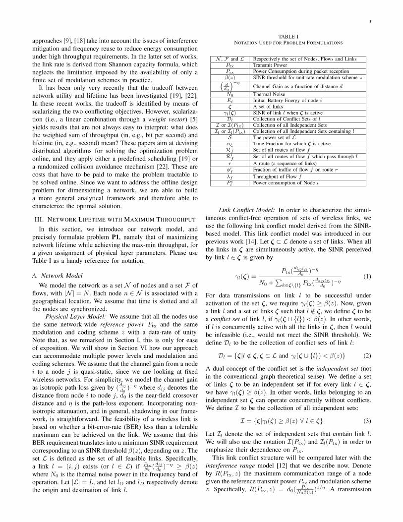
S A B

Fig. 1. A Simple Example Network

To understand the problems TO and P1 and their solutions,let us first work them out for the simple network shown inFig 1. The network consists of 3 nodes S, A and B withtwo flows, one from A destined to S, and another from B

5

destined to S. The nodes are equally spaced. Let P (1)tx be the

minimum transmit power level such that the links (A, S) and(B, A) are feasible, but not the link (B, S), and let P (2)

tx bethe minimum transmit power level such that the link (B, S)is feasible. Clearly, P (1)

tx ≤ P(2)tx . Also, for Ptx < P

(1)tx the

network is disconnected.For P (1)

tx ≤ Ptx < P(2)tx , the collection of independent sets

is just the collection of singleton sets of the following links:(A, B), (B, A), (A, S) and (S, A). The best throughput isachieved by scheduling the independent set {(B, A)} for 1/3rdof the time, and the set {(A, S)} for 2/3rd of the time. Thissolution is also unique so P1 is trivial in this case. The max-min throughput (i.e., the solution of TO) is 1/3. The powerconsumption of node A is 1

3Prx + 23Ptx, that of node B is

13Ptx, and that of node S is 2

3Prx. Let us assume that the initialbattery energies are EA = EB = E and ES =∞. Clearly, thepower consumption of node A is greater than that of node B,and the power consumption of node S is irrelevant, since it hasno energy constraint. Therefore, the lifetime (i.e., the solutionof P1) is nothing but the lifetime of node A, E

13Prx+ 2

3Ptx.

For Ptx ≥ P (2)tx , two new independent sets become feasible,

viz., the singletons {(B, S)} and {(S, B)}. Hence, the bestthroughput is achieved by scheduling the set {(B, S)} for 1/2the time, and the set {(A, S)} for 1/2 the time. Again, thesolution is unique so P1 is trivial. The solution of TO is 1/2,and the solution of P1 is E

12Ptx

since both nodes A and Bare transmitting for 1/2 the time. So the overall trend in thesolutions of TO and P1 is the following. The solution of TO isnon-decreasing and shows non-negative jumps whenever newindependent sets are created. The solution of P1 is decreasingbetween the points of creation of independent sets, and thejump is positive in this case. Of course, note that there areexactly two points at which new independent sets are created,viz., P (1)

tx and P (2)tx .

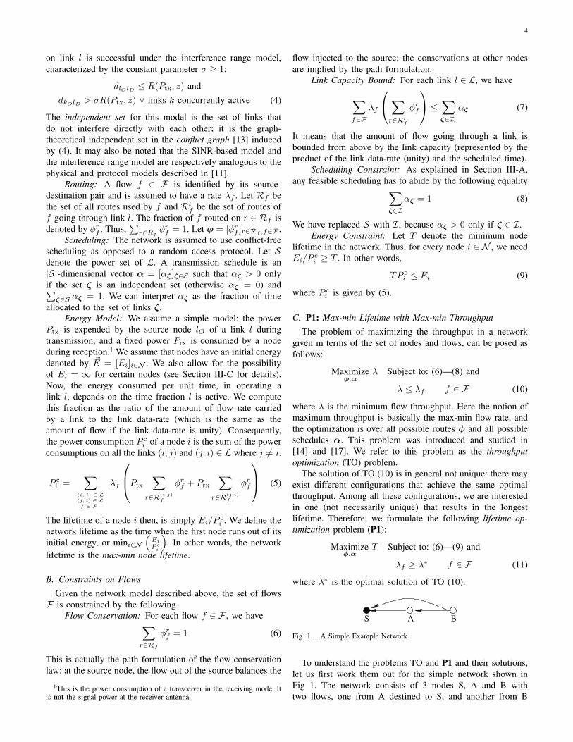
To further illustrate the solutions of TO (10) and P1 (11),we solve them for the two networks shown in Fig. 2. The set

(a) Grid network. (b) Arbitrary network.

Fig. 2. Two networks with 25 nodes (a) and 30 nodes (b).

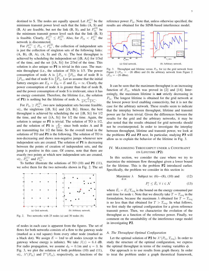
of nodes in each case is apparent from the figures. The set offlows for both networks consists of a flow to the gateway node(marked as a red square) from every other node (marked asa black dot). We assign E = 1mJ to all nodes (except to thegateway whose energy is infinite). We take β(z) = 6.4 dB.For radio propagation, we assume d0 = 0.1m and η = 3. InFig. 3, we plot the solution of both problems (10) and (11),viz., λ∗(Ptx) and T ∗(Ptx), respectively, as functions of the

reference power Ptx. Note that, unless otherwise specified, theresults are obtained for the SINR-based interference model.

−35 −30 −25 −20 −150.01

0.015

0.02

0.025

0.03

0.035

0.04

0.045

Ptx

(dBm)−35 −30 −25 −20 −15

0

500

1000

1500

2000

2500

3000

3500

λ*(P

tx)

T*(P

tx)

−35 −30 −25 −200.02

0.025

0.03

0.035

Ptx

(dBm)−35 −30 −25 −20

0

2000

4000

6000

λ*(P

tx)

T*(P

tx)

(a) Grid network. (b) Arbitrary network.

Fig. 3. Throughput and lifetime versus Ptx for (a) the grid network fromFigure 2 (Prx = −26 dBm) and (b) the arbitrary network from Figure 2(Prx = −29 dBm).

It can be seen that the maximum throughput is an increasingfunction of Ptx, which was proved in [2] and [14]. Inter-estingly, the maximum lifetime is not strictly decreasing inPtx. The longest lifetime is obtained for the grid network atthe lowest power level enabling connectivity, but it is not thecase for the arbitrary network. These results seem to indicatethat the interplay between throughput, lifetime and transmitpower are far from trivial. Given the differences between theresults for the grid and the arbitrary networks, it may bealso noted that the results obtained for grid networks shouldnot be overinterpreted. In order to investigate the interplaybetween throughput, lifetime and transmit power, we look atthe problems P2 and P3 next. In particular, studying P3 willallow us to explain the behavior of the lifetime in Fig. 3.

IV. MAXIMIZING THROUGHPUT UNDER A CONSTRAINTON LIFETIME (P2)

In this section, we consider the case where we try tomaximize the minimum flow throughput given a lower boundfor the lifetime. This is the problem P2 introduced earlier.Specifically, the problem we consider in this section is:

Maximizeφ,α

λ Subject to: (6)—(8), (10) and (12)

P ci ≤ Ei ∀ i ∈ N (13)

where Ei = Ei/Treq is the bound on the energy consumed perunit time for node i. Note that we directly take T = Treq in theformulation, because the maximum λ obtained for T = Treq

is no less than that obtained for T > Treq. In what follows,we first study the optimal configuration for a given referencetransmit power. Then, we characterize the evolution of thethroughput as a function of the reference power. Finally, wecomment on the unsuitability of the interference range modelin investigating P2.

A. The Throughput Optimal Configuration

Let the optimal solution of P2 be λ∗(Ptx, Treq). In order tostudy the structure of the optimal configuration, we expressthe optimal throughput in terms of the routing variables φ.

Our approach is to use results from graph theory. In orderto treat the problem under a graph theoretical framework,

6

we need to embed the link conflict structure (as defined inSection III-A) into a graph the way it is done in [14]. Sucha graph is termed an extended conflict graph (ECG) [14].The idea behind the transformation is the following. Eachset of links ζ ∈ Dl (refer to (2)) conflicts with the link l.Say, ζ = {m1,m2,m3}. Then, scheduling l,m1,m2 and m3

simultaneously is infeasible. This constraint can be representedas “scheduling l means m1 should not be scheduled OR m2

should not be scheduled OR m3 should not be scheduled”. Torepresent these constraints, we replicate each physical link intomultiple copies called “virtual” links, with each copy realizingone of the OR-clauses derived from all ζ ∈ Dl. Then, in theECG, a vertex represents a virtual link and an edge existsbetween two vertices if and only if the corresponding virtuallinks are involved in a scheduling constraint.

This extension allows us to apply graph theoretical results.For example, a graph theoretic independent set in an ECG isequivalent to the definition in (3). Also, a clique q in an ECGrepresents a set of virtual links such that for every pair ofthem (say) l and m, the real link l belongs to some conflictset of the real link m, and vice versa. We say a node i ∈ N is“involved” in clique q (or i ` q) if at least one “virtual” copyof (i, j) or (j, i) belongs to q for some node j ∈ N .

Now recall that in any graph, the size of the largest cliqueis a lower bound on its chromatic number2. A perfect graph isone in which the chromatic number is equal to the size of thelargest clique, for every induced subgraph. Thus, for a perfectgraph, the lower bound is tight. Vertex coloring of the ECGis analogous to creating a feasible link schedule. A clique inan ECG is basically a set of virtual links all of which contendwith one another. Clearly, in a feasible schedule, each of theselinks would have to be scheduled at different times (analogousto being assigned a different color). In other words, the sumof the time-fractions for which virtual links are active shouldbe less than or equal to unity, in every clique in the ECG.

Now, this is necessary but not sufficient to guarantee afeasible schedule. If the ECG is a perfect graph, it would alsobe sufficient. An alternate way to derive a sufficient conditionfor a feasible schedule is to restrict the sum of the time-fractions for which virtual links are active to be less than afactor κ ∈ (0, 1] within every clique in the ECG. Clearly, κdepends on the network topology and the transmit power Ptx.It can now be noted that the ECG being a perfect graph isequivalent to κ being equal to unity.

Proposition 1: The optimal throughput λ∗(Ptx, Treq) isbounded above and below as follows:

λ∗(Ptx, Treq) ≤ maxφ

{minq,i`q

[1

wq(φ),

1

wi(φ)

]}(14)

λ∗(Ptx, Treq) ≥ maxφ

{minq,i`q

[κ

wq(φ),

1

wi(φ)

]}(15)

2The chromatic number of a graph is the minimum number of colorsrequired for vertex coloring. Vertex coloring is the assignment of colors tovertices of a graph in such a way that no two vertices which are connectedby an edge share the same color.

where wq(φ) and wi(φ) are given by:

wq(φ) =∑l∈q

∑f∈F

∑r∈Rlf

φrf

wi(φ) = E−1i

∑(i, j) ∈ L(j, i) ∈ Lf ∈ F

Ptx

∑r∈R(i,j)

f

φrf + Prx

∑r∈R(j,i)

f

φrf

Remark: The upper bound on the optimal throughput

comes from the necessary condition for a feasible schedule:that the time-fractions for which virtual links are active shouldadd up to less than or equal to unity in every clique in the ECG.The lower bound comes from the sufficient condition: that suchtime-fractions need to add up to less than or equal to κ in everyclique. In addition to the scheduling constraints, the energyconstraint due to the lifetime requirement Treq also figures inthe upper and lower bounds on the optimal throughput. Thequantities wq and wi can be thought of as the “cost” of usingthe clique q for scheduling time, and the node i for its energy,respectively.

Now, let us define φ as a routing scheme which max-imizes the right-hand side term within braces in (14), i.e,φ = arg maxφminq,i`q

[1

wq(φ) ,1

wi(φ)

]. Also, given a routing

φ, let us define λ∗(φ) as the solution of the problem:

Maximizeα

λ Subject to: (6)—(8), (10) and (13) (16)

Given φ

In other words, λ∗(φ) is the maximum achievable throughputunder the routing φ, while ensuring a minimum lifetime ofTreq. Now, Proposition 1 can be equivalently stated as follows,to capture the performance of the routing φ defined above.Note that the constant κ is the same as that in Proposition 1.

Proposition 2: For some κ ∈ (0, 1] which depends on theconflict structure and a given reference transmit power Ptx,

κλ∗(Ptx, Treq) ≤ λ∗(φ) ≤ λ∗(Ptx, Treq)

In particular, we have λ∗(φ) = λ∗(Ptx, Treq) if the ECGinduced by the link conflict structure is perfect.

Remark: The above proposition states that the routingscheme φ achieves a throughput which is within a factor κ ofthe optimal throughput, provided the optimal schedule is usedonce the routing is fixed. This can viewed as separating theoptimal routing problem from the optimal scheduling problem.Such an approach would achieve optimal performance only ifthe ECG is a perfect graph.

B. Optimal Throughput vs. Transmit Power

We now look at how changing the reference power Ptx

affects the optimal throughput λ∗(Ptx, Treq). We first considerTO (P2 with Treq = 0) and then P2 in general. We will useP to denote the maximum allowed value of Ptx. Please referto Table II for a summary of additional notation pertaining tothe Propositions to follow.

Definition 1: Let Np for p ∈ [0, P ] be the counting processwhich counts the number of independent sets in a networkwhen all the network nodes use a transmit power Ptx = p. Let

7

TABLE IINOTATION USED FOR PROPOSITIONS

Np Process counting independent sets vs. transmit power{Pn} Point Sequence of Np

λ∗(Ptx, 0) Solution of TOλ∗(Ptx, Treq) Solution of P2T ∗(Ptx, ρ) Solution of P3

∆λ(p) Variation of solution of TO at p∆λ(p, Treq) Variation of solution of P2 at p

∆T (p, ρ) Variation of solution of P3 at pg(p, Treq) Derivative of continuous part of solution of P2 at ph(p, ρ) Derivative of continuous part of solution of P3 at pC(Ptx, ρ) Configuration Ensemble

{Pn} denote the sequence of transmit power levels at whichnew independent sets are created.

Remark: For a fixed set of nodes N , Np would actuallybe a deterministic process, and the points {Pn} would bedetermined only by the locations of the nodes.

We first show that λ∗(Ptx, 0) is a non-decreasing functionof Ptx. Let us define ∆λ(p) = limp′↑p(λ

∗(p, 0)− λ∗(p′, 0)).Proposition 3: Let Ptx ∈ [0, P ]. Then we have that:

λ∗(Ptx, 0) =

∫ Ptx

0

∆λ(p)Np(dp) and ∆λ(p) ≥ 0

Remark: In other words, the optimal throughput is con-stant in [Pn, Pn+1) and has a non-negative jump at each Pn.We have already seen exactly this trend for the case of thesimple network of Fig. 1. The proposition is actually just aspecial case of the general result that high transmit powerincreases throughput [2], [14]. However, it is instructive tostate and prove it using the notation of the point process Np,since its point sequence actually determines the evolution ofthe solution of problems P2 and P3, and not just of TO.

Now let us look at the case where Treq > 0. Again, letus define ∆λ(p, Treq) = limp′↑p(λ

∗(p, Treq) − λ∗(p′, Treq))

and g(p, Treq) = limp′→pλ∗(p,Treq)−λ∗(p′,Treq)

p−p′ . In otherwords, g(p, Treq) is the derivative of the continuous part ofλ∗(Ptx, Treq) at p and ∆λ(p, Treq) is the throughput variationat power level p.

Proposition 4: Let Ptx ∈ [0, P ]. Then we have that:

λ∗(Ptx, Treq) =

∫ Ptx

0

∆λ(p, Treq)NP (dp)+

∫ Ptx

0

g(p, Treq)dp

We also have that ∆λ(p, Treq) ≥ 0 and g(p, Treq) ≤ 0.Remark: In other words, the optimal throughput

λ∗(Ptx, Treq) as a function of Ptx has non-negative variationsat {Pn} but is non-increasing between any two successivepoints Pn and Pn+1.

Remark: Let us work out the trend of the solution of P2vs transmit power for the simple example of Fig. 1. As wesaw earlier, for P (1)

tx ≤ Ptx ≤ P(2)tx , scheduling the set {(B,

A)} for 1/3rd the time, and the set {(A, S)} for 2/3rd thetime, provided the solution for TO. Now, due to the minimumlifetime requirement, Treq, this schedule may not be feasible.So, we schedule {(B, A)} for a time fraction ρ

3 and {(A, S)}for a time fraction 2ρ

3 , where 0 ≤ ρ ≤ 1 is a factor whichwe will use for meeting the lifetime requirement. This yields

a throughput of ρ3 . Clearly, we require the lifetime of node

A to be greater than Treq, i.e., Eρ3Prx+ 2ρ

3 Ptx≥ Treq. In other

words, ρ = min( 3ETreq(Prx+2Ptx) , 1). Therefore, the max-min

throughput (i.e., the solution of P2) is min( ETreq(Prx+2Ptx) ,

13 )

Similarly, for Ptx ≥ P(2)tx , the solution of P2 can be

worked out to be min( ETreqPtx

, 12 ). Thus, as per Proposition 4,

λ∗(Ptx, Treq) is non-increasing between jumps, and has non-negative jumps.

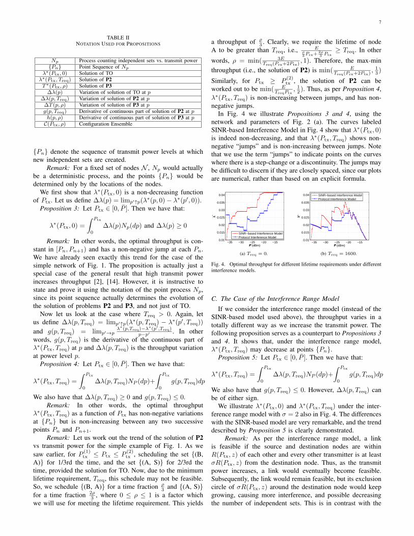
In Fig. 4 we illustrate Propositions 3 and 4, using thenetwork and parameters of Fig. 2 (a). The curves labeledSINR-based Interference Model in Fig. 4 show that λ∗(Ptx, 0)is indeed non-decreasing, and that λ∗(Ptx, Treq) shows non-negative “jumps” and is non-increasing between jumps. Notethat we use the term “jumps” to indicate points on the curveswhere there is a step-change or a discontinuity. The jumps maybe difficult to discern if they are closely spaced, since our plotsare numerical, rather than based on an explicit formula.

−35 −30 −25 −20 −150.01

0.015

0.02

0.025

0.03

0.035

0.04

P (dBm)

λ*

SINR−based Interference ModelProtocol Interference Model

−35 −30 −25 −20 −150.01

0.015

0.02

0.025

0.03

0.035

0.04

P (dBm)

λ*

SINR−based Interference ModelProtocol Interference Model

(a) Treq = 0. (b) Treq = 1600.

Fig. 4. Optimal throughput for different lifetime requirements under differentinterference models.

C. The Case of the Interference Range Model

If we consider the interference range model (instead of theSINR-based model used above), the throughput varies in atotally different way as we increase the transmit power. Thefollowing proposition serves as a counterpart to Propositions 3and 4. It shows that, under the interference range model,λ∗(Ptx, Treq) may decrease at points {Pn}.

Proposition 5: Let Ptx ∈ [0, P ]. Then we have that:

λ∗(Ptx, Treq) =

∫ Ptx

0

∆λ(p, Treq)NP (dp)+

∫ Ptx

0

g(p, Treq)dp

We also have that g(p, Treq) ≤ 0. However, ∆λ(p, Treq) canbe of either sign.

We illustrate λ∗(Ptx, 0) and λ∗(Ptx, Treq) under the inter-ference range model with σ = 2 also in Fig. 4. The differenceswith the SINR-based model are very remarkable, and the trenddescribed by Proposition 5 is clearly demonstrated.

Remark: As per the interference range model, a linkis feasible if the source and destination nodes are withinR(Ptx, z) of each other and every other transmitter is at leastσR(Ptx, z) from the destination node. Thus, as the transmitpower increases, a link would eventually become feasible.Subsequently, the link would remain feasible, but its exclusioncircle of σR(Ptx, z) around the destination node would keepgrowing, causing more interference, and possible decreasingthe number of independent sets. This is in contrast with the

8

SINR-based model in which a link actually becomes moreimmune to interference as the power increases, and hencemore independent sets are created. Thus, the interference rangemodel is inaccurate: the throughput is overestimated at lowpowers but underestimated at intermediate power levels.

V. MAXIMIZING LIFETIME UNDER A CONSTRAINT ONTHROUGHPUT (P3)

In this section, we consider the case where the data rateof each flow f ∈ F is required to be greater than λreq. Theproblem aims at maximizing the network lifetime T underthe constraint that λf ≥ λreq,∀f ∈ F . We refer to thisproblem as P3. Let us define the cumulative data from flowf transported over link (i, j) over the entire lifetime T asxf(i,j) = λfT

(∑r∈R(i,j)

f

φrf

)and the total time for which

the independent set ζ is scheduled over the lifetime T asαζ = Tαζ . Now P3 can be formulated as:

Maximizex,α

T (17)∑j:(i,j)∈L

xf(i,j) −∑

j:(j,i)∈L

xf(j,i)≥≤

λreqT1{i=fs}−λreqT1{i=fd}

∀ f ∈ F∀ i ∈ N (18)

∑f∈F x

fl −

∑ζ∈Il αζ ≤ 0 ∀ l ∈ L (19)∑ζ∈I αζ = T (20)∑

j∈Nf∈F

Ptxxf(i,j) + Prxx

f(j,i) ≤ Ei ∀ i ∈ N (21)

where x = [xf(i,j)](i,j)∈L,f∈F and α = [αζ ]ζ∈S . The con-straint (18) comes from flow conservation: the incoming flowshould balance the outgoing flow for a given node. Since werequire λf ≥ λreq, this constraint is an inequality rather thanan equality as suggested by the conservation law. The objectiveT has been absorbed into the cumulative data flow variablesxfl and the aggregated scheduling variables αζ in order toformulate P3 as a linear program.

Note that, given an arbitrary λreq, the problem might notbe feasible. However, we can guarantee feasibility (and thusavoiding the complexity of feasibility verification) by requiringλreq = ρλ∗(Ptx, 0) where ρ ≤ 1 and λ∗(Ptx, 0) is the optimalsolution of TO (P2 with Treq = 0).

A. Optimal Lifetime vs. Transmit Power

We investigate the trend of the optimal lifetime T ∗, asa function of the reference transmit power. We want tocharacterize the trend of T ∗(Ptx, ρ) as Ptx varies in [0, P ].Note that the lower bound λreq(Ptx) = ρλ∗(Ptx, 0) is alsoa function of Ptx.3 The following proposition shows thatT ∗(Ptx, ρ) has a similar trend (i.e., is piecewise continu-ous) as λ∗(Ptx, Treq) given by Proposition 4. Let us define∆T (p, ρ) = limp′↑p(T

∗(p, ρ) − T ∗(p′, ρ)) and h(p, ρ) =

limp′→pT∗(p,ρ)−T∗(p′,ρ)

p−p′ .

3This differs from P2, where the lower bound of the lifetime is a constantfor all Ptx ∈ [0, P ]. The reason is that λreq cannot be taken arbitrarily; ithas to be defined with respect to the maximum achievable throughput for thegiven Ptx in order to preserve the feasibility of the problem P3.

Proposition 6: Let Ptx ∈ [0, P ]. Then we have that:

T ∗(Ptx, ρ) =

∫ Ptx

0

∆T (p, ρ)Np(dp) +

∫ Ptx

0

h(p, ρ)dp

We also have that h(p, ρ) ≤ 0. However, ∆T (Pn, ρ) can beof either sign.

Remark: In other words, the optimal lifetime T ∗(Ptx, ρ)as a function of Ptx is non-increasing between any twosuccessive points Pn and Pn+1, but could show positive ornegative variations at {Pn}. Thus T ∗(Ptx, ρ) need not be adecreasing function of Ptx as a whole.

Remark: Again, let us try to work out the trend of thesolution of P3 vs. transmit power, for the simple network ofFig. 1 to understand Proposition 6. For P (1)

tx ≤ Ptx ≤ P(2)tx ,

the max-min throughput is 1/3. So, to meet a throughputrequirement of ρ

3 , we need to schedule {(B, A)} for a timefraction ρ

3 and {(A, S)} for a time fraction 2ρ3 . Since this is the

only possible configuration, the solution of P3 is trivial. Thelifetime of the network is nothing but 3E

ρ(Prx+2Ptx) . Similarly,

for Ptx ≥ P (2)tx , the maximum network lifetime can be worked

out to be 2EρPtx

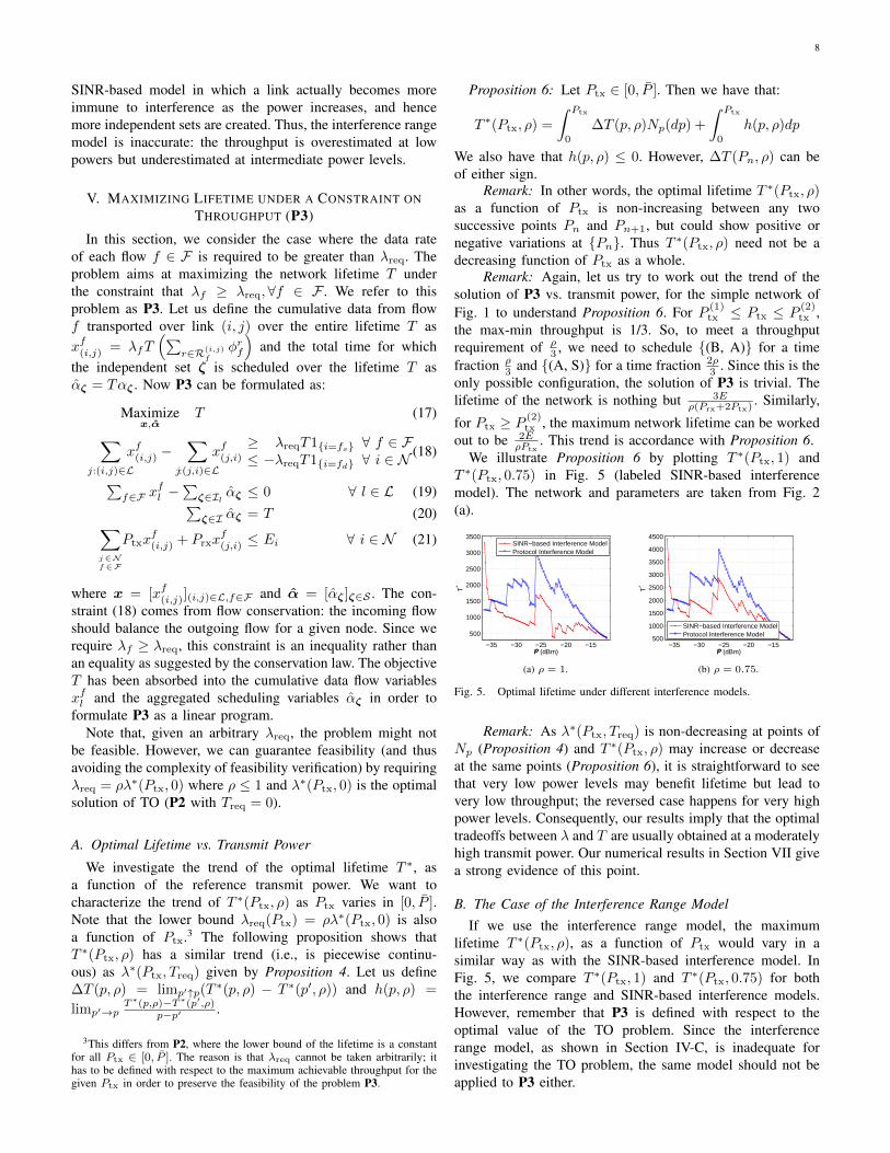
. This trend is accordance with Proposition 6.We illustrate Proposition 6 by plotting T ∗(Ptx, 1) and

T ∗(Ptx, 0.75) in Fig. 5 (labeled SINR-based interferencemodel). The network and parameters are taken from Fig. 2(a).

−35 −30 −25 −20 −15

500

1000

1500

2000

2500

3000

3500

T*

P (dBm)

SINR−based Interference ModelProtocol Interference Model

−35 −30 −25 −20 −15500

1000

1500

2000

2500

3000

3500

4000

4500

P (dBm)T

*

SINR−based Interference ModelProtocol Interference Model

(a) ρ = 1. (b) ρ = 0.75.

Fig. 5. Optimal lifetime under different interference models.

Remark: As λ∗(Ptx, Treq) is non-decreasing at points ofNp (Proposition 4) and T ∗(Ptx, ρ) may increase or decreaseat the same points (Proposition 6), it is straightforward to seethat very low power levels may benefit lifetime but lead tovery low throughput; the reversed case happens for very highpower levels. Consequently, our results imply that the optimaltradeoffs between λ and T are usually obtained at a moderatelyhigh transmit power. Our numerical results in Section VII givea strong evidence of this point.

B. The Case of the Interference Range ModelIf we use the interference range model, the maximum

lifetime T ∗(Ptx, ρ), as a function of Ptx would vary in asimilar way as with the SINR-based interference model. InFig. 5, we compare T ∗(Ptx, 1) and T ∗(Ptx, 0.75) for boththe interference range and SINR-based interference models.However, remember that P3 is defined with respect to theoptimal value of the TO problem. Since the interferencerange model, as shown in Section IV-C, is inadequate forinvestigating the TO problem, the same model should not beapplied to P3 either.

9

C. The Tradeoff between Throughput and Lifetime

The solution of P3 clearly depends on the choice of ρ,since λreq = ρλ∗(Ptx, 0). Here, we investigate the trendof the solution of P3 as a function of ρ. As ρ decreases,we are essentially relaxing the throughput requirement, andexpecting to improve the lifetime T ∗(Ptx, ρ). This is thetradeoff we investigate. Now, unlike P2 (whose parameterTreq is unbounded), the parameter λreq(Ptx) of P3 is boundedwithin [0, λ∗(Ptx, 0)] for all Ptx ∈ [0, P ]. This simplifies ourinvestigation. We first give a definition to facilitate furtherdiscussions.

Definition 2: Duty cycle scaling refers to a specific strategyof trading throughput for lifetime. Given a schedule α and arouting φ which achieve a flow throughput of λf for flow f ∈F , duty cycle scaling by a factor ρ < 1 refers to scaling theoperation time of each link l,

∑f∈F λf

(∑r∈Rlf

φrf

), by ρ

which is feasible since the operating time is less than or equalto the time for which the link is scheduled,

∑ζ∈Il(Ptx) αζ .

When the operation time of a link is strictly shorter thanits scheduled time, we assume that both the transmitter andthe receiver will switch to sleep mode during the spare timeto conserve energy. The duty cycle scaling utilizes this mech-anism to trade throughput for lifetime. The next propositionis a direct consequence of this definition. It shows that, if weaccept a decrease in throughput, duty cycle scaling leads toa lower bound on the optimal lifetime. In other words, thetradeoff is biased towards the lifetime in proportional sense:sacrificing a certain fraction of throughput gains a larger orequal fraction of improvement in lifetime.

Proposition 7: Given a fixed Ptx and two required sourcerates λ(1)

req(Ptx) = ρ1λ∗(Ptx, 0) and λ(2)

req(Ptx) = ρ2λ∗(Ptx, 0)

with ρ1 > ρ2, we have

T ∗(Ptx, ρ2) ≥ ρ1

ρ2T ∗(Ptx, ρ1)

An interesting question that we turn to now, is whetherthe inequality of Proposition 7 is strict, and if so, underwhat conditions. In order to answer this question, let usconsider the feasible network configurations that achieve athroughput of ρλ∗(Ptx, 0). A feasible network configurationis an assignment of the flow variables xfl and the schedulingvariables αζ such that (18) holds with λreq = ρλ∗(Ptx, 0). Foreach such network configuration, we consider the collectionof independent sets ζ for which αζ > 0. We denote thiscollection by I∗i (Ptx, ρ), where i is a generic index. We nowdefine a configuration ensemble C(Ptx, ρ) as the set

C(Ptx, ρ) = {I∗i (Ptx, ρ)|i = 1, 2, . . . , |C(Ptx, ρ)|} (22)

The problem P3 can be solved by finding among all theconfigurations in the configuration ensemble C(Ptx, ρ), onethat achieves the best lifetime.

Now, for ρ1 > ρ2, we know that any configuration achievinga throughput ρ1λ

∗(Ptx, 0) can be duty cycle scaled to achieveρ2λ∗(Ptx, 0). Therefore, we have C(Ptx, ρ1) ⊆ C(Ptx, ρ2).

Therefore, C(Ptx, ρ) grows with decreasing ρ. In other words,more collections of independent sets are included in theconfiguration ensemble as ρ is decreased. This accounts for theinequality in the Proposition 7. However, the size of C(Ptx, ρ)

is bounded from above by the size of the power set of I(Ptx).As a consequence, C(Ptx, ρ) will reach its maximum size forsome small enough ρ0 ∈ [0, 1]. We formally define this in thefollowing:

Definition 3: We say C(Ptx, ρ) is complete if C(Ptx, ρ)includes all the elements of the power set of I(Ptx) that yielda connected routing topology for f ∈ F . Let ρ0 be the largestρ for which C(Ptx, ρ) is complete.

Remark: In order to understand the notion of configura-tion ensembles, and the Definition 3, let us use the examplegiven in Fig. 1. Let Ptx ≥ P

(2)tx . As we have discussed

earlier, the maximum throughput achievable λ∗(Ptx, 0) = 12 .

Now, observe that by scheduling the independent sets {(B,S)} and {(A, S)} for a time-fraction ρ

2 each, any throughputbetween 0 and 1

2 can be achieved. However, by schedulingthe independent set {(B, A)} for a time-fraction 1

3 and theindependent set {(A, S)} for a time-fraction 2

3 , the maximumachievable throughput is only 1

3 . Thus, for a max-min through-put requirement between 1

3 and 12 (i.e., for 2

3 < ρ ≤ 1), onlythe configuration consisting of independent sets {(B, S)} and{(A, S)} can be used. For ρ ≤ 2

3 , the other configurationconsisting of independent sets {(B, A)} and {(A, S)} can alsobe used. Thus, we have for Ptx ≥ P (2)

tx :

C(Ptx, ρ) =

{{{(B, S)}, {(A, S)}

}}for

2

3< ρ ≤ 1 (23)

=

{{{(B, S)}, {(A, S)}

},{{(B, A)}, {(A, S)}

}}for ρ ≤ 2

3(24)

Thus, we see that C(Ptx, ρ) is increasing with decreasing ρ.Also, it is easy to see that C(Ptx, ρ) cannot grow any largerthan the right-hand side of (24). Thus, ρ0 = 2

3 for the simplenetwork in Fig. 1, for Ptx ≥ P (2)

tx .Based on Definition 3, we can state the sufficient condition

for the equality in Proposition 7 to hold:Proposition 8: If ρ0 ≥ ρ1 > ρ2, then

T ∗(Ptx, ρ2) =ρ1

ρ2T ∗(Ptx, ρ1)

Essentially, if the configuration ensemble is sufficiently large(or in other words, the throughput requirement ρλ∗(Ptx, 0) issufficiently low), the tradeoff between throughput and lifetimeis strictly proportional.

Remark: Note that the condition of ρ1 and ρ2 beingless than or equal to ρ0 in Proposition 8 is not a necessarycondition, but a sufficient one. In particular, for the simpleexample of Fig. 1, we know that Proposition 8 would applyfor ρ ≤ 2

3 . However, as we saw earlier in the remarks followingProposition 6, the solution of P3 for Ptx ≥ P

(2)tx is obtained

by duty-cycle scaling for any ρ, by scheduling the independentsets {(B, S)} and {(A, S)} for a time-fraction ρ

2 each. Thus,the equality in Proposition 8 applies for any ρ ≤ 1, althoughρ0 = 2

3 .The previous results describe the tradeoffs at a fixed transmit

power. Based on Propositions 4 and 6, the following propertyfor the optimal solutions of both P2 and P3 within the fullrange of variation of the reference power [0, P ] is immediate:

10

Proposition 9: The optimal solutions of both P2 and P3 areachieved at a point of Np.

This proposition reduces our search scope for the optimaltradeoffs from a continuous spectrum of [0, P ] to a few discretepoints given by Np.

Remark: In fact, Proposition 9 applies to any trade-off utility function Γ(λ, T ) which is a monotonically non-decreasing function of both the throughput and lifetime whenthe other is fixed. We actually prove this general case in theappendix.

D. Identifying the Optimal Lifetime Given a Feasible Through-put Requirement λreq

As we saw earlier, a throughput requirement λreq is feasibleat Ptx if λreq = ρλ∗(Ptx, 0) for some ρ ≤ 1. Clearly, λreq isfeasible for some Ptx ∈ [0, P ], if λreq = θλ∗(P , 0) for someθ ≤ 1. Now, given a feasible λreq, among all combinations ofPtx and ρ which satisfy λreq = ρλ∗(Ptx, 0), we would like toidentify that combination for which T ∗(Ptx, ρ) is the highest.This corresponds to the maximum lifetime that the networkcan provide while delivering a minimum throughput of λreq.

If we were to directly use P3 to identify this optimallifetime, we would have to solve a tremendous number ofinstances of P3 (each with a different Ptx and ρ). Fortunately,Proposition 9 allows us to significantly reduce the computa-tional complexity. In summary, we take the following stepsto identify the optimal lifetime and its corresponding networkconfigurations.

1) Given a known network topology, compute the points{Pn} of Np, where optimal tradeoff points can befound (by Proposition 9), as well as {λ∗(Pn, 0)}. Thecomputation is done by solving P3 instances at Pn forwhich λ∗(Pn, 0) ≥ λreq.

2) At each power P ∈ {Pn}, solve a P3 instance with a ρsuch that λreq = ρλ∗(Pn, 0).

3) An optimal tradeoff point with respect to a certain λreq

is obtained by maximizing over T ∗(P,

λreq

λ∗(P,0)

)for all

P ∈ {Pn}.Similarly, we can compute λ∗(Ptx, Treq) for Ptx ∈ [0, P ],

by solving a sequence of P2 over {Pn}. In general, thecomplexity of this algorithm is mainly determined by thecomplexity of solving a P3 (or P2) instance and the numberof jumps in {Pn}. For the complexity of solving a P3 (or P2)instance, we refer to [17] for details.

VI. EXTENDING OUR APPROACH TO MULTIPLE POWERSAND MODULATIONS

The results presented so far are based on the assumptionof a single power level and modulation scheme. In practice,a node may have a choice of using a power level and amodulation scheme from a finite set of power levels, and afinite set of modulation schemes, respectively. To incorporatesuch cases, we assume a network-wide reference power level.We assume that each node can transmit at a finite number ofpower levels each obtained via a fixed offset with respect tothe network-wide reference power. Then, with multiple power

−36 −34 −32 −30 −28 −26 −24 −22 −200.01

0.015

0.02

0.025

0.03

0.035

Ptx

(dBm)

λ*

Treq

≤ 1600

Treq

= 3100

Treq

= 4600

Treq

= 6100

Treq

= 7600

Treq

= 9500

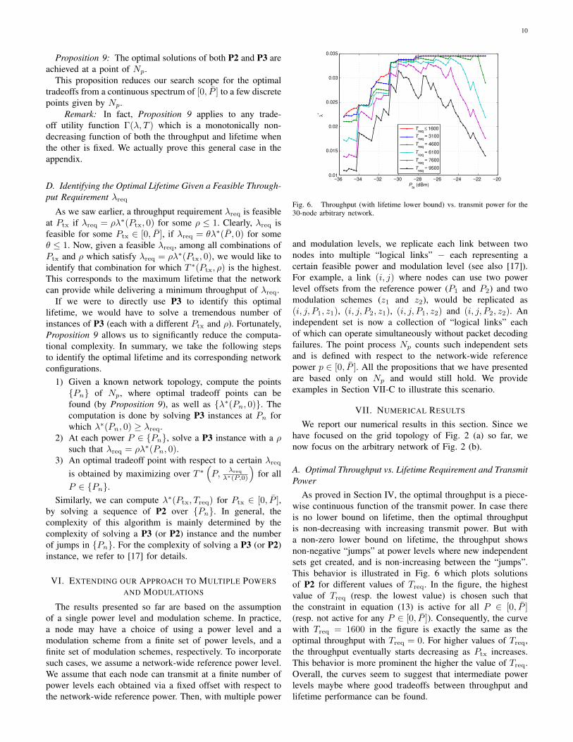
Fig. 6. Throughput (with lifetime lower bound) vs. transmit power for the30-node arbitrary network.

and modulation levels, we replicate each link between twonodes into multiple “logical links” − each representing acertain feasible power and modulation level (see also [17]).For example, a link (i, j) where nodes can use two powerlevel offsets from the reference power (P1 and P2) and twomodulation schemes (z1 and z2), would be replicated as(i, j, P1, z1), (i, j, P2, z1), (i, j, P1, z2) and (i, j, P2, z2). Anindependent set is now a collection of “logical links” eachof which can operate simultaneously without packet decodingfailures. The point process Np counts such independent setsand is defined with respect to the network-wide referencepower p ∈ [0, P ]. All the propositions that we have presentedare based only on Np and would still hold. We provideexamples in Section VII-C to illustrate this scenario.

VII. NUMERICAL RESULTS

We report our numerical results in this section. Since wehave focused on the grid topology of Fig. 2 (a) so far, wenow focus on the arbitrary network of Fig. 2 (b).

A. Optimal Throughput vs. Lifetime Requirement and TransmitPower

As proved in Section IV, the optimal throughput is a piece-wise continuous function of the transmit power. In case thereis no lower bound on lifetime, then the optimal throughputis non-decreasing with increasing transmit power. But witha non-zero lower bound on lifetime, the throughput showsnon-negative “jumps” at power levels where new independentsets get created, and is non-increasing between the “jumps”.This behavior is illustrated in Fig. 6 which plots solutionsof P2 for different values of Treq. In the figure, the highestvalue of Treq (resp. the lowest value) is chosen such thatthe constraint in equation (13) is active for all P ∈ [0, P ](resp. not active for any P ∈ [0, P ]). Consequently, the curvewith Treq = 1600 in the figure is exactly the same as theoptimal throughput with Treq = 0. For higher values of Treq,the throughput eventually starts decreasing as Ptx increases.This behavior is more prominent the higher the value of Treq.Overall, the curves seem to suggest that intermediate powerlevels maybe where good tradeoffs between throughput andlifetime performance can be found.

11

2000 3000 4000 5000 6000 7000 8000 90000.031

0.032

0.033

0.034

0.035

λ*

Treq

2000 3000 4000 5000 6000 7000 8000 9000−32

−30

−28

−26

−24

P*

λ*

P*

Fig. 7. Maximum Achievable Throughput and transmit power curves asfunction of Treq for the 30-node arbitrary network.

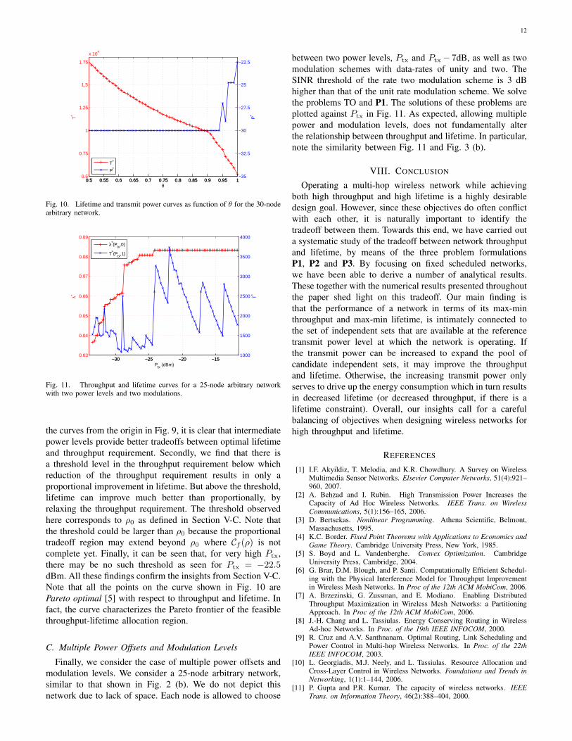
It is also instructive to look at the maximum achieveablethroughput for a fixed lifetime requirement, by optimizing overall possible reference transmit power levels. These results havebeen depicted in Fig. 7. The curve marked λ∗ represents themaximum achieveable throughput as a function of the lifetimerequirement Treq. It is obtained by maximizing the solution ofP2 over Ptx ∈ [0, P ]. The curve marked P ∗ represents theminimum transmit power level at which the solution of P2achieves the corresponding throughput. There are a number ofpoints to note. The curve marked λ∗ is smooth, remains flatfor low values of Treq and starts decreasing for Treq ≥ 5000time units. In other words, throughput has to be sacrificed toimprove lifetime. The value of the plateau is given by the(unconstrained) maximum achievable throughput, i.e., for a30-node network with unit link rate, 1/30. At lower valuesof Treq, this throughput can be reached for lower value ofthe reference power, but when Treq increases while remainingbelow 5000 time units, the reference power at which the max-min throughput is achieved increases. This is again is supportof our intuition that very low powers do not provide sufficientflexibility (in terms of independent sets) to achieve a highlifetime and throughput. Note that the λ∗ curve in Fig. 7 doesnot describe a Pareto frontier [5] as a whole since all Treqsless than 5000 correspond to the same λ∗. But the portion ofthe curve for Treq ≥ 5000 does. This is because, for a vector[Treq, λ

∗] on the curve, one can easily show that any vectorv � [Treq, λ

∗], except [Treq, λ∗] itself, is not feasible.

B. Optimal Lifetime vs. Throughput Requirement and TransmitPower

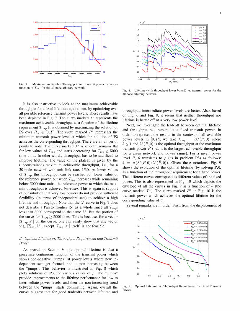
As proved in Section V, the optimal lifetime is also apiecewise continuous function of the transmit power whichshows non-negative “jumps” at power levels where new in-dependent sets get formed, and is non-increasing betweenthe “jumps”. This behavior is illustrated in Fig. 8 whichplots solutions of P3, for various values of ρ. The “jumps”provide improvements to the lifetime performance for low tointermediate power levels, and then the non-increasing trendbetween the “jumps” starts dominating. Again, overall thecurves suggest that for good tradeoffs between lifetime and

−36 −34 −32 −30 −28 −26 −24 −22 −200

0.2

0.4

0.6

0.8

1

1.2

1.4

1.6

1.8

2x 10

4

Ptx (dBm)

T*

ρ = 1ρ = 0.9ρ = 0.8ρ = 0.7ρ = 0.6ρ = 0.5

Fig. 8. Lifetime (with throughput lower bound) vs. transmit power for the30-node arbitrary network.

throughput, intermediate power levels are better. Also, basedon Fig. 6 and Fig. 8, it seems that neither throughput norlifetime is better off at a very low power level.

Next, we investigate the tradeoff between optimal lifetimeand throughput requirement, at a fixed transmit power. Inorder to represent the results in the context of all availablepower levels in [0, P ], we take λreq = θλ∗(P , 0) whereθ ≤ 1 and λ∗(P , 0) is the optimal throughput at the maximumtransmit power P (i.e., it is the largest achievable throughputfor a given network and power range). For a given powerlevel P , θ translates to ρ (as in problem P3) as follows:θ = ρ

(λ∗(P, 0)/λ∗(P , 0)

). Given these notations, Fig. 9

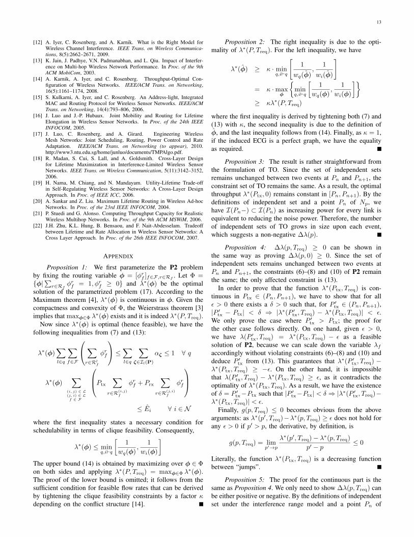
shows the evolution of the optimal lifetime (by solving P3),as a function of the throughput requirement for a fixed power.The different curves correspond to different values of the fixedpower. This is also represented in Fig. 10 which depicts theenvelope of all the curves in Fig. 9 as a function of θ (thecurve marked T ∗). The curve marked P ∗ in Fig. 10 is thetransmit power which achieves the optimal lifetime for thecorresponding value of θ.

Several remarks are in order. First, from the displacement of

0.4 0.5 0.6 0.7 0.8 0.9 10.2

0.4

0.6

0.8

1

1.2

1.4

1.6

1.8

2x 10

4

θ

T*

Ptx = −36.50 dBm

Ptx = −34.00 dBm

Ptx = −32.25 dBm

Ptx = −30.00 dBm

Ptx = −26.25 dBm

Ptx = −22.50 dBm

Fig. 9. Optimal Lifetime vs. Throughput Requirement for Fixed TransmitPower.

12

0.5 0.55 0.6 0.65 0.7 0.75 0.8 0.85 0.9 0.95 10.5

0.75

1

1.25

1.5

1.75

x 104

T*

θ

0.5 0.55 0.6 0.65 0.7 0.75 0.8 0.85 0.9 0.95 1−35

−32.5

−30

−27.5

−25

−22.5

P*

T*

P*

Fig. 10. Lifetime and transmit power curves as function of θ for the 30-nodearbitrary network.

−30 −25 −20 −150.03

0.04

0.05

0.06

0.07

0.08

0.09

λ*

Ptx (dBm)

−30 −25 −20 −151000

1500

2000

2500

3000

3500

4000

T*

λ*(Ptx,0)

T*(Ptx,1)

Fig. 11. Throughput and lifetime curves for a 25-node arbitrary networkwith two power levels and two modulations.

the curves from the origin in Fig. 9, it is clear that intermediatepower levels provide better tradeoffs between optimal lifetimeand throughput requirement. Secondly, we find that there isa threshold level in the throughput requirement below whichreduction of the throughput requirement results in only aproportional improvement in lifetime. But above the threshold,lifetime can improve much better than proportionally, byrelaxing the throughput requirement. The threshold observedhere corresponds to ρ0 as defined in Section V-C. Note thatthe threshold could be larger than ρ0 because the proportionaltradeoff region may extend beyond ρ0 where Cf (ρ) is notcomplete yet. Finally, it can be seen that, for very high Ptx,there may be no such threshold as seen for Ptx = −22.5dBm. All these findings confirm the insights from Section V-C.Note that all the points on the curve shown in Fig. 10 arePareto optimal [5] with respect to throughput and lifetime. Infact, the curve characterizes the Pareto frontier of the feasiblethroughput-lifetime allocation region.

C. Multiple Power Offsets and Modulation Levels

Finally, we consider the case of multiple power offsets andmodulation levels. We consider a 25-node arbitrary network,similar to that shown in Fig. 2 (b). We do not depict thisnetwork due to lack of space. Each node is allowed to choose

between two power levels, Ptx and Ptx− 7dB, as well as twomodulation schemes with data-rates of unity and two. TheSINR threshold of the rate two modulation scheme is 3 dBhigher than that of the unit rate modulation scheme. We solvethe problems TO and P1. The solutions of these problems areplotted against Ptx in Fig. 11. As expected, allowing multiplepower and modulation levels, does not fundamentally alterthe relationship between throughput and lifetime. In particular,note the similarity between Fig. 11 and Fig. 3 (b).

VIII. CONCLUSION

Operating a multi-hop wireless network while achievingboth high throughput and high lifetime is a highly desirabledesign goal. However, since these objectives do often conflictwith each other, it is naturally important to identify thetradeoff between them. Towards this end, we have carried outa systematic study of the tradeoff between network throughputand lifetime, by means of the three problem formulationsP1, P2 and P3. By focusing on fixed scheduled networks,we have been able to derive a number of analytical results.These together with the numerical results presented throughoutthe paper shed light on this tradeoff. Our main finding isthat the performance of a network in terms of its max-minthroughput and max-min lifetime, is intimately connected tothe set of independent sets that are available at the referencetransmit power level at which the network is operating. Ifthe transmit power can be increased to expand the pool ofcandidate independent sets, it may improve the throughputand lifetime. Otherwise, the increasing transmit power onlyserves to drive up the energy consumption which in turn resultsin decreased lifetime (or decreased throughput, if there is alifetime constraint). Overall, our insights call for a carefulbalancing of objectives when designing wireless networks forhigh throughput and lifetime.

REFERENCES

[1] I.F. Akyildiz, T. Melodia, and K.R. Chowdhury. A Survey on WirelessMultimedia Sensor Networks. Elsevier Computer Networks, 51(4):921–960, 2007.

[2] A. Behzad and I. Rubin. High Transmission Power Increases theCapacity of Ad Hoc Wireless Networks. IEEE Trans. on WirelessCommunications, 5(1):156–165, 2006.

[3] D. Bertsekas. Nonlinear Programming. Athena Scientific, Belmont,Massachusetts, 1995.

[4] K.C. Border. Fixed Point Theorems with Applications to Economics andGame Theory. Cambridge University Press, New York, 1985.

[5] S. Boyd and L. Vandenberghe. Convex Optimization. CambridgeUniversity Press, Cambridge, 2004.

[6] G. Brar, D.M. Blough, and P. Santi. Computationally Efficient Schedul-ing with the Physical Interference Model for Throughput Improvementin Wireless Mesh Networks. In Proc of the 12th ACM MobiCom, 2006.

[7] A. Brzezinski, G. Zussman, and E. Modiano. Enabling DistributedThroughput Maximization in Wireless Mesh Networks: a PartitioningApproach. In Proc of the 12th ACM MobiCom, 2006.

[8] J.-H. Chang and L. Tassiulas. Energy Conserving Routing in WirelessAd-hoc Networks. In Proc. of the 19th IEEE INFOCOM, 2000.

[9] R. Cruz and A.V. Santhnanam. Optimal Routing, Link Scheduling andPower Control in Multi-hop Wireless Networks. In Proc. of the 22thIEEE INFOCOM, 2003.

[10] L. Georgiadis, M.J. Neely, and L. Tassiulas. Resource Allocation andCross-Layer Control in Wireless Networks. Foundations and Trends inNetworking, 1(1):1–144, 2006.

[11] P. Gupta and P.R. Kumar. The capacity of wireless networks. IEEETrans. on Information Theory, 46(2):388–404, 2000.

13

[12] A. Iyer, C. Rosenberg, and A. Karnik. What is the Right Model forWireless Channel Interference. IEEE Trans. on Wireless Communica-tions, 8(5):2662–2671, 2009.

[13] K. Jain, J. Padhye, V.N. Padmanabhan, and L. Qiu. Impact of Interfer-ence on Multi-hop Wireless Network Performance. In Proc. of the 9thACM MobiCom, 2003.

[14] A. Karnik, A. Iyer, and C. Rosenberg. Throughput-Optimal Con-figuration of Wireless Networks. IEEE/ACM Trans. on Networking,16(5):1161–1174, 2008.

[15] S. Kulkarni, A. Iyer, and C. Rosenberg. An Address-light, IntegratedMAC and Routing Protocol for Wireless Sensor Networks. IEEE/ACMTrans. on Networking, 14(4):793–806, 2006.

[16] J. Luo and J.-P. Hubaux. Joint Mobility and Routing for LifetimeElongation in Wireless Sensor Networks. In Proc. of the 24th IEEEINFOCOM, 2005.

[17] J. Luo, C. Rosenberg, and A. Girard. Engineering WirelessMesh Networks: Joint Scheduling, Routing, Power Control and RateAdaptation. IEEE/ACM Trans. on Networking (to appear), 2010.http://www3.ntu.edu.sg/home/junluo/documents/TMPAlgo.pdf.

[18] R. Madan, S. Cui, S. Lall, and A. Goldsmith. Cross-Layer Designfor Lifetime Maximization in Interference-Limited Wireless SensorNetworks. IEEE Trans. on Wireless Communication, 5(11):3142–3152,2006.

[19] H. Nama, M. Chiang, and N. Mandayam. Utility-Lifetime Trade-offin Self-Regulating Wireless Sensor Networks: A Cross-Layer DesignApproach. In Proc. of IEEE ICC, 2006.

[20] A. Sankar and Z. Liu. Maximum Lifetime Routing in Wireless Ad-hocNetworks. In Proc. of the 23rd IEEE INFOCOM, 2004.

[21] P. Stuedi and G. Alonso. Computing Throughput Capacity for RealisticWireless Multihop Networks. In Proc. of the 9th ACM MSWiM, 2006.

[22] J.H. Zhu, K.L. Hung, B. Bensaou, and F. Nait-Abdesselam. Tradeoffbetween Lifetime and Rate Allocation in Wireless Sensor Networks: ACross Layer Approach. In Proc. of the 26th IEEE INFOCOM, 2007.

APPENDIX

Proposition 1: We first parameterize the P2 problemby fixing the routing variable φ = [φrf ]f∈F,r∈Rf . Let Φ ={φ|

∑r∈Rf φ

rf = 1, φrf ≥ 0} and λ∗(φ) be the optimal

solution of the parametrized problem (17). According to theMaximum theorem [4], λ∗(φ) is continuous in φ. Given thecompactness and convexity of Φ, the Weierstrass theorem [3]implies that maxφ∈Φ λ

∗(φ) exists and it is indeed λ∗(P, Treq).Now since λ∗(φ) is optimal (hence feasible), we have the

following inequalities from (7) and (13):

λ∗(φ)∑l∈q

∑f∈F

∑r∈Rlf

φrf

≤∑l∈q

∑ζ∈Il(P)

αζ ≤ 1 ∀ q

λ∗(φ)∑

(i, j) ∈ L(j, i) ∈ Lf ∈ F

Ptx

∑r∈R(i,j)

f

φrf + Prx

∑r∈R(j,i)

f

φrf

≤ Ei ∀ i ∈ N

where the first inequality states a necessary condition forschedulability in terms of clique feasibility. Consequently,

λ∗(φ) ≤ minq,i`q

[1

wq(φ),

1

wi(φ)

]The upper bound (14) is obtained by maximizing over φ ∈ Φon both sides and applying λ∗(P, Treq) = maxφ∈Φ λ

∗(φ).The proof of the lower bound is omitted; it follows from thesufficient condition for feasible flow rates that can be derivedby tightening the clique feasibility constraints by a factor κdepending on the conflict structure [14].

Proposition 2: The right inequality is due to the opti-mality of λ∗(P, Treq). For the left inequality, we have

λ∗(φ) ≥ κ · minq,i`q

[1

wq(φ),

1

wi(φ)

]

= κ ·maxφ

{minq,i`q

[1

wq(φ),

1

wi(φ)

]}≥ κλ∗(P, Treq)

where the first inequality is derived by tightening both (7) and(13) with κ, the second inequality is due to the definition ofφ, and the last inequality follows from (14). Finally, as κ = 1,if the induced ECG is a perfect graph, we have the equalityas required.

Proposition 3: The result is rather straightforward fromthe formulation of TO. Since the set of independent setsremains unchanged between two events at Pn and Pn+1, theconstraint set of TO remains the same. As a result, the optimalthroughput λ∗(Ptx, 0) remains constant in [Pn, Pn+1). By thedefinitions of independent set and a point Pn of Np, wehave I(Pn−) ⊂ I(Pn) as increasing power for every link isequivalent to reducing the noise power. Therefore, the numberof independent sets of TO grows in size upon each event,which suggests a non-negative ∆λ(p).

Proposition 4: ∆λ(p, Treq) ≥ 0 can be shown inthe same way as proving ∆λ(p, 0) ≥ 0. Since the set ofindependent sets remains unchanged between two events atPn and Pn+1, the constraints (6)–(8) and (10) of P2 remainthe same; the only affected constraint is (13).

In order to prove that the function λ∗(Ptx, Treq) is con-tinuous in Ptx ∈ (Pn, Pn+1), we have to show that for allε > 0 there exists a δ > 0 such that, for P ′tx ∈ (Pn, Pn+1),|P ′tx − Ptx| < δ ⇒ |λ∗(P ′tx, Treq) − λ∗(Ptx, Treq)| < ε.We only prove the case where P ′tx > Ptx; the proof forthe other case follows directly. On one hand, given ε > 0,we have λ(P ′tx, Treq) = λ∗(Ptx, Treq) − ε as a feasiblesolution of P2, because we can scale down the variable λfaccordingly without violating constraints (6)–(8) and (10) anddeduce P ′tx from (13). This guarantees that λ∗(P ′tx, Treq) −λ∗(Ptx, Treq) ≥ −ε. On the other hand, it is impossiblethat λ(P ′tx, Treq) − λ∗(Ptx, Treq) ≥ ε, as it contradicts theoptimality of λ∗(Ptx, Treq). As a result, we have the existenceof δ = P ′tx−Ptx such that |P ′tx−Ptx| < δ ⇒ |λ∗(P ′tx, Treq)−λ∗(Ptx, Treq)| < ε.

Finally, g(p, Treq) ≤ 0 becomes obvious from the abovearguments: as λ∗(p′, Treq)−λ∗(p, Treq) ≥ ε does not hold forany ε > 0 if p′ > p, the derivative, by definition, is

g(p, Treq) = limp′→p

λ∗(p′, Treq)− λ∗(p, Treq)

p′ − p≤ 0

Literally, the function λ∗(Ptx, Treq) is a decreasing functionbetween “jumps”.

Proposition 5: The proof for the continuous part is thesame as Proposition 4. We only need to show ∆λ(p, Treq) canbe either positive or negative. By the definitions of independentset under the interference range model and a point Pn of

14

Np, we have, on one hand, I(Pn−) 6⊂ I(Pn) as increasingthe transmit power for a node i raises the interference rangeσR(Ptx, z) and hence a link l tends to interfere with morelinks. On the other hand, we have I(Pn−) 6⊃ I(Pn) asa higher transmit power brings more links and hence newindependent sets. Therefore, the number of independent sets ofP2 may increase of decrease in size upon each event dependingon which of the above subsequences is dominating, whichsuggests the required results.

Proposition 6: According to Proposition 3, λreq(Ptx) =ρλ∗(Ptx, 0) remains constant in (Pn, Pn+1). Moreover, the setof independent sets remains unchanged between two events atPn and Pn+1. Therefore, the constraints (18) and (19) remainthe same; the only affected constraint is (21).

In order to prove that the function T ∗(Ptx, ρ) is continuousin Ptx ∈ (Pn, Pn+1), we have to show that for all ε > 0there exists a δ > 0 such that, for P ′tx ∈ (Pn, Pn+1),|P ′tx − Ptx| < δ ⇒ |T ∗(P ′tx, ρ) − T ∗(Ptx, ρ)| < ε. We onlyprove the case where P ′tx > Ptx; the proof for the othercase follows directly. On one hand, given ε > 0, we haveT (P ′tx, ρ) = T ∗(Ptx, ρ) − ε as a feasible solution of P3,because we can scale down variable xf(i,j) accordingly withoutviolating constraints (18) and (19) and deduce P ′tx from (21).This guarantees that T ∗(P ′tx, ρ) − T ∗(Ptx, ρ) ≥ −ε. On theother hand, it is impossible that T ∗(P ′tx, ρ)− T ∗(Ptx, ρ) ≥ ε,as it contradicts the optimality of T ∗(Ptx, ρ). As a result, wehave the existence of δ = P ′tx − Ptx such that |P ′tx − Ptx| <δ ⇒ |T ∗(P ′tx, ρ)− T ∗(Ptx, ρ)| < ε.

Finally, h(p, ρ) ≤ 0 becomes obvious from the abovearguments: as T ∗(p′, ρ)− T ∗(p, ρ) ≥ ε does not hold for anyε > 0 if p′ > p, the derivative, by definition, is

h(p, ρ) = limp′→p

T ∗(p′, ρ)− T ∗(p, ρ)

p′ − p≤ 0

Literally, the function T ∗(P, ρ) is a decreasing function be-tween “jumps”.

Proposition 7: we can easily check that ρ1ρ2T ∗(Ptx, ρ1)

is an achievable lifetime under λ(2)req(Ptx): it is the outcome

of keeping the optimal configuration for T ∗(Ptx, ρ1) andapplying duty cycle scaling with a factor ρ2

ρ1.

Proposition 8: According to the assumption, Cf (Ptx, ρ1)is complete and hence cannot be larger. This ensures thatCf (Ptx, ρ1) = Cf (Ptx, ρ2) for any ρ2 < ρ1. Assume in con-tradiction that ρ2T

∗(Ptx, ρ2) > ρ1T∗(Ptx, ρ1), then keeping

the configuration that achieves T ∗(Ptx, ρ2) and applying dutycycle scaling with a factor ρ1

ρ2leads to a lifetime larger than

T ∗(Ptx, ρ1), a contradiction.

Proposition 9: We prove the proposition for a moregeneral case where Γ(λ, T ) is a monotonically non-decreasingfunction of either one of throughput and lifetime when anotheris fixed. The proof is by contradiction. Without loss of gener-ality, we assume that the optimal solution is only achieved ata point P ∗tx ∈ (Pn, Pn+1), for some integer n, with optimalvalues Γ(λ(P ∗tx), T (P ∗tx)). Now, we fix Treq = T (P ∗tx) andreduce Ptx to Pn. By Proposition 4, the optimal throughput at

Pn is at least λ(P ∗tx). However, since the power is decreasedand T ∗(Ptx) is decreasing in Ptx for Ptx ∈ (Pn, Pn+1)(by Proposition 6), the optimal lifetime T ∗(Pn), by fixingλreq = λ(P ∗tx), at Pn is larger than T (P ∗tx). As a conse-quence, Γ(λ(P ∗tx), T (P ∗tx)) ≤ Γ(λ(P ∗tx), T ∗(Pn)) given thenon-decreasing property of Γ, a contradiction.

Jun Luo received his B.S. and M.S. degrees bothin electrical engineering from Tsinghua University,Beijing, PRC, in 1997 and 2000, respectively, andhis PhD degree in computer science from EPFL(Swiss Federal Institute of Technology in Lausanne),Lausanne, Switzerland, in 2006. From 2006 to 2008,he has worked as a post-doctoral research fellow inthe Department of Electrical and Computer Engi-neering, University of Waterloo, Waterloo, Canada.

In 2008, he joined the faculty of the Schoolof Computer Engineering, Nanyang Technological

University in Singapore, where he is currently an Assistant Professor. Hisresearch interests include wireless networking, distributed systems, multime-dia protocols, network modeling and performance analysis, applied operationsresearch, as well as network security. He is a member of ACM and IEEE.

For more information, check http://www3.ntu.edu.sg/home/junluo/.

Aravind Iyer received his B.Tech. and M.Tech.degrees in Electrical Engineering, from the IndianInstitute of Technology (IIT) Bombay in 2002, andhis Ph.D. degree from the School of Electricaland Computer Engineering, at Purdue University, in2007. He is currently with the Vehicular Communi-cation and Information Management group in theIndia Science Laboratory, General Motors GlobalResearch and Development, Bangalore. His researchinterests include the design, modeling and opti-mization of multi-hop wireless networks such as

vehicular wireless networks, sensor networks, ad hoc networks and wirelessmesh networks, and wireless network security.

Catherine Rosenberg was born and educatedin France (Ecole Nationale Superieure desTelecommunications de Bretagne, Diplomed’Ingenieur in EE in 1983 and University of Paris,Orsay, Doctorat en Sciences in CS in 1986) andin the USA (UCLA, MS in CS in 1984). Shehas worked in several countries including USA,UK, Canada, France and India. In particular, sheworked for Nortel Networks in the UK, AT&TBell Laboratories in the USA, Alcatel in Franceand taught at Purdue University (USA) and Ecole

Polytechnique of Montreal (Canada).In 2004, she joined the University of Waterloo where she holds a

University Research Chair. Since 2007, she is a member of the ScientificBoard of France-Telecom. Her research interests are broadly in networkingwith currently an emphasis in wireless networking and in traffic engineering(Quality of Service, Network Design, and Routing). She has authored over100 papers and has been awarded eight patents in the USA.