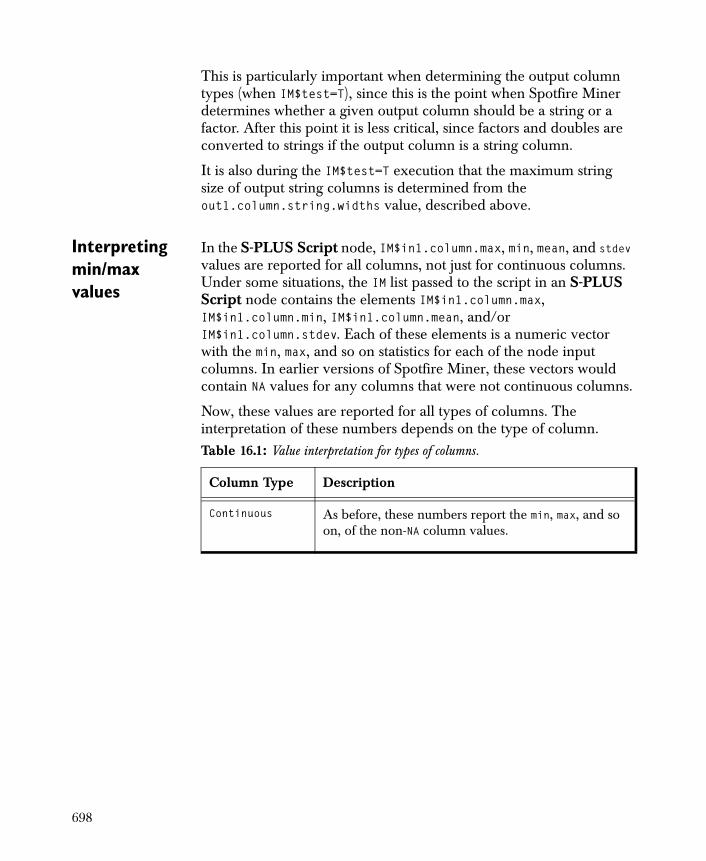
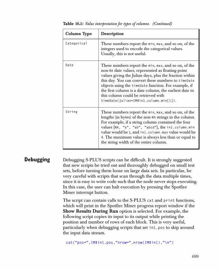
756
TIBCO Spotfire Miner ™ 8.2 User’s Guide November 2010 TIBCO Software Inc.


IMPORTANT INFORMATION
SOME TIBCO SOFTWARE EMBEDS OR BUNDLES OTHER TIBCO SOFTWARE. USE OF SUCH EMBEDDED OR BUNDLED TIBCO SOFTWARE IS SOLELY TO ENABLE THE FUNCTIONALITY (OR PROVIDE LIMITED ADD-ON FUNCTIONALITY) OF THE LICENSED TIBCO SOFTWARE. THE EMBEDDED OR BUNDLED SOFTWARE IS NOT LICENSED TO BE USED OR ACCESSED BY ANY OTHER TIBCO SOFTWARE OR FOR ANY OTHER PURPOSE.
USE OF TIBCO SOFTWARE AND THIS DOCUMENT IS SUBJECT TO THE TERMS AND CONDITIONS OF A LICENSE AGREEMENT FOUND IN EITHER A SEPARATELY EXECUTED SOFTWARE LICENSE AGREEMENT, OR, IF THERE IS NO SUCH SEPARATE AGREEMENT, THE CLICKWRAP END USER LICENSE AGREEMENT WHICH IS DISPLAYED DURING DOWNLOAD OR INSTALLATION OF THE SOFTWARE (AND WHICH IS DUPLICATED IN THE TIBCO SPOTFIRE MINER LICENSES). USE OF THIS DOCUMENT IS SUBJECT TO THOSE TERMS AND CONDITIONS, AND YOUR USE HEREOF SHALL CONSTITUTE ACCEPTANCE OF AND AN AGREEMENT TO BE BOUND BY THE SAME.
This document contains confidential information that is subject to U.S. and international copyright laws and treaties. No part of this document may be reproduced in any form without the written authorization of TIBCO Software Inc.
TIBCO Software Inc., TIBCO, Spotfire, TIBCO Spotfire Miner, TIBCO Spotfire S+, Insightful, the Insightful logo, the tagline "the Knowledge to Act," Insightful Miner, S+, S-PLUS, TIBCO Spotfire Axum, S+ArrayAnalyzer, S+EnvironmentalStats, S+FinMetrics, S+NuOpt, S+SeqTrial, S+SpatialStats, S+Wavelets, S-PLUS Graphlets, Graphlet, Spotfire S+ FlexBayes, Spotfire S+ Resample, TIBCO Spotfire S+ Server, TIBCO Spotfire Statistics Services, and TIBCO Spotfire Clinical Graphics are either registered trademarks or trademarks of TIBCO Software Inc. and/or subsidiaries of TIBCO Software Inc. in the United States and/or other countries. All other product and company names and marks mentioned in this document are the property of their respective owners and are mentioned for identification purposes only. This software may be available on
ii

multiple operating systems. However, not all operating system platforms for a specific software version are released at the same time. Please see the readme.txt file for the availability of this software version on a specific operating system platform.
THIS DOCUMENT IS PROVIDED “AS IS” WITHOUT WARRANTY OF ANY KIND, EITHER EXPRESS OR IMPLIED, INCLUDING, BUT NOT LIMITED TO, THE IMPLIED WARRANTIES OF MERCHANTABILITY, FITNESS FOR A PARTICULAR PURPOSE, OR NON-INFRINGEMENT. THIS DOCUMENT COULD INCLUDE TECHNICAL INACCURACIES OR TYPOGRAPHICAL ERRORS. CHANGES ARE PERIODICALLY ADDED TO THE INFORMATION HEREIN; THESE CHANGES WILL BE INCORPORATED IN NEW EDITIONS OF THIS DOCUMENT. TIBCO SOFTWARE INC. MAY MAKE IMPROVEMENTS AND/OR CHANGES IN THE PRODUCT(S) AND/OR THE PROGRAM(S) DESCRIBED IN THIS DOCUMENT AT ANY TIME.
Copyright © 1996-2010 TIBCO Software Inc. ALL RIGHTS RESERVED. THE CONTENTS OF THIS DOCUMENT MAY BE MODIFIED AND/OR QUALIFIED, DIRECTLY OR INDIRECTLY, BY OTHER DOCUMENTATION WHICH ACCOMPANIES THIS SOFTWARE, INCLUDING BUT NOT LIMITED TO ANY RELEASE NOTES AND "READ ME" FILES.
TIBCO Software Inc. Confidential Information
Reference The correct bibliographic reference for this document is as follows:
TIBCO Spotfire Miner™ 8.2 User’s Guide, TIBCO Software Inc.
Technical Support
For technical support, please visit http://spotfire.tibco.com/support and register for a support account.
iii

iv
Important Information ii
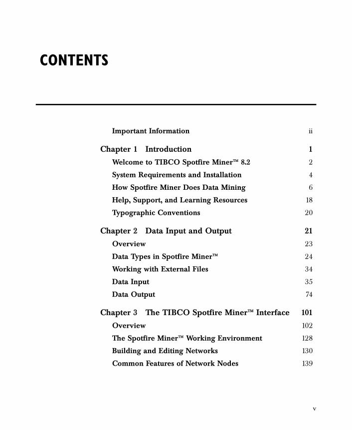
Chapter 1 Introduction 1
Welcome to TIBCO Spotfire Miner™ 8.2 2
System Requirements and Installation 4
How Spotfire Miner Does Data Mining 6
Help, Support, and Learning Resources 18
Typographic Conventions 20
Chapter 2 Data Input and Output 21
Overview 23
Data Types in Spotfire Miner™ 24
Working with External Files 34
Data Input 35
Data Output 74
Chapter 3 The TIBCO Spotfire Miner™ Interface 101
Overview 102
The Spotfire Miner™ Working Environment 128
Building and Editing Networks 130
Common Features of Network Nodes 139
CONTENTS
v
Contents
Chapter 4 Data Exploration 151
Overview 153
Creating One-Dimensional Charts 154
Computing Correlations and Covariances 170
Crosstabulating Categorical Data 176
Computing Descriptive Statistics 181
Comparing Data 184
Viewing Tables 188
Chapter 5 Data Cleaning 191
Overview 192
Missing Values 194
Duplicate Detection 200
Outlier Detection 208
Technical Details 218
References 223
Chapter 6 Data Manipulation 225
Overview 227
Manipulating Rows 228
Manipulating Columns 253
Using the Spotfire Miner™ Expression Language 285
Chapter 7 Classification Models 309
Overview 311
Logistic Regression Models 319
Classification Trees 344
Classification Neural Networks 362
Naive Bayes Models 383
References 393
vi
Contents
Chapter 8 Regression Models 395
Overview 396
Linear Regression Models 404
Regression Trees 426
Regression Neural Networks 441
References 456
Chapter 9 Clustering 457
Overview 458
The K-Means Component 461
Technical Details 468
K-Means Clustering Example 471
References 481
Chapter 10 Dimension Reduction 483
Overview 484
Principal Components 485
An Example Using Principal Components 490
Technical Details 493
Chapter 11 Association Rules 495
Overview 496
Association Rules Node Options 497
Definitions 501
Data Input Types 503
Groceries Example 505
Chapter 12 Survival 511
Introduction 512
Basic Survival Models Background 513
vii
Contents
A Banking Customer Churn Example 524
A Time Varying Covariates Example 527
Technical Details for Cox Regression Models 529
References 533
Chapter 13 Model Assessment 535
Overview 536
Assessing Classification Models 540
Assessing Regression Models 546
Chapter 14 Deploying Models 549
Overview 550
Predictive Modeling Markup Language 551
Export Report 556
Chapter 15 Advanced Topics 561
Overview 562
Pipeline Architecture 563
The Advanced Page 564
Notes on Data Blocks and Caching 568
Memory Intensive Functions 573
Size Recommendations for Spotfire Miner™ 575
Command Line Options 578
Increasing Java Memory 580
Importing and Exporting Data with JDBC 581
Chapter 16 The S-PLUS Library 587
Overview 589
S-PLUS Data Nodes 592
S-PLUS Chart Nodes 597
viii

Contents
S-PLUS Data Manipulation Nodes 667
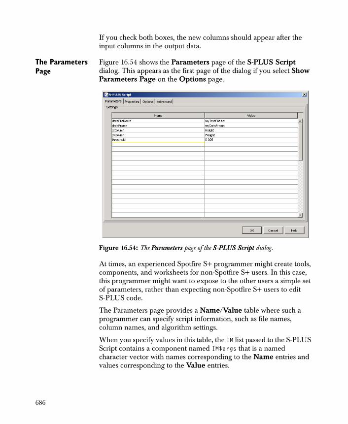
S-PLUS Script Node 677
References 716
Index 717
ix

Contents
x
Welcome to TIBCO Spotfire Miner™ 8.2 2
System Requirements and Installation 4
How Spotfire Miner Does Data Mining 6Define Goals 7Access Data 7Explore Data 10Model Data 13Deploy Model 15The Spotfire S+ Library 16
Help, Support, and Learning Resources 18Online Help 18Online Manuals 18Data Mining References 19
Typographic Conventions 20
INTRODUCTION 1
1

WELCOME TO TIBCO SPOTFIRE MINER™ 8.2
TIBCO Spotfire Miner™ 8.2 is the latest version of TIBCO Software Inc.’s data mining tool, one we believe makes data mining easier and more reliable than any other tool available today.
Spotfire Miner is a sophisticated yet easy-to-use data mining tool set that appeals to analysts in a broad range of data-intensive industries that must model customer behavior accurately, forecast business performance, or identify the controlling properties of their products and processes.
Spotfire Miner’s full lifecycle, data management, modeling, and deployment capabilities are useful for a wide variety of functions and industries. Spotfire Miner users include researchers, scientists, analysts, and academics. Some typical uses include optimizing customer relationships (CRM), building predictive models for finance, examining gene expression data in the biopharmaceutical industry, and optimizing processes in manufacturing, but there are many other applications in the commercial and public sectors.
Spotfire Miner is useful to researchers, engineers, and analysts seeking to model and improve their products, distribution channels, and supply chains against any measure of effectiveness, such as time-to-solution, long- or short-term profits, quality, and costs.
Key Features and Benefits of Spotfire Miner
Scale Models to Handle Data Growth
Spotfire Miner can mine very large data sets efficiently. Our methods for out-of-memory data analysis mean you can mine all your data, not just samples, now and far into the future.
Learn How to Use Spotfire Miner Quickly
Spotfire Miner requires no programming. The visual, icon-based networks support every step of the data mining process. The highly responsive interface adapts to the size of data you are processing.
Process Large Data Sets with More Accurate Results
Accessing the right data, cleaning the data, and preparing the data for analysis is where much of the work occurs in data mining. Spotfire Miner’s dedicated features can make this labor-intensive process fun.
2

Using Spotfire Miner, you can explore patterns or reveal data quality problems with its visualizers, while its robust methods for outlier detection spot the value hidden in rare events.
Spotfire Miner offers methods for repairing missing or illegal data values more precisely.
Spotfire Miner can handle data manipulation and transformation problems from the routine to the tricky using built-in components or,
in conjunction with Spotfire S+®, advanced functions in the S-PLUS language.
Build Models with Enhanced Predictive Power
While other vendors offer only “black-box” solutions that approximate the business problem, our comprehensive set of data mining algorithms can be tailored to your specific needs. Spotfire Miner is also extensible so it supports your custom analytics and reports.
Dedicated graphs and reports help you evaluate and compare quickly the performance of multiple models to ensure your predictions are as accurate as possible. We have also tested the models to ensure that they hold up under the stresses of deployment by employing robust analytic methods that effectively handle data quality variations often seen in “real” production environments.
3
SYSTEM REQUIREMENTS AND INSTALLATION
Spotfire Miner is supported on the Windows platforms. The system requirements and general installation instructions are provided below.
• Windows 7® (32-bit and 64-bit)
• Windows® Vista SP2 (32-bit and 64-bit)
• Windows XP® SP3 (32-bit)
The minimum recommended system configuration for running the server is as follows:
• One (or more) 1 Ghz processors
• A minimum of 1 GB of RAM
• Approximately 1GB space reserved for the system swap file.
• At least 500 MB free disk space (plus 50 MB of free disk space for the typical installation if you are not installing on C:\).
• An SVGA or better graphics card and monitor.
To install Spotfire Miner, from the installation media, double-click the INSTALL.TXT file. Follow the step-by-step installation instructions.
After you install Spotfire Miner, on the Microsoft Windows task bar, click the Start � Programs � TIBCO � Spotfire Miner 8.2 program group. This program group contains the following options:
• TIBCO Spotfire Miner launches the Spotfire Miner application.
• TIBCO Spotfire Miner Help displays the help system.
• TIBCO Spotfire Miner Release Notes displays the release notes.
To start Spotfire Miner:
• From the Start menu, choose Programs � TIBCO � Spotfire Miner 8.2 � TIBCO Spotfire Miner.
4

• Double-click the TIBCO Spotfire Miner 8.2 shortcut icon on your desktop (added by default during installation).
5
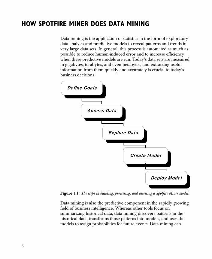
HOW SPOTFIRE MINER DOES DATA MINING
Data mining is the application of statistics in the form of exploratory data analysis and predictive models to reveal patterns and trends in very large data sets. In general, this process is automated as much as possible to reduce human-induced error and to increase efficiency when these predictive models are run. Today’s data sets are measured in gigabytes, terabytes, and even petabytes, and extracting useful information from them quickly and accurately is crucial to today’s business decisions.
Data mining is also the predictive component in the rapidly growing field of business intelligence. Whereas other tools focus on summarizing historical data, data mining discovers patterns in the historical data, transforms those patterns into models, and uses the models to assign probabilities for future events. Data mining can
Figure 1.1: The steps in building, processing, and assessing a Spotfire Miner model.
Define Goals
Access Data
Explore Data
Create Model
Deploy Model
6

answer questions such as “What are expected sales by region next year?” or “Which current customers are likely to respond to future mailings?”
There are five steps involved in the building, creation, and assessment of a Spotfire Miner model, as shown in Figure 1.1. A key advantage to using Spotfire Miner is that all components required to perform these steps are readily available without having to go outside the product.
Define Goals This is a key step, because it begins with the end in mind: What information do you want from Spotfire Miner? Keeping this goal in mind drives the model you create and run in Spotfire Miner, and the more specific the goal, the better you can implement a Spotfire Miner model to realize it.
Let’s say you work in sales for a telephone company, and you want to determine which customers to target for advertising a new long-distance international service. You can create a model in Spotfire Miner that filters your customer database for those who make long-distance calls to specific countries. Based on the number of phone calls made, when they were made, and the length of each phone call, you can use this information to optimize the pricing structure for the new service. Then you can run a predictive model that determines the probability that an existing customer will order this new service, and you can deploy the model by targeting those specific customers for your advertising campaign. You save advertising dollars by limiting the advertising circulation and increasing the likelihood that those to whom you send the advertising will respond.
Access Data Once you have defined your goals, the next step is to access the data you plan to process in your model. Using Spotfire Miner, you can input data from several different sources. See Chapter 2 for more detailed information about the possible input data sources.
7
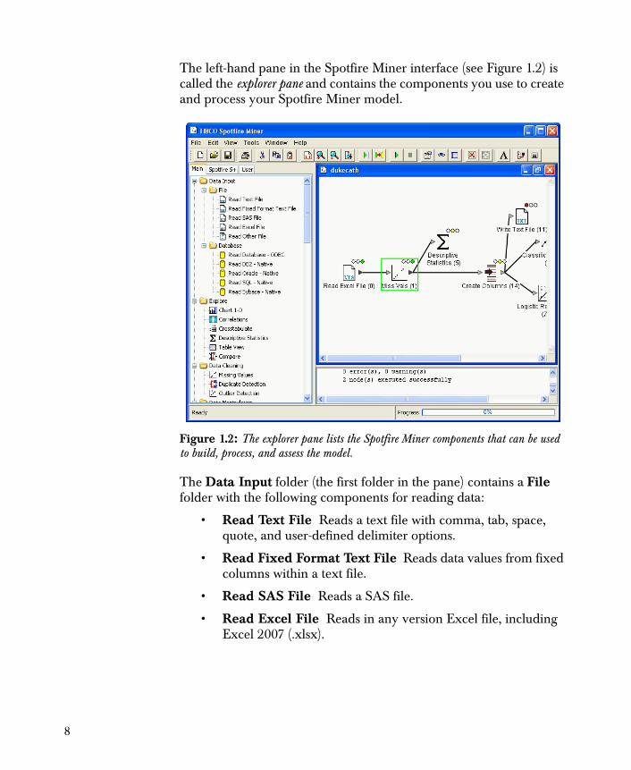
The left-hand pane in the Spotfire Miner interface (see Figure 1.2) is called the explorer pane and contains the components you use to create and process your Spotfire Miner model.
The Data Input folder (the first folder in the pane) contains a File folder with the following components for reading data:
• Read Text File Reads a text file with comma, tab, space, quote, and user-defined delimiter options.
• Read Fixed Format Text File Reads data values from fixed columns within a text file.
• Read SAS File Reads a SAS file.
• Read Excel File Reads in any version Excel file, including Excel 2007 (.xlsx).
Figure 1.2: The explorer pane lists the Spotfire Miner components that can be used to build, process, and assess the model.
8
• Read Other File Reads a file in another format, such as
Microsoft Access® 2000 or 2007, Gauss, or SPSS.
Spotfire Miner also features several native databases drivers in the Database folder. You can import tables from any of the following databases:
• Read Database - ODBC
• Read DB2 - Native
• Read Oracle - Native
• Read SQL - Native
• Read Sybase - Native
You can also write to these data formats by using the components in the Data Output folder:
• Write Text File Writes a text file with comma, tab, space, quote, and user-defined delimiter options.
• Write Fixed Format Text File Creates fixed format text files of your data.
• Write SAS File Writes a SAS file.
• Write Other File Writes a file in another format, such as
Microsoft Access® 2000 or 2007, Gauss, or SPSS.
Note
Microsoft Access 1997 is no longer supported as of Spotfire Miner 8.1
Note
As of Spotfire Miner version 8.2, native database drivers are deprecated. In lieu of these drivers, you should use JDBC/ODBC drivers for all supported database vendors.
9

• Write Excel File Writes any version Microsoft Excel® file, including Excel 2007 (xlsx).
You can also export to database tables in any of the following:
• Write Database - ODBC
• Write DB2 - Native
• Write Oracle - Native
• Write SQL - Native
• Write Sybase - Native
Explore Data Understanding your data is critical to building effective models because it affects how you prepare a suitable data set for modeling in Spotfire Miner. You might want to merge tables from two distinct sources that have different names for the same variables; for example, the variable Male might be represented by "M" in one table and "X" in another. Perhaps you have a data set where you want to convert a column of continuous data ("1" and "2") to categorical data ("yes" and "no") to be consistent with all your other data sets. Knowing these differences exist helps you determine how to modify your data set prior to modeling it in Spotfire Miner.
Spotfire Miner contains several components to help you prepare your data.
The Explore folder provides the following components for displaying and summarizing data to help you decide if these data should be used in your model:
Note
Microsoft Access 1997 is no longer supported as of Spotfire Miner 8.1
Note
As of Spotfire Miner version 8.2, native database drivers are deprecated. In lieu of these drivers, you should use JDBC/ODBC drivers for all supported database vendors.
10
• Chart 1-D Creates basic one-dimensional charts of the variables in your data set.
• Correlations Computes correlations and covariances for pairs of variables in your data set and displays the results in a scrollable grid.
• Crosstabulate Produces tables of counts for various combinations of levels in categorical variables.
• Descriptive Statistics Computes basic descriptive statistics for the variables in your data set and displays them with one-dimensional charts.
• Table View Displays your data set in a tabular format.
• Compare Compares two nodes and displays statistics on each, including the union, intersection, logical, absolute and relative differences, with user-specified tolerances.
The Data Cleaning folder contains components for handling missing values and providing outlier detection:
• Missing Values Handles missing values in your data set by dropping rows, or it can generate values from a distribution, the mean of the data, or a constant.
• Duplicate Detection Provides a method of detecting row duplicates in a rectangular data set.
• Outlier Detection Provides you with a reliable method of detecting multidimensional outliers in your data set.
Each of these components performs a specific function in Spotfire Miner. For example, using the Table View component, you can quickly determine if several of the columns appear to be constant for all rows in a data set. You can then use the Descriptive Statistics component to verify if they are indeed constant or only appear to be. The Correlations component can be used to detect correlation (equal or close to one) or nonpredictive variables (close to zero), which should be eliminated prior to modeling.
Select and Transform Variables
Now that you’ve selected and prepared your data set, the next step is to transform it, if necessary. You might need to recode columns, filter rows that aren’t predictive or useful to the analysis, or split existing
11
columns into new columns. Typically, 60%-80% of the time you spend in data mining is spent iterating in the “Prepare Data” and “Select and Transform Variables” steps.
In Spotfire Miner, you can perform a variety of processes to manipulate rows or columns: sorting, filtering, and splitting are examples of how you can transform your data set.
The complete list of components used in this step can be found in the Data Manipulation folder in the explorer pane.
The Rows folder contains:
• Aggregate Condenses the information in your data set by applying descriptive statistics according to one or more categorical or continuous columns.
• Append Creates a new data set by combining the rows of two or more other data sets.
• Filter Rows Selects or excludes rows of your data set using the Spotfire Miner expression language.
• Partition Randomly samples the rows of your data set and separates them into subsets.
• Sample Samples the rows of your data set to create a subset.
• Shuffle Randomly shuffles the rows of your data set.
• Sort Reorders the rows of your data set based on the values in selected columns.
• Split Divides a data set into two parts using the Spotfire Miner expression language by either including or excluding particular rows.
• Stack Combines separate columns of a data set into a single column.
• Unstack Splits a single column into multiple columns based on a grouping column.
The Columns folder contains:
• Bin Creates new categorical variables from numeric (continuous) variables or redefines existing categorical variables by renaming or combining groups.
12
• Create Columns Computes an additional variable using the Spotfire Miner expression language and appends it as a column to your data set.
• Filter Columns Excludes columns that are not needed in your analysis.
• Join Creates a new data set by combining the columns of two or more other data sets.
• Modify Columns Filters and renames the columns of your data set. Also, you can set the type and role of the columns.
• Transpose Swaps rows for columns in a node.
• Normalize Adjusts the scale of numeric columns to make columns more comparable.
• Reorder Columns Changes the order of the columns in the output.
All of the components listed above can be further classified into one of the following three categories:
1. Transformations Includes Bin, Create Columns, Aggregate, and other components that generate new data, whether the new data are based on a transformation of variables in the original data or are the result of a computational process.
2. SQL-like manipulations Includes Filter Columns, Sort, Append, Join, Reorder Columns and other functions that do not generate new data but instead manipulate existing data.
3. Sampling operations Includes Sample and Partition, which sample the data and use the subset for data manipulation.
These components allow you to transform your data without having to process it outside Spotfire Miner, which can save a tremendous amount of processing time.
Model Data Now that the data have been read in, cleaned, and transformed (if necessary), you are ready to build a model. The goal is to build a model so you can compare the results you get from processing your data set iteratively with different techniques and then to optimize the performance in the final model. It’s common to iterate within this phase, modifying variables and building successively more powerful
13
models as you gain more knowledge of the data. Changing these variables might require returning to the “Prepare Data” or “Select and Transform Variables” steps if you discover further processing is required. For instance, building a model might cause you to consider transforming an income column to a different scale or binning a continuous variable.
Figure 1.2 shows an example of two components used to evaluate a classification problem: Logistic Regression and Classification Tree. The model is processed and the results confirmed in the next step, “Validate Model.”
The components used in this step can be found in the Model folder.
The Classification folder contains:
• Logistic Regression A variation of ordinary regression used when the observed outcome is restricted to two values.
• Classification Tree Uses recursive partitioning algorithms to define a set of rules to predict the class of a dependent categorical variable as a function of the independent variables.
• Classification Neural Network Produces a formula that predicts the class of a dependent categorical variable as a function of the independent variables.
• Naive Bayes Predicts the class of a dependent categorical variable as a function of the independent variables.
The Regression folder contains:
• Linear Regression Models the relationship between the dependent and independent variables by fitting a linear equation.
• Regression Tree Uses recursive partitioning algorithms to define a set of rules to predict the value of a continuous dependent variable as a function of the independent variables.
• Regression Neural Network Produces a formula that predicts the value of a continuous dependent variable as a function of the independent variables.
The Clustering folder contains:
14
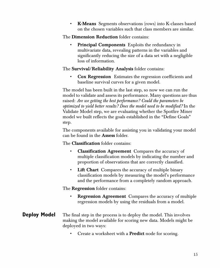
• K-Means Segments observations (rows) into K-classes based on the chosen variables such that class members are similar.
The Dimension Reduction folder contains:
• Principal Components Exploits the redundancy in multivariate data, revealing patterns in the variables and significantly reducing the size of a data set with a negligible loss of information.
The Survival/Reliability Analysis folder contains:
• Cox Regression Estimates the regression coefficients and baseline survival curves for a given model.
The model has been built in the last step, so now we can run the model to validate and assess its performance. Many questions are thus raised: Are we getting the best performance? Could the parameters be optimized to yield better results? Does the model need to be modified? In the Validate Model step, we are evaluating whether the Spotfire Miner model we built reflects the goals established in the “Define Goals” step.
The components available for assisting you in validating your model can be found in the Assess folder.
The Classification folder contains:
• Classification Agreement Compares the accuracy of multiple classification models by indicating the number and proportion of observations that are correctly classified.
• Lift Chart Compares the accuracy of multiple binary classification models by measuring the model’s performance and the performance from a completely random approach.
The Regression folder contains:
• Regression Agreement Compares the accuracy of multiple regression models by using the residuals from a model.
Deploy Model The final step in the process is to deploy the model. This involves making the model available for scoring new data. Models might be deployed in two ways:
• Create a worksheet with a Predict node for scoring.
15
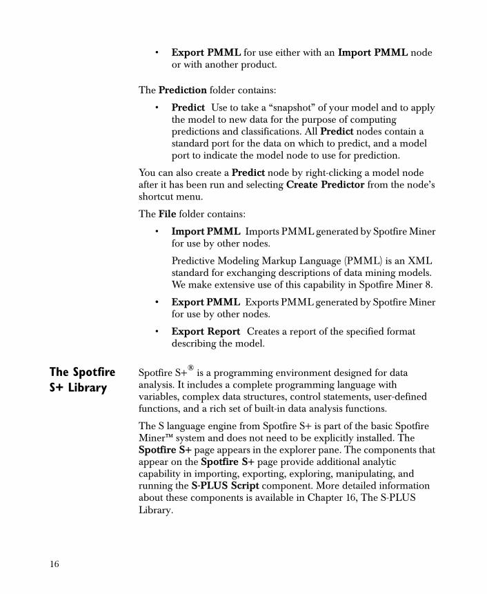
• Export PMML for use either with an Import PMML node or with another product.
The Prediction folder contains:
• Predict Use to take a “snapshot” of your model and to apply the model to new data for the purpose of computing predictions and classifications. All Predict nodes contain a standard port for the data on which to predict, and a model port to indicate the model node to use for prediction.
You can also create a Predict node by right-clicking a model node after it has been run and selecting Create Predictor from the node’s shortcut menu.
The File folder contains:
• Import PMML Imports PMML generated by Spotfire Miner for use by other nodes.
Predictive Modeling Markup Language (PMML) is an XML standard for exchanging descriptions of data mining models. We make extensive use of this capability in Spotfire Miner 8.
• Export PMML Exports PMML generated by Spotfire Miner for use by other nodes.
• Export Report Creates a report of the specified format describing the model.
The Spotfire S+ Library
Spotfire S+® is a programming environment designed for data analysis. It includes a complete programming language with variables, complex data structures, control statements, user-defined functions, and a rich set of built-in data analysis functions.
The S language engine from Spotfire S+ is part of the basic Spotfire Miner™ system and does not need to be explicitly installed. The Spotfire S+ page appears in the explorer pane. The components that appear on the Spotfire S+ page provide additional analytic capability in importing, exporting, exploring, manipulating, and running the S-PLUS Script component. More detailed information about these components is available in Chapter 16, The S-PLUS Library.
16

Note
Spotfire Miner works only with the included Spotfire S+ libraries and S language engine; you cannot use an externally-installed version of Spotfire S+ with Spotfire Miner.
17

HELP, SUPPORT, AND LEARNING RESOURCES
There are a variety of ways to accelerate your progress with Spotfire Miner. This section describes the learning and support resources available to you.
Online Help Spotfire Miner offers an online help system to make learning and using Spotfire Miner easier. The help system is based on Microsoft HTML Help, the current standard for Windows software products. For complete details on how to use the help system, see the help topic entitled Using the Help System.
Context-sensitive help is also available by clicking the Help buttons in the various dialogs and by right-clicking network nodes.
Online Manuals This User’s Guide as well as the Getting Started Guide are available online through the main Help menu. The Getting Started Guide is particularly useful because it provides both a quick tour of the product and a more extensive tutorial introduction.
The Installation and Administration Guide is available at the top level of the Spotfire Miner CD distribution.
18
Data Mining References
General Data Mining
Berry, Michael J.A. and Linoff, Gordon (2000). Mastering Data Mining: The Art and Science of Customer Relationship Management. Wiley Computer Pub., New York.
Bishop, Christopher M. (1995). Neural Networks for Pattern Recognition. Clarendon Press, Oxford; Oxford University Press, New York.
Cios, Krzysztof J., editor (2000). Medical Data Mining and Knowledge Discovery. Physica-Verlag, New York.
Han, Jiawei and Kamber, Micheline (2001). Data Mining: Concepts and Techniques. Morgan Kaufmann Publishers, San Francisco.
Hastie, Trevor; Tibshirani, Robert; and Friedman, Jerome (2001). The Elements of Statistical Learning: Data Mining, Inference, and Prediction. Springer, New York.
Pyle, Dorian (1999). Data Preparation for Data Mining. Morgan Kaufmann Publishers, San Francisco.
Rud, Olivia Parr (2001). Data Mining Cookbook: Modeling Data for Marketing, Risk, and Customer Relationship Management. Wiley, New York.
Witten, Ian H. and Frank, Eibe (2000). Data Mining: Practical Machine Learning Tools and Techniques with Java Implementations. Morgan Kaufmann, San Francisco.
Statistical Models Used in Data Mining
Breiman, Leo; Friedman, Jerome; Olshen, Richard A.; and Stone, Charles (1984). Classification and Regression Trees. Wadsworth International Group, Belmont, California.
McCullagh, P. and Nelder, J.A. (1999). Generalized Linear Models, 2nd ed. Chapman & Hall, Boca Raton, Florida.
Reed, Russell D. and Marks II, Robert J. (1999). Neural Smithing: Supervised Learning in Feedforward Artificial Neural Networks. The MIT Press, Cambridge, Massachusetts.
Ripley, B.D. (1996). Pattern Recognition and Neural Networks. Cambridge University Press, New York.
Venables, W.N. and Ripley, B.D. (1999). Modern Applied Statistics With S-PLUS, 3rd ed. Springer, New York.
19

TYPOGRAPHIC CONVENTIONS
Throughout this User’s Guide, the following typographic conventions are used:
• This font is used for variable names, code samples, and programming language expressions.
• This font is used for elements of the Spotfire Miner user interface, for operating system files and commands, and for user input in dialog fields.
• This font is used for emphasis and book titles.
• CAP/SMALLCAP letters are used for key names. For example, the Shift key appears as SHIFT.
• When more than one key must be pressed simultaneously, the two key names appear with a hyphen (-) between them. For example, the key combination of SHIFT and F1 appears as SHIFT-F1.
• Menu selections are shown in an abbreviated form using the arrow symbol (�) to indicate a selection within a menu, as in File � New.
20
Overview 23
Data Types in Spotfire Miner™ 24Categorical Data 24Strings 24Dates 26
Working with External Files 34Reading External Files and Databases 34Using Absolute and Relative Paths 34
Data Input 35Read Text File 35Read Fixed Format Text File 40Read Spotfire Data 44Read SAS File 47Read Excel File 50Read Other File 53Read Database ODBC 56Read DB2 Native 61Read Oracle Native 63Read SQL Native 67Read Sybase Native 70Read Database JDBC 72
Data Output 74Write Text File 74Write Fixed Format Text File 77Write SAS File 79Write Spotfire Data 81Write Excel File 82Write Other File 83Write Database ODBC 86
DATA INPUT AND OUTPUT 2
21

Write DB2 Native 89Write Oracle Native 91Write SQL Native 94Write Sybase Native 97Write Database JDBC 99
22

OVERVIEW
All Spotfire Miner™ networks need to have some way for data to enter the pipeline and some way for results to come out. These tasks are easily accomplished with Spotfire Miner’s data input and data output components, the focus of this chapter.
Because Spotfire Miner works seamlessly with the software you already use, you can import data from and export data to many sources, including spreadsheets such as Excel and Lotus, databases such as DB2, and analytical software such as SAS and SPSS.
In the sections that follow, we first offer some general information that applies to all of Spotfire Miner’s input and output components and then explore each component in detail.
23
DATA TYPES IN SPOTFIRE MINER™
Spotfire Miner supports four distinct data types:
• Categorical
• Continuous
• String
• Date
In this section, we offer some tips for working with categorical and string data and then present a more detailed discussion of dates.
Categorical Data
A categorical column can only support up to a fixed number of different string values. The default is 500 levels but you can change this setting in the Worksheet Properties dialog. If more than this number of distinct levels is read, the values are read as missing values and a warning is printed. If a categorical column runs over the 500-level limit, this is usually a sign that it should be read in and processed as a string column.
By default, columns with numeric values are read as continuous columns, and columns with nonnumeric characters are read as string columns. String columns are best used for storing identifying information that is typically different for each row and which is not used in modeling. Often we want to use nonnumeric columns as categorical (nominal) columns, so we need to read these columns as categorical columns rather than string columns.
Strings Each string column has a fixed size that determines the longest string that can be stored in the column. The default size for string columns is specified in the Worksheet Properties dialog (initially set to 32 characters). The data input (or Read) nodes attempt to detect the maximum string length for each string column, and set the string column width accordingly. If a Read data input node reads a longer string, it truncates the string, and generates a warning message. In this case, you can explicitly set the string column width for selected columns on the Modify Columns page of the properties dialogs for the data input components.
24
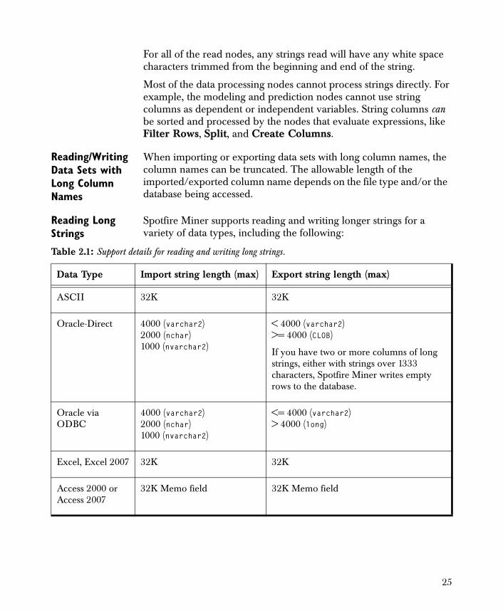
For all of the read nodes, any strings read will have any white space characters trimmed from the beginning and end of the string.
Most of the data processing nodes cannot process strings directly. For example, the modeling and prediction nodes cannot use string columns as dependent or independent variables. String columns can be sorted and processed by the nodes that evaluate expressions, like Filter Rows, Split, and Create Columns.
Reading/Writing Data Sets with Long Column Names
When importing or exporting data sets with long column names, the column names can be truncated. The allowable length of the imported/exported column name depends on the file type and/or the database being accessed.
Reading Long Strings
Spotfire Miner supports reading and writing longer strings for a variety of data types, including the following:
Table 2.1: Support details for reading and writing long strings.
Data Type Import string length (max) Export string length (max)
ASCII 32K 32K
Oracle-Direct 4000 (varchar2) 2000 (nchar) 1000 (nvarchar2)
< 4000 (varchar2)>= 4000 (CLOB)
If you have two or more columns of long strings, either with strings over 1333 characters, Spotfire Miner writes empty rows to the database.
Oracle via ODBC
4000 (varchar2) 2000 (nchar) 1000 (nvarchar2)
<= 4000 (varchar2)> 4000 (long)
Excel, Excel 2007 32K 32K
Access 2000 or Access 2007
32K Memo field 32K Memo field
25
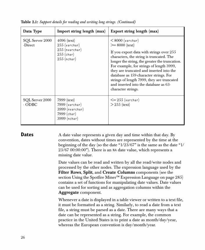
Dates A date value represents a given day and time within that day. By convention, dates without times are represented by the time at the beginning of the day (so the date “1/23/67” is the same as the date “1/23/67 00:00:00”). There is an NA date value, which represents a missing date value.
Date values can be read and written by all the read/write nodes and processed by the other nodes. The expression language used by the Filter Rows, Split, and Create Columns components (see the section Using the Spotfire Miner™ Expression Language on page 285) contains a set of functions for manipulating date values. Date values can be used for sorting and as aggregation columns within the Aggregate component.
Whenever a date is displayed in a table viewer or written to a text file, it must be formatted as a string. Similarly, to read a date from a text file, a string must be parsed as a date. There are many ways that a date can be represented as a string. For example, the common practice in the United States is to print a date as month/day/year, whereas the European convention is day/month/year.
SQL Server 2000 -Direct
4096 (text)255 (varchar)255 (nvarchar)255 (char)255 (nchar)
< 8000 (varchar)>= 8000 (text)
If you export data with strings over 255 characters, the string is truncated. The longer the string, the greater the truncation. For example, for strings of length 3999, they are truncated and inserted into the database as 159-character strings. For strings of length 7999, they are truncated and inserted into the database as 63-character strings.
SQL Server 2000 - ODBC
7999 (text)7999 (varchar)3999 (nvarchar)7999 (char)3999 (nchar)
<= 255 (varchar)> 255 (text)
Table 2.1: Support details for reading and writing long strings. (Continued)
Data Type Import string length (max) Export string length (max)
26
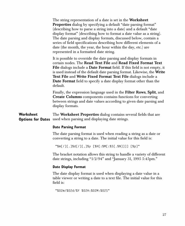
The string representation of a date is set in the Worksheet Properties dialog by specifying a default “date parsing format” (describing how to parse a string into a date) and a default “date display format” (describing how to format a date value as a string). The date parsing and display formats, discussed below, contain a series of field specifications describing how different elements of a date (the month, the year, the hour within the day, etc.) are represented in a formatted date string.
It is possible to override the date parsing and display formats in certain nodes. The Read Text File and Read Fixed Format Text File dialogs include a Date Format field. If this field is not empty, it is used instead of the default date parsing format. Likewise, the Write Text File and Write Fixed Format Text File dialogs include a Date Format field to specify a date display format other than the default.
Finally, the expression language used in the Filter Rows, Split, and Create Columns components contains functions for converting between strings and date values according to given date parsing and display formats.
Worksheet Options for Dates
The Worksheet Properties dialog contains several fields that are used when parsing and displaying date strings.
Date Parsing Format
The date parsing format is used when reading a string as a date or converting a string to a date. The initial value for this field is:
"%m[/][.]%d[/][,]%y [%H[:%M[:%S[.%N]]]] [%p]"
The bracket notation allows this string to handle a variety of different date strings, including “1/2/94” and “January 31, 1995 5:45pm.”
Date Display Format
The date display format is used when displaying a date value in a table viewer or writing a date to a text file. The initial value for this field is:
"%02m/%02d/%Y %02H:%02M:%02S"
27
This produces a simple string with the day represented by three numbers and the time within the day on the 24-hour clock, such as “01/31/1995 17:45:00.”
Date Century Cutoff
This field value is used when parsing and formatting two-digit years. Its value is a year number beginning a 100-year sequence. When parsing a two-digit year, it is interpreted as a year within that 100-year range. For example, if the century cutoff is 1930, the two-digit year “40” would be interpreted as 1940, and “20” would be interpreted as 2020. The initial value of this field is 1950.
Date Parsing Formats
Date parsing formats are used to convert character strings to date values. If the entire input string is not matched by the parsing format string or if the resulting time or date is not valid, an NA value will be read. (To skip characters in a string, use %c or %w.)
A date parsing format might contain any of the following parsing specifications:
* Anything not in this list matches itself explicitly.
%c Any single character, which is skipped. This is primarily useful for skipping things like days of the week, which if abbreviated could be skipped by %3c (see also %w), and for skipping the rest of the string, %$c.
%d Input day within month as integer.
%H Input hour as integer.
%m Input month, as integer or as alpha string (for example, January). If an alpha string, case does not matter, and any substring of a month that distinguishes it from the other months will be accepted (for example, Jan).
%M Input minute as integer.
%n Input milliseconds as integer, without considering field width as in %N.
%N Input milliseconds as integer. A field width (either given explicitly or inferred from input string) of 1 or 2 will cause input of 10ths or 100ths of a second instead, as if the digits were following a period. Field widths greater than 3 are likely to result in illegal input.
28
%p Input string am or pm, with matching as for months. If pm is given and hour is before 13, the time is bumped into the afternoon. If am is given and hour is 12, the time is bumped into the morning. Note that this only modifies previously parsed hours.
%S Input seconds as integer.
%w A whitespace-delimited word, which is skipped. Note there is no width or delimiter specification for this; if this is desired, use %c.
%y Input year as integer. If less than 100, the Date Century Cutoff field in the Worksheet Properties dialog is used to determine the actual year.
%Y Input year as integer, without considering the century.
%Z Time zone string. Accepts a whitespace-delimited word unless another delimiter or width is specified. (Currently not supported.)
%(digits)(char) If there are one or more digits between a % and the specification character, these are parsed as an integer and specify the field width to be used. The following (digits) characters are scanned for the specified item.
%:(delim)(char) If there is a colon and any single character between a % and the specification character, the field is taken to be all the characters up to but not including the given delimiter character. The delimiter itself is not scanned or skipped by the format.
%$(char) If there is a $ between a % and a specification character, the field goes to the end of the input string.
whitespace Whitespace (spaces, tabs, carriage returns, etc.) is ignored in the input format string. In the string being parsed, any amount of whitespace can appear between elements of the date/time. Thus, the parsing format %H:%M: %S will parse 5: 6:45.
[...] Specify optional specification. Text and specifications within the brackets might optionally be included. This does not support fancy backtracking between multiple optional specs.
29
%%,%[,%] The %, [, and ] characters, which must be matched.
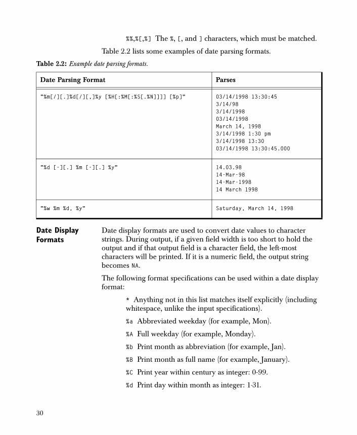
Table 2.2 lists some examples of date parsing formats.
Date Display Formats
Date display formats are used to convert date values to character strings. During output, if a given field width is too short to hold the output and if that output field is a character field, the left-most characters will be printed. If it is a numeric field, the output string becomes NA.
The following format specifications can be used within a date display format:
* Anything not in this list matches itself explicitly (including whitespace, unlike the input specifications).
%a Abbreviated weekday (for example, Mon).
%A Full weekday (for example, Monday).
%b Print month as abbreviation (for example, Jan).
%B Print month as full name (for example, January).
%C Print year within century as integer: 0-99.
%d Print day within month as integer: 1-31.
Table 2.2: Example date parsing formats.
Date Parsing Format Parses
"%m[/][.]%d[/][,]%y [%H[:%M[:%S[.%N]]]] [%p]" 03/14/1998 13:30:453/14/983/14/199803/14/1998March 14, 19983/14/1998 1:30 pm3/14/1998 13:3003/14/1998 13:30:45.000
"%d [-][.] %m [-][.] %y" 14.03.9814-Mar-9814-Mar-199814 March 1998
"%w %m %d, %y" Saturday, March 14, 1998
30
%D Print day within year as integer: 1-366.
%H Hour (24-hour clock) as integer: 0-23.
%I Hour (12-hour clock) as integer: 1-12.
%m Print month as integer: 1-12.
%M Minutes as integer: 0-59.
%N Milliseconds as integer. It is a good idea to pad with zeros if this is after a decimal point! A width of less than 3 will cause printing of 10ths or 100ths of a second instead: 0-999.
%p Insert am or pm.
%q Quarter of the year, as integer: 1-4.
%Q Quarter of the year, as Roman numeral: I-IV.
%S Seconds as integer: 0-59 (60 for leap second).
%y Print year as two-digit integer. The Date Century Cutoff field in the Worksheet Properties dialog is used to determine the actual year.
%Y Print full year as integer (see also %C).
%Z Print the time zone. (Currently not supported.)
%z Print the time zone, using different time zone names depending on whether the date is in daylight savings time. (Currently not supported.)
%% The % character.
%(digits)(char) If there are one or more digits between % and the specification character, these are parsed as an integer and specify the field width to be used. The value is printed, right-justified using (digits) characters. If (digits) begins with zero, the field is left-padded with zeros if it is a numeric field; otherwise, it is left-padded with spaces. If a numeric value is too long for the field width, the field is replaced with asterisk (*) characters to indicate overflow; character strings can be abbreviated by specifying short fields.
31
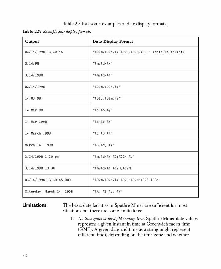
Table 2.3 lists some examples of date display formats.
Limitations The basic date facilities in Spotfire Miner are sufficient for most situations but there are some limitations:
1. No time zones or daylight savings time. Spotfire Miner date values represent a given instant in time at Greenwich mean time (GMT). A given date and time as a string might represent different times, depending on the time zone and whether
Table 2.3: Example date display formats.
Output Date Display Format
03/14/1998 13:30:45 "%02m/%02d/%Y %02H:%02M:%02S" (default format)
3/14/98 "%m/%d/%y"
3/14/1998 "%m/%d/%Y"
03/14/1998 "%02m/%02d/%Y"
14.03.98 "%02d.%02m.%y"
14-Mar-98 "%d-%b-%y"
14-Mar-1998 "%d-%b-%Y"
14 March 1998 "%d %B %Y"
March 14, 1998 "%B %d, %Y"
3/14/1998 1:30 pm "%m/%d/%Y %I:%02M %p"
3/14/1998 13:30 "%m/%d/%Y %02H:%02M"
03/14/1998 13:30:45.000 "%02m/%02d/%Y %02H:%02M:%02S.%03N"
Saturday, March 14, 1998 "%A, %B %d, %Y"
32

daylight savings time is in effect for the given date. The basic Spotfire Miner facilities assume that all date strings represent times in GMT.
2. English-only month and weekday names. Date parsing and formatting in Spotfire Miner use the English month names ( January, February, etc.) and weekday names (Monday, Tuesday, etc.).
3. No holiday functions. When processing dates, sometimes it is useful to determine whether a given day is a holiday in a given country. The basic date facilities in Spotfire Miner do not include functions for determining whether a given date is a holiday.
33
WORKING WITH EXTERNAL FILES
Reading External Files and Databases
The data input nodes do not detect when the external file or database being read has changed. For example, suppose you run a network in your worksheet that contains a Read Text File node and then change the values in the text file. If you run the network again, a cached copy of the original data set is used and the new version of the file is not read in. To force the new data in the file to be read, first invalidate the Read Text File node and then rerun the network.
Using Absolute and Relative Paths
Most of the properties dialogs for the data input and output components have a File Name field for specifying the path name of the file to be read or written. If the file name starts with a drive letter or double slash, it is an absolute file path. For example, C:\temp.txt or \\servername\department\temp.txt are absolute file paths. These identify a particular file on your computer. If you copy your Spotfire Miner worksheet file to another computer, these file paths might not exist.
If a file name is not an absolute file path, it is interpreted as a relative file path. Such a file name is interpreted relative to the Default File Directory specified in the Worksheet Properties dialog. If this is empty (the default), it uses the location of the Spotfire Miner worksheet data directory for the worksheet containing the data input or output node. For example, suppose that the default file directory is empty, and the worksheet data directory is e:\miner\test.wsd. If a Read Text File node on this worksheet specifies a file name of temp.txt, it is interpreted as e:\miner\temp.txt. A relative file path of devel\temp.txt is interpreted as e:\miner\devel\temp.txt. Using relative file paths is a good way to make your worksheet data directory and related data files easily transportable.
Hint
When you select a file by clicking the Browse button next to the File Name field and navigating to a file location, the file’s absolute file path is stored in the File Name field. To convert an absolute file name into a relative file name, simply edit the name in the File Name field.
34
DATA INPUT
Spotfire Miner provides the following data input components:
• Read Text File
• Read Fixed Format Text File
• Read SAS File
• Read Excel File
• Read Other File
In addition, the following database nodes are available:
• Read Database - ODBC
• Read DB2 - Native
• Read Oracle - Native
• Read SQL Server - Native
• Read Sybase - Native
• Read Database - JDBC
In this section, we discuss each component in turn.
Read Text File Use the Read Text File component to specify a data set for your analysis. Spotfire Miner reads the data from the designated text file according to the options you specify.
Spotfire Miner supports reading and writing long text strings for specific file and database types. See Table 2.1 for more information.
General Procedure
The following outlines the general approach for using the Read Text File component:
1. Click and drag a Read Text File component from the explorer pane and drop it on your worksheet.
Note
As of Spotfire Miner version 8.2, native database drivers are deprecated. In lieu of these drivers, you should use JDBC/ODBC drivers for all supported database vendors.
35
2. Use the properties dialog for Read Text File to specify the text file to be read.
3. Run your network.
4. Launch the node’s viewer.
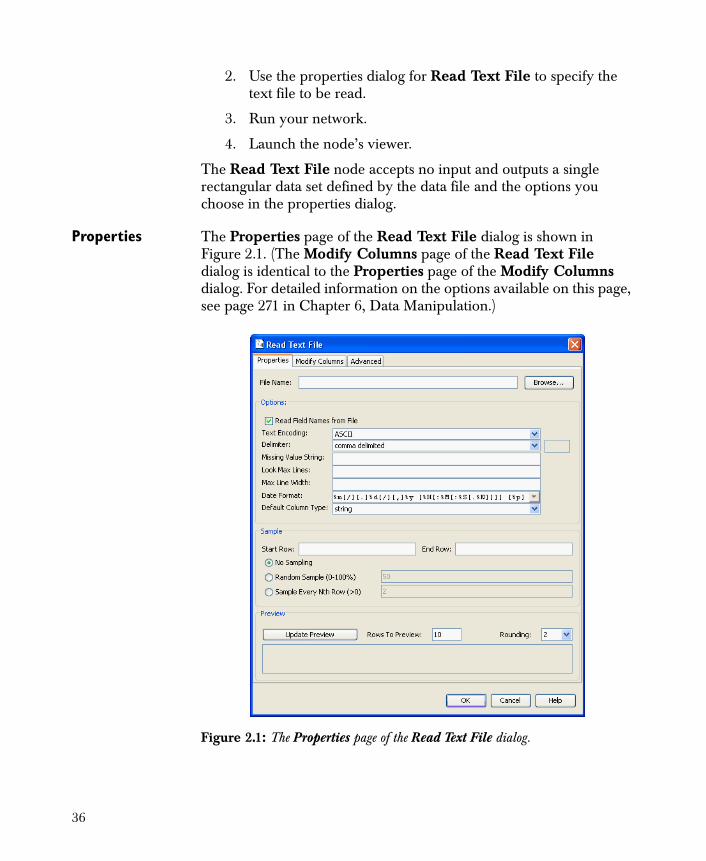
The Read Text File node accepts no input and outputs a single rectangular data set defined by the data file and the options you choose in the properties dialog.
Properties The Properties page of the Read Text File dialog is shown in Figure 2.1. (The Modify Columns page of the Read Text File dialog is identical to the Properties page of the Modify Columns dialog. For detailed information on the options available on this page, see page 271 in Chapter 6, Data Manipulation.)
Figure 2.1: The Properties page of the Read Text File dialog.
36
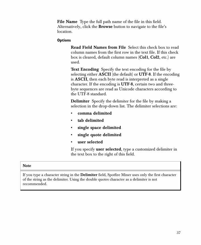
File Name Type the full path name of the file in this field. Alternatively, click the Browse button to navigate to the file’s location.
Options
Read Field Names from File Select this check box to read column names from the first row in the text file. If this check box is cleared, default column names (Col1, Col2, etc.) are used.
Text Encoding Specify the text encoding for the file by selecting either ASCII (the default) or UTF-8. If the encoding is ASCII, then each byte read is interpreted as a single character. If the encoding is UTF-8, certain two and three-byte sequences are read as Unicode characters according to the UTF-8 standard.
Delimiter Specify the delimiter for the file by making a selection in the drop-down list. The delimiter selections are:
• comma delimited
• tab delimited
• single space delimited
• single quote delimited
• user selected
If you specify user selected, type a customized delimiter in the text box to the right of this field.
Note
If you type a character string in the Delimiter field, Spotfire Miner uses only the first character of the string as the delimiter. Using the double quotes character as a delimiter is not recommended.
37
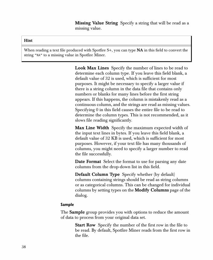
Missing Value String Specify a string that will be read as a missing value.
Look Max Lines Specify the number of lines to be read to determine each column type. If you leave this field blank, a default value of 32 is used, which is sufficient for most purposes. It might be necessary to specify a larger value if there is a string column in the data file that contains only numbers or blanks for many lines before the first string appears. If this happens, the column is mistakenly read as a continuous column, and the strings are read as missing values. Specifying 0 in this field causes the entire file to be read to determine the column types. This is not recommended, as it slows file reading significantly.
Max Line Width Specify the maximum expected width of the input text lines in bytes. If you leave this field blank, a default value of 32 KB is used, which is sufficient for most purposes. However, if your text file has many thousands of columns, you might need to specify a larger number to read the file successfully.
Date Format Select the format to use for parsing any date columns from the drop-down list in this field.
Default Column Type Specify whether (by default) columns containing strings should be read as string columns or as categorical columns. This can be changed for individual columns by setting types on the Modify Columns page of the dialog.
Sample
The Sample group provides you with options to reduce the amount of data to process from your original data set.
Start Row Specify the number of the first row in the file to be read. By default, Spotfire Miner reads from the first row in the file.
Hint
When reading a text file produced with Spotfire S+, you can type NA in this field to convert the string "NA" to a missing value in Spotfire Miner.
38
End Row Specify the number of the last row in the file to be read. By default, Spotfire Miner reads to the end of the file.
No Sampling Select this check box to read all rows (except as modified by the Start Row and End Row fields).
Random Sample (0-100%) Given a number between 0.0 and 100.0, Spotfire Miner selects each row (between Start Row and End Row) according to that probability. Note that this does not guarantee the exact number of output rows. For example, if the data file has 100 rows and the random probability is 10%, then you might get 10 rows, or 13, or 8. The random number generator is controlled by the Random Seed field on the Advanced page of the dialog so the random selection can be reproduced if desired.
Sample Every Nth Row (>0) Select this check box to read the first row between Start Row and End Row, and every Nth row thereafter, according to an input number N.
Preview
Before reading the entire data file, Spotfire Miner can display a preview of the data in the Preview area at the bottom of the Properties page. The Rows To Preview value determines the maximum number of rows that are displayed. By default, 10 rows are previewed to help you assess the format of the data set that Spotfire Miner will read. Note that this value is used only for preview purposes and does not affect the number of rows that are actually imported.
To preview your data, type the number of rows you want to preview in the Rows To Preview text box and click the Update Preview button. You can resize any of the columns in the Preview area by dragging the lines that divide the columns. To control the number of decimal digits that are displayed for continuous values, make a selection in the Rounding drop-down list and click the Update Preview button again. The default value for Rounding is 2.
Using the Viewer The viewer for the Read Text File component, as for all the data input/output components, is the node viewer, an example of which is shown in Figure 2.2. For a complete discussion of the node viewer and the information it displays, see the section The Table Viewer on page 146 as well as the online help.
39

Read Fixed Format Text File
Use the Read Fixed Format Text File component to read data values from fixed columns within a text file. Spotfire Miner reads the data from the designated file according to the options you specify.
Spotfire Miner supports reading and writing long text strings for specific file and database types. See Table 2.1 for more information.
General Procedure
The following outlines the general approach for using the Read Fixed Format Text File component:
1. Click and drag a Read Fixed Format Text File component from the explorer pane and drop it on your worksheet.
2. Use the properties dialog for Read Fixed Format Text File to specify the file to be read and the data dictionary to be used.
3. Run your network.
4. Launch the node’s viewer.
The Read Fixed Format Text File node accepts no input and outputs a single rectangular data set defined by the data file and the options you choose in the properties dialog.
Figure 2.2: The viewer for the Read Text File component.
40
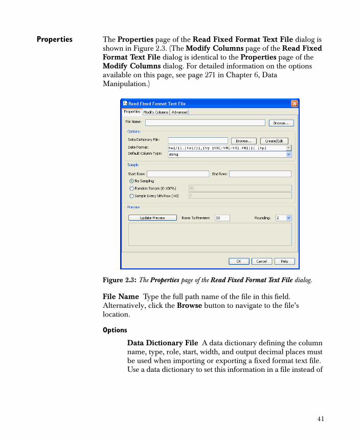
Properties The Properties page of the Read Fixed Format Text File dialog is shown in Figure 2.3. (The Modify Columns page of the Read Fixed Format Text File dialog is identical to the Properties page of the Modify Columns dialog. For detailed information on the options available on this page, see page 271 in Chapter 6, Data Manipulation.)
File Name Type the full path name of the file in this field. Alternatively, click the Browse button to navigate to the file’s location.
Options
Data Dictionary File A data dictionary defining the column name, type, role, start, width, and output decimal places must be used when importing or exporting a fixed format text file. Use a data dictionary to set this information in a file instead of
Figure 2.3: The Properties page of the Read Fixed Format Text File dialog.
41
interactively in the Modify Columns page of the dialog. The data dictionary file can be either a text file or an XML file that specifies the following information for each column:
• name The name for the input data column.
• type The column data type. One of the strings continuous, categorical, string, or date.
• role The column role. One of the strings dependent, independent, information, prediction, or partition. The default value is information.
• start The start column for the column data in each line. The first column is column 1.
• width The number of characters containing the column data.
• output decimal places The number of decimal places to use when outputting a continuous value. This defaults to zero.
When a data dictionary is written as a text file, these fields are specified in this order, separate by commas.
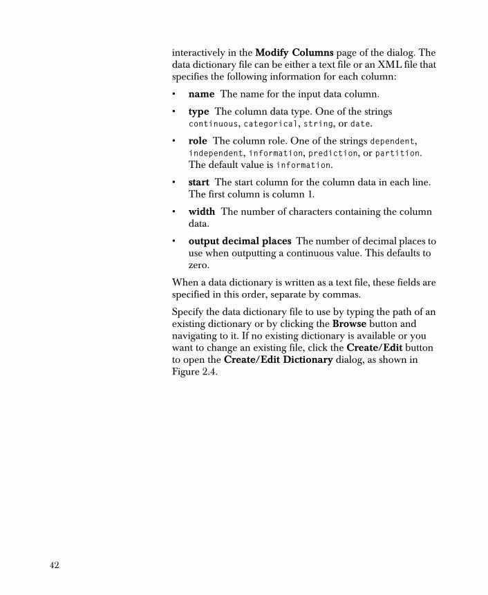
Specify the data dictionary file to use by typing the path of an existing dictionary or by clicking the Browse button and navigating to it. If no existing dictionary is available or you want to change an existing file, click the Create/Edit button to open the Create/Edit Dictionary dialog, as shown in Figure 2.4.
42
If a dictionary resides in the Data Dictionary File field, this dictionary is automatically loaded into the Create/Edit Dictionary dialog. Once the dialog is open, you might insert new columns into the dictionary, delete columns from the dictionary, move a column up (in the desired order), and/or move a column down to a desired location.
Keep in mind that Type and Role are optional fields in a data dictionary. Start and Width are semi-optional in that you must enter enough information for a file to be read or written. For example, if all the starts are omitted, the dictionary should provide all the widths, and the read/write nodes will assume that the initial start column is 1. Output decimal places (required only by a write node) is optional; if omitted, Spotfire Miner assumes that you do not want any decimals to be output.
To save your new or changed data dictionary, click the Save & Close button. (That is, name your new data dictionary or overwrite an old dictionary.) This selected name will then populate the Data Dictionary File field in the properties dialog.
The Date Format and Default Column Type fields are identical to those in the Read Text File dialog. For detailed information on these options, see the discussion beginning on page 37.
Figure 2.4: The Create/Edit Dictionary dialog.
43

Sample
The Sample group in the Read Fixed Format Text File dialog is identical to the Sample group in the Read Text File dialog. For detailed information on using this feature, see page 38.
Preview
The Preview group in the Read Fixed Format Text File dialog is identical to the Preview group in the Read Text File dialog. For detailed information on using this feature, see page 39.
Using the Viewer The viewer for the Read Fixed Format Text File component, as for all the data input/output components, is the node viewer, an example of which is shown in Figure 2.2. For a complete discussion of the node viewer and the information it displays, see the section The Table Viewer on page 146 as well as the online help.
Read Spotfire Data
Use the Read Spotfire Data component to specify a Spotfire data set for your analysis. Spotfire Miner reads the data from the designated
TIBCO Spotfire® text file according to the options you specify.
The Spotfire data file format is a simple text-based format used by the Spotfire application. A Spotfire data file contains column names and column types. It recognizes the semicolon as the separator between values.
The Spotfire data file format supports various data types: Datetime, date, time, integer, real, string, BLOB. Note that Spotfire Miner supports only datetime, continuous, categorical, and strings.
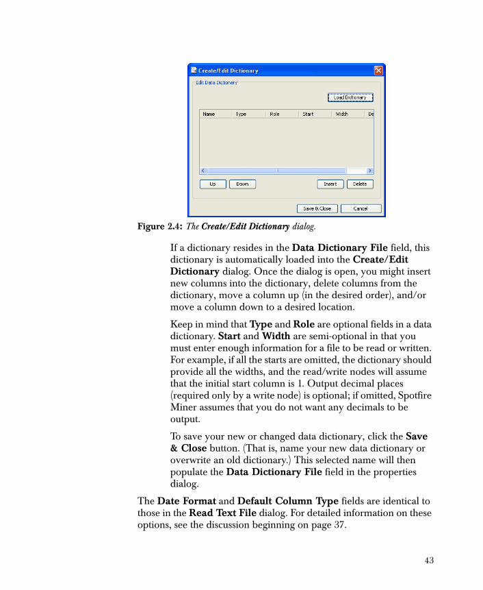
The following table shows the conversion between Spotfire and Spotfire Miner data types when importing data into Spotfire Miner:
44
Spotfire Miner does not support binary large objects (BLOB). Unrecognized Spotfire data types (date, time, and BLOB) are imported as strings by default.
General Procedure
The following outlines the general approach for using the Read Spotfire Data component:
1. Click and drag a Read Spotfire Data component from the explorer pane and drop it on your worksheet.
2. Use the properties dialog for Read Spotfire Data to specify the Spotfire file to be read.
3. Run your network.
4. Launch the node’s viewer.
The Read Spotfire Data node accepts no input and outputs a single rectangular data set defined by the data file and the options you choose in the properties dialog.
Table 2.4: Spotfire to Spotfire Miner data type conversion.
Spotfire Data Type Spotfire Miner Data Type
String string
Integer continuous
Real continuous
DateTime date
Date string
Time string
Binary large object (BLOB) string
45
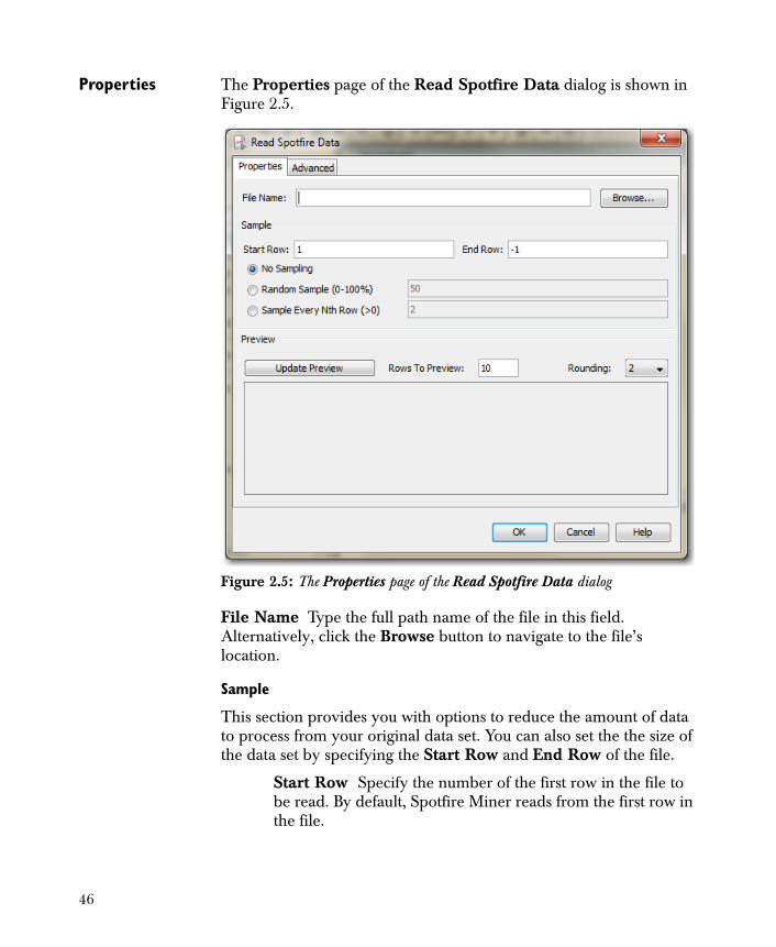
Properties The Properties page of the Read Spotfire Data dialog is shown in Figure 2.5.
File Name Type the full path name of the file in this field. Alternatively, click the Browse button to navigate to the file’s location.
Sample
This section provides you with options to reduce the amount of data to process from your original data set. You can also set the the size of the data set by specifying the Start Row and End Row of the file.
Start Row Specify the number of the first row in the file to be read. By default, Spotfire Miner reads from the first row in the file.
Figure 2.5: The Properties page of the Read Spotfire Data dialog
46
End Row Specify the number of the last row in the file to be read. By default, Spotfire Miner reads to the end of the file.
No Sampling Read all rows (except as modified by Start Row and End Row options).
Random Sample (0-100%) Given a number between 0.0 and 100.0, it selects each row (between Start Row and End Rows) according to that probability. Note that this does not guarantee the exact number of output rows. For example, if the data file has 100 rows and the random probability is 10%, then you might get 10 rows, or 13, or 8. The random number generator is controlled by the random seed fields in the Advanced Properties page of the dialog, so the random selection can be reproduced if desired.
Sample Every Nth Row (> 0) Reads the first row between the Start Row and End Row, and every Nth row after, according to an input number N.
Using the Viewer The viewer for the Read Spotfire Data component is the node viewer. For a complete discussion of the node viewer and the information it displays, see the section The Table Viewer on page 146 as well as the online help.
Read SAS File Use the Read SAS File component specify a SAS data set for your analysis. Spotfire Miner reads the data from the designated SAS file according to the options you specify.
Spotfire Miner supports reading 64-bit or compressed SAS files.
General Procedure
The following outlines the general approach for using the Read SAS File component:
1. Click and drag a Read SAS File component from the explorer pane and drop it on your worksheet.
2. Use the properties dialog for Read SAS File to specify the SAS file to be read.
3. Run your network.
4. Launch the node’s viewer.
47
The Read SAS File node accepts no input and outputs a single rectangular data set defined by the data file and the options you choose in the properties dialog.
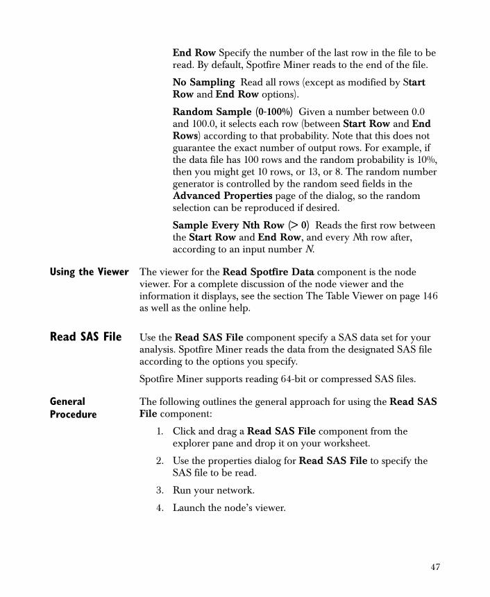
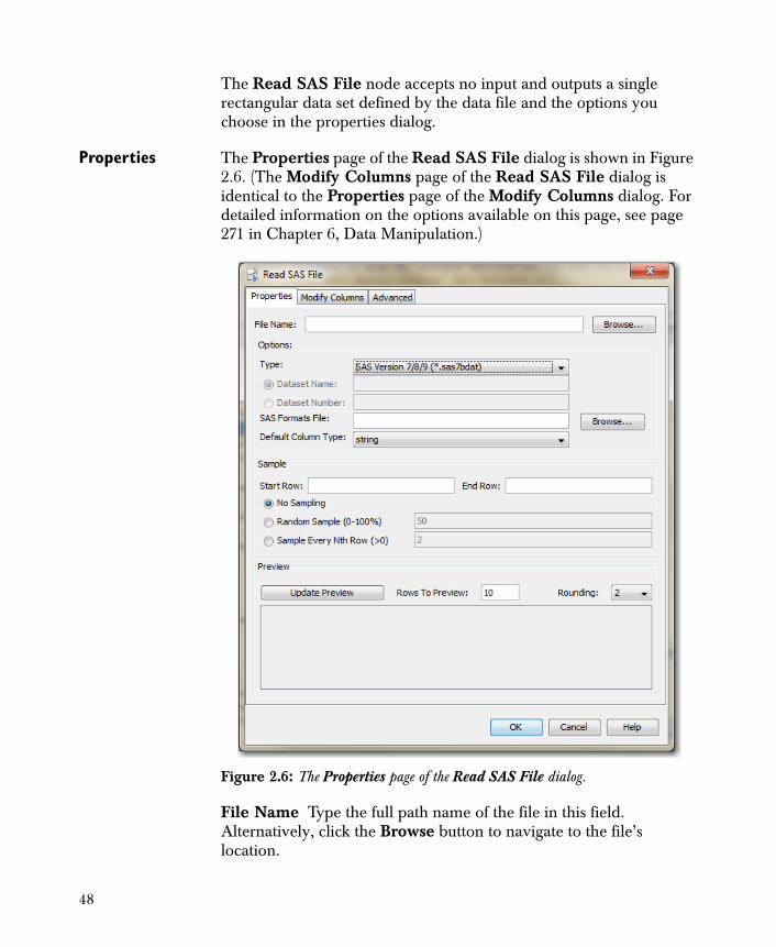
Properties The Properties page of the Read SAS File dialog is shown in Figure 2.6. (The Modify Columns page of the Read SAS File dialog is identical to the Properties page of the Modify Columns dialog. For detailed information on the options available on this page, see page 271 in Chapter 6, Data Manipulation.)
File Name Type the full path name of the file in this field. Alternatively, click the Browse button to navigate to the file’s location.
Figure 2.6: The Properties page of the Read SAS File dialog.
48
Options
Type Select the type of SAS file from the drop-down list. The available selections are:
• SAS Version 7/8
• SAS - Windows/OS2
• SAS - HP IBM & SUN UNIX
• SAS - Dec UNIX
• SAS Transport File
Note that if you select SAS Transport File, you can specify the dataset name or number, but not both. (If you leave both options blank, the first dataset in the transport file is imported.)
Dataset Name If, for Type, you select SAS Transport File, you can specify the name of the dataset. The dataset name must match exactly, including case. If you do not know the name, you can set the Dataset Number instead.
Dataset Number If, for Type, you select SAS Transport File, you can use this option to specify the number of the dataset in the file (that is, 1 to get the first, 2 to get the second, and so on). By default, the first page is used.
SAS Formats File You can specify a sas7bcat file for a sas7bdat file. If you leave this blank, the file is imported with no formatting information.
The Default Column Type field is identical to that in the Read Text File dialog. For detailed information on this option, see the discussion beginning on page 37.
Note
Some SAS files might contain data columns with “value labels,” where a data column contains actual values such as continuous values as well as a string label corresponding to each actual value. By default, such columns are read as categorical values, with the value label strings used as the categorical levels. If such a column is explicitly read as a string or continuous column (by changing the type in Modify Columns), the actual values are read instead of the value labels.
49
Sample
The Sample group in the Read SAS File dialog is identical to the Sample group in the Read Text File dialog. For detailed information on using this feature, see page 38.
Preview
The Preview group in the Read SAS File dialog is identical to the Preview group in the Read Text File dialog. For detailed information on using this feature, see page 39.
Using the Viewer The viewer for the Read SAS File component is the node viewer. For a complete discussion of the node viewer and the information it displays, see the section The Table Viewer on page 146 as well as the online help.
Read Excel File Use the Read Excel File component to specify an Excel file for your analysis. Spotfire Miner reads the data from the designated Excel file according to the options you specify.
Spotfire Miner supports reading and writing long text strings for specific file and database types. See Table 2.1 for more information.
50
General Procedure
The following outlines the general approach for using the Read Excel File component:
1. Click and drag a Read Excel File component from the explorer pane and drop it on your worksheet.
2. Use the properties dialog for Read Excel File to specify the Excel file to be read.
3. Run your network.
4. Launch the node’s viewer.
The Read Excel File node accepts no input and outputs a single rectangular data set defined by the data file and the options you choose in the properties dialog.
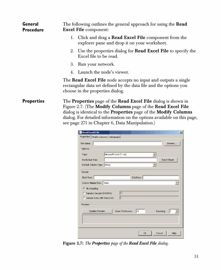
Properties The Properties page of the Read Excel File dialog is shown in Figure 2.7. (The Modify Columns page of the Read Excel File dialog is identical to the Properties page of the Modify Columns dialog. For detailed information on the options available on this page, see page 271 in Chapter 6, Data Manipulation.)
Figure 2.7: The Properties page of the Read Excel File dialog.
51
File Name Type the full path name of the file in this field. Alternatively, click the Browse button to navigate to the file’s location.
Options
Type: Specify whether your Excel file is standard .xls or is Excel 2007 (.xlsx).
Worksheet Tab Specify the name of the sheet tab in the Excel file to be read. Clicking the Select Sheet button will display a list of the sheet names to choose from.
The Default Column Type field is identical to that in the Read Text File dialog. For detailed information on this option, see the discussion beginning on page 37.
Preview
The Sample group provides you with options to reduce the amount of data to process from your original data set.
Start Row Specify the number of the first row in the file to be read. By default, Spotfire Miner reads from the first row in the file.
End Row Specify the number of the last row in the file to be read. By default, Spotfire Miner reads to the end of the file.
Columns Name Row Specify the number of the row containing the column names. If you use the default (Auto), Spotfire Miner determines the row to use for column names.
No Sampling Select this check box to read all rows (except as modified by the Start Row and End Row fields).
Random Sample (0-100%) Given a number between 0.0 and 100.0, Spotfire Miner selects each row (between Start Row and End Row) according to that probability. Note that this does not guarantee the exact number of output rows. For example, if the data file has 100 rows and the random probability is 10%, then you might get 10 rows, or 13, or 8. The random number generator is controlled by the Random Seed field on the Advanced page of the dialog so the random selection can be reproduced if desired.
52
Sample Every Nth Row (>0) Select this check box to read the first row between Start Row and End Row, and every Nth row thereafter, according to an input number N.
Preview
The Preview group in the Read Excel File dialog is identical to the Preview group in the Read Text File dialog. For detailed information on using this feature, see page 39.
Using the Viewer The viewer for the Read Excel File component is the node viewer. For a complete discussion of the node viewer and the information it displays, see the section The Table Viewer on page 146 as well as the online help.
Read Other File
Use the Read Other File component to specify a data set for your analysis. Spotfire Miner reads the data from the designated file, recognizing nontext formats such as Matlab and SPSS.
General Procedure
The following outlines the general approach for using the Read Other File component:
1. Click and drag a Read Other File component from the explorer pane and drop it on your worksheet.
2. Use the properties dialog for Read Other File to specify the file to be read.
3. Run your network.
4. Launch the node’s viewer.
The Read Other File node accepts no input and outputs a single rectangular data set defined by the data file and the options you choose in the properties dialog.
53
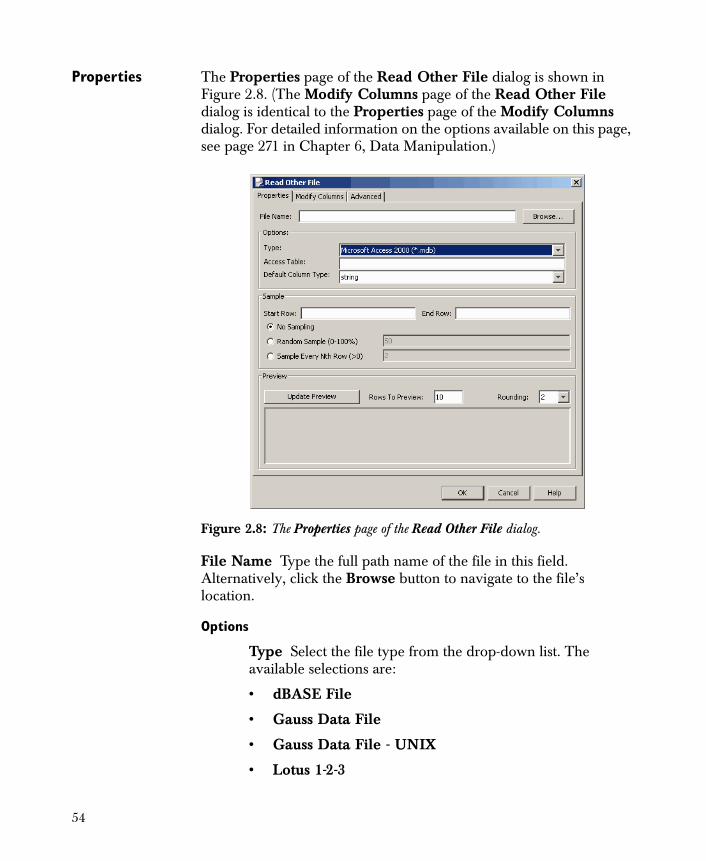
Properties The Properties page of the Read Other File dialog is shown in Figure 2.8. (The Modify Columns page of the Read Other File dialog is identical to the Properties page of the Modify Columns dialog. For detailed information on the options available on this page, see page 271 in Chapter 6, Data Manipulation.)
File Name Type the full path name of the file in this field. Alternatively, click the Browse button to navigate to the file’s location.
Options
Type Select the file type from the drop-down list. The available selections are:
• dBASE File
• Gauss Data File
• Gauss Data File - UNIX
• Lotus 1-2-3
Figure 2.8: The Properties page of the Read Other File dialog.
54
• Matlab Matrix
• Microsoft Access 2000
• Microsoft Access 2007
• Minitab Workbook
• Quattro Pro Worksheet
• SPSS Data File
• SPSS Portable Data File
• Stata Data File
• Systat File
Access Table When reading a Microsoft Access 2000 or 2007 file, specify the name of the Access table in this field.
The Default Column Type field is identical to that in the Read Text File dialog. For detailed information on this option, see the discussion beginning on page 37.
Note
Although it is possible to read Microsoft Access database files using the Read Database - ODBC component, reading them directly using the Read Other File component is significantly faster (10 times faster) than going through ODBC.
If either the Access 2000 or Access 2007 type is specified, when the node is executed, Spotfire Miner checks whether the system has the right driver files installed for reading these file types. If not, an error is printed indicating that the correct driver cannot be found.
Note that Access 1997 is no longer supported as of Spotfire Miner 8.1.
Note
Some data files might contain data columns with “value labels,” where a data column contains actual values such as continuous values as well as a string label corresponding to each actual value. By default, such columns are read as categorical values, with the value label strings used as the categorical levels. If such a column is explicitly read as a string or continuous column (by changing the type in Modify Columns), the actual values are read instead of the value labels.
55
Sample
The Sample group in the Read Other File dialog is identical to the Sample group in the Read Text File dialog. For detailed information on using this feature, see page 38.
Preview
The Preview group in the Read Other File dialog is identical to the Preview group in the Read Text File dialog. For detailed information on using this feature, see page 39.
Using the Viewer The viewer for the Read Other File component is the node viewer. For a complete discussion of the node viewer and the information it displays, see the section The Table Viewer on page 146 as well as the online help.
Read Database ODBC
Use the Read Database - ODBC component to specify a data set from a database for your analysis. Spotfire Miner reads the data via Open DataBase Connectivity (ODBC) from database formats such as Oracle and DB2.
Applications such as Oracle and DB2, as well as most commercial databases (generically known as data sources), support the ODBC standard. Designed to provide a unified, standard way to exchange data between databases, ODBC has become widely supported. Each application typically has an ODBC driver that allows the application to accept or distribute data via the ODBC interface.
Spotfire Miner supports reading and writing long text strings for specific file and database types. See Table 2.1 for more information.
The ODBC Data Source Administrator
The ODBC Data Source Administrator manages database drivers and data sources. You must have the Administrator installed on your computer before you continue. To see if the Administrator is already
Note
This component is only available on Microsoft Windows. Spotfire Miner supports ODBC versions 2.0 and 3.0.
Some databases have limitations on reading/writing data in specific formats, so there might be problems in reading or writing all column types from all databases.
56
installed, open Administrative Tools in the Control Panel and verify that it contains the Data Sources (ODBC) icon. To check your version, start the Administrator by double-clicking the Data Sources (ODBC) icon and then click the About tab.
ODBC Drivers An ODBC driver is a dynamically linked library (DLL) that connects a database to the ODBC interface. Applications call functions in the ODBC interface, which are implemented in the database-specific drivers. The use of drivers isolates applications from database-specific calls in the same way that printer drivers isolate word processing programs from printer-specific commands.
You must provide an appropriate ODBC driver for your database. Contact your database vendor or a third-party ODBC driver vendor for assistance.
To determine which drivers are already installed on your computer, start the Administrator and click the Drivers tab. The name, version, company, file name, and file creation date of each ODBC driver installed on the computer are displayed. To add a new driver or to delete an installed driver, use the driver’s setup program.
Defining a Data Source
A data source is a logical name for a data repository or database. It points to the data you want to access, the application that has the data, and the computer and network connections necessary to reach the data. Adding or configuring a data source can be done using the Administrator.
To add a data source, open the Administrator. If you are running Administrator 3.0, you can then click the tab that corresponds to the type of DSN (Data Source Name) you want to create. The type of DSN controls access to the data source you are creating, as follows:
• User DSNs are specific to the login account that is in effect when they are created. They are local to a computer and dedicated to the current user.
• System DSNs are local to a computer but not dedicated to a particular user. Any user having login privileges can use a data source set up with a System DSN.
57

Click the appropriate tab and then click the Add button. (If you are running Administrator 2.0, you can create a User DSN by clicking the Add button from the initial dialog. Or, to create a System DSN, click that button and then the Add button in the subsequent dialog.) The Create New Data Source dialog appears.
Select the ODBC driver for the database you want to connect to and click Finish. If the list of drivers in the Create New Data Source dialog is empty or does not contain a driver for your database or application, you need to install the database or its ODBC driver.
At this point, a driver-specific dialog should appear asking database-and driver-specific information required to connect to the database. Fill in the required fields and click OK. The new data source should be visible the next time you use the Read Database - ODBC component.
General Procedure
The following outlines the general approach for using the Read Database - ODBC component:
1. Click and drag a Read Database - ODBC component from the explorer pane and drop it on your worksheet.
2. Use the properties dialog for Read Database - ODBC to specify the data to be read.
3. Run your network.
4. Launch the node’s viewer.
The Read Database - ODBC node accepts no input and outputs a single rectangular data set defined by the specified data in the database and the options you choose in the properties dialog.
Properties The Properties page of the Read Database - ODBC dialog is shown in Figure 2.9. (The Modify Columns page of the Read Database - ODBC dialog is identical to the Properties page of the
58
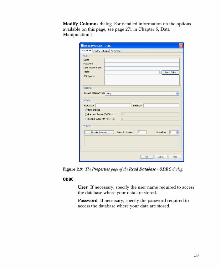
Modify Columns dialog. For detailed information on the options available on this page, see page 271 in Chapter 6, Data Manipulation.)
ODBC
User If necessary, specify the user name required to access the database where your data are stored.
Password If necessary, specify the password required to access the database where your data are stored.
Figure 2.9: The Properties page of the Read Database - ODBC dialog.
59
Data Source Name Specify the name of the ODBC system data source. These names are listed in the Administrator.
Table Specify the name of the table to be read.
Select Table Click this button to display a list of the tables in the database. Select one to copy the name to the Table field.
SQL Query Specify the Structured Query Language (SQL) statement to be executed for the table to be read.
Options
The Default Column Type field is identical to that in the Read Text File dialog. For detailed information on this option, see the discussion beginning on page 37.
Sample
The Sample group in the Read Database dialog is identical to the Sample group in the Read Text File dialog. For detailed information on using this feature, see page 38.
Hint
To verify your data source names and settings, open Administrative Tools in the Control Panel, double-click Data Sources (ODBC), and then click the System DSN or User DSN tab of the ODBC Data Source Administrator dialog.
Note
For some databases, the names of tables and columns in SQL statements are expected to be in all uppercase letters. If you have tables and columns whose names contain lowercase characters, you might need to enclose them in quotes in the SQL statement. For example, if the table ABC contains a column Fuel, it can be used in an SQL statement as follows:
select * from ABC where "Fuel"<3
If you are trying to read a SQL Server table that begins with a number (e.g., 1234FUEL), do not choose the table name in the drop-down box. Instead, enter the table name with square brackets around it in the SQL Query field:
select * from [1234FUEL]
60
Preview
The Preview group in the Read Database dialog is identical to the Preview group in the Read Text File dialog. For detailed information on using this feature, see page 39.
Using the Viewer The viewer for the Read Database - ODBC component is the node viewer. For a complete discussion of the node viewer and the information it displays, see the section The Table Viewer on page 146 as well as the online help.
Read DB2 Native
Use the Read DB2 - Native component to specify a data set from a database for your analysis. Spotfire Miner reads the data via an installed DB2 client.
DB2 Client The DB2 client must be installed and configured in order for Spotfire Miner to successfully access DB2 databases. For information on the requirements and procedures please refer to the DB2 documentation.
General Procedure
The following outlines the general approach for using the Read DB2 - Native component:
1. Click and drag a Read DB2 - Native component from the explorer pane and drop it on your worksheet.
2. Use the properties dialog for Read DB2 - Native to specify the data to be read.
3. Run your network.
4. Launch the node’s viewer.
Note
Spotfire Miner supports DB2 client version 7.1.
Note
As of Spotfire Miner version 8.2, native database drivers are deprecated. In lieu of these drivers, you should use JDBC/ODBC drivers for all supported database vendors.
61
The Read DB2 - Native node accepts no input and outputs a single rectangular data set defined by the specified data in the database and the options you choose in the properties dialog.
Properties The Properties page of the Read DB2 - Native dialog is shown in Figure 2.10. (The Modify Columns page of the Read DB2 - Native dialog is identical to the Properties page of the Modify Columns dialog. For detailed information on the options available on this page, see page 271 in Chapter 6, Data Manipulation.)
Native DB2
User If necessary, specify the user name required to access the database where your data are stored.
Password If necessary, specify the password required to access the database where your data are stored.
Figure 2.10: The Properties page of the Read DB2 - Native dialog.
62
Database Specify the name of the database to be accessed.
Table Specify the name of the table to be read.
Select Table Click this button to display a list of the tables in the database. Select one to copy the name to the Table field.
SQL Query Specify the Structured Query Language (SQL) statement to be executed for the table to be read.
Options
The Default Column Type field is identical to that in the Read Text File dialog. For detailed information on this option, see the discussion beginning on page 37.
Sample
The Sample group in the Read DB2 - Native dialog is identical to the Sample group in the Read Text File dialog. For detailed information on using this feature, see page 38.
Preview
The Preview group in the Read DB2 - Native dialog is identical to the Preview group in the Read Text File dialog. For detailed information on using this feature, see page 39.
Using the Viewer The viewer for the Read DB2 - Native component is the node viewer. For a complete discussion of the node viewer and the information it displays, see the section The Table Viewer on page 146 as well as the online help.
Read Oracle Native
Use the Read Oracle - Native component to specify a data set from a database for your analysis. Spotfire Miner reads the data via an installed DB2 client.
Note
For some databases, the names of tables and columns in SQL statements are expected to be in all uppercase letters. If you have tables and columns whose names contain lowercase characters, you might need to enclose them in quotes in the SQL statement. For example, if the table ABC contains a column Fuel, it can be used in an SQL statement as follows:
select * from ABC where "Fuel"<3
63
Spotfire Miner supports reading and writing long text strings for specific file and database types. See Table 2.1 for more information.
Oracle Client The Oracle client must be installed and configured in order for Spotfire Miner to successfully access Oracle databases. For information on the requirements and procedures please refer to the Oracle documentation.
General Procedure
The following outlines the general approach for using the Read Oracle - Native component:
1. Click and drag a Read Oracle - Native component from the explorer pane and drop it on your worksheet.
2. Use the properties dialog for Read Oracle - Native to specify the data to be read.
3. Run your network.
4. Launch the node’s viewer.
The Read Oracle - Native node accepts no input and outputs a single rectangular data set defined by the specified data in the database and the options you choose in the properties dialog.
Note
Spotfire Miner supports Oracle client version 9i.
Note
As of Spotfire Miner version 8.2, native database drivers are deprecated. In lieu of these drivers, you should use JDBC/ODBC drivers for all supported database vendors.
64
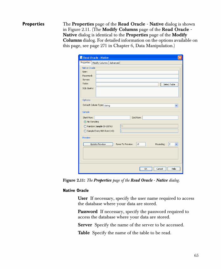
Properties The Properties page of the Read Oracle - Native dialog is shown in Figure 2.11. (The Modify Columns page of the Read Oracle - Native dialog is identical to the Properties page of the Modify Columns dialog. For detailed information on the options available on this page, see page 271 in Chapter 6, Data Manipulation.)
Native Oracle
User If necessary, specify the user name required to access the database where your data are stored.
Password If necessary, specify the password required to access the database where your data are stored.
Server Specify the name of the server to be accessed.
Table Specify the name of the table to be read.
Figure 2.11: The Properties page of the Read Oracle - Native dialog.
65
Select Table Click this button to display a list of the tables in the database. Select one to copy the name to the Table field.
SQL Query Specify the Structured Query Language (SQL) statement to be executed for the table to be read.
Options
The Default Column Type field is identical to that in the Read Text File dialog. For detailed information on this option, see the discussion beginning on page 37.
Sample
The Sample group in the Read Oracle - Native dialog is identical to the Sample group in the Read Text File dialog. For detailed information on using this feature, see page 38.
Preview
The Preview group in the Read Oracle - Native dialog is identical to the Preview group in the Read Text File dialog. For detailed information on using this feature, see page 39.
Using the Viewer The viewer for the Read Oracle - Native component is the node viewer. For a complete discussion of the node viewer and the information it displays, see the section The Table Viewer on page 146 as well as the online help.
Note
For some databases, the names of tables and columns in SQL statements are expected to be in all uppercase letters. If you have tables and columns whose names contain lowercase characters, you might need to enclose them in quotes in the SQL statement. For example, if the table ABC contains a column Fuel, it can be used in an SQL statement as follows:
select * from ABC where "Fuel"<3
If you are trying to read a SQL Server table that begins with a number (e.g., 1234FUEL), do not choose the table name in the drop-down box. Instead, enter the table name with square brackets around it in the SQL Query field:
select * from [1234FUEL]
66
Read SQL Native
Use the Read SQL - Native component to specify a data set from a database for your analysis. Spotfire Miner reads the data via an installed Microsoft SQL Server client.
Spotfire Miner supports reading and writing long text strings for specific file and database types. See Table 2.1 for more information.
Microsoft SQL Server Client
The Microsoft SQL Server client must be installed and configured in order for Spotfire Miner to successfully access Microsoft SQL Server databases. For information on the requirements and procedures please refer to the Microsoft SQL Server documentation.
General Procedure
The following outlines the general approach for using the Read SQL - Native component:
1. Click and drag a Read SQL - Native component from the explorer pane and drop it on your worksheet.
2. Use the properties dialog for Read SQL - Native to specify the data to be read.
3. Run your network.
4. Launch the node’s viewer.
The Read SQL - Native node accepts no input and outputs a single rectangular data set defined by the specified data in the database and the options you choose in the properties dialog.
Note
This component is only available on Microsoft Windows.
Note
As of Spotfire Miner version 8.2, native database drivers are deprecated. In lieu of these drivers, you should use JDBC/ODBC drivers for all supported database vendors.
67
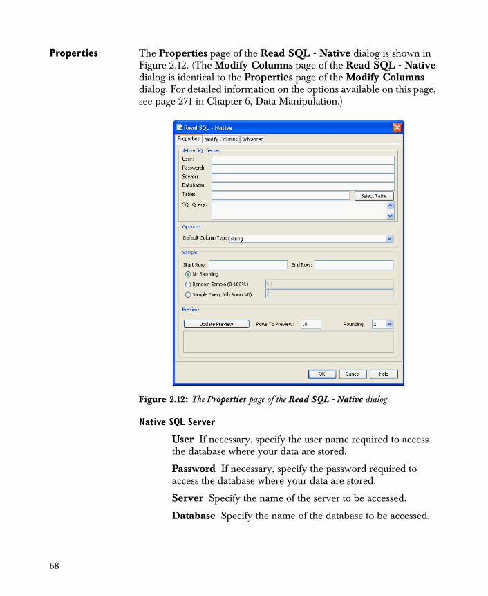
Properties The Properties page of the Read SQL - Native dialog is shown in Figure 2.12. (The Modify Columns page of the Read SQL - Native dialog is identical to the Properties page of the Modify Columns dialog. For detailed information on the options available on this page, see page 271 in Chapter 6, Data Manipulation.)
Native SQL Server
User If necessary, specify the user name required to access the database where your data are stored.
Password If necessary, specify the password required to access the database where your data are stored.
Server Specify the name of the server to be accessed.
Database Specify the name of the database to be accessed.
Figure 2.12: The Properties page of the Read SQL - Native dialog.
68

Table Specify the name of the table to be read. If you are trying to read a table that begins with a number (e.g., 1234FUEL), don't choose the table name in the drop-down box, but instead enter the table name with square brackets around it in the SQL Query field:
SELECT * FROM [1234FUEL]
Select Table Click this button to display a list of the tables in the database. Select one to copy the name to the Table field.
SQL Query Specify the Structured Query Language (SQL) statement to be executed for the table to be read.
Options
The Default Column Type field is identical to that in the Read Text File dialog. For detailed information on this option, see the discussion beginning on page 37.
Sample
The Sample group in the Read SQL - Native dialog is identical to the Sample group in the Read Text File dialog. For detailed information on using this feature, see page 38.
Preview
The Preview group in the Read SQL - Native dialog is identical to the Preview group in the Read Text File dialog. For detailed information on using this feature, see page 39.
Using the Viewer The viewer for the Read SQL - Native component is the node viewer. For a complete discussion of the node viewer and the information it displays, see the section The Table Viewer on page 146 as well as the online help.
Note
For some databases, the names of tables and columns in SQL statements are expected to be in all uppercase letters. If you have tables and columns whose names contain lowercase characters, you might need to enclose them in quotes in the SQL statement. For example, if the table ABC contains a column Fuel, it can be used in an SQL statement as follows:
select * from ABC where "Fuel"<3
69
Read Sybase Native
Use the Read Sybase - Native component to specify a data set from a database for your analysis. Spotfire Miner reads the data via an installed Sybase client.
Sybase Client The Sybase client must be installed and configured to for you to run in order for Spotfire Miner to successfully access Sybase databases. For information on the requirements and procedures please refer to the Sybase documentation.
General Procedure
The following outlines the general approach for using the Read Sybase - Native component:
1. Click and drag a Read Sybase - Native component from the explorer pane and drop it on your worksheet.
2. Use the properties dialog for Read Sybase - Native to specify the data to be read.
3. Run your network.
4. Launch the node’s viewer.
The Read Sybase - Native node accepts no input and outputs a single rectangular data set defined by the specified data in the database and the options you choose in the properties dialog.
Note
Spotfire Miner supports Sybase client version 12.5.
Note
As of Spotfire Miner version 8.2, native database drivers are deprecated. In lieu of these drivers, you should use JDBC/ODBC drivers for all supported database vendors.
70
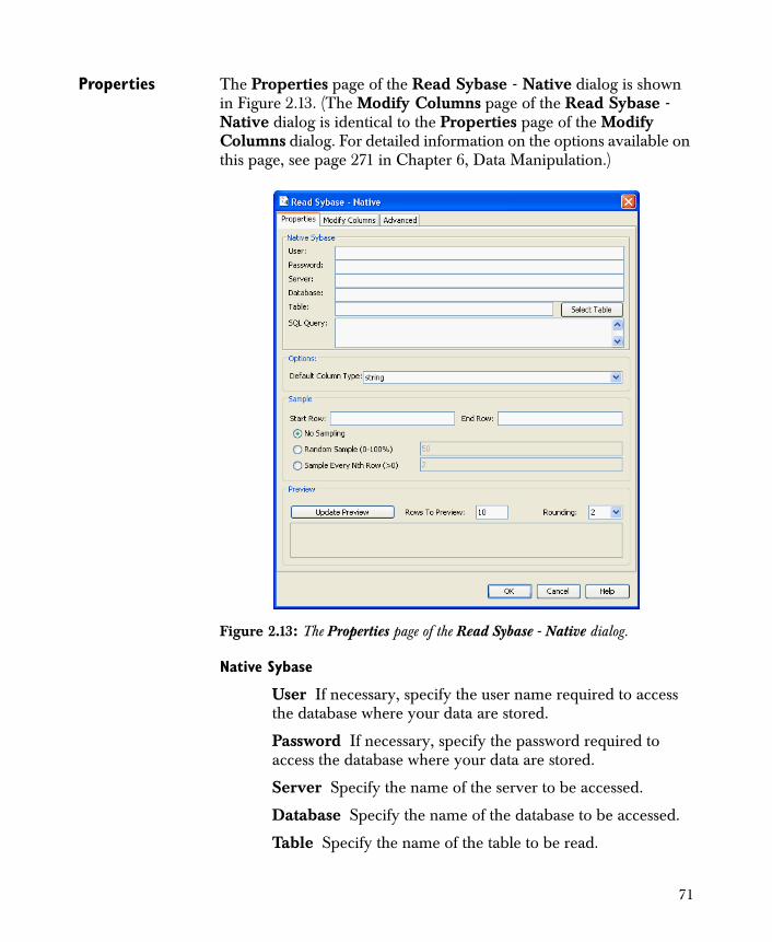
Properties The Properties page of the Read Sybase - Native dialog is shown in Figure 2.13. (The Modify Columns page of the Read Sybase - Native dialog is identical to the Properties page of the Modify Columns dialog. For detailed information on the options available on this page, see page 271 in Chapter 6, Data Manipulation.)
Native Sybase
User If necessary, specify the user name required to access the database where your data are stored.
Password If necessary, specify the password required to access the database where your data are stored.
Server Specify the name of the server to be accessed.
Database Specify the name of the database to be accessed.
Table Specify the name of the table to be read.
Figure 2.13: The Properties page of the Read Sybase - Native dialog.
71
Select Table Click this button to display a list of the tables in the database. Select one to copy the name to the Table field.
SQL Query Specify the Structured Query Language (SQL) statement to be executed for the table to be read.
Options
The Default Column Type field is identical to that in the Read Text File dialog. For detailed information on this option, see the discussion beginning on page 37.
Sample
The Sample group in the Read Sybase - Native dialog is identical to the Sample group in the Read Text File dialog. For detailed information on using this feature, see page 38.
Preview
The Preview group in the Read Sybase - Native dialog is identical to the Preview group in the Read Text File dialog. For detailed information on using this feature, see page 39.
Using the Viewer The viewer for the Read Sybase - Native component is the node viewer. For a complete discussion of the node viewer and the information it displays, see the section The Table Viewer on page 146 as well as the online help.
Read Database JDBC
The Read Database - JDBC component is provided in a separate library; it is not part of the Main library. For detailed information about using this library, see the section Importing and Exporting Data with JDBC on page 581.
Note
For some databases, the names of tables and columns in SQL statements are expected to be in all uppercase letters. If you have tables and columns whose names contain lowercase characters, you might need to enclose them in quotes in the SQL statement. For example, if the table ABC contains a column Fuel, it can be used in an SQL statement as follows:
select * from ABC where "Fuel"<3
72

The JDBC library provides nodes that implement the read and write capability of the sjdbc package, a Spotfire S+ library provided with Spotfire Miner. The sjdbc library includes a Help file, which you can find in MHOME/splus/library/sjdbc (where MHOME is your Spotfire Miner installation directory).
Use the Read Database - JDBC component to read data from a relational data source (for example, a SQL database) or from a tabular data source (for example, a spreadsheet). To read from a database using JDBC, you must use the appropriate JDBC driver to connect to the JDBC interface.
73
DATA OUTPUT
Spotfire Miner provides the following data output components:
• Write Text File
• Write Fixed Format Text File
• Write SAS File
• Write Excel File
• Write Other File
In addition, the following database nodes are available:
• Write Database - ODBC
• Write DB2 - Native
• Write Oracle - Native
• Write SQL Server - Native
• Write Sybase - Native
In this section, we discuss each component in turn.
Spotfire Miner supports outputting long text strings. See Table 2.1 for size information and caveats about writing long strings using different database types.
Write Text File Use the Write Text File component to create ASCII text files of your data sets.
Spotfire Miner supports reading and writing long text strings for specific file and database types. See Table 2.1 for more information.
Note
As of Spotfire Miner version 8.2, native database drivers are deprecated. In lieu of these drivers, you should use JDBC/ODBC drivers for all supported database vendors.
74
General Procedure
The following outlines the general approach for using the Write Text File component:
1. Link a Write Text File node in your worksheet to any node that outputs data.
2. Use the properties dialog for Write Text File to specify options for the text file you want to create.
3. Run your network.
4. Launch the node’s viewer.
The Write Text File node accepts a single input containing rectangular data and returns no output.
Properties The Properties page of the Write Text File dialog is shown in Figure 2.14.
File Name Type the full path name of the file you want to create in this field. Alternatively, click the Browse button to navigate to the file’s location.
Figure 2.14: The Properties page of the Write Text File dialog.
75
Options
Write Column Names Select this check box to write column names to the first row in the text file.
Text Encoding Specify the text encoding for the file by selecting either ASCII (the default) or UTF-8. If the encoding is ASCII, then each character is written as a single byte. If the encoding is UTF-8, certain Unicode characters are written as two and three-byte sequences according to the UTF-8 standard.
Delimiter Specify the delimiter for the file by making a selection in the drop-down list. The delimiter selections are:
• comma delimited
• tab delimited
• single space delimited
• single quote delimited
• user selected
If you specify user selected, type a customized delimiter in the text box to the right of this field.
Missing Value String Specify a string that will be written as a missing value. For categorical and string columns, a missing value is always written as a blank. Note that only the first 8 characters of this field are used.
Date Format Select the format to use for any date columns from the drop-down list in this field.
Using the Viewer The viewer for the Write Text File component is the node viewer. For a complete discussion of the node viewer and the information it displays, see the section The Table Viewer on page 146 as well as the online help.
Note
If you type a character string in the Delimiter field, Spotfire Miner uses only the first character of the string as the delimiter. Using the double quotes character as a delimiter is not recommended.
76

Write Fixed Format Text File
Use the Write Fixed Format Text File component to create fixed format text files of your data sets.
Spotfire Miner supports reading and writing long text strings for specific file and database types. See Table 2.1 for more information.
General Procedure
The following outlines the general approach for using the Write Fixed Format Text File component:
1. Link a Write Fixed Format Text File node in your worksheet to any node that outputs data.
2. Use the properties dialog for Write Fixed Format Text File to specify the file to be created and the data dictionary to be used.
3. Run your network.
4. Launch the node’s viewer.
The Write Fixed Format Text File node accepts a single input containing rectangular data and returns no output.
77
Properties The Properties page of the Write Fixed Format Text File dialog is shown in Figure 2.15.
File Name Type the full path name of the file you want to create in this field. Alternatively, click the Browse button to navigate to the file’s location.
Options
The Data Dictionary File field is identical to that in the Read Fixed Format Text File dialog. For detailed information on this option, see the discussion beginning on page 41.
Date Format Select the format to use for any date columns from the drop-down list in this field.
Using the Viewer The viewer for the Write Fixed Format Text File component is the node viewer. For a complete discussion of the node viewer and the information it displays, see the section The Table Viewer on page 146 as well as the online help.
Figure 2.15: The Properties page of the Write Fixed Format Text File dialog.
78
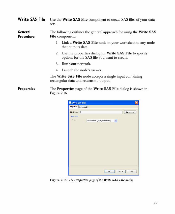
Write SAS File Use the Write SAS File component to create SAS files of your data sets.
General Procedure
The following outlines the general approach for using the Write SAS File component:
1. Link a Write SAS File node in your worksheet to any node that outputs data.
2. Use the properties dialog for Write SAS File to specify options for the SAS file you want to create.
3. Run your network.
4. Launch the node’s viewer.
The Write SAS File node accepts a single input containing rectangular data and returns no output.
Properties The Properties page of the Write SAS File dialog is shown in Figure 2.16.
Figure 2.16: The Properties page of the Write SAS File dialog.
79
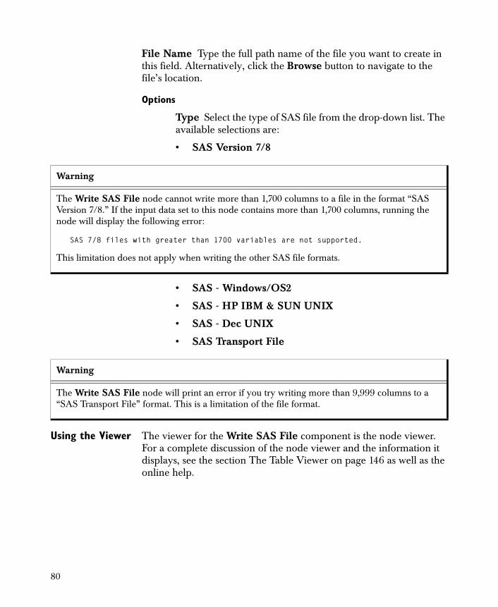
File Name Type the full path name of the file you want to create in this field. Alternatively, click the Browse button to navigate to the file’s location.
Options
Type Select the type of SAS file from the drop-down list. The available selections are:
• SAS Version 7/8
• SAS - Windows/OS2
• SAS - HP IBM & SUN UNIX
• SAS - Dec UNIX
• SAS Transport File
Using the Viewer The viewer for the Write SAS File component is the node viewer. For a complete discussion of the node viewer and the information it displays, see the section The Table Viewer on page 146 as well as the online help.
Warning
The Write SAS File node cannot write more than 1,700 columns to a file in the format “SAS Version 7/8.” If the input data set to this node contains more than 1,700 columns, running the node will display the following error:
SAS 7/8 files with greater than 1700 variables are not supported.
This limitation does not apply when writing the other SAS file formats.
Warning
The Write SAS File node will print an error if you try writing more than 9,999 columns to a “SAS Transport File” format. This is a limitation of the file format.
80

Write Spotfire Data
Use the Write Spotfire Data component to create TIBCO Spotfire® files of your data sets.
General Procedure
The following outlines the general approach for using the Write Spotfire Data component:
1. Link a Write Spotfire Data node in your worksheet to any node that outputs data.
2. Use the properties dialog for Write Spotfire Data to specify the name of the file to output the data to.
3. Run your network.
4. Launch the node’s viewer.
The Write Spotfire Data node accepts a single input containing rectangular data and returns no output.
Properties The Properties page of the Write Spotfire Data dialog is shown in Figure 2.16.
Figure 2.17: The Properties page of the Write Spotfire Data dialog.
81
File Name Type the full path name of the file you want to create in this field. Alternatively, click the Browse button to navigate to the file’s location.
The following table shows the conversion between Spotfire Miner and Spotfire data types when exporting data to Spotfire:
Using the Viewer The viewer for the Write Spotfire Data component is the node viewer. For a complete discussion of the node viewer and the information it displays, see the section The Table Viewer on page 146 as well as the online help.
Write Excel File
Use the Write Excel File component to create Excel files of your data sets.
Spotfire Miner supports reading and writing long text strings for specific file and database types. See Table 2.1 for more information.
General Procedure
The following outlines the general approach for using the Write Excel File component:
1. Link a Write Excel File node in your worksheet to any node that outputs data.
2. Use the properties dialog for Write Excel File to specify name and path of the Excel file you want to create.
3. Run your network.
4. Launch the node’s viewer.
The Write Excel File node accepts a single input containing rectangular data and returns no output.
Table 2.5: Spotfire Miner to Spotfire data type conversion.
Spotfire Miner Data Types Spotfire Data Types
string String
categorical String
continuous Real
date DateTime
82
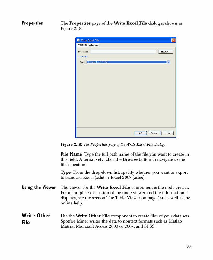
Properties The Properties page of the Write Excel File dialog is shown in Figure 2.18.
File Name Type the full path name of the file you want to create in this field. Alternatively, click the Browse button to navigate to the file’s location.
Type From the drop-down list, specify whether you want to export to standard Excel (.xls) or Excel 2007 (.xlsx).
Using the Viewer The viewer for the Write Excel File component is the node viewer. For a complete discussion of the node viewer and the information it displays, see the section The Table Viewer on page 146 as well as the online help.
Write Other File
Use the Write Other File component to create files of your data sets. Spotfire Miner writes the data to nontext formats such as Matlab Matrix, Microsoft Access 2000 or 2007, and SPSS.
Figure 2.18: The Properties page of the Write Excel File dialog.
83
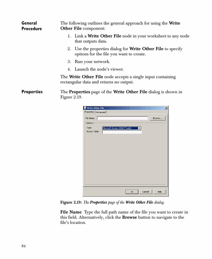
General Procedure
The following outlines the general approach for using the Write Other File component:
1. Link a Write Other File node in your worksheet to any node that outputs data.
2. Use the properties dialog for Write Other File to specify options for the file you want to create.
3. Run your network.
4. Launch the node’s viewer.
The Write Other File node accepts a single input containing rectangular data and returns no output.
Properties The Properties page of the Write Other File dialog is shown in Figure 2.19.
File Name Type the full path name of the file you want to create in this field. Alternatively, click the Browse button to navigate to the file’s location.
Figure 2.19: The Properties page of the Write Other File dialog.
84
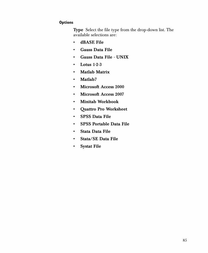
Options
Type Select the file type from the drop-down list. The available selections are:
• dBASE File
• Gauss Data File
• Gauss Data File - UNIX
• Lotus 1-2-3
• Matlab Matrix
• Matlab7
• Microsoft Access 2000
• Microsoft Access 2007
• Minitab Workbook
• Quattro Pro Worksheet
• SPSS Data File
• SPSS Portable Data File
• Stata Data File
• Stata/SE Data File
• Systat File
85
Access Table When writing a Microsoft Access 2000 or 2007 file, specify the name of the Access table in this field.
Using the Viewer The viewer for the Write Other File component is the node viewer. For a complete discussion of the node viewer and the information it displays, see the section The Table Viewer on page 146 as well as the online help.
Write Database ODBC
Use the Write Database - ODBC component to create database tables of your data sets. Spotfire Miner writes the data via Open DataBase Connectivity (ODBC) to database formats such as Oracle and DB2.
Notes
A Lotus 1-2-3 worksheet file cannot contain more than a fixed maximum number of rows. This is a limitation imposed by Lotus 1-2-3 and exists for all Lotus 1-2-3 worksheets. If the Write Other File node tries to write more than 8,190 rows to a Lotus 1-2-3 file, an error is printed and the file is closed.
Although it is possible to write Microsoft Access database files using the Write Database - ODBC component, writing them directly using the Write Other File component is significantly faster (10 times faster) than going through ODBC.
If you specify the Access 2000 or Access 2007 type, when the node runs, Spotfire Miner checks whether the system has the right driver files installed for writing these file types. If not, it displays an error indicating that the driver could not be found.
Access 1997 types are no longer supported, as of Spotfire Miner 8.1.
A Quattro Pro worksheet file cannot contain more than a fixed maximum number of rows. This is a limitation imposed by Quattro Pro and exists for all Quattro Pro worksheets. If the Write Other File node tries to write more than 8,190 rows to a Quattro Pro file, an error is printed and the file is closed.
86
Spotfire Miner supports reading and writing long text strings for specific file and database types. See Table 2.1 for more information.
For more information on using ODBC, see page 56 earlier in this chapter.
General Procedure
The following outlines the general approach for using the Write Database - ODBC component:
1. Link a Write Database - ODBC node in your worksheet to any node that outputs data.
2. Use the properties dialog for Write Database - ODBC to specify options for writing data to the database.
3. Run your network.
4. Launch the node’s viewer.
The Write Database - ODBC node accepts a single input containing rectangular data and returns no output.
Note
This component is only available on Microsoft Windows. Spotfire Miner supports ODBC versions 2.0 and 3.0.
Some databases have limitations on reading/writing data in specific formats, so there might be problems in reading or writing all column types from all databases.
87
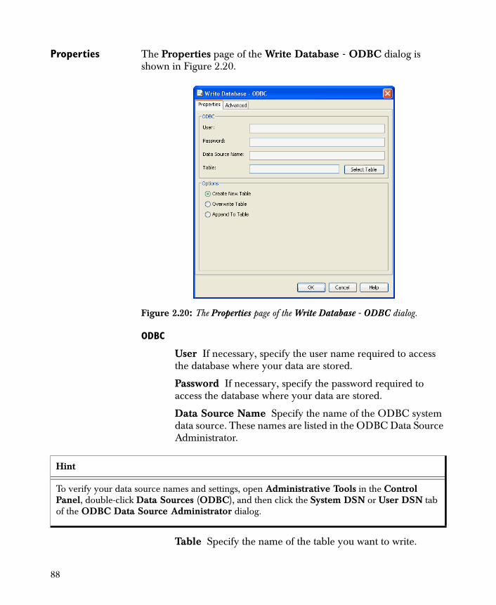
Properties The Properties page of the Write Database - ODBC dialog is shown in Figure 2.20.
ODBC
User If necessary, specify the user name required to access the database where your data are stored.
Password If necessary, specify the password required to access the database where your data are stored.
Data Source Name Specify the name of the ODBC system data source. These names are listed in the ODBC Data Source Administrator.
Table Specify the name of the table you want to write.
Figure 2.20: The Properties page of the Write Database - ODBC dialog.
Hint
To verify your data source names and settings, open Administrative Tools in the Control Panel, double-click Data Sources (ODBC), and then click the System DSN or User DSN tab of the ODBC Data Source Administrator dialog.
88
Select Table Click this button to display a list of the tables in the database. Select one to copy the name to the Table field.
Options
Create New Table Select this to prevent accidently changing existing tables. The output table is written only if a table with the specified name does not currently exist. If a table with this name already exists in the database, executing the node will print an error, and the database will not be changed.
Overwrite Table Select this if you are willing to overwrite existing tables. If this is selected, the output table is written whether or not it already exists. If it already exists, the current contents are deleted, and the table is recreated with the new output data.
Append To Table Select this to append the output data as new rows at the end of an existing table. If the output data contains column names that don’t appear in the existing table, these columns will be discarded. If the table doesn’t currently exist, a new table is created.
Using the Viewer The viewer for the Write Database - ODBC component is the node viewer. For a complete discussion of the node viewer and the information it displays, see the section The Table Viewer on page 146 as well as the online help.
Write DB2 Native
Use the Write DB2 - Native component to create database tables of your data sets. Spotfire Miner writes the data via an installed DB2 client.
Note
Spotfire Miner supports DB2 client version 7.1.
Previously, Spotfire Miner created fixed-length strings when exporting data to a DB2 database; however, this design did not allow for long strings to be exported. Now, when you export data to a DB2 database, Spotfire Miner creates the columns as varchar, rather than char, to accommodate up to 32,672 characters in a string. For more information on using DB2, see page 61 earlier in this chapter.
89
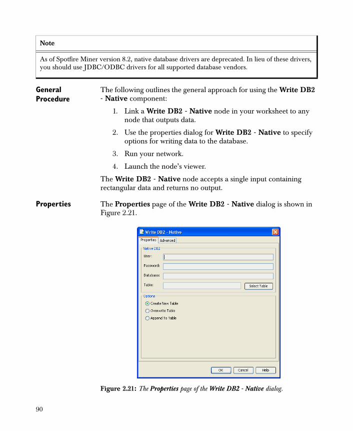
General Procedure
The following outlines the general approach for using the Write DB2 - Native component:
1. Link a Write DB2 - Native node in your worksheet to any node that outputs data.
2. Use the properties dialog for Write DB2 - Native to specify options for writing data to the database.
3. Run your network.
4. Launch the node’s viewer.
The Write DB2 - Native node accepts a single input containing rectangular data and returns no output.
Properties The Properties page of the Write DB2 - Native dialog is shown in Figure 2.21.
Note
As of Spotfire Miner version 8.2, native database drivers are deprecated. In lieu of these drivers, you should use JDBC/ODBC drivers for all supported database vendors.
Figure 2.21: The Properties page of the Write DB2 - Native dialog.
90
Native DB2
User If necessary, specify the user name required to access the database where your data are stored.
Password If necessary, specify the password required to access the database where your data are stored.
Database Specify the name of the database to be accessed.
Table Specify the name of the table you want to write.
Select Table Click this button to display a list of the tables in the database. Select one to copy the name to the Table field.
Options
Create New Table Select this to prevent accidently changing existing tables. The output table is written only if a table with the specified name does not currently exist. If a table with this name already exists in the database, executing the node will print an error, and the database will not be changed.
Overwrite Table Select this if you are willing to overwrite existing tables. If this is selected, the output table is written whether or not it already exists. If it already exists, the current contents are deleted, and the table is recreated with the new output data.
Append To Table Select this to append the output data as new rows at the end of an existing table. If the output data contains column names that don’t appear in the existing table, these columns will be discarded. If the table doesn’t currently exist, a new table is created.
Using the Viewer The viewer for the Write DB2 - Native component is the node viewer. For a complete discussion of the node viewer and the information it displays, see the section The Table Viewer on page 146 as well as the online help.
Write Oracle Native
Use the Write Oracle - Native component to create database tables of your data sets. Spotfire Miner writes the data via an installed Oracle client.
91

Spotfire Miner supports reading and writing long text strings for specific file and database types. See Table 2.1 for more information.
For more information on using Oracle, see page 63 earlier in this chapter.
General Procedure
The following outlines the general approach for using the Write Oracle - Native component:
1. Link a Write Oracle - Native node in your worksheet to any node that outputs data.
2. Use the properties dialog for Write Oracle - Native to specify options for writing data to the database.
3. Run your network.
4. Launch the node’s viewer.
The Write Oracle - Native node accepts a single input containing rectangular data and returns no output.
Note
Spotfire Miner supports Oracle client version 9i.
Note
As of Spotfire Miner version 8.2, native database drivers are deprecated. In lieu of these drivers, you should use JDBC/ODBC drivers for all supported database vendors.
92
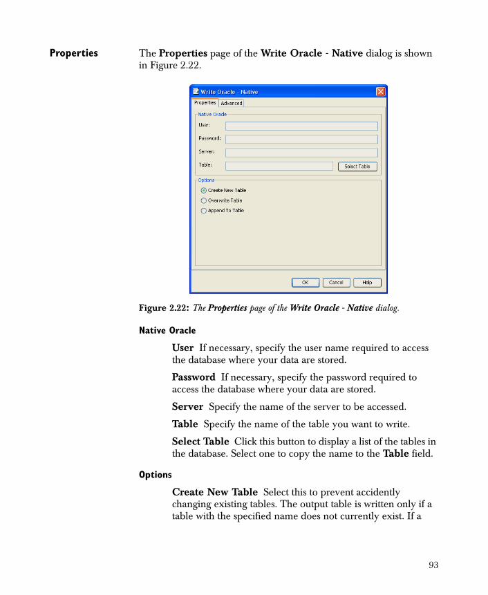
Properties The Properties page of the Write Oracle - Native dialog is shown in Figure 2.22.
Native Oracle
User If necessary, specify the user name required to access the database where your data are stored.
Password If necessary, specify the password required to access the database where your data are stored.
Server Specify the name of the server to be accessed.
Table Specify the name of the table you want to write.
Select Table Click this button to display a list of the tables in the database. Select one to copy the name to the Table field.
Options
Create New Table Select this to prevent accidently changing existing tables. The output table is written only if a table with the specified name does not currently exist. If a
Figure 2.22: The Properties page of the Write Oracle - Native dialog.
93

table with this name already exists in the database, executing the node will print an error, and the database will not be changed.
Overwrite Table Select this if you are willing to overwrite existing tables. If this is selected, the output table is written whether or not it already exists. If it already exists, the current contents are deleted, and the table is recreated with the new output data.
Append To Table Select this to append the output data as new rows at the end of an existing table. If the output data contains column names that don’t appear in the existing table, these columns will be discarded. If the table doesn’t currently exist, a new table is created.
Using the Viewer The viewer for the Write Oracle - Native component is the node viewer. For a complete discussion of the node viewer and the information it displays, see the section The Table Viewer on page 146 as well as the online help.
Write SQL Native
Use the Write SQL - Native component to create database tables of your data sets. Spotfire Miner writes the data via an installed Microsoft SQL Server client.
Spotfire Miner supports reading and writing long text strings for specific file and database types. See Table 2.1 for more information.
For more information on using Microsoft SQL Server, see page 67 earlier in this chapter.
Note
This component is only available on Microsoft Windows.
Note
As of Spotfire Miner version 8.2, native database drivers are deprecated. In lieu of these drivers, you should use JDBC/ODBC drivers for all supported database vendors.
94
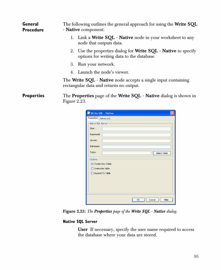
General Procedure
The following outlines the general approach for using the Write SQL - Native component:
1. Link a Write SQL - Native node in your worksheet to any node that outputs data.
2. Use the properties dialog for Write SQL - Native to specify options for writing data to the database.
3. Run your network.
4. Launch the node’s viewer.
The Write SQL - Native node accepts a single input containing rectangular data and returns no output.
Properties The Properties page of the Write SQL - Native dialog is shown in Figure 2.23.
Native SQL Server
User If necessary, specify the user name required to access the database where your data are stored.
Figure 2.23: The Properties page of the Write SQL - Native dialog.
95
Password If necessary, specify the password required to access the database where your data are stored.
Server Specify the name of the server to be accessed.
Database Specify the name of the database to be accessed.
Table Specify the name of the table you want to write.
Select Table Click this button to display a list of the tables in the database. Select one to copy the name to the Table field.
Options
Create New Table Select this to prevent accidently changing existing tables. The output table is written only if a table with the specified name does not currently exist. If a table with this name already exists in the database, executing the node will print an error, and the database will not be changed.
Overwrite Table Select this if you are willing to overwrite existing tables. If this is selected, the output table is written whether or not it already exists. If it already exists, the current contents are deleted, and the table is recreated with the new output data.
Append To Table Select this to append the output data as new rows at the end of an existing table. If the output data contains column names that don’t appear in the existing table, these columns will be discarded. If the table doesn’t currently exist, a new table is created.
Using the Viewer The viewer for the Write SQL - Native component is the node viewer. For a complete discussion of the node viewer and the information it displays, see the section The Table Viewer on page 146 as well as the online help.
96

Write Sybase Native
Use the Write Sybase - Native component to create database tables of your data sets. Spotfire Miner writes the data via an installed Sybase client.
For more information on using Sybase, see page 70 earlier in this chapter.
General Procedure
The following outlines the general approach for using the Write Sybase - Native component:
1. Link a Write Sybase - Native node in your worksheet to any node that outputs data.
2. Use the properties dialog for Write Sybase - Native to specify options for writing data to the database.
3. Run your network.
4. Launch the node’s viewer.
The Write Sybase - Native node accepts a single input containing rectangular data and returns no output.
Note
Spotfire Miner supports Sybase client version 12.5.
Note
As of Spotfire Miner version 8.2, native database drivers are deprecated. In lieu of these drivers, you should use JDBC/ODBC drivers for all supported database vendors.
97
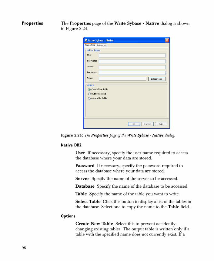
Properties The Properties page of the Write Sybase - Native dialog is shown in Figure 2.24.
Native DB2
User If necessary, specify the user name required to access the database where your data are stored.
Password If necessary, specify the password required to access the database where your data are stored.
Server Specify the name of the server to be accessed.
Database Specify the name of the database to be accessed.
Table Specify the name of the table you want to write.
Select Table Click this button to display a list of the tables in the database. Select one to copy the name to the Table field.
Options
Create New Table Select this to prevent accidently changing existing tables. The output table is written only if a table with the specified name does not currently exist. If a
Figure 2.24: The Properties page of the Write Sybase - Native dialog.
98
table with this name already exists in the database, executing the node will print an error, and the database will not be changed.
Overwrite Table Select this if you are willing to overwrite existing tables. If this is selected, the output table is written whether or not it already exists. If it already exists, the current contents are deleted, and the table is recreated with the new output data.
Append To Table Select this to append the output data as new rows at the end of an existing table. If the output data contains column names that don’t appear in the existing table, these columns will be discarded. If the table doesn’t currently exist, a new table is created.
Using the Viewer The viewer for the Write Sybase - Native component is the node viewer. For a complete discussion of the node viewer and the information it displays, see the section The Table Viewer on page 146 as well as the online help.
Write Database JDBC
The Write Database - JDBC component is provided in a separate library; it is not part of the Main library. For detailed information about using this library, see the section Importing and Exporting Data with JDBC on page 581.
The JDBC library provides nodes that implement the read and write capability of the sjdbc package, a Spotfire S+ library provided with Spotfire Miner. The sjdbc library includes a Help file, which you can find in MHOME/splus/library/sjdbc (where MHOME is your Spotfire Miner installation directory).
Use the Write Database - JDBC component to write data to a relational data source (for example, a SQL database) or to a tabular data source (for example, a spreadsheet). To write to a database using JDBC, you must use the appropriate JDBC driver to connect to the JDBC interface.
99

100

Overview 102The Main Menu 103The Toolbar 119The Explorer Pane 120The Desktop Pane 127The Message Pane 127The Command Line Pane 127
The Spotfire Miner™ Working Environment 128Worksheet Directories 128The Examples Folder 129
Building and Editing Networks 130Building a Network 131Running and Stopping a Network 136
Common Features of Network Nodes 139Shortcut Menus 139Properties Dialogs 139Viewers 145
THE TIBCO SPOTFIRE MINER™ INTERFACE 3
101
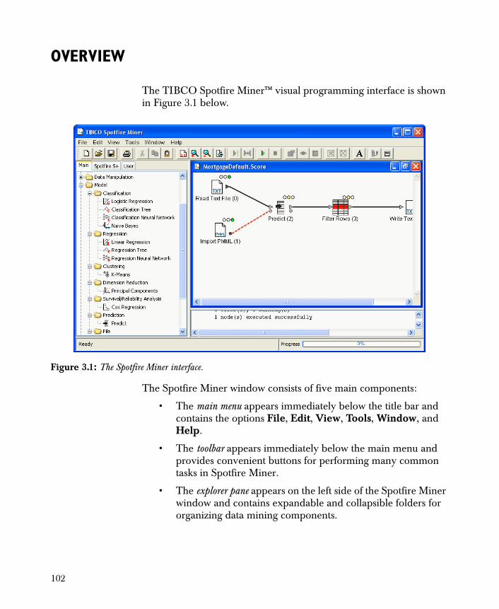
OVERVIEW
The TIBCO Spotfire Miner™ visual programming interface is shown in Figure 3.1 below.
The Spotfire Miner window consists of five main components:
• The main menu appears immediately below the title bar and contains the options File, Edit, View, Tools, Window, and Help.
• The toolbar appears immediately below the main menu and provides convenient buttons for performing many common tasks in Spotfire Miner.
• The explorer pane appears on the left side of the Spotfire Miner window and contains expandable and collapsible folders for organizing data mining components.
Figure 3.1: The Spotfire Miner interface.
102
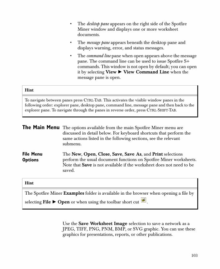
• The desktop pane appears on the right side of the Spotfire Miner window and displays one or more worksheet documents.
• The message pane appears beneath the desktop pane and displays warning, error, and status messages.
• The command line pane when open appears above the message pane. The command line can be used to issue Spotfire S+ commands. This window is not open by default; you can open it by selecting View � View Command Line when the message pane is open.
The Main Menu The options available from the main Spotfire Miner menu are discussed in detail below. For keyboard shortcuts that perform the same actions listed in the following sections, see the relevant submenu.
File Menu Options
The New, Open, Close, Save, Save As, and Print selections perform the usual document functions on Spotfire Miner worksheets. Note that Save is not available if the worksheet does not need to be saved.
Use the Save Worksheet Image selection to save a network as a JPEG, TIFF, PNG, PNM, BMP, or SVG graphic. You can use these graphics for presentations, reports, or other publications.
Hint
To navigate between panes press CTRL-TAB. This activates the visible window panes in the following order: explorer pane, desktop pane, command line, message pane and then back to the explorer pane. To navigate through the panes in reverse order, press CTRL-SHIFT-TAB.
Hint
The Spotfire Miner Examples folder is available in the browser when opening a file by
selecting File � Open or when using the toolbar short cut .
103
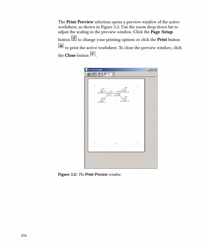
The Print Preview selection opens a preview window of the active worksheet, as shown in Figure 3.2. Use the zoom drop-down list to adjust the scaling in the preview window. Click the Page Setup
button to change your printing options or click the Print button
to print the active worksheet. To close the preview window, click
the Close button .
Figure 3.2: The Print Preview window.
104
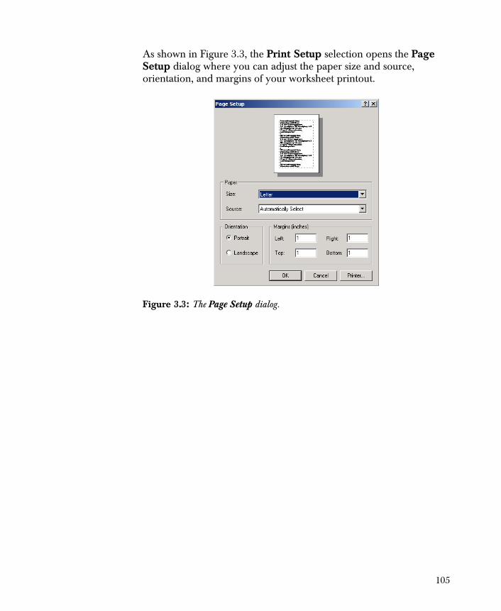
As shown in Figure 3.3, the Print Setup selection opens the Page Setup dialog where you can adjust the paper size and source, orientation, and margins of your worksheet printout.
Figure 3.3: The Page Setup dialog.
105

The Properties selection opens the Worksheet Properties dialog, which displays the file name and path, size, and other information for the current worksheet. An example is shown in Figure 3.4.
You can add version, author and other comment information on this page.
The Parameters tab of the Worksheet Properties dialog, shown in Figure 3.6, can contain the default values any named parameters that apply to the entire worksheet. When you run the worksheet, the text property you specify in the node dialog uses the value you specify in the parameters list of this dialog. This feature is useful if you need to use the same parameter repeatedly in the same worksheet, and you want to be able to set its value in one location. Setting a default parameter value works only with text properties, such as a file name or the name of an S-PLUS script.
Figure 3.4: The Properties dialog for the active worksheet.
106
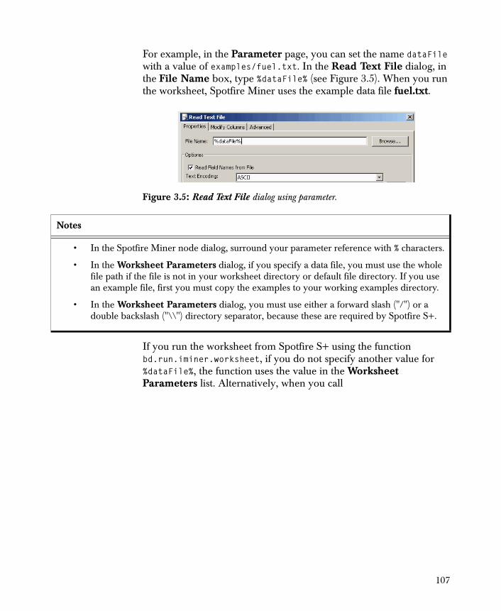
For example, in the Parameter page, you can set the name dataFile with a value of examples/fuel.txt. In the Read Text File dialog, in the File Name box, type %dataFile% (see Figure 3.5). When you run the worksheet, Spotfire Miner uses the example data file fuel.txt.
If you run the worksheet from Spotfire S+ using the function bd.run.iminer.worksheet, if you do not specify another value for %dataFile%, the function uses the value in the Worksheet Parameters list. Alternatively, when you call
Figure 3.5: Read Text File dialog using parameter.
Notes
• In the Spotfire Miner node dialog, surround your parameter reference with % characters.
• In the Worksheet Parameters dialog, if you specify a data file, you must use the whole file path if the file is not in your worksheet directory or default file directory. If you use an example file, first you must copy the examples to your working examples directory.
• In the Worksheet Parameters dialog, you must use either a forward slash ("/") or a double backslash ("\\") directory separator, because these are required by Spotfire S+.
107
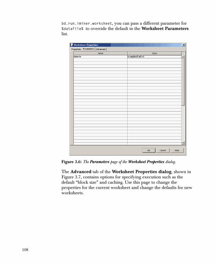
bd.run.iminer.worksheet, you can pass a different parameter for %dataFile% to override the default in the Worksheet Parameters list.
The Advanced tab of the Worksheet Properties dialog, shown in Figure 3.7, contains options for specifying execution such as the default “block size” and caching. Use this page to change the properties for the current worksheet and change the defaults for new worksheets.
Figure 3.6: The Parameters page of the Worksheet Properties dialog.
108

Default Maximum String Size Sets the width of strings in your data sets. By default, it is equal to 32, which means that each entry in a string column can contain no more than 32 characters; entries that exceed this limit are truncated. To increase or decrease the maximum string size, type a new value in the text box. Note that the maximum should be larger than the widest entry in a string column since strings can include multibyte unicode characters and each string must contain a termination character.
Maximum Categorical Levels Specifies the maximum number of levels a categorical variable can have. By default, this value is 500 but you can type another number. (The value in this field is constrained to be an integer in the range between 500 and 65,534.)
Figure 3.7: The Advanced page of the Worksheet Properties dialog.
109
Number of Digits in Viewers Controls the number of decimal digits that are displayed in the node viewers.
Date Parsing Format Controls the default date parsing string used when reading a string as a date or when converting a string to a date. The initial value for this field is:
%m[/][.]%d[/][,]%y [%H[:%M[:%S[.%N]]]] [%p]
The bracket notation allows this string to handle a variety of different date strings, including 1/2/94 and January 31, 1995 5:45pm. (For detailed information, see the section Date Parsing Formats on page 28.)
Date Display Format Controls the default date format string used when displaying a date value in a table viewer or when writing a date to a text file. The initial value for this field is:
%02m/%02d/%Y %02H:%02M:%02S
This produces a simple string with the day represented by three numbers and the time within the day on the 24-hour clock, such as 01/31/1995 17:45:00. (For detailed information, see the section Date Display Formats on page 30.)
Date Century Cutoff A year number beginning a 100-year sequence that is used when parsing and formatting two-digit years. When parsing a two-digit year, it is interpreted as a year within that 100-year range. For example, if the century cutoff is 1930, the two-digit year “40” is interpreted as 1940 and “20” is interpreted as 2020. The initial value of this field is 1950.
Decimal & Thousands Symbol Specifies the symbols to be used as the decimal marker (default is a period (.)) and thousands separator (default is a comma (,)). This field takes a
110
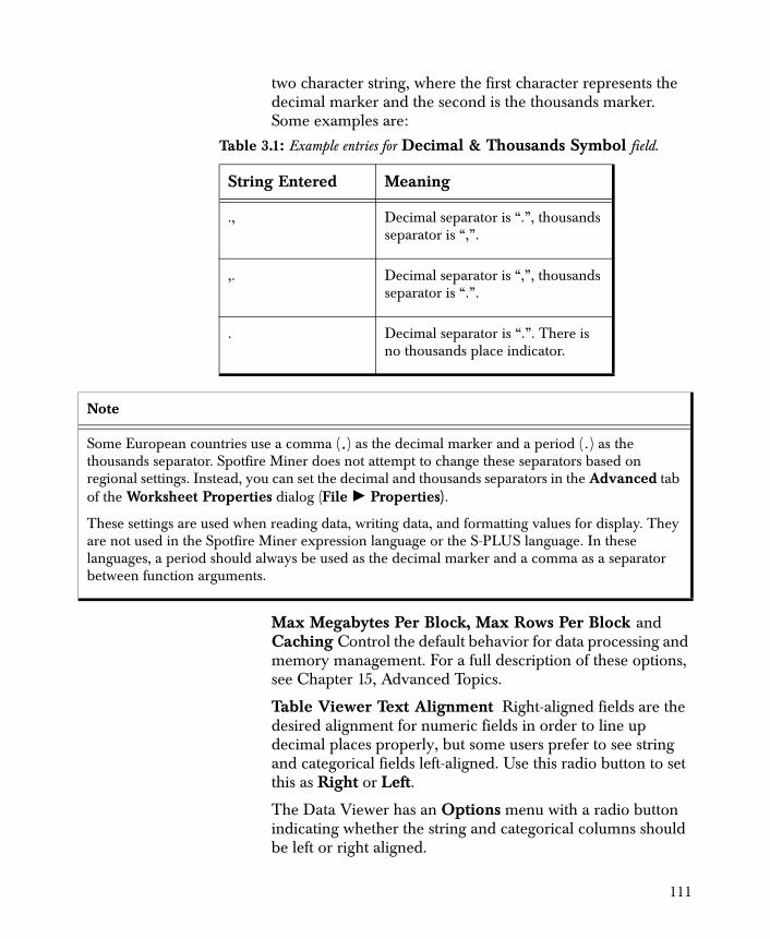
two character string, where the first character represents the decimal marker and the second is the thousands marker. Some examples are:
Max Megabytes Per Block, Max Rows Per Block and Caching Control the default behavior for data processing and memory management. For a full description of these options, see Chapter 15, Advanced Topics.
Table Viewer Text Alignment Right-aligned fields are the desired alignment for numeric fields in order to line up decimal places properly, but some users prefer to see string and categorical fields left-aligned. Use this radio button to set this as Right or Left.
The Data Viewer has an Options menu with a radio button indicating whether the string and categorical columns should be left or right aligned.
Table 3.1: Example entries for Decimal & Thousands Symbol field.
String Entered Meaning
., Decimal separator is “.”, thousands separator is “,”.
,. Decimal separator is “,”, thousands separator is “.”.
. Decimal separator is “.”. There is no thousands place indicator.
Note
Some European countries use a comma (,) as the decimal marker and a period (.) as the thousands separator. Spotfire Miner does not attempt to change these separators based on regional settings. Instead, you can set the decimal and thousands separators in the Advanced tab of the Worksheet Properties dialog (File � Properties).
These settings are used when reading data, writing data, and formatting values for display. They are not used in the Spotfire Miner expression language or the S-PLUS language. In these languages, a period should always be used as the decimal marker and a comma as a separator between function arguments.
111
Use Current Defaults, Use Factory Defaults, and Set Defaults for New Worksheets Clicking Use Current Defaults applies the settings in this page to the current worksheet. Clicking Use Factory Defaults resets them to the factory settings, and clicking Set Defaults for New Worksheets applies the settings in this page to all new worksheets.
Random Seeds Specifies the node setting for Fix All Node Random Seeds or Allow A New Seed Every Time.
Default File Directory The location of the files used in the read/write nodes, if the specified read/write filename is not an absolute file name. If this is not specified, it defaults to the location of the .imw (worksheet) file.
Worksheet Data Directory The location of the .wsd directory. If not specified, it is assumed to be in the same directory as the .imw file.
Spotfire S+ Working Chapter Specifies the first library in searchPaths() when the S-PLUS script node is executed. If not set, it uses %Documents%\Spotfire Miner. Note the directory has to actually be a Spotfire S+ chapter when it is used. In addition, changes to Spotfire S+ Working Chapter do not take effect until a new worksheet is opened or until the current worksheet is closed and opened.
Finally, for ease of access, the bottom of the File menu lists the five most recently opened worksheets.
Edit Menu Options
Undo, Redo, Cut, Copy, Paste, and Delete perform the usual editing functions on nodes in Spotfire Miner worksheets, as well as on text in dialog fields.
Note
The location of the %Documents% folder depends on which version of Microsoft Windows® you are running. By default:
• On Windows XP: C:\Documents and Settings\username\My Documents\Spotfire Miner.
• On Windows Vista: C:\users\username\Documents\Spotfire Miner.
112
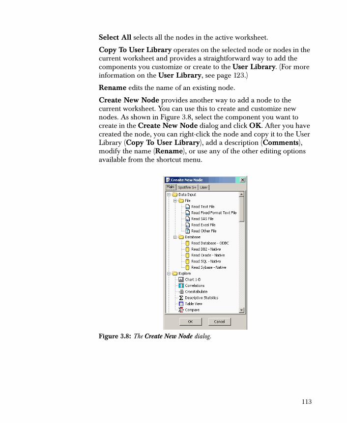
Select All selects all the nodes in the active worksheet.
Copy To User Library operates on the selected node or nodes in the current worksheet and provides a straightforward way to add the components you customize or create to the User Library. (For more information on the User Library, see page 123.)
Rename edits the name of an existing node.
Create New Node provides another way to add a node to the current worksheet. You can use this to create and customize new nodes. As shown in Figure 3.8, select the component you want to create in the Create New Node dialog and click OK. After you have created the node, you can right-click the node and copy it to the User Library (Copy To User Library), add a description (Comments), modify the name (Rename), or use any of the other editing options available from the shortcut menu.
Figure 3.8: The Create New Node dialog.
113
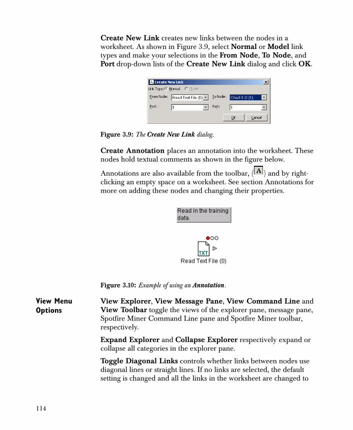
Create New Link creates new links between the nodes in a worksheet. As shown in Figure 3.9, select Normal or Model link types and make your selections in the From Node, To Node, and Port drop-down lists of the Create New Link dialog and click OK.
Create Annotation places an annotation into the worksheet. These nodes hold textual comments as shown in the figure below.
Annotations are also available from the toolbar, ( ) and by right-clicking an empty space on a worksheet. See section Annotations for more on adding these nodes and changing their properties.
View Menu Options
View Explorer, View Message Pane, View Command Line and View Toolbar toggle the views of the explorer pane, message pane, Spotfire Miner Command Line pane and Spotfire Miner toolbar, respectively.
Expand Explorer and Collapse Explorer respectively expand or collapse all categories in the explorer pane.
Toggle Diagonal Links controls whether links between nodes use diagonal lines or straight lines. If no links are selected, the default setting is changed and all the links in the worksheet are changed to
Figure 3.9: The Create New Link dialog.
Figure 3.10: Example of using an Annotation.
114
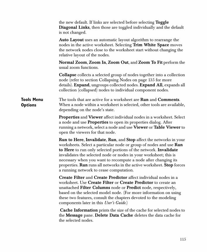
the new default. If links are selected before selecting Toggle Diagonal Links, then those are toggled individually and the default is not changed.
Auto Layout uses an automatic layout algorithm to rearrange the nodes in the active worksheet. Selecting Trim White Space moves the network nodes close to the worksheet start without changing the relative layout of the nodes.
Normal Zoom, Zoom In, Zoom Out, and Zoom To Fit perform the usual zoom functions.
Collapse collects a selected group of nodes together into a collection node (refer to section Collapsing Nodes on page 135 for more details). Expand, ungroups collected nodes. Expand All, expands all collection (collapsed) nodes to individual component nodes.
Tools Menu Options
The tools that are active for a worksheet are Run and Comments. When a node within a worksheet is selected, other tools are available, depending on the node’s state.
Properties and Viewer affect individual nodes in a worksheet. Select a node and use Properties to open its properties dialog. After running a network, select a node and use Viewer or Table Viewer to open the viewers for that node.
Run to Here, Invalidate, Run, and Stop affect the networks in your worksheets. Select a particular node or group of nodes and use Run to Here to run only selected portions of the network. Invalidate invalidates the selected node or nodes in your worksheet; this is necessary when you want to recompute a node after changing its properties. Run runs all networks in the active worksheet. Stop forces a running network to cease computation.
Create Filter and Create Predictor affect individual nodes in a worksheet. Use Create Filter or Create Predictor to create an unattached Filter Columns node or Predict node, respectively, based on the selected model node. (For more information on using these two features, consult the chapters devoted to the modeling components later in this User’s Guide.)
Cache Information prints the size of the cache for selected nodes to the Message pane. Delete Data Cache deletes the data cache for the selected nodes.
115
Comments opens the Comment Editor, shown in Figure 3.11, which you can use to record your notations about individual worksheets or particular nodes in a worksheet. There are two types of comments: description and discussion. The type to add or edit is displayed in the Comment Type field.
Options opens the Global Properties dialog, where you can specify global options that affect your Spotfire Miner sessions, including the default working and temp directories.
The Properties page of the Global Properties dialog, shown in Figure 3.12, contains the following fields:
Working Directory Specify the working directory for Spotfire Miner to use as the starting location when searching for input files, saving documents, writing to output files, and storing log files. By default, your working directory location matches your default home directory, as indicated by the operating system.
Figure 3.11: The Comment Editor dialog.
116

On Microsoft Windows, this is a location such as %Documents%\Spotfire Miner. To specify a different working directory, click the Browse button and navigate to the desired location.
Temp Directory Specify the temporary directory for Spotfire Miner to use as the default location for storing temporary files, such as HTML files output from a tree viewer. The default location of the temporary directory varies depending on whether you use Windows Vista or Windows XP. To specify a different temporary directory, click the Browse button and navigate to the desired location.
Text Editor This field provides a way to specify a default text editing program.
Show Startup Dialog When starting Spotfire Miner, by default, you are prompted whether to open a new worksheet or asked to select an existing worksheet to open. You can choose to open Spotfire Miner with no open worksheets by clearing the check box.
Figure 3.12: The Properties page of the Global Properties dialog.
117
Activate Intelligent Double Click By default, when you double-click a node in a network, its properties dialog is opened. However, you can set the double-click behavior to vary based on the state of the node. When you select this check box, double-clicking a node opens the viewer if the node is ready to be viewed and the properties dialog otherwise.
Display Viewer After Run To Here Sets the option to display the viewer each time you select Run to Here.
The Library submenu contains tools for manipulating and managing the libraries. This is the same menu that is obtained by right-clicking on a library tab or on blank space in the explorer pane. These library tools (Manage Libraries, Library Properties, Hide Library, Create New Library, Save Library As, Revert Library, and Create New Folder) are discussed in the section Other Library Operations on page 125 and the section Library Manager on page 124.
Window Menu Options
Close Viewer closes all non-HTML viewers. By default, all open viewers are closed. Clear the check boxes next to viewers that you want to remain open.
Tile Horizontal, Tile Vertical, and Cascade arrange your windows in the desktop pane when multiple worksheet document windows are open. Selecting Minimize All minimizes all open windows. The minimized windows are arranged in a row at the bottom of the desktop pane when Arrange Icons is selected.
At the bottom of the Window menu, Spotfire Miner lists the names of all your open worksheets so that you can move easily between them.
Help Menu Options
The Help menu gives you access to the online help system and the PDF versions of the Getting Started Guide and this User’s Guide. For complete details on using the Spotfire Miner help system, see the Using the Help System help topic.
About displays the About Spotfire Miner dialog with version, serial number, and copyright information.
118
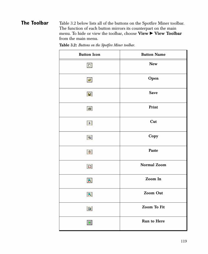
The Toolbar Table 3.2 below lists all of the buttons on the Spotfire Miner toolbar. The function of each button mirrors its counterpart on the main menu. To hide or view the toolbar, choose View � View Toolbar from the main menu.Table 3.2: Buttons on the Spotfire Miner toolbar.
Button Icon Button Name
New
Open
Save
Cut
Copy
Paste
Normal Zoom
Zoom In
Zoom Out
Zoom To Fit
Run to Here
119
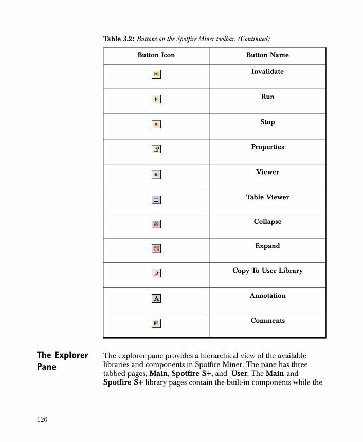
The Explorer Pane
The explorer pane provides a hierarchical view of the available libraries and components in Spotfire Miner. The pane has three tabbed pages, Main, Spotfire S+, and User. The Main and Spotfire S+ library pages contain the built-in components while the
Invalidate
Run
Stop
Properties
Viewer
Table Viewer
Collapse
Expand
Copy To User Library
Annotation
Comments
Table 3.2: Buttons on the Spotfire Miner toolbar. (Continued)
Button Icon Button Name
120
User library page contains the components that you create. To hide or view the explorer pane, choose View � View Explorer from the main menu.
The Main Library The Main Library organizes components into high-level categories so that related components are easy to find. The organization of the categories encourages a particular methodology in the networks you build; that is, first you identify your data sources, then you explore and clean the data, then you manipulate the data, then you build models, and so on.
In the explorer pane, the high-level categories appear with small folder icons and the components themselves appear with unique icons that visually signify their functions.
• To expand or collapse a category, double-click its name.
• To expand (or collapse) all categories simultaneously in the explorer pane, choose View � Expand Explorer (or View � Collapse Explorer) from the main menu.
• To hide or unhide the explorer pane, choose View � View Explorer from the main menu.
Right-clicking a component in the explorer pane opens a shortcut menu that contains Help, Delete, Paste, Cut, Copy, Undo and Redo which perform the usual Windows operations on the nodes. There are also the following Spotfire Miner specific options:
Create New Node Adds a node of this type to the current worksheet.
Set Default Properties Opens the properties dialog for the component, where you can set the component’s properties to the desired default values. These defaults are used each time a new component of this type is created.
Hint
In the explorer pane, use the up and down arrow keys to navigate through all the folders and components. Use the left and right arrow keys to collapse and expand, respectively, individual folders or components. With a particular component highlighted in the explorer pane, press ENTER to create this node in the active worksheet. To navigate between the library tabs, first press ESC and then press the left or right arrow key.
121
Copy To User Library Copies the currently selected node to the User library.
Rename Renames a node.
Comments Opens the comment editor dialog as show in Figure 3.11. When Comment Type shows Description, the comments replace the contents of the Description field after you click Add. You can add more discussion comments by selecting Discussion in Comment Type, typing the comment into the Edit Comment box, and then clicking Add.
The Spotfire S+ Library
The Spotfire S+ Library contains components of the S language engine. The library is organized and manipulated in the same ways as the Main library. Refer to the above section for those details.
The S language engine from Spotfire S+ is part of the basic Spotfire Miner™ system and does not need to be explicitly installed. The Spotfire S+ page appears in the explorer pane.
See Chapter 16, The S-PLUS Library for more information about the S language engine and the S-PLUS nodes, demonstrations of transforming a data set by writing S-PLUS expressions. Consult the printed or online documentation for Spotfire S+ for more detailed information about the S language.
Note
If you plan to use the Spotfire Miner Spotfire S+ node extensively, you could also benefit from using TIBCO Spotfire S+ , which provides features that are not included in Spotfire Miner, such as the Spotfire S+ GUI, the Workbench developer environment, the Spotfire S+ console application (sqpe), the Spotfire S+ Excel Add-In, and the Spotfire S+ SPSS Add-In, plus support for Automation and for other interfaces (including OLE, DDE, and COM).
Note
Spotfire Miner works only with the included Spotfire S+ libraries and S language engine; you cannot use an externally-installed version of Spotfire S+ with Spotfire Miner.
122
The User Library The User Library is the location where you can store the components you customize or create. For example, if you find that you typically manipulate your data in a particular way, you can set these options in your data manipulation node, save the node with a new name, and store it in the User Library for future use.
Copying Nodes To Libraries
To copy a node to the User Library, do one of the following:
• Click to select the node and choose Edit � Copy To User Library from the main menu.
• Right-click the node and choose Copy To User Library from the shortcut menu.
• Click or CTRL-click the node, and then drag it to the user library tab, wait until the User library pane appears, and then continue dragging the node until it is positioned where you want it in the library.
To copy nodes to other libraries or between libraries, click the node and then drag it to the library tab, wait until the library pane appears, and then continue dragging the node until it is positioned where you want it in the library.
Deleting Library Components
To delete a component from a library, right-click the node, and then click Delete.
123
Library Manager The library manager lists the libraries that are available in the current Spotfire Miner session. You can open the Library Manager (shown in Figure 3.13) dialog by clicking Tools � Library � Manage Libraries or right-clicking a library tab in the explorer pane and selecting Manage Libraries.
Selecting Show next to the library exposes the library in the explorer pane. To hide a library, clear its check box.
Each library is defined in a file, typically named *.iml. For each library, Library Manager shows the Library Name, used to label the tab in the explorer, and the File, the original name of the file defining the library.
Browse displays user libraries that you can add to the explorer pane. When you click Browse, a dialog appears for selecting a library definition file, which is added to the list. The original file name is saved when the library is added, but the library definition file is copied into a user settings directory, so manually editing the original file does not change the library.
New creates a new custom library. Clicking New displays a dialog for specifying a Library Name, which is used to save the new library file, and to label the library tab in the explorer.
Figure 3.13: The Library Manager dialog.
124
Remove permanently removes a user-created library from Spotfire Miner. Select the library name or file from the list, and then click Remove. In the resulting dialog, confirm removing the library. You can load the original library file again later, but changes you made since you loaded the original library file are lost.
You cannot remove system libraries. If you attempt to remove a system library (Main, User, or Spotfire S+) you are prompted to hide the library instead.
Other Library Operations
You can copy, delete, or rename the components and folders in all libraries using standard procedures, as described above in the section The Main Library.
You can perform other operations on libraries (in addition to Manage Libraries). These operations are available from the Tools � Library menu, or by right-clicking a library tab in the explorer pane. The library tools menu is shown in Figure 3.14.
Create New Folder adds a new folder into the current library.
Set Default Properties sets the node defaults for future nodes of the selected type. Default properties can be overwritten through the Properties dialog for the selected node. Note, however, that not all
Hint
To preserve changes to a library so you can use it later or pass it to other users, right-click the library tab, select Save Library As, and then type a new library name. This saves the current state of the library into the specified file.
You can make a library read-only on the library properties dialog (available from Tools � Library � Library Properties).
Figure 3.14: Library tools menu.
125
properties can be set in advance using Set Default Properties, for example, information that requires knowing which data set is being used.
Create New Library creates a new custom library, just like the New button in the library manager dialog.
Save Library As prompts you to specify a file name, and writes a copy of the current library definition into the file. This file can be read using the Browse button in the library manager.
Library Properties shows a dialog for setting the library title used for labeling the explorer tab, a text description, an author field, and a check box which shows whether the library is read-only.
Hide Library hides the current library, just like unchecking the Show box in the library manager dialog.
Revert Library restores the library to the state it had when it was loaded, discarding any changes made. This shows a dialog so you can confirm that you wish to overwrite any changes.
126
The Desktop Pane
The desktop pane can contain one or more open worksheet documents. A worksheet is populated via drag-and-drop or double-click operations initiated from the explorer pane. You can drag components from the explorer pane and drop them into worksheets to form the nodes of a work flow diagram. After you place and link the nodes, they form a network that reads, manipulates, graphs, and models your data.
The Message Pane
The message pane contains output text, the purpose of which is to display status, warning, and error messages. The shortcut menu for the message pane provides menu selections for clearing all text from the pane and for copying selected text to the clipboard.
To hide or view the message pane, choose View � View Message Pane from the main menu.
The Command Line Pane
Using the command line pane, you can type in Spotfire S+ commands. The results appear in the message pane. You can find more details about this feature in the Chapter 16, The S-PLUS Library.
Hint
In the desktop pane, press ENTER to navigate through each node and link in the active worksheet; press SHIFT-ENTER to navigate in the reverse direction. With a particular node selected in the desktop pane, press F5 to display its properties dialog, F9 to run the network to this node, or F4 to display the node’s viewer.
127
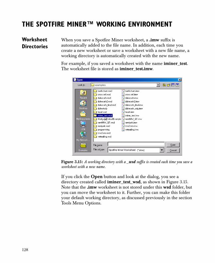
THE SPOTFIRE MINER™ WORKING ENVIRONMENT
Worksheet Directories
When you save a Spotfire Miner worksheet, a .imw suffix is automatically added to the file name. In addition, each time you create a new worksheet or save a worksheet with a new file name, a working directory is automatically created with the new name.
For example, if you saved a worksheet with the name iminer_test. The worksheet file is stored as iminer_test.imw.
If you click the Open button and look at the dialog, you see a directory created called iminer_test_wsd, as shown in Figure 3.15. Note that the .imw worksheet is not stored under this wsd folder, but you can move the worksheet to it. Further, you can make this folder your default working directory, as discussed previously in the section Tools Menu Options.
Figure 3.15: A working directory with a _wsd suffix is created each time you save a worksheet with a new name.
128
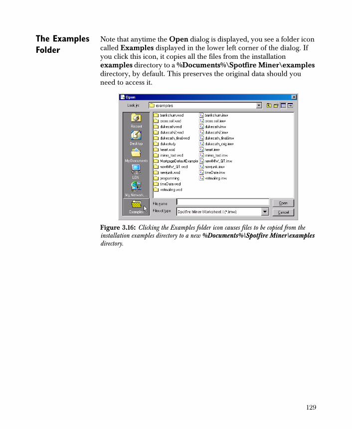
The Examples Folder
Note that anytime the Open dialog is displayed, you see a folder icon called Examples displayed in the lower left corner of the dialog. If you click this icon, it copies all the files from the installation examples directory to a %Documents%\Spotfire Miner\examples directory, by default. This preserves the original data should you need to access it.
Figure 3.16: Clicking the Examples folder icon causes files to be copied from the installation examples directory to a new %Documents%\Spotfire Miner\examples directory.
129
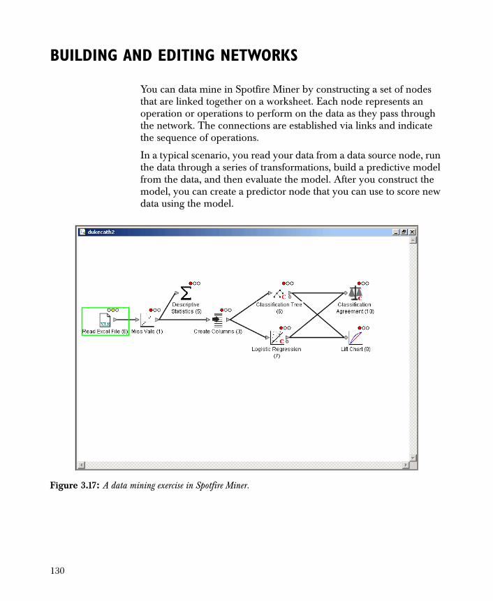
BUILDING AND EDITING NETWORKS
You can data mine in Spotfire Miner by constructing a set of nodes that are linked together on a worksheet. Each node represents an operation or operations to perform on the data as they pass through the network. The connections are established via links and indicate the sequence of operations.
In a typical scenario, you read your data from a data source node, run the data through a series of transformations, build a predictive model from the data, and then evaluate the model. After you construct the model, you can create a predictor node that you can use to score new data using the model.
Figure 3.17: A data mining exercise in Spotfire Miner.
130
Building a Network
To build a network in Spotfire Miner, add components from the explorer pane to your worksheet in the desktop pane, link them together to form a network, specify the required properties for each, and then run the network. A worksheet can contain multiple, unconnected networks.
Adding Nodes To add a node to a worksheet, do one of the following:
• Double-click the component’s name in the explorer pane, and then reposition the node in the worksheet, if necessary.
• Select the component’s name in the explorer pane, press ENTER, and then reposition the node in the worksheet, if necessary.
• Click and drag the component from the explorer pane and drop it in place in the worksheet.
• On the main menu, select Edit � Create New Node
• Right-click the worksheet pane and select Create New Node.
The explorer pane groups components into a hierarchy that suggests the general order of operations.
When you first add a component to a worksheet, its status indicator is red, showing that it is not ready to be run.
Note
The data mining components in the explorer pane are referred to as nodes in the desktop pane, because that is where they are linked together to form a network.
Hint
For ease of reference, Spotfire Miner assigns each node in a network an index number that appears just to the right of its name in a worksheet. Because Spotfire Miner uses these numbers as references in the message pane, it is easy to distinguish multiple nodes of the same type in a complicated network.
131
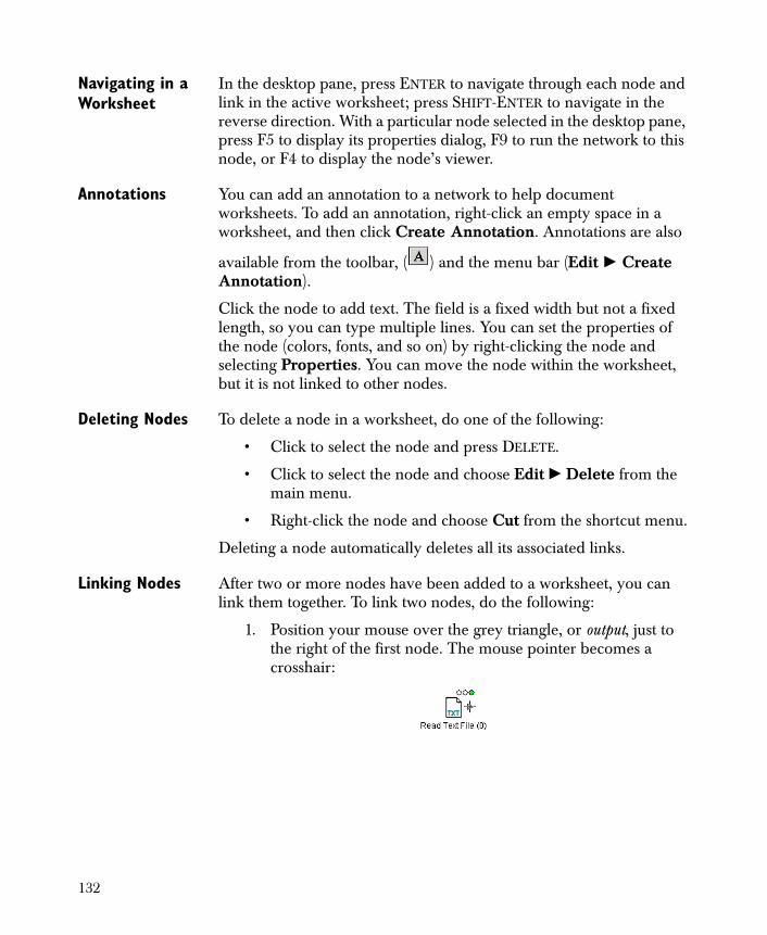
Navigating in a Worksheet
In the desktop pane, press ENTER to navigate through each node and link in the active worksheet; press SHIFT-ENTER to navigate in the reverse direction. With a particular node selected in the desktop pane, press F5 to display its properties dialog, F9 to run the network to this node, or F4 to display the node’s viewer.
Annotations You can add an annotation to a network to help document worksheets. To add an annotation, right-click an empty space in a worksheet, and then click Create Annotation. Annotations are also
available from the toolbar, ( ) and the menu bar (Edit � Create Annotation).
Click the node to add text. The field is a fixed width but not a fixed length, so you can type multiple lines. You can set the properties of the node (colors, fonts, and so on) by right-clicking the node and selecting Properties. You can move the node within the worksheet, but it is not linked to other nodes.
Deleting Nodes To delete a node in a worksheet, do one of the following:
• Click to select the node and press DELETE.
• Click to select the node and choose Edit � Delete from the main menu.
• Right-click the node and choose Cut from the shortcut menu.
Deleting a node automatically deletes all its associated links.
Linking Nodes After two or more nodes have been added to a worksheet, you can link them together. To link two nodes, do the following:
1. Position your mouse over the grey triangle, or output, just to the right of the first node. The mouse pointer becomes a crosshair:
132
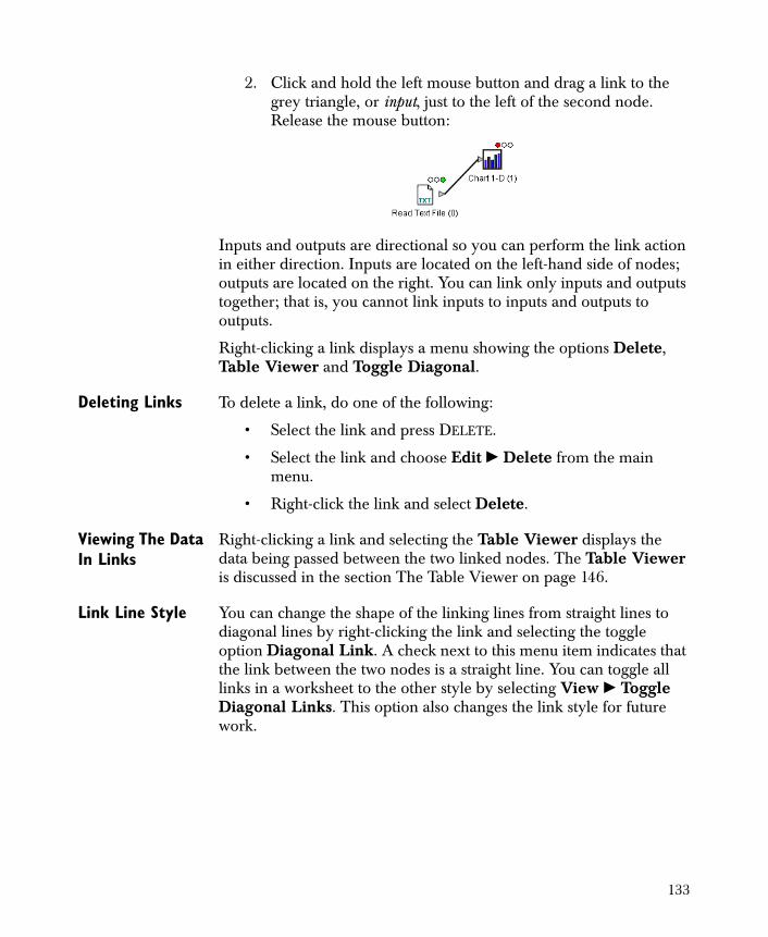
2. Click and hold the left mouse button and drag a link to the grey triangle, or input, just to the left of the second node. Release the mouse button:
Inputs and outputs are directional so you can perform the link action in either direction. Inputs are located on the left-hand side of nodes; outputs are located on the right. You can link only inputs and outputs together; that is, you cannot link inputs to inputs and outputs to outputs.
Right-clicking a link displays a menu showing the options Delete, Table Viewer and Toggle Diagonal.
Deleting Links To delete a link, do one of the following:
• Select the link and press DELETE.
• Select the link and choose Edit � Delete from the main menu.
• Right-click the link and select Delete.
Viewing The Data In Links
Right-clicking a link and selecting the Table Viewer displays the data being passed between the two linked nodes. The Table Viewer is discussed in the section The Table Viewer on page 146.
Link Line Style You can change the shape of the linking lines from straight lines to diagonal lines by right-clicking the link and selecting the toggle option Diagonal Link. A check next to this menu item indicates that the link between the two nodes is a straight line. You can toggle all links in a worksheet to the other style by selecting View � Toggle Diagonal Links. This option also changes the link style for future work.
133

A diamond-shaped symbol (as opposed to a triangle) on an input indicates it accepts multiple links. Otherwise, each input takes a single link and each output allows multiple links.
Copying Nodes You can use any of the standard copy and paste functions to copy a single node, multiple nodes, or an entire network. When selecting multiple nodes to copy, use CTRL-click.
You can also copy nodes by selecting the nodes and holding down the CTRL key while dragging. If you end the drag on a worksheet, the nodes are added to the worksheet where the drag ends. If you end the drag in the User Library, the first selected node is added to the User Library.
Model Ports A model port accepts and delivers model specifications between nodes. This is in contrast to the data ports (triangles), which accept and deliver rectangular tables of data. Model ports appear as circles on the lower right of model nodes and on the lower left of predict nodes. Model port links appear as red dashed lines to distinguish them from data node links.
Connecting a model node to a predict node dynamically links the prediction with the model, so that when the model changes the prediction changes. If you delete the link between the model and the predict nodes, the model used for prediction is static and does not change if you update the original model. The model ports are light grey when the node is dynamically linked to a model and black when the node is statically linked.
Specifying Properties for Nodes
In general, you can specify a node’s properties only after the node is linked. Usually, you must specify a node’s properties prior to running the network. When a node’s properties are properly set, its status indicator changes from red to yellow, showing that it is ready to be run.
Notes
An output is black if it has a data cache; otherwise, it is grey. For more information on data caches, see Chapter 15, Advanced Topics.
When you hover the mouse pointer over the input or output ports of a node icon, a tooltip appears explaining the functionality of that port.
134
To open the properties dialog for any node in a network, do one of the following:
• Double-click the node.
• Select the node and click the Properties button on the Spotfire Miner toolbar.
• Right-click the node and select Properties from the shortcut menu.
Properties vary by component type. For detailed information on the properties of a specific component, consult the relevant section later in this User’s Guide. For characteristics common to many of the properties dialogs, see the section Properties Dialogs on page 139.
Specifying File Names
Anywhere a file name is required, you can specify either the entire path or just the file name. If you specify just the file name, the path is taken to be the Default File Directory from the Advanced tab of the Worksheet Properties page (File � Properties � Advanced).
Collapsing Nodes You can collect nodes into groups, and then collapse them to form a collection node. To create a collection node, select the nodes to be grouped, then do one of the following:
• Select View � Collapse
• Right-click on the group of nodes and select Collapse from the context menu.
• Click the collapse button ( )on the toolbar.
You can ungroup or expand the nodes by selecting the grouped node and doing one of the following:
• Right-click the group then select Expand.
• Click the plus sign (+) in the upper left corner of the node.
• Select View � Expand.
• Click the expand button ( ) on the toolbar.
You can specify the properties for the collection node by selecting it and right-clicking to obtain the context menu, and then selecting properties. Notice that you can also change the properties for the individual node
135
Specifying Properties for Collection Nodes
The properties page for collection nodes has three pages, Contents, Ports and Appearance.
The Contents page shows the individual nodes. You can add, delete, or run nodes from here, or you can change individual node properties.
The Ports page provides tools to edit the tool tips for the port or change the order of the ports using the Up and Down buttons. Each port has a line on this page. By default, only the ports that have a link externally are visible. You cannot hide the externally-linked ports unless you first delete the link. If you select the box corresponding to an editable port, that port is visible on the collection node.
The Appearance page contains a directory path for the GUI symbol and help file for the collection node.
Creating Customized Components
You can copy nodes from a worksheet in the explorer pane to create a User Library of customized components. Components created in this way retain all the properties set at the time they are added to the library. For more information, see the section The User Library on page 123.
Running and Stopping a Network
Spotfire Miner gives you a choice in how to run your networks. You can run a single network, multiple networks, a single node, or that portion of a network up to and including a particular node.
Running Nodes and Networks
To run all nodes on a worksheet, do one of the following:
• Click the Run button on the Spotfire Miner toolbar.
• Choose Tools � Run from the main menu.
To run a single node or that portion of a network up to and including a particular node, do one of the following:
• Select the node and click the Run to Here button on the Spotfire Miner toolbar.
• Select the node and choose Tools � Run to Here from the main menu.
136
• Right-click the node and select Run to Here from the shortcut menu.
Node Priority In some instances, you might need to ensure that one node is executed before another. For example, an S-PLUS node to create a model object must be run before a node that predicts using it. To ensure the execution order of a node, go to the Advanced tab of the Properties dialog for a node and select from the menu for the Order of Operations Execute After field. Refer to section The Advanced Page on page 564 for more details.
Status Indicators Each node of a network displays a “status indicator” that has three possible states:
• Red When you first add a node to a worksheet, its status indicator is red. The node is not ready to be run.
• Yellow When a node’s properties are properly set, its status indicator changes from red to yellow. The node is ready to be run.
• Green After a node has been successfully executed, its status indicator changes from yellow to green.
Usually, you must set a node’s properties before you run it, and in most cases you can specify the properties only after linking the node.
Data Caches When running a network, Spotfire Miner can create a data cache for each node in the network. Whether the data is cached depends on the cache property set for the node (caching or no caching).
• If you specify node caching, the node’s output port color is black.
• If you specify no node caching, the output port is light grey.
Cached nodes do not need to re-execute on run unless their properties change. For example, if you are using a Read Text File node in your network, and the contents of the data source change, you must invalidate the cached nodes first before rerunning the network.
137

Invalidating Nodes
Invalidating a node forces the node’s status to be yellow, so that you must rerun it to view or pass on the node’s results. To invalidate a node, do one of the following:
• Select the node and click the Invalidate button on the Spotfire Miner toolbar.
• Select the node and choose Tools � Invalidate from the main menu.
• Right-click the node and select Invalidate from the shortcut menu.
Stopping a Running Network
To stop a running network, do one of the following:
• Click the Stop button on the Spotfire Miner toolbar.
• Choose Tools � Stop from the main menu.
Spotfire Miner might display a confirmation dialog to inform you that the network has stopped running. When you stop a running network, no intermediate status is maintained; you must rerun the network from the start.
138

COMMON FEATURES OF NETWORK NODES
Many of the nodes in your Spotfire Miner networks have certain features in common, which we explore in this section.
Shortcut Menus
All of the nodes in Spotfire Miner have shortcut menus associated with them that duplicate many of the selections available from the main menu or the Spotfire Miner toolbar. A sample shortcut menu is shown in Figure 3.18 below.
Properties Dialogs
All nodes have properties dialogs that are specific to their particular component type. Many of the dialogs share common features and functionality, which is the focus of this section.
Figure 3.18: A shortcut menu for a network node.
Note
Some selections on the shortcut menu, such as Create Filter and Create Predictor, are available only for certain kinds of nodes.
139

Opening the Properties Dialog
To open the properties dialog for any node, do one of the following:
• Double-click the node.
• Click the node to select it and then click the Properties
button on the Spotfire Miner toolbar.
• Click the node to select it and then choose Tools � Properties from the main menu.
• Right-click the node and select Properties from the shortcut menu.
Hint
By default, when you double-click a node in a network, its properties dialog is opened. However, you can set the double-click behavior to vary based on the state of the node; that is, double-clicking a node opens the viewer if the node is ready to be viewed and the properties dialog otherwise. To set this preference, choose Tools � Options from the main menu to open the Global Properties dialog, select the Activate Intelligent Double Click check box on the Properties page, and click OK.
140
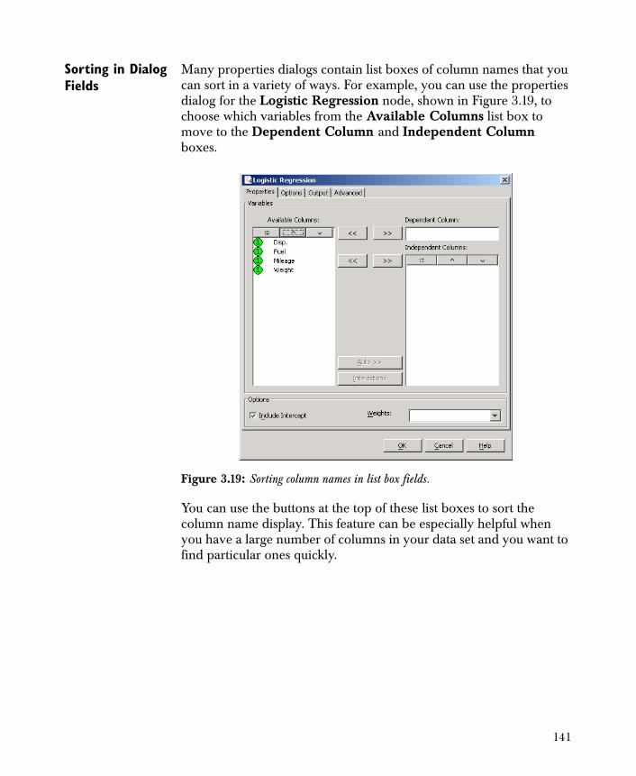
Sorting in Dialog Fields
Many properties dialogs contain list boxes of column names that you can sort in a variety of ways. For example, you can use the properties dialog for the Logistic Regression node, shown in Figure 3.19, to choose which variables from the Available Columns list box to move to the Dependent Column and Independent Column boxes.
You can use the buttons at the top of these list boxes to sort the column name display. This feature can be especially helpful when you have a large number of columns in your data set and you want to find particular ones quickly.
Figure 3.19: Sorting column names in list box fields.
141
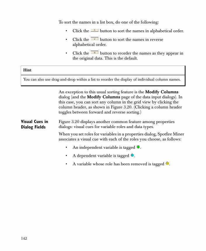
To sort the names in a list box, do one of the following:
• Click the button to sort the names in alphabetical order.
• Click the button to sort the names in reverse alphabetical order.
• Click the button to reorder the names as they appear in the original data. This is the default.
An exception to this usual sorting feature is the Modify Columns dialog (and the Modify Columns page of the data input dialogs). In this case, you can sort any column in the grid view by clicking the column header, as shown in Figure 3.20. (Clicking a column header toggles between forward and reverse sorting.)
Visual Cues in Dialog Fields
Figure 3.20 displays another common feature among properties dialogs: visual cues for variable roles and data types.
When you set roles for variables in a properties dialog, Spotfire Miner associates a visual cue with each of the roles you choose, as follows:
• An independent variable is tagged .
• A dependent variable is tagged .
• A variable whose role has been removed is tagged .
Hint
You can also use drag-and-drop within a list to reorder the display of individual column names.
142
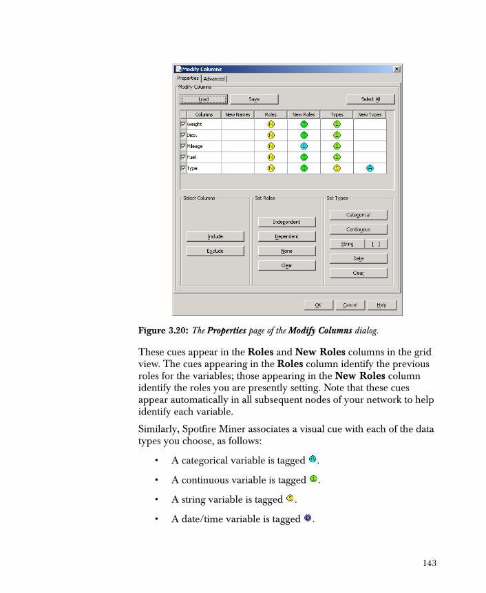
These cues appear in the Roles and New Roles columns in the grid view. The cues appearing in the Roles column identify the previous roles for the variables; those appearing in the New Roles column identify the roles you are presently setting. Note that these cues appear automatically in all subsequent nodes of your network to help identify each variable.
Similarly, Spotfire Miner associates a visual cue with each of the data types you choose, as follows:
• A categorical variable is tagged .
• A continuous variable is tagged .
• A string variable is tagged .
• A date/time variable is tagged .
Figure 3.20: The Properties page of the Modify Columns dialog.
143
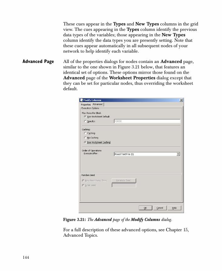
These cues appear in the Types and New Types columns in the grid view. The cues appearing in the Types column identify the previous data types of the variables; those appearing in the New Types column identify the data types you are presently setting. Note that these cues appear automatically in all subsequent nodes of your network to help identify each variable.
Advanced Page All of the properties dialogs for nodes contain an Advanced page, similar to the one shown in Figure 3.21 below, that features an identical set of options. These options mirror those found on the Advanced page of the Worksheet Properties dialog except that they can be set for particular nodes, thus overriding the worksheet default.
For a full description of these advanced options, see Chapter 15, Advanced Topics.
Figure 3.21: The Advanced page of the Modify Columns dialog.
144
Viewers Each of the nodes in Spotfire Miner is associated with a viewer that you can launch after running a node successfully. Every node (and
link) has a Table Viewer, symbolized by the icon. Some nodes have an additional node-specific viewer. If a node-specific viewer
exists, it is the default viewer (represented by the icon) for that node. In the absence of a node-specific view, the Table Viewer and the Viewer is the same.
Launching a Viewer
To launch the default Viewer or Table Viewer for any node, first run the node, and then do one of the following:
• Select the node, and then click either the Viewer button
or the Table Viewer button on the Spotfire Miner toolbar.
• Select the node and choose Tools � Viewer or Tools � Table Viewer from the main menu.
• Right-click the node and select Viewer or Table Viewer from the shortcut menu.
Hint
By default, when you double-click a node in a network, its properties dialog is opened. However, you can set the double-click behavior to vary based on the state of the node; that is, double-clicking a node opens the viewer if the node is ready to be viewed and the properties dialog otherwise. To set this preference, choose Tools � Options from the main menu to open the Global Properties dialog, select the Activate Intelligent Double Click check box on the Properties page, and click OK.
145
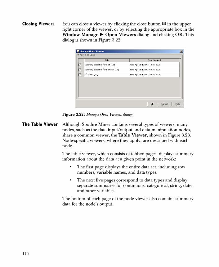
Closing Viewers You can close a viewer by clicking the close button in the upper right corner of the viewer, or by selecting the appropriate box in the Window Manage � Open Viewers dialog and clicking OK. This dialog is shown in Figure 3.22.
The Table Viewer Although Spotfire Miner contains several types of viewers, many nodes, such as the data input/output and data manipulation nodes, share a common viewer, the Table Viewer, shown in Figure 3.23. Node-specific viewers, where they apply, are described with each node.
The table viewer, which consists of tabbed pages, displays summary information about the data at a given point in the network:
• The first page displays the entire data set, including row numbers, variable names, and data types.
• The next five pages correspond to data types and display separate summaries for continuous, categorical, string, date, and other variables.
The bottom of each page of the node viewer also contains summary data for the node’s output.
Figure 3.22: Manage Open Viewers dialog.
146
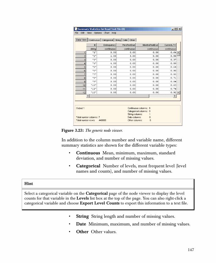
In addition to the column number and variable name, different summary statistics are shown for the different variable types:
• Continuous Mean, minimum, maximum, standard deviation, and number of missing values.
• Categorical Number of levels, most frequent level (level names and counts), and number of missing values.
• String String length and number of missing values.
• Date Minimum, maximum, and number of missing values.
• Other Other values.
Figure 3.23: The generic node viewer.
Hint
Select a categorical variable on the Categorical page of the node viewer to display the level counts for that variable in the Levels list box at the top of the page. You can also right-click a categorical variable and choose Export Level Counts to export this information to a text file.
147
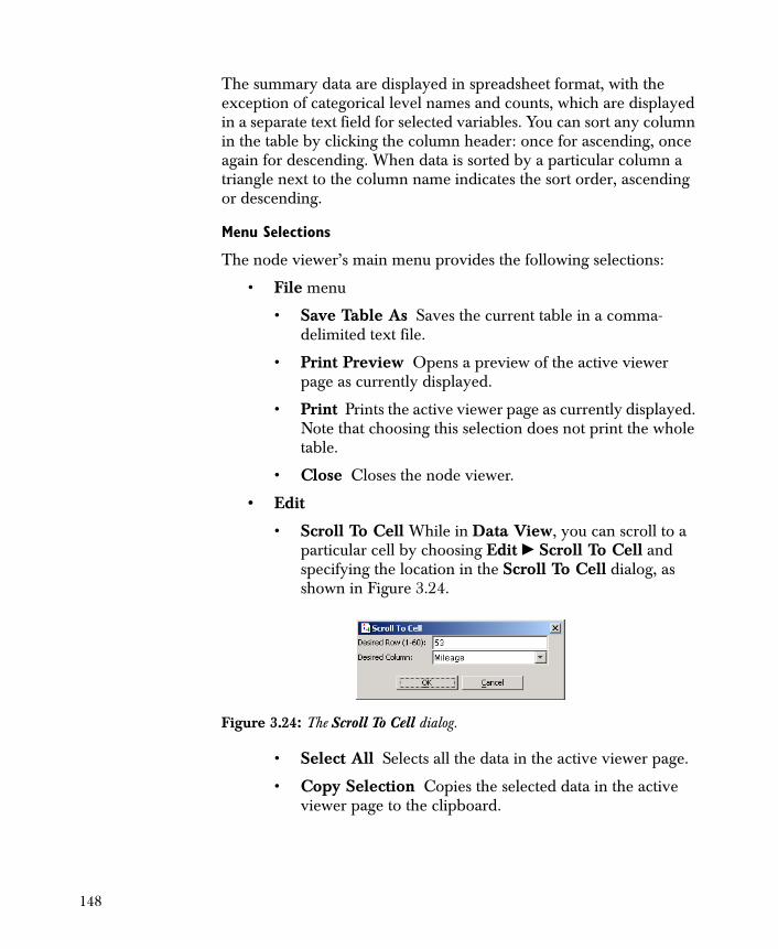
The summary data are displayed in spreadsheet format, with the exception of categorical level names and counts, which are displayed in a separate text field for selected variables. You can sort any column in the table by clicking the column header: once for ascending, once again for descending. When data is sorted by a particular column a triangle next to the column name indicates the sort order, ascending or descending.
Menu Selections
The node viewer’s main menu provides the following selections:
• File menu
• Save Table As Saves the current table in a comma-delimited text file.
• Print Preview Opens a preview of the active viewer page as currently displayed.
• Print Prints the active viewer page as currently displayed. Note that choosing this selection does not print the whole table.
• Close Closes the node viewer.
• Edit
• Scroll To Cell While in Data View, you can scroll to a particular cell by choosing Edit � Scroll To Cell and specifying the location in the Scroll To Cell dialog, as shown in Figure 3.24.
• Select All Selects all the data in the active viewer page.
• Copy Selection Copies the selected data in the active viewer page to the clipboard.
Figure 3.24: The Scroll To Cell dialog.
148
• View
• Output For nodes with multiple outputs, such as Partition, select the desired output port name to switch between the different port viewers.
• View HTML Summary Creates an HTML summary of the various data types in the current node. If the node has more than one output port, all ports are summarized.
• Options
• Rounding Sets the number of decimal places to display.
• Left Align Text / Right Align Text For all columns containing string data, aligns the text with either the left or right edge of the table’s column.
• Chart This menu provides tools for graphing the data in the viewer.
• Summary Charts If a row (a variable) in the Continuous, Categorical, or Date pages is selected, this option is available. This option creates a 1-D chart for the selected variable.
• Additional charts are available through the Spotfire S+ Library. Selecting a chart type under this menu displays a Properties dialog. From this dialog, click Apply to create the plot, and/or click Add to add a graphing node with the specified properties to the current worksheet. See Chapter 16, The S-PLUS Library for details.
• Help Displays the Spotfire Miner help system.
Note
If you are using a browser other than Internet Explorer® such as Mozilla™ (Firefox®) or
Netscape®, and you try to view an HTML chart or summary, Spotfire Miner reuses an open browser session. See your browser documentation for information about changing this behavior if you want to launch a new browser instance for Spotfire Miner HTML charts and summaries.
149

150

Overview 153
Creating One-Dimensional Charts 154General Procedure 154Chart Types 154Properties 161Conditioned Charts 164Using the Viewer 165An Example 169
Computing Correlations and Covariances 170General Procedure 170Definitions 171Properties 172Using the Viewer 173Output 174An Example 174
Crosstabulating Categorical Data 176General Procedure 176Properties 177Using the Viewer 178An Example 180
Computing Descriptive Statistics 181General Procedure 181Properties 182Using the Viewer 183
Comparing Data 184General Procedure 184Properties 184Using the Viewer 187
DATA EXPLORATION 4
151

Viewing Tables 188General Procedure 188Using the Viewer 189
152

OVERVIEW
The main purpose of the exploration phase of data mining is to provide you with a high-level understanding of the structure of your data. For example, charts and descriptive statistics are helpful for examining and visualizing the distribution of your data, as they reveal variables in your data that are nearly constant or variables that have large numbers of missing values. Correlations are helpful for determining whether two variables in your data are related, while crosstabulations can determine the distribution of data among the levels in categorical variables. Tables are useful for viewing both the values and the data types for each column. Finally, you can compare columns, rows, or even cells in two inputs, helpful when you are looking for small- or large-scale differences.
Spotfire Miner™ includes five components dedicated to data exploration:
• Chart 1-D. This component creates basic one-dimensional graphs of the variables in a data set. The supported chart types are pie charts, bar charts, column charts, dot charts, histograms, and box plots.
• Correlations. This component computes correlations and covariances for pairs of variables in a data set.
• Crosstabulate. This component produces tables of counts for various combinations of levels in categorical variables.
• Descriptive Statistics. This component computes basic descriptive statistics for the variables in a data set and displays them with one-dimensional charts.
• Table View. This component displays data in a tabular format, allowing you to see both the data values and the data types (continuous, categorical, string, or date).
• Compare. This component creates an absolute, relative, or Boolean comparison of each column, row, or cell for two inputs.
In this chapter, we describe the properties that are specific to the data exploration components. For a discussion of the options common to all components (those available on the Advanced page of the properties dialogs), see Chapter 15, Advanced Topics.
153
CREATING ONE-DIMENSIONAL CHARTS
To create univariate charts of the variables in a data set, use the Chart 1-D component. This component creates basic one-dimensional charts for both categorical and continuous variables. It also supports conditioned charts, where the values in a variable are conditioned on the levels in a specified categorical variable.
This section describes the types of charts you can create with the Chart 1-D component, the options you can set in its properties dialog, and the viewer you use to see the charts you create.
General Procedure
The following outlines the general approach for creating charts with the Chart 1-D component:
1. Link a Chart 1-D node in your worksheet to any node that outputs data.
2. Use the properties dialog for Chart 1-D to specify the variables you want to graph as well as the types of charts to create.
3. Run your network. Launch the viewer for the Chart 1-D node.
The Chart 1-D component accepts a single input containing rectangular data and returns no output.
Chart Types The Chart 1-D component supports pie charts, bar charts, column charts, dot charts, histograms, and box plots. Pie charts, bar charts, column charts, and dot charts are supported for categorical variables, while histograms and box plots are supported for continuous variables.
The following charts use variables from the examples/vetmailing.txt data set.
154
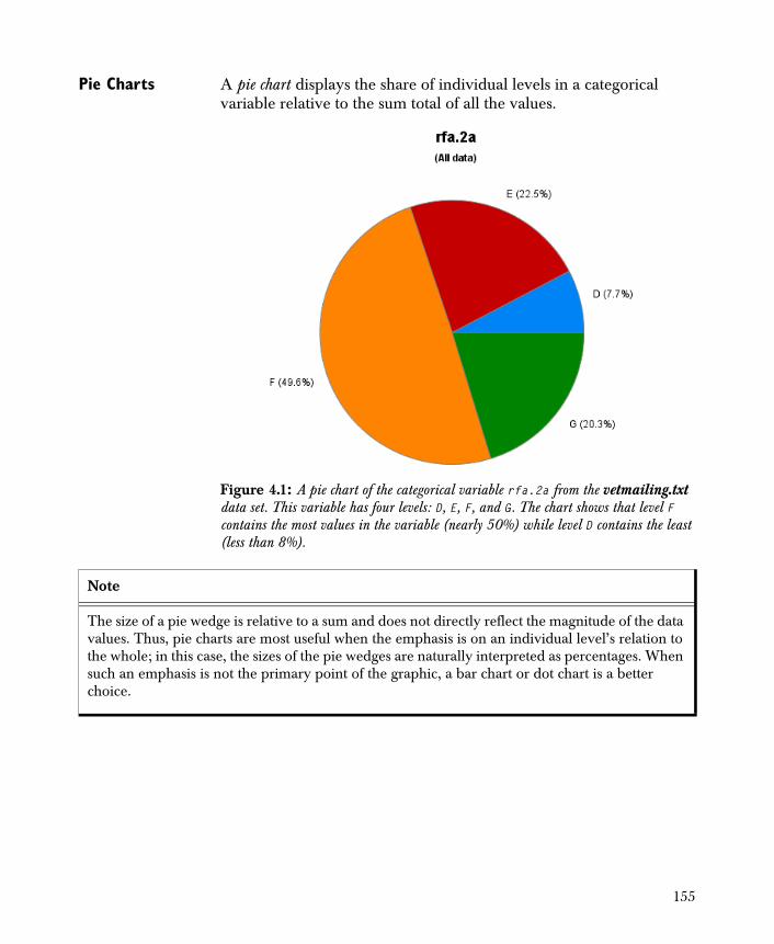
Pie Charts A pie chart displays the share of individual levels in a categorical variable relative to the sum total of all the values.
Figure 4.1: A pie chart of the categorical variable rfa.2a from the vetmailing.txt data set. This variable has four levels: D, E, F, and G. The chart shows that level F contains the most values in the variable (nearly 50%) while level D contains the least (less than 8%).
Note
The size of a pie wedge is relative to a sum and does not directly reflect the magnitude of the data values. Thus, pie charts are most useful when the emphasis is on an individual level’s relation to the whole; in this case, the sizes of the pie wedges are naturally interpreted as percentages. When such an emphasis is not the primary point of the graphic, a bar chart or dot chart is a better choice.
155
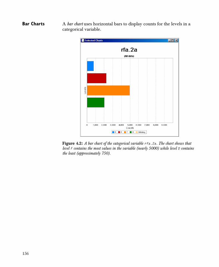
Bar Charts A bar chart uses horizontal bars to display counts for the levels in a categorical variable.
Figure 4.2: A bar chart of the categorical variable rfa.2a. The chart shows that level F contains the most values in the variable (nearly 5000) while level D contains the least (approximately 750).
156
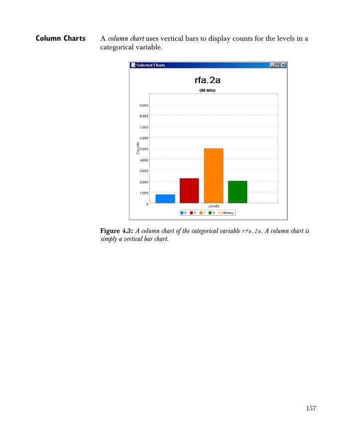
Column Charts A column chart uses vertical bars to display counts for the levels in a categorical variable.
Figure 4.3: A column chart of the categorical variable rfa.2a. A column chart is simply a vertical bar chart.
157
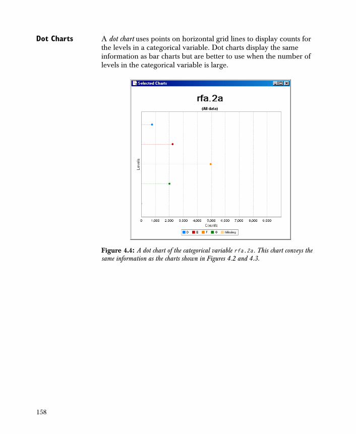
Dot Charts A dot chart uses points on horizontal grid lines to display counts for the levels in a categorical variable. Dot charts display the same information as bar charts but are better to use when the number of levels in the categorical variable is large.
Figure 4.4: A dot chart of the categorical variable rfa.2a. This chart conveys the same information as the charts shown in Figures 4.2 and 4.3.
158
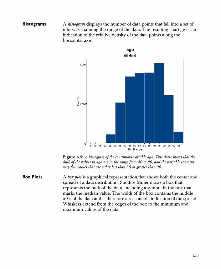
Histograms A histogram displays the number of data points that fall into a set of intervals spanning the range of the data. The resulting chart gives an indication of the relative density of the data points along the horizontal axis.
Box Plots A box plot is a graphical representation that shows both the center and spread of a data distribution. Spotfire Miner draws a box that represents the bulk of the data, including a symbol in the box that marks the median value. The width of the box contains the middle 50% of the data and is therefore a reasonable indication of the spread. Whiskers extend from the edges of the box to the minimum and maximum values of the data.
Figure 4.5: A histogram of the continuous variable age. This chart shows that the bulk of the values in age are in the range from 40 to 80, and the variable contains very few values that are either less than 30 or greater than 90.
159
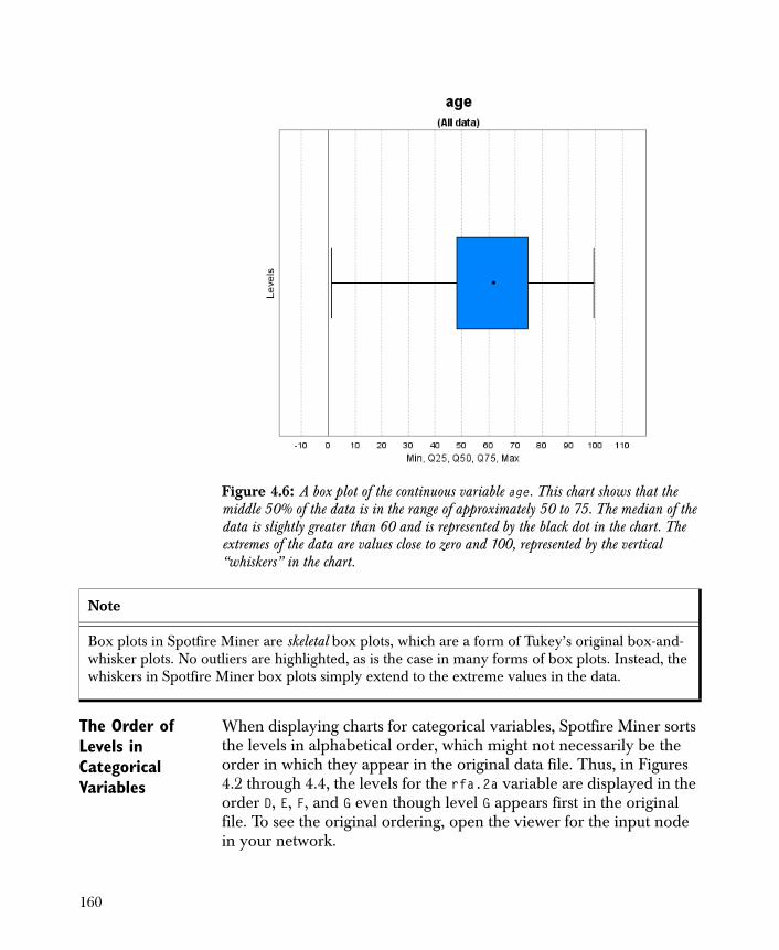
The Order of Levels in Categorical Variables
When displaying charts for categorical variables, Spotfire Miner sorts the levels in alphabetical order, which might not necessarily be the order in which they appear in the original data file. Thus, in Figures 4.2 through 4.4, the levels for the rfa.2a variable are displayed in the order D, E, F, and G even though level G appears first in the original file. To see the original ordering, open the viewer for the input node in your network.
Figure 4.6: A box plot of the continuous variable age. This chart shows that the middle 50% of the data is in the range of approximately 50 to 75. The median of the data is slightly greater than 60 and is represented by the black dot in the chart. The extremes of the data are values close to zero and 100, represented by the vertical “whiskers” in the chart.
Note
Box plots in Spotfire Miner are skeletal box plots, which are a form of Tukey’s original box-and-whisker plots. No outliers are highlighted, as is the case in many forms of box plots. Instead, the whiskers in Spotfire Miner box plots simply extend to the extreme values in the data.
160
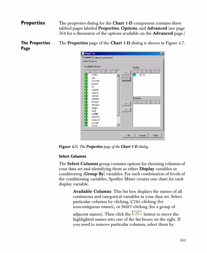
Properties The properties dialog for the Chart 1-D component contains three tabbed pages labeled Properties, Options, and Advanced (see page 564 for a discussion of the options available on the Advanced page.)
The Properties Page
The Properties page of the Chart 1-D dialog is shown in Figure 4.7.
Select Columns
The Select Columns group contains options for choosing columns of your data set and identifying them as either Display variables or conditioning (Group By) variables. For each combination of levels of the conditioning variables, Spotfire Miner creates one chart for each display variable.
Available Columns This list box displays the names of all continuous and categorical variables in your data set. Select particular columns by clicking, CTRL-clicking (for noncontiguous names), or SHIFT-clicking (for a group of
adjacent names). Then click the button to move the highlighted names into one of the list boxes on the right. If you need to remove particular columns, select them by
Figure 4.7: The Properties page of the Chart 1-D dialog.
161
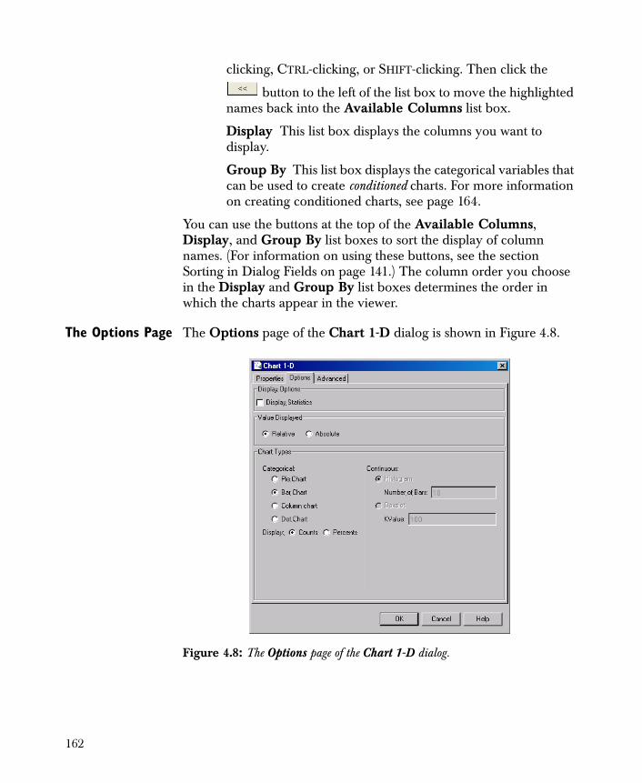
clicking, CTRL-clicking, or SHIFT-clicking. Then click the
button to the left of the list box to move the highlighted names back into the Available Columns list box.
Display This list box displays the columns you want to display.
Group By This list box displays the categorical variables that can be used to create conditioned charts. For more information on creating conditioned charts, see page 164.
You can use the buttons at the top of the Available Columns, Display, and Group By list boxes to sort the display of column names. (For information on using these buttons, see the section Sorting in Dialog Fields on page 141.) The column order you choose in the Display and Group By list boxes determines the order in which the charts appear in the viewer.
The Options Page The Options page of the Chart 1-D dialog is shown in Figure 4.8.
Figure 4.8: The Options page of the Chart 1-D dialog.
162
Display Options
Display Statistics Select this check box to display a set of descriptive statistics beneath each chart.
Value Displayed
Relative This option causes Spotfire Miner to use counts or percents relative to the conditioned data counts.
Absolute This option causes Spotfire Miner to use the absolute row count as a basis for percentages and chart scaling.
Chart Types
In the Chart Types group, select the type of chart you want to see. When you move categorical variables to the Display list, the categorical chart types are activated. Likewise, when you move continuous variables to the Display list, the continuous chart types are activated.
Categorical Select one of Pie Chart, Bar Chart, Column Chart, or Dot Chart.
Continuous Select either Histogram or Boxplot.
Display Select Counts to have counts displayed on the y-axis (column chart) or x-axis (bar and dot charts). Select Percents to have percentages displayed. (This option is not available with pie charts.)
Quantile Approximation
The Quantile Approximation group contains an option that affects how the quantiles in box plots are computed. The quantiles in the box plot are the median (the center dot) and the lower and upper quartiles (the box edges). Because Spotfire Miner data sets are usually very large, it is not always reasonable to sort all values in a variable when determining its quantiles. Instead, Spotfire Miner employs an approximation technique that sorts only a certain window of the data; values less than or greater than the extreme values of the window are placed at either end but are not sorted.
KValue The size of the window in the approximation is determined by this field. By default, KValue is equal to 100 so that the window consists of 100 points that are sorted. The
163
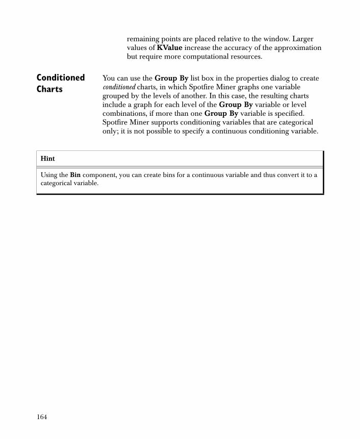
remaining points are placed relative to the window. Larger values of KValue increase the accuracy of the approximation but require more computational resources.
Conditioned Charts
You can use the Group By list box in the properties dialog to create conditioned charts, in which Spotfire Miner graphs one variable grouped by the levels of another. In this case, the resulting charts include a graph for each level of the Group By variable or level combinations, if more than one Group By variable is specified. Spotfire Miner supports conditioning variables that are categorical only; it is not possible to specify a continuous conditioning variable.
Hint
Using the Bin component, you can create bins for a continuous variable and thus convert it to a categorical variable.
164
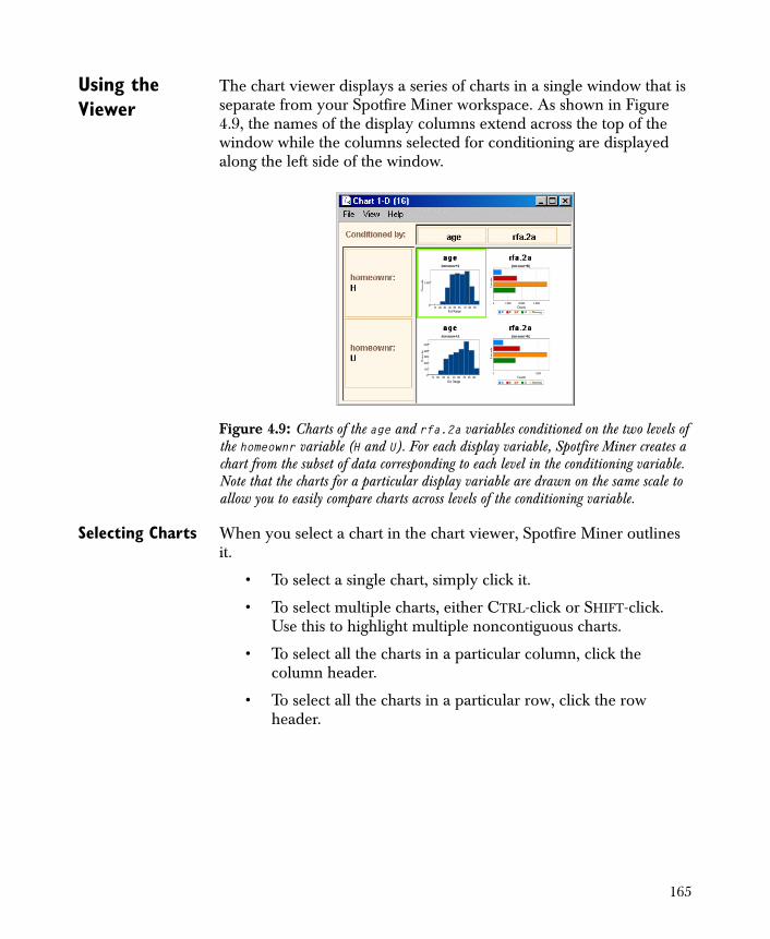
Using the Viewer
The chart viewer displays a series of charts in a single window that is separate from your Spotfire Miner workspace. As shown in Figure 4.9, the names of the display columns extend across the top of the window while the columns selected for conditioning are displayed along the left side of the window.
Selecting Charts When you select a chart in the chart viewer, Spotfire Miner outlines it.
• To select a single chart, simply click it.
• To select multiple charts, either CTRL-click or SHIFT-click. Use this to highlight multiple noncontiguous charts.
• To select all the charts in a particular column, click the column header.
• To select all the charts in a particular row, click the row header.
Figure 4.9: Charts of the age and rfa.2a variables conditioned on the two levels of the homeownr variable (H and U). For each display variable, Spotfire Miner creates a chart from the subset of data corresponding to each level in the conditioning variable. Note that the charts for a particular display variable are drawn on the same scale to allow you to easily compare charts across levels of the conditioning variable.
165
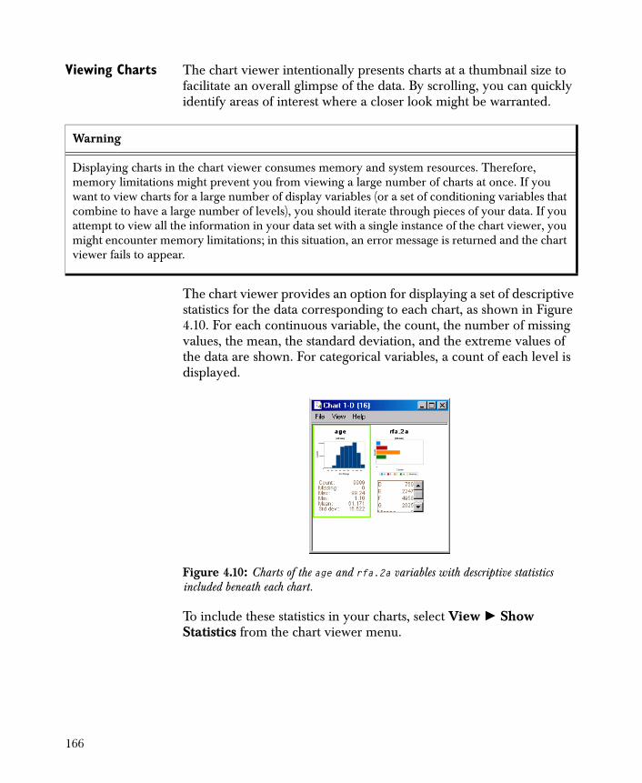
Viewing Charts The chart viewer intentionally presents charts at a thumbnail size to facilitate an overall glimpse of the data. By scrolling, you can quickly identify areas of interest where a closer look might be warranted.
The chart viewer provides an option for displaying a set of descriptive statistics for the data corresponding to each chart, as shown in Figure 4.10. For each continuous variable, the count, the number of missing values, the mean, the standard deviation, and the extreme values of the data are shown. For categorical variables, a count of each level is displayed.
To include these statistics in your charts, select View � Show Statistics from the chart viewer menu.
Warning
Displaying charts in the chart viewer consumes memory and system resources. Therefore, memory limitations might prevent you from viewing a large number of charts at once. If you want to view charts for a large number of display variables (or a set of conditioning variables that combine to have a large number of levels), you should iterate through pieces of your data. If you attempt to view all the information in your data set with a single instance of the chart viewer, you might encounter memory limitations; in this situation, an error message is returned and the chart viewer fails to appear.
Figure 4.10: Charts of the age and rfa.2a variables with descriptive statistics included beneath each chart.
166
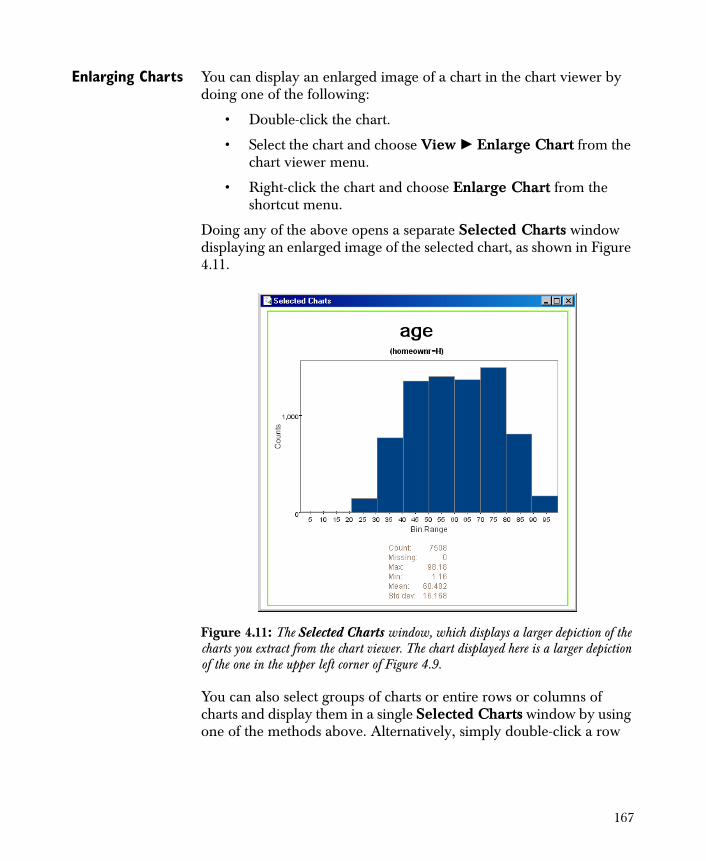
Enlarging Charts You can display an enlarged image of a chart in the chart viewer by doing one of the following:
• Double-click the chart.
• Select the chart and choose View � Enlarge Chart from the chart viewer menu.
• Right-click the chart and choose Enlarge Chart from the shortcut menu.
Doing any of the above opens a separate Selected Charts window displaying an enlarged image of the selected chart, as shown in Figure 4.11.
You can also select groups of charts or entire rows or columns of charts and display them in a single Selected Charts window by using one of the methods above. Alternatively, simply double-click a row
Figure 4.11: The Selected Charts window, which displays a larger depiction of the charts you extract from the chart viewer. The chart displayed here is a larger depiction of the one in the upper left corner of Figure 4.9.
167

(or column) heading to view an individual row (or column) of charts. This way, you can view quickly all the charts associated with particular variables or levels in the conditioning columns.
Each Selected Charts window supports individual or group chart selection just like the chart viewer. Use it to “drill down” into the data as much as you would like.
Formatting Charts
To alter the cosmetic properties of an individual chart, use the Chart Properties dialog, shown in Figure 4.12. This dialog contains options for modifying certain aspects of all Spotfire Miner charts that display in the chart viewer (and Selected Charts window), with the exception of pie charts.
Note
The Enlarge Chart options enlarge a maximum of ten charts only. If you select more than ten charts in the chart viewer, only the first ten charts are displayed.
Figure 4.12: The Chart Properties dialog. The values shown in this figure are typical of the defaults you see for histograms in Spotfire Miner.
168
To open the Chart Properties dialog, do one of the following:
• Select the chart and choose View � View Chart Properties from the chart viewer menu.
• Right-click the chart and choose Chart Properties from the shortcut menu.
Use the Chart Properties dialog to change the range, tick marks, and labels of the axes. For more details, see the online help.
Saving, Printing, and Copying Charts
To save or print a chart in the chart viewer or Selected Charts window, do one of the following:
• Select the chart and choose Save Chart or Print Chart, respectively, from the File menu; or
• Right-click the chart and choose Save Chart or Print Chart, respectively, from the shortcut menu.
To copy a chart, select the chart and then select File � Copy Chart to Clipboard. You can then paste the file to another location.
An Example Using the vetmailing.txt data set located in the username/examples folder under your Spotfire Miner installation directory, follow the steps below to reproduce the results shown in Figure 4.9.
1. Read the data into Spotfire Miner and link the output to a Chart 1-D node.
2. Open the properties dialog of the Chart 1-D node.
3. Specify the columns age and rfa.2a as the Display variables.
4. Specify the categorical column homeownr as the Group By variable.
5. Run the node and open the viewer.
It is also possible to specify multiple conditioning columns. In this case, each unique combination of the levels in the conditioning variables results in a separate chart. The column order you choose in the Group By list box determines the order in which the charts appear in the viewer.
169
COMPUTING CORRELATIONS AND COVARIANCES
Correlation and covariance are two measures of association commonly used to determine whether two variables are linearly related. If two variables in a data set are highly correlated, you will not likely gain any additional information or predictive power by including both in a model.
To view correlations and covariances of the variables in a data set, use the Correlations component. This computes correlations of pairs variables in a data set and displays the results in a grid that is similar to the viewer for the Table View component.
This section describes the general process for computing correlations and covariances with Correlations and using its viewer to interpret the results. Spotfire Miner supports correlations and covariances for continuous variables only; it is not possible to include a categorical variable in the computations.
General Procedure
The following outlines the general approach for computing correlations with the Correlations component:
1. Link a Correlations node in your worksheet to any node that outputs data.
2. Use the properties dialog for Correlations to specify the variables you want to include in the computations.
3. Run your network.
4. Launch the viewer for the Correlations node.
The Correlations component accepts a single input containing rectangular data and continuous variables. It’s output is a data set containing the correlations or covariances for the variables you specify.
170
Definitions The covariance of two variables, X and Y, is the average value of the product of the deviation of X from its mean and the deviation of Y from its mean. The variables are positively associated if, when X is larger than its mean, Y tends to be larger than its mean as well (or, when X is smaller than its mean, Y tends to be smaller than its mean as well). In this case, the covariance is a positive number. The variables are negatively associated if, when X is larger than its mean, Y tends to be smaller than its mean (or vice versa). Here, the covariance is a negative number. The scale of the covariance depends on the scale of the data values in X and Y; it is possible to have very large or very small covariance values.
The correlation of two variables is a dimensionless measure of association based on the covariance; it is the covariance divided by the product of the standard deviations for the two variables. Correlation is always in the range [-1, 1] and does not depend on the scale of the data values. The variables X and Y are positively associated if their correlation is close to 1 and negatively associated if it is close to -1. Because of these properties, correlation is often a more useful measure of association than covariance.
Note
Correlation measures the strength of the linear relationship between two variables. If you create a scatter plot for two variables that have correlation near 1, the points will appear as a line with positive slope. Likewise, if you create a scatter plot for two variables that have correlation near -1, you will see points along a line with negative slope.
A correlation near zero implies that two variables do not have a linear relationship. However, this does not necessarily mean the variables are completely unrelated. It is possible, for example, that the variables are related quadratically or cubically, associations which are not detected by the correlation measure.
171

Properties The Properties page of the Correlations dialog is shown in Figure 4.13.
Select Columns
The Select Columns group contains options for choosing columns of your data set and identifying them as either Correlation Columns or Target Columns. Spotfire Miner computes correlations and covariances for each correlation/target pair. For example, if you choose 4 correlation columns and 2 target columns, Spotfire Miner computes a matrix that has 4 rows and 2 columns in which each entry contains the correlation or covariance of the designated variables.
The Available Columns field is identical to that in the Chart 1-D dialog. For information on this option, see page 161.
It is possible to designate a single column as both a correlation column and a target column. If the Target Columns list is empty, Spotfire Miner assumes that all correlation columns are target columns as well and thus computes a square correlation matrix.
Figure 4.13: The Properties page of the Correlations dialog.
172
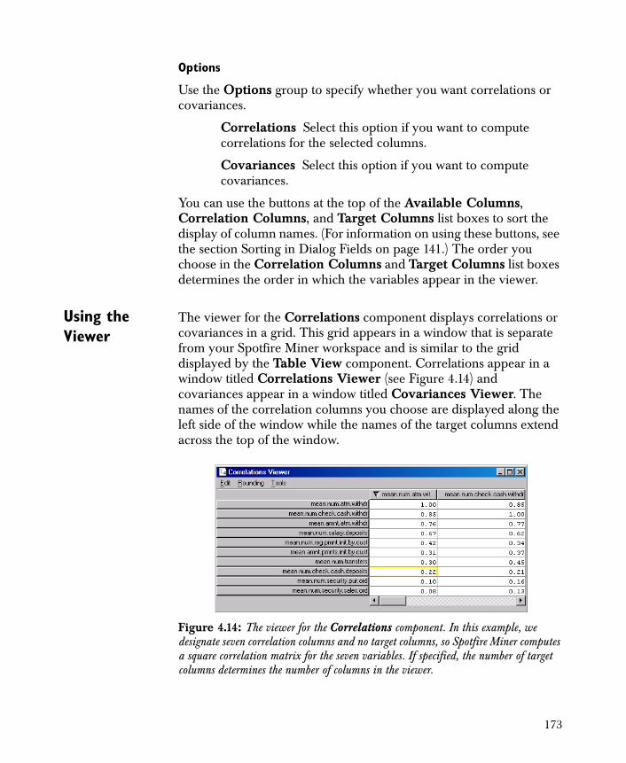
Options
Use the Options group to specify whether you want correlations or covariances.
Correlations Select this option if you want to compute correlations for the selected columns.
Covariances Select this option if you want to compute covariances.
You can use the buttons at the top of the Available Columns, Correlation Columns, and Target Columns list boxes to sort the display of column names. (For information on using these buttons, see the section Sorting in Dialog Fields on page 141.) The order you choose in the Correlation Columns and Target Columns list boxes determines the order in which the variables appear in the viewer.
Using the Viewer
The viewer for the Correlations component displays correlations or covariances in a grid. This grid appears in a window that is separate from your Spotfire Miner workspace and is similar to the grid displayed by the Table View component. Correlations appear in a window titled Correlations Viewer (see Figure 4.14) and covariances appear in a window titled Covariances Viewer. The names of the correlation columns you choose are displayed along the left side of the window while the names of the target columns extend across the top of the window.
Figure 4.14: The viewer for the Correlations component. In this example, we designate seven correlation columns and no target columns, so Spotfire Miner computes a square correlation matrix for the seven variables. If specified, the number of target columns determines the number of columns in the viewer.
173
You can use the scroll bar at the bottom of the viewer to scroll through the correlations for all the columns. You can also resize any of the columns by dragging the lines that divide the column headings at the top of the viewer.
Like the viewer for the Table View component, you can use the Rounding menu options to control the display of decimal places for the values. By default, Spotfire Miner displays all values with two decimal places of accuracy.
The viewer for the Correlations component also provides a feature for sorting the values in a given column of the grid. To sort the values in descending order, click a column’s heading so that the triangle in the heading points downward. To sort the values in ascending order, click the column’s heading so that the triangle points upward.
Output The output from the Correlations component is a data set containing the correlations or covariances. This is an n x m+1 data set, where n is the number of items entered in the Correlations Columns field and m is the number of items entered in the Target Columns field. The first column in the output is a string variable containing the names of the columns specified in the Correlations Columns field of the dialog. The other columns on the output correspond to the columns selected in the Target Columns field of the dialog.
An Example Using the cross.sell.csv data set located in the examples folder under your Spotfire Miner installation directory, follow the steps below to reproduce the results shown in Figure 4.14.
1. Read the data into Spotfire Miner and link the output to a Correlations node.
2. Open the properties dialog of the Correlations node.
Note
It is important to understand that the viewer for Correlations is not generally editable nor is it a spreadsheet. You cannot use the viewer to change column names, rearrange columns, or change individual values, for example. Instead, the viewer is designed to simply display a grid of the computed correlations or covariances without allowing extensive manipulation features.
174
3. Specify all the columns from mean_num_atm_withdr to mean_amnt_pmnts_init_by_cust as the Correlation Columns.
4. Run the node and open the viewer.
In this example data set, the variables mean_num_atm_withdr and mean_num_check_cash_withdr give the mean number of ATM withdrawals and the mean number of withdrawals from checking accounts for particular customers of a hypothetical bank. In Figure 4.14, note that the correlation for these two variables is high (0.85). This means the variables are closely related: customers tend to make withdrawals from their checking accounts using ATMs. Therefore, including both of these variables in a model will not likely provide more information or predictive power.
175
CROSSTABULATING CATEGORICAL DATA
A crosstabulation is a collection of one or more two-way tables that is useful for understanding the distribution among the different categories in a data set. It displays counts of observations for all combinations of the levels in a set of categorical variables.
To view a crosstabulation of the variables in a data set, use the Crosstabulate component. You can display the results as both a series of HTML tables and as a set of conditioned bar charts that visually display the distribution of data for each combination of levels.
This section describes the general process for crosstabulating data with Crosstabulate and using its viewers to see the results. Spotfire Miner supports crosstabulations for categorical variables only; it is not possible to include a continuous or string variable in the computations. Using the Bin component, however, you can create bins for a continuous variable to effectively convert it to a categorical variable. The Modify Columns component can convert string variables to categorical.
General Procedure
The following outlines the general approach for crosstabulating data with the Crosstabulate component:
1. Link a Crosstabulate node in your worksheet to any node that outputs data.
2. Use the properties dialog for Crosstabulate to specify the variables you want to include in the computations.
3. Run your network.
4. Launch the viewer for the Crosstabulate node.
The Crosstabulate component accepts a single input containing rectangular data and categorical variables. It returns no output.
176
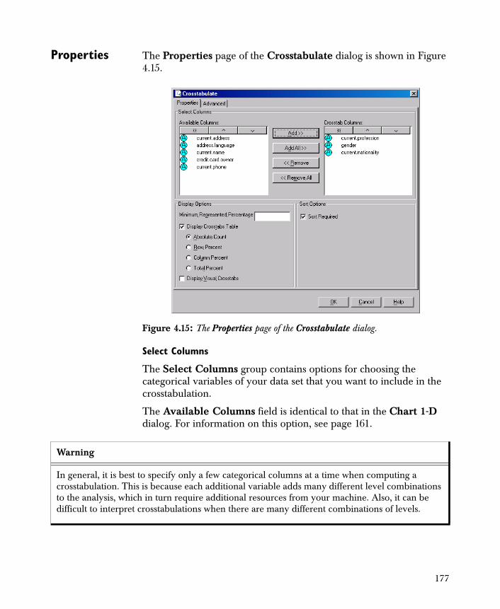
Properties The Properties page of the Crosstabulate dialog is shown in Figure 4.15.
Select Columns
The Select Columns group contains options for choosing the categorical variables of your data set that you want to include in the crosstabulation.
The Available Columns field is identical to that in the Chart 1-D dialog. For information on this option, see page 161.
Figure 4.15: The Properties page of the Crosstabulate dialog.
Warning
In general, it is best to specify only a few categorical columns at a time when computing a crosstabulation. This is because each additional variable adds many different level combinations to the analysis, which in turn require additional resources from your machine. Also, it can be difficult to interpret crosstabulations when there are many different combinations of levels.
177

Options
The Options group contains options for determining how the crosstabulation is displayed.
Display Crosstabs Table Select this check box to return an HTML file containing the tables in a list format. If this option is selected, then you can select what values are displayed in the table cells: Absolute Count, Row Percent, Column Percent, or Total Percent.
Display Visual Crosstabs Select this check box to return a series of conditioned bar charts showing the distribution of data for each combination of levels in the specified categorical columns.
You can use the buttons at the top of the Available Columns and Crosstab Columns list boxes to sort the display of column names. The last column listed in Crosstab Columns forms the columns in the resulting two-way tables; the next-to-last column forms the rows in the two-way tables. The next column up varies most rapidly in the output; the very first column specified in Crosstab Columns varies the slowest in the output. You can drag the column names up and down in the Crosstab Columns field to put them in the desired order. (For information on using these buttons, see the section Sorting in Dialog Fields on page 141.) The order you choose in Crosstab Columns determines the order in which the tables and charts appear in the viewer.
Sort Options
Sort Required If this is not selected, the data must be pre-sorted, in ascending order with NA’s on the bottom, in the order specified in the Crosstab Columns field. In some cases, your data might already be sorted, so clearing (unchecking) this box ensures the data is not needlessly sorted a second time. However, since this is rarely the case, this option should almost always be selected. If it is not, and the data are not sorted correctly, the resulting tables will be incorrect.
Using the Viewer
The viewer for the Crosstabulate component depends on the options you choose in the Options group of the properties dialog. The viewer for the Display Crosstabs Table option is an HTML file
178
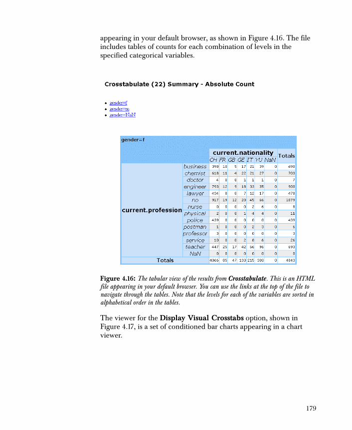
appearing in your default browser, as shown in Figure 4.16. The file includes tables of counts for each combination of levels in the specified categorical variables.
The viewer for the Display Visual Crosstabs option, shown in Figure 4.17, is a set of conditioned bar charts appearing in a chart viewer.
Figure 4.16: The tabular view of the results from Crosstabulate. This is an HTML file appearing in your default browser. You can use the links at the top of the file to navigate through the tables. Note that the levels for each of the variables are sorted in alphabetical order in the tables.
179
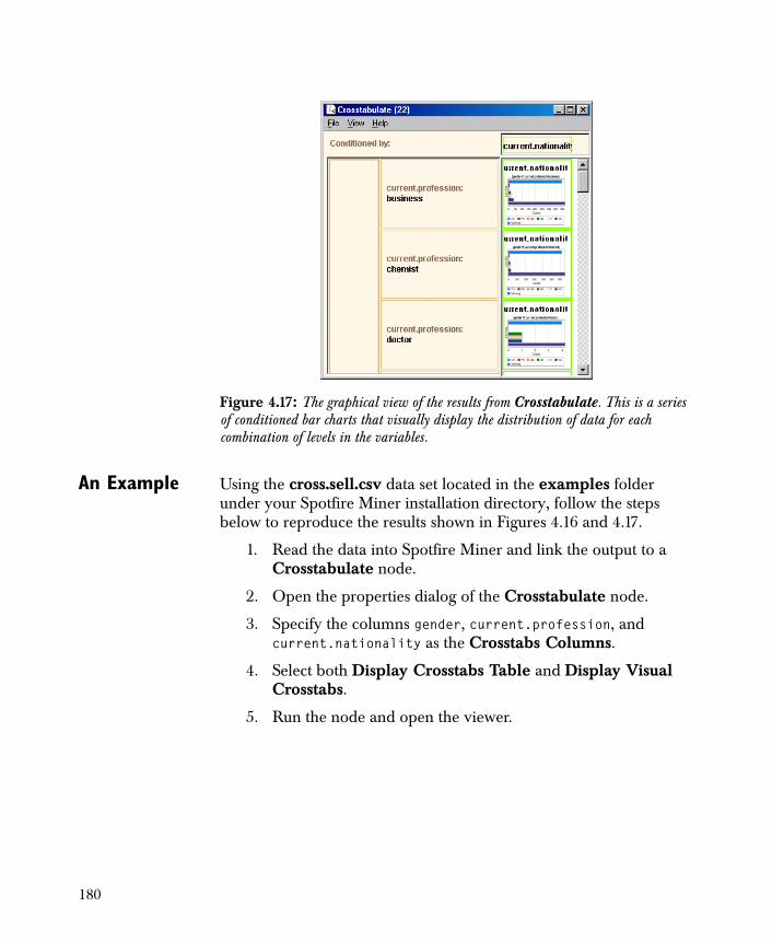
An Example Using the cross.sell.csv data set located in the examples folder under your Spotfire Miner installation directory, follow the steps below to reproduce the results shown in Figures 4.16 and 4.17.
1. Read the data into Spotfire Miner and link the output to a Crosstabulate node.
2. Open the properties dialog of the Crosstabulate node.
3. Specify the columns gender, current.profession, and current.nationality as the Crosstabs Columns.
4. Select both Display Crosstabs Table and Display Visual Crosstabs.
5. Run the node and open the viewer.
Figure 4.17: The graphical view of the results from Crosstabulate. This is a series of conditioned bar charts that visually display the distribution of data for each combination of levels in the variables.
180
COMPUTING DESCRIPTIVE STATISTICS
To compute descriptive statistics of the variables in a data set, use the Descriptive Statistics component. For continuous variables, Spotfire Miner computes a count of the values, the number of missing values, the mean, the standard deviation, and the extreme values. For categorical variables, Spotfire Miner returns a count for each level and a count of the missing values. The descriptive statistics for each variable are displayed with a chart; Spotfire Miner displays histograms for continuous variables and bar charts for categorical variables.
This section describes the options you can set in the Descriptive Statistics properties dialog and the viewer you use to see the results.
General Procedure
The following outlines the general approach for using the Descriptive Statistics component:
1. Link a Descriptive Statistics node in your worksheet to any node that outputs data.
2. Use the properties dialog for Descriptive Statistics to specify the variables you want summarized. By default, Spotfire Miner computes descriptive statistics for all the variables in a data set.
3. Run your network.
4. Launch the viewer for the Descriptive Statistics node.
The Descriptive Statistics component accepts a single input containing rectangular data and returns no output.
Note
The Descriptive Statistics component produces results identical to those produced by the default settings for the Chart 1-D component with the Show Statistics option selected.
181
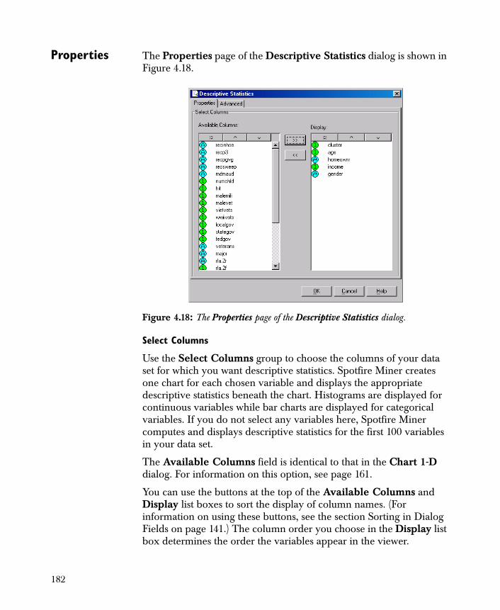
Properties The Properties page of the Descriptive Statistics dialog is shown in Figure 4.18.
Select Columns
Use the Select Columns group to choose the columns of your data set for which you want descriptive statistics. Spotfire Miner creates one chart for each chosen variable and displays the appropriate descriptive statistics beneath the chart. Histograms are displayed for continuous variables while bar charts are displayed for categorical variables. If you do not select any variables here, Spotfire Miner computes and displays descriptive statistics for the first 100 variables in your data set.
The Available Columns field is identical to that in the Chart 1-D dialog. For information on this option, see page 161.
You can use the buttons at the top of the Available Columns and Display list boxes to sort the display of column names. (For information on using these buttons, see the section Sorting in Dialog Fields on page 141.) The column order you choose in the Display list box determines the order the variables appear in the viewer.
Figure 4.18: The Properties page of the Descriptive Statistics dialog.
182
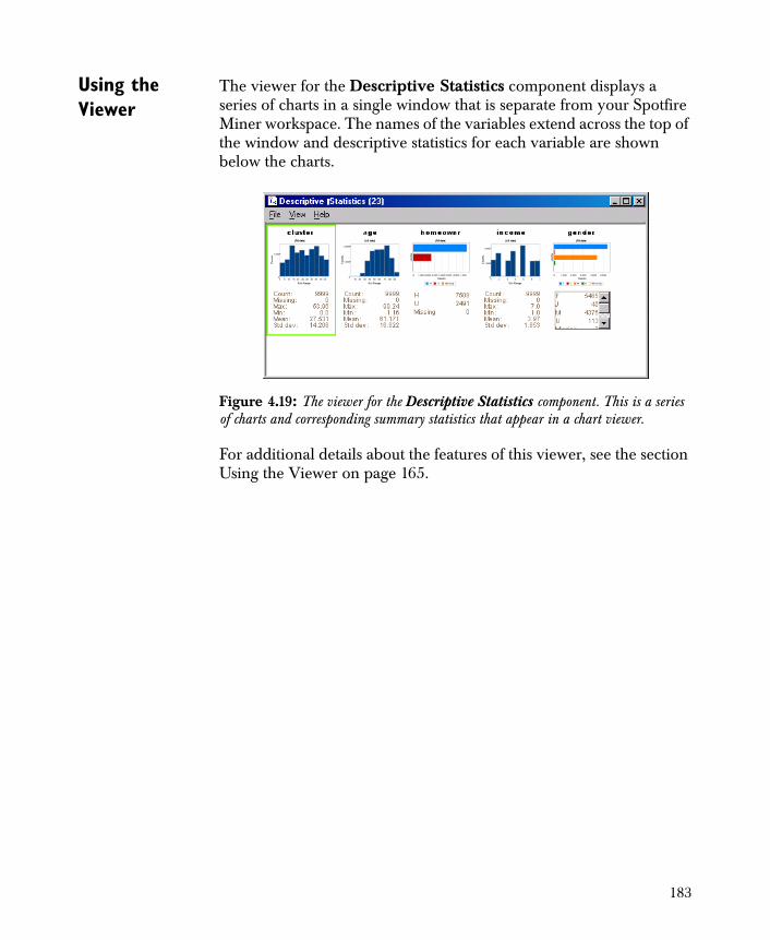
Using the Viewer
The viewer for the Descriptive Statistics component displays a series of charts in a single window that is separate from your Spotfire Miner workspace. The names of the variables extend across the top of the window and descriptive statistics for each variable are shown below the charts.
For additional details about the features of this viewer, see the section Using the Viewer on page 165.
Figure 4.19: The viewer for the Descriptive Statistics component. This is a series of charts and corresponding summary statistics that appear in a chart viewer.
183
COMPARING DATA
To compare the values in two inputs, use the Compare component. For continuous variables, Spotfire Miner can compute the absolute, relative, or logical differences of two data sets. For categorical and string columns, Spotfire Miner computes only a logical difference. In addition, Spotfire Miner can compare the union or the intersection of the two inputs, and a tolerance can be set for computation.
This section describes the options you can set in the Compare properties dialog and the viewer you use to see the results.
General Procedure
The following outlines the general approach for using the Compare component:
1. Link a Compare node in your worksheet to any two nodes that output data.
2. Use the properties dialog for Compare to specify the variables you want to compare. By default, Spotfire Miner computes comparisons for all the variables in the input data sets.
3. Run your network.
4. Launch the viewer for the Compare node.
The Compare component accepts two inputs containing rectangular data and returns the data set with options you specified.
Properties The properties dialog for the Compare component contains three tabbed pages labeled Properties, Options, and Advanced. (see page 564 for a discussion of the options available on the Advanced page.
184
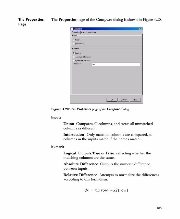
The Properties Page
The Properties page of the Compare dialog is shown in Figure 4.20.
Inputs
Union Compares all columns, and treats all unmatched columns as different.
Intersection Only matched columns are compared, so columns in the inputs match if the names match.
Numeric
Logical Outputs True or False, reflecting whether the matching columns are the same.
Absolute Difference Outputs the numeric difference between inputs.
Relative Difference Attempts to normalize the differences according to this formalism:
Figure 4.20: The Properties page of the Compare dialog.
xd x1 row[ ] x2 row[ ]–=
185
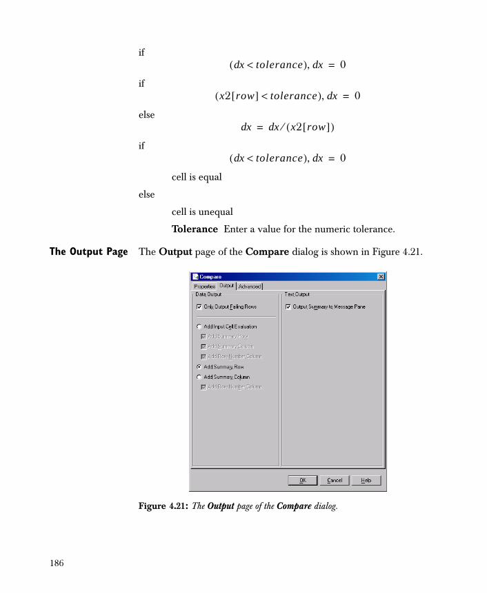
if
if
else
if
cell is equal
else
cell is unequal
Tolerance Enter a value for the numeric tolerance.
The Output Page The Output page of the Compare dialog is shown in Figure 4.21.
xd tolerance<( ) xd, 0=
x2 row[ ] tolerance<( ) xd, 0=
xd x x2 row[ ]( )⁄d=
xd tolerance<( ) xd, 0=
Figure 4.21: The Output page of the Compare dialog.
186
Data Output
Only Output Failing Rows Select this option to filter equal rows from output.
Add Input Cell Evaluation This options provides a cell-by-cell comparison of the inputs:
Add Summary Row This option provides two rows of column summaries at the bottom of the output. The first row gives the maximum difference value, and the second row gives the relative mean difference for each column.
Add Summary Column This option adds a column to the input reflecting whether each row is judged to be equivalent.
Add Row Number Column This option adds a row number column to the inputs.
Add Summary Row This option adds a cell-by-cell comparison of the outputs.
Add Summary Columns This option adds a column to the output reflecting whether each row is judged to be equivalent.
Add Row Number Column This option adds a row number column to the output.
Text Output
Output Summary to Message Pane Select this if you want to output the summary to the message pane.
Using the Viewer
The viewer for the Compare component depends on the options you choose in the Options group of the properties dialog.
187
VIEWING TABLES
To view a data set in a tabular format, use the Table View component. This component displays your data in a grid that has options for controlling the decimal accuracy of numeric values.
This section describes the general process for displaying tables with Table View. It is important to understand that the grid displayed by Table View is not generally editable nor is it a spreadsheet. You cannot use the viewer to change column names, rearrange columns, or change individual values, for example. Instead, the viewer is designed to simply display a grid of your data without allowing extensive manipulation features. To manipulate your data, use one of the Spotfire Miner components designed for that purpose (see Chapter 6, Data Manipulation).
General Procedure
The following outlines the general approach for creating tables with the Table View component:
1. Link a Table View node in your worksheet to any node that outputs data.
2. Run your network.
3. Launch the viewer for the Table View node.
The Table View component accepts a single input containing rectangular data and returns no output. Its properties dialog has no component-specific options, so you can include a Table View node in your network and run it without setting any properties.
Note
The Table View component is included in Spotfire Miner 8 primarily for backward compatibility with version 1.0. The generic node viewer (see page 146) provides the same tabular display of data, making a separate Table View node in a network unnecessary.
188
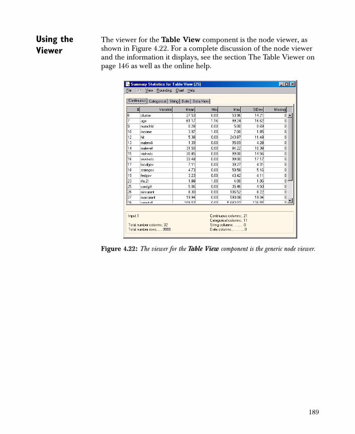
Using the Viewer
The viewer for the Table View component is the node viewer, as shown in Figure 4.22. For a complete discussion of the node viewer and the information it displays, see the section The Table Viewer on page 146 as well as the online help.
Figure 4.22: The viewer for the Table View component is the generic node viewer.
189

190
Overview 192
Missing Values 194General Procedure 195Properties 195Using the Viewer 198An Example 198
Duplicate Detection 200General Procedure 200Background 200Properties 202Using the Viewer 206An Example 206
Outlier Detection 208General Procedure 208Background 209Properties 210Using the Viewer 214An Example 214
Technical Details 218
References 223
DATA CLEANING 5
191
OVERVIEW
This chapter describes the three Spotfire Miner™ components that are used specifically to clean data. Many of the other nodes in Spotfire Miner are useful in cleaning data; for example, the summary and graphics nodes are useful for finding extreme values (outliers) or incorrectly entered values.
One of the most common data cleaning techniques is recoding values that were entered incorrectly (for example, the city Milwaukee entered as Milwaukee, Milwakee, and Millwaukee.) You can use the Create Columns node with an ifelse statement to correct these types of errors. (See the section S-PLUS Data Manipulation Nodes on page 667 for more information about ifelse and other functions in the Expression Language.) You can also use the same node to turn user-specified missing values (for example, -99 for Age) into missing values that Spotfire Miner recognizes (NA).
• Missing Values Use this component to manage your data’s missing values in one of the five following ways:
• Filter from your data set all rows containing missing values.
• Attempt to generate sensible values for those that are missing based on the distributions of data in the columns.
• Replace the missing values with the means of the corresponding columns.
• Carry a previous observation forward.
• Replace the missing values with a constant you choose.
• Duplicate Detection Use this component to detect duplicate rows in your data. Based on the information returned by Duplicate Detection, you might choose to filter rows that are flagged by the component as duplicates.
• Outlier Detection Use this component to detect multidimensional outliers in your data. Based on the information returned by Outlier Detection, you might choose to filter certain rows that are flagged by the component as outliers.
192

This chapter describes the properties that are specific to the data cleaning components. For a discussion of the options common to all components (those available in the Advanced page of the properties dialogs), see Chapter 15, Advanced Topics.
193
MISSING VALUES
When importing ASCII data, Spotfire Miner identifies blank fields as missing values. Other data formats, such as SAS and SPSS data files, have their own internal missing value representation. When it imports these files, Spotfire Miner maps these missing values to Spotfire Miner missing values. When you view a Spotfire Miner data set using the Table Viewer, notice that missing values are displayed as blank fields.
Often, data sets use other special values for missing value (for example, -99). Spotfire Miner does not always automatically recognize these special values as missing values. You can explicitly recode such results as missing values using the expression language and the data manipulation node Create Columns.
For more information, see the section Create Columns on page 257 of Chapter 6, Data Manipulation, and the section S-PLUS Data Manipulation Nodes on page 667 of Chapter 16, The S-PLUS Library.
The Missing Values component supports five different approaches for dealing with missing values in your data set:
1. Drop Rows Drops all rows that contain missing values from your data set.
2. Generate from Distribution Generates sensible values from the marginal distributions of the columns that contain missing values. For a categorical variable, Spotfire Miner generates values based on the proportion of observations corresponding to each level. For a continuous variable, Spotfire Miner computes a histogram of the data, and then generates values based on the heights of the histogram bars.
3. Replace with Mean Replaces each missing value with the average of the values in the corresponding column. For a categorical variable, missing values are replaced with the level that appears most often; in the event of ties, Spotfire Miner chooses the first level that appears in the data set.
4. Replace with Constant Replaces each missing value with a constant you specify.
194

5. Last Observation Carried Forward Replaces a missing value as follows:
• If you set a Key Column, replaces the value with the last non-missing value corresponding to the current Key Column category. (Note that a key column must be a Categorical.)
• If you do not set a Key Column, replaces the value with the last non-missing value.
This section describes the general process for using these options in the Missing Values component.
General Procedure
The following outlines the general approach to using the Missing Values component:
1. In your worksheet, from any node that outputs data, link a Missing Values node.
2. Use the properties dialog for Missing Values to specify the method to use for dealing with missing values in your data set.
3. Run your network.
4. To verify the results, launch the viewer for the Missing Values node.
The Missing Values component accepts a single input containing rectangular data. It outputs a single rectangular data set defined by the input data and the options you choose for dealing with missing values. For example, if you choose to drop all rows containing missing values, the output data are identical to the input data, except that all observations with missing values are eliminated.
Properties The properties dialog for the Missing Values component contains two tabbed pages labeled Properties and Advanced (see page 564 for a discussion of the options available on the Advanced page.)
195
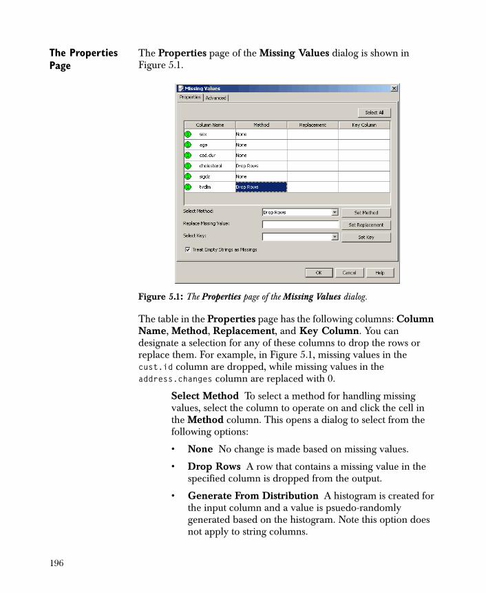
The Properties Page
The Properties page of the Missing Values dialog is shown in Figure 5.1.
The table in the Properties page has the following columns: Column Name, Method, Replacement, and Key Column. You can designate a selection for any of these columns to drop the rows or replace them. For example, in Figure 5.1, missing values in the cust.id column are dropped, while missing values in the address.changes column are replaced with 0.
Select Method To select a method for handling missing values, select the column to operate on and click the cell in the Method column. This opens a dialog to select from the following options:
• None No change is made based on missing values.
• Drop Rows A row that contains a missing value in the specified column is dropped from the output.
• Generate From Distribution A histogram is created for the input column and a value is psuedo-randomly generated based on the histogram. Note this option does not apply to string columns.
Figure 5.1: The Properties page of the Missing Values dialog.
196
• Replace with Mean The mean is substituted for missing values. Note this option does not apply to string columns.
• Replace with Constant A constant specified by the user is substituted for missing values.
• Last Observation Carried Forward Replaces missing values with a previous observation. If you set a Key Column, it replaces the value with the last non-missing value corresponding to the current Key Column category. (Note that the Key Column must be a categorical.) If you do not set a Key Column, it replaces the value with the last non-missing value.
To set a group of columns to the same method, select each column using CTRL or SHIFT, as needed. Using the Select Method box at the bottom of the dialog, select the method each column should use. After you select a method, click the Set Method button.
Replace Missing Value To replace missing values with a specific value, you must specify a replacement. Select the desired column, click the Replacement column, and type the replacement in the box.
To set a group of columns to the same replacement value, select each column using CTRL or SHIFT, as needed. In the Replace Missing Value box at the bottom of the dialog, type the value that each column should use. After you have provided a replacement value, click Set Replacement. Note that values for continuous data columns should be numeric, and values for date columns should be dates.
Key Column To use Last Observation Carried Forward, set the appropriate type for Method as described above and click the Key Column column. Select from a list of categorical columns in the input. This column is an index that determines the value to use for replacement.
To set a group of columns to the same replacement value, elect each column using CTRL or SHIFT as needed. Using the Select Key list box at the bottom of the dialog, select the Key Column each column should use. After you select the Key Column, click Set Key.
197
You can use the buttons at the top of the table to sort the data in Column Name, Method, Replacement, and Key Column.
Treat Empty Strings as Missings Select this check box to indicate that if a column containing a string is empty, it should be treated as a missing value, rather than as an empty string.
Using the Viewer
The viewer for the Missing Values component is the node viewer, an example of which is shown in Figure 5.9. For a complete discussion of the node viewer and the information it displays, see the section The Table Viewer on page 146 as well as the online help.
An Example Using the cross.sell.csv data set located in the examples folder under your home directory, follow the steps below to reproduce the results shown in Figure 5.2.
1. Use a Read Text File node to open the cross.sell.csv data set.
2. Run the node and open its viewer.
3. Scroll through the Continuous and Categorical pages of the node viewer, and note that there are many missing values in this data set.
4. Link the Read Text File node to a Missing Values node.
5. Open the properties dialog for Missing Values.
6. On the Properties page, click the Select All button.
7. Select the Replace with Mean option in the Select Method section and click Set Method button. Click OK to close the dialog.
8. Run the network and open the viewer.
198
Figure 5.2: The Continuous (left) and String (right) pages of the viewer for Missing Values. Note that there are no longer any missing values in the data set.
199
DUPLICATE DETECTION
The Duplicate Detection component provides a method of detecting row duplicates in a rectangular data set.
This section discusses duplicate detection at a high level, describes the properties for the Duplicate Detection component, provides general guidance for interpreting the output from the component, and gives simple examples for illustration.
All figures in this section use variables from the fuel.txt data set, which is stored as a text file in the examples folder under your default home directory.
General Procedure
The following outlines the general approach to using the Duplicate Detection component:
1. Link a Duplicate Detection node in your worksheet to any node that outputs data.
2. Use the properties dialog for Duplicate Detection to specify the columns you want to include in the analysis and the type of output to return.
3. Run the network.
4. To verify the results, launch the viewer for Duplicate Detection.
Background The Duplicate Detection component accepts a single input containing rectangular data.
Select to consider for duplicates. The values in all the columns specified must be identical in at least two observations for the two observations to be considered duplicates. For example, you can specify that columns LastName, FirstName, and MiddleInitial all have to be the same for observations to be considered duplicated.
Spotfire Miner computes a new categorical column, named DUPLICATED by default. This variable contains true if the observation is considered a duplicate; otherwise, it contains false.
You can output:
• The DUPLICATED column, along with all original data.
200
• Only the DUPLICATED column.
• Only the observations that are not duplicated, with or without the DUPLICATED column.
• Only observations that are duplicates, with or without the DUPLICATED column.
Also, you can specify an option consider the first instance of a duplicate as a duplicate. That is, you can specify that the first instance of a value (or combination of values, if you specify more than one column for duplicate detection) that is duplicated later in the data set is not considered a duplicate.
The DUPLICATED column (if output) is a categorical value. Clicking the Categorical tab in the Data Viewer and selecting the Duplicated variable displays in the Levels box the numbers of false and true results, based on your selection in the Duplicate Definition group on the Properties page. Figure 5.3 displays the results of running the Duplicate Detection node on the Fuel data set, checking for duplicates only for the Weight variable, and accepting the default options (which includes Include First Occurrence as Duplicate in the Duplicate Definition group.) Using this option, notice that nine Weight variables are duplicated in the data set.
201

When analyzing data, you might want to identify and manipulate variables that contain duplicates of data in other rows. For example, if your data includes ID numbers, and you want to find multiple instances of any ID number, use the Duplicate Detection node. This node provides several options for identifying, displaying, or filtering either all duplicates or the first instances of duplicates.
Properties The properties dialog for the Duplicate Detection component contains three tabbed pages labeled Properties, Output, and Advanced (see page 564 for a discussion of the options available on the Advanced page.)
The Properties Page
The Properties page of the Duplicate Detection dialog is shown in Figure 5.4.
Figure 5.3: Categorical page of the Duplicate Detection dialog.
202
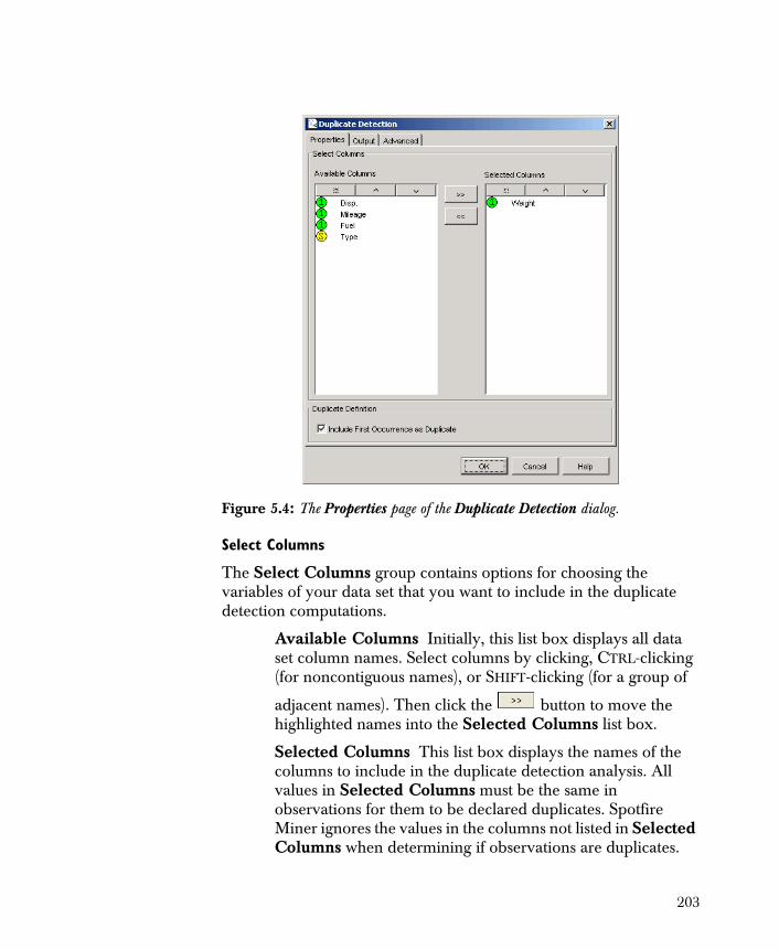
Select Columns
The Select Columns group contains options for choosing the variables of your data set that you want to include in the duplicate detection computations.
Available Columns Initially, this list box displays all data set column names. Select columns by clicking, CTRL-clicking (for noncontiguous names), or SHIFT-clicking (for a group of
adjacent names). Then click the button to move the highlighted names into the Selected Columns list box.
Selected Columns This list box displays the names of the columns to include in the duplicate detection analysis. All values in Selected Columns must be the same in observations for them to be declared duplicates. Spotfire Miner ignores the values in the columns not listed in Selected Columns when determining if observations are duplicates.
Figure 5.4: The Properties page of the Duplicate Detection dialog.
203
To remove columns, in the Selected Columns list box, select them by clicking, CTRL-clicking, or SHIFT-clicking. Then click
the button to the left of the list box to move the highlighted names back into the Available Columns list box.
Use the buttons at the top of the Available Columns and Selected Columns list boxes to sort the display of column names. This is helpful when you have a large number of columns in your data set, and you want to find particular ones quickly. You can sort the column names:
• In the order they appear in the input data, which is the default.
• In alphabetical order.
• In reverse alphabetical order.
You can also use drag-and-drop within the lists to reorder the display of an individual column name.
Duplicate Definition
Use the Duplicate Definition group to indicate whether to tag the first row in a set of duplicate rows as a duplicate.
• To create an indicator column of all non-unique rows, select Include First Definition as Duplicate check box, and, on the Options page, select Output Duplicated State.
204
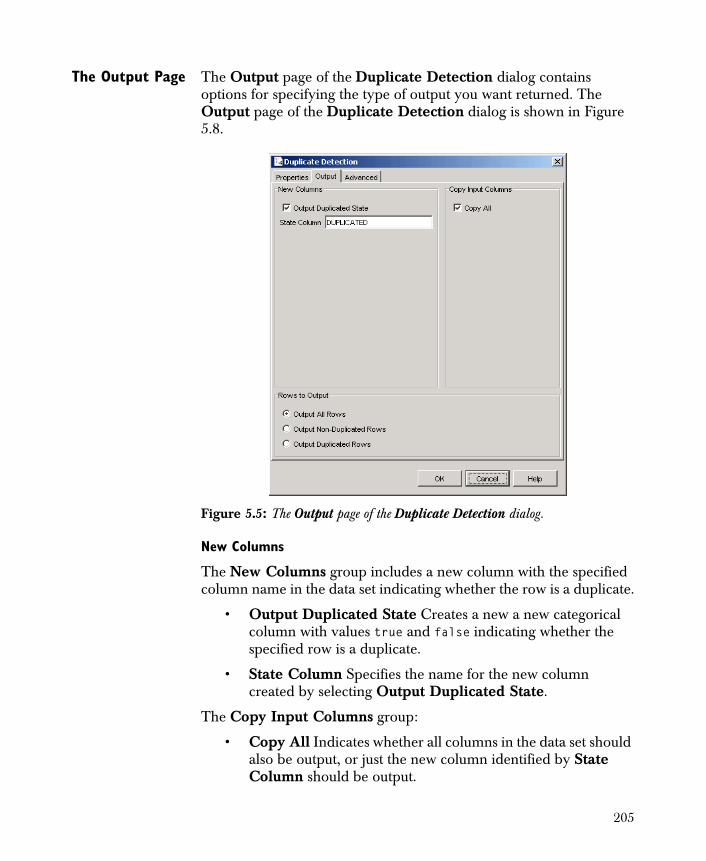
The Output Page The Output page of the Duplicate Detection dialog contains options for specifying the type of output you want returned. The Output page of the Duplicate Detection dialog is shown in Figure 5.8.
New Columns
The New Columns group includes a new column with the specified column name in the data set indicating whether the row is a duplicate.
• Output Duplicated State Creates a new a new categorical column with values true and false indicating whether the specified row is a duplicate.
• State Column Specifies the name for the new column created by selecting Output Duplicated State.
The Copy Input Columns group:
• Copy All Indicates whether all columns in the data set should also be output, or just the new column identified by State Column should be output.
Figure 5.5: The Output page of the Duplicate Detection dialog.
205
The Rows to Output group specifies whether to output all rows, whether or not they are duplicated or non-duplicated, or whether to output only the duplicated or the non-duplicated rows.
• Output All Rows Specifies that all rows, including duplicates, are output. This option is useful for identifying duplicates only if you also select Output Duplicated State.
• Output Non-Duplicated Rows Outputs a subset of only the non-duplicated rows in the data set.
• Output Duplicated Rows Outputs a subset of only the duplicated rows in the data set.
Using the Viewer
The viewer for the Duplicate Detection component is the node viewer, an example of which is shown in Figure 5.9. For a complete discussion of the node viewer and the information it displays, see the section The Table Viewer on page 146 as well as the online help.
An Example Using the fuel.txt data set located in the examples folder under your home directory, follow the steps below to reproduce the results shown in Figure 5.9.
1. Use a Read Text File node to open the fuel.txt data set. This data set contains four continuous variables and one string variable for various samples of car fuel efficiency and type.
2. Link the Read Text File node to an Duplicate Detection node.
3. Open the properties dialog for Duplicate Detection.
4. In the Available Columns list box, select the variable
Weight, and then click the button to move this name into the Selected Columns field.
5. Click the Output tab of the dialog and review the defaults.
6. Run the network and open the viewer.
206

7. Notice that the data set now includes a new column, DUPLICATED, which indicates whether the row contains a weight shared by another row in the data set. Scroll down to Row 15, the first instance of a true value in the DUPLICATED column. Note that the weight is 2885.00. Now scroll down to Row 45, where the weight is also 2885.00.
8. Click the Categorical tab, and then select the only row in the display, for the variable DUPLICATED. (See Figure 5.3 for an illustration.)
Figure 5.6: The Data View after running the Duplicate Detection node on the Fuel data set.
207

OUTLIER DETECTION
The Outlier Detection component provides a reliable method of detecting multidimensional outliers in your data. The method is based on the computation of robust Mahalanobis distances for the rows in your data set.
This section discusses outlier detection at a high level, describes the properties for the Outlier Detection component, provides general guidance for interpreting the output from the component, and gives a full example for illustration. Spotfire Miner supports outlier computations for continuous variables only. Although it is possible to include a single categorical variable in the analysis for conditioning purposes, it is not possible to include a categorical variable in the computations of the robust Mahalanobis distances.
Unless otherwise specified, all figures in this section use variables from the glass.txt data set, which is stored as a text file in the examples folder under your default document directory.
General Procedure
The following outlines the general approach to using the Outlier Detection component:
1. Link an Outlier Detection node in your worksheet to any node that outputs data.
2. Use the properties dialog for Outlier Detection to specify the columns you want to include in the analysis and the type of output you want to return.
3. Run your network.
4. To verify the results, launch the viewer for Outlier Detection.
The Outlier Detection component accepts a single input containing rectangular data and continuous variables. It outputs a data set containing a combination of the following, based on the options you choose in the properties dialog:
• A column containing the squared distances computed by the Outlier Detection algorithm.
• A column containing two values, "yes" and "no", which indicate whether each row is considered an outlier.
208
• A column containing the original row index. This option is particularly useful when not all of the original data rows are returned.
• All of the original input variables you select for the analysis.
• All of the rows that are not considered outliers.
Additionally, you have the option of returning all the original data rows, only those rows not considered an outlier, or only the rows that are considered outliers.
Background When analyzing and modeling data, you might find sometimes that some values are surprising because they are far from the majority of the data in some sense. Such values are called outliers . Detecting these values is extremely important in data mining for two reasons:
1. The outliers might result from errors in the data gathering and management process. “Noisy” data values such as these usually produce models with poor predictive performance.
2. The outliers can be your most important data values. This occurs, for example, when trying to detect credit card or insurance fraud; the outliers in a customer database can indicate fraudulent behavior.
Outliers are multidimensional in character, which makes their detection a challenging task. Detecting outliers well is a key task in data cleaning since a single bad data value has the potential to dramatically affect business decisions. Spotfire Miner’s Outlier Detection component can identify unusual values in your data by observing multiple variables simultaneously and providing signals when the data are possible outliers. Simplistic outlier detection methods often look at a single variable at a time; therefore, they can easily miss values that look reasonable for any one variable but which, when taken together, represent a clear outlier. See the section Why Robust Distances Are Preferable on page 218 for an example.
The Outlier Detection component processes the input data, constructs a robust dependency model, and then estimates which input rows are outliers relative to the bulk of the data. It works by using advanced robust estimation techniques to calculate the covariances between all columns that you choose to include in the analysis. From the covariances, Spotfire Miner computes a single (squared) distance for each row in the data set; this value is based on a
209
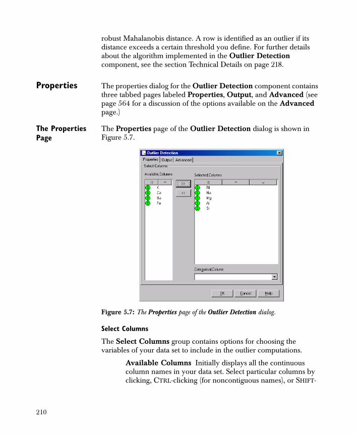
robust Mahalanobis distance. A row is identified as an outlier if its distance exceeds a certain threshold you define. For further details about the algorithm implemented in the Outlier Detection component, see the section Technical Details on page 218.
Properties The properties dialog for the Outlier Detection component contains three tabbed pages labeled Properties, Output, and Advanced (see page 564 for a discussion of the options available on the Advanced page.)
The Properties Page
The Properties page of the Outlier Detection dialog is shown in Figure 5.7.
Select Columns
The Select Columns group contains options for choosing the variables of your data set to include in the outlier computations.
Available Columns Initially displays all the continuous column names in your data set. Select particular columns by clicking, CTRL-clicking (for noncontiguous names), or SHIFT-
Figure 5.7: The Properties page of the Outlier Detection dialog.
210
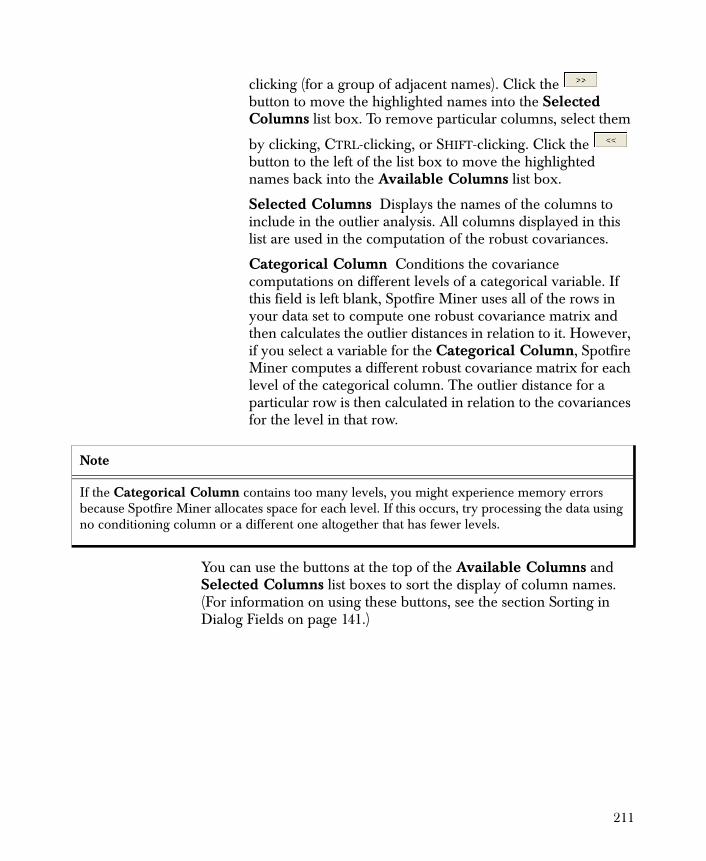
clicking (for a group of adjacent names). Click the button to move the highlighted names into the Selected Columns list box. To remove particular columns, select them
by clicking, CTRL-clicking, or SHIFT-clicking. Click the button to the left of the list box to move the highlighted names back into the Available Columns list box.
Selected Columns Displays the names of the columns to include in the outlier analysis. All columns displayed in this list are used in the computation of the robust covariances.
Categorical Column Conditions the covariance computations on different levels of a categorical variable. If this field is left blank, Spotfire Miner uses all of the rows in your data set to compute one robust covariance matrix and then calculates the outlier distances in relation to it. However, if you select a variable for the Categorical Column, Spotfire Miner computes a different robust covariance matrix for each level of the categorical column. The outlier distance for a particular row is then calculated in relation to the covariances for the level in that row.
You can use the buttons at the top of the Available Columns and Selected Columns list boxes to sort the display of column names. (For information on using these buttons, see the section Sorting in Dialog Fields on page 141.)
Note
If the Categorical Column contains too many levels, you might experience memory errors because Spotfire Miner allocates space for each level. If this occurs, try processing the data using no conditioning column or a different one altogether that has fewer levels.
211
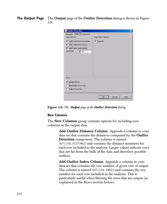
The Output Page The Output page of the Outlier Detection dialog is shown in Figure 5.8.
New Columns
The New Columns group contains options for including new columns in the output data.
Add Outlier Distance Column Appends a column to your data set that contains the distances computed by the Outlier Detection component. The column is named OUTLIER.DISTANCE and contains the distance measures for each row included in the analysis. Larger values indicate rows that are far from the bulk of the data and therefore possible outliers.
Add Outlier Index Column Appends a column to your data set that contains the row number of given row of output. The column is named OUTLIER.INDEX and contains the row number for each row included in the analysis. This is particularly useful when filtering the rows that are output (as explained in the Rows section below).
Figure 5.8: The Output page of the Outlier Detection dialog.
212
Add Outlier State Column Appends a categorical column to your data set that indicates whether each row is an outlier. The column is named OUTLIER.STATE and contains two levels: "yes" and "no". This option is most useful when the All Input Rows option is selected.
Threshold This value indirectly determines how large a distance must be before the corresponding row is considered an outlier. You can think of this as the fraction of “clean” data that Spotfire Miner recognizes as clean. See the Technical Details section for the statistical distribution assumptions for setting this value. The default value is 0.99, which means Spotfire Miner recognizes as outliers approximately 1% of the actual nonoutlier rows in your data. To specify a different value, type a number between 0.0 and 1.0 in the text box. Typical values are 0.95, 0.99, and 0.999.
Copy Input Columns
The Copy Input Columns group contains an option for copying the input columns to the output data set. Select the Copy All check box if you want all of the columns in the input data set to be copied to the output data. This includes both the Selected Columns and the Available Columns you choose on the Properties page of the dialog as well as any categorical, date, or string variables in the input data. If this check box is cleared, the output data contains only the selected columns OUTLIER.DISTANCE, OUTLIER.INDEX, and OUTLIER.STATE (as specified under New Columns).
Rows
The Rows group determines which rows are returned in the output data set.
All Input Rows Returns all rows.
Non-Outlier Rows Only Returns only those rows that are not considered outliers (according to the values in the OUTLIER.STATE column).
Outlier Rows Only Returns only the outlier rows (according to the values in the OUTLIER.STATE column).
213
Using the Viewer
The viewer for the Outlier Detection component is the node viewer, an example of which is shown in Figure 5.9. For a complete discussion of the node viewer and the information it displays, see the section The Table Viewer on page 146 as well as the online help.
An Example Using the glass.txt data set located in the examples folder under your home directory, follow the steps below to reproduce the results shown in Figure 5.9.
1. Use a Read Text File node to open the glass.txt data set. This data set contains nine continuous variables and one categorical variable for various samples of glass. The continuous variables are the percentages of various chemical constituents of the glass samples.
2. Use the Modify Columns page of Read Text File to change the variable Type from continuous to categorical.
3. Link the Read Text File node to an Outlier Detection node.
4. Open the properties dialog for Outlier Detection.
5. In the Available Columns list box, select the first five
variables (RI, Na, Mg, Al, Si) and click the button to move these names into the Selected Columns field.
6. Click the Output tab of the dialog.
7. Run the network and open the viewer.
Note
When categorical variables such as Type have numeric levels, by default Spotfire Miner imports them from the data file as continuous, and you must change their types manually to categorical. To change them when importing the data, you can use the Modify Columns page of the data input component, or you can use a Modify Columns component after Spotfire Miner has read in the data.
214
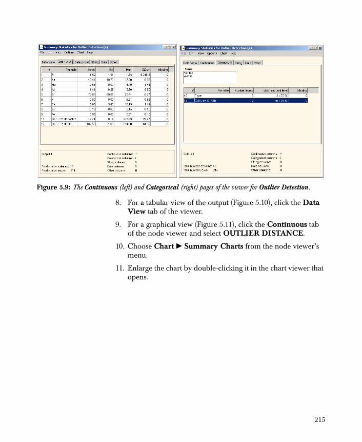
8. For a tabular view of the output (Figure 5.10), click the Data View tab of the viewer.
9. For a graphical view (Figure 5.11), click the Continuous tab of the node viewer and select OUTLIER DISTANCE.
10. Choose Chart � Summary Charts from the node viewer’s menu.
11. Enlarge the chart by double-clicking it in the chart viewer that opens.
Figure 5.9: The Continuous (left) and Categorical (right) pages of the viewer for Outlier Detection.
215
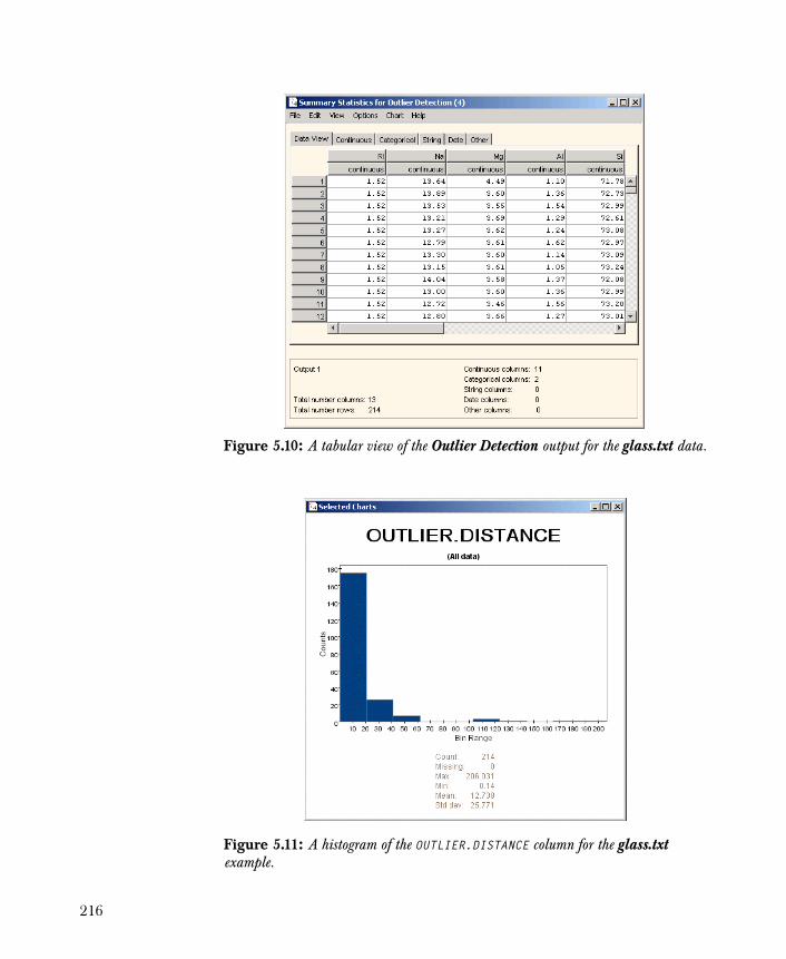
Figure 5.10: A tabular view of the Outlier Detection output for the glass.txt data.
Figure 5.11: A histogram of the OUTLIER.DISTANCE column for the glass.txt example.
216
Interpreting the Results
When you run the above example, the Outlier Detection algorithm generates the following in the message pane of the Spotfire Miner interface:
Outlier Detection (1): number vars=5, threshold=0.99,chi square distance threshold=15.0863Outlier Detection (1): found 50 outlier rows,164 non-outlier rows, 0 NA rows
The 99% threshold point is equal to approximately 15.1 for the five variables included in the analysis, so that rows with a distance measure greater than 15.1 are declared outliers. This results in Spotfire Miner declaring 23% of the data points (50 rows) as outliers, while the remaining 76% (164 rows) represents the central bulk of the data.
This histogram in Figure 5.11 suggests that the Mahalanobis distances are clustered into two groups separated by a threshold point of approximately 100-110. This is much larger than the chi-squared 99% threshold point of 15.1 computed in the example. As a reasonable first step in cleaning these data, you can use the Filter Rows component to remove those rows from the data set corresponding to cutoff distances larger than 100, and then re-run the Outlier Detection algorithm on the filtered data. We recommend performing an analysis such as this as a complement to the automatic threshold computed by Spotfire Miner.
217
TECHNICAL DETAILS
This section provides technical background on the robust estimation of covariance matrices that motivates the design of the Outlier Detection component. This section also gives details concerning the specific algorithm for robust covariance estimation and distance computation that is implemented in Spotfire Miner.
Why Robust Distances Are Preferable
The classical squared Mahalanobis distance is commonly used to detect outliers. It is computed according to the following equation:
Here, is the transpose of the ith row of the data set, is a vector of
sample means of the columns in the data set, and is the sample covariance matrix. Unfortunately, these classical estimates are extremely sensitive to the presence of multidimensional outliers. Even a small fraction of outliers can distort the estimates, to the extent that they become very misleading and virtually useless in many data mining applications.
Spotfire Miner uses robust Mahalanobis distances based on a highly scalable, robust covariance matrix estimate that is not greatly influenced by the presence of outliers. Figures 5.12 and 5.13 below illustrate two key concepts regarding the appeal of this approach:
1. Outliers can distort the classical covariance matrix estimates and associated classical distances, rendering them unreliable for detecting multidimensional outliers.
2. The robust distances based on a new robust covariance matrix estimate are very powerful at detecting outliers that render the classical distances useless.
For illustration, consider Figure 5.12, which shows all pair-wise scatter plots of a five-dimensional data set called “Woodmod.” These data are a modified version of the wood gravity data from Rousseeuw and Leroy (1987); the data set is not included in Spotfire Miner. The Woodmod data have several multidimensional outliers that show up
(5.1)
d 2
d 2 xi( ) xi μ–( )TC
1–xi μ–( )=
xi μ
C
218
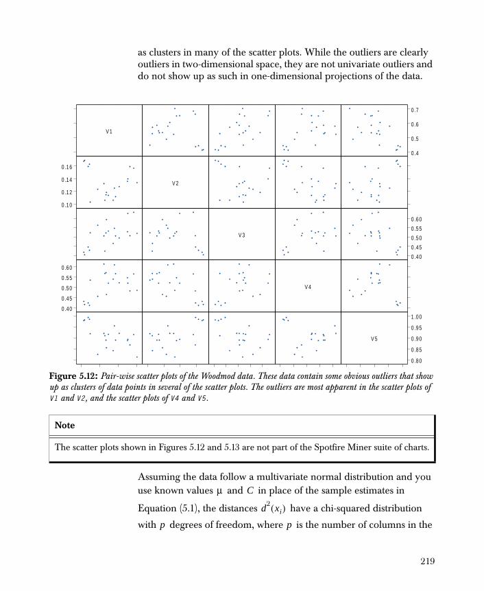
as clusters in many of the scatter plots. While the outliers are clearly outliers in two-dimensional space, they are not univariate outliers and do not show up as such in one-dimensional projections of the data.
Assuming the data follow a multivariate normal distribution and you use known values and in place of the sample estimates in
Equation (5.1), the distances have a chi-squared distribution
with degrees of freedom, where is the number of columns in the
Figure 5.12: Pair-wise scatter plots of the Woodmod data. These data contain some obvious outliers that show up as clusters of data points in several of the scatter plots. The outliers are most apparent in the scatter plots of V1 and V2, and the scatter plots of V4 and V5.
Note
The scatter plots shown in Figures 5.12 and 5.13 are not part of the Spotfire Miner suite of charts.
V 1
0 .10
0 .12
0 .14
0 .16
0 .40
0 .45
0 .50
0 .55
0 .60
V 2
V 3
V 4
0 .4
0 .5
0 .6
0 .7
0 .40
0 .45
0 .50
0 .55
0 .60
V 5
0 .80
0 .85
0 .90
0 .95
1 .00
μ C
d2 xi( )
p p
219

outlier analysis. In data mining, you typically encounter very large data set sizes, so the sample estimates are close to their true values. Therefore, it is not unreasonable to use a chi-squared percent point
such as 0.95 or 0.99 ( or ) as a threshold with which to
compare . This is the rationale behind the Outlier Detection
implementation: it declares to be an outlier if its squared robust Mahalanobis distance exceeds this threshold.
Using the classical approach for the Woodmod data as given by Equation (5.1), you obtain the results in the right panel of Figure 5.13. The horizontal dashed line is the square root of the 95% point of a chi-squared distribution with degrees of freedom. Clearly, no points are declared outliers. This is because the outliers have distorted
the classical covariance matrix estimate so much that it does not produce reliable Mahalanobis distances.
Using the robust approach for the Woodmod data, however, you obtain the results in the left panel of Figure 5.13. The approach based
on robust and detects not only the cluster of four very large outliers evident in the pair-wise scatter plots of Figure 5.12 but also three additional, moderately-sized outliers that are not so evident in the scatter plots.
For further explanation of the difference between the classical and robust approaches for the Woodmod data, see the discussion of this example in “Scalable robust covariance and correlation estimates for data mining” by Alqallaf, Konis, Martin, and Zamar (2002), Proceedings of the eighth ACM SIGKDD international conference on knowledge discovery and data mining.
χ2p 0.95, χ2
p 0.99,
d2 xi( )
xi
p 5=
C
C μ
220
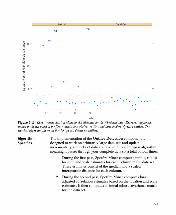
Algorithm Specifics
The implementation of the Outlier Detection component is designed to work on arbitrarily large data sets and update incrementally as blocks of data are read in. It is a four-pass algorithm, meaning it passes through your complete data set a total of four times.
1. During the first pass, Spotfire Miner computes simple, robust location and scale estimates for each column in the data set. These estimates consist of the median and a scaled interquartile distance for each column.
2. During the second pass, Spotfire Miner computes bias-adjusted correlation estimates based on the location and scale estimates. It then computes an initial robust covariance matrix for the data set.
Figure 5.13: Robust versus classical Mahalanobis distances for the Woodmod data. The robust approach, shown in the left panel of the figure, detects four obvious outliers and three moderately-sized outliers. The classical approach, shown in the right panel, detects no outliers.
5
10
15
5 10 15 20
ROBUST
6
819
CLASSICAL
Index
Squ
are
Roo
t of
Mah
alan
obis
Dis
tanc
e
221
3. During the third pass, Spotfire Miner forms the final positive-definite, robust covariance matrix.
4. During the fourth pass, Spotfire Miner uses the covariance matrix to compute a robust Mahalanobis distance for each row in the data set. These are the distances the Outlier Detection component returns in the OUTLIER.DISTANCE column.
To determine whether a particular row is indeed an outlier, Spotfire Miner computes a cutoff distance based on the quantiles of a chi-squared distribution. The probability for the quantiles is the value of the Threshold option from the Options page of the properties dialog; this is 0.99 by default. The degrees of freedom for the distribution is equal to the number of columns you include in the analysis (that is, the total number in the Selected Columns list of the Properties page of the dialog). Rows with squared distances that are larger than this cutoff are flagged as outliers and correspond to a value of "yes" in the OUTLIER.STATE column.
This method enables fast computation for data mining applications. The algorithm runs linearly in , the number of rows in the data set, and quadratically in , the number of selected columns in the analysis. For complete mathematical details on the method and its rationale, see Alqallaf, Konis, Martin, and Zamar (2002).
n
p
222
REFERENCES
Alqallaf, F. A., Konis, K. P., Martin, R. D., and Zamar, R. H. (2002). “Scalable robust covariance and correlation estimates for data mining.” Proceedings of the eighth ACM SIGKDD international conference on knowledge discovery and data mining.
Maronna, R.A. and Zamar, R.H. (2002). Robust multivariate estimates for high dimensional data sets. Technometrics 44, 307-317.
Rousseeuw, P.J. and Leroy, A.M. (1987). Robust Regression and Outlier Detection . New York: Wiley.
223

224
Overview 227
Manipulating Rows 228Aggregate 228Append 233Filter Rows 235Partition 237Sample 239Shuffle 242Sort 242Split 245Stack 247Unstack 250
Manipulating Columns 253Bin 253Create Columns 257Filter Columns 260Recode Columns 262Join 268Modify Columns 271Normalize 276Reorder Columns 279Transpose 282
Using the Spotfire Miner™ Expression Language 285Value Types 287NA Handling 287Error Handling 287Column References 288Double and String Constants 289Operators 290
DATA MANIPULATION 6
225

Functions 291
226
OVERVIEW
Data manipulation is critical for transforming your data from their original format into a form that is compatible with model building. For instance, CRM models are typically built from a flat structure where every customer is represented in a single row. Transactional systems, on the other hand, store customer data in highly normalized data structures; for example, customers and their transactions might be in separate tables with one-to-many relationships.
Spotfire Miner™ gives you the ability to select, aggregate, and denormalize your data to create good predictive views. Data manipulation components in Spotfire Miner support both row-based and column-based operations.
227
MANIPULATING ROWS
Spotfire Miner provides the following components for performing row-based data manipulations:
• Aggregate
• Append
• Filter Rows
• Partition
• Sample
• Shuffle
• Sort
• Split
• Stack
• Unstack
In this section, we discuss each component in turn.
Aggregate The Aggregate component condenses the information in your data set by applying descriptive statistics according to one or more categorical columns. This is also known as roll up functionality and is similar to pivot tables in Microsoft Excel.
General Procedure
The following outlines the simplest and most common approach for using the Aggregate component:
1. Link an Aggregate node in your worksheet to any node that outputs data.
2. Use the properties dialog for Aggregate to specify the columns in your data set that you want to summarize as well as the type of descriptive statistics to use. In this case:
• Highlight a categorical column in the Input Columns list box and click Add to place it in the Aggregate By list.
228

• Highlight a continuous variable in the Input Columns list box, choose a descriptive statistic from the Aggregate Function drop-down list, and click the Add Column button. This places the column name in the grid view at the bottom of the dialog. (Note that the Output Column is named according to both the column name and the chosen descriptive statistic.) Repeat this step until you have chosen all columns you want to summarize and then click OK.
3. Run your network.
4. Launch the node’s viewer.
In the above case, for each column in the grid view, Spotfire Miner computes the chosen descriptive statistic for each level in the categorical variable. (See below for details on all the available options for using the Aggregate component.)
The Aggregate node accepts a single input containing rectangular data and outputs a single rectangular data set defined by the options you choose.
The number of columns in the output data set is equal to the total number of variables you place in the Aggregate By list box and in the grid view. The number of rows in the data set is determined by the number of unique combinations of levels and values in the Aggregate By variables. For example, suppose you place two categorical variables in the Aggregate By list, one with 10 levels and one with 5. In this scenario, the number of rows in the output data set is equal to 50.
Using Sort in Aggregate
In the Advanced page, if Sort Required is selected, then the input data is sorted by the columns in Aggregate By, so each of the blocks is guaranteed to have unique values for these columns. If Sort Required is not selected, the input data is not sorted, and the blocks are determined by scanning through the rows in order. When any of the Aggregate By values changes, it signals the beginning of another block. If the data is already sorted, make sure Sort Required is not selected.
Note that if Sort Required is not checked, all inputs should be presorted, in ascending order, with NA’s on the top.
229
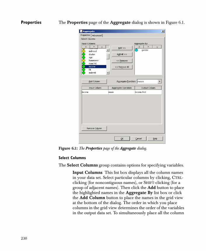
Properties The Properties page of the Aggregate dialog is shown in Figure 6.1.
Select Columns
The Select Columns group contains options for specifying variables.
Input Columns This list box displays all the column names in your data set. Select particular columns by clicking, CTRL-clicking (for noncontiguous names), or SHIFT-clicking (for a group of adjacent names). Then click the Add button to place the highlighted names in the Aggregate By list box or click the Add Column button to place the names in the grid view at the bottom of the dialog. The order in which you place columns in the grid view determines the order of the variables in the output data set. To simultaneously place all the column
Figure 6.1: The Properties page of the Aggregate dialog.
230
names in the Aggregate By list box, click the Add All button. It is not possible to place a single column in both the Aggregate By list and the grid view.
Aggregate By The columns in this list determine how the descriptive statistics are applied:
• If a single categorical column is chosen, Spotfire Miner computes the descriptive statistics for each level in the variable.
• If a single continuous, string, or date column is chosen, Spotfire Miner computes the statistics for each unique value in the variable.
• If multiple columns are chosen, Spotfire Miner computes the statistics for each combination of levels (categorical variables) and unique values (continuous, string, or date variables).
If you need to remove particular columns from the Aggregate By list, select them by clicking, CTRL-clicking, or SHIFT-clicking. Then click the Remove button to remove the highlighted names. To simultaneously remove all the column names, click the Remove All button.
Grid View
The grid view at the bottom of the page displays the columns you want to summarize as well as the descriptive statistics computed for those variables. It is possible to include a single column multiple times in the grid view if you need to compute multiple descriptive statistics for it.
Input Column This area of the grid displays the names of the variables.
Aggregate Operation This area of the grid displays the descriptive statistic for each variable.
Output Column This area of the grid displays the names that will be used in the output to identify the summarized data. By default, the entries in Output Column are named according to both the column names and the chosen descriptive statistics.
231

You can change any of the entries in the grid view as follows:
• To change an entry under Input Column, click the entry. This opens a drop-down list containing all variable names in the data set.
• To change an entry under Aggregate Operation, click the entry. This opens a drop-down list containing all possible descriptive statistics for the particular variable (see Aggregate Function below).
• To change an entry under Output Column, double-click the entry. This activates a text box in which you can type a new column name.
If you need to remove particular columns from the grid view, select the rows that contain them by clicking, CTRL-clicking, or SHIFT-clicking. Then click the Remove Column button.
Use the Aggregate Function drop-down list to choose which descriptive statistic you want to compute for a particular column before you add the column to the grid view. To choose a statistic for a column that is already in the grid view, click its entry under Aggregate Operation. For continuous variables, the available descriptive statistics are the first and last values (first and last), a count of the values (count), the sum of the values (sum), the arithmetic average, standard deviation, and variance (mean, stdDev, and var), the extreme values (min and max), and the range of the values (range). For noncategorical variables, the choices are simply first, last, and count.
Sort Options On the Advanced page, there is an option for specifying whether or not to sort the input data before performing the Aggregate. This option improves performance, but should only be used if the input has been previously sorted in the order specified by the Aggregate By list box.
Using the Viewer The viewer for the Aggregate component, as for all the data manipulation components, is the node viewer, an example of which is shown in Figure 6.2. For a complete discussion of the node viewer and the information it displays, see the section The Table Viewer on page 146 as well as the online help.
232
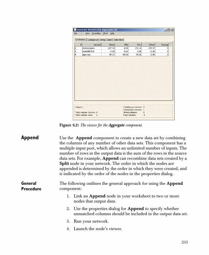
Append Use the Append component to create a new data set by combining the columns of any number of other data sets. This component has a multiple-input port, which allows an unlimited number of inputs. The number of rows in the output data is the sum of the rows in the source data sets. For example, Append can recombine data sets created by a Split node in your network. The order in which the nodes are appended is determined by the order in which they were created, and is indicated by the order of the nodes in the properties dialog.
General Procedure
The following outlines the general approach for using the Append component:
1. Link an Append node in your worksheet to two or more nodes that output data.
2. Use the properties dialog for Append to specify whether unmatched columns should be included in the output data set.
3. Run your network.
4. Launch the node’s viewer.
Figure 6.2: The viewer for the Aggregate component.
233
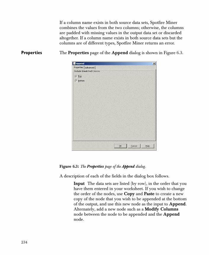
If a column name exists in both source data sets, Spotfire Miner combines the values from the two columns; otherwise, the columns are padded with missing values in the output data set or discarded altogether. If a column name exists in both source data sets but the columns are of different types, Spotfire Miner returns an error.
Properties The Properties page of the Append dialog is shown in Figure 6.3.
A description of each of the fields in the dialog box follows.
Input The data sets are listed (by row), in the order that you have them entered in your worksheet. If you wish to change the order of the nodes, use Copy and Paste to create a new copy of the node that you wish to be appended at the bottom of the output, and use this new node as the input to Append. Alternately, add a new node such as a Modify Columns node between the node to be appended and the Append node.
Figure 6.3: The Properties page of the Append dialog.
234
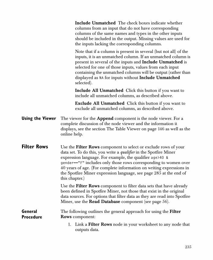
Include Unmatched The check boxes indicate whether columns from an input that do not have corresponding columns of the same names and types in the other inputs should be included in the output. Missing values are used for the inputs lacking the corresponding columns.
Note that if a column is present in several (but not all) of the inputs, it is an unmatched column. If an unmatched column is present in several of the inputs and Include Unmatched is selected for one of those inputs, values from each input containing the unmatched columns will be output (rather than displayed as NA for inputs without Include Unmatched selected).
Include All Unmatched Click this button if you want to include all unmatched columns, as described above.
Exclude All Unmatched Click this button if you want to exclude all unmatched columns, as described above.
Using the Viewer The viewer for the Append component is the node viewer. For a complete discussion of the node viewer and the information it displays, see the section The Table Viewer on page 146 as well as the online help.
Filter Rows Use the Filter Rows component to select or exclude rows of your data set. To do this, you write a qualifier in the Spotfire Miner expression language. For example, the qualifier age>40 & gender=="F" includes only those rows corresponding to women over 40 years of age. (For complete information on writing expressions in the Spotfire Miner expression language, see page 285 at the end of this chapter.)
Use the Filter Rows component to filter data sets that have already been defined in Spotfire Miner, not those that exist in the original data sources. For options that filter data as they are read into Spotfire Miner, use the Read Database component (see page 56).
General Procedure
The following outlines the general approach for using the Filter Rows component:
1. Link a Filter Rows node in your worksheet to any node that outputs data.
235
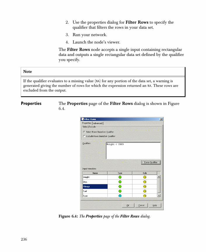
2. Use the properties dialog for Filter Rows to specify the qualifier that filters the rows in your data set.
3. Run your network.
4. Launch the node’s viewer.
The Filter Rows node accepts a single input containing rectangular data and outputs a single rectangular data set defined by the qualifier you specify.
Properties The Properties page of the Filter Rows dialog is shown in Figure 6.4.
Note
If the qualifier evaluates to a missing value (NA) for any portion of the data set, a warning is generated giving the number of rows for which the expression returned an NA. These rows are excluded from the output.
Figure 6.4: The Properties page of the Filter Rows dialog.
236
Select/Exclude
The Select/Exclude group determines whether the qualifier includes or excludes the specified rows.
Select Rows Based on Qualifier Select this option to keep all of the rows defined by the qualifier.
Exclude Rows Based on Qualifier Select this option to exclude all of the rows defined by the qualifier.
Qualifier Type a valid conditional expression in the Spotfire Miner expression language to define your qualifier. The idea is to construct an expression that implicitly creates a logical column for your data set; the rows defined by the qualifier are those rows for which the logical column is true. Thus, if you choose Select Rows Based on Qualifier above, Spotfire Miner returns all rows for which the column is true. If you choose Exclude Rows Based on Qualifier, Spotfire Miner returns all rows for which the column is false. When you click the Parse Qualifier button, the current expression is parsed, and a window pops up displaying any parsing errors. This also includes any type-checking errors that occur, such as when an expression does not return a logical value. An error is displayed with information about the position in the expression where the error occurred.
Input Variables This scrollable table shows the input column names, types, and roles and is useful for finding the names of available inputs when constructing new expressions.
Using the Viewer The viewer for the Filter Rows component is the node viewer. For a complete discussion of the node viewer and the information it displays, see the section The Table Viewer on page 146 as well as the online help.
Partition Use the Partition component to randomly sample the rows of your data set to partition it into three subsets for building, testing, and validating your models.
General Procedure
The following outlines the general approach for using the Partition component:
1. Link a Partition node in your worksheet to any node that outputs data.
237
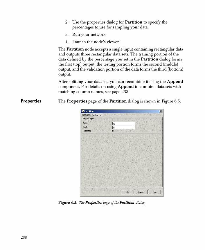
2. Use the properties dialog for Partition to specify the percentages to use for sampling your data.
3. Run your network.
4. Launch the node’s viewer.
The Partition node accepts a single input containing rectangular data and outputs three rectangular data sets. The training portion of the data defined by the percentage you set in the Partition dialog forms the first (top) output, the testing portion forms the second (middle) output, and the validation portion of the data forms the third (bottom) output.
After splitting your data set, you can recombine it using the Append component. For details on using Append to combine data sets with matching column names, see page 233.
Properties The Properties page of the Partition dialog is shown in Figure 6.5.
Figure 6.5: The Properties page of the Partition dialog.
238
Percentages
The Percentages group determines the percentages to use for partitioning your data into training, testing, and validation groups. Note that Spotfire Miner uses a default value of zero percent for the validation group but adjusts this value automatically as you change the values in the Train and Test fields.
Train Specify the percentage of your original data to use for the training data set. By default, this value is set to 70.
Test Specify the percentage of your original data to use for the testing data set. By default, this value is set to 30.
Using the Viewer The viewer for the Partition component is the node viewer. For a complete discussion of the node viewer and the information it displays, see the section The Table Viewer on page 146 as well as the online help.
Sample Use the Sample component to sample the rows of your data set. One reason for doing this is to change the proportional representation of certain characteristics in the data. For example, you might want to guarantee that 50% of your data is such that gender="M". Sampling can also increase performance by reducing a large data set to a smaller, representative one, and it can increase model accuracy by lifting the representation of a particular characteristic.
Use the Sample component to sample data sets that have already been defined in Spotfire Miner, not those that exist in the original data sources. For options that sample data as they are read into Spotfire Miner, use the Read Database component (see page 56).
General Procedure
The following outlines the general approach for using the Sample component:
1. Link a Sample node in your worksheet to any node that outputs data.
2. Use the properties dialog for Sample to specify both the sampling method Spotfire Miner uses and the size limit for the resulting data set.
3. Run your network.
4. Launch the node’s viewer.
239
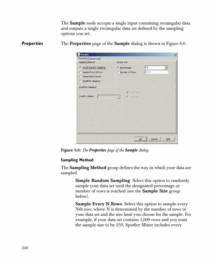
The Sample node accepts a single input containing rectangular data and outputs a single rectangular data set defined by the sampling options you set.
Properties The Properties page of the Sample dialog is shown in Figure 6.6.
Sampling Method
The Sampling Method group defines the way in which your data are sampled.
Simple Random Sampling Select this option to randomly sample your data set until the designated percentage or number of rows is reached (see the Sample Size group below).
Sample Every N Rows Select this option to sample every Nth row, where N is determined by the number of rows in your data set and the size limit you choose for the sample. For example, if your data set contains 1,000 rows and you want the sample size to be 250, Spotfire Miner includes every
Figure 6.6: The Properties page of the Sample dialog.
240
fourth row in the sample. A starting row between 1 and N is randomly selected, and every Nth row from the starting point is included in the sample.
Sample First N Rows Select this option to sample only the first N rows of your data set, where N is determined by the size limit you choose.
Stratified Sampling Select this option to sample your data set according to the levels in a particular categorical variable; this is known as stratified sampling. When you choose this method, the options in the Stratified Sampling group are activated (see below).
Sample Size
The Sample Size group determines the size of your sample in either percentage or raw terms.
Percentage Select this option to limit the size of your sample according to a particular percentage of the size of your original data set. When you choose this option, the corresponding drop-down list is activated, allowing you to choose various values from 0% to 100%. If you choose 50%, for example, Spotfire Miner continues sampling until the size of your sample is roughly half the size of your data set.
Number of Rows Select this option to designate a raw upper limit on the number of rows in your sample. When you choose this option, the corresponding text box is activated, allowing you to type in the number of rows. By default, this is set to 1,000 and Spotfire Miner continues sampling until the number of rows in your sample is equal to 1,000.
Stratified Sampling
The Stratified Sampling group is enabled only when this method is chosen in the Sampling Method group above. The options in this group allow you to sample your data set according to the levels in the categorical variable defined by the Stratify Column option. Spotfire Miner currently supports the following sampling choices:
Proportional Select this option to sample your data set according to the proportions of the levels in the variable chosen as the Stratify Column. For example, if the column
241
has three levels that show up in 50%, 30%, and 20% of the original data, respectively, the levels in the sample will have those proportions as well.
Equal Size Select this option to sample your data until each level in the categorical variable appears an equal number of times.
Using the Viewer The viewer for the Sample component is the node viewer. For a complete discussion of the node viewer and the information it displays, see the section The Table Viewer on page 146 as well as the online help.
Shuffle The Shuffle component randomly shuffles the rows of your data set, reordering the values in each of the columns as a result.
General Procedure
The following outlines the general approach for using the Shuffle component:
1. Link a Shuffle node in your worksheet to any node that outputs data.
2. Run your network.
3. Launch the node’s viewer.
The Shuffle node accepts a single input containing rectangular data and outputs a single rectangular data set that is identical to the input data set except that the rows are randomly shuffled.
Using the Viewer The viewer for the Shuffle component is the node viewer. For a complete discussion of the node viewer and the information it displays, see the section The Table Viewer on page 146 as well as the online help.
Sort Use the Sort component to reorder the rows of your data set based on the sorted values in particular columns. Spotfire Miner sorts the rows according to the first column you choose, breaking ties with any subsequent columns you select.
242
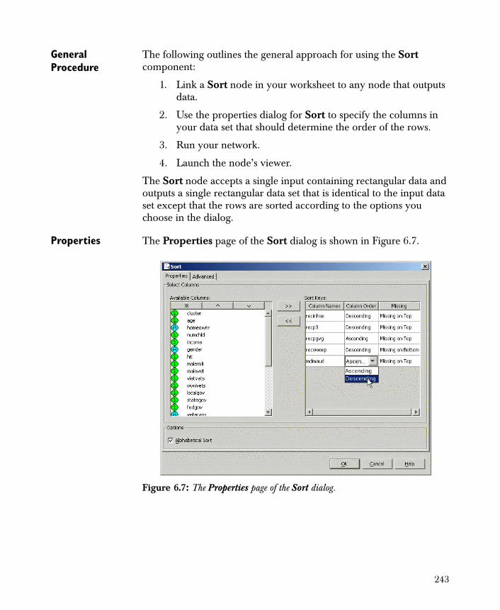
General Procedure
The following outlines the general approach for using the Sort component:
1. Link a Sort node in your worksheet to any node that outputs data.
2. Use the properties dialog for Sort to specify the columns in your data set that should determine the order of the rows.
3. Run your network.
4. Launch the node’s viewer.
The Sort node accepts a single input containing rectangular data and outputs a single rectangular data set that is identical to the input data set except that the rows are sorted according to the options you choose in the dialog.
Properties The Properties page of the Sort dialog is shown in Figure 6.7.
Figure 6.7: The Properties page of the Sort dialog.
243
Select Columns
Available Columns This list box initially displays all the column names in your data set. Select a particular column
from the list and click the button to move it to the Sort Keys grid. The order in which you move columns determines how the rows of the data set are sorted. Spotfire Miner sorts the values in the first column you choose and reorders the rows accordingly. If there are ties, Spotfire Miner attempts to break them according to the sorted values in the second column, then the third column, and so on.
Sort Keys The Sort Keys grid displays the names of the columns that you choose. By default, each column is sorted in ascending order and any missing values are placed at the top. To sort a particular column in descending order instead, click the column’s entry in the Column Order field of the grid. This opens a drop-down list from which you can choose Descending. Likewise, to place missing values at the end of a sorted column, click the appropriate entry under Missing and choose Missing on Bottom.
If you need to remove a particular column from the Sort Keys grid, select it by clicking in the grid row containing the
column name and then click the button. This moves the column back into the Available Columns list box.
Options
Alphabetical Sort This check box affects categorical variables and string columns. When selected, nonnumeric categorical variables and string columns are sorted alphabetically, where the order A-Z is ascending and the order Z-A is descending. When not selected, categorical variables are sorted according to the order they are read in from the original data file. To check this ordering, open the viewer for the input node in your network (for example, Read Text File). In the summary statistics of the viewer, levels (categorical variables) and strings (string columns) appear in ascending order.
244
Using the Viewer The viewer for the Sort component is the node viewer. For a complete discussion of the node viewer and the information it displays, see the section The Table Viewer on page 146 as well as the online help.
Split Use the Split component to divide a data set into two parts based on a conditional expression that either includes or excludes particular rows. To do this, you write a qualifier in the Spotfire Miner expression language. For example, the qualifier gender=="F" splits the data set according to gender. (For complete information on writing expressions in the Spotfire Miner expression language, see page 285 at the end of this chapter.)
General Procedure
The following outlines the general approach for using the Split component:
1. Link a Split node in your worksheet to any node that outputs data.
2. Use the properties dialog for Split to specify the qualifier that splits the rows of your data set into two groups.
3. Run your network.
4. Launch the node’s viewer.
The Split node accepts a single input containing rectangular data and outputs two rectangular data sets. (This component is similar to Filter Rows except that it has two outputs rather than one.) The portion of the data set for which the qualifier is true forms the first (top) output,
Note
If you want to use your data set for training, testing, and validating a model, use the Partition component instead. Information on the Partition component is found on page 237.
245
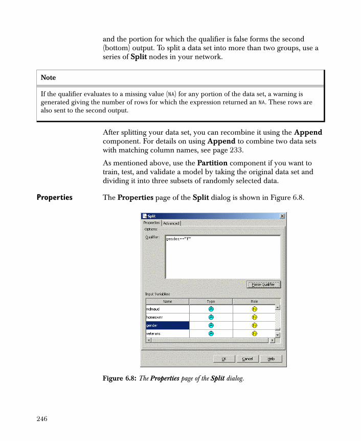
and the portion for which the qualifier is false forms the second (bottom) output. To split a data set into more than two groups, use a series of Split nodes in your network.
After splitting your data set, you can recombine it using the Append component. For details on using Append to combine two data sets with matching column names, see page 233.
As mentioned above, use the Partition component if you want to train, test, and validate a model by taking the original data set and dividing it into three subsets of randomly selected data.
Properties The Properties page of the Split dialog is shown in Figure 6.8.
Note
If the qualifier evaluates to a missing value (NA) for any portion of the data set, a warning is generated giving the number of rows for which the expression returned an NA. These rows are also sent to the second output.
Figure 6.8: The Properties page of the Split dialog.
246
Options
Qualifier Type a valid conditional expression in the Spotfire Miner expression language to define your qualifier. The idea is to construct an expression that implicitly creates a logical column for your data set; the rows defined by the qualifier are those rows for which the logical column is true. In the first output of the Split component, Spotfire Miner returns all rows for which the column is true; in the second output, Spotfire Miner returns all rows for which the column is false. When you click the Parse Qualifier button, the current expression is parsed, and a window pops up displaying any parsing errors. This also includes any type-checking errors that occur, such as when an expression does not return a logical value. An error is displayed with information about the position in the expression where the error occurred.
Input Variables This scrollable table shows the input column names, types, and roles and is useful for finding the names of available inputs when constructing new expressions.
Using the Viewer The viewer for the Split component is the node viewer. For a complete discussion of the node viewer and the information it displays, see the section The Table Viewer on page 146 as well as the online help.
Stack The Stack component stacks separate columns of a data set into a single column.
General Procedure
The following outlines the general approach for using the Stack component:
1. Link a Stack node in your worksheet to any node that outputs data.
2. Use the properties dialog for Stack to specify the columns to stack and replicate.
3. Run your network.
4. Launch the node’s viewer.
The Stack node accepts a single input containing rectangular data and outputs the same rectangular data set with the new column appended to it.
247
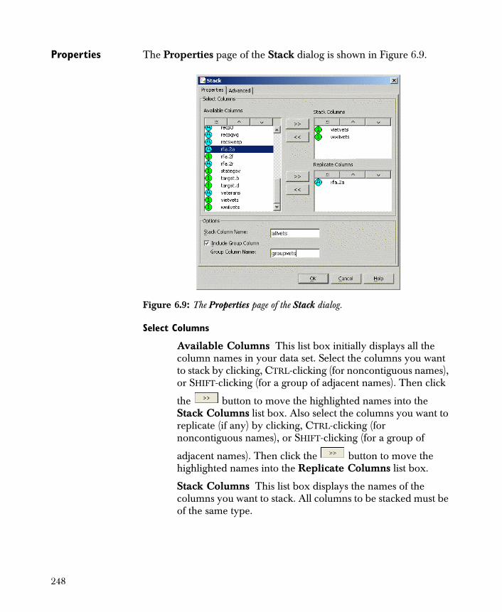
Properties The Properties page of the Stack dialog is shown in Figure 6.9.
Select Columns
Available Columns This list box initially displays all the column names in your data set. Select the columns you want to stack by clicking, CTRL-clicking (for noncontiguous names), or SHIFT-clicking (for a group of adjacent names). Then click
the button to move the highlighted names into the Stack Columns list box. Also select the columns you want to replicate (if any) by clicking, CTRL-clicking (for noncontiguous names), or SHIFT-clicking (for a group of
adjacent names). Then click the button to move the highlighted names into the Replicate Columns list box.
Stack Columns This list box displays the names of the columns you want to stack. All columns to be stacked must be of the same type.
Figure 6.9: The Properties page of the Stack dialog.
248
If you need to remove particular columns from this field, select them by clicking, CTRL-clicking, or SHIFT-clicking.
Then click the button to move the highlighted names back into the Available Columns list box.
Replicate Columns This list box displays the names of the columns you want to replicate. These columns are replicated in parallel with the stacked column. Each row will contain a stacked value and the corresponding values of the replicated column.
If you need to remove particular columns from this field, select them by clicking, CTRL-clicking, or SHIFT-clicking.
Then click the button to move the highlighted names back into the Available Columns list box.
Options
Stack Column Name Specify a name for the new stacked column in this field.
Include Group Column Select this check box to create an additional group column and append it to the output data set. The group column is filled with integers indicating the column from which each cell in the newly stacked column came.
Group Column Name If you selected the Include Group Column check box, specify a name for the group column in this field.
Using the Viewer The viewer for the Stack component is the node viewer. For a complete discussion of the node viewer and the information it displays, see the section The Table Viewer on page 146 as well as the online help.
249
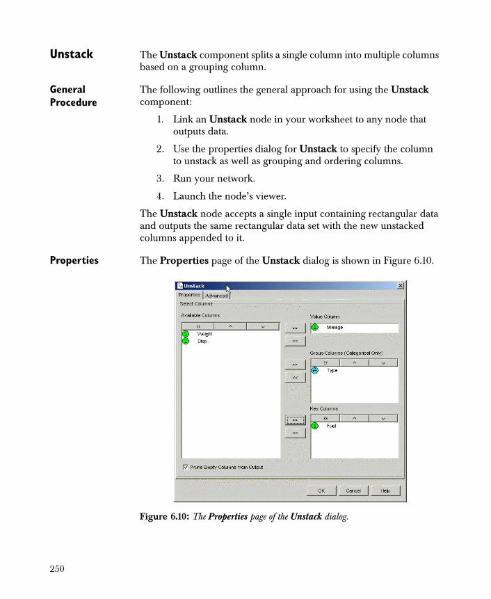
Unstack The Unstack component splits a single column into multiple columns based on a grouping column.
General Procedure
The following outlines the general approach for using the Unstack component:
1. Link an Unstack node in your worksheet to any node that outputs data.
2. Use the properties dialog for Unstack to specify the column to unstack as well as grouping and ordering columns.
3. Run your network.
4. Launch the node’s viewer.
The Unstack node accepts a single input containing rectangular data and outputs the same rectangular data set with the new unstacked columns appended to it.
Properties The Properties page of the Unstack dialog is shown in Figure 6.10.
Figure 6.10: The Properties page of the Unstack dialog.
250
Select Columns
Available Columns This list box initially displays all the column names in your data set. Select the column you want to
unstack by clicking it and then clicking the button to move the highlighted name into the Value Column field. Also select the columns you want to move into the Group Columns and Key Columns list boxes by clicking, CTRL-clicking (for noncontiguous names), or SHIFT-clicking (for a
group of adjacent names). Then click the button to move the highlighted names into the corresponding list box.
Value Column This field displays the name of the column containing the data you want to unstack.
Group Columns (Categorical Only) This list box displays the names of the categorical columns that will be the basis for creating the new unstacked columns. The levels of the columns in this field become the column names of the new unstacked columns, which are then filled with the corresponding values from the Value Column. For example, if you select a column with the three levels A, B, and C, the Unstack node creates three new columns labeled A, B, and C. If there are any missing values in a selected Group Column, the missing data will be treated as another level labeled NaN.
If you need to remove particular columns from the Group Columns field, select them by clicking, CTRL-clicking, or
SHIFT-clicking. Then click the button to move the highlighted names back into the Available Columns list box.
Key Columns This list box displays the names of the columns you want to use to order the new unstacked columns. Columns in this field are used to establish uniqueness or row position for similar values in the Group Columns. Any combination of values in the Key Columns that are not unique will lead to a loss of data, as the last nonunique value will be used.
251
If you need to remove particular columns from the Key Columns field, select them by clicking, CTRL-clicking, or
SHIFT-clicking. Then click the button to move the highlighted names back into the Available Columns list box.
To unstack multiple Group Columns, Spotfire Miner uses the cross-product of the Group Columns’ categories. This can lead to category combinations that do not actually exist in the data. To remove these unused columns, check the Prune Empty Columns from Output checkbox.
For specific examples using the Unstack component, see the online help.
Using the Viewer The viewer for the Unstack component is the node viewer. For a complete discussion of the node viewer and the information it displays, see the section The Table Viewer on page 146 as well as the online help.
252
MANIPULATING COLUMNS
Spotfire Miner provides the following components for performing column-based data manipulations:
• Bin
• Create Columns
• Filter Columns
• Recode Columns
• Join
• Modify Columns
• Transpose
• Normalize
• Reorder Columns
In this section, we discuss each component in turn.
Bin Use the Bin component to create new categorical variables from numeric (continuous) variables or to redefine existing categorical variables by renaming or combining groups.
General Procedure
The following outlines the general approach for using the Bin component:
1. Link a Bin node in your worksheet to any node that outputs data.
2. Use the properties dialog for Bin to specify the source columns and the number of bins to be created.
3. Run your network.
4. Launch the node’s viewer.
The Bin node accepts a single input containing rectangular data and outputs a single rectangular data set containing the new, binned categorical variables in place of the continuous variables.
You can link together multiple Bin nodes in your network to use different numbers of bins for different variables in your data set.
253

Properties The Properties page of the Bin dialog is shown in Figure 6.11.
Select Columns
Available Columns This list box initially displays all the column names in your data set. Select particular columns by clicking, CTRL-clicking (for noncontiguous names), or SHIFT-clicking (for a group of adjacent names). Then click the Add button to move the highlighted names into the Selected Columns list box. To simultaneously move all the column names, click the Add All button.
Selected Columns This list box displays the names of the source columns.
If you need to remove particular columns from this field, select them by clicking, CTRL-clicking, or SHIFT-clicking. Then click the Remove button to move the highlighted names back into the Available Columns list box. To simultaneously remove all the column names, click the Remove All button.
Figure 6.11: The Properties page of the Bin dialog.
254
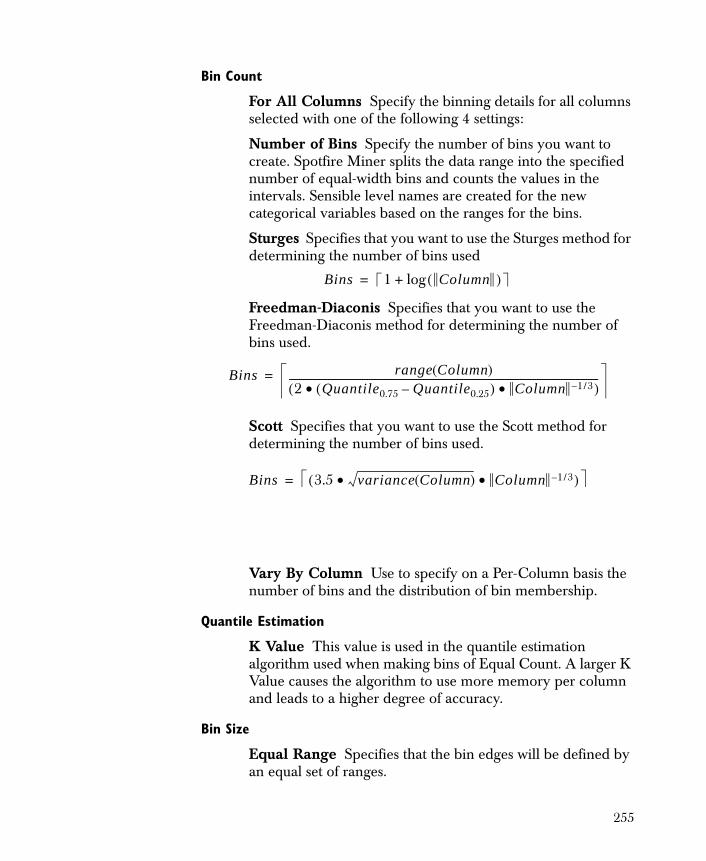
Bin Count
For All Columns Specify the binning details for all columns selected with one of the following 4 settings:
Number of Bins Specify the number of bins you want to create. Spotfire Miner splits the data range into the specified number of equal-width bins and counts the values in the intervals. Sensible level names are created for the new categorical variables based on the ranges for the bins.
Sturges Specifies that you want to use the Sturges method for determining the number of bins used
Freedman-Diaconis Specifies that you want to use the Freedman-Diaconis method for determining the number of bins used.
Scott Specifies that you want to use the Scott method for determining the number of bins used.
Vary By Column Use to specify on a Per-Column basis the number of bins and the distribution of bin membership.
Quantile Estimation
K Value This value is used in the quantile estimation algorithm used when making bins of Equal Count. A larger K Value causes the algorithm to use more memory per column and leads to a higher degree of accuracy.
Bin Size
Equal Range Specifies that the bin edges will be defined by an equal set of ranges.
Bins 1 Column( )log+=
Bins range Column( )2 Quantile0.75 Quantile0.25–( )• Column 1 3/–•( )
-------------------------------------------------------------------------------------------------------------------------------=
Bins 3.5 variance Column( ) Column 1 3/–••( )=
255
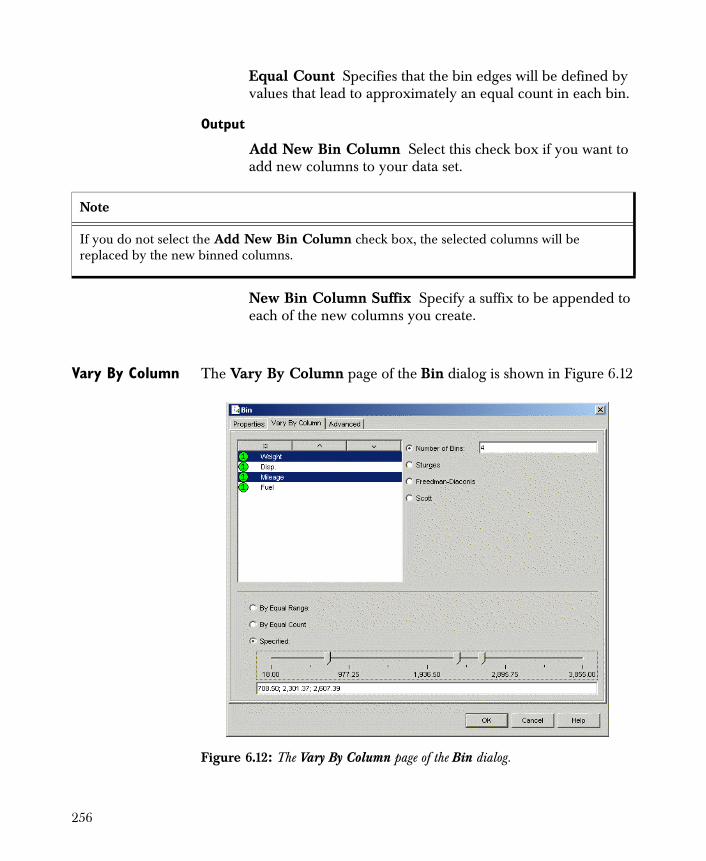
Equal Count Specifies that the bin edges will be defined by values that lead to approximately an equal count in each bin.
Output
Add New Bin Column Select this check box if you want to add new columns to your data set.
New Bin Column Suffix Specify a suffix to be appended to each of the new columns you create.
Vary By Column The Vary By Column page of the Bin dialog is shown in Figure 6.12
Note
If you do not select the Add New Bin Column check box, the selected columns will be replaced by the new binned columns.
Figure 6.12: The Vary By Column page of the Bin dialog.
256
This page is where you can set bin properties for individual or groups of columns. First, select the desired columns from the list box on the left using CTRL and SHIFT as needed. Once a column or a group of columns has been selected, notice that the range values appear in the slide bar below the Bin Range radio button. To adjust the number of bins, you can either:
1. Set the Number of Bins in the edit field.
2. Use the Sturges method for determining the number of bins.
3. Use the Freedman-Diaconis method for determining the number of bins.
4. Use the Scott method for determining the number of bins.
There are two different ways to set the bin boundaries:
1. By Equal Range A set of boundary points can be automatically generated at equal intervals from the data minimum to the max value for the column or group of columns selected.
2. By Equal Count A set of boundary points are generated with the aim of creating bins of equal counts.
3. Specified Set the boundaries yourself by dragging the sliders to the desired boundary values or typing values into the text field.
Using the Viewer The viewer for the Bin component is the node viewer. For a complete discussion of the node viewer and the information it displays, see the section The Table Viewer on page 146 as well as the online help.
Create Columns
Use the Create Columns component to compute an additional variable and append it as a column to your data set. To do this, you write an expression in the Spotfire Miner expression language. For example, the expression Income/12 defines a new column of average monthly income from the existing variable Income. (For complete information on writing expressions in the Spotfire Miner expression language, see page 285 at the end of this chapter.)
You can modify an existing column by giving its name as the output column name. When the node is executed, the output includes a list of the added and modified columns.
257
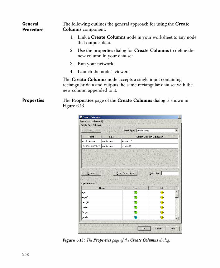
General Procedure
The following outlines the general approach for using the Create Columns component:
1. Link a Create Columns node in your worksheet to any node that outputs data.
2. Use the properties dialog for Create Columns to define the new column in your data set.
3. Run your network.
4. Launch the node’s viewer.
The Create Columns node accepts a single input containing rectangular data and outputs the same rectangular data set with the new column appended to it.
Properties The Properties page of the Create Columns dialog is shown in Figure 6.13.
Figure 6.13: The Properties page of the Create Columns dialog.
258
Create New Columns
Select Type Specify a type for the new column by selecting continuous, categorical, string, or date from the drop-down list. Then click the Add button to activate the grid view and insert a row for the new column.
Grid View The grid view displays a row for each new column you create. Initially, only Type is filled in.
• Name To add or change a column name, double-click the cell under Name. This activates a text box in which you can type a new column name.
• Type To change the data type for the new column, click the cell under Type. This opens a drop-down list containing the four possible column types from which you can make a selection.
• Column Creation Expression To add or change an entry under Column Creation Expression, double-click the entry. This activates a text box in which you can type a new expression. Define your column by typing a valid expression in the Spotfire Miner expression language in this field. In most cases, you will use the standard arithmetic operators (+, -, *, /, etc.) to rescale one of your columns or to compute a new column from existing variables in your data.
If you need to remove particular columns from the grid view, select the rows that contain them by clicking, CTRL-clicking, or SHIFT-clicking. Then click the Remove button.
When you click the Parse Expressions button, the current expressions are parsed, and a window pops up displaying any parsing errors. This also includes any type-checking errors that occur, such as when an expression returns a type that is inconsistent with the output type of the column. An error is displayed with information about the position in the expression where the error occurred.
String Size Specify the string width for any new string columns.
259
Input Variables This scrollable table shows the input column names, types, and roles and is useful for finding the names of available inputs when constructing new expressions.
Using the Viewer The viewer for the Create Columns component is the node viewer. For a complete discussion of the node viewer and the information it displays, see the section The Table Viewer on page 146 as well as the online help.
Filter Columns Use the Filter Columns component to exclude columns that are not needed during your analysis, thus reducing both resource consumption and computation time.
Use the Filter Columns component to filter data sets that have already been defined in Spotfire Miner, not those that exist in the original data sources. For options that filter data as they are read into Spotfire Miner, use the Read Database component (see page 56).
General Procedure
The following outlines the general approach for using the Filter Columns component:
1. Link a Filter Columns node in your worksheet to any node that outputs data.
2. Use the properties dialog for Filter Columns to specify the columns in your data set that you want to keep.
3. Run your network.
4. Launch the node’s viewer.
The Filter Columns node accepts a single input containing rectangular data and outputs a single rectangular data set defined by the columns you choose.
Hint
You can also use the Modify Columns component to filter the columns of your data set.
260
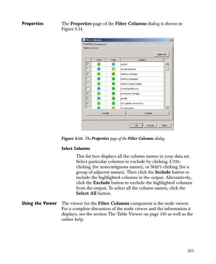
Properties The Properties page of the Filter Columns dialog is shown in Figure 6.14.
Select Columns
This list box displays all the column names in your data set. Select particular columns to exclude by clicking, CTRL-clicking (for noncontiguous names), or SHIFT-clicking (for a group of adjacent names). Then click the Include button to include the highlighted columns in the output. Alternatively, click the Exclude button to exclude the highlighted columns from the output. To select all the column names, click the Select All button.
Using the Viewer The viewer for the Filter Columns component is the node viewer. For a complete discussion of the node viewer and the information it displays, see the section The Table Viewer on page 146 as well as the online help.
Figure 6.14: The Properties page of the Filter Columns dialog.
261
Recode Columns
Use the Recode Columns component to create a new column from an existing column. Typically, you would use Recode Columns to recode a Categorical to another Categorical; however, you can also use it to change a column’s data type. You can also use it to overwrite an existing column, assigning a different data type or values.
General Procedure
The following outlines the general approach for using the Recode Columns component:
1. Link a Recode Columns node in your worksheet to any node that outputs data.
2. Optionally, use the properties dialog for Recode Columns to specify new data type.
3. Use the Edit Recoding Table to map new value(s) for the recoded columns.
4. Run your network.
5. Launch the node’s viewer.
The Recode Columns node accepts a single input containing rectangular data and outputs a single rectangular data set defined by the columns you choose. All unselected columns are passed to the output unchanged.
262

Properties The Properties page of the Recode Columns dialog is shown in Figure 6.14.
Select Column to Recode
This drop-down list box displays all the column names in your data set that can be recoded. Note that you can recode only continuous, categorical, and string types. The date data type is not supported, so any columns with the date type do not appear on the list. From the list, select a column to recode, and then click Add to add it to the grid view. You can add more than one column to the grid view to recode. (To remove a column from the grid view, click anywhere in its row, and then click Remove.)
Figure 6.15: The Properties page of the Recode Columns dialog.
263
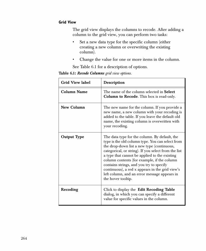
Grid View
The grid view displays the columns to recode. After adding a column to the grid view, you can perform two tasks:
• Set a new data type for the specific column (either creating a new column or overwriting the existing column).
• Change the value for one or more items in the column.
See Table 6.1 for a description of options.Table 6.1: Recode Columns grid view options.
Grid View label Description
Column Name The name of the column selected in Select Column to Recode. This box is read-only.
New Column The new name for the column. If you provide a new name, a new column with your recoding is added to the table. If you leave the default old name, the existing column is overwritten with your recoding.
Output Type The data type for the column. By default, the type is the old column type. You can select from the drop-down list a new type (continuous, categorical, or string). If you select from the list a type that cannot be applied to the existing column contents (for example, if the column contains strings, and you try to specify continuous), a red x appears in the grid view’s left column, and an error message appears in the hover tooltip.
Recoding Click to display the Edit Recoding Table dialog, in which you can specify a different value for specific values in the column.
264
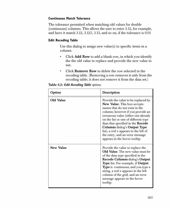
Continuous Match Tolerance
The tolerance permitted when matching old values for double (continuous) columns. This allows the user to enter 3.12, for example, and have it match 3.12, 3.125, 3.13, and so on, if the tolerance is 0.01
Edit Recoding Table
Use this dialog to assign new value(s) to specific items in a column.
• Click Add Row to add a blank row, in which you identify the the old value to replace and provide the new value to use.
• Click Remove Row to delete the row selected in the recoding table. (Removing a row removes it only from the recoding table; it does not remove it from the data set.)
Table 6.2: Edit Recoding Table options.
Option Description
Old Value Provide the value to be replaced by New Value. This box accepts names that do not exist in the column; however if you provide an erroneous value (either one already on the list or one of different type than that specified in the Recode Columns dialog’s Output Type list), a red x appears to the left of the entry, and an error message appears in the hover tooltip.
New Value Provide the value to replace the Old Value. The new value must be of the data type specified in the Recode Columns dialog’s Output Type list. For example, if Output Type is continuous, and you type a string, a red x appears in the left column of the grid, and an error message appears in the hover tooltip.
265
Recoding rules
• You can use an Old Value name only once.
• You can recode missing values by leaving Old Value blank and specifying a New Value.
• You can recode Old Value as blank by providing its name and leaving New Value blank.
• You can assign a single new value to multiple old values.
• Only values can be used in the recoding table. It cannot take an expression. (For example, you cannot specify <5 for “all values less than 5.”) To use an expression, use the Crerate Columns node and the Expression Language.
• If you provide a value in Old Value that does not exist in the specified column, the output is unchanged (unless you specify an asterisk (*), in which case all unmatched values are recoded as the corresponding New Value).
Using the Viewer The viewer for the Recode Columns component is the node viewer. For a complete discussion of the node viewer and the information it displays, see the section The Table Viewer on page 146 as well as the online help.
Example The following simple walkthrough uses the fuel.txt example file.
To recode columns in fuel.txt
1. Create a worksheet and add a Read Text File node. Double-click to open its Properties dialog.
2. Read in the example file fuel.txt by clicking Browse, Examples, and selecting the file. Click OK, and then run the node.
3. View the data by right-clicking the node and selecting Viewer. Note that all columns are continuous, except Type, which is a string.
4. Drag a Recode Columns node to the worksheet and connect the two nodes. Open the Recode Columns dialog.
5. In the Select Column to Recode drop-down list, select Type, and then click Add.
266
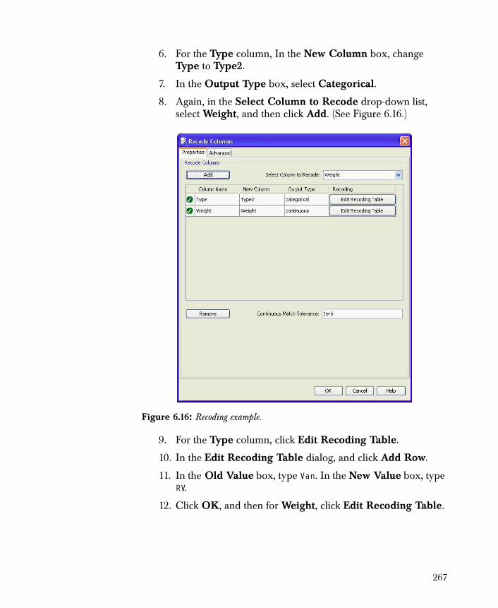
6. For the Type column, In the New Column box, change Type to Type2.
7. In the Output Type box, select Categorical.
8. Again, in the Select Column to Recode drop-down list, select Weight, and then click Add. (See Figure 6.16.)
9. For the Type column, click Edit Recoding Table.
10. In the Edit Recoding Table dialog, and click Add Row.
11. In the Old Value box, type Van. In the New Value box, type RV.
12. Click OK, and then for Weight, click Edit Recoding Table.
Figure 6.16: Recoding example.
267
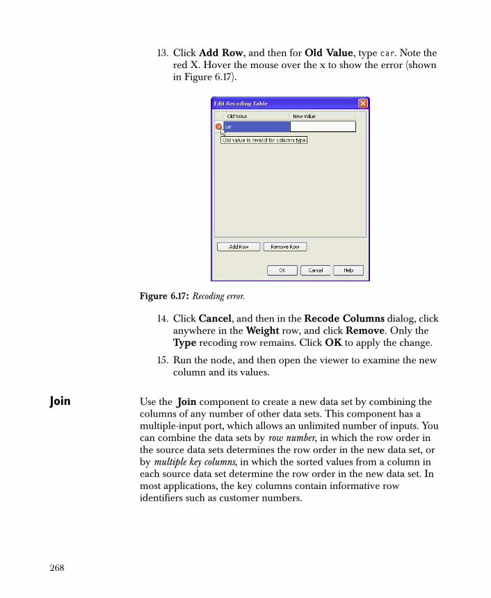
13. Click Add Row, and then for Old Value, type car. Note the red X. Hover the mouse over the x to show the error (shown in Figure 6.17).
14. Click Cancel, and then in the Recode Columns dialog, click anywhere in the Weight row, and click Remove. Only the Type recoding row remains. Click OK to apply the change.
15. Run the node, and then open the viewer to examine the new column and its values.
Join Use the Join component to create a new data set by combining the columns of any number of other data sets. This component has a multiple-input port, which allows an unlimited number of inputs. You can combine the data sets by row number, in which the row order in the source data sets determines the row order in the new data set, or by multiple key columns, in which the sorted values from a column in each source data set determine the row order in the new data set. In most applications, the key columns contain informative row identifiers such as customer numbers.
Figure 6.17: Recoding error.
268
If a key column name is the same for all inputs, the Set For All Inputs group can be used to set all of the corresponding key column values. If the key columns have differing names (such as “Last Name” in one input and “Surname” in another), the different names can be specified separately in the grid of properties.
The order in which the nodes are joined affects the order of the output columns. This order is determined by the order in which they were created, and is indicated by the order of the nodes in the Properties page. If you want to change the order of the nodes, use Copy and Paste to create a new copy of the node that you wish to be place at the bottom of the list, and use this new node as the input to Join. Alternately, add a new node such as a Modify Columns node between the node to be joined and the Join node.
If you wish to eliminate some of the output columns, follow the Join node with a Filter Columns or Modify Columns node. If you wish to change the order of the output columns, use a Reorder Columns node.
General Procedure
The following outlines the general approach for using the Join component:
1. Link a Join node in your worksheet to any two or more nodes that output data.
2. Use the properties dialog for Join to specify how the source data sets are to be joined, whether unmatched rows should be included in the new data set, and what the suffix should be for duplicate column names.
3. Run your network.
4. Launch the node’s viewer.
Using Sort in Join
In the Advanced page, if Sort Required is not checked and the key column is not the first column in the input data sets for Join, the output column names do not correspond to correct data, and rows are replicated. All inputs must be sorted according to key column, and should be presorted in ascending order, with NA's on the bottom.
The Join component matches a missing value (NaN) in the key column to all other values, which is typically not the desired behavior. To avoid this, use a Missing Values component to drop rows with missing values for the key, or to replace the missing values with some other value.
269
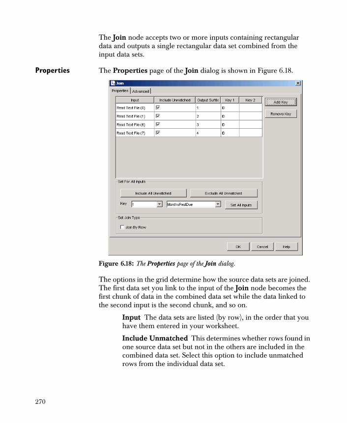
The Join node accepts two or more inputs containing rectangular data and outputs a single rectangular data set combined from the input data sets.
Properties The Properties page of the Join dialog is shown in Figure 6.18.
The options in the grid determine how the source data sets are joined. The first data set you link to the input of the Join node becomes the first chunk of data in the combined data set while the data linked to the second input is the second chunk, and so on.
Input The data sets are listed (by row), in the order that you have them entered in your worksheet.
Include Unmatched This determines whether rows found in one source data set but not in the others are included in the combined data set. Select this option to include unmatched rows from the individual data set.
Figure 6.18: The Properties page of the Join dialog.
270
Note that Spotfire Miner pads any unmatched rows with missing values in the output data. If you want to exclude unmatched rows altogether, clear this check box.
Output Suffix This determines the suffix added to column names that are present in the source data sets to prevent duplicate column names in the returned data set.
By default, the suffixes are 1, 2, 3, and so on, corresponding to the order of the input data sets.
Key 1 Choose one key column from each data set with which to order the rows. The sorted values from a column in each source data set determine the row order in the new data set. Click Add Key and Remove Key to add or remove keys as needed to output additional columns.
Set For All Inputs
Click Include All Unmatched or Exclude All Unmatched as a global option for the columns selected above. If you want to change the key column for all data sets, select the key number (e.g., Key 1 or Key 2) and select the appropriate column (in the field to the right of the key number). Click Set All Inputs to set this change.
Set Join Type
Select Join By Row if you want to join the data sets by row instead of by column. The default is to join by column.
Using the Viewer The viewer for the Join component is the node viewer. For a complete discussion of the node viewer and the information it displays, see the section The Table Viewer on page 146 as well as the online help.
Modify Columns
The Modify Columns component can be used to filter and rename the columns of your data set.
Hint
The Filter Columns component can also be used to filter the columns of your data set.
271

You can also use the Modify Columns component to change column types and define the dependent and independent variables for modeling purposes. You might need to change column types when, for example, a categorical variable consists of integer values. In this case, Spotfire Miner reads the values as continuous and you must manually change the column type to categorical.
It is not strictly necessary to define modeling roles with Modify Columns, as each of the classification and regression components have options that allow you to do this as well. However, it is helpful when you want to compute the same model using multiple modeling components. In fact, this is the main purpose of the feature: you can use Modify Columns to define dependent and independent variables and link the output to multiple modeling nodes to quickly compare the different outcomes. Not that when you do this, Spotfire Miner does not display the columns automatically in the Dependent and Independent fields of the modeling dialogs. That way, you to change your model, if necessary.
General Procedure
The following outlines the general approach for using the Modify Columns component:
1. Link a Modify Columns node in your worksheet to any node that outputs data.
2. Use the properties dialog for Modify Columns to specify the column information you want to change.
3. Run your network.
4. Launch the node’s viewer.
The Modify Columns node accepts a single input containing rectangular data and outputs a single rectangular data set defined by the options you choose.
272
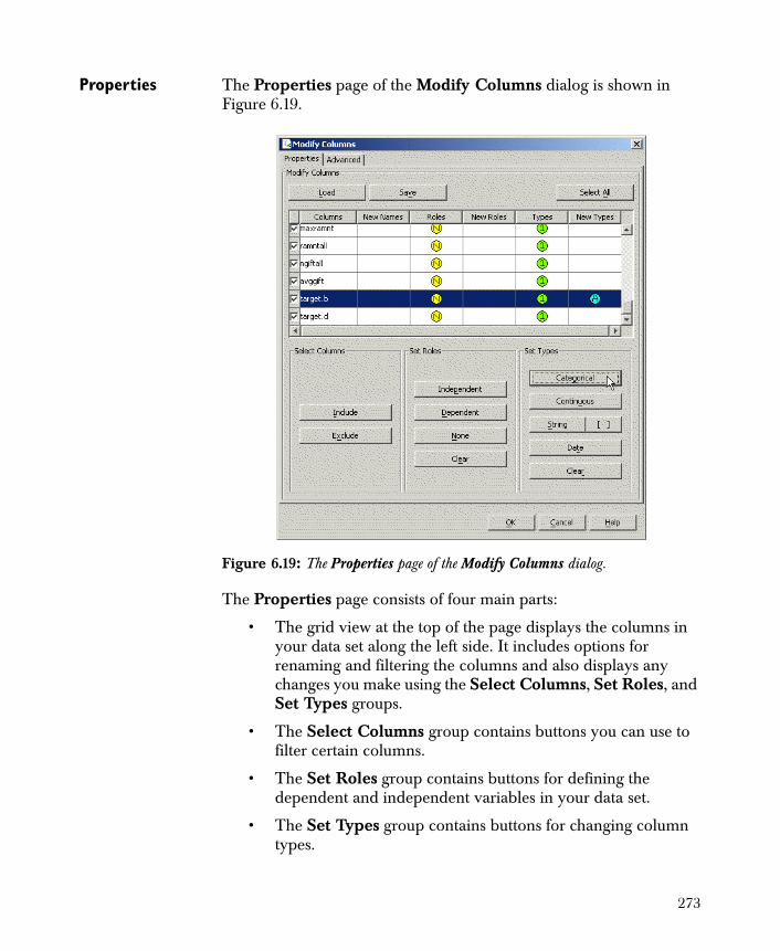
Properties The Properties page of the Modify Columns dialog is shown in Figure 6.19.
The Properties page consists of four main parts:
• The grid view at the top of the page displays the columns in your data set along the left side. It includes options for renaming and filtering the columns and also displays any changes you make using the Select Columns, Set Roles, and Set Types groups.
• The Select Columns group contains buttons you can use to filter certain columns.
• The Set Roles group contains buttons for defining the dependent and independent variables in your data set.
• The Set Types group contains buttons for changing column types.
Figure 6.19: The Properties page of the Modify Columns dialog.
273

Grid View
The rows of the grid view at the top of the page display the column names of your data set. You can resize any of the columns in the grid view by dragging the lines that divide the columns. You can also sort any column by clicking its header.
• To rename a particular column, double-click the corresponding cell under the New Names heading. This activates an editable text box in which you can type a new column name.
• To filter a particular column, clear the check box next to its name. Spotfire Miner excludes all columns that have cleared check boxes from the data set it returns.
• To select particular columns in your data set, click their rows in the grid view (use CTRL-click for noncontiguous rows or SHIFT-click for a group of adjacent rows). This highlights the corresponding rows of the grid, which is necessary when using any of the buttons in the Select Columns, Set Roles, or Set Types groups (see below). To select all the columns in the data set, click the Select All button at the top of the page. Note that this simply highlights all the rows in the grid view but does not select any check boxes that have been cleared.
• Click the Save button to save the current column settings as a data dictionary or click Load to load a data dictionary file. Data dictionaries are used to define column names, types, roles, start, width, and output decimal places when importing or exporting fixed format files. For more information on using data dictionaries, see page 40.
Select Columns
The Select Columns group contains the Include and Exclude buttons, which you can use to filter the columns of your data set. These options are alternatives to the check boxes in the grid view and are most useful when you want to filter multiple columns simultaneously. After selecting the desired columns in the grid view, do one of the following:
• Click the Include button to include the selected columns in the data set that Spotfire Miner returns.
274
• Click the Exclude button to exclude the selected columns from the data set that Spotfire Miner returns.
Note that the check boxes in the grid view are selected or cleared depending on the button you click.
Set Roles
The Set Roles group contains the Independent, Dependent, None, and Clear buttons, which allow you to define the role each variable assumes in models. After selecting the desired columns in the grid view, do one of the following:
• Click the Independent button to define the selected columns as independent variables.
• Click the Dependent button to define the selected columns as dependent variables.
• Click the None button to remove previous roles for the selected columns.
• Click the Clear button to clear new roles for the selected columns.
Set Types
The Set Types group contains the Categorical, Continuous, String, Date, and Clear buttons, which allow you to define column types. After selecting the desired columns in the grid view, do one of the following:
• Click the Categorical button to define the selected columns as categorical variables.
• Click the Continuous button to define the selected columns as continuous variables.
Hint
Spotfire Miner associates a visual cue with each of the roles you choose. For more information, see the section Visual Cues in Dialog Fields on page 142.
275
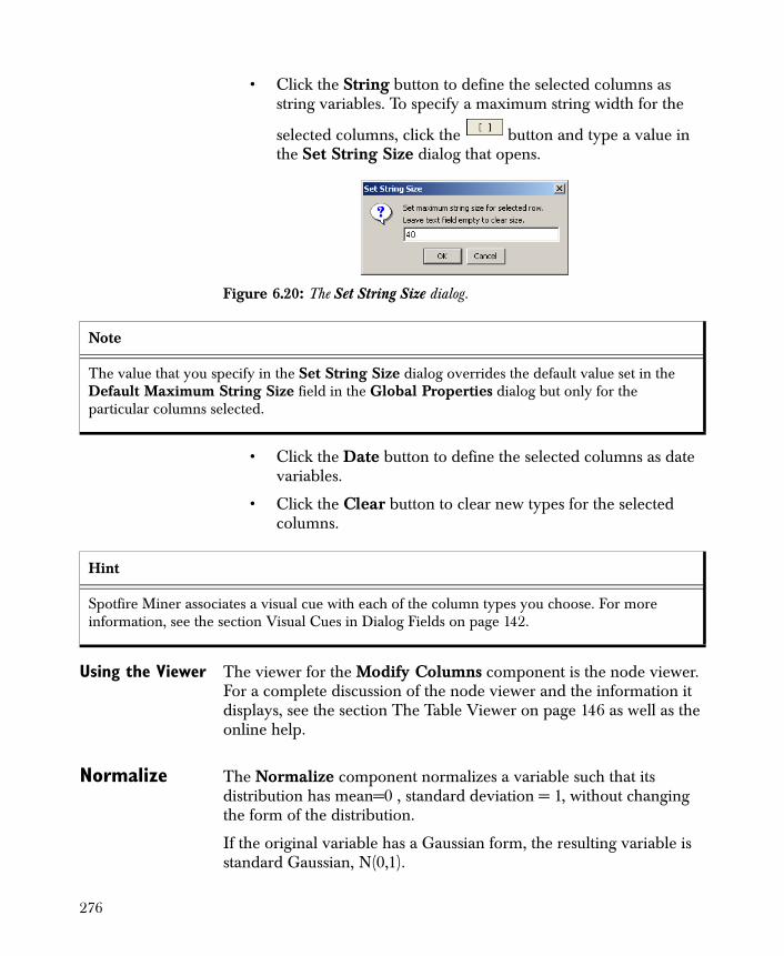
• Click the String button to define the selected columns as string variables. To specify a maximum string width for the
selected columns, click the button and type a value in the Set String Size dialog that opens.
• Click the Date button to define the selected columns as date variables.
• Click the Clear button to clear new types for the selected columns.
Using the Viewer The viewer for the Modify Columns component is the node viewer. For a complete discussion of the node viewer and the information it displays, see the section The Table Viewer on page 146 as well as the online help.
Normalize The Normalize component normalizes a variable such that its distribution has mean=0 , standard deviation = 1, without changing the form of the distribution.
If the original variable has a Gaussian form, the resulting variable is standard Gaussian, N(0,1).
Figure 6.20: The Set String Size dialog.
Note
The value that you specify in the Set String Size dialog overrides the default value set in the Default Maximum String Size field in the Global Properties dialog but only for the particular columns selected.
Hint
Spotfire Miner associates a visual cue with each of the column types you choose. For more information, see the section Visual Cues in Dialog Fields on page 142.
276

You use the Normalize component to put all (or a group) of your variables on the same scale. This is important in clustering, for example, where Euclidean distance is computed between p-dimensional points. If some of your columns have values in the 1,000s and others are between 0 and 1, the variables that are in the 1,000s will totally dominate any distance calculations.
General Procedure
The following outlines the general approach for using the Normalize component:
1. Link a Normalize node in your worksheet to any node that outputs data.
2. Use the properties dialog for Normalize to specify the columns you want to normalize.
3. Run your network.
4. Launch the node’s viewer.
The Normalize node accepts a single input containing rectangular data and outputs a single rectangular data set defined by the options you choose.
277
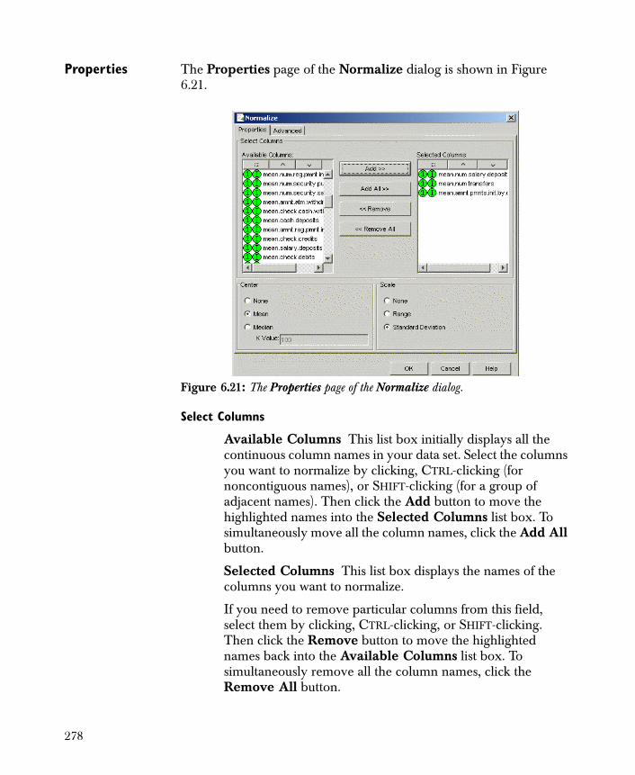
Properties The Properties page of the Normalize dialog is shown in Figure 6.21.
Select Columns
Available Columns This list box initially displays all the continuous column names in your data set. Select the columns you want to normalize by clicking, CTRL-clicking (for noncontiguous names), or SHIFT-clicking (for a group of adjacent names). Then click the Add button to move the highlighted names into the Selected Columns list box. To simultaneously move all the column names, click the Add All button.
Selected Columns This list box displays the names of the columns you want to normalize.
If you need to remove particular columns from this field, select them by clicking, CTRL-clicking, or SHIFT-clicking. Then click the Remove button to move the highlighted names back into the Available Columns list box. To simultaneously remove all the column names, click the Remove All button.
Figure 6.21: The Properties page of the Normalize dialog.
278
Center
Specify either Mean or Median to have the mean or median, respectively, of each column subtracted from the values in that column. Selecting None for Center (but some value other than None for Scale) keeps the location of the data the same but puts all the columns on a common scale. You might want to do this in clustering, for example, so that no single column dominates the algorithm.
Scale
Specify either Range or Standard Deviation to have the values in each column divided by its range or standard deviation, respectively. Selecting None for Scale (but some value other than None for Center) puts all the data around a common center. You might want to do this, for example, if you want to plot all the data on a common axis so that you can compare the spread of the data.
Using the Viewer The viewer for the Normalize component is the node viewer. For a complete discussion of the node viewer and the information it displays, see the section The Table Viewer on page 146 as well as the online help.
Reorder Columns
The Reorder Columns component changes the order of the columns in the output. This node is especially useful if the data set has a large number of columns, or if positioning two or more columns side-by-side produces a more useful view of the data.
General Procedure
The following outlines the general approach for using the Reorder Columns component:
1. Link a Reorder Columns node in your worksheet to any node that outputs data.
2. Use the properties dialog for Reorder Columns and use the buttons to reorder the columns.
3. Run your network.
4. Launch the node’s viewer.
The Reorder Columns node accepts a single input containing rectangular data and outputs the same rectangular data, with the columns ordered as specified in the Properties page.
279
Properties The Properties page of the Reorder Columns dialog is shown in Figure 6.22.
Output Order
Indicates the order of the output columns. This list always shows numbers in order: 1, 2, 3, and so on.
Column Name
The column in the text box containing the name of the column to move.
Input Order
The column in the text box that indicates the order number of the input columns. When you move an item up or down the list, this number stays the same as the original input column number. (See the figure above for an illustration.)
Figure 6.22: The Properties page of the Reorder Columns node.
280
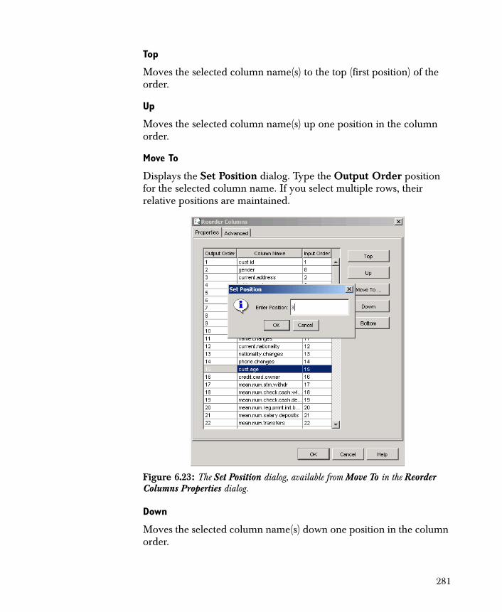
Top
Moves the selected column name(s) to the top (first position) of the order.
Up
Moves the selected column name(s) up one position in the column order.
Move To
Displays the Set Position dialog. Type the Output Order position for the selected column name. If you select multiple rows, their relative positions are maintained.
Down
Moves the selected column name(s) down one position in the column order.
Figure 6.23: The Set Position dialog, available from Move To in the Reorder Columns Properties dialog.
281
Bottom
Moves the selected column name(s) to the bottom (last position) of the order.
Using the Viewer The viewer for the Reorder Columns component is the node viewer. For a complete discussion of the node viewer and the information it displays, see the section The Table Viewer on page 146 as well as the online help.
Transpose The Transpose component turns a set of columns into a set of rows.
General Procedure
The following outlines the general approach for using the Transpose component:
1. Link a Transpose node in your worksheet to any node that outputs data.
2. Use the properties dialog for Transpose to specify the columns you wish were rows.
3. Run your network.
4. Launch the node’s viewer.
The Transpose node accepts a single input containing rectangular data and outputs selected columns as subsequent rows.
282
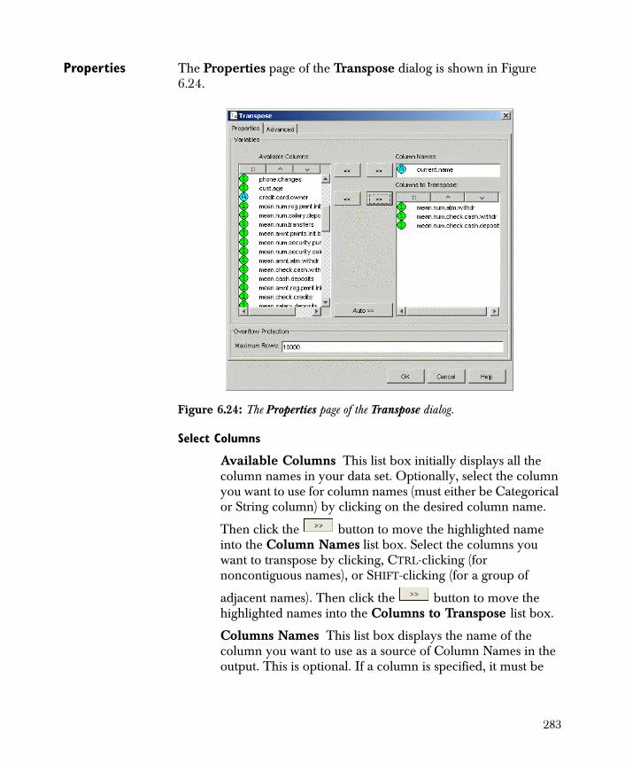
Properties The Properties page of the Transpose dialog is shown in Figure 6.24.
Select Columns
Available Columns This list box initially displays all the column names in your data set. Optionally, select the column you want to use for column names (must either be Categorical or String column) by clicking on the desired column name.
Then click the button to move the highlighted name into the Column Names list box. Select the columns you want to transpose by clicking, CTRL-clicking (for noncontiguous names), or SHIFT-clicking (for a group of
adjacent names). Then click the button to move the highlighted names into the Columns to Transpose list box.
Columns Names This list box displays the name of the column you want to use as a source of Column Names in the output. This is optional. If a column is specified, it must be
Figure 6.24: The Properties page of the Transpose dialog.
283
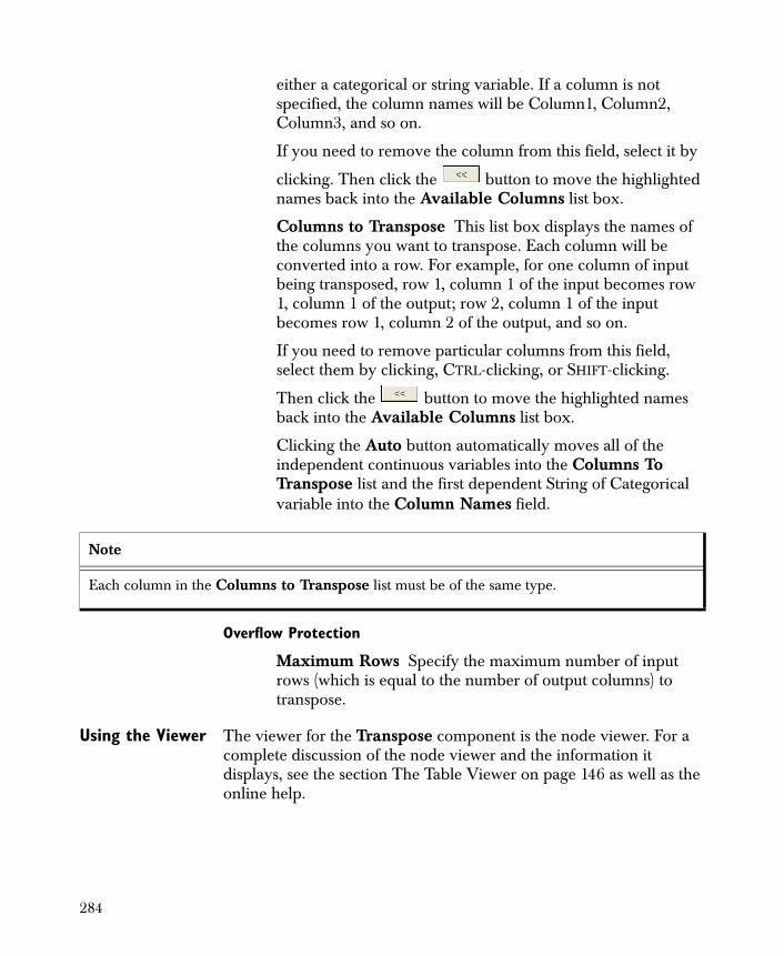
either a categorical or string variable. If a column is not specified, the column names will be Column1, Column2, Column3, and so on.
If you need to remove the column from this field, select it by
clicking. Then click the button to move the highlighted names back into the Available Columns list box.
Columns to Transpose This list box displays the names of the columns you want to transpose. Each column will be converted into a row. For example, for one column of input being transposed, row 1, column 1 of the input becomes row 1, column 1 of the output; row 2, column 1 of the input becomes row 1, column 2 of the output, and so on.
If you need to remove particular columns from this field, select them by clicking, CTRL-clicking, or SHIFT-clicking.
Then click the button to move the highlighted names back into the Available Columns list box.
Clicking the Auto button automatically moves all of the independent continuous variables into the Columns To Transpose list and the first dependent String of Categorical variable into the Column Names field.
Overflow Protection
Maximum Rows Specify the maximum number of input rows (which is equal to the number of output columns) to transpose.
Using the Viewer The viewer for the Transpose component is the node viewer. For a complete discussion of the node viewer and the information it displays, see the section The Table Viewer on page 146 as well as the online help.
Note
Each column in the Columns to Transpose list must be of the same type.
284
USING THE SPOTFIRE MINER™ EXPRESSION LANGUAGE
The Spotfire Miner expression language is designed to be easily understood by users familiar with Excel formulas and with Spotfire S+ and other programming languages. It is a simple, straightforward tool for writing qualifiers and expressions for use in the Filter Rows, Split, and Create Columns components.
An expression is a combination of constants, operators, function calls, and references to input column values that is evaluated to return a single value. For example, if the input columns of a given node include a column named Price, the following is a legal expression:
max(Price+17.5,100)
Within the node, the expression is evaluated once for every input row, and the value is either used as a logical value (in Filter Rows or Split) or output as a new column value (in Create Columns).
One feature of the expression language that might be unfamiliar to some users is that it enforces strong type checking within an expression. Each subexpression within an expression has a single type that can be determined at parse time, and operators and functions check the types of their arguments at parse time. By enforcing type checking, many of the errors you might make in constructing expressions can be detected during parsing, before trying to execute a transformation on a large data set.
Strong typing does not prevent having functions and operators that can take more than one argument type. For example, the expression language currently supports both <double>+<double> (addition) and <string>+<string> (string concatenation). However, the permissible types are still restricted; that is, <double>+<logical> will give a parse error.
While you can create and use logical values within the expression language, such values cannot be represented in a Big Data object. The expression language type checking has been relaxed so that continuous columns can be read as logical values, and logical expression values can be output as continuous values, without your having to do explicit conversions.
285
When a continuous column value is converted to a logical value, the conversion is:
• NA ==> NA
• 0 ==> false
• <anything else>==> true
When a logical expression is output to a continuous column, the conversion is:
• NA ==> NA
• true ==> 1
• false ==> 0
The conversion occurs only when reading column values and outputting the value of the whole expression. Continuous versus logical types are still checked within an expression. For example, if Weight is a continuous column, then the expression 1000+(Weight>3000) still causes an error, because + cannot add a continuous and a logical value.
Example of converting a logical to a continuous value:
Use the Create Columns node to create a new continuous column with the expression num>0. The new column has the value:
• NA if num is NA.
• 1 if num is greater than 0.
• 1 otherwise.
Example of converting a continuous to a logical value:
Use the Create Columns node to create a continuous column num. Access this using the expression ifelse(num, 'non-zero','zero'), which calculates:
• "non-zero" if num is non-zero.
• zero' if num is zero.
• NA if num is an NA value.
286

Value Types The expression language supports four types of values:
• Doubles (floating point numbers)
• Strings
• Dates
• Logical values (true, false, or NA).
Spotfire Miner string and categorical values are both manipulated as strings within the expression language. Logical values can be created and manipulated within an expression but cannot be read to or written to Spotfire Miner data sets. All four types support the NA (missing) value.
NA Handling All of the operations and expressions in the expression language are designed to detect NA (missing) argument values and work appropriately. In most cases, if any of the arguments to a function is NA, then the result is NA. There are some exceptions, however, such as ifelse, & (and), and | (or). For example, given the expression A|B, if A is true, the result is true, even if B is NA.
One counterintuitive result is that string manipulations return NA if any of their arguments is NA. For example, consider the following expression:
"The value is: "+PRICE
If the value of Price is the number 1.3, this constructs the string "The value is: 1.3". If the value of Price is NA, then the result is a string NA value.
To explicitly detect NA values, use the is.na function.
Error Handling Most errors can be detected at parsing time. These include simple parsing errors (like unbalanced parentheses) and type errors.
Currently, the expression language operators and functions do not generate any run-time errors. For example, taking the square root of a negative number returns an NA value rather than generating an error.
287
Column References
A column reference is a name that looks like a variable in an expression as, for example, the name ABC in the expression ABC+1. A column reference can be distinguished from a function name, because all function names must be immediately followed by an opening parenthesis.
A column reference name is a sequence of alphabetic and numeric characters. Names might include the underscore and period characters but might not begin with a digit (0-9). Note also that column reference names are case sensitive. The following are examples of column reference names:
myCol, abc_3, xyz.4
Column names with disallowed characters (like spaces) can be accessed by calling the function get with a string constant specifying the column name, as follows:
get("strange chars!")
Note that the argument to get must be a string constant; it cannot be a computed value.
Whenever an expression references a column name X directly, as in X>0, or via the get function in get('X')>0, this refers to the value of a column in the input dataset. You might want to access an output column value computed by a Create Columns expression. For example, to compute one new column, "XBOUND", with the expression ifelse(X>1000,1000,X), and a second new column "Y" with the expression XBOUND*100, you could use two Create Columns nodes--one to compute each column--but this is inconvenient and inefficient.
Alternatively, you could calculate "Y" with the expression
ifelse(X>1000,1000,X)*100
but this leads to complicated expressions.
The getNew function allows one expression in a Create Columns node to refer to a column value computed by another expression. It has a single argument, which can be either a column name or a constant string, like the get function. The above example could be handled by a single Create Columns node creating two columns:
288
• new column "XBOUND", with expression ifelse(X>1000,1000,X)
• new column "Y" with expression getNew(XBOUND)*100
The order that the expressions are specified does not matter. It is possible to reference columns defined after the current expression; however, it is not possible for an expression to refer to its own new value via getNew, directly or through a series of getNew calls in multiple expressions. For example, an error would occur if a single Create Columns node had the following expressions
• new column "X" with expression getNew(Y)*100
• new column "Y" with expression getNew(X)+10
An expression is evaluated once for every row in the input data set. A column reference is evaluated by retrieving the value of the named column in the input dataset, for the current row.
Double and String Constants
Normal double and string constants are supported. Doubles might have a decimal point and exponential notation. Strings are delimited by double quote characters and might include backslashes to include double quote and backslash characters within a string. The normal backslash codes also work (\r, \n). Unicode characters can be specified with \u0234. Strings might also be delimited with single quotes, in which case double quote characters can appear unquoted. Some examples:
0.123, 12.34e34, -12 : numeric constants."foo", "x\ny'z" : string constants.'foo', 'x\ny"y' : string constants.
289
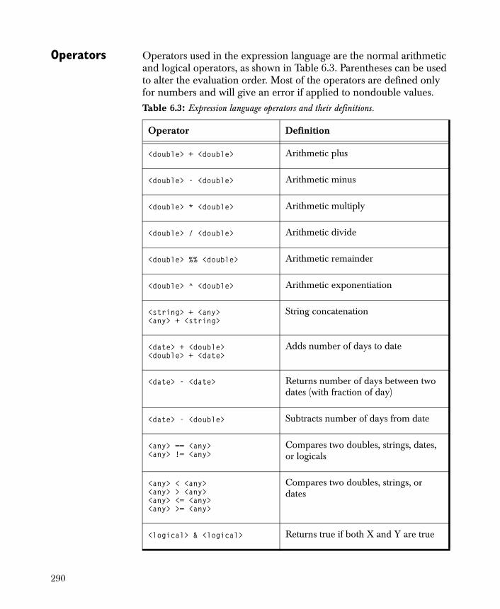
Operators Operators used in the expression language are the normal arithmetic and logical operators, as shown in Table 6.3. Parentheses can be used to alter the evaluation order. Most of the operators are defined only for numbers and will give an error if applied to nondouble values.Table 6.3: Expression language operators and their definitions.
Operator Definition
<double> + <double> Arithmetic plus
<double> - <double> Arithmetic minus
<double> * <double> Arithmetic multiply
<double> / <double> Arithmetic divide
<double> %% <double> Arithmetic remainder
<double> ^ <double> Arithmetic exponentiation
<string> + <any><any> + <string>
String concatenation
<date> + <double><double> + <date>
Adds number of days to date
<date> - <date> Returns number of days between two dates (with fraction of day)
<date> - <double> Subtracts number of days from date
<any> == <any><any> != <any>
Compares two doubles, strings, dates, or logicals
<any> < <any><any> > <any> <any> <= <any><any> >= <any>
Compares two doubles, strings, or dates
<logical> & <logical> Returns true if both X and Y are true
290
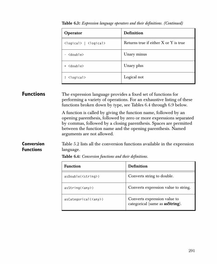
Functions The expression language provides a fixed set of functions for performing a variety of operations. For an exhaustive listing of these functions broken down by type, see Tables 6.4 through 6.9 below.
A function is called by giving the function name, followed by an opening parenthesis, followed by zero or more expressions separated by commas, followed by a closing parenthesis. Spaces are permitted between the function name and the opening parenthesis. Named arguments are not allowed.
Conversion Functions
Table 5.2 lists all the conversion functions available in the expression language.
<logical> | <logical> Returns true if either X or Y is true
- <double> Unary minus
+ <double> Unary plus
! <logical> Logical not
Table 6.3: Expression language operators and their definitions. (Continued)
Operator Definition
Table 6.4: Conversion functions and their definitions.
Function Definition
asDouble(<string>) Converts string to double.
asString(<any>) Converts expression value to string.
asCategorical(<any>) Converts expression value to categorical (same as asString).
291
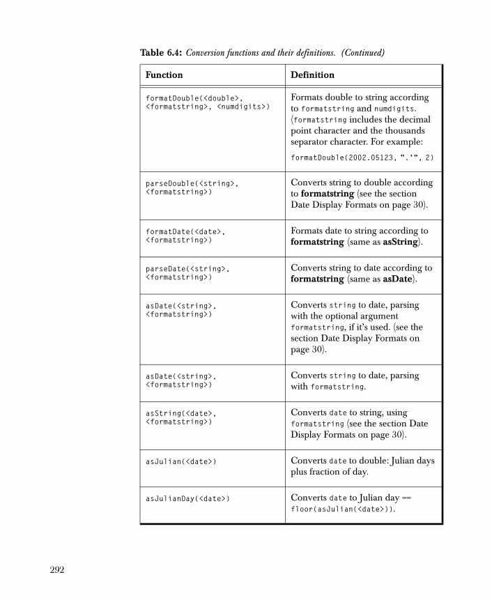
formatDouble(<double>, <formatstring>, <numdigits>)
Formats double to string according to formatstring and numdigits. (formatstring includes the decimal point character and the thousands separator character. For example:
formatDouble(2002.05123, ".'", 2)
parseDouble(<string>, <formatstring>)
Converts string to double according to formatstring (see the section Date Display Formats on page 30).
formatDate(<date>, <formatstring>)
Formats date to string according to formatstring (same as asString).
parseDate(<string>, <formatstring>)
Converts string to date according to formatstring (same as asDate).
asDate(<string>, <formatstring>)
Converts string to date, parsing with the optional argument formatstring, if it’s used. (see the section Date Display Formats on page 30).
asDate(<string>, <formatstring>)
Converts string to date, parsing with formatstring.
asString(<date>, <formatstring>)
Converts date to string, using formatstring (see the section Date Display Formats on page 30).
asJulian(<date>) Converts date to double: Julian days plus fraction of day.
asJulianDay(<date>) Converts date to Julian day == floor(asJulian(<date>)).
Table 6.4: Conversion functions and their definitions. (Continued)
Function Definition
292
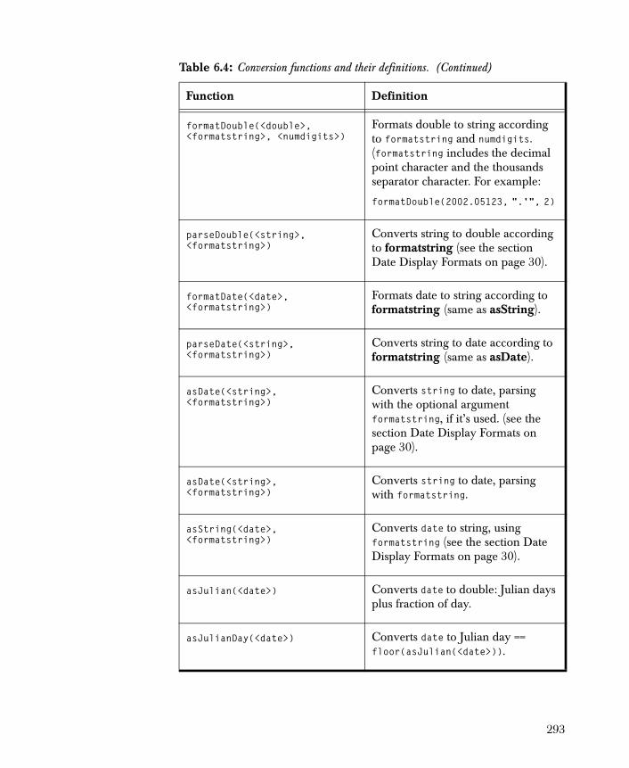
formatDouble(<double>, <formatstring>, <numdigits>)
Formats double to string according to formatstring and numdigits. (formatstring includes the decimal point character and the thousands separator character. For example:
formatDouble(2002.05123, ".'", 2)
parseDouble(<string>, <formatstring>)
Converts string to double according to formatstring (see the section Date Display Formats on page 30).
formatDate(<date>, <formatstring>)
Formats date to string according to formatstring (same as asString).
parseDate(<string>, <formatstring>)
Converts string to date according to formatstring (same as asDate).
asDate(<string>, <formatstring>)
Converts string to date, parsing with the optional argument formatstring, if it’s used. (see the section Date Display Formats on page 30).
asDate(<string>, <formatstring>)
Converts string to date, parsing with formatstring.
asString(<date>, <formatstring>)
Converts date to string, using formatstring (see the section Date Display Formats on page 30).
asJulian(<date>) Converts date to double: Julian days plus fraction of day.
asJulianDay(<date>) Converts date to Julian day == floor(asJulian(<date>)).
Table 6.4: Conversion functions and their definitions. (Continued)
Function Definition
293
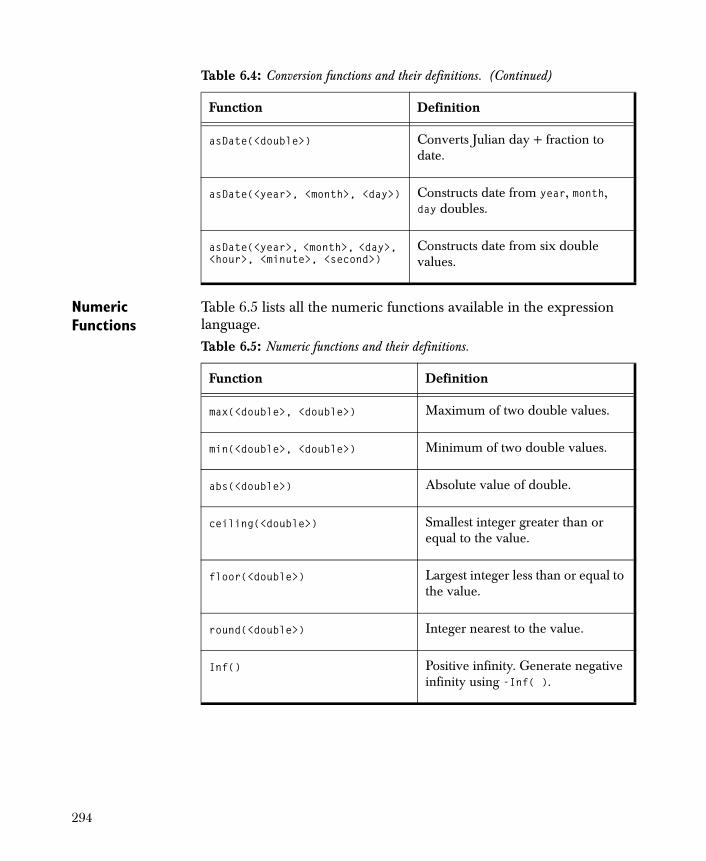
Numeric Functions
Table 6.5 lists all the numeric functions available in the expression language.
asDate(<double>) Converts Julian day + fraction to date.
asDate(<year>, <month>, <day>) Constructs date from year, month, day doubles.
asDate(<year>, <month>, <day>, <hour>, <minute>, <second>)
Constructs date from six double values.
Table 6.4: Conversion functions and their definitions. (Continued)
Function Definition
Table 6.5: Numeric functions and their definitions.
Function Definition
max(<double>, <double>) Maximum of two double values.
min(<double>, <double>) Minimum of two double values.
abs(<double>) Absolute value of double.
ceiling(<double>) Smallest integer greater than or equal to the value.
floor(<double>) Largest integer less than or equal to the value.
round(<double>) Integer nearest to the value.
Inf() Positive infinity. Generate negative infinity using -Inf( ).
294
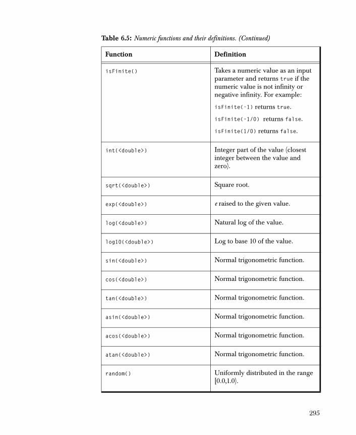
isFinite() Takes a numeric value as an input parameter and returns true if the numeric value is not infinity or negative infinity. For example:
isFinite(-1) returns true.
isFinite(-1/0) returns false.
isFinite(1/0) returns false.
int(<double>) Integer part of the value (closest integer between the value and zero).
sqrt(<double>) Square root.
exp(<double>) e raised to the given value.
log(<double>) Natural log of the value.
log10(<double>) Log to base 10 of the value.
sin(<double>) Normal trigonometric function.
cos(<double>) Normal trigonometric function.
tan(<double>) Normal trigonometric function.
asin(<double>) Normal trigonometric function.
acos(<double>) Normal trigonometric function.
atan(<double>) Normal trigonometric function.
random() Uniformly distributed in the range [0.0,1.0).
Table 6.5: Numeric functions and their definitions. (Continued)
Function Definition
295
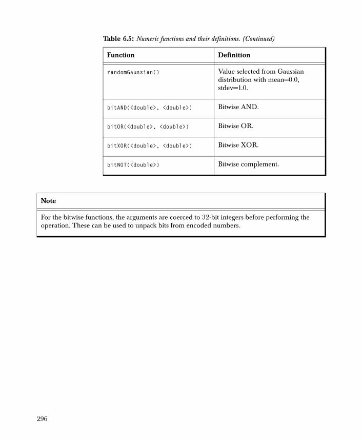
randomGaussian() Value selected from Gaussian distribution with mean=0.0, stdev=1.0.
bitAND(<double>, <double>) Bitwise AND.
bitOR(<double>, <double>) Bitwise OR.
bitXOR(<double>, <double>) Bitwise XOR.
bitNOT(<double>) Bitwise complement.
Table 6.5: Numeric functions and their definitions. (Continued)
Function Definition
Note
For the bitwise functions, the arguments are coerced to 32-bit integers before performing the operation. These can be used to unpack bits from encoded numbers.
296
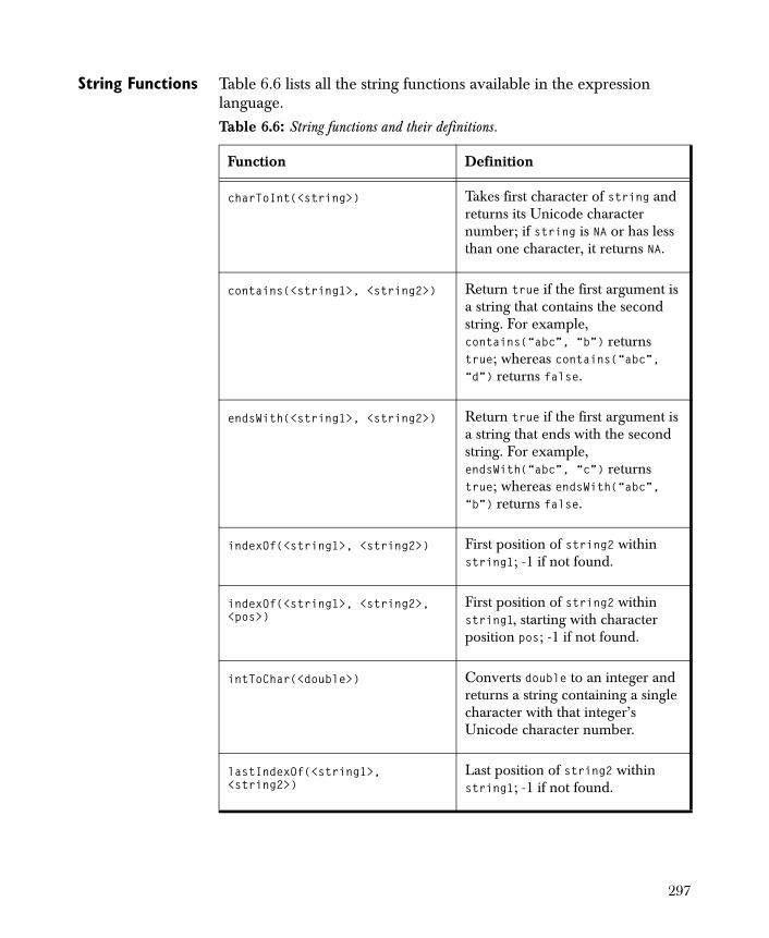
String Functions Table 6.6 lists all the string functions available in the expression language.Table 6.6: String functions and their definitions.
Function Definition
charToInt(<string>) Takes first character of string and returns its Unicode character number; if string is NA or has less than one character, it returns NA.
contains(<string1>, <string2>) Return true if the first argument is a string that contains the second string. For example, contains(“abc”, “b”) returns true; whereas contains(“abc”, “d”) returns false.
endsWith(<string1>, <string2>) Return true if the first argument is a string that ends with the second string. For example, endsWith(“abc”, “c”) returns true; whereas endsWith(“abc”, “b”) returns false.
indexOf(<string1>, <string2>) First position of string2 within string1; -1 if not found.
indexOf(<string1>, <string2>, <pos>)
First position of string2 within string1, starting with character position pos; -1 if not found.
intToChar(<double>) Converts double to an integer and returns a string containing a single character with that integer’s Unicode character number.
lastIndexOf(<string1>, <string2>)
Last position of string2 within string1; -1 if not found.
297
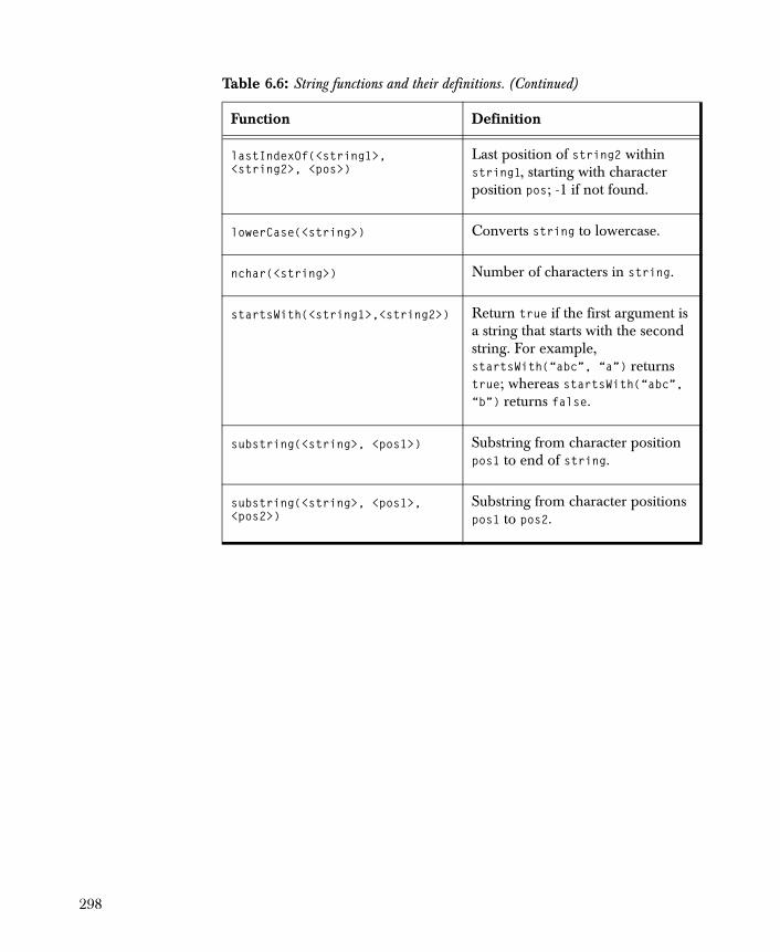
lastIndexOf(<string1>, <string2>, <pos>)
Last position of string2 within string1, starting with character position pos; -1 if not found.
lowerCase(<string>) Converts string to lowercase.
nchar(<string>) Number of characters in string.
startsWith(<string1>,<string2>) Return true if the first argument is a string that starts with the second string. For example, startsWith(“abc”, “a”) returns true; whereas startsWith(“abc”, “b”) returns false.
substring(<string>, <pos1>) Substring from character position pos1 to end of string.
substring(<string>, <pos1>, <pos2>)
Substring from character positions pos1 to pos2.
Table 6.6: String functions and their definitions. (Continued)
Function Definition
298
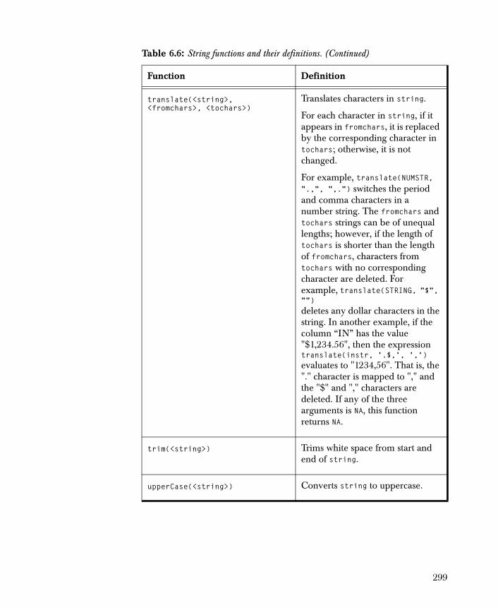
translate(<string>, <fromchars>, <tochars>)
Translates characters in string.
For each character in string, if it appears in fromchars, it is replaced by the corresponding character in tochars; otherwise, it is not changed.
For example, translate(NUMSTR, ".,", ",.") switches the period and comma characters in a number string. The fromchars and tochars strings can be of unequal lengths; however, if the length of tochars is shorter than the length of fromchars, characters from tochars with no corresponding character are deleted. For example, translate(STRING, "$", "") deletes any dollar characters in the string. In another example, if the column “IN” has the value "$1,234.56", then the expression translate(instr, '.$,', ',') evaluates to "1234,56". That is, the "." character is mapped to "," and the "$" and "," characters are deleted. If any of the three arguments is NA, this function returns NA.
trim(<string>) Trims white space from start and end of string.
upperCase(<string>) Converts string to uppercase.
Table 6.6: String functions and their definitions. (Continued)
Function Definition
299
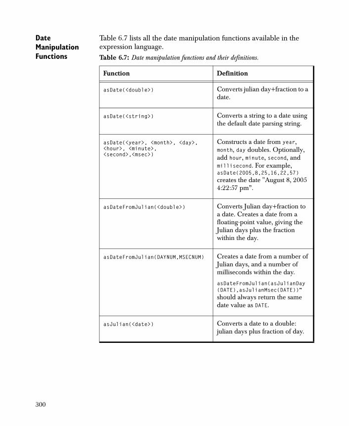
Date Manipulation Functions
Table 6.7 lists all the date manipulation functions available in the expression language.Table 6.7: Date manipulation functions and their definitions.
Function Definition
asDate(<double>) Converts julian day+fraction to a date.
asDate(<string>) Converts a string to a date using the default date parsing string.
asDate(<year>, <month>, <day>, <hour>, <minute>, <second>,<msec>)
Constructs a date from year, month, day doubles. Optionally, add hour, minute, second, and millisecond. For example, asDate(2005,8,25,16,22,57) creates the date "August 8, 2005 4:22:57 pm”.
asDateFromJulian(<double>) Converts Julian day+fraction to a date. Creates a date from a floating-point value, giving the Julian days plus the fraction within the day.
asDateFromJulian(DAYNUM,MSECNUM) Creates a date from a number of Julian days, and a number of milliseconds within the day.
asDateFromJulian(asJulianDay(DATE),asJulianMsec(DATE))" should always return the same date value as DATE.
asJulian(<date>) Converts a date to a double: julian days plus fraction of day.
300
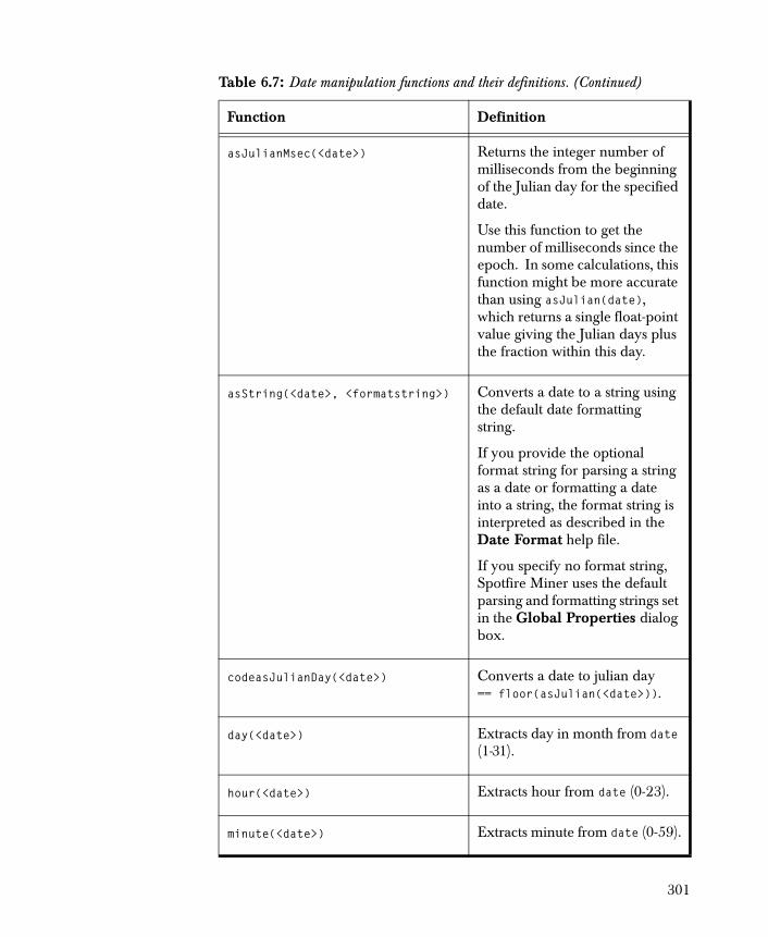
asJulianMsec(<date>) Returns the integer number of milliseconds from the beginning of the Julian day for the specified date.
Use this function to get the number of milliseconds since the epoch. In some calculations, this function might be more accurate than using asJulian(date), which returns a single float-point value giving the Julian days plus the fraction within this day.
asString(<date>, <formatstring>) Converts a date to a string using the default date formatting string.
If you provide the optional format string for parsing a string as a date or formatting a date into a string, the format string is interpreted as described in the Date Format help file.
If you specify no format string, Spotfire Miner uses the default parsing and formatting strings set in the Global Properties dialog box.
codeasJulianDay(<date>) Converts a date to julian day == floor(asJulian(<date>)).
day(<date>) Extracts day in month from date (1-31).
hour(<date>) Extracts hour from date (0-23).
minute(<date>) Extracts minute from date (0-59).
Table 6.7: Date manipulation functions and their definitions. (Continued)
Function Definition
301

Data Set Functions
Table 6.8 lists all the data set functions available in the expression language.
month(<date>) Extracts month from date (1-12).
msec(<date>) Extracts millisecond from date (0-999).
now() Returns date representing the current date and time.
quarter(<date>) Extracts quarter of year from date (1-4).
second(<date>) Extracts second from date (0-59).
weekday(<date>) Extracts day of week from date (Sun=0, Mon=1, ..., Sat=6).
workday(<date>) Returns logical true if weekday is Monday-Friday.
year(<date>) Extracts year from date.
yearday(<date>) Extracts day of year from date (1-366).
Table 6.7: Date manipulation functions and their definitions. (Continued)
Function Definition
Table 6.8: Data set functions and their definitions.
Function Definition
columnMax(<id>) Maximum value for column.
columnMean(<id>) Mean value for column.
columnMin(<id>) Minimum value for column.
302
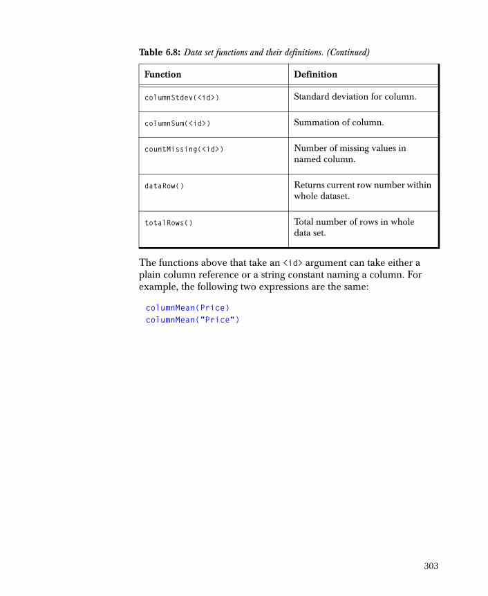
The functions above that take an <id> argument can take either a plain column reference or a string constant naming a column. For example, the following two expressions are the same:
columnMean(Price)columnMean("Price")
columnStdev(<id>) Standard deviation for column.
columnSum(<id>) Summation of column.
countMissing(<id>) Number of missing values in named column.
dataRow() Returns current row number within whole dataset.
totalRows() Total number of rows in whole data set.
Table 6.8: Data set functions and their definitions. (Continued)
Function Definition
303
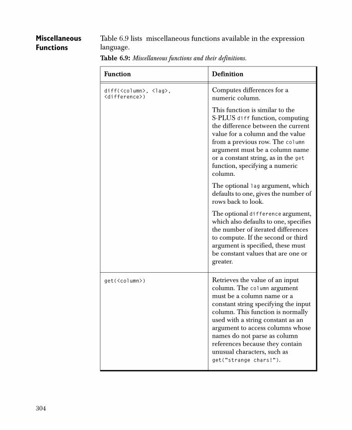
Miscellaneous Functions
Table 6.9 lists miscellaneous functions available in the expression language.Table 6.9: Miscellaneous functions and their definitions.
Function Definition
diff(<column>, <lag>, <difference>)
Computes differences for a numeric column.
This function is similar to the S-PLUS diff function, computing the difference between the current value for a column and the value from a previous row. The column argument must be a column name or a constant string, as in the get function, specifying a numeric column.
The optional lag argument, which defaults to one, gives the number of rows back to look.
The optional difference argument, which also defaults to one, specifies the number of iterated differences to compute. If the second or third argument is specified, these must be constant values that are one or greater.
get(<column>) Retrieves the value of an input column. The column argument must be a column name or a constant string specifying the input column. This function is normally used with a string constant as an argument to access columns whose names do not parse as column references because they contain unusual characters, such as get("strange chars!").
304
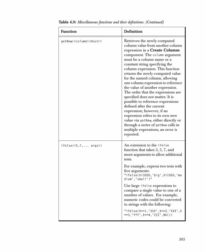
getNew(<column>)Hostri Retrieves the newly-computed column value from another column expression in a Create Columns component. The column argument must be a column name or a constant string specifying the column expression. This function returns the newly-computed value for the named column, allowing one column expression to reference the value of another expression. The order that the expressions are specified does not matter. It is possible to reference expressions defined after the current expression; however, if an expression refers to its own new value via getNew, either directly or through a series of getNew calls in multiple expressions, an error is reported.
ifelse(<5,7,... args>) An extension to the ifelse function that takes 3, 5, 7, and more arguments to allow additional tests.
For example, express two tests with five arguments: "ifelse(X>3000,'big',X>1000,'medium','small')"
Use large ifelse expressions to compare a single value to one of a number of values. For example, numeric codes could be converted to strings with the following:
"ifelse(X==1,'XXX',X==2,'XXX',X==3,'YYY',X==4,'ZZZ',NA())
Table 6.9: Miscellaneous functions and their definitions. (Continued)
Function Definition
305
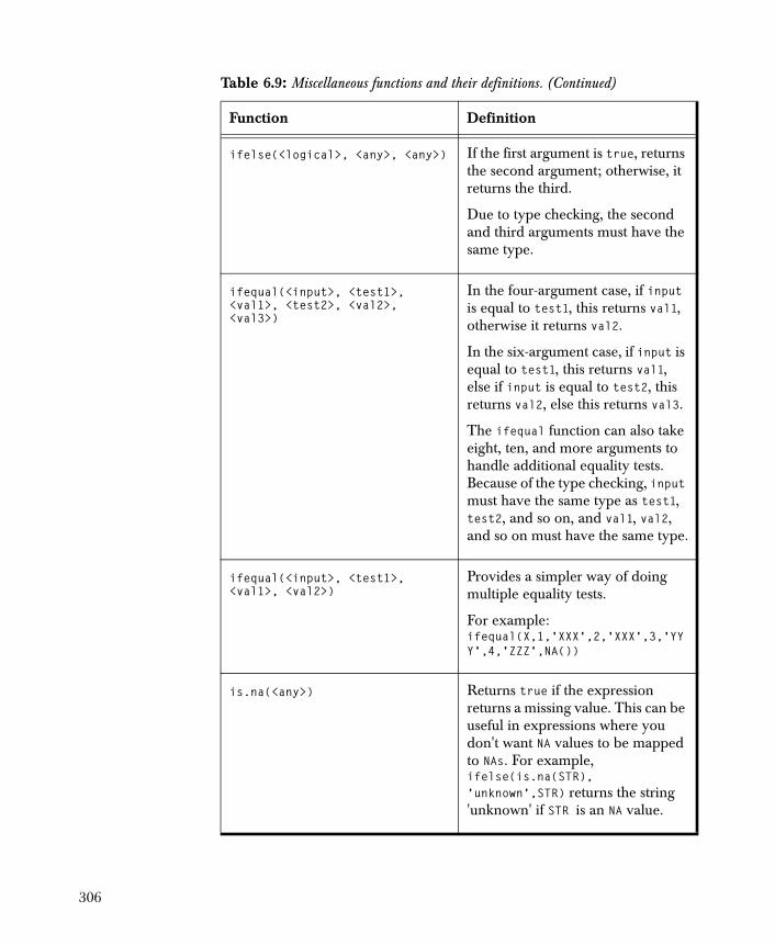
ifelse(<logical>, <any>, <any>) If the first argument is true, returns the second argument; otherwise, it returns the third.
Due to type checking, the second and third arguments must have the same type.
ifequal(<input>, <test1>, <val1>, <test2>, <val2>, <val3>)
In the four-argument case, if input is equal to test1, this returns val1, otherwise it returns val2.
In the six-argument case, if input is equal to test1, this returns val1, else if input is equal to test2, this returns val2, else this returns val3.
The ifequal function can also take eight, ten, and more arguments to handle additional equality tests. Because of the type checking, input must have the same type as test1, test2, and so on, and val1, val2, and so on must have the same type.
ifequal(<input>, <test1>, <val1>, <val2>)
Provides a simpler way of doing multiple equality tests.
For example: ifequal(X,1,'XXX',2,'XXX',3,'YYY',4,'ZZZ',NA())
is.na(<any>) Returns true if the expression returns a missing value. This can be useful in expressions where you don't want NA values to be mapped to NAs. For example, ifelse(is.na(STR),'unknown',STR) returns the string 'unknown' if STR is an NA value.
Table 6.9: Miscellaneous functions and their definitions. (Continued)
Function Definition
306
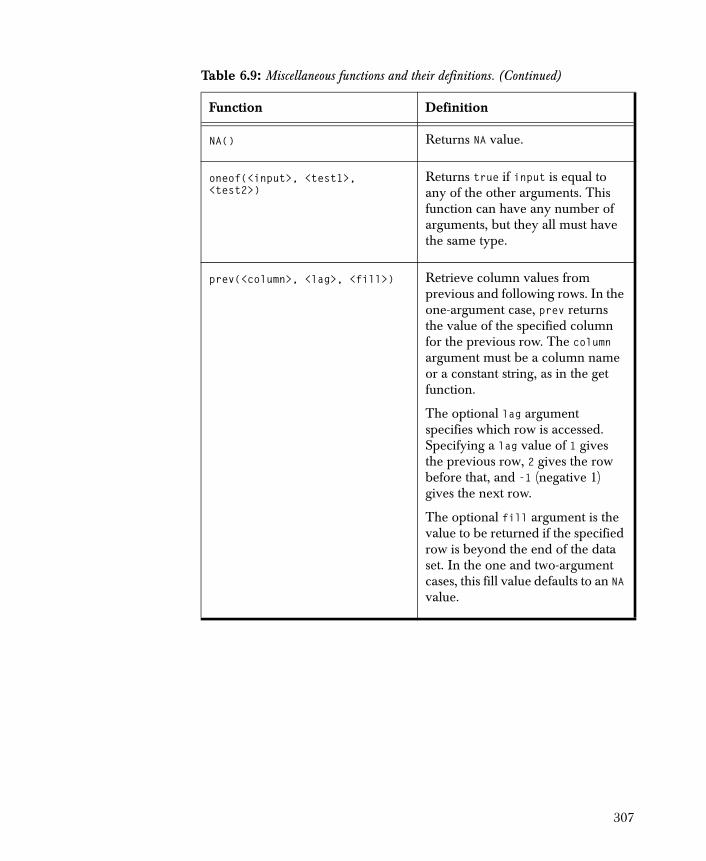
NA() Returns NA value.
oneof(<input>, <test1>, <test2>)
Returns true if input is equal to any of the other arguments. This function can have any number of arguments, but they all must have the same type.
prev(<column>, <lag>, <fill>) Retrieve column values from previous and following rows. In the one-argument case, prev returns the value of the specified column for the previous row. The column argument must be a column name or a constant string, as in the get function.
The optional lag argument specifies which row is accessed. Specifying a lag value of 1 gives the previous row, 2 gives the row before that, and -1 (negative 1) gives the next row.
The optional fill argument is the value to be returned if the specified row is beyond the end of the data set. In the one and two-argument cases, this fill value defaults to an NA value.
Table 6.9: Miscellaneous functions and their definitions. (Continued)
Function Definition
307
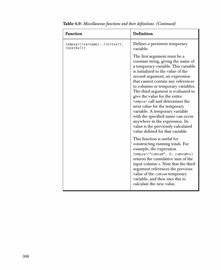
tempvar(<varname>, <initval>, <nextVal>)
Defines a persistent temporary variable.
The first argument must be a constant string, giving the name of a temporary variable. This variable is initialized to the value of the second argument, an expression that cannot contain any references to columns or temporary variables. The third argument is evaluated to give the value for the entire tempvar call and determines the next value for the temporary variable. A temporary variable with the specified name can occur anywhere in the expression. Its value is the previously-calculated value defined for that variable.
This function is useful for constructing running totals. For example, the expression tempvar("cumsum", 0, cumsum+x) returns the cumulative sum of the input column x. Note that the third argument references the previous value of the cumsum temporary variable, and then uses this to calculate the new value.
Table 6.9: Miscellaneous functions and their definitions. (Continued)
Function Definition
308
Overview 311General Procedure 311Selecting Dependent and Independent Variables 313Selecting Output 314Creating Predict Nodes 316
Logistic Regression Models 319Mathematical Definitions 319Properties 320Using the Viewer 325Creating a Filter Column node 328A Cross-Sell Example 330Technical Details 341
Classification Trees 344Background 344Properties 348Using the Viewer 355A Cross-Sell Example (Continued) 357
Classification Neural Networks 362Background 362Properties 365Using the Viewer 370A Cross-Sell Example (Continued) 374Technical Details 379
Naive Bayes Models 383Background 383Properties 384Using the Viewer 385A Promoter Gene Sequence Example 386Technical Details 389
CLASSIFICATION MODELS 7
309

References 393
310
OVERVIEW
You use classification models when you wish to compute predictions for a discrete or categorical dependent variable. Common examples of dependent variables in this type of model are binary variables in which there are exactly two levels (such as, the acceptance or rejection of a marketing offer) and multinomial variables that have more than two levels (such as, disease type). The variables in the model that determine the predictions are called the independent variables. All other variables in the data set are simply information or identification variables; common examples include customer number, telephone, and address.
Spotfire Miner™ includes components for four types of classification models: Logistic Regression, Classification Tree, Classification Neural Network, and Naive Bayes. In this chapter, we discuss each model at a high level, describe the options available for these components, give full examples for illustration, and provide technical details for the underlying algorithms. The options we describe here are specific to the classification modeling components. For information on the Advanced pages of the properties dialogs, see Chapter 15, Advanced Topics (the options in the Advanced pages apply to all components).
In the remainder of this overview, we describe the options that are common to all four models. For descriptions of model-specific options, see the appropriate sections in this chapter.
General Procedure
The following outlines the general approach to using classification models in Spotfire Miner:
1. Link a model node in your worksheet to any node that outputs data. The input data set to the model node is called the training data because it is used to train your model.
2. Use the properties dialog for the model to specify the dependent and independent variables and the type of data you want to output.
3. Run your network.
4. Launch the viewer for the model node.
311

5. Based on the information in the viewer, modify your model if desired and rerun the network.
6. When you are satisfied with results, create a Predict node for the model.
7. Link the Predict node to a node that outputs your scoring data and then run the new network. Typically, the scoring data set contains all variables in the model except the dependent variable.
All classification models in Spotfire Miner accept a single input containing rectangular data. They output a data set containing any of the following, based on options you choose in the properties dialogs:
• A column containing the probabilities computed by the model.
• A column containing the classifications predicted by the model.
• A column containing two values, 1 and 0, which indicate whether the predicted classification agrees with the actual classification in the dependent variable.
• All of the independent variables in your data set.
• The dependent variable in your data set.
• All other columns in your data set besides the dependent and independent variables.
312
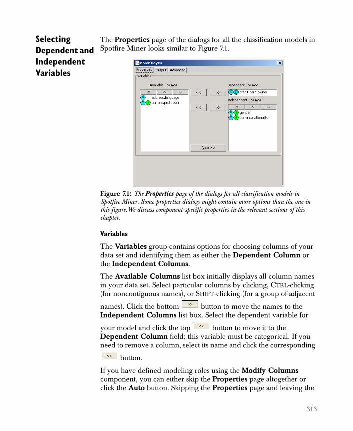
Selecting Dependent and Independent Variables
The Properties page of the dialogs for all the classification models in Spotfire Miner looks similar to Figure 7.1.
Variables
The Variables group contains options for choosing columns of your data set and identifying them as either the Dependent Column or the Independent Columns.
The Available Columns list box initially displays all column names in your data set. Select particular columns by clicking, CTRL-clicking (for noncontiguous names), or SHIFT-clicking (for a group of adjacent
names). Click the bottom button to move the names to the Independent Columns list box. Select the dependent variable for
your model and click the top button to move it to the Dependent Column field; this variable must be categorical. If you need to remove a column, select its name and click the corresponding
button.
If you have defined modeling roles using the Modify Columns component, you can either skip the Properties page altogether or click the Auto button. Skipping the Properties page and leaving the
Figure 7.1: The Properties page of the dialogs for all classification models in Spotfire Miner. Some properties dialogs might contain more options than the one in this figure.We discuss component-specific properties in the relevant sections of this chapter.
313
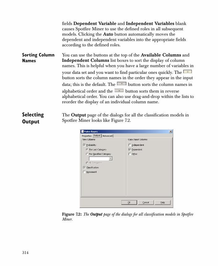
fields Dependent Variable and Independent Variables blank causes Spotfire Miner to use the defined roles in all subsequent models. Clicking the Auto button automatically moves the dependent and independent variables into the appropriate fields according to the defined roles.
Sorting Column Names
You can use the buttons at the top of the Available Columns and Independent Columns list boxes to sort the display of column names. This is helpful when you have a large number of variables in your data set and you want to find particular ones quickly. The button sorts the column names in the order they appear in the input data; this is the default. The button sorts the column names in alphabetical order and the button sorts them in reverse alphabetical order. You can also use drag-and-drop within the lists to reorder the display of an individual column name.
Selecting Output
The Output page of the dialogs for all the classification models in Spotfire Miner looks like Figure 7.2.
Figure 7.2: The Output page of the dialogs for all classification models in Spotfire Miner.
314
New Columns
The New Columns group contains options for including new columns in the output data.
Probability Select this check box if you want the output data to include a column containing the probability estimated from the model for each observation. The name of the column Spotfire Miner creates is either PREDICT.prob or Pr(x), where x is the name of the level you choose. By default, Spotfire Miner returns the estimated probabilities for the last of the sorted levels of the dependent variable. When the dependent variable is binary and the default option is used the probability column is named PREDICT.prob. If the probabilities for another level are more meaningful, select the For Specified Category radio button and choose the appropriate level from the drop-down list. You can also type the level in the box.
Classification Select this check box if you want the output data to include a column named PREDICT.class containing the predicted class for each observation. The predicted class is that class that had the maximum estimated probability: if Pr(x) is the maximum estimated probability, Spotfire Miner predicts the class of the observation to be x.
Agreement Select this check box if you want the output data to include a column named PREDICT.agreement indicating the agreement between the actual class and the predicted class. A value of 1 for a particular observation indicates the actual class and the predicted class agree for the observation; a value of 0 indicates they do not.
Copy Input Columns
The Copy Input Columns group contains options for copying the input columns to the output data set. Select the Independent check box if you want Spotfire Miner to copy all of the independent variables in the model to the output data set. Select the Dependent check box if you want Spotfire Miner to copy the dependent variable. Select the Other check box if you want Spotfire Miner to copy all columns that are neither the dependent nor the independent variables but are part of the original data set.
315
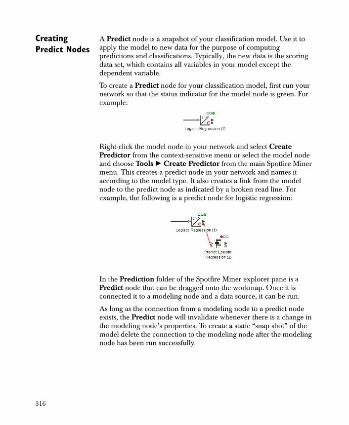
Creating Predict Nodes
A Predict node is a snapshot of your classification model. Use it to apply the model to new data for the purpose of computing predictions and classifications. Typically, the new data is the scoring data set, which contains all variables in your model except the dependent variable.
To create a Predict node for your classification model, first run your network so that the status indicator for the model node is green. For example:
Right-click the model node in your network and select Create Predictor from the context-sensitive menu or select the model node and choose Tools � Create Predictor from the main Spotfire Miner menu. This creates a predict node in your network and names it according to the model type. It also creates a link from the model node to the predict node as indicated by a broken read line. For example, the following is a predict node for logistic regression:
In the Prediction folder of the Spotfire Miner explorer pane is a Predict node that can be dragged onto the workmap. Once it is connected it to a modeling node and a data source, it can be run.
As long as the connection from a modeling node to a predict node exists, the Predict node will invalidate whenever there is a change in the modeling node’s properties. To create a static “snap shot” of the model delete the connection to the modeling node after the modeling node has been run successfully.
316
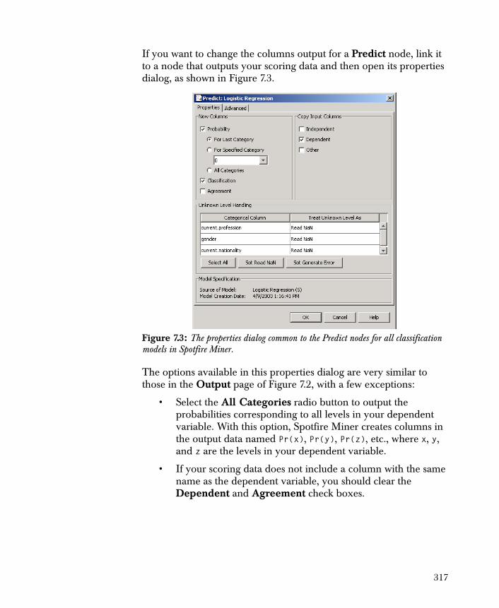
If you want to change the columns output for a Predict node, link it to a node that outputs your scoring data and then open its properties dialog, as shown in Figure 7.3.
The options available in this properties dialog are very similar to those in the Output page of Figure 7.2, with a few exceptions:
• Select the All Categories radio button to output the probabilities corresponding to all levels in your dependent variable. With this option, Spotfire Miner creates columns in the output data named Pr(x), Pr(y), Pr(z), etc., where x, y, and z are the levels in your dependent variable.
• If your scoring data does not include a column with the same name as the dependent variable, you should clear the Dependent and Agreement check boxes.
Figure 7.3: The properties dialog common to the Predict nodes for all classification models in Spotfire Miner.
317

• The Unknown Level Handling will allow you to specify the action to take if a category class is observed in the scoring data that was not observed when fitting the model. Here you can either generate a missing value (referred to as NaN, “not-a-number”), the default, or to generate an error.
• The Model Specification identifies which node generated the predict node as well as the date and time of the creation.
318
LOGISTIC REGRESSION MODELS
In logistic regression , you model the probability of a binary event occurring as a linear function of a set of independent variables. Logistic regression models are a special type of linear model in which the dependent variable is categorical and has exactly two levels. Some common examples of dependent variables in logistic regression models include the acceptance or rejection of a marketing offer, the presence or absence of disease, and the success or failure of a electronic component.
This section discusses logistic regression at a high level, describes the properties for the Logistic Regression component, provides general guidance for interpreting the model output and the information contained in the viewer, and gives a full example for illustration. Unless otherwise specified, all screen shots in this section use variables from the kyphosis.txt data set, which is stored as a text file in the examples folder under your Spotfire Miner installation directory.
Mathematical Definitions
A linear model provides a way of estimating a dependent variable , conditional on a linear function of a set of independent variables,
. Mathematically, this is written as:
In this equation, the terms are the coefficients of the linear model; the intercept of the model is and is the residual. Estimates of the
coefficients, are computed from the training data from which an
estimate of the dependent variable, is computed by substituting the estimated coefficients into Equation (7.1). An estimate of the residual,
, is then the difference between the observed dependent variable and its estimate.
(7.1)
Y
X1 X2 … X, p, ,
Y β0 βiXi ε+i 1=
p
+=
βi
β0 ε
βi
Y
ε
319
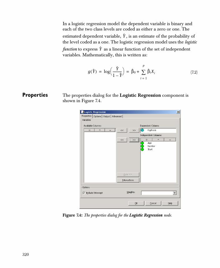
In a logistic regression model the dependent variable is binary and each of the two class levels are coded as either a zero or one. The
estimated dependent variable, , is an estimate of the probability of the level coded as a one. The logistic regression model uses the logistic
function to express as a linear function of the set of independent variables. Mathematically, this is written as:
Properties The properties dialog for the Logistic Regression component is shown in Figure 7.4.
(7.2)
Y
Y
g Y( ) Y
1 Y–------------ log β0 βiXi
i 1=
p
+= =
Figure 7.4: The properties dialog for the Logistic Regression node.
320
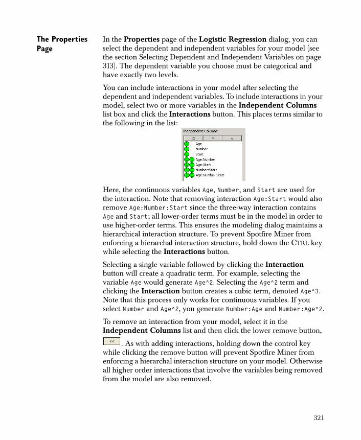
The Properties Page
In the Properties page of the Logistic Regression dialog, you can select the dependent and independent variables for your model (see the section Selecting Dependent and Independent Variables on page 313). The dependent variable you choose must be categorical and have exactly two levels.
You can include interactions in your model after selecting the dependent and independent variables. To include interactions in your model, select two or more variables in the Independent Columns list box and click the Interactions button. This places terms similar to the following in the list:
Here, the continuous variables Age, Number, and Start are used for the interaction. Note that removing interaction Age:Start would also remove Age:Number:Start since the three-way interaction contains Age and Start; all lower-order terms must be in the model in order to use higher-order terms. This ensures the modeling dialog maintains a hierarchical interaction structure. To prevent Spotfire Miner from enforcing a hierarchal interaction structure, hold down the CTRL key while selecting the Interactions button.
Selecting a single variable followed by clicking the Interaction button will create a quadratic term. For example, selecting the variable Age would generate Age^2. Selecting the Age^2 term and clicking the Interaction button creates a cubic term, denoted Age^3. Note that this process only works for continuous variables. If you select Number and Age^2, you generate Number:Age and Number:Age^2.
To remove an interaction from your model, select it in the Independent Columns list and then click the lower remove button,
. As with adding interactions, holding down the control key while clicking the remove button will prevent Spotfire Miner from enforcing a hierarchal interaction structure on your model. Otherwise all higher order interactions that involve the variables being removed from the model are also removed.
321
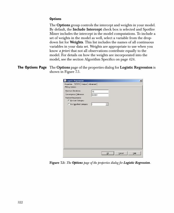
Options
The Options group controls the intercept and weights in your model. By default, the Include Intercept check box is selected and Spotfire Miner includes the intercept in the model computations. To include a set of weights in the model as well, select a variable from the drop-down list for Weights. This list includes the names of all continuous variables in your data set. Weights are appropriate to use when you know a priori that not all observations contribute equally to the model. For details on how the weights are incorporated into the model, see the section Algorithm Specifics on page 424.
The Options Page The Options page of the properties dialog for Logistic Regression is shown in Figure 7.5.
Figure 7.5: The Options page of the properties dialog for Logistic Regression.
322
Fitting Options
The Fitting Options group contains tuning parameters for the algorithm underlying the Logistic Regression component.
Maximum Iterations There is a trade off between accuracy of the estimated coefficients and the number of iterations to achieve the desired accuracy. If convergence is not achieved in the default of 10 iterations, increase the maximum number of iterations and reexecute the node. It is possible that colinearities among your independent variables will prevent the coefficients from ever converging.
Convergence Tolerance Use to control the relative precision of the estimated coefficients. The default of 0.0001 will guarantee four digits of precision for the estimated coefficients. Decreasing the convergence tolerance will generally require more iterations.
For information regarding the fitting algorithm for the Logistic Regression component, see the section Technical Details on page 341.
It is mentioned earlier in this section that the dependent variable in logistic regression is binary and to perform computations one of the categorical levels is coded as a one and the other as a zero. These coded levels are sometimes referred to as the “positive” and the “negative” responses, respectively. The radio buttons in the Options page allow you to choose which class level gets coded as the “positive” level. This will affect the signs of the coefficients for the logistic regression model and is only relevant if you plan to use the coefficients to interpret the effect each independent variable has on the dependent variable.
If you select the wrong level, the magnitude of the coefficients for your model will be correct but their signs will be reversed. This will result in an incorrect interpretation of the effect that the independent variable has to on the probability of an outcome.
323
For Last Category Select this radio button if the last level in your dependent variable is the “positive” response (that is, acceptance of a marketing offer, presence of a disease, a surviving patient).
For Specified Category If the first level is the positive response or you are unsure of the level ordering in your dependent variable, select this radio button instead and choose the appropriate level from the drop-down list or type it in.
Note
A positive coefficient means that increasing the independent variable increases the probability of the dependent variable level that is coded as a one, the “positive” level. If the independent variable is categorical, a positive coefficient means that the associated independent variable class level increases the chance of a “positive” response in the dependent variables.
Note
The For Last Category and For Specified Category radio buttons on the Options page do not affect the probabilities and classifications predicted by the logistic regression model. If you are interested in the probabilities and classifications only, you can safely ignore these options.
324

The Output Page The Output page of the properties dialog for the Logistic Regression component is shown in Figure 7.6.
In the Output page, you can select the type of output you want the Logistic Regression component to return. See the section Selecting Output on page 314 for more details.
Using the Viewer
The viewer for the Logistic Regression component is an HTML file appearing in your default browser. The file includes tables that are useful for interpreting the computed coefficients for your model. If you are interested only in the probabilities and classifications predicted by the model, you can skip this section.
For example, the following information is displayed in Figure 7.7:
• The name of the dependent variable, Kyphosis.
• A table of Coefficient Estimates, which includes the following:
• The coefficient estimates for the intercept and the three independent variables (Age, Number, and Start).
Figure 7.6: The Output page of the Logistic Regression dialog.
325
• The standard error for each coefficient estimate.
The standard error for an estimate is a measure of its variability. If the standard error for a coefficient is small in comparison to the magnitude of the coefficient estimate, the estimate is fairly precise.
• The t-statistic for each coefficient estimate.
The t-statistic for an estimate tests whether the coefficient is significantly different from zero. Or to rephrase, a t-statistic is a measure of significance for a variable in the model and is the ratio of the coefficient estimate divided by its standard error. In general, a t-statistic greater than 1.96 in magnitude indicate the coefficient that are significantly different from zero and the associated variable should therefore be kept in the model. In Figure 7.7, the t-statistics imply the coefficient for Start and the intercept are very significant in the model.
• The p-value for each t-statistic indicates if the corresponding coefficient is significant in the model. In general, if the p-value is less than 0.05 the t-statistic is greater than 1.96. This suggests that the coefficients are significant. In Figure 7.7, the small p-values for Start implies the term is very significant and the variables Age and Number contribute to the model but less so. Generally, a test for the intercept is uninformative since we rarely expect the regression surface to intersect with the origin.
• An Analysis of Deviance table, which includes the Regression, Error, and Null deviance and the corresponding degrees of freedom (DF). As noted earlier, deviance is a measure of model discrepancy used in logistic regression. As with the Analysis of Variance for a linear model with Gaussian errors the Analysis of Deviance is a partition of a model discrepancy from an oversimplified model, the Null model, into the two components Regression and Error. The Null deviance is analogous to the Total sum of squares in an Analysis of Variance. The Regression deviance measures the portion of the Null deviance explained by the model and the Error is what is left over. Further refinement of the Regression deviance by partitioning it by each independent variable is impractical in Data Mining since it would require dropping
326

each variable and refitting the model and taking the difference in the Error deviance. The Term Importance statistic discussed next can give a substitute for this refined model assessment for categorical independent variables.
• A Term Importance table showing the importance of each variable in the model. For logistic regression, importance for a variable is Wald statistic testing each effect to be zero. Since each of the independent variables are continuous for the Kyphosis example, these statistics contribute no additional information beyond the t-statistics in the coefficient table. You will note that the Wald statistic for a variable is the square of the t-statistic. The Wald statistic is useful for categorical independent variables where there is a coefficient for each class level and the coefficient t-statistic shows the significance of each class level, making it difficult to assess how the variable contributes to the model as a whole. For categorical
327
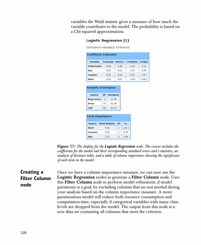
variables the Wald statistic gives a measure of how much the variable contributes to the model. The probability is based on a Chi-squared approximation.
Creating a Filter Column node
Once we have a column importance measure, we can now use the Logistic Regression nodes to generate a Filter Column node. Uses this Filter Column node to perform model refinement, if model parsimony is a goal, by excluding columns that are not needed during your analysis based on the column importance measure. A more parsimonious model will reduce both resource consumption and computation time, especially if categorical variables with many class levels are dropped from the model. The output from this node is a new data set containing all columns that meet the criterion.
Figure 7.7: The display for the Logistic Regression node. The viewer includes the coefficients for the model and their corresponding standard errors and t-statistics, an analysis of deviance table, and a table of column importance showing the significance of each term in the model.
328
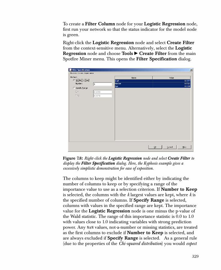
To create a Filter Column node for your Logistic Regression node, first run your network so that the status indicator for the model node is green.
Right-click the Logistic Regression node and select Create Filter from the context-sensitive menu. Alternatively, select the Logistic Regression node and choose Tools � Create Filter from the main Spotfire Miner menu. This opens the Filter Specification dialog.
The columns to keep might be identified either by indicating the number of columns to keep or by specifying a range of the importance value to use as a selection criterion. If Number to Keep is selected, the columns with the k largest values are kept, where k is the specified number of columns. If Specify Range is selected, columns with values in the specified range are kept. The importance value for the Logistic Regression node is one minus the p-value of the Wald statistic. The range of this importance statistic is 0.0 to 1.0 with values close to 1.0 indicating variables with strong prediction power. Any NaN values, not-a-number or missing statistics, are treated as the first columns to exclude if Number to Keep is selected, and are always excluded if Specify Range is selected. As a general rule (due to the properties of the Chi-squared distribution) you would expect
Figure 7.8: Right-click the Logistic Regression node and select Create Filter to display the Filter Specification dialog. Here, the Kyphosis example gives a excessively simplistic demonstration for ease of exposition.
329
a Wald statistic to be equal to its degrees of freedom if the variable does not contribute any prediction power. For these variables the p-value is relatively large so one minus the p-value is small.
When you select OK, the new Filter Columns node is added to the worksheet. Link this node to any output data node as described in the section Manipulating Columns in Chapter 6, Data Manipulation.
A Cross-Sell Example
Cross-selling is the practice of offering new products to existing customers. A key ingredient of successful cross-selling is to identify those individuals in the customer database who are most likely to respond to the new offer. Once identified, such customers can be additionally motivated, perhaps by a targeted mailing campaign.
In this cross-sell example, we use the Logistic Regression component to identify a subset of banking customers. We build a model that predicts who among the existing customer base are most likely to respond positively to an offer for a new credit card. We use two data sets in this example, a training data set and a scoring data set. The training data set is named xsell.sas7bdat, and the scoring data set is named xsell_scoring.sas7bdat. Both files are stored as SAS files in the examples folder under your Spotfire Miner installation directory.
There are two main columns of interest in the xsell.sas7bdat data set: cust_id and credit_card_owner. The column cust_id is informational and uniquely identifies each customer record. The column credit_card_owner is a binary categorical level with exactly two levels; a value of 1 indicates the customer has the credit card the bank is offering and a value of 0 indicates the customer does not. We use credit_card_owner as the dependent variable in the logistic regression model we build. For descriptions of the remaining variables, see the online help system.
330
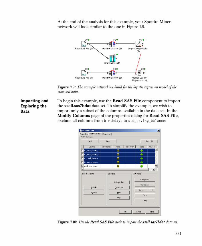
At the end of the analysis for this example, your Spotfire Miner network will look similar to the one in Figure 7.9.
Importing and Exploring the Data
To begin this example, use the Read SAS File component to import the xsell.sas7bdat data set. To simplify the example, we wish to import only a subset of the columns available in the data set. In the Modify Columns page of the properties dialog for Read SAS File, exclude all columns from birthdays to std_saving_balance:
Figure 7.9: The example network we build for the logistic regression model of the cross-sell data.
Figure 7.10: Use the Read SAS File node to import the xsell.sas7bdat data set.
331
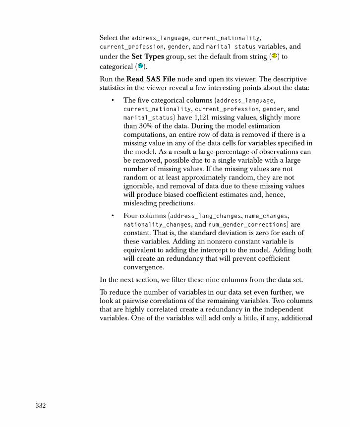
Select the address_language, current_nationality, current_profession, gender, and marital status variables, and under the Set Types group, set the default from string ( ) to categorical ( ).
Run the Read SAS File node and open its viewer. The descriptive statistics in the viewer reveal a few interesting points about the data:
• The five categorical columns (address_language, current_nationality, current_profession, gender, and marital_status) have 1,121 missing values, slightly more than 30% of the data. During the model estimation computations, an entire row of data is removed if there is a missing value in any of the data cells for variables specified in the model. As a result a large percentage of observations can be removed, possible due to a single variable with a large number of missing values. If the missing values are not random or at least approximately random, they are not ignorable, and removal of data due to these missing values will produce biased coefficient estimates and, hence, misleading predictions.
• Four columns (address_lang_changes, name_changes, nationality_changes, and num_gender_corrections) are constant. That is, the standard deviation is zero for each of these variables. Adding an nonzero constant variable is equivalent to adding the intercept to the model. Adding both will create an redundancy that will prevent coefficient convergence.
In the next section, we filter these nine columns from the data set.
To reduce the number of variables in our data set even further, we look at pairwise correlations of the remaining variables. Two columns that are highly correlated create a redundancy in the independent variables. One of the variables will add only a little, if any, additional
332
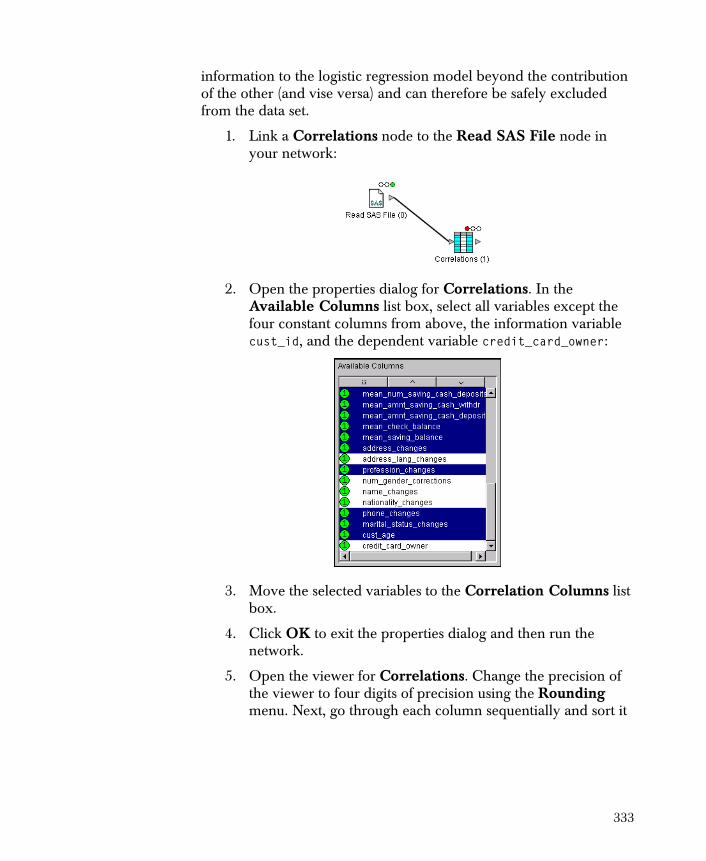
information to the logistic regression model beyond the contribution of the other (and vise versa) and can therefore be safely excluded from the data set.
1. Link a Correlations node to the Read SAS File node in your network:
2. Open the properties dialog for Correlations. In the Available Columns list box, select all variables except the four constant columns from above, the information variable cust_id, and the dependent variable credit_card_owner:
3. Move the selected variables to the Correlation Columns list box.
4. Click OK to exit the properties dialog and then run the network.
5. Open the viewer for Correlations. Change the precision of the viewer to four digits of precision using the Rounding menu. Next, go through each column sequentially and sort it
333
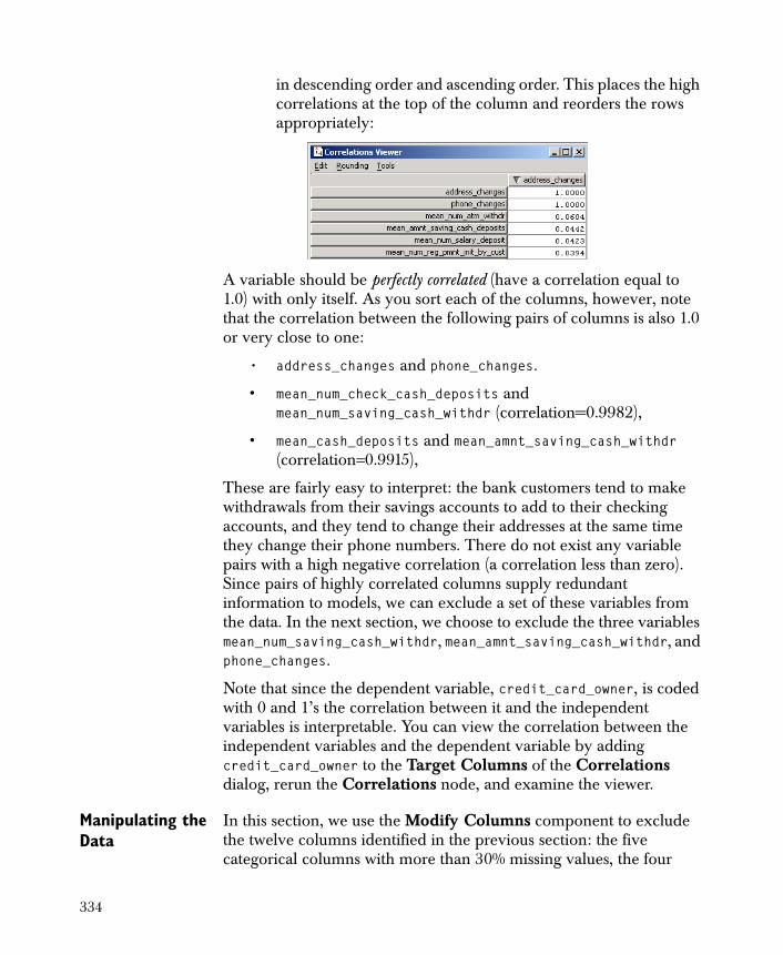
in descending order and ascending order. This places the high correlations at the top of the column and reorders the rows appropriately:
A variable should be perfectly correlated (have a correlation equal to 1.0) with only itself. As you sort each of the columns, however, note that the correlation between the following pairs of columns is also 1.0 or very close to one:
• address_changes and phone_changes.
• mean_num_check_cash_deposits and mean_num_saving_cash_withdr (correlation=0.9982),
• mean_cash_deposits and mean_amnt_saving_cash_withdr (correlation=0.9915),
These are fairly easy to interpret: the bank customers tend to make withdrawals from their savings accounts to add to their checking accounts, and they tend to change their addresses at the same time they change their phone numbers. There do not exist any variable pairs with a high negative correlation (a correlation less than zero). Since pairs of highly correlated columns supply redundant information to models, we can exclude a set of these variables from the data. In the next section, we choose to exclude the three variables mean_num_saving_cash_withdr, mean_amnt_saving_cash_withdr, and phone_changes.
Note that since the dependent variable, credit_card_owner, is coded with 0 and 1’s the correlation between it and the independent variables is interpretable. You can view the correlation between the independent variables and the dependent variable by adding credit_card_owner to the Target Columns of the Correlations dialog, rerun the Correlations node, and examine the viewer.
Manipulating the Data
In this section, we use the Modify Columns component to exclude the twelve columns identified in the previous section: the five categorical columns with more than 30% missing values, the four
334
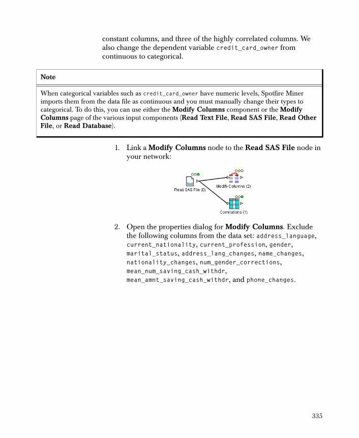
constant columns, and three of the highly correlated columns. We also change the dependent variable credit_card_owner from continuous to categorical.
1. Link a Modify Columns node to the Read SAS File node in your network:
2. Open the properties dialog for Modify Columns. Exclude the following columns from the data set: address_language, current_nationality, current_profession, gender, marital_status, address_lang_changes, name_changes, nationality_changes, num_gender_corrections, mean_num_saving_cash_withdr, mean_amnt_saving_cash_withdr, and phone_changes.
Note
When categorical variables such as credit_card_owner have numeric levels, Spotfire Miner imports them from the data file as continuous and you must manually change their types to categorical. To do this, you can use either the Modify Columns component or the Modify Columns page of the various input components (Read Text File, Read SAS File, Read Other File, or Read Database).
335
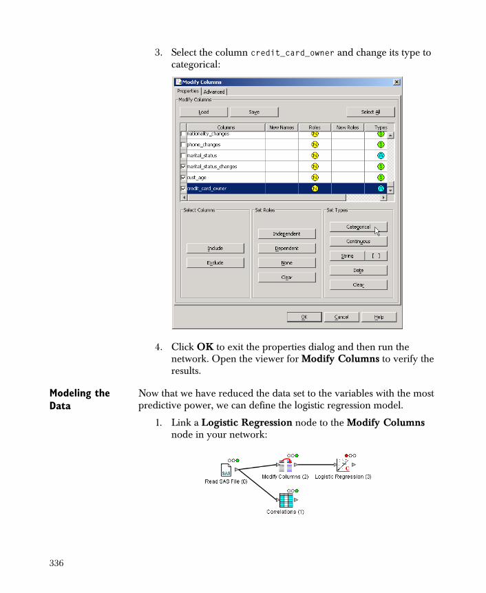
3. Select the column credit_card_owner and change its type to categorical:
4. Click OK to exit the properties dialog and then run the network. Open the viewer for Modify Columns to verify the results.
Modeling the Data
Now that we have reduced the data set to the variables with the most predictive power, we can define the logistic regression model.
1. Link a Logistic Regression node to the Modify Columns node in your network:
336
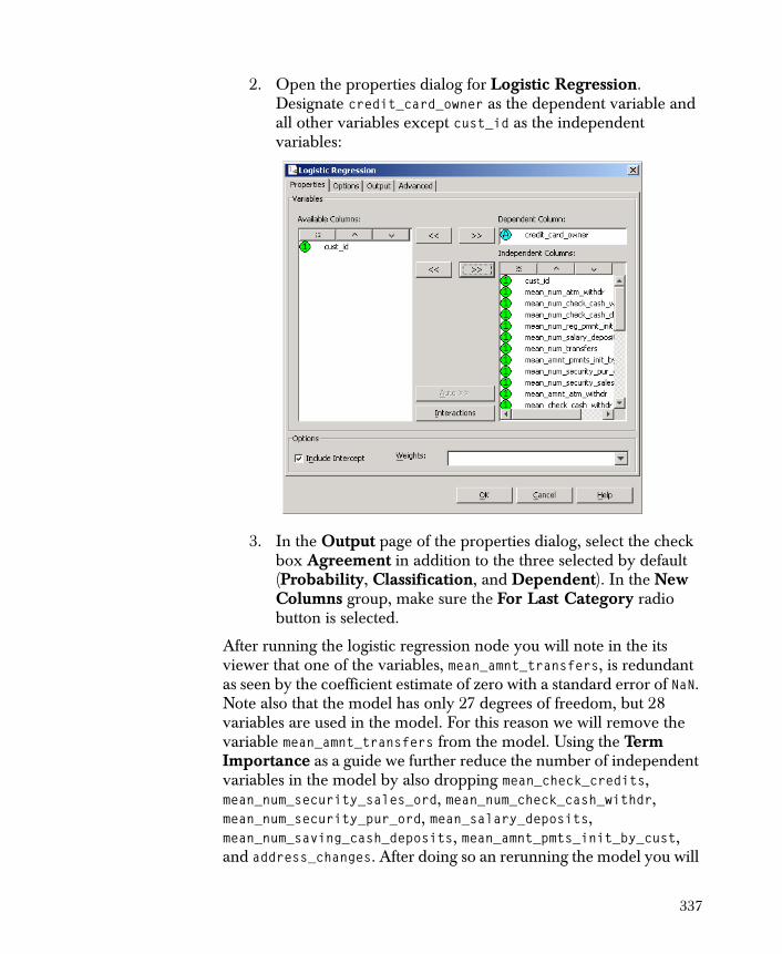
2. Open the properties dialog for Logistic Regression. Designate credit_card_owner as the dependent variable and all other variables except cust_id as the independent variables:
3. In the Output page of the properties dialog, select the check box Agreement in addition to the three selected by default (Probability, Classification, and Dependent). In the New Columns group, make sure the For Last Category radio button is selected.
After running the logistic regression node you will note in the its viewer that one of the variables, mean_amnt_transfers, is redundant as seen by the coefficient estimate of zero with a standard error of NaN. Note also that the model has only 27 degrees of freedom, but 28 variables are used in the model. For this reason we will remove the variable mean_amnt_transfers from the model. Using the Term Importance as a guide we further reduce the number of independent variables in the model by also dropping mean_check_credits, mean_num_security_sales_ord, mean_num_check_cash_withdr, mean_num_security_pur_ord, mean_salary_deposits, mean_num_saving_cash_deposits, mean_amnt_pmts_init_by_cust, and address_changes. After doing so an rerunning the model you will
337
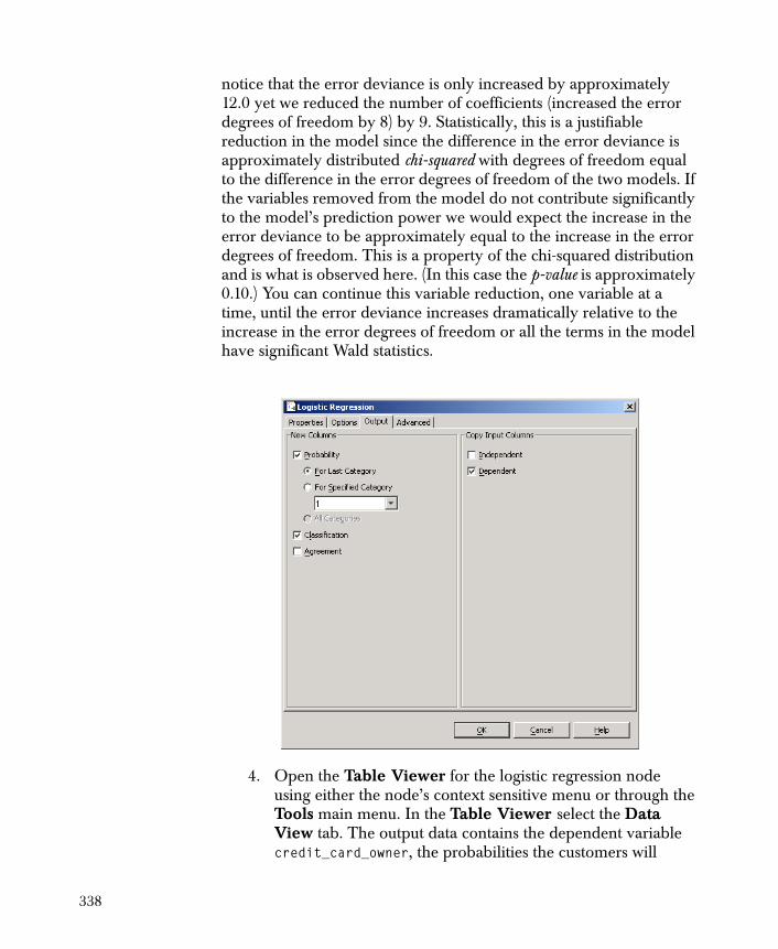
notice that the error deviance is only increased by approximately 12.0 yet we reduced the number of coefficients (increased the error degrees of freedom by 8) by 9. Statistically, this is a justifiable reduction in the model since the difference in the error deviance is approximately distributed chi-squared with degrees of freedom equal to the difference in the error degrees of freedom of the two models. If the variables removed from the model do not contribute significantly to the model’s prediction power we would expect the increase in the error deviance to be approximately equal to the increase in the error degrees of freedom. This is a property of the chi-squared distribution and is what is observed here. (In this case the p-value is approximately 0.10.) You can continue this variable reduction, one variable at a time, until the error deviance increases dramatically relative to the increase in the error degrees of freedom or all the terms in the model have significant Wald statistics.
4. Open the Table Viewer for the logistic regression node using either the node’s context sensitive menu or through the Tools main menu. In the Table Viewer select the Data View tab. The output data contains the dependent variable credit_card_owner, the probabilities the customers will
338
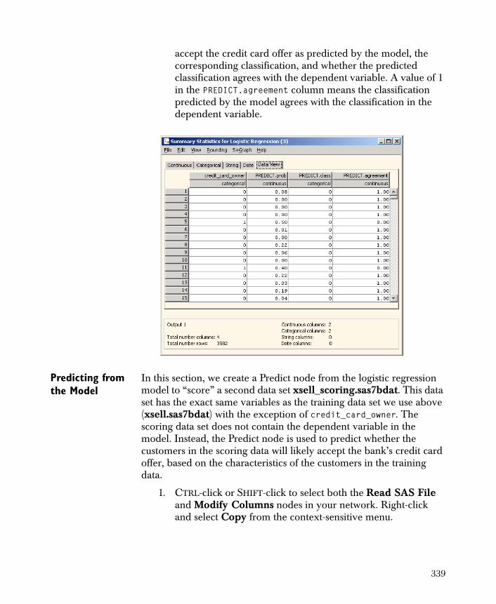
accept the credit card offer as predicted by the model, the corresponding classification, and whether the predicted classification agrees with the dependent variable. A value of 1 in the PREDICT.agreement column means the classification predicted by the model agrees with the classification in the dependent variable.
Predicting from the Model
In this section, we create a Predict node from the logistic regression model to “score” a second data set xsell_scoring.sas7bdat. This data set has the exact same variables as the training data set we use above (xsell.sas7bdat) with the exception of credit_card_owner. The scoring data set does not contain the dependent variable in the model. Instead, the Predict node is used to predict whether the customers in the scoring data will likely accept the bank’s credit card offer, based on the characteristics of the customers in the training data.
1. CTRL-click or SHIFT-click to select both the Read SAS File and Modify Columns nodes in your network. Right-click and select Copy from the context-sensitive menu.
339
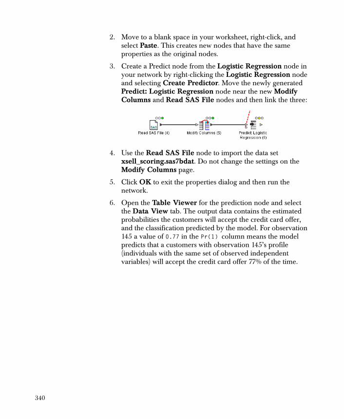
2. Move to a blank space in your worksheet, right-click, and select Paste. This creates new nodes that have the same properties as the original nodes.
3. Create a Predict node from the Logistic Regression node in your network by right-clicking the Logistic Regression node and selecting Create Predictor. Move the newly generated Predict: Logistic Regression node near the new Modify Columns and Read SAS File nodes and then link the three:
4. Use the Read SAS File node to import the data set xsell_scoring.sas7bdat. Do not change the settings on the Modify Columns page.
5. Click OK to exit the properties dialog and then run the network.
6. Open the Table Viewer for the prediction node and select the Data View tab. The output data contains the estimated probabilities the customers will accept the credit card offer, and the classification predicted by the model. For observation 145 a value of 0.77 in the Pr(1) column means the model predicts that a customers with observation 145’s profile (individuals with the same set of observed independent variables) will accept the credit card offer 77% of the time.
340

Technical Details
This section gives a brief overview to the fitting algorithm implemented in the Logistic Regression component.
The parameter estimates computed by the Spotfire Miner Logistic Regression component are maximum likelihood estimates produced by iteratively re-weighted least-squares (IRLS). This is a standard, well-understood technique for fitting logistic regression models. Essentially, the log-likelihood is maximized by solving the score equations:
As in Equation (7.2), the terms here are the coefficients and is the dependent variable. For logistic regression models, these score equations are nonlinear in and must therefore be solved iteratively, specifically using iteratively re-weighted least squares. For additional details, see Chambers and Hastie (1992) or McCullagh and Nelder (1989).
. (7.3)
l β y,( )
∂l β Y,( ) ∂β⁄ 0=
β Y
β
341
If weights are supplied, then the deviance for observation i is
, where is the user-
supplied weight. is the estimate of the probability at the current
iteration. The weights used in iteratively re-weighted least squares is
.
The fitting options available in the Advanced page of the Logistic Regression properties dialog control the convergence tolerance and maximum number of iterations Spotfire Miner computes in searching for the optimal coefficient estimates. There are three stopping criteria for the search algorithm: coefficient convergence, relative function convergence, and exceeding the maximum number of iterations. Convergence of the coefficient estimates of a logistic regression model is never guaranteed. A set of unique coefficient estimates might not exist if extreme linear relationships exist between your independent variables (the variables aren’t really independent). Moreover, it is possible that for some combination of your independent variables, the predicted probability is approaching zero or one. In this case one or more of the estimated coefficients will be moving toward plus or minus infinity and, therefore, never converge. For both of these situations, however, the predicted values will still tend to converge and an alternative stopping criterion, based on a measure of discrepancy used in logistic regression called the deviance, will terminate the search and a “relative function convergence” warning message is issued. If your interest is only in prediction, then relative function convergence is sufficient for your needs. Relative function convergence could muddle any interpretation of how the independent variables effect the dependent variable’s outcome. If neither the coefficient nor deviance has converged within the specified maximum number of iterations, the search is terminated with an “exceeded maximum number of iterations” warning. By default, the Maximum Iterations option is 10 and the Convergence Tolerance is 0.0001
The deviance is a measure of discrepancy between the predicted probabilities and the observed dependent variable and is the logarithm of the ratio of likelihoods. The simplest model is the null model and it uses the observed mean of the dependent variable (coded as zeros and ones) as the predicted probability for all observations. This model is an oversimplification and has the smallest likelihood
wi yi μiˆlog⋅ 1 yi–( ) 1 μi
ˆ–( )log⋅+( )⋅ wi
μiˆ
wi μiˆ 1 μi
ˆ–( )⋅ ⋅
342
achievable. A full model is a model that gives a perfect fit to the data, and the maximum achievable likelihood, so that the predicted probabilities are equal to the 0-1 coding of the dependent variable. The discrepancy of a fit is proportional to twice the difference between the maximum log likelihood achievable and that of the model being investigated.
The least-squares step in each iteration is computed by the technique implemented in the Linear Regression component. This method does not require all data to be in memory and instead is designed to update incrementally as more chunks of data are read in. For details, see the section Algorithm Specifics on page 424. In addition, the levels in categorical variables are coded in the same manner they are in the Linear Regression component; see the section The Coding of Levels in Categorical Variables on page 425.
343
CLASSIFICATION TREES
Classification trees are tree-based models that provide a simple yet powerful way to predict a categorical response based on a collection of predictor variables. The data are recursively partitioned into two groups based on predictor (independent) variables. This is repeated until the response (dependent) variable is homogenous. The sequence of splits of the predictor variables can be displayed as a binary tree, hence the name.
This section discusses classification trees at a high level, describes the properties for the Classification Tree component, provides general guidance for interpreting the model output and the information contained in the viewer, and gives a full example for illustration. Unless otherwise specified, all screen shots in this section use variables from the vetmailing.txt data set, which is stored as a text file in the examples folder under your Spotfire Miner installation directory.
Background Here, we provide the background necessary for understanding the options available for Spotfire Miner classification trees. This section is not designed to be a complete reference for the field of classification trees, however. There are many resources available that give broad overviews of the subject; see Breiman, Friedman, Olshen, & Stone (1984), Ripley (1996), or Hastie, Tibshirani, & Friedman (2001) for a general treatment.
A classification tree can be described as a series of rules. For a response and set of predictors , , , , a classification tree rule would be of the form:
if and
then is most likely category 2
The simplicity of the model display and prediction rules make classification trees an attractive data mining tool. Other advantages of tree models include:
• Invariance to monotone re-expression of the predictor variables
y x1 x2 … xp
x1 23< x2 A B{ , }∈
y
344
• Can easily capture nonlinear behavior in a predictor as well as interactions among predictors
• Unlike logistic regression, can model categorical response variables with more than two levels
Growing a Tree Trees are grown by a greedy algorithm. To find the first split at the root of the tree, every possible binary split for each predictor variable is considered, and a figure-of-merit is computed for each of these splits. The training data are then partitioned into two sets at the split that gave the best figure-of-merit over all predictor variables and all possible splits. The figure-of-merit and what is considered “best” are described below. The algorithm is now repeated on each of the two partitions of the data. The splitting continues until the growth limits (minimum figure-of-merit, number of points in a split, or others) are reached. The last partitions are called leaf or terminal nodes.
Each terminal node is represented by either a single class or a vector of probabilities, determined by the training set observations in the node. The single class is the class which occurs most frequently in the node. The estimated probabilities are the proportions of each class in the node.
To predict the response variable given values for predictor variables, an observation is “dropped down the tree”: at each node, the split determines whether the observation goes right or left. Finally it ends up at a terminal node. The prediction is the representation for that node.
For example, if the observation you are trying to predict ends up in a terminal node that consists of training set responses of
Red, Red, Red, Green, Blue
then the predicted probabilities would be
Pr(Red) = 3/5, Pr(Green) = 1/5, Pr(Blue) = 1/5
and the predicted class would be Red.
Pruning a Tree Depending on the growth limits, you can grow a very extensive tree that will actually reproduce the observed response variables (each unique observation ends up in its own terminal node). Such trees are of little value in predicting new observations; the tree model has
345
overfitted the training data. To prevent such behavior, a technique called pruning is applied to the tree—nodes that do not significantly improve the fit are pruned off. Usually, some form of cross-validation is used to decide which nodes to prune.
Ensemble Trees Recent research results have shown that combining the results from multiple trees fit to the same data can give better predictions than a single tree. These combinations of trees are called ensembles.
Several methods have been developed for computing multiple trees. Bagging (Breiman, 1996) uses the resampling idea of bootstrapping to draw multiple samples with replacement from the original data. Trees are fit on each sample, and the predictions are the average of the predictions from all the trees. The trees are usually grown quite deep and not pruned back. The averaging across deep trees, each computed on a slightly different set of observations, leads to better predictions than any single tree.
Another ensemble method is boosting (Schapire, 1990). Like bagging, it resamples the data but uses weighted sampling, giving more weight to observations that have been difficult to predict in the earlier trees.
Spotfire Miner uses a modification of the bagging idea to fit ensembles of trees on large data sets. Rather than bootstrapping from a single sample of data, Spotfire Miner considers each block or chunk of data read in from the pipeline as a type of bootstrap sample and fits a tree to that chunk of data. Rather than keeping all the trees to average over, only the K best trees are kept, where K is user-specified and “best” is chosen by a form of cross-validation.
Trees in Spotfire Miner
Spotfire Miner gives you the option of fitting a single tree or an ensemble of trees. Often, data mining is done on very large data sets. The tree methods in Spotfire Miner have been developed to handle this.
A single tree representation might be desired as a concise description of the data. This representation is easily understood by people not familiar with data mining methods. For a single tree, you can specify the maximum number of rows to use in fitting the tree. If the total number of observations is greater than this, a random sample from all the data, of the size you specify, is used. Options are available for cross-validation and pruning on a single tree.
346
For the best predictions, an ensemble tree usually performs better than a single tree. For an ensemble tree, you can specify how many trees to keep and how many observations to use in each tree.
The underlying tree-fitting algorithm in Spotfire Miner is based on the recursive partitioning code called RPART by Therneau and Atkinson (1997).
A Note on Missing Values
Missing values in the predictors and the response are dropped when fitting a tree. During prediction, missing values are allowed in the predictors. For a particular observation, if a prediction can be computed using the available non-missing predictors, then a valid prediction is returned. If the tree requires a predictor and its value is missing, then a missing value (NaN) is output as the prediction.
At each categorical split, the tree checks whether the observation has a level in the set of levels for the left side of the split; otherwise, it goes to the right side of the split. The algorithm goes to the right side of the split whenever a “new” level is seen.
347
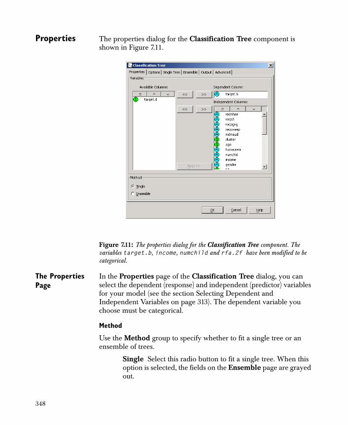
Properties The properties dialog for the Classification Tree component is shown in Figure 7.11.
The Properties Page
In the Properties page of the Classification Tree dialog, you can select the dependent (response) and independent (predictor) variables for your model (see the section Selecting Dependent and Independent Variables on page 313). The dependent variable you choose must be categorical.
Method
Use the Method group to specify whether to fit a single tree or an ensemble of trees.
Single Select this radio button to fit a single tree. When this option is selected, the fields on the Ensemble page are grayed out.
Figure 7.11: The properties dialog for the Classification Tree component. The variables target.b, income, numchild and rfa.2f have been modified to be categorical.
348
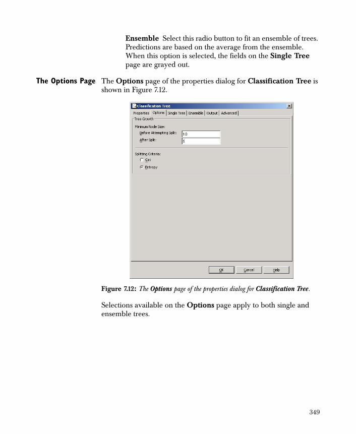
Ensemble Select this radio button to fit an ensemble of trees. Predictions are based on the average from the ensemble. When this option is selected, the fields on the Single Tree page are grayed out.
The Options Page The Options page of the properties dialog for Classification Tree is shown in Figure 7.12.
Selections available on the Options page apply to both single and ensemble trees.
Figure 7.12: The Options page of the properties dialog for Classification Tree.
349
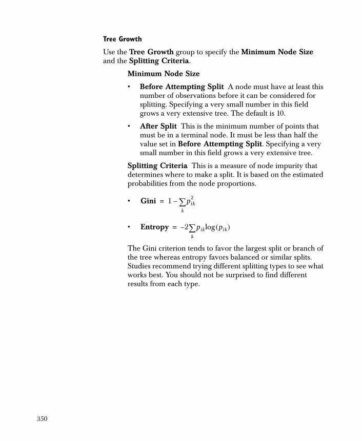
Tree Growth
Use the Tree Growth group to specify the Minimum Node Size and the Splitting Criteria.
Minimum Node Size
• Before Attempting Split A node must have at least this number of observations before it can be considered for splitting. Specifying a very small number in this field grows a very extensive tree. The default is 10.
• After Split This is the minimum number of points that must be in a terminal node. It must be less than half the value set in Before Attempting Split. Specifying a very small number in this field grows a very extensive tree.
Splitting Criteria This is a measure of node impurity that determines where to make a split. It is based on the estimated probabilities from the node proportions.
•
•
The Gini criterion tends to favor the largest split or branch of the tree whereas entropy favors balanced or similar splits. Studies recommend trying different splitting types to see what works best. You should not be surprised to find different results from each type.
Gini 1 pik2
k–=
Entropy 2 pik pik( )logk–=
350
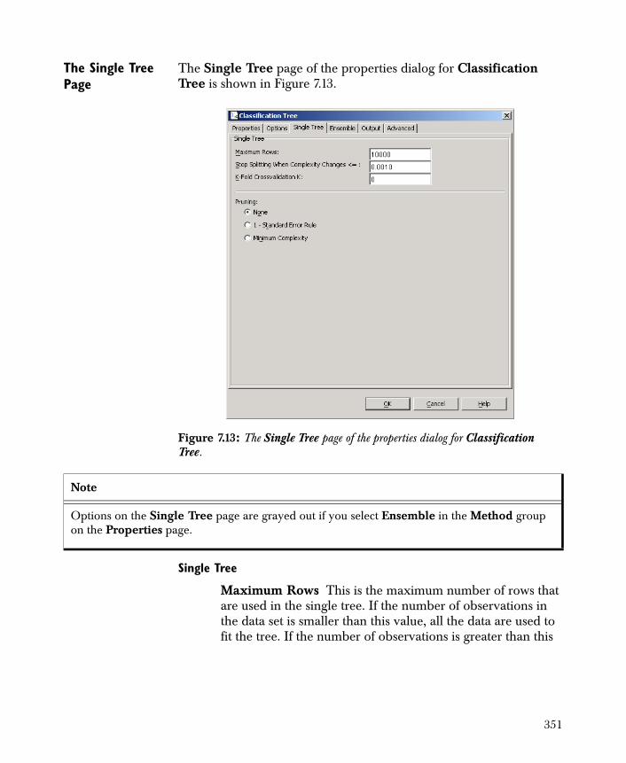
The Single Tree Page
The Single Tree page of the properties dialog for Classification Tree is shown in Figure 7.13.
Single Tree
Maximum Rows This is the maximum number of rows that are used in the single tree. If the number of observations in the data set is smaller than this value, all the data are used to fit the tree. If the number of observations is greater than this
Figure 7.13: The Single Tree page of the properties dialog for Classification Tree.
Note
Options on the Single Tree page are grayed out if you select Ensemble in the Method group on the Properties page.
351

value, then a random sample from all the data is drawn, and the single tree is fit on this sample. If this value is set too large, the data might not fit in memory, and the tree cannot be fit.
Stop Splitting When Complexity Changes <= Complexity is a value between 0 and 1 that measures how good the current tree is relative to a more complex (more nodes) tree. See Ripley (1996) Chapter 7. This value, along with the Minimum Node Size settings on the Options page, determines how deep the tree is. Specifying a smaller value results in a deeper tree. The default value is less than or equal to 0.0010.
K-Fold Crossvalidation K Specifying an integer value greater than 1 in this field causes cross-validation to be performed. The data are divided into K equal size groups. For each group, the remaining (K-1) groups are used to fit a tree, and this tree is used to predict the left-out group. This gives a cross-validated estimate of prediction error that can be used to select the best size tree to return (pruning). Cross-validation involves fitting K different trees; the computation time is considerably longer than fitting just a single tree.
Pruning
• None No pruning is done.
• 1 - Standard Error Rule Select the tree that is within 1 standard error of the minimum cross-validated error. This can only be selected if K-Fold Crossvalidation is performed.
• Minimum Complexity The tree with the minimum cross-validated error is returned. This can only be selected if K-Fold Crossvalidation is performed.
Note
The Maximum Rows value automatically becomes the node’s Rows Per Block setting on the Advanced page of the properties dialog.
352
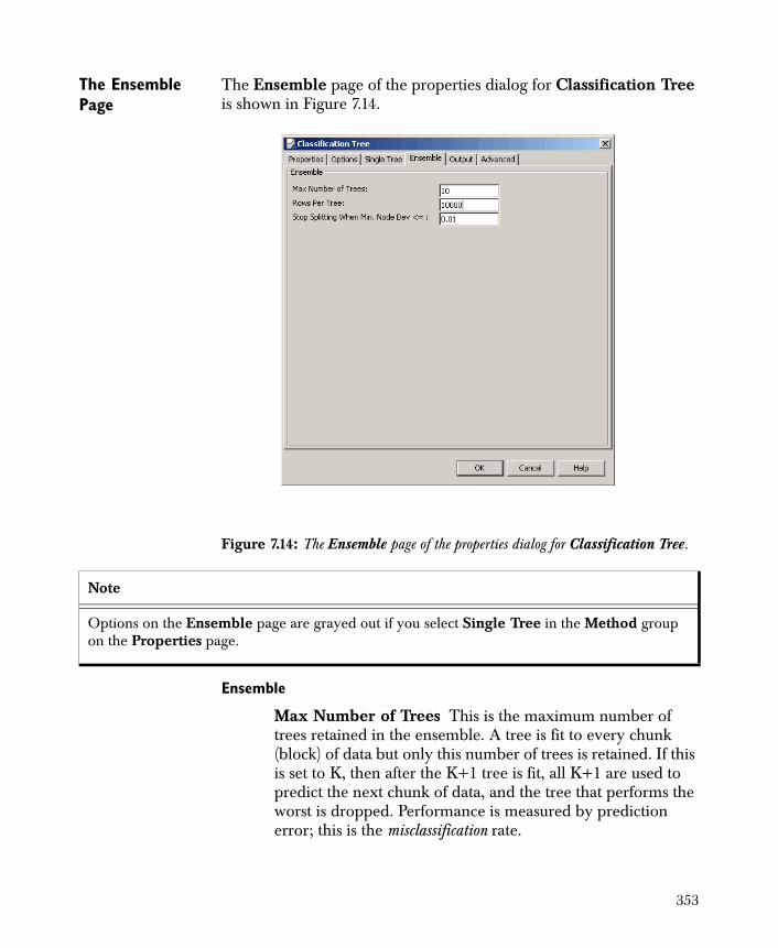
The Ensemble Page
The Ensemble page of the properties dialog for Classification Tree is shown in Figure 7.14.
Ensemble
Max Number of Trees This is the maximum number of trees retained in the ensemble. A tree is fit to every chunk (block) of data but only this number of trees is retained. If this is set to K, then after the K+1 tree is fit, all K+1 are used to predict the next chunk of data, and the tree that performs the worst is dropped. Performance is measured by prediction error; this is the misclassification rate.
Figure 7.14: The Ensemble page of the properties dialog for Classification Tree.
Note
Options on the Ensemble page are grayed out if you select Single Tree in the Method group on the Properties page.
353

Rows Per Tree This is the number of observations used in each tree.
Stop Splitting When Min. Node Dev <= This value, along with the Minimum Node Size settings on the Options page, controls how deep the tree is grown. Making this value smaller results in a deeper tree. The Complexity value is not used since Complexity is more expensive to compute. Complexity is needed for pruning, but pruning is not done for ensemble trees.
The Output Page The Output page of the properties dialog for Classification Tree is shown in Figure 7.15.
Note
The Rows Per Tree value automatically becomes the node’s Rows Per Block setting on the Advanced page of the properties dialog.
Figure 7.15: The Output page of the Classification Tree dialog.
354
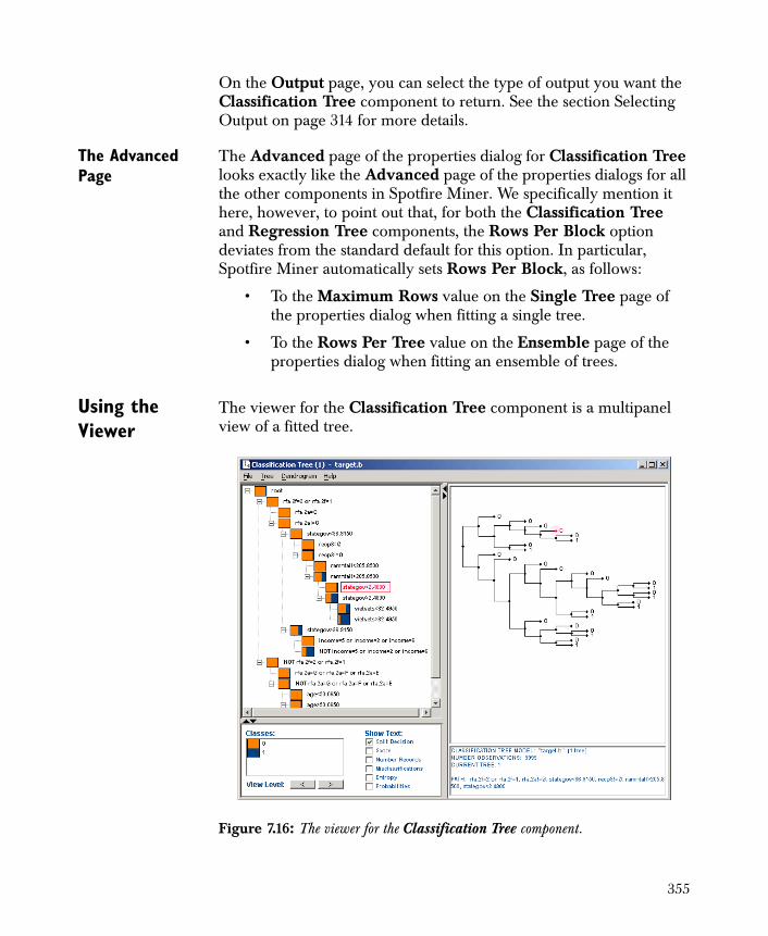
On the Output page, you can select the type of output you want the Classification Tree component to return. See the section Selecting Output on page 314 for more details.
The Advanced Page
The Advanced page of the properties dialog for Classification Tree looks exactly like the Advanced page of the properties dialogs for all the other components in Spotfire Miner. We specifically mention it here, however, to point out that, for both the Classification Tree and Regression Tree components, the Rows Per Block option deviates from the standard default for this option. In particular, Spotfire Miner automatically sets Rows Per Block, as follows:
• To the Maximum Rows value on the Single Tree page of the properties dialog when fitting a single tree.
• To the Rows Per Tree value on the Ensemble page of the properties dialog when fitting an ensemble of trees.
Using the Viewer
The viewer for the Classification Tree component is a multipanel view of a fitted tree.
Figure 7.16: The viewer for the Classification Tree component.
355
The top right panel displays the tree structure in a dendrogram. From the Dendrogram menu at the top on the viewer, you can select Map Split Importance to Depth. Doing so redraws the tree with the depth of the branches from a fit proportional to the change in the fitting criteria between the node and the sum of the two children nodes. This provides a quick visual view of the importance of each split.
The top left panel is an expandable, hierarchical view of the tree. This view is linked to the dendrogram view so that clicking on nodes in either view highlights that node in the other view. For classification trees, the nodes in the hierarchical view show the distribution of the classes in that node in a colored rectangle. Alternatively, from the Tree menu, you can set the display so the rectangle only displays the winner (the class with the largest proportion in that node). The tree view can be expanded or collapsed by making the appropriate selection from the Tree menu at the top of the viewer.
The bottom left panel controls what information is displayed in the hierarchical view. If a tree ensemble (multiple trees) was fit, then the slider at the bottom can be used to cycle through the views of the various trees.
The bottom right panel is an informational panel that describes the tree that is currently being viewed. When nodes are highlighted in either tree view, the path to that node is described here.
A summary description of the tree in HTML can be produced and viewed by selecting Display HTML from the Tree menu at the top of the viewer. In addition, a bar chart showing the importance of each predictor in the tree model can be drawn by selecting View Column Importance from the Tree menu. Importance for a predictor is measured in terms of how much the splits made for that predictor contribute to the total reduction in the fitting criterion. Finally, you can generate a tree comparison table by selecting Compare Trees from the Tree menu.
356
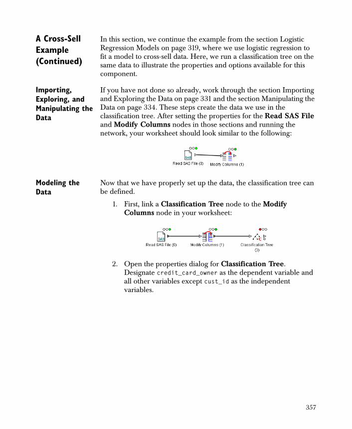
A Cross-Sell Example (Continued)
In this section, we continue the example from the section Logistic Regression Models on page 319, where we use logistic regression to fit a model to cross-sell data. Here, we run a classification tree on the same data to illustrate the properties and options available for this component.
Importing, Exploring, and Manipulating the Data
If you have not done so already, work through the section Importing and Exploring the Data on page 331 and the section Manipulating the Data on page 334. These steps create the data we use in the classification tree. After setting the properties for the Read SAS File and Modify Columns nodes in those sections and running the network, your worksheet should look similar to the following:
Modeling the Data
Now that we have properly set up the data, the classification tree can be defined.
1. First, link a Classification Tree node to the Modify Columns node in your worksheet:
2. Open the properties dialog for Classification Tree. Designate credit_card_owner as the dependent variable and all other variables except cust_id as the independent variables.
357
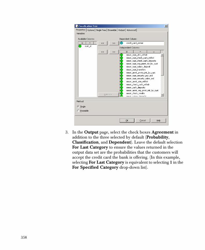
3. In the Output page, select the check boxes Agreement in addition to the three selected by default (Probability, Classification, and Dependent). Leave the default selection For Last Category to ensure the values returned in the output data set are the probabilities that the customers will accept the credit card the bank is offering. (In this example, selecting For Last Category is equivalent to selecting 1 in the For Specified Category drop-down list).
358
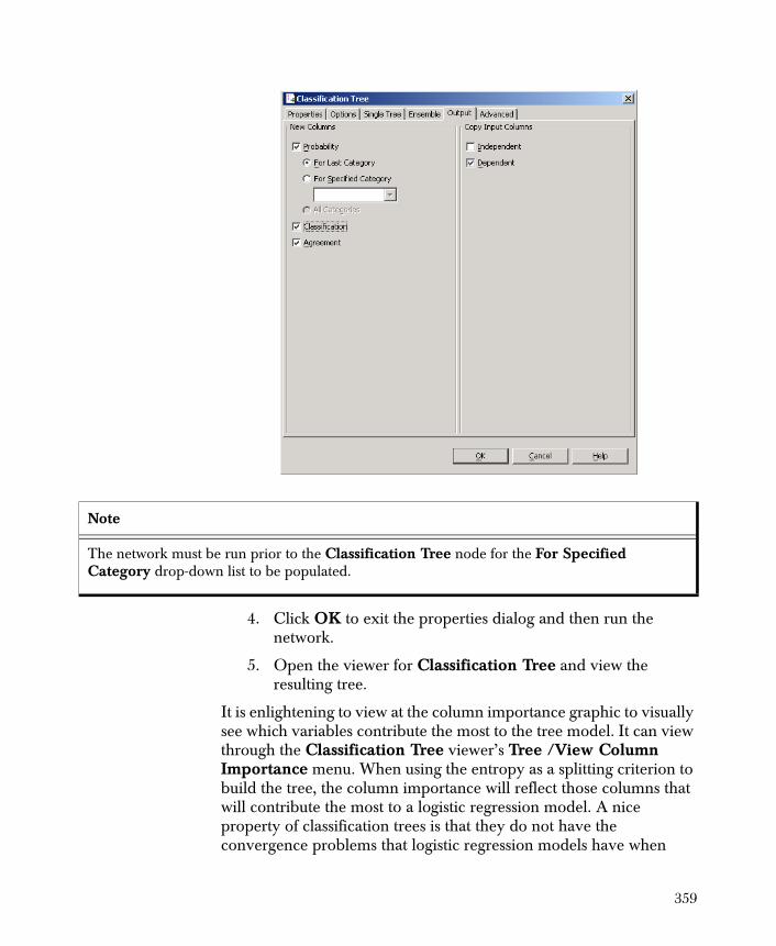
4. Click OK to exit the properties dialog and then run the network.
5. Open the viewer for Classification Tree and view the resulting tree.
It is enlightening to view at the column importance graphic to visually see which variables contribute the most to the tree model. It can view through the Classification Tree viewer’s Tree /View Column Importance menu. When using the entropy as a splitting criterion to build the tree, the column importance will reflect those columns that will contribute the most to a logistic regression model. A nice property of classification trees is that they do not have the convergence problems that logistic regression models have when
Note
The network must be run prior to the Classification Tree node for the For Specified Category drop-down list to be populated.
359
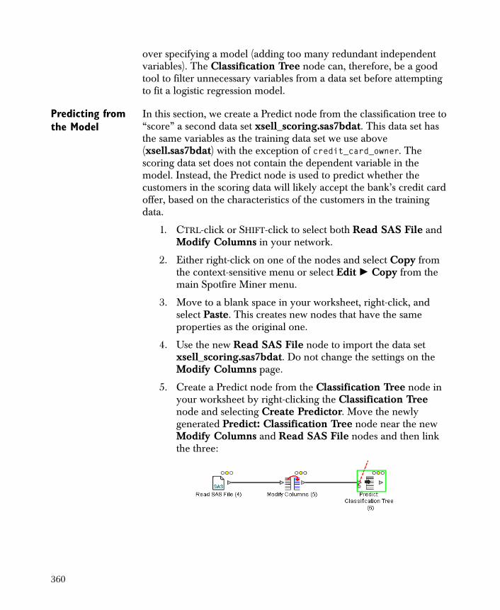
over specifying a model (adding too many redundant independent variables). The Classification Tree node can, therefore, be a good tool to filter unnecessary variables from a data set before attempting to fit a logistic regression model.
Predicting from the Model
In this section, we create a Predict node from the classification tree to “score” a second data set xsell_scoring.sas7bdat. This data set has the same variables as the training data set we use above (xsell.sas7bdat) with the exception of credit_card_owner. The scoring data set does not contain the dependent variable in the model. Instead, the Predict node is used to predict whether the customers in the scoring data will likely accept the bank’s credit card offer, based on the characteristics of the customers in the training data.
1. CTRL-click or SHIFT-click to select both Read SAS File and Modify Columns in your network.
2. Either right-click on one of the nodes and select Copy from the context-sensitive menu or select Edit � Copy from the main Spotfire Miner menu.
3. Move to a blank space in your worksheet, right-click, and select Paste. This creates new nodes that have the same properties as the original one.
4. Use the new Read SAS File node to import the data set xsell_scoring.sas7bdat. Do not change the settings on the Modify Columns page.
5. Create a Predict node from the Classification Tree node in your worksheet by right-clicking the Classification Tree node and selecting Create Predictor. Move the newly generated Predict: Classification Tree node near the new Modify Columns and Read SAS File nodes and then link the three:
360

6. Open the properties dialog for the Predict: Classification Tree node. In the Properties page, clear the Dependent check box, which is selected by default.
7. Click OK to exit the properties dialog and then run the network.
361
CLASSIFICATION NEURAL NETWORKS
A classification neural network is a “black-box” classification scheme for computing probabilities and predicting classes. The term “black-box” refers to the fact that there is little interpretable information about the relationships between the dependent and independent variables through the structure and estimated parameters of the model. The goal of this technique is to estimate the probabilities associated with each level based on the information in your data set. To use this technique, your dependent variable should be categorical with two or more levels.
This section discusses classification neural networks at a high level: it describes the properties for the Classification Neural Network component, provides general guidance for interpreting the output and the information contained in the viewer, and gives a full example for illustration. Unless otherwise specified, all screenshots in this section use variables from the glass.txt data set, stored as a text file in the examples folder under your Spotfire Miner installation directory, where the variable Type modified to the categorical data type.
Background Here, we provide the background necessary for understanding the options available for Spotfire Miner classification neural networks. This section is not designed to be a complete reference for the field of neural networks, however. There are many resources available that give broad overviews of the subject; see Hastie, Tibshirani, & Friedman (2001) or Ripley (1996) for a general treatment.
A classification neural network is a two-stage classification model. The main idea behind the technique is to first compute linear combinations of the independent variables, and then model the levels in the dependent variable as a nonlinear function of the
362

combinations. This is represented schematically in Figure 7.17. The outputs from the network are probabilities that each input pattern belongs to a particular class of the dependent variable.
In the middle set of nodes represents the linear combinations of the independent variables; the collection of nodes is called the hidden layer since it includes values that are not directly observable. It is possible to include up to three hidden layers in a Spotfire Miner classification neural network. Each layer adds another set of linear combinations of the outputs from the previous layer. If you include zero layers, the network collapses to a standard linear model.
The unknown parameters in a classification neural network are called weights ; they are simply the coefficients associated with the linear combinations. Schematically, these unknown parameters are the weights of the links in the diagram above. The neural network computes estimates for the weights by passing through the data multiple times, deriving different linear combinations, and updating the weights accordingly. Each pass through the data is called an epoch. In this way, the neural network “learns” from the data.
,
Figure 7.17: A diagram of a classification neural network. The independent variables are fed to the input nodes, through the hidden layer(s), to the output nodes. Each link in the diagram represents a linear combination. The output nodes return the predicted probabilities for the levels in the dependent variable.
Independen t V ariab le 2
Independen t V ariab le 3
Independen t V ariab le 4
363

Not visible in Figure 7.17 is the bias node. It has weights to each node in the hidden layers and the output nodes. These weights act as “intercepts” in the model.
Spotfire Miner supports five different methods for computing the weights in a classification neural network:
• Resilient propagation
• Quick propagation
• Delta-bar-delta
• Online
• Conjugate gradient
Reed and Marks (1999) discusses the mathematical derivations for each of these methods in detail; see also the section Technical Details on page 379.
364

Properties The properties dialog for the Classification Neural Network component is shown in Figure 7.18.
The Properties Page
In the Properties page of the Classification Neural Network dialog, you can select the dependent and independent variables for your model (see the section Selecting Dependent and Independent Variables on page 313). The dependent variable you choose must be categorical.
Viewer
Select the Show Error Graph During Run in the Viewer group. When you run the network, a small window displaying a plot of the error on the ordinate and the epoch (iteration) number on the abscissa. Below the graph is an Open Viewer and when clicked the Neural Networks Viewer is displayed.
Figure 7.18: The properties dialog for the Classification Neural Network component.
365
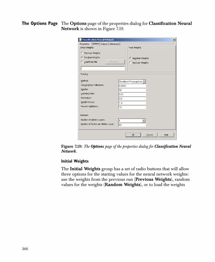
The Options Page The Options page of the properties dialog for Classification Neural Network is shown in Figure 7.19.
Initial Weights
The Initial Weights group has a set of radio buttons that will allow three options for the starting values for the neural network weights: use the weights from the previous run (Previous Weights), random values for the weights (Random Weights), or to load the weights
Figure 7.19: The Options page of the properties dialog for Classification Neural Network.
366

from a file (Load from File). If you choose Load from File, click the Browse button to navigate to the file that was saved during a previous training session.
Final Weights
A neural network is an overspecified model in that there rarely exists a unique set of weights that minimizes the objective function and it is possible that a set of new weights in the training process will increase the objective function. Because of this, two neural networks are retained in memory: the current neural network and the neural network that achieved the lowest objective function. On completion of a run only one copy is retained and the Final Weights radio buttons allow the user to choose which set of weights to keep. Pressing the Use Best Weights button will result in retaining the set of weights that achieved the smallest error. Press the Use Last Weights button to use the set of weights on the last epoch regardless of whether it had the smallest error or not.
Training
The Training group contains options for controlling the way Spotfire Miner trains the classification neural network on your set of independent variables.
Method Select one of the five supported methods for computing the weights from the Method drop-down list.
Convergence Tolerance This is one of the stopping criteria for the iterative training algorithm. Spotfire Miner makes successive passes through your data until either the maximum number of epochs is exceeded, the relative change in the objective function for the optimization algorithm is below some tolerance, or the user terminates the training session through the Neural Network Viewer. Decreasing the
Warning
The Load from File option for the initial weights of a neural network will only work when the specified file is saved by a Spotfire Miner’s Neural Network Viewer and contains a neural network that has the identical network configuration. The Spotfire Miner’s Neural Network Viewer allows a user to save a “snap shot” of a neural network during the weight training so that a user might return to that state of the optimization at a latter time.
367
convergence tolerance might provide more accurate predictions but requires additional resources from your machine.
Epochs This option determines the maximum number of passes the algorithm makes through the data.
Learning Rate This is a parameter typically small, with a default value of 0.01, and it must be in the range of ). This is the step size scale for the steepest descent optimization algorithm. It affects how quickly the neural network learns from your data and converges to a set of probabilities and predictions; smaller values imply a slower learning rate while larger values imply a quicker one. There is a trade-off between speed and reliability, however. A learning rate that is too large for a particular network might converge quickly, but to an unreliable solution.
Momentum This is a parameter that must be in the range of 0 to 1. Its effect is to smooth the trajectory of the algorithm as it iteratively computes weights for the neural network, speeding up the computations in some instances. Momentum tends to amplify the effective learning rate, so large values for the Momentum parameter usually pair best with smaller Learning Rate values.
Weight Decay This is a parameter that must be in the range of 0 to 1; a value of 0 indicates no weight decay while a value of 1 indicates full weight decay. This parameter helps the algorithm dynamically adjust the complexity of the network by gradually shifting the weight values toward zero in each successive pass through the data. By encouraging small weights, the weight decay acts as a regularizer, smoothing the functions involved in the computations.
Percent Validation. Enter the percentage of rows used for validating the training model. This determines the number of rows from the training data that is randomly sampled from each chunk of data. On each pass through the data, the (pseudo) random number generator’s seed is reset to ensure that the same observations are used for validation.
0 1,[ ]
368

Network
The Network group contains options for controlling the size and complexity of the classification neural network.
Number of Hidden Layers Select 0, 1, 2, or 3 from this drop-down list. Single-layer networks are usually sufficient for most problems, but there are instances where two- or three-layer networks compute classifications more reliably and efficiently than single-layer ones.
Number of Nodes per Hidden Layer Type the number of nodes you want in the text box; this value determines the number of nodes in each hidden layer of your network. Generally speaking, a large number of nodes can fit your data exactly but tends to require impractical amounts of time and memory to compute. In addition, a large number of nodes can cause the neural network to become overtrained , where the network fits your data exactly but does not generalize well to compute predictions for your scoring data.
369
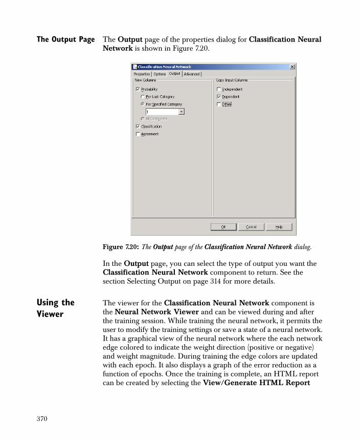
The Output Page The Output page of the properties dialog for Classification Neural Network is shown in Figure 7.20.
In the Output page, you can select the type of output you want the Classification Neural Network component to return. See the section Selecting Output on page 314 for more details.
Using the Viewer
The viewer for the Classification Neural Network component is the Neural Network Viewer and can be viewed during and after the training session. While training the neural network, it permits the user to modify the training settings or save a state of a neural network. It has a graphical view of the neural network where the each network edge colored to indicate the weight direction (positive or negative) and weight magnitude. During training the edge colors are updated with each epoch. It also displays a graph of the error reduction as a function of epochs. Once the training is complete, an HTML report can be created by selecting the View/Generate HTML Report
Figure 7.20: The Output page of the Classification Neural Network dialog.
370

menu item from the Neural Network Viewer. If you are interested only in the probabilities and classifications predicted by the model, you can skip this section.
371
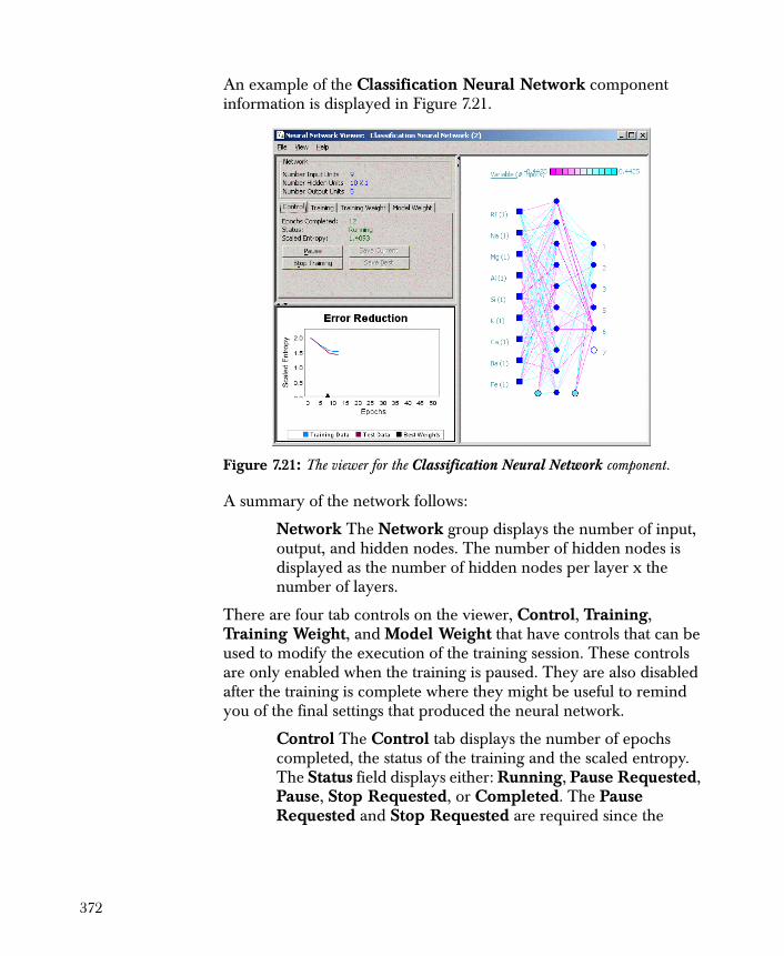
An example of the Classification Neural Network component information is displayed in Figure 7.21.
A summary of the network follows:
Network The Network group displays the number of input, output, and hidden nodes. The number of hidden nodes is displayed as the number of hidden nodes per layer x the number of layers.
There are four tab controls on the viewer, Control, Training, Training Weight, and Model Weight that have controls that can be used to modify the execution of the training session. These controls are only enabled when the training is paused. They are also disabled after the training is complete where they might be useful to remind you of the final settings that produced the neural network.
Control The Control tab displays the number of epochs completed, the status of the training and the scaled entropy. The Status field displays either: Running, Pause Requested, Pause, Stop Requested, or Completed. The Pause Requested and Stop Requested are required since the
Figure 7.21: The viewer for the Classification Neural Network component.
372

execution of the computations and the viewer are on separate execution threads and communication between the threads is not done until after a full pass through the data is complete.
The Control tab has the controls to pause, stop (terminate) and resume, as well as the controls for saving current or best neural networks. Once the network is paused, the controls in the Training, Training Weight, and Model Weight tabs are enabled as well as the Save Current and Save Best buttons in the Control tab.
The Save buttons in the Control tab will either save the current network or the best network. During the training session at least two neural networks are kept in memory. These are the neural networks that have the lowest cross entropy and the current network. Generally, they are the same neural network, but it is possible that the current neural network has an entropy greater than the best.
Training The Training tab displays the current method of optimization, convergence tolerance, maximum number of epochs, learning rate, momentum, and weight decay.
In the Training tab, the optimization method can be changed where the choices are Resilient Propagation, Quick Propagation, Delta Bar Delta, Online and Conjugate Gradient. These methods are all described in Reed and Marks (1999). The momentum and weight decay options are not used in the Conjugate Gradient method and, instead of using an exact line search, the Conjugate Gradient method utilizes the learning rate parameter to control the step size and step halving is used, if necessary, to find step size that will lower the entropy. Generally, it is not a good idea to change the learning rate for the Resilient Propagation or Delta Bar Delta since they are adaptive learning rate techniques: Each weight has its own learning rate that is updated with each epoch. Modifying the learning rate in this case resets the learning rate for each weight to the new constant.
Training Weight Settings The Training Weight Settings tab has a set of three radio buttons that will allow jittering of the weights, load previous saved weights to reinstantiate a previous state, or to continue with the current weights (the default).
373
Jittering the weights might be helpful if it is suspected that the optimization is in a local minimum. When the Load From File radio button is selected, the Load button is enabled. Selecting the Load button will display the system Open File dialog.
The edges of the graphic display of the neural network are colored to give a visual display of each weight’s value. Use the Show weights by color checkbox to turn off the color display. This feature might be useful to in increasing speed since the weights do not need to be passed between the viewer and the computational code.
Model Weight Settings Use to determine which set of weights are to be retained at the end of the training session: the best weights, the last weights, or to display a Open File Dialog so that you can browse for a weights file.
A summary description of the neural network in HTML can be produced and viewed by selecting Display HTML from the View menu at the top of the viewer..
A Cross-Sell Example (Continued)
In this section, we continue the example from the section Logistic Regression Models on page 319, where we use logistic regression to fit a model to cross-sell data. Here, we run a classification neural network on the same data to illustrate the properties and options available for this component.
Importing, Exploring, and Manipulating the Data
If you have not done so already, work through the section Importing and Exploring the Data on page 331 and the section Manipulating the Data on page 334. These steps create the data we use in the classification neural network. After setting the properties for the Read SAS File and Modify Columns nodes in those sections and running the network, your worksheet should look similar to the following:
374
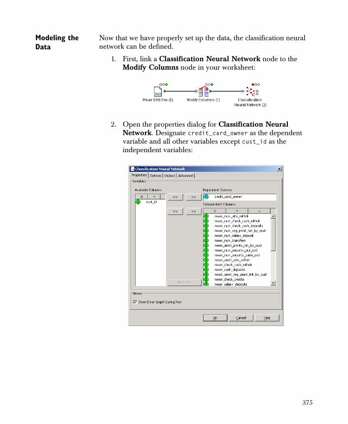
Modeling the Data
Now that we have properly set up the data, the classification neural network can be defined.
1. First, link a Classification Neural Network node to the Modify Columns node in your worksheet:
2. Open the properties dialog for Classification Neural Network. Designate credit_card_owner as the dependent variable and all other variables except cust_id as the independent variables:
375
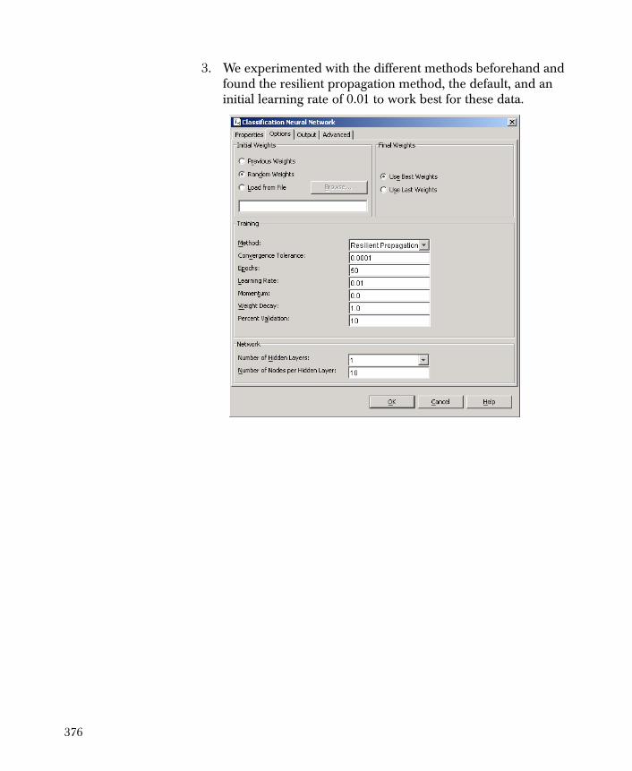
3. We experimented with the different methods beforehand and found the resilient propagation method, the default, and an initial learning rate of 0.01 to work best for these data.
376
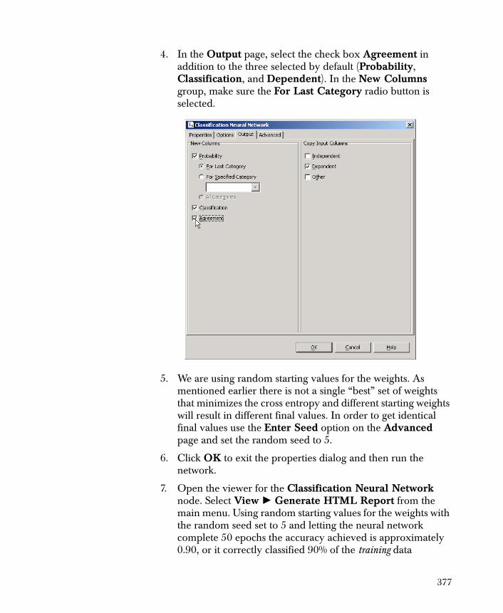
4. In the Output page, select the check box Agreement in addition to the three selected by default (Probability, Classification, and Dependent). In the New Columns group, make sure the For Last Category radio button is selected.
5. We are using random starting values for the weights. As mentioned earlier there is not a single “best” set of weights that minimizes the cross entropy and different starting weights will result in different final values. In order to get identical final values use the Enter Seed option on the Advanced page and set the random seed to 5.
6. Click OK to exit the properties dialog and then run the network.
7. Open the viewer for the Classification Neural Network node. Select View � Generate HTML Report from the main menu. Using random starting values for the weights with the random seed set to 5 and letting the neural network complete 50 epochs the accuracy achieved is approximately 0.90, or it correctly classified 90% of the training data
377
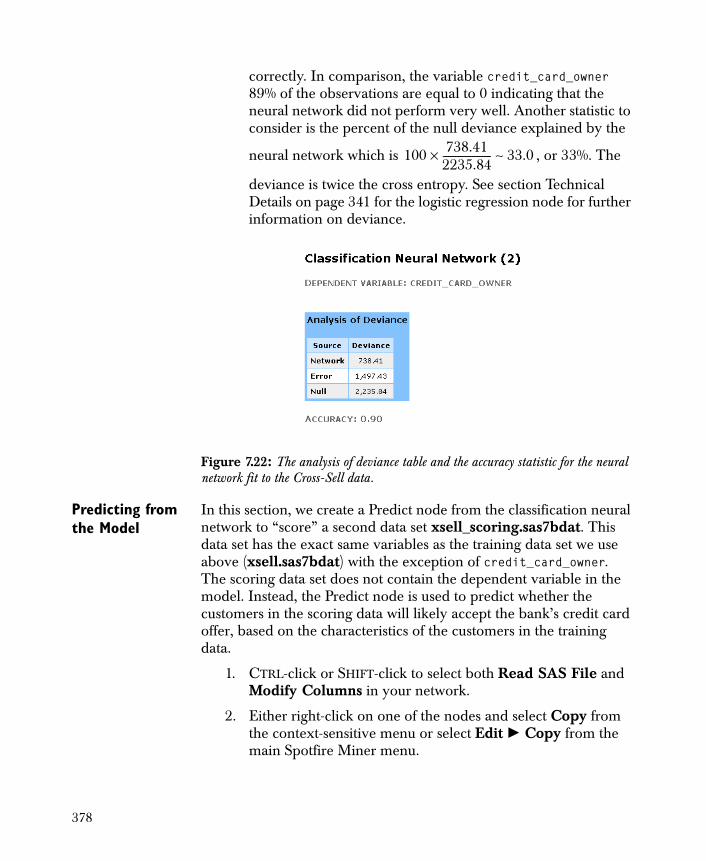
correctly. In comparison, the variable credit_card_owner 89% of the observations are equal to 0 indicating that the neural network did not perform very well. Another statistic to consider is the percent of the null deviance explained by the
neural network which is , or 33%. The
deviance is twice the cross entropy. See section Technical Details on page 341 for the logistic regression node for further information on deviance.
Predicting from the Model
In this section, we create a Predict node from the classification neural network to “score” a second data set xsell_scoring.sas7bdat. This data set has the exact same variables as the training data set we use above (xsell.sas7bdat) with the exception of credit_card_owner. The scoring data set does not contain the dependent variable in the model. Instead, the Predict node is used to predict whether the customers in the scoring data will likely accept the bank’s credit card offer, based on the characteristics of the customers in the training data.
1. CTRL-click or SHIFT-click to select both Read SAS File and Modify Columns in your network.
2. Either right-click on one of the nodes and select Copy from the context-sensitive menu or select Edit � Copy from the main Spotfire Miner menu.
Figure 7.22: The analysis of deviance table and the accuracy statistic for the neural network fit to the Cross-Sell data.
100 738.412235.84--------------------× 33.0∼
378
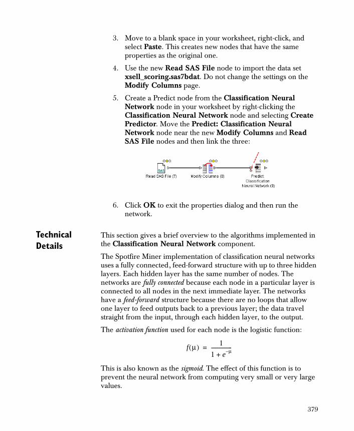
3. Move to a blank space in your worksheet, right-click, and select Paste. This creates new nodes that have the same properties as the original one.
4. Use the new Read SAS File node to import the data set xsell_scoring.sas7bdat. Do not change the settings on the Modify Columns page.
5. Create a Predict node from the Classification Neural Network node in your worksheet by right-clicking the Classification Neural Network node and selecting Create Predictor. Move the Predict: Classification Neural Network node near the new Modify Columns and Read SAS File nodes and then link the three:
6. Click OK to exit the properties dialog and then run the network.
Technical Details
This section gives a brief overview to the algorithms implemented in the Classification Neural Network component.
The Spotfire Miner implementation of classification neural networks uses a fully connected, feed-forward structure with up to three hidden layers. Each hidden layer has the same number of nodes. The networks are fully connected because each node in a particular layer is connected to all nodes in the next immediate layer. The networks have a feed-forward structure because there are no loops that allow one layer to feed outputs back to a previous layer; the data travel straight from the input, through each hidden layer, to the output.
The activation function used for each node is the logistic function:
This is also known as the sigmoid. The effect of this function is to prevent the neural network from computing very small or very large values.
f μ( ) 1
1 e μ–+-----------------=
379
The objective function Spotfire Miner minimizes in the optimization algorithm is the cross-entropy function:
Here, denotes the complete set of (unknown) weights, is the number of independent variables in the model, is the number of levels in the dependent variable, and is the activation function. Spotfire Miner makes successive passes through your data until either the maximum number of epochs is exceeded or the relative change in this objective function is below the convergence tolerance you set in the Options page of the properties dialog.
For a dependent variable with levels, there are output nodes in the neural network. Spotfire Miner disregards the last output node since it is redundant. Moreover, the softmax function is used to normalize the outputs:
This function ensures that . That is, it ensures the output
probabilities add to 1.
Learning Algorithms
Spotfire Miner supports five different learning algorithms for classification neural networks. Variations of back-propagation and batch learning are the primary methods; supported variants of batch learning include resilient propagation, delta-bar-delta, quick propagation, and online. You can also modify the batch learning method by adjusting the learning rate, momentum, and weight decay parameters in the Options page of the properties dialog.
The resilient propagation and delta-bar-delta algorithms are adaptive, in that each weight has its own learning rate that is adjusted at each epoch according to heuristic rules.
1. Resilient Propagation
R θ( ) yik fk xi( )( )logk 1=
K
i 1=
P
–=
θ P
K
f
K K 1–
gk x( ) exk
exj
j 1=
K
---------------=
gk x( )k 1=
380
In resilient propagation, each weight’s learning rate is adjusted by the signs of the gradient terms.
2. Delta-Bar-Delta
The delta-bar-delta algorithm uses an estimate of curvature that increases the learning rate linearly if the partial derivative with respect to the weight continues to maintain the same sign; the estimate decreases the learning rate exponentially if the derivative changes sign.
3. Quick Propagation
Quick propagation also uses weight decay and momentum but manipulates the partial derivatives differently. The algorithm approximates the error surface with a quadratic polynomial so that the update to the weights is the minimum of the parabola. Both the quick propagation and delta-bar-delta learning algorithms assume the weights are independent. In practice, however, the weights tend to be correlated.
4. Online
The online method updates the weights with each block of data. Instead of randomly picking observations from the data, it is assumed the data is ordered in a random fashion.
5. Conjugate Gradient
Spotfire Miner also provides the conjugate gradient optimization algorithm, but it uses an inexact line search and uses the learning rate to control the step size. An exact line search would require several passes through the data in order to determine the step size. While computing the gradient the neural network node is also evaluating the cross entropy of the model from the previous pass through the data. If the entropy has increased as a result of the step taken from the previous epoch the step is halved and the model is reevaluated. The algorithm will halve the step up to 5 times after which it will continue with the current step. Jittering the weights, available through the neural network viewer, might be a useful tool if the conjugate gradient algorithm is step halving. Moreover, since the learning rate is used to control the step size, it is advisable to start with a small learning rate in the beginning of the training session and perhaps increasing it as the training progresses. The initial learning rate should be inversely proportional to the size of the training data: the more rows in the training data the smaller the initial learning rate.
381

Reed and Marks (1999) give mathematical derivations for all five learning algorithms implemented in Spotfire Miner.
Initialization of Weights
Spotfire Miner provide three methods of initializing weights: uniform random values, weights from the previous learning run, or loading weights saved to a file from a previous learning run. When initializing weights to a node using random values, the range for the random values is , where is the number of inputs to a node. If you are going to initialize the weights from the previous run or from weights saved to a file it is imperative that the input variables, number of hidden layers, or the output variable are consistent with the current configuration.
2.4 k⁄– 2.4 k⁄,( ) k
382
NAIVE BAYES MODELS
Naive Bayes is a simple classification model based on Bayes’ rule for conditional probability. To use this technique, your dependent variable should be categorical with two or more levels and your independent variables must be categorical as well. The goal is to estimate the probabilities associated with each level of the dependent variable based on the information in your independent variables.
This section discusses Naive Bayes models at a high level, describes the properties for the Naive Bayes component, provides general guidance for interpreting the output and the information contained in the viewer, and gives a full example for illustration. All screenshots in this section use variables from the promoter.txt data set, which is stored as a text file in the examples folder under your Spotfire Miner installation directory.
Background Naive Bayes is a very simple classification technique that makes two assumptions about the independent variables in your model:
• They are equally important.
• Their influences on the dependent variable are independent from one another. For example, if your model includes independent variables for income and gender, this assumption implies the effect of income level on the dependent variable is the same for men and women.
These are not very realistic expectations given the nature of real-life data. Surprisingly, though, Naive Bayes has been shown in practice to perform as well as or better than more sophisticated techniques despite these assumptions. For independent variables that are highly correlated, however, the technique does not tend to perform well so some intelligent variable selection is needed before Naive Bayes can produce good results.
The Spotfire Miner implementation of Naive Bayes supports categorical data only. You can convert continuous variables to categoricals using the Bin component.
383
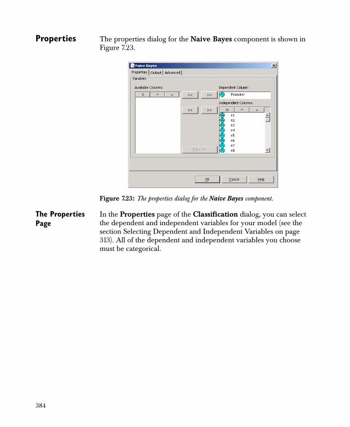
Properties The properties dialog for the Naive Bayes component is shown in Figure 7.23.
The Properties Page
In the Properties page of the Classification dialog, you can select the dependent and independent variables for your model (see the section Selecting Dependent and Independent Variables on page 313). All of the dependent and independent variables you choose must be categorical.
Figure 7.23: The properties dialog for the Naive Bayes component.
384
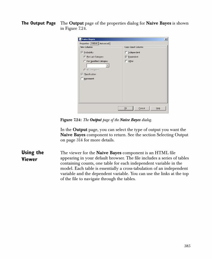
The Output Page The Output page of the properties dialog for Naive Bayes is shown in Figure 7.24.
In the Output page, you can select the type of output you want the Naive Bayes component to return. See the section Selecting Output on page 314 for more details.
Using the Viewer
The viewer for the Naive Bayes component is an HTML file appearing in your default browser. The file includes a series of tables containing counts, one table for each independent variable in the model. Each table is essentially a cross-tabulation of an independent variable and the dependent variable. You can use the links at the top of the file to navigate through the tables.
Figure 7.24: The Output page of the Naive Bayes dialog.
385
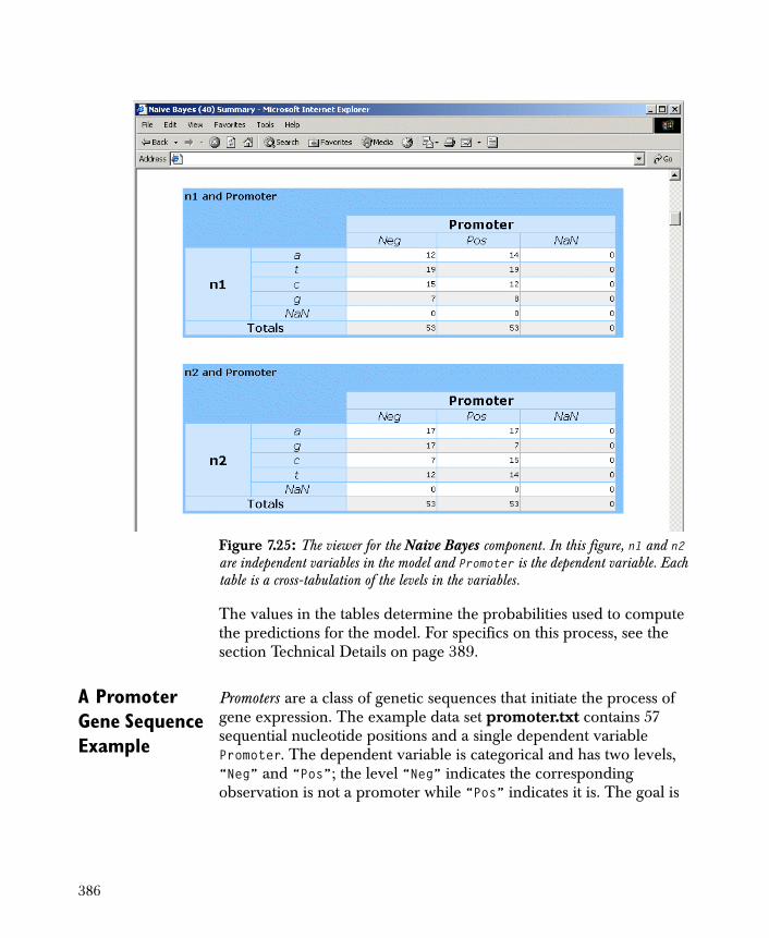
The values in the tables determine the probabilities used to compute the predictions for the model. For specifics on this process, see the section Technical Details on page 389.
A Promoter Gene Sequence Example
Promoters are a class of genetic sequences that initiate the process of gene expression. The example data set promoter.txt contains 57 sequential nucleotide positions and a single dependent variable Promoter. The dependent variable is categorical and has two levels, “Neg” and “Pos”; the level “Neg” indicates the corresponding observation is not a promoter while “Pos” indicates it is. The goal is
Figure 7.25: The viewer for the Naive Bayes component. In this figure, n1 and n2 are independent variables in the model and Promoter is the dependent variable. Each table is a cross-tabulation of the levels in the variables.
386
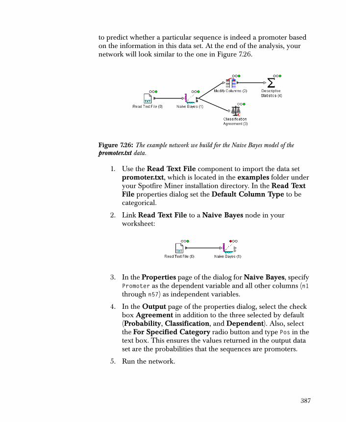
to predict whether a particular sequence is indeed a promoter based on the information in this data set. At the end of the analysis, your network will look similar to the one in Figure 7.26.
1. Use the Read Text File component to import the data set promoter.txt, which is located in the examples folder under your Spotfire Miner installation directory. In the Read Text File properties dialog set the Default Column Type to be categorical.
2. Link Read Text File to a Naive Bayes node in your worksheet:
3. In the Properties page of the dialog for Naive Bayes, specify Promoter as the dependent variable and all other columns (n1 through n57) as independent variables.
4. In the Output page of the properties dialog, select the check box Agreement in addition to the three selected by default (Probability, Classification, and Dependent). Also, select the For Specified Category radio button and type Pos in the text box. This ensures the values returned in the output data set are the probabilities that the sequences are promoters.
5. Run the network.
Figure 7.26: The example network we build for the Naive Bayes model of the promoter.txt data.
387
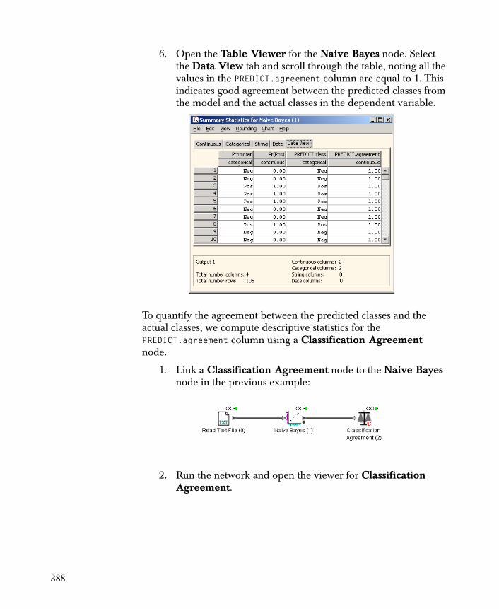
6. Open the Table Viewer for the Naive Bayes node. Select the Data View tab and scroll through the table, noting all the values in the PREDICT.agreement column are equal to 1. This indicates good agreement between the predicted classes from the model and the actual classes in the dependent variable.
To quantify the agreement between the predicted classes and the actual classes, we compute descriptive statistics for the PREDICT.agreement column using a Classification Agreement node.
1. Link a Classification Agreement node to the Naive Bayes node in the previous example:
2. Run the network and open the viewer for Classification Agreement.
388
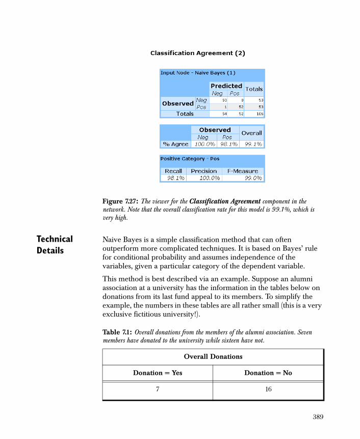
Technical Details
Naive Bayes is a simple classification method that can often outperform more complicated techniques. It is based on Bayes’ rule for conditional probability and assumes independence of the variables, given a particular category of the dependent variable.
This method is best described via an example. Suppose an alumni association at a university has the information in the tables below on donations from its last fund appeal to its members. To simplify the example, the numbers in these tables are all rather small (this is a very exclusive fictitious university!).
Figure 7.27: The viewer for the Classification Agreement component in the network. Note that the overall classification rate for this model is 99.1%, which is very high.
Table 7.1: Overall donations from the members of the alumni association. Seven members have donated to the university while sixteen have not.
Overall Donations
Donation = Yes Donation = No
7 16
389
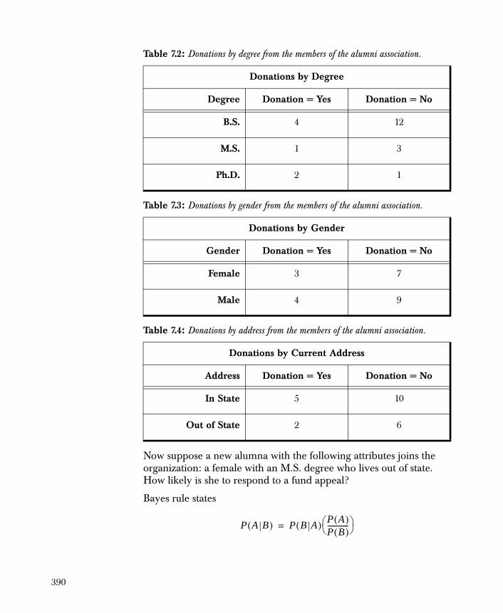
Now suppose a new alumna with the following attributes joins the organization: a female with an M.S. degree who lives out of state. How likely is she to respond to a fund appeal?
Bayes rule states
Table 7.2: Donations by degree from the members of the alumni association.
Donations by Degree
Degree Donation = Yes Donation = No
B.S. 4 12
M.S. 1 3
Ph.D. 2 1
Table 7.3: Donations by gender from the members of the alumni association.
Donations by Gender
Gender Donation = Yes Donation = No
Female 3 7
Male 4 9
Table 7.4: Donations by address from the members of the alumni association.
Donations by Current Address
Address Donation = Yes Donation = No
In State 5 10
Out of State 2 6
P A B( ) P B A( ) P A( )P B( )------------ =
390

where is the probability of event given that event has occurred. If we naively assume that, given donation status, the variables degree, gender, and current address are independent, then we can obtain the combined probability by multiplying the individual probabilities:
For now, we ignore the denominator in this expression.
Similarly, the probability of the new alumna not donating to the organization is:
The two probabilities given in Equations (7.4) and (7.5) must sum to one, so we avoid computing the denominator term by normalizing:
. (7.4)
. (7.5)
P A B( ) A B
P Yes | M.S., Female, Out of State( )
P M.S., Female, Out of State | Yes( ) P Yes( )P M.S., Female, Out of State( )---------------------------------------------------------------- =
P M.S. | Yes( )P F | Yes( )P Out of State | Yes( ) P Yes( )P M.S., F, Out of State( )-------------------------------------------------- =
17---
37---× 2
7---× 7
23------×
P M.S., Female, Out of State( )----------------------------------------------------------------=
P No | M.S., Female, Out of State( )
P M.S. | No( )P F | No( )P Out of State | No( ) P No( )P M.S., F, Out of State( )-------------------------------------------------- =
316------
716------× 6
16------× 16
23------×
P M.S., Female, Out of State( )----------------------------------------------------------------=
P Yes | M.S., Female, Out of State( )
391
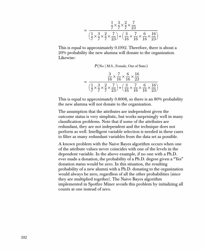
This is equal to approximately 0.1992. Therefore, there is about a 20% probability the new alumna will donate to the organization. Likewise:
This is equal to approximately 0.8008, so there is an 80% probability the new alumna will not donate to the organization.
The assumption that the attributes are independent given the outcome status is very simplistic, but works surprisingly well in many classification problems. Note that if some of the attributes are redundant, they are not independent and the technique does not perform as well. Intelligent variable selection is needed in these cases to filter as many redundant variables from the data set as possible.
A known problem with the Naive Bayes algorithm occurs when one of the attribute values never coincides with one of the levels in the dependent variable. In the above example, if no one with a Ph.D. ever made a donation, the probability of a Ph.D. degree given a “Yes” donation status would be zero. In this situation, the resulting probability of a new alumni with a Ph.D. donating to the organization would always be zero, regardless of all the other probabilities (since they are multiplied together). The Naive Bayes algorithm implemented in Spotfire Miner avoids this problem by initializing all counts at one instead of zero.
17---
37---× 2
7---× 7
23------×
17---
37---× 2
7---× 7
23------×
316------
716------× 6
16------× 16
23------×
+
-------------------------------------------------------------------------------------------------=
P No | M.S., Female, Out of State( )
316------
716------× 6
16------× 16
23------×
17---
37---× 2
7---× 7
23------×
316------
716------× 6
16------× 16
23------×
+
-------------------------------------------------------------------------------------------------=
392

REFERENCES
Breiman, L. (1996). Bagging predictors. Machine Learning, 26:123-140.
Breiman, L., Friedman, J., Olshen, R.A., and Stone, C. (1984). Classification and Regression Trees. CRC Press, LLC.
Chambers, J.M. and Hastie, T.J. (Eds.) (1992). Statistical Models in S. London: Chapman and Hall.
Hastie, T., Tibshirani, R., and Friedman, J. (2001). The Elements of Statistical Learning: Data Mining, Inference, and Prediction . New York: Springer.
McCullagh, P. and Nelder, J.A. (1989). Generalized Linear Models (2nd ed.). London: Chapman and Hall.
Reed, R.D. and Marks, R.J. (1999). Neural Smithing . Cambridge, Massachusetts: The MIT Press.
Ripley, B.D. (1996). Pattern Recognition and Neural Networks . Cambridge: Cambridge University Press.
Schapire, R. (1990). The strength of weak learnability. Machine Learning, 5:197-227.
Therneau, T. and Atkinson, E. (1997). An Introduction to Recursive Partitioning Using the RPART Routines. Mayo Foundation Technical Report.
393

394
Overview 396General Procedure 396Selecting Dependent and Independent Variables 398Selecting Output 400Creating Predict Nodes 401
Linear Regression Models 404Mathematical Definitions 404Properties 405Using the Viewer 409Creating a Filter Column node 412A House Pricing Example 414Technical Details 424
Regression Trees 426Background 426Properties 429Using the Viewer 436A House Pricing Example (Continued) 438
Regression Neural Networks 441Background 441Properties 443Using the Viewer 447A House Pricing Example (Continued) 451Technical Details 453
References 456
REGRESSION MODELS 8
395
OVERVIEW
You use regression models when you wish to compute predictions for a continuous dependent variable. Common examples of dependent variables in this type of model are income and bank balances. The variables in the model that determine the predictions are called the independent variables. All other variables in your data set are simply information or identification variables; common examples include customer number, telephone, and address.
Spotfire Miner™ includes components for three types of regression models: Linear Regression, Regression Tree, and Regression Neural Network. In this chapter, we discuss each model at a high level, describe the options available for these components, give full examples for illustration, and provide technical details for the underlying algorithms. The options we describe here are specific to the regression modeling components. For information on the Advanced pages of the properties dialogs, see Chapter 15, Advanced Topics (the options in the Advanced pages apply to all components).
In the remainder of this overview, we describe the options that are common to all three models. For descriptions of model-specific options, see the appropriate sections in this chapter.
General Procedure
The following outlines the general approach to using regression models in Spotfire Miner:
1. Link a model node in your worksheet to any node that outputs data. The input data set to the model node is called the training data because it is used to train your model.
2. Use the properties dialog for the model to specify the dependent and independent variables and the type of data you want to output.
3. Run your network.
4. Launch the viewer for the model node.
5. Based on the information in the viewer, modify your model if desired and rerun the network.
6. When you are satisfied with results, create a Predict node for the model.
396

7. Link the Predict node to a node that outputs your scoring data and then run the new network. Typically, the scoring data set contains all variables in the model except the dependent variable.
All regression models in Spotfire Miner accept a single input containing rectangular data. They output a data set containing any of the following, based on options you choose in the properties dialogs:
• A column containing the fitted values predicted by the model.
• A column containing the residuals for the predictions. A residual is the difference between the actual value in the dependent variable and the predicted variable.
• All of the independent variables used in your model.
• The dependent variable in your data set.
• All other columns in your data set besides the dependent and independent variables.
397
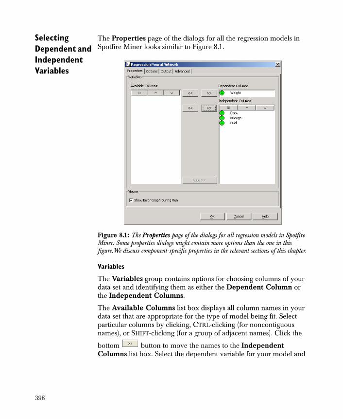
Selecting Dependent and Independent Variables
The Properties page of the dialogs for all the regression models in Spotfire Miner looks similar to Figure 8.1.
Variables
The Variables group contains options for choosing columns of your data set and identifying them as either the Dependent Column or the Independent Columns.
The Available Columns list box displays all column names in your data set that are appropriate for the type of model being fit. Select particular columns by clicking, CTRL-clicking (for noncontiguous names), or SHIFT-clicking (for a group of adjacent names). Click the
bottom button to move the names to the Independent Columns list box. Select the dependent variable for your model and
Figure 8.1: The Properties page of the dialogs for all regression models in Spotfire Miner. Some properties dialogs might contain more options than the one in this figure.We discuss component-specific properties in the relevant sections of this chapter.
398
click the top button to move it to the Dependent Column field; this variable must be continuous. If you need to remove a
column, select its name and click the corresponding button.
If you have defined modeling roles using the Modify Columns component, you can either skip the Properties page altogether or click the Auto button. Skipping the Properties page and leaving the fields Dependent Variable and Independent Variables blank causes Spotfire Miner to use the defined roles in the model. Clicking the Auto button automatically moves the dependent and independent variables into the appropriate fields according to the defined roles.
Sorting Column Names
You can use the buttons at the top of the Available Columns and Independent Columns list boxes to sort the display of column names. This is helpful when you have a large number of variables in your data set and you want to find particular ones quickly. The button sorts the column names in the order they appear in the input data; this is the default. The button sorts the column names in alphabetical order and the button sorts them in reverse alphabetical order. You can also use drag-and-drop within the lists to reorder the display of an individual column name.
399
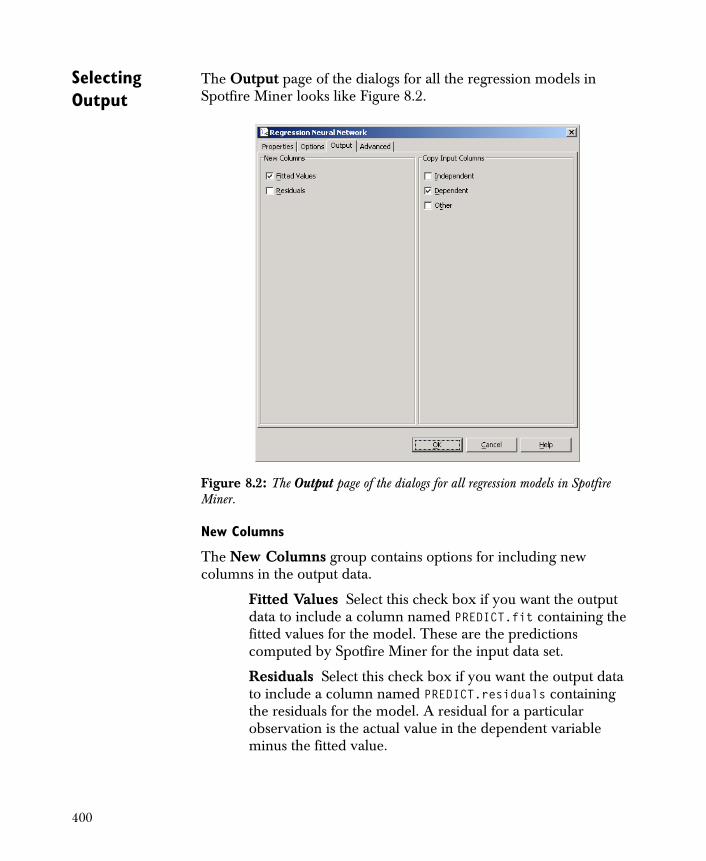
Selecting Output
The Output page of the dialogs for all the regression models in Spotfire Miner looks like Figure 8.2.
New Columns
The New Columns group contains options for including new columns in the output data.
Fitted Values Select this check box if you want the output data to include a column named PREDICT.fit containing the fitted values for the model. These are the predictions computed by Spotfire Miner for the input data set.
Residuals Select this check box if you want the output data to include a column named PREDICT.residuals containing the residuals for the model. A residual for a particular observation is the actual value in the dependent variable minus the fitted value.
Figure 8.2: The Output page of the dialogs for all regression models in Spotfire Miner.
400

Copy Input Columns
The Copy Input Columns group contains options for copying the input columns to the output data set. Select the Independent check box if you want Spotfire Miner to copy all of the independent variables in the model to the output data set. Select the Dependent check box if you want Spotfire Miner to copy the dependent variable. Select the Other check box if you want Spotfire Miner to copy all columns that are neither the dependent nor the independent variables but are part of the original data set.
Creating Predict Nodes
A Predict node is a snapshot of your regression model. Use it to apply the model to new data for the purpose of computing predictions and regressions. Typically, the new data is the scoring data set, which contains all variables in your model except the dependent variable.
To create a Predict node for your regression model, first run your network so that the status indicator for the model node is green. For example:
Right-click the model node in your network and select Create Predictor from the context-sensitive menu. Alternatively, select the model node and choose Tools � Create Predictor from the main Spotfire Miner menu. This creates a Predict node in your network and names it according to the model type. A dotted line between the predict node and its model node acts as a visual cue to the relationship between the two nodes. If the model node is modified, e.g. a new independent variable is added, the Predict node will be
401
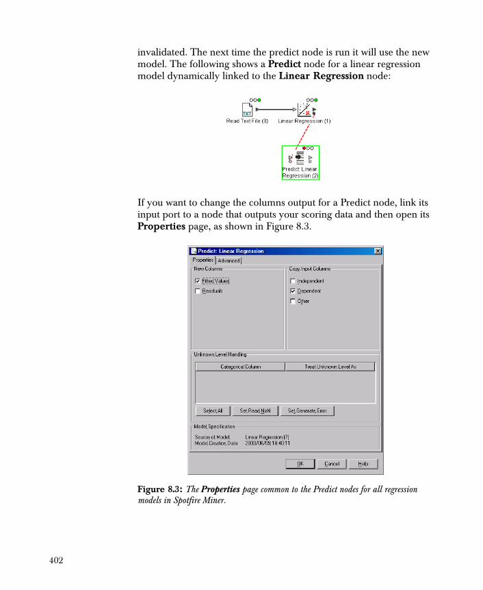
invalidated. The next time the predict node is run it will use the new model. The following shows a Predict node for a linear regression model dynamically linked to the Linear Regression node:
If you want to change the columns output for a Predict node, link its input port to a node that outputs your scoring data and then open its Properties page, as shown in Figure 8.3.
Figure 8.3: The Properties page common to the Predict nodes for all regression models in Spotfire Miner.
402

The options available in this properties dialog are very similar to those in the Output page of Figure 8.2.
Warning
A Predict node does not contain information regarding any manipulation or cleaning operations you perform on the training data set. This means you must perform the same operations on your scoring data as you do on the training data. See the cross-sell example in this chapter (specifically, the section Predicting from the Model on page 339) for an illustration.
403
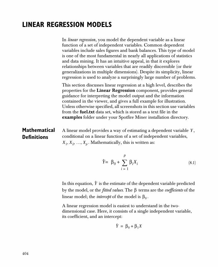
LINEAR REGRESSION MODELS
In linear regression , you model the dependent variable as a linear function of a set of independent variables. Common dependent variables include sales figures and bank balances. This type of model is one of the most fundamental in nearly all applications of statistics and data mining. It has an intuitive appeal, in that it explores relationships between variables that are readily discernible (or their generalizations in multiple dimensions). Despite its simplicity, linear regression is used to analyze a surprisingly large number of problems.
This section discusses linear regression at a high level, describes the properties for the Linear Regression component, provides general guidance for interpreting the model output and the information contained in the viewer, and gives a full example for illustration. Unless otherwise specified, all screenshots in this section use variables from the fuel.txt data set, which is stored as a text file in the examples folder under your Spotfire Miner installation directory.
Mathematical Definitions
A linear model provides a way of estimating a dependent variable , conditional on a linear function of a set of independent variables,
. Mathematically, this is written as:
In this equation, is the estimate of the dependent variable predicted by the model, or the fitted values. The terms are the coefficients of the linear model; the intercept of the model is .
A linear regression model is easiest to understand in the two-dimensional case. Here, it consists of a single independent variable, its coefficient, and an intercept:
(8.1)
Y
X1 X2 … X, p, ,
Y β0 βiXii 1=
p
+=
Y
ββ0
Y β0 β1X+=
404
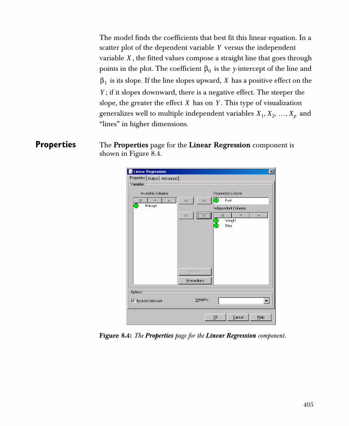
The model finds the coefficients that best fit this linear equation. In a scatter plot of the dependent variable versus the independent variable , the fitted values compose a straight line that goes through points in the plot. The coefficient is the y-intercept of the line and
is its slope. If the line slopes upward, has a positive effect on the
; if it slopes downward, there is a negative effect. The steeper the slope, the greater the effect has on . This type of visualization generalizes well to multiple independent variables and “lines” in higher dimensions.
Properties The Properties page for the Linear Regression component is shown in Figure 8.4.
Y
X
β0
β1 X
Y
X Y
X1 X2 … X, p, ,
Figure 8.4: The Properties page for the Linear Regression component.
405
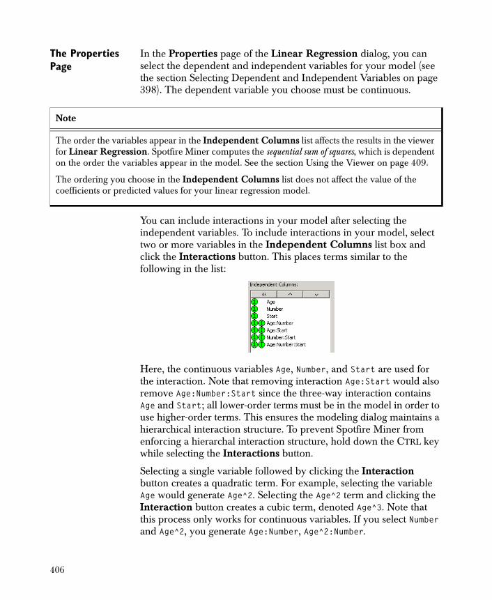
The Properties Page
In the Properties page of the Linear Regression dialog, you can select the dependent and independent variables for your model (see the section Selecting Dependent and Independent Variables on page 398). The dependent variable you choose must be continuous.
You can include interactions in your model after selecting the independent variables. To include interactions in your model, select two or more variables in the Independent Columns list box and click the Interactions button. This places terms similar to the following in the list:
Here, the continuous variables Age, Number, and Start are used for the interaction. Note that removing interaction Age:Start would also remove Age:Number:Start since the three-way interaction contains Age and Start; all lower-order terms must be in the model in order to use higher-order terms. This ensures the modeling dialog maintains a hierarchical interaction structure. To prevent Spotfire Miner from enforcing a hierarchal interaction structure, hold down the CTRL key while selecting the Interactions button.
Selecting a single variable followed by clicking the Interaction button creates a quadratic term. For example, selecting the variable Age would generate Age^2. Selecting the Age^2 term and clicking the Interaction button creates a cubic term, denoted Age^3. Note that this process only works for continuous variables. If you select Number and Age^2, you generate Age:Number, Age^2:Number.
Note
The order the variables appear in the Independent Columns list affects the results in the viewer for Linear Regression. Spotfire Miner computes the sequential sum of squares, which is dependent on the order the variables appear in the model. See the section Using the Viewer on page 409.
The ordering you choose in the Independent Columns list does not affect the value of the coefficients or predicted values for your linear regression model.
406

To remove an interaction from your model, select it in the Independent Columns list and then click the lower remove button,
. As with adding interactions, holding down the control key while clicking the remove button will prevent Spotfire Miner from enforcing a hierarchal interaction structure on your model. Otherwise all higher order interactions that involve the variables being removed from the model are also removed.
Options
The Options group controls the intercept and weights in your model. By default, the Include Intercept check box is selected and Spotfire Miner includes the intercept in the model computations. To include a set of weights in the model as well, select a variable from the drop-down list for Weights. This list includes the names of all continuous variables in your data set. Weights are appropriate to use when you know a priori that not all observations contribute equally to the model. For details on how the weights are incorporated into the model, see the section Algorithm Specifics on page 424.
407
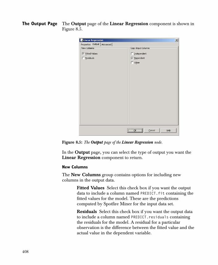
The Output Page The Output page of the Linear Regression component is shown in Figure 8.5.
In the Output page, you can select the type of output you want the Linear Regression component to return.
New Columns
The New Columns group contains options for including new columns in the output data.
Fitted Values Select this check box if you want the output data to include a column named PREDICT.fit containing the fitted values for the model. These are the predictions computed by Spotfire Miner for the input data set.
Residuals Select this check box if you want the output data to include a column named PREDICT.residuals containing the residuals for the model. A residual for a particular observation is the difference between the fitted value and the actual value in the dependent variable.
Figure 8.5: The Output page of the Linear Regression node.
408
Copy Input Columns
The Copy Input Columns group contains options for copying the input columns to the output data set. Select the Independent check box if you want Spotfire Miner to copy all of the independent variables in the model to the output data set. Select the Dependent check box if you want Spotfire Miner to copy the dependent variable. Select the Other check box if you want Spotfire Miner to copy all columns that are neither the dependent nor the independent variables but are columns in the data set.
Using the Viewer
The viewer for the Linear Regression component is an HTML file appearing in your default browser. To launch the viewer, right-click the Linear Regression node and select Viewer.
The file includes tables that are useful for interpreting the computed coefficients for your model. If you are interested only in the predictions computed by the model, you can skip this section.
An example of the output is displayed in Figure 8.6. The tables, their components, and other summary statistics are listed as follows:
• The name of the dependent variable, Fuel.
• A table of Coefficient Estimates, which includes the following:
• The coefficient estimates for the intercept and the two independent variables (Disp. and Weight).
• The standard error for each coefficient estimate.
The standard error for an estimate is a measure of its variability. If the standard error for a coefficient is small in comparison to the scale of the data for the corresponding variable, the estimate is fairly precise.
• The t-statistic for each coefficient estimate.
The t-statistic for an estimate tests whether the coefficient is significantly different from zero. Or to rephrase, a t-statistic is a measure of significance for a variable in the model. In general, t-statistics greater than 2.0 in magnitude indicate coefficients that are significant and
409
variables that should therefore be kept in the model. In Figure 8.6, the t-statistics imply both the coefficient for Disp. and the intercept are very significant in the model.
• The p-value for each t-statistic indicates if the corresponding coefficient is significant in the model. In general, small p-values (< .05) indicate a significant coefficient.
• An Analysis of Variance table, which includes the following:
• The regression sum of squares, mean square value, F-statistic, corresponding degrees of freedom (DF), and Pr(F).
These regression statistics are associated with the computed model and are commonly referred to as the sums of squares for the model. The degrees of freedom for this is one less than the number of coefficients computed for the model. If the regression sum of squares is large, the fitted model is a significant improvement over the null model , which contains an intercept but no independent variables. A large F-statistic provides additional evidence that the regression model is significant.
• The sum of squares, mean square value, F-statistic, and degrees of freedom for each term in the model.
The sums of squares reflect the amount of variance each term contributes to the overall model variation. In Figure 8.6, the large sum of squares and F-statistic for Weight indicates this variable is very significant in the model. These sums of squares are sequential , in that they rely on the ordering of the independent variables in the model. If you choose a different ordering for your independent variables, you will see different results here.
• The error sum of squares and corresponding degrees of freedom.
The error sum of squares is the difference between the total sum of squares and the regression sum of squares. Likewise, the degrees of freedom for this is the difference between the total degrees of freedom and regression degrees of freedom. In general, this value is related to the
410

quantity that is minimized in the fitting algorithm to determine the coefficients, so that smaller sums of squares imply better models.
• The total sum of squares and corresponding degrees of freedom. The degrees of freedom for this is one less than the number of observations in the data set.
• The Multiple R-squared value.
This is the proportion of variance in the dependent variable that is explained by the model. In Figure 8.6, the value 0.74 indicates that 74% of the variance in Fuel is explained by the simple linear model of the two independent variables Disp. and Weight.
• A table of Correlated Coefficients, which includes the following:
• The correlated coefficients and the threshold correlation. Only three pairs of coefficients with correlations greater than the threshold are listed. The default threshold correlation is 0.5.
• A Term Importance table showing the importance of each variable in the model. For linear regression, importance for a variable is the sum of squares for that variable given that all others are in the model. The column importance statistic measures the amount the sum of squares error will increase if that term is dropped from the model (and that term only since, typically, variables are not orthogonal).
411
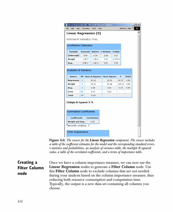
Creating a Filter Column node
Once we have a column importance measure, we can now use the Linear Regression nodes to generate a Filter Column node. Use this Filter Column node to exclude columns that are not needed during your analysis based on the column importance measure, thus reducing both resource consumption and computation time. Typically, the output is a new data set containing all columns you choose.
Figure 8.6: The viewer for the Linear Regression component. The viewer includes a table of the coefficient estimates for the model and the corresponding standard errors, t-statistics and probabilities, an analysis of variance table, the multiple R-squared value, a table of the correlated coefficients, and a terms of importance table.
412
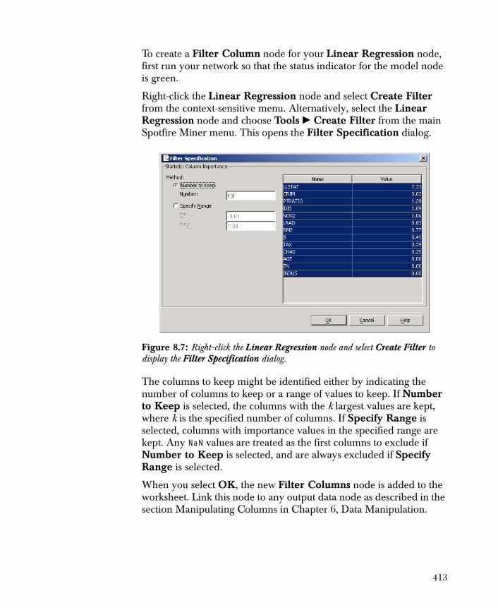
To create a Filter Column node for your Linear Regression node, first run your network so that the status indicator for the model node is green.
Right-click the Linear Regression node and select Create Filter from the context-sensitive menu. Alternatively, select the Linear Regression node and choose Tools � Create Filter from the main Spotfire Miner menu. This opens the Filter Specification dialog.
The columns to keep might be identified either by indicating the number of columns to keep or a range of values to keep. If Number to Keep is selected, the columns with the k largest values are kept, where k is the specified number of columns. If Specify Range is selected, columns with importance values in the specified range are kept. Any NaN values are treated as the first columns to exclude if Number to Keep is selected, and are always excluded if Specify Range is selected.
When you select OK, the new Filter Columns node is added to the worksheet. Link this node to any output data node as described in the section Manipulating Columns in Chapter 6, Data Manipulation.
Figure 8.7: Right-click the Linear Regression node and select Create Filter to display the Filter Specification dialog.
413
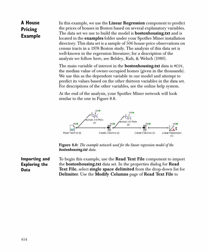
A House Pricing Example
In this example, we use the Linear Regression component to predict the prices of houses in Boston based on several explanatory variables. The data set we use to build the model is bostonhousing.txt and is located in the examples folder under your Spotfire Miner installation directory. This data set is a sample of 506 house-price observations on census tracts in a 1978 Boston study. The analysis of this data set is well-known in the regression literature; for a description of the analysis we follow here, see Belsley, Kuh, & Welsch (1980).
The main variable of interest in the bostonhousing.txt data is MEDV, the median value of owner-occupied homes (given in the thousands). We use this as the dependent variable in our model and attempt to predict its values based on the other thirteen variables in the data set. For descriptions of the other variables, see the online help system.
At the end of the analysis, your Spotfire Miner network will look similar to the one in Figure 8.8.
Importing and Exploring the Data
To begin this example, use the Read Text File component to import the bostonhousing.txt data set. In the properties dialog for Read Text File, select single space delimited from the drop-down list for Delimiter. Use the Modify Columns page of Read Text File to
Figure 8.8: The example network used for the linear regression model of the bostonhousing.txt data.
414
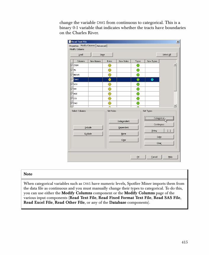
change the variable CHAS from continuous to categorical. This is a binary 0-1 variable that indicates whether the tracts have boundaries on the Charles River.
Note
When categorical variables such as CHAS have numeric levels, Spotfire Miner imports them from the data file as continuous and you must manually change their types to categorical. To do this, you can use either the Modify Columns component or the Modify Columns page of the various input components (Read Text File, Read Fixed Format Text File, Read SAS File, Read Excel File, Read Other File, or any of the Database components).
415

To explore the relationships between pairs of variables in the data set, we create a set of pairwise scatter plots.
1. Link a Multiple 2-D Plots node to the Read Text File node in your network:
The Multiple 2-D Plots node is available from the Spotfire S+ tab of the Explorer Pane. It is under the Explore/Multiple Columns folder.
2. Open the properties dialog for Multiple 2-D Plots. Designate MEDV as the single entry in the Y Columns list and all other variables as the X Columns. Select the Points radio button and then click OK.
The Multiple 2-D Plots component is useful for creating scatter plots from large data. See the section Multiple 2-D Plots on page 639 for more information. Since our dataset has only 506 observations we create standard scatter plots by selecting the Points radio button.
Note
The Multiple 2-D Plots node with the Points option is used to create all the scatter plots at once. The Scatter Plot node could also be used here. It has many options for the plot including fitting smoothing curves, titles, and axes labels. If we use the Scatter Plot component, however, each plot requires its own node.
416
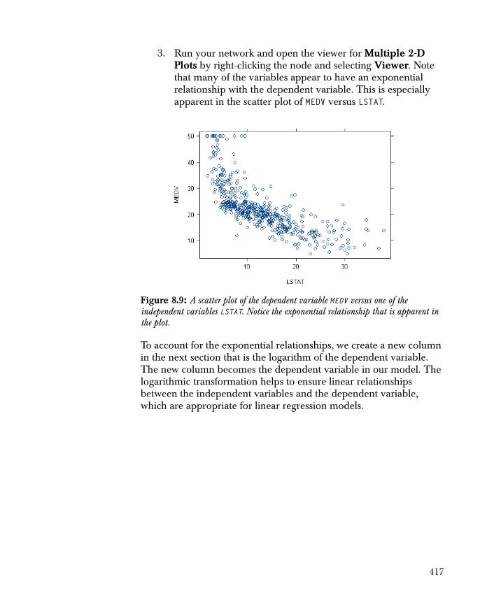
3. Run your network and open the viewer for Multiple 2-D Plots by right-clicking the node and selecting Viewer. Note that many of the variables appear to have an exponential relationship with the dependent variable. This is especially apparent in the scatter plot of MEDV versus LSTAT.
To account for the exponential relationships, we create a new column in the next section that is the logarithm of the dependent variable. The new column becomes the dependent variable in our model. The logarithmic transformation helps to ensure linear relationships between the independent variables and the dependent variable, which are appropriate for linear regression models.
Figure 8.9: A scatter plot of the dependent variable MEDV versus one of the independent variables LSTAT. Notice the exponential relationship that is apparent in the plot.
417
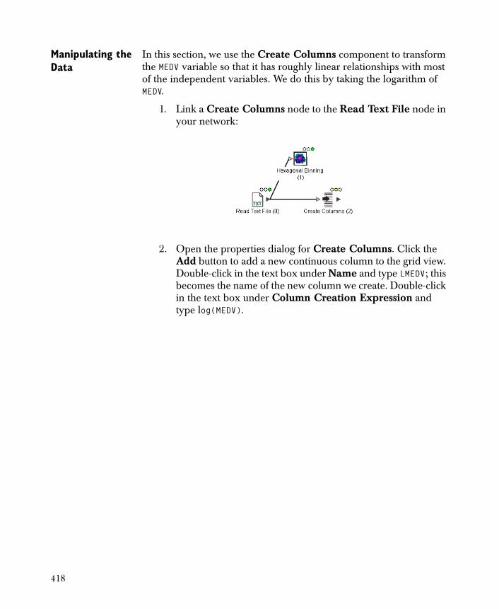
Manipulating the Data
In this section, we use the Create Columns component to transform the MEDV variable so that it has roughly linear relationships with most of the independent variables. We do this by taking the logarithm of MEDV.
1. Link a Create Columns node to the Read Text File node in your network:
2. Open the properties dialog for Create Columns. Click the Add button to add a new continuous column to the grid view. Double-click in the text box under Name and type LMEDV; this becomes the name of the new column we create. Double-click in the text box under Column Creation Expression and type log(MEDV).
418
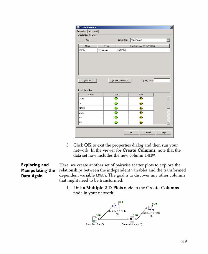
3. Click OK to exit the properties dialog and then run your network. In the viewer for Create Columns, note that the data set now includes the new column LMEDV.
Exploring and Manipulating the Data Again
Here, we create another set of pairwise scatter plots to explore the relationships between the independent variables and the transformed dependent variable LMEDV. The goal is to discover any other columns that might need to be transformed.
1. Link a Multiple 2-D Plots node to the Create Columns node in your network:
419
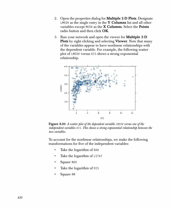
2. Open the properties dialog for Multiple 2-D Plots. Designate LMEDV as the single entry in the Y Columns list and all other variables except MEDV as the X Columns. Select the Points radio button and then click OK.
3. Run your network and open the viewer for Multiple 2-D Plots by right-clicking and selecting Viewer. Note that many of the variables appear to have nonlinear relationships with the dependent variable. For example, the following scatter plot of LMEDV versus DIS shows a strong exponential relationship.
To account for the nonlinear relationships, we make the following transformations for five of the independent variables:
• Take the logarithm of RAD
• Take the logarithm of LSTAT
• Square NOX
• Take the logarithm of DIS
• Square RM
Figure 8.10: A scatter plot of the dependent variable LMEDV versus one of the independent variables DIS. This shows a strong exponential relationship between the two variables.
420
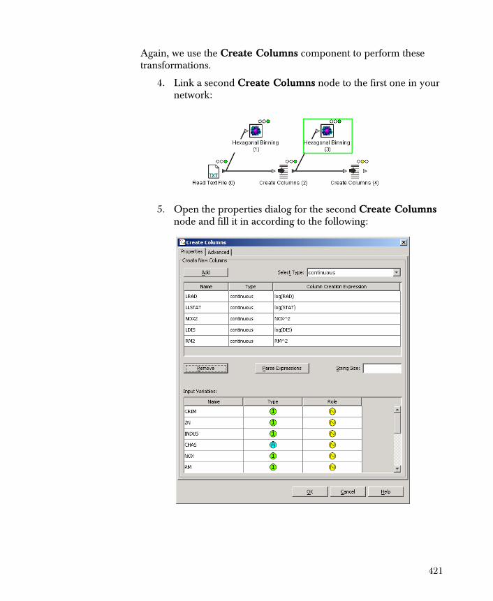
Again, we use the Create Columns component to perform these transformations.
4. Link a second Create Columns node to the first one in your network:
5. Open the properties dialog for the second Create Columns node and fill it in according to the following:
421
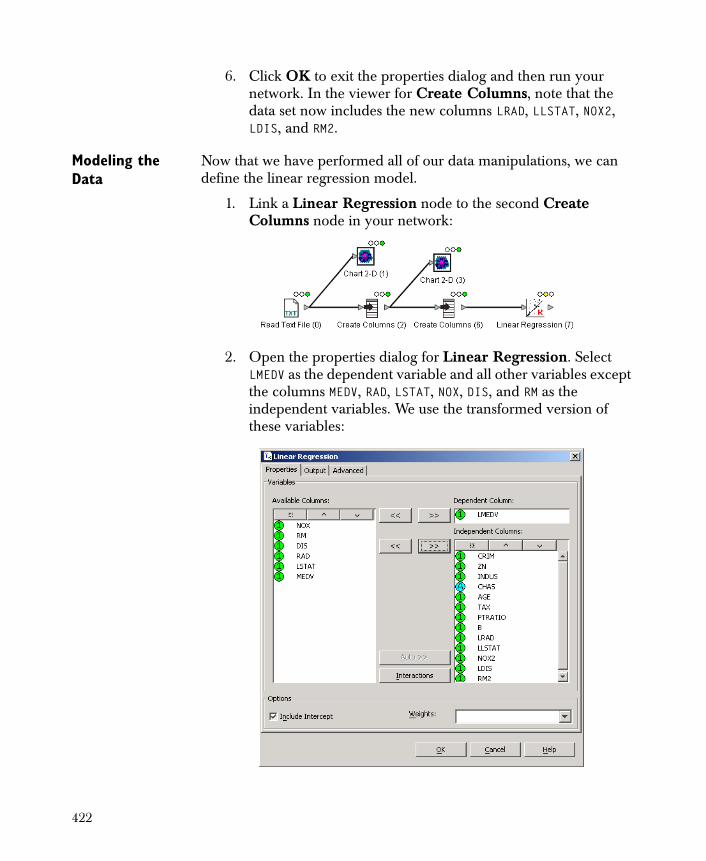
6. Click OK to exit the properties dialog and then run your network. In the viewer for Create Columns, note that the data set now includes the new columns LRAD, LLSTAT, NOX2, LDIS, and RM2.
Modeling the Data
Now that we have performed all of our data manipulations, we can define the linear regression model.
1. Link a Linear Regression node to the second Create Columns node in your network:
2. Open the properties dialog for Linear Regression. Select LMEDV as the dependent variable and all other variables except the columns MEDV, RAD, LSTAT, NOX, DIS, and RM as the independent variables. We use the transformed version of these variables:
422
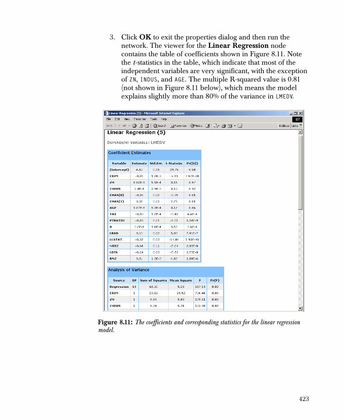
3. Click OK to exit the properties dialog and then run the network. The viewer for the Linear Regression node contains the table of coefficients shown in Figure 8.11. Note the t-statistics in the table, which indicate that most of the independent variables are very significant, with the exception of ZN, INDUS, and AGE. The multiple R-squared value is 0.81 (not shown in Figure 8.11 below), which means the model explains slightly more than 80% of the variance in LMEDV.
Figure 8.11: The coefficients and corresponding statistics for the linear regression model.
423
Technical Details
This section gives a brief overview to the fitting algorithm implemented in the Linear Regression component.
Algorithm Specifics
Spotfire Miner computes the coefficients for a linear regression model using a standard least-squares approach. For the values in a dependent variable , Spotfire Miner computes a set of
predicted values by minimizing the sum of the squared residuals:
In weighted regression, each residual is multiplied by the corresponding weight in this minimization criteria:
The least-squares algorithm implemented in Spotfire Miner does not require all data to be in memory and instead is designed to update incrementally as more chunks of data are read in. This allows the Linear Regression component to produce accurate results whether the data are read in one large chunk or several smaller ones.
The algorithm is a stable method based on QR decompositions and Householder transformations. Spotfire Miner uses Householder transformations to avoid the instabilities commonly associated with stiff, rank deficient, or near-rank deficient problems. This approach runs linearly in , the number of rows in each block of data, and
quadratically in , the number of variables in the model. The total memory consumption is approximately twice the chunk size and does not increase as the number of data chunks increases.
For a complete mathematical justification of this method, see Bun (2002) and Lanson and Hanson (1995).
y1 y2 … yn, , ,
y1 y2 … yn, , ,
yi yi–( )2
i 1=
n
wi
wi yi yi–( )2
i 1=
n
ni
p
424
The Coding of Levels in Categorical Variables
When a categorical variable is used as an independent variable in a linear regression model, Spotfire Miner codes the levels with indicator variables. A categorical with levels is represented as a matrix with
columns containing zeros and ones; the ones indicate a particular class level.
A coefficient for each indicator variable in a categorical cannot usually be estimated because of dependencies among the coefficients in the overall model. That is, a model will be over-specified and will not be full column rank. After Spotfire Miner computes a QR decomposition, a set of wrap-up computations apply so-called sigma restrictions to the coefficients for categorical variables. These restrictions force the sum of the coefficients for a categorical variable to be zero.
For interaction terms that involve categorical variables, the sum of the coefficients over each class variable index is zero. To clarify this point, assume the categorical variables A and B have two levels each. Let the coefficients , , , and estimate the interaction terms A(1):B(1), A(1):B(2), A(2):B(1) and A(2):B(2) respectively, where A(i):B(j) represents the interaction term between the ith level of A and the jth level of B. Then
Equivalently,
Note that only three of the restrictions are required; the fourth is implied. This leaves 4 coefficients minus 3 restrictions, giving 1 degree of freedom for the interaction terms.
Numerically, the sigma restrictions in Spotfire Miner are implemented as outlined by Sallas and Lionti (1988).
K
K
βk βk 1+ βk 2+ βk 3+
βk βk 2++ βk 1+ βk 3++ βk βk 1++ βk 2+ βk 3++ 0= = = =
βk βk 3+ βk 1+– βk 2+–= = =
Note
Note that Spotfire Miner and Spotfire S+ produce different output for regression models (linear or logistic). Spotfire Miner does not use contrasts like Spotfire S+.
425
REGRESSION TREES
Regression trees are tree-based models that provide a simple yet powerful way to predict a continuous response based on a collection of predictor variables. The data are recursively partitioned into two groups based on predictor (independent) variables. This is repeated until the response (dependent) variable is homogenous. The sequence of splits of the predictor variables can be displayed as a binary tree, hence the name.
This section discusses regression trees at a high level, describes the properties for the Regression Tree component, provides general guidance for interpreting the model output and the information contained in the viewer, and gives a full example for illustration. Unless otherwise specified, all screenshots in this section use variables from the vetmailing.txt data set, which is stored as a text file in the examples folder under your Spotfire Miner installation directory.
Background Here, we provide the background necessary for understanding the options available for Spotfire Miner regression trees. This section is not designed to be a complete reference for the field of regression trees, however. There are many resources available that give broad overviews of the subject; see Breiman, Friedman, Olshen, & Stone (1984), Ripley (1996), or Hastie, Tibshirani, & Friedman (2001) for a general treatment.
A regression tree can be described as a series of rules. For a response and set of predictors , , , , a regression tree rule would be
of the form:
if and and
then the predicted value of is 8.45
The simplicity of the model display and prediction rules make regression trees an attractive data mining tool. Other advantages of tree models include:
• Invariance to monotone re-expression of the predictor variables
y x1 x2 … xp
x1 14< x2 D E F, ,{ }∈ x3 125<
y
426
• Can easily capture nonlinear behavior in a predictor as well as interactions among predictors
Growing a Tree Trees are grown by a greedy algorithm. To find the first split from the root of the tree, every possible binary split for each predictor variable is considered, and a figure-of-merit is computed for each of these splits. The data are then partitioned into two sets at the split that gave the best figure-of-merit over all predictor variables and all possible splits (the figure-of-merit and what is considered “best” are described below). The algorithm is now repeated on each of the two partitions of the data. The splitting continues until the growth limits (minimum figure-of-merit, number of points in a split, or others) are reached. The last partitions are called leaf or terminal nodes.
Each terminal node is represented by the average of the training set response variables in the terminal node.
To predict the response variable given values for predictor variables, an observation is “dropped down the tree”: at each node, the split determines whether the observation goes right or left. Finally it ends up at a terminal node. The predictions are the average of the training set response variables in the terminal node.
Depending on the growth limits, you can grow a very extensive tree that will actually reproduce the observed response variables (each unique observation ends up in its own terminal node). Such trees are of little value in predicting new observations; the tree model has overfit the training data. To prevent such behavior, a technique called pruning is applied to the tree—nodes that do not significantly improve the fit are pruned off. Usually, some form of cross-validation is used to decide which nodes to prune.
Ensemble Trees Recent research results have shown that combining the results from multiple trees fit to the same data can give better predictions than a single tree. These combinations of trees are called ensembles.
Several methods have been developed for computing multiple trees. Bagging (Breiman, 1996) uses the resampling idea of bootstrapping to draw multiple samples with replacement from the original data. Trees are fit on each sample, and the predictions are the average of the predictions from all the trees. The trees are usually grown quite deep and not pruned back. The averaging across deep trees, each computed on a slightly different set of observations, leads to better predictions than any single tree.
427
Another ensemble method is boosting (Schapire, 1990). Like bagging, it resamples the data but uses weighted sampling, giving more weight to observations that have been difficult to predict in the earlier trees.
Spotfire Miner uses a modification of the bagging idea to fit ensembles of trees on large data sets. Rather than bootstrapping from a single sample of data, Spotfire Miner considers each block or chunk of data read in from the pipeline as a type of bootstrap sample and fits a tree to that chunk of data. Rather than keeping all the trees to average over, only the K best trees are kept, where K is user-specified and “best” is chosen by a form of cross-validation.
Trees in Spotfire Miner
Spotfire Miner gives you the option of fitting a single tree or an ensemble of trees. Often, data mining is done on very large data sets. The tree methods in Spotfire Miner have been developed to handle this.
A single tree representation might be desired as a concise description of the data. This representation is easily understood by people not familiar with data mining methods. For a single tree, you can specify the maximum number of rows to use in fitting the tree. If the total number of observations is greater than this, a random sample from all the data, of the size you specify, is used. Options are available for cross-validation and pruning on a single tree.
For the best predictions, an ensemble tree usually performs better than a single tree. For an ensemble tree, you can specify how many trees to keep and how many observations to use in each tree.
The underlying tree-fitting algorithm in Spotfire Miner is based on the recursive partitioning code called RPART by Therneau and Atkinson (1997).
A Note on Missing Values
Missing values in the predictors and the response are dropped when fitting a tree. During prediction, missing values are allowed in the predictors. For a particular observation, if a prediction can be computed using the available non-missing predictors, then a valid prediction is returned. If the tree requires a predictor and its value is missing, then a missing value (NaN) is output as the prediction.
If a predictor has a new level that was not present when the model was trained, a missing value (NaN) is also output as the prediction.
428
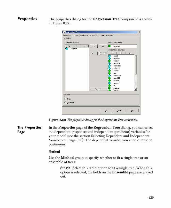
Properties The properties dialog for the Regression Tree component is shown in Figure 8.12.
The Properties Page
In the Properties page of the Regression Tree dialog, you can select the dependent (response) and independent (predictor) variables for your model (see the section Selecting Dependent and Independent Variables on page 398). The dependent variable you choose must be continuous.
Method
Use the Method group to specify whether to fit a single tree or an ensemble of trees.
Single Select this radio button to fit a single tree. When this option is selected, the fields on the Ensemble page are grayed out.
Figure 8.12: The properties dialog for the Regression Tree component.
429
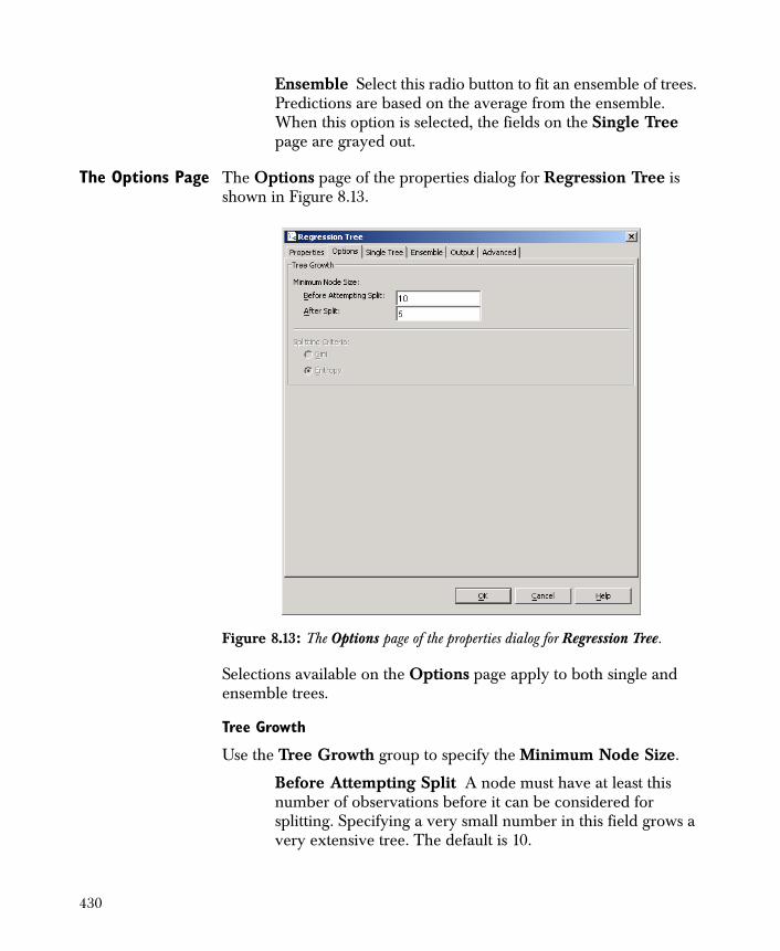
Ensemble Select this radio button to fit an ensemble of trees. Predictions are based on the average from the ensemble. When this option is selected, the fields on the Single Tree page are grayed out.
The Options Page The Options page of the properties dialog for Regression Tree is shown in Figure 8.13.
Selections available on the Options page apply to both single and ensemble trees.
Tree Growth
Use the Tree Growth group to specify the Minimum Node Size.
Before Attempting Split A node must have at least this number of observations before it can be considered for splitting. Specifying a very small number in this field grows a very extensive tree. The default is 10.
Figure 8.13: The Options page of the properties dialog for Regression Tree.
430

After Split This is the minimum number of points that must be in a terminal node. It must be less than or equal to half the value set in Before Attempting Split. Specifying a very small number in this field grows a very extensive tree.
Splitting Criteria
The Splitting Criteria determines where to make a split into two groups. In regression, a good split most reduces the sum of squared errors for the parent node. A covariate and split point are chosen to
maximize the difference , where
is the average sum of squares for the parent node, and , are the average sums of squares for the right and left nodes, respectively, after splitting. stands for the value of a response variable, and is the mean of the responses at the node.
SSP SSL SSR )+(– SSP
yi y–( )2
n--------------------=
SSR SSL
yi y
Note
The Splitting Criteria field is applicable to classification trees only and thus is grayed out in the Regression Tree dialog. There is a choice of splitting criteria only for classification.
431
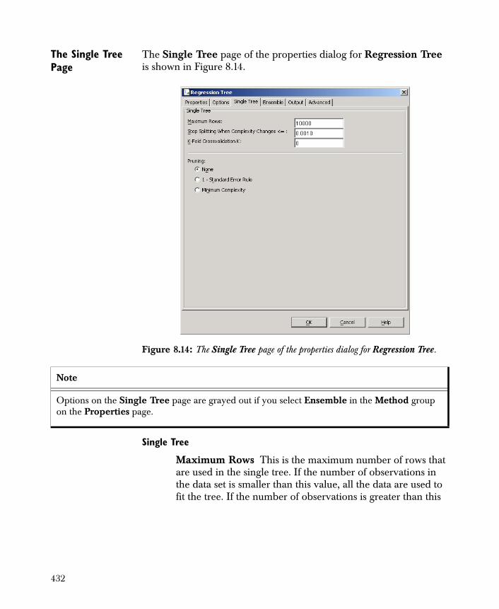
The Single Tree Page
The Single Tree page of the properties dialog for Regression Tree is shown in Figure 8.14.
Single Tree
Maximum Rows This is the maximum number of rows that are used in the single tree. If the number of observations in the data set is smaller than this value, all the data are used to fit the tree. If the number of observations is greater than this
Figure 8.14: The Single Tree page of the properties dialog for Regression Tree.
Note
Options on the Single Tree page are grayed out if you select Ensemble in the Method group on the Properties page.
432
value, then a random sample from all the data is drawn, and the single tree is fit on this sample. If this value is set too large, the data might not fit in memory, and the tree cannot be fit.
Stop Splitting When Complexity Changes <= Complexity is a value between 0 and 1 that measures how good the current tree is relative to a more complex (more nodes) tree. See Ripley (1996) Chapter 7. This value, along with the Minimum Node Size settings on the Options page, determines how deep the tree is. Specifying a smaller value results in a deeper tree. The default value is less than or equal to 0.0010.
K-Fold Crossvalidation K. Specifying an integer value greater than 1 in this field causes cross-validation to be performed. The data are divided into K equal size groups. For each group, the remaining (K-1) groups are used to fit a tree, and this tree is used to predict the left-out group. This gives a cross-validated estimate of prediction error that can be used to select the best size tree to return (pruning). Cross-validation involves fitting K different trees; the computation time is considerably longer than fitting just a single tree.
Pruning
• None No pruning is done.
• 1 - Standard Error Rule Select the tree that is within 1 standard error of the minimum cross-validated error. This can only be selected if K-Fold Crossvalidation is performed.
• Minimum Complexity The tree with the minimum cross-validated error is returned. This can only be selected if K-Fold Crossvalidation is performed.
Note
The Maximum Rows value automatically becomes the node’s Rows Per Block setting on the Advanced page of the properties dialog.
433

The Ensemble Page
The Ensemble page of the properties dialog for Regression Tree is shown in Figure 8.15.
Ensemble
Max Number of Trees This is the maximum number of trees retained in the ensemble. A tree is fit to every chunk (block) of data but only this number of trees is retained. If this is set to K, then after the K+1 tree is fit, all K+1 are used to predict the next chunk of data, and the tree that performs the worst is dropped. Performance is measured by prediction error; this is the residual sum of squares.
Figure 8.15: The Ensemble page of the properties dialog for Regression Tree.
Note
Options on the Ensemble page are grayed out if you select Single Tree in the Method group on the Properties page.
434
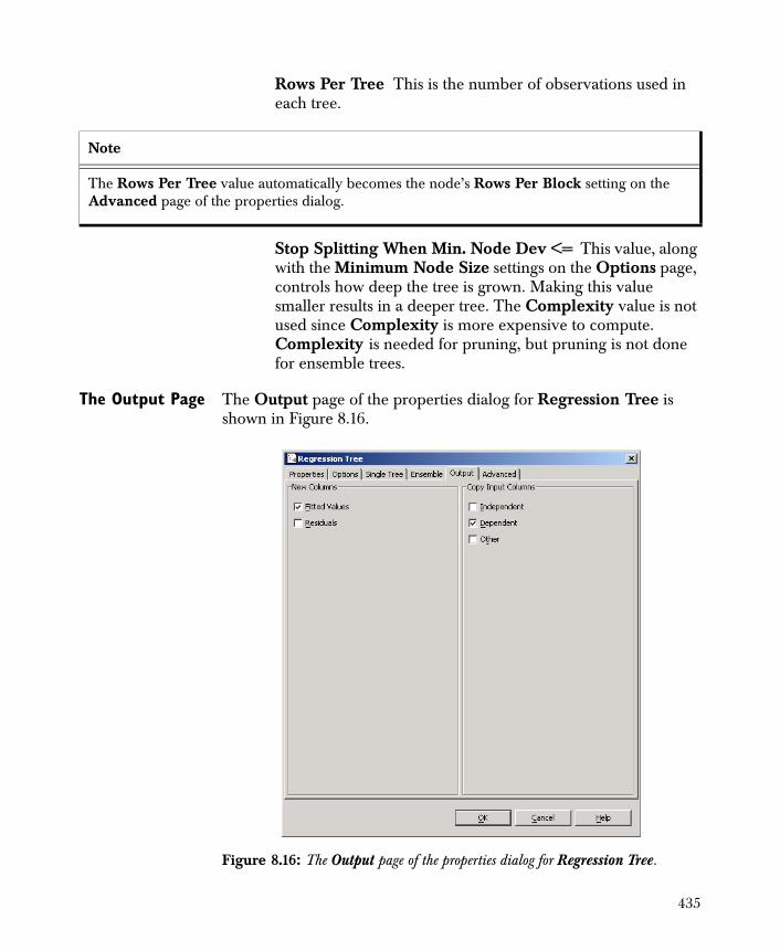
Rows Per Tree This is the number of observations used in each tree.
Stop Splitting When Min. Node Dev <= This value, along with the Minimum Node Size settings on the Options page, controls how deep the tree is grown. Making this value smaller results in a deeper tree. The Complexity value is not used since Complexity is more expensive to compute. Complexity is needed for pruning, but pruning is not done for ensemble trees.
The Output Page The Output page of the properties dialog for Regression Tree is shown in Figure 8.16.
Note
The Rows Per Tree value automatically becomes the node’s Rows Per Block setting on the Advanced page of the properties dialog.
Figure 8.16: The Output page of the properties dialog for Regression Tree.
435
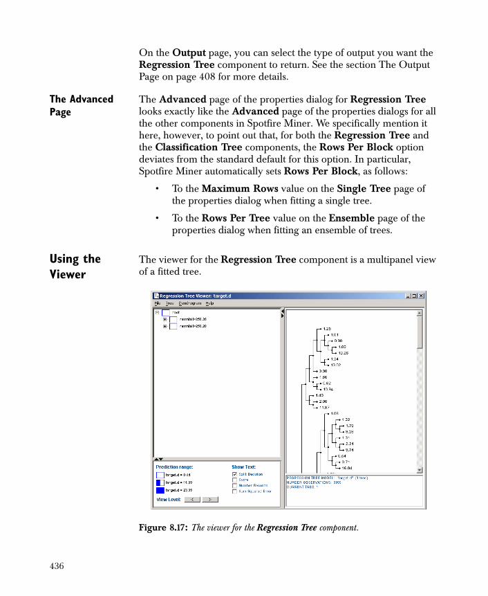
On the Output page, you can select the type of output you want the Regression Tree component to return. See the section The Output Page on page 408 for more details.
The Advanced Page
The Advanced page of the properties dialog for Regression Tree looks exactly like the Advanced page of the properties dialogs for all the other components in Spotfire Miner. We specifically mention it here, however, to point out that, for both the Regression Tree and the Classification Tree components, the Rows Per Block option deviates from the standard default for this option. In particular, Spotfire Miner automatically sets Rows Per Block, as follows:
• To the Maximum Rows value on the Single Tree page of the properties dialog when fitting a single tree.
• To the Rows Per Tree value on the Ensemble page of the properties dialog when fitting an ensemble of trees.
Using the Viewer
The viewer for the Regression Tree component is a multipanel view of a fitted tree.
Figure 8.17: The viewer for the Regression Tree component.
436
The top right panel displays the tree structure in a dendrogram. From the Dendrogram menu at the top on the viewer, you can select Map Split Importance to Depth. Doing so redraws the tree with the depth of the branches from a fit proportional to the change in the fitting criteria between the node and the sum of the two children nodes. This provides a quick visual view of the importance of each split.
The top left panel is an expandable, hierarchical view of the tree. This view links to the dendrogram view: if you click nodes in either view, you can highlight that node in the other view. You can expand or collapse the tree view by selecting the appropriate menu item from the Tree menu.
From the File menu, you can save the tree view in a graphical format suitable for a Web site, a slide presentation, or print production. When you select a format, consider the medium used for displaying the tree, required quality of the image, amount of acceptable compression, and so on. Note that the graphical image you save of a tree retains the current level of expansion. (For example, a large, fully-expanded tree will not result in an image that fits on a single page.)
The bottom left panel controls what information is displayed in the hierarchical view. If a tree ensemble (multiple trees) was fit, then the slider at the bottom can be used to cycle through the views of the various trees.
The bottom right panel is an informational panel that describes the tree that is currently being viewed. When nodes are highlighted in either tree view, the path to that node is described here.
A summary description of the tree in HTML can be produced and viewed by selecting Display HTML from the Tree menu at the top of the viewer. In addition, a bar chart showing the importance of each predictor in the tree model can be drawn by selecting View Column Importance from the Tree menu. Importance for a predictor is measured in terms of how much the splits made for that predictor contribute to the total reduction in the fitting criterion. Finally, you can generate a tree comparison table by selecting Compare Trees from the Tree menu.
437
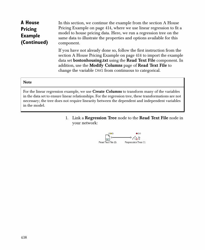
A House Pricing Example (Continued)
In this section, we continue the example from the section A House Pricing Example on page 414, where we use linear regression to fit a model to house pricing data. Here, we run a regression tree on the same data to illustrate the properties and options available for this component.
If you have not already done so, follow the first instruction from the section A House Pricing Example on page 414 to import the example data set bostonhousing.txt using the Read Text File component. In addition, use the Modify Columns page of Read Text File to change the variable CHAS from continuous to categorical.
1. Link a Regression Tree node to the Read Text File node in your network:
Note
For the linear regression example, we use Create Columns to transform many of the variables in the data set to ensure linear relationships. For the regression tree, these transformations are not necessary; the tree does not require linearity between the dependent and independent variables in the model.
438
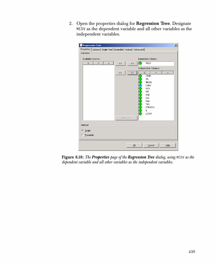
2. Open the properties dialog for Regression Tree. Designate MEDV as the dependent variable and all other variables as the independent variables.
Figure 8.18: The Properties page of the Regression Tree dialog, using MEDV as the dependent variable and all other variables as the independent variables.
439
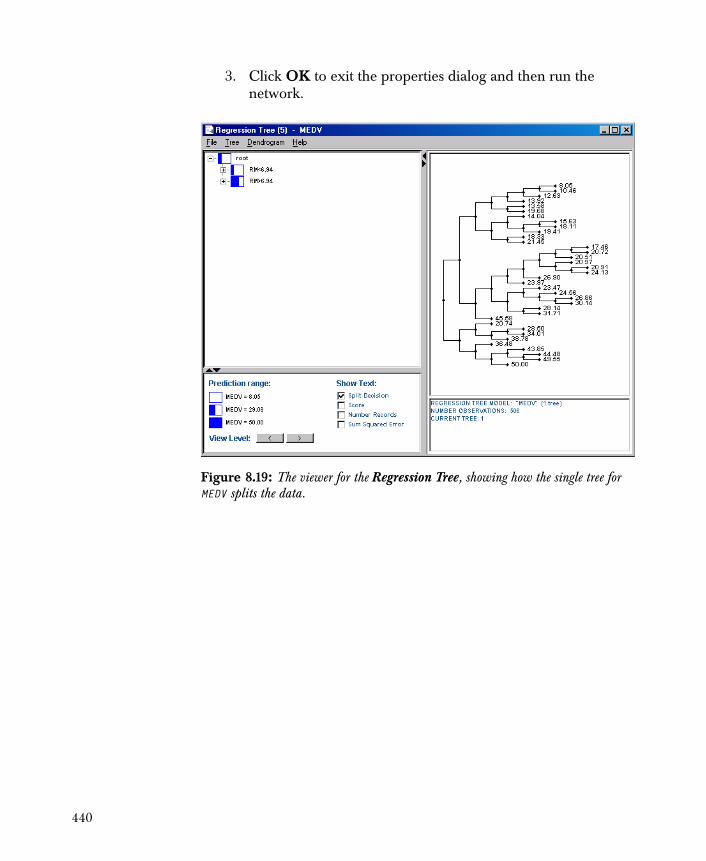
3. Click OK to exit the properties dialog and then run the network.
Figure 8.19: The viewer for the Regression Tree, showing how the single tree for MEDV splits the data.
440
REGRESSION NEURAL NETWORKS
A regression neural network is a black-box regression scheme for predicting the values of a continuous dependent variable. This section discusses regression neural networks at a high level, describes the properties for the Regression Neural Network component, provides general guidance for interpreting the output and the information contained in the viewer, and gives a full example for illustration. Unless otherwise specified, all screenshots in this section use variables from the fuel.txt data set, which is stored as a text file in the examples folder under your Spotfire Miner installation directory.
Background Here, we provide the background necessary for understanding the options available for Spotfire Miner regression neural networks. This section is not designed to be a complete reference for the field of neural networks, however. There are many resources available that give broad overviews of the subject; see Hastie, Tibshirani, & Friedman (2001) or Ripley (1996) for a general treatment.
A regression neural network is a two-stage regression model. The main idea behind the technique is to first compute linear combinations of the independent variables, and then model the dependent variable as a nonlinear function of the combinations. This is represented schematically in Figure 8.20. The output from the network is the predicted value of the dependent variable associated with each input pattern. The intercept terms in the linear combinations are called the bias nodes.
441
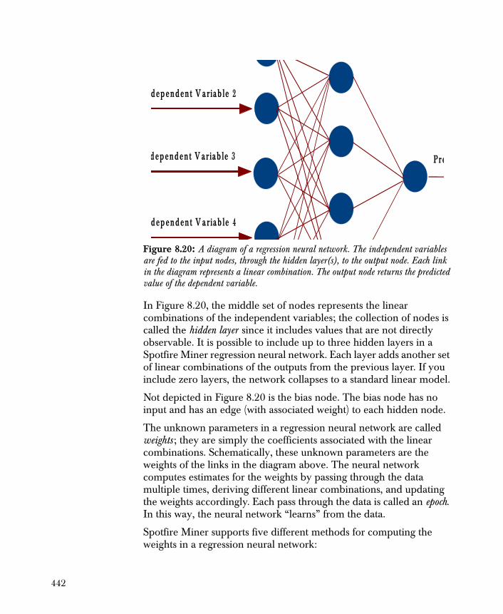
In Figure 8.20, the middle set of nodes represents the linear combinations of the independent variables; the collection of nodes is called the hidden layer since it includes values that are not directly observable. It is possible to include up to three hidden layers in a Spotfire Miner regression neural network. Each layer adds another set of linear combinations of the outputs from the previous layer. If you include zero layers, the network collapses to a standard linear model.
Not depicted in Figure 8.20 is the bias node. The bias node has no input and has an edge (with associated weight) to each hidden node.
The unknown parameters in a regression neural network are called weights ; they are simply the coefficients associated with the linear combinations. Schematically, these unknown parameters are the weights of the links in the diagram above. The neural network computes estimates for the weights by passing through the data multiple times, deriving different linear combinations, and updating the weights accordingly. Each pass through the data is called an epoch. In this way, the neural network “learns” from the data.
Spotfire Miner supports five different methods for computing the weights in a regression neural network:
Figure 8.20: A diagram of a regression neural network. The independent variables are fed to the input nodes, through the hidden layer(s), to the output node. Each link in the diagram represents a linear combination. The output node returns the predicted value of the dependent variable.
dependen t V ariab le 2
dependen t V ariab le 3
dependen t V ariab le 4
Pre
442
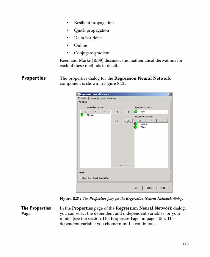
• Resilient propagation
• Quick propagation
• Delta-bar-delta
• Online
• Conjugate gradient
Reed and Marks (1999) discusses the mathematical derivations for each of these methods in detail.
Properties The properties dialog for the Regression Neural Network component is shown in Figure 8.21.
The Properties Page
In the Properties page of the Regression Neural Network dialog, you can select the dependent and independent variables for your model (see the section The Properties Page on page 406). The dependent variable you choose must be continuous.
Figure 8.21: The Properties page for the Regression Neural Network dialog.
443
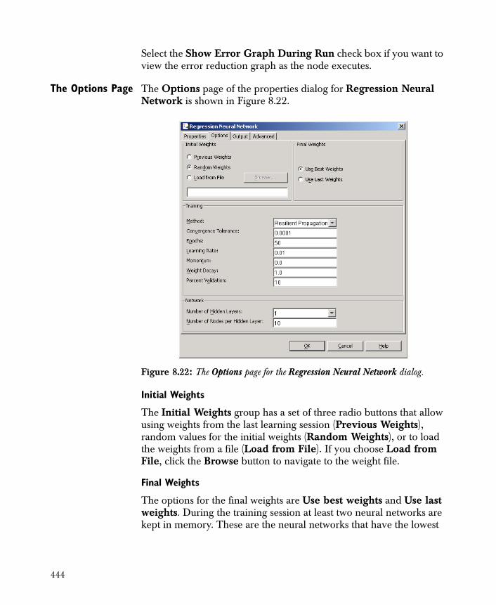
Select the Show Error Graph During Run check box if you want to view the error reduction graph as the node executes.
The Options Page The Options page of the properties dialog for Regression Neural Network is shown in Figure 8.22.
Initial Weights
The Initial Weights group has a set of three radio buttons that allow using weights from the last learning session (Previous Weights), random values for the initial weights (Random Weights), or to load the weights from a file (Load from File). If you choose Load from File, click the Browse button to navigate to the weight file.
Final Weights
The options for the final weights are Use best weights and Use last weights. During the training session at least two neural networks are kept in memory. These are the neural networks that have the lowest
Figure 8.22: The Options page for the Regression Neural Network dialog.
444
sum of squares error and the current network. Generally, they are the same neural network, but it is possible that the current neural network has an error greater than the best.
Training
The Training group contains options for controlling the way Spotfire Miner trains the neural network on your set of independent variables.
Method Select one of the methods for computing the weights from the Method drop-down list.
Convergence Tolerance This is one of the stopping criteria for the iterative training algorithm. Spotfire Miner makes successive passes through your data until either the maximum number of epochs is exceeded, the relative change in the objective function for the optimization algorithm is below some tolerance, or the user terminates the training session through the Neural Network Viewer. Decreasing the convergence tolerance might provide more accurate predictions but requires additional resources from your machine.
Epochs This option determines the maximum number of passes the algorithm makes through the data.
Learning Rate This parameter is typically small, with a default value of 0.01, and it must be in the range of ). This is the step size scale for the steepest descent optimization algorithm. It affects how quickly the neural network learns from your data and converges to a set of probabilities and predictions; smaller values imply a slower learning rate while larger values imply a quicker one. There is a trade-off between speed and reliability, however. A learning rate that is too large for a particular network might converge quickly, but to an unreliable solution.
Momentum This is a parameter that must be in the range of 0 to 1. Its effect is to smooth the trajectory of the algorithm as it iteratively computes weights for the neural network, speeding up the computations in some instances. Momentum tends to amplify the effective learning rate, so large values for the Momentum parameter usually pair best with smaller Learning Rate values.
0 1,[ ]
445

Weight Decay This is a parameter that must be in the range of 0 to 1; a value of 0 indicates no weight decay while a value of 1 indicates full weight decay. This parameter helps the algorithm dynamically adjust the complexity of the network by gradually shifting the weight values toward zero in each successive pass through the data. By encouraging small weights, the weight decay acts as a regularizer, smoothing the functions involved in the computations.
Percent Validation. Enter the percentage of rows used for validating the training model. This determines the number of rows from the training data that is randomly sampled from each chunk of data. On each pass through the data, the (pseudo) random number generator’s seed is reset to ensure that the same observations are used for validation.
Network
The Network group contains options for controlling the size and complexity of the classification neural network.
Number of Hidden Layers Select 0, 1, 2, or 3 from this drop-down list. Single-layer networks are usually sufficient for most problems, but there are instances where two- or three-layer networks compute regression more reliably and efficiently than single-layer ones.
Number of Nodes per Hidden Layer Type the number of nodes you want in the text box; this value determines the number of nodes in each hidden layer of your network. Generally speaking, a large number of nodes can fit your data exactly but tends to require impractical amounts of time and memory to compute. In addition, a large number of nodes can cause the neural network to become overtrained , where the network fits your data exactly but does not generalize well to compute predictions for your scoring data.
446
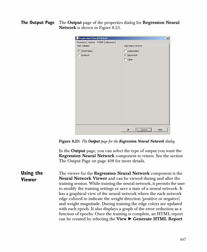
The Output Page The Output page of the properties dialog for Regression Neural Network is shown in Figure 8.23.
In the Output page, you can select the type of output you want the Regression Neural Network component to return. See the section The Output Page on page 408 for more details.
Using the Viewer
The viewer for the Regression Neural Network component is the Neural Network Viewer and can be viewed during and after the training session. While training the neural network, it permits the user to modify the training settings or save a state of a neural network. It has a graphical view of the neural network where the each network edge colored to indicate the weight direction (positive or negative) and weight magnitude. During training the edge colors are updated with each epoch. It also displays a graph of the error reduction as a function of epochs. Once the training is complete, an HTML report can be created by selecting the View � Generate HTML Report
Figure 8.23: The Output page for the Regression Neural Network dialog.
447
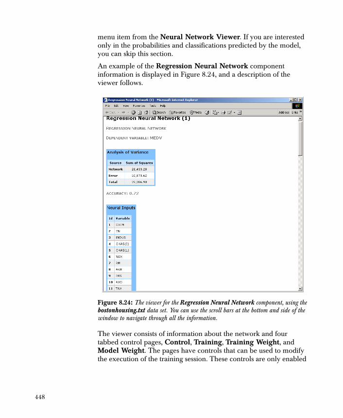
menu item from the Neural Network Viewer. If you are interested only in the probabilities and classifications predicted by the model, you can skip this section.
An example of the Regression Neural Network component information is displayed in Figure 8.24, and a description of the viewer follows.
The viewer consists of information about the network and four tabbed control pages, Control, Training, Training Weight, and Model Weight. The pages have controls that can be used to modify the execution of the training session. These controls are only enabled
Figure 8.24: The viewer for the Regression Neural Network component, using the bostonhousing.txt data set. You can use the scroll bars at the bottom and side of the window to navigate through all the information.
448
when the training is paused. They are also disabled after the training is complete where they might be useful to remind you of the final settings that produced the neural network.
Network
The Network group displays the number of input, output, and hidden nodes. The number of hidden nodes is displayed as the number of hidden nodes per layer x the number of layers.
Control
The Control tab displays the number of epochs completed, the status of the training and the scaled entropy. The Status field displays either: Running, Pause Requested, Pause, Stop Requested, or Completed. The Pause Requested and Stop Requested are required since the execution of the computations and the viewer are on separate execution threads and communication between the threads is not done until after a full pass through the data is complete.
The Control tab has the controls to pause, stop (terminate) and resume, as well as the controls for saving current or best neural networks. Once the network is paused, the controls in the Training, Training Weight, and Model Weight tabs are enabled as well as the Save Current and Save Best buttons in the Control tab.
The Save buttons in the Control tab will either save the current network or the best network. During the training session at least two neural networks are kept in memory. These are the neural networks that have the lowest cross entropy and the current network. Generally, they are the same neural network, but it is possible that the current neural network has an entropy greater than the best.
Training
The Training tab displays the current method of optimization, convergence tolerance, maximum number of epochs, learning rate, momentum, and weight decay.
In the Training tab, the optimization method can be changed where the choices are Resilient Propagation, Quick Propagation, Delta Bar Delta, Online and Conjugate Gradient. These methods are all described in Reed and Marks (1999). The momentum and weight decay options are not used in the Conjugate Gradient method and, instead of using an exact line search, the Conjugate Gradient
449
method utilizes the learning rate parameter to control the step size and step halving is used, if necessary, to find step size that will lower the entropy. Generally, it is not a good idea to change the learning rate for the Resilient Propagation or Delta Bar Delta since they are adaptive learning rate techniques: Each weight has its own learning rate that is updated with each epoch. Modifying the learning rate in this case resets the learning rate for each weight to the new constant.
Training Weight Settings
The Training Weight Settings tab has a set of three radio buttons that will allow jittering of the weights, load previous saved weights to reinstantiate a previous state, or to continue with the current weights (the default).
Jittering the weights might be helpful if it is suspected that the optimization is in a local minimum. When the Load From File radio button is selected, the Load button is enabled. Selecting the Load button will display the system Open File dialog.
The edges of the graphic display of the neural network are colored to give a visual display of each weight’s value. Use the Show weights by color checkbox to turn off the color display. This feature might be useful to increase speed, since the weights do not need to be passed between the viewer and the computational code.
Model Weight Settings
Use this tab to determine which set of weights are to be retained at the end of the training session: the best weights, the last weights, or to display a Open File Dialog so that you can browse for a weights file.
HTML Summaries
A summary description of the neural network in HTML can be produced and viewed by selecting Display HTML from the View menu at the top of the viewer.
450

A House Pricing Example (Continued)
In this section, we continue the example from the section A House Pricing Example (Continued) on page 438, where we used linear regression to fit a model to house pricing data. Here, we run a regression neural network on the same data to illustrate the properties and options available for this component.
If you have not already done so, follow the first instruction from the section A House Pricing Example on page 414 to import the example data set bostonhousing.txt using the Read Text File component. In addition, use the Modify Columns page of Read Text File to change the variable CHAS from continuous to categorical.
1. Link a Regression Neural Network node to the Read Text File node in your network:
2. Open the properties dialog for Regression Neural Network. Designate MEDV as the dependent variable and all other variables as the independent variables.
Note
For the linear regression example, we use Create Columns to transform many of the variables in the data set to ensure linear relationships. For the regression neural network we build, however, these transformations are not necessary; the neural network does not require linearity between the dependent and independent variables in the model.
451
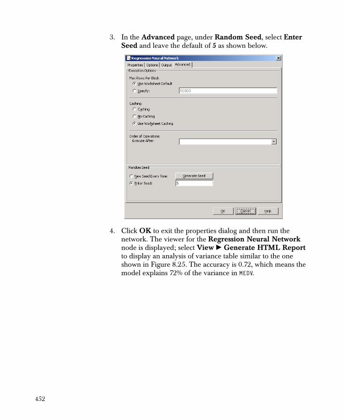
3. In the Advanced page, under Random Seed, select Enter Seed and leave the default of 5 as shown below.
4. Click OK to exit the properties dialog and then run the network. The viewer for the Regression Neural Network node is displayed; select View � Generate HTML Report to display an analysis of variance table similar to the one shown in Figure 8.25. The accuracy is 0.72, which means the model explains 72% of the variance in MEDV.
452
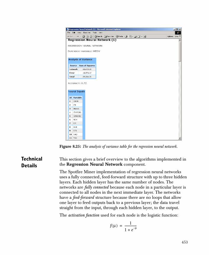
Technical Details
This section gives a brief overview to the algorithms implemented in the Regression Neural Network component.
The Spotfire Miner implementation of regression neural networks uses a fully connected, feed-forward structure with up to three hidden layers. Each hidden layer has the same number of nodes. The networks are fully connected because each node in a particular layer is connected to all nodes in the next immediate layer. The networks have a feed-forward structure because there are no loops that allow one layer to feed outputs back to a previous layer; the data travel straight from the input, through each hidden layer, to the output.
The activation function used for each node is the logistic function:
Figure 8.25: The analysis of variance table for the regression neural network.
f μ( ) 1
1 e μ–+-----------------=
453

This is also known as the sigmoid. The effect of this function is to prevent the neural network from computing very small or very large values.
The objective function is the sum-of-squared-errors function (SSE). Spotfire Miner makes successive passes through your data until either the maximum number of epochs is exceeded or the relative change in the SSE is below the convergence tolerance you set in the Options page of the properties dialog.
Learning Algorithms
Spotfire Miner supports five different learning algorithms for regression neural networks. Variations of back-propagation and batch learning are the primary methods; supported variants of batch learning include resilient propagation, delta-bar-delta, quick propagation, and online. You can also modify the batch learning method by adjusting the learning rate, momentum, and weight decay parameters in the Options page of the properties dialog.
The resilient propagation and delta-bar-delta algorithms are adaptive, in that each weight has its own learning rate that is adjusted at each epoch according to heuristic rules.
1. Resilient Propagation
In resilient propagation, each weight’s learning rate is adjusted by the signs of the gradient terms.
2. Delta-Bar-Delta
The delta-bar-delta algorithm uses an estimate of curvature that increases the learning rate linearly if the partial derivative with respect to the weight continues to maintain the same sign; the estimate decreases the learning rate exponentially if the derivative changes sign.
3. Quick Propagation
Quick propagation also uses weight decay and momentum but manipulates the partial derivatives differently. The algorithm approximates the error surface with a quadratic polynomial so that the update to the weights is the minimum of the parabola. Both the quick propagation and delta-bar-delta learning algorithms assume the weights are independent. In practice, however, the weights tend to be correlated.
454

4. Online
The online method updates the weights with each block of data. Instead of randomly picking observations from the data, it is assumed the data is ordered in a random fashion.
5. Conjugate Gradient
Spotfire Miner also provides the conjugate gradient optimization algorithm, but it uses an inexact line search and uses the learning rate to control the step size. An exact line search would require several passes through the data in order to determine the step size. While computing the gradient the neural network node is also evaluating the SSE of the model from the previous pass through the data. If the SSE has increased as a result of the step taken from the previous epoch the step is halved and the model is reevaluated. The algorithm will halve the step up to 5 times after which it will continue with the current step. Jittering the weights, available through the neural network viewer, might be a useful tool if the conjugate gradient algorithm is step halving. Moreover, since the learning rate is used to control the step size, it is advisable to start with a small learning rate in the beginning of the training session and perhaps increasing it as the training progresses. The initial learning rate should be inversely proportional to the size of the training data: the more rows in the training data the smaller the initial learning rate.
Reed and Marks (1999) give mathematical derivations for all five learning algorithms implemented in Spotfire Miner.
Initialization of Weights
Spotfire Miner provide three methods of initializing weights: uniform random values, weights from the previous learning run, or loading weights saved to a file from a previous learning run. When initializing weights to a node using random values, the range for the random values is , where is the number of inputs to a node. If you are going to initialize the weights from the previous run or from weights saved to a file it is imperative that the input variables, number of hidden layers, or the output variable are consistent with the current configuration.
2.4 k⁄– 2.4 k⁄,( ) k
455
REFERENCES
Belsley, D.A., Kuh, E., and Welsch, R.E. (1980). Regression Diagnostics: Identifying Influential Data and Sources of Collinearity. New York: John Wiley & Sons, Inc.
Breiman, L. (1996). Bagging predictors. Machine Learning, 26:123-140.
Breiman, L., Friedman, J., Olshen, R.A., and Stone, C. (1984). Classification and Regression Trees. CRC Press, LLC.
Bun, Y. (2002). Recursive Block Update QR Factorization with Column Pivoting for Linear Least Squares Problems. Insightful Corporation white paper.
Hastie, T., Tibshirani, R., and Friedman, J. (2001). The Elements of Statistical Learning: Data Mining, Inference, and Prediction . New York: Springer.
Lawson, C.L. and Hanson R.J. (1995). Solving Least Squares Problems, Siam.
Ripley, B.D. (1996). Pattern Recognition and Neural Networks . Cambridge: Cambridge University Press.
Sallas, W.M. and Lionti, A.M. (1988). Some Useful Computing Formulas for the Nonfull Rank Linear Model with Linear Equality Restriction. Joint Statistical Meetings, New Orleans, August 22-25, 1988.
Schapire, R. (1990). The strength of weak learnability. Machine Learning, 5:197-227.
Therneau, T. and Atkinson, E. (1997). An Introduction to Recursive Partitioning Using the RPART Routines. Mayo Foundation Technical Report.
456
Overview 458
The K-Means Component 461General Procedure 461Tips for Better Cluster Results 467
Technical Details 468Scalable K-Means Algorithm 468Coding of Categorical Variables 470
K-Means Clustering Example 471
References 481
CLUSTERING 9
457

OVERVIEW
Cluster analysis is the process of segmenting observations into classes or clusters so that the degree of similarity is strong between members of the same cluster and weak between members of different clusters. Spotfire Miner™ uses modified K-means clustering to group similar objects and classify them as a quantifiable result. If you are involved in market research, you could use clustering to group respondents according to their buying preferences. If you are performing medical research, you might be able to better determine treatment if diseases are properly grouped. Purchases, economic background, and spending habits are just a few examples of information that can be grouped, and once these objects are grouped, you can then apply this knowledge to reveal patterns and relationships on a large scale.
Figure 9.1: Running a clustering example using the K-Means node in Spotfire Miner
458
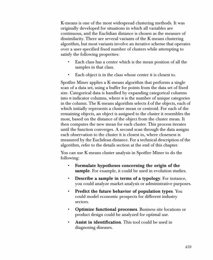
K-means is one of the most widespread clustering methods. It was originally developed for situations in which all variables are continuous, and the Euclidian distance is chosen as the measure of dissimilarity. There are several variants of the K-means clustering algorithm, but most variants involve an iterative scheme that operates over a user-specified fixed number of clusters while attempting to satisfy the following properties:
• Each class has a center which is the mean position of all the samples in that class.
• Each object is in the class whose center it is closest to.
Spotfire Miner applies a K-means algorithm that performs a single scan of a data set, using a buffer for points from the data set of fixed size. Categorical data is handled by expanding categorical columns into m indicator columns, where m is the number of unique categories in the column. The K-means algorithm selects k of the objects, each of which initially represents a cluster mean or centroid. For each of the remaining objects, an object is assigned to the cluster it resembles the most, based on the distance of the object from the cluster mean. It then computes the new mean for each cluster. This process iterates until the function converges. A second scan through the data assigns each observation to the cluster it is closest to, where closeness is measured by the Euclidean distance. For a technical description of the algorithm, refer to the details section at the end of this chapter.
You can use K-means cluster analysis in Spotfire Miner to do the following:
• Formulate hypotheses concerning the origin of the sample. For example, it could be used in evolution studies.
• Describe a sample in terms of a typology. For instance, you could analyze market analysis or administrative purposes.
• Predict the future behavior of population types. You could model economic prospects for different industry sectors.
• Optimize functional processes. Business site locations or product design could be analyzed for optimal use.
• Assist in identification. This tool could be used in diagnosing diseases.
459

• Measure the different effects of treatments on classes within the population. An analysis of variance could be run to determine efficacy of treatment.
Unlike the Classification node that analyzes previously categorized data objects, clustering does not rely on predefined class labels. In general, the class labels are not present in the training data because they are not known to begin with, and clustering can be used to create such labels. For this reason, clustering is a form of learning by observation (unsupervised), rather than learning by examples (supervised). You can create a Predict: K-Means node from the Spotfire Miner K-Means node to segment new observations into the cluster they are closest to, measured by the Euclidean distance to the cluster centroid.
Clustering is used in several applications, including pattern recognition, image processing, market research, and sample description. By clustering, one can identify dense and sparse regions to ultimately discover overall distribution patterns and correlations among data attributes.
460
THE K-MEANS COMPONENT
Clustering performed in Spotfire Miner uses a modified K-means clustering algorithm, which assumes that each cluster has a center defined as the mean position of all samples in that cluster, and that each object is in the cluster whose center is closest to it.
The K-Means component classifies information in your data set by grouping continuous or categorical variables according to user-specified criteria. You can select the data, specify which columns to include, how many clusters to generate, and options to control the algorithm.
General Procedure
The following outlines the simplest and most common approach for using the K-Means component:
1. Link a K-Means node in your worksheet to any node that outputs data.
2. Use the properties dialog for K-Means to specify the columns in your data set that you want to cluster and the Number of Clusters you want to create.
Properties The properties of the K-Means dialog are accessed by double-clicking the K-Means node or right-clicking and select Properties.
461
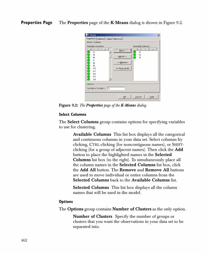
Properties Page The Properties page of the K-Means dialog is shown in Figure 9.2.
Select Columns
The Select Columns group contains options for specifying variables to use for clustering.
Available Columns This list box displays all the categorical and continuous columns in your data set. Select columns by clicking, CTRL-clicking (for noncontiguous names), or SHIFT-clicking (for a group of adjacent names). Then click the Add button to place the highlighted names in the Selected Columns list box (to the right). To simultaneously place all the column names in the Selected Columns list box, click the Add All button. The Remove and Remove All buttons are used to move individual or entire columns from the Selected Columns back to the Available Columns list.
Selected Columns This list box displays all the column names that will be used in the model.
Options
The Options group contains Number of Clusters as the only option.
Number of Clusters Specify the number of groups or clusters that you want the observations in your data set to be separated into.
Figure 9.2: The Properties page of the K-Means dialog.
462
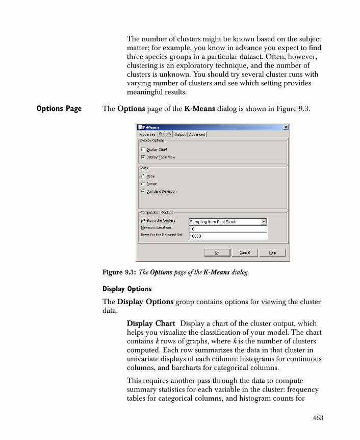
The number of clusters might be known based on the subject matter; for example, you know in advance you expect to find three species groups in a particular dataset. Often, however, clustering is an exploratory technique, and the number of clusters is unknown. You should try several cluster runs with varying number of clusters and see which setting provides meaningful results.
Options Page The Options page of the K-Means dialog is shown in Figure 9.3.
Display Options
The Display Options group contains options for viewing the cluster data.
Display Chart Display a chart of the cluster output, which helps you visualize the classification of your model. The chart contains k rows of graphs, where k is the number of clusters computed. Each row summarizes the data in that cluster in univariate displays of each column: histograms for continuous columns, and barcharts for categorical columns.
This requires another pass through the data to compute summary statistics for each variable in the cluster: frequency tables for categorical columns, and histogram counts for
Figure 9.3: The Options page of the K-Means dialog.
463
continuous variables. This extra pass through the data can take quite a while if there are many observations or if the number of clusters is large.
Display Table View Display a table of the cluster data. This includes a table of the k cluster centers, the scaling factors that were applied to the data, and a table of the cluster sizes and the within-cluster sum-of-squares. The within-cluster sum-of-squares is the sum of the squared distances of all observations in the cluster to its center. Note this option is selected by default.
Scale
The Scale group provides you with options to control how the data is scaled. For example, if you had observations for x and y between 0 and 1 and for z between 1000 and 2000, the distance calculations to any center would be dominated by the z column. To force columns to have a more equal contribution, you can scale them first. Scaling by the range maps all the data to the interval of 0 to 1. Scaling by the standard deviation results in all columns having a standard deviation (spread) of 1.
None No weighting is performed.
Range Each column is divided by its range.
Standard Deviation Each column is divided by its standard deviation. This is the default option.
Computation Options
The Computation Options group includes processing options when the model is run.
Initializing the Centers This has a drop-down menu with the following data options available:
• First K Data Points The first unique k rows of data are used as the initial centers.
• Sampling from First Block Select a random sample of k rows from the first block of data as the initial centers. You can set the block (or chunk) size in the Advanced page of the node.
464
• HClust on First Block Select this option to compute the initial centers from the first block of data set using the hierarchical clustering method.
• HClust on Sampling from the Entire Dataset Select this option to compute the initial centers using the hierarchical clustering method on a sample from the entire dataset. The sample size depends on the available virtual memory. This option is computationally the slowest but it produces the best result because it estimates the initial centers from the entire dataset. The closer the initial centers are to the true centers, the better result computed by the scalable K-Means.
The K-means algorithm starts with initial estimates of the cluster centers. The default is to randomly select k rows from the first block of data. If the first block of data is not representative of all your data, you might want to use the Shuffle node to shuffle your data before passing it to the K-Means node. If you shuffle the data through the first k rows, it is equivalent to a random sample from the original data.
Maximum Iterations The number of iterations that you want to run within a block. This is the number of iterations of the standard K-Means algorithm that is applied to the combined new data from the block, the retained set, and the current centers.
Rows for the Retained Set As each block (or chunk) of data is processed, observations that do not cluster well are kept in the retain set. At the next step in the algorithm, the observations are added to the new chunk of data and the K-means clustering is run on this combined set. Making the retained set large leads to more accurate clustering. However, the retained set plus the current chunk size must fit into memory at once, so it cannot be arbitrarily large.
Enter 0 to let Spotfire Miner internally set the number of retained rows based on the available virtual memory.
465
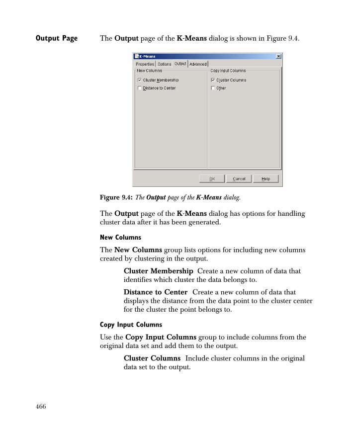
Output Page The Output page of the K-Means dialog is shown in Figure 9.4.
The Output page of the K-Means dialog has options for handling cluster data after it has been generated.
New Columns
The New Columns group lists options for including new columns created by clustering in the output.
Cluster Membership Create a new column of data that identifies which cluster the data belongs to.
Distance to Center Create a new column of data that displays the distance from the data point to the cluster center for the cluster the point belongs to.
Copy Input Columns
Use the Copy Input Columns group to include columns from the original data set and add them to the output.
Cluster Columns Include cluster columns in the original data set to the output.
Figure 9.4: The Output page of the K-Means dialog.
466

Other Include all other columns that are not cluster columns in the original data set to the output.
Tips for Better Cluster Results
Clustering is a form of unsupervised learning, and often there is no single correct answer. To get the most informative results, you might need to run the clustering with several to many different numbers of clusters requested.
If your data is on a widely varying scale, be sure to select one of the Scale options.
Setting the retain set size to any large value generally gives better results. Note that all data from a chunk plus the retain set data must fit into memory at the same time. As mentioned in the previous section, entering a 0 in the Rows for the Retained Set option internally sets Spotfire Miner to base the number of rows in the retained set on the amount of virtual memory.
Finally, only try to cluster on meaningful columns. Using phone numbers, customer identification, or street addresses can possibly hinder the algorithm and add nothing to the final cluster results.
467
TECHNICAL DETAILS
Scalable K-Means Algorithm
The scalable K-Means algorithm used in Spotfire Miner updates the resultant k clusters one chunk at a time by applying the standard K-Means algorithm to the chunk of data combined with a retained set. The retained set contains data points that are far from the previous centers. The following describes the steps of the algorithm:
1. Empty the retained set’s buffer.
2. Initialize k centers and assign zero weight to them.
3. Read a new block from the data set and assign a unit weight to each observation.
4. Combine the three sets: the retained set, the k centers, and the new block of data set.
5. Apply the standard K-Means algorithm to the combined set.
6. Refill the retained set with observations whose distances to their centers are the largest.
7. Compress the remaining observations to the centers and update the centers and weights.
8. Repeat step 3 if more data is available.
Steps 1, 2 and 3 are the initial steps needed to initialize three sets of data points: the retained set, centers, and a new block of the data set. Step 4 combines the three sets preparing a single data set for the standard K-Means operation.
In step 5, the standard K-Means is applied to the data set prepared by step 4. The standard K-Means is based on a heuristic strategy by iteratively moving observations from one cluster to another in search for local minimum within-cluster sums of squares. For this scalable K-Means algorithm, the standard K-Means algorithm minimizes the within-cluster weighted sums of squares:
Minimize where is the within-cluster weighted sums of
squares of the kth cluster computed as
SSk
k 1=
K
SSk
468
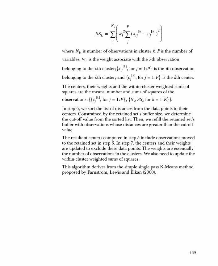
where is number of observations in cluster k. P is the number of
variables. is the weight associate with the i-th observation
belonging to the kth cluster; is the ith observation
belonging to the kth cluster; and is the kth center.
The centers, their weights and the within-cluster weighted sums of squares are the means, number and sums of squares of the
observations: { , }.
In step 6, we sort the list of distances from the data points to their centers. Constrained by the retained set’s buffer size, we determine the cut-off value from the sorted list. Then, we refill the retained set’s buffer with observations whose distances are greater than the cut-off value.
The resultant centers computed in step 5 include observations moved to the retained set in step 6. In step 7, the centers and their weights are updated to exclude these data points. The weights are essentially the number of observations in the clusters. We also need to update the within-cluster weighted sums of squares.
This algorithm derives from the simple single pass K-Means method proposed by Farnstrom, Lewis and Elkan (2000).
SSk wi2
xijk[ ]
cjk[ ]
–( )2
j
P
i
Nk
=
Nk
wi
{xijk[ ], for j 1:P= }
{cjk[ ], for j 1:P= }
{cjk[ ], for j 1:P= } {Nk SSk, for k 1:K= }
469
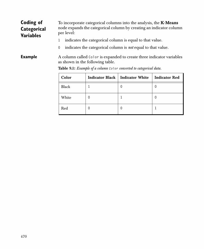
Coding of Categorical Variables
To incorporate categorical columns into the analysis, the K-Means node expands the categorical column by creating an indicator column per level:
1 indicates the categorical column is equal to that value.
0 indicates the categorical column is not equal to that value.
Example A column called Color is expanded to create three indicator variables as shown in the following table.Table 9.1: Example of a column Color converted to categorical data.
Color Indicator Black Indicator White Indicator Red
Black 1 0 0
White 0 1 0
Red 0 0 1
470
K-MEANS CLUSTERING EXAMPLE
The syncontrol.txt data set in the examples directory contains 600 examples of control charts synthetically generated by the process in Alcock and Manolopoulos (1999). The data are available from the UCI KDD Archive (Hettich and Bay, 1999). The original data set was grouped by row number into six different classes of controls, but the data rows have been shuffled in syncontrol.txt. The six classes are as follows:
• Normal
• Cyclic
• Increasing trend
• Decreasing trend
• Upward shift
• Downward shift
The data set contains 100 examples from each of the six classes. In this example, we apply Spotfire Miner K-Means clustering to the syncontrol.txt time series data in order to compare centers of control chart classes. The following steps describe how to run this Clustering example:
1. Click and drag the Read Text File, Descriptive Statistics, K-Means, and Table View components to the workspace, as shown in Figure 9.5 on the following page.
2. Link the output of the Read Text File node to both the Descriptive Statistics and K-Means nodes. Link the Table View node to the output of the K-Means node.
471
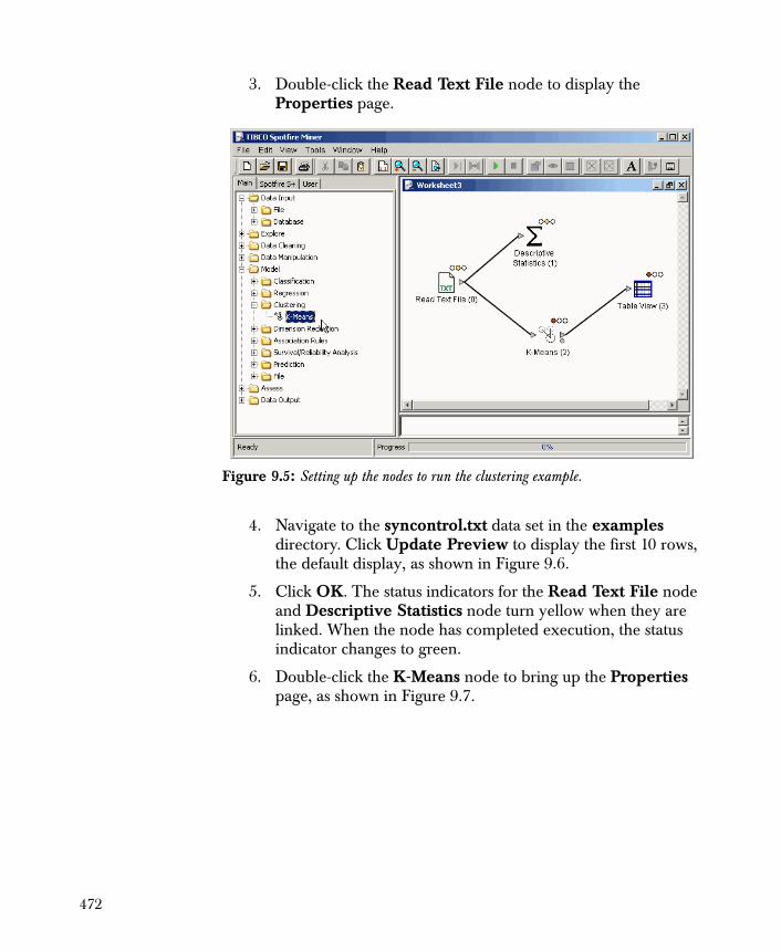
3. Double-click the Read Text File node to display the Properties page.
4. Navigate to the syncontrol.txt data set in the examples directory. Click Update Preview to display the first 10 rows, the default display, as shown in Figure 9.6.
5. Click OK. The status indicators for the Read Text File node and Descriptive Statistics node turn yellow when they are linked. When the node has completed execution, the status indicator changes to green.
6. Double-click the K-Means node to bring up the Properties page, as shown in Figure 9.7.
Figure 9.5: Setting up the nodes to run the clustering example.
472
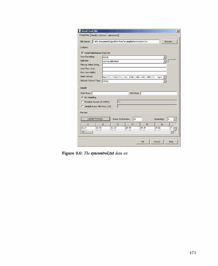
Figure 9.6: The syncontrol.txt data set.
473
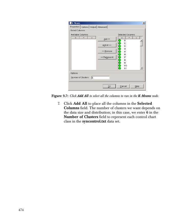
7. Click Add All to place all the columns in the Selected Columns field. The number of clusters we want depends on the data size and distribution; in this case, we enter 6 in the Number of Clusters field to represent each control chart class in the syncontrol.txt data set.
Figure 9.7: Click Add All to select all the columns to run in the K-Means node.
474
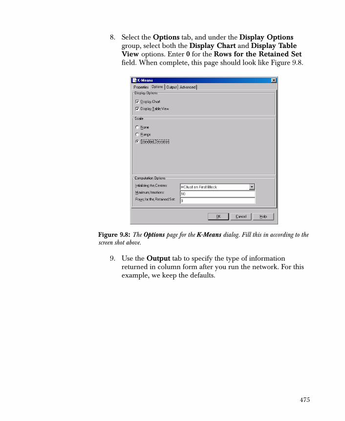
8. Select the Options tab, and under the Display Options group, select both the Display Chart and Display Table View options. Enter 0 for the Rows for the Retained Set field. When complete, this page should look like Figure 9.8.
9. Use the Output tab to specify the type of information returned in column form after you run the network. For this example, we keep the defaults.
Figure 9.8: The Options page for the K-Means dialog. Fill this in according to the screen shot above.
475
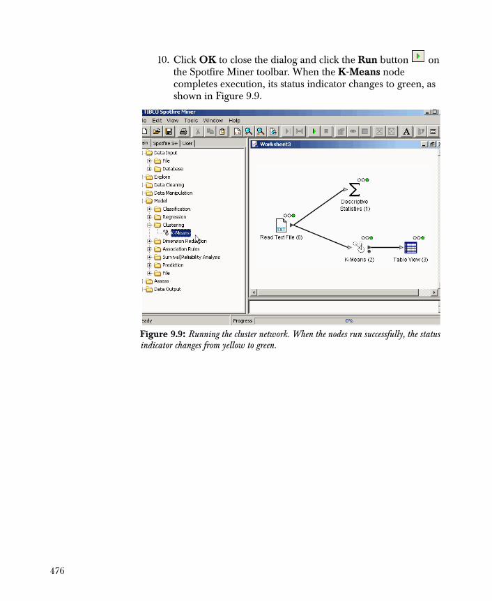
10. Click OK to close the dialog and click the Run button on the Spotfire Miner toolbar. When the K-Means node completes execution, its status indicator changes to green, as shown in Figure 9.9.
Figure 9.9: Running the cluster network. When the nodes run successfully, the status indicator changes from yellow to green.
476
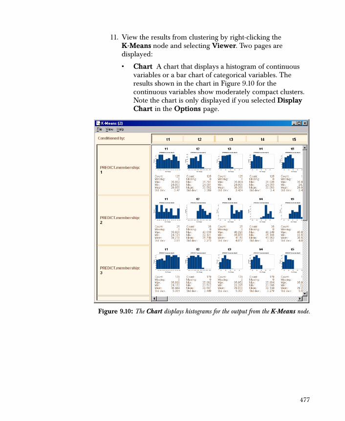
11. View the results from clustering by right-clicking the K-Means node and selecting Viewer. Two pages are displayed:
• Chart A chart that displays a histogram of continuous variables or a bar chart of categorical variables. The results shown in the chart in Figure 9.10 for the continuous variables show moderately compact clusters. Note the chart is only displayed if you selected Display Chart in the Options page.
Figure 9.10: The Chart displays histograms for the output from the K-Means node.
477
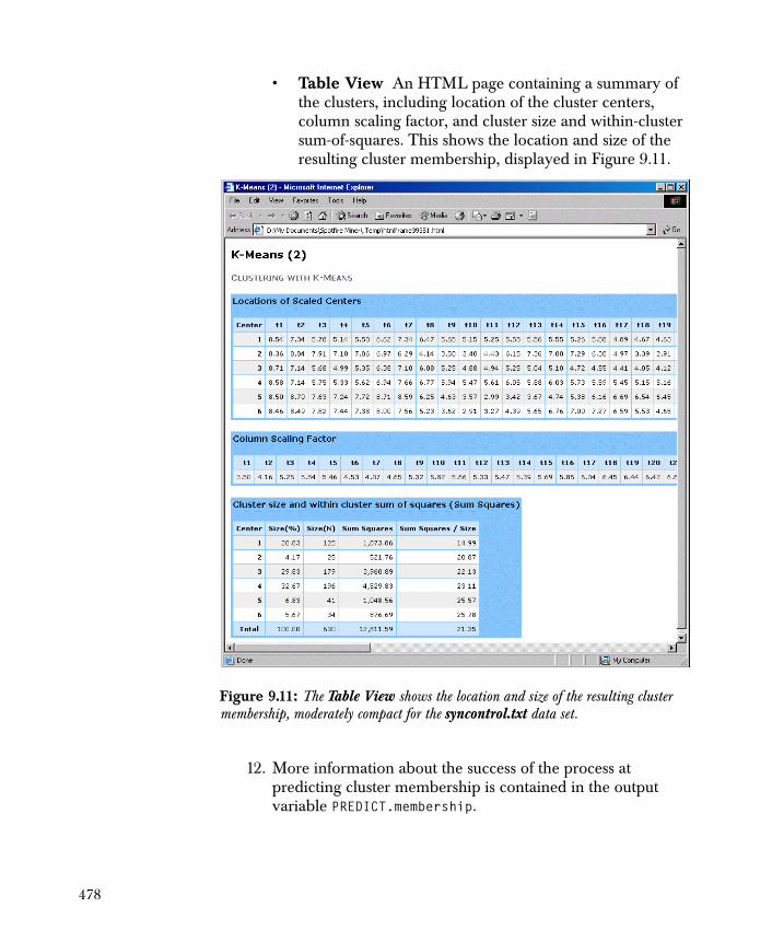
• Table View An HTML page containing a summary of the clusters, including location of the cluster centers, column scaling factor, and cluster size and within-cluster sum-of-squares. This shows the location and size of the resulting cluster membership, displayed in Figure 9.11.
12. More information about the success of the process at predicting cluster membership is contained in the output variable PREDICT.membership.
Figure 9.11: The Table View shows the location and size of the resulting cluster membership, moderately compact for the syncontrol.txt data set.
478
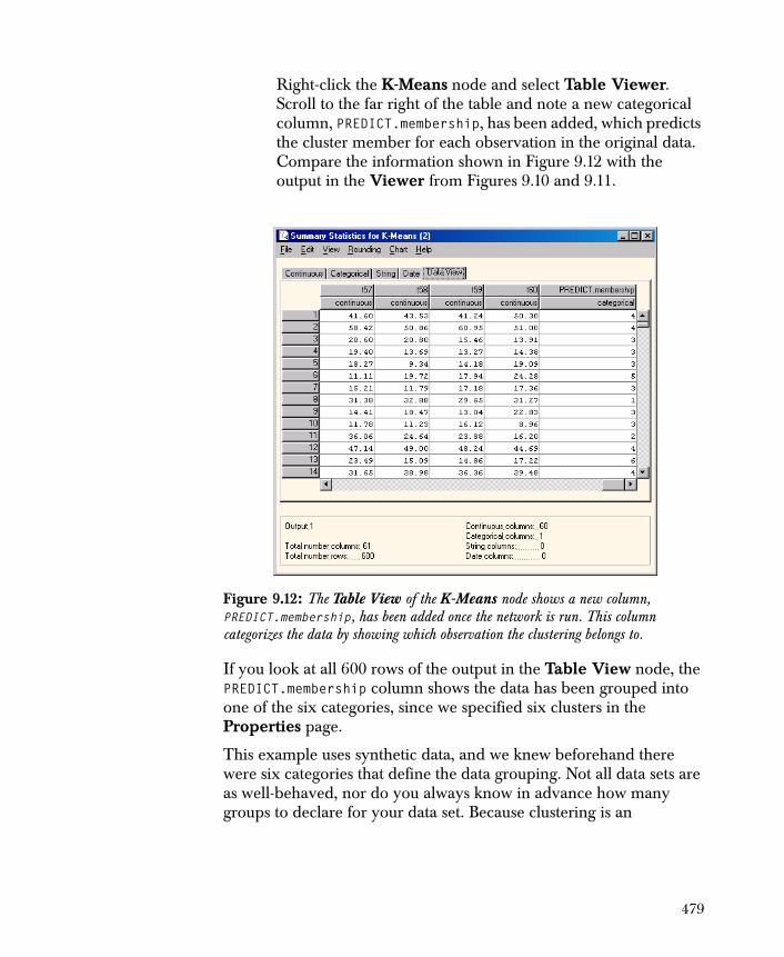
Right-click the K-Means node and select Table Viewer. Scroll to the far right of the table and note a new categorical column, PREDICT.membership, has been added, which predicts the cluster member for each observation in the original data. Compare the information shown in Figure 9.12 with the output in the Viewer from Figures 9.10 and 9.11.
If you look at all 600 rows of the output in the Table View node, the PREDICT.membership column shows the data has been grouped into one of the six categories, since we specified six clusters in the Properties page.
This example uses synthetic data, and we knew beforehand there were six categories that define the data grouping. Not all data sets are as well-behaved, nor do you always know in advance how many groups to declare for your data set. Because clustering is an
Figure 9.12: The Table View of the K-Means node shows a new column, PREDICT.membership, has been added once the network is run. This column categorizes the data by showing which observation the clustering belongs to.
479

exploratory process, you might need to rerun the data set several times using different options to reveal the underlying structure of the data set.
480
REFERENCES
Alcock, R.J. and Y. Manolopoulos. 1999. Time-series similarity queries employing a feature-based approach. In proceedings of the 7th Hellenic Conference on Informatics. Ioannina, Greece.
Farnstrom, F., J. Lewis. and C. Elkan. 2000. Scalability of clustering algorithms revisited. SIGKDD Explorations, 2(1), pp. 51-57.
Hartigan, J.A. 1975. Clustering Algorithms. New York: John Wiley & Sons, Inc.
Hettich, S. and S.D. Bay. 1999. The UCI KDD Archive [http://kdd.ics.uci.edu]. Irvine, CA: University of California, Department of Information and Computer Science.
Kaufman, L. and P.J. Rousseeuw. 1990. Finding Groups in Data: An Introduction to Cluster Analysis. New York: John Wiley & Sons, Inc.
481

482

Overview 484
Principal Components 485General Procedure 485Properties 486
An Example Using Principal Components 490
Technical Details 493
DIMENSION REDUCTION 10
483
OVERVIEW
When collecting multivariate data, it is common to discover that multicollinearity exists in the variables. One implication of these correlations is that there will be some redundancy in the information provided by the variables. Principal Components Analysis (PCA) exploits the redundancy in multivariate data, revealing patterns in the variables and significantly reducing the size of a data set with a negligible loss of information.
Spotfire Miner™ provides a Principal Component component as a dimension reduction tool. For example, consider the cross-selling data, the xsell.sas7bdat file located in the examples directory of the Spotfire Miner installation. After data cleaning (described in the example below), there are potentially 31 variables in this data set that could be used as predictors for credit card ownership. The Principal Components node can reduce the number of predictor variables to 13 and retain approximately 92 percent of the variation contained in 31columns. The scores computed from the Principal Components node can then be used as predictors in a logistic regression. Care must be taken when using the principal components as predictors for a dependent variable since the principal components are computed independently of the dependent variable. Retention of the principal components that have the highest variance is not the same as choosing those principal components that have a highest correlation with the dependent variable. This is demonstrated in the example below.
Typically, principal components are computed from numeric variables (columns). At times, it might be useful to include categorical columns in a PCA, and Spotfire Miner allows their inclusion. The section Technical Details describes how categorical columns are handled.
484

PRINCIPAL COMPONENTS
The Principal Components component can be found in the Model folder under the subfolder labeled Dimension Reduction.
General Procedure
The following outlines the simplest and most common approach for using the Principal Components component:
1. Link a Principal Components node on your worksheet to any node that outputs data, such as a Read Text File or Read SAS File node.
2. Use the properties dialog for Principal Components to specify the columns in your data set that you want to use in the your PCA.
Figure 10.1: The Principal Components component is located in the Model folder, under the subfolder Dimension Reduction.
485
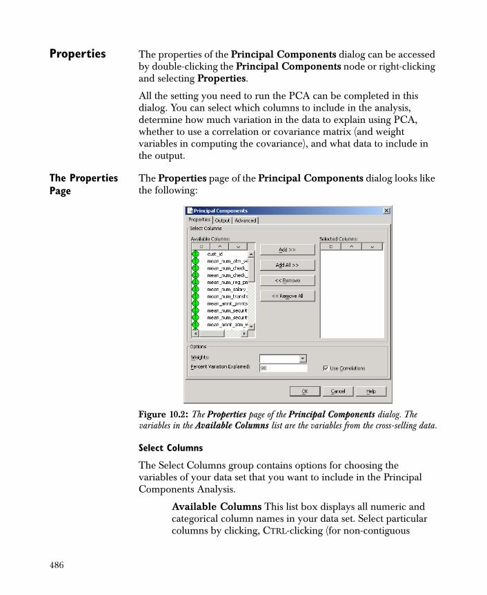
Properties The properties of the Principal Components dialog can be accessed by double-clicking the Principal Components node or right-clicking and selecting Properties.
All the setting you need to run the PCA can be completed in this dialog. You can select which columns to include in the analysis, determine how much variation in the data to explain using PCA, whether to use a correlation or covariance matrix (and weight variables in computing the covariance), and what data to include in the output.
The Properties Page
The Properties page of the Principal Components dialog looks like the following:
Select Columns
The Select Columns group contains options for choosing the variables of your data set that you want to include in the Principal Components Analysis.
Available Columns This list box displays all numeric and categorical column names in your data set. Select particular columns by clicking, CTRL-clicking (for non-contiguous
Figure 10.2: The Properties page of the Principal Components dialog. The variables in the Available Columns list are the variables from the cross-selling data.
486
names), or SHIFT-clicking (for a group of adjacent names). Click the Add button to move the highlighted names into the Selected Columns list box. You can click the Add All button to simultaneously place all column names in the Selected Columns list. If you need to remove particular columns, select them by clicking, CTRL-clicking, or SHIFT-clicking, and then clicking the Remove button. Alternatively, click the Remove All button to simultaneously remove all variables from the Selected Columns list.
Selected Columns This list box displays all the column names that are used in the model.
Options
The Options group contains the Weights, Percent Variation Explained, and Use Correlations options to control how the PCA is performed.
Weights Select a variable in the data set to use as weight when computing the covariance or correlation matrix.
Percent Variation Explained Enter the percent variation in the data that you want to be explained by the principal components. The default value is 90, but any value greater than 0 and less than or equal to 100 can be used. The first principal component is the linear combination of the variables that has the highest variance. The second principal component is the linear combination orthogonal to the first that has the next highest variance.
Use Correlations Select this if you want to use the correlation matrix to compute the principal component variance and loadings. Typically, computations on a correlation matrix are preferred unless all the columns have the same scale. If you do not select this option, the computations use the covariance matrix of the selected columns.
487
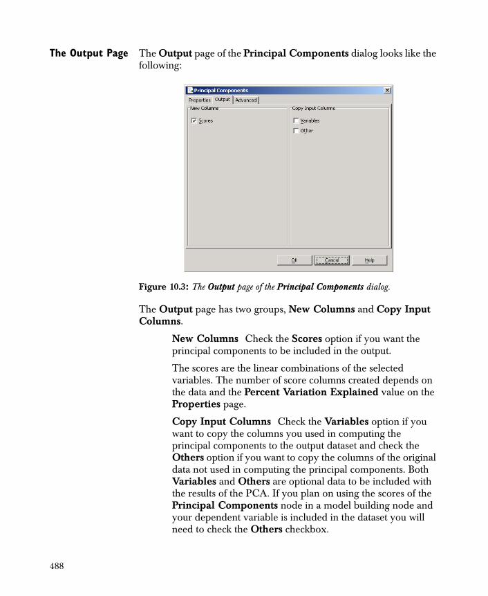
The Output Page The Output page of the Principal Components dialog looks like the following:
The Output page has two groups, New Columns and Copy Input Columns.
New Columns Check the Scores option if you want the principal components to be included in the output.
The scores are the linear combinations of the selected variables. The number of score columns created depends on the data and the Percent Variation Explained value on the Properties page.
Copy Input Columns Check the Variables option if you want to copy the columns you used in computing the principal components to the output dataset and check the Others option if you want to copy the columns of the original data not used in computing the principal components. Both Variables and Others are optional data to be included with the results of the PCA. If you plan on using the scores of the Principal Components node in a model building node and your dependent variable is included in the dataset you will need to check the Others checkbox.
Figure 10.3: The Output page of the Principal Components dialog.
488
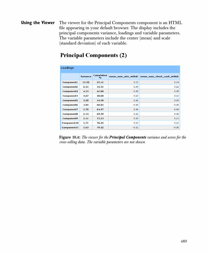
Using the Viewer The viewer for the Principal Components component is an HTML file appearing in your default browser. The display includes the principal components variance, loadings and variable parameters. The variable parameters include the center (mean) and scale (standard deviation) of each variable.
Figure 10.4: The viewer for the Principal Components variance and scores for the cross-selling data. The variable parameters are not shown
489

AN EXAMPLE USING PRINCIPAL COMPONENTS
We will build the network displayed in Figure 10.6 using the cross-selling data in the xsell.sas7bdat SAS file found in the examples directory. For this example we assume you are familiar with the Read SAS File, Modify Columns, and Correlations nodes.
1. Move a new Read SAS File node onto the worksheet and read the xsell.sas7bdat file. In the Modify Columns page of the properties dialog exclude all columns from birthdays to std_saving_balance. Also drop columns address_language, address_lang_changes, name_changes, nationality_changes, num_gender_corrections, current_nationality, current_profession, gender, marital_status. These variables either have too many missing values or are constant.
2. Click and drag a Principal Components component onto the worksheet.
3. Right-click to open the Principal Components node’s properties dialog, and add all variables except cust.id and credit.card.owner to the Selected Columns list.
4. Ensure the Use Correlations option is checked. This is the default setting.
5. In the Percent Variation Explained Enter in 100.
6. Select the Output tab and make sure the Scores check box is selected in the New Columns group; by doing this, you include columns of principal component scores as output when you run the Principal Components Analysis. Select the Other check box in the Copy Input Columns group to copy the dependent variable credit.card.owner in the output. Exit the dialog using the OK button.
7. Drop a Correlations node onto the worksheet connecting the output from the Principal Components node to it.
8. Run the network.
Upon opening the Principal Components viewer you will note that it took 29 principal components to explain 100% of the variability in the 31 columns of data and the principal components beyond the first 22 only contribute the last 1%.
490
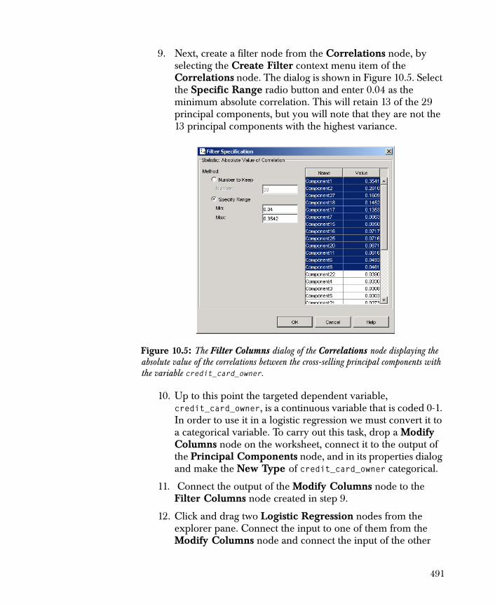
9. Next, create a filter node from the Correlations node, by selecting the Create Filter context menu item of the Correlations node. The dialog is shown in Figure 10.5. Select the Specific Range radio button and enter 0.04 as the minimum absolute correlation. This will retain 13 of the 29 principal components, but you will note that they are not the 13 principal components with the highest variance.
10. Up to this point the targeted dependent variable, credit_card_owner, is a continuous variable that is coded 0-1. In order to use it in a logistic regression we must convert it to a categorical variable. To carry out this task, drop a Modify Columns node on the worksheet, connect it to the output of the Principal Components node, and in its properties dialog and make the New Type of credit_card_owner categorical.
11. Connect the output of the Modify Columns node to the Filter Columns node created in step 9.
12. Click and drag two Logistic Regression nodes from the explorer pane. Connect the input to one of them from the Modify Columns node and connect the input of the other
Figure 10.5: The Filter Columns dialog of the Correlations node displaying the absolute value of the correlations between the cross-selling principal components with the variable credit_card_owner.
491
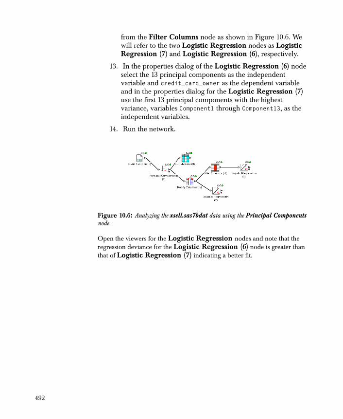
from the Filter Columns node as shown in Figure 10.6. We will refer to the two Logistic Regression nodes as Logistic Regression (7) and Logistic Regression (6), respectively.
13. In the properties dialog of the Logistic Regression (6) node select the 13 principal components as the independent variable and credit_card_owner as the dependent variable and in the properties dialog for the Logistic Regression (7) use the first 13 principal components with the highest variance, variables Component1 through Component13, as the independent variables.
14. Run the network.
Open the viewers for the Logistic Regression nodes and note that the regression deviance for the Logistic Regression (6) node is greater than that of Logistic Regression (7) indicating a better fit.
Figure 10.6: Analyzing the xsell.sas7bdat data using the Principal Components node.
492

TECHNICAL DETAILS
If there is a categorical column included in the PCA, it is first expanded into k indicator columns, where k is the number of levels in that categorical column. For a given row in the data set, the i-th column in the expanded set is 1 if the row corresponds to the i-th level; it is 0 otherwise.
After expanding each categorical column, the correlation or covariance matrix is computed for all the selected columns.
Assuming the correlation matrix of the selected variables is used in the principal component analysis and is of dimension , then
PCA computes the eigen values and their associated
eigen vectors of the correlation matrix. If only c of the k of the
eigen values and vectors are retained, then we can assume the following:
1. The th principal component score, , is the
orthogonal projection of centered and scaled variables,
, in the direction or , where m is
the k-vector of variable means, and S is a diagonal
matrix of variable standard deviations. The are referred to
as the principal component loadings or coefficients.
2) The are uncorrelated and have a variance of .
3) The sum of the is equal to the rank of the
correlation matrix.
4) The percent variance explained by the c principal components is sum of the divided by the rank of the correlation
matrix.
If the variable covariance matrix is used instead of the correlation matrix, the variables are not scaled when computing the principal component scores and the sum of the variances, is
equal to the trace of the covariance matrix.
k k×λj 1 2 … k,,,=
vj
j λj 1 2 … c,,,=
z x m–( )S 1–= vj yj vj
Tz=
k k×vj
yj λj
λj 1 2 … k,,,=
λj 1 2 … c,,,=
λj 1 2 … k,,,=
493

A word of caution: Principal components are constructed independently of the dependent variable and restricting attention to the first principal components with the largest eigenvalues can introduce high bias by discarding components with small eigenvalues but are closely associated with the dependent variable.
c k<
494
Overview 496
Association Rules Node Options 497Properties Page 497Options Page 497Output Page 499
Definitions 501Support 501Confidence 501Lift 502
Data Input Types 503
Groceries Example 505Setting the Association Rules 505
ASSOCIATION RULES 11
495

OVERVIEW
Association rules specify how likely certain items occur together with other items in a set of transactions. The classic example used to describe association rules is the "market basket" analogy, where each transaction contains the set of items bought on one shopping trip. The store manager might want to ask questions, such as “if a shopper buys chips, does the shopper usually also buy dip?” Using a market basket analysis, the store manager can discover association rules for these items, so he knows whether he should plan on stocking chips and dip amounts accordingly and place the items near each other in the store.
496
ASSOCIATION RULES NODE OPTIONS
This section describes the options available in the Association Rules node dialog. For a simple example of applying an association rules analysis, see the section Groceries Example on page 505.
Properties Page
Access the properties of the Association Rules dialog by double-clicking the Association Rules node or right-clicking and selecting Properties.
Available Columns and Item Columns
You can specify the columns to analyze by selecting column names from the Available Columns list box and adding them to the Item Columns list box. You might want to exclude items that appear in every transaction, for example, because these items do not provide interesting results.
Transaction ID Columns
If your data’s input format contains transaction IDs, you can add this column to this box. See Table 11.1 for more information about the Transaction Id input format.
Input Format
The option Input Format specifies how the transaction items are read from the input data. For more detailed information about the recognized input formats, see Table 11.1.
Sort ID Columns
If your data’s input format contains transaction IDs, you can sort by this column. See Table 11.1 for more information about the Transaction Id input format.
Options Page Access the options of the Association Rules dialog by double-clicking the Association Rules node, and then clicking the Options tab. Use the Options tab to control how the algorithm is applied to give meaningful results.
497
Minimum Support
Indicates the minimum support for items and rules, as a fraction (from 0.0 to 1.0) of the total number of input transactions. The default is 0.1. Note that the definition of rule support is affected by Rule Support Both.
Minimum Confidence
Indicates the minimum confidence for generated rules, as a fraction (from 0.0 to 1.0) of the total number of input transactions. The default is 0.8.
Minimum Rule Items
Determines the minimum number of antecedents your rule can have. (Remember: you can have one and only one consequent.) For example, if you set Minimum Rule Items to 1, then your results can return rules with just the consequent and no antecedents. (The default is 2, which allows for one consequent and at least one antecedent.)
Maximum Rule Items
Determines the maximum number of antecedents for the rule. The default 5 allows for 1 consequent and up to 4 antecedents.
Prescan Items
Indicates that the transactions are to be scanned and the initial item list created out of memory. If you do not select this option, Spotfire Miner constructs a table of all unique items that appear in the input transactions, even if most of the items do not appear in rules (because they do not appear in enough transactions). If the input data contains many different items, such as thousands of SKUs for retail data, you could run out of memory and fail with an error. By selecting Prescan Items, you can avoid possible memory problems, but at the cost of additional runtime.
Rule Support Both
Indicates whether to include both the consequent and the antecedent when calculating the support. For more on support, see the section Definitions on page 501.
498
Output Page Access the output options of the Association Rules dialog by double-clicking the Association Rules node, and then clicking the Output tab. Use the Output tab to specify which elements (rule strings, measures, and so on) are output by the function.
Output Rule Strings
Specifies that the output data includes a column named "rule" containing the generated rule formatted as a string. For example, the rule string "aa <- bb cc" is a rule with a single consequent item "aa" and two antecedent items "bb" and "cc". The antecedent items are always sorted alphabetically within a rule.
Output Rule Items
Specifies that the output data includes a column named "con1" containing the generated rule consequent, and columns "ant1", "ant2", and so on, containing the rule antecedents. If a given rule has only one antecedent, columns "ant2" and so on are empty strings. Using these columns, it is possible to process the rule items without parsing the rule strings.
Output Rule Sizes
Specifies that the output data includes several columns with values measuring the number of items in each generated rule: "conSize" is the number of consequent items in the rule (currently always 1), "antSize" is the number of antecedent items in the rule, and "ruleSize" is the total number of items in the rule.
Output Measures
Specifies that the output data includes the columns "support", "confidence", and "lift" with calculated numeric measures for each generated rule. Note that the definition of rule support is affected by the Options page setting Rule Support Both.
Output Counts
Specifies that the output data includes columns giving raw counts for each generated rule. You can use these values to calculate measures such as "support", as well as more complicated measures for the rules. The raw count columns are:
499
• "conCount": The number of input transactions containing the rule consequent.
• "antCount": The number of input transactions containing the antecedents.
• "ruleCount": The number containing both consequent and antecedents.
• "transCount": The total number of transactions in the input set.
• "itemCount": The number of items used for creating rules.
The "transCount" and "itemCount" values are the same for every rule.
Available Output Columns
Lists all of the columns available for output.
Sort Output Columns By
The list of output columns names used to sort the result. The result data is sorted by each of these columns, in alphabetical order (for string columns) or descending order (for numeric columns). The default sorts rules with the highest lift values first, and sorts rules with the same lift value in alphabetical order.
500

DEFINITIONS
This section definitions of some of the key terms for understanding association rules.
Support The input of an itemset is defined as the proportion of transactions containing all of the items in the itemset.
Support measures significance (that is, the importance) of a rule. The user determines the minimum support threshold: that is, the minimum rule support for generated rules. The default value for the minimum rule support is 0.1. Any rule with a support below the minimum is disregarded.
The support of a rule can be defined in different ways. By default, support is measured as follows:
support = ruleCount / transCount
or
< the # of transactions containing the rule consequent and antecedent> / <the total number of transactions>
If you do not select Rule Support Both, only the antecedent is included in the support calculation. That is:
support = antCount / transCount
Confidence Confidence is also called strength. It can be interpreted as an estimate of the probability of finding the antecedent of the rule under the condition that a transaction also contains the consequent.
confidence = ruleCount / antCount
= <# transactions with rule consequent and antecedents>
/ <# transactions with rule antecedents>
The default value for the minimum confidence is 0.8. Any rule with a confidence below the minimum is disregarded.
501
Lift Often the Association Rules node returns too many rules, given the Minimum Support and Minimum Confidence constraints. If this is the case, you might want to apply another measure to rank your results. Lift is such a measure. Greater lift values indicate stronger associations. (Hahsler et al, 2008).
Lift is defined as the ratio of the observed confidence to that expected by chance.
lift = (ruleCount / antCount) / (conCount / transCount)
= ( <# transactions w rule consequent and antecedents> /
<# transactions w rule antecedents> ) /
( <# transactions w rule consequent> /
<total # transactions> )
Note that in small databases, lift can be subject to a lot of noise; it is most useful for analyzing larger databases.
For a more in-depth discussion of support, confidence, and lift, see Chapter 3 of the Big Data User’s Guide (SHOME/help/BigData.pdf) in the Spotfire S+ documentation.
502
DATA INPUT TYPES
The Association Rules node handles input data formatted in the four ways described below. In each input format, the input data contains a series of transactions, where each transaction contains a set of items.
Table 11.1: Association Rules Data Input Formats
Input Format Description
Item List Each input row contains one transaction. The transaction items are all non-NA, non-empty strings in the item columns. There must be enough columns to handle the maximum number of items in a single transaction. For example (column names and the first two rows):
"i1", "i2", "i3", "i4", "i5", "i6"
"milk", "cheese", "bread" , , ,
"meat", "bread" , , , , ,
The first transaction contains items "milk", "cheese", and "bread", and the second transaction contains items "meat" and "bread".
Column Value Each input row contains one transaction. Items are created by combining column names and column values to produce strings of the form "<col>=<val>". This is useful for applying association rules to surveys where the results are encoded into a set of factor values.
This format is not suitable for the groceries example described for the three other input types. For example:
"Weight", "Mileage", "Fuel"
"medium", "high", "low"
"medium", "high", "low"
"low", "high", "low"
"medium", "high", "low"
The first, second, and fourth transactions contain the items "Weight=medium", "Mileage=high", and "Fuel=low". The third transaction contains the items "Weight=low", "Mileage=high", and "Fuel=low".
503
Column Flag Each input row contains one transaction. The column names are the item names, and each column's item is included in the transaction if the column's value is "flagged." More specifically, if an item column is numeric, it is flagged if its value is anything other than 0.0 or NA. If the column is a string or factor, the item is flagged if the value is anything other than "0", NA, or an empty string.
For example, the file MHOME/examples/groceries.cf.txt starts with the following two transactions, encoding the same transactions as the example above:
"bread", "meat", "cheese", "milk", "cereal", "chips", "dip"
1, 0, 1, 1, 0, 0, 0
1, 1, 0, 0, 0, 0, 0
This format is not suitable for data where there are a large number of possible items, such as a retail market basket analysis with thousands of SKUs, because it requires so many columns.
Transaction Id One or more rows specify each transaction. Each row has a Transaction ID column, specifying which transaction contains the items. This is a very efficient format when individual transactions can have a large number of items, and when there are many possible distinct items.
For example, for two transactions, encoding the same transactions as the example above:
"id", "item"
10001, "bread"
10001, "cheese"
10001, "milk"
10002, "meat"
10002, "bread"
Table 11.1: Association Rules Data Input Formats
Input Format Description
504
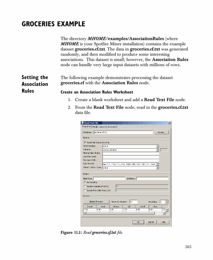
GROCERIES EXAMPLE
The directory MHOME/examples/AssociationRules (where MHOME is your Spotfire Miner installation) contains the example dataset groceries.cf.txt. The data in groceries.cf.txt was generated randomly, and then modified to produce some interesting associations. This dataset is small; however, the Association Rules node can handle very large input datasets with millions of rows.
Setting the Association Rules
The following example demonstrates processing the dataset groceries.cf with the Association Rules node.
Create an Association Rules Worksheet
1. Create a blank worksheet and add a Read Text File node.
2. From the Read Text File node, read in the groceries.cf.txt data file.
Figure 11.1: Read groceries.cf.txt file.
505
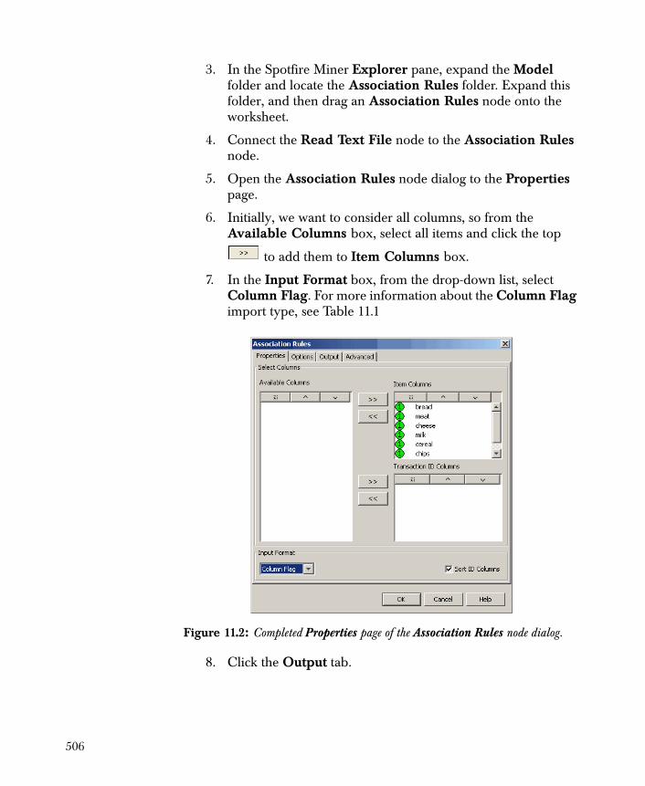
3. In the Spotfire Miner Explorer pane, expand the Model folder and locate the Association Rules folder. Expand this folder, and then drag an Association Rules node onto the worksheet.
4. Connect the Read Text File node to the Association Rules node.
5. Open the Association Rules node dialog to the Properties page.
6. Initially, we want to consider all columns, so from the Available Columns box, select all items and click the top
to add them to Item Columns box.
7. In the Input Format box, from the drop-down list, select Column Flag. For more information about the Column Flag import type, see Table 11.1
8. Click the Output tab.
Figure 11.2: Completed Properties page of the Association Rules node dialog.
506
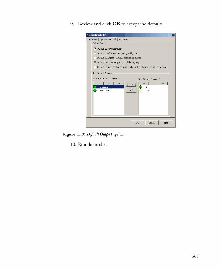
9. Review and click OK to accept the defaults.
10. Run the nodes.
Figure 11.3: Default Output options.
507
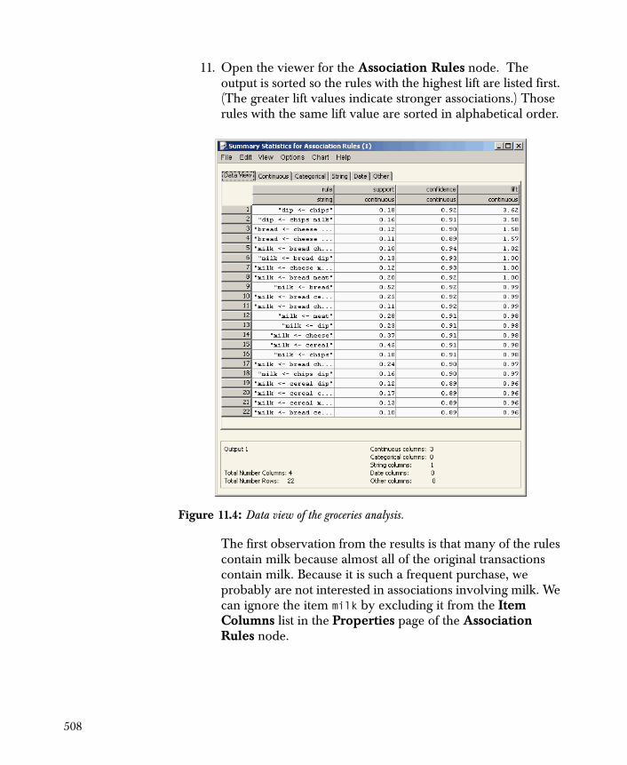
11. Open the viewer for the Association Rules node. The output is sorted so the rules with the highest lift are listed first. (The greater lift values indicate stronger associations.) Those rules with the same lift value are sorted in alphabetical order.
The first observation from the results is that many of the rules contain milk because almost all of the original transactions contain milk. Because it is such a frequent purchase, we probably are not interested in associations involving milk. We can ignore the item milk by excluding it from the Item Columns list in the Properties page of the Association Rules node.
Figure 11.4: Data view of the groceries analysis.
508
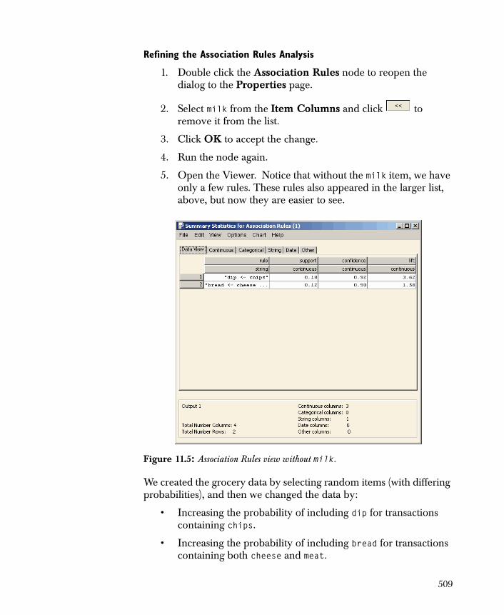
Refining the Association Rules Analysis
1. Double click the Association Rules node to reopen the dialog to the Properties page.
2. Select milk from the Item Columns and click to remove it from the list.
3. Click OK to accept the change.
4. Run the node again.
5. Open the Viewer. Notice that without the milk item, we have only a few rules. These rules also appeared in the larger list, above, but now they are easier to see.
We created the grocery data by selecting random items (with differing probabilities), and then we changed the data by:
• Increasing the probability of including dip for transactions containing chips.
• Increasing the probability of including bread for transactions containing both cheese and meat.
Figure 11.5: Association Rules view without milk.
509

510

Introduction 512
Basic Survival Models Background 513Properties 516
A Banking Customer Churn Example 524
A Time Varying Covariates Example 527
Technical Details for Cox Regression Models 529Mathematical Definitions 530Computational Details 530
References 533
SURVIVAL 12
511
INTRODUCTION
Survival analysis models are used to analyze time-to-event data. These models were originally developed in biostatistics where the patient survival was analyzed. Engineering reliability analysis is another field where survival analysis methods have been developed and applied. Survival models are now being used in CRM data mining for customer attrition modeling. Businesses want to know which customers are going leave (churn), when are they leaving, and why. This information can help forecast revenues as well as drive promotional messages.
Conventional statistical models (for example, logistic regression and classification trees) have been successfully used at predicting which customer will churn. However, these models do not predict when the customer will leave or how long they will stay. Survival models address this issue by modeling the time-to-event occurrence.
512
BASIC SURVIVAL MODELS BACKGROUND
There are many different models for analysis of survival time. Which model to use depends on the type of inference to be made and the form and distribution of the data.
The basic quantity employed to described time-to-event phenomena is the survival function, the probability of an individual surviving beyond time . It is defined as
In manufacturing, is often referred to as the reliability function. The survival function is a non-decreasing function with value of 1 at the origin and 0 at infinity. The rate of decline varies with the risk of experiencing the event at time .
The hazard function or instantaneous event (death, failure, churn) rate is defined as
the negative slope of the log of the survival function. It is related to the probability that the event will occur in a small interval around t given that the event has not occurred before time t.
A distinguishing feature in data for survival models is the presence of censoring. Censoring occurs when we have observations to analyze that have not had the event (churn, failure, death, etc.) occur yet. At the time of analysis we know that the event time is greater than the time observed to date.
Survival data is typically presented as a pair, , where is the
observed survival time and is the censoring indicator. if
an event is observed and 0 if the observation is censored. The number at risk at time , , is the number of observations with
event or censoring time greater than , such as
xS x( ) Pr X x>( )=
S x( )
x
h t( )td
d– S t( )( )log( )=
ti δi( , ) tiδi δi 1=
s r s( )s
r s( ) yi s( )i 1=
n
=
513
where if .
Similarly, we can define as the number of deaths (events)
occurring at time .
Spotfire Miner™ implements the Cox proportional hazard model. This is the most commonly used regression model for survival data. This model is considered semi-parametric because it does not assume any particular form for the hazard function, . It assumes that predictors (covariates) act multiplicatively on the unknown baseline hazard. The hazard for a given set of predictors is written as
The Cox proportional hazard model allows evaluation of the effect of particular predictors on survival by testing the significance of their beta coefficients. Predicted survival curves can easily be computed.
A simple extension to the Cox model is to allow for a different baseline hazard for different strata. The hazard function for an individual in stratum j is:
When a variable is entered into the model as a strata component rather than a covariate it allows for non-proportional hazards to exist between levels of that variable. This results in different shapes for the baseline survival curves.
The Cox proportional hazard model can be extended to allow time varying covariates in the model. An example of this would be using a monthly measure of mortgage interest rates when modeling loan prepayment. The mortgage rates would have an effect on the probability someone would refinance their loan (prepay) and the rates would change every month.
The computational details of fitting Cox proportional hazard regression models are described in the section Technical Details for Cox Regression Models of this chapter. The references, in particular Harrell (2001) and Therneau and Grambsch (2000), contain further theoretical and computation details.
yi s( ) 1= s ti≤
d s( )s
h t( )
X
h t( ) h0 t( )eXβ=
h t( ) hj t( )eXβ=
514
General Procedure
The following outlines the general approach to using a simple Cox regression model in Spotfire Miner:
1. Link a Cox Regression node in your worksheet to any node that outputs data.
2. Use the Properties dialog for the Cox Regression node to specify the dependent variables, including Stop time and Event status, and the independent variables. On the Options tab of the dialog, set the Event codes.
3. Run your network.
4. Launch the viewer for the model node.
5. Based on the information in the viewer, modify your model if desired and rerun the network.
6. To compute relative risk or survival probabilities for new data, create a Predict node for the model.
7. Link the node outputting your new data to the predict node.
8. Use the Properties dialog for the Predict Cox Regression node to select type of prediction - relative risk and/or survival probabilities.
9. Run the network to compute the predictions.
The Cox Regression node accepts a single input containing rectangular data. It outputs a data set containing any of the following based on what options you choose in the properties dialogs:
• A column containing the relative risk for each observation
• A column containing the survival probabilities for each observation. This can be at a single specific time for all observations or you can specify a column in the input data that contains a time value for each observation.
• All of the independent variables used in your model.
• The dependent variables used (this is at least two columns, a stop time and an event indicator).
• All other columns in your data set besides the independent and dependent variables.
515
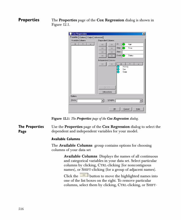
Properties The Properties page of the Cox Regression dialog is shown in Figure 12.1.
The Properties Page
Use the Properties page of the Cox Regression dialog to select the dependent and independent variables for your model.
Available Columns
The Available Columns group contains options for choosing columns of your data set
Available Columns Displays the names of all continuous and categorical variables in your data set. Select particular columns by clicking, CTRL-clicking (for noncontiguous names), or SHIFT-clicking (for a group of adjacent names).
Click the button to move the highlighted names into one of the list boxes on the right. To remove particular columns, select them by clicking, CTRL-clicking, or SHIFT-
Figure 12.1: The Properties page of the Cox Regression dialog.
516
clicking, and then click the button to the left of the list box to move the highlighted names back into the Available Columns list box.
Dependent Columns
The Cox Regression model requires you to set at least two columns under the Dependent Columns section, which are described below.
ID Identifies and individual and is used to generate a Start column for a survival model with time-varying covariates.
Stop Gives the time to the Event (death/churn/ failure) or time to censoring.
If time-varying covariates are used, this is the time to event or the end of a time interval over which the time-varying covariate is constant.
Start Needed only when you have time-varying covariates. This is the beginning of an interval over which the time-varying covariate is constant.
Event Contains two possible values, one value to denote an event has occurred, the other value denotes the observation is censored.
The section Time Varying Covariates describes how your data must be organized when using ID and Start.
Independent Columns
You can include interactions in your model after selecting the dependent and independent variables. To include interactions in your model, select two or more variables from Independent Columns, and then click Interactions.
In normal use, all lower-order terms must be in the model to use higher-order terms; however, removing lower-order terms also removes higher-order terms. To prevent Spotfire Miner from enforcing a hierarchal interaction structure, press and hold the CTRL key while clicking Interactions.
517
As with adding interactions, pressing and holding the CTRL key while clicking Remove prevents Spotfire Miner from enforcing a hierarchal interaction structure on your model. Otherwise, all higher order interactions that involve the variables being removed from the model are also removed.
Strata
You can select a column to be included as a strata variable in the model. If you select a column, a separate baseline hazard is created for each unique value in the Strata column.
Weights
A vector of case weights. If weights is a vector of integers, the estimated coefficients are equivalent to estimating the model from data with the individual cases replicated as many times as indicated by weights. Multiplying all weights by a positive constant c does not change the estimated coefficients or the robust standard errors computed by the Cox model. However, the standard errors of the coefficients will decrease by a factor of sqrt(c). By default, no weights are included in the model.
Time Varying Covariates
The Spotfire Miner Cox Regression model allows time varying covariates. Observations for an individual are then broken down into time intervals with a start and stop time. Over each interval all the covariates are constant. Whenever the value of a covariate changes a new interval is defined. The event variable for each of these intervals indicates censoring except for the last interval where the event (failure, death, churn) could occur (or the final interval could also be censored).
The data for a time varying covariates Cox Regression model must have each time interval, specified by the Start and Stop columns, as a separate row in input data. If you do not specify the Start column, an ID column is required to identify all rows in the data that belong to the same subject. In this case, Spotfire Miner generates a Start column based on the sorted Stop times of an individual. The first generated Start time is zero. The observations for a single subject do not have to appear sequentially in the data file. (The algorithm sorts internally to group the observations when necessary.)
518
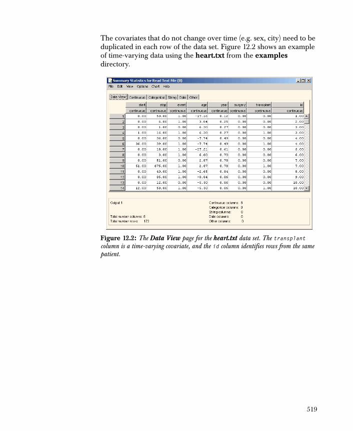
The covariates that do not change over time (e.g. sex, city) need to be duplicated in each row of the data set. Figure 12.2 shows an example of time-varying data using the heart.txt from the examples directory.
Figure 12.2: The Data View page for the heart.txt data set. The transplant column is a time-varying covariate, and the id column identifies rows from the same patient.
519
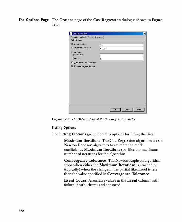
The Options Page The Options page of the Cox Regression dialog is shown in Figure 12.3.
Fitting Options
The Fitting Options group contains options for fitting the data.
Maximum Iterations The Cox Regression algorithm uses a Newton-Raphson algorithm to estimate the model coefficients. Maximum Iterations specifies the maximum number of iterations for the algorithm.
Convergence Tolerance The Newton-Raphson algorithm stops when either the Maximum Iterations is reached or (typically) when the change in the partial likelihood is less then the value specified in Convergence Tolerance.
Event Codes Associates values in the Event column with failure (death, churn) and censored.
Figure 12.3: The Options page of the Cox Regression dialog.
520
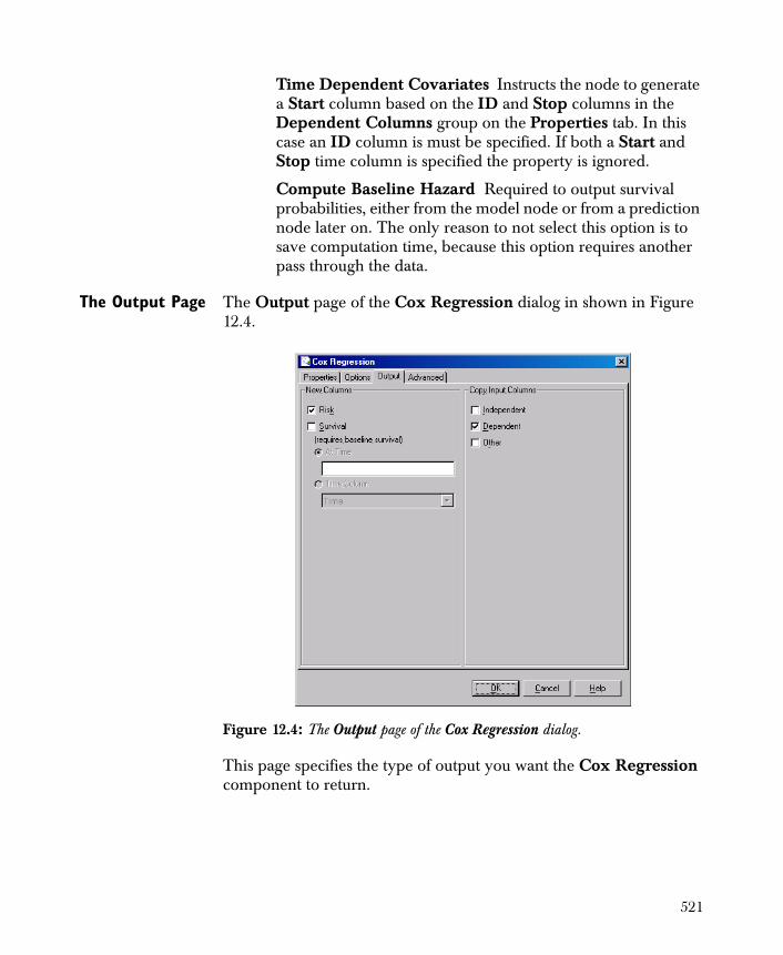
Time Dependent Covariates Instructs the node to generate a Start column based on the ID and Stop columns in the Dependent Columns group on the Properties tab. In this case an ID column is must be specified. If both a Start and Stop time column is specified the property is ignored.
Compute Baseline Hazard Required to output survival probabilities, either from the model node or from a prediction node later on. The only reason to not select this option is to save computation time, because this option requires another pass through the data.
The Output Page The Output page of the Cox Regression dialog in shown in Figure 12.4.
This page specifies the type of output you want the Cox Regression component to return.
Figure 12.4: The Output page of the Cox Regression dialog.
521
New Columns
The New Columns group contains options for including new columns in the output data.
Risk Outputs data to include the relative risk and its standard error for each observation. These columns are named PREDICT.risk and PREDICT.risk.se, respectively.
Survival Specifies that output data includes the predicted survival probability for each observation. This column is named PREDICT.survival. If At Time is selected, the survival probability is computed for the time specified in the text box. Alternatively, the survival probability at a different time for each observation is computed if you specify one of the input data columns as a time.
Copy Input Columns
The Copy Input Columns group contains options for copying the input columns to the output data set.
• Independent copies all independent variables in the model to the output data set.
• Dependent copies the dependent variable.
• Other copies all columns that are neither the dependent nor the independent variables but are part of the original data set.
Using the Viewer The viewer for the Cox Regression component is an HTML file containing both text and graphics. The text section displays a summary of the model fit. A table of coefficient estimates, their standard errors is shown. The table also includes a z-statistic for each coefficient and the p-value for the test that the coefficient is zero.
522
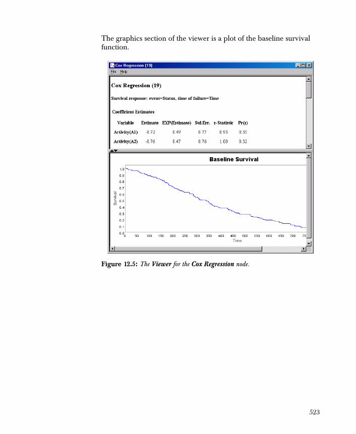
The graphics section of the viewer is a plot of the baseline survival function.
Figure 12.5: The Viewer for the Cox Regression node.
523
A BANKING CUSTOMER CHURN EXAMPLE
In this example, use Cox Regression component to predict bank customer churn. The data file we use is bankchurn.txt, which is included in the examples directory, and this file contains information on customers at a fictitious financial institution. Each row in the file represent a customer. Variables in the data include state of residence, customer age, sex, and a categorical account activity indicator that the bank research department has developed. There is also a time variable that indicates how long the person has been a bank customer and a status variable that is 1 if the person is no longer a customer and 0 if they still are.
The financial institution is interested in predicting customer churn - when will customers stop being their customers. They are also interested in knowing which variables are most important at predicting churn. In practical applications, the institution would look at a much larger data set with many more variables.
To run this example, do the following steps:
1. Double-click a Read Text File component to move it from the explorer pane to the desktop.
2. Double-click the Read Text File node to open the Properties page, and click the Browse button to navigate to bankchurn.txt in the Examples folder. Click OK.
3. Click the Modify Columns tab and change the data type of the variables Sex and Activity from String to Categorical.
4. Double-click a Cox Regression component to move it from the explorer pane to the desktop.
5. Connect the Read Text File node to a Cox Regression node.
524
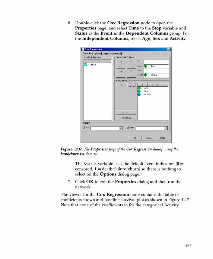
6. Double-click the Cox Regression node to open the Properties page, and select Time to the Stop variable and Status as the Event in the Dependent Columns group. For the Independent Columns, select Age, Sex and Activity.
The Status variable uses the default event indicators (0 = censored, 1 = death/failure/churn) so there is nothing to select on the Options dialog page.
7. Click OK to exit the Properties dialog and then run the network.
The viewer for the Cox Regression node contains the table of coefficients shown and baseline survival plot as shown in Figure 12.7. Note that none of the coefficients in for the categorical Activity
Figure 12.6: The Properties page of the Cox Regression dialog, using the bankchurn.txt data set.
525
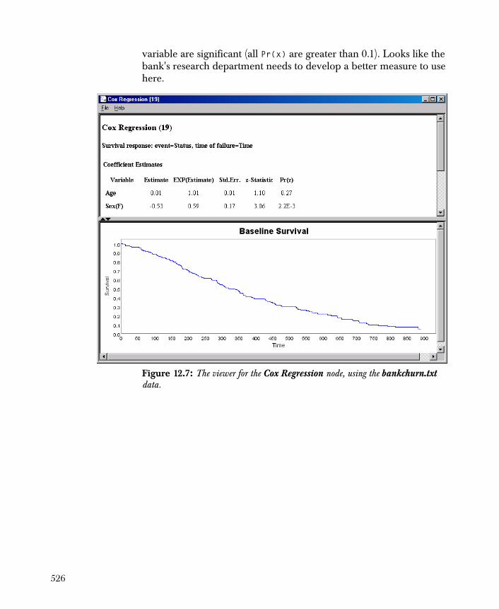
variable are significant (all Pr(x) are greater than 0.1). Looks like the bank's research department needs to develop a better measure to use here.
Figure 12.7: The viewer for the Cox Regression node, using the bankchurn.txt data.
526
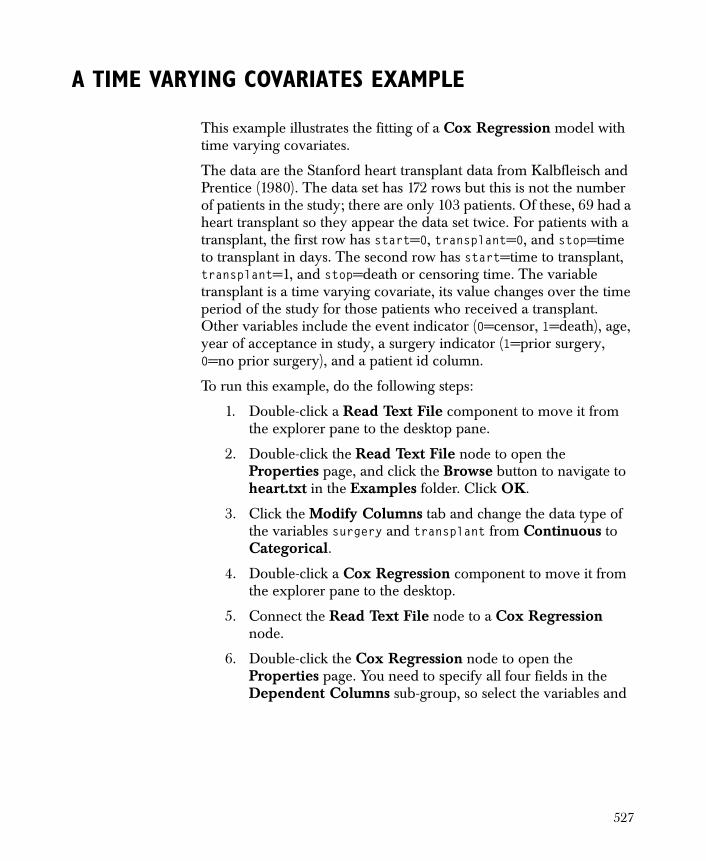
A TIME VARYING COVARIATES EXAMPLE
This example illustrates the fitting of a Cox Regression model with time varying covariates.
The data are the Stanford heart transplant data from Kalbfleisch and Prentice (1980). The data set has 172 rows but this is not the number of patients in the study; there are only 103 patients. Of these, 69 had a heart transplant so they appear the data set twice. For patients with a transplant, the first row has start=0, transplant=0, and stop=time to transplant in days. The second row has start=time to transplant, transplant=1, and stop=death or censoring time. The variable transplant is a time varying covariate, its value changes over the time period of the study for those patients who received a transplant. Other variables include the event indicator (0=censor, 1=death), age, year of acceptance in study, a surgery indicator (1=prior surgery, 0=no prior surgery), and a patient id column.
To run this example, do the following steps:
1. Double-click a Read Text File component to move it from the explorer pane to the desktop pane.
2. Double-click the Read Text File node to open the Properties page, and click the Browse button to navigate to heart.txt in the Examples folder. Click OK.
3. Click the Modify Columns tab and change the data type of the variables surgery and transplant from Continuous to Categorical.
4. Double-click a Cox Regression component to move it from the explorer pane to the desktop.
5. Connect the Read Text File node to a Cox Regression node.
6. Double-click the Cox Regression node to open the Properties page. You need to specify all four fields in the Dependent Columns sub-group, so select the variables and
527
move them to the appropriate fields, as shown in Figure 12.8. Note that the ID = id specification is not necessary here
because the Start column is specified.
7. Click the Options tab and select Time Dependent Covariates. This step is optional because the Start column is specified.
8. Run the network by clicking the Run button ( ).
9. Select the Cox Regression node and click the Viewer button
( ).
The viewer for the model shows a very steep decline in baseline survival (about 100 days), and then a very gradual out to the end of the observation time. The table of coefficients indicate the transplant does not have a have a significant effect on survival in this model. Before drawing any conclusions for this data, many more models should be considered and these are presented elsewhere (Kalbfleisch and Prentice 1980, Therneau and Grambsch 2000, Insightful 2001).
Figure 12.8: Selecting the variables to be used from the heart.txt data set.
528
TECHNICAL DETAILS FOR COX REGRESSION MODELS
In the Cox Proportional Hazard Regression model, each row of data represents an entity, such as an individual or an object. The dependent variable is a column that identifies whether the event occurred, typically coded as 1 or 0 (1 if it occurred). An auxiliary column is required that records the time of the event (or non-event). If the event did not occur by the recorded time, the observation is (right) censored; that is, it is not known when the event occurred for the individual but it is known that it either occurred after the recorded time or never at all.
The same entity appears in multiple rows when the covariates (the independent variables) are time-dependent. Each observation in the data applies to an interval of time over which the time dependent covariate is constant. An additional time column records the beginning of the time interval, while the other time column records the end of the time interval. Only the last observation for an individual can have the event code; all others should have the censored code. An ID column is required to identify all rows that belong to the same entity.
The regression coefficients for the Cox regression model measure the relative risk of an event occurring, given the value of the corresponding independent variable. For a positive continuous covariate, there is an increase in the risk of the event occurring if the corresponding coefficient estimate is positive, and a decrease in the risk of the event occurring if the coefficient estimate is negative. For categorical covariates, there are one or more coefficients associated with the covariate, and the risk measure is relative to one of the class values. In this case, there is one fewer coefficient than the number of class values, and the risk is relative to the last of the alphabetically-sorted class values.
The baseline survival function is a step function with one entry for every unique event time in the training data. Both the estimated coefficients and the estimated baseline survival function are used to compute survival estimates for new observations. The coefficients compute the relative risk of the observation, which is independent of time, and the estimated survival is then value of the baseline survival function at the observed time raised to the power of the risk estimate.
529
Mathematical Definitions
In Cox's Proportional Hazards Regression model, there is a linear component, much like linear and logistic regression, composed of the independent variables and the coefficients. Let the independent variables for the i-th observation be denoted by the row vector
and denote the vector of coefficients by . The relative risk
of a set of observations is then , where is the base of
the natural logarithm.
The hazard function in survival analysis, denoted , measures the probability of an event occurring for an individual at time t given that the event has not occurred up to that time. For Cox's Proportional Hazards Regression model, we have
where is the baseline hazard. As suggested by its name and the
definition of , the covariates act multiplicatively on the baseline
hazard function, or equivalently, the hazard ratio for two individuals is constant over time.
The cumulative baseline hazard is defined as .
From this we get the baseline survival function and the survival
function for the i-th individual is then and the
survival function for the i-th individual is then .
Computational Details
The computations for the coefficient estimates and baseline survival functions are taken from Terry Therneau's proportional hazard code. (Therneau and Grambsch, 2000). These two functions (coxph and survfit, respectively) are distributed in S-PLUS 6 and higher.
The coefficient estimates are based on the partial likelihood introduced by Cox (1975). Let the set of individuals at risk at time t be denoted . This is the set of individuals that have not experienced
1 p×xi p 1× β
r xi( ) exiβ= e
h t( )
hi t( ) h0 t( )r xi( )=
h0 t( )
hi t( )
H0 t( ) h0 x( ) xd
0
t
=
So t( ) eH0 t( )–
=
Si t( ) S0 t( )[ ]r xi( )
=
R t( )
530
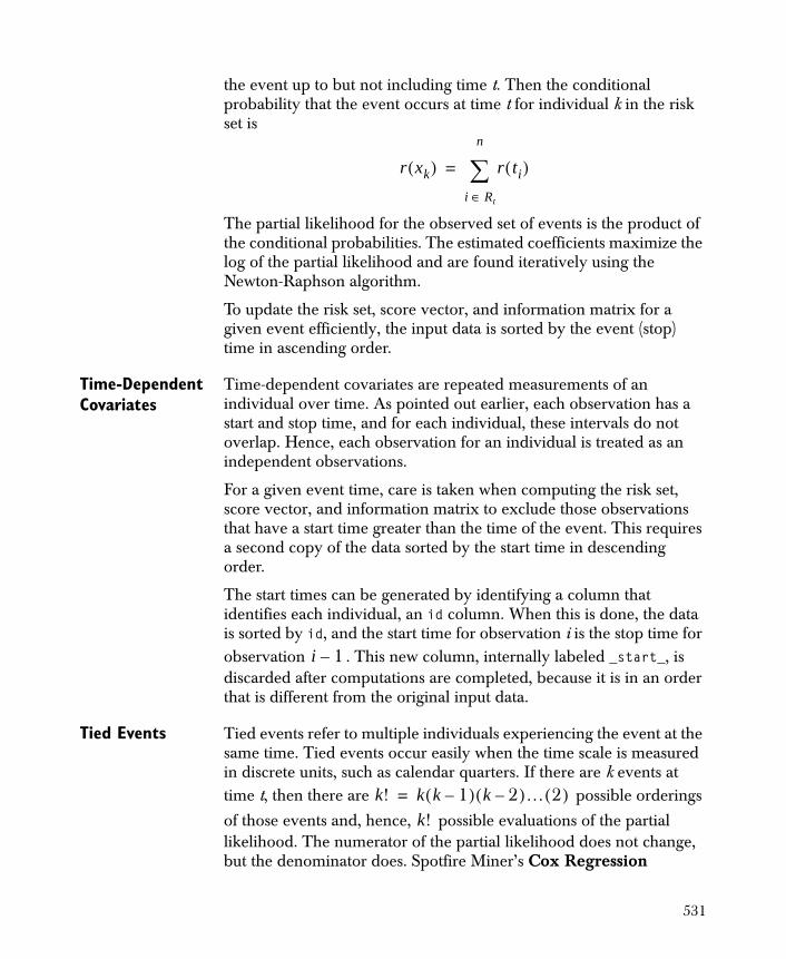
the event up to but not including time t. Then the conditional probability that the event occurs at time t for individual k in the risk set is
The partial likelihood for the observed set of events is the product of the conditional probabilities. The estimated coefficients maximize the log of the partial likelihood and are found iteratively using the Newton-Raphson algorithm.
To update the risk set, score vector, and information matrix for a given event efficiently, the input data is sorted by the event (stop) time in ascending order.
Time-Dependent Covariates
Time-dependent covariates are repeated measurements of an individual over time. As pointed out earlier, each observation has a start and stop time, and for each individual, these intervals do not overlap. Hence, each observation for an individual is treated as an independent observations.
For a given event time, care is taken when computing the risk set, score vector, and information matrix to exclude those observations that have a start time greater than the time of the event. This requires a second copy of the data sorted by the start time in descending order.
The start times can be generated by identifying a column that identifies each individual, an id column. When this is done, the data is sorted by id, and the start time for observation i is the stop time for observation . This new column, internally labeled _start_, is discarded after computations are completed, because it is in an order that is different from the original input data.
Tied Events Tied events refer to multiple individuals experiencing the event at the same time. Tied events occur easily when the time scale is measured in discrete units, such as calendar quarters. If there are k events at time t, then there are possible orderings
of those events and, hence, possible evaluations of the partial likelihood. The numerator of the partial likelihood does not change, but the denominator does. Spotfire Miner’s Cox Regression
r xk( ) r ti( )i Rt∈
n
=
i 1–
k! k k 1–( ) k 2–( )… 2( )=
k!
531
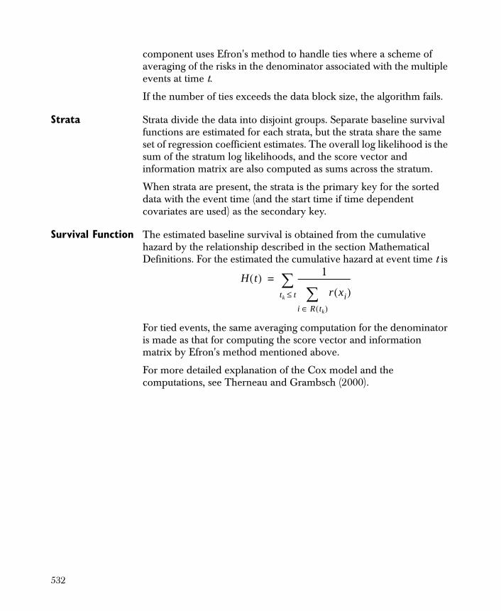
component uses Efron's method to handle ties where a scheme of averaging of the risks in the denominator associated with the multiple events at time t.
If the number of ties exceeds the data block size, the algorithm fails.
Strata Strata divide the data into disjoint groups. Separate baseline survival functions are estimated for each strata, but the strata share the same set of regression coefficient estimates. The overall log likelihood is the sum of the stratum log likelihoods, and the score vector and information matrix are also computed as sums across the stratum.
When strata are present, the strata is the primary key for the sorted data with the event time (and the start time if time dependent covariates are used) as the secondary key.
Survival Function The estimated baseline survival is obtained from the cumulative hazard by the relationship described in the section Mathematical Definitions. For the estimated the cumulative hazard at event time t is
For tied events, the same averaging computation for the denominator is made as that for computing the score vector and information matrix by Efron's method mentioned above.
For more detailed explanation of the Cox model and the computations, see Therneau and Grambsch (2000).
H t( ) 1
r xi( )i R tk( )∈
----------------------------tk t≤=
532
REFERENCES
Cox, D.R. (1975). Partial likelihood. Biometrika, 62, 269-276.
Harrell, Frank E., Jr. (2001). Regression Modeling Strategies. New York: Springer-Verlag.
Insightful 2001.
Kalbfleisch, J. D. and Prentice, R. L. (1980). The Statistical Analysis of Failure Time Data. New York: Wiley.
Therneau, T.M. and Grambsch, P.M., (2000). Modeling Survival Data: Extending the Cox Model. New York: Springer-Verlag.
533

534

Overview 536
Assessing Classification Models 540General Procedure 540Classification Agreement 540Lift Chart 542
Assessing Regression Models 546General Procedure 546Definitions 546Using the Viewer 548
MODEL ASSESSMENT 13
535
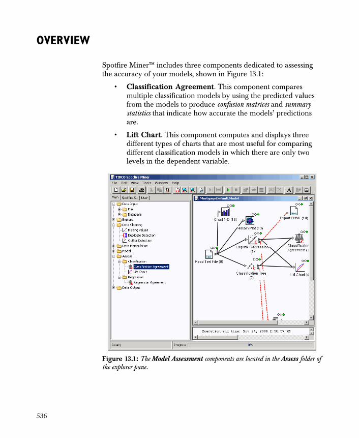
OVERVIEW
Spotfire Miner™ includes three components dedicated to assessing the accuracy of your models, shown in Figure 13.1:
• Classification Agreement. This component compares multiple classification models by using the predicted values from the models to produce confusion matrices and summary statistics that indicate how accurate the models’ predictions are.
• Lift Chart. This component computes and displays three different types of charts that are most useful for comparing different classification models in which there are only two levels in the dependent variable.
Figure 13.1: The Model Assessment components are located in the Assess folder of the explorer pane.
536
• Regression Agreement. This component compares multiple regression models by using the residuals from the models to compute various measures of error.
This chapter describes the results returned by these components and shows how you can use the information to assess your models.
As a complement to the techniques described in this chapter, it is usually a good idea to split your data set into two or three independent pieces to assess how well a particular model performs. You can use the Partition component to split your data into training , test , and validation data sets:
• The training data set is used to create a model and the corresponding Predict node. You can use the assessment components in Spotfire Miner to determine how well the model performs in accurately predicting the training data set.
• The test data set is run through the Predict node to determine whether the model is overtrained , which means it fits your training data set well but does not generalize to predict accurate values on other data sets. The test data set can be used to select your model and modify as necessary.
• The validation data set is run through Predict nodes for multiple models to assist you in choosing a best model for your data.
Usually, data sets are split into proportions of 50/25/25, 60/30/10, or 40/30/30 for training, test, and validation, respectively. When using only training and test data sets, a typical split is 70/30.
537
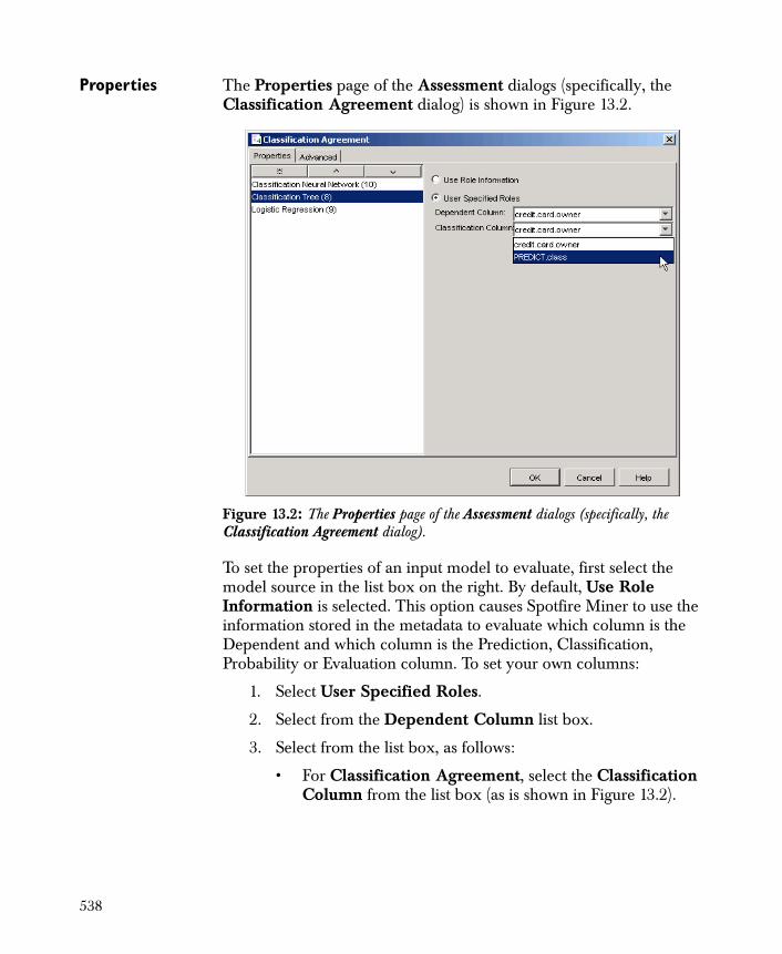
Properties The Properties page of the Assessment dialogs (specifically, the Classification Agreement dialog) is shown in Figure 13.2.
To set the properties of an input model to evaluate, first select the model source in the list box on the right. By default, Use Role Information is selected. This option causes Spotfire Miner to use the information stored in the metadata to evaluate which column is the Dependent and which column is the Prediction, Classification, Probability or Evaluation column. To set your own columns:
1. Select User Specified Roles.
2. Select from the Dependent Column list box.
3. Select from the list box, as follows:
• For Classification Agreement, select the Classification Column from the list box (as is shown in Figure 13.2).
Figure 13.2: The Properties page of the Assessment dialogs (specifically, the Classification Agreement dialog).
538
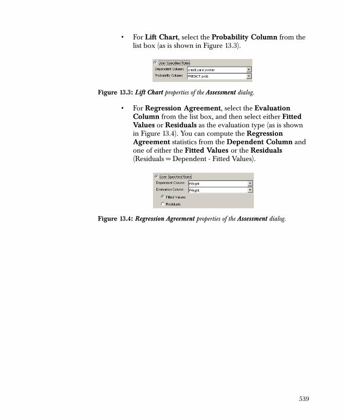
• For Lift Chart, select the Probability Column from the list box (as is shown in Figure 13.3).
• For Regression Agreement, select the Evaluation Column from the list box, and then select either Fitted Values or Residuals as the evaluation type (as is shown in Figure 13.4). You can compute the Regression Agreement statistics from the Dependent Column and one of either the Fitted Values or the Residuals (Residuals = Dependent - Fitted Values).
Figure 13.3: Lift Chart properties of the Assessment dialog.
Figure 13.4: Regression Agreement properties of the Assessment dialog.
539
ASSESSING CLASSIFICATION MODELS
Spotfire Miner has two components dedicated to assessing classification models: Classification Agreement and Lift Chart. The Classification Agreement component produces confusion matrices and related statistics for your models while Lift Chart creates three different types of charts that visually display the lift of your models. As input, both of these components accept the output from one or more classification models. For example, you might link multiple Logistic Regression nodes to the assessment nodes in your network to compare the different models. Alternatively, you might link Classification Tree, Classification Neural Network, and Naive Bayes nodes to the assessment nodes to compare how the different algorithms perform for the same model.
General Procedure
The following outlines the general approach to using the classification assessment components in Spotfire Miner:
1. Link one or more classification models in your worksheet to the Classification Agreement and/or Lift Chart nodes.
2. Run your network.
3. Launch the viewers for the assessment nodes.
Both the Classification Agreement and Lift Chart components accept one or more inputs from classification model nodes. They return no output.
Classification Agreement
The Classification Agreement component compares the accuracy of multiple classification models. It uses the predicted values from the models to produce a confusion matrix, which indicates the number and proportion of observations that are classified correctly by the models.
540
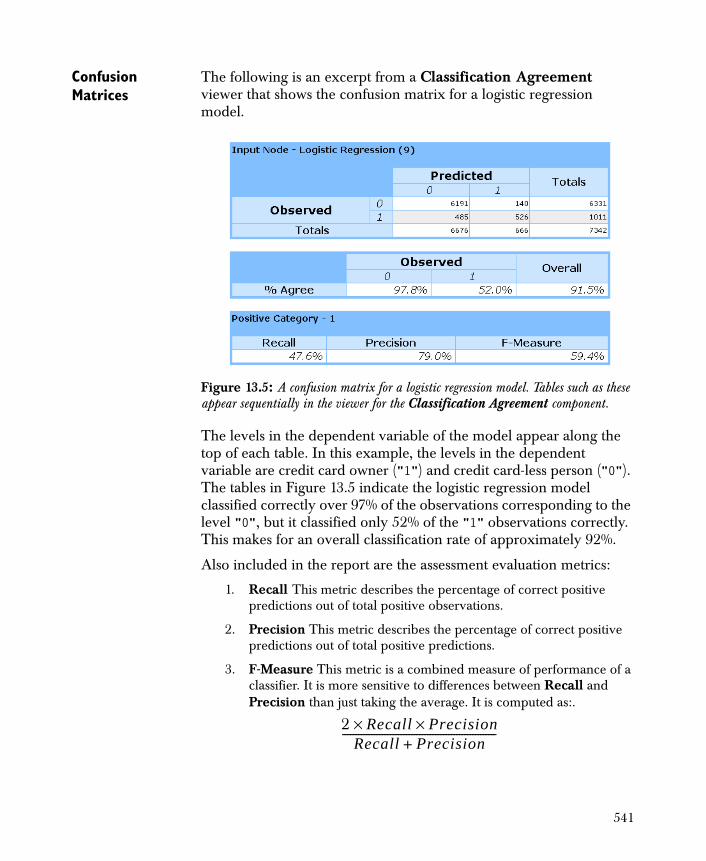
Confusion Matrices
The following is an excerpt from a Classification Agreement viewer that shows the confusion matrix for a logistic regression model.
The levels in the dependent variable of the model appear along the top of each table. In this example, the levels in the dependent variable are credit card owner ("1") and credit card-less person ("0"). The tables in Figure 13.5 indicate the logistic regression model classified correctly over 97% of the observations corresponding to the level "0", but it classified only 52% of the "1" observations correctly. This makes for an overall classification rate of approximately 92%.
Also included in the report are the assessment evaluation metrics:
1. Recall This metric describes the percentage of correct positive predictions out of total positive observations.
2. Precision This metric describes the percentage of correct positive predictions out of total positive predictions.
3. F-Measure This metric is a combined measure of performance of a classifier. It is more sensitive to differences between Recall and Precision than just taking the average. It is computed as:.
Figure 13.5: A confusion matrix for a logistic regression model. Tables such as these appear sequentially in the viewer for the Classification Agreement component.
2 Recall× Precision×Recall Precision+
----------------------------------------------------------
541
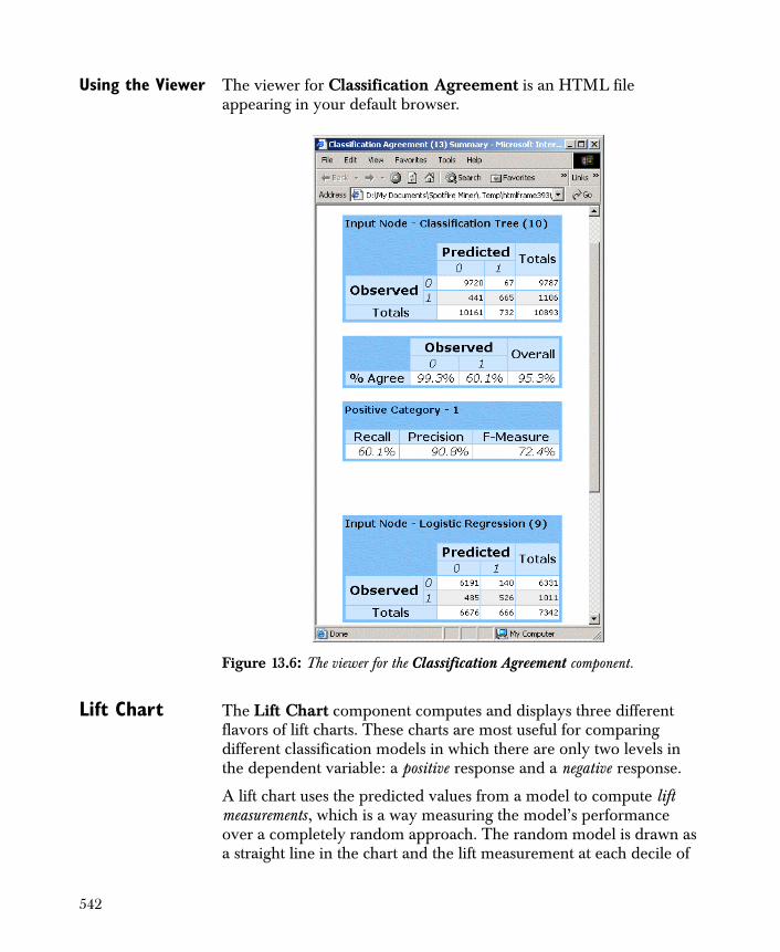
Using the Viewer The viewer for Classification Agreement is an HTML file appearing in your default browser.
Lift Chart The Lift Chart component computes and displays three different flavors of lift charts. These charts are most useful for comparing different classification models in which there are only two levels in the dependent variable: a positive response and a negative response.
A lift chart uses the predicted values from a model to compute lift measurements , which is a way measuring the model’s performance over a completely random approach. The random model is drawn as a straight line in the chart and the lift measurement at each decile of
Figure 13.6: The viewer for the Classification Agreement component.
542
the predicted data is drawn relative to the line. If the model performs better than random, the lift measurements are positive, resulting in a curve above the straight line. If the model performs only as good as the random approach, the lift measurements hover around the straight line.
Chart Types Cumulative gain chart
This type of chart displays the percentage of positive responses predicted by the models versus the percentage of the population. The data are ordered from highest predicted probability of response to lowest. The y-axis “gain” is the percentage of observed positive responses for that decile of the population. The baseline for comparison is a diagonal line and the curve for each model is given in the legend under the chart. The best model for the data is the one with the highest curve above the straight line.
Figure 13.7: A cumulative gain chart for two different models: a logistic regression and a classification neural network. The curve corresponding to the logistic regression has the highest “gain” above the straight line, which indicates the tree provides the most improvement over the completely random model.
543
Lift chart
This type of chart displays the lift for each model versus the percentage of the population. In Spotfire Miner, lift is calculated as the ratio between the results obtained with the predictive and random models. The data are ordered from highest predicted probability of response to lowest. The y-axis lift value is the ratio of the percentage of observed positive responses to the total percentage of the population of that decile. The baseline for comparison is a horizontal line at and the curve for each model is given in the legend under the chart. The best model for the data is typically the one with the greatest area between its curve and the baseline. However, if it only provides higher lift on the first two deciles, it might already be the better model.
ROC chart
Receiver operating characteristic (ROC) charts are used most often in the biopharmaceutical and financial industries. They tend to look similar to cumulative gain charts but display sensitivity of the models versus specificity. Sensitivity is defined as the ratio of the predicted
Figure 13.8: A lift chart for the same two models from Figure 13.7.
y 1=
544
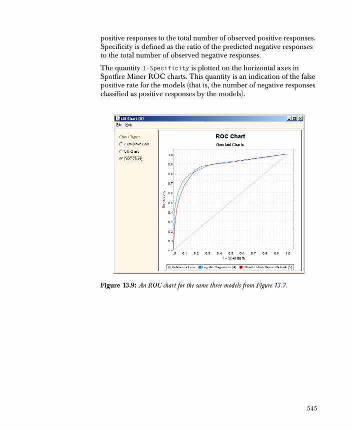
positive responses to the total number of observed positive responses. Specificity is defined as the ratio of the predicted negative responses to the total number of observed negative responses.
The quantity 1-Specificity is plotted on the horizontal axes in Spotfire Miner ROC charts. This quantity is an indication of the false positive rate for the models (that is, the number of negative responses classified as positive responses by the models).
Figure 13.9: An ROC chart for the same three models from Figure 13.7.
545
ASSESSING REGRESSION MODELS
The Regression Agreement component in Spotfire Miner is designed to assess your regression models. It compares the accuracy of multiple regression models by using the residuals to compute various measures of errors. As input, Regression Agreement accepts the output from one or more regression models. For example, you might link multiple Linear Regression nodes to the Regression Agreement node in your network to compare the different models. Alternatively, you might link both a Regression Tree and a Regression Neural Network to Regression Agreement to compare how the different algorithms perform for the same model.
General Procedure
The following outlines the general approach to using the Regression Agreement component in Spotfire Miner:
1. Link one or more regression models in your worksheet to the Regression Agreement node.
2. Run your network.
3. Launch the viewer for Regression Agreement.
The Regression Agreement component accepts one or more inputs from regression model nodes and returns no output. By default, the role information from the metadata is used. You can specify roles in the dialog to override this default.
Definitions The Regression Agreement component uses the residuals from your models to compute three types of errors:
1. Mean squared error. This is the arithmetic average of the squared error between the actual values and the predicted values. For each observation, Spotfire Miner squares the residual (the predicted value subtracted from the value of the dependent variable) and then computes the average across all observations. This is expressed as
yi yiˆ–( )
2
i 1=
n
n
-------------------------------
546

2. Mean absolute error. This is the arithmetic average of the absolute error between the actual values and the predicted values. For each observation, Spotfire Miner takes the absolute value of the residual and then computes the average across all observations. This is expressed as
3. Relative squared error. Suppose is an actual value in the
dependent variable, is its predicted value, and is the mean of the values in the dependent variable. The relative squared error is equal to
where is the number of observations in the data set. This error provides a measure of how well the model performed against the naive model of simply predicting the mean of the dependent variable. Relative squared errors close to 0 indicate a good model while values close to 1 indicate a poor model (no better than a model predicting the constant mean value m given above), and values greater than 1 indicate a really bad model.
You can subtract the relative squared error from 1 to obtain the multiple R-squared value, which identifies how much of the variance in the dependent variable is explained by the model. For example, if your multiple r-squared value is 0.56, then approximately 56% of the variance in your dependent variable is explained by the model.
yi yiˆ–
i 1=
n
n
--------------------------
yi
yi m
yi yiˆ–( )
2
i 1=
n
yi m–( )2
i 1=
n
------------------------------
n
547
Using the Viewer
The viewer for Regression Agreement is an HTML file appearing in your default browser.
Figure 13.10: The viewer for the Regression Agreement component.
548

Overview 550
Predictive Modeling Markup Language 551Export PMML 552Import PMML 554
Export Report 556
DEPLOYING MODELS 14
549
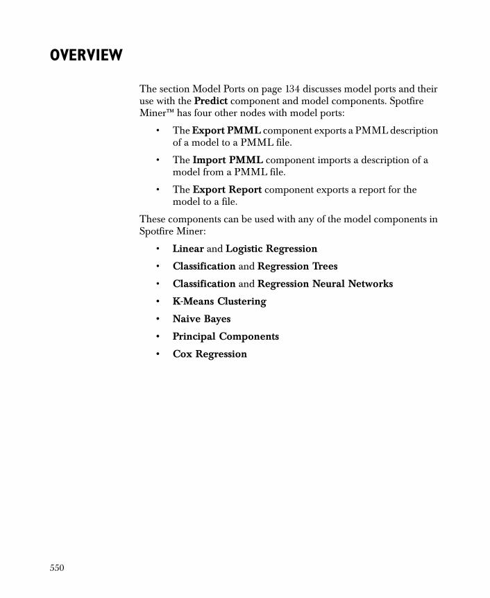
OVERVIEW
The section Model Ports on page 134 discusses model ports and their use with the Predict component and model components. Spotfire Miner™ has four other nodes with model ports:
• The Export PMML component exports a PMML description of a model to a PMML file.
• The Import PMML component imports a description of a model from a PMML file.
• The Export Report component exports a report for the model to a file.
These components can be used with any of the model components in Spotfire Miner:
• Linear and Logistic Regression
• Classification and Regression Trees
• Classification and Regression Neural Networks
• K-Means Clustering
• Naive Bayes
• Principal Components
• Cox Regression
550

PREDICTIVE MODELING MARKUP LANGUAGE
Predictive Model Markup Language (PMML) is an XML specification for defining predictive models. It is intended to provide a way for model descriptions to be exchanged between products in a standard vendor-neutral manner.
The PMML standard is developed and maintained by the Data Mining Group. This is a vendor-led group that develops data mining standards:
www.dmg.org
Spotfire Miner is able to export models as PMML and import a PMML file to create a model. All of the components with a model output port are supported.
The models with standard definitions in PMML are:
• Linear and Logistic Regression
• Classification and Regression Trees
• Classification and Regression Neural Networks
• K-Means Clustering
• Naive Bayes
For models not covered in the PMML specification, we use the Extension mechanism provided in PMML. These models are:
• Principal Components
• Cox Regression
• Ensemble Trees
Additional model information used by Spotfire Miner but not specified in PMML is also stored using the PMML Extension mechanism.
PMML Conformance
In this version of Spotfire Miner, we have confirmed that PMML exported from Spotfire Miner is valid PMML and can be imported properly by Spotfire Miner.
551
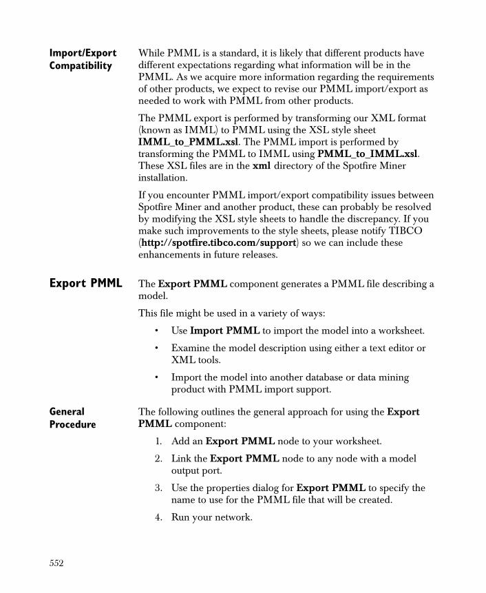
Import/Export Compatibility
While PMML is a standard, it is likely that different products have different expectations regarding what information will be in the PMML. As we acquire more information regarding the requirements of other products, we expect to revise our PMML import/export as needed to work with PMML from other products.
The PMML export is performed by transforming our XML format (known as IMML) to PMML using the XSL style sheet IMML_to_PMML.xsl. The PMML import is performed by transforming the PMML to IMML using PMML_to_IMML.xsl. These XSL files are in the xml directory of the Spotfire Miner installation.
If you encounter PMML import/export compatibility issues between Spotfire Miner and another product, these can probably be resolved by modifying the XSL style sheets to handle the discrepancy. If you make such improvements to the style sheets, please notify TIBCO (http://spotfire.tibco.com/support) so we can include these enhancements in future releases.
Export PMML The Export PMML component generates a PMML file describing a model.
This file might be used in a variety of ways:
• Use Import PMML to import the model into a worksheet.
• Examine the model description using either a text editor or XML tools.
• Import the model into another database or data mining product with PMML import support.
General Procedure
The following outlines the general approach for using the Export PMML component:
1. Add an Export PMML node to your worksheet.
2. Link the Export PMML node to any node with a model output port.
3. Use the properties dialog for Export PMML to specify the name to use for the PMML file that will be created.
4. Run your network.
552
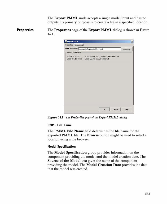
The Export PMML node accepts a single model input and has no outputs. Its primary purpose is to create a file in a specified location.
Properties The Properties page of the Export PMML dialog is shown in Figure 14.1.
PMML File Name
The PMML File Name field determines the file name for the exported PMML file. The Browse button might be used to select a location using a file browser.
Model Specification
The Model Specification group provides information on the component providing the model and the model creation date. The Source of the Model text gives the name of the component providing the model. The Model Creation Date provides the date that the model was created.
Figure 14.1: The Properties page of the Export PMML dialog.
553
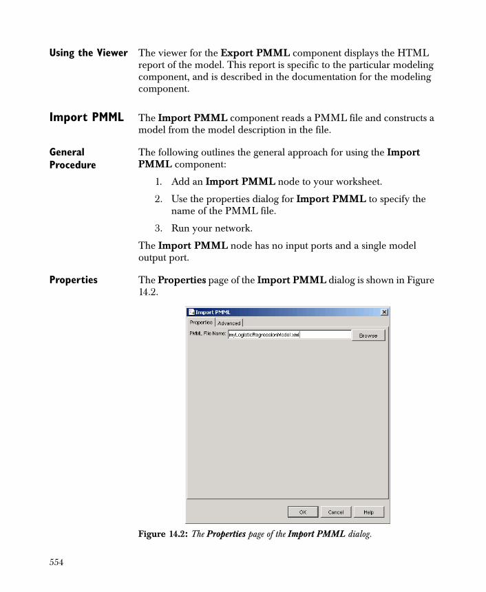
Using the Viewer The viewer for the Export PMML component displays the HTML report of the model. This report is specific to the particular modeling component, and is described in the documentation for the modeling component.
Import PMML The Import PMML component reads a PMML file and constructs a model from the model description in the file.
General Procedure
The following outlines the general approach for using the Import PMML component:
1. Add an Import PMML node to your worksheet.
2. Use the properties dialog for Import PMML to specify the name of the PMML file.
3. Run your network.
The Import PMML node has no input ports and a single model output port.
Properties The Properties page of the Import PMML dialog is shown in Figure 14.2.
Figure 14.2: The Properties page of the Import PMML dialog.
554

PMML File Name
The PMML File Name field determines the file name for the imported PMML file. The Browse button might be used to select a location using a file browser.
Using the Viewer The viewer for the Import PMML component displays the HTML report of the model. This report is specific to the particular modeling component, and is described in the documentation for the modeling component.
555
EXPORT REPORT
The Export Report component generates a file describing a model. The reports are generated by using XSL transforms (XSLT) to create HTML files, or XSL formatting objects (XSL:FO) to create PDF, PostScript, or RTF files.
General Procedure
The steps required to use the Export Report component:
1. Add an Export Report node to your worksheet, and link it to any model with an output port.
2. Use the properties dialog for Export Report to specify the name to use for the file to be created.
3. Run your network.
The Export Report node accepts a single model input and has no outputs. Its primary purpose is to create a file in a specified location.
Properties The Properties page of the Export Report dialog is shown in Figure 14.3.
Figure 14.3: The Properties page of the Export Report dialog.
556
File Name
The File Name field determines the file name for the exported report file. The Browse button might be used to select a location using a file browser.
Format
Select which of the formats you want to output the data: HTML (*.htm), PDF (*.pdf), PostScript (*.ps), or RTF (*.rtf).
Note there are limitations when reports in specific format types are generated. For example, you can create a PDF, but you cannot change page orientation (portrait/landscape) and make other changes normally available.
Model Specification
The Model Specification group provides information on the component providing the model and the model creation date. The Source of the Model text gives the name of the component providing the model. The Model Creation Date provides the date that the model was created.
557
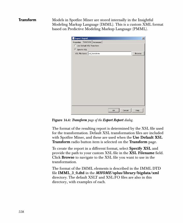
Transform Models in Spotfire Miner are stored internally in the Insightful Modeling Markup Language (IMML). This is a custom XML format based on Predictive Modeling Markup Language (PMML).
The format of the resulting report is determined by the XSL file used for the transformation. Default XSL transformation files are included with Spotfire Miner, and these are used when the Use Default XSL Transform radio button item is selected on the Transform page.
To create the report in a different format, select Specify XSL and provide the path to your custom XSL file in the XSL Filename field. Click Browse to navigate to the XSL file you want to use in the transformation.
The format of the IMML elements is described in the IMML DTD file IMML_3_0.dtd in the MHOME/splus/library/bigdata/xml directory. The default XSLT and XSL:FO files are also in this directory, with examples of each.
Figure 14.4: Transform page of the Export Report dialog.
558

Using the Viewer The viewer for the Export Report component displays the report of the model. This report is specific to the particular modeling component, and is described in the documentation for the modeling component.
559

560
Overview 562
Pipeline Architecture 563
The Advanced Page 564Worksheet Advanced Options 565Max Rows Per Block 565Max Megabytes Per Block 565Order of Operations 565Caching 566Random Seed 566Worksheet Random Seeds Option 567
Notes on Data Blocks and Caching 568Deleting Data Caches 570Worksheet Data Directories 572
Memory Intensive Functions 573
Size Recommendations for Spotfire Miner™ 575
Command Line Options 578Running Spotfire Miner in Batch 579
Increasing Java Memory 580
Importing and Exporting Data with JDBC 581JDBC Example Workflow 581
ADVANCED TOPICS 15
561

OVERVIEW
The previous chapters have shown how you can create, process, and assess models in Spotfire Miner™ by cleaning and manipulating data, applying statistical nodes, and using lift charts to determine the efficacy of your model. The models can be generated using the Spotfire Miner interface to “drag and drop” components in the workspace without any high-level knowledge of the Spotfire Miner architecture or what options are available to process your data more efficiently. If you are a novice user, you can learn how to process models in Spotfire Miner quickly.
However, knowledge of the advanced features in Spotfire Miner, such as the pipeline architecture, buffering, caching, data set limitations, and other capabilities can help you better understand how to leverage Spotfire Miner to meet your specific goals. The goal of this chapter is to introduce these high-level elements to the advanced Spotfire Miner user, so you can better understand the flexibility and power of Spotfire Miner. We discuss the pipeline architecture that drives Spotfire Miner, how “block size” of data affects processing, caching options, and memory-intensive functions.
562
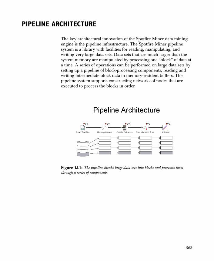
PIPELINE ARCHITECTURE
The key architectural innovation of the Spotfire Miner data mining engine is the pipeline infrastructure. The Spotfire Miner pipeline system is a library with facilities for reading, manipulating, and writing very large data sets. Data sets that are much larger than the system memory are manipulated by processing one “block” of data at a time. A series of operations can be performed on large data sets by setting up a pipeline of block-processing components, reading and writing intermediate block data in memory-resident buffers. The pipeline system supports constructing networks of nodes that are executed to process the blocks in order.
Figure 15.1: The pipeline breaks large data sets into blocks and processes them through a series of components.
563
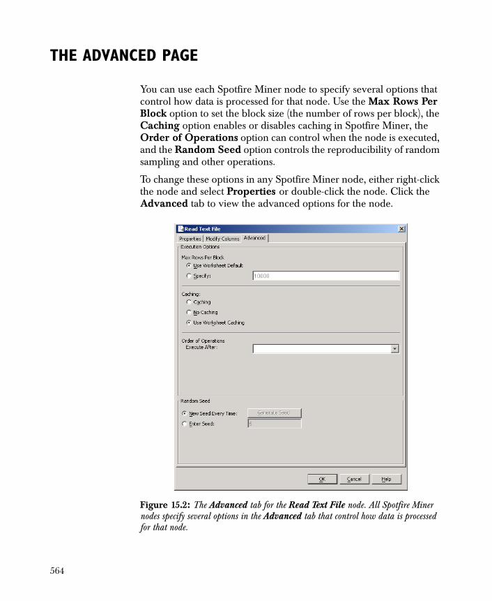
THE ADVANCED PAGE
You can use each Spotfire Miner node to specify several options that control how data is processed for that node. Use the Max Rows Per Block option to set the block size (the number of rows per block), the Caching option enables or disables caching in Spotfire Miner, the Order of Operations option can control when the node is executed, and the Random Seed option controls the reproducibility of random sampling and other operations.
To change these options in any Spotfire Miner node, either right-click the node and select Properties or double-click the node. Click the Advanced tab to view the advanced options for the node.
Figure 15.2: The Advanced tab for the Read Text File node. All Spotfire Miner nodes specify several options in the Advanced tab that control how data is processed for that node.
564
Worksheet Advanced Options
The Max Rows Per Block and Caching options for a node can be set to use default values associated with the worksheet. These worksheet values are set in the Worksheet Properties dialog. To access the Worksheet Properties dialog, go to File � Properties in the main menu and select the Advanced tab. Enter a new value, if desired, in the Max Rows Per Block field and click OK to save the changes. The default value for the worksheet block size is 10,000. The Max Megabytes Per Block and Random Seeds worksheet fields are described below
Max Rows Per Block
Spotfire Miner partitions large data sets into rectangular structures of rows and columns called blocks. The number of columns in a block is equal to the number of columns in the data. The number of rows is estimated so the whole block fits into RAM. The block size is set to a reasonable default of 10,000 rows, but this can be adjusted.
Use the Max Rows Per Block advanced option to specify one of the following two block size options for the node:
Use Worksheet Default Use the worksheet block size set in the Worksheet Properties dialog. This is the default value.
Specify Sets the default block size for an individual node. Enter a new block size in the field to the right and click OK to save the changes.
Max Megabytes Per Block
Spotfire Miner could run out of memory if it tried allocating a data block with a large block size and thousands of columns. You could prevent this by reducing the block size, but this is inconvenient. To avoid this situation, Spotfire Miner automatically reduces the block size according to the Max Megabytes Per Block worksheet property. This property, set in the Worksheet Properties dialog, specifies the maximum number of megabytes that a data block can have. If the block size implies a greater memory size, then the block size is reduced until the data block can fit within this limit. This does not change the Max Rows Per Block value itself, just the block size used when executing a node.
Order of Operations
The Order of Operations option influences the order that nodes are executed. This order is primarily determined by the links connecting the nodes, so that the node outputting a data set is executed before a
565

node consuming the data set. However, there are cases where this doesn’t determine the complete order of execution. The Order of Operations list box displays a list of all of the other nodes in the worksheet. Selecting one of these will ensure that the current node is executed after the selected node, if possible.
Suppose a worksheet contains a network that sends data to a Write Text File node to store it in a file, as well as a completely separate network that uses a Read Text File node to read this file. You would want the Read Text File node to execute after the Write Text File node, even though there is no explicit link between them. You could do this by setting the Order of Operations option for the Read Text File node to name the Write Text File node.
This option is automatically set when a Predictor node is created from a modeling node, specifying that the predictor should be executed after the modeling node.
Caching Spotfire Miner allows the output data produced by a node to be cached or automatically stored in a disk file. The Caching advanced option allows three different ways to cache output data from a node:
Caching Enable caching for the node.
No Caching Disable caching for the node.
Use Worksheet Caching Use the caching option set in the Worksheet Properties dialog, which is accessed from the main menu. This is the default.
For details on caching, see the section Notes on Data Blocks and Caching on page 568.
Random Seed Use the Random Seed group to control the behavior of the random seed Spotfire Miner uses when sampling your data set. If you are not concerned about reproducibility, it is best to use a new seed each time a sample is generated. However, if you need to reproduce a sample exactly, you can designate your own random seed.
There are two options in the Random Seed group, New Seed Every Time and Enter Seed.
New Seed Every Time. Select this radio button to use a new seed each time Spotfire Miner samples your data set.
566

Enter Seed. Select this radio button to specify your own seed when Spotfire Miner samples your data set. When you choose this option, both the corresponding text box and the Generate Seed button are activated. In the text box, type any integer. Alternatively, you can click the Generate Seed button to randomly generate a new seed; each time you click Generate Seed, the seed appears in the text box
Worksheet Random Seeds Option
Use the Random Seeds worksheet option to quickly fix all of the random seeds in a worksheet. If Allow New Seed Every Time is selected (the default), the random seed is determined using the node’s advanced properties, as described above. If Fix All Node Random Seeds is selected, then the seeds generated for nodes with the New Seed Every Time advanced option selected will be reproducible from one execution to another.
Sometimes, while developing a worksheet, you might wish to temporarily fix the random seeds for all of the nodes, so repeated executions are totally reproducible. You could do this by opening the properties of each node, and specifying a seed with the Enter Seed option, but this is extremely inconvenient. Selecting Fix All Node Random Seeds in the Worksheet Properties allows fixing all of the seeds with one simple operation.
567
NOTES ON DATA BLOCKS AND CACHING
If the size of the data at a particular node is small enough to fit in the available RAM, a node can accept the input as a single data set and perform any operation on the data set. A new data set can be created and returned, and side effects such as printing and graphing can be used to display information. If the data is too large to fit in RAM, then the data will be broken into multiple data sets and the function will be applied to each of the data sets. As an example, a 1,000,000 row by 10 column data set of double values is 76MB in size, so it could be handled as a single data set on a machine with 256MB RAM. If the data set was 10,000,000 rows by 100 columns, it would be 7.4GB in size and would have to be handled as multiple blocks.
You can control how the data produced by nodes is cached. In most situations, it is not necessary to change the default caching properties. If you do want to change these values, it is important to understand how caching works.
By default, every node in the network caches its output data. This means that the output data produced by the node is stored in a disk file. Until the properties of the node are changed or the node is invalidated, this data cache can be read by further nodes without re-executing the node that produced it. As you connect new nodes to the outputs of the existing nodes, these new nodes can execute quickly by reading their input data from the existing data cache files.
In the event you are setting up a network and exploring small data sets, it is very useful to have disk caches for all of the nodes in the network. However, there are two potential issues with node caches:
1. Disk space. Each node cache stores a complete copy of the output of its node. When processing large data sets, the disk cache files can become very large. In addition, if a network uses a chain of nodes to manipulate the data, there would be a separate disk cache after every node in the chain.
2. Execution time. It takes more time to write and read cache files to the disk. In some situations, this might be a significant fraction of the execution time.
568
During network execution, whenever the elapsed time is displayed, the total number of bytes used by all of the data cache files is printed. This can help you decide whether it is worth considering disabling caching to save disk space. For example, you might see this:
execution time=0.6 Seconds, data cache size=3.8MB, mem=4MB
This information is also displayed when a node is invalidated:
invalidated Modify Columns (2), data cache size=1.9MB; max=3.9MB
Invalidating nodes or executing networks with caching disabled can cause the total cache size to increase and decrease during an operation: whenever the maximum size is different from the current size, both are printed.
The data cache files are stored in the *.wsd directory, created in the same location as the Spotfire Miner worksheet file (*.imw). When working with large sets of data, the *.wsd directory containing disk cache files for each node can get large. There are a few ways to reduce the size of this directory:
• Delete the data caches. Explicitly delete the data cache files for particular valid nodes, by using the Delete Data Caches menu item (described below). This is the preferred way to reduce the size of the *.wsd directory.
• Invalidating the nodes. You could invalidate all of the nodes before exiting if you don’t want to keep any of the cache files associated with a node.
• Delete the *.wsd directory. If you are not currently running Spotfire Miner and you can rerun the network from scratch, deleting this directory could save significant disk space. All the information defining the actual network is stored in the Spotfire Miner worksheet (*.imw) file. For more information on worksheets, see Chapter 3, The TIBCO Spotfire Miner™ Interface.
If reducing disk space usage is more important than avoiding recomputation, the caching can be turned off for one or more nodes.
Suppose that the node and worksheet properties are set so that caching is disabled for some nodes. In some cases, the execution engine will create temporary caches while executing the network.
569
This happens with nodes that need to scan through their input data multiple times, such as the Sort node or most of the modeling nodes. In this case, the data is stored in a data cache file and read multiple times. If the node that produced the data has caching disabled, the temporary data cache will be deleted after the node has been executed.
Another case where cache files might be created, even if caching is disabled, is use of the Table View node. This node needs to access all of the data that can be viewed, so a data cache is saved for its input data.
Disabling caching would be most useful when processing data in production mode: if a network is large, it is not changed very often, and it is often being used to process large data sets. You can decrease the amount of disk space used and possibly improve the processing time if caching is disabled. The downside is that cache files are unavailable for incremental computation, but that might be an acceptable trade-off.
Deleting Data Caches
If a node has caching turned on, it creates a data cache file for each of its outputs. A node can also have other cache files, containing statistics about its output data, constructed models, etc. All of these files are stored in the wsd directory associated with the worksheet.
When processing large data sets, these cache files can get very large. All of the cache files associated with a node can be deleted by invalidating the node, but this also invalidates all nodes downstream.
Warning
It is possible to get unexpected results when caching is disabled on a node that produces different results on repeated executions, such as a node using random numbers with a new seed generated every time. For example, consider a Partition node with No Caching and New Seed Every Time selected, and its first output is connected to two Write Text File nodes that write the data to files A.txt and B.txt.
If you click Run to Here on the node writing A.txt, the Partition node executes and its data is written to file A.txt. Then, if you select Run to Here on the node writing B.txt, this re-executes the Partition node, generating a different partition, and writing it to file B.txt.
If the Partition node was set with caching enabled, the Partion node would be executed only once, and the same data would be written to A.txt and B.txt.
570
It is possible to delete the data caches for a node without invalidating the node. This can be done by selecting one or more valid nodes, and selecting the Tools � Delete Data Cache menu item. This prints a message in the message pane describing how many data cache files have been deleted, for example:
deleted 2 data cache(s) with total size 11KB
It is important to understand the ramifications of deleting data cache files. If you delete the data cache files for a node X, and then you attach another node Y to an output of X, executing Y will re-execute X, in order to re-create its output data. Another result is that you cannot view the data from the data cache until the node is re-executed.
You typically would only want to delete the data caches for a node when you are sure that you will never need that data again. For example, suppose that you are incrementally constructing and executing a large network. Over time, the data cache files will pile up. At some point, you might realize that you won't need the data caches from the early nodes (reading the initial data, and performing initial data cleaning), so you can delete these data cache files without effecting the rest of the network.
There is a visual sign in the worksheet that indicates whether a node has data cache files: If a node has data cache files, its output port triangles are dark, otherwise they are light gray.
The Tools � Cache Information menu item prints, for each of the selected valid nodes, the size of the data caches and of any other cache files. This information is printed in the message pane, for example:
cache information for 4 valid node(s): Read Text File (0): data cache=6.3MB, other caches=34KB Missing Values (2): data cache=6.3MB, other caches=28KB Filter Columns (4): data cache=3.4MB, other caches=14KB Classification Tree (3): data cache=130KB, other caches=83KB totals: data cache=16.2MB, other caches=161KB
Note that the "other cache" size for the classification tree node is relatively large: this includes the classification tree model constructed by this node.
571

Worksheet Data Directories
When executing a worksheet, data cache and other temporary files are stored in a worksheet data directory. Normally, this directory is named *.wsd, created in the same location as the Spotfire Miner worksheet file (*.imw). This directory can be changed by setting the Worksheet Data Directory field in the Worksheet Properties dialog. To access the Worksheet Properties dialog, go to File � Properties in the main menu and select the Advanced tab.
Normally, the Worksheet Data Directory field is empty. This signifies that the worksheet data directory is a directory *.wsd in the same location as the *.imw worksheet file. If this is set to another directory, when the dialog is closed, the contents of the current worksheet directory are copied to the new directory.
572

MEMORY INTENSIVE FUNCTIONS
There are no well-defined guidelines to determine which operations in Spotfire Miner require more memory than others. In general, data manipulation nodes consume less memory than modeling nodes, but this depends on the algorithm behind the operation. As a simple example, modifying the columns of a data set is generally less memory intensive than performing a linear regression, and a linear regression is generally less memory intensive than a logistic regression.
The best way to see which nodes are consuming the most memory is to look at the values printed out in the message window during node execution. When a node has finished executing, Spotfire Miner prints out the amount of memory allocated as well as the data cache size in the message pane. For example, after reading in a text file, you would see a message similar to the following:
executing: {Read Text File (1)}execution time=0.1 Seconds, data cache size=144 Bytes,mem=203KB
The mem value printed in the message window is a rough estimate of the amount of memory allocated during the execution of the node. If this value looks too high, you can reduce the memory allocated by reducing the block size for that node or by modifying other parameters to the node which might be affecting memory usage.
For example, using the default block size of 10,000 when reading in the sample data set in vetmailing.txt from the examples directory, the output in the message window looks like the following:
executing: {Read Text File (0)}execution time=0.9 Seconds, data cache size=1.9MB,mem=2.1MB
Right-click the node, choose Properties, and click the Advanced tab. Change the Max Rows Per Block setting to 1000. Rerunning the node gives the following:
executing: {Read Text File (0)}execution time=0.9 Seconds, data cache size=1.9MB,mem=388KB
573

As you can see, the memory allocated is reduced significantly by reducing the block size. Tracking the memory allocated and the data cache size displayed in the Spotfire Miner message pane are the best way to determine which nodes in your network are consuming the most memory.
574
SIZE RECOMMENDATIONS FOR SPOTFIRE MINER™
Spotfire Miner can handle very large data sets through the use of the pipeline architecture. To help you determine the disk space necessary to run these data sets, we provide the following assumptions and recommendations to assist in your processing.
Worst-case Scenario Assumptions
To provide conservative estimates of disk space required to process very large data sets, we make these assumptions:
• All nodes create copies of the data.
• Data is not reduced in terms of columns and rows in the .imw worksheet (this is a very pessimistic assumption).
Upper Limit Estimation for .wsd Disk Space
We calculate the amount of disk space required for processing using the following formula:
number of rows in input file
x
number of columns in input file
x
number of nodes
+
size of input file
+
size of input file
+
size of output file (must be <= input file)
For the size of input file multiplied by the number of nodes, this assumes that each node makes a full copy of the data. Further, the size of the input file determines the temporary space, the size necessary to store the input data, and the size of the output data.
To be safe, a very conservative estimate of recommended disk space is
size of input file x (number of nodes+3)
575
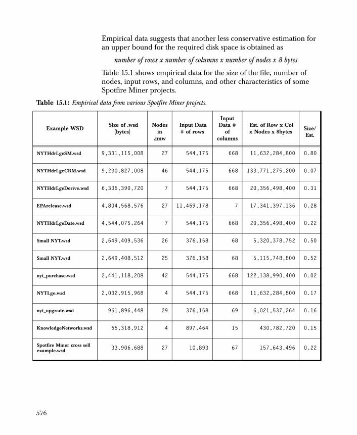
Empirical data suggests that another less conservative estimation for an upper bound for the required disk space is obtained as
number of rows x number of columns x number of nodes x 8 bytes
Table 15.1 shows empirical data for the size of the file, number of nodes, input rows, and columns, and other characteristics of some Spotfire Miner projects.
Table 15.1: Empirical data from various Spotfire Miner projects.
Example WSD Size of .wsd
(bytes)
Nodes
in .imw
Input Data # of rows
Input Data #
of columns
Est. of Row x Col x Nodes x 8bytes
Size/Est.
NYTHdrLgeSM.wsd 9,331,115,008 27 544,175 668 11,632,284,800 0.80
NYTHdrLgeCRM.wsd 9,230,827,008 46 544,175 668 133,771,275,200 0.07
NYTHdrLgeDerive.wsd 6,335,390,720 7 544,175 668 20,356,498,400 0.31
EPArelease.wsd 4,804,568,576 27 11,469,178 7 17,341,397,136 0.28
NYTHdrLgeDate.wsd 4,544,075,264 7 544,175 668 20,356,498,400 0.22
Small NYT.wsd 2,649,409,536 26 376,158 68 5,320,378,752 0.50
Small NYT.wsd 2,649,408,512 25 376,158 68 5,115,748,800 0.52
nyt_purchase.wsd 2,441,118,208 42 544,175 668 122,138,990,400 0.02
NYTLge.wsd 2,032,915,968 4 544,175 668 11,632,284,800 0.17
nyt_upgrade.wsd 961,896,448 29 376,158 69 6,021,537,264 0.16
KnowledgeNetworks.wsd 65,318,912 4 897,464 15 430,782,720 0.15
Spotfire Miner cross sell example.wsd 33,906,688 27 10,893 67 157,643,496 0.22
576
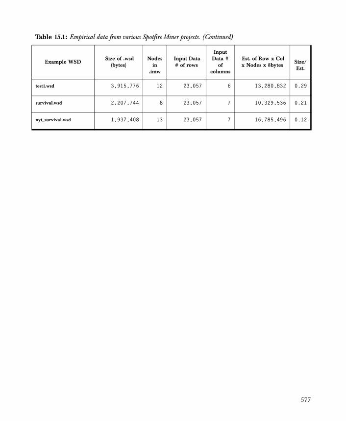
test1.wsd 3,915,776 12 23,057 6 13,280,832 0.29
survival.wsd 2,207,744 8 23,057 7 10,329,536 0.21
nyt_survival.wsd 1,937,408 13 23,057 7 16,785,496 0.12
Table 15.1: Empirical data from various Spotfire Miner projects. (Continued)
Example WSD Size of .wsd
(bytes)
Nodes
in .imw
Input Data # of rows
Input Data #
of columns
Est. of Row x Col x Nodes x 8bytes
Size/Est.
577
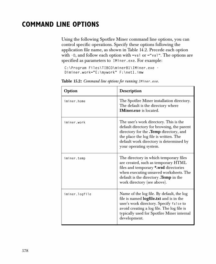
COMMAND LINE OPTIONS
Using the following Spotfire Miner command line options, you can control specific operations. Specify these options following the application file name, as shown in Table 14.2. Precede each option with -D, and follow each option with =val or ="val". The options are specified as parameters to IMiner.exe. For example:
C:\Program Files\TIBCO\miner82\IMiner.exe -Diminer.work="E:\mywork" F:\net1.imw
Table 15.2: Command line options for running IMiner.exe.
Option Description
iminer.home The Spotfire Miner installation directory. The default is the directory where IMiner.exe is located.
iminer.work The user's work directory. This is the default directory for browsing, the parent directory for the .Temp directory, and the place the log file is written. The default work directory is determined by your operating system.
iminer.temp The directory in which temporary files are created, such as temporary HTML files and temporary *.wsd directories when executing unsaved worksheets. The default is the directory .Temp in the work directory (see above).
iminer.logfile Name of the log file. By default, the log file is named logfile.txt and is in the user's work directory. Specify false to avoid creating a log file. The log file is typically used for Spotfire Miner internal development.
578
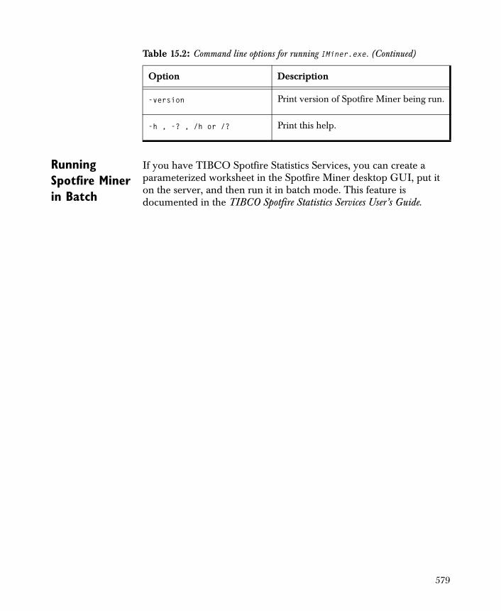
Running Spotfire Miner in Batch
If you have TIBCO Spotfire Statistics Services, you can create a parameterized worksheet in the Spotfire Miner desktop GUI, put it on the server, and then run it in batch mode. This feature is documented in the TIBCO Spotfire Statistics Services User’s Guide.
-version Print version of Spotfire Miner being run.
-h , -? , /h or /? Print this help.
Table 15.2: Command line options for running IMiner.exe. (Continued)
Option Description
579
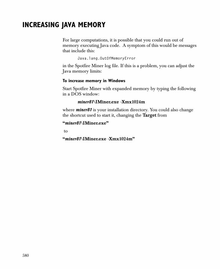
INCREASING JAVA MEMORY
For large computations, it is possible that you could run out of memory executing Java code. A symptom of this would be messages that include this:
Java.lang.OutOfMemoryError
in the Spotfire Miner log file. If this is a problem, you can adjust the Java memory limits:
To increase memory in Windows
Start Spotfire Miner with expanded memory by typing the following in a DOS window:
miner82\IMiner.exe -Xmx1024m
where miner82 is your installation directory. You could also change the shortcut used to start it, changing the Target from
“miner82\IMiner.exe”
to
“miner82\IMiner.exe -Xmx1024m”
580
IMPORTING AND EXPORTING DATA WITH JDBC
You can import and export data from a relational database or a tabular data source using a JDBC driver and the JDBC library. The JDBC library provides two nodes:
• Read Database - JDBC.
• Write Database - JDBC.
For an overview of these nodes, see the section Read Database JDBC on page 72 and the section Write Database JDBC on page 99.
JDBC Example Workflow
The JDBC library’s Read Database - JDBC and Write Database - JDBC nodes are customized S-PLUS Script nodes that use functions in the Spotfire S+ sjdbc library. To use either (or both), just attach the library, put the node(s) on your worksheet, and set a few parameters in the node dialog(s).
To attach the library
1. On the menu, click Tools � Library � Manage Libraries.
2. Click Browse.
3. In the Load Existing Libraries dialog, in the left pane, click the Examples folder.
4. Select JDBC.iml, and then click Open.
5. Click OK to load the library.
Note that in the Spotfire Miner Explorer pane, the tab labeled JDBC appears.
6. Click the JDBC tab to display the JDBC pane.
To use the Read Database - JDBC node
1. Click and drag the Read Database - JDBC node onto your worksheet.
581

2. Double-click the node to open its Parameters page. (See Figure 15.3.)
3. On the Parameters page, set values for the following:
Figure 15.3: Parameters page for the Read Database - JDBC script node .
Table 15.3: Read Database - JDBC Parameters
Parameter Description
driverClass The name of the Java class for required the JDBC driver. For example, for the Microsoft SQL Server 2005 driver, driverClass is com.microsoft.sqlserver.jdbc.SQLServerDriver.
con The JDBC connection string. The connection string format depends on the driver. For example, for the Microsoft SQL Server 2005 driver, con has the following format:
“jdbc:sqlserver://<host>:1433;databaseName=<database>;user=<username>;password=<password>;"
582
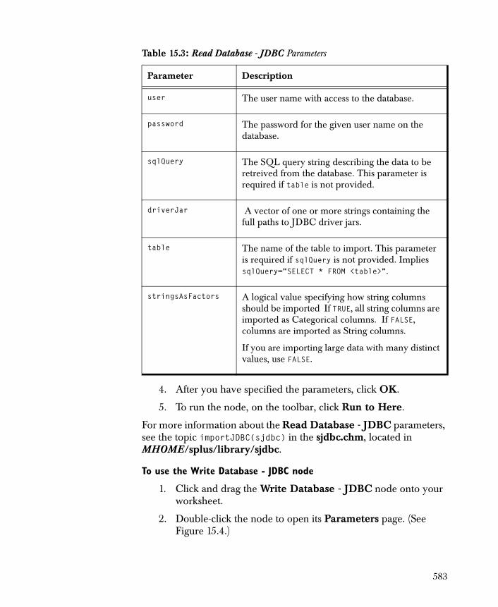
4. After you have specified the parameters, click OK.
5. To run the node, on the toolbar, click Run to Here.
For more information about the Read Database - JDBC parameters, see the topic importJDBC(sjdbc) in the sjdbc.chm, located in MHOME/splus/library/sjdbc.
To use the Write Database - JDBC node
1. Click and drag the Write Database - JDBC node onto your worksheet.
2. Double-click the node to open its Parameters page. (See Figure 15.4.)
user The user name with access to the database.
password The password for the given user name on the database.
sqlQuery The SQL query string describing the data to be retreived from the database. This parameter is required if table is not provided.
driverJar A vector of one or more strings containing the full paths to JDBC driver jars.
table The name of the table to import. This parameter is required if sqlQuery is not provided. Implies sqlQuery="SELECT * FROM <table>".
stringsAsFactors A logical value specifying how string columns should be imported If TRUE, all string columns are imported as Categorical columns. If FALSE, columns are imported as String columns.
If you are importing large data with many distinct values, use FALSE.
Table 15.3: Read Database - JDBC Parameters
Parameter Description
583

3. On the Parameters page, set values for the following:
Figure 15.4: Parameters page for the Write Database - JDBC script node .
Table 15.4: Write Database - JDBC Parameters
Parameter Description
driverClass The name of the Java class for required the JDBC driver. For example, for the Microsoft SQL Server 2005 driver, driverClass is com.microsoft.sqlserver.jdbc.SQLServerDriver.
con The JDBC connection string. The connection string format depends on the driver. For example, for the Microsoft SQL Server 2005 driver, con has the following format:
“jdbc:sqlserver://<host>:1433;databaseName=<database>;user=<username>;password=<password>;"
user The user name with access to the database.
584
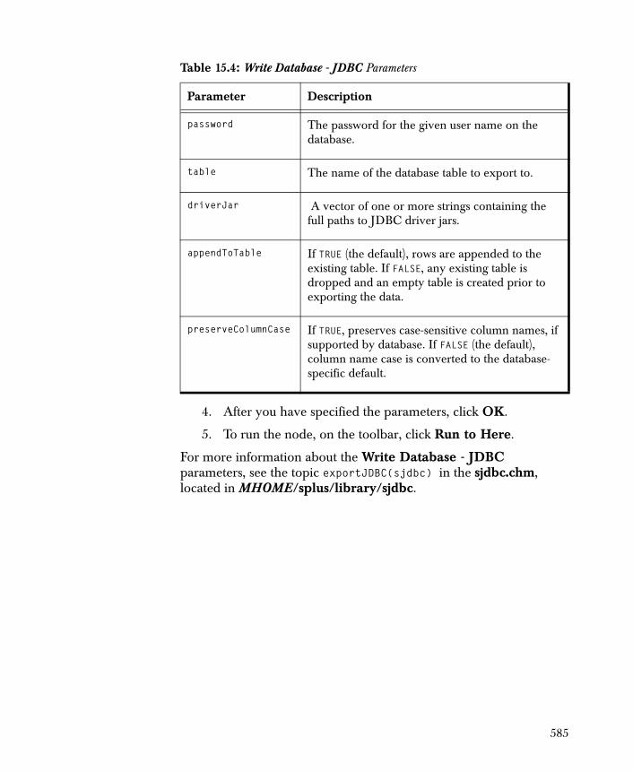
4. After you have specified the parameters, click OK.
5. To run the node, on the toolbar, click Run to Here.
For more information about the Write Database - JDBC parameters, see the topic exportJDBC(sjdbc) in the sjdbc.chm, located in MHOME/splus/library/sjdbc.
password The password for the given user name on the database.
table The name of the database table to export to.
driverJar A vector of one or more strings containing the full paths to JDBC driver jars.
appendToTable If TRUE (the default), rows are appended to the existing table. If FALSE, any existing table is dropped and an empty table is created prior to exporting the data.
preserveColumnCase If TRUE, preserves case-sensitive column names, if supported by database. If FALSE (the default), column name case is converted to the database-specific default.
Table 15.4: Write Database - JDBC Parameters
Parameter Description
585

586
Overview 589
S-PLUS Data Nodes 592Read S-PLUS Data 592Write S-PLUS Data 594
S-PLUS Chart Nodes 597Overview 597Using the Graph Window 598One Column - Continuous 600One Column - Categorical 608Two Columns - Continuous 614Two Columns - Mixed 625Three Columns 631Multiple Columns 638Time Series 646Common Pages 654
S-PLUS Data Manipulation Nodes 667S-PLUS Create Columns 669S-PLUS Filter Rows 672S-PLUS Split 674
S-PLUS Script Node 677Properties 678Processing Multiple Data Blocks 687The Test Phase 687Input List Elements 688Output List Elements 691Size of the Input Data Frames 697Date and String Values 697Interpreting min/max values 698Debugging 699
THE S-PLUS LIBRARY 16
587

Processing Data Using the Execute Big Data Script Option700
Loading Spotfire S+ Modules 702Examples Using the S-PLUS Script Node 703
References 716
588
OVERVIEW
TIBCO Spotfire S+® is a programming environment designed for data analysis. It includes a complete programming language with variables, complex data structures, control statements, user-defined functions, and a rich set of built-in data analysis functions.
The S language engine from Spotfire S+ is part of the basic Spotfire Miner™ system and does not need to be explicitly installed. The Spotfire S+ page appears in the explorer pane.
This chapter presents the features of the S language engine and the S-PLUS nodes, and it demonstrates how you can transform your data set by writing S-PLUS expressions. This chapter does not describe the S language engine in detail. Consult the Spotfire S+ printed or online documentation for more detailed information.
The S language engine from Spotfire S+ is available through the S-PLUS Script node, located in the Spotfire S+ page of the explorer pane (shown in Figure 16.1). The S language engine expands the charting, data manipulation, and programming capabilities of Spotfire Miner.
Note
Spotfire Miner works only with the included Spotfire S+ libraries and S language engine, and you cannot use an externally-installed version of Spotfire S+ with Spotfire Miner. If you plan to work with Spotfire S+ or the S language extensively, consider using Spotfire S+.
Spotfire S+ provides features that are not included in Spotfire Miner, such as the Spotfire S+ GUI, Spotfire S+ Workbench integrated developer environment, Spotfire S+ console application (sqpe), plus support for Automation and for other interfaces (including OLE, DDE, and COM).
589
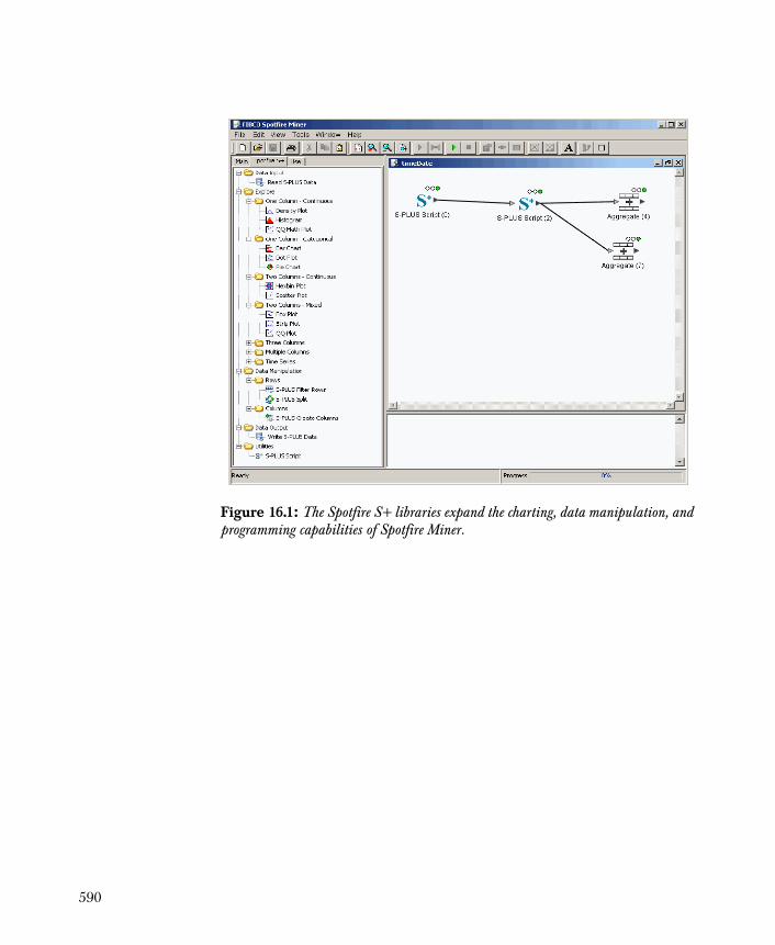
Figure 16.1: The Spotfire S+ libraries expand the charting, data manipulation, and programming capabilities of Spotfire Miner.
590
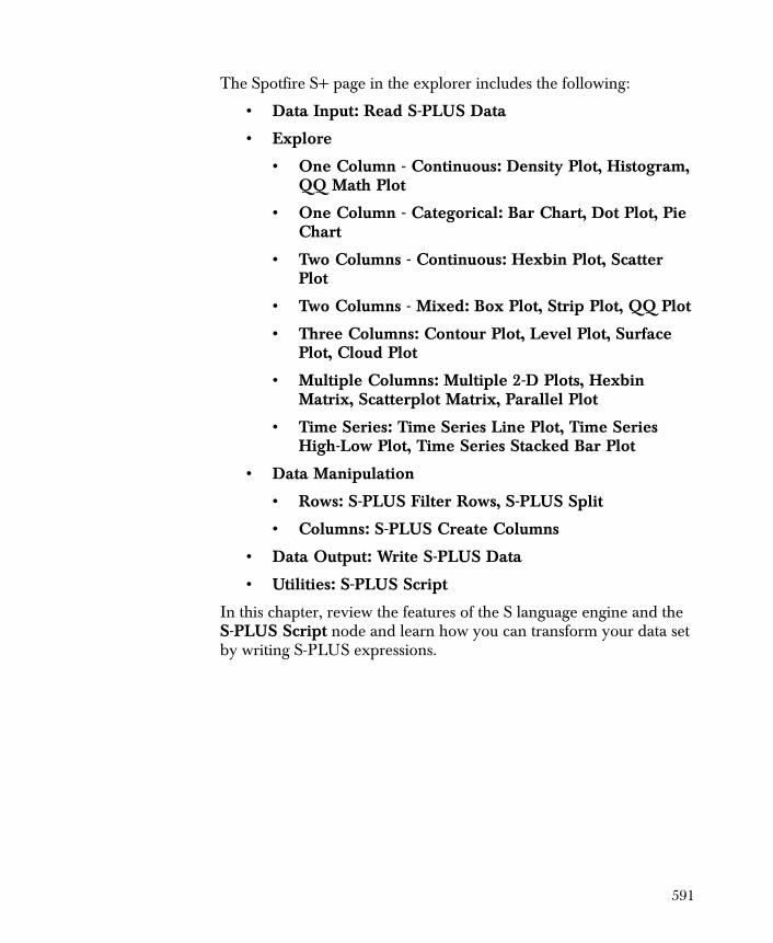
The Spotfire S+ page in the explorer includes the following:
• Data Input: Read S-PLUS Data
• Explore
• One Column - Continuous: Density Plot, Histogram, QQ Math Plot
• One Column - Categorical: Bar Chart, Dot Plot, Pie Chart
• Two Columns - Continuous: Hexbin Plot, Scatter Plot
• Two Columns - Mixed: Box Plot, Strip Plot, QQ Plot
• Three Columns: Contour Plot, Level Plot, Surface Plot, Cloud Plot
• Multiple Columns: Multiple 2-D Plots, Hexbin Matrix, Scatterplot Matrix, Parallel Plot
• Time Series: Time Series Line Plot, Time Series High-Low Plot, Time Series Stacked Bar Plot
• Data Manipulation
• Rows: S-PLUS Filter Rows, S-PLUS Split
• Columns: S-PLUS Create Columns
• Data Output: Write S-PLUS Data
• Utilities: S-PLUS Script
In this chapter, review the features of the S language engine and the S-PLUS Script node and learn how you can transform your data set by writing S-PLUS expressions.
591

S-PLUS DATA NODES
The Read S-PLUS Data and Write S-PLUS Data components incorporate data from Spotfire S+ into a Spotfire Miner worksheet.
Access the data by specifying the name of the Spotfire S+ data frame and its location. The two possible types of locations are:
• A Spotfire S+ data dump (*.sdd) file containing a text description of the data frame. This can be created using the File � Save menu or the data.dump() function in Spotfire S+ for Windows.
• A Spotfire S+ chapter. This is a directory containing binary representations of Spotfire S+ objects.
Think of both a Spotfire S+ data dump file and a Spotfire S+ chapter as databases, with the “table name” as the name of the Spotfire S+ data frame. In Read S-PLUS Data, you must specify the Data Frame Name, because both a data dump file and a chapter can contain multiple data frames.
Read S-PLUS Data
Use the Read S-PLUS Data component to specify a Spotfire S+ data set to use in your analysis.
General Procedure
The following outlines the general approach for using the Read S-PLUS Data component:
1. Click and drag a Read S-PLUS Data component from the explorer pane and drop it on your worksheet.
2. Use the Properties dialog for Read S-PLUS Data to specify the Spotfire S+ data frame to be read.
3. Run the network.
4. Launch the node’s viewer.
Note
The Read S-PLUS Data node reads in data frames; it does not read in bdFrames. To read data from a bdFrame, use an S-PLUS Script node. See the section S-PLUS Script Node on page 677 for more information.
592
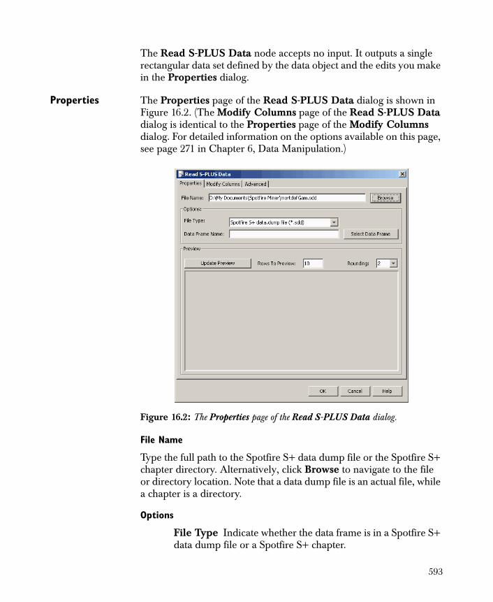
The Read S-PLUS Data node accepts no input. It outputs a single rectangular data set defined by the data object and the edits you make in the Properties dialog.
Properties The Properties page of the Read S-PLUS Data dialog is shown in Figure 16.2. (The Modify Columns page of the Read S-PLUS Data dialog is identical to the Properties page of the Modify Columns dialog. For detailed information on the options available on this page, see page 271 in Chapter 6, Data Manipulation.)
File Name
Type the full path to the Spotfire S+ data dump file or the Spotfire S+ chapter directory. Alternatively, click Browse to navigate to the file or directory location. Note that a data dump file is an actual file, while a chapter is a directory.
Options
File Type Indicate whether the data frame is in a Spotfire S+ data dump file or a Spotfire S+ chapter.
Figure 16.2: The Properties page of the Read S-PLUS Data dialog.
593
Data Frame Name Specify the name of the data frame. If the File Name has been specified, Select Data Frame launches a dialog showing the names of the objects in the data dump file or chapter.
Preview
The Preview group in the Read S-PLUS Data dialog is identical to the Preview group in the Read Text File dialog. For detailed information on using this feature, see page 39.
Using the Viewer The viewer for the Read S-PLUS Data component is identical to the viewer for the Read Text File component. For more information, see the online help for Node Viewer.
Write S-PLUS Data
Use the Write S-PLUS Data component to create Spotfire S+ data objects of your data sets. You can write a data set into a Spotfire S+ data dump file or a valid Spotfire S+ chapter as a Spotfire S+ data frame.
General Procedure
The following outlines the general approach for using the Write S-PLUS Data component:
1. Click and drag a Write S-PLUS Data component from the explorer pane and drop it on your worksheet.
2. Link the Write S-PLUS Data node in your worksheet to any node that outputs data.
3. Use the Properties dialog for Write S-PLUS Data to specify options for the Spotfire S+ data frame to create.
4. Run the network.
5. Launch the node’s viewer.
Warning
The Write S-PLUS Data component can add a new data frame to an existing Spotfire S+ chapter; however, it cannot add a new data frame to an existing Spotfire S+ data dump file. If the specified file name is an existing Spotfire S+ data dump file, its current contents are deleted when the new data frame is written.
594
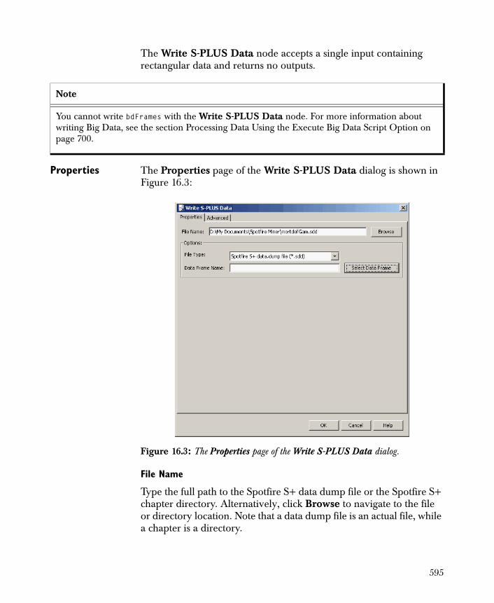
The Write S-PLUS Data node accepts a single input containing rectangular data and returns no outputs.
Properties The Properties page of the Write S-PLUS Data dialog is shown in Figure 16.3:
File Name
Type the full path to the Spotfire S+ data dump file or the Spotfire S+ chapter directory. Alternatively, click Browse to navigate to the file or directory location. Note that a data dump file is an actual file, while a chapter is a directory.
Note
You cannot write bdFrames with the Write S-PLUS Data node. For more information about writing Big Data, see the section Processing Data Using the Execute Big Data Script Option on page 700.
Figure 16.3: The Properties page of the Write S-PLUS Data dialog.
595
Options
File Type Indicate whether the data frame is in a Spotfire S+ data dump file or a Spotfire S+ chapter.
Data Frame Name Specify the name of the data frame. If you specify File Name, Select Data Frame launches a dialog showing the names of the objects in the data dump file or chapter.
Using the Viewer The viewer for the Write S-PLUS Data component is identical to the viewer for the Write Text File component. For more information, see the online help for Node Viewer.
596
S-PLUS CHART NODES
Overview The S-PLUS Chart nodes are available from two locations:
• The Explore folder in the Spotfire S+ tab of the explorer.
• The Chart menu for the default viewer.
The chart nodes give you access to nearly all of the Trellis functions in Spotfire S+: xyplot, densityplot, histogram, qqmath, barchart, dotplot, piechart, bwplot, stripplot, qq, contourplot, levelplot, wireframe, splom, and parallel. Non-Trellis hexagonal binning and time series plots are also available.
General Procedure
The basic procedure for creating charts is the same, regardless of the type of chart you choose.
To create a chart using a node on the worksheet:
1. Click and drag a chart component from the explorer pane and drop it on your worksheet.
1. Link the chart node in your worksheet to any node that outputs data.
2. Use the properties dialog to specify the columns to chart. Set other options if desired. Click OK to accept the changes to the dialog.
3. Run your network.
4. Launch the node’s viewer. This displays the chart in a Graph Window.
You can create the chart without closing the dialog. Click Apply to commit the changes to the dialog, execute a Run to Here on the chart node, and display the viewer.
To create a chart using the default viewer’s Chart menu:
1. Select the appropriate menu item to display the properties dialog. The column lists correspond to the columns in the viewer.
2. Use the properties dialog to specify the columns to chart. Set other options as needed.
3. Click Apply to create the chart in a Graph Window.
597
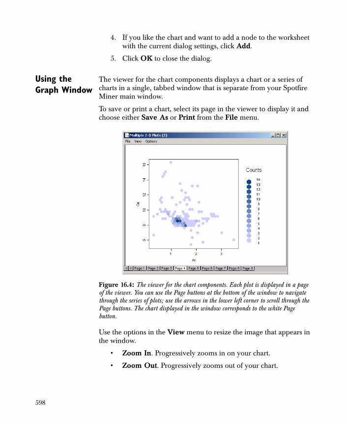
4. If you like the chart and want to add a node to the worksheet with the current dialog settings, click Add.
5. Click OK to close the dialog.
Using the Graph Window
The viewer for the chart components displays a chart or a series of charts in a single, tabbed window that is separate from your Spotfire Miner main window.
To save or print a chart, select its page in the viewer to display it and choose either Save As or Print from the File menu.
Use the options in the View menu to resize the image that appears in the window.
• Zoom In. Progressively zooms in on your chart.
• Zoom Out. Progressively zooms out of your chart.
Figure 16.4: The viewer for the chart components. Each plot is displayed in a page of the viewer. You can use the Page buttons at the bottom of the window to navigate through the series of plots; use the arrows in the lower left corner to scroll through the Page buttons. The chart displayed in the window corresponds to the white Page button.
598
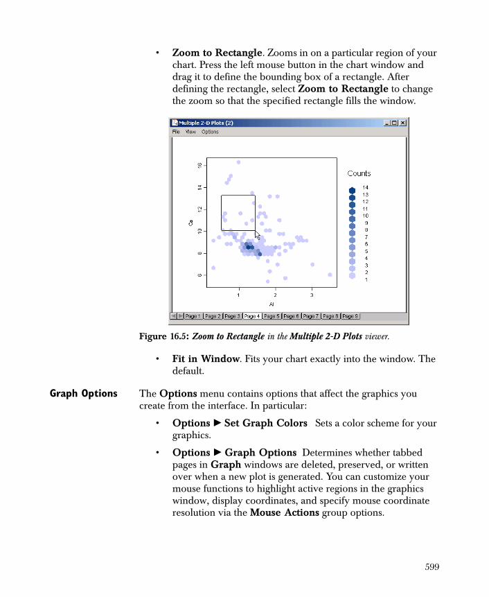
• Zoom to Rectangle. Zooms in on a particular region of your chart. Press the left mouse button in the chart window and drag it to define the bounding box of a rectangle. After defining the rectangle, select Zoom to Rectangle to change the zoom so that the specified rectangle fills the window.
• Fit in Window. Fits your chart exactly into the window. The default.
Graph Options The Options menu contains options that affect the graphics you create from the interface. In particular:
• Options � Set Graph Colors Sets a color scheme for your graphics.
• Options � Graph Options Determines whether tabbed pages in Graph windows are deleted, preserved, or written over when a new plot is generated. You can customize your mouse functions to highlight active regions in the graphics window, display coordinates, and specify mouse coordinate resolution via the Mouse Actions group options.
Figure 16.5: Zoom to Rectangle in the Multiple 2-D Plots viewer.
599
To alter cosmetic properties of your charts, use the Options � Set Graph Colors and Options � Graph Options dialogs shown in Figure 16.6 and Figure 16.7. These dialogs contain options to modify certain aspects of your bivariate charts, including the color scheme. For more details, see the online help system.
One Column - Continuous
This section contains information about basic plot types useful for exploring a single continuous column.
• Density Plot Displays an estimate of the underlying probability density function for a column.
Figure 16.6: The Set Graph Colors dialog.
Figure 16.7: The Graph Options dialog.
600
• Histogram Displays of the number of data points that fall in each of a specified number of intervals. A histogram gives an indication of the relative density of the data points along the horizontal axis.
• QQ Math Plot Determines a good approximation to a data set’s distribution. The most common is the normal probability plot, or normal qqplot, which is used to test whether the distribution of a data set is nearly Gaussian.
These visualization plots are exploratory data analysis tools that you can use to grasp the nature of your data. Such an understanding can help you avoid the misuse of statistical inference methods, such as using a method appropriate only for a normal (Gaussian) distribution when the distribution is strongly non-normal.
Data Page The Density Plot, Histogram, and QQ Math Plot property dialogs have the same Data page:
Columns
Value Specifies the continuous column to chart.
Figure 16.8: The Data page of the Density Plot dialog.
601
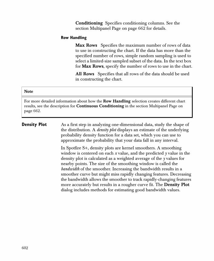
Conditioning Specifies conditioning columns. See the section Multipanel Page on page 662 for details.
Row Handling
Max Rows Specifies the maximum number of rows of data to use in constructing the chart. If the data has more than the specified number of rows, simple random sampling is used to select a limited-size sampled subset of the data. In the text box for Max Rows, specify the number of rows to use in the chart.
All Rows Specifies that all rows of the data should be used in constructing the chart.
Density Plot As a first step in analyzing one-dimensional data, study the shape of the distribution. A density plot displays an estimate of the underlying probability density function for a data set, which you can use to approximate the probability that your data fall in any interval.
In Spotfire S+, density plots are kernel smoothers. A smoothing window is centered on each x value, and the predicted y value in the density plot is calculated as a weighted average of the y values for nearby points. The size of the smoothing window is called the bandwidth of the smoother. Increasing the bandwidth results in a smoother curve but might miss rapidly changing features. Decreasing the bandwidth allows the smoother to track rapidly-changing features more accurately but results in a rougher curve fit. The Density Plot dialog includes methods for estimating good bandwidth values.
Note
For more detailed information about how the Row Handling selection creates different chart results, see the description for Continuous Conditioning in the section Multipanel Page on page 662.
602
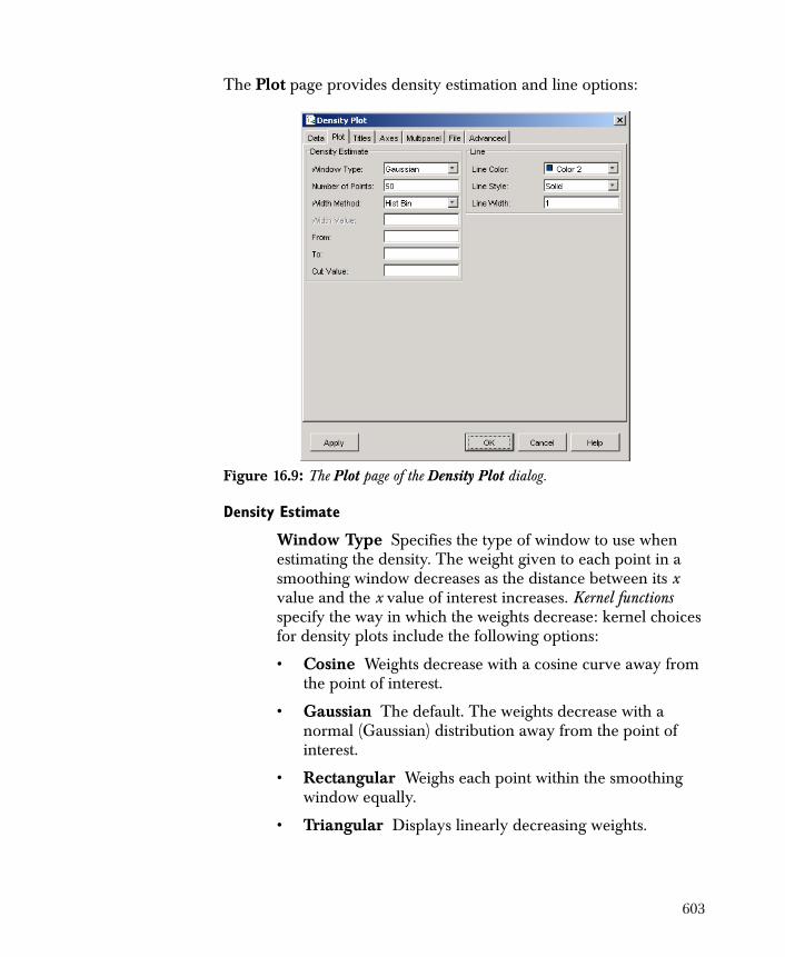
The Plot page provides density estimation and line options:
Density Estimate
Window Type Specifies the type of window to use when estimating the density. The weight given to each point in a smoothing window decreases as the distance between its x value and the x value of interest increases. Kernel functions specify the way in which the weights decrease: kernel choices for density plots include the following options:
• Cosine Weights decrease with a cosine curve away from the point of interest.
• Gaussian The default. The weights decrease with a normal (Gaussian) distribution away from the point of interest.
• Rectangular Weighs each point within the smoothing window equally.
• Triangular Displays linearly decreasing weights.
Figure 16.9: The Plot page of the Density Plot dialog.
603

Number of Points Specifies the number of equally-spaced points at which to estimate the density.
Width Method Specifies the algorithm for computing the width of the smoothing window. Available methods are:
• Hist Bin Histogram bin.
• Normal Ref Normal reference density.
• Biased CV Biased cross-validation.
• Unbiased CV Unbiased cross-validation.
• Est Deriv Sheather & Jones pilot estimation of derivatives.
• Specified Value Defines a custom window.
Width Value Specifies the width to use if Width Method is set to Specified Value.
From Specifies the minimum value at which to estimate the density.
To Specifies the maximum value at which to estimate the density.
Cut Value Specifies the fraction of the window width that the x values are to be extended by. The default is .75 for the Gaussian window and .5 for the other windows.
Line
Line Color Specifies the color of the line.
Line Style Specifies the style of line, such as solid or dashed.
Line Width Specifies the line width.
For more information on the methods used to compute the width of a smoothing window, see Venables and Ripley (1999).
Histogram Histograms display the number of data points that fall in each of a specified number of intervals. A histogram gives an indication of the relative density of the data points along the horizontal axis. For this reason, density plots are often superposed with (scaled) histograms.
604
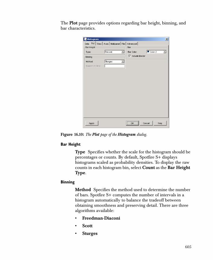
The Plot page provides options regarding bar height, binning, and bar characteristics.
Bar Height
Type Specifies whether the scale for the histogram should be percentages or counts. By default, Spotfire S+ displays histograms scaled as probability densities. To display the raw counts in each histogram bin, select Count as the Bar Height Type.
Binning
Method Specifies the method used to determine the number of bars. Spotfire S+ computes the number of intervals in a histogram automatically to balance the tradeoff between obtaining smoothness and preserving detail. There are three algorithms available:
• Freedman-Diaconi
• Scott
• Sturges
Figure 16.10: The Plot page of the Histogram dialog.
605

You can also define your own number of intervals by selecting Specified Value from the Binning Method list, and then typing a number for the Number of Bins.
Number of Bins Specify the number of histogram bins. Used when the Method is Specified Value.
Bar
Bar Color Specifies the color for the histogram bars.
Include Border Draws a border around each bar.
By default, the Histogram dialog displays vertical bars. For details on horizontal bar plots, see the section Bar Chart on page 610.
For more information on the methods used to compute the number of bins, see Venables and Ripley (1999).
QQ Math Plot The quantile-quantile plot, or qqplot, is a tool for determining a good approximation to a data set’s distribution. In a qqplot, the ordered data are graphed against quantiles of a known theoretical distribution. If the data points are drawn from the theoretical distribution, the resulting plot is close to a straight line in shape. The most common in this class of one-dimensional plots is the normal probability plot, or normal qqplot, which is used to test whether the distribution of a data set is nearly normal (Gaussian).
606
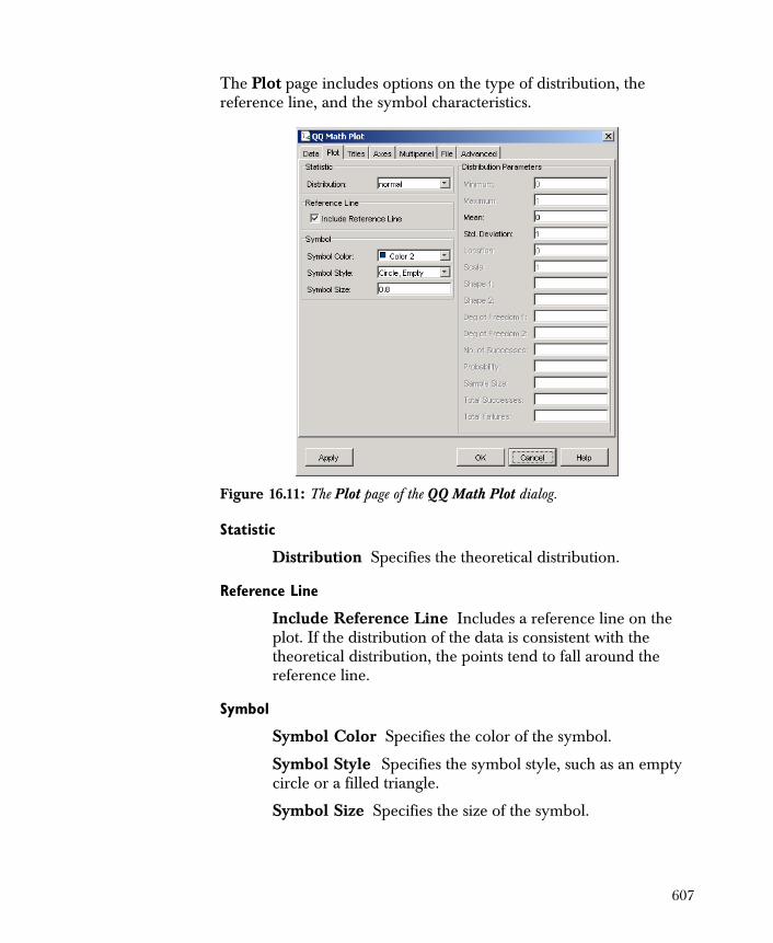
The Plot page includes options on the type of distribution, the reference line, and the symbol characteristics.
Statistic
Distribution Specifies the theoretical distribution.
Reference Line
Include Reference Line Includes a reference line on the plot. If the distribution of the data is consistent with the theoretical distribution, the points tend to fall around the reference line.
Symbol
Symbol Color Specifies the color of the symbol.
Symbol Style Specifies the symbol style, such as an empty circle or a filled triangle.
Symbol Size Specifies the size of the symbol.
Figure 16.11: The Plot page of the QQ Math Plot dialog.
607
Distribution Parameters
Use the controls in the Distribution Parameters group to specify the parameters of the theoretical distributions. The parameters available vary by distribution.
One Column - Categorical
This section describes three basic plot types useful for exploring a single categorical column.
• Bar Chart: Displays the relative magnitudes of observations in a data set. A bar is plotted for each data point, where the height of a bar is determined by the value of the data point. The Bar Chart dialog can also tabulate counts for a categorical column.
• Dot Plot: Displays the same information as a bar chart or pie chart, but in a form that is often easier to grasp.
• Pie Chart: Displays the share of individual values in a variable, relative to the sum total of all the values.
These visualization plots help you grasp the nature of your data. Such an understanding can help you avoid the misuse of statistical inference methods, such as using a method appropriate only for a normal (Gaussian) distribution when the distribution is strongly non-normal.
608
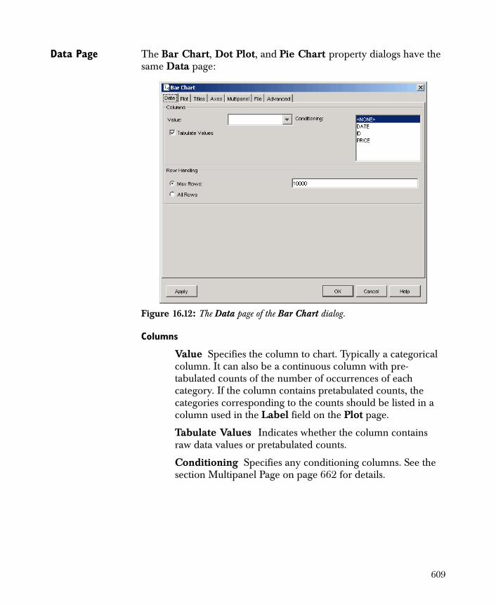
Data Page The Bar Chart, Dot Plot, and Pie Chart property dialogs have the same Data page:
Columns
Value Specifies the column to chart. Typically a categorical column. It can also be a continuous column with pre-tabulated counts of the number of occurrences of each category. If the column contains pretabulated counts, the categories corresponding to the counts should be listed in a column used in the Label field on the Plot page.
Tabulate Values Indicates whether the column contains raw data values or pretabulated counts.
Conditioning Specifies any conditioning columns. See the section Multipanel Page on page 662 for details.
Figure 16.12: The Data page of the Bar Chart dialog.
609
Row Handling
Max Rows Specifies the maximum number of rows of data to use in constructing the chart. If the data has more than the specified number of rows, simple random sampling is used to select a limited-size sampled subset of the data. In the text box for Max Rows, specify the number of rows to use in the chart.
All Rows Specifies that all rows of the data should be used in constructing the chart.
Bar Chart A bar chart displays a bar for each point in a set of observations, where the height of a bar is determined by the value of the data point. The Bar Chart dialog also contains an option for tabulating the values in your data set according to the levels of a categorical variable. Use this to view a count of the observations that are associated with each level of a factor variable.
By default, Spotfire S+ generates horizontal bar charts from the menu options. If you require vertical bar charts, you should use the function barplot in an S-PLUS Script node.
Note
For more detailed information about how the Row Handling selection creates different chart results, see the description for Continuous Conditioning in the section Multipanel Page on page 662.
610
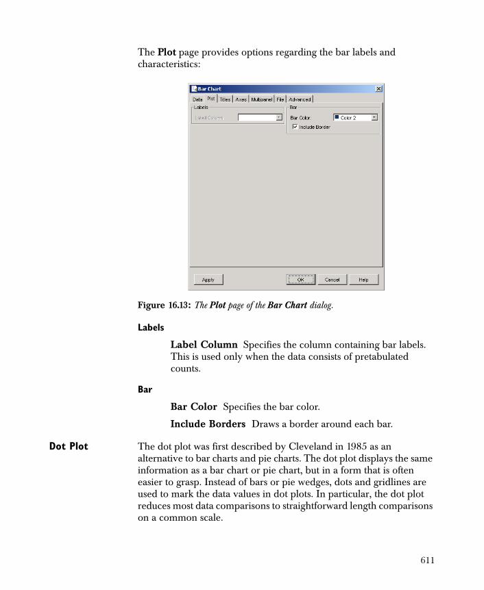
The Plot page provides options regarding the bar labels and characteristics:
Labels
Label Column Specifies the column containing bar labels. This is used only when the data consists of pretabulated counts.
Bar
Bar Color Specifies the bar color.
Include Borders Draws a border around each bar.
Dot Plot The dot plot was first described by Cleveland in 1985 as an alternative to bar charts and pie charts. The dot plot displays the same information as a bar chart or pie chart, but in a form that is often easier to grasp. Instead of bars or pie wedges, dots and gridlines are used to mark the data values in dot plots. In particular, the dot plot reduces most data comparisons to straightforward length comparisons on a common scale.
Figure 16.13: The Plot page of the Bar Chart dialog.
611
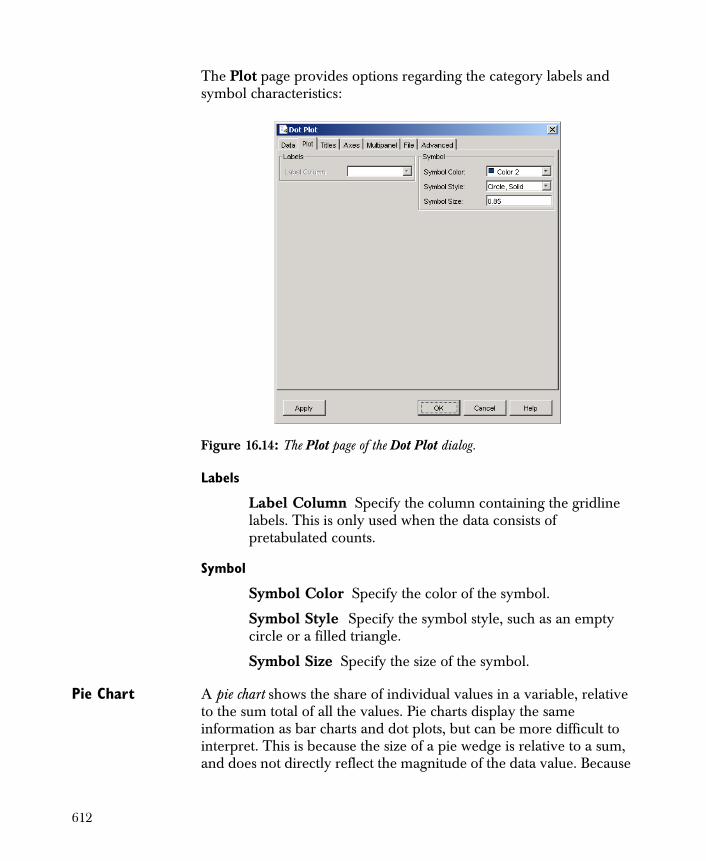
The Plot page provides options regarding the category labels and symbol characteristics:
Labels
Label Column Specify the column containing the gridline labels. This is only used when the data consists of pretabulated counts.
Symbol
Symbol Color Specify the color of the symbol.
Symbol Style Specify the symbol style, such as an empty circle or a filled triangle.
Symbol Size Specify the size of the symbol.
Pie Chart A pie chart shows the share of individual values in a variable, relative to the sum total of all the values. Pie charts display the same information as bar charts and dot plots, but can be more difficult to interpret. This is because the size of a pie wedge is relative to a sum, and does not directly reflect the magnitude of the data value. Because
Figure 16.14: The Plot page of the Dot Plot dialog.
612
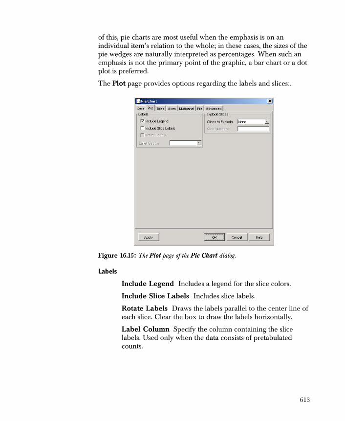
of this, pie charts are most useful when the emphasis is on an individual item’s relation to the whole; in these cases, the sizes of the pie wedges are naturally interpreted as percentages. When such an emphasis is not the primary point of the graphic, a bar chart or a dot plot is preferred.
The Plot page provides options regarding the labels and slices:.
Labels
Include Legend Includes a legend for the slice colors.
Include Slice Labels Includes slice labels.
Rotate Labels Draws the labels parallel to the center line of each slice. Clear the box to draw the labels horizontally.
Label Column Specify the column containing the slice labels. Used only when the data consists of pretabulated counts.
Figure 16.15: The Plot page of the Pie Chart dialog.
613
Explode Slices
Slices to Explode Select whether All, None or Specified slices should be exploded out from the pie.
Slice Numbers If Slices to Explode is Specified, this should be a comma-separated set of true (T) and false (F) values indicating which slices to explode.
Two Columns - Continuous
Spotfire Miner has two components for plotting one continuous column against another: Hexbin Plot and Scatter Plot.
The standard plot for this situation is the scatter plot, with one point for each row of data. The Scatter Plot component provides a wide range of options regarding symbols, lines, smoothers, regression lines, and grouping, as well as the title, axis, and multipanel conditioning options available in the other Spotfire S+ chart components.
When handling a large number of points, the scatter plot suffers from a few weaknesses:
• The points start to overlap and form a blob, where you cannot discern the number of points at each location.
• Because each row of data is plotted as a single item, rendering the plot can take a long time and a lot of memory.
Hexbin Plot avoids these problems. With Hexbin Plot, the plot areas are divided into hexagonal bins, and the number of points falling in each bin is counted. Then each bin containing points is drawn with the color reflecting the number of points in the bin.
614

Data Page The Scatter Plot and the Hexbin Plot dialog have the same Data page.
Columns
x Axis Value Specifies the column with the data values to plot on the x-axis.
y Axis Value Specifies the column with the data values to plot on the y-axis.
Conditioning Specifies the conditioning columns. See the section Multipanel Page on page 662 for details.
Row Handling
Max Rows Specifies the maximum number of rows of data to use in constructing the chart. If the data has more than the specified number of rows, simple random sampling is used to select a limited-size sampled subset of the data. In the text box for Max Rows, specify the number of rows to use in the chart.
Figure 16.16: The Data page of the Scatter Plot and Hexbin Plot dialog.
615
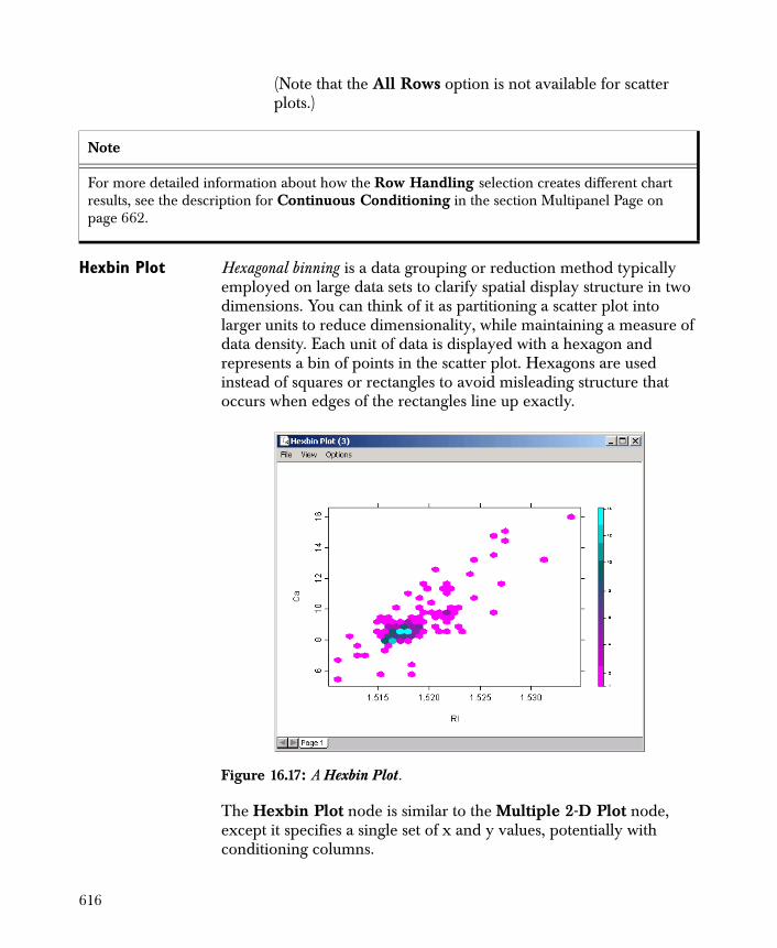
(Note that the All Rows option is not available for scatter plots.)
Hexbin Plot Hexagonal binning is a data grouping or reduction method typically employed on large data sets to clarify spatial display structure in two dimensions. You can think of it as partitioning a scatter plot into larger units to reduce dimensionality, while maintaining a measure of data density. Each unit of data is displayed with a hexagon and represents a bin of points in the scatter plot. Hexagons are used instead of squares or rectangles to avoid misleading structure that occurs when edges of the rectangles line up exactly.
The Hexbin Plot node is similar to the Multiple 2-D Plot node, except it specifies a single set of x and y values, potentially with conditioning columns.
Note
For more detailed information about how the Row Handling selection creates different chart results, see the description for Continuous Conditioning in the section Multipanel Page on page 662.
Figure 16.17: A Hexbin Plot.
616
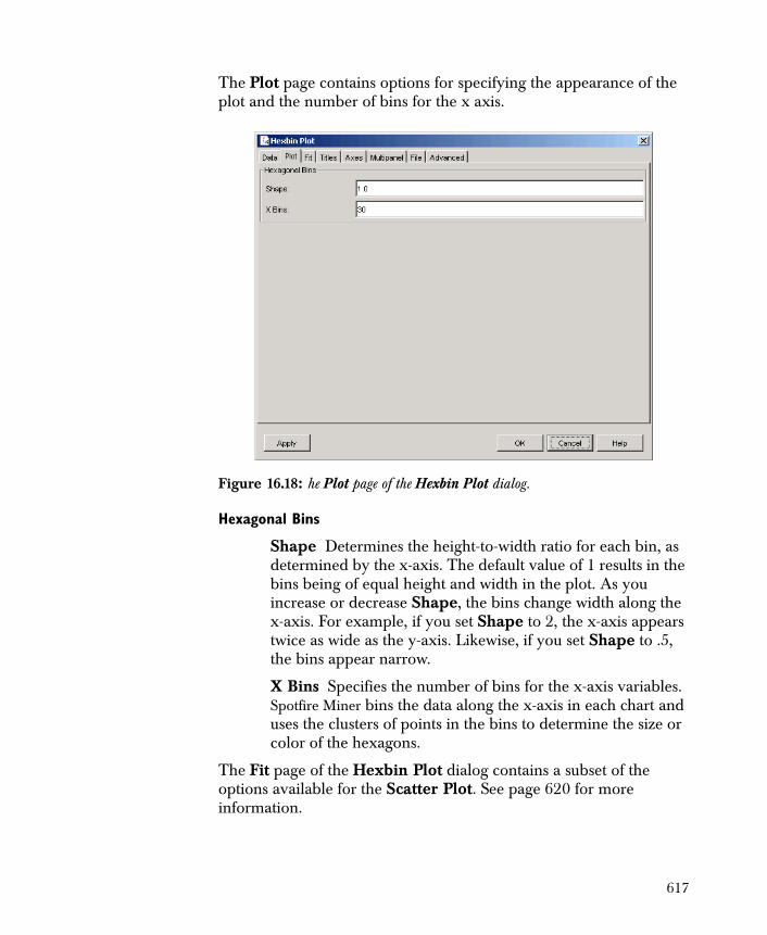
The Plot page contains options for specifying the appearance of the plot and the number of bins for the x axis.
Hexagonal Bins
Shape Determines the height-to-width ratio for each bin, as determined by the x-axis. The default value of 1 results in the bins being of equal height and width in the plot. As you increase or decrease Shape, the bins change width along the x-axis. For example, if you set Shape to 2, the x-axis appears twice as wide as the y-axis. Likewise, if you set Shape to .5, the bins appear narrow.
X Bins Specifies the number of bins for the x-axis variables. Spotfire Miner bins the data along the x-axis in each chart and uses the clusters of points in the bins to determine the size or color of the hexagons.
The Fit page of the Hexbin Plot dialog contains a subset of the options available for the Scatter Plot. See page 620 for more information.
Figure 16.18: he Plot page of the Hexbin Plot dialog.
617
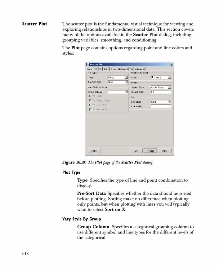
Scatter Plot The scatter plot is the fundamental visual technique for viewing and exploring relationships in two-dimensional data. This section covers many of the options available in the Scatter Plot dialog, including grouping variables, smoothing, and conditioning.
The Plot page contains options regarding point and line colors and styles:
Plot Type
Type Specifies the type of line and point combination to display.
Pre-Sort Data Specifies whether the data should be sorted before plotting. Sorting make no difference when plotting only points, but when plotting with lines you will typically want to select Sort on X.
Vary Style By Group
Group Column Specifies a categorical grouping column to use different symbol and line types for the different levels of the categorical.
Figure 16.19: The Plot page of the Scatter Plot dialog.
618
Vary Color Varies the color for different levels of the categorical.
Vary Symbol Style Varies the symbol style for different levels of the categorical.
Vary Line Style Varies the line style for different levels of the categorical.
Include Legend Includes a legend indicating the symbol and line type for each category.
Symbol/Line Color
Color Specifies the symbol and line color.
Symbol
Symbol Style Specifies the symbol style.
Symbol Size Specifies the symbol size.
Line
Line Style Specifies the line style.
Line Width Specifies the line width.
619

The Fit page contains options for adding regression lines and smoothers to the plot:
Regression
Regression Type Select Least Squares or Robust to add a regression line to each plot. Plots must have at least 2 points to include a least squares line, and 6 points to include a robust regression line.
You can fit a straight line to your scatter plot data and superpose the fit with the data. Such a fit helps you visually assess how well the data conforms to a linear relationship between two variables. When the linear fit seems adequate, the fitted straight line plot provides a good visual indication of both the slope of bivariate data, and the variation of the data about the straight line fit. The Scatter Plot dialog includes two kinds of line fits in the Fit tab:
• Linear Least Squares: computes a line fit via a least squares algorithm.
Figure 16.20: The Fit page of the Scatter Plot dialog.
620
The method of least squares fits a line to data so that the sum of the squared residuals is minimized. Suppose a set of
observations of the response variable correspond to a set of
values of the predictor according to the model ,
where and . The
ith residual is defined as the difference between the ith
observation and the ith fitted value : that is,
. The method of least squares finds a set of fitted
values that minimizes the sum .
• Robust MM: computes a line fit via a robust fitting criterion. Robust line fits are useful for fitting linear relationships when the random variation in the data is not Gaussian (normal), or when the data contain significant outliers.
The least squares fit of a straight line is not robust, and outliers can have a large influence on the location of the line. A robust method is one that is not significantly influenced by outliers, no matter how large. Robust fitting methods are useful when the random variation in the data is not normal (Gaussian), or when the data contain significant outliers. In such situations, standard least squares might return inaccurate fits. Robust MM is one robust fitting method used to guard against outlying observations.
Smooth
Smoothing Type Specifies a scatter plot smoother to add to the plots. Plots must have at least 6 points to include a smoother.
# Output Points Specifies the number of points at which to calculate the smoother values for use in plotting the smooth.
Smoothers attempt to create a smooth curve showing the general trend in the data. The simplest smoothers use a running average, where the fit at a particular x value is calculated as a weighted average of the y
n
yi
xi y f x( )=
y y1 y2 … yn, , ,( )= x x1 x2 … xn, , ,( )=
ri
yi yiˆ f xi( )=
ri yi yi–=
ri2
i 1=
n
621
values for nearby points. The weight given to each point decreases as the distance between its x value and the x value of interest increases. In the simplest kind of running average smoother, all points within a certain distance (or window) from the point of interest are weighted equally in the average for that point. The window width is called the bandwidth of the smoother, and is usually given as a percentage of the total number of data points. Increasing the bandwidth results in a smoother curve fit but might miss rapidly changing features. Decreasing the bandwidth allows the smoother to track rapidly changing features more accurately, but results in a rougher curve fit.
More sophisticated smoothers add variations to the running average approach. For example, smoothly decreasing weights or local linear fits might be used. However, all smoothers have some type of smoothness parameter (bandwidth) controlling the smoothness of the curve. The issue of good bandwidth selection is complicated and has been treated in many statistical research papers. You can, however, gain a good feeling for the practical consequences of varying the bandwidth by experimenting with smoothers on real data.
This section describes how to use four different types of smoothers.
• Kernel Smoother: a generalization of running averages in which different weight functions, or kernels, might be used. The weight functions provide transitions between points that are smoother than those in the simple running average approach.
• Loess Smoother: a noise-reduction approach that is based on local linear or quadratic fits to the data.
• Spline Smoother: a technique in which a sequence of polynomials is pieced together to obtain a smooth curve.
• Supersmoother: a highly automated variable span smoother. It obtains fitted values by taking weighted combinations of smoothers with varying bandwidths.
• User: Indicates that a user can provide any S-PLUS function in the Function Name box of the User-Defined Smoothing group.
You can use a smoother’s bandwidth to control the degree of smoothness in a curve fit.
622
Kernel Specs
Bandwidth Specifies the kernel bandwidth.
Kernel Type Specifies the kernel type.
A kernel smoother is a generalization of running averages in which different weight functions, or kernels, might be used. The weight functions provide transitions between points that are smoother than those in the simple running average approach. The default kernel is the normal or Gaussian kernel, in which the weights decrease with a Gaussian distribution away from the point of interest. Other choices include a triangle, a box, and the Parzen kernel. In a triangle kernel, the weights decrease linearly as the distance from the point of interest increases, so that the points on the edge of the smoothing window have a weight near zero. A box or boxcar smoother weighs each point within the smoothing window equally, and a Parzen kernel is a box convolved with a triangle.
You can experiment with the smoothing parameter by varying the value in the Bandwidth field.
Loess Specs
Span Specifies the loess span.
Degree Specifies the degree of the polynomial that is used in the local fit at each point.
Family Specifies the assumed distribution of the errors in the smoothed curve.
The loess smoother, developed by W.S. Cleveland and others at Bell Laboratories (1979), is a clever approach to smoothing that is essentially a noise-reduction algorithm. It is based on local linear or quadratic fits to the data: at each point, a line or parabola is fit to the points within the smoothing window, and the predicted value is taken as the y value for the point of interest. Weighted least squares is used to compute the line or parabola in each window. Connecting the computed y values results in a smooth curve.
For loess smoothers, the bandwidth is referred to as the span of the smoother. The span is a number between 0 and 1, representing the percentage of points that should be included in the fit for a particular smoothing window. Smaller values result in less smoothing, and very small values close to 0 are not recommended. If the span is not
623
specified, an appropriate value is computed using cross-validation. For small samples ( ), or if there are substantial serial correlations between observations close in x value, a pre-specified fixed span smoother should be used.
You can experiment with the smoothing parameter by varying the value in the Span field.
You can also experiment with the degree of the polynomial that is used in the local fit at each point. If you select Two as the Degree in the Fit tab, local quadratic fits are used instead of local linear fits. The Family field in the Fit tab governs the assumed distribution of the errors in the smoothed curve. The default family is Symmetric, which combines local fitting with a robustness feature that guards against distortion by outliers. The Gaussian option employs strictly local fitting methods, and can be affected by large outliers.
Smoothing Spline Specs
Deg. of Freedom Specifies the effective degrees of freedom.
Spline smoothers are computed by piecing together a sequence of polynomials. Cubic splines are the most widely used in this class of smoothers, and involve locally cubic polynomials. The local polynomials are computed by minimizing a penalized residual sum of squares. Smoothness is assured by having the value, slope, and curvature of neighboring polynomials match at the points where they meet. Connecting the polynomials results in a smooth fit to the data. The more accurately a smoothing spline fits the data values, the rougher the curve, and vice versa.
The smoothing parameter for splines is called the degrees of freedom. The degrees of freedom controls the amount of curvature in the fit, and corresponds to the degree of the local polynomials. The lower the degrees of freedom, the smoother the curve. The degrees of freedom automatically determines the smoothing window, by governing the trade-off between smoothness of the fit and fidelity to the data values. For data points, the degrees of freedom should be
between 1 and . Specifying degrees of freedom results in a curve that passes through each of the data points exactly.
n 50<
n
n 1– n 1–
624
You can experiment with the smoothing parameter by varying the value in the Degrees of Freedom field. If you select Crossvalidate as the Degrees of Freedom, the smoothing parameter is computed internally by cross-validation.
Supersmoother Specs
Span Specifies the supersmoother span.
The supersmoother is a highly automated variable span smoother. It obtains fitted values by taking a weighted combination of smoothers with varying bandwidths. Like loess smoothers, the main parameter for supersmoothers is called the span. The span is a number between 0 and 1, representing the percentage of points that should be included in the fit for a particular smoothing window. Smaller values result in less smoothing, and very small values close to 0 are not recommended. If the span is not specified, an appropriate value is computed using cross-validation. For small samples ( ), or if there are substantial serial correlations between observations close in x value, a pre-specified fixed span smoother should be used.
User-Defined Smoothing
Function Name Specifies the name of an S-PLUS function to use in computing the smooth.
Other
Other Arguments Specifies any other arguments to the smoothing functions. This should be a comma-delimited set of name=value pairs.
Two Columns - Mixed
Two column plots using one continuous and one categorical column help you determine how the continuous column values differ between categories. In this section, we examine three basic plot types useful for exploring a continuous column within categories.
• Box Plot: a graphical representation showing the center and spread of a distribution, as well as any outlying data points.
• Strip Plot: a one-dimensional scatter plot.
• QQ Plot: a powerful tool for comparing the distributions of two sets of data.
n 50<
625
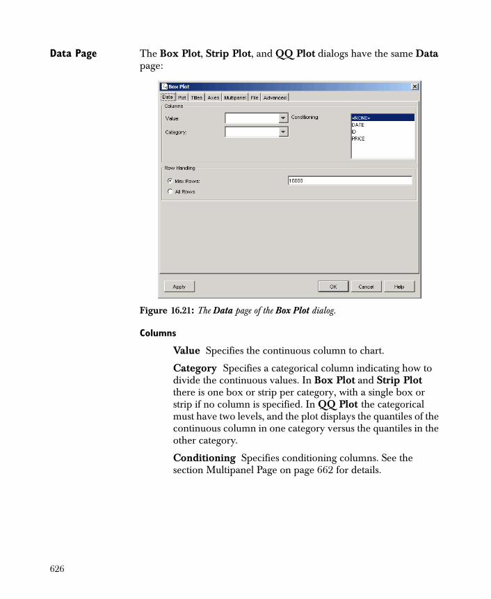
Data Page The Box Plot, Strip Plot, and QQ Plot dialogs have the same Data page:
Columns
Value Specifies the continuous column to chart.
Category Specifies a categorical column indicating how to divide the continuous values. In Box Plot and Strip Plot there is one box or strip per category, with a single box or strip if no column is specified. In QQ Plot the categorical must have two levels, and the plot displays the quantiles of the continuous column in one category versus the quantiles in the other category.
Conditioning Specifies conditioning columns. See the section Multipanel Page on page 662 for details.
Figure 16.21: The Data page of the Box Plot dialog.
626
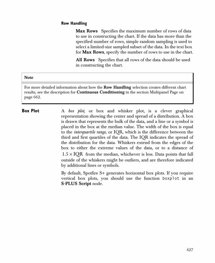
Row Handling
Max Rows Specifies the maximum number of rows of data to use in constructing the chart. If the data has more than the specified number of rows, simple random sampling is used to select a limited-size sampled subset of the data. In the text box for Max Rows, specify the number of rows to use in the chart.
All Rows Specifies that all rows of the data should be used in constructing the chart.
Box Plot A box plot, or box and whisker plot, is a clever graphicalrepresentation showing the center and spread of a distribution. A boxis drawn that represents the bulk of the data, and a line or a symbol isplaced in the box at the median value. The width of the box is equalto the interquartile range, or IQR, which is the difference between thethird and first quartiles of the data. The IQR indicates the spread ofthe distribution for the data. Whiskers extend from the edges of thebox to either the extreme values of the data, or to a distance of
from the median, whichever is less. Data points that falloutside of the whiskers might be outliers, and are therefore indicatedby additional lines or symbols.
By default, Spotfire S+ generates horizontal box plots. If you requirevertical box plots, you should use the function boxplot in anS-PLUS Script node.
Note
For more detailed information about how the Row Handling selection creates different chart results, see the description for Continuous Conditioning in the section Multipanel Page on page 662.
1.5 IQR×
627
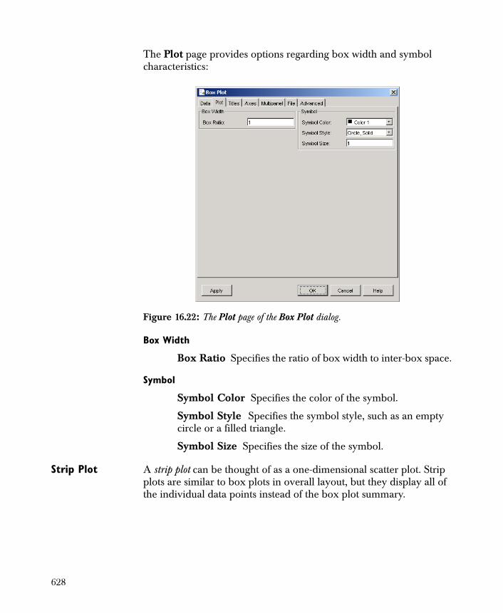
The Plot page provides options regarding box width and symbol characteristics:
Box Width
Box Ratio Specifies the ratio of box width to inter-box space.
Symbol
Symbol Color Specifies the color of the symbol.
Symbol Style Specifies the symbol style, such as an empty circle or a filled triangle.
Symbol Size Specifies the size of the symbol.
Strip Plot A strip plot can be thought of as a one-dimensional scatter plot. Strip plots are similar to box plots in overall layout, but they display all of the individual data points instead of the box plot summary.
Figure 16.22: The Plot page of the Box Plot dialog.
628
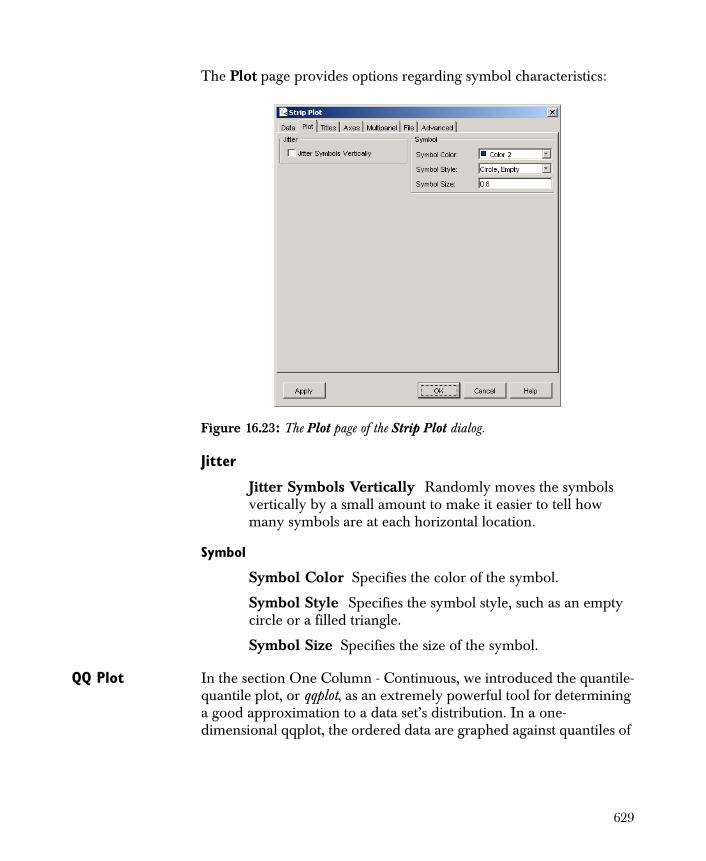
The Plot page provides options regarding symbol characteristics:
Jitter
Jitter Symbols Vertically Randomly moves the symbols vertically by a small amount to make it easier to tell how many symbols are at each horizontal location.
Symbol
Symbol Color Specifies the color of the symbol.
Symbol Style Specifies the symbol style, such as an empty circle or a filled triangle.
Symbol Size Specifies the size of the symbol.
QQ Plot In the section One Column - Continuous, we introduced the quantile-quantile plot, or qqplot, as an extremely powerful tool for determining a good approximation to a data set’s distribution. In a one-dimensional qqplot, the ordered data are graphed against quantiles of
Figure 16.23: The Plot page of the Strip Plot dialog.
629
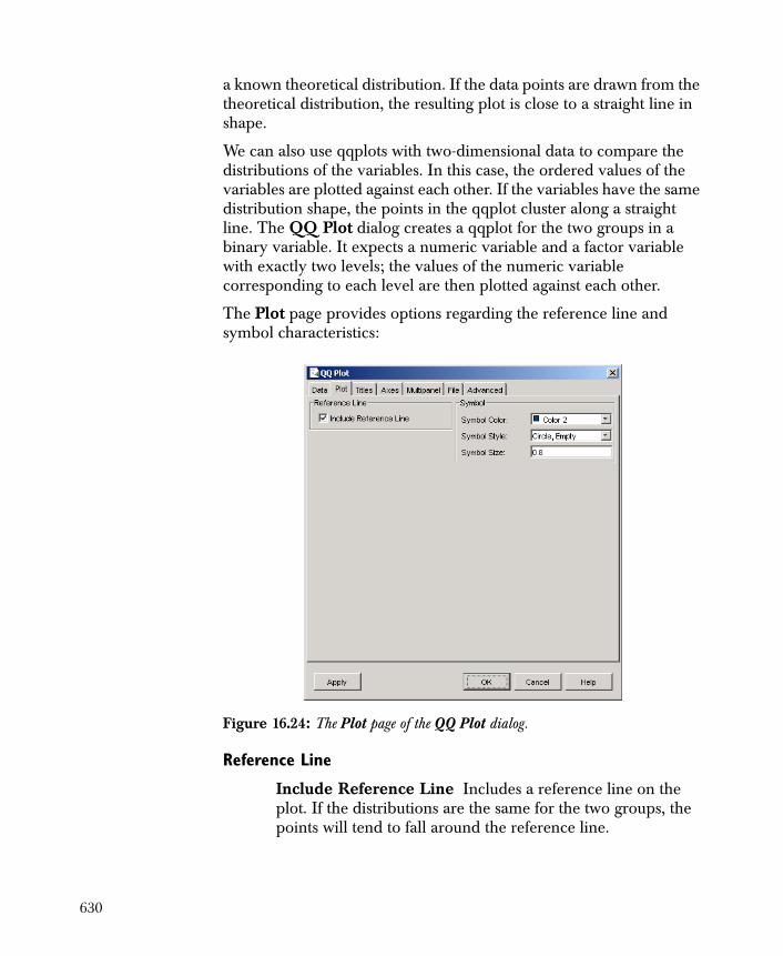
a known theoretical distribution. If the data points are drawn from the theoretical distribution, the resulting plot is close to a straight line in shape.
We can also use qqplots with two-dimensional data to compare the distributions of the variables. In this case, the ordered values of the variables are plotted against each other. If the variables have the same distribution shape, the points in the qqplot cluster along a straight line. The QQ Plot dialog creates a qqplot for the two groups in a binary variable. It expects a numeric variable and a factor variable with exactly two levels; the values of the numeric variable corresponding to each level are then plotted against each other.
The Plot page provides options regarding the reference line and symbol characteristics:
Reference Line
Include Reference Line Includes a reference line on the plot. If the distributions are the same for the two groups, the points will tend to fall around the reference line.
Figure 16.24: The Plot page of the QQ Plot dialog.
630
Symbol
Symbol Color Specifies the color of the symbol.
Symbol Style Specifies the symbol style, such as an empty circle or a filled triangle.
Symbol Size Specifies the size of the symbol.
Three Columns Three-dimensional data has three numeric columns, and the relationships between the columns form a surface in 3D space. Because the depth cues in three-dimensional plots are sometimes insufficient to convey all of the information, special considerations must be made when visualizing three-dimensional data. Instead of viewing the surface alone, we can analyze projections, slices, or rotations of the surface. In this section, we examine four basic plot types useful for exploring a three-dimensional data object.
• Contour Plot: uses contour lines to represent heights of three-dimensional data in a flat, two-dimensional plane.
• Level Plot: uses colors to represent heights of three-dimensional data in a flat, two-dimensional plane. Level plots and contour plots are essentially identical, but they have defaults that allow you to view a particular surface differently.
• Surface Plot: approximates the shape of a data set in three dimensions.
• Cloud Plot: displays a three-dimensional scatter plot of points.
631
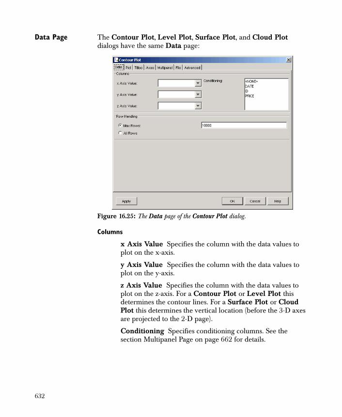
Data Page The Contour Plot, Level Plot, Surface Plot, and Cloud Plot dialogs have the same Data page:
Columns
x Axis Value Specifies the column with the data values to plot on the x-axis.
y Axis Value Specifies the column with the data values to plot on the y-axis.
z Axis Value Specifies the column with the data values to plot on the z-axis. For a Contour Plot or Level Plot this determines the contour lines. For a Surface Plot or Cloud Plot this determines the vertical location (before the 3-D axes are projected to the 2-D page).
Conditioning Specifies conditioning columns. See the section Multipanel Page on page 662 for details.
Figure 16.25: The Data page of the Contour Plot dialog.
632
Row Handling
Max Rows Specifies the maximum number of rows of data to use in constructing the chart. If the data has more than the specified number of rows, simple random sampling is used to select a limited-size sampled subset of the data. In the text box for Max Rows, specify the number of rows to use in the chart.
(Note that the All Rows option is not available for cloud plots.).
Contour Plot A contour plot is a representation of three-dimensional data in a flat, two-dimensional plane. Each contour line represents a height in the z direction from the corresponding three-dimensional surface. Contour plots are often used to display data collected on a regularly-spaced grid; if gridded data is not available, interpolation is used to fit and plot contours.
Note
For more detailed information about how the Row Handling selection creates different chart results, see the description for Continuous Conditioning in the section Multipanel Page on page 662.
633

The Plot page provides options regarding the interpolation, contours, fills, and lines:
Interpolate
Interpolate to Grid Before Plotting Indicates that the data values do not represent a regularly-spaced grid. Interpolation will be used to create regularly-spaced data.
X Grid Size Specifies the number of points on the x-axis when interpolating.
Y Grid Size Specifies the number of points on the y-axis when interpolating.
Contour Levels
Number of Cuts Specifies the number of contour levels to display.
Use Pretty Contour Levels Places the contour cut points at rounded values for nicer labeling.
Figure 16.26: The Plot page of the Contour Plot dialog.
634
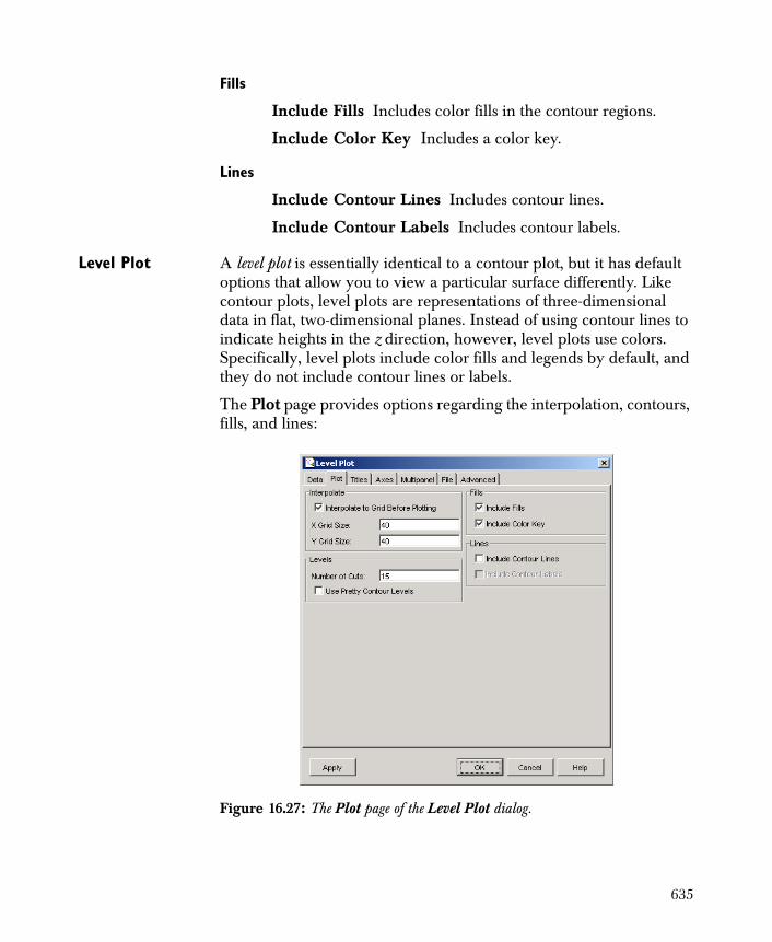
Fills
Include Fills Includes color fills in the contour regions.
Include Color Key Includes a color key.
Lines
Include Contour Lines Includes contour lines.
Include Contour Labels Includes contour labels.
Level Plot A level plot is essentially identical to a contour plot, but it has default options that allow you to view a particular surface differently. Like contour plots, level plots are representations of three-dimensional data in flat, two-dimensional planes. Instead of using contour lines to indicate heights in the z direction, however, level plots use colors. Specifically, level plots include color fills and legends by default, and they do not include contour lines or labels.
The Plot page provides options regarding the interpolation, contours, fills, and lines:
Figure 16.27: The Plot page of the Level Plot dialog.
635
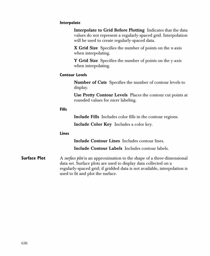
Interpolate
Interpolate to Grid Before Plotting Indicates that the data values do not represent a regularly-spaced grid. Interpolation will be used to create regularly-spaced data.
X Grid Size Specifies the number of points on the x-axis when interpolating.
Y Grid Size Specifies the number of points on the y-axis when interpolating.
Contour Levels
Number of Cuts Specifies the number of contour levels to display.
Use Pretty Contour Levels Places the contour cut points at rounded values for nicer labeling.
Fills
Include Fills Includes color fills in the contour regions.
Include Color Key Includes a color key.
Lines
Include Contour Lines Includes contour lines.
Include Contour Labels Includes contour labels.
Surface Plot A surface plot is an approximation to the shape of a three-dimensional data set. Surface plots are used to display data collected on a regularly-spaced grid; if gridded data is not available, interpolation is used to fit and plot the surface.
636
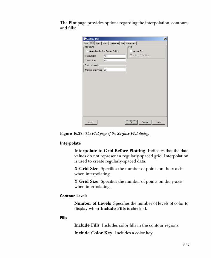
The Plot page provides options regarding the interpolation, contours, and fills:
Interpolate
Interpolate to Grid Before Plotting Indicates that the data values do not represent a regularly-spaced grid. Interpolation is used to create regularly-spaced data.
X Grid Size Specifies the number of points on the x-axis when interpolating.
Y Grid Size Specifies the number of points on the y-axis when interpolating.
Contour Levels
Number of Levels Specifies the number of levels of color to display when Include Fills is checked.
Fills
Include Fills Includes color fills in the contour regions.
Include Color Key Includes a color key.
Figure 16.28: The Plot page of the Surface Plot dialog.
637
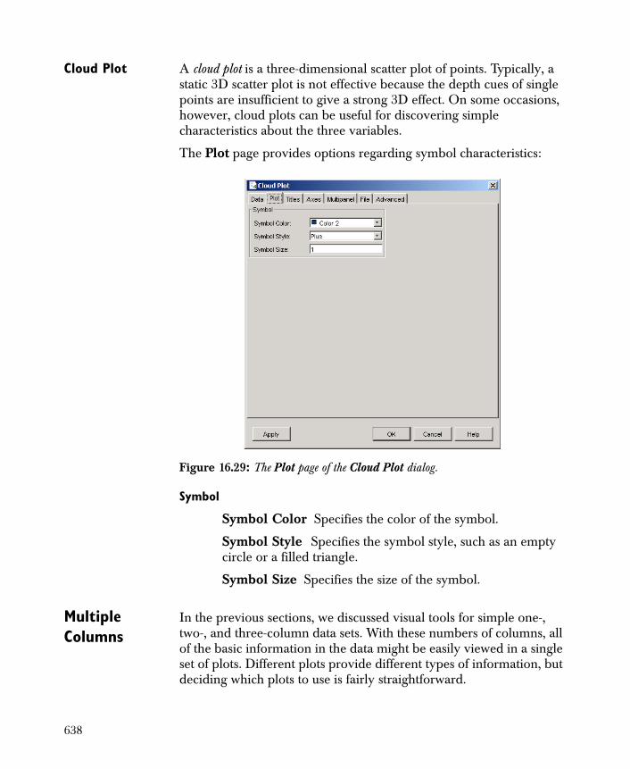
Cloud Plot A cloud plot is a three-dimensional scatter plot of points. Typically, a static 3D scatter plot is not effective because the depth cues of single points are insufficient to give a strong 3D effect. On some occasions, however, cloud plots can be useful for discovering simple characteristics about the three variables.
The Plot page provides options regarding symbol characteristics:
Symbol
Symbol Color Specifies the color of the symbol.
Symbol Style Specifies the symbol style, such as an empty circle or a filled triangle.
Symbol Size Specifies the size of the symbol.
Multiple Columns
In the previous sections, we discussed visual tools for simple one-, two-, and three-column data sets. With these numbers of columns, all of the basic information in the data might be easily viewed in a single set of plots. Different plots provide different types of information, but deciding which plots to use is fairly straightforward.
Figure 16.29: The Plot page of the Cloud Plot dialog.
638
With multidimensional data, visualization is more involved. In addition to univariate and bivariate relationships, variables might have interactions such that the relationship between any two variables changes depending on the remaining variables. Standard one- and two-column plots do not allow us to look at interactions between multiple variables, and must therefore be complemented with techniques specifically designed for multidimensional data. In this section, we discuss both standard and novel visualization tools for multidimensional data.
• Multiple 2-D Plots: displays simple two-variable hexbin or scatterplots for multiple different combinations of x and y columns.
• Hexbin Matrix: displays an array of pairwise hexbin plots illustrating the relationship between any pair of variables.
• Scatterplot Matrix: displays an array of pairwise scatter plots illustrating the relationship between any pair of variables.
• Parallel Plot: displays the variables in a data set as horizontal panels, and connects the values for a particular observation with a set of line segments.
Two additional techniques for visualizing multidimensional data are grouping variables and multipanel conditioning. These are discussed in the section Multipanel Page. The conditioning options that we discuss are not specific to scatter plots, but are available in most of the chart components. You can therefore use the options to create multiple histograms, box plots, etc., conditioned on the value of a particular variable in your data set.
Multiple 2-D Plots
To create bivariate charts of pairs of variables in your data set, use the Multiple 2-D Plots component. This component creates basic two-dimensional charts, including hexagonal binning charts and points plots. Spotfire Miner supports bivariate charts for continuous variables only.
Note
To produce conditioned plots, use a hexbin plot or a scatter plot. See the section Hexbin Plot on page 616 or the section Scatter Plot on page 618 for more information.
639

This section describes the types of charts you can create with the Multiple 2-D Plots component, the options you can set in its properties dialog, and the viewer you use to see the charts you create. All examples in this section use variables from the glass.txt data set, which is stored as a text file in the examples folder under your Spotfire Miner installation directory.
The Properties page of the Multiple 2-D Plots dialog provides options for specifying the columns to plot and the type of charts to plot.
Available Columns
The Select Columns group contains options for choosing variables of your data set and identifying them as either X Columns or Y Columns. Spotfire Miner displays all pair-wise charts of the variables you choose. For example, if you choose four X Columns and five Y Columns, Spotfire Miner displays twenty different charts in a a single, tabbed window. See the section Using the Graph Window on page 598 for more information.
Figure 16.30: The Properties page of the Multiple 2-D Plots dialog.
640
Sorting column names
Use the buttons at the top of the Available Columns, X Columns, and Y Columns list boxes to sort the display of column names when you have a large number of columns in your data set and you want to find particular ones quickly. Click to sort the column names in the order they appear in the input data (the default). Click to sort the column names in alphabetical order, or click to sort them in reverse alphabetical order. You can use drag-and-drop within the lists to reorder the display of an individual column name.
The column order of the X Columns and Y Columns list boxes determines the order the charts appear in the viewer.
Chart types
The Chart Types group contains options for designating the type of chart you want for your variables. Select Hexagonal Bins to create hexagonal binning charts, and then set the following options:
Style Spotfire Miner supports five styles for displaying the hexagons in a plot. The default is Grayscale, which displays lower-density hexagons in darker colors and high-density hexagons in light colors. The Lattice and Centroids styles display the hexagons in a range of sizes to indicate density; smaller hexagons indicate low-density bins, while larger hexagons indicate high-density bins. Lattice places the center of each hexagon according to the grid Spotfire Miner uses to determine the bins. Centroids places a hexagon’s center at its center of mass. The two styles Nested Lattice and Nested Centroids, use colors to indicate depth in each hexagon.
Shape Determines the height-to-width ratio for the plotting region. The default value of 1 results in x and y axes equal in size in the plot. If you set Shape to 2, the y axis in each of your plots appears twice as long as the x axis.
X Bins Specifies the number of bins for the x-axis variables. Spotfire Miner bins the data along the x axis in each chart and uses the clusters of points in the bins to determine the size or color of the hexagons.
Figure 16.31 shows a Multiple 2-D plot using the glass.txt data set.
641
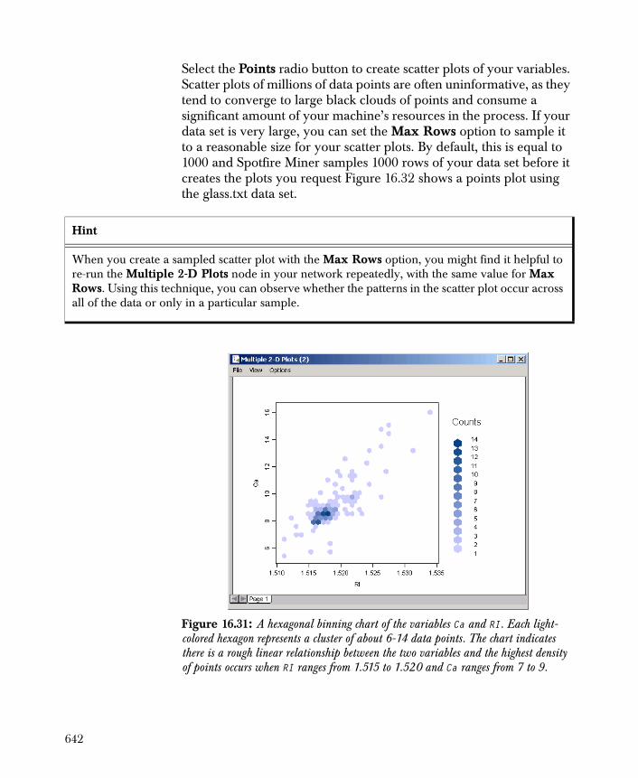
Select the Points radio button to create scatter plots of your variables. Scatter plots of millions of data points are often uninformative, as they tend to converge to large black clouds of points and consume a significant amount of your machine’s resources in the process. If your data set is very large, you can set the Max Rows option to sample it to a reasonable size for your scatter plots. By default, this is equal to 1000 and Spotfire Miner samples 1000 rows of your data set before it creates the plots you request Figure 16.32 shows a points plot using the glass.txt data set.
.
Hint
When you create a sampled scatter plot with the Max Rows option, you might find it helpful to re-run the Multiple 2-D Plots node in your network repeatedly, with the same value for Max Rows. Using this technique, you can observe whether the patterns in the scatter plot occur across all of the data or only in a particular sample.
Figure 16.31: A hexagonal binning chart of the variables Ca and RI. Each light-colored hexagon represents a cluster of about 6-14 data points. The chart indicates there is a rough linear relationship between the two variables and the highest density of points occurs when RI ranges from 1.515 to 1.520 and Ca ranges from 7 to 9.
642
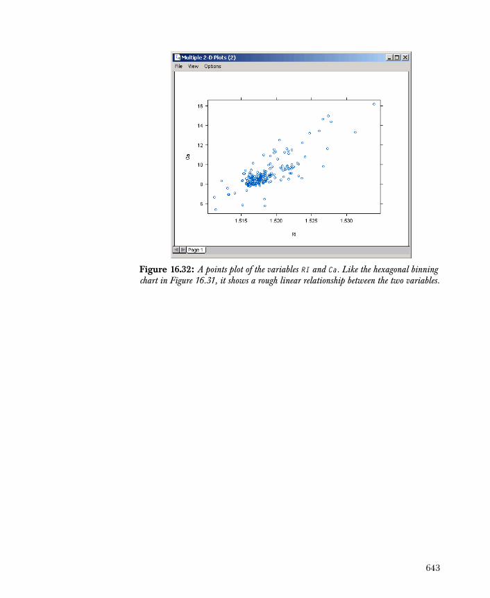
Figure 16.32: A points plot of the variables RI and Ca. Like the hexagonal binning chart in Figure 16.31, it shows a rough linear relationship between the two variables.
643
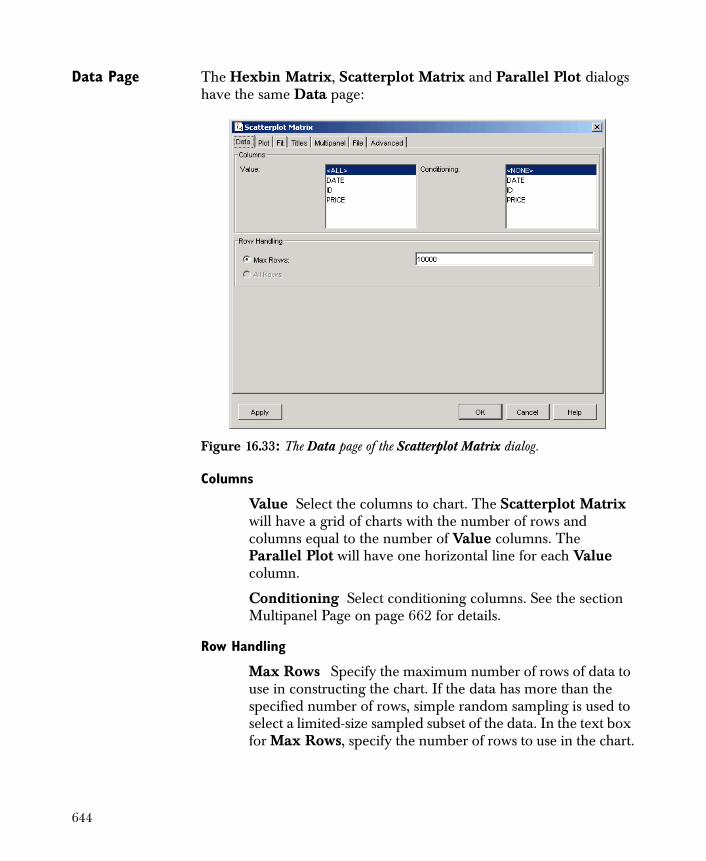
Data Page The Hexbin Matrix, Scatterplot Matrix and Parallel Plot dialogs have the same Data page:
Columns
Value Select the columns to chart. The Scatterplot Matrix will have a grid of charts with the number of rows and columns equal to the number of Value columns. The Parallel Plot will have one horizontal line for each Value column.
Conditioning Select conditioning columns. See the section Multipanel Page on page 662 for details.
Row Handling
Max Rows Specify the maximum number of rows of data to use in constructing the chart. If the data has more than the specified number of rows, simple random sampling is used to select a limited-size sampled subset of the data. In the text box for Max Rows, specify the number of rows to use in the chart.
Figure 16.33: The Data page of the Scatterplot Matrix dialog.
644
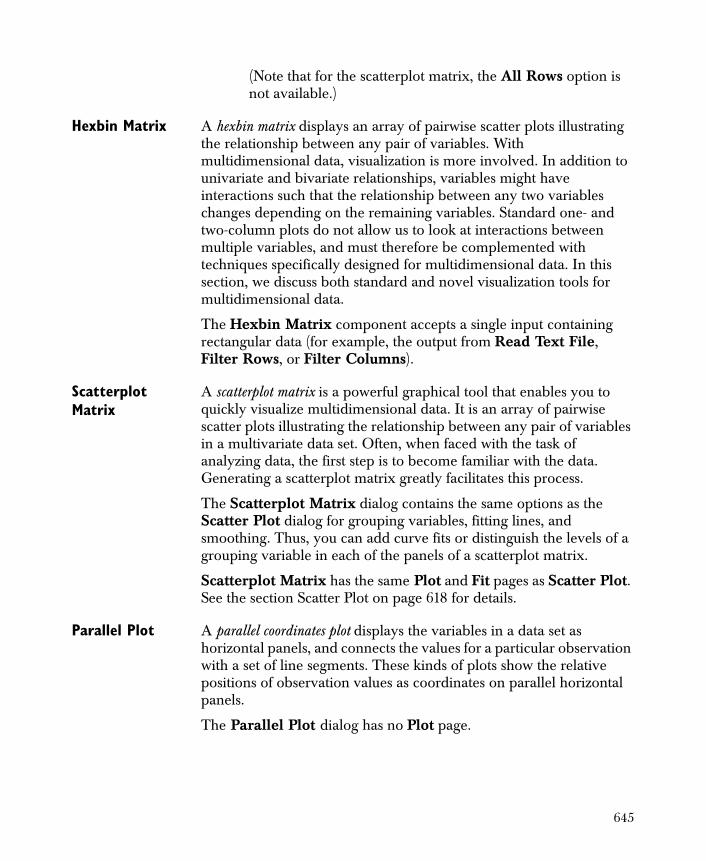
(Note that for the scatterplot matrix, the All Rows option is not available.)
Hexbin Matrix A hexbin matrix displays an array of pairwise scatter plots illustrating the relationship between any pair of variables. With multidimensional data, visualization is more involved. In addition to univariate and bivariate relationships, variables might have interactions such that the relationship between any two variables changes depending on the remaining variables. Standard one- and two-column plots do not allow us to look at interactions between multiple variables, and must therefore be complemented with techniques specifically designed for multidimensional data. In this section, we discuss both standard and novel visualization tools for multidimensional data.
The Hexbin Matrix component accepts a single input containing rectangular data (for example, the output from Read Text File, Filter Rows, or Filter Columns).
Scatterplot Matrix
A scatterplot matrix is a powerful graphical tool that enables you to quickly visualize multidimensional data. It is an array of pairwise scatter plots illustrating the relationship between any pair of variables in a multivariate data set. Often, when faced with the task of analyzing data, the first step is to become familiar with the data. Generating a scatterplot matrix greatly facilitates this process.
The Scatterplot Matrix dialog contains the same options as the Scatter Plot dialog for grouping variables, fitting lines, and smoothing. Thus, you can add curve fits or distinguish the levels of a grouping variable in each of the panels of a scatterplot matrix.
Scatterplot Matrix has the same Plot and Fit pages as Scatter Plot. See the section Scatter Plot on page 618 for details.
Parallel Plot A parallel coordinates plot displays the variables in a data set as horizontal panels, and connects the values for a particular observation with a set of line segments. These kinds of plots show the relative positions of observation values as coordinates on parallel horizontal panels.
The Parallel Plot dialog has no Plot page.
645

Time Series Time series are multivariate data sets that are associated with a set of ordered positions, where the positions are an important feature of the values and their analysis. These data can arise in many contexts. For example, in the financial marketplace, trading tickers record the price and quantity of each trade at particular times throughout the day. Such data can be analyzed to assist in making market predictions. This section discusses three plots that are helpful in visualizing time series data.
• Line Plots: successive values of the data are connected by straight lines.
• High-Low Plots: vertical lines are used to indicate the daily, monthly, or yearly extreme values in a time series, and hatch marks are drawn on the lines to represent the opening and closing values. This type of plot is most often used to display financial data.
• Stacked Bar Plots: multiple y values determine segment heights in a bar chart.
The time series plot dialogs do not have the same Data page.
Time Series Line Plot
With time series data, it is often useful to view a line plot, where the successive values of the data are connected by straight lines. By using straight line segments to connect the points, you can see more clearly the overall trend or shape in the ordered data values.
646
The Data page for Line Plot is not used in any other dialogs:
Columns
Date Column Select a Date column to use on the x-axis.
Series Columns Select series columns with values to plot on the y-axis.
Row Handling
Max Rows Specify the maximum number of rows of data to use in constructing the chart. If the data has more than the specified number of rows, simple random sampling is used to select a limited-size sampled subset of the data. In the text box for Max Rows, specify the number of rows to use in the chart.
(Note that for a line plot, the All Rows option is not available.)
Figure 16.34: The Data page of the Line Plot dialog.
647
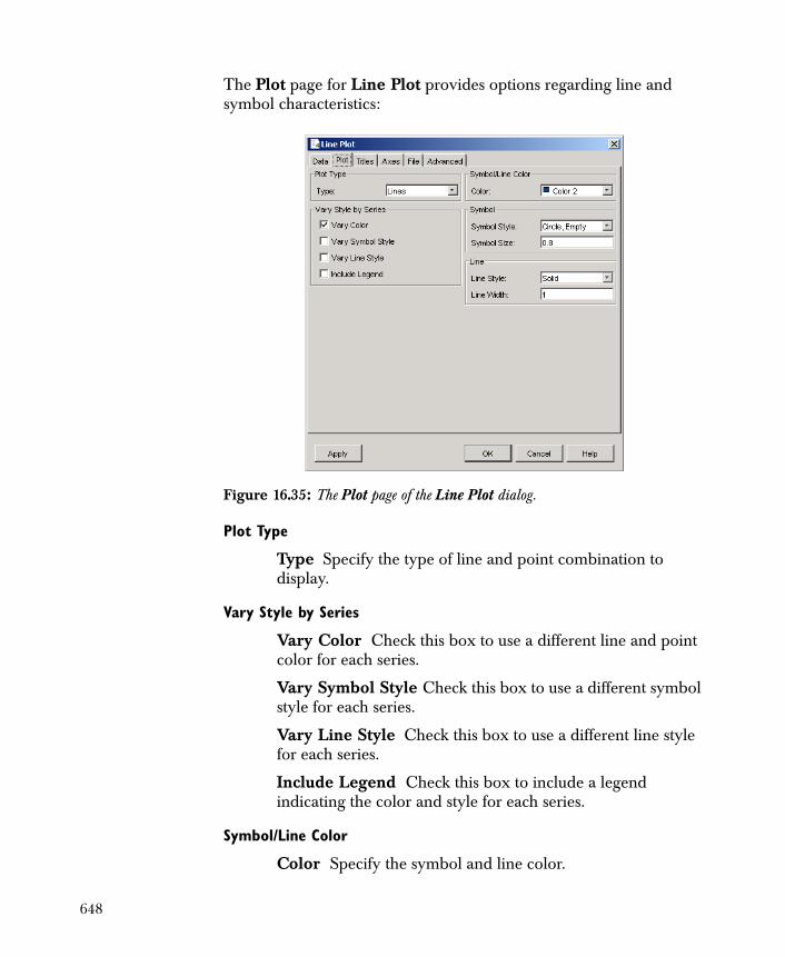
The Plot page for Line Plot provides options regarding line and symbol characteristics:
Plot Type
Type Specify the type of line and point combination to display.
Vary Style by Series
Vary Color Check this box to use a different line and point color for each series.
Vary Symbol Style Check this box to use a different symbol style for each series.
Vary Line Style Check this box to use a different line style for each series.
Include Legend Check this box to include a legend indicating the color and style for each series.
Symbol/Line Color
Color Specify the symbol and line color.
Figure 16.35: The Plot page of the Line Plot dialog.
648

Symbol
Symbol Style Specify the symbol style, such as an empty circle or a filled triangle.
Symbol Size Specify the size of the symbol.
Line
Line Style Specify the line style.
Line Width Specify the line width.
Time Series High-Low Plot
A high-low plot typically displays lines indicating the daily, monthly, or yearly extreme values in a time series. These kinds of plots can also include average, opening, and closing values, and are referred to as high-low-open-close plots in these cases. Meaningful high-low plots can thus display from three to five columns of data, and illustrate simultaneously important characteristics about time series data. Because of this, they are most often used to display financial data.
In typical high-low plots, vertical lines are drawn to indicate the range of values in a particular time unit (i.e., day, month, or year). If opening and closing values are included in the plot, they are represented by small horizontal hatch marks on the lines: left-pointing hatch marks indicate opening values and right-pointing marks indicate closing values. One variation on the high-low plot is the candlestick plot. Where typical high-low plots display the opening and closing values of a financial series with lines, candlestick plots use filled rectangles. The color of the rectangle indicates whether the difference is positive or negative. In Spotfire S+, white rectangles represent positive differences, when closing values are larger than opening values. Blue rectangles indicate negative differences, when opening values are larger than closing values.
649
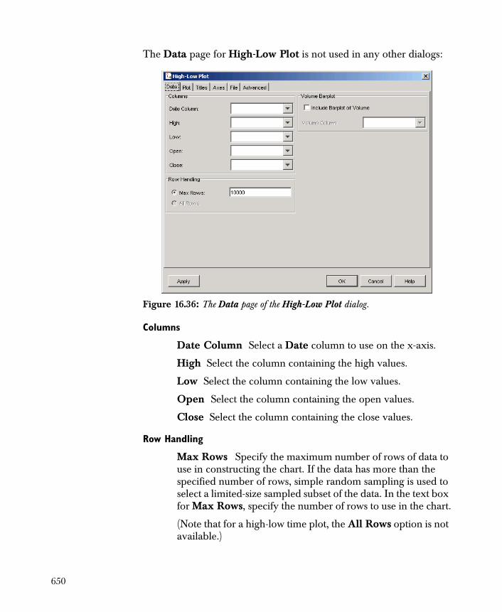
The Data page for High-Low Plot is not used in any other dialogs:
Columns
Date Column Select a Date column to use on the x-axis.
High Select the column containing the high values.
Low Select the column containing the low values.
Open Select the column containing the open values.
Close Select the column containing the close values.
Row Handling
Max Rows Specify the maximum number of rows of data to use in constructing the chart. If the data has more than the specified number of rows, simple random sampling is used to select a limited-size sampled subset of the data. In the text box for Max Rows, specify the number of rows to use in the chart.
(Note that for a high-low time plot, the All Rows option is not available.)
Figure 16.36: The Data page of the High-Low Plot dialog.
650
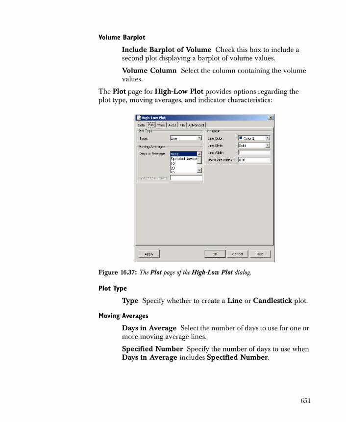
Volume Barplot
Include Barplot of Volume Check this box to include a second plot displaying a barplot of volume values.
Volume Column Select the column containing the volume values.
The Plot page for High-Low Plot provides options regarding the plot type, moving averages, and indicator characteristics:
Plot Type
Type Specify whether to create a Line or Candlestick plot.
Moving Averages
Days in Average Select the number of days to use for one or more moving average lines.
Specified Number Specify the number of days to use when Days in Average includes Specified Number.
Figure 16.37: The Plot page of the High-Low Plot dialog.
651
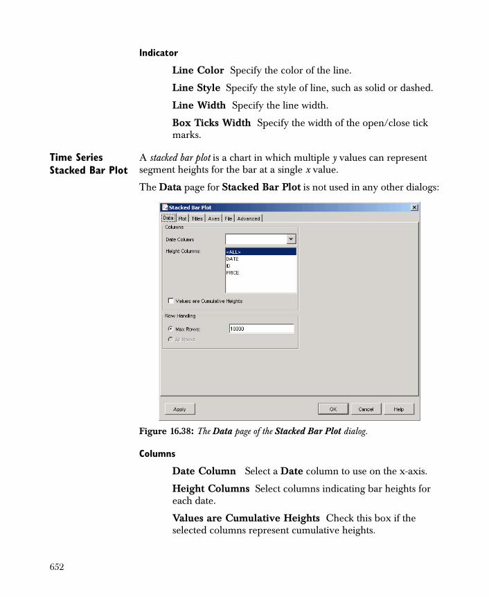
Indicator
Line Color Specify the color of the line.
Line Style Specify the style of line, such as solid or dashed.
Line Width Specify the line width.
Box Ticks Width Specify the width of the open/close tick marks.
Time Series Stacked Bar Plot
A stacked bar plot is a chart in which multiple y values can represent segment heights for the bar at a single x value.
The Data page for Stacked Bar Plot is not used in any other dialogs:
Columns
Date Column Select a Date column to use on the x-axis.
Height Columns Select columns indicating bar heights for each date.
Values are Cumulative Heights Check this box if the selected columns represent cumulative heights.
Figure 16.38: The Data page of the Stacked Bar Plot dialog.
652
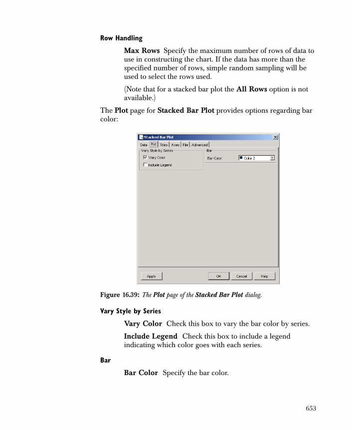
Row Handling
Max Rows Specify the maximum number of rows of data to use in constructing the chart. If the data has more than the specified number of rows, simple random sampling will be used to select the rows used.
(Note that for a stacked bar plot the All Rows option is not available.)
The Plot page for Stacked Bar Plot provides options regarding bar color:
Vary Style by Series
Vary Color Check this box to vary the bar color by series.
Include Legend Check this box to include a legend indicating which color goes with each series.
Bar
Bar Color Specify the bar color.
Figure 16.39: The Plot page of the Stacked Bar Plot dialog.
653
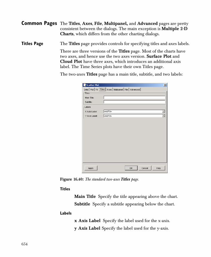
Common Pages The Titles, Axes, File, Multipanel, and Advanced pages are pretty consistent between the dialogs. The main exception is Multiple 2-D Charts, which differs from the other charting dialogs.
Titles Page The Titles page provides controls for specifying titles and axes labels.
There are three versions of the Titles page. Most of the charts have two axes, and hence use the two axes version. Surface Plot and Cloud Plot have three axes, which introduces an additional axis label. The Time Series plots have their own Titles page.
The two-axes Titles page has a main title, subtitle, and two labels:
Titles
Main Title Specify the title appearing above the chart.
Subtitle Specify a subtitle appearing below the chart.
Labels
x Axis Label Specify the label used for the x-axis.
y Axis Label Specify the label used for the y-axis.
Figure 16.40: The standard two-axes Titles page.
654
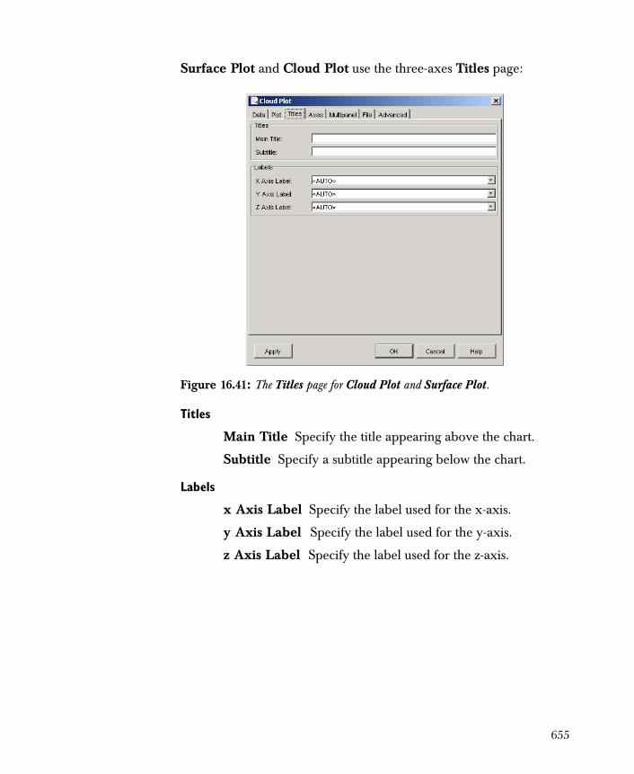
Surface Plot and Cloud Plot use the three-axes Titles page:
Titles
Main Title Specify the title appearing above the chart.
Subtitle Specify a subtitle appearing below the chart.
Labels
x Axis Label Specify the label used for the x-axis.
y Axis Label Specify the label used for the y-axis.
z Axis Label Specify the label used for the z-axis.
Figure 16.41: The Titles page for Cloud Plot and Surface Plot.
655
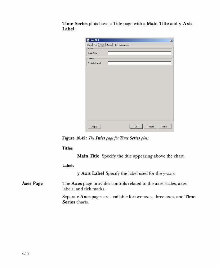
Time Series plots have a Title page with a Main Title and y Axis Label:
Titles
Main Title Specify the title appearing above the chart.
Labels
y Axis Label Specify the label used for the y-axis.
Axes Page The Axes page provides controls related to the axes scales, axes labels, and tick marks.
Separate Axes pages are available for two-axes, three-axes, and Time Series charts.
Figure 16.42: The Titles page for Time Series plots.
656
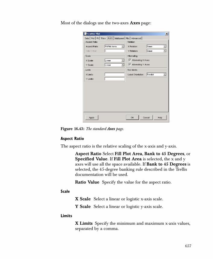
Most of the dialogs use the two-axes Axes page:
Aspect Ratio
The aspect ratio is the relative scaling of the x-axis and y-axis.
Aspect Ratio Select Fill Plot Area, Bank to 45 Degrees, or Specified Value. If Fill Plot Area is selected, the x and y axes will use all the space available. If Bank to 45 Degrees is selected, the 45-degree banking rule described in the Trellis documentation will be used.
Ratio Value Specify the value for the aspect ratio.
Scale
X Scale Select a linear or logistic x-axis scale.
Y Scale Select a linear or logistic y-axis scale.
Limits
X Limits Specify the minimum and maximum x-axis values, separated by a comma.
Figure 16.43: The standard Axes page.
657
Y Limits Specify the minimum and maximum y-axis values, separated by a comma.
Relation
X Relation Specify the relationship between the x-axes on various panels when using multipanel conditioning. The default value of Same ensures that the horizontal or vertical axes on each panel will be identical. Sliced gives the same number of data units to corresponding axes on each panel, ensuring that the number of units per centimeter is identical. Using Free results in each panel having an axis that accommodates just the data in that panel. For Sliced and Free, axes will be drawn for each panel, using more space on the display.
Y Relation Specify the relationship between the y-axes on various panels when using multipanel conditioning.
Alternating
Alternating X Axes Specify whether the x-axes should alternate between left and right placement when using multipanel conditioning.
Alternating Y Axes Specify whether the x-axes should alternate between top and bottom placement when using multipanel conditioning.
Tick Marks
Label Orientation Select whether the axis labels should be Parallel to the axis, Perpendicular to the axis, or always Horizontal.
See the Spotfire S+ help file trellis.args for details on these settings.
658
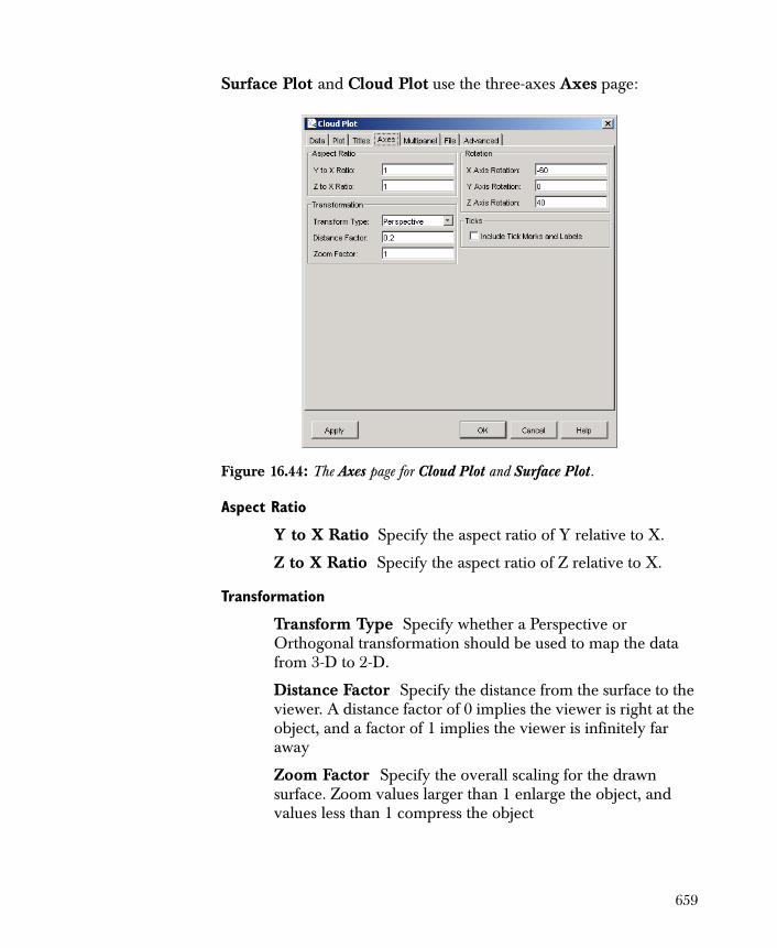
Surface Plot and Cloud Plot use the three-axes Axes page:
Aspect Ratio
Y to X Ratio Specify the aspect ratio of Y relative to X.
Z to X Ratio Specify the aspect ratio of Z relative to X.
Transformation
Transform Type Specify whether a Perspective or Orthogonal transformation should be used to map the data from 3-D to 2-D.
Distance Factor Specify the distance from the surface to the viewer. A distance factor of 0 implies the viewer is right at the object, and a factor of 1 implies the viewer is infinitely far away
Zoom Factor Specify the overall scaling for the drawn surface. Zoom values larger than 1 enlarge the object, and values less than 1 compress the object
Figure 16.44: The Axes page for Cloud Plot and Surface Plot.
659

Rotation
By default, Spotfire S+ rotates a surface plot 40 degrees about the z axis and -60 degrees about the x axis before displaying it. To change this setting, enter new values in the Rotation fields; rotating each axis 0 degrees results in a view from the top of the surface, looking down in the x-y plane.
X Axis Rotation Rotation of the x-axis in degrees.
Y Axis Rotation Rotation of the y-axis in degrees.
Z Axis Rotation Rotation of the z-axis in degrees.
Ticks
Include Tick Marks and Labels The arrows along the axes indicate the direction of increasing values for each of the variables. Check this box to include tick marks instead of arrows.
See the Spotfire S+ help file trellis.args for details on these settings.
660

The Time Series chart dialogs use the time series Axes page:
Scale
Y Scale Select a linear or logistic y-axis scale.
Grid
Include Reference Grid Check this box to include a reference grid.
Tick Marks
Include Tick Marks on Top Axis Check this box to include tick marks on the top axis. Tick marks are always present on the bottom axis.
Include Tick Marks on Right Axis Check this box to include tick marks on the right axis. Tick marks are always present on the left axis.
Figure 16.45: The Axes page for Time Series plots.
661
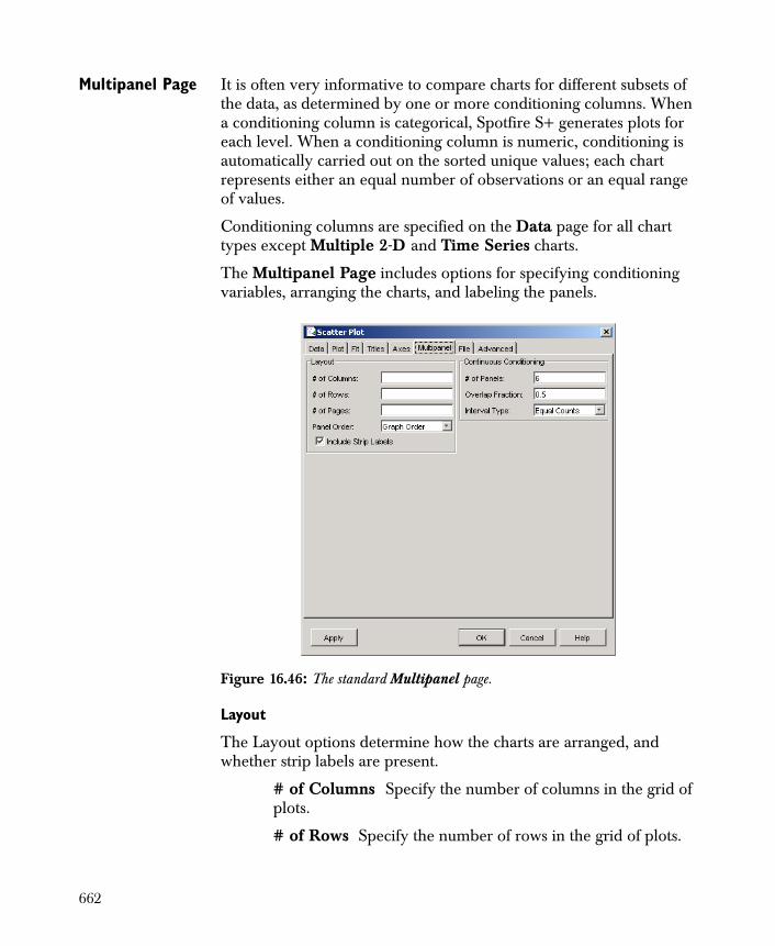
Multipanel Page It is often very informative to compare charts for different subsets of the data, as determined by one or more conditioning columns. When a conditioning column is categorical, Spotfire S+ generates plots for each level. When a conditioning column is numeric, conditioning is automatically carried out on the sorted unique values; each chart represents either an equal number of observations or an equal range of values.
Conditioning columns are specified on the Data page for all chart types except Multiple 2-D and Time Series charts.
The Multipanel Page includes options for specifying conditioning variables, arranging the charts, and labeling the panels.
Layout
The Layout options determine how the charts are arranged, and whether strip labels are present.
# of Columns Specify the number of columns in the grid of plots.
# of Rows Specify the number of rows in the grid of plots.
Figure 16.46: The standard Multipanel page.
662
# of Pages Specify the number of pages to use.
Panel Order Select Graph Order to arrange the plots from bottom to top based on the conditioning column levels, and Table Order to arrange the plots from top to bottom.
Include Strip Labels Check this box to include strip labels indicating the conditioning column levels.
Continuous Conditioning
The Continuous Conditioning options determine how continuous column values are converted to categorical values.
# of Panels Select the number of categories to create. Specifies the number of bins requested when converting the continuous column to a category. If no rows fall into a category, the category is dropped before plotting, and the number of panels is fewer than the number specified. That is, the panel is dropped, rather displaying an empty panel with no plot.
Overlap Fraction Select the fraction of overlap between neighboring bins.
Interval Type Specify the method for creating the bins. With Equal Counts, each bin will have the same number of points. With Equal Ranges, each bin will have the same width. Unique Values is used when the continuous values should be treated as category levels.
When All Rows selected in the Properties page, the One Column - Categorical and Three Column plots perform tabulations and interpolations on the full data, and then call the regular data.frame Trellis function to create a plot. With these plots, any Continuous Conditioning columns are converted to categorical columns using a Bin node. Non-overlapping bins are used to create one categorical value per row.
For these plot types (that is, bar charts, dot plots, pie charts, level plots, contour plots, and wireframes), the Trellis graphs created by selecting Max Rows vs. All Rows on the Data page differ:
• Because Max Rows uses overlapping intervals by default, and All Rows uses non-overlapping intervals, the points in each panel differ. To display the same plot for All Rows and
663
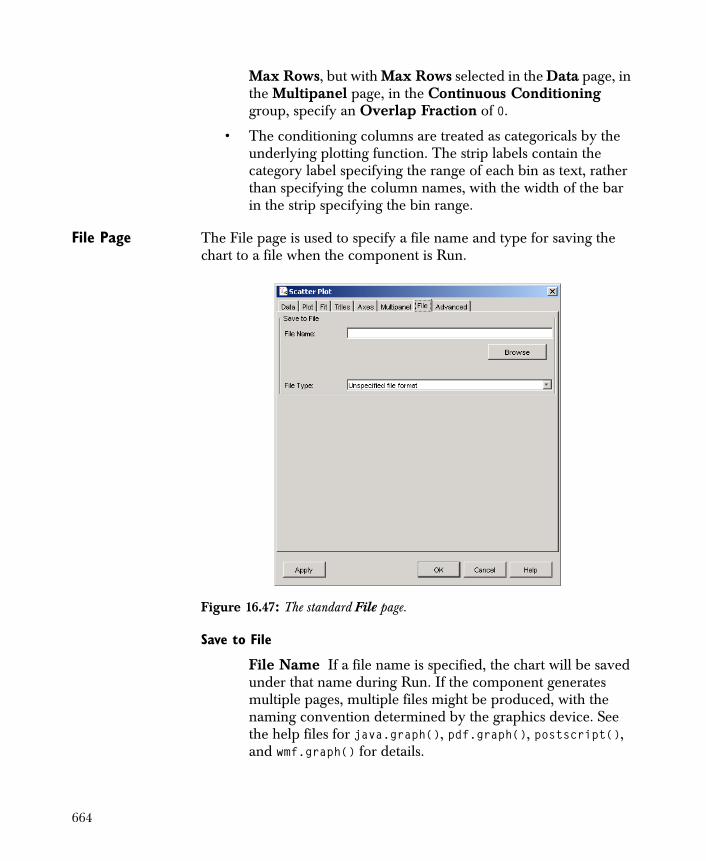
Max Rows, but with Max Rows selected in the Data page, in the Multipanel page, in the Continuous Conditioning group, specify an Overlap Fraction of 0.
• The conditioning columns are treated as categoricals by the underlying plotting function. The strip labels contain the category label specifying the range of each bin as text, rather than specifying the column names, with the width of the bar in the strip specifying the bin range.
File Page The File page is used to specify a file name and type for saving the chart to a file when the component is Run.
Save to File
File Name If a file name is specified, the chart will be saved under that name during Run. If the component generates multiple pages, multiple files might be produced, with the naming convention determined by the graphics device. See the help files for java.graph(), pdf.graph(), postscript(), and wmf.graph() for details.
Figure 16.47: The standard File page.
664
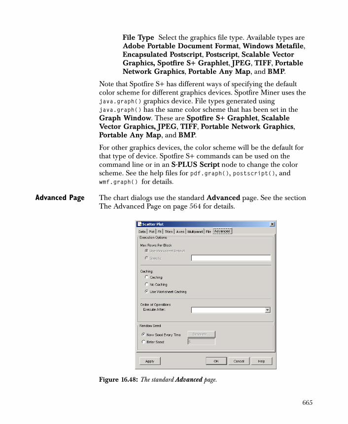
File Type Select the graphics file type. Available types are Adobe Portable Document Format, Windows Metafile, Encapsulated Postscript, Postscript, Scalable Vector Graphics, Spotfire S+ Graphlet, JPEG, TIFF, Portable Network Graphics, Portable Any Map, and BMP.
Note that Spotfire S+ has different ways of specifying the default color scheme for different graphics devices. Spotfire Miner uses the java.graph() graphics device. File types generated using java.graph() has the same color scheme that has been set in the Graph Window. These are Spotfire S+ Graphlet, Scalable Vector Graphics, JPEG, TIFF, Portable Network Graphics, Portable Any Map, and BMP.
For other graphics devices, the color scheme will be the default for that type of device. Spotfire S+ commands can be used on the command line or in an S-PLUS Script node to change the color scheme. See the help files for pdf.graph(), postscript(), and wmf.graph() for details.
Advanced Page The chart dialogs use the standard Advanced page. See the section The Advanced Page on page 564 for details.
Figure 16.48: The standard Advanced page.
665

For all charts except Multiple 2-D Charts, the Max Rows Per Block field is disabled since the number of rows used is determined by the Max Rows field on the Data page. The Random Seed group controls the seed used when sampling down to the specified number of rows, if the number of rows in the data exceeds the Max Rows value.
666
S-PLUS DATA MANIPULATION NODES
The Create Columns, Filter Rows, and Split components introduced in Chapter 6, Data Manipulation, allow you to create new data values and select data rows from a data set by specifying expressions in a simple expression language.
There are three Spotfire S+ Library expression components that perform exactly the same operations as their Spotfire Miner equivalent components, except that the user-specified expressions are interpreted within the S-PLUS language, rather than the Spotfire Miner expression language:
• S-PLUS Create Columns
• S-PLUS Filter Rows
• S-PLUS Split
Many expressions are exactly the same in the expression language and the S-PLUS language. For example, both the Filter Rows and S-PLUS Filter Rows components could use the expression
Mileage > 28 & Mileage < 32
to select those data rows where the column Mileage is in the specified range. The S-PLUS expression components are particularly useful when calling built-in S-PLUS functions that are not supported by the expression language or calling pre-existing user-written functions.
Evaluating S-PLUS Expressions
Normally, it is not necessary to understand how Spotfire Miner evaluates the S-PLUS expressions in the S-PLUS Create Columns, S-PLUS Filter Rows, and S-PLUS Split nodes. Simple expressions act as if they were being executed on every row individually. For example, if the expression in the S-PLUS Create Columns node is A+B, the newly created column contains, in each row, the value of column A plus the value of column B in the same row.
For more complicated expressions, it might be useful to understand exactly how Spotfire Miner evaluates these expressions. Spotfire Miner reads and evaluates the expression on one block of data at a time (the number of rows in a block is set in the Advanced properties of the node). When evaluating the expression for each block, a variable is created for each column containing a vector of elements.
667
For example, if there are five rows in a block, while evaluating A+B, the variables might be assigned, using S-PLUS vector syntax, as follows:
A <- c(1,3,2,4,5)B <- c(4,5,7,6,3)
Most S-PLUS functions and operations (such as +) can handle vectors as arguments, so the expression A+B produces the vector c(5,8,9,10,8), given the above values for A and B. Spotfire S+ also handles combinations of vector and single values, so that the expression A+1 would produce the value c(2,4,3,5,6).
There are several cases where it is necessary to know about the evaluation of vectors. One case occurs when calling summary functions, which perform an operation on the current vector, not the entire data set. For example, if you calculate mean(Weight), this calculates the mean for the column Weight in the current data block, not the entire data set. If you want to access the precomputed mean for the entire data set, use the S-PLUS Script node.
Another case is for functions that need to know the length of the vectors. One such function is rnorm, used to generate random normal values. If the expression
rnorm(1,121,3)
is used within S-PLUS Create Columns, this function returns a single value (specified by the first argument of the function), which is then used for each row in the output block for the newly-created column. This is probably not what was desired. In this case, a better expression would be
rnorm(length(A),121,3)
which returns a vector of random values whose length is equal to the length of the input vector A, returned by length(A).
Data Types in Spotfire Miner and Spotfire S+
Spotfire Miner supports four data types: continuous, categorical, string, and date. When Spotfire Miner data is sent into any of the S-PLUS nodes for processing, the rectangular Spotfire Miner data is converted into a Spotfire S+ data frame. The Spotfire Miner data values are converted into Spotfire S+ data vectors as follows:
668
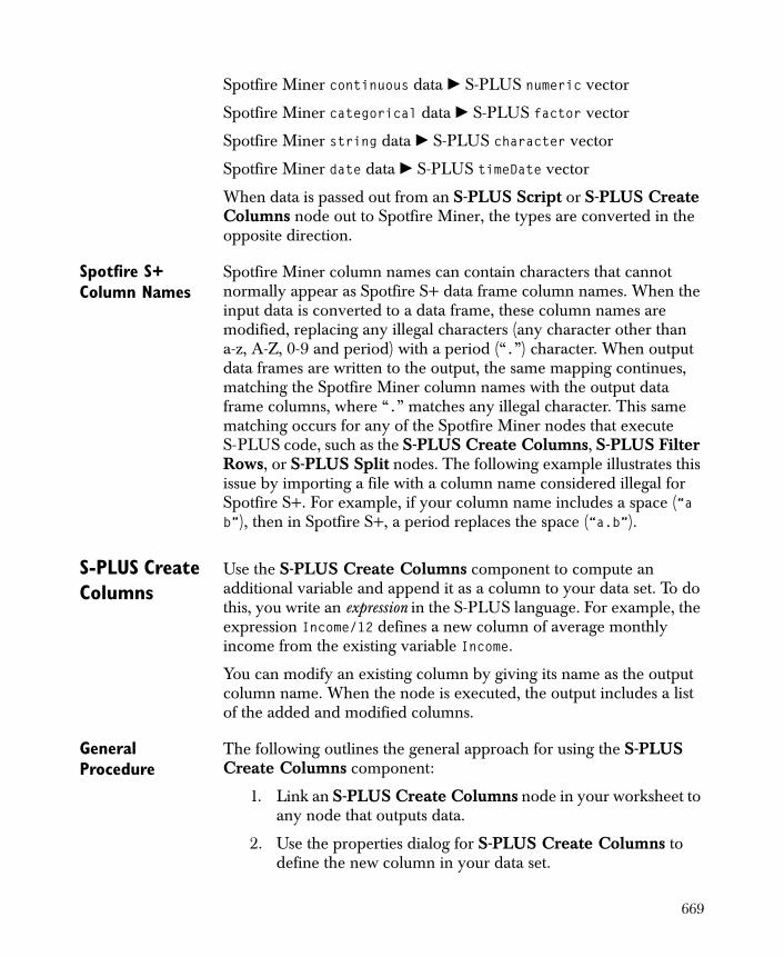
Spotfire Miner continuous data � S-PLUS numeric vector
Spotfire Miner categorical data � S-PLUS factor vector
Spotfire Miner string data � S-PLUS character vector
Spotfire Miner date data � S-PLUS timeDate vector
When data is passed out from an S-PLUS Script or S-PLUS Create Columns node out to Spotfire Miner, the types are converted in the opposite direction.
Spotfire S+ Column Names
Spotfire Miner column names can contain characters that cannot normally appear as Spotfire S+ data frame column names. When the input data is converted to a data frame, these column names are modified, replacing any illegal characters (any character other than a-z, A-Z, 0-9 and period) with a period (“.”) character. When output data frames are written to the output, the same mapping continues, matching the Spotfire Miner column names with the output data frame columns, where “.” matches any illegal character. This same matching occurs for any of the Spotfire Miner nodes that execute S-PLUS code, such as the S-PLUS Create Columns, S-PLUS Filter Rows, or S-PLUS Split nodes. The following example illustrates this issue by importing a file with a column name considered illegal for Spotfire S+. For example, if your column name includes a space (“a b”), then in Spotfire S+, a period replaces the space (“a.b”).
S-PLUS Create Columns
Use the S-PLUS Create Columns component to compute an additional variable and append it as a column to your data set. To do this, you write an expression in the S-PLUS language. For example, the expression Income/12 defines a new column of average monthly income from the existing variable Income.
You can modify an existing column by giving its name as the output column name. When the node is executed, the output includes a list of the added and modified columns.
General Procedure
The following outlines the general approach for using the S-PLUS Create Columns component:
1. Link an S-PLUS Create Columns node in your worksheet to any node that outputs data.
2. Use the properties dialog for S-PLUS Create Columns to define the new column in your data set.
669
3. Run your network.
4. Launch the node’s viewer.
The S-PLUS Create Columns node accepts a single input containing rectangular data and outputs the same rectangular data set with the new column appended to it.
Properties The Properties page of the S-PLUS Create Columns dialog is shown in Figure 16.49.
Create New Columns
Select Type Specify a type for the new column by selecting continuous, categorical, string, or date from the drop-down list. Then click the Add button to activate the grid view and insert a row for the new column.
Figure 16.49: The Properties page of the S-PLUS Create Columns dialog.
670
Grid View The grid view displays a row for each new column you create. Initially, only Type is filled in.
• Name To add or change a column name, double-click the cell under Name. This activates a text box in which you can type a new column name.
• Type To change the data type for the new column, click the cell under Type. This opens a drop-down list containing the four possible column types from which you can make a selection.
• Column Creation Expression To add or change an entry under Column Creation Expression, double-click the entry. This activates a text box in which you can type a new expression. Define your column by typing a valid expression in the S-PLUS language in this field.
If you need to remove particular columns from the grid view, select the rows that contain them by clicking, CTRL-clicking, or SHIFT-clicking. Then click the Remove button.
When you click the Parse Expressions button, the current expressions are parsed, and a window pops up displaying any parsing errors.
String Size Specify the string width for any new string columns.
Input Variables This scrollable table shows the input column names, types, and roles and is useful for finding the names of available inputs when constructing new expressions.
Using the Viewer The viewer for the S-PLUS Create Columns component is the node viewer. For a complete discussion of the node viewer and the information it displays, see the section The Table Viewer on page 146 as well as the online help.
Note
Any Spotfire Miner column names that cannot normally appear as Spotfire S+ data frame column names are displayed in a converted form that can be used in an S-PLUS expression. For example, the column name “Pr(0)” will be displayed as “Pr.0.” and this can be used in expressions such as Pr.0.+10
671

S-PLUS Filter Rows
Use the S-PLUS Filter Rows component to select or exclude rows of your data set. To do this, you write a qualifier in the S-PLUS language. For example, the qualifier age>40 & gender=="F" includes only those rows corresponding to women over 40 years of age.
Use the S-PLUS Filter Rows component to filter data sets that have already been defined in Spotfire Miner, not those that exist in the original data sources. For options that filter data as they are read into Spotfire Miner, see the Read components.
General Procedure
The following outlines the general approach for using the S-PLUS Filter Rows component:
1. Link a S-PLUS Filter Rows node in your worksheet to any node that outputs data.
2. Use the properties dialog for S-PLUS Filter Rows to specify the qualifier that filters the rows in your data set.
3. Run your network.
4. Launch the node’s viewer.
The S-PLUS Filter Rows node accepts a single input containing rectangular data and outputs a single rectangular data set defined by the qualifier you specify.
672
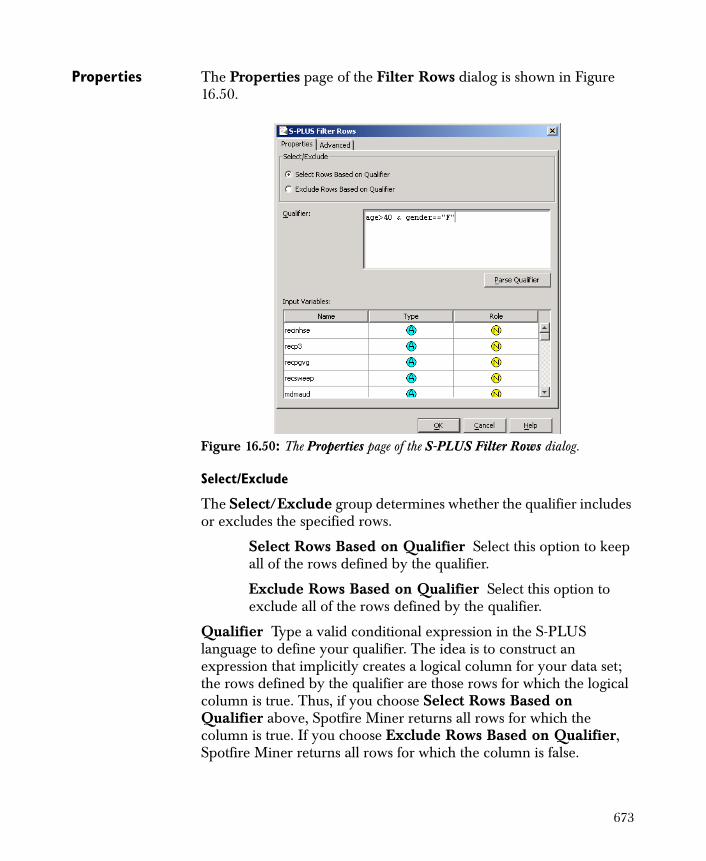
Properties The Properties page of the Filter Rows dialog is shown in Figure 16.50.
Select/Exclude
The Select/Exclude group determines whether the qualifier includes or excludes the specified rows.
Select Rows Based on Qualifier Select this option to keep all of the rows defined by the qualifier.
Exclude Rows Based on Qualifier Select this option to exclude all of the rows defined by the qualifier.
Qualifier Type a valid conditional expression in the S-PLUS language to define your qualifier. The idea is to construct an expression that implicitly creates a logical column for your data set; the rows defined by the qualifier are those rows for which the logical column is true. Thus, if you choose Select Rows Based on Qualifier above, Spotfire Miner returns all rows for which the column is true. If you choose Exclude Rows Based on Qualifier, Spotfire Miner returns all rows for which the column is false.
Figure 16.50: The Properties page of the S-PLUS Filter Rows dialog.
673
When you click the Parse Qualifier button, the current expression is parsed, and a window pops up displaying any parsing errors.
Input Variables This scrollable table shows the input column names, types, and roles and is useful for finding the names of available inputs when constructing new expressions.
Using the Viewer The viewer for the Filter Rows component is the node viewer. For a complete discussion of the node viewer and the information it displays, see the section The Table Viewer on page 146 as well as the online help.
S-PLUS Split Use the S-PLUS Split component to divide a data set into two parts based on a conditional expression that either includes or excludes particular rows. To do this, you write a qualifier in the S-PLUS language. For example, the qualifier gender=="F" splits the data set according to gender.
General Procedure
The following outlines the general approach for using the S-PLUS Split component:
1. Link an S-PLUS Split node in your worksheet to any node that outputs data.
2. Use the properties dialog for S-PLUS Split to specify the qualifier that splits the rows of your data set into two groups.
3. Run your network.
4. Launch the node’s viewer.
The S-PLUS Split node accepts a single input containing rectangular data and outputs two rectangular data sets. (This component is similar to S-PLUS Filter Rows except that it has two outputs rather than one.) The portion of the data set for which the qualifier is true forms the first (top) output, and the portion for which the qualifier is false
Note
Any Spotfire Miner column names that cannot normally appear as Spotfire S+ data frame column names are displayed in a converted form that can be used in an S-PLUS expression. For example, the column name “Pr(0)” will be displayed as “Pr.0.” and this can be used in expressions such as Pr.0.+10
674

forms the second (bottom) output. To split a data set into more than two groups, use an S-PLUS Script node or a series of S-PLUS Split nodes in your network.
Properties The Properties page of the S-PLUS Split dialog is shown in Figure 16.51.
Options
Qualifier Type a valid conditional expression in the S-PLUS language to define your qualifier. The idea is to construct an expression that implicitly creates a logical column for your data set; the rows defined by the qualifier are those rows for which the logical column is true. In the first output of the S-PLUS Split component, Spotfire Miner returns all rows for which the column is true; in the second output, Spotfire Miner returns all rows for which the column is false.
When you click the Parse Qualifier button, the current expression is parsed, and a window pops up displaying any parsing errors.
Figure 16.51: The Properties page of the S-PLUS Split dialog.
675
Input Variables This scrollable table shows the input column names, types, and roles and is useful for finding the names of available inputs when constructing new expressions.
Using the Viewer The viewer for the S-PLUS Split component is the node viewer. For a complete discussion of the node viewer and the information it displays, see the section The Table Viewer on page 146 as well as the online help.
Note
Any Spotfire Miner column names that cannot normally appear as Spotfire S+ data frame column names are displayed in a converted form that can be used in an S-PLUS expression. For example, the column name “Pr(0)” will be displayed as “Pr.0.” and this can be used in expressions such as Pr.0.+10
676
S-PLUS SCRIPT NODE
The S-PLUS Script node performs transformations on a data set by specifying a series of S-PLUS commands. This node has been designed so that simple transformations are easy to specify, while allowing access to more complex features when needed.
Often, this node is used to transform an input data set. For example, suppose the input data contains a column named ABC and you want to perform the following value replacement: if a value in ABC is less than 10.0, replace it with the fixed value 10.0. You could do this by using the following simple script:
IM$in1$ABC[IM$in1$ABC<10] <- 10.0IM$in1
This script is executed to process each data block in the input data. Each time it is executed, the variable IM$in1 contains a data frame with the values of the input block. The first line finds the rows where ABC is less than 10, and then replaces them with 10.0. The second line returns the updated value of IM$in1 as the output from the node. You can perform many simple transformations in this manner.
Here is another example script, where the input columns are copied to the output, along with several new columns. The column ABC is used to create the two new columns TIMES.TWO and PLUS.ONE:
x <- IM$in1$ABCdata.frame(IM$in1, data.frame(TIMES.TWO=x*2,PLUS.ONE=x+1))
The body of your S-PLUS script implicitly defines an S-PLUS function with a single argument IM (for “Spotfire Miner”). The IM argument is a list with several named elements that you can access within the script. These elements map to the data inputs, among other functions. For example, IM$in1 contains the data from the first input to the S-PLUS Script node, IM$in2 contains the data from the second input to the node, etc. The final value in your script is the return value of the function. You can use the S-PLUS function return to return a value from the middle of the script. To return multiple outputs, seethe section Output List Elements on page 691.
677

General Procedure
The following outlines the general approach for using the S-PLUS Script component:
1. Add an S-PLUS Script node to the worksheet.
2. Enter the script on the Properties page.
3. Adjust the number of inputs and outputs on the Options page.
4. Set other options if necessary.
5. If the script takes inputs, link the inputs to any nodes that output data.
6. Run your network.
7. Launch the node’s viewer.
The number of inputs and outputs for the S-PLUS Script node varies based on the script. Each input and output contains rectangular data.
Properties The Properties dialog for the S-PLUS Script component contains three tabbed pages labeled Properties, Options, and Advanced (see page 564 for a discussion of the options available on the Advanced page.)
If the Show Parameters Page check box on the Options page is selected, the dialog displays an additional Parameters page as the first page in the dialog.
678
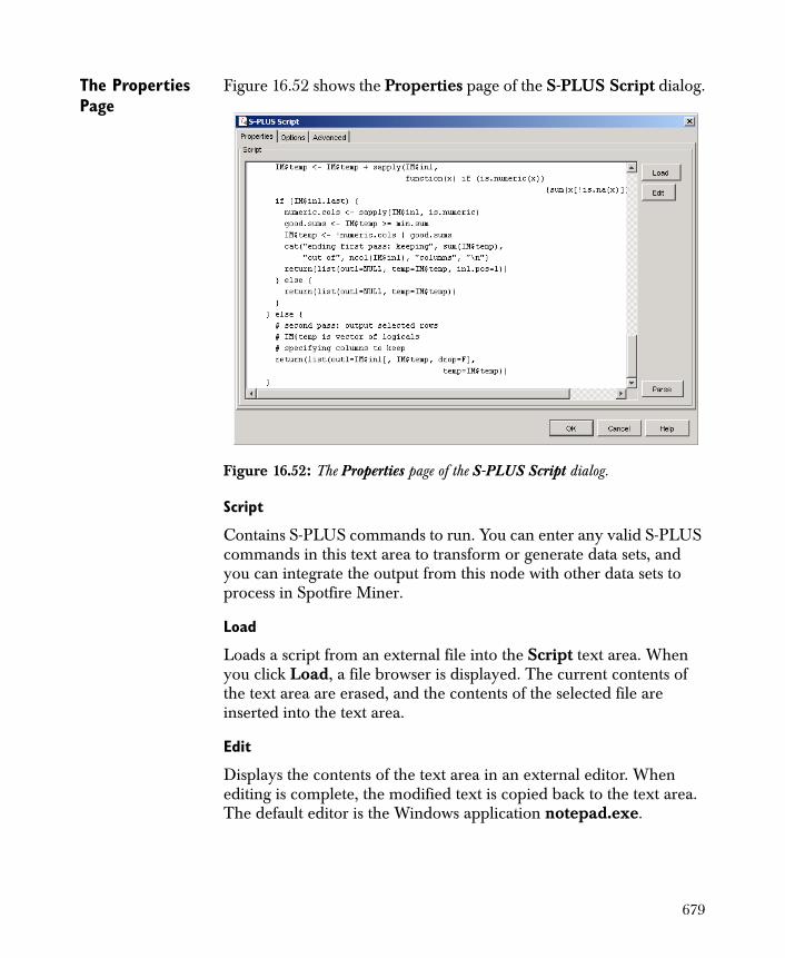
The Properties Page
Figure 16.52 shows the Properties page of the S-PLUS Script dialog.
Script
Contains S-PLUS commands to run. You can enter any valid S-PLUS commands in this text area to transform or generate data sets, and you can integrate the output from this node with other data sets to process in Spotfire Miner.
Load
Loads a script from an external file into the Script text area. When you click Load, a file browser is displayed. The current contents of the text area are erased, and the contents of the selected file are inserted into the text area.
Edit
Displays the contents of the text area in an external editor. When editing is complete, the modified text is copied back to the text area. The default editor is the Windows application notepad.exe.
Figure 16.52: The Properties page of the S-PLUS Script dialog.
679
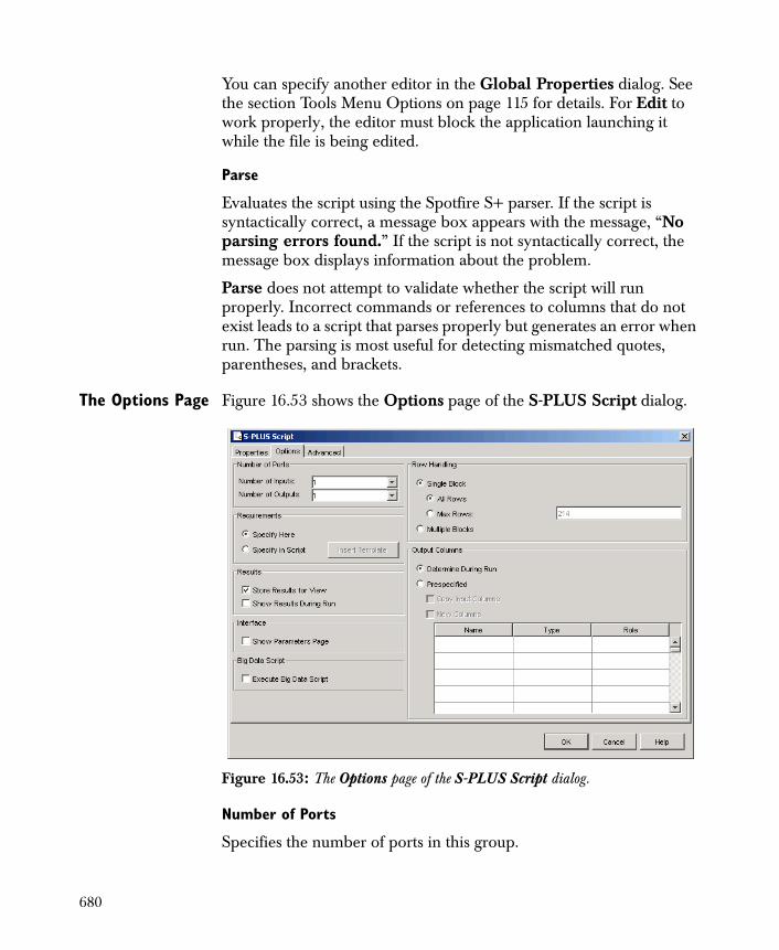
You can specify another editor in the Global Properties dialog. See the section Tools Menu Options on page 115 for details. For Edit to work properly, the editor must block the application launching it while the file is being edited.
Parse
Evaluates the script using the Spotfire S+ parser. If the script is syntactically correct, a message box appears with the message, “No parsing errors found.” If the script is not syntactically correct, the message box displays information about the problem.
Parse does not attempt to validate whether the script will run properly. Incorrect commands or references to columns that do not exist leads to a script that parses properly but generates an error when run. The parsing is most useful for detecting mismatched quotes, parentheses, and brackets.
The Options Page Figure 16.53 shows the Options page of the S-PLUS Script dialog.
Number of Ports
Specifies the number of ports in this group.
Figure 16.53: The Options page of the S-PLUS Script dialog.
680