738
TIBCO Spotfire S+ ® 8.1 Guide to Statistics, Volume 1 November 2008 TIBCO Software Inc.

TIBCO Spotfire S+® 8.1Guide to Statistics, Volume 1
November 2008
TIBCO Software Inc.

IMPORTANT INFORMATION
SOME TIBCO SOFTWARE EMBEDS OR BUNDLES OTHER TIBCO SOFTWARE. USE OF SUCH EMBEDDED OR BUNDLED TIBCO SOFTWARE IS SOLELY TO ENABLE THE FUNCTIONALITY (OR PROVIDE LIMITED ADD-ON FUNCTIONALITY) OF THE LICENSED TIBCO SOFTWARE. THE EMBEDDED OR BUNDLED SOFTWARE IS NOT LICENSED TO BE USED OR ACCESSED BY ANY OTHER TIBCO SOFTWARE OR FOR ANY OTHER PURPOSE.
USE OF TIBCO SOFTWARE AND THIS DOCUMENT IS SUBJECT TO THE TERMS AND CONDITIONS OF A LICENSE AGREEMENT FOUND IN EITHER A SEPARATELY EXECUTED SOFTWARE LICENSE AGREEMENT, OR, IF THERE IS NO SUCH SEPARATE AGREEMENT, THE CLICKWRAP END USER LICENSE AGREEMENT WHICH IS DISPLAYED DURING DOWNLOAD OR INSTALLATION OF THE SOFTWARE (AND WHICH IS DUPLICATED IN THE TIBCO SPOTFIRE S+® INSTALLATION AND ADMINISTRATION GUIDE). USE OF THIS DOCUMENT IS SUBJECT TO THOSE TERMS AND CONDITIONS, AND YOUR USE HEREOF SHALL CONSTITUTE ACCEPTANCE OF AND AN AGREEMENT TO BE BOUND BY THE SAME.
This document contains confidential information that is subject to U.S. and international copyright laws and treaties. No part of this document may be reproduced in any form without the written authorization of TIBCO Software Inc.
TIBCO Software Inc., TIBCO, Spotfire, TIBCO Spotfire S+, Insightful, the Insightful logo, the tagline "the Knowledge to Act," Insightful Miner, S+, S-PLUS, TIBCO Spotfire Axum, S+ArrayAnalyzer, S+EnvironmentalStats, S+FinMetrics, S+NuOpt, S+SeqTrial, S+SpatialStats, S+Wavelets, S-PLUS Graphlets, Graphlet, Spotfire S+ FlexBayes, Spotfire S+ Resample, TIBCO Spotfire Miner, TIBCO Spotfire S+ Server, and TIBCO Spotfire Clinical Graphics are either registered trademarks or trademarks of TIBCO Software Inc. and/or subsidiaries of TIBCO Software Inc. in the United States and/or other countries. All other product and company names and marks mentioned in this document are the property of their respective owners and are mentioned for
ii

identification purposes only. This software may be available on multiple operating systems. However, not all operating system platforms for a specific software version are released at the same time. Please see the readme.txt file for the availability of this software version on a specific operating system platform.
THIS DOCUMENT IS PROVIDED “AS IS” WITHOUT WARRANTY OF ANY KIND, EITHER EXPRESS OR IMPLIED, INCLUDING, BUT NOT LIMITED TO, THE IMPLIED WARRANTIES OF MERCHANTABILITY, FITNESS FOR A PARTICULAR PURPOSE, OR NON-INFRINGEMENT. THIS DOCUMENT COULD INCLUDE TECHNICAL INACCURACIES OR TYPOGRAPHICAL ERRORS. CHANGES ARE PERIODICALLY ADDED TO THE INFORMATION HEREIN; THESE CHANGES WILL BE INCORPORATED IN NEW EDITIONS OF THIS DOCUMENT. TIBCO SOFTWARE INC. MAY MAKE IMPROVEMENTS AND/OR CHANGES IN THE PRODUCT(S) AND/OR THE PROGRAM(S) DESCRIBED IN THIS DOCUMENT AT ANY TIME.
Copyright © 1996-2008 TIBCO Software Inc. ALL RIGHTS RESERVED. THE CONTENTS OF THIS DOCUMENT MAY BE MODIFIED AND/OR QUALIFIED, DIRECTLY OR INDIRECTLY, BY OTHER DOCUMENTATION WHICH ACCOMPANIES THIS SOFTWARE, INCLUDING BUT NOT LIMITED TO ANY RELEASE NOTES AND "READ ME" FILES.
TIBCO Software Inc. Confidential Information
Reference The correct bibliographic reference for this document is as follows:
TIBCO Spotfire S+® 8.1 Guide to Stats Volume 1 TIBCO Software Inc.
Technical Support
For technical support, please visit http://spotfire.tibco.com/support and register for a support account.
iii

ACKNOWLEDGMENTS
TIBCO Spotfire S+ would not exist without the pioneering research of the Bell Labs S team at AT&T (now Lucent Technologies): John Chambers, Richard A. Becker (now at AT&T Laboratories), Allan R. Wilks (now at AT&T Laboratories), Duncan Temple Lang, and their colleagues in the statistics research departments at Lucent: William S. Cleveland, Trevor Hastie (now at Stanford University), Linda Clark, Anne Freeny, Eric Grosse, David James, José Pinheiro, Daryl Pregibon, and Ming Shyu.
TIBCO Software Inc. thanks the following individuals for their contributions to this and earlier releases of TIBCO Spotfire S+: Douglas M. Bates, Leo Breiman, Dan Carr, Steve Dubnoff, Don Edwards, Jerome Friedman, Kevin Goodman, Perry Haaland, David Hardesty, Frank Harrell, Richard Heiberger, Mia Hubert, Richard Jones, Jennifer Lasecki, W.Q. Meeker, Adrian Raftery, Brian Ripley, Peter Rousseeuw, J.D. Spurrier, Anja Struyf, Terry Therneau, Rob Tibshirani, Katrien Van Driessen, William Venables, and Judy Zeh.
iv

TIBCO SPOTFIRE S+ BOOKS
The TIBCO Spotfire S+® documentation includes books to address your focus and knowledge level. Review the following table to help you choose the Spotfire S+ book that meets your needs. These books are available in PDF format in the following locations:
• In your Spotfire S+ installation directory (SHOME\help on Windows, SHOME/doc on UNIX/Linux).
• In the Spotfire S+ Workbench, from the Help � Spotfire S+ Manuals menu item.
• In Microsoft® Windows®, in the Spotfire S+ GUI, from the Help � Online Manuals menu item.
Spotfire S+ documentation.
Information you need if you... See the...
Are new to the S language and the Spotfire S+ GUI, and you want an introduction to importing data, producing simple graphs, applying statistical
models, and viewing data in Microsoft Excel®
.
Getting Started Guide
Are a new Spotfire S+ user and need how to use Spotfire S+, primarily through the GUI.
User’s Guide
Are familiar with the S language and Spotfire S+, and you want to use the Spotfire S+ plug-in, or customization, of the Eclipse Integrated Development Environment (IDE).
Spotfire S+ Workbench User’s Guide
Have used the S language and Spotfire S+, and you want to know how to write, debug, and program functions from the Commands window.
Programmer’s Guide
Are familiar with the S language and Spotfire S+, and you want to extend its functionality in your own application or within Spotfire S+.
Application Developer’s Guide
v

Are familiar with the S language and Spotfire S+, and you are looking for information about creating or editing graphics, either from a Commands window or the Windows GUI, or using Spotfire S+ supported graphics devices.
Guide to Graphics
Are familiar with the S language and Spotfire S+, and you want to use the Big Data library to import and manipulate very large data sets.
Big Data User’s Guide
Want to download or create Spotfire S+ packages for submission to the Comprehensive S-PLUS Archive Network (CSAN) site, and need to know the steps.
Guide to Packages
Are looking for categorized information about individual Spotfire S+ functions.
Function Guide
If you are familiar with the S language and Spotfire S+, and you need a reference for the range of statistical modelling and analysis techniques in Spotfire S+. Volume 1 includes information on specifying models in Spotfire S+, on probability, on estimation and inference, on regression and smoothing, and on analysis of variance.
Guide to Statistics, Vol. 1
If you are familiar with the S language and Spotfire S+, and you need a reference for the range of statistical modelling and analysis techniques in Spotfire S+. Volume 2 includes information on multivariate techniques, time series analysis, survival analysis, resampling techniques, and mathematical computing in Spotfire S+.
Guide to Statistics, Vol. 2
Spotfire S+ documentation. (Continued)
Information you need if you... See the...
vi

GUIDE TO STATISTICS CONTENTS OVERVIEW
Volume 1Introduction
Chapter 1 Introduction to Statistical Analysis in Spotfire S+ 1
Chapter 2 Specifying Models in Spotfire S+ 27
Chapter 3 Probability 49
Chapter 4 Descriptive Statistics 93
Estimation and Inference
Chapter 5 Statistical Inference for One- and Two-Sample Problems 117
Chapter 6 Goodness of Fit Tests 159
Chapter 7 Statistical Inference for Counts and Proportions 181
Chapter 8 Cross-Classified Data and Contingency Tables 203
Chapter 9 Power and Sample Size 221
Regression and Smoothing
Chapter 10 Regression and Smoothing for Continuous Response Data 235
Chapter 11 Robust Regression 331
Chapter 12 Generalizing the Linear Model 379
Chapter 13 Local Regression Models 433
Chapter 14 Linear and Nonlinear Mixed-Effects Models 461
Chapter 15 Nonlinear Models 525
v

Contents Overview
Analysis of Variance
Chapter 16 Designed Experiments and Analysis of Variance 567
Chapter 17 Further Topics in Analysis of Variance 617
Chapter 18 Multiple Comparisons 673
Index, Volume 1 699
Volume 2Multivariate Techniques
Chapter 19 Principal Components Analysis 37
Chapter 20 Classification and Regression Trees 1
Chapter 21 Factor Analysis 65
Chapter 22 Discriminant Analysis 83
Chapter 23 Cluster Analysis 107
Chapter 24 Hexagonal Binning 153
Chapter 25 Analyzing Time Series and Signals 163
Survival Analysis
Chapter 26 Overview of Survival Analysis 235
Chapter 27 Estimating Survival 249
Chapter 28 The Cox Proportional Hazards Model 271
Chapter 29 Parametric Regression in Survival Models 347
Chapter 30 Life Testing 377
Chapter 31 Expected Survival 415
vi

Contents Overview
Other Topics Chapter 32 Quality Control Charts 443
Chapter 33 Resampling Techniques: Bootstrap and Jackknife 475
Chapter 34 Mathematical Computing in Spotfire S+ 501
Index, Volume 2 543
vii

Contents Overview
viii
Spotfire S+ Books iv
Technical Support vi
Guide to Statistics Contents Overview vii
Preface xix
Chapter 1 Introduction to Statistical Analysis in Spotfire S+ 1
Introduction 2
Developing Statistical Models 3
Data Used for Models 4
Statistical Models in Spotfire S+ 8
Example of Data Analysis 14
Chapter 2 Specifying Models in Spotfire S+ 27
Introduction 28
Basic Formulas 29
Interactions 32
The Period Operator 36
Combining Formulas with Fitting Procedures 37
Contrasts: The Coding of Factors 39
Useful Functions for Model Fitting 44
Optional Arguments to Model-Fitting Functions 46
CONTENTS
xi

Contents
References 48
Chapter 3 Probability 49
Introduction 51
Important Concepts 52
Spotfire S+ Probability Functions 56
Common Probability Distributions for Continuous Variables 60
Common Probability Distributions for Discrete Variables 69
Other Continuous Distribution Functions in Spotfire S+ 76
Other Discrete Distribution Functions in Spotfire S+ 84
Examples: Random Number Generation 86
References 91
Chapter 4 Descriptive Statistics 93
Introduction 94
Summary Statistics 95
Measuring Error in Summary Statistics 106
Robust Measures of Location and Scale 110
References 115
Chapter 5 Statistical Inference for One- and Two-Sample Problems 117
Introduction 118
Background 123
One Sample: Distribution Shape, Location, and Scale 129
Two Samples: Distribution Shapes, Locations, and Scales 136
Two Paired Samples 143
xii

Contents
Correlation 149
References 158
Chapter 6 Goodness of Fit Tests 159
Introduction 160
Cumulative Distribution Functions 161
The Chi-Square Goodness-of-Fit Test 165
The Kolmogorov-Smirnov Goodness-of-Fit Test 168
The Shapiro-Wilk Test for Normality 172
One-Sample Tests 174
Two-Sample Tests 178
References 180
Chapter 7 Statistical Inference for Counts and Proportions 181
Introduction 182
Proportion Parameter for One Sample 184
Proportion Parameters for Two Samples 186
Proportion Parameters for Three or More Samples 189
Contingency Tables and Tests for Independence 192
References 201
Chapter 8 Cross-Classified Data and Contingency Tables 203
Introduction 204
Choosing Suitable Data Sets 209
Cross-Tabulating Continuous Data 213
Cross-Classifying Subsets of Data Frames 216
Manipulating and Analyzing Cross-Classified Data 219
xiii
Contents
Chapter 9 Power and Sample Size 221
Introduction 222
Power and Sample Size Theory 223
Normally Distributed Data 224
Binomial Data 229
References 234
Chapter 10 Regression and Smoothing for Continuous Response Data 235
Introduction 237
Simple Least-Squares Regression 239
Multiple Regression 247
Adding and Dropping Terms from a Linear Model 251
Choosing the Best Model—Stepwise Selection 257
Updating Models 260
Weighted Regression 261
Prediction with the Model 270
Confidence Intervals 272
Polynomial Regression 275
Generalized Least Squares Regression 280
Smoothing 290
Additive Models 301
More on Nonparametric Regression 307
References 328
Chapter 11 Robust Regression 331
Introduction 333
Overview of the Robust MM Regression Method 334
Computing Robust Fits 337
Visualizing and Summarizing Robust Fits 341
xiv

Contents
Comparing Least Squares and Robust Fits 345
Robust Model Selection 349
Controlling Options for Robust Regression 353
Theoretical Details 359
Other Robust Regression Techniques 367
References 378
Chapter 12 Generalizing the Linear Model 379
Introduction 380
Generalized Linear Models 381
Generalized Additive Models 385
Logistic Regression 387
Probit Regression 404
Poisson Regression 407
Quasi-Likelihood Estimation 415
Residuals 418
Prediction from the Model 420
Advanced Topics 424
References 432
Chapter 13 Local Regression Models 433
Introduction 434
Fitting a Simple Model 435
Diagnostics: Evaluating the Fit 436
Exploring Data with Multiple Predictors 439
Fitting a Multivariate Loess Model 446
Looking at the Fitted Model 452
Improving the Model 455
xv
Contents
Chapter 14 Linear and Nonlinear Mixed-Effects Models 461
Introduction 463
Representing Grouped Data Sets 465
Fitting Models Using the lme Function 479
Manipulating lme Objects 483
Fitting Models Using the nlme Function 493
Manipulating nlme Objects 497
Advanced Model Fitting 505
References 523
Chapter 15 Nonlinear Models 525
Introduction 526
Optimization Functions 527
Examples of Nonlinear Models 539
Inference for Nonlinear Models 544
References 565
Chapter 16 Designed Experiments and Analysis of Variance 567
Introduction 568
Experiments with One Factor 570
The Unreplicated Two-Way Layout 578
The Two-Way Layout with Replicates 591
Many Factors at Two Levels: 2k Designs 602
References 615
Chapter 17 Further Topics in Analysis of Variance 617
Introduction 618
Model Coefficients and Contrasts 619
xvi
Contents
Summarizing ANOVA Results 626
Multivariate Analysis of Variance 654
Split-Plot Designs 656
Repeated-Measures Designs 658
Rank Tests for One-Way and Two-Way Layouts 662
Variance Components Models 664
Appendix: Type I Estimable Functions 668
References 670
Chapter 18 Multiple Comparisons 673
Overview 674
Advanced Applications 684
Capabilities and Limits 694
References 696
Index 699
xvii

Contents
xviii
Preface
PREFACE
Introduction Welcome to the Spotfire S+ Guide to Statistics, Volume 1.
This book is designed as a reference tool for TIBCO Spotfire S+ userswho want to use the powerful statistical techniques in Spotfire S+.The Guide to Statistics, Volume 1 covers a wide range of statistical andmathematical modeling. No single user is likely to tap all of theseresources, since advanced topics such as survival analysis and timeseries are complete fields of study in themselves.
All examples in this guide are run using input through theCommands window, which is the traditional method of accessing thepower of Spotfire S+. Many of the functions can also be run throughthe Statistics dialogs available in the graphical user interface. Wehope that you find this book a valuable aid for exploring both thetheory and practice of statistical modeling.
Online Version The Guide to Statistics, Volume 1 is also available online:
• In Windows, through the Online Manuals entry of the main Help menu, or in the /help/statman1.pdf file of your Spotfire S+ home directory.
• In Solaris or Linux, in the /doc/statman1.pdf file of your home directory.
You can view it using an Adobe Acrobat Reader, which is requiredfor reading any of the Spotfire S+manuals.
The online version of the Guide to Statistics, Volume 1 has particularadvantages over print. For example, you can copy and paste exampleSpotfire S+ code into the Commands window and run it withouthaving to type the function calls explicitly. (When doing this, becareful not to paste the greater-than “>” prompt character, and notethat distinct colors differentiate between input and output in theonline manual.)
A second advantage to the online guide is that you can perform full-text searches. To find information on a certain function, first search,and then browse through all occurrences of the function’s name in theguide. A third advantage is in the contents and index entries: allentries are links; click an entry to go to the selected page.
xix

Chapter
Evolution of SPOTFIRE S+
Spotfire S+ has evolved from its beginnings as a research tool. Thecontents of this guide have grown, and will continue to grow, as theSpotfire S+ language is improved and expanded. This means thatsome examples in the text might not exactly match the formatting ofthe output you obtain; however, the underlying theory andcomputations are as described here.
In addition to the range of functionality covered in this guide, thereare additional modules, libraries, and user-written functions availablefrom a number of sources. Refer to the User’s Guide for more details.
Companion Guides
The Guide to Statistics, Volume 2, together with Guide to Statistics,Volume 1, is a companion volume to the User’s Guide , the Programmer’sGuide, and the Application Developer’s Guide. These manuals, as well asthe rest of the manual set, are available in electronic form. For a
complete list of manuals, see the section Spotfire S+® Books in theintroductory material.
This volume covers the following topics:
• Overview of statistical modeling in Spotfire S+
• The Spotfire S+ statistical modeling framework
• Review of probability and descriptive statistics
• Statistical inference for one, two, and many sample problems, both continuous and discrete
• Cross-classified data and contingency tables
• Power and sample size calculations
• Regression models
• Analysis of variance and multiple comparisons
The Guide to Statistics, Volume 2 covers tree models, multivariateanalysis techniques, cluster analysis, survival analysis, quality controlcharts, resampling techniques, and mathematical computing.
xx

Introduction 2
Developing Statistical Models 3
Data Used for Models 4Data Frame Objects 4Continuous and Discrete Data 4Summaries and Plots for Examining Data 5
Statistical Models in Spotfire S+ 8The Unity of Models in Data Analysis 9
Example of Data Analysis 14The Iterative Process of Model Building 14Exploring the Data 15Fitting the Model 18Fitting an Alternative Model 24Conclusions 25
INTRODUCTION TO STATISTICAL ANALYSIS IN SPOTFIRE S+ 1
1

Chapter 1 Introduction to Statistical Analysis in Spotfire S+
INTRODUCTION
All statistical analysis has, at its heart, a model which attempts todescribe the structure or relationships in some objects or phenomenaon which measurements (the data) are taken. Estimation, hypothesistesting, and inference, in general, are based on the data at hand and aconjectured model which you may define implicitly or explicitly. Youspecify many types of models in TIBCO Spotfire S+ using formulas,which express the conjectured relationships between observedvariables in a natural way. The power of Spotfire S+ as a statisticalmodeling language lies in its convenient and useful way of organizingdata, its wide variety of classical and modern modeling techniques,and its way of specifying models.
The goal of this chapter is to give you a feel for data analysis inSpotfire S+: examining the data, selecting a model, and displayingand summarizing the fitted model.
2

Developing Statistical Models
DEVELOPING STATISTICAL MODELS
The process of developing a statistical model varies depending onwhether you follow a classical, hypothesis-driven approach(confirmatory data analysis) or a more modern, data-driven approach(exploratory data analysis). In many data analysis projects, bothapproaches are frequently used. For example, in classical regressionanalysis, you usually examine residuals using exploratory dataanalytic methods for verifying whether underlying assumptions of themodel hold. The goal of either approach is a model which imitates, asclosely as possible, in as simple a way as possible, the properties ofthe objects or phenomena being modeled. Creating a model usuallyinvolves the following steps:
1. Determine the variables to observe. In a study involving a classical modeling approach, these variables correspond to the hypothesis being tested. For data-driven modeling, these variables are the link to the phenomena being modeled.
2. Collect and record the data observations.
3. Study graphics and summaries of the collected data to discover and remove mistakes and to reveal low-dimensional relationships between variables.
4. Choose a model describing the important relationships seen or hypothesized in the data.
5. Fit the model using the appropriate modeling technique.
6. Examine the fit using model summaries and diagnostic plots.
7. Repeat steps 4–6 until you are satisfied with the model.
There are a wide range of possible modeling techniques to choosefrom when developing statistical models in Spotfire S+. Among theseare linear models (lm), analysis of variance models (aov), generalizedlinear models (glm), generalized additive models (gam), localregression models (loess), and tree-based models (tree).
3
Chapter 1 Introduction to Statistical Analysis in Spotfire S+
DATA USED FOR MODELS
This section provides descriptions of the most common types of dataobjects used when developing models in Spotfire S+. There are alsobrief descriptions and examples of common Spotfire S+ functionsused for developing and displaying models.
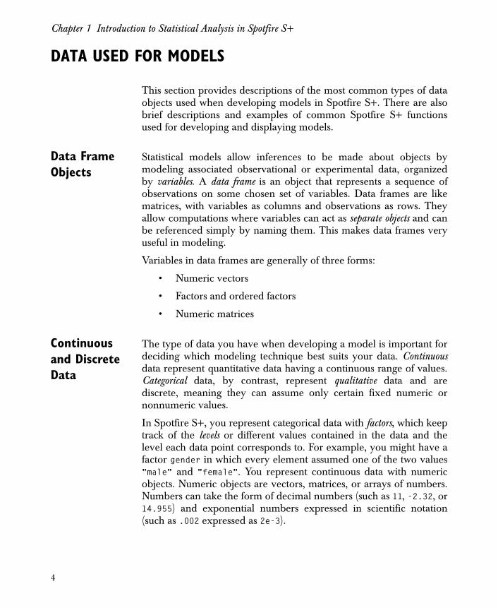
Data Frame Objects
Statistical models allow inferences to be made about objects bymodeling associated observational or experimental data, organizedby variables. A data frame is an object that represents a sequence ofobservations on some chosen set of variables. Data frames are likematrices, with variables as columns and observations as rows. Theyallow computations where variables can act as separate objects and canbe referenced simply by naming them. This makes data frames veryuseful in modeling.
Variables in data frames are generally of three forms:
• Numeric vectors
• Factors and ordered factors
• Numeric matrices
Continuous and Discrete Data
The type of data you have when developing a model is important fordeciding which modeling technique best suits your data. Continuousdata represent quantitative data having a continuous range of values.Categorical data, by contrast, represent qualitative data and arediscrete, meaning they can assume only certain fixed numeric ornonnumeric values.
In Spotfire S+, you represent categorical data with factors, which keeptrack of the levels or different values contained in the data and thelevel each data point corresponds to. For example, you might have afactor gender in which every element assumed one of the two values"male" and "female". You represent continuous data with numericobjects. Numeric objects are vectors, matrices, or arrays of numbers.Numbers can take the form of decimal numbers (such as 11, -2.32, or14.955) and exponential numbers expressed in scientific notation(such as .002 expressed as 2e-3).
4

Data Used for Models
A statistical model expresses a response variable as some function of aset of one or more predictor variables. The type of model you selectdepends on whether the response and predictor variables arecontinuous (numeric) or categorical (factor). For example, theclassical regression problem has a continuous response andcontinuous predictors, but the classical ANOVA problem has acontinuous response and categorical predictors.
Summaries and Plots for Examining Data
Before you fit a model, you should examine the data. Plots provideimportant information on mistakes, outliers, distributions, andrelationships between variables. Numerical summaries provide astatistical synopsis of the data in a tabular format.
Among the most common functions to use for generating plots andsummaries are the following:
• summary: provides a synopsis of an object. The following example displays a summary of the kyphosis data frame:
> summary(kyphosis)
Kyphosis Age Number Start absent:64 Min.: 1.00 Min.: 2.000 Min.: 1.00 present:17 1st Qu.: 26.00 1st Qu.: 3.000 1st Qu.: 9.00 Median: 87.00 Median: 4.000 Median:13.00 Mean: 83.65 Mean: 4.049 Mean:11.49 3rd Qu.:130.00 3rd Qu.: 5.000 3rd Qu.:16.00 Max.:206.00 Max.:10.000 Max.:18.00
• plot: a generic plotting function, plot produces different kinds of plots depending on the data passed to it. In its most common use, it produces a scatter plot of two numeric objects.
• hist: creates histograms.
• qqnorm: creates quantile-quantile plots.
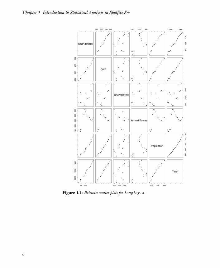
• pairs: creates, for multivariate data, a matrix of scatter plots showing each variable plotted against each of the other variables. To create the pairwise scatter plots for the data in the matrix longley.x, use pairs as follows:
> pairs(longley.x)
The resulting plot appears as in Figure 1.1.
5
Chapter 1 Introduction to Statistical Analysis in Spotfire S+
Figure 1.1: Pairwise scatter plots for longley.x.
GNP deflator
250 350 450 550
•
•• •
•• ••
••
••
• •• •
•
• ••
•••
••••
•••
••
150 250 350
•
• ••
•••
••••
•••• •
•
• ••
•• •• •
••
•• • • •
1950 1960
9010
011
0
•
• • •
•• • • •
••
•• • • •
250
350
450
550
••••
••••
••
• •
••••
GNP
•• •
•
••• •
••• •
••
••
•• •
•
••••
••••
•••
•
•• •
•
••
••••
• •
••
••
•• •
•
••
• ••
•• •
••
••
• •
••
•••
•
• • •
•
••
•
•
• •
••
•• •
•
• • •
•
• •
•
•
Unemployed
••
••
•••
•
•••
•
••
•
•
••
••
•• •
•
• • •
•
• •
•
•
200
300
400
• •
••
•• •
•
• • •
•
• •
•
•
150
200
250
300
350
••••
•
•••
•• •
• •••
•
••• •
•
• ••
•• •
• • ••
•
••
••
•
•••
•••
••• •
•
Armed Forces
••••
•
• ••
•• •
• • • •
•
••
• •
•
• ••
•• •
• • • •
•
• •••
•••••
••
•••••
• ••
•••••
••
••
•••
•
•••
••
••
••••
•••
••
••••
•••
••
••
••••
•
Population
110
115
120
125
130
• ••
••
••
••
••
••
••
•
90 100
1950
1955
1960
••••
•••••
••
•••••
•••
•••••
••
••
•••
•
200 300 400
••
••
•••
••••
•••
••
••
••
•••
••
••
••••
•
110 120 130
••••••
••••
•••
••
•
Year
6
Data Used for Models
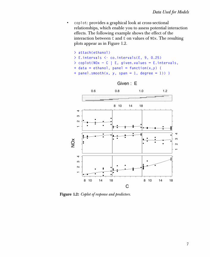
• coplot: provides a graphical look at cross-sectional relationships, which enable you to assess potential interaction effects. The following example shows the effect of the interaction between C and E on values of NOx. The resulting plots appear as in Figure 1.2.
> attach(ethanol)> E.intervals <- co.intervals(E, 9, 0.25)> coplot(NOx ~ C | E, given.values = E.intervals,+ data = ethanol, panel = function(x,y) { + panel.smooth(x, y, span = 1, degree = 1)) }
Figure 1.2: Coplot of response and predictors.
••
••
•••
• • • • •
•
8 10 14 18
12
34
•
•• •
••
•••• ••
••
•
••
•
•••••
•
•
8 10 14 18
•••••
•
•
•
• •• •• ••
••••
•••• •• •
•••
•• ••
•• •
••
•
12
34
••
•• ••
••
••••
12
34
•• • •• ••••
•• ••
8 10 14 18
•• • •••••• •• • •
0.6 0.8 1.0 1.2
C
NO
x
Given : E
7
Chapter 1 Introduction to Statistical Analysis in Spotfire S+
STATISTICAL MODELS IN SPOTFIRE S+
The development of statistical models is, in many ways, datadependent. The choice of the modeling technique you use depends onthe type and structure of your data and what you want the model totest or explain. A model may predict new responses, show generaltrends, or uncover underlying phenomena. This section gives generalselection criteria to help you develop a statistical model.
The fitting procedure for each model is based on a unified modelingparadigm in which:
• A data frame contains the data for the model.
• A formula object specifies the relationship between the response and predictor variables.
• The formula and data frame are passed to the fitting function.
• The fitting function returns a fit object.
There is a relatively small number of functions to help you fit andanalyze statistical models in Spotfire S+.
• Fitting models:
• lm: linear (regression) models.
• aov and varcomp: analysis of variance models.
• glm: generalized linear models.
• gam: generalized additive models.
• loess: local regression models.
• tree: tree models.
• Extracting information from a fitted object:
• fitted: returns fitted values.
• coefficients or coef: returns the coefficients (if present).
• residuals or resid: returns the residuals.
8

Statistical Models in Spotfire S+
• summary: provides a synopsis of the fit.
• anova: for a single fit object, produces a table with rows corresponding to each of the terms in the object, plus a row for residuals. If two or more fit objects are used as arguments, anova returns a table showing the tests for differences between the models, sequentially, from first to last.
• Plotting the fitted object:
• plot: plot a fitted object.
• qqnorm: produces a normal probability plot, frequently used in analysis of residuals.
• coplot: provides a graphical look at cross-sectional relationships for examining interaction effects.
• For minor modifications in a model, use the update function (adding and deleting variables, transforming the response, etc.).
• To compute the predicted response from the model, use the predict function.
The Unity of Models in Data Analysis
Because there is usually more than one way to model your data, youshould learn which type(s) of model are best suited to various types ofresponse and predictor data. When deciding on a modelingtechnique, it helps to ask: “What do I want the data to explain? Whathypothesis do I want to test? What am I trying to show?”
Some methods should or should not be used depending on whetherthe response and predictors are continuous, factors, or a combinationof both. Table 1.1 organizes the methods by the type of data they canhandle.
9

Chapter 1 Introduction to Statistical Analysis in Spotfire S+
Linear regression models a continuous response variable, y, as alinear combination of predictor variables xj, for j = 1,...,p. For a singlepredictor, the data fit by a linear model scatter about a straight line orcurve. A linear regression model has the mathematical form
,
where ε i, referred to, generally, as the error, is the difference betweenthe ith observation and the model. On average, for given values of thepredictors, you predict the response best with the following equation:
.
Analysis of variance models are also linear models, but all predictorsare categorical, which contrasts with the typically continuouspredictors of regression. For designed experiments, use analysis ofvariance to estimate and test for effects due to the factor predictors.For example, consider the catalyst data frame, which contains thedata below.
Table 1.1: Criteria for developing models.
Model Response Predictors
lm Continuous Both
aov Continuous Factors
glm Both Both
gam Both Both
loess Continuous Both
tree Both Both
yi β0 βjxijj 1=
p
∑ ε i+ +=
y β0 βjxjj 1=
p
∑+=
10

Statistical Models in Spotfire S+
> catalyst
Temp Conc Cat Yield 1 160 20 A 602 180 20 A 723 160 40 A 544 180 40 A 685 160 20 B 526 180 20 B 837 160 40 B 458 180 40 B 80
Each of the predictor terms, Temp, Conc, and Cat, is a factor with twopossible levels, and the response term, Yield, contains numeric data.Use analysis of variance to estimate and test for the effect of thepredictors on the response.
Linear models produce estimates with good statistical propertieswhen the relationships are, in fact, linear, and the errors are normallydistributed. In some cases, when the distribution of the response isskewed, you can transform the response, using, for example, squareroot, logarithm, or reciprocal transformations, and produce a betterfit. In other cases, you may need to include polynomial terms of thepredictors in the model. However, if linearity or normality does nothold, or if the variance of the observations is not constant, andtransformations of the response and predictors do not help, youshould explore other techniques such as generalized linear models,generalized additive models, or classification and regression trees.
Generalized linear models assume a transformation of the expected (oraverage) response is a linear function of the predictors, and thevariance of the response is a function of the mean response:
.
Generalized linear models, fitted using the glm function, allow you tomodel data with distributions including normal, binomial, Poisson,gamma, and inverse normal, but still require a linear relationship inthe parameters.
η E y( )( ) β0 βjxjj 1=
p
∑+=
VAR y( ) φV μ( )=
11
Chapter 1 Introduction to Statistical Analysis in Spotfire S+
When the linear fit provided by glm does not produce a good fit, analternative is the generalized additive model, fit with the gam function.In contrast to glm, gam allows you to fit nonlinear data-dependentfunctions of the predictors. The mathematical form of a generalizedadditive model is:
where the fj term represents functions to be estimated from the data.The form of the model assumes a low-dimensional additive structure.That is, the pieces represented by functions, fi, of each predictoradded together predict the response without interaction.
In the presence of interactions, if the response is continuous and theerrors about the fit are normally distributed, local regression (or loess)models, allow you to fit a multivariate function which includeinteraction relationships. The form of the model is:
where g represents the regression surface.
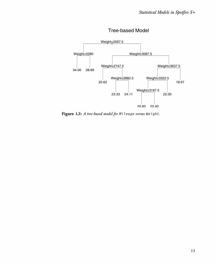
Tree-based models have gained in popularity because of theirflexibility in fitting all types of data. Tree models are generally usedfor exploratory analysis. They allow you to study the structure ofdata, creating nodes or clusters of data with similar characteristics.The variance of the data within each node is relatively small, since thecharacteristics of the contained data is similar. The following exampledisplays a tree-based model using the data frame car.test.frame:
> car.tree <- tree(Mileage ~ Weight, car.test.frame)> plot(car.tree, type = "u")> text(car.tree)> title("Tree-based Model")
The resulting plot appears as in Figure 1.3.
η E y( )( ) fj xj( )j 1=
p
∑=
yi g xi1 xi2 … xip, , ,( ) ε i+=
12
Statistical Models in Spotfire S+
Figure 1.3: A tree-based model for Mileage versus Weight.
|Weight<2567.5
Weight<2280 Weight<3087.5
Weight<2747.5
Weight<2882.5
Weight<3637.5
Weight<3322.5
Weight<3197.5
34.00 28.89
25.62
23.33 24.11
20.60 20.40
22.00
18.67
Tree-based Model
13
Chapter 1 Introduction to Statistical Analysis in Spotfire S+
EXAMPLE OF DATA ANALYSIS
The example that follows describes only one way of analyzing datathrough the use of statistical modeling. There is no perfect cookbookapproach to building models, as different techniques do differentthings, and not all of them use the same arguments when doing theactual fitting.
The Iterative Process of Model Building
As discussed at the beginning of this chapter, there are some generalsteps you can take when building a model:
1. Determine the variables to observe. In a study involving a classical modeling approach, these variables correspond directly to the hypothesis being tested. For data-driven modeling, these variables are the link to the phenomena being modeled.
2. Collect and record the data observations.
3. Study graphics and summaries of the collected data to discover and remove mistakes and to reveal low-dimensional relationships between variables.
4. Choose a model describing the important relationships seen or hypothesized in the data.
5. Fit the model using the appropriate modeling technique.
6. Examine the fit through model summaries and diagnostic plots.
7. Repeat steps 4–6 until you are satisfied with the model.
At any point in the modeling process, you may find that your choiceof model does not appropriately fit the data. In some cases, diagnosticplots may give you clues to improve the fit. Sometimes you may needto try transformed variables or entirely different variables. You mayneed to try a different modeling technique that will, for example,allow you to fit nonlinear relationships, interactions, or different errorstructures. At times, all you need to do is remove outlying, influentialdata, or fit the model robustly. A point to remember is that there is noone answer on how to build good statistical models. By iterativelyfitting, plotting, testing, changing, and then refitting, you arrive at thebest model for your data.
14
Example of Data Analysis
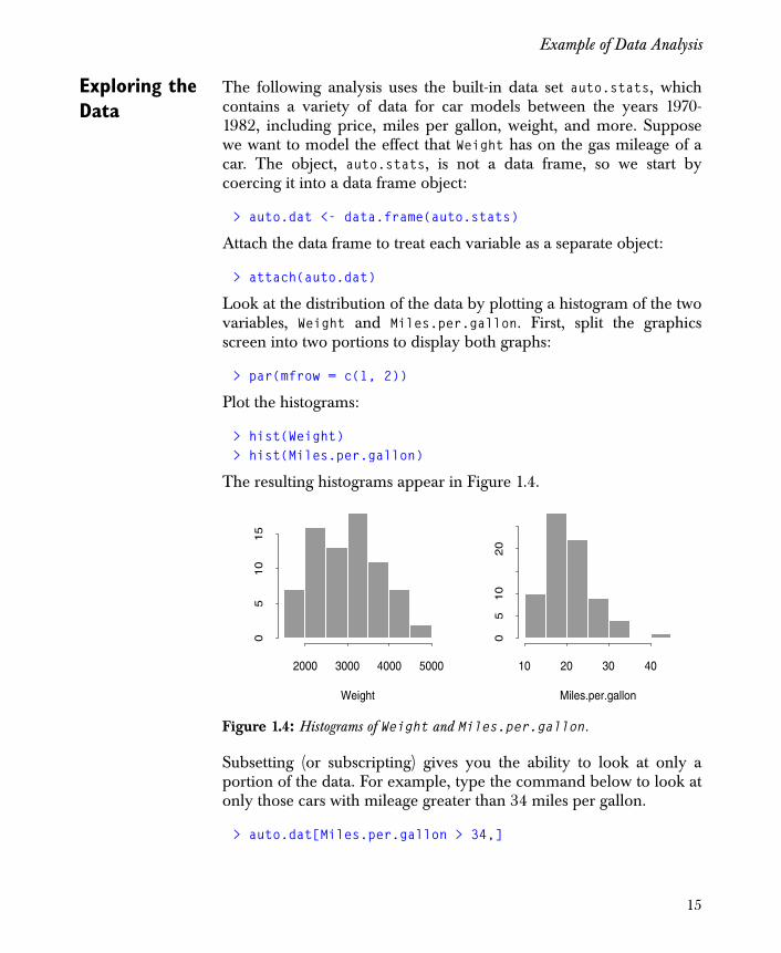
Exploring the Data
The following analysis uses the built-in data set auto.stats, whichcontains a variety of data for car models between the years 1970-1982, including price, miles per gallon, weight, and more. Supposewe want to model the effect that Weight has on the gas mileage of acar. The object, auto.stats, is not a data frame, so we start bycoercing it into a data frame object:
> auto.dat <- data.frame(auto.stats)
Attach the data frame to treat each variable as a separate object:
> attach(auto.dat)
Look at the distribution of the data by plotting a histogram of the twovariables, Weight and Miles.per.gallon. First, split the graphicsscreen into two portions to display both graphs:
> par(mfrow = c(1, 2))
Plot the histograms:
> hist(Weight)> hist(Miles.per.gallon)
The resulting histograms appear in Figure 1.4.
Subsetting (or subscripting) gives you the ability to look at only aportion of the data. For example, type the command below to look atonly those cars with mileage greater than 34 miles per gallon.
> auto.dat[Miles.per.gallon > 34,]
Figure 1.4: Histograms of Weight and Miles.per.gallon.
2000 3000 4000 5000
05
10
15
Weight
10 20 30 40
05
10
20
Miles.per.gallon
15

Chapter 1 Introduction to Statistical Analysis in Spotfire S+
Price Miles.per.gallon Repair (1978) Datsun 210 4589 35 5 Subaru 3798 35 5Volk Rabbit(d) 5397 41 5
Repair (1977) Headroom Rear.Seat Trunk Weight Datsun 210 5 2.0 23.5 8 2020 Subaru 4 2.5 25.5 11 2050Volk Rabbit(d) 4 3.0 25.5 15 2040 Length Turning.Circle Displacement Gear.Ratio Datsun 210 165 32 85 3.70 Subaru 164 36 97 3.81Volk Rabbit(d) 155 35 90 3.78
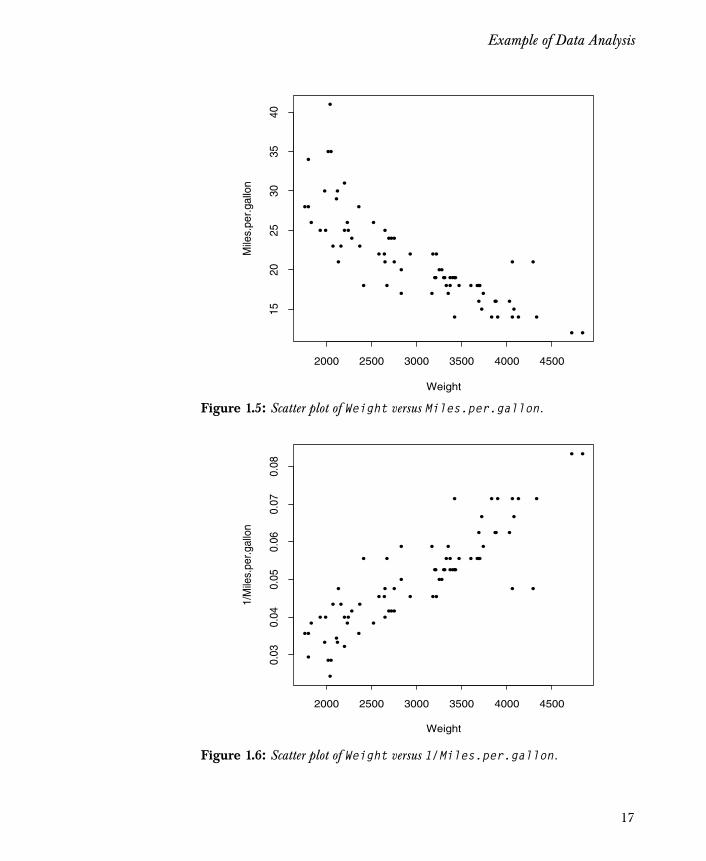
Suppose you want to predict the gas mileage of a particular autobased upon its weight. Create a scatter plot of Weight versusMiles.per.gallon to examine the relationship between the variables.First, reset the graphics window to display only one graph, and thencreate the scatter plot:
> par(mfrow = c(1,1))> plot(Weight, Miles.per.gallon)
The plot appears in Figure 1.5. The figure displays a curved scatteringof the data, which might suggest a nonlinear relationship. Create aplot from a different perspective, giving gallons per mile (1/Miles.per.gallon) as the vertical axis:
> plot(Weight, 1/Miles.per.gallon)
The resulting scatter plot appears in Figure 1.6.
16
Example of Data Analysis
Figure 1.5: Scatter plot of Weight versus Miles.per.gallon.
Figure 1.6: Scatter plot of Weight versus 1/Miles.per.gallon.
•
•
•
•
•
•
•
•
•
•
•
•
•
••
•
•
•
••
•
•
•
•
•
•
•
•
••
•
•
•
•
•
••
•
•
•
• ••
•
••
•••
•
•
•
•
•
•
••
• •••• •
•
•
•
•
•
•
•
•
•
•
•
Weight
Mile
s.pe
r.ga
llon
2000 2500 3000 3500 4000 4500
1520
2530
3540
•
•
•
•
••
•
•
•
•
•
•
•
••
•
•
•
•••
•
•
•
•
•
•
•
••
•
•
•
•
•
••
•
•
•
• •
•
•
••
•••
•
•
•
•
•
•
• •
• •••• •
••
•
•
•
•
•
•
••
•
Weight
1/M
iles.
per.g
allo
n
2000 2500 3000 3500 4000 4500
0.03
0.04
0.05
0.06
0.07
0.08
17
Chapter 1 Introduction to Statistical Analysis in Spotfire S+
Fitting the Model
Gallons per mile is more linear with respect to weight, suggesting thatyou can fit a linear model to Weight and 1/Miles.per.gallon. Theformula 1/Miles.per.gallon ~ Weight describes this model. Fit themodel by using the lm function, and name the fitted object fit1:
> fit1 <- lm(1/Miles.per.gallon ~ Weight)
As with any Spotfire S+ object, when you type the name, fit1,Spotfire S+ prints the object. In this case, Spotfire S+ uses the specificprint method for lm objects:
> fit1
Call:lm(formula = 1/Miles.per.gallon ~ Weight)
Coefficients: (Intercept) Weight 0.007447302 1.419734e-05Degrees of freedom: 74 total; 72 residualResidual standard error: 0.006363808
Plot the regression line to see how well it fits the data. The resultingline appears in Figure 1.7.
> abline(fit1)
18

Example of Data Analysis
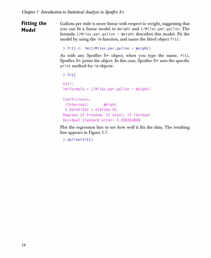
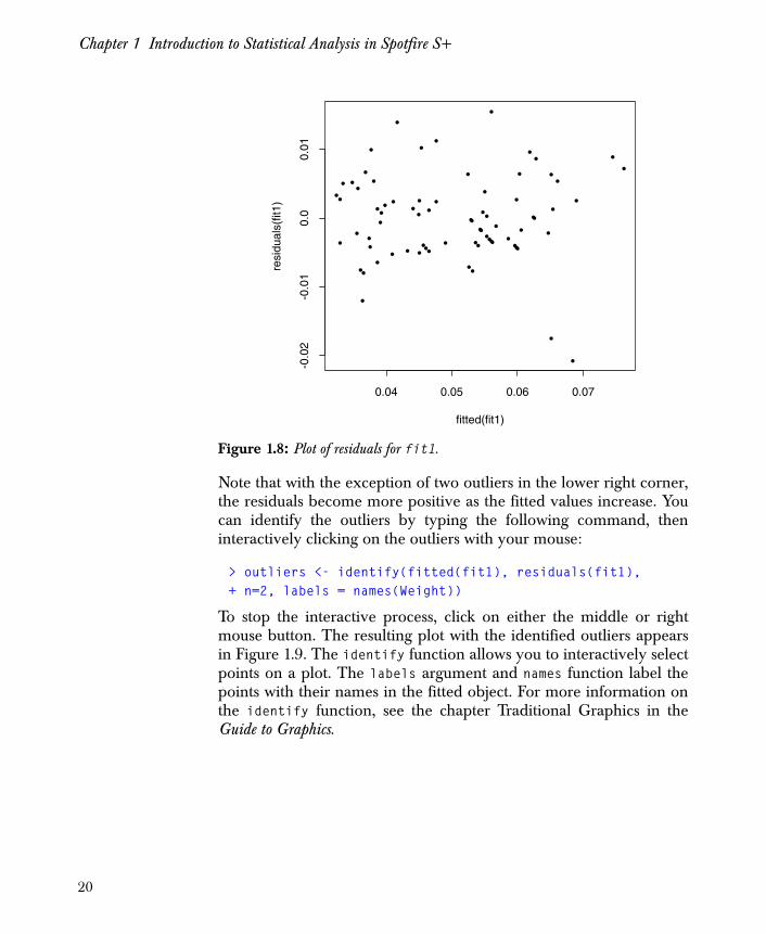
Judging from Figure 1.7, the regression line does not fit well in theupper range of Weight. Plot the residuals versus the fitted values to seemore clearly where the model does not fit well.
> plot(fitted(fit1), residuals(fit1))
The plot appears as in Figure 1.8.
Figure 1.7: Regression line of fit1.
•
•
•
•
••
•
•
•
•
•
•
•
••
•
•
•
•••
•
•
•
•
•
•
•
••
•
•
•
•
•
••
•
•
•
• •
•
•
••
•••
•
•
•
•
•
•
• •
• •••• •
••
•
•
•
•
•
•
••
•
Weight
1/M
iles.
per.
gallo
n
2000 2500 3000 3500 4000 4500
0.03
0.04
0.05
0.06
0.07
0.08
19
Chapter 1 Introduction to Statistical Analysis in Spotfire S+
Note that with the exception of two outliers in the lower right corner,the residuals become more positive as the fitted values increase. Youcan identify the outliers by typing the following command, theninteractively clicking on the outliers with your mouse:
> outliers <- identify(fitted(fit1), residuals(fit1),+ n=2, labels = names(Weight))
To stop the interactive process, click on either the middle or rightmouse button. The resulting plot with the identified outliers appearsin Figure 1.9. The identify function allows you to interactively selectpoints on a plot. The labels argument and names function label thepoints with their names in the fitted object. For more information onthe identify function, see the chapter Traditional Graphics in theGuide to Graphics.
Figure 1.8: Plot of residuals for fit1.
•
•
•
•
•
••
•
•
•
•
•
•
•
•
•
•
•
••
••
•
•
• •
••
••
•
• ••
•
•••
•
•
• ••
••
•
••
••
••
•
••
•
•
•
•
•••
••
•
•
•
•
•
•
•
••
•
fitted(fit1)
resi
dual
s(fit
1)
0.04 0.05 0.06 0.07
-0.0
2-0
.01
0.0
0.01
20

Example of Data Analysis
The outliers in Figure 1.9 correspond to cars with better gas mileagethan other cars in the study with similar weights. You can remove theoutliers using the subset argument to lm.
> fit2 <- lm(1/Miles.per.gallon ~ Weight,+ subset = -outliers)
Plot Weight versus 1/Miles.per.gallon with two regression lines:one for the fit1 object and one for the fit2 object. Use the ltygraphics parameter to differentiate between the regression lines:
> plot(Weight, 1/Miles.per.gallon)> abline(fit1, lty=2)> abline(fit2)
The two lines appear with the data in Figure 1.10.
A plot of the residuals versus the fitted values shows a better fit. Theplot appears in Figure 1.11.
> plot(fitted(fit2), residuals(fit2))
Figure 1.9: Plot with labeled outliers.
•
•
•
•
•
••
•
•
•
•
•
•
•
•
•
•
•
••
••
•
•
• •
••
••
•
• ••
•
•••
•
•
• ••
••
•
••
••
••
•
••
•
•
•
•
•••
••
•
•
•
•
•
•
•
••
•
fitted(fit1)
resi
dual
s(fit
1)
0.04 0.05 0.06 0.07
-0.0
2-0
.01
0.0
0.01
Olds 98
Cad. Seville
21

Chapter 1 Introduction to Statistical Analysis in Spotfire S+
Figure 1.10: Regression lines of fit1 versus fit2.
Figure 1.11: Plot of residuals for fit2.
•
•
•
•
••
•
•
•
•
•
•
•
••
•
•
•
•••
•
•
•
•
•
•
•
••
•
•
•
•
•
••
•
•
•
• •
•
•
••
•••
•
•
•
•
•
•
• •
• •••• •
••
•
•
•
•
•
•
••
•
Weight
1/M
iles.
per.g
allo
n
2000 2500 3000 3500 4000 4500
0.03
0.04
0.05
0.06
0.07
0.08
•
•
•
•
•
••
•
•
•
•
•
•
•
•
•
•
••
• •
•
•
••
• •
••
•
••
•
• •
••
•
•
••
•
•
•
••
•
••
•
•
•
•
•
•
•
•
•••
••
•
•
•
•
•
•
•
•• •
fitted(fit2)
resi
dual
s(fit
2)
0.03 0.04 0.05 0.06 0.07 0.08
-0.0
100.
00.
005
0.01
00.
015
22

Example of Data Analysis
To see a synopsis of the fit contained in fit2, use summary as follows:
> summary(fit2)
Call: lm(formula = 1/Miles.per.gallon ~ Weight,subset = - outliers)Residuals: Min 1Q Median 3Q Max -0.01152 -0.004257 -0.0008586 0.003686 0.01441
Coefficients: Value Std. Error t value Pr(>|t|)(Intercept) 0.0047 0.0026 1.8103 0.0745 Weight 0.0000 0.0000 18.0625 0.0000
Residual standard error: 0.00549 on 70 degrees of freedom Multiple R-squared: 0.8233F-statistic: 326.3 on 1 and 70 degrees of freedom, the p-value is 0Correlation of Coefficients: (Intercept)Weight -0.9686
The summary displays information on the spread of the residuals,coefficients, standard errors, and tests of significance for each of thevariables in the model (which includes an intercept by default). Inaddition, the summary displays overall regression statistics for the fit.As expected, Weight is a very significant predictor of 1/Miles.per.gallon. The amount of the variability of 1/Miles.per.gallon explained by Weight is about 82%, and theresidual standard error is .0055, down about 14% from that of fit1.
To see the individual coefficients for fit2, use coef as follows:
> coef(fit2)
(Intercept) Weight 0.004713079 1.529348e-05
23
Chapter 1 Introduction to Statistical Analysis in Spotfire S+
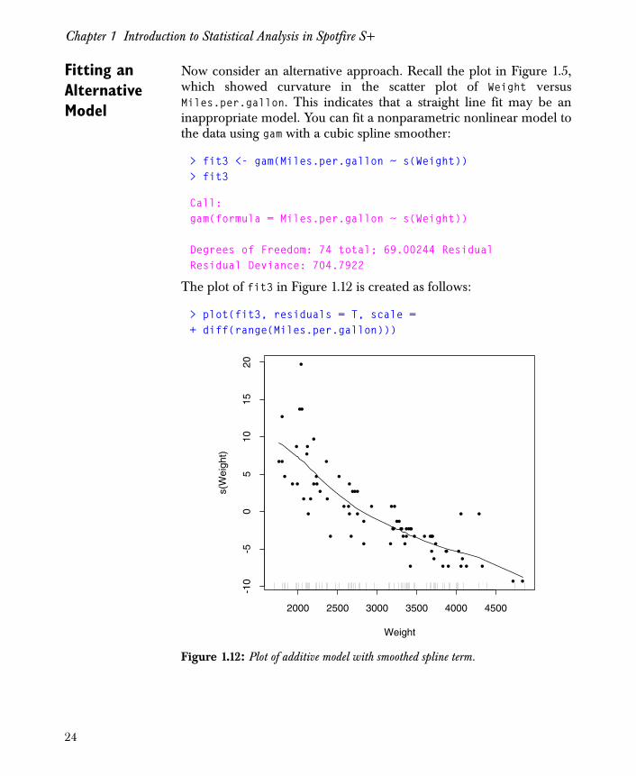
Fitting an Alternative Model
Now consider an alternative approach. Recall the plot in Figure 1.5,which showed curvature in the scatter plot of Weight versusMiles.per.gallon. This indicates that a straight line fit may be aninappropriate model. You can fit a nonparametric nonlinear model tothe data using gam with a cubic spline smoother:
> fit3 <- gam(Miles.per.gallon ~ s(Weight))> fit3
Call:gam(formula = Miles.per.gallon ~ s(Weight))
Degrees of Freedom: 74 total; 69.00244 ResidualResidual Deviance: 704.7922
The plot of fit3 in Figure 1.12 is created as follows:
> plot(fit3, residuals = T, scale =+ diff(range(Miles.per.gallon)))
Figure 1.12: Plot of additive model with smoothed spline term.
Weight
s(W
eigh
t)
2000 2500 3000 3500 4000 4500
-10
-50
510
1520
•
•
•
•
•
•
•
•
•
•
•
•
•
••
•
•
•
••
•
•
•
•
•
•
•
•
••
•
•
•
•
•
••
•
•
•
• ••
•
••
•••
•
•
•
•
•
•
••
• •••• •
•
•
•
•
•
•
•
•
•
•
•
24

Example of Data Analysis
The cubic spline smoother in the plot appears to give a good fit to thedata. You can check the fit with diagnostic plots of the residuals as wedid for the linear models. You should also compare the gam modelwith a linear model using aov to produce a statistical test.
Use the predict function to make predictions from models. Thenewdata argument to predict specifies a data frame containing thevalues at which the predictions are required. If newdata is notsupplied, the predict function makes predictions at the dataoriginally supplied to fit the gam model, as in the following example:
> predict.fit3 <- predict(fit3)
Create a new object predict.high and print it to display cars withpredicted miles per gallon greater than 30:
> predict.high <- predict.fit3[predict.fit3 > 30]> predict.high
Ford Fiesta Honda Civic Plym Champ 30.17946 30.49947 30.17946
Conclusions The previous example shows a few simple methods for taking dataand iteratively fitting models until the desired results are achieved.The chapters that follow discuss in far greater detail the modelingtechniques mentioned in this section. Before proceeding further, it isgood to remember that:
• General formulas define the structure of models.
• Data used in model-fitting are generally in the form of data frames.
• Different methods can be used on the same data.
• A variety of functions are available for diagnostic study of the fitted models.
• The Spotfire S+ functions, like model-fitting in general, are designed to be very flexible for users. Handling different preferences and procedures in model-fitting are what make Spotfire S+ very effective for data analysis.
25

Chapter 1 Introduction to Statistical Analysis in Spotfire S+
26
Introduction 28
Basic Formulas 29Continuous Data 30Categorical Data 30General Formula Syntax 31
Interactions 32Continuous Data 33Categorical Data 33Nesting 33Interactions Between Continuous and Categorical
Variables 34
The Period Operator 36
Combining Formulas with Fitting Procedures 37The data Argument 37Composite Terms in Formulas 38
Contrasts: The Coding of Factors 39Built-In Contrasts 39Specifying Contrasts 41
Useful Functions for Model Fitting 44
Optional Arguments to Model-Fitting Functions 46
References 48
SPECIFYING MODELS IN SPOTFIRE S+ 2
27

Chapter 2 Specifying Models in Spotfire S+
INTRODUCTION
Models are specified in TIBCO Spotfire S+ using formulas, whichexpress the conjectured relationships between observed variables in anatural way. Formulas specify models for the wide variety ofmodeling techniques available in Spotfire S+. You can use the sameformula to specify a model for linear regression (lm), analysis ofvariance (aov), generalized linear modeling (glm), generalizedadditive modeling (gam), local regression (loess), and tree-basedregression (tree).
For example, consider the following formula:
mpg ~ weight + displ
This formula can specify a least squares regression with mpg regressedon two predictors, weight and displ, or a generalized additive modelwith purely linear effects. You can also specify smoothed fits forweight and displ in the generalized additive model as follows:
mpg ~ s(weight) + s(displ)
You can then compare the resulting fit with the purely linear fit to seeif some nonlinear structure must be built into the model.
Formulas provide the means for you to specify models for allmodeling techniques: parametric or nonparametric, classical ormodern. This chapter provides you with an introduction to the syntaxused for specifying statistical models. The chapters that follow makeuse of this syntax in a wide variety of specific examples.
28
Basic Formulas
BASIC FORMULAS
A formula is a Spotfire S+ expression that specifies the form of amodel in terms of the variables involved. For example, to specify thatmpg is modeled as a linear model of the two predictors weight anddispl, use the following formula:
mpg ~ weight + displ
The tilde (~) character separates the response variable from theexplanatory variables. For something to be interpreted as a variable,it must be one of the following:
• Numeric vector, for continuous data
• Factor or ordered factor, for categorical data
• Matrix
For each numeric vector in a model, Spotfire S+ fits one coefficient.For each matrix, Spotfire S+ fits one coefficient for each column. Forfactors, the equivalent of one coefficient is fit for each level of thefactor; see the section Contrasts: The Coding of Factors on page 39for more details.
If your data set includes a character variable, you should convert it toa factor before including it in a model formula. You can do this withthe factor function, as follows:
> test.char <- c(rep("Green",2), rep("Blue",2),+ rep("Red",2))> test.char[1] "Green" "Green" "Blue" "Blue" "Red" "Red"
> data.class(test.char)[1] "character"
> test.fac <- factor(test.char)> test.fac[1] Green Green Blue Blue Red Red
29

Chapter 2 Specifying Models in Spotfire S+
> data.class(test.fac)[1] "factor"
> levels(test.fac)[1] "Blue" "Green" "Red"
You can use any acceptable Spotfire S+ expression in place of avariable, provided the expression evaluates to somethinginterpretable as one or more variables. Thus, the formula
log(mpg) ~ weight + poly(displ, 2)
specifies that the natural logarithm of mpg is modeled as a linearfunction of weight and a quadratic polynomial of displ.
Continuous Data
Each continuous variable you provide in a formula generates onecoefficient in the fitted model. Thus, the formula
mpg ~ weight + displ
fits the model
mpg = β0 + β1 weight + β2 displ + ε
Implicitly, a Spotfire S+ formula always includes an intercept term,which is β0 in the above formula. You can, however, remove theintercept by specifying the model with -1 as an explicit predictor:
mpg ~ -1 + weight + displ
Similarly, you can include an intercept by including +1 as anexplicitly predictor.
When you provide a numeric matrix as one term in a formula,Spotfire S+ interprets each column of the matrix as a separatevariable in the model. Any names associated with the columns arecarried along as labels in the subsequent fits.
Categorical Data
When you specify categorical variables (factors or ordered factors) aspredictors in formulas, the modeling functions fit the equivalent of acoefficient for each level of the variable. For example, to modelsalary as a linear function of age (continuous) and gender (factor),specify the following formula:
salary ~ age + gender
30
Basic Formulas
Different parameters are computed for the two levels of gender. Thisis equivalent to fitting two dummy variables: one for males and one forfemales. Thus, you need not create and specify dummy variables inthe model.
Although multiple dummy variables are returned, only oneadditional parameter is computed for each factor variable in aformula. This because the parameters are not independent of theintercept term; more details are provided in the section Contrasts:The Coding of Factors.
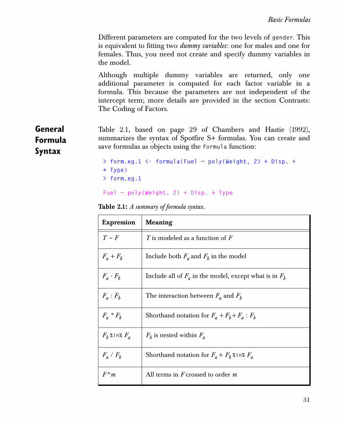
General Formula Syntax
Table 2.1, based on page 29 of Chambers and Hastie (1992),summarizes the syntax of Spotfire S+ formulas. You can create andsave formulas as objects using the formula function:
> form.eg.1 <- formula(Fuel ~ poly(Weight, 2) + Disp. ++ Type)> form.eg.1
Fuel ~ poly(Weight, 2) + Disp. + Type
Table 2.1: A summary of formula syntax.
Expression Meaning
T ~ F T is modeled as a function of F
Fa + Fb Include both Fa and Fb in the model
Fa - Fb Include all of Fa in the model, except what is in Fb
Fa : Fb The interaction between Fa and Fb
Fa * Fb Shorthand notation for Fa + Fb+ Fa : Fb
Fb %in% Fa Fb is nested within Fa
Fa / Fb Shorthand notation for Fa + Fb %in% Fa
F^m All terms in F crossed to order m
31

Chapter 2 Specifying Models in Spotfire S+
INTERACTIONS
You can specify interactions for categorical data (factors), continuousdata, or a mixture of the two. In each case, additional parameters arecomputed that are appropriate for the different types of variablesspecified in the model. The syntax for specifying an interaction is thesame in each case, but the interpretation varies depending on the datatypes.
To specify a particular interaction between two or more variables, usea colon (:) between the variable names. Thus, to specify theinteraction between gender and race, use the following term:
gender:race
You can use an asterisk (*) to specify all terms in the model createdby subsets of the named variables. Thus,
salary ~ age * gender
is equivalent to
salary ~ age + gender + age:gender
You can remove terms with a minus or hyphen (-). For example, theformula
salary ~ gender*race*education - gender:race:education
is equivalent to
salary ~ gender + race + education + gender:race + gender:education + race:education
This is a model consisting of all terms in the full model except thethree-way interaction. Another way to specify this model is by usingthe power notation. The following formula includes all terms of ordertwo or less:
salary ~ (gender + race + education) ^ 2
32

Interactions
Continuous Data
By specifying interactions between continuous variables in a formula,you include multiplicative terms in the corresponding model. Thus,the formula
mpg ~ weight * displ
fits the model
mpg = β0 + β1weight + β2displ + β3(weight)(displ) + ε
Categorical Data
For categorical data, interactions add coefficients for eachcombination of the levels in the named factors. For example, considertwo factors, Opening and Mask, with three and five levels, respectively.The Opening:Mask term in a formula adds 15 additional parameters tothe model. For example, you can specify a two-way analysis ofvariance with the following notation:
skips ~ Opening + Mask + Opening:Mask
Using the asterisk operator *, this simplifies to:
skips ~ Opening*Mask
Either formula fits the following model:
skips = μ + Openingi + Maskj + (Opening : Mask)ij + ε
In practice, because of dependencies among the parameters, onlysome of the total number of parameters specified by a model arecomputed.
Nesting Nesting arises in models when the levels of one or more factors makesense only within the levels of other factors. For example, in samplingthe U.S. population, a sample of states is drawn, from which a sampleof counties is drawn, from which a sample of cities is drawn, fromwhich a sample of families or households is drawn. Counties arenested within states, cities are nested within counties, and householdsare nested within cities.
33

Chapter 2 Specifying Models in Spotfire S+
In Spotfire S+ formulas, there is special syntax to specify the nestingof factors within other factors. For example, you can write the county-within-state model using the term
county %in% state
You can state the model more succinctly with
state / county
This syntax means “state and county within state,” and is thusequivalent to the following formula terms:
state + county %in% state
The slash operator (/) in nested models is the counterpart of theasterisk (*), which is used for factorial models; see the previous sectionfor examples of formulas for factorial models.
The syntax for nested models can be extended to included multiplelevels of nesting. For example, you can specify the full state-county-city-household model as follows:
state / county / city / household
Interactions Between Continuous and Categorical Variables
For continuous data combined with categorical data, interactions addone coefficient for the continuous variable for each level of thecategorical variable. This arises, for example, in models that havedifferent slope estimates for different groups, where the categoricalvariables specify the groups.
When you combine continuous and categorical data using the nestingsyntax, it is possible to specify analysis of covariance models. Forexample, suppose gender (categorical) and age (continuous) arepredictors in a model. You can fit separate slopes for each genderusing the following nesting syntax:
salary ~ gender / age
This fits an analysis of covariance model equivalent to:
μ + genderi + βi age
Note that this is also equivalent to a model with the term gender*age.However, the parametrization for the two models is different. Whenyou fit the nested model, Spotfire S+ computes estimates of the
34

Interactions
individual slopes for each group. When you fit the factorial model,you obtain an overall slope estimate plus the deviations in the slopefor the different group contrasts.
For example, with the term gender/age, the formula expands intomain effects for gender followed by age within each level of gender.One coefficient is computed for age from each level of gender, andanother coefficient estimates the contrast between the two levels ofgender. Thus, the nested formula fits the following type of model:
The intercept is μ, the contrast is , and the model has coefficients βifor age within each level of gender. Thus, you obtain separate slopeestimates for each group.
Conversely, the formula with the term gender*age fits the followingmodel:
You obtain the overall slope estimate , plus the deviations in theslope for the different group contrasts.
You can fit the equal slope, separate intercept model by specifying:
salary ~ gender + age
This fits a model equivalent to:
SalaryM μ αg β1 age×+ +=
SalaryF μ αg– β2 age×+=
αg
SalaryM μ αg– β age γ age×–×+=
SalaryF μ αg β age γ age×+×+ +=
β
μ genderi β age×+ +
35

Chapter 2 Specifying Models in Spotfire S+
THE PERIOD OPERATOR
The single period (.) operator can act as a default left or right side of aformula. There are numerous ways you can use periods in formulas.For example, consider the function update, which allows you tomodify existing models. The following example uses the data framefuel.frame to display the usage of the single “.” in formulas. First, wedefine a model that includes only an intercept term:
> fuel.null <- lm(Fuel ~ 1, data = fuel.frame)
Next, we use update to add the Weight variable to the model:
> fuel.wt <- update(fuel.null, . ~ . + Weight)> fuel.wt
Call:lm(formula = Fuel ~ Weight, data = fuel.frame)
Coefficients: (Intercept) Weight 0.3914324 0.00131638Degrees of freedom: 60 total; 58 residualResidual standard error: 0.3877015
The periods on either side of the tilde (~) in the above example arereplaced by the left and right sides of the formula used to fit the objectfuel.null.
Another use of the period operator arises when referencing dataframe objects in formulas. In the following example, we fit a linearmodel for the data frame fuel.frame:
> lm(Fuel ~ ., data = fuel.frame)
Here, the new model includes all columns in fuel.frame aspredictors, with the exception of the response variable Fuel. In theexample
> lm(skips ~ .^2, data = solder.balance)
all columns in solder.balance enter the model as both main effectsand second-order interactions.
36

Combining Formulas with Fitting Procedures
COMBINING FORMULAS WITH FITTING PROCEDURES
The data Argument
Once you specify a model with its associated formula, you can fit it toa given data set by passing the formula and the data to theappropriate fitting procedure. For the following example, create thedata frame auto.dat from the data set auto.stats by typing
> auto.dat <- data.frame(auto.stats)
The auto.dat data frame contains numeric columns namedMiles.per.gallon, Weight, and Displacement, among others. Youcan fit a linear model using these three columns as follows:
> lm(Miles.per.gallon ~ Weight + Displacement, + data = auto.dat)
You can fit a smoothed model to the same data with the call:
> loess(Miles.per.gallon ~ s(Weight) + s(Displacement),+ data = auto.dat)
All Spotfire S+ fitting procedures accept a formula and an optionaldata frame as the first two arguments. If the individual variables are inyour search path, you can omit the data specification:
> lm(Miles.per.gallon ~ Weight + Displacement)> loess(Miles.per.gallon ~ s(Weight) + s(Displacement))
This occurs, for example, when you create the variables explicitly inyour working directory, or when you attach a data frame to yoursearch path using the attach function.
Warning
If you attach a data frame for fitting models and have objects in your .Data directory with names that match those in the data frame, the data frame variables are masked and are not used in the actual model fitting. For more details, see the help file for the masked function.
37

Chapter 2 Specifying Models in Spotfire S+
Composite Terms in Formulas
As we previously mention, certain operators such as +, -, *, and /have special meanings when used in formula expressions. Because ofthis, the operators must appear at the top level in a formula and onlyon the right side of the tilde (~). However, if the operators appearwithin arguments to functions in the formula, they work as theynormally do in Spotfire S+. For example:
Kyphosis ~ poly(Age, 2) + I((Start > 12) * (Start - 12))
Here, the * and - operators appear within arguments to the Ifunction, and thus evaluate as normal arithmetic operators. The solepurpose of the I function is, in fact, to protect special operators on theright sides of formulas.
You can use any acceptable Spotfire S+ expression in place of anyvariable within a formula, provided the expression evaluates tosomething interpretable as one or more variables. The expressionmust evaluate to one of the following:
• Numeric vector
• Factor or ordered factor
• Matrix
Thus, certain composite terms, including poly, I, and bs, can be usedas formula variables. For details, see the help files for these functions.
38

Contrasts: The Coding of Factors
CONTRASTS: THE CODING OF FACTORS
A coefficient for each level of a factor cannot usually be estimatedbecause of dependencies among the coefficients in the overall model.An example of this is the sum of all dummy variables for a factor, whichis a vector of all ones that has length equal to the number of levels inthe factor. Overparameterization induced by dummy variables isremoved prior to fitting, by replacing the dummy variables with a setof linear combinations of the dummy variables, which are
1. functionally independent of each other, and
2. functionally independent of the sum of the dummy variables.
A factor with levels has possible independent linearcombinations. A particular choice of linear combinations of thedummy variables is called a set of contrasts. Any choice of contrasts fora factor alters the specific individual coefficients in the model, butdoes not change the overall contribution of the factor to the fit.Contrasts are represented in Spotfire S+ as matrices in which thecolumns sum to zero, and the columns are linearly independent ofboth each other and a vector of all ones.
Built-In Contrasts
Spotfire S+ provides four different kinds of contrasts as built-infunctions
1. Treatment contrasts
The default setting in Spotfire S+ options. The function contr.treatment implements treatment contrasts. Note that these are not true contrasts, but simply include each level of a factor as a dummy variable, excluding the first one. This generates statistically dependent coefficients, even in balanced experiments.
> contr.treatment(4)
2 3 41 0 0 02 1 0 03 0 1 04 0 0 1
2. Helmert contrasts
k k 1–
39

Chapter 2 Specifying Models in Spotfire S+
The function contr.helmert implements Helmert contrasts. The th linear combination is the difference between the
st level and the average of the first levels. The following example returns a Helmert parametrization based upon four levels:
> contr.helmert(4)
[,1] [,2] [,3]1 -1 -1 -12 1 -1 -13 0 2 -14 0 0 3
3. Orthogonal polynomials
The function contr.poly implements polynomial contrasts. Individual coefficients represent orthogonal polynomials if the levels of the factor are equally spaced numeric values. In general, contr.poly produces orthogonal contrasts for a factor with levels, representing polynomials of degree 1 to
. The following example uses four levels:
> contr.poly(4)
L Q C[1,] -0.6708204 0.5 -0.2236068[2,] -0.2236068 -0.5 0.6708204[3,] 0.2236068 -0.5 -0.6708204[4,] 0.6708204 0.5 0.2236068
4. Sum contrasts
The function contr.sum implements sum contrasts. This produces contrasts between the th level and each of the first
levels:
> contr.sum(4)
[,1] [,2] [,3]1 1 0 02 0 1 03 0 0 14 -1 -1 -1
jj 1+ j
k 1–
kk 1–
kk 1–
40

Contrasts: The Coding of Factors
Specifying Contrasts
Use the functions C, contrasts, and options to specify contrasts. UseC to specify a contrast as you type a formula; it is the simplest way toalter the choice of contrasts. Use contrasts to specify a contrastattribute for a factor variable. Use options to specify the defaultchoice of contrasts for all factor variables. We discuss each of thesethree approaches below.
Many fitting functions also include a contrast argument, whichallows you to fit a model using a particular set of contrasts, withoutaltering the factor variables involved or your session options. See thehelp files for individual fitting functions such as lm for more details.
The C Function As previously stated, the C function is the simplest way to alter thechoice of contrasts. A typical call to the function is C(object, contr),where object is a factor or ordered factor and contr is the contrast toalter. An optional argument, how.many, specifies the number ofcontrasts to assign to the factor. The value returned by C is the factorwith a "contrasts" attribute equal to the specified contrast matrix.
For example, in the solder.balance data set, you can specify sumcontrasts for the Mask column with the call C(Mask, sum). You canalso use a custom contrast function, special.contrast, that returns amatrix of the desired dimension with the callC(Mask, special.contrast).
You can also specify contrasts by supplying the contrast matrixdirectly. For example, consider a factor vector quality that has fourlevels:
> quality <- factor(+ c("tested-low", "low", "high", "tested-high"),+ levels = c("tested-low", "low", "high", "tested-high"))
> levels(quality)
Note
If you create your own contrast function, it must return a matrix with the following properties:
• The number of rows must be equal to the number of levels specified, and the number of columns must be one less than the number of rows.
• The columns must be linearly independent of each other and of a vector of all ones.
41
Chapter 2 Specifying Models in Spotfire S+
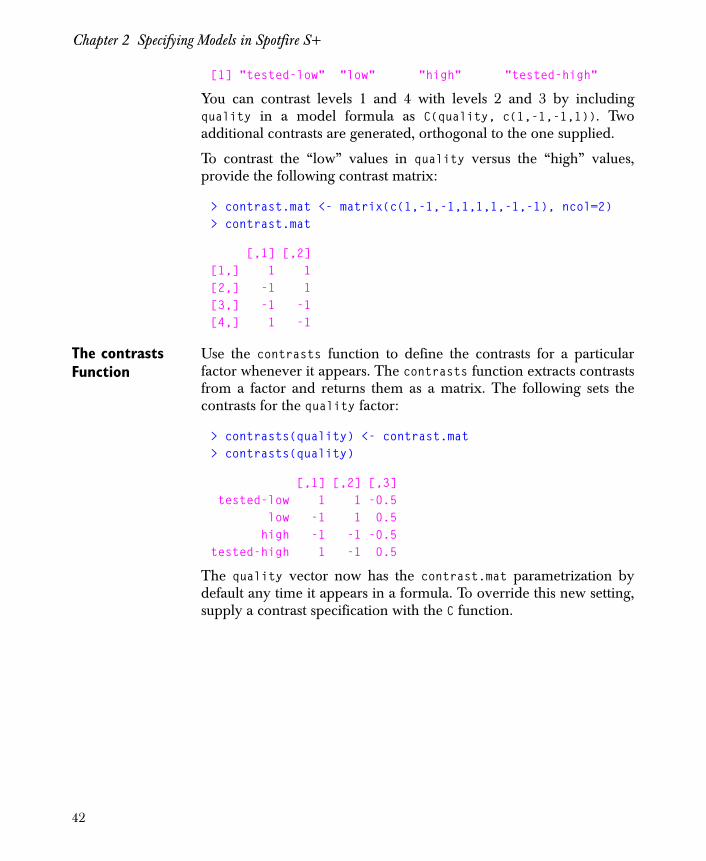
[1] "tested-low" "low" "high" "tested-high"
You can contrast levels 1 and 4 with levels 2 and 3 by includingquality in a model formula as C(quality, c(1,-1,-1,1)). Twoadditional contrasts are generated, orthogonal to the one supplied.
To contrast the “low” values in quality versus the “high” values,provide the following contrast matrix:
> contrast.mat <- matrix(c(1,-1,-1,1,1,1,-1,-1), ncol=2)> contrast.mat
[,1] [,2][1,] 1 1[2,] -1 1[3,] -1 -1[4,] 1 -1
The contrasts Function
Use the contrasts function to define the contrasts for a particularfactor whenever it appears. The contrasts function extracts contrastsfrom a factor and returns them as a matrix. The following sets thecontrasts for the quality factor:
> contrasts(quality) <- contrast.mat> contrasts(quality)
[,1] [,2] [,3] tested-low 1 1 -0.5 low -1 1 0.5 high -1 -1 -0.5tested-high 1 -1 0.5
The quality vector now has the contrast.mat parametrization bydefault any time it appears in a formula. To override this new setting,supply a contrast specification with the C function.
42

Contrasts: The Coding of Factors
Setting the contrasts Option
Use the options function to change the default choice of contrasts forall factors, as in the following example:
> options()$contrasts
factor ordered "contr.treatment" "contr.poly"
> options(contrasts = c(factor = "contr.helmert",+ ordered = "contr.poly"))
> options()$contrasts
[1] "contr.helmert" "contr.poly"
43

Chapter 2 Specifying Models in Spotfire S+
USEFUL FUNCTIONS FOR MODEL FITTING
As model building proceeds, you’ll find several functions useful foradding and deleting terms in formulas. The update function startswith an existing fit and adds or removes terms as you specify. Forexample, create a linear model object as follows:
> fuel.lm <- lm(Mileage ~ Weight + Disp., data = fuel.frame)
You can use update to change the response to Fuel, using a period onthe right side of the tilde (~)to represent the current state of the modelin fuel.lm:
> update(fuel.lm, Fuel ~ . )
The period operator in this call includes every predictor in fuel.lm inthe new model. Only the response variable changes.
You can drop the Disp. term, keeping the response as Mileage withthe command:
> update(fuel.lm, . ~ . - Disp.)
Another useful function is drop1, which computes statistics obtainedby dropping each term from the model one at a time. For example:
> drop1(fuel.lm)
Single term deletions
Model: Mileage ~ Weight + Disp. Df Sum of Sq RSS Cp<none> 380.3 420.3Weight 1 323.4 703.7 730.4Disp. 1 0.6 380.8 407.5
Each line presents model summary statistics that correspond todropping the term indicated in the first column. The first line in thetable corresponds to the original model; no terms (<none>) aredeleted.
44

Useful Functions for Model Fitting
There is also an add1 function which adds one term at a time. Thesecond argument to add1 provides the scope for added terms. Thescope argument can be a formula or a character vector indicating theterms to be added. The resulting table prints a line for each termindicated by the scope argument:
> add1(fuel.lm, c("Type", "Fuel"))
Single term additions
Model: Mileage ~ Weight + Disp. Df Sum of Sq RSS Cp<none> 380.271 420.299 Type 5 119.722 260.549 367.292 Fuel 1 326.097 54.173 107.545
45

Chapter 2 Specifying Models in Spotfire S+
OPTIONAL ARGUMENTS TO MODEL-FITTING FUNCTIONS
In most model-building calls, you’ll need to specify the data frame touse. You may need arguments that check for missing values in thedata frame, or select only particular portions of the data frame to usein the fit. The following list summarizes the standard optionalarguments available for most model-fitting functions.
• data: specifies a data frame in which to interpret the variables named in the formula, subset and weights arguments. The following example fits a linear model to data in the fuel.frame data frame:
> fuel.lm <- lm(Fuel ~ Weight + Disp.,+ data = fuel.frame)
• weights: specifies a vector of observation of weights. If weights is supplied, the fitting algorithm minimizes the sum of the squared residuals multiplied by the weights:
.
Negative weights generate a Spotfire S+ error. We recommend that the weights be strictly positive, since zero weights give no residuals; to exclude observations from your model, use the subset argument instead. The following example fits a linear model to the claims data frame, and passes number to the weights argument:
> claims.lm <- lm(cost ~ age + type + car.age,+ data = claims, weights = number, + na.action = na.exclude)
• subset: indicates a subset of the rows of the data to be used in the fit. The subset expression should evaluate to a logical or numeric vector, or a character vector with appropriate row names. The following example fits a linear model to data in the auto.dat data frame, excluding those observations for which Miles.per.gallon is greater than 35:
> auto.lm <- lm(1/Miles.per.gallon ~ Weight, + data = auto.dat, subset = Miles.per.gallon < 35)
wiri2∑
46

Optional Arguments to Model-Fitting Functions
• na.action: specifies a missing-data filter function. This is applied to the model frame after any subset argument has been used. The following example passes na.exclude to the na.action argument, which drops any row of the data frame that contains a missing value:
> ozone.lm <- lm(ozone ~ temperature + wind,+ data = air, subset = wind > 8, + na.action = na.exclude)
Each model fitting function has nonstandard optional arguments, notlisted above, which you can use to fit the appropriate model. Thefollowing chapters describe the available arguments for each modeltype.
47

Chapter 2 Specifying Models in Spotfire S+
REFERENCES
Chambers, J.M., Hastie T.J. (Eds.) (1992). Statistical Models in S.London: Chapman & Hall.
48

Introduction 51
Important Concepts 52Random Variables 52Probability Density and Cumulative Distribution
Functions 52Mean 54Variance and Deviation 54Quantiles 55Moments 55
Spotfire S+ Probability Functions 56Random Number Generator r 56Probability Function p 56Density Function d 57Quantile Function q 57
Common Probability Distributions for Continuous Variables 60
Uniform Distribution 60Normal Distribution 61Chi-Square Distribution 64t Distribution 65F Distribution 67
Common Probability Distributions for Discrete Variables 69
Binomial Distribution 69Poisson Distribution 71Hypergeometric Distribution 74
Other Continuous Distribution Functions in Spotfire S+ 76Beta Distribution 76
PROBABILITY 3
49

Chapter 3 Probability
Exponential Distribution 76Gamma Distribution 77Weibull Distribution 77Logistic Distribution 78Cauchy Distribution 79Lognormal Distribution 80Distribution of the Range of Standard Normals 81Multivariate Normal Distribution 82Stable Family of Distributions 82
Other Discrete Distribution Functions in Spotfire S+ 84Geometric Distribution 84Negative Binomial Distribution 84Distribution of Wilcoxon Rank Sum Statistic 85
Examples: Random Number Generation 86Inverse Distribution Functions 86The Polar Method 88
References 91
50
Introduction
INTRODUCTION
Probability theory is the branch of mathematics that is concernedwith random, or chance, phenomena. With random phenomena,repeated observations under a specified set of conditions do notalways lead to the same outcome. However, many randomphenomena exhibit a statistical regularity. Because of this, a solidunderstanding of probability theory is fundamental to most statisticalanalyses.
A probability is a number between 0 and 1 that tells how often aparticular event is likely to occur if an experiment is repeated manytimes. A probability distribution is used to calculate the theoreticalprobability of different events. Many statistical methods are based onthe assumption that the observed data are a sample from a populationwith a known theoretical distribution. This assumption is crucial. Ifwe proceed with an analysis under the assumption that a particularsample is from a known distribution when it is not, our results will bemisleading and invalid.
In this chapter, we review the basic definitions and terminology that provide the foundation for statistical models in TIBCO Spotfire S+. This chapter is not meant to encompass all aspects of probability theory. Rather, we present the facts as concise statements and relate them to the functions and distributions that are built into Spotfire S+. We begin with formal definitions and important concepts, including mathematical descriptions of a random variable and a probability density. We then introduce the four basic probability functions in Spotfire S+, and illustrate how they are used in conjunction with particular distributions. As a final example, we show how to transform uniform random numbers to ones from other distributions.
51

Chapter 3 Probability
IMPORTANT CONCEPTS
Random Variables
A random variable is a function that maps a set of events, or outcomesof an experiment, onto a set of values. For example, if we consider theexperiment of tossing a coin, a random variable might be the numberof times the coin shows heads after ten tosses. The random variable inthis experiment can only assume a finite number of values 0, 1, ..., 10,and so it is called a discrete random variable. Likewise, if we observe thefailure rates of machine components, a random variable might belifetime of a particular component. The random variable in thisexperiment can assume infinitely many real values, and so it is calleda continuous random variable.
Probability Density and Cumulative Distribution Functions
The probability density function (pdf) for a random variable provides acomplete description of the variable’s probability characteristics. If is a discrete random variable, then its density function isdefined as
.
In words, the density gives the probability that assumes a particularfinite value x. Because of this definition, is sometimes referred
to as the frequency function for a discrete random variable. For tobe valid, it must be nonnegative and the sum of all possibleprobabilities must equal 1:
,
where can assume the values .
For a continuous random variable , the density is used to find
the probability that assumes a range of values, :
.
XfX x( )
fX x( ) P X x=( )=
XfX x( )
fX x( )
fX xi( )i 1=
n
∑ 1=
X x1 x2 … xn, , ,
Y fY y( )
Y a Y b< <
P a Y b< <( ) fY y( )a
b
∫=
52
Important Concepts
Since a continuous random variable can assume infinitely many realvalues, the probability that is equal to any single value is zero:
.
As with discrete variables, the probabilities for all possible values of acontinuous variable must be nonnegative and sum to 1:
.
It is sometimes convenient to consider the cumulative distributionfunction (cdf), which also describes the probability characteristics of arandom variable. For a discrete random variable , the distribution
is the probability that is less than some value x. Thecumulative distribution is found by summing probabilities for all realvalues less than x:
.
If is a continuous random variable, the cumulative distributionfunction takes the following form:
.
These equations illustrate a relationship between the density anddistribution functions for a random variable. If one function is known,the other can be easily calculated. Because of this relationship, theterms distribution and density are often used interchangeably whendescribing the overall probability characteristics of a randomvariable.
Y
P Y( a ) fY y( )a
a
∫ 0= = =
fY y( ) yd∞–
∞
∫ 1=
XFX x( ) X
FX x( ) P X x≤( ) fX t( )t x≤∑= =
YFY y( )
FY y( ) P Y y≤( ) fY y( )∞–
y
∫= =
53
Chapter 3 Probability
Mean The mean or expected value of a random variable describes the center ofthe variable’s density function. If is a discrete random variable andassumes the values with probabilities
, then the mean is given by the weightedsum
.
If is a continuous random variable with a probability densityfunction , the mean is given by
.
Variance and Deviation
The variance and standard deviation of a random variable are measuresof dispersion. The variance is the average value of the squareddeviation from the variable’s mean, and the standard deviation is thesquare root of the variance. If is a discrete random variable with
density function and mean , the variance is given by theweighted sum
.
The standard deviation of , , provides an indication of how
dispersed the values are about . In practice, it issometimes desirable to compute the mean absolute deviation of arandom variable instead of its variance. For a discrete variable , the
mean deviation is .
Likewise, if is a continuous random variable with density function
and mean , the variance is defined to be:
.
Xx1 x2 … xn, , ,
fX x1( ) fX x2 )( … fX xn )(, , , μX
μX xi fX xi )(i 1=
n
∑=
YfY y( ) μY
μY yfY y( ) yd∞–
∞
∫=
X
fX x( ) μX σX2
σX2 xi μX–( )2fX xi( )
i 1=
n
∑=
X σX
x1 x2 … xn, , , μX
Xxi μX– fX xi( )
i∑
Y
fY y( ) μY σY2
σY2 y μY )2fY y( )–( yd
∞–
∞
∫=
54

Important Concepts
The standard deviation of is , and the mean absolute deviation
is .
Quantiles The pth quantile of a probability distribution is defined to be thevalue t such that , where p is a probability between 0 and 1.For a random variable , this definition is equivalent to the statement
. Special cases include those quantiles corresponding to, and . When , the quantile is
called the median of the probability distribution. When and, the quantiles are called the upper quartile and lower quartile,
respectively. The difference between the upper and lower quartiles ofa distribution is often referred to as the interquartile range, or IQR.
The mode of a probability distribution function is a quantile for whichthe function reaches a local maximum. If a distribution has only onelocal maximum across its range of values, then it is said to beunimodal. Likewise, if a distribution has exactly two local maximums,then it is said to be bimodal. This statistical property is not related tothe Spotfire S+ function mode, which returns the data class of aSpotfire S+ object.
Moments The moments of a random variable provide a convenient way ofsummarizing a few of the quantities discussed in this section. The rthmoment of a random variable is defined to be the expected value
of the quantity . In practice, central moments are often used in placeof ordinary moments. If a random variable has mean , the rthcentral moment is defined to be the expected value of the quantity
. The first central moment is similar to the mean absolutedeviation, and the second central moment is the variance of adistribution. The third central moment is called the skewness, and is ameasure of asymmetry in a probability density function. The fourthcentral moment is called the kurtosis, and is a measure of peakednessin a density function.
Y σY
y μY– fY y( ) yd∞–∞∫
FF t( ) p=
XP X t )≤( p=
1 2⁄ p, 3 ⁄= = p 1 4⁄= p 1 2⁄=
p 3 4⁄=
p 1 4⁄=
X
Xr
X μX
X μX–( )r
55
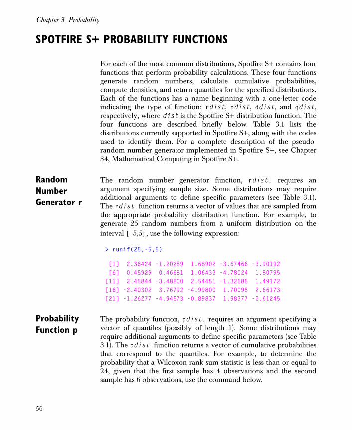
Chapter 3 Probability
SPOTFIRE S+ PROBABILITY FUNCTIONS
For each of the most common distributions, Spotfire S+ contains fourfunctions that perform probability calculations. These four functionsgenerate random numbers, calculate cumulative probabilities,compute densities, and return quantiles for the specified distributions.Each of the functions has a name beginning with a one-letter codeindicating the type of function: rdist, pdist, ddist, and qdist,respectively, where dist is the Spotfire S+ distribution function. Thefour functions are described briefly below. Table 3.1 lists thedistributions currently supported in Spotfire S+, along with the codesused to identify them. For a complete description of the pseudo-random number generator implemented in Spotfire S+, see Chapter34, Mathematical Computing in Spotfire S+.
Random Number Generator r
The random number generator function, rdist, requires anargument specifying sample size. Some distributions may requireadditional arguments to define specific parameters (see Table 3.1).The rdist function returns a vector of values that are sampled fromthe appropriate probability distribution function. For example, togenerate 25 random numbers from a uniform distribution on theinterval , use the following expression:
> runif(25,-5,5)
[1] 2.36424 -1.20289 1.68902 -3.67466 -3.90192 [6] 0.45929 0.46681 1.06433 -4.78024 1.80795[11] 2.45844 -3.48800 2.54451 -1.32685 1.49172[16] -2.40302 3.76792 -4.99800 1.70095 2.66173[21] -1.26277 -4.94573 -0.89837 1.98377 -2.61245
Probability Function p
The probability function, pdist, requires an argument specifying avector of quantiles (possibly of length 1). Some distributions mayrequire additional arguments to define specific parameters (see Table3.1). The pdist function returns a vector of cumulative probabilitiesthat correspond to the quantiles. For example, to determine theprobability that a Wilcoxon rank sum statistic is less than or equal to24, given that the first sample has 4 observations and the secondsample has 6 observations, use the command below.
5– 5[ , ]
56

Spotfire S+ Probability Functions
> pwilcox(24, 4, 6)
[1] 0.6952381
Density Function d
The density function, ddist, requires an argument specifying avector of quantiles (possibly of length 1). Some distributions mayrequire additional arguments to define specific parameters (see Table3.1). The ddist function returns a vector of corresponding valuesfrom the appropriate probability density function. For example, todetermine the probability that a Wilcoxon rank sum statistic is equalto 24, given that the first sample has 4 observations and the secondsample has 6 observations, use the following command:
> dwilcox(24,4,6)
[1] 0.07619048
Quantile Function q
The quantile function, qdist, requires an argument specifying avector of probabilities (possibly of length 1). Some distributions mayrequire additional arguments to define specific parameters (see Table3.1). The qdist function returns a vector of quantiles correspondingto the probabilities for the appropriate distribution function. Forexample, to compute the 0.95 quantile of a chi-square distributionthat has 5 degrees of freedom, use the following expression:
> qchisq(.95, 5)
[1] 11.0705
The result says that 95% of numbers drawn from the given chi-squaredistribution will have values less than 11.0705.
57

Chapter 3 Probability
Table 3.1: Probability distributions in Spotfire S+.
Code DistributionRequired Parameters
Optional Parameters Defaults
beta beta shape1, shape2
binom binomial size, prob
cauchy Cauchy location, scale location=0, scale=1
chisq chi-square df
exp exponential rate 1
f F df1, df2
gamma Gamma shape rate rate=1
geom geometric prob
hyper hypergeometric m, n, k
lnorm lognormal meanlog, sdlog meanlog=0, sdlog=1
logis logistic location, scale location=0, scale=1
mvnorm multivariate normal mean, cov, sd, rho mean=rep(0,d), cov=diag(d), sd=1
nbinom negative binomial size, prob
norm normal mean, sd mean=0, sd=1
nrange range of standard normals
size
58

Spotfire S+ Probability Functions
pois Poisson lambda
stab stable index skewness skewness=0
t Student’s t df
unif uniform min, max min=0, max=1
weibull Weibull shape scale scale=1
wilcox Wilcoxon rank sum statistic
m, n
Table 3.1: Probability distributions in Spotfire S+. (Continued)
Code DistributionRequired Parameters
Optional Parameters Defaults
59

Chapter 3 Probability
COMMON PROBABILITY DISTRIBUTIONS FOR CONTINUOUS VARIABLES
A continuous random variable is one that can assume any valuewithin a given range. Examples of continuous variables includeheight, weight, personal income, distance, and dollar amount. Thissection describes five of the most common continuous distributions:uniform, normal, chi-square, t , and F. See the section OtherContinuous Distribution Functions in Spotfire S+ for descriptions ofadditional distributions.
Uniform Distribution
The uniform distribution describes variables that can assume anyvalue in a particular range with equal probability. That is, all possiblevalues of a uniform random variable have the same relativefrequency, and all have an equal chance of appearing. Given theendpoints of the interval as parameters, the probability densityfunction for a uniform random variable is defined as:
.
Outside of the interval , the density is equal to zero. Plots of thisdensity function for various values of and all have the samerectangular shape, with a constant maximum of in theinterval .
Spotfire S+ functions
dunif, punif, qunif, runif
Each of these functions has optional parameters for the min andmax of the defined density interval. By default, the values for theseparameters are and .
There is a Spotfire S+ function sample that also produces a vector ofvalues uniformly chosen from a given population. For an example ofthis function, see the section Common Probability Distributions forDiscrete Variables.
a b,[ ]
fa b, x( ) 1b a–------------ a x b≤ ≤,=
a b,[ ]a b
1 b a–( )⁄a b,[ ]
a( )b( )
a 0= b 1=
60

Common Probability Distributions for Continuous Variables
Command line example
A common application of continuous uniform random variables is inqueueing theory. For example, suppose a bus arrives every 15minutes at a certain bus stop, on the quarter hour. If passengers arriverandomly at the bus stop between 7:00 and 7:15 a.m., what is theprobability that a particular person will wait more than 12 minutes fora bus? This will occur if the passenger arrives between 7:00 and 7:03.
> punif(3,0,15)-punif(0,0,15)
[1] 0.2
Therefore, a passenger has a 20% chance of waiting more than 12minutes for the bus.
Windows GUI Example
1. Open an empty data set by clicking the New Data Set button on the standard toolbar.
2. Type the values 0 and 3 in the first column.
3. Highlight the column and select Data � Distribution Functions.
4. By default, Spotfire S+ generates cumulative probability values. Select uniform in the Distribution field, and change the Minimum and Maximum parameters to 0 and 15.
5. Click OK.
6. The values 0.00 and 0.20 appear in the second column of the data window, which is named Probability. This means that the probability of arriving between 7:00 and 7:03 is
, or 20%.
Normal Distribution
The normal, or Gaussian, distribution is unimodal and symmetricabout its mean. Given the mean and the standard deviation as parameters, the probability density function for a normal randomvariable is defined as:
.
0.20 0.00–
μ σ 0>
fμ σ, x( ) 1
2πσ2----------------exp 1
2--- x μ–
σ-----------⎝ ⎠
⎛ ⎞ 2–=
61

Chapter 3 Probability
Plots of this density function for various values of and all havethe same “bell” shape, with a global maximum at and tails thatapproach zero as becomes large or small.
In theory, the normal distribution ranges from negative to positiveinfinity, implying that normal random variables can assume any realvalue. However, the bulk of the values that a normal variable assumesare within two standard deviations of its mean. For example, considerthe standard normal distribution, where and . Sixty-eightpercent of the values that a standard normal variable assumes will fallin the range from -1.00 to +1.00. In addition, ninety-five percent ofthe values will fall in the range from -1.96 to +1.96.
Spotfire S+ functions
dnorm, pnorm, qnorm, rnorm
Each of these functions has optional parameters for mean and sd. By default, the values for these parameters are and
.
Command line example 1
The following command shows how to plot histograms of multiple25-observation samples, each having mean 0 and standard deviation1.
> hist(rnorm(25,0,1))
Repeat this many times and observe the variation in the distributions.
Windows GUI Example 1
1. Open an empty data set by clicking the New Data Set button on the standard toolbar.
2. Select Data � Random Numbers.
3. In the dialog that appears, the name of the new data window is filled for the Data Set, and Sample is filled for the Target Column. Specify a Sample Size of 25, and leave the defaults for Distribution, Mean, and Standard Deviation.
4. Click Apply.
μ σμ
x
μ 0= σ 1=
μ( )σ( ) μ 0=
σ 1=
62

Common Probability Distributions for Continuous Variables
5. Highlight the Sample column in the data window, open the Plots 2D palette, and select Histogram.
6. Put the Random Numbers dialog and the graph sheet side by side, and click Apply to create a new sample and plot. Repeat this many times and observe the variation in the distributions.
Command line example 2
Suppose pulmonary function is standardized on a normal distributionwith mean 0 and standard deviation 1. If a score of -1.5 is consideredto be poor pulmonary health for young people, what percentage ofchildren are in poor pulmonary health?
> pnorm(-1.5,0,1)
[1] 0.0668072
Thus, about 7% of children are classified as having poor pulmonaryhealth.
Windows GUI Example 2
1. Open an empty data set by clicking the New Data Set button on the standard toolbar.
2. Type -1.5 in the first cell.
3. Highlight the column and select Data � Distribution Functions. By default, Spotfire S+ uses a normal distribution with mean 0 and standard deviation 1.
4. Click OK.
5. The value 0.07 appears in the second column of the data window, which is named Probability. To see more decimal places in the display, highlight the columns and click the Increase Precision button on the DataSet toolbar.
The Central Limit Theorem
The normal distribution is very important in statistical analyses, andarises often in nearly every field of study. Generally speaking, anyvariable that is a sum of numerous independent random variables canbe approximated by a normal distribution. Consequently, the normaldistribution offers a reasonable approximation for many variablesthat may not strictly follow a normal distribution. The Central LimitTheorem formalizes this idea. In practice, the normal approximation
63
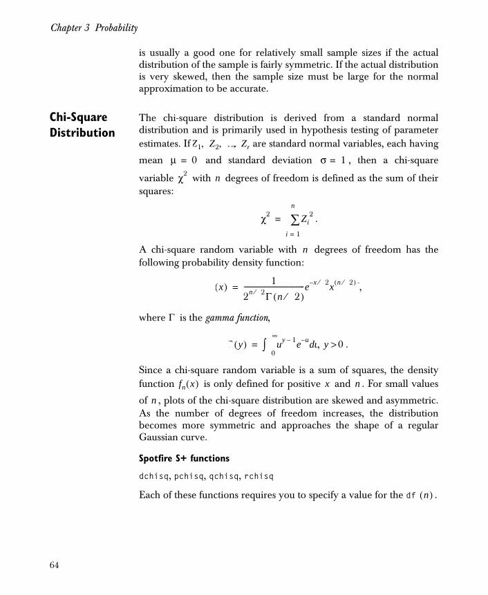
Chapter 3 Probability
is usually a good one for relatively small sample sizes if the actualdistribution of the sample is fairly symmetric. If the actual distributionis very skewed, then the sample size must be large for the normalapproximation to be accurate.
Chi-Square Distribution
The chi-square distribution is derived from a standard normaldistribution and is primarily used in hypothesis testing of parameterestimates. If are standard normal variables, each having
mean and standard deviation , then a chi-square
variable with degrees of freedom is defined as the sum of theirsquares:
.
A chi-square random variable with degrees of freedom has thefollowing probability density function:
,
where is the gamma function,
, .
Since a chi-square random variable is a sum of squares, the densityfunction is only defined for positive and . For small values
of , plots of the chi-square distribution are skewed and asymmetric.As the number of degrees of freedom increases, the distributionbecomes more symmetric and approaches the shape of a regularGaussian curve.
Spotfire S+ functions
dchisq, pchisq, qchisq, rchisq
Each of these functions requires you to specify a value for the df .
Z1 Z2 … Zn, , ,
μ 0= σ 1=
χ2 n
χ2 Zi2
i 1=
n
∑=
n
x( ) 1
2n 2⁄ Γ n 2⁄( )------------------------------------e x 2⁄– x n 2⁄( ) –=
Γ
Γ y( ) uy 1– e u– ud0
∞
∫= y 0>
fn x( ) x n
n
n( )
64

Common Probability Distributions for Continuous Variables
Command line example
Find the upper and lower 2.5th percentile of a chi-square distributionwith 12 degrees of freedom.
> qchisq(0.975,12)
[1] 23.3366
> qchisq(0.025,12)
[1] 4.403789
Windows GUI Example
1. Open an empty data set by clicking the New Data Set button on the standard toolbar.
2. Type the values 0.975, and 0.025 in the first column. Highlight the column and click the Increase Precision button on the DataSet toolbar to increase the precision of the display.
3. Highlight the first column and select Data � Distribution Functions.
4. In the Result Type field, select Quantile. From the Distribution dropdown list, select chisquare. In the Degrees of Freedom field, type 12.
5. Click OK.
6. The values 23.34 and 4.40 appear in the second column of the data window, which is named Quantile.
t Distribution The distribution is derived from both a standard normaldistribution and a chi-square distribution. If is a standard normal
variable and is a chi-square random variable with degrees offreedom, then a variable with degrees of freedom is defined to bethe ratio
.
tZ
χ2 nt n
t Z
χ2 n⁄-------------------=
65
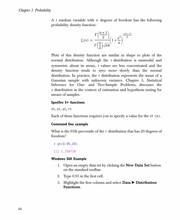
Chapter 3 Probability
A random variable with degrees of freedom has the followingprobability density function:
Plots of this density function are similar in shape to plots of thenormal distribution. Although the distribution is unimodal andsymmetric about its mean, values are less concentrated and thedensity function tends to zero more slowly than the normaldistribution. In practice, the distribution represents the mean of aGaussian sample with unknown variance. Chapter 5, StatisticalInference for One- and Two-Sample Problems, discusses the
distribution in the context of estimation and hypothesis testing formeans of samples.
Spotfire S+ functions
dt, pt, qt, rt
Each of these functions requires you to specify a value for the df .
Command line example
What is the 95th percentile of the distribution that has 20 degrees offreedom?
> qt(0.95,20)
[1] 1.724718
Windows GUI Example
1. Open an empty data set by clicking the New Data Set button on the standard toolbar.
2. Type 0.95 in the first cell.
3. Highlight the first column and select Data � Distribution Functions.
t n
fn x( )Γ n 1+
2------------⎝ ⎠
⎛ ⎞
Γ n2---⎝ ⎠
⎛ ⎞ nπ------------------------ 1 x2
n-----+⎝ ⎠
⎛ ⎞n 1+( )–2
--------------------
=
tt
t
t
n( )
t
66
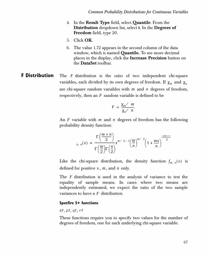
Common Probability Distributions for Continuous Variables
4. In the Result Type field, select Quantile. From the Distribution dropdown list, select t. In the Degrees of Freedom field, type 20.
5. Click OK.
6. The value 1.72 appears in the second column of the data window, which is named Quantile. To see more decimal places in the display, click the Increase Precision button on the DataSet toolbar.
F Distribution The distribution is the ratio of two independent chi-squarevariables, each divided by its own degrees of freedom. If and
are chi-square random variables with and degrees of freedom,respectively, then an random variable is defined to be
.
An variable with and degrees of freedom has the followingprobability density function:
Like the chi-square distribution, the density function is
defined for positive , , and only.
The distribution is used in the analysis of variance to test theequality of sample means. In cases where two means areindependently estimated, we expect the ratio of the two samplevariances to have a distribution.
Spotfire S+ functions
df, pf, qf, rf
These functions require you to specify two values for the number ofdegrees of freedom, one for each underlying chi-square variable.
Fχm χn
m nF
Fχm m⁄χn n⁄-----------------=
F m n
m n, x( )Γ m n+
2-------------⎝ ⎠
⎛ ⎞
Γ m2----⎝ ⎠
⎛ ⎞ Γ n2---⎝ ⎠
⎛ ⎞----------------------------xm 2⁄ 1– m
n----⎝ ⎠
⎛ ⎞ m 2⁄1 mx
n-------+⎝ ⎠
⎛ ⎞m n+(–
2-------------------
=
fm· n, x( )
x m n
F
F
67

Chapter 3 Probability
Command line example
Find the upper 5th percentile of an distribution with 4 and 10degrees of freedom.
> qf(0.95,4,10)
[1] 3.47805
Windows GUI Example
1. Open an empty data set by clicking the New Data Set button on the standard toolbar.
2. Type 0.95 in the first cell.
3. Highlight the first column and select Data � Distribution Functions.
4. In the Result Type field, select Quantile. From the Distribution dropdown list, select f. In the Degrees of Freedom 1 field, type 4, and in the Degrees of Freedom 2 field, type 10.
5. Click OK.
6. The value 3.48 appears in the second column of the data window, which is named Quantile. To see more decimal places in the display, click the Increase Precision button on the DataSet toolbar.
F
68
Common Probability Distributions for Discrete Variables
COMMON PROBABILITY DISTRIBUTIONS FOR DISCRETE VARIABLES
A discrete random variable is one that can assume only a finitenumber of values. Examples of discrete variables include the outcomeof rolling a die, the outcome of flipping a coin, and the gender of anewborn child. Many discrete probability distributions are based onthe Bernoulli trial, an experiment in which there is only two possibleoutcomes. The outcomes are often denoted as “head” and “tail”, or“success” and “failure”. Mathematically, it is convenient to designatethe two outcomes as 1 and 0. A variable is a Bernoulli randomvariable with parameter if assumes the values 1 and 0 with theprobabilities and , where .
In Spotfire S+ you can generate a series of Bernoulli trials using thesample function. The following command returns a Bernoulli sampleof size 20 with replacement, using probabilities of 0.35 and 0.65 for 0and 1, respectively:
> sample(0:1, 20, T, c(0.35, 0.65))
[1] 0 0 0 1 1 0 0 1 1 1 1 0 0 0 1 1 1 1 0 1
This section describes three of the most common discretedistributions: binomial, Poisson, and hypergeometric. See the sectionOther Discrete Distribution Functions in Spotfire S+ for descriptionsof additional distributions.
Binomial Distribution
The binomial distribution describes the probability that one of twoevents occurs a certain number of times in trials. If are independent Bernoulli random variables, each having aprobability parameter and possible values of 0 or 1, then abinomial random variable is defined as their sum:
.
Xp X
P X 1=( ) p= P X 0=( ) 1 p–= 0 p 1≤ ≤
n X1 X2 … Xn, , ,
pX
X Xi
i 1=
n
∑=
69

Chapter 3 Probability
A binomial random variable with parameters and has thefollowing probability density function:
,
where . This density gives the probability that
exactly successes occur in Bernoulli trials.
Spotfire S+ functions
dbinom, pbinom, qbinom, rbinom
Each of these functions require you to specify values for the size and prob parameters.
Command line example
A classic illustration for the binomial distribution is the coin toss. Thefollowing examples compute the probability of getting 6 heads with10 throws of a fair coin.
What is the probability of getting 6 heads with 10 throws of a fair( ) coin?
> dbinom(6,10,0.5)
[1] 0.2050781
What is the probability of getting at most 6 heads with 10 throws of afair coin?
> pbinom(6,10,0.5)
[1] 0.828125
Suppose someone is tossing a coin, and you are not sure whether thecoin is fair. In 10 throws, what is the largest number of heads youwould expect in order to be 95% confident that the coin is fair?
> qbinom(0.95,10,0.5)
[1] 8
n p
fn p, k( )nk⎝ ⎠
⎛ ⎞ pk 1 p–( )n k–=
nk⎝ ⎠
⎛ ⎞ n!k! n k–( )!-----------------------=
k n
n( )p( )
p 0.5=
70

Common Probability Distributions for Discrete Variables
Thus, if 9 or 10 tosses showed heads, you would suspect that the coinmight not be fair.
Windows GUI Example
1. Open an empty data set by clicking the New Data Set button on the standard toolbar.
2. Type 6 in the first cell.
3. Highlight the first column and choose Data � Distribution Functions.
4. In the Result Type field, select Density. From the Distribution dropdown list, select binomial. Type 0.5 in the Probability field and type 10 in the Sample Size field.
5. Click Apply.
6. The value 0.21 appears in the second column of the data window, which is named Density.
7. To find the probability of throwing at most 6 heads with 10 throws of the coin, change the Result Type field to Probability in the Distribution Functions dialog.
8. Click Apply.
9. The value 0.83 appears in a Probability column of the data window.
10. To find the maximum number of heads that you would expect from 10 throws to be 95% confident that the coin is fair, type 0.95 in the first cell of a new column in the data window. Name the new column V4.
11. In the Distribution Functions dialog, type V4 in the Source Column field, and change the Result Type to Quantile.
12. Click OK.
13. The value 8 appears in a Quantile column of the data window.
Poisson Distribution
The Poisson distribution is the limit of a binomial distribution, as thenumber of Bernoulli trials gets large and the probability of asuccess gets small. Formally, a binomial distribution approaches a
np
71
Chapter 3 Probability
Poisson distribution if and in a way such that theirproduct remains constant, . A Poisson random variable with aparameter has the following probability density function:
,
In practice, computing exact binomial probabilities is convenient forsmall sample sizes only, which suggests when Poisson approximationscan arise. Suppose is a binomial random variable that describes thenumber of times an event occurs in a given interval of time. Assumethat we can divide the time interval into a large number of equalsubintervals, so that the probability of an event in each subinterval isvery small. Three conditions must hold for a Poisson approximationto be valid in this situation. First, the number of events that occur inany two subintervals must be independent of one another. Second,the probability that an event occurs is the same in each subinterval oftime. Third, the probability of two or more events occurring in aparticular subinterval is negligible in comparison to the probability ofa single event. A process that meets these three conditions is called aPoisson process, and arises in fields as diverse as queueing theory andinsurance analysis.
A Poisson random variable with parameter has a mean value of .Consequently, the number of events that occur in a Poisson processover subintervals of time has a mean value of .
Spotfire S+ functions
dpois, ppois, qpois, rpois
Each of these functions requires you to specify a value for lambda.
Command line example
The following example is taken from Rosner (1995). The number ofdeaths attributed to typhoid fever over a 1-year period is a Poissonrandom variable with . What is the probability distributionfor the number of deaths over a 6-month period? To find this, we usea parameter of 2.3, since the time interval in question is half of 1 year.
n ∞→ p 0→np λ=
λ
fλ k( ) λke λ–
k!-------------= k 0 1 2 …, , ,=
X
λ λ
t λ t
λ 4.6=
72

Common Probability Distributions for Discrete Variables
To find the probability of 0, 1, 2, 3, 4, or 5 deaths in a 6-monthperiod, use the following command:
> dpois(0:5,2.3)
[1] 0.10025884 0.23059534 0.26518464 0.20330823 0.11690223 [6] 0.05377503
To find the probability of more than 5 deaths, use the followingcommand:
> 1-ppois(5,2.3)
[1] 0.03
Windows GUI Example
1. Open an empty data set by clicking the New Data Set button on the standard toolbar.
2. Highlight the first column and choose Data � Fill. Select <END> from the dropdown list for Columns, type 6 in the Length field, and type 0 in the Start field.
3. Click OK.
4. A sequence of integers from 0.00 to 5.00 appear in the first column, which is named V1.
5. Highlight the column and choose Data � Distribution Functions.
6. In the Result Type field, select Density. From the Distribution dropdown list, select poisson. Type 2.3 in the field for Mean.
7. Click Apply.
8. The values 0.10, 0.23, 0.27, 0.20, 0.12, and 0.05 appear in the second column of the data window, which is named Density. To see more decimal places in the display, click the Increase Precision button on the DataSet toolbar.
9. To find the probability that more than 5 deaths occur in a 6-month period, type 5 in the first cell of a new column and name the column V3.
73
Chapter 3 Probability
10. In the Distribution Functions dialog, type V3 in the Source Column field, and change the Result Type to Quantile.
11. Click OK.
12. The value 0.97 appears in a Probability column of the data window. This means that the probability that more than five deaths occur is , or 0.3.
Hypergeometric Distribution
The hypergeometric distribution is used in the analysis of twocategorical variables, and is best described by the classic Urn Model.Suppose an urn contains balls, of which are red and are black. A hypergeometric random variable denotes the number ofred balls drawn when balls are taken from the urn withoutreplacement. Given the parameters , , and , the hypergeometricprobability density function is:
.
This density gives the probability that exactly red balls are drawnfrom the urn.
The hypergeometric distribution is similar to the binomialdistribution: where a binomial variable is sampled from a finitepopulation with replacement, a hypergeometric variable is sampledwithout replacement. In fact, as and the proportion of redballs in the urn approaches , the hypergeometric distributionconverges to a corresponding binomial distribution.
Hypergeometric random variables arise primarily in acceptancesampling in manufacturing. That is, the number of sample productsthat should be tested for quality in a particular batch follows ahypergeometric distribution. Such information can be used todetermine an acceptable limit for the number of defective products.
1 0.97–
b m n b m–=
km n k
fm n k, , r( )
mr⎝ ⎠
⎛ ⎞ nk r–⎝ ⎠
⎛ ⎞
m n+
k⎝ ⎠⎛ ⎞
--------------------------=
r
b ∞→p
74

Common Probability Distributions for Discrete Variables
Spotfire S+ functions
dhyper, phyper, qhyper, rhyper
These functions require you to specify values for the number of redballs in the urn , the number of black balls in the urn , and thenumber of balls drawn without replacement .
Command line example
A box contains 100 balls, of which 50 are red and 50 are black. Tenballs are drawn from the box at random without replacement. What isthe probability that all of the balls chosen will be red?
> dhyper(10, 50, 50, 10)
[1] 0.000593
Thus, the probability of choosing ten out of ten red balls from the boxis quite low.
Windows GUI Example
1. Open an empty data set by clicking the New Data Set button on the standard toolbar.
2. Type 10 in the first cell.
3. Highlight the first column and choose Data � Distribution Functions.
4. In the Results Type field, select Density. From the Distribution dropdown list, choose hypergeometric. Type 10 for the Sample Size, and type 50 for both the Total Successes and Total Failures.
5. Click OK.
6. The values 0.00 appears in the second column of the data window, which is named Density. To see more decimal places in the display, click the Increase Precision button on the DataSet toolbar.
m( ) n( )k( )
75
Chapter 3 Probability
OTHER CONTINUOUS DISTRIBUTION FUNCTIONS IN SPOTFIRE S+
Beta Distribution
The beta distribution is very versatile, and plots of the distributionfunction can assume a wide variety of shapes. This flexibility allowsmany uncertainties to be described by beta random variables.Example applications include statistical likelihood ratio tests, randomwalks, and Bayesian inference in decision theory.
The standard form of the beta probability density function is:
,
where , and are positive shape parameters, and is thebeta function,
.
Spotfire S+ functions
dbeta, pbeta, qbeta, rbeta
Each of these functions requires you to specify values for the twoshape parameters.
Exponential Distribution
The exponential distribution is one-sided and is characterized by amemoryless property. It is often used to model the lifetimes of machinecomponents and the wait times in Poisson processes. For example,suppose that the random variable denotes the lifetime of aparticular electronic component. Given that the component survivesfor months, the probability that it survives for more is notdependent on . Formally, the memoryless property is stated in thefollowing conditional probability:
.
In Poisson processes, exponential random variables describe the waittimes between events.
fa b, x( ) 1B a b,( )-------------------xa 1– 1 x–( )b 1–=
0 x 1≤ ≤ a b B
B a b,( ) ua 1– 1 u–( )b 1– ud0
1
∫=
X
t st
P X t s X t>+>( ) P X s>( )=
76

Other Continuous Distribution Functions in Spotfire S+
The exponential probability density function is defined as follows:
,
where and is a positive parameter.
Spotfire S+ functions
dexp, pexp, qexp, rexp
Each of these functions has an optional argument for the rate parameter. By default, .
Gamma Distribution
The gamma distribution is a generalization of the exponentialdistribution. Where an exponential variable models the wait timeuntil the next event in a Poisson process, a gamma random variablemodels the wait time until the nth event. In applied work, gammadistributions provide models for many physical situations, includingmeteorological precipitation processes and personal income data inthe United States.
The probability density function for a gamma random variable isdefined as:
,
where , is a shape parameter, and (the inverse of ) is ascale parameter, and is the gamma function.
Spotfire S+ functions
dgamma, pgamma, qgamma, rgamma
Each of these functions requires you to specify a value for the shape parameter. They also have optional arguments for the rate
parameter, which is defined to be 1 by default.
Weibull Distribution
The Weibull distribution is closely related to the exponentialdistribution, and is commonly used in manufacturing to test thebreaking strength of materials. In this context, Weibull randomvariables can model the lifetimes of machine components morerealistically than exponential random variables. This is because the
fλ x( ) λe λx–=
x 0> λ
λ( )λ 1=
fα λ, x( ) λα
Γ α( )------------xα 1– e λx–=
x 0> α 0> β λΓ
α( ) λ( )
77

Chapter 3 Probability
Weibull distribution has a failure rate (or hazard function) that varieswith time, whereas the exponential has a constant failure rate due tothe memoryless property. In some contexts, the lifetime of particularcomponents may increase or decrease with time, making the Weibulldistribution more appropriate.
The probability density function for Weibull random variables is:
,
where , is a positive shape parameter, and is a positivescale parameter. When , this distribution corresponds to anexponential distribution with a hazard rate of . The failure rate ofthe Weibull distribution decreases with time when , isconstant when , and increases when . In Spotfire S+, theWeibull distribution is the default for Parametric Survival and LifeTesting.
Spotfire S+ functions
dweibull, pweibull, qweibull, rweibull
Each of these functions requires you to specify a value for the shape parameter. They also have an optional argument for the scale parameter, which is defined to be 1 by default.
Logistic Distribution
The logistic distribution is similar in shape to a Gaussian distribution,though it has longer tails. Logistic random variables are used heavilyto model growth curves, but they have also been used in bioassaystudies and other applications.
The probability density function for a logistic random variable isdefined to be:
,
where is a location parameter and is a positive scale parameter.
fα β, x( ) αβα-----xα 1– x
β---⎝ ⎠
⎛ ⎞ α–⎝ ⎠
⎛ ⎞exp=
x 0> α βα 1=
1 β⁄0 β 1< <
β 1= β 1>
α( )β( )
fλ θ, x( )
λ x–θ
------------⎝ ⎠⎛ ⎞exp
θ 1 λ x–θ
------------⎝ ⎠⎛ ⎞exp+⎝ ⎠
⎛ ⎞ 2-------------------------------------------------=
λ θ
78
Other Continuous Distribution Functions in Spotfire S+
With respect to growth curves, the logistic distribution function satisfies the following: the derivative of with respect to isproportional to with . The interpretationof this statement is that the rate of growth is proportional to theamount already grown, multiplied by the amount of growth that isstill expected.
Spotfire S+ functions
dlogis, plogis, qlogis, rlogis
Each of these functions has optional arguments for the location and scale parameters. By default, the values of these argumentsare and .
Cauchy Distribution
Like the Gaussian distribution, the Cauchy distribution is unimodaland symmetric. Like the distribution, however, plots of the Cauchydistribution have tails that tend to zero much more slowly than anormal distribution. Given two independent standard normalvariables and , each having mean 0 and standard deviation 1, a
standard Cauchy random variable is defined as their quotient:
.
Thus, a standard Cauchy random variable follows a distributionwith one degree of freedom. A general Cauchy variable is defined bymultiplying by a positive scale parameter , and then adding alocation parameter .
Given and , the probability density function for a general Cauchyrandom variable is:
.
The density function for a standard Cauchy variable corresponds tothe case when and .
FF x
F x( ) A–[ ] B F x( )–[ ] A B<
λ( )θ( )
λ 0= θ 1=
t
Z1 Z2
Z
ZZ1
Z2-----=
t
Z θλ
λ θ
fλ θ, x( ) πθ 1 x λ–θ
------------⎝ ⎠⎛ ⎞ 2
+⎝ ⎠⎛ ⎞ 1–
=
λ 0= θ 1=
79
Chapter 3 Probability
The Cauchy density has a few peculiar properties that providecounterexamples to some accepted statistical results. For example, thetails of the density are long enough so that its mean and variance donot exist. In other words, the density decreases so slowly that a widerange of values can occur with significant probability, and so theintegral expressions for the mean and variance diverge.
Spotfire S+ functions
dcauchy, pcauchy, qcauchy, rcauchy
Each of these functions has optional arguments for the location and scale parameters. By default, the values of these parametersare and .
Lognormal Distribution
The lognormal distribution is a logarithmic transformation of thenormal distribution. Given a normal random variable withparameters and , a lognormal random variable is defined to beits exponential:
.
Thus, the natural logarithm of data that follows a lognormaldistribution should be approximately Gaussian.
The probability density function for a lognormal random variable is:
,
where , and and are the mean and standard deviation,respectively, of the logarithm of the random variable. With this
definition, is a scale parameter for the distribution, and is ashape parameter.
The lognormal distribution is sometimes referred to as theantilognormal distribution, since it is the distribution of an exponential(or antilogarithm) of a normal variable. When applied to economicdata, particularly production functions, it is sometimes called theCobb-Douglas distribution. In some cases, lognormal random variablescan represent characteristics like weight, height, and density morerealistically than a normal distribution. Such variables cannot assume
λ( )θ( )
λ 0= θ 1=
Yμ σ X
X eY=
fμ σ, x( ) 1σx 2π---------------- 1
2σ2-------- x μ–log( )2–⎝ ⎠
⎛ ⎞exp–=
x 0> μ σ 0>
eμ σ
80

Other Continuous Distribution Functions in Spotfire S+
negative values, and so they are naturally described by a lognormaldistribution. Additionally, with a small enough , it is possible toconstruct a lognormal distribution that closely resembles a normaldistribution. Thus, even if a normal distribution is felt to beappropriate, it might be replaced by a suitable lognormal distribution.
Spotfire S+ functions
dlnorm, plnorm, qlnorm, rlnorm
Each of these functions has optional arguments for the meanlog and sdlog parameters. By default, the values of these argumentsare and .
Distribution of the Range of Standard Normals
The distribution of the range of standard normal random variables isprimarily used for the construction of R-charts in quality controlwork. Given standard normal variables , each withmean 0 and standard deviation 1, the range is defined as the differencebetween the minimum and maximum of the variables.
Spotfire S+ functions
dnrange, pnrange, qnrange, rnrange
Each of these functions requires you to specify a value for the size of the sample. They also have an optional nevals argument that
defines the number of iterations in the density, probability, andquantile computations. The probability density function for the rangeof standard normals is a complicated integral equation, and cantherefore require significant computation resources. A higher value ofnevals will result in better accuracy, but will consume more machinetime. By default, nevals is set to 200.
σ
μ( )σ( )
μ 0= σ 1=
n Z1 Z2 … Zn, , ,
n( )
81
Chapter 3 Probability
Multivariate Normal Distribution
The multivariate normal distribution is the extension of the Gaussiandistribution to more than one dimension. Let be the number ofdimensions in the multivariate distribution, let be a vector of length
specifying the mean in each dimension, and let be a variance-covariance matrix. The probability density function for amultivariate normal random variable is given by:
,
where is the vector , and is the determinant of .
Spotfire S+ functions
dmvnorm, pmvnorm, rmvnorm
Each of these functions has an optional argument for the mean vector. In addition, you can specify the variance-covariance matrix
through the cov and sd arguments. If supplied, the variance-covariance matrix is the product of the cov matrix and the sdargument, which contains the standard deviations for eachdimension. By default, mean is a vector of zeros, cov is an identitymatrix, and sd is a vector of ones.
Stable Family of Distributions
Stable distributions are of considerable mathematical interest. Afamily is considered stable if the convolution of two distributions fromthe family also belongs to the family. Each stable distribution is thelimit distribution of a suitably scaled sum of independent andidentically distributed random variables. Statistically, they are usedwhen an example of a very long-tailed distribution is required.
Spotfire S+ functions
rstab
The rstab function requires a value from the interval for anindex argument. For small values of the index, the distributiondegenerates to point mass at 0. An index of 2 corresponds to thenormal distribution, and an index of 1 corresponds to the Cauchydistribution. Smaller index values produce random numbers fromstable distributions with longer tails. The rstab function also has anoptional skewness argument that indicates the modified skewness of
dμ
d Σ d d×
μ Σ, x( ) 2π( ) d 2⁄– Σ 1 2⁄– 12--- x μ–( )′ Σ 1– x μ–( )–⎝ ⎠
⎛ ⎞exp=
x x1 x2 … xd, , ,( ) Σ Σ
μ( ) Σ( )
0 2 ],(
82

Other Continuous Distribution Functions in Spotfire S+
the distribution. Negative values correspond to left-skewed randomnumbers, where the median is smaller than the mean (if it exists).Positive values of skewness correspond to right-skewed randomnumbers, where the median is larger than the mean. By default, theskewness is set to 0.
Spotfire S+ contains only the rstab probability function for the stablefamily of distributions. The efficient computation of density,probability, and quantile values is currently an open problem.
83

Chapter 3 Probability
OTHER DISCRETE DISTRIBUTION FUNCTIONS IN SPOTFIRE S+
Geometric Distribution
The geometric distribution describes the number of failures beforethe first success in a sequence of Bernoulli trials. In binomialdistributions, we think of the number of trials and the probability ofa success as fixed parameters, so that the number of successes isthe random variable. Reversing the problem, we could ask how manytrials would be required to achieve the first success. In thisformulation, the number of failures is the random variable, and and
are fixed.
A geometric random variable with a parameter has the followingprobability density function:
,
This density gives the probability that exactly failures occur beforea success is achieved.
Spotfire S+ functions
dgeom, pgeom, qgeom, rgeom
Each of these functions require you to specify a value for the prob parameter.
Negative Binomial Distribution
The negative binomial distribution is a generalization of thegeometric distribution. It models the number of failures beforeexactly successes occur in a sequence of Bernoulli trials. When
, a negative binomial random variable follows a geometricdistribution, and in general, a negative binomial variable is a sum of independent geometric variables.
Given the probability of a success and the number of successes asparameters, the negative binomial probability density function is:
,
np k
pk 1=
p
fp n( ) p 1 p–( )n= n 0 1 2 …, , ,=
n
p( )
rr 1=
r
p r
fp r, k( )r k 1–+
k⎝ ⎠⎛ ⎞ pr 1 p–( )k= k 0 1 2 …, , ,=
84
Other Discrete Distribution Functions in Spotfire S+
This density gives the probability that exactly failures occur before successes are achieved.
Spotfire S+ functions
dnbinom, pnbinom, qnbinom, rnbinom
Each of these functions require you to specify values for the size and prob parameters.
Distribution of Wilcoxon Rank Sum Statistic
The Wilcoxon rank sum statistic, also known as the Mann-Whitney teststatistic, is a nonparametric method for comparing two independentsamples. The test itself is best described in terms of treatment andcontrol groups. Given a set of experimental units, we randomlyselect and assign them to a control group, leaving units for atreatment group. After measuring the effect of the treatment on allunits, we group the observations together and rank them inorder of size. If the sum of the ranks in the control group is too smallor too large, then it’s possible that the treatment had an effect.
The distribution of the Wilcoxon rank sum statistic describes theprobability characteristics of the test values. Given and as
parameters, the rank sum statistic takes on values between
and .
Spotfire S+ functions
dwilcox, pwilcox, qwilcox, rwilcox
Each of these functions require you to specify sizes ( and ) for thetwo independent samples.
The wilcox functions are available in Spotfire S+ via the commandline only.
kr
r( )p( )
m n+
n m
m n+
m nm m 1+( )
2-----------------------
m m 2n 1+ +( )2
------------------------------------
m n
85

Chapter 3 Probability
EXAMPLES: RANDOM NUMBER GENERATION
In this section, we illustrate two of the common algorithms forrandom number generation: the inverse cdf method and the polarmethod. The algorithms we discuss are both standard techniques fromintroductory statistics textbooks, and involve transformations ofuniform random variables. The techniques can thus be applied todevelop random number generators for distributions that are notimplemented in Spotfire S+. The algorithms we present do notencompass all random number generators for all distributions, anddue to efficiency considerations, they are not the algorithmsimplemented in Spotfire S+. Nevertheless, they are solid examples ofhow the Spotfire S+ probability functions can be modified to servedifferent analytical needs.
For details on the pseudo-random number generator implemented inSpotfire S+, see Chapter 34, Mathematical Computing in Spotfire S+.
Inverse Distribution Functions
A fundamental result from probability theory states that if is auniform random variable on the interval , and another variable
for some function , then the cumulative distributionfunction for is . This leads to the inverse cdf method for generatingrandom numbers from a uniform distribution:
1. Given a distribution function , find an expression
for the inverse function .
2. Generate uniform random variables on the interval , and
substitute them into . The resulting values are randomly sampled from the distribution .
This method is practical for those distribution functions with inversesthat can be easily calculated.
The Exponential Distribution
Exponential random variables have a probability density function
, where and is a positive parameter. The
exponential distribution function is the integral of over positive
values, which gives . Solving for , we find the
U0 1[ , ]
X F 1– U( )= FX F
u F x( )=
x F 1– u( )=
0 1[ , ]
F 1–
F
fλ x( ) λe λx–= x 0> λ
Fλ fλ
x Fλ x( ) 1 e λx––= Fλ x
86
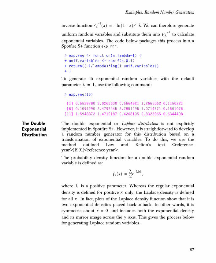
Examples: Random Number Generation
inverse function . We can therefore generate
uniform random variables and substitute them into to calculateexponential variables. The code below packages this process into aSpotfire S+ function exp.rng.
> exp.rng <- function(n,lambda=1) {+ unif.variables <- runif(n,0,1)+ return((-1/lambda)*log(1-unif.variables))+ }
To generate 15 exponential random variables with the defaultparameter , use the following command:
> exp.rng(15)
[1] 0.5529780 3.0265630 0.5664921 1.2665062 0.1150221 [6] 0.1091290 2.4797445 2.7851495 1.0714771 0.1501076[11] 1.5948872 1.4719187 0.4208105 0.8323065 0.6344408
The Double Exponential Distribution
The double exponential or Laplace distribution is not explicitlyimplemented in Spotfire S+. However, it is straightforward to developa random number generator for this distribution based on atransformation of exponential variables. To do this, we use themethod outlined Law and Kelton’s text <reference-year>(1991)<reference-year>.
The probability density function for a double exponential randomvariable is defined as:
,
where is a positive parameter. Whereas the regular exponentialdensity is defined for positive only, the Laplace density is definedfor all . In fact, plots of the Laplace density function show that it istwo exponential densities placed back-to-back. In other words, it issymmetric about and includes both the exponential densityand its mirror image across the axis. This gives the process belowfor generating Laplace random variables.
Fλ1– x( ) 1 x–( )ln– λ⁄=
Fλ1–
λ 1=
fλ x( ) λ2---e λ x–=
λx
x
x 0=
y
87
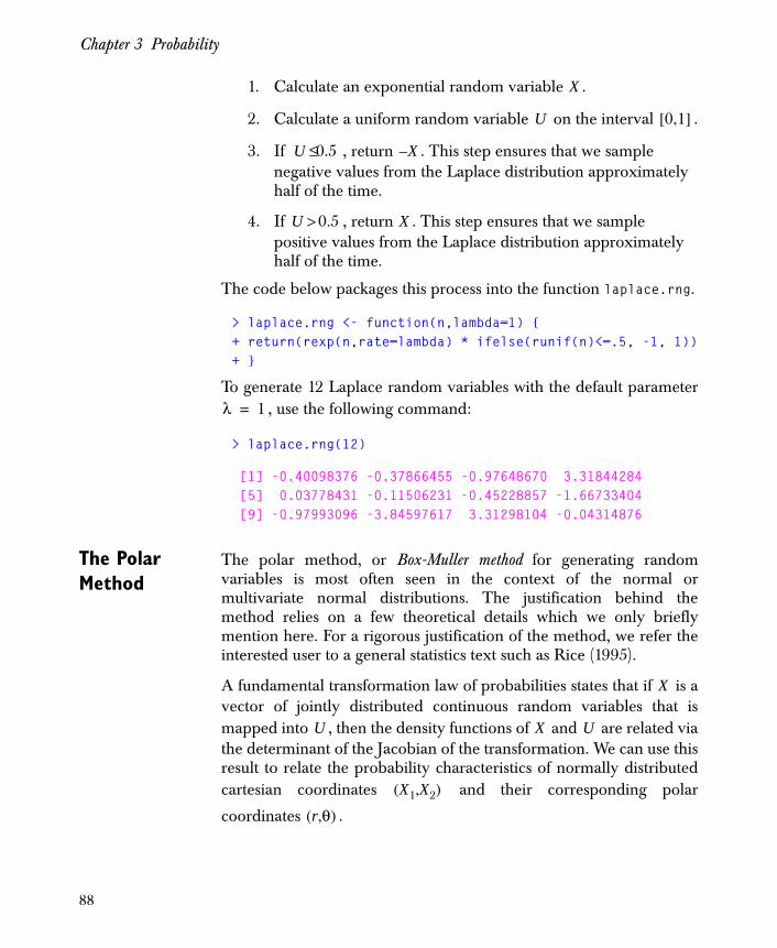
Chapter 3 Probability
1. Calculate an exponential random variable .
2. Calculate a uniform random variable on the interval .
3. If , return . This step ensures that we sample negative values from the Laplace distribution approximately half of the time.
4. If , return . This step ensures that we sample positive values from the Laplace distribution approximately half of the time.
The code below packages this process into the function laplace.rng.
> laplace.rng <- function(n,lambda=1) {+ return(rexp(n,rate=lambda) * ifelse(runif(n)<=.5, -1, 1))+ }
To generate 12 Laplace random variables with the default parameter, use the following command:
> laplace.rng(12)
[1] -0.40098376 -0.37866455 -0.97648670 3.31844284 [5] 0.03778431 -0.11506231 -0.45228857 -1.66733404 [9] -0.97993096 -3.84597617 3.31298104 -0.04314876
The Polar Method
The polar method, or Box-Muller method for generating randomvariables is most often seen in the context of the normal ormultivariate normal distributions. The justification behind themethod relies on a few theoretical details which we only brieflymention here. For a rigorous justification of the method, we refer theinterested user to a general statistics text such as Rice (1995).
A fundamental transformation law of probabilities states that if is avector of jointly distributed continuous random variables that ismapped into , then the density functions of and are related viathe determinant of the Jacobian of the transformation. We can use thisresult to relate the probability characteristics of normally distributedcartesian coordinates and their corresponding polar
coordinates .
X
U 0 1[ , ]
U 0.5≤ X–
U 0.5> X
λ 1=
X
U X U
X1 X2( , )
r θ( , )
88

Examples: Random Number Generation
The Normal Distribution
The two-dimensional polar method for generating normal randomvariables is:
1. Generate two uniform random variables and on the
interval .
2. Calculate the values
.
3. It can be shown with the fundamental transformation law that and are independent Gaussian random variables with
mean 0 and standard deviation . Graphically,
is the radius of the point in polar coordinates, and
is the angle .
4. To calculate normal random variables with arbitrary mean , return the values and .
The code below packages this process into the Spotfire S+ functiongaussian.rng.
> gaussian.rng <- function(n,mu=0,sigma=1) {+ x <- vector(mode="numeric")+ # Check whether n is even or odd.+ if(abs(n/2-floor(n/2))<.Machine$double.eps) {+ odd.indices <- seq(from=1,to=n,by=2)+ even.indices <- seq(from=2,to=n,by=2)+ unif.variables <- runif(n,0,1) }+ else { odd.indices <- seq(from=1,to=n,by=2)+ even.indices <- seq(from=2,to=n+1,by=2)+ unif.variables <- runif(n+1,0,1) }+ u1 <- unif.variables[odd.indices]+ u2 <- unif.variables[even.indices]+ x[odd.indices] <- sqrt(-2*sigma*log(u1))*cos(2*pi*u2)+ x[even.indices] <- sqrt(-2*sigma*log(u1))*sin(2*pi*u2)+ x <- x+mu+ return(x[1:n])+ }
U1 U2
0 1[ , ]
X1 2σ U1( )ln– 2πU2( )cos=
X2 2σ U1( )ln– 2πU2( )sin=
X1 X2
σ 2σ U1( )ln–
r X1 X2( , )
2πU2 θ
μX1 μ+ X2 μ+
89

Chapter 3 Probability
To generate 12 Gaussian random variables with the defaultparameters and , use the following command:
> gaussian.rng(12)
[1] -1.54634074 -0.37344362 -0.10249664 0.24225650 [5] 1.02383498 0.80662589 0.40487670 -2.15404022 [9] -1.22147040 0.02814069 0.17593919 -1.33878256
μ 0= σ 1=
90

References
REFERENCES
Altman, D.G. (1991). Practical Statistics for Medical Research. London:Chapman & Hall.
Chambers, J.M. & Hastie, T.J. (1993). Statistical Models in S. London:Chapman & Hall.
Chambers, J.M., Mallows, C.L., & Stuck, B.W. (1976). A method forsimulating random variables. Journal of the American StatisticalAssociation, 71(354):340-344.
DeGroot, M.H. (1975). Probability and Statistics. Reading,Massachusetts: Addison-Wesley Publishing Company.
Evans, M., Hastings, N., and Peacock, B. (1993). StatisticalDistributions (2nd ed.). New York: John Wiley & Sons, Inc.
Freedman, D., Pisani, R., & Purves, R. (1978). Statistics. New York:W.W Norton and Company.
Hanushek, E.A. & Jackson, J.E. (1977). Statistical Methods for SocialScientists. Orlando, FL: Academic Press, Inc.
Hartley, H.O. (1942). The range in random samples. Biometrika,32:334-348.
Hoel, P.G., Port, S.C., & Stone, C.J. (1971). Introduction to ProbabilityTheory. Boston: Houghton Mifflin Company.
Iversen, G.R. & Gergen, M. (1997). Statistics: The Conceptual Approach.New York: Springer-Verlag Inc.
Johnson, N.L., Kotz, S., & Balakrishnan, N. (1994). ContinuousUnivariate Distributions, Vol.1 (2nd ed.). New York: John Wiley & Sons,Inc.
Johnson, N.L., Kotz, S., & Balakrishnan, N. (1995). ContinuousUnivariate Distributions, Vol.2 (2nd ed.). New York: John Wiley & Sons,Inc.
Larsen, R.J. & Marx, M.L. (1981). An Introduction to MathematicalStatistics and Its Applications. Englewood Cliffs, NJ: Prentice-Hall, Inc.
Law, A.M., & Kelton, W.D. (1991). Simulation Modeling and Analysis.New York: McGraw-Hill, Inc.
91

Chapter 3 Probability
Miller, I. & Freund, J.E. (1977). Probability and Statistics for Engineers(2nd ed.). Englewood Cliffs, NJ: Prentice-Hall, Inc.
Rice, J.A. (1995). Mathematical Statistics and Data Analysis (2nd ed.).Belmont, CA: Duxbury Press.
Rosner, B. (1995). Fundamentals of Biostatistics (4th ed.). Belmont, CA:Duxbury Press.
Venables, W.N. & Ripley B.D. (1997). Modern Applied Statistics withSpotfire S+ (2nd ed.). New York: Springer-Verlag.
92
Introduction 94
Summary Statistics 95Measures of Central Tendency 95Measures of Dispersion 98Measures of Shape 102The summary Function 105
Measuring Error in Summary Statistics 106Standard Error of the Mean 106Confidence Intervals 107
Robust Measures of Location and Scale 110M Estimators of Location 110Measures of Scale Based on M Estimators 112
References 115
DESCRIPTIVE STATISTICS 4
93
Chapter 4 Descriptive Statistics
INTRODUCTION
When collecting data from a particular population, a researcher oftenknows a few defining characteristics about the population. Forexample, the researcher may know that the data is from a nearlynormal population, in the sense that its theoretical distribution is closeto Gaussian. It is sometimes tempting to jump directly into complexdata analyses and assume that a known theoretical distribution fullydescribes the data. However, it is usually wise to assume little, andinstead examine the data in a rigorous manner.
There are two complementary approaches when initially examining adata set: exploratory data analysis and descriptive statistics. Exploratorydata analysis involves various graphs that illustrate relationships inthe data set. An example of this technique is provided in Chapter 1,Introduction to Statistical Analysis in Spotfire S+. In this chapter, wediscuss common descriptive statistics that are used to numericallyexamine the characteristics of a data set. Given a set of observations , we think of them as random samplesfrom a population with a particular distribution. In this context,descriptive statistics are estimates of the location, scale, and shape ofthe distribution. We begin by discussing common measures such asthe sample mean and variance. We then present a few of the morerobust measures, such as M estimators, Huber estimates, and bisquarefunctions.
Throughout this chapter, we include examples in which descriptivestatistics are used and computed in TIBCO Spotfire S+. Whereverpossible, we provide menu examples for the Spotfire S+ graphicaluser interface (GUI). At this time, however, there are somecomputations that are available only through the command linefunctions.
nX1 X2 … Xn, , ,
94

Summary Statistics
SUMMARY STATISTICS
Measures of Central Tendency
Measures of central tendency provide an indication of the center of apopulation. Because of this, they are sometimes referred to as measuresof location. Estimates of population centers are useful in determiningthe expected value of a sample, or where (on average) an observationfrom the population tends to lie.
Mean The mean is by far the most common measure of central tendency.
Given a sample , the mean is simply the arithmeticaverage of the observations:
.
It can be shown that is an unbiased estimate of the true mean of thepopulation. Suppose the theoretical distribution from which theobservations are sampled has a mean of . Then the expected value
of is equal to , and the sample mean provides an unbiased
estimate of the true mean. In other words, is equal to the true meanof the population on average.
Command line example
The Spotfire S+ function mean requires you to specify a numericvector, and it returns the arithmetic average of the vector.
> mean(lottery.payoff)
[1] 290.3583
GUI example
1. Choose Statistics � Data Summaries � Summary Statistics.
2. Type lottery.payoff in the field for Data Set.
3. Click on the Statistics tab, and deselect all options except for Mean.
X1 X2 … Xn, , , X
X 1n--- Xi
i 1=
n
∑=
X
μ
X μ
X
95
Chapter 4 Descriptive Statistics
4. Click OK.
5. The value 290.3583 appears in a Report window.
The sample mean is attractive as a measure of location because it is a
conceptually straightforward estimate. However, is very sensitiveto outlying observations. By changing a single observation in asample, the arithmetic mean can be made arbitrarily large orarbitrarily small. As a result, it is often used in conjunction with robustmeasures of location, which are insensitive to outlying data points.We discuss a few of the simpler robust measures here. For additionalstatistics, see the section Robust Measures of Location and Scale.
Trimmed Mean The first robust measure of location that we discuss is the trimmedmean. Given a sample, we first sort the observations in ascendingorder. If we know that a certain percentage of the observations areprone to extreme values, we discard them from either end of thesorted data before computing the mean. As a result, the trimmedmean estimates the population center more closely than thearithmetic mean, especially in the presence of outliers.
Example
The Spotfire S+ function mean has an optional trim argument forcomputing the trimmed mean of a vector. A value between 0 and 0.5,representing the percentage of observations to be discarded fromeither extreme of the data vector, can be specified for trim. Thearithmetic average of the trimmed vector is returned. This examplecomputes the 20% trimmed mean of the lottery.payoff vector.
> mean(lottery.payoff, trim=0.2)
[1] 274.1558
Median The second robust measure of location that we discuss is the median.Given a sample of size , we first sort the observations in ascendingorder. If is odd, the median is defined to be the middle value. If
is even, then is equal to the average of the two middle values.The median is not affected by extreme values in a sample, and istherefore quite robust against outlying observations.
X
nn M
n M
96

Summary Statistics
Command line example
The Spotfire S+ function median requires you to specify a numericvector, and it returns the median of the vector.
> median(lottery.payoff)
[1] 270.25
Note that the median of the lottery.payoff vector is lower than thearithmetic mean. This indicates that the data vector has a few largevalues that influence the mean.
GUI example
1. Choose Statistics � Data Summaries � Summary Statistics.
2. Type lottery.payoff in the field for Data Set.
3. Click on the Statistics tab, and deselect all options except for Median.
4. Click OK.
5. The value 270.25 appears in a Report window.
Mode The third robust measure of location that we discuss is the mode. Themode of a sample is defined to be the most frequently occurring valuein it. Graphically, the mode is the value at which a histogram of thedata reaches a maximum. For fairly symmetric distributions of data,the mode is a good indicator of the population center. For skeweddistributions, the mode can indicate whether the bulk of the valuesoccur in the higher or lower ranges.
Example
You can use the Spotfire S+ function table to compute the mode of asample. The following two commands define and test a function thatreturns the mode of a numeric vector. Note that this statisticalproperty is not related to the Spotfire S+ function mode, which returnsthe data class of a Spotfire S+ object.
> Mode <- function(x) {+ tab <- table(x)+ Mode <- as.numeric(names(tab)[table(x) == max(tab)])+ return(c(mode=Mode, count=max(tab))) }
97

Chapter 4 Descriptive Statistics
> Mode(lottery.payoff)
mode count 127 4
This result says that the value 127 occurs most often (4 times) in thelottery.payoff vector. This value is considerably less than either themean or the median, which may indicate that a large number of thelottery.payoff observations are in the lower range of values.
Measures of Dispersion
Measures of dispersion provide an indication of the variability, or“scatteredness,” in a collection of data points. Because of this,dispersion statistics are sometimes referred to as measures of scale.Many of these statistics are based on averaging the distance of eachobservation from the center of the data, and therefore involvemeasures of location.
Range As a first measure of scale in a data set, it is often natural to examinethe range, which is the difference between the maximum andminimum values.
Command line example
The Spotfire S+ function range requires you to specify a numericobject, and it returns the minimum and maximum values in theobject.
> range(lottery.payoff)
[1] 83.0 869.5
GUI example
1. Choose Statistics � Data Summaries � Summary Statistics.
2. Type lottery.payoff in the field for Data Set.
3. Click on the Statistics tab, and deselect all options except for Minimum and Maximum.
4. Click OK.
5. The values 83.0 and 869.5 appear in a Report window.
98
Summary Statistics
Variance and Standard Deviation
The variance of a sample is the average value of the squared deviationfrom the sample mean, and the standard deviation is the square root ofthe variance. Given a sample and the arithmetic mean
of the sample , the variance is defined as:
.
The standard deviation of the sample is therefore equal to . The sum
of squares for the sample is equal to .
If is the average of the squared deviation, one might expect a
divisor of instead of . However, it can be shown that is anunbiased estimate of the population variance, whereas a divisor of produces a biased estimate. Suppose the theoretical distribution from
which the observations are sampled has a variance of . Then the
expected value of is equal to , and the sample variance provides
an unbiased estimate of the true variance. In other words, is equalto the true variance of the population on average.
Command line example
The Spotfire S+ functions var and stdev require you to specify anumeric vector, and they return the sample variance and standarddeviation of the vector, respectively.
> var(lottery.payoff)
[1] 16612.21
> stdev(lottery.payoff)
[1] 128.8884
We can also compute the biased estimate of variance with an optionalargument to var:
> var(lottery.payoff, unbiased=F)
X1 X2 … Xn, , ,
X s2
s2 1n 1–------------ Xi X–( )2
i 1=
n
∑=
s
Xi X–( )2
i∑
s2
n n 1– s2
n
σ2
s2 σ2
s2
99
Chapter 4 Descriptive Statistics
[1] 16546.81
The standard deviation using the biased estimate is the square root ofthis value, or 128.6344. By default, the unbiased argument is set toTRUE, giving an estimate of the variance that uses the divisor.
With the SumSquares argument, we can compute the unnormalizedsum of squares for lottery.payoff:
> var(lottery.payoff, SumSquares=T)
[1] 4202890
GUI example
1. Choose Statistics � Data Summaries � Summary Statistics.
2. Type lottery.payoff in the field for Data Set.
3. Click on the Statistics tab, and deselect all options except for Variance and Std. Deviation.
4. Click OK.
5. The unbiased variance 16612.21 and corresponding standard deviation 128.8884 appear in a Report window.
Like the sample mean, the range and sample variance are both verysensitive to outliers. As a result, they are often used in conjunctionwith robust measures of scale, which are insensitive to outlyingobservations. We discuss a few of the simpler robust measures here.For additional statistics, see the section Robust Measures of Locationand Scale.
Median Absolute Deviation
The first robust measure of scale that we discuss is the median absolutedeviation, or MAD. Given a collection of data points and a measure of the population center, the MAD is the mediandistance from the to the center. For example, if the population
center is the mean , the MAD is defined as the median of the values
. If the population center is the median , the MAD is
defined as the median of the values .
n 1–
X1 X2 … Xn, , ,
Xi
X
Xi X– MXi M–
100
Summary Statistics
Example
The Spotfire S+ function mad requires you to specify a numericvector, and it returns the median absolute deviation of the vector. Themad function includes an optional center argument, which defines themeasure of location to use in the computation. By default, center isequal to the median of the sample.
> mad(lottery.payoff)
[1] 122.3145
With the following syntax, we compute the median absolutedeviation using the 20% trimmed mean as the population center:
> mad(lottery.payoff,+ center = mean(lottery.payoff, trim=0.2))
[1] 123.2869
Interquartile Range
The second robust measure of scale that we discuss is the interquartilerange, or IQR. Given a collection of data points , theIQR is the difference between the upper and lower (or third and first)quartiles of the sample. The IQR is the visual tool used in boxplots todisplay the spread of a sample around its median.
Command line example
You can use the Spotfire S+ function quantile to compute theinterquartile range of a sample. The following two commands defineand test a function that returns the IQR of a numeric vector.
> iqr <- function (x) diff(quantile(x, c(0.25, 0.75)))> iqr(lottery.payoff)
75% 169.75
Note that the quantile function interpolates between data points tofind the specified quantiles. For integer samples, it is sometimesdesirable to compute the quartiles without interpolation. In thissituation, the boxplot function can be used with the plot=F argument.The boxplot function defines quantiles to be exactly equal to a datapoint, or halfway between two points. This was the method firstintroduced by Tukey for computing quantiles, presumably because it
X1 X2 … Xn, , ,
101
Chapter 4 Descriptive Statistics
made the computations by hand easier. The following commandsdefine a function for returning the IQR of a numeric vector withoutinterpolation:
> iqr.data <- function(x) {+ temp.boxplot <- boxplot(x, plot=F)+ upper.quart <- temp.boxplot$stats[2,1]+ lower.quart <- temp.boxplot$stats[4,1]+ return(upper.quart-lower.quart)+ }
> iqr.data(lottery.payoff)
[1] 171
GUI example
1. Choose Statistics � Data Summaries � Summary Statistics.
2. Type lottery.payoff in the field for Data Set.
3. Click on the Statistics tab, and deselect all options except for First Quartile and Third Quartile.
4. Click OK.
5. The values 194.25 and 364.00 appear in a Report window. The interquartile range is , or 169.75.
Measures of Shape
Measures of shape describe the overall pattern in the distribution of datavalues. For example, generate a histogram of a collection of datapoints. Measures of shape might describe how symmetric orasymmetric the distribution in the histogram is, whether it has aunique center or multiple centers, or if the distribution is relativelyflat. The most popular measures of shape compare a particular dataset to a normal distribution. The normal distribution provides areference point, and the measures of shape indicate how similar ordifferent the data is to a Gaussian density function.
364.00 194.25–
102
Summary Statistics
The measures of shape that Spotfire S+ computes are based on therth central moment of a sample. Given a sample with
arithmetic mean , the rth central moment is defined as:
.
Skewness Skewness is a signed measure that describes the degree of symmetry,or departure from symmetry, in a distribution. For a sample withsecond and third central moments of and , respectively, the
coefficient of skewness is defined to be:
.
Positive values of indicate skewness (or long-tailedness) to theright, negative values indicate skewness to the left, and values close tozero indicate a nearly-symmetric distribution. Spotfire S+ implementsa variation of called Fisher’s G1 measure to calculate skewness. If
the size of a sample is , Fisher’s G1 measure of skewness is:
.
Command line example
> skewness(lottery.payoff)
[1] 1.021289
This value is positive, which indicates a long tail to the right of thedistribution’s center. The result matches our conclusions from therobust measures of location: both the median and mode oflottery.payoff are considerably less than the mean, which implythat a few large values skew the distribution.
X1 X2 … Xn, , ,
X mr
mr1n--- Xi X–( )r
i 1=
n
∑=
m2 m3
b1
b1m3
m23 2⁄
--------------=
b1
b1
n
g1b1 n n 1–( )
n 2–------------------------------=
103
Chapter 4 Descriptive Statistics
GUI example
1. Choose Statistics � Data Summaries � Summary Statistics.
2. Type lottery.payoff in the field for Data Set.
3. Click on the Statistics tab, and deselect all options except for Skewness.
4. Click OK.
5. The value 1.021289 appears in a Report window.
Kurtosis Kurtosis is a measure that describes the degree of peakedness in adistribution. For a sample with second and fourth central moments of
and , respectively, the coefficient of kurtosis is defined to be:
.
Large values of usually imply a high peak at the center of the data,
and small values of imply a broad peak at the center. Spotfire S+
implements a variation of called Fisher’s G2 measure to calculate
kurtosis. If the size of a sample is , Fisher’s G2 measure of kurtosisis:
.
Command line example
> kurtosis(lottery.payoff)
[1] 1.554491
GUI example
1. Choose Statistics � Data Summaries � Summary Statistics.
2. Type lottery.payoff in the field for Data Set.
3. Click on the Statistics tab, and deselect all options except for Kurtosis.
m2 m4 b2
b2m4
m22
------=
b2
b2
b2
n
g2n 1+( ) n 1–( )n 2–( ) n 3–( )
---------------------------------- b23 n 1–( )
n 1+--------------------–=
104

Summary Statistics
4. Click OK.
5. The value 1.554491 appears in a Report window.
The summary Function
The Spotfire S+ function summary can operate on numeric objects toreturn basic descriptive statistics in a tabular format. The output of thesummary function includes the minimum, maximum, quartiles, mean,and median of numeric data. It is useful for printing purposes, and forviewing a group of descriptive statistics together in one table.
Command line example
> summary(lottery.payoff)
Min. 1st Qu. Median Mean 3rd Qu. Max. 83 194.25 270.25 290.36 364 869.5
GUI example
1. Choose Statistics � Data Summaries � Summary Statistics.
2. Type lottery.payoff in the field for Data Set.
3. Click on the Statistics tab, and deselect all options except for Mean and the Quantiles group: Minimum, First Quartile, Median, Third Quartile, Maximum.
4. Click OK.
5. The values 83.0, 194.25, 270.25, 290.36, 364.0, and 869.5 appear in a Report window.
105

Chapter 4 Descriptive Statistics
MEASURING ERROR IN SUMMARY STATISTICS
Once we compute summary statistics for a particular collection ofdata points, we are interested in measuring the amount of variation inthe estimates. This informs us how much emphasis we should give theestimates when proceeding with statistical analyses of the data. Twocommon measures of the variability in descriptive statistics are calledstandard error and confidence intervals. In this section, we discuss thesemeasures for the sample mean only, as they are both based on large-sample asymptotics. Their justifications rely on normalapproximations, which are not necessarily meaningful in the contextof the sample variance and other measures.
Standard Error of the Mean
The standard error of the mean (or SEM) is a measure of the variation in
the location estimate . Suppose that a sample is from
a population with a true mean and variance of and ,
respectively. We compute the sample mean and the sample
variance , and we wish to find a measure of the potential error in
. Since is an unbiased estimate, its expected value is equal to thetrue mean . Moreover, it can be shown that the standard deviation
of is equal to . The following estimate is therefore definedas the standard error of the mean:
.
In practice, the SEM is useful in the context of repeated sampling. Forinstance, suppose multiple samples of size are taken from the same
population. In this situation, we think of the arithmetic mean as arandom variable with a particular distribution. The Central Limit
Theorem tells us that, after enough samples, the distribution of is
approximately normal with parameters and . Since the bulk of
X X1 X2 … Xn, , ,
μ σ2
X
s2
X Xμ
X σ n⁄ SX
SXsn
-------=
n
X
X
μ σ2
106

Measuring Error in Summary Statistics
the values in a normal distribution occur within two standarddeviations of the mean, we expect the arithmetic mean of a sample to
be within twice the SEM of .
Command line example
You can use the Spotfire S+ function stdev to compute the standarderror of the mean for a sample. The following two commands defineand test a function that returns the SEM of a numeric vector.
> sem <- function(x) c(mean = mean(x),+ SEM = stdev(x)/sqrt(length(x)))> sem(lottery.payoff)
mean SEM 290.3583 8.087176
GUI example
1. Choose Statistics � Data Summaries � Summary Statistics.
2. Type lottery.payoff in the field for Data Set.
3. Click on the Statistics tab, and deselect all options except for Mean and Std. Error of Mean.
4. Click OK.
5. The values 290.358268 and 8.087176 appear in a Report window.
Confidence Intervals
A confidence interval is a range of values that contains an estimate withsome specified probability, or confidence. If a confidence interval spansa relatively small range, we can be reasonably sure that an estimate isaccurate. Conversely, if an interval is large, then the estimate can varywidely from sample to sample. In most analyses, 95% confidencelevels are used to understand the variability and uncertainty in anestimate.
Spotfire S+ computes upper and lower confidence levels for the
sample mean by using multiples of the SEM. Suppose that asample is from a population with a true mean of . We
first calculate the sample mean and the standard error of the mean
X
XX1 X2 … Xn, , , μ
X
107

Chapter 4 Descriptive Statistics
. For point estimates such as , Spotfire S+ implements confidence
intervals based on quantiles of a distribution. This is because the
standardized quantity follows a distribution with
degrees of freedom. The upper and lower % confidence levelsare therefore defined as:
,
where is a function that returns quantiles of the distribution
with degrees of freedom. To compute 95% confidence levels,we set .
Command line example
You can use the Spotfire S+ function t.test to compute confidencelevels for the mean of numeric vector. The t.test function has anoptional conf.level argument, which is set to 0.95 by default.
> t.test(lottery.payoff)
One-sample t-Test
data: lottery.payoff t = 35.9035, df = 253, p-value = 0alternative hypothesis: true mean is not equal to 095 percent confidence interval: 274.4315 306.2850 sample estimates: mean of x 290.3583
This result says that the 95% lower confidence level for the mean is274.4315, and the upper confidence level is 306.285. If we takemultiple samples similar to the lottery.payoff vector, we can expectabout 95% of the sample means to lie between 274.4315 and 306.285.
SX X
t
X μ–( ) SX⁄ t n 1–
1 α–( )
X SX qn 1–α2---⎝ ⎠
⎛ ⎞±
qn 1– t
n 1–
α 0.05=
108

Measuring Error in Summary Statistics
GUI example
1. Choose Statistics � Data Summaries � Summary Statistics.
2. Type lottery.payoff in the field for Data Set.
3. Click on the Statistics tab, and deselect all options except for Mean and Conf. Limits for Mean. Leave the Conf. Level option at 0.95.
4. Click OK.
5. The values 290.358268, 274.431506, and 306.285029 appear in a Report window.
109
Chapter 4 Descriptive Statistics
ROBUST MEASURES OF LOCATION AND SCALE
M Estimators of Location
M estimators are a class of robust location measures that seek to find acompromise between the sample mean and median. Given a sample
from a population with a true standard deviation of ,it can be shown that the sample mean minimizes the function
.
Likewise, the median of the sample minimizes the function
.
M estimators minimize the general function
,
where is some weight function and the solution is the robustmeasure of location.
A wide variety of weight functions have been proposed forM estimators. Spotfire S+ implements two choices for : Huberfunctions and Tukey’s bisquare functions. A Huber function is definedas:
,
where is equal to -1, 0, or 1 depending on the sign of , and is a tuning constant. This function is linear from to and is
constant outside of this interval. Thus, assigns the constant weight
to outlying observations. Tukey’s bisquare function isdefined as:
X1 X2 … Xn, , , σ
h1 μ( )Xi μ–
σ--------------⎝ ⎠
⎛ ⎞2
i 1=
n
∑=
h2 μ( ) Xi μ–
σ--------------
i 1=
n
∑=
h μ( ) ΨXi μ–
σ--------------⎝ ⎠
⎛ ⎞
i 1=
n
∑=
Ψ μ
ΨΨ
ΨH x( )x x c<
sign x( )c x c≥⎩⎨⎧
=
sign x( ) xc c– c
ΨH
sign x( )c Ψ
110

Robust Measures of Location and Scale
,
where is a tuning constant. This function is a fifth degreepolynomial from to and is zero outside of this interval. UnlikeHuber functions, bisquare functions completely ignore extremeoutliers.
In practice, the true standard deviation of a population is not known,and must be approximated to compute M estimators of location.
Therefore, a robust measure of scale (such as the MAD) is neededin calculations of functions.
Example
You can use the Spotfire S+ function location.m to compute a robustM estimator for the center of a numeric vector. The location.mfunction includes optional scale, psi.fun, and parameters
arguments, which respectively define the measure of scale ( ), function, and tuning constant ( ) to use in the computation. Bydefault, scale is the median absolute deviation from the median ofthe sample, psi.fun is equal to Tukey’s bisquare function, andparameters is set to 5.
> location.m(lottery.payoff)
[1] 279.2969attr(, "convergence"): sum width evals 1.584635e-013 1.752494e-008 5attr(, "call"):location.m(x = lottery.payoff)
With the following syntax, we compute an M estimator of locationusing a Huber function. In this case, the default value ofparameters is equal to 1.45.
> location.m(lottery.payoff, psi.fun="huber")
[1] 279.8903attr(, "convergence"):
ΨT x( ) x c2 x2–( )2
x c≤0 x c>⎩
⎨⎧
=
cc– c
σ
σΨ
σ Ψc
Ψ
111

Chapter 4 Descriptive Statistics
sum width evals 8.326673e-016 8.677228e-007 5attr(, "call"):location.m(x = lottery.payoff, psi.fun = "huber")
Measures of Scale Based on M Estimators
Spotfire S+ implements two robust measures of scale that are basedon M estimators of location: bisquare A estimates and Huber estimates.
A estimates use the asymptotic variance of M estimators as acomputationally straightforward way to approximate scale. Supposethat a sample of size has an M estimator of location that we
compute using a function and a scale estimate . To simplify
notation, let be the vector of sample values and
let . It can be shown that the asymptotic variance
of takes the form:
,
where is a constant, is the derivative of with respect to ,
and denotes expected value. Replacing the expected value signswith summations and taking the square root of the result, we obtainthe following A estimate of scale:
.
Spotfire S+ implements A estimates that use the median absolutedeviation for and Tukey’s bisquare function for . The value for
is chosen so that is a consistent estimate for Gaussian models; itis set to 0.9471 in Spotfire S+.
τ
n μM
Ψ sM
X X1 X2 … Xn, , ,( )=
Y X μM–( ) sM⁄=
A2 μM
A2 k2sM2 E Ψ2 Y( )[ ]
E Ψ' Y( )[ ]( )2
-----------------------------------=
k Ψ' Ψ μM
E
AksM n Ψ2 Yi( )
i∑
Ψ' Yi( )i∑
------------------------------------=
sM Ψ
k A
112
Robust Measures of Location and Scale
The class of estimates was first introduced in the context ofregression by Yohai and Zamar in 1986. Suppose that a sample of size
has an M estimator of location that we compute using a scale
estimate . To simplify notation, let be the
vector of sample values and let . A estimate ofscale is defined to be:
,
where is a constant and is a weight function. The value for ischosen so that is a consistent estimate for Gaussian models; it is setto 1.048 in Spotfire S+. The estimates implemented in Spotfire S+use the median absolute deviation for and Huber’s function for the weight function:
.
The constant is a tuning parameter that can be adjusted to obtaindesired asymptotic properties from .
Example
You can use the Spotfire S+ functions scale.a and scale.tau tocompute robust measures of scale based on M estimators of location.The scale.a function computes bisquare A estimates, and thescale.tau function computes Huber estimates. Both functionsinclude optional center and tuning arguments, which define themeasure of location in the MAD calculations and the tuning constants( ) for and , respectively. By default, center is the median of thesample in both functions, tuning is set to 3.85 in scale.a, and tuningis equal to 1.95 in scale.tau.
τ
n μM
sM X X1 X2 … Xn, , ,( )=
Y X μM–( ) sM⁄= τ
τ ksM1n--- ρ Yi( )
i∑=
k ρ kτ
τsM ρH
ρH x( )x2 x c≤
c2 x c>⎩⎨⎧
=
cτ
τ
c Ψ ρ
113

Chapter 4 Descriptive Statistics
The following two commands compute A estimates of scale for thelottery.payoff vector. The first command uses the median oflottery.payoff as the estimate of location, and the second commanduses an M estimator.
> scale.a(lottery.payoff)
[1] 118.2306
> scale.a(lottery.payoff,+ center = location.m(lottery.payoff))
[1] 119.2025
The next two commands compute estimates of scale forlottery.payoff. The first command uses the median as the estimateof location, and the second command uses an M estimator.
> scale.tau(lottery.payoff)
[1] 120.8589
> scale.tau(lottery.payoff,+ center = location.m(lottery.payoff))
[1] 122.1694
τ
114

References
REFERENCES
Altman, D.G. (1991). Practical Statistics for Medical Research. London:Chapman & Hall.
Freedman, D., Pisani, R., & Purves, R. (1978). Statistics. New York:W.W Norton and Company.
Hoaglin, D.C., Mosteller, F., & Tukey, J.W. (1983). UnderstandingRobust and Exploratory Data Analysis. New York: John Wiley & Sons,Inc.
Iversen, G.R. & Gergen, M. (1997). Statistics: The Conceptual Approach.New York: Springer-Verlag, Inc.
Miller, I. & Freund, J.E. (1977). Probability and Statistics for Engineers(2nd ed.). Englewood Cliffs, NJ: Prentice-Hall, Inc.
Rice, J.A. (1995). Mathematical Statistics and Data Analysis (2nd ed.).Belmont, CA: Duxbury Press.
Rosner, B. (1995). Fundamentals of Biostatistics (4th ed.). Belmont, CA:Duxbury Press.
Tukey, J.W. (1977). Exploratory Data Analysis. Reading, Massachusetts:Addison-Wesley Publishing Company.
Velleman, P.F. & Hoaglin, D.C. (1981). Applications, Basics, andComputing of Exploratory Data Analysis. Boston: Duxbury Press.
Wilcox, R.R. (1997). Introduction to Robust Estimation and HypothesisTesting. San Diego: Academic Press.
Yohai, V.J. & Zamar, R. (1986). High breakdown-point estimates ofregression by means of the minimization of an efficient scale. TechnicalReport No. 84, Department of Statistics, University of Washington,Seattle.
Yohai, V.J. & Zamar, R. (1988). High breakdown-point estimates ofregression by means of the minimization of an efficient scale. Journalof the American Statistical Association, 83:406-413.
115

Chapter 4 Descriptive Statistics
116
Introduction 118
Background 123Exploratory Data Analysis 123Statistical Inference 125Robust and Nonparametric Methods 127
One Sample: Distribution Shape, Location, and Scale 129Setting Up the Data 130Exploratory Data Analysis 130Statistical Inference 133
Two Samples: Distribution Shapes, Locations, and Scales 136
Setting Up the Data 137Exploratory Data Analysis 137Statistical Inference 138
Two Paired Samples 143Setting Up the Data 145Exploratory Data Analysis 145Statistical Inference 147
Correlation 149Setting Up the Data 151Exploratory Data Analysis 151Statistical Inference 153
References 158
STATISTICAL INFERENCE FOR ONE- AND TWO-SAMPLE PROBLEMS 5
117
Chapter 5 Statistical Inference for One- and Two-Sample Problems
INTRODUCTION
Suppose you have one or two samples of data that are continuous inthe sense that the individual observations can take on any possiblevalue in an interval. You often want to draw conclusions from yourdata concerning underlying “population” or distribution modelparameters that determine the character of the observed data. Theparameters that are most often of interest are the mean and variancein the case of one sample, and the relative means and variances andthe correlation coefficient in the case of two samples. This chaptershows you how to use TIBCO Spotfire S+ to carry out statisticalinference for these parameters.
Often, your samples of data are assumed to come from a distributionthat is normal, or Gaussian. A normal distribution has the familiar bell-shaped population “frequency” curve (or probability density) shown bythe solid line in Figure 5.1. Another common assumption is that theobservations within a sample are serially uncorrelated with one another.In fact, the data seldom come from an exactly normal distribution.Usually, a more accurate assumption is that the samples are drawnfrom a nearly normal distribution—that is, a nearly bell-shaped curvewhose tails do not go to zero in quite the same way as those of the truenormal distribution, as shown by the dotted line in Figure 5.1.
It is important that you be aware that nearly normal distributions,which have “heavier tails” than a normal distribution, give rise tooutliers, that is, unusually aberrant or deviant data values. Forexample, in Figure 5.1 the left-hand tail of the nearly normaldistribution is heavier than the tail of the normal distribution, but theright hand tail is not, and so this nearly normal distribution generatesoutliers which fall to the left (smaller values than) the bulk of the data.
Even though your data have only a nearly normal distribution, ratherthan a normal distribution, you can use a normal distribution as agood “nominal” model, as indicated by Figure 5.1. Thus, you areinterested in knowing the values of the parameters of a normaldistribution (or of two normal distributions in the case of two samples)that provide a good nominal distribution model for your data.
118
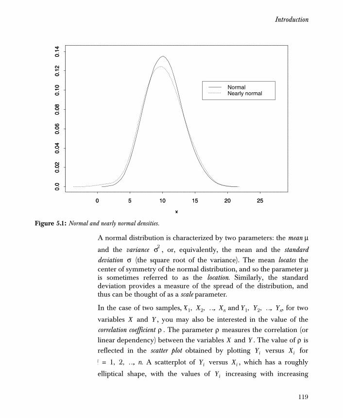
Introduction
A normal distribution is characterized by two parameters: the mean μ
and the variance , or, equivalently, the mean and the standarddeviation (the square root of the variance). The mean locates thecenter of symmetry of the normal distribution, and so the parameter μis sometimes referred to as the location. Similarly, the standarddeviation provides a measure of the spread of the distribution, andthus can be thought of as a scale parameter.
In the case of two samples, and , for two
variables and , you may also be interested in the value of thecorrelation coefficient . The parameter ρ measures the correlation (orlinear dependency) between the variables and . The value of ρ isreflected in the scatter plot obtained by plotting versus for
. A scatterplot of versus , which has a roughly
elliptical shape, with the values of increasing with increasing
Figure 5.1: Normal and nearly normal densities.
x
0 5 10 15 20 25
0.0
0.02
0.04
0.06
0.08
0.10
0.12
0.14
x
0 5 10 15 20 25
0.0
0.02
0.04
0.06
0.08
0.10
0.12
0.14
NormalNearly normal
σ2
σ
X1 X2 … X, n, , Y1 Y2 … Y, n, ,
X Yρ
X YYi Xi
i 1 2 … n, , ,= Yi Xi
Yi
119
Chapter 5 Statistical Inference for One- and Two-Sample Problems
values of , corresponds to positive correlation (see, for example,
Figure 5.7). An elliptically-shaped scatter plot with the values of
decreasing with increasing values of corresponds to negative
correlation . A circular shape to the scatter plot corresponds to azero value for the correlation coefficient .
Keep in mind that the correlation between two variables and , asjust described, is quite distinct from serial correlation between theobservations within one or both of the samples when the samples arecollected over time. Whereas the former reveals itself in a scatterplotof the versus the , the latter reveals itself in scatter plots of theobservations versus lagged values of the observations; for example, ascatter plot of versus or a scatter plot of versus . Ifthese scatter plots have a circular shape, the data are seriallyuncorrelated. Otherwise, the data have some serial correlation.
Generally, you must be careful not to assume that data collected overtime are serially uncorrelated. You need to check this assumptioncarefully, because the presence of serial correlation invalidates mostof the methods of this chapter.
To summarize: You want to draw conclusions from your data
concerning the population mean and variance parameters and for one sample of data, and you want to draw conclusions from yourdata concerning the population means , , the population
variances , and the population correlation coefficient ρ for two
samples of data. You frame your conclusions about the aboveparameters in one of the following two types of statistical inferencestatements, illustrated for the case of the population mean μ in a one-sample problem:
• A CONFIDENCE INTERVAL. With probability , the mean lies within the confidence interval (L,U).
• A HYPOTHESIS TEST. The computed statistic T compares the null hypothesis that the mean μ has the specified value μ0
with the alternative hypothesis that . At any level of significance greater than the reported p-value for T, we reject the null hypothesis in favor of the alternative hypothesis.
Xi ρ
Yi
Xi
ρρ
X Y
Yi Xi
Yi Yi 1+ Xi Xi 1+
μ σ2
μ1 μ2
σ12 σ2
2
1 α–
μ
μ μ0≠
120
Introduction
A more complete description of confidence intervals and hypothesistests is provided in the section Statistical Inference on page 125.
Classical methods of statistical inference, such as Student’s t methods,rely on the assumptions that the data come from a normal distributionand the observations within a sample are serially uncorrelated. If yourdata contain outliers, or are strongly nonnormal, or if theobservations within a sample are serially correlated, the classicalmethods of statistical inference can give you very misleading results.Fortunately, there are robust and nonparametric methods which givereliable statistical inference for data that contain outliers or arestrongly nonnormal. Special methods are needed for dealing withdata that are serially correlated. See, for example, Heidelberger andWelch (1981).
In this chapter, you learn to use Spotfire S+ functions for making bothclassical and robust or nonparametric statistical inference statementsfor the population means and variances for one and two samples, andfor the population correlation coefficient for two samples. The basicsteps in using Spotfire S+ functions are essentially the same no matterwhich of the above parameters you are interested in. They are asfollows:
1. Setting up your data.
Before Spotfire S+ can be used to analyze the data, you must put the data in a form that Spotfire S+ recognizes.
2. Exploratory data analysis (EDA).
EDA is a graphically-oriented method of data analysis which helps you determine whether the data support the assumptions required for the classical methods of statistical inference: an outlier-free nearly normal distribution and serially uncorrelated observations.
3. Statistical inference.
Once you’ve verified that your sample or samples are nearly normal, outlier-free, and uncorrelated, you can use classical methods of statistical inference that assume a normal distribution and uncorrelated observations, to draw conclusions from your data.
121

Chapter 5 Statistical Inference for One- and Two-Sample Problems
If your data are not nearly normal and outlier-free, the results of the classical methods of statistical inference may be misleading. Hence, you often need robust or nonparametric methods, as described in the section Robust and Nonparametric Methods on page 127.
122
Background
BACKGROUND
This section prepares you for using the Spotfire S+ functions in theremainder of the chapter by providing brief background informationon the following three topics: exploratory data analysis, statisticalinference, and robust and nonparametric methods.
Exploratory Data Analysis
The classical methods of statistical inference depend heavily on theassumption that your data are outlier-free and nearly normal, and thatyour data are serially uncorrelated. Exploratory data analysis (EDA)uses graphical displays to help you obtain an understanding ofwhether or not such assumptions hold. Thus, you should always carryout some graphical exploratory data analysis to answer the followingquestions:
• Do the data come from a nearly normal distribution?
• Do the data contain outliers?
• If the data were collected over time, is there any evidence of serial correlation (correlation between successive values of the data)?
You can get a pretty good picture of the shape of the distributiongenerating your data, and also detect the presence of outliers, bylooking at the following collection of four plots: a histogram, a boxplot,a density plot, and a normal qq-plot. Examples of these four plots areprovided in Figure 5.2.
Density plots are essentially smooth versions of histograms, whichprovide smooth estimates of population frequency, or probability densitycurves; for example, the normal and nearly normal curves of Figure5.1. Since the latter are smooth curves, it is both appropriate andmore pleasant to look at density plots than at histograms.
A normal qq-plot (or quantile-quantile plot) consists of a plot of theordered values of your data versus the corresponding quantiles of astandard normal distribution; that is, a normal distribution with meanzero and variance one. If the qq-plot is fairly linear, your data arereasonably Gaussian; otherwise, they are not.
123
Chapter 5 Statistical Inference for One- and Two-Sample Problems
Of these four plots, the histogram and density plot give you the bestpicture of the distribution shape, while the boxplot and normalqq-plot give the clearest display of outliers. The boxplot also gives aclear indication of the median (the solid dot inside the box), and theupper and lower quartiles (the upper and lower ends of the box).
A simple Spotfire S+ function can create all four suggesteddistributional shape EDA plots, and displays them all on a singlescreen or a single hard copy plot. Define the function as follows:
> eda.shape <- function(x) {+ par(mfrow = c(2, 2))+ hist(x)+ boxplot(x)+ iqd <- summary(x)[5] - summary(x)[2]+ plot(density(x, width = 2 * iqd), + xlab = "x", ylab = "", type = "l")+ qqnorm(x, pch = 1)+ qqline(x)+ invisible()+ }
This function is used to make the EDA plots you see in the remainderof this chapter. The argument width = 2*iqd to density sets thedegree of smoothness of the density plot in a good way. For moredetails on writing functions, see the Programmer’s Guide .
If you have collected your data over time, the data may contain serialcorrelation. That is, the observations may be correlated with oneanother at different times. The assessment of whether or not there isany time series correlation in the context of confirmatory dataanalysis for location and scale parameters is an often-neglected task.
You can check for obvious time series features, such as trends andcycles, by looking at a plot of your data against time, using thefunction ts.plot. You can check for the presence of less obviousserial correlation by looking at a plot of the autocorrelation functionfor the data, using the acf function. These plots can be created, anddisplayed one above the other, with the following Spotfire S+function.
124

Background
> eda.ts <- function(x) {+ par(mfrow = c(2, 1))+ ts.plot(as.ts(x), type = "b", pch = 1)+ acf(x)+ invisible()+ }
This function is used to make the time series EDA plots you find inthe remainder of this chapter. See, for example, Figure 5.3. Thediscussion of Figure 5.3 includes a guideline for interpreting the acfplot.
Statistical Inference
Formal methods of statistical inference provide probability-basedstatements about population parameters such as the mean, variance,and correlation coefficient for your data. You may be interested in asimple point estimate of a population parameter. For example, thesample mean is a point estimate of the population mean. However, apoint estimate neither conveys any uncertainty about the value of theestimate, nor indicates whether a hypothesis about the populationparameter is to be rejected. To address these two issues, you willusually use one or both of the following methods of statisticalinference: confidence intervals and hypothesis tests.
We define these two methods for you, letting represent any one ofthe parameters you may be interested in; for example, may be themean , or the difference between two means , or the
correlation coefficient .
CONFIDENCE INTERVALS. A confidence intervalfor the true but unknown parameter is any interval of the form(L,U), such that the probability is that (L,U) contains . Theprobability with which the interval (L,U) fails to cover q is
Warning
If either the time series plot or the acf plot suggests the presence of serial correlation, you can place little credence in the results computed in this chapter, using either the Student’s t statistic approach or using the nonparametric Wilcoxon approach. A method for estimating the population mean in the presence of serial correlation is described by Heidelberger and Welch (1981). Seek expert assistance, as needed.
θθ
μ μ1 μ2–
ρ
1 α–( )100%θ
1 α– θα
125
Chapter 5 Statistical Inference for One- and Two-Sample Problems
sometimes called the error rate of the interval. The quantity is called the confidence level of the confidence interval.
Common values of are , which yield %,
%, and % confidence intervals, respectively.
HYPOTHESIS TESTS. A hypothesis test is a probability-basedmethod for making a decision concerning the value of a populationparameter (for example, the population mean or standarddeviation in a one-sample problem), or the relative values of twopopulation parameters and (for example, the difference
between the population means in a two-sample problem).You begin by forming a null hypothesis and an alternative hypothesis. Forexample, in the two-sample problem your null hypothesis is often thehypothesis that , and your alternative hypothesis is one of thefollowing:
• The two-sided alternative
• The greater-than alternative
• The less-than alternative
Your decision to accept the null hypothesis, or to reject the nullhypothesis in favor of your alternative hypothesis is based on theobserved value of a suitably chosen test statistic . The
probability that the statistic exceeds the observed value whenyour null hypothesis is in fact true, is called the p-value.
For example, suppose you are testing the null hypothesis that
against the alternative hypothesis that in a one-sample
problem. The p-value is the probability that the absolute value of exceeds the absolute value of for your data, when the nullhypothesis is true.
In formal hypothesis testing, you proceed by choosing a “good”statistic and specifying a level of significance, which is the probabilityof rejecting a null hypothesis when the null hypothesis is in fact true.
1 α–( ) 100%×α α 0.01, 0.05, 0.1= 99
95 90
θ μσ
θ1 θ2
μ1 μ2–
θ1 θ2=
θ1 θ2≠
θ1 θ2>
θ1 θ2<
T tobs= T
T tobs
θ θ0=
θ θ0≠
Ttobs
T
126
Background
In terms of formal hypothesis testing, your p-value has the followinginterpretation: the p-value is the level of significance for which yourobserved test statistic value lies on the boundary betweenacceptance and rejection of the null hypothesis. At any significancelevel greater than the p-value, you reject the null hypothesis, and atany significance level less than the p-value you accept the nullhypothesis. For example, if your p-value is 0.03, you reject the nullhypothesis at a significance level of 0.05, and accept the nullhypothesis at a significance level of 0.01.
Robust and Nonparametric Methods
Two problems frequently complicate your statistical analysis. Forexample, Student’s t test, which is the basis for most statisticalinference on the mean-value locations of normal distributions, relieson two critical assumptions:
1. The observations have a common normal (or Gaussian)
distribution with mean μ and variance .
2. The observations are independent.
However, one or both of these assumptions often fail to hold inpractice.
For example, if the actual distribution for the observations is anoutlier-generating, heavy-tailed deviation from an assumed Gaussiandistribution, the confidence level remains quite close to ,but the average confidence interval length is considerably larger thanunder normality. The p values based on the Student’s t test are alsoheavily influenced by outliers.
In this example, and more generally, you would like to have statisticalmethods with the property that the conclusions you draw are notmuch affected if the distribution for the data deviates somewhat fromthe assumed model; for example, if the assumed model is a normal,or Gaussian distribution, and the actual model for the data is a nearlynormal distribution. Such methods are called robust. In this chapteryou will learn how to use a Spotfire S+ function to obtain robust pointestimates and robust confidence intervals for the populationcorrelation coefficient.
For one and two-sample location parameter problems (amongothers), there exist strongly robust alternatives to classical methods, inthe form of nonparametric statistics. The term nonparametric means that
tobs
σ2
1 α–( )100%
127

Chapter 5 Statistical Inference for One- and Two-Sample Problems
the methods work even when the actual distribution for the data is farfrom normal; that is, when the data do not have to have even a nearlynormal distribution. In this chapter, you will learn to use one of thebest of the nonparametric methods for constructing a hypothesis testp-value, namely the Wilcoxon rank method, as implemented in theSpotfire S+ function wilcox.test.
It is important to keep in mind that serial correlation in the data canquickly invalidate the use of both classical methods (such as Student’st) and nonparametric methods (such as the Wilcoxon rank method)for computing confidence intervals and p values. For example, a 95%Student’s t confidence interval can have a much higher error ratethan 5% when there is a small amount of positive correlation in thedata. Also, most modern robust methods are oriented towardobtaining insensitivity toward outliers generated by heavy-tailednearly normal distributions, and are not designed to cope with serialcorrelation. For information on how to construct confidence intervalsfor the population mean when your data are serially correlated andfree of outliers, see Heidelberger and Welch (1981).
128

One Sample: Distribution Shape, Location, and Scale
ONE SAMPLE: DISTRIBUTION SHAPE, LOCATION, AND SCALE
In 1876, the French physicist Cornu reported a value of 299,990 km/sec for c, the speed of light. In 1879, the American physicist A.A.Michelson carried out several experiments to verify and improve onCornu’s value.
Michelson obtained the following 20 measurements of the speed oflight:
850 740 900 1070 930 850 950 980 980 8801000 980 930 650 760 810 1000 1000 960 960
To obtain Michelson’s actual measurements in km/sec, add 299,000km/sec to each of the above values.
The twenty observations can be thought of as observed values oftwenty random variables with a common but unknown mean-valuelocation μ. If the experimental setup for measuring the speed of lightis free of bias, then it is reasonable to assume that μ is the true speedof light.
In evaluating this data, we seek answers to at least five questions:
1. What is the speed of light ?
2. Has the speed of light changed relative to our best previous value ?
3. What is the uncertainty associated with our answers to (1) and (2)?
4. What is the shape of the distribution of the data?
5. The measurements were taken over time. Is there any evidence of serial correlation?
The first three questions were probably in Michelson’s mind when hegathered his data. The last two must be answered to determine whichtechniques can be used to obtain valid statistical inferences from thedata. For example, if the shape of the distribution indicates a nearlynormal distribution without outliers, we can use the Student’s t tests inattempting to answer question (2). If the data contain outliers or arefar from normal, we should use a robust method or a nonparametric
μ
μ0
129
Chapter 5 Statistical Inference for One- and Two-Sample Problems
method such as the Wilcoxon signed-rank test. On the other hand, ifserial correlation exists, neither the Student’s t nor the Wilcoxon testoffers valid conclusions.
In this section, we use Spotfire S+ to carefully analyze the Michelsondata. Identical techniques can be used to explore and analyze any setof one-sample data.
Setting Up the Data
The data form a single, ordered set of observations, so they areappropriately described in Spotfire S+ as a vector. Use the scanfunction to create the vector mich:
> mich <- scan()
1: 850 740 900 1070 9306: 850 950 980 980 88011: 1000 980 930 650 76016: 810 1000 1000 960 96021:
Exploratory Data Analysis
To start, we can evaluate the shape of the distribution, by making a setof four EDA plots, using the eda.shape function described in thesection Exploratory Data Analysis on page 123:
> eda.shape(mich)
The plots, shown in Figure 5.2, reveal a distinctly skewed distribution,skewed toward the left (that is, toward smaller values), but rathernormal in the middle region. The distribution is thus not normal, andprobably not even "nearly" normal.
The solid horizontal line in the box plot is located at the median of thedata, and the upper and lower ends of the box are located at the upperquartile and lower quartile of the data, respectively. To get precisevalues for the median and quartiles, use the summary function:
> summary(mich)
Min. 1st Qu. Median Mean 3rd Qu. Max. 650 850 940 909 980 1070
The summary shows, from left to right, the smallest observation, thefirst quartile, the median, the mean, the third quartile, and the largestobservation. From this summary you can compute the interquartile
130
One Sample: Distribution Shape, Location, and Scale
range, . The interquartile range provides a usefulcriterion for identifying outliers—any observation which is more than
above the third quartile or below the first quartile is asuspected outlier.
To examine possible serial correlation, or dependency, make twoplots using the eda.ts function defined in the section ExploratoryData Analysis on page 123.
IQR 3Q 1Q–=
1.5 IQR×
Figure 5.2: Exploratory data analysis plots.
700 800 900 1100
02
46
8
x
700
800
900
1000
x
600 800 1000
0.0
0.00
10.
002
0.00
3
Quantiles of Standard Normal
x
-2 -1 0 1 2
700
800
900
1000
131
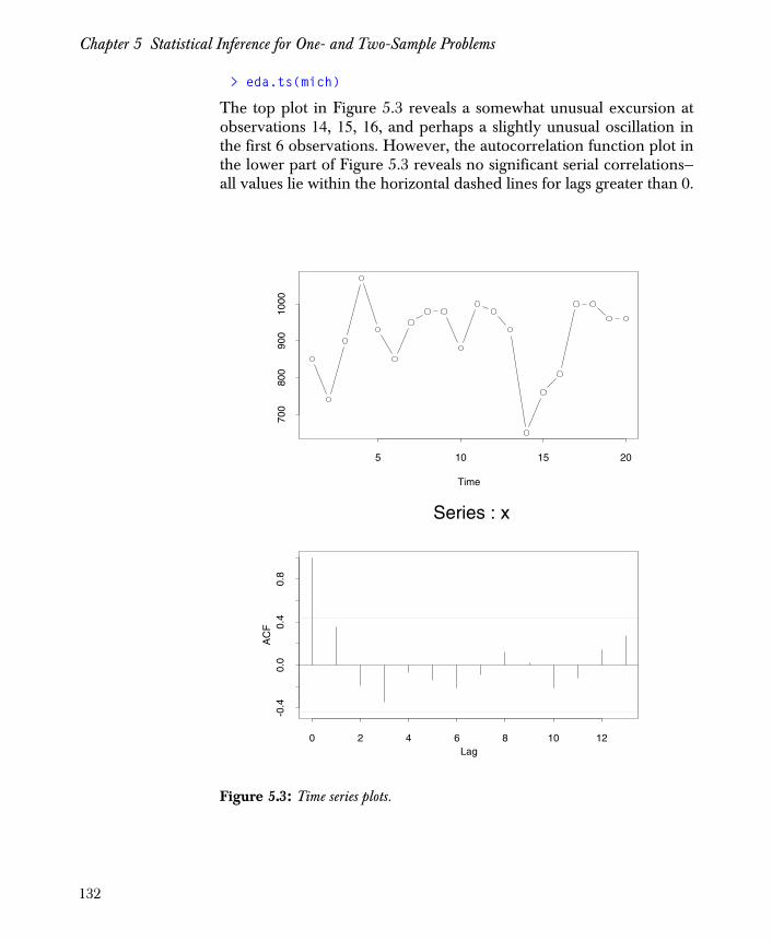
Chapter 5 Statistical Inference for One- and Two-Sample Problems
> eda.ts(mich)
The top plot in Figure 5.3 reveals a somewhat unusual excursion atobservations 14, 15, 16, and perhaps a slightly unusual oscillation inthe first 6 observations. However, the autocorrelation function plot inthe lower part of Figure 5.3 reveals no significant serial correlations—all values lie within the horizontal dashed lines for lags greater than 0.
Figure 5.3: Time series plots.
Time
5 10 15 20
700
800
900
1000
Lag
AC
F
0 2 4 6 8 10 12
-0.4
0.0
0.4
0.8
Series : x
132

One Sample: Distribution Shape, Location, and Scale
Statistical Inference
Because the Michelson data are not normal, you should probably usethe Wilcoxon signed-rank test rather than the Student’s t test for yourstatistical inference. For illustrative purposes, we’ll use both.
To compute Student’s t confidence intervals for the population mean-value location parameter μ, and to compute Student’s t significancetest p values for the parameter , use the function t.test.
To perform the test, you specify the confidence level, thehypothesized mean-value location , and the hypothesis being tested,as follows:
• conf.level specifies the confidence level of the confidence interval. Usual values are 0.90, 0.95, or 0.99. The default is 0.95.
• mu specifies the null hypothesis value of . The default is μ0 = 0, which is often inappropriate for one-sample problems.
You should choose carefully, using either a previously accepted value or a value suggested by the data before sampling.
• alternative specifies the specific hypothesis being tested. There are three options:
• "two.sided" tests the hypothesis that the true mean is not equal to . This is the default alternative.
• "greater" tests the hypothesis that the true mean is greater than .
• "less" tests the hypothesis that the true mean is less than .
For Michelson’s data, suppose you want to test the null hypothesisvalue (plus 299,000) against a two-sided alternative. To dothis, use t.test with the argument mu=990, as in the command below:
> t.test(mich, mu = 990)
One-sample t-Test
data: micht = -3.4524, df = 19, p-value = 0.0027
μ0
μ
μ0 μ
μ
μ0
μ0
μ0
μ0 990=
133

Chapter 5 Statistical Inference for One- and Two-Sample Problems
alternative hypothesis: true mean is not equal to 99095 percent confidence interval: 859.8931 958.1069sample estimates: mean of x 909
The p value is 0.0027, which is highly significant. Spotfire S+ returnsother useful information besides the p value, including the t statisticvalue, the degrees of freedom (df), the sample mean, and theconfidence interval.
134
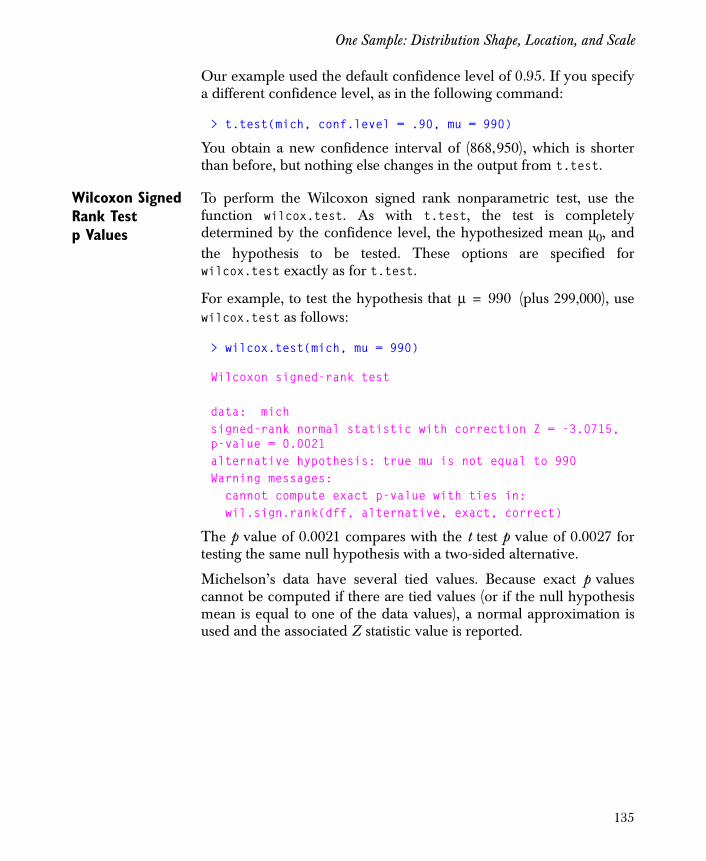
One Sample: Distribution Shape, Location, and Scale
Our example used the default confidence level of 0.95. If you specifya different confidence level, as in the following command:
> t.test(mich, conf.level = .90, mu = 990)
You obtain a new confidence interval of (868,950), which is shorterthan before, but nothing else changes in the output from t.test.
Wilcoxon Signed Rank Test p Values
To perform the Wilcoxon signed rank nonparametric test, use thefunction wilcox.test. As with t.test, the test is completelydetermined by the confidence level, the hypothesized mean μ0, andthe hypothesis to be tested. These options are specified forwilcox.test exactly as for t.test.
For example, to test the hypothesis that (plus 299,000), usewilcox.test as follows:
> wilcox.test(mich, mu = 990)
Wilcoxon signed-rank test
data: michsigned-rank normal statistic with correction Z = -3.0715, p-value = 0.0021alternative hypothesis: true mu is not equal to 990Warning messages: cannot compute exact p-value with ties in: wil.sign.rank(dff, alternative, exact, correct)
The p value of 0.0021 compares with the t test p value of 0.0027 fortesting the same null hypothesis with a two-sided alternative.
Michelson’s data have several tied values. Because exact p valuescannot be computed if there are tied values (or if the null hypothesismean is equal to one of the data values), a normal approximation isused and the associated Z statistic value is reported.
μ 990=
135

Chapter 5 Statistical Inference for One- and Two-Sample Problems
TWO SAMPLES: DISTRIBUTION SHAPES, LOCATIONS, AND SCALES
Suppose you are a nutritionist interested in the relative merits of twodiets, one featuring high protein, the other low protein. Do the twodiets lead to differences in mean weight gain? Consider the data inTable 5.1, which shows the weight gains (in grams) for two lots offemale rats, under the two diets.
Table 5.1: Weight gain data.
High Protein Low Protein
134 70
146 118
104 101
119 85
124 107
161 132
107 94
83
113
129
97
123
136
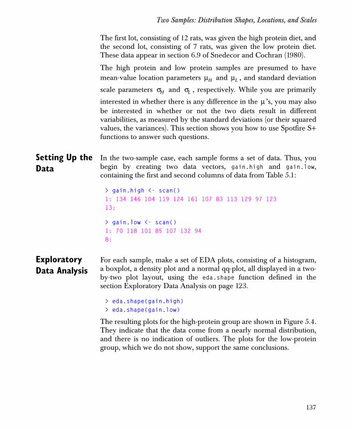
Two Samples: Distribution Shapes, Locations, and Scales
The first lot, consisting of 12 rats, was given the high protein diet, andthe second lot, consisting of 7 rats, was given the low protein diet.These data appear in section 6.9 of Snedecor and Cochran (1980).
The high protein and low protein samples are presumed to havemean-value location parameters and , and standard deviation
scale parameters and , respectively. While you are primarily
interested in whether there is any difference in the ’s, you may alsobe interested in whether or not the two diets result in differentvariabilities, as measured by the standard deviations (or their squaredvalues, the variances). This section shows you how to use Spotfire S+functions to answer such questions.
Setting Up the Data
In the two-sample case, each sample forms a set of data. Thus, youbegin by creating two data vectors, gain.high and gain.low,containing the first and second columns of data from Table 5.1:
> gain.high <- scan()1: 134 146 104 119 124 161 107 83 113 129 97 12313:
> gain.low <- scan()1: 70 118 101 85 107 132 948:
Exploratory Data Analysis
For each sample, make a set of EDA plots, consisting of a histogram,a boxplot, a density plot and a normal qq-plot, all displayed in a two-by-two plot layout, using the eda.shape function defined in thesection Exploratory Data Analysis on page 123.
> eda.shape(gain.high)> eda.shape(gain.low)
The resulting plots for the high-protein group are shown in Figure 5.4.They indicate that the data come from a nearly normal distribution,and there is no indication of outliers. The plots for the low-proteingroup, which we do not show, support the same conclusions.
μH μL
σH σL
μ
137

Chapter 5 Statistical Inference for One- and Two-Sample Problems
Since the data were not collected in any specific time order, you neednot make any exploratory time series plots to check for serialcorrelation.
Statistical Inference
Is the mean weight gain the same for the two groups of rats?Specifically, does the high-protein group show a higher averageweight gain? From our exploratory data analysis, we have goodreason to believe that Student’s t test will provide a valid test of our
Figure 5.4: EDA plots for high-protein group.
80 100 140 180
01
23
4
x
8010
012
014
016
0
x
50 100 150 200
0.0
0.00
50.
010
0.01
5
Quantiles of Standard Normal
x
-1 0 1
8010
012
014
016
0
138
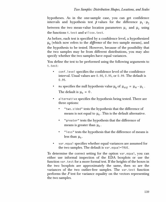
Two Samples: Distribution Shapes, Locations, and Scales
hypotheses. As in the one-sample case, you can get confidenceintervals and hypothesis test p values for the difference μ1 - μ2
between the two mean-value location parameters and usingthe functions t.test and wilcox.test.
As before, each test is specified by a confidence level, a hypothesizedμ0 (which now refers to the difference of the two sample means), andthe hypothesis to be tested. However, because of the possibility thatthe two samples may be from different distributions, you may alsospecify whether the two samples have equal variances.
You define the test to be performed using the following arguments tot.test:
• conf.level specifies the confidence level of the confidence interval. Usual values are 0.90, 0.95, or 0.99. The default is 0.95.
• mu specifies the null hypothesis value μ0 of .
The default is .
• alternative specifies the hypothesis being tested. There are three options:
• "two.sided" tests the hypothesis that the difference of means is not equal to . This is the default alternative.
• "greater" tests the hypothesis that the difference of means is greater than .
• "less" tests the hypothesis that the difference of means is less than .
• var.equal specifies whether equal variances are assumed for the two samples. The default is var.equal=TRUE.
To determine the correct setting for the option var.equal, you caneither use informal inspection of the EDA boxplots or use thefunction var.test for a more formal test. If the heights of the boxes inthe two boxplots are approximately the same, then so are thevariances of the two outlier-free samples. The var.test functionperforms the F test for variance equality on the vectors representingthe two samples.
μ1 μ2
μdiff μH μL–=
μ0 0=
μ0
μ0
μ0
139

Chapter 5 Statistical Inference for One- and Two-Sample Problems
For the weight gain data, the var.test function returns:
> var.test(gain.high, gain.low)
F test for variance equalitydata: gain.high and gain.lowF = 1.0755, num df = 11, denom df = 6, p-value = 0.9788alternative hypothesis: true ratio of variances is not equal to 195 percent confidence interval: 0.198811 4.173718sample estimates: variance of x variance of y 457.4545 425.3333
The evidence supports the assumption that the variances are thesame, so var.equal=T is a valid choice.
We are interested in two alternative hypotheses: the two-sidedalternative that and the one-sided alternative that
. To test these, we run the standard two-sample t testtwice, once with the default two-sided alternative and a second timewith the one-sided alternative alt="g".
You get both a confidence interval for , and a two-sided test
of the null hypothesis that , by the following simple useof t.test:
> t.test(gain.high, gain.low)
Standard Two-Sample t-Testdata: gain.high and gain.lowt = 1.8914, df = 17, p-value = 0.0757alternative hypothesis: true difference in means is not equal to 095 percent confidence interval: -2.193679 40.193679sample estimates: mean of x mean of y 120 101
The p value is 0.0757, so the null hypothesis is rejected at the 0.10level, but not at the 0.05 level. The confidence interval is (-2.2, 40.2).
μH μL– 0=
μH μL– 0>
μH μL–
μH μL– 0=
140

Two Samples: Distribution Shapes, Locations, and Scales
To test the one-sided alternative that , use t.test againwith the argument alternative="greater" (abbreviated below forease of typing):
> t.test(gain.high, gain.low, alt = "g")
Standard Two-Sample t-Test
data: gain.high and gain.lowt = 1.8914, df = 17, p-value = 0.0379alternative hypothesis: true difference in means is greater than 095 percent confidence interval: 1.525171 NAsample estimates:mean of x mean of y 120 101
In this case, the p value is just half of the p value for the two-sidedalternative. This relationship between the p values of the one-sidedand two-sided alternatives holds in general. You also see that whenyou use the alt="g" argument, you get a lower confidence bound.This is the natural one-sided confidence interval corresponding to the“greater than” alternative.
Hypothesis Test p-Values Using wilcox.test
To get a two-sided hypothesis test p value for the “two-sided”alternative, based on the Wilcoxon rank sum test statistic, usewilcox.test, which takes the same arguments as t.test:
> wilcox.test(gain.high, gain.low)
Wilcoxon rank-sum test
data: gain.high and gain.lowrank-sum normal statistic with correction Z = 1.6911, p-value = 0.0908alternative hypothesis: true mu is not equal to 0
Warning messages: cannot compute exact p-value with ties in: wil.rank.sum(x, y, alternative, exact, correct)
μH μL– 0>
141

Chapter 5 Statistical Inference for One- and Two-Sample Problems
The above p value of 0.0908, based on the normal approximation(used because of ties in the data), is rather close to the t statisticp value of 0.0757.
142

Two Paired Samples
TWO PAIRED SAMPLES
Often two samples of data are collected in the context of a comparativestudy. A comparative study is designed to determine the differencebetween effects, rather than the individual effects. For example,consider the data in Table 5.2, which give values of wear for two kindsof shoe sole material, A and B, along with the differences in values.
In the table, (L) indicates the material was used on the left sole and(R) indicates it was used on the right sole.
The experiment leading to this data, described in Box, Hunter, andHunter (1978), was carried out by taking 10 pairs of shoes and puttinga sole of material A on one shoe and a sole of material B on the othershoe in each pair. Which material type went on each shoe was
Table 5.2: Comparing shoe sole material
Boy wear.A wear.B wear.A-wear.B
1 14.0(R) 13.2(L) 0.8
2 8.8(R) 8.2(L) 0.6
3 11.2(L) 10.9(R) 0.3
4 14,2(R) 14.3(L) -0.1
5 11.8(L) 10.7(R) 1.1
6 6.4(R) 6.6(L) -0.2
7 9.8(R) 9.5(L) 0.3
8 11.3(R) 10.8(L) 0.5
9 9.3(L) 8.8(R) 0.5
10 13.6(R) 13.3(L) 0.3
143
Chapter 5 Statistical Inference for One- and Two-Sample Problems
determined by randomizing, with equal probability that material Awas on the right shoe or left shoe. A group of 10 boys then wore theshoes for a period of time, after which the amount of wear wasmeasured. The problem is to determine whether shoe material A or Bis longer wearing.
You could treat this problem as a two-sample location problem anduse either t.test or wilcox.test, as described in the section TwoSamples: Distribution Shapes, Locations, and Scales on page 136, totest for a difference in the means of wear for material A and materialB. However, you will not be very successful with this approachbecause there is considerable variability in wear of both materialstypes A and B from individual to individual, and this variability tendsto mask the difference in wear of material A and B when you use anordinary two-sample test.
However, the above experiment uses paired comparisons. Each boywears one shoe with material A and one shoe with material B. Ingeneral, pairing involves selecting similar individuals or things. Oneoften uses self-pairing as in the above experiment, in which twoprocedures, often called treatments, are applied to the same individual(either simultaneously or at two closely spaced time intervals) or tosimilar material. The goal of pairing is to make a comparison moresensitive by measuring experimental outcome differences on eachpair, and combining the differences to form a statistical test orconfidence interval. When you have paired data, you use t.test andwilcox.test with the optional argument paired = T.
The use of paired versions of t.test and wilcox.test leads toimproved sensitivity over the usual versions when the variability ofdifferences is smaller than the variability of each sample; for example,when the variability of differences of material wear between materialsA and B is smaller than the variability in wear of material A andmaterial B.
144
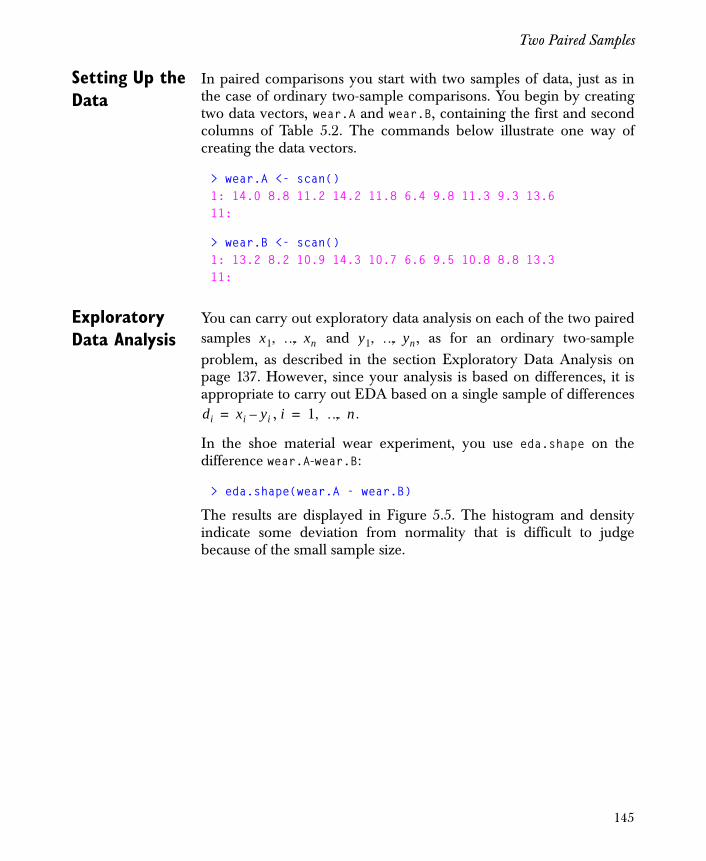
Two Paired Samples
Setting Up the Data
In paired comparisons you start with two samples of data, just as inthe case of ordinary two-sample comparisons. You begin by creatingtwo data vectors, wear.A and wear.B, containing the first and secondcolumns of Table 5.2. The commands below illustrate one way ofcreating the data vectors.
> wear.A <- scan()1: 14.0 8.8 11.2 14.2 11.8 6.4 9.8 11.3 9.3 13.611:
> wear.B <- scan()1: 13.2 8.2 10.9 14.3 10.7 6.6 9.5 10.8 8.8 13.311:
Exploratory Data Analysis
You can carry out exploratory data analysis on each of the two pairedsamples and , as for an ordinary two-sampleproblem, as described in the section Exploratory Data Analysis onpage 137. However, since your analysis is based on differences, it isappropriate to carry out EDA based on a single sample of differences
, .
In the shoe material wear experiment, you use eda.shape on thedifference wear.A-wear.B:
> eda.shape(wear.A - wear.B)
The results are displayed in Figure 5.5. The histogram and densityindicate some deviation from normality that is difficult to judgebecause of the small sample size.
x1 … x, n, y1 … y, n,
di xi yi–= i 1 … n, ,=
145
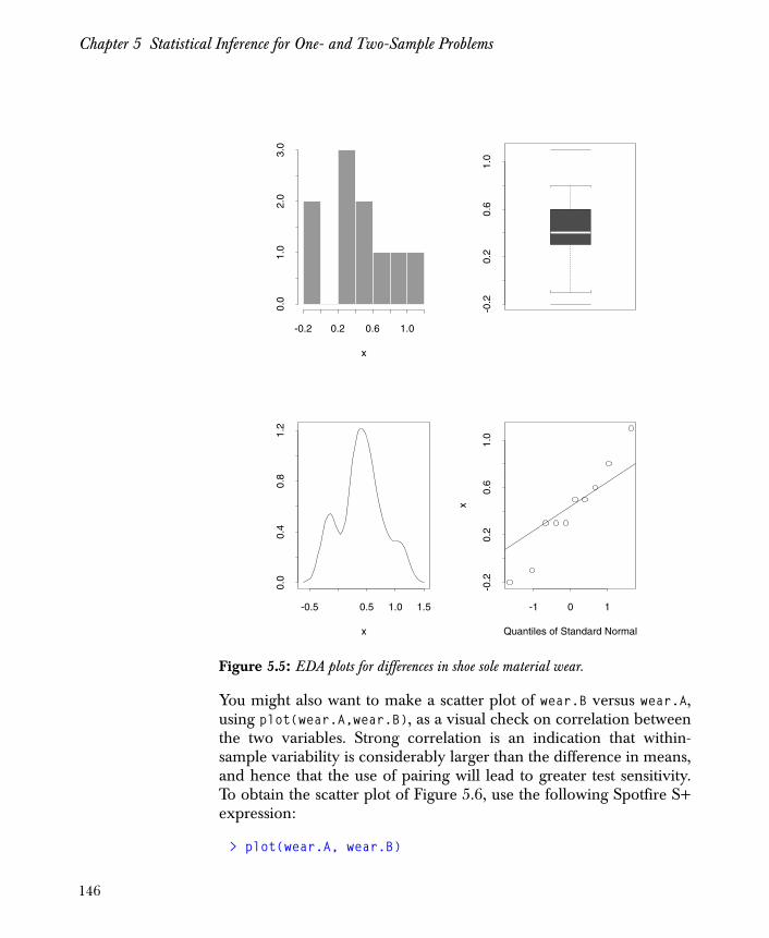
Chapter 5 Statistical Inference for One- and Two-Sample Problems
You might also want to make a scatter plot of wear.B versus wear.A,using plot(wear.A,wear.B), as a visual check on correlation betweenthe two variables. Strong correlation is an indication that within-sample variability is considerably larger than the difference in means,and hence that the use of pairing will lead to greater test sensitivity.To obtain the scatter plot of Figure 5.6, use the following Spotfire S+expression:
> plot(wear.A, wear.B)
Figure 5.5: EDA plots for differences in shoe sole material wear.
-0.2 0.2 0.6 1.0
0.0
1.0
2.0
3.0
x
-0.2
0.2
0.6
1.0
x
-0.5 0.5 1.0 1.5
0.0
0.4
0.8
1.2
Quantiles of Standard Normal
x
-1 0 1
-0.2
0.2
0.6
1.0
146

Two Paired Samples
Statistical Inference
To perform a paired t test on the shoe material wear data, with thedefault two-sided alternative use t.test with the paired argument, asfollows:
> t.test(wear.A, wear.B, paired = T)
Paired t-Test
data: wear.A and wear.Bt = 3.3489, df = 9, p-value = 0.0085alternative hypothesis: true mean of differences is not equal to 095 percent confidence interval: 0.1330461 0.6869539sample estimates: mean of x - y 0.41
Figure 5.6: Scatter plot of wear.A versus wear.B.
•
•
•
•
•
•
•
•
•
•
wear.A
wea
r.B
8 10 12 14
810
1214
147
Chapter 5 Statistical Inference for One- and Two-Sample Problems
The p value of .0085 is highly significant for testing the difference inmean wear of materials A and B. You also get the 95% confidenceinterval (0.13, 0.67) for the difference in mean values. You can controlthe type of alternative hypothesis with the alt optional argument, andyou can control the confidence level with the conf.level optionalargument, as usual. To perform a paired Wilcoxon test (often calledthe Wilcoxon signed rank test) on the shoe material data, with thedefault two-sided alternative use wilcox.test with the pairedargument, as follows:
> wilcox.test(wear.A, wear.B, paired = T)
Wilcoxon signed-rank test
data: wear.A and wear.Bsigned-rank normal statistic with correction Z = 2.4495, p-value = 0.0143alternative hypothesis: true mu is not equal to 0
Warning messages: cannot compute exact p-value with ties in: wil.sign.rank(dff, alternative, exact, correct)
The p value of 0.0143 is highly significant for testing the nullhypothesis of equal centers of symmetry for the distributions ofwear.A and wear.B. You can control the type of alternative hypothesisby using the optional argument alt as usual.
148
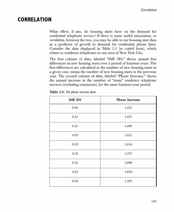
Correlation
CORRELATION
What effect, if any, do housing starts have on the demand forresidential telephone service? If there is some useful association, orcorrelation , between the two, you may be able to use housing start dataas a predictor of growth in demand for residential phone lines.Consider the data displayed in Table 5.3 (in coded form), whichrelates to residence telephones in one area of New York City.
The first column of data, labeled “Diff. HS,” shows annual firstdifferences in new housing starts over a period of fourteen years. Thefirst differences are calculated as the number of new housing starts ina given year, minus the number of new housing starts in the previousyear. The second column of data, labeled “Phone Increase,” showsthe annual increase in the number of “main” residence telephoneservices (excluding extensions), for the same fourteen-year period.
Table 5.3: The phone increase data.
Diff. HS Phone Increase
0.06 1.135
0.13 1.075
0.14 1.496
-0.07 1.611
-0.05 1.654
-0.31 1.573
0.12 1.689
0.23 1.850
-0.05 1.587
149
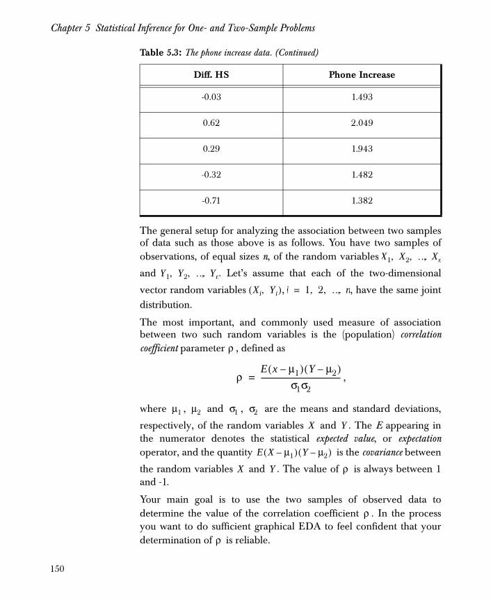
Chapter 5 Statistical Inference for One- and Two-Sample Problems
The general setup for analyzing the association between two samplesof data such as those above is as follows. You have two samples ofobservations, of equal sizes n, of the random variables
and . Let’s assume that each of the two-dimensional
vector random variables , , have the same jointdistribution.
The most important, and commonly used measure of associationbetween two such random variables is the (population) correlationcoefficient parameter , defined as
,
where , and , are the means and standard deviations,
respectively, of the random variables and . The E appearing inthe numerator denotes the statistical expected value, or expectationoperator, and the quantity is the covariance between
the random variables and . The value of is always between 1and -1.
Your main goal is to use the two samples of observed data todetermine the value of the correlation coefficient . In the processyou want to do sufficient graphical EDA to feel confident that yourdetermination of is reliable.
-0.03 1.493
0.62 2.049
0.29 1.943
-0.32 1.482
-0.71 1.382
Table 5.3: The phone increase data. (Continued)
Diff. HS Phone Increase
X1 X2 … X, n, ,
Y1 Y2 … Y, n, ,
Xi Yi,( ) i 1 2 … n, , ,=
ρ
ρE x μ1–( ) Y μ2–( )
σ1σ2-------------------------------------------=
μ1 μ2 σ1 σ2
X Y
E X μ1–( ) Y μ2–( )
X Y ρ
ρ
ρ
150
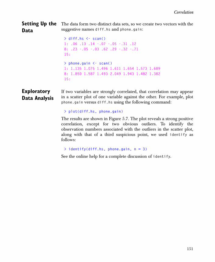
Correlation
Setting Up the Data
The data form two distinct data sets, so we create two vectors with thesuggestive names diff.hs and phone.gain:
> diff.hs <- scan()1: .06 .13 .14 -.07 -.05 -.31 .128: .23 -.05 -.03 .62 .29 -.32 -.7115:
> phone.gain <- scan()1: 1.135 1.075 1.496 1.611 1.654 1.573 1.6898: 1.850 1.587 1.493 2.049 1.943 1.482 1.38215:
Exploratory Data Analysis
If two variables are strongly correlated, that correlation may appearin a scatter plot of one variable against the other. For example, plotphone.gain versus diff.hs using the following command:
> plot(diff.hs, phone.gain)
The results are shown in Figure 5.7. The plot reveals a strong positivecorrelation, except for two obvious outliers. To identify theobservation numbers associated with the outliers in the scatter plot,along with that of a third suspicious point, we used identify asfollows:
> identify(diff.hs, phone.gain, n = 3)
See the online help for a complete discussion of identify.
151

Chapter 5 Statistical Inference for One- and Two-Sample Problems
The obvious outliers occur at the first and second observations. Inaddition, the suspicious point (labeled “3” in the scatter plot) occurs atthe third observation time.
Since you have now identified the observation times of the outliers,you can gain further insight by making a time series plot of eachseries:
> plot(diff.hs, type = "b")> plot(phone.gain, type = "b")
You should also make an autocorrelation plot for each series:
> acf(diff.hs)> acf(phone.gain)
The results are shown in Figure 5.8. Except for the first threeobservations of the two series phone.gain and diff.hs, there is astrong similarity of shape exhibited in the two time series plots. Thisaccounts for the strong positive correlation between the two variables
Figure 5.7: Scatter plot of phone.gain versus diff.hs.
•
•
•
••
•
•
•
•
•
•
•
•
•
diff.hs
phon
e.ga
in
-0.6 -0.4 -0.2 0.0 0.2 0.4 0.6
1.2
1.4
1.6
1.8
2.0
1
2
3
152
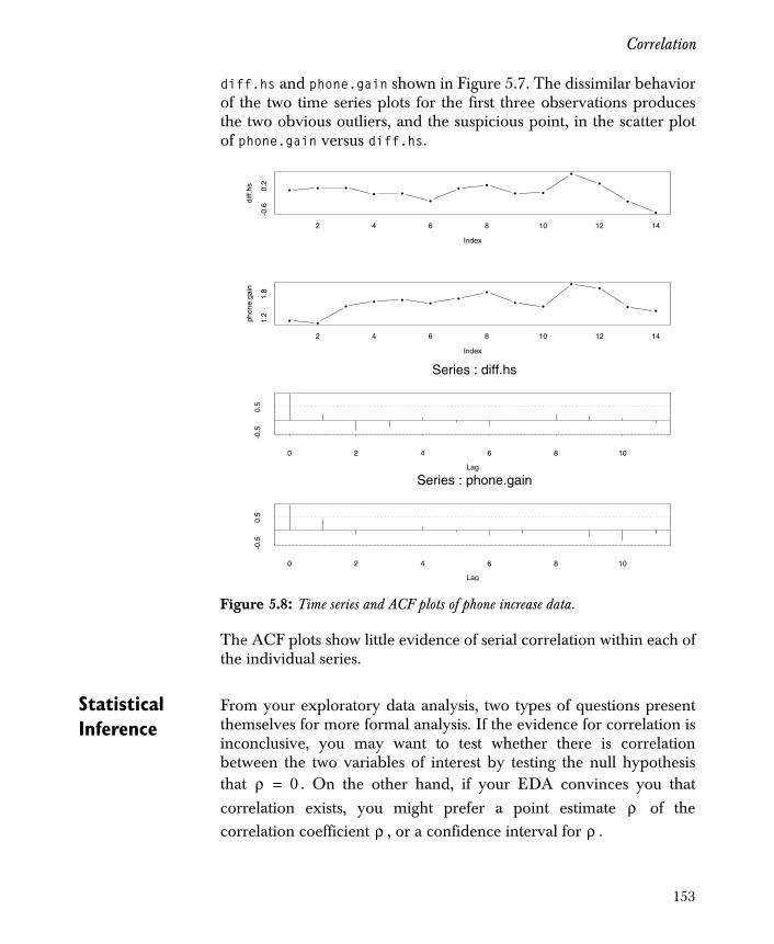
Correlation
diff.hs and phone.gain shown in Figure 5.7. The dissimilar behaviorof the two time series plots for the first three observations producesthe two obvious outliers, and the suspicious point, in the scatter plotof phone.gain versus diff.hs.
The ACF plots show little evidence of serial correlation within each ofthe individual series.
Statistical Inference
From your exploratory data analysis, two types of questions presentthemselves for more formal analysis. If the evidence for correlation isinconclusive, you may want to test whether there is correlationbetween the two variables of interest by testing the null hypothesisthat . On the other hand, if your EDA convinces you thatcorrelation exists, you might prefer a point estimate of thecorrelation coefficient , or a confidence interval for .
Figure 5.8: Time series and ACF plots of phone increase data.
• • •• •
•
• •• •
••
•
•
Indexdi
ff.hs
2 4 6 8 10 12 14
-0.6
0.2
• •
•• • •
••
• •
• •
• •
Index
phon
e.ga
in
2 4 6 8 10 12 14
1.2
1.8
Lag
0 2 4 6 8 10
-0.5
0.5
Series : diff.hs
Lag
0 2 4 6 8 10
-0.5
0.5
Series : phone.gain
ρ 0=
ρρ ρ
153
Chapter 5 Statistical Inference for One- and Two-Sample Problems
Hypothesis Test p-Values
You can get p values for the null hypothesis that by using thefunction cor.test. To perform this test, you specify the alternativehypothesis to be tested and the test method to use, as follows:
• alternative specifies the alternative hypothesis to be tested. There are three options:
• "two.sided" (the default alternative) tests the alternative hypothesis that ρ ≠ 0.
• "greater" tests the alternative hypothesis that ρ > 0.
• "less" tests the alternative hypothesis that ρ < 0.
You can also use the abbreviated forms alt="g" and alt="l".
• method specifies which of the following methods is used:
• "pearson" (the default) uses the standard Pearson sample correlation coefficient.
• "kendall" uses the rank-based Kendall’s measure of correlation.
• "spearman" uses the rank-based Spearman’s measure of correlation.
You can abbreviate these methods by using enough of the characterstring to determine a unique match; here "p", "k", and "s" work.
Because both Kendall’s and Spearman’s methods are based onranks, they are not so sensitive to outliers and nonnormality as thestandard Pearson estimate.
Below is a simple use of cor.test to test the alternative hypothesisthat there is a positive correlation in the phone gain data. We use thedefault choice of the classical Pearson estimate with the one-sidedalternative alt="g".
ρ 0=
τ
ρ
τ ρ
154

Correlation
> cor.test(diff.hs, phone.gain, alt = "g")
Pearson product-moment correlation
data: diff.hs and phone.gaint = 1.9155, df = 12, p-value = 0.0398alternative hypothesis: true coef is greater than 0sample estimates: cor 0.4839001
You get a normal theory t-statistic having the modest value of 1.9155,and a p value of 0.0398. The estimate of is 0.48, to two decimalplaces. There are 14 bivariate observations, and since the mean isestimated for each sample under the null hypothesis that , thenumber of degrees of freedom (df) is 12.
Since your EDA plots reveal two obvious bivariate outliers in thephone gain data, the nonparametric alternatives, either Kendall’s orSpearman’s , are preferable in determining p values for this case.Using Kendall’s method, we obtain the following results:
> cor.test(diff.hs, phone.gain, alt = "g",method = "k")
Kendall’s rank correlation tau
data: diff.hs and phone.gainnormal-z = 2.0834, p-value = 0.0186alternative hypothesis: true tau is greater than 0sample estimates: tau 0.4175824
The p-value obtained from Kendall’s method is smaller than thatobtained from the Pearson method. The null hypothesis is rejected ata level of 0.05. Spearman’s , by contrast, yields a p value similar tothat of the standard Pearson method.
ρ
ρ 0>
τρ
ρ
155
Chapter 5 Statistical Inference for One- and Two-Sample Problems
Point Estimates and Confidence Intervals for ρ
You may want an estimate of , or a confidence interval for .The function cor.test gives you the classical sample correlationcoefficient estimate of , when you use the default Pearson’smethod. However, cor.test does not provide you with a robustestimate of , (since neither Kendall’s nor Spearman’s providean unbiased estimate of ). Furthermore, cor.test does not provideany kind of confidence interval for .
To obtain a robust point estimate of , use the function cor with anonzero value for the optional argument trim. You should specify afraction α between 0 and 0.5 for the value of this argument. Thisresults in a robust estimate which consists of the ordinary samplecorrelation coefficient based on the fraction ( ) of the dataremaining after “trimming” away a fraction . In most cases, settrim=0.2. If you think your data contain more than 20% outliers, youshould use a larger fraction in place of 0.2. The default value istrim=0, which yields the standard Pearson sample correlationcoefficient.
Applying cor to the phone gain data, you get:
> cor(diff.hs, phone.gain, trim = 0.2)
[1] 0.7145078
Comparing this robust estimate to our earlier value for obtainedusing cor.test, we see the robust estimate yields a larger estimate of
. This is what you expect, since the two outliers cause the standardsample correlation coefficient to have a value smaller than that of the“bulk” of the data.
Warning
The values returned for tau and rho (0.407 and 0.504, respectively, for the phone gain data) do not provide unbiased estimates of the true correlation ρ. Transformations of tau and rho are required to obtain unbiased estimates of ρ.
ρ ρ ρ
r ρ
ρ τ ρρ
ρ
ρ
1 α–
α
ρ
ρ
156

Correlation
To obtain a confidence interval for , we’ll use the followingprocedure (as in Snedecor and Cochran (1980)). First, transform using Fisher’s z transform, which consists of taking the inversehyperbolic tangent transform . Then, construct aconfidence interval for the correspondingly transformed true
correlation coefficient . Finally, transform this intervalback to the original scale by transforming each endpoint of thisinterval with the hyperbolic tangent transformation tanh.
To implement the procedure just described as a Spotfire S+ function,create the function cor.confint as follows:
> cor.confint <- function(x, y, conf.level = .95, trim = 0)+ {+ z <- atanh(cor(x, y, trim))+ b <- qnorm((1 - conf.level)/2)/(length(x) - 3)^.5+ ci.z <- c(z - b, z + b)+ conf.int <- tanh(ci.z)+ conf.int+ }
You can now use your new function cor.confint on the phone gaindata:
> cor.confint(diff.hs, phone.gain)
[1] 0.80722628 -0.06280425
> cor.confint(diff.hs, phone.gain, trim = .2)
[1] 0.9028239 0.2962300
When you use the optional argument trim=0.2, you are basing theconfidence interval on a robust estimate of ρ, and consequently youget a robust confidence interval. Since the robust estimate has thevalue 0.72, which is larger than the standard (nonrobust) estimatevalue of 0.48, you should be reassured to get an interval which isshifted upward, and is also shorter, than the nonrobust interval yougot by using cor.confint with the default option trim=0.
ρρ
x ρ( )atanh=
ρ ρ( )atanh=
157

Chapter 5 Statistical Inference for One- and Two-Sample Problems
REFERENCES
Bishop, Y.M.M., Fienberg, S.J., & Holland, P.W. (1980). DiscreteMultivariate Analysis: Theory and Practice. Cambridge, MA: The MITPress .
Box, G.E.P., Hunter, W.G., & Hunter, J.S. (1978). Statistics forExperimenters: An Introduction to Design, Data Analysis and ModelBuilding. New York: John Wiley & Sons, Inc.
Conover, W.J. (1980). Practical Nonparametric Statistics (2nd ed.). NewYork: John Wiley & Sons, Inc.
Heidelberger, P. & Welch, P.D. (1981). A spectral method forconfidence interval generation and run-length control in simulations.Communications of the ACM 24:233-245.
Hogg, R.V. & Craig, A.T. (1970). Introduction to Mathematical Statistics(3rd ed.). Toronto, Canada: Macmillan.
Mood, A.M., Graybill, F.A., & Boes, D.C. (1974). Introduction to theTheory of Statistics (3rd ed.). New York: McGraw-Hill.
Snedecor, G.W. & Cochran, W.G. (1980). Statistical Methods (7th ed.).Ames, IA: Iowa State University Press.
158

Introduction 160
Cumulative Distribution Functions 161
The Chi-Square Goodness-of-Fit Test 165
The Kolmogorov-Smirnov Goodness-of-Fit Test 168
The Shapiro-Wilk Test for Normality 172
One-Sample Tests 174Comparison of Tests 174Composite Tests for a Family of Distributions 174
Two-Sample Tests 178
References 180
GOODNESS OF FIT TESTS 6
159
Chapter 6 Goodness of Fit Tests
INTRODUCTION
Most TIBCO Spotfire S+ functions for hypothesis testing assume acertain distributional form (often normal) and then use data to makeconclusions about certain parameters of the distribution, often themean or variance. In Chapter 5, Statistical Inference for One- andTwo-Sample Problems, we describe EDA techniques to informallytest the assumptions of these procedures. Goodness of fit (GOF) testsare another, more formal tool to assess the evidence for assuming acertain distribution.
There are two types of GOF problems, corresponding to the numberof samples. They ask the following questions:
1. One sample. Does the sample arise from a hypothesized distribution?
2. Two sample. Do two independent samples arise from the same distribution?
Spotfire S+ implements the two best-known GOF tests:
• Chi-square, in the chisq.gof function.
• Kolmogorov-Smirnov, in the ks.gof function.
The chi-square test applies only in the one-sample case; theKolmogorov- Smirnov test can be used in both the one-sample andtwo-sample cases.
Both the chi-square and Kolmogorov-Smirnov GOF tests work formany different distributions. In addition, Spotfire S+ includes thefunction shapiro.test, which computes the Shapiro-Wilk W-statisticfor departures from normality. This statistic can be more powerfulthan the other two tests for determining whether a particular data setarises from the normal (Gaussian) distribution.
This chapter describes all three tests, together with a graphicalfunction, cdf.compare, that can be used as an exploratory tool forevaluating goodness of fit.
160
Cumulative Distribution Functions
CUMULATIVE DISTRIBUTION FUNCTIONS
For a random variable , a cumulative distribution function (cdf),, assigns a measure between 0 and 1 of the
probability that . If form a random sample from a
continuous distribution with observed values , an empirical
distribution function Fn can be defined for all , , so that is the proportion of observed values less than or equal to .
The empirical distribution function estimates the unknown cdf.
To decide whether two samples arise from the same unknowndistribution, a natural procedure is to compare their empiricaldistribution functions. Likewise, for one sample, you can compare itsempirical distribution function with a hypothesized cdf. For moreinformation on cumulative distribution functions, see Chapter 1,Probability.
A graphical comparison of either one empirical distribution functionwith a known cdf, or of two empirical distribution functions, can beobtained easily in Spotfire S+ using the function cdf.compare. Forexample, consider the plot shown in Figure 6.1. In this example, theempirical distribution function and a hypothetical cdf are quite close.This plot is produced using the cdf.compare function as follows:
# Set the seed for reproducibility.> set.seed(222)> z <- rnorm(100)> cdf.compare(z, distribution = "normal")
XF x( ) P X x≤[ ]=
X x< X1 … X, n,
x1 … x, n,
x ∞ x ∞< <–Fn x( ) x
161
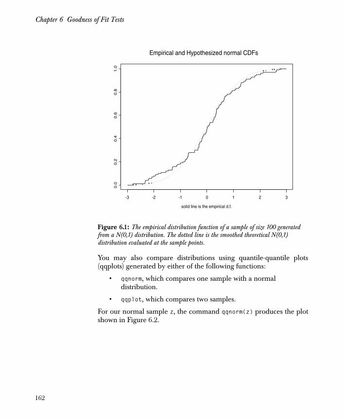
Chapter 6 Goodness of Fit Tests
You may also compare distributions using quantile-quantile plots(qqplots) generated by either of the following functions:
• qqnorm, which compares one sample with a normal distribution.
• qqplot, which compares two samples.
For our normal sample z, the command qqnorm(z) produces the plotshown in Figure 6.2.
Figure 6.1: The empirical distribution function of a sample of size 100 generated from a N(0,1) distribution. The dotted line is the smoothed theoretical N(0,1) distribution evaluated at the sample points.
Empirical and Hypothesized normal CDFs
solid line is the empirical d.f.
-3 -2 -1 0 1 2 3
0.0
0.2
0.4
0.6
0.8
1.0
162

Cumulative Distribution Functions
Departures from linearity show how the sample differs from thenormal, or how the two sample distributions differ. To comparesamples with distributions other than the normal, you may produceqqplots using the function ppoints. For more details, see the chapterTraditional Graphics in the Guide to Graphics.
In many cases, the graphical conclusions drawn from eithercdf.compare or the qqplots make more formal tests such as thechi-square or Kolmogorov-Smirnov unnecessary. For example,consider the two empirical distributions compared in Figure 6.3.They clearly have different distribution functions:
> x <- rnorm(30)> y <- runif(30)> cdf.compare(x, y)
Figure 6.2: A qqnorm plot of a sample from a normal distribution.
Quantiles of Standard Normal
z
-2 -1 0 1 2
-3-2
-10
12
163
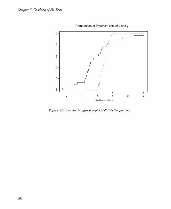
Chapter 6 Goodness of Fit Tests
Figure 6.3: Two clearly different empirical distribution functions.
Comparison of Empirical cdfs of x and y
dotted line is cdf of y
-2 -1 0 1 2 3
0.0
0.2
0.4
0.6
0.8
1.0
164
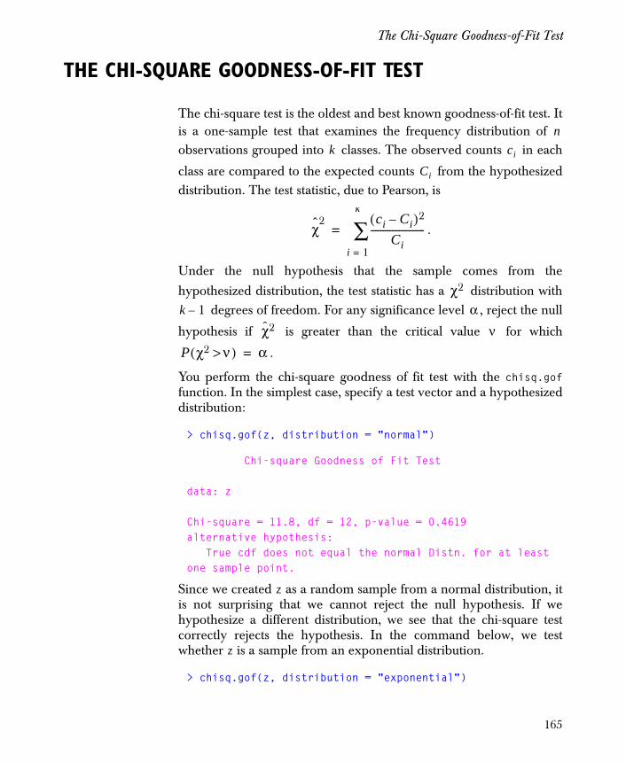
The Chi-Square Goodness-of-Fit Test
THE CHI-SQUARE GOODNESS-OF-FIT TEST
The chi-square test is the oldest and best known goodness-of-fit test. Itis a one-sample test that examines the frequency distribution of observations grouped into classes. The observed counts in each
class are compared to the expected counts from the hypothesizeddistribution. The test statistic, due to Pearson, is
.
Under the null hypothesis that the sample comes from the
hypothesized distribution, the test statistic has a distribution with degrees of freedom. For any significance level , reject the null
hypothesis if is greater than the critical value for which
.
You perform the chi-square goodness of fit test with the chisq.goffunction. In the simplest case, specify a test vector and a hypothesizeddistribution:
> chisq.gof(z, distribution = "normal")
Chi-square Goodness of Fit Test
data: z
Chi-square = 11.8, df = 12, p-value = 0.4619 alternative hypothesis: True cdf does not equal the normal Distn. for at least one sample point.
Since we created z as a random sample from a normal distribution, itis not surprising that we cannot reject the null hypothesis. If wehypothesize a different distribution, we see that the chi-square testcorrectly rejects the hypothesis. In the command below, we testwhether z is a sample from an exponential distribution.
> chisq.gof(z, distribution = "exponential")
nk ci
Ci
χ2 ci Ci–( )2
Ci-----------------------
i 1=
k
∑=
χ2
k 1– α
χ2 ν
P χ2 ν>( ) α=
165
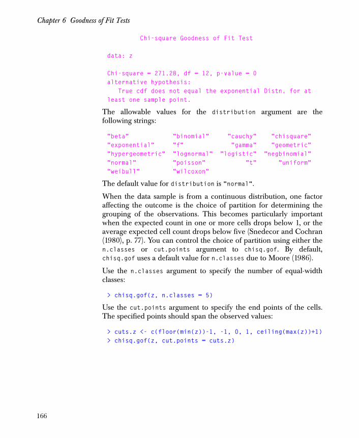
Chapter 6 Goodness of Fit Tests
Chi-square Goodness of Fit Test
data: z
Chi-square = 271.28, df = 12, p-value = 0 alternative hypothesis: True cdf does not equal the exponential Distn. for at least one sample point.
The allowable values for the distribution argument are thefollowing strings:
"beta" "binomial" "cauchy" "chisquare""exponential" "f" "gamma" "geometric""hypergeometric" "lognormal" "logistic" "negbinomial""normal" "poisson" "t" "uniform""weibull" "wilcoxon"
The default value for distribution is "normal".
When the data sample is from a continuous distribution, one factoraffecting the outcome is the choice of partition for determining thegrouping of the observations. This becomes particularly importantwhen the expected count in one or more cells drops below 1, or theaverage expected cell count drops below five (Snedecor and Cochran(1980), p. 77). You can control the choice of partition using either then.classes or cut.points argument to chisq.gof. By default,chisq.gof uses a default value for n.classes due to Moore (1986).
Use the n.classes argument to specify the number of equal-widthclasses:
> chisq.gof(z, n.classes = 5)
Use the cut.points argument to specify the end points of the cells.The specified points should span the observed values:
> cuts.z <- c(floor(min(z))-1, -1, 0, 1, ceiling(max(z))+1)> chisq.gof(z, cut.points = cuts.z)
166

The Chi-Square Goodness-of-Fit Test
Chi-square tests apply to any type of variable: continuous, discrete, ora combination of these. For large sample sizes ( ), the chi-squareis the only valid test when the hypothesized distribution is discrete. Inaddition, the chi-square test easily adapts to the situation whenparameters of a distribution are estimated. However, information islost by grouping the data, especially for continuous variables.
n 50≥
167

Chapter 6 Goodness of Fit Tests
THE KOLMOGOROV-SMIRNOV GOODNESS-OF-FIT TEST
Suppose and are two cdfs. In the one-sample situation, is
the empirical distribution function and is a hypothesized cdf; in
the two-sample situation, and are both empirical distributionfunctions. Possible hypotheses and alternatives concerning these cdfsare:
• Two-sided
H0: for all
HA: for at least one value of
• One-sided (“less” alternative)
H0: for all
HA: for at least one value of .
• One-sided (“greater” alternative)
H0: for all
HA: for at least one value of
The Kolmogorov-Smirnov (KS) test is a method for testing the abovehypotheses. Corresponding to each alternative hypothesis is a teststatistic, as follows.
• Two-sided Test:
• Less Alternative:
• Greater Alternative:
Thus, the KS test is based on the maximum vertical distance betweenthe distributions and . If the test statistic is greater thansome critical value, the null hypothesis is rejected.
F1 F2 F1
F2
F1 F2
F1 x( ) F2 x( )= x
F1 x( ) F2 x( )≠ x
F1 x( ) F2 x( )≥ x
F1 x( ) F2 x( )< x
F1 x( ) F2 x( )≤ x
F1 x( ) F2 x( )> x
T supx F1 x( ) F2 x( )–=
T- supx F2 x( ) F1 x( )–=
T+ supx F1 x( ) F2 x( )–=
F1 x( ) F2 x( )
168
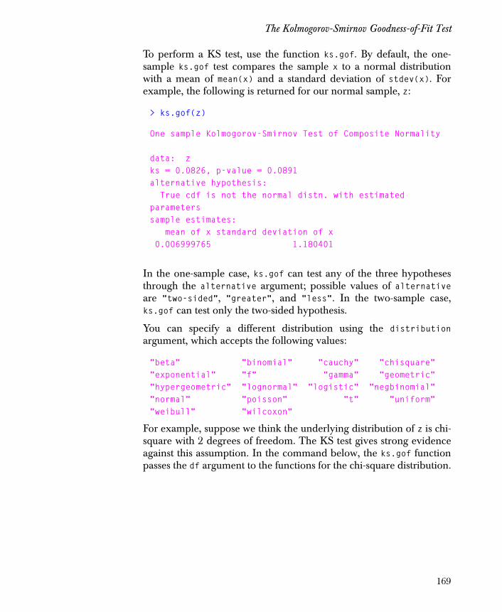
The Kolmogorov-Smirnov Goodness-of-Fit Test
To perform a KS test, use the function ks.gof. By default, the one-sample ks.gof test compares the sample x to a normal distributionwith a mean of mean(x) and a standard deviation of stdev(x). Forexample, the following is returned for our normal sample, z:
> ks.gof(z)
One sample Kolmogorov-Smirnov Test of Composite Normality
data: z ks = 0.0826, p-value = 0.0891 alternative hypothesis: True cdf is not the normal distn. with estimated parameters sample estimates: mean of x standard deviation of x 0.006999765 1.180401
In the one-sample case, ks.gof can test any of the three hypothesesthrough the alternative argument; possible values of alternativeare "two-sided", "greater", and "less". In the two-sample case,ks.gof can test only the two-sided hypothesis.
You can specify a different distribution using the distributionargument, which accepts the following values:
"beta" "binomial" "cauchy" "chisquare""exponential" "f" "gamma" "geometric""hypergeometric" "lognormal" "logistic" "negbinomial""normal" "poisson" "t" "uniform""weibull" "wilcoxon"
For example, suppose we think the underlying distribution of z is chi-square with 2 degrees of freedom. The KS test gives strong evidenceagainst this assumption. In the command below, the ks.gof functionpasses the df argument to the functions for the chi-square distribution.
169

Chapter 6 Goodness of Fit Tests
> ks.gof(z, alternative = "greater", + distribution = "chisquare", df = 2)
One-sample Kolmogorov-Smirnov TestHypothesized distribution = chisquare
data: z ks = 0.4906, p-value = 0 alternative hypothesis: True cdf is greater than the chisquare distn. with the specified parameters
Figure 6.4, created as follows, also shows that this assumption is notreasonable:
> cdf.compare(z, dist = "chisquare", df = 2)
The chisq.gof test gives further confirmation:
> chisq.gof(z, dist = "chisquare", n.param.est = 0, df = 2)
Chi-square Goodness of Fit Test
data: z Chi-square = 314.96, df = 12, p-value = 0 alternative hypothesis: True cdf does not equal the chisquare Distn. for at least one sample point.
Note that chisq.gof tests only the two sided alternative.
170

The Kolmogorov-Smirnov Goodness-of-Fit Test
Figure 6.4: Similar to Figure 6.3, except the dotted line shows a chi-square cdf with 2 degrees of freedom.
Empirical and Hypothesized chisquare CDFs
solid line is the empirical d.f.
-3 -2 -1 0 1 2 3
0.0
0.2
0.4
0.6
0.8
1.0
171
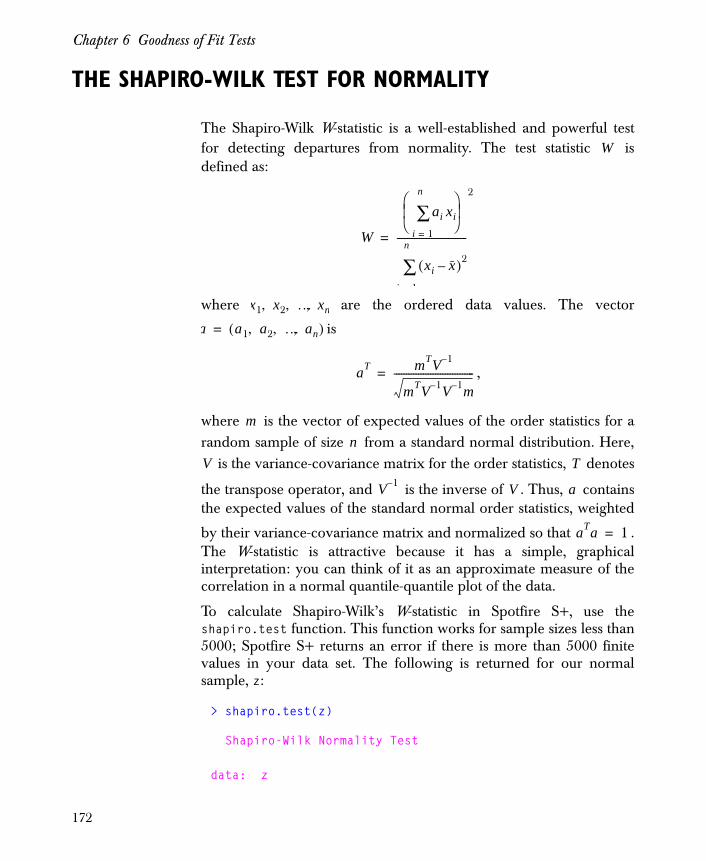
Chapter 6 Goodness of Fit Tests
THE SHAPIRO-WILK TEST FOR NORMALITY
The Shapiro-Wilk W-statistic is a well-established and powerful testfor detecting departures from normality. The test statistic isdefined as:
where are the ordered data values. The vector
is
,
where is the vector of expected values of the order statistics for arandom sample of size from a standard normal distribution. Here,
is the variance-covariance matrix for the order statistics, denotes
the transpose operator, and is the inverse of . Thus, containsthe expected values of the standard normal order statistics, weighted
by their variance-covariance matrix and normalized so that .The W-statistic is attractive because it has a simple, graphicalinterpretation: you can think of it as an approximate measure of thecorrelation in a normal quantile-quantile plot of the data.
To calculate Shapiro-Wilk’s W-statistic in Spotfire S+, use theshapiro.test function. This function works for sample sizes less than5000; Spotfire S+ returns an error if there is more than 5000 finitevalues in your data set. The following is returned for our normalsample, z:
> shapiro.test(z)
Shapiro-Wilk Normality Test
data: z
W
W
ai xi
i 1=
n
∑⎝ ⎠⎜ ⎟⎛ ⎞
xi x–( )2
i 1
n
∑
-----------------------------
2
=
x1 x2 … xn, , ,
a a1 a2 … an, , ,( )=
aT mTV 1–
mTV 1– V 1– m---------------------------------=
mn
V T
V 1– V a
aTa 1=
172

The Shapiro-Wilk Test for Normality
W = 0.9853, p-value = 0.3348
Small p-values indicate that the null hypothesis of normality isprobably not true. Since we generated z from a normal distribution, itis not surprising that we cannot reject the null hypothesis.
173

Chapter 6 Goodness of Fit Tests
ONE-SAMPLE TESTS
Comparison of Tests
As we mention in the section The Chi-Square Goodness-of-Fit Test onpage 165, the chi-square test divides the data into categories. Whilethis may be appropriate for discrete data, it can be an arbitraryprocess when the data are from a continuous distribution. The resultsof the chi-square test can vary with how the data are divided,especially when dealing with continuous distributions. Because of thischaracteristic, the one-sample Kolmogorov-Smirnov test is morepowerful than the chi-square test when the hypothesized distributionis continuous. That is, it is more likely to reject the null hypothesiswhen it should.
In general, both the chi-square and Kolmogorov-Smirnov GOF testsare less powerful for detecting departures from normality than theShapiro-Wilk test. This is because the Shapiro-Wilk test is designedspecifically for normal distributions, and does not test the goodness offit for other distributions. In addition, the chi-square andKolmogorov-Smirnov tests must estimate distribution parametersfrom the data if none are provided; we discuss this in detail in thenext section.
Composite Tests for a Family of Distributions
When distribution parameters are estimated from a sample ratherthan specified in advance, the tests described in this chapter may nolonger be adequate. Instead, different tables of critical values areneeded. The tables for the Kolmogorov-Smirnov test, for example,vary according the the following criteria:
• Different distributions
• Estimated parameters
• Methods of estimation
• Sample sizes
The null hypothesis is composite in these cases: rather thanhypothesizing that the data have a distribution with specificparameters, we hypothesize only that the distribution belongs to aparticular family of distributions, such as the normal. This family ofdistributions results from allowing all possible parameter values.
174
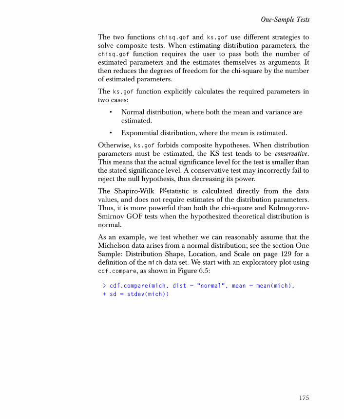
One-Sample Tests
The two functions chisq.gof and ks.gof use different strategies tosolve composite tests. When estimating distribution parameters, thechisq.gof function requires the user to pass both the number ofestimated parameters and the estimates themselves as arguments. Itthen reduces the degrees of freedom for the chi-square by the numberof estimated parameters.
The ks.gof function explicitly calculates the required parameters intwo cases:
• Normal distribution, where both the mean and variance are estimated.
• Exponential distribution, where the mean is estimated.
Otherwise, ks.gof forbids composite hypotheses. When distributionparameters must be estimated, the KS test tends to be conservative .This means that the actual significance level for the test is smaller thanthe stated significance level. A conservative test may incorrectly fail toreject the null hypothesis, thus decreasing its power.
The Shapiro-Wilk W-statistic is calculated directly from the datavalues, and does not require estimates of the distribution parameters.Thus, it is more powerful than both the chi-square and Kolmogorov-Smirnov GOF tests when the hypothesized theoretical distribution isnormal.
As an example, we test whether we can reasonably assume that theMichelson data arises from a normal distribution; see the section OneSample: Distribution Shape, Location, and Scale on page 129 for adefinition of the mich data set. We start with an exploratory plot usingcdf.compare, as shown in Figure 6.5:
> cdf.compare(mich, dist = "normal", mean = mean(mich),+ sd = stdev(mich))
175

Chapter 6 Goodness of Fit Tests
We now use the ks.gof function, which estimates parameters for themean and variance:
> ks.gof(mich, dist = "normal")
One sample Kolmogorov-Smirnov Test of Composite Normality
data: mich ks = 0.1793, p-value = 0.0914 alternative hypothesis: True cdf is not the normal distn. with estimated parameters sample estimates: mean of x standard deviation of x 909 104.926
If distribution parameters are estimated, the degrees of freedom forchisq.gof depend on the method of estimation. In practice, you mayestimate the parameters from the original data and set the argumentn.param.est to the number of parameters estimated. The chisq.gof
Figure 6.5: Exploratory plot of cdf of the Michelson data.
Empirical and Hypothesized normal CDFs
solid line is the empirical d.f.700 800 900 1000
0.0
0.2
0.4
0.6
0.8
1.0
176
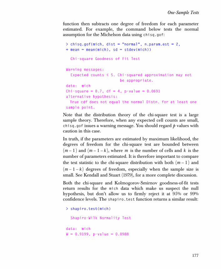
One-Sample Tests
function then subtracts one degree of freedom for each parameterestimated. For example, the command below tests the normalassumption for the Michelson data using chisq.gof:
> chisq.gof(mich, dist = "normal", n.param.est = 2,+ mean = mean(mich), sd = stdev(mich))
Chi-square Goodness of Fit Test
Warning messages: Expected counts < 5. Chi-squared approximation may not be appropriate.data: mich Chi-square = 8.7, df = 4, p-value = 0.0691 alternative hypothesis: True cdf does not equal the normal Distn. for at least one sample point.
Note that the distribution theory of the chi-square test is a largesample theory. Therefore, when any expected cell counts are small,chisq.gof issues a warning message. You should regard p values withcaution in this case.
In truth, if the parameters are estimated by maximum likelihood, thedegrees of freedom for the chi-square test are bounded between( ) and ( ), where is the number of cells and is thenumber of parameters estimated. It is therefore important to comparethe test statistic to the chi-square distribution with both ( ) and( ) degrees of freedom, especially when the sample size issmall. See Kendall and Stuart (1979), for a more complete discussion.
Both the chi-square and Kolmogorov-Smirnov goodness-of-fit testsreturn results for the mich data which make us suspect the nullhypothesis, but don’t allow us to firmly reject it at 95% or 99%confidence levels. The shapiro.test function returns a similar result:
> shapiro.test(mich)
Shapiro-Wilk Normality Test
data: mich W = 0.9199, p-value = 0.0988
m 1– m 1– k– m k
m 1–
m 1– k–
177

Chapter 6 Goodness of Fit Tests
TWO-SAMPLE TESTS
In the two-sample case, you can use the ks.gof function, with thesecond sample y filling in for the hypothesized distribution. Theassumptions of the two-sample KS test are:
• The samples are random samples,
• The samples are mutually independent, and
• The data are measured on at least an ordinal scale.
In addition, the test gives exact results only if the underlyingdistributions are continuous.
For example, the following commands graphically compare the cdfsof two vectors, x and y, that are generated from a normal andexponential distribution, respectively:
> x <- rnorm(30)> y <- rexp(100)> par(mfrow = c(1,2))> qqplot(x, y)> cdf.compare(x, y)
Figure 6.6 shows the results; the qqplot is not linear and the cdfs arequite different. This graphical evidence is verified by a formal KS test:
> ks.gof(x, y)
Two-Sample Kolmogorov-Smirnov Test
data: x and y ks = 0.4667, p-value = 0.0001 alternative hypothesis: cdf of x does not equal the cdf of y for at least one sample point.
178
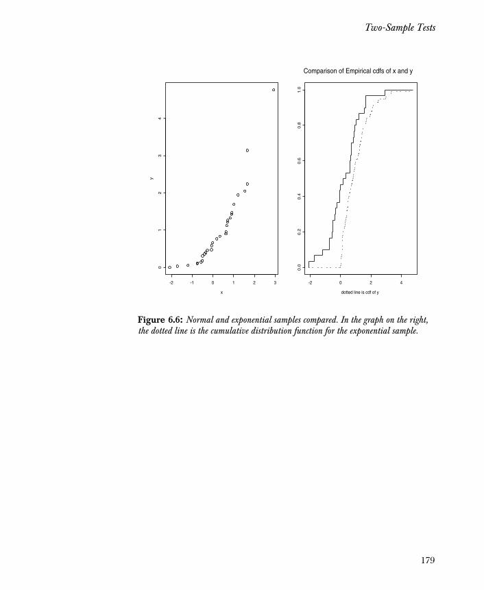
Two-Sample Tests
Figure 6.6: Normal and exponential samples compared. In the graph on the right, the dotted line is the cumulative distribution function for the exponential sample.
x
y
-2 -1 0 1 2 3
01
23
4
Comparison of Empirical cdfs of x and y
dotted line is cdf of y
-2 0 2 4
0.0
0.2
0.4
0.6
0.8
1.0
179

Chapter 6 Goodness of Fit Tests
REFERENCES
Kendall, M.G. & Stuart, A. (1979). The Advanced Theory of Statistics,Volume 2: Inference and Relationship (4th ed.). New York: OxfordUniversity Press.
Millard, S.P. and Neerchal, N.K. (2001). Environmental Statistics withSpotfire S+ . Boca Raton, Florida: CRC Press LLC.
Moore, D.S. (1986). Tests of chi-squared type. In D'Agostino, R.B. &Stevens, M.A. (Eds.) Goodness-of-Fit Techniques. New York: MarcelDekker.
Snedecor, G.W. & Cochran, W.G. (1980). Statistical Methods (7th ed.).Ames, Iowa: Iowa State University Press.
180
Introduction 182
Proportion Parameter for One Sample 184Setting Up the Data 184Hypothesis Testing 184Confidence Intervals 185
Proportion Parameters for Two Samples 186Setting Up the Data 186Hypothesis Testing 186Confidence Intervals 188
Proportion Parameters for Three or More Samples 189Setting Up the Data 189Hypothesis Testing 190Confidence Intervals 191
Contingency Tables and Tests for Independence 192The Chi-Square and Fisher Tests of Independence 193The Chi-Square Test of Independence 195Fisher’s Exact Test of Independence 196The Mantel-Haenszel Test of Independence 196McNemar’s Test for Symmetry Using Matched Pairs 199
References 201
STATISTICAL INFERENCE FOR COUNTS AND PROPORTIONS 7
181
Chapter 7 Statistical Inference for Counts and Proportions
INTRODUCTION
This chapter shows you how to use TIBCO Spotfire S+ statisticalinference functions for two types of problems that involve counts orproportions. With these functions, you can obtain confidence intervalsfor the unknown population parameters and p values for hypothesistests of the parameter values.
The first type of problem is one where you have one or moresamples, or sets of trials, in which the count for each samplerepresents the number of times that a certain interesting outcomeoccurs. By common convention, we refer to the occurrence of theoutcome of interest as a “success.” For example, if you play roulette100 times at a casino, and you bet on red each time, you areinterested in counting the number of times that the color red comesup. This count is a number between 0 and 100. When you divide thiscount by 100 you get a proportion (that is, a number between 0 and1). This proportion is a natural estimate of the probability that redcomes up on the roulette wheel.
Another example is provided by the famous Salk vaccine trials. Thesetrials involved two groups, one of which received the vaccine and oneof which received a placebo. For each group, the count of interest wasthe number of individuals who contracted polio. The ratio of thenumber of individuals who contracted polio to the total number ofindividuals in the group is a proportion that provides a naturalestimate of the probability of contracting polio within that group.
The underlying probability model for problems of this first type is thebinomial distribution. For each set of trials i , this distribution ischaracterized by the number of trials and the probability that asuccess occurs on each trial. This probability is called a proportionparameter. Your main interest is in making statistical inferencestatements concerning the probabilities of occurrence of
the event of interest for each of the sets of trials.
The second type of problem is one where you have counts on thenumber of occurrences of several possible outcomes for each of twovariables. For example, you may be studying three types of cancerand three types of diet (such as low-, medium- and high-fat diets). Thetwo variables of interest may be “type of cancer” and “type of diet.”
pi
p1 p2 … p, m, ,
m
182

Introduction
For a fixed set of individuals, you have counts on the number ofindividuals who fall jointly in each of the categories defined by thesimultaneous occurrence of a type of cancer and a diet classification.For problems of this kind, the data is arranged in a two-way tablecalled a contingency table .
In this second kind of problem, your main interest is to determinewhether there is any association between the two variables of interest.The probability model for such problems is one of statisticalindependence between the two variables.
The first three sections of this chapter cover the first type of problemdescribed above, for which the proportion parameters are theprobabilities of success, in m sets of binomial trials. Thelast section covers the second type of problem, where you areinterested in testing the null hypothesis of independence between twovariables.
p1 p2 … p, m, ,
183
Chapter 7 Statistical Inference for Counts and Proportions
PROPORTION PARAMETER FOR ONE SAMPLE
When you play roulette and bet on red, you expect your probabilityof winning to be close to, but slightly less than, 0.5. You expect thisbecause (in the United States) a roulette wheel has 18 red slots, 18black slots, and two additional slots labeled “0” and “00,” for a total of38 slots into which the ball can fall. Thus, for a “fair” (that is, perfectlybalanced) wheel, you expect the probability of red to be
. You hope that the house is not cheating youby altering the roulette wheel so that the probability of red is less than0.474.
To test whether a given sample has a particular proportion parameter,use the binom.test function.
Setting Up the Data
In the roulette case there is little to do, since the only data are thenumber n of trials and the number x of successes. These two valuescan be directly supplied as arguments to binom.test, as shown in theexamples below.
Hypothesis Testing
You can test the null hypothesis that using the functionbinom.test. For example, if you bet on red 100 times and red comesup 42 times, you get a p value for this null hypothesis against thetwo-sided alternative that as follows:
> binom.test(42, 100, p = 0.474)$p.value
[1] 0.3167881
The two-sided alternative is the default alternative for binom.test.You can get a p value for a one-sided alternative by using the optionalargument alt. For example, in the roulette wheel example you areconcerned that the house might cheat you in some way so that .Use the following to test the null hypothesis against this one-sidedalternative:
> binom.test(42, 100, p = 0.474, alt = "l")$p.value
[1] 0.1632416
p0 18 38⁄ 0.474= =
p p0=
p 0.474≠
p p0<
184
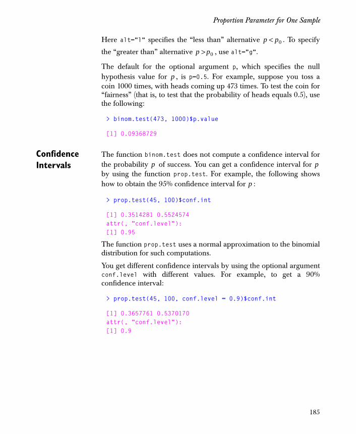
Proportion Parameter for One Sample
Here alt="l" specifies the “less than” alternative . To specify
the “greater than” alternative , use alt="g".
The default for the optional argument p, which specifies the nullhypothesis value for , is p=0.5. For example, suppose you toss acoin 1000 times, with heads coming up 473 times. To test the coin for“fairness” (that is, to test that the probability of heads equals 0.5), usethe following:
> binom.test(473, 1000)$p.value
[1] 0.09368729
Confidence Intervals
The function binom.test does not compute a confidence interval forthe probability of success. You can get a confidence interval for by using the function prop.test. For example, the following showshow to obtain the 95% confidence interval for :
> prop.test(45, 100)$conf.int
[1] 0.3514281 0.5524574attr(, "conf.level"):[1] 0.95
The function prop.test uses a normal approximation to the binomialdistribution for such computations.
You get different confidence intervals by using the optional argumentconf.level with different values. For example, to get a 90%confidence interval:
> prop.test(45, 100, conf.level = 0.9)$conf.int
[1] 0.3657761 0.5370170attr(, "conf.level"):[1] 0.9
p p0<
p p0>
p
p p
p
185

Chapter 7 Statistical Inference for Counts and Proportions
PROPORTION PARAMETERS FOR TWO SAMPLES
In the Salk vaccine trials, two large groups were involved in theplacebo-control phase of the study. The first group, which receivedthe vaccination, consisted of 200,745 individuals. The second group,which received a placebo, consisted of 201,229 individuals. Therewere 57 cases of polio in the first group and 142 cases of polio in thesecond group.
You assume a binomial model for each group, with a probability
of contracting polio in the first group and a probability ofcontracting polio in the second group. You are mainly interested inknowing whether or not the vaccine is effective. Thus you are mainlyinterested in knowing the relationship between and .
You can use prop.test to obtain hypothesis test p values concerningthe values of and , and to obtain confidence intervals for the
difference between the values and .
Setting Up the Data
The first two arguments to prop.test are vectors containing,respectively, the number of successes and the total number of trials.For consistency with the one-sample case, we name these vectors xand n. In the case of the Salk vaccine trials, a “success” corresponds tocontracting polio (although one hardly thinks of this as a literalsuccess!). Thus, you create the vectors x and n as follows:
> x <- c(57, 142)> n <- c(200745, 201229)
Hypothesis Testing
For two-group problems, you can use either of two null hypotheses:an equal probabilities null hypothesis that , with norestriction on the common value of these probabilities other than thatthey be between 0 and 1, or a completely specified probabilities nullhypothesis, where you provide specific probabilities for both and
, and test whether the true probabilities are equal to thosehypothesized.
p1
p2
p1 p2
p1 p2
p1 p2
p1 p2=
p1
p2
186
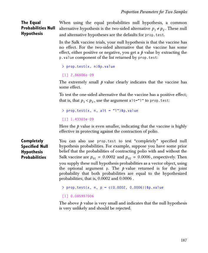
Proportion Parameters for Two Samples
The Equal Probabilities Null Hypothesis
When using the equal probabilities null hypothesis, a commonalternative hypothesis is the two-sided alternative . These nulland alternative hypotheses are the defaults for prop.test.
In the Salk vaccine trials, your null hypothesis is that the vaccine hasno effect. For the two-sided alternative that the vaccine has someeffect, either positive or negative, you get a p value by extracting thep.value component of the list returned by prop.test:
> prop.test(x, n)$p.value
[1] 2.86606e-09
The extremely small p value clearly indicates that the vaccine hassome effect.
To test the one-sided alternative that the vaccine has a positive effect;that is, that , use the argument alt="l" to prop.test:
> prop.test(x, n, alt = "l")$p.value
[1] 1.43303e-09
Here the p value is even smaller, indicating that the vaccine is highlyeffective in protecting against the contraction of polio.
Completely Specified Null Hypothesis Probabilities
You can also use prop.test to test “completely” specified nullhypothesis probabilities. For example, suppose you have some priorbelief that the probabilities of contracting polio with and without theSalk vaccine are and , respectively. Thenyou supply these null hypothesis probabilities as a vector object, usingthe optional argument p. The p value returned is for the jointprobability that both probabilities are equal to the hypothesizedprobabilities; that is, 0.0002 and 0.0006 .
> prop.test(x, n, p = c(0.0002, 0.0006))$p.value
[1] 0.005997006
The above p value is very small and indicates that the null hypothesisis very unlikely and should be rejected.
p1 p2≠
p1 p2<
p01 0.0002= p02 0.0006=
187
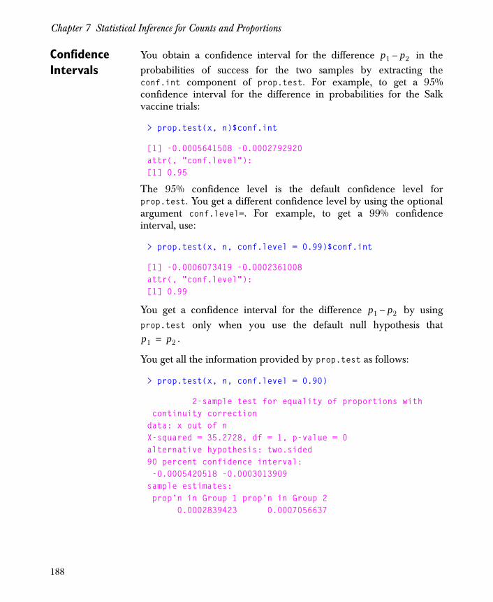
Chapter 7 Statistical Inference for Counts and Proportions
Confidence Intervals
You obtain a confidence interval for the difference in theprobabilities of success for the two samples by extracting theconf.int component of prop.test. For example, to get a 95%confidence interval for the difference in probabilities for the Salkvaccine trials:
> prop.test(x, n)$conf.int
[1] -0.0005641508 -0.0002792920attr(, "conf.level"):[1] 0.95
The 95% confidence level is the default confidence level forprop.test. You get a different confidence level by using the optionalargument conf.level=. For example, to get a 99% confidenceinterval, use:
> prop.test(x, n, conf.level = 0.99)$conf.int
[1] -0.0006073419 -0.0002361008attr(, "conf.level"):[1] 0.99
You get a confidence interval for the difference by usingprop.test only when you use the default null hypothesis that
.
You get all the information provided by prop.test as follows:
> prop.test(x, n, conf.level = 0.90)
2-sample test for equality of proportions with continuity correctiondata: x out of nX-squared = 35.2728, df = 1, p-value = 0alternative hypothesis: two.sided90 percent confidence interval: -0.0005420518 -0.0003013909sample estimates: prop’n in Group 1 prop’n in Group 2 0.0002839423 0.0007056637
p1 p2–
p1 p2–
p1 p2=
188

Proportion Parameters for Three or More Samples
PROPORTION PARAMETERS FOR THREE OR MORE SAMPLES
Sometimes you may have three or more samples of subjects, witheach subject characterized by the presence or absence of somecharacteristic. An alternative, but equivalent, terminology is that youhave three or more sets of trials, with each trial resulting in a successor failure. For example, consider the data shown in Table 7.1 for fourdifferent studies of lung cancer patients, as presented by Fleiss (1981).
Each study has a certain number of patients, as shown in the secondcolumn of the table, and for each study a certain number of thepatients were smokers, as shown in the third column of the table. Forthis data, you are interested in whether the probability of a patientbeing a smoker is the same in each of the four studies, that is, whethereach of the studies involve patients from a homogeneous population.
Setting Up the Data
The first argument to prop.test is a vector containing the number ofsubjects having the characteristic of interest for each of the groups (orthe number of successes for each set of trials). The second argumentto prop.test is a vector containing the number of subjects in eachgroup (or the number of trials for each set of trials). As in the one andtwo sample cases, we call these vectors x and n.
Table 7.1: Smoking status among lung cancer patients in four studies.
Study Number of Patients Number of Smokers
1 86 83
2 93 90
3 136 129
4 82 70
189

Chapter 7 Statistical Inference for Counts and Proportions
For the smokers data in Table 7.1, you create the vectors x and n asfollows:
> x <- c(83, 90, 129, 70)> n <- c(86, 93, 136, 82)
Hypothesis Testing
For problems with three or more groups, you can use either an equalprobabilities null hypothesis or a completely specified probabilitiesnull hypothesis.
The Equal Probabilities Null Hypothesis
In the lung cancer study, the null hypothesis is that the probability ofbeing a smoker is the same in all groups. Because the default nullhypothesis for prop.test is that all groups (or sets of trials) have thesame probability of success, you get a p value as follows:
> prop.test(x, n)$p.value
[1] 0.005585477
The p value of 0.006 is highly significant, so you can not accept thenull hypothesis that all groups have the same probability that apatient is a smoker. To see all the results returned by prop.test, use:
> prop.test(x, n)
4-sample test for equality of proportions without continuity correction
data: x out of nX-squared = 12.6004, df = 3, p-value = 0.0056alternative hypothesis: two.sidedsample estimates:prop’n in Group 1 prop’n in Group 2 prop’n in Group 3 0.9651163 0.9677419 0.9485294prop’n in Group 4 0.8536585
Completely Specified Null Hypothesis Probabilities
If you want to test a completely specified set of null hypothesisprobabilities, you need to supply the optional argument p, with thevalue of this argument being a vector of probabilities having the samelength as the first two arguments, x and n.
190

Proportion Parameters for Three or More Samples
For example, in the lung cancer study, to test the null hypothesis thatthe first three groups have a common probability 0.95 of a patientbeing a smoker, while the fourth group has a probability 0.90 of apatient being a smoker, create the vector p as follows, then use it as anargument to prop.test:
> p <- c(0.95, 0.95, 0.95, 0.90)> prop.test(x, n, p)$p.value
[1] 0.5590245Warning messages: Expected counts < 5. Chi-square approximation may not beappropriate in prop.test(x,n,p).
Alternatively, you could use
> prop.test(x, n, p = c(0.95, 0.95, 0.95, 0.90))$p.value
Confidence Intervals
Confidence intervals are not computed by prop.test when you havethree or more groups (or sets of trials).
191

Chapter 7 Statistical Inference for Counts and Proportions
CONTINGENCY TABLES AND TESTS FOR INDEPENDENCE
The Salk vaccine trials in the early 1950s resulted in the datapresented in Table 7.2.
There are two categorical variables for the Salk trials: vaccinationstatus, which has the two levels “vaccinated” and “placebo,” and poliostatus, which has the three levels “no polio,” “non-paralytic polio,”and “paralytic polio.” Of 200,745 individuals who were vaccinated,24 contracted non-paralytic polio, 33 contracted paralytic polio, andthe remaining 200,688 did not contract any kind of polio. Of 201,229individuals who received the placebo, 27 contracted non-paralyticpolio, 115 contracted paralytic polio, and the remaining 201,087 didnot contract any kind of polio.
Tables such as Table 7.2 are called contingency tables . A contingencytable lists the number of counts for the joint occurrence of two levels(or possible outcomes), one level for each of two categorical variables.The levels for one of the categorical variables correspond to thecolumns of the table, and the levels for the other categorical variablecorrespond to the rows of the table.
When working with contingency table data, your primary interest ismost often determining whether there is any association in the formof statistical dependence between the two categorical variables whosecounts are displayed in the table. The null hypothesis is that the twovariables are statistically independent. You can test this nullhypothesis with the functions chisq.test and fisher.test. Thefunction chisq.test is based on the classic chi-square test statistic,and the associated p value computation entails some approximations.
Table 7.2: Contingency table of Salk vaccine trials data.
No PolioNon-paralytic
PolioParalytic
Polio Totals
Vaccinated 200,688 24 33 200,745
Placebo 201,087 27 115 201,229
Totals 401,775 51 148 401,974
192
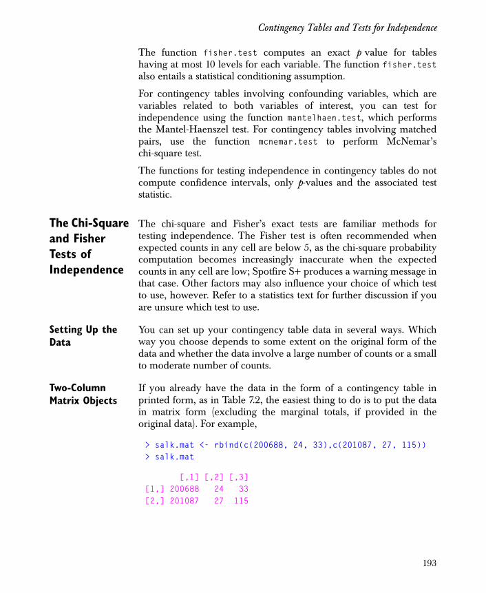
Contingency Tables and Tests for Independence
The function fisher.test computes an exact p value for tableshaving at most 10 levels for each variable. The function fisher.testalso entails a statistical conditioning assumption.
For contingency tables involving confounding variables, which arevariables related to both variables of interest, you can test forindependence using the function mantelhaen.test, which performsthe Mantel-Haenszel test. For contingency tables involving matchedpairs, use the function mcnemar.test to perform McNemar’schi-square test.
The functions for testing independence in contingency tables do notcompute confidence intervals, only p-values and the associated teststatistic.
The Chi-Square and Fisher Tests of Independence
The chi-square and Fisher’s exact tests are familiar methods fortesting independence. The Fisher test is often recommended whenexpected counts in any cell are below 5, as the chi-square probabilitycomputation becomes increasingly inaccurate when the expectedcounts in any cell are low; Spotfire S+ produces a warning message inthat case. Other factors may also influence your choice of which testto use, however. Refer to a statistics text for further discussion if youare unsure which test to use.
Setting Up the Data
You can set up your contingency table data in several ways. Whichway you choose depends to some extent on the original form of thedata and whether the data involve a large number of counts or a smallto moderate number of counts.
Two-Column Matrix Objects
If you already have the data in the form of a contingency table inprinted form, as in Table 7.2, the easiest thing to do is to put the datain matrix form (excluding the marginal totals, if provided in theoriginal data). For example,
> salk.mat <- rbind(c(200688, 24, 33),c(201087, 27, 115))> salk.mat
[,1] [,2] [,3][1,] 200688 24 33[2,] 201087 27 115
193

Chapter 7 Statistical Inference for Counts and Proportions
You could obtain the same result in a slightly different way as follows:
> salk.mat <- matrix(c(200688, 24, 33, 201087, 27, 115),+ 2, 3, byrow = T)
Two Vector Objects
You may be given the raw data in the form of two equal-length codedvectors, one for each variable. In such cases, the length of the vectorscorresponds to the number of individuals, with each entry indicatingthe level by a numeric coding. For example, suppose you have twovariables from a clinical trial of the drug propranolol (Snow, 1965).The vector status is coded for control or propranolol status, and thevector drug is coded yes or no indicating whether the patient survivedat least 28 days with the prescribed drug. The raw data are stored intwo columns of a built-in data frame named propranolol:
> propranolol$status
[1] control control control control prop control prop [8] control prop control prop prop control prop [15] prop control control prop prop prop prop [22] control prop control control prop control control[29] control control control control prop control prop [36] control prop prop prop control prop control[43] prop control prop control prop control control[50] prop prop prop control prop prop prop [57] control control control prop prop control prop [64] control prop control prop control prop control[71] prop control prop control prop control prop [78] control prop control prop control prop control[85] prop control prop control control prop prop
> propranolol$drug
[1] yes yes yes no yes yes yes yes yes yes yes no no yes[15] yes no no yes yes yes yes no yes yes no yes no yes[29] no yes no yes no yes yes no no yes yes yes yes yes[43] yes yes yes no yes no yes yes yes yes yes yes yes yes[57] yes yes yes no yes yes yes no no no yes yes yes yes[71] no no yes yes yes yes yes yes yes yes yes yes yes yes[85] yes yes yes no no yes no
194
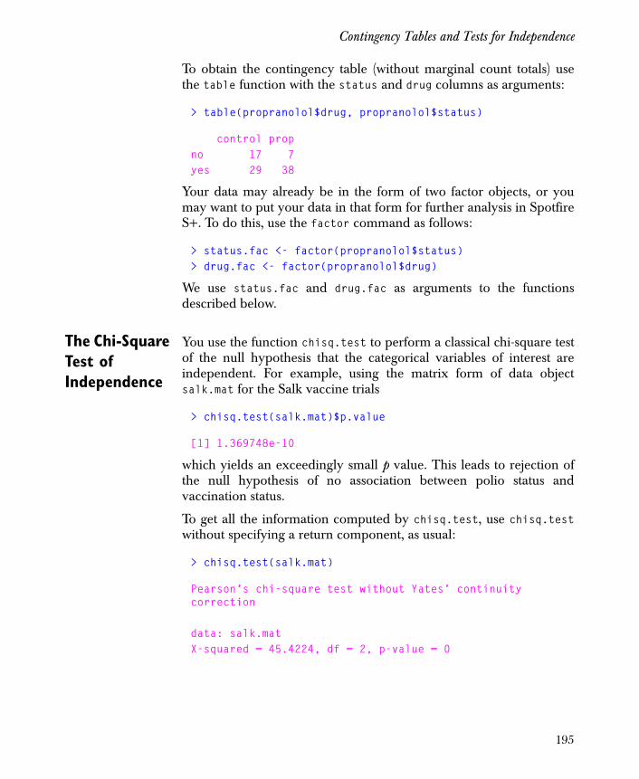
Contingency Tables and Tests for Independence
To obtain the contingency table (without marginal count totals) usethe table function with the status and drug columns as arguments:
> table(propranolol$drug, propranolol$status)
control propno 17 7yes 29 38
Your data may already be in the form of two factor objects, or youmay want to put your data in that form for further analysis in SpotfireS+. To do this, use the factor command as follows:
> status.fac <- factor(propranolol$status)> drug.fac <- factor(propranolol$drug)
We use status.fac and drug.fac as arguments to the functionsdescribed below.
The Chi-Square Test of Independence
You use the function chisq.test to perform a classical chi-square testof the null hypothesis that the categorical variables of interest areindependent. For example, using the matrix form of data objectsalk.mat for the Salk vaccine trials
> chisq.test(salk.mat)$p.value
[1] 1.369748e-10
which yields an exceedingly small p value. This leads to rejection ofthe null hypothesis of no association between polio status andvaccination status.
To get all the information computed by chisq.test, use chisq.testwithout specifying a return component, as usual:
> chisq.test(salk.mat)
Pearson’s chi-square test without Yates’ continuity correction
data: salk.matX-squared = 45.4224, df = 2, p-value = 0
195

Chapter 7 Statistical Inference for Counts and Proportions
You could also use the two factor objects status.fac and drug.fac asfollows:
> chisq.test(status.fac, drug.fac)
Pearson's chi-square test with Yates' continuity correction
data: status.fac and drug.fac X-square = 4.3198, df = 1, p-value = 0.0377
The results are the same no matter which way you have set up thedata.
Fisher’s Exact Test of Independence
You can perform an exact test of indepence by using the Spotfire S+function fisher.test. You can use any data object type that can beused with chisq.test. For example, using the factor objects for thepropranolol clinical trial:
> fisher.test(status.fac, drug.fac)
Fisher's exact test
data: status.fac and drug.fac p-value = 0.0314 alternative hypothesis: two.sided
When using fisher.test you should be aware that the p value iscomputed conditionally on the fixed marginal counts of thecontingency table you are analyzing. That is, the inference does notextend to all possible tables that might be obtained by repeating theexperiment and getting different marginal counts.
The Mantel-Haenszel Test of Independence
A cancer study produced the data shown in Table 7.3 and Table 7.4, asreported by Rosner (1986). In these tables, “case” refers to anindividual who had cancer and “control” refers to an individual whodid not have cancer. A “passive” smoker is an individual who liveswith a smoker. A smoker can also be a passive smoker if that smokerlives with a spouse who also smokes.
196

Contingency Tables and Tests for Independence
For each of these tables, you can use chisq.test or fisher.test totest for independence between cancer status and passive smokingstatus. The data are presented in separate tables because “smokingstatus,” that is, being a smoker or not being a smoker, could be aconfounding variable , because both smoking status and passive smokingstatus are related to the outcome, cancer status, and because smokingstatus may be related to the smoking status of the spouse. You wouldlike to be able to combine the information in both tables so as toproduce an overall test of independence between cancer status andpassive smoking status. You can do so for two or more two-by-twotables, by using the function mantelhaen.test, which performs theMantel-Haenszel test.
Since the data are now associated with three categorical variables, thetwo main variables of interest plus a confounding variable, you canprepare your data in any one of the three forms listed below.
Table 7.3: Nonsmokers in cancer study.
Case-Control Status Passive SmokerNot a Passive
Smoker
case 120 111
control 80 155
Table 7.4: Smokers in cancer study.
Case-Control Status Passive SmokerNot a Passive
Smoker
case 161 117
control 130 124
197
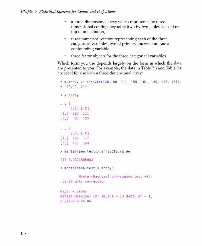
Chapter 7 Statistical Inference for Counts and Proportions
• a three-dimensional array which represents the three dimensional contingency table (two-by-two tables stacked on top of one another)
• three numerical vectors representing each of the three categorical variables, two of primary interest and one a confounding variable
• three factor objects for the three categorical variables
Which form you use depends largely on the form in which the dataare presented to you. For example, the data in Table 7.3 and Table 7.4are ideal for use with a three-dimensional array:
> x.array <- array(c(120, 80, 111, 155, 161, 130, 117, 124),+ c(2, 2, 2))
> x.array
, , 1 [,1] [,2][1,] 120 111[2,] 80 155
, , 2 [,1] [,2][1,] 161 117[2,] 130 124
> mantelhaen.test(x.array)$p.value
[1] 0.0001885083
> mantelhaen.test(x.array)
Mantel-Haenszel chi-square test with continuity correction
data: x.arrayMantel-Haenszel chi-square = 13.9423, df = 1,p-value = 2e-04
198

Contingency Tables and Tests for Independence
McNemar’s Test for Symmetry Using Matched Pairs
In some experiments with two categorical variables, one of thevariables specifies two or more groups of individuals who receivedifferent treatments. In such situations, matching of individuals isoften carried out in order to increase the precision of statisticalinference. However, when matching is carried out the observationsusually are not independent. In such cases, the inference obtainedfrom chisq.test, fisher.test and mantelhaen.test is not validbecause these tests all assume independent observations. Thefunction mcnemar.test allows you to obtain a valid inference forexperiments where matching is carried out.
Consider, for example, the data in Table 7.5, as reported by Rosner(1986). In this table, each entry represents one pair. For instance, the“5” in the lower left cell means that in 5 pairs, the individual withtreatment A died, while the individual that that person was pairedwith, who received treatment B, survived.
Your interest is in the relative effectiveness of treatments A and B intreating a rare form of cancer. Each count in the table is associatedwith a matched pair of individuals.
A pair in the table for which one member of a matched pair surviveswhile the other member dies is called a discordant pair. There are 16discordant pairs in which the individual who received treatment Asurvives and the individual who received treatment B dies. There are5 discordant pairs with the reverse situation in which the individualwho received treatment A dies and the individual who receivedtreatment B survives.
If both treatments are equally effective, then you expect these twotypes of discordant pairs to occur with “nearly” equal frequency. Putin terms of probabilities, your null hypothesis is that , where
Table 7.5: Matched pair data for cancer study.
Survive With Treatment B
Die With Treatment B
survive with treatment A 90 16
die with treatment A 5 510
p1 p2=
199

Chapter 7 Statistical Inference for Counts and Proportions
is the probability that the first type of discordancy occurs in a
matched pair of individuals, and is the probability that the secondtype of discordancy occurs.
We illustrate the use of mcnemar.test on the above data, putting thedata into the form of a matrix object:
> x.matched <- cbind(c(90, 5),c(16, 510))> x.matched
[,1] [,2][1,] 90 16[2,] 5 510
> mcnemar.test(x.matched)$p.value
[1] 0.02909633
> mcnemar.test(x.matched)
McNemar’s chi-square test with continuity correction
data: x.matchedMcNemar’s chi-square = 4.7619, df = 1, p-value = 0.0291
You can use mcnemar.test with two numeric vector objects, or twofactor objects, as the data arguments (just as with the other functionsin this section). You can also use mcnemar.test with matched pairtables having more than two rows and more than two columns. Insuch cases, the null hypothesis is symmetry of the probabilities associated with each row and column of the table; that is, the nullhypothesis is that for each combination of and .
p1
p2
pij
pij pji= i j
200

References
REFERENCES
Bishop, Y.M.M. and Fienberg, S.J., & Holland, P.W. (1980). DiscreteMultivariate Analysis: Theory and Practice . Cambridge, MA: The MITPress.
Conover, W.J. (1980). Practical Nonparametric Statistics (2nd ed.). NewYork: John Wiley & Sons, Inc.
Fienberg, S.E. (1983). The Analysis of Cross-Classified Categorical Data,(2nd ed.). Cambridge, MA: The MIT Press.
Fleiss, J.L. (1981). Statistical Methods for Rates and Proportions (2nd ed.).New York: John Wiley & Sons, Inc.
Lehmann, E.L. (1975). Nonparametrics: Statistical Methods Based onRanks. San Francisco: Holden-Day.
Rosner, B. (1986). Fundamentals of Biostatistics . Boston: DuxburyPress.
Snedecor, G.W. & Cochran, W.G. (1980). Statistical Methods (7th ed.).Ames, Iowa: Iowa State University Press.
Snow, P.J.D. (1965). Effect of propranolol in myocardial infarction.Lancet 2: 551-553.
201

Chapter 7 Statistical Inference for Counts and Proportions
202

Introduction 204
Choosing Suitable Data Sets 209
Cross-Tabulating Continuous Data 213
Cross-Classifying Subsets of Data Frames 216
Manipulating and Analyzing Cross-Classified Data 219
CROSS-CLASSIFIED DATA AND CONTINGENCY TABLES 8
203
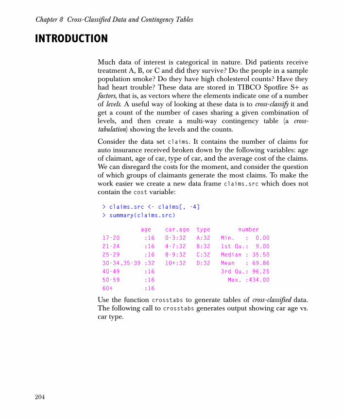
Chapter 8 Cross-Classified Data and Contingency Tables
INTRODUCTION
Much data of interest is categorical in nature. Did patients receivetreatment A, B, or C and did they survive? Do the people in a samplepopulation smoke? Do they have high cholesterol counts? Have theyhad heart trouble? These data are stored in TIBCO Spotfire S+ asfactors, that is, as vectors where the elements indicate one of a numberof levels. A useful way of looking at these data is to cross-classify it andget a count of the number of cases sharing a given combination oflevels, and then create a multi-way contingency table (a cross-tabulation) showing the levels and the counts.
Consider the data set claims. It contains the number of claims forauto insurance received broken down by the following variables: ageof claimant, age of car, type of car, and the average cost of the claims.We can disregard the costs for the moment, and consider the questionof which groups of claimants generate the most claims. To make thework easier we create a new data frame claims.src which does notcontain the cost variable:
> claims.src <- claims[, -4]> summary(claims.src)
age car.age type number17-20 :16 0-3:32 A:32 Min. : 0.0021-24 :16 4-7:32 B:32 1st Qu.: 9.0025-29 :16 8-9:32 C:32 Median : 35.5030-34,35-39 :32 10+:32 D:32 Mean : 69.8640-49 :16 3rd Qu.: 96.2550-59 :16 Max. :434.0060+ :16
Use the function crosstabs to generate tables of cross-classified data.The following call to crosstabs generates output showing car age vs.car type.
204
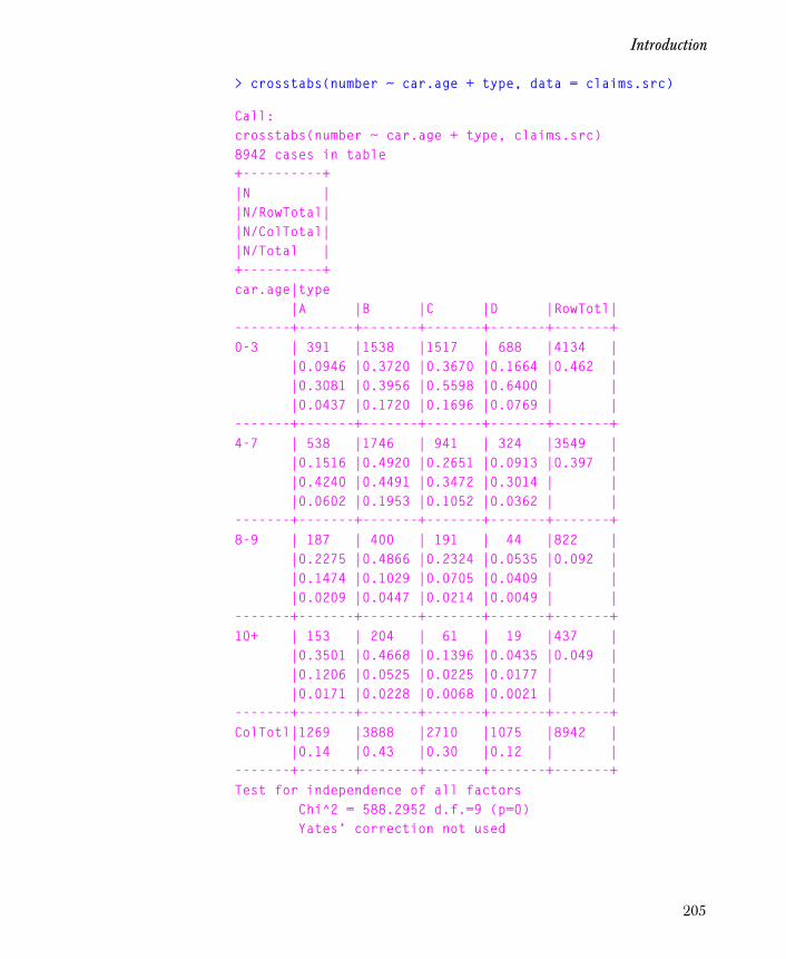
Introduction
> crosstabs(number ~ car.age + type, data = claims.src)
Call:crosstabs(number ~ car.age + type, claims.src)8942 cases in table+----------+|N ||N/RowTotal||N/ColTotal||N/Total |+----------+car.age|type |A |B |C |D |RowTotl|-------+-------+-------+-------+-------+-------+0-3 | 391 |1538 |1517 | 688 |4134 | |0.0946 |0.3720 |0.3670 |0.1664 |0.462 | |0.3081 |0.3956 |0.5598 |0.6400 | | |0.0437 |0.1720 |0.1696 |0.0769 | |-------+-------+-------+-------+-------+-------+4-7 | 538 |1746 | 941 | 324 |3549 | |0.1516 |0.4920 |0.2651 |0.0913 |0.397 | |0.4240 |0.4491 |0.3472 |0.3014 | | |0.0602 |0.1953 |0.1052 |0.0362 | |-------+-------+-------+-------+-------+-------+8-9 | 187 | 400 | 191 | 44 |822 | |0.2275 |0.4866 |0.2324 |0.0535 |0.092 | |0.1474 |0.1029 |0.0705 |0.0409 | | |0.0209 |0.0447 |0.0214 |0.0049 | |-------+-------+-------+-------+-------+-------+10+ | 153 | 204 | 61 | 19 |437 | |0.3501 |0.4668 |0.1396 |0.0435 |0.049 | |0.1206 |0.0525 |0.0225 |0.0177 | | |0.0171 |0.0228 |0.0068 |0.0021 | |-------+-------+-------+-------+-------+-------+ColTotl|1269 |3888 |2710 |1075 |8942 | |0.14 |0.43 |0.30 |0.12 | |-------+-------+-------+-------+-------+-------+Test for independence of all factors Chi^2 = 588.2952 d.f.=9 (p=0) Yates’ correction not used
205

Chapter 8 Cross-Classified Data and Contingency Tables
The first argument to crosstabs is a formula that tells which variablesto include in the table. The second argument is the data set where thevariables are found. The complete call to crosstabs is stored in theresulting object as the attribute "call" and is printed at the top of thetable.
Following the formula at the top of the table, the next item ofinformation is the number of cases; that is, the total count of all thevariables considered. In this example, this is the total of the numbervariable, sum(claims.src$number). After the total number of cases,the output from crosstabs provides a key that tells you how tointerpret the cells of the table. In the key, N is the count. Below N arethe proportions of the whole that the count represents: the proportionof the row total, the proportion of the column total, and theproportion of the table total. If there are only two terms in theformula, the table total is the same as the number of cases.
A quick look at the counts in the table, and in particular at the rowtotals (4134, 3549, 822, 437), shows that there are fewer older cars thannewer cars. Relatively few cars survive to be eight or nine years old,and the number of cars over ten years old is one-tenth that of carsthree years or newer. It is slightly more surprising to note the fourtypes of cars don’t seem to age equally. You can get an inkling of thisby comparing the cells near the top of the table with those near thebottom; however, if you compare the third figure in each cell, the onethe key tells us is N/ColTotal, the progression becomes clear. Of carsof type D, 64% are no more than three years old, while only 4% areeight or nine, and less than 2% are over 10. Compare this to type Acars, where there are slightly more in the 4-7 year age group than inthe 0-3 year, the proportion between eight and nine is 0.1474 and theproportion over ten years is 0.1206.
It seems as if the type of car is related to its age. If we look below the
table where the results of the test for independence are written, wesee that the p value is so small it appears as 0. Of course, we mustremember these data are from insurance claims forms. This is not asample of all the cars on the road, but just those that were accidentsand had insurance policies with the company that collected the data.
There may also be an interaction between car type/car age and theage of the owner (which seems likely), and between the age of theowner and the likelihood of an automobile accident.
χ2
206
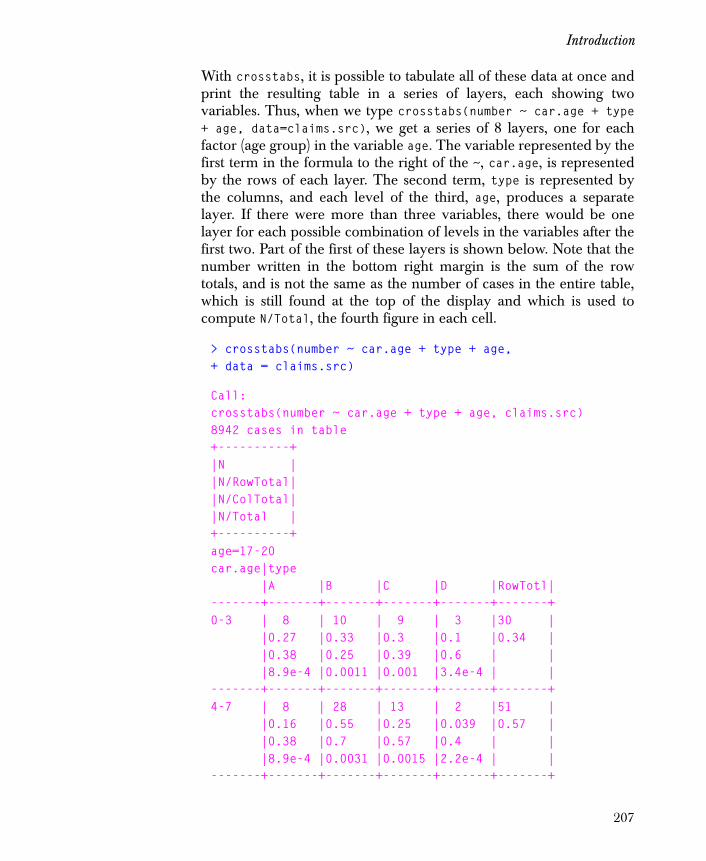
Introduction
With crosstabs, it is possible to tabulate all of these data at once andprint the resulting table in a series of layers, each showing twovariables. Thus, when we type crosstabs(number ~ car.age + type+ age, data=claims.src), we get a series of 8 layers, one for eachfactor (age group) in the variable age. The variable represented by thefirst term in the formula to the right of the ~, car.age, is representedby the rows of each layer. The second term, type is represented bythe columns, and each level of the third, age, produces a separatelayer. If there were more than three variables, there would be onelayer for each possible combination of levels in the variables after thefirst two. Part of the first of these layers is shown below. Note that thenumber written in the bottom right margin is the sum of the rowtotals, and is not the same as the number of cases in the entire table,which is still found at the top of the display and which is used tocompute N/Total, the fourth figure in each cell.
> crosstabs(number ~ car.age + type + age, + data = claims.src)
Call:crosstabs(number ~ car.age + type + age, claims.src)8942 cases in table+----------+|N ||N/RowTotal||N/ColTotal||N/Total |+----------+age=17-20 car.age|type |A |B |C |D |RowTotl|-------+-------+-------+-------+-------+-------+0-3 | 8 | 10 | 9 | 3 |30 | |0.27 |0.33 |0.3 |0.1 |0.34 | |0.38 |0.25 |0.39 |0.6 | | |8.9e-4 |0.0011 |0.001 |3.4e-4 | |-------+-------+-------+-------+-------+-------+4-7 | 8 | 28 | 13 | 2 |51 | |0.16 |0.55 |0.25 |0.039 |0.57 | |0.38 |0.7 |0.57 |0.4 | | |8.9e-4 |0.0031 |0.0015 |2.2e-4 | |-------+-------+-------+-------+-------+-------+
207
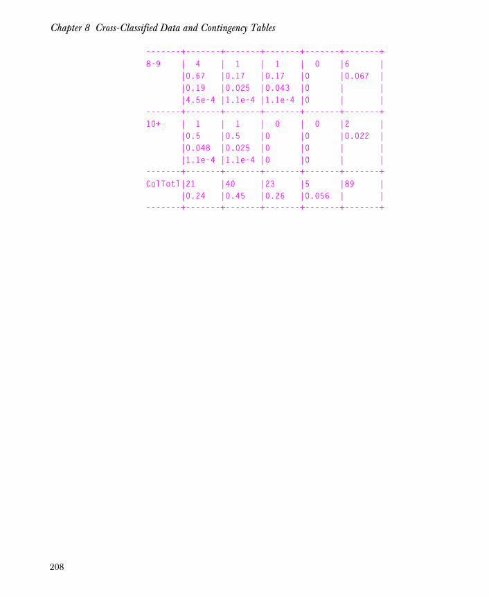
Chapter 8 Cross-Classified Data and Contingency Tables
-------+-------+-------+-------+-------+-------+8-9 | 4 | 1 | 1 | 0 |6 | |0.67 |0.17 |0.17 |0 |0.067 | |0.19 |0.025 |0.043 |0 | | |4.5e-4 |1.1e-4 |1.1e-4 |0 | |-------+-------+-------+-------+-------+-------+10+ | 1 | 1 | 0 | 0 |2 | |0.5 |0.5 |0 |0 |0.022 | |0.048 |0.025 |0 |0 | | |1.1e-4 |1.1e-4 |0 |0 | |-------+-------+-------+-------+-------+-------+ColTotl|21 |40 |23 |5 |89 | |0.24 |0.45 |0.26 |0.056 | |-------+-------+-------+-------+-------+-------+
208

Choosing Suitable Data Sets
CHOOSING SUITABLE DATA SETS
Cross-tabulation is a technique for categorical data. You tabulate thenumber of cases for each combination of factors between yourvariables. In the claims data set these numbers were alreadytabulated. However, when looking at data that have been gathered asa count, you must always keep in mind exactly what is beingcounted—thus we can tell that of the 40-49 year old car owners whosubmitted insurance claims, 43% owned cars of type B, and of the carsof type B whose owners submitted insurance claims, 25% were ownedby 40-49 year olds.
The data set guayule also has a response variable which is a count,while all the predictor variables are factors. Here, the thing beingcounted is the number of rubber plants that sprouted from seeds of anumber of varieties subjected to a number of treatments. However,this experiment was designed so that the same number of seeds wereplanted for each possible combination of the factors of the controllingvariables. Since we know the exact make-up of the larger populationfrom which our counts are taken, we can observe the relative size ofcounts with complaisance and draw conclusions with greatconfidence. The difference between guayule and claims is that withthe former we can view the outcome variable as a binomial responsevariable (“sprouted”/“didn’t sprout”) for which we have tabulated oneof the outcomes (“sprouted”), and in the claims data set we can’t.
Another data set in which all the controlling variables are factors issolder.
> summary(solder)
Opening Solder Mask PadType Panel skipsS:300 Thin :450 A1.5:180 L9 : 90 1:300 Min. : 0.00M:300 Thick:450 A3 :270 W9 : 90 2:300 1st Qu.: 0.00L:300 A6 : 90 L8 : 90 3:300 Median : 2.00 B3 :180 L7 : 90 Mean : 5.53 B6 :180 D7 : 90 3rd Qu.: 7.00 L6 : 90 Max. :48.00 (Other):360
209
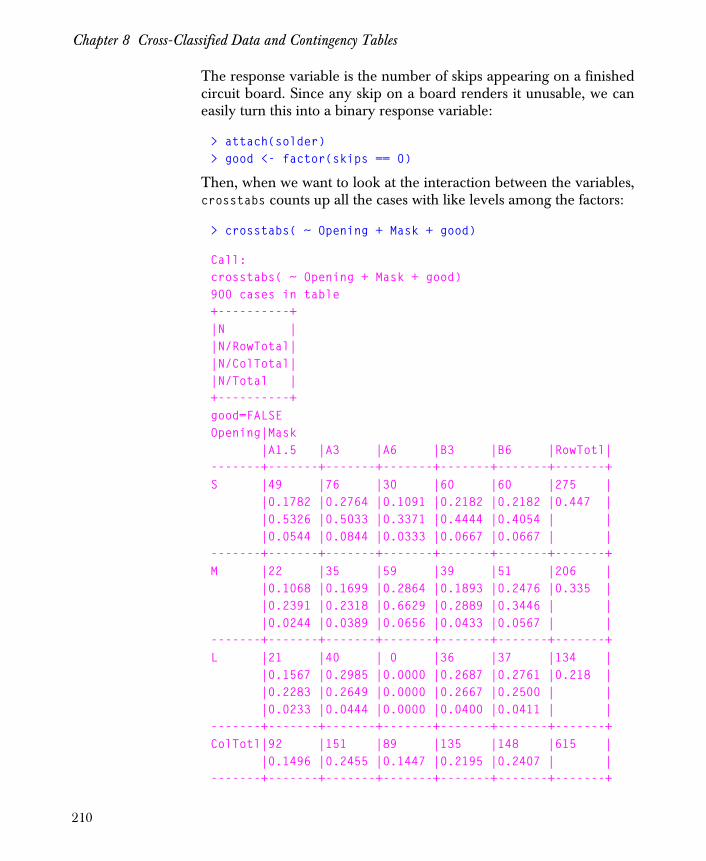
Chapter 8 Cross-Classified Data and Contingency Tables
The response variable is the number of skips appearing on a finishedcircuit board. Since any skip on a board renders it unusable, we caneasily turn this into a binary response variable:
> attach(solder)> good <- factor(skips == 0)
Then, when we want to look at the interaction between the variables,crosstabs counts up all the cases with like levels among the factors:
> crosstabs( ~ Opening + Mask + good)
Call:crosstabs( ~ Opening + Mask + good)900 cases in table+----------+|N ||N/RowTotal||N/ColTotal||N/Total |+----------+good=FALSEOpening|Mask |A1.5 |A3 |A6 |B3 |B6 |RowTotl|-------+-------+-------+-------+-------+-------+-------+S |49 |76 |30 |60 |60 |275 | |0.1782 |0.2764 |0.1091 |0.2182 |0.2182 |0.447 | |0.5326 |0.5033 |0.3371 |0.4444 |0.4054 | | |0.0544 |0.0844 |0.0333 |0.0667 |0.0667 | |-------+-------+-------+-------+-------+-------+-------+M |22 |35 |59 |39 |51 |206 | |0.1068 |0.1699 |0.2864 |0.1893 |0.2476 |0.335 | |0.2391 |0.2318 |0.6629 |0.2889 |0.3446 | | |0.0244 |0.0389 |0.0656 |0.0433 |0.0567 | |-------+-------+-------+-------+-------+-------+-------+L |21 |40 | 0 |36 |37 |134 | |0.1567 |0.2985 |0.0000 |0.2687 |0.2761 |0.218 | |0.2283 |0.2649 |0.0000 |0.2667 |0.2500 | | |0.0233 |0.0444 |0.0000 |0.0400 |0.0411 | |-------+-------+-------+-------+-------+-------+-------+ColTotl|92 |151 |89 |135 |148 |615 | |0.1496 |0.2455 |0.1447 |0.2195 |0.2407 | |-------+-------+-------+-------+-------+-------+-------+
210

Choosing Suitable Data Sets
good=TRUEOpening|Mask |A1.5 |A3 |A6 |B3 |B6 |RowTotl|-------+-------+-------+-------+-------+-------+-------+S |11 |14 | 0 | 0 | 0 |25 | |0.4400 |0.5600 |0.0000 |0.0000 |0.0000 |0.088 | |0.1250 |0.1176 |0.0000 |0.0000 |0.0000 | | |0.0122 |0.0156 |0.0000 |0.0000 |0.0000 | |-------+-------+-------+-------+-------+-------+-------+M |38 |25 | 1 |21 | 9 |94 | |0.4043 |0.2660 |0.0106 |0.2234 |0.0957 |0.330 | |0.4318 |0.2101 |1.0000 |0.4667 |0.2812 | | |0.0422 |0.0278 |0.0011 |0.0233 |0.0100 | |-------+-------+-------+-------+-------+-------+-------+L |39 |80 | 0 |24 |23 |166 | |0.2349 |0.4819 |0.0000 |0.1446 |0.1386 |0.582 | |0.4432 |0.6723 |0.0000 |0.5333 |0.7188 | | |0.0433 |0.0889 |0.0000 |0.0267 |0.0256 | |-------+-------+-------+-------+-------+-------+-------+ColTotl|88 |119 |1 |45 |32 |285 | |0.3088 |0.4175 |0.0035 |0.1579 |0.1123 | |-------+-------+-------+-------+-------+-------+-------+Test for independence of all factors Chi^2 = 377.3556 d.f.= 8 (p=0) Yates' correction not used
In the first example above we specified where to look for thevariables age, car.age and type by giving the data frame claims.srcas the second argument of crosstabs. In the second example, weattached the data frame solder and let crosstabs find the variables inthe search list. Both methods work because, when crosstabs goes tointerpret a term in the formula, it looks first in the data framespecified by the argument data and then in the search list.
You can specifiy a data set to crosstabs with the name of a dataframe, or a frame number in which to find an attached data frame.Using a frame number gives the advantage of speed that comes fromattaching the data frame, while protecting against the possibility ofhaving masked the name of one of the variables with something inyour .Data directory.
211

Chapter 8 Cross-Classified Data and Contingency Tables
For example,
> attach(guayule)> search()
[1] ".Data"[2] "guayule" . . .
> rubber <- crosstabs(plants ~ variety + treatment, + data = 2)
If you specify a data frame and do not give a formula, crosstabs usesthe formula ~ ., that is, it cross-classifies all the variables in the dataframe. Any variable names not found in the specified data frame(which is all of them if you don’t specify any) are sought in the searchlist.
212

Cross-Tabulating Continuous Data
CROSS-TABULATING CONTINUOUS DATA
As seen in the example of the solder data frame above, it is fairlyeasy to turn a continuous response variable into a binomial responsevariable. Clearly, we could have used any logical expression thatmade sense to do so; we could have chosen any cutoff point foracceptable numbers of skips.
A somewhat harder problem is presented by the case where you wanta multinomial factor from continuous data. You can make judicioususe of the cut function to turn the continuous variables into factors,but you need to put care and thought into the points at which toseparate the data into ranges. The quartiles given by the functionsummary offer a good starting point. The data frame kyphosisrepresents data on 81 children who have had corrective spinalsurgery. The variables here are whether a postoperative deformity(kyphosis) is present, the age of the child in months, the number ofvertebrae involved in the operation, and beginning of the range ofvertebrae involved.
> summary(kyphosis)
Kyphosis Age Number Startabsent :64 Min. : 1.00 Min. : 2.000 Min. : 1.00present:17 1st Qu.: 26.00 1st Qu.: 3.000 1st Qu.: 9.00 Median : 87.00 Median : 4.000 Median :13.00 Mean : 83.65 Mean : 4.049 Mean :11.49 3rd Qu.:130.00 3rd Qu.: 5.000 3rd Qu.:16.00 Max. :206.00 Max. :10.000 Max. :18.00
The summary of these variables suggests that two year intervals mightbe a reasonable division for the age. We use the cut function to breakthe variable Age into factors at a sequence of points at 24 monthintervals and to label the resulting levels with the appropriate range ofyears. Since there are at most nine values for Number we leave it alonefor the moment. Since the mean of the Start variable is close to thefirst quartile, a fairly coarse division of Start is probably sufficient.We could require that cut simply divide the data into four segmentsof equal length with the command cut(Start, 4), but the results ofthis, while mathematically correct, look a bit bizarre; the first level
213

Chapter 8 Cross-Classified Data and Contingency Tables
created is "0.830+ thru 5.165". The pretty function divides therange of Start into equal intervals with whole number end points,and the cut function makes them into levels with reasonable names:
> attach(kyphosis)> kyphosis.fac <- data.frame(Kyphosis = Kyphosis,+ Age = cut(Age, c(seq(from=0, to=144, by=24), 206),+ labels = c("0-2", "2-4", "4-6", "6-8", "8-10",+ "10-12", "12+")),+ Number = Number, Start = cut(Start, pretty(Start, 4)))> detach(2)> summary(kyphosis.fac)
Kyphosis Age Number Start absent :64 0-2 :20 Min. : 2.000 0+ thru 5:13 present:17 2-4 : 7 1st Qu.: 3.000 5+ thru 10:14 4-6 : 8 Median : 4.000 10+ thru 15:32 6-8 : 9 Mean : 4.049 15+ thru 20:22 8-10 :11 3rd Qu.: 5.000 10-12:14 Max. :10.000 12+ :12
The cross-tabulation of this data can then be easily examined:
> crosstabs(~ Age + Kyphosis, data = kyphosis.fac)
Call:crosstabs( ~ Age + Kyphosis, kyphosis.fac)81 cases in table+----------+|N ||N/RowTotal||N/ColTotal||N/Total |+----------+Age |Kyphosis |absent |present|RowTotl|-------+-------+-------+-------+0-2 |19 | 1 |20 | |0.950 |0.050 |0.247 | |0.297 |0.059 | | |0.235 |0.012 | |-------+-------+-------+-------+
214

Cross-Tabulating Continuous Data
2-4 | 6 | 1 |7 | | | . . . | |-------+-------+-------+-------+10-12 | 9 | 5 |14 | |0.643 |0.357 |0.173 | |0.141 |0.294 | | |0.111 |0.062 | |-------+-------+-------+-------+12+ |11 | 1 |12 | |0.917 |0.083 |0.148 | |0.172 |0.059 | | |0.136 |0.012 | |-------+-------+-------+-------+ColTotl|64 |17 |81 | |0.79 |0.21 | |-------+-------+-------+-------+Test for independence of all factors Chi^2 = 9.588004 d.f.= 6 (p=0.1431089) Yates' correction not used Some expected values are less than 5, don't trust stated p-value
215

Chapter 8 Cross-Classified Data and Contingency Tables
CROSS-CLASSIFYING SUBSETS OF DATA FRAMES
There are two ways to subset a data frame for cross-classification.First, the crosstabs function cross-tabulates only those variablesspecified in the formula. If there is one variable in the data frame inwhich you are not interested, don’t mention it. Second, you canchoose which rows you want to consider with the subset argument.You can use anything you would normally use to subscript the rowsof a data frame. Thus, the subset argument can be an expression thatevaluates to a logical vector, or a vector of row numbers or rownames. See the chapter Writing Functions in Spotfire S+ in theProgrammer’s Guide for details on subscripting.
As an example, recall the solder data set. You can look at the relationbetween the variables without turning skips explicitly into a binomialvariable by using it to subscript the rows of the data frame:
> crosstabs(~ Solder + Opening, data = solder, + subset = skips < 10)
Call:crosstabs( ~ Solder+Opening, solder, subset = skips<10)729 cases in table+----------+|N ||N/RowTotal||N/ColTotal||N/Total |+----------+Solder |Opening |S |M |L |RowTotl|-------+-------+-------+-------+-------+Thin | 50 |133 |140 |323 | |0.155 |0.412 |0.433 |0.44 | |0.294 |0.494 |0.483 | | |0.069 |0.182 |0.192 | |-------+-------+-------+-------+-------+Thick |120 |136 |150 |406 | |0.296 |0.335 |0.369 |0.56 | |0.706 |0.506 |0.517 | | |0.165 |0.187 |0.206 | |
216
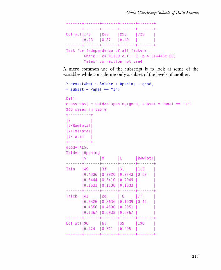
Cross-Classifying Subsets of Data Frames
-------+-------+-------+-------+-------+-------+-------+-------+-------+-------+ColTotl|170 |269 |290 |729 | |0.23 |0.37 |0.40 | |-------+-------+-------+-------+-------+Test for independence of all factors Chi^2 = 20.01129 d.f.= 2 (p=4.514445e-05) Yates' correction not used
A more common use of the subscript is to look at some of thevariables while considering only a subset of the levels of another:
> crosstabs( ~ Solder + Opening + good, + subset = Panel == "1")
Call:crosstabs( ~ Solder+Opening+good, subset = Panel == "1")300 cases in table+----------+|N ||N/RowTotal||N/ColTotal||N/Total |+----------+good=FALSESolder |Opening |S |M |L |RowTotl|-------+-------+-------+-------+-------+Thin |49 |33 |31 |113 | |0.4336 |0.2920 |0.2743 |0.59 | |0.5444 |0.5410 |0.7949 | | |0.1633 |0.1100 |0.1033 | |-------+-------+-------+-------+-------+Thick |41 |28 | 8 |77 | |0.5325 |0.3636 |0.1039 |0.41 | |0.4556 |0.4590 |0.2051 | | |0.1367 |0.0933 |0.0267 | |-------+-------+-------+-------+-------+ColTotl|90 |61 |39 |190 | |0.474 |0.321 |0.205 | |-------+-------+-------+-------+-------+
217
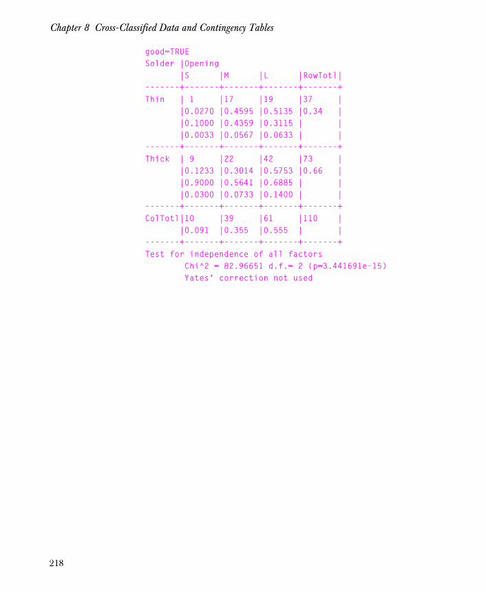
Chapter 8 Cross-Classified Data and Contingency Tables
good=TRUESolder |Opening |S |M |L |RowTotl|-------+-------+-------+-------+-------+Thin | 1 |17 |19 |37 | |0.0270 |0.4595 |0.5135 |0.34 | |0.1000 |0.4359 |0.3115 | | |0.0033 |0.0567 |0.0633 | |-------+-------+-------+-------+-------+Thick | 9 |22 |42 |73 | |0.1233 |0.3014 |0.5753 |0.66 | |0.9000 |0.5641 |0.6885 | | |0.0300 |0.0733 |0.1400 | |-------+-------+-------+-------+-------+ColTotl|10 |39 |61 |110 | |0.091 |0.355 |0.555 | |-------+-------+-------+-------+-------+Test for independence of all factors Chi^2 = 82.96651 d.f.= 2 (p=3.441691e-15) Yates' correction not used
218
Manipulating and Analyzing Cross-Classified Data
MANIPULATING AND ANALYZING CROSS-CLASSIFIED DATA
When you apply crosstabs to a data frame, you get amultidimensional array whose elements are the counts and whosedimensions are the variables involved in the cross-tabulations. Thefirst factor variable is the first (or row) dimension, the second is thesecond (or column) dimension, the third is the third dimension, etc. Ifyou wish to do more than tabulate data, say compute means or sumsof cross-classified data, you can apply functions to the elements of thearray with the function tapply; see the online help for tapply formore information.
219

Chapter 8 Cross-Classified Data and Contingency Tables
220

Introduction 222
Power and Sample Size Theory 223
Normally Distributed Data 224One-Sample Test of Gaussian Mean 224Comparing Means from Two Samples 226
Binomial Data 229One-Sample Test of Binomial Proportion 229Comparing Proportions from Two Samples 230
References 234
POWER AND SAMPLE SIZE 9
221
Chapter 9 Power and Sample Size
INTRODUCTION
When contemplating a study, one of the first statistical questions thatarises is “How big does my sample need to be?” The required samplesize is a function of the alternative hypothesis, the probabilities ofType I and Type II errors, and the variability of the population(s)under study. Two functions are available in TIBCO Spotfire S+ forcomputing power and sample size requirements:normal.sample.size and binomial.sample.size. Depending on theinput, these functions provide the following:
• For given power and alternative hypothesis, the required sample size;
• For given sample size and power, the detectable difference;
• For given sample size and alternative hypothesis, the power to distinguish between the hypotheses.
These functions can be applied in one- and two-sample studies. Theyproduce tables from vectorized input that are suitable for passing toTrellis graphics functions.
222
Power and Sample Size Theory
POWER AND SAMPLE SIZE THEORY
Intuitively, we have a sense that the sample size required for a studydepends on how small of a difference we’re trying to detect, howmuch variability is inherent in our data, and how certain we want tobe of our results. In a classical hypothesis test of H0 (null hypothesis)versus Ha (alternative hypothesis), there are four possible outcomes,two of which are erroneous:
• Don’t reject H0 when is H0 true.
• Reject H0 when H0 is false.
• Reject H0 when H0 is true (type I error).
• Don’t reject H0 when H0 is false (type II error).
To construct a test, the distribution of the test statistic under H0 isused to find a critical region which will ensure the probability ofcommitting a type I error does not exceed some predetermined level.This probability is typically denoted α. The power of the test is itsability to correctly reject the null hypothesis, or 1 - Pr(type II error),which is based on the distribution of the test statistic under Ha. Therequired sample size is then a function of
1. The null and alternative hypotheses;
2. The target α;
3. The desired power to detect Ha;
4. The variability within the population(s) under study.
Our objective is, for a given test, to find a relationship between theabove factors and the sample size that enables us to select a samplesize consistent with the desired α and power.
223

Chapter 9 Power and Sample Size
NORMALLY DISTRIBUTED DATA
One-Sample Test of Gaussian Mean
When conducting a one-sample test of a normal mean, we start bywriting our assumptions and hypotheses:
where i = 1,...,n, and σ2 is known. To perform a two-sided test ofequality the hypotheses is as follows:
Our best estimate of μ is the sample mean, which is normallydistributed:
The test statistic is
We reject H0 if , which guarantees a level α test. Thepower of the test to detect μ = μ0 is
We can think of the left side of the sum as the lower power, or thepower to detect , and the right side as the upper power, or the
power to detect . Solving for n using both the upper and
lower power is difficult, but we note that when , the
upper power is negligible (< α/2). Similarly, the lower power is smallwhen . Therefore, the equation can be simplified by using
Xi N μ σ2,( )∼
H0:μ μ0=
Ha:μ μa=
X N μ σ2
n-----,⎝ ⎠
⎛ ⎞∼
Z n X μ0–( ) σ⁄=
Z N μ μ0– 1,( )∼
Z N 0 1,( )∼ for H0
Z Z1 α 2⁄–>
Power Φn μ0 μa–( )
σ----------------------------- Z1 α 2⁄––⎝ ⎠
⎛ ⎞ Φn μa μ0–( )
σ----------------------------- Z1 α 2⁄––⎝ ⎠
⎛ ⎞+=
μa μ0<
μa μ0>
μa μ0– 0<
μa μ0– 0>
224

Normally Distributed Data
the absolute value of the difference between μa and μ0 andconsidering only one side of the sum. This results in the followingsample size formula:
Comments • While only one of the upper and lower power is used in deriving the sample size formula, the Spotfire S+ function normal.sample.size uses both the upper and lower power when computing the power of a two-tailed test for a given sample size.
• In practice, the variance of the population is seldom known and the test statistic is based on the t distribution. Using the t distribution to derive a sample size requires an iterative approach, since the sample size is needed to specify the degrees of freedom. The difference between the quantile value for the t distribution versus the standard normal distribution is significant only when small sample sizes are required. Thus, the standard formula based on the normal distribution is chosen. Keep in mind that for samples sizes less than 10, the power of a t test could be significantly less than the target power.
• The formula for a one-tailed test is derived along similar lines. It is exactly the same as the two-tailed formula with the exception that is replaced by .
Examples The function for computing sample size for normally distributed datais normal.sample.size. This function can be used to compute samplesize, power, or minimum detectable difference, and automaticallychooses what to compute based on the input information. Here aresome simple examples:
# One-sample case, using all the defaults> normal.sample.size(mean.alt = 0.3)
mean.null sd1 mean.alt delta alpha power n11 0 1 0.3 0.3 0.05 0.8 88
# Reduce output with summary> summary(normal.sample.size(mean.alt = 0.3))
n σ Z1 α 2⁄– ZPower+( )( ) μa μo–⁄[ ]2=
Z1 α– 2⁄ Z1 α–
225
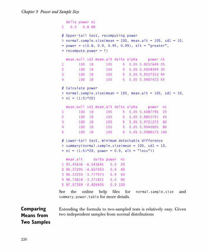
Chapter 9 Power and Sample Size
delta power n11 0.3 0.8 88
# Upper-tail test, recomputing power> normal.sample.size(mean = 100, mean.alt = 105, sd1 = 10,+ power = c(0.8, 0.9, 0.95, 0.99), alt = "greater",+ recompute.power = T)
mean.null sd1 mean.alt delta alpha power n11 100 10 105 5 0.05 0.8037649 252 100 10 105 5 0.05 0.9054399 353 100 10 105 5 0.05 0.9527153 444 100 10 105 5 0.05 0.9907423 64
# Calculate power> normal.sample.size(mean = 100, mean.alt = 105, sd1 = 10,+ n1 = (1:5)*20)
mean.null sd1 mean.alt delta alpha power n11 100 10 105 5 0.05 0.6087795 202 100 10 105 5 0.05 0.8853791 403 100 10 105 5 0.05 0.9721272 604 100 10 105 5 0.05 0.9940005 805 100 10 105 5 0.05 0.9988173 100
# Lower-tail test, minimum detectable difference> summary(normal.sample.size(mean = 100, sd1 = 10,+ n1 = (1:5)*20, power = 0.9, alt = "less"))
mean.alt delta power n11 93.45636 -6.543641 0.9 202 95.37295 -4.627053 0.9 403 96.22203 -3.777973 0.9 604 96.72818 -3.271821 0.9 805 97.07359 -2.926405 0.9 100
See the online help files for normal.sample.size andsummary.power.table for more details.
Comparing Means from Two Samples
Extending the formula to two-sampled tests is relatively easy. Giventwo independent samples from normal distributions
226
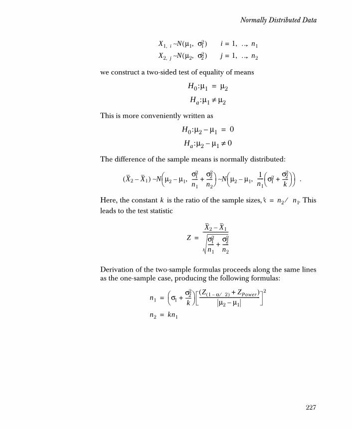
Normally Distributed Data
we construct a two-sided test of equality of means
This is more conveniently written as
The difference of the sample means is normally distributed:
.
Here, the constant is the ratio of the sample sizes, . Thisleads to the test statistic
Derivation of the two-sample formulas proceeds along the same linesas the one-sample case, producing the following formulas:
X1 i, N μ1 σ12,( )∼ i 1 … n1, ,=
X2 j, N μ2 σ22,( )∼ j 1 … n2, ,=
H0:μ1 μ2=
Ha:μ1 μ2≠
H0:μ2 μ1– 0=
Ha:μ2 μ1– 0≠
X2 X1–( ) N μ2 μ1–σ1
2
n1-----
σ22
n2-----+,⎝ ⎠
⎛ ⎞ N μ2 μ1–1n1----- σ1
2 σ22
k-----+⎝ ⎠
⎛ ⎞,⎝ ⎠⎛ ⎞∼ ∼
k k n2 n1⁄=
ZX2 X1–
σ12
n1-----
σ22
n2-----+
---------------------=
n1 σ1σ2
2
k-----+⎝ ⎠
⎛ ⎞ Z 1 α 2⁄–( ) ZPower+( )μ2 μ1–
--------------------------------------------------2
=
n2 kn1=
227

Chapter 9 Power and Sample Size
Examples For two-sample cases, use normal.sample.size with mean2 instead ofmean.alt. A few simple examples are provided below.
# Don't round sample size> summary(normal.sample.size(mean2 = 0.3, exact.n = T))
delta power n1 n21 0.3 0.8 174.4195 174.4195
# Round sample size, then recompute power> summary(normal.sample.size(mean2 = 0.3, recompute = T))
delta power n1 n21 0.3 0.8013024 175 175
# Unequal sample sizes, lower tail test# The prop.n2 argument is equal to k from the # above derivation.> normal.sample.size(mean = 100, mean2 = 94, sd1 = 15,+ prop.n2 = 2, power = 0.9, alt = "less")
mean1 sd1 mean2 sd2 delta alpha power n1 n2 prop.n21 100 15 94 15 -6 0.05 0.9 81 162 2
228
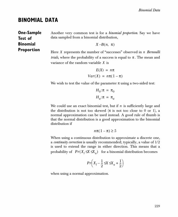
Binomial Data
BINOMIAL DATA
One-Sample Test of Binomial Proportion
Another very common test is for a binomial proportion. Say we havedata sampled from a binomial distribution,
Here represents the number of “successes” observed in Bernoullitrials, where the probability of a success is equal to . The mean andvariance of the random variable is
We wish to test the value of the parameter π using a two-sided test:
We could use an exact binomial test, but if is sufficiently large andthe distribution is not too skewed (π is not too close to 0 or 1), anormal approximation can be used instead. A good rule of thumb isthat the normal distribution is a good approximation to the binomialdistribution if
When using a continuous distribution to approximate a discrete one,a continuity correction is usually recommended; typically, a value of 1/2is used to extend the range in either direction. This means that aprobability of for a binomial distribution becomes
when using a normal approximation.
X B n π,( )∼
X nπ
X
E X( ) nπ=
Var X( ) nπ 1 π–( )=
H0:π π0=
Ha:π πa=
n
nπ 1 π–( ) 5≥
Pr Xl X Xu≤ ≤( )
Pr Xl12---– X Xu
12---+≤ ≤⎝ ⎠
⎛ ⎞
229

Chapter 9 Power and Sample Size
If the continuity correction is temporarily suppressed, the sample sizeformula is derived very much as in the normal case:
There have been several suggestions concerning how to bestincorporate a continuity correction into the sample-size formula. Theone adopted by the Spotfire S+ function binomial.sample.size for aone-sample test is
Examples # One-sample case, using all the defaults> binomial.sample.size(p.alt = 0.3)
p.null p.alt delta alpha power n11 0.5 0.3 -0.2 0.05 0.8 57
# Minimal output> summary(binomial.sample.size(p.alt = 0.3))
delta power n11 -0.2 0.8 57
# Compute power> binomial.sample.size(p = 0.2, p.alt = 0.12, n1 = 250)
p.null p.alt delta alpha power n11 0.2 0.12 -0.08 0.05 0.8997619 250
Comparing Proportions from Two Samples
The two-sample test for proportions is a bit more involved than theothers we’ve looked at. Say we have data sampled from two binomialdistributions
n*π0 1 π0–( )Z1 α 2⁄– π0 1 π0–( )ZPower+
πa π0–--------------------------------------------------------------------------------------------------------
2
=
n n* 2πa π0–--------------------+=
X1 B n1 π1,( )∼
X2 B n2 π2,( )∼
230
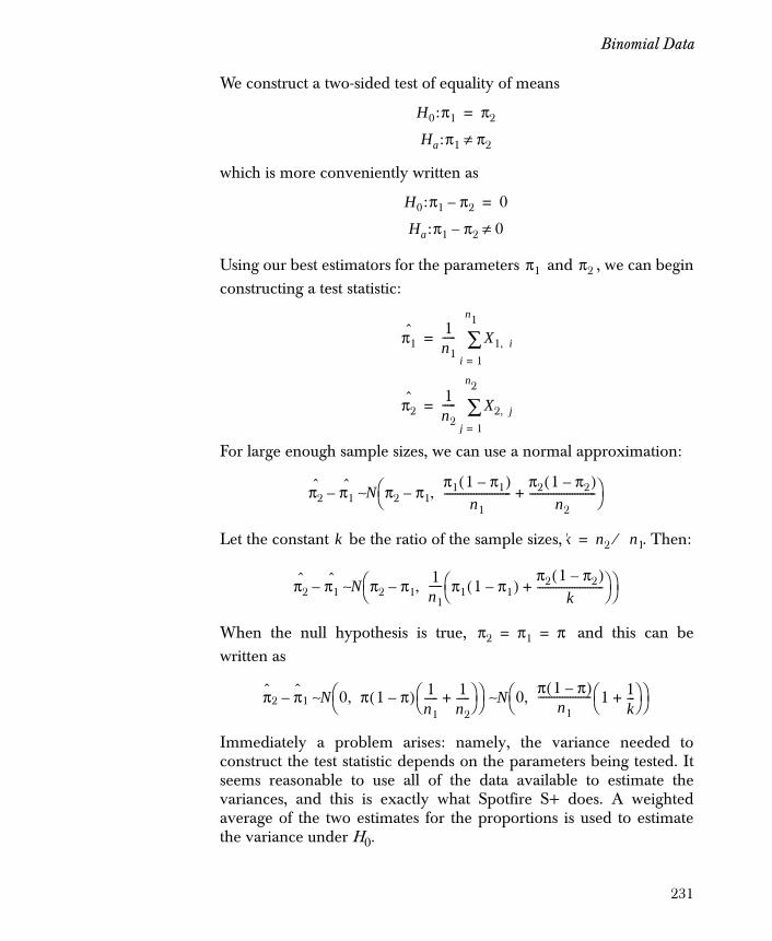
Binomial Data
We construct a two-sided test of equality of means
which is more conveniently written as
Using our best estimators for the parameters and , we can beginconstructing a test statistic:
For large enough sample sizes, we can use a normal approximation:
Let the constant be the ratio of the sample sizes, . Then:
When the null hypothesis is true, and this can bewritten as
Immediately a problem arises: namely, the variance needed toconstruct the test statistic depends on the parameters being tested. Itseems reasonable to use all of the data available to estimate thevariances, and this is exactly what Spotfire S+ does. A weightedaverage of the two estimates for the proportions is used to estimatethe variance under H0.
H0:π1 π2=
Ha:π1 π2≠
H0:π1 π2– 0=
Ha:π1 π2– 0≠
π1 π2
π1ˆ 1
n1----- X1 i,
i 1=
n1
∑=
π2ˆ 1
n2----- X2 j,
j 1=
n2
∑=
π2ˆ π1
ˆ– N π2 π1–π1 1 π1–( )
n1-------------------------
π2 1 π2–( )n2
-------------------------+,⎝ ⎠⎛ ⎞∼
k k n2 n1⁄=
π2ˆ π1
ˆ– N π2 π1–1n1----- π1 1 π1–( )
π2 1 π2–( )k
-------------------------+⎝ ⎠⎛ ⎞,⎝ ⎠
⎛ ⎞∼
π2 π1 π= =
π2 π1– N 0 π 1 π–( ) 1n1----- 1
n2-----+⎝ ⎠
⎛ ⎞,⎝ ⎠⎛ ⎞ N 0 π 1 π–( )
n1-------------------- 1 1
k---+⎝ ⎠
⎛ ⎞,⎝ ⎠⎛ ⎞∼ ∼
231
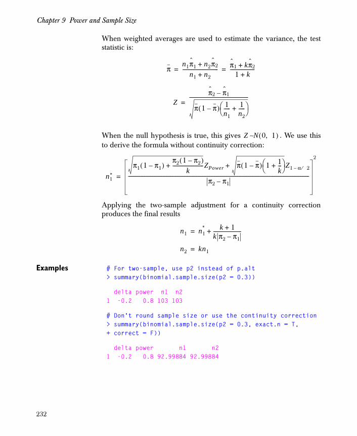
Chapter 9 Power and Sample Size
When weighted averages are used to estimate the variance, the teststatistic is:
When the null hypothesis is true, this gives . We use thisto derive the formula without continuity correction:
Applying the two-sample adjustment for a continuity correctionproduces the final results
Examples # For two-sample, use p2 instead of p.alt> summary(binomial.sample.size(p2 = 0.3))
delta power n1 n21 -0.2 0.8 103 103
# Don't round sample size or use the continuity correction> summary(binomial.sample.size(p2 = 0.3, exact.n = T,+ correct = F))
delta power n1 n21 -0.2 0.8 92.99884 92.99884
πn1π1 n2π2+
n1 n2+----------------------------- π1 kπ2+
1 k+--------------------= =
Zπ2 π1–
π 1 π–( ) 1n1----- 1
n2-----+⎝ ⎠
⎛ ⎞------------------------------------------------
=
Z N 0 1,( )∼
n1*
π1 1 π1–( )π2 1 π2–( )
k-------------------------+ ZPower π 1 π–( ) 1 1
k---+⎝ ⎠
⎛ ⎞ Z1 α 2⁄–+
π2 π1–---------------------------------------------------------------------------------------------------------------------------------------------------
2
=
n1 n1* k 1+
k π2 π1–-----------------------+=
n2 kn1=
232

Binomial Data
# Round sample size, then recompute power> summary(binomial.sample.size(p2 = 0.3, recompute = T))
delta power n1 n21 -0.2 0.8000056 103 103
# Unequal sample sizes, lower tail test# The prop.n2 argument is equal to k from the # above derivation.> binomial.sample.size(p = 0.1, p2 = 0.25, prop.n2 = 2,+ power = 0.9, alt = "less")
p1 p2 delta alpha power n1 n2 prop.n21 0.1 0.25 0.15 0.05 0.9 92 184 2
# Compute minimum detectable difference (delta),# given sample size and power.> binomial.sample.size(p = 0.6, n1 = 500, prop.n2 = 0.5,+ power = c(0.8, 0.9, 0.95))
p1 p2 delta alpha power n1 n2 prop.n21 0.6 0.7063127 0.1063127 0.05 0.80 500 250 0.52 0.6 0.7230069 0.1230069 0.05 0.90 500 250 0.53 0.6 0.7367932 0.1367932 0.05 0.95 500 250 0.5
# Compute power> binomial.sample.size(p = 0.3, p2 = seq(0.31, 0.35,+ by = 0.01), n1 = 1000, prop.n2 = 0.5)
p1 p2 delta alpha power n1 n2 prop.n21 0.3 0.31 0.01 0.05 0.06346465 1000 500 0.52 0.3 0.32 0.02 0.05 0.11442940 1000 500 0.53 0.3 0.33 0.03 0.05 0.20446778 1000 500 0.54 0.3 0.34 0.04 0.05 0.32982868 1000 500 0.55 0.3 0.35 0.05 0.05 0.47748335 1000 500 0.5
233

Chapter 9 Power and Sample Size
REFERENCES
Rosner, B. (1990). Fundamentals of Biostatistics (3rd ed.). Boston: PWS-Kent.
Fisher, L.D. & Van Belle, G. (1993). Biostatistics. New York: JohnWiley & Sons, Inc.
Fleiss, J.L. (1981). Statistical Methods for Rates and Proportions. NewYork: John Wiley & Sons, Inc.
234
Introduction 237
Simple Least-Squares Regression 239Diagnostic Plots for Linear Models 242Other Diagnostics 245
Multiple Regression 247
Adding and Dropping Terms from a Linear Model 251
Choosing the Best Model—Stepwise Selection 257
Updating Models 260
Weighted Regression 261Example: Weighted Linear Regression 261Observation Weights vs. Frequencies 265
Prediction with the Model 270
Confidence Intervals 272
Polynomial Regression 275
Generalized Least Squares Regression 280Example: The Ovary Data Set 282Manipulating gls Objects 283
Smoothing 290Locally Weighted Regression Smoothing 290Using the Super Smoother 292Using the Kernel Smoother 295Smoothing Splines 298Comparing Smoothers 299
REGRESSION AND SMOOTHING FOR CONTINUOUS RESPONSE DATA
10
235

Chapter 10 Regression and Smoothing for Continuous Response Data
Additive Models 301
More on Nonparametric Regression 307Alternating Conditional Expectations 307Additivity and Variance Stabilization 312Projection Pursuit Regression 318
References 328
236
Introduction
INTRODUCTION
Regression is a tool for exploring relationships between variables.Linear regression explores relationships that are readily described bystraight lines, or their generalization to many dimensions. Asurprisingly large number of problems can be analyzed using thetechniques of linear regression, and even more can be attacked bymeans of transformations of the original variables that result in linearrelationships among the transformed variables. In recent years, thetechniques themselves have been extended through the addition ofrobust methods and generalizations of the classical linear regressiontechniques. These generalizations allow familiar problems incategorical data analysis such as logistic and Poisson regression to besubsumed under the heading of the generalized linear model (GLM),while still further generalizations allow a predictor to be replaced byan arbitrary smooth function of the predictor in building a generalizedadditive model (GAM).
This chapter describes regression and smoothing in the case of aunivariate, continuous response. We start with simple regression,which is regression with a single predictor variable: fitting the model,examining the fitted models, and analyzing the residuals. We thenexamine multiple regression, varying models by adding and droppingterms as appropriate. Again, we examine the fitted models andanalyze the residuals. We then consider the special case of weightedregression, which underlies many of the robust techniques andgeneralized regression methods.
One important reason for performing regression analysis is to get amodel useful for prediction. The section Prediction with the Modeldescribes how to use TIBCO Spotfire S+ to obtain predictions fromyour fitted model, and the section Confidence Intervals describeshow to obtain pointwise and simultaneous confidence intervals.
The classical linear regression techniques make several strongassumptions about the underlying data, and the data can fail to satisfythese assumptions in different ways. For example, the regression linemay be thrown off by one or more outliers or the data may not befitted well by any straight line. In the first case, we can bring robustregression methods into play; these minimize the effects of outliers
237

Chapter 10 Regression and Smoothing for Continuous Response Data
while retaining the basic form of the linear model. Conversely, therobust methods are often useful in identifying outliers. We discussrobust regression in detail in a later chapter.
In the second case, we can expand our notion of the linear model,either by adding polynomial terms to our straight line model, or byreplacing one or more predictors by an arbitrary smooth function ofthe predictor, converting the classical linear model into a generalizedadditive model (GAM).
Scatterplot smoothers are useful tools for fitting arbitrary smoothfunctions to a scatter plot of data points. The smoother summarizesthe trend of the measured response as a function of the predictorvariables. We describe several scatterplot smoothers available inSpotfire S+, and describe how the smoothed values they return canbe incorporated into additive models.
238

Simple Least-Squares Regression
SIMPLE LEAST-SQUARES REGRESSION
Simple regression uses the method of least squares to fit a continuous,univariate response as a linear function of a single predictor variable.In the method of least squares, we fit a line to the data so as tominimize the sum of the squared residuals. Given a set of nobservations of the response variable corresponding to a set of
values of the predictor and an arbitrary model , the ith
residual is defined as the difference between the ith observation
and the fitted value , that is, .
To do simple regression with Spotfire S+, use the function lm (forlinear model) with a simple formula linking your chosen responsevariable to the predictor variable. In many cases, both the responseand the predictor are components of a single data frame, which canbe specified as the data argument to lm. For example, consider the airpollution data in the built-in data set air:
> air[, c(1,3)]
ozone temperature 1 3.448217 67 2 3.301927 72 3 2.289428 74 4 2.620741 62 5 2.843867 65 . . .
A scatter plot of the data is shown in Figure 10.1.
yi
xi y f x( )=
yi
yi f xi( )= ri yi yi–=
239

Chapter 10 Regression and Smoothing for Continuous Response Data
From the scatter plot, we hypothesize a linear relationship betweentemperature and ozone concentration. We choose ozone as theresponse and temperature as the single predictor. The choice ofresponse and predictor variables is driven by the subject matter inwhich the data arise, rather than by statistical considerations.
To fit the model, use lm as follows:
> ozone.lm <- lm(ozone ~ temperature, data = air)
The first argument, ozone ~ temperature, is the formula specifyingthat the variable ozone is modeled as a function of temperature. Thesecond argument specifies that the data for the linear model iscontained in the data frame air.
Figure 10.1: Scatter plot of ozone against temperature.
••
•
••
•
•
••
••
•
•
•
•
•
•
•
•
•
•
•
•
••
•
•
••
•
•
• •
•
•
•
•
•
•
••
•
•
•
•
•
•
•
•
•
•
•
•
•
•
•
••
•
•
•
•
•
•
•
•
•
•
•
••
•
•
•
•
•
• •
•
•••
• •
•
•
•
•••
•
•
••
••
•
••
•
••
•
•
•
•
•
•••
temperature
ozon
e
60 70 80 90
12
34
5
240
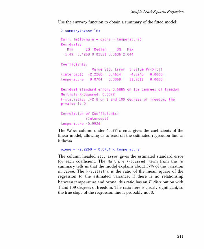
Simple Least-Squares Regression
Use the summary function to obtain a summary of the fitted model:
> summary(ozone.lm)
Call: lm(formula = ozone ~ temperature)Residuals: Min 1Q Median 3Q Max -1.49 -0.4258 0.02521 0.3636 2.044
Coefficients: Value Std. Error t value Pr(>|t|)(Intercept) -2.2260 0.4614 -4.8243 0.0000temperature 0.0704 0.0059 11.9511 0.0000
Residual standard error: 0.5885 on 109 degrees of freedomMultiple R-Squared: 0.5672F-statistic: 142.8 on 1 and 109 degrees of freedom, the p-value is 0
Correlation of Coefficients: (Intercept)temperature -0.9926
The Value column under Coefficients gives the coefficients of thelinear model, allowing us to read off the estimated regression line asfollows:
ozone = -2.2260 + 0.0704 x temperature
The column headed Std. Error gives the estimated standard errorfor each coefficient. The Multiple R-Squared term from the lmsummary tells us that the model explains about 57% of the variationin ozone. The F-statistic is the ratio of the mean square of theregression to the estimated variance; if there is no relationshipbetween temperature and ozone, this ratio has an distribution with1 and 109 degrees of freedom. The ratio here is clearly significant, sothe true slope of the regression line is probably not 0.
F
241
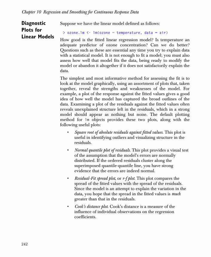
Chapter 10 Regression and Smoothing for Continuous Response Data
Diagnostic Plots for Linear Models
Suppose we have the linear model defined as follows:
> ozone.lm <- lm(ozone ~ temperature, data = air)
How good is the fitted linear regression model? Is temperature anadequate predictor of ozone concentration? Can we do better?Questions such as these are essential any time you try to explain datawith a statistical model. It is not enough to fit a model; you must alsoassess how well that model fits the data, being ready to modify themodel or abandon it altogether if it does not satisfactorily explain thedata.
The simplest and most informative method for assessing the fit is tolook at the model graphically, using an assortment of plots that, takentogether, reveal the strengths and weaknesses of the model. Forexample, a plot of the response against the fitted values gives a goodidea of how well the model has captured the broad outlines of thedata. Examining a plot of the residuals against the fitted values oftenreveals unexplained structure left in the residuals, which in a strongmodel should appear as nothing but noise. The default plottingmethod for lm objects provides these two plots, along with thefollowing useful plots:
• Square root of absolute residuals against fitted values. This plot is useful in identifying outliers and visualizing structure in the residuals.
• Normal quantile plot of residuals. This plot provides a visual test of the assumption that the model’s errors are normally distributed. If the ordered residuals cluster along the superimposed quantile-quantile line, you have strong evidence that the errors are indeed normal.
• Residual-Fit spread plot, or r-f plot. This plot compares the spread of the fitted values with the spread of the residuals. Since the model is an attempt to explain the variation in the data, you hope that the spread in the fitted values is much greater than that in the residuals.
• Cook’s distance plot. Cook’s distance is a measure of the influence of individual observations on the regression coefficients.
242
Simple Least-Squares Regression
Calling plot as follows yields the six plots shown in Figure 10.2:
> par(mfrow = c(2,3))> plot(ozone.lm)
The line is shown as a dashed line in the third plot (far right oftop row). In the case of simple regression, this line is visuallyequivalent to the regression line. The regression line appears tomodel the trend of the data reasonably well. The residuals plots (leftand center, top row) show no obvious pattern, although fiveobservations appear to be outliers. By default, as in Figure 10.2, thethree most extreme values are identified in each of the residuals plotsand the Cook’s distance plot. You can request a different number ofpoints by using the id.n argument in the call to plot; for this model,id.n=5 is a good choice.
Another useful diagnostic plot is the normal plot of residuals (left plot,bottom row). The normal plot gives no reason to doubt that theresiduals are normally distributed.
Figure 10.2: Default plots for lm objects.
•
•
•
• •
•
• •• •
•
•
•
•
•
•
•
•
•
•
•
•
•
•
•
•
•
•
•
••
•
•
•
•
•
•
•
•••
•
•
•
•
•
•
•
•
•
•
•
•
•
•
•
••
•
•
•
•
•
•
•
•
•
•
•
•
•
•
•
•
•
•
•
•
•
•
•
•
•
•
•
•
•
•
••
••
•
•
•
•
•
•
•
•
•
• •
•
•
•
•
•
•
•
Fitted : temperature
Residu
als
2.0 2.5 3.0 3.5 4.0 4.5
-10
12
45
23
77
•
•
•
• •
•
•
•
•
•
•
•
•
•
•
•
•
•
•
•
•
•
•
•
•
•
•
•
••
•
•
•
•
•
•
•
•
•
••
•
•
•
•
••
•
•
• •
•
•
•
•
•
••
•
•
•
•
•
•
•
•
•
•
•
•
•
•
•
•
•
•
• •
•
•
•
•
•
•
•
•
•
•
•
•
•
•
•
•
•
•
•
•
•
•
•
• •
•
•
•
•
•
•
•
fits
sqrt(ab
s(Resid
uals))
2.0 2.5 3.0 3.5 4.0 4.5
0.20.4
0.60.8
1.01.2
1.4
4523
77
••
•
•
•
•
•
•
•
•
•
•
•
•
•
•
•
•
•
•
•
•
•
•
•
•
•
••
•
•
• •
•
•
•
•
•
•
•
•
•
•
•
•
•
•
•
•
•
•
•
•
•
•
•
••
•
•
•
•
•
•
•
•
•
•
•
•
•
•
•
•
•
•
• •
•
••
•
••
•
•
•
••
••
•
•
•
•
•
•
•
•
•
•
•
•
•
•
•
•
•
••
Fitted : temperature
ozone
2.0 2.5 3.0 3.5 4.0 4.5
12
34
5
•
•
•
••
•
••••
•
•
•
•
•
•
•
•
•
•
•
•
•
•
•
•
•
•
•
••
•
•
•
•
•
•
•
••••
•
•
•
•
•
•
•
•
•
•
•
•
•
•
•
••
•
•
•
•
•
•
•
•
•
•
•
•
•
•
•
•
•
•
•
•
•
•
•
•
•
•
•
•
•
•
••
••
•
•
•
•
•
•
•
•
•
••
•
•
•
•
•
•
•
Quantiles of Standard Normal
Residu
als
-2 -1 0 1 2
-10
12
45
23
77
••••
••••••••••••••••••••••••••••••••••••••••••••••••••••••••••••••••••
•••••••••••••••••••••••••••••••••••••••
••
Fitted Values
0.0 0.4 0.8
-10
12
••
••••••••••••••••••••••••
••••••••••••••••••••••••••••••••••••••••••••••••••••••••••
••••••••••••••••••••••••
••
•
Residuals
0.0 0.4 0.8
-10
12
f-value
ozone
Cook’s
Distan
ce
0 20 40 60 80 1000.0
0.02
0.04
0.06
1777
20
y y=
243
Chapter 10 Regression and Smoothing for Continuous Response Data
The r-f plot, on the other hand (middle plot, bottom row), shows aweakness in this model; the spread of the residuals is actually greaterthan the spread in the original data. However, if we ignore the fiveoutlying residuals, the residuals are more tightly bunched than theoriginal data.
The Cook’s distance plot shows four or five heavily influentialobservations. As the regression line fits the data reasonably well, theregression is significant, and the residuals appear normallydistributed, we feel justified in using the regression line as a way toestimate the ozone concentration for a given temperature. Oneimportant issue remains—the regression line explains only 57% of thevariation in the data. We may be able to do somewhat better byconsidering the effect of other variables on the ozone concentration.See the section Multiple Regression for this further analysis.
At times, you are not interested in all of the plots created by thedefault plotting method. To view only those plots of interest to you,call plot with the argument ask=T. This call brings up a menu listingthe available plots:
> par(mfrow = c(1,1))> plot(ozone.lm, id.n = 5, ask = T)
Make a plot selection (or 0 to exit):
1: plot: All2: plot: Residuals vs Fitted Values3: plot: Sqrt of abs(Residuals) vs Fitted Values4: plot: Response vs Fitted Values5: plot: Normal QQplot of Residuals6: plot: r-f spread plot7: plot: Cook’s DistancesSelection:Enter the number of the desired plot.
If you want to view all the plots, but want them all to appear in a fullgraphics window, do not set par(mfrow=c(2,3)) before calling plot,and do not use the ask=T argument. Instead, before calling plot, callpar(ask=T). This tells Spotfire S+ to prompt you before displayingeach additional plot.
244

Simple Least-Squares Regression
Other Diagnostics
The Durbin-Watson statistic can be used to test for first-ordercorrelation in the residuals of a linear model. The statistic is definedas:
,
where are the residuals and is their arithmetic mean.The statistic is bounded between 0 and 4; small values indicatepossible positive autocorrelation and large values indicate possiblenegative autocorrelation. For completely independent residuals, is symmetric around 2. If the test is significant, the observations inyour data set may not be independent and you should check thevalidity of your model assumptions.
The null distribution for the Durbin-Watson test statistic depends onthe data matrix used to compute the linear model. Thus, significancetables are not built into Spotfire S+. Instead, you can obtainapproximate bounds for significance levels using the tables found inDurbin and Watson (1950); these tables are also available in manygeneral statistics texts.
In Spotfire S+, the Durbin-Watson test statistic is implemented in thefunction durbinWatson, which has a method for the class "lm" as wellas a default method for numeric vectors. The code used to computethe statistic is sum((diff(x))^2)/var(x, SumSquares=T), where x is avector. Thus, is simply the ratio of the sum of squared, successivedifferences to the sum of squared deviations from the mean.
For example, we obtain the following from durbinWatson for ourlinear model ozone.lm:
> durbinWatson(ozone.lm)
Durbin-Watson Statistic: 1.819424 Number of observations: 111
DW
DW
et et 1+–( )2
t 1=
n 1–
∑
et e–( )2
t 1=
n
∑
-------------------------------------=
e1 e2 … en, , , e
DW
DW
245

Chapter 10 Regression and Smoothing for Continuous Response Data
The Durbin-Watson test statistic works well if the observations areequispaced in space or time. In general, however, correlated residualsare difficult to diagnose and it is best to analyze the data collectionprocess for any potential correlation.
246

Multiple Regression
MULTIPLE REGRESSION
You can construct linear models involving more than one predictor aseasily in Spotfire S+ as models with a single predictor. In general,each predictor contributes a single term in the model formula; a singleterm may contribute more than one coefficient to the fit.
For example, consider the built-in data sets stack.loss and stack.x.Together, these data sets contain information on ammonia loss in amanufacturing process. The stack.x data set is a matrix with threecolumns representing three predictors: air flow, water temperature,and acid concentration. The stack.loss data set is a vectorcontaining the response. To make our computations easier, combinethese two data sets into a single data frame, then attach the dataframe:
> stack.df <- data.frame(stack.loss, stack.x)> stack.df
stack.loss Air.Flow Water.Temp Acid.Conc. 1 42 80 27 89 2 37 80 27 88 3 37 75 25 90 . . .
> attach(stack.df)
For multivariate data, it is usually a good idea to view the data as awhole using the pairwise scatter plots generated by the pairsfunction:
> pairs(stack.df)
The resulting plot is shown in Figure 10.3.
247
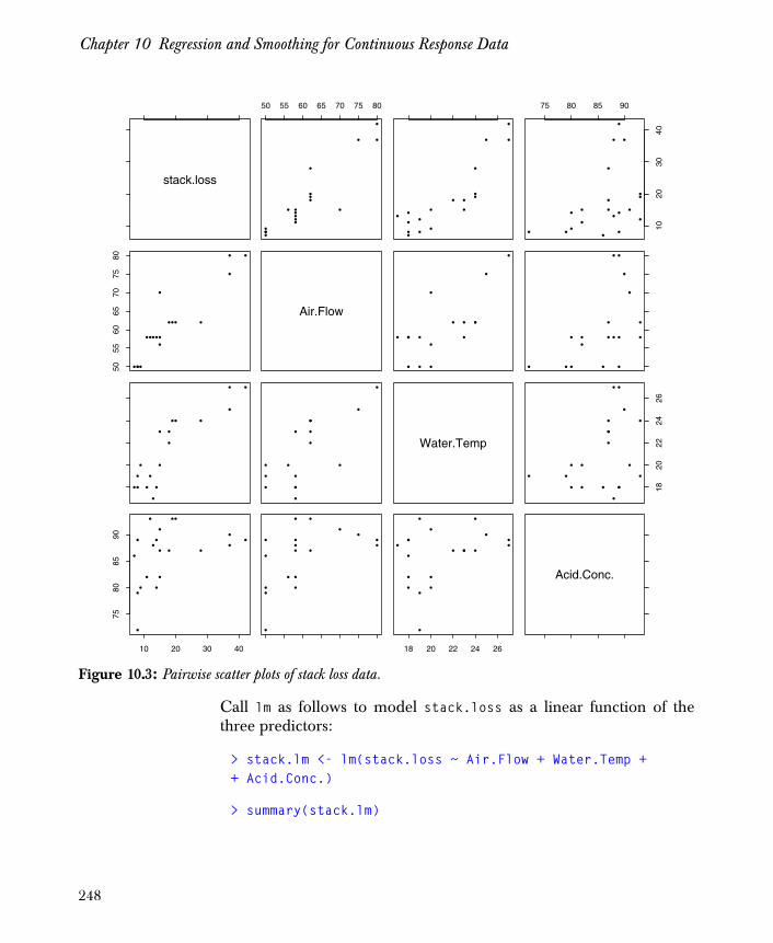
Chapter 10 Regression and Smoothing for Continuous Response Data
Call lm as follows to model stack.loss as a linear function of thethree predictors:
> stack.lm <- lm(stack.loss ~ Air.Flow + Water.Temp ++ Acid.Conc.)
> summary(stack.lm)
Figure 10.3: Pairwise scatter plots of stack loss data.
stack.loss
50 55 60 65 70 75 80
•
••
•
•••
•••••
••••
• •
•
••
•
• • ••
•••• •
•• • •
•
75 80 85 90
1020
3040
•
• •
•
• ••
•• ••• •
••• • •
• •
5055
6065
7075
80 ••
•
••••
•••••
••••
•
•
Air.Flow
•
•
•• • •
••• • •
• • •
•
•
••
•
• •
•• ••• •
••• • •
•
•
••
••
••••
•
••
••
•••• •
•
••
•••
•
••••
••• • •
Water.Temp
1820
2224
26
••
••
••
••
• ••
••
••• •
• • •
10 20 30 40
7580
8590 •
••
••
••
•
•
••
•
•
•
•
•
••
•
•••
•
•
•
•
•
••
•
•
•
•
•
••
•
•
18 20 22 24 26
••
•
•• •
•
•
•
••
•
•
•
•
•
•••
•
Acid.Conc.
248
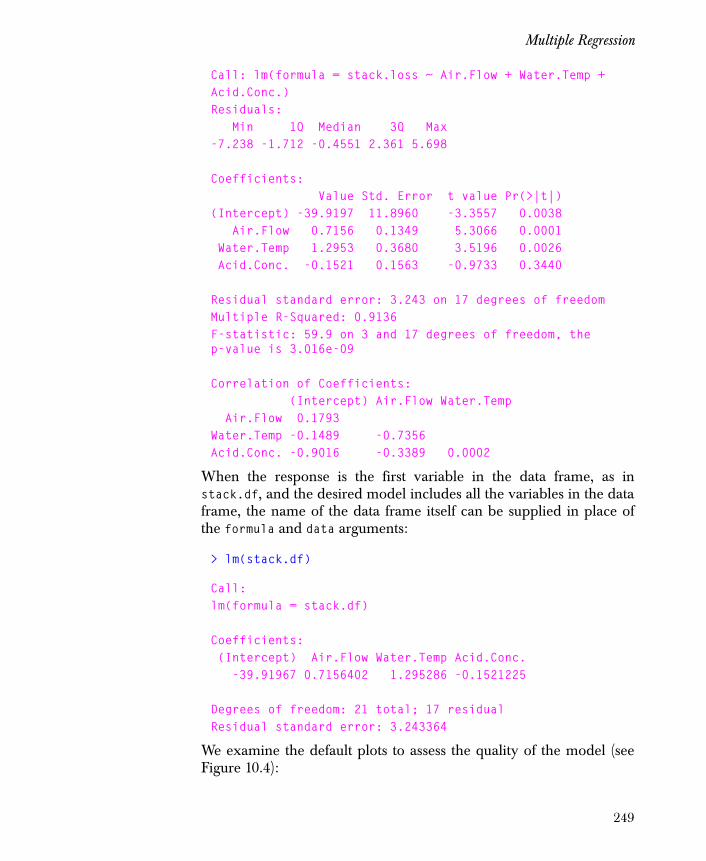
Multiple Regression
Call: lm(formula = stack.loss ~ Air.Flow + Water.Temp +Acid.Conc.)Residuals: Min 1Q Median 3Q Max-7.238 -1.712 -0.4551 2.361 5.698
Coefficients: Value Std. Error t value Pr(>|t|)(Intercept) -39.9197 11.8960 -3.3557 0.0038 Air.Flow 0.7156 0.1349 5.3066 0.0001 Water.Temp 1.2953 0.3680 3.5196 0.0026 Acid.Conc. -0.1521 0.1563 -0.9733 0.3440
Residual standard error: 3.243 on 17 degrees of freedomMultiple R-Squared: 0.9136F-statistic: 59.9 on 3 and 17 degrees of freedom, the p-value is 3.016e-09
Correlation of Coefficients: (Intercept) Air.Flow Water.Temp Air.Flow 0.1793Water.Temp -0.1489 -0.7356Acid.Conc. -0.9016 -0.3389 0.0002
When the response is the first variable in the data frame, as instack.df, and the desired model includes all the variables in the dataframe, the name of the data frame itself can be supplied in place ofthe formula and data arguments:
> lm(stack.df)
Call:lm(formula = stack.df)
Coefficients: (Intercept) Air.Flow Water.Temp Acid.Conc. -39.91967 0.7156402 1.295286 -0.1521225
Degrees of freedom: 21 total; 17 residualResidual standard error: 3.243364
We examine the default plots to assess the quality of the model (seeFigure 10.4):
249
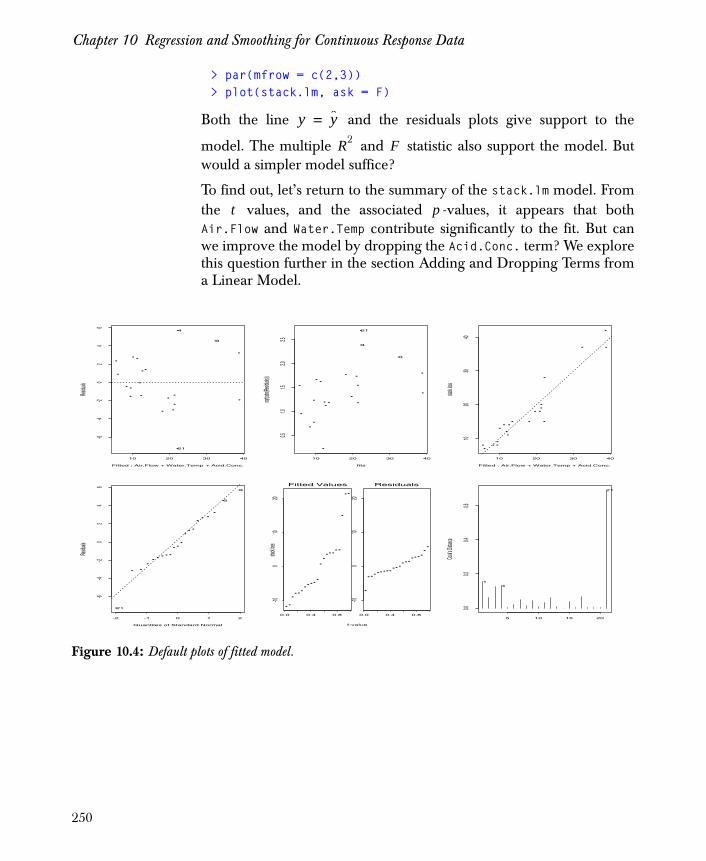
Chapter 10 Regression and Smoothing for Continuous Response Data
> par(mfrow = c(2,3))> plot(stack.lm, ask = F)
Both the line and the residuals plots give support to the
model. The multiple and statistic also support the model. Butwould a simpler model suffice?
To find out, let’s return to the summary of the stack.lm model. Fromthe values, and the associated -values, it appears that bothAir.Flow and Water.Temp contribute significantly to the fit. But canwe improve the model by dropping the Acid.Conc. term? We explorethis question further in the section Adding and Dropping Terms froma Linear Model.
y y=
R2 F
t p
Figure 10.4: Default plots of fitted model.
•
•
•
•
•
•
•
•
•
•
••
•
•
•
•
•
• •
•
•
Fitted : Air.Flow + Water.Temp + Acid.Conc.
Residua
ls
10 20 30 40
-6-4
-20
24
6
3
4
21
•
•
•
•
•
•
•
•
•
•
••
•
•
•
•
•
•
•
•
•
fits
sqrt(ab
s(Resid
uals))
10 20 30 40
0.51.0
1.52.0
2.5
3
4
21 •
••
•
• •••
•••
•
••
••
•••
• •
Fitted : Air.Flow + Water.Temp + Acid.Conc.
stack.lo
ss10 20 30 40
1020
3040
•
•
•
•
•
•
•
•
•
•
• •
•
•
•
•
•
••
•
•
Quantiles of Standard Normal
Residua
ls
-2 -1 0 1 2
-6-4
-20
24
6
3
4
21• •
•• •
••• ••
•
•
•
•• •• •
•
••
Fitted Values
0.0 0.4 0.8
-100
1020
•
• •• •• •••
•• •• ••
•• ••
••
Residuals
0.0 0.4 0.8
-100
1020
f-value
stack.lo
ss
Cook’s
Distan
ce
5 10 15 20
0.00.2
0.40.6
41
21
250

Adding and Dropping Terms from a Linear Model
ADDING AND DROPPING TERMS FROM A LINEAR MODEL
In the section Multiple Regression, we fitted a linear model with threepredictors of which only two appeared to be significant. Can weimprove the model stack.lm by dropping one or more terms?
The drop1 function takes a fitted model and returns an ANOVA tableshowing the effects of dropping in turn each term in the model:
> drop1(stack.lm)
Single term deletionsModel:stack.loss ~ Air.Flow + Water.Temp + Acid.Conc. Df Sum of Sq RSS Cp <none> 178.8300 262.9852 Air.Flow 1 296.2281 475.0580 538.1745Water.Temp 1 130.3076 309.1376 372.2541Acid.Conc. 1 9.9654 188.7953 251.9118
The columns of the returned value show the degrees of freedom foreach deleted term, the sum of squares corresponding to the deletedterm, the residual sum of squares from the resulting model, and the
statistic for the terms in the reduced model.
The statistic (actually, what is shown is the statistic, the
likelihood version of the statistic—the two are related by the
equation ) provides a convenient criterion for
determining whether a model is improved by dropping a term. If anyterm has a statistic lower than that of the current model (shown on
the line labeled <none>), the term with the lowest statistic is
dropped. If the current model has the lowest statistic, the model isnot improved by dropping any term. The regression literaturediscusses many other criteria for adding and dropping terms. See, forexample, Chapter 8 of Weisberg (1985).
Cp
Cp AIC
Cp
AIC σ2
Cp n+( )=
Cp
Cp
Cp
251
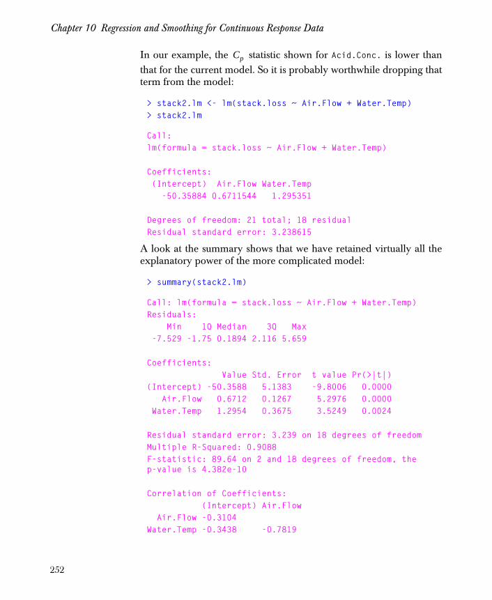
Chapter 10 Regression and Smoothing for Continuous Response Data
In our example, the statistic shown for Acid.Conc. is lower thanthat for the current model. So it is probably worthwhile dropping thatterm from the model:
> stack2.lm <- lm(stack.loss ~ Air.Flow + Water.Temp)> stack2.lm
Call:lm(formula = stack.loss ~ Air.Flow + Water.Temp)
Coefficients: (Intercept) Air.Flow Water.Temp -50.35884 0.6711544 1.295351
Degrees of freedom: 21 total; 18 residualResidual standard error: 3.238615
A look at the summary shows that we have retained virtually all theexplanatory power of the more complicated model:
> summary(stack2.lm)
Call: lm(formula = stack.loss ~ Air.Flow + Water.Temp)Residuals: Min 1Q Median 3Q Max -7.529 -1.75 0.1894 2.116 5.659
Coefficients: Value Std. Error t value Pr(>|t|)(Intercept) -50.3588 5.1383 -9.8006 0.0000 Air.Flow 0.6712 0.1267 5.2976 0.0000 Water.Temp 1.2954 0.3675 3.5249 0.0024
Residual standard error: 3.239 on 18 degrees of freedomMultiple R-Squared: 0.9088F-statistic: 89.64 on 2 and 18 degrees of freedom, the p-value is 4.382e-10
Correlation of Coefficients: (Intercept) Air.Flow Air.Flow -0.3104Water.Temp -0.3438 -0.7819
Cp
252
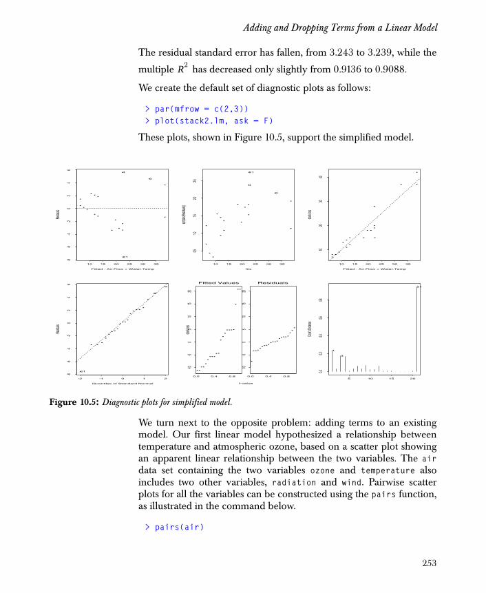
Adding and Dropping Terms from a Linear Model
The residual standard error has fallen, from 3.243 to 3.239, while the
multiple has decreased only slightly from 0.9136 to 0.9088.
We create the default set of diagnostic plots as follows:
> par(mfrow = c(2,3))> plot(stack2.lm, ask = F)
These plots, shown in Figure 10.5, support the simplified model.
We turn next to the opposite problem: adding terms to an existingmodel. Our first linear model hypothesized a relationship betweentemperature and atmospheric ozone, based on a scatter plot showingan apparent linear relationship between the two variables. The airdata set containing the two variables ozone and temperature alsoincludes two other variables, radiation and wind. Pairwise scatterplots for all the variables can be constructed using the pairs function,as illustrated in the command below.
> pairs(air)
R2
Figure 10.5: Diagnostic plots for simplified model.
•
•
•
•
•
••
•
•
••
••
•
••
•
•
•
Fitted : Air.Flow + Water.Temp
Residu
als
10 15 20 25 30 35
-8-6
-4-2
02
46
3
4
21
•
•
•
•
•
••
•
•
•
•
•
•
•
•
•
•
•
•
fits
sqrt(ab
s(Resid
uals))
10 15 20 25 30 35
0.51.0
1.52.0
2.53
4
21 •
••
•
• •••
••
•
••
••
••
• •
Fitted : Air.Flow + Water.Temp
stack.l
oss
10 15 20 25 30 35
1020
3040
•
•
•
•
•
••
•
•
• ••
••
•
•• •
•
•
•
Quantiles of Standard Normal
Residu
als
-2 -1 0 1 2
-8-6
-4-2
02
46
3
4
21 • •
••
•
•
•• •
• •
•
•
•
• •• •
•
••
Fitted Values
0.0 0.4 0.8
-10-5
05
1015
20
•
• •••• •••
•• •••• •• •
•••
Residuals
0.0 0.4 0.8
-10-5
05
1015
20
f-value
stack.l
oss
Cook’s
Distan
ce
5 10 15 20
0.00.2
0.40.6
0.8
3
1
21
253

Chapter 10 Regression and Smoothing for Continuous Response Data
The resulting plot is shown in Figure 10.6. The plot in the top row,third column of Figure 10.6 corresponds to the scatter plot shown inFigure 10.1.
From the pairwise plots, it appears that the ozone varies somewhatlinearly with each of the variables radiation, temperature, and wind,and the dependence on wind has a negative slope.
Figure 10.6: Pairwise scatter plots for ozone data.
ozone
0 50 150 250
••
••
••
•
•••
••
•
•
•
•
•
•
•
••
•
•
••
•
•
• •
•
•• •
•
•
•
•
•
••••
•
•
•
••
••
•
•
••
•
•
•
•••
•
••
•
••
•
•
•
•
•
••
•
•
•
•
•
••
•
•••••
•
••
••• •
•
••
••
•
••
•• •
••
•
•
•
•• •
• •
••
••
•
•• •
••
•
•
•
•
•
•
•
••
•
•
••
•
•
••
•
•• •
•
•
•
•
•
•••
•
•
•
••
••
•
•
••
•
•
•
•••
•
••
•
••
•
•
•
•
•
•••
•
•
•
•
• •
•
••••••
••
••••
•
••
••
•
••
•••
••
•
•
•
•••
5 10 15 20
12
34
5
• •
••
• •
•
•• •
••
•
•
•
•
•
•
•
••
•
•
••
•
•
• •
•
•••
•
•
•
•
•
••• •
•
•
•
••
••
•
•
••
•
•
•
•• •
•
••
•
••
•
•
•
•
•
••
•
•
•
•
•
• •
•
•••••
•
••
••••
•
••
••
•
••
•• •
••
•
•
•
•• •
050
150
250
•
••
• •
•
•
••
•
•
••
•
•
•
•
•
•
•
•
••
•
•
••
•
•
•
•
••
•••
•
•
• ••
•
•
•
•
•• •
••
•
•
•
• •
•
•••
•
•
•
••
••
•
•
••
•
•
•
•
•
••
••••
••
•• •
••
••••
••
•
•
•
••
•
•
•
•
•
•
••
••
•
•
radiation•
••
• •
•
•
••
•
•
••
•
•
•
•
•
•
•
•
••
•
•
••
•
•
•
•
••
•••
•
•
• ••
•
•
•
•
•••
••
•
•
•
• •
•
•••
•
•
•
•••
•
•
•
••
•
•
•
•
•
••
• •• •
•••••
••
•••
••
••
•
•
••
•
•
•
•
•
•
••
• •
•
••
••
••
•
•
••
•
•
••
•
•
•
•
•
•
•
•
••
•
•
••
•
•
•
•
••
•••
•
•
• ••
•
•
•
•
• ••
••
•
•
•
• •
•
•• •
•
•
•
••
••
•
•
••
•
•
•
•
•
••
• •• •
••
•• •
• •
•••
•••
•
•
•
• •
•
•
•
•
•
•
••
• •
•
•
•
••
••
••
••
•
•
••
•
•
••
•
• •
•
••
•
•
••
•
•
•
•
••
•••
••
••
•
•
•• •••
••
•
• ••
••
••
••• •
•• ••
••
••
•• ••
•
••
•
••
••
••• •
••
••••
•
• •
• •
•
•
•
•
•
•
•
•
•
•
•
• •
• •
••
••
••
••
•
•
••
•
•
••
•
• •
•
••
•
•
••
•
•
•
•
••
•••
• •
•••
•
•
•• • ••
••
•
••••
••
•••• •
••••
••
••
••• •
•
••
•
•••
•• •••
••
•••
•
•
••
• •
•
•
•
•
•
•
•
•
•
•
•
••
•
temperature
6070
8090
•
••
••
••
••
•
•
••
•
•
••
•
• •
•
••
•
•
••
•
•
•
•
••
• ••
• •
•••
•
•
••• ••
••
•
•••
••••
•• ••
• ••••
••
••
•• •
•
••
•
••
••••• •
••
•••
•
•
••
••
•
•
•
•
•
•
•
•
•
•
•
••
•
1 2 3 4 5
510
1520
••
••
•
•
•
•••
•• •
•
•••
•
•
••
•
••
•
•
•
•
•
•
•
••
•
••
•
•
•••
•
• ••
•
•
••
•
•• ••
•
•• ••
•
•
•
•
•
•
••••
••
• •
••
•
•
••
•
•• ••
••
•
•
••••
••
•
• •
•
•
• •
•
•
•••
•
•
•
•
•
••
••
•
•
•
• ••
•••
•
•••
•
•
••
•
••
•
•
•
•
•
•
•
••
•
••
•
•
•••
•
•••
•
•
••
•
••••
•
• •••
•
•
•
•
•
•
• •••
••
••
••
•
•
••
•
••••
••
•
•
••• •
• •
•
• •
•
•
• •
•
•
•••
•
•
•
•
•
60 70 80 90
• •
••
•
•
•
•••
•• •
•
•••
•
•
• •
•
••
•
•
•
•
•
•
•
••
•
••
•
•
•••
•
• ••
•
•
••
•
••••
•
••••
•
•
•
•
•
•
••••
••
••
••
•
•
••
•
••••
••
•
•
••••
••
•
••
•
•
••
•
•
•••
•
•
•
•
• wind
254

Adding and Dropping Terms from a Linear Model
We can use the add1 function to add the terms wind and radiation inturn to our previously fitted model:
> ozone.add1 <- add1(ozone.lm, ~ temperature + wind ++ radiation)> ozone.add1
Single term additions
Model:ozone ~ temperature Df Sum of Sq RSS Cp <none> 37.74698 39.13219 wind 1 5.839621 31.90736 33.98517radiation 1 3.839049 33.90793 35.98575
The first argument to add1 is a fitted model object, the second aformula specifying the scope; that is, the possible choices of terms tobe added to the model. A response is not necessary in the formulasupplied; the response must be the same as that in the fitted model.The returned object is an ANOVA table like that returned by drop1,showing the sum of squares due to the added term, the residual sumof squares of the new model, and the modified statistic for theterms in the augmented model. Each row of the ANOVA tablerepresents the effects of a single term added to the base model. Ingeneral, it is worth adding a term if the statistic for that term islowest among the rows in the table, including the base model term. Inour example, we conclude that it is worthwhile adding the wind term.
Our choice of temperature as the original predictor in the model,however, was completely arbitrary. We can gain a truer picture of theeffects of adding terms by starting from a simple intercept model:
> ozone0.lm <- lm(ozone ~ 1, data = air)> ozone0.add1 <- add1(ozone0.lm, ~ temperature + wind ++ radiation)
Cp
Cp
255

Chapter 10 Regression and Smoothing for Continuous Response Data
The obvious conclusion from the output is that we should start withthe temperature term, as we did originally:
> ozone0.add1
Single term additions
Model:ozone ~ 1 Df Sum of Sq RSS Cp <none> 87.20876 88.79437temperature 1 49.46178 37.74698 40.91821 wind 1 31.28305 55.92571 59.09694 radiation 1 15.53144 71.67732 74.84855
256
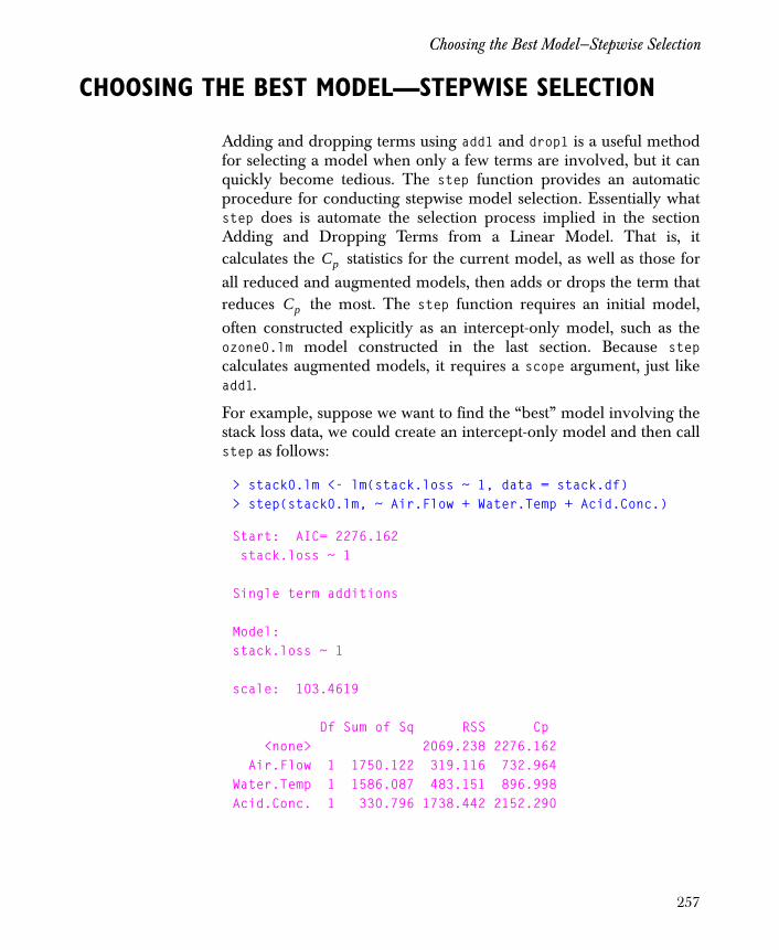
Choosing the Best Model—Stepwise Selection
CHOOSING THE BEST MODEL—STEPWISE SELECTION
Adding and dropping terms using add1 and drop1 is a useful methodfor selecting a model when only a few terms are involved, but it canquickly become tedious. The step function provides an automaticprocedure for conducting stepwise model selection. Essentially whatstep does is automate the selection process implied in the sectionAdding and Dropping Terms from a Linear Model. That is, itcalculates the statistics for the current model, as well as those forall reduced and augmented models, then adds or drops the term thatreduces the most. The step function requires an initial model,often constructed explicitly as an intercept-only model, such as theozone0.lm model constructed in the last section. Because stepcalculates augmented models, it requires a scope argument, just likeadd1.
For example, suppose we want to find the “best” model involving thestack loss data, we could create an intercept-only model and then callstep as follows:
> stack0.lm <- lm(stack.loss ~ 1, data = stack.df)> step(stack0.lm, ~ Air.Flow + Water.Temp + Acid.Conc.)
Start: AIC= 2276.162 stack.loss ~ 1
Single term additions
Model:stack.loss ~ 1
scale: 103.4619
Df Sum of Sq RSS Cp <none> 2069.238 2276.162 Air.Flow 1 1750.122 319.116 732.964Water.Temp 1 1586.087 483.151 896.998Acid.Conc. 1 330.796 1738.442 2152.290
Cp
Cp
257

Chapter 10 Regression and Smoothing for Continuous Response Data
Step: AIC= 732.9637 stack.loss ~ Air.Flow
Single term deletions
Model:stack.loss ~ Air.Flow
scale: 103.4619
Df Sum of Sq RSS Cp <none> 319.116 732.964Air.Flow 1 1750.122 2069.238 2276.162Single term additions
Model:stack.loss ~ Air.Flow
scale: 103.4619
Df Sum of Sq RSS Cp <none> 319.1161 732.9637Water.Temp 1 130.3208 188.7953 809.5668Acid.Conc. 1 9.9785 309.1376 929.9090Call:lm(formula = stack.loss ~ Air.Flow, data = stack.df)
Coefficients: (Intercept) Air.Flow -44.13202 1.020309
Degrees of freedom: 21 total; 19 residualResidual standard error (on weighted scale): 4.098242
258
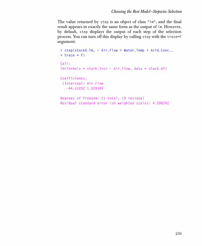
Choosing the Best Model—Stepwise Selection
The value returned by step is an object of class "lm", and the finalresult appears in exactly the same form as the output of lm. However,by default, step displays the output of each step of the selectionprocess. You can turn off this display by calling step with the trace=Fargument:
> step(stack0.lm, ~ Air.Flow + Water.Temp + Acid.Conc.,+ trace = F)
Call:lm(formula = stack.loss ~ Air.Flow, data = stack.df)
Coefficients: (Intercept) Air.Flow -44.13202 1.020309
Degrees of freedom: 21 total; 19 residualResidual standard error (on weighted scale): 4.098242
259

Chapter 10 Regression and Smoothing for Continuous Response Data
UPDATING MODELS
We built our alternate model for the stack loss data by explicitlyconstructing a second call to lm. For models involving only one ortwo predictors, this is not usually too burdensome. However, if youare looking at many different combinations of many differentpredictors, constructing the full call repeatedly can be tedious.
The update function provides a convenient way for you to fit newmodels from old models, by specifying an updated formula or otherarguments. For example, we could create the alternate modelstack2.lm using update as follows:
> stack2a.lm <- update(stack.lm, .~. - Acid.Conc.,+ data = stack.df)> stack2a.lm
Call:lm(formula = stack.loss ~ Air.Flow + Water.Temp, data =stack.df)
Coefficients: (Intercept) Air.Flow Water.Temp -50.35884 0.6711544 1.295351
Degrees of freedom: 21 total; 18 residualResidual standard error: 3.238615
The first argument to update is always a model object, and additionalarguments for lm are passed as necessary. The formula argumenttypically makes use of the “.” notation on either side of the “~”. The“.” indicates “as in previous model.” The “-” and “+” operators areused to delete or add terms. See Chapter 2, Specifying Models inSpotfire S+, for more information on formulas with update.
260
Weighted Regression
WEIGHTED REGRESSION
You can supply weights in fitting any linear model; this cansometimes improve the fit of models with repeated values in thepredictor. Weighted regression is the appropriate method in thosecases where it is known a priori that not all observations contributeequally to the fit.
Example: Weighted Linear Regression
The claims data set contains information on the average cost ofinsurance claims for automobile accidents. The 128 rows of the dataframe represent all possible combinations of three predictorvariables: age, car.age, and type. An additional variable, number,gives the number of claims that correspond to each combination. Theoutcome variable, cost, is the average cost of the claims in eachcategory. An insurance company may be interested in using data likethis to set premiums.
We want to fit a regression model predicting cost from age, car.age,and type. We begin with a simple scatter plot of the number of claimsversus the average cost:
> plot(claims$number, claims$cost)
The result is displayed in Figure 10.7. The plot shows that thevariability of cost is much greater for the observations with smallernumbers of claims. This is what we expect: if each combination of
age, car.age, and type has the same variance before averaging,
then the mean cost for a group of claims is . Thus, as the sizeof a group grows, the variability decreases.
σ2
n σ2 n⁄
261
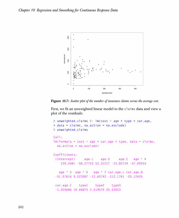
Chapter 10 Regression and Smoothing for Continuous Response Data
First, we fit an unweighted linear model to the claims data and view aplot of the residuals:
> unweighted.claims <- lm(cost ~ age + type + car.age,+ data = claims, na.action = na.exclude)> unweighted.claims
Call:lm(formula = cost ~ age + car.age + type, data = claims,
na.action = na.exclude)
Coefficients: (Intercept) age.L age.Q age.C age ^ 4 239.2681 -58.27753 53.31217 -23.83734 -37.09553
age ^ 5 age ^ 6 age ^ 7 car.age.L car.age.Q -51.57616 9.523087 -12.60742 -112.1761 -20.12425
car.age.C type1 type2 type3 -1.035686 10.46875 3.519079 25.53023
Figure 10.7: Scatter plot of the number of insurance claims versus the average cost.
••
••
•
••
•
•
•
•
•
•
•
•
••
•
•
•
•
•
•
•
•
•
•
•
••
•
•
••
•
•
•
•
•
•
•
•
•
•
••
•
•
••
•
•
•
•
•
•
•
•
•
•
•
••
•
• •
••
••
•
•
•
•
•
••
•
•
• ••
•
••
•
•
•
••
•
••
•
•
••
•
•
••
••
•
•
•
•
•
••
•
•••
•
•••
•
•
•
•
•
claims$number
cla
ims$cost
0 100 200 300 400
0200
400
600
800
262
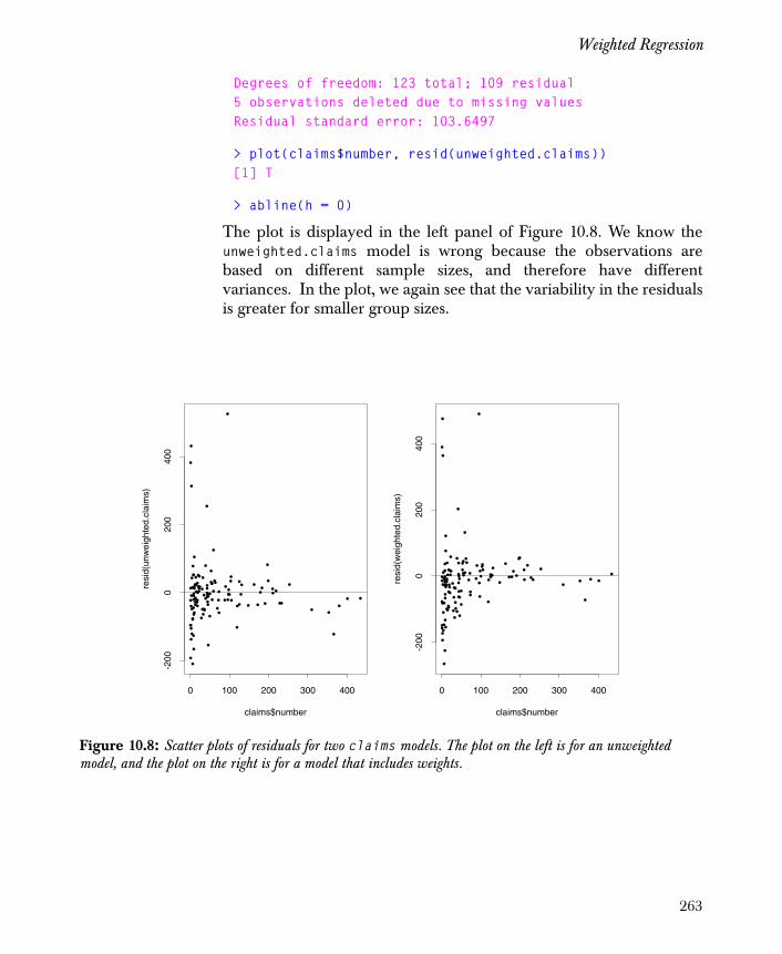
Weighted Regression
Degrees of freedom: 123 total; 109 residual5 observations deleted due to missing values Residual standard error: 103.6497
> plot(claims$number, resid(unweighted.claims))[1] T
> abline(h = 0)
The plot is displayed in the left panel of Figure 10.8. We know theunweighted.claims model is wrong because the observations arebased on different sample sizes, and therefore have differentvariances. In the plot, we again see that the variability in the residualsis greater for smaller group sizes.
Figure 10.8: Scatter plots of residuals for two claims models. The plot on the left is for an unweighted model, and the plot on the right is for a model that includes weights.
••
•
•
•
•
•
••
•
•
•
•
•
••
•
•
••••
••
•
•
•
•
•
•
•• • ••
•
••
•• •
•
•
•
•
•
••
• ••
•
•
•••
••
••
•
•
••
••
•
•••
••
•
•
•
•••
•
••••
•
••
• •
•
•
•• •
•
•
•
•
•
• •••
• •
•
•
•
••
••
••••
••
••
••
••
claims$number
resi
d(un
wei
ghte
d.cl
aim
s)
0 100 200 300 400
-200
020
040
0
••
•
•
•
••
••
•
•
•
•
•
•
•
•
•
•
•
••
•
•
•
•
•
•
•
•
•
•• •
•
•
••
•
••
•
•
•
•
•
•
•• •
•
•
•
•
•
•
••
•
•
•
••
••
•
•
•••
•
•
•
•
•
••
•
• • •
•
••
•
•
•
•
••
•
• •
•
••
•
•
•••
•
••
•
•
•
•
•
•
•••
•
• ••
••
••
•
•
claims$number
resi
d(w
eigh
ted.
clai
ms)
0 100 200 300 400
-200
020
040
0
263
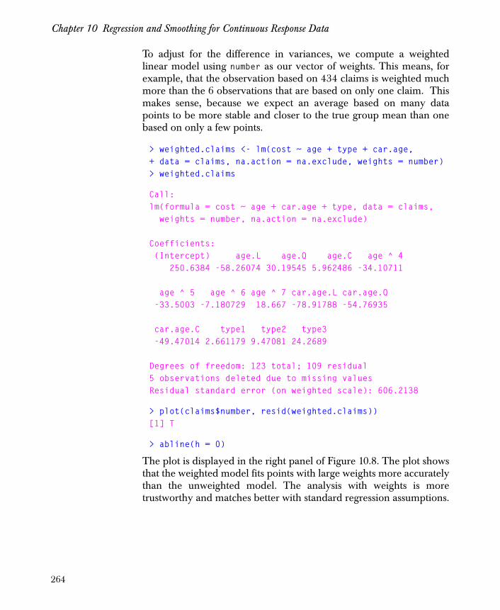
Chapter 10 Regression and Smoothing for Continuous Response Data
To adjust for the difference in variances, we compute a weightedlinear model using number as our vector of weights. This means, forexample, that the observation based on 434 claims is weighted muchmore than the 6 observations that are based on only one claim. Thismakes sense, because we expect an average based on many datapoints to be more stable and closer to the true group mean than onebased on only a few points.
> weighted.claims <- lm(cost ~ age + type + car.age,+ data = claims, na.action = na.exclude, weights = number)> weighted.claims
Call:lm(formula = cost ~ age + car.age + type, data = claims,
weights = number, na.action = na.exclude)
Coefficients: (Intercept) age.L age.Q age.C age ^ 4 250.6384 -58.26074 30.19545 5.962486 -34.10711
age ^ 5 age ^ 6 age ^ 7 car.age.L car.age.Q -33.5003 -7.180729 18.667 -78.91788 -54.76935
car.age.C type1 type2 type3 -49.47014 2.661179 9.47081 24.2689
Degrees of freedom: 123 total; 109 residual5 observations deleted due to missing values Residual standard error (on weighted scale): 606.2138
> plot(claims$number, resid(weighted.claims))[1] T
> abline(h = 0)
The plot is displayed in the right panel of Figure 10.8. The plot showsthat the weighted model fits points with large weights more accuratelythan the unweighted model. The analysis with weights is moretrustworthy and matches better with standard regression assumptions.
264
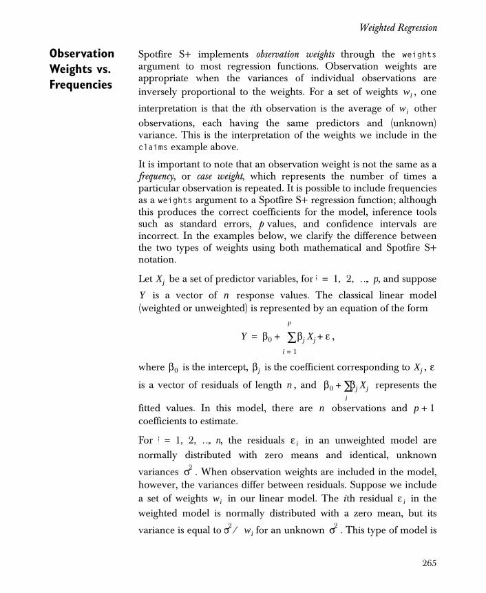
Weighted Regression
Observation Weights vs. Frequencies
Spotfire S+ implements observation weights through the weightsargument to most regression functions. Observation weights areappropriate when the variances of individual observations areinversely proportional to the weights. For a set of weights , one
interpretation is that the ith observation is the average of otherobservations, each having the same predictors and (unknown)variance. This is the interpretation of the weights we include in theclaims example above.
It is important to note that an observation weight is not the same as afrequency, or case weight, which represents the number of times aparticular observation is repeated. It is possible to include frequenciesas a weights argument to a Spotfire S+ regression function; althoughthis produces the correct coefficients for the model, inference toolssuch as standard errors, p values, and confidence intervals areincorrect. In the examples below, we clarify the difference betweenthe two types of weights using both mathematical and Spotfire S+notation.
Let be a set of predictor variables, for , and suppose
is a vector of response values. The classical linear model(weighted or unweighted) is represented by an equation of the form
,
where is the intercept, is the coefficient corresponding to ,
is a vector of residuals of length , and represents the
fitted values. In this model, there are observations and coefficients to estimate.
For , the residuals in an unweighted model arenormally distributed with zero means and identical, unknown
variances . When observation weights are included in the model,however, the variances differ between residuals. Suppose we includea set of weights in our linear model. The ith residual in theweighted model is normally distributed with a zero mean, but its
variance is equal to for an unknown . This type of model is
wi
wi
Xj j 1 2 … p, , ,=
Y n
Y β0 βj Xj ε+
j 1=
p
∑+=
β0 βj Xj ε
n β0 βj Xjj∑+
n p 1+
i 1 2 … n, , ,= ε i
σ2
wi ε i
σ2 wi⁄ σ2
265

Chapter 10 Regression and Smoothing for Continuous Response Data
appropriate if the ith observation is the average of other
observations, each having the same variance . Another situation inwhich this weighted model can be used is when the relative precisionof the observations is known in advance.
The main difference between observation weights and frequencieslies in the degrees of freedom for a particular model. In Spotfire S+,the degrees of freedom for both weighted and unweighted models isequal to the number of observations minus the number of parametersestimated. For example, a linear model with observations and onepredictor has degrees of freedom, since both a slope and anintercept are estimated. In contrast, the degrees of freedom for amodel with frequencies is equal to the sum of the frequencies minusthe number of parameters estimated. The degrees of freedom doesnot affect the coefficients in a Spotfire S+ regression, but it is used tocompute standard errors, p values, and confidence intervals. If youuse a weights argument to represent frequencies in a regressionfunction, you will need to exercise extreme caution in interpreting thestatistical results.
For example, consider the following three contrived linear models.First, we create arbitrary vectors x and y, where the first five elementsin x are identical to each other. We then compute a linear model forthe vectors. For reproducibility, we use the set.seed function.
wi
σ2
Note
Spotfire S+ does not currently support weighted regression when the absolute precision of the observations is known. This situation arises often in physics and engineering, when the uncertainty associated with a particular measurement is known in advance due to properties of
the measuring procedure or device. In this type of regression, the individual are known,
weights are supplied, and need not be estimated. Because of the treatment of
weights in Spotfire S+, however, is always estimated. If you know the absolute precision of
your observations, it is possible to supply them as to the weights argument in a Spotfire S+ regression function. This computes the correct coefficients for your model, but the standard
errors and other inference tools will be incorrect, since they are based on estimates of .
σi2
wi 1 σi2⁄= σ2
σ2
1 σi2⁄
σ2
nn 2–
266

Weighted Regression
> set.seed(0)> x <- c(rep(1, 5), 2:10)> x
[1] 1 1 1 1 1 2 3 4 5 6 7 8 9 10
> y <- runif(14)> y
[1] 0.96065916 0.93746001 0.04410193 0.76461851 0.70585769 [6] 0.50355052 0.92864822 0.84027312 0.54710167 0.48780511[11] 0.39898473 0.26351962 0.92592463 0.42851457
> unweighted.lm1 <- lm(y ~ x)> unweighted.lm1
Call:lm(formula = y ~ x)
Coefficients: (Intercept) x 0.7162991 -0.02188421
Degrees of freedom: 14 total; 12 residualResidual standard error: 0.288045
Next, we create vectors x2 and y2 that are identical to x and y, onlythe five repeated x values have identical y values. This simulates adata set with repeated observations. In our example, we choose themean of the first five y values to be the repeated y2 value, and thencompute a linear model for the vectors:
> x2 <- x> y2 <- c(rep(mean(y[1:5]), times=5), y[6:14])> y2
[1] 0.6825395 0.6825395 0.6825395 0.6825395 0.6825395 [6] 0.5035505 0.9286482 0.8402731 0.5471017 0.4878051[11] 0.3989847 0.2635196 0.9259246 0.4285146
267

Chapter 10 Regression and Smoothing for Continuous Response Data
> unweighted.lm2 <- lm(y2 ~ x2)> unweighted.lm2
Call:lm(formula = y2 ~ x2)
Coefficients: (Intercept) x2 0.7162991 -0.02188421
Degrees of freedom: 14 total; 12 residualResidual standard error: 0.1911415
Note that both of these models have fourteen observations and 12degrees of freedom. Finally, we create vectors x3 and y3 that areidentical to x2 and y2, only the five repeated values are condensedinto one. To account for this, we assign a weight of 5 to the firstobservation and compute a weighted regression for x3 and y3:
> x3 <- 1:10> y3 <- c(y2[1], y2[6:14])> y3
[1] 0.6825395 0.5035505 0.9286482 0.8402731 0.5471017 [6] 0.4878051 0.3989847 0.2635196 0.9259246 0.4285146
> w3 <- c(5, rep(1, 9))> w3
[1] 5 1 1 1 1 1 1 1 1 1
> weighted.lm <- lm(y3 ~ x3, weights = w3)> weighted.lm
Call:lm(formula = y3 ~ x3, weights = w3)
Coefficients: (Intercept) x3 0.7162991 -0.02188421
Degrees of freedom: 10 total; 8 residualResidual standard error (on weighted scale): 0.2340995
268
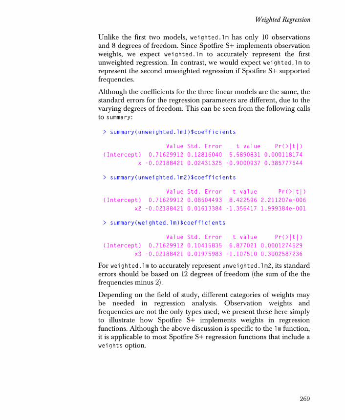
Weighted Regression
Unlike the first two models, weighted.lm has only 10 observationsand 8 degrees of freedom. Since Spotfire S+ implements observationweights, we expect weighted.lm to accurately represent the firstunweighted regression. In contrast, we would expect weighted.lm torepresent the second unweighted regression if Spotfire S+ supportedfrequencies.
Although the coefficients for the three linear models are the same, thestandard errors for the regression parameters are different, due to thevarying degrees of freedom. This can be seen from the following callsto summary:
> summary(unweighted.lm1)$coefficients
Value Std. Error t value Pr(>|t|) (Intercept) 0.71629912 0.12816040 5.5890831 0.000118174 x -0.02188421 0.02431325 -0.9000937 0.385777544
> summary(unweighted.lm2)$coefficients
Value Std. Error t value Pr(>|t|) (Intercept) 0.71629912 0.08504493 8.422596 2.211207e-006 x2 -0.02188421 0.01613384 -1.356417 1.999384e-001
> summary(weighted.lm)$coefficients
Value Std. Error t value Pr(>|t|) (Intercept) 0.71629912 0.10415835 6.877021 0.0001274529 x3 -0.02188421 0.01975983 -1.107510 0.3002587236
For weighted.lm to accurately represent unweighted.lm2, its standarderrors should be based on 12 degrees of freedom (the sum of the thefrequencies minus 2).
Depending on the field of study, different categories of weights maybe needed in regression analysis. Observation weights andfrequencies are not the only types used; we present these here simplyto illustrate how Spotfire S+ implements weights in regressionfunctions. Although the above discussion is specific to the lm function,it is applicable to most Spotfire S+ regression functions that include aweights option.
269
Chapter 10 Regression and Smoothing for Continuous Response Data
PREDICTION WITH THE MODEL
Much of the value of a linear regression model is that, if it accuratelymodels the underlying phenomenon, it can provide reliable predictionsabout the response for a given value of the predictor. The predictfunction takes a fitted model object and a data frame of new data, andreturns a vector corresponding to the predicted response. Thevariable names in the new data must correspond to those of theoriginal predictors; the response may or may not be present, but ifpresent is ignored.
For example, suppose we want to predict the atmospheric ozoneconcentration from the following vector of temperatures:
> newtemp <- c(60, 62, 64, 66, 68, 70, 72)
We can obtain the desired predictions using predict as follows:
> predict(ozone.lm, data.frame(temperature = newtemp))
1 2 3 4 5 6 1.995822 2.136549 2.277276 2.418002 2.558729 2.699456
7 2.840183
The predicted values do not stand apart from the originalobservations.
You can use the se.fit argument to predict to obtain the standarderror of the fitted value at each of the new data points. Whense.fit=T, the output of predict is a list, with a fit componentcontaining the predicted values and an se.fit component containingthe standard errors
270

Prediction with the Model
For example,
> predict(ozone.lm, data.frame(temperature = newtemp),+ se.fit = T)
$fit: 1 2 3 4 5 6 1.995822 2.136549 2.277276 2.418002 2.558729 2.699456
7 2.840183
$se.fit: 1 2 3 4 5 0.1187178 0.1084689 0.09856156 0.08910993 0.08027508
6 7 0.07228355 0.06544499
$residual.scale:[1] 0.5884748
$df:[1] 109
You can use this output list to compute pointwise and simultaneousconfidence intervals for the fitted regression line. See the sectionConfidence Intervals for details. See the predict help file for adescription of the remaining components of the return list,residual.scale and df, as well as a description of predict’s otherarguments.
271

Chapter 10 Regression and Smoothing for Continuous Response Data
CONFIDENCE INTERVALS
How reliable is the estimate produced by a simple regression?Provided the standard assumptions hold (that is, normal, identicallydistributed errors with constant variance ), we can constructconfidence intervals for each point on the fitted regression line basedon the distribution, and simultaneous confidence bands for thefitted regression line using the distribution.
In both cases, we need the standard error of the fitted value, se.fit,which is computed as follows (Weisberg, 1985, p. 21):
where = a given point in the predictor space. For a fitted object ofclass "lm", you can use the predict function as follows to calculatese.fit:
> predict(ozone.lm, se.fit = T)
For a given point in the predictor space, a ( )% confidenceinterval for the fitted value corresponding to is the set of values such that
,
where computes the qth quantile of the distribution with degrees of freedom. The pointwise function takes the output ofpredict (produced with the se.fit=T flag) and returns a listcontaining three vectors: the vector of lower bounds, the fitted values,and the vector of upper bounds giving the confidence intervals for thefitted values for the predictor. The output from pointwise is suitable,for example, as input for the error.bar function. The followingcommand computes pointwise prediction intervals for the ozone.lmmodel.
σ
tF
se.fit σ 1n--- x x–( )2
xi x–( )2
i∑------------------------+
⎝ ⎠⎜ ⎟⎜ ⎟⎜ ⎟⎛ ⎞ 1
2---
=
x
x 1 α–
x y
t α 2 n 2–,⁄( ) se.fit×– y y t α 2⁄ n 2–,( )+ se.f×< <
t q d,( ) t d
272
Confidence Intervals
> pointwise(predict(ozone.lm, se.fit = T))
$upper: 1 2 3 4 5 6 2.710169 3.011759 3.138615 2.42092 2.593475 2.250401
7 8 9 10 11 12 2.363895 2.828752 2.651621 2.769185 2.193888 2.535673
. . .
$fit: 1 2 3 4 5 6 2.488366 2.840183 2.98091 2.136549 2.347639 1.925458
7 8 9 10 11 12 2.066185 2.629093 2.418002 2.558729 1.855095 2.277276
. . .
$lower: 1 2 3 4 5 6 2.266563 2.668607 2.823205 1.852177 2.101803 1.600516
7 8 9 10 11 12 1.768476 2.429434 2.184384 2.348273 1.516301 2.018878
. . .
It is tempting to believe that the curves resulting from connecting allthe upper points and all the lower points would give a confidenceinterval for the entire curve. This, however, is not the case; theresulting curve does not have the desired confidence level across itswhole range. What is required instead is a simultaneous confidenceinterval, obtained by replacing the distribution with the distribution. A Spotfire S+ function for creating such simultaneousconfidence intervals (and by default, plotting the result) can bedefined with the code below.
t F
273
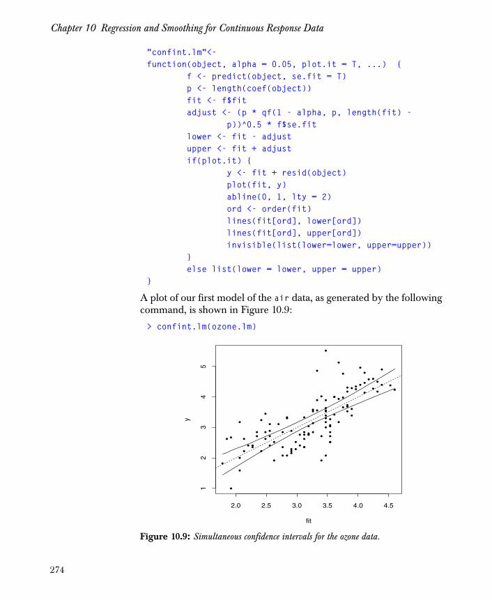
Chapter 10 Regression and Smoothing for Continuous Response Data
"confint.lm"<-function(object, alpha = 0.05, plot.it = T, ...) { f <- predict(object, se.fit = T) p <- length(coef(object)) fit <- f$fit adjust <- (p * qf(1 - alpha, p, length(fit) - p))^0.5 * f$se.fit lower <- fit - adjust upper <- fit + adjust if(plot.it) { y <- fit + resid(object) plot(fit, y) abline(0, 1, lty = 2) ord <- order(fit) lines(fit[ord], lower[ord]) lines(fit[ord], upper[ord]) invisible(list(lower=lower, upper=upper)) } else list(lower = lower, upper = upper)}
A plot of our first model of the air data, as generated by the followingcommand, is shown in Figure 10.9:
> confint.lm(ozone.lm)
Figure 10.9: Simultaneous confidence intervals for the ozone data.
••
•
••
•
•
••
••
•
•
•
•
•
•
•
•
•
•
•
•
••
•
•
••
•
•
• •
•
•
•
•
•
•
••
•
•
•
•
•
•
•
•
•
•
•
•
•
•
•
••
•
•
•
•
•
•
•
•
•
•
•
••
•
•
•
•
•
• •
•
•••
• •
•
•
•
•••
•
•
••
••
•
••
•
••
•
•
•
•
•
•••
fit
y
2.0 2.5 3.0 3.5 4.0 4.5
12
34
5
274

Polynomial Regression
POLYNOMIAL REGRESSION
Thus far in this chapter, we’ve dealt with data sets for which thegraphical evidence clearly indicated a linear relationship between thepredictors and the response. For such data, the linear model is anatural and elegant choice, providing a simple and easily analyzeddescription of the data. But what about data that does not exhibit alinear dependence? For example, consider the scatter plot shown inFigure 10.10. Clearly, there is some functional relationship between thepredictor E (for Ethanol) and the response NOx (for Nitric Oxide), butjust as clearly the relationship is not a straight line.
Figure 10.10: Scatter plot showing nonlinear dependence.
•
•
•
•
•
•
•
•
•
•
•
•••
•
•••
•
•
•
•
•
•
•
•
•
•
•
•
•
•
•
•
•
•
•
•
•
•
•
•
•
•
•
•
•
•
•
•
•
•
•
••
••
•
•
•
•
•
•
•
•
••
•
•
•
•
•
•
•
•
•
•
••
•
•
••••
••
•
E
NO
x
0.6 0.8 1.0 1.2
12
34
275
Chapter 10 Regression and Smoothing for Continuous Response Data
How should we model such data? One approach is to add polynomialterms to the basic linear model, then use least-squares techniques asbefore. The classical linear model (with the intercept termrepresented as the coefficient of a dummy variable of all 1’s) isrepresented by an equation of the following form:
where the predictors enter the equation as linear terms. Moregenerally, classical linear regression techniques apply to any equationof the form
where the are new variables formed as combinations of theoriginal predictors. For example, consider a cubic polynomialrelationship given by the following equation:
We can convert this to the desired form by the following assignments:
Once these assignments are made, the coefficients can bedetermined as usual using the classical least-squares techniques.
(10.1)
(10.2)
(10.3)
X0
Y βk Xk ε+
k 0=
n
∑=
Xk
Y βkZk ε+
k 0=
n
∑=
Zk
Y βk xk ε+
k 0=
3
∑=
x0 Z0=
x1 Z1=
x2 Z2=
x3 Z3=
βk
276

Polynomial Regression
To perform a polynomial regression in Spotfire S+, use lm togetherwith the poly function. Use poly on the right hand side of the formulaargument to lm to specify the independent variable and degree of thepolynomial. For example, consider the following made-up data:
x <- runif(100, 0, 100)y <- 50 - 43*x + 31*x^2 - 2*x^3 + rnorm(100)
We can fit this as a polynomial regression of degree 3 as follows:
> xylm <- lm(y ~ poly(x, 3))> xylm
Call:lm(formula = y ~ poly(x, 3))
Coefficients:(Intercept) poly(x, 3)1 poly(x, 3)2 poly(x, 3)3 -329798.8 -3681644 -1738826 -333975.4
Degrees of freedom: 100 total; 96 residualResidual standard error: 0.9463133
The coefficients that appear in the object xylm are the coefficients forthe orthogonal form of the polynomial. To recover the simplepolynomial form, use the function poly.transform:
> poly.transform(poly(x,3), coef(xylm))
x^0 x^1 x^2 x^3 49.9119 -43.01118 31.00052 -2.000005
These coefficients are very close to the exact values used to create y.
If the coefficients returned from a regression involving poly are sodifficult to interpret, why not simply model the polynomial explicitly?That is, why not use the formula y ~ x + x^2 + x^3 instead of theformula involving poly? In our example, there is little difference.However, in problems involving polynomials of higher degree,severe numerical problems can arise in the model matrix. Using polyavoids these numerical problems, because poly uses an orthogonalset of basis functions to fit the various “powers” of the polynomial.
277
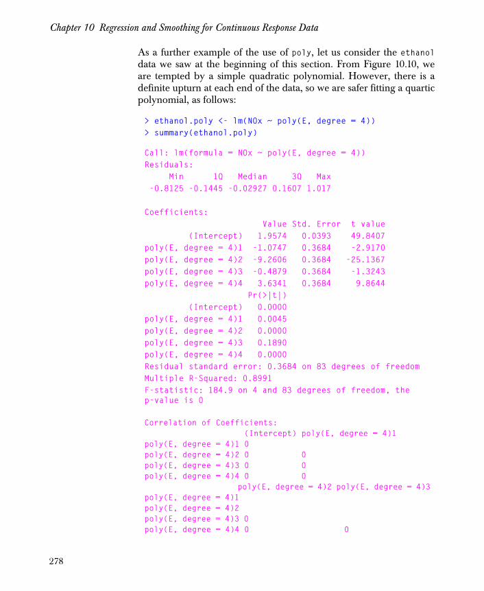
Chapter 10 Regression and Smoothing for Continuous Response Data
As a further example of the use of poly, let us consider the ethanoldata we saw at the beginning of this section. From Figure 10.10, weare tempted by a simple quadratic polynomial. However, there is adefinite upturn at each end of the data, so we are safer fitting a quarticpolynomial, as follows:
> ethanol.poly <- lm(NOx ~ poly(E, degree = 4))> summary(ethanol.poly)
Call: lm(formula = NOx ~ poly(E, degree = 4))Residuals: Min 1Q Median 3Q Max -0.8125 -0.1445 -0.02927 0.1607 1.017
Coefficients: Value Std. Error t value (Intercept) 1.9574 0.0393 49.8407poly(E, degree = 4)1 -1.0747 0.3684 -2.9170poly(E, degree = 4)2 -9.2606 0.3684 -25.1367poly(E, degree = 4)3 -0.4879 0.3684 -1.3243poly(E, degree = 4)4 3.6341 0.3684 9.8644 Pr(>|t|) (Intercept) 0.0000poly(E, degree = 4)1 0.0045poly(E, degree = 4)2 0.0000poly(E, degree = 4)3 0.1890poly(E, degree = 4)4 0.0000Residual standard error: 0.3684 on 83 degrees of freedomMultiple R-Squared: 0.8991F-statistic: 184.9 on 4 and 83 degrees of freedom, the p-value is 0
Correlation of Coefficients: (Intercept) poly(E, degree = 4)1 poly(E, degree = 4)1 0 poly(E, degree = 4)2 0 0 poly(E, degree = 4)3 0 0 poly(E, degree = 4)4 0 0 poly(E, degree = 4)2 poly(E, degree = 4)3 poly(E, degree = 4)1 poly(E, degree = 4)2 poly(E, degree = 4)3 0 poly(E, degree = 4)4 0 0
278

Polynomial Regression
> poly.transform(poly(E, 4), coef(ethanol.poly))
x^0 x^1 x^2 x^3 x^4 174.3601 -872.2071 1576.735 -1211.219 335.356
In the summary output, the P(>|t|) value for the fourth ordercoefficient is equal to zero. Thus, the probability that the model doesnot include a fourth order term is zero, and the term is highlysignificant. Although the ethanol data looks fairly quadratic in Figure10.10, a simple quadratic model would result in more error than in thequartic model ethanol.poly.
279
Chapter 10 Regression and Smoothing for Continuous Response Data
GENERALIZED LEAST SQUARES REGRESSION
Generalized least squares models are regression (or ANOVA) modelsin which the errors have a nonstandard covariance structure. Likesimple least squares regression, the method of generalized least squares(GLS) uses maximum likelihood or restricted maximum likelihood tofit a continuous, univariate response as a linear function of a singlepredictor variable. In GLS, however, the errors are allowed to becorrelated and/or to have unequal variances.
To fit a linear model in Spotfire S+ with generalized least squaresregression, use the function gls. Several arguments are available ingls, but a typical call is in one of three forms:
gls(model, data, correlation) # correlated errorsgls(model, data, weights) # heteroscedastic errorsgls(model, data, correlation, weights) # both
The model argument is a two-sided linear formula specifying themodel for the expected value of the response variable; this is identicalto the model argument required by lm. In many cases, both theresponse and the predictor are components of a single data frame,which can be specified as the optional data argument to gls.
The arguments that exemplify the flexibility of gls are correlationand weights. The optional argument correlation specifies thewithin-group correlation structure for a grouped data set. In groupeddata, the values of the response variable are grouped according to oneor more factors; these data are discussed in detail in Chapter 14,Linear and Nonlinear Mixed-Effects Models. The correlationstructures available in gls are organized into corStruct classes, asshown in Table 10.1. The optional argument weights to gls specifiesthe form of the errors variance-covariance function, which is used tomodel heteroscedasticity in the within-group errors. The availablevariance functions are organized into varFunc classes, as shown inTable 10.2.
280
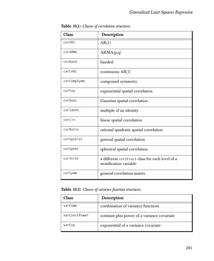
Generalized Least Squares Regression
Table 10.1: Classes of correlation structures.
Class Description
corAR1 AR(1)
corARMA ARMA(p,q)
corBand banded
corCAR1 continuous AR(1)
corCompSymm compound symmetry
corExp exponential spatial correlation
corGaus Gaussian spatial correlation
corIdent multiple of an identity
corLin linear spatial correlation
corRatio rational quadratic spatial correlation
corSpatial general spatial correlation
corSpher spherical spatial correlation
corStrat a different corStruct class for each level of a stratification variable
corSymm general correlation matrix
Table 10.2: Classes of variance function structures.
Class Description
varComb combination of variance functions
varConstPower constant plus power of a variance covariate
varExp exponential of a variance covariate
281
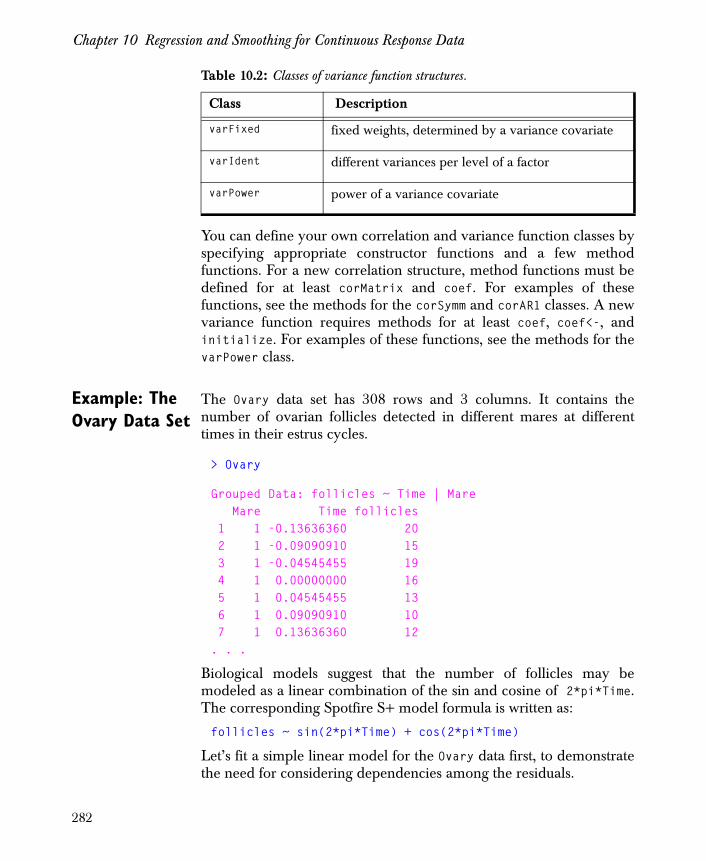
Chapter 10 Regression and Smoothing for Continuous Response Data
You can define your own correlation and variance function classes byspecifying appropriate constructor functions and a few methodfunctions. For a new correlation structure, method functions must bedefined for at least corMatrix and coef. For examples of thesefunctions, see the methods for the corSymm and corAR1 classes. A newvariance function requires methods for at least coef, coef<-, andinitialize. For examples of these functions, see the methods for thevarPower class.
Example: The Ovary Data Set
The Ovary data set has 308 rows and 3 columns. It contains thenumber of ovarian follicles detected in different mares at differenttimes in their estrus cycles.
> Ovary
Grouped Data: follicles ~ Time | Mare Mare Time follicles 1 1 -0.13636360 20 2 1 -0.09090910 15 3 1 -0.04545455 19 4 1 0.00000000 16 5 1 0.04545455 13 6 1 0.09090910 10 7 1 0.13636360 12. . .
Biological models suggest that the number of follicles may bemodeled as a linear combination of the sin and cosine of 2*pi*Time.The corresponding Spotfire S+ model formula is written as:
follicles ~ sin(2*pi*Time) + cos(2*pi*Time)
Let’s fit a simple linear model for the Ovary data first, to demonstratethe need for considering dependencies among the residuals.
varFixed fixed weights, determined by a variance covariate
varIdent different variances per level of a factor
varPower power of a variance covariate
Table 10.2: Classes of variance function structures.
Class Description
282

Generalized Least Squares Regression
> Ovary.lm <- lm(follicles ~ + sin(2*pi*Time) + cos(2*pi*Time), data = Ovary)
We can view a plot of the residuals with the following command:
> plot(Ovary.lm, which = 1)
The result is shown in Figure 10.11, and suggests that we try a moregeneral variance-covariance structure for the error term in our model.
We use the gls function with a power variance structure instead ofstandard linear regression. In our generalized least squares model, thevariance increases with a power of the absolute fitted values.
> Ovary.fit1 <- gls(follicles ~ + sin(2*pi*Time) + cos(2*pi*Time), data = Ovary,+ weights = varPower())
Manipulating gls Objects
The fitted objects returned by the gls function are of class "gls". Avariety of methods are available for displaying, updating, andevaluating the estimation results.
The print method displays a brief description of the estimationresults returned by gls. For the Ovary.fit1 object, the results are
> Ovary.fit1
Figure 10.11: Residuals plot from a simple linear fit to the Ovary data set.
Fitted : sin(2 * pi * Time) + cos(2 * pi * Time)
Res
idua
ls
10 12 14
-10
-50
510
15
47
11
82
283

Chapter 10 Regression and Smoothing for Continuous Response Data
Generalized least squares fit by REML Model: follicles ~ sin(2 * pi * Time) + cos(2 * pi * Time) Data: Ovary Log-restricted-likelihood: -895.8303 Coefficients: (Intercept) sin(2 * pi * Time) cos(2 * pi * Time) 12.22151 -3.292895 -0.8973728 Variance function: Structure: Power of variance covariate Formula: ~ fitted(.) Parameter estimates: power 0.4535912Degrees of freedom: 308 total; 305 residualResidual standard error: 1.451151
A more complete description of the estimation results is returned bythe summary function:
> summary(Ovary.fit1)
Generalized least squares fit by REML Model: follicles ~ sin(2 * pi * Time) + cos(2 * pi * Time) Data: Ovary AIC BIC logLik 1801.661 1820.262 -895.8303
284

Generalized Least Squares Regression
Variance function: Structure: Power of variance covariate Formula: ~ fitted(.) Parameter estimates: power 0.4535912 Coefficients: Value Std.Error t-value p-value (Intercept) 12.22151 0.2693741 45.37003 <.0001sin(2 * pi * Time) -3.29290 0.3792688 -8.68222 <.0001cos(2 * pi * Time) -0.89737 0.3591879 -2.49834 0.013 Correlation: (Intr) s(2*p*T)sin(2 * pi * Time) -0.165 cos(2 * pi * Time) -0.321 0.021 Standardized residuals: Min Q1 Med Q3 Max -2.303092 -0.7832415 -0.02163715 0.6412627 3.827058 Residual standard error: 1.451151Degrees of freedom: 308 total; 305 residual
Diagnostic plots for assessing the quality of a fitted gls model areobtained using the plot method. Figure 10.12 shows the plotdisplayed by the command:
> plot(Ovary.fit1)
285
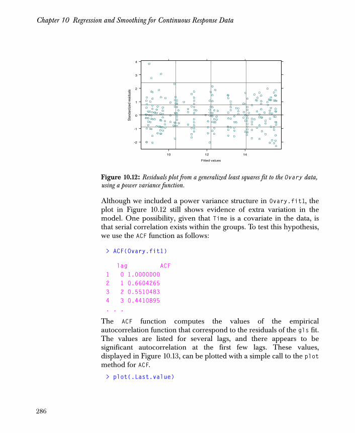
Chapter 10 Regression and Smoothing for Continuous Response Data
Although we included a power variance structure in Ovary.fit1, theplot in Figure 10.12 still shows evidence of extra variation in themodel. One possibility, given that Time is a covariate in the data, isthat serial correlation exists within the groups. To test this hypothesis,we use the ACF function as follows:
> ACF(Ovary.fit1)
lag ACF1 0 1.00000002 1 0.66042653 2 0.55104834 3 0.4410895. . .
The ACF function computes the values of the empiricalautocorrelation function that correspond to the residuals of the gls fit.The values are listed for several lags, and there appears to besignificant autocorrelation at the first few lags. These values,displayed in Figure 10.13, can be plotted with a simple call to the plotmethod for ACF.
> plot(.Last.value)
Figure 10.12: Residuals plot from a generalized least squares fit to the Ovary data, using a power variance function.
-2
-1
0
1
2
3
4
10 12 14
Fitted values
Sta
ndar
dize
d re
sidu
als
286
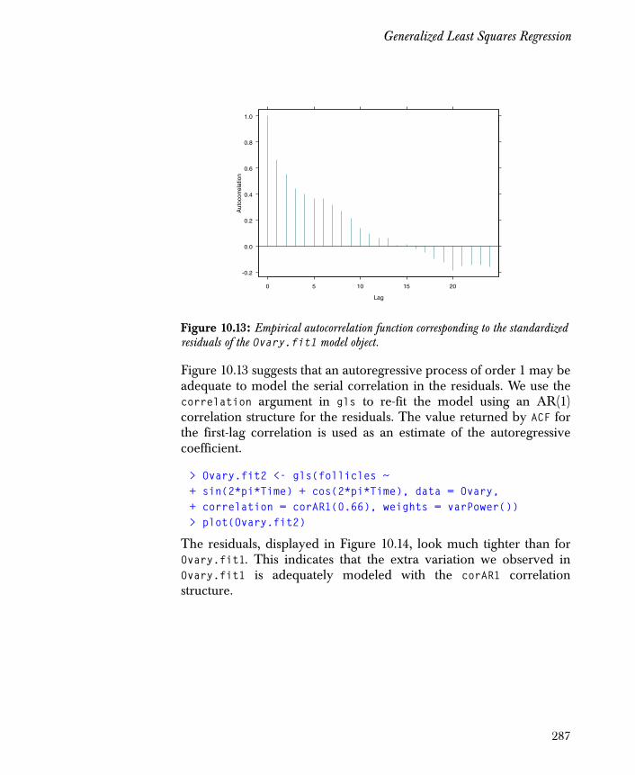
Generalized Least Squares Regression
Figure 10.13 suggests that an autoregressive process of order 1 may beadequate to model the serial correlation in the residuals. We use thecorrelation argument in gls to re-fit the model using an AR(1)correlation structure for the residuals. The value returned by ACF forthe first-lag correlation is used as an estimate of the autoregressivecoefficient.
> Ovary.fit2 <- gls(follicles ~ + sin(2*pi*Time) + cos(2*pi*Time), data = Ovary,+ correlation = corAR1(0.66), weights = varPower())> plot(Ovary.fit2)
The residuals, displayed in Figure 10.14, look much tighter than forOvary.fit1. This indicates that the extra variation we observed inOvary.fit1 is adequately modeled with the corAR1 correlationstructure.
Figure 10.13: Empirical autocorrelation function corresponding to the standardized residuals of the Ovary.fit1 model object.
-0.2
0.0
0.2
0.4
0.6
0.8
1.0
0 5 10 15 20
Lag
Aut
ocor
rela
tion
287
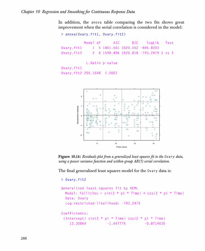
Chapter 10 Regression and Smoothing for Continuous Response Data
In addition, the anova table comparing the two fits shows greatimprovement when the serial correlation is considered in the model:
> anova(Ovary.fit1, Ovary.fit2)
Model df AIC BIC logLik TestOvary.fit1 1 5 1801.661 1820.262 -895.8303 Ovary.fit2 2 6 1598.496 1620.818 -793.2479 1 vs 2
L.Ratio p-valueOvary.fit1 Ovary.fit2 205.1648 <.0001
The final generalized least squares model for the Ovary data is:
> Ovary.fit2
Generalized least squares fit by REML Model: follicles ~ sin(2 * pi * Time) + cos(2 * pi * Time) Data: Ovary Log-restricted-likelihood: -793.2479
Coefficients: (Intercept) sin(2 * pi * Time) cos(2 * pi * Time) 12.30864 -1.647776 -0.8714635
Figure 10.14: Residuals plot from a generalized least squares fit to the Ovary data, using a power variance function and within-group AR(1) serial correlation.
-2
-1
0
1
2
11 12 13 14
Fitted values
Sta
ndar
dize
d re
sidu
als
288

Generalized Least Squares Regression
Correlation Structure: AR(1) Parameter estimate(s): Phi 0.7479559Variance function: Structure: Power of variance covariate Formula: ~ fitted(.) Parameter estimates: power -0.7613254Degrees of freedom: 308 total; 305 residualResidual standard error: 32.15024
289
Chapter 10 Regression and Smoothing for Continuous Response Data
SMOOTHING
Polynomial regression can be useful in many situations. However, thechoice of terms is not always obvious, and small effects can be greatlymagnified or lost completely by the wrong choice. Another approachto analyzing nonlinear data, attractive because it relies on the data tospecify the form of the model, is to fit a curve to the data pointslocally. With this technique, the curve at any point depends only onthe observations at that point and some specified neighboring points.Because such a fit produces an estimate of the response that is lessvariable than the original observed response, the result is called asmooth, and procedures for producing such fits are called scatterplotsmoothers. Spotfire S+ offers a variety of scatterplot smoothers:
• loess.smooth, a locally weighted regression smoother.
• smooth.spline, a cubic smoothing spline, with local behavior similar to that of kernel-type smoothers.
• ksmooth, a kernel-type scatterplot smoother.
• supsmu, a very fast variable span bivariate smoother.
Halfway between the global parametrization of a polynomial fit andthe local, nonparametric fit provided by smoothers are the parametricfits provided by regression splines. Regression splines fit a continuouscurve to the data by piecing together polynomials fit to differentportions of the data. Thus, like smoothers, they are local fits. Likepolynomials, they provide a parametric fit. In Spotfire S+, regressionsplines can be used to specify the form of a predictor in a linear ormore general model, but are not intended for top-level use.
Locally Weighted Regression Smoothing
In locally weighted regression smoothing, we build the smoothfunction pointwise as follows:
1. Take a point, say . Find the nearest neighbors of ,
which constitute a neighborhood . The number of
neighbors is specified as a percentage of the total number of points. This percentage is called the span.
s x( )
x0 k x0
N x0( )
k
290

Smoothing
2. Calculate the largest distance between and another point in the neighborhood:
3. Assign weights to each point in using the tri-cube weight function:
where
4. Calculate the weighted least squares fit of on the
neighborhood . Take the fitted value .
5. Repeat for each predictor value.
Use the loess.smooth function to calculate a locally weightedregression smooth. For example, suppose we want to smooth theethanol data. The following expressions produce the plot shown inFigure 10.15:
> plot(E, NOx)> lines(loess.smooth(E, NOx))
The figures shows the default smoothing, which uses a span of 2/3.For most uses, you will want to specify a smaller span, typically in therange of 0.3 to 0.5.
x0
Δ x0( ) maxN x0( ) x0 x1–=
N x0( )
Wx0 x1–
Δ x0( )-------------------⎝ ⎠
⎛ ⎞
W u( ) 1 u3–( )
3
0⎩⎨⎧
= for 0 u 1<≤otherwise
yN x0( ) y0 s x0( )=
291

Chapter 10 Regression and Smoothing for Continuous Response Data
Using the Super Smoother
With loess, the span is constant over the entire range of predictorvalues. However, a constant value will not be optimal if either theerror variance or the curvature of the underlying function variesover the range of . An increase in the error variance requires anincrease in the span whereas an increase in the curvature of requiresa decrease. Local cross-validation avoids this problem by choosing aspan for the predictor values based on only the leave-one-out
residuals whose predictor values are in the neighborhood of .The super smoother, supsmu, uses local cross-validation to choose thespan. Thus, for one-predictor data, it can be a useful adjunct to loess.
For example, Figure 10.16 shows the result of super smoothing theresponse NOx as a function of E in the ethanol data (dotted line)superimposed on a loess smooth. To create the plot, use thefollowing commands:
> scatter.smooth(E, NOx, span = 1/4)> lines(supsmu(E, NOx), lty = 2)
Figure 10.15: Loess-smoothed ethanol data.
•
•
•
•
•
•
•
•
•
•
•
•••
•
•••
•
•
•
•
•
•
•
•
•
•
•
•
•
•
•
•
•
•
•
•
•
•
•
•
•
•
•
•
•
•
•
•
•
•
•
••
••
•
•
•
•
•
•
•
•
••
•
•
•
•
•
•
•
•
•
•
••
•
•
••••
••
•
E
NO
x
0.6 0.8 1.0 1.2
12
34
fx
f
xj
xi xj
292

Smoothing
Local Cross-Validation
Let denote the linear smoother value at when span is
used. We wish to choose so as to minimize the meansquared error
where we are considering the joint random variable model for .Since
we would like to choose to minimize
Figure 10.16: Super smoothed ethanol data (the dotted line).
•
•
•
•
•
•
•
•
•
•
•
•••
•
•••
•
•
•
•
•
•
•
•
•
•
•
•
•
•
•
•
•
•
•
•
•
•
•
•
•
•
•
•
•
•
•
•
•
•
•
••
••
•
•
•
•
•
•
•
•
••
•
•
•
•
•
•
•
•
•
•
••
•
•
••••
••
•
E
NO
x
0.6 0.8 1.0 1.2
12
34
s x k( ) x kk k X( )=
e2 k( ) EXY Y s X k( )–[ ]2=
X Y,( )
EXY Y s X k( )–[ ]2 EXEY X Y s X k( )–[ ]2=
k k x( )=
ex2 k( ) EY X x Y s X k( )–[ ]2
= =
EY X x Y s x k( )–[ ]2 .==
293

Chapter 10 Regression and Smoothing for Continuous Response Data
However, we have only the data , , and not the
true conditional distribution needed to compute , and so we
cannot calculate . Thus we resort to cross-validation and try to
minimize the cross-validation estimate of :
.
Here is the “leave-one-out” smooth at , that is, is
constructed using all the data , , except for ,
and then the resultant local least squares line is evaluated at
thereby giving . The leave-one-out residuals
are easily obtained from the ordinary residuals
using the standard regression model relation
.
Here , , are the diagonals of the so-called “hat” matrix,
, where, for the case at hand of local straight-lineregression, is a 2-column matrix.
xi yi,( ) i 1 … n, ,=
Ey X x=
ex2 k( )
ex2 k( )
eCV2 k( ) yi s i( ) xi k( )–[ ]2
i 1=
n
∑=
si xi k( ) xi s i( ) xi k( )
xj yj,( ) j 1 … n, ,= xi yi,( )
xi
s i( ) x k( )
r i( ) k( ) yi s i( ) xi k( )–=
ri k( ) yi s xi k( )–=
r i( ) k( )ri k( )hii
-----------=
hii i 1 … n, ,=
H X XTX( )1–XT=
X
294

Smoothing
Using the Kernel Smoother
A kernel-type smoother is a type of local average smoother that, foreach target point xi in predictor space, calculates a weighted average
of the observations in a neighborhood of the target point:
where
are weights which sum to one:
.
The function used to calculate the weights is called a kernelfunction, which typically has the following properties:
• for all t
•
• for all t (symmetry)
Note that the first two properties are those of a probability densityfunction. The parameter in the equation for the weights is thebandwidth parameter, which determines how large a neighborhood ofthe target point is used to calculate the local average. A largebandwidth generates a smoother curve, while a small bandwidthgenerates a wigglier curve. Hastie and Tibshirani (1990) point out thatthe choice of bandwidth is much more important than the choice ofkernel.
To perform kernel smoothing in Spotfire S+, use the ksmoothfunction. The kernels available in ksmooth are shown in Table 10.3.
(10.4)
yi
yi wijyj
j 1=
n
∑=
wij Kxi xj–
b--------------⎝ ⎠
⎛ ⎞K
xi xj–
b--------------⎝ ⎠
⎛ ⎞
Kxi xk–
b---------------⎝ ⎠
⎛ ⎞
k 1=
n
∑-----------------------------------= =
wij 1=
j 1=
n
∑
K
K t( ) 0≥
K t( ) td∞–
∞∫ 1=
K t–( ) K t( )m=
b
295
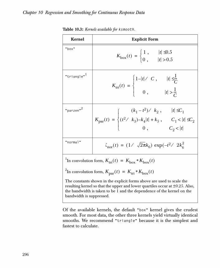
Chapter 10 Regression and Smoothing for Continuous Response Data
Of the available kernels, the default "box" kernel gives the crudestsmooth. For most data, the other three kernels yield virtually identicalsmooths. We recommend "triangle" because it is the simplest andfastest to calculate.
Table 10.3: Kernels available for ksmooth.
Kernel Explicit Form
"box"
"triangle"1
"parzen"2
"normal"
1In convolution form,
2In convolution form,
The constants shown in the explicit forms above are used to scale the resulting kernel so that the upper and lower quartiles occur at ±0.25. Also, the bandwidth is taken to be 1 and the dependence of the kernel on the bandwidth is suppressed.
Kbox t( )1 , t 0.5≤0 , t 0.5>⎩
⎨⎧
=
Ktri t( )1 t C⁄ , – t 1
C----≤
0 , t 1C---->⎩
⎪⎨⎪⎧
=
Kpar t( )
k1 t2–( ) k2⁄ , t C1≤
t2 k3⁄( ) k4 t k5 , +– C1 t C2≤<
0 , C2 t<⎩⎪⎨⎪⎧
=
Knor t( ) 1 2πk6⁄( ) exp t2 2k62⁄–(=
Ktri t( ) Kbox * Kbox t( )=
Kpar t( ) Ktri * Kbox t( )=
296

Smoothing
The intuitive sense of the kernel estimate is clear: Values of such
that is close to get relatively heavy weights, while values of
such that is far from get small or zero weight. The bandwidth
parameter determines the width of , and hence controls thesize of the region around for which receives relatively largeweights. Since bias increases and variance decreases with increasingbandwidth , selection of is a compromise between bias andvariance in order to achieve small mean squared error. In practicethis is usually done by trial and error. For example, we can compute akernel smooth for the ethanol data as follows:
> plot(E, NOx)> lines(ksmooth(E, NOx, kernel="triangle", bandwidth=0.2))> lines(ksmooth(E, NOx, kernel="triangle", bandwidth=0.1),+ lty=2)> legend(0.54, 4.1, c("bandwidth=0.2", "bandwidth=0.1"),+ lty = c(1,2))
The resulting plot is shown in Figure 10.17.
Figure 10.17: Kernel smooth of ethanol data for two bandwidths.
yi yj
xj xi yj
xj xi
b K t b⁄( )xi yj
b b
E
NO
x
0.6 0.8 1.0 1.2
12
34 bandwidth=0.2
bandwidth=0.1
297
Chapter 10 Regression and Smoothing for Continuous Response Data
Smoothing Splines
A cubic smoothing spline behaves approximately like a kernel smoother,
but it arises as the function that minimizes the penalized residual sumof squares given by
over all functions with continuous first and integrable secondderivatives. The parameter is the smoothing parameter,corresponding to the span in loess or supsmu or the bandwidth inksmooth.
To generate a cubic smoothing spline in Spotfire S+, use the functionsmooth.spline to smooth to the input data:
> plot(E, NOx)> lines(smooth.spline(E, NOx))
You can specify a different using the spar argument, although it isnot intuitively obvious what a “good” choice of might be. Whenthe data is normalized to have a minimum of 0 and a maximum of 1,and when all weights are equal to 1, = spar. More generally, therelationship is given by λ = (max(x)-min(x))^3·mean(w)·spar. Youshould either let Spotfire S+ choose the smoothing parameter, usingeither ordinary or generalized cross-validation, or supply analternative argument, df, which specifies the degrees of freedom for thesmooth. For example, to add a smooth with approximately 5 degreesof freedom to our previous plot, use the following:
> lines(smooth.spline(E, NOx, df = 5), lty = 2)
The resulting plot is shown in Figure 10.18.
f
PRSS yi f xi( )–( )2
i 1=
n
∑ λ f″ t( )( )2 td∫+=
λ
λλ
λ
298
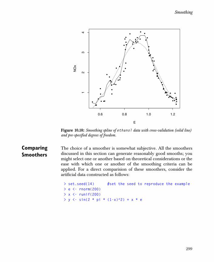
Smoothing
Comparing Smoothers
The choice of a smoother is somewhat subjective. All the smoothersdiscussed in this section can generate reasonably good smooths; youmight select one or another based on theoretical considerations or theease with which one or another of the smoothing criteria can beapplied. For a direct comparision of these smoothers, consider theartificial data constructed as follows:
> set.seed(14) #set the seed to reproduce the example> e <- rnorm(200)> x <- runif(200)> y <- sin(2 * pi * (1-x)^2) + x * e
Figure 10.18: Smoothing spline of ethanol data with cross-validation (solid line) and pre-specified degrees of freedom.
•
•
•
•
•
•
•
•
•
•
•
•••
•
•••
•
•
•
•
•
•
•
•
•
•
•
•
•
•
•
•
•
•
•
•
•
•
•
•
•
•
•
•
•
•
•
•
•
•
•
••
••
•
•
•
•
•
•
•
•
••
•
•
•
•
•
•
•
•
•
•
••
•
•
••••
••
•
E
NO
x
0.6 0.8 1.0 1.2
12
34
299
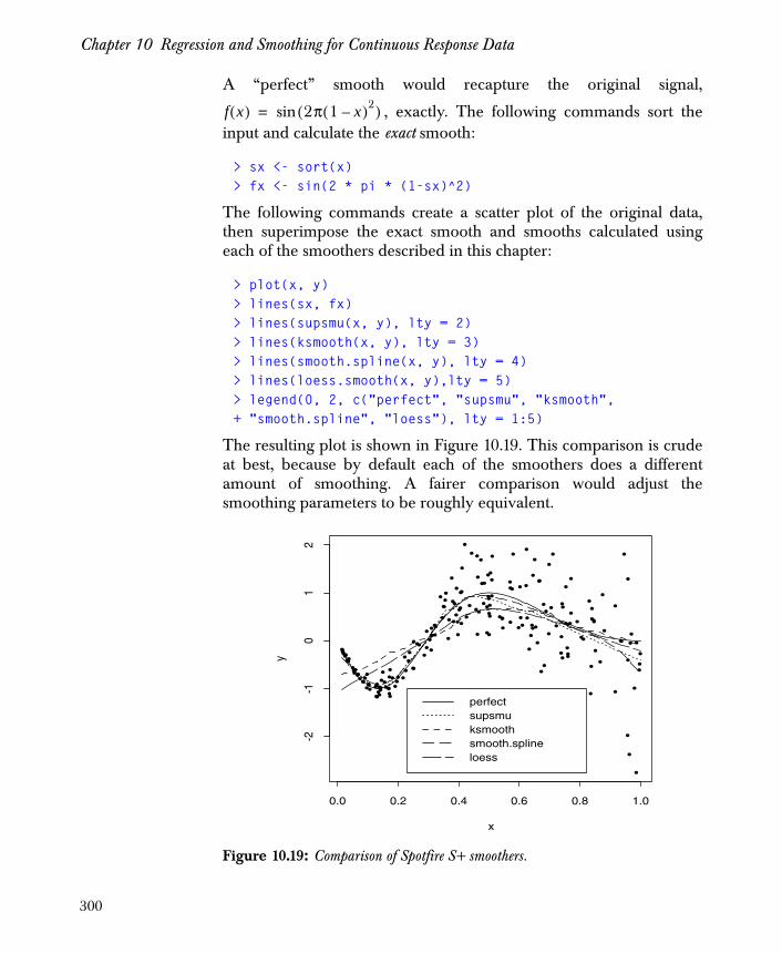
Chapter 10 Regression and Smoothing for Continuous Response Data
A “perfect” smooth would recapture the original signal,
, exactly. The following commands sort theinput and calculate the exact smooth:
> sx <- sort(x)> fx <- sin(2 * pi * (1-sx)^2)
The following commands create a scatter plot of the original data,then superimpose the exact smooth and smooths calculated usingeach of the smoothers described in this chapter:
> plot(x, y)> lines(sx, fx)> lines(supsmu(x, y), lty = 2)> lines(ksmooth(x, y), lty = 3)> lines(smooth.spline(x, y), lty = 4)> lines(loess.smooth(x, y),lty = 5)> legend(0, 2, c("perfect", "supsmu", "ksmooth",+ "smooth.spline", "loess"), lty = 1:5)
The resulting plot is shown in Figure 10.19. This comparison is crudeat best, because by default each of the smoothers does a differentamount of smoothing. A fairer comparison would adjust thesmoothing parameters to be roughly equivalent.
Figure 10.19: Comparison of Spotfire S+ smoothers.
f x( ) 2π 1 x–( )2( )sin=
••
•
••
•
•
••
•
•
•
•
•
•
•
•
•
•• •
•
•
•
•
•
•
•
•
•
•
••
•
••
•
•
•
•
••
••
•
•
•
•
•
• ••
•
•
••
•
•
•
•
•
• •
•
•
• ••
•
••
•
•
•
•
•
•
•
•
•
•
•
••
•
•
•
•
•
•
•
•
••
•
••
•
•
•• •
•
•
•
•
•
•
•
•
•
•
••
•
•
•
•
•
•
•
•
•
•
•
•
•
•
••
• •
•
•
•
•
•
•
•
•
•
•••
•
•
•
• •
•
•
•
•
•
•
•
•
•
•
•
•
•
•
•
••
••
•
•
•
•
••
•
•
•
•
•
••
•
•
•
•
••
•
•
•
•
•
•
•
•
•
•
•
••
x
y
0.0 0.2 0.4 0.6 0.8 1.0
-2-1
01
2
perfectsupsmuksmoothsmooth.splineloess
300
Additive Models
ADDITIVE MODELS
An additive model extends the notion of a linear model by allowingsome or all linear functions of the predictors to be replaced byarbitrary smooth functions of the predictors. Thus, the standard linearmodel
is replaced by the additive model
.
The standard linear regression model is a simple case of an additivemodel. Because the forms of the are generally unknown, they areestimated using some form of scatterplot smoother.
To fit an additive model in Spotfire S+, use the gam function, wheregam stands for generalized additive model. You provide a formula whichmay contain ordinary linear terms as well as terms fit using any of thefollowing:
• loess smoothers, using the lo function;
• smoothing spline smoothers, using the s function;
• natural cubic splines, using the ns function;
• B-splines, using the bs function;
• polynomials, using poly.
The three functions ns, bs, and poly result in parametric fits; additivemodels involving only such terms can be analyzed in the classicallinear model framework. The lo and s functions introducenonparametric fitting into the model. For example, the following calltakes the ethanol data and models the response NOx as a function ofthe loess-smoothed predictor E:
> attach(ethanol)> ethanol.gam <- gam(NOx ~ lo(E, degree = 2))
Y βiXi ε+
i 0=
n
∑=
Y α fi Xi( ) ε+
i 1=
n
∑+=
fi
301
Chapter 10 Regression and Smoothing for Continuous Response Data
> ethanol.gam
Call:gam(formula = NOx ~ lo(E, degree = 2))
Degrees of Freedom: 88 total; 81.1184 ResidualResidual Deviance: 9.1378
In the call to lo, we specify that the smooth is to be locally quadraticby using the argument degree=2. For data that is less obviouslynonlinear, we would probably be satisfied with the default, which islocally linear fitting. The printed gam object closely resembles aprinted lm object from linear regression—the call producing the modelis shown, followed by the degrees of freedom and the residual deviancewhich serves the same role as the residual sum of squares in the linearmodel. The deviance is a function of the log-likelihood function,which is related to the probability mass function for the
observation given . The log-likelihood for a sample of nobservations is defined as follows:
The deviance is then defined as
where maximizes the log-likelihood over unconstrained, and is the dispersion parameter. For a continuous response with normalerrors, as in the models we’ve been considering in this chapter, the
dispersion parameter is just the variance , and the deviancereduces to the residual sum of squares. As with the residual sum ofsquares, the deviance can be made arbitrarily small by choosing aninterpolating solution. As in the linear model case, however, wegenerally have a desire to keep the model as simple as possible. In thelinear case, we try to keep the number of parameters, that is, thequantities estimated by the model coefficients, to a minimum.Additive models are generally nonparametric, but we can define fornonparametric models an equivalent number of parameters, which wewould also like to keep as small as possible.
f yi μi;( )
yi μi
l m; y( ) log f yi; μi( )i 1=
n
∑=
D y; m( )
D y; m( )φ
-------------------- 2l m∗ ; y( ) 2l m; y( )–=
μ∗ μ φ
σ2
302
Additive Models
The equivalent number of parameters for gam models is defined interms of degrees of freedom, or df. In fitting a parametric model, onedegree of freedom is required to estimate each parameter. For anadditive model with parametric terms, one degree of freedom isrequired for each coefficient the term contributes to the model. Thus,for example, consider a model with an intercept, one term fit as acubic polynomial, and one term fit as a quadratic polynomial. Theintercept term contributes one coefficient and requires one degree offreedom, the cubic polynomial contributes three coefficients and thusrequires three degrees of freedom, and the quadratic polynomialcontributes two coefficients and requires two more degrees offreedom. Thus, the entire model has six parameters, and uses sixdegrees of freedom. A minimum of six observations is required to fitsuch a model.
Models involving smoothed terms use both parametric andnonparametric degrees of freedom; parametric degrees of freedomresult from fitting a linear (parametric) component for each smoothterm, while the nonparametric degrees of freedom result from fittingthe smooth after the linear part has been removed. The differencebetween the number of observations and the degrees of freedomrequired to fit the model is the residual degrees of freedom. Conversely,the difference between the number of observations and the residualdegrees of freedom is the degrees of freedom required to fit themodel, which is the equivalent number of parameters for the model.
The summary method for gam objects shows the residual degrees offreedom, the parametric and nonparametric degrees of freedom foreach term in the model, together with additional information:
> summary(ethanol.gam)
Call: gam(formula = NOx ~ lo(E, degree = 2))Deviance Residuals: Min 1Q Median 3Q Max -0.6814987 -0.1882066 -0.01673293 0.1741648 0.8479226
(Dispersion Parameter for Gaussian family taken to be 0.1126477 )
Null Deviance: 111.6238 on 87 degrees of freedom
Residual Deviance: 9.137801 on 81.1184 degrees of freedom
303
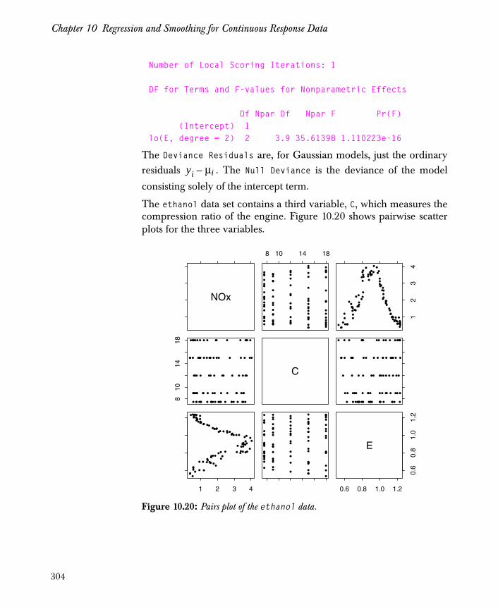
Chapter 10 Regression and Smoothing for Continuous Response Data
Number of Local Scoring Iterations: 1
DF for Terms and F-values for Nonparametric Effects
Df Npar Df Npar F Pr(F) (Intercept) 1lo(E, degree = 2) 2 3.9 35.61398 1.110223e-16
The Deviance Residuals are, for Gaussian models, just the ordinaryresiduals . The Null Deviance is the deviance of the model
consisting solely of the intercept term.
The ethanol data set contains a third variable, C, which measures thecompression ratio of the engine. Figure 10.20 shows pairwise scatterplots for the three variables.
Figure 10.20: Pairs plot of the ethanol data.
yi μi–
NOx
8 10 14 18
•
•
•
•
•
•
••
•
•
•
• • ••
•••
•
•
•
•
•
••
•
•
•
•
•
••
•
•
••
•
•
•
•
•
••
••
•
•
•
•
•
•
•
•
••
••
•
•
•
•
•
•
•
•
•••
••
•
•
•
•
•
•
•
• •
•
•
•• • •• •
•
12
34
•
•
•
•
•
•
••
•
•
•
••••
• ••
•
•
•
•
•
••
•
•
•
•
•
••
•
•
••
•
•
•
•
•
••
••
•
•
•
•
•
•
•
•
••
• •
•
•
•
•
•
•
•
•
•• •
••
•
•
•
•
•
•
•
••
•
•
••••••
•
810
1418
••• ••
•• •
•• ••
•
•
•
• •
• •
••••
• •
• •
• ••
• •• ••
• ••• •
•• ••
• •• •• ••
•
• •
••
• ••• • ••
•• •
••
•• •
• • •••
•••
•
••
••
•
•
• •
C •• •• •
• ••
• •• •
•
•
•
• •
••
• •• •
••
• •
• ••
•• •• •
••• ••
• •• •
• •• •• ••
•
••
••
• •• •• • •
• ••
• •
• ••
• • • • •
• ••
•
• •
••
•
•
• •
1 2 3 4
•
•
••
•
•
••
•
•
•
••
•• •
••
•
•
••
••
•
•
•
•
•
•
•
•
•
••
•
••
••
•
••
•
•••
••
••
•
••
•
••
••
•
•
••
•
•
••
•
•
•
•
••
•
•
•
•
••
•
•
•
•••••
•
•
•
••
•
•
••
•
•
•
• •
•• •
• •
•
•
••
•••
•
•
•
•
•
•
•
•
••
•
••
••
•
••
•
•••
••
••
•
••
•
••
••
•
•
••
•
•
••
•
•
•
•
••
•
•
•
•
••
•
•
•
• • • • •
•
0.6 0.8 1.0 1.2
0.6
0.8
1.0
1.2
E
304
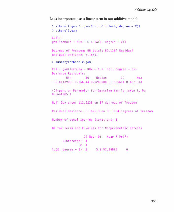
Additive Models
Let’s incorporate C as a linear term in our additive model:
> ethanol2.gam <- gam(NOx ~ C + lo(E, degree = 2))> ethanol2.gam
Call:gam(formula = NOx ~ C + lo(E, degree = 2))
Degrees of Freedom: 88 total; 80.1184 ResidualResidual Deviance: 5.16751
> summary(ethanol2.gam)
Call: gam(formula = NOx ~ C + lo(E, degree = 2))Deviance Residuals: Min 1Q Median 3Q Max -0.6113908 -0.166044 0.0268504 0.1585614 0.4871313
(Dispersion Parameter for Gaussian family taken to be 0.0644985 )
Null Deviance: 111.6238 on 87 degrees of freedom
Residual Deviance: 5.167513 on 80.1184 degrees of freedom
Number of Local Scoring Iterations: 1
DF for Terms and F-values for Nonparametric Effects
Df Npar Df Npar F Pr(F) (Intercept) 1 C 1lo(E, degree = 2) 2 3.9 57.95895 0
305
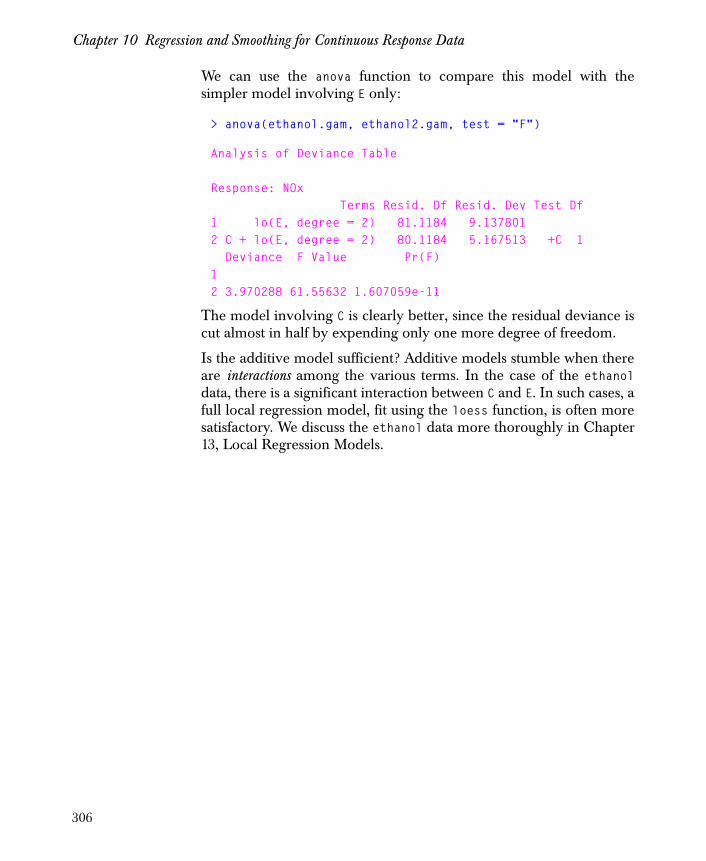
Chapter 10 Regression and Smoothing for Continuous Response Data
We can use the anova function to compare this model with thesimpler model involving E only:
> anova(ethanol.gam, ethanol2.gam, test = "F")
Analysis of Deviance Table
Response: NOx Terms Resid. Df Resid. Dev Test Df1 lo(E, degree = 2) 81.1184 9.1378012 C + lo(E, degree = 2) 80.1184 5.167513 +C 1 Deviance F Value Pr(F)12 3.970288 61.55632 1.607059e-11
The model involving C is clearly better, since the residual deviance iscut almost in half by expending only one more degree of freedom.
Is the additive model sufficient? Additive models stumble when thereare interactions among the various terms. In the case of the ethanoldata, there is a significant interaction between C and E. In such cases, afull local regression model, fit using the loess function, is often moresatisfactory. We discuss the ethanol data more thoroughly in Chapter13, Local Regression Models.
306
More on Nonparametric Regression
MORE ON NONPARAMETRIC REGRESSION
The additive models fitted by gam in the section Additive Models aresimple examples of nonparametric regression. The machinery ofgeneralized additive models, proposed by Hastie and Tibshirani(1990), is just one approach to such nonparametric models. SpotfireS+ includes several other functions for performing nonparametricregression, including the ace function, which implements the firstproposed technique for nonparametric regression—alternatingconditional expectations. Spotfire S+ also includes AVAS (Additiveand VAriance Stabilizing transformations) and projection pursuitregression. This section describes these varieties of nonparametricregression.
Alternating Conditional Expectations
Alternating conditional expectations or ace, is an intuitively appealingtechnique introduced by Breiman and Friedman (1985). The idea is tofind nonlinear transformations of the
response and predictors , respectively, such that theadditive model
is a good approximation for the data , . Let
be random variables with joint distribution , and let
expectations be taken with respect to . Consider the goodness-of-fitmeasure
(10.5)
(10.6)
θ y( ) φ1 x1( ) φ2 x2( ) … φp xp( ), , , ,
y x1 x2 … x, p, ,
θ y( ) φ1 x1( ) φ2 x2( ) … φp xp( ) ε+ + + +=
yi xi1 … x, ip, , i 1 … n, ,=
yi x1 x2 … x, p, , , F
F
e2 e2 θ , φ1, ...,φp( )
E θ y( ) φk xk( )k 1=
p
∑–
Eθ2 y( )------------------------------------------------------= =
307

Chapter 10 Regression and Smoothing for Continuous Response Data
The measure is the fraction of variance not explained by
regressing on . The data-based version of is
where and the , estimates of and the , are standardized so
that and the have mean zero: and
, . For the usual linear regression case,
where
and
with the least squares regression coefficients, we have
(10.7)
e2
θ y( ) φ x1( ) … φ xp( ), , e2
e2
θ yi( ) φk xik( )k 1=
p
∑–
i 1=
n
∑
θ2 yi( )i 1=
n
∑---------------------------------------------------------------=
θ φj θ φj
θ yi( ) φj xij( ) θ yi( )i 1=
n
∑ 0=
φk xik( )i 1=
n
∑ 0= k 1 … p, ,=
θ yi( ) yi y–=
φ1 xi1 x1–( ) xi1 x1–( )β1 ,…, φp xip xp–( ) xip xp–( )βp==
β1 , …, βp
eLS2 RSS
SSY----------
yi y–( ) xik xk–( )βk
k 1=
p
∑–
i 1=
n
∑
yi y–( )2
i 1=
n
∑--------------------------------------------------------------------------------≡=
308
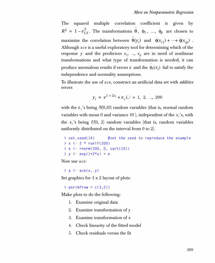
More on Nonparametric Regression
The squared multiple correlation coefficient is given by
. The transformations , , …, are chosen to
maximize the correlation between and .
Although ace is a useful exploratory tool for determining which of theresponse and the predictors are in need of nonlineartransformations and what type of transformation is needed, it can
produce anomalous results if errors and the fail to satisfy the
independence and normality assumptions.
To illustrate the use of ace, construct an artificial data set with additiveerrors
,
with the ’s being N(0,10) random variables (that is, normal random
variables with mean 0 and variance 10 ), independent of the ’s, with
the ’s being U(0, 2) random variables (that is, random variablesuniformly distributed on the interval from 0 to 2).
> set.seed(14) #set the seed to reproduce the example> x <- 2 * runif(200)> e <- rnorm(200, 0, sqrt(10))> y <- exp(1+2*x) + e
Now use ace:
> a <- ace(x, y)
Set graphics for 3 x 2 layout of plots:
> par(mfrow = c(3,2))
Make plots to do the following:
1. Examine original data
2. Examine transformation of y
3. Examine transformation of x
4. Check linearity of the fitted model
5. Check residuals versus the fit
R2 1 eLS2–= θ φ1 φp
θ yi( ) φ xi1( ) … φ xip( )+ +
y x1 … x, p,
ε φ1 xi( )
yi e1 2xi+ ε i i+= i 1 2 … 200, , ,=
ε i
xi
xi
309
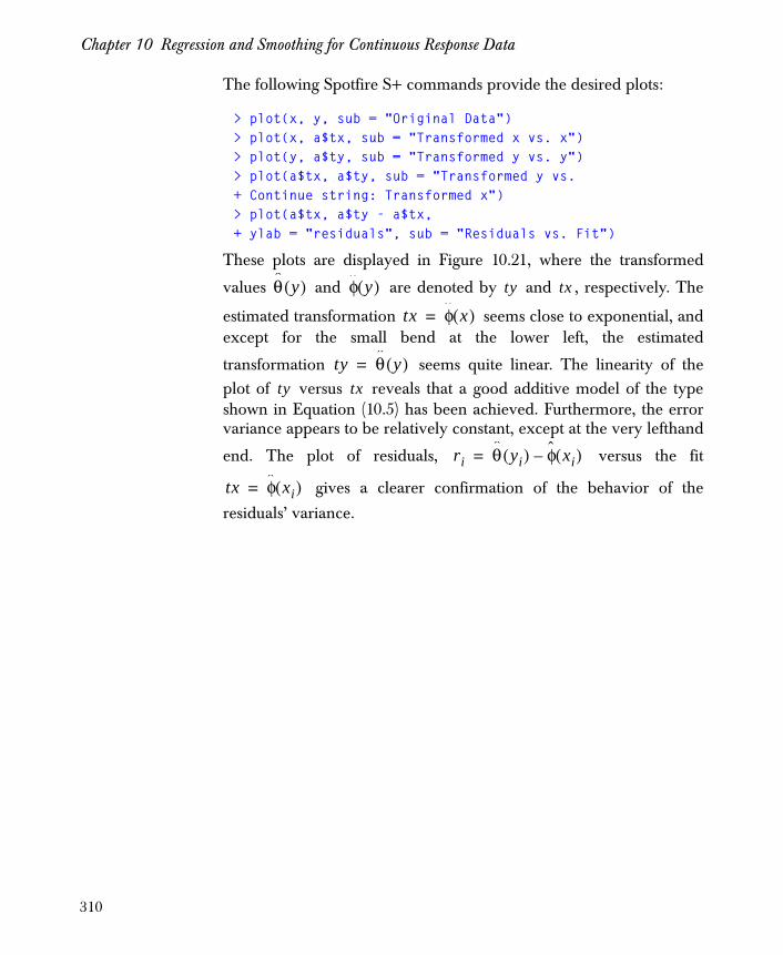
Chapter 10 Regression and Smoothing for Continuous Response Data
The following Spotfire S+ commands provide the desired plots:
> plot(x, y, sub = "Original Data")> plot(x, a$tx, sub = "Transformed x vs. x")> plot(y, a$ty, sub = "Transformed y vs. y")> plot(a$tx, a$ty, sub = "Transformed y vs.+ Continue string: Transformed x")> plot(a$tx, a$ty - a$tx,+ ylab = "residuals", sub = "Residuals vs. Fit")
These plots are displayed in Figure 10.21, where the transformed
values and are denoted by and , respectively. The
estimated transformation seems close to exponential, andexcept for the small bend at the lower left, the estimated
transformation seems quite linear. The linearity of theplot of versus reveals that a good additive model of the typeshown in Equation (10.5) has been achieved. Furthermore, the errorvariance appears to be relatively constant, except at the very lefthand
end. The plot of residuals, versus the fit
gives a clearer confirmation of the behavior of the
residuals’ variance.
θ y( ) φ y( ) ty tx
tx φ x( )=
ty θ y( )=ty tx
ri θ yi( ) φ xi( )–=
tx φ xi( )=
310

More on Nonparametric Regression
Figure 10.21: ace example with additive errors .
•
•
•••
•
•
•
•
•
•
•
••
•••
•
••
•
••
• ••
•
•
•
•
••
•
•
•
•
•
•
•
••
•
•
• •
•
•
•
•
•
•
•
• •
•
•
•
•
•
•
•
•
•
••
•
••
•
••
•
•
•
•
• •
•
••
•
••
•
•••
•
•
•
•
•
•
•
•
•••
•
•
•
•
•
•
•
••
•
•
•
•
•
•
•
•
•
•
•••
•
•
•
•
•
•
•
•
•
•
•••
•
•
••
••
•
•
••
•
•
•
••
•
••
•
•
•
••
•
•
•
•
•
••
•
•
•
•
•
•
•
••
•
••
•
• •
•
•
•
•
•
•
•
••
•
• •
••
•
••
•
•
•
•
•
Original Datax
y
0.0 0.5 1.0 1.5 2.0
020
4060
8010
012
014
0
•
•
••
••
•
•
•
••
•
• •
••
•
•
••
•
••
•• •
•
•
•
•
••
•
•
•
•
•
•
•
•
•
•
•
• •
•
•
•
•
•
•
•
••
••
•
••
•
•
•
•
••
•
••
•
•
•
•
•
••
••
•
••
•
••
•
•••
•
•
•
•
•
•
•
•
•• •
•
•
•
•
•
•
•
••
•
•
•
•
• •
•
•
•
•
•••
•
•
•
•
•
•
•
•
•
•
•••
•
•
••• •
•
•
••
•
•
•
••
•
••
•
•
•
••
•
•
•
•
•
••
•
•
•
•
•
•
•
••
•
••
•
• •
•
•
•
•
••
•
• •
•
• •
• •
•
••
•
•
•
•
•
Transformed x vs. xx
a$tx
0.0 0.5 1.0 1.5 2.0
-10
12
•
•
•••
•
•
•
•
•
•
•
••
•••
•
• •
•
••
•••
•
•
•
•
••
•
•
•
•
•
•
•
••
•
•
••
•
•
•
•
•
•
•
••
••
•
•
•
•
•
•
•
••
•
••
•
••
•
•
•
•
••
•
• •
•
••
•
•••
•
•
•
•
•
•
•
•
•• •
•
•
•
•
•
•
•
••
•
•
•
•
••
•
•
•
•
•••
•
•
•
•
•
•
•
•
•
•
•••
•
•
••• •
•
•
••
•
•
•
••
•
••
•
•
•
••
•
•
•
•
•
• •
•
•
•
•
•
•
•
••
•
••
•
• •
•
•
•
•
•
•
•
••
•
••
• •
•
• ••
•
•
•
•
Transformed y vs. yy
a$ty
0 20 40 60 80 100 120 140
-10
12
•
•
•••
•
•
•
•
•
•
•
••
•••
•
• •
•
••
• ••
•
•
•
•
••
•
•
•
•
•
•
•
••
•
•
••
•
•
•
•
•
•
•
••
••
•
•
•
•
•
•
•
••
•
••
•
••
•
•
•
•
• •
•
• •
•
••
•
•••
•
•
•
•
•
•
•
•
•• •
•
•
•
•
•
•
•
••
•
•
•
•
••
•
•
•
•
•••
•
•
•
•
•
•
•
•
•
•
•••
•
•
••••
•
•
••
•
•
•
••
•
••
•
•
•
••
•
•
•
•
•
••
•
•
•
•
•
•
•
••
•
••
•
••
•
•
•
•
•
•
•
••
•
• •
••
•
• ••
•
•
•
•
Transformed y vs. Transformed xa$tx
a$ty
-1 0 1 2
-10
12
•
•
•
•
••
••
•
•
•
•
•
•
•
•• •
•
•
•
•
•
•
•
•
•
•
•
•
••
•
•
• ••
•
•
•
•
••
••
•
••
•
•
•
•
•
•
•
•
•
•
•
•
•
•
•
•
•
•
• •
•
•
•
•
•
•
•
•
•
••
••
••
•
•
••
•
•
•
•
•
•
•
•
•
••
•
•
•
•
•
•
•
•
•
•
•
•
•
•
•
••
•
•
•
•
• •
•
•
•
•
•
•
•
••
•
•
•
•
•
••
•
•
•
•••
•••
••
•
•
•
•
•
••
•
•
•
•
•
•
•
•••
••
•
•
•
•
••
•
•
•
••
•
••
•
•
•
•
•
•
•
•
•
•
•••
•
•
•
•
•
•
Residuals vs. Fita$tx
resi
dual
s
-1 0 1 2
-0.1
0.0
0.1
0.2
311
Chapter 10 Regression and Smoothing for Continuous Response Data
Additivity and Variance Stabilization
The term AVAS stands for additivity and variance stabilizingtransformation. Like ace, the Spotfire S+ function avas tries to findtransformations , such that
provides a good additive model approximation for the data, . However, avas differs from ace in that
it chooses to achieve a special variance stabilizing feature. Inparticular the goal of avas is to estimate transformations which have the properties
and
Here is the conditional expectation of given . Theadditivity structure of Equation (10.9) is the same as for ace, andcorrespondingly the ’s are calculated by the backfitting algorithm
cycling through until convergence. The variancestabilizing aspect comes from Equation (10.9). As in the case of ace,
estimates and , are computed to
approximately satisfy Equation (10.8) through Equation (10.11), withthe conditional expectations in Equation (10.8) and Equation (10.11)estimated using the super smoother scatterplot smoother (see supsmu
(10.8)
(10.9)
(10.10)
(10.11)
θ y( ) φ1 x1( ) … φ, p xp( ),
θ y( ) φ1 x1( ) φ2 x2( ) … φp xp( ) ε+ + + +=
yi xi1 … x, ip, , i 1 2 … n, , ,=
θ y( )θ φ1 … φ, p, ,
E θ y( ) x1 … xp, ,[ ] φi xi( )i 1=
p
∑=
var θ y( ) φi xi( )i 1=
p
∑ constant=
E z w[ ] z w
φi
φk xk( ) E θ y( ) φi xi( ) xk
i k≠
∑–=
k 1 2 … p, , ,=
θ yi( ) φj xik( ) k 1 2 … p, , ,=
312
More on Nonparametric Regression
function documentation). The equality in Equation (10.9) isapproximately achieved by estimating the classic stabilizingtransformation.
To illustrate the use of avas, construct an artificial data set withadditive errors
with the ’s being N(0, 10) random variables (that is, normal random
variables with mean 0 and variance 10), independent of the ’s, with
the ’s being U(0, 2) random variables (that is, random variablesuniformly distributed on the interval from 0 to 2).
> set.seed(14) #set the seed to reproduce the example> x <- runif(200, 0, 2)> e <- rnorm(200, 0, sqrt(10))> y <- exp(1+2*x) + e
Now use avas:
> a <- avas(x, y)
Set graphics for a 3 x 2 layout of plots:
> par(mfrow = c(3,2))
Make plots to: (1) examine original data; (2) examine transformationof ; (3) examine transformation of ; (4) check linearity of the fittedmodel; (5) check residuals versus the fit:
> plot(x, y, sub = "Original data")> plot(x, a$tx, sub = "Transformed x vs. x")> plot(y, a$ty, sub = "Transformed y vs. y")> plot(a$tx, a$ty, sub = "Transformed y vs. Transformed x")> plot(a$tx, a$ty - a$tx, ylab = "Residuals",+ sub = "Residuals vs. Fit")
These plots are displayed in Figure 10.22 where the transformed
values and are denoted by and , respectively. The
estimated transformation seems close to exponential, and
the estimated transformation seems linear. The plot of
yi e1 2xi+ ε i i ,+= i 1, ..., 200=
ε i
xi
xi
x y
θ y( ) φ x( ) ty tx
tx φ x( )=
ty θ y( )= ty
313

Chapter 10 Regression and Smoothing for Continuous Response Data
versus reveals that a linear additive model holds; that is, we haveachieved a good additive approximation of the type in Equation(10.8). In this plot the error variance appears to be relatively constant.
The plot of residuals, , versus the fit gives further confirmation of this.
Figure 10.22: avas example with additive errors.
tx
ri θ yi( ) φ xi( )–= tx φ xi( )=
•
•
•••
•
•
•
•
•
•
•
••
•••
•
••
•
••
• ••
•
•
•
•
••
•
•
•
•
•
•
•
••
•
•
• •
•
•
•
•
•
•
•
• •
•
•
•
•
•
•
•
•
•
••
•
••
•
••
•
•
•
•
• •
•
••
•
••
•
•••
•
•
•
•
•
•
•
•
•••
•
•
•
•
•
•
•
••
•
•
•
•
•
•
•
•
•
•
•••
•
•
•
•
•
•
•
•
•
•
•
••
•
•
•
••
•
•
•
••
•
•
•
••
•
••
•
•
•
••
•
•
•
•
•
••
•
•
•
•
•
•
•
••
•
••
•
• •
•
•
•
•
•
•
•
••
•
• •
••
•
••
•
•
•
•
•
x
y
0.0 0.5 1.0 1.5 2.0
020
4060
8010
012
014
0
•
•
•
•
••
•
•
•
••
•
• •
••
•
•
••
•
••
•• •
•
•
•
•
••
•
•
•
•
•
•
•
•
•
•
•
••
•
•
•
•
•
•
•
••
••
•
••
•
•
•
•
••
•
••
•
••
•
•
••
••
•
••
•
••
•
•
••
•
•
•
•
•
•
•
•
•••
•
•
•
•
•
•
•
••
•
•
•
•
• •
•
•
•
•
•••
•
•
•
•
•
•
•
•
•
•
•
••
•
•
••• •
•
•
••
•
•
•
••
•
••
•
•
•
••
•
•
•
•
•
••
•
•
•
•
•
•
•
••
•
•
•
•
• •
•
•
•
•
••
•
• •
•
• •
••
•
•
••
•
•
•
•
x
a$tx
0.0 0.5 1.0 1.5 2.0
-10
12
•
•
•••
•
•
•
•
•
•
•
••
•••
•
••
•
••
•••
•
•
•
•
••
•
•
•
•
•
•
•
••
•
•
••
•
•
•
•
•
•
•
• •
•
••
•
•
•
•
•
•
••
•
••
•
••
•
•
•
•
••
•
••
•
••
•
•••
•
•
•
•
•
•
•
•
•••
•
•
•
•
•
•
•
••
•
•
•
•
•
•
•
•
•
•
•••
•
•
•
•
•
•
•
•
•
•
•••
•
•
••
••
•
•
••
•
•
•
••
•
••
•
•
•
••
•
•
•
•
•
• •
•
•
•
•
•
•
•
••
•
••
•
• •
•
•
•
•
•
•
•
••
•
••
••
•
••
•
•
•
•
•
y
a$ty
0 20 40 60 80 100 120 140
-10
12
•
•
•••
•
•
•
•
•
•
•
••
•••
•
••
•
••
• ••
•
•
•
•
••
•
•
•
•
•
•
•
••
•
•
• •
•
•
•
•
•
•
•
• •
•
••
•
•
•
•
•
•
••
•
••
•
••
•
•
•
•
• •
•
••
•
••
•
•••
•
•
•
•
•
•
•
•
•• •
•
•
•
•
•
•
•
••
•
•
•
•
•
•
•
•
•
•
•••
•
•
•
•
•
•
•
•
•
•
•••
•
•
••
••
•
•
••
•
•
•
• •
•
••
•
•
•
••
•
•
•
•
•
••
•
•
•
•
•
•
•
••
•
••
•
••
•
•
•
•
•
•
•
••
•
• •
••
•
••
•
•
•
•
•
a$tx
a$ty
-1 0 1 2
-10
12
•
••
•
•
••
•
•
•
•
•
•
•
•
•• ••
•
•
•
•
•
•
•
•
•
•
•
•• •
•
•••
•
•
•
•
•
•
•
•
••
•
•
•
•
•
•
••
••
•
•
•
•
•
•
•
•
•
• •
•
•
•
•
•
•
•
•
•
••
•
•
•
•
•
•
••
•
•
•
•
•
•
•
•
•
••
•
•
•
•
•
•
•
•
•
•
•
•
••
•
•
•
•
••
••
•
••
•
•
• •
•
••
•
•
•
•
•
•
•
•
• •
•
••
•
•
•
• •
•
••
•
•
••
•
•
•
•
•
•
•
•
•
•
••
•
•
••
• •
•
•
•
•
• •
••
•
•
•
•
•
•
•
•
•
••
•
•
•
•
•
•
•
•
a$tx
Res
idua
ls
-1 0 1 2
-0.2
-0.1
0.0
0.1
0.2
314

More on Nonparametric Regression
Key Properties • Suppose that the true additive model is
with independent of , and var(ε) = constant. Then the iterative avas algorithm for Equation (10.9) through Equation (10.11), described below for the data versions of Equation (10.9) through Equation (10.11), yields a
sequence of transformations , which
converge to the true transformation as the
number of iterations tends to infinity. Correspondingly, the data-based version of this iteration yields a sequence of
transformations , which, at convergence,
provide estimates of the true model
transformations .
• avas appears not to suffer from some of the anomalies of ace, for example, not finding good estimates of a true additive model (Equation (10.12)) when normality of and joint normality of fail to hold. See the example below.
• avas is a generalization of the Box and Cox (1964) maximum-
likelihood procedure for choosing power transformation of the response. The function avas also generalizes the Box and Tidwell (1962) procedure for choosing transformations of the carriers , and is much more convenient than the Box-Tidwell procedure. See also Weisberg (1985).
• is a monotone transformation, since it is the integral of a nonnegative function (see the section Further Details on page 316). This is important if one wants to predict by inverting
: monotone transformations are invertible, and hence we
(10.12)θ0 y( ) φi0 xi( )
i 1=
p
∑ ε+=
ε x1 x2 … xp, , ,
θ j( ) φ1j( ) … φp
j( ), , ,
θ0 φ10 … φp
0, , ,
j
θj( )
φ1j( )
… φpj( )
, , ,
θ φ1 … φp, , ,
θ0 φ10 … φp
0, , ,
εφ1 x1( ) … φp xp( ), ,
yλ
x1 x2 … xp, , ,
θ y( )
y
θ
315

Chapter 10 Regression and Smoothing for Continuous Response Data
can predict with . This predictor
has no particular optimality property, but is simply one straightforward way to get a prediction of once an avas model has been fit.
Further Details Let
where is an arbitrary transformation of , will be the“previous” estimate of in the overall iterative proceduredescribed below. Given the variance function , it is known that
will be constant if is computed according to the rule
for an appropriate constant . See Box and Cox (1964).
The detailed steps in the population version of the avas algorithm areas follows:
1. Initialize:
Set and backfit on
to get . See the description of ace for details of backfitting.
y y θ 1– φi xi( )i 1=
p
∑=
y
(10.13)
(10.14)
v u( ) VAR θ y( ) φi xi( ) u=
i 1=
p
∑=
θ y( ) y θ y( )θ y( )
v u( )
VAR g θ y( )( ) φi xi( ) u=
i 1=
p
∑
g
t( )ud
v1 2⁄ u(------------------
ct∫=
c
y( ) y Ey–( ) VAR1 2⁄ y(⁄= x1 … x, p,
φ1 … φp, ,
316

More on Nonparametric Regression
2. Get new transformation of y:
• Compute variance function:
• Compute variance stabilizing transformation:
• Set and standardize:
3. Get new ’s:
Backfit on to obtain new estimates
.
4. Iterate steps 2 and 3 until
doesn’t change.
Of course the above algorithm is actually carried out using the sampleof data , , with expectations replaced bysample averages, conditional expectations replaced by scatterplotsmoothing techniques and VAR’s replaced by sample variances.
In particular, super smoother is used in the backfitting step to obtain
, . An estimate of is
obtained as follows: First the scatter plot of
(10.15)
v u( ) VAR θ y( ) φi xi( ) u=
i 1=
p
∑=
t( )ud
v1 2⁄ u(------------------
ct∫=
θ y( ) g θ y( )( )–
θ y( ) θ y( ) Eθ y( )–
VAR1 2⁄ θ y( )-----------------------------------–
φi
θ y( ) x1 x2 … x, p, ,
φ1 … φ, p,
R2 1 e2– 1 E θ y( ) φi xi( )
i 1=
p
∑–
2
–= =
yi xi1 … x, ip, , i 1 … n, ,=
φ1 xi1( ) … φ, p xip( ), i 1=( ) … n, , v u( ) v u( )
317
Chapter 10 Regression and Smoothing for Continuous Response Data
versus is
smoothed using a running straight lines smoother. Then the result isexponentiated. This gives an estimate , and is
truncated below at 10-10 to insure positivity and avoid dividing byzero in the integral in Equation (10.14); the integration is carried outusing a trapezoidal rule.
Projection Pursuit Regression
The basic idea behind projection pursuit regression, ppreg, is asfollows. Let and denote the response and
explanatory vector, respectively. Suppose you have observations
and corresponding predictors , .
Let , denote p-dimensional unit vectors, as “direction”
vectors, and let . The ppreg function allows you to find
, direction vectors and good nonlinear
transformations such that
provides a “good” model for the data , , . The“projection” part of the term projection pursuit regression indicatesthat the carrier vector x is projected onto the direction vectors
to get the lengths of the projections, and the
“pursuit” part indicates that an optimization technique is used to find“good” direction vectors .
logri2 log θ yi( ) φj xij( )
j 1=
p
∑–
2
= ui φj xij( )j 1=
p
∑=
v u( ) 0≥ v u( )
(10.16)
y x x1 x2 … x, p, ,( )T=
yi
xi xi1 xi2 …xip, ,( )T= i 1 2 … n, , ,=
a1 a2 …, ,
y 1n--- yi
i 1=
n
∑=
M M0= a1 a2 … aM0, , ,
φ1 φ2 … φ, M0, ,
y y βmφm amT x( )
m 1=
M0
∑+≈
yi xi i 1 2 … n, , ,=
a1 a2 … aM0, , , aTx
a1 a2 … aM0, , ,
318

More on Nonparametric Regression
More formally, and are presumed to satisfy the conditionalexpectation model
where , and the have been standardized to have meanzero and unity variance:
The observations , , are assumed to
be independent and identically distributed random variables like and , that is, they satisfy the model in Equation (10.17).
The true model parameters , , , in Equation(10.17) minimize the mean squared error
over all possible , , and .
Equation (10.17) includes the additive ace models under therestriction . This occurs when and
, , , and
the ’s are absorbed into the ’s. Furthermore, the ordinary linear
model is obtained when , assuming the predictors x areindependent with mean 0 and variance 1. Then
, , and
, where the are the regression coefficients.
(10.17)
(10.18)
(10.19)
y x
E y x1, x2, ..., xp[ ] μy βmφm amT x( )
m 1=
M0
∑+=
μy E y( )= φm
Eφm amT x( ) 0,= Eφm
2 amT x( ) 0,= m 1 ... M0, ,=
yi xi xi1 … x, ip,( )T= i 1 … n, ,=
yx
βm φm am m 1 … M, 0,=
E y μy– βmφm amT x( )
m 1=
M0
∑–
2
βm φm am
θ y( ) y= M0 p=
a1 1 0 … 0, , ,( )T= a2 0 1 0 … 0, , , ,( )T= ap 0 0 … 0 1, , , ,( )T=
βm φm
M0 1=
aT b1, ..., bp( ) b12 + … + bp
2⁄= φ1 t( ) t=
β1 b12 + … + bp
2= bj
319

Chapter 10 Regression and Smoothing for Continuous Response Data
The projection pursuit model in Equation (10.17) includes thepossibility of having interactions between the explanatory variables.For example, suppose that
This is described by Equation (10.17) with , ,
, , , , and
. For then
so that
.
Neither ace nor avas is able to model interactions. It is this ability topick up interactions that led to the invention of projection pursuitregression by Friedman and Stuetzle (1981), and it is what makesppreg a useful complement to ace and avas.
The two variable interactions shown above can be used to illustratethe ppreg function. The two predictors, and are generated as
uniform random variates on the interval -1 to 1. The response, , isthe product of and plus a normal error with mean zero andvariance 0.04.
> set.seed(14) #set the seed to reproduce the example> x1 <- runif(400, -1, 1)> x2 <- runif(400, -1, 1)> eps <- rnorm(400, 0, 0.2)> y <- x1 * x2 + eps> x <- cbind(x1, x2)
(10.20)E y x1 x2,[ ] x1x2=
μy 0= M0 2=
β1 β214---= = a1
T 1 1,( )= a2T 1 1–,( )= φ1 t( ) t2=
φ2 t( ) t2–=
φ1 a1Tx( ) x1 x2+( )2 x1
2 2x1x2 x22
+ += =
φ2 a2Tx( ) x1 x2–( )2
– x– 12 2x1x2 x2
2–+= =
βmφm aTx( )m 1=
2
∑ x1x2=
x1 x2
yx1 x2
320
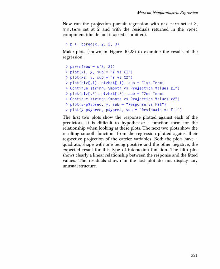
More on Nonparametric Regression
Now run the projection pursuit regression with max.term set at 3,min.term set at 2 and with the residuals returned in the ypredcomponent (the default if xpred is omitted).
> p <- ppreg(x, y, 2, 3)
Make plots (shown in Figure 10.23) to examine the results of theregression.
> par(mfrow = c(3, 2))> plot(x1, y, sub = "Y vs X1")> plot(x2, y, sub = "Y vs X2")> plot(p$z[,1], p$zhat[,1], sub = "1st Term:+ Continue string: Smooth vs Projection Values z1")> plot(p$z[,2], p$zhat[,2], sub = "2nd Term:+ Continue string: Smooth vs Projection Values z2")> plot(y-p$ypred, y, sub = "Response vs Fit")> plot(y-p$ypred, p$ypred, sub = "Residuals vs Fit")
The first two plots show the response plotted against each of thepredictors. It is difficult to hypothesize a function form for therelationship when looking at these plots. The next two plots show theresulting smooth functions from the regression plotted against theirrespective projection of the carrier variables. Both the plots have aquadratic shape with one being positive and the other negative, theexpected result for this type of interaction function. The fifth plotshows clearly a linear relationship between the response and the fittedvalues. The residuals shown in the last plot do not display anyunusual structure.
321

Chapter 10 Regression and Smoothing for Continuous Response Data
Further Details The forward stepwise procedure
An initial M-term model of the form given by the right-hand side ofEquation (10.17), with the constraints of Equation (10.18) and ,is estimated by a forward stepwise procedure, as described byFriedman and Stuetzle (1981).
Figure 10.23: Projection pursuit example.
••
•
•
•
•
•
•
•
•
• •
•
•
•
•
•
•
••
•
•
••
•
••
•
•
•
•
•
•
•
•
•
•
•
•
•
•
•
••
•
•
••
•
•
•
•
•
•
•
•
•
••
••
••
•
••
•
•
•
•
••
•
••
•
•
•
••
•
•
••
•
•
•
•
•
•
•
•
•
•
•
•
•
•
••
•
•
•
•
• ••
••
••
•
•
••
•
•
•
•
•
•
•
•
•
•
•
•
•
•
•
•
• •
•
•
•
•
•
•
••
•
•
•
•
•
•
•
•
•
•
•
•
•
•
•
•
•
•
•
•
•
• •
•
•
•
•
•
••
•
•
•
•••
•
•• •
•
•
•
•
•
••
•
•
•
•
•
•
• ••
•
•
•
•
•
•
•
•
•
•
•
•
•
•
••
•
•
•
•
•
•
•
•
•
•
•
•
•
•
•
•
•
•
•
•
•• •• •
•
•
•
•
•
•
•
••
•
•
•
•
••
•
•
•
•
•
••
••
•
••••
•
•
•
•
•
•
•
••
••
•
•
•
••
••
•
••
••
•
• •
• •
•
•
•
•
•
•
•
•
•
•••
•
••
•
••
•
•
•
•••
•
•
•
•
•
•
••
•
•
••
•
•
•
•
•
•
••
•
•
•
•
•
•
•
•
•
•
•
•
• •
•
•
•
• ••
•
•• •
••
••
•
••
•
••
•
••
•••
••
•
•
•
•
•
•
• ••
•
•
•
•
•
•
•
•
•
•
Y vs X1x1
y
-1.0 -0.5 0.0 0.5 1.0-1
.0-0
.50.0
0.5
1.0
••
•
•
•
•
•
•
•
•
• •
•
•
•
•
•
•
••
•
•
••
•
••
•
•
•
•
•
•
•
•
•
•
•
•
•
•
•
••
•
•
••
•
•
•
•
•
•
•
•
•
••
••
••
•
••
•
•
•
•
••
•
••
•
•
•
••
•
•
• •
•
•
•
•
•
•
•
•
•
•
•
•
•
•
••
•
•
•
•
• ••
••
••
•
•
• •
•
•
•
•
•
•
•
•
•
•
•
•
•
•
•
•
••
•
•
•
•
•
•
••
•
•
•
•
•
•
•
•
•
•
•
•
•
•
•
•
•
•
•
•
•
••
•
•
•
•
•
••
•
•
•
• ••
•
•••
•
•
•
•
•
••
•
•
•
•
•
•
• ••
•
•
•
•
•
•
•
•
•
•
•
•
•
•
••
•
•
•
•
•
•
•
•
•
•
•
•
•
•
•
•
•
•
•
•
• • •••
•
•
•
•
•
•
•
••
•
•
•
•
••
•
•
•
•
•
••
••
•
•• ••
•
•
•
•
•
•
•
••
••
•
•
•
••
••
•
••
••
•
• •
••
•
•
•
•
•
•
•
•
•
• ••
•
••
•
••
•
•
•
•• •
•
•
•
•
•
•
••
•
•
••
•
•
•
•
•
•
••
•
•
•
•
•
•
•
•
•
•
•
•
••
•
•
•
•••
•
•• •
••
••
•
••
•
••
•
••
•••
••
•
•
•
•
•
•
• ••
•
•
•
•
•
•
•
•
•
•
Y vs X2x2
y
-1.0 -0.5 0.0 0.5 1.0
-1.0
-0.5
0.0
0.5
1.0
••••••••
••••••••••••••••••••••
•••••••••••••••••••••••
••••••••••••••••••••••••••
••••••••••••••••••••••••••••
••••••••••••••••••••••••••••••••••••
•••••••••••••••••••••••••••••••••••••••••••••••••••••••••••••••••••••••••••••••••••••••••••••••••••••••••••••••••••••••••••••••••••••••••••••••••••••••••••••••••••••••••••••••••••••••••••••••••••••••••••••••••••••••••••
••••••••••••••••••••
•••••••••••••
••••
•
1st Term:Smooth vs Projection Values z1
p$z[, 1]
p$zh
at[, 1]
-1.0 -0.5 0.0 0.5 1.0
-4-3
-2-1
01
••••••••••••
•••••
••••••••••
•••••••••••••••••••••••••••••••••••••••••••••••••••••••••••••••••••••••••••••••••••••••••••••••••••••••••••••••••••••••••••••••••••••••••••••••••••••••••••••••••••••••••••••••••••••••••••••••••••••••••••••••••••••••••••••••••••••••••••••
•••••••••••••••••••••••••••
••••••••••••••••••••••••••
•••••••••••••••••••
•••••••••••••
•••••••••••••••••••••••••••••••••
•••••••••
••••••••
•
2nd Term:Smooth vs Projection Values z2
p$z[, 2]
p$zh
at[, 2]
-1.0 -0.5 0.0 0.5 1.0-1
01
23
••
•
•
•
•
•
•
•
•
• •
•
•
•
•
•
•
••
•
•
••
•
••
•
•
•
•
•
•
•
•
•
•
•
•
•
•
•
• •
•
•
••
•
•
•
•
•
•
•
•
•
••
••
••
•
••
•
•
•
•
••
•
••
•
•
•
••
•
•
• •
•
•
•
•
•
•
•
•
•
•
•
•
•
•
••
•
•
•
•
•••
••
••
•
•
••
•
•
•
•
•
•
•
•
•
•
•
•
•
•
•
•
••
•
•
•
•
•
•
••
•
•
•
•
•
•
•
•
•
•
•
•
•
•
•
•
•
•
•
•
•
• •
•
•
•
•
•
• •
•
•
•
•••
•
•••
•
•
•
•
•
••
•
•
•
•
•
•
• ••
•
•
•
•
•
•
•
•
•
•
•
•
•
•
••
•
•
•
•
•
•
•
•
•
•
•
•
•
•
•
•
•
•
•
•
•• •• •
•
•
•
•
•
•
•
••
•
•
•
•
••
•
•
•
•
•
••
••
•
•• • •
•
•
•
•
•
•
•
••
••
•
•
•
••
••
•
••
• •
•
••
••
•
•
•
•
•
•
•
•
•
•••
•
••
•
••
•
•
•
•• •
•
•
•
•
•
•
••
•
•
••
•
•
•
•
•
•
••
•
•
•
•
•
•
•
•
•
•
•
•
• •
•
•
•
•••
•
•••
••
••
•
••
•
••
•
••
•••
••
•
•
•
•
•
•
• ••
•
•
•
•
•
•
•
•
•
•
Response vs Fity - p$ypred
y
-1.0 -0.5 0.0 0.5
-1.0
-0.5
0.0
0.5
1.0
•
••
•
•
•
•
•
•
•
•
•
••
•
•
•
•
•
••
• •
•
•
•
•
• •
•
• •
••
••
••
•
•
•
••
•
•
•
•
•
•
••
•
•
••
•
•
•
•
•
•
•
•
•
•
•
•
•
••
••
•
•
••
•
•
•
••
•
•
•
•
•
•
•
••
•
•
••
••
•
•
• •
• •
•
•
••
•
••
••
•
•
•
••
••
•
•
•
••
•
•
•
•
•
•
•
•
••
•
•
••
•
•
•
•
•
•
•
• • • •
•
•
••
•
•
•
•
••
• ••
•
•
•
••
•
•
•
•
•
•
•
•
•
•
•
• •
•
•
•
•
•
•
•
••
•
•
•
•
••
•
•
•
•
• •
•
•
•
•
••
•
•
• ••
•
•
•
•
•
••• •
•
•
•
•
•
•
•
•
•
•
•
•
•
•
• ••
•
••
•
••
•
•
••
•
••
••
•
• •
••
••
•
•
•
•
•
••
•••
•
••
•
•
•
•
•
•
•
••
•
••
•
•
••
••
• ••
•
•
•
•
•
•
•
•
•
•
•
•
•
••
•
•
•
•
•
•
•
•
•
•
•
•
•
•
•
•
•
• •
•
••
• •••
•
•
•••
•
•
•
•
•
•
•
•
•
•
•
•
•
• •
•
•
•
••
•
•
•
•
• •
•
•
•
••
•
••
•
••
•
•
•
•
•
•
•
•
•
•
•
•
•
•
• •
•
•
••
•
•
• •
Residuals vs Fity - p$ypred
p$yp
red
-1.0 -0.5 0.0 0.5
-0.6
-0.4
-0.2
0.0
0.2
0.4
0.6
M M0>
322

More on Nonparametric Regression
First, a trial direction is used to compute the values ,
, where . Then, with , you
have available a scatter plot of data , , which may
be smoothed to obtain an estimate of the conditional
expectation for the identically distributed
random variables , . Super Smoother is used for this
purpose; see the documentation for supsmu. This depends upon
the trial direction vector , so we write . Now is
varied to minimize the weighted sum of squares,
where for each a1 in the optimization procedure, a new is
computed using super smoother. The weights are user-specified,
with the default being all weights unitary: . The final results of
this optimization will be denoted simply and , where has
been standardized according to Equation (10.18) and the
corresponding value is computed. We now have the
approximation , where .
Next we treat as the response, where now
, and fit a second term , where , to
this modified response, in exactly the same manner that we fitted
to . This gives the approximation
or .
(10.21)
a1 zi1 a1Txi=
i 1 … n, ,= xi xi1 … x, ip,( )T= yi1 yi y–=
yi zi1,( ) i 1 … n, ,=
φ1 zi1( )E y z1[ ] E yi zi1[ ]=
yi zi1 a1Txi=
φ1
a1 φ1 φ1 a1,= a1
wi yi φ1 a1, zi1( )–[ ]2
i 1=
n
∑
φ1 a1,
wi
wi 1≡
a1 φˆ1 φˆ1
β1
yi y β1φ1 a1Txi( )+≈ i 1 … n, ,=
yi2( ) yi y β1φ1 zi1( )––=
zi1 a1Txi= β2φ2 zi2( ) zi2 a2
Txi=
β1φ1 a1Txi( ) yi
1( ) yi2( ) β2φ2 zi2( )≈
yi y β1φ1 zi1( ) β2φ2 zi2( )+ +≈
323
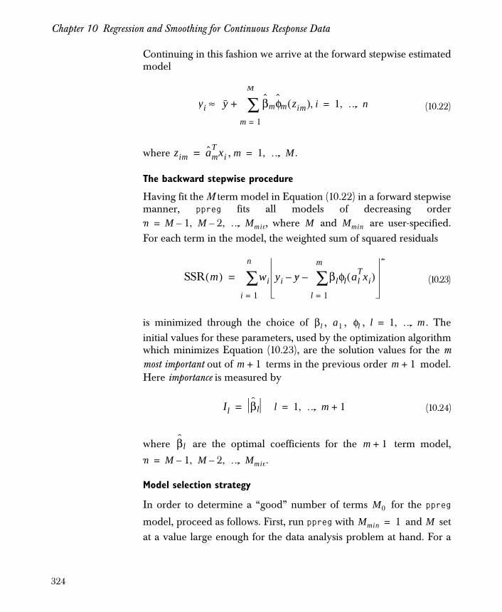
Chapter 10 Regression and Smoothing for Continuous Response Data
Continuing in this fashion we arrive at the forward stepwise estimatedmodel
where , .
The backward stepwise procedure
Having fit the M term model in Equation (10.22) in a forward stepwisemanner, ppreg fits all models of decreasing order
, where and are user-specified.For each term in the model, the weighted sum of squared residuals
is minimized through the choice of , , , . Theinitial values for these parameters, used by the optimization algorithmwhich minimizes Equation (10.23), are the solution values for the mmost important out of terms in the previous order model.Here importance is measured by
where are the optimal coefficients for the term model,
.
Model selection strategy
In order to determine a “good” number of terms for the ppreg
model, proceed as follows. First, run ppreg with and setat a value large enough for the data analysis problem at hand. For a
, (10.22)
(10.23)
(10.24)
yi y βmφm zim( )m 1=
M
∑+≈ i 1 … n, ,=
zim amT xi= m 1 … M, ,=
m M 1– M 2– … M, min, ,= M Mmin
SSR m( ) wi yi y– βlφl alTxi( )
l 1=
m
∑–
2
i 1=
n
∑=
βl a1 φl l 1 … m, ,=
m 1+ m 1+
Il βl= l 1 … m, 1+,=
βl m 1+
m M 1– M 2– … Mmin, , ,=
M0
Mmin 1= M
324
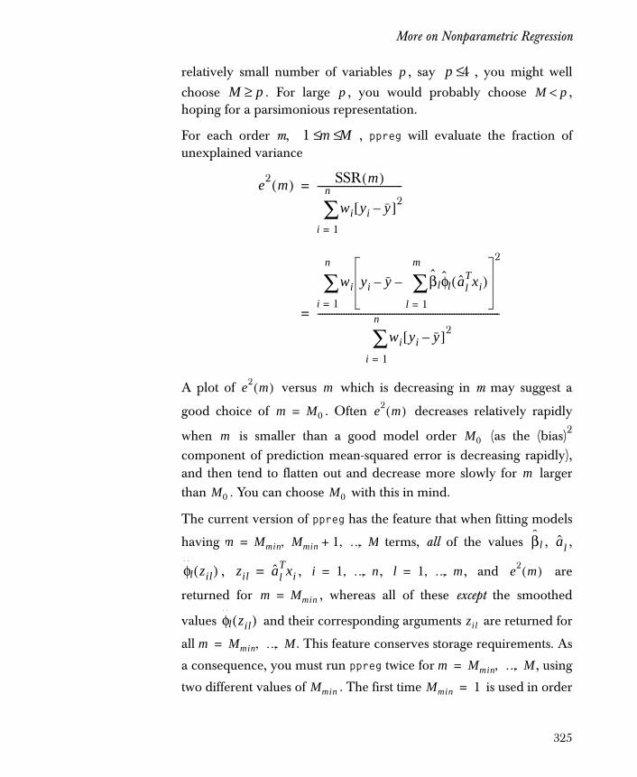
More on Nonparametric Regression
relatively small number of variables , say , you might well
choose . For large , you would probably choose ,hoping for a parsimonious representation.
For each order m, , ppreg will evaluate the fraction ofunexplained variance
A plot of versus which is decreasing in m may suggest a
good choice of . Often decreases relatively rapidly
when is smaller than a good model order (as the (bias)2
component of prediction mean-squared error is decreasing rapidly),and then tend to flatten out and decrease more slowly for largerthan . You can choose with this in mind.
The current version of ppreg has the feature that when fitting models
having terms, all of the values , ,
, , , , and are
returned for , whereas all of these except the smoothed
values and their corresponding arguments are returned for
all . This feature conserves storage requirements. As
a consequence, you must run ppreg twice for , using
two different values of . The first time is used in order
p p 4≤M p≥ p M p<
1 m M≤ ≤
e2 m( ) SSR m( )
wi yi y–[ ]2
i 1=
n
∑-----------------------------------=
wi yi y– βlφl alTxi( )
l 1=
m
∑–
2
i 1=
n
∑
wi yi y–[ ]2
i 1=
n
∑----------------------------------------------------------------------------=
e2 m( ) m
m M0= e2 m( )
m M0
mM0 M0
m Mmin Mmin 1+ … M, , ,= βl al
φl zil( ) zil alTxi= i 1 … n, ,= l 1 … m, ,= e2 m( )
m Mmin=
φl zil( ) zil
m Mmin … M, ,=
m Mmin … M, ,=
Mmin Mmin 1=
325

Chapter 10 Regression and Smoothing for Continuous Response Data
to examine , (among other things) and choose agood order . The second time is used in order obtain
all output, including and values.
Multivariate response
All of the preceding discussion has been concentrated on the case of asingle response , with observed values . In fact, ppreg is
designed to handle multivariate responses with observed
values , , . For this case, ppreg allows youto fit a good model
by minimizing the multivariate response weighted sum of squaredresiduals
and choosing a good value . Here the are user-specified
response weights (with default ), the are user-specified
observation weights (with default ), and . Note
that a single set of ’s is used for all responses , ,whereas the different behavior of the different responses is modeled
by different linear combinations of the ’s by virtue of the different
sets of coefficients , .
(10.25)
(10.26)
e2 m( ) m 1 … M, ,=
M0 Mmin M0=
φl zil( ) zil
y y1 … y, n,
y1 … y, q,
yij i 1 … n, ,= j 1 … q, ,=
yj yj βmjφm amT x( )
m 1=
M0
∑+≈
SSRq m( ) Wj wi yij yj– βljφl alTxi( )
l 1=
m
∑–
2
i 1=
n
∑j 1=
q
∑=
m M0= Wj
Wj 1≡ wi
wi 1≡ yj1n--- yij
i 1=
n
∑=
φm yij j 1 … q, ,=
φm
βj βij, ..., βmj( )T
= j 1 … q, ,=
326
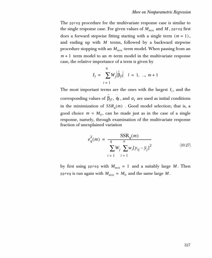
More on Nonparametric Regression
The ppreg procedure for the multivariate response case is similar tothe single response case. For given values of and , ppreg first
does a forward stepwise fitting starting with a single term ,and ending up with terms, followed by a backward stepwiseprocedure stopping with an -term model. When passing from an
term model to an -term model in the multivariate responsecase, the relative importance of a term is given by
The most important terms are the ones with the largest , and the
corresponding values of , , and are used as initial conditions
in the minimization of . Good model selection; that is, a
good choice , can be made just as in the case of a singleresponse, namely, through examination of the multivariate responsefraction of unexplained variation
by first using ppreg with and a suitably large . Then
ppreg is run again with and the same large .
(10.27)
Mmin Mm 1=( )
MMmin
m 1+ m
Il Wj βjl
j 1=
q
∑= l 1 … m, 1+,=
Il
βjl φl al
SSRq m( )
m M0=
eq2 m( )
SSRq m( )
Wj wi yij yj–[ ]2
i 1=
n
∑j 1=
q
∑-------------------------------------------------------=
Mmin 1= M
Mmin M0= M
327
Chapter 10 Regression and Smoothing for Continuous Response Data
REFERENCES
Box, G.E.P. & Tidwell, P.W. (1962). Transformations of independentvariables. Technometrics 4:531-550.
Box, G.E.P. & Cox, D.R. (1964). An analysis of transformations (withdiscussion). Journal of the Royal Statistical Society, Series B 26:211-246.
Breiman, L. & Friedman, J.H. (1985). Estimating optimaltransformations for multiple regression and correlation (withdiscussion). Journal of the American Statistical Association 80:580-619.
Durbin, J. and Watson, G.S. (1950). Testing for serial correlation inleast squares regression I. Biometrika 37: 409-428.
Friedman, J.H. & Stuetzle, W. (1981). Projection pursuit regression.Journal of the American Statistical Association 76:817-823.
Friedman, J.H. (1984). SMART Users Guide, no. 1. Stanford, CA:Laboratory for Computational Statistics, Dept. of Statistics, StanfordUniversity .
Friedman, J.H. (1984). A Variable Span Smoother, Tech. Rept. 5. Stanford,CA: Laboratory for Computational Statistics, Dept. of Statistics,Stanford University.
Friedman, J.H. (1985). Classification and Multiple Regression ThroughProjection Pursuit, Tech. Rept. 12. Stanford, CADept. of Statistics,Stanford University.
Hampel, F.R., Ronchetti, E.M., Rousseeuw, P.J., & Stahel, W.A.(1986). Robust Statistics: The Approach Based on Influence Functions. NewYork: John Wiley & Sons, Inc.
Hastie, T. & Tibshirani, R. (1990). Generalized Additive Models. London:Chapman and Hall.
Heiberger, R.M. & Becker, R.A. (1992). Design of an S function forrobust regression using iteratively reweighted least squares. Journal ofComputational and Graphical Statistics 1:181-196.
Huber, P.J. (1973). Robust regression: Asymptotics, conjectures, andMonte Carlo. Annals of Statistics 1:799-821.
Huber, P.J. (1981). Robust Statistics. New York: John Wiley & Sons, Inc.
328

References
Millard, S.P. and Neerchal, N.K. (2001). Environmental Statistics withSpotfire S+. Boca Raton, Florida: CRC Press LLC.
Rousseeuw, P.J. (1984). Least median of squares regression. Journal ofthe American Statistical Association 79:871-888.
Rousseeuw, P.J. & Leroy, A.M. (1987). Robust Regression and OutlierDetection. New York: John Wiley & Sons, Inc.
Silverman, B.W. (1986). Density Estimation for Statistics and DataAnalysis. London: Chapman and Hall.
Tibshirani, R. (1988). Estimating transformations for regression viaadditivity and variance stabilization. Journal of the American StatisticalAssociation 83:394-405.
Watson, G.S. (1966). Smooth regression analysis. Sankhya, Series A26:359-378.
Weisberg, S. (1985). Applied Linear Regression (2nd ed.). New York:John Wiley & Sons, Inc.
329

Chapter 10 Regression and Smoothing for Continuous Response Data
330
Introduction 333
Overview of the Robust MM Regression Method 334Key Robustness Features of the Method 334The Essence of the Method: A Special M-Estimate 334The lmRobMM Function 335Comparison of Least Squares and Robust Fits 336Robust Model Selection 336
Computing Robust Fits 337Example: The oilcity Data 337Least Squares and Robust Fits 338Least Squares and Robust Model Objects 340
Visualizing and Summarizing Robust Fits 341The plot Function 341The summary Function 343
Comparing Least Squares and Robust Fits 345Comparison Objects for Least Squares and Robust
Fits 345Visualizing Comparison Objects 346Statistical Inference from Comparison Objects 347
Robust Model Selection 349Robust F and Wald Tests 349Robust FPE Criterion 351
Controlling Options for Robust Regression 353Efficiency at Gaussian Model 353Alternative Loss Function 353Confidence Level of Bias Test 355Resampling Algorithms 357
ROBUST REGRESSION 11
331

Chapter 11 Robust Regression
Theoretical Details 359Initial Estimates 359Loss Functions 360Robust R-Squared 362Robust Deviance 363Robust F Test 364Robust Wald Test 364Robust FPE (RFPE) 364Breakdown Points 365
Other Robust Regression Techniques 367Least Trimmed Squares Regression 367Least Median Squares Regression 370Least Absolute Deviation Regression 370M-Estimates of Regression 372Comparison of Least Squares, Least Trimmed
Squares, and M-Estimates 375
References 378
332

Introduction
INTRODUCTION
Robust regression techniques are an important complement to classicalleast squares regression. Robust techniques provide answers similar toleast squares regression when the data are linear and have normallydistributed errors. The results differ significantly, however, when theerrors do not satisfy the normality conditions or when the datacontain significant outliers. TIBCO Spotfire S+ includes severalrobust regression techniques; this chapter focuses on robust MMregression. This is the technique we officially recommend, as itprovides both high-quality estimates and a wealth of diagnostic andinference tools.
Other robust regression techniques available in Spotfire S+ are leasttrimmed squares (LTS) regression, least median squares (LMS) regression,least absolute deviations (L1) regression, and M-estimates of regression.These are discussed briefly in the section Other Robust RegressionTechniques.
Spotfire S+ also includes the S+MissingData library, which extendsthe statistical modeling capabilities of Spotfire S+ to support model-based missing data methods. You can load this library into yourSpotfire S+ session by either typing library(missing) in theCommands window, or if you are using the Windows version,choose File � Load Library from the main menu. For moreinformation, see the file library/missing/missing.pdf in yourSpotfire S+ program group or if you are on Windows, select Help �Online Manuals � Missing Data Analysis Library.
333

Chapter 11 Robust Regression
OVERVIEW OF THE ROBUST MM REGRESSION METHOD
This section provides an overview of the Spotfire S+ tools you canuse to compute a modern linear regression model with robust MMregression. The tools we discuss include both inference forcoefficients and model selection.
Key Robustness Features of the Method
The robust MM method has the following general features:
• In data-oriented terms, a robust MM fit is minimally influenced by outliers in the independent variables space, in the response (dependent variable) space, or in both.
• In probability-oriented terms, the robust fit minimizes the maximum possible bias of the coefficients estimates. The bias minimized is due to a non-Gaussian contamination model that generates outliers, subject to achieving a desired (large sample size) efficiency for the coefficient estimates when the data has a Gaussian distribution.
• Statistical inference tools produced by the robust fit are based on large sample size approximations for such quantities as standard errors and “t-statistics” of coefficients, R-squared values, etc.
For further information, see the section Theoretical Details.
The Essence of the Method: A Special M-Estimate
A robust MM model has the form
where is the scalar response associated with ith observation, is ap-dimensional vector of independent predictor values,
represents the coefficients, and the are errors.
Spotfire S+ computes a robust M-estimate that minimizes theobjective function
.
yi xiTβ ε i ,+= i 1 ... n, ,=
yi xi
β β1 β2 … βp, , ,( )= ε i
β
ρyi xi
Tβ–
s-------------------
⎝ ⎠⎜ ⎟⎛ ⎞
i 1=
n
∑
334
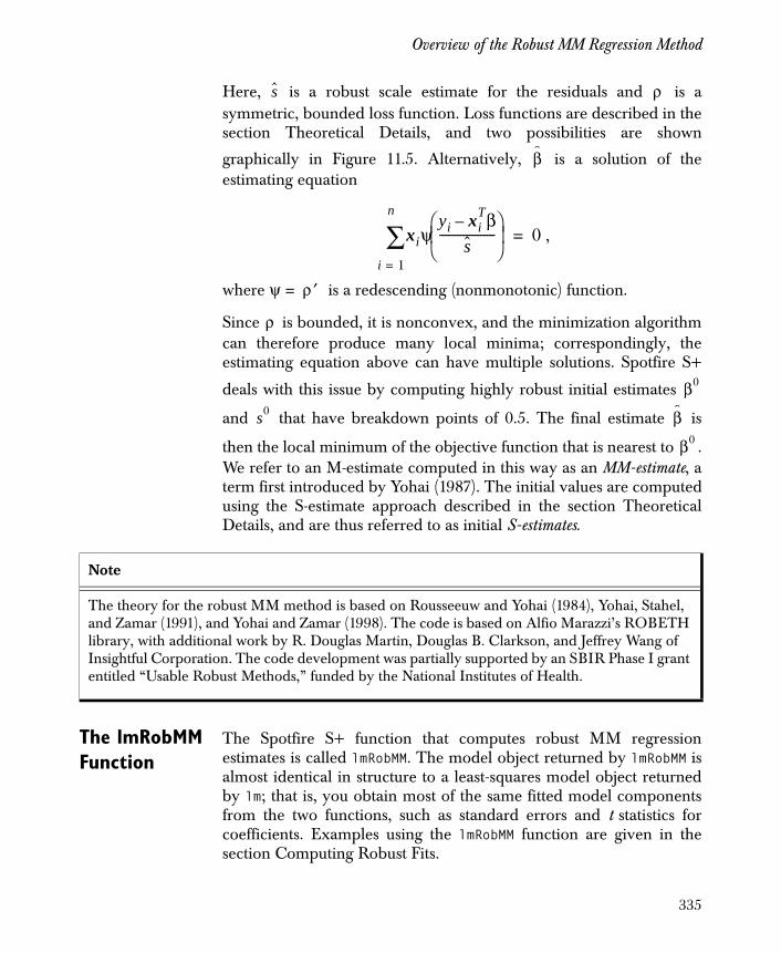
Overview of the Robust MM Regression Method
Here, is a robust scale estimate for the residuals and is asymmetric, bounded loss function. Loss functions are described in thesection Theoretical Details, and two possibilities are shown
graphically in Figure 11.5. Alternatively, is a solution of theestimating equation
,
where is a redescending (nonmonotonic) function.
Since is bounded, it is nonconvex, and the minimization algorithmcan therefore produce many local minima; correspondingly, theestimating equation above can have multiple solutions. Spotfire S+
deals with this issue by computing highly robust initial estimates
and that have breakdown points of 0.5. The final estimate is
then the local minimum of the objective function that is nearest to .We refer to an M-estimate computed in this way as an MM-estimate, aterm first introduced by Yohai (1987). The initial values are computedusing the S-estimate approach described in the section TheoreticalDetails, and are thus referred to as initial S-estimates.
The lmRobMM Function
The Spotfire S+ function that computes robust MM regressionestimates is called lmRobMM. The model object returned by lmRobMM isalmost identical in structure to a least-squares model object returnedby lm; that is, you obtain most of the same fitted model componentsfrom the two functions, such as standard errors and t statistics forcoefficients. Examples using the lmRobMM function are given in thesection Computing Robust Fits.
s ρ
β
xiψyi xi
Tβ–
s-------------------
⎝ ⎠⎜ ⎟⎛ ⎞
i 1=
n
∑ 0=
ψ ρ′=
ρ
β0
s0 β
β0
Note
The theory for the robust MM method is based on Rousseeuw and Yohai (1984), Yohai, Stahel, and Zamar (1991), and Yohai and Zamar (1998). The code is based on Alfio Marazzi’s ROBETH library, with additional work by R. Douglas Martin, Douglas B. Clarkson, and Jeffrey Wang of Insightful Corporation. The code development was partially supported by an SBIR Phase I grant entitled “Usable Robust Methods,” funded by the National Institutes of Health.
335
Chapter 11 Robust Regression
Comparison of Least Squares and Robust Fits
Spotfire S+ includes a special function compare.fits that isspecifically designed to facilitate the comparison of least squares fitsand robust fits for a linear regression model. Objects returned bycompare.fits can be printed, summarized, and plotted, resulting intabular and graphical displays that make it easy for you to comparethe two types of fits. Examples using the compare.fits function aregiven in the section Comparing Least Squares and Robust Fits.
Robust Model Selection
It is not enough to use a robust regression method when you try todecide which of several alternative models to use. You also need arobust model selection criterion. To this end, you might use one of thefollowing three tests: the robust F-test, the robust Wald test, and therobust FPE (RFPE) criterion. See the section Robust Model Selectionfor further details.
336

Computing Robust Fits
COMPUTING ROBUST FITS
Example: The oilcity Data
The Spotfire S+ data frame oilcity contains monthly excess returnson the stocks of Oil City Petroleum, Inc., from April 1979 toDecember 1989. The data set also contains the monthly excessreturns of the market for the same time period. Returns are defined asthe relative change in the stock price over a one-month interval, andexcess returns are computed relative to the monthly return of a 90-dayU.S. Treasury bill at the risk-free rate.
A scatter plot of the oilcity data, displayed in Figure 11.1, shows thatthere is one large outlier in the data. The command below producesthe graph.
> plot(oilcity$Market, oilcity$Oil, + xlab = "Market Returns", ylab = "Oil City Returns")
Figure 11.1: Scatter plot of the oilcity data.
••
•• •
•
•
•
•
•
•
••
•
•••••
•
•
• ••
•••
•••
• ••
••
••••
•
•
••
••
•
••
•• •• •••
•
•
•• ••
•••
•
•
••
• •••• •••••
•
••• ••• •••
•
• •••
•
••
• ••
•
•
•• • •
•
•
• •• ••• •••
••• • ••• •
••• •
•
Market Returns
Oil
City
Ret
urns
-0.2 -0.1 0.0
01
23
45
337
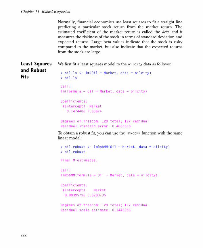
Chapter 11 Robust Regression
Normally, financial economists use least squares to fit a straight linepredicting a particular stock return from the market return. Theestimated coefficient of the market return is called the beta, and itmeasures the riskiness of the stock in terms of standard deviation andexpected returns. Large beta values indicate that the stock is riskycompared to the market, but also indicate that the expected returnsfrom the stock are large.
Least Squares and Robust Fits
We first fit a least squares model to the oilcity data as follows:
> oil.ls <- lm(Oil ~ Market, data = oilcity)> oil.ls
Call:lm(formula = Oil ~ Market, data = oilcity)
Coefficients: (Intercept) Market 0.1474486 2.85674
Degrees of freedom: 129 total; 127 residualResidual standard error: 0.4866656
To obtain a robust fit, you can use the lmRobMM function with the samelinear model:
> oil.robust <- lmRobMM(Oil ~ Market, data = oilcity)> oil.robust
Final M-estimates.
Call:lmRobMM(formula = Oil ~ Market, data = oilcity)
Coefficients: (Intercept) Market -0.08395796 0.8288795
Degrees of freedom: 129 total; 127 residualResidual scale estimate: 0.1446265
338
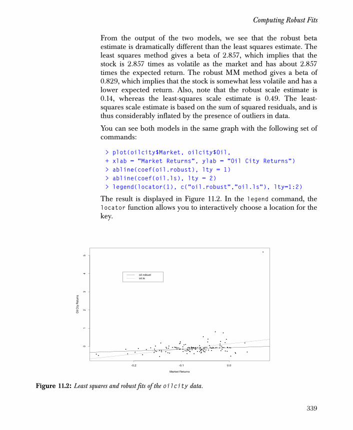
Computing Robust Fits
From the output of the two models, we see that the robust betaestimate is dramatically different than the least squares estimate. Theleast squares method gives a beta of 2.857, which implies that thestock is 2.857 times as volatile as the market and has about 2.857times the expected return. The robust MM method gives a beta of0.829, which implies that the stock is somewhat less volatile and has alower expected return. Also, note that the robust scale estimate is0.14, whereas the least-squares scale estimate is 0.49. The least-squares scale estimate is based on the sum of squared residuals, and isthus considerably inflated by the presence of outliers in data.
You can see both models in the same graph with the following set ofcommands:
> plot(oilcity$Market, oilcity$Oil, + xlab = "Market Returns", ylab = "Oil City Returns")> abline(coef(oil.robust), lty = 1)> abline(coef(oil.ls), lty = 2)> legend(locator(1), c("oil.robust","oil.ls"), lty=1:2)
The result is displayed in Figure 11.2. In the legend command, thelocator function allows you to interactively choose a location for thekey.
Figure 11.2: Least squares and robust fits of the oilcity data.
••
•
• •
•
•
•
•
•
•
•
•
•
•
••
••
•
•
• ••
••
•••
•
• ••
••
•
••••
•
••
••
•
•
•
•
• ••
•••
•
•
••
•••
••
•
•
•
••
••• • •••
••
•
••• ••• •••
•
• •••
•
••
••
•
•
•
•• • •
•
•
• •• ••• •••
••• • •
•• •
••• •
•
Market Returns
Oil
City
Ret
urns
-0.2 -0.1 0.0
01
23
45
oil.robustoil.ls
339

Chapter 11 Robust Regression
Least Squares and Robust Model Objects
Objects returned by the lm function are of class "lm":
> data.class(oil.ls)
[1] "lm"
On the other hand, objects returned by lmRobMM are of class"lmRobMM":
> data.class(oil.robust)
[1] "lmRobMM"
As with objects of class "lm", you can easily visualize, print andsummarize objects of class "lmRobMM" using the generic functionsplot, print and summary. With the names function, you can see thatlmRobMM objects contain many of the same components as lm objects,in addition to components that are needed for the robust fittingalgorithm:
> names(oil.ls)
[1] "coefficients" "residuals" "fitted.values" [4] "effects" "R" "rank" [7] "assign" "df.residual" "contrasts" [10] "terms" "call"
> names(oil.robust)
[1] "coefficients" "T.coefficients" [3] "scale" "T.scale" [5] "cov" "T.cov" [7] "dev" "T.dev" [9] "residuals" "T.residuals" [11] "r.squared" "T.r.squared" [13] "M.weights" "T.M.weights" [15] "fitted.values" "T.fitted.values" [17] "mm.bias" "ls.bias" [19] "iter.refinement" "iter.final.coef" [21] "iter.final.scale" "df.residual" [23] "rank" "est" [25] "robust.control" "qr" [27] "assign" "contrasts" [29] "terms" "call"
340
Visualizing and Summarizing Robust Fits
VISUALIZING AND SUMMARIZING ROBUST FITS
The plot Function
For simple linear regression models, like the ones computed for theoilcity data in the previous section, it is easy to see outliers in ascatter plot. In multiple regression models, however, determiningwhether there are outliers in the data is not as straightforward.Nevertheless, Spotfire S+ makes it easy for you to visualize outliers ina multiple regression. To illustrate this point, we use the well-known“stack loss” data, which has been analyzed by a large number ofstatisticians.
The stack loss data contains the percent loss of ammonia during 21consecutive days at an oxidation plant. Ammonia is lost when it isdissolved in water to produce nitric acid. Three variables mayinfluence the loss of ammonia during this process: air flow, watertemperature, and acid concentration. The stack loss response data iscontained in the vector stack.loss, and the three independentvariables are contained in the matrix stack.x. The followingcommand combines the response and predictor variables into a dataframe named stack.df:
> stack.df <- data.frame(Loss = stack.loss, stack.x)
To compute a least squares fit for stack.df, use the lm function asfollows:
> stack.ls <- lm(Loss ~ + Air.Flow + Water.Temp + Acid.Conc., data = stack.df)
To compute a robust fit for the same linear model, use:
> stack.robust <- lmRobMM(Loss ~ + Air.Flow + Water.Temp + Acid.Conc., data = stack.df)
We now use the plot function to visualize the robust fit, as illustratedin the command below. Note that plots of Cook's distance values arenot currently available for robust linear model objects.
341
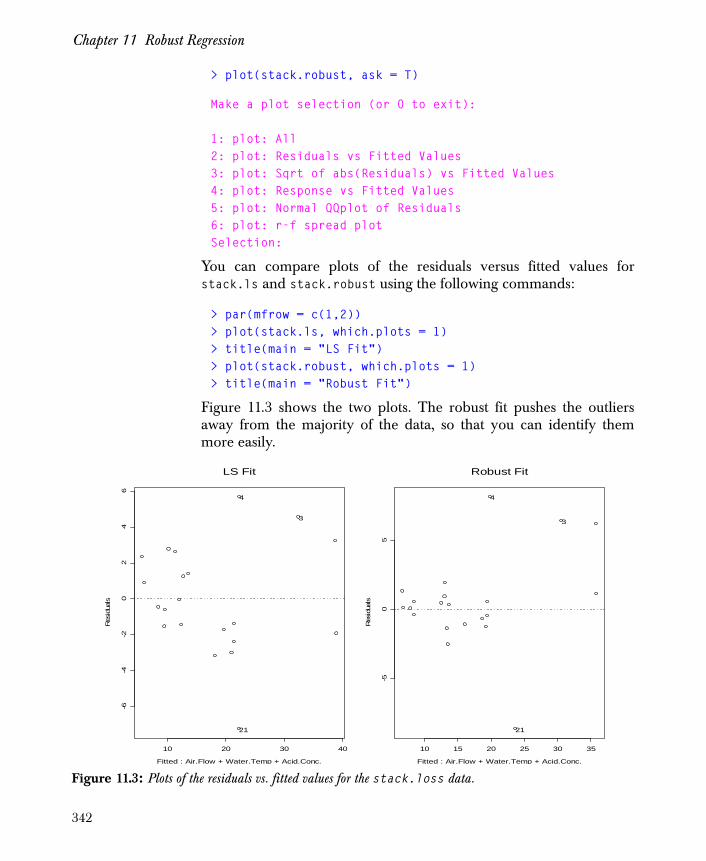
Chapter 11 Robust Regression
> plot(stack.robust, ask = T)
Make a plot selection (or 0 to exit):
1: plot: All2: plot: Residuals vs Fitted Values3: plot: Sqrt of abs(Residuals) vs Fitted Values4: plot: Response vs Fitted Values5: plot: Normal QQplot of Residuals6: plot: r-f spread plotSelection:
You can compare plots of the residuals versus fitted values forstack.ls and stack.robust using the following commands:
> par(mfrow = c(1,2))> plot(stack.ls, which.plots = 1)> title(main = "LS Fit")> plot(stack.robust, which.plots = 1)> title(main = "Robust Fit")
Figure 11.3 shows the two plots. The robust fit pushes the outliersaway from the majority of the data, so that you can identify themmore easily.
Figure 11.3: Plots of the residuals vs. fitted values for the stack.loss data.Fitted : Air.Flow + Water.Temp + Acid.Conc.
Res
idua
ls
10 20 30 40
-6-4
-20
24
6
3
4
21
LS Fit
Fitted : Air.Flow + Water.Temp + Acid.Conc.
Res
idua
ls
10 15 20 25 30 35
-50
5
3
4
21
Robust Fit
342

Visualizing and Summarizing Robust Fits
The summary Function
The summary function for lmRobMM objects provides the usual types ofinference tools, including t-values and p-values. In addition, it alsoprovides some information specific to robust models, such as tests forbias. For example, the command below displays a detailed summaryof the oil.robust object computed in the section Least Squares andRobust Fits.
> summary(oil.robust)
Final M-estimates.
Call: lmRobMM(formula = Oil ~ Market, data = oilcity)
Residuals: Min 1Q Median 3Q Max -0.4566 -0.08875 0.03082 0.1031 5.218
Coefficients: Value Std. Error t value Pr(>|t|)(Intercept) -0.0840 0.0281 -2.9931 0.0033 Market 0.8289 0.2834 2.9247 0.0041
Residual scale estimate: 0.1446 on 127 degrees of freedom
Proportion of variation in response explained by model: 0.0526
Test for Bias Statistics P-value M-estimate 2.16 0.3396400LS-estimate 22.39 0.0000138
Correlation of Coefficients: (Intercept)Market 0.8169
The seed parameter is : 1313
343

Chapter 11 Robust Regression
Note that the standard errors, t-values, and p-values are displayed inthe same format as they are in lm summaries. The standard errors forlmRobMM objects are computed from the robust covariance matrix ofthe estimates. For technical details regarding the computation ofrobust covariance matrices, refer to Yohai, Stahel, and Zamar (1991).
The summary method for lmRobMM provides another piece of usefulinformation: the Proportion of variation in response explained
by model, usually known as the R2 value. Spotfire S+ calculates arobust version of this statistic, as described in the section TheoreticalDetails.
Finally, there is a Test for Bias section in the summary output forlmRobMM objects. This section provides the test statistics of bias forboth the final M-estimates and the least squares (LS) estimates againstthe initial S-estimates. In the oil.robust example, the test for bias ofthe final M-estimates yields a p-value of 0.33, which suggests that thebias of the final M-estimates relative to the initial S-estimates is notsignificant at the default 0.90 level. This is why the final M-estimatesare reported in the summary output instead of the initial estimates. Thetest for bias of the least squares estimates relative to the S-estimatesyields a p-value of 0, which indicates that the LS estimate is highlybiased. This suggests that the robust MM model is preferred over theleast squares model. For technical details regarding the calculations ofthe tests for bias, see Yohai, Zamar, and Stahel (1991).
344
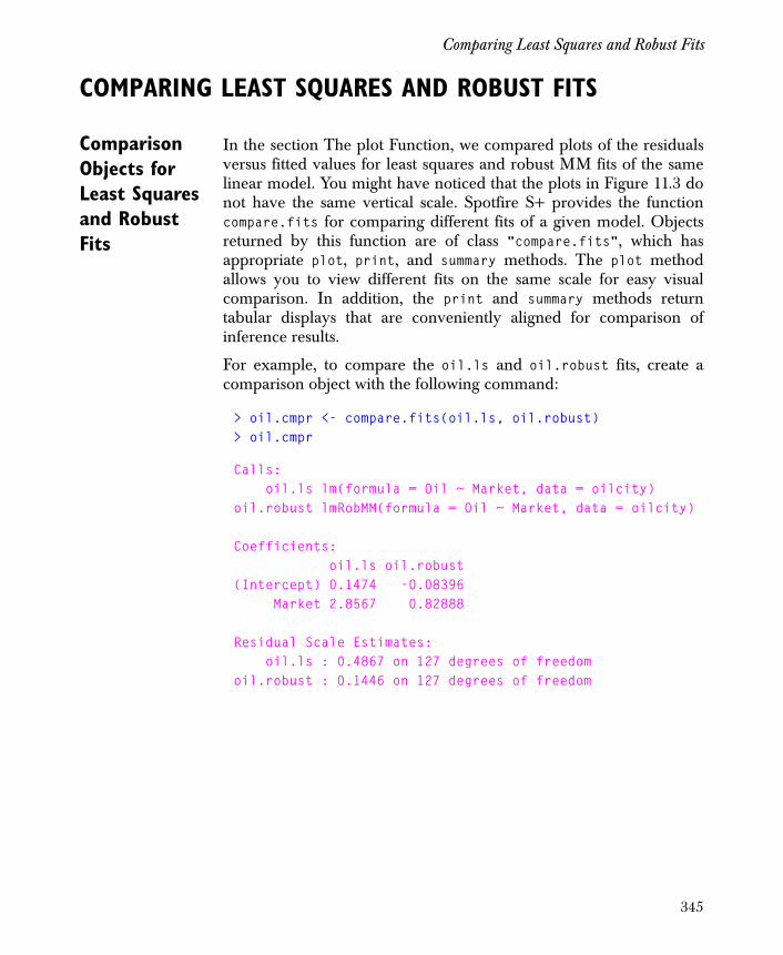
Comparing Least Squares and Robust Fits
COMPARING LEAST SQUARES AND ROBUST FITS
Comparison Objects for Least Squares and Robust Fits
In the section The plot Function, we compared plots of the residualsversus fitted values for least squares and robust MM fits of the samelinear model. You might have noticed that the plots in Figure 11.3 donot have the same vertical scale. Spotfire S+ provides the functioncompare.fits for comparing different fits of a given model. Objectsreturned by this function are of class "compare.fits", which hasappropriate plot, print, and summary methods. The plot methodallows you to view different fits on the same scale for easy visualcomparison. In addition, the print and summary methods returntabular displays that are conveniently aligned for comparison ofinference results.
For example, to compare the oil.ls and oil.robust fits, create acomparison object with the following command:
> oil.cmpr <- compare.fits(oil.ls, oil.robust)> oil.cmpr
Calls: oil.ls lm(formula = Oil ~ Market, data = oilcity)oil.robust lmRobMM(formula = Oil ~ Market, data = oilcity)
Coefficients: oil.ls oil.robust(Intercept) 0.1474 -0.08396 Market 2.8567 0.82888
Residual Scale Estimates: oil.ls : 0.4867 on 127 degrees of freedomoil.robust : 0.1446 on 127 degrees of freedom
345
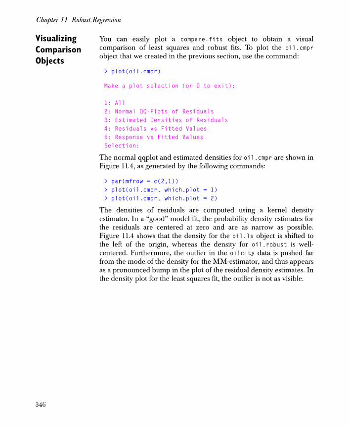
Chapter 11 Robust Regression
Visualizing Comparison Objects
You can easily plot a compare.fits object to obtain a visualcomparison of least squares and robust fits. To plot the oil.cmprobject that we created in the previous section, use the command:
> plot(oil.cmpr)
Make a plot selection (or 0 to exit):
1: All2: Normal QQ-Plots of Residuals3: Estimated Densities of Residuals4: Residuals vs Fitted Values5: Response vs Fitted ValuesSelection:
The normal qqplot and estimated densities for oil.cmpr are shown inFigure 11.4, as generated by the following commands:
> par(mfrow = c(2,1))> plot(oil.cmpr, which.plot = 1)> plot(oil.cmpr, which.plot = 2)
The densities of residuals are computed using a kernel densityestimator. In a “good” model fit, the probability density estimates forthe residuals are centered at zero and are as narrow as possible.Figure 11.4 shows that the density for the oil.ls object is shifted tothe left of the origin, whereas the density for oil.robust is well-centered. Furthermore, the outlier in the oilcity data is pushed farfrom the mode of the density for the MM-estimator, and thus appearsas a pronounced bump in the plot of the residual density estimates. Inthe density plot for the least squares fit, the outlier is not as visible.
346

Comparing Least Squares and Robust Fits
Statistical Inference from Comparison Objects
A detailed comparison of two model fits, including t-values andp-values, can be obtained with the summary method for compare.fitsobjects. For example:
> summary(oil.cmpr)
Calls: oil.ls lm(formula = Oil ~ Market, data = oilcity)oil.robust lmRobMM(formula = Oil ~ Market, data = oilcity)
Residual Statistics: Min 1Q Median 3Q Max
Figure 11.4: Normal qqplots and residual density estimates for the linear fits in oil.cmpr.
-2 -1 0 1 2
01
23
45
oil.ls oil.robust
-1 0 1 2 3 4 5
0.0
0.5
1.0
1.5
2.0
oil.ls oil.robust
347

Chapter 11 Robust Regression
oil.ls -0.6952 -0.17323 -0.05444 0.08407 4.842oil.robust -0.4566 -0.08875 0.03082 0.10314 5.218
Coefficients: Value Std. Error t value oil.ls_(Intercept) 0.14745 0.07072 2.085oil.robust_(Intercept) -0.08396 0.02805 -2.993 oil.ls_Market 2.85674 0.73175 3.904 oil.robust_Market 0.82888 0.28341 2.925
Pr(>|t|) oil.ls_(Intercept) 0.0390860oil.robust_(Intercept) 0.0033197 oil.ls_Market 0.0001528 oil.robust_Market 0.0040852
Residual Scale Estimates: oil.ls : 0.4867 on 127 degrees of freedomoil.robust : 0.1446 on 127 degrees of freedom
Proportion of variation in response(s) explained by model(s): oil.ls : 0.1071oil.robust : 0.0526
Correlations: oil.ls Market(Intercept) 0.7955736
oil.robust Market(Intercept) 0.8168674
Warning
When the p-values for the tests of bias indicate that the final M-estimates are highly biased relative to the initial S-estimates, the final M-estimates are not used in a lmRobMM fit. In this case, the asymptotic approximations for the inference results may not be very good, and you should thus not trust them.
348
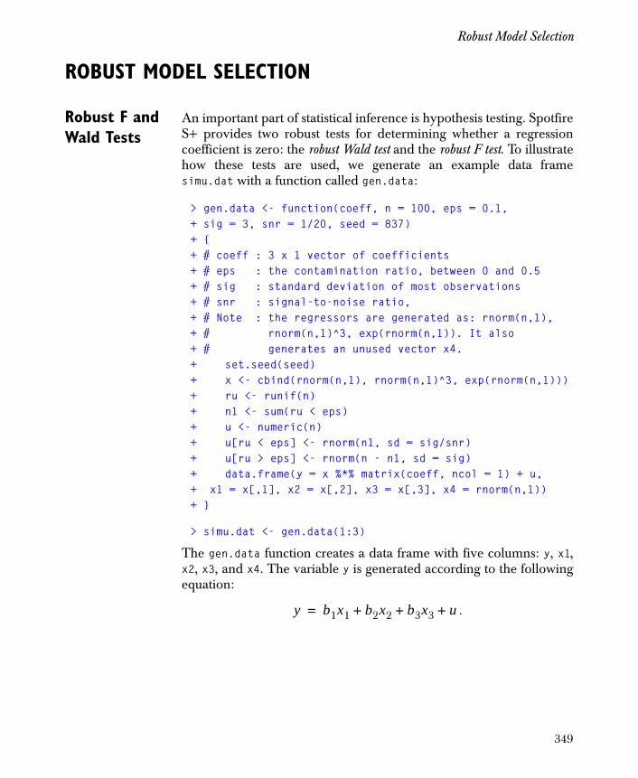
Robust Model Selection
ROBUST MODEL SELECTION
Robust F and Wald Tests
An important part of statistical inference is hypothesis testing. SpotfireS+ provides two robust tests for determining whether a regressioncoefficient is zero: the robust Wald test and the robust F test. To illustratehow these tests are used, we generate an example data framesimu.dat with a function called gen.data:
> gen.data <- function(coeff, n = 100, eps = 0.1,+ sig = 3, snr = 1/20, seed = 837)+ {+ # coeff : 3 x 1 vector of coefficients+ # eps : the contamination ratio, between 0 and 0.5+ # sig : standard deviation of most observations+ # snr : signal-to-noise ratio,+ # Note : the regressors are generated as: rnorm(n,1),+ # rnorm(n,1)^3, exp(rnorm(n,1)). It also+ # generates an unused vector x4.+ set.seed(seed)+ x <- cbind(rnorm(n,1), rnorm(n,1)^3, exp(rnorm(n,1)))+ ru <- runif(n)+ n1 <- sum(ru < eps)+ u <- numeric(n)+ u[ru < eps] <- rnorm(n1, sd = sig/snr)+ u[ru > eps] <- rnorm(n - n1, sd = sig)+ data.frame(y = x %*% matrix(coeff, ncol = 1) + u,+ x1 = x[,1], x2 = x[,2], x3 = x[,3], x4 = rnorm(n,1))+ }
> simu.dat <- gen.data(1:3)
The gen.data function creates a data frame with five columns: y, x1,x2, x3, and x4. The variable y is generated according to the followingequation:
.y b1x1 b2x2 b3x3 u+ + +=
349
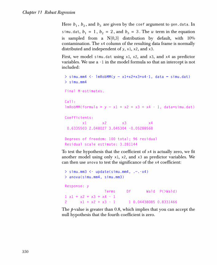
Chapter 11 Robust Regression
Here , , and are given by the coef argument to gen.data. In
simu.dat, , , and . The term in the equationis sampled from a N(0,3) distribution by default, with 10%contamination. The x4 column of the resulting data frame is normallydistributed and independent of y, x1, x2, and x3.
First, we model simu.dat using x1, x2, and x3, and x4 as predictorvariables. We use a -1 in the model formula so that an intercept is notincluded:
> simu.mm4 <- lmRobMM(y ~ x1+x2+x3+x4-1, data = simu.dat)> simu.mm4
Final M-estimates.
Call:lmRobMM(formula = y ~ x1 + x2 + x3 + x4 - 1, data=simu.dat)
Coefficients: x1 x2 x3 x4 0.6335503 2.048027 3.045304 -0.05288568
Degrees of freedom: 100 total; 96 residualResidual scale estimate: 3.281144
To test the hypothesis that the coefficient of x4 is actually zero, we fitanother model using only x1, x2, and x3 as predictor variables. Wecan then use anova to test the significance of the x4 coefficient:
> simu.mm3 <- update(simu.mm4, .~.-x4)> anova(simu.mm4, simu.mm3)
Response: y Terms Df Wald P(>Wald)1 x1 + x2 + x3 + x4 - 1 2 x1 + x2 + x3 - 1 1 0.04438085 0.8331466
The p-value is greater than 0.8, which implies that you can accept thenull hypothesis that the fourth coefficient is zero.
b1 b2 b3
b1 1= b2 2= b3 3= u
350
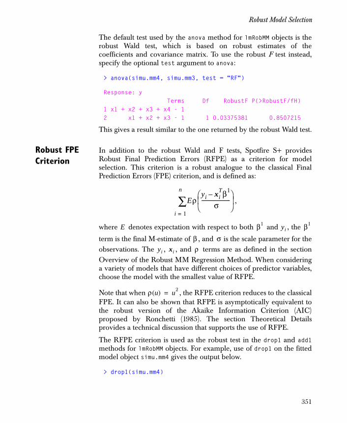
Robust Model Selection
The default test used by the anova method for lmRobMM objects is therobust Wald test, which is based on robust estimates of thecoefficients and covariance matrix. To use the robust F test instead,specify the optional test argument to anova:
> anova(simu.mm4, simu.mm3, test = "RF")
Response: y Terms Df RobustF P(>RobustF/fH)1 x1 + x2 + x3 + x4 - 1 2 x1 + x2 + x3 - 1 1 0.03375381 0.8507215
This gives a result similar to the one returned by the robust Wald test.
Robust FPE Criterion
In addition to the robust Wald and F tests, Spotfire S+ providesRobust Final Prediction Errors (RFPE) as a criterion for modelselection. This criterion is a robust analogue to the classical FinalPrediction Errors (FPE) criterion, and is defined as:
,
where denotes expectation with respect to both and , the
term is the final M-estimate of , and is the scale parameter for theobservations. The , , and terms are as defined in the sectionOverview of the Robust MM Regression Method. When consideringa variety of models that have different choices of predictor variables,choose the model with the smallest value of RFPE.
Note that when , the RFPE criterion reduces to the classicalFPE. It can also be shown that RFPE is asymptotically equivalent tothe robust version of the Akaike Information Criterion (AIC)proposed by Ronchetti (1985). The section Theoretical Detailsprovides a technical discussion that supports the use of RFPE.
The RFPE criterion is used as the robust test in the drop1 and add1methods for lmRobMM objects. For example, use of drop1 on the fittedmodel object simu.mm4 gives the output below.
> drop1(simu.mm4)
Eρyi xi
Tβ1–
σ----------------------
⎝ ⎠⎜ ⎟⎛ ⎞
i 1=
n
∑
E β1 yi β1
β σyi xi ρ
ρ u( ) u2=
351

Chapter 11 Robust Regression
Single term deletions Model:y ~ x1 + x2 + x3 + x4 - 1 Df RFPE <none> 24.24090 x1 1 24.46507 x2 1 52.19715 x3 1 64.32581 x4 1 23.95741
The model obtained by dropping x4 has a lower RFPE than themodel that includes all four predictor variables. This indicates thatdropping x4 results in a better model.
You can also use the add1 function to explore the relevance ofvariables. For example, use the following command to investigatewhether x4 helps to predict y in the simu.mm3 model:
> add1(simu.mm3, "x4")
Single term additions Model:y ~ x1 + x2 + x3 - 1 Df RFPE<none> 24.10179 x4 1 24.38765
As expected, the model without x4 is preferred, since the RFPEincreases when x4 is added.
Warning
When the p-values for the tests of bias indicate that the final M-estimates are highly biased relative to the initial S-estimates, the final M-estimates are not used in a lmRobMM fit. If this applies to any of the models considered by drop1 and add1, you should not trust the corresponding RFPE values.
352
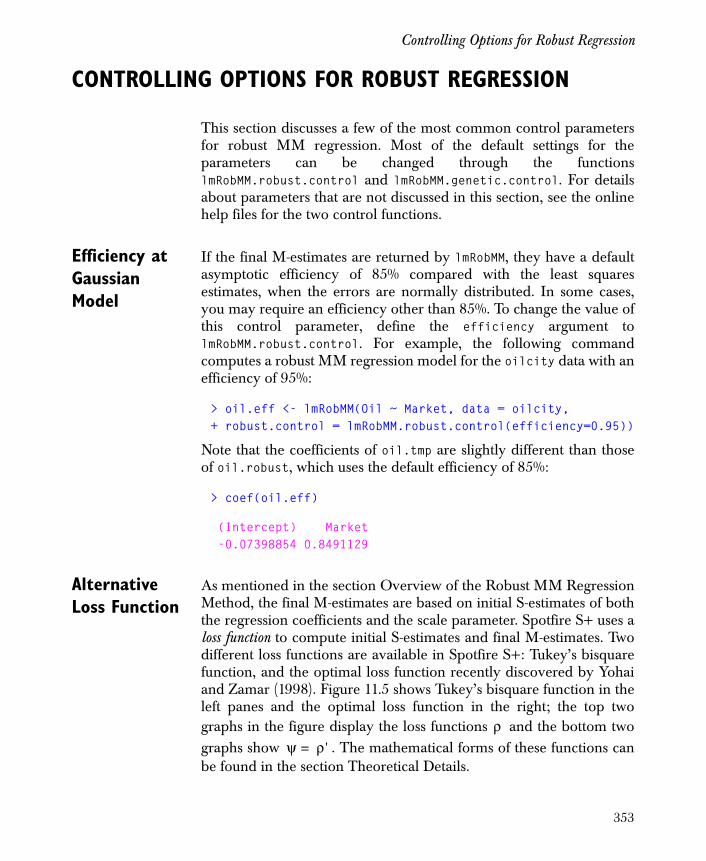
Controlling Options for Robust Regression
CONTROLLING OPTIONS FOR ROBUST REGRESSION
This section discusses a few of the most common control parametersfor robust MM regression. Most of the default settings for theparameters can be changed through the functionslmRobMM.robust.control and lmRobMM.genetic.control. For detailsabout parameters that are not discussed in this section, see the onlinehelp files for the two control functions.
Efficiency at Gaussian Model
If the final M-estimates are returned by lmRobMM, they have a defaultasymptotic efficiency of 85% compared with the least squaresestimates, when the errors are normally distributed. In some cases,you may require an efficiency other than 85%. To change the value ofthis control parameter, define the efficiency argument tolmRobMM.robust.control. For example, the following commandcomputes a robust MM regression model for the oilcity data with anefficiency of 95%:
> oil.eff <- lmRobMM(Oil ~ Market, data = oilcity,+ robust.control = lmRobMM.robust.control(efficiency=0.95))
Note that the coefficients of oil.tmp are slightly different than thoseof oil.robust, which uses the default efficiency of 85%:
> coef(oil.eff)
(Intercept) Market -0.07398854 0.8491129
Alternative Loss Function
As mentioned in the section Overview of the Robust MM RegressionMethod, the final M-estimates are based on initial S-estimates of boththe regression coefficients and the scale parameter. Spotfire S+ uses aloss function to compute initial S-estimates and final M-estimates. Twodifferent loss functions are available in Spotfire S+: Tukey’s bisquarefunction, and the optimal loss function recently discovered by Yohaiand Zamar (1998). Figure 11.5 shows Tukey’s bisquare function in theleft panes and the optimal loss function in the right; the top twographs in the figure display the loss functions and the bottom twographs show . The mathematical forms of these functions canbe found in the section Theoretical Details.
ρψ ρ'=
353
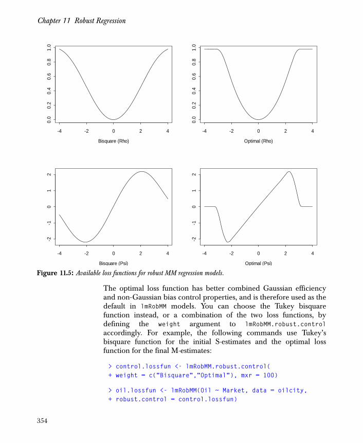
Chapter 11 Robust Regression
The optimal loss function has better combined Gaussian efficiencyand non-Gaussian bias control properties, and is therefore used as thedefault in lmRobMM models. You can choose the Tukey bisquarefunction instead, or a combination of the two loss functions, bydefining the weight argument to lmRobMM.robust.controlaccordingly. For example, the following commands use Tukey’sbisquare function for the initial S-estimates and the optimal lossfunction for the final M-estimates:
> control.lossfun <- lmRobMM.robust.control(+ weight = c("Bisquare","Optimal"), mxr = 100)
> oil.lossfun <- lmRobMM(Oil ~ Market, data = oilcity,+ robust.control = control.lossfun)
Figure 11.5: Available loss functions for robust MM regression models.
Bisquare (Rho)
-4 -2 0 2 4
0.0
0.2
0.4
0.6
0.8
1.0
Optimal (Rho)
-4 -2 0 2 4
0.0
0.2
0.4
0.6
0.8
1.0
Bisquare (Psi)
-4 -2 0 2 4
-2-1
01
2
Optimal (Psi)
-4 -2 0 2 4
-2-1
01
2
354
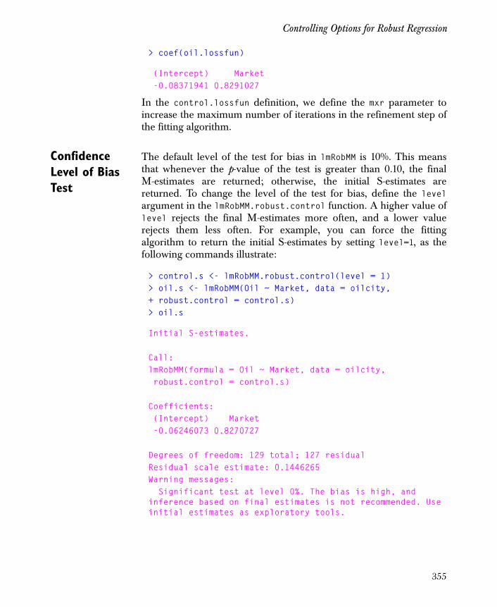
Controlling Options for Robust Regression
> coef(oil.lossfun)
(Intercept) Market -0.08371941 0.8291027
In the control.lossfun definition, we define the mxr parameter toincrease the maximum number of iterations in the refinement step ofthe fitting algorithm.
Confidence Level of Bias Test
The default level of the test for bias in lmRobMM is 10%. This meansthat whenever the p-value of the test is greater than 0.10, the finalM-estimates are returned; otherwise, the initial S-estimates arereturned. To change the level of the test for bias, define the levelargument in the lmRobMM.robust.control function. A higher value oflevel rejects the final M-estimates more often, and a lower valuerejects them less often. For example, you can force the fittingalgorithm to return the initial S-estimates by setting level=1, as thefollowing commands illustrate:
> control.s <- lmRobMM.robust.control(level = 1)> oil.s <- lmRobMM(Oil ~ Market, data = oilcity,+ robust.control = control.s)> oil.s
Initial S-estimates.
Call:lmRobMM(formula = Oil ~ Market, data = oilcity, robust.control = control.s)
Coefficients: (Intercept) Market -0.06246073 0.8270727
Degrees of freedom: 129 total; 127 residualResidual scale estimate: 0.1446265Warning messages: Significant test at level 0%. The bias is high, and inference based on final estimates is not recommended. Use initial estimates as exploratory tools.
355
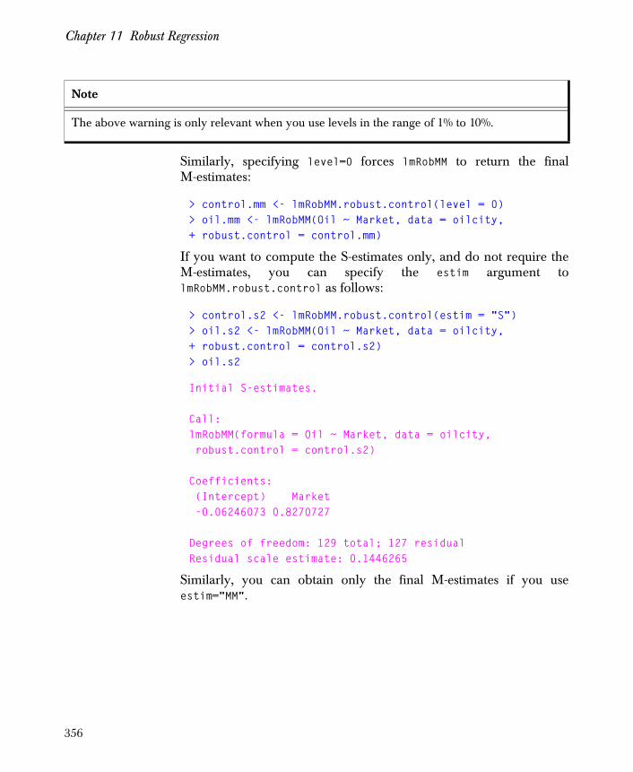
Chapter 11 Robust Regression
Similarly, specifying level=0 forces lmRobMM to return the finalM-estimates:
> control.mm <- lmRobMM.robust.control(level = 0)> oil.mm <- lmRobMM(Oil ~ Market, data = oilcity,+ robust.control = control.mm)
If you want to compute the S-estimates only, and do not require theM-estimates, you can specify the estim argument tolmRobMM.robust.control as follows:
> control.s2 <- lmRobMM.robust.control(estim = "S")> oil.s2 <- lmRobMM(Oil ~ Market, data = oilcity,+ robust.control = control.s2)> oil.s2
Initial S-estimates.
Call:lmRobMM(formula = Oil ~ Market, data = oilcity, robust.control = control.s2)
Coefficients: (Intercept) Market -0.06246073 0.8270727
Degrees of freedom: 129 total; 127 residualResidual scale estimate: 0.1446265
Similarly, you can obtain only the final M-estimates if you useestim="MM".
Note
The above warning is only relevant when you use levels in the range of 1% to 10%.
356
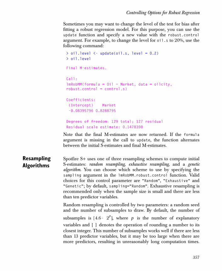
Controlling Options for Robust Regression
Sometimes you may want to change the level of the test for bias afterfitting a robust regression model. For this purpose, you can use theupdate function and specify a new value with the robust.controlargument. For example, to change the level for oil.s to 20%, use thefollowing command:
> oil.level <- update(oil.s, level = 0.2)> oil.level
Final M-estimates. Call:lmRobMM(formula = Oil ~ Market, data = oilcity, robust.control = control.s) Coefficients: (Intercept) Market -0.08395796 0.8288795 Degrees of freedom: 129 total; 127 residualResidual scale estimate: 0.1478398
Note that the final M-estimates are now returned. If the formulaargument is missing in the call to update, the function alternatesbetween the initial S-estimates and final M-estimates.
Resampling Algorithms
Spotfire S+ uses one of three resampling schemes to compute initialS-estimates: random resampling, exhaustive resampling, and a geneticalgorithm. You can choose which scheme to use by specifying thesampling argument in the lmRobMM.robust.control function. Validchoices for this control parameter are "Random", "Exhaustive" and"Genetic"; by default, sampling="Random". Exhaustive resampling isrecommended only when the sample size is small and there are lessthan ten predictor variables.
Random resampling is controlled by two parameters: a random seedand the number of subsamples to draw. By default, the number of
subsamples is , where is the number of explanatoryvariables and denotes the operation of rounding a number to itsclosest integer. This number of subsamples works well if there are lessthan 13 predictor variables, but it may be too large when there aremore predictors, resulting in unreasonably long computation times.
4.6 2p⋅[ ] p [ ]
357
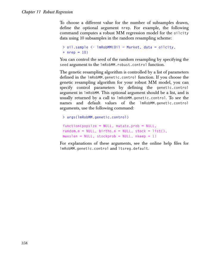
Chapter 11 Robust Regression
To choose a different value for the number of subsamples drawn,define the optional argument nrep. For example, the followingcommand computes a robust MM regression model for the oilcitydata using 10 subsamples in the random resampling scheme:
> oil.sample <- lmRobMM(Oil ~ Market, data = oilcity,+ nrep = 10)
You can control the seed of the random resampling by specifying theseed argument to the lmRobMM.robust.control function.
The genetic resampling algorithm is controlled by a list of parametersdefined in the lmRobMM.genetic.control function. If you choose thegenetic resampling algorithm for your robust MM model, you canspecify control parameters by defining the genetic.controlargument in lmRobMM. This optional argument should be a list, and isusually returned by a call to lmRobMM.genetic.control. To see thenames and default values of the lmRobMM.genetic.controlarguments, use the following command:
> args(lmRobMM.genetic.control)
function(popsize = NULL, mutate.prob = NULL,random.n = NULL, births.n = NULL, stock = list(),maxslen = NULL, stockprob = NULL, nkeep = 1)
For explanations of these arguments, see the online help files forlmRobMM.genetic.control and ltsreg.default.
358

Theoretical Details
THEORETICAL DETAILS
Initial Estimates
As mentioned in the section Overview of the Robust MM RegressionMethod, the minimization algorithm that lmRobMM uses to computecoefficients can produce many optimal solutions to the objectivefunction
Here is the scalar response associated with ith observation, is ap-dimensional vector of independent predictor values, and
represents the coefficients. Spotfire S+ deals with
this issue by computing highly robust initial estimates and forthe coefficients and scale parameter, respectively. The initial estimatesare calculated using the S-estimate method introduced by Rousseeuwand Yohai (1984), as part of an overall computational strategyproposed by Yohai, Stahel, and Zamar (1991).
The S-estimate approach has as its foundation an M-estimate of anunknown scale parameter for the observations. The observations areassumed to be robustly centered, in that a robust location estimate has
been subtracted from each for . The M-estimate isobtained by solving the equation
where is a symmetric, bounded function. It is known that such ascale estimate has a breakdown point of 0.5 (Huber, 1981), and thatone can find min-max bias robust M-estimates of scale (Martin andZamar, 1989 and 1993).
. (11.1)
(11.2)
ρyi xi
Tβ–
s-------------------
⎝ ⎠⎜ ⎟⎛ ⎞
i 1=
n
∑
yi xi
β β1 β2 … βp, , ,( )=
β0 s0
s
yi i 1 2 … n, , ,= s
1n--- ρ
yis----⎝ ⎠
⎛ ⎞
i 1=
n
∑ 0.5=
ρ
359

Chapter 11 Robust Regression
Consider the following modification of Equation (11.2):
For each value of , we have a corresponding robust scale estimate
. The initial S-estimate is the value that minimizes :
This presents a second nonlinear optimization problem, one forwhich the solution is traditionally found by a random resamplingalgorithm followed by a local search, as described in Yohai, Stahel,and Zamar (1991). Spotfire S+ allows you to use an exhaustive formof resampling for small problems, or a genetic algorithm in place of
the resampling scheme. Once the initial S-estimate is computed,the The final M-estimate is the local minimum of Equation (11.1) that
is nearest to .
For details on the numerical algorithms implemented in lmRobMM, seeMarazzi (1993).
Loss Functions A robust M-estimate for the coefficients in a linear model isobtained by minimizing Equation (11.1). The in the equation is aloss function, which is a convex weight function of the residuals; thederivative of is usually denoted by . In lmRobMM, two differentweight functions can be used for both the initial S-estimates and thefinal M-estimates: Tukey’s bisquare function and the optimal weightfunction introduced in Yohai and Zamar (1998).
(11.3)
(11.4)
1n p–------------ ρ
yi xiTβ–
s β( )-------------------
⎝ ⎠⎜ ⎟⎛ ⎞
i 1=
n
∑ 0.5=
β
s β( ) β0 s β( )
β0 argminβs β( )=
β0
β0
βρ
ρ ψ
360

Theoretical Details
Tukey’s bisquare function and its derivative are as follows:
In these equations, is a tuning constant. The Yohai and Zamaroptimal function and its derivative are:
where is a tuning constant and
,
.
See Figure 11.5 for the general shapes of these two loss functions.
ρ r( )rc--⎝ ⎠
⎛ ⎞ 63 r
c--⎝ ⎠
⎛ ⎞ 4– 3 r
c--⎝ ⎠
⎛ ⎞ 2+ if r c≤
1 if r c>⎝⎜⎜⎜⎛
=
ψ r( )6c--- r
c--⎝ ⎠
⎛ ⎞ 12c
------ rc--⎝ ⎠
⎛ ⎞ 3–
6c--- r
c--⎝ ⎠
⎛ ⎞ 5+ if r c≤
1 if r c>⎝⎜⎜⎜⎛
=
c
ρ r( )
3.25c2 if rc-- 3>
c2 1.792 h1rc--⎝ ⎠
⎛ ⎞ 2h2
rc--⎝ ⎠
⎛ ⎞ 4h3
rc--⎝ ⎠
⎛ ⎞ 6h4
rc--⎝ ⎠
⎛ ⎞ 8+ + + + if 2 r
c-- 3≤<
r2
2---- if r
c-- 2≤
⎝⎜⎜⎜⎜⎜⎜⎜⎜⎛
=
ψ r( )
0 if rc-- 3>
c g1rc-- g2
rc--⎝ ⎠
⎛ ⎞ 3g3
rc--⎝ ⎠
⎛ ⎞ 5g4
rc--⎝ ⎠
⎛ ⎞ 7+ + + if 2 r
c-- 3≤<
r if rc-- 2≤
⎝⎜⎜⎜⎜⎜⎜⎜⎛
=
c
g1 1.944 g2,– 1.728 g3, 0.312 g4,– 0.016= = = =
h1g1
2----- h2,
g2
4----- h3,
g3
6----- h4,
g4
8-----= = = =
361

Chapter 11 Robust Regression
Yohai and Zamar (1998) showed that their loss function above isoptimal in the following sense: the final M-estimate obtained usingthis function has a breakdown point of 0.5. In addition, it minimizesthe maximum bias under contamination distributions (locally forsmall fractions of contamination), subject to achieving a desiredefficiency when the data are Gaussian.
The Gaussian efficiency of the final M-estimate is controlled by thechoice of tuning constant in the weight function. As discussed in thesection Controlling Options for Robust Regression, you can specify adesired Gaussian efficiency with the efficiency argument tolmRobMM.robust.control. Once a value is chosen, Spotfire S+automatically adjusts the tuning parameter to achieve the desiredefficiency.
Robust R-Squared
The robust R2 statistic is calculated as follows:
• Initial S-estimator
If an intercept is included in the model, then
,
where is the number of observations, is the number of
predictor variables, and is the initial S-estimate for the
scale parameter. The term is the minimized from Equations (11.3) and (11.4), for a regression model that has only an intercept .
If an intercept is included in the model, then
.
c
β0
R2 n 1–( )sμ2 n p–( ) s0( )
2–
n 1–( )sμ2
---------------------------------------------------------=
n p
s0
sμ s μ( )
μ
R2 ns 0( )2 n p–( ) s0( )2
–
ns 0( )2---------------------------------------------------=
362
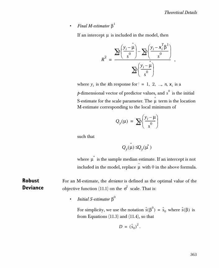
Theoretical Details
• Final M-estimator
If an intercept is included in the model, then
,
where is the ith response for , is a
p-dimensional vector of predictor values, and is the initial
S-estimate for the scale parameter. The term is the location M-estimate corresponding to the local minimum of
such that
where is the sample median estimate. If an intercept is not
included in the model, replace with 0 in the above formula.
Robust Deviance
For an M-estimate, the deviance is defined as the optimal value of the
objective function (11.1) on the scale. That is:
• Initial S-estimator
For simplicity, we use the notation where is from Equations (11.3) and (11.4), so that
.
β1
μ
R2ρ
yi μ–
s0-------------
⎝ ⎠⎜ ⎟⎛ ⎞
ρyi xi
Tβ1–
s0----------------------
⎝ ⎠⎜ ⎟⎛ ⎞
∑–∑
ρyi μ–
s0-------------
⎝ ⎠⎜ ⎟⎛ ⎞
∑--------------------------------------------------------------------=
yi i 1 2 … n, , ,= xi
s0
μ
Qy μ( ) ρyi μ–
s0-------------
⎝ ⎠⎜ ⎟⎛ ⎞
∑=
Qy μ( ) Qy μ*( )≤
μ*
μ
σ2
β0
s β0( ) s0= s β( )
D s0( )2=
363
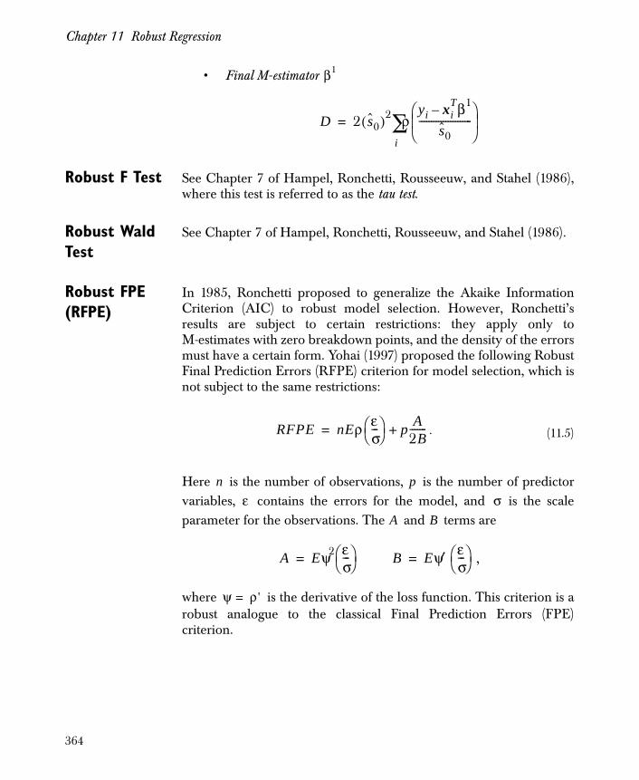
Chapter 11 Robust Regression
• Final M-estimator
Robust F Test See Chapter 7 of Hampel, Ronchetti, Rousseeuw, and Stahel (1986),where this test is referred to as the tau test.
Robust Wald Test
See Chapter 7 of Hampel, Ronchetti, Rousseeuw, and Stahel (1986).
Robust FPE (RFPE)
In 1985, Ronchetti proposed to generalize the Akaike InformationCriterion (AIC) to robust model selection. However, Ronchetti’sresults are subject to certain restrictions: they apply only toM-estimates with zero breakdown points, and the density of the errorsmust have a certain form. Yohai (1997) proposed the following RobustFinal Prediction Errors (RFPE) criterion for model selection, which isnot subject to the same restrictions:
Here is the number of observations, is the number of predictorvariables, contains the errors for the model, and is the scaleparameter for the observations. The and terms are
,
where is the derivative of the loss function. This criterion is arobust analogue to the classical Final Prediction Errors (FPE)criterion.
β1
D 2 s0( )2 ρyi xi
Tβ1–
s0----------------------
⎝ ⎠⎜ ⎟⎛ ⎞
i∑=
. (11.5)RFPE nEρ εσ---⎝ ⎠
⎛ ⎞ p A2B-------+=
n pε σ
A B
A Eψ2 εσ---⎝ ⎠
⎛ ⎞= B Eψ′ εσ---⎝ ⎠
⎛ ⎞=
ψ ρ '=
364
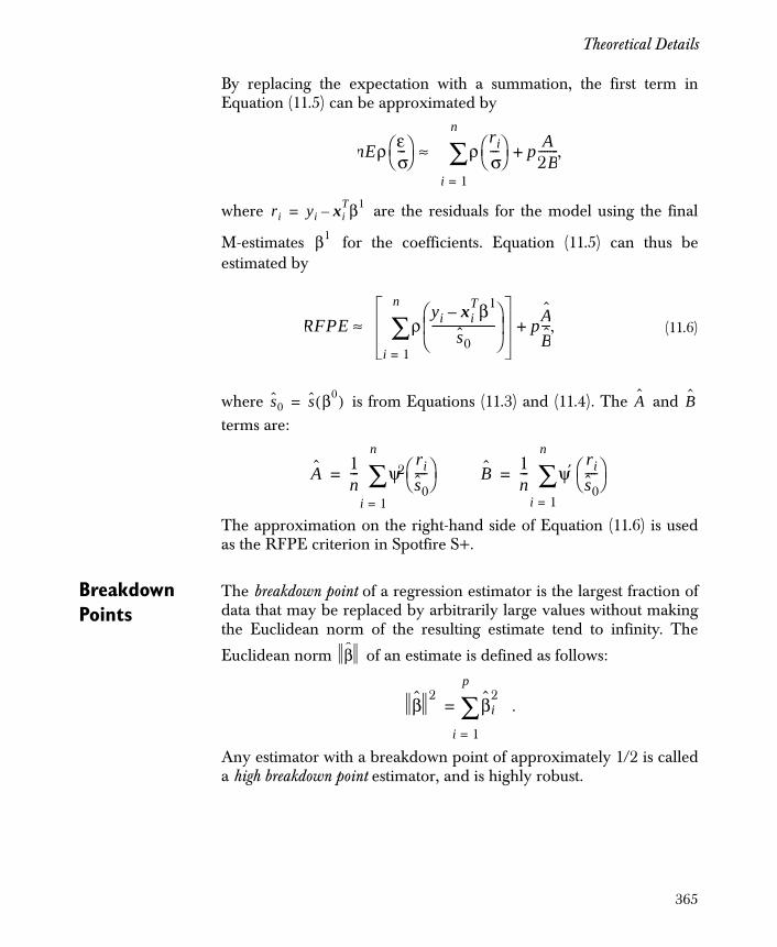
Theoretical Details
By replacing the expectation with a summation, the first term inEquation (11.5) can be approximated by
,
where are the residuals for the model using the final
M-estimates for the coefficients. Equation (11.5) can thus beestimated by
where is from Equations (11.3) and (11.4). The and terms are:
The approximation on the right-hand side of Equation (11.6) is usedas the RFPE criterion in Spotfire S+.
Breakdown Points
The breakdown point of a regression estimator is the largest fraction ofdata that may be replaced by arbitrarily large values without makingthe Euclidean norm of the resulting estimate tend to infinity. The
Euclidean norm of an estimate is defined as follows:
.
Any estimator with a breakdown point of approximately 1/2 is calleda high breakdown point estimator, and is highly robust.
, (11.6)
nEρ εσ---⎝ ⎠
⎛ ⎞ ρriσ---⎝ ⎠
⎛ ⎞ p A2B-------+
i 1=
n
∑≈
ri yi xiTβ1–=
β1
RFPE ρyi xi
Tβ1–
s0----------------------
⎝ ⎠⎜ ⎟⎛ ⎞
i 1=
n
∑ pAB---+≈
s0 s β0( )= A B
A 1n--- ψ2
ris0----⎝ ⎠
⎛ ⎞
i 1=
n
∑= B 1n--- ψ′
ris0----⎝ ⎠
⎛ ⎞
i 1=
n
∑=
β
β2
βi2
i 1=
p
∑=
365
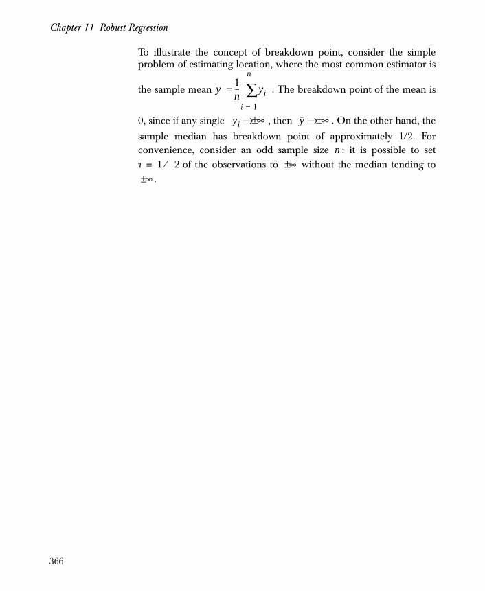
Chapter 11 Robust Regression
To illustrate the concept of breakdown point, consider the simpleproblem of estimating location, where the most common estimator is
the sample mean . The breakdown point of the mean is
0, since if any single , then . On the other hand, the
sample median has breakdown point of approximately 1/2. Forconvenience, consider an odd sample size : it is possible to set
of the observations to without the median tending to.
y 1n--- yi
i 1=
n
∑=
yi ∞±→ y ∞±→
nn 1 2⁄= ∞±
∞±
366

Other Robust Regression Techniques
OTHER ROBUST REGRESSION TECHNIQUES
Least Trimmed Squares Regression
Least trimmed squares (LTS) regression, introduced by Rousseeuw(1984), is a highly robust method for fitting a linear regression model.
The LTS estimate for the coefficients in a linear modelminimizes the following objective function:
where is the ith ordered residual. The value of is often set to be
slightly larger than half of , the number of observations in the
model. In contrast, the ordinary least squares estimate for theregression coefficients minimizes the sum of all squared residuals:
Thus, LTS is equivalent to ordering the residuals from a least squaresfit, trimming the observations that correspond to the largest residuals,and then computing a least squares regression model for theremaining observations. The ordinary least squares estimator lacks
robustness because a single observation can cause to take on anyvalue. The same is true of M-estimators, which are discussed in thesection M-Estimates of Regression.
To compute a least trimmed squares regression model, use the ltsregfunction. For the stack.df data introduced in the section Visualizingand Summarizing Robust Fits, we compute LTS estimates as follows:
> stack.lts <- ltsreg(Loss ~ ., data = stack.df)
, (11.7)
. (11.8)
βLTS
ri2β
i 1=
q
∑
riβ qn
βLS
ri2β
i 1=
n
∑
βLS
367
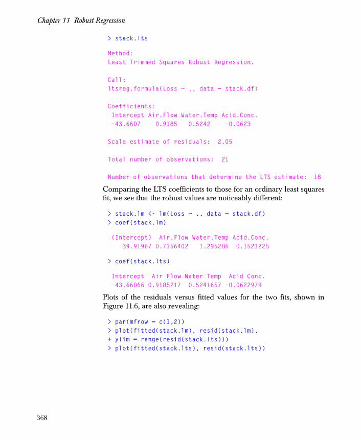
Chapter 11 Robust Regression
> stack.lts
Method:Least Trimmed Squares Robust Regression.
Call:ltsreg.formula(Loss ~ ., data = stack.df)
Coefficients: Intercept Air.Flow Water.Temp Acid.Conc. -43.6607 0.9185 0.5242 -0.0623
Scale estimate of residuals: 2.05
Total number of observations: 21
Number of observations that determine the LTS estimate: 18
Comparing the LTS coefficients to those for an ordinary least squaresfit, we see that the robust values are noticeably different:
> stack.lm <- lm(Loss ~ ., data = stack.df)> coef(stack.lm)
(Intercept) Air.Flow Water.Temp Acid.Conc. -39.91967 0.7156402 1.295286 -0.1521225
> coef(stack.lts)
Intercept Air Flow Water Temp Acid Conc. -43.66066 0.9185217 0.5241657 -0.0622979
Plots of the residuals versus fitted values for the two fits, shown inFigure 11.6, are also revealing:
> par(mfrow = c(1,2))> plot(fitted(stack.lm), resid(stack.lm),+ ylim = range(resid(stack.lts)))> plot(fitted(stack.lts), resid(stack.lts))
368
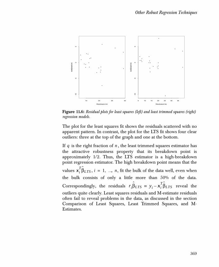
Other Robust Regression Techniques
The plot for the least squares fit shows the residuals scattered with noapparent pattern. In contrast, the plot for the LTS fit shows four clearoutliers: three at the top of the graph and one at the bottom.
If is the right fraction of , the least trimmed squares estimator hasthe attractive robustness property that its breakdown point isapproximately 1/2. Thus, the LTS estimator is a high-breakdownpoint regression estimator. The high breakdown point means that the
values , , fit the bulk of the data well, even when
the bulk consists of only a little more than 50% of the data.
Correspondingly, the residuals reveal the
outliers quite clearly. Least squares residuals and M-estimate residualsoften fail to reveal problems in the data, as discussed in the sectionComparison of Least Squares, Least Trimmed Squares, and M-Estimates.
Figure 11.6: Residual plots for least squares (left) and least trimmed squares (right) regression models.
•
•
•
•
•
••
•
•
•
••
•
•
•
•
•
• •
•
•
fitted(stack.lm)
resi
d(st
ack.
lm)
10 20 30 40
-10
-50
5
•
•
•
•
••
•
•
•
••
•
•
•
•
••
••
•
•
fitted(stack.lts)
resi
d(st
ack.
lts)
5 10 15 20 25 30 35
-10
-50
5
q n
xiTβLTS i 1 … n, ,=
riβLTS yi xiTβLTS–=
369
Chapter 11 Robust Regression
Least Median Squares Regression
Similar to least trimmed squares regression is a method called leastmedian of squares (LMS). Rather than minimize a sum of the squaredresiduals as LTS does, LMS minimizes the median of the squaredresiduals (Rousseeuw 1984). In Spotfire S+, the lmsreg functionperforms least median of squares regression.
LMS regression has a high breakdown point of almost 50%. That is,almost half of the data can be corrupted in an arbitrary fashion, andthe estimates obtained by LMS continue to model the majority of thedata well. However, least median of squares is statistically veryinefficient. It is due to this inefficiency that we recommend thelmRobMM and ltsreg functions over lmsreg.
Least Absolute Deviation Regression
The idea of least absolute deviation (L1) regression is actually older thanthat of least squares, but until the development of high-speedcomputers, it was too cumbersome to have wide applicability. As its
name implies, L1 regression finds the coefficients estimate thatminimizes the sum of the absolute values of the residuals:
.
In Spotfire S+, the function l1fit is used to compute a least absolutedeviation regression model (note that the second character in thefunction name is the number “1”, not the letter “l”). As an example,consider again the stack loss data introduced in the sectionVisualizing and Summarizing Robust Fits. We construct an L1regression model using l1fit as follows:
> stack.l1 <- l1fit(stack.x, stack.loss)> stack.l1
$coefficients: Intercept Air Flow Water Temp Acid Conc. -39.68986 0.8318838 0.5739132 -0.06086949
βL1
riβ
i 1=
n
∑
370

Other Robust Regression Techniques
$residuals: [1] 5.06087255 0.00000000 5.42898655 7.63478327 [5] -1.21739066 -1.79130375 -1.00000000 0.00000000 [9] -1.46376956 -0.02028821 0.52753741 0.04058089[13] -2.89854980 -1.80289757 1.18260884 0.00000000[17] -0.42608649 0.00000000 0.48695672 1.61739194[21] -9.48115635
Plots of the residuals against the fitted values for statck.l1 show theoutliers more clearly than the least squares regression model, but notas clearly as ltsreg does in Figure 11.6:
> par(mfrow = c(1,2))> plot(fitted(stack.lm), resid(stack.lm),+ ylim = range(resid(stack.l1)))> plot(stack.loss - resid(stack.l1), resid(stack.l1))
The resulting plot is shown in Figure 11.7.
Figure 11.7: Residual plots for least squares (left) and least absolute deviation (right) regression models.
•
•
•
•
•
••
•
•
•
••
•
•
•
•
•
• •
•
•
fitted(stack.lm)
resi
d(st
ack.
lm)
10 20 30 40
-10
-50
5 •
•
•
•
••
•
•
•
••
•
•
•
•
••
••
•
•
stack.loss - resid(stack.l1)
resi
d(st
ack.
l1)
10 15 20 25 30 35
-10
-50
5
371

Chapter 11 Robust Regression
M-Estimates of Regression
The M-estimator of regression was first introduced by Huber in 1973. For
a given function, an M-estimate of regression minimizes theobjective function:
Least squares regression corresponds to and L1 regression
corresponds to . Generally, the value of is dependent
on the value of , which is usually unknown.
Although M-estimates are protected against wild values in theresponse variable, they are sensitive to high leverage points, which havevery different values compared to the other data points in a model.In particular, a typographical error in an explanatory variable canhave a dramatic affect on an M-estimate, while least trimmed squareshandles this situation easily. One advantage of M-estimates is thatthey can be computed in much less time than LTS or other high-breakdown point estimators. For more discussion about high leveragepoints, see the section Comparison of Least Squares, Least TrimmedSquares, and M-Estimates.
In Spotfire S+, you can calculate M-estimates of regression using therreg function, which computes iteratively reweighted least-squares fits. Inthe fitting algorithm, an initial model is calculated using traditionalweighted least squares by default. The algorithm computes a new setof weights based on the results of the initial fit. The new weights arethen used in another weighted least squares fit, and so on. Spotfire S+continues iteratively until some convergence criteria are satisfied or aspecified maximum number of iterations is reached.
To use the rreg function, the only required arguments are x, thevector or matrix of explanatory variables, and y, the vector response.For example, a typical call to rreg using the stack loss data is:
> stack.M <- rreg(stack.x, stack.loss)
. (11.9)
ρ βM
ρriβσ
-------⎝ ⎠⎛ ⎞
i 1=
n
∑
ρ x( ) x2=
ρ x( ) x= βM
σ
x
372

Other Robust Regression Techniques
> stack.M
$coefficients: (Intercept) Air Flow Water Temp Acid Conc. -42.07438 0.8978265 0.731816 -0.1142602
$residuals: [1] 2.65838630 -2.45587390 3.72541082 6.78619020 [5] -1.75017776 -2.48199378 -1.52824862 -0.52824862 [9] -1.89068795 -0.03142924 0.99691253 0.61446835[13] -2.80290885 -1.27786270 2.17952419 0.83674360[17] -0.49471517 0.30510621 0.68755039 1.52911203[21] -10.01211661
$fitted.values: [1] 39.341614 39.455874 33.274589 21.213810 19.750178 [6] 20.481994 20.528249 20.528249 16.890688 14.031429[11] 13.003087 12.385532 13.802909 13.277863 5.820476[16] 6.163256 8.494715 7.694894 8.312450 13.470888[21] 25.012117
$w: [1] 0.87721539 0.91831885 0.77235329 0.41742415 0.95387576 [6] 0.90178786 0.95897484 0.99398847 0.93525890 0.99958817[11] 0.97640677 0.98691782 0.89529949 0.98052477 0.92540436[16] 0.98897286 0.99387986 0.99933718 0.99574820 0.96320721[21] 0.07204303
$int:[1] T
$conv:[1] 0.175777921 0.036317063 0.021733577 0.013181419[5] 0.007426725 0.003341872 0.093998053 0.055029889
$status:[1] "converged"
You can control the choice of by specifying a weight function as themethod argument to rreg. Currently, there are eleven weightfunctions built into Spotfire S+, and there is not yet a consensus onwhich method is the “best.” See the rreg help file for details on each
ρ
373
Chapter 11 Robust Regression
of the weight functions available. The default weight function usesHuber’s function until convergence, and then a bisquare function fortwo more iterations. Huber’s function is defined as:
where is a tuning constant. The bisquare function implemented inrreg is:
.
Here again, is a tuning parameter.
The following call to rreg defines a simple weight function for the
stack loss data that corresponds to the least squares choice :
> stack.MLS <- rreg(stack.x, stack.loss,+ method = function(u) 2*abs(u), iter = 100)
Warning messages: failed to converge in 100 steps
> coef(stack.MLS)
(Intercept) Air Flow Water Temp Acid Conc. -39.68049 0.7166834 1.298541 -0.156553
> coef(stack.lm)
(Intercept) Air.Flow Water.Temp Acid.Conc. -39.91967 0.7156402 1.295286 -0.1521225
ρ x( )1 abs x( ) c<c
abs x( )---------------- abs x( ) c≥
⎩⎪⎨⎪⎧
=
c
ρ x( )1 x
c--⎝ ⎠
⎛ ⎞ 2–⎝ ⎠
⎛ ⎞ 2x c<
0 x c≥⎩⎪⎨⎪⎧
=
c
ρ x( ) x2=
374
Other Robust Regression Techniques
Comparison of Least Squares, Least Trimmed Squares, and M-Estimates
Plots of residuals are often used to reveal outliers in linear models. Asdiscussed in the section Least Trimmed Squares Regression, LTS is anrobust method that isolates outliers quite clearly in plots. However,residuals from least squares and M-estimator regression models oftenfail to reveal problems in the data. We illustrate this point with acontrived example.
First, we construct an artificial data set with sixty percent of the datascattered about the line , and the remaining forty percent in anoutlying cluster centered at .
# set the seed to reproduce this example> set.seed(14)> x30 <- runif(30, mean = 0.5, sd = 4.5)> e30 <- rnorm(30, mean = 0, sd = 0.2)> y30 <- 2 + x30 + e30> x20 <- rnorm(20, mean = 6, sd = 0.5)> y20 <- rnorm(20, mean = 2, sd = 0.5)> x <- c(x30, x20)> y <- c(y30, y20)
We plot the data, and then fit three different regression lines: theordinary least squares line, an M-estimate line, and the least trimmedsquared line.
> plot(x, y)> abline(lm(y ~ x))> text(5, 3.4, "LS")> abline(rreg(x, y))> text(4, 3.2, "M")> abline(ltsreg(x, y))> text(4, 6.5, "LTS")
The resulting plot is shown in Figure 11.8. Note that all threeregression lines are influenced by the leverage points in the outlyingcluster.
y x=
6 2( , )
375
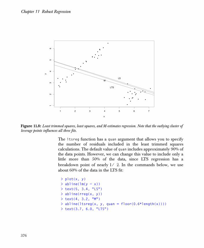
Chapter 11 Robust Regression
The ltsreg function has a quan argument that allows you to specifythe number of residuals included in the least trimmed squarescalculations. The default value of quan includes approximately 90% ofthe data points. However, we can change this value to include only alittle more than 50% of the data, since LTS regression has abreakdown point of nearly . In the commands below, we useabout 60% of the data in the LTS fit:
> plot(x, y)> abline(lm(y ~ x))> text(5, 3.4, "LS")> abline(rreg(x, y))> text(4, 3.2, "M")> abline(ltsreg(x, y, quan = floor(0.6*length(x))))> text(3.7, 6.0, "LTS")
Figure 11.8: Least trimmed squares, least squares, and M-estimates regression. Note that the outlying cluster of leverage points influences all three fits.
•
•
•
•
•
•
•
•
•
•
•
•
•
•
•••
•
•
•
•
•
•
•
•
•
• •
•
•
•
•
•••
•
•
•
••
••
•
•
•
•
•
••
•
x
y
1 2 3 4 5 6 7
12
34
56
LSM
LTS
1 2⁄
376
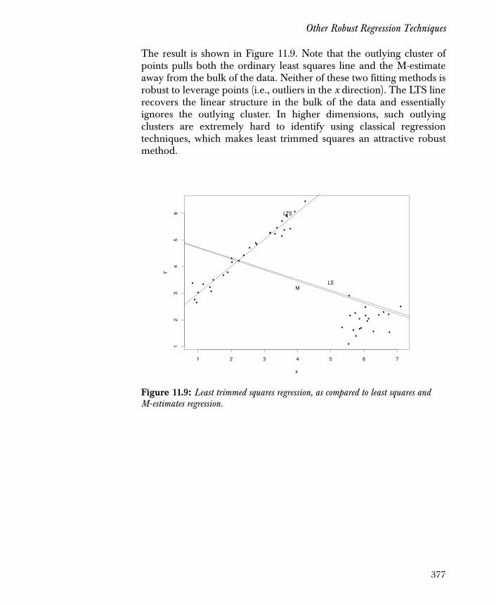
Other Robust Regression Techniques
The result is shown in Figure 11.9. Note that the outlying cluster ofpoints pulls both the ordinary least squares line and the M-estimateaway from the bulk of the data. Neither of these two fitting methods isrobust to leverage points (i.e., outliers in the x direction). The LTS linerecovers the linear structure in the bulk of the data and essentiallyignores the outlying cluster. In higher dimensions, such outlyingclusters are extremely hard to identify using classical regressiontechniques, which makes least trimmed squares an attractive robustmethod.
Figure 11.9: Least trimmed squares regression, as compared to least squares and M-estimates regression.
•
•
•
•
•
•
•
•
•
•
•
•
•
•
•••
•
•
•
•
•
•
•
•
•
• •
•
•
•
•
•••
•
•
•
••
••
•
•
•
•
•
••
•
x
y
1 2 3 4 5 6 7
12
34
56
LSM
LTS
377
Chapter 11 Robust Regression
REFERENCES
Hampel, F., Ronchetti, E.M., Rousseeuw, P.J., & Stahel, W.A. (1986).Robust Statistics: the Approach Based on Influence Functions. New York:John Wiley & Sons, Inc.
Huber, P.J. (1981). Robust Statistics. New York: John Wiley & Sons, Inc.
Marazzi, A. (1993). Algorithms, Routines, and S Functions for RobustStatistics. Pacific Grove, CA: Wadsworth & Brooks/Cole.
Martin, R.D. & Zamar, R.H. (1989). Asymptotically min-max robustM-estimates of scale for positive random variables. Journal of theAmerican Statistical Association 84: 494-501.
Martin, R.D. & Zamar, R.H. (1993). Bias robust estimates of scale.Annals of Statistics 21: 991-1017.
Ronchetti, E. (1985). Robust model selection in regression. Spotfire S+Statistics & Probability Letters 3: 21-23.
Rousseeuw, P.J. (1984). Least median of squares regression. Journal ofthe American Statistical Association 79: 871-881.
Rousseeuw, P.J. & Yohai, V. (1984). Robust regression by means ofS-estimators. In Robust and Nonlinear Time Series Analysis, J. Franke, W.Hardle, & R.D. Martin (Eds.). Lecture Notes in Statistics, 26: 256-272.New York: Springer-Verlag.
Wilcox, R.R. (1997). Introduction to Robust Estimation and HypothesisTesting. San Diego: Academic Press.
Yohai, V.J. (1987). High Breakdown-Point and High EfficiencyEstimates for Regression. Annals of Statistics 15: 642-665.
Yohai, V.J. (1997). A New Robust Model Selection Criterion forLinear Models: RFPE (unpublished note).
Yohai, V., Stahel, W.A., & Zamar, R.H. (1991). A procedure for robustestimation and inference in linear regression. In Directions in RobustStatistics and Diagnostics, Part II, W.A. Stahel & S.W. Weisberg (Eds.).New York: Springer-Verlag.
Yohai, V.J. & Zamar, R.H. (1998). Optimal locally robust M-estimatesof regression. Journal of Statistical Planning and Inference 64: 309-323.
378

Introduction 380
Generalized Linear Models 381
Generalized Additive Models 385
Logistic Regression 387Fitting a Linear Model 388Fitting an Additive Model 394Returning to the Linear Model 398Legal Forms of the Response Variable 402
Probit Regression 404
Poisson Regression 407
Quasi-Likelihood Estimation 415
Residuals 418
Prediction from the Model 420Predicting the Additive Model of Kyphosis 420Safe Prediction 422
Advanced Topics 424Fixed Coefficients 424Family Objects 425
References 432
GENERALIZING THE LINEAR MODEL 12
379
Chapter 12 Generalizing the Linear Model
INTRODUCTION
Least squares estimation of regression coefficients for linear modelsdates back to the early nineteenth century. It met with immediatesuccess as a simple way of mathematically summarizing relationshipsbetween observed variables of real phenomena. It quickly becameand remains one of the most widely used statistical methods ofpracticing statisticians and scientific researchers.
Because of the simplicity, elegance, and widespread use of the linearmodel, researchers and statisticians have tried to adapt itsmethodology to different data configurations. For example, it shouldbe possible to relate a categorical response (or some transformation ofit) to a set of predictor variables, similar to the role a continuousresponse takes in the linear model. Although conceptually plausible,the development of regression models for categorical responseslacked solid theoretical foundation until the introduction of thegeneralized linear model by Nelder and Wedderburn (1972).
This chapter focuses on generalized linear models and generalizedadditive models, as they apply to categorical responses. In particular,we focus on logistic, probit, and Poisson regressions. We also includea brief discussion on the quasi-likelihood method, which fits modelswhen an exact likelihood cannot be specified.
380

Generalized Linear Models
GENERALIZED LINEAR MODELS
The linear model discussed in Chapter 10, Regression and Smoothingfor Continuous Response Data, is a special case of the generalizedlinear model. A linear model provides a way of estimating theresponse variable , conditional on a linear function of the values
of some set of predictors variables, .Mathematically, we write this as:
For the linear model, the variance of is assumed to be constant, and
is denoted by .
A generalized linear model (GLM) provides a way of estimating afunction of the mean response as a linear combination of some set ofpredictors. This is written as:
The function of the mean response, , is called the link function,and the linear function of the predictors, , is called the linearpredictor. For the generalized linear model, the variance of may be afunction of the mean response :
.
To compute generalized linear models in TIBCO Spotfire S+, we canuse the glm function.
. (12.1)
. (12.2)
Yx1 x2 … x, p, , X1 X2 … X, p, ,
E Y x( ) β0 βixii 1=
p
∑+=
Y
var Y( ) σ2=
g E Y x( )( ) g μ( ) β0 βixii 1=
p
∑+ η x( )= = =
g μ( )η x( )
Yμ
var Y( ) φV μ( )=
381
Chapter 12 Generalizing the Linear Model
Three special cases of generalized linear models are the logistic,probit, and Poisson regressions. Logistic regression models data inwhich the response variable is categorical and follows a binomialdistribution. To do a logistic regression in Spotfire S+, we declare thebinomial family in glm. This uses the logit link function
,
and the variance function defined by
.
Here, is the probability of an event occurring, and corresponds tothe mean response of a binary (0-1) variable. In logistic regression, wemodel the probability of some event occurring as a linear function ofa set of predictors. The most common examples of logistic responsevariables include the presence/absence of AIDS, the presence/absence of a plant species in a vegetation sample, and the failure/non-failure of a electronic component in a radio.
Like logistic regression, probit regression models data in which theresponse variable follows a binomial distribution. It describes theprobability of some event occurring as a linear function of predictors,and therefore uses the same variance function as logistic models:
.
However, probit regression uses the probit link function
,
where is the Gaussian cumulative distribution function, and isits inverse. To do a probit regression in Spotfire S+, we declare thebinomial(link=probit) family in glm. This kind of regression ispopular in bioassay problems.
g p( ) logit p( ) p1 p–------------log= =
var Y( ) φ p1 p–------------=
p
var Y( ) φ p1 p–------------=
g p( ) F 1– p( )=
F F 1–
382

Generalized Linear Models
Poisson regression models data in which the response variablerepresents counts. To do a Poisson regression in Spotfire S+, wedeclare the poisson family in glm. This uses the log link function
,
and the variance function defined by
.
The Poisson family is useful for modeling count data that typicallyfollows a Poisson distribution. Common examples include tables ofrates, in which the rate of a particular event is classified according to anumber of categorical predictors. The example we present in thesection Poisson Regression models the number of soldering skips as afunction of various controlled factors in a solder experiment.
Usually, is fixed to be 1 in the variance function of a generalizedlinear model. When we cannot assume that , we must use thequasi family in glm for quasi-likelihood estimation. This is the case ofover- or under-dispersion, as discussed in McCullagh and Nelder(1989). The quasi-likelihood family allows us to estimate theparameters in a model without specifying the underlying distributionfunction. In this case, the link and variance functions are all that areused to fit the model. Once these are known, the same iterativeprocedure used for fitting the other families can be used to estimatethe model parameters. For more details, see Chambers and Hastie(1992) and McCullagh and Nelder (1989).
Other families are available in glm for modeling various kinds of dataas linear functions of predictors. For example, normal and inversenormal distributions are specified with the gaussian andinverse.gaussian families. Table 12.1 lists the distribution familiesavailable for use with the glm function.
g μ( ) μ( )log=
var Y( ) φμ=
φφ 1=
383
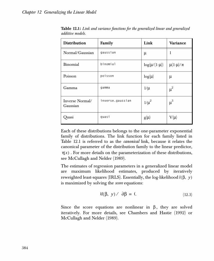
Chapter 12 Generalizing the Linear Model
Each of these distributions belongs to the one-parameter exponentialfamily of distributions. The link function for each family listed inTable 12.1 is referred to as the canonical link, because it relates thecanonical parameter of the distribution family to the linear predictor,
. For more details on the parameterization of these distributions,see McCullagh and Nelder (1989).
The estimates of regression parameters in a generalized linear modelare maximum likelihood estimates, produced by iterativelyreweighted least-squares (IRLS). Essentially, the log-likelihood is maximized by solving the score equations:
Since the score equations are nonlinear in , they are solvediteratively. For more details, see Chambers and Hastie (1992) orMcCullagh and Nelder (1989).
Table 12.1: Link and variance functions for the generalized linear and generalized additive models.
Distribution Family Link Variance
Normal/Gaussian gaussian μ 1
Binomial binomial log(μ/(1-μ)) μ(1-μ)/n
Poisson poisson log(μ) μ
Gamma gamma 1/μ μ2
Inverse Normal/Gaussian
inverse.gaussian 1/μ2 μ3
Quasi quasi g(μ) V(μ)
. (12.3)
η x( )
l β y,( )
∂l β y,( ) ∂β⁄ 0=
β
384

Generalized Additive Models
GENERALIZED ADDITIVE MODELS
The section Generalized Linear Models discusses an extension oflinear models to data with error distributions other than normal(Gaussian). By using the glm function, we can fit data with Gaussian,binomial, Poisson, gamma, or inverse Gaussian errors. Thisdramatically broadens the kind of data for which we can buildregression models.
The primary restriction of a GLM is the fact that the linear predictor is still a linear function of the parameters in the model. The
generalized additive model (GAM) extends the generalized linearmodel by fitting nonparametric functions to estimate relationshipsbetween the response and the predictors. The nonparametricfunctions are estimated from the data using smoothing operations. Tocompute generalized additive models in Spotfire S+, we can use thegam function. Because GLMs are a special instance of GAMs, we canfit genearlized linear models using the gam function as well.
The form of a generalized additive model is:
where is the link function and is a constant intercept term. InEquation (12.4), corresponds to the nonparametric functiondescribing the relationship between the transformed mean response
and the ith predictor. In this context, is referred to as theadditive predictor, and is entirely analogous to the linear predictor of aGLM as defined in Equation (12.2). As for the generalized linearmodel, the variance of in a GAM may be function of the meanresponse :
.
, (12.4)
η x( )
g E Y( x )( ) g μ( ) α fi xi( )i 1=
p
∑+ η x( )= = =
g μ( ) αfi
g μ( ) η x( )
Yμ
var Y( ) φV μ( )=
385

Chapter 12 Generalizing the Linear Model
All of the distribution families listed in Table 12.1 are available forgeneralized additive models. Thus fully nonparametric, nonlinearadditive regression models can be fit to binomial data (logistic andprobit regression) and count data (Poisson regression), as well as todata with error distributions given by the other families in Table 12.1.
Two functions that are useful for fitting a gam are s and lo. Both ofthese functions are used to fit smooth relationships between thetransformed response and the predictors. The s function fits cubicB-splines to estimate the smooth, and lo fits a locally weighted least-squares regression to estimate the smooth. For more details on usingthese functions, see their help files.
386
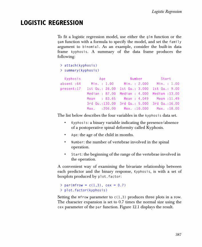
Logistic Regression
LOGISTIC REGRESSION
To fit a logistic regression model, use either the glm function or thegam function with a formula to specify the model, and set the familyargument to binomial. As an example, consider the built-in dataframe kyphosis. A summary of the data frame produces thefollowing:
> attach(kyphosis)> summary(kyphosis)
Kyphosis Age Number Startabsent :64 Min. : 1.00 Min. : 2.000 Min. : 1.00present:17 1st Qu.: 26.00 1st Qu.: 3.000 1st Qu.: 9.00 Median : 87.00 Median : 4.000 Median :13.00 Mean : 83.65 Mean : 4.049 Mean :11.49 3rd Qu.:130.00 3rd Qu.: 5.000 3rd Qu.:16.00 Max. :206.00 Max. :10.000 Max. :18.00
The list below describes the four variables in the kyphosis data set.
• Kyphosis: a binary variable indicating the presence/absence of a postoperative spinal deformity called Kyphosis.
• Age: the age of the child in months.
• Number: the number of vertebrae involved in the spinal operation.
• Start: the beginning of the range of the vertebrae involved in the operation.
A convenient way of examining the bivariate relationship betweeneach predictor and the binary response, Kyphosis, is with a set ofboxplots produced by plot.factor:
> par(mfrow = c(1,3), cex = 0.7)> plot.factor(kyphosis)
Setting the mfrow parameter to c(1,3) produces three plots in a row.The character expansion is set to 0.7 times the normal size using thecex parameter of the par function. Figure 12.1 displays the result.
387
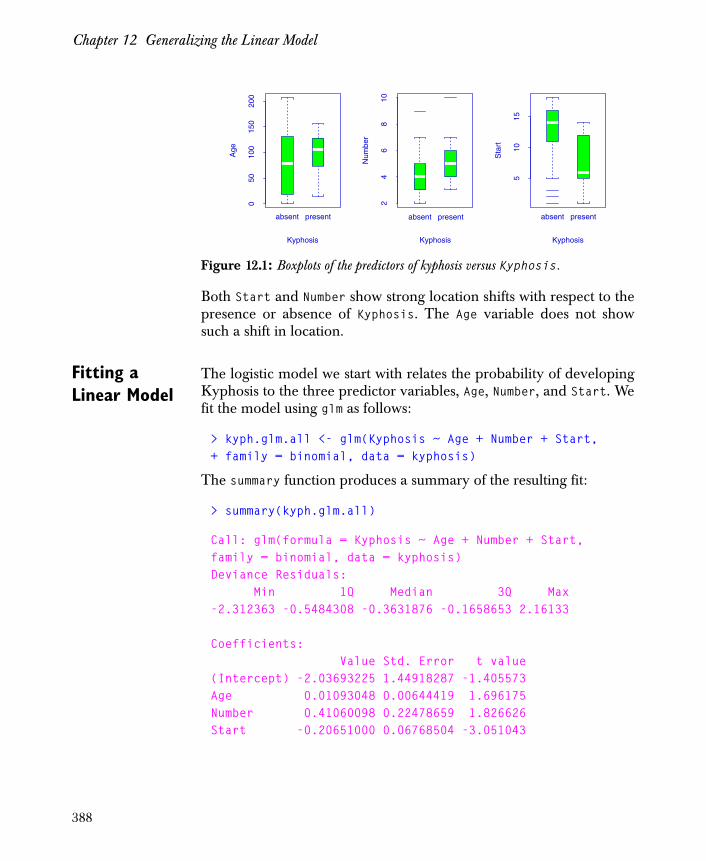
Chapter 12 Generalizing the Linear Model
Both Start and Number show strong location shifts with respect to thepresence or absence of Kyphosis. The Age variable does not showsuch a shift in location.
Fitting a Linear Model
The logistic model we start with relates the probability of developingKyphosis to the three predictor variables, Age, Number, and Start. Wefit the model using glm as follows:
> kyph.glm.all <- glm(Kyphosis ~ Age + Number + Start,+ family = binomial, data = kyphosis)
The summary function produces a summary of the resulting fit:
> summary(kyph.glm.all)
Call: glm(formula = Kyphosis ~ Age + Number + Start,family = binomial, data = kyphosis)Deviance Residuals: Min 1Q Median 3Q Max-2.312363 -0.5484308 -0.3631876 -0.1658653 2.16133
Coefficients: Value Std. Error t value(Intercept) -2.03693225 1.44918287 -1.405573Age 0.01093048 0.00644419 1.696175Number 0.41060098 0.22478659 1.826626Start -0.20651000 0.06768504 -3.051043
Figure 12.1: Boxplots of the predictors of kyphosis versus Kyphosis.0
5010
015
020
0
Age
absent present
Kyphosis
24
68
10
Num
ber
absent present
Kyphosis
510
15
Sta
rt
absent present
Kyphosis
388

Logistic Regression
(Dispersion Parameter for Binomial family taken to be 1 )
Null Deviance: 83.23447 on 80 degrees of freedom
Residual Deviance: 61.37993 on 77 degrees of freedom
Number of Fisher Scoring Iterations: 5
Correlation of Coefficients: (Intercept) Age Number Age -0.4633715Number -0.8480574 0.2321004 Start -0.3784028 -0.2849547 0.1107516
The summary includes:
1. a replica of the call that generated the fit,
2. a summary of the deviance residuals (we discuss residuals later in this chapter),
3. a table of estimated regression coefficients, their standard errors, and the partial t-test of their significance,
4. estimates of the null and residual deviances, and
5. a correlation matrix of the coefficient estimates.
The partial t-tests indicate that Start is important even after adjustingfor Age and Number, but they provide little information on the othertwo variables.
You can produce an analysis of deviance for the sequential additionof each variable by using the anova function, specifying the chi-squaretest to test for differences between models. The command belowshows this test for the kyph.glm.all model object.
> anova(kyph.glm.all, test = "Chi")
Analysis of Deviance Table
Binomial model
Response: Kyphosis
Terms added sequentially (first to last)
389

Chapter 12 Generalizing the Linear Model
Df Deviance Resid. Df Resid. Dev Pr(Chi) NULL 80 83.23447 Age 1 1.30198 79 81.93249 0.2538510Number 1 10.30593 78 71.62656 0.0013260Start 1 10.24663 77 61.37993 0.0013693
Here we see that Number is important after adjusting for Age. Wealready know that Number loses its importance after adjusting for Ageand Start. In addition, Age does not appear to be important as alinear predictor.
You can examine the bivariate relationships between the probabilityof Kyphosis and each of the predictors by fitting a “null” model andthen adding each of the terms, one at a time. The null model in thisexample has a single intercept term, and is specified with the formulaKyphosis ~ 1:
> kyph.glm.null <- glm(Kyphosis ~ 1, family = binomial,+ data = kyphosis)> add1(kyph.glm.null, ~ . + Age + Number + Start)
Single term additions
Model: Kyphosis ~ 1 Df Sum of Sq RSS Cp<none> 81.00000 83.02500Age 1 1.29546 79.70454 83.75454Number 1 10.55222 70.44778 74.49778Start 1 16.10805 64.89195 68.94195
The Cp statistic is used to compare models that are not nested. A smallCp value corresponds to a better model, in the sense of a smallerresidual deviance penalized by the number of parameters that areestimated in fitting the model.
From the above analysis, Start is clearly the best single variable touse in a linear model. These statistical conclusions, however, shouldbe verified by looking at graphical displays of the fitted values andresiduals. The plot method for generalized linear models is calledplot.glm, and produces four diagnostic plots:
1. a plot of deviance residuals versus the fitted values,
2. a plot of the square root of the absolute deviance residuals versus the linear predictor values,
390

Logistic Regression
3. a plot of the response versus the fitted values, and
4. a normal quantile plot of the Pearson residuals.
This set of plots is similar to those produced by the plot method for lmobjects.
Systematic curvature in the residual plots might be indicative ofproblems in the choice of link, the wrong scale for one of thepredictors, or omission of a quadratic term in a predictor. Largeresiduals can also be detected in these plots, and may be indicative ofoutlying observations that need to be removed from the analysis. Theplot of the absolute residuals against predicted values gives a visualcheck on the adequacy of the assumed variance function. The normalquantile plot is useful in detecting extreme observations deviatingfrom a general trend. However, one should exercise caution in notover-interpreting the shape of this plot, which is not necessarily ofinterest in the nonlinear context.
Figure 12.2 displays the four plots for the model involving all threepredictor variables: Age, Number, and Start. The plots are producedwith the following commands:
> par(mfrow = c(2,2))> plot(kyph.glm.all)
391
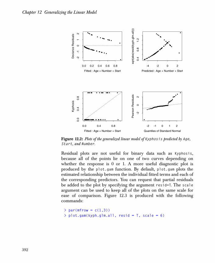
Chapter 12 Generalizing the Linear Model
Residual plots are not useful for binary data such as Kyphosis,because all of the points lie on one of two curves depending onwhether the response is 0 or 1. A more useful diagnostic plot isproduced by the plot.gam function. By default, plot.gam plots theestimated relationship between the individual fitted terms and each ofthe corresponding predictors. You can request that partial residualsbe added to the plot by specifying the argument resid=T. The scaleargument can be used to keep all of the plots on the same scale forease of comparison. Figure 12.3 is produced with the followingcommands:
> par(mfrow = c(1,3))> plot.gam(kyph.glm.all, resid = T, scale = 6)
Figure 12.2: Plots of the generalized linear model of Kyphosis predicted by Age, Start, and Number.
••
•
•
•••••
••
•
•
••••
•• •
•
•
•
•
•
• ••• •• • ••
•••
•
•
•
•
•
•
•
•
•
• •
•
• ••
••
•••
•
••
••
•
•••• •••
•••
•
••
•
••
•
•
Fitted : Age + Number + StartD
evia
nce
Res
idua
ls
0.0 0.2 0.4 0.6 0.8
-2-1
01
2
••
••
•• • • •
••
•
•
••
•
•
•
••
•
•
•
• •
••
•
••
•
••
•
•
• •
•
•
•
•
•
•
•
•
•
••
•
••
•
•
•
•••
••
•
•••
• •••
•
••
••
•
•
•
•
•
••
•
•
Predicted : Age + Number + Start
sqrt
(abs
(res
id(k
yph.
glm
.all)
))
-4 -2 0 2
0.4
0.8
1.2
••
•
••••••
••
• •••• • •• ••
••
•
•
• ••• •• • •• •••
•
•
• •
• •••
•
• •
•
• ••
•
• •••
•
••
••
••••• ••• ••• •• •
•
••
•
•
Fitted : Age + Number + Start
Kyp
hosi
s
0.0 0.4 0.8
0.0
0.4
0.8
• •
•
•• ••••
••
••
•• ••• •• ••
•
•
•
•• • •• ••• ••
••
•
•
•
••
•
••
•
••
•
•••••• • •
•
••
• •
•••• •• • •• • •
•••
•
• •
•
•
Quantiles of Standard NormalP
ears
on R
esid
uals
-2 -1 0 1 2
-20
2
392

Logistic Regression
These plots give a quick assessment of how well the model fits thedata by examining the fit of each term in the formula. The plots are ofthe adjusted relationship for each predictor, versus each predictor.When the relationship is linear, the label on the vertical axis reducesto the variable name. We will see the utility of this plot method andthe reason for the labels in the next section, where we plot additivemodels produced by gam.
Both plot.glm and plot.gam produce multiple plots. You can,however, choose which plots you look at by using the argumentask=T. This option produces a menu of available plots from whichyou select the number of the plot that you would like to see. Forexample, here is the menu of default GLM plots:
> plot(kyph.glm.all, ask = T)
Make a plot selection (or 0 to exit):
1: plot: All2: plot: Residuals vs Fitted Values3: plot: Sqrt of abs(Residuals) vs Predictions4: plot: Response vs Fitted Values5: plot: Normal QQplot of Std. ResidualsSelection:
Figure 12.3: Additional plots of the generalized linear model of Kyphosis predicted by Age, Number, and Start.
AgeA
ge
0 100 200
-20
12
3
•
•
•
•••
•••
••
•
••
•
••
••
••
•
•
••
••
••
•
•••• ••
•
•
•
•
•
•••
•
•
••
•
•
••
•
•
••
•
•
•
•
••
•
••
•
••
••
••••
•
•
•
•
••
•
Number
Num
ber
2 4 6 8 10
-20
12
3
••
•
••
•••
•
••
• ••
••
•••
••
••
•
•
•
•••••
•
•• •••
•
•
•
•
••
••
•
• •
•
•
••
•
••
••
•
•
•
•
•
•• ••
•••
••••
•• •
•
•
•
•
•
Start
Sta
rt
0 5 10
-20
12
3
•
•
•
•
•••••
• •
•
•
•
•••• •
•
•
• •
•
•
•
•
• ••••
• ••
•
•
•
•
•
•
••
•
•
•
••
•
••
•
•
••••
•
• •
•
•
•
••
•
••
•
•••
•• •
•
•
••
•
•
393
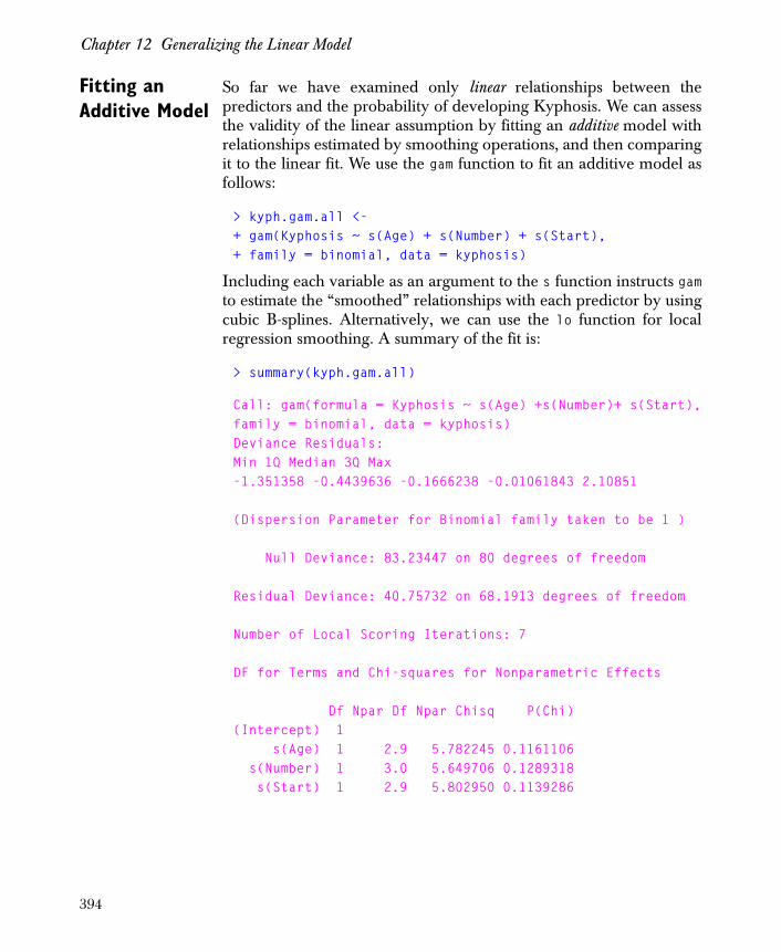
Chapter 12 Generalizing the Linear Model
Fitting an Additive Model
So far we have examined only linear relationships between thepredictors and the probability of developing Kyphosis. We can assessthe validity of the linear assumption by fitting an additive model withrelationships estimated by smoothing operations, and then comparingit to the linear fit. We use the gam function to fit an additive model asfollows:
> kyph.gam.all <-+ gam(Kyphosis ~ s(Age) + s(Number) + s(Start),+ family = binomial, data = kyphosis)
Including each variable as an argument to the s function instructs gamto estimate the “smoothed” relationships with each predictor by usingcubic B-splines. Alternatively, we can use the lo function for localregression smoothing. A summary of the fit is:
> summary(kyph.gam.all)
Call: gam(formula = Kyphosis ~ s(Age) +s(Number)+ s(Start),family = binomial, data = kyphosis)Deviance Residuals:Min 1Q Median 3Q Max-1.351358 -0.4439636 -0.1666238 -0.01061843 2.10851
(Dispersion Parameter for Binomial family taken to be 1 )
Null Deviance: 83.23447 on 80 degrees of freedom
Residual Deviance: 40.75732 on 68.1913 degrees of freedom
Number of Local Scoring Iterations: 7
DF for Terms and Chi-squares for Nonparametric Effects
Df Npar Df Npar Chisq P(Chi)(Intercept) 1 s(Age) 1 2.9 5.782245 0.1161106 s(Number) 1 3.0 5.649706 0.1289318 s(Start) 1 2.9 5.802950 0.1139286
394

Logistic Regression
The summary of a gam fit is similar to the summary of a glm fit. Onenoticeable difference, however, is in the analysis of deviance table.For an additive fit, the tests correspond to approximate partial tests forthe importance of the smooth for each term in the model. These testsare typically used to screen variables for inclusion in the model. For asingle-variable model, this is equivalent to testing for a differencebetween a linear fit and a smooth fit that includes both linear andsmooth terms. The approximate nature of the partial tests is discussedin detail in Hastie and Tibshirani (1990).
Since Start is the best single variable to use in the Kyphosis model,we fit a base GAM with a smooth of Start. For comparison, we fittwo additional models that build on the base model: one with asmooth of the Age variable and one with a smooth of the Numbervariable.
> kyph.gam.start <- gam(Kyphosis ~ s(Start), + family = binomial, data = kyphosis)
> kyph.gam.start.age <-+ gam(Kyphosis ~ s(Start) + s(Age),+ family = binomial, data = kyphosis)
> kyph.gam.start.number <-+ gam(Kyphosis ~ s(Start) + s(Number),+ family = binomial, data = kyphosis)
We produce the following analysis of deviance tables:
> anova(kyph.gam.start, kyph.gam.start.age, test = "Chi")
Analysis of Deviance Table
Response: Kyphosis
Terms Resid. Df Resid. Dev1 s(Start) 76.24543 59.112622 s(Start) + s(Age) 72.09458 48.41713 Test Df Deviance Pr(Chi)12 +s(Age) 4.150842 10.69548 0.0336071
> anova(kyph.gam.start, kyph.gam.start.number,+ test = "Chi")
395

Chapter 12 Generalizing the Linear Model
Analysis of Deviance Table
Response: Kyphosis
Terms Res.Df Res.Dev1 s(Start) 76.24543 59.112622 s(Start)+s(Number) 72.18047 54.17895 Test Df Deviance Pr(Chi)12 +s(Number) 4.064954 4.933668 0.3023856
The indication is that Age is important in the model even with Startincluded, whereas Number is not important under the same conditions.
With the following commands, we plot the fit that includes the Ageand Start variables, adding partial residuals and maintaining thesame scale for all figures:
> par(mfrow = c(2,2))> plot(kyph.gam.start.age, resid = T, scale = 8)
The result is displayed in the top two plots of Figure 12.4. With thefollowing command, we plot the fit and add pointwise confidenceintervals:
> plot(kyph.gam.start.age, se = T, scale = 10)
The result is displayed in the bottom two plots of Figure 12.4. Noticethe labels on the vertical axes, which reflect the smoothing operationincluded in the modeling.
396

Logistic Regression
The summary of the additive fit with smooths of Age and Startappears as follows:
> summary(kyph.gam.start.age)
Call: gam(formula = Kyphosis ~ s(Start) + s(Age),family = binomial, data = kyphosis)
Figure 12.4: The partial fits for the generalized additive logistic regression model of Kyphosis with Age and Start as predictors.
Start
s(S
tart
)
5 10 15
-6-4
-20
2
•
•
•
•
•
•
•
••
•
•
•
••
•
•
•
•
•
•
•
•
•
•
•
•
•
•
•••
••
•
•
•
•
•
••
•
•••
•
•
•
•
•
•
•
•
•
•
••
•
•
•
•
• •
•
•
•
•
•
•
•
••
•
•
••
•
••
•
•
Age
s(A
ge)
0 50 100 150 200
-4-2
02
4
••
•
•••
•
•
•
•
•
•
••
•
•
•
•
•
••
••
•
•
••
•
•
•
•••
•
•
•
•
•
•
••
• ••
••
••
•
••
•
•
•
••
•
•
•
•
••
•
•
••
•
••
••
•
••
•
•
•
••
•
Start
s(S
tart
)
5 10 15
-10
-50
Age
s(A
ge)
0 50 100 150 200
-6-4
-20
2
397
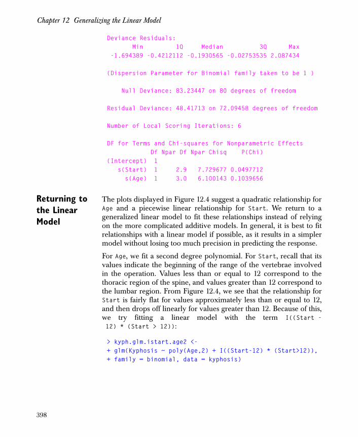
Chapter 12 Generalizing the Linear Model
Deviance Residuals: Min 1Q Median 3Q Max -1.694389 -0.4212112 -0.1930565 -0.02753535 2.087434
(Dispersion Parameter for Binomial family taken to be 1 )
Null Deviance: 83.23447 on 80 degrees of freedom
Residual Deviance: 48.41713 on 72.09458 degrees of freedom
Number of Local Scoring Iterations: 6
DF for Terms and Chi-squares for Nonparametric Effects Df Npar Df Npar Chisq P(Chi)(Intercept) 1 s(Start) 1 2.9 7.729677 0.0497712 s(Age) 1 3.0 6.100143 0.1039656
Returning to the Linear Model
The plots displayed in Figure 12.4 suggest a quadratic relationship forAge and a piecewise linear relationship for Start. We return to ageneralized linear model to fit these relationships instead of relyingon the more complicated additive models. In general, it is best to fitrelationships with a linear model if possible, as it results in a simplermodel without losing too much precision in predicting the response.
For Age, we fit a second degree polynomial. For Start, recall that itsvalues indicate the beginning of the range of the vertebrae involvedin the operation. Values less than or equal to 12 correspond to thethoracic region of the spine, and values greater than 12 correspond tothe lumbar region. From Figure 12.4, we see that the relationship forStart is fairly flat for values approximately less than or equal to 12,and then drops off linearly for values greater than 12. Because of this,we try fitting a linear model with the term I((Start -12) * (Start > 12)):
> kyph.glm.istart.age2 <-+ glm(Kyphosis ~ poly(Age,2) + I((Start-12) * (Start>12)),+ family = binomial, data = kyphosis)
398

Logistic Regression
The I function is used here to prevent the "*" from being used forfactor expansion in the formula sense. Figure 12.5 displays theresulting fit, along with the partial residuals and pointwise confidenceintervals. To generate these plots, we use the plot.gam function in thesame way that we did for Figure 12.4:
> par(mfrow = c(2,2))> plot.gam(kyph.glm.istart.age2, resid = T, scale = 8)> plot.gam(kyph.glm.istart.age2, se = T, scale = 10)
Figure 12.5: The partial fits for the generalized linear logistic regression model of Kyphosis with quadratic fit for Age and piecewise linear fit for Start.
Age
poly
(Age
, 2)
0 50 100 150 200
-4-2
02
4
• •
•
•••
••
••
•
•
••
•
•
•
•
•
••
••
•
•
••
•
•
•• •
•
•
•
•
•
•
•
••
• ••
••
••
•
••
•
•
•
••
•
•
•
•
••
•
•
• •
•
••
••
•
•
••
•
•
•
•
•
StartI((
Sta
rt - 1
2) *
(Sta
rt >
12))
0 5 10 15
-6-4
-20
24
•
•
•
•
•
•
•
••
•
•
•
• •
•
•
•
•
•
•
•
• •
•
•
•
•
•
•••
••
•
•
•
•
•
•
••
•••
•
•
•
•
•
•
•
•
•
•
••
•
•
•
•
• •
•
•
•
•
•
•
•
•
•
•
•
••
•
••
•
•
Age
poly
(Age
, 2)
0 50 100 150 200
-8-6
-4-2
02
4
Start
I((S
tart
- 12)
* (S
tart
> 12
))
5 10 15
-8-6
-4-2
02
4
399

Chapter 12 Generalizing the Linear Model
The summary of the fit follows:
> summary(kyph.glm.istart.age2)
Call: glm(formula = Kyphosis ~ poly(Age, 2) + I((Start - 12) * (Start > 12)), family = binomial, data = kyphosis)
Deviance Residuals: Min 1Q Median 3Q Max-1.42301 -0.5014355 -0.1328078 -0.01416602 2.116452Coefficients: Value Std. Error t value (Intercept) -0.6849607 0.4570976 -1.498500 poly(Age, 2)1 5.7719269 4.1315471 1.397038 poly(Age, 2)2 -10.3247767 4.9540479 -2.084109I((Start-12)*(Start>12)) -1.3510122 0.5072018 -2.663658
(Dispersion Parameter for Binomial family taken to be 1 )
Null Deviance: 83.23447 on 80 degrees of freedom
Residual Deviance: 51.95327 on 77 degrees of freedom
Number of Fisher Scoring Iterations: 6
Correlation of Coefficients: (Intercept) poly(Age,2)1 poly(Age,2)2 poly(Age, 2)1 -0.1133772 poly(Age, 2)2 0.5625194 0.0130579I((Start-12)*(Start>12)) -0.3261937 -0.1507199 -0.0325155
Contrasting the summary of the linear fit kyph.glm.istart.age2 withthe additive fit kyph.gam.start.age, we can see the followingimportant details:
1. The linear fit is more parsimonious. The effective number of parameters estimated in the linear model is approximately 5 less than for the additive model with smooths.
400
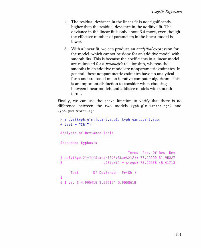
Logistic Regression
2. The residual deviance in the linear fit is not significantly higher than the residual deviance in the additive fit. The deviance in the linear fit is only about 3.5 more, even though the effective number of parameters in the linear model is lower.
3. With a linear fit, we can produce an analytical expression for the model, which cannot be done for an additive model with smooth fits. This is because the coefficients in a linear model are estimated for a parametric relationship, whereas the smooths in an additive model are nonparametric estimates. In general, these nonparametric estimates have no analytical form and are based on an iterative computer algorithm. This is an important distinction to consider when choosing between linear models and additive models with smooth terms.
Finally, we can use the anova function to verify that there is nodifference between the two models kyph.glm.istart.age2 andkyph.gam.start.age:
> anova(kyph.glm.istart.age2, kyph.gam.start.age,+ test = "Chi")
Analysis of Deviance Table
Response: Kyphosis
Terms Res. Df Res. Dev1 poly(Age,2)+I((Start-12)*(Start>12)) 77.00000 51.953272 s(Start) + s(Age) 72.09458 48.41713
Test Df Deviance Pr(Chi)12 1 vs. 2 4.905415 3.536134 0.6050618
401

Chapter 12 Generalizing the Linear Model
Legal Forms of the Response Variable
The required formula argument to glm is in the same format as mostother formulas in Spotfire S+, with the response on the left side of atilde (~) and the predictor variables on the right. In logistic regression,however, the response can assume a few different forms:
1. If the response is a logical vector or a two-level factor, it is treated as a 0/1 binary vector. The zero values correspond to failures and the ones correspond to successes. This is the form of the response variable in all of the example kyphosis models above.
2. If the response is a multilevel factor, Spotfire S+ assumes the first level codes failures (0) and all of the remaining levels code successes (1).
3. If the response is a two-column matrix, Spotfire S+ assumes the first column holds the number of successes for each trial and the second column holds the number of failures.
4. If the response is a general numeric vector, Spotfire S+ assumes that it holds the proportion of successes. That is, the ith value in the response vector is , where denotes the
number of successes out of total trials. In this case, the must be given as weights to the weights argument in glm.
As an simple example of a two-column response, we tabulate the datain the Kyphosis variable of the kyphosis data set:
> kyph.table <- table(kyphosis$Kyphosis)> kyph.mat <- t(as.matrix(kyph.table))> kyph.mat
absent present [1,] 64 17
The following call to glm creates a generalized linear model using thefirst column of kyph.mat as the response. Because it is the first columnof the matrix, absent is assumed to be a success in the model:
> kyph1.glm <- glm(kyph.mat ~ 1, family = binomial)
si ni⁄ si
ni ni
402

Logistic Regression
> kyph1.glm
Call:glm(formula = kyph.mat ~ 1, family = binomial)
Coefficients: (Intercept) 1.32567
Degrees of Freedom: 1 Total; 0 ResidualResidual Deviance: 0
If we use the full vector Kyphosis in a similar call, Spotfire S+assumes that present is a success in the model. This is becausepresent is the second level of the factor variable and is thereforecoded to the binary value 1 (success). Likewise, absent is the firstlevel of Kyphosis, and is therefore coded to 0 (failure):
> levels(kyphosis$Kyphosis)
[1] "absent" "present"
> kyph2.glm <- glm(Kyphosis ~ 1, family = binomial, + data = kyphosis)> kyph2.glm
Call:glm(formula = Kyphosis ~ 1, family = binomial, data =
kyphosis)
Coefficients: (Intercept) -1.32567
Degrees of Freedom: 81 Total; 80 ResidualResidual Deviance: 83.23447
We can rename absent to be the success indicator with the followingcommand:
> kyph3.glm <- glm(Kyphosis=="absent" ~ 1, + family = binomial, data = kyphosis)
403

Chapter 12 Generalizing the Linear Model
PROBIT REGRESSION
To fit a probit regression model, use either the glm function or the gamfunction with a formula to specify the model, and set the familyargument to binomial(link=probit). As an example, consider thedata frame kyphosis. In the previous section, we computed variouslogistic regression models for the variables in kyphosis. From ouranalysis, we determined that the best model waskyph.glm.istart.age2:
> kyph.glm.istart.age2
Call:glm(formula = Kyphosis ~ poly(Age, 2) + I((Start - 12) * (Start > 12)),
family = binomial, data = kyphosis)
Coefficients: (Intercept) poly(Age, 2)1 poly(Age, 2)2 -0.6849607 5.771927 -10.32478 I((Start - 12) * (Start > 12)) -1.351012
Degrees of Freedom: 81 Total; 77 ResidualResidual Deviance: 51.95327
To compute the same model as a probit regression, use the probitlink function as follows:
> kyph.probit <- glm(Kyphosis ~ poly(Age, 2) ++ I((Start - 12) * (Start > 12)), + family = binomial(link=probit), data = kyphosis)
> summary(kyph.probit)
Call: glm(formula = Kyphosis ~ poly(Age, 2) + I((Start - 12)* (Start > 12)), family = binomial(link = probit), data = kyphosis)
Deviance Residuals: Min 1Q Median 3Q Max -1.413873 -0.5227573 -0.09664452 -0.0005086466 2.090332
404

Probit Regression
Coefficients: Value Std. Error (Intercept) -0.3990572 0.2516421 poly(Age, 2)1 3.4305340 2.2995511 poly(Age, 2)2 -6.1003327 2.6288017I((Start - 12) * (Start > 12)) -0.7516299 0.2564483
t value (Intercept) -1.585813 poly(Age, 2)1 1.491828 poly(Age, 2)2 -2.320575I((Start - 12) * (Start > 12)) -2.930922
(Dispersion Parameter for Binomial family taken to be 1 )
Null Deviance: 83.23447 on 80 degrees of freedom
Residual Deviance: 51.63156 on 77 degrees of freedom
Number of Fisher Scoring Iterations: 6
Correlation of Coefficients: (Intercept) poly(Age, 2)1 poly(Age, 2)1 -0.0536714 poly(Age, 2)2 0.4527154 0.0306960 I((Start - 12) * (Start > 12)) -0.3762806 -0.1765981
poly(Age, 2)2 poly(Age, 2)1 poly(Age, 2)2 I((Start - 12) * (Start > 12)) 0.00393
Often, it is difficult to distinguish between logistic and probit models,since the underlying distributions approximate each other well inmany circumstances. That is, the logistic distribution is similar to theGaussian distribution, only with longer tails. Unless the sample size isextremely large, the subtle differences between the two distributionscan be difficult to see. If a substantial proportion of responses areconcentrated in the tails of the distribution, where the logistic andGaussian distributions differ, then the probit and logit links can givesignificantly different results. When both models fit well, the
405

Chapter 12 Generalizing the Linear Model
parameter estimates in a logistic model are about 1.6 to 1.8 times theesimates in the probit model. For more details, see either Venables &Ripley (1997) or Agresti (1990).
406
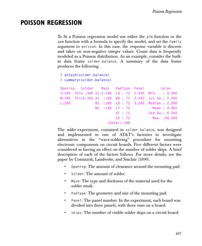
Poisson Regression
POISSON REGRESSION
To fit a Poisson regression model use either the glm function or thegam function with a formula to specify the model, and set the familyargument to poisson. In this case, the response variable is discreteand takes on non-negative integer values. Count data is frequentlymodeled as a Poisson distribution. As an example, consider the built-in data frame solder.balance. A summary of the data frameproduces the following:
> attach(solder.balance)> summary(solder.balance)
Opening Solder Mask PadType Panel skipsS:240 Thin :360 A1.5:180 L9 : 72 1:240 Min. : 0.000M:240 Thick:360 A3 :180 W9 : 72 2:240 1st Qu.: 0.000L:240 B3 :180 L8 : 72 3:240 Median : 2.000 B6 :180 L7 : 72 Mean : 4.965 D7 : 72 3rd Qu.: 6.000 L6 : 72 Max. :48.000 (Other):288
The solder experiment, contained in solder.balance, was designedand implemented in one of AT&T’s factories to investigatealternatives in the “wave-soldering” procedure for mountingelectronic components on circuit boards. Five different factors wereconsidered as having an effect on the number of solder skips. A briefdescription of each of the factors follows. For more details, see thepaper by Comizzoli, Landwehr, and Sinclair (1990).
• Opening: The amount of clearance around the mounting pad.
• Solder: The amount of solder.
• Mask: The type and thickness of the material used for the solder mask.
• PadType: The geometry and size of the mounting pad.
• Panel: The panel number. In the experiment, each board was divided into three panels, with three runs on a board.
• skips: The number of visible solder skips on a circuit board.
407
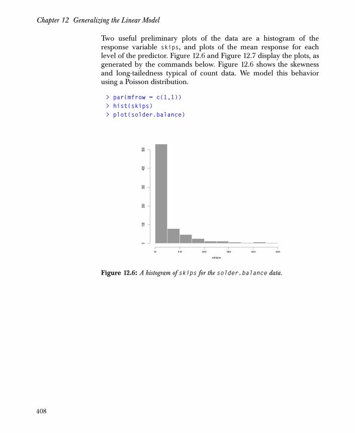
Chapter 12 Generalizing the Linear Model
Two useful preliminary plots of the data are a histogram of theresponse variable skips, and plots of the mean response for eachlevel of the predictor. Figure 12.6 and Figure 12.7 display the plots, asgenerated by the commands below. Figure 12.6 shows the skewnessand long-tailedness typical of count data. We model this behaviorusing a Poisson distribution.
> par(mfrow = c(1,1))> hist(skips)> plot(solder.balance)
Figure 12.6: A histogram of skips for the solder.balance data.
0 10 20 30 40 50
010
020
030
040
050
0
skips
408
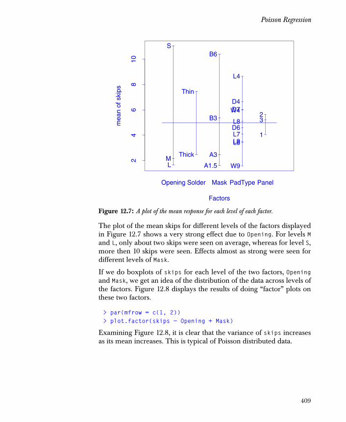
Poisson Regression
The plot of the mean skips for different levels of the factors displayedin Figure 12.7 shows a very strong effect due to Opening. For levels Mand L, only about two skips were seen on average, whereas for level S,more then 10 skips were seen. Effects almost as strong were seen fordifferent levels of Mask.
If we do boxplots of skips for each level of the two factors, Openingand Mask, we get an idea of the distribution of the data across levels ofthe factors. Figure 12.8 displays the results of doing “factor” plots onthese two factors.
> par(mfrow = c(1, 2))> plot.factor(skips ~ Opening + Mask)
Examining Figure 12.8, it is clear that the variance of skips increasesas its mean increases. This is typical of Poisson distributed data.
Figure 12.7: A plot of the mean response for each level of each factor.
Factors
mea
n of
ski
ps
24
68
10
S
ML
Thin
Thick
A1.5
A3
B3
B6
W4D4
L4
D6
L6
D7
L7
L8
W9
L91
23
Opening Solder Mask PadType Panel
409

Chapter 12 Generalizing the Linear Model
We proceed now to model skips as a function of the controlledfactors in the experiment. We start with a simple-effects model forskips as follows:
> paov <- glm(skips ~ ., family = poisson,+ data = solder.balance)
> anova(paov, test = "Chi")
Analysis of Deviance Table
Poisson model
Response: skips
Terms added sequentially (first to last) Df Deviance Resid. Df Resid. Dev Pr(Chi) NULL 719 6855.690Opening 2 2524.562 717 4331.128 0.000000e+00 Solder 1 936.955 716 3394.173 0.000000e+00 Mask 3 1653.093 713 1741.080 0.000000e+00PadType 9 542.463 704 1198.617 0.000000e+00 Panel 2 68.137 702 1130.480 1.554312e-15
Figure 12.8: Boxplots for each level of the two factors Opening and Mask.
010
2030
40
skip
s
S M L
Opening
010
2030
40
skip
s
A1.5 A3 B3 B6
Mask
410
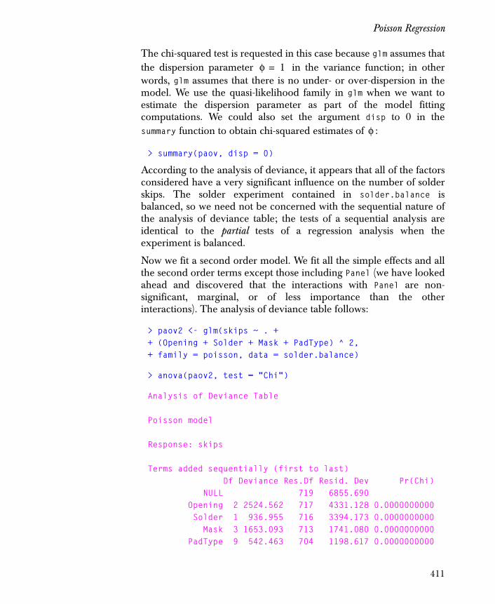
Poisson Regression
The chi-squared test is requested in this case because glm assumes thatthe dispersion parameter in the variance function; in otherwords, glm assumes that there is no under- or over-dispersion in themodel. We use the quasi-likelihood family in glm when we want toestimate the dispersion parameter as part of the model fittingcomputations. We could also set the argument disp to 0 in thesummary function to obtain chi-squared estimates of :
> summary(paov, disp = 0)
According to the analysis of deviance, it appears that all of the factorsconsidered have a very significant influence on the number of solderskips. The solder experiment contained in solder.balance isbalanced, so we need not be concerned with the sequential nature ofthe analysis of deviance table; the tests of a sequential analysis areidentical to the partial tests of a regression analysis when theexperiment is balanced.
Now we fit a second order model. We fit all the simple effects and allthe second order terms except those including Panel (we have lookedahead and discovered that the interactions with Panel are non-significant, marginal, or of less importance than the otherinteractions). The analysis of deviance table follows:
> paov2 <- glm(skips ~ . ++ (Opening + Solder + Mask + PadType) ^ 2,+ family = poisson, data = solder.balance)
> anova(paov2, test = "Chi")
Analysis of Deviance Table
Poisson model
Response: skips
Terms added sequentially (first to last) Df Deviance Res.Df Resid. Dev Pr(Chi) NULL 719 6855.690 Opening 2 2524.562 717 4331.128 0.0000000000 Solder 1 936.955 716 3394.173 0.0000000000 Mask 3 1653.093 713 1741.080 0.0000000000 PadType 9 542.463 704 1198.617 0.0000000000
φ 1=
φ
411
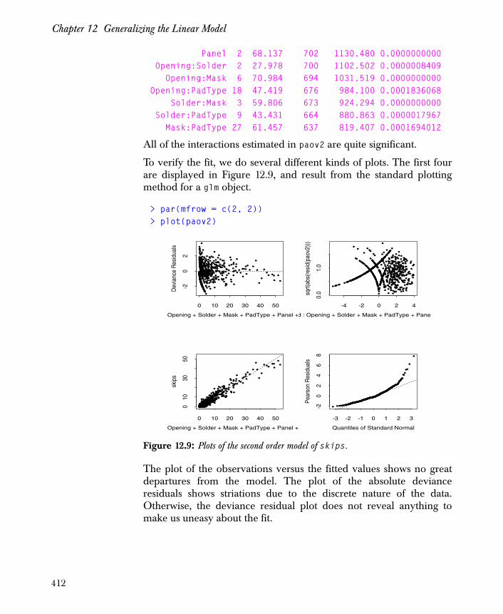
Chapter 12 Generalizing the Linear Model
Panel 2 68.137 702 1130.480 0.0000000000 Opening:Solder 2 27.978 700 1102.502 0.0000008409 Opening:Mask 6 70.984 694 1031.519 0.0000000000Opening:PadType 18 47.419 676 984.100 0.0001836068 Solder:Mask 3 59.806 673 924.294 0.0000000000 Solder:PadType 9 43.431 664 880.863 0.0000017967 Mask:PadType 27 61.457 637 819.407 0.0001694012
All of the interactions estimated in paov2 are quite significant.
To verify the fit, we do several different kinds of plots. The first fourare displayed in Figure 12.9, and result from the standard plottingmethod for a glm object.
> par(mfrow = c(2, 2))> plot(paov2)
The plot of the observations versus the fitted values shows no greatdepartures from the model. The plot of the absolute devianceresiduals shows striations due to the discrete nature of the data.Otherwise, the deviance residual plot does not reveal anything tomake us uneasy about the fit.
Figure 12.9: Plots of the second order model of skips.
•••••••••••••••••••••••••••••
•
••
••
••••••
•
•
••
••••
•
•••••
•
•
•
••
•
•
•
••
•
•
••
••••••
••
••
•
•••
••••••••
•
•••
••••
•
••
•
•
•
•••
••
••
•••
•
•
•
•••••
••••
•
•
•
•
•
•••
•
•
•
•
•
••••
••
•••• •
•
•
•
••
•
••
•
•
•
••
•••
••
••
•
••
••
•
•
•
••••
•
••••••••••••
•
••••••••
•
•
••••
••
•••••
•
••
•
••
•
•
•
•
•
•
•
•••
•••••
•
••
•
•••
••••
•
•••
•••
•••
•••••
•
•
••••••
•••
•
•••
••
•
•
•
••••
•••••
••••
•
•
•
••
•
•
•
•
••
•
••
•
•••
•
•
••
••
•
•
•
•
•
••
••• •
•••••••• ••
•
•
••
•
•
•
•
•
•••
••
•
••••
•
•
•
•
•••
•
••
•
•
•
•
•
••
•••••••
•
•
•
•••
•
••••
••••••
•
•
•
••
•
••
••••
•
••
•••
• •
•
•
••
••
•••
•
•
••
•
••
•
•• •••
•••
•
••
•
••
•
••
•
••
•
•
•••
•
•
•••
••
•••••
•
•
•
•
•
••••
•
•
•••••••••
•
••••••
•
••
•
•••
• ••••
•
•
••
•••
•
•
•
• •
•
•
••
••
•
••
••
•
•
•••
••••••••••••
•
••
••
••
•
••
•••
•
•
•••
•
•
•
•
••
•
•
•
•
•
•
•
•
••
•
••
•
•
•
•••
••
•
•••
•
•
•
•
•
• ••••
•
••
••••
•
•• •
•
•
•
•
•
•
•
•••
•••
•
•••
••
••
••
•
••
••
•• ••
•
•
••
••
•
•
•
•
•• •
•
•
••
•
•
•
••••
•
•• •
•••
••
•
••
• •
•
•
••
••
••
•
••
••
••
•
•
•
•
Opening + Solder + Mask + PadType + Panel +
Dev
ianc
e R
esid
uals
0 10 20 30 40 50
-20
2
• ••• ••• ••
• •• • ••• ••• ••• ••
• •• • •• • •• •
•
••
•
•
• •• • ••
•
••
•
••• ••
• •• • •
•
•
•
••
•
•
•
•
•
•
•
••
••
•
•••
••
•
•
•
• •••
••• •
•
••
•
•
••••••
•
••
•
••
•••
•••
•
•• ••
•••
• •••
•
•• •
•
••
•
•
•••
••
•
•
•• ••• •
••
•
•
• •
•
•
••••
•
• •
•
•
•
•••
••
••
•
•
•
•••
•
•
•
• •••••
• •• • ••• ••• •
•
• ••
• ••• ••
•
•
•••• •
•
•• ••
••••
•
•••
•
•
•
•
•
•
•
• •
•
•••
• •
•
•
•
•• •
•
•
••
•
•
•
•••••
••
••
• ••
•
•
••
••
•
•
•
• ••
•••
• •
•••• • ••
• •••
•
••
•
•
•
•
••••
•
••
•
•
•
••
•• ••
•
•
••••
•
•
••
••
•
•••••
•••
•
••
• ••
•
•
••
•
•
•
•
•
•
••
• •
•• ••
•
•
•••
• • •
•• •••••
•
••
• ••• •• •
••• ••
•
••• ••
••
•
••
•
•
•
•
•
•
•
• •
•
•
•
•
•
••
•
•
• • ••
•
••
••
•
•
••
•
••
•
•••
•• • •
•
••
•
•
••••
•
• ••
•
•
•
•
••
••
••
••
• ••
• •••
•
•
•
•
••
•
••
••
•
•••••
•
••
• ••
• ••• ••
•
••
• ••
•••
•
•
•
• •
••••
•
•
•
• ••• •
•• ••
• •
•
•
•
•
•••
• •••••• ••
• ••
•
••• ••
•
•
•
•
••• •
•
• ••
•
•
•••• •
•
•
•
•
•
•
•••
•
••
•
•
••
••
•
•
•
••
•
•
•
•
••
•
•••
•
•
•
•
••
•
•
•
•
•
•
•
•
•
•
•
• •
•
•
••
••
•
•
••
•
••
•
••
•
•• ••
•• ••
••
•
•
••
•
•
•
••• •
•••
•••
••
• •
•
•
•
• •
•••
•
••
•
••
•
•
••
•
•
•
•
•
••
•
••
•
•
•
• ••
d : Opening + Solder + Mask + PadType + Panelsq
rt(ab
s(re
sid(
paov
2)))
-4 -2 0 2 4
0.0
1.0
•••••••••••••••••••••••••••••••••••••••••••
•••••••••••••••••••••••••••••••••••••••••••••••••••••••••••••••••• ••• •
•
• ••
•••••• •
••
•••• •
•
••••••••••••••••••••••••
••••••••••••••••••••••••••• ••••••••••••••••••••••••••••••••••••••••••••••••••••••••• •
•
•••••••••
••••••
•• ••• •
•
••
••••
•
••••
••••••
•••••
••••
••
••••••••••••••••••••••••••••••••••••••••••••••••••••••••• •
••• •• •
••
•••
• ••• •••
••• ••••• •••••••
•••••••••
•••••••••••••••••••
•••••••••••••••••••••••••••
•
•
••••
••
••
•
••
•••
•••• •
•
••
•
•••
• ••
•••••••••••••••••••••••••••••••••••••
••••••••••••••
•••••••
••••
••
• ••
• ••
••
••
•••
•
•• ••
•••• ••
• ••
•••
•
••
•••••••
••••••
••
••••••• •••
••
•
••
•••••• •
•••••
• ••
••••••
• •••
••• ••
•
•
•
•
••
••
•
•
•
••
••
•
••
•
•
•
Opening + Solder + Mask + PadType + Panel +
skip
s
0 10 20 30 40 50
010
3050
••••••••• •••••••••••••• ••••••••••
•
••
••
••••••
•
•
••
••••
•
•••••
•
••
•••
••
•••
•••
•• ••••••
••
•
••••••••
••••
•••
••••
•••
•
•
••••
••
•
•
•••
•
•
•
••••••
•••
•
•
••
••
••
•
••
•
•••••
••
• ••••
•
••
••
••
•
••
•• •
•••
••
••
•
• •
••
•
•
•
••••
•
• •••••••••••
•
••• ••••••
•
•
••••
••
•••••
•••
•• •
•
•
••
•
•
•
•••
•••
••
•••
••
••
•••
•
•
•••
••••
• •
•••••
•
•
•• ••
••
•••
•
•••••
••
•
••••••• •
•
•• ••
•
••
••
••
•
•
••
•••
•
••••
•
••
•••
••
•
•
••
••••••
•• • •••••
•
••
•
••
••
••
••••
••••
•
•
••
•
••
•
•••
•
•
•
•
•
••
••••••••
•
•
•••
•• •••
•••
•••
••
•••
•••
••
••
•••
•• •
••
•
•• •
••
•••
•
•
••
•• •
•••• •
•
• • ••
•••
••
•
•••
••
••
•••
•
••••
••
••• • •
•
••
•
••
••••
••
•• •••••
•
•
••••••
•
••
••
••••••
••
•
•• •••
•
••
••
•
•
•• •
••
••
•••
••••
••••••••• ••••
••
••
•••
••
••••
•
••
•••
•
•
••
••
•
••
•
•
•
• •
•
•••
•
•
•• •
••
•
•••
•
•
••
••• ••
•
••
•••
••
•
• ••
•
•
•
•
•
•
••••
•••
•• ••
••••
•••
••
••
••••
•
•
••
•••
••
•• ••
•
•
••
••
•
•••
•
•
•••
•••
••
•
••
••
••
••
••
••
••
•
•• ••
•
•
•
•
Quantiles of Standard Normal
Pear
son
Res
idua
ls
-3 -2 -1 0 1 2 3
-20
24
68
412
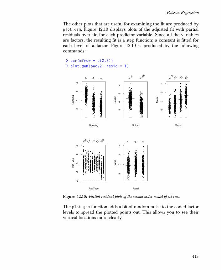
Poisson Regression
The other plots that are useful for examining the fit are produced byplot.gam. Figure 12.10 displays plots of the adjusted fit with partialresiduals overlaid for each predictor variable. Since all the variablesare factors, the resulting fit is a step function; a constant is fitted foreach level of a factor. Figure 12.10 is produced by the followingcommands:
> par(mfrow = c(2,3))> plot.gam(paov2, resid = T)
The plot.gam function adds a bit of random noise to the coded factorlevels to spread the plotted points out. This allows you to see theirvertical locations more clearly.
Figure 12.10: Partial residual plots of the second order model of skips.
Ope
ning
-20
24
Opening
S M L
••••••••••• •••••••••• •• •••••••
••••
•
••
•
•
••••••
•
•
••
••••
•
•••••
••
•
••
•
•
•
••
•
•
••
••••••
••
••
•
•••
•••
••
•••
•
•••
••••
•
••
•
•
•
•••
••
•
•
•••
•
•
•
•••••
••••
•
•
•
•
•
••
•
•
•
•
•
•
••••
•
•
•••
••
•
•
•
••
•
••
•
•
•
••••
•
••
••
•
••
••
•
•
•
••••
•
•••• •••• ••••
•
•••••••••
•
•
••••
••
••• ••
•
• •
•
••
•
•
•
•
•
•
•
•• •
•
••
•
•
•
•
•
•
•••
•
••
•
•
•••
•••
•••
•••• • •
•
••••
•
•
•••
•
•••
••
•
•
•
••••
•••••
••
•
•
•
•
•
••
•
•
•
•
•
•
•
• •
•
• ••
•
•
••
••
•
•
••
•
•
•
• •••
•••
•••••••
•
•
••
•
•
•
•
•
•
••
••
•
•••
•
•
•
•
•
•••
•
••
•
•
•
•
•
••
•••• •••
•
•
•
•••
•
••••
••
••••
•
•
•
••
•
• •
•••
••
••
•
••
••
•
•
••
••
••
•
•
•
••
•
••
•
•••••
••
•
•
••
•
•
••
••
•
••
•
•
•
••
•
•
•••
••
•••
•
•
•
•
•
•
•
•••
•
•
•
••••••• •
•
•
••• •••
••
••
••
•••••
••
•
•
••••
•
•
•
••
•
•
••••
•••
••
•
•
•••
•••••• ••••••
•
• •
••
••
•
••
•••
•
•
••
•
•
•
•
•
••
•
•
•
•
•
•
•
•
••
•
••
•
•
•
•
••
••
•
••
•
•
•
•
•
•
•••••
•
•
•••
••
•
••
•
•
•
•
•
•
•
•
••
•
•••
•
•••
••
••
••
•
••
••
•••
•
•
•
•
•
••
•
•
•
•
•••
•
•
••
•
•
•
•
•••
•
••
•
•••
••
•
••
••
•
•
•••
••
•
•
•
•
••
••
•
•
•
• Sol
der
-20
24
Solder
Thin Thick
• •••• ••••••••••••••••••• ••••• •••• •
•
••
•
•
• •• •• •
•
•
••
••• •
•
•••• •
•
•
•
• •
•
•
•
••
•
•
••
••••• •
••
••
•
•••
•••
••
•••
•
•••
• •••
•
••
•
•
•
•••
••
•
•
•••
•
•
•
•• •••
••••
•
•
•
•
•
••
•
•
•
•
•
•
••••
••
•••
• •
•
•
•
••
•
••
•
•
•
••
••
•
••
••
•
••
••
•
•
•
• •••
•
•••• •••• ••••
•
•••• •••••
•
•
••••
••
•• •••
•
••
•
••
•
•
•
•
•
•
•
•••
•
•••
•
•
••
•
•••
•••
•
•
••
•
•••
•• •
••• ••
•
•
•••
•
•
•
•••
•
• ••
••
•
•
•
••••
•••••
•••
•
•
•
•
••
•
•
•
•
•
•
•
••
•
• ••
•
•
••
••
•
•
•
•
•
•
•
••••
•••••
• ••• •
•
•
••
•
•
•
•
•
•
••
••
•
•••
•
•
•
•
•
• ••
•
••
•
•
•
•
•
••
•••••••
•
•
•
• ••
•
•• ••
••
••••
•
•
•
••
•
••
•••
•
•
••
•
••
••
•
•
••
••
••
•
•
•
••
•
• •
•
••••
•
•••
•
••
•
•
••
••
•
••
•
•
•
••
•
•
•••
••
••••
•
•
•
•
•
•
••••
•
•
••••
•• ••
•
•
•• ••••
•
•
••
•••
••••••
•
•
••
• •
•
•
•
••
•
•
••
••• ••
••
•
•
•••
•• •••••••• ••
•
••
••
••
•
•
•
•••
•
•
••
•
•
•
•
•
••
•
•
•
•
•
•
•
•
• •
•
••
•
•
•
•
••
••
•
• •
•
•
•
•
•
•
••••
•
•
•
•••
••
•
••
•
•
•
•
•
•
•
•
•••
•• •
•
•••
••
••
••
•
••
••
•• •
•
•
•
••
••
•
•
•
•
• ••
•
•
••
•
•
•
•
•••
•
•• •
•••
••
•
••
••
•
•
••
•
•••
•
••
••
••
•
•
•
•
Mas
k
-20
24
Mask
A1.5
A3 B3 B6
••• •••••••• ••••••••••• ••••••••••••
•
••
•
•
••••••
•
•
••
••••
•
•••••
•
•
•
••
•
•
•
••
•
•
••
•••
•••
••
••
•
•••
•••••
•••
•
•••
••••
•
••
•
•
•
•••
••
•
•
•••
•
•
•
•••••
••••
•
•
•
•
•
••
•
•
•
•
•
•
••••
•
••••
••
•
•
•
••
•
••
•
•
•
••••
•
••
••
•
••
••
•
•
•
••••
•
••••••••••••
•
•••••••••
•
•
••••
••
••• ••
•
••
•
••
•
•
•
•
•
•
•
•••
•
•••
•
•
•
•
•
•••
•
••
•
•
•••
•••
•••
•••••
•
•
•••
•
•
•
•••
•
•••
••
•
•
•
••••
•••••
••
•
•
•
•
•
••
•
•
•
•
•
•
•
••
•
•••
•
•
••
••
•
•
•
•
•
•
•
••••
•••••
•••••
•
•
••
•
•
•
•
•
•
••
••
•
•••
•
•
•
•
•
•••
•
••
•
•
•
•
•
••
•••••••
•
•
•
•••
•
••••
••
•••
•
•
•
•
••
•
••
•••
•
•
••
•
••
••
•
•
••
••
••
•
•
•
••
•
••
•
••••
•
••
•
•
••
•
•
••
••
•
••
•
•
•
••
•
•
•••
••
••••
•
•
•
•
•
•
••••
•
•
••••••••
•
•
••••••
•
•
••
••
•••••••
•
•
••
••
•
•
•
••
•
•
••••
•
••
••
•
•
•••
••••••••••••
•
••
••
••
•
•
•
•••
•
•
••
•
•
•
•
•
••
•
•
•
•
•
•
•
•
••
•
••
•
•
•
•
••
••
•
••
•
•
•
•
•
•
•••••
•
•
•••
••
•
•••
•
•
•
•
•
•
•
•••
•••
•
•••
••
••
••
•
••
••
•••
•
•
•
•
•
••
•
•
•
•
•••
•
•
••
•
•
•
•
•••
•
•••
•••
••
•
••
••
•
•
••
•
•••
•
•
•
••
••
•
•
•
•
Pad
Typ
e
-4-2
02
4
PadType
W4
L4 L6 L7 W9
••• ••••••
••• •••••• •••
•••
•••
•••••• •
•
••
•
•
••• •••
•
•
• •
••••
•
•••
••
•
•
•
• •
•
•
•
••
•
•
••
••
•••
•
••
••
•
•••
•••••
•••
•
••• ••• •
•
• •
•
•
•
•• •
••
•
•
•
••
•
•
•
• ••••
••
••
•
•
•
•
•
••
•
•
••
•
•
•••
•
•
••••
••
•
•
•
•
•
•
•
•
•
•
•
••
••
•
••
•
•
•
•
•
••
•
•
•
••••
•
•••• •••
••• ••
•
•••
•••
•••
•
•
• •••
••
•
••• •
•
••
•
• •
•
•
•
•
•
•
•
•••
••••
•
•
• •
•
•••
•••
•
•
•• •
•••
••
•
•••••
•
•
• •••
•
•
•
••
•
•••
••
•
•
•
• ••••••
••
••
•
•
•
•
•
••
•
•
•
•
•
•
•
••
•
•••
•
•
•
•
•• •
•
•
•
•
•
•
••••
•
•••
••• •••
•
•
• •
•
•
•
•
•
•
••
••
•
•••
•
•
•
•
•
• ••
•
••
•
•
•
•
•
••
•••
••••
•
•
•
•• •
•
•
•••
••
•
•••
•
•
•
••
•••
•••
•
•
••
•
••
••
•
•
••
••
• •
•
•
•
••
•
•• •
••
•••
••
•
•
•••
•
••
••
•
••
•
•
•
••
•
•
••
•
••
••••
•
•
•
•
•
•
••
••
•
•
•• ••
• •••
•
•
•
•••••
•
•
••
•••
•••
•••
•
•
•
•••
•
•
•
••
• •
••
••
•
••
• •
•
•
••• ••• •••
••• •••
•
••
••
•
•
•
••
•• •
•
•
••
•
•
•
•
•
••
•
•
•
•
•
•
•
•
•
•
•
•
•
•
•
•
•
••
••
•
•••
•
•
•
•
•
••• •
•
•
•
••
•
••
•
••
•
•
•
•
•
•
•
•
•
••
•••
•
•••
••
• •
••
•
••
••
•••
•
•
•
• •
••
•
•
•
•
•••
•
•
••
•
•
•
•
•••
•
••
•
•••
••
•
•• •
•
•
•
••
•
••
•
•
••
••
••
••
•
•
Pan
el
-20
24
Panel
1 2 3
• • •• • •• • ••
• •• • •• • •• • •• • ••
• •• • •
• • ••
•
••
•
•
• • •• • •
•
•
••
• •• •
•
• • •• •
•
•
•
••
•
•
•
• •
•
•
••
• •• • ••
• •
• •
•
• • •
• • •• •
•
• •
•
• • •
• • ••
•
••
•
•
•
• ••
• •
•
•
•• •
•
•
•
•• • ••
•
•• •
•
•
•
•
•
•
••
•
•
•
•
•
• • ••
•
•
•
• •
••
•
••
••
•
••
•
•
•
••
••
•
••
•
•
•
••
• •
•
•
•
• • ••
•
•• • •• • •• • •• •
•
• • ••• •
• • •
•
•
•• • •
•
•
•
• • ••
•
••
•
••
•
•
•
•
•
•
•
•• •
•
• •
••
•
•
•
•
•• •
•
• •
•
•
••
•
• ••
•••
• •
• • •
•
•
••
•
••
•
•
• •
•
• • •
• •
•
•
•
•• • •
• • ••
•
••
•
•
•
•
•
••
•
•
•
•
•
•
•
• •
•
• • •
•
•
••
• •
•
•
•
•
•
••
• ••
•
••
•
••
• •
•• •
•
•
•
•
•
•
•
•
•
•
••
• •
•
• • ••
•
•
•
•
•• •
•
• •
•
•
•
•
•
• •
• • •• • ••
•
•
•
• ••
•
•• • •
• •
•• •
•
•
•
•
• •
•
• •
•
•
•
•
•
• •
••
•
• •
•
•
• •
••
••
•
•
•
••
•
• •
•
• •••
•
•
••
•
• •
•
•
••
• •
•
••
•
•
•
• •
•
•
••
•
• •
• • ••
•
•
•
•
•
•
••• •
•
•
•
••
••• • •
•
•
•• • •
• •
•
•
••
••
••
• ••
••
•
•
•• • •
•
•
•
••
•
•
•••
•
•
••
••
•
•
• • •
• • •• • •• • •• • •
•
• •
• •
••
•
•
•
• ••
•
•
•
•
•
•
•
•
•
• •
•
•
•
•
•
•
•
•
••
•
••
•
•
•
•
••
••
•
• ••
•
•
•
•
•
•• ••
•
•
••
••
• •
•
•••
•
•
•
•
•
•
•
•
••
•
••
•
•
• •
• •
••
••
•
• •
• •
•• •
•
•
•
•
•
• •
•
•
•
•
• ••
•
•
••
•
•
•
•
• ••
•
•••
• ••
••
•
••
• •
•
•
•
••
•
•
•
•
•
•
•••
•
•
•
•
•
413

Chapter 12 Generalizing the Linear Model
These plots produced by plot.gam indicate that the data is modeledreasonably well. Please note, however, that the default plots will showonly glaring lack of fit.
Note
The warning message about interaction terms not being saved can be safely ignored here.
414
Quasi-Likelihood Estimation
QUASI-LIKELIHOOD ESTIMATION
Quasi-likelihood estimation allows you to estimate regressionrelationships without fully knowing the error distribution of theresponse variable. Essentially, you provide link and variancefunctions that are used in the estimation of the regression coefficients.Although the link and variance functions are typically associated witha theoretical likelihood, the likelihood need not be specified, and fewerassumptions are made in estimation and inference.
As a simple analogy, there is a connection between normal-theoryregression models and least-squares regression estimates. Least-squares estimation gives identical parameter estimates to thoseproduced from normal-theory models. However, least-squaresestimation assumes far less; only second moment assumptions aremade by least-squares, compared to full distribution assumptions ofnormal-theory models.
Quasi-likelihood estimation for the distributions of Table 12.1 isanalogous to least-squares estimation for the normal distribution. Forthe Gaussian family, IRLS is equivalent to standard least-squaresestimation. Used in this context, quasi-likelihood estimation allows usto estimate the dispersion parameter in under- or over-dispersedregression models. For example, an under- or over-dispersed logisticregression model can be estimated using quasi-likelihoodmethodology, by supplying the appropriate link and variancefunctions for the binomial family.
However, quasi-likelihood estimation extends beyond the familiesrepresented in Table 12.1. Any modeling situation for which suitablelink and variance functions can be derived can be modeled using thequasi-likelihood methodology. Several good examples of this kind ofapplication are presented in McCullagh and Nelder (1989).
415

Chapter 12 Generalizing the Linear Model
As an example of quasi-likelihood estimation, we return to a Poissonregression model for the solder.balance data frame. Recall that wemodeled skips as a function of all the factors, plus all the two-wayinteractions except those including Panel. The modeling call was:
> paov2$call
glm(formula = skips ~ . + (Opening + Solder + Mask + PadType)^2, family = poisson, data = solder.balance)
When we declare the family argument to be Poisson, the dispersionparameter is set to 1. In many problems, this assumption is not valid.We can use the quasi-likelihood methodology to force the estimationof the dispersion parameter. For the solder experiment, weaccomplish this as follows:
> paov3 <-glm(formula = skips ~ . ++ (Opening + Solder + Mask + PadType) ^ 2,+ family = quasi(link="log", var="mu"),+ data = solder.balance)
A summary of the fit reveals that the dispersion parameter isestimated to be 1.4, suggesting over-dispersion:
> summary(paov3)$dispersion
Quasi-likelihood 1.400785
We now recompute the ANOVA table, computing F-statistics to testfor effects:
> anova(paov3, test = "F")
Analysis of Deviance Table
Quasi-likelihood model
Response: skips
Terms added sequentially (first to last) Df Deviance R.Df Res. Dev F Value Pr(F) NULL 719 6855.690 Opening 2 2524.562 717 4331.128 901.1240 0.00000000 Solder 1 936.955 716 3394.173 668.8786 0.00000000
416

Quasi-Likelihood Estimation
Mask 3 1653.093 713 1741.080 393.3729 0.00000000 PadType 9 542.463 704 1198.617 43.0285 0.00000000 Panel 2 68.137 702 1130.480 24.3210 0.00000000 Opening:Solder 2 27.978 700 1102.502 9.9864 0.00005365 Opening:Mask 6 70.984 694 1031.519 8.4457 0.00000001Opening:PadType 18 47.419 676 984.100 1.8806 0.01494805 Solder:Mask 3 59.806 673 924.294 14.2316 0.00000001 Solder:PadType 9 43.431 664 880.863 3.4449 0.00036929 Mask:PadType 27 61.457 637 819.407 1.6249 0.02466031
All of the factors and interactions are still significant even when wemodel the over-dispersion. This gives us more assurance in ourprevious conclusions.
417

Chapter 12 Generalizing the Linear Model
RESIDUALS
Residuals are the principal tool for assessing how well a model fits thedata. For regression models, residuals are used to assess theimportance and relationship of a term in the model, as well as tosearch for anomalous values. For generalized models, we have theadditional task of assessing and verifying the form of the variance as afunction of the mean response.
Generalized models require a generalization of the residual, so that itcan be used in the same way as the Gaussian residuals of a linearmodel. In fact, four different kinds of residuals are defined to assesshow well a generalized model fits, to determine the form of thevariance function, and to diagnose problem observations.
• "deviance": Deviance residuals are defined as
where is the contribution of the ith observation to the deviance.
The deviance itself is . Consequently,
deviance residuals are reasonable for detecting observations with unduly large influence in the fitting process, since they reflect the same criterion that is used in the fitting.
• "working": Working residuals are the difference between the working response and the linear predictor at the final iteration of the IRLS algorithm. They are defined as:
.
These residuals are returned when you extract the residuals component directly from a glm object.
• "pearson": The Pearson residuals are defined as
.
riD sign yi μi–( ) di=
di
D i riD( )
2∑=
riW yi μi–( )
ηi∂μi∂
-------=
riP yi μi–
V μi( )------------------=
418

Residuals
Their sum-of-squares
is the chi-squared statistic. Pearson residuals are a rescaled version of the working residuals. When proper account is
taken of the associated weights, .
• "response": The response residuals are simply .
You compute residuals for glm and gam objects with the residualsfunction, or resid for short. The type argument allows you to specifyone of "deviance", "working", "pearson", or "response". By default,deviance residuals are computed. To plot the deviance residualsversus the fitted values of a model, type the following command:
> plot(fitted(glmobj), resid(glmobj))
Alternatively, to plot the Pearson residuals versus the fitted values,type:
> plot(fitted(glmobj), resid(glmobj, type = "pearson"))
Selecting which residuals to plot is somewhat a matter of personalpreference. The deviance residual is the default because a largedeviance residual corresponds to an observation that does not fit themodel well, in the same sense that a large residual for the linearmodel does not fit well. You can find additional detail on residuals inMcCullagh and Nelder (1989).
χ2 yi μi–( )2
V μi( )----------------------
i 1=
n
∑=
riP wiri
W=
yi μi–
419
Chapter 12 Generalizing the Linear Model
PREDICTION FROM THE MODEL
Prediction for generalized linear models and generalized additivemodels is similar to prediction for linear models. An important pointto remember, however, is that for either of the generalized models,predictions can be on one of two scales. You can predict:
• on the scale of the linear predictor, which is the transformed scale after applying the link function, or
• on the scale of the original response variable.
Since prediction is based on the linear predictor , computingpredicted values on the scale of the original response effectivelytransforms (evaluated at the predictor data) via the inverse linkfunction.
The type argument to either predict.glm or predict.gam allows youto choose one of three options for predictions.
1. "link": Computes predictions on the scale of the linear predictor (the link scale).
2. "response": Computes predictions on the scale of the response.
3. "terms": Computes a matrix of predictions on the scale of the linear predictor, one column for each term in the model.
Specifying type="terms" allows you to compute the component ofthe prediction for each term separately. Summing the columns of thematrix and adding the intercept term is equivalent to specifyingtype="link".
Predicting the Additive Model of Kyphosis
As an example, consider the additive model with Kyphosis modeledas smooths of Start and Age:
> kyph.gam.start.age
Call:gam(formula = Kyphosis ~ s(Start) + s(Age),family = binomial, data = kyphosis)Degrees of Freedom: 81 total; 72.09458 ResidualResidual Deviance: 48.41713
η x( )
η x( )
420

Prediction from the Model
If we are interested in plotting the prediction surface over the range ofthe data, we start by generating appropriate sequences of values foreach predictor. We then store the sequences in a data frame withvariable labels that correspond to the variables in the model:
> attach(kyphosis)> kyph.margin <- data.frame(+ Start = seq(from=min(Start), to=max(Start), length=40),+ Age = seq(from=min(Age), to=max(Age), length=40))
Since a GAM is additive, we need to do predictions only at themargins and then sum them together to form the entire predictionsurface. We produce the marginal fits by specifying type="terms".
> margin.fit <- predict(kyph.gam.start.age, kyph.margin,+ type = "terms")
Now generate the surface for the marginal fits.
> kyph.surf <- outer(margin.fit[,1], margin.fit[,2], "+")> kyph.surf <- kyph.surf + attr(margin.fit, "constant")> kyph.surf <- binomial()$inverse(kyph.surf)
The first line adds the marginal pieces of the predictions together tocreate a matrix of surface values, the second line adds in the constantintercept term, and the third line applies the inverse link function totransform the predictions back to the scale of the original response.Now we produce the plot using the persp function (or contour orimage if we wish):
> persp(kyph.margin[,1], kyph.margin[,2], kyph.surf,+ xlab = "Start", ylab = "Age", zlab = "Kyphosis")
Figure 12.11 displays the resulting plot.
421

Chapter 12 Generalizing the Linear Model
Safe Prediction Prediction for linear and generalized linear models is a two-stepprocedure.
1. Compute a model matrix using the new data where you want predictions.
2. Multiply the model matrix by the coefficients extracted from the fitted model.
This procedure works perfectly fine as long as the model has nocomposite terms that are dependent on some overall summary of avariable. For example:
(x - mean(x))/sqrt(var(x))(x - min(x))/diff(range(x))poly(x)bs(x)ns(x)
The reason that the prediction procedure does not work for suchcomposite terms is that the resulting coefficients are dependent on thesummaries used in computing the terms. If the new data are differentfrom the original data used to fit the model (which is more than likelywhen you provide new data), the coefficients are inappropriate. Oneway around this problem is to eliminate such dependencies on data
Figure 12.11: Plot of the probability surface for developing Kyphosis based age in months and start position.
510
15
Start50
100
150
200
Age
00.
20.
40.
60.
81
Kyp
hosi
s
422

Prediction from the Model
summaries. For example, change mean(x) and var(x) to theirnumeric values, rather than computing them from the data at the timeof fitting the model. For the spline functions bs and ns, provide theknots explicity in the call to the function, rather than letting thefunction compute them from the overall data. If the removal ofdependencies on the overall data is possible, prediction can be madesafe for new data. However, when the dependencies cannot beremoved, as is the case when using s or lo in gam, use thepredict.gam function explicitly. This function computes predictionsin as safe a way as possible, given the need for generality. To illustratethis method, suppose that the data used to produce a generalized fit isnamed old.data, and new.data is supplied for predictions:
1. A new data frame, both.data, is constructed by combining old.data and new.data.
2. The model frame and model matrix are constructed from the combined data frame both.data. The model matrix is
separated into two pieces and , corresponding to old.data and new.data.
3. The parametric part of fit is refit using .
4. The coefficients from this new fit are then applied to to obtain the new predictions.
5. For gam objects with both parametric and nonparametric components, an additional step is taken to evaluate the fitted nonlinear functions at the new data values.
This procedure works perfectly for terms with mean and var in them,as well as for poly. For other kinds of composite terms, such as bsknots placed at equally spaced (in terms of percentiles) quantiles ofthe distribution of the predictor, predict.gam works approximately.Because the knots produced by the combined data will, in general, bedifferent from the knots produced by the original data, there will besome error in predicting the new data. If the old data and the newdata have roughly the same distribution, the error in predicting thenew data should be small.
XO Xn
XO
Xn
423

Chapter 12 Generalizing the Linear Model
ADVANCED TOPICS
Fixed Coefficients
A commonly used device in generalized linear models is the offset,which is a component of the linear predictor that has a fixedcoefficient. The effect of these components is to offset the value of thelinear predictor by a certain fixed amount. In Spotfire S+, you canspecify offsets in GLMs by including offset terms directly in themodel formula. For example, consider the following simple logisticregression model for the kyphosis data set:
> fit1 <- glm(Kyphosis ~ Age + Start,+ family=binomial, data=kyphosis)
The coef function returns the coefficients of the model:
> coef(fit1)
(Intercept) Age Start 0.2250435 0.009507095 -0.237923
With the following syntax, we can force the intercept to be 0.25 andthe coefficient for Age to be 0.01:
> fit2 <- glm(Kyphosis ~ + offset(0.25 + 0.01*Age) + Start - 1,+ family=binomial, data=kyphosis)
> coef(fit2)
Start -0.2443723
The -1 in the model formula is needed to prevent the fitting of anintercept term, since it is already included in the offset component.
Offsets allow for a kind of residual analysis in generalized linearmodels. By specifying offsets, you can evaluate the contribution ofparticular terms to a fit, while holding other terms constant. Inaddition, a variable can be included as both a regression term and anoffset in a model formula. With this kind of model, you can test thehypothesis that the variable’s regression coefficient is any fixed value.
424
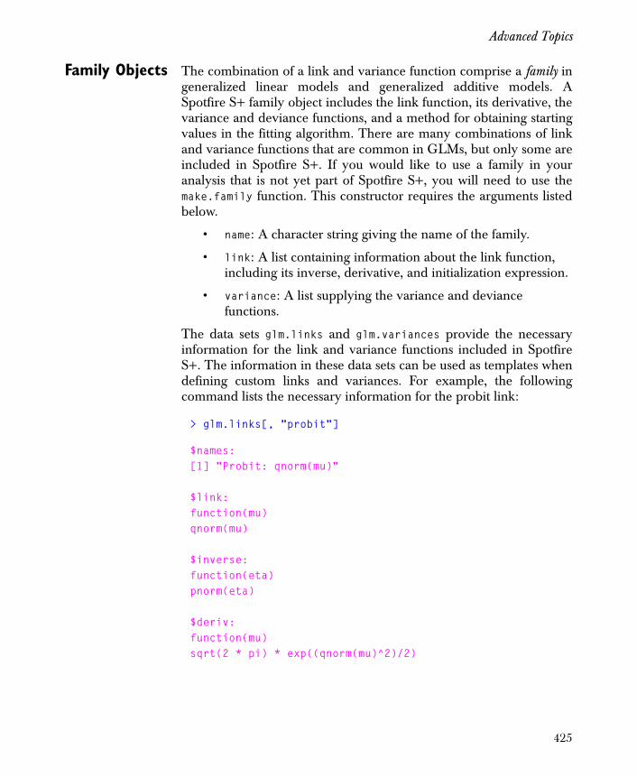
Advanced Topics
Family Objects The combination of a link and variance function comprise a family ingeneralized linear models and generalized additive models. ASpotfire S+ family object includes the link function, its derivative, thevariance and deviance functions, and a method for obtaining startingvalues in the fitting algorithm. There are many combinations of linkand variance functions that are common in GLMs, but only some areincluded in Spotfire S+. If you would like to use a family in youranalysis that is not yet part of Spotfire S+, you will need to use themake.family function. This constructor requires the arguments listedbelow.
• name: A character string giving the name of the family.
• link: A list containing information about the link function, including its inverse, derivative, and initialization expression.
• variance: A list supplying the variance and deviance functions.
The data sets glm.links and glm.variances provide the necessaryinformation for the link and variance functions included in SpotfireS+. The information in these data sets can be used as templates whendefining custom links and variances. For example, the followingcommand lists the necessary information for the probit link:
> glm.links[, "probit"]
$names:[1] "Probit: qnorm(mu)"
$link:function(mu)qnorm(mu)
$inverse:function(eta)pnorm(eta)
$deriv:function(mu)sqrt(2 * pi) * exp((qnorm(mu)^2)/2)
425
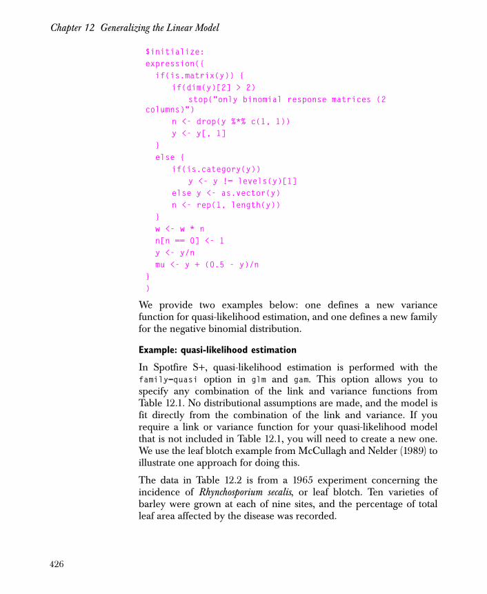
Chapter 12 Generalizing the Linear Model
$initialize:expression({
if(is.matrix(y)) {if(dim(y)[2] > 2)
stop("only binomial response matrices (2 columns)")
n <- drop(y %*% c(1, 1))y <- y[, 1]
}else {
if(is.category(y))y <- y != levels(y)[1]
else y <- as.vector(y)n <- rep(1, length(y))
}w <- w * nn[n == 0] <- 1y <- y/nmu <- y + (0.5 - y)/n
})
We provide two examples below: one defines a new variancefunction for quasi-likelihood estimation, and one defines a new familyfor the negative binomial distribution.
Example: quasi-likelihood estimation
In Spotfire S+, quasi-likelihood estimation is performed with thefamily=quasi option in glm and gam. This option allows you tospecify any combination of the link and variance functions fromTable 12.1. No distributional assumptions are made, and the model isfit directly from the combination of the link and variance. If yourequire a link or variance function for your quasi-likelihood modelthat is not included in Table 12.1, you will need to create a new one.We use the leaf blotch example from McCullagh and Nelder (1989) toillustrate one approach for doing this.
The data in Table 12.2 is from a 1965 experiment concerning theincidence of Rhynchosporium secalis, or leaf blotch. Ten varieties ofbarley were grown at each of nine sites, and the percentage of totalleaf area affected by the disease was recorded.
426
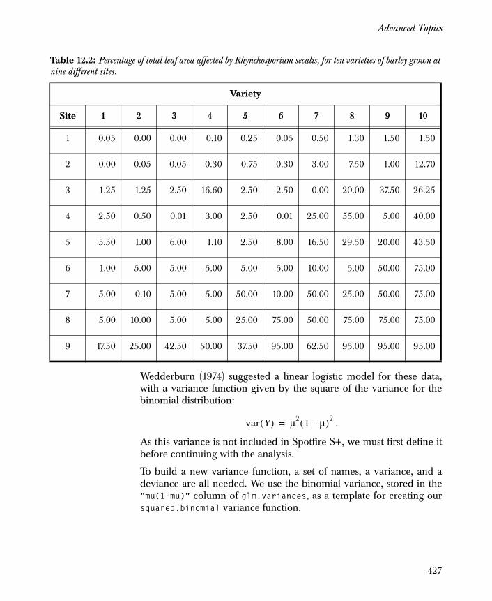
Advanced Topics
Wedderburn (1974) suggested a linear logistic model for these data,with a variance function given by the square of the variance for thebinomial distribution:
.
As this variance is not included in Spotfire S+, we must first define itbefore continuing with the analysis.
To build a new variance function, a set of names, a variance, and adeviance are all needed. We use the binomial variance, stored in the"mu(1-mu)" column of glm.variances, as a template for creating oursquared.binomial variance function.
Table 12.2: Percentage of total leaf area affected by Rhynchosporium secalis, for ten varieties of barley grown at nine different sites.
Variety
Site 1 2 3 4 5 6 7 8 9 10
1 0.05 0.00 0.00 0.10 0.25 0.05 0.50 1.30 1.50 1.50
2 0.00 0.05 0.05 0.30 0.75 0.30 3.00 7.50 1.00 12.70
3 1.25 1.25 2.50 16.60 2.50 2.50 0.00 20.00 37.50 26.25
4 2.50 0.50 0.01 3.00 2.50 0.01 25.00 55.00 5.00 40.00
5 5.50 1.00 6.00 1.10 2.50 8.00 16.50 29.50 20.00 43.50
6 1.00 5.00 5.00 5.00 5.00 5.00 10.00 5.00 50.00 75.00
7 5.00 0.10 5.00 5.00 50.00 10.00 50.00 25.00 50.00 75.00
8 5.00 10.00 5.00 5.00 25.00 75.00 50.00 75.00 75.00 75.00
9 17.50 25.00 42.50 50.00 37.50 95.00 62.50 95.00 95.00 95.00
var Y( ) μ2 1 μ–( )2=
427

Chapter 12 Generalizing the Linear Model
> squared.binomial <- list(+ name = "Binomial Squared: mu^2*(1-mu)^2", + variance = function(mu) mu^2 * (1 - mu)^2,+ deviance = function(mu, y, w, residuals = F)+ {+ devy <- y+ nz <- y != 0+ devy[nz] <- (2*y[nz]-1) * log(y[nz] / (1-y[nz])) - 2+ devmu <- (2*y-1)*log(mu/(1-mu)) - y/mu - (1-y)/(1-mu)+ if(any(small <- mu^2*(1-mu^2) < .Machine$double.eps))+ {+ warning("fitted values close to 0 or 1")+ smu <- mu[small]+ sy <- y[small]+ smu <- ifelse(smu < .Machine$double.eps,+ .Machine$double.eps, smu)+ onemsmu <- ifelse((1 - smu) < .Machine$double.eps,+ .Machine$double.eps, 1 - smu)+ devmu[small] <- (2*sy-1)*(log(smu)-log(onesmu)) -+ sy/smu - (1 - sy)/(onesmu)+ }+ devi <- 2 * (devy - devmu)+ if(residuals) sign(y - mu) * sqrt(abs(devi) * w)+ else sum(devi)+ }+ )
We can now use the squared binomial variance when computingquasi-likelihood models. For example, the commands below computeWedderburn’s model for the leaf blotch data. We create an R.secalisdata set containing the information from Table 12.2, and then call glmwith the family=quasi option. For clarity, we convert the data valuesto decimal percentages.
> R.secalis <- data.frame(+ fac.design(c(9,10), factor.names = list(+ site = 1:9, variety = 1:10)),+ incidence = scan())1: 0.0005 0 0.0125 0.025 0.055 0.01 0.05 0.05 0.17510: 0 0.0005 0.0125 0.005 0.01 0.05 0.001 0.1 0.2519: 0 0.0005 0.025 0.0001 0.06 0.05 0.05 0.05 0.42528: 0.001 0.003 0.166 0.03 0.011 0.05 0.05 0.05 0.5
428
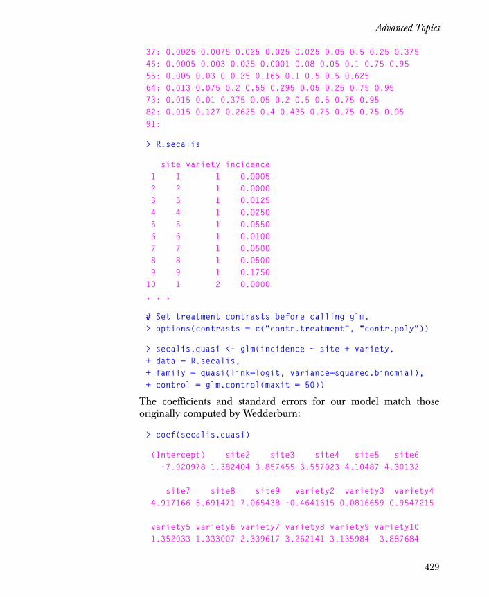
Advanced Topics
37: 0.0025 0.0075 0.025 0.025 0.025 0.05 0.5 0.25 0.37546: 0.0005 0.003 0.025 0.0001 0.08 0.05 0.1 0.75 0.9555: 0.005 0.03 0 0.25 0.165 0.1 0.5 0.5 0.62564: 0.013 0.075 0.2 0.55 0.295 0.05 0.25 0.75 0.9573: 0.015 0.01 0.375 0.05 0.2 0.5 0.5 0.75 0.9582: 0.015 0.127 0.2625 0.4 0.435 0.75 0.75 0.75 0.9591:
> R.secalis
site variety incidence 1 1 1 0.0005 2 2 1 0.0000 3 3 1 0.0125 4 4 1 0.0250 5 5 1 0.0550 6 6 1 0.0100 7 7 1 0.0500 8 8 1 0.0500 9 9 1 0.175010 1 2 0.0000. . .
# Set treatment contrasts before calling glm.> options(contrasts = c("contr.treatment", "contr.poly"))
> secalis.quasi <- glm(incidence ~ site + variety, + data = R.secalis,+ family = quasi(link=logit, variance=squared.binomial),+ control = glm.control(maxit = 50))
The coefficients and standard errors for our model match thoseoriginally computed by Wedderburn:
> coef(secalis.quasi)
(Intercept) site2 site3 site4 site5 site6 -7.920978 1.382404 3.857455 3.557023 4.10487 4.30132
site7 site8 site9 variety2 variety3 variety4 4.917166 5.691471 7.065438 -0.4641615 0.0816659 0.9547215
variety5 variety6 variety7 variety8 variety9 variety10 1.352033 1.333007 2.339617 3.262141 3.135984 3.887684
429

Chapter 12 Generalizing the Linear Model
Example: negative binomial distribution
The negative binomial distribution arises when modeling“overdispersed Poisson data,” which is frequency data in which thevariance is greater than mean. This type of data can arise in Poissonprocesses that have variable length, or in processes where each eventcontributes a variable amount to the total. The negative binomialdistribution assumes many forms in these contexts; we create a newfamily for a particular form in which the variance is quadratic. Foradditional technical details, see Venables and Ripley (1997) andMcCullagh and Nelder (1989).
Suppose we have a response variable that is Poisson with a mean of. We assume that itself is random, and follows a gamma
distribution with mean and variance , for a parameter .Thus, the variance of is proportional to the square of its mean. Thismixture of distributions results in the following negative binomialdistribution for :
,
where and is the gamma function. For fixed , thenegative binomial distribution in this form has a canonical link givenby
and the variance function .
We use the make.family function to create a family for the negativebinomial distribution. For simplicity, we use the code for the log andlogit link functions as templates for creating the negative binomiallink. The code for the variance function below is taken from Venablesand Ripley (1997).
> neg.binomial <- function(theta = + stop("theta must be given")) {+ nb.link <- list(+ names = "log(mu/(mu + theta))",+ link = substitute(function(mu, th = .Theta)
YZ Z
μ μ μ2 θ⁄+ θZ
Y
fμ θ, y( ) Γ θ y+( )μyθθ
Γ θ( )y! μ θ+( )θ y+--------------------------------------------=
y 1 2 …, ,= Γ θ
η μ( ) μμ θ+------------⎝ ⎠
⎛ ⎞log=
var Y( ) μ μ2 θ⁄+=
430

Advanced Topics
+ log(mu/(mu + th)), + frame = list(.Theta = theta)),+ inverse = substitute(function(eta, th = .Theta)+ {+ tmp <- care.exp(eta)+ return((tmp * th) / (1 - tmp))+ },+ frame = list(.Theta = theta)),+ deriv = substitute(function(mu, th = .Theta)+ {+ d <- mu * (mu + th)+ if(any(tiny <- (d < .Machine$double.eps))) {+ warning("Model unstable")+ d[tiny] <- .Machine$double.eps+ }+ return(th / d)+ },+ frame = list(.Theta = theta)),+ initialize = expression(mu <- y + (y==0)/6)+ )+ nb.variance <- list(+ names = "mu + mu^2/theta",+ variance = substitute(function(mu, th = .Theta)+ mu * (1 - mu/th),+ frame = list(.Theta = theta)),+ deviance = substitute(+ function(mu, y, w, residuals = F, th = .Theta)+ {+ devi <- 2 * w * (y * log(pmax(1,y) / mu) -+ (y + th) * log((y + th) / (mu + th)))+ if(residuals) + return(sign(y - mu) * sqrt(abs(devi)))+ else + return(sum(devi))+ },+ frame = list(.Theta = theta))+ )+ make.family(+ name = "Negative binomial",+ link = nb.link,+ variance = nb.variance) }
431

Chapter 12 Generalizing the Linear Model
REFERENCES
Agresti, Alan. (1990). Categorical Data Analysis. New York: John &Sons.
Chambers, J.M. and Hastie, T.J. (Eds.) (1993). Statistical Models in S.London: Chapman and Hall.
Comizzoli R.B., Landwehr J.M., and Sinclair J.D. (1990). Robustmaterials and processes: Key to reliability. AT&T Technical Journal,69(6): 113--128.
Hastie, T. and Tibshirani, R. (1990). Generalized Additive Models.London: Chapman and Hall.
McCullagh, P. and Nelder, J.A. (1989). Generalized Linear Models (2nded.). London: Chapman and Hall.
Nelder, J.A. and Wedderburn, R.W.M. (1972). Generalized linearmodels. Journal of the Royal Statistical Society (Series A) 135: 370-384.
Venables, W.N. and Ripley, B.D. (1997). Modern Applied Statistics withSpotfire S+ (2nd ed.). New York: Springer-Verlag, Inc.
Wedderburn, R.W.M. (1974). Quasilikelihood functions, generalizedlinear models and the Gauss-Newton method. Biometrika 61: 439-447.
432

Introduction 434
Fitting a Simple Model 435
Diagnostics: Evaluating the Fit 436
Exploring Data with Multiple Predictors 439Conditioning Plots 439Creating Conditioning Values 441Constructing a Conditioning Plot 441Analyzing Conditioning Plots 443
Fitting a Multivariate Loess Model 446
Looking at the Fitted Model 452
Improving the Model 455
LOCAL REGRESSION MODELS 13
433

Chapter 13 Local Regression Models
INTRODUCTION
In both Chapter 10, Regression and Smoothing for ContinuousResponse Data, and Chapter 12, Generalizing the Linear Model, wediscuss fitting curves or surfaces to data. In both of these earlierchapters, a significant limitation on the surfaces considered was thatthe effects of the terms in the model were expected to enter the modeladditively, without interactions between terms.
Local regression models provide much greater flexibility in that themodel is fitted as a single smooth function of all the predictors. Thereare no restrictions on the relationships among the predictors.
Local regression models in TIBCO Spotfire S+ are created using theloess function, which uses locally weighted regression smoothing, asdescribed in the section Smoothing on page 290. In that section, thefocus was on the smoothing function as an estimate of one predictor’scontribution to the model. In this chapter, we use locally weightedregression to fit the complete regression surface.
434
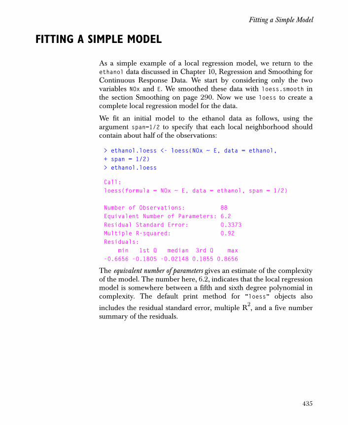
Fitting a Simple Model
FITTING A SIMPLE MODEL
As a simple example of a local regression model, we return to theethanol data discussed in Chapter 10, Regression and Smoothing forContinuous Response Data. We start by considering only the twovariables NOx and E. We smoothed these data with loess.smooth inthe section Smoothing on page 290. Now we use loess to create acomplete local regression model for the data.
We fit an initial model to the ethanol data as follows, using theargument span=1/2 to specify that each local neighborhood shouldcontain about half of the observations:
> ethanol.loess <- loess(NOx ~ E, data = ethanol,+ span = 1/2)> ethanol.loess
Call:loess(formula = NOx ~ E, data = ethanol, span = 1/2)
Number of Observations: 88Equivalent Number of Parameters: 6.2Residual Standard Error: 0.3373Multiple R-squared: 0.92Residuals: min 1st Q median 3rd Q max-0.6656 -0.1805 -0.02148 0.1855 0.8656
The equivalent number of parameters gives an estimate of the complexityof the model. The number here, 6.2, indicates that the local regressionmodel is somewhere between a fifth and sixth degree polynomial incomplexity. The default print method for "loess" objects also
includes the residual standard error, multiple R2, and a five numbersummary of the residuals.
435

Chapter 13 Local Regression Models
DIAGNOSTICS: EVALUATING THE FIT
How good is our initial fit? The following function calls plot the loessobject against a scatter plot of the original data:
> attach(ethanol)> plot(ethanol.loess, xlim = range(E),+ ylim = range(NOx, fitted(ethanol.loess)))> points(E, NOx)
The resulting plot, shown in Figure 13.1, captures the trendreasonably well. The following expressions plot the residuals againstthe predictor E to check for lack of fit:
> scatter.smooth(E, resid(ethanol.loess), span = 1,+ degree = 1)> abline(h = 0)
The resulting plot, shown in Figure 13.2, indicates no lack of fit.
Figure 13.1: Locally weighted smooth of ethanol data.
E
NO
x
0.6 0.8 1.0 1.2
12
34
•
•
•
•
•
•
•
•
•
•
•
•••
•
•••
•
•
•
•
•
•
•
•
•
•
•
•
•
•
•
•
•
•
•
•
•
•
•
•
•
•
•
•
•
•
•
•
•
•
•
••
••
•
•
•
•
•
•
•
•
••
•
•
•
•
•
•
•
•
•
•
••
•
•
••••
••
•
436

Diagnostics: Evaluating the Fit
Is there a surplus of fit? That is, can we increase the span of the dataand still get a good fit? To see, let’s refit our model, using update:
> ethanol.loess2 <- update(ethanol.loess, span = 1)> ethanol.loess2
Call:loess(formula = NOx ~ E, data = ethanol, span = 1)Number of Observations: 88Equivalent Number of Parameters: 3.5Residual Standard Error: 0.5126Multiple R-squared: 0.81Residuals: min 1st Q median 3rd Q max-0.9791 -0.4868 -0.064 0.3471 0.9863
Figure 13.2: Residual plot for loess smooth.
•• •
• •••
•• •••
•
•
•
•
•
•
••
••
•
•
•
•
•
•
•••
••
•
••
•
•
•
•
•
••
•
•
•
•
•
•••
•
•
••
•
•
•
•
•
•
• •
•
•
•
•
•
•
••
••
•
•
•
•
••
•
•
•
•
•
•
•
•
•
E
resi
d(et
hano
l.loe
ss)
0.6 0.8 1.0 1.2
-0.5
0.0
0.5
437

Chapter 13 Local Regression Models
By increasing the span, we reduce somewhat the equivalent numberof parameters; this model is thus more parsimonious than our firstmodel. We do seem to have lost some fit and gained some residualerror. The diagnostic plots, shown in Figure 13.3, reveal a lesssatisfying fit in the main plot, and much obvious structure left in theresiduals.
The residuals are also more broadly spread than those of the firstmodel. We confirm this with a call to anova as follows:
> anova(ethanol.loess2, ethanol.loess)
Model 1:loess(formula = NOx ~ E, data = ethanol, span = 1)Model 2:loess(formula = NOx ~ E, data = ethanol, span = 1/2)Analysis of Variance Table ENP RSS Test F Value Pr(F)1 3.5 22.0840 1 vs 2 32.79 8.2157e-152 6.2 9.1685
The difference between the models is highly significant, so we stickwith our original model.
Figure 13.3: Diagnostic plots for loess fit with span 1.
E
NO
x
0.6 0.8 1.0 1.2
12
34
•
•
•
•
•
•
•
•
•
•
•
•••
•
•••
•
•
•
•
•
••
•
•
•
•
•
••
•
•
••
•
•
•
•
•
•
•
••
•
•
•
•
•
•
•
•
••
• •
•
•
•
•
•
•
•
•
•••
••
•
•
•
•
•
•
•
••
•
•
••••••
•
•
••
• ••
•
•
•
••
••
•
•
•
••
•
•
•
•
•
•
•
••
•
•
•
••
•
•
••
•
•
••
•
••
•
•
•
•
•
•
•
•
••
••
•
•
•
•
•
•
•
•
••
••
•
•
•
•
•
•
•
•
••
•
•
•
•
•
•
•
••
•
•
E
resi
d(et
hano
l.loe
ss2)
0.6 0.8 1.0 1.2
-1.0
0.0
1.0
438
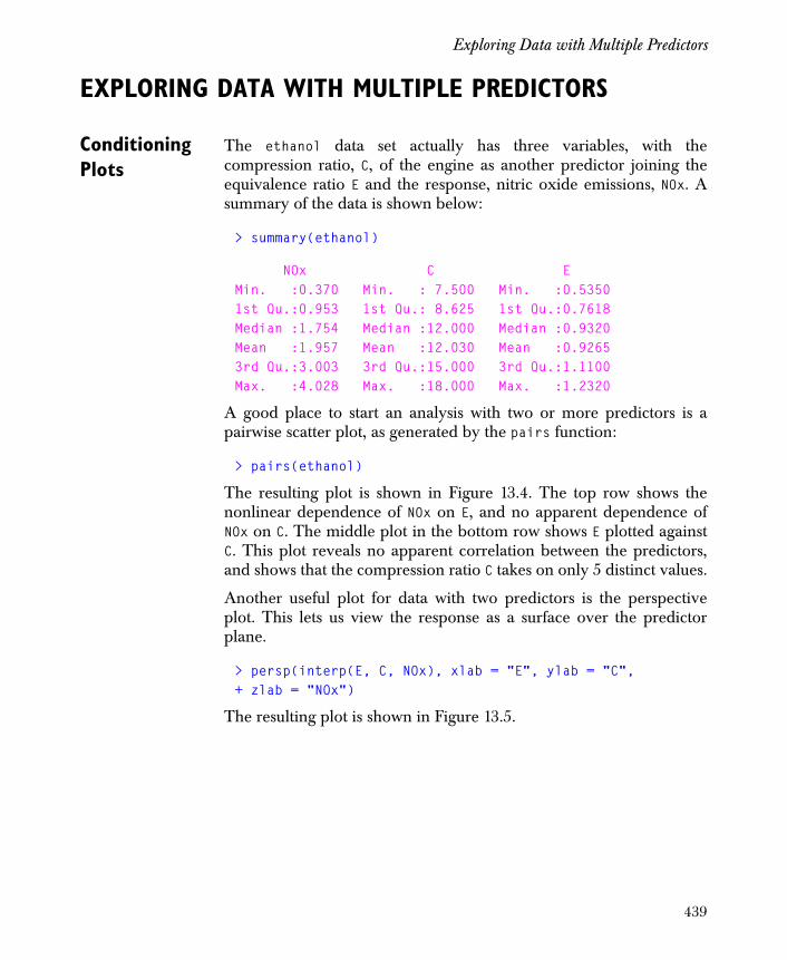
Exploring Data with Multiple Predictors
EXPLORING DATA WITH MULTIPLE PREDICTORS
Conditioning Plots
The ethanol data set actually has three variables, with thecompression ratio, C, of the engine as another predictor joining theequivalence ratio E and the response, nitric oxide emissions, NOx. Asummary of the data is shown below:
> summary(ethanol)
NOx C EMin. :0.370 Min. : 7.500 Min. :0.53501st Qu.:0.953 1st Qu.: 8.625 1st Qu.:0.7618Median :1.754 Median :12.000 Median :0.9320Mean :1.957 Mean :12.030 Mean :0.92653rd Qu.:3.003 3rd Qu.:15.000 3rd Qu.:1.1100Max. :4.028 Max. :18.000 Max. :1.2320
A good place to start an analysis with two or more predictors is apairwise scatter plot, as generated by the pairs function:
> pairs(ethanol)
The resulting plot is shown in Figure 13.4. The top row shows thenonlinear dependence of NOx on E, and no apparent dependence ofNOx on C. The middle plot in the bottom row shows E plotted againstC. This plot reveals no apparent correlation between the predictors,and shows that the compression ratio C takes on only 5 distinct values.
Another useful plot for data with two predictors is the perspectiveplot. This lets us view the response as a surface over the predictorplane.
> persp(interp(E, C, NOx), xlab = "E", ylab = "C", + zlab = "NOx")
The resulting plot is shown in Figure 13.5.
439
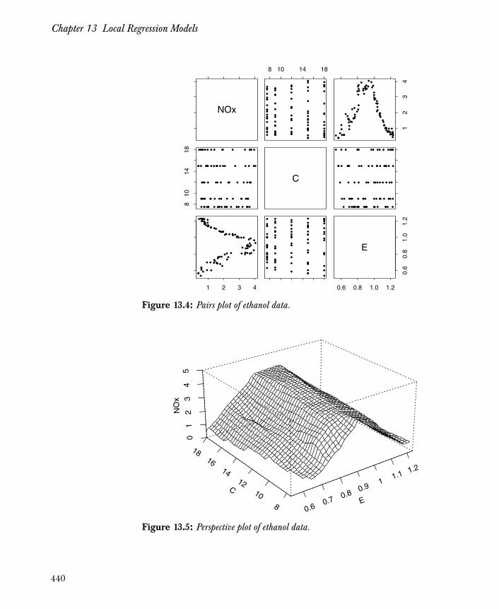
Chapter 13 Local Regression Models
Figure 13.4: Pairs plot of ethanol data.
Figure 13.5: Perspective plot of ethanol data.
NOx
8 10 14 18
•
•
•
•
•
•
••
•
•
•
• • ••
•••
•
•
•
•
•
••
•
•
•
•
•
••
•
•
••
•
•
•
•
•
••
••
•
•
•
•
•
•
•
•
••
••
•
•
•
•
•
•
•
•
•••
••
•
•
•
•
•
•
•
• •
•
•
•• • •• •
•
12
34
•
•
•
•
•
•
••
•
•
•
••••
• ••
•
•
•
•
•
••
•
•
•
•
•
••
•
•
••
•
•
•
•
•
••
••
•
•
•
•
•
•
•
•
••
• •
•
•
•
•
•
•
•
•
•• •
••
•
•
•
•
•
•
•
••
•
•
••••••
•
810
1418
••• ••
•• •
•• ••
•
•
•
• •
• •
••••
• •
• •
• ••
• •• ••
• ••• •
•• ••
• •• •• ••
•
• •
••
• ••• • ••
•• •
••
•• •
• • •••
•••
•
••
••
•
•
• •
C •• •• •
• ••
• •• •
•
•
•
• •
••
• •• •
••
• •
• ••
•• •• •
••• ••
• •• •
• •• •• ••
•
••
••
• •• •• • •
• ••
• •
• ••
• • • • •
• ••
•
• •
••
•
•
• •
1 2 3 4
•
•
••
•
•
••
•
•
•
••
•• •
••
•
•
••
••
•
•
•
•
•
•
•
•
•
••
•
••
••
•
••
•
•••
••
••
•
••
•
••
••
•
•
••
•
•
••
•
•
•
•
••
•
•
•
•
••
•
•
•
•••••
•
•
•
••
•
•
••
•
•
•
• •
•• •
• •
•
•
••
•••
•
•
•
•
•
•
•
•
••
•
••
••
•
••
•
•••
••
••
•
••
•
••
••
•
•
••
•
•
••
•
•
•
•
••
•
•
•
•
••
•
•
•
• • • • •
•
0.6 0.8 1.0 1.2
0.6
0.8
1.0
1.2
E
0.60.7
0.80.9
11.1 1.2
E8
10
12
14
16
18
C
01
23
45
NO
x
440

Exploring Data with Multiple Predictors
One conclusion we cannot draw from the pairwise scatter plot is thatthere is no effect of C on NOx. Such an effect might well exist, but bemasked by the strong effect of E. Another type of plot, the conditioningplot, or coplot, can reveal such hidden effects.
A coplot shows how a response depends upon a predictor given otherpredictors. Basically, the idea is to create a matrix of conditioningpanels; each panel graphs the response against the predictor for thoseobservations whose value of the given predictor lie in an interval.
To create a coplot:
1. (Optional) Create the conditioning values. The coplot function creates default values if conditioning values are omitted, but they are not usually as good as those created specifically for the data at hand.
2. Use the coplot function to create the plot.
We discuss these steps in detail in the following subsections.
Creating Conditioning Values
How you create conditioning values depends on the nature of thevalues taken on by the predictor, whether continuous or discrete.
For continuous data, the conditioning values are intervals, createdusing the function co.intervals. For example, the following callcreates nine intervals for the predictor E:
> E.intervals <- co.intervals(E, number = 9, overlap = 1/4)
For data taking on discrete values, the conditioning values are thesorted, unique values. For example, the following call creates theconditioning values for the predictor C:
> C.points <- sort(unique(C))
Constructing a Conditioning Plot
To construct a conditioning plot, use coplot using a formula with thespecial form A ~ B | C, where A is the response, B is the predictor ofinterest, and C is the given predictor. Thus, to see the effect of C onNOx given E, use the formula NOx ~ C | E.
441
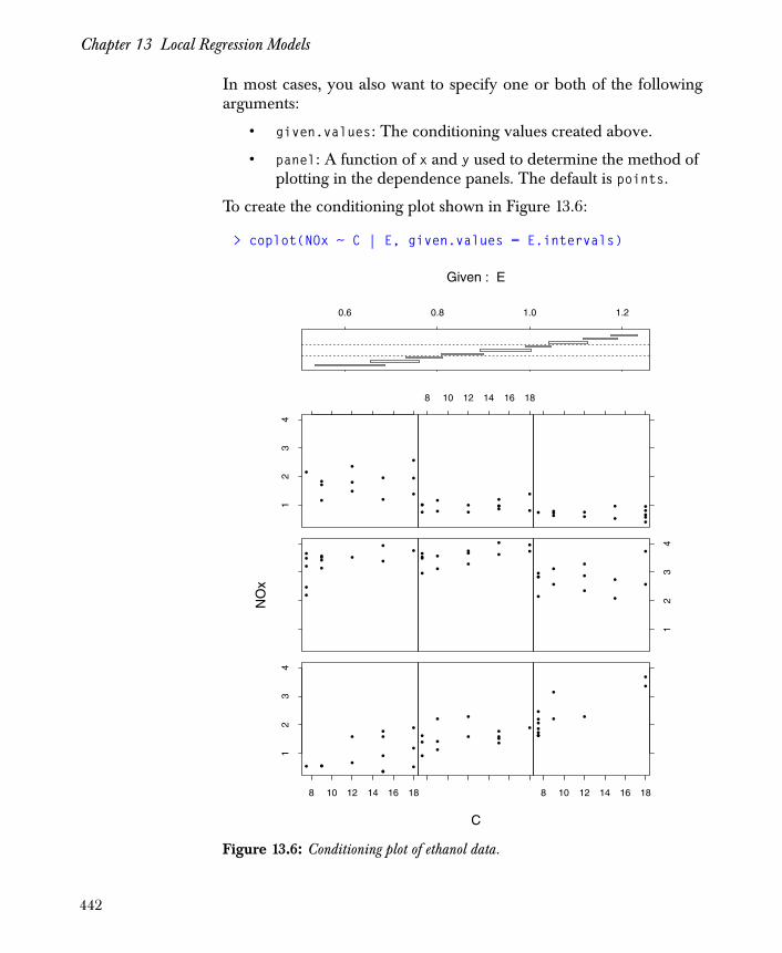
Chapter 13 Local Regression Models
In most cases, you also want to specify one or both of the followingarguments:
• given.values: The conditioning values created above.
• panel: A function of x and y used to determine the method of plotting in the dependence panels. The default is points.
To create the conditioning plot shown in Figure 13.6:
> coplot(NOx ~ C | E, given.values = E.intervals)
Figure 13.6: Conditioning plot of ethanol data.
••
••
••
•• • •
• •
•
8 10 12 14 16 18
12
34
•
•
••
•
••••
•
••
••
•
••
•
••
••
•
•
•
8 10 12 14 16 18
••••
•
•
•
•
• •• ••
•
•
••••
•••
••
••
••
•
•• •
••
••
•
•
•
12
34
••
•
• ••
•
••
•
•
•
12
34
•• • ••
••••
•
•••
8 10 12 14 16 18
•• • ••
••••
•• •
•
0.6 0.8 1.0 1.2
C
NO
xGiven : E
442

Exploring Data with Multiple Predictors
Analyzing Conditioning Plots
To read the coplot, move from left to right, bottom to top. The scatterplots on the bottom row show an upward trend, while those on theupper two rows show a flat trend. We can more easily see the trendby using a smoothing function inside the conditioning panels, whichwe can do by specifying the panel argument to coplot as follows:
> coplot(NOx ~ C | E, given.values = E.intervals,+ panel = function(x, y) panel.smooth(x, y,+ degree = 1, span = 1))
The resulting plot is shown in Figure 13.7.
Figure 13.7: Smooth conditioning plot of ethanol data.
••
••
••
•• • •
• •
•
8 10 12 14 16 18
12
34
•
•
••
•
••••
•
••
••
•
••
•
••
••
•
•
•
8 10 12 14 16 18
••••
•
•
•
•
• •• ••
•
•
••••
•••
••
••
••
•
•• •
••
••
•
•
•
12
34
••
•
• ••
•
••
•
•
•
12
34
•• • ••
••••
•
•••
8 10 12 14 16 18
•• • ••
••••
•• •
•
0.6 0.8 1.0 1.2
C
NO
x
Given : E
443
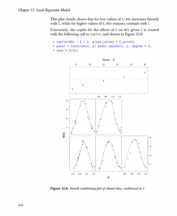
Chapter 13 Local Regression Models
This plot clearly shows that for low values of E, NOx increases linearlywith C, while for higher values of E, NOx remains constant with C.
Conversely, the coplot for the effects of E on NOx given C is createdwith the following call to coplot, and shown in Figure 13.8:
> coplot(NOx ~ E | C, given.values = C.points,+ panel = function(x, y) panel.smooth(x, y, degree = 2,+ span = 2/3))
Figure 13.8: Smooth conditioning plot of ethanol data, conditioned on C.
•
•
•
•
•
•
•
•
•
•
•
•
•
•
•
•
•
•
•
•
•
•
0.6 0.8 1.0 1.2
•
•
•
•
•
•
•
•
•
•
•
•
•
•
•
••
•
•
•
•
•
•
•
•
•
••
••
•
0.6 0.8 1.0 1.2
12
34
•
•
•
•
•
•
•
•
•
•
•
•
•
•
•
•
•
•
•
12
34
•
•
•
•
•
•
•
•
••
•
• •
••
•
0.6 0.8 1.0 1.2
8 10 12 14 16 18
E
NO
xGiven : C
444

Exploring Data with Multiple Predictors
Comparing the two coplots, we can see that NOx changes more rapidlyas a function of E with C fixed than as a function of C with E fixed.Also, the variability of the residuals is small compared to the effect ofE, but noticeable compared to the effect of C.
445

Chapter 13 Local Regression Models
FITTING A MULTIVARIATE LOESS MODEL
We have learned quite a bit about the ethanol data without fitting amodel: there is a strong nonlinear dependence of NOx on E and thereis an interaction between C and E. We can use this knowledge toshape our initial local regression model. First, we specify a formulathat includes as predictors both E and C, namely NOx ~ C * E. Then,we accept the default of local quadratic fitting to better model thenonlinear dependence.
> ethanol.m <- loess(NOx ~ C * E, data = ethanol)> ethanol.m
Call:loess(formula = NOx ~ C * E, data = ethanol)
Number of Observations: 88Equivalent Number of Parameters: 9.4Residual Standard Error: 0.3611Multiple R-squared: 0.92Residuals: min 1st Q median 3rd Q max-0.7782 -0.3517 -0.05283 0.195 0.6338
We search for lack of fit by plotting the residuals against each of thepredictors:
> par(mfrow = c(1,2))> scatter.smooth(C, residuals(ethanol.m), span = 1, deg=2)> abline(h = 0)> scatter.smooth(E, residuals(ethanol.m), span = 1, deg=2)> abline(h = 0)
The resulting plot is shown in Figure 13.9. The right-hand plot in thefigure shows considerable lack of fit, so we reduce the span from thedefault 0.75 to 0.4:
> ethanol.m2 <- update(ethanol.m, span = .4)
446

Fitting a Multivariate Loess Model
> ethanol.m2
Call: loess(formula = NOx ~ C * E, data = ethanol,span = 0.4)
Number of Observations: 88Equivalent Number of Parameters: 15.3Residual Standard Error: 0.2241Multiple R-squared: 0.97Residuals: min 1st Q median 3rd Q max-0.4693 -0.1865 -0.03518 0.1027 0.3739
Repeating the commands for generating the diagnostic plots withethanol.m2 replacing ethanol.m yields the plot shown in Figure13.10.
Figure 13.9: Diagnostic plot for loess model of ethanol data.
Figure 13.10: Diagnostic plot for first revised model.
•
•
•
••••
•
•
•••
•
•• •• •
••
•
•
•
•
•
•
•
•
•
•
•
•
•
•
••
•
••••
••
•
•
•
•
•
•
•
• ••
••
••
•
•••
•
• ••••
•
•
••
•
•
•
•
•
••
•
•
•
•
• • •
•
•
•
C
resi
d(et
hano
l.m)
8 10 14 18
-0.8
-0.2
0.4
•
•
•
• ••
•
•
•
••
•
•
••• ••
••
•
•
•
•
•
•
•
•
•
•
•
•
•
•
••
•
• •••
••
•
•
•
•
•
•
•
•••
••
••
•
• ••
•
•••
•••
•
••
•
•
•
•
•
• •
•
•
•
•
•••
•
•
•
E
resi
d(et
hano
l.m)
0.6 0.8 1.0 1.2-0
.8-0
.20.
4
•
•
•
••
•
••
••••
• •••
•
•
••
•
•
• •••
•
••
•
•
•
•
•
•••••• •
••
•
•
•
•
••
•
•
•
••
••
•
••
•
•
• •••
••
•
•• •
•
•
•
•••
•
•
•
•
•
•
•
•
•
•
C
resi
d(et
hano
l.m2)
8 10 14 18
-0.4
0.0
0.4
•
•
•
••
•
••
• •••
•• ••
•
•
••
•
•
• •••
•
••
•
•
•
•
•
•••• •••
••
•
•
•
•
••
••
•
•
••
••
•
• •
•
•
•• ••
• •
•
•••
•
•
•
•••
•
•
•
•
•
•
•
•
•
•
E
resi
d(et
hano
l.m2)
0.6 0.8 1.0 1.2
-0.4
0.0
0.4
447
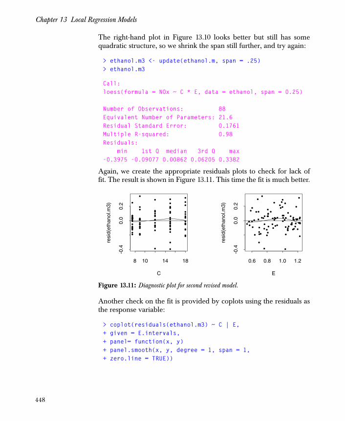
Chapter 13 Local Regression Models
The right-hand plot in Figure 13.10 looks better but still has somequadratic structure, so we shrink the span still further, and try again:
> ethanol.m3 <- update(ethanol.m, span = .25)> ethanol.m3
Call:loess(formula = NOx ~ C * E, data = ethanol, span = 0.25)
Number of Observations: 88Equivalent Number of Parameters: 21.6Residual Standard Error: 0.1761Multiple R-squared: 0.98Residuals: min 1st Q median 3rd Q max-0.3975 -0.09077 0.00862 0.06205 0.3382
Again, we create the appropriate residuals plots to check for lack offit. The result is shown in Figure 13.11. This time the fit is much better.
Another check on the fit is provided by coplots using the residuals asthe response variable:
> coplot(residuals(ethanol.m3) ~ C | E,+ given = E.intervals,+ panel= function(x, y)+ panel.smooth(x, y, degree = 1, span = 1, + zero.line = TRUE))
Figure 13.11: Diagnostic plot for second revised model.
•
•
•••
•
•• ••••
•
••
•
•
••
•
•
••
•
••
•
•• •
•
•
•
•
••••
•
• •
••
•
•
•
•
•••
•
•
•
••
•••
••
•
•
• •••
•
•
•
••
•
••
•
•
•• •
•
•
•
••
•
• •
•
C
resi
d(et
hano
l.m3)
8 10 14 18
-0.4
0.0
0.2
•
•
•••
•
•••••
•
•
••
•
•
••
•
•
• •
•
••
•
•••
•
•
•
•
•••
•
•
••
••
•
•
•
•
••
•
•
•
•
••
• • •
••
•
•
•••••
•
•
••
•
••
•
•
• ••
•
•
•
••
•
••
•
E
resi
d(et
hano
l.m3)
0.6 0.8 1.0 1.2
-0.4
0.0
0.2
448
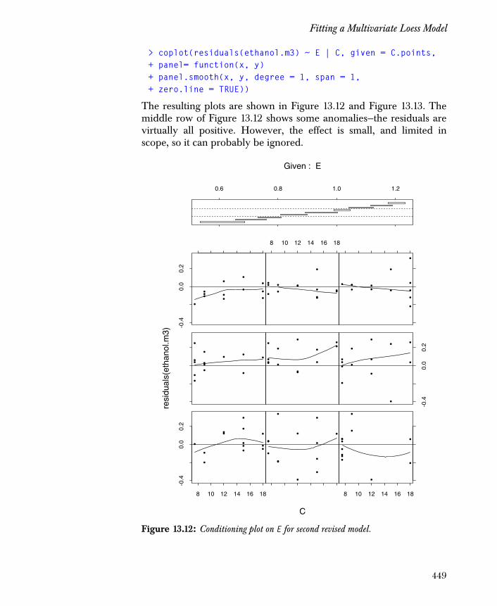
Fitting a Multivariate Loess Model
> coplot(residuals(ethanol.m3) ~ E | C, given = C.points,+ panel= function(x, y)+ panel.smooth(x, y, degree = 1, span = 1, + zero.line = TRUE))
The resulting plots are shown in Figure 13.12 and Figure 13.13. Themiddle row of Figure 13.12 shows some anomalies—the residuals arevirtually all positive. However, the effect is small, and limited inscope, so it can probably be ignored.
Figure 13.12: Conditioning plot on E for second revised model.
•
•
•
•
•
•
•
••
•
• •
•
8 10 12 14 16 18
-0.4
0.0
0.2
•
•
•
•
•
•
•
•••
• •
•
•
••
••
•
•
•
•
• •
•
8 10 12 14 16 18
•
•••
•
••
•
•
••
•
•
•
•
•
•
•
•
•
•
•
•
•
•
•
•
•
•
••
•
•
••
•
•
•
•
-0.4
0.0
0.2
•
• ••
•
••
•
•
••
•
-0.4
0.0
0.2
••
•
•
••
••
•••
•
•
8 10 12 14 16 18
•• •
•
••
•
••
•
• •
•
0.6 0.8 1.0 1.2
C
resi
dual
s(et
hano
l.m3)
Given : E
449

Chapter 13 Local Regression Models
As a final test, we create several additional diagnostic plots to checkthe distribution of the error terms. The plots generated by thefollowing commands are shown in Figure 13.14.
> par(mfrow=c(2, 2))> plot(fitted(ethanol.m3), sqrt(abs(resid(ethanol.m3))))> plot(C, sqrt(abs(resid(ethanol.m3))))> plot(E, sqrt(abs(resid(ethanol.m3))))
Figure 13.13: Conditioning plot on C for second revised model.
•
• ••
•
•
•
•
••
•• •
•
•
•
•
•• •
•
•
0.6 0.8 1.0 1.2
•
••
•
•
•
••
•
•
•
•
•
•• •
• •
•
•••
••
•
•
•
•
•
•
•
0.6 0.8 1.0 1.2
-0.4
-0.2
0.0
0.2
•
••
•
•
•
•
•
•
•
•
•
•
•
•
•
•
•
•
-0.4
-0.2
0.0
0.2
•
•
•
•
•
•
•
•
•
•••
•
•
•
•
0.6 0.8 1.0 1.2
8 10 12 14 16 18
E
resi
dual
s(et
hano
l.m3)
Given : C
450
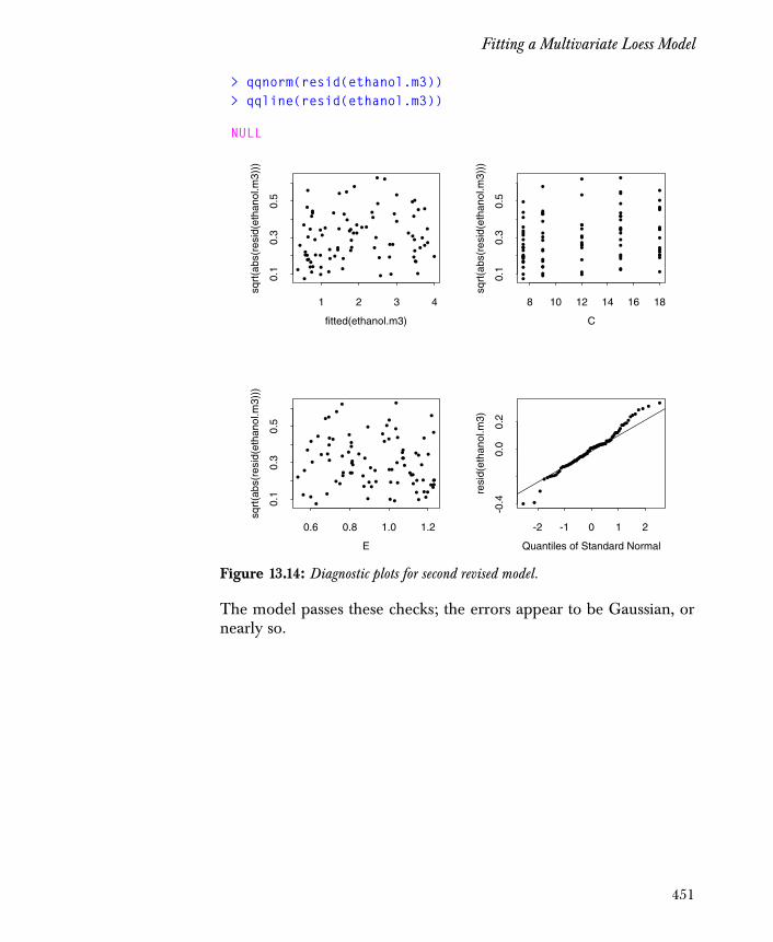
Fitting a Multivariate Loess Model
> qqnorm(resid(ethanol.m3))> qqline(resid(ethanol.m3))
NULL
The model passes these checks; the errors appear to be Gaussian, ornearly so.
Figure 13.14: Diagnostic plots for second revised model.
•
•
• •
•
•
••
•
••
•
•
•
•• •
•
•
••
••
•
••
•
•
• •
•
•
•
•
•
••
•
•
• •
•
•
•
•
•
•
••
••
•
•
•
•
•• •
•
•
•
•
••
••
•
•
•
••
• •
•
•
•
•••
•
•
•
•
••
•
•
•
fitted(ethanol.m3)
sqrt
(abs
(res
id(e
than
ol.m
3)))
1 2 3 4
0.1
0.3
0.5
•
•
••
•
•
••
•
••
•
•
•
••• •
•
••
••
•
••
•
•
• •
•
•
•
•
•
••
•
•
• •
•
•
•
•
•
•
••
••
•
•
•
•
•••
•
•
•
•
••
••
•
•
•
••
••
•
•
•
•• •
•
•
•
•
••
•
•
•
C
sqrt
(abs
(res
id(e
than
ol.m
3)))
8 10 12 14 16 18
0.1
0.3
0.5
•
•
••
•
•
••
•
••
•
•
•
•• •
•
•
••
••
•
••
•
•
••
•
•
•
•
•
••
•
•
••
•
•
•
•
•
•
••
••
•
•
•
•
•• •
•
•
•
•
••
•••
•
•
••
• •
•
•
•
• ••
•
•
•
•
••
•
•
•
E
sqrt
(abs
(res
id(e
than
ol.m
3)))
0.6 0.8 1.0 1.2
0.1
0.3
0.5
•
•
•••
•
••••••
•
••
•
•
••
•
•
••
•
••
•
•••
•
•
•
•
•• •
•
•
••
••
•
•
•
•
••
•
•
•
•
••
• ••
••
•
•
•••••
•
•
••
•
••
•
•
•••
•
•
•
••
•
••
•
Quantiles of Standard Normal
resi
d(et
hano
l.m3)
-2 -1 0 1 2
-0.4
0.0
0.2
451
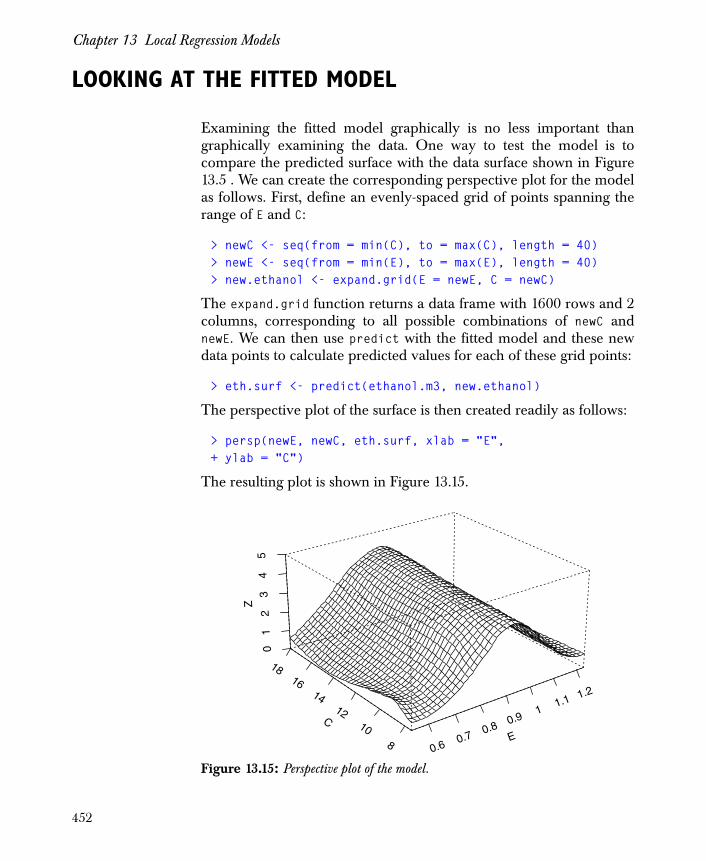
Chapter 13 Local Regression Models
LOOKING AT THE FITTED MODEL
Examining the fitted model graphically is no less important thangraphically examining the data. One way to test the model is tocompare the predicted surface with the data surface shown in Figure13.5 . We can create the corresponding perspective plot for the modelas follows. First, define an evenly-spaced grid of points spanning therange of E and C:
> newC <- seq(from = min(C), to = max(C), length = 40)> newE <- seq(from = min(E), to = max(E), length = 40)> new.ethanol <- expand.grid(E = newE, C = newC)
The expand.grid function returns a data frame with 1600 rows and 2columns, corresponding to all possible combinations of newC andnewE. We can then use predict with the fitted model and these newdata points to calculate predicted values for each of these grid points:
> eth.surf <- predict(ethanol.m3, new.ethanol)
The perspective plot of the surface is then created readily as follows:
> persp(newE, newC, eth.surf, xlab = "E",+ ylab = "C")
The resulting plot is shown in Figure 13.15.
Figure 13.15: Perspective plot of the model.
0.60.7
0.80.9
11.1 1.2
E8
10
12
14
16
18
C
01
23
45
Z
452

Looking at the Fitted Model
Not surprisingly, the surfaces look quite similar, with the modelsurface somewhat smoother than the data surface. The data surfacehas a noticeable wrinkle for E � 0.7, C � 14. This wrinkle is smoothedout in the model surface. Another graphical view is probablyworthwhile.
The default graphical view for "loess" objects with multiplepredictors is a set of coplots, one per predictor, created using the plotfunction.
> par(ask=T)> plot(ethanol.m3, confidence = 7)
The resulting plots are shown in Figure 13.16 and Figure 13.17. Onefeature that is immediately apparent, and somewhat puzzling, is thecurvy form of the bottom row of Figure 13.16. Our preliminarycoplots revealed that the dependence of NOx on C was approximatelylinear for small values of E. Thus, the model as fitted has a noticeabledeparture from our understanding of the data.
Figure 13.16: Default conditioning plot of the model, first predictor.
8 10 12 14 16 18 8 10 12 14 16 18
-10
12
34
-10
12
34
8 10 12 14 16 18
0.6 0.8 1.0 1.2
C
NO
x
Given : E
453

Chapter 13 Local Regression Models
Figure 13.17: Default conditioning plot of the model, second predictor.
0.6 0.8 1.0 1.2 0.6 0.8 1.0 1.2
-10
12
34
-10
12
34
0.6 0.8 1.0 1.2
8 10 12 14 16 18
E
NOx
Given : C
454

Improving the Model
IMPROVING THE MODEL
The model in ethanol.m3 is fit using local quadratic fitting for allterms corresponding to C*E. This means that the model contains the
following fitting variables: a constant, E, C, EC, C2, and E2. However,our original look at the data led us to believe that the effect of C waspiecewise linear; it thus makes sense to fit C parametrically, and dropthe quadratic term. We can make these changes using the updatefunction as follows:
> ethanol.m4 <- update(ethanol.m3, drop.square = "C",+ parametric = "C")> ethanol.m4
Call:loess(formula = NOx ~ C * E, span = 0.25, parametric = "C", drop.square = "C")
Number of Observations: 88Equivalent Number of Parameters: 18.2Residual Standard Error: 0.1808Multiple R-squared: 0.98Residuals: min 1st Q median 3rd Q max-0.4388 -0.07358 -0.009093 0.06616 0.5485
The coplot, Figure 13.18 and Figure 13.19, now shows the appropriatelinear fit, and we have introduced no lack of fit, as shown by theresiduals plots in Figure 13.20.
455
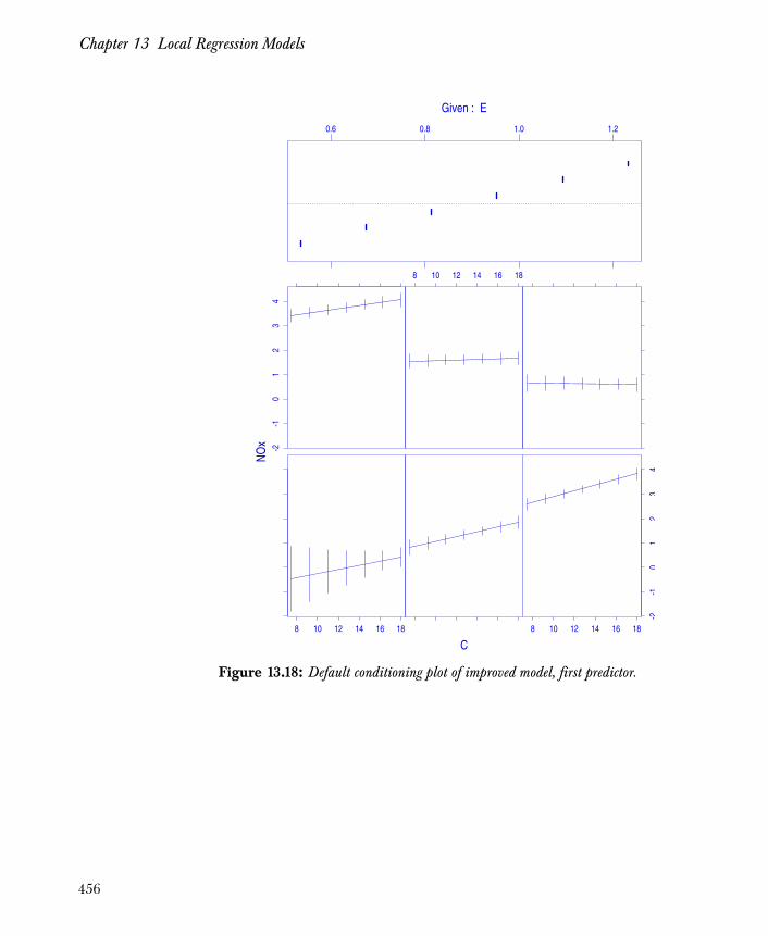
Chapter 13 Local Regression Models
Figure 13.18: Default conditioning plot of improved model, first predictor.
8 10 12 14 16 18 8 10 12 14 16 18
-2-1
01
23
4
-2-1
01
23
48 10 12 14 16 18
0.6 0.8 1.0 1.2
C
NO
x
Given : E
456
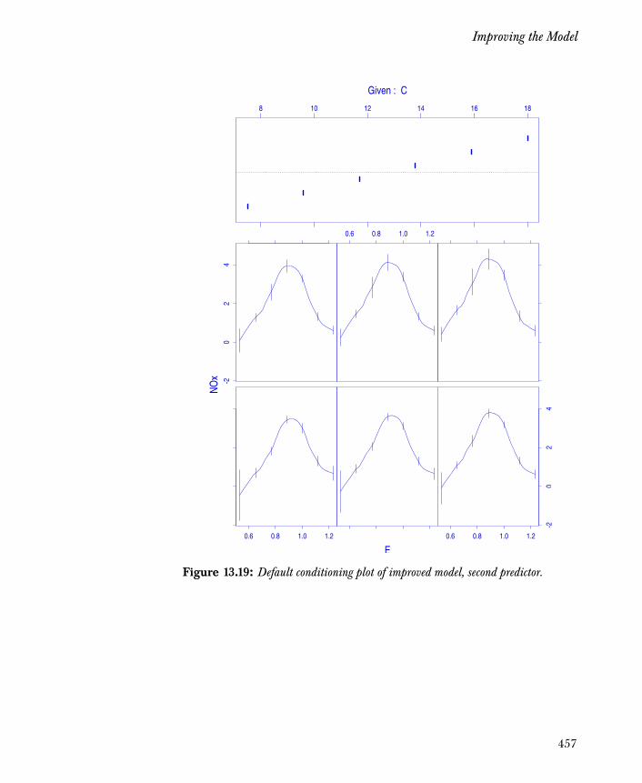
Improving the Model
Figure 13.19: Default conditioning plot of improved model, second predictor.
0.6 0.8 1.0 1.2 0.6 0.8 1.0 1.2
-20
24
-20
24
0.6 0.8 1.0 1.2
8 10 12 14 16 18
E
NO
x
Given : C
457
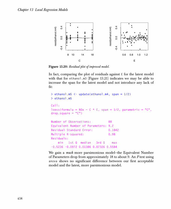
Chapter 13 Local Regression Models
In fact, comparing the plot of residuals against E for the latest modelwith that for ethanol.m3 (Figure 13.21) indicates we may be able toincrease the span for the latest model and not introduce any lack offit:
> ethanol.m5 <- update(ethanol.m4, span = 1/2)> ethanol.m5
Call:loess(formula = NOx ~ C * E, span = 1/2, parametric = "C", drop.square = "C")
Number of Observations: 88Equivalent Number of Parameters: 9.2Residual Standard Error: 0.1842Multiple R-squared: 0.98Residuals: min 1st Q median 3rd Q max-0.5236 -0.0972 0.01386 0.07326 0.5584
We gain a much more parsimonious model—the Equivalent Numberof Parameters drop from approximately 18 to about 9. An F-test usinganova shows no significant difference between our first acceptablemodel and the latest, more parsimonious model.
Figure 13.20: Residual plot of improved model.
•••••
••• •
••
•
••
•
•
•••
•
•••
•
•
••
••
••
•
•
•
•••
•
••
•
••
•
•
•
•••••
•••
•••
•
•
••
•
• •••
•
•
•••
•
••
•
•
••
•
•
•
•
••
•
•
••
C
resi
d(et
hano
l.m4)
8 10 14 18
-0.4
0.0
0.4
••
•• ••
•••••
•
••
•
•
•••
•
•• •
•
•
••
••
••
•
•
•
•••
•
••
•
••
•
•
•
• ••
••
••
••
• ••
•
••
•
••••
•
•
• ••
•
• •
•
•
••
•
•
•
•
••
•
•
••
E
resi
d(et
hano
l.m4)
0.6 0.8 1.0 1.2
-0.4
0.0
0.4
458
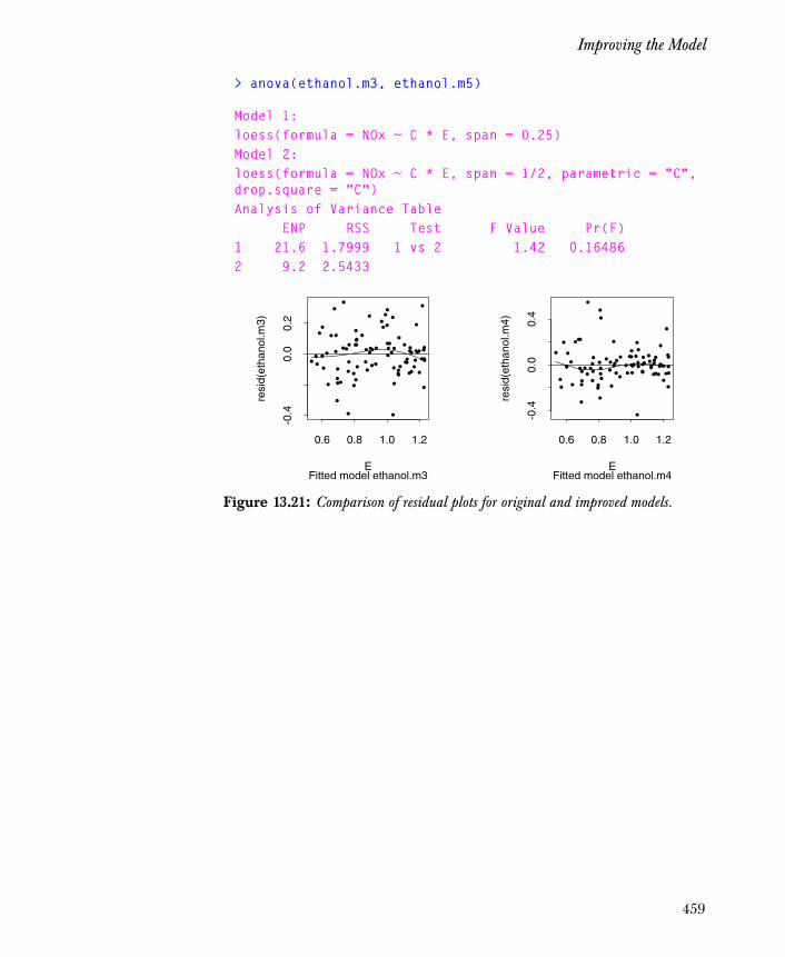
Improving the Model
> anova(ethanol.m3, ethanol.m5)
Model 1:loess(formula = NOx ~ C * E, span = 0.25)Model 2:loess(formula = NOx ~ C * E, span = 1/2, parametric = "C", drop.square = "C")Analysis of Variance Table ENP RSS Test F Value Pr(F)1 21.6 1.7999 1 vs 2 1.42 0.164862 9.2 2.5433
Figure 13.21: Comparison of residual plots for original and improved models.
•
•
•••
•
•••••
•
•
••
•
•
••
•
•
• •
•
••
•
•••
•
•
•
•
•••
•
•
••
••
•
•
•
•
••
•
•
•
•
••
• • •
••
•
•
•••••
•
•
••
•
••
•
•
• ••
•
•
•
••
•
••
•
E
resi
d(et
hano
l.m3)
0.6 0.8 1.0 1.2
-0.4
0.0
0.2
Fitted model ethanol.m3
••
•• ••
•••••
•
••
•
•
•••
•
•• •
•
•
••
••
••
•
•
•
•••
•
••
•
••
•
•
•
• ••
••
••
••
• ••
•
••
•
••••
•
•
• ••
•
• •
•
•
••
•
•
•
•
••
•
•
••
E
resi
d(et
hano
l.m4)
0.6 0.8 1.0 1.2
-0.4
0.0
0.4
Fitted model ethanol.m4
459

Chapter 13 Local Regression Models
460
Introduction 463
Representing Grouped Data Sets 465The groupedData Class 465Example: The Orthodont Data Set 466Example: The Pixel Data Set 470Example: The CO2 Data Set 472Example: The Soybean Data Set 476
Fitting Models Using the lme Function 479Model Definitions 479Arguments 481
Manipulating lme Objects 483The print Method 483The summary Method 484The anova Method 486The plot method 487Other Methods 489
Fitting Models Using the nlme Function 493Model Definition 493Arguments 494
Manipulating nlme Objects 497The print Method 497The summary Method 499The anova Method 501The plot Method 501Other Methods 502
Advanced Model Fitting 505Positive-Definite Matrix Structures 505Correlation Structures and Variance Functions 507
LINEAR AND NONLINEAR MIXED-EFFECTS MODELS 14
461

Chapter 14 Linear and Nonlinear Mixed-Effects Models
Self-Starting Functions 513Modeling Spatial Dependence 520
References 523
462

Introduction
INTRODUCTION
Mixed-effects models provide a powerful and flexible tool foranalyzing grouped data, which is data that can be classified accordingto one or more grouping variables. Mixed-effects models incorporateboth fixed and random effects:
• Fixed effects are parameters associated with an entire population, or with repeatable levels of experimental factors.
• Random effects are parameters associated with experimental units drawn at random from a population.
Such models typically describe relationships between a responsevariable and covariates that are grouped according to one or moreclassification factors. Common applications are longitudinal data,repeated measures data, multilevel data, and block designs. Byassociating common random effects to observations sharing the samelevel of a classification factor, mixed-effects models flexibly representthe covariance structure induced by grouping.
This chapter describes a set of functions, classes, and methods for theanalysis of linear and nonlinear mixed-effects models in Spotfire S+.The methods provide a comprehensive set of tools for analyzinglinear and nonlinear mixed-effects models with an arbitrary numberof nested grouping levels. They supersede the modeling facilitiesavailable in release 3 of S (Chambers and Hastie, 1992) and releases5.1 (Unix) and 2000 (Windows) of S-PLUS.
This chapter illustrates how to:
• Represent grouped data sets using the groupedData class.
• Fit basic linear mixed-effects models using the lme function and manipulate the returned objects.
• Fit basic nonlinear mixed-effects models using the nlme function and manipulate the returned objects.
• Fit advanced linear and nonlinear mixed-effects models by defining positive-definite matrices, correlation structures, and variance functions.
The analysis of several sample data sets illustrates many of theavailable features. A detailed description of all functions, classes, andmethods can be found in the on-line help files.
463

Chapter 14 Linear and Nonlinear Mixed-Effects Models
The code for the methods discussed in this chapter was contributedby Douglas M. Bates of the University of Wisconsin and José C.Pinheiro of Bell Laboratories. Their book, Mixed Effects Models in S andSpotfire S+ (2000), contains a careful description of the statisticaltheory behind mixed-effects models, as well as detailed examples ofthe software for fitting and displaying them. For discussions ofadvanced topics not presented in this chapter, we refer the reader tothe Pinheiro and Bates text.
464

Representing Grouped Data Sets
REPRESENTING GROUPED DATA SETS
The data sets used for fitting mixed-effects models have severalcharacteristics in common. They consist of measurements of acontinuous response at several levels of a covariate (for example,time, dose, or treatment). The measurements are grouped accordingto one or more factors. Additional covariates may also be present,some of which may vary within a group (inner covariates) and some ofwhich may not (outer covariates).
A natural way to represent such data in Spotfire S+ is as a data framecontaining the response, the primary covariate, the grouping factor(s),and any additional factors or continuous covariates. The differentroles of the variables in the data frame can be described by a formulaof the form
response ~ primary | grouping1/grouping2/...
This is similar to the display formula in a Trellis plot, as discussed inBecker, Cleveland, and Shyu (1996).
The groupedData Class
The formula and the data for a grouped data set are packagedtogether in a groupedData object. The constructor (the function usedto create objects of a given class) for groupedData takes a formula anda data frame as arguments. The call to the constructor establishes theroles of the variables, stores descriptive labels for plots, and convertsthe grouping factors to ordered factors so the panels in plots areordered in a natural way. By default, the order of the grouping factorsis determined by a summary function applied to the response andsplit according to the groups, taking into account the nesting order.The default summary function is the maximum. Additionally, labelscan be given for the response and the primary covariate, and theirunits can be specified as arbitrary strings. The reason for separatingthe labels and the units is to allow the units to propagate to derivedquantities, such as the residuals from a fitted model.
When outer factors are present, they are given by a formula such asouter = ~Sex or outer = ~ Treatment*Type. When multiplegrouping factors are present, a list of such formulas must be supplied.Inner factors are described in a similar way. When establishing the
465

Chapter 14 Linear and Nonlinear Mixed-Effects Models
order of the levels of the grouping factor, and hence the order ofpanels in a plot, re-ordering is only permitted within combinations oflevels for the outer factors.
Trellis parameters can be used to control the graphical presentation ofgrouped data. See the online help files for plot.nffGroupedData,plot.nfnGroupedData and plot.nmGroupedData for details. The firsttwo functions plot groupedData objects with single levels of grouping,and plot.nmGroupedData displays objects with multiple groupinglevels.
Extractor functions can be used on groupedData objects to obtain thedifferent components of the display formula. Functions such asgetGroups, getCovariate, and getResponse can be applied to extractthe corresponding element in the data set. In addition, groupedDataobjects can be summarized by group using the function gsummary.
Example: The Orthodont Data Set
As a first example of grouped data, consider the orthodontic studypresented in Potthoff and Roy (1964). These data consist of fourdistance measurements (in millimeters) made at ages 8, 10, 12, and 14years, on 16 boys and 11 girls. The measurements represent thedistance from the center of the pituitary to the pterygomaxillaryfissure.
The data from the orthodontic study are stored in the example dataset Orthodont, which has the following variables:
• The 108 observations in the data set are grouped into 27 categories by Subject.
• The 27 subjects are classified into two groups by Sex, an indicator variable assuming the value "Male" for boys and "Female" for girls.
• Each of the subjects has four measures of distance, corresponding to the four age values.
This is an example of balanced repeated measures data, with a singlelevel of grouping (Subject). We wish to predict distance from age,using Subject as a grouping variable and Sex as an outer covariate.
To create a new groupedData object for Orthodont, use the classconstructor as follows:
# Assign Orthodont to your working directory.
466

Representing Grouped Data Sets
> Orthodont <- Orthodont> Orthodont <- groupedData(distance ~ age | Subject,+ data = Orthodont, outer = ~ Sex,+ labels = list(x = "Age",+ y="Distance from pituitary to pterygomaxillary fissure"),+ units = list(x = "(yr)", y = "(mm)"))
The print method returns the display formula and the data frameassociated with a groupedData object.
> print(Orthodont)
Grouped Data: distance ~ age | Subject distance age Subject Sex 1 26.0 8 M01 Male 2 25.0 10 M01 Male 3 29.0 12 M01 Male 4 31.0 14 M01 Male...105 24.5 8 F11 Female106 25.0 10 F11 Female107 28.0 12 F11 Female108 28.0 14 F11 Female
You can also use the names and formula methods to return thevariable names and their roles in a groupedData object.
> names(Orthodont)
[1] "distance" "age" "Subject" "Sex"
> formula(Orthodont)
distance ~ age | Subject
467
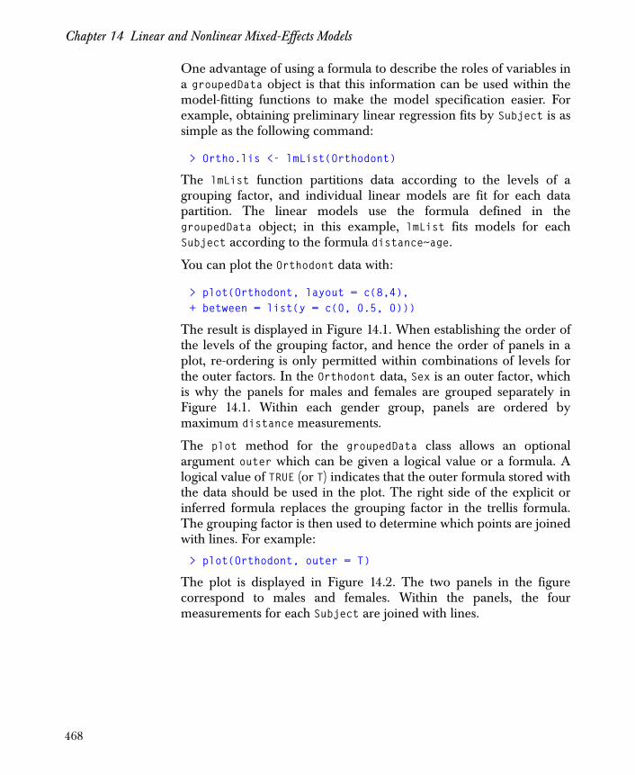
Chapter 14 Linear and Nonlinear Mixed-Effects Models
One advantage of using a formula to describe the roles of variables ina groupedData object is that this information can be used within themodel-fitting functions to make the model specification easier. Forexample, obtaining preliminary linear regression fits by Subject is assimple as the following command:
> Ortho.lis <- lmList(Orthodont)
The lmList function partitions data according to the levels of agrouping factor, and individual linear models are fit for each datapartition. The linear models use the formula defined in thegroupedData object; in this example, lmList fits models for eachSubject according to the formula distance~age.
You can plot the Orthodont data with:
> plot(Orthodont, layout = c(8,4),+ between = list(y = c(0, 0.5, 0)))
The result is displayed in Figure 14.1. When establishing the order ofthe levels of the grouping factor, and hence the order of panels in aplot, re-ordering is only permitted within combinations of levels forthe outer factors. In the Orthodont data, Sex is an outer factor, whichis why the panels for males and females are grouped separately inFigure 14.1. Within each gender group, panels are ordered bymaximum distance measurements.
The plot method for the groupedData class allows an optionalargument outer which can be given a logical value or a formula. Alogical value of TRUE (or T) indicates that the outer formula stored withthe data should be used in the plot. The right side of the explicit orinferred formula replaces the grouping factor in the trellis formula.The grouping factor is then used to determine which points are joinedwith lines. For example:
> plot(Orthodont, outer = T)
The plot is displayed in Figure 14.2. The two panels in the figurecorrespond to males and females. Within the panels, the fourmeasurements for each Subject are joined with lines.
468

Representing Grouped Data Sets
Figure 14.1: Orthodontic growth patterns in 16 boys (M) and 11 girls (F) between 8 and 14 years of age. Panels within each gender group are ordered by maximum response.
20
25
30
M11
8 10 12 14
M16 M08
8 10 12 14
M05 M14
8 10 12 14
M02 M07
8 10 12 14
M03
M04 M12 M06 M13 M15 M01 M09
20
25
30
M10
20
25
30
F10 F09 F06 F01 F05 F08 F07 F02
F03 F04
8 10 12 14
20
25
30
F11
Age (yr)
Dis
tanc
e fr
om p
ituita
ry to
pte
rygo
max
illar
y fis
sure
(m
m)
469
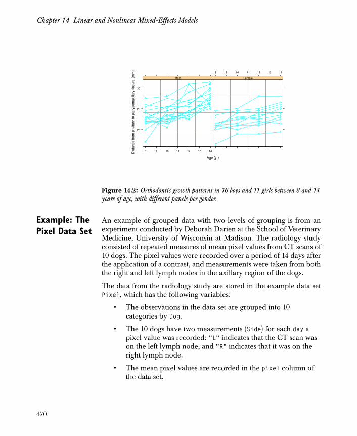
Chapter 14 Linear and Nonlinear Mixed-Effects Models
Example: The Pixel Data Set
An example of grouped data with two levels of grouping is from anexperiment conducted by Deborah Darien at the School of VeterinaryMedicine, University of Wisconsin at Madison. The radiology studyconsisted of repeated measures of mean pixel values from CT scans of10 dogs. The pixel values were recorded over a period of 14 days afterthe application of a contrast, and measurements were taken from boththe right and left lymph nodes in the axillary region of the dogs.
The data from the radiology study are stored in the example data setPixel, which has the following variables:
• The observations in the data set are grouped into 10 categories by Dog.
• The 10 dogs have two measurements (Side) for each day a pixel value was recorded: "L" indicates that the CT scan was on the left lymph node, and "R" indicates that it was on the right lymph node.
• The mean pixel values are recorded in the pixel column of the data set.
Figure 14.2: Orthodontic growth patterns in 16 boys and 11 girls between 8 and 14 years of age, with different panels per gender.
20
25
30
Male
8 9 10 11 12 13 14
Female
8 9 10 11 12 13 14
Age (yr)
Dis
tanc
e fr
om p
ituita
ry to
pte
rygo
max
illar
y fis
sure
(m
m)
470

Representing Grouped Data Sets
The purpose of the experiment was to model the mean pixel value asa function of time, in order to estimate the time when the maximummean pixel value was attained. We therefore wish to predict pixelfrom day, using both Dog and Side as grouping variables.
To create a new groupedData object for the Pixel data, use the classconstructor as follows:
# Assign Pixel to your working directory.> Pixel <- Pixel> Pixel <- groupedData(pixel ~ day | Dog/Side,+ data = Pixel, labels = list(+ x = "Time post injection", y = "Pixel intensity"),+ units = list(x = "(days)"))
> Pixel
Grouped Data: pixel ~ day | Dog/Side Dog Side day pixel 1 1 R 0 1045.8 2 1 R 1 1044.5 3 1 R 2 1042.9 4 1 R 4 1050.4 5 1 R 6 1045.2 6 1 R 10 1038.9 7 1 R 14 1039.8 8 2 R 0 1041.8 9 2 R 1 1045.610 2 R 2 1051.011 2 R 4 1054.112 2 R 6 1052.713 2 R 10 1062.014 2 R 14 1050.815 3 R 0 1039.8. . .
Plot the grouped data with the following command:
> plot(Pixel, displayLevel = 1, inner = ~Side)
The result is displayed in Figure 14.3. The grouping variable Dogdetermines the number of panels in the plot, and the inner factor Sidedetermines which points in a panel are joined by lines. Thus, there
471
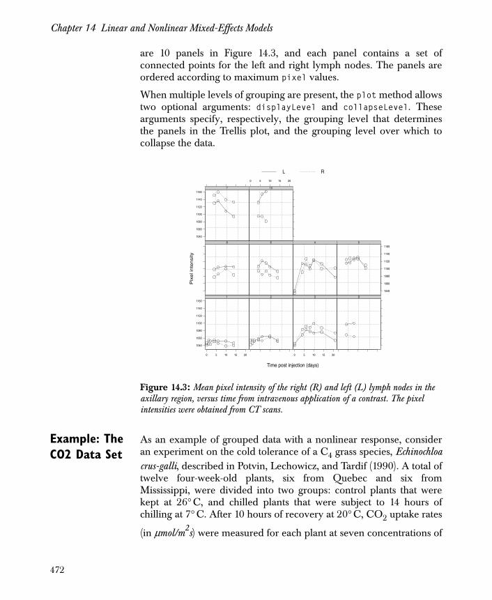
Chapter 14 Linear and Nonlinear Mixed-Effects Models
are 10 panels in Figure 14.3, and each panel contains a set ofconnected points for the left and right lymph nodes. The panels areordered according to maximum pixel values.
When multiple levels of grouping are present, the plot method allowstwo optional arguments: displayLevel and collapseLevel. Thesearguments specify, respectively, the grouping level that determinesthe panels in the Trellis plot, and the grouping level over which tocollapse the data.
Example: The CO2 Data Set
As an example of grouped data with a nonlinear response, consideran experiment on the cold tolerance of a C4 grass species, Echinochloacrus-galli, described in Potvin, Lechowicz, and Tardif (1990). A total oftwelve four-week-old plants, six from Quebec and six fromMississippi, were divided into two groups: control plants that werekept at 26° C, and chilled plants that were subject to 14 hours ofchilling at 7° C. After 10 hours of recovery at 20° C, CO2 uptake rates
(in μmol/m2s) were measured for each plant at seven concentrations of
Figure 14.3: Mean pixel intensity of the right (R) and left (L) lymph nodes in the axillary region, versus time from intravenous application of a contrast. The pixel intensities were obtained from CT scans.
1040
1060
1080
1100
1120
1140
1160
0 5 10 15 20
1 2
0 5 10 15 20
3 9
8 6 4
1040
1060
1080
1100
1120
1140
11605
1040
1060
1080
1100
1120
1140
11607
0 5 10 15 20
10
Time post injection (days)
Pix
el i
nte
nsi
ty
L R
472

Representing Grouped Data Sets
ambient CO2: 100, 175, 250, 350, 500, 675, and 1000 μL/L. Eachplant was subjected to the seven concentrations of CO2 in increasing,consecutive order.
The data from the CO2 study are stored in the example data set CO2,which has the following variables:
• The 84 observations in the data set are grouped into 12 categories by Plant.
• The 12 plants are classified into two groups by Type, an indicator variable assuming the values "Quebec" and "Mississippi".
• The 12 plants are classified into two additional groups according to Treatment, which indicates whether a plant was "nonchilled" or "chilled".
• Each plant has seven uptake measurements, corresponding to the seven concentration (conc) values.
The objective of the experiment was to evaluate the effect of planttype and chilling treatment on the CO2 uptake. We therefore wish topredict uptake from conc, using Plant as a grouping variable andboth Treatment and Type as outer covariates.
To create a new groupedData object for the CO2 data, use the classconstructor as follows:
# Assign CO2 to your working directory.> CO2 <- CO2> CO2 <- groupedData(uptake ~ conc | Plant, data = CO2,+ outer = ~ Treatment * Type,+ labels = list(x = "Ambient carbon dioxide concentration",+ y = "CO2 uptake rate"),+ units = list(x = "(uL/L)", y = "(umol/m^2 s)"))
> CO2
Grouped Data: uptake ~ conc | Plant Plant Type Treatment conc uptake 1 Qn1 Quebec nonchilled 95 16.0 2 Qn1 Quebec nonchilled 175 30.4 3 Qn1 Quebec nonchilled 250 34.8 . . .
473
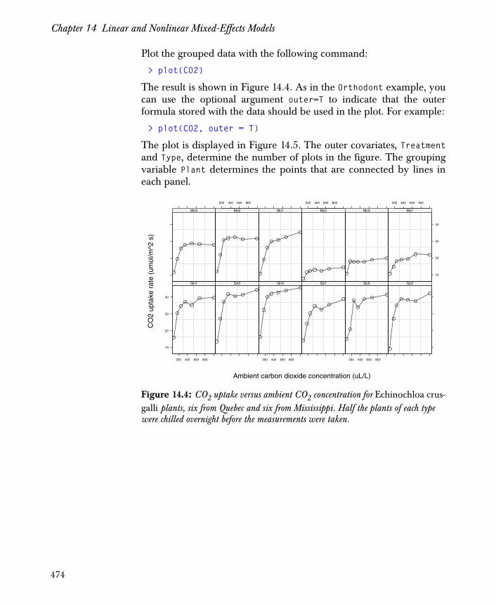
Chapter 14 Linear and Nonlinear Mixed-Effects Models
Plot the grouped data with the following command:
> plot(CO2)
The result is shown in Figure 14.4. As in the Orthodont example, youcan use the optional argument outer=T to indicate that the outerformula stored with the data should be used in the plot. For example:
> plot(CO2, outer = T)
The plot is displayed in Figure 14.5. The outer covariates, Treatmentand Type, determine the number of plots in the figure. The groupingvariable Plant determines the points that are connected by lines ineach panel.
Figure 14.4: CO2 uptake versus ambient CO2 concentration for Echinochloa crus-galli plants, six from Quebec and six from Mississippi. Half the plants of each type were chilled overnight before the measurements were taken.
10
20
30
40
Qn1
200 400 600 800
Qn2 Qn3
200 400 600 800
Qc1 Qc3
200 400 600 800
Qc2
Mn3 Mn2
200 400 600 800
Mn1 Mc2
200 400 600 800
Mc3
10
20
30
40
Mc1
200 400 600 800
Ambient carbon dioxide concentration (uL/L)
CO
2 up
take
rat
e (u
mol
/m^2
s)
474

Representing Grouped Data Sets
Figure 14.5: CO2 uptake versus ambient CO2 by Treatment and Type.
10
20
30
40
nonchilledQuebec
200 400 600 800
chilledQuebec
nonchilledMississippi
10
20
30
40
chilledMississippi
200 400 600 800
Ambient carbon dioxide concentration (uL/L)
CO
2 up
take
rat
e (u
mol
/m^2
s)
475

Chapter 14 Linear and Nonlinear Mixed-Effects Models
We can also obtain a numeric summary of the CO2 data by group,using the gsummary function as follows:
> gsummary(CO2)
Plant Type Treatment conc uptake Qn1 Qn1 Quebec nonchilled 435 33.22857Qn2 Qn2 Quebec nonchilled 435 35.15714Qn3 Qn3 Quebec nonchilled 435 37.61429Qc1 Qc1 Quebec chilled 435 29.97143Qc3 Qc3 Quebec chilled 435 32.58571Qc2 Qc2 Quebec chilled 435 32.70000Mn3 Mn3 Mississippi nonchilled 435 24.11429Mn2 Mn2 Mississippi nonchilled 435 27.34286Mn1 Mn1 Mississippi nonchilled 435 26.40000Mc2 Mc2 Mississippi chilled 435 12.14286Mc3 Mc3 Mississippi chilled 435 17.30000Mc1 Mc1 Mississippi chilled 435 18.00000
Example: The Soybean Data Set
Another example of grouped data with a nonlinear response comesfrom an experiment described in Davidian and Giltinan (1995),which compares growth patterns of two genotypes of soybean. Onegenotype is a commercial variety, Forrest, and the other is anexperimental strain, Plant Introduction #416937. The data werecollected in the three years from 1988 to 1990. At the beginning of thegrowing season in each year, 16 plots were planted with seeds (8 plotswith each genotype). Each plot was sampled eight to ten times atapproximately weekly intervals. At sampling time, six plants wererandomly selected from each plot, leaves from these plants wereweighed, and the average leaf weight per plant was calculated for theplot. Different plots in different sites were used in different years.
The data from the soybean study are stored in the example data setSoybean, which has the following variables:
• The observations in the data set are grouped into 48 categories by Plot, a variable that provides unique labels for the 16 plots planted in each of the 3 years.
• The 48 plots are classified into three groups by Year, which indicates whether the plot was planted in "1988", "1989", or "1990".
476

Representing Grouped Data Sets
• The 48 plots are classified into two additional groups according to Variety, which indicates whether a plot contained the commercial strain of plants (F) or the experimental strain (P).
• The average leaf weight at each Time for the plots is recorded in the weight column of the data set.
The objective of the soybean experiment was to model the growthpattern in terms of average leaf weight. We therefore wish to predictweight from Time, using Plot as a grouping variable and bothVariety and Year as outer covariates.
To create a new groupedData object for the Soybean data, use the classconstructor as follows:
# Assign Soybean to your working directory.> Soybean <- Soybean> Soybean <- groupedData(weight ~ Time | Plot,+ data = Soybean, outer = ~ Variety * Year,+ labels = list(x = "Time since planting",+ y = "Leaf weight/plant"),+ units = list(x = "(days)", y = "(g)"))
> Soybean
Grouped Data: weight ~ Time | Plot Plot Variety Year Time weight 1 1988F1 F 1988 14 0.10600 2 1988F1 F 1988 21 0.26100 3 1988F1 F 1988 28 0.66600 4 1988F1 F 1988 35 2.11000 5 1988F1 F 1988 42 3.56000 6 1988F1 F 1988 49 6.23000 7 1988F1 F 1988 56 8.71000 8 1988F1 F 1988 63 13.35000 9 1988F1 F 1988 70 16.3417010 1988F1 F 1988 77 17.7508311 1988F2 F 1988 14 0.1040012 1988F2 F 1988 21 0.26900. . .
477
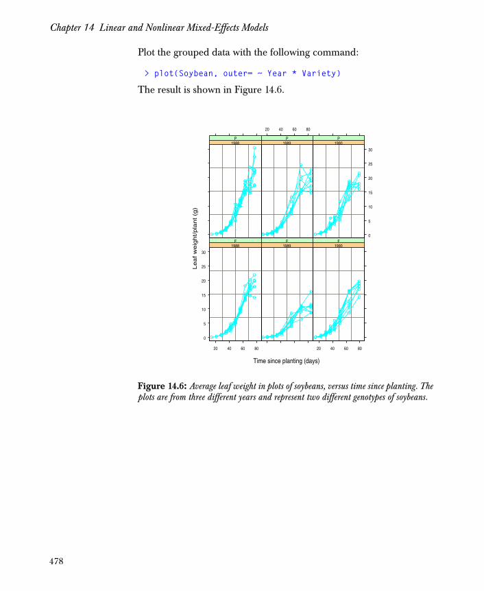
Chapter 14 Linear and Nonlinear Mixed-Effects Models
Plot the grouped data with the following command:
> plot(Soybean, outer= ~ Year * Variety)
The result is shown in Figure 14.6.
Figure 14.6: Average leaf weight in plots of soybeans, versus time since planting. The plots are from three different years and represent two different genotypes of soybeans.
0
5
10
15
20
25
30
1988F
20 40 60 80
1989F
1990F
20 40 60 80
1988P
1989P
20 40 60 80
0
5
10
15
20
25
30
1990P
Time since planting (days)
Leaf w
eig
ht/pla
nt (g
)
478
Fitting Models Using the lme Function
FITTING MODELS USING THE LME FUNCTION
The Spotfire S+ function lme fits a linear mixed-effects model asdescribed in Laird and Ware (1982), or a multilevel linear mixed-effects model as described in Longford (1993) and Goldstein (1995).The models are fitted using either maximum likelihood or restrictedmaximum likelihood. The lme function produces objects of class"lme".
Model Definitions
Example: the Orthodont data
The plot of the individual growth curves in Figure 14.1 suggests that alinear model might adequately explain the orthodontic distance as afunction of age. However, the intercepts and slopes of the lines seemto vary with the individual patient. The corresponding linear mixed-effects model is given by the following equation:
where represents the distance for the ith individual at age , andβ0 and β1 are the population average intercept and the population
average slope, respectively. The and terms are the effects in
intercept and slope associated with the ith individual, and is the
within-subject error term. It is assumed that the bi = (bi0,bi1)T are
independent and identically distributed with a N(0,σ2D) distribution,
where represents the covariance matrix for the random effects.Furthermore, we assume that the ε ij are independent and identically
distributed with a N(0,σ2) distribution, independent of the bi.
(14.1)dij β0 bi0+( ) β1 bi1+( )agej ε ij++=
dij j
bi0 bi1
ε ij
σ2D
479
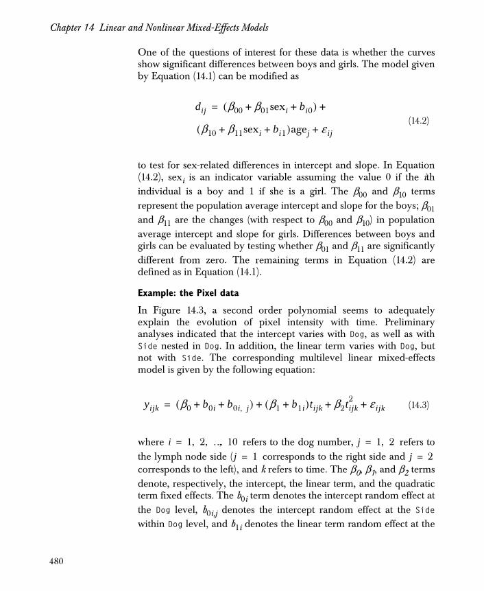
Chapter 14 Linear and Nonlinear Mixed-Effects Models
One of the questions of interest for these data is whether the curvesshow significant differences between boys and girls. The model givenby Equation (14.1) can be modified as
to test for sex-related differences in intercept and slope. In Equation(14.2), sexi is an indicator variable assuming the value 0 if the ithindividual is a boy and 1 if she is a girl. The β00 and β10 termsrepresent the population average intercept and slope for the boys; β01and β11 are the changes (with respect to β00 and β10) in populationaverage intercept and slope for girls. Differences between boys andgirls can be evaluated by testing whether β01 and β11 are significantlydifferent from zero. The remaining terms in Equation (14.2) aredefined as in Equation (14.1).
Example: the Pixel data
In Figure 14.3, a second order polynomial seems to adequatelyexplain the evolution of pixel intensity with time. Preliminaryanalyses indicated that the intercept varies with Dog, as well as withSide nested in Dog. In addition, the linear term varies with Dog, butnot with Side. The corresponding multilevel linear mixed-effectsmodel is given by the following equation:
where refers to the dog number, refers tothe lymph node side ( corresponds to the right side and corresponds to the left), and k refers to time. The β0, β1, and β2 termsdenote, respectively, the intercept, the linear term, and the quadraticterm fixed effects. The b0i term denotes the intercept random effect atthe Dog level, b0i,j denotes the intercept random effect at the Sidewithin Dog level, and b1i denotes the linear term random effect at the
(14.2)
(14.3)
dij β00 β01sexi bi0+ +( ) +=
β10 β11sexi bi1+ +( )agej ε ij+
yijk β0 b0i b0i j,+ +( ) β1 b1i+( )tijk β2tijk2 ε ijk+ + +=
i 1 2 … 10, , ,= j 1 2,=
j 1= j 2=
480

Fitting Models Using the lme Function
Dog level. The y variable is the pixel intensity, t is the time sincecontrast injection, and ε ijk is the error term. It is assumed that the
bi = (b0i ,b1i)T are independent and identically distributed with a
N(0,σ2D1) distribution, where represents the covariance matrixfor random effects at the Dog level. The bi,j = [b0i,j] are independent of
the bi, and independent and identically distributed with a N(0,σ2D2)
distribution, where represents the covariance matrix forrandom effects at the Side within Dog level. The ε ijk are independent
and identically distributed with a N(0,σ2) distribution, independent ofthe bi and the bi,j .
Arguments The typical call to the lme function is of the form
lme(fixed, data, random)
Only the first argument is required. The arguments fixed and randomare generally given as formulas. Any linear formula is allowed forboth arguments, giving the model formulation considerableflexibility. The optional argument data specifies the data frame inwhich the model’s variables are available.
Other arguments in the lme function allow for flexible definitions ofthe within-group correlation and heteroscedasticity structures, thesubset of the data to be modeled, the method to use when fitting themodel, and the list of control values for the estimation algorithm. Seethe lme online help file for specific details on each argument.
Example: the Orthodont data
For the model given by Equation (14.1), the fixed and randomformulas are written as follows:
fixed = distance ~ age, random = ~ age
For the model given by Equation (14.2), these formulas are:
fixed = distance ~ age * Sex, random = ~ age
Note that the response variable is given only in the formula for thefixed argument, and that random is usually a one-sided linearformula. If the random argument is omitted, it is assumed to be thesame as the right side of the fixed formula.
σ2D1
σ2D2
481
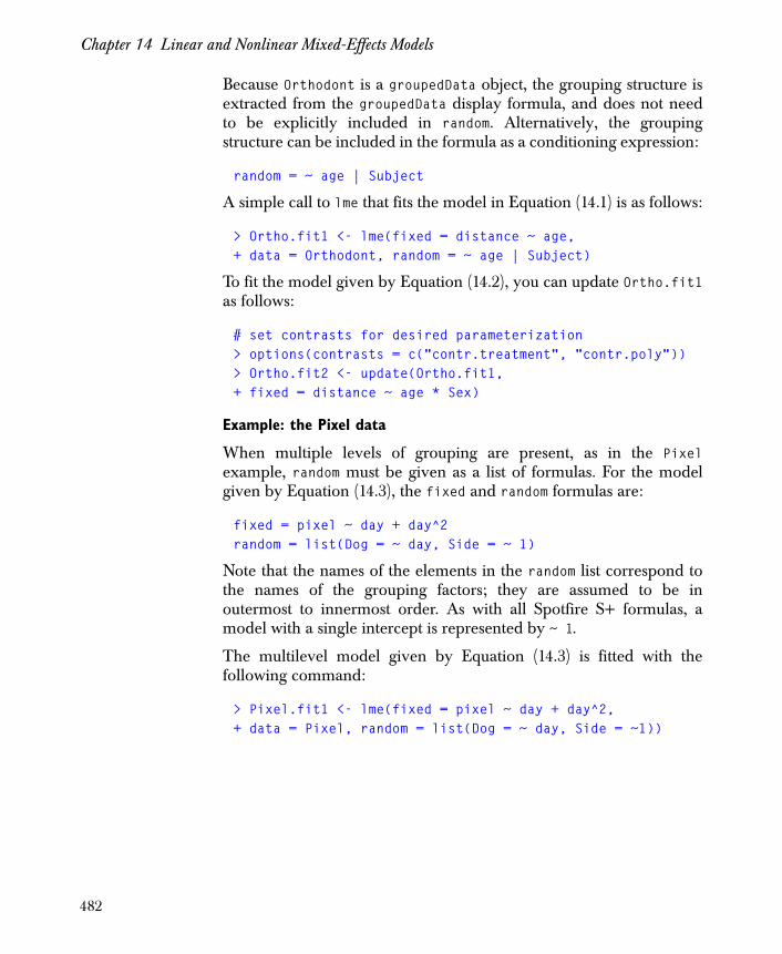
Chapter 14 Linear and Nonlinear Mixed-Effects Models
Because Orthodont is a groupedData object, the grouping structure isextracted from the groupedData display formula, and does not needto be explicitly included in random. Alternatively, the groupingstructure can be included in the formula as a conditioning expression:
random = ~ age | Subject
A simple call to lme that fits the model in Equation (14.1) is as follows:
> Ortho.fit1 <- lme(fixed = distance ~ age,+ data = Orthodont, random = ~ age | Subject)
To fit the model given by Equation (14.2), you can update Ortho.fit1as follows:
# set contrasts for desired parameterization> options(contrasts = c("contr.treatment", "contr.poly"))> Ortho.fit2 <- update(Ortho.fit1,+ fixed = distance ~ age * Sex)
Example: the Pixel data
When multiple levels of grouping are present, as in the Pixelexample, random must be given as a list of formulas. For the modelgiven by Equation (14.3), the fixed and random formulas are:
fixed = pixel ~ day + day^2 random = list(Dog = ~ day, Side = ~ 1)
Note that the names of the elements in the random list correspond tothe names of the grouping factors; they are assumed to be inoutermost to innermost order. As with all Spotfire S+ formulas, amodel with a single intercept is represented by ~ 1.
The multilevel model given by Equation (14.3) is fitted with thefollowing command:
> Pixel.fit1 <- lme(fixed = pixel ~ day + day^2,+ data = Pixel, random = list(Dog = ~ day, Side = ~1))
482

Manipulating lme Objects
MANIPULATING LME OBJECTS
A call to the lme function returns an object of class "lme". The onlinehelp file for lmeObject contains a description of the returned objectand each of its components. There are several methods available forlme objects, including print, summary, anova, and plot. Thesemethods are described in the following sections.
The print Method
A brief description of the lme estimation results is returned by theprint method. It displays estimates of the fixed effects, as well asstandard deviations and correlations of random effects. If fitted, thewithin-group correlation and variance function parameters are alsoprinted. For the Ortho.fit1 object defined in the section Argumentson page 481, the results are as follows:
> print(Ortho.fit1)
Linear mixed-effects model fit by REML Data: Orthodont Log-restricted-likelihood: -221.3183 Fixed: distance ~ age (Intercept) age 16.76111 0.6601852 Random effects: Formula: ~ age | Subject Structure: General positive-definite StdDev Corr (Intercept) 2.3270357 (Inter age 0.2264279 -0.609 Residual 1.3100396 Number of Observations: 108Number of Groups: 27
483

Chapter 14 Linear and Nonlinear Mixed-Effects Models
The summary Method
A complete description of the lme estimation results is returned by thesummary function. For the Ortho.fit2 object defined in the sectionArguments on page 481, the results are given by the followingcommand:
> summary(Ortho.fit2)Linear mixed-effects model fit by REML Data: Orthodont AIC BIC logLik 448.5817 469.7368 -216.2908
Random effects: Formula: ~ age | Subject Structure: General positive-definite StdDev Corr (Intercept) 2.4055020 (Inter age 0.1803458 -0.668 Residual 1.3100393
Fixed effects: distance ~ age + Sex + age:Sex Value Std.Error DF t-value p-value(Intercept) 16.34062 1.018532 79 16.04331 <.0001 age 0.78438 0.086000 79 9.12069 <.0001 Sex 1.03210 1.595733 25 0.64679 0.5237 age:Sex -0.30483 0.134735 79 -2.26243 0.0264 Correlation: (Intr) age Sex age -0.880 Sex -0.638 0.562 age:Sex 0.562 -0.638 -0.880
Standardized Within-Group Residuals: Min Q1 Med Q3 Max -3.168077 -0.3859386 0.007103473 0.4451539 3.849464
Number of Observations: 108Number of Groups: 27
The approximate standard errors for the fixed effects are computedusing an algorithm based on the asymptotic theory described inPinheiro (1994). In the results for Ortho.fit2, the significant, negativefixed effect between age and Sex indicate that the orthodontic
484
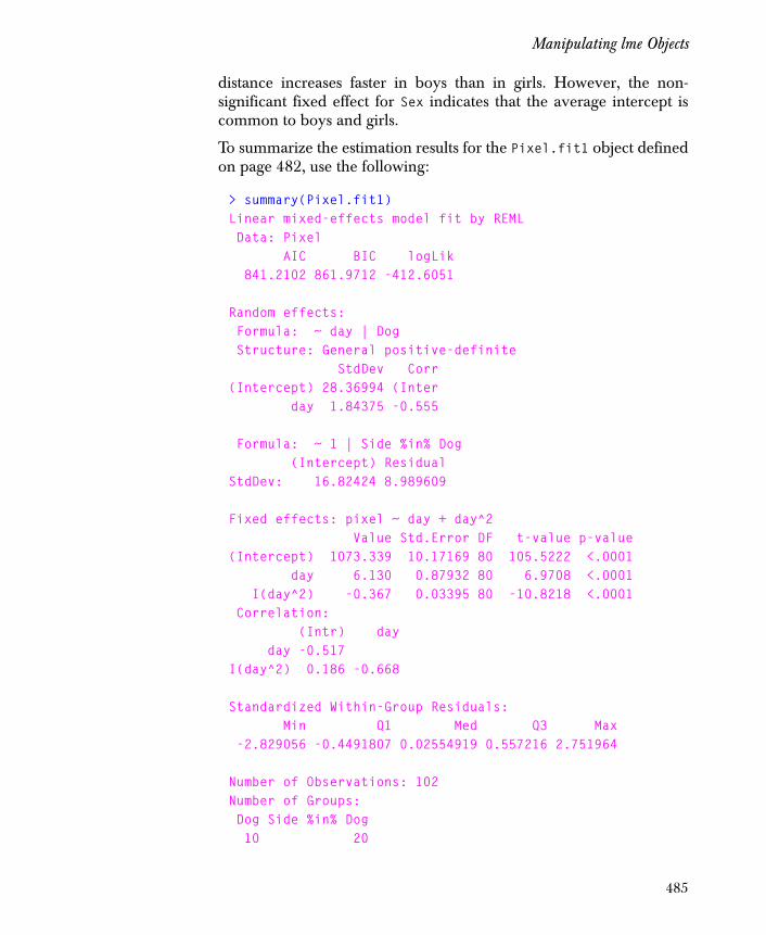
Manipulating lme Objects
distance increases faster in boys than in girls. However, the non-significant fixed effect for Sex indicates that the average intercept iscommon to boys and girls.
To summarize the estimation results for the Pixel.fit1 object definedon page 482, use the following:
> summary(Pixel.fit1)Linear mixed-effects model fit by REML Data: Pixel AIC BIC logLik 841.2102 861.9712 -412.6051
Random effects: Formula: ~ day | Dog Structure: General positive-definite StdDev Corr (Intercept) 28.36994 (Inter day 1.84375 -0.555
Formula: ~ 1 | Side %in% Dog (Intercept) Residual StdDev: 16.82424 8.989609
Fixed effects: pixel ~ day + day^2 Value Std.Error DF t-value p-value(Intercept) 1073.339 10.17169 80 105.5222 <.0001 day 6.130 0.87932 80 6.9708 <.0001 I(day^2) -0.367 0.03395 80 -10.8218 <.0001 Correlation: (Intr) day day -0.517 I(day^2) 0.186 -0.668
Standardized Within-Group Residuals: Min Q1 Med Q3 Max -2.829056 -0.4491807 0.02554919 0.557216 2.751964
Number of Observations: 102Number of Groups: Dog Side %in% Dog 10 20
485

Chapter 14 Linear and Nonlinear Mixed-Effects Models
The anova Method
A likelihood ratio test can be used to test the difference between fixedeffects in different lme models. The anova method provides thiscapability for lme objects.
As an example, we compare the Ortho.fit1 and Ortho.fit2 objectsdefined for the Orthodont data set. Since the two models havedifferent fixed effects structures, we must re-fit them using maximumlikelihood estimation before calling the anova function. Use theupdate function to re-fit the objects as follows:
> Ortho.fit1.ML <- update(Ortho.fit1, method = "ML")> Ortho.fit2.ML <- update(Ortho.fit2, method = "ML")
The call to anova produces:
> anova(Ortho.fit1.ML, Ortho.fit2.ML)
Model df AIC BIC logLikOrtho.fit1.ML 1 6 451.2116 467.3044 -219.6058Ortho.fit2.ML 2 8 443.8060 465.2630 -213.9030
Test L.Ratio p-valueOrtho.fit1.ML Ortho.fit2.ML 1 vs 2 11.40565 0.0033
Recall that Ortho.fit2.ML includes terms that test for sex-relateddifferences in the data. The likelihood ratio test strongly rejects thenull hypothesis of no differences between boys and girls. For smallsample sizes, likelihood ratio tests tend to be too liberal whencomparing models with nested fixed effects structures, and shouldtherefore be used with caution. We recommend using the Wald-typetests provided by the anova method (when a single model object ispassed to the function), as these tend to have significance levels closeto nominal, even for small samples.
Warning
Likelihood comparisons between restricted maximum likelihood (REML) fits with different fixed effects structures are not meaningful. To compare such models, you should re-fit the objects using maximum likelihood (ML) before calling anova.
486
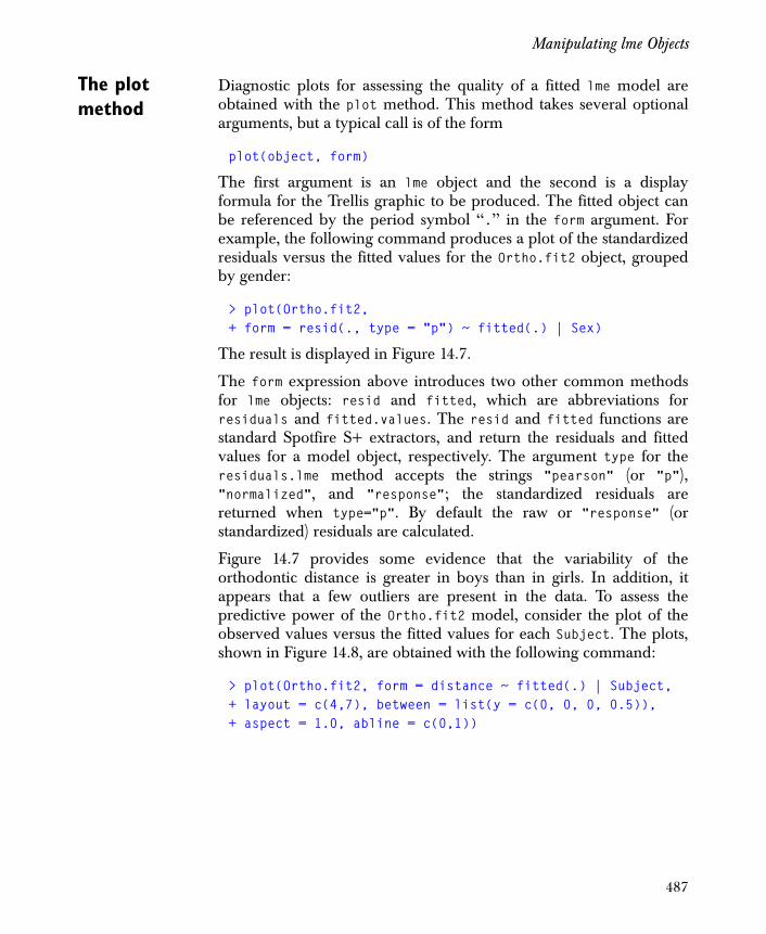
Manipulating lme Objects
The plot method
Diagnostic plots for assessing the quality of a fitted lme model areobtained with the plot method. This method takes several optionalarguments, but a typical call is of the form
plot(object, form)
The first argument is an lme object and the second is a displayformula for the Trellis graphic to be produced. The fitted object canbe referenced by the period symbol ‘‘.’’ in the form argument. Forexample, the following command produces a plot of the standardizedresiduals versus the fitted values for the Ortho.fit2 object, groupedby gender:
> plot(Ortho.fit2,+ form = resid(., type = "p") ~ fitted(.) | Sex)
The result is displayed in Figure 14.7.
The form expression above introduces two other common methodsfor lme objects: resid and fitted, which are abbreviations forresiduals and fitted.values. The resid and fitted functions arestandard Spotfire S+ extractors, and return the residuals and fittedvalues for a model object, respectively. The argument type for theresiduals.lme method accepts the strings "pearson" (or "p"),"normalized", and "response"; the standardized residuals arereturned when type="p". By default the raw or "response" (orstandardized) residuals are calculated.
Figure 14.7 provides some evidence that the variability of theorthodontic distance is greater in boys than in girls. In addition, itappears that a few outliers are present in the data. To assess thepredictive power of the Ortho.fit2 model, consider the plot of theobserved values versus the fitted values for each Subject. The plots,shown in Figure 14.8, are obtained with the following command:
> plot(Ortho.fit2, form = distance ~ fitted(.) | Subject,+ layout = c(4,7), between = list(y = c(0, 0, 0, 0.5)),+ aspect = 1.0, abline = c(0,1))
487

Chapter 14 Linear and Nonlinear Mixed-Effects Models
Figure 14.7: Standardized residuals versus fitted values for the Ortho.fit2 model object, grouped by gender.
Figure 14.8: Observed distances versus fitted values by Subject for the Ortho.fit2 model object.
-2
0
2
4Male
18 20 22 24 26 28 30 32
Female
18 20 22 24 26 28 30 32
Fitted values (mm)
Sta
ndar
dize
d re
sidu
als
20
25
30
M16
18 22 26 30
M05 M02
18 22 26 30
M11
M07 M08 M03
20
25
30
M12
20
25
30
M13 M14 M09 M15
M06 M04 M01
20
25
30
M10
20
25
30
F10 F09 F06 F01
F05 F07 F02
20
25
30
F08
20
25
30
F03 F04
18 22 26 30
F11
Fitted values (mm)
Dis
tanc
e fr
om p
ituita
ry to
pte
rygo
max
illar
y fis
sure
(m
m)
488

Manipulating lme Objects
For most of the subjects, there is very good agreement between theobserved and fitted values, indicating that the fit is adequate.
The form argument to the plot method for lme objects providesvirtually unlimited flexibility in generating customized diagnosticplots. As a final example, consider the plot of the standardizedresiduals (at the Side within Dog level) for the Pixel.fit1 object,grouped by Dog. The plot, similar to the one shown in Figure 14.9, isobtained with the following command:
> plot(Pixel.fit1, form = Dog ~ resid(., type = "p"))
The residuals seem to be symmetrically scattered around zero withsimilar variabilities, except possibly for dog number 4.
Other Methods Standard Spotfire S+ methods for extracting components of fittedobjects, such as residuals, fitted.values, and coefficients, canalso be used on lme objects. In addition, lme includes the methodsfixed.effects and random.effects for extracting the fixed effectsand the random effects estimates; abbreviations for these functionsare fixef and ranef, respectively. For example, the two commandsbelow return coefficients and fixed effects.
Figure 14.9: Standardized residuals by Dog for the Pixel.fit1 model object.
1
10
2
3
4
5
6
7
8
9
-3 -2 -1 0 1 2
Standardized residuals
Dog
489

Chapter 14 Linear and Nonlinear Mixed-Effects Models
> coef(Ortho.fit2)
(Intercept) age Sex age:SexM16 15.55737 0.6957276 1.032102 -0.3048295M05 14.69529 0.7759009 1.032102 -0.3048295...F04 18.00174 0.8125880 1.032102 -0.3048295F11 18.53692 0.8858555 1.032102 -0.3048295
> fixef(Pixel.fit1)
(Intercept) day I(day^2) 1073.339 6.129597 -0.3673503
The next command returns the random effects at the Dog level for thePixel.fit1 object:
> ranef(Pixel.fit1, level = 1)
1 -24.714229 -1.1953707410 19.365854 -0.09936872 2 -23.582059 -0.43243128 3 -27.080310 2.19475596 4 -16.658544 3.09597260 5 25.299771 -0.56127136 6 10.823243 -1.03699983 7 49.353938 -2.27445838 8 -7.053961 0.99025533 9 -5.753702 -0.68108358
Random effects estimates can be visualized with the Spotfire S+function plot.ranef.lme, designed specifically for this purpose. Thisfunction offers great flexibility for the display of random effects. Thesimplest display produces a dot plot of the random effects for eachcoefficient, as in the following example:
> plot(ranef(Pixel.fit1, level = 1))
490

Manipulating lme Objects
Predicted values for lme objects are returned by the predict method.For example, if you are interested in predicting the averageorthodontic measurement for both boys and girls at ages 14, 15, and16, as well as for subjects M01 and F10 at age 13, first create a new dataframe as follows:
> Orthodont.new <- data.frame(+ Sex = c("Male", "Male", "Male", "Female", "Female",+ "Female", "Male", "Female"), + age = c(14, 15, 16, 14, 15, 16, 13, 13),+ Subject = c(NA, NA, NA, NA, NA, NA, "M01", "F10"))
You can then use the following command to compute the subject-specific and population predictions:
> predict(Ortho.fit2, Orthodont.new, level = c(0,1))
Subject predict.fixed predict.Subject1 NA 27.32188 NA2 NA 28.10625 NA3 NA 28.89063 NA4 NA 24.08636 NA5 NA 24.56591 NA6 NA 25.04545 NA7 M01 26.53750 29.172648 F10 23.60682 19.80758
The level argument is used to define the desired prediction levels,with zero referring to the population predictions.
Finally, the intervals method for lme objects computes confidenceintervals for the parameters in a mixed-effects model:
> intervals(Ortho.fit2)
Approximate 95% confidence intervals
Fixed effects: lower est. upper(Intercept) 14.3132878 16.3406250 18.36796224 age 0.6131972 0.7843750 0.95555282 Sex -2.2543713 1.0321023 4.31857585 age:Sex -0.5730137 -0.3048295 -0.03664544
491

Chapter 14 Linear and Nonlinear Mixed-Effects Models
Random Effects: Level: Subject lower est. upper sd((Intercept)) 1.00636826 2.4055020 5.7498233 sd(age) 0.05845914 0.1803458 0.5563649cor((Intercept),age) -0.96063585 -0.6676196 0.3285589
Within-group standard error: lower est. upper 1.084768 1.310039 1.582092
The models considered so far do not assume any special form for therandom effects variance-covariance matrix. See the section AdvancedModel Fitting for a variety of specifications of both the random effectscovariance matrix and the within-group correlation structure. Beyondthe available covariance structures, customized structures can bedesigned by the user; this topic is also addressed in the sectionAdvanced Model Fitting.
492
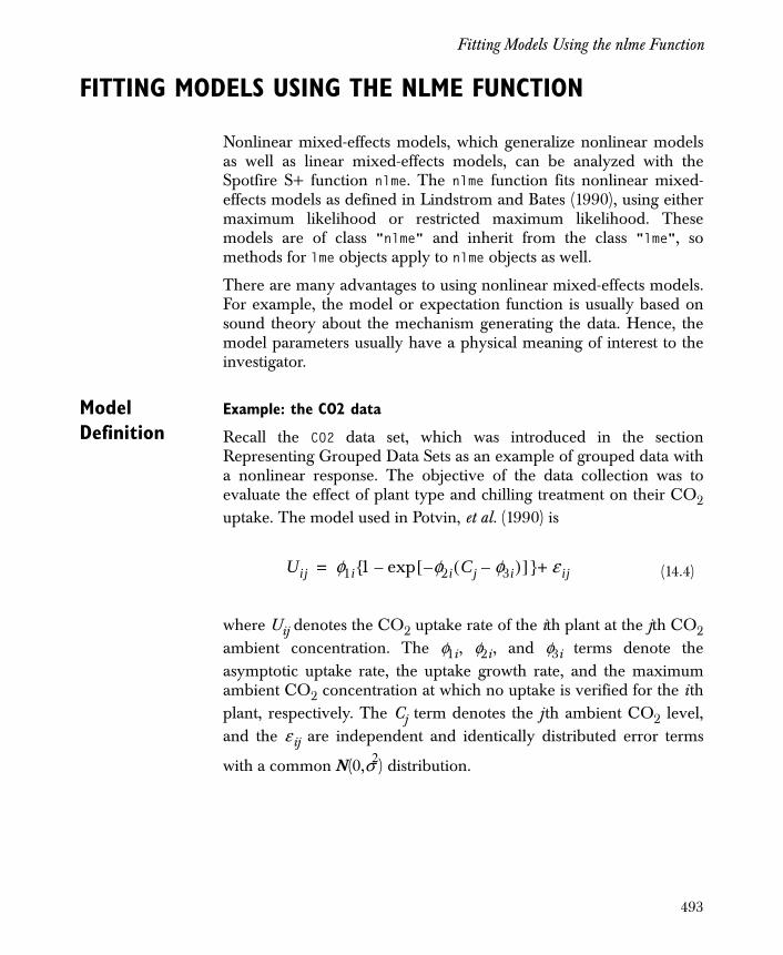
Fitting Models Using the nlme Function
FITTING MODELS USING THE NLME FUNCTION
Nonlinear mixed-effects models, which generalize nonlinear modelsas well as linear mixed-effects models, can be analyzed with theSpotfire S+ function nlme. The nlme function fits nonlinear mixed-effects models as defined in Lindstrom and Bates (1990), using eithermaximum likelihood or restricted maximum likelihood. Thesemodels are of class "nlme" and inherit from the class "lme", somethods for lme objects apply to nlme objects as well.
There are many advantages to using nonlinear mixed-effects models.For example, the model or expectation function is usually based onsound theory about the mechanism generating the data. Hence, themodel parameters usually have a physical meaning of interest to theinvestigator.
Model Definition
Example: the CO2 data
Recall the CO2 data set, which was introduced in the sectionRepresenting Grouped Data Sets as an example of grouped data witha nonlinear response. The objective of the data collection was toevaluate the effect of plant type and chilling treatment on their CO2uptake. The model used in Potvin, et al. (1990) is
where Uij denotes the CO2 uptake rate of the ith plant at the jth CO2ambient concentration. The φ1i , φ2i , and φ3i terms denote theasymptotic uptake rate, the uptake growth rate, and the maximumambient CO2 concentration at which no uptake is verified for the ithplant, respectively. The Cj term denotes the jth ambient CO2 level,and the ε ij are independent and identically distributed error terms
with a common N(0,σ2) distribution.
(14.4)Uij φ1i 1 exp φ– 2i Cj φ3i–( )[ ]–{ } ε ij+=
493

Chapter 14 Linear and Nonlinear Mixed-Effects Models
Arguments Several optional arguments can be used with the nlme function, but atypical call is of the form
nlme(model, data, fixed, random, start)
The model argument is required and consists of a formula specifyingthe nonlinear model to be fitted. Any Spotfire S+ nonlinear formulacan be used, giving the function considerable flexibility.
The arguments fixed and random are formulas (or lists of formulas)that define the structures of the fixed and random effects in themodel. Only the fixed argument is required; by default, random isequivalent to fixed, so the random argument can be omitted. As in allSpotfire S+ formulas, a 1 on the right side of the fixed or randomformulas indicates that a single intercept is associated with the effect.However, any linear formula can be used instead. Again, this givesthe model considerable flexibility, as time-dependent parameters canbe easily incorporated. This occurs, for example, when a fixedformula involves a covariate that changes with time.
Usually, every parameter in a mixed-effects model has an associatedfixed effect, but it may or may not have an associated random effect.Since we assume that all random effects have zero means, theinclusion of a random effect without a corresponding fixed effect isunusual. Note that the fixed and random formulas can beincorporated directly into the model declaration, but the approachused in nlme allows for more efficient derivative calculations.
The data argument to nlme is optional and names a data frame inwhich the variables for the model, fixed, and random formulas arefound. The optional start argument provides a list of starting valuesfor the iterative algorithm. Only the fixed effects starting estimates arerequired; the default starting estimates for the random effects are zero.
Example: the CO2 data
For the CO2 uptake data, we obtain the following model formulafrom Equation (14.4):
uptake ~ A * (1 - exp(-B * (conc - C)))
where A = φ1, B = φ2, and C = φ3. To force the rate parameter φ2 to bepositive while preserving an unrestricted parametrization, you cantransform with as follows:
uptake ~ A * (1 - exp(-exp(lB) * (conc - C)))
B lB B( )log=
494

Fitting Models Using the nlme Function
Alternatively, you can define a Spotfire S+ function that contains themodel formula:
> CO2.func <- + function(conc, A, lB, C) A*(1 - exp(-exp(lB)*(conc - C)))
The model argument in nlme then looks like
uptake ~ CO2.func(conc, A, lB, C)
The advantage of the latter approach is that the analytic derivatives ofthe model function can be passed to nlme as a gradient attribute ofthe value returned by CO2.func. The analytic derivatives can then beused in the optimization algorithm. For example, we use the SpotfireS+ function deriv to create expressions for the derivatives:
> CO2.func <- + deriv(~ A * ( 1 - exp(-exp(lB) * (conc - C))),+ c("A", "lB", "C"), function(conc, A, lB, C){})
If the value returned by a function like CO2.func does not have agradient attribute, numerical derivatives are used in the optimizationalgorithm.
To fit a model for the CO2 data in which all parameters are randomand no covariates are included, use the following fixed and randomformulas:
fixed = A + lB + C ~ 1, random = A + lB + C ~ 1
Alternatively, the random argument can be omitted since it isequivalent to the fixed formula by default. Because CO2 is agroupedData object, the grouping structure does not need to beexplicitly given in random, as it is extracted from the groupedDatadisplay formula. However, it is possible to include the groupingstructure as a conditioning expression in the formula:
random = A + lB + C ~ 1 | Plant
If you want to estimate the (fixed) effects of plant type and chillingtreatment on the parameters in the model, use
fixed = A + lB + C ~ Type * Treatment,random = A + lB + C ~ 1
495

Chapter 14 Linear and Nonlinear Mixed-Effects Models
The following simple call to nlme fits the model given by Equation(14.4):
> CO2.fit1 <- + nlme(model = uptake ~ CO2.func(conc, A, lB, C), + fixed = A + lB + C ~ 1, data = CO2, + start = c(30, log(0.01), 50))
The initial values for the fixed effects are obtained from Potvin, et al.(1990).
496

Manipulating nlme Objects
MANIPULATING NLME OBJECTS
Objects returned by the nlme function are of class "nlme". The onlinehelp file for nlmeObject contains a description of the returned objectand each of its components. The nlme class inherits from the lme class,so that all methods described for lme objects are also available fornlme objects. In fact, with the exception of the predict method, allmethods are common to both classes. We illustrate their uses herewith the CO2 uptake data.
The print Method
The print method provides a brief description of the nlme estimationresults. It displays estimates of the standard deviations andcorrelations of random effects, the within-group standard deviation,and the fixed effects. For the CO2.fit1 object defined in the sectionArguments on page 494, the results are as follows:
> print(CO2.fit1)
Nonlinear mixed-effects model fit by maximum likelihood Model: uptake ~ CO2.func(conc, A, lB, C) Data: CO2 Log-likelihood: -201.3103 Fixed: A + lB + C ~ 1 A lB C 32.47374 -4.636204 43.5424
Random effects: Formula: list(A ~ 1 , lB ~ 1 , C ~ 1 ) Level: Plant Structure: General positive-definite StdDev Corr A 9.5100551 A lB lB 0.1283327 -0.160 C 10.4010223 0.999 -0.139Residual 1.7664129
Number of Observations: 84Number of Groups: 12
497

Chapter 14 Linear and Nonlinear Mixed-Effects Models
Note that there is strong correlation between the A and the C randomeffects, and that both of these have small correlations with the lBrandom effect. A scatterplot matrix provides a graphical descriptionof the random effects correlation structure. We generate a scatterplotmatrix with the pairs method:
> pairs(CO2.fit1, ~ranef(.))
The result is shown in Figure 14.10.
The correlation between A and C may be due to the fact that the planttype and chilling treatment, which are not included in the CO2.fit1model, affect A and C in similar ways. The plot.ranef.lme functioncan be used to explore the dependence of individual parameters onplant type and chilling factor. The following command produces theplot displayed in Figure 14.11.
> plot(ranef(CO2.fit1, augFrame = T),+ form = ~Type*Treatment, layout = c(3,1))
Figure 14.10: Scatterplot matrix of the estimated random effects in CO2.fit1.
-15 -10 -5
0 5 10
0
5
10
-15
-10
-5A
-0.15 -0.10 -0.05
0.00 0.05 0.10
0.00
0.05
0.10
-0.15
-0.10
-0.05lB
-20 -15 -10 -5
-5 0 5 10
-5
0
5
10
-20
-15
-10
-5C
498
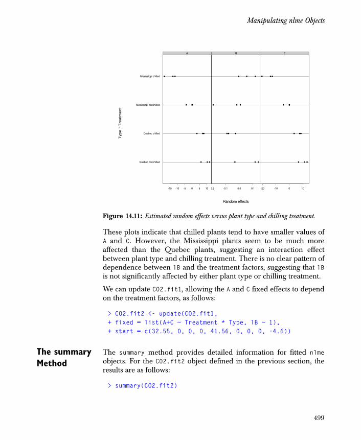
Manipulating nlme Objects
These plots indicate that chilled plants tend to have smaller values ofA and C. However, the Mississippi plants seem to be much moreaffected than the Quebec plants, suggesting an interaction effectbetween plant type and chilling treatment. There is no clear pattern ofdependence between lB and the treatment factors, suggesting that lBis not significantly affected by either plant type or chilling treatment.
We can update CO2.fit1, allowing the A and C fixed effects to dependon the treatment factors, as follows:
> CO2.fit2 <- update(CO2.fit1,+ fixed = list(A+C ~ Treatment * Type, lB ~ 1),+ start = c(32.55, 0, 0, 0, 41.56, 0, 0, 0, -4.6))
The summary Method
The summary method provides detailed information for fitted nlmeobjects. For the CO2.fit2 object defined in the previous section, theresults are as follows:
> summary(CO2.fit2)
Figure 14.11: Estimated random effects versus plant type and chilling treatment.
Quebec nonchilled
Quebec chilled
Mississippi nonchilled
Mississippi chilled
-15 -10 -5 0 5 10
A
0.2 -0.1 0.0 0.1
lB
-20 -10 0 10
C
Random effects
Typ
e *
Tre
atm
ent
499

Chapter 14 Linear and Nonlinear Mixed-Effects Models
Nonlinear mixed-effects model fit by maximum likelihood Model: uptake ~ CO2.func(conc, A, lB, C) Data: CO2 AIC BIC logLik 392.4073 431.3004 -180.2037
Random effects: Formula: list(A ~ 1 , lB ~ 1 , C ~ 1 ) Level: Plant Structure: General positive-definite StdDev Corr A.(Intercept) 2.3709337 A.(In) lB lB 0.1475418 -0.336 C.(Intercept) 8.1630618 0.355 0.761 Residual 1.7113057
Fixed effects: list(A + C ~ Treatment * Type, lB ~ 1) Value Std.Error DF t-value A.(Intercept) 42.24934 1.49761 64 28.21125 A.Treatment -3.69231 2.05807 64 -1.79407 A.Type -11.07858 2.06458 64 -5.36603A.Treatment:Type -9.57430 2.94275 64 -3.25352 C.(Intercept) 46.30206 6.43499 64 7.19536 C.Treatment 8.82823 7.22978 64 1.22109 C.Type 3.00775 8.04748 64 0.37375C.Treatment:Type -49.01624 17.68013 64 -2.77239 lB -4.65063 0.08010 64 -58.06061 p-value A.(Intercept) <.0001 A.Treatment 0.0775 A.Type <.0001A.Treatment:Type 0.0018 C.(Intercept) <.0001 C.Treatment 0.2265 C.Type 0.7098C.Treatment:Type 0.0073 lB <.0001 Correlation: . . .
The small p-values of the t-statistics associated with theTreatment:Type effects indicate that both factors have a significanteffect on parameters A and C. This implies that their joint effect is notjust the sum of the individual effects.
500

Manipulating nlme Objects
The anova Method
For the fitted object CO2.fit2, you can investigate the joint effect ofTreatment and Type on both A and C using the anova method.
> anova(CO2.fit2, + Terms = c("A.Treatment", "A.Type", "A.Treatment:Type"))
F-test for: A.Treatment, A.Type, A.Treatment:Type numDF denDF F-value p-value1 3 64 51.77643 <.0001
> anova(CO2.fit2, + Terms = c("C.Treatment", "C.Type", "C.Treatment:Type"))
F-test for: C.Treatment, C.Type, C.Treatment:Type numDF denDF F-value p-value 1 3 64 2.939699 0.0397
The p-values of the Wald F-tests suggest that Treatment and Type havea stronger influence on A than on C.
The plot Method
Diagnostic plots for nlme objects can be obtained with the plotmethod, in the same way that they are generated for lme objects. Forthe CO2.fit2 model, plots grouped by Treatment and Type of thestandardized residuals versus fitted values are shown in Figure 14.12.The figure is obtained with the following command:
> plot(CO2.fit2, form = + resid(., type = "p") ~ fitted(.) | Type * Treatment,+ abline = 0)
The plots do not indicate any departures from the assumptions in themodel: no outliers seem to be present and the residuals aresymmetrically scattered around the line, with constant spreadfor different levels of the fitted values.
y 0=
501
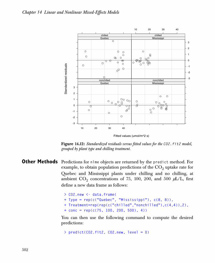
Chapter 14 Linear and Nonlinear Mixed-Effects Models
Other Methods Predictions for nlme objects are returned by the predict method. Forexample, to obtain population predictions of the CO2 uptake rate forQuebec and Mississippi plants under chilling and no chilling, atambient CO2 concentrations of 75, 100, 200, and 500 μL/L, firstdefine a new data frame as follows:
> CO2.new <- data.frame(+ Type = rep(c("Quebec", "Mississippi"), c(8, 8)),+ Treatment=rep(rep(c("chilled","nonchilled"),c(4,4)),2),+ conc = rep(c(75, 100, 200, 500), 4))
You can then use the following command to compute the desiredpredictions:
> predict(CO2.fit2, CO2.new, level = 0)
Figure 14.12: Standardized residuals versus fitted values for the CO2.fit2 model, grouped by plant type and chilling treatment.
-3
-2
-1
0
1
2
3
Quebecnonchilled
10 20 30 40
Mississippinonchilled
Quebecchilled
-3
-2
-1
0
1
2
3
Mississippichilled
10 20 30 40
Fitted values (umol/m^2 s)
Sta
ndar
dize
d re
sidu
als
502
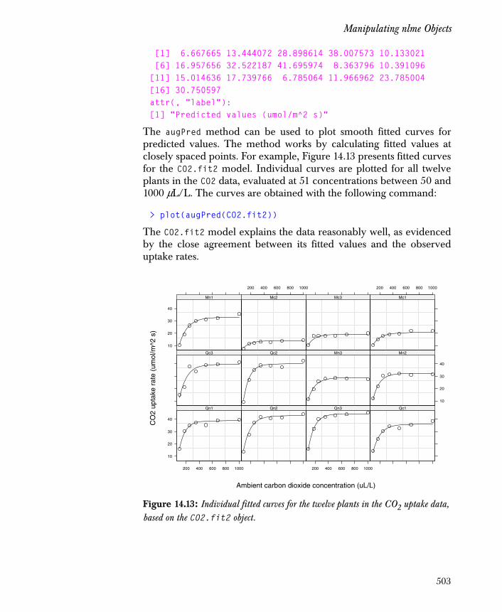
Manipulating nlme Objects
[1] 6.667665 13.444072 28.898614 38.007573 10.133021 [6] 16.957656 32.522187 41.695974 8.363796 10.391096[11] 15.014636 17.739766 6.785064 11.966962 23.785004[16] 30.750597attr(, "label"):[1] "Predicted values (umol/m^2 s)"
The augPred method can be used to plot smooth fitted curves forpredicted values. The method works by calculating fitted values atclosely spaced points. For example, Figure 14.13 presents fitted curvesfor the CO2.fit2 model. Individual curves are plotted for all twelveplants in the CO2 data, evaluated at 51 concentrations between 50 and1000 μL/L. The curves are obtained with the following command:
> plot(augPred(CO2.fit2))
The CO2.fit2 model explains the data reasonably well, as evidencedby the close agreement between its fitted values and the observeduptake rates.
Figure 14.13: Individual fitted curves for the twelve plants in the CO2 uptake data, based on the CO2.fit2 object.
10
20
30
40
Qn1
200 400 600 800 1000
Qn2 Qn3
200 400 600 800 1000
Qc1
Qc3 Qc2 Mn3
10
20
30
40
Mn2
10
20
30
40
Mn1 Mc2
200 400 600 800 1000
Mc3 Mc1
200 400 600 800 1000
Ambient carbon dioxide concentration (uL/L)
CO
2 up
take
rat
e (u
mol
/m^2
s)
503

Chapter 14 Linear and Nonlinear Mixed-Effects Models
Methods for extracting components from a fitted nlme object are alsoavailable, and are identical to those for lme objects. Some of the mostcommonly used methods are coef, fitted, fixef, ranef, resid, andintervals. For more details on these extractors, see the online helpfiles and the section Other Methods on page 489.
504
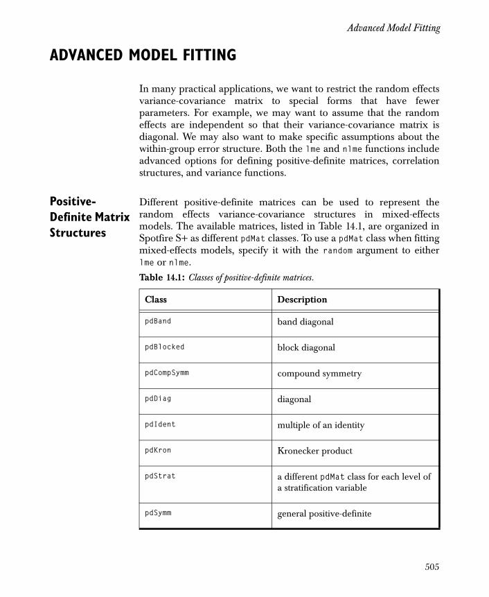
Advanced Model Fitting
ADVANCED MODEL FITTING
In many practical applications, we want to restrict the random effectsvariance-covariance matrix to special forms that have fewerparameters. For example, we may want to assume that the randomeffects are independent so that their variance-covariance matrix isdiagonal. We may also want to make specific assumptions about thewithin-group error structure. Both the lme and nlme functions includeadvanced options for defining positive-definite matrices, correlationstructures, and variance functions.
Positive-Definite Matrix Structures
Different positive-definite matrices can be used to represent therandom effects variance-covariance structures in mixed-effectsmodels. The available matrices, listed in Table 14.1, are organized inSpotfire S+ as different pdMat classes. To use a pdMat class when fittingmixed-effects models, specify it with the random argument to eitherlme or nlme. Table 14.1: Classes of positive-definite matrices.
Class Description
pdBand band diagonal
pdBlocked block diagonal
pdCompSymm compound symmetry
pdDiag diagonal
pdIdent multiple of an identity
pdKron Kronecker product
pdStrat a different pdMat class for each level of a stratification variable
pdSymm general positive-definite
505

Chapter 14 Linear and Nonlinear Mixed-Effects Models
By default, the pdSymm class is used to represent a random effectscovariance matrix. You can define your own pdMat class by specifyinga constructor function and, at a minimum, methods for the functionspdConstruct, pdMatrix and coef. For examples of these functions, seethe methods for the pdSymm and pdDiag classes.
Example: the Orthodont data
We return to the Ortho.fit2 model that we created in the sectionArguments on page 494. To fit a model with independent slope andintercept random effects, we include a diagonal variance-covariancematrix using the pdDiag class:
> Ortho.fit3 <- update(Ortho.fit2, random = pdDiag(~age))> Ortho.fit3
Linear mixed-effects model fit by REML Data: Orthodont Log-restricted-likelihood: -216.5755 Fixed: distance ~ age + Sex + age:Sex (Intercept) age Sex age:Sex 16.34062 0.784375 1.032102 -0.3048295
Random effects: Formula: ~ age | Subject Structure: Diagonal (Intercept) age ResidualStdDev: 1.554607 0.08801665 1.365502
Number of Observations: 108Number of Groups: 27
The grouping structure is inferred from the groupedData displayformula in the Orthodont data. Alternatively, the grouping structurecan be passed to the random argument as follows:
random = list(Subject = pdDiag(~age))
Example: the CO2 data
Recall the CO2.fit2 object defined in the section The print Methodon page 497. We wish to test whether we can assume that the randomeffects in CO2.fit2 are independent. To do this, use the commandsbelow.
506

Advanced Model Fitting
> CO2.fit3 <- update(CO2.fit2, random = pdDiag(A+lB+C~1))> anova(CO2.fit2, CO2.fit3)
Model df AIC BIC logLik TestCO2.fit2 1 16 392.4073 431.3004 -180.2037 CO2.fit3 2 13 391.3921 422.9927 -182.6961 1 vs 2
L.Ratio p-valueCO2.fit2 CO2.fit3 4.984779 0.1729
As evidenced by the large p-value for the likelihood ratio test in theanova output, the independence of the random effects seemsplausible. Note that because the two models have the same fixedeffects structure, the test based on restricted maximum likelihood ismeaningful.
Correlation Structures and Variance Functions
The within-group error covariance structure can be flexibly modeledby combining correlation structures and variance functions.Correlation structures are used to model within-group correlationsthat are not captured by the random effects. These are generallyassociated with temporal or spatial dependencies. The variancefunctions are used to model heteroscedasticity in the within-grouperrors.
Similar to the positive-definite matrices described in the previoussection, the available correlation structures and variance functions areorganized into corStruct and varFunc classes. Table 14.2 and Table14.3 list the standard classes for each structure. Table 14.2: Classes of correlation structures.
Class Description
corAR1 AR(1)
corARMA ARMA(p,q)
corBand banded
corCAR1 continuous AR(1)
507

Chapter 14 Linear and Nonlinear Mixed-Effects Models
corCompSymm compound symmetry
corExp exponential spatial correlation
corGaus Gaussian spatial correlation
corIdent multiple of an identity
corLin linear spatial correlation
corRatio rational quadratic spatial correlation
corSpatial general spatial correlation
corSpher spherical spatial correlation
corStrat a different corStruct class for each level of a stratification variable
corSymm general correlation matrix
Table 14.3: Classes of variance function structures.
Class Description
varComb combination of variance functions
varConstPower constant plus power of a variance covariate
varExp exponential of a variance covariate
varFixed fixed weights, determined by a variance covariate
Table 14.2: Classes of correlation structures. (Continued)
Class Description
508
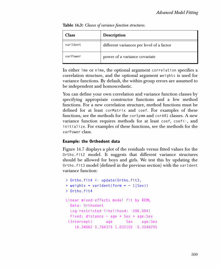
Advanced Model Fitting
In either lme or nlme, the optional argument correlation specifies acorrelation structure, and the optional argument weights is used forvariance functions. By default, the within-group errors are assumed tobe independent and homoscedastic.
You can define your own correlation and variance function classes byspecifying appropriate constructor functions and a few methodfunctions. For a new correlation structure, method functions must bedefined for at least corMatrix and coef. For examples of thesefunctions, see the methods for the corSymm and corAR1 classes. A newvariance function requires methods for at least coef, coef<-, andinitialize. For examples of these functions, see the methods for thevarPower class.
Example: the Orthodont data
Figure 14.7 displays a plot of the residuals versus fitted values for theOrtho.fit2 model. It suggests that different variance structuresshould be allowed for boys and girls. We test this by updating theOrtho.fit3 model (defined in the previous section) with the varIdentvariance function:
> Ortho.fit4 <- update(Ortho.fit3,+ weights = varIdent(form = ~ 1|Sex))> Ortho.fit4
Linear mixed-effects model fit by REML Data: Orthodont Log-restricted-likelihood: -206.0841 Fixed: distance ~ age + Sex + age:Sex (Intercept) age Sex age:Sex 16.34062 0.784375 1.032102 -0.3048295
varIdent different variances per level of a factor
varPower power of a variance covariate
Table 14.3: Classes of variance function structures.
Class Description
509
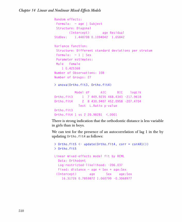
Chapter 14 Linear and Nonlinear Mixed-Effects Models
Random effects: Formula: ~ age | Subject Structure: Diagonal (Intercept) age Residual StdDev: 1.448708 0.1094042 1.65842
Variance function: Structure: Different standard deviations per stratum Formula: ~ 1 | Sex Parameter estimates: Male Female 1 0.425368Number of Observations: 108Number of Groups: 27
> anova(Ortho.fit3, Ortho.fit4)
Model df AIC BIC logLik Ortho.fit3 1 7 449.9235 468.4343 -217.9618Ortho.fit4 2 8 430.9407 452.0958 -207.4704 Test L.Ratio p-value Ortho.fit3 Ortho.fit4 1 vs 2 20.98281 <.0001
There is strong indication that the orthodontic distance is less variablein girls than in boys.
We can test for the presence of an autocorrelation of lag 1 in the byupdating Ortho.fit4 as follows:
> Ortho.fit5 <- update(Ortho.fit4, corr = corAR1())> Ortho.fit5
Linear mixed-effects model fit by REML Data: Orthodont Log-restricted-likelihood: -206.037 Fixed: distance ~ age + Sex + age:Sex (Intercept) age Sex age:Sex 16.31726 0.7859872 1.060799 -0.3068977
510

Advanced Model Fitting
Random effects: Formula: ~ age | Subject Structure: Diagonal (Intercept) age ResidualStdDev: 1.451008 0.1121105 1.630654
Correlation Structure: AR(1) Formula: ~ 1 | Subject Parameter estimate(s): Phi -0.05702521Variance function: Structure: Different standard deviations per stratum Formula: ~ 1 | Sex Parameter estimates: Male Female 1 0.4250633Number of Observations: 108Number of Groups: 27
> anova(Ortho.fit4, Ortho.fit5)
Model df AIC BIC logLik TestOrtho.fit4 1 8 428.1681 449.3233 -206.0841 Ortho.fit5 2 9 430.0741 453.8736 -206.0370 1 vs 2
L.Ratio p-valueOrtho.fit4 Ortho.fit5 0.094035 0.7591
The large p-value of the likelihood ratio test indicates that theautocorrelation is not present.
Note that the correlation structure is used together with the variancefunction, representing a heterogeneous AR(1) process (Littel, et al .,1996). Because the two structures are defined and constructedseparately, a given correlation structure can be combined with any ofthe available variance functions.
511

Chapter 14 Linear and Nonlinear Mixed-Effects Models
Example: the Pixel data
In the form argument of the varFunc constructors, a fitted lme or nlmeobject can be referenced with the period ‘‘.’’ symbol. For example,recall the Pixel.fit1 object defined in the section Arguments onpage 481. To use a variance function that is an arbitrary power of thefitted values in the model, update Pixel.fit1 as follows:
> Pixel.fit2 <- update(Pixel.fit1,+ weights = varPower(form = ~ fitted(.)))> Pixel.fit2
Linear mixed-effects model fit by REML Data: Pixel Log-restricted-likelihood: -412.4593 Fixed: pixel ~ day + day^2 (Intercept) day I(day^2) 1073.314 6.10128 -0.3663864
Random effects: Formula: ~ day | Dog Structure: General positive-definite StdDev Corr(Intercept) 28.503164 (Inter day 1.872961 -0.566
Formula: ~ 1 | Side %in% Dog (Intercept) ResidualStdDev: 16.66015 4.4518e-006
Variance function: Structure: Power of variance covariate Formula: ~ fitted(.) Parameter estimates: power 2.076777Number of Observations: 102Number of Groups: Dog Side %in% Dog 10 20
> anova(Pixel.fit1, Pixel.fit2)
512
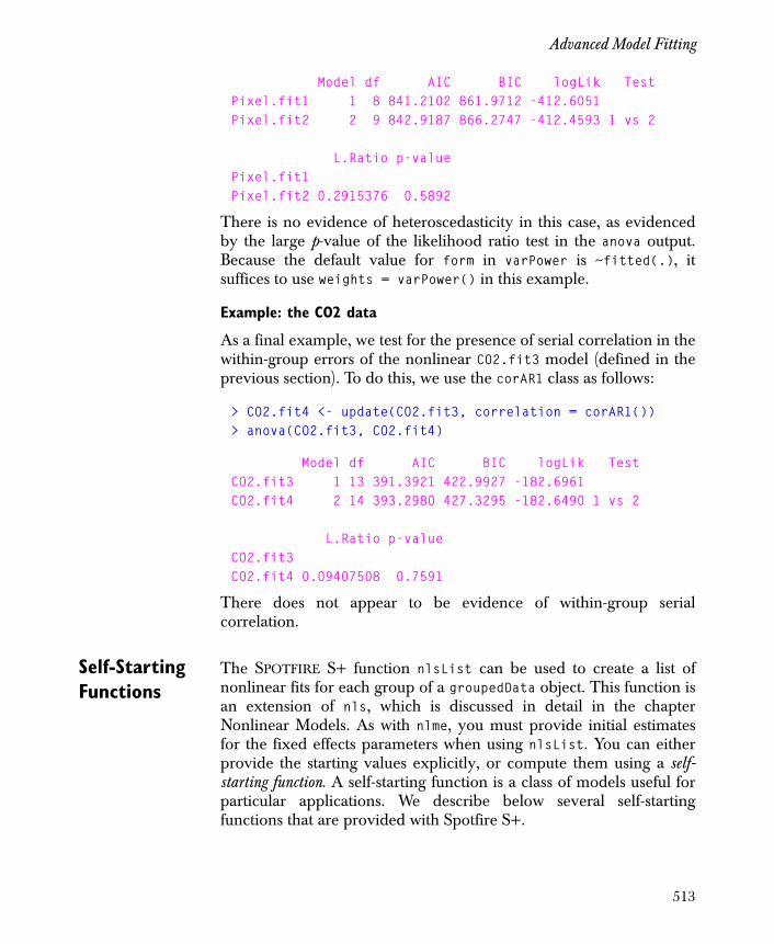
Advanced Model Fitting
Model df AIC BIC logLik TestPixel.fit1 1 8 841.2102 861.9712 -412.6051 Pixel.fit2 2 9 842.9187 866.2747 -412.4593 1 vs 2
L.Ratio p-valuePixel.fit1 Pixel.fit2 0.2915376 0.5892
There is no evidence of heteroscedasticity in this case, as evidencedby the large p-value of the likelihood ratio test in the anova output.Because the default value for form in varPower is ~fitted(.), itsuffices to use weights = varPower() in this example.
Example: the CO2 data
As a final example, we test for the presence of serial correlation in thewithin-group errors of the nonlinear CO2.fit3 model (defined in theprevious section). To do this, we use the corAR1 class as follows:
> CO2.fit4 <- update(CO2.fit3, correlation = corAR1())> anova(CO2.fit3, CO2.fit4)
Model df AIC BIC logLik TestCO2.fit3 1 13 391.3921 422.9927 -182.6961 CO2.fit4 2 14 393.2980 427.3295 -182.6490 1 vs 2
L.Ratio p-valueCO2.fit3 CO2.fit4 0.09407508 0.7591
There does not appear to be evidence of within-group serialcorrelation.
Self-Starting Functions
The SPOTFIRE S+ function nlsList can be used to create a list ofnonlinear fits for each group of a groupedData object. This function isan extension of nls, which is discussed in detail in the chapterNonlinear Models. As with nlme, you must provide initial estimatesfor the fixed effects parameters when using nlsList. You can eitherprovide the starting values explicitly, or compute them using a self-starting function. A self-starting function is a class of models useful forparticular applications. We describe below several self-startingfunctions that are provided with Spotfire S+.
513

Chapter 14 Linear and Nonlinear Mixed-Effects Models
One way of providing initial values to nlsList is to include them inthe data set as a parameters attribute. In addition, both nlsList andnlme have optional start arguments that can be used to provide theinitial estimates as input. Alternatively, a function that derives initialestimates can be added to the model formula itself as an attribute.This constitutes a selfStart function in Spotfire S+. When a self-starting function is used in calls to nlsList and nlme, initial estimatesfor the parameters are taken directly from the initial attribute of thefunction.
The following four self-starting functions are useful in biostatisticsapplications.
• Biexponential model:
The corresponding Spotfire S+ function is SSbiexp(input, A1, lrc1, A2, lrc2), where input=t is a covariate and A1=α1, A2=α2, lrc1=β1, and lrc2=β2 are parameters.
• First-order Compartment model:
The corresponding Spotfire S+ function is SSfol(Dose, input, lCl, lKa, lKe), where Dose=d is a covariate representing the initial dose, input=t is a covariate representing the time at which to evaluate the model, and lCl=α, lKa=β, and lKe=γ are parameters.
• Four-parameter Logistic model:
The corresponding Spotfire S+ function is SSfpl(input, A, B, xmid, scal), where input=x is a covariate and A=α, B=β, xmid=γ , and scal=θ are parameters.
α1e e–β1t α2e e–
β2t+
eβ eγ e eγ t– e eβ––(⋅ ⋅ ⋅
eα eβ eγ–( )⋅
--------------------------------------------------------------
α β α–
1 e x γ–( )– θ⁄+
-----------------------------------+
514
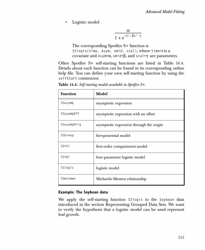
Advanced Model Fitting
• Logistic model:
The corresponding Spotfire S+ function is SSlogis(time, Asym, xmid, scal), where time=t is a covariate and Asym=α, xmid=β, and scal=γ are parameters.
Other Spotfire S+ self-starting functions are listed in Table 14.4.Details about each function can be found in its corresponding onlinehelp file. You can define your own self-starting function by using theselfStart constructor.
Example: The Soybean data
We apply the self-starting function SSlogis to the Soybean dataintroduced in the section Representing Grouped Data Sets. We wantto verify the hypothesis that a logistic model can be used representleaf growth.
Table 14.4: Self-starting models available in Spotfire S+.
Function Model
SSasymp asymptotic regression
SSasympOff asymptotic regression with an offset
SSasympOrig asymptotic regression through the origin
SSbiexp biexponential model
SSfol first-order compartment model
SSfpl four-parameter logistic model
SSlogis logistic model
SSmicmen Michaelis-Menten relationship
α1 e t β–( )– γ⁄
+----------------------------------
515

Chapter 14 Linear and Nonlinear Mixed-Effects Models
The nlsList call is as follows:
> Soybean.nlsList <- nlsList(weight ~+ SSlogis(Time, Asym, xmid, scal) | Plot, data = Soybean)
Error in nls(y ~ 1/(1 + exp((xmid - x)/scal)), data ..: singular gradient matrix
The error message indicates that nls could not compute a fit for oneof the groups in the data set. The object Soybean.nlsList isnevertheless created.
The results in Soybean.nlsList show that the 1989P8 group in theSoybean data could not be fitted appropriately with the logistic model.We can see this directly by using the coef function.
> coef(Soybean.nlsList)
Asym xmid scal1988F4 15.151338 52.83361 5.1766411988F2 19.745503 56.57514 8.4067201988F1 20.338576 57.40265 9.6048701988F7 19.871706 56.16236 8.0697181988F5 30.647205 64.12857 11.2623511988F8 22.776430 59.32964 9.000267. . .1989P2 28.294391 67.17185 12.5227201989P8 NA NA NA1990F2 19.459767 66.28652 13.158397. . .1990P5 19.543787 51.14830 7.2919761990P2 25.787317 62.35974 11.6570191990P4 26.132712 61.20345 10.973765
An nlme method exists for nlsList objects, which allows you to fitpopulation parameters and individual random effects for an nlsListmodel. For example, the following simple call computes a mixed-effects model from the Soybean.nlsList object.
Warning
On occasion, nlsList returns errors when it cannot adequately fit one or more groups in the data set. When this occurs, fits for the remaining groups are still computed.
516

Advanced Model Fitting
> Soybean.fit1 <- nlme(Soybean.nlsList)> summary(Soybean.fit1)
Nonlinear mixed-effects model fit by maximum likelihood Model: weight ~ SSlogis(Time, Asym, xmid, scal) Data: Soybean AIC BIC logLik 1499.667 1539.877 -739.8334
Random effects: Formula: list(Asym ~ 1 , xmid ~ 1 , scal ~ 1 ) Level: Plot Structure: General positive-definite StdDev Corr Asym 5.200969 Asym xmid xmid 4.196918 0.721 scal 1.403934 0.711 0.959Residual 1.123517
Fixed effects: list(Asym ~ 1 , xmid ~ 1 , scal ~ 1 ) Value Std.Error DF t-value p-valueAsym 19.25326 0.8031745 362 23.97145 <.0001xmid 55.02012 0.7272288 362 75.65724 <.0001scal 8.40362 0.3152215 362 26.65941 <.0001 Correlation: Asym xmidxmid 0.724 scal 0.620 0.807
Standardized Within-Group Residuals: Min Q1 Med Q3 Max -6.086247 -0.2217542 -0.03385827 0.2974177 4.845216
Number of Observations: 412Number of Groups: 48
The Soybean.fit1 object does not incorporate covariates or within-group errors. Comparing the estimated standard deviations andmeans of Asym, xmid, and scal, the asymptotic weight Asym has thehighest coefficient of variation (5.2/19.25 = 0.27). Modeling thisrandom effects parameter is the focus of the following analyses.
517
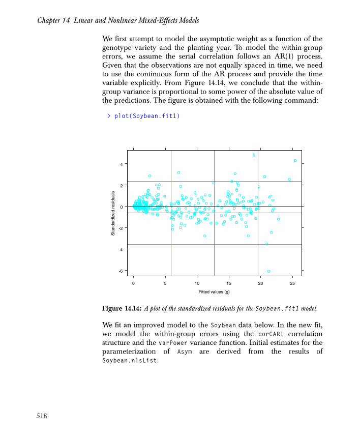
Chapter 14 Linear and Nonlinear Mixed-Effects Models
We first attempt to model the asymptotic weight as a function of thegenotype variety and the planting year. To model the within-grouperrors, we assume the serial correlation follows an AR(1) process.Given that the observations are not equally spaced in time, we needto use the continuous form of the AR process and provide the timevariable explicitly. From Figure 14.14, we conclude that the within-group variance is proportional to some power of the absolute value ofthe predictions. The figure is obtained with the following command:
> plot(Soybean.fit1)
We fit an improved model to the Soybean data below. In the new fit,we model the within-group errors using the corCAR1 correlationstructure and the varPower variance function. Initial estimates for theparameterization of Asym are derived from the results ofSoybean.nlsList.
Figure 14.14: A plot of the standardized residuals for the Soybean.fit1 model.
-6
-4
-2
0
2
4
0 5 10 15 20 25
Fitted values (g)
Sta
ndar
dize
d re
sidu
als
518

Advanced Model Fitting
> Soybean.fit2 <- nlme(weight ~ + SSlogis(Time, Asym, xmid, scal), data = Soybean,+ fixed = list(Asym ~ Variety * Year, xmid ~ 1, scal ~ 1),+ random = list(Asym ~ 1, xmid ~ 1, scal ~ 1), + start = c(20.08425, 2.03699, -3.785161, 0.3036094,+ 1.497311, -1.084704, 55.02058, 8.402632),+ correlation = corCAR1(form = ~Time), + weights = varPower())
Figure 14.15 displays a plot the residuals for the updated model,obtained with the following command:
> plot(Soybean.fit2)
The residuals plot confirms our choice of variance structure. Theanova function is used to compare the Soybean.fit1 andSoybean.fit2 models. The progress in the log-likelihood, AIC, andBIC is tremendous.
> anova(Soybean.fit1, Soybean.fit2)
Model df AIC BIC logLikSoybean.fit1 1 10 1499.667 1539.877 -739.8334Soybean.fit2 2 17 678.592 746.950 -322.2962
Test L.Ratio p-valueSoybean.fit1 Soybean.fit2 1 vs 2 835.0744 <.0001
We conclude that both the genotype variety and planting year have alarge impact on the limiting leaf weight of the plants. Theexperimental strain gains 2.5 grams in the limit.
519
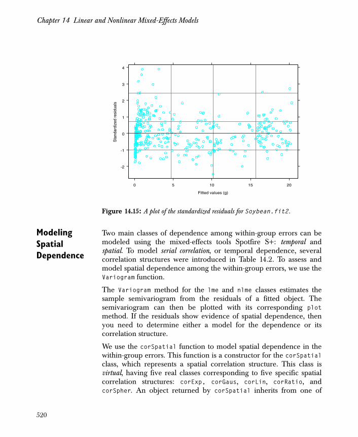
Chapter 14 Linear and Nonlinear Mixed-Effects Models
Modeling Spatial Dependence
Two main classes of dependence among within-group errors can bemodeled using the mixed-effects tools Spotfire S+: temporal andspatial. To model serial correlation, or temporal dependence, severalcorrelation structures were introduced in Table 14.2. To assess andmodel spatial dependence among the within-group errors, we use theVariogram function.
The Variogram method for the lme and nlme classes estimates thesample semivariogram from the residuals of a fitted object. Thesemivariogram can then be plotted with its corresponding plotmethod. If the residuals show evidence of spatial dependence, thenyou need to determine either a model for the dependence or itscorrelation structure.
We use the corSpatial function to model spatial dependence in thewithin-group errors. This function is a constructor for the corSpatialclass, which represents a spatial correlation structure. This class isvirtual, having five real classes corresponding to five specific spatialcorrelation structures: corExp, corGaus, corLin, corRatio, andcorSpher. An object returned by corSpatial inherits from one of
Figure 14.15: A plot of the standardized residuals for Soybean.fit2.
-2
-1
0
1
2
3
4
0 5 10 15 20
Fitted values (g)
Sta
ndar
dize
d re
sidu
als
520
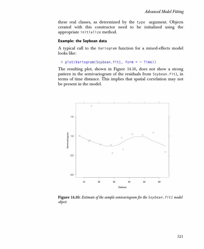
Advanced Model Fitting
these real classes, as determined by the type argument. Objectscreated with this constructor need to be initialized using theappropriate initialize method.
Example: the Soybean data
A typical call to the Variogram function for a mixed-effects modellooks like:
> plot(Variogram(Soybean.fit1, form = ~ Time))
The resulting plot, shown in Figure 14.16, does not show a strongpattern in the semivariogram of the residuals from Soybean.fit1, interms of time distance. This implies that spatial correlation may notbe present in the model.
Figure 14.16: Estimate of the sample semivariogram for the Soybean.fit1 model object.
0.0
0.5
1.0
1.5
10 20 30 40 50 60
Distance
Se
miv
ario
gra
m
521

Chapter 14 Linear and Nonlinear Mixed-Effects Models
Refitting Soybean.fit2 without the AR(1) correlation structure showsthat the model may indeed be overparameterized:
> Soybean.fit3 <- update(Soybean.fit2, correlation = NULL)> anova(Soybean.fit1, Soybean.fit3, Soybean.fit2)
Model df AIC BIC logLikSoybean.fit1 1 10 1499.667 1539.877 -739.8334Soybean.fit3 2 16 674.669 739.005 -321.3344Soybean.fit2 3 17 678.592 746.950 -322.2962
Test L.Ratio p-valueSoybean.fit1 Soybean.fit3 1 vs 2 836.9981 <.0001Soybean.fit2 2 vs 3 1.9237 0.1654
This indicates that only the change in the fixed effects model and theuse of a variance function explain the improvement we see inSoybean.fit2. The model without the correlation structure is simpler,and therefore preferred.
522
References
REFERENCES
Becker, R.A., Cleveland, W.S., & Shyu, M.J. (1996). The visual designand control of trellis graphics displays. Journal of Computational andGraphical Statistics, 5(2): 123-156.
Chambers, J.M. & Hastie, T.J. (Eds.) (1992). Statistical Models in S.London: Chapman and Hall.
Davidian, M. & Giltinan, D.M. (1995). Nonlinear Models for RepeatedMeasurement Data. London: Chapman & Hall.
Goldstein, H. (1995). Multilevel Statistical Models. New York: HalstedPress.
Laird, N.M. & Ware, J.H. (1982). Random-effects models forlongitudinal data. Biometrics 38: 963-974.
Lindstrom, M.J. & Bates, D.M. (1990). Nonlinear mixed effectsmodels for repeated measures data. Biometrics 46: 673-687.
Littel, R.C., Milliken, G.A., Stroup, W.W., & Wolfinger, R.D. (1996).SAS Systems for Mixed Models. Cary, NC: SAS Institute Inc..
Longford, N.T. (1993). Random Coefficient Models. New York: OxfordUniversity Press.
Milliken, G.A. & Johnson, D.E. (1992). Analysis of Messy Data, Volume1: Designed Experiments. London: Chapman & Hall.
Pinheiro, J.C. (1994). Topics in Mixed Effect Models. Ph.D. thesis,Department of Statistics, University of Wisconsin-Madison.
Pinheiro, J.C. & Bates, D.M. (2000). Mixed-Effects Models in S andSpotfire S+ . New York: Springer-Verlag.
Potthoff, R.F. & Roy, S.N. (1964). A generalized multivariate analysisof variance model useful especially for growth curve problems.Biometrika 51: 313-326.
Potvin, C., Lechowicz, M.J., & Tardif, S. (1990). The statistical analysisof ecophysiological response curves obtained from experimentsinvolving repeated measures. Ecology 71: 1389-1400.
Venables, W.N. & Ripley, B.D. (1997) Modern Applied Statistics withSpotfire S+, 2nd Edition. New York: Springer-Verlag.
523

Chapter 14 Linear and Nonlinear Mixed-Effects Models
524

Introduction 526
Optimization Functions 527Finding Roots 528Finding Local Maxima and Minima of Univariate
Functions 529Finding Maxima and Minima of Multivariate
Functions 530Solving Nonnegative Least Squares Problems 535Solving Nonlinear Least Squares Problems 537
Examples of Nonlinear Models 539Maximum Likelihood Estimation 539Nonlinear Regression 542
Inference for Nonlinear Models 544Likelihood Models 544Least Squares Models 544The Fitting Algorithms 544Specifying Models 545Parametrized Data Frames 547Derivatives 548Fitting Models 554Profiling the Objective Function 560
References 565
NONLINEAR MODELS 15
525

Chapter 15 Nonlinear Models
INTRODUCTION
This chapter covers the fitting of nonlinear models such as innonlinear regression, likelihood models, and Bayesian estimation.Nonlinear models are more general than the linear models usuallydiscussed. Specifying nonlinear models typically requires one ormore of the following: more general formulas, extended data frames,starting values, and derivatives.
The two most common fitting criteria for nonlinear modelsconsidered are Minimum sum and Minimum sum-of-squares.Minimum sum minimizes the sum of contributions from observations(the maximum likelihood problem). Minimum sum-of-squaresminimizes the sum of squared residuals (the nonlinear least-squaresregression problem).
The first sections of this chapter summarize the use of the nonlinearoptimization functions. Starting with the section Examples ofNonlinear Models, the use of the ms and nls functions are examined,along with corresponding examples and theory, in much more detail.
526

Optimization Functions
OPTIMIZATION FUNCTIONS
TIBCO Spotfire S+ has several functions for finding roots ofequations and local maxima and minima of functions, as shown inTable 15.1.
Table 15.1: The range of Spotfire S+ functions for finding roots, maxima, and minima.
Function Description
polyroot Finds the roots of a complex polynomial equation.
uniroot Finds the root of a univariate real-valued function in a user-supplied interval.
peaks Finds local maxima in a set of discrete points.
optimize Approximates a local optimum of a continuous univariate function within a given interval.
ms Finds a local minimum of a multivariate function.
nlmin Finds a local minimum of a nonlinear function using a general quasi-Newton optimizer.
nlminb Finds a local minimum for smooth nonlinear functions subject to bound-constrained parameters.
nls Finds a local minimum of the sums of squares of one or more multivariate functions.
nlregb Finds a local minimum for sums of squares of nonlinear functions subject to bound-constrained parameters.
nnls Finds the least-squares solution subject to the constraint that the coefficients be nonnegative.
527

Chapter 15 Nonlinear Models
Finding Roots The function polyroot finds the roots (zeros) of the complex-valued
polynomial equation . The input to
polyroot is the vector of coefficients . For example, to
solve the equation , use polyroot as follows:
> polyroot(c(6, 5, 1))
[1] -2+2.584939e-26i -3-2.584939e-26i
Since 2.584939e-26i is equivalent to zero in machine arithmetic,polyroot returns -2 and -3 for the roots of the polynomial, asexpected.
The function uniroot finds a zero of a continuous, univariate, real-valued function within a user-specified interval for which the functionhas opposite signs at the endpoints. The input to uniroot includes thefunction, the lower and upper endpoints of the interval, and anyadditional arguments to the function. For example, suppose you havethe function:
> my.fcn
function(x, amp=1, per=2*pi, horshft=0, vershft=0){ amp * sin(((2*pi)/per) * (x-horshft)) + vershft}
This is the sine function with amplitude abs(amp), period abs(per),horizontal (phase) shift horshft and vertical shift vershft. To find aroot of the function my.fcn in the interval using itsdefault arguments, type:
> uniroot(my.fcn, interval = c(pi/2, 3*pi/2))
$root[1] 3.141593. . .
To find a root of my.fcn in the interval with the periodset to , type the following command.
> uniroot(my.fcn, interval = c(pi/4, 3*pi/4), per = pi)
akzk … a1z a0+ + + 0=
c a0 … a, k,( )
z2 5z 6+ + 0=
π 2⁄ 3π 2⁄,
π 4⁄ 3π 4⁄,
π
528
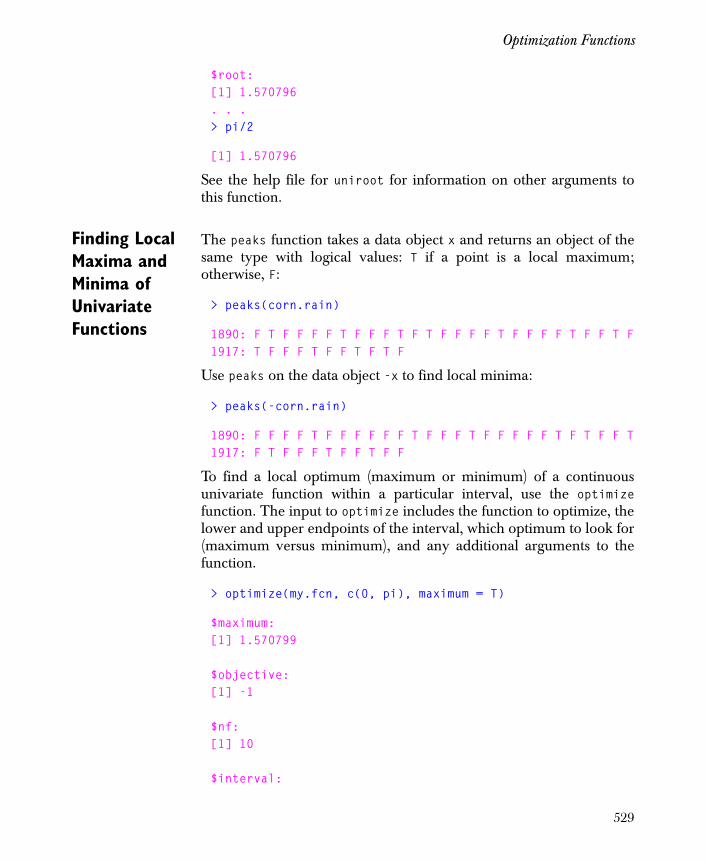
Optimization Functions
$root:[1] 1.570796. . .> pi/2
[1] 1.570796
See the help file for uniroot for information on other arguments tothis function.
Finding Local Maxima and Minima of Univariate Functions
The peaks function takes a data object x and returns an object of thesame type with logical values: T if a point is a local maximum;otherwise, F:
> peaks(corn.rain)
1890: F T F F F F T F F F T F T F F F F T F F F F T F F T F1917: T F F F T F F T F T F
Use peaks on the data object -x to find local minima:
> peaks(-corn.rain)
1890: F F F F T F F F F F F T F F F T F F F F F T F T F F T1917: F T F F F T F F T F F
To find a local optimum (maximum or minimum) of a continuousunivariate function within a particular interval, use the optimizefunction. The input to optimize includes the function to optimize, thelower and upper endpoints of the interval, which optimum to look for(maximum versus minimum), and any additional arguments to thefunction.
> optimize(my.fcn, c(0, pi), maximum = T)
$maximum:[1] 1.570799
$objective:[1] -1
$nf:[1] 10
$interval:
529

Chapter 15 Nonlinear Models
[1] 1.570759 1.570840. . .
> pi/2
[1] 1.570799
> optimize(my.fcn, c(0, pi), maximum = F, per = pi)
$minimum:[1] 2.356196
$objective:[1] -1
$nf:[1] 9
$interval:[1] 2.356155 2.356236. . .
> 3*pi/4
[1] 2.356194
See the help file for optimize for information on other arguments tothis function.
Finding Maxima and Minima of Multivariate Functions
Spotfire S+ has two functions to find the local minimum of amultivariate function: nlminb (Nonlinear Minimization with BoxConstraints) and ms (Minimize Sums).
The two required arguments to nlminb are objective (the function to minimize) and start (a vector of starting values for theminimization). The function must take as its first argument a vectorof parameters over which the minimization is carried out. By default,there are no boundary constraints on the parameters. The nlminbfunction, however, also takes the optional arguments lower and upperthat specify bounds on the parameters. Additional arguments to canbe passed in the call to nlminb.
f
f
f
530

Optimization Functions
1. Example: using nlminb to find a local minimum
> my.multvar.fcn
function(xvec, ctr = rep(0, length(xvec))){ if(length(xvec) != length(ctr)) stop("lengths of xvec and ctr do not match") sum((xvec - ctr)^2)}
> nlminb(start = c(0,0), objective = my.multvar.fcn,+ ctr = c(1,2))
$parameters:[1] 1 2
$objective:[1] 3.019858e-30
$message:[1] "ABSOLUTE FUNCTION CONVERGENCE". . .
2. Example: using nlminb to find a local maximum
To find a local maximum of , use nlminb on . Since unary minuscannot be performed on a function, you must define a new functionthat returns -1 times the value of the function you want to maximize:
> fcn.to.maximize
function(xvec){ - xvec[1]^2 + 2 * xvec[1] - xvec[2]^2 + 20 * xvec[2] + 40}
> fcn.to.minimize
function(xvec){ - fcn.to.maximize(xvec)}
f f–
531

Chapter 15 Nonlinear Models
> nlminb(start = c(0, 0), objective = fcn.to.minimize)
$parameters:[1] 1 10
$objective:[1] -141
$message:[1] "RELATIVE FUNCTION CONVERGENCE". . .
3. Example: using nlminb to find a constrained minimum
To find the local minimum of a multivariate function subject toconstraints, use nlminb with the lower and/or upper arguments. As anexample of constrained minimization, consider the following functionnorm.neg.2.ll, which is (minus a constant) -2 times the log-likelihoodfunction of a Gaussian distribution:
> norm.neg.2.ll <-+ function(theta, y)+ {+ length(y) * log(theta[2]) ++ (1/theta[2]) * sum((y - theta[1])^2)+ }
This function assumes that observations from a normal distributionare stored in the vector y. The vector theta contains the mean(theta[1]) and variance (theta[2]) of this distribution. To find themaximum likelihood estimates of the mean and variance, we need tofind the values of theta[1] and theta[2] that minimizenorm.neg.2.ll for a given set of observations stored in y. We mustuse the lower argument to nlminb because the estimate of variancemust be greater than zero:
> set.seed(12)> my.obs <- rnorm(100, mean = 10, sd = 2)> nlminb(start = c(0,1), objective = norm.neg.2.ll,+ lower = c(-Inf, 0), y = my.obs)
$parameters:[1] 9.863812 3.477773
532

Optimization Functions
$objective:[1] 224.6392
$message:[1] "RELATIVE FUNCTION CONVERGENCE". . .
> mean(my.obs)
[1] 9.863812
> (99/100) * var(my.obs)
[1] 3.477774
4. Example: using ms
The Minimum Sums function ms also minimizes a multivariatefunction, but in the context of the modeling paradigm. It thereforeexpects a formula rather than a function as its main argument. Here,the last example is redone with ms, where mu is the estimate of thepopulation mean and ss is the estimate of the population variance
.
> ms( ~length(y) * log(ss) + (1/ss) * sum((y - mu)^2),+ data = data.frame(y = my.obs),+ start = list(mu = 0, ss = 1))
value: 224.6392parameters: mu ss9.863813 3.477776
formula: ~length(y) * log(ss) + (1/ss) * sum((y-mu)^2)
1 observations
call: ms(formula = ~length(y) * log(ss) + (1/ss) * sum((y - mu)^2),data = data.frame(y=my.obs), start=list(mu=0, ss=1))
μ
σ2
533
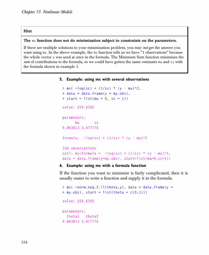
Chapter 15 Nonlinear Models
5. Example: using ms with several observations
> ms( ~log(ss) + (1/ss) * (y - mu)^2,+ data = data.frame(y = my.obs),+ start = list(mu = 0, ss = 1))
value: 224.6392
parameters: mu ss9.863813 3.477776
formula: ~log(ss) + (1/ss) * (y - mu)^2
100 observationscall: ms(formula = ~log(ss) + (1/ss) * (y - mu)^2,data = data.frame(y=my.obs), start=list(mu=0,ss=1))
6. Example: using ms with a formula function
If the function you want to minimize is fairly complicated, then it isusually easier to write a function and supply it in the formula.
> ms( ~norm.neg.2.ll(theta,y), data = data.frame(y = + my.obs), start = list(theta = c(0,1)))
value: 224.6392
parameters: theta1 theta29.863813 3.477776
Hint
The ms function does not do minimization subject to constraints on the parameters.
If there are multiple solutions to your minimization problem, you may not get the answer you want using ms. In the above example, the ms function tells us we have “1 observations” because the whole vector y was used at once in the formula. The Minimum Sum function minimizes the sum of contributions to the formula, so we could have gotten the same estimates mu and ss with the formula shown in example 5.
534
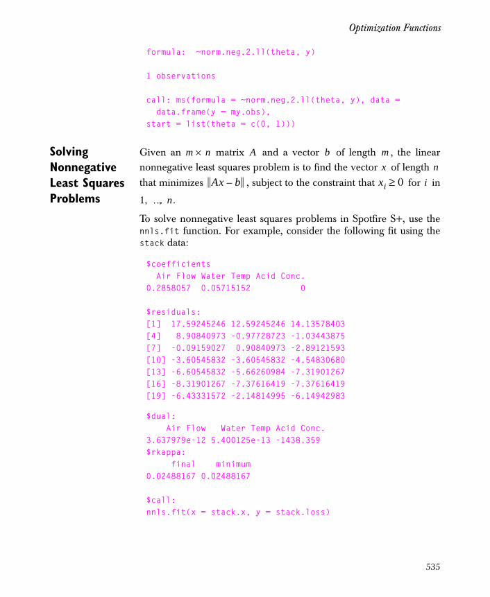
Optimization Functions
formula: ~norm.neg.2.ll(theta, y)
1 observations
call: ms(formula = ~norm.neg.2.ll(theta, y), data = data.frame(y = my.obs),start = list(theta = c(0, 1)))
Solving Nonnegative Least Squares Problems
Given an matrix and a vector of length , the linearnonnegative least squares problem is to find the vector of length
that minimizes , subject to the constraint that for in
.
To solve nonnegative least squares problems in Spotfire S+, use thennls.fit function. For example, consider the following fit using thestack data:
$coefficients Air Flow Water Temp Acid Conc.0.2858057 0.05715152 0
$residuals:[1] 17.59245246 12.59245246 14.13578403[4] 8.90840973 -0.97728723 -1.03443875[7] -0.09159027 0.90840973 -2.89121593[10] -3.60545832 -3.60545832 -4.54830680[13] -6.60545832 -5.66260984 -7.31901267[16] -8.31901267 -7.37616419 -7.37616419[19] -6.43331572 -2.14814995 -6.14942983
$dual: Air Flow Water Temp Acid Conc.3.637979e-12 5.400125e-13 -1438.359$rkappa: final minimum0.02488167 0.02488167
$call:nnls.fit(x = stack.x, y = stack.loss)
m n× A b mx n
Ax b– xi 0≥ i
1 … n, ,
535
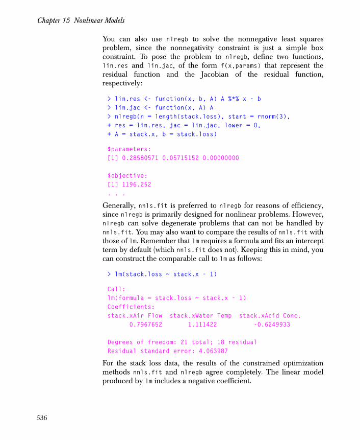
Chapter 15 Nonlinear Models
You can also use nlregb to solve the nonnegative least squaresproblem, since the nonnegativity constraint is just a simple boxconstraint. To pose the problem to nlregb, define two functions,lin.res and lin.jac, of the form f(x,params) that represent theresidual function and the Jacobian of the residual function,respectively:
> lin.res <- function(x, b, A) A %*% x - b> lin.jac <- function(x, A) A> nlregb(n = length(stack.loss), start = rnorm(3),+ res = lin.res, jac = lin.jac, lower = 0,+ A = stack.x, b = stack.loss)
$parameters:[1] 0.28580571 0.05715152 0.00000000
$objective:[1] 1196.252. . .
Generally, nnls.fit is preferred to nlregb for reasons of efficiency,since nlregb is primarily designed for nonlinear problems. However,nlregb can solve degenerate problems that can not be handled bynnls.fit. You may also want to compare the results of nnls.fit withthose of lm. Remember that lm requires a formula and fits an interceptterm by default (which nnls.fit does not). Keeping this in mind, youcan construct the comparable call to lm as follows:
> lm(stack.loss ~ stack.x - 1)
Call:lm(formula = stack.loss ~ stack.x - 1)Coefficients:stack.xAir Flow stack.xWater Temp stack.xAcid Conc. 0.7967652 1.111422 -0.6249933
Degrees of freedom: 21 total; 18 residualResidual standard error: 4.063987
For the stack loss data, the results of the constrained optimizationmethods nnls.fit and nlregb agree completely. The linear modelproduced by lm includes a negative coefficient.
536
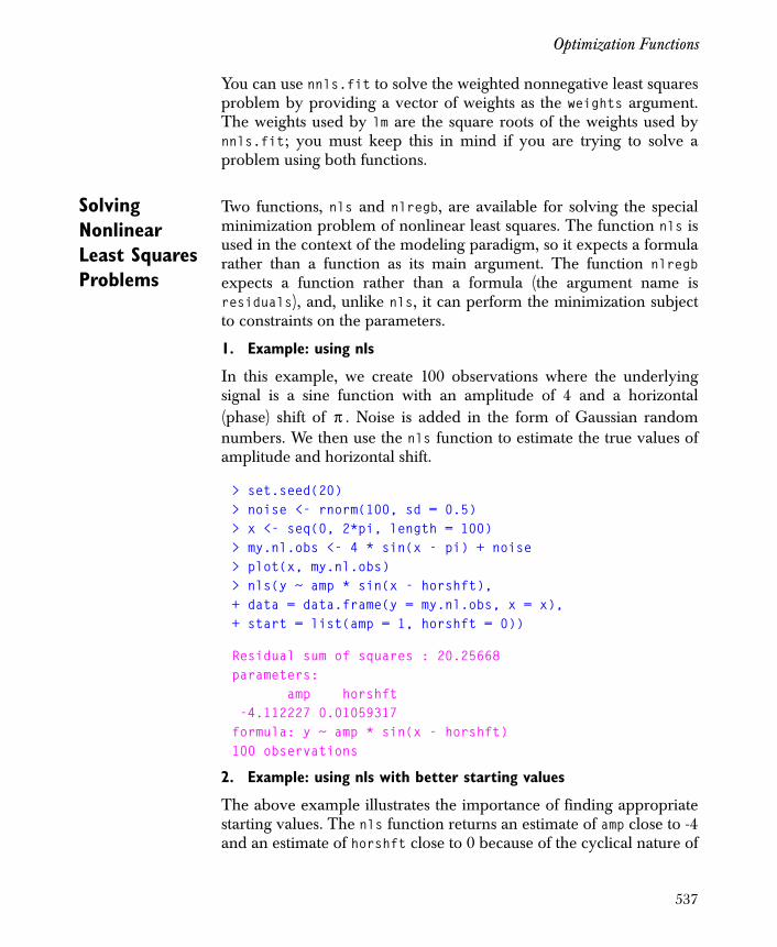
Optimization Functions
You can use nnls.fit to solve the weighted nonnegative least squaresproblem by providing a vector of weights as the weights argument.The weights used by lm are the square roots of the weights used bynnls.fit; you must keep this in mind if you are trying to solve aproblem using both functions.
Solving Nonlinear Least Squares Problems
Two functions, nls and nlregb, are available for solving the specialminimization problem of nonlinear least squares. The function nls isused in the context of the modeling paradigm, so it expects a formularather than a function as its main argument. The function nlregbexpects a function rather than a formula (the argument name isresiduals), and, unlike nls, it can perform the minimization subjectto constraints on the parameters.
1. Example: using nls
In this example, we create 100 observations where the underlyingsignal is a sine function with an amplitude of 4 and a horizontal(phase) shift of . Noise is added in the form of Gaussian randomnumbers. We then use the nls function to estimate the true values ofamplitude and horizontal shift.
> set.seed(20)> noise <- rnorm(100, sd = 0.5)> x <- seq(0, 2*pi, length = 100)> my.nl.obs <- 4 * sin(x - pi) + noise> plot(x, my.nl.obs)> nls(y ~ amp * sin(x - horshft),+ data = data.frame(y = my.nl.obs, x = x),+ start = list(amp = 1, horshft = 0))
Residual sum of squares : 20.25668parameters: amp horshft -4.112227 0.01059317formula: y ~ amp * sin(x - horshft)100 observations
2. Example: using nls with better starting values
The above example illustrates the importance of finding appropriatestarting values. The nls function returns an estimate of amp close to -4and an estimate of horshft close to 0 because of the cyclical nature of
π
537

Chapter 15 Nonlinear Models
the sine function: . If we start with initialestimates of amp and horshft closer to their true values, nls gives usthe estimates we want.
> nls(y ~ amp * sin(x - horshft),+ data = data.frame(y = my.nl.obs, x = x),+ start = list(amp = 3, horshft = pi/2))
Residual sum of squares : 20.25668parameters: amp horshft 4.112227 -3.131formula: y ~ amp * sin(x - horshft)100 observations
3. Example: creating my.new.func and using nlregb
We can use the nlregb function to redo the above example andspecify that the value of amp must be greater than 0:
> my.new.fcn
function(param, x, y){ amp <- param[1] horshft <- param[2] y - amp * sin(x - horshft)}
> nlregb(n = 100, start = c(3,pi/2),+ residuals = my.new.fcn,+ lower = c(0, -Inf), x = x, y = my.nl.obs)
$parameters:[1] 4.112227 3.152186
$objective:[1] 20.25668
$message:[1] "BOTH X AND RELATIVE FUNCTION CONVERGENCE"
$grad.norm:[1] 5.960581e-09
x π–( )sin x( )sin–=
538

Examples of Nonlinear Models
EXAMPLES OF NONLINEAR MODELS
Maximum Likelihood Estimation
Parameters are estimated by maximizing the likelihood function.Suppose independent observations are distributed with probabilitydensities , where is a vector of parameters. Thelikelihood function is defined as
The problem is to find the estimate that maximizes the likelihoodfunction for the observed data. Maximizing the likelihood isequivalent to minimizing the negative of the log-likelihood:
Example One: Ping-Pong
Each member of the U.S. Table Tennis Association is assigned arating based on the member’s performance in tournaments. Winninga match boosts the winner’s rating and lowers the loser’s rating somenumber of points depending on the current ratings of the two players.Using these data, two questions we might like to ask are the following:
1. Do players with a higher rating tend to win over players with a lower rating?
2. Does a larger difference in rating imply that the higher-rated player is more likely to win?
Assuming a logistic distribution in which isproportional to the difference in rating and the average rating of thetwo players, we get:
. (15.1)
. (15.2)
npi θ( ) p yi θ,( )= θ
L y θ;( ) pi θ( )i 1=
n
∏=
θ
l θ( ) L y θ;( )( )log– pi θ( )( )log–
i 1=
n
∑= =
. (15.3)
p 1 p–( )⁄( )log
pie
Diα Riβ+
1 eDiα Riβ++
------------------------------=
539
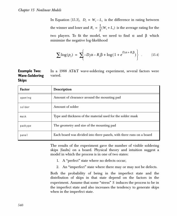
Chapter 15 Nonlinear Models
In Equation (15.3), is the difference in rating between
the winner and loser and is the average rating for the
two players. To fit the model, we need to find and whichminimize the negative log-likelihood
Example Two: Wave-Soldering Skips
In a 1988 AT&T wave-soldering experiment, several factors werevaried.
The results of the experiment gave the number of visible solderingskips (faults) on a board. Physical theory and intuition suggest amodel in which the process is in one of two states:
1. A “perfect” state where no defects occur;
2. An “imperfect” state where there may or may not be defects.
Both the probability of being in the imperfect state and thedistribution of skips in that state depend on the factors in theexperiment. Assume that some “stress” induces the process to be inthe imperfect state and also increases the tendency to generate skipswhen in the imperfect state.
. (15.4)
Di Wi Li–=
Ri12--- Wi Li+( )=
α β
pi( )log–∑ D– iα Riβ 1 eDiα Riβ+
+( )log+–⎩ ⎭⎨ ⎬⎧ ⎫
∑=
Factor Description
opening Amount of clearance around the mounting pad
solder Amount of solder
mask Type and thickness of the material used for the solder mask
padtype The geometry and size of the mounting pad
panel Each board was divided into three panels, with three runs on a board
S
540
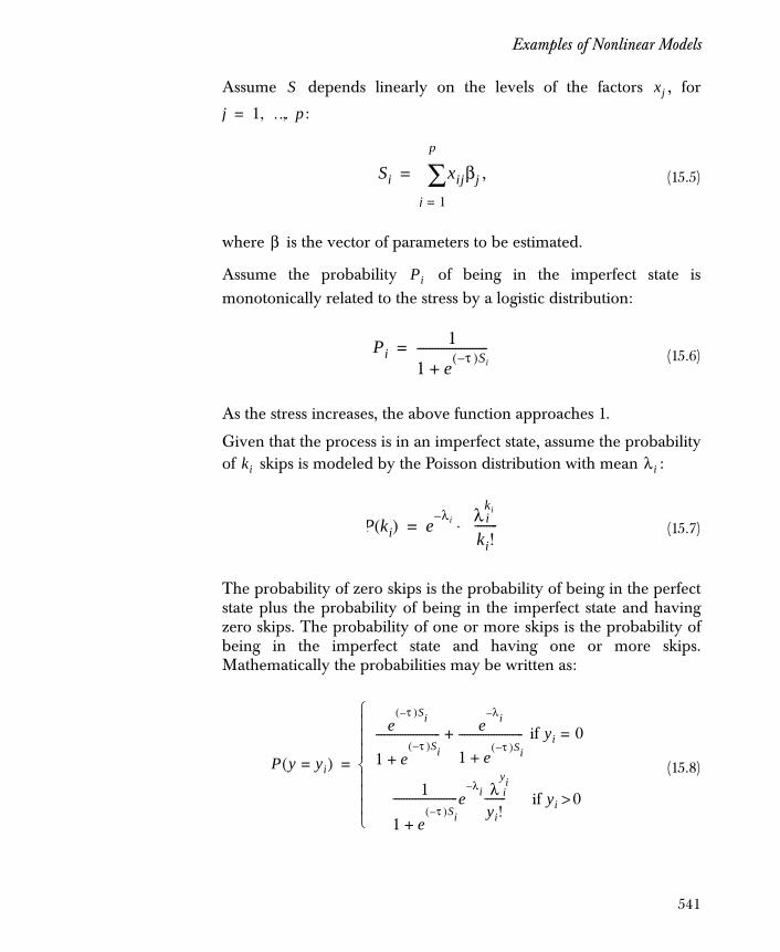
Examples of Nonlinear Models
Assume depends linearly on the levels of the factors , for
:
where is the vector of parameters to be estimated.
Assume the probability of being in the imperfect state ismonotonically related to the stress by a logistic distribution:
As the stress increases, the above function approaches 1.
Given that the process is in an imperfect state, assume the probabilityof skips is modeled by the Poisson distribution with mean :
The probability of zero skips is the probability of being in the perfectstate plus the probability of being in the imperfect state and havingzero skips. The probability of one or more skips is the probability ofbeing in the imperfect state and having one or more skips.Mathematically the probabilities may be written as:
, (15.5)
(15.6)
(15.7)
(15.8)
S xj
j 1 … p, ,=
Si xijβj
j 1=
p
∑=
β
Pi
Pi1
1 eτ–( )Si+
------------------------=
ki λ i
P ki( ) eλ– i λ
kii
ki!--------⋅=
P y yi=( )
eτ–( )Si
1 eτ–( )Si+
------------------------ eλ– i
1 eτ–( )Si+
------------------------+ if yi 0=
1
1 eτ–( )Si+
------------------------eλ– i λ
yii
yi!-------- if yi 0>
⎩⎪⎪⎪⎨⎪⎪⎪⎧
=
541
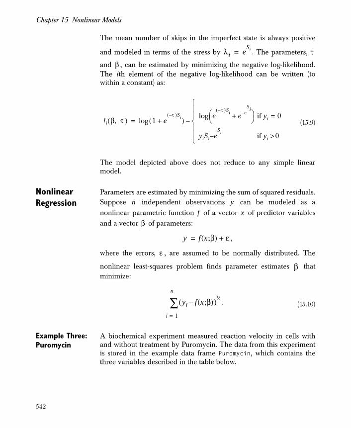
Chapter 15 Nonlinear Models
The mean number of skips in the imperfect state is always positive
and modeled in terms of the stress by . The parameters,
and , can be estimated by minimizing the negative log-likelihood.The ith element of the negative log-likelihood can be written (towithin a constant) as:
The model depicted above does not reduce to any simple linearmodel.
Nonlinear Regression
Parameters are estimated by minimizing the sum of squared residuals.Suppose independent observations can be modeled as anonlinear parametric function of a vector of predictor variablesand a vector of parameters:
,
where the errors, , are assumed to be normally distributed. The
nonlinear least-squares problem finds parameter estimates thatminimize:
Example Three: Puromycin
A biochemical experiment measured reaction velocity in cells withand without treatment by Puromycin. The data from this experimentis stored in the example data frame Puromycin, which contains thethree variables described in the table below.
(15.9)
λ i eSi= τ
β
li β τ,( ) 1 eτ–( )Si+( )log
eτ–( )Si e e–
Si+⎝ ⎠
⎛ ⎞log if yi 0=
yiSi e–Si if yi 0>
⎩⎪⎪⎨⎪⎪⎧
–=
. (15.10)
n yf x
β
y f x β;( ) ε+=
ε
β
yi f x β;( )–( )2
i 1=
n
∑
542
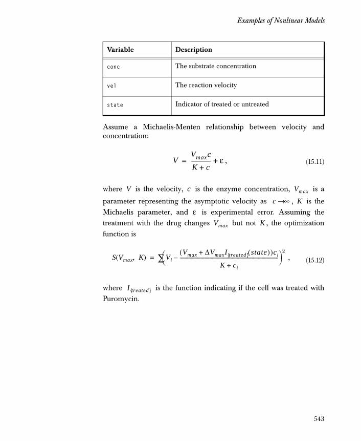
Examples of Nonlinear Models
Assume a Michaelis-Menten relationship between velocity andconcentration:
where is the velocity, is the enzyme concentration, is a
parameter representing the asymptotic velocity as , is theMichaelis parameter, and is experimental error. Assuming thetreatment with the drug changes but not , the optimizationfunction is
where is the function indicating if the cell was treated withPuromycin.
Variable Description
conc The substrate concentration
vel The reaction velocity
state Indicator of treated or untreated
, (15.11)
, (15.12)
VVmaxcK c+-------------- ε+=
V c Vmax
c ∞→ Kε
Vmax K
S Vmax K,( ) ViVmax ΔVmaxI treated{ } state( )+( )ci
K ci+-------------------------------------------------------------------------------–⎝ ⎠
⎛ ⎞ 2
∑=
I treated{ }
543
Chapter 15 Nonlinear Models
INFERENCE FOR NONLINEAR MODELS
Likelihood Models
With likelihood models, distributional results are asymptotic.Maximum likelihood estimates tend toward a normal distributionwith a mean equal to the true parameter and a variance matrix givenby the inverse of the information matrix (i.e., the negative of thesecond derivatives of the log-likelihood).
Least Squares Models
In least-squares models approximations to quantities such as standarderrors or correlations of parameter estimates are used. Theapproximation proceeds as follows:
1. Replace the nonlinear model with its linear Taylor series approximation at the parameter estimates.
2. Use the methods for linear statistical inference on the approximation.
Consequently, the nonlinear inference results are called linearapproximation results.
The Fitting Algorithms
Minimum-sum algorithm
This section deals with the general optimization of an objectivefunction modeled as a sum. The algorithm is a version of Newton’smethod based on a quadratic approximation of the objective function.If both first and second derivatives are supplied, the approximation isa local one using the derivatives. If no derivatives or only the firstderivative are supplied, the algorithm approximates the secondderivative information. It does this in a way specifically designed forminimization.
The algorithm actually used is taken from the PORT subroutinelibrary which evolved from the published algorithm by Gay (1983).Two key features of this algorithm are:
1. A quasi-Newton approximation for second derivatives.
2. A “trust region” approach controlling the size of the region in which the quadratic approximation is believed to be accurate.
The algorithm is capable of working with user models specifying 0, 1,or 2 orders of derivatives.
544
Inference for Nonlinear Models
Nonlinear least-squares algorithm
The Gauss-Newton algorithm is used with a step factor to ensure thatthe sum of squares decreases at each iteration. A line-search methodis used, as opposed to the trust region employed in the minimum-sumalgorithm. The step direction is determined by a quadratic model.The algorithm proceeds as follows:
1. The residuals are calculated, and the gradient is calculated or approximated (depending on the data) at the current parameter values.
2. A linear least-squares fit of the residual on the gradient gives the parameter increment.
3. If applying the full parameter increment increases the sum of squares rather than decreasing it, the length of the increment is successively halved until the sum of squares is decreased.
4. The step factor is retained between iterations and started at min{2*(previous step factor), 1}.
If the gradient is not specified analytically, it is calculated using finitedifferences with forward differencing. For partially linear models, theincrement is calculated using the Golub-Pereyra method (Golub andPereyra, 1973) as implemented by Bates and Lindstrom (1986).
Specifying Models
Nonlinear models typically require specifying more details thanmodels of other types. The information typically required to fit anonlinear model, using the Spotfire S+ functions ms or nls, is:
1. A formula
2. Data
3. Starting values
Formulas For nonlinear models a formula is a Spotfire S+ expression involvingdata, parameters in the model, and any other relevant quantities. Theparameters must be specified in the formula because there is noassumption about where they are to be placed (as in linear models, forexample). Formulas are typically specified differently depending onwhether you have a minimum-sum problem or nonlinear least-squares problem.
545
Chapter 15 Nonlinear Models
In the puromycin example, you would specify a formula for thesimple model (described in Equation (15.11)) by:
vel ~ Vm*conc / (K + conc)
The parameters Vm and K are specified along with the data vel andconc. Since there is no explicit response for minimum-sum models(for example, likelihood models), it is left off in the formula.
In the ping-pong example (ignoring the average rating effect), theformula for Equation (15.4) is:
~ -D*alpha + log(1 + exp(D*alpha))
where D is a variable in the data and alpha is the parameter to fit.Note that the model here is based only on the difference in ratings,ignoring for the moment the average rating.
Simplifying Formulas
Some models can be organized as simple expressions involving oneor more Spotfire S+ functions that do all the work. Note that D*alphaoccurs twice in the formula for the ping-pong model. You can write ageneral function for the log-likelihood in terms of D*alpha.
> lprob <- function(lp) log(1 + exp(lp)) - lp
Recall that lp is the linear predictor for the GLM. A simplerexpression for the model is now:
~ lprob( D * alpha )
Having lprob now makes it easy to add additional terms orparameters.
Implications of the Formulas
For nonlinear least-squares formulas the response on the left of ~ andthe predictor on the right must evaluate to numeric vectors of thesame length. The fitting algorithm tries to estimate parameters tominimize the sum of squared differences between response andprediction. If the response is left out the formula is interpreted as aresidual vector.
For Minimum-Sum formulas, the right of ~ must evaluate to anumeric vector. The fitting algorithm tries to estimate parameters tominimize the sum of this “predictor” vector. The concept here islinked to maximum-likelihood models. The computational form doesnot depend on an MLE concept. The elements of the vector may beanything and there need not be more than one.
546
Inference for Nonlinear Models
The evaluated formulas can include derivatives with respect to theparameters. The derivatives are supplied as attributes to the vectorthat results when the predictor side of the formula is evaluated. Whenexplicit derivatives are not supplied, the algorithms use numericapproximations.
Parametrized Data Frames
Relevant data for nonlinear modeling includes:
• Variables
• Initial estimates of parameters
• Fixed values occurring in a model formula
Parametrized data frames allow you to “attach” relevant data to a dataframe when the data do not occupy an entire column. Information isattached as a "parameter" attribute of the data frame. The parameterfunction returns or modifies the entire list of parameters and isanalogous to the attributes function. Similarly the param functionreturns or modifies one parameter at a time and is analogous to theattr function. You could supply values for Vm and K to the Puromycindata frame with:
# Assign Puromycin to your working directory.> Puromycin <- Puromycin> parameters(Puromycin) <- list(Vm = 200, K = 0.1)
The parameter values can be retrieved with:
> parameters(Puromycin)
$Vm:[1] 200
$K:[1] 0.1
The class of Puromycin is now:
> class(Puromycin)
[1] "pframe"
Now, when Puromycin is attached, the parameters Vm and K areavailable when referred to in formulas.
547
Chapter 15 Nonlinear Models
Starting Values; Identifying Parameters
Before the formulas can be evaluated, the fitting functions must knowwhich names in the formula are parameters to be estimated and musthave starting values for these parameters. The fitting functionsdetermine this in the following way:
1. If the start argument is supplied, its names are the names of the parameters to be estimated, and its values are the corresponding starting values.
2. If start is missing, the parameters attribute of the data argument defines the parameter names and values.
Derivatives Supplying derivatives of the predictor side of the formula with respectto the parameters along with the formula can reduce the number ofiterations (thus speeding up the computations), increase numericalaccuracy, and improve the chance of convergence. In generalderivatives should be used whenever possible.
The fitting algorithms can use both first derivatives (the gradient) andsecond derivatives (the Hessian). The derivatives are supplied to thefitting functions as attributes to the formula. Recall that evaluating theformula gives a vector of values. Evaluating the first derivativeexpression should give values for each of the parameters, that isan matrix. Evaluating the second derivative expression shouldgive n values for each of the partial derivatives, that is, an
array.
First Derivatives The negative log-likelihood for the simple ping-pong model is:
Hint
Explicitly use the start argument to name and initialize parameters.
You can easily see what the starting values are in the call component of the fit and you can arrange to keep particular parameters constant when that makes sense.
nn p
n p×p p×
n p× p×
(15.13)l α( ) 1 eDiα+( )log Diα–[ ]∑=
548
Inference for Nonlinear Models
Differentiating with respect to and simplifying gives the gradient:
The gradient is supplied to the fitting function as the gradientattribute of the formula:
> form.pp <- ~log(1 + exp( D*alpha ) ) - D*alpha> attr(form.pp, "gradient") <-+ ~ -D / ( 1 + exp( D*alpha ) )> form.pp
~ log(1 + exp(D * alpha)) - D * alphaGradient: ~ - D/(1 + exp(D * alpha))
When a function is used to simplify a formula, build the gradient intothe function. The lprob function is used to simplify the formulaexpression to ~lprob(D*alpha):
> lprob <- function(lp) log(1 + exp(lp)) - lp
An improved version of lprob adds the gradient:
> lprob2 <- function(lp, X)+ {+ elp <- exp(lp)+ z <- 1 + elp+ value <- log(z) - lp+ attr(value, "gradient") <- -X/z+ value+ }
Note lp is again the linear predictor and is the data in the linearpredictor. With the gradient built into the function, you don’t need toadd it as an attribute to the formula; it is already an attribute to theobject hence used in the formula.
(15.14)
α
∂l∂α------
Di–
1 eDiα+( )
------------------------∑=
X
549
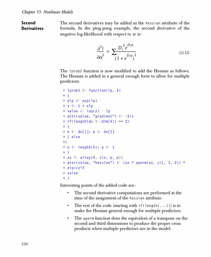
Chapter 15 Nonlinear Models
Second Derivatives
The second derivatives may be added as the hessian attribute of theformula. In the ping-pong example, the second derivative of thenegative log-likelihood with respect to is:
The lprob2 function is now modified to add the Hessian as follows.The Hessian is added in a general enough form to allow for multiplepredictors.
> lprob3 <- function(lp, X)+ {+ elp <- exp(lp)+ z <- 1 + elp+ value <- log(z) - lp+ attr(value, "gradient") <- -X/z+ if(length(dx <- dim(X)) == 2)+ {+ n <- dx[1]; p <- dx[2]+ } else+{+ n <- length(X); p <- 1+ }+ xx <- array(X, c(n, p, p))+ attr(value, "hessian") <- (xx * aperm(xx, c(1, 3, 2)) *+ elp)/z^2+ value+ }
Interesting points of the added code are:
• The second derivative computations are performed at the time of the assignment of the hessian attribute.
• The rest of the code (starting with if(length(...))) is to make the Hessian general enough for multiple predictors.
• The aperm function does the equivalent of a transpose on the second and third dimensions to produce the proper cross products when multiple predictors are in the model.
(15.15)
α
∂2l
∂α2--------
Di2e
Diα
1 eDiα+( )
2--------------------------∑=
550
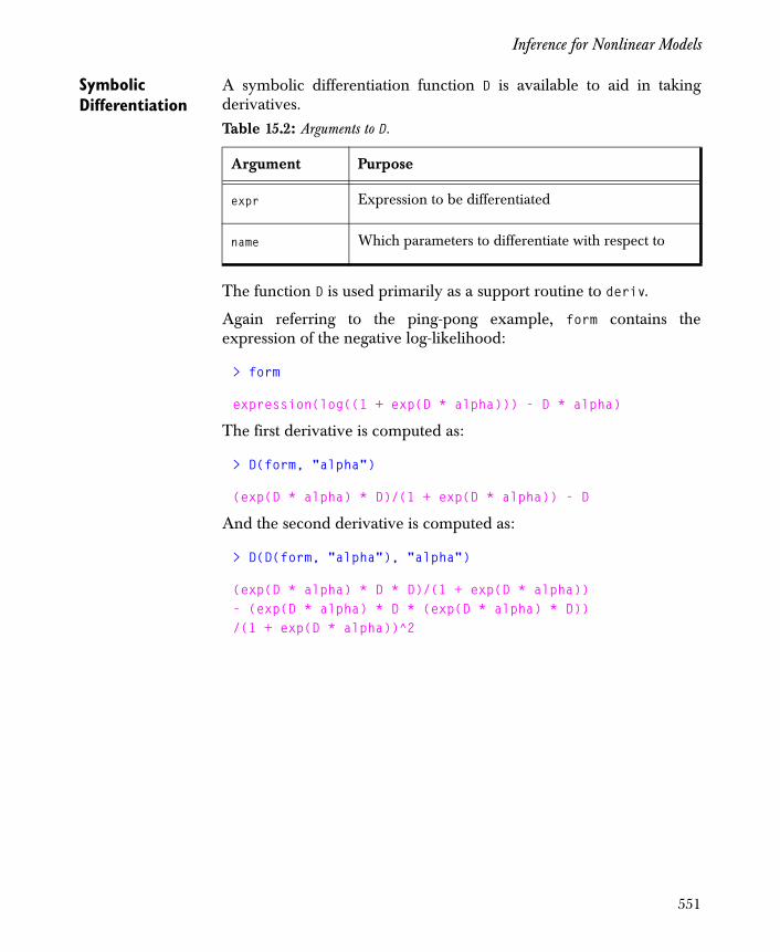
Inference for Nonlinear Models
Symbolic Differentiation
A symbolic differentiation function D is available to aid in takingderivatives.
The function D is used primarily as a support routine to deriv.
Again referring to the ping-pong example, form contains theexpression of the negative log-likelihood:
> form
expression(log((1 + exp(D * alpha))) - D * alpha)
The first derivative is computed as:
> D(form, "alpha")
(exp(D * alpha) * D)/(1 + exp(D * alpha)) - D
And the second derivative is computed as:
> D(D(form, "alpha"), "alpha")
(exp(D * alpha) * D * D)/(1 + exp(D * alpha))- (exp(D * alpha) * D * (exp(D * alpha) * D))/(1 + exp(D * alpha))^2
Table 15.2: Arguments to D.
Argument Purpose
expr Expression to be differentiated
name Which parameters to differentiate with respect to
551

Chapter 15 Nonlinear Models
Improved Derivatives
The deriv function takes an expression, computes a derivative,simplifies the result, then returns an expression or function forcomputing the original expression along with its derivative(s).
Periods are used in front of created object names to avoid conflictwith user-chosen names. The deriv function returns an expression inthe form expected for nonlinear models.
> deriv(form, "alpha")
expression({
.expr1 <- D * alpha
.expr2 <- exp(.expr1)
.expr3 <- 1 + .expr2
.value <- (log(.expr3)) - .expr1
.grad <- array(0, c(length(.value), 1), list(NULL, "alpha"))
.grad[, "alpha"] <- ((.expr2 * D)/.expr3) - Dattr(.value, "gradient") <- .grad.value
})
Table 15.3: Arguments to deriv.
Argument Purpose
expr Expression to be differentiated, typically a formula, in which case the expression returned computes the right side of the ~ and its derivatives.
namevec Character vector of names of parameters.
function.arg Optional argument vector or prototype for a function.
tag Base of the names to be given to intermediate results. Default is ".expr".
552

Inference for Nonlinear Models
If the function.arg argument is supplied, a function is returned:
> deriv(form, "alpha", c("D", "alpha"))
function(D, alpha){
.expr1 <- D * alpha
.expr2 <- exp(.expr1)
.expr3 <- 1 + .expr2
.value <- (log(.expr3)) - .expr1
.actualArgs <- match.call()["alpha"]if(all(unlist(lapply(as.list(.actualArgs), is,name)))) {
.grad <- array(0, c(length(.value), 1), list(NULL, "alpha"))
.grad[, "alpha"] <- ((.expr2 * D)/.expr3) - Ddimnames(.grad) <- list(NULL, .actualArgs)attr(.value, "gradient") <- .grad
}.value
}
The namevec argument can be a vector:
> deriv(vel ~ Vm * (conc/(K + conc)), c("Vm", "K"))
expression({ .expr1 <- K + conc
.expr2 <- conc/.expr1
.value <- Vm * .expr2
.grad <- array(0, c(length(.value), 2), list(NULL, c("Vm","K")))
.grad[, "Vm"] <- .expr2
.grad[, "K"] <- - (Vm * (conc/(.expr1^2)))attr(.value, "gradient") <- .grad.value
})
The symbolic differentiation interprets each parameter as a scalar.Generalization from scalar to vector parameters (for example, lprob2)must be done by hand. Use parentheses to help deriv find relevantsubexpressions. Without the redundant parentheses around conc/(K + conc) the expression returned by deriv is not as simple aspossible.
553
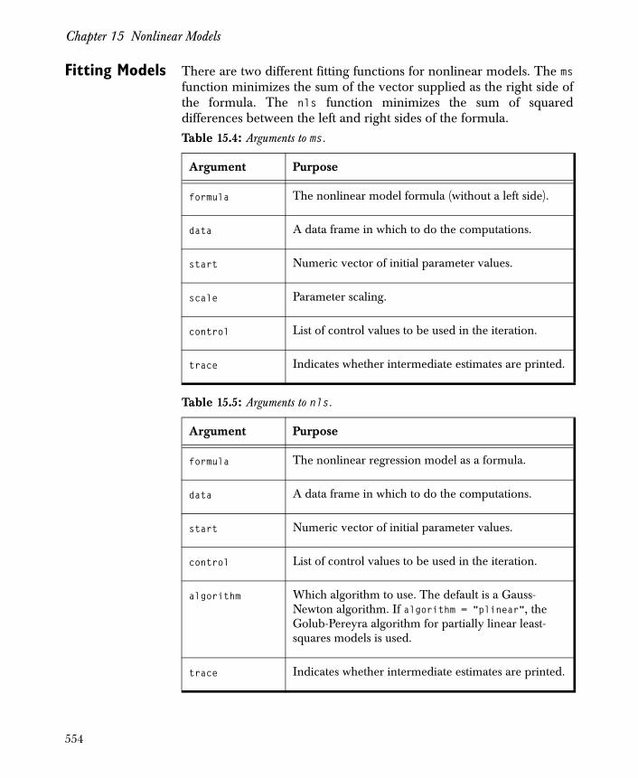
Chapter 15 Nonlinear Models
Fitting Models There are two different fitting functions for nonlinear models. The msfunction minimizes the sum of the vector supplied as the right side ofthe formula. The nls function minimizes the sum of squareddifferences between the left and right sides of the formula. Table 15.4: Arguments to ms.
Argument Purpose
formula The nonlinear model formula (without a left side).
data A data frame in which to do the computations.
start Numeric vector of initial parameter values.
scale Parameter scaling.
control List of control values to be used in the iteration.
trace Indicates whether intermediate estimates are printed.
Table 15.5: Arguments to nls.
Argument Purpose
formula The nonlinear regression model as a formula.
data A data frame in which to do the computations.
start Numeric vector of initial parameter values.
control List of control values to be used in the iteration.
algorithm Which algorithm to use. The default is a Gauss-Newton algorithm. If algorithm = "plinear", the Golub-Pereyra algorithm for partially linear least-squares models is used.
trace Indicates whether intermediate estimates are printed.
554

Inference for Nonlinear Models
Fitting a Model to the Puromycin Data
Before fitting a model, take a look at the data displayed in Figure 15.1.
> attach(Puromycin)> plot(conc,vel, type = "n")> text(conc, vel, ifelse(state == "treated", "T", "U"))
1. Estimating starting values
Obtain an estimate of for each group as the maximum valueeach group attains.
• The treated group has a maximum of about 200.
• The untreated group has a maximum of about 160.
The value of is the concentration at which reaches ,roughly 0.1 for each group.
Figure 15.1: vel versus conc for treated (T) and untreated (U) groups.
conc
vel
0.0 0.2 0.4 0.6 0.8 1.0
5010
015
020
0
T
T
T
T
T
T
TT
T
TTT
U
U
UU
U
U
UU
U
U U
Vmax
K V Vmax 2⁄
555
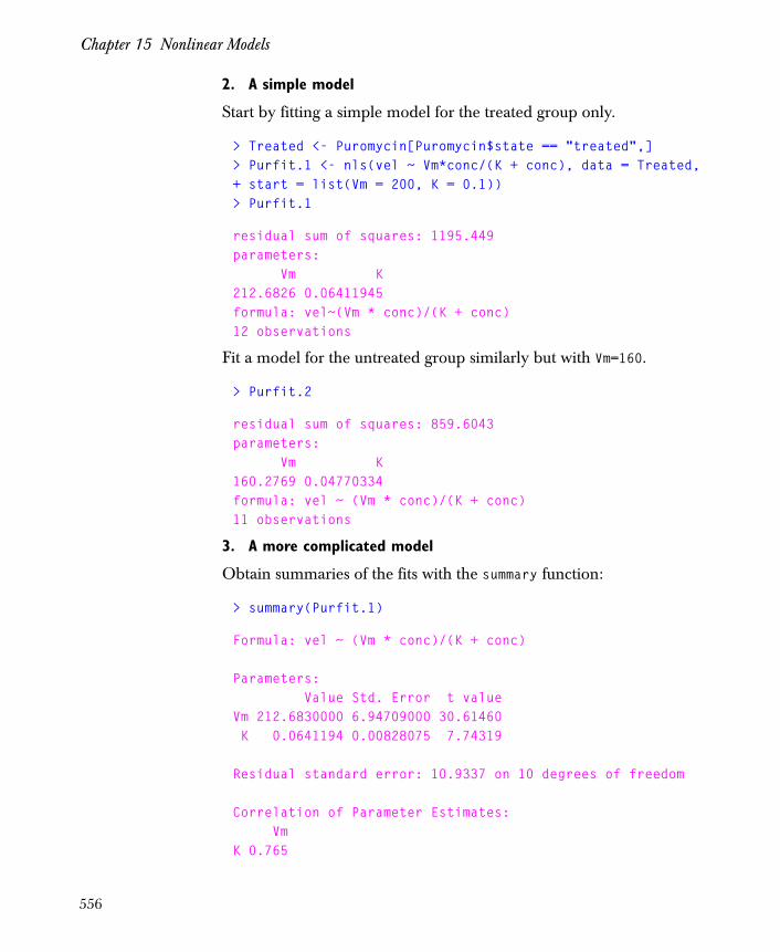
Chapter 15 Nonlinear Models
2. A simple model
Start by fitting a simple model for the treated group only.
> Treated <- Puromycin[Puromycin$state == "treated",]> Purfit.1 <- nls(vel ~ Vm*conc/(K + conc), data = Treated,+ start = list(Vm = 200, K = 0.1))> Purfit.1
residual sum of squares: 1195.449parameters: Vm K212.6826 0.06411945formula: vel~(Vm * conc)/(K + conc)12 observations
Fit a model for the untreated group similarly but with Vm=160.
> Purfit.2
residual sum of squares: 859.6043parameters: Vm K160.2769 0.04770334formula: vel ~ (Vm * conc)/(K + conc)11 observations
3. A more complicated model
Obtain summaries of the fits with the summary function:
> summary(Purfit.1)
Formula: vel ~ (Vm * conc)/(K + conc)
Parameters: Value Std. Error t value Vm 212.6830000 6.94709000 30.61460 K 0.0641194 0.00828075 7.74319
Residual standard error: 10.9337 on 10 degrees of freedom
Correlation of Parameter Estimates: Vm K 0.765
556
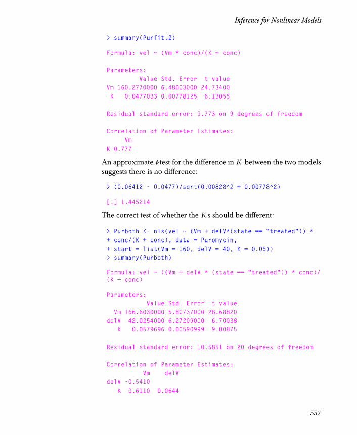
Inference for Nonlinear Models
> summary(Purfit.2)
Formula: vel ~ (Vm * conc)/(K + conc)
Parameters: Value Std. Error t value Vm 160.2770000 6.48003000 24.73400 K 0.0477033 0.00778125 6.13055
Residual standard error: 9.773 on 9 degrees of freedom
Correlation of Parameter Estimates: Vm K 0.777
An approximate t-test for the difference in between the two modelssuggests there is no difference:
> (0.06412 - 0.0477)/sqrt(0.00828^2 + 0.00778^2)
[1] 1.445214
The correct test of whether the s should be different:
> Purboth <- nls(vel ~ (Vm + delV*(state == "treated")) * + conc/(K + conc), data = Puromycin,+ start = list(Vm = 160, delV = 40, K = 0.05))> summary(Purboth)
Formula: vel ~ ((Vm + delV * (state == "treated")) * conc)/(K + conc)
Parameters: Value Std. Error t value Vm 166.6030000 5.80737000 28.68820delV 42.0254000 6.27209000 6.70038 K 0.0579696 0.00590999 9.80875
Residual standard error: 10.5851 on 20 degrees of freedom
Correlation of Parameter Estimates: Vm delV delV -0.5410 K 0.6110 0.0644
K
K
557
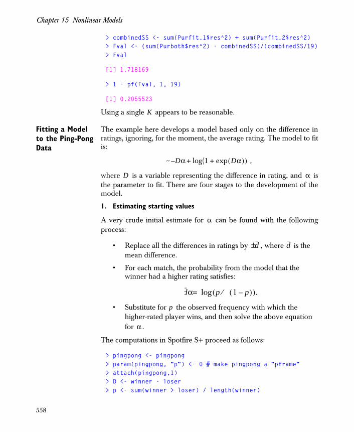
Chapter 15 Nonlinear Models
> combinedSS <- sum(Purfit.1$res^2) + sum(Purfit.2$res^2)> Fval <- (sum(Purboth$res^2) - combinedSS)/(combinedSS/19)> Fval
[1] 1.718169
> 1 - pf(Fval, 1, 19)
[1] 0.2055523
Using a single appears to be reasonable.
Fitting a Model to the Ping-Pong Data
The example here develops a model based only on the difference inratings, ignoring, for the moment, the average rating. The model to fitis:
~ ,
where is a variable representing the difference in rating, and isthe parameter to fit. There are four stages to the development of themodel.
1. Estimating starting values
A very crude initial estimate for can be found with the followingprocess:
• Replace all the differences in ratings by , where is the mean difference.
• For each match, the probability from the model that the winner had a higher rating satisfies:
.
• Substitute for the observed frequency with which the higher-rated player wins, and then solve the above equation for .
The computations in Spotfire S+ proceed as follows:
> pingpong <- pingpong> param(pingpong, "p") <- 0 # make pingpong a "pframe"> attach(pingpong,1)> D <- winner - loser> p <- sum(winner > loser) / length(winner)
K
D– α log(1 exp Dα)( )+ +
D α
α
d± d
dα p 1 p–( )⁄( )log=
p
α
558

Inference for Nonlinear Models
> p
[1] 0.8223401
> alpha <- log(p/(1-p))/mean(D)> alpha
[1] 0.007660995
> detach(1, save = "pingpong")
2. A simple model
Recall the lprob function which calculates the log-likelihood for theping-pong problem:
> lprob
function(lp) log(1 + exp(lp)) - lp
The model is fitted as follows:
> attach(pingpong)> fit.alpha <- ms( ~ lprob( D * alpha ),+ start = list(alpha = 0.0077))> fit.alpha
value: 1127.635
parameters: alpha0.01114251
formula: ~ lprob(D * alpha)3017 observationscall: ms(formula= ~lprob(D * alpha),start = list(alpha = 0.0077))
3. Adding the gradient
To fit the model with the gradient added to the formula, use lprob2.
> fit.alpha.2 <- ms( ~ lprob2( D*alpha, D),+ start = list(alpha = 0.0077))> fit.alpha.2
559
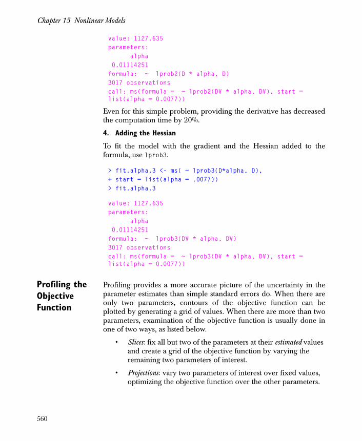
Chapter 15 Nonlinear Models
value: 1127.635 parameters: alpha 0.01114251formula: ~ lprob2(D * alpha, D) 3017 observationscall: ms(formula = ~ lprob2(DV * alpha, DV), start = list(alpha = 0.0077))
Even for this simple problem, providing the derivative has decreasedthe computation time by 20%.
4. Adding the Hessian
To fit the model with the gradient and the Hessian added to theformula, use lprob3.
> fit.alpha.3 <- ms( ~ lprob3(D*alpha, D),+ start = list(alpha = .0077))> fit.alpha.3
value: 1127.635 parameters: alpha 0.01114251formula: ~ lprob3(DV * alpha, DV) 3017 observationscall: ms(formula = ~ lprob3(DV * alpha, DV), start = list(alpha = 0.0077))
Profiling the Objective Function
Profiling provides a more accurate picture of the uncertainty in theparameter estimates than simple standard errors do. When there areonly two parameters, contours of the objective function can beplotted by generating a grid of values. When there are more than twoparameters, examination of the objective function is usually done inone of two ways, as listed below.
• Slices: fix all but two of the parameters at their estimated values and create a grid of the objective function by varying the remaining two parameters of interest.
• Projections: vary two parameters of interest over fixed values, optimizing the objective function over the other parameters.
560
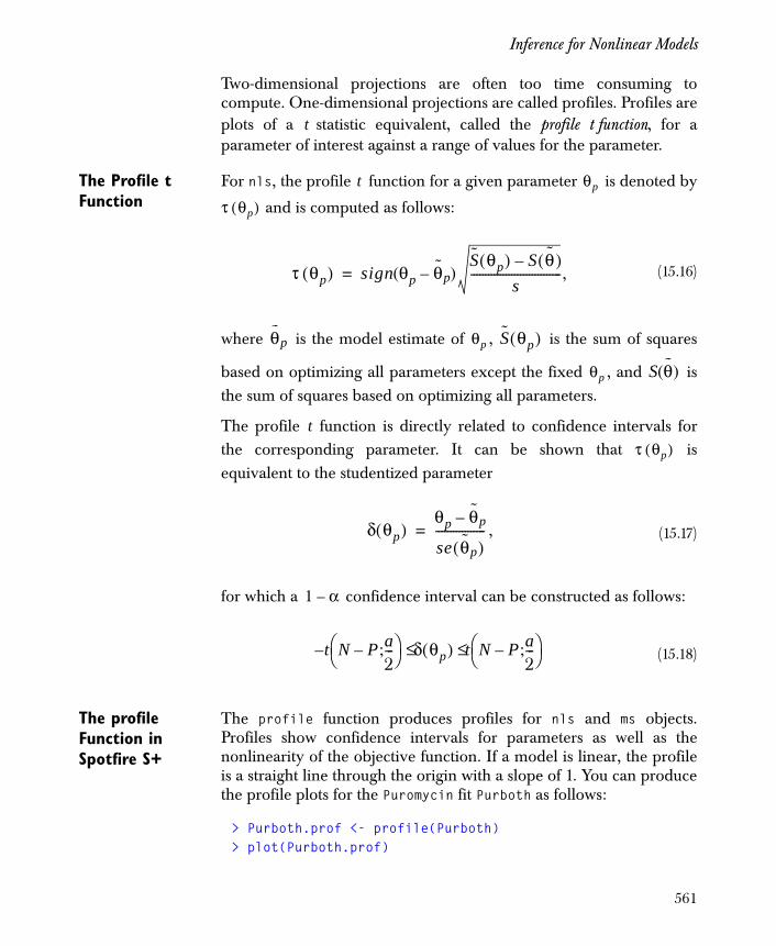
Inference for Nonlinear Models
Two-dimensional projections are often too time consuming tocompute. One-dimensional projections are called profiles. Profiles areplots of a statistic equivalent, called the profile t function, for aparameter of interest against a range of values for the parameter.
The Profile t Function
For nls, the profile function for a given parameter is denoted by
and is computed as follows:
where is the model estimate of , is the sum of squares
based on optimizing all parameters except the fixed , and isthe sum of squares based on optimizing all parameters.
The profile function is directly related to confidence intervals forthe corresponding parameter. It can be shown that isequivalent to the studentized parameter
for which a confidence interval can be constructed as follows:
The profile Function in Spotfire S+
The profile function produces profiles for nls and ms objects.Profiles show confidence intervals for parameters as well as thenonlinearity of the objective function. If a model is linear, the profileis a straight line through the origin with a slope of 1. You can producethe profile plots for the Puromycin fit Purboth as follows:
> Purboth.prof <- profile(Purboth)> plot(Purboth.prof)
t
, (15.16)
, (15.17)
(15.18)
t θp
τ θp( )
τ θp( ) sign θp θp–( )S θp( ) S θ( )–
s-------------------------------=
θp θp S θp( )
θp S θ( )
tτ θp( )
δ θp( )θp θp–
se θp( )-----------------=
1 α–
t N P a2---;–⎝ ⎠
⎛ ⎞– δ θp( ) t N P a2---;–⎝ ⎠
⎛ ⎞≤ ≤
561

Chapter 15 Nonlinear Models
The object returned by profile has a component for each parameterthat contains the evaluations of the profile function, plus someadditional attributes. The component for the Vm parameter is:
> Purboth.prof$Vm
tau par.vals.Vm par.vals.delV par.vals.K 1 -3.9021051 144.6497 54.60190 0.04501306 2 -3.1186052 148.8994 52.07216 0.04725929 3 -2.3346358 153.2273 49.54358 0.04967189 4 -1.5501820 157.6376 47.01846 0.05226722 5 -0.7654516 162.1334 44.50315 0.05506789 6 0.0000000 166.6040 42.02591 0.05797157 7 0.7548910 171.0998 39.57446 0.06103225 8 1.5094670 175.6845 37.12565 0.06431820 9 2.2635410 180.3616 34.67194 0.0678369310 3.0171065 185.1362 32.20981 0.0716030511 3.7701349 190.0136 29.73812 0.0756363012 4.5225948 194.9997 27.25599 0.07995897
Figure 15.2 shows profile plots for the three-parameter Puromycin fit.Each plot shows the profile function ( ), when the parameter on thex-axis ranges over the values shown and the other parameters areoptimized. The surface is quite linear with respect to these threeparameters.
t
t τ
562
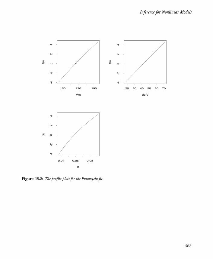
Inference for Nonlinear Models
Figure 15.2: The profile plots for the Puromycin fit.
Vm
tau
150 170 190
-4-2
02
4
delV
tau
20 30 40 50 60 70
-4-2
02
4
K
tau
0.04 0.06 0.08
-4-2
02
4
563
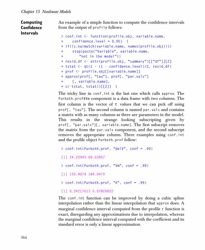
Chapter 15 Nonlinear Models
Computing Confidence Intervals
An example of a simple function to compute the confidence intervalsfrom the output of profile follows:
> conf.int <- function(profile.obj, variable.name,+ confidence.level = 0.95) {+ if(is.na(match(variable.name, names(profile.obj))))+ stop(paste("Variable", variable.name,+ "not in the model"))+ resid.df <- attr(profile.obj, "summary")[["df"]][2]+ tstat <- qt(1 - (1 - confidence.level)/2, resid.df)+ prof <- profile.obj[[variable.name]]+ approx(prof[, "tau"], prof[, "par.vals"]+ [, variable.name],+ c(-tstat, tstat))[[2]] }
The tricky line in conf.int is the last one which calls approx. ThePurboth.prof$Vm component is a data frame with two columns. Thefirst column is the vector of values that we can pick off usingprof[, "tau"]. The second column is named par.vals and containsa matrix with as many columns as there are parameters in the model.This results in the strange looking subscripting given byprof[, "par.vals"][, variable.name]. The first subscript removesthe matrix from the par.vals component, and the second subscriptremoves the appropriate column. Three examples using conf.intand the profile object Purboth.prof follow:
> conf.int(Purboth.prof, "delV", conf = .99)
[1] 24.20945 60.03857
> conf.int(Purboth.prof, "Vm", conf = .99)
[1] 150.4079 184.0479
> conf.int(Purboth.prof, "K", conf = .99)
[1] 0.04217613 0.07826822
The conf.int function can be improved by doing a cubic splineinterpolation rather than the linear interpolation that approx does. Amarginal confidence interval computed from the profile function isexact, disregarding any approximations due to interpolation, whereasthe marginal confidence interval computed with the coefficient and itsstandard error is only a linear approximation.
τ
t
564

References
REFERENCES
Bates D.M. & Lindstrom M.J. (1986). Nonlinear least squares withconditionally linear parametrics. Proceedings of the American StatisticalComputing Section, 152-157.
Comizzoli R.B., Landwehr J.M., & Sinclair J.D. (1990). Robustmaterials and processes: Key to reliability. AT&T Technical Journal,69(6):113--128.
Gay D.M. (1983). Algorithm 611: Subroutines for unconstrainedminimization using a model/trust-region approach. ACM Transactionson Mathematical Software 9:503-524.
Golub G.H. & Pereyra V. (1973). The differentiation of pseudo-inverses and nonlinear least squares problems whose variablesseparate. SIAM Journal on Numerical Analysis 10:413-432.
565

Chapter 15 Nonlinear Models
566
Introduction 568Setting Up the Data Frame 568The Model and Analysis of Variance 569
Experiments with One Factor 570Setting Up the Data Frame 571A First Look at the Data 572The One-Way Layout Model and Analysis of Variance 574
The Unreplicated Two-Way Layout 578Setting Up the Data Frame 579A First Look at the Data 580The Two-Way Model and ANOVA (One Observation
Per Cell) 583
The Two-Way Layout with Replicates 591Setting Up the Data Frame 592A First Look at the Data 593The Two-Way Model and ANOVA (with Replicates) 594Method for Two-Factor Experiments with Replicates 597Method for Unreplicated Two-Factor Experiments 599Alternative Formal Methods 601
Many Factors at Two Levels: 2k Designs 602Setting Up the Data Frame 602A First Look at the Data 604
Estimating All Effects in the 2k Model 605Using Half-Normal Plots to Choose a Model 610
References 615
DESIGNED EXPERIMENTS AND ANALYSIS OF VARIANCE 16
567
Chapter 16 Designed Experiments and Analysis of Variance
INTRODUCTION
This chapter discusses how to analyze designed experiments.Typically, the data have a numeric response and one or morecategorical variables (factors) that are under the control of theexperimenter. For example, an engineer may measure the yield ofsome process using each combination of four catalysts and threespecific temperatures. This experiment has two factors, catalyst andtemperature, and the response is the yield.
Traditionally, the analysis of experiments has centered on theperformance of an Analysis of Variance (ANOVA). In more recentyears graphics have played an increasingly important role. There is alarge literature on the design and analysis of experiments; Box,Hunter, and Hunter is an example.
This chapter consists of sections which show you how to use TIBCOSpotfire S+ to analyze experimental data for each of the followingsituations:
• Experiments with one factor
• Experiments with two factors and a single replicate
• Experiments with two factors and two or more replicates
• Experiments with many factors at two levels: designs
Each of these sections stands alone. You can read whichever sectionis appropriate to your problem, and get the analysis done withouthaving to read the other sections. This chapter uses examples fromBox, Hunter, and Hunter (1978) and thus is a useful supplement in acourse which covers the material of Chapters 6, 7, 9, 10, and 11 ofBox, Hunter, and Hunter.
Setting Up the Data Frame
In analyzing experimental data using Spotfire S+, the first thing youdo is set up an appropriate data frame for your experimental data. Youmay think of the data frame as a matrix, with the columns containingvalues of the variables. Each row of the data frame contains anobserved value of the response (or responses), and the correspondingvalues of the experimental factors.
2k
568

Introduction
A First Look at the Data
Use the functions plot.design, plot.factor, and possiblyinteraction.plot to graphically explore your data.
The Model and Analysis of Variance
It is important that you have a clear understanding of exactly whatmodel is being considered when you carry out the analysis ofvariance. Use aov to carry out the analysis of variance, and usesummary to display the results.
In using aov, you use formulas to specify your model. The examples inthis chapter introduce you to simple uses of formulas. You maysupplement your understanding of how to use formulas in Spotfire S+by reading Chapter 2, Specifying Models in Spotfire S+ (in this book),or Chapter 2, Statistical Models, and Chapter 5, Analysis of Variance;Designed Experiments (in Chambers and Hastie (1992)).
Diagnostic Plots For each analysis, you should make the following minimal set of plotsto convince yourself that the model being entertained is adequate:
• Histogram of residuals (using hist)
• Normal qq-plot of residuals (using qqnorm)
• Plot of residuals versus fit (using plot)
When you know the time order of the observations, you should alsomake plots of the original data and the residuals in the order in whichthe data were collected.
The diagnostic plots may indicate inadequacies in the model fromone or more of the following sources: existence of interactions,existence of outliers, and existence of nonhomogeneous errorvariance.
569

Chapter 16 Designed Experiments and Analysis of Variance
EXPERIMENTS WITH ONE FACTOR
The simplest kind of experiments are those in which a singlecontinuous response variable is measured a number of times for eachof several levels of some experimental factor.
For example, consider the data in Table 16.1 (from Box, Hunter, andHunter (1978)), which consists of numerical values of bloodcoagulation times for each of four diets. Coagulation time is thecontinuous response variable, and diet is a qualitative variable, orfactor, having four levels: A, B, C, and D. The diets corresponding tothe levels A, B, C, and D were determined by the experimenter.
Your main interest is to see whether or not the factor “diet” has anyeffect on the mean value of blood coagulation time. The experimentalfactor, “diet” in this case, is often called the treatment.
Table 16.1: Blood coagulation times for four diets.
Diet
A B C D
62 63 68 56
60 67 66 62
63 71 71 60
59 64 67 61
65 68 63
66 68 64
63
59
570

Experiments with One Factor
Formal statistical testing for whether or not the factor level affects themean is carried out using the method of analysis of variance(ANOVA). This needs to be complemented by exploratory graphicsto provide confirmation that the model assumptions are sufficientlycorrect to validate the formal ANOVA conclusion. Spotfire S+provides tools for you to do both the data exploration and formalANOVA.
Setting Up the Data Frame
In order to analyze the data, you need to get it into a form thatSpotfire S+ can use for the analysis of variance. You do this by settingup a data frame. First create a numeric vector coag:
> coag <- scan()
1: 62 60 63 595: 63 67 71 64 65 6611: 68 66 71 67 68 6817: 56 62 60 61 63 64 63 5925:
Next, create a factor called diet, that corresponds to coag:
> diet <- factor(rep(LETTERS[1:4], c(4,6,6,8)))> diet
[1] A A A A B B B B B B C C C C C C D D D D D D D D
Now create a data frame with columns diet and coag:
> coag.df <- data.frame(diet,coag)
The data frame object coag.df is a matrix-like object, so it looks like amatrix when you display it on your screen:
> coag.df
diet coag 1 A 62 2 A 60 3 A 63 . . .23 D 6324 D 59
571
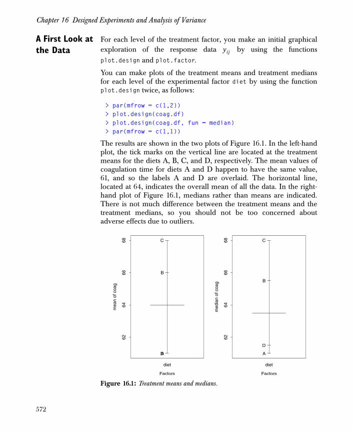
Chapter 16 Designed Experiments and Analysis of Variance
A First Look at the Data
For each level of the treatment factor, you make an initial graphicalexploration of the response data by using the functionsplot.design and plot.factor.
You can make plots of the treatment means and treatment mediansfor each level of the experimental factor diet by using the functionplot.design twice, as follows:
> par(mfrow = c(1,2))> plot.design(coag.df)> plot.design(coag.df, fun = median)> par(mfrow = c(1,1))
The results are shown in the two plots of Figure 16.1. In the left-handplot, the tick marks on the vertical line are located at the treatmentmeans for the diets A, B, C, and D, respectively. The mean values ofcoagulation time for diets A and D happen to have the same value,61, and so the labels A and D are overlaid. The horizontal line,located at 64, indicates the overall mean of all the data. In the right-hand plot of Figure 16.1, medians rather than means are indicated.There is not much difference between the treatment means and thetreatment medians, so you should not be too concerned aboutadverse effects due to outliers.
Figure 16.1: Treatment means and medians.
yij
Factors
mea
n of
coa
g
6264
6668
A
B
C
D
diet
Factors
med
ian
of c
oag
6264
6668
A
B
C
D
diet
572

Experiments with One Factor
The function plot.factor produces a box plotbox plot of theresponse data for each level of the experimental factor:
> plot.factor(coag.df)
The resulting plot is shown in Figure 16.2. This plot indicates that theresponses for diets A and D are quite similar, while the medianresponses for diets B and C are considerably larger relative to thevariability reflected by the heights of the boxes. Thus, you suspectthat diet has an effect on blood coagulation time.
If the exploratory graphical display of the response usingplot.factor indicates that the interquartile distance of the box plotsdepends upon the median, then a transformation to make the errorvariance constant is called for. The transformation may be selectedwith a “spread versus level” plot. See, for example, the section TheTwo-Way Layout with Replicates, or Hoaglin, Mosteller, and Tukey(1983).
Figure 16.2: Box plots for each treatment.
60
65
70
co
ag
A B C D
diet
573

Chapter 16 Designed Experiments and Analysis of Variance
The One-Way Layout Model and Analysis of Variance
The classical model for experiments with a single factor is
where is the mean value of the response for the th level of the
experimental factor. There are levels of the experimental factor,and measurements are taken on the response
variable for level of the experimental factor.
Using the treatment terminology, there are treatments, and is
called the th treatment mean. The above model is often called theone-way layout model. For the blood coagulation experiment, there are
diets, and the means μ1, μ2, μ3, and μ4 correspond to diets A,
B, C, and D, respectively. The numbers of observations are ,
, and .
You carry out the analysis of variance with the function aov:
> aov.coag <- aov(coag ~ diet, coag.df)
The first argument to aov above is the formula coag ~ diet. Thisformula is a symbolic representation of the one-way layout modelequation; the formula excludes the error term . The secondargument to aov is the data frame you created, coag.df, whichprovides the data needed to carry out the ANOVA. The names dietand coag, used in the formula coag ~ diet, need to match the namesof the variables in the data frame coag.df.
To display the ANOVA table, use summary. The p-value returned bysummary for aov.coag is 0.000047, which is highly significant.
> summary(aov.coag)
Df Sum of Sq Mean Sq F Value Pr(F) diet 3 228 76.0 13.5714 4.65847e-05Residuals 20 112 5.6
yij μi ε ij+=j 1 ... Ji, ,=
i 1 ... I, ,=
μi iI
Ji yi1 yi2 … y, iJ, ,
i
I μi
i
I 4=
JA 4=
JB JC 6= = JD 8=
ε ij
574
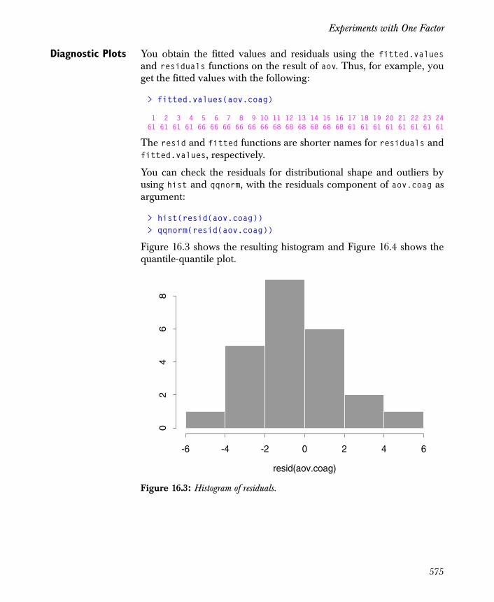
Experiments with One Factor
Diagnostic Plots You obtain the fitted values and residuals using the fitted.valuesand residuals functions on the result of aov. Thus, for example, youget the fitted values with the following:
> fitted.values(aov.coag)
1 2 3 4 5 6 7 8 9 10 11 12 13 14 15 16 17 18 19 20 21 22 23 2461 61 61 61 66 66 66 66 66 66 68 68 68 68 68 68 61 61 61 61 61 61 61 61
The resid and fitted functions are shorter names for residuals andfitted.values, respectively.
You can check the residuals for distributional shape and outliers byusing hist and qqnorm, with the residuals component of aov.coag asargument:
> hist(resid(aov.coag))> qqnorm(resid(aov.coag))
Figure 16.3 shows the resulting histogram and Figure 16.4 shows thequantile-quantile plot.
Figure 16.3: Histogram of residuals.
-6 -4 -2 0 2 4 6
02
46
8
resid(aov.coag)
575

Chapter 16 Designed Experiments and Analysis of Variance
The shape of the histogram, and the linearity of the normal qq-plot,both indicate that the error distribution is quite Gaussian. The flatsections in the qq-plot are a consequence of tied values in the data.
You can check for nonhomogeneity of error variance and possibleoutliers by plotting the residuals versus the fit:
> plot(fitted(aov.coag), resid(aov.coag))
This plot reveals no unusual features and is not shown.
Details An alternate form of the one-way layout model is the overall mean pluseffects form:
where is the overall mean and is the effect for level (or
treatment) . The ith treatment mean in the one-way layout
formulation is related to and by
.
Figure 16.4: Normal qq-plot of residuals.
•
•
•
•
•
•
•
•
•
• •
•
•
•
• •
•
•
•
•
•
•
•
•
Quantiles of Standard Normal
resi
d(a
ov.
coag)
-2 -1 0 1 2
-4-2
02
4
yij μ αi ε ij+ +=
μ αi
i μi
μ αi
μi μ αi+=
576

Experiments with One Factor
The effects satisfy the constraint
,
where is the number of replications for the ith treatment. Thefunction aov fits the one-way model in the overall mean plus effectsform:
.
See the section Model Coefficients and Contrasts for more on this.
To obtain the effects, use model.tables as follows:
> model.tables(aov.coag)
Tables of effects
diet A B C D -3 2 4 -3 rep 4 6 6 8Warning messages:Model was refit to allow projection in: model.tables(aov.coag)
You can get the treatment means as follows:
> model.tables(aov.coag, type = "means")
Tables of means
Grand mean
64
diet A B C D 61 66 68 61rep 4 6 6 8Warning messages:Model was refit to allow projection in: model.tables(aov.coag, type = "means")
αi
n1α1 n2α2 … nIαI+ + + 0=
ni
yij μ αi rij+ +=
577
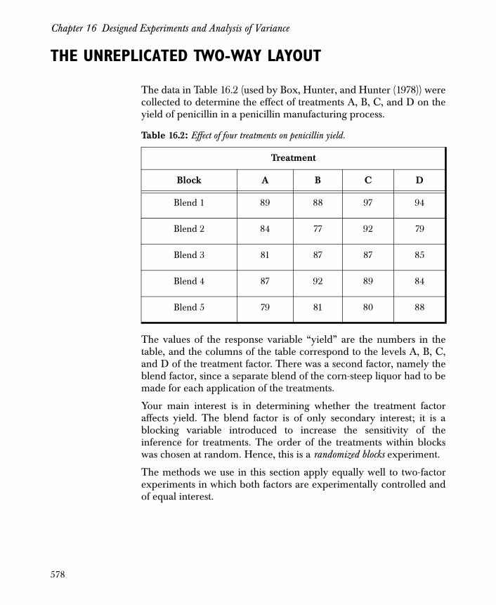
Chapter 16 Designed Experiments and Analysis of Variance
THE UNREPLICATED TWO-WAY LAYOUT
The data in Table 16.2 (used by Box, Hunter, and Hunter (1978)) werecollected to determine the effect of treatments A, B, C, and D on theyield of penicillin in a penicillin manufacturing process.
The values of the response variable “yield” are the numbers in thetable, and the columns of the table correspond to the levels A, B, C,and D of the treatment factor. There was a second factor, namely theblend factor, since a separate blend of the corn-steep liquor had to bemade for each application of the treatments.
Your main interest is in determining whether the treatment factoraffects yield. The blend factor is of only secondary interest; it is ablocking variable introduced to increase the sensitivity of theinference for treatments. The order of the treatments within blockswas chosen at random. Hence, this is a randomized blocks experiment.
The methods we use in this section apply equally well to two-factorexperiments in which both factors are experimentally controlled andof equal interest.
Table 16.2: Effect of four treatments on penicillin yield.
Treatment
Block A B C D
Blend 1 89 88 97 94
Blend 2 84 77 92 79
Blend 3 81 87 87 85
Blend 4 87 92 89 84
Blend 5 79 81 80 88
578
The Unreplicated Two-Way Layout
Setting Up the Data Frame
Table 16.2 is balanced :each entry or cell of the table (that is, each rowand column combination) has the same number of observations (oneobservation per cell, in the present example). With balanced data,you can use fac.design to create the data frame.
First, create a list fnames with two components named blend andtreatment, where blend contains the level names of the blend factorand treatment contains the level names of the treatment factor:
> fnames <- list(blend = paste("Blend ", 1:5),+ treatment = LETTERS[1:4])
Then use fac.design to create the design data frame pen.design
> pen.design <- fac.design(c(5,4), fnames)
The first argument, c(5,4), to fac.design specifies the design ashaving two factors because its length is two. The 5 specifies five levelsfor the first factor, blend, and the 4 specifies four levels for the secondfactor, treatment. The second argument, fnames, specifies the factornames and the labels for their levels.
The design data frame pen.design that you just created contains thefactors blend and treatment as its first and second columns,respectively.
Now create yield to match pen.design:
> yield <- scan()
1: 89 84 81 87 796: 88 77 87 92 8111: 97 92 87 89 8016: 94 79 85 84 8821:
You can now use data.frame to combine the design data framepen.design and the response yield into the data frame pen.df:
> pen.df <- data.frame(pen.design, yield)
Now look at pen.df:
> pen.df
579
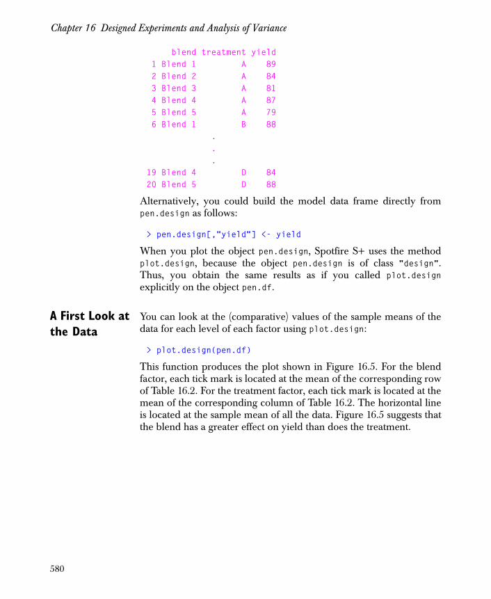
Chapter 16 Designed Experiments and Analysis of Variance
blend treatment yield 1 Blend 1 A 89 2 Blend 2 A 84 3 Blend 3 A 81 4 Blend 4 A 87 5 Blend 5 A 79 6 Blend 1 B 88 . . .19 Blend 4 D 8420 Blend 5 D 88
Alternatively, you could build the model data frame directly frompen.design as follows:
> pen.design[,"yield"] <- yield
When you plot the object pen.design, Spotfire S+ uses the methodplot.design, because the object pen.design is of class "design".Thus, you obtain the same results as if you called plot.designexplicitly on the object pen.df.
A First Look at the Data
You can look at the (comparative) values of the sample means of thedata for each level of each factor using plot.design:
> plot.design(pen.df)
This function produces the plot shown in Figure 16.5. For the blendfactor, each tick mark is located at the mean of the corresponding rowof Table 16.2. For the treatment factor, each tick mark is located at themean of the corresponding column of Table 16.2. The horizontal lineis located at the sample mean of all the data. Figure 16.5 suggests thatthe blend has a greater effect on yield than does the treatment.
580
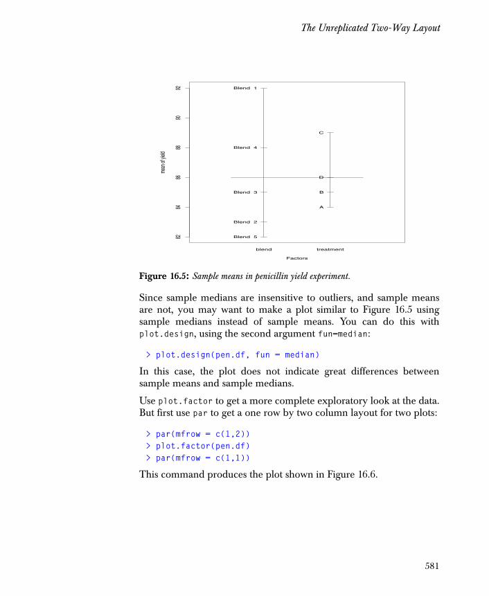
The Unreplicated Two-Way Layout
Since sample medians are insensitive to outliers, and sample meansare not, you may want to make a plot similar to Figure 16.5 usingsample medians instead of sample means. You can do this withplot.design, using the second argument fun=median:
> plot.design(pen.df, fun = median)
In this case, the plot does not indicate great differences betweensample means and sample medians.
Use plot.factor to get a more complete exploratory look at the data.But first use par to get a one row by two column layout for two plots:
> par(mfrow = c(1,2))> plot.factor(pen.df)> par(mfrow = c(1,1))
This command produces the plot shown in Figure 16.6.
Figure 16.5: Sample means in penicillin yield experiment.
Factors
mean
of yie
ld
8284
8688
9092 Blend 1
Blend 2
Blend 3
Blend 4
Blend 5
A
B
C
D
blend treatment
581
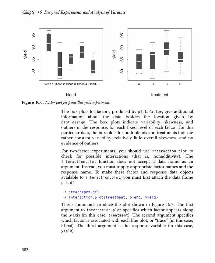
Chapter 16 Designed Experiments and Analysis of Variance
The box plots for factors, produced by plot.factor, give additionalinformation about the data besides the location given byplot.design. The box plots indicate variability, skewness, andoutliers in the response, for each fixed level of each factor. For thisparticular data, the box plots for both blends and treatments indicaterather constant variability, relatively little overall skewness, and noevidence of outliers.
For two-factor experiments, you should use interaction.plot tocheck for possible interactions (that is, nonadditivity). Theinteraction.plot function does not accept a data frame as anargument. Instead, you must supply appropriate factor names and theresponse name. To make these factor and response data objectsavailable to interaction.plot, you must first attach the data framepen.df:
> attach(pen.df)> interaction.plot(treatment, blend, yield)
These commands produce the plot shown in Figure 16.7. The firstargument to interaction.plot specifies which factor appears alongthe x-axis (in this case, treatment). The second argument specifieswhich factor is associated with each line plot, or “trace” (in this case,blend). The third argument is the response variable (in this case,yield).
Figure 16.6: Factor plot for penicillin yield experiment.
8085
9095
yiel
d
Blend 1 Blend 2 Blend 3 Blend 4 Blend 5
blend
8085
9095
yiel
d
A B C D
treatment
582

The Unreplicated Two-Way Layout
Without replication it is often difficult to interpret an interaction plotsince random error tends to dominate. There is nothing striking inthis plot.
The Two-Way Model and ANOVA (One Observation Per Cell)
The additive model for experiments with two factors, A and B, andone observation per cell is:
where is the overall mean, is the effect of the th level of factor
A and is the effect of the th level of factor B.
For the penicillin data above, factor A is “blend” and factor B is“treatment.” Blend has levels and treatment has levels.
To estimate the additive model, use aov:
> aov.pen <- aov(yield ~ blend + treatment, pen.df)
The formula yield ~ blend + treatment specifies that a two factoradditive model is fit, with yield the response, and blend andtreatment the factors.
Figure 16.7: Interaction plot of penicillin experiment.
treatment
mean
of yield
8085
9095
A B C D
blend
Blend 1Blend 5Blend 3Blend 4Blend 2
yij μ αiA αi
B ε ij+ + +=i 1 … I, ,=
j 1 … J, ,=
μ αiA i
αjB j
I 5= J 5=
583
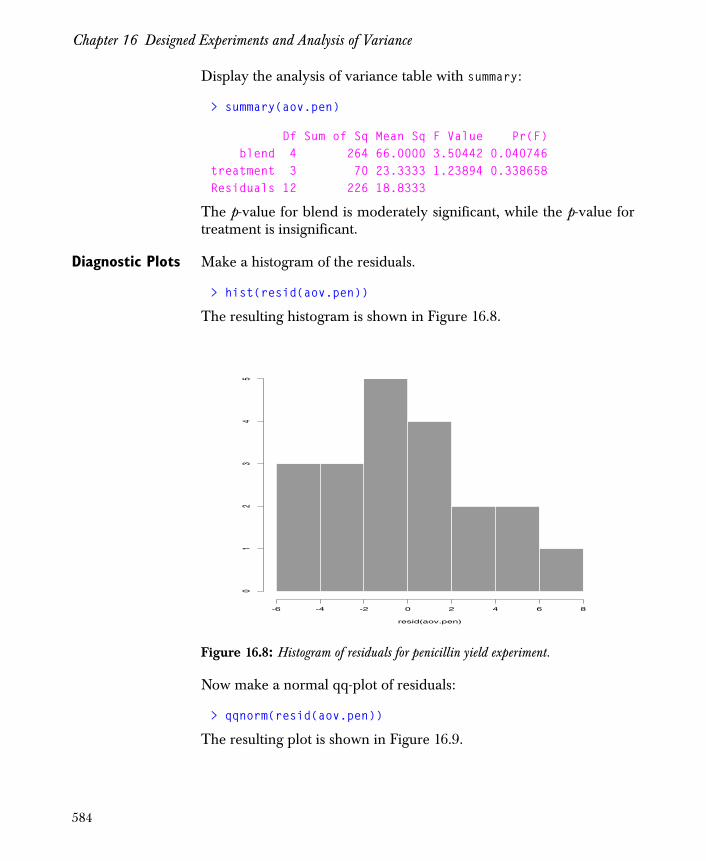
Chapter 16 Designed Experiments and Analysis of Variance
Display the analysis of variance table with summary:
> summary(aov.pen)
Df Sum of Sq Mean Sq F Value Pr(F) blend 4 264 66.0000 3.50442 0.040746treatment 3 70 23.3333 1.23894 0.338658Residuals 12 226 18.8333
The p-value for blend is moderately significant, while the p-value fortreatment is insignificant.
Diagnostic Plots Make a histogram of the residuals.
> hist(resid(aov.pen))
The resulting histogram is shown in Figure 16.8.
Now make a normal qq-plot of residuals:
> qqnorm(resid(aov.pen))
The resulting plot is shown in Figure 16.9.
Figure 16.8: Histogram of residuals for penicillin yield experiment.
-6 -4 -2 0 2 4 6 8
01
23
45
resid(aov.pen)
584

The Unreplicated Two-Way Layout
The central four cells of the histogram in Figure 16.8 are consistentwith a fairly normal distribution in the middle. The linearity of thenormal qq-plot in Figure 16.9, except near the ends, also suggests thatthe distribution is normal in the middle. The relatively larger valuesof the outer two cells of the histogram, and the flattening of thenormal qq-plot near the ends, both suggest that the error distributionis slightly more short-tailed than a normal distribution. This is not amatter of great concern for the ANOVA F tests.
Make a plot of residuals versus the fit:
> plot(fitted(aov.pen), resid(aov.pen))
The resulting plot is shown in Figure 16.10. The plot of residualsversus fit gives some slight indication that smaller error variance isassociated with larger values of the fit.
Figure 16.9: Quantile-quantile plot of residuals for penicillin yield experiment.
•
•
•
•
•
•
•
•
•
•
•
•
•
•
•
•
•
•
•
•
Quantiles of Standard Normal
resi
d(ao
v.pe
n)
-2 -1 0 1 2
-4-2
02
46
585

Chapter 16 Designed Experiments and Analysis of Variance
Guidance Since there is some indication of inhomogeneity of error variance, wenow consider transforming the response, yield.
You may want to test for the existence of a multiplicative interaction,specified by the model
.
When the unknown parameter is not zero, multiplicativeinteraction exists. A test for the null hypothesis of no interaction maybe carried out using the test statistic for Tukey’s one degree offreedom for nonadditivity.
A Spotfire S+ function, tukey.1, is provided in the section Details.You can use it to compute and the p-value. For the penicillindata:
> tukey.1(aov.pen, pen.df)
$T.1df:[1] 0.09826791
$p.value:[1] 0.7597822
Figure 16.10: Residuals vs. fitted values for penicillin yield experiment.
•
•
•
•
•
•
•
•
•
•
•
•
•
•
•
•
•
•
•
•
fitted(aov.pen)
resi
d(ao
v.pe
n)
80 85 90 95
-4-2
02
46
yij μ αiA αj
B θαiAαj
B ε ij+ + + +=
θ
T1df
T1df
586

The Unreplicated Two-Way Layout
The statistic has a p-value of , which is notsignificant. Therefore, there is no indication of a multiplicativeinteraction.
Assuming that the response values are positive, you can find outwhether or not the data suggest a specific transformation to removemultiplicative interaction as follows: Plot the residuals for theadditive fit versus the comparison values
.
If this plot reveals a linear relationship with estimated slope , thenyou should analyze the data again, using as new response values the
power transformation of the original response variables , with
exponent
.
(If , use log( ).) See Hoaglin, Mosteller, and Tukey (1983) fordetails.
A Spotfire S+ function called comp.plot, for computing the
comparison values , plotting versus , and computing , isprovided in the section Details. Applying comp.plot to the penicillindata gives the results shown below and in Figure 16.11:
> comp.plot(aov.pen, pen.df)
$theta.hat:[1] 4.002165
$std.error:[1] 9.980428
$R.squared: R2 0.008854346
T1df 0.098= p 0.76=
rij
cijαi
Aαj
B
μ------------=
θ
yijλ yij
λ 1 θ–=
λ 0= yij
cij rij cij θ
587
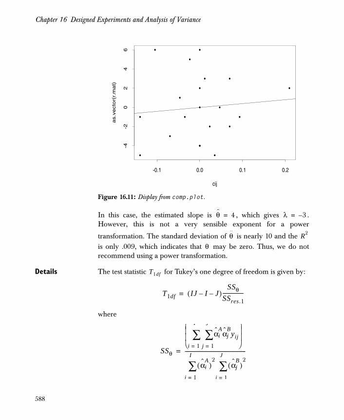
Chapter 16 Designed Experiments and Analysis of Variance
In this case, the estimated slope is , which gives .However, this is not a very sensible exponent for a power
transformation. The standard deviation of is nearly 10 and the is only .009, which indicates that may be zero. Thus, we do notrecommend using a power transformation.
Details The test statistic for Tukey’s one degree of freedom is given by:
where
Figure 16.11: Display from comp.plot.
•
•
••
•
•
•
•
•
•
•
•
•
•
•
•
•
•
•
•
cij
as.v
ecto
r(r.
mat)
-0.1 0.0 0.1 0.2
-4-2
02
46
θ 4= λ 3–=
θ R2
θ
T1df
T1df IJ I– J–( )SSθ
SSres.1----------------=
SSθ
αiA
αjByij
j 1=
J
∑i 1=
I
∑⎝ ⎠⎜ ⎟⎜ ⎟⎛ ⎞
αiA
( )2
i 1=
I
∑ αjB
( )2
j 1=
J
∑-----------------------------------------------=
588

The Unreplicated Two-Way Layout
with the , the additive model estimates of the and , and
the residuals from the additive model fit. The statistic has anF1,IJ-I-J distribution.
Here is a function tukey.1 to compute the Tukey one degree offreedom for nonadditivity test. You can create your own version ofthis function by typing tukey.1 <- and then the definition of thefunction.
> tukey.1 <- function(aov.obj, data) {+ vnames <- names(aov.obj$contrasts)+ if(length(vnames) != 2)+ stop("the model must be two-way")+ vara <- data[, vnames[1]]+ varb <- data[, vnames[2]]+ na <- length(levels(vara))+ nb <- length(levels(varb))+ resp <- data[, as.character(attr(aov.obj$terms,+ "variables")[attr(aov.obj$terms, "response" )])]+ cfs <- coef(aov.obj)+ alpha.A <- aov.obj$contrasts[[vnames[1]]] %*% cfs[+ aov.obj$assign[[vnames[1]]]]+ alpha.B <- aov.obj$contrasts[[vnames[2]]] %*% cfs[+ aov.obj$assign[[vnames[2]]]]+ r.mat <- matrix(0, nb, na)+ r.mat[cbind(as.vector(unclass(varb)), as.vector(+ unclass(vara)))] <- resp+ SS.theta.num <- sum((alpha.B %*% t(alpha.A)) * r.mat)^2+ SS.theta.den <- sum(alpha.A^2) * sum(alpha.B^2)+ SS.theta <- SS.theta.num/SS.theta.den+ SS.res <- sum(resid(aov.obj)^2)+ SS.res.1 <- SS.res - SS.theta+ T.1df <- ((na * nb - na - nb) * SS.theta)/SS.res.1+ p.value <- 1 - pf(T.1df, 1, na * nb - na - nb)+ list(T.1df = T.1df, p.value = p.value) }
SSres.1 SSres SSθ–=
SSres rij2
j 1=
J
∑i 1=
I
∑=
αiA
αjB
αiA αj
B
rij T1df
589

Chapter 16 Designed Experiments and Analysis of Variance
Here is a function comp.plot for computing a least-squares fit to theplot of residuals versus comparison values:
> comp.plot <- function(aov.obj, data)+ {+ vnames <- names(aov.obj$contrasts)+ if(length(vnames) != 2)+ stop("the model must be two-way")+ vara <- data[, vnames[1]]+ varb <- data[, vnames[2]]+ cfs <- coef(aov.obj)+ alpha.A <- aov.obj$contrasts[[vnames[1]]] %*% cfs[+ aov.obj$assign[[vnames[1]]]]+ alpha.B <- aov.obj$contrasts[[vnames[2]]] %*% cfs[+ aov.obj$assign[[vnames[2]]]]+ cij <- alpha.B %*% t(alpha.A)+ cij <- c(cij)/cfs[aov.obj$assign$"(Intercept)"]+ na <- length(levels(vara))+ nb <- length(levels(varb))+ r.mat <- matrix(NA, nb, na)+ r.mat[cbind(as.vector(unclass(varb)), as.vector(+ unclass(vara)))] <- resid(aov.obj)+ plot(cij, as.vector(r.mat))+ ls.fit <- lsfit(as.vector(cij), as.vector(r.mat))+ abline(ls.fit)+ output <- ls.print(ls.fit, print.it = F)+ list(theta.hat = output$coef.table[2, 1], + std.error = output$coef.table[2, 2], + R.squared = output$summary[2])+ }
590
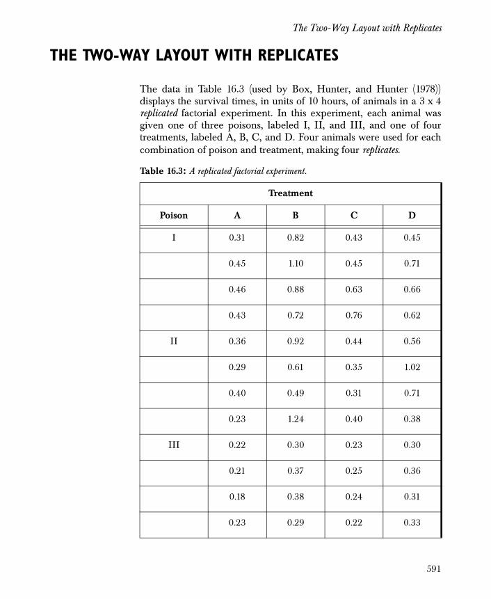
The Two-Way Layout with Replicates
THE TWO-WAY LAYOUT WITH REPLICATES
The data in Table 16.3 (used by Box, Hunter, and Hunter (1978))displays the survival times, in units of 10 hours, of animals in a 3 x 4replicated factorial experiment. In this experiment, each animal wasgiven one of three poisons, labeled I, II, and III, and one of fourtreatments, labeled A, B, C, and D. Four animals were used for eachcombination of poison and treatment, making four replicates.
Table 16.3: A replicated factorial experiment.
Treatment
Poison A B C D
I 0.31 0.82 0.43 0.45
0.45 1.10 0.45 0.71
0.46 0.88 0.63 0.66
0.43 0.72 0.76 0.62
II 0.36 0.92 0.44 0.56
0.29 0.61 0.35 1.02
0.40 0.49 0.31 0.71
0.23 1.24 0.40 0.38
III 0.22 0.30 0.23 0.30
0.21 0.37 0.25 0.36
0.18 0.38 0.24 0.31
0.23 0.29 0.22 0.33
591
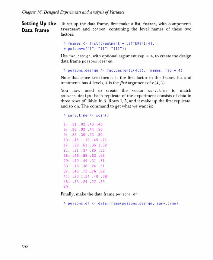
Chapter 16 Designed Experiments and Analysis of Variance
Setting Up the Data Frame
To set up the data frame, first make a list, fnames, with componentstreatment and poison, containing the level names of these twofactors:
> fnames <- list(treatment = LETTERS[1:4],+ poison=c("I", "II", "III"))
Use fac.design, with optional argument rep = 4, to create the designdata frame poisons.design:
> poisons.design <- fac.design(c(4,3), fnames, rep = 4)
Note that since treatments is the first factor in the fnames list andtreatments has 4 levels, 4 is the first argument of c(4,3).
You now need to create the vector surv.time to matchpoisons.design. Each replicate of the experiment consists of data inthree rows of Table 16.3. Rows 1, 5, and 9 make up the first replicate,and so on. The command to get what we want is:
> surv.time <- scan()
1: .31 .82 .43 .455: .36 .92 .44 .569: .22 .30 .23 .3013: .45 1.10 .45 .7117: .29 .61 .35 1.0221: .21 .37 .25 .3625: .46 .88 .63 .6629: .40 .49 .31 .7133: .18 .38 .24 .3137: .43 .72 .76 .6241: .23 1.24 .40 .3845: .23 .29 .22 .3349:
Finally, make the data frame poisons.df:
> poisons.df <- data.frame(poisons.design, surv.time)
592
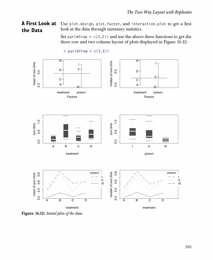
The Two-Way Layout with Replicates
A First Look at the Data
Use plot.design, plot.factor, and interaction.plot to get a firstlook at the data through summary statistics.
Set par(mfrow = c(3,2)) and use the above three functions to get thethree row and two column layout of plots displayed in Figure 16.12:
> par(mfrow = c(3,2))
Figure 16.12: Initial plots of the data.
Factors
mea
n of
sur
v.tim
e
0.3
0.5
A
B
C
D
I
II
III
treatment poison
Factors
med
ian
of s
urv.
time
0.3
0.5
A
B
C
D
I
II
III
treatment poison
0.2
0.6
1.0
surv
.tim
e
A B C D
treatment
0.2
0.6
1.0
surv
.tim
e
I II III
poison
treatment
mea
n of
sur
v.tim
e
0.2
0.4
0.6
0.8
A B C D
poison
IIIIII
treatment
med
ian
of s
urv.
time
0.2
0.4
0.6
0.8
A B C D
poison
IIIIII
593
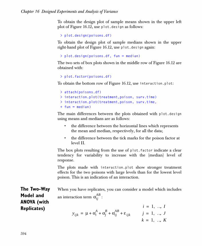
Chapter 16 Designed Experiments and Analysis of Variance
To obtain the design plot of sample means shown in the upper leftplot of Figure 16.12, use plot.design as follows:
> plot.design(poisons.df)
To obtain the design plot of sample medians shown in the upperright-hand plot of Figure 16.12, use plot.design again:
> plot.design(poisons.df, fun = median)
The two sets of box plots shown in the middle row of Figure 16.12 areobtained with:
> plot.factor(poisons.df)
To obtain the bottom row of Figure 16.12, use interaction.plot:
> attach(poisons.df)> interaction.plot(treatment,poison, surv.time)> interaction.plot(treatment,poison, surv.time,+ fun = median)
The main differences between the plots obtained with plot.designusing means and medians are as follows:
• the difference between the horizontal lines which represents the mean and median, respectively, for all the data;
• the difference between the tick marks for the poison factor at level II.
The box plots resulting from the use of plot.factor indicate a cleartendency for variability to increase with the (median) level ofresponse.
The plots made with interaction.plot show stronger treatmenteffects for the two poisons with large levels than for the lowest levelpoison. This is an indication of an interaction.
The Two-Way Model and ANOVA (with Replicates)
When you have replicates, you can consider a model which includes
an interaction term :αijAB
yijk μ αiA αj
B αijAB ε ijk+ + + +=
i 1 … I, ,=
j 1 … J, ,=
k 1 … K, ,=
594
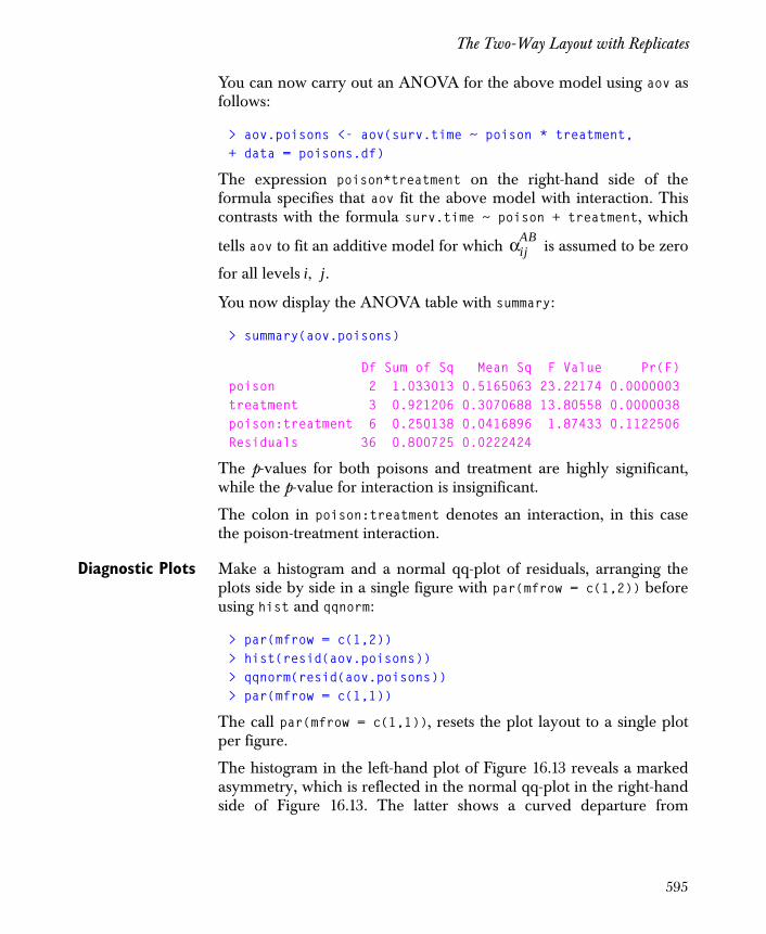
The Two-Way Layout with Replicates
You can now carry out an ANOVA for the above model using aov asfollows:
> aov.poisons <- aov(surv.time ~ poison * treatment,+ data = poisons.df)
The expression poison*treatment on the right-hand side of theformula specifies that aov fit the above model with interaction. Thiscontrasts with the formula surv.time ~ poison + treatment, which
tells aov to fit an additive model for which is assumed to be zero
for all levels .
You now display the ANOVA table with summary:
> summary(aov.poisons)
Df Sum of Sq Mean Sq F Value Pr(F)poison 2 1.033013 0.5165063 23.22174 0.0000003treatment 3 0.921206 0.3070688 13.80558 0.0000038poison:treatment 6 0.250138 0.0416896 1.87433 0.1122506Residuals 36 0.800725 0.0222424
The p-values for both poisons and treatment are highly significant,while the p-value for interaction is insignificant.
The colon in poison:treatment denotes an interaction, in this casethe poison-treatment interaction.
Diagnostic Plots Make a histogram and a normal qq-plot of residuals, arranging theplots side by side in a single figure with par(mfrow = c(1,2)) beforeusing hist and qqnorm:
> par(mfrow = c(1,2))> hist(resid(aov.poisons))> qqnorm(resid(aov.poisons))> par(mfrow = c(1,1))
The call par(mfrow = c(1,1)), resets the plot layout to a single plotper figure.
The histogram in the left-hand plot of Figure 16.13 reveals a markedasymmetry, which is reflected in the normal qq-plot in the right-handside of Figure 16.13. The latter shows a curved departure from
αijAB
i j,
595

Chapter 16 Designed Experiments and Analysis of Variance
linearity toward the lower left part of the plot, and a break in linearityin the upper right part of the plot. Evidently, all is not well (see thediscussion on transforming the data in the Guidance section below).
Make a plot of residuals versus fit:
> plot(fitted(aov.poisons), resid(aov.poisons))
The result, displayed in Figure 16.14, clearly reveals a strongrelationship between the residuals and the fitted values. Thevariability of the residuals increases with increasing fitted values. Thisis another indication that transformation would be useful.
Guidance When the error variance for an experiment varies with the expectedvalue of the observations, a variance stabilizing transformation willoften reduce or eliminate such behavior.
We shall show two methods for determining an appropriate variancestabilizing transformation, one which requires replicates and onewhich does not.
Figure 16.13: Histogram and normal qq-plot of residuals.
-0.4 -0.2 0.0 0.2 0.4
05
10
15
20
resid(aov.poisons)
••
••
••
•
•
•• ••
•
•
•
•
•
•
•
•
• •• • ••
•• •
•
•
••
••• •
•
•
•
•
•
•
•
•• • •
Quantiles of Standard Normal
resi
d(a
ov.
po
iso
ns)
-2 -1 0 1 2
-0.2
0.0
0.2
0.4
596
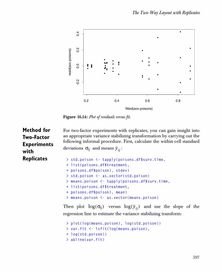
The Two-Way Layout with Replicates
Method for Two-Factor Experiments with Replicates
For two-factor experiments with replicates, you can gain insight intoan appropriate variance stabilizing transformation by carrying out thefollowing informal procedure. First, calculate the within-cell standarddeviations and means :
> std.poison <- tapply(poisons.df$surv.time,+ list(poisons.df$treatment,+ poisons.df$poison), stdev)> std.poison <- as.vector(std.poison)> means.poison <- tapply(poisons.df$surv.time,+ list(poisons.df$treatment,+ poisons.df$poison), mean)> means.poison <- as.vector(means.poison)
Then plot versus and use the slope of the
regression line to estimate the variance stabilizing transform:
> plot(log(means.poison), log(std.poison))> var.fit <- lsfit(log(means.poison),+ log(std.poison))> abline(var.fit)
Figure 16.14: Plot of residuals versus fit.
••
• •
•
••
•
••
• •
•
•
•
•
•
•
•
•
••• • •
•
• ••
•
•
•
•
•• •
•
•
•
•
•
•
•
•
•
•• •
fitted(aov.poisons)
resi
d(ao
v.po
ison
s)
0.2 0.4 0.6 0.8
-0.2
0.0
0.2
0.4
σij yij
log σij( ) log yij( )
597

Chapter 16 Designed Experiments and Analysis of Variance
> theta <- var.fit$coef[2]> theta
X 1.97704
Now let and choose to be that value among the set of
values which is closest to . If , then make
the transformation . Otherwise, make the power
transformation . Now you should repeat the complete
analysis described in the previous subsections, using the response
in place of .
Since for the poisons experiment you get , you choose .
This gives a reciprocal transformation , where are the
values you used in the response with surv.time. You can think of thenew response as representing the rate of dying.
The model can be refit using the transformed response:
> summary(aov(1/surv.time ~ poison*treatment, + data = poisons.df))
Df Sum of Sq Mean Sq F Value Pr(F)poison 2 34.87712 17.43856 72.63475 0.0000000treatment 3 20.41429 6.80476 28.34307 0.0000000poison:treatment 6 1.57077 0.26180 1.09042 0.3867329Residuals 36 8.64308 0.24009
With the transformation the p-values for the main effects havedecreased while the p-value for the interaction has increased—a moresatisfactory fit. The diagnostic plots with the new response are muchimproved also.
λˆ 1 θ–= λ
1 12---– 0 1
2--- 1, , , ,–
⎭
⎫λ λ 0=
yij log yij=
yijk yijkλ
=
yijk
yijk
θ 2≈ λ 1–=
yijk yijk1–
= yijk
yijk
598
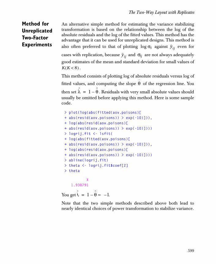
The Two-Way Layout with Replicates
Method for Unreplicated Two-Factor Experiments
An alternative simple method for estimating the variance stabilizingtransformation is based on the relationship between the log of theabsolute residuals and the log of the fitted values. This method has theadvantage that it can be used for unreplicated designs. This method isalso often preferred to that of plotting against even for
cases with replication, because and are not always adequately
good estimates of the mean and standard deviation for small values of.
This method consists of plotting log of absolute residuals versus log of
fitted values, and computing the slope of the regression line. You
then set . Residuals with very small absolute values shouldusually be omitted before applying this method. Here is some samplecode.
> plot(log(abs(fitted(aov.poisons)[+ abs(resid(aov.poisons)) > exp(-10)])),+ log(abs(resid(aov.poisons)[+ abs(resid(aov.poisons)) > exp(-10)])))> logrij.fit <- lsfit(+ log(abs(fitted(aov.poisons)[+ abs(resid(aov.poisons)) > exp(-10)])),+ log(abs(resid(aov.poisons)[+ abs(resid(aov.poisons)) > exp(-10)])))> abline(logrij.fit)> theta <- logrij.fit$coef[2]> theta
X 1.930791
You get .
Note that the two simple methods described above both lead tonearly identical choices of power transformation to stabilize variance.
σijlog yij
yij σij
K K 8<( )
θ
λ 1 θ–=
λ 1 θ 1–≈–=
599

Chapter 16 Designed Experiments and Analysis of Variance
Details You will find that a nonconstant standard deviation for observations ( for the two-factor experiment with replicates) is well-
explained by a power law relationship in many data sets. Inparticular, for some constant and some exponent , we have
where is the standard deviation of the and is the mean of the
. If you then use a power law transformation
for some fixed exponent , it can be shown that the standard
deviation for the transformed data , is given by
.
You can therefore make have a constant value, independent of
the mean of the original data (and independent of the
approximate mean of the transformed data ), by choosing
.
Note that
.
Suppose you plot log versus log for a two-factor experiment
with replicates and find that this plot results in a fairly good straight
line fit with slope , where is an estimate of and is an
estimate of . Then the slope provides an estimate of , and so
you set . Since a fractional exponent is not very natural,
one often chooses the closest value in the following “natural” set.
yi yijk
B θ
σy Bηθ≈
σy yi η
yi
yi yiλ
=
λσy yi
σy Kληλ 1 θ–( )–=
σy
η yi
ηλ yi
λ 1 θ–=
log σy log K θ log η+≈
σij yij
θ σij σy yij
η θ θ
λ 1 θ–= λ
λ
600

The Two-Way Layout with Replicates
Alternative Formal Methods
There are two alternative formal approaches to stabilizing thevariance. One approach is to select the power transformation thatminimizes the residual squared error. This is equivalent tomaximizing the log-likelihood function and is sometimes referred toas a Box-Cox analysis (see, for example, Weisberg (1985); Box(1988); Haaland (1989)).
The second approach seeks to stabilize the variance without the use ofa transformation, by including the variance function directly in themodel. This approach is called generalized least squares/variancefunction estimation (see, for example, Carroll and Ruppert (1988);Davidian and Haaland (1990)).
Transformations are easy to use and may provide a simpler, moreparsimonious model (Box (1988)). On the other hand, modeling thevariance function directly allows the analysis to proceed on theoriginal scale and allows more direct insight into the nature of thevariance function. In cases when the stability of the variance iscritical, either of these methods have better statistical properties thanthe simple informal graphical methods described above.
1– Reciprocal12---– Reciprocal square root
0 Log12--- Square root
1 No transformation
601
Chapter 16 Designed Experiments and Analysis of Variance
MANY FACTORS AT TWO LEVELS: 2K DESIGNS
The data in Table 16.4 come from an industrial product developmentexperiment in which a response variable called conversion is measured(in percent) for each possible combination of two levels of fourfactors, listed below.
• K: catalyst charge (10 or 15 pounds)
• Te: temperature ( )
• P: pressure (50 or 80 pounds per square inch)
• C: concentration (10% or 12%)
The levels are labeled “-” and “+” in the table. All the factors in theexperiment are quantitative, so the “-” indicates the “low” level andthe “+” indicates the “high” level for each factor. This data set wasused by Box, Hunter, and Hunter (1978).
The design for this experiment is called a 24 design because there are
24 = 16 possible combinations of two levels for four factors.
Setting Up the Data Frame
To set up the data frame first create a list of the four factor names withthe corresponding pairs of levels labels:
> fnames <- list(K = c("10","15"), Te = c("220","240"),+ P = c("50","80"), C = c("10","12"))
Now use fac.design to create the 2k design data frame devel.design:
> devel.design <- fac.design(rep(2,4), fnames)
The first argument to fac.design is a vector of length four, whichspecifies that there are four factors. Each entry of the vector is a 2,which specifies that there are two levels for each factor.
Since devel.design matches Table 16.4, you can simply scan in thecoversion data:
> conversion <- scan()1: 71 61 90 82 68 61 87 809: 61 50 89 83 59 51 85 7817:
220 or 240° C
602

Many Factors at Two Levels: 2k Designs
Table 16.4: Data from product development experiment.
Factor
ObservationNumber K Te P C Conversion(%) Run Order
1 – – – – 71 (8)
2 + – – – 61 (2)
3 – + – – 90 (10)
4 + + – – 82 (4)
5 – – + – 68 (15)
6 + – + – 61 (9)
7 – + + – 87 (1)
8 + + + – 80 (13)
9 – – – + 61 (16)
10 + – – + 50 (5)
11 – + – + 89 (11)
12 + + – + 83 (14)
13 – – + + 59 (3)
14 + – + + 51 (12)
15 – + + + 85 (6)
16 + + + + 78 (7)
603

Chapter 16 Designed Experiments and Analysis of Variance
Finally, create the data frame devel.df:
> devel.df <- data.frame(devel.design, conversion)> devel.df
K Te P C conversion 1 10 220 50 10 71 2 15 220 50 10 61 3 10 240 50 10 90 . . .15 10 240 80 12 8516 15 240 80 12 78
A First Look at the Data
Use plot.design and plot.factor to make an initial graphicalexploration of the data. To see the design plot with sample means, usethe following command, which yields the plot shown in Figure 16.15:
> plot.design(devel.df)
To see the design plot with sample medians, use:
> plot.design(devel.df, fun = median)
Figure 16.15: Sample means for product development experiment.
Factors
mea
n of
con
vers
ion
6065
7075
8085
10
15
220
240
5080
10
12
K Te P C
604
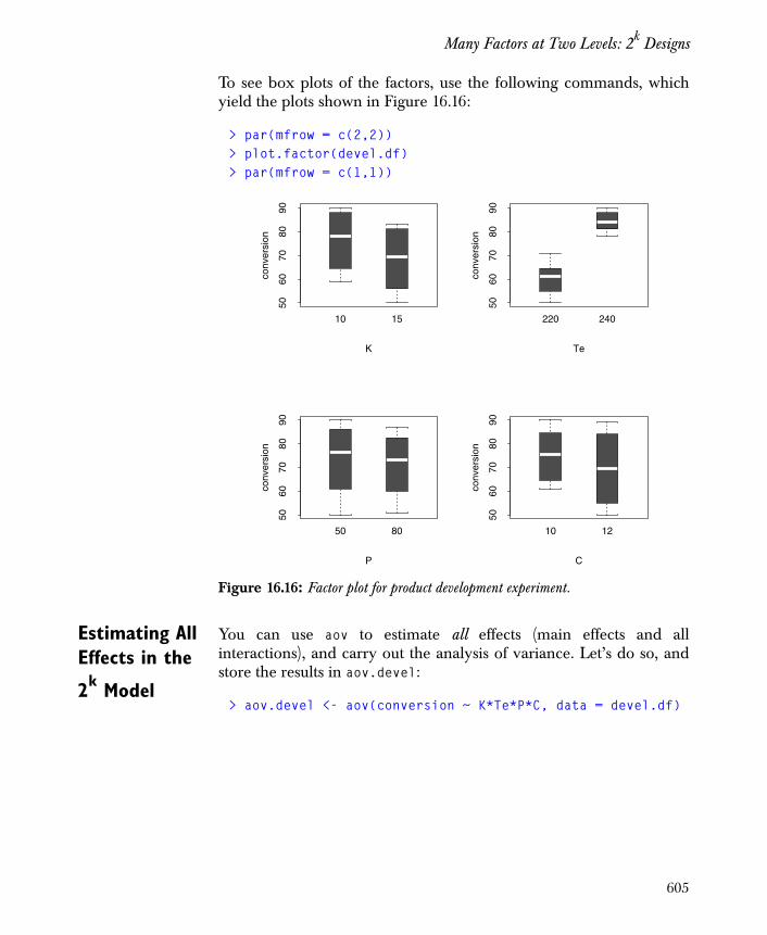
Many Factors at Two Levels: 2k Designs
To see box plots of the factors, use the following commands, whichyield the plots shown in Figure 16.16:
> par(mfrow = c(2,2))> plot.factor(devel.df)> par(mfrow = c(1,1))
Estimating All Effects in the
2k Model
You can use aov to estimate all effects (main effects and allinteractions), and carry out the analysis of variance. Let’s do so, andstore the results in aov.devel:
> aov.devel <- aov(conversion ~ K*Te*P*C, data = devel.df)
Figure 16.16: Factor plot for product development experiment.
5060
7080
90
conv
ersi
on
10 15
K
5060
7080
90
conv
ersi
on
220 240
Te
5060
7080
90
conv
ersi
on
50 80
P
5060
7080
90
conv
ersi
on
10 12
C
605
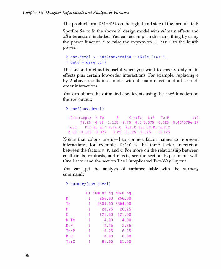
Chapter 16 Designed Experiments and Analysis of Variance
The product form K*Te*P*C on the right-hand side of the formula tells
Spotfire S+ to fit the above 24 design model with all main effects andall interactions included. You can accomplish the same thing by usingthe power function ^ to raise the expression K+Te+P+C to the fourthpower:
> aov.devel <- aov(conversion ~ (K+Te+P+C)^4, + data = devel.df)
This second method is useful when you want to specify only maineffects plus certain low-order interactions. For example, replacing 4by 2 above results in a model with all main effects and all second-order interactions.
You can obtain the estimated coefficients using the coef function onthe aov output:
> coef(aov.devel)
(Intercept) K Te P C K:Te K:P Te:P K:C 72.25 -4 12 -1.125 -2.75 0.5 0.375 -0.625 -5.464379e-17 Te:C P:C K:Te:P K:Te:C K:P:C Te:P:C K:Te:P:C 2.25 -0.125 -0.375 0.25 -0.125 -0.375 -0.125
Notice that colons are used to connect factor names to representinteractions, for example, K:P:C is the three factor interactionbetween the factors K, P, and C. For more on the relationship betweencoefficients, contrasts, and effects, see the section Experiments withOne Factor and the section The Unreplicated Two-Way Layout.
You can get the analysis of variance table with the summarycommand:
> summary(aov.devel)
Df Sum of Sq Mean SqK 1 256.00 256.00Te 1 2304.00 2304.00P 1 20.25 20.25C 1 121.00 121.00K:Te 1 4.00 4.00K:P 1 2.25 2.25Te:P 1 6.25 6.25K:C 1 0.00 0.00Te:C 1 81.00 81.00
606

Many Factors at Two Levels: 2k Designs
P:C 1 0.25 0.25K:Te:P 1 2.25 2.25K:Te:C 1 1.00 1.00K:P:C 1 0.25 0.25Te:P:C 1 2.25 2.25K:Te:P:C 1 0.25 0.25
The ANOVA table does not provide any statistics. This is becauseyou have estimated 16 parameters with 16 observations. There are nodegrees of freedom left for estimating the error variance, and hencethere is no error mean square to use as the denominator of the statistics. However, the ANOVA table can give you some idea ofwhich effects are the main contributors to the response variation.
Estimating All
Effects in the 2k Model With Replicates
On some occasions, you may have replicates of a design. In this
case, you can estimate the error variance as well as all effects. For
example, the data in Table 16.5 is from a replicated 23 pilot plant
F
F
2k
σ2
607
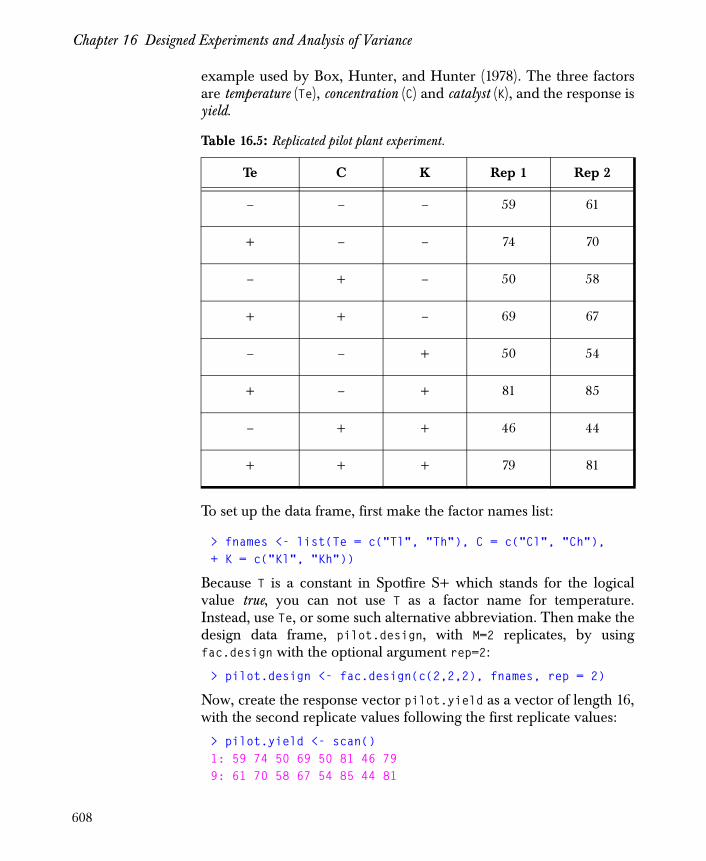
Chapter 16 Designed Experiments and Analysis of Variance
example used by Box, Hunter, and Hunter (1978). The three factorsare temperature (Te), concentration (C) and catalyst (K), and the response isyield.
To set up the data frame, first make the factor names list:
> fnames <- list(Te = c("Tl", "Th"), C = c("Cl", "Ch"),+ K = c("Kl", "Kh"))
Because T is a constant in Spotfire S+ which stands for the logicalvalue true, you can not use T as a factor name for temperature.Instead, use Te, or some such alternative abbreviation. Then make thedesign data frame, pilot.design, with M=2 replicates, by usingfac.design with the optional argument rep=2:
> pilot.design <- fac.design(c(2,2,2), fnames, rep = 2)
Now, create the response vector pilot.yield as a vector of length 16,with the second replicate values following the first replicate values:
> pilot.yield <- scan()1: 59 74 50 69 50 81 46 799: 61 70 58 67 54 85 44 81
Table 16.5: Replicated pilot plant experiment.
Te C K Rep 1 Rep 2
– – – 59 61
+ – – 74 70
– + – 50 58
+ + – 69 67
– – + 50 54
+ – + 81 85
– + + 46 44
+ + + 79 81
608
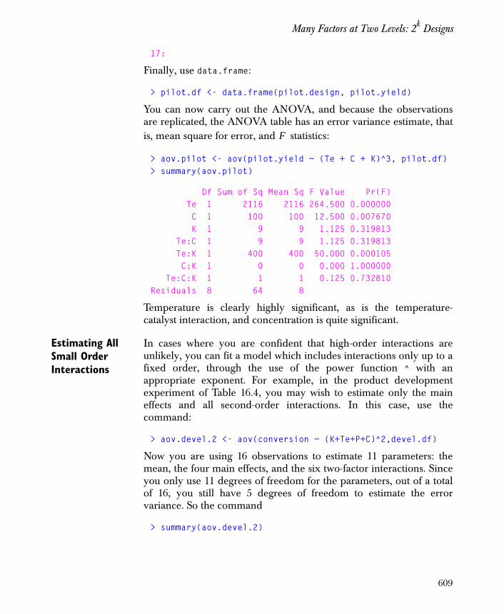
Many Factors at Two Levels: 2k Designs
17:
Finally, use data.frame:
> pilot.df <- data.frame(pilot.design, pilot.yield)
You can now carry out the ANOVA, and because the observationsare replicated, the ANOVA table has an error variance estimate, thatis, mean square for error, and statistics:
> aov.pilot <- aov(pilot.yield ~ (Te + C + K)^3, pilot.df)> summary(aov.pilot)
Df Sum of Sq Mean Sq F Value Pr(F) Te 1 2116 2116 264.500 0.000000 C 1 100 100 12.500 0.007670 K 1 9 9 1.125 0.319813 Te:C 1 9 9 1.125 0.319813 Te:K 1 400 400 50.000 0.000105 C:K 1 0 0 0.000 1.000000 Te:C:K 1 1 1 0.125 0.732810Residuals 8 64 8
Temperature is clearly highly significant, as is the temperature-catalyst interaction, and concentration is quite significant.
Estimating All Small Order Interactions
In cases where you are confident that high-order interactions areunlikely, you can fit a model which includes interactions only up to afixed order, through the use of the power function ^ with anappropriate exponent. For example, in the product developmentexperiment of Table 16.4, you may wish to estimate only the maineffects and all second-order interactions. In this case, use thecommand:
> aov.devel.2 <- aov(conversion ~ (K+Te+P+C)^2,devel.df)
Now you are using 16 observations to estimate 11 parameters: themean, the four main effects, and the six two-factor interactions. Sinceyou only use 11 degrees of freedom for the parameters, out of a totalof 16, you still have 5 degrees of freedom to estimate the errorvariance. So the command
> summary(aov.devel.2)
F
609
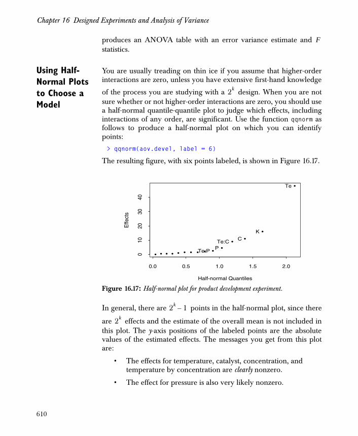
Chapter 16 Designed Experiments and Analysis of Variance
produces an ANOVA table with an error variance estimate and statistics.
Using Half-Normal Plots to Choose a Model
You are usually treading on thin ice if you assume that higher-orderinteractions are zero, unless you have extensive first-hand knowledge
of the process you are studying with a design. When you are notsure whether or not higher-order interactions are zero, you should usea half-normal quantile-quantile plot to judge which effects, includinginteractions of any order, are significant. Use the function qqnorm asfollows to produce a half-normal plot on which you can identifypoints:
> qqnorm(aov.devel, label = 6)
The resulting figure, with six points labeled, is shown in Figure 16.17.
In general, there are points in the half-normal plot, since there
are effects and the estimate of the overall mean is not included inthis plot. The y-axis positions of the labeled points are the absolutevalues of the estimated effects. The messages you get from this plotare:
• The effects for temperature, catalyst, concentration, and temperature by concentration are clearly nonzero.
• The effect for pressure is also very likely nonzero.
F
Figure 16.17: Half-normal plot for product development experiment.
2k
• • • • • • • • • • •• •
•
•
Half-normal Quantiles
Effe
cts
0.0 0.5 1.0 1.5 2.0
010
2030
40
Te
K C Te:C
P Te:P
2k 1–
2k
610

Many Factors at Two Levels: 2k Designs
You can examine the marginal effects better by creating a plot with asmaller y-range:
> qqnorm(aov.devel, label = 6, ylim = c(0,20))
A full qq-plot of the effects can give you somewhat more information.To get this type of plot, use the following:
> qqnorm(aov.devel, full = T, label = 6)
Having determined from the half-normal plot which effects arenonzero, now fit a model having terms for the main effects plus theinteraction between temperature and concentration:
> aov.devel.small <- aov(conversion ~ K+P+Te*C, + data = devel.df)
You can now get an ANOVA summary, including an error varianceestimate:
> summary(aov.devel.small)
Df Sum of Sq Mean Sq F Value Pr(F)K 1 256.00 256.000 136.533 0.000000375P 1 20.25 20.250 10.800 0.008200654Te 1 2304.00 2304.000 1228.800 0.000000000C 1 121.00 121.000 64.533 0.000011354Te:C 1 81.00 81.000 43.200 0.000062906Residuals 10 18.75 1.875
Diagnostic Plots Once you have tentatively identified a model for a experiment,you should make the usual graphical checks based on the residualsand fitted values. In the product development example, you shouldexamine the following plots:
> hist(resid(aov.devel.small))> qqnorm(resid(aov.devel.small))> plot(fitted(aov.devel.small), resid(aov.devel.small))
2k
611

Chapter 16 Designed Experiments and Analysis of Variance
The latter two plots are shown in Figure 16.18 and Figure 16.19.
You should also make plots using the time order of the runs:
> run.ord <- scan()
1: 8 2 10 4 15 9 1 13 16 5 11 14 3 12 6 717:
> plot(run.ord, resid(aov.devel.small))> plot(run.ord, fitted(aov.devel.small))
This gives a slight hint that the first runs were more variable than thelatter runs.
Figure 16.18: Quantile-quantile plot of residuals, product development example.
•
•
•••
•
•
••
•
•
•
• •
•
•
Quantiles of Standard Normal
resi
d(ao
v.de
vel.s
mal
l)
-2 -1 0 1 2
-2-1
01
2
612

Many Factors at Two Levels: 2k Designs
Details The function aov returns, by default, coefficients corresponding to thefollowing usual ANOVA form for the ηi:
In this form of the model, each takes on just two values: 1 and
2. There are values of the -tuple index , and the
parameter is the overall mean. The parameters correspond to
the main effects, for . The parameters correspond to
the two-factor interactions, the parameters correspond to the
three-factor interactions, and the remaining coefficients are the higher-order interactions.
Figure 16.19: Fitted values vs. residuals, product development example.
•
•
•••
•
•
••
•
•
•
••
•
•
fitted(aov.devel.small)
resi
d(ao
v.de
vel.s
mal
l)
50 60 70 80 90
-2-1
01
2
ηi ηi1…ikμ + αi1
1 αi2
2 … αik
k+ + += =
+ αi1i2
12 αi1i3
13 … αik 1– ik
k 1– k,+ + +
+ …
+ αi1i2…ik
123…k
2k im
2k k i1 i2 … i, k, ,
μ αim
m
m 1 … k, ,= αimin
mn
αilimin
lmn
613

Chapter 16 Designed Experiments and Analysis of Variance
The coefficients for the main effects satisfy the constraint
for , where the denote the
number of replications for the ith treatment. All higher-orderinteractions satisfy the constraint that the weighted sum over anyindividual subscript index is zero. For example,
, , etc. Because
of the constraints on the parameters in this form of the model, itsuffices to specify one of the two values for each effect. The function
aov returns estimates for the “high” levels (for example, ).
An estimated effect (in the sense usually used in models) is equalto the difference between the estimate at the high level minus theestimate at the low level:
.
Since , we have
.
In the case of a balanced design, and the estimated effect
simplifies to .
n1i α1
in2
i α2i
+ 0= i 1 2 … k, , ,= ni
ni1112
αi1112
ni1212
αi1212
+ 0= n1i2i4
124α1i2i4
124n2i2i4
124α2i2i4
124+ 0=
α2i α2
12,
2k
α1 α21 α1
1–=
n11α1
1n2
1α2
1+ 0=
α1 α21
1n2
1
n11
-----+⎝ ⎠⎜ ⎟⎛ ⎞
=
n11 n2
1=
α12α2
1=
614
References
REFERENCES
Box, G.E.P., Hunter, W.G., and Hunter, J.S. (1978). Statistics forExperimenters: An Introduction to Design, Data Analysis. New York: JohnWiley & Sons, Inc.
Box, G.E.P. (1988). Signal-to-noise ratios, performance criteria, andtransformations. Technometrics 30:1-17.
Carroll, R.J. & Ruppert, D. (1988). Transformation and Weighting inRegression. New York: Chapman and Hall.
Chambers, J.M. & Hastie, T.J. (Eds.) (1992). Statistical Models in S.London: Chapman and Hall.
Davidian, M. & Haaland, P.D. (1990). Regression and calibrationwith non-constant error variance. Chemometrics and IntelligentLaboratory Systems 9:231-248.
Haaland, P. (1989). Experimental Design in Biotechnology. New York:Marcel Dekker.
Hoaglin, D.C., Mosteller, F., & Tukey, J.W. (1983). UnderstandingRobust and Exploratory Data Analysis. New York: John Wiley & Sons,Inc.
Weisberg, S. (1985). Applied Linear Regression (2nd ed.). New York:John Wiley & Sons, Inc.
615

Chapter 16 Designed Experiments and Analysis of Variance
616

Introduction 618
Model Coefficients and Contrasts 619
Summarizing ANOVA Results 626Splitting Treatment Sums of Squares Into
Contrast Terms 626Treatment Means and Standard Errors 629Balanced Designs 629
2k Factorial Designs 633Unbalanced Designs 634Analysis of Unweighted Means 637
Multivariate Analysis of Variance 654
Split-Plot Designs 656
Repeated-Measures Designs 658
Rank Tests for One-Way and Two-Way Layouts 662The Kruskal-Wallis Rank Sum Test 662The Friedman Rank Sum Test 663
Variance Components Models 664Estimating the Model 664Estimation Methods 665Random Slope Example 666
Appendix: Type I Estimable Functions 668
References 670
FURTHER TOPICS IN ANALYSIS OF VARIANCE 17
617

Chapter 17 Further Topics in Analysis of Variance
INTRODUCTION
Chapter 16, Designed Experiments and Analysis of Variance,describes the basic techniques for using TIBCO Spotfire S+ foranalysis of variance. This chapter extends the concepts to severalrelated topics as follows:
• Multivariate analysis of variance (MANOVA);
• Split-plot designs;
• Repeated measures;
• Nonparametric tests for one-way and blocked two-way designs;
• Variance components models.
These topics are preceded by a discussion of model coefficients andcontrasts. This information is important in interpreting the availableANOVA summaries.
618
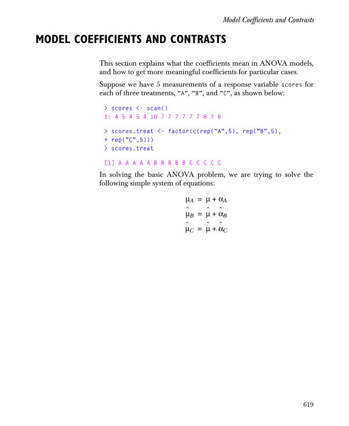
Model Coefficients and Contrasts
MODEL COEFFICIENTS AND CONTRASTS
This section explains what the coefficients mean in ANOVA models,and how to get more meaningful coefficients for particular cases.
Suppose we have 5 measurements of a response variable scores foreach of three treatments, "A", "B", and "C", as shown below:
> scores <- scan()1: 4 5 4 5 4 10 7 7 7 7 7 7 8 7 6
> scores.treat <- factor(c(rep("A",5), rep("B",5),+ rep("C",5)))> scores.treat
[1] A A A A A B B B B B C C C C C
In solving the basic ANOVA problem, we are trying to solve thefollowing simple system of equations:
μA μ αA+=
μB μ αB+=
μC μ αC+=
619

Chapter 17 Further Topics in Analysis of Variance
Consider:
The problem is that the matrix is singular. That is, we cannot
solve for the alphas.
Use the Helmert contrast matrix .
y
4545410777777876
1 11 11 11 11 11 11 11 11 11 11 11 11 11 11 1
μ
αA
αB
αC
ε 1 Xa
μ
αA
αB
αC
ε+=+==
1 Xa
Ca
1– 1–
1 1–
0 2
=
620
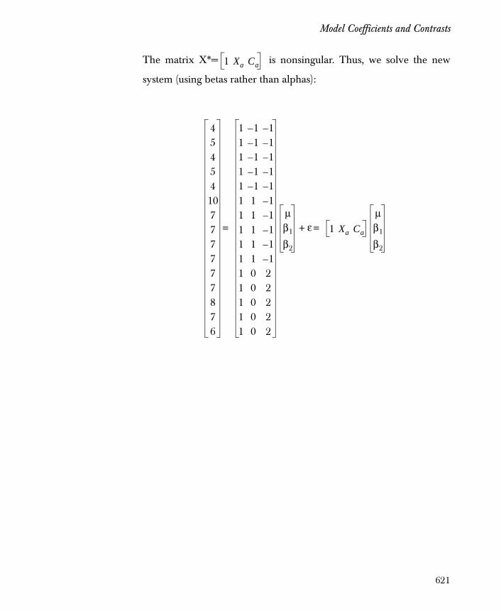
Model Coefficients and Contrasts
The matrix X*= is nonsingular. Thus, we solve the new
system (using betas rather than alphas):
1 Xa Ca
4545410777777876
1 1– 1–
1 1– 1–
1 1– 1–
1 1– 1–
1 1– 1–
1 1 1–
1 1 1–
1 1 1–
1 1 1–
1 1 1–
1 0 21 0 21 0 21 0 21 0 2
μβ1
β2
ε 1 Xa Ca
μβ1
β2
=+=
621

Chapter 17 Further Topics in Analysis of Variance
The matrix is nonsingular; therefore, we can solve for the
the solution .
Because y = , it follows that
or simply .
Thus, we can calculate the original alphas:
If we use aov as usual to create the aov object scores.aov, we can use
the coef function to look at the solved values , , and :
> scores.aov <- aov(scores ~ scores.treat)> coef(scores.aov)
(Intercept) scores.treat1 scores.treat2 6.333333 1.6 0.3333333
In our example, the contrast matrix is as follows:
1 Xa Ca
μβ1
β2
6.3331.6
0.333
=
1 Xa
μ
αA
αB
αC
1 Xa Ca
μβ1
β2
=
Xa
αA
αB
αC
XaCaβ1
β2
= α Caβ=
Caβ1– 1–
1 1–
0 2
1.60.333
1.933–
1.2660.667
α===
μ β1 β2
1– 1–
1 1–
0 2⎝ ⎠⎜ ⎟⎜ ⎟⎜ ⎟⎛ ⎞
622
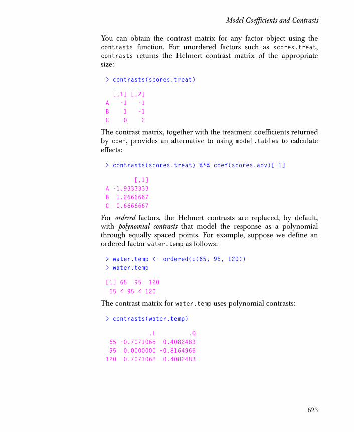
Model Coefficients and Contrasts
You can obtain the contrast matrix for any factor object using thecontrasts function. For unordered factors such as scores.treat,contrasts returns the Helmert contrast matrix of the appropriatesize:
> contrasts(scores.treat)
[,1] [,2]A -1 -1B 1 -1C 0 2
The contrast matrix, together with the treatment coefficients returnedby coef, provides an alternative to using model.tables to calculateeffects:
> contrasts(scores.treat) %*% coef(scores.aov)[-1]
[,1]A -1.9333333B 1.2666667C 0.6666667
For ordered factors, the Helmert contrasts are replaced, by default,with polynomial contrasts that model the response as a polynomialthrough equally spaced points. For example, suppose we define anordered factor water.temp as follows:
> water.temp <- ordered(c(65, 95, 120))> water.temp
[1] 65 95 120 65 < 95 < 120
The contrast matrix for water.temp uses polynomial contrasts:
> contrasts(water.temp)
.L .Q 65 -0.7071068 0.4082483 95 0.0000000 -0.8164966120 0.7071068 0.4082483
623

Chapter 17 Further Topics in Analysis of Variance
For the polynomial contrasts, represents the linear component of
the response, represents the quadratic component, and so on.When examining ANOVA summaries, you can split a factor’s effectsinto contrast terms to examine each component’s contribution to themodel. See the section Splitting Treatment Sums of Squares IntoContrast Terms for complete details.
β1
β2
624
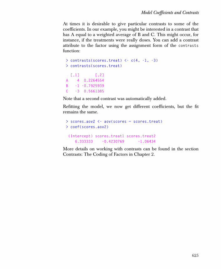
Model Coefficients and Contrasts
At times it is desirable to give particular contrasts to some of thecoefficients. In our example, you might be interested in a contrast thathas A equal to a weighted average of B and C. This might occur, forinstance, if the treatments were really doses. You can add a contrastattribute to the factor using the assignment form of the contrastsfunction:
> contrasts(scores.treat) <- c(4, -1, -3)> contrasts(scores.treat)
[,1] [,2]A 4 0.2264554B -1 -0.7925939C -3 0.5661385
Note that a second contrast was automatically added.
Refitting the model, we now get different coefficients, but the fitremains the same.
> scores.aov2 <- aov(scores ~ scores.treat)> coef(scores.aov2)
(Intercept) scores.treat1 scores.treat2 6.333333 -0.4230769 -1.06434
More details on working with contrasts can be found in the sectionContrasts: The Coding of Factors in Chapter 2.
625
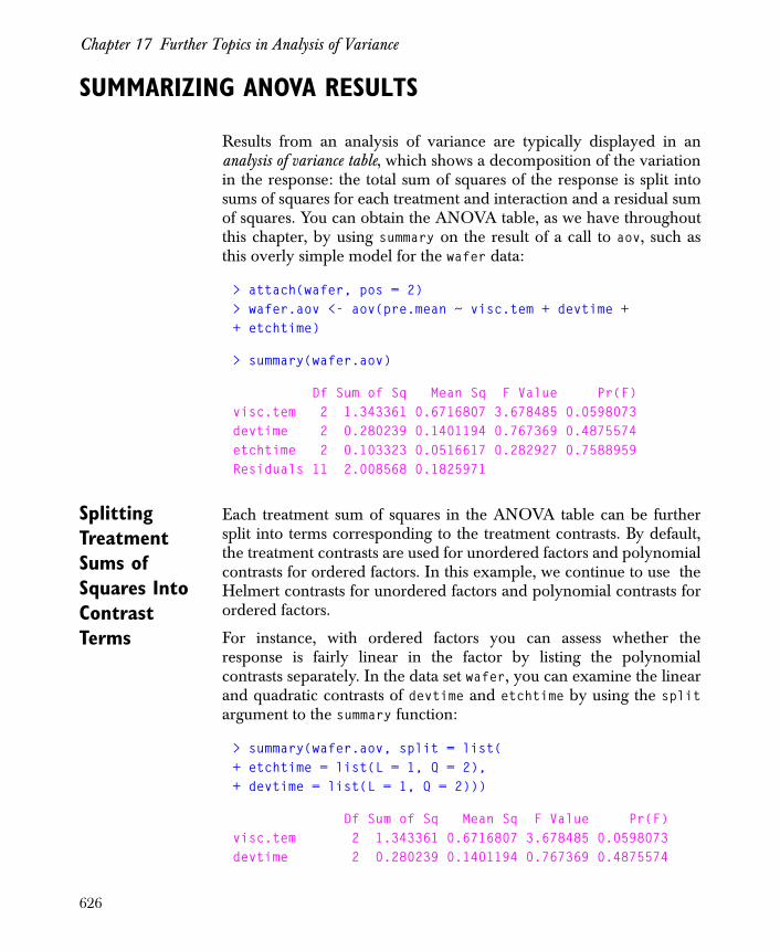
Chapter 17 Further Topics in Analysis of Variance
SUMMARIZING ANOVA RESULTS
Results from an analysis of variance are typically displayed in ananalysis of variance table, which shows a decomposition of the variationin the response: the total sum of squares of the response is split intosums of squares for each treatment and interaction and a residual sumof squares. You can obtain the ANOVA table, as we have throughoutthis chapter, by using summary on the result of a call to aov, such asthis overly simple model for the wafer data:
> attach(wafer, pos = 2)> wafer.aov <- aov(pre.mean ~ visc.tem + devtime ++ etchtime)
> summary(wafer.aov)
Df Sum of Sq Mean Sq F Value Pr(F)visc.tem 2 1.343361 0.6716807 3.678485 0.0598073devtime 2 0.280239 0.1401194 0.767369 0.4875574etchtime 2 0.103323 0.0516617 0.282927 0.7588959Residuals 11 2.008568 0.1825971
Splitting Treatment Sums of Squares Into Contrast Terms
Each treatment sum of squares in the ANOVA table can be furthersplit into terms corresponding to the treatment contrasts. By default,the treatment contrasts are used for unordered factors and polynomialcontrasts for ordered factors. In this example, we continue to use theHelmert contrasts for unordered factors and polynomial contrasts forordered factors.
For instance, with ordered factors you can assess whether theresponse is fairly linear in the factor by listing the polynomialcontrasts separately. In the data set wafer, you can examine the linearand quadratic contrasts of devtime and etchtime by using the splitargument to the summary function:
> summary(wafer.aov, split = list(+ etchtime = list(L = 1, Q = 2),+ devtime = list(L = 1, Q = 2)))
Df Sum of Sq Mean Sq F Value Pr(F)visc.tem 2 1.343361 0.6716807 3.678485 0.0598073devtime 2 0.280239 0.1401194 0.767369 0.4875574
626

Summarizing ANOVA Results
devtime: L 1 0.220865 0.2208653 1.209577 0.2949025 devtime: Q 1 0.059373 0.0593734 0.325161 0.5799830etchtime 2 0.103323 0.0516617 0.282927 0.7588959 etchtime: L 1 0.094519 0.0945188 0.517636 0.4868567 etchtime: Q 1 0.008805 0.0088047 0.048219 0.8302131Residuals 11 2.008568 0.1825971
Each of the (indented) split terms sum to their overall sum of squares.
The split argument can evaluate only the effects of the contrastsused to specify the ANOVA model: if you wish to test a specificcontrast, you need to set it explicitly before fitting the model. Thus, ifyou want to test a polynomial contrast for an unordered factor, youmust specify polynomial contrasts for the factor before fitting themodel. The same is true for other nondefault contrasts. For instance,the variable visc.tem in the wafer data set is a three-level factorconstructed by combining two levels of viscosity (204 and 206) withtwo levels of temperature (90 and 105).
> levels(visc.tem)
[1] "204,90" "206,90" "204,105"
To assess viscosity, supposing temperature has no effect, we define acontrast that takes the difference of the middle and the sum of the firstand third levels of visc.tem; the contrast matrix is automaticallycompleted:
# Assign visc.tem to your working directory.> visc.tem <- visc.tem> contrasts(visc.tem) <- c(-1, 2, -1)> contrasts(visc.tem)
[,1] [,2]204,90 -1 -7.071068e-01206,90 2 -1.110223e-16204,105 -1 7.071068e-01
> wafer.aov <- aov( pre.mean ~ visc.tem + devtime ++ etchtime)
# Detach the data set.> detach(2)
627

Chapter 17 Further Topics in Analysis of Variance
In this fitted model, the first contrast for visc.aov reflects the effect ofviscosity, as the summary shows below.
628

Summarizing ANOVA Results
> summary(wafer.aov, split = list(+ visc.tem = list(visc = 1)))
Df Sum of Sq Mean Sq F Value Pr(F)visc.tem 2 1.343361 0.671681 3.678485 0.0598073 visc.tem: visc 1 1.326336 1.326336 7.263730 0.0208372devtime 2 0.280239 0.140119 0.767369 0.4875574etchtime 2 0.103323 0.051662 0.282927 0.7588959Residuals 11 2.008568 0.182597
Treatment Means and Standard Errors
Commonly the ANOVA model is written in the form grand mean plustreatment effects,
The treatment effects, , , and , reflect changes in theresponse due to the combination of treatments. In thisparametrization, the effects (weighted by the replications) areconstrained to sum to zero.
Unfortunately, the use of the term effect in ANOVA is notstandardized: in factorial experiments an effect is the differencebetween treatment levels, in balanced designs it is the difference fromthe grand mean, and in unbalanced designs there are (at least) twodifferent standardizations that make sense.
The coefficients of an aov object returned by coef(aov.object) arecoefficients for the contrast variables derived by the aov function,rather than the grand-mean-plus-effects decomposition. The functionsdummy.coef and model.tables translate the internal coefficients intothe more natural treatment effects.
Balanced Designs
In a balanced design, both computing and interpreting effects arestraightforward. The following example uses the gun data frame,which is a design object with 36 rows representing runs of teams ofthree men loading and firing naval guns, attempting to get off asmany rounds per minute as possible. The three predictor variablesspecify the team, the physiques of the men on it, and the loadingmethod used. The outcome variable is the rounds fired per minute.
yijk μ αi βj αβ( )ij ε ijk+ + + +=
αi βj αβ( )ij
629
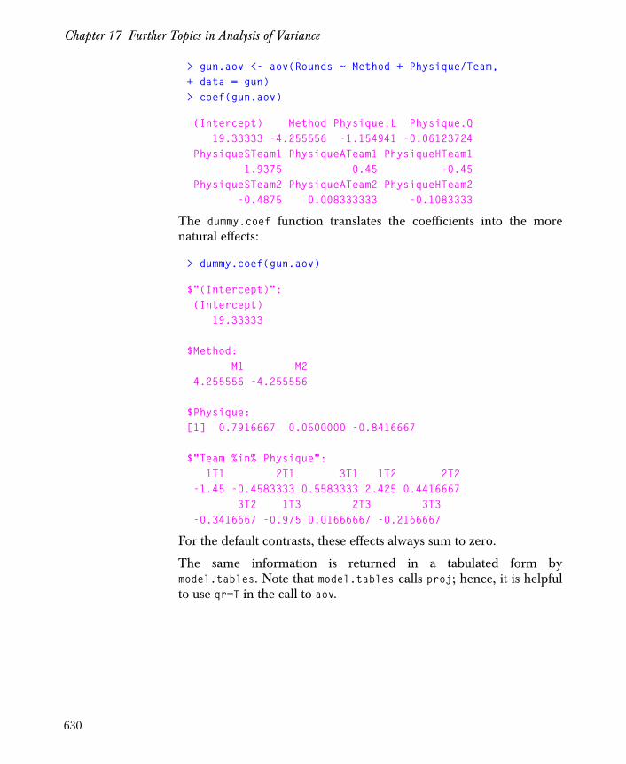
Chapter 17 Further Topics in Analysis of Variance
> gun.aov <- aov(Rounds ~ Method + Physique/Team, + data = gun)> coef(gun.aov)
(Intercept) Method Physique.L Physique.Q 19.33333 -4.255556 -1.154941 -0.06123724 PhysiqueSTeam1 PhysiqueATeam1 PhysiqueHTeam1 1.9375 0.45 -0.45 PhysiqueSTeam2 PhysiqueATeam2 PhysiqueHTeam2 -0.4875 0.008333333 -0.1083333
The dummy.coef function translates the coefficients into the morenatural effects:
> dummy.coef(gun.aov)
$"(Intercept)": (Intercept) 19.33333
$Method: M1 M2 4.255556 -4.255556
$Physique:[1] 0.7916667 0.0500000 -0.8416667
$"Team %in% Physique": 1T1 2T1 3T1 1T2 2T2 -1.45 -0.4583333 0.5583333 2.425 0.4416667 3T2 1T3 2T3 3T3 -0.3416667 -0.975 0.01666667 -0.2166667
For the default contrasts, these effects always sum to zero.
The same information is returned in a tabulated form bymodel.tables. Note that model.tables calls proj; hence, it is helpfulto use qr=T in the call to aov.
630
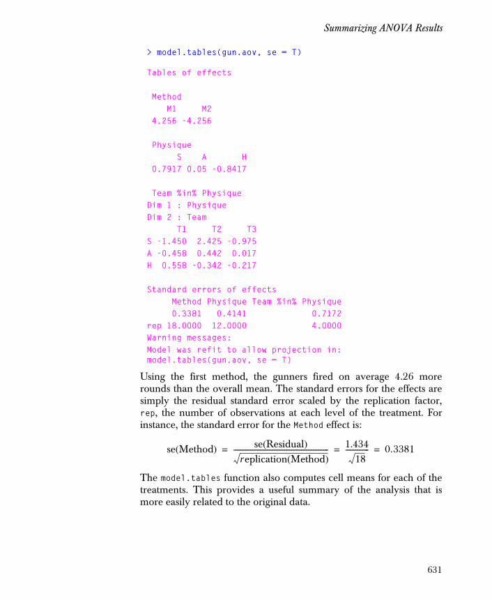
Summarizing ANOVA Results
> model.tables(gun.aov, se = T)
Tables of effects
Method M1 M2 4.256 -4.256
Physique S A H 0.7917 0.05 -0.8417
Team %in% PhysiqueDim 1 : PhysiqueDim 2 : Team T1 T2 T3S -1.450 2.425 -0.975A -0.458 0.442 0.017H 0.558 -0.342 -0.217
Standard errors of effects Method Physique Team %in% Physique 0.3381 0.4141 0.7172rep 18.0000 12.0000 4.0000Warning messages: Model was refit to allow projection in: model.tables(gun.aov, se = T)
Using the first method, the gunners fired on average 4.26 morerounds than the overall mean. The standard errors for the effects aresimply the residual standard error scaled by the replication factor,rep, the number of observations at each level of the treatment. Forinstance, the standard error for the Method effect is:
The model.tables function also computes cell means for each of thetreatments. This provides a useful summary of the analysis that ismore easily related to the original data.
se Method( ) se Residual( )
replication Method( )-------------------------------------------------------- 1.434
18-------------- 0.3381= = =
631
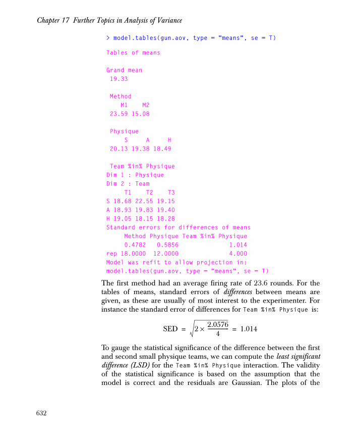
Chapter 17 Further Topics in Analysis of Variance
> model.tables(gun.aov, type = "means", se = T)
Tables of means
Grand mean 19.33
Method M1 M2 23.59 15.08
Physique S A H 20.13 19.38 18.49
Team %in% PhysiqueDim 1 : PhysiqueDim 2 : Team T1 T2 T3S 18.68 22.55 19.15A 18.93 19.83 19.40H 19.05 18.15 18.28Standard errors for differences of means Method Physique Team %in% Physique 0.4782 0.5856 1.014rep 18.0000 12.0000 4.000Model was refit to allow projection in: model.tables(gun.aov, type = "means", se = T)
The first method had an average firing rate of 23.6 rounds. For thetables of means, standard errors of differences between means aregiven, as these are usually of most interest to the experimenter. Forinstance the standard error of differences for Team %in% Physique is:
To gauge the statistical significance of the difference between the firstand second small physique teams, we can compute the least significantdifference (LSD) for the Team %in% Physique interaction. The validityof the statistical significance is based on the assumption that themodel is correct and the residuals are Gaussian. The plots of the
SED 2 2.05764
-----------------× 1.014= =
632
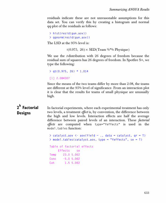
Summarizing ANOVA Results
residuals indicate these are not unreasonable assumptions for thisdata set. You can verify this by creating a histogram and normalqq-plot of the residuals as follows:
> hist(resid(gun.aov))> qqnorm(resid(gun.aov))
The LSD at the 95% level is:
We use the t-distribution with 26 degrees of freedom because theresidual sum of squares has 26 degrees of freedom. In Spotfire S+, wetype the following:
> qt(0.975, 26) * 1.014
[1] 2.084307
Since the means of the two teams differ by more than 2.08, the teamsare different at the 95% level of significance. From an interaction plotit is clear that the results for teams of small physique are unusuallyhigh.
2k Factorial Designs
In factorial experiments, where each experimental treatment has onlytwo levels, a treatment effect is, by convention, the difference betweenthe high and low levels. Interaction effects are half the averagedifference between paired levels of an interaction. These factorialeffects are computed when type="feffects" is used in themodel.tables function:
> catalyst.aov <- aov(Yield ~ ., data = catalyst, qr = T)> model.tables(catalyst.aov, type = "feffects", se = T)
Table of factorial effects Effects seTemp 23.0 5.062Conc -5.0 5.062Cat 1.5 5.062
t 0.975 26,( ) SED Team %*% Physique( )×
633
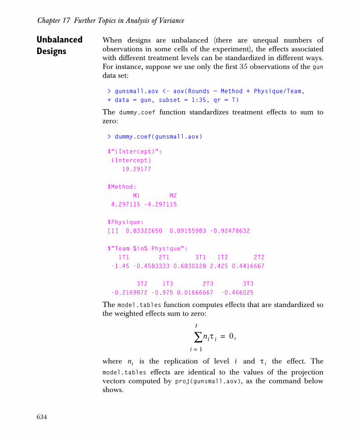
Chapter 17 Further Topics in Analysis of Variance
Unbalanced Designs
When designs are unbalanced (there are unequal numbers ofobservations in some cells of the experiment), the effects associatedwith different treatment levels can be standardized in different ways.For instance, suppose we use only the first 35 observations of the gundata set:
> gunsmall.aov <- aov(Rounds ~ Method + Physique/Team,+ data = gun, subset = 1:35, qr = T)
The dummy.coef function standardizes treatment effects to sum tozero:
> dummy.coef(gunsmall.aov)
$"(Intercept)": (Intercept) 19.29177
$Method: M1 M2 4.297115 -4.297115
$Physique:[1] 0.83322650 0.09155983 -0.92478632
$"Team %in% Physique": 1T1 2T1 3T1 1T2 2T2 -1.45 -0.4583333 0.6830128 2.425 0.4416667
3T2 1T3 2T3 3T3 -0.2169872 -0.975 0.01666667 -0.466025
The model.tables function computes effects that are standardized sothe weighted effects sum to zero:
,
where is the replication of level and the effect. Themodel.tables effects are identical to the values of the projectionvectors computed by proj(gunsmall.aov), as the command belowshows.
niτ i
i 1=
T
∑ 0=
ni i τ i
634

Summarizing ANOVA Results
> model.tables(gunsmall.aov)
Tables of effects
Method M1 M2 4.135 -4.378rep 18.000 17.000
Physique S A H 0.7923 0.05065 -0.9196rep 12.0000 12.00000 11.0000
Team %in% PhysiqueDim 1 : PhysiqueDim 2 : Team T1 T2 T3S -1.450 2.425 -0.975rep 4.000 4.000 4.000A -0.458 0.442 0.017rep 4.000 4.000 4.000H 0.639 -0.261 -0.505rep 4.000 4.000 3.000
With this standardization, treatment effects are orthogonal:consequently cell means can be computed by simply adding effects tothe grand mean; standard errors are also more readily computed.
> model.tables(gunsmall.aov, type = "means", se = T)
Standard error information not returned as design is unbalanced.Standard errors can be obtained through se.contrast.Tables of meansGrand mean
19.45
Method M1 M2 23.59 15.08rep 18.00 17.00
635
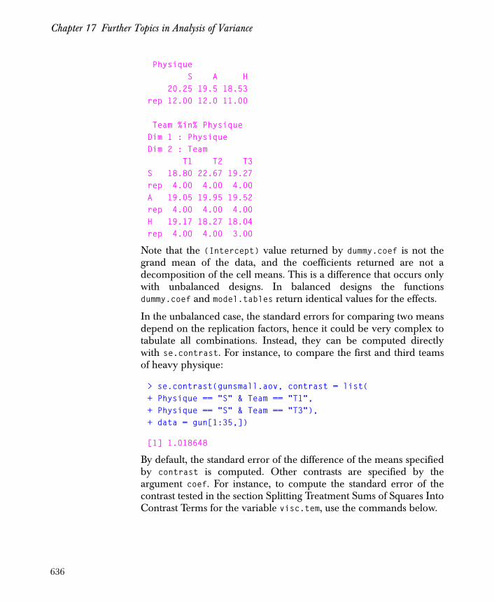
Chapter 17 Further Topics in Analysis of Variance
Physique S A H 20.25 19.5 18.53rep 12.00 12.0 11.00
Team %in% PhysiqueDim 1 : PhysiqueDim 2 : Team T1 T2 T3S 18.80 22.67 19.27rep 4.00 4.00 4.00A 19.05 19.95 19.52rep 4.00 4.00 4.00H 19.17 18.27 18.04rep 4.00 4.00 3.00
Note that the (Intercept) value returned by dummy.coef is not thegrand mean of the data, and the coefficients returned are not adecomposition of the cell means. This is a difference that occurs onlywith unbalanced designs. In balanced designs the functionsdummy.coef and model.tables return identical values for the effects.
In the unbalanced case, the standard errors for comparing two meansdepend on the replication factors, hence it could be very complex totabulate all combinations. Instead, they can be computed directlywith se.contrast. For instance, to compare the first and third teamsof heavy physique:
> se.contrast(gunsmall.aov, contrast = list(+ Physique == "S" & Team == "T1",+ Physique == "S" & Team == "T3"),+ data = gun[1:35,])
[1] 1.018648
By default, the standard error of the difference of the means specifiedby contrast is computed. Other contrasts are specified by theargument coef. For instance, to compute the standard error of thecontrast tested in the section Splitting Treatment Sums of Squares IntoContrast Terms for the variable visc.tem, use the commands below.
636
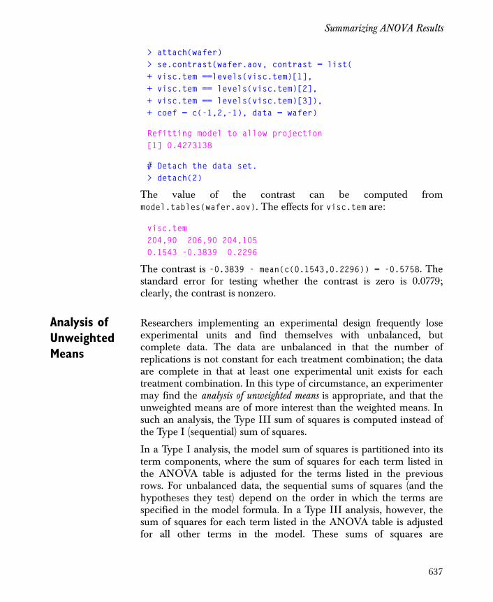
Summarizing ANOVA Results
> attach(wafer)> se.contrast(wafer.aov, contrast = list(+ visc.tem ==levels(visc.tem)[1],+ visc.tem == levels(visc.tem)[2],+ visc.tem == levels(visc.tem)[3]),+ coef = c(-1,2,-1), data = wafer)
Refitting model to allow projection[1] 0.4273138
# Detach the data set.> detach(2)
The value of the contrast can be computed frommodel.tables(wafer.aov). The effects for visc.tem are:
visc.tem204,90 206,90 204,1050.1543 -0.3839 0.2296
The contrast is -0.3839 - mean(c(0.1543,0.2296)) = -0.5758. Thestandard error for testing whether the contrast is zero is 0.0779;clearly, the contrast is nonzero.
Analysis of Unweighted Means
Researchers implementing an experimental design frequently loseexperimental units and find themselves with unbalanced, butcomplete data. The data are unbalanced in that the number ofreplications is not constant for each treatment combination; the dataare complete in that at least one experimental unit exists for eachtreatment combination. In this type of circumstance, an experimentermay find the analysis of unweighted means is appropriate, and that theunweighted means are of more interest than the weighted means. Insuch an analysis, the Type III sum of squares is computed instead ofthe Type I (sequential) sum of squares.
In a Type I analysis, the model sum of squares is partitioned into itsterm components, where the sum of squares for each term listed inthe ANOVA table is adjusted for the terms listed in the previousrows. For unbalanced data, the sequential sums of squares (and thehypotheses they test) depend on the order in which the terms arespecified in the model formula. In a Type III analysis, however, thesum of squares for each term listed in the ANOVA table is adjustedfor all other terms in the model. These sums of squares are
637

Chapter 17 Further Topics in Analysis of Variance
independent of the order that the terms are specified in the modelformula. If the data are balanced, the sequential sum of squares equalsthe Type III sum of squares. If the data are unbalanced but complete,then the Type III sums of squares are those obtained from Yates'weighted squares-of-means technique. In this case, the hypothesestested by the Type III sums of squares for the main effects is that thelevels of the unweighted means are equal.
For general observational studies, the sequential sum of squares maybe of more interest to an analyst. For a designed experiment, ananalyst may find the Type III sum of squares of more use.
The argument ssType to the methods anova.lm and summary.aovcompute the Type III sums of squares. To obtain the Type IIIanalysis for an aov object, use the option ssType=3 in the call to anovaor summary. In addition, the multicomp function can be used tocompute unweighted means. In this section, we provide examples todemonstrate these capabilities in an analysis of a designedexperiment.
The Baking Data The fat-surfactant example below is taken from Milliken and Johnson(1984, p. 166), where they analyze an unbalanced randomized blockfactorial design. Here, the specific volume of bread loaves baked fromdough that is mixed from each of nine Fat and Surfactant treatmentcombinations is measured. The experimenters blocked on four Flourtypes. Ten loaves had to be removed from the experiment, but atleast one loaf existed for each Fat x Surfactant combination and allmarginal means are estimable. Therefore, the Type III hypotheses aretestable. The data are given in Table 17.1.
The commands below create a Baking data set from the informationin Table 17.1.
> Baking <- data.frame(+ Fat = factor(+ c(rep(1,times=12), rep(2,times=12), rep(3,times=12))),+ Surfactant = factor(+ rep(c(1,1,1,1,2,2,2,2,3,3,3,3), times=3)),+ Flour = factor(rep(1:4, times=9)),+ Specific.Vol = c(6.7, 4.3, 5.7, NA, 7.1, NA, 5.9, 5.6,+ NA, 5.5, 6.4, 5.8, NA, 5.9, 7.4, 7.1, NA, 5.6, NA, 6.8,+ 6.4, 5.1, 6.2, 6.3, 7.1, 5.9, NA, NA, 7.3, 6.6,+ 8.1, 6.8, NA, 7.5, 9.1, NA))
638

Summarizing ANOVA Results
> Baking
Fat Surfactant Flour Specific.Vol 1 1 1 1 6.7 2 1 1 2 4.3 3 1 1 3 5.7 4 1 1 4 NA 5 1 2 1 7.1 6 1 2 2 NA 7 1 2 3 5.9 8 1 2 4 5.6 9 1 3 1 NA10 1 3 2 5.5. . .
The overparametrized model is:
for , , and . In this model, the
are coefficients corresponding to the levels in Fat, the correspond
to Flour, the correspond to Surfactant, and the are
Table 17.1: Specific volumes from a baking experiment.
Fat Surfactant Flour 1 Flour 2 Flour 3 Flour 4
1
1
2
3
6.7
7.1
4.3
5.5
5.7
5.9
6.4
5.6
5.8
2
1
2
3 6.4
5.9
5.6
5.1
7.4
6.2
7.1
6.8
6.3
3
1
2
3
7.1
7.3
5.9
6.6
7.5
8.1
9.1
6.8
μijk μ bi fj sk fs( )jk+ + + +=
i 1 … 4, ,= j 1 2 3, ,= k 1 2 3, ,= bi
fj
sk fs( )jk
639
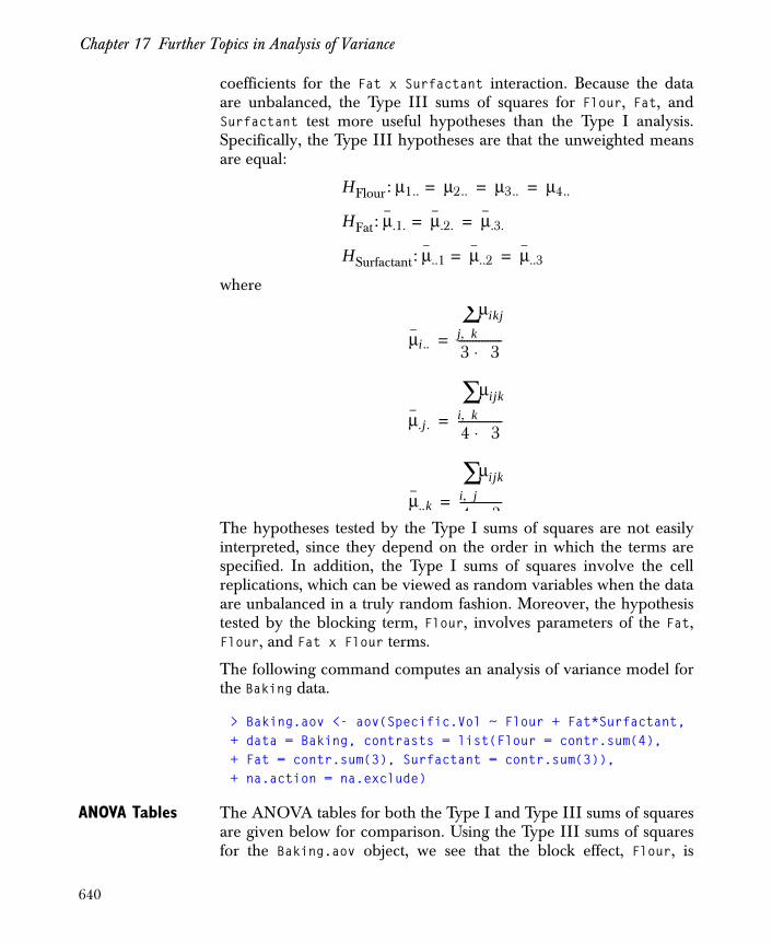
Chapter 17 Further Topics in Analysis of Variance
coefficients for the Fat x Surfactant interaction. Because the dataare unbalanced, the Type III sums of squares for Flour, Fat, andSurfactant test more useful hypotheses than the Type I analysis.Specifically, the Type III hypotheses are that the unweighted meansare equal:
where
The hypotheses tested by the Type I sums of squares are not easilyinterpreted, since they depend on the order in which the terms arespecified. In addition, the Type I sums of squares involve the cellreplications, which can be viewed as random variables when the dataare unbalanced in a truly random fashion. Moreover, the hypothesistested by the blocking term, Flour, involves parameters of the Fat,Flour, and Fat x Flour terms.
The following command computes an analysis of variance model forthe Baking data.
> Baking.aov <- aov(Specific.Vol ~ Flour + Fat*Surfactant,+ data = Baking, contrasts = list(Flour = contr.sum(4),+ Fat = contr.sum(3), Surfactant = contr.sum(3)),+ na.action = na.exclude)
ANOVA Tables The ANOVA tables for both the Type I and Type III sums of squaresare given below for comparison. Using the Type III sums of squaresfor the Baking.aov object, we see that the block effect, Flour, is
HFlour: μ1.. μ2.. μ3.. μ4..= = =
HFat: μ.1. μ.2. μ.3.= =
HSurfactant: μ..1 μ..2 μ..3= =
μi..
μikjj k,∑3 3⋅---------------=
μ.j.
μijki k,∑4 3⋅---------------=
μ..k
μijki j,∑4 3---------------=
640

Summarizing ANOVA Results
significant. In addition, Fat appears to be significant, but Surfactantis not (at a test size of ). In the presence of a significantinteraction, however, the test of the marginal means probably haslittle meaning for Fat and Surfactant.
> anova(Baking.aov)
Analysis of Variance Table Response: Specific.Vol Terms added sequentially (first to last) Df Sum of Sq Mean Sq F Value Pr(F) Flour 3 6.39310 2.131033 12.88269 0.0002587 Fat 2 10.33042 5.165208 31.22514 0.0000069 Surfactant 2 0.15725 0.078625 0.47531 0.6313678Fat:Surfactant 4 5.63876 1.409691 8.52198 0.0010569 Residuals 14 2.31586 0.165418
> anova(Baking.aov, ssType = 3)
Analysis of Variance Table Response: Specific.Vol Type III Sum of Squares Df Sum of Sq Mean Sq F Value Pr(F) Flour 3 8.69081 2.896937 17.51280 0.00005181 Fat 2 10.11785 5.058925 30.58263 0.00000778 Surfactant 2 0.99721 0.498605 3.01421 0.08153989Fat:Surfactant 4 5.63876 1.409691 8.52198 0.00105692 Residuals 14 2.31586 0.165418
Unweighted Means
The unweighted means computed below estimate the means given inthe Type III hypotheses for Flour, Fat, and Surfactant. The meansfor Flour x Surfactant in the overparametrized model are
.
α 0.05=
μ.jk
μijki∑
4------------=
641

Chapter 17 Further Topics in Analysis of Variance
We use the multicomp function with the argumentcomparisons="none" to compute the unweighted means and theirstandard errors.
# Unweighted means for Flour.> multicomp(Baking.aov, comparisons="none", focus="Flour")
95 % simultaneous confidence intervals for specified linear combinations, by the Sidak method
critical point: 2.8297 response variable: Specific.Vol
intervals excluding 0 are flagged by '****'
Estimate Std.Error Lower Bound Upper Bound 1 7.30 0.199 6.74 7.87 ****2 5.71 0.147 5.29 6.12 ****3 6.98 0.162 6.52 7.44 ****4 6.54 0.179 6.04 7.05 ****
# Unweighted means for Fat.> multicomp(Baking.aov, comparisons="none", focus="Fat")
95 % simultaneous confidence intervals for specified linear combinations, by the Tukey method
critical point: 2.6177 response variable: Specific.Vol
intervals excluding 0 are flagged by '****'
Estimate Std.Error Lower Bound Upper Bound 1 5.85 0.136 5.49 6.21 ****2 6.58 0.148 6.19 6.96 ****3 7.47 0.156 7.06 7.88 ****
642

Summarizing ANOVA Results
# Unweighted means for Surfactant.> multicomp(Baking.aov, comparisons = "none", + focus = "Surfactant")
95 % simultaneous confidence intervals for specified linear combinations, by the Tukey method
critical point: 2.6177 response variable: Specific.Vol
intervals excluding 0 are flagged by '****'
Estimate Std.Error Lower Bound Upper Bound 1 6.4 0.150 6.00 6.79 ****2 6.6 0.143 6.22 6.97 ****3 6.9 0.147 6.52 7.29 ****
# Unweighted means for Fat x Surfactant.> multicomp(Baking.aov, comparisons="none", focus="Fat",+ adjust = list(Surfactant = seq(3)))
95 % simultaneous confidence intervals for specified linear combinations, by the Sidak method
critical point: 3.2117 response variable: Specific.Vol
intervals excluding 0 are flagged by '****'
Estimate Std.Error Lower Bound Upper Bound 1.adj1 5.54 0.240 4.76 6.31 ****2.adj1 7.02 0.241 6.25 7.80 ****3.adj1 6.63 0.301 5.66 7.59 ****1.adj2 5.89 0.239 5.12 6.66 ****2.adj2 6.71 0.301 5.74 7.67 ****3.adj2 7.20 0.203 6.55 7.85 ****1.adj3 6.12 0.241 5.35 6.90 ****2.adj3 6.00 0.203 5.35 6.65 ****3.adj3 8.59 0.300 7.62 9.55 ****
643

Chapter 17 Further Topics in Analysis of Variance
In the output from multicomp, the unweighted means are given in theEstimate column. In the table for the Fat x Surfactant interaction,the adjX labels represent the levels in Surfactant. Thus, the value7.02 is the estimated mean specific volume at the second level in Fatand the first level in Surfactant.
Multiple Comparisons
The statistic for the Fat x Surfactant interaction in the Type IIIANOVA table is significant, so the tests for the marginal means of Fatand Surfactant have little meaning. We can, however, use multicompto find all pairwise comparisons of the mean Fat levels for each levelof Surfactant, and those of Surfactant for each level of Fat.
> multicomp(Baking.aov, focus = "Fat",+ adjust = list(Surfactant = seq(3)))
95 % simultaneous confidence intervals for specified linear combinations, by the Sidak method
critical point: 3.2117 response variable: Specific.Vol
intervals excluding 0 are flagged by '****'
Estimate Std.Error Lower Bound Upper Bound 1.adj1-2.adj1 -1.490 0.344 -2.590 -0.381 ****1.adj1-3.adj1 -1.090 0.377 -2.300 0.120 2.adj1-3.adj1 0.394 0.394 -0.872 1.660 1.adj2-2.adj2 -0.817 0.390 -2.070 0.434 1.adj2-3.adj2 -1.310 0.314 -2.320 -0.300 ****2.adj2-3.adj2 -0.492 0.363 -1.660 0.674 1.adj3-2.adj3 0.123 0.316 -0.891 1.140 1.adj3-3.adj3 -2.470 0.378 -3.680 -1.250 ****2.adj3-3.adj3 -2.590 0.363 -3.750 -1.420 ****
> multicomp(Baking.aov, focus = "Surfactant", + adjust = list(Fat = seq(3)))
95 % simultaneous confidence intervals for specified linear combinations, by the Sidak method
critical point: 3.2117 response variable: Specific.Vol
intervals excluding 0 are flagged by '****'
F
644
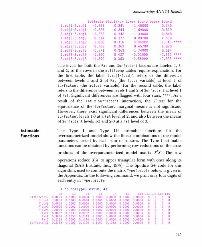
Summarizing ANOVA Results
Estimate Std.Error Lower Bound Upper Bound 1.adj1-2.adj1 -0.355 0.341 -1.45000 0.740 1.adj1-3.adj1 -0.587 0.344 -1.69000 0.519 2.adj1-3.adj1 -0.232 0.342 -1.33000 0.868 1.adj2-2.adj2 0.314 0.377 -0.89700 1.530 1.adj2-3.adj2 1.020 0.316 0.00922 2.040 ****2.adj2-3.adj2 0.708 0.363 -0.45700 1.870 1.adj3-2.adj3 -0.571 0.363 -1.74000 0.594 1.adj3-3.adj3 -1.960 0.427 -3.33000 -0.590 ****2.adj3-3.adj3 -1.390 0.363 -2.55000 -0.225 ****
The levels for both the Fat and Surfactant factors are labeled 1, 2,and 3, so the rows in the multicomp tables require explanation. Forthe first table, the label 1.adj1-2.adj1 refers to the differencebetween levels 1 and 2 of Fat (the focus variable) at level 1 ofSurfactant (the adjust variable). For the second table, the labelrefers to the difference between levels 1 and 2 of Surfactant at level 1of Fat. Significant differences are flagged with four stars, ****. As aresult of the Fat x Surfactant interaction, the test for theequivalence of the Surfactant marginal means is not significant.However, there exist significant differences between the mean ofSurfactant levels 1-3 at a Fat level of 2, and also between the meansof Surfactant levels 1-3 and 2-3 at a Fat level of 3.
Estimable Functions
The Type I and Type III estimable functions for theoverparametrized model show the linear combinations of the modelparameters, tested by each sum of squares. The Type I estimablefunctions can be obtained by performing row reductions on the cross
products of the overparameterized model matrix . The row
operations reduce to upper triangular form with ones along itsdiagonal (SAS Institute, Inc., 1978). The Spotfire S+ code for thisalgorithm, used to compute the matrix TypeI.estim below, is given inthe Appendix. In the following command, we print only four digits ofeach entry in TypeI.estim.
> round(TypeI.estim, 4) L2 L3 L4 L6 L7 L9 L10 L12 L13 L15 L16 (Intercept) 0.0000 0.0000 0.0000 0.0000 0.0000 0.0000 0.0000 0 0 0 0 Flour1 1.0000 0.0000 0.0000 0.0000 0.0000 0.0000 0.0000 0 0 0 0 Flour2 0.0000 1.0000 0.0000 0.0000 0.0000 0.0000 0.0000 0 0 0 0 Flour3 0.0000 0.0000 1.0000 0.0000 0.0000 0.0000 0.0000 0 0 0 0 Flour4 -1.0000 -1.0000 -1.0000 0.0000 0.0000 0.0000 0.0000 0 0 0 0 Fat1 0.0667 -0.0833 0.0952 1.0000 0.0000 0.0000 0.0000 0 0 0 0 Fat2 -0.3000 -0.1250 -0.2143 0.0000 1.0000 0.0000 0.0000 0 0 0 0 Fat3 0.2333 0.2083 0.1190 -1.0000 -1.0000 0.0000 0.0000 0 0 0 0 Surfactant1 0.2333 0.2083 0.1190 0.1152 0.1338 1.0000 0.0000 0 0 0 0
F
XtX
XtX
645
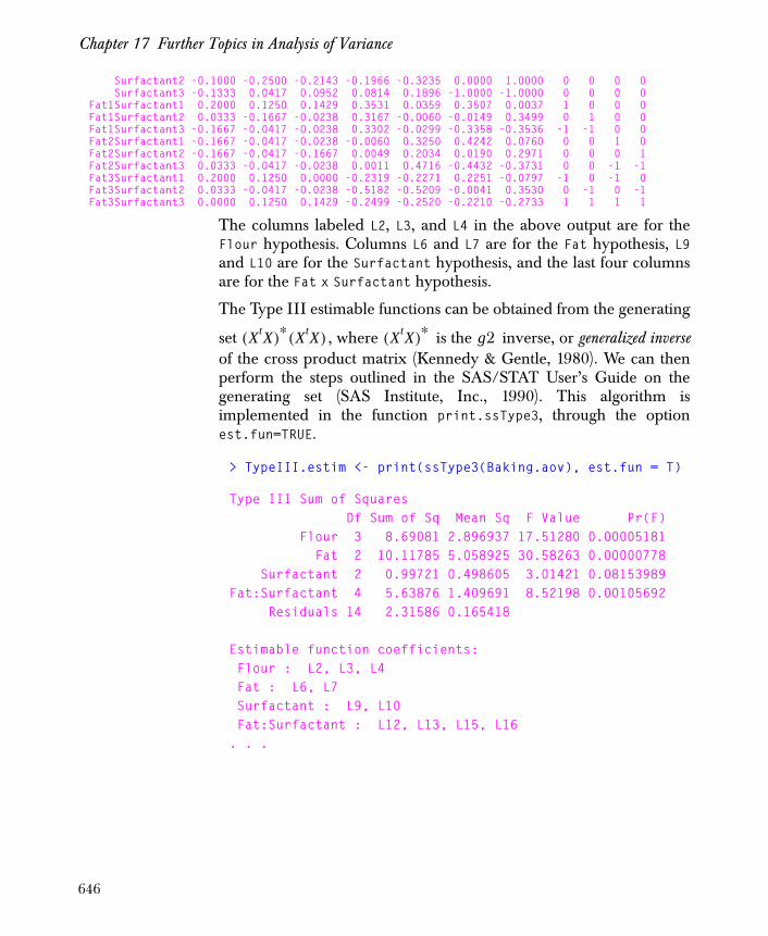
Chapter 17 Further Topics in Analysis of Variance
Surfactant2 -0.1000 -0.2500 -0.2143 -0.1966 -0.3235 0.0000 1.0000 0 0 0 0 Surfactant3 -0.1333 0.0417 0.0952 0.0814 0.1896 -1.0000 -1.0000 0 0 0 0Fat1Surfactant1 0.2000 0.1250 0.1429 0.3531 0.0359 0.3507 0.0037 1 0 0 0Fat1Surfactant2 0.0333 -0.1667 -0.0238 0.3167 -0.0060 -0.0149 0.3499 0 1 0 0Fat1Surfactant3 -0.1667 -0.0417 -0.0238 0.3302 -0.0299 -0.3358 -0.3536 -1 -1 0 0Fat2Surfactant1 -0.1667 -0.0417 -0.0238 -0.0060 0.3250 0.4242 0.0760 0 0 1 0Fat2Surfactant2 -0.1667 -0.0417 -0.1667 0.0049 0.2034 0.0190 0.2971 0 0 0 1Fat2Surfactant3 0.0333 -0.0417 -0.0238 0.0011 0.4716 -0.4432 -0.3731 0 0 -1 -1Fat3Surfactant1 0.2000 0.1250 0.0000 -0.2319 -0.2271 0.2251 -0.0797 -1 0 -1 0Fat3Surfactant2 0.0333 -0.0417 -0.0238 -0.5182 -0.5209 -0.0041 0.3530 0 -1 0 -1Fat3Surfactant3 0.0000 0.1250 0.1429 -0.2499 -0.2520 -0.2210 -0.2733 1 1 1 1
The columns labeled L2, L3, and L4 in the above output are for theFlour hypothesis. Columns L6 and L7 are for the Fat hypothesis, L9and L10 are for the Surfactant hypothesis, and the last four columnsare for the Fat x Surfactant hypothesis.
The Type III estimable functions can be obtained from the generating
set , where is the inverse, or generalized inverseof the cross product matrix (Kennedy & Gentle, 1980). We can thenperform the steps outlined in the SAS/STAT User’s Guide on thegenerating set (SAS Institute, Inc., 1990). This algorithm isimplemented in the function print.ssType3, through the optionest.fun=TRUE.
> TypeIII.estim <- print(ssType3(Baking.aov), est.fun = T)
Type III Sum of Squares Df Sum of Sq Mean Sq F Value Pr(F) Flour 3 8.69081 2.896937 17.51280 0.00005181 Fat 2 10.11785 5.058925 30.58263 0.00000778 Surfactant 2 0.99721 0.498605 3.01421 0.08153989Fat:Surfactant 4 5.63876 1.409691 8.52198 0.00105692 Residuals 14 2.31586 0.165418
Estimable function coefficients: Flour : L2, L3, L4 Fat : L6, L7 Surfactant : L9, L10 Fat:Surfactant : L12, L13, L15, L16. . .
XtX( )∗ XtX( ) XtX( )∗ g2
646
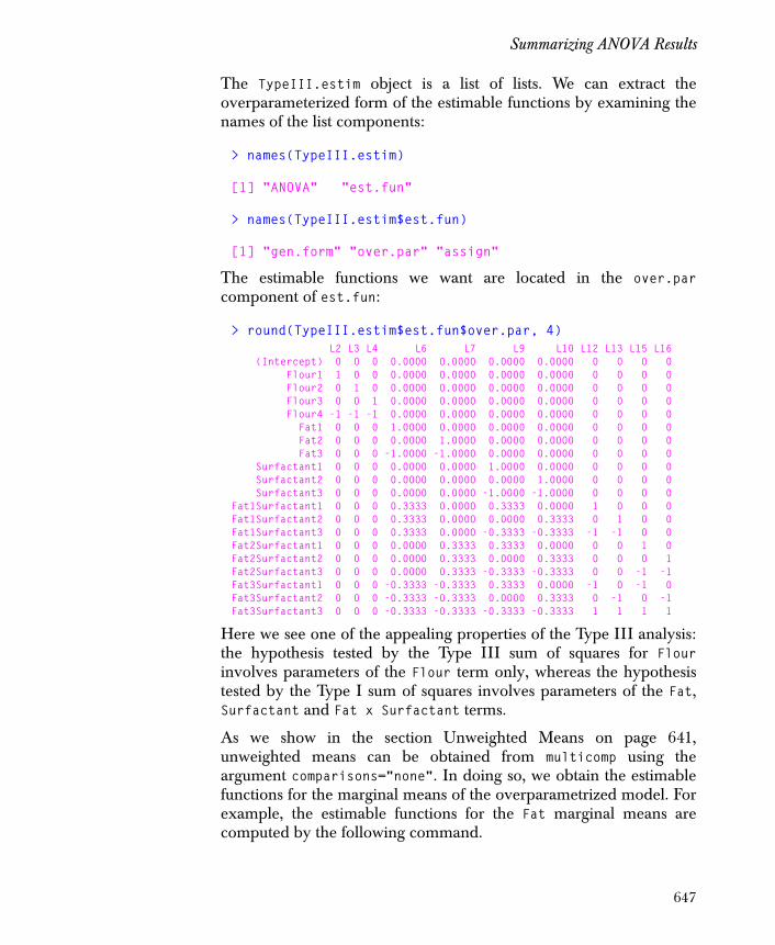
Summarizing ANOVA Results
The TypeIII.estim object is a list of lists. We can extract theoverparameterized form of the estimable functions by examining thenames of the list components:
> names(TypeIII.estim)
[1] "ANOVA" "est.fun"
> names(TypeIII.estim$est.fun)
[1] "gen.form" "over.par" "assign"
The estimable functions we want are located in the over.parcomponent of est.fun:
> round(TypeIII.estim$est.fun$over.par, 4) L2 L3 L4 L6 L7 L9 L10 L12 L13 L15 L16 (Intercept) 0 0 0 0.0000 0.0000 0.0000 0.0000 0 0 0 0 Flour1 1 0 0 0.0000 0.0000 0.0000 0.0000 0 0 0 0 Flour2 0 1 0 0.0000 0.0000 0.0000 0.0000 0 0 0 0 Flour3 0 0 1 0.0000 0.0000 0.0000 0.0000 0 0 0 0 Flour4 -1 -1 -1 0.0000 0.0000 0.0000 0.0000 0 0 0 0 Fat1 0 0 0 1.0000 0.0000 0.0000 0.0000 0 0 0 0 Fat2 0 0 0 0.0000 1.0000 0.0000 0.0000 0 0 0 0 Fat3 0 0 0 -1.0000 -1.0000 0.0000 0.0000 0 0 0 0 Surfactant1 0 0 0 0.0000 0.0000 1.0000 0.0000 0 0 0 0 Surfactant2 0 0 0 0.0000 0.0000 0.0000 1.0000 0 0 0 0 Surfactant3 0 0 0 0.0000 0.0000 -1.0000 -1.0000 0 0 0 0Fat1Surfactant1 0 0 0 0.3333 0.0000 0.3333 0.0000 1 0 0 0Fat1Surfactant2 0 0 0 0.3333 0.0000 0.0000 0.3333 0 1 0 0Fat1Surfactant3 0 0 0 0.3333 0.0000 -0.3333 -0.3333 -1 -1 0 0Fat2Surfactant1 0 0 0 0.0000 0.3333 0.3333 0.0000 0 0 1 0Fat2Surfactant2 0 0 0 0.0000 0.3333 0.0000 0.3333 0 0 0 1Fat2Surfactant3 0 0 0 0.0000 0.3333 -0.3333 -0.3333 0 0 -1 -1Fat3Surfactant1 0 0 0 -0.3333 -0.3333 0.3333 0.0000 -1 0 -1 0Fat3Surfactant2 0 0 0 -0.3333 -0.3333 0.0000 0.3333 0 -1 0 -1Fat3Surfactant3 0 0 0 -0.3333 -0.3333 -0.3333 -0.3333 1 1 1 1
Here we see one of the appealing properties of the Type III analysis:the hypothesis tested by the Type III sum of squares for Flourinvolves parameters of the Flour term only, whereas the hypothesistested by the Type I sum of squares involves parameters of the Fat,Surfactant and Fat x Surfactant terms.
As we show in the section Unweighted Means on page 641,unweighted means can be obtained from multicomp using theargument comparisons="none". In doing so, we obtain the estimablefunctions for the marginal means of the overparametrized model. Forexample, the estimable functions for the Fat marginal means arecomputed by the following command.
647

Chapter 17 Further Topics in Analysis of Variance
> Fat.mcomp <- multicomp(Baking.aov, focus = "Fat",+ comparisons = "none")> round(Fat.mcomp$lmat, 4)
1 2 3 (Intercept) 1.0000 1.0000 1.0000 Flour1 0.2500 0.2500 0.2500 Flour2 0.2500 0.2500 0.2500 Flour3 0.2500 0.2500 0.2500 Flour4 0.2500 0.2500 0.2500 Fat1 1.0000 0.0000 0.0000 Fat2 0.0000 1.0000 0.0000 Fat3 0.0000 0.0000 1.0000 Surfactant1 0.3333 0.3333 0.3333 Surfactant2 0.3333 0.3333 0.3333 Surfactant3 0.3333 0.3333 0.3333Fat1Surfactant1 0.3333 0.0000 0.0000Fat1Surfactant2 0.3333 0.0000 0.0000Fat1Surfactant3 0.3333 0.0000 0.0000Fat2Surfactant1 0.0000 0.3333 0.0000Fat2Surfactant2 0.0000 0.3333 0.0000Fat2Surfactant3 0.0000 0.3333 0.0000Fat3Surfactant1 0.0000 0.0000 0.3333Fat3Surfactant2 0.0000 0.0000 0.3333Fat3Surfactant3 0.0000 0.0000 0.3333
The reader can verify that the Type III estimable functions for Fat arethe differences between columns 1 and 3, and between columns 2 and3. Thus, the L6 column in the over.par component of TypeIII.estimis the difference between the first and third columns of theFat.mcomp$lmat object above. Likewise, the L7 column in the outputfrom TypeIII.estim is the difference between the second and thirdcolumns of Fat.mcomp$lmat.
Sigma Restricted Parametrization
The function lm reparametrizes a linear model in an attempt to makethe model matrix full column rank. In this section, we explore theanalysis of the unweighted means for Fat using the sigma restrictedlinear model. In the sigma restricted parameterization, the sum of thelevel estimates of each effect is constrained to be zero. That is,
.bii∑ fj
j∑ sk
k∑ fs( )jk
j∑ fs( )jk
k∑ 0= = = = =
648

Summarizing ANOVA Results
Therefore, any effect that we sum over in the mean estimate vanishes.Specifically, we have for the Fat variable inBaking.aov. We use the sigma restrictions to compute Baking.aov onpage 640, since we specify contr.sum in the contrasts argument toaov. For clarity, the command is repeated here:
> Baking.aov <- aov(Specific.Vol ~ Flour + Fat*Surfactant,+ data = Baking, contrasts = list(Flour = contr.sum(4),+ Fat = contr.sum(3), Surfactant = contr.sum(3)),+ na.action = na.exclude)
In this setting, the unweighted means for Fat can be computed withthe estimable functions given in L below.
# Define a vector of descriptive row names.> my.rownames <- c("(Intercept)", + "Flour1", "Flour2", "Flour3", "Fat1", "Fat2",+ "Surfactant1", "Surfactant2", + "Fat1Surfactant1", "Fat2Surfactant1",+ "Fat1Surfactant2", "Fat2Surfactant2")
> L <- as.matrix(data.frame(+ Fat.1 = c(1,0,0,0,1,rep(0,7)),+ Fat.2 = c(1,0,0,0,0,1,rep(0,6)),+ Fat.3 = c(1,0,0,0,-1,-1,rep(0,6)),+ row.names = my.rownames))
> L
Fat.1 Fat.2 Fat.3 (Intercept) 1 1 1 Flour1 0 0 0 Flour2 0 0 0 Flour3 0 0 0 Fat1 1 0 -1 Fat2 0 1 -1 Surfactant1 0 0 0 Surfactant2 0 0 0Fat1Surfactant1 0 0 0Fat2Surfactant1 0 0 0Fat1Surfactant2 0 0 0Fat2Surfactant2 0 0 0
f1 f2 f3+ + 0=
649
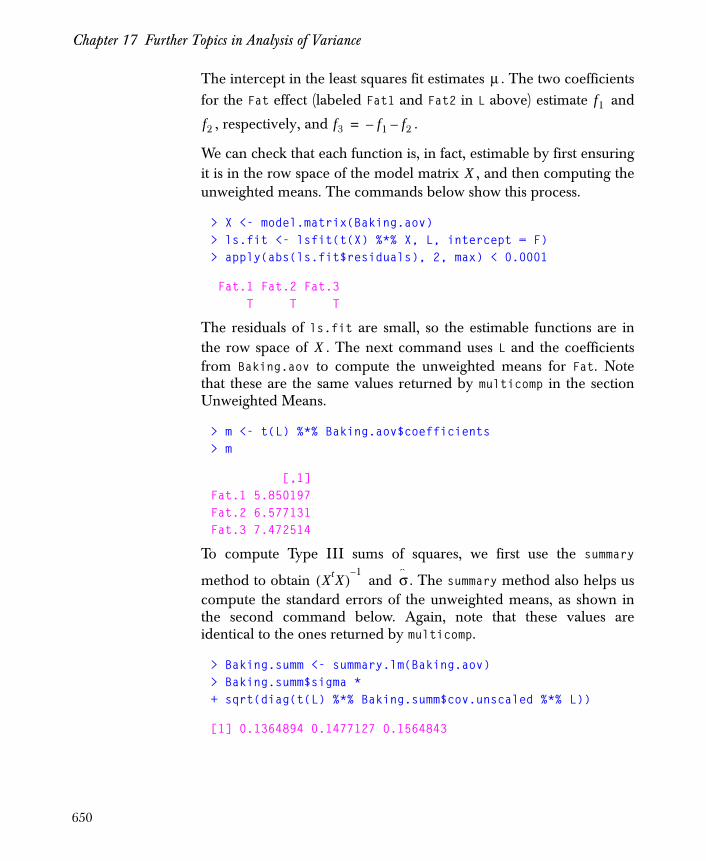
Chapter 17 Further Topics in Analysis of Variance
The intercept in the least squares fit estimates . The two coefficientsfor the Fat effect (labeled Fat1 and Fat2 in L above) estimate and
, respectively, and .
We can check that each function is, in fact, estimable by first ensuringit is in the row space of the model matrix , and then computing theunweighted means. The commands below show this process.
> X <- model.matrix(Baking.aov)> ls.fit <- lsfit(t(X) %*% X, L, intercept = F)> apply(abs(ls.fit$residuals), 2, max) < 0.0001
Fat.1 Fat.2 Fat.3 T T T
The residuals of ls.fit are small, so the estimable functions are inthe row space of . The next command uses L and the coefficientsfrom Baking.aov to compute the unweighted means for Fat. Notethat these are the same values returned by multicomp in the sectionUnweighted Means.
> m <- t(L) %*% Baking.aov$coefficients> m
[,1]Fat.1 5.850197Fat.2 6.577131Fat.3 7.472514
To compute Type III sums of squares, we first use the summary
method to obtain and . The summary method also helps uscompute the standard errors of the unweighted means, as shown inthe second command below. Again, note that these values areidentical to the ones returned by multicomp.
> Baking.summ <- summary.lm(Baking.aov)> Baking.summ$sigma * + sqrt(diag(t(L) %*% Baking.summ$cov.unscaled %*% L))
[1] 0.1364894 0.1477127 0.1564843
μf1
f2 f3 f1– f2–=
X
X
XtX( )1–
σ
650
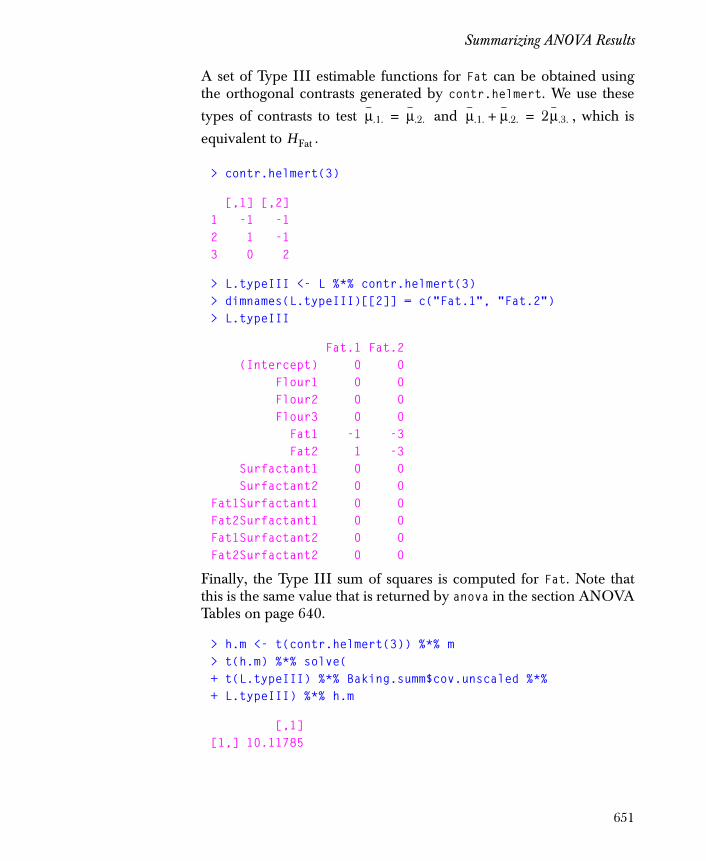
Summarizing ANOVA Results
A set of Type III estimable functions for Fat can be obtained usingthe orthogonal contrasts generated by contr.helmert. We use these
types of contrasts to test and , which is
equivalent to .
> contr.helmert(3)
[,1] [,2]1 -1 -12 1 -13 0 2
> L.typeIII <- L %*% contr.helmert(3)> dimnames(L.typeIII)[[2]] = c("Fat.1", "Fat.2")> L.typeIII
Fat.1 Fat.2 (Intercept) 0 0 Flour1 0 0 Flour2 0 0 Flour3 0 0 Fat1 -1 -3 Fat2 1 -3 Surfactant1 0 0 Surfactant2 0 0Fat1Surfactant1 0 0Fat2Surfactant1 0 0Fat1Surfactant2 0 0Fat2Surfactant2 0 0
Finally, the Type III sum of squares is computed for Fat. Note thatthis is the same value that is returned by anova in the section ANOVATables on page 640.
> h.m <- t(contr.helmert(3)) %*% m> t(h.m) %*% solve(+ t(L.typeIII) %*% Baking.summ$cov.unscaled %*% + L.typeIII) %*% h.m
[,1][1,] 10.11785
μ.1. μ.2.= μ.1. μ.2.+ 2μ.3.=
HFat
651
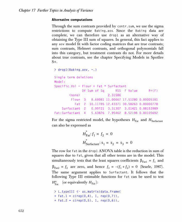
Chapter 17 Further Topics in Analysis of Variance
Alternative computations
Through the sum contrasts provided by contr.sum, we use the sigmarestrictions to compute Baking.aov. Since the Baking data arecomplete, we can therefore use drop1 as an alternative way ofobtaining the Type III sum of squares. In general, this fact applies toany aov model fit with factor coding matrices that are true contrasts;sum contrasts, Helmert contrasts, and orthogonal polynomials fallinto this category, but treatment contrasts do not. For more detailsabout true contrasts, see the chapter Specifying Models in SpotfireS+.
> drop1(Baking.aov, ~.)
Single term deletionsModel:Specific.Vol ~ Flour + Fat * Surfactant Df Sum of Sq RSS F Value Pr(F) <none> 2.31586 Flour 3 8.69081 11.00667 17.51280 0.00005181 Fat 2 10.11785 12.43371 30.58263 0.00000778 Surfactant 2 0.99721 3.31307 3.01421 0.08153989Fat:Surfactant 4 5.63876 7.95462 8.52198 0.00105692
For the sigma restricted model, the hypotheses and can also be expressed as
The row for Fat in the drop1 ANOVA table is the reduction in sum ofsquares due to Fat, given that all other terms are in the model. Thissimultaneously tests that the least squares coefficients and
are zero, and hence (Searle, 1987).The same argument applies to Surfactant. It follows that thefollowing Type III estimable functions for Fat can be used to test
(or equivalently ):
> L.typeIII <- as.matrix(data.frame(+ Fat.1 = c(rep(0,4), 1, rep(0,7)),+ Fat.2 = c(rep(0,5), 1, rep(0,6)),
HFat HSurfactant
HFat* : f1 f2 0= =
HSurfactant* : s1 s2 s3 0= = =
βFat1 f1=
βFat2 f2= f3 f1 f2+( )– 0= =
H∗Fat
HFat
652

Summarizing ANOVA Results
+ row.names = my.rownames))
> L.typeIII
Fat.1 Fat.2 (Intercept) 0 0 Flour1 0 0 Flour2 0 0 Flour3 0 0 Fat1 1 0 Fat2 0 1 Surfactant1 0 0 Surfactant2 0 0Fat1Surfactant1 0 0Fat2Surfactant1 0 0Fat1Surfactant2 0 0Fat2Surfactant2 0 0
> h.c <- t(L.typeIII) %*% Baking.aov$coef> t(h.c) %*% solve(t(L.typeIII) %*%+ Baking.summ$cov.unscaled %*% L.typeIII) %*% h.c
[,1][1,] 10.11785
Again, this is the same value for the Type III sum of squares that bothanova and drop1 return.
653
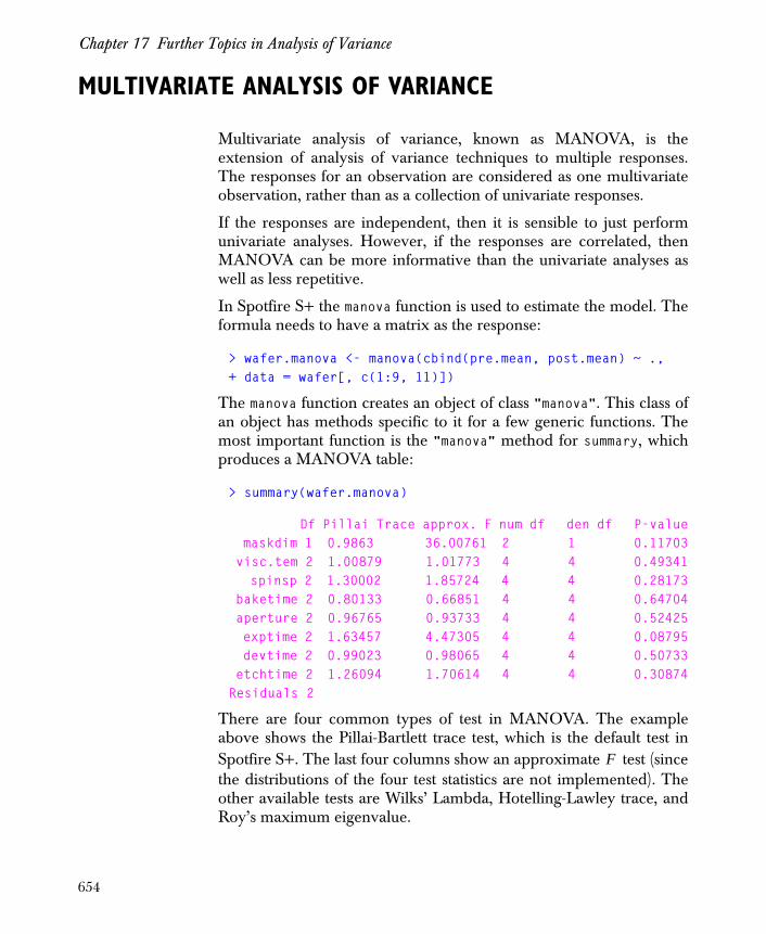
Chapter 17 Further Topics in Analysis of Variance
MULTIVARIATE ANALYSIS OF VARIANCE
Multivariate analysis of variance, known as MANOVA, is theextension of analysis of variance techniques to multiple responses.The responses for an observation are considered as one multivariateobservation, rather than as a collection of univariate responses.
If the responses are independent, then it is sensible to just performunivariate analyses. However, if the responses are correlated, thenMANOVA can be more informative than the univariate analyses aswell as less repetitive.
In Spotfire S+ the manova function is used to estimate the model. Theformula needs to have a matrix as the response:
> wafer.manova <- manova(cbind(pre.mean, post.mean) ~ .,+ data = wafer[, c(1:9, 11)])
The manova function creates an object of class "manova". This class ofan object has methods specific to it for a few generic functions. Themost important function is the "manova" method for summary, whichproduces a MANOVA table:
> summary(wafer.manova)
Df Pillai Trace approx. F num df den df P-value maskdim 1 0.9863 36.00761 2 1 0.11703 visc.tem 2 1.00879 1.01773 4 4 0.49341 spinsp 2 1.30002 1.85724 4 4 0.28173 baketime 2 0.80133 0.66851 4 4 0.64704 aperture 2 0.96765 0.93733 4 4 0.52425 exptime 2 1.63457 4.47305 4 4 0.08795 devtime 2 0.99023 0.98065 4 4 0.50733 etchtime 2 1.26094 1.70614 4 4 0.30874Residuals 2
There are four common types of test in MANOVA. The exampleabove shows the Pillai-Bartlett trace test, which is the default test inSpotfire S+. The last four columns show an approximate test (sincethe distributions of the four test statistics are not implemented). Theother available tests are Wilks’ Lambda, Hotelling-Lawley trace, andRoy’s maximum eigenvalue.
F
654
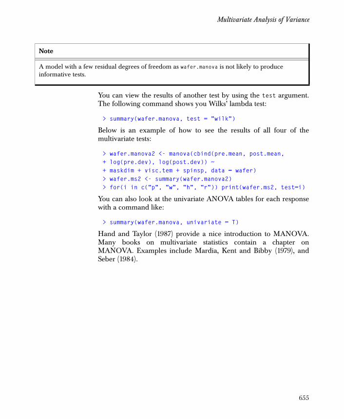
Multivariate Analysis of Variance
You can view the results of another test by using the test argument.The following command shows you Wilks’ lambda test:
> summary(wafer.manova, test = "wilk")
Below is an example of how to see the results of all four of themultivariate tests:
> wafer.manova2 <- manova(cbind(pre.mean, post.mean,+ log(pre.dev), log(post.dev)) ~ + maskdim + visc.tem + spinsp, data = wafer)> wafer.ms2 <- summary(wafer.manova2)> for(i in c("p", "w", "h", "r")) print(wafer.ms2, test=i)
You can also look at the univariate ANOVA tables for each responsewith a command like:
> summary(wafer.manova, univariate = T)
Hand and Taylor (1987) provide a nice introduction to MANOVA.Many books on multivariate statistics contain a chapter onMANOVA. Examples include Mardia, Kent and Bibby (1979), andSeber (1984).
Note
A model with a few residual degrees of freedom as wafer.manova is not likely to produce informative tests.
655

Chapter 17 Further Topics in Analysis of Variance
SPLIT-PLOT DESIGNS
A split-plot design contains more than one source of error. This canarise because factors are applied at different scales, as in the guayuleexample below.
Split-plots are also encountered because of restrictions on therandomization. For example, an experiment involving oventemperature and baking time will probably not randomize the oventemperature totally, but rather only change the temperature after allof the runs for that temperature have been made. This type of designis often mistakenly analyzed as if there were no restrictions on therandomization (an indication of this can be p-values that are close to1). See Hicks (1973) and Daniel (1976).
Spotfire S+ includes the guayule data frame which is also discussed inChambers and Hastie (1992). This experiment was on eight varietiesof guayule (a rubber producing shrub) and four treatments on theseeds. Since a flat (a shallow box for starting seedlings) was not largeenough to contain all 32 combinations of variety and treatment, thedesign was to use only a single variety in each flat and to apply eachtreatment within each flat. Thus the flats each consist of four sub-plots. This is a split-plot design since flats are the experimental unitfor varieties, but the sub-plots are the experimental unit for thetreatments. The response is the number of plants that germinated ineach sub-plot.
To analyze a split-plot design like this, put the variable thatcorresponds to the whole plot in an Error term in the formula of theaov call:
> gua.aov1 <- aov(plants ~ variety * treatment ++ Error(flats), data = guayule)
As usual, you can get an ANOVA table with summary:
> summary(gua.aov1)
Error: flats Df Sum of Sq Mean Sq F Value Pr(F)variety 7 763.156 109.0223 1.232036 0.3420697Residuals 16 1415.833 88.4896
656
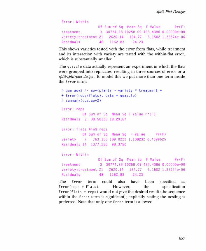
Split-Plot Designs
Error: Within Df Sum of Sq Mean Sq F Value Pr(F)treatment 3 30774.28 10258.09 423.4386 0.00000e+00variety:treatment 21 2620.14 124.77 5.1502 1.32674e-06Residuals 48 1162.83 24.23
This shows varieties tested with the error from flats, while treatmentand its interaction with variety are tested with the within-flat error,which is substantially smaller.
The guayule data actually represent an experiment in which the flatswere grouped into replicates, resulting in three sources of error or asplit-split-plot design . To model this we put more than one term insidethe Error term:
> gua.aov2 <- aov(plants ~ variety * treatment ++ Error(reps/flats), data = guayule)> summary(gua.aov2)
Error: reps Df Sum of Sq Mean Sq F Value Pr(F)Residuals 2 38.58333 19.29167
Error: flats %in% reps Df Sum of Sq Mean Sq F Value Pr(F)variety 7 763.156 109.0223 1.108232 0.4099625Residuals 14 1377.250 98.3750
Error: Within Df Sum of Sq Mean Sq F Value Pr(F)treatment 3 30774.28 10258.09 423.4386 0.00000e+00variety:treatment 21 2620.14 124.77 5.1502 1.32674e-06Residuals 48 1162.83 24.23
The Error term could also have been specified asError(reps + Flats). However, the specificationError(flats + reps) would not give the desired result (the sequencewithin the Error term is significant); explicitly stating the nesting ispreferred. Note that only one Error term is allowed.
657
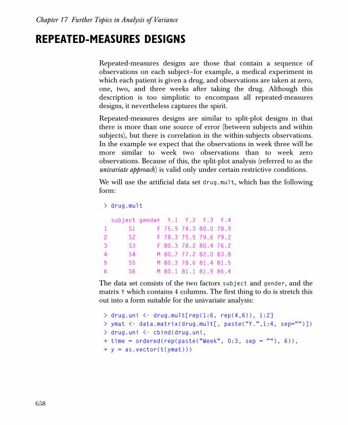
Chapter 17 Further Topics in Analysis of Variance
REPEATED-MEASURES DESIGNS
Repeated-measures designs are those that contain a sequence ofobservations on each subject—for example, a medical experiment inwhich each patient is given a drug, and observations are taken at zero,one, two, and three weeks after taking the drug. Although thisdescription is too simplistic to encompass all repeated-measuresdesigns, it nevertheless captures the spirit.
Repeated-measures designs are similar to split-plot designs in thatthere is more than one source of error (between subjects and withinsubjects), but there is correlation in the within-subjects observations.In the example we expect that the observations in week three will bemore similar to week two observations than to week zeroobservations. Because of this, the split-plot analysis (referred to as theunivariate approach) is valid only under certain restrictive conditions.
We will use the artificial data set drug.mult, which has the followingform:
> drug.mult
subject gender Y.1 Y.2 Y.3 Y.41 S1 F 75.9 74.3 80.0 78.92 S2 F 78.3 75.5 79.6 79.23 S3 F 80.3 78.2 80.4 76.24 S4 M 80.7 77.2 82.0 83.85 S5 M 80.3 78.6 81.4 81.56 S6 M 80.1 81.1 81.9 86.4
The data set consists of the two factors subject and gender, and thematrix Y which contains 4 columns. The first thing to do is stretch thisout into a form suitable for the univariate analysis:
> drug.uni <- drug.mult[rep(1:6, rep(4,6)), 1:2]> ymat <- data.matrix(drug.mult[, paste("Y.",1:4, sep="")])> drug.uni <- cbind(drug.uni, + time = ordered(rep(paste("Week", 0:3, sep = ""), 6)),+ y = as.vector(t(ymat)))
658

Repeated-Measures Designs
The univariate analysis treats the data as a split-plot design:
> summary(aov(y ~ gender*time + Error(subject), + data = drug.uni))
Error: subject Df Sum of Sq Mean Sq F Value Pr(F)gender 1 60.80167 60.80167 19.32256 0.01173Residuals 4 12.58667 3.14667
Error: Within Df Sum of Sq Mean Sq F Value Pr(F)time 3 49.10833 16.36944 6.316184 0.0081378gender:time 3 14.80167 4.93389 1.903751 0.1828514Residuals 12 31.10000 2.59167
Tests in the Within stratum are valid only if the data satisfy thecircularity property, in addition to the usual conditions. Circularitymeans that the variance of the difference of measures at differenttimes is constant; for example, the variance of the difference betweenthe measures at week 0 and week 3 should be the same as thevariance of the difference between week 2 and week 3. We also needthe assumption that actual contrasts are used; for example, thecontr.treatment function should not be used. When circularity doesnot hold, then the p-values for the tests will be too small.
One approach is to perform tests which are as conservative aspossible. Conservative tests are formed by dividing the degrees offreedom in both the numerator and denominator of the F test by thenumber of repeated measures minus one. In our example there arefour repeated measures on each subject, so we divide by 3. The split-plot and the conservative tests are:
> 1 - pf(6.316184, 3, 12) # usual univariate test
[1] 0.008137789
> 1 - pf(6.316184, 1, 4) # conservative test
[1] 0.06583211
These two tests are telling fairly different tales, so the data analystwould probably move on to one of two alternatives. A Huynh-Feldtadjustment of the degrees of freedom provides a middle ground
659

Chapter 17 Further Topics in Analysis of Variance
between the tests above—see Winer, Brown and Michels (1991), forinstance. The multivariate approach, discussed below, substantiallyrelaxes the assumptions.
The univariate test for time was really a test on three contrasts. In themultivariate setting we want to do the same thing, so we need to usecontrasts in the response:
> drug.man <- manova(ymat %*% contr.poly(4) ~ gender,+ data = drug.mult)> summary(drug.man, intercept = T) Df Pillai Trace approx. F num df den df P-value(Intercept) 1 0.832005 3.301706 3 2 0.241092 gender 1 0.694097 1.512671 3 2 0.421731 Residuals 4
The line marked (Intercept) corresponds to time in the univariateapproach, and similarly the gender line here corresponds togender:time. The p-value of 0.24 is larger than either of theunivariate tests; the price of the multivariate analysis being moregenerally valid is that quite a lot of power is lost. Although themultivariate approach is preferred when the data do not conform tothe required conditions, the univariate approach is preferred whenthey do. The trick, of course, is knowing which is which.
Let’s look at the univariate summaries that this MANOVA produces:
> summary(drug.man, intercept = T, univar = T)Response: .L Df Sum of Sq Mean Sq F Value Pr(F)(Intercept) 1 22.188 22.1880 4.327255 0.1059983gender 1 6.912 6.9120 1.348025 0.3101900Residuals 4 20.510 5.1275Response: .Q Df Sum of Sq Mean Sq F Value Pr(F)(Intercept) 1 5.415000 5.415000 5.30449 0.0826524gender 1 4.001667 4.001667 3.92000 0.1188153Residuals 4 4.083333 1.020833
Response: .C Df Sum of Sq Mean Sq F Value Pr(F)(Intercept) 1 21.50533 21.50533 13.22049 0.0220425gender 1 3.88800 3.88800 2.39016 0.1969986Residuals 4 6.50667 1.62667
660

Repeated-Measures Designs
If you add up the respective degrees of freedom and sums of squares,you will find that the result is the same as the univariate Withinstratum. For this reason, the univariate test is sometimes referred to asthe average F test.
The above discussion has focused on classical inference, whichshould not be done before graphical exploration of the data.
Many books discuss repeated measures. Some examples are Handand Taylor (1987), Milliken and Johnson (1984), Crowder and Hand(1990), and Winer, Brown, and Michels (1991).
661
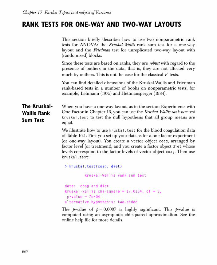
Chapter 17 Further Topics in Analysis of Variance
RANK TESTS FOR ONE-WAY AND TWO-WAY LAYOUTS
This section briefly describes how to use two nonparametric ranktests for ANOVA: the Kruskal-Wallis rank sum test for a one-waylayout and the Friedman test for unreplicated two-way layout with(randomized) blocks.
Since these tests are based on ranks, they are robust with regard to thepresence of outliers in the data; that is, they are not affected verymuch by outliers. This is not the case for the classical tests.
You can find detailed discussions of the Kruskal-Wallis and Friedmanrank-based tests in a number of books on nonparametric tests; forexample, Lehmann (1975) and Hettmansperger (1984).
The Kruskal-Wallis Rank Sum Test
When you have a one-way layout, as in the section Experiments withOne Factor in Chapter 16, you can use the Kruskal-Wallis rank sum testkruskal.test to test the null hypothesis that all group means areequal.
We illustrate how to use kruskal.test for the blood coagulation dataof Table 16.1. First you set up your data as for a one-factor experiment(or one-way layout). You create a vector object coag, arranged byfactor level (or treatment), and you create a factor object diet whoselevels correspond to the factor levels of vector object coag. Then usekruskal.test:
> kruskal.test(coag, diet)
Kruskal-Wallis rank sum test
data: coag and dietKruskal-Wallis chi-square = 17.0154, df = 3, p-value = 7e-04alternative hypothesis: two.sided
The p-value of p = 0.0007 is highly significant. This p-value iscomputed using an asymptotic chi-squared approximation. See theonline help file for more details.
F
662
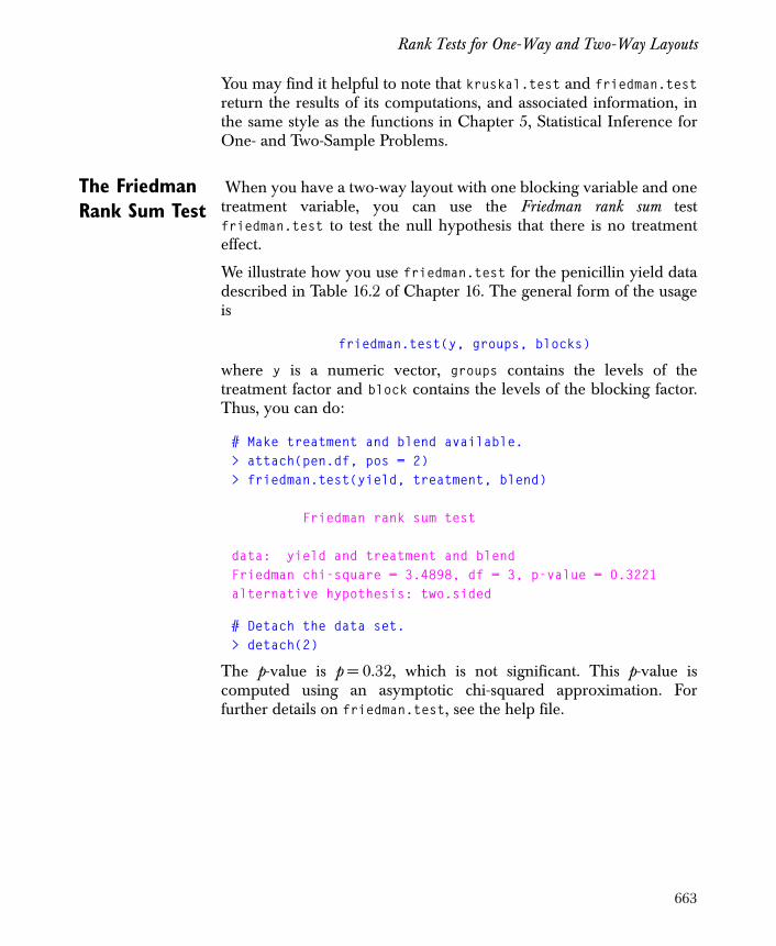
Rank Tests for One-Way and Two-Way Layouts
You may find it helpful to note that kruskal.test and friedman.testreturn the results of its computations, and associated information, inthe same style as the functions in Chapter 5, Statistical Inference forOne- and Two-Sample Problems.
The Friedman Rank Sum Test
When you have a two-way layout with one blocking variable and onetreatment variable, you can use the Friedman rank sum testfriedman.test to test the null hypothesis that there is no treatmenteffect.
We illustrate how you use friedman.test for the penicillin yield datadescribed in Table 16.2 of Chapter 16. The general form of the usageis
friedman.test(y, groups, blocks)
where y is a numeric vector, groups contains the levels of thetreatment factor and block contains the levels of the blocking factor.Thus, you can do:
# Make treatment and blend available.> attach(pen.df, pos = 2) > friedman.test(yield, treatment, blend)
Friedman rank sum test
data: yield and treatment and blend Friedman chi-square = 3.4898, df = 3, p-value = 0.3221alternative hypothesis: two.sided
# Detach the data set.> detach(2)
The p-value is p = 0.32, which is not significant. This p-value iscomputed using an asymptotic chi-squared approximation. Forfurther details on friedman.test, see the help file.
663

Chapter 17 Further Topics in Analysis of Variance
VARIANCE COMPONENTS MODELS
Variance components models are used when there is interest in thevariability of one or more variables other than the residual error. Forexample, manufacturers often run experiments to see which parts ofthe manufacturing process contribute most to the variability of thefinal product. In this situation variability is undesirable, and attentionis focused on improving those parts of the process that are mostvariable. Animal breeding is another area in which variancecomponents models are routinely used. Some data, from surveys forexample, that have traditionally been analyzed using regression canmore profitably be analyzed using variance component models.
Estimating the Model
To estimate a variance component model, you first need to useis.random to state which factors in your data are random. A variablethat is marked as being random will have a variance component inany models that contain it. Only variables that inherit from class"factor" can be declared random. Although is.random works onindividual factors, it is often more practical to use it on the columns ofa data frame. You can see if variables are declared random by usingis.random on the data frame:
> is.random(pigment)
Batch Sample Test F F F
Declare variables to be random by using the assignment form ofis.random:
> pigment <- pigment> is.random(pigment) <- c(T, T, T)> is.random(pigment)
Batch Sample Test T T T
664

Variance Components Models
Because we want all of the factors to be random, we could havesimply done the following:
> is.random(pigment) <- T
The value on the right is replicated to be the length of the number offactors in the data frame.
Once you have declared your random variables, you are ready toestimate the model using the varcomp function. This function takes aformula and other arguments very much like lm or aov. Because thepigment data are from a nested design, the call has the followingform:
> pigment.vc <- varcomp(Moisture ~ Batch/Sample,+ data = pigment)> pigment.vc
Variances: Batch Sample %in% Batch Residuals 7.127976 28.53333 0.9166667Call:varcomp(formula = Moisture ~ Batch/Sample, data = pigment)
The result of varcomp is an object of class "varcomp". You can usesummary on "varcomp" objects to get more details about the fit, andyou can use plot to get qq-plots for the normal distribution on theestimated effects for each random term in the model.
Estimation Methods
The method argument to varcomp allows you to choose the type ofvariance component estimator. Maximum likelihood and REML(restricted maximum likelihood) are two of the choices. REML is verysimilar to maximum likelihood but takes the number of fixed effectsinto account; the usual unbiased estimate of variance in the one-sample model is an REML estimate. See Harville (1977) for moredetails on these estimators.
The default method is a MINQUE (minimum norm quadraticunbiased estimate); this class of estimator is locally best at a particularspot in the parameter space. The MINQUE option in Spotfire S+ islocally best if all of the variance components (except that for theresiduals) are zero. The MINQUE estimate agrees with REML forbalanced data. See Rao (1971) for details. This method was made the
665

Chapter 17 Further Topics in Analysis of Variance
default because it is less computationally intense than the othermethods, however, it can do significantly worse for severelyunbalanced data (Swallow and Monahan (1984)).
You can get robust estimates by using method="winsor". This methodcreates new data by moving outlying points or groups of pointstoward the rest of the data. One of the standard estimators is thenapplied to this possibly revised data. Burns (1992) gives details of thealgorithm along with simulation results. This method uses muchlarger amounts of memory than the other methods if there are a largenumber of random levels, such as in a deeply nested design.
Random Slope Example
We now produce a more complicated example in which there arerandom slopes and intercepts. The data consist of several pairs ofobservations on each of several individuals in the study. An examplemight be that the y values represent the score on a test and the xvalues are the time at which the test was taken.
Let’s start by creating simulated data of this form. We create data for30 subjects and 10 observations per subject:
> subject <- factor(rep(1:30, rep(10,30)))> set.seed(357) # makes these numbers reproducible> trueslope <- rnorm(30, mean = 1)> trueint <- rnorm(30, sd = 0.5)> times <- rchisq(300, 3)> scores <- rep(trueint, rep(10,30)) + + times * rep(trueslope, rep(10,30)) + rnorm(300)> test.df <- data.frame(subject, times, scores)> is.random(test.df) <- T> is.random(test.df)
subject T
Even though we want to estimate random slopes and randomintercepts, the only variable that is declared random is subject. Ourmodel for the data has two coefficients: the mean slope (averagedover subjects) and the mean intercept. It also has three variances: thevariance for the slope, the variance for the intercept, and the residualvariance.
666

Variance Components Models
The following command estimates this model using MaximumLikelihood, as the default MINQUE is not recommended for thistype of model:
> test.vc <- varcomp(scores ~ times * subject,+ data = test.df, method = "ml")
This seems very simple. We can see how it works by looking at howthe formula get expanded. The right side of the formula is expandedinto four terms:
scores ~ 1 + times + subject + times:subject
The intercept term in the formula, represented by 1, gives the meanintercept. The variable times is fixed and produces the mean slope.The subject variable is random and produces the variancecomponent for the random intercept. Since any interactioncontaining a random variable is considered random, the last term,times:subject, is also random; this term gives the variancecomponent for the random slope. Finally, there is always a residualvariance.
Now we can look at the estimates:
> test.vc
Variances: subject times:subject Residuals 0.3162704 1.161243 0.8801149Message:[1] "RELATIVE FUNCTION CONVERGENCE"Call:varcomp(formula = scores ~ times*subject, data=test.df, method = "ml")
This shows the three variance components. The variance of theintercept, which has true value 0.25, is estimated as 0.32. Next,labeled times:subject is the variance of the slope, and finally theresidual variance. We can also view the estimates for the coefficientsof the model, which have true values of 0 and 1.
> coef(test.vc)
(Intercept) times 0.1447211 1.02713
667
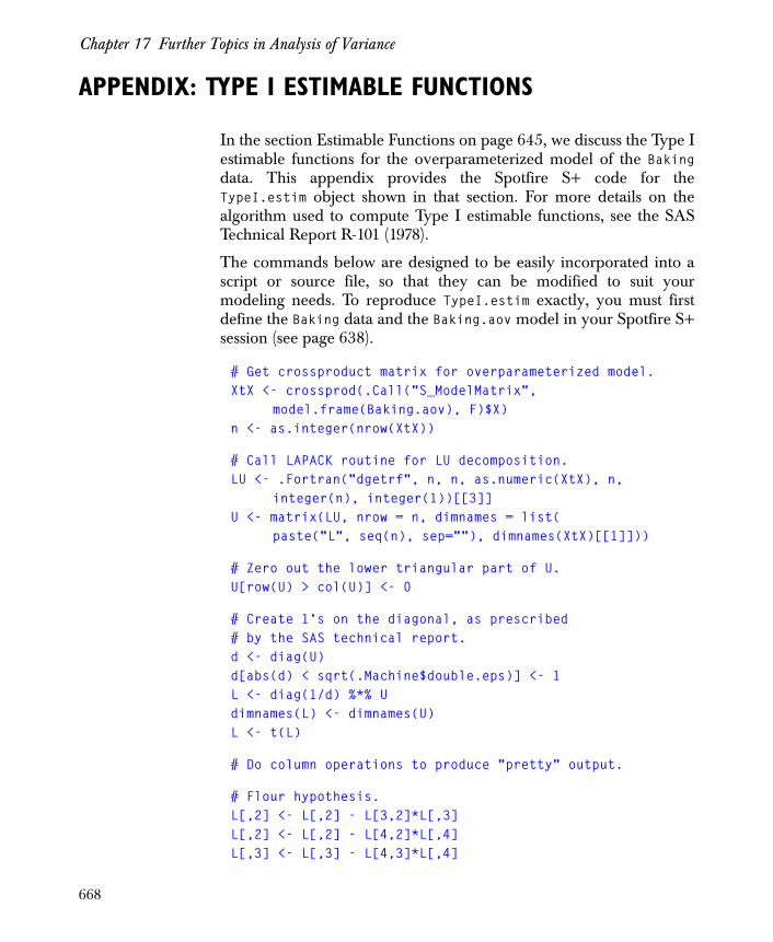
Chapter 17 Further Topics in Analysis of Variance
APPENDIX: TYPE I ESTIMABLE FUNCTIONS
In the section Estimable Functions on page 645, we discuss the Type Iestimable functions for the overparameterized model of the Bakingdata. This appendix provides the Spotfire S+ code for theTypeI.estim object shown in that section. For more details on thealgorithm used to compute Type I estimable functions, see the SASTechnical Report R-101 (1978).
The commands below are designed to be easily incorporated into ascript or source file, so that they can be modified to suit yourmodeling needs. To reproduce TypeI.estim exactly, you must firstdefine the Baking data and the Baking.aov model in your Spotfire S+session (see page 638).
# Get crossproduct matrix for overparameterized model.XtX <- crossprod(.Call("S_ModelMatrix",
model.frame(Baking.aov), F)$X)n <- as.integer(nrow(XtX))
# Call LAPACK routine for LU decomposition.LU <- .Fortran("dgetrf", n, n, as.numeric(XtX), n,
integer(n), integer(1))[[3]]U <- matrix(LU, nrow = n, dimnames = list(
paste("L", seq(n), sep=""), dimnames(XtX)[[1]]))
# Zero out the lower triangular part of U.U[row(U) > col(U)] <- 0
# Create 1's on the diagonal, as prescribed # by the SAS technical report.d <- diag(U)d[abs(d) < sqrt(.Machine$double.eps)] <- 1L <- diag(1/d) %*% Udimnames(L) <- dimnames(U)L <- t(L)
# Do column operations to produce "pretty" output.
# Flour hypothesis.L[,2] <- L[,2] - L[3,2]*L[,3]L[,2] <- L[,2] - L[4,2]*L[,4]L[,3] <- L[,3] - L[4,3]*L[,4]
668
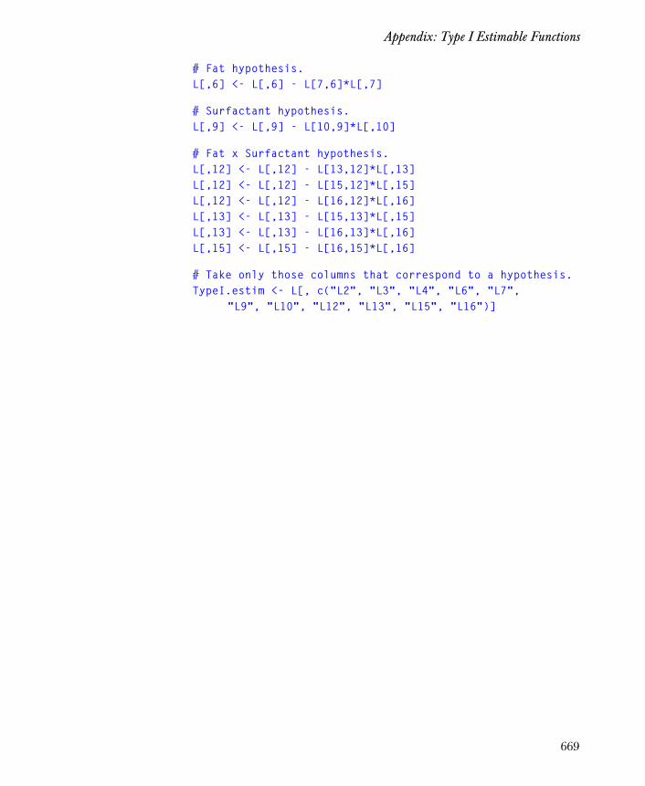
Appendix: Type I Estimable Functions
# Fat hypothesis.L[,6] <- L[,6] - L[7,6]*L[,7]
# Surfactant hypothesis.L[,9] <- L[,9] - L[10,9]*L[,10]
# Fat x Surfactant hypothesis.L[,12] <- L[,12] - L[13,12]*L[,13]L[,12] <- L[,12] - L[15,12]*L[,15]L[,12] <- L[,12] - L[16,12]*L[,16]L[,13] <- L[,13] - L[15,13]*L[,15]L[,13] <- L[,13] - L[16,13]*L[,16]L[,15] <- L[,15] - L[16,15]*L[,16]
# Take only those columns that correspond to a hypothesis.TypeI.estim <- L[, c("L2", "L3", "L4", "L6", "L7",
"L9", "L10", "L12", "L13", "L15", "L16")]
669

Chapter 17 Further Topics in Analysis of Variance
REFERENCES
Burns, P.J. (1992). Winsorized REML estimates of variance components.Technical report, Statistical Sciences, Inc.
Chambers, J.M. & Hastie, T.J. (Eds.) (1992). Statistical Models in S.London: Chapman and Hall.
Crowder, M.J. & Hand, D.J. (1990). Analysis of Repeated Measures.London: Chapman and Hall.
Daniel, C. (1976). Applications of Statistics to Industrial Experimentation.New York: John Wiley & Sons, Inc.
Hand, D.J. & Taylor, C.C. (1987). Multivariate Analysis of Variance andRepeated Measures. London: Chapman and Hall.
Harville, D.A. (1977). Maximum likelihood approaches to variancecomponent estimation and to related problems (with discussion).Journal of the American Statistical Association 72:320-340.
Hettmansperger, T.P. (1984). Statistical Inference Based on Ranks. NewYork: John Wiley & Sons, Inc.
Hicks, C.R. (1973). Fundamental Concepts in the Design of Experiments.New York: Holt, Rinehart and Winston.
Kennedy, W.J., Gentle, J.E., (1980), Statistical Computing. New York:Marcel Dekker, (p. 396).
Lehmann, E.L. (1975). Nonparametrics: Statistical Methods Based onRanks. San Francisco: Holden-Day.
Mardia, K.V., Kent, J.T., & Bibby, J.M. (1979). Multivariate Analysis.London: Academic Press.
Milliken, G.A. & Johnson, D.E., (1984), Analysis of Messy Data VolumeI: Designed Experiments. New York: Van Norstrand Reinhold Co. (p.473).
Rao, C.R. (1971). Estimation of variance and covariancecomponents—MINQUE theory. Journal of Multivariate Analysis 1:257-275.
SAS Institute, Inc. (1978). Tests of Hypotheses in Fixed-Effects LinearModels. SAS Technical Report R-101. Cary, NC: SAS Institute, Inc..
670

References
SAS Institute, Inc. (1990). SAS/Stat User’s Guide, Fourth Edition. Cary,NC: SAS Institute, Inc., (pp. 120-121).
Searle, S.R., (1987), Linear Models for Unbalanced Data. New York:John Wiley & Sons, (p. 536).
Seber, G.A.F. (1984). Multivariate Observations. New York: John Wiley& Sons, Inc.
Swallow, W.H. & Monahan, J.F. (1984). Monte Carlo comparison ofANOVA, MIVQUE, REML, and ML estimators of variancecomponents. Technometrics 26:47-57.
Winer, B.J., Brown, D.R., & Michels, K.M. (1991). Statistical Principlesin Experimental Design. New York: McGraw-Hill.
671

Chapter 17 Further Topics in Analysis of Variance
672

Overview 674The fuel.frame Data 674Honestly Significant Differences 677Rat Growth Hormone Treatments 678Upper and Lower Bounds 681Calculation of Critical Points 682Error Rates for Confidence Intervals 683
Advanced Applications 684Adjustment Schemes 685Toothaker’s Two-Factor Design 686Setting Linear Combinations of Effects 689Textbook Parameterization 689Overparameterized Models 691Multicomp Methods Compared 692
Capabilities and Limits 694
References 696
MULTIPLE COMPARISONS 18
673
Chapter 18 Multiple Comparisons
OVERVIEW
This chapter describes the use of the function multicomp in theanalysis of multiple comparisons. This particular section describessimple calls to multicomp for standard comparisons in one-waylayouts. The section Advanced Applications tells how to usemulticomp for nonstandard designs and comparisons. In the sectionCapabilities and Limits, the capabilities and limitations of thisfunction are summarized.
The fuel.frame Data
When an experiment has been carried out in order to compare effectsof several treatments, a classical analytical approach is to begin with atest for equality of those effects. Regardless of whether you embracethis classical strategy, and regardless of the outcome of this test, youare usually not finished with the analysis until determining where anydifferences exist, and how large the differences are (or might be); thatis, until you do multiple comparisons of the treatment effects.
As a simple start, consider the built-in TIBCO Spotfire S+ data frameon fuel consumption of vehicles, fuel.frame. Each row provides thefuel consumption (Fuel) in 100*gallons/mile for a vehicle model, aswell as the Type group of the model: Compact, Large, Medium, Small,Sporty, or Van. There is also information available on the Weight andDisplacement of the vehicle. Figure 18.1 shows a box plot of fuelconsumption, the result of the following commands.
> attach(fuel.frame, pos = 2)> boxplot(split(Fuel, Type))> detach(2)
674

Overview
Not surprisingly, the plot suggests that there are differences betweenvehicle types in terms of mean fuel consumption. This is confirmedby a one-factor analysis of variance test of equality obtained by a callto aov.
> aovout.fuel <- aov(Fuel ~ Type, data = fuel.frame)> anova(aovout.fuel)
Analysis of Variance TableResponse: FuelTerms added sequentially (first to last)
Df Sum of Sq Mean Sq F Value Pr(F)Type 5 24.23960 4.847921 27.22058 1.220135e-13Residuals 54 9.61727 0.178098
The box plots show some surprising patterns, and inspire somequestions. Do small cars really have lower mean fuel consumptionthan compact cars? If so, by what amount? What about small versussporty cars? Vans versus large cars? Answers to these questions areoffered by an analysis of all pairwise differences in mean fuelconsumption, which can be obtained from a call to multicomp.
> mca.fuel <- multicomp(aovout.fuel, focus = "Type")
Figure 18.1: Fuel consumption box plot.
3.0
3.5
4.0
4.5
5.0
5.5
Compact Large Medium Small Sporty Van
675

Chapter 18 Multiple Comparisons
> plot(mca.fuel)> mca.fuel
95 % simultaneous confidence intervals for specifiedlinear combinations, by the Tukey methodcritical point: 2.9545response variable: Fuelintervals excluding 0 are flagged by '****'
Estimate Std. Lower Upper Error Bound BoundCompact-Large -0.800 0.267 -1.590 -0.0116 ****Compact-Medium -0.434 0.160 -0.906 0.0387Compact-Small 0.894 0.160 0.422 1.3700 ****Compact-Sporty 0.210 0.178 -0.316 0.7360Compact-Van -1.150 0.193 -1.720 -0.5750 ****Large-Medium 0.366 0.270 -0.432 1.1600Large-Small 1.690 0.270 0.896 2.4900 ****Large-Sporty 1.010 0.281 0.179 1.8400 ****Large-Van -0.345 0.291 -1.210 0.5150Medium-Small 1.330 0.166 0.839 1.8200 ****Medium-Sporty 0.644 0.183 0.103 1.1800 ****Medium-Van -0.712 0.198 -1.300 -0.1270 ****Small-Sporty -0.684 0.183 -1.220 -0.1440 ****Small-Van -2.040 0.198 -2.620 -1.4600 ****Sporty-Van -1.360 0.213 -1.980 -0.7270 ****
Figure 18.2: Fuel consumption ANOVA.
((
((
((
((
((
(((
((
))
))
))
))
))
)))
))
Compact-LargeCompact-Medium
Compact-SmallCompact-Sporty
Compact-VanLarge-Medium
Large-SmallLarge-Sporty
Large-VanMedium-Small
Medium-SportyMedium-VanSmall-Sporty
Small-VanSporty-Van
-3.0 -2.5 -2.0 -1.5 -1.0 -0.5 0.0 0.5 1.0 1.5 2.0 2.5
simultaneous 95 % confidence limits, Tukey methodresponse variable: Fuel
676
Overview
As the output and plot in Figure 18.2 indicate, this default call tomulticomp has resulted in the calculation of simultaneous 95%confidence intervals for all pairwise differences between vehicle Fuelmeans, based on the levels of Type, sometimes referred to as MCAcomparisons (Hsu, 1996). The labeling states that Tukey’s method(Tukey, 1953) has been used; since group sample sizes are unequal,this is actually equivalent to what is commonly known as the Tukey-Kramer (Kramer, 1956) multiple comparison method.
Honestly Significant Differences
The output indicates via asterisks the confidence intervals whichexclude zero; in the plot, these can be identified by noting intervalsthat do not intersect the vertical reference line at zero. Theseidentified statistically significant comparisons correspond to pairs of(long run) means which can be declared different by Tukey’s HSD(honestly significant difference) method. Not surprisingly, we can assertthat most of the vehicle types have different mean fuel consumptionrates. If we require 95% confidence in all of our statements, we cannotclaim different mean fuel consumption rates between the compactand medium types, the compact and sporty types, the large andmedium types, and the large and van types.
Note we should not assert that these pairs have equal meanconsumption rates. For example, the interval for Compact-Mediumstates that this particular difference in mean fuel consumption isbetween -0.906 and 0.0387 units. Hence, the medium vehicle typemay have larger mean fuel consumption than the compact, by asmuch as 0.9 units. Only an engineer can judge the importance of adifference of this size; if it is considered trivial, then using theseintervals we can claim that for all practical purposes these two typeshave equal mean consumption rates. If not, there may still be animportant difference between these types, and we would need moredata to resolve the question.
The point to the above discussion is that there is more information inthese simultaneous intervals than is provided by a collection ofsignificance tests for differences. This is true whether the tests arereported via conclusions “Reject”/“Do not reject”, or via p-values oradjusted p-values. This superior level of information using confidenceintervals has been acknowledged by virtually all modern texts onmultiple comparisons (Hsu, 1996; Bechhofer, Santner, and
677
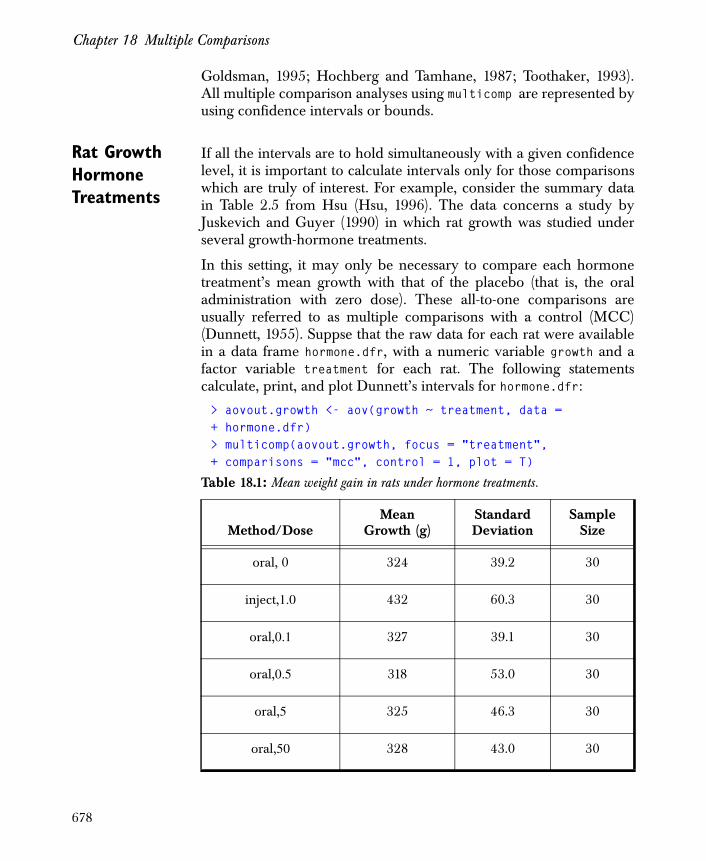
Chapter 18 Multiple Comparisons
Goldsman, 1995; Hochberg and Tamhane, 1987; Toothaker, 1993).All multiple comparison analyses using multicomp are represented byusing confidence intervals or bounds.
Rat Growth Hormone Treatments
If all the intervals are to hold simultaneously with a given confidencelevel, it is important to calculate intervals only for those comparisonswhich are truly of interest. For example, consider the summary datain Table 2.5 from Hsu (Hsu, 1996). The data concerns a study byJuskevich and Guyer (1990) in which rat growth was studied underseveral growth-hormone treatments.
In this setting, it may only be necessary to compare each hormonetreatment’s mean growth with that of the placebo (that is, the oraladministration with zero dose). These all-to-one comparisons areusually referred to as multiple comparisons with a control (MCC)(Dunnett, 1955). Suppse that the raw data for each rat were availablein a data frame hormone.dfr, with a numeric variable growth and afactor variable treatment for each rat. The following statementscalculate, print, and plot Dunnett’s intervals for hormone.dfr:
> aovout.growth <- aov(growth ~ treatment, data =+ hormone.dfr)> multicomp(aovout.growth, focus = "treatment",+ comparisons = "mcc", control = 1, plot = T)
Table 18.1: Mean weight gain in rats under hormone treatments.
Method/DoseMean
Growth (g)Standard Deviation
SampleSize
oral, 0 324 39.2 30
inject,1.0 432 60.3 30
oral,0.1 327 39.1 30
oral,0.5 318 53.0 30
oral,5 325 46.3 30
oral,50 328 43.0 30
678
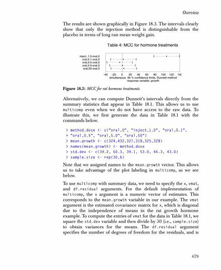
Overview
The results are shown graphically in Figure 18.3. The intervals clearlyshow that only the injection method is distinguishable from theplacebo in terms of long run mean weight gain.
Alternatively, we can compute Dunnett’s intervals directly from thesummary statistics that appear in Table 18.1. This allows us to usemulticomp even when we do not have access to the raw data. Toillustrate this, we first generate the data in Table 18.1 with thecommands below.
> method.dose <- c("oral,0", "inject,1.0", "oral,0.1",+ "oral,0.5", "oral,5.0", "oral,50")> mean.growth <- c(324,432,327,318,325,328)> names(mean.growth) <- method.dose> std.dev <- c(39.2, 60.3, 39.1, 53.0, 46.3, 43.0)> sample.size <- rep(30,6)
Note that we assigned names to the mean.growth vector. This allowsus to take advantage of the plot labeling in multicomp, as we seebelow.
To use multicomp with summary data, we need to specify the x, vmat,and df.residual arguments. For the default implementation ofmulticomp, the x argument is a numeric vector of estimates. Thiscorresponds to the mean.growth variable in our example. The vmatargument is the estimated covariance matrix for x, which is diagonaldue to the independence of means in the rat growth hormoneexample. To compute the entries of vmat for the data in Table 18.1, wesquare the std.dev variable and then divide by 30 (i.e., sample.size)to obtain variances for the means. The df.residual argumentspecifies the number of degrees of freedom for the residuals, and is
Figure 18.3: MCC for rat hormone treatments.
((
(((
))
)))
inject.,1.0-oral,0oral,0.1-oral,0oral,0.5-oral,0oral,5.0-oral,0oral,50-oral,0
-40 -20 0 20 40 60 80 100 120 140simultaneous 95 % confidence limits, Dunnett method
response variable: growth
Table 4: MCC for hormone treatments
679
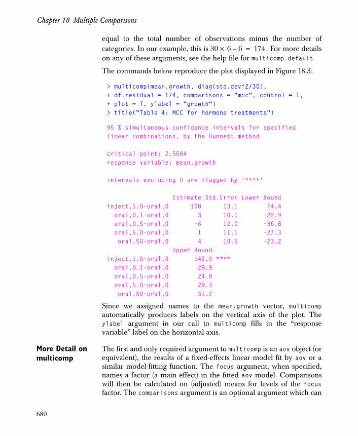
Chapter 18 Multiple Comparisons
equal to the total number of observations minus the number ofcategories. In our example, this is . For more detailson any of these arguments, see the help file for multicomp.default.
The commands below reproduce the plot displayed in Figure 18.3:
> multicomp(mean.growth, diag(std.dev^2/30),+ df.residual = 174, comparisons = "mcc", control = 1,+ plot = T, ylabel = "growth")> title("Table 4: MCC for hormone treatments")
95 % simultaneous confidence intervals for specified linear combinations, by the Dunnett method
critical point: 2.5584 response variable: mean.growth
intervals excluding 0 are flagged by '****'
Estimate Std.Error Lower Boundinject,1.0-oral,0 108 13.1 74.4 oral,0.1-oral,0 3 10.1 -22.9 oral,0.5-oral,0 -6 12.0 -36.8 oral,5.0-oral,0 1 11.1 -27.3 oral,50-oral,0 4 10.6 -23.2 Upper Bound inject,1.0-oral,0 142.0 **** oral,0.1-oral,0 28.9 oral,0.5-oral,0 24.8 oral,5.0-oral,0 29.3 oral,50-oral,0 31.2
Since we assigned names to the mean.growth vector, multicompautomatically produces labels on the vertical axis of the plot. Theylabel argument in our call to multicomp fills in the “responsevariable” label on the horizontal axis.
More Detail on multicomp
The first and only required argument to multicomp is an aov object (orequivalent), the results of a fixed-effects linear model fit by aov or asimilar model-fitting function. The focus argument, when specified,names a factor (a main effect) in the fitted aov model. Comparisonswill then be calculated on (adjusted) means for levels of the focusfactor. The comparisons argument is an optional argument which can
30 6 6–× 174=
680
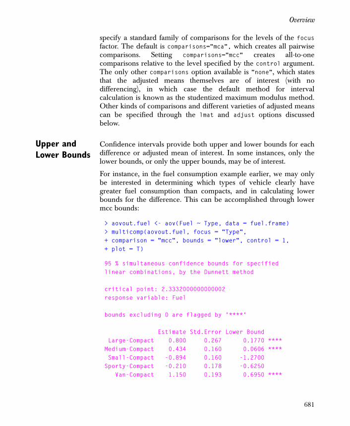
Overview
specify a standard family of comparisons for the levels of the focusfactor. The default is comparisons="mca", which creates all pairwisecomparisons. Setting comparisons="mcc" creates all-to-onecomparisons relative to the level specified by the control argument.The only other comparisons option available is "none", which statesthat the adjusted means themselves are of interest (with nodifferencing), in which case the default method for intervalcalculation is known as the studentized maximum modulus method.Other kinds of comparisons and different varieties of adjusted meanscan be specified through the lmat and adjust options discussedbelow.
Upper and Lower Bounds
Confidence intervals provide both upper and lower bounds for eachdifference or adjusted mean of interest. In some instances, only thelower bounds, or only the upper bounds, may be of interest.
For instance, in the fuel consumption example earlier, we may onlybe interested in determining which types of vehicle clearly havegreater fuel consumption than compacts, and in calculating lowerbounds for the difference. This can be accomplished through lowermcc bounds:
> aovout.fuel <- aov(Fuel ~ Type, data = fuel.frame)> multicomp(aovout.fuel, focus = "Type", + comparison = "mcc", bounds = "lower", control = 1, + plot = T)
95 % simultaneous confidence bounds for specifiedlinear combinations, by the Dunnett method
critical point: 2.3332000000000002response variable: Fuel
bounds excluding 0 are flagged by '****'
Estimate Std.Error Lower Bound Large-Compact 0.800 0.267 0.1770 ****Medium-Compact 0.434 0.160 0.0606 **** Small-Compact -0.894 0.160 -1.2700Sporty-Compact -0.210 0.178 -0.6250 Van-Compact 1.150 0.193 0.6950 ****
681
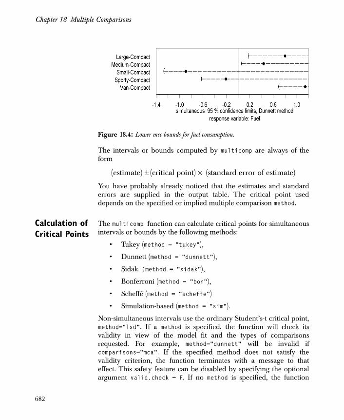
Chapter 18 Multiple Comparisons
The intervals or bounds computed by multicomp are always of theform
You have probably already noticed that the estimates and standarderrors are supplied in the output table. The critical point useddepends on the specified or implied multiple comparison method.
Calculation of Critical Points
The multicomp function can calculate critical points for simultaneousintervals or bounds by the following methods:
• Tukey (method = "tukey"),
• Dunnett (method = "dunnett"),
• Sidak (method = "sidak"),
• Bonferroni (method = "bon"),
• Scheffé (method = "scheffe")
• Simulation-based (method = "sim").
Non-simultaneous intervals use the ordinary Student’s-t critical point,method="lsd". If a method is specified, the function will check itsvalidity in view of the model fit and the types of comparisonsrequested. For example, method="dunnett" will be invalid ifcomparisons="mca". If the specified method does not satisfy thevalidity criterion, the function terminates with a message to thateffect. This safety feature can be disabled by specifying the optionalargument valid.check = F. If no method is specified, the function
Figure 18.4: Lower mcc bounds for fuel consumption.
(estimate) (critical point)± (standard error of estimate)×
682
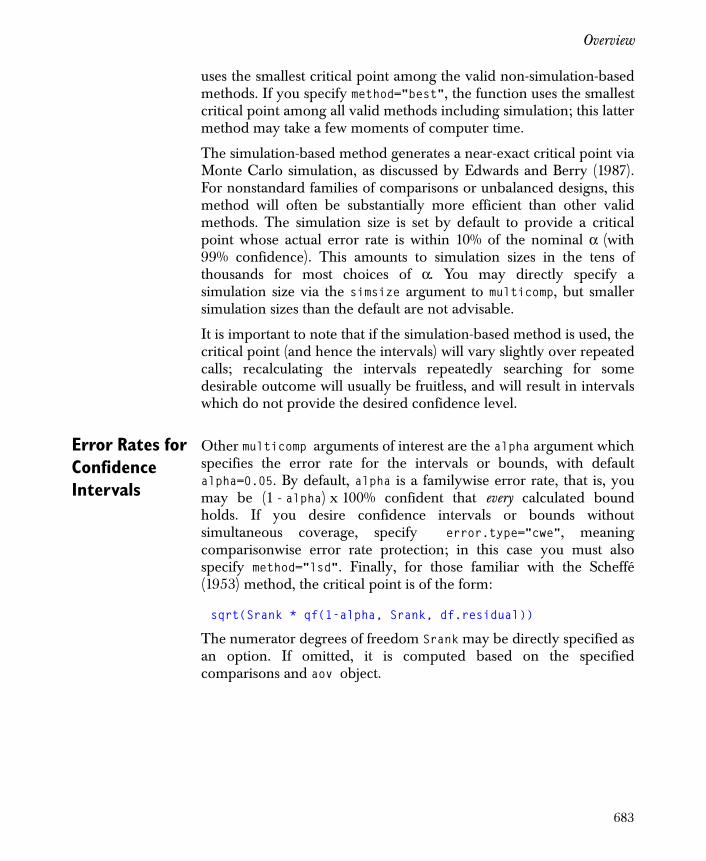
Overview
uses the smallest critical point among the valid non-simulation-basedmethods. If you specify method="best", the function uses the smallestcritical point among all valid methods including simulation; this lattermethod may take a few moments of computer time.
The simulation-based method generates a near-exact critical point viaMonte Carlo simulation, as discussed by Edwards and Berry (1987).For nonstandard families of comparisons or unbalanced designs, thismethod will often be substantially more efficient than other validmethods. The simulation size is set by default to provide a criticalpoint whose actual error rate is within 10% of the nominal α (with99% confidence). This amounts to simulation sizes in the tens ofthousands for most choices of α. You may directly specify asimulation size via the simsize argument to multicomp, but smallersimulation sizes than the default are not advisable.
It is important to note that if the simulation-based method is used, thecritical point (and hence the intervals) will vary slightly over repeatedcalls; recalculating the intervals repeatedly searching for somedesirable outcome will usually be fruitless, and will result in intervalswhich do not provide the desired confidence level.
Error Rates for Confidence Intervals
Other multicomp arguments of interest are the alpha argument whichspecifies the error rate for the intervals or bounds, with defaultalpha=0.05. By default, alpha is a familywise error rate, that is, youmay be (1 - alpha) x 100% confident that every calculated boundholds. If you desire confidence intervals or bounds withoutsimultaneous coverage, specify error.type="cwe", meaningcomparisonwise error rate protection; in this case you must alsospecify method="lsd". Finally, for those familiar with the Scheffé(1953) method, the critical point is of the form:
sqrt(Srank * qf(1-alpha, Srank, df.residual))
The numerator degrees of freedom Srank may be directly specified asan option. If omitted, it is computed based on the specifiedcomparisons and aov object.
683
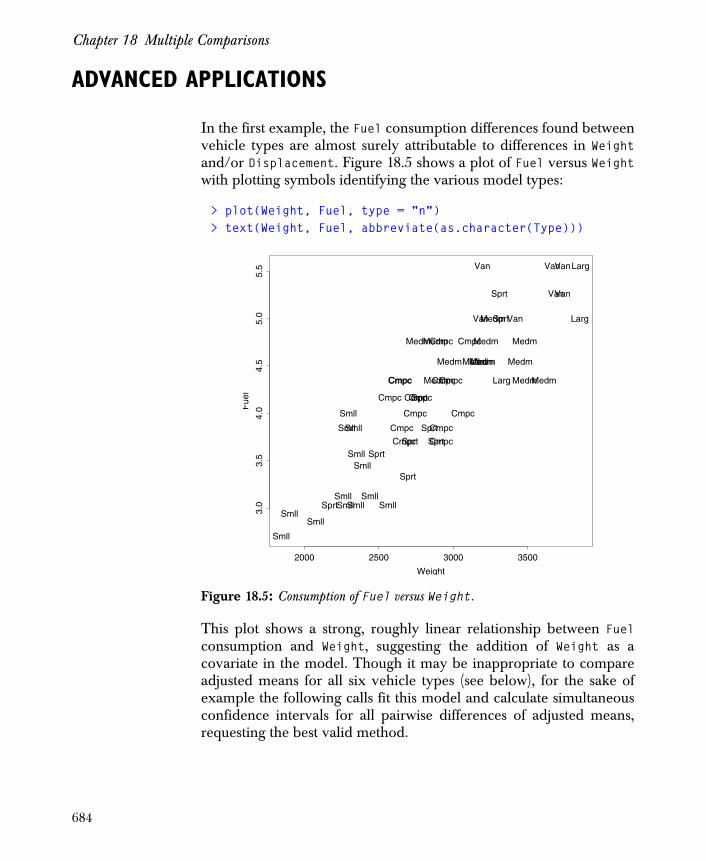
Chapter 18 Multiple Comparisons
ADVANCED APPLICATIONS
In the first example, the Fuel consumption differences found betweenvehicle types are almost surely attributable to differences in Weightand/or Displacement. Figure 18.5 shows a plot of Fuel versus Weightwith plotting symbols identifying the various model types:
> plot(Weight, Fuel, type = "n")> text(Weight, Fuel, abbreviate(as.character(Type)))
This plot shows a strong, roughly linear relationship between Fuelconsumption and Weight, suggesting the addition of Weight as acovariate in the model. Though it may be inappropriate to compareadjusted means for all six vehicle types (see below), for the sake ofexample the following calls fit this model and calculate simultaneousconfidence intervals for all pairwise differences of adjusted means,requesting the best valid method.
Figure 18.5: Consumption of Fuel versus Weight.
Weight
Fue
l
2000 2500 3000 3500
3.0
3.5
4.0
4.5
5.0
5.5
SmllSmll
Smll
Smll Smll
Smll
Smll
Smll
Smll
Smll
Smll
Smll
Smll
Sprt
Sprt
Sprt
Sprt
Sprt
Sprt
Sprt
Sprt
SprtCmpc
Cmpc
Cmpc
Cmpc
Cmpc
Cmpc
Cmpc
Cmpc
CmpcCmpc
Cmpc
Cmpc
Cmpc
Cmpc
Cmpc
Medm
Medm
Medm MedmMedmMedm
MedmMedm
Medm
Medm
Medm Medm
MedmLarg
Larg
Larg
Van VanVan
Van
VanVan
Van
684
Advanced Applications
> lmout.fuel.ancova <- lm(Fuel ~ Type + Weight,+ data = fuel.frame)> multicomp(lmout.fuel.ancova, focus = "Type",+ method = "best", plot = T)
The “best” valid method for this particular setting is the simulation-based method; Tukey’s method has not been shown to be valid in thepresence of covariates when there are more than three treatments.The intervals show that, adjusting for weight, the mean fuelconsumption of the various vehicle types are in most cases within oneunit of each other. The most notable exception is the van type, whichis showing higher mean fuel consumption than the small and sportytypes, and most likely higher than the compact, medium and largetypes.
Adjustment Schemes
When there is more than one term in the lm model, multicompcalculates standard adjusted means for levels of the focus factor andthen takes differences as specified by the comparisons argument.Covariates are adjusted to their grand mean value. If there are otherfactors in the model, the standard adjusted means for levels of thefocus factor use the average effect over the levels of any other (non-nested) factors. This adjustment scheme can be changed using theadjust argument, which specifies a list of adjustment levels for non-focus terms in the model. Any terms excluded from the adjust list
Figure 18.6: Fuel consumption ANCOVA (adjusted for Weight).
((
((
((
((
((
((
((
(
))
))
))
))
))
))
)))
Compact-LargeCompact-Medium
Compact-SmallCompact-Sporty
Compact-VanLarge-Medium
Large-SmallLarge-Sporty
Large-VanMedium-Small
Medium-SportyMedium-VanSmall-Sporty
Small-VanSporty-Van
-2.0 -1.5 -1.0 -0.5 0.0 0.5 1.0 1.5
simultaneous 95 % confidence limits, simulation-based methodresponse variable: Fuel
685

Chapter 18 Multiple Comparisons
are adjusted in the standard way. The adjust list may includemultiple adjustment values for each term; a full set of adjusted meansfor the focus factor is calculated for each combination of valuesspecified by the adjust list. Differences (if any) specified by thecomparisons argument are then calculated for each combination ofvalues specified by the adjust list.
Toothaker’s Two-Factor Design
Besides allowing you to specify covariate values for adjustment, theadjust argument can be used to calculate simple effects comparisonswhen factors interact, or (analogously) when covariate slopes aredifferent. This is best illustrated by an example: Toothaker (1993)discusses a two-factor design, using the data collected by Frank(1984). Subjects are female undergraduates, with response the scoreon a 20-item multiple choice test over a taped lecture. Factors arecognitive style (cogstyle, levels FI = Field independent and FD = Fielddependent) and study technique (studytech, levels NN = no notes,SN = student notes, PO = partial outline supplied, CO = completeoutline). The following code fits the model and performs a standardtwo-factor analysis of variance.
> score <- c(13, 13, 10, 16, 14, 11, 13, 13, 11, 16, 15, 16,+ 10, 15, 19, 19, 17, 19, 17, 20, 17, 18, 17, 18, 18, 19,+ 19, 18, 17, 19, 17, 19, 17, 19, 17, 15, 18, 17, 15, 15,+ 19, 16, 17, 19, 15, 20, 16, 19, 16, 19, 19, 18, 11, 14,+ 11, 10, 15, 10, 16, 16, 17, 11, 16, 11, 10, 12, 16, 16,+ 17, 16, 16, 16, 14, 14, 16, 15, 15, 15, 18, 15, 15, 14,+ 15, 18, 19, 18, 18, 16, 16, 18, 16, 18, 19, 15, 16, 19,+ 18, 19, 19, 18, 17, 16, 17, 15)
> cogstyle <- factor(c(rep("FI", 52), rep("FD", 52)))> studytec <- factor(c(rep("NN", 13), rep("SN", 13),+ rep("PO", 13), rep("CO", 13), rep("NN", 13), + rep("SN", 13), rep("PO",13), rep("CO",13)))
> interaction.plot(cogstyle, studytec, score)> aovout.students <- aov( score ~ cogstyle * studytec)
> anova(aovout.students)
686
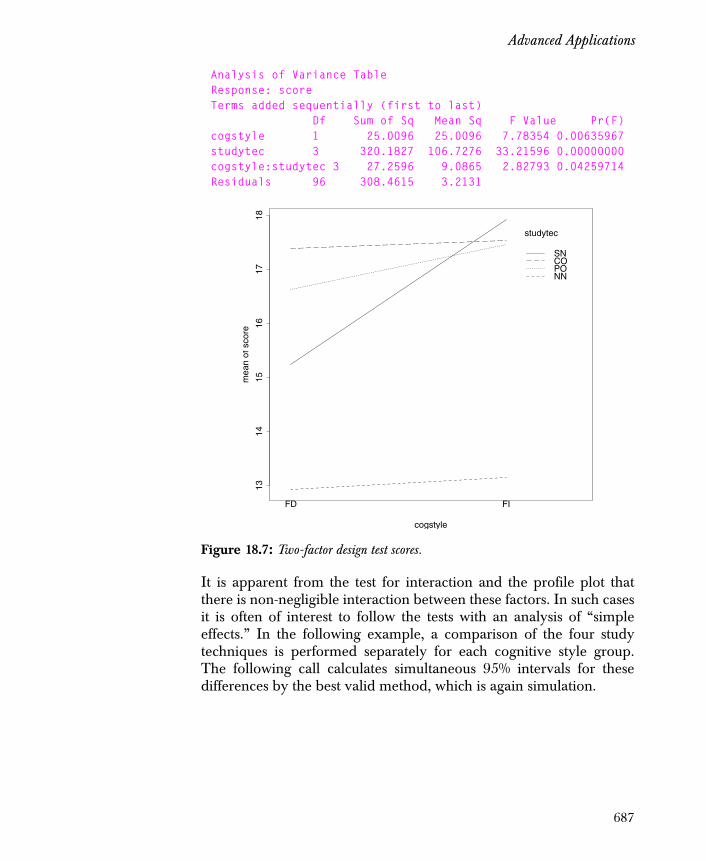
Advanced Applications
Analysis of Variance TableResponse: scoreTerms added sequentially (first to last) Df Sum of Sq Mean Sq F Value Pr(F)cogstyle 1 25.0096 25.0096 7.78354 0.00635967studytec 3 320.1827 106.7276 33.21596 0.00000000cogstyle:studytec 3 27.2596 9.0865 2.82793 0.04259714Residuals 96 308.4615 3.2131
It is apparent from the test for interaction and the profile plot thatthere is non-negligible interaction between these factors. In such casesit is often of interest to follow the tests with an analysis of “simpleeffects.” In the following example, a comparison of the four studytechniques is performed separately for each cognitive style group.The following call calculates simultaneous 95% intervals for thesedifferences by the best valid method, which is again simulation.
Figure 18.7: Two-factor design test scores.
cogstyle
mea
n of
sco
re
1314
1516
1718
FD FI
studytec
SNCOPONN
687
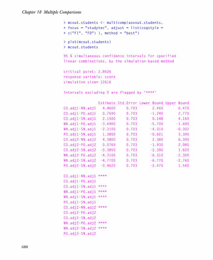
Chapter 18 Multiple Comparisons
> mcout.students <- multicomp(aovout.students,+ focus = "studytec", adjust = list(cogstyle =+ c("FI", "FD") ), method = "best")
> plot(mcout.students)> mcout.students
95 % simultaneous confidence intervals for specified linear combinations, by the simulation-based method
critical point: 2.8526 response variable: score simulation size= 12616
intervals excluding 0 are flagged by '****'
Estimate Std.Error Lower Bound Upper BoundCO.adj1-NN.adj1 4.4600 0.703 2.460 6.470CO.adj1-PO.adj1 0.7690 0.703 -1.240 2.770CO.adj1-SN.adj1 2.1500 0.703 0.148 4.160NN.adj1-PO.adj1 -3.6900 0.703 -5.700 -1.690NN.adj1-SN.adj1 -2.3100 0.703 -4.310 -0.302PO.adj1-SN.adj1 1.3800 0.703 -0.621 3.390CO.adj2-NN.adj2 4.3800 0.703 2.380 6.390CO.adj2-PO.adj2 0.0769 0.703 -1.930 2.080CO.adj2-SN.adj2 -0.3850 0.703 -2.390 1.620NN.adj2-PO.adj2 -4.3100 0.703 -6.310 -2.300NN.adj2-SN.adj2 -4.7700 0.703 -6.770 -2.760PO.adj2-SN.adj2 -0.4620 0.703 -2.470 1.540 CO.adj1-NN.adj1 ****CO.adj1-PO.adj1 CO.adj1-SN.adj1 ****NN.adj1-PO.adj1 ****NN.adj1-SN.adj1 ****PO.adj1-SN.adj1 CO.adj2-NN.adj2 ****CO.adj2-PO.adj2 CO.adj2-SN.adj2 NN.adj2-PO.adj2 ****NN.adj2-SN.adj2 ****PO.adj2-SN.adj2
688

Advanced Applications
Setting Linear Combinations of Effects
In many situations, the setting calls for inference on a collection ofcomparisons or linear combinations other than those availablethrough specifications of the focus, adjust, and comparisonsarguments. The lmat argument to multicomp allows you to directlyspecify any collection of linear combinations of the model effects forinference. It is a matrix (or an expression evaluating to a matrix)whose columns specify linear combinations of the model effects forwhich confidence intervals or bounds are desired. Specified linearcombinations are checked for estimability; if inestimable, the functionterminates with a message to that effect. You may disable this safetyfeature by specifying the optional argument est.check=F.Specification of lmat overrides any focus or adjust arguments; atleast one of lmat or focus must be specified. Differences requested orimplied by the comparisons argument are taken over the columns oflmat. In many instances no such further differencing would bedesired, in which case you should specify comparisons="none".
Textbook Parameteriza-tion
Linear combinations in lmat use the textbook parameterization of themodel. For example, the fuel consumption analysis of covariancemodel parameterization has eight parameters: an Intercept, sixcoefficients for the factor Type (Compact, Large, Medium, Small,Sporty, Van) and a coefficient for the covariate Weight. Note that thelevels of the factor object Type are listed in alphabetical order in theparameter vector.
Figure 18.8: Simple effects for study techniques.
((
((
((
((
((
((
))
))
))
))
))
))
CO.adj1-NN.adj1CO.adj1-PO.adj1CO.adj1-SN.adj1NN.adj1-PO.adj1NN.adj1-SN.adj1PO.adj1-SN.adj1CO.adj2-NN.adj2CO.adj2-PO.adj2CO.adj2-SN.adj2NN.adj2-PO.adj2NN.adj2-SN.adj2PO.adj2-SN.adj2
-7 -6 -5 -4 -3 -2 -1 0 1 2 3 4 5 6 7
simultaneous 95 % confidence limits, simulation-based methodresponse variable: score
689

Chapter 18 Multiple Comparisons
In the fuel consumption problem, many would argue that it is notappropriate to compare, for example, adjusted means of Smallvehicles and Large vehicles, since these two groups’ weights do notoverlap. Inspection of Figure 18.5 shows that, under thisconsideration, comparisons are probably only appropriate within twoweight groups: Small, Sporty, and Compact as a small weight group;Medium, Large, and Van as a large weight group. We can accomplishcomparisons within the two Weight groups using the following matrix,which is assumed to be in the object lmat.fuel. Note the columnlabels, which will be used to identify the intervals in the created figureand plot.
The code below creates the intervals. If we restrict attention to thesecomparisons only, we cannot assert any differences in adjusted meanfuel consumption.
> multicomp.lm(lmout.fuel.ancova, lmat = lmat.fuel,+ comparisons = "none", method = "best", plot = T)
Table 18.2: The Weight comparison matrix in the file lmat.fuel.
Com-Sma Com-Spo Sma-Spo Lar-Med Lar-Van Med-Van
Intercept 0 0 0 0 0 0
Compact 1 1 0 0 0 0
Large 0 0 0 1 1 0
Medium 0 0 0 -1 0 1
Small -1 0 1 0 0 0
Sporty 0 -1 -1 0 0 0
Van 0 0 0 0 -1 -1
Weight 0 0 0 0 0 0
690
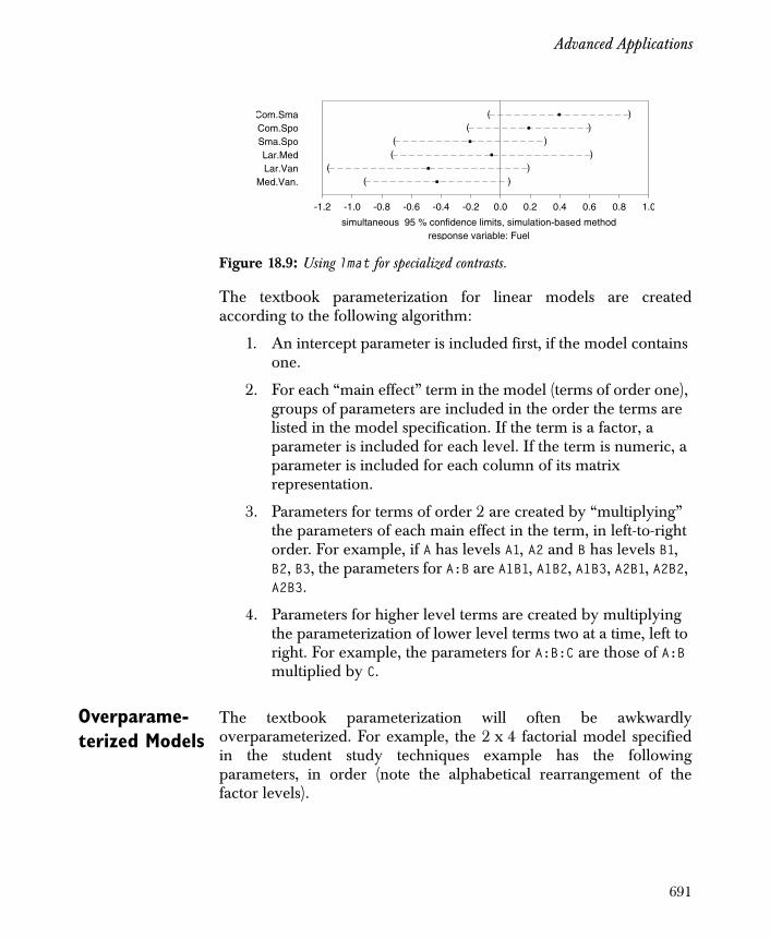
Advanced Applications
The textbook parameterization for linear models are createdaccording to the following algorithm:
1. An intercept parameter is included first, if the model contains one.
2. For each “main effect” term in the model (terms of order one), groups of parameters are included in the order the terms are listed in the model specification. If the term is a factor, a parameter is included for each level. If the term is numeric, a parameter is included for each column of its matrix representation.
3. Parameters for terms of order 2 are created by “multiplying” the parameters of each main effect in the term, in left-to-right order. For example, if A has levels A1, A2 and B has levels B1, B2, B3, the parameters for A:B are A1B1, A1B2, A1B3, A2B1, A2B2, A2B3.
4. Parameters for higher level terms are created by multiplying the parameterization of lower level terms two at a time, left to right. For example, the parameters for A:B:C are those of A:B multiplied by C.
Overparame-terized Models
The textbook parameterization will often be awkwardlyoverparameterized. For example, the 2 x 4 factorial model specifiedin the student study techniques example has the followingparameters, in order (note the alphabetical rearrangement of thefactor levels).
Figure 18.9: Using lmat for specialized contrasts.
((
((
((
))
))
))
Com.SmaCom.SpoSma.SpoLar.MedLar.Van
Med.Van.
-1.2 -1.0 -0.8 -0.6 -0.4 -0.2 0.0 0.2 0.4 0.6 0.8 1.0
simultaneous 95 % confidence limits, simulation-based methodresponse variable: Fuel
691

Chapter 18 Multiple Comparisons
• Intercept
• FD, FI
• CO, NN, PO, SN
• FDCO, FDNN, FDPO, FDSN, FICO, FINN, FIPO, FISN
Clearly, care must be taken in creating an lmat for factorial designs,especially with crossed and/or nested terms. The flexibility lmatprovides for creating study-specific linear combinations can beextremely valuable, though. If you are in doubt about the actualtextbook parameterization of a given linear model, it may help to runa standard analysis and inspect the lmat created, which is part of theoutput list of multicomp. For example, for the simple effects analysisof the student test scores of Figure 18.8, the implied lmat can be seenusing the command:
> mcout.students$lmat
Multicomp Methods Compared
The function multicomp.lm, after checking estimability of specifiedlinear combinations and creating a vector of estimates, a covariancematrix, and degrees of freedom, calls the base functionmulticomp.default. The function multicomp.default will be directlyvaluable in many settings. It uses a vector of estimates bvec andassociated covariance matrix vmat as required arguments, withoptional degrees of freedom df.residual (possibly Inf, the default) tocalculate confidence intervals on linear combinations of bvec. Theselinear combinations can be specified through an optional lmatargument and/or comparisons argument; there is neither a focus noran adjust argument. Linear combinations of bvec defined bycolumns of lmat (if any; the default lmat is an identity matrix) arecalculated, followed by any differences specified or implied by thecomparisons argument. The multicomp.lm options method, bounds,alpha, error.type, crit.point, sim.size, Srank, valid.check, andplot are also available in multicomp.default.
The function multicomp.default can be very useful as a means ofcalculating intervals based on summary data, or using the results ofsome model-fitting program other than lm; bvec must be consideredas a realization of a multivariate normal vector. If the matrix vmatincorporates any estimate of variance considered to be a realized chi-square variable, the degrees of freedom df.residual must bespecified.
692
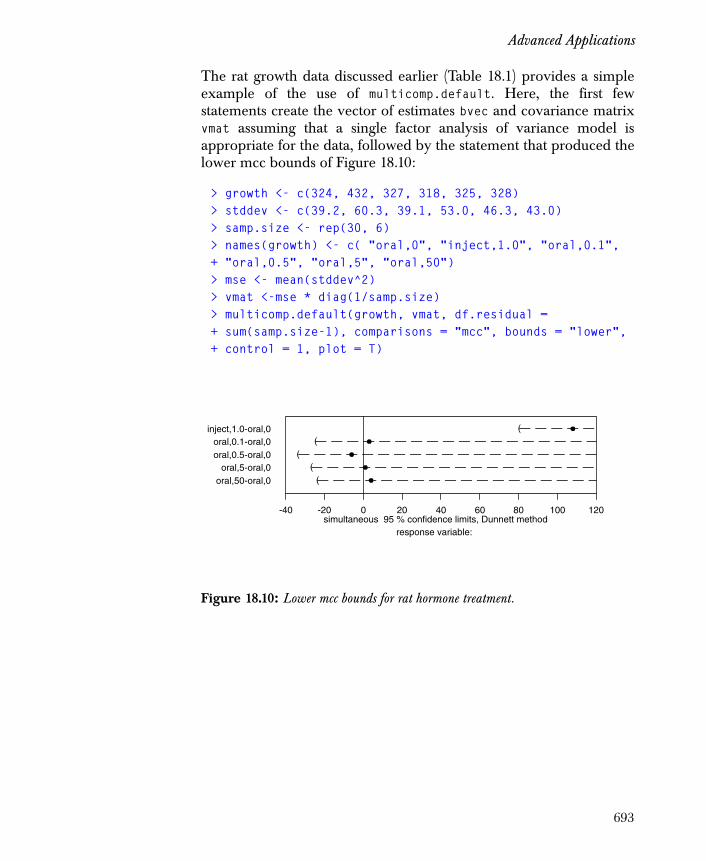
Advanced Applications
The rat growth data discussed earlier (Table 18.1) provides a simpleexample of the use of multicomp.default. Here, the first fewstatements create the vector of estimates bvec and covariance matrixvmat assuming that a single factor analysis of variance model isappropriate for the data, followed by the statement that produced thelower mcc bounds of Figure 18.10:
> growth <- c(324, 432, 327, 318, 325, 328)> stddev <- c(39.2, 60.3, 39.1, 53.0, 46.3, 43.0)> samp.size <- rep(30, 6)> names(growth) <- c( "oral,0", "inject,1.0", "oral,0.1",+ "oral,0.5", "oral,5", "oral,50")> mse <- mean(stddev^2)> vmat <-mse * diag(1/samp.size)> multicomp.default(growth, vmat, df.residual =+ sum(samp.size-1), comparisons = "mcc", bounds = "lower",+ control = 1, plot = T)
Figure 18.10: Lower mcc bounds for rat hormone treatment.
((
((
(
inject,1.0-oral,0oral,0.1-oral,0oral,0.5-oral,0
oral,5-oral,0oral,50-oral,0
-40 -20 0 20 40 60 80 100 120simultaneous 95 % confidence limits, Dunnett method
response variable:
693
Chapter 18 Multiple Comparisons
CAPABILITIES AND LIMITS
In summary, the function multicomp uses the information in a linearmodel; that is, a fitted fixed effects linear model. Through somecombination of the focus, adjust, comparisons and lmat arguments,any collection of estimable linear combinations of the fixed effectsmay be estimated, and simultaneous or non-simultaneous intervals orbounds computed by any of the applicable methods mentionedabove. Specified linear combinations are checked for estimabilityunless you specify est.check=F. Specified methods are checked forvalidity unless you specify valid.check=F.
The function multicomp.default uses a specified vector of parameterestimates bvec and a covariance matrix vmat, which will usually havesome associated degrees of freedom df.residual specified. Possiblythrough some combination of the comparisons or lmat arguments,any collection of linear combinations of the parameters may beestimated, and simultaneous or non-simultaneous intervals or boundscomputed by any of the applicable methods discussed above.Specified methods are checked for validity unless you specifyvalid.check=F.
The output from either procedure is an object of class "multicomp", alist containing elements table (a matrix of calculated linearcombination estimates, standard errors, and lower and/or upperbounds), alpha, error.type, method, crit.point, lmat (the finalmatrix of linear combinations specified or implied), and otherancillary information pertaining to the intervals. If the argumentplot=T is specified, the intervals/bounds are plotted on the activedevice. If not, the created multicomp object can be used as anargument to plot (see plot.multicomp).
The critical points for the methods of Tukey and Dunnett arecalculated by numerically using the Spotfire S+ quantile functionsqtukey, qdunnett, qmvt, and qmvt.sim, which may be directly usefulto advanced users for their own applications.
694
Capabilities and Limits
What the function multicomp does not do:
1. Any stagewise or multiple range test. The simultaneous testing procedures attributed to Fisher, Tukey, Scheffé, Sidak and Bonferroni are implied by the use of the corresponding method and noting which of the calculated intervals excludes zero. The multiple range tests of Duncan(1955) and Newman-Keuls (Newman, 1939; Keuls, 1952) do not provide familywise error protection, and are not very efficient for comparisonwise error protection; modern texts on multiple comparisons recommend uniformly against these two multiple range tests (Hsu, 1996; Hochberg and Tamhane, 1987; Bechofer et al., 1996; Toothaker 1993).
2. Multiple comparisons with the “best” treatment (MCB; Hsu, 1996, chapter 4), or any ranking and selection procedure (Bechofer, et al., 1995) other than selection of treatments better than a control implied by Dunnett’s one-sided methods. Users familiar with these methods and reasonably proficient at Spotfire S+ programming will be able to code many of these procedures through creative use of multicomp with the comparisons="mcc" option.
695

Chapter 18 Multiple Comparisons
REFERENCES
Bechhofer R.E., Santner T.J., & Goldsman D.M. (1995). Design andAnalysis of Experiments for Statistical Selection, Screening, and MultipleComparisons. New York: John Wiley & Sons, Inc.
Duncan D.B. (1955). Multiple range and multiple F tests. Biometrics11:1-42.
Dunnett C.W. (1955). A multiple comparison procedure forcomparing several treatments with a control. Journal of the AmericanStatistical Association 50:1096-1121.
Edwards D. & Berry J.J. (1987). The efficiency of simulation-basedmultiple comparisons. Biometrics 43:913-928.
Frank, B.M. (1984). Effect of field independence-dependence andstudy technique on learning from a lecture. American EducationResearch Journal 21, 669-678.
Hsu J.C. (1996). Multiple Comparisons: Theory and Methods. London:Chapman and Hall.
Hochberg, Y. & Tamhane, A.C. (1987). Multiple ComparisonProcedures. New York: John Wiley & Sons, Inc.
Juskevich J.C. & Guyer C.G. (1990). Bovine growth hormone: humanfood safety evaluation. Science 249:875-884.
Kramer C.Y. (1956). Extension of multiple range tests to group meanswith unequal numbers of replications. Biometrics 12:309-310.
Keuls M. (1952). The use of the ‘studentized range’ in connectionwith an analysis of variance. Euphytica 1:112-122.
Newman D. (1939). The distribution of the range in samples from anormal population, expressed in terms of an independent estimate ofstandard deviation. Biometrika 31:20-30.
Scheffé H. (1953). A method for judging all contrasts in the analysis ofvariance. Biometrika 40:87-104.
Sidak A. (1967). Rectangular confidence regions for the means ofmultivariate normal distributions. Journal of the Amererican StatisticalAssociation 62:626-633.
696

References
Toothaker L.E. (1993). Multiple Comparison Procedures. London: SagePublications.
Tukey J.W. (1953). Unpublished report, Princeton University.
697

Chapter 18 Multiple Comparisons
698

Index
INDEX
Symbols%in% operator
formula 34* operator
formula 32, 34formulas 595, 606
+ operatorformulas 595
. operatorformula 36
/ operatorformula 34
: operatorvariable interaction 32
^ operatorformulas 32, 606, 609
~ operator 29
Numerics2k designs
creating design data frame 602details of ANOVA 613diagnostic plots 610, 611EDA 604estimating effects 605, 607, 609example of 24 design 602replicates 607small order interactions 609
Aace
algorithm 307compared to avas 312example 309
ace function 309
ace goodness-of-fit measure 307acf function 124, 152add1 function
generalized linear models 390add1 function 45
linear models 255additive models
see generalized additive modelsadditive predictor
mathematical definition 385additivity and variance stabilizing
transformationsee avas 312
A estimates of scale 112AIC
related to Cp statistic 251air data set 239, 253algorithms
ace 307ANOVA 629avas 312backfitting 312correlation coefficient 150cubic smoothing splines 298deviance 302generalized additive models 12generalized linear models 11glm function 384, 415goodness-of-fit measure 307kernel-type smoothers 295L1 regression 370least squares regression 367least trimmed squares
regression 367linear models 10local cross-validation for
variable span smoothers 293
699

Index
locally weighted regression smoothing 291
Tukey’s one degree of freedom 588
alternating conditional expectationssee ace
alternative hypothesis 126 analysis of deviance tables, see
ANOVA tablesanalysis of variance see ANOVAANOVA
2k designs 604–614checking for interaction 594data type of predictors 10diagnostic plots 575diagnostic plots for 584, 595,
611EDA 572, 580, 593, 604effects table 577estimating effects 605, 607, 609factorial effects 633fitting functions 8grand mean plus treatment
effects form 629interaction 582one-way layout 574–577rank sum tests 662repeated-measures designs 659robust methods 662small-order interactions 609split-plot designs 656treatment means 577two-way additive model 583two-way replicated 594–601two-way unreplicated 578–590unbalanced designs 634variance stabilizing 597, 599,
601ANOVA, see also MANOVAanova function
chi-squared test 389, 411F test 416generalized additive models 395generalized linear models 389,
410, 411, 416
anova function 519anova function 9anova function
additive models 306ANOVA models
residuals 584, 595ANOVA tables 9, 595, 606, 609, 626
F statistics 416generalized additive models 306logistic regression 389, 395Poisson regression 410, 411quasi-likelihood estimation 416
aov.coag data setcreated 574
aov.devel.2 data setcreated 609
aov.devel.small data setcreated 611
aov.devel data setcreated 605
aov.pilot data setcreated 609
aov function 82k model 605arguments 574default coefficients returned 613estimating effects 609extracting output 606one-way layout 574, 577two-way layout 595two-way layout additive model
583aov function
repeated-measures designs 659split-plot designs 656
approx function 564auto.stats data set 15autocorrelation function
plot 124, 152avas
algorithm for population version 316
avasalgorithm 312backfitting algorithm 312
700

Index
compared to ace 312example 313key properties 315
avas function 313
Bbackfitting 317Bernoulli trial 69, 71, 84
definition 69beta distribution 57, 76beta function 76binom.test function 184binomial coefficients 74
definition 70binomial distribution 57, 69, 182
relation to geometric distribution 84
relation to hypergeometric distribution 74
relation to Poisson distribution 71
binomial family 387, 404inverse link function 421logit link 382probit link 382
blocking variable 578Box-Cox maximum-likelihood
procedure 315boxplot function
used to compute quartiles 101boxplots 123, 387, 409, 573, 582,
594Box-Tidwell procedure 315breakdown point 365B-splines 394B-splines 298
Ccancer study data 196canonical links 384catalyst data set 10catalyst data set 633categorical data
cross-classification 204categorical data see also factorscategorical variables 30
interactions 33Cauchy distribution 57, 79
stable 82cdf.compare function 160, 161, 170,
175, 178 CDF. See cumulative distribution
functionsCentral Limit Theorem 63, 106central moments
of a probability distribution 55of a sample 103
C function 41chisq.gof function 160, 165, 170
cut.points argument 166distribution argument 166estimating parameters 175n.classes argument 166n.param.est argument 176warning messages 177
chisq.test function 192chi-square distribution 57, 64chi-squared test 192, 195, 206, 389,
411chi-square goodness of fit test 160
choice of partition 166comparison with other one-
sample tests 174continuous variables 167distributions 166large sample theory 177mathematical definition 165
claims data set 204classification trees see also tree-
based modelscoag.df data frame
created 571coagulation data 570coefficients
converting to treatment effects 629
estimated 606extracting 8
701

Index
fixing 424coefficients function
abbreviated coef 8coef function 424coef function 8, 23, 606cognitive style study 686comp.plot function
defined 590comparative study 143comparing means
two samples 226comparing proportions
two samples 230comparison values 587conditioning plots 7, 9
analyzing 443conditioning panels 441conditioning values 441constructing 441local regression models 453residuals as response variable
448conditioning values 441confidence intervals 120, 191, 564,
681binomial distribution 185confidence level 126, 185correlation coefficient 157error rate 125for the sample mean 106, 107pointwise 272simultaneous 272two-sample 188
confint.lm functiondefined 273
contingency tables 183, 192, 195choosing suitable data 209continuous data 213creating 204reading 206subsetting data 216
continuous data 4converting to factors 213cross-tabulating 213
continuous random variable 52, 60, 76
continuous response variable 570continuous variables
interactions 33contr.helmert function 40contr.poly function 40contr.sum function 40contr.treatment function 39contrasts
adding to factors 625creating contrast functions 41Helmert 39polynomial 40specifying 41, 42, 43sum 40treatment 39
contrasts function 42contrasts function 625coplot function 7, 9coplots
see conditioning plotscor.confint function
created 157cor.test function 154corelation
serial 120cor function 156correlation
example 149serial 124, 245shown by scatterplots 120
correlation coefficient 119algorithm 150Kendall’s t measure 154, 155Pearson product-moment 154p-values
p-values 154rank-based measure 154, 155Spearman’s r measure 154, 155
correlation structures 505correlation structures and variance
functions 507corStruct classes 280, 507counts 182
702
Index
Cp statistic 390Cp statistic 251, 257cross-classification 204crosstabs function 204, 219
arguments 206, 216return object 206
cross-validationalgorithm 293
cubic smoothing splines 298algorithm 298
cumulative distribution functions 53, 161
See also probability distributions
cut function 213
Ddata
categorical 4continuous 4organizing see data framessummaries 5
data framesattaching to search list 247design data frame 579, 592, 602
degrees of freedom 134, 303nonparametric 303parametric 303smoothing splines 298
density function. See probability density function
density plot 123derivatives 548deriv function 552design data frames 579, 592, 602designed experiments
one factor 570–577randomized blocks 578replicated 591two-way layout 578
devel.design data framecreated 602
devel.df data framecreated 604
deviance 418algorithm 302
deviance residuals 418D function 551diagnostic plots
ANOVA 584linear regression 242local regression models 436multiple regression 249outliers 575
diff.hs data set 151discrete random variable 52, 69, 84dispersion parameter 383, 416
obtaining chi-squared estimates 411
distribution functions. See probability distributions
double exponential distributionrandom number generation 87
drop1 function 44linear models 251
drug.fac data set 195drug.mult data set 658drug data set 194dummy.coef function 630Dunnett’s intervals 678, 679durbinWatson function 245Durbin-Watson statistic 245dwilcox function 57
EEDA
see exploratory data analysiseda.shape
defined 124eda.ts function 124EDA functions
interaction.plot 582plot.design 572, 580, 594plot.factor 573, 581
empirical distribution function 161ethanol data set 275Euclidean norm 365example functions
703

Index
comp.plot 590confint.lm 273cor.confint function 157eda.shape 124eda.ts 124tukey.1 589
examples2k design of pilot plant data 6072k design of product
development data 602ace example with artificial data
set 309ANOVA of coagulation data
570ANOVA of gun data 629ANOVA of penicillin yield data
578ANOVA of poison data 591ANOVA table of wafer data
626avas with artificial data set 313binomial model of Salk vaccine
trial data 186binomial test with roulette 184chi-squared test on propranolol
drug data 196chi-squared test on Salk vaccine
data 195coplot of ethanol data 441correlation of phone and
housing starts data 149developing a model of auto data
14Fisher’s exact test on
propranolol drug data 196goodness of fit tests for the
Michelson data 175hypothesis testing of lung
cancer data 190linear model of air pollution
data 239logistic regression model of
kyphosis data 387MANOVA of wafer data 654
Mantel-Haenszel test on cancer study data 196
McNemar chi-squared test on cancer study data 199
multiple regression with ammonia loss data 247
new family for the negative binomial distribution 430
new variance function for quasi-likelihood estimation 426
one-sample speed of light data 129
paired samples of shoe wear data 144
parameterization of scores data 619
perspective plot of fitted data 452
Poisson regression model of solder.balance data 407
probit regression model of kyphosis data 404
proportions test with roulette 185
quasi-likelihood estimation of leaf blotch data 426
quasi-likelihood estimation of solder.balance data 416
repeated-measure design ANOVA of drug data 658
split-plot design ANOVA of rubber plant data 656
two-sample weight gain data 137
variance components model of pigment data 665
weighted regression of course revenue data 261
expected value 112of a random variable 54
exploratory data analysis 121four plot function 124interaction 582phone and housing starts data
151
704

Index
plots 5serial correlation 124shoe wear data 145speed of light data 130time series function 124weight gain data 137
exponential distribution 57, 76random number generation 86relation to gamma distribution
77relation to Weibull distribution
77
Ffac.design function 579, 602factorial effects 633factors 4
adding contrasts 625creating from continuous data
213levels 4parametrization 39plotting 387, 409, 582setting contrasts 42, 43
family functions 383, 425binomial 382, 387, 404creating a new family 425in generalized additive models
386inverse link function 421Poisson 383, 407quasi 383
F distribution 57, 67first derivatives 548fisher.test function 192Fisher’s exact test 193, 196fitted.values function
abbreviated fitted 575fitted function 8, 575, 576, 585,
596, 612fitted values
ANOVA models 585, 596, 599, 611
extracting 8
lm models 242fitting methods
formulas 37functions, listed 8missing data filter functions 47optional arguments to functions
46specifiying data frame 46subsetting rows of data frames
46weights 46
fitting models 554 fixed coefficients, See offsetsformula function 31formulas 28–45, 545
automatically generating 249categorical variables 30, 33, 34changing terms 44, 45conditioning plots 441continuous variables 30, 33, 34contrasts 39expressions 30fitting procedures 37generating function 31implications 546interactions 32, 33, 34intercept term 30linear models 239matrix terms 30nesting 33, 34, 35no intercept 424offsets 424operators 29, 31, 32, 34, 36polynomial elements 277simplifying 546specifying interactions 595, 606,
609syntax 31, 36updating 44, 45variables 29, 30
friedman.test function 663Friedman rank sum test 662, 663F-statistic
linear models 241F statistics 416
705

Index
F test 416F-test
local regression models 458fuel.frame data 674fuel consumption problem 690
Ggain.high data set 137gain.low data set 137gam function 385, 387, 404, 407
available families 386binomial family 394family argument 387, 404, 407
gam function 8, 24gam function
returned object 303gamma distribution 57, 77gamma function 66, 67, 77
definition 64 GAMs, see generalized additive
modelsGaussian distribution. See normal
distributionGaussian mean
one-sample test of 224generalized additive models
algorithm 12, 301analysis of deviance tables 395ANOVA tables 306contrasted with generalized
linear models 400degrees of freedom 303deviance 418fitting function 8link function 385lo function 386logistic regression 394marginal fits 421mathematical definition 385plotting 396prediction 420residual deviance 302residuals 418s function 386
smoothing functions 385, 386summary of fit 394, 395, 397
generalized linear modelsadding terms 390algorithm 11analysis of deviance tables 416canonical links 384composite terms 422contrasted with generalized
additive models 400deviance 418dispersion parameter 383, 411,
416fitting function 8fixing coefficients 424logistic regression 387logit link function 382log link function 383mathematical definition 381plotting 390, 412Poisson regression 407prediction 420probit link function 382probit regression 404quasi-likelihood estimation 383,
415residuals 418safe prediction 422specifying offsets 424summary of fit 388, 400using the gam function 385
geometric distribution 57, 84relation to negative binomial
distribution 84glm.links data set 425glm.variances data set 425glm function 387, 404, 407
algorithm 384, 415available families 383binomial family 382family argument 387, 404, 407Poisson family 383quasi family 383residuals component 418
glm function 8
706
Index
GLMs, see generalized linear models
GOF. See goodness of fit testsgoodness-of-fit measure
algorithm 307goodness of fit tests 160
chi-square 160, 165, 174, 177comparison of one-sample tests
174composite 174conservative tests 175Kolmogorov-Smirnov 160, 168,
174, 178one-sample 160, 165, 168, 172Shapiro-Wilk 160, 172, 174, 175two-sample 160, 168, 178
gradient attribute 549groupData class 465grouped datasets 465guayule data set 209, 656gun data set 629, 634
Hhalf-normal QQ-plots 610Helmert contrasts 39hessian attribute 550hist function 408hist function 5, 575, 584, 595histograms 5, 123, 575, 584, 595horshft argument 528Hotelling-Lawley trace test 654Huber psi functions
for M estimates of location 110Huber rho functions
for tau estimates of scale 113hypergeometric distribution 57, 74hypothesis testing 120, 126
goodness of fit 160one sample proportions 184p-values 154three sample proportions 190two sample proportions 186
Iidentify function 20identifying plotted points 20I function 398importance
in ppreg 324inner covariates 465interaction.plot function 582,
594interactions 320
checking for 582, 594specifying 32, 595, 606specifying order 609
intercept 30no-intercept model 424
intercept-only model 255interquartile range
of a probability distribution 55of a sample 101
IQR. See interquartile rangeis.random function 664iteratively reweighted least squares
384, 415score equations 384
KKendall’s t measure 154, 155kernel functions 295, 296kernel-type smoother
algorithm 295Kolmogorov-Smirnov goodness of
fit test 160comparison with other one-
sample tests 174distributions 169hypotheses tested 168interpretation 168mathematical definition 168one-sample 168two-sample 168, 178
kruskal.test function 662Kruskal-Wallis rank sum test 662ks.gof function 160, 176
707

Index
alternative argument 169distribution argument 169estimating parameters 175one-sample 169two-sample 178
ksmooth function 295kernels available 295
KS test. See Kolmogorov-Smirnov goodness of fit test
kurtosisof a probability distribution 55of a sample 104
kurtosis function 104kyphosis data set 387, 404kyphosis data set 5kyphosis data set 213
Ll1fit function 370L1 regression 370
algorithm 370Laplace distribution. See double
exponential distributionleast absolute deviation regression
see L1 regressionleast squares regression 239
algorithm 367least squares regression,
mathematical representation 276least squares vs. robust fitted model
objects 340least trimmed squares regression
algorithm 367breakdown point 369
leave-one-out residuals 294level of significance 126levels
experimental factor 570likelihood models 544linear dependency, see correlationlinear mixed-effects models
fitting 479model definitions 479
linear models
adding terms 255algorithm 10confidence intervals 272diagnostic plots 242, 243, 249,
253dropping terms 251fitting function 8, 239, 280intercept-only model 255mathematical definition 381modifying 251, 260pointwise confidence intervals
272polynomial regression 275predicted values 270selecting 251, 257serial correlation in 245simultaneous confidence
intervals 272stepwise selection 257summary of fitted model 241updating 260
linear models see also generalized linear models
linear predictor 385, 420mathematical definition 381
linear regression 237link functions
canonical 384in generalized additive models
385in generalized linear models
425log 383logit 382mathematical definition 381probit 382, 425
lme functionadvanced fitting 505arguments 481
lme objectsanalysis of variance 486extracting components 489ploting 487predicting values 491printing 483
708
Index
summarizing 484lm function 8, 18, 240
multiple regression 248subset argument 21
lm function 239, 280arguments 249polynomial regression 277
lmRobMM function 335locally weighted regression
smoothing 290, 434algorithm 291
local maxima and minima 529local regression models 12, 434
diagnostic plots 446diagnostic plots for 436dropping terms 455fitting function 8improving the model 455multiple predictors 446one predictor 435parametric terms 455plotting 452predicted values 452returned values 435
local regression smoothing 394location.m function 111loess 290
scatterplot smoother 290scatterplot smoothing 291
loess.smooth function 291loess function 8, 435, 436, 453loess models see local regression
modelsloess smoother function 301lo function 386, 394lo function 301logistic distribution 57, 78logistic regression 387
analysis of deviance tables 389, 395
binary response 402contrasted with probit
regression 405Cp statistic 390factor response 402
logit link function 382numeric response 402tabulated response 402t-tests 389using the gam function 386, 394
logit link functionmathematical definition 382
log link functionmathematical definition 383
lognormal distribution 57, 80lprob function 546, 549ltsreg function 367lung cancer study 189
MMAD. See median absolute
deviationmad function 101make.family function 425, 430Mann-Whitney test statistic. See
Wilcoxon testMANOVA 654
repeated-measures designs 660test types available 654
manova function 654Mantel-Haenszel test 193, 196maximum
of a sample 98, 105maximum likelihood estimate
for variance components models 665
maximum likelihood method 479, 486
mcnemar.test function 199McNemar chi-squared test 193, 199mean 119
computing median absolute deviation 100
computing sample moments 103
computing sample variance 99confidence intervals 107of a probability distribution 54of a sample 95, 105, 110
709

Index
of Poisson distribution 72standard deviation 106standard error 106, 107trimmed mean 96
mean absolute deviationof a random variable 54
mean function 95trimmed mean 96
median 124computing median absolute
deviation 100of a probability distribution 55of a sample 96, 105, 110
median absolute deviation (MAD) 100
computing A estimates of scale 112
computing M estimates of location 111
computing tau estimates of scale 113
median function 97M estimates of location 110
asymptotic variance 112computing A estimates of scale
112computing tau estimates of scale
113M-estimates of regression 372
fitting function 372Michaelis-Menten relationship 543mich data set 175mich data set
created 130Michelson speed-of-light data 129,
175minimum
of a sample 98, 105minimum sum 526minimum-sum algorithm 544minimum sum function 534minimum sum-of-squares 526missing data
filters 47mixed-effects model 463
MM-estimate 335mode
of a probability distribution 55of a sample 97
modelmixed-effects 463nonlinear mixed-effects 493
model.tables function 577model.tables function 630model data frame 579, 592, 604models 28–45
data format 4data type of variables 9development steps 3example 14extracting information 8fitting functions 8iterative process 14missing data 47modifying 9nesting formulas 33, 34paradigm for creating 8parameterization 34plotting 9prediction 9specifying all terms 32specifying interactions 32types available in Spotfire S+ 3
models see also fitting methodsmoments
of a probability distribution 55ms function 526, 534
arguments to 554multicomp
Lmat argument 689multicomp function
df.residual argument 679using summary data 679vmat argument 679
multicomp function 675alpha argument 683comparisons argument 680control argument 681est.check argument 694focus argument 680
710

Index
simsize argument 683valid.check option 682
multilevel linear mixed-effects models 479
multiple comparisons 674from summary data 679with a control (MCC) 678
multiple regression 247diagnostic plots 249
multiple R-squaredlinear models 241
multivariate analysis of variancesee MANOVA
multivariate normal distribution 57, 82
Nnamevec argument 553negative binomial distribution 57,
84in generalized linear models
430nesting formulas 33, 34nlimb function 530nlme function
advanced fitting 505Arguments 494
nlme function 493, ??–520nlme objects
analysis of variance 501extractnig components 504plotting 501predicting values 502printing 497summarizing 499
nlminb function 532nlregb function 538nls function 526, 537
arguments to 554nlsList function 513nlsList function ??–520nnls.fit 536nnls.fit function 535
nonlinear least-squares algorithm 545
nonlinear mixed-effects modelsfitting 493model definition 493
nonlinear models 526nonnegative least squares problem
535nonparametric methods 121nonparametric regression
ace 307normal (Gaussian) distribution 57,
61Central Limit Theorem 63, 106in probit regression 382lognormal 80multivariate 57, 82random number generation 89stable 82standard 62
nregb function 536null hypothesis 126
completely specified probabilities 186, 187
equal-probabilities 186, 187null model 255, 390
Oobservation weights
in ppreg 326offset function 424offsets
in generalized linear models 424
oil.df data set 337one-sample test
binomial proportion 229Gaussian mean 224
one-way layout 570, 574overall mean plus effects form
576robust methods 662
- operatorformula 32
711
Index
operatorsformula 29, 31, 32, 34, 36, 595,
606, 609optimise function 529optimization functions 527options function 43outer covariates 465outer function 421outliers 118
checking for 575, 576, 582identifying 20sensitivity to 581
over-dispersion 416in regression models 415
overparameterized models 691
Ppaired comparisons 144paired t-test 148pairs function 5, 439
linear models 253pairs function 247pairwise scatter plots
see scatterplot matricesparameter function 547parametrized data frames 547param function 547PDF. See probability density
functionpdMat classes 505peaks function 529Pearson product-moment
correlation 154Pearson residuals 418pen.design data frame
converted to model data frame 580
created 579pen.df data frame
created 579penicillin yield data 578, 579perspective plots 439
local regression models 452perspective plots, creating grid 452
persp function 421phone.gain data set 151phone increase data 149pigment data 665pigment data set 665Pillai-Bartlett trace test 654pilot.design data frame
created 608pilot.df data frame
created 609pilot.yield vector 608pilot plant data 608ping-pong example 539, 548, 551,
558plot.design function 572, 580,
581, 594, 604plot.factor function 387, 409plot.factor function 573, 581,
594, 605plot.gam function 392, 396, 413plot.glm function 390, 412
ask argument 393plot function 5, 9plots
autocorrelation plot 152boxplots 123, 387, 409, 573,
582, 594conditioning plots 7, 9, 441density plot 123density plots 123diagnostic 436
for ANOVA 595, 611diagnostic for ANOVA 575exploratory data analysis 5, 123factor plots 387, 409histograms 5, 123, 575, 584, 595interactively selecting points 20normal probability plot 9perspective 439qq-plots 123quantile-quantile 5, 584, 595,
610, 611quantile-quantile plot 123quantile-quantile plots 575scatterplot matrices 5, 439
712
Index
surface plots 421plotting
design data frames 580factors 387, 409, 582fitted models 9generalized additive models 396generalized linear models 390,
412linear models 243local regression models 436,
453residuals in linear models 243
point estimates 156pointwise confidence intervals
linear models 272pointwise function 272poison data 591, 592poisons.design data set
created 592poisons.df data frame
created 592Poisson distribution 57, 71
in Poisson regression 383mean 72
Poisson family 407log link function 383
Poisson process 72, 76, 77, 430Poisson regression 407
analysis of deviance tables 410, 411
log link function 383using the gam function 386
poly.transform function 277poly function 277polynomial contrasts 40polynomial regression 277polynomials
formula elements 277orthogonal form transformed to
simple form 277polyroot function 528positive-definite matrices 505power law 600ppreg
backward stepwise procedure 324
forward stepwise procedure 322model selection strategy 324multivariate response 326
ppreg function 318examples 320
predict.gam functionsafe prediction 423type argument 420
predict.glm functiontype argument 420
predicted response 9predicted values 452predict function 9, 25
linear models 270, 272returned value 270
prediction 25generalized additive models 420generalized linear models 420linear models 270safe 422
predictor variable 5probability
definition 51probability density curves 123probability density function 52
computing 57See also probability
distributionsprobability distributions 51, 53
beta 76binomial 69, 182Cauchy 79chi-square 57, 64comparing graphically 161computing 56empirical 161exponential 76, 86F 67gamma 77geometric 84hypergeometric 74listed 57logistic 78
713

Index
lognormal 80multivariate normal 82negative binomial 84normal (Gaussian) 61, 89, 118Poisson 71range of standard normals 81stable 82t 65uniform 56, 60Weibull 77Wilcoxon rank sum statistic 56,
57, 85probit link function 425
mathematical definition 382probit regression 404
contrasted with logistic regression 405
probit link function 382using the gam function 386
product development data 602profile function 561profile projections 560profiles for ms 561profiles for nls 561profile slices 560profile t function 561profiling 560projection pursuit regression
algorithm 318, 320prop.test function 185, 186proportions 182
confidence intervals 185, 188one sample 184three or more samples 189two samples 186
propranolol data 194puromycin experiment 542p-values 126, 128pwilcox function 56
Qqchisq function 57qqnorm function 5, 9, 575, 584, 595,
610
qqnorm functionlinear models 243
qqplot function 178qq-plots
see quantile-quantile plotsquantile function
used to compute quartiles 101quantile-quantile plots 5, 123
full 611half-normal 610residuals 575, 584, 595, 611
quantilescomputing 57of a probability distribution 55
quartiles 124of a probability distribution 55of a sample 101, 105
quasi family 383quasi-likelihood estimation 383, 415
defining a new variance function 426
Rrandomized blocks 578random number generation 56, 86
double exponential (Laplace) 87exponential 86normal (Gaussian) 89
random variable 52continuous 52, 60, 76discrete 52, 69, 84
rangeof a sample 98, 105of standard normal random
variables 81range function 98rat growth-hormone study 678, 693regression
diagnostic plots 242generalized additive models 385generalized linear models 381least absolute deviation 370least squares 239linear models 8, 10
714

Index
logistic 382, 386, 387M-estimates 372multiple predictors 247one variable 239overview 237Poisson 383, 386, 407polynomial terms 275probit 382, 386, 404quasi-likelihood estimation 383,
415robust techniques 333simple 239stepwise model selection 257updating models 260weighted 261
regression line 243confidence intervals 272
regression splines 290regression trees see also tree-based
modelsrepeated-measures designs 658replicated factorial experiments 591resid function 8, 575, 576, 585,
596, 612 resid function, see residuals
functionresidual deviance 302residuals
ANOVA models 575, 584, 595, 599, 611
definition 239deviance 418extracting 8generalized additive models 418generalized linear models 418local regression models 436normal plots 243Pearson 418plotting in linear models 243response 419serial correlation in 245working 418
residuals function 419type argument 419
residuals function
abbreviated resid 8, 575response
lm models 242response residuals 419response variable 5
logistic regression 402response weights
in ppreg 326restricted maximum likelihood
method (REML) 479robust estimates 96, 100, 111
A estimates of scale 112interquartile range (IQR) 101median 96median absolute deviation 100,
111, 112, 113M estimates of location 110,
112, 113mode 97tau estimates of scale 113trimmed mean 96
robust methods 121robust regression 333
least absolute deviation 370M-estimates 372
Roy’s maximum eigenvalue test 654rreg function 372
weight functions 374runif function 56
Ssalk.mat data set 193Salk vaccine trials data 186, 192, 193sample function 60, 69sample mean. See meansample sum of squares. See sum of
squaressample variance. See variancescale.a function 114scale.tau function 114scatterplot matrices 5, 247, 253, 439scatter plots 146scatterplot smoothers 237, 290
locally weighted regression 291
715

Index
score equations 384scores.treat data set 619scores data set 619second derivatives 550self-starting function ??–520
biexponential model 514first-order compartment model
514four-parameter logistic model
514logistic model 515
SEM. See standard errors function 386, 394s function 301shapiro.test function 172, 177
allowable sample size 172Shapiro-Wilk test for normality 160,
175comparison with other one-
sample tests 174interpretation 172mathematical definition 172
shoe wear data 143simple effects comparisons 686simultaneous confidence intervals
273linear models 272
skewnessof a probability distribution 55of a sample 103
skewness function 103smooth.spline function 298smoothers 237
comparing 299cubic smoothing spline 290cubic spline 298kernel-type 290, 295locally weighted regression 290variable span 290, 292
smoothing functions 385cubic B-splines 394local regression smoothing 394
solder.balance data set 407solder data set 209soybean data 476–520
Spearman’s r measure 154, 155splines
B-splines 298cubic smoothing splines 298degrees of freedom 298regression 290
split-plot designs 656stable distribution 57, 82stack.df data set
defined 247stack.loss data set 247stack.x data set 247standard deviation 119
of a probability distribution 54of a sample 99of the sample mean 106
standard errorlinear models 241of the sample mean 106, 107predicted values 270
statistical inference 125alternative hypothesis 126assumptions 121confidence intervals 125counts and proportions 182difference of the two sample
means 139equality of variances 139hypothesis tests 125null hypothesis 126
status.fac data set 195status data set 194stdev function 99
used to compute standard error 107
step function 257displaying each step 259
stepwise model selection 257straight line regression 237Student’s t-test 127
one-sample 133paired test 147two-sample 139
sum contrasts 40summarizing data 5
716

Index
summary.gam function 394, 397summary.glm function 388, 400
disp argument 411dispersion component 416
summary function 105generalized additive models
394, 397generalized linear models 388,
400summary function 5, 9, 23, 241
ANOVA models 606sum of squares
of a sample 99, 100super smoother 312, 317, 323supersmoother 292supsm function 292supsmu
use with ppreg 323surface plots 421symbolic differentiation 551
Tt.test function 108t.test function 133, 139, 147table function 402
used to compute modes 97table function 195tau estimates of scale 113t distribution 57, 65
computing confidence intervals 108
relation to Cauchy distribution 79
test.vc data set 667textbook parameterization of the lm
model 689t measure of correlation 154, 155Toothaker’s two-factor design 686transformations
variance stabilizing 312treatment 570
ANOVA models 574treatment contrasts 39
tree-based modelsfitting function 8
tree function 8tri-cube weight function 291trimmed mean 96t-tests
see Student’s t-testtukey.1 function 586
defined 589Tukey’s bisquare functions
for A estimates of scale 112for M estimates of location 110
Tukey’s method 677Tukey’s one degree of freedom 586,
588Tukey-Kramer multiple comparison
method 677two-way layout
additive model 583details 600multiplicative interaction 586power law 600replicated 591–601replicates 594, 596robust methods 663unreplicated 578–590variance stabilizing 597, 599
Uunbiased estimates
sample mean 95sample variance 99, 100
under-dispersionin regression models 415
uniform distribution 56, 57, 60random number generation 86
uniroot function 528update function 9, 44, 437, 455
linear models 260updating models 9
linear models 260local regression models 437,
455
717

Index
Vvar.test function 139varcomp function 8varcomp function 665varFunc classes 280, 507var function 99
computing biased/unbiased estimates 100
computing the sum of squares 100
SumSquares argument 100variables
continuous 30variance 119
biased/unbiased estimates 99of a probability distribution 54of a sample 99, 106
variance components models 664estimation methods 665maximum likelihood estimate
665MINQUE estimate 665random slope example 666restricted maximum likelihood
(REML) estimate 665winsorized REML estimates
666variance functions 505
in generalized additive models 385
in generalized linear models 381, 425
in logistic regression 382
in Poisson regression 383in probit regression 382
variance stabilizing 597, 599Box-Cox analysis 601least squares 601
vershft argument 528
Wwafer data 626wafer data set 626wave-soldering skips experiment
540wear.Ascom data set 145wear.Bscom data set 145Weibull distribution 57, 77weighted regression 46, 237, 261weight gain data 136wilcox.test 128wilcox.test function 135, 139, 141,
148Wilcoxon test 128, 129
one-sample 135paired test 148two-sample 85, 141
Wilks’ lambda test 655working residuals 418 W-statistic. See Shapiro-Wilk test
for normality
Yyield data set
created 579
718


