Laboratoire de Physique Statistique, Ecole Normale Supérieure, Paris, France
STEFAN LLEWELLYN SMITH
Department of Mechanical & Aerospace Engineering, Jacobs School of Engineering, University of California, San Diego,La Jolla, California
W. R. YOUNG
Scripps Institution of Oceanography, University of California, San Diego, La Jolla, California
(Manuscript received 30 July 2003, in final form 20 January 2004)
ABSTRACT
The radiative flux of internal wave energy (the “tidal conversion”) powered by the oscillating flow of auniformly stratified fluid over a two-dimensional submarine ridge is computed using an integral-equationmethod. The problem is characterized by two nondimensional parameters, A and B. The first parameter, A,is the ridge half-width scaled by �h, where h is the uniform depth of the ocean far from the ridge and � isthe inverse slope of internal tidal rays (horizontal run over vertical rise). The second parameter, B, is theridge height scaled by h. Two topographic profiles are considered: a triangular or tent-shaped ridge and a“polynomial” ridge with continuous topographic slope. For both profiles, complete coverage of the (A, B)parameter space is obtained by reducing the problem to an integral equation, which is then discretized andsolved numerically. It is shown that in the supercritical regime (ray slopes steeper than topographic slopes)the radiated power increases monotonically with B and decreases monotonically with A. In the subcriticalregime the radiated power has a complicated and nonmonotonic dependence on these parameters. As A →0 recent results are recovered for the tidal conversion produced by a knife-edge barrier. It is shownanalytically that the A → 0 limit is regular: if A � 1 the reduction in tidal conversion below that at A � 0is proportional to A2. Further, the knife-edge model is shown to be indicative of both conversion rates andthe structure of the radiated wave field over a broad region of the supercritical parameter space. As Aincreases the topographic slopes become gentler, and at a certain value of A the ridge becomes “critical”;that is, there is a single point on the flanks at which the topographic slope is equal to the slope of an internaltidal beam. The conversion decreases continuously as A increases through this transition. Visualization ofthe disturbed buoyancy field shows prominent singular lines (tidal beams). In the case of a triangular ridgethese beams originate at the crest of the triangle. In the case of a supercritical polynomial ridge, the beamsoriginate at the shallowest point on the flank at which the topographic slope equals the ray slope.
1. Introduction
The passage of the barotropic tide over submarinetopography is a main source of the mechanical energyrequired to power the internal gravity wave field andmix the stably stratified ocean (Ledwell et al. 2000;
Munk and Wunsch 1998). Satellite altimetry has showndeep-sea tidal energy losses concentrated at submarineridges and island arcs (Egbert and Ray 2001; Ray andMitchum 1996). Observational and modeling studieshave focused on the Hawaiian Ridge as an accessiblesite at which these processes might be investigated(Merrifield and Holloway 2002; Rudnick et al. 2003).Thus, there is a powerful motivation to understand thefactors that control the tidally powered radiation of in-ternal gravity waves (the “tidal conversion”) from arealistically steep and tall ridge.
Corresponding author address: W. R. Young, Scripps Institutionof Oceanography, University of California, San Diego, La Jolla,CA 92023-0230.E-mail: [email protected]
The main theoretical approach to this tidal conver-sion problem uses ideas developed first by Bell(1975a,b; see also Khatiwala 2003; Llewellyn Smith andYoung 2002; St. Laurent and Garrett 2002). In Bell’swork the crucial approximations are that topographicslopes are small relative to the slope of internal tidalbeams, and that the height of the topography is muchless than the depth of the ocean. With these two restric-tions, the bottom boundary condition can be appliedapproximately at a flat surface, say z � 0. This simpli-fication allows the linear superposition of different to-pographic sinusoids and the application of Fourieranalysis so that the conversion rate is obtained in termsof the topographic spectral density. We refer to the twoapproximations introduced by Bell as the weak topog-raphy approximation (WTA).
Independent of Bell, in 1973 P. G. Baines developeda procedure that avoids linearization of the bottomboundary condition around z � 0. At first, Baines alsorestricted consideration to the subcritical case, in whichthe slope of the topography is everywhere less than theslope of the tidal beams (referred to by Baines as “flatbump” topography). In 1982, Baines dealt with thecomplementary case of supercritical topography(“steep” topography). Thus, using the method ofBaines (1973, 1982) one can, in principle, deal with ar-bitrary topography, but the calculations are difficult,particularly for the supercritical case, where Baines wasforced to make some additional approximations. In thisarticle we will develop a fresh approach to the problemof tidal generation by a submarine ridge. Our method,based on results of Robinson (1969) and LlewellynSmith and Young (2003), works in both the sub- andsupercritical cases and results in compact estimates ofthe radiated tidal energy.
We consider several idealized models of a submarineridge (see Fig. 1) and attempt a broad survey of param-eter space. But we also have in mind the specific ex-ample of the Hawaiian Ridge. The height of the Ha-waiian Ridge is comparable to the depth of the ocean,and the slope of the flanks is significantly steeper thanthe slope of internal wave rays (i.e., the HawaiianRidge is strongly supercritical). For both these reasons,the WTA is inapplicable to Hawaii. The most relevantHawaiian example from the work of Baines is the “sym-metric cosine ridge” (Baines 1973). However, Baines’sresults for the symmetric cosine are restricted to thesubcritical case.
Recent work by St. Laurent et al. (2003) provides thefirst theory that comes to grips with the strongly super-critical topography characteristic of Hawaii. Two rel-evant topographic profiles from St. Laurent et al. arethe “knife-edge barrier” and the “top-hat ridge.” In the
case of the knife edge, a two-dimensional ridge of width�a � x � a and height 0 � z � b is replaced by a knifeedge (zero width) of the same height, b. The knife edgeis the most extreme example of a strongly supercriticalridge and can be regarded as the end member of afamily of topographic profiles in which a → 0 with bfixed. This knife-edge model is particularly useful be-cause it can be solved analytically (Llewellyn Smith andYoung 2003). St. Laurent et al.’s solution of the top-hatridge shows that broadening the knife into a flat-toppedblock makes only a small increase in the conversionrate above that of a knife edge with the same height.This anticipates one of our results based on the profilesin Fig. 1: the seemingly pathological knife edge pro-vides quantitatively accurate estimates of the conver-sion produced by strongly supercritical ridges of finitewidth. Moreover, aside from interesting details close tothe ridge, the radiation pattern of the knife edge is verysimilar to that of finite-width ridges (see Fig. 1). A limi-
FIG. 1. Snapshots of the total buoyancy field, N2z � � in (2.8),associated with the internal tide radiation from three idealizedsupercritical ridges, all with b/h � 3/5. (top) The knife-edge ridgewith C � a/�b � 0. (middle) The triangular ridge in (2.1) with C� a/�b � 1/3. (bottom) The “polynomial” ridge in (2.2) with C �a/�b � 1/3. This figure uses nondimensional coordinates in whichthe depth of the ocean is 0 � Z � � and tidal rays travel at 45°paths. The tidal beams are the prominent linear singularities origi-nating at, or near, the ridge crest. The nondimensional conversionfactor M, defined in (1.3), varies by less than 7% among the threedifferent cases.
1054 J O U R N A L O F P H Y S I C A L O C E A N O G R A P H Y VOLUME 36
tation of the abrupt topographies analyzed by St. Lau-rent et al. (2003) is that one cannot study the transitionfrom sub- to supercritical topography by continuouslyvarying the slope of the ridge flanks. This is a motiva-tion for studying the profiles in the lower panels of Fig.1: with fixed height one can start in the knife-edge limitand smoothly increase the width of the ridge. Duringthis process the slope of the flanks decreases monotoni-cally and continuously, and at a particular width theridge becomes completely subcritical; that is, the topo-graphic slopes are everywhere less than the ray slopesof internal gravity waves. Thus, the super- to subcriticaltransition is captured. Provided that the ridge height ismuch less than the ocean depth, further increases in thewidth move one into the domain of validity of theWTA.
We focus exclusively on the two-dimensional prob-lem and represent the tidal flow as
U � U cos�tx̂, 1.1
where x̂ is a unit vector in the x direction. This oscilla-tory flow impinges on a ridge of height b and width 2a.The ocean has total depth h so that the gap above theridge crest is h � b (see Fig. 2). In addition to the tidalfrequency � there are two other important frequenciesin this problem: the Coriolis frequency f and the buoy-ancy frequency N (assumed to be uniform). From thesethree frequencies, and the internal wave dispersion re-lation, we obtain the inverse slope (run over rise) ofinternal tidal rays in terms of the dimensional param-eter1:
� �N
��2 � f 2. 1.2
Consider parameters roughly matching Hawaii: f � 5 10�5 s�1 and � � 2.8f (corresponding to a 12.4-h tidalperiod). For the buoyancy frequency we use the verticalaverage of N near Hawaii, estimated by LlewellynSmith and Young (2003) as close to one cycle per hour,or N � 35f. With these numbers, � � 13.5. Thus a tidalbeam rises vertically through 1 m for every 13.5 m ofhorizontal excursion. Realistic topographic slopes caneasily be steeper than one part in 13.5. One of ourconclusions is that in both the sub- and supercritical
cases the converted tidal power is best written in termsof the external dimensional variables as
C ��
4b2�U2N�1 �
f 2
�2 M�b
h,
a
�h,
�
N,
U
�a,· · ·�,
1.3
where � is the average density of seawater and M is adimensionless function. The dimensions of C are wattsper meter of ridge. The expression in (1.3) is con-structed so that the strongest dependence of C on theexternal parameters is contained in the dimensionalprefactor.
As a numerical example, take b � 4500 m, � � 1000kg m�3, and U � 0.01 m s�1. For the frequencies we usevalues of (�, N, f ) in the previous paragraph. Then thedimensional prefactor in (1.3) is
�
4b2�U2N�1 �
f 2
�2 � 2.6 103 W m�1.
1.4
If the length of the ridge is 2000 km then the totalconversion is 5.2 M GW. Llewellyn Smith and Young(2003) showed that in a realistically stratified ocean,with N being a strong function of z, a more accurateestimate is obtained by using N evaluated at the ridgecrest, z � b, in formulas such as (1.3). If the ridgepenetrates the thermocline this can easily increase (1.4)by a factor of 2 or 3.
It is interesting to compare (1.4) with observationalestimates of energy flux. Near the Hawaiian Ridge es-timated fluxes are in the range 6 to 15 103 W m�1
(Ray and Mitchum 1996; Kang et al. 2000; Egbert andRay 2001; Merrifield et al. 2001; Merrifield and Hollo-way 2002). For the Mendocino Escarpment, a recent
1 Because N � � the hydrostatic approximation is formally jus-tified. We make this simplification in (1.2) and throughout thepaper. However, N � � does not ensure that the hydrostaticapproximation is uniformly valid: the radiated wave field developsvery small length scales within the internal tidal beams. Thesesingularities result in density inversions and localized failure ofboth the hydrostatic approximation and the linearization assump-tion (see section 6).
FIG. 2. Geometry of the triangular ridge. The height of the ridgeis b, and the width at the base is 2a; the total depth of the oceanis h. The nondimensional inverse slope is C � a/�h, where � is theinverse slope of internal tidal rays given in (1.2).
JUNE 2006 P É T R É L I S E T A L . 1055
estimate is 7 103 W m�1 (Althaus et al. 2003). For theAleutian Ridge, Cummins et al. (2001) estimate a fluxof 3 103 W m�1.
In (1.3), C depends quadratically on the height of theridge through the factor b2. This quadratic dependenceon the ridge height b is apparent in Baines’s (1973)results for the subcritical symmetric cosine ridge (seehis Fig. 6). There is some weaker residual dependenceon b contained in the function M. Moreover, the stron-gest dependence of M on the various nondimensionalgroups is through the first two: b/h and a/�h. The suc-cessive arguments, �/N, U/(�a), and so on, are all smallparameters. For brevity we will suppress reference tothese small parameters and regard M mainly as a func-tion of the nondimensional ridge height b/h and thenondimensional half-width a/�h.
Thus, one of our main goals is to understand quan-titatively the tidal conversion produced by the idealizedridges of Fig. 1 by calculating the function M(b/h, a/�h).There are two limiting cases already understood fromearlier investigations. The first case is the WTA, ob-tained from the limit
MWTA� a
�h� � limb�h→0
M�b
h,
a
�h�. 1.5
The upper panel of Fig. 3 shows the functions MWTA(a/�h)corresponding to the triangular and the polynomial to-pographic profiles in the lower panels of Fig. 1. Theseresults are obtained using the formulas in either Khati-wala (2003) or Llewellyn Smith and Young (2002) [see(2.6) and (2.7) below].
The second analytic case is that of a knife-edge bar-rier, corresponding to
Mknife�b
h� � lima��h→0
M�b
h,
a
�h� 1.6
(St. Laurent et al. 2003). In this instance, LlewellynSmith and Young (2003) have shown that
Mknife�b
h� �4
�B2 �0
B
Z� 1 � cosZ
cosZ � cosBdZ,
1.7
where B � �b/h is the nondimensional height of theridge. The right-hand side of (1.7) is shown in the lowerpanel of Fig. 3. Notice that M is defined so thatMknife(0) � 1 and Mknife(b/h) increases monotonicallywith b/h. However, the rise is gradual and it is not untilb/h � 0.92 that Mknife reaches 2. Again, this emphasizes
FIG. 3. (top) The function MWTA(A) defined by the right-hand sides of (2.6) and (2.7) fortriangular and polynomial ridges, respectively. Note that limA→0MWTA(A) � 8 ln2/�2 � 0.562for the triangle and 64/9�2 � 0.721 for the polynomial ridge. (bottom) The function Mknife(B)defined by the right-hand side of (1.7).
1056 J O U R N A L O F P H Y S I C A L O C E A N O G R A P H Y VOLUME 36
that the main dependence of C on the ridge height b isthrough the factor b2 on the right-hand side of (1.3).
The domain of validity of the approximation MWTA
has no overlap with that of Mknife. Indeed, Fig. 3 showsthat the limits in (1.5) and (1.6) do not commute. Thisis obvious physically: taking first a/�h → 0 we bid adieuforever to the WTA. One of goals here is to “fill in” theparameter space between the two analytic cases, MWTA
and Mknife, shown in Fig. 3. In an earlier discussion ofthis issue, St. Laurent et al. (2003) emphasized that theconversion produced by a knife-edge ridge with B � 1is just 2 times that of a witch of Agnesi ridge with thesame height but a small slope. In other words, theWTA, extrapolated recklessly to A � 0, is in error by afactor of 2. For the triangular and polynomial ridgeprofiles used here, this reckless extrapolation gives1/0.562 � 1.78 and 1/0.721 � 1.39, rather than 2. Thus,an annoying open issue concerns the behavior of M inthe gap between the knife-edge limit and the WTA: asA increases with B fixed does M have an intermediatemaximum, or does M decrease monotonically? Our re-sults show that in the supercritical regime, M decreasesmonotonically as A increases with B fixed. While theform of this transition is interesting, and rather sensi-tive to the topographic profile, there is no intermediatemaximum. In the subcritical regime, M has complicatednonmonotonic structure.
In section 2 we formulate the problem of tidal con-version by a ridge using a method originally developedby Robinson (1969). Robinson obtained an analytic ex-pression for the Green’s function, or “vortex solution,”of the internal gravity wave equation. This Green’sfunction represents waves propagating away from apoint source in an ocean of finite depth h. By super-posing these singular solutions along the surface of theridge with a weight function, one can enforce the topo-graphic boundary condition and so transform the prob-lem into an integral equation. The solution of this in-tegral equation is the weight function. For the knifeproblem this was the approach taken by LlewellynSmith and Young (2003). In that case the integral equa-tion was solved analytically and resulted ultimately in(1.7). In the present problem, with nonzero half-width,a, the integral equation is more complex, and a numeri-cal solution in section 3 is our main approach. Resultsare presented in section 4. In section 5, we investigatethe limit of a narrow ridge with an arbitrary profile. Weshow that the knife edge is obtained as a regular limitby taking the nondimensional half-width, A � �a/�h, tozero. We present conclusions in section 6. Appendix Acontains formulas and details underlying our numericalsolution of the integral equation. In appendix B weinvestigate the limit in which the faces of the triangular
ridge are almost critical, that is, the topographic slopeb/a is almost equal to the ray slope ��1. This “critical”ridge presents challenges to the numerical method ofsection 4, so the analytic results of appendix B establisha useful landmark in the parameter space.
2. Formulation
a. The ridge
We idealize the ocean as a rotating, inviscid fluidlayer in which the tide sloshes to and fro along the xdirection, as in (1.1); z denotes the vertical. We assumethat the ridge is symmetric about x � 0. We use twomain models of the submarine topography: the trian-gular ridge
z � �b1 � |x|�a, if |x| � a,
0, otherwise,2.1
and a “polynomial ridge”
z � �b�1 � x�a2�2, if |x| � a,
0, otherwise.2.2
The geometry of the triangular ridge is illustrated inFig. 2. In both cases the maximum height of the topog-raphy is b and the ridge width at the base is 2a. Forsubsequent developments it is convenient to write thebottom boundary in the form
x � �qz, 2.3
where the function q(z) decreases monotonically withincreasing z, from q(0) � a to q(b) � 0. For the trian-gular ridge in (2.1),
qz � a�1 �z
b�, 2.4
and for the polynomial hump in (2.2),
qz � a�1 ��z
b. 2.5
We record here some results obtained by applyingthe WTA to the idealized ridges in (2.1) and (2.2). Thisapproximation is valid if both b/h � 1 and �b/a � 1.Then the formulas in either Khatiwala (2003) orLlewellyn Smith and Young (2002), applied to the tri-angular ridge, give
MWTA� a
�h� �32
�2A2 �n�1
n�3 sin4�nA
2 �, 2.6
where A � �a/�h is a nondimensional half-width of theridge. The right-hand side of (2.6) is the solid curve inthe upper panel of Fig. 3. Figure 3 also shows the con-
JUNE 2006 P É T R É L I S E T A L . 1057
version in the WTA limit for polynomial ridge in (2.2).In this case
MWTA� a
�h� �512
�2A8 �n�1
n�9�n2A2 � 3 sinnA
� 3nA cosnA�2. 2.7
For the triangular ridge, (2.6) shows that M vanisheswhen A is a multiple of 2�—the first of these zeroes isapparent in Fig. 3. At these special values of the ridgewidth there is destructive interference and no tidal con-version; no internal waves are radiated, and instead thedisturbance is confined to the neighborhood of theridge. We shall see that for the triangular ridge these“null” points survive in the general case; that is, thezeroes of M are not artifacts of the WTA. For the poly-nomial hump, M never exactly vanishes. But (2.7) isalso very small when A is close to multiples of 2�.
b. Governing equations
The density is written as
� � �01 � g�1N2z � g�1, 2.8
where N is the uniform buoyancy frequency and �(x, z,t) is the buoyancy of the disturbance. Because the to-pography is independent of y, so too is the disturbancecreated by tidal action. The governing equations for theinduced velocity (u, �, w), rescaled pressure p, andbuoyancy � are
ut � f� � px � 0,�t � fu � 0,
pz � ,t � N2w � 0, and
ux � wz � 0. 2.9
In these equations f is the Coriolis frequency.The velocity in the (x, z) plane can be represented
using a streamfunction �(x, z, t): (u, w) � (��z, �x).The problem then reduces to solving the internal grav-ity wave equation,
�zztt � f2�zz � N2�xx � 0. 2.10
The bottom boundary condition is
���qz, z� � Uz cos�t. 2.11
The condition in (2.11) ensures that the total stream-function, �Uz cos(�t) � �, vanishes on the bottom.
c. The steady-state wave field
We consider the steady-state wave conversion bylooking for time-periodic solutions with the tidal fre-quency: we introduce � � �r � i�i, where
� � Uℜe�i�t � U r cos�t � i sin�t.
2.12
The function � satisfies the hyperbolic equation
N2 xx � �2 � f 2 zz, 2.13
with the boundary conditions
��qz, z� � z and x, h � 0. 2.14
The mathematical problem is completed by insistingthat the energy flux is away from the ridge. This radia-tion condition ensures that � has both a real and animaginary part.
Because the ridge is symmetric about x � 0, the so-lution �(x, z, t) reverses sign every half period: �(x, z, t� �/�) � ��(�x, z, t). This symmetry implies that thesolution of (2.13) and (2.14) is an even function of x:
x, z � �x, z. 2.15
The main quantity of interest is the conversion rateof barotropic tidal energy into internal gravity waves.To calculate the conversion rate we begin with the en-ergy equation obtained from (2.9):
12u2 � �2 � N�22t � �xpz � �zpx � 0.
2.16
For the periodic flow, the average of (2.16) over thetidal cycle implies that
� · J � 0, 2.17
where J is the phase average of the energy flux (�pz,��px); using (2.12) this phase-averaged flux can bewritten as
J �iU2�0
4��N2 *x � * x, ��2 � f 2 *z � * z�.
2.18
d. The Green’s function
The main tool used in this work is Green’s functionG(x � x�, z, z�), found by Robinson (1969). This fun-damental function is defined by
N2Gxx � �2 � f 2Gzz � iN2���x � x��z � z�,
2.19
with the boundary conditions that
Gx � x�, 0, z� � Gx � x�, h, z� � 0. 2.20
1058 J O U R N A L O F P H Y S I C A L O C E A N O G R A P H Y VOLUME 36
The definition of G is completed by requiring that thereis only outgoing radiation. Explicitly, this Green’s func-tion is
Gx � x�, z, z� �1� �n�1
n�1 sinnZ sinnZ�ein|X�X�|,
2.21
where (X, Z) are nondimensional coordinates defined by
X ��x
�hand Z �
�z
h. 2.22
Notice that the nondimensional depth of the ocean is �and that tidal beams travel at 45° in the (X, Z) plane.
e. The integral equation
Using the Green’s function G we represent the solu-tion of (2.13) as a linear superposition of singularitieslocated on both the positive and negative sides of theridge. If the density of singularities is �(z) then therepresentation is
x, z �12 �0
b
�z�{G �x � qz�, z, z��
� G �x � qz�, z, z��} dz�. 2.23
Notice that to enforce the symmetry (2.15) we haveused the same density, �(z), on both x � �q(z). [For anasymmetric ridge one would use different densities��(z) on x � q�(z).]
Evaluating (2.23) on the topography, x � �q(z), pro-duces our integral equation
z � �0
b
�z�Rz, z� dz�. 2.24
Using the notation q� � q(z�), the kernel is
Rz, z� �12
Gq � q�, z, z� �12
Gq � q�, z, z�,
2.25
where G is the Green’s function in (2.21). If q � q� � 0this integral equation collapses to that solved byLlewellyn Smith and Young (2003).
The kernel R is a complex function with the symme-try R(z, z�) � R(z�, z). An explicit expression for Rbased on the series in (2.21) is
Rz, z� �1
2� �n�1
n�1 sinnZ sinnZ��einQ�Q� � ein|Q�Q�|�,
2.26
where Q(Z) � �q(z)/�h is the nondimensional bottomfunction.
For the models in (2.4) and (2.5) the nondimensionalbottom functions are
QZ � A�1 �Z
B� and QZ � A�1 ��Z
B,
2.27
where A � �a/�h and B � ��z/h.
f. Energy flux and conversion
We obtain the conversion, C in (1.3), most simply bycalculating the total outgoing energy flux at a large dis-tance from the ridge:
C � 2�0
h
Jx � a, z · x̂ dz, 2.28
where J is the flux in (2.18), and the factor of 2 on theright-hand side accounts for the energy radiated to x � 0.
If x is positive and large (the far field) then the rep-resentation in (2.23) condenses to
x, z �h
� �n�1
�n
nsinnZ einX, 2.29
where
�n �1� �
0
B
�Z� sinnZ� cos�nQZ�� dZ�.
2.30
Inserting (2.30) into (2.28) gives
C �1
2��U2h2�1 �
f 2
�2N �n�1
�n�*n
n. 2.31
The function M defined by (1.3) is then
M �2
B2 �n�1
�n�*n
n. 2.32
Substituting (2.30) into (2.32) and exchanging summa-tion with integration gives
M �2
�B2 �0
B
dZ�0
B
dZ��Z�*Z�R rZ, Z�,
2.33
where R r(Z, Z�) is the real part of R(Z, Z�) in (2.26).Using the integral equation in (2.24) and the symmetryR(Z, Z�) � R(Z�, Z), we can eliminate the double in-tegral in (2.33) and show that
JUNE 2006 P É T R É L I S E T A L . 1059
M �2
�B2 �0
B
�rZZ dZ, 2.34
where �r(Z) is the real part of �(Z). In (2.32), (2.33),and (2.34) we now have three different expressions forthe function M defined in (1.3). We will use each ofthese representations for different purposes in the se-quel.
3. Solving the integral equation
The integral equation in (2.24), rewritten in terms ofnondimensional variables, is
Z � �0
B
RZ, Z��Z� dZ�, 3.1
where the kernel R is defined by the series in (2.26).This is a Fredholm integral equation of the first kind.
We discretize the coordinate 0 � Z � B using a gridZn, n � 0, 1, . . . , N. We used both the “Chebyshevgrid,” Zn � B sin(�n/2N), and the “squared Chebyshevgrid,” Zn � B sin2(�n/2N). Both grids increase resolu-tion near the crest of the ridge. The second also in-creases resolution near the base of the ridge. The mid-point of the nth interval is Zn � (Zn � Zn�1)/2, and thegrid spacing is �n � Zn � Zn�1. In interval n, whereZn�1 � Z � Zn, we represent the topography as
QZ � Q̃n � SnZ, 3.2
where
Q̃n �ZnQn�1 � Zn�1Qn
Zn � Zn�1, 3.3
with Qn � Q(Zn) and Sn � �(Qn � Qn�1)/�n. SinceQ(Z) is monotonically decreasing, our definition en-sures that Sn � 0. This positivity simplifies subsequentabsolute value signs.
To ensure that the discretization maintains the sym-metric structure of the kernel we integrate (3.1) fromZ � Zn�1 to Z � Zn and obtain
12Zn
2 � Zn�12 � �
0
B
R nZ��Z� dZ�, n � 1, . . . , N,
3.4
where
R nZ� � �Zn�1
Zn
RZ,Z� dZ. 3.5
Next, we discretize the Z� integral in (3.4) to obtain aset of N linear equations for the unknowns �k � �(Zk):
12Zn
2 � Zn�12 � �
k�1
N
Wnk�k, n � 1, . . . , N,
3.6
where
Wnk � �Zn�1
Zn
dZ�Zk�1
Zk
dZ�RZ, Z�. 3.7
Notice that the N N matrix Wnk is symmetric but notHermitian. The linear system (3.6) can be solved withstandard techniques to yield �k, and then M is obtainedfrom the discretized version of (2.34):
M �2
�B2 �k�1
N
ℜ�kZk�k. 3.8
The calculation of the matrix Wnk is detailed in appen-dix A. Table 1 summarizes the numerical parametersused to obtain the results in this paper.
The numerical solution of Fredholm integral equa-tions of the first kind is not entirely straightforward.The numerical procedure described above reduces theintegral equation to the matrix equation in (3.6), andthe difficulty is that the matrix Wnk is sometimes illconditioned (i.e., nearly singular). We were unpreparedfor this possibility because in the earlier case of theknife-edge barrier (C � 0) the kernel of the integralequation is so singular that (3.6) is well conditioned.Unpleasantly, this is not characteristic of the generalcase C � 0. Thus, while the numerical solution to (3.6)exists, it sometimes (depending on A and B) containssmall-scale noise that does not disappear as the resolu-tion N is increased. Some examples are shown in Fig. 4.
TABLE 1. Parameters used in the numerical solution of the in-tegral equation. Here N is the number of grid points, e.g., for theChebyshev grid Zn � B sin(�n/2N ). To calculate the matrix Wnk
in (3.7) using the method described in appendix A we truncate theseries in (A.4)–(A.7) at p � P. In the neighborhood of C � 1 forthe triangle and C � 1.5 for the polynomial ridge, the series isslowly convergent, and we increase P as indicated above.
Figures N P
1, 6, 8 320 50004 320 300 000 for C � 1.5 and 20 000
for C � 1.755, 9 (top) 40 300 000 for 0.95 � C � 1.05;
20 000 otherwise7, 9 (bottom) 40 300 000 for 1.1 � C � 1.5;
20 000 otherwise11 20 20 000
1060 J O U R N A L O F P H Y S I C A L O C E A N O G R A P H Y VOLUME 36
However, the conversion rate is an integral of theweight function, given by the sum (3.8) in the numericalformulation. Because integration is a smoothing opera-tion, M converges as the resolution is increased, despitethe noise in �. Similarly, the field �(x, y) is also anintegral of the weight function, as in (2.23), and thisintegral is also forgiving of small-scale noise in �(z).Nevertheless, in plots of the buoyancy field, values of �very close to the peak of the topography were ne-glected. In addition, we used a filter to smooth Gibbs’sphenomena from the solution.
4. Results
The density �(z) is obtained by solving the integralequation in (2.24). We discretize the interval 0 � z � busing the procedure outlined in section 3. With �(z) inhand, the function M is most conveniently calculatedusing (3.8).
a. The triangular ridge
In the top panel of Fig. 5, M for the triangular ridgeis plotted as a function of the variable
C �A
B�
a
�b, 4.1
where C is the ratio of the inverse ridge slope, a/b, tothe inverse ray slope � � N/��2 � f 2. At C � 0 we re-cover the limit of a knife-edge barrier. As C increasesthe knife opens into a triangular ridge so that if 0 � C� 1 then the triangular ridge is supercritical. At C � 1the slope of the triangular ridge is critical and if C � 1the slope is subcritical.
Using the inverse slope parameter C, rather than thenondimensional half-width A, collapses the curves inthe top panel of Fig. 5 in the supercritical regime 0 � C� 1 for low values of b/h. At the critical condition, C �1, the function M seems to have a break in slope butremains continuous. Once C � 1 the ridge is subcriticaland the WTA limit of a gently sloping ridge is ap-proached, provided C is large enough. However, forpractical purposes “large enough” is simply C � 1: theWTA result shown in the top panel of Fig. 5 is tolerablyaccurate once C � 1. This reinforces the conclusion ofBalmforth et al. (2002) that the WTA works through-out the entire subcritical regime.
FIG. 4. Weight functions, �(Z ), for the polynomial ridge. The vertical coordinate is 0 � Z� B � 0.8�. Solid curves: real part of �(Z ); dotted curves: imaginary part of �(Z ). (left) Aworst case; (right) a best case. The small-scale noise in the left-hand panel arises because thematrix Wnk in (3.6) is nearly singular.
JUNE 2006 P É T R É L I S E T A L . 1061
Also shown in the top panel Fig. 5 is the point oobtained in appendix B with an analytic reduction of(2.24) pivoted around C � 1 and B � 1. Because thenumerical procedure struggles when C is close to 1, thislandmark is useful as an indication of the magnitude ofpossible numerical errors in Fig. 5 at the critical condi-tion. The bottom panel of Fig. 5 shows a wider view ofthe (A, B) parameter space. When A is greater thanabout 3 or 4 the function M has a rather complicatedand nonmonotonic dependence on both A and B. How-ever, in the supercritical regime, with 0 � C � 1, thestructure of M is both simple and in accord with theintuition that M increases monotonically with B anddecreases monotonically with A.
The isopycnal displacements around the triangularridge are shown in Fig. 6. Prominent disturbances form-ing the classic “X” of internal wave beam geometry areemitted from the crest of the triangular ridge. Muchweaker disturbances also emanate from the corners atthe bottom of the ridge. These faint corners in theisopycnals are visible in the C � 0.625 panel of Fig. 6.The panel with C � 1.25 shows a subcritical case. The
conversion is weaker, and the secondary beams ema-nating from the basal corners are clear. Isopycnals be-tween the beams are strongly distorted. The panel withC � 1.5 is a parameter setting at which M � 0; thesnapshot in Fig. 6 is at an instant when there is nodisplacement. The panel with C � 1.75 shows a case inwhich the ridge is so wide that the main beams origi-nating at the ridge crest reflect off the flanks beforeescaping.
b. The polynomial ridge
We now turn to the polynomial ridge with the profiledefined in (2.2). As a nondimensional measure of theinverse slope we continue to use C � a/�b to charac-terize the polynomial ridge. Because the topographicslope changes continuously, the geometry of the poly-nomial ridge is slightly more complicated than that ofthe triangular ridge. The inflection points of the poly-nomial ridge are at
X � �A��3. 4.2
FIG. 5. (top) Function M as a function of C for the triangular ridge in (2.1). The lineindicated by the times signs is the A → 0 limit of the WTA series on the right-hand side of(2.6), viz., MWTA(0) � 8 ln2/�2 � 0.562. The open-circle point at (1, 16/27 � 0.593) is predictedusing a perturbation expansion pivoted round b/h � 1 and C � 1 (see appendix B). (bottom)Function M as a function of A for the triangular ridge. This presentation of the results showsthe structure of the WTA approximation when A is large. With the height b/h fixed, Mgenerally decreases as the nondimensional half-width, A, increases. However, the decrease isnonmonotonic, and the curve with b/h � 0.9 has a null point at which M � 0 (indicating noconversion) at around A � 3.45. For more discussion of null points see section 4d.
1062 J O U R N A L O F P H Y S I C A L O C E A N O G R A P H Y VOLUME 36
Using the nondimensional coordinates (so that the rayslope is unity) the topographic slope at these inflectionpoints is 8/(3�3C). Because the maximum slope is atthe inflection points, if C � 8/3�3 � 1.54 then theflanks of the polynomial ridge are subcritical every-where. On the other hand, if C � 8/3�3 then the to-pographic inflection points in (4.2) are surrounded bysupercritical topographic slopes. The supercritical sec-tion of the flank is bounded by a both a shallow criticalpoint and a deep critical point.
Figure 7 shows the function M in (1.3) for the poly-nomial ridge. The critical condition C � 8/3�3 is closeto an inflection point of M as a function of the inverse
slope C. However, the critical condition is not as strik-ing as the break at C � 1 that is evident in Fig. 5. Thelower panel of Fig. 7 shows a wider view of the (A, B)parameter space of the polynomial ridge.
Figure 8 shows snapshots of the isopycnals’ displace-ments around the polynomial ridge. The upper threepanels of Fig. 8 are all supercritical cases. In particu-lar, the panel with C � 1.5 � 8/3�3 is slightly super-critical. The beams are emitted from the uppermostpoints on the ridge flank at which the topographic slopeis critical. The conversion is decreasing as the beamsstart to merge. In the subcritical case (C � 1.75) theconversion is weak, as are the beams. These results arerelevant to observational results such as those of Rud-nick et al. (2003), who observe enhanced internal tideactivity in locations above the Hawaiian Ridge and at-tempt to deduce its region of origin. Our results showthat for the supercritical polynomial ridge the beamsoriginate at the shallow critical points on the ridgeflanks.
The top three panels of Fig. 8 illustrate some inter-esting differences between tidal conversion at the Ha-waiian Ridge and at the Mendocino Escarpment. TheMendocino Escarpment is so steep that the internaltidal beams radiating from the crest strike the bottomwithout hitting the flanks on the way down (Althaus etal. 2003). The top panel of Fig. 8 shows an analogousexample of a very steep ridge that is supercritical nearlyall the way to the basement. Indeed, this is just thesituation envisaged by the knife-edge model of St. Lau-rent et al. (2003). On the other hand, the simulations ofconversion at Hawaii shown by Merrifield at al. (2001,2002) show an internal tidal beam generated at the rimof the ridge crest that travels downward and reflects offthe lower part of the flank where the slope is subcritical.The third panel of Fig. 8 shows this more complicatedcase in which the rays generated at points with super-critical slope subsequently reflect off a subcritical sec-tion of the flanks.
c. The modal split
Using the series, in (2.32) the cumulative fraction ofenergy flux carried by the first n modes is
Fn � �k�1
n
k�1�k�*k��k�1
k�1�k�*k. 4.3
Figure 9 shows F1 through F4 as a function of C at b/h� 0.8. At C � 0 (the knife), 70% of the energy is inmode 1. In both panels the fraction of energy flux inmode 1, F1, decreases to below 0.4 as C increases toabout 1.2. This result is relevant to interpreting mea-surements made using satellite altimetry (Ray andMitchum 1996), which only detects mode 1. The de-
FIG. 6. Snapshots of the isopycnal patterns around a triangularridge. In all cases b/h � B/� � 0.8. The width of the ridge iscontrolled by the dimensionless parameter C � A/B � a/�b; M isthe dimensionless factor in (1.3). The critical condition is C � 1,so the top panel is supercritical and the lower three panels aresubcritical. The third panel, C � 1.5, shows an example of a non-radiating ridge (see section 4d). Nonradiating ridges have the spe-cial property that at some phase of the tidal cycle the isopycnaldisturbances vanish.
JUNE 2006 P É T R É L I S E T A L . 1063
crease in F1 from 0.7 to below 0.4 over the range, 0 � C� 1.2, shows that satellite altimetry could be systemati-cally low by 50%.
d. Null points of the ridges
In the (A, B) parameter space of the triangular ridgethere are “null points” at which the conversion vanishesexactly. The WTA equation in (2.6) shows that M � 0at (A, B) � (2n�, 0). Each of these points lies on acurve that extends into the (A, B) plane for nonzero B.For instance, the third panel of Fig. 6, with C � 1.5 and(A, B) � (4�/5, 6�/5), shows another nonradiating tri-angular ridge with M � 0. Another example is the curveb/h � 0.9 in the lower panel of Fig. 5: that curve has anull point (M � 0) at around A � 3.45.
There is a simple geometric construction, illustratedin Fig. 10, that determines these curious nonradiatingsolutions of the triangular ridge. In order for the con-version to vanish, the upward ray leaving the crest, B, ofthe triangular ridge must reflect off the surface at S andarrive precisely at the slope break located at X � A inFig. 10. Some geometry shows that this requires
A � B � 2�. 4.4
This condition determines the null curve with n � 1.The nth null curve is determined by a ray leaving B inFig. 10 and making n reflections at the surface before
arriving at A. This geometry leads to a complicated nthorder polynomial relation between A and B not pre-sented here.
Turning now to the case of the polynomial ridge,there are also special values of A and B at which thereis very little radiation: this is already apparent in theWTA equation in (2.7), which predicts very small con-version when A is a multiple of 2�. In the lower panelof Fig. 7 the dotted curve with b/h � 0.9 has conspicu-ous dips (i.e., deep minima of M) at certain values of A.These minima are polynomial-ridge analogs of the non-radiating triangular ridge. The impression one has isthat when C is large rays generated near the crest of theridge bounce off the flanks before escaping. The ensu-ing destructive interference is responsible for non-monotonic dependence on ridge width in both the poly-nomial and triangular cases.
5. The knife-edge limit
In this section we use perturbation theory to calcu-late the conversion for a narrow peak that, in the limitC → 0, becomes the knife-edge barrier considered bySt. Laurent et al. (2003) and Llewellyn Smith andYoung (2003). Although the knife-edge case has beensolved exactly, this solution has been greeted with someskepticism. Clearly there is a considerable idealizationinvolved in reducing the width of the ridge to zero while
FIG. 7. (top) Function M in (1.3) as a function of the inverse slope C � a/�b for thepolynomial ridge in (2.2). The times sign denotes the A → 0 limit of the WTA result in (2.7),viz., MWTA(0) � 64/9�2 � 0.721. (bottom) Function M as a function of A in order to displaythe WTA limit.
1064 J O U R N A L O F P H Y S I C A L O C E A N O G R A P H Y VOLUME 36
fixing the height. The narrow-peak expansion in thissection shows that this limit is not singular and more-over provides compact expressions for the first correc-tions to the results of St. Laurent et al. (2003) andLlewellyn Smith and Young (2003). We find that theknife edge is a good approximation to a ridge of finitehalf-width, a, provided that a � �b, that is, providedthat the flanks of the ridge slope more steeply than theinternal wave rays. In physical terms, this condition en-sures that downward-traveling internal waves, gener-ated at or near the crest of the ridge, stay well clear ofthe flanks.
To take the limit a → 0 with b fixed we write thenondimensional topography function as Q(z) �CQ1(Z) and take C → 0. The numerical results of theprevious section strongly suggest that in this limit the
conversion function can be expanded as a power seriesin C 2:
M � MknifeB � C2M2B � OC4, 5.1
where Mknife(B) is the defined on the right-hand side of(1.7) and M2(B) is a negative definite function of theridge height, B. The numerical solution gives no indi-cation of singular terms involving, for instance, |C| orln|C|.
Our goal is to confirm the regular perturbation ex-pansion (5.1) by explicitly calculating M2 for the trian-gular profile, Q1(Z) � B � Z, and for the polynomialridge Q1(Z) � B�1 � �Z/B. We proceed by solving(2.24) perturbatively with C � 1. We expand the kernel as
RZ, Z� � R 0Z, Z� � iCR 1Z, Z� � C2R 2Z, Z�
� OC3, 5.2
where R n is obtained formally from (2.26):
R 0Z, Z� �1
2�log�sin�Z � Z�
2 ��sin�Z � Z�
2 ��,5.3
R 1Z, Z� �12
Q1Z�Z � Z�, and 5.4
R 2Z, Z� � �1
2��Q1
2Z � Q12Z��
�n�1
n sinnZ sinnZ�, 5.5
where R 0 is the kernel for the knife case and both R 1
and R 2 are distributions. Note that these kernels arereal and symmetric. The density is also expanded as�(z) � �0(z) � iC�1(z) � C2�2(z) � O(C3), where each�n is real.
Introducing the expansions above into the integralequation and collecting powers of C we obtain the hi-erarchy
�0
B
R 0Z, Z��0Z� dZ� � Z, 5.6
�0
B
R 0Z, Z��1Z� dZ� � ��0
B
R 1Z, Z��0Z� dZ�,
5.7
and
�0
B
R 0Z, Z��2Z� dZ� � �0
B
R 1Z, Z��1Z� dZ�
� �0
B
R 2Z, Z��0Z� dZ�.
5.8
FIG. 8. Isopycnal patterns around a polynomial ridge. In allcases b/h � B/� � 0.8. The width of the ridge is controlled by thedimensionless parameter C � A/B � a/�b; M is the dimensionlessfactor in (1.3). The critical condition is C � 8/[2(3)1/2] � 1.54; thusthe upper three panels are supercritical and the bottom panel issubcritical.
JUNE 2006 P É T R É L I S E T A L . 1065
The first equation, (5.6), was solved for �0(z) by Llewel-lyn Smith and Young (2003):
�0Z � 2� 1 � cosZ
cosZ � cosB. 5.9
At first glance it seems that we need to solve the twoequations in (5.7) and (5.8) in order to use either (2.33)or (2.34) to obtain M2. Fortunately there are some re-markable simplifications that make the calculation ofM2 rather straightforward: manipulating (but not solv-ing) (5.6)–(5.8) we obtain
M2 �1
�B2 �0
B
Q1Z�0Z�1Z dZ
�2
�B2 �0
B
dZ�0
B
dZ��0Z�0Z�R 2Z, Z�.
5.10
With (5.10) we do not need to explicitly calculate �2(z).Key results leading to (5.10) are (using an abbrevi-
ated notation)
���0Z�R 0Z, Z��2Z � �0Z�R 1Z, Z��1Z
� �0Z�R 2Z, Z��0Z � 0 5.11
and
���1Z�R 0Z, Z��1Z � �1Z�R 1Z, Z��0Z � 0.
5.12
The results above are deduced from (5.6)–(5.8) usingthe symmetry R n(Z, Z�) � R n(Z�, Z). An extra simpli-fication comes in the case of the triangle, where we canshow that for the final term in (5.10)
�0
B �0
B
�0Z�R 2Z, Z��0Z dZ dZ� � 0.
5.13
FIG. 10. The geometric construction above gives the condition(4.4) that determines the first null curve in the (A, B) plane. Thebottom is LBAM.
FIG. 9. (top) Fractions F1 through F4 for the triangular ridge as a function of C. (bottom)Fractions F1 through F4 for the polynomial ridge. In both cases b/h � 0.8. Note the differentvertical scales in the two panels. The triangular ridge (top) has M � 0 at C � 1.5. Near thisnull point, the energy flux is no longer carried dominantly by the lowest modes.
1066 J O U R N A L O F P H Y S I C A L O C E A N O G R A P H Y VOLUME 36
This identity above, which we first discovered numeri-cally, can be proved by differentiating (5.6) twice withrespect to Z, using also (2.26) and (5.3). For the tri-angle, hence, we do not need to handle the distributionR 2(Z, Z�), which is defined only by a divergent series in(5.5). For the polynomial ridge, however, we need thefull result (5.10) since the smoothness of Q1(Z) nearZ � B is such that the operations required to pass from(5.6) to (5.13) are not permitted.
To calculate M2 using (5.10) we must solve (5.7) for�1(z). Because of the � function in R 1 this integral equa-tion for �1 simplifies to
�Q1Z� 1 � cosZ
cosZ � cosB� �
0
B
R 0Z, Z��1Z� dZ�,
5.14
where we have used (5.9) for �0(z). After specifying atopographic profile via Q1(Z), (5.14) must usually besolved numerically. As an example, Fig. 11 comparesM(B, C) calculated from the two-term expansion basedon (5.10) and (5.14) (curves) with the numerical solu-tion of the complete integral equation in (2.24) (sym-bols). The agreement is very good. The final panel in
FIG. 11. (top left) Function M for the triangular ridge with b/h � 0.8, 0.5, 0.3, and 0.1 plottedas a function of C. Symbols: numerical results. Curves: small-C approximation (5.1). Lowerdots: limit b � h. (top right) Results for the polynomial ridge. (bottom) Curvature �M2/Mknife
for the triangular ridge.
JUNE 2006 P É T R É L I S E T A L . 1067
Fig. 11 shows the behavior of the curvature �M2/Mknife
as a function of B.Isolated analytic results based on solving (5.14) are
possible. For example, using the triangular profile,Q1(Z) � B � Z, with B � 1, we managed to obtain�1(Z) and M2. The final result is
M2 � �13 �1 �
24
�2 ln2ln2 � 1� �0.1609.
5.15
This is the small-B limit of the curve in the top left-handpanel of Fig. 11.
6. Conclusions
We have calculated the conversion due to a subma-rine ridge, concentrating on two topographic profiles:the triangular ridge and the polynomial ridge. Our re-sults agree in the limit of a narrow ridge with those ofSt. Laurent et al. (2003) and Llewellyn Smith andYoung (2003) for the knife-edge barrier. In the limit ofgentle slopes and low barriers we recover the WTAresults. From Figs. 5 and 7, we conclude that one canobtain a good rough estimate of the tidal conversion byusing the knife-edge result for a supercritical ridge andthe WTA result if the ridge is subcritical. In otherwords, these analytic cases apply to broad and comple-mentary regions of the (A, B) parameter space. Manyopen questions remain, of which probably the mostcompelling is the effect of three-dimensionality.
Another issue concerns the physical processes thatheal the singularities and inversions evident in thebuoyancy field shown in Figs. 1, 6, and 8. The small-scale features and density inversions within, and closeto, the internal tidal beams are not an artifact of thehydrostatic approximation: the nonhydrostatic (butsubcritical) solutions of Balmforth et al. (2002) showthat this singularity develops as the critical slope con-dition is approached. And Robinson (1969) showedthat the buoyancy perturbation diverges like |�|�1/2,where � is the normal distance from the tidal beam.Because the linear theory predicts that the disturbancediverges within the beams, the density field inevitablybecomes inverted close to the singularity even if theincident velocity, U in (1.1), is very small. This singu-larity of linear, inviscid, and nondiffusive theory indi-cates missing physics and leads one to wonder if ourestimates of the conversion rate are compromised.
There are several reasons for optimism. First, Rob-inson (1969) gave a local analysis of these beams andshowed that there is no flux of mass, momentum, orenergy into the singularity. In this sense tidal beams are
“less singular” than, for instance, hydraulic jumps (i.e.,there is a flux of energy into a hydraulic jump). Second,we have shown that the first few vertical modes containa large fraction of the converted energy (see Fig. 9).Thus, small-scale mixing, localized within the beams,may not affect the energy-containing modes. Di Loren-zo et al. (2006) have compared the analytic formulas inthis paper with energy conversion obtained using a non-linear primitive equation ocean model. They find satis-factory quantitative agreement between the numericalmodel and the theory presented here. Moreover, themodel results are insensitive to large variations in theexplicit viscosity and diffusivity. This supports therough argument made above that dissipation can healthe tidal singularity without significantly affecting theenergy carried by the first few vertical modes.
Acknowledgments. This research was partiallyfunded by NASA Goddard Grant NAG5-12388 and byNSF Grant OCE 0220362. We thank Gary Egbert andJonas Nycander for helpful comments.
APPENDIX A
Calculation of Wnk
The most unpleasant task is calculating the matrixWnk in (3.7)—the integrand in (3.7) is potentially sin-gular, so midpoint or trapezoidal approaches are notrecommended. After trying various alternatives we de-cided that the most straightforward approach is also thebest: we substitute the series in (2.26) into (3.7) andexchange summation and integration. This gives
Wnk � Wnk1 � Wnk
2, A.1
where
Wnk1 �
12� �p�1
p�1�Zn�1
Zn
dZ�Zk�1
Zk
dZ� sinpZ sinpZ�eipQ�Q� A.2
and
Wnk2 �
12� �p�1
p�1�Zn�1
Zn
dZ�Zk�1
Zk
dZ� sinpZ sinpZ�eip|Q�Q�|. A.3
The matrix W(1)nk factors neatly into
Wnk1 �
12� �p�1
p�1eipQ̃k�Q̃nUnpUkp, A.4
where Q̃k is defined in (3.3) and
1068 J O U R N A L O F P H Y S I C A L O C E A N O G R A P H Y VOLUME 36
Unp � �Zn�1
Zn
sinpZe�ipSnZ dZ, �1ip�eip1�SnZ̃n
1 � Snsin�1
2p�n1 � Sn�
e�ip1�SnZ̃n
1 � Snsin�1
2p�n1 � Sn .
A.5
If n � k we can also factor W(2)nk . Suppose n � k, so that
Z � Z� and |Q � Q�| � Q� � Q. [We assume that Q(Z)decreases monotonically with increasing Z, from Q(0)� A to Q(B) � 0.] Then
Wnk2 �
12� �p�1
p�1eipQ̃k�Q̃nU*npUkp, if n � k.
A.6
To get the terms with n � k we use the symmetry W(2)nk
� W(2)kn . Next, consider the diagonal terms, W(2)
nn :
Wnn2 �
12� �p�1
p�1Jpn, Sn, A.7
where
Jpn � �Zn�1
Zn
dZ�Zn�1
Zn
dZ� sinpZ sinpZ�eipSn|Z�Z�|.
A.8
After some calculation
Jpn �14
�n2�Kpn � Lpn�, A.9
where
Kpn � �0
2
2 � � cos��ei�Sn� d�, ��Sn
2 � 1 � 2i�SnSn2 � 1 �
12Sn � 12e2i�Sn � 1 �
12Sn � 12e2i�Sn � 1
�2Sn2 � 12
and
Lpn � 2 cos2pZn�0
2
d�ei�Sn��0
1���2
d� cos2��, � cos2pZncos2� � iSn sin2� � e2i�Sn
�2Sn2 � 1
.
In the above, � � p�n/2.
APPENDIX B
A Nearly Critical Triangular Ridge
In this appendix we outline the calculation that leadsto the point (C, M) � (1, 16/27), indicated by o in Fig.
5. We need Robinson’s (1969) result that the sum of theseries in (2.21) is
Gx � x�, z, z� �1
4�ln��, B.1
where
��X � X�, Z, Z� �
sin� |X � X�| � Z � Z�
2 � sin� |X � X�| � Z � Z�
2 �sin� |X � X�| � Z � Z�
2 � sin� |X � X�| � Z � Z�
2 � . B.2
The argument of the logarithm might be negative, inwhich case one must use the branch determined by theradiation condition:
Gx � x�, z, z �1
4�ln|��| �
i4
L��, B.3
where the function L is equal to 0 or �1, as in Fig. B1.Notice that ln(xy) � ln(x) � ln(y) (e.g., consider x � y
� �1). Using (B.2) in (2.25) we have an alternative tothe series representation of R in (2.26).
We now suppose that C is close to 1 with C2 � 1 � �and work in the limit (�, B) � 1. We take the expressionfor the kernel R based on (B.2) and make some simpli-fications, for example, expanding the various sines inthe Taylor series. After some working the resulting re-duction of the integral equation in (2.24) is
JUNE 2006 P É T R É L I S E T A L . 1069
8�� � �0
1
����ln� 1 � � � ��
1 � �1 � ��� ln�� 4���
�� � ��2 d��, B.4
where � z/b � Z/B. Recalling the branch of the loga-rithm in (B.3), this integral equation becomes
8�� � �0
1
����ln� 1 � � � ��
1 � �1 � ���� ln� 4���
�� � ��2�d��
� i��1��
1
��� d�� � i�H��0
1
��� d��, B.5
where H(�) is the step function. Differentiating withrespect to and rearranging,
8� �1
�1 � � �0
1
���d��
� �0
1 � 11 � � � ��
�2
� � ������d�� � i��1 � �.
B.6
At this point � has disappeared from the problem. Thissuggests that !1
0 �( ) d � 0 in order for � to drop out of(B.5).
We now put (B.6) into a standard form by defining � (1 � y)/2 and � � (1 � t)/2. We also define "(t) by
�t � ��1 � t
2 �. B.7
Notice that the definition above implies that
�1 � � � ��1 � y
2 � � ��y. B.8
Then (B.6) becomes
8� �2
1 � y2 ��1
1
�t dt � ��1
1 � 1y � t
�2
t � y��t dt
� i���y. B.9
Last, we let y � �x so that
8� �2
1 � x2 ��1
1
�t dt � ��1
1 � 2t � x
�1
t � x��t dt
� i��x. B.10
For now we assume, and this can be verified a poste-riori, that the solution satisfies the two following con-ditions:
��1
1
�t dt � 0, ��x � ��*x. B.11
Introducing "r and "i, the real and imaginary part of", and using (B.11) we can write (B.10) as the twocoupled equations
8�
3� �
�1
1 �rt
t � xdt �
��ix
3and
0 � ��1
1 �it
t � xdt � ��rx. B.12
We introduce S�(t) � "r(t) � "i(t)/�3, which satisfies
8�
3� �
�1
1 S�t
t � xdt #
�S�x
�3. B.13
These two equations can be transformed into a Rie-mann problem and solved analytically (Pipkin 1991),giving
S�x �
4�x #13�
�31 � x21�31 # x1�3. B.14
The solution of (B.10) is hence
�x �4
�31 � x21�3
�ei��3
x �13
1 � x1�3 � e�i��3
x �13
1 � x1�3�.
B.15
We can now compute the conversion. The simplestapproach is to use the expression (2.34) in the small-Blimit. Then
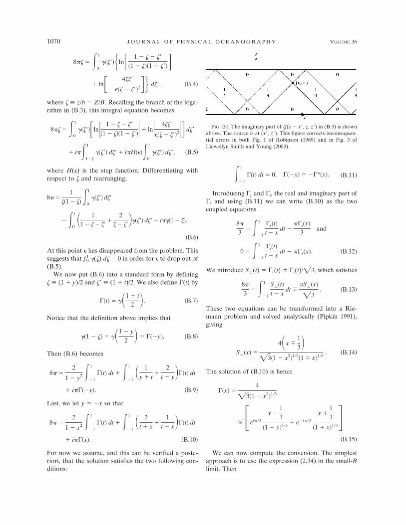
FIG. B1. The imaginary part of G (x � x�, z, z�) in (B.3) is shownabove. The source is at (x�, z�). This figure corrects inconsequen-tial errors in both Fig. 1 of Robinson (1969) and in Fig. 3 ofLlewellyn Smith and Young (2003).
1070 J O U R N A L O F P H Y S I C A L O C E A N O G R A P H Y VOLUME 36
M �2� �
0
1
�r�� d� �1
��3�
�1
1 ��1 � x
1 � x�2�3�x �13�
� �1 � x
1 � x�1�3�x �13� dx . B.16
This gives M � 16/27 � 0.593. This is the point o in theupper panel of Fig. 5 that falls slightly below the nu-merical curves. For convergence near C � 1 the nu-merical formulation requires many terms in the series(A.4) and (A.7), and thus there is some uncertainty inthe Fig. 5 curves near C � 1. The proximity of o to thesecurves is therefore reassuring. The numerical curves,and the calculation in this appendix, suggest that M iscontinuous at C � 1, but that dM/dC → $ as C → 1from below.
REFERENCES
Althaus, A. M., E. Kunze, and T. B. Sanford, 2003: Internal tideradiation from the Mendocino Escarpment. J. Phys. Ocean-ogr., 33, 1501–1527.
Baines, P. G., 1973: The generation of internal tides by flat-bumptopography. Deep-Sea Res., 20, 179–205.
——, 1982: On internal tide generation models. Deep-Sea Res., 29,307–382.
Balmforth, N. J., G. R. Ierley, and W. R. Young, 2002: Tidal con-version by subcritical topography. J. Phys. Oceanogr., 32,2900–2914.
Bell, T. H., 1975a: Lee waves in stratified fluid with simple har-monic time dependence. J. Fluid Mech., 67, 705–722.
——, 1975b: Topographically generated internal waves in theopen ocean. J. Geophys. Res., 80, 320–327.
Cummins, P. F., J. Y. Cherniawsky, and M. G. G. Foreman, 2001:North Pacific internal tides from the Aleutian Ridge: Al-timeter observations and modeling. J. Mar. Res., 59, 167–191.
Di Lorenzo, E., W. R. Young, and S. G. Llewellyn Smith, 2006:Numerical and analytical estimates of M2 tidal conversion atsteep oceanic ridges. J. Phys. Oceanogr., 36, 1072–1084.
Egbert, G. D., and R. D. Ray, 2001: Estimates of M2 tidal energydissipation from TOPEX/Poseidon altimeter data. J. Geo-phys. Res., 106, 22 475–22 502.
Kang, S. K., M. G. G. Foreman, W. R. Crawford, and J. Y. Cher-niawsky, 2000: Numerical modeling of internal tide genera-tion along the Hawaiian Ridge. J. Phys. Oceanogr., 30, 1083–1098.
Khatiwala, S., 2003: Generation of internal tides in the ocean.Deep-Sea Res. I, 50, 3–21.
Ledwell, J. R., E. T. Montgomery, K. L. Polzin, L. C. St. Laurent,R. W. Schmitt, and J. M. Toole, 2000: Evidence of enhancedmixing over rough topography in the abyssal ocean. Nature,403, 179–182.
Llewellyn Smith, S. G., and W. R. Young, 2002: Conversion of thebarotropic tide. J. Phys. Oceanogr., 32, 1554–1566.
——, and ——, 2003: Tidal conversion at a very steep ridge. J.Fluid Mech., 495, 171–191.
Merrifield, M. A., and P. E. Holloway, 2002: Model estimates ofM2 internal tide energetics at the Hawaiian Ridge. J. Geo-phys. Res., 107, 3179, doi:10.1029/2001JC000996.
——, ——, and T. M. S. Johnston, 2001: The generation of inter-nal tides at the Hawaiian Ridge. Geophys. Res. Lett., 28, 559–562.
Munk, W. H., and C. I. Wunsch, 1998: Abyssal recipes II: Ener-getics of tidal and wind mixing. Deep-Sea Res., 45, 1977–2010.
Pipkin, A. C., 1991. A Course on Integral Equations. SpringerVerlag, 268 � xiii pp.
Ray, R. D., and G. T. Mitchum, 1996: Surface manifestation ofinternal tides generated near Hawaii. Geophys. Res. Lett., 23,2101–2104.
Robinson, R. M., 1969: The effects of a barrier on internal waves.Deep-Sea Res., 16, 421–429.
Rudnick, D. L., and Coauthors, 2003: From tides to mixing alongthe Hawaiian Ridge. Science, 301, 355–357.
St. Laurent, L., and C. J. R. Garrett, 2002: The role of internaltides in mixing the deep ocean. J. Phys. Oceanogr., 32, 2882–2899.
——, S. Stringer, C. J. R. Garrett, and D. Perrault-Joncas, 2003:The generation of internal tides at abrupt topography. Deep-Sea Res. I, 50, 987–1003.