Tidal evolution of the northwest European shelf seas from the Last

Glacial Maximum to the present

Katsuto Uehara,1,2 James D. Scourse,1 Kevin J. Horsburgh,1,3 Kurt Lambeck,4 and

Anthony P. Purcell4

Received 8 February 2006; revised 28 April 2006; accepted 15 June 2006; published 23 September 2006.

[1] Two-dimensional paleotidal simulations have been undertaken to investigate tidal andtide-dependent changes (tidal amplitudes, tidal current velocities, seasonal stratification,peak bed stress vectors) that have occurred in the NW European shelf seas during the last20 ka. The simulations test the effect of shelf-wide isostatic changes of sea level byincorporating results from two different crustal rebound models, and the effect of theocean-tide variability by setting open boundary values either fixed to the present state orvariable according to the results of a global paleotidal model. The use of the differentcrustal rebound models does not affect the overall changes in tidal patterns, but thetiming of the changes is sensitive to the local isostatic effects that differ between themodels. The incorporation of ocean-tide changes greatly augments the amplitude of tidesand tidal currents in the Celtic and Malin seas before 10 ka BP, and has a large impact on thedistribution of seasonally stratified conditions, magnitude of peak bed stress vectors andtidal dissipation in the shelf seas. The predictions on seasonal stratification are supported bywell-dated evidence on tidal mixing front migration in the Celtic Sea. Additionalexperiments using the global model suggest that the variability of offshore tides has beencaused mainly by changes of eustatic sea level and ice-sheet extent. In particular, a largedecrease observed at 10–8 ka BP is attributed to the opening of Hudson Strait accompaniedby the retreat of the Laurentide Ice Sheet.

Citation: Uehara, K., J. D. Scourse, K. J. Horsburgh, K. Lambeck, and A. P. Purcell (2006), Tidal evolution of the northwest

European shelf seas from the Last Glacial Maximum to the present, J. Geophys. Res., 111, C09025, doi:10.1029/2006JC003531.

1. Introduction

[2] Reconstructions of tidal changes in continental shelfseas over glacial-interglacial timescales provide essentialinformation for estimating tide-dependent parameters suchas sea level index points, location of tidal fronts, peak bedstress vectors, and tidal dissipation. These parameters arevaluable in a range of paleoenvironmental contexts from sealevel studies to the evolution of ecosystems and their bio-geochemistry. Since the pioneering work of Scott andGreenberg [1983] on the Bay of Fundy, a number of studieshave investigated such changes (see Hinton [1997] forreviews on early paleotidal models).[3] For the NW European shelf (Figure 1), Austin [1991]

and Scourse and Austin [1995] used a two-dimensionalmodel [Flather, 1976] of the lunar semi-diurnal M2 constit-uent to reconstruct changes in tidal amplitudes, peak bed

stress vectors and seasonal stratification across the shelfduring the Holocene. Though Scourse and Austin [1995]did correct for tectonic uplift in the central English Channel,these studies did not incorporate vertical crustal movementdue to isostasy. A similar rigid crust approach was adopted inthe earlier M2 paleotidal modeling exercise by Belderson etal. [1986] and the more recent studies by Hinton [1995] andHall and Davies [2004].[4] Though these studies assumed a uniform depth change

over the whole shelf, isostatic correction to the shelf geom-etry is not small in areas where loading and unloading ofBritish and Fennoscandian ice sheets have been substantial(Figure 2). It is therefore necessary to consider crustalrebound in order to reconstruct the evolution of the shelf-wide tidal regime. Three paleotidal modeling exercises[Gerritsen and Berentsen, 1998; Shennan et al., 2000; Vander Molen and De Swart, 2001] have explicitly integrated theisostatic change by using a glacio-isostatic-adjustment (GIA)model output as input terms for the tidal modeling. However,these studies were confined to the Holocene and to relativelysmall regions in order to address different specific objectives.[5] Recent studies using global paleocean-tide models

indicate a large change of M2 tides in the North Atlanticduring the early phase of deglaciation as a result of thechanging sea level. Thomas and Sundermann [1999] inves-tigated changes of global ocean tides and tidal torques since

JOURNAL OF GEOPHYSICAL RESEARCH, VOL. 111, C09025, doi:10.1029/2006JC003531, 2006ClickHere

for

FullArticle

1School of Ocean Sciences, University of Wales (Bangor), Anglesey,UK.

2Also at Research Institute for Applied Mechanics, Kyushu University,Kasuga, Fukuoka, Japan.

3Now at Proudman Oceanographic Laboratory, Liverpool, UK.4Research School of Earth Sciences, Australian National University,

Canberra, ACT, Australia.

Copyright 2006 by the American Geophysical Union.0148-0227/06/2006JC003531$09.00

C09025 1 of 15

the Last Glacial Maximum (LGM) and found that M2

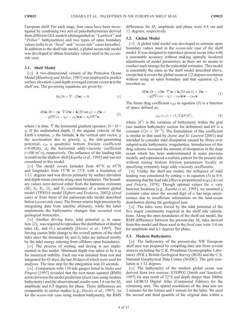
amplitudes in the Atlantic increased distinctly between theLGM and 8ka BP. Egbert et al. [2004] tuned a hydrodynamicglobal ocean model, paying particular attention to the param-eterisations of self-attraction and loading (SAL) and internaltidal dissipation, and obtained a global solution whose RMSerror when compared to present-day altimetry was of theorder 5 cm. They applied their model from the LGM to thepresent and found that M2 amplitudes at the LGM weresignificantly different with amplitudes a factor of two largerin parts of the North Atlantic at 20 ka BP. Our results alsoshow a large change of M2 amplitudes in the NE Atlantic at16–8 ka BP (Figure 3) and lend support to these earlierstudies. The large amplitude changes found in the NorthAtlantic are most likely due to the quasi-resonant conditionof the basin with respect to the semi-diurnal frequency[Platzman et al., 1981; Egbert et al., 2004]. Arbic et al.[2004] employed a global model similar to Egbert et al.[2004] to investigate tidal changes in the Labrador Seaduring the last 65 ka in relation to the occurrence of Heinrichevents. They also found enhanced M2 tides at the estimated

discharge point of the Hudson Strait ice stream at 16–7 kaBP.[6] The impact of ocean-tide changes occurring over

geological timescales on shelf tides has not been imple-mented in most regional- and shelf-scale paleotidal studiesbecause it has previously been assumed that tides in the deepocean are unaffected by the eustatic sea level change ofapproximately 130 m. Hinton [1995, 1996] and Shennan etal. [2000] considered the changes of tides along openboundaries in their SW North Sea models by runninglarger-scale North Atlantic models out to 30�W. However,our results and those cited above suggest that semi-diurnaltidal forcing for any shelf model is very sensitive to changesin the ocean tide and that this boundary condition is likely tobe the dominant factor in the temporal evolution of tidalbehavior on the shelf.[7] The overall aim of this study is to reconstruct the tidal

evolution on the NW European shelf from the LGM to thepresent. We recognize that the rate of both eustatic andisostatic changes were greatest in the period between theLGM and the base of the Holocene, and therefore thedynamical implications of changes in sea level are mostprofound during this period. We have therefore not restrictedour analysis to the Holocene, so enabling a comparison of themagnitude of Holocene changes with the earlier deglacialphase. Our specific objectives have been (1) to use themodelsto interrogate the dynamical implications of different gen-erations of GIA models (Peltier [1994] and a revised versionof Lambeck [1995]), (2) to analyse the significance oftemporal changes in the ocean tide on shelf-sea dynamicsby running the model with both present-day open boundaryconditions and those derived from a paleotidal ocean modelrun for the period of interest, and (3) to comparemodel outputwith empirical data on the evolution of seasonal stratification[Austin and Scourse, 1997; Scourse et al., 2002].

2. Location

[8] The NW European shelf seas are located on thenortheastern margin of the North Atlantic and are generallyshallower than 200 m (Figure 1). The North Sea is shallowerthan 50 m south of about 55�N and gradually deepenstowards the north. The Celtic Sea and the English Channelincrease in depth towards the shelf edge and are open to theAtlantic Ocean. The Irish Sea is semi-enclosed, and isconnected to the Celtic and Malin seas through St. Georges’Channel and North Channel respectively. The eastern part ofthe Irish Sea is a shallow shelf generally less than 80 m deep,but the western part is dominated by a north-south trendingtrough reaching depths over 250 m. The Malin Sea andwestern Irish Shelf open to the Atlantic Ocean to thenorthwest. The Norwegian margin is dominated by the deepNorwegian Trench that extends from the Skagerrak to theopen Atlantic northeast of the Shetland Islands. The modeldomain is defined by latitudes from 45�N to 65�N andlongitudes from 15�W to 15�E. It extends southwards alongthe western French Shelf and into the open North Atlantic toinclude the Faeroe Islands, Rockall Trough, Iceland-FaeroeRidge, Faeroe-Shetland Channel, the Iceland Basin, and intothe Norwegian Sea.[9] The tides and tidal currents of the NW European shelf

seas are dominated by M2, and less significantly by S2

Figure 1. Map of modeled region, including locations ofselected sea level reference points in (a) a north-southtransect through the Irish Sea, extending south to Brest andnorth to the Faeroe Islands, and (b) an east-west transectalong the English Channel, extending west to the Isles ofScilly and east to the German Bight. Locations selected are,for the north-south transect, (N1) east Faeroe Islands, (N2)south Faeroe Islands, (N3) Cape Wrath, (N4) Firth of Clyde,(N5) Bangor (northWales), (N6) Core site 199, (N7) the Islesof Scilly, and (N8) Brest, and for the east-west transect, (N7)the Isles of Scilly, (N8) Brest, (E1) Jersey, (E2) the Isle ofWight, (E3) London, (E4) Lower Thames, (E5) Texel and(E6) the German Bight. Point (F) off Flamborough Headindicates the location of stations used in Figure 8b.

C09025 UEHARA ET AL.: PALEOTIDES IN NW EUROPEAN SHELF SEAS

2 of 15

C09025

(relative significance is ca. 30–50%). Diurnal constituentssuch as K1 andO1 are comparable with the semi-diurnal onesonly near semi-diurnal amphidromes, and in limitedregions such as the outer shelf around northwest Scotland[Cartwright et al., 1980; Proctor and Davies, 1996]. Wetherefore confine most of our analysis to M2 and S2.[10] A distinctive feature of this shelf in terms of its

morphological evolution during the last glacial cycle is thespatially complex isostatic deformation forced by loading

and unloading of local (British and Fennoscandian) and far-field (Laurentide) ice sheets [Lambeck, 1993, 1995, 1996].

3. Methods

[11] Paleotides in the NW European shelf seas havebeen estimated by applying paleobathymetries for every1000 years from 20 ka BP to the present day to a two-dimensional finite-difference model covering the NW

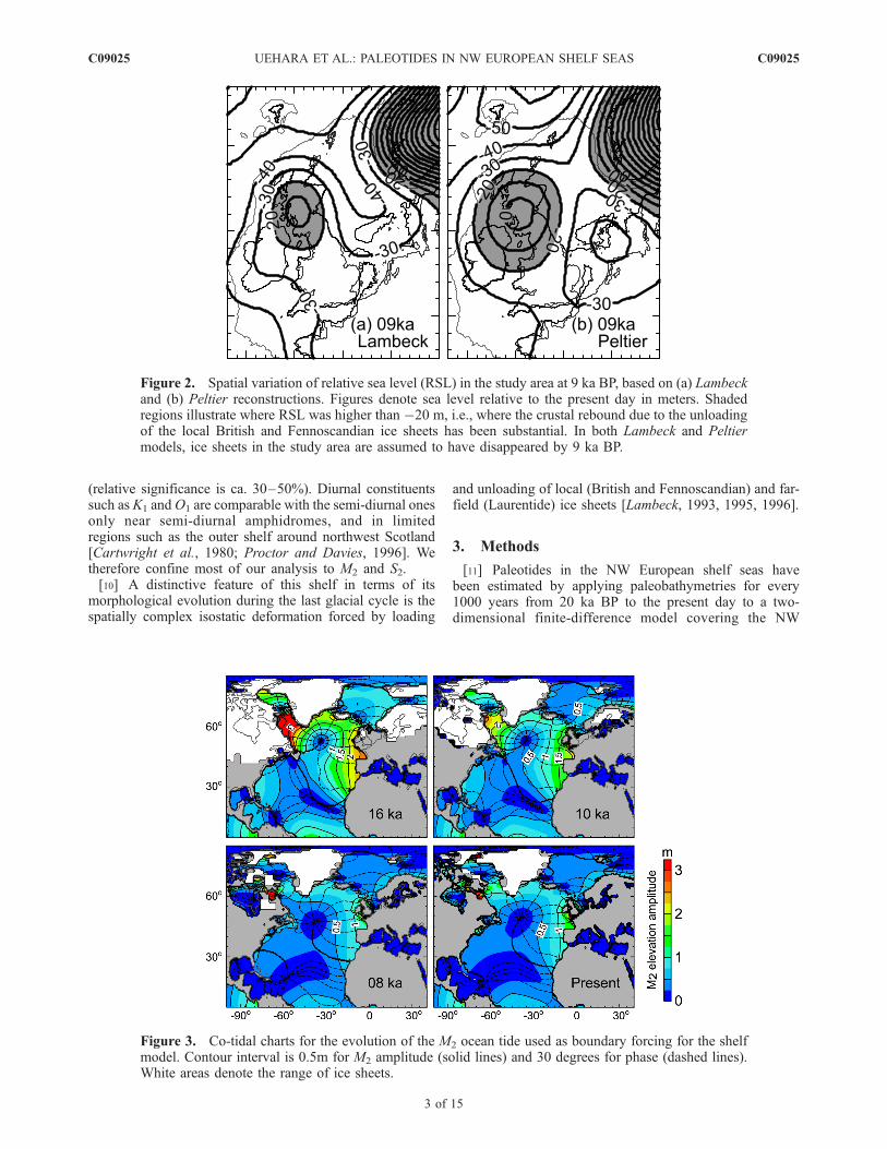
Figure 2. Spatial variation of relative sea level (RSL) in the study area at 9 ka BP, based on (a) Lambeckand (b) Peltier reconstructions. Figures denote sea level relative to the present day in meters. Shadedregions illustrate where RSL was higher than �20 m, i.e., where the crustal rebound due to the unloadingof the local British and Fennoscandian ice sheets has been substantial. In both Lambeck and Peltiermodels, ice sheets in the study area are assumed to have disappeared by 9 ka BP.

Figure 3. Co-tidal charts for the evolution of the M2 ocean tide used as boundary forcing for the shelfmodel. Contour interval is 0.5m for M2 amplitude (solid lines) and 30 degrees for phase (dashed lines).White areas denote the range of ice sheets.

C09025 UEHARA ET AL.: PALEOTIDES IN NW EUROPEAN SHELF SEAS

3 of 15

C09025

European shelf. For each stage, four cases have been inves-tigated by combining two sets of paleobathymetries derivedfrom different GIA models (distinguished as ‘‘Lambeck’’ and‘‘Peltier’’ bathymetries) and two types of open boundaryvalues (refer to as ‘‘fixed’’ and ‘‘ocean-tide’’ cases hereafter).In addition to the shelf tide model, a global ocean-tide modelwas developed to obtain boundary values used in the ocean-tide case.

3.1. Shelf Model

[12] A two-dimensional version of the Princeton OceanModel [Blumberg andMellor, 1987] was employed to predictsurface elevation h and depth-averaged current vector u in theshelf sea. The governing equations are given by:

@�=@t þr � Duð Þ ¼ 0; ð1Þ

@Du=@t þ u � rð ÞDuþ k 2W sin’ð Þ � Du ¼� gDr � � �eð Þ � cDjujuþ AhDr2u;

ð2Þ

where t is time, r the horizontal gradient operator, D = H +�, H the undisturbed depth, W the angular velocity of theEarth’s rotation, ’ the latitude, k the vertical unit vector, gthe acceleration due to gravity, �e the tide-generatingpotential, cD a quadratic bottom friction coefficient(=0.0026), Ah the horizontal eddy-viscosity coefficient(=100 m2/s), respectively. The influence of the loading tideis small on the shallow shelf [Kantha et al., 1995] andwas notconsidered in this model.[13] The model covers latitudes from 45�N to 65�N

and longitudes from 15�W to 15�E with a resolution of1/12 degrees and was driven primarily by surface elevationand depth-mean currents along open boundaries. The bound-ary values were derived either from the harmonic constants(M2, S2, K1, O1, and N2 constituents) of a modern globalmodel (TPXO.6 model [Egbert and Erofeeva, 2002]) (fixedcase) or from those of the paleocean-tide model describedbelow (ocean-tide case). The former retains high precision byintegrating data from satellite altimetry, while the latterimplements the bathymetric changes that occurred overgeological timescales.[14] Another driving force, tidal potential �e in equa-

tion (2), was required to reproduce the distribution of diurnaltides (K1 and O1) accurately [Davies et al., 1997]. Thisforcing causes little change to the overall pattern of the shelftides since the dominant M2 and S2 tides are induced mostlyby the tidal energy entering from offshore open boundaries.[15] The process of wetting and drying is not imple-

mented in this model. Minimum depth was taken to be 6 mfor numerical stability. Each run was initiated from rest andintegrated for 45 days, the last 30 days of which were used foranalyses. The time step for the integration was 10 seconds.[16] Comparison with 130 tide gauges listed in Sinha and

Pingree [1997] revealed that the root mean squared (RMS)errors between the model prediction (fixed case using modernbathymetry) and the observational results were 5.6 cm forM2

amplitude and 6.5 degrees for phase. These differences arecomparable to earlier studies [e.g., Davies et al., 1997]. Asfor the ocean-tide case using modern bathymetry, the RMS

differences for M2 amplitude and phase were 6.8 cm and12 degrees, respectively.

3.2. Global Model

[17] A global tidal model was developed to estimate openboundary values used in the ocean-tide case of the shelfmodel. It was designed to reproduce present ocean tides witha reasonable accuracy without making spatially localizedadjustments of model parameters, as there are no means toconduct such tunings for the paleotidal estimates. This modelis essentially the same as the shelf model described above,except that it covers the global ocean at 1/2 degrees resolutionwithout using an open boundary and that equation (2) isrewritten as:

@Du=@t þ Du � rð Þuþ k 2W sin�ð Þ � Du ¼� gDr �� � �eð Þ � cDjuju� cDTu:

ð3Þ

The linear drag coefficient cDT in equation (3) is a functionof space defined as:

cDT x; yð Þ ¼ 1=2ð ÞkNhh2i; ð4Þ

where hh2i is the variation of bathymetry within the grid(see modern bathymetry section for definition) and kN is aconstant (12 � 10�8). The formulation of this coefficientis similar to that used by Jayne and St. Laurent [2001] andintended to consider tidal dissipation caused by flows oversubgrid-scale bathymetric irregularities. Introduction of thisdrag scheme increased the amount of dissipation in the deepocean which has been underestimated in some previousmodels, and reproduced a realistic pattern for the present tidewithout tuning bottom friction parameters locally orspecifying extremely large eddy-viscosity coefficients.[18] Unlike the shelf-sea model, the influence of tidal

loading was considered by setting � in equation (3) to 0.9,assuming that the load tide effect is proportional to g� [Accadand Pekeris, 1978]. Though optimal values for � varybetween locations [e.g., Kantha et al., 1995], we assumed aconstant value since the second digit of a has large uncer-tainties due to insufficient information on the land-oceandistribution during the geological past.[19] The tides were forced by the tidal potential of the

five major constituents required in the shelf tide calcula-tions. Along the open boundaries of the shelf-sea model, theRMS differences between the present-day M2 tides derivedfrom this model and those used in the fixed case were 3.4 cmfor amplitude and 4.1 degrees for phase.

3.3. Modern Bathymetry

[20] The bathymetry of the present-day NW Europeanshelf area was prepared by compiling data sets from severalsources including the U.K. Proudman Oceanographic Labo-ratory (POL), British Geological Survey (BGS) and the U.S.National Geophysical Data Center (NGDC). The grid reso-lution is 1/12 degrees.[21] The bathymetry of the modern global ocean was

derived from two sources: ETOPO2 [Smith and Sandwell,1997] for area north of 72�S and depth deeper than 1000mand GEBCO Digital Atlas (Centennial Edition) for theremaining area. The spatial resolutions of the data sets are2 minutes for the former and 1 minute for the latter. We usedthe second and third quantile of the original data within a

C09025 UEHARA ET AL.: PALEOTIDES IN NW EUROPEAN SHELF SEAS

4 of 15

C09025

model grid (30 minutes resolution) to compute representativedepth hhi and subgrid-scale variability hh2i in equation (4):

hhi ¼ 2=Nð ÞX3N=4

i¼1þN=4hi; ð5Þ

hh2i ¼ 2=Nð ÞX3N=4

i¼1þN=4hi � hhið Þ2; ð6Þ

where N is the number of depth data in a model grid and hidenotes each depth in an ascending order. Depths for shallowregions such as the NW European Shelf, the East China Sea,and the northern Australian Shelf were modified by usinglocal digital bathymetry including those supplied by theJapan Oceanographic Data Center (JODC) and GeoscienceAustralia.

3.4. Paleobathymetries

[22] Paleobathymetries around the NW European Shelfwere prepared for every 1 ka since 20 ka BP to the presentby combining the modern shelf bathymetry with changes ofrelative sea levels (RSLs) estimated from two GIA models:a revised version of Lambeck [1995] (‘‘Lambeck’’ model)and ICE-4G (VM2) model [Peltier, 1994] (‘‘Peltier’’ model).The Lambeckmodel is constrained to the NWEuropean Shelfregion and has spatial resolution of 0.703125 degrees inlongitude and 0.15748 degrees in latitude (resolution of theice model was 1/4 degrees in longitude and 1/8 degrees inlatitude, 1/2 degrees in longitude and 1/4 degrees in latitude,for British and Fennoscandian ice sheets, respectively). ThePeltier model covers the global area at 1 degree resolution.[23] The Lambeck model supersedes Lambeck [1995] by

conducting a new iteration using improved ice-sheet modelsfor Scandinavia and North America [Lambeck and Purcell,2001], an improved model for the global changes in icevolumes during the last glacial cycle [Lambeck andChappell, 2001] and improved high-resolution solutionsof the rebound formulation [Lambeck et al., 2003]. BothLambeck and Peltier models predict crustal and geoid dis-placement of the ice sheets from the LGM to the present day,though differences in model settings such as spatial andtemporal extent of ice sheets or viscous structure of thelithosphere cause slight differences in the RSL estimations.[24] The RSL and ice data were converted separately to a

1/12 degree mesh using a natural neighbor technique. Waterdepth at a particular age was derived as the sum of RSL andthe present depth. Grid points where values of the convertedice data were larger than 1m (Lambeck; the altitude of icesurface) or 0.6 (Peltier; original data describe nonice and iceregions as 0 and 1) are regarded as ice-covered. All ice area isregarded as grounded since there are no precise data on thepositions and migration of grounding lines during the past.[25] To compare the bathymetry derived from bothmodels,

RSL distribution around the NW European seas at 9 ka BP isshown in Figure 2. By this early Holocene period, all icesheets in the study area are assumed to have disappeared. It isfound that most of the basic features are similar between themodels: high RSLs (deeper water depth) are found on thenorthern Britain and along Scandinavian coasts which areinfluenced by the unloading of British and Fennoscandian icesheets, while RSLs are low (shallow) in the North and Celtic

seas and in the area north of the shelf. In addition, the spatialvariability of RSLs across the shelf was more than 40 metersin both models, which is an order of magnitude larger thanthose found in the offshore South Atlantic or Indian oceans asa whole at the same period.[26] Despite overall similarities, there are two apparent

differences between the model results, apart from smallervolumetric extent of the British Ice Sheet predicted in theLambeck model. One is before 15 ka BP, when RSL in theouter Celtic Sea was higher and the shelf sea was moredeveloped in the Lambeck model. Another is found after12 ka BP: RSL was higher in the present southeast NorthSea compared to those in the northern North Sea in theLambeck model (Figure 2a) while the opposite trend wasgenerated by the Peltier model (Figure 2b).[27] Paleobathymetry used in the global ocean-tide model

was prepared in the same manner as for the shelf model,except that the grid resolution was 1/2 degree and was basedexclusively on the Peltier model. For the bathymetry at 9 kaBP an additional data set was created by applying a differentregridding scheme (linear interpolation) to the ice data toexamine the sensitivity of the tidal model to ice distribution.

4. Results

[28] As our primary interest is in the tidal changes of theNW European shelf seas, most of the discussion is restrictedto the area between 12�W and 6�E longitude and 47.5�Nand 61�N latitude. Note that dates shown in this study aredescribed in calendar years which are different (older byvarying amounts) from the radiocarbon years adopted inmostof the earlier shelf-tide studies [e.g., Shennan et al., 2000;Van der Molen and De Swart, 2001].

4.1. M2 Tidal Amplitudes

[29] Figure 4a depicts co-tidal charts of M2 tides for thepresent-day situation, and for selected time slices obtainedusing Lambeck bathymetry and the open boundary valuewhich integrates temporal changes in ocean tides. Figure 4aalso illustrates the spatial extent of the shelf sea at eachstage, which has evolved extensively with the rise of sealevel.[30] In the Celtic Sea, a region with M2 amplitudes larger

than 2.5 m is observed along the paleocoastline around48.5�N at 16 ka BP, which shifts eastward with the retreat ofthe shorelines. This result is consistent with that of Egbert etal. [2004] who obtained M2 amplitudes of about 3m alongthe eastern margin of the North Atlantic as well as in theLabrador Sea during the LGM. After 12 ka BP, the highamplitude area splits into two parts: along the Brittany coast(northern France) and in the Bristol Channel. M2 amplitudesin the English Channel decrease in the west and increase inthe east after ca. 10 ka BP. M2 amplitudes larger than 2.5 mare also found in the area west of Scotland before 10 ka BPand along the west coast of Ireland before 12 ka BP, anddeveloped after 8–7 ka BP in the eastern Irish Sea. Changesin M2 amplitudes largely cease after 6 ka BP.[31] The evolution of the shelf amphidromic system is

also evident in Figure 4a. Amphidromes represent the nodesof standing waves in a rotating system, and are formed bythe interaction of incident and reflected Kelvin waves. Theposition of amphidromes is affected bywater depth, frictional

C09025 UEHARA ET AL.: PALEOTIDES IN NW EUROPEAN SHELF SEAS

5 of 15

C09025

Figure 4. Modeled M2 elevation amplitudes and phases for selected time slices based on Lambeckpaleobathymetry: (a) ocean-tide and (b) fixed boundary cases. Contour interval ofM2 elevation amplitude(solid) and phase (dashed) are 0.5 meter and 30 degrees, respectively.

Figure 5. M2 tidal elevation differences between 12 ka BP and present for cases derived from differentpaleo-bathymetries and open boundary values: (a) Lambeck/fixed, (b) Lambeck/ocean-tide, (c) Peltier/fixed, and (d) Peltier/ocean-tide cases. Hatched (shaded) regions depict where M2 amplitudes at 12 ka BPwere more than 0.5 m greater (smaller) than at present.

C09025 UEHARA ET AL.: PALEOTIDES IN NW EUROPEAN SHELF SEAS

6 of 15

C09025

effects and the topography. The amphidromes near thesoutheast of Ireland and the central part of the EnglishChannel, seen in the present-day situation of Figure 4a, aredegenerate (the phase lines intersect on land) but thesequence shows them becoming less degenerate with timeas water depth increases, resulting in less attenuation of thereflected Kelvin wave. The depth increase also shifts amphi-dromes away from the reflection point of the Kelvin wavethrough the increase of tidal wavelength. For example, theEnglish Channel amphidrome moves from east to west of theIsle of Wight during the last 9 ka.[32] In the North Sea, an amphidrome first develops at the

mouth of the paleo-embayment around 59�N at 16 ka BP(Figure 4a). As the embayment extends to the south, anotheramphidrome emerges around 56�N by 14 ka BP. Distancesbetween these amphidromes and the head of the embaymentat 12 ka BP (Figure 4a) are consistent with those inferredfrom the theory of standing waves in an idealized gulf if auniform depth of 16 m is assumed. As the depth increases,the southern amphidrome shifts eastward and larger tidalamplitudes develop along the English coast. The northernamphidrome degenerates towards SW Norway by 10 ka BPalong with the disappearance of a paleo-promontory sepa-rating the embayment and the Skagerrak. At 9–7 ka BP,detachment of Dogger Bank (ca. 3�E, 55�N) from thesouthern coast of the North Sea causes the incident Kelvinwave to bifurcate at around 55�N traveling either along thenorth coast of the bank or towards the southern coast of theNorth Sea. As a result, amphidromes appear both north andsouth of the bank at this period (8 ka BP in Figure 4a). Theamphidromes coalesce after the bank is submerged to formthe present-day situation. In the Southern Bight (SW NorthSea), an amphidrome emerges after the opening of the Straitof Dover at 9 ka BP in the Lambeck case or at 8 ka BP in thePeltier case.[33] M2 amplitudes obtained with the boundary values

fixed to the present situation (Figure 4b) are smaller thanthose predicted in ocean-tide case results (Figure 4a) in timeslices prior to 10 ka BP, especially in the western part of theshelf. Despite the large difference in tidal amplitudes, thelocation of amplitude maxima and of amphidromes arealmost the same in the ocean-tide and fixed cases since thesecharacteristics are mainly a function of wavelength andgeometry.[34] Comparison of M2 amplitude differences between

12 ka BP and the present derived from all four cases

(Figure 5) suggests that the variation in the offshore tidescaused significant enhancement of tidal amplitudes in thewestern part of the shelf prior to 10 ka BP, much larger thanthe differences resulting from alternative GIA bathymetries.On the other hand,M2 amplitudes in the North Sea, especiallyin the region between 54�N and 58�N, are less affected by thechange of ocean tides and show some sensitivity to the modelbathymetry used (Figure 5). Dependence of tidal pattern onthe usage of different GIA models is also found in the outerCeltic Sea prior to 15 ka BP, when tides and the shelfgeometry evolved more rapidly in the Lambeck case than inthe Peltier case due to higher RSL predicted in the former.

4.2. M2 Tidal Currents

[35] Figure 6 depicts the amplitude distribution of M2

tidal currents predicted by Lambeck/ocean-tide runs for thesame time slices as in Figure 4. The introduction of ocean-tide variability generates a significant increase in the mag-nitude of the tidal current on the western side of the shelfprior to 10 ka BP, with a smaller impact on the velocity fieldin the North Sea.[36] A region of intense tidal currents exceeding 1.25 m/s,

observed in the Celtic Sea during the early stages ofdeglaciation (see 16 ka BP in Figure 6), shifts landward withthe rise of sea level and is found mostly in the EnglishChannel after 12 ka BP. After 8 ka BP its spatial extent isconfined to the central English Channel between the Isle ofWight and the Cotentin Peninsula.[37] Such strong M2 currents are also observed along the

shelf edge of the Malin Sea at 16 ka BP due partly to theshallower depth along the shelf edge compared to the innershelf area, and also to the enhanced tidal prism caused bythe developed M2 tides on the inner shelf. Current velocitiesof the diurnal constituents (K1 and O1) in this area, whichare comparable to the semi-diurnal counterparts at present,do not differ significantly from the present values.[38] With the exception of the channel between the

islands of Shetland and Orkney, M2 tidal currents strongerthan 0.75 m/s are not found in the North Sea until 9 ka BPin the Lambeck case or until 8 ka BP in the Peltier case,when a strong tidal flow is generated between the emergentDogger Bank and the landbridge in the SW North Sea. Afterthis time, strong tidal currents have developed mainly alongthe English coast in the SW North Sea.[39] The largest differences between the M2 tidal current

distributions predicted by the Lambeck and Peltier cases,

Figure 6. Variation of M2 current amplitude for the Lambeck/ocean-tide case. Contour interval is0.25 m/s.

C09025 UEHARA ET AL.: PALEOTIDES IN NW EUROPEAN SHELF SEAS

7 of 15

C09025

other than in timing, are found in the northern North Seabetween 14 to 12 ka BP, when the M2 current stronger than0.5 m/s occurs at the mouth of the paleo-embayment in theLambeck case while in the southwest region of the embay-ment when forced by Peltier. This discrepancy is due to thelow RSL (shallow depth) predicted along the mouth of theembayment which forms a sill-like feature in the Lambeckbathymetry while the bay mouth is deeper and wider in thePeltier reconstructions (see Figure 2).

4.3. Mean High Water Spring Tide (MHWST)

[40] As the derivation of past MHWST elevation is essen-tial when making tidal corrections to sea level index points,curves of MHWST at selected locations along N-S and E-Wtransects (Figure 1) have been plotted for the Lambeck/ocean-tide case against time slices from 20 ka BP to thepresent day (Figure 7).[41] In this study, MHWST is estimated as the sum of M2

and S2. Though this is not the formal definition of MHWST,

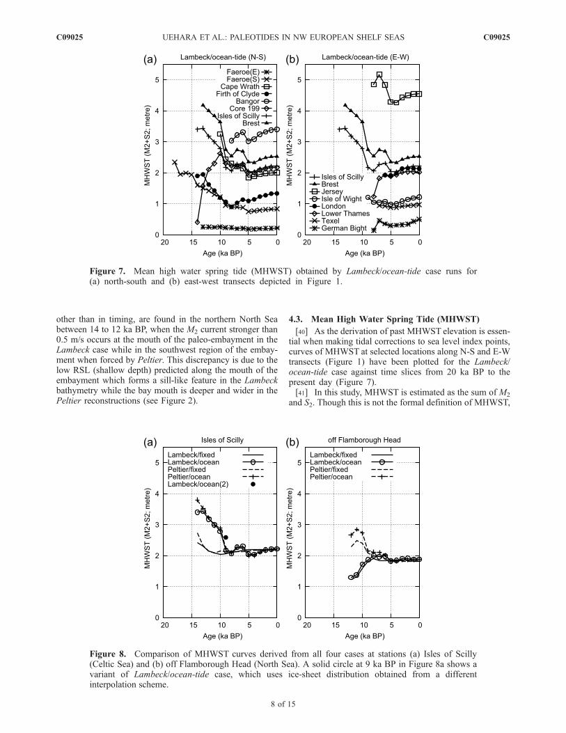
Figure 7. Mean high water spring tide (MHWST) obtained by Lambeck/ocean-tide case runs for(a) north-south and (b) east-west transects depicted in Figure 1.

Figure 8. Comparison of MHWST curves derived from all four cases at stations (a) Isles of Scilly(Celtic Sea) and (b) off Flamborough Head (North Sea). A solid circle at 9 ka BP in Figure 8a shows avariant of Lambeck/ocean-tide case, which uses ice-sheet distribution obtained from a differentinterpolation scheme.

C09025 UEHARA ET AL.: PALEOTIDES IN NW EUROPEAN SHELF SEAS

8 of 15

C09025

comparison between observed harmonic constants andMHWST at 63 standard ports listed in the Admiralty TideTable Volume 1 (2004 edition) shows that the amplitudes ofM2 and S2 tides can explain the observed MHWST in thestudy area to within 7%, which is probably smaller thanmodel errors originating from uncertainty in the paleoba-thymetries and tidal variability at nearshore regions.[42] Curves of MHWST for fixed case results (not shown)

were generally smooth and did not deviate more than 0.5 mfrom the present value except in the earliest runs for theCape Wrath and Lower Thames stations, and before 12 kaBP at station Core 199. Factors affecting the shape of curvesinclude the movement of amphidromes, development ofinner bay tides (e.g. at Bangor), and the opening of localchannels (e.g. 6 ka BP at Jersey). MHWST at Faeroe (E)station has been virtually constant over 13 ka because a stableamphidrome resided close to the reference point. Inclusion ofocean-tide variability generally causes a significant enhance-ment of MHWST before 10 ka BP, typically by 25–50%from the fixed case results, and a smaller modification after8 ka BP (Figure 7). Except at the Firth of Clyde station, asharp decrease of MHWST is observed on the western side ofthe shelf between 10 and 9 ka BP.[43] Superposition of curves obtained from all four cases

illustrates that MHWST in the Celtic Sea is virtuallyinsensitive to the bathymetric model used, while the changeof ocean tides has had a significant impact on the evolutionof MHWST before 10 ka BP (Figure 8a). Prediction ofMHWST at 9 ka BP is found to depend largely on thedistribution of ice sheets in unresolved Hudson Strait, asindicated for the Lambeck/ocean-tide case in Figure 8a.Though the significant decrease of MHWST between 10–8 ka BP seems to be a robust feature, a small modulation ofMHWST observed in ocean-tide reconstructions during 8–3 ka BP might be a model artefact of the global predictionscaused by uncertainties of paleogeography in high latitudeareas, as will be discussed in section 5.[44] MHWST off Flamborough Head in the western

North Sea is sensitive to the different bathymetric modelsat ages prior to 10 ka BP (Figure 8b). In the Peltier case, theMHWST shows a peak value at 11 ka BP followed by adecreasing trend while the estimated value was smaller thanpresent for time slices prior to 10 ka BP in the Lambeckcase. This discrepancy seems to have been caused by thedifference of the water depth predicted for the North Sea;RSL is higher (deeper) in the Peltier model compared to theLambeck model at around 10 ka BP (see Figure 2).

[45] MHWST estimates of the SW North Sea by Shennanet al. [2000], who undertook a high-resolution paleotidalsimulation in this region for the last 10 14C ka, showtemporal trends similar to the Lambeck case in Figure 8b.This resemblance is probably due to the incorporation ofpaleobathymetries from Lambeck [1995] in their shelf-scaletidal model. Comparison of MHWST predicted by Shennanet al. [2000] and that of the Lambeck case in the currentstudy (Figure 8b) shows that our model gives estimates 30 cmhigher around Flamborough Head. This difference may havebeen caused by geographical changes related to the move-ment of sediments in The Wash in the regional model ofShennan et al. [2000]. In their regional model, the paleo-coastline in this embayment extends largely towards thepresent land during the mid-Holocene, which is known tohave had the effect of lowering the tidal amplitudes in thisregion [Hinton, 1995]. Even though the influence of coastalsedimentation on shelf-scale tidal regimes is generally lim-ited to localized areas [e.g., Uehara et al., 2002], similardiscrepancies may have occurred at several locations on theNW European Shelf, including the former tidal basins in TheNetherlands [Van der Spek, 1997].

4.4. Seasonal Stratification

[46] The region of seasonal stratification in the NWEuropean shelf seas is strongly linked to the strength ofthe tidal current juj in terms of a parameter proposed bySimpson and Hunter [1974]:

S ¼ log10 H=cDhjuj3i� �

; ð7Þ

where h i denotes averaging over a tidal cycle. Pingree andGriffiths [1978] have shown, using an M2 tidal numericalmodel, that the transition of the water column from avertically mixed state to a stratified state occurs when S isbetween 1 and 2, and that the tidal mixing front is likely toreside around the contour line of S = 1.5. We adopt thesecriteria to estimate such transitions, and modify the thresholdvalues to S = 0.87, 1.83 and 1.35 respectively, to reflect ourfive-constituent model.[47] Figure 9 illustrates the positions of tidal mixing front

boundaries for the Lambeck/ocean-tide case estimated fromthe distribution of S. The position of the front in the CelticSea at 14 ka BP is close to the shelf break; with rising sealevel it migrates landwards, splitting into two separate frontalsystems in the inner Celtic Sea and the western English

Figure 9. Predicted distribution of stratification parameter, S, based on Lambeck/ocean-tide case runs.Dark grey indicates S < 0.87 (mixed), medium grey colors indicate 0.87 < S < 1.83 (transitional orfrontal), and light grey indicates S > 1.83 (stratified). Awhite line corresponds to S = 1.35, indicating thelocation of a tidal front.

C09025 UEHARA ET AL.: PALEOTIDES IN NW EUROPEAN SHELF SEAS

9 of 15

C09025

Channel after 7 ka BP. In the North Sea, a tidallymixed area isfound mainly north of 54�N before 10 ka BP and south of55�N after 8 ka BP.[48] The ratio of tidally mixed to total shelf area has been

relatively constant for the last 5 ka, around 20%, regardlessof the type of bathymetric model and the open boundaryvalue used. Before 10 ka BP, a tidally mixed region domi-nated in the Celtic Sea and also increased in the Malin andNorth seas (Figure 9). As a result, the ratio of the mixed areaincreased to as much as 60–70% in the Lambeck/ocean-tidecase between 19–13 ka BP or 40–50% between 17–10 kaBP in the Peltier/ocean-tide case.[49] Geological proxy data can be used to verify the

accuracy of the model output with respect to stratification.Based on microfossil (benthic foraminifera) and stable iso-topic data from radiocarbon-dated BGS vibrocore 51/�09/199 (Core 199) from the Celtic Sea (Figure 1), Austin andScourse [1997] were able to identify a transition fromsummer mixed to stratified water at this location at around9 ka BP. This study verified the nonisostatically correctedM2

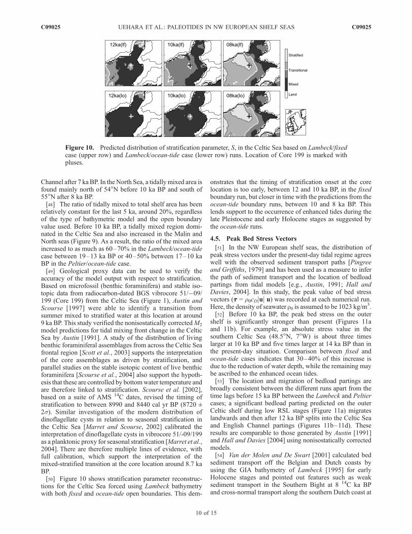
model predictions for tidal mixing front change in the CelticSea by Austin [1991]. A study of the distribution of livingbenthic foraminiferal assemblages from across the Celtic Seafrontal region [Scott et al., 2003] supports the interpretationof the core assemblages as driven by stratification, andparallel studies on the stable isotopic content of live benthicforaminifera [Scourse et al., 2004] also support the hypoth-esis that these are controlled by bottomwater temperature andare therefore linked to stratification. Scourse et al. [2002],based on a suite of AMS 14C dates, revised the timing ofstratification to between 8990 and 8440 cal yr BP (8720 ±2). Similar investigation of the modern distribution ofdinoflagellate cysts in relation to seasonal stratification inthe Celtic Sea [Marret and Scourse, 2002] calibrated theinterpretation of dinoflagellate cysts in vibrocore 51/-09/199as a planktonic proxy for seasonal stratification [Marret et al.,2004]. There are therefore multiple lines of evidence, withfull calibration, which support the interpretation of themixed-stratified transition at the core location around 8.7 kaBP.[50] Figure 10 shows stratification parameter reconstruc-

tions for the Celtic Sea forced using Lambeck bathymetrywith both fixed and ocean-tide open boundaries. This dem-

onstrates that the timing of stratification onset at the corelocation is too early, between 12 and 10 ka BP, in the fixedboundary run, but closer in time with the predictions from theocean-tide boundary runs, between 10 and 8 ka BP. Thislends support to the occurrence of enhanced tides during thelate Pleistocene and early Holocene stages as suggested bythe ocean-tide runs.

4.5. Peak Bed Stress Vectors

[51] In the NW European shelf seas, the distribution ofpeak stress vectors under the present-day tidal regime agreeswell with the observed sediment transport paths [Pingreeand Griffiths, 1979] and has been used as a measure to inferthe path of sediment transport and the location of bedloadpartings from tidal models [e.g., Austin, 1991; Hall andDavies, 2004]. In this study, the peak value of bed stressvectors (���� = �0cDjuj u) was recorded at each numerical run.Here, the density of seawater r0 is assumed to be 1023 kg/m3.[52] Before 10 ka BP, the peak bed stress on the outer

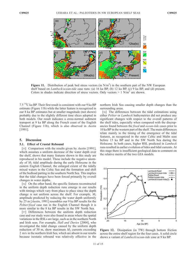
shelf is significantly stronger than present (Figures 11aand 11b). For example, an absolute stress value in thesouthern Celtic Sea (48.5�N, 7�W) is about three timeslarger at 10 ka BP and five times larger at 14 ka BP than inthe present-day situation. Comparison between fixed andocean-tide cases indicates that 30–40% of this increase isdue to the reduction of water depth, while the remaining maybe ascribed to the enhanced ocean tides.[53] The location and migration of bedload partings are

broadly consistent between the different runs apart from thetime lags before 15 ka BP between the Lambeck and Peltiercases; a significant bedload parting predicted on the outerCeltic shelf during low RSL stages (Figure 11a) migrateslandwards and then after 12 ka BP splits into the Celtic Seaand English Channel partings (Figures 11b–11d). Theseresults are comparable to those generated by Austin [1991]and Hall and Davies [2004] using nonisostatically correctedmodels.[54] Van der Molen and De Swart [2001] calculated bed

sediment transport off the Belgian and Dutch coasts byusing the GIA bathymetry of Lambeck [1995] for earlyHolocene stages and pointed out features such as weaksediment transport in the Southern Bight at 8 14C ka BPand cross-normal transport along the southern Dutch coast at

Figure 10. Predicted distribution of stratification parameter, S, in the Celtic Sea based on Lambeck/fixedcase (upper row) and Lambeck/ocean-tide case (lower row) runs. Location of Core 199 is marked withpluses.

C09025 UEHARA ET AL.: PALEOTIDES IN NW EUROPEAN SHELF SEAS

10 of 15

C09025

7.5 14C ka BP. Their first result is consistent with our 9 ka BPestimate (Figure 11b) while the latter feature is recognized inour 8 ka BP estimates but at smaller magnitude (not shown)probably due to the slightly different time slices adopted inboth models. Our result indicates a cross-normal sedimenttransport at 9 ka BP along the French coast of the EnglishChannel (Figure 11b), which is also observed in Austin[1991].

5. Discussion

5.1. Effect of Crustal Rebound

[55] Comparison with the results given by Austin [1991],which assumes a uniform decrease of the water depth overthe shelf, shows that many features shown in this study arereproduced in his model. These include the negative anom-aly of M2 tidal amplitude during the early Holocene in theeastern English Channel, the enlarged extent of the tidallymixed waters in the Celtic Sea and the formation and shiftof the bedload parting in the southern North Sea. This impliesthat the tidal changes have been forced primarily by overallchanges in water depths.[56] On the other hand, the specific features reconstructed

in the uniform depth reduction runs emerge in our resultswith timings which vary from place to place since the depthchange is not uniform across the shelf. For example, M2

amplitude predicted by reducing the water depth uniformlyby 25 m [Austin, 1991] resembles our 9 ka BP results for thePeltier/fixed case run in the English Channel though it ismore similar to the 8 ka BP results in the SW North Sea.[57] Differences between the uniform depth reduction

case and our study were also found in areas where the spatialvariations in the RSLs are large, such as in the northern Northand Irish seas. For example, Hall and Davies [2004], whoinvestigated the tidal change caused by the uniform depthreduction of 30 m, show maximum M2 currents exceeding2 m/s in the northern Irish Sea, which are absent in our resultsbecause isostatic rebound was relatively effective in the

northern Irish Sea causing smaller depth changes than thesurrounding areas.[58] The differences between the tidal estimations using

either Peltier or Lambeck bathymetries did not produce anysignificant changes with respect to the overall patterns ofthe shelf tides, especially when compared with the discrep-ancies found between the fixed and ocean-tide cases prior to10 kaBP in the western part of the shelf. Themain differencesrelate mainly to the timing of the emergence of the tidalfeatures, as recognized in the outer Celtic and Malin seasbefore 15 ka BP and in the SW North Sea during theHolocene. In both cases, higher RSL predicted in Lambeckruns resulted in earlier evolution of tides and tidal currents. Atthis stage there is insufficient geological data to comment onthe relative merits of the two GIA models.

Figure 12. Dissipation (in TW) through bottom frictionacross the entire shelf region for the four cases. A solid circleshows a variant of Lambeck/ocean-tide case at 9 ka BP.

Figure 11. Distribution of peak bed stress vectors (in N/m2) in the southern part of the NW Europeanshelf based on Lambeck/ocean-tide case runs: (a) 16 ka BP, (b) 12 ka BP, (c) 9 ka BP, and (d) present.Colors in shades indicate direction of stress vectors. Only vectors > 1 N/m2 are shown.

C09025 UEHARA ET AL.: PALEOTIDES IN NW EUROPEAN SHELF SEAS

11 of 15

C09025

[59] These results suggest that the overall change of tidalpatterns can be explained primarily by the uniform eustaticrise of sea level, while local isostatic effects played asignificant modulating role in determining the actual timingof the changes. In addition, some modifications of the tidalfeatures emerge in regions where the isostatic effect is large,such as in the northern Irish and North seas.

5.2. Dissipation

[60] The modeled tidal dissipation through bottom fric-tion is shown in Figure 12 for all four cases conducted inthis study. The estimate for the present-day situation (0.22–0.23 TWor 0.18–0.19 TW forM2 only) agrees with Flather[1976] based on a shelf-tide model (0.19 TW for M2 only),is slightly larger than Egbert et al. [2004] obtained from ahydrodynamic global model (0.16 TW for M2 only), and isconsistent with the value derived from TPXO.4a model(0.19 TW for M2 only [Egbert and Ray, 2001, Plate 3]).[61] In the fixed cases, dissipation on the shelf increased

continuously from 20 ka BP to 8 ka BP and then graduallydecreased to the present value. The ocean-tide cases, on theother hand, generate distinctly high dissipation rates between17 ka BP and 10 ka BP (Lambeck case) or 14 ka BP and 10 kaBP (Peltier case) compared to those predicted for ages after8 ka BP. This large dissipation rate is due mostly to the strongtidal currents in the Celtic and Malin seas induced by theenhanced ocean tides along the western boundary of themodel. The dissipation rate at 9 ka BP in the ocean-tide casesdepends on the ice-sheet distribution in Hudson Strait, asindicated for the Lambeck/ocean-tide case in Figure 12.[62] The overall change in the shelf tidal dissipation rates

can be explained primarily by regional effects in the English

Channel and the Celtic Sea. At present, dissipation in theEnglish Channel, which occupies only 7% of the whole shelfarea, accounts for about 40% of the total dissipation on theshelf. While the English Channel has been the largest sink oftidal energy during the last 8 ka BP, the Celtic Sea was themain focus of tidal dissipation before 10 ka BP. In particular,more than half the total dissipation occurred in the Celtic Seabetween 17–13 ka BP (Lambeck case) or between 16–12 kaBP (Peltier case). This regional difference in the timing ofmaximum dissipation, implied by our modeling study, sug-gests the possibility of finding geological proxy evidence toconfirm it. Thus there is an opportunity for future observa-tional studies to substantiate the proposed tidal evolution.[63] Differences between the Lambeck and Peltier cases

were much smaller than those between the fixed and ocean-tide cases except before 15 ka BP, when higher RSL andmoredeveloped outer-shelf geometry predicted in the Lambeckreconstruction gave rise to an earlier onset of the highdissipation phase. Higher dissipation rate observed in theLambeck case between 14 and 12 ka BP may be ascribed tostronger tidal current along the edge of theMalin Shelf due tolower RSL (shallower depth) predicted in the Lambeckmodel.[64] The temporal change of global dissipation rate

obtained from the ocean-tide model shows features differentfrom that within the shelf seas, suggesting a larger role of(internal) tidal dissipation in the deep oceans during the earlyphase of deglaciation. The total rate was largest at 20 ka BPand decreased slightly until 10 ka BP followed by a distinctdrop at 10–8 ka BP and has been roughly constant since 5 kaBP. This is consistent with the findings of Egbert et al.[2004]; their data and our model results are shown in

Figure 13. (a) Temporal change of global dissipation rate derived from the ocean-tide model results(forced only by M2 tides) and Egbert et al. [2004]. (b) M2 amplitude change off the Celtic Sea (15�W,50�N) under different bathymetric settings; either applying the Peltier bathymetry (GIA; thick lines) orreducing the global depth uniformly to the sea level at (30�W, 30�N) in the central N Atlantic (UDR; thinlines with symbols). A thick dashed line denotes a GIA run made with Hudson Strait closed, while a thinline with circles shows a HDR case which incorporates the change of ice-sheet extents. ‘‘UDR + GIA’’cases apply the GIA bathymetry only at regions south of 60�S (triangle) or in the Hudson Bay andLabrador Sea (square) and employ UDR at remaining areas.

C09025 UEHARA ET AL.: PALEOTIDES IN NW EUROPEAN SHELF SEAS

12 of 15

C09025

Figure 13a. Their estimate for 20 ka BP (3.96TW) agreeswell with our result (3.86TW; M2 only), though it issmaller than ours for present conditions (2.68TW versus3.08TW). This discrepancy is probably due to the lowerhorizontal resolution adopted in our study. The similaritybetween the results for the LGM can be attributed to thesmaller contribution of shallow shelf seas at that time.

5.3. Ocean Tide Variability

[65] It is worth discussing briefly the relevant geologicalmechanisms that affect the ocean-tide variability in the NEAtlantic since the ocean tide is the relevant boundary condi-tion to co-oscillatory shelf models and is therefore thedominant control on the evolution of tides and tide-relatedparameters in the western part of the NW European Shelf.[66] Figure 13b plots changes of M2 amplitude at a

location west of the Celtic Sea (15�W, 50�N) derived withdifferent bathymetric adjustments. The changes obtainedfrom bathymetries implementing full GIA effects (thicksolid curve) show features similar to the shelf-tide changesin the Celtic Sea; amplitude decreased until 8 ka BP with asignificant drop at 10–8 ka BP, followed by a smallervariability after 8 ka BP. The predicted values at 20 kaBP and at present (1.9 m and 0.9 m, respectively) are moresimilar to the results by Egbert et al. [2004] (2.0 m and 0.9 m)than those of Thomas and Sundermann [1999] (1.6 m and1.0 m). Comparison between the curves suggests that eventhough M2 amplitudes in the NE Atlantic show someincrease from the imposition of a uniform depth reduction(pluses in Figure 13b), inclusion of coastline changes due tothe advance of ice sheets (open circles in Figure 13b) isnecessary to account for the enhanced amplitude observed inthe full GIA results for ages prior to 10 ka BP. In particular,the disappearance of ice sheets at 10–8 ka BP, which hasoccurred mainly in Hudson Strait and in Baffin Bay, seemsto be responsible for the large reduction of M2 amplitudesobserved in the NE Atlantic. Closure of the Hudson Straitgives rise to a systematic increase of M2 amplitudes (thickdashed line in Figure 13b).[67] The coastline changes may have had two major

impacts on tidal amplitudes in the North Atlantic. One isthe disappearance of a tidal energy sink through the exposureand isolation of the Hudson Bay/Labrador Sea, which is thelargest sink in the present-day world ocean [Egbert and Ray,2001]. Another is a decrease in the magnitude of dampingcoefficients caused by the increase in depth and the decreasein average velocities over the basin. The reduction of damp-ing coefficients enhances the tidal amplitude efficiently whenthe basin is near resonance as in the North Atlantic [Egbert etal., 2004].[68] The connection between the ice cover over Hudson

Bay and the magnitude of ocean tides was also pointed outby Arbic et al. [2004] for tides in the Labrador Sea. Theirresults on the amplitude change at (64�W, 61.5�N) showed alarge decrease at 17 ka BP and a distinct peak at 11–10 kaBP, followed by a rapid decrease at 7–6 ka BP, and are notconsistent with our results for the same location. Thisdiscrepancy may have been caused by the different GIAmodels used (Milne et al. [1999] versus Peltier [1994]), sincethe ocean-tide model used in Arbic et al. [2004] and in ourstudy show similar amplitude changes when the depth wasreduced uniformly from the present level. The similarities

between Egbert et al. [2004] and our results may stem fromthe same GIA model. Though the large amplitude drop at 7–6 ka BP presented by Arbic et al. [2004] for the Labrador Seamay have occurred also in the NE Atlantic, it seems to beearlier than the timing suggested by the proxy data from theCeltic Sea.[69] M2 amplitudes in the full GIA case are slightly

smaller than those obtained by the uniform depth reductioncases at 8 ka BP and 5–2 ka BP (Figure 13b). Additionalexperiments which apply the GIA bathymetry at particularregions, whilst reducing depth uniformly in the remainingarea, suggest that the amplitude deficits are caused by theemergence of a depressed seafloor after the melting of icesheets in the Hudson Bay and the Labrador Sea at 8 ka BP(squares in Figure 13b), and in the Southern Ocean at 5 kaBP (triangles). As the model results are sensitive to the gridlocation of the unresolved Hudson Strait, and because thedistribution of Antarctic ice sheets is not well determinedfrom observational data, some uncertainty may exist in thesmall tidal changes predicted for the last 8 ka.[70] Model results indicate several factors which give rise

to small changes in M2 amplitudes at near-present stages.The two GIA cases show an increase in M2 amplitudes atthis location over the last 5 ka, which demonstrates theimportance of GIA since such increase is not obtained withuniform depth reduction. The eustatic sea level rise causessmall though systematic decrease in M2 amplitudes at thislocation; ca. 2 mm (0.2%) if the sea level rose uniformlyby 1 m to the present level. M2 amplitudes in the shelfarea such as NW French coast also decrease in response tothe sea level rise under the fixed boundary condition. Forthe present-day situation, small coastline changes along theLabrador Sea cause changes in M2 amplitudes as largeas 4 mm off the Celtic Sea, suggesting that model with higherresolution would be necessary to discuss recent smallchanges in M2 amplitudes.[71] As in other paleoocean-tide studies, the form of

parameterisation here for internal tidal dissipation is depen-dent on the buoyancy frequency. Model results are thereforecontingent on the assumed paleo-stratification which ispoorly known. As Egbert et al. [2004] point out, with anincrease of dissipation in the form of internal tide a betterknowledge of stratification at the LGM becomes important,and remains a challenge for observational marine geology.For example, the M2 amplitude at 10 ka BP at the Isles ofScilly station predicted by the shelf model (Figure 8a) woulddecrease from 2.8 m to 2.0 m for the Lambeck/ocean-tidecase if the magnitude of the internal tidal dissipation used inthe ocean-tide prediction was doubled, which is an extremecase. Nevertheless, our results show that significant changesto the ocean tides have taken place over the last 20 ka BP, andthat decreasedM2 amplitudes in the NE Atlantic are the mostsignificant factor for shelf-sea models of this period. Leadingorder effects to shelf-sea processes are controlled by theradically different ocean tidal forcing, rather than the subtledifferences inherent in the GIA models.

6. Conclusions

[72] From the paleotidal simulations conducted for theNW European shelf seas, the following results have beenobtained:

C09025 UEHARA ET AL.: PALEOTIDES IN NW EUROPEAN SHELF SEAS

13 of 15

C09025

[73] 1. The tides and tidal currents on the western part ofthe shelf were significantly larger than present prior to 10 kaBP, driven by enhanced ocean tides in the North Atlantic.This had a large impact on seasonal stratification, bottomstress vectors, and tidal dissipation. On the other hand, tidalchanges have been generally small during the last 8 ka whensea level was close to its present level.[74] 2. Though the isostatic rebound effect acted only

locally to modify the overall pattern of the shelf tides, itappears to have played a role in determining the exact timingof the main tidal changes. The overall differences betweenthe different GIA models used were small, though thedifferent scenarios do modify the tidal patterns in areas wherethe isostatic rebound effect is large. Timing is important whenmaking comparisons with geological proxy data; althoughocean boundary forcing is the main driver of differences inthe shelf model results, improved loading histories and GIAmodels are still likely to be required for understanding thedetail of the geological record.[75] 3. The change in ocean tides off the shelf area seems

to have been related to the emergence of shallow seas andshrinkage of ice sheets during deglaciation. In particular,significant reduction of M2 amplitudes seems to have oc-curred at 10–8 ka BPwhich is ascribed mainly to the openingof the Hudson Strait. The timing of the large amplitudechange agrees with proxy paleoceanographic data from theCeltic Sea. This work makes clear that – irrespective of thedetails of amplitude - changes to oceanic tides are the mostimportant driver for changes to tide-dependent shelfprocesses, therefore any geological evidence for a chang-ing tidal regime on the continental shelf lends furthersupport to the notion of a changing oceanic regime.[76] Our results suggest that geographic changes in high

latitudes have affected the tides in the NW European Shelf.As well as a better understanding of paleo-stratification ofthe ocean, more accurate data on paleogeographies in theCanadian Arctic and Antarctic shelves are required to obtainmore realistic reconstructions of the shelf tides during thegeological past.

[77] Acknowledgments. This study was supported by the bilateralprogramme between the Japan Society for the Promotion of Science (JSPS)and The Royal Society. Authors would like to thank two anonymousreviewers for their constructive comments.

ReferencesAccad, Y., and C. L. Pekeris (1978), Solution of the tidal equations for theM2 and S2 tides in the world oceans from a knowledge of the tidalpotential alone, Philos. Trans. R. Soc. London, A290, 235–266.

Arbic, B. K., D. R. MacAyeal, J. X. Mitrovica, and G. A. Milne (2004),Palaeoclimate: Ocean tides and Heinrich events, Nature, 432, 460,doi:10.1038/432460a.

Austin, R. M. (1991), Modelling Holocene tides on the NW Europeancontinental shelf, Terra Nova, 3(3), 276–288.

Austin, W. E. N., and J. D. Scourse (1997), Evolution of seasonal stratifica-tion in the Celtic Sea during the Holocene, J. Geol. Soc. London, 154(2),249–256.

Belderson, R. H., R. D. Pingree, and D. K. Griffiths (1986), Low sea-leveltidal origin of Celtic Sea sand banks—evidence from numerical model-ling of M2 tidal streams, Mar. Geol., 73(1–2), 99–108.

Blumberg, A. F., and G. L. Mellor (1987), A description of a three-dimensional coastal ocean circulation model, in Three-DimensionalCoastal Ocean Models, Coastal Estuarine Stud., vol. 4, edited byN. S. Heaps, pp. 1–16, AGU, Washington, D. C.

Cartwright, D. E., J. M. Huthnance, R. Spencer, and J. M. Vassie(1980), On the St Kilda shelf tidal regime, Deep Sea Res., 27A(1),61–70.

Davies, A. M., S. C. M. Kwong, and R. A. Flather (1997), A three-dimensional model of diurnal and semidiurnal tides on the European shelf,J. Geophys. Res., 102(C4), 8625–8656.

Egbert, G. D., and S. Y. Erofeeva (2002), Efficient Inverse Modeling ofBarotropic Ocean Tides, J. Atmos. Oceanic Technol., 19(2), 183–204.

Egbert, G. D., and R. D. Ray (2001), Estimates of M2 tidal energy dissipa-tion from TOPEX/Poseidon altimeter data, J. Geophys. Res., 106(C10),22,475–22,502.

Egbert, G. D., R. D. Ray, and B. G. Bills (2004), Numerical modeling of theglobal semidiurnal tide in the present day and in the last glacial max-imum, J. Geophys. Res., 109, C03003, doi:10.1029/2003JC001973.

Flather, R. A. (1976), A tidal model of the north-west European continentalshelf, Mem. Soc. R. Sci. Liege, Ser. 6, 10, 141–164.

Gerritsen, H., and C. W. J. Berentsen (1998), A modelling study of tidallyinduced equilibrium sand balances in the North Sea during the Holocene,Cont. Shelf Res., 18(2–4), 151–200.

Hall, P., and A. M. Davies (2004), Modelling tidally induced sediment-transport paths over the northwest European shelf: the influence ofsea-level reduction, Ocean Dyn., 54(2), 126–141, doi:10.1007/s10236-003-0070-7.

Hinton, A. C. (1995), Holocene tides of The Wash, U.K.: The influence ofwater-depth and coastline-shape changes on the record of sea-levelchange, Mar. Geol., 124(1–4), 87–111.

Hinton, A. C. (1996), Tides in the northeast Atlantic: considerations formodelling water depth changes, Quat. Sci. Rev., 15(8–9), 873–894.

Hinton, A. C. (1997), Tidal changes, Prog. Phys. Geogr., 21(3), 425–433.Jayne, S. R., and L. C. St. Laurent (2001), Parameterizing tidal dissipationover rough topography, Geophys. Res. Lett., 28(5), 811–814.

Kantha, L. H., C. Tierney, J. W. Lopez, S. D. Desai, M. E. Parke, andL. Drexler (1995), Barotropic tides in the global oceans from a non-linear tidal model assimilating altimetric tides: 2. Altimetric and geo-physical implications, J. Geophys. Res., 100(C12), 25,309–25,317.

Lambeck, K. (1993), Glacial rebound of the British-Isles. 1. Preliminarymodel results, Geophys. J. Int., 115(3), 941–959.

Lambeck, K. (1995), Late Devensian and Holocene shorelines of theBritish Isles and North Sea from models of glacio-hydro-isostatic re-bound, J. Geol. Soc. London, 152(3), 437–448.

Lambeck, K. (1996), Glaciation and sea-level change for Ireland and theIrish Sea since Late Devensian/Midlandian time, J. Geol. Soc. London,153(6), 853–872.

Lambeck, K., and J. Chappell (2001), Sea Level Change Through the LastGlacial Cycle, Science, 292, 679–686.

Lambeck, K., and A. P. Purcell (2001), Sea-level change in the Irish Seasince the Last Glacial Maximum: constraints from isostatic modelling,J. Quat. Sci., 16(5), 497–506, doi:10.1002/jqs.638.

Lambeck, K., A. Purcell, P. Johnston, M. Nakada, and Y. Yokoyama(2003), Water-load definition in the glacio-hydro-isostatic sea-level equa-tion, Quat. Sci. Rev., 22(2–4), 309–318.

Marret, F., and J. Scourse (2002), Control of modern dinoflagellate cystdistribution in the Irish and Celtic seas by seasonal stratification dy-namics, Mar. Micropaleontol., 47, 101–116.

Marret, F., J. Scourse, and W. Austin (2004), Holocene shelf-sea seasonalstratification dynamics: a dinoflagellate cyst record from the Celtic Sea,NW European shelf, Holocene, 14(5), 689–696.

Milne, G. A., J. X. Mitrovica, and J. L. Davis (1999), Near-field hydro-isostasy: the implementation of a revised sea-level equation, Geophys.J. Int., 139, 464–482.

Peltier, W. R. (1994), Ice-Age paleotopography, Science, 265, 195–201.Pingree, R. D., and D. K. Griffiths (1978), Tidal Fronts on the Shelf SeasAround the British Isles, J. Geophys. Res., 83(C9), 4615–4622.

Pingree, R. D., and D. K. Griffiths (1979), Sand transport paths around theBritish Isles resulting from M2 and M4 tidal interactions, J. Mar. Biol.Assoc. U.K., 59, 497–513.

Platzman, G. W., G. A. Curtis, K. S. Hansen, and R. D. Slater (1981),Normal Modes of the World Ocean. Part II: Description of Modes inthe Period Range 8 to 80 hours, J. Phys. Oceanogr., 11(5), 579–603.

Proctor, R., and A. M. Davies (1996), A three dimensional hydrodynamicmodel of tides off the north-west coast of Scotland, J. Mar. Syst., 7(1),43–66.

Scott, D. B., and D. A. Greenberg (1983), Relative sea level rise and tidaldevelopment in the Fundy tidal system, Can. J. Earth Sci., 20(10), 1554–1564.

Scott, G. A., J. D. Scourse, and W. E. N. Austin (2003), The distribution ofbenthic foraminifera in the Celtic Sea: The significance of seasonal stra-tification, J. Foraminiferal Res., 33(1), 32–61.

Scourse, J. D., and R. M. Austin (1995), Palaeotidal modelling of conti-nental shelves: Marine implications of a landbridge in the Strait of Doverduring the Holocene and Middle Pleistocene, in Island Britain: A Qua-ternary Perspective, edited by R. C. Preece, Geol. Soc. Spec. Publ., 96,75–88.

C09025 UEHARA ET AL.: PALEOTIDES IN NW EUROPEAN SHELF SEAS

14 of 15

C09025

Scourse, J. D., W. E. N. Austin, B. T. Long, D. J. Assinder, and D. Huws(2002), Holocene evolution of seasonal stratification in the Celtic Sea:refined age model, mixing depths and foraminiferal stratigraphy, Mar.Geol., 191(3–4), 119–145.

Scourse, J. D., H. Kennedy, G. A. Scott, and W. E. N. Austin (2004), Stableisotopic analyses of modern benthic foraminifera from seasonally strati-fied shelf seas: disequilibria and the ‘seasonal’ effect, Holocene, 14(5),747–758.

Shennan, I., K. Lambeck, R. Flather, B. Horton, J. McArthur, J. Innes,J. Lloyd, M. Rutherford, and R. Kingfield (2000), Modelling westernNorth Sea palaeogeographies and tidal changes during Holocene, inHolocene Land-Ocean Interaction and Environmental Change aroundthe North Sea, edited by I. Shennan and J. E. Andrews, Geol. Soc.Spec. Publ., 166, 299–319.

Simpson, J. H., and J. R. Hunter (1974), Fronts in the Irish Sea, Nature,250, 404–406.

Sinha, B., and R. D. Pingree (1997), The principal lunar semidiurnal tideand its harmonics: baseline solutions for M2 and M4 constituents on theNorth-West European Continental Shelf, Cont. Shelf Res., 17(11), 1321–1365.

Smith, W. H. F., and D. T. Sandwell (1997), Global Sea Floor Topographyfrom Satellite Altimetry and Ship Depth Soundings, Science, 277, 1956–1962.

Thomas, M., and J. Sundermann (1999), Tides and tidal torques of theworld ocean since the last glacial maximum, J. Geophys. Res.,104(C2), 3159–3183.

Uehara, K., Y. Saito, and K. Hori (2002), Paleotidal regime in the Chang-jiang (Yangtze) Estuary, the East China Sea, and the Yellow Sea at 6 kaand 10 ka estimated from a numerical model, Mar. Geol., 183(1–4),179–192.

Van der Molen, J., and H. E. De Swart (2001), Holocene tidal conditionsand tide-induced sand transport in the southern North Sea, J. Geophys.Res., 106(C5), 9339–9362.

Van der Spek, A. J. F. (1997), Tidal asymmetry and long-term evolution ofHolocene tidal basins in The Netherlands: simulation of palaeo-tides inthe Schelde estuary, Mar. Geol., 141(1–4), 71–90.

�����������������������K. J. Horsburgh, Proudman Oceanographic Laboratory, Liverpool L3

5DA, UK.K. Lambeck and A. P. Purcell, Research School of Earth Sciences,

Australian National University, Canberra, ACT 0200, Australia.J. D. Scourse, School of Ocean Sciences, University of Wales (Bangor),

Menai Bridge, Anglesey LL59 5AB, UK.K. Uehara, Research Institute for Applied Mechanics, Kyushu University,

Kasuga, Fukuoka 816-8580, Japan. (uehara@riam.kyushu-u.ac.jp)

C09025 UEHARA ET AL.: PALEOTIDES IN NW EUROPEAN SHELF SEAS

15 of 15

C09025