105
Tidal phenomena in the Scheldt Estuary 1202016-000 © Deltares, 2010 L.C. van Rijn
Tidal phenomena in the Scheldt Estuary
1202016-000 © Deltares, 2010
L.C. van Rijn


Title Tidal phenomena in the Scheldt Estuary Project 1202016-000
Pages 99
Keywords Tidal wave propagation; Tidal Dynamics; Scheldt Estuary Summary The Scheldt Estuary is a large-scale estuary in the south-west part of the Netherlands. The estuary is connected to the Scheldt river, which originates in the north-west of France. The total length of the Scheldt river including the estuary is about 350 km; the tide penetrates up to the city of Gent in Belgium (about 180 km from the mouth). The length of the estuary is about 60 km (up to Bath). Various analytical and numerical solution methods have been used and compared to measured data for a schematized estuary (exponentially decreasing width). The effects of water depth, channel dimensions and tidal storage on tidal range have been studied. Non-linear effects have also been discussed. References LTV Zandhuishouding Schelde Estuarium 2010 Version Date Author Initials Review Initials Approval Initials aug. 2010 prof. dr. ir. L.C.
van Rijn ir. K. Kuijper ir. T. Schilperoort
ir. M.D. Taal State final


9 September 2010, final
Tidal phenomena in the Scheldt Estuary
i
Contents
1 Introduction 1
2 Basic tidal characteristics 3 2.1 Tidal wave propagation 3 2.2 Tidal constituents 4 2.3 Phenomena affecting wave propagation 5
3 Basic equations and solutions for tides in estuaries 9 3.1 Definitions and characteristics 9 3.2 Analytical solution of energy flux equation for prismatic and converging channels 21 3.3 Analytical solution of tidal wave equations for prismatic channels 24 3.4 Analytical solution of tidal wave equations for converging channel 28 3.5 Numerical solution of tidal wave equations for converging channels 34
4 Computational examples for schematized Scheldt Estuary 35 4.1 Tidal data of Scheldt Estuary 35 4.2 Computed and measured tidal range for Scheldt Estuary 37
4.2.1 Case definitions 37 4.2.2 Comparison of measured and computed tidal range 39
4.3 Effect of water depth on tidal range 45 4.4 Effect of channel dimensions on tidal range 46 4.5 Effect of cross-section on tidal range 49 4.6 Effect of local tidal storage variation on tidal range 53 4.7 Non-linear effects and tidal asymmetry 54
5 Summary and conclusions 65
6 References 71 Appendices
A Analytical and numerical results for prismatic channels A-1
B Analytical and numerical results for converging tidal channels B-1


9 September 2010, final
Tidal phenomena in the Scheldt Estuary
1 of 99
1 Introduction
The Scheldt Estuary is a large-scale estuary in the south-west part of the Netherlands. The estuary is connected to the Scheldt river, which originates in the north-west of France. The total length of the Scheldt river including the estuary is about 350 km; the tide penetrates up to the city of Gent in Belgium (about 180 km from the mouth). The length of the estuary is about 60 km (up to Bath). The cross-sections of the Estuary show two to three deeper channels with shoals in between and tidal flats close to the banks.The width of the mouth at Westkapelle (The Netherlands) is about 25 km and gradually decreases to about 0.8 km at Antwerp. The shape of the Scheldt Estuary is very similar to that of other large-scale alluvial estuaries in the world. The width and the area of the cross-section reduce in upstream (landward) direction with a river outlet at the end of the estuary resulting in a converging (funnel-shape) channel system. The bottom of the tide-dominated section generally is fairly horizontal. Tidal flats are present along the estuary (deltas). The tidal range in estuaries is affected by four dominant processes (see Dyer, 1997; McDowell and O’Connor, 1977; Savenije, 2005 and Prandle, 2009):
• inertia related to acceleration and deceleration effects; • amplification (or shoaling) due to the decrease of the width and depth (convergence) in
landward direction; • damping due to bottom friction and • partial reflection at abrupt changes of the cross-section and at the landward end of the estuary (in
the absence of a river). The Scheldt Estuary has important environmental and commercial qualities. It is the main shipping route to the Port of Antwerp in Belgium. The depth of the navigation channel to the Port of Antwerp in Belgium is a problematic issue between The Netherlands and Belgium because of conflicting interests (commercial versus environmental). Large vessels require a deep tidal channel to Antwerp, which enhances tidal amplification with negative environmental consequences. Since 1900, the main shipping channel has been deepened (by dredging and dumping activities) by a few metres. Furthermore, sand mining activities have been done regularly. Both types of dredging works may have affected the tidal range along the estuary. The tidal range at the mouth (Westkapelle and Vlissingen) has been approximately constant over the last century, but the tidal range inside the estuary has gone up by about 1 m (Pieters, 2002). Particularly, the high water levels have gone up considerably. The low water levels have gone down slightly at some locations (about 0.2 m at Antwerp) despite sea level rise of about 0.2 m per century. To be able to evaluate the consequences of the ongoing channel deepening on the tidal range, it is of prime importance to understand the basic character of the tidal wave propagation in the Scheldt Estuary. The most basic questions are:
• what is the role of the shape and dimensions of the tidal channels (both in planform and in the cross-section) on tidal wave propagation and tidal storage?
• what is the role of bottom friction in relation to the depth of the main channels? • what is the role of reflection of the tidal wave against abrupt changes of the cross-section and at
the landward end near Bath? • what is the role of tidal storage? • what is the role of tidal wave asymmetry (non-linear effects)?

2 of 99
Tidal phenomena in the Scheldt Estuary
9 September 2010, final
These questions will be addressed in this report (by Prof. Dr. L.C. van Rijn; Deltares and University of Utrecht) by using measured data (only present situation; no historical developments) and a range of models: energy-flux approach, analytical solutions of the linearized equations of continuity and momentum and 1D and 2DH numerical models including non-linear terms. The analytical and numerical models have been used to identify the most important processes and parameters (sensitivity computations) for schematic cases with boundary conditions as present in the Scheldt Estuary. This approach generates basal information and knowledge of the tidal propagation in the Scheldt Estuary. K. Kuijper of Deltares is gratefully acknowledged for his detailed comments.

9 September 2010, final
Tidal phenomena in the Scheldt Estuary
3 of 99
2 Basic tidal characteristics
2.1 Tidal wave propagation In oceans, seas and estuaries there is a cyclic rise and fall of the water surface, which is known as the vertical astronomical tide. The tide is a long wave with a period of about 12 hours and 25 min (semi-diurnal tide) in most places. At some locations the tide has a dominant period of about 24 hours. The crest and the trough of the wave (with a length of several hundreds of kilometres) are known as high tide or High Water (HW) and low tide or Low Water (LW), see Figure 2.1. The wave height between low water (LW) and high water (HW) is known as the tidal range. Successive tides have different tidal ranges because the propagation of the tide is generated by the complicated motion of the Earth (around the Sun and around its own axis) and the Moon (around the Earth). Moreover, tidal propagation is affected by shoaling (funelling) due to the decrease of the channel cross-section in narrowing estuaries, by damping due to bottom friction, by reflection against boundaries and by deformation due to differences in propagation velocities at low and high water.
Figure 2.1 Tidal curve The generation of the astronomical tide is the result of gravitational interaction between the Moon, the Sun and the Earth. Meteorological influences, which are random in occurrence, also affect the local tidal motions. The orbit of the Moon around the Earth has a period of 29.6 days and both have an orbit around the Sun in 365.2 days. There are 4 tides per day generated in the oceans. The Moon causes 2 tides and the Sun also causes 2 tides. The tides of the Sun are only half as big as those generated by the Moon. Even though the mass of the Sun is 27 million times greater than that of the Moon, the Moon is 390 times closer to the Earth resulting in a gravitational pull on the ocean that is twice as large as that of the Sun. The tide has a return period of about 12 hours and 25 min (semi-diurnal tide) in most places. The 25 min delay between two successive high tides is the result of the rotation of the Moon around the Earth. The Earth makes a half turn in 12 hours, but during those 12 hours the Moon has also moved. It takes about 25 min for the Earth to catch up to the new position of the Moon. The orbit of the Moon around the Earth is, on average, 29 days, 12 hours and 44 minutes (total of 708,8 hours to cover a circle of 360o or a sector angle of 0.508o per hour). Thus, the Moon moves over a sector angle of 6.1o per 12 hours. The Earth covers a circle of 360o in 24 hours or a sector angle of 15o per hour. So, it takes about 6.1/15 = 0.4 hour (about 25 minutes) for the Earth to catch up with the Moon.

4 of 99
Tidal phenomena in the Scheldt Estuary
9 September 2010, final
Based on this, the tide shifts over 50 minutes per day of 24 hours; so each new day HW will be 50 minutes later. If the time of the first High Water (HW) at a certain location (semi-diurnal tide) is known at the day of New Moon (Spring tide), the time of the next HW is 12 hours and 24 minutes later and so on. The phase shift of 50 min per day is not constant but varies between 25 and and 75 min, because of the elliptical shape of the orbit of the Moon. Over the period of 29,6 days there are 2 spring tides and 2 neap tides; the period from spring tide to neap tide is, on average, 7.4 days. The orbits of the Moon around the Earth and the Earth around the Sun are both elliptical, yielding a maximum and a minimum gravitational force. The axis of the Earth is inclined to the plane of its orbit around the Sun and the orbital plane of the Moon around the Earth is also inclined to the axis of the Earth. Consequently, the gravitational tide-generating force at a given location on Earth is a complicated but deterministic process. The largest force component is generated by the Moon and has a period of 12.25 hr (M2-constituent). This force reaches its maximum value once in 29 days when the Moon is nearest to the Earth. Spring tide near coasts does not really occur when the Sun and the Moon are in line, but generally one to three days later. This time lag is known as the tide age. Another time lag is known as port establishment and represents the time interval for a tidal wave generated in the deep ocean to reach a certain port. The rotation of the Earth introduces an apparent force acting on bodies. This force is significant in oceans, seas, wide estuaries and large lakes. The rotation-induced force is known as the Coriolis force or geostrophic force. A fluid particle moving with velocity v experiences a Coriolis force perpendicular to its direction. The force is pointed to the right on the northern hemisphere and to the left on the southern hemisphere. The Coriolis force is maximum at the North and South pole and is zero at the Equator.
2.2 Tidal constituents The tide-generating force can be expressed as a series of harmonic constituents. The periods and relative amplitudes of the seven major astronomical constituents, which account for about 83% of the total tide-generating force, are (Table 2.1): Table 2.1 Tidal constituents
Origin Symbol Period (hours) RelativeStrength (%) Main Lunar, semi-diurnal Main Solar, semi-diurnal Lunar elliptic,semi-diurnal Lunar-Solar, semi-diurnal Lunar-Solar, diurnal Main Lunar, diurnal Main Solar, diurnal
M2 S2 N2 K2 K1 O1 P1
12.42 12.00 12.66 11.97 23.93 25.82 24.07
100 46.6 19.2 12.7 58.4 41.5 19.4
In deep water the tidal phenomena can be completely described by a series of astronomical constituents. In shallow water near coasts and in estuaries, the tidal wave is deformed by the effect of shoaling, reflection and damping (bottom friction). These deformations can be described by a Fourier series yielding additional higher harmonic tides which are known as partial tides or shallow water tides.
9 September 2010, final
Tidal phenomena in the Scheldt Estuary
5 of 99
These higher harmonic components can only be determined by tidal analysis of water level registra-tions at each location. The well-known neap-spring tidal cycle of 14.8 days is produced by the principal lunar and solar semi-diurnal components M2 and S2, and has a mean spring amplitude of M2+S2 and a mean neap amplitude of M2−S2.
2.3 Phenomena affecting wave propagation A progressive harmonic wave propagating in deep water without wave deformation/distortion is an ideal situation. Basic phenomena affecting the propagation of waves, are:
• reflection, • amplification, • deformation, • damping.
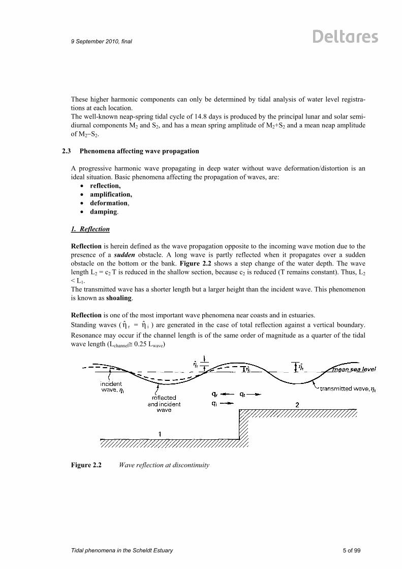
1. Reflection Reflection is herein defined as the wave propagation opposite to the incoming wave motion due to the presence of a sudden obstacle. A long wave is partly reflected when it propagates over a sudden obstacle on the bottom or the bank. Figure 2.2 shows a step change of the water depth. The wave length L2 = c2 T is reduced in the shallow section, because c2 is reduced (T remains constant). Thus, L2 < L1. The transmitted wave has a shorter length but a larger height than the incident wave. This phenomenon is known as shoaling. Reflection is one of the most important wave phenomena near coasts and in estuaries. Standing waves ( η r = η i ) are generated in the case of total reflection against a vertical boundary. Resonance may occur if the channel length is of the same order of magnitude as a quarter of the tidal wave length (Lchannel≅ 0.25 Lwave)
Figure 2.2 Wave reflection at discontinuity

6 of 99
Tidal phenomena in the Scheldt Estuary
9 September 2010, final
Figure 2.3 Amplification (shoaling), deformation and damping of waves 2. Amplification Amplification (or ‘shoaling’) is herein defined as the increase of the wave height due to the gradual change of the geometry of the system (depth and width). Amplification or shoaling is also known as wave funneling in convergent channels (decreasing width and depth in landward direction) and is an important phenomenon in estuaries where the depth and width are gradually decreasing. The principle of tidal wave amplification can be easily understood by considering the wave energy flux equation, which is known as Green’s law (1837). The total energy of a sinusoidal tidal wave per unit length is equal to E = 0.125ρg bH2 with b= width of channel, H = wave height. The propagation velocity of a sinusoidal wave is given by: co= (gho)0.5 with ho= water depth. Assuming that there is no reflection and no loss of energy (due to bottom friction), the energy flux is constant resulting in: Eoco = Ex cx or Hx/Ho=(bx/bo)−0.5 (hx/ho)−0.25. Thus, the tidal wave height Hx increases for decreasing width and depth. The wave length L= co T will decrease as co will decrease for decreasing depth resulting in a shorter and higher wave (Figure 2.3). The variation of the tidal range H in a real estuary with exponentially decreasing width and depth can be derived from an overall energy-based approach including bottom friction, assuming that the width and depth are varying exponentially (see later).

9 September 2010, final
Tidal phenomena in the Scheldt Estuary
7 of 99
3. Deformation A harmonic wave propagating from deep water to shallow water cannot remain harmonic (sinusoidal) due to the decreasing water depth. Furthermore, the water depth (h) varies along the wave profile. The water depth is largest under the wave crest and smallest under the wave trough. As the propagation velocity is proportional to h0.5, the wave crest will propagate faster than the wave trough, and the wave shape will change which is known as deformation (Figure 2.3). The wave is then no longer a smooth sinusoidal wave; the tidal high water becomes a sharply peaked event and low water is a long flat event. The deformed wave profile (wave skewness) can be described by additional sinusoidal components known as higher harmonics of the basic wave. Bottom friction and shoaling will also lead to wave deformation. Bore-type asymmetric waves can only be described by higher harmonics if a phase shift is introduced between the base wave and the higher harmonic wave. 4. Damping Friction between the flowing water and the bottom causes a loss of energy and as a result the wave height will be reduced (energy ≅ H2L). When the water depth is approximately constant, the wave height will decrease exponentially during propagation (Figure 2.3). Non-linearity of the friction term (bottom friction ≈ u 2 or u |u |) generates higher frequency components than the basic frequency ω of a tidal wave (ω = 2π/T). Consider a harmonic wave entering an estuary where bottom friction becomes important. The current velocity at sea can be described as: u = u sin(ωt). Friction becomes increasingly important in the shallower parts of the estuary and is represented by the term g u 2/C2. Near the mouth of the estuary, the friction term can be represented as (applying Fourier series expansion): g u 2/C2 = g [ u 2/C2][sin(ωt)]2 = g [ u 2/C2][(8/(3π)) sin(ωt) + (8/15) sin(3ωt) + ......] (2.1) Thus, higher harmonic components with frequencies 3ω, etc. are generated. The parameter [1/(3π)][8g/C2] | u | = [1/(3π)] f | u | is known as the linearized Lorentz-friction parameter with f = 8g/C2= Darcy-Weisbach friction factor. According to the energy principle of Lorentz, the total energy dissipation in a tidal cycle is the same for both linearized and quadratic friction.


9 September 2010, final
Tidal phenomena in the Scheldt Estuary
9 of 99
3 Basic equations and solutions for tides in estuaries
3.1 Definitions and characteristics Basically, an estuary is the (widened) outlet of a river to the sea and is governed by oscillating tidal flow coming from the (saline) sea and by the quasi-steady (fresh) water flow coming from the river in a complicated hydraulic system consisting of channels and shoals. Sometimes, a narrowing bay without river inflow is also known as an estuary. Drowned valleys (rias) and fjords also are examples of estuaries. A bay connected to the sea by a narrow channel (tidal inlet) is known as a lagoon or semi-enclosed basin. An alluvial channel with a movable sediment bed (banks are usually fixed) is a highly dynamic morphological system with meandering channels and shoals; sediments may be imported from riverine and marine sources. Sediments may also be exported over the seaward boundary of the estuary depending on the tidal asymmetry characteristics and the magnitude of the fresh water discharge of the river (density differences). Stratified or well-mixed flow conditions depend on the ratio of the river discharge and the tidal discharge. The shape of alluvial estuaries is similar all over the world, see Dyer (1997), McDowell and O’Connor (1977), Savenije (2005) and Prandle (2009). The width and the area of the cross-section reduce in upstream (landward) direction with a river outlet at the end of the estuary resulting in a converging (funnel-shaped) channel system, see Figure 3.1. The bottom of the tide-dominated section is almost horizontal. Often, there is a mouth bar at the entrance of the estuary. Tidal flats or islands may be present along the estuary (deltas). Davies (1964) has classified tidal estuaries based on the tidal range H into:
• micro-tide (H < 2 m), • meso-tide (2 < H < 4 m), • macro-tide (H > 4 m).
B-x
+xBo
Q-river
tidal excursion = 10 to 20 km
HW High water
LW Low water
H
h
Mouth bar
SEA
MSL mean sea level
Figure 3.1 Tidal estuary (plan shape and longitudinal section)

10 of 99
Tidal phenomena in the Scheldt Estuary
9 September 2010, final
A typical feature of estuaries is shallowness, although the water depth in the mouth of the estuary can be quite large (order of 10 to 20 m). Both shoaling and bottom friction are important, the latter becoming dominant in the river section with smaller water depths causing the tide to damp out. The tidal flow is bi-directional in the horizontal section on the seaward side of the estuary and uni-directional in the sloping river section on the landward side of the estuary. The tidal range (H= 2 η ) in estuaries is affected by the following dominant processes:
• shoaling or amplification due to the decrease of the width in landward direction, • damping due to bottom friction, • deformation due to non-linear effects, • (partial reflection) at landward end of the estuary.
As a result of these processes there is a phase difference between the vertical (water levels) and horizontal (currents) tide. The horizontal tide has a phase lead of about 1 to 3 hours with respect to the vertical tide. The variation of the tidal range H along the estuary can be classified, as follows:
• tidal range is constant H = Ho (defined as an ideal or synchronous estuary); • tidal range increases H > Ho (amplified estuary); • tidal range decreases H < Ho (damped estuary).
with: H = tidal range and Ho = tidal range at entrance (mouth). The offshore astronomical tide is composed of various constituents (see Table 2.1). The most important constituent is the semi-diurnal M2-component. The first harmonic of this constituent is M4. Generally, the M4-component is small offshore, but rapidly increases within estuaries due to bottom friction and channel geometry (see Speer and Aubrey, 1985; Parker, 1991). The M2-component and its first harmonic M4 dominate the non-linear processes within estuaries. Non-linear interaction between other constituents is also possible in shallow estuaries. Analysis of field observations has shown that interaction of M2 and its first harmonic M4 explains the most important features of tidal asymmetries. The type of tidal distortion (flood or ebb dominance) depends on the relative phasing of M4 to M2. Defining: η = ηM2 + ηM4 with ηM2 = η M2 cos(ω2t − θ2); ηM4= η M4 cos(ω4t − θ4) and ω4 = 2ω2 Aη = tidal water level asymmetry = η M4/ η M2 and φη = relative M2 - M4 phase = 2θ2− θ4 Similar definitions are valid for the tidal currents: u = u M2 + u M4 with u M2 = u M2 cos(ω2t − ϕ2); u M4 = u M4 cos(ω4t − ϕ4) and ω4 = 2ω2 Au = tidal velocity asymmetry = u M4/ u M2 and φu = relative M2 - M4 phase = 2ϕ2 − ϕ4 An undistorted tide has Aη = 0. A distorted but symmetric tide has φ = ± 90o and Aη >0 If M4 has a water level phase of 0o to 180o and a velocity phase of −90o to +90o relative to M2 with Aη>0, then the distorted composite tide has u flood> u ebb and is defined as flood dominant (Tflood<Tebb). If M4 has a water level phase of 180o to 360o and a velocity phase of 90o to 270o relative to M2 with Aη>0, then the distorted composite tide has u ebb> u flood and is defined as ebb dominant (Tebb<Tflood).

9 September 2010, final
Tidal phenomena in the Scheldt Estuary
11 of 99
The basic causes of tidal deformation or tidal asymmetry are (see Speer and Aubrey, 1985; Friedrichs, 1993; Friedrichs and Aubrey, 1988; Parker, 1991):
• frictional damping, which is largest at low tide with smaller water depths resulting in flood dominance (ebb velocities are smaller than flood velocities);
• large volumes of water above wide tidal flats by which the flood velocities in the main channel are slowed down (drag in side planes) resulting in ebb dominance (flood velocity smaller than ebb velocity).
Hereafter, only the M2-component is considered. Non-linear effects are discussed in Section 4.7. The mass balance and momentum balance equations for a simple prismatic channel with constant cross-sections read, as (h = ho+η and thus ∂h/∂x = ∂ho/∂x + ∂η/∂x = + Ib +∂η/∂x): ∂η h ∂ u u ∂η ______ + _________ + ________ = 0 (3.1) ∂t ∂x ∂x ∂ u u ∂ u g ∂η g |u | u ______ + _________ + ________
+ ____________ = 0 (3.2) ∂t ∂x ∂x C2 h with: η = water level elevation with respect to horizontal mean sea level (MSL), u = depth-averaged velocity, h = water depth, ho = water depth to horizontal mean sea level, Ib = bottom slope, C = Chézy-coefficient. These two equations contain several non-linear terms (h ∂ u /∂x, u ∂η/∂x; u ∂ u /∂x and |u |u ), which can only be taken into account properly by using a numerical solution method. To find analytical solutions, these terms have either to be neglected or to be linearized. Since, analytical solutions are instructive to reveal the effects of bottom friction and width convergence, various methods will be explored below both for a prismatic channel and a converging channel. The classical solution of the linearized mass and momentum balance equations for a prismatic channel of constant depth and width is well-known (Hunt, 1964; Dronkers, 1964; Ippen, 1966; Verspuy, 1985; Parker, 1984; Friedrichs, 1993 and Dronkers, 2005). This solution for a prismatic channel represents an exponentially damped sinusoidal wave which dies out gradually in a channel with an open end or is reflected in a channel with a closed landward end. In a frictionless system with depth ho both the incoming and reflected wave have a phase speed of co= (gho)0.5 and have equal amplitudes resulting in a standing wave with a virtual wave speed equal to infinity due to superposition of the incoming and reflected wave. Including (linear) friction the wave speed of each wave is smaller than the classical value co (damped co-oscillation). Using this classical approach, the tidal wave propagation in funnel-type estuary can only be considered by schematizing the channel into a series of sections, each with its own constant width and depth, following Dronkers (1964) and many others. Unfortunately, this approach eliminates to large extent the effects of convergence in width and depth on the complex wave number and thus on the wave speed (Jay, 1991). A better approach is to represent the planform of the estuary by a geometric function. When an exponential function with a single length scale parameter (Lb) is used, the linearized equations can still be solved analytically and are of an elegant simplicity.

12 of 99
Tidal phenomena in the Scheldt Estuary
9 September 2010, final
The solution for a funnel-type channel with exponential width and constant depth is less well-known. Hunt (1964) was one of the first to explore analytical solutions for converging channels using exponential and power functies to represent the width variations. Both LeFloch (1961) and Hunt (1964) have given solutions for exponentially converging channels with constant depth. However, their equations are not very transparent. Furthermore, they have not given the full solution including the precise damping coefficient and wave speed expressions for both amplified and damped converging channels. Hunt (1964) briefly presents his solution for a converging channel and focusses on an application for the Thames Estuary in England. The analytical model is found to give very reasonable results fitting the friction coefficient. Hunt shows that strongly convergent channels can produce a single forward propagating tidal wave with a phase lead of the horizontal and vertical tide close to 90o, mimicking a standing wave system (apparent standing wave). A basic feature of this system is that the wave speed is much larger than the classical value co= (gho)0.5, in line with observations. For example, the observed speed of the tidal wave in the amplified Scheldt Estuay in The Netherlands is between 13 and 16 m/s, whereas the classical value is of about 10 m/s. Parker (1984) has given a particular solution for a converging tidal channel with a closed end focussing on the tidal characteristics (only M2-tide) of the Delaware Estuary (USA). He shows that the solution based on linear friction and exponential decreasing width yields very reasonable results for the Delaware Estuary fitting the friction coefficient. Harleman (1966) also included the effect of width convergence by combining Greens’ law and the expressions for a prismatic channel. Predictive expressions for the friction coefficient and wave speed were not given. Instead, he used measured tidal data to determine the friction coefficient and wave length. Godin (1988) and Prandle and Rahman (1980) have addressed a channel with both converging width and depth. They show that the analytical solution can be formulated in terms of Bessel functions for tidal elevations and tidal velocities in open and closed channels. However, the complex Bessel functions involved obscured any immediate physical interpretation. Therefore, their results were illustrated in diagrammatic form (contours of amplitude and phase) for a high and low friction coefficient. Like Hunt, Jay (1991) based on an analytical perturbation model of the momentum equation for convergent channels (including river flow and tidal flats) has shown that a single, incident tidal wave may mimic a standing wave by having an approximately 90o degree phase difference between the tidal velocities and tidal surface elvations and a very large wave speed without the presence of a reflected wave. The tidal wave behaviour to lowest order is dominated by friction and the rate of channel convergence. Friedrichs and Aubrey (1994) have presented a first-order solution of tidal wave propagation which retains and clarifies the most important properties of tides in strongly convergent channels with both weak and strong friction. Their scaling analysis of the continuity and momentum equation clearly shows that the dominant effects are: friction, surface slope and along-channel gradients of the cross-sectional area (rate of convergence). Local advective acceleration is much smaller than the other parameters. The solution of the first order equation is of constant amplitude and has a phase speed near the frictionless wave speed, like a classical progressive wave, yet velocity leads elevation by 90o, like a classical standing wave. The second order solution at the dominant frequency is also a uni-directional wave with an amplitude which is exponentially modulated. If inertia is finite and convergence is strong, the amplitude increases along the channel, whereas if inertia is weak and convergence is limited, amplitude decays.

9 September 2010, final
Tidal phenomena in the Scheldt Estuary
13 of 99
Lanzoni and Seminara (1998) have presented linear and non-linear solutions for tidal propagation in weakly and strongly convergent channels by considering four limiting cases defined by the relative intensity of dissipation versus local inertia and convergence. In weakly dissipative channels the tidal propagation is essentially a weakly non-linear problem. As channel convergence increases, the distortion of the tidal wave is enhanced and both the tidal wave speed and height increase leading to ebb dominance. In strongly dissipative channels the tidal wave propagation is a strongly non-linear process with strong distortion of the wave profile leading to flood dominance. They use a non-linear parabolic approximation of the full momentum equation. Prandle (2003) has presented localized analytical solutions for the propagation of a single tidal wave in channels with strongly convergent triangular cross-sections, neglecting the advective terms and linearizing the friction term. The solutions apply at any location where the cross-sectional shape remains reasonably congruent and the spatial gradient of tidal elevation amplitude is relatively small (ideal or synchronous estuary). Analyzing the tidal characteristics of some 50 estuaries, he proposed an expression for the bed friction coefficient as function of the mud content yielding a decreasing friction coefficient for increasing mud content. Finally, Savenije et al. (2008) have presented analytical solutions of the one-dimensional hydrodynamic equations in a set of four equations for the tidal amplitude, the peak tidal velocity, the wave speed and the phase difference between horizontal and vertical tide. Only bulk parameters are considered; hence the time effect is not resolved. Since reflection is not considered, their equations cannot deal with closed end channels. Various approaches have been used to arrive at their four equations. According to the authors, the combination of different approaches may introduce inconsistencies, which may limit the applicability of the equations. This may not be a real problem as long as measured data sets are available for calibration of the tidal parameters. Herein, it will be shown that the linearized solution for a converging channel of constant depth with and without reflection can be expressed by transparent equations which are very similar to the classical expressions for a prismatic channel. These expressions are easily implemented in a spreadsheet model allowing quickscan computations of the dominant tidal parameters in the initial stage of a project (feasibility studies). It is noted that the linearized solution cannot deal with the various sources of non-linearity such as quadratic friction, finite amplitude, variation of the water depth under the crest and trough, effects of river flow and effects of tidal flats causing differences in wave speed and hence wave deformation (see Jay, 1991). These effects will be discussed for a series of schematized cases based on detailed numerical solutions including all terms. Multiple tidal constituents and overtides cannot be taken into account by analytical models including bottom friction. The offshore astronomical tide is composed of various constituents. The most important constituent is the semi-diurnal M2-component. The first harmonic of this constituent is M4 (amplitude of about 0.1 m to 0.15 m in the Scheldt Estuary and fairly constant within the estuary). Generally, the M4-component is small offshore, but may increase within estuaries due to bottom friction and channel geometry (see Speer and Aubrey, 1985; Parker, 1991). The M2-component and its first harmonic M4 dominates the non-linear processes within estuaries. Non-linear interaction between other constituents is also possible in shallow estuaries. Analysis of field observations has shown that interaction of M2 and its first harmonic M4 explains the most important features of tidal asymmetries. The type of tidal distortion (flood or ebb dominance) depends on the relative phasing of M4 to M2. In shallow friction-dominated estuaries generally, a saw-tooth type of tidal wave (sometimes a tidal bore) is generated, which cannot be represented by higher harmonics.

14 of 99
Tidal phenomena in the Scheldt Estuary
9 September 2010, final
Nowadays, we have sophisticated numerical models to deal with the non-linearities involved and the multiple constituents, if present. One-dimensional numerical models can be setup easily and quickly and produce fairly accurate results if the geometry and topography is resolved in sufficient detail. Analytical models can only deal with schematized cases, but offer the advantage of simplicity and transparency. Simple spreadsheet solutions can be made for a quickscan of the parameters involved. The influence of basic human interventions such as channel deepening and widening can be assessed quickly. These simple models can be easily combined with salt intrusion models, sediment transport models, ecological models, etc for a quick first analysis of the problems involved. Based on this, the parameter range can be narrowed down substantially so that the minimum number of numerical model runs need to be made. Hereafter the most important tidal characteristics are presented and discussed. Analytical solutions are presented in Sections 3.2, 3.3 and 3.4. 1. Tidal wave speed The wave speed c= (g ho)0.5 of a frictionless tidal wave in a deep, prismatic channel can be derived from the mass balance and momentum balance equations. The wave speed can also be derived in a simple way from the following equation, which states that the flow acceleration depends on the (positive or accelerating-type) water surface slope: u /T = g ( η /L) (3.3) with: L = wave length. An accelerating or positive water surface slope means that the water level decreases in the direction of the flow. The wave front moves forward with speed c. The amount of water (discharge) moving forward which needs to be supplied per unit time is: Q = 2 c η .
The discharge under the crest (moving forward) is : + u ho The discharge under the trough (moving backward) is : − u ho The total discharge is 2 u ho Thus: 2 c η = 2 u ho or u = ( η /ho) c (3.4) Combining Equation (3.3) and (3.4), it follows that (c = L/T): c2 = g ho or c = ± (g ho)0.5 (3.5) This approach can also be applied to a converging estuary with constant depth ho and b = bcr exp(−x/Lb) and x = horizontal coordinate (here positive in landward direction), bcr= width at crest, Lb = converging length scale (of the order of 10 to 20 km for strongly converging estuaries). The peak tidal velocity u is assumed to be approximately constant. The width at the wave crest is b = bcr and the width at the wave trough (at x = −0.5L) is btr = bcr exp(0.5L/Lb) and L = wave length (of the order of 150 to 200 km).
9 September 2010, final
Tidal phenomena in the Scheldt Estuary
15 of 99
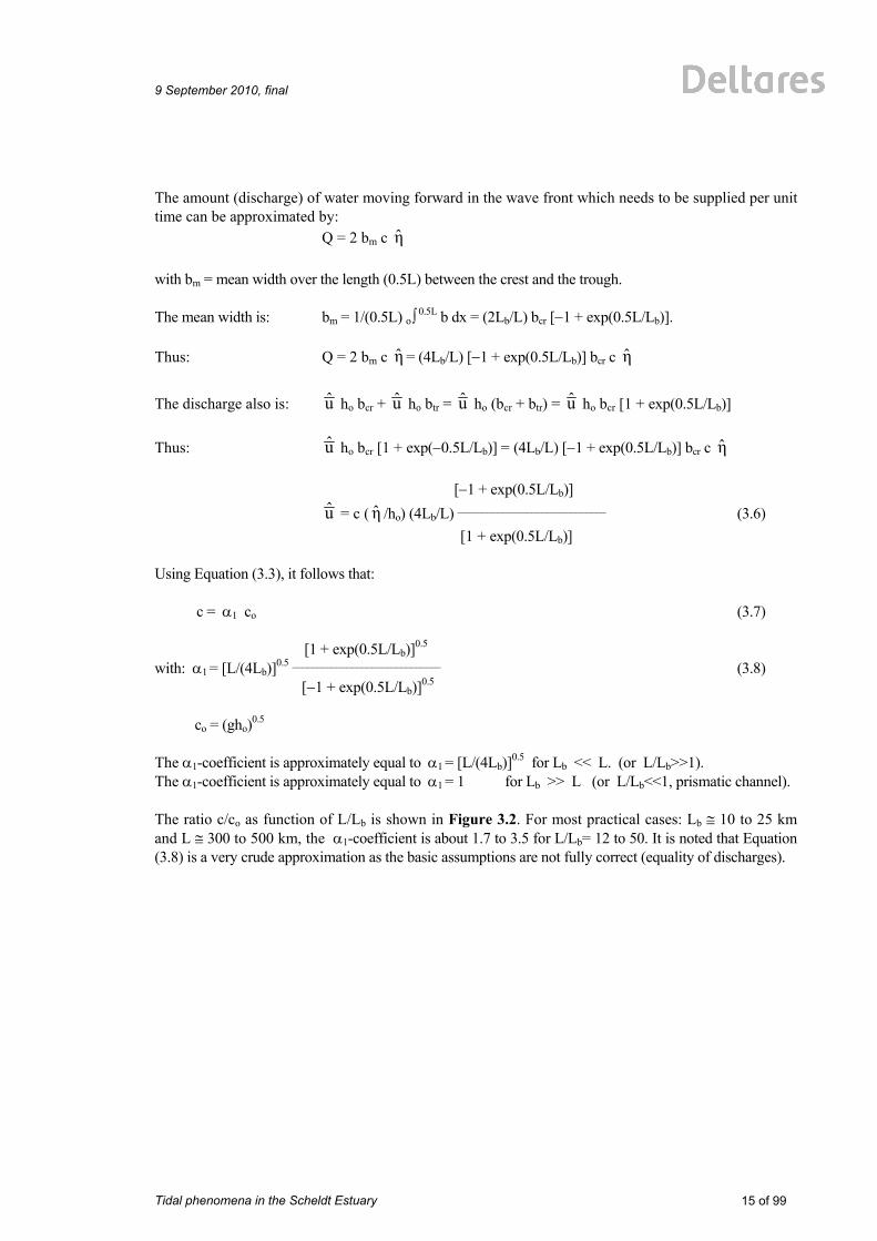
The amount (discharge) of water moving forward in the wave front which needs to be supplied per unit time can be approximated by: Q = 2 bm c η with bm = mean width over the length (0.5L) between the crest and the trough. The mean width is: bm = 1/(0.5L) o∫ 0.5L b dx = (2Lb/L) bcr [−1 + exp(0.5L/Lb)]. Thus: Q = 2 bm c η = (4Lb/L) [−1 + exp(0.5L/Lb)] bcr c η The discharge also is: u ho bcr + u ho btr = u ho (bcr + btr) = u ho bcr [1 + exp(0.5L/Lb)] Thus: u ho bcr [1 + exp(−0.5L/Lb)] = (4Lb/L) [−1 + exp(0.5L/Lb)] bcr c η [−1 + exp(0.5L/Lb)] u = c ( η /ho) (4Lb/L) ______________________________ (3.6) [1 + exp(0.5L/Lb)] Using Equation (3.3), it follows that: c = α1 co (3.7) [1 + exp(0.5L/Lb)]0.5 with: α1 = [L/(4Lb)]0.5 ______________________________ (3.8) [−1 + exp(0.5L/Lb)]0.5 co = (gho)0.5 The α1-coefficient is approximately equal to α1 = [L/(4Lb)]0.5 for Lb << L. (or L/Lb>>1). The α1-coefficient is approximately equal to α1 = 1 for Lb >> L (or L/Lb<<1, prismatic channel). The ratio c/co as function of L/Lb is shown in Figure 3.2. For most practical cases: Lb ≅ 10 to 25 km and L ≅ 300 to 500 km, the α1-coefficient is about 1.7 to 3.5 for L/Lb= 12 to 50. It is noted that Equation (3.8) is a very crude approximation as the basic assumptions are not fully correct (equality of discharges).

16 of 99
Tidal phenomena in the Scheldt Estuary
9 September 2010, final
02468
101214161820
0.1 1 10 100 1000
L/Lb
C/C
o
Figure 3.2 Ratio c/co as function of L/Lb Thus, the frictionless wave speed in a strongly converging estuary is strongly amplified. Wave speed data of the Scheldt Estuary yield c/co ≅ 1.2 to 1.6 (Savenije, 2005; see also Table 3.3). Equation (3.8) yields α1 ≅ 2 for the Scheldt Estuary using L ≅ 400 km and Lb ≅25 km, which is somewhat larger than measured values (as friction has been neglected to derive Equation 3.8). The tidal wave speed is reduced by bottom friction, which can be easily shown by analyzing Equation (3.34). Using scaling parameters, linear friction and neglecting the term u ∂ u /∂x, it follows that: u /T = g ( η /L) − m u (3.9) Using: u = ( η /ho) c, this can be re-arranged into: c = α2 (gho)0.5 (3.10) with: α2 = [1/(1 + m T)]0.5, m = friction coefficient (> 0) and T = tidal period. Since the α2-coefficient is always smaller than 1, the wave speed is reduced by bottom friction. In the case of a standing wave system the water surface moves up and down almost horizontally if the channel length is much smaller than the tidal wave length. Thus, HW occurs everywhere at the same time along the channel. This can be interpreted as an ‘apparent’ wave speed which is infinitely large.

9 September 2010, final
Tidal phenomena in the Scheldt Estuary
17 of 99
2. Tidal excursion The tidal excursion is the distance travelled by a fluid particle between the time of LWS and HWS (about 0.5T), and can be approximated as follows: Le = t-LWS∫
t-HWS u dt = 0∫0.5T u sin(ωt) dt = 2 u /ω = (1/π) u T (3.11) with: u = tidal fluid velocity, u = peak tidal velocity, tLWS, tHWS= time at low water slack (LWS) and high water slack (LWS), see Figure 3.3. The tidal excursion is of the order of Le =10 to 20 km, using u ≅ 1 m/s and T ≅ 12 hours (43200 s). 3. Flood volume The flood volume (approximately equal to the Tidal Prism) is the volume of water entering the estuary during the flood period) and reduces in landward direction. The tidal flood volume is defined as: Vf = b h t-LWS∫
t-HWS u dt = b h 0∫0.5T u sin(ωt) dt = (1/π) u b h T = Le b h = Q T/π (3.12)
5. Phase shifts between vertical and horizontal tide Bottom friction and channel geometry (shoaling) cause a phase shift between the horizontal tide (current velocities) and the vertical tide (water levels). A phase shift of 3 hours (≅ 90o) represents a standing wave pattern. In the Scheldt Estuary (The Netherlands) the horizontal tide reverses earlier (about 1 to 2.5 hours) than the vertical tide, as shown in Figure 3.3; see also De Kramer (2002). The time period with nearly zero current velocities is known as Slack Water. The vertical and horizontal tides can be represented as: η = η cos(ωt)
u = u cos(ωt + ϕ1) = u cos(ωt + 90o − ϕ2) with: u = peak tidal velocity (positive velocity is flood velocity), ϕ1 = phase lead (if ϕ1 < 0, then phase lag; horizontal tide reverses later); ϕ1 + ϕ2 = 90o; ϕ1 = 0o for a progressive wave, ϕ1 = 90o for a standing wave. Thus: ϕ1 = 0o: progressive tidal wave, ϕ1 = 90o: standing tidal wave (phase lead of 3 hours in semi-diurnal conditions), ϕ1 = 0o to 90o: mixed tidal wave.

18 of 99
Tidal phenomena in the Scheldt Estuary
9 September 2010, final
-2.5
-2
-1.5
-1
-0.5
0
0.5
1
1.5
2
2.5
0 10000 20000 30000 40000 50000 60000 70000
Time (s)
Wat
er le
vel (
m) a
nd v
eloc
ity (m
/s) Tidal water level
Tidal velocity
ϕ2 ϕ1
ϕ2 ϕ1
Figure 3.3 Phase shift between vertical and horizontal tide; flood velocity is positive (ϕ1 = 0o and ϕ2 = 90o
for progressive wave) (ϕ1 = 90o = 0.5π and ϕ2 = 0o
for standing wave) Tidal progressive waves mainly occur in relatively deep and long prismatic channels (no damping, shoaling and reflection). The classical formula of wave propagation velocity of a progressive wave in relatively deep water (H<<ho) is c = (gho)0.5. As long as H<<ho, this expression yields very reasonable values. Tidal data shows that the wave speed increases in amplified tidal channels (H>Ho) and decreases in damped tidal channels (H<Ho), see Savenije (2005) and Savenije et al. (2008). The wave speed of the tidal crest (HW = High Water) is larger than the wave speed of the tidal trough (LW = Low Water) due to differences of the water depth; cHW ≅ [g(ho+0.5H)]0.5 and cLW ≅ [g(ho−0.5H)]0.5 with H= tidal range. This leads to deformation of the tidal wave (crest moves faster than trough). The phase angle is defined with respect to the time moment of zero-crossing of the vertical tide. The phase difference between the vertical and horizontal tide can also be defined as the phase difference ϕ2 between HW (High Water of vertical tide) and HWS (High Water Slack of horizontal tide), which is a phase lag as the reversal of the horizontal tide (HWS) is later than reversal of the vertical tide (HW).

9 September 2010, final
Tidal phenomena in the Scheldt Estuary
19 of 99
Figure 3.4 Phase shift between near-bed and near-surface velocities at slack water There also is a phase shift between the near-bed and near-surface velocities (Figure 3.4). The near-bed velocities reverse earlier than the near-surface velocities, especially at Low Water Slack when the water depth is smallest and bottom friction is largest. This can be explained as follows. The near-bed velocities are smaller than the near-surface velocities due to bottom friction. The horizontal pressure gradient generated by the water level gradient (∂η/∂x term) is constant over the depth. As a result the lower horizontal fluid momentum near the bed can be earlier overcome by the pressure-gradient than the higher fluid momentum at the water surface. River discharge affects the duration of the flood and ebb phases of the tide. The flood phase and the flood velocities will be reduced and the ebb phase and the ebb velocities will be enhanced by increasing river discharges. The phase lead of the velocity with respect to the water level variation can be estimated from the tidal prism (Savenije, 2005). The flood volume is given by: Vf = bo ho t-LWS∫
t-HWS u o sinωt dt ≅ bo ho o∫0.5T u o sinωt dt = bo ho u o T/π = Q o T/π (3.13) The flood volume in a damped estuary (with exponentially reducing tidal range) can also be determined as: Vf = o∫∞ (b HLWS-HWS) dx = o∫
∞ Ho cosϕ1 exp(−μD x) bo exp(−β x ) dx = Ho bo cosϕ1 (μD+β)−1 (3.14) with: t-LWS= time of low water slack, t-HWS = time of high water slack., Ho = tidal range at x = 0, HLWS-HWS= Ho cosϕ1 exp(−μD x)= tidal range between times of low water slack and high water slack, ϕ1= phase lead of velocity with respect to water level elevation, μD= 1/Lw= damping coefficient (positive value), b= boexp(−β x) = width, bo= width at x=0, β = 1/Lb = convergence coefficient (positive value), x = horizontal coordinate (positive in landward direction), Lw= damping length scale. Based on Equations (3.13) and (3.14), it follows that: Ho bo cosϕ1 (μD+β)−1 = bo ho u o T/π (μD+β) cosϕ1 = ho u o T __________ (3.15) (π Ho)

20 of 99
Tidal phenomena in the Scheldt Estuary
9 September 2010, final
Thus, the phase lead increases with increasing damping coefficient (greater bottom friction) and increasing convergence (larger β or smaller Lb). Equation (3.15) is only valid for a damped estuary with a gradually reducing width (weakly converging estuary) and decreasing tidal range, which implies that Lb ≅ 100 km or larger (β < 0.00001). The damping length LW also is of the order of 100 km or larger (μD <0.00001). Using: Ho = 4 m, T = 40.000 s, ho = 10 m, u o = 1 m/s, it follows that: cosϕ1 = 50.000 (μD+β) < 1. Most often, cosϕ1 will be in the range of 0.5 to 1 or ϕ1 in the range of 60o to 90o or 2 to 3 hours for a semi-diurnal tidal period of 12 hours. 6. Stokes drift Due to the tidal variation of the water level, the net discharge over the tidal cycle is not zero. The velocity defined as u net = qnet/T is known as the Stokes drift: qstokes = (1/T) 0∫T q dt = (1/T) 0∫T ( u h) dt (3.16) Using: u = u cos(ωt+ϕ1) (symmetrical tide; ϕ1= phase lead, see Figure 3.3) and h = ho + η cosωt, it follows that: qstokes = (1/T) 0∫T { u cos(ωt+ϕ1)}{ho + η cosωt} dt
= ( u ho/T) 0∫T cos(ωt+ϕ1) dt + ( u η /T) 0∫T cosωt cos(ωt+ϕ1) dt
= ( u ho/T) 0∫T(cosωt cosϕ1 − sinωt sinϕ1)dt + ( u η /T) 0∫T{(cosωt)2cosϕ1 − sinωt cosωt sinϕ1}dt
= ( u ho/T)[cosϕ1 ∫cosωt dt−sinϕ1 ∫sinωt dt]+( u η /T)[cosϕ1 ∫(cosωt)2dt−0.5sinϕ1 ∫sin2ωt dt]
= ( u η /T) cosϕ1 0∫T(cosωt)2 dt The integrals 0∫
T cosωt dt, 0∫T sinωt dt and 0∫
T sin2ωt dt are zero as the functions are periodic over time T. Thus: qstokes = ( u η /T) cosϕ1 0∫T (cosωt)2 dt = ( u η /T) cosϕ1 (0.5T) = 0.5 u η cosϕ1
u stokes ≅ 0.5 ( η /ho) cosϕ1 u (3.17) The Stokes drift velocity is maximum for ϕ1 = 0 (no phase shift between horizontal and vertical tide) and zero for ϕ1= 90o (standing wave system). Generally, ϕ1 = 60o to 85o. Using: η /ho ≅ 0.2, cosϕ= 0.5 and u ≅ 1 m/s, resulting in: u stokes ≅ 0.05 m/s in landward direction. Since the Stokes drift leads to the accumulation of fluid within the estuary, the mean water level will gradually go up towards the landward end of the estuary resulting in a water level gradient by which a return flow is driven (vertical circulation). 7. Width of ideal converging estuary The width of an ideal estuary defined as an estuary with constant depth (ho = constant) and constant amplitudes of the vertical and horizontal tides ( η = constant and u = constant) can be determined from the flood volume (approximately equal to the tidal prism). The frictionless wave propagation velocity in an ideal estuary is co = (gho)0.5.
9 September 2010, final
Tidal phenomena in the Scheldt Estuary
21 of 99
Based on Equation (3.12), the flood volume (no river) can be expressed as: Vf = 2 Q /ω = 2 A u /ω The variation of the flood volume along the estuary is: dVf/dx = 2( u /ω) dA/dx = 2( u /ω) ho db/dx (3.18) with A= b ho and b = width (decreasing in landward direction; x is positive in landward direction). Also the increase/decrease of the tidal prism over length Δx is approximately equal to the product of the tidal range, the length Δx and the width b, as follows: ΔVf = 2 η b Δx or dVf/dx = −2 η b (3.19) Negative sign is introduced because volume decreases in positive x-direction. This yields: 2( u /ω) ho db/dx = −2 η b
(1/b) db/dx = −( η /ho) (ω/ u )
b= bo exp{−( η /ho) (ω/ u ) x} = bo exp(−x/Lb) (3.20) with: Lb = (ho/ η ) ( u /ω)= converging length scale
Using: η /ho = u /(co cosϕ) for a progressive wave in a tidal channel (see Table 3.2), it follows that: Lb = (co/ω) cosϕ = [cosϕ/(2π)] coT = [cosϕ/(2π)] Lwave,o ≅ 1/10 Lwave (3.21) Equation (3.21) represents the converging length scale (width reduction) at which the peak tidal velocity is constant along the estuary (depth also constant). This converging length scale parameter is governed by the ratio co/ω and the phase lead angle ϕ. The ϕ-value is about 1 to 2 hours or 30o to 60o and thus cosϕ ≅ 0.85 to 0.5, resulting in Lb ≅ 1/10 Lwave with Lwave = frictionless tidal wave length.
3.2 Analytical solution of energy flux equation for prismatic and converging channels The principle of tidal wave amplification defined as the increase of the wave height due to the funnel planform of the estuary (decreasing depth and width) can be easily understood by considering the wave energy flux, which is known as the law of Green (1837). This phenomenon is also known as wave shoaling or wave funneling. The total energy of a tidal wave per unit area is equal to E = 0.125ρg b H2 with b= width of channel, H = wave height. The claasical wave propagation velocity of a wave is given by: co= (gho)0.5 with ho= water depth. Assuming that there is no reflection and no loss of energy (due to bottom friction), the energy flux is constant resulting in: Eoco = Ex cx or Hx/Ho= (bx/bo)−0.5
(hx/ho)−0.25. Thus, the tidal wave height Hx increases for decreasing width and depth. The wave length L= co T will decrease as co will decrease for decreasing depth resulting in a shorter, but higher wave. The variation of the tidal range H in an estuary with exponentially decreasing width and depth can be derived by considering the energy flux involved. Assuming exponential reducing depth and width, it follows that: h = ho exp(−γx) , b = bo exp(−βx) with β = 1/Lb, γ= 1/Lh and x is positive in landward direction, bo = width at mouth x = 0, ho = depth at mouth.

22 of 99
Tidal phenomena in the Scheldt Estuary
9 September 2010, final
Waves transfer energy in horizontal direction during wave propagation. To be able to propagate itself, a wave must transfer energy to the fluid in rest in front of the wave. The rate at which energy is transferred from one section to another section is known as energy flux F. Basically, it is the time-averaged work done by the dynamic pressure force per unit time during a wave period. Wave energy is extracted from the system through the work done by the bed-shear stress (causing wave damping). It is realized that the representation of a tidal wave by a single progressive sinusoidal wave is a crude schematization of a real distorted tidal wave (including reflection) in an estuary. Therefore, this method only yields a first order description of the bulk parameters involved (tidal range H) for conditions without much reflection. The energy flux balance reads, as: d(b F )/dx + b Dw = 0 b d F /dx + Fdb/dx + b Dw = 0 (3.22) with: F = 0.125 ρ g H2 co = E co = energy flux through per unit width and per unit time and Dw = energy dissipation per unit area and time by the bed-shear stress, b = width of estuary channel, E = 0.125 ρ g H2
= energy of a wave per unit area, co = wave propagation velocity. The time-averaged work done by the bed-shear stress is (see Van Rijn, 2011): D w = 0.125 ρ f u 3 (2/T) o∫ 0.5T cos3(ωt) dt = 1/(6π) ρ f u 3
= 4/(3π) ρ (g/C2) u 3 (3.23) The width of the estuary channel is represented as: b = bo exp(−βx) = bo exp(−x/Lb) (3.24) and db/dx = −β bo exp(−βx)= −β b (3.25) with: bo = width at entrance x = 0, β = 1/Lb = convergence coefficient (width reduction coefficient), Lb = convergence length scale. The length scale Lb is of the order of 10 to 50 km for most estuaries. The energy flux balance Equation (3.22) can be expressed, as (see Van Rijn, 2011): f u 2 dH/dx = 0.5(β+γ) H − _____________________ (3.26) 3π g h cos(ϕ1) In a channel of constant depth (h= ho= constant and thus γ= 0) it follows that: u = (0.5H/ho) c cos(ϕ1) and c = (1+αc) co = (1+αc) (gho)0.5 for a real wave. This yields: f H γr (1+αc)2 cos(ϕ1) dH/dx = 0.5β H − _______________________________
= β H − μd H = (β − μd) H 12π ho
dH/dx = (0.5β − μd) H or H = Ho exp{(0.5β − μd)x} (3.27) with: x = horizontal distance (positive in landward direction), β = 1/Lb = convergence coefficient or amplification coefficient, μd = 1/Lw = f /(12π) γr (1+αc)2 (1/ho) cos(ϕ1) = damping coefficient,
9 September 2010, final
Tidal phenomena in the Scheldt Estuary
23 of 99
γr = H/ho = relative wave height (0.2 to 0.4), Lw = friction length scale parameter, Lb = convergence length scale parameter, Ho = tidal range value at entrance x = 0, ϕ1 = phase lead of horizontal tide with respect to vertical tide. αc = wave celerity coefficient (0.1 to 0.2 for amplified estuary);(−0.1 to −0.2 for damped estuary). Neglecting friction (f= 0), Equation (3.26) yields: dH/dx = 0.5(β+γ) H or H/Ho=exp[0.5(β+γ)x] Equation (3.27) is based on the assumption that γr = H/ho is approximately constant along the estuary. The αc-parameter represents the increase or decrease of the real wave speed with respect to the (classical) ideal wave speed co= (gho)0.5 in an amplified or damped estuary. The αc-parameter is about 0.1 to 0.2 for an amplified estuary, defined by Lb<(gho)0.5T/(4π) The αc-parameter is about −0.1 to −0.2 for a damped estuary, defined by Lb>(gho)0.5T/(4π) The αc parameter is zero for an ideal estuary where the tidal range is constant (αc= 0 and c = co) The β-coefficient represents the amplification (‘shoaling’) of tidal energy due to the width reduction in positive x-direction (landward). The μd-coefficient represents the damping of tidal energy due to bottom friction. If 0.5β = μd, the tidal range is constant (reduction due to friction is fully compensated by the amplification effect, which is often associated with an ‘ideal’ estuary), resulting in (αc= 0 and c = co): 6π ho Lb = ___________________ (3.28) f γr cos(ϕ1) Using: cos(ϕ1) = 0.2 to 0.8, f = 8g/C2= 0.02 to 0.05, γr = 0.2 to 0.4, the ‘ideal’ Lb-length scale parameter varies roughly in the range of Lb = 2000 ho to 10000 ho. A basic problem of Equations (3.26 and 3.27) is that the parameters ϕ1 and αc cannot be estimated with sufficient accuracy a priori. When data are available, they can be determined through calibration. Another option is to use the analytical solution results of the linearized equations (see Section 3.4). In the case of a compound channel (consisting of main channel and tidal flats), the depth ho should be replaced by the effective wave propagation depth heff = Ac/bs = (bc/bs) ho= αh ho resulting in: f H 2 c2 cos(ϕ1) dH/dx = 0.5β H − _________________________ (3.29) 12π g (αh ho)3 with: αh= (bc/bs)ho<1, bc= width of main channel, bs= total surface width, ho= depth of main channel.

24 of 99
Tidal phenomena in the Scheldt Estuary
9 September 2010, final
3.3 Analytical solution of tidal wave equations for prismatic channels 1. Schematization and basic equations In a prismatic channel with constant cross-section (depth and width are constant), the phase shift between the horizontal and the vertical tide (Figure 3.3) is caused by bottom friction. This can be illustrated by the analytical solution of the mass and momentum balance equations for a prismatic channel (cross-section is constant, bottom slope is constant, see Figure 3.5), see also Dronkers (1964), Hunt (1964), Ippen (1966), Verspuy (1985) and Dronkers (2005). The basic assumptions are:
• channel depth (ho) to MSL is assumed to be constant in space and time: (h = ho+ η); ho = constant (bottom of Figure 3.5 is assumed to be horizontal);
• convective acceleration ( u ∂ u /∂x = 0) is neglected; • linearized friction is used; • fluid density is constant; • river discharge (Qr) is constant; • x-coordinate is negative in landward direction and positive in seaward direction.
Mean Sea Level
ho
zb
η
z
-x horizontal datum
Qr
Sea
x = 0
+x
Figure 3.5 Tidal wave in a prismatic tidal channel ( constant width) Due to linearization of the friction term the solution can be represented by a sinusoidal function in time and space. Non-linear effects (higher harmonics) deforming the tidal wave profile are not included. It is remarked that only one (primary) tidal wave is included (M2-component). The equations of continuity and motion for depth-averaged flow are: b ∂η ∂Q ______ + ______ = 0 (3.30) ∂t ∂x 1 ∂Q g ∂η Q | Q| ________ + ________
+ ____________ = 0 (3.31) A ∂t ∂x C2 A2 R in which: A = b ho = area of cross-section, bs= b = surface width, ho = depth to MSL (mean sea level), R = hydraulic radius (≅ ho if b>>ho) and C = Chézy-coefficient (constant).

9 September 2010, final
Tidal phenomena in the Scheldt Estuary
25 of 99
An analytical solution can be derived when the friction term is linearized. The equation of motion becomes: 1 ∂Q g ∂ η _______ + _________ + n Q = 0 (3.32) A ∂t ∂x in which: n is a constant friction factor, n = (8g | Q |)/(3πC2A2R)= Lorentz-friction parameter (m–2s–1)
in the case Qr = 0, m = n A = (8g | Q |)/(3πC2AR)= Lorentz-friction parameter (1/s), Q = characteristic peak tidal discharge (average value over traject), C = Chézy-coefficient, R = hydraulic radius. Assuming a rectangular cross-section and the width and depth to be constant in space and time (b = constant, h ≅ ho = constant), Equations (3.30) and (3.31) can also be expressed as: ∂η ho ∂ u ______ + _________ = 0 (3.33) ∂t ∂x ∂ u g ∂η ______ + _______ + m u = 0 (3.34) ∂t ∂x in which: u = cross-section averaged velocity, u = amplitude of tidal current velocity, m = (8g | u |)/(3πC2R) = friction coefficient. In the case of a very wide channel (b>>ho): u ≅ u = depth-averaged velocity and R ≅ ho. In the case of a compound cross-section consisting of a main channel and tidal flats it may be assumed that the flow over the tidal flats is of minor importance and only contributes to the tidal storage. The discharge is conveyed through the main channel. This can to some extent be represented by using co= (g heff)0.5 with heff = Ac/bs = αh hc and αh = Ac/(bs hc) = (bc/bs) hc= (bc/bs) ho, Ac= area of main channel (= bc hc= bcho), hc = ho= depth of main channel, bc= width of main channel and bs= surface width. The transfer of momentum from the main flow to the flow over the tidal flats can be seen as additional drag exerted on the main flow (by shear stresses in the side planes between the main channel and the tidal flats). This effect can be included crudely by increasing the friction in the main channel. If the hydraulic radius (R) is used to compute the friction parameters (m and C) and the wave propagation depth (heff= R), the tidal wave propagation in a compound channel will be similar to that in a rectangular channel with the same cross-section A.

26 of 99
Tidal phenomena in the Scheldt Estuary
9 September 2010, final
2. Types of boundary conditions The various types of boundary conditions (in complex notation; index c) are presented in Table 3.1. Table 3.1 Types of boundary conditions
Boundary Case Entrance of channel x = 0 Exit of channel x = L I Channel of infinite length Open: η c,o = given (known Open: η c,L = 0,
Q c,L = 0 or Q c,L = Qriver II Channel of finite length Open: η c,o = given (known)
Q c,o = given (known)
Open: η c,L = unknown,
Q c,L = unknown III Channel closed at end Open: η c,o = given (known) Closed: Q c,L = 0 IV Channel between two large tidal basins
Open: η c,o = given (known) Open: η c,L = given
V Channel between large basin and lake with constant level
Open: η c,o = given (lnown) Open: η c,L = 0
3. Analytical solution The analytical solution with and without reflection is summarized in Table 3.2 (see Van Rijn, 2011). The solution for a prismatic channel can also be used for a converging channel by schematizing the converging channel into a series of prismatic channels (sections) with decreasing width, see Figure 3.6. The reflection at each transition in width has to be included. The computation proceeds from the seaward boundary to the landward boundary using complex variables. The computed variables (in complex notation) at the end of each section are the input variables at the entrance of the next section. This approach is known as the four-pole method (Verspuy, 1985; Van Rijn, 2011). The tidal water level and discharge and phases (phase lead of discharge with respect to water level) at the seaward boundary should be known.
Figure 3.6 Schematized converging tidal channel in series of prismatic channel sections

9 September 2010, final
Tidal phenomena in the Scheldt Estuary
27 of 99
Table 3.2 Analytical solutions for prismatic and converging channels (with and without reflection)
TYPE OF WAVE
PRISMATIC CHANNELS CONVERGING CHANNELS
Excluding reflection at landward end (channel open at end)
ηx,t = η o [e
−μx] [cos(ωt − kx)]
u x,t = u o [e −μx ] cos(ωt − kx+ϕ)
with: u o= − ( η o/ho) (ω/k) [cosϕ] μ = friction parameter k = wave number ϕ = phase lead x = horizontal coordinate; positive in landward direction
ηx,t = η o [e
−εx] [cos(ωt − kx)]
u x,t = u o [e −εx ] cos(ωt − kx+ϕ)
with: ε = −0.5β + μ u o= − ( η o/ho) (ω/k) [cosϕ] c = ω/k, tanϕ = sinϕ/cosϕ = (0.5β+μ)/k, sinϕ = (0.5β+μ)/[(0.5β+μ)2 + k2]0.5 cosϕ = (k)/[(0.5β+μ)2 + k2]0.5, μ = friction parameter (see Section 3.4) k = wave number (see Section 3.4) ϕ = phase lead (between hor. and vert. tide) β = 1/Lb = convergence parameter x = horizontal coordinate; positive in landward direction
Including reflection at landward end (channel closed at end)
ηx,t = 0.5 η o ( fA)–1 [e–μ(x–L)cos(ωt – k(x–L)) + eμ(x–L)cos(ωt + k(x–L))] u x,t= 0.5 ω ( η o/ho) (fA)–1 (k2+μ2)–0.5
[e–μ(x–L)cos(ωt – k(x–L) + ϕ) – eμ(x–L)cos(ωt + k(x–L) + ϕ)] with: fA = amplification/damping factor = = [cos2(kL) + sinh2(μL)]0.5
L = channel length x = horizontal coordinate; positive in landward direction
ηx,t = 0.5 η o ( fA)–1 [e(ε1)x+μLcos(ωt – k(x–L)) + e(ε2)x–μLcos(ωt + k(x–L))] u x,t=0.5ω( η o/ho)(fA)–1(k2+μ2)–0.5
[e(ε1)x+μLcos(ωt – k(x–L) + ϕ) – e(ε2)x–μLcos(ωt + k(x–L) + ϕ)]
with: ε1 = 0.5β − μ ε2 = 0.5β + μ fA = amplification/damping factor = = [cos2(kL) + sinh2(μL)]0.5
L = channel length; x = horizontal coordinate; positive in landward direction

28 of 99
Tidal phenomena in the Scheldt Estuary
9 September 2010, final
3.4 Analytical solution of tidal wave equations for converging channel 1. Schematization and basic equations An analytical solution of the mass and momentum balance equations can also be obtained for a converging (funnel type) channel (see Figure 3.1), if the channel width is represented by an exponential function (b = bo eβx), see also Hunt (1964), Mazumder and Bose (1995) and Prandle (2009). The basic assumptions are:
• bottom is assumed to be horizontal (Ib = 0); channel depth to MSL is assumed to be constant in space and time (h = ho+η); depth ho = constant;
• width is b = bo eβx with β=1/Lb= convergence coefficient, Lb = converging length scale, constant in time;
• convective acceleration ( u ∂ u /∂x = 0) is neglected; • linearized friction is used; • fluid density is constant; • x-coordinate is negative in landward direction and positive in seaward direction.
The equations of continuity and motion for depth-averaged flow are: b ∂η ∂Q ______ + ______ = 0 (3.35) ∂t ∂x 1 ∂Q g ∂η Q |Q| ________ + ________ + ____________ = 0 (3.36) A ∂t ∂x C2 A2 R in which: A = b ho = cross-section area, b = width, ho= depth to mean sea level, R = hydraulic radius and C = Chézy-coefficient are constants. An analytical solution can be found when the friction term is linearized, as follows: 1 ∂Q g ∂ η _______ + _________ + n Q = 0 (3.37) A ∂t ∂x in which: n is a constant friction factor, n = (8g | Q |)/(3πC2A2R). The mass balance equation can be expressed as (A = b h and h = ho+η ): b ∂η b ho ∂ u u b ∂η u ho ∂b ______ + ___________ + ___________ + ___________ = 0 (3.38) ∂t ∂x ∂x ∂x The gradient of the width is: ∂b/∂x = β bo eβx = β b. Neglecting the term u b ∂η/∂x, the mass balance equation becomes:
9 September 2010, final
Tidal phenomena in the Scheldt Estuary
29 of 99
b ∂η b ho ∂ u ______ + ___________ + u β b ho
= 0 (3.39) ∂t ∂x or ∂η ho ∂ u ______ + _________ + u β ho
= 0 (3.40) ∂t ∂x The momentum equation can be simplified to: ∂(bho u ) g ∂ η ______________ + _________ + n b ho u = 0 (3.41) b ho ∂t ∂x or ∂ u g ∂ η ______ + _________ + m u = 0 (3.42) ∂t ∂x with: u = cross-section-averaged velocity, m = nA = n b ho = (8g | u |)/(3πC2R) ≅ (8g | u |)/(3πC2ho) = Lorentz-friction parameter (dimension 1/s), u = characteristic peak velocity (average value over traject), C= Chézy = coefficient, R = hydraulic radius. In the case of a compound cross-section consisting of a main channel and tidal flats it may be assumed that the flow over the tidal flats is of minor importance and only contributes to the tidal storage. The discharge is conveyed through the main channel. This can to some extent be represented by using co= (g heff)0.5 with heff = Ac/bs = αh hc and αh = Ac/(bs hc) = (bc/bs) hc= (bc/bs) ho, Ac= area of main channel (= bc hc= bcho), hc = ho= depth of main channel, bc= width of main channel and bs= surface width. The transfer of momentum from the main flow to the flow over the tidal flats can be seen as additional drag exerted on the main flow (by shear stresses in the side planes between the main channel and the tidal flats). This effect can be included crudely by increasing the friction in the main channel. If the hydraulic radius (R) is used to compute the friction parameters (m and C) and the wave propagation depth (heff= R), the tidal wave propagation in a compound channel will be similar to that in a rectangular channel with the same cross-section A. 2. Analytical solutions The solution is given by Van Rijn (2011) and is summarized in Table 3.2. Three subcases (Case A, B and C) can be distinguished to determine the μ-parameter and the k-parameter, as follows: Case A: Amplitude of water level and velocity are constant (ideal estuary) β = 2 ω/co = 2 ko or 1/Lb = 2ko or Lb = Lwave,o/(4π) or (3.43) Lb = co/(2 ω) = (g ho)0.5T/(4π) = Lwave,o./(4π) Using: ho = 3 m and T = 43200 s, Lb ≅ 20.000 m (20 km) ho = 5 m and T = 43200 s, Lb ≅ 25.000 m (25 km) ho = 10 m and T = 43200 s, Lb ≅ 35.000 m (35 km) If Lb = Lwave,o/(4π), then μ = k = ko and the amplitudes of water level and velocity are constant (β = 2 k = 2μ).

30 of 99
Tidal phenomena in the Scheldt Estuary
9 September 2010, final
Case B: Amplification is dominant β ≥ 2 ω/co or Lb ≤ (g ho)0.5T/(4π) (3.44) k = 0.50.5 (ω/co) α0.5 [−1 + {1+ m2/(ω2α2)}0.5]0.5 with α = 0.25 β2 (co/ω)2 − 1 k = 0.50.5 (ko) α0.5 [−1 + {1+ m2/(ω2α2)}0.5]0.5 with α = 0.25 β2 (1/ko)2 − 1 and ko= ω/co μ = (m ω)/(2 co
2 ) (1/k) (positive damping parameter; eμx < 0 with x < 0) (3.45) μ can also be expressed as: μ = 0.50.5 (ω/co) α0.5 [1 + {1+ m2/(ω2α2)}0.5]0.5 The actual propagation velocity or phase velocity c can be expressed as: L ω co c = ____ = ____ = ___________________________ (3.46) T k (0.5α)0.5 (−1 + a2)0.5 with: a2 = [1+ m2/(ω2α2)]0.5 This latter expression yields a wave propagation velocity larger than that of a frictionless wave (c > co) in practical cases (similar to Equation 3.8), since (0.5α)0.5 (−1 + a2)0.5 < 1. Practical values: a2 ≅ 2 to 3. Tidal amplification is dominant in deep estuaries with strong width reduction (strong convergence). The tidal amplification is fairly linear, see Figures 4.4, 4.6, 4.7. In short estuaries a near-standing wave pattern can be generated with a phase lead close to 3 hours (relatively large ‘apparent’ wave speed). Observations in amplified estuaries also show that the real wave speed (c) is larger than the classical value (co = (gho)0.5). Table 3.3 shows observed wave speeds (mean of chigh-water and clow-water) in the Scheldt Estuary on 21 June 1995 (Savenije, 2005). The wave speed of high water is somewhat larger than that of low water. Table 3.3 Observed and classical wave speeds in Scheldt Estuary (Savenije, 2005)
Traject Scheldt Estuary
cobserved (m/s)
co (m/s)
0 to 20 km 15 8 to 10 20 to 40 km 15 8 to 10 40 to 60 km 15 8 to 10 60 to 80 km 13 8 to 10 80 to 100 km 11 8 to 10 100 to 120 km 11 8 to 10
Case C: Damping is dominant β ≤ 2 ω/co or Lb ≥ (g ho)0.5T/(4π) (3.47) k = 0.50.5 (ω/co) α0.5 [1 + {1+ m2/(ω2α2)}0.5]0.5 with α = 1 − 0.25 β2 (co/ω)2 k = 0.50.5 (ko) α0.5 [1 + {1+ m2/(ω2α2)}0.5]0.5 with α = 1 − 0.25 β2 (1/ko)2 and ko= ω/co μ = (m ω)/(2 co
2 ) (1/k) (positive damping parameter; eμx < 0 with x < 0) (3.48) μ can also be expressed as: μ = 0.50.5 (ω/co) α0.5 [−1 + {1+ m2/(ω2α2)}0.5]0.5
9 September 2010, final
Tidal phenomena in the Scheldt Estuary
31 of 99
The actual propagation velocity c is: L ω co c = ____ = ____ = _________________________ (3.49) T k (0.5α)0.5 (1 + a2)0.5 with: a2 = (1+ m2/(ω2α2))0.5 This latter expression yields a wave propagation velocity which is smaller than that of a frictionless wave (c < co) in practical cases, since (0.5α)0.5 (1 + a2)0.5 > 1. Practical values: a2 ≅ 1 to 5. Savenije(2005) shows measured wave speed data of a small and shallow estuary (Incomati) in Mozambique, where the measured wave speeds are much smaller than the frictionless values (co). Further inland (tidal river), the water depth generally decreases significantly resulting in a relatively rapid reduction of the tidal range due to dominant bottom friction. This effect cannot be represented by the proposed analytical method, which is based on a constant depth. However, the method can be used by schematizing the estuary and tidal river in a series of channels, each with its own width and depth characteristics. Summarizing, the variation of the tidal range H along an estuary can be, as follows:
• tidal range is constant H = Ho and c = co (ideal estuary; Case A); • tidal range increases H > Ho and c > co (amplified estuary; Case B); • tidal range decreases H < Ho and c < co (damped estuary; Case C).
with: H = tidal range, Ho = tidal range at entrance (mouth), c = wave propagation velcvocity (wave speed) and co = (gho)0.5. In Case B and Case C the β-parameter and the μ parameter are positive values. Hence, the phase lead ϕ is always positive and increases with increasing values of β and μ. Since β = 1/Lb, estuaries with a small value of Lb (5 to 10 km) have a relatively large phase lead of the velocity with respect to the water level. Tidal bores can be generated during springtide conditions in estuaries with a rapidly reducing width resulting in relatively strong amplification (unstable wave front). In a prismatic channel (β = 0 or Lb= ∞) the phase lead only depends on the friction parameter μ. The phase lead is 0 for μ = 0 (no friction). The tidal range H = 2 η is: H = Ho e(−0.5β + μ) x (3.50) which is similar to Equation (3.27). The β-parameter is the same, but the μ-parameter of Equation (3.50) (based on linear friction) is different from the μ-parameter of Equation (3.27), which is based on quadratic friction. In the Example Case of the Scheldt Estuary the μ-parameter is about 0.000016 and β = 0.00004, giving H/Ho=exp{(-0.00002+0.000016)(-100.000)}= 1.5 after 100 km, which is somewhat larger than the observed data, see Table 4.3.

32 of 99
Tidal phenomena in the Scheldt Estuary
9 September 2010, final
In an ideal estuary, the tidal range H remains constant and the wave speed c is equal to co= (gho)0.5. Basically, the shoaling process (increase of potential energy) is balanced by the damping process (energy dissipation by friction). Based on Equation (3.50), the tidal range H remains constant, if: −0.5β + μ = 0 or β = 2 μ or Lb = 1/(2μ), with 2μ = (2 m ω)/(2 k co
2 ) = m c/co2
1 co
2 Lb = ______ = _______ 2μ m c Using: m = (8g | u |)/(3πC2ho) = f | u |)/(3πho) = Lorentz-friction parameter; u o= (0.5H/ho) c cos(ϕ1) and c = (1+αc) co for a real wave, it follows that (ϕ = ϕ1, see Figure 3.3): 1 co
2 co 3π ho co 6π ho co Lb = ______ = ______ = _____________ = _________________ = __________________________________ 2μ m c m (1+αc) f | u | (1+αc) f (H/ho) c cos(ϕ1) (1+αc) 6π ho 6π ho Lb = ____________________________ = ___________________ (3.51) f γr (1+αc)2 cos(ϕ1) f γr cos(ϕ1) Since μ = k for an ideal estuary, it is also valid that: Lb = 1/(2k) = Lwave/(4π) (3.52) In an ideal estuary with constant tidal range, the wave propagation speed is equal the the classical value (c = co) and thus αc = 0.

9 September 2010, final
Tidal phenomena in the Scheldt Estuary
33 of 99
0.1
1
10
100
1000 10000 100000
Dimensionless width scale (Lb/ho)
Beta
/(2u)
, c/c
o an
d Ph
i
Beta/(2u) for h = 10 mc/co for h = 10 mPhase lead Phi (hours) for h = 10 mBeta/(2u) for h = 5 mc/co for h = 5 mPhase lead Phi (hours) for h = 5 m
Amplification Damping
Figure 3.7 Amplification and damping in an estuary with exponential width 3. Practical examples The analytical solution has been used (spreadsheet model TIDAL MOTION.xls) to plot the ratio of β/(2μ), c/co and phi (in hours) as a function of the parameter Lb/ho. Figure 3.7 shows the results for a depth of ho = 10 m and ho = 5 m. The ratio η o/ho = 0.2. The width at the mouth is bo = 25 km. The ks-value is ks = 0.03 m (Scheldt Case). An ideal estuary with a constant tidal range is present for β/(2μ) = 1. Larger values of β/(2μ) for a strongly converging estuary yield an amplified estuary and smaller values of β/(2μ) lead to a damped estuary. The ratio of the wave speed (c) and the frictionless wave speed (co) is in the range of 10 for a strongly converging estuary to 0.8 for a weakly converging estuary. The wave speed is always larger than the classical wave speed in the case of amplification. The phase lead is about 3 hours in a stronly converging estuary and about 1 hour in a weakly converging estuary. The analytical model for a converging tidal channel has been applied to various cases showing very reasonable results (Van Rijn, 2011): Scheldt Estuary (The Netherlands), Hooghly Estuary (India), Delaware Estuary (USA) and the Yangtze Estuary (China).

34 of 99
Tidal phenomena in the Scheldt Estuary
9 September 2010, final
3.5 Numerical solution of tidal wave equations for converging channels The most universal solution of the tidal wave equations including non-linear terms and reflection can only be obtained by using numerical models, using either a 1D cross-section-averaged approach or a 2DH depth-averaged approach. Herein, the results of the DELFT1D-model (SOBEK) and the DELFT2DH-model of Deltares/Delft Hydraulics are presented for various schematized cases with boundary conditions as present in the Scheldt Estuary (The Netherlands), see Chapter 4. The water levels are computed in the nodal points and the velocities (discharges) in the reaches between the nodes. The results are compared with those of the Analytical models (spreadsheet TIDAL MOTION.xls). The results show that Analytical models can be used to obtain information of the basic trends of the solutions, but these models cannot deal very well with reflections in the most landward section of the estuary. Due to the effects of linearisation, the application of the analytical models for most practical cases requires iterative computations to estimate the velocity amplitude or schematization of the channel into relatively small subsections. This later approach is laborious and offers no real advantage with respect to numerical models, which also contain the non-linear terms (so more physics). One-dimensional numerical models including all non-linear terms can be setup easily and quickly.

9 September 2010, final
Tidal phenomena in the Scheldt Estuary
35 of 99
4 Computational examples for schematized Scheldt Estuary
4.1 Tidal data of Scheldt Estuary The Scheldt Estuary in the south-west part of the Netherlands and in the north-west part of Belgium (see Figure 4.1) is connected to the Scheldt river, which originates in the north-west of France. The total length of the Scheldt river including the estuary is about 350 km; the tide penetrates up to the city of Gent in Belgium (about 180 km from the mouth). The length of the estuary is about 60 km (up to Bath). The cross-sections of the estuary show two to three deeper channels with shoals in between and tidal flats close to the banks. The width of the mouth at Westkapelle (The Netherlands) is about 25 km and gradually decreases to about 0.8 km at Antwerp, see Table 4.1. The width-averaged water depth (ho) to MSL at mouth between Vlissingen and Hansweert is about 12 m. The width-averaged water depth (ho) to MSL between Hansweert and Bath is about 11 m. The bottom is almost horizontal up to x = 80 km from the mouth. Since 1900, the main shipping channel has been deepened (by dredging and dumping activities) various times affecting the tidal range along the estuary. The tidal range at the mouth (Westkapelle and Vlissingen) has been approximately constant over the last century, but the the tidal range inside the estuary has gone up by about 0.5 to 1 m due to various channel deepenings (Pieters, 2002), see Table 4.2. Particularly, the high water levels have gone up considerably. The low water levels have gone down slightly at some locations (about 0.2 m at Antwerp) despite sea level rise of about 0.2 m per century. A detailed description of the historical developments is given by Pieters (2002). Table 4.1 Tidal data (spring tide) of Scheldt Estuary in period 2000 to 2010
Stations Distance x (km)
Width b (km)
Tidal range H (m)
H/Ho (measured)
Westkapelle (mouth) 0 25 4.2 (= Ho) 1 Vlissingen 12 6 4.5 1.07 Terneuzen 30 6 4.8 1.14 Hansweert 45 6 5.0 1.19 Bath 63 3 5.5 1.31 Antwerpen 95 0.8 5.85 1.39 Rupelmonde 110 <0.5 5.95 1.42 Temse 115 <0.5 5.85 1.39 Dendermonde 130 <0.5 4.2 1.0 Gent 160 <0.5 2.34 0.55

36 of 99
Tidal phenomena in the Scheldt Estuary
9 September 2010, final
Table 4.2 Tidal data of Scheldt Estuary in 1900 and 2010
Location 1900 2010 LW
(m to NAP) HW (m to NAP)
Tidal range(m)
LW (m to NAP)
HW (m to NAP)
Tidal range (m)
Vlissingen − 1.9 + 1.7 3.6 − 1.8 + 2.0 3.8 Bath − 2.3 + 2.2 4.5 − 2.2 + 2.8 5.0 Antwerpen − 2.1 + 2.3 4.4 − 2.3 + 3.0 5.3
Figure 4.1 Scheldt Estuary, The Netherlands The tide is semi-diurnal with a tidal range (Ho) at the mouth (Westkapelle) varying in the range of 2.4 m at neap tide to 4.2 m at spring tide. The maximum peak tidal velocity at mouth ( u o ) varies in the range of 0.8 to 1.2 m/s. The two most important tidal constituents are the M2 and the S2-components. The tidal curve at the mouth (Westkapelle) has a very regular (almost sinusoidal) pattern, see Figure 4.2. The tidal range increases in landward direction up to Rupelmunde (upstream of Antwerp), see Table 4.1, and decreases from there in landward direction. The discharge of the Scheldt river varies in the range of 50 to 200 m3/s. Given the relatively small river discharge, the estuary is a well-mixed flow system with a constant fluid density over the water depth. Measured tidal data during spring tide at various stations in the Scheldt Estuary are shown in Table 4.1 (based on De Kramer, 2002) and in Figure 4.2.

9 September 2010, final
Tidal phenomena in the Scheldt Estuary
37 of 99
Figure 4.2 Vertical tide (meters to mean level) at three stations in Scheldt Estuary, The
Netherlands
4.2 Computed and measured tidal range for Scheldt Estuary
4.2.1 Case definitions Various analytical and numerical solution methods have been used to compute the tidal parameters in prismatic and converging tidal channels, see Annex A and B. To study the effects of channel depth, length and channel planform, the following cases are defined (see also Figure 4.3): CASE 1: Converging width over 60 km (width bo = 25000 m, bL=60 km= 2000 m), depth h= 10 m, ks= 0.05 m CASE 3: Converging width over 60 km (width bo = 25000 m, bL=60 km= 2000 m), depth h= 5 m, ks= 0.05 m CASE 2: Converging width over 60 km (width bo = 25000 m, bL=60 km= 2000 m) Constant width (prismatic) over 60 tot 180 km (b= 2000 m), depth h= 10 m, ks= 0.05 m CASE 4: Converging width over 60 km (width bo = 25000 m, bL=60 km= 2000 m) Constant width (prismatic) over 60 tot 180 km (b= 2000 m), depth h= 5 m, ks= 0.05 m CASE 5: Converging width over 180 km (width bo = 25000 m, bL=180 km= 19 m), depth h= 10 m, ks= 0.05 m CASE 6: Converging width over 180 km (width bo = 25000 m, bL=180 km= 19 m), depth h= 5 m, ks= 0.05 m with: bo= width at mouth, bL= width at end of channel, Lb= converging width length scale = 25000 m. Similar cases have been used for fully prismatic channels.

38 of 99
Tidal phenomena in the Scheldt Estuary
9 September 2010, final
The boundary conditions are: Mouth (x= 0): water level amplitude: η = η cos(ωt) with η = 2.1 m and ω = 2π/T, T = 12 hours, water level variation is represented by hourly values, Closed end (x = L): discharge Q = 0 m3/s The water depth is defined as the depth to mean sea level (MSL); tidal levels are defined to MSL. Figure 4.3 Width of converging channel (CASES 1 to 6)
-15
-10
-5
0
5
10
15
0 10 20 30 40 50 60 70 80 90 100 110 120 130 140 150 160 170 180
Distance (km)
Wid
th (k
m)
CASE 2 and 4
-15
-10
-5
0
5
10
15
0 10 20 30 40 50 60Distance (km)
Wid
th (k
m)
CASE 1 and 3
-15
-10
-5
0
5
10
15
0 10 20 30 40 50 60 70 80 90 100 110 120 130 140 150 160 170 180
Distance (km)
Wid
th (k
m)
CASE 5 and 6

9 September 2010, final
Tidal phenomena in the Scheldt Estuary
39 of 99
4.2.2 Comparison of measured and computed tidal range Energy-flux method The most simple method to compute the tidal range along the Scheldt Estuary is the energy-flux method, see Equations 3.22 to 3.27. The estuary can be represented by an exponential decreasing width b=bo exp(−x/Lb). The convergence length scale parameter Lb is of the order of 25 km and β = 1/Lb=1/25000 ≅ 0.00004 (giving widths of 7.5 km, 2.5 km and 1 km at Terneuzen, Bath and Antwerpen) in agreement with measured data (see Table 4.1). The bed roughness is taken as ks = 0.05 m resulting in C ≅ 60 m0.5/s or f = 0.0218. The water depth is ho= 10 m (Case 1). The damping parameter is approximately μd = 0.0000175 using a phase shift value of ϕ1= 60o and thus cosϕ1 = 0.5 (ϕ1 ≅ 60o ≅ 2 hours; T= 12 hours). The damping parameter is μd = 0.0000148 for a phase shift value of ϕ1= 65o. Thus: 0.5β > μd or amplification is dominant with respect to damping resulting in an increase of the tidal range. The tidal range at the mouth is set to 4.2 m. The relative tidal range at the mouth is about 0.42 (water depth=10 m; γr = 0.42). The wave speed is set to c= 1.2 co with co= (gho)0.5, αc= 0.2. Using μd = 0.0000175 it follows that: H/Ho = exp{(0.00002 − 0.0000175)x} or H/Ho = 1.28 after 100 km (=100,000 m), which is fairly close to measured values (H/Ho ≅ 1.3 , see Table 4.3). Computed values are shown in Table 4.3 (last column) for ϕ1= 60o and ϕ1= 65o. Equation (3.8) can also be used to estimate the (frictionless) wave speed. Using L ≅ 400 km, the frictionless wave speed is c ≅ 2co. To obtain H/Ho ≅1.3, the ϕ1 needs to be about 80o. The measured tidal data at various stations along the estuary (Table 4.3) show an amplification factor of the tide of about 1.4 for springtide between the Station West Kapelle (mouth x = 0) and Station Antwerpen, which is close to the amplification factors produced by Equation (3.27). This is a very encouraging result given the rather crude schematization to arrive at Equation (3.27). The amplification is rather sensitive to the ϕ1-parameter. It is noted that the parameters of the μd-expression cannot be predicted with great accuracy a priori. In this example most parameters are known from the measured data and both the C-value and the ϕ1-parameter have been used to obtain a good fit with the observed amplification (calibration). Table 4.3 Tidal data (spring tide) of Scheldt Estuary in period 2000 to 2010
Stations Distance x (km)
Width b (km)
Tidal range H (m)
H/Ho (measured)
H/Ho (computed) ϕ1=60o ϕ1=65o
Westkapelle (mouth) 0 25 4.2 (= Ho) 1 1 1 Vlissingen 12 6 4.5 1.07 1.03 1.06 Terneuzen 30 6 4.8 1.14 1.08 1.17 Hansweert 45 6 5.0 1.19 1.12 1.26 Bath 63 3 5.5 1.31 1.17 1.39 Antwerpen 95 0.8 5.85 1.39 1.27 1.64 Rupelmonde 110 <0.5 5.95 1.42 1.32 1.77 Temse 115 <0.5 5.85 1.39 Dendermonde 130 <0.5 4.2 1.0 Gent 160 <0.5 2.34 0.55

40 of 99
Tidal phenomena in the Scheldt Estuary
9 September 2010, final
0
1
2
3
4
5
6
7
0 10 20 30 40 50 60 70 80 90 100Distance from mouth (km)
Tida
l ran
ge (m
)
observed tidal rangecomputed ks=0.01 mcomputed ks=0.05 m
West-Kapelle
Vlissingen
TerneuzenHansweert Bath
Antwerpen
Figure 4.4 Observed and computed tidal range values along Scheldt Estuary; energy flux method Figure 4.4 shows the computed tidal range values along the Scheldt Estuary based on the energy-flux method for two bed roughness values. The computed peak tidal velocity u (≅ 0.8 m/s) and the phase shift angle ϕ1 (≅79o) are now taken from the linearized solution (Section 3.4). Observed tidal range values are also shown. The observed tidal range values at stations Bath and Antwerpen show the effect of reflection (additional increase of tidal range). The computed values are too small at the end of the Estuary as reflection is not included. Linearized analytical method and numerical methods Figures 4.5 to 4.7 show the tidal range along the estuary based on the linearized solution for an exponential decreasing width (converging estuary channel; Case 1 with water depth of ho= 10 m). Numerical values (1D) are also shown. The river discharge has been neglected. Three bottom roughness values have been used: ks = 0.03, 0.05 and 0.1 m. The computed characteristic parameters for ks = 0.03 m are: ω = 0.00014 (1/s), m = 0.000158 (1/s), co= 9.9 m/s, c = 19.6 m/s (c ≅ 2co), k = 7.11 10−6 (1/m), μ = 1.59 10−5 (1/m) and ϕ = 2.74 hours. The analytical results (without reflection) show that the computed tidal amplification is in close agreement (within 10%) with the observed values for a roughness value of ks = 0.03 to 0.05 m. The computed wave speed is about 19 to 17 m/s for these roughness values, which is somewhat larger than the measured data (see Table 3.3 and 4.4). The analytical solution yields a phase lead of about 2.7 hours, which is somewhat larger than the observed value of about 2 hours. The peak tidal velocities at the mouth are in the range of −0.75 to −0.85 m/s. The tidal amplification is somewhat too small for larger ks-values. Figure 4.5 shows the tidal water level and velocity variation at x = 50 km and at the mouth (x = 0) for ks = 0.03 m. The negative flood velocity is plotted as a positive value. The phase shift of HW is about 1 hour over 50 km. The peak flood velocity at x = 50 km is about 2.7 hours before the time of HW at x = 50 km. Figure 4.6 shows the width of the estuary and the computed amplitudes of the water level and the velocity along the estuary (based on ks = 0.05 m). The computed water level amplitudes based on the analytical method for converging channels are in close agreement (within 5%) with the observed values.

9 September 2010, final
Tidal phenomena in the Scheldt Estuary
41 of 99
Figure 4.7 shows the measured and computed tidal range along the estuary based on ks-values in the range of 0.03 to 0.1 m and Lb= in the range of 20 to 30 km. The computed values (without reflection; open end at Antwerp) are in good agreement (within 10%) with the observed values. The results of the 1D numerical model (with and without reflection; closed and and open end) are also shown. The numerical results with reflection are based on a closed channel at Antwerp (x= 95 km).The numerical results without reflection are based on an open end at Antwerp by extending the channel (from Antwerp at 95 km) to about 180 km. The width at the end of the (closed) channel is set to 100 m. The numerical model results show that reflection yields an important contribution in the landward half of the Scheldt Estuary. This is in agreement with the analytical results of Pieters (2002) based on the classical four-pole equations taking reflection into account. Dronkers (2005) also is of the opinion that wave reflection plays an important role in the Scheldt Estuary. It is not unreasonable to explain the tidal amplification by the presence of wave reflection given the geometry of the Scheldt Estuary with many bends and the relatively wide landward end of the estuary, where the relatively small Scheldt river enters the system. Compared with the numerical results for a converging channel without reflection (open end channel), the analytical model based on linearized equations without reflection yields values which are substantially too large in the landward half of the estuary (see Figure 4.7). The analytical model including reflection produces values which are much too large (see Figure B7). Table 4.4 Measured and computed tidal data (spring tide) of Scheldt Estuary based on analytical linearized method for a converging channel
Stations Distance x (km)
Width b (m)
Observed Tidal range H (m)
Computed Tidal range H (m) ks = 0.03 m C = 65 m0.5/s
Computed Tidal range H (m) ks = 0.05 m C = 61 m0.5/s
Computed Tidal range H (m) ks = 0.1 m C = 55 m0.5/s
West Kapelle (mouth)
0 25000 4.2 (= Ho) 4.20 4.20 4.20
Vlissingen 12 15500 4.5 4.40 4.38 4.36 Terneuzen 30 7500 4.8 4.75 4.70 4.64 Hansweert 45 4100 5.0 5.04 4.96 4.88 Bath 63 2000 5.5 5.50 5.32 5.19 Antwerpen 95 550 5.85 6.20 6.00 5.76 c= 19.6 m/s
(wave speed) c= 17.7 m/s c= 16.1 m/s
ϕ = 2.74 hrs (phase lead)
ϕ = 2.70 hrs ϕ = 2.66 hrs

42 of 99
Tidal phenomena in the Scheldt Estuary
9 September 2010, final
-3
-2
-1
0
1
2
3
0 1 2 3 4 5 6 7 8 9 10 11 12 13 14 15
time (hours)
Wat
er le
vel (
m) a
nd c
urre
nt v
eloc
ity (m
/s)
Water level at location xcurrent velocity at location xWater level at mouth (x=0)Current velocity at mouth (x=0)
Flood water level is positiveFlood velocity (negative) is plotted as positive value
Ebb
Figure 4.5 Water level and velocity at x = 50 km and at x = 0 m for ks= 0.03 m, Scheldt Estuary Figure 4.6 Width, water level amplitude and velocity amplitude along estuary, Western Scheldt Figure 4.6 Water level amplitude and velocity amplitude along estuary, Scheldt Estuary
-2-1.5
-1-0.5
00.5
11.5
22.5
33.5
44.5
5
-70000 -60000 -50000 -40000 -30000 -20000 -10000 0
Distance (m)
Wat
er le
vel a
mpl
itude
(m) a
nd
velo
city
am
plitu
de (m
/s)
0
4000
8000
12000
16000
20000
24000
28000
32000
Wid
th (m
)
Water level amplitude (based on ks= 0.05 m)Velocity amplitude (negative= flood)Observed water level amplitudeWidth b
Bath HansweertTerneuzen Vlissingen

9 September 2010, final
Tidal phenomena in the Scheldt Estuary
43 of 99
0
1
2
3
4
5
6
7
0 10 20 30 40 50 60 70 80 90 100Distance from mouth (km)
Tida
l ran
ge (m
)
observed tidal rangeanalytical; ks= 0.03 m; Lb= 25 km (excl. reflection)Analytical; ks= 0.05 m; Lb= 25 km (excl. reflection)Analytical; ks= 0.1 m; Lb= 25 km (excl. reflection)Analytical; ks= 0.05 m; Lb= 20 km (excl. reflection)Analytical; ks= 0.05 m; Lb= 30 km (excl. reflection)1D numerical model including reflection (ks=0.05 m)1D numerical model excluding reflection (ks=0.05 m)
West-Kapelle
Vlissingen
TerneuzenHansweert Bath
Antwerpen
Figure 4.7 Tidal range along estuary for different ks- and Lb-values, Scheldt Estuary Analytical four-pole method The tidal flow in the Scheldt Estuary can also be simulated by using the four-pole equations (see Section 3.3), which are based on a combination of the incoming wave and the reflected wave. The estuary is schematized into eight sections, each of constant width and depth, see Table 4.5. The water level and discharge at the end of each section are used as boundary conditions at the entrance of the next section. The bed roughness is assumed to be ks = 0.05 m resulting in a Chézy-coefficient of about 60 m0.5/s. The peak tidal flood velocity at the mouth is assumed to be about 0.6 m/s resulting in a discharge of about 135000 m3/s. The phase lead of the discharge with respect to the water level is assumed to be in the range of 60o (2 hours) to 85o (2.95 hours). The best results are obtained for a phase shift of 85o. The results are presented in Table 4.5 and in Figure 4.8. The computed μ-coefficient varies between 0.00000583 (based on Q = 125000 m3/s) in section 1 and 0.0000072 (based on Q = 25000 m3/s) in section 8; the k-coefficient varies between 0.0000153 and 0.0000158. The amplitude of the reflected wave at x = 0 m (at the mouth Westkapelle) is about 0.92 m and the amplitude of the incoming wave is about 1.35 m for a phase shift of 85o. The computation goes from section to section in landward direction. In each new section a new incoming and reflected wave is computed based on the section parameters. Figure 4.8 shows the computed amplitudes of the water level and the discharge. Measured water level amplitudes are also shown. Computed values are in good agreement with measured values for a phase lead of ϕ = 85o. The largest discrepancy is about 10%. Sensitivity computations show that amplification of the tidal wave in landward direction does only occur for phase lead values (discharge at x = 0 m) larger than about 70o, see Figure 4.8. The water levels in the landward end section of the estuary are only realistic for a phase lead of about 85o. To obtain a realistic solution with amplification (as measured), the reflected wave is of prime importance. This is in strong contrast with the analytical solution method for a converging estuary which only represents the incoming wave (without reflection), see Section 3.4. This method was also employed by Pieters (2002). His results also show a reflected wave of about 1 m, which is approximately constant along the estuary. The phase shift between the incoming and reflected wave is about 65o at the mouth decreasing to about 30o at the end of the estuary. The phase difference at the mouth of the estuary was assumed to be 70o.

44 of 99
Tidal phenomena in the Scheldt Estuary
9 September 2010, final
The major drawback of this method is that the convergence (shoaling) process within each prismatic channel section is neglected. The tide will be damped exponentially due to bottom friction along the section length. To correct for the absence of convergence, an apparent reflected wave has to be introduced. So channel convergence is replaced by wave reflection at each transition in channel section. Another deficiency is that the phase lead between the vertical and the horizontal tide is not part of the solution, but has to be known (input value) from measured data, otherwise no solution is possible. Pieters (2002; see page 65 of his report) also has fitted this value to get the best overall results along the estuary. Figure 4.8 shows that the results are very sensitive to this phase shift. Finally, the method is not really predictive as the phase shift between the vertical and horizontal tide is unknown for future scenarios with changed channel characteristics (channel depth and width changes).
0
0.5
1
1.5
2
2.5
3
0 10 20 30 40 50 60 70
Distance from mouth (km)
Wat
er le
vel t
o M
SL
(m)
0
25000
50000
75000
100000
125000
150000
Dis
char
ge (m
3/s)
Water level amplitude (Phi=85)Water level amplitude (Phi=70)Water level amplitude (Phi=60)Measured water level amplitude Discharge amplitude (Phi=85)Discharge amplitude (Phi=70)Discharge amplitude (Phi=60)
Figure 4.8 Water level and discharge amplitudes (spring tide) in Scheldt Estuary
based on four-pole method Table 4.5 Computed tidal data (spring tide) of Scheldt Estuary based on four-pole method
Para meters
Section 1 (mouth)
2 3 4 5 6 7 Section 8 (end)
Width (m) 22500 19500 16500 13500 10500 7500 5000 3500 Depth (m) 10 10 10 10 10 10 10 10 Length (m) 2000 2000 2000 2000 2000 2000 25000 25000 Roughness (m) 0.05 0.05 0.05 0.05 0.05 0.05 0.05 0.05 Water level (m) and phase at entrance of section
2.1 0o
2.115 0.4
2.13 0.1
2.146 0.5
2.163 0.2
2.183 0.7
2.205 1
2.64 18o
Discharge (m3/s) at entrance of esection
135000 (0.6 m/s)
121800 110300 100500 92400 86000 81700 40000 (1.27 m/s)
Phase lead of discharge at entrance of section
85o
84.5 83.9 83.3 82.7 82.2 81.8 83.7o
Water level (m) andphase at end of section
2.115 0.4o
2.13 0.1
2.146 0.5
2.163 0.2
2.183 0.7
2.205 1
2.641 18
2.70 9o
Discharge (m3/s) and phase at end of section
122000 84.5o
110300 83.9
100500 83.3
92400 82.7
86000 82.2
81700 81.8
40000 83.7
25000 35o

9 September 2010, final
Tidal phenomena in the Scheldt Estuary
45 of 99
4.3 Effect of water depth on tidal range Figure 4.9 shows the ratio of the tidal range (Hx=60km/Ho) at x = 60 km and at the entrance x = 0 as a function of the water depth (in the range of 5 to 20 m) based on the energy-flux equation (3.26) and various other methods. The results of the analytical methods are all for a channel with an open end (no reflection). The analytical wave speed c and the phase angle ϕ1 are taken from the expressions of Table 3.2, which are valid for a converging channel. The analytical results based on the linearized model valid for a converging channel, are also shown. The phase angle ϕ1 (see Table 3.2) is also shown. Tidal damping due to bottom friction (ks = 0.05 m) dominates for water depths smaller than about 7 m resulting in a ratio (Hx=60km/Ho) smaller than 1. The tidal range shows amplification (>1) for water depths larger than about 7 m. Thus, increasing the water depth by dredging leads to a larger tidal range along the estuary. The maximum amplification based on the analytical solution of the linearized momentum eqution is about 1.3 at a water depth of about 11 m. A further increase of the depth does not lead to larger amplification values. The maximum amplification based on the energy-flux equation (3.26) is somewhat smaller (1.2) than that based on the linearized mass and momentum balance equations. The phase shift angle ϕ1 gradually increases from 60o at a depth of 5 m to about 90o at a depth of 20 m. The results of the Savenije-expressions (2005) are also shown using the same values of ϕ1 and c (from linearized equations). The results of the numerical DELFT1D-model (see Figure 4.3; Case 1) taking all terms into account are also shown, both for a channel (rectangular cross-section) with a closed end (with reflection) and an open end (no reflection). The results of the numerical model show a significant effect of reflection at the channel end. The numerical results for a channel with an open end have been estimated from the computed water levels at x= 45 km and x= 60 km from Case 2 (see Figure 4.3; converging channel connected to a prismatic channel) and are, therefore, somewhat uncertain. The tidal range ratio is somewhat smaller (about 20%) for a channel with an open end and water depths smaller than 15 m. Compared with the numerical results (without reflection), the results of the energy-based model are too large (maximum 25%) for water depths between 8 and 15 m. Both the numerical model and the energy-based model are based on quadratic friction. The linearized model shows systematic overprediction for water depths larger than about 7 m. The Savenije-model shows overprediction over the full range of water depths. Figure 4.9 also shows the effect of the bed roughness (ks = 0.05 and 0.001 m) on the ratio of tidal range (Hx=60km/Ho) based on the energy equation (3.26). A smaller ks-value leads to a larger amplification factor for depth smaller than 15 m. Friction has almost no effect for depths larger than about 15 m.

46 of 99
Tidal phenomena in the Scheldt Estuary
9 September 2010, final
00.10.20.30.40.50.60.70.80.9
11.11.21.31.41.51.61.71.8
0 5 10 15 20 25Water depth (m)
Ratio
of t
idal
ran
ge H
x=60
/Ho
0
10
20
30
40
50
60
70
80
90
Pha
se s
hift
angl
e (d
egre
es)
Ratio of Hx=60km and Ho; Linearized model; no reflection (open end)Ratio of Hx=60km and Ho; Energy-based model; no reflection (open end)Ratio of Hx=60km and Ho; Savenije-model; no relfection (open end)Ratio of Hx=60km and Ho; 1D numerical model; reflection (closed end)Ratio of Hx=60km and Ho; 1D numerical model; no reflection (open end)Phase shift angle; Linearized model
00.10.20.30.40.50.60.70.80.9
11.11.21.3
0 5 10 15 20 25
Water depth (m)
Ratio
of t
idal
rang
e Hx
=60/
Ho
Energy-based model; rectangular cross-section (ks= 0.05 m)
Energy-based model; rectangular cross-section (ks= 0.001 m)
Figure 4.9 Ratio Hx=60km/Ho for a converging channel (Scheldt Estuary) Top: Results of various methods (ks= 0.05 m = constant) Bottom: Effect of ks for energy-based method
4.4 Effect of channel dimensions on tidal range Based on the numerical model results for short (60 km) and long (180 km) converging and prismatic channels, the following features can be observed: Deep channel (water depth h = 10 m), see Figure 4.10
• the tidal range is largest in converging channels due to the funneling effect; the tidal range is almost 10 m in a fully converging channel with a length of 180 m; reflection is important in the landward end section;
• the tidal range in a short prismatic channel is dominated by reflection and is almost equal to that in a short converging channel;

9 September 2010, final
Tidal phenomena in the Scheldt Estuary
47 of 99
• the tidal range in a long prismatic channel is dominated by bottom friction resulting in a large decrease of the tidal range; thus the tidal range in prismatic channels is largely controlled by the channel length;
• the tidal range between x = 0 and 40 km is not much affected by the total channel length, except for a long prismatic channel;
• the tidal range in a long converging channel is much larger than in a long prismatic channel (factor 5);
Shallow channel (water depth h = 5 m), see Figure 4.11
• the tidal range in short and long converging channels is substantially larger than that in short and long prismatic channels; the convergence or funneling effect is much more important than the reflection effect and the bottom friction effect;
• the tidal range in short channels is significantly affected by reflection at the landward end of the channel;
• the tidal range in a long converging channel shows a gradual decrease due to bottom friction, but the tidal range increases again in the landward end section due to reflection.
0
2
4
6
8
10
12
0 20 40 60 80 100 120 140 160 180 20
Distance (km)
Tida
l ran
ge (m
)
prismaticconverging
prismatic
Converging-prismatic
Water depth h= 10 m
converging
Figure 4.10 Comparison of computed tidal ranges for prismatic channel and converging channel (h=10 m); numerical model results

48 of 99
Tidal phenomena in the Scheldt Estuary
9 September 2010, final
0
0.5
1
1.5
2
2.5
3
3.5
4
4.5
0 20 40 60 80 100 120 140 160 180 200
Distance (km)
Tida
l ran
ge (m
)
prismatic
prismatic
converging-prismatic
converging
converging
Water depth h = 5 m
Figure 4.11 Comparison of computed tidal ranges for prismatic channel and converging channel
(h=5 m); numerical model results Summarizing all results for converging channels, it can be concluded that: Short and deep converging channel: convergence is dominant in entrance section and
reflection in landward section; tidal ranges increases (amplication); Short and shallow converging channel: bottom friction is dominant in entrance section;
reflection is dominant in landward end section; tidal range decreases in middle, but increases near end;
Long and deep converging-prismatic channel: convergence is dominant in entrance section; bottom friction is dominant in middle section and reflection in landward end section; tidal range decreases in prismatic section Long and shallow converging-prismatic channel: bottom friction is dominant in major part of the
channel; tidal range decreases almost completely; Long and deep converging channel: convergence is dominant in entire channel; reflection occurs in landward end section; tidal range increases significantly; Long and shallow converging channel: bottom friction is slightly dominant in entire
channel; reflection occurs in landward end section; tidal range desceases slightly in landward direction

9 September 2010, final
Tidal phenomena in the Scheldt Estuary
49 of 99
4.5 Effect of cross-section on tidal range The analytical models are most valid for a rectangular cross-section. Real tidal channels, however, have a compound cross-section with one or more deeper channels with shallow flats or floods plains in between and along the banks. The relative importance of the water conveyed through the main channels and above the tidal flats can be obtained from hypsometric curves, which express the horizontal area as a function of depth in a certain channel section (Deltares, 2010). Figure 4.12 shows the hypsometric curve for the section Vlissingen to Bath. The vertical axis shows the depth contour below NAP (about mean sea level, MSL) and the horizontal axis shows the horizontal area at the depth contour. For example, the horizontal area at the −10 m depth contour is 1.1 108 m2 between Vlissingen and Bath. The blue area above the curve expresses the total conveyance volume and is about 25 108 m3 below NAP. Thus, the total water volume below NAP is about 2500 million m3 for this section. Given a section length of about 50 km and a mean section width of about 4 km, the mean section depth is about 12.5 m. The total volume above the −2 m depth contour represents the tidal storage volume above the tidal flats (Vstorage) and is relatively small compared to the total volume in the channels (Vchannel) below the −2 m NAP depth contour. Figure 4.13 shows the ratio Vstorage and Vchannel as a function of time for three channel sections: VlissingenTerneuzen, Terneuzen-Hansweert and Hansweert-Bath. The storage volume is about 5% to 10% of the total channel volume and decreases slightly in time between 1955 and 2005..
Hypsometric curve Vlissingen-Bath2008
-60
-50
-40
-30
-20
-10
0
10
0.0E+00 5.0E+07 1.0E+08 1.5E+08 2.0E+08 2.5E+08 3.0E+08
Area [m2]
Dep
th [m
NAP
]
Hyps. curve
HW
Mean
LW
Conveyance volume
Storage volume
Figure 4.12 Hypsometry for the section Vlissingen-Bath in the year 2008 (Deltares, 2010). Blue: water volume in channel.
Yellow: water volume on flats with upper and lower bounds of NAP+2m and NAP-2m.

50 of 99
Tidal phenomena in the Scheldt Estuary
9 September 2010, final
Ratio of water volume storage on intertidal areas [-2m, +2m NAP] and water volume in tidal channels [<NAP and excluding intertidal areas]
0.00
0.02
0.04
0.06
0.08
0.10
0.12
0.14
1950 1960 1970 1980 1990 2000 2010
Vst
orag
e/Vch
anne
l [-]
Vli-Tern
Tern-Han
Han-Bath
Figure 4.13 Ratio of water volume on the intertidal flats and in the channels for the sections Vlissingen-Terneuzen, Terneuzen-Hansweert and Hansweert-Bath (Deltares, 2010).
b
A
bc bp2bp1
hcmain channel (Ac)
flood plains/tidal flats(Ap)
bs
_h
hp1 hp2
Figure 4.14 Regular and compound channels

9 September 2010, final
Tidal phenomena in the Scheldt Estuary
51 of 99
To evaluate the effect of the cross-section on the computed water levels, various computations have been made for a compound cross-section consisting of one main channel and tidal flood plains (Figure 4.14) using the 1Dand 2DH numerical models and both analytical models (energy-based model and linearized model). The results are compared to those for a converging channel with a rectangular cross-section. A converging-prismatic channel (CASE 2) has been considered only using the Numerical models. The tidal range at x= 60 km is not much affected by reflection for Case 2. The width at the mouth is bs,o= 25000 m. The analytical models have also been applied (Case 1 with open end); the effect of the cross-section is taken into account by using the hydraulic radius in the friction term. Two methods have been used to compute the wave speed co: based on the hydraulic radius (R= A/bs) and based on the effective wave propagation depth (heff= hc bc/bo). The compound cross-section is assumed to consist of one main channel and tidal flats; bc,o= 10000 m, bp,o= 15000 m and hflats= 3 m, bs,o= 25000 m (see Figure 4.14). The depth of the main channel (compound cross-section) is hc= ho. The width of the main channel is bc. The total surface width is bs. A compound cross-section with hc= ho= 20 m, hflat= 3 m, bs= 25000 m, bc= 10000 m, bp= 15000 m (A= 245000 m2) has a hydraulic radius R≅ 9.8 m. Using this approach, the compound cross-section can be replaced by a rectangular cross-section with h= 9.8 m and b= 25000 m (A= 245000 m2) to give the same tidal range along the channel. Another approach is to use heff= (bc,o/bs,o)ho= 8 m as the wave propagation depth. This will result in a smaller wave speed co = (g heff)0.5and smaller tidal range values. The width of the cross-section at the mouth is bs,o= 25000 m. The total width of the tidal flats in this example is 15000 m at the mouth (60% of the total width), which is an extreme situation and does not really apply to the Scheldt Estuary, see Figure 4.12.
0
0.1
0.2
0.3
0.4
0.5
0.6
0.7
0.8
0.9
1
1.1
1.2
1.3
1.4
1.5
0 5 10 15 20 25 30 35 40 45 50
Water depth of main channel (m)
Rat
io o
f tid
al r
ange
Hx=
60/H
o
1D Numerical model; rectangular cross-section (bc,o=bo=25000 m)1D Numerical model; compound cross-section (bc,o=10000 m; bo=25000 m)Energy-based model; rectangular cross-section (bc,o=bo=25000 m)Energy-based model; compound cross-section (bc,o=10000 m, bo=25000 m)Linearized model; rectangular cross-section (bc,o=bo=25000 m)Linearized model; compound cross-section based on R (bc,o=10000 m, bo= 25000 m)Linearized model; compound cross-section based on h-eff (bc,o=10000 m, bo=25000 m)2 DH Numerical model; compound cross-section (bc,o=10000 m, bo=25000 m)
Figure 4.15 Ratio Hx=60km/Ho for a converging channel with open end (no reflection); effect of cross-
section (width of tidal flats is 60% of total width)

52 of 99
Tidal phenomena in the Scheldt Estuary
9 September 2010, final
00.10.20.30.40.50.60.70.80.9
11.11.21.31.41.5
0 5 10 15 20 25 30 35 40 45 50
Water depth of main channel (m)
Rat
io o
f tid
al r
ange
Hx=
60/H
o
Linearized model; rectangular cross-section (channel w idth=25000 m)
Linearized model; compound cross-section (tidal flats is 60% of total w idth)
Linearized model; compound cross-section (tidal flats is 40% of total w idth)
Linearized model; compound cross-section (tidal flats is 20% of total w idth)
Figure 4.16 Ratio Hx=60km/Ho for a converging channel with open end (no reflection); effect of cross-
section for different contributions of tidal flats Figure 4.15 shows the effect of the cross-section on the ratio Hx=60km/Ho based on various models. The analytical results of the linearized model and the energy-based model show that significant amplification only occurs in a compound channel when the depth of the main channel is relatively large (ho> 15 m). For example, a compound cross-section with a channel depth of 20 m and an effective depth of 9.8 m (equal to hydraulic radius) has an analytical amplification factor of 1.25 (see Figure 4.15), which is exactly equal to that of a rectangular cross-section with a depth of 9.8 m. This value (amplification= 1.25) is somewhat larger than that (amplification= 1.18) of a rectangular channel with a depth of 20 m. If the main channel depth is larger than about 25 m, the amplification factor based on the analytical results gradually decreases. The numerical results for a channel with an open end have been estimated from the computed water levels at x= 45 km and x= 60 km from Case 2 (see Figure 4.3; converging channel connected to a prismatic channel) and are, therefore, somewhat uncertain. The numerical model results show tidal damping for water depths smaller than about 10 m, both for a rectangular and a compound cross-section. The tidal damping is largest for a compound channel. The differences are largest for smaller depths. The numerical model results only show slight amplification for larger water depths (maximum 1.15). It is noted that the representation of a compound channel by using the concept of hydraulic radius to represent the frictional depth and the wave propagation depth is questionable. Based on this concept, the bed-shear stress is distributed evenly along the wet perimeter of the cross-section. The results of the 1D and 2DH numerical models show, however, reasonably good agreement for a channel with a compound cross-section, which puts some confidence on the simple 1D concepts. The analytical results of the energy-based model for a compound cross-section are in reasonable agreement with the numerical results for water depths smaller than 13 m. The analytical results of the energy-based model are slightly overpredicted for water depths between 15 and 30 m. The analytical results of the linearized model for a compound cross-section are too small compared with the numerical results for water depths smaller than about 13 m, particularly if the effective wave propagation depth is used.
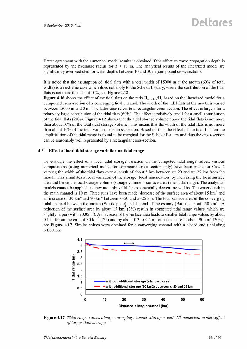
9 September 2010, final
Tidal phenomena in the Scheldt Estuary
53 of 99
Better agreement with the numerical model results is obtained if the effective wave propagation depth is represented by the hydraulic radius for h < 13 m. The analytical results of the linearized model are significantly overpredicted for water depths between 10 and 30 m (compound cross-section). It is noted that the assumption of tidal flats with a total width of 15000 m at the mouth (60% of total width) is an extreme case which does not apply to the Scheldt Estuary, where the contribution of the tidal flats is not more than about 10%, see Figure 4.12. Figure 4.16 shows the effect of the tidal flats on the ratio Hx=60km/Ho based on the linearized model for a compound cross-section of a converging tidal channel. The width of the tidal flats at the mouth is varied between 15000 m and 0 m. The latter case refers to a rectangular cross-section. The effect is largest for a relatively large contribution of the tidal flats (60%). The effect is relatively small for a small contribution of the tidal flats (20%). Figure 4.12 shows that the tidal storage volume above the tidal flats is not more than about 10% of the total tidal storage volume. This means that the width of the tidal flats is not more than about 10% of the total width of the cross-section. Based on this, the effect of the tidal flats on the amplification of the tidal range is found to be marginal for the Scheldt Estuary and thus the cross-section can be reasonably well represented by a rectangular cross-section.
4.6 Effect of local tidal storage variation on tidal range To evaluate the effect of a local tidal storage variation on the computed tidal range values, various computations (using numerical model for compound cross-section only) have been made for Case 2 varying the width of the tidal flats over a length of about 5 km between x= 20 and x= 25 km from the mouth. This simulates a local variation of the storage (local innundation) by increasing the local surface area and hence the local storage volume (storage volume is surface area times tidal range). The analytical models cannot be applied, as they are only valid for exponentially decreasing widths. The water depth in the main channel is 10 m. Three runs have been made: decrease of the surface area of about 15 km2 and an increase of 30 km2 and 90 km2 between x=20 and x=25 km. The total surface area of the converging tidal channel between the mouth (Westkapelle) and the end of the estuary (Bath) is about 450 km2. A reduction of the surface area by about 15 km2 (3%) results in computed tidal range values, which are slightly larger (within 0.05 m). An increase of the surface area leads to smaller tidal range values by about 0.1 m for an increase of 30 km2 (7%) and by about 0.3 to 0.4 m for an increase of about 90 km2 (20%), see Figure 4.17. Similar values were obtained for a converging channel with a closed end (including reflection).
00.5
11.5
22.5
33.5
44.5
0 10 20 30 40 50 60
Distance along channel (km)
Tida
l ran
ge (m
)
w ithout additional storage (standard case)with additional storage (90 km2) between x=20 and 25 km
Figure 4.17 Tidal range values along converging channel with open end (1D numerical model);effect
of larger tidal storage

54 of 99
Tidal phenomena in the Scheldt Estuary
9 September 2010, final
4.7 Non-linear effects and tidal asymmetry The analytical solutions presented in Section 3.3 and 3.4 above do not express the non-linear effects, as they are based on linear equations. All non-linear terms (h∂ u /∂x, u ∂ u /∂x ; ∂(η u )/∂x and u 2) have been neglected or linearized. Thus, the wave speed is constant and the peak flood and ebb velocities are equal (no asymmetry). The generation of second harmonics (e.g. M4) can be explained by the shallow water equations (Parker, 1991). The wave speed without friction is c = (gh)0.5 is about constant if the wave height is small compared to the water depth (η << h). In shallow water where η is not small compared to the depth, the wave crest will travel faster than the wave trough. The resulting wave profile will be distorted from a perfect sinusoidal wave profile giving a faster rise to HW and a slower fall to LW; HW will occur earlier and LW will occur later. Given a phase lead of the velocity with respect to the water level elevation, the end of the flood flow will largely coincides with the tidal rise resulting in less friction due to the larger water depth, while the end of the ebb flow will coincide with the tidal fall with smaller water depths resulting in enhanced friction. As a result the tidal asymmetry will be enhanced ( u ebb < u flood). Subtracting the original sinusoidal profile from the distorted profile, yields the energy of the second harmonic and other even harmonics, which represent the asymmetry effect of the non-linear continuity term ∂(η u )/∂x. When η is not small compared to h, the velocity u cannot be neglected with respect to the wave speed c, so the wave speed at the crest actually is c+ u and at the trough c – u , which also results in wave asymmetry (Parker, 1991). This is the effect of the inertial term in the momentum equation u ∂ u /∂x (which has been neglected in the analytical solutions). The importance of the inertial term is reduced by reflection making the wave closer to a standing wave, by friction and by the decrease of the width. The first order effects of friction (linear friction) are to decrease the wave speed and to attenuate the wave amplitude. This will not distort the wave profile, but HW and LW will be delayed and decreased in amplitude. Non-linear friction ( u 2) will also lead to distortion of the wave profile. The frictional loss per unit volume of fluid is smaller for greater depths and larger for smaller depths, so the crest will travel faster than the trough. Distortion of the wave profile (due to differences in bottom friction during flood and ebb) may also lead to a small, but gradual increase of the mean sea level at the end of the basin (mean sea level slope). For example, at the end of the Scheldt Estuary (The Netherlands), the mean water level is about 0.15 m higher than that at the mouth (Pieters, 2002), see also Figures A9 to A12 for prismatic channels and Figures B13 to B18 for converging channels. 1. Higher order harmonics Second order harmonics are generated because the maximum wave speed and minimum amplitude attenuation occur at the crest and the opposite occurs at the trough. The tide is distorted in an asymmetric nature, which can be represented by second harmonics. Quadratic friction ( u 2) causes maximum amplitude attenuation and minimum wave propagation at both maximum flood and maximum ebb; attenuation is minimum at slack water. The result of this asymmetry effect is a third harmonic (e.g. M6) and other smaller odd harmonics. When two tidal constituents are present there is a modulation of the distortion and attenuation effects, resulting in new compound tidal constituents. For example, when M2 and N2 are in phase, so that their respective high waters occur at the same time; the total depth under the crest of the combined wave will be greater than when they are out of phase 14 days later. Similarly, the total depth under the trough when M2 and N2 are in phase will be smaller than when they are out of phase. Thus, M4-generation due to greater depth at the crest than at the trough will be modulated by the 28 day variation of the combined M2+N2 effects, leading to a 28 day modulation of M4 and a new constituent NM4.

9 September 2010, final
Tidal phenomena in the Scheldt Estuary
55 of 99
When the tidal velocity consists of two major constituents ( u = u 1 cos ω1t + u 2 cos ω2t), the terms involving a product of constituents generate constituents at the difference frequency and at the sum frequency, which is illustrated below: u 2 = ( u 1 cos ω1t + u 2 cos ω2t)2 = u 2 = ( u 1 cos ω1t)2 +( u 2 cos ω1t)2 + 2 u 1 u 2 cos ω1t cos ω2t u 2 = ( u 1 cos ω1t)2 +( u 2 cos ω1t)2 + u 1 u 2 [ cos((ω1−ω2)t) + cos((ω1+ω2)t)] Maximum flood and ebb currents will be greatest when M2 and N2 currents are in phase. Because of quadratic friction, the loss when M2 and N2 are in phase will be greater than the sum of the individual losses of M2 and N2; the combined wave will travel slower and be damped more. The opposite will be true 14 days later. In real estuaries the phase difference between the vertical and horizontal tide will also have a pronounced effect on this. In shallow friction-dominated estuaries generally, a saw-tooth type of tidal wave (sometimes a tidal bore) is generated, which cannot be represented by higher harmonics. Furthermore, the effect of a mean river flow may be important. A mean river flow makes the ebb current velocities larger and the flood current velocities smaller. Due to quadratic friction, the increased loss during the ebb phase is greater than the decreased loss during the flood phase. The result is a greater loss than if the mean flow is absent and thus greater damping of the tidal wave and a reduced tidal range. Friction effects being greater during ebb than during flood (asymmetry effects) also lead to the generation of M4-harmonics; low waters are delayed and high waters are made earlier. When the river flow is greater than the tidal flow, the flow becomes uni-directional. When the river discharge increases, the mean sea level also increases due to frictional momentum loss from the mean flow. This increase in water depth increases the wave speed, via the non-linear continuity term. Figure 4.18 shows the amplitude of the M2, M4 and M6-components at 4 stations (Bath, Hansweert, Terneuzen and Vlissingen) in the Scheldt Estuary over the period 1910 to 2010. The M2-amplitude varies between 1.7 m at Vlissingen to 2.1 m at Bath (increase in landward direction). The M2-amplitude gradually increases in time in Vlissingen, Terneuzen and Hansweert. The M2-amplitude in Station Bath shows a pronounced increase in the period between 1970 and 1980 (probably due to channel deepenings). The M4-amplitude varies between 0.08 m and 0.13 m before 1970 and between 0.10 m and 0.14 m after 1970 (less than 10% of the M2-amplitude). In the latter period the M4-amplitude is approximately the same for all stations. The M6-amplitude varies between 0.08 m and 0.13 m after 1970 and increases in landward direction as a result of the increased friction due to smaller depth. The effect of storm surges (larger water depths) on the tide can also be explained in terms of changes in wave speed and frictional damping. The lower the frequency of the surge, the smaller the current velocities associated with the surge and the less important are the terms u ∂u /∂x and u 2. At the surge crest the total depth will be significantly larger and the tidal wave speed will increase. This will increase the tidal wave length and reduce the tidal velocities and therefore reduce frictional attenuation.

56 of 99
Tidal phenomena in the Scheldt Estuary
9 September 2010, final
Figure 4.18 M2, M4 and M6-amplitudes as function of time (1910-2010) in Scheldt Estuary (Deltares,
2010) If the flood duration (Tf) is shorter than the ebb duration (Te), the peak flood velocity will be larger than the peak ebb velocity assuming that the total tidal inflow volume is, on average, equal to the total tidal outflow volume. The area under half a sine-wave is equal to: 2 (0.5T) u /π The area under the flood part of the wave is: 2 Tf u f/π The area under the ebb part of the wave is: 2 Te u e/π Thus: 2Tf u f/π = 2Te u e/π and Tf + Te = T resulting in u f / u e = Te/Tf = (T−Tf)/Tf The peak discharges are: Q f = b u f (ho + η ) and Q e= b u e(ho − η )
Q f / Q e= [(T−Tf)/Tf][(ho + η )/(ho − η )] = [(T−Tf)/Tf][(1 + η /ho)/(1 − η /ho)]
Q f / Q e= 1.3 to 1.7 for η /ho in the range of 0.1 to 0.2

9 September 2010, final
Tidal phenomena in the Scheldt Estuary
57 of 99
2. Wave speed at LW and HW According to Lamb (1963), the wave speed c = (g ho)0.5 of a tidal wave with a finite wave height ( η /ho in range of 0.1 to 0.3) is relative to the tidal current velocity. The absolute wave speed is: c = u + (gh)0.5
cHW ≅ u + (g ho)0.5 [(1 + 1.5 η /ho)] cLW ≅ u + (g ho)0.5 [(1 – 1.5 η /ho)] The propagation velocities of the wave crest (High Water, HW) and the wave trough (Low Water, LW) can be estimated by applying the linearized mass balance and momentum balance equations for a prismatic channel. Applying these equations around the time of High Water (similarly around LW), the water depth is equal to h = ho± η and the velocity is of the order of ± u . The linearized mass balance and momentum balance equations for a simple prismatic channel with constant cross-section (and horizontal bottom Ib = 0) for the time period around HW are, as follows: ∂η (ho± η )∂ u ± u ∂η ______ + ______________ + ________ = 0 (4.1) ∂t ∂x ∂x ∂ u ± u ∂ u g ∂η m1 u ______ + _________ + ________ + _________ = 0 (4.2) ∂t ∂x ∂x ho± η m1 = 8/(3π) (g/C2) | u |= Lorentz-friction parameter (in m/s). Using: η = η sin(ωt−kx) and u = u sin(ωt−kx) with u = ( η /h) c cosϕ and assuming that η and u are approximately constant along the channel, Equations (4.1) and (4.2) can be expressed (through elimination of ∂ u /∂x term) for the wave crest (HW) as: ∂ u u ∂η u 2 ∂η g ∂η m1 u ______ − _____________ − ______________ + _________ + ________ = 0 (4.3) ∂t (ho+ η )∂t (ho+ η )∂x ∂x ho+ η Using: ∂η/∂t = η ω cos(ωt−kx), ∂η/∂x = − η k cos(ωt−kx),
∂u /∂t = u ω cos(ωt−kx), ∂ u /∂x = − u k cos(ωt−kx), it follows that: ω u cos(ωt−kx) − [ u /(ho+ η )] η ω cos(ωt−kx) + [{ u 2/(ho+ η )} η k − g k η ] cos(ωt−kx) + + {m1/(ho+ η )} u sin(ωt−kx) = 0

58 of 99
Tidal phenomena in the Scheldt Estuary
9 September 2010, final
The cos-terms and sin-terms are eliminated by introducing a scaling parameter ε acting on the friction term, yielding: ω u − [ u ηω /(ho+ η )] + [{ u 2 η k /(ho+ η )} − g k η ] + ε {m1/(ho+ η )} u = 0 (4.4) Using: cHW= ω/k, u = ( η /h) cHW cosϕ1 and ε = scaling coefficient of bottom friction term with respect
to the other terms (velocity around HW is smaller than u due to phase differences), Equation (4.4) can be expressed as: g ho [1 + η /ho] cHW
2 = _____________________________________________ (4.5) [(cosϕ1){1 + ( η /ho)2 + ε m1/(ω ho)}]
A similar expression can be derived for LW resulting in a term with [1 − η /ho]. Assuming ( η /ho)2 ≅ 0, it follows that: co [1 ± η /ho]0.5
cHW or cLW = _____________________________________ = α1 α2 co (4.6) [(cosϕ1) {1 + ε m1/(ω ho)}]0.5
with: α1 = [1 ± η /ho]0.5 ≅ [1 ± 0.5 η /ho], α2 = [(cosϕ1) {1 + ε m1/(ω ho)}]−0.5
co= (g ho)0.5 The α1-coefficient expresses the effect of a larger or smaller water depth on the wave speed and is < 1 at LW and > 1 at HW. Using η /ho ≅ 0.2, the wave speed co increases by about 10% under the wave crest (HW) and decreases by about 10% under the wave trough (LW). These values are comparable to the values presented by Savenije (2005) for the Scheldt Estuary (depth of 8 to 10 m) in the south-west part of The Netherlands and the Incomati Estuary (depth of 4 to 8 m) in Mozambique: cHW ≅ 1.1cLW or cHW ≅ 1.05 cmean and cLW ≅ 0.95 cmean for Scheldt Estuary, cHW ≅ 1.15cLW or cHW ≅ 1.07 cmean and cLW ≅ 0.93 cmean for Hooghly Estuary, India cHW ≅ 1.3cLW or cHW ≅ 1.15 cmean and cLW ≅ 0.85 cmean for Incomati Estuary, Mozambique. The α2-coefficient expresses the effect of bottom friction on the wave speed and is always < 1 in a prismatic channel (damped estuary). Using: H = 4 m, η = 2 m, cosϕ1 ≅ 0.7, u ≅ 1 m/s, ε ≅ 0.5, C ≅ 50 m0.5/s, m1 = (8/(3π)) (g/C2) u ≅ 0.003 m/s, ω ≅ 0.00015, ho = 10 m, it follows that: α2 = 0.85. Thus, the wave speed co is reduced by about 15% due to the bottom friction effect. If friction is neglected then m1= 0 and cosϕ = 1 (no phase difference).

9 September 2010, final
Tidal phenomena in the Scheldt Estuary
59 of 99
Based on the classical equation c = (gh)0.5, the propagation velocities of High Water (HW) and Low Water (LW) in a prismatic channel can simply be estimated by using: cHW = (gh)0.5 = [g (ho+ η )]0.5 = co (1 + η /ho)0.5 ≅ co (1 + 0.5 η /ho) (4.7) cLW = (gh)0.5 = [g (ho− η )]0.5 = co (1 − η /ho)0.5 ≅ co (1 − 0.5 η /ho) (4.8) with: co = (gho)0.5, ho = water depth to mean sea level, η = amplitude of tidal wave. The propagation velocities of High Water (HW) and Low Water (LW) may also be estimated by using the propagation velocity of a translation wave or bore-type wave in a prismatic channel, resulting in: cHW = co (1 + 1.5 η /ho)0.5 ≅ co (1 + 0.75 η /ho) (4.9) cLW = co (1 − 1.5 η /ho)0.5 ≅ co (1 − 0.75 η /ho) (4.10) Equations (4.9) and (4.10) yield an increase/decrease of about 10% to 20% (based on η /ho ≅ 0.2 to 0.3) with respect to the co= (gho)0.5. Sumarizing, the propagation velocity of HW and LW in a prismatic channel can be estimated by using: cHW = cmean (1 + β η /ho) cLW = cmean (1 − β η /ho) with β in the range of 0.5 to 0.75. Measured data also show β-values in the range 0.5 to 0.75. In an estuary the distance between the crest (HW) and trough (LW) of the tidal wave is of the order of 100 km. The time interval between the crest and the trough of the wave is about 0.5T (≅ 6 hours) for a semi-diurnal tide. The wave speed co is of the order of 5 to 10 m/s. The difference between the wave speed of HW and LW is of the order of 1 to 2 m/s. Since the wave crest moves faster than the wave trough, the crest-trough distance can be reduced by about (0.2co)(0.5T) = 40 km in 6 hours resulting in an asymmetric wave. 3. Increase of mean water level Non-linear friction ( u 2) will lead to the distortion of the wave profile. The frictional loss per unit volume of fluid is smaller for greater depths and larger for smaller depths, so the crest will travel faster than the trough. Distortion of the wave profile (due to differences in bottom friction during flood and ebb) may also lead to a small, but gradual increase of the mean sea level at the end of the basin (mean sea level slope). For example, at the end of the Scheldt Estuary (The Netherlands), the mean water level is about 0.15 m higher than that at the mouth (Pieters, 2002), see also Figures A9 to A12 for prismatic channels and Figures B.13 to B18 for converging channels. Table 4.6 shows computed values (in the range of 0.05 to 0.5 m) of the maximum increase of the mean water surface level in prismatic and converging channels. The values are relatively small for short and deep channels and relatively large for long and shallow channels.
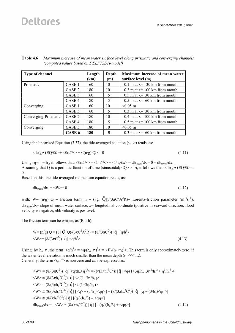
60 of 99
Tidal phenomena in the Scheldt Estuary
9 September 2010, final
Table 4.6 Maximum increase of mean water surface level along prismatic and converging channels
(computed values based on DELFT2DH-model)
Type of channel Length (km)
Depth (m)
Maximum increase of mean water surface level (m)
Prismatic CASE 1 60 10 0.1 m at x= 30 km from mouth CASE 2 180 10 0.3 m at x= 100 km from mouth CASE 3 60 5 0.5 m at x= 30 km from mouth CASE 4 180 5 0.5 m at x= 60 km from mouth Converging CASE 1 60 10 <0.05 m CASE 3 60 5 0.3 m at x= 30 km from mouth Converging-Prismatic CASE 2 180 10 0.4 m at x= 100 km from mouth CASE 4 180 5 0.5 m at x= 100 km from mouth Converging CASE 5 180 10 <0.05 m CASE 6 180 5 0.3 m at x= 60 km from mouth
Using the linearized Equation (3.37), the tide-averaged equation (<...>) reads, as: <1/(gA) ∂Q/∂t> + <∂η/∂x> + <(n/g) Q> = 0 (4.11) Using: η= h − ho, it follows that: <∂η/∂x> = <∂h/∂x> − <∂ho/∂x> = dhmean/dx – 0 = dhmean/dx. Assuming that Q is a periodic function of time (sinusoidal; <Q> ≅ 0), it follows that: <1/(gA) ∂Q/∂t> ≅ 0. Based on this, the tide-averaged momentum equation reads, as: dhmean/dx + <W>= 0 (4.12) with: W= (n/g) Q = friction term, n = (8g | Q |)/(3πC2A2R)= Lorentz-friction parameter (m–2s–1), dhmean/dx= slope of mean water surface, x= longitudinal coordinate (positive in seaward direction; flood velocity is negative; ebb velocity is positive). The friction term can be written, as (R ≅ h): W= (n/g) Q = (8 | Q |Q)/(3πC2A2R) = (8/(3πC2)) | q | (q/h3) <W>= (8/(3πC2)) | q | <q/h3> (4.13) Using: h= ho+η, the term <q/h3> = <q/(ho+η)3> = < u /(ho+η)2>. This term is only approximately zero, if the water level elevation is much smaller than the mean depth (η <<< ho). Generally, the term <q/h3> is non-zero and can be expressed as: <W> = (8/(3πC2)) | q | <q/(ho+η)3> = (8/(3πho
3C2)) | q | <q/(1+3η/ho+3η2/ho2 + η3/ho
3)> <W> ≅ (8/(3πho
3C2)) | q | <q/(1+3η/ho )> <W> ≅ (8/(3πho
3C2)) | q | <q(1−3η/ho )> <W> ≅ (8/(3πho
3C2)) | q | [<q> − (3/ho)<qη>] = (8/(3πho3C2)) | q | [qr − (3/ho)<qη>]
<W> ≅ (8/(πho4C2)) | q | [(qr )(ho/3) − <qη>]
dhmean/dx = –<W> ≅ (8/(πho4C2)) | q | [− (qr )(ho/3) + <qη>] (4.14)

9 September 2010, final
Tidal phenomena in the Scheldt Estuary
61 of 99
It is noted that the tide-averaged discharge is equal to the river discharge: <q> = qr Using: η = η cosωt and u = − u cos(ωt+ϕ1), the tidal discharge (q) is: q = (ho + η) u = – (ho+ η cosωt) u cos(ωt+ϕ1) = – ho u cos(ωt+ϕ1) – u η (cosωt) cos(ωt+ϕ1) Thus, the term q η is: q η = – ho u η (cosωt) cos(ωt+ϕ1) – u η 2 (cosωt)2 cos(ωt+ϕ1)
q η/ho2 = – u ( η /ho) (cosωt) cos(ωt+ϕ1) – u ( η /ho)2 (cosωt)2 cos(ωt+ϕ1)
The last term is much smaller than the first term and can be neglected, resulting in: q η/ho
2 = – u ( η /ho) (cosωt) cos(ωt+ϕ1)
q η = – u ho η (cosωt) cos(ωt+ϕ1) = – q η (cosωt) cos(ωt+ϕ1)
with: q = u ho The tide-averaged value is (see also Equations (3.16) and (3.17)): <qη> = –0.5 η q cosϕ1 Thus: dhmean/dx = –<W> ≅ – (8/(πho
4C2)) | q | [− (qr )(ho/3) – 0.5 η q cosϕ1] (4.15) Using Equation (3.17): u stokes= −0.5 cosϕ1 ( η /ho) u = −0.5 ( η q ) (1/ho
2) cosϕ1 = net landward fluid velocity (positive x-direction is seaward) and qr= u r ho, it follows that: dhmean/dx = –<W> ≅ (8/(πho
4C2)) | q | [− u r ho2/3 + ho
2 u stokes] dhmean/dx = –<W> ≅ (8/(πho
2C2)) | q | [− u r /3 + u stokes]
dhmean/dx = –<W> ≅ (8/(πhoC2)) | u | [− u r /3 + u stokes] dhmean/dx = –<W> ≅ (m/g) [3 u stokes − u r] dhmean/dx = –<W> ≅ (m/g) [−3 |u stokes| − u r] dhmean/dx = –<W> ≅ − (m/g) [ u r + 3 |u stokes|] (4.16) with: u r = qr/h = river velocity (positive value) and m = (8g | u |)/(3πC2ho) = Lorentz-friction parameter (1/s); m ≅ 10–4. Both the river velocity and the Stokes drift are functions of x in a converging tidal channel and generally are of the same order of magnitude. Equation (4.16) yields a negative value or hmean decreasing in positive (seaward) x-direction or hmean increasing in landward direction.

62 of 99
Tidal phenomena in the Scheldt Estuary
9 September 2010, final
If the river velocity is small with respect to the Stokes drift, then: dhmean/dx= − (m/g) [3 |u stokes|]= – (4/π) (g/C2) ( u /co)2 ( η /ho) cosϕ1 (4.17) with: co= (g ho)0.5 = wave speed. Using: (4/π) (g/C2) ≅ 0.003, ( u /co) ≅ 0.1, ( η /ho) ≅ 0.1, cosϕ1 ≅ 0.5 for the Scheldt Estuary, it follows that: dhmean/dx ≅ 0.015 10–4 (0.015 m per 10 km) in reasonable agreement with measured data. Figure 4.19 shows computed values of the mean water surface level increase along a converging channel (rectangular cross-section) based on the linearized analytical model. The mean water level increase at the mouth is set to 0. The channel length is 100 km. The converging length scale is Lb= 25 km (Scheldt Estuary). The width at the mouth is bo= 25 km (at Westkapelle). The tidal amplitude at the mouth is 2.1 m. The bed roughness value is ks= 0.05 m. The tidal period is T= 43200 s. The river velocity is assumed to be zero ( u r= 0 m/s). The increase of the mean water surface level is rather large (up to 1.2 m at the channel end) for a shallow depth of 5 m and decreases for larger depths. Figure 4.20 shows the Stokes drift (in m/s) along a converging channel (rectangular cross-section) based on the linearized analytical model. The Stokes drift decreases from about 0.1 m/s to about 0.05 m/s for a shallow depth of 5 m due to the decrease of the tidal amplitude (tidal damping due to relatively large effect of bottom friction). The Stokes drift increases for larger depths due to increase of the tidal amplitude (tidal amplification). The surface slope of the mean water level and hence the mean water level (hmean) at the end of the estuary where the river enters, depends on the local values of ( u /co)2, ( η /ho) and cosϕ1 (see Equation 4.17). These parameters may vary considerably on the neap-spring cycle (14 days) and thus the mean water level at the end of the tidal channel will vary on the neap-spring cycle resulting in a low-frequency surface wave (14 days) at the end of the channel (additional river tide). Furthermore, low-frequency variations of the river discharge will also introduce low-frequency variations of the mean water level. The tidal range also is affected by the river discharge, because the tidal penetration length reduces for increasing discharge values and thus the tidal range at a fixed station in the river section is smaller for increasing discharge values (tidal wave will not reach as far into the river). A smaller tidal range reduces the mean water level increase. The water depth itself will be larger in the river section for increasing discharge values (higher river stage). Since, all effects will occur simultaneously, the tide-related variations of the mean water level in the river section are complicated, although they are relatively small in absolute sense (see also Buschman et al., 2009).

9 September 2010, final
Tidal phenomena in the Scheldt Estuary
63 of 99
0
0.2
0.4
0.6
0.8
1
1.2
1.4
0 10000 20000 30000 40000 50000 60000 70000 80000 90000 100000
Distance along channel (m)
Incr
ease
of m
ean
wat
er le
vel (
m)
water depth= 5 mwater depth= 7 mwater depth= 10 m
Figure 4.19 Increase of mean water surface level along converging channel (linearized model)
0
0.02
0.04
0.06
0.08
0.1
0.12
0 10000 20000 30000 40000 50000 60000 70000 80000 90000 100000
Distance along channel (m)
Stok
es d
rift
(m/s
)
water depth= 5 mwater depth= 7 mwater depth= 10 m
Figure 4.20 Stokes drift along converging channel (linearized model) Godin (1999) shows that the neap-spring variation of LW at Quebec in the Upper St Lawrence Estuary (Canada) is substantially affected by the river discharge. The neap-spring variation of LW is about 0.5 m during periods with high discharge values (of the order of 10000 m3/s due to snow melt) and about 1 m during periods with low discharge values. HW is not so much affected by these processes. Long-term tidal predictions for the river section are not very accurate as the temporal variation of the river discharge is often unknown. Daily predictions can be done if the river discharge is known on a daily basis.


9 September 2010, final
Tidal phenomena in the Scheldt Estuary
65 of 99
5 Summary and conclusions
The Scheldt Estuary is a large-scale estuary in the south-west part of the Netherlands. The estuary is connected to the Scheldt river, which originates in the north-west of France. The total length of the Scheldt river, including the estuary is about 350 km; the tide penetrates up to the city of Gent in Belgium (about 180 km from the mouth). The length of the estuary is about 60 km (up to Bath). The cross-sections of the estuary show two to three deeper channels with shoals in between and tidal flats close to the banks. The width of the mouth at Westkapelle (The Netherlands) is about 25 km, about 5 km near Vlissingen and gradually decreases to about 0.8 km at Antwerp. The convergence length scale is of the order of Lb=25 km. The width-averaged water depth (ho) to MSL at the mouth between Vlissingen and Hansweert is about 12 m. The width-averaged water depth (ho) to MSL between Hansweert and Bath is about 11.5 m. The bottom is almost horizontal up to x = 80 km from the mouth. The discharge of the river Scheldt is quite small varying in the range of 50 to 200 m3/s resulting in well-mixed density conditions in the estuary. The tidal range in estuaries is affected by four dominant processes:
• inertia related to acceleration an deceleration effects, • amplification (or shoaling) due to the decrease of the width and depth (convergence) in
landward direction, • damping due to bottom friction and, • partial reflection at abrupt changes of the cross-section and at the landward end of the estuary (in
the absence of a river).
The Scheldt Estuary has important environmental and commercial qualities. It is the main shipping route to the Port of Antwerp in Belgium. The depth of the navigation channel to the Port of Antwerp in Belgium is a problematic issue between The Netherlands and Belgium because of conflicting interests (commercial versus environmental). Large vessels require a deep tidal channel to Antwerp, which enhances tidal amplification with negative environmental consequences. Since 1970, the main shipping channel has been deepened (by dredging and dumping activities) various times affecting the tidal range between the mouth and Antwerp. At present the navigation depth below mean low water is about 14 m. Analysis of the (present) measured tidal data in the Scheldt Estuary shows the following basic characteristics:
• the semi-diurnal water level variation at the mouth (Westkappelle) is quite regular; the tidal range during springtide is about 4.2 m; the tidal range during neap tide is about 2.6 m.
• the tidal range increases (amplification) in landward direction to about 5.5 m at Bath and 5.85 m at Antwerp during spring tide;
• the propagation speed of the tidal wave (mean of HW and LW) varies between 15 m/s at the mouth (0 to 20 km) and 11 m/s at the landward end (Bath);
• the tidal water level curve at the mouth is slightly asymmetric with a sharp tidal rise just before high water; the peak tidal discharge during flood is about 30% larger than the peak tidal discharge during ebb;
• the phase shift (phase lead) between the horizontal and vertical tide is about 1 to 2.5 hours.

66 of 99
Tidal phenomena in the Scheldt Estuary
9 September 2010, final
Basic questions related to the tidal wave penetration in the Scheldt Estuary, are: • what is the role of the shape and dimensions of the tidal channels (both in planform and in the
cross-section) on tidal wave propagation and tidal storage?; • what is the role of bottom friction in relation to the depth of the main channels? • what is the role of reflection of the tidal wave against abrupt changes of the cross-section and at
the landward end near Bath? • what is the role of tidal storage? • what is the role of tidal wave asymmetry (non-linear effects)?
Literature information and model analysis have been used to address these questions using data of the Scheldt Estuary. Friedrichs and Aubrey (1994) have convincingly shown that the convergence length scale Lb of the width (width b= bo exp(−x/Lb)) and the convergence length scale LA of the cross-sectional area A=Ao exp(−x/LA)) are of the same order of magnitude and are much smaller than the length scale LU of the horizontal velocity variations in most tidal channels. This implies that the non-linear convective acceleration term ( u ∂ u /∂x; u =cross-section-averaged velocity) is negligibly small in the major part of the estuary with exception of the region close to the landward boundary where a river (open end) or a zero tidal flow boundary (closed end) may be present. For the channels considered by Friedrichs and Aubrey (1994) the along-channel gradients in discharge are dominated by along-channel gradients in cross-sectional (rate of convergence) area as regards the continuity equation. They also show that the local acceleration term (∂ u /∂t) is relatively small compared to the other terms. The most important effects are the rate of channel convergence, the pressure term (water surface slope term) and the frictional term. The classical solution of the linearized mass and momentum balance equations for a prismatic channel of constant depth represents an exponentially damped sinusoidal wave which dies out gradually in a channel with an open end or is reflected in a channel with a closed landward end. Amplification of the tide can only be obtained by including the reflected wave. Using this classical approach, the tidal wave propagation in funnel-type estuary can only be considered by schematizing the channel into a series of sections, each with its own constant width and depth. Unfortunately, this approach eliminates to large extent the effects of convergence in width and depth on the complex wave number and thus on the wave speed (Jay, 1991). The analytical solution for a funnel-type (converging) channel with exponential width and constant depth shows that strongly convergent channels can produce a single forward propagating tidal wave with a phase lead of the horizontal and vertical tide close to 90o, mimicing a standing wave system (apparent standing wave). A basic feature of this system is that the wave speed is much larger than the classical value co= (gho)0.5, in line with observations of the Scheldt Estuary. The analytical model for a converging tidal channel has also been applied to other cases showing very reasonable results (Van Rijn, 2011): Hooghly Estuary (India), Delaware Estuary (USA) and the Yangtze Estuary (China). The amplification of the M2-tide in the Scheldt Estuary can be simulated quite well by both the analytical and numerical models applied using a bed roughness value in the range of 0.03 to 0.1 m. Analysis of the linearized tidal wave equations for a convergent tidal channel (funnel-type) shows that the Scheldt Estuary with a ratio of the convergence length scale and the mean water depth of about Lb/ho=2500 is an amplified estuary (Figure 3.7). This type of estuary is characterized by a tidal wave speed which is larger than the classical value of co= (gho)0.5. The measured wave speed in the Scheldt Estuary varies between 15 and 11 m/s; the computed classical wave speed values are in the range of 8 to 10 m/s.

9 September 2010, final
Tidal phenomena in the Scheldt Estuary
67 of 99
The tidal flow in the Scheldt Estuary can also be simulated by using the classical four-pole equations (Dronkers, 1964; Verspuy, 1985; Pieters 2002,), which are based on a combination of the incoming wave and the reflected wave. The funnel-type estuary has to be schematized into a series of coupled sections, each of constant width and depth. Computed values are in good agreement with measured values for a phase lead of ϕ = 85o. To obtain a realistic solution with amplification (as measured), the reflected wave is of prime importance (about 1 m at the mouth). Effect of channel dimensions Numerical models (1D and 2DH) including non-linear terms and reflection have been used to study the effects of channel length (short channel of 60 km to long channels of 180 km) and channel depth (shallow channel of 5 m and deep channel of 10 m) of converging tidal channels. Summarizing all results, it can be concluded that: Short and deep converging channel: convergence is dominant in entrance section and
reflectionin landward section of the channel; tidal ranges increases (amplication);
Short and shallow converging channel: bottom friction are dominant in entrance section;
reflection is dominant in landward end section; tidal range decreases in middle and increases near end;
Long and deep converging-prismatic channel: convergence is dominant in entrance section; bottom friction is dominant in middle section and reflection in landward end section; tidal range decreases in prismatic section; Long and shallow converging-prismatic channel: bottom friction is dominant in major part of the
channel; tidal range decreases almost completely; Long and deep converging channel: convergence is dominant in entire channel; reflection occurs in landward end section; tidal range increases significantly; Long and shallow converging channel: bottom friction is slightly dominant in entire
channel; reflection occurs in landward end section;
tidal range decreases slightly in landward direction The effect of water depth on the amplification of the tidal range has been studied in more detail for the Scheldt Estuary (length of 60 km). Figure 4.7 shows the ratio of the tidal range (Hx=60km/Ho) at x = 60 km and at the entrance x = 0 as a function of the water depth (in the range of 5 to 20 m) based on various model results. Tidal damping due to bottom friction dominates for water depths smaller than about 7 m resulting in a ratio (Hx=60km/Ho) smaller than 1. Friction has almost no effect for depths larger than about 15 m. The tidal range shows amplification (>1) for water depths larger than about 7 m. Thus, increasing the water depth by dredging leads to a larger tidal range along the estuary. The maximum amplification based on the analytical solution of the linearized momentum equation (without reflection) is about 1.3 at a water depth of about 11 m. A further increase of the depth does not lead to larger amplification values. The results of the numerical DELFT1D-model taking all terms into account are also shown, both for a channel (rectangular cross-section) with a closed end (with reflection) and an open end (no reflection).

68 of 99
Tidal phenomena in the Scheldt Estuary
9 September 2010, final
The results of the numerical model show a significant effect of reflection at the channel end. The tidal range ratio is somewhat smaller (about 20%) for a channel with an open end and water depths smaller than 15 m. Comparing the results of the analytical and numerical solution methods, it is remarkable that the analytical method without reflection gives the correct tidal range values (close to measured values). The analytical model neglecting reflection seems to overpredict the amplification effect somewhat. The numerical model results show that the amplification effect is caused by both channel convergence and wave reflection. The increase of the tidal range inside the Scheldt Estuary over the last centrury can be very well explained by the increase of the channel depth over the last century. Based on Figure 4.7, an increase of the channel depth from 7 to 10 m leads to an increase of the amplification effect of about 25% or an increase of about 1 m of the tidal range at 60 km from the mouth. A further (future) increase of the channel depth does not seem to lead to any further substantial increase of the tidal range based on the linearized analytical solution of the tidal wave equations. Effect of cross-section The effect of the cross-section on the tidal range has also been studied in more detail. The analytical models are most valid for a rectangular cross-section. Real tidal channels, however, have a compound cross-section with one or more deeper channels with shallow flats or floods plains in between and along the banks. To evaluate the effect of the cross-section on the computed water levels, various computations have been made for a compound cross-section consisting of one main channel and tidal flood plains using the 1D numerical model and analytical models. The results are compared to those for a converging channel with a rectangular cross-section. A converging channel with an open end has been considered only (no reflection at landward end). The width at the mouth is 25000 m (Westkapelle). The compound cross-section is assumed to consist of one main channel and tidal flats. The analytical results of the linearized model and the energy-based model show that significant amplification only occurs in a compound channel when the depth of the main channel is relatively large (ho> 15 m). The numerical model results show tidal damping for water depths smaller than about 10 m, both for a rectangular and a compound cross-section. The tidal damping is largest for a compound channel. The differences are largest for smaller depths. The numerical model results only show slight amplification for larger water depths (maximum amplification of 1.15). The analytical results of the energy-based model for a compound cross-section are in reasonable agreement with the numerical results for water depths smaller than 13 m. The analytical results of the energy-based model are slightly overpredicted for water depths between 15 and 30 m. The analytical results of the linearized model for a compound cross-section are too small compared with the numerical results for water depths smaller than about 13 m, particularly if the effective wave propagation depth is used. Better agreement with the numerical model results is obtained if the effective wave propagation depth is represented by the hydraulic radius for h < 13 m. The analytical results of the linearized model are significantly overpredicted for water depths between 10 and 30 m (compound cross-section). The contribution of the tidal flats to the total tidal storage volume is less than 10% for the Scheldt Estuary. This means that the width of the tidal flats is not more than about 10% of the total width of the cross-section. Based on this, the effect of the tidal flats on the amplification of the tidal range is found to be marginal for the Scheldt Estuary and thus the cross-section can be reasonably well represented by a rectangular cross-section. Effect of reflection The planform of the Scheldt Estuary is characterized by a decreasing width in landward direction and the presence of various bends (near Hansweert and Bath), which may lead to partial reflections. The width variations are most pronounced in the entrance between Westkapelle and Vlissingen and near the river outlet between Bath and Antwerp.

9 September 2010, final
Tidal phenomena in the Scheldt Estuary
69 of 99
Analysis of the tidal range data shows that the amplification is relatively large at Bath and Antwerp (see Figure 4.4) suggesting a pronounced effect of wave reflection at the most landward end of the estuary (of the order of 0.5 to 1 m) and/or a somewhat stronger channel convergence near the landward end. Pure reflection occurs due to the presence of obstacles such as a very abrupt change in depth and width or a closed wall at the end of the channel. The effects of a gradual reduction of the width and depth are taken into account by the continuity equation leading to amplification if the rate of convergence dominates over the rate of frictional damping, as shown by the analytical solution of the linearized wave equations for converging tidal channels neglecting wave reflection. This solution shows that strongly convergent channels can produce a single forward propagating tidal wave with a phase lead of the horizontal and vertical tide close to 90o, mimicing a standing wave system (apparent standing wave). The convergence effect can also be shown by using the energy-flux method known as Green’s law. This latter method yields amplification factors for the Scheldt Estuary, which are very close (within 10%) to measured values without considering wave reflection. Using the classical aproach based on the wave equations for prismatic tidal channels, the amplification in a funnel-type estuary can only be explained by schematizing the estuary into a series of coupled prismatic channels (see Figure 3.6) and including the reflected wave to compensate for channel convergence which is not represented. Unfortunately, this approach eliminates to large extent the effects of convergence in width and depth on the complex wave number and thus on the wave speed (Jay, 1991). A better approach is to represent the planform of the estuary by a geometric function (exponential function allowing an analytical solution of the linearized wave equations). Application of the numerical models for converging channels with a closed end shows that wave reflection only plays a role in the most landward end of the channel over a length of 20 to 40 km (see Figures 4.10 and 4.11). Figure 4.10 shows that when a converging channel (depth of 10 m) with a length of 60 km and a closed end is extended with a long prismatic section (up to 180 km), the tidal range at the end of the converging section (at 60 km) is reduced by about 1 m (see also Figure 4.7). Thus, channel reflection in the Scheldt Estuary with a fully closed end near Bath would lead to a reflected wave of the order of 1 m. In reality, the Scheldt Estuary is open at the end (near Bath), but the bend near Bath may lead to some partial reflection. The reflected wave (of the order of 0.5 m) will propagate in seaward direction and gradually dampen out due to the increase of the width in seaward direction (divergence) and due to bottom friction and will not be noticeable at the mouth (Westkapelle). Effect of local tidal storage variation To evaluate the effect of a local tidal storage variation on the computed tidal range values, various computations (using numerical model for compound cross-section only) have been made varying the local width of the tidal flats over a length of about 5 km between x= 20 and x= 25 km from the mouth. This simulates a local variation of the storage (local innundation). The analytical models cannot be applied, as they are only valid for exponentially decreasing widths. The water depth in the main channel is 10 m. Three runs have been made: decrease of the storage area (surface area) of about 15 km2 and an increase of 30 km2 and 90 km2. The total surface area of the converging tidal channel between the mouth (Westkapelle) and the end of the estuary (Bath) channel is about 450 km2. A reduction of the tidal storage (surface area) by about 15 km2 (3%) results in computed tidal range values, which are slightly larger (within 0.05 m). An increase of the tidal storage leads to smaller tidal range values by about 0.1 m for a surface area increase of 30 km2 (7%) and by about 0.3 to 0.4 m for a surface area increase of about 90 km2 (20%). Similar values were obtained for a converging channel with a closed end (including reflection).
70 of 99
Tidal phenomena in the Scheldt Estuary
9 September 2010, final
Non-linear effects The analytical solutions of the tidal wave equations presented in this report do not express the non-linear effects, as they are based on linear equations. All non-linear terms have been neglected or linearized. Thus, the wave speed is constant and the peak flood and ebb velocities are equal (no asymmetry). The wave speed without friction is c = (gh)0.5 which is about constant if the wave height is small compared to the water depth (η << h). In shallow water where η is not small compared to the depth, the wave crest will travel faster than the wave trough. The wave propagation speeds at LW and at HW can be estimated by using: cHW = cmean (1 + β η /ho) and cLW = cmean (1 − β η /ho) with η = tidal wave amplitude, ho= mean water depth, β= coefficient in the range of 0.5 to 1.5. Measured data show β-values in the range 0.5 to 0.75. The resulting wave profile will be distorted from a perfect sinusoidal wave profile giving a faster rise to HW and a slower fall to LW; HW will occur earlier and LW will occur later. Given a phase lead of the velocity with respect to the water level elevation, the end of the flood flow will largely coincides with the tidal rise resulting in less friction due to the larger water depth, while the end of the ebb flow will coincide with the tidal fall with smaller water depths resulting in enhanced friction. As a result the tidal asymmetry will be enhanced ( u ebb < u flood). If the flood duration (Tf) is shorter than the ebb duration (Te), the peak flood velocity will be larger (about 30%) than the peak ebb velocity assuming that the total tidal inflow volume is, on average, equal to the total tidal outflow volume. These effects are, however, small in the Scheldt Estuary as the M4 and M6-amplitudes (higher harmonics) are relatively small (smaller than 10% of the M2-amplitude). When η is not small compared to h, the velocity u cannot be neglected with respect to the wave speed c, so the wave speed at the crest actually is c+ u and at the trough c – u , which also results in wave asymmetry. This is the effect of the inertial term in the momentum equation u ∂u /∂x (which has been neglected in the analytical solutions). Distortion of the wave profile (due to differences in bottom friction during flood and ebb) will also lead to a small, but gradual increase of the mean sea level at the end of the basin (mean sea level slope). For example, at the end of the Scheldt Estuary (The Netherlands), the mean water level is about 0.15 m higher than that at the mouth (Pieters, 2002). The increase of the mean water level surface can be estimated from the linearized tide-averaged wave equation resulting in: dhmean/dx ≅ − (m/g) [ u r + 3 |u stokes|] with: u r = qr/h = river velocity (positive value), u stokes = qnet/T = tide-averaged drift velocity and m = (8g | u |)/(3πC2ho) = Lorentz-friction parameter (m ≅ 10–4 1/s). Both the river velocity and the Stokes drift are functions of x in a converging tidal channel and generally are of the same order of magnitude. Using: (4/π) (g/C2) ≅ 0.003, ( u /co) ≅ 0.1, ( η /ho) ≅ 0.1, cosϕ1 ≅ 0.5, it follows that: dhmean/dx ≅ 0.015 10–4 (0.015 m per 10 km) for the Scheldt Estuary, which is in reasonable agreement with measured data.

9 September 2010, final
Tidal phenomena in the Scheldt Estuary
71 of 99
6 References
Buschman, F.A., Hoitink, A.J.F., Van der Vegt, M. and Hoekstra, P., 2009. Subtidal water level variation controlled by river flow and tides. Water Resources Research, Vol. 45, W10420
Davies, L.J., 1964. A morphogenic approach to the worlds’ shorelines. Zeitschrift für Geomorphologie, Vol. 8, p. 127-142
Deltares, 2010. LTV O & M Safety:Data analysis and hypothesis Western Scheldt, Project 1202019, Delft, The Netherlands
De Kramer. J., 2002. Water movement in Western Scheldt Estuary (in Dutch). Dep. of Physical Geography, Report ICG 02/6. University of Utrecht, Utrecht, The Netherlands
Dronkers, J.J., 1964. Tidal computation sin rivers and coastal waters. p. 518. North-Holland, New York
Dronkers, J., 2005. Dynamics of Coastal Systems. World Scientific
Dyer, K.R., 1997. Estuaries: a physical introduction. Wiley and Sons, Aberdeen, U.K.
Friedrichs, C.T., 1993. Hydrodynamics and morphodynamics of shallow tidal channels and intertidal flats. Ph.D. Thesis, Mass. Inst. of Technology, Woods Hole Oceanographic Inst., Woods Hole, Massachusetts, USA
Friedrichs, C.T. and Aubrey, D.G., 1988. Non-linear tidal distortion in shallow well-mixed estuaries: a synthesis. Estuarine, Coastal and Shelf Science, Vol. 27, p. 521-545
Friedrichs, C.T. and Aubrey, D.G., 1994. Tidal propagation in strongly convergent channels. Journal of Geophysical Research, Vol. 99, No. C2, p. 3321-3336
Godin, G., 1988. Tides. Centro de investigacion cientifica y de educacion superior de ensenada. Baja California, Mexico.
Godin, G., 1999. The propagation of tides up rivers with special considerations on the upper Saint Lawrence river. Estuarine, Coastal and Shelf Science, Vol. 48, p. 307-324
Green, G., 1837. On the motion of waves in a variable canal of small depth and width. Trans. Cambridge Philos. Soc., 6, p. 457-462
Harleman, D.R.F., 1966. Tidal dynamics in estuaries, Part II: Real estuaries. In: Estuaries and Coastline Hydrodynamics, edited by A.T. Ippen et al., Mc Graw-Hill, New York.
Hunt, J.N., 1964. Tidal oscillations in estuaries. Geophysical Journal of the Royal Astronomical Society, Vol.8, p. 440-455
Ippen, A., 1966. Tidal dynamics in estuaries, Part I: Estuaries of rectangular cross-section. In: Estuaries and Coastline Hydrodynamics, edited by A.T. Ippen et al., Mc Graw-Hill, New York.
Jay, D.A. 1991. Greens’s law revisited: tidal long-wave propagation in channels with strong topography. Journal of Geophysical Research, Vol. 96, No. C11, p. 20585-20598
Lamb, H., 1963,1966. Hydrodynamics. Cambridge Press
Lanzoni, S. and Seminara, G., 1998. On tide propagation in convergent estuaries. Journal of Physical Research, Vol. 103, p. 30793-30812.
Le Floch, J.F., 1961. Propagation de la marée dans l’estuaire de la Seine et en Seine-Maritieme. Centre de Recherches et d’études Océanographiques. Paris, France.

72 of 99
Tidal phenomena in the Scheldt Estuary
9 September 2010, final
Lorentz, H.A., 1922. Including resistance in tidal flow equations (in Dutch). De Ingenieur, p. 695, The Netherlands (in Dutch)
Lorentz, H.A., 1926. Report Commission Zuiderzee 1918-1926 (in Dutch). Alg. Landsdrukkerij, Den Haag, The Netherlands (in Dutch)
Mazumder, N.C. and Bose, S., 1995. Formation and propagation of tidal bore. Journal of Waterway, Port, Coastal and Ocean Engineering, ASCE, Vol. 121, No. 3
McDowell, D.M. and O’Connor, B.A., 1977. Hydraulic behaviour of estuaries. MacMillan Press, London, U.K.
Parker, B.B., 1984. Frictional effects on the tidal dynamics of a shallow estuary. Doctoral Thesis. John Hopkins University, Baltimore, Maryland, USA
Parker, B.B., 1991. The relative importance of the various nonlinear mechanisms in a wide range of tidal interactions (review). In: Tidal Hydrodynamics by B.B. Parker, John Wiley and Sons, p. 237-268
Pieters, T., 2002. The tide in the Western Scheldt Estuary (in Dutch). Document BGW-0102. Consultancy Tidal Waters, Vlissingen, The Netherlands
Prandle, D, 2003. Relationships between tidal dynamics and bathymetry in strongly convergent estuaries. Journal Physical Oceanography, Vol. 33, p. 2738-2750.
Prandle, D, 2009. Estuaries. Cambridge University Press
Prandle, D. and Rahman, M., 1980. Tidal response in estuaries. Journal Physical Oceanography, Vol. 10, p. 1552-1573
Savenije, H.H.G, 2005. Salinity and tides in alluvial estuaries. Elsevier
Savenije, H.H.G., Toffolon, M., Haas, J. and Veling, E.J.M., 2008. Analytical description of tidal dynamics in convergent estuaries. Journal of Geophysical Research, Vol. 113, C10025, doi:10,1029/2007JC004408
Speer, P.E. and Aubrey, D.G., 1985. A study of non-linear tidal propagation in shallow inlet/estuarine systems, part II: theory. Estuarine, Coastal and Shelf Science, Vol. 21, p. 207-224
Van Rijn, L.C., 1993, 2011. Principles of fluid flow in rivers, estuaries and coastal seas. Aqua Puclications (www.aquapublications.nl)
Verspuy, C., 1985. Lecture Notes: Long waves (in Dutch). Delft University of Technology, Delft, The Netherlands

9 September 2010, final
Tidal phenomena in Western Scheldt Estuary
A-1
A Analytical and numerical results for prismatic channels
The following cases are defined (Figure A1): CASE 1: Length = 60000 m, width b = 1000 m, depth h = 10 m, bed roughness ks = 0.05 m CASE 2: Length = 180000 m, width b = 1000 m, depth h = 10 m, bed roughness ks = 0.05 m CASE 3: Length = 60000 m, width b = 1000 m, depth h = 5 m, bed roughness ks = 0.05 m CASE 4: Length = 180000 m, width b = 1000 m, depth h = 5 m, bed roughness ks = 0.05 m The boundary conditions are: Mouth: water level amplitude: η = η cos(ωt) with η = 2.1 m and ω = 2π/T, T = 12 hours, water level variation is represented by hourly values, Closed end: discharge Q = 0 m3/s The water depth is defined as the depth to mean sea level; tidal variation is defined as the variation around mean sea level. Table A1 presents the computed results at the mouth (x= 0) of the estuary based on the three models applied. The phase difference between the peak depth-averaged velocity and the peak water level (HW) is in the range of 0.8 to 1 hour for CASE 2 and in the range of 1 to 1.5 hours for CASES 1, 3 and 4. The discharge values at the mouth are within 30% for CASE 1 and within 20% for CASES 2, 3 and 4.
-2
-1.5
-1
-0.5
0
0.5
1
1.5
2
0 10 20 30 40 50 60 70 80 90 100 110 120 130 140 150 160 170 180 190 200
Distance (km)
Wid
th (k
m)
CASE 1 and 3 CASE 2 and 4
Figure A1 Width of prismatic channels (CASES 1 to 4)

A-2 of
9 September 2010, final
Tidal phenomena in Western Scheldt Estuary
Table A1 Computed data at mouth (x = 0) for prismatic channel CASES 1 to 4 based on three models
CASE Maximum flood
velocity (m/s)
Maximum ebb velocity (m/s)
Maximum flood discharge (m3/s)
Maximum ebb discharge (m3/s)
Phase of velocity to water level (hours; degrees)
1 (L= 60 km) (h=10 m)
DELFT1D: 1.5 DELFT2DH: 1.64 ANAL: 1.35
1.6 1.81 1.35
17400 19000 13500
15600 17200 13500
1.6 hours (50o 1.4 hours (40o) 1.1 hours (33o)
2 (L= 180 km) (h=10 m)
DELFT1D: 1.09 DELFT2DH: 1.10 ANAL: 1.35
1.27 1.34 1.35
13000 13200 13500
11000 11400 13500
0.8 hours (25o) 1.0 hours (30o) 0.9 hours (27o)
3 (L= 60 km) (h=5 m)
DELFT1D: 1.19 DELFT2DH: 1.19 ANAL: 1.30
1.34 1.77 1.30
8300 8200 6600
6600 6100 6600
1.1 hours (33o) 1.3 hours (40o) 1.3 hours (40o)
4 (L= 180 km) (h= 5 m)
DELFT1D: 1.09 DELFT2DH: 1.13 ANAL: 1.30
1.30 1.54 1.30
7500 7600 6600
5700 5600 6600
1.1 hours (33o) 1.3 hours (40o) 1.2 hours (35o)
-3-2.8-2.6-2.4-2.2
-2-1.8-1.6-1.4-1.2
-1-0.8-0.6-0.4-0.2
00.20.40.60.8
11.21.41.61.8
22.22.42.62.8
3
72 78 84 90 96 102 108 114 120 126
Time (hours)
Wat
er le
vel t
o m
sl (m
) and
vel
ocity
(m/s
)
-30-28-26-24-22-20-18-16-14-12-10-8-6-4-2024681012141618202224262830
disc
harg
e (m
2/s)
Water levels (m) at x=0Depth-averaged velocities (m/s) at x=0Discharge per unit w idth (m2/s) at x=0
Figure A2 Water levels, depth-averaged velocities and discharge per unit width at x=0 m for CASE
1 (prismatic channel) based on DELFT2DH-model

9 September 2010, final
Tidal phenomena in Western Scheldt Estuary
A-3
-3-2.8-2.6-2.4-2.2
-2-1.8-1.6-1.4-1.2
-1-0.8-0.6-0.4-0.2
00.20.40.60.8
11.21.41.61.8
22.22.42.62.8
3
72 78 84 90 96 102 108 114 120 126
Time (hours)
Wat
er le
vel t
o m
sl (m
) and
vel
ocity
(m/s
)
-30-28-26-24-22-20-18-16-14-12-10-8-6-4-2024681012141618202224262830
disc
harg
e (m
2/s)
Water levels (m) at x=0Depth-averaged velocities (m/s) at x=0Discharge per unit w idth (m2/s) at x=0
Figure A3 Water levels, depth-averaged velocities and discharge per unit width at x=0 m for CASE
3 (prismatic channel) based on DELFT2DH-model Figures A2 and A3 present computed water levels, velocities and discharges at x= 0 for CASES 1 and 3 of the DELFT2DH-model showing various non-linear effects: flood duration (5 to 5.5 hours) is shorter than ebb duration hour (6.5 to 7 hours); maximum flood velocity is smaller than maximum ebb velocity; maximum flood discharge occurs slightly later than maximum flood velocity; maximum ebb discharge occurs earlier than maximum ebb velocity (continuity requires: 0∫
tfl qflood dt = tfl∫tebb qebb dt).
The phase lead of the depth-averaged velocity and the discharge with respect to the water level curve can be clearly observed. The time moments of the maximum velocity and the maximum discharge are slightly different. Figure A4 shows the computed tidal range along the channel for CASES 1 to 4 based on the DELFT1D-model and the DELFT2DH-model. Amplification due to wave reflection can be observed for CASE 1 with a short channel length of 60 km and a mean water depth of h = 10 m. The computed wave propagation speed is about 12 m/s for CASE 1. The tidal range at the end of the channel (L = 60 km) is larger than that at the mouth.
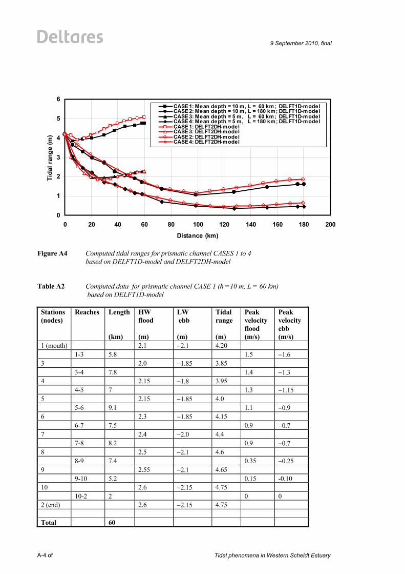
A-4 of
9 September 2010, final
Tidal phenomena in Western Scheldt Estuary
0
1
2
3
4
5
6
0 20 40 60 80 100 120 140 160 180 200
Distance (km)
Tida
l ran
ge (m
)
CASE 1: Mean depth = 10 m, L = 60 km; DELFT1D-modelCASE 2: Mean depth = 10 m, L = 180 km; DELFT1D-modelCASE 3: Mean depth = 5 m, L = 60 km; DELFT1D-modelCASE 4: Mean depth = 5 m, L = 180 km; DELFT1D-modelCASE 1: DELFT2DH-modelCASE 3: DELFT2DH-modelCASE 2: DELFT2DH-modelCASE 4: DELFT2DH-model
Figure A4 Computed tidal ranges for prismatic channel CASES 1 to 4 based on DELFT1D-model and DELFT2DH-model Table A2 Computed data for prismatic channel CASE 1 (h =10 m, L = 60 km) based on DELFT1D-model
Stations (nodes)
Reaches Length (km)
HW flood (m)
LW ebb (m)
Tidal range (m)
Peak velocity flood (m/s)
Peak velocity ebb (m/s)
1 (mouth) 2.1 −2.1 4.20 1-3 5.8 1.5 −1.6 3 2.0 −1.85 3.85 3-4 7.8 1.4 −1.3 4 2.15 −1.8 3.95 4-5 7 1.3 −1.15 5 2.15 −1.85 4.0 5-6 9.1 1.1 −0.9 6 2.3 −1.85 4.15 6-7 7.5 0.9 −0.7 7 2.4 −2.0 4.4 7-8 8.2 0.9 −0.7 8 2.5 −2.1 4.6 8-9 7.4 0.35 −0.25 9 2.55 −2.1 4.65 9-10 5.2 0.15 -0.10 10 2.6 −2.15 4.75 10-2 2 0 0 2 (end) 2.6 −2.15 4.75 Total 60

9 September 2010, final
Tidal phenomena in Western Scheldt Estuary
A-5
The DELFT2DH-model yields slightly larger tidal range values (10% to 15%). Reducing the water depth to h = 5 m (CASE 3) leads to reduction of the tidal range. However, the tidal range is slightly amplified in the landward half of the channel due to reflection. The DELFT2DH-model yields slightly larger tidal range values (15% to 20%). Increasing the length of the channel to 180 km (CASE 2 and CASE 4) also leads to reduction of the tidal range and wave reflection in the landward end section of the channel. Bottom friction increases for decreasing water depths resulting in smaller tidal ranges. The DELFT2DH-model yields significantly larger tidal range values at the end of the channel (180 km) compared with the DELFT1D-model. Due to non-linear effects the HW-values increase more in landward direction than the LW values, see Table A2 (CASE 1). These effects also lead to an increase of the mean water level in the landward part of the channel (about 0.2 m at the end for CASE 1) compared to mean sea level at the mouth. The increase of mean water level is also present in the Scheldt Estuary (about 0.15 m near Bath; Pieters, 2002). Figures A5 and A6 show the computed tidal range for CASE 1 and CASE 3 (short channel, L = 60 km) based on the DELFT1D-model and the Analytical model with reflection and without reflection. Two methods have been used to estimate the ‘linearized’ friction coefficient: based on u o and on 0.5 u o (see Table A3). The latter value yields a better estimate of the channel-averaged friction value (less friction). Including reflection at the end of the channel, the Analytical model produces amplification for CASE 1 (h= 10 m) which is in agreement with the numerical results. The Analytical model does not yield good results in the landward part of the channel (30 to 60 km) for CASE 3 (h= 5 m) when reflection is neglected. The computed values in section 0-30 km are systematically too large.
0
1
2
3
4
5
6
0 10 20 30 40 50 60
Distance (km)
Tida
l ran
ge (m
)
DELFT1D-model (phi=2 hours)DELFT2DH-modelAnalytical w ithout reflection; friction based on UoAnalytical w ithout reflection; friction based on 0.5UoAnalytical w ith reflection; friction based on UoAnalytical w ith reflcetion; friction based on 0.5Uo
CASE 1: h=10 m; L= 60 km
Figure A5 Computed tidal range for prismatic channel CASE 1 (DELFT1D and Analytical model)

A-6 of
9 September 2010, final
Tidal phenomena in Western Scheldt Estuary
0
0.5
1
1.5
2
2.5
3
3.5
4
4.5
0 10 20 30 40 50 60
Distance (km)
Tida
l ran
ge (m
)
DELFT1D-model (phi=1 hour)Analytical without reflection; friction based on UoAnalytical with reflection; friction based on UoAnalytical w ithout reflection; friction based on 0.5UoAnalytical w ith reflection; friction based on 0.5UoDELFT2DH-model
Case 3: h= 5 m; L= 60 km
Figure A6 Computed tidal range for prismatic channel CASE 3 (DELFT1D and Analytical model) Figures A7 and A8 show the computed tidal range for CASE 2 and CASE 4 (long channel, L = 180 km) based on the DELFT1D-model and the Analytical model with and without reflection. Including reflection, the Analytical model yields reasonable values over the whole length of the channel. Reflection at the end of the channel is of minor importance for CASE 4 (long and shallow channel).
0
0.5
1
1.5
2
2.5
3
3.5
4
4.5
0 20 40 60 80 100 120 140 160 180
Distance (km)
Tida
l ran
ge (m
)
DELFT1D-modelDELFT2DH-modelAnalytical w ithout reflection; friction based on UoAnalytical w ithout reflection; friction based on 0.5UoAnalytical w ith reflection; friction based on UoAnalytical w ith reflection; friction based on 0.5Uo
CASE 2: h= 10 m; L = 180 km
Figure A7 Computed tidal range for prismatic channel CASE 2 based on DELFT1D-model and Analytical model

9 September 2010, final
Tidal phenomena in Western Scheldt Estuary
A-7
0
0.5
1
1.5
2
2.5
3
3.5
4
4.5
0 20 40 60 80 100 120 140 160 180
Distance (km)
Tida
l ran
ge (m
)
DELFT1D-modelDELFT2DH-modelAnalytical w ithout reflection; friction based on UoAnalytical w ithout reflection; friction based on 0.5UoAnalytical w ith reflection; friction based on UoAnalytical w ith reflection; friction based on 0.5Uo
CASE 4: h= 5 m; L= 180 km
Figure A8 Computed tidal range for prismatic channel CASE 4 based on DELFT1D-model and Analytical model Table A3 Computed peak velocities and phase shift values at x= 0 km (prismatic channel) based
on analytical model
CASE Excluding Reflection Including Reflection Friction based on
u o Friction
based on 0.5 u o
Friction based on u o
Friction based on 0.5 u o
u o
(m/s)
ϕ u o
(m/s)
ϕ u o
(m/s)
ϕ u o
(m/s)
ϕ
1 1.35 32o 1.65 26o 1.65 34o 2.05 29o 2 1.35 32o 1.65 26o 1.30 32o 1.50 25o 3 1.30 39o 1.65 36o 1.30 39o 1.75 36o 4 1.30 39o 1.65 36o 1.30 39o 1.65 36o
Figures A9 to A12 show the tidal range values and the mean water surface levels with respect to the mean sea level at x = 0 (mouth) based on the depth-averaged DELFT2DH-model. The effects of the inclusion of the non-linear terms can be clearly observed: a) HW larger than LW and 2) increase of the mean surface level. The results show: CASE 1: gradual increase of tidal range due to reflection, particularly HW; LW remains approximately constant; CASE 2: gradual decrease of tidal range up to x= 100 km due to bottom friction; increase of tidal range between x= 100 and 180 km due to reflection; CASE 3: gradual decrease of tidal range up to x= 20 km due to bottom friction; approximately constant
tidal range between x= 20 and 30 km; gradual increase of tidal range between x= 30 and 60 km due to reflection;
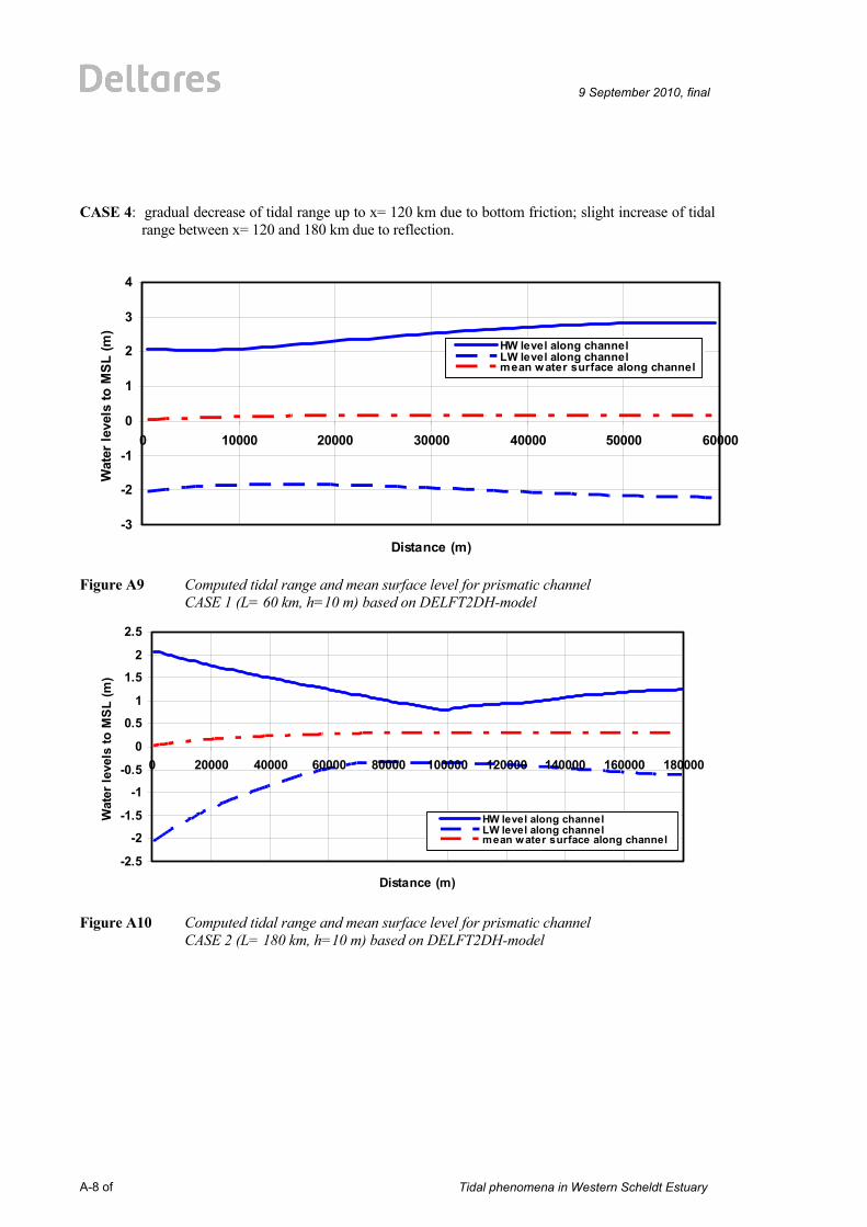
A-8 of
9 September 2010, final
Tidal phenomena in Western Scheldt Estuary
CASE 4: gradual decrease of tidal range up to x= 120 km due to bottom friction; slight increase of tidal
range between x= 120 and 180 km due to reflection.
-3
-2
-1
0
1
2
3
4
0 10000 20000 30000 40000 50000 60000
Distance (m)
Wat
er le
vels
to M
SL
(m)
HW level along channelLW level along channelmean water surface along channel
Figure A9 Computed tidal range and mean surface level for prismatic channel CASE 1 (L= 60 km, h=10 m) based on DELFT2DH-model
-2.5
-2
-1.5
-1
-0.5
0
0.5
1
1.5
2
2.5
0 20000 40000 60000 80000 100000 120000 140000 160000 180000
Distance (m)
Wat
er le
vels
to M
SL (m
)
HW level along channelLW level along channelmean water surface along channel
Figure A10 Computed tidal range and mean surface level for prismatic channel CASE 2 (L= 180 km, h=10 m) based on DELFT2DH-model

9 September 2010, final
Tidal phenomena in Western Scheldt Estuary
A-9
-2
-1.5
-1
-0.5
0
0.5
1
1.5
2
2.5
0 10000 20000 30000 40000 50000 60000
Distance (m)
Wat
er le
vels
to M
SL
(m)
HW level along channelLW level along channelmean water surface along channel
Figure A11 Computed tidal range and mean surface level for prismatic channel CASE 3 (L= 60 km, h=5 m) based on DELFT2DH-model
-2.5
-2
-1.5
-1
-0.5
0
0.5
1
1.5
2
2.5
0 20000 40000 60000 80000 100000 120000 140000 160000 180000
Distance (m)
Wat
er le
vels
to M
SL
(m)
HW level along channelLW level along channelmean water surface along channel
Figure A12 Computed tidal range and mean surface level for prismatic channel CASE 4 (L= 180 km, h=5 m) based on DELFT2DH-model

9 September 2010, final
Tidal phenomena in Western Scheldt Estuary
B-1
B Analytical and numerical results for converging tidal channels
The following cases are defined: CASE 1: Converging width over 60 km (width bo = 25000 m, bL=60 km= 2000 m), depth h= 10 m, ks= 0.05 m CASE 3: Converging width over 60 km (width bo = 25000 m, bL=60 km= 2000 m), depth h= 5 m, ks= 0.05 m CASE 2: Converging width over 60 km (width bo = 25000 m, bL=60 km= 2000 m) Constant width (prismatic) over 60 tot 180 km (b= 2000 m), depth h= 10 m, ks= 0.05 m CASE 4: Converging width over 60 km (width bo = 25000 m, bL=60 km= 2000 m) Constant width (prismatic) over 60 tot 180 km (b= 2000 m), depth h= 5 m, ks= 0.05 m CASE 5: Converging width over 180 km (width bo = 25000 m, bL=180 km= 19 m), depth h= 10 m, ks= 0.05 m CASE 6: Converging width over 180 km (width bo = 25000 m, bL=180 km= 19 m), depth h= 5 m, ks= 0.05 m with: bo= width at mouth, bL= width at end of channel, Lb= converging width length scale = 25000 m; see Figure B1 (width parameters of converging section 0 to 60 km are based on Scheldt Estuary data). The boundary conditions are: Mouth (x= 0): water level amplitude: η = η cos(ωt) with η = 2.1 m and ω = 2π/T, T = 12 hours, water level variation is represented by hourly values, Closed end (x = L): discharge Q = 0 m3/s The water depth is defined as the depth to mean sea level (MSL); tidal levels are defined to MSL.

B-2 of
9 September 2010, final
Tidal phenomena in Western Scheldt Estuary
Table B1 Computed data at mouth (x = 0) for CASES 1 to 6
CASE Maximum flood
velocity (m/s)
Maximum ebb velocity (m/s)
Maximum flood discharge (m3/s)
Maximum ebb discharge (m3/s)
Phase of velocity to water level (hours; degrees)
1 (L= 60 km) (h=10 m)
DELFT1D: 0.76 DELFT2DH: 0.83 ANAL. ex. reflection: 0.83 ANAL. inc. reflection: 1.35
0.70 0.72 0.83 1.35
190000 214000 207000 337500
160000 165000 207000 337500
2.4 hours (72o) 3 hours (90o) 2.6 hours (77o) 2.4 hours (72o)
2 (L= 180 km) (h=10 m)
DELFT1D: 0.70 DELFT2DH: 0.73 ANAL. ex. reflection: 0.83 ANAL. inc. reflection: 1.13
0.72 0.73 0.83 1.13
182000 192000 207000 282500
162000 172000 207000 282500
2.4 hours (72o) 2.7 hours (81o) 2.6 hours (77o) 2.5 hours (74o)
3 (L= 60 km) (h=5 m)
DELFT1D: 0.95 DELFT2DH: 0.99 ANAL. ex. reflection: 1.05 ANAL. inc. reflection: 1.35
1.15 1.24 1.05 1.35
148000 154000 134000 168750
132000 136000 134000 168750
1.8 hours (54o) 2.1 hours (63o) 2.0 hours (60o) 1.9 hours (58o)
4 (L= 180 km) (h= 5 m)
DELFT1D: 0.95 DELFT2DH: 0.97 ANAL. ex. reflection: 1.05 ANAL. inc. reflection: 1.48
1.12 1.15 1.05 1.48
144000 150000 134000 185000
122000 126000 134000 185000
1.8 hours (54o) 2.1 hours (63o) 2.0 hours (60o) 1.9 hours (57o)
5 (L= 180 km) (h= 10 m)
DELFT2DH: 0.82 ANAL. ex. reflection: 0.82 ANAL. inc. reflection: 1.37
0.81 0.82 1.37
215000 206000 342500
195000 206000 342500
2.5 hours (75o) 2.6 hours (77o) 2.4 hours (72o)
6 (L= 180 km) (h= 5 m)
DELFT2DH: 0.96 ANAL. ex. reflection: 1.07 ANAL. inc. reflection: 1.32
1.16 1.07 1.32
150000 133000 165000
125000 133000 165000
1.7 hours (51o) 2.0 hours (59o) 1.9 hours (58o)
Table B1 presents the computed results at the mouth (x= 0) of the estuary channel (width = 25000 km) based on the three models applied. The phase difference between the peak depth-averaged velocity and the peak water level (HW) is in the range of 2.4 to 3 hours for CASE 1, 2 and 5 (deep channels h= 10 m) and in the range of 1.8 to 2 hours for CASE 3, 4 and 6 (shallow channels h= 5 m). The discharge values at the mouth are within 15% to 20%.

9 September 2010, final
Tidal phenomena in Western Scheldt Estuary
B-3
Figure B1 Width of converging channel (CASES 1 to 6)
-15
-10
-5
0
5
10
15
0 10 20 30 40 50 60 70 80 90 100 110 120 130 140 150 160 170 180
Distance (km)
Wid
th (k
m)
CASE 2 and 4
-15
-10
-5
0
5
10
15
0 10 20 30 40 50 60Distance (km)
Wid
th (k
m)
CASE 1 and 3
-15
-10
-5
0
5
10
15
0 10 20 30 40 50 60 70 80 90 100 110 120 130 140 150 160 170 180
Distance (km)
Wid
th (k
m)
CASE 5 and 6

B-4 of
9 September 2010, final
Tidal phenomena in Western Scheldt Estuary
Figures B2 and B3 present computed water levels, velocities and discharges at x= 0 for CASES 1 and 3 of the DELFT2DH-model showing various non-linear effects:
• flood duration (5 to 5.5 hours) is smaller than ebb duration hour (6.5 to 7 hours); • maximum flood velocity is about equal to maximum ebb velocity for CASES 1 and 2 and
smaller for CASES 3 and 4 (Table B1); • maximum flood discharge occurs slightly later than maximum flood velocity; • maximum ebb discharge occurs earlier than maximum ebb velocity (continuity requires: 0∫tfl qflood
dt = tfl∫tebb qebb dt). The phase lead of the depth-averaged velocity and the discharge with respect to water level curve can be clearly observed. The time moments of the maximum velocity and the maximum discharge are slightly different. Figures B4 and B5 present computed water levels, velocities and discharges at x= 0 for CASES 5 and 6 of the DELFT2DH-model showing similar effects.
-3-2.8-2.6-2.4-2.2
-2-1.8-1.6-1.4-1.2
-1-0.8-0.6-0.4-0.2
00.20.40.60.8
11.21.41.61.8
22.22.42.62.8
3
72 78 84 90 96 102 108 114 120 126
Time (hours)
Wat
er le
vel t
o m
sl (m
) and
vel
ocity
(m/s
)
-300000
-260000
-220000
-180000
-140000
-100000
-60000
-20000
20000
60000
100000
140000
180000
220000
260000
300000
disc
harg
e (m
3/s)
Water levels (m) at x=0 Depth-averaged velocities (m/s) at x=0Discharge (m3/s) at x=0
Figure B2 Computed water levels, depth-averaged velocities and discharge at the mouth for
converging channel CASE 1 based on DELFT2DH-model

9 September 2010, final
Tidal phenomena in Western Scheldt Estuary
B-5
-3-2.8-2.6-2.4-2.2
-2-1.8-1.6-1.4-1.2
-1-0.8-0.6-0.4-0.2
00.20.40.60.8
11.21.41.61.8
22.22.42.62.8
3
72 78 84 90 96 102 108 114 120 126
Time (hours)
Wat
er le
vel t
o m
sl (m
) and
vel
ocity
(m/s
)
-300000
-260000
-220000
-180000
-140000
-100000
-60000
-20000
20000
60000
100000
140000
180000
220000
260000
300000
disc
harg
e (m
3/s)
Water levels (m) at x=0Depth-averaged velocities (m/s) at x=0Discharge (m3/s) at x=0
Figure B3 Computed water levels, depth-averaged velocities and discharge at the mouth for converging channel CASE 3 based on DELFT2DH-model
-3-2.8-2.6-2.4-2.2
-2-1.8-1.6-1.4-1.2
-1-0.8-0.6-0.4-0.2
00.20.40.60.8
11.21.41.61.8
22.22.42.62.8
3
72 78 84 90 96 102 108 114 120 126
Time (hours)
Wat
er le
vel t
o m
sl (m
) and
vel
ocity
(m/s
)
-300000
-200000
-100000
0
100000
200000
300000
Disc
harg
e (m
3/s)
Water levels (m) at x= 0 mDepth-averaged velocities (m/s) at x= 0 mDischarge (m3/s) at x= 0 m
Figure B4 Computed water levels, depth-averaged velocities and discharge at the mouth for
converging channel CASE 5 based on DELFT2DH-model

B-6 of
9 September 2010, final
Tidal phenomena in Western Scheldt Estuary
-3-2.8-2.6-2.4-2.2
-2-1.8-1.6-1.4-1.2
-1-0.8-0.6-0.4-0.2
00.20.40.60.8
11.21.41.61.8
22.22.42.62.8
3
72 78 84 90 96 102 108 114 120 126
Time (hours)
Wat
er le
vel t
o m
sl (m
) and
vel
ocity
(m/s
)
-300000
-200000
-100000
0
100000
200000
300000
Dis
char
ge (m
3/s)
Water levels (m) at x= 0 mDepth-averaged velocities (m/s) at x= 0 mDischarge (m3/s) at x= 0 m
Figure B5 Computed water levels, depth-averaged velocities and discharge at the mouth for
converging channel CASE 6 based on DELFT2DH-model Figure B6 shows the computed tidal range values for CASES 1 to 6 based on the numerical model results (DELFT2DH). Amplification can be observed for a deep channel with a converging width over the entire channel length (CASE 1 and 5). Wave reflection does occur at the landward end section. Slight damping of the tidal range due to bottom friction can be observed for a shallow channel with a fully converging width. The damping of the tidal range is considerably larger if the width remains constant after 60 km (CASE 2 and CASE 4).
0
2
4
6
8
10
12
0 20 40 60 80 100 120 140 160 180 200
Distance (km)
Tida
l ran
ge (m
)
CASE 2: Mean depth = 10 m, L = 180 km; converging-constant widthCASE 4: Mean depth = 5 m, L = 180 km; converging-constant widthCASE 5: Mean depth = 10 m, L = 180 km; converging w idthCASE 6: Mean depth = 5 m, L = 180 km; converging w idthCASE 1: Mean depth = 10 m, L= 60 km, converging w idthCASE 3: Mean depth = 5 m, L= 60 km; converging w idth
h= 10 m
h=5 m
h= 10 m
h= 5 m
h= 10 m
h= 5 m
Figure B6 Tidal range values for converging channel CASES 1 to 6 based on numerical model
results

9 September 2010, final
Tidal phenomena in Western Scheldt Estuary
B-7
0
1
2
3
4
5
6
7
8
9
10
0 10 20 30 40 50 60
Distance (km)
Tida
l ran
ge (m
)
CASE 1: DELFT1D-model (h=10 m)CASE 3: DELFT1D-model (h=5 m)CASE 1: Analytical model (no reflection)CASE 1: DELFT2DH-modelCASE 3: DELFT2DH-modelCASE 1: Analytical model (w ith reflection)CASE 3: Analytical model (no reflection)CASE 3: Analytical model (w ith reflection) CASE 1; h= 10 m
CASE 3; h= 5 m
Figure B7 Computed tidal ranges for converging channel CASES 1 and 3 (L = 60 km; h=10 and 5
m) based on DELFT1D-model, DELFT2DH-model and Analytical model Figure B7 shows the computed tidal range along the channel for CASES 1 and 3 based on the three models applied. The Analytical model has been applied with reflection and without reflection (see Table 3.2). All models predict amplification due to the width convergence and reflection for CASE 1 with a short channel length of 60 km and a mean water depth of h = 10 m. Inclusion of reflection leads to a strong over-estimation of the tidal range in the landward half of the channel (about 30 km). Linear friction is too small to generate sufficient friction to damp the wave in this part of the channel. Exclusion of reflection yields almost perfect agreement of the Analytical model results with the numerical model results. The computed wave propagation speed according to the analytical model is about 17 m/s (without reflection) and about 12 m/s (with reflection) for CASE 1, which is significantly larger than the classical value of c= (g ho)0.5 ≅ 10 m/s. The tidal range at the landward end of the channel (L = 60 km) is larger than that at the mouth (amplification). The measured tidal range data of the Scheldt Estuary also shows amplification over a length of about 100 km. Table B2 Computed data for converging channel CASE 1 and CASE 3 (L = 60 km, h =10 m and
5 m) based on DELFT1D-model
Stations (nodes)
Reach Width (km)
Length (km)
HW flood (m) h=10m h= 5 m
LW ebb (m) h=10 m h= 5 m
Tidal range (m) h=10 m 5 m
Peak velocity flood (m/s) h=10 m h= 5 m
Peak velocity ebb (m/s) h=10 m 5 m
1 (mouth) 25 2.1 2.1
−2.1 −2.1
4.20 4.20
1-3 1.5 0.76 0.96 −0.70 −1.15 3 24.7 2.1
2.08 −2.1 −1.95
4.20 4.03
3-4 2.5 0.75 0.96 −0.68 −1.10 4 22.2 2.12
2.06 −2.11 −1.78
4.23 3.84
4-5 3 0.75 0.90 −0.67 −1.0 5 19.3 2.15
2.03 −2.12 −1.71
4.27 3.74

B-8 of
9 September 2010, final
Tidal phenomena in Western Scheldt Estuary
5-6 3.5 0.75 0.95 −0.66 −0.95 6 16.8 2.17
1.94 −2.13 1.61
4.30 3.55
6-7 4 0.75 0.95 −0.64 −0.87 7 14.3 2.20
1.99 −2.15 −1.49
4.35 3.48
7-8 3.5 0.75 0.95 −0.60 −0.75 8 12.5 2.24
2.02 −2.16 −1.49
4.40 3.51
8-9 3 0.74 0.95 −0.58 −0.75 9 10.9 2.28
2.05 −2.18 −1.49
4.46 3.54
9-10 4 0.73 0.97 −0.56 −0.74 10 9.2 2.32
2.07 −2.21 −1.46
4.53 3.53
10-11 5.5 0.70 0.96 −0.50 −0.70 11 7.5 2.38
2.10 −2.32 −1.39
4.70 3.49
11-12 7.5 0.62 0.90 −0.45 −0.62 12 5.5 2.45
2.18 −2.42 −1.42
4.87 3.60
12-13 7.5 0.53 0.82 −0.37 −0.51 13 4 2.52
2.37 −2.51 −1.48
5.03 3.83
13-14 8 0.32 0.56 −0.23 −0.33 14 3 2.55
2.48 −2.55 −1.50
5.10 3.98
14-15 5.5 0.11 0.20 −0.08 −0.12 15 2 2.56
2.52 −2.56 −1.50
5.12 5.04
15-2 1.5 0 0 0 0 2 (end) 2 2.54
2.59 −2.55 −1.47
5.09 5.06
Reducing the water depth to h = 5 m (CASE 3) leads to a significant reduction of the tidal range over the section 0 to 40 km, see Figure B7. However, the numerical model results show that the tidal range is slightly amplified in the landward section of the channel (x= 40 to 60 km) due to reflection. The DELFT2DH-model yields slightly larger tidal range values (15%) than the DELFT1D-model. The Analytical model can represent the reflection effects at the end of the channel reasonably well, but the computed tidal range in the section 25 to 55 km is much too small. Neglecting the reflection effect, the computed tidal range in the landward section based on the analytical model is much too small. The tidal range values and peak depth-averaged values along the channel of CASE 1 and 3 are also shown in Table B2 based on DELFT1D-model. The maximum value of HW is larger than the maximum value of LW and the peak velocities of flood and ebb are different due to non-linear effects. Figures B8 and B9 show the computed tidal range values along the long channel (L = 180 km) for CASES 2 and 4 based on the three models applied. The DELFT1D-model and the DELFT2DH-model show good agreement (within 10% to 15%). The tidal range remains approximately constant up to x = 50 km for CASE 2 and then gradually decreases to about 2 m at x = 120 km due to bottom friction; reflection can be observed at the landward end of the channel resulting in a tidal range of about 2.5 m at the end of the channel. Wave damping due to bottom friction dominates in CASE 4 with a small depth of 5 m.

9 September 2010, final
Tidal phenomena in Western Scheldt Estuary
B-9
0
1
2
3
4
5
6
0 20 40 60 80 100 120 140 160 180
Distance (km)
Tida
l ran
ge (m
)
DELFT1D-modelDELFT2DH-modelAnalytical (Q not equal at x=60 km; no reflection at end)Analytical (Q not equal at x=60 km; w ith reflection at end)Analytical (Q equal at x=60 km; no reflection at end)Analytical (Q equal at x=60 km; w ith reflection at end)
CASE 2; h= 10 m
Figure B8 Computed tidal ranges for converging-prismatic channel CASE 2 (L = 180 km; h=10
m) based on DELFT1D-model, DELFT2DH-model and Analytical model
0
0.5
1
1.5
2
2.5
3
3.5
4
4.5
0 20 40 60 80 100 120 140 160 180
Distance (km)
Tida
l ran
ge (m
)
DELFT1D-model (h=5 m)DELFT2DH-modelAnalytical (Q not equal at x=60 km; no reflection at end)Analytical (Q equal at x=60 km; no reflection at end)Analytical (Q not equal at x=60 km; with reflection at end)Analytical (Q equal at x=60 km; w ith reflection at end)
CASE 4; h= 5 m
Figure B9 Computed tidal ranges for converging-prismatic channel CASE 4 (L = 180 km; h= 5
m) based on DELFT1D-model, DELFT2DH-model and Analytical model To apply the Analytical model for the long, converging-prismatic channel, the channel has been divided into two seperate channels (converging section 0 to 60 km and prismatic (constant width) section of 60 to 180 km). The output of the water level and the discharge at the end of the converging section (x= 60 km) has been used as input for the prismatic section. This approach is referred to as ‘discharge equal’ at x= 60 km in Figures B8 and B9. The Analytical model results are also shown for another approach in which only the water level is equal at x= 60 km, but the discharge is not equal at x = 60 km. The differences of the results of both approaches show the effect of uncertainties in the matching conditions at the connection point at x= 60 km. As can be observed, the Analytical model cannot represent the numerical model results with sufficient accuray for CASE 2. The Analytical model results for CASE 4 are considerably better, but the tidal range values are significantly under-predicted at the landward end section of the channel (110 to 180 km).

B-10 of
9 September 2010, final
Tidal phenomena in Western Scheldt Estuary
0
2
4
6
8
10
12
0 20 40 60 80 100 120 140 160 180
Distance (km)
Tida
l ran
ge (m
)
DELFT2DH-modelAnalytical model (no reflection at end; friction based on Uo)Analytical model (w ith reflection at end; friction based on Uo)
CASE 5; h= 10 m
Figure B10 Computed tidal ranges for converging channel CASE 5 (L = 180 km; h= 10 m) based on DELFT2DH-model and Analytical model
0
0.5
1
1.5
2
2.5
3
3.5
4
4.5
0 20 40 60 80 100 120 140 160 180
Distance (km)
Tida
l ran
ge (m
)
DELFT2DH-modelAnalytical model (no reflection at end; friction based on Uo)Analytical model (w ith reflection at end; friction based on Uo)Analytical model(no reflection at end; friction based on 0.55 Uo)Analytical model (w ith reflection at end; friction based on 0.7Uo)
CASE 6; h= 5 m
Figure B11 Computed tidal ranges for converging channel CASE 6 (L = 180 km; h= 5 m) based on DELFT2DH-model and Analytical model Figures B10 and B11 show the computed tidal range along the long channel (L = 180 km) for CASES 5 and 6 with a converging channel over the entire length of the channel based on the DELFT2DH-model and the Analytical model. The Analytical model results without reflection for CASE 5 are in good agreement with the numerical model results, except in the landward end section of the channel (140 to 180 km). The Analytical model with reflection for CASE 5 yields values which are substantially too small in the middle part of the channel. The effect of the reflected wave is too strong at the landward end of the channel. The Analytical model yields values for CASE 6 which are much too small if the friction coefficient is based on the peak velocity at the mouth. The results for CASE 6 can be improved by using a smaller (channel-averaged) characteristic peak velocity, see Figure B11.

9 September 2010, final
Tidal phenomena in Western Scheldt Estuary
B-11
Comparing the numerical model results for a long channel (180 km) with a fully converging width and converging-constant width, the following features can be observed (Figure B12):
• the tidal range increases significantly (amplification) for a deep, fully converging channel (CASE 1 and 5) due to the dominant funneling effect; reflection at the landward end of the channel contributes also to the amplication effect;
• the tidal range is damped due to bottom friction for a shallow, fully converging channel (CASE 6) and for a deep and shallow converging-prismatic channel (CASE 2 and 4);
• the tidal range is considerably larger in a fully converging channel (CASE 6) than that in a converging-prismatic channel (CASE 2 and 4), both for a deep and shallow channel (prismatic channel has constant width);
• the tidal range in the entrance section between x = 0 and 20 km is not much affected by the exponential or exponential-constant planform of the channel between 60 and 180 km.
0
2
4
6
8
10
12
0 20 40 60 80 100 120 140 160 180 200
Distance (km)
Tida
l ran
ge (m
)
CASE 2: Mean depth = 10 m, L = 180 km; converging-constant w idthCASE 4: Mean depth = 5 m, L = 180 km; converging-constant w idthCASE 5: Mean depth = 10 m, L = 180 km; converging w idthCASE 6: Mean depth = 5 m, L = 180 km; converging w idth
h= 10 m
h=5 m
h= 10 m
h= 5 m
Figure B12 Comparison of computed tidal ranges for converging-prismatic channel and converging
channel based on DELFT1D-model Figures B13 to B18 show the tidal range values and the mean water surface levels with respect to the mean sea level at x = 0 (mouth) based on the depth-averaged DELFT2DH-model. Analytical model results are shown for CASE 3 and CASE 6. The Analytical linearized model with reflection included does not represent the non-linear effects resulting in a symmetrical solution with respect to MSL. The increase of the mean water surface level can be included by using Equation (4.16), see Section 4.7 on non-linear effects. Differences between both models are up to 1 m, particularly for HW. The effects of the inclusion of the non-linear terms by the numerical model can be clearly observed: a) the maximum value of HW is larger than the maximum value of LW and b) increase of the mean surface level. The results show: CASE 1: gradual and symmetric increase of tidal range due to shoaling and reflection; CASE 2: slight increase of tidal range up to x = 50 km due to shoaling; decrease of the tidal range
between x= 50 and 110 km due to bottom friction; slight increase between x = 110 and 180 km due to reflection; the maximum value of HW is larger than the maximum value of LW due to non-linear effects;
CASE 3: slight decrease of the tidal range up to x = 30 km, mainly due to decrease of LW due to bottom friction; slight increase of the tidal range between x = 30 and 60 km due to reflection; overall the tidal range remains fairly constant;

B-12 of
9 September 2010, final
Tidal phenomena in Western Scheldt Estuary
CASE 4: HW remains approximately constant up to 50 km; LW decreases significantly up to 50 km
due to bottom friction; gradual decrease of tidal range up to x = 130 km due to bottom friction; slight increase of tidal range between x = 130 and 180 km due to reflection;
CASE 5: HW shows a strong increase along the channel and reflection at the landward end of the channel; LW increases slightly along the channel; the mean water level remains fairly constant;
CASE 6: HW remains fairly constant up to 160 km and increases strongly between 160 and 180 km due to reflection; LW decreases slightly up to 80 km and remains fairly constant between 80 and 180 km; the mean water level increases significantly.
Summarizing all results for converging channels, it can be concluded that: Short and deep converging channel: convergence is dominant in entrance section and
reflection in landward section of the channel; tidal ranges increases (amplication);
Short and shallow converging channel: bottom friction is dominant in entrance section;
reflection is dominant in landward end section; tidal range decreases in middle, but increases near end;
Long and deep converging-prismatic channel: convergence is dominant in entrance section; bottom friction is dominant in middle section and reflection in landward end section; tidal range decreases in prismatic section; Long and shallow converging-prismatic channel: bottom friction is dominant in major part of the
channel; tidal range decreases almost completely; Long and deep converging channel: convergence is dominant in entire channel; reflection occurs in landward end section; tidal range increases significantly; Long and shallow converging channel: bottom friction is slightly dominant in entire
channel; reflection occurs in landward end section; tidal range desceases slightly in landward direction

9 September 2010, final
Tidal phenomena in Western Scheldt Estuary
B-13
-3-2.5
-2-1.5
-1-0.5
00.5
11.5
22.5
3
0 10000 20000 30000 40000 50000 60000
Distance (m)
Wat
er le
vels
to M
SL
(m)
HW level along channelLW level along channelmean water surface along channel
Figure B13 Computed tidal range and mean surface level for converging channel CASE 1 (L= 60 km, h=10 m) based on DELFT2DH-model
-3-2.5
-2-1.5
-1-0.5
00.5
11.5
22.5
3
0 20000 40000 60000 80000 100000 120000 140000 160000 180000
Distance (m)
Wat
er le
vels
to M
SL (m
)
HW level along channelLW level along channelmean water surface along channel
Figure B14 Computed tidal range and mean surface level for converging channel CASE 2 (L= 180 km, h=10 m) based on DELFT2DH-model

B-14 of
9 September 2010, final
Tidal phenomena in Western Scheldt Estuary
-4-3.5
-3-2.5
-2-1.5
-1-0.5
00.5
11.5
22.5
33.5
4
0 10000 20000 30000 40000 50000 60000
Distance (m)
Wat
er le
vels
to M
SL
(m)
HW level along channel numerical modelLW level along channel numerical modellmean water surface along channel numerical modelHW level analytical modelLW level analytical model
Figure B15 Computed tidal range and mean surface level for converging channel CASE 3 (L= 60 km, h= 5 m) based on DELFT2DH-model
-3-2.5
-2-1.5
-1-0.5
00.5
11.5
22.5
3
0 20000 40000 60000 80000 100000 120000 140000 160000 180000
Distance (m)
Wat
er le
vels
to M
SL (m
)
HW level along channelLW level along channelmean surface level along channel
Figure B16 Computed tidal range and mean surface level for converging channel CASE 4 (L= 180 km, h= 5 m) based on DELFT2DH-model

9 September 2010, final
Tidal phenomena in Western Scheldt Estuary
B-15
-6
-4
-2
0
2
4
6
8
0 20000 40000 60000 80000 100000 120000 140000 160000 180000
Distance (m)
Wat
er le
vels
to M
SL
(m)
HW along channelLW along channelmean surface level along channel
Figure B17 Computed tidal range and mean surface level for converging channel CASE 5 (L= 180 km, h= 10 m) based on DELFT2DH-model
-4
-3
-2
-1
0
1
2
3
4
0 20000 40000 60000 80000 100000 120000 140000 160000 180000
Distance (m)
Wat
er le
vels
to M
SL
(m)
HW along channel numerical modelLW along channel numerical modelmean surface level along channel numerical model HW along channel analytical modelLW along channel analytical model
Figure B18 Computed tidal range and mean surface level for converging channel CASE 6 (L= 180 km, h= 5 m) based on DELFT2DH-model 4.3.4 Comparison of prismatic and converging channels Comparing the numerical model results of short (60 km) and long (180 km) prismatic and converging channels, the following features can be observed: Deep channel (water depth h = 10 m), see Figure B19
• the tidal range is largest in converging channels due to the funneling effect; the tidal range is almost 10 m in a fully converging channel with a length of 180 m; reflection is important in the landward end section;
• the tidal range in a short prismatic channel is dominated by reflection and is almost equal to that in a short converging channel;
• the tidal range in a long prismatic channel is dominated by bottom friction resulting in a large decrease of the tidal range; thus the tidal range in prismatic channels is largely controlled by the channel length;

B-16 of
9 September 2010, final
Tidal phenomena in Western Scheldt Estuary
• the tidal range between x = 0 and 40 km is not much affected by the total channel length, except for a long prismatic channel;
• the tidal range in a long converging channel is much larger than in a long prismatic channel (factor 5);
Shallow channel (water depth h = 5 m), see Figure B20
• the tidal range in short and long converging channels is substantially larger than that in short and long prismatic channels; the convergence or funneling effect is much more important than the reflection effect and the bottom friction effect;
• the tidal range in short channels is significantly affected by reflection at the landward end of the channel;
• the tidal range in a long converging channel shows a gradual decrease due to bottom friction, but the tidal range increases again in the landward end section due to reflection.
0
2
4
6
8
10
12
0 20 40 60 80 100 120 140 160 180 200
Distance (km)
Tida
l ran
ge (m
)
prismaticconverging
prismatic
Converging-prismatic
Water depth h= 10 m
converging
Figure B19 Comparison of computed tidal ranges for prismatic channel and converging channel (h=10 m); numerical model results

9 September 2010, final
Tidal phenomena in Western Scheldt Estuary
B-17
0
0.5
1
1.5
2
2.5
3
3.5
4
4.5
0 20 40 60 80 100 120 140 160 180 200
Distance (km)
Tida
l ran
ge (m
)
prismatic
prismatic
converging-prismatic
converging
converging
Water depth h = 5 m
Figure B20 Comparison of computed tidal ranges for prismatic channel and converging channel (h=5 m); numerical model results


