Tide induced piping risk assessed by transient groundwater flow M. P. M. Sanders 1 and J .S. Van der Schrier Royal Haskoning ABSTRACT Dutch dike and levee design codes provide a solid framework for the design of dikes and levees. One of the failure modes that have to be considered by these codes is ‘piping’. In the Netherlands, piping is usually checked under the assumption of stationary flow boundary conditions. Piping risk is assessed from the critical hydraulic gradient, using empirical relationships accounting for soil type, layering and particle size. The paper presents a case history of a dike design in a tidal environment. The tidal effects on the groundwater heads are assessed by transient groundwater flow analysis. The case concerns the design against piping through an overflow dike, which is part of a flood storage area. The area is located along the River Dijle between Antwerp and Mechelen (Belgium). The critical heads for the check of the piping risk were assessed by Plaxflow, a finite element code that is capable of carrying out transient groundwater flow analyses as well as steady state ones. In the analysis presented herein, the normal ground water fluctuations, which are strongly affected by tide, have firstly been modelled with Plaxflow as a calibration exercise. Once this had been done, the critical gradients were assessed under design conditions. The benefit of using a transient flow analysis for the verification of piping will be demonstrated in the paper. Based on the calculation results it could be demonstrated that in contrary to the stationary flow analysis no mitigating piping measures were required. Keywords: Dijle River, Dijle valley, piping, Sellmeijer, Bligh, transient groundwater flow, Plaxflow, tidal environment 1 Royal Haskoning, Postbus 151 – 6500 AD Nijmegen, the Netherlands. [email protected]1 INTRODUCTION When following the Dutch dike design codes [1,2] one of the failure modes to be assessed in a dike design is ‘piping’. Piping refers to the development of an erosion canal or flow pipe, through or beneath a dike. Such a flow pipe can develop in a cohesionless (sandy) water-bearing layer that is covered by a relatively impermeable cohesive (clayey) layer. Under a critical hydraulic gradient particle transport starts from the flow exit point. Sandy particles are taken by the flow and the resulting erosion canal migrates backwards at a continuously increasing speed until a full dike collapse develops. The principle is illustrated in Figure 1. Piping risk is usually assessed from the design hydraulic gradient using empirical relationships accounting for soil type and soil grading. The design hydraulic gradient is the ratio between the maximum head difference over the dike and the shortest groundwater flow path through the piping susceptible soil. Figure 1. Principle of the failure mode ‘piping’. [1] Clay Sand ∆H L
Transcript
Tide induced piping risk assessed by transient groundwater flow
M. P. M. Sanders1 and J .S. Van der Schrier Royal Haskoning
ABSTRACT
Dutch dike and levee design codes provide a solid framework for the design of dikes and levees. One of the failure modes that have to be considered by these codes is ‘piping’. In the Netherlands, piping is usually checked under the assumption ofstationary flow boundary conditions. Piping risk is assessed from the critical hydraulic gradient, using empirical relationshipsaccounting for soil type, layering and particle size. The paper presents a case history of a dike design in a tidal environment. Thetidal effects on the groundwater heads are assessed by transient groundwater flow analysis. The case concerns the design against piping through an overflow dike, which is part of a flood storage area. The area is located along the River Dijle betweenAntwerp and Mechelen (Belgium). The critical heads for the check of the piping risk were assessed by Plaxflow, a finite elementcode that is capable of carrying out transient groundwater flow analyses as well as steady state ones. In the analysis presentedherein, the normal ground water fluctuations, which are strongly affected by tide, have firstly been modelled with Plaxflow as a calibration exercise. Once this had been done, the critical gradients were assessed under design conditions. The benefit of using a transient flow analysis for the verification of piping will be demonstrated in the paper. Based on the calculation results it could be demonstrated that in contrary to the stationary flow analysis no mitigating piping measures were required. Keywords: Dijle River, Dijle valley, piping, Sellmeijer, Bligh, transient groundwater flow, Plaxflow, tidal environment
1 Royal Haskoning, Postbus 151 – 6500 AD Nijmegen, the Netherlands. [email protected]
1 INTRODUCTION
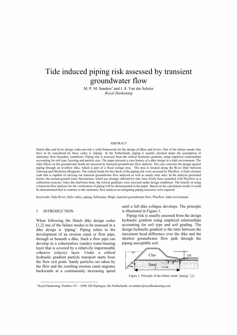
When following the Dutch dike design codes [1,2] one of the failure modes to be assessed in a dike design is ‘piping’. Piping refers to the development of an erosion canal or flow pipe, through or beneath a dike. Such a flow pipe can develop in a cohesionless (sandy) water-bearing layer that is covered by a relatively impermeable cohesive (clayey) layer. Under a critical hydraulic gradient particle transport starts from the flow exit point. Sandy particles are taken by the flow and the resulting erosion canal migrates backwards at a continuously increasing speed
until a full dike collapse develops. The principle is illustrated in Figure 1.
Piping risk is usually assessed from the design hydraulic gradient using empirical relationships accounting for soil type and soil grading. The design hydraulic gradient is the ratio between the maximum head difference over the dike and the shortest groundwater flow path through the piping susceptible soil.
Figure 1. Principle of the failure mode ‘piping’. [1]
Clay
Sand
∆H
L
The design hydraulic gradient is not easy to determine for the dikes in the Dijle valley, as the flow boundary conditions fluctuate strongly due to tidal water movements. The determination of the design hydraulic gradient by steady state flow analysis, using the extreme water levels as starting point may result in an over conservative dike design.
Royal Haskoning has been asked to design a flood storage area along the River Dijle. Following an initial appraisal, it was clear that a steady state analysis would result in a costly design. It was recognized that a transient flow analysis could be of benefit, as it might prove that an extensive dike improvement could be avoided.
The client was the Government of Belgium ‘Waterwegen en Zeekanaal NV, department Zeeschelde’.
In this paper, the adopted approach for the piping assessment based on transient flow analysis is presented and the results are discussed.
2 THE DIJLE PROJECT
A storm combined with high river discharge in the River Dijle result in a sudden rise of water level in the river that directly threatens the cities Antwerp and Mechelen. The Dijle project concerns the design of a large-scale flood storage area to hold water temporarily to reduce the water level in the river.
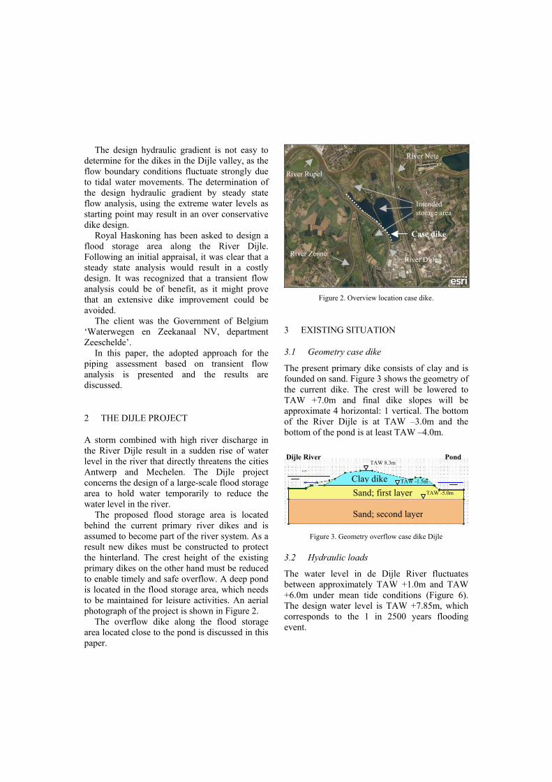
The proposed flood storage area is located behind the current primary river dikes and is assumed to become part of the river system. As a result new dikes must be constructed to protect the hinterland. The crest height of the existing primary dikes on the other hand must be reduced to enable timely and safe overflow. A deep pond is located in the flood storage area, which needs to be maintained for leisure activities. An aerial photograph of the project is shown in Figure 2.
The overflow dike along the flood storage area located close to the pond is discussed in this paper.
Figure 2. Overview location case dike.
3 EXISTING SITUATION
3.1 Geometry case dike
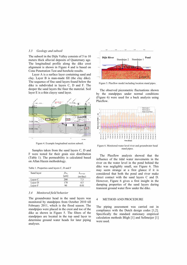
The present primary dike consists of clay and is founded on sand. Figure 3 shows the geometry of the current dike. The crest will be lowered to TAW +7.0m and final dike slopes will be approximate 4 horizontal: 1 vertical. The bottom of the River Dijle is at TAW –3.0m and the bottom of the pond is at least TAW –4.0m.
Figure 3. Geometry overflow case dike Dijle
3.2 Hydraulic loads
The water level in de Dijle River fluctuates between approximately TAW +1.0m and TAW +6.0m under mean tide conditions (Figure 6). The design water level is TAW +7.85m, which corresponds to the 1 in 2500 years flooding event.
Case dike
River Dijle
Intended storage area
River Nete
River Zenne
River Rupel
Dijle River Pond
Sand; second layer
Clay dikeSand; first layer
TAW -1.5m
TAW -5.0m
TAW 8.3m
3.3 Geology and subsoil
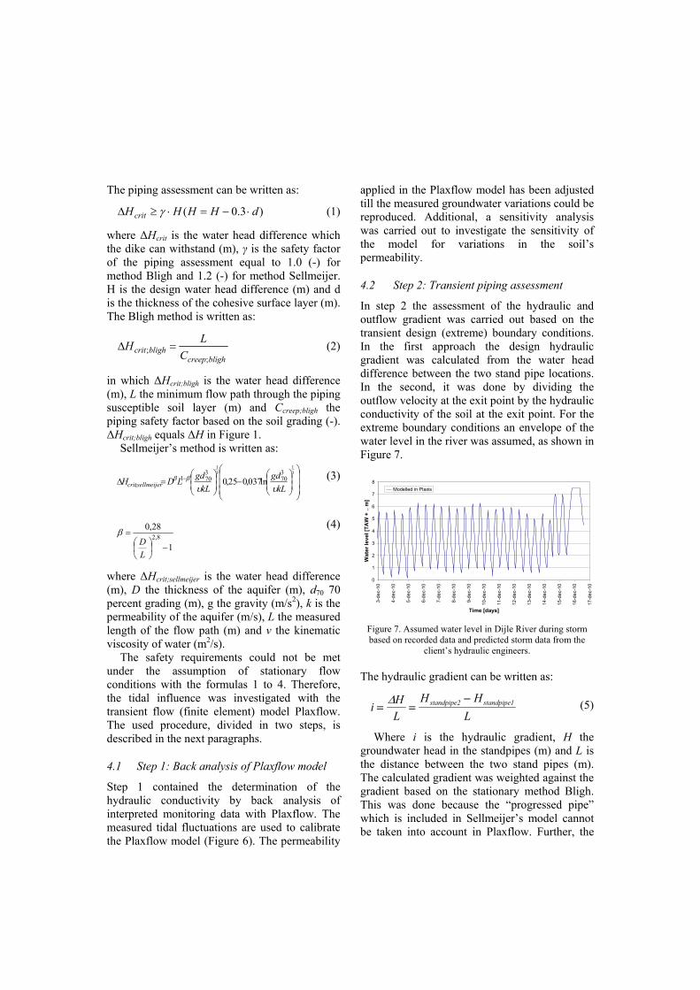
The subsoil in the Dijle Valley consists of 5 to 10 meters thick alluvial deposits of Quaternary age. The longitudinal profile along the dike crest alignment is shown in Figure 4 and is based on Cone Penetration Test and borehole results.
Layer A is a surface layer containing sand and clay. Layer B is man-made fill (the clay dike). The sequence of fine sand layers found below the dike is subdivided in layers C, D and F. The deeper the sand layers the finer the material. Soil layer E is a thin clayey sand layer.
Figure 4. Example longitudinal section subsoil.
Samples taken from the sand layers C, D and
F were tested for their grain size distribution (Table 1). The permeability is calculated based on Allan Hazen methodology.
Table 1. Properties sand layers C, D and F
Sand layer D70 [µm]
kaverage (m/day)
Layer C 200 7.3 Layer D 170 4.5 Layer F 90 0.01
3.4 Monitored field behavior
The groundwater head in the sand layers was monitored by standpipes from October 2010 till February 2011, which is the flood season. The standpipes were placed in the crest and toe of the dike as shown in Figure 5. The filters of the standpipes are located in the top sand layer to determine ground water heads for later piping analyses.
Figure 5. Plaxflow model including location stand pipes. The observed piezometric fluctuations shown
by the standpipes under normal conditions (Figure 6) were used for a back analysis using Plaxflow.
0
1
2
3
4
5
6
7
28-n
ov-1
0
29-n
ov-1
0
30-n
ov-1
0
1-de
c-10
2-de
c-10
3-de
c-10
4-de
c-10
5-de
c-10
6-de
c-10
7-de
c-10
8-de
c-10
9-de
c-10
10-d
ec-1
0
11-d
ec-1
0
12-d
ec-1
0
13-d
ec-1
0
14-d
ec-1
0
15-d
ec-1
0
16-d
ec-1
0
17-d
ec-1
0
18-d
ec-1
0
19-d
ec-1
0
20-d
ec-1
0
21-d
ec-1
0
Time [Days]
Wat
er le
vel [
TAW
+ ..
m]
Stand pipe 1Stand pipe 2Water level River
Figure 6. Monitored water level river and groundwater head
stand pipes. The Plaxflow analysis showed that the
influence of the tidal water movements in the river on the water level in the pond behind the dike was negligibly small, see Figure 6. This may seem strange at a first glance if it is considered that both the pond and river make direct contact with the sand layers C and D. However, Figure 6 gives a first insight in the damping properties of the sand layers during transient ground water flow under the dike.
4 METHOD AND PROCEDURE
The piping assessment was carried out in compliance with the Dutch design codes [1,2]. Specifically the standard stationary empirical calculation methods Bligh [1] and Sellmeijer [1] were used.
Layer B
Layer D
Layer F
Layer C
Layer E
Layer ATAW 0 m
TAW -5 m
TAW -10m
TAW -15m
Dijle River Pond Standpipe 2 Standpipe 1
Layer F
Layer C/DClay dike
The piping assessment can be written as:
)3.0( dHHHHcrit ⋅−=⋅≥∆ γ (1)
where ∆Hcrit is the water head difference which the dike can withstand (m), γ is the safety factor of the piping assessment equal to 1.0 (-) for method Bligh and 1.2 (-) for method Sellmeijer. H is the design water head difference (m) and d is the thickness of the cohesive surface layer (m). The Bligh method is written as:
blighcreep
blighcrit CLH
;; =∆ (2)
in which ∆Hcrit;bligh is the water head difference (m), L the minimum flow path through the piping susceptible soil layer (m) and Ccreep;bligh the piping safety factor based on the soil grading (-). ∆Hcrit;bligh equals ∆H in Figure 1.
Sellmeijer’s method is written as:
−
=∆ −
31
31
370
3701
; ln037,025,0kL
gdkL
gdLDH sellmeijercrit υυββ (3)
1
28,08,2
−
=
LD
β (4)
where ∆Hcrit;sellmeijer is the water head difference (m), D the thickness of the aquifer (m), d70 70 percent grading (m), g the gravity (m/s2), k is the permeability of the aquifer (m/s), L the measured length of the flow path (m) and ν the kinematic viscosity of water (m2/s).
The safety requirements could not be met under the assumption of stationary flow conditions with the formulas 1 to 4. Therefore, the tidal influence was investigated with the transient flow (finite element) model Plaxflow. The used procedure, divided in two steps, is described in the next paragraphs.
4.1 Step 1: Back analysis of Plaxflow model
Step 1 contained the determination of the hydraulic conductivity by back analysis of interpreted monitoring data with Plaxflow. The measured tidal fluctuations are used to calibrate the Plaxflow model (Figure 6). The permeability
applied in the Plaxflow model has been adjusted till the measured groundwater variations could be reproduced. Additional, a sensitivity analysis was carried out to investigate the sensitivity of the model for variations in the soil’s permeability.
4.2 Step 2: Transient piping assessment
In step 2 the assessment of the hydraulic and outflow gradient was carried out based on the transient design (extreme) boundary conditions. In the first approach the design hydraulic gradient was calculated from the water head difference between the two stand pipe locations. In the second, it was done by dividing the outflow velocity at the exit point by the hydraulic conductivity of the soil at the exit point. For the extreme boundary conditions an envelope of the water level in the river was assumed, as shown in Figure 7.
0
1
2
3
4
5
6
7
8
3-de
c-10
4-de
c-10
5-de
c-10
6-de
c-10
7-de
c-10
8-de
c-10
9-de
c-10
10-d
ec-1
0
11-d
ec-1
0
12-d
ec-1
0
13-d
ec-1
0
14-d
ec-1
0
15-d
ec-1
0
16-d
ec-1
0
17-d
ec-1
0
Time [days]
Wat
er le
vel [
TAW
+ ..
m]
Modelled in Plaxis
Figure 7. Assumed water level in Dijle River during storm based on recorded data and predicted storm data from the
client’s hydraulic engineers.
The hydraulic gradient can be written as:
L
HHLHi standpipe1standpipe2 −==
∆ (5)
Where i is the hydraulic gradient, H the groundwater head in the standpipes (m) and L is the distance between the two stand pipes (m). The calculated gradient was weighted against the gradient based on the stationary method Bligh. This was done because the “progressed pipe” which is included in Sellmeijer’s model cannot be taken into account in Plaxflow. Further, the
hydraulic gradient determined using Sellmeijer for the stationary boundary conditions was higher than the gradient of Bligh method. This meant that in the Dijle project, the Bligh method was a more conservative approach.
The Bligh gradient is based on the d50 of the concerning sand layer and is in this case [1]:
067.01511
;===
BlighcreepCi (6)
The d50 of the piping susceptible soils are in between 150 and 210 µm which relates in accordance with Bligh to Ccreep;Bligh = 15.
The outflow gradient is the exit velocity divided by the permeability of the sand layer.
kvi = (7)
Where v is the exit velocity (m/s) and k is the permeability (m/s) of the piping susceptible sand layer. The outflow gradient was measured up to the gradient based on the method Bligh as well.
5 CALCULATION RESULTS
The results of the design methods are discussed below on the basis of the steps described above.
5.1 Permeability resulting from ground investigation and Plaxflow back analysis
The results of the permeability analysis are shown in Table 2. The results are based on the particle size distribution and the Plaxflow back analysis. The table shows that the Plaxflow permeability results fit very well with the permeability assessed from particle size distributions by Allan Hazen.
Table 2. Permeability results
Method kaverage layer C (m/day)
kaverage layer D (m/day)
kaverage layer F (m/day)
Grading of sand samples 7.3 4.5 0.01
Plaxflow analysis 8 5 0.01
5.2 Transient piping assessment
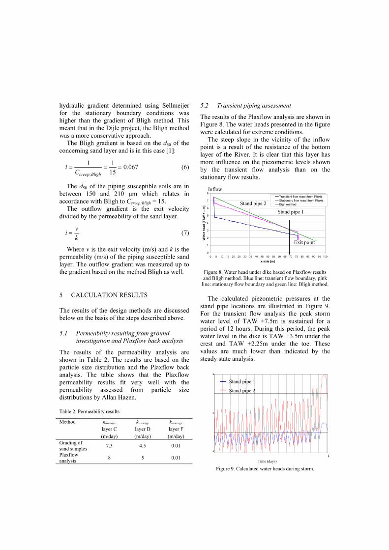
The results of the Plaxflow analysis are shown in Figure 8. The water heads presented in the figure were calculated for extreme conditions.
The steep slope in the vicinity of the inflow point is a result of the resistance of the bottom layer of the River. It is clear that this layer has more influence on the piezometric levels shown by the transient flow analysis than on the stationary flow results.
Transient flow result from PlaxisStationary flow result from PlaxisBigh method
Figure 8. Water head under dike based on Plaxflow results and Bligh method. Blue line: transient flow boundary, pink
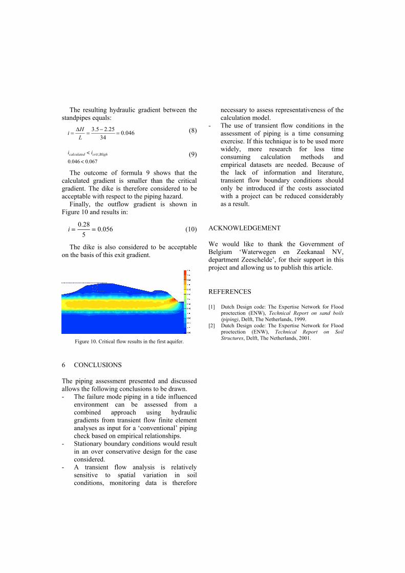
line: stationary flow boundary and green line: Bligh method. The calculated piezometric pressures at the
stand pipe locations are illustrated in Figure 9. For the transient flow analysis the peak storm water level of TAW +7.5m is sustained for a period of 12 hours. During this period, the peak water level in the dike is TAW +3.5m under the crest and TAW +2.25m under the toe. These values are much lower than indicated by the steady state analysis.
Head
[day]14131211109876543210
Hea
d [m
]
3,485
2,485
1,485
Figure 9. Calculated water heads during storm.
Stand pipe 2 Stand pipe 1
Inflow
Exit point
Time (days)
2.5m
3.5m
1.5m
Head
Stand pipe 2
Stand pipe 1
10 12 14
The resulting hydraulic gradient between the standpipes equals:
3.5 2.25 0.04634
HiL∆ −
= = = (8)
067.0046.0
;
<
< Blighcritcalculated ii (9)
The outcome of formula 9 shows that the calculated gradient is smaller than the critical gradient. The dike is therefore considered to be acceptable with respect to the piping hazard.
Finally, the outflow gradient is shown in Figure 10 and results in:
056.0528.0
==i (10)
The dike is also considered to be acceptable on the basis of this exit gradient.
Figure 10. Critical flow results in the first aquifer.
6 CONCLUSIONS
The piping assessment presented and discussed allows the following conclusions to be drawn. - The failure mode piping in a tide influenced
environment can be assessed from a combined approach using hydraulic gradients from transient flow finite element analyses as input for a ‘conventional’ piping check based on empirical relationships.
- Stationary boundary conditions would result in an over conservative design for the case considered.
- A transient flow analysis is relatively sensitive to spatial variation in soil conditions, monitoring data is therefore
necessary to assess representativeness of the calculation model.
- The use of transient flow conditions in the assessment of piping is a time consuming exercise. If this technique is to be used more widely, more research for less time consuming calculation methods and empirical datasets are needed. Because of the lack of information and literature, transient flow boundary conditions should only be introduced if the costs associated with a project can be reduced considerably as a result.
ACKNOWLEDGEMENT
We would like to thank the Government of Belgium ‘Waterwegen en Zeekanaal NV, department Zeeschelde’, for their support in this project and allowing us to publish this article.
REFERENCES
[1] Dutch Design code: The Expertise Network for Flood proctection (ENW), Technical Report on sand boils (piping), Delft, The Netherlands, 1999.
[2] Dutch Design code: The Expertise Network for Flood proctection (ENW), Technical Report on Soil Structures, Delft, The Netherlands, 2001.