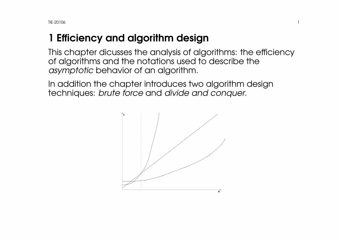
TIE-20106 1 1 Efficiency and algorithm design This chapter dicusses the analysis of algorithms: the efficiency of algorithms and the notations used to describe the asymptotic behavior of an algorithm. In addition the chapter introduces two algorithm design techniques: brute force and divide and conquer. t n
Transcript
TIE-20106 1
1 Efficiency and algorithm designThis chapter dicusses the analysis of algorithms: the efficiencyof algorithms and the notations used to describe theasymptotic behavior of an algorithm.
In addition the chapter introduces two algorithm designtechniques: brute force and divide and conquer.
t
n
TIE-20106 2
1.1 Asymptotic notationsIt is occasionally important to know the exact time it takes toperform a certain operation (in real time systems for example).
Most of the time it is enough to know how the running time ofthe algorithm changes as the input gets larger.• The advantage: the calculations are not tied to a given
processor, architecture or a programming language.• In fact, the analysis is not tied to programming at all but can
be used to describe the efficiency of any behaviour thatconsists of successive operations.
TIE-20106 3
• The time efficiency analysis is simplified by assuming that alloperations that are independent of the size of the inputtake the same amount of time to execute.• Furthermore, the amount of times a certain operation is
done is irrelevant as long as the amount is constant.•We investigate how many times each row is executed
during the execution of the algorithm and add the resultstogether.
TIE-20106 4
• The result is further simplified by removing any constantcoefficients and lower-order terms.⇒ This can be done since as the input gets large enoughthe lower-order terms get insigficant when compared to theleading term.⇒ The approach naturally doesn’t produce reliable resultswith small inputs. However, when the inputs are small,programs usually are efficient enough in any case.• The final result is the efficiency of the algorithm and is
denoted it with the greek alphabet theta, Θ.
f (n) = 23n2 + 2n + 15⇒ f ∈ Θ(n2)
f (n) = 12n lg n + n⇒ f ∈ Θ(n lg n)
TIE-20106 5
Example 1: addition of the elements in an array
1 for i := 1 to A.length do2 sum := sum + A[i]
• if the size of the array A is n, line 1 is executed n + 1 times• line 2 is executed n times• the running time increases as n gets larger:
n time = 2n + 1
1 3
10 21
100 201
1000 2001
10000 20001
• notice how the value of n dominates the running time
TIE-20106 6
• let’s simplify the result as described earlier by taking awaythe constant coefficients and the lower-order terms:
f (n) = 2n + 1⇒ n
⇒ we get f ∈ Θ(n) as the result
⇒ the running time depends linearly on the size of the input.
TIE-20106 7
Example 2: searching from an unsorted array
1 for i := 1 to A.length do2 if A[i] = x then3 return i
• the location of the searched element in the array affectsthe running time.• the running time depends now both on the size of the input
and on the order of the elements⇒ we must separately handle the best-case, worst-caseand average-case efficiencies.
TIE-20106 8
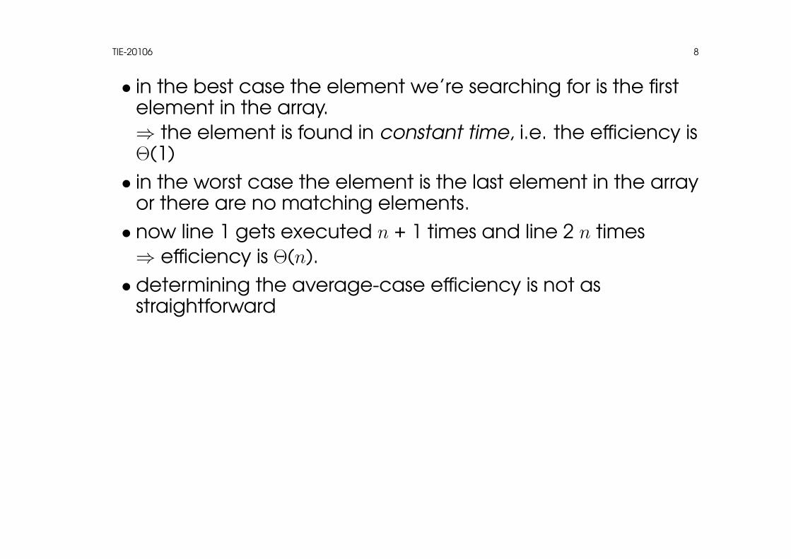
• in the best case the element we’re searching for is the firstelement in the array.⇒ the element is found in constant time, i.e. the efficiency isΘ(1)• in the worst case the element is the last element in the array
or there are no matching elements.• now line 1 gets executed n + 1 times and line 2 n times⇒ efficiency is Θ(n).• determining the average-case efficiency is not as
straightforward
TIE-20106 9
• first we must make some assumptions on the average,typical inputs:
– the probability p that the element is in the array is(0 ≤ p ≤ 1)
– the probability of finding the first match in each positionin the array is the same
•we can find out the average amount of comparisons byusing the probabilities• the probability that the element is not found is 1 - p, and we
must make n comparisons• the probability for the first match occuring at the index i, isp/n, and the amount of comparisons needed is i• the number of comparisons is:
[1 · pn
+ 2 · pn
+ · · · + i · pn· · · + n · p
n] + n · (1− p)
TIE-20106 10
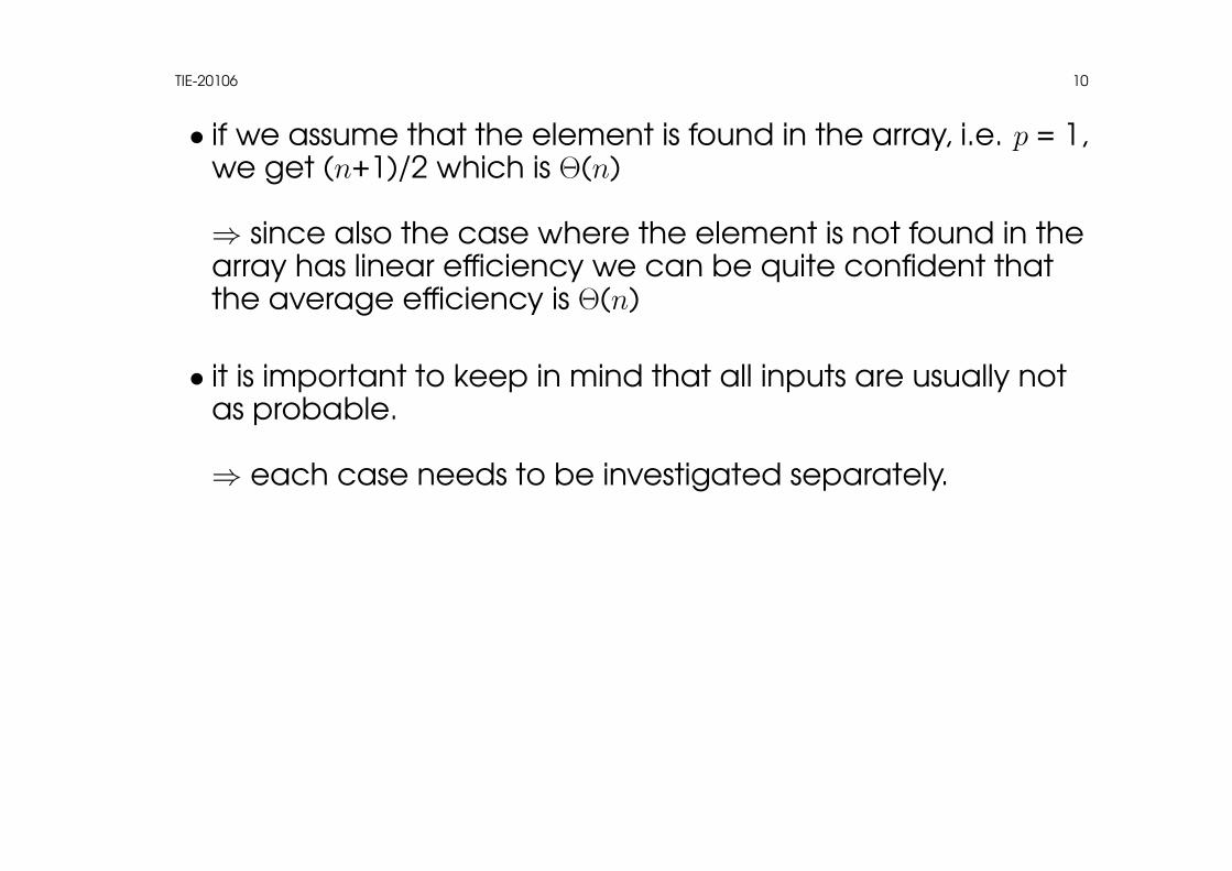
• if we assume that the element is found in the array, i.e. p = 1,we get (n+1)/2 which is Θ(n)
⇒ since also the case where the element is not found in thearray has linear efficiency we can be quite confident thatthe average efficiency is Θ(n)
• it is important to keep in mind that all inputs are usually notas probable.
⇒ each case needs to be investigated separately.
TIE-20106 11
Example 3: finding the common element in two arrays1 for i := 1 to A.length do2 for j := 1 to B .length do3 if A[i] = B[j] then4 return A[i]
• line 1 is executed 1 – (n + 1) times• line 2 is executed 1 – (n · (n + 1)) times• line 3 is executed 1 – (n · n) times• line 4 is executed at most once
TIE-20106 12
• the algorithm is fastest when the first element of both arraysis the same⇒ the best case efficiency is Θ(1)• in the worst case there are no common elements in the
arrays or the last elements are the same⇒ the efficiency is 2n2 + 2n + 1 = Θ(n2)
• on average we can assume that both arrays need to beinvestigated approximately half way through.⇒ the efficiency is Θ(n2) (or Θ(nm) if the arrays are ofdifferent lengths)
TIE-20106 13
1.2 Algorithm Design Technique: Brute ForceThe most straightforward algorithm design technique coveredon the course is brute force.• initially the entire input is unprocessed• the algorithm processes a small piece of the input on each
round⇒ the amount of processed data gets larger and theamount of unprocessed data gets smaller• finally there is no unprocessed data and the algorithm halts
These types of algorithms are easy to implement and workefficiently on small inputs.
TIE-20106 14
The Insertion-Sort seen earlier is a “brute force” algorithm.
• initially the entire array is (possibly) unsorted• on each round the size of the sorted range in the beginning
of the array increases by one element• in the end the entire array is sorted
TIE-20106 15
INSERTION-SORT
INSERTION-SORT(A) (input in array A)1 for j := 2 to A.length do (move the limit of the sorted range)2 key := A[j] (handle the first unsorted element)3 i := j − 14 while i > 0 and A[i] > key do(find the correct location of the new element)5 A[i + 1] := A[i] (make room for the new element)6 i := i− 17 A[i + 1] := key (set the new element to it’s correct location)
• line 1 is executed n times• lines 2 and 3 are executed n - 1 times• line 4 is executed at least n - 1 and at most (2 + 3 + 4 + · · · +n - 2) times• lines 5 and 6 are executed at least 0 and at most (1 + 2 + 3
+ 4 + · · · + n - 3) times
TIE-20106 16
• in the best case the entire array is already sorted and therunning time of the entire algorithm is at least Θ(n)
• in the worst case the array is in a reversed order. Θ(n2) timeis used• once again determining the average case is more difficult:• let’s assume that out of randomly selected element pairs
half is in an incorrect order in the array
⇒ the amount of comparisons needed is half the amount ofthe worst case where all the element pairs were in anincorrect order
⇒ the average-case running time is the worst-case runningtime divided by two: [(n - 1)n]/ 4 = Θ(n2)
TIE-20106 17
1.3 Algorithm Design Technique: Divide andConquerWe’ve earlier seen the brute force algorithm design techniqueand the algorithm INSERTION-SORT as an example of it.
Now another technique called divide and conquer isintroduced. It is often more efficient than the brute forceapproach.
• the problem is divided into several subproblems that are likethe original but smaller in size.• small subproblems are solved straightforwardly• larger subproblems are further divided into smaller units• finally the solutions of the subproblems are combined to get
the solution to the original problem
Let’s get back to the claim made earlier about the complexitynotation not being fixed to programs and take an everyday,concrete example
TIE-20106 18
Example: finding the false goldcoin
• The problem is well-known from logic problems.•We have n gold coins, one of which is false. The false coin
looks the same as the real ones but is lighter than the others.We have a scale we can use and our task is to find the falsecoin.•We can solve the problem with Brute Force by choosing a
random coin and by comparing it to the other coins one ata time.⇒ At least 1 and at most n - 1 weighings are needed. Thebest-case efficiency is Θ(1) and the worst and average caseefficiencies are Θ(n).• Alternatively we can always take two coins at random and
weigh them. At most n/2 weighings are needed and theefficiency of the solution is still the same.
TIE-20106 19
The same problem can be solved moreefficiently with divide and conquer:
• Divide the coins into the two pans onthe scales. The coins on the heavierside are all authentic, so they don’tneed to be investigated further.•Continue the search similarly with the
lighter half, i.e. the half that con-tains the false coin, until there is onlyone coin in the pan, the coin that weknow is false.
possible false ones genuine for sure
• The solution is recursive and the base case is the situationwhere there is only one possible coin that can be false.
TIE-20106 20
• The amount of coins on each weighing is 2 to the power ofthe amount of weighings still required: on the highest levelthere are 2weighings coins, so based on the definition of thelogarithm:
2weighings = n⇒ log2n = weighings
•Only log2n weighings is needed, which is significantly fewerthan n/2 when the amount of coins is large.⇒ The complexity of the solution is Θ(lg n) both in the bestand the worst-case.
TIE-20106 21
1.4 QUICKSORT
Let’s next cover a very efficient sorting algorithm QUICKSORT.
QUICKSORT is a divide and conquer algorithm.
The division of the problem into smaller subproblems• Select one of the elements in the array as a pivot, i.e. the
element which partitions the array.•Change the order of the elements in the array so that all
elements smaller or equal to the pivot are placed before itand the larger elements after it.•Continue dividing the upper and lower halves into smaller
subarrays, until the subarrays contain 0 or 1 elements.
TIE-20106 22
Smaller subproblems:• Subarrays of the size 0 and 1 are already sorted
Combining the sorted subarrays:
• The entire (sub) array is automatically sorted when its upperand lower halves are sorted.– all elements in the lower half are smaller than the
elements in the upper half, as they should be
QUICKSORT-algorithmQUICKSORT(A, p, r)1 if p < r then (do nothing in the trivial case)2 q := PARTITION(A, p, r) (partition in two)3 QUICKSORT(A, p, q − 1) (sort the elements smaller than the pivot)4 QUICKSORT(A, q + 1, r) (sort the elements larger than the pivot)
TIE-20106 23
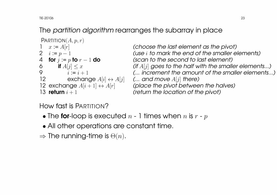
The partition algorithm rearranges the subarray in placePARTITION(A, p, r)
1 x := A[r] (choose the last element as the pivot)2 i := p− 1 (use i to mark the end of the smaller elements)4 for j := p to r − 1 do (scan to the second to last element)6 if A[j] ≤ x (if A[j] goes to the half with the smaller elements...)9 i := i + 1 (... increment the amount of the smaller elements...)12 exchange A[i]↔ A[j] (... and move A[j] there)12 exchange A[i + 1]↔ A[r] (place the pivot between the halves)13 return i + 1 (return the location of the pivot)
How fast is PARTITION?• The for-loop is executed n - 1 times when n is r - p• All other operations are constant time.⇒ The running-time is Θ(n).
TIE-20106 24
Determining the running-time of QUICKSORT is more difficultsince it is recursive. Therefore the equation for its running timewould also be recursives.
Finding the recursive equation is, however, beyond the goalsof this course so we’ll settle for a less formal approach
• As all the operations of QUICKSORT except PARTITION and therecursive call are constant time, let’s concentrate on thetime used by the instances of PARTITION.
1 1
1 11
n
n
n
1
1
11
12 2n − n − 1
n − n − 1
TIE-20106 25
• The total time is the sum of the running times of the nodes inthe picture abowe.• The execution is constant time for an array of size 1.• For the other the execution is linear to the size of the array.⇒ The total time is Θ(the sum of the numbers of the nodes).
TIE-20106 26
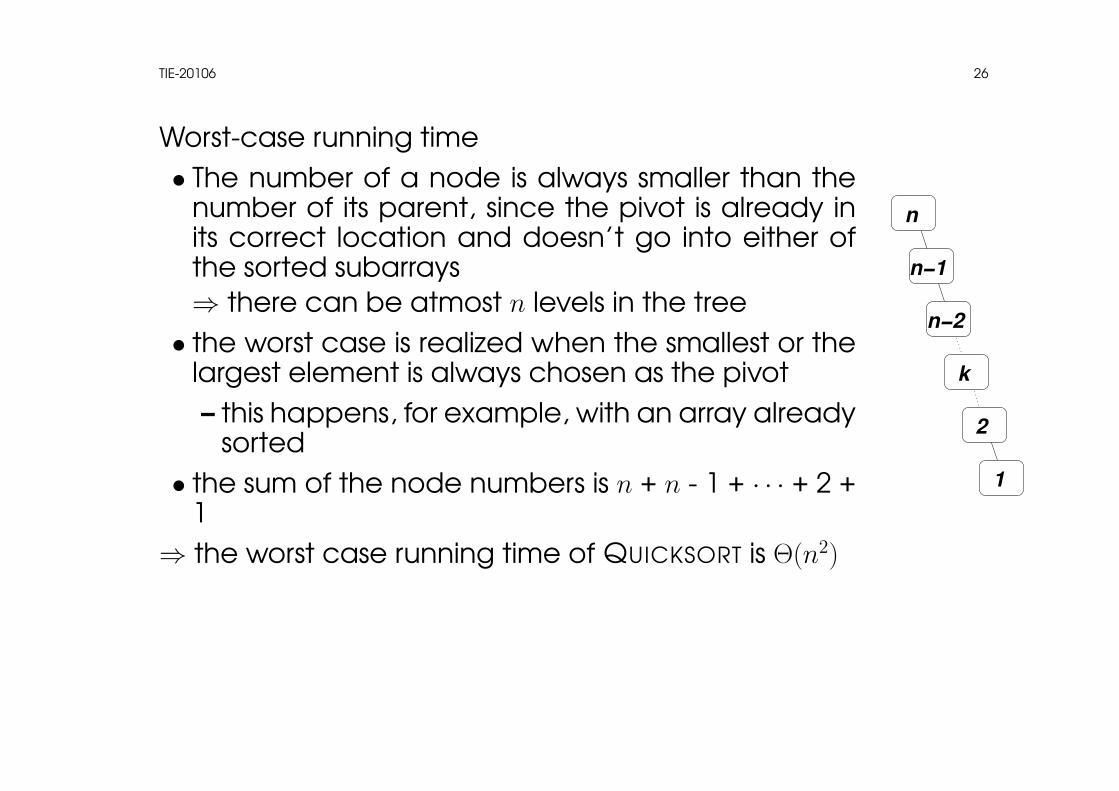
Worst-case running time• The number of a node is always smaller than the
number of its parent, since the pivot is already inits correct location and doesn’t go into either ofthe sorted subarrays⇒ there can be atmost n levels in the tree• the worst case is realized when the smallest or the
largest element is always chosen as the pivot– this happens, for example, with an array already
sorted• the sum of the node numbers is n + n - 1 + · · · + 2 +
1⇒ the worst case running time of QUICKSORT is Θ(n2)
n−1
n−2
k
2
1
n
TIE-20106 27
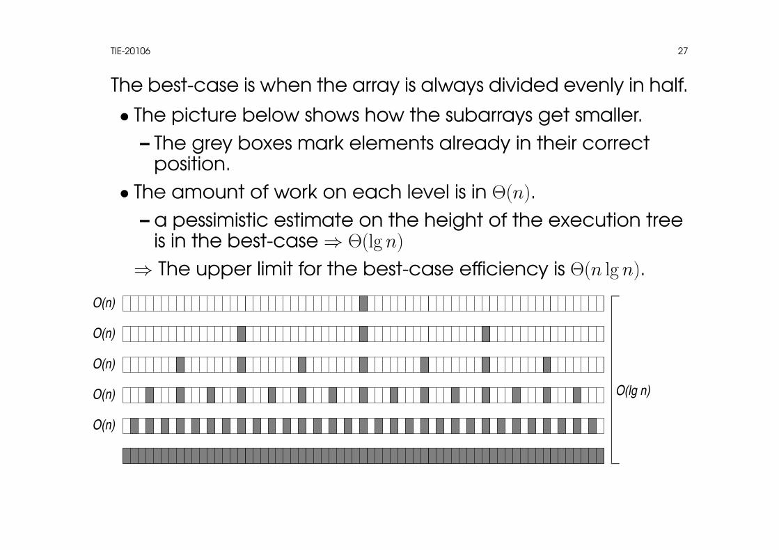
The best-case is when the array is always divided evenly in half.
• The picture below shows how the subarrays get smaller.– The grey boxes mark elements already in their correct
position.• The amount of work on each level is in Θ(n).
– a pessimistic estimate on the height of the execution treeis in the best-case⇒ Θ(lg n)
⇒ The upper limit for the best-case efficiency is Θ(n lg n).
O(lg n)
O(n)
O(n)
O(n)
O(n)
O(n)
TIE-20106 28
The best-case and the worst-case efficiencies of QUICKSORTdiffer significantly.
• It would be interesting to know the average-caserunning-time.• Analyzing it is beyond the goals of the course but it has
been shown that if the data is evenly distributed its averagerunning-time is Θ(n lg n).• Thus the average running-time is quite good.
TIE-20106 29
An unfortunate fact with QUICKSORT is that its worst-caseefficiency is poor and in practise the worst-case situation isquite probable.• It is easy to see that there can be situations where the data
is already sorted or almost sorted.⇒ A way to decrease the risk of the systematic occurence ofthe worst-case situation’s likelyhood is needed.
Randomization has proved to be quite efficient.
TIE-20106 30
Advantages and disadvantages of QUICKSORT
Advantages:• sorts the array very efficiently in average
– the average-case running-time is Θ(n lg n)
– the constant coefficient is small• requires only a constant amount of extra memory• if well-suited for the virtual memory environment
Disadvantages:• the worst-case running-time is Θ(n2)
•without randomization the worst-case input is far toocommon• the algorithm is recursive⇒ the stack uses extra memory• instability
TIE-20106 31
1.5 Algorithm Design Technique: RandomizationRandomization is one of the design techniques of algorithms.
• A pathological occurence of the worst-case inputs can beavoided with it.• The best-case and the worst-case running-times don’t
usually change, but their likelyhood in practise decreases.• Disadvantageous inputs are exactly as likely as any other
inputs regardless of the original distribution of the inputs.• The input can be randomized either by randomizing it
before running the algorithm or by embedding therandomization into the algorithm.
– the latter approach usually gives better results– often it is also easier than preprocessing the input.
TIE-20106 32
• Randomization is usually a good idea when– the algorithm can continue its execution in several ways– it is difficult to see which way is a good one– most of the ways are good– a few bad guesses among the good ones don’t make
much damage• For example, QUICKSORT can choose any element in the
array as the pivot– besides the almost smallest and the almost largest
elements, all other elements are a good choise– it is difficult to guess when making the selection whether
the element is almost the smallest/largest– a few bad guesses now and then doesn’t ruin the
efficiency of QUICKSORT
⇒ randomization can be used with QUICKSORT
TIE-20106 33
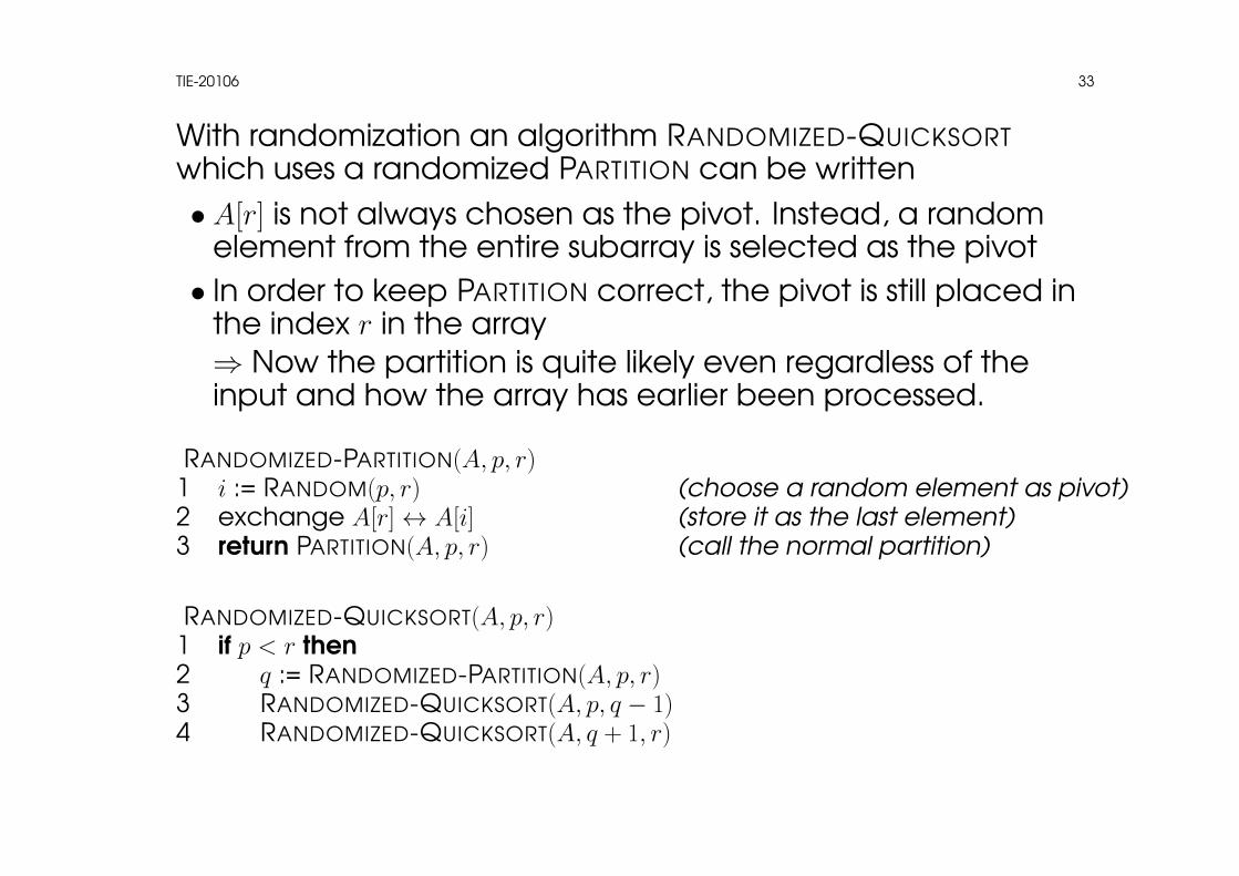
With randomization an algorithm RANDOMIZED-QUICKSORTwhich uses a randomized PARTITION can be written• A[r] is not always chosen as the pivot. Instead, a random
element from the entire subarray is selected as the pivot• In order to keep PARTITION correct, the pivot is still placed in
the index r in the array⇒ Now the partition is quite likely even regardless of theinput and how the array has earlier been processed.
RANDOMIZED-PARTITION(A, p, r)1 i := RANDOM(p, r) (choose a random element as pivot)2 exchange A[r]↔ A[i] (store it as the last element)3 return PARTITION(A, p, r) (call the normal partition)
RANDOMIZED-QUICKSORT(A, p, r)1 if p < r then2 q := RANDOMIZED-PARTITION(A, p, r)3 RANDOMIZED-QUICKSORT(A, p, q − 1)4 RANDOMIZED-QUICKSORT(A, q + 1, r)
TIE-20106 34
The running-time of RANDOMIZED-QUICKSORT is Θ(n lg n) onaverage just like with normal QUICKSORT.• However, the assumption made in analyzing the
average-case running-time that the pivot-element is thesmallest, the second smallest etc. element in the subarraywith the same likelyhood holds for RANDOMIZED-QUICKSORTfor sure.• This holds for the normal QUICKSORT only if the data is evenly
distributed.⇒ RANDOMIZED-QUICKSORT is better than the normal QUICKSORTin general
TIE-20106 35
QUICKSORT can be made more efficient with other methods:• An algorithm efficient with small inputs (e.g.INSERTIONSORT)
can be used to sort the subarrays.– they can also be left unsorted and in the end sort the
entire array with INSERTIONSORT
• The median of three randomly selected elements can beused as the pivot.• It’s always possible to use the median as the pivot.
TIE-20106 36
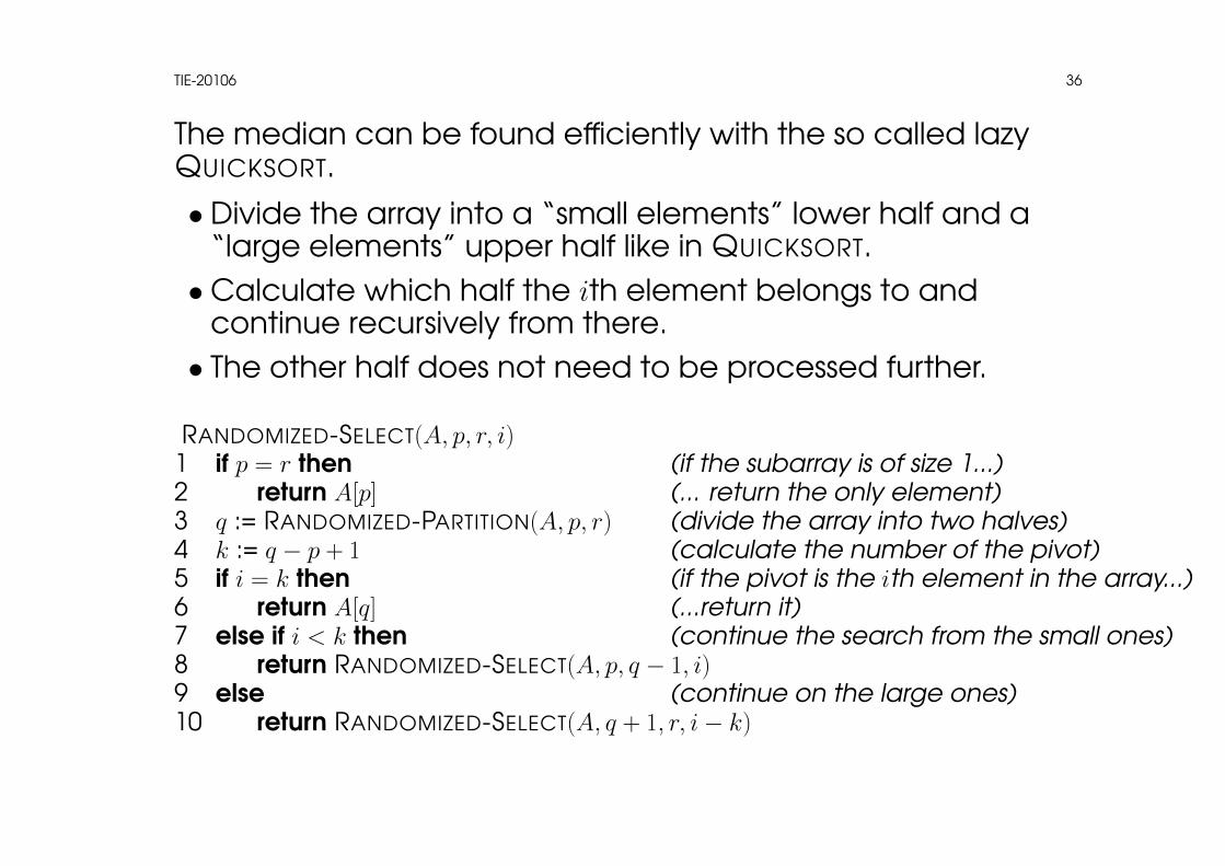
The median can be found efficiently with the so called lazyQUICKSORT.
• Divide the array into a “small elements” lower half and a“large elements” upper half like in QUICKSORT.•Calculate which half the ith element belongs to and
continue recursively from there.• The other half does not need to be processed further.
RANDOMIZED-SELECT(A, p, r, i)1 if p = r then (if the subarray is of size 1...)2 return A[p] (... return the only element)3 q := RANDOMIZED-PARTITION(A, p, r) (divide the array into two halves)4 k := q − p + 1 (calculate the number of the pivot)5 if i = k then (if the pivot is the ith element in the array...)6 return A[q] (...return it)7 else if i < k then (continue the search from the small ones)8 return RANDOMIZED-SELECT(A, p, q − 1, i)9 else (continue on the large ones)10 return RANDOMIZED-SELECT(A, q + 1, r, i− k)
TIE-20106 37
The lower-bound for the running-time of RANDOMIZED-SELECT:• Again everything else is constant time except the call of
RANDOMIZED-PARTITION and the recursive call.• In the best-case the pivot selected by
RANDOMIZED-PARTITION is the ith element and the executionends.• RANDOMIZED-PARTITION is run once for the entire array.⇒ The algorithm’s best case running-time is Θ(n).
The upper-bound for the running-time of RANDOMIZED-SELECT:
• RANDOMIZED-PARTITION always ends up choosing the smallestor the largest element and the ith element is left in thelarger half.• the amount of work is decreased only by one step on each
level of recursion.
⇒ The worst case running-time of the algorithm is Θ(n2).
TIE-20106 38
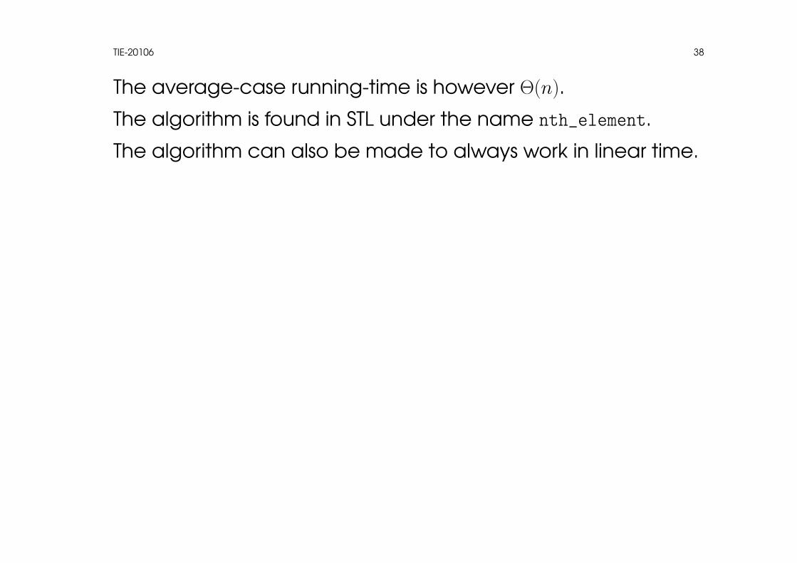
The average-case running-time is however Θ(n).
The algorithm is found in STL under the name nth_element.
The algorithm can also be made to always work in linear time.