Tilburg University Hedging Double Barriers with Singles Sbuelz, A. Publication date: 2000 Link to publication Citation for published version (APA): Sbuelz, A. (2000). Hedging Double Barriers with Singles. (CentER Discussion Paper; Vol. 2000-112). Tilburg: Finance. General rights Copyright and moral rights for the publications made accessible in the public portal are retained by the authors and/or other copyright owners and it is a condition of accessing publications that users recognise and abide by the legal requirements associated with these rights. - Users may download and print one copy of any publication from the public portal for the purpose of private study or research - You may not further distribute the material or use it for any profit-making activity or commercial gain - You may freely distribute the URL identifying the publication in the public portal Take down policy If you believe that this document breaches copyright, please contact us providing details, and we will remove access to the work immediately and investigate your claim. Download date: 19. Apr. 2020
Transcript
Tilburg University
Hedging Double Barriers with Singles
Sbuelz, A.
Publication date:2000
Link to publication
Citation for published version (APA):Sbuelz, A. (2000). Hedging Double Barriers with Singles. (CentER Discussion Paper; Vol. 2000-112). Tilburg:Finance.
General rightsCopyright and moral rights for the publications made accessible in the public portal are retained by the authors and/or other copyright ownersand it is a condition of accessing publications that users recognise and abide by the legal requirements associated with these rights.
- Users may download and print one copy of any publication from the public portal for the purpose of private study or research - You may not further distribute the material or use it for any profit-making activity or commercial gain - You may freely distribute the URL identifying the publication in the public portal
Take down policyIf you believe that this document breaches copyright, please contact us providing details, and we will remove access to the work immediatelyand investigate your claim.
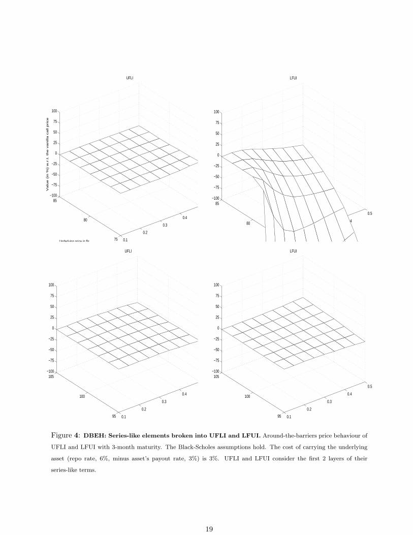
4 DBEH: Series-like elements broken into UFLI and LFUI. Around-the-barriers price be-
haviour of UFLI and LFUI with 3-month maturity. The Black-Scholes assumptions hold. The cost
of carrying the underlying asset (repo rate, 6%, minus asset’s payout rate, 3%) is 3%. UFLI and
LFUI consider the first 2 layers of their series-like terms. . . . . . . . . . . . . . . . . . . . . . 19
Barrier derivatives are the most liquid among the over-the-counter derivatives. Over-the-counter
markets have become stronger and stronger in the industry.1 European, continuously-monitored
barrier options are European options with an American feature. Option’s existence depends on
whether the underlying price breaches, before or at maturity, some prespecified levels, called barri-
ers. Given one barrier, single knockin options come to life and single knockouts expire if the barrier
is hit. Given two barriers, the double barrier corridor encompasses the initial underlying price.
Double knockins come to life and double knockouts expire if either barrier is hit. A portfolio of a
knockin and a knockout written on the same barriers and strike is equivalent to a vanilla option
with the same strike. Thus, one can focus on knockins only.
Barrier options are very popular because they are cheaper than their vanilla counterparts. This
endears them to hedge funds, which thrive on achieving the biggest bang for their buck.2 Via double
barriers, investors enjoy even greater leverage potential: Single knockouts typically have barriers
too close for comfort and single knockins have less knockin chances without much discount. A
double knockin may be bought by a fund manager who bets against market consensus’ direction
but hedges her bet for marking-to-market purposes. It may also be bought by a trader who foresees
a bigger volatility than the market consensus’ one in both bullish and bearish scenarios.
The double barrier clause states: if either barrier is hit. This creates a double barrier interde-
pendence and makes pricing and hedging difficult: A double knockin is not simply the sum of two
single knockins written on the corridor extrema. I call that sum the Basic Portfolio. The Basic
Portfolio is a super-replicating hedge: if the upper (lower) barrier is hit first, the single barrier
contract written on the lower (upper) barrier contributes positive unwanted value. The hedger
needs to add extra layers to get exact replication.
This work shows that, under the Black-Scholes assumptions, double barrier interdependence
commands extra hedging layers all made of single knockins with the same maturity as the double
barrier knockin.
The following numerical example shows the structure of those hedging layers. The current
underlying price is $90. Consider a double knockin call with lower barrier $80 and upper barrier
$100. Its strike is $90. The double knockin call3 is priced $12.8079. The double knockin price is
mainly made of the $100-in price ($12.7587) as the logprice drift is positive and the probability of
reaching the $100 level first is high. The following table shows barriers, strikes, portfolio amounts,1Dupont (2001) documents that, as of December 1999, over-the-counter transactions accounted for around 86
percent ($88 trillion) of the total notional value of derivatives contracts, exchanges for about 14 percent ($14 trillion).2This generates problems because hedge fund managers have a strong incentive to drive the underlying market
towards their long knockin barriers. From The Economist, London, March 18, 1995; Anonymous.
... A fierce battle between a buyer and seller of knock-in options. In late 1994 ..., Merrill Lynch, ...,
and a fund managed on behalf of Micheal Steinhardt, a well-known hedge fund manager, slugged it out
in the market for Venezuelan Brady bonds (repackaged debt partially backed by American Treasury
bonds). The fund owned a knock-in option and was trying to push up prices by buying huge quantities
of bonds. Merrill, which had sold the option, used all of its muscle to keep them below the point at
which the option would have been triggered. This may explain why trading volumes in this otherwise
obscure market soared: ..., at the height of the battle, some $1.5 billion-worth of the almost $7 billion
outstanding Venezuelan Brady bonds changed hands, pushing up prices by 10%.3Other option parameters are: annualized riskfree rate equal to 5%, logprice annualized volatility equal to 30%,
1-year maturity, and payout rate equal to 0.
1
portfolio amounts in $s of the single knockin positions that constitute the hedging layers.
An example of Double Barrier Exact Hedge (DBEH)
Knockin barrier in $s Strike in $s Amount Amount in $s
381.47 343.32 0.2434 0.000015
305.18 343.32 -0.2434 -0.000023
244.14 219.73 0.3898 0.009642
195.31 219.73 -0.3898 -0.011746
156.25 140.63 0.6243 0.835973
125.00 140.63 -0.6243 -0.887747
(upper barrier) 100.00 90.00 1.0000 12.758694
(initial spot price) 90.00 (original strike) 90
(lower barrier) 80.00 90.00 1.0000 3.757592
64.00 57.60 -1.6017 -3.667750
51.20 57.60 1.6017 0.113625
40.96 36.86 -2.5655 -0.100540
32.77 36.86 2.5655 0.000559
26.21 23.59 -4.1093 -0.000413
20.97 23.59 4.1093 0.000000
Sum of the amounts in $s = Double knockin price
12.807870
The table illustrates how these single barrier options have barriers which take progressive dis-
tance from the original barrier corridor $80 / $100. Summing the portfolio amounts in $s of all the
first 14 single knockins (from barrier level $21 to barrier level $381) gives the double knockin exact
price. The Basic Portfolio, the sum of a $80-in and a $100-in only, is priced $16.5163. The full
replicating portfolio is made of a countable infinity of single knockin positions and I call it Double
Barrier Exact Hedge (DBEH ). The first few positions of the DBEH are sufficient to achieve good
replication of the double knockin. Rebates associated to barrier options are special cases of them
so that the pricing and hedging analysis here developed embraces them.
1. Contributions
The DBEH contributes along these lines. (1) It is static. (2) It exhibits an automatically-
in feature along the barriers, because it has barrier-like nature as its target contract, the double
knockin. (3) It takes account of the drift towards either barrier generated by a non-trivial cost of
carrying the underlying asset. (4) It establishes an explicit link between single barrier pricing and
double barrier pricing. Tests of hedging performance, carried out in Section 3., suggest that (1)
and (2) are the most relevant for practical purposes.
2
Portfolio amounts of the DBEH are static, that is, not time-varying except for the first passage
time of the underlying price through either barrier. Static hedging has the advantage of suffering
less from transaction costs and pricing model misspecification as you trade at most 2 times. The
path-dependent options here examined often have high gammas and vegas, that is, their delta
(value sensitivity to underlying price changes) is highly time-varying and option prices are quite
sensitive to volatility changes. In this case, static hedging is much likely to be easier and cheaper
than dynamic hedging. The first analysis of static hedging of path-dependent options is due to
Bowie and Carr (1994) and Derman, Ergener, and Kani (1994). Dupont (2001) discusses the latest
developments in static hedging of barrier options and applies a technique, mean-square hedging,
designed to minimize the size of the hedging error when perfect replication is not possible.
Static hedging of double barrier options by means of non-barrier options has been proposed by
Carr, Ellis and Gupta (1998) (CEG) and by Andersen, Andreasen, and Eliezer (2000). Along the
barriers, the hedger should fully unwind the hedge because the double barrier contract automatically
either comes to life or terminates. Trading along the barriers may be difficult. The main element
of DBEH is the Basic Portfolio. Thus, if $100 is reached before $80 in due time, the $100-in leg
automatically kicks in. With the DBEH, the hedger must only unwind its non-triggered legs.
If the underlying asset commands a positive (negative) cost of carry, then its risk-adjusted price
exhibits a drift towards the upper barrier (lower barrier). Even in presence of such non-trivial risk-
adjusted drift, the DBEH remains exact. I show that, with zero cost of carry, the DBEH specializes
to the hedge proposed by CEG. This is because, if you break down the DBEH legs into subportfolios
of non-barrier options, the two hedges correspond layer by layer. The DBEH needs a countable
infinity of single knockins while the hedge proposed by Andersen, Andreasen, and Eliezer (2000)
handles general price-dependent volatility but needs an along-all-strikes continuum of European
options and an along-all-maturities continuum of calendar spreads. I show that the cost-of-carry
effect is not massive even for low levels of logprice volatility.
Single barrier option prices are well known (see Merton (1973), Cox and Rubinstein (1985),
Benson and Daniel (1991), Hudson (1991), Reiner and Rubinstein (1991), Heynen and Kat (1994),
Rich (1994), and Trippi (1994)). However, double barrier pricing is difficult because of the double
barrier interdependence. The mathematics which unravels that interdependence is awkward, so
that existing closed-form prices (Douady (1999), Hui (1996), Hui, Lo, and Yuen (2000), Kunitomo
and Ikeda (1992), Lin (1997), Pelsser (2000)) achieve elegance at the expenses of financial intuition.
The DBEH states that the double barrier option price is a weighted sum of single barrier option
prices with weights which do not depend on the initial underlying price.
Geman and Yor (1996) and Jamshidian (1997) start from techniques based on time-horizon
Laplace transforms and suggest numerical techniques for double option pricing. The analysis here
develops the financial-engineering potential in those techniques by carving out explicit pricing and
static-hedging results.
The rest of this work is organized as follows. Section 2 shows how the DBEH works. Sections 3
discusses its hedging performance. Section 4 concludes. The appendix gives technical details and
proofs of the propositions.
3
2. The Double Barrier Exact Hedge (DBEH)
Here I show that, under the Black-Scholes assumptions, the double barrier option price is a
weighted sum of single barrier option prices. Such pricing results cast light on the financial nature
of the contract. The key feature is that they project the risk of double barrier instruments on to
single barrier instruments.
Let CLknockin (S0,K, T ) (CU
knockin (S0,K, T )) denote the price of a single knockin call with barrier
L (U). The three arguments of the price function are the initial price S0 of the underlying asset ,
the strike price K, and the option maturity T . The lower barrier L and upper barrier U straddle
the initial underlying price S0 and the strike K (L ≤ S0 ≤ U and L ≤ K ≤ U). The double knockin
call, with price
CL,Uknockin (S0,K, T ) ,
is a call option which is initiated whenever either the upper barrier U or the lower barrier L is
touched before or at option maturity. The instantaneous return rate of the riskfree asset is the
constant r and the underlying asset offers a constant instantaneous payout rate d. C (S0,K, T )
denotes the standard call price.
The DBEH unravels the pricing and hedging difficulty of double barrier options in a way which
makes it easily comparable with the existing double barrier option literature, in particular with the
double barrier option decomposition of Carr, Ellis and Gupta (1998).
Proposition 1 Under the Black-Scholes assumptions, the double knockin call price has the follow-
ing exact decomposition:
CL,Uknockin (S0,K, T ) = (‘Double Barrier Exact Hedge (DBEH)’)
CUknockin (S0,K, T ) + CL
knockin (S0,K, T ) + (‘Basic Portfolio’)
∞∑
n=1
(
mBS (0, lnL, ln U)mBS (0, lnU, ln L)
)+n
×(
UL
)+2n
× CL(U
L )−2n
knockin
(
S0,K(
UL
)−2n
, T
)
−
(‘U-First-L-In Portfolio (UFLI), Part I’)
∞∑
n=1
(
mBS (0, ln U, ln L)mBS (0, ln L, ln U)
)+n
×(
UL
)−2n
× CL(U
L )+2n
knockin
(
S0,K(
UL
)+2n
, T
)
+
(‘U-First-L-In Portfolio (UFLI), Part II’)
∞∑
n=1
(
mBS (0, ln U, ln L)mBS (0, lnL, ln U)
)+n
×(
UL
)−2n
× CU(U
L )+2n
knockin
(
S0,K(
UL
)+2n
, T
)
−
(‘L-First-U-In Portfolio (LFUI), Part I’)
4
∞∑
n=1
(
mBS (0, ln L, lnU)mBS (0, ln U, ln L)
)+n
×(
UL
)+2n
× CU(U
L )−2n
knockin
(
S0,K(
UL
)−2n
, T
)
,
(‘L-First-U-In Portfolio (LFUI), Part II’)
where the constant σ is the local volatility of the underlying logprice. The portfolio-weight factors
are
mBS (0, ln L, ln U) = e+(ln L−ln U)
�− r−d− 1
2 σ2
σ2
�e+|ln L−ln U |
− |r−d− 1
2 σ2|σ2
!
and
mBS (0, ln U, lnL) = e+(ln U−ln L)
�− r−d− 1
2 σ2
σ2
�e+|ln U−ln L|
− |r−d− 1
2 σ2|σ2
!.
mBS (λ, x0, b) is the moment generating function of the risk-adjusted logprice’s first exit time through
some barrier b once it starts from the initial level x0. λ (λ ≥ 0) is the moment generating function
parameter.
Proof. See the appendix.
Notice that Part II of LFUI dominates in absolute value part I of UFLI. They have the same
portfolio amounts, same strikes, but LFUI has higher down-in barriers than UFLI. On the other
hand, Part I of LFUI is dominated in absolute value by Part II of UFLI. They have the same
portfolio amounts, same strikes, but UFLI has lower up-in barriers than LFUI. Given that the
original strike is within the double barrier corridor, Part II of UFLI actually consists of vanilla call
options because its up-in barriers are lower than their corresponding strikes. Table I displays the
structure of the DBEH.
Portfolio amounts and single barriers are fully characterized in terms of the risk-adjusted prob-
ability of the price ever travelling the distance [L,U ] from L to U and in the opposite direction,
mBS (0, ln L, ln U) and mBS (0, ln U, lnL). Indeed, these two excursion probabilities make the port-
folio weights. The factor(U
L
)−1rescales the single knockin option prices, their strikes, and their
barriers.(U
L
)−1would be the risk-adjusted probability of the price ever travelling from L to U
and in the opposite direction if the risk-adjusted price had zero local drift. Zero local drift for the
underlying asset implies zero cost of carry and this is a natural assumption only for forwards).
Proposition 2 Under the Black-Scholes assumptions and with zero cost of carry, the static hedge
proposed by CEG and the DBEH coincide in every respect.
Proof. See the appendix.
Table II illustrates the equivalence between the two hedges in the case of zero carrying costs.
Since they corrispond layer by layer, their hedging architecture is the same. CEG conveniently rep-
resents each UFLI knockin position with one non-barrier (less exotic) option position but represents
each LFUI knockin position with three non-barrier option positions.
A. Hedging Architecture
If the upper (lower) barrier is hit first, the single barrier contract written on the lower (upper)
barrier contributes positive unwanted value. Figure 1 quantifies such unwanted value. Much of the
5
Table I: The Double Barrier Exact Hedge (DBEH)
EQ denotes expectation under the risk-adjusted probability measure and TU (TL) is the first time the underlying
price reaches the upper barrier U (L). The arguments of the option price functions are the underlying asset price
(S0 is the current underlying price), the strike price K, and the time to maturity, T . CL,Uknockin denotes the price of a
double knockin call with upper barrier U and lower barrier L. r is the risk-free rate and d is the asset’s payout ratio.
σ is the local volatility of the underlying logprice. r, d, and σ are constant.
CL,Uknockin (S0, K, T ) =
+CUknockin (S0, K, T ) + CL
knockin (S0, K, T )
Basic Portfolio
−EQ �e−rTU 1{TU <TL}CLknockin (U, K, T − TU ) | S0
�U-First-L-In (UFLI)
−EQ �e−rTL1{TL<TU}CUknockin (L, K, T − TL) | S0
�.
L-First-U-In (LFUI)
−EQ �e−rTU 1{TU <TL}CLknockin (U, K, T − TU ) | S0
�=
+P∞
n=1 e+2
(r−d− 1
2 σ2)σ2 +1
!n(ln U−ln L)
× CL( U
L )−2n
knockin
S0, K
�UL
�−2n
, T
!| {z }
(single barrier (L( UL )−2n) down-and-in calls with barrier below the strike (K( U
L )−2n))
−P∞
n=1 e−2
(r−d− 1
2 σ2)σ2 +1
!n(ln U−ln L)
× CL( U
L )+2n
knockin
S0, K
�UL
�+2n
, T
!| {z }
(single barrier (L( UL )+2n) up-and-in calls with barrier below the strike (K( U
L )+2n) = standard calls )
,
−EQ �e−rTL1{TL<TU}CUknockin (L, K, T − TL) | S0
�=
+P∞
n=1 e−2
(r−d− 1
2 σ2)σ2 +1
!n(ln U−ln L)
× CU( U
L )+2n
knockin
S0, K
�UL
�+2n
, T
!| {z }
(single barrier (U( UL )+2n) up-and-in calls with barrier above the strike (K( U
L )+2n))
−P∞
n=1 e+2
(r−d− 1
2 σ2)σ2 +1
!n(ln U−ln L)
× CU( U
L )−2n
knockin
S0, K
�UL
�−2n
, T
!| {z }
(single barrier (U( UL )−2n) down-and-in calls with barrier above the strike (K( U
L )−2n))
.
6
Table II: The static hedge of Carr, Ellis, and Gupta (1998)
The arguments of the option price functions are the current underlying asset spot price, S0, the strike priceK, and the time to maturity, T . CL,U
knockin denotes the price of a double knockin call with upper barrier Uand lower barrier L. C denotes the price of a standard call. P denotes the price of a standard put. BP(GP ) is the price of a European bynary (gap) put option, BC (GC) is the price of a European bynary(gap) call option. The risk-free rate and the asset’s payout ratio are equal so that the risk-neutral driftof the underlying asset price is zero. The local volatility of the returns on the underlying asset can betime-dependent and price-dependent but must satisfy a logprice-symmetric condition: The volatility of theunderlying asset price is a known function σ (St, t) of the underlying price St at time t and it satisfies thesymmetry conditionσ (St, t) = σ
(
S20
St, t
)
for all St ≥ 0 and t in [0, T ], where S0 is the current underlyingprice. The symmetric condition is satisfied under the Black-Scholes assumptions.
CL,Uknockin (S0, K, T ) =
+�KU−1C
�S0, K−1U2, T
�+ (U −K)
�2BC (S0, U, T ) + U−1C (S0, U, T )
��| {z }(single barrier (U) up-and-in call with barrier below the strike (K))
+ KL−1P�S0, K−1L2, T
�| {z }(single barrier (L) down-and-in call with barrier below the strike (K))
+P∞
n=1
�UL
�+n
KL−1P
S0,�
LK
�L�
UL
�−2n
, T
!!| {z }
(single barrier (L( UL )−2n) down-and-in calls with barrier below the strike (K( U
L )−2n))
−P∞
n=1
�UL
�−n
C
S0, K
�UL
�2n
, T
!!| {z }
(single barrier (L( UL )+2n) up-and-in calls with barrier below the strike (K( U
L )+2n) = standard calls )
+P∞
n=1
0BBBBB@�
UL
�−n
0BBBBB@KU−1C
�S0,� U
K
�U�U
L
�+2n , T�
+(U −K)
0BB@ 2e+2n(ln U−ln L)×BC
�S0, U
�UL
�+2n , T�
+U−1C�S0, U
�UL
�+2n , T�1CCA1CCCCCA1CCCCCA| {z }
(single barrier (U( UL )+2n) up-and-in calls with barrier above the strike (K( U
L )+2n))
−P∞
n=1
0BBB@�UL
�+n
0BBB@P�S0, K
�UL
�−2n , T�
+(U −K)
0@ U−12GP�S0, U
�UL
�−2n , T�
+U−1C�S0, U
�UL
�−2n , T� 1A
1CCCA1CCCA| {z }
(single barrier (U( UL )−2n) down-and-in calls with barrier above the strike (K( U
L )−2n))
7
action happens at the lower barrier. Along there, for high logprice volatility levels (50%), the U -in
call makes the Basic Portfolio nearly 100% exceed the vanilla call value.
0.1
0.2
0.3
0.4
0.5
75
80
85−100
−75
−50
−25
0
25
50
75
100
Underlying logprice volatility
$100−IN CALL
Underlying price in $s
Valu
e (in
%) w
.r.t.
the
vani
lla c
all p
rice
0.1
0.2
0.3
0.4
0.5
95
100
105−100
−75
−50
−25
0
25
50
75
100
$80−IN CALL
0.1
0.2
0.3
0.4
0.5
75
80
850
2
4
6
8
10
Underlying logprice volatility
$100−IN CALL
Underlying price in $s
Valu
e in
$s
0.1
0.2
0.3
0.4
0.5
95
100
1050
2
4
6
8
10
$80−IN CALL
Figure 1: Unwanted value contribution along the two barriers. The $80-in and $100-in calls have strike $90
and 3-month maturity. The Black-Scholes assumptions hold. The cost of carrying the underlying asset (repo rate,
6%, minus asset’s payout rate, 3%) is 3%.
The value of UFLI (Parts I and II) eliminates the unwanted value along the upper barrier.
Indeed, UFLI is a short position in a L-in call that becomes available as soon as the upper barrier
U is hit first before or at maturity, with today’s value
−EQ (
e−rTU 1{TU<TL}CLknockin (U,K, T − TU ) | S0
)
.
EQ denotes expectation under the risk-adjusted probability measure and TU (TL) is the first time
the underlying price reaches the upper barrier U (L). If the lower barrier is hit first, the indicator
function calculated on the event TU < TL is zero so that there is zero unwanted contribution there.
The value of LFUI (Parts I and II) offsets the unwanted value along the lower barrier. Indeed,
LFUI is a short position in a U -in call that becomes available as soon as the lower barrier L is hit
first before or at maturity, with today’s value
−EQ (
e−rTL1{TL<TU}CUknockin (L,K, T − TL) | S0
)
.
If the upper barrier is hit first, the indicator function calculated on the event TL < TU is zero
so that there is zero unwanted contribution there.
8
CEG, pp. 1174-1176, describe step by step how this architecture works. Consider the replication
of the $80 / $100 double barrier knockin call. One must zero out unwanted value along each barrier.
For example, along $100, the positive influence of the $80-in call is offset by selling an amount
mBS (0, ln 100, ln 80)mBS (0, ln 80, ln 100)
×(
10080
)−2
= 0.6243
of up-in calls with barrier 80(100
80
)+2 = 125 and strike 90(100
80
)+2 = 140.63.
Along $80, the positive influence of the $100-in call is offset by selling an amount
mBS (0, ln 80, ln 100)mBS (0, ln 100, ln 80)
×(
10080
)+2
= 1.6017
of down-in calls with barrier 100(100
80
)−2 = 64 and strike 90(100
80
)−2 = 57.60. However, these short
positions generate negative value along the opposite barrier so that other knockin positions must
be added. Each additional position hedges at one barrier but creates an error at the other barrier.
The size of that error decreases to zero with the number of hedging layers added.
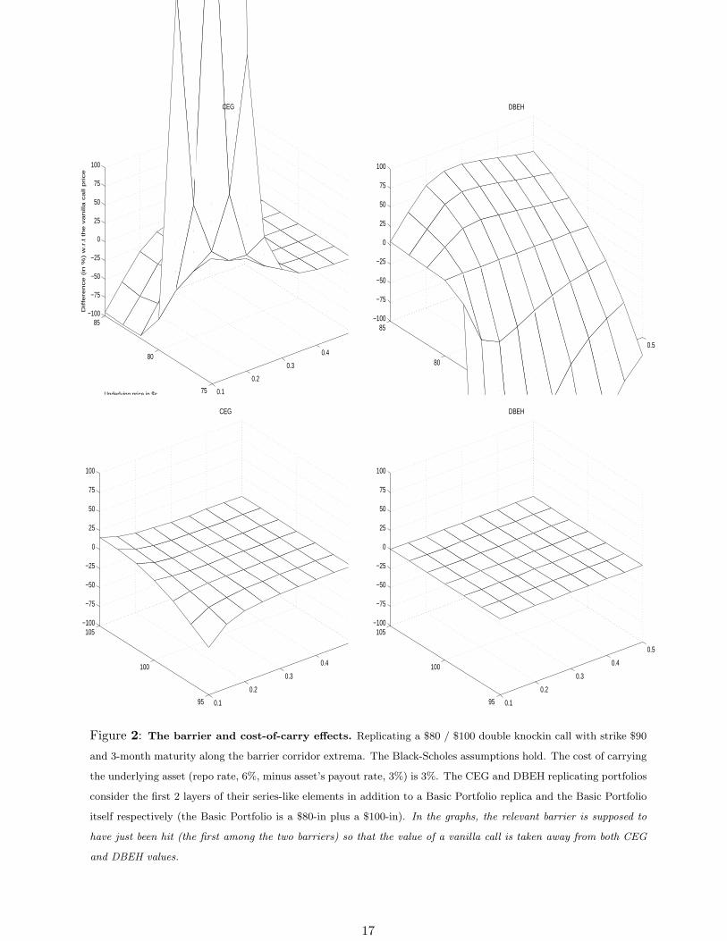
3. The Cost-Of-Carry Effect and The Barrier Effect
How important is keeping track of a drift towards either barrier generated by a non-zero cost
of carry of the underlying asset? An answer is the evaluation, along both barriers, of the part of
the replicating portfolio proposed by CEG which is meant to be zero over there if the carrying cost
had been zero. In Figure 2, the cost of carry is 3% and the relevant barrier is supposed to have
been just hit so that the value of a vanilla call is taken away from both CEG and DBEH values.
The CEG and DBEH portfolios consider the first 2 layers of their series-like elements in addition
to a non-barrier Basic Portfolio replica and the Basic Portfolio itself respectively. This means that
the series terms with n = 1 and n = 2 in Tables I and II are considered. These are the knockin
positions involved by the DBEH.
Knockin barrier in $s Strike in $s Position type DBEH position nature
244.14 219.73 long LFUI Part I, n = 2
195.31 219.73 short UFLI Part II, n = 2
156.25 140.63 long LFUI Part I, n = 1
125.00 140.63 short UFLI Part II, n = 1
(upper barrier) 100.00 90.00 1 unit long Basic Portfolio
(initial spot price) 90.00 (original strike) 90
(lower barrier) 80.00 90.00 1 unit long Basic Portfolio
64.00 57.60 short LFUI Part II, n = 1
51.20 57.60 long UFLI Part I, n = 1
40.96 36.86 short LFUI Part II, n = 2
32.77 36.86 long UFLI Part I, n = 2
9
Figure 2 shows that CEG is substantially off zero (its value is falling 50% short of the vanilla
call price) only along $80 and for quite low logprice volatility levels (10%). However, Figure 1
makes clear that, at such volatility levels, there is no vanilla price action at all. For high volatility
levels, CEG is zero along both barriers. Volatility is likely to be high around the barriers so that
the cost of carry should have only second-order effects. These conclusions are stable across option
maturity.
DBEH portfolio amounts vary with the logprice volatility whereas CEG portfolio amounts are
pegged to (10080 )±n with n = 1, 2. Consider for example n = 1. The maximum percentage absolute
difference between mBS(0,ln 80,ln 100)mBS(0,ln 100,ln 80)(
10080 )2 and 100
80 is 60% in the volatility range [10%, 50%]. This
goes up to 140% for mBS(0,ln 100,ln 80)mBS(0,ln 80,ln 100)(
10080 )−2 and (100
80 )−1. In both cases, the maximum difference
does not fade out to zero as volatility picks up. However, such volatility effect on DBEH portfolio
amounts becomes irrelevant when one looks at the portfolio amounts in $s. Fixing the portfolio-
amount volatility does not affect height and shape of the DBEH graphs in Figures 2, 3, and 4.
Even fixing two different portfolio-amount volatility levels in UFLI and LFUI (to accomodate some
volatility smirk, for example) is basically neutral. Thus, DBEH graphs take portfolio amounts
calculated at varying volatility levels within the range [10%, 50%], but they well represent also a
volatility-static DBEH strategy where the replicating agent fixes portfolio amounts according to
her best guess about the along-the-barriers volatility scenarios.
The hedger can project the risk of barrier instruments, and in particular of double barrier
ones, on to simple European options. This means that, as soon as either barrier is hit, ‘manual’
unwinding of the hedge must take place. This exposes barrier option hedgers to underlying market
price manipulation and spurious volatility. This can be the case if the counterpart of the barrier
option hedger is a hedge fund. Hedge funds typically use the cheapest means to place big, one-way
bets. The temptation to nudge prices can be hard to resist if the result will make a big difference
to hedge funds’ performance, and hence to the fees their managers earn.