Page 1
Tiling Stencil Computations to Maximize Parallelism
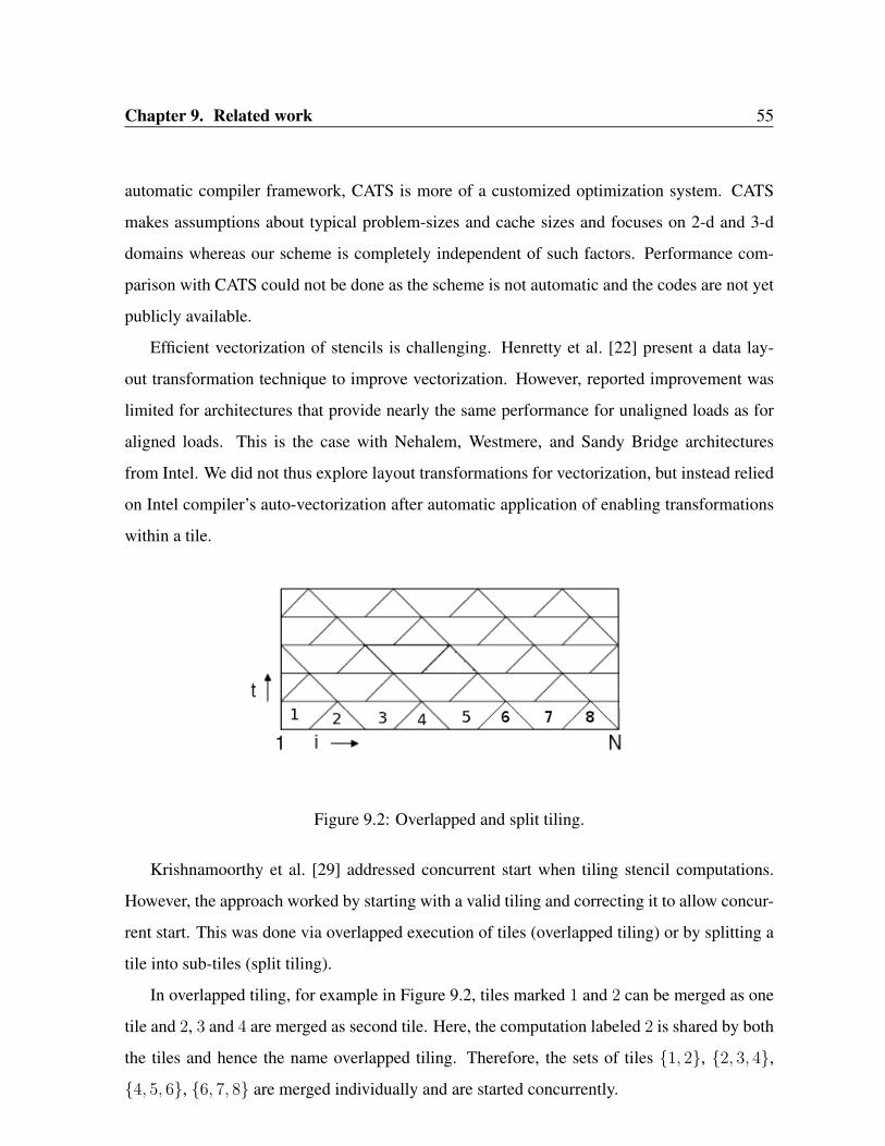
A THESIS
SUBMITTED FOR THE DEGREE OF
Master of Science (Engineering)
IN THE COMPUTER SCIENCE AND ENGINEERING
by
Vinayaka Prakasha Bandishti
Computer Science and Automation
Indian Institute of Science
BANGALORE – 560 012
DECEMBER 2013
Page 2
i
c⃝Vinayaka Prakasha Bandishti
DECEMBER 2013All rights reserved
Page 4
Acknowledgements
First of all, I would like to convey my deepest gratitude to my advisor Dr. Uday Bondhugula for
his guidance and persistent help without which this dissertation would not have been possible.
I have learnt a great deal from him. Discussions with him have led to the key ideas in this
thesis.
I would like to take this opportunity to thank all my friends and labmates especially, Irshad
Pananilath for the immense help towards the implementation of this work.
I would like to thank Mrs. Lalitha, Mrs. Suguna and Mrs. Meenakshi for taking care
of the administrative tasks smoothly. I would also like to thank all the non-technical staff of
the department for making my stay in the department comfortable. I am greatly indebted to
IISc, Bangalore and Department of Computer Science and Automation for all the facilities it
provides to students.
I would like to thank IBM for funding my travel to the SC’12 conference.
Finally, I want to thank Ministry of Human Resource Development, Department of Educa-
tion, for granting scholarship to support me during this course.
i
Page 5
Publications based on this Thesis
1. V. Bandishti, I. Pananilath, and U. Bondhugula. Tiling Stencil Computations to Max-
imize Parallelism, ACM/IEEE International Conference for High Performance Com-
puting, Networking, Storage and Analysis (Supercomputing’12), Salt Lake City, Utah,
pages 40:1 - 40:11, November 2012.
2. U. Bondhugula, V. Bandishti, G. Portron, A. Cohen, and N. Vasilache. Optimizing Time-
iterated Computations with Periodic Boundary Conditions, under review at ACM SIG-
PLAN International Conference on Programming Language Design and Implementation
(PLDI’14), Edinburgh, UK, June 2014.
ii
Page 6
Abstract
Stencil computations are iterative kernels often used to simulate the change in a discretized
spatial domain over time (e.g., computational fluid dynamics) or to solve for unknowns in a
discretized space by converging to a steady state (i.e., partial differential equations). They are
commonly found in many scientific and engineering applications. Most stencil computations
allow tile-wise concurrent start, i.e., there always exists a face of the iteration space and a set of
tiling hyperplanes such that all tiles along that face can be started concurrently. This provides
load balance and maximizes parallelism.
Loop tiling is a key transformation used to exploit both data locality and parallelism from
stencils simultaneously. Numerous works exist that target improving locality, controlling fre-
quency of synchronization, and volume of communication wherever applicable. But, con-
current start-up of tiles that evidently translates into perfect load balance and often reduction
in frequency of synchronization is completely ignored. Existing automatic tiling frameworks
often choose hyperplanes that lead to pipelined start-up and load imbalance. We address this is-
sue with a new tiling technique that ensures concurrent start-up as well as perfect load balance
whenever possible. We first provide necessary and sufficient conditions on tiling hyperplanes
to enable concurrent start for programs with affine data accesses. We then discuss an iterative
approach to find such hyperplanes.
It is not possible to directly apply automatic tiling techniques to periodic stencils because
of the wrap-around dependences in them. To overcome this, we use iteration space folding
techniques as a pre-processing stage after which our technique can be applied without any
further change.
iii
Page 7
iv
We have implemented our techniques on top of Pluto - a source-level automatic parallelizer.
Experimental evaluation on a 12-core Intel Westmere shows that our code is able to outperform
a tuned domain-specific stencil code generator by 4% to 2×, and previous compiler techniques
by a factor of 1.5× to 15×. For the swim benchmark from SPECFP2000, we achieve an
improvement of 5.12× on a 12-core Intel Westmere and 2.5× on a 16-core AMD Magny-
Cours machines, over the auto-parallelizer of Intel C Compiler.
Page 8
Contents
Acknowledgements i
Publications based on this Thesis ii
Abstract iii
1 Introduction 1
2 Background and notation 62.1 Conical and strict conical combination . . . . . . . . . . . . . . . . . . . . . 62.2 Characterizing a stencil program . . . . . . . . . . . . . . . . . . . . . . . . 72.3 Polyhedral model . . . . . . . . . . . . . . . . . . . . . . . . . . . . . . . . 82.4 Dependences and tiling hyperplanes . . . . . . . . . . . . . . . . . . . . . . 9
3 Motivation 133.1 Pipelined start-up vs. Concurrent start-up . . . . . . . . . . . . . . . . . . . 133.2 Rectangular tiling and inter-tile dependences . . . . . . . . . . . . . . . . . . 14
4 Conditions for concurrent start-up 184.1 Constraints for concurrent start-up . . . . . . . . . . . . . . . . . . . . . . . 184.2 Lower dimensional concurrent start-up . . . . . . . . . . . . . . . . . . . . . 214.3 The case of multiple statements . . . . . . . . . . . . . . . . . . . . . . . . . 21
5 Approach for finding hyperplanes iteratively 235.1 Iterative scheme . . . . . . . . . . . . . . . . . . . . . . . . . . . . . . . . . 235.2 Examples . . . . . . . . . . . . . . . . . . . . . . . . . . . . . . . . . . . . 27
5.2.1 Example-2d-heat . . . . . . . . . . . . . . . . . . . . . . . . . . . . 275.2.2 Example-1d-heat . . . . . . . . . . . . . . . . . . . . . . . . . . . . 295.2.3 Example-3d-heat . . . . . . . . . . . . . . . . . . . . . . . . . . . . 29
6 Handling periodic stencils 316.1 Smashing . . . . . . . . . . . . . . . . . . . . . . . . . . . . . . . . . . . . 326.2 Smashing in action: Ring . . . . . . . . . . . . . . . . . . . . . . . . . . . . 336.3 Iteration space smashing . . . . . . . . . . . . . . . . . . . . . . . . . . . . 34
v
Page 9
CONTENTS vi
7 Implementation 377.1 Implementation on top of Pluto . . . . . . . . . . . . . . . . . . . . . . . . . 377.2 Code versioning to help vectorization . . . . . . . . . . . . . . . . . . . . . 38
8 Experimental evaluation 408.1 Benchmarks . . . . . . . . . . . . . . . . . . . . . . . . . . . . . . . . . . . 408.2 Hardware setup . . . . . . . . . . . . . . . . . . . . . . . . . . . . . . . . . 428.3 Significance of concurrent start . . . . . . . . . . . . . . . . . . . . . . . . . 428.4 Results for non-periodic stencils . . . . . . . . . . . . . . . . . . . . . . . . 448.5 Results for periodic stencils . . . . . . . . . . . . . . . . . . . . . . . . . . . 49
9 Related work 53
10 Conclusion 57
Bibliography 58
Page 10
List of Tables
8.1 Problem sizes for the benchmarks in the format ⟨spacesize⟩dimension x ⟨timesize⟩ 418.2 Details of architectures used for experiments . . . . . . . . . . . . . . . . . . 428.3 Details of hardware counters for cache behavior in experiments for heat-2d on
a single core of Intel machine . . . . . . . . . . . . . . . . . . . . . . . . . . 448.4 Summary of performance - non-periodic stencils . . . . . . . . . . . . . . . 488.5 Details of cache behavior in experiments for swim on 12 cores of Intel machine 518.6 Summary of performance -periodic stencils . . . . . . . . . . . . . . . . . . 52
vii
Page 11
Chapter 1
Introduction
Onset of the last decade saw the advent of multicore processors. Earlier, improving the hard-
ware was the de facto path to improvement in program performance. Multi-level caches grow-
ing in size, aggressive instruction issues and deeper pipelines tried to exploit more ‘instruction
level parallelism’ (ILP). Along with these techniques, a steady increase in the processor clock
speed was the trend for performance improvement. The techniques required no extra effort on
the part of compiler/language designers and programmers to achieve the desired performance
gains. This transparency made them very popular. But, this trend hit a dead end because of
three factors or walls[24]
• ‘Power wall’- Increased processor clock speeds resulted in high power dissipation and
reached a saturation point.
• ‘ILP wall’- Deeper pipelines were accompanied by higher pipeline-penalties and they
could never identify coarser-grained parallelisms like thread-level parallelism and data-
level parallelism which are visible only at a much higher level of program abstraction.
• ‘Memory wall’- The gap between processor speeds and memory speeds reached a point
where the memory bandwidth was a serious bottleneck in performance and further in-
creasing the processor speed was little meaningful.
These paved the way for a radical change in microprocessor architecture - a shift from single
core CPUs to multi-core CPUs. This trend of using many small processing units in parallel,
1
Page 12
Chapter 1. Introduction 2
instead of trying to improve a single processing unit is expected to prevail for many years to
come.
With the emergence of multicore as the default processor design, the task of performance
improvement now demanded efforts from higher layers of the ‘systems’ - programmers and
compiler designers. The multicores now require programs that have explicitly marked parallel
parts. Writing a race-free deterministic parallel program is very challenging, often prone to
errors [11]. Debugging is also a nightmare as errors in an incorrect parallel program are often
very difficult to reproduce. Automatic parallelization, is therefore, a very popular choice.
It requires no effort on part of the programmer. This process of automatically converting a
sequential program to into a program with explicitly marked parallel parts has been the subject
of many works[9, 20, 5].
Polyhedral model forms the backbone of such automatic parallelization for regular pro-
grams. It can succinctly represent regular programs and reason about the correctness and
goodness of complex loop transformations. Current techniques give a lot of importance to
achieving maximum locality gains. While doing so they identify the parts of the program that
can be executed in parallel.
Many workloads have enough parallelism to keep all cores busy throughout the execution.
Ideally any automatic parallelizer must try to exploit this property and engage every core in
useful work throughout the execution of the program whenever possible. But currently, no
special attention is given in this regard to make sure that no core sits idle waiting for work.
This work aims to fill these holes and provides techniques to maximize parallelism using which
an optimizer can produce codes that enable concurrent start-up of all cores. This results in a
steady state throughout the execution where all the cores are busy doing the same amount of
maximal work.
Stencil computations constitute a major part of the workloads that allow concurrent start-
up. Stencils are a very common class of programs appearing in many scientific and engi-
neering applications that are computationally intensive. They are characterized by regular
computational structure and hence allow automatic compile-time analysis and transformation
for exploiting data-locality and parallelism.
Page 13
Chapter 1. Introduction 3
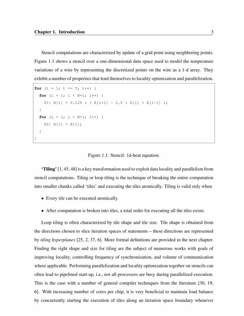
Stencil computations are characterized by update of a grid point using neighboring points.
Figure 1.1 shows a stencil over a one-dimensional data space used to model the temperature
variations of a wire by representing the discretized points on the wire as a 1-d array. They
exhibit a number of properties that lend themselves to locality optimization and parallelization.
for (t = 1; t <= T; t++) {
for (i = 1; i < N+1; i++) {
S1: B[i] = 0.125 * ( A[i+1] - 2.0 * A[i] + A[i-1] );
}
for (i = 1; i < N+1; i++) {
S2: A[i] = B[i];
}
}
Figure 1.1: Stencil: 1d-heat equation.
‘Tiling’ [1, 45, 48] is a key transformation used to exploit data locality and parallelism from
stencil computations. Tiling or loop tiling is the technique of breaking the entire computation
into smaller chunks called ‘tiles’ and executing the tiles atomically. Tiling is valid only when
• Every tile can be executed atomically.
• After computation is broken into tiles, a total order for executing all the tiles exists.
Loop tiling is often characterized by tile shape and tile size. Tile shape is obtained from
the directions chosen to slice iteration spaces of statements – these directions are represented
by tiling hyperplanes [25, 2, 37, 6]. More formal definitions are provided in the next chapter.
Finding the right shape and size for tiling are the subject of numerous works with goals of
improving locality, controlling frequency of synchronization, and volume of communication
where applicable. Performing parallelization and locality optimization together on stencils can
often lead to pipelined start-up, i.e., not all processors are busy during parallelized execution.
This is the case with a number of general compiler techniques from the literature [30, 19,
6]. With increasing number of cores per chip, it is very beneficial to maintain load balance
by concurrently starting the execution of tiles along an iteration space boundary whenever
Page 14
Chapter 1. Introduction 4
possible. Concurrent start-up for stencil computations not only eliminates pipeline fill-up and
drain delay, but also ensures perfect load balance. Processors end up executing the same
maximal amount of work in parallel between two synchronization points.
Some works have looked at eliminating pipelined start-up [46, 29] by tweaking or modi-
fying already obtained tile shapes from existing frameworks. However, these approaches have
undesired side-effects including difficulty in performing code generation. No implementations
of these have been reported to date. The approach we propose in this dissertation works by
actually searching for tiling hyperplanes that have the desired property of concurrent start, in-
stead of fixing or tweaking hyperplanes found with undesired properties. To the best of our
knowledge, prior to this work, it was not clear if and under what conditions such hyperplanes
exist, and how they can be found. In addition, their performance on aspects other than con-
current start in comparison with existing compiler techniques has to be studied, though the
work of Strzodka et al. [42] does study this but in a more specific context than we intend to
here. A comparison of compiler-based and domain-specific stencil optimization efforts has
also not been performed in the past. We address all of these in this dissertation. In summary,
our contributions are as follows:
• We provide necessary and sufficient conditions for hyperplanes to allow concurrent start-
up.
• We provide a sound and complete technique to find such hyperplanes.
• We show how the technique can be extended to periodic stencils.
• Our experimental evaluation shows an improvement of 4% to 2× over a domain-specific
compiler Pochoir [43] and factor of 1.5× to 15× improvement over previous compiler
techniques on a set of benchmarks on a 12-core Intel Westmere machine.
• For swim benchmark (SPECFP 2000), we achieve an improvement of 5.12× on a 12-
core Intel Westmere and 2.5× on a 16-core AMD Magny-Cours over the auto-parallelizer
of Intel C Compiler.
Page 15
Chapter 1. Introduction 5
• We have implemented and integrated our approach into Pluto to work automatically
(available at http://pluto-compiler.sourceforge.net).
The rest of the dissertation is organized as follows. Chapter 2 provides the required back-
ground and introduces the notations used. Chapter 3 provides the necessary motivation for
our contributions. Chapter 4 characterizes the conditions for concurrent start-up. Chapter 5
describes our approach to find solutions with the desired properties. How we address the ad-
ditional concerns posed by periodic stencils is explained in Chapter 6. Chapter 7 discusses
the implementation of our algorithm. Experimental evaluation and results are given in Chap-
ter 8. Chapter 9 discusses the previous works related to our contributions and conclusions are
presented in Chapter 10.
Page 16
Chapter 2
Background and notation
In this chapter, we provide an overview of the polyhedral model and current state-of-the-art
automatic tiling techniques. A few fundamental concepts of linear algebra related to cones
and hyperplanes on which our contributions are built upon, are also included in this chapter.
Detailed background on these topics can be found in [1, 4, 25, 2, 6].
All row vectors are typeset in bold lowercase, while column vectors are typeset with an
arrow overhead. All square matrices are typeset in uppercase and Z represents the set of
integers. In any 2d-space discussed as example, vertical dimension is the first dimension and
horizontal dimension is the second.
2.1 Conical and strict conical combination
Given a finite set of vectors x1, x2, . . . , xn, a conical combination or conical sum of these is a
vector of the form
λ1x1 + λ2x2 + · · ·+ λnxn (2.1)
∀λi, λi ≥ 0.
For example, in Figure 2.1, the region between the dashed rays contains all the conical
combinations of vectors (1,−1) and (1, 1). Such a region for any set of vectors forms a cone
6
Page 17
Chapter 2. Background and notation 7
....
(1, 1)
.
(1,−1)
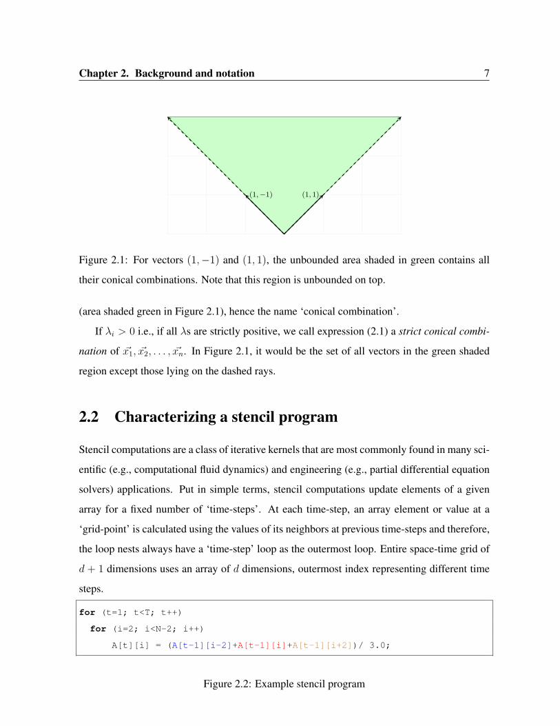
Figure 2.1: For vectors (1,−1) and (1, 1), the unbounded area shaded in green contains all
their conical combinations. Note that this region is unbounded on top.
(area shaded green in Figure 2.1), hence the name ‘conical combination’.
If λi > 0 i.e., if all λs are strictly positive, we call expression (2.1) a strict conical combi-
nation of x1, x2, . . . , xn. In Figure 2.1, it would be the set of all vectors in the green shaded
region except those lying on the dashed rays.
2.2 Characterizing a stencil program
Stencil computations are a class of iterative kernels that are most commonly found in many sci-
entific (e.g., computational fluid dynamics) and engineering (e.g., partial differential equation
solvers) applications. Put in simple terms, stencil computations update elements of a given
array for a fixed number of ‘time-steps’. At each time-step, an array element or value at a
‘grid-point’ is calculated using the values of its neighbors at previous time-steps and therefore,
the loop nests always have a ‘time-step’ loop as the outermost loop. Entire space-time grid of
d + 1 dimensions uses an array of d dimensions, outermost index representing different time
steps.
for (t=1; t<T; t++)
for (i=2; i<N-2; i++)
A[t][i] = (A[t-1][i-2]+A[t-1][i]+A[t-1][i+2])/ 3.0;
Figure 2.2: Example stencil program
Page 18
Chapter 2. Background and notation 8
Figure 2.2 shows a stencil over a one-dimensional data space used to model, for example,
a 1d-heat equation. Even though stencils have no outer parallelism, there still exists significant
opportunity to exploit parallelism. For instance, in our example code in Figure 2.2, the inner
loop i is parallel, i.e., all the i iterations for a particular time-step t can be executed in parallel.
It is this inherent property of a stencil that we try to exploit. Example in Figure 2.2 serves as
the running example for the rest of the chapter.
2.3 Polyhedral model
The polyhedral model abstracts a dynamic instance or iteration of each statement into an in-
teger point in a space called the statement’s iteration domain. For a regular program with
loop nests in which the data access functions and loop bounds are affine combinations (linear
combination with a constant) of the enclosing loop variables and parameters, the set of such
integer points forms a well-defined polyhedron. This polyhedron which can be represented as
a set of linear equalities and inequalities in terms of loop iterators and program parameters, is
called the statement’s iteration space. Similarly, the exact dependences between the iterations
of statements can also be captured. Using the information of iteration space and dependences,
the polyhedral model reasons about when a sequence of loop transformations is legal. Using
some heuristics, it can also explain when a loop transformation is good. Linear Algebra and
Integer Linear Programming form the heart of machinery of the polyhedral model.
As described in [10],
‘the task of program optimization (often for parallelism and locality) in the polyhedral model
may be viewed in terms of three phases:
• Static dependence analysis of the input program
• Transformations in the polyhedral abstraction
• Generation of code for the transformed program’
This work fits well into the central phase. The formal definitions, explanations and exam-
ples for the jargon of the polyhedral model can be found in the next section.
Page 19
Chapter 2. Background and notation 9
2.4 Dependences and tiling hyperplanes
Let S1, S2, . . . , Sn be the statements of a program, and let S = {S1, S2, . . . , Sn}. The iteration
space of a statement can be represented as a polyhedron (Figure 2.4). The dimensions of the
polyhedron correspond to surrounding loop iterators as well as program parameters.
Definition: Affine loop nests are sequences of imperfectly nested loops with loop bounds and
array accesses that are affine functions of outer loop variables and program parameters.
Definition: Program parameters are symbols that do not vary in the portion of the code we
are representing; they are typically the problem sizes. In our example N and T are program
parameters.
Definition: Each integer point in the polyhedron, also called an iteration vector, contains
values for induction variables of loops surrounding the statement from outermost to innermost.
(t, i) is iteration vector for the statement in our example in Figure 2.2.
Definition: The data dependence graph, DDG = (S, E) is a directed multi-graph with each
vertex representing a statement in the program and edge e from Si to Sj representing a poly-
hedral dependence from a dynamic instance of Si to one of Sj . Figure 2.3 shows the DDG for
our example program in Figure 2.2.
Figure 2.3: DDG for example in Figure 2.2. The three edges in different colors correspond to
dependences between three read accesses on RHS and one write access on LHS.
Page 20
Chapter 2. Background and notation 10
.. i.2
.N-3
.
t
.
T-1
.
1
Figure 2.4: Iteration space and dependences for the example in Figure 2.2. Black dots are the
dynamic instances of the statement. Colored arrows are the dependences between the iterations
corresponding to the three edges in DDG (Figure 2.3).
Definition: Every edge e is characterized by a polyhedron Pe, called dependence polyhedron
which precisely captures all the dependences between the dynamic instances of Si and Sj .
As mentioned earlier, the ability to capture the exact conditions on when a dependence exists
through linear equalities and inequalities rests on the fact that there exists an affine relation
between the iterations and the accessed data for regular programs. Conjunction of all these
inequalities and equalities itself forms the dependence polyhedron.
One can obtain a less powerful representation such as a constant distance vector or direc-
tion vector from dependence polyhedra by analyzing the relation between source and target
iterators. For most of the examples in the dissertation,we have used constant distance vectors
for simplicity. The reader is referred to [4] for a more detailed explanation of the polyhedral
representation.
Definition: A hyperplane is an n− 1 dimensional affine subspace of an n dimensional space.
For example, any line is a hyperplane in a 2-d space, and any 2-d plane is a hyperplane in 3-d
space.
Page 21
Chapter 2. Background and notation 11
A hyperplane for a statement Si is of the form:
ϕSi(x) = h· x+ h0 (2.2)
where h0 is the translation or the constant shift component, and x is an iteration of Si. h itself
can be viewed as a vector oriented in a direction normal to the hyperplane.
Prior research [31, 6] provides conditions for a hyperplane to be a valid tiling hyperplane.
For ϕs1 ,ϕs2 , . . . ,ϕsk to be valid statement-wise tiling hyperplanes for S1, S2,, . . . , Sk respec-
tively, the following should hold for each edge e from Si to Sj:
ϕsj (t)− ϕsi(s) ≥ 0, ⟨s, t⟩ ∈ Pe,∀e ∈ E (2.3)
The above constraint implies that all dependences have non-negative components along each of
the hyperplanes, i.e., their projections on the these hyperplane normals are never in a direction
opposite to that of the hyperplane normals.
In addition, the tiling hyperplanes should be linearly independent of each other. Each
statement has as many linearly independent tiling hyperplanes as its loop nest dimensionality.
Among the many possible hyperplanes, the optimal solution according to a cost function
is chosen. A cost function that has worked in the past is based on minimizing dependence
distances lexicographically with hyperplanes being found from outermost to innermost [6].
If all iteration spaces are bounded, there exists an affine function v(p) = u· p+ w that bounds
δe(t) for every dependence edge e:
v(p)− (ϕsi (t)− ϕsj (s)) ≥ 0, ⟨s, t⟩ ∈ Pe, ∀e ∈ E (2.4)
where p is a vector of program parameters. The coefficients u, w are then minimized.
Page 22
Chapter 2. Background and notation 12
..
(1, 0)
.
(1, 2)
.
(1,−2)
.
(2, 1)
.
(2,−1)
Figure 2.5: d1 = (1, 2), d2 = (1, 0) and d3 = (1,−2) are the dependences. For any hyperplane
ϕ in the cone formed by (2, 1) and (2,−1),ϕ· d1 ≥ 0 ∧ ϕ· d2 ≥ 0 ∧ ϕ· d3 ≥ 0 holds good.
Cost function chooses (1, 0) and (2, 1) as tiling hyperplanes.
Validity constraints on the tiling hyperplanes ensure the following:
• In the transformed space, all dependences have non-negative components along all bases.
• Any rectangular tiling in the transformed space is valid.
Example: Consider the program in Figure 2.2. As all the dependences are self dependences
and also uniform, they can be represented by constant vectors. The dependences are:
(d1 d2 d3
)=
1 1 1
−2 0 2
Equation 2.3 can now be written as
ϕ·
1 1 1
−2 0 2
≥(0 0 0
)(2.5)
Equation 2.5 forces the chosen hyperplane to have non-negative components along all de-
pendences. Therefore, any hyperplane in the cone of (2,−1) and (2, 1) is a valid one (Fig-
ure 2.5). However, cost function (2.4) ends up choosing (1, 0) and (2, 1).
Page 23
Chapter 3
Motivation
In this chapter, we contrast pipelined start-up and concurrent start-up of a loop nest. We
explain the advantages the concurrent start-up provides over pipelined and also how stencils
are inherently amenable to concurrent start-up. We then discuss how the inter-tile dependences
introduced by tiling can affect the concurrent start-up along a face.
3.1 Pipelined start-up vs. Concurrent start-up
Consider the iteration spaces in Figure 3.1 and Figure 3.2. The iterations shaded under green
are executed in first time-step, yellow under second and red under third. In pipelined start-up,
in the beginning, threads wait in a queue for iterations to be ready to be executed (pipeline
fill-up) and towards the end, threads sit idle because there is no enough work to keep all the
threads busy (pipeline drain). Unlike this, in case of concurrent start-up, all the threads are
busy from the start till end.
Hence, to achieve maximum parallelism we must try to exploit concurrent start whenever
possible.
13
Page 24
Chapter 3. Motivation 14
i
t
N-2
T-1 b b b b b
b b b b b
b b b b b
b b b b b
b b b b b
0 1 2 3
1
2
3
Figure 3.1: Pipelined start-up
i
t
N-2
T-1 b b b b b
b b b b b
b b b b b
b b b b b
b b b b b
0 1 2 3
1
2
3
Figure 3.2: Concurrent start-up
3.2 Rectangular tiling and inter-tile dependences
As mentioned earlier, once the transformation is applied, the transformed space can be tiled
rectangularly. Figure 3.3 shows the transformed space with with t1 = t and t2 = 2t + i
corresponding to the hyperplanes found at the end of the previous chapter for the code in
Figure 2.2, serving as the new ‘bases’ or ‘axes’. All the dependences in this transformed space
now lie in the cone of these bases. By assuming that inter-tile dependences in the transformed
space are unit vectors along all the bases, we can be sure that any inter-tile dependence is
satisfied (Figure 3.3). It is important to note here that this approximation is actually accurate
for stencils i.e., it is also necessary that we consider inter-tile dependences along every base
as the dependences span the entire iteration space (there is no outer parallelism). In the rest of
the dissertation we refer to these safely approximated inter-tile dependences as simply inter-
tile dependences. Thus if C ′ is the matrix whose columns are the approximated inter-tile
dependences in the transformed space, C ′ will be a unit matrix.
Let TR be the reduced transformation matrix which has only the h components (Eqn. 2.2)
of all hyperplanes as rows. TR of any statement is thus a square matrix which can be obtained
by eliminating the columns producing translation and any other rows meant to specify loop
distribution at any level [28, 14, 6]. As the inter-tile dependences are all intra-statement and
are not affected by the translation components of tiling hyperplanes, we have:
C ′ = TR·C
Page 25
Chapter 3. Motivation 15
..
t1 = t
.t2 = 2t+ i
.
(0, 1)
.
(1, 0)
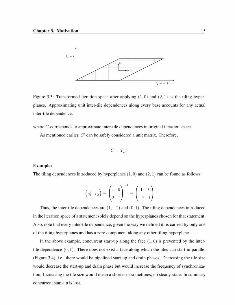
Figure 3.3: Transformed iteration space after applying (1, 0) and (2, 1) as the tiling hyper-
planes. Approximating unit inter-tile dependences along every base accounts for any actual
inter-tile dependence.
where C corresponds to approximate inter-tile dependences in original iteration space.
As mentioned earlier, C ′ can be safely considered a unit matrix. Therefore,
C = T−1R
Example:
The tiling dependences introduced by hyperplanes (1, 0) and (2, 1) can be found as follows:
(c1 c2
)=
1 0
2 1
−1
=
1 0
−2 1
Thus, the inter-tile dependences are (1,−2) and (0, 1). The tiling dependences introduced
in the iteration space of a statement solely depend on the hyperplanes chosen for that statement.
Also, note that every inter-tile dependence, given the way we defined it, is carried by only one
of the tiling hyperplanes and has a zero component along any other tiling hyperplane.
In the above example, concurrent start-up along the face (1, 0) is prevented by the inter-
tile dependence (0, 1). There does not exist a face along which the tiles can start in parallel
(Figure 3.4), i.e., there would be pipelined start-up and drain phases. Decreasing the tile size
would decrease the start-up and drain phase but would increase the frequency of synchroniza-
tion. Increasing the tile size would mean a shorter or sometimes, no steady-state. In summary
concurrent start-up is lost.
Page 26
Chapter 3. Motivation 16
..
iteration dependence
.
inter-tile dependence
.
(0, 1)
.
(1, -2)
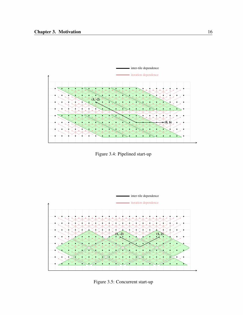
Figure 3.4: Pipelined start-up
..
iteration dependence
.
inter-tile dependence
.
(1, 2)
.
(1, -2)
Figure 3.5: Concurrent start-up
Page 27
Chapter 3. Motivation 17
Transform should be found in such a way that it does not introduce any inter-tile depen-
dence that prohibits concurrent start-up. If we had chosen (2,−1), which is also valid, instead
of (1, 0) as tiling hyperplane, i.e., if (2,−1) and (2, 1) were chosen as the tiling hyperplanes,
then the inter-tile dependences introduced would be (1,−2) and (1, 2) (Figure 3.5). Both have
positive components along the normal (1, 0), i.e., all tiles along the normal (1, 0) could be
started concurrently.
In the next chapter, we provide conditions on hyperplanes that would avoid (1, 0) and
instead select (2,−1), for this example.
Page 28
Chapter 4
Conditions for concurrent start-up
If all the iterations along a face can be started concurrently, the face is said to allow point-
wise concurrent start-up. Similarly, if all the tiles along a face can be started concurrently, the
face is said to allow tile-wise concurrent start-up. In this section, we provide conditions for
which tiling hyperplanes of any statement allow concurrent start-up along a given face of its
iteration space. A face of an iteration space is referred by its normal f. Theorem 1 introduces
the constraints in terms of inter-tile dependences. Theorem 2 and Theorem 3 map Theorem 1
from inter-tile dependences onto tiling hyperplanes. We also prove that these constraints are
both necessary and sufficient for concurrent start-up.
4.1 Constraints for concurrent start-up
Theorem 1: For a statement, a transformation enables tile-wise concurrent start-up along a
face f iff the tile schedule is in the same direction as the face and carries all inter-tile depen-
dences.
Let to be the outer tile schedule. If f is the face allowing concurrent start and C is the
matrix containing approximate inter-tile dependences of the original iteration space, then,
k1to = k2f, k1, k2 ∈ Z+
18
Page 29
Chapter 4. Conditions for concurrent start-up 19
to·C ≥ 1
Hence,
f·C ≥ 1
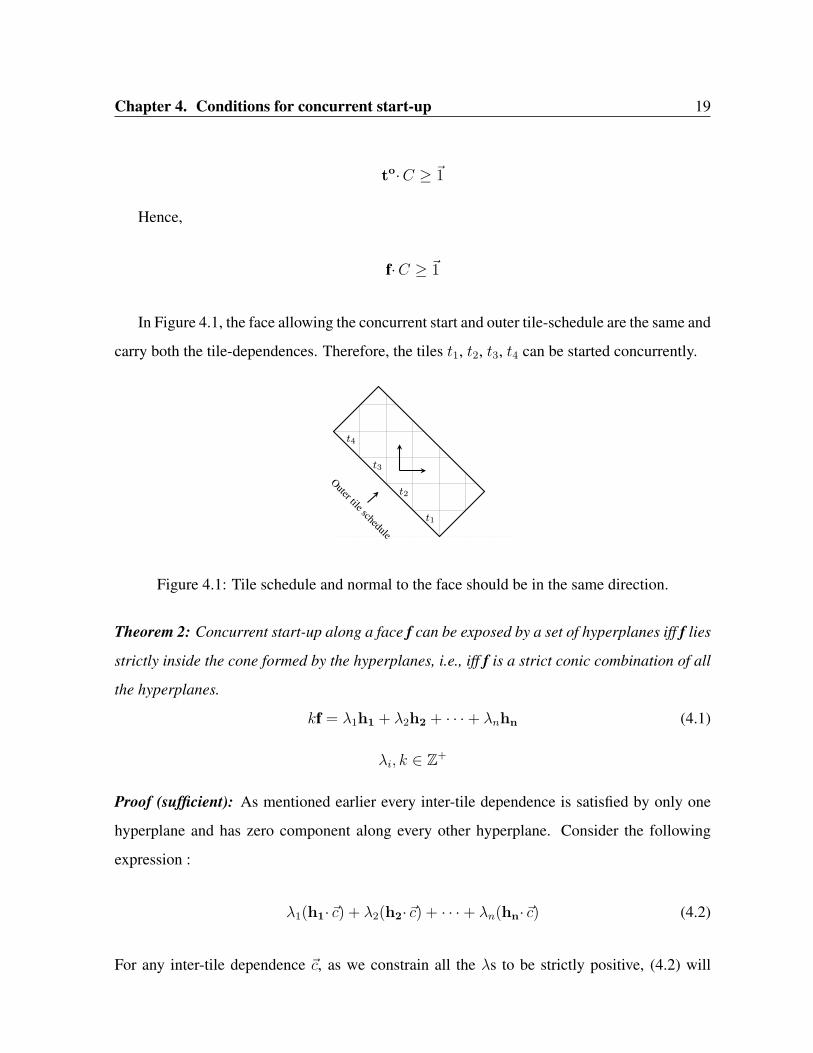
In Figure 4.1, the face allowing the concurrent start and outer tile-schedule are the same and
carry both the tile-dependences. Therefore, the tiles t1, t2, t3, t4 can be started concurrently.
..t1
.
t2
.
t3
.
t4
.
Outer tile schedule
Figure 4.1: Tile schedule and normal to the face should be in the same direction.
Theorem 2: Concurrent start-up along a face f can be exposed by a set of hyperplanes iff f lies
strictly inside the cone formed by the hyperplanes, i.e., iff f is a strict conic combination of all
the hyperplanes.
kf = λ1h1 + λ2h2 + · · ·+ λnhn (4.1)
λi, k ∈ Z+
Proof (sufficient): As mentioned earlier every inter-tile dependence is satisfied by only one
hyperplane and has zero component along every other hyperplane. Consider the following
expression :
λ1(h1· c) + λ2(h2· c) + · · ·+ λn(hn· c) (4.2)
For any inter-tile dependence c, as we constrain all the λs to be strictly positive, (4.2) will
Page 30
Chapter 4. Conditions for concurrent start-up 20
always be positive. Thus, by choosing all h such that
kf = λ1h1 + λ2h2 + · · ·+ λnhn
we ensure f· c ≥ 1 for all inter-tile dependences. Therefore, from Theorem 1, concurrent
start is enabled. □
Proof (necessary): Let us assume that we have concurrent start along the face f, but f does not
strictly lie inside the cone formed by the hyperplanes, i.e., (4.1) does not hold good. Without
loss of generality, we can assume that k ∈ Z+, but there exist no λs which are all strictly
positive integers. We now argue that, for at least one inter-tile dependence c , the sum (4.2)
≤ 0 because every tile dependence is carried by only one of the chosen hyperplanes and there
exists at least one λ such that λ ≤ 0. Therefore, f· c will also be zero or negative, which means
concurrent start is inhibited along f. This is a contradiction. □
For the face f that allows concurrent start, let f ′ be its counterpart in the transformed space.
We now provide an alternative result for concurrent start that is equivalent to the one above.
Theorem 3: A transformation T allows concurrent start along f iff f·T−1R ≥ 1 .
Proof: From Theorem 1 we have, for the transformed space, the condition for concurrent start
becomes
f ′·C ′ ≥ 1 (4.3)
We know that in the transformed space, we approximate all inter-tile dependences by unit
vectors along every base. Therefore, C ′ is a unit matrix. Since the normals are not affected by
translations, the normal f ′ after transformation T is given by f·T−1R .
Therefore, (4.3) becomes
f·T−1R ≥ 1
Page 31
Chapter 4. Conditions for concurrent start-up 21
The above can be viewed in a different manner. We know that the inter-tile dependences
introduced in the original iteration space can be approximated as
C = T−1R
From Theorem 1 we have,
f·T−1R ≥ 1 □
4.2 Lower dimensional concurrent start-up
By making the outer tile schedule parallel to the face allowing concurrent start (as discussed
in the previous section), one can obtain n − 1 degrees of concurrent start-up, i.e., all tiles on
the face can be started concurrently. But, in practice, exploiting all of these degrees may result
in more complex code. The above conditions can be placed only on the first few hyperplanes
to obtain what we term lower dimensional concurrent start. For instance, the constraints can
be placed only on the first two hyperplanes so that one degree of concurrent start is exploited.
Such transformations may not only generate better code owing to prefetching and vectoriza-
tion, but also achieve coarser grained parallelization.
4.3 The case of multiple statements
In case of multiple statements, every strongly connected component in the dependence graph
can have only one outer tile schedule. So, all statements which have to be started concurrently
and together should have the same face that allows concurrent start. If they do not have the
same face allowing concurrent start, one of those has to be chosen for the outer tile schedule.
These are beyond the scope of this work, since in the case of stencils, the following are always
true:
• Every statement’s iteration space has the same dimensionality and same face f that allows
concurrent start.
Page 32
Chapter 4. Conditions for concurrent start-up 22
• Transitive self dependences are all carried by this face.
For example, for the stencil in Figure 1.1 (an imperfect loop nest with 2 statements), hy-
perplanes found by our scheme are (2, 1) and (2,−1). However, S2 is given a constant shift of
1 with respect to both the hyperplanes to preserve validity. Therefore, transformations for the
two statements corresponding to the found hyperplanes are 2t+ i, 2t− i for S1, and 2t+ i+1,
2t− i+ 1 for S2.
Page 33
Chapter 5
Approach for finding hyperplanes
iteratively
In this chapter, we present a scheme that is an extension to the Pluto algorithm [6] so that
hyperplanes that satisfy properties introduced in the previous chapter are found. Though The-
orem 2 and Theorem 3 are equivalent to each other, we use Theorem 2 in our scheme as it
provides simple linear inequalities and is easy to implement.
5.1 Iterative scheme
Along with constraints imposed to respect dependences and encode an objective function, the
following additional constraints are added while finding hyperplanes iteratively.
For a given statement, let f be the face along which we would like to start concurrently,
H be the set of hyperplanes already found, and n be the dimensionality of the iteration space
(same as the number of hyperplanes to find). Then, we add the following additional constraints:
1. For the first n− 1 hyperplanes, h is linearly independent of f ∪H , as opposed to just H .
2. For the last hyperplane hn, hn is strictly inside the cone formed by f and the negatives
of the already found n− 1 hyperplanes, i.e.,
23
Page 34
Chapter 5. Approach for finding hyperplanes iteratively 24
λnhn = kf + λ1(−h1) + λ2(−h2) + · · ·+ λn−1(−hn−1), (5.1)
λi, k ∈ Z+
In Algorithm 1, we show only our additions to the iterative algorithm proposed in [6].
Algorithm 1 Finding tiling hyperplanes that allow concurrent start1: Initialize H = ∅
2: for n− 1 times do
3: Build constraints to preserve dependences.
4: Add constraints such that the hyperplane to be found is linearly independent of f ∪H
5: Add cost function constraints and minimize cost function for the optimal solution.
6: H = h ∪H
7: end for
8: Add constraint (5.1) for the last hyperplane so that it strictly lies inside the cone of the face and nega-
tives of the n− 1 hyperplanes already found (H)
If it is not possible to find hyperplanes with these additional constraints, we report that tile-
wise concurrent start is not possible. If there exists a set of hyperplanes that exposes tile-wise
concurrent start, we now prove that the above algorithm will find it.
Proof: (soundness)
When the algorithm returns a set of hyperplanes, we can be sure that all of them are indepen-
dent of each other and that they also satisfy Equation (5.1) which is obtained by just rearrang-
ing the terms of Equation (4.1). Trivially, our scheme of finding the hyperplanes is sound, i.e.,
whenever our scheme gives a set of hyperplanes as output, the output is always correct. □
Proof: (completeness)
We prove by contradiction that whenever our scheme reports no solution, there does not exist
any valid set of hyperplanes. Suppose there exists a valid set of hyperplanes but our scheme
fails to find them. The scheme can fail at two points:
Page 35
Chapter 5. Approach for finding hyperplanes iteratively 25
Case 1: While finding the first n− 1 hyperplanes
The only constraint the first n−1 hyperplanes have is of being linearly independent of one
another, and of the face that allows concurrent start. If there exist n linearly independent valid
tiling hyperplanes for this computation, since the face with concurrent start f is one feasible
choice, there exist n − 1 tiling hyperplanes linearly independent of f . Hence, our algorithm
does not fail at this step if the original Pluto algorithm [6] is able to find n linearly independent
ones.
Case 2: While finding the the last hyperplane
Let us assume that our scheme fails while trying to find the last hyperplane hn. This implies
that for any hyperplane strictly inside the cone formed by the face allowing concurrent start
and the negatives of the already found hyperplanes, there exists a dependence which makes the
tiling hyperplane an invalid one, i.e., there exists a dependence distance d such that
hn· d ≤ −1
From Equation (5.1), we have
λnhn· d = k(f · d) + λ1(−h1· d) + λ2(−h2· d) + . . .
+λn−1(−hn−1· d) (5.2)
Consider RHS of Equation (5.2). As all hyperplanes are valid, (hi· d) ≥ 0 and λis are
all positive, all terms except for the first one are negative. For any stencil, the face allowing
concurrent start always carries all dependences.
f · d ≥ 1,∀d
If dependences are all constant distance vectors, all λi(−h· d) terms are independent of pro-
gram parameters. So, we could always choose k large enough and λis small so that hn· d ≥ 1
for any dependence d.
Page 36
Chapter 5. Approach for finding hyperplanes iteratively 26
In the general case of affine dependences, our algorithm can fail to find hn in only two
cases. The first is when it is not statically possible to choose λis. This can happen when both
of the following conditions are true:
• Some dependences are non-uniform.
• Components of these non-uniform dependences are parametric in the orthogonal sub-
space of the face allowing concurrent start, but constant along the face itself.
In this case, only point-wise concurrent start is possible, but tile-wise concurrent start is not
possible (Figure 5.1). In order for our algorithm to succeed, one of the λs would have to
depend on a program parameter (typically the problem size) and this is not admissible.
The second case is the expected one that does not even allow point-wise concurrent start.
Here, f does not carry all dependences (Figure 5.2). □
j
i
N
N b b b b b
b b b b b
b b b b b
b b b b b
b b b b b
0 1 2 3
1
2
3
Figure 5.1: No tile-wise concurrent start
possible
j
i
N
N b b b b b
b b b b b
b b b b b
b b b b b
b b b b b
0 1 2 3
1
2
3
Figure 5.2: Even point-wise concurrent
start is not possible
Page 37
Chapter 5. Approach for finding hyperplanes iteratively 27
5.2 Examples
We provide examples showing hyperplanes found by our scheme for 1d, 2d and 3d heat sten-
cils. For simplicity, we show the memory-inefficient version with the time iterator as one of
the data dimensions.
5.2.1 Example-2d-heat
for (t = 0; t < T; t++)
for (i = 1; i < N-1; i++)
for (j = 1; j < N-1; j++)
A[t+1][i][j]
= 0.125 *(A[t][i+1][j] -2.0*A[t][i][j] +A[t][i-1][j])
+ 0.125 *(A[t][i][j+1] -2.0*A[t][i][j] +A[t][i][j-1])
+ A[t][i][j];
Figure 5.3: 2d-heat stencil (representative version).
Figure 5.3 shows the 2d-heat stencil. The code in 5.3 has its face allowing concurrent
f =(1 0 0
). For this code, the transformation computed by Algorithm 1 for full concurrent
start is:
H =
1 1 0
1 0 1
1 −1 −1
(5.3)
i.e., the transformation for (t, i, j) will be (t + i, t + j, t − i − j). The inter-tile dependences
induced by the above transform can be found as the columns of the inverse of H (normalized
in case of fractional components) :
norm
1 1 0
1 0 1
1 −1 −1
−1 =
1 1 1
2 −1 −1
−1 2 −1
Page 38
Chapter 5. Approach for finding hyperplanes iteratively 28
Here, we can verify that Theorem 1 holds good.
[1 0 0
]·
1 1 1
2 −1 −1
−1 2 −1
=
1
1
1
Figure 5.4 shows the shape of a tile formed by the above transformation.
Figure 5.4: Tile shape for 2d-heat stencil obtained by our algorithm. The arrows represent
hyperplanes.
For lower dimensional concurrent start, the transformation computed by Algorithm 1 is:1 1 0
1 −1 0
1 0 1
i.e., the transformation for (t, i, j) will be (t + i, t − i, t + j). This enables concurrent start
in only one dimension. The tile schedule is created out of the two outermost loops and only
second loop is parallel, i.e., not all the tiles along the face allowing concurrent start, but all
tiles along one edge of the face can be started concurrently.
Page 39
Chapter 5. Approach for finding hyperplanes iteratively 29
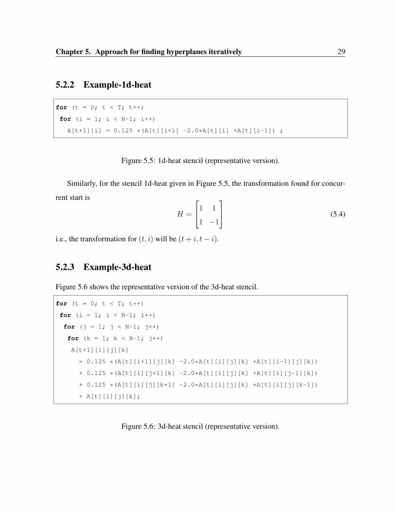
5.2.2 Example-1d-heat
for (t = 0; t < T; t++)
for (i = 1; i < N-1; i++)
A[t+1][i] = 0.125 *(A[t][i+1] -2.0*A[t][i] +A[t][i-1]) ;
Figure 5.5: 1d-heat stencil (representative version).
Similarly, for the stencil 1d-heat given in Figure 5.5, the transformation found for concur-
rent start is
H =
1 1
1 −1
(5.4)
i.e., the transformation for (t, i) will be (t+ i, t− i).
5.2.3 Example-3d-heat
Figure 5.6 shows the representative version of the 3d-heat stencil.
for (t = 0; t < T; t++)
for (i = 1; i < N-1; i++)
for (j = 1; j < N-1; j++)
for (k = 1; k < N-1; j++)
A[t+1][i][j][k]
= 0.125 *(A[t][i+1][j][k] -2.0*A[t][i][j][k] +A[t][i-1][j][k])
+ 0.125 *(A[t][i][j+1][k] -2.0*A[t][i][j][k] +A[t][i][j-1][k])
+ 0.125 *(A[t][i][j][k+1] -2.0*A[t][i][j][k] +A[t][i][j][k-1])
+ A[t][i][j][k];
Figure 5.6: 3d-heat stencil (representative version).
Page 40
Chapter 5. Approach for finding hyperplanes iteratively 30
The transformation found for 3d-heat stencil for full concurrent start is
H =
1 1 0 0
1 0 1 0
1 0 0 1
1 −1 −1 −1
(5.5)
i.e., the transformation for (t, i, j, k) will be (t+ i, t+ j, t+ k, t− i− j − k).
For lower dimensional concurrent start, the transformation computed by Algorithm 1 for 3d-
heat stencil is: 1 1 0 0
1 −1 0 0
1 0 1 0
1 0 0 1
i.e., the transformation for (t, i, j, k) will be (t+ i, t− i, t+ j, t+ k).
Page 41
Chapter 6
Handling periodic stencils
In the same way as the example in Figure 2.2 simulates the heat changes of a wire, its periodic
version simulates the heat changes on a ring. Periodic stencils are mainly used for modeling
hollow objects or shells.
Typically, to discretize the points on the hollow object onto an array, the object can be
thought be cut and unrolled, resulting in a space of one less dimension. For example, to model
the points on ring, it can be thought to be cut at one point and unrolled to form a wire. Now,
we can easily map the points of the wire onto a 1-d array. Similarly, a cylinder or torus can
be cut open into a plane and then mapped onto a 2-d array. Figure 6.1 shows the C code of
heat-1d-periodic version.
for (t = 1; t <= N; t++) {
for (i = 0; i < N; i++) {
S: A[t][i]
= 0.125 * ( A[t-1][(i==N-1)? (0) : (i+1)] +
A[t-1][i] +
A[t-1][(i==0)?(N-1):(i-1)] );
}
}
Figure 6.1: Stencil: periodic 1d heat equation
31
Page 42
Chapter 6. Handling periodic stencils 32
N
N b b b b b
b b b b b
b b b b b
b b b b b
b b b b b
0 1 2 3
1
2
3
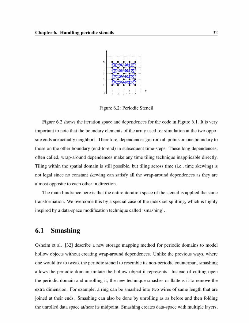
Figure 6.2: Periodic Stencil
Figure 6.2 shows the iteration space and dependences for the code in Figure 6.1. It is very
important to note that the boundary elements of the array used for simulation at the two oppo-
site ends are actually neighbors. Therefore, dependences go from all points on one boundary to
those on the other boundary (end-to-end) in subsequent time-steps. These long dependences,
often called, wrap-around dependences make any time tiling technique inapplicable directly.
Tiling within the spatial domain is still possible, but tiling across time (i.e., time skewing) is
not legal since no constant skewing can satisfy all the wrap-around dependences as they are
almost opposite to each other in direction.
The main hindrance here is that the entire iteration space of the stencil is applied the same
transformation. We overcome this by a special case of the index set splitting, which is highly
inspired by a data-space modification technique called ‘smashing’.
6.1 Smashing
Osheim et al. [32] describe a new storage mapping method for periodic domains to model
hollow objects without creating wrap-around dependences. Unlike the previous ways, where
one would try to tweak the periodic stencil to resemble its non-periodic counterpart, smashing
allows the periodic domain imitate the hollow object it represents. Instead of cutting open
the periodic domain and unrolling it, the new technique smashes or flattens it to remove the
extra dimension. For example, a ring can be smashed into two wires of same length that are
joined at their ends. Smashing can also be done by unrolling as as before and then folding
the unrolled data space at/near its midpoint. Smashing creates data-space with multiple layers,
Page 43
Chapter 6. Handling periodic stencils 33
but eliminates wrap-around dependences. In the ring example, smashing the single data-space
results in two layers. These layers can be stored as two different arrays or as a single two
dimensional array where one of the dimensions has a size of two.
6.2 Smashing in action: Ring
For the example code in Figure 6.1, let us define the neighbor functions Right and Left which
give right and left neighbors of a point in space dimension, respectively.
Right(i) =
(0), if i = N − 1.
(i+ 1), if i < N − 1.
Left(i) =
(N − 1), if i = 0.
(i− 1), if i > 0.
It is clear from the above functions that, at boundaries, neighbors are at a distance that is
problem-size dependent. Smashing makes sure that all the neighbors are at a constant distance
throughout, thus resulting in constant dependences.
Now, Smash(i) is the mapping after smashing for a point i in space dimension onto a 2-d
array of size N/2× 2.
Smash(i) =
(i, 0), if i < N/2.
(N − 1− i, 1), if i >= N/2.
After smashing, the new neighbor functions are SRight and SLeft. These new neighbor
functions eliminate the wrap-around dependences and therefore time tiling the stencil can now
be done just as in the case of a non-periodic stencil.
Page 44
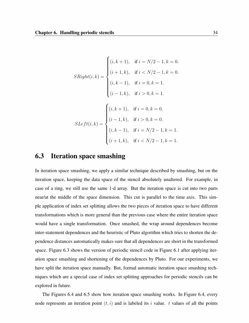
Chapter 6. Handling periodic stencils 34
SRight(i, k) =
(i, k + 1), if i = N/2− 1, k = 0.
(i+ 1, k), if i < N/2− 1, k = 0.
(i, k − 1), if i = 0, k = 1.
(i− 1, k), if i > 0, k = 1.
SLeft(i, k) =
(i, k + 1), if i = 0, k = 0.
(i− 1, k), if i > 0, k = 0.
(i, k − 1), if i = N/2− 1, k = 1.
(i+ 1, k), if i < N/2− 1, k = 1.
6.3 Iteration space smashing
In iteration space smashing, we apply a similar technique described by smashing, but on the
iteration space, keeping the data space of the stencil absolutely unaltered. For example, in
case of a ring, we still use the same 1-d array. But the iteration space is cut into two parts
near/at the middle of the space dimension. This cut is parallel to the time axis. This sim-
ple application of index set splitting allows the two pieces of iteration space to have different
transformations which is more general than the previous case where the entire iteration space
would have a single transformation. Once smashed, the wrap around dependences become
inter-statement dependences and the heuristic of Pluto algorithm which tries to shorten the de-
pendence distances automatically makes sure that all dependences are short in the transformed
space. Figure 6.3 shows the version of periodic stencil code in Figure 6.1 after applying iter-
ation space smashing and shortening of the dependences by Pluto. For our experiments, we
have split the iteration space manually. But, formal automatic iteration space smashing tech-
niques which are a special case of index set splitting approaches for periodic stencils can be
explored in future.
The Figures 6.4 and 6.5 show how iteration space smashing works. In Figure 6.4, every
node represents an iteration point (t, i) and is labeled its i value. t values of all the points
Page 45
Chapter 6. Handling periodic stencils 35
for (t = 1; t <= N; t++) {
for (j = 0; j < N/2 ; j++) {
S1: A[t][j]
= 0.125 * ( A[t-1][j+1] +
A[t-1][j] +
A[t-1][(j==0)?(N-1):(j-1)] );
S2: A[t][N-1-j]
= 0.125 * ( A[t-1][(j==0)? (0) : (N-i)] +
A[t-1][N-1-j] +
A[t-1][N-2-j] );
}
}
Figure 6.3: Smashed stencil: periodic 1d heat equation
remain unchanged after smashing and for simplicity, we have chosen omit them in the figure.
In Figure 6.5, there are two layers of iteration space but no wrap-around dependences. Every
node represents two iteration points whose i values are separated by ‘|’.
Page 46
Chapter 6. Handling periodic stencils 36
..
1
.
1
.
1
.
1
.
1
.
2
.
2
.
2
.
2
.
2
.
3
.
3
.
3
.
3
.
3
.
4
.
4
.
4
.
4
.
4
.
5
.
5
.
5
.
5
.
5
.
6
.
6
.
6
.
6
.
6
.
7
.
7
.
7
.
7
.
7
.
8
.
8
.
8
.
8
.
8
. N.
T
Figure 6.4: Before iteration space smashing
..
1|8
.
1|8
.
1|8
.
1|8
.
1|8
.
2|7
.
2|7
.
2|7
.
2|7
.
2|7
.
3|6
.
3|6
.
3|6
.
3|6
.
3|6
.
4|5
.
4|5
.
4|5
.
4|5
.
4|5
. N.
T
Figure 6.5: After iteration space smashing
Page 47
Chapter 7
Implementation
In this section, we discuss the implementation of our scheme and the tools used for it. We also
provide insights about the code versioning we perform on generated codes to help vectoriza-
tion.
7.1 Implementation on top of Pluto
We have implemented our approach on top of the publicly available source-to-source polyhe-
dral tool chain: Pluto [35]. It uses the Cloog [13] library for code generation, and PIP [34]
to solve for coefficients of hyperplanes. Pluto uses Clan [4] to extract the polyhedral abstrac-
tion from source code. But, for our experiments Clan could not be used as our stencil source
codes involve modulo operations which cannot be parsed by Clan. So, we have integrated
PET library [33] into Pluto to take care of such modulo operations. We have also incorporated
lower dimensional concurrent start in our implementation. PrimeTile [21] is used to perform
unroll-jam on Pluto generated code for some benchmarks.
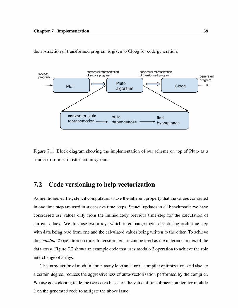
Figure 7.1 depicts our implementation on top Pluto. PET takes a C program as input and
generates the polyhedral representation of it in terms of isl structures [26]. In our implemen-
tation inside Pluto algorithm, we first convert the isl structures into Pluto’s internal represen-
tation. We find the dependence polyhedra using the polyhedral representation. We then find
hyperplanes using the algorithm described in Algorithm 1. After finding the transformations,
37
Page 48
Chapter 7. Implementation 38
the abstraction of transformed program is given to Cloog for code generation.
Figure 7.1: Block diagram showing the implementation of our scheme on top of Pluto as a
source-to-source transformation system.
7.2 Code versioning to help vectorization
As mentioned earlier, stencil computations have the inherent property that the values computed
in one time-step are used in successive time-steps. Stencil updates in all benchmarks we have
considered use values only from the immediately previous time-step for the calculation of
current values. We thus use two arrays which interchange their roles during each time-step
with data being read from one and the calculated values being written to the other. To achieve
this, modulo 2 operation on time dimension iterator can be used as the outermost index of the
data array. Figure 7.2 shows an example code that uses modulo 2 operation to achieve the role
interchange of arrays.
The introduction of modulo limits many loop and unroll compiler optimizations and also, to
a certain degree, reduces the aggressiveness of auto-vectorization performed by the compiler.
We use code cloning to define two cases based on the value of time dimension iterator modulo
2 on the generated code to mitigate the above issue.
Page 49
Chapter 7. Implementation 39
double A[2][N];
for (t = 0; t < T; t++) {
for (i = 1; i < N-1; i++) {
A[(t+1)%2][i] = 0.125 *(A[t%2][i+1]-2.0*A[t%2][i] +A[t%2][i-1]) ;
}
}
Figure 7.2: 1d-heat stencil with modulo indexing
Figure7.3 shows the versioned code equivalent to the code in Figure 7.2.
double A[2][N];
for (t = 0; t < T; t++) {
if(t%2==0)
for (i = 1; i < N-1; i++)
A[1][i] = 0.125 *(A[0][i+1]-2.0*A[0][i] +A[0][i-1]);
else
for (i = 1; i < N-1; i++)
A[0][i] = 0.125 *(A[1][i+1]-2.0*A[1][i] +A[1][i-1]);
}
Figure 7.3: 1d-heat stencil without modulo indexing
Page 50
Chapter 8
Experimental evaluation
We compare the performance of our system with Pluto serving as the state-of-the-art from the
compiler works, and the Pochoir stencil compiler [43] representing the state-of-the-art among
domain-specific works. Throughout the section, the legend pipeline represents code gener-
ated by Pluto without our enhancement, diamond represents codes generated by our lower
dimensional concurrent start approach built on top of Pluto, exploiting concurrent start in one
dimension, pochoir for codes generated by Pochoir and icc-par for original code compiled
with icc using “-parallel” flag.
Emphasis of these experiments is on
• ascertaining how important concurrent start-up really is.
• verifying if concurrent start-up actually translates into better load balance and scalability
of generated code.
• confirming that the new set of hyperplanes do not degrade the previous cache benefits.
8.1 Benchmarks
All benchmarks use double-precision floating-point computation. icc (version 12.1.3) is used
to compile all codes with options “-O3 -fp-model precise”; hence, only value-safe optimiza-
tions are performed. The optimal tile sizes and unroll factors are determined empirically with a
40
Page 51
Chapter 8. Experimental evaluation 41
limited amount of search. The problem sizes for various benchmarks are shown in Table 8.1 in
⟨spacesize⟩dimension x ⟨timesize⟩ format. These are taken from the Pochoir suite. For all the
benchmarks, the respective problem sizes make sure that the data required by the benchmark
does not fit into cache and hence are meaningful.
Benchmark Problem Size
1d-heat 1600000x1000
2d-heat 160002x500
3d-heat 1503x100
game-of-life 160002x500
apop 20000x1000
3d7pt 1603x100
1d-heat-p 1600000x1000
2d-heat-p 160002x500
3d-heat-p 3003x200
Table 8.1: Problem sizes for the benchmarks in the format ⟨spacesize⟩dimension x ⟨timesize⟩
• 1d/2d/3d-heat : Heat equations are examples of symmetric stencils. We evaluate the
performance of discretized 1-d, 2-d and 3-d heat equation stencils with non-periodic
boundary conditions. 1d-heat is a 3-point stencil, while 2d-heat and 3d-heat are 5-point
and 7-point stencils respectively.
• 1d/2d/3d-heat-p: These are the periodic equivalents of the heat stencils mentioned ear-
lier.
• Game of Life: Conway’s Game of Life [18] is an 8-point stencil where the state of each
point in the next time iteration depends on its 8 neighbors. We consider a particular
version of the game called B2S23, where a point is “born” if it has exactly two live
neighbors and a point survives the current stage if it has exactly either two or three
neighbors.
Page 52
Chapter 8. Experimental evaluation 42
• 3d7pt: An order-1 3D 7-point stencil [15] from the Berkeley auto-tuner framework.
• APOP: APOP [23] is a one dimensional 3-point stencil that calculates the price of the
American put stock option.
8.2 Hardware setup
We use two hardware configurations as shown in Table 8.2 in our experiments.
Intel Xeon E5645 AMD Opteron 6136
Microarchitecture Westmere-EP Magny-Cours
Clock 2.4 GHz 2.4 GHz
Cores / socket 6 8
Total cores 12 16
L1 cache / Core 32 KB 128 KB
L2 cache / Core 512 KB 512 KB
L3 cache / Socket 12 MB 12 MB
RAM 24GB DDR3 (1333 MHz) 64GB DDR3 (1333 MHz)
Compiler icc (version 12.1.3) icc (version 12.1.3)
Compiler flags -O3 -fp-model precise -O3 -fp-model precise
Linux kernel 2.6.32 2.6.35
Table 8.2: Details of architectures used for experiments
8.3 Significance of concurrent start
In this section, we demonstrate the importance of our enhancement over existing schemes
quantitatively. Though pipeline drain and start-up can be minimized by tweaking tile sizes
(besides making sure there are enough tiles in the wavefront), this could constrain tile sizes
leading to loss of locality and/or increase in frequency of synchronization. In addition, all
of this is highly problem-size dependent. It is true that for some problem sizes one can be
Page 53
Chapter 8. Experimental evaluation 43
0
10
20
30
40
50
60
0 2 4 6 8 10 12
GF
LOP
s
Number of cores
diamond-64x64x64pipeline-64x64x64pipeline-16x64x64pochoir
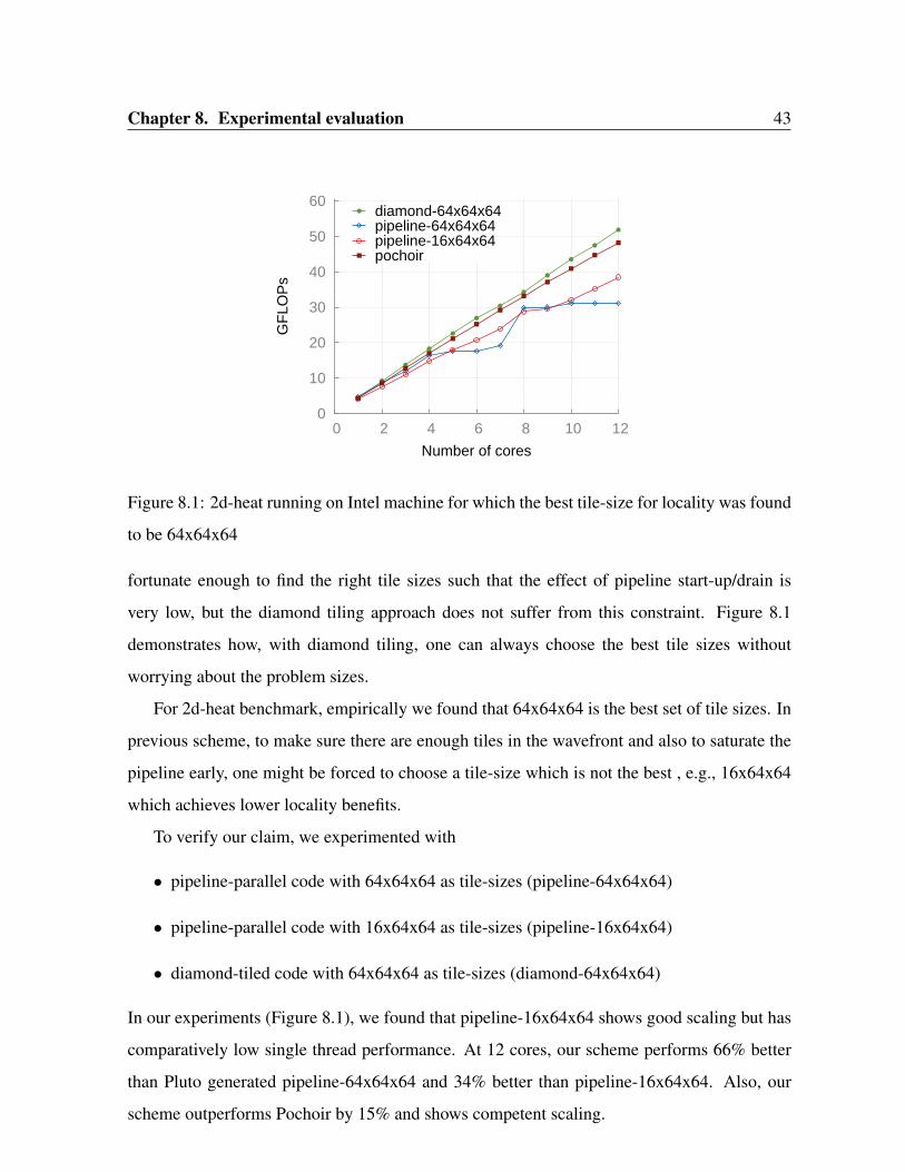
Figure 8.1: 2d-heat running on Intel machine for which the best tile-size for locality was found
to be 64x64x64
fortunate enough to find the right tile sizes such that the effect of pipeline start-up/drain is
very low, but the diamond tiling approach does not suffer from this constraint. Figure 8.1
demonstrates how, with diamond tiling, one can always choose the best tile sizes without
worrying about the problem sizes.
For 2d-heat benchmark, empirically we found that 64x64x64 is the best set of tile sizes. In
previous scheme, to make sure there are enough tiles in the wavefront and also to saturate the
pipeline early, one might be forced to choose a tile-size which is not the best , e.g., 16x64x64
which achieves lower locality benefits.
To verify our claim, we experimented with
• pipeline-parallel code with 64x64x64 as tile-sizes (pipeline-64x64x64)
• pipeline-parallel code with 16x64x64 as tile-sizes (pipeline-16x64x64)
• diamond-tiled code with 64x64x64 as tile-sizes (diamond-64x64x64)
In our experiments (Figure 8.1), we found that pipeline-16x64x64 shows good scaling but has
comparatively low single thread performance. At 12 cores, our scheme performs 66% better
than Pluto generated pipeline-64x64x64 and 34% better than pipeline-16x64x64. Also, our
scheme outperforms Pochoir by 15% and shows competent scaling.
Page 54
Chapter 8. Experimental evaluation 44
tile-sizes L2 misses in billions L2 requests in billions percentage of misses
pipeline-16x64x64 3.35 22.7 14.7
pipeline-64x64x64 2.03 21.7 9.3
diamond-64x64x64 2.05 21.1 9.7
pochoir 3.04 24.0 12.6
icc-par 2.9 47.4 6.1
Table 8.3: Details of hardware counters for cache behavior in experiments for heat-2d on a
single core of Intel machine
Further, hyperplanes found by our scheme cannot be better than those found by Pluto with
respect to the cost function. Therefore, single-thread performance of code generated by our
scheme may reduce. However, by using hyperplanes found by our scheme to only demarcate
tiles and the hyperplanes that would be found by the Pluto algorithm without our enhancement
to scan points inside a tile, we obtain desired benefits for intra-tile execution. To support this
claim and also to verify the results of the above experiment, we have collected the hardware
counters L2 cache misses and requests. Table 8.3 shows L2 cache behavior for 2d-heat running
on a single core of our Intel machine.
8.4 Results for non-periodic stencils
Our scheme consistently outperforms Pluto’s pipeline-parallel scheme for all benchmarks. We
perform better than Pochoir on 1d-heat, 2d-heat, 3d-heat, 3d7pt and perform comparably with
Pochoir for APOP and Game of Life. The running times for different benchmarks and the
speedup factors we get over other schemes are presented in Table 8.4. The speedup factors
reported are when running all of them on 12 cores.
Page 55
Chapter 8. Experimental evaluation 45
0
10
20
30
40
50
0 2 4 6 8 10 12
GF
LOP
s
Number of cores
diamondpipelinepochoir
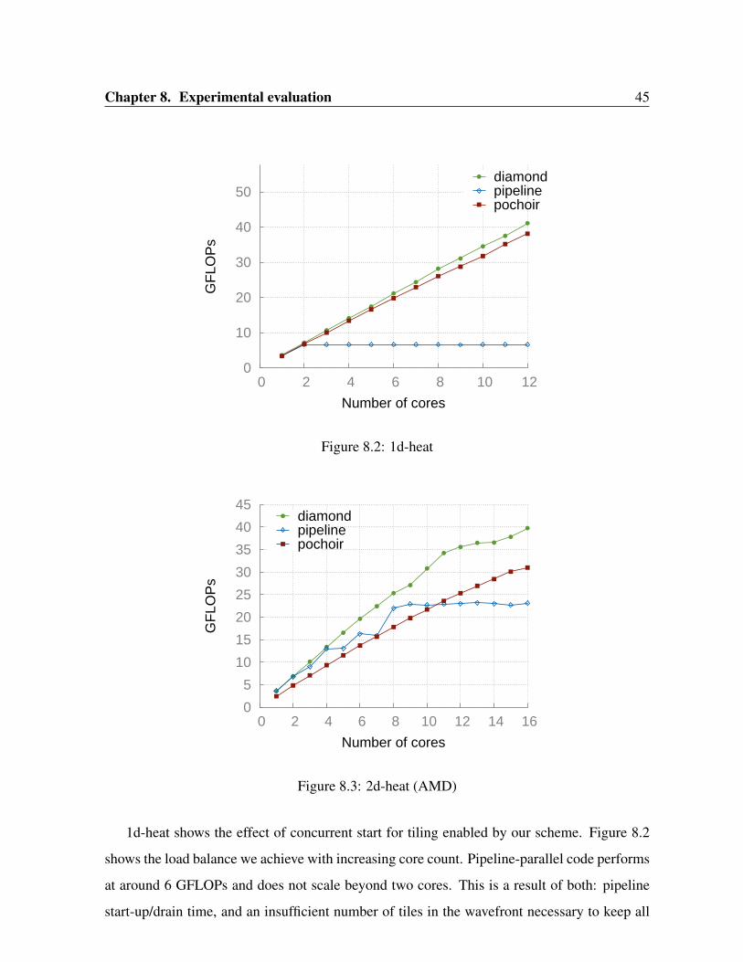
Figure 8.2: 1d-heat
0
5
10
15
20
25
30
35
40
45
0 2 4 6 8 10 12 14 16
GF
LOP
s
Number of cores
diamondpipelinepochoir
Figure 8.3: 2d-heat (AMD)
1d-heat shows the effect of concurrent start for tiling enabled by our scheme. Figure 8.2
shows the load balance we achieve with increasing core count. Pipeline-parallel code performs
at around 6 GFLOPs and does not scale beyond two cores. This is a result of both: pipeline
start-up/drain time, and an insufficient number of tiles in the wavefront necessary to keep all
Page 56
Chapter 8. Experimental evaluation 46
processors busy. Using our new tiling hyperplanes, one is able to distribute iterations corre-
sponding to the entire data space equally among all cores. The same maximal amount of work
is done by processors between two synchronizations as the tile schedule is parallel to the face
that allows concurrent start.
For 2d-heat, we perform better than both Pochoir and Pluto’s pipeline-parallel approach.
We have discussed already the improvements on Intel machine (Figure 8.1). We also tested the
three schemes on the AMD Opteron 16-core setup, and we see similar improvements with our
scheme (Figure 8.3). Performance of pipeline-parallel code saturates after 8 cores for the same
reasons as mentioned for 1d-heat. Our scheme performs 72% better than pipeline-parallel code
and 28% better than Pochoir.
0
10
20
30
40
50
0 2 4 6 8 10 12
GF
LOP
s
Number of cores
diamondpipelinepochoir
Figure 8.4: 3d-heat
On the 3d-heat benchmark, pipeline-parallel code performs poorly while both Pochoir and
our scheme scale well (Figure 8.4). Pochoir achieves about 21% of the machine peak and our
scheme achieves 24.2%. CPU utilization is as expected with our technique while Pluto suffers
from load imbalance here. For our scheme, though scaling seen with 1,2,4,8,12 cores is almost
ideal, it is flat between 5 and 8 cores. This is due to the number of tiles available not being
a multiple of the number of threads. This load imbalance can be eliminated using dynamic
scheduling techniques [3] and can be explored in future. In addition, the tile to thread mapping
Page 57
Chapter 8. Experimental evaluation 47
we employed is not conscious of locality, i.e., inter-tile reuse can be exploited with another
suitable mapping. Integrating the complementary techniques presented in [42] may improve
performance further.
0
5
10
15
20
25
30
0 2 4 6 8 10 12
GF
LOP
s
Number of cores
diamondpipelinepochoir
Figure 8.5: 3D 7-point Stencil
0
100
200
300
400
500
600
700
800
900
0 2 4 6 8 10 12
Tim
e (s
econ
ds)
Number of cores
diamondpipelinepochoir
Figure 8.6: Game of Life
Page 58
Chapter 8. Experimental evaluation 48
0
20
40
60
80
100
0 2 4 6 8 10 12
Tim
e (m
s)
Number of cores
diamondpipelinepochoir
Figure 8.7: American Put Option Pricing
The rest of the benchmarks, 3d7pt (Figure 8.5), game-of-life (Figure 8.6) and APOP (Fig-
ure 8.7), show similar behavior as the already discussed benchmarks, for all the three schemes.
The ‘Game of Life’ does not use any floating-point operations in the stencil. Performance
is thus reported directly via running time. Similarly, performance for APOP is also reported
in running time as it depends on the conditional inside the loop nest as well and not just the
floating point operations.
Table 8.4 summarizes the performance numbers for 12 cores on Intel multicore machine.
Benchmark Performance (12 cores) Speedup over
icc-par pochoir pipeline diamond icc-par pochoir pipeline
1d-heat 2.61s 171.7ms 965ms 155.8ms 16.75 1.10 6.19
2d-heat 8.44m 28.43s 41.18s 24.72s 20.48 1.15 1.66
3d-heat 1.60s 156.6ms 315ms 135ms 11.85 1.16 2.33
game-of-life 13.50m 52.51s 2.98m 64.09s 12.64 0.82 2.79
apop 46.70ms 12.19ms 63.40ms 11.70ms 3.99 1.04 5.42
3d7pt 1.6s 181.9ms 309ms 143.2ms 11.17 1.27 2.15
Table 8.4: Summary of performance - non-periodic stencils
Page 59
Chapter 8. Experimental evaluation 49
8.5 Results for periodic stencils
For periodic stencils, we use manually smashed code as input to Pluto to generate pipeline-
parallel code and also to generate diamond-tiled code using our scheme. Apart from the
already discussed code versioning to remove ‘modulo 2’ operation, we use similar code-
versioning to differentiate between boundary tiles and non-boundary tiles. Only boundary tiles
have to take care of the periodic conditions, and the rest of the computation is same as that of a
non-periodic stencil. Pochoir also uses a similar mechanism to differentiate between boundary
blocks and internal blocks. Such differentiation allows removal of unnecessary conditionals
from code for internal tiles.
0
10
20
30
40
50
0 2 4 6 8 10 12
GF
LOP
s
Number of cores
diamondpipelinepochoir
Figure 8.8: 1d-heat-periodic
For 1d-heat-periodic, performance of all the three schemes follows the same trend as that
of non-periodic version (Figure 8.8). Our scheme performs 20% better than Pochoir and about
15× better compared to pipeline-parallel code. We can also note that overall performance
for all the three schemes worsens compared to non-periodic version owing to the boundary
conditions introduced.
For 2d-heat-periodic, pipeline-parallel code does not scale after 8 cores, but both our
scheme and Pochoir continue to show good scaling (Figure 8.9). Our scheme is performs
57% better than pipeline-parallel code at 12-cores, but is worse by 14% compared to Pochoir.
This gap in performance becomes visible at the single-thread performance itself, and as the
Page 60
Chapter 8. Experimental evaluation 50
0
10
20
30
40
50
60
0 2 4 6 8 10 12
GF
LOP
s
Number of cores
diamondpipelinepochoir
Figure 8.9: 2d-heat-periodic
number of cores goes up, this performance gap also yawns, correspondingly. In fact, the per-
formance of Pochoir in this case seems like an anomaly as it is consistently better than the
performance of its own non-periodic version. Pochoir being a ‘black box’ optimizer, it is very
difficult to understand why this anomaly exists. Our efforts to understand this have not been
successful.
0
5
10
15
20
25
0 2 4 6 8 10 12
GF
LOP
s
Number of cores
diamondpipelinepochoir
Figure 8.10: 3d-heat-periodic
Both our scheme and pipeline-parallel approach outperform Pochoir for 3d-heat-periodic
(Figure 8.10). But, Pochoir code behaves erratic after 6 cores in terms of performance, hence
we feel it is not a strong comparison.
Page 61
Chapter 8. Experimental evaluation 51
0
5
10
15
20
25
30
35
40
45
0 2 4 6 8 10 12
Tim
e(s)
Number of cores
icc-parpipelinediamond
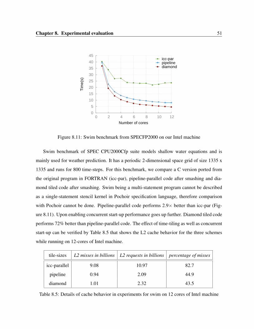
Figure 8.11: Swim benchmark from SPECFP2000 on our Intel machine
Swim benchmark of SPEC CPU2000Cfp suite models shallow water equations and is
mainly used for weather prediction. It has a periodic 2-dimensional space grid of size 1335 x
1335 and runs for 800 time-steps. For this benchmark, we compare a C version ported from
the original program in FORTRAN (icc-par), pipeline-parallel code after smashing and dia-
mond tiled code after smashing. Swim being a multi-statement program cannot be described
as a single-statement stencil kernel in Pochoir specification language, therefore comparison
with Pochoir cannot be done. Pipeline-parallel code performs 2.9× better than icc-par (Fig-
ure 8.11). Upon enabling concurrent start-up performance goes up further. Diamond tiled code
performs 72% better than pipeline-parallel code. The effect of time-tiling as well as concurrent
start-up can be verified by Table 8.5 that shows the L2 cache behavior for the three schemes
while running on 12-cores of Intel machine.
tile-sizes L2 misses in billions L2 requests in billions percentage of misses
icc-parallel 9.08 10.97 82.7
pipeline 0.94 2.09 44.9
diamond 1.01 2.32 43.5
Table 8.5: Details of cache behavior in experiments for swim on 12 cores of Intel machine
Page 62
Chapter 8. Experimental evaluation 52
0
10
20
30
40
50
60
0 2 4 6 8 10 12 14 16
Tim
e(s)
Number of cores
icc-parpipelinediamond
Figure 8.12: Swim benchmark from SPECFP2000 on our AMD machine
We observe a similar trend of performance for all the three schemes on our AMD machine.
Figure 8.12 depicts the timings for C version compiled with ‘-parallel’ flag of icc, pipeline-
parallel code after smashing and diamond-tiled code after smashing for runs on up to 16 cores.
Our scheme shows an improvement of 2.5× over icc-par and 53% over pipeline-parallel code
on 16 cores.
Table 8.6 summarizes the experimental results for the above discussed benchmarks.
Benchmark Performance (12 cores) Speedup over
icc-par pochoir pipeline diamond icc-par pochoir pipeline
1d-heat-p 4.3s 195ms 2.5s 162.4ms 26.5 1.2 15.4
2d-heat-p 570s 27.3s 49.8s 31.7s 22.7 0.86 1.57
3d-heat-p 38.19s 11.5s 10.58s 4.9s 7.79 2.34 2.15
swim 23.62s - 7.97s 4.61s 5.12 - 1.72
Table 8.6: Summary of performance -periodic stencils
Page 63
Chapter 9
Related work
A significant amount of work has been done on optimizing stencil computations. These
works fall into two categories. One body of works is in the form of developing compiler
optimizations [46, 38, 29, 8], and the other on building domain-specific stencil compilers or
domain-specific optimization studies [27, 16, 41, 42, 12, 40, 44, 43]. Among the compiler
techniques, the polyhedral compiler works have been implemented in some production com-
pilers [20, 39, 7], and are also available publicly as tools [35, 36]. They are in the form of
more general transformation frameworks and more or less subsume previous compiler works
for stencils. Other significant body of works studies optimization specific to stencils, and a
number of these works are very recent. Many of these are publicly available as well such as
Pochoir [43]. Such systems have the opportunity to provide much higher performance than
compiler-based ones owing to the greater amount of knowledge they have about computation.
Pochoir [43] is a highly tuned stencil specific compiler and runtime system for multicores.
It provides a C++ template library using which a programmer can describe a specification of
a stencil in terms of dimensions, width of the stencil, its shape etc.. For example, Figure 9.1
shows description of a heat-1d kernel using Pochoir specification language.
Pochoir uses a cache-oblivious tiling mechanism. It builds upon the concept of ‘trape-
zoidal decompositions’ introduced by Frigo and Strumpen [17] and improves upon it by a
novel technique called ‘hyperspace cut’. Hyperspace cuts perform simultaneous space cuts on
53
Page 64
Chapter 9. Related work 54
Pochoir_Kernel_1D(heat_1D_fn, t, i)
a(t+1,i) = 0.125 * (a(t,i+1) - 2.0 * (t,i) + a(t,i-1));
Pochoir_Kernel_End
Figure 9.1: Stencil: 1d heat equation
multiple dimensions allowing Pochoir to exploit asymptotically more parallelism as the num-
ber of space dimensions increases. These decompositions and cuts are performed recursively
and resulting tiles are shaped like trapezoids. After tiling, Pochoir writes a high performing
Cilk code as output.
In addition, Pochoir performs optimizations to take care of conditionals at boundaries
which is comparable to code-cloning that we perform. It also performs a base-case coars-
ening for recursive cuts which is very similar to our tile-size choices. To ensure it does not
suffer from load imbalance, its runtime implements a smart work stealing mechanism. This
work falls in the domain-specific category of optimizers. Our scheme on the other hand is
a dependence-driven one and is oblivious to the input code being a stencil. Our experimen-
tal evaluation included a comparison with Pochoir. In addition, though our techniques are
implemented in a polyhedral source-to-source compiler, they apply to either body of works.
Strzodka et al. [42] present a technique, cache accurate time skewing (CATS), for tiling
stencils, and report significant improvement over Pluto and other simpler manual optimization
strategies for 2-d and 3-d domains. The work argues that for typical cache sizes and problem
sizes of 2-d and 3-d domains, not tiling in all space dimensions can be more beneficial than
tiling in all space dimensions and time. This decision of not tiling in all dimensions results
in tiles that are huge in some dimensions. But this can be easily achieved by our scheme
by choosing a huge tile-size in one tiling dimension. We could use such tube-like tiles in
some of our experiments and verify the claim by CATS scheme that it is more SIMD friendly.
Diamond-shaped tiles that are automatically found by our technique are also used by CATS in
a particular way. However, their scheme also pays attention to additional orthogonal aspects
such as mapping of tiles to threads and is presumably far more cache-friendly than our scheme.
These aspects can be explored in future to enhance our approach. While ours is an end-to-end
Page 65
Chapter 9. Related work 55
automatic compiler framework, CATS is more of a customized optimization system. CATS
makes assumptions about typical problem-sizes and cache sizes and focuses on 2-d and 3-d
domains whereas our scheme is completely independent of such factors. Performance com-
parison with CATS could not be done as the scheme is not automatic and the codes are not yet
publicly available.
Efficient vectorization of stencils is challenging. Henretty et al. [22] present a data lay-
out transformation technique to improve vectorization. However, reported improvement was
limited for architectures that provide nearly the same performance for unaligned loads as for
aligned loads. This is the case with Nehalem, Westmere, and Sandy Bridge architectures
from Intel. We did not thus explore layout transformations for vectorization, but instead relied
on Intel compiler’s auto-vectorization after automatic application of enabling transformations
within a tile.
Figure 9.2: Overlapped and split tiling.
Krishnamoorthy et al. [29] addressed concurrent start when tiling stencil computations.
However, the approach worked by starting with a valid tiling and correcting it to allow concur-
rent start. This was done via overlapped execution of tiles (overlapped tiling) or by splitting a
tile into sub-tiles (split tiling).
In overlapped tiling, for example in Figure 9.2, tiles marked 1 and 2 can be merged as one
tile and 2, 3 and 4 are merged as second tile. Here, the computation labeled 2 is shared by both
the tiles and hence the name overlapped tiling. Therefore, the sets of tiles {1, 2}, {2, 3, 4},
{4, 5, 6}, {6, 7, 8} are merged individually and are started concurrently.
Page 66
Chapter 9. Related work 56
In the split tiling approach, there is no merging of tiles. Tiles 2, 4 , 6 and 8 can be started
concurrently followed by the execution of 1, 3, 5 and 7 in parallel.
With such approaches, one misses natural ways of tiling that inherently do not suffer from
pipelined start-up. We have showed that, in all those cases, there exist valid tiling hyperplanes
that allow concurrent start. The key problem with both overlapped tiling and split tiling is
the difficulty in performing code generation automatically. No implementation of these tech-
niques currently exists. In addition, our conditions for concurrent start work with arbitrary
affine dependences while those in [29] were presented for uniform dependences, i.e., when
dependences can be represented by constant distance vectors.
A survey by Wonnacott et al.[47] reviews many works in polyhedral model that aim to
exploit maximum parallelism available using new tiling techniques. The survey concludes that
the works previous to ours fell into two classes:
• Ideas in general-purpose domains that remain unimplemented due to the difficulties
posed by complex tile shapes and orientations they result in.
• Implemented techniques that fail to achieve asymptotic scaling as the available paral-
lelism increases.
Our work bridges this gap and provides techniques applicable to any regular program that
allows tile-wise concurrent start to achieve maximum parallelism, along with a fully automatic
implementation of it.
Page 67
Chapter 10
Conclusion
We have designed and evaluated new techniques for tiling stencil computations. These tech-
niques, in addition to the usual benefits of tiling, provide concurrent start-up whenever pos-
sible. Evidently, such concurrent start-up enabled provides perfect load balance at tile level
granularity and also translates into asymptotic scalability. We showed that tile-wise concur-
rent start is enabled if the face of the iteration space that allows point-wise concurrent start
strictly lies in the cone formed by all tiling hyperplanes. We then provided an approach to find
such hyperplanes. The presented techniques are automatic and have been implemented in a
source-level parallelizer, Pluto.
Experimental evaluation on a 12-core Intel multicore shows that our code is able to outper-
form a tuned domain-specific stencil code generator in most of the cases by about 4% to 2×.
We outperform previous compiler techniques by a factor of 1.5× to 15× on 12 cores over a
set of benchmarks. For swim benchmark (SPECFP 2000), our scheme achieves 5× improve-
ment over the auto-parallelizer of Intel C Compiler on our 12-core Intel Westmere and 2.5× on
16-core AMD Magny-Cours. We are not aware of any SPEC performance numbers that come
close to this result, obtained either through manual or automatic schemes. Our implementation
is publicly available in the latest release of Pluto.
57
Page 68
Bibliography
[1] A. V. Aho, R. Sethi, and J. D. Ullman. Compilers: principles, techniques, and tools.
Addison-Wesley Longman Publishing Co., Inc., Boston, MA, USA, 1986.
[2] C. Ancourt and F. Irigoin. Scanning polyhedra with do loops. In ACM SIGPLAN sympo-
sium on Principles and Practice of Parallel Programming, pages 39–50, 1991.
[3] M. Baskaran, N. Vydyanathan, U. Bondhugula, J. Ramanujam, A. Rountev, and P. Sa-
dayappan. Compiler-assisted dynamic scheduling for effective parallelization of loop
nests on multicore processors. In ACM SIGPLAN PPoPP, pages 219–228, 2009.
[4] C. Bastoul. Clan: The Chunky Loop Analyzer. Clan user guide.
[5] C. Bastoul. Code generation in the polyhedral model is easier than you think. In IEEE
International Conference on Parallel Architectures and Compilation Techniques, pages
7–16, Sept. 2004.
[6] U. Bondhugula, M. Baskaran, S. Krishnamoorthy, J. Ramanujam, A. Rountev, and P. Sa-
dayappan. Automatic transformations for communication-minimized parallelization and
locality optimization in the polyhedral model. In ETAPS CC, Apr. 2008.
[7] U. Bondhugula, O. Gunluk, S. Dash, and L. Renganarayanan. A model for fusion and
code motion in an automatic parallelizing compiler. In Proceedings of the 19th interna-
tional conference on Parallel architectures and compilation techniques, PACT ’10, pages
343–352. ACM, 2010.
58
Page 69
BIBLIOGRAPHY 59
[8] U. Bondhugula, A. Hartono, J. Ramanujam, and P. Sadayappan. A practical automatic
polyhedral program optimization system. In ACM SIGPLAN PLDI, June 2008.
[9] U. Bondhugula, J. Ramanujam, and P. Sadayappan. Pluto: A practical and fully au-
tomatic polyhedral parallelizer and locality optimizer. Technical Report OSU-CISRC-
10/07-TR70, The Ohio State University, Oct. 2007.
[10] U. K. R. Bondhugula. Effective Automatic Parallelization and Locality Optimization
using the Polyhedral Model. PhD thesis, The Ohio State University, Aug 2008.
[11] J.-D. Choi and S. L. Min. Race frontier: reproducing data races in parallel-program
debugging. In Proceedings of the third ACM SIGPLAN symposium on Principles and
practice of parallel programming, PPOPP ’91, pages 145–154, New York, NY, USA,
1991. ACM.
[12] M. Christen, O. Schenk, and H. Burkhart. Patus: A code generation and autotuning
framework for parallel iterative stencil computations on modern microarchitectures. In
Parallel Distributed Processing Symposium (IPDPS), 2011 IEEE International, pages
676 –687, may 2011.
[13] CLooG: The Chunky Loop Generator. http://www.cloog.org.
[14] A. Cohen, S. Girbal, D. Parello, M. Sigler, O. Temam, and N. Vasilache. Facilitating the
search for compositions of program transformations. In ACM International conference
on Supercomputing, pages 151–160, June 2005.
[15] K. Datta. Auto-tuning Stencil Codes for Cache-Based Multicore Platforms. PhD thesis,
EECS Department, University of California, Berkeley, Dec 2009.
[16] K. Datta, M. Murphy, V. Volkov, S. Williams, J. Carter, L. Oliker, D. A. Patterson,
J. Shalf, and K. A. Yelick. Stencil computation optimization and auto-tuning on state-of-
the-art multicore architectures. In SC, page 4, 2008.
Page 70
BIBLIOGRAPHY 60
[17] M. Frigo and V. Strumpen. Cache oblivious stencil computations. In Proceedings of
the 19th annual international conference on Supercomputing, ICS ’05, pages 361–366,
2005.
[18] M. Gardner. Mathematical Games. Scientific American, 1970.
[19] M. Griebl, P. Feautrier, and A. Großlinger. Forward communication only placements and
their use for parallel program construction. In LCPC, pages 16–30, 2005.
[20] T. Grosser, H. Zheng, R. Aloor, A. Simburger, A. Groblinger, and L.-N. Pouchet. Polly
polyhedral optimization in LLVM. In Proceedings of the First International Workshop
on Polyhedral Compilation Techniques (IMPACT), 2011, 2011.
[21] A. Hartono, M. Manik, A. Baskaran, C. Bastoul, A. Cohen, S. Krishnamoorthy, B. Norris,
and J. Ramanujam. Primetile: A parametric multi-level tiler for imperfect loop nests,
2009.
[22] T. Henretty, K. Stock, L.-N. Pouchet, F. Franchetti, J. Ramanujam, and P. Sadayap-
pan. Data layout transformation for stencil computations on short simd architectures.
In ETAPS International Conference on Compiler Construction (CC’11), pages 225–245,
Saarbrucken, Germany, Mar. 2011.
[23] J. Hull. Options, futures, and other derivatives. Pearson Prentice Hall, Upper Saddle
River, NJ [u.a.], 6. ed., pearson internat. ed edition, 2006.
[24] Multi-core processor. http://en.wikipedia.org/wiki/Multi-
core processor#Technical factors.
[25] F. Irigoin and R. Triolet. Supernode partitioning. In Proceedings of the 15th ACM
SIGPLAN-SIGACT symposium on Principles of programming languages, POPL ’88,
pages 319–329, 1988.
[26] Integer Set Library. Sven Verdoolaege, An Integer Set Library for Program Analysis.
Page 71
BIBLIOGRAPHY 61
[27] S. Kamil, K. Datta, S. Williams, L. Oliker, J. Shalf, and K. Yellick. Implicit and explicit
optimization for stencil computations. In ACM SIGPLAN workshop on Memory Systems
Perofmance and Correctness, 2006.
[28] W. Kelly and W. Pugh. A unifying framework for iteration reordering transformations.
Technical Report CS-TR-3430, Dept. of Computer Science, University of Maryland, Col-
lege Park, 1995.
[29] S. Krishnamoorthy, M. Baskaran, U. Bondhugula, J. Ramanujam, A. Rountev, and P. Sa-
dayappan. Effective Automatic Parallelization of Stencil Computations. In ACM SIG-
PLAN symposium on Programming Languages Design and Implementation, July 2007.
[30] A. Lim, G. I. Cheong, and M. S. Lam. An affine partitioning algorithm to maximize
parallelism and minimize communication. In ACM ICS, pages 228–237, 1999.
[31] A. Lim and M. S. Lam. Maximizing parallelism and minimizing synchronization with
affine partitions. Parallel Computing, 24(3-4):445–475, 1998.
[32] N. Osheim, M. Strout, D. Roston, and S. Rajopadhye. Smashing: Folding Space to
Tile through Time. In International Workshop on Languages and Compilers for Parallel
Computing (LCPC), 2008.
[33] Polyhedral extraction tool. http://freecode.com/projects/libpet.
[34] PIP: The Parametric Integer Programming Library. http://www.piplib.org.
[35] PLUTO: A polyhedral automatic parallelizer and locality optimizer for multicores.
http://pluto-compiler.sourceforge.net.
[36] POCC: Polyhedral compiler collection. http://pocc.sourceforge.net.
[37] J. Ramanujam and P. Sadayappan. Tiling multidimensional iteration spaces for multi-
computers. Journal of Parallel and Distributed Computing, 16(2):108–230, 1992.
[38] L. Renganarayanan, M. Harthikote-Matha, R. Dewri, and S. V. Rajopadhye. Towards
optimal multi-level tiling for stencil computations. In IPDPS, pages 1–10, 2007.
Page 72
BIBLIOGRAPHY 62
[39] RSTREAM - High Level Compiler, Reservoir Labs. http://www.reservoir.com.
[40] N. Sedaghati, R. Thomas, L.-N. Pouchet, R. Teodorescu, and P. Sadayappan. StVEC:
A vector instruction extension for high performance stencil computation. In 20th Inter-
national Conference on Parallel Architecture and Compilation Techniques (PACT’11),
Galveston Island, Texas, Oct. 2011.
[41] R. Strzodka, M. Shaheen, D. Pajak, and H.-P. Seidel. Cache oblivious parallelograms in
iterative stencil computations. In ICS, pages 49–59, 2010.
[42] R. Strzodka, M. Shaheen, D. Pajak, and H.-P. Seidel. Cache accurate time skewing in
iterative stencil computations. In ICPP, pages 571–581, 2011.
[43] Y. Tang, R. A. Chowdhury, B. C. Kuszmaul, C.-K. Luk, and C. E. Leiserson. The pochoir
stencil compiler. In SPAA, pages 117–128, 2011.
[44] J. Treibig, G. Wellein, and G. Hager. Efficient multicore-aware parallelization strategies
for iterative stencil computations. Journal of Computational Science, 2(2):130 – 137,
2011.
[45] M. J. Wolfe. High Performance Compilers for Parallel Computing. Addison-Wesley
Longman Publishing Co., Inc., Boston, MA, USA, 1995.
[46] D. Wonnacott. Using time skewing to eliminate idle time due to memory bandwidth and
network limitations. In Proceedins of the 14th International Parallel and Distributed
Processing Symposium (IPDPS), pages 171 –180, 2000.
[47] D. G. Wonnacott and M. Mills Strout. On the scalability of loop tiling techniques. In
Proceedings of the 3rd International Workshop on Polyhedral Compilation Techniques
(IMPACT), 2013, 2013.
[48] J. Xue. Loop tiling for parallelism. Kluwer Academic Publishers, Norwell, MA, USA,
2000.