TIME CONSISTENCY AND THE DURATION OF GOVERNMENT DEBT:A SIGNALLING THEORY OF QUANTITATIVE EASING
Saroj BhattaraiGauti B. Eggertsson
Bulat Gafarov
Working Paper 21336http://www.nber.org/papers/w21336
NATIONAL BUREAU OF ECONOMIC RESEARCH1050 Massachusetts Avenue
Cambridge, MA 02138July 2015
We thank Roberto Billi, Jim Bullard, Guillermo Calvo, Oli Coibion, Giuseppe Ferrero, Mark Gertler,Marc Giannoni, Andy Levin, Emi Nakamura, Ricardo Reis, Tao Zha, seminar participants at HECMontreal, Emory University, University of Texas at Austin, and Brown University, and conferenceparticipants at NBER ME spring meeting, HKIMR/New York Fed Conference on Domestic and InternationalDimensions of Unconventional Monetary Policy, Society of Economic Dynamics Annual meeting,Mid-west Macro spring meeting, CEPR European Summer Symposium in International Macroeconomics,Annual Conference on Computing and Finance, NBER Japan Project Meeting, Annual Research Conferenceat Swiss National Bank, ECB Workshop on Non-Standard Monetary Policy Measures, Annual ResearchConference at De Nederlandsche Bank, Latin American Meetings of Econometric Society, and ColumbiaUniversity Conference on Macroeconomic Policy and Safe Assets for helpful comments and suggestions.First version: Sept 2013; This version: June 2015. The views expressed herein are those of the authorsand do not necessarily reflect the views of the National Bureau of Economic Research.
NBER working papers are circulated for discussion and comment purposes. They have not been peer-reviewed or been subject to the review by the NBER Board of Directors that accompanies officialNBER publications.
Time Consistency and the Duration of Government Debt: A Signalling Theory of QuantitativeEasingSaroj Bhattarai, Gauti B. Eggertsson, and Bulat GafarovNBER Working Paper No. 21336July 2015JEL No. E31,E4,E42,E43,E5,E52,E62,E63
ABSTRACT
We present a signalling theory of Quantitative Easing (QE) at the zero lower bound on the short termnominal interest rate. QE is effective because it generates a credible signal of low future real interestrates in a time consistent equilibrium. We show these results in two models. One has coordinated monetaryand fiscal policy. The other an independent central bank with balance sheet concerns. Numerical experimentsshow that the signalling effect can be substantial in both models.
Saroj BhattaraiUniversity of Texas at AustinDepartment of Economics2225 Speedway, Stop C3100Austin, TX [email protected]
Gauti B. EggertssonDepartment of EconomicsBrown University64 Waterman StreetProvidence, RI 02912and [email protected]
Bulat GafarovPennsylvania State Universityand National Research UniversityHigher School of [email protected]
“The problem with Quantitative Easing (QE) is it works in practice, but it doesn’t work in
theory,” Ben Bernanke, Chairman of the Federal Reserve, Jan 16, 2014 just before leaving offi ce.
1 Introduction
Since the onset of the economics crisis in 2008, the Federal Reserve has expanded its balance sheet
by large amounts, on the order of 3 trillion mostly under the rubric of Quantitative Easing (QE).
To date the accumulated amount of QE corresponds to about 20% percent of annual GDP. The
enormous scale of this policy has largely been explained by the fact that the Federal Reserve was
unable to cut the Federal Fund rate further, due the zero lower bound on the short term nominal
interest rate. Meanwhile, high unemployment, slow growth, and low inflation desperately called
for further stimulus measures.
Many commentators argue that QE in the United States prevented a much stronger contraction,
and that QE is a key reason for why the US has recovered more rapidly from the Great Recession
than some its counterparts. As pointed out by Ben Bernanke, however, one problem is that even
if this might be true in practice, a coherent theoretical rationale has been hard to formulate. This
paper contributes to filling this gap. We providing an explicit theoretical underpinning for QE:
It works because it allows the central bank to credibly commit to expansionary future policy in a
zero lower bound situation. We not only explicitly account for QE in theory, but also show some
numerical examples in which the effect is non-trivial.
What is QE? Under our interpretation, it is when the central bank buys long-term government
debt with money. We interpret this action though the lenses of two models. First, we treat the
central bank and the treasury as one agent, i.e. policy is coordinated and budget constraints of the
Treasury and the central bank are consolidated. Second, we treat the central bank as “independent”
in the sense that it faces its own budget constraint (and thus cares about it own balance sheet)
and its objective may be different from social welfare.
Consider first QE under coordinated monetary and fiscal policy, the main benchmark in the
paper.1 Since the nominal interest rate was zero when QE was implemented in the United States,
it makes no difference if QE was done by printing money (or more precisely bank reserves) or by
issuing short-term government debt: both are government issued papers that yield a zero interest
rate. From the perspective of the government as a whole, QE at zero nominal interest rates can then
simply be thought of as shortening the maturity of outstanding government debt. The government
is simply exchanging long term bonds in the hands of the public with short term ones.
Consider next QE from the perspective of the central bank in isolation. QE creates a “duration
mismatch”on the balance sheet of the central bank as it is issuing money/reserves (“short-term
debt”) in exchange for long term treasuries (“long term assets”). This opens up the possibility of
possible future balance sheet losses/gains by the central bank, because the price of its liabilities
1Here we will be abstracting from variation in real government spending, a focus of Christiano, Eichenbaum andRebelo (2011), Eggertsson (2010), Woodford (2011) and Werning (2012).
2
may fall/rise relative to its assets. We can interpret QE as simply increasing the size of the balance
sheet of the central bank, keeping the extent of the duration mismatch on its balance sheet fixed.
Alternatively we can interpret it as only increasing the duration on its asset side, keeping the
liability side and size of the balance sheet unchanged. Either interpretation is valid, and we will
look at the data to sort out which interpretation fits the facts better for a particular QE episode.
Whether we consider QE from the perspective of a consolidated government budget constraint,
or an independent central bank, we arrive at the same conclusion. In both settings, QE operates
as a “signal”for lower future short term interest rates in a way we make precise.
The main goal of QE in the United States was to reduce long-term interest rates, even when the
short-term nominal interest rate could not be reduced further, and thereby, stimulate the economy.
Indeed, several empirical studies find evidence of reduction in long-term interest rates following
these policy interventions by the Federal Reserve (see e.g. Gagnon et al (2011), Krishnamurthy
and Vissing-Jorgensen (2011), Hamilton and Wu (2012), Swanson and Williams (2013) and Bauer
and Rudebusch (2013)).2
From a theoretical perspective however, the effect of such policy is not obvious since open market
operations of this kind are neutral (or irrelevant) in standard macroeconomic models holding the
future interest rate reaction function constant. This may have motivated Ben Bernanke’s quote
cited above. This was pointed out first in a well-known contribution by Wallace (1981) and further
extended by Eggertsson and Woodford (2003) to a model with sticky prices and an explicit zero
lower bound on nominal interest rates. These papers showed how absent some restrictions in asset
trade that prevent arbitrage, a change in the relative supplies of various assets in the hands of the
private sector has no effect on equilibrium quantities and asset prices.
For this reason, some papers have recently incorporated frictions such as participation con-
straints due to “preferred habitat” motives in order to make assets of different maturities im-
perfect substitutes. This in turn negates the neutrality of open market operations as in such an
environment, QE can reduce long-term interest rates because it decreases the risk-premium, see
for example Chen, Curdia, and Ferrero (2012). Others, such as Gertler and Karadi (2012), provide
a framework in which these operations can have an effect due to limits to arbitrage.3 Overall,
our reading of this literature is that the effect of QE is modest in these models, with the possible
exception of QE1 when there were significant disruptions in the financial markets.
As pointed out by Eggertsson and Woodford (2003) (and further illustrated in Woodford (2012)
in the context of the crisis) QE need not be effective only because it reduces risk premiums or due
to limits on arbitrage. QE can also reduce long-term interest rates if it signals to the private
2For example, Gagnon et al (2011) estimate that the $1.75 trillion worth 2009 program reduced long-term interestrates by 58 basis points while Krishnamurthy and Vissing-Jorgensen (2011) estimate that the $600 billion worth 2010program reduced long-term interest rates by 33 basis points. In addition, Hamilton and Wu (2012), Swanson andWilliams (2013), and Bauer and Rudebusch (2013) also find similar effects on long-term interest rates. Note howeverthat empirical studies typically measure nominal interest rates, while theoretically, it is the ability to influence realinterest rates that matter.
3Del Negro et al (2012) is another example which focuses more on QE1 which has an effect in their model due toimperfect liquidity of private paper. That work, however, is less suitable to think about QE2 and QE3.
3
sector that the central bank will keep the short-term interest rates low once the zero lower bound
is no longer a constraint, i.e. signals a change in the policy rule taken as given in Eggertsson
and Woodford’s (2003) irrelevant result. In fact, arguably, much of the findings of the empirical
literature on reduction of long-term interest rates due to QE can be attributed to expectations
of low future short-term interest rates. Indeed, Krishnamurthy and Vissing-Jorgensen (2011) and
Bauer and Rudebusch (2013) find evidence in support of this channel in their study of the various
QE programs.
Our contribution in this paper is to provide a formal theoretical model of such a “signalling”role
of QE in a standard general equilibrium model. To do this we analyze a Markov Perfect Equilibrium
(MPE) in a game between the government and the private sector. In this equilibrium, agents will
use the “natural” state variables of the game to predict the behavior of future governments. QE
will have an effect because it changes the endogenous state variables of the game. In this respect
our model of signaling is different from models in a related literature on signalling in which central
bank types are fixed (they can either be “doves” or “hawks”, see e.g. Barro (1986)). In these
models, central banks use nominal interest rates to signal how much they care about inflation.
Our signalling mechanism is different from this literature, because the central bank’s “type” or
preference for inflation is derived endogenously and depends upon the size and composition of the
asset holdings of the central bank (moreover, there is full information about the preferences of the
government). Thus our interpretation of “signalling” is somewhat different, namely, it has to do
with credibly changing the central banks’future policy incentives, or “types” in the language of
this earlier literature.
The paper connects more closely to the theoretical literature on how the maturity structure of
debt can be manipulated to eliminate the dynamic inconsistency problems in monetary models.
Well known examples include Lucas and Stokey (1983), Persson, Persson, and Svensson (1987 and
2006), Calvo and Guidotti (1990 and 1992) and Alvarez, Kehoe, and Neumeyer (2004). While the
focus of these papers is generally on policies that eliminates the government’s incentive to inflate,
our application is the opposite. In our setting, the maturity structure of debt is made shorter to
solve the deflation bias (Eggertsson (2006)) that arises when the zero bound is binding. In terms
of modelling strategy, a key difference relative to this work is that because we assume sticky prices,
the government has an effect not only on inflation, but also on the real interest rate which gives
rise to a new margin for policy that will prove to be important. Finally, the part of our paper with
an independent central bank that has balance sheet concerns is related to Jeanne and Svensson
(2007) and Berriel and Bhattarai (2009). The key difference is that this work focuses on the effects
of foreign exchange intervention and does not have long-term assets, while we analyze the size and
maturity composition of central bank balance sheet in order to connect to QE.
Below we outline the organization of the paper and preview some of the key findings. We
start out by defining a Markov Perfect Equilibrium (MPE) in the standard New Keynesian model
(Section 2). The key difference relative to standard treatments is that we allow for long-term
government debt. An important simplification is that we assume that the long-term debt is of
4
some fixed duration and we will interpret QE as a one-time reduction in this duration. We defer
to Section 5 to define the MPE with time varying and optimally chosen duration of government
debt.
We first define the equilibrium in the fully non-linear model, assuming that monetary and
fiscal policy are coordinated. In this case a natural objective for the government is utility function
of the representative agent. We then (Section 3) show how the model can be approximated via
log-linearization of the constraints and quadratic approximation of social welfare. This is helpful
because it simplifies the model considerably and allows for a more transparent discussion of the
main results. A key proposition (Proposition 1) shows that the MPE of this approximate economy is
equivalent to a first order approximation of the MPE of the non-linear model. This is an important
step, because linear-quadratic approximation are in general not valid for this class of problems.4
An important element of Section 3 is that we define the MPE not only in the context of
coordinated monetary and fiscal policy but also if the central bank has its own objective and
budget constraint. One conclusion that emerges from Section 3 is that which model one adopts has
critical effects on how one interprets the data. If we think of the government as a unified entity then
what is important is the term structure of the government debt held in the hands of the private
sector. In contrast, for an independent central bank, what is important is the size and duration of
the central banks assets and liabilities on its balance sheet. We use the model to organize the data
under both approaches. The main findings of the data section will then serve as the basis of the
numerical experiments in Section 4.
The baseline New Keynesian model is perhaps too simple for us to take numerical simulations
literally as point estimates of the effect of QE. Nevertheless, we think it is useful to explicitly
parameterize the model to organize the key results and get some sense for the orders of magnitudes.
This is what we do in Section 4. To parameterize the model we ask it to replicate five targets,
which we formalize by choosing parameters to minimize the mean squared errors of the model
variables relative to the targets. We construct the targets as follows. First, we want the model
to generate a substantial recession. To do so, we ask the model to generate a recession at zero
interest rate due to drop in the effi cient rate of interest as in Eggertsson and Woodford (2003).
More specifically, we ask the model to generate a fall in inflation of 2 percent, an output gap of -10
percent, and an expected duration of liquidity trap of 3 years. We then use the numbers about the
size of QE we construct in Section 3 and ask the model to generate a response to this policy on
future inflation and long-term yields estimated by Krishnamurthy and Vissing-Jorgensen (2011).
The approach is then to ask the parameterized model the following question: Given that we match
these five targets as best as we can, what does the model predict would have happened to output
and inflation in the absence of QE? The answer to this question is that output would have been
30 basis point lower and inflation 14 basis points lower (annualized) in the model with coordinated
monetary and fiscal policy for the episode we label QE2. For the central bank with balance sheet
4Recent literature on log-linear approximations at the ZLB suggests that these approximations can be surprisinglyaccurate, even under extreme circumstances such as those that are meant to replicate the Great Depression at theZLB (Eggertsson and Singh (2015)). We do no consider such extreme examples here, however.
5
concerns model, the analogous numbers are 45 basis points for output and 14 for inflation. What
we label as the Maturity Extension Program or QE3 in contrast had a bigger effect, yielding 90
basis points for output and 40 basis point for inflation under coordinated policy but these effects
are smaller for a central bank with balance sheet concerns. These experiments suggest that the
signalling effect can in principle be substantial in modern monetary models.
2 Benchmark model
We start by outlining our benchmark model in which case monetary and fiscal policy are coordi-
nated to maximize social welfare under discretion (i.e. the government cannot commit to future
policy). The model is a standard general equilibrium sticky-price closed economy set-up with an
output cost of taxation, along the lines of Eggertsson (2006). The main difference in the model
from the literature is the introduction of long-term government debt. While it may seem like a
distraction to write out the fully non-linear model and define the equilibrium in that context, as
we will later on analyze a linear quadratic version of this model, this is useful for two reasons.
First, we will formally show that the linearized first-order conditions of the government’s original
non-linear problem are the same as in our linear quadratic model (and this in general need not
be the case, see e.g. Eggertsson (2006)). Second, the non-linear version of the problem will be
important in section 5 once we allow for fully time-varying duration of government debt, where the
linear quadratic approximation is no longer valid. Laying out the model in this way, also, makes
transparent the relationship between social welfare and the ad-hoc objectives we will assign to the
central bank when it is independent in an alternative variation of the model which we propose in
Section 3. There, again, we will be working in a linear quadratic framework.
2.1 Private sector
A representative household maximizes expected discounted utility over the infinite horizon
Et
∞∑t=0
βtUt = Et
∞∑t=0
βt [u (Ct) + g (Gt)− v(ht))] ξt (1)
where β is the discount factor, Ct is household consumption of the final good, Gt is government
consumption of the final good, ht is labor supplied, and ξt is a shock. Et is the mathematical
expectation operator conditional on period-t information, u (.) is concave and strictly increasing in
Ct, g (.) is concave and strictly increasing in Gt, and v (.) is increasing and convex in ht.5
The final good is an aggregate of a continuum of varieties indexed by i, Ct =∫ 1
0
[ct(i)
ε−1ε di
] εε−1
,
where ε > 1 is the elasticity of substitution among the varieties. The optimal price index for the
final good is given by Pt =[∫ 1
0 pt(i)1−εdi
] 11−ε
, where pt(i) is the price of the variety i. The demand
5We abstract from money in the model and are thus directly considering the “cash-less limit.”
6
for the individual varieties is then given by ct(i)Ct
=(pt(i)Pt
)−ε. Finally, Gt is defined analogously to
Ct and so we omit detailed description of government spending.The household is subject to a sequence of flow budget constraints
where nt is nominal wage, Zt(i) is nominal profit of firm i, BSt is the household’s holding of one-
period risk-less nominal government bond at the beginning of period t+1, Bt is a perpetuity bond,
St its price, and ρ its decay factor (further described below). At+1 is the value of the complete set
of state-contingent securities at the beginning of period t+ 1 and Qt,t+1 is the stochastic discount
factor between periods t and t+ 1 that is used to value random nominal income in period t+ 1 in
monetary units at date t.6 Finally, it−1 is the nominal interest rate on government bonds at the
beginning of period t and Tt is government taxes.
The way we introduce long term bonds into the model is to assume that government debt
not only takes the form of a one period risk-free debt, BSt , but that the government also issues a
perpetuity in period t which pays ρj dollars j + 1 periods later, for each j ≥ 0 and some decay
factor 0 ≤ ρ < β−1.7 St is the price of the perpetuity nominal bond which depends on the decay
factor ρ. The main convenience of introducing long term bond in this way is that we can consider
government debt of arbitrary duration. For example, a value of ρ = 0 implies that this bond is
simply a short-term bond while ρ = 1 corresponds to a classic console bond. More generally, in
an environment with stable prices, the duration of this bond is (1 − βρ)−1. Thus, this simple
assumption allows us to explore a change in the duration of government debt in a transparent way.
The appendix contains details on why the budget constraint takes the form (2). In particular, the
modeling of long-term bond in this way admits a simple recursive formulation of the price of old
government bonds.
For now, observe that we treat ρ as a constant. We will explore a one-time reduction in this
duration as a main “comparative static”of interest. In other words, a reduction in ρ answers the
question: What does a permanent reduction in the maturity of government debt do?8 Toward the
end of the paper, however, we will extend the analysis so that ρ becomes a time varying choice
variable ρt. The main reason for our initial benchmark assumption is simplicity (and the fact that
we get a clean comparative static). But perhaps more importantly, we will see later that a one-time
reduction in ρ (in a liquidity trap) turns out to be a reasonably good approximation because ρt is
close to a random walk under optimal policy under discretion at a positive interest rate.
The maximization problem of the household is now entirely standard, with the additional
feature of the portfolio choice between long and short term bonds.9 Let us now turn to the firm
6The household is subject to a standard no-Ponzi game condition.7We follow Woodford (2001).8When we move towards an independent central bank, the thought experiment will be somewhat different, as we
soon explain.9The problem of the household is thus to choose {Ct+s, ht+s, BSt+s, Bt+s, At+s} to maximize (1) subject
to a sequence of flow budget constraints given by (2), while taking as exogenously given initial wealth and{Pt+s,nt+s, it+s, St+s(ρ), Qt,t+s, ξt+s, Zt+s(i), Tt+s}.
7
side of the model. There is a continuum of monopolistically competitive firms indexed by i. Each
firm produces a variety i according to the production function that is linear in labor yt(i) = ht(i).
As in Rotemberg (1983), firms face a cost of changing prices given by d(
p(i)pt−1(i)
).10 The demand
function for variety i is given byyt(i)
Yt=
(pt(i)
Pt
)−ε(3)
where Yt is total demand for goods. The firm maximizes expected discounted profits
Et
∞∑s=0
Qt,t+sZt+s(i) (4)
where the period profits Zt(i) are given by
Zt(i) =
[(1 + s)Ytpt(i)
1−εP εt − nt(i)Ytpt(i)−εP εt − d(
pt(i)
pt−1(i)
)Pt
]where s is a production subsidy which we will set to eliminate the steady state distortion of
monopolistic competition as is common in the literature.11
We can now write down the necessary conditions for equilibrium that arise from the maximiza-
tion problems of the private sector described above. We focus on a symmetric equilibrium where all
firms charge the same price and produce the same amount of output. The households optimality
conditions are given byvh (ht)
uC (Ct)=ntPt
(5)
1
1 + it= Et
[βuC(Ct+1)ξt+1
uC(Ct)ξtΠ−1t+1
](6)
St = Et
[βuC(Ct+1)ξt+1
uC(Ct)ξtΠ−1t+1 (1 + ρSt+1)
](7)
where Πt = PtPt−1
is gross inflation.12 The firm’s optimality condition from price-setting is given by
where with some abuse of notion we have replaced vh with vy since in a symmetric equilibrium
ht(i) = yt(i) = Yt.
10Our result are not sensitive to assuming instead the alternative Calvo model of price setting, provided we do notassume there are large resource costs of price changes. This is explained in detail in Eggertsson and Singh (2015).The reason we adapt the Rotemberg specification is simplicity, i.e., it allows us to abstract from price dispersion asa state variable.11The problem of the firm is thus to choose {pt+s(i)} to maximize (4), while taking as exogenously given{Pt+s,Yt+s, nt+s, Qt,t+s, ξt+s}12We may also add a standard transversality condition as a part of these conditions or a natural borrowing limit.
8
2.2 Government
There is an output cost of taxation (for example, as in Barro (1979)) captured by the function
s(Tt − T ) where T is the steady-state level of taxes. Thus, in steady-state, there is no tax cost.
Total government spending is then given by
Ft = Gt + s(Tt − T )
where Gt is aggregate government consumption of the composite final good defined before.
It remains to write down the (consolidated) flow budget constraint of the government. Note
that the government issues both a one-period bond BSt and the perpetuity Bt. We can write the
Next, we assume that the one-period bond is in net-zero supply (i.e. BSt = 0, which makes clear
that we only introduce this bond explicitly as the one period risk free short term nominal rate is
the key policy instrument of monetary policy), and write the budget constraint in real terms as
Stbt = (1 + ρSt) bt−1Π−1t + (Ft − Tt) (9)
where bt = BtPt. We now define fiscal policy as the choice of Tt, Ft , and bt. For simplicity, we will
from now on suppose that total government spending is constant so that Ft = F. Conventional
monetary policy is the choice of it. We simply impose the zero bound constraint on the setting of
monetary policy so that13
it ≥ 0. (10)
2.3 Private sector equilibrium
The goods market clearing condition gives the overall resource constraint as
Yt = Ct + Ft + d (Πt) . (11)
We can then define the private sector equilibrium, that is the set of possible equilibria that are
consistent with household and firm maximization and the technological constraints of the model. A
private sector equilibrium is a collection of stochastic processes {Yt+s, Ct+s, bt+s, St+s, Πt+s, it+s,
Qt,t+s, Tt+s, Ft+s, Gt+s} for s ≥ 0 that satisfy equations (5)-(10), for each s ≥ 0, given bt−1 and an
exogenous stochastic process for {ξt+s}. To determine the set of possible equilibria in the model,we now need to be explicit about how policy is determined.
13This bound can be explicitly derived in a variety of environments, see e.g. Eggertsson and Woodford (2003) whoassume money in the utility function.
9
2.4 Markov-perfect equilibrium
We characterize a Markov-perfect (time-consistent) Equilibrium in which the government cannot
commit and acts with discretion every period.14 A key assumption in a Markov-perfect Equilibrium
is that government policy cannot commit to actions for the future government. Following Lucas
and Stokey (1983), however, we suppose that the government is able to commit to paying back the
nominal value of its debt.15 The only way the government can influence future governments, then,
is via any endogenous state variables that may enter the private sector equilibrium conditions.
Before writing up the problem of the government, it is therefore necessary to write the system in
a way that makes clear what are the endogenous state variables of the game we study.
Define the expectation variables fEt , gEt , and h
Et . The necessary and suffi cient conditions for
a private sector equilibrium are now that the variables {Yt, Ct, bt, St, Πt, it, Tt} satisfy: (a) the
following conditions
St(ρ)bt = (1 + ρSt(ρ)) bt−1Π−1t + (F − Tt) (12)
1 + it =uC (Ct) ξt
βfEt, it ≥ 0 (13)
St(ρ) =1
uC (Ct) ξtβgEt (14)
βhEt = εYt
[ε− 1
εuC (Ct) ξt − vy (Yt) ξt
]+ uC (Ct) ξtd
′ (Πt) Πt (15)
Yt = Ct + F + d (Πt) (16)
given bt−1 and the expectations fEt , gEt , and h
Et ; (b) expectations are rational so that
fEt = Et[uC (Ct+1) ξt+1Π−1
t+1
](17)
gEt = Et[uC (Ct+1) ξt+1Π−1
t+1 (1 + ρSt+1(ρ))]
(18)
hEt = Et[uC (Ct+1) ξt+1d
′ (Πt+1) Πt+1
]. (19)
Note that the possible private sector equilibrium defined above depends only on the endogenous
state variable bt−1 and the shock ξt. Given that the government cannot commit to future policy
(apart from through the endogenous state variable), a Markov-perfect Equilibrium then requires
that the expectations fEt , gEt , and h
Et are only a function of these two state variables, i.e, we can
define the expectation functions
fEt = fE(bt, ξt), gEt = gE(bt, ξt), and hEt = hE(bt, ξt). (20)
We can now write the discretionary government’s optimization problem as a dynamic program-
14See Maskin and Tirole (2001) for a formal definition of the Markov-perfect Equilibrium.15One could model this more explicitly by assuming that the cost of outright default is arbitrarily high.
10
ming problem
V (bt−1, ξt) = maxit,Tt
[U (.) + βEtV (bt, ξt+1)] (21)
subject to the private sector equilibrium conditions (12)-(16) and the expectation functions (20).
Note that in equilibrium, the expectation functions satisfy the rational expectation restrictions (17)-
(19). Here, U (.) is the utility function of the household in (1) and V (.) is the value function.16
The detailed formulation of this maximization problem and the associated first-order necessary
conditions, as well as their linear approximation, are provided in the appendix.17
3 Linear-quadratic approach
For most of our analysis we take a linear-quadratic approach to the optimal policy problem, which
we will show explicitly is a correct approximation to the original non-linear optimal policy problem
of the government that is maximizing social welfare. This characterization will directly apply when
we consider the consolidated government. In this section, we also consider an independent central
bank. The problem of the independent central bank will be similar to that of the consolidated
government, apart from that it has its own budget constraint and an objective that may deviate
from social welfare due to political economy constraints. We consider first the coordinated policy,
and then move to an independent central bank.
3.1 Coordinated monetary and fiscal policy
We start with the baseline model above of the coordinated government case where the budget
constraints are consolidated and government objective is to maximize welfare. We approximate
our non-linear model of the previous section around an effi cient non-stochastic steady-state with
zero inflation.18 Moreover, there are no tax collection costs in steady-state.19 Thus, there is a
non-zero steady-state level of debt.20 In steady-state, we assume that there is some fixed total
market-value of public debt Sb = Γ. Then, the following relationships hold
1 + i = β−1, S =β
1− ρβ , b =1− ρββ
Γ and T = F +1− ββ
Γ.
We log-linearize the private sector equilibrium conditions around the steady state above to obtain
Yt = EtYt+1 − σ(ıt − Etπt+1 − ret ) (22)
πt = κYt + βEtπt+1 (23)
16Using compact notation, note that we can write the utility function as [u (Ct) + g (F − s(Tt − T ))− v (Yt)]ξt.17Note here that we assume that the government and the private-sector move simultaneously.18Variables without a t subscript denote a variable in steady state. Note that output is going to be at the effi cient
level in steady state because of the assumption of the production subsidy (appropriately chosen) we have made before.19We can think of this as being due to a limited set of lump sum taxation.20The steady-state is effi cient even with non-zero steady-state debt because of our assumption that taxes do not
entail output loss in steady-state.
11
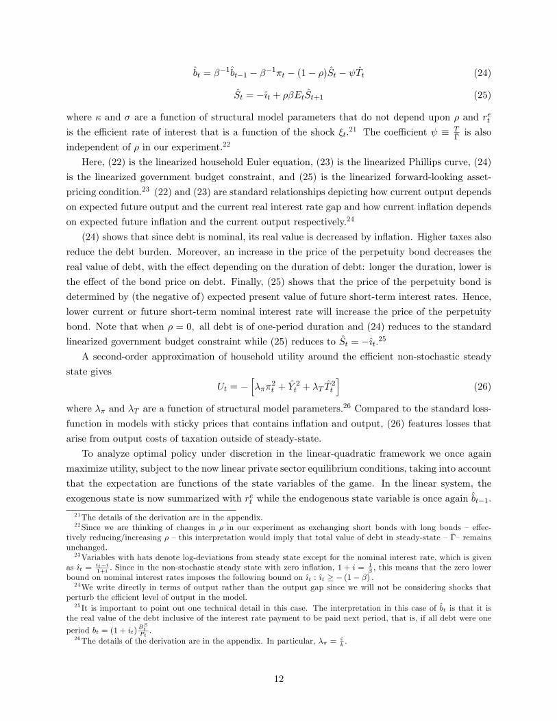
bt = β−1bt−1 − β−1πt − (1− ρ)St − ψTt (24)
St = −ıt + ρβEtSt+1 (25)
where κ and σ are a function of structural model parameters that do not depend upon ρ and retis the effi cient rate of interest that is a function of the shock ξt.21 The coeffi cient ψ ≡ T
Γis also
independent of ρ in our experiment.22
Here, (22) is the linearized household Euler equation, (23) is the linearized Phillips curve, (24)
is the linearized government budget constraint, and (25) is the linearized forward-looking asset-
pricing condition.23 (22) and (23) are standard relationships depicting how current output depends
on expected future output and the current real interest rate gap and how current inflation depends
on expected future inflation and the current output respectively.24
(24) shows that since debt is nominal, its real value is decreased by inflation. Higher taxes also
reduce the debt burden. Moreover, an increase in the price of the perpetuity bond decreases the
real value of debt, with the effect depending on the duration of debt: longer the duration, lower is
the effect of the bond price on debt. Finally, (25) shows that the price of the perpetuity bond is
determined by (the negative of) expected present value of future short-term interest rates. Hence,
lower current or future short-term nominal interest rate will increase the price of the perpetuity
bond. Note that when ρ = 0, all debt is of one-period duration and (24) reduces to the standard
linearized government budget constraint while (25) reduces to St = −ıt.25
A second-order approximation of household utility around the effi cient non-stochastic steady
state gives
Ut = −[λππ
2t + Y 2
t + λT T2t
](26)
where λπ and λT are a function of structural model parameters.26 Compared to the standard loss-
function in models with sticky prices that contains inflation and output, (26) features losses that
arise from output costs of taxation outside of steady-state.
To analyze optimal policy under discretion in the linear-quadratic framework we once again
maximize utility, subject to the now linear private sector equilibrium conditions, taking into account
that the expectation are functions of the state variables of the game. In the linear system, the
exogenous state is now summarized with ret while the endogenous state variable is once again bt−1.
21The details of the derivation are in the appendix.22Since we are thinking of changes in ρ in our experiment as exchanging short bonds with long bonds — effec-
tively reducing/increasing ρ —this interpretation would imply that total value of debt in steady-state — Γ—remainsunchanged.23Variables with hats denote log-deviations from steady state except for the nominal interest rate, which is given
as ıt = it−i1+i
. Since in the non-stochastic steady state with zero inflation, 1 + i = 1β, this means that the zero lower
bound on nominal interest rates imposes the following bound on ıt : ıt ≥ − (1− β) .24We write directly in terms of output rather than the output gap since we will not be considering shocks that
perturb the effi cient level of output in the model.25 It is important to point out one technical detail in this case. The interpretation in this case of bt is that it is
the real value of the debt inclusive of the interest rate payment to be paid next period, that is, if all debt were one
period bt = (1 + it)BStPt.
26The details of the derivation are in the appendix. In particular, λπ = εk.
12
Moreover, the expectation variables appearing in the system are now EtYt+1, EtSt+1, and Etπt+1.
Accordingly, we will define the game in terms of the state variables (ret , bt−1) and the government
now takes as given the expectation functions Y E(bt, ret ), S
E(bt, ret ), and π
E(bt, ret ).
The discretionary government’s optimization problem can then be written recursively as a
linear-quadratic dynamic programming problem
V (bt−1, ret ) = min[λππ
2t + Y 2
t + λT T2t + βEtV (bt, r
et+1)]
s.t.
Yt = Y E(bt, ret )− σ(ıt − πE(bt, r
et )− ret )
πt = κYt + βπE(bt, ret )
bt = β−1bt−1 − β−1πt − (1− ρ)St − ψTt
St = −ıt + ρβSE(bt, ret ).
Observe that once again, in equilibrium, the expectation functions need to satisfy the rational
expectations restrictions that EtYt+1 = Y E(bt, ret ), EtSt+1 = SE(bt, r
et ), and Etπt+1 = πE(bt, r
et ).
We prove in the proposition below that this linear-quadratic approach gives identical linear
optimality conditions as the one obtained by linearizing the non-linear optimality conditions of the
original non-linear government maximization problem that we described in the previous section.
This provides the formal justification for our simplified approach.
Proposition 1 The linearized dynamic system of the non-linear Markov Perfect Equilibrium is
equivalent to the linear dynamic system of the linear-quadratic Markov Perfect Equilibrium.
Proof. In Appendix.
3.1.1 Interpreting data from QE through the lens of the model
Let us now briefly review the data we will use when we do numerical experiments with this bench-
mark model. We are asking the data to give us some numbers for the following thought experiment:
What happens when you reduce the maturity of government debt? In the context of the model, we
are interested in getting some values for changes in ρ as representing a particular unconventional
monetary policy intervention.
According to the model, under coordinated policy and consolidated budget constraints we
should only be considering the debt held by the public (thus, we net out government debt held
by the Federal Reserve). Consistent with the model, also, we count reserves issued by the Federal
Reserve as short-term government debt. The duration of the consolidated government’s debt is
given below in Fig. 1.27 The vertical dashed lines are important events associated with the Federal27 In generating this figure, we first use estimates from Chadha, Turner, and Zampoli (2013) on the duration of
treasury debt held outside the Federal Reserve, which we then augment with data on reserves issued by the FederalReserve that is available from public sources (FRED).
13
Reserve buying long-term treasury bonds: November 2008 and March 2009 (Quantitative Easing
1); November 2010 (Quantitative Easing 2 (QE 2)); September 2011 (Maturity Extension Program
(MEP)); and September 2012 and December 2012 (Quantitative Easing 3 (QE3)). Around those
dates, the maturity of outstanding government debt declined. The baseline estimation of our model
will be based on the November 2010 or the Quantitative Easing 2 (QE2) program, a common focal
point in the literature. Given the parameter estimates from the QE2 program, we can also assess
the macroeconomic impact of the September 2011 or the Maturity Extension Program (MEP).
The reduction in maturity observed in Fig. 1 will be the input in our policy experiments under
coordinated policy and consolidated budget constraints.28
3.2 An independent central bank
We now present an alternate model where the central bank faces its own budget constraint and
minimizes an ad-hoc loss function that captures directly its balance sheet concerns. This model
has a political economy related justification to why the central bank might care about transfers to
the treasury. This alternative formulation, as will become clear, will also require us to view the
data through different lenses than in the last subsection. As we shall see later on, however, the
central insights will remain the same, i.e. QE has an effect via signalling.
We are now interested in studying the problem from the perspective of an independent central
bank that need not act in concert with the rest of the government. The first step is to explicitly
write down its budget constraint, before we move on to its objectives. We consider the case where
the central bank holds long-term assets (long term government debt). It buys these assets by
issuing one-period liabilities (approximating interest-bearing reserves). We also introduce some
“seigniorage net of operations cost”of the central bank that is not time-varying (similar to fiscal
spending that is not time-varying in our previous characterization when monetary and fiscal policy
are coordinated). Denote central bank holdings of assets by BCBt and its liabilities by Lt (with
prices Sγt and Qt respectively) and the “seigniorage net of operations cost” by K. The assets of
the central bank are in the form of a perpetuity bond of the same kind we analyzed before with
duration γ. Moreover, let Vt be the transfers to the treasury.
The flow budget constraint of the central bank is then given by
Sγt BCBt + PtVt −QtLt − PtK = (1 + γSγt )BCB
t−1 − Lt−1
where the price of the liabilities, Qt, is inverse of the (gross) short-term nominal interest rate.29
This can be written in real terms as
Sγt bCBt −Qtlt = (1 + γSγt ) bCBt−1Π−1
t − lt−1Π−1t +K − Vt.
28We will for the rest of the paper take September 2011, September 2012, December 2012 as one policy interventionand with abuse of terminology, refer it as MEP.29For earlier work in this vein, see Jeanne and Svensson (2007) and Berriel and Bhattarai (2009). For recent work
exploring the implications of the central bank budget constraint, see Hall and Reis (2013) and Del Negro and Sims(2015), who explore positive issues related to solvency and determinacy.
14
The debt of the treasury is now either held by the central bank or the general public. The market
clearing condition for treasury debt (BTt ) is thus given by B
Tt = BCB
t + Bt where Bt is debt held
by the public. We assume that the treasury follows passive fiscal policy that ensures stable debt
dynamics. Thus we completely abstract from fiscal policy considerations. We also assume for
simplicity that all central bank reserves are held by the public.
With some algebra outlined in the footnote, and some simplifying assumptions, we can write
the linearized budget constraint as[bCBt − lt
]= β−1
[bCBt−1 − lt−1
]− (1− γ) Sγt + Qt − ψV Vt (27)
where ψV ≡ VSγbCB
.30 Moreover, the price of the long term assets, Sγt , is given by the same
asset-pricing condition as before
Sγt = −ıt + γβEtSγt+1
while the price of the short-term asset, which is just the negative of the short-term interest rate,
is given by Qt = −ıt.Before we made the critical assumption that in steady state the market value of public debt was
given by some fixed number Sb = Γ that we linearized around. Here, the most important parameter
is the scale of the balance sheet, measured by ψV . This number reflects how large the asset side of
the balance sheet, SγbCB, is relative to the steady state transfers to the treasury, V. Also, note here
that the budget constraint is written in terms of the difference between the central banks holding
of long term government debt bCBt which has a fixed duration of γ and it own issuance of short
term debt (interest bearing reserves) lt. It can thus be re-written in terms of the net asset position
of the bank, which we define as bN,CBt = bCBt − lt. We will use that formulation later below.There are several noteworthy features in (27). First notice that up to first-order inflation has
30The two nonlinear asset pricing conditions will take the form
Sγt = Et
[βuC(Ct+1)ξt+1uCCt)ξt
Π−1t+1(1 + γSγt+1
)], Qt =
1
1 + it= Et
[βuC(Ct+1)ξt+1uC(Ct)ξt
Π−1t+1
].
In steady-state, like before, we have Q−1 = 1 + i = β−1, Sγ = β1−γβ . Moreover, define, as before S
γbT = Γ, which
from market clearing gives(bCB + b
)= Γ. The central bank budget constraint is then given in steady-state by
SγbCB −Ql = (1 + γSγ) bCB − l +K − V.
We will focus on a steady-state where SγbCB = Ql. Since Sγ
Q= 1
1−γβ , we will havebCB
l= (1− γβ) . This then
implies that K = V. We can now linearize the non-linear asset pricing and central bank budget constraint. First,we have Sγt = Qt + γβEtS
γt+1where in terms of our previous notation the following holds Qt = −ıt. Thus, we have
exactly like before the asset pricing condition for the long-term asset Sγt = −ıt + γβEtSγt+1. The linearized budget
constraint is now given by[bCBt − Ql
SγbCBlt
]= β−1
[bCBt−1 −
Ql
SγbCBlt−1
]− β−1
[1− Ql
SγbCB
]πt − (1− γ) St +
Ql
SγbCBQt − ψV Vt
where ψV = VSγbCB
is a parameter. We have to make some assumptions on the steady-state ratio of (mkt value)of liabilities to assets of the central bank: Ql
SγbCB. We will assume that it is 1. That gives the linearized budget
constraint in the text.
15
no effect on the net asset position of the bank. The reason for this is that inflation depreciates the
value of the assets (nominal long term bonds) and liabilities (short term nominal debt) to exactly
the same extent. This is a critical difference relative to the consolidated budget constraint. Long
term debt does, however, have an important effect on the net asset position of the central bank.
This is because while assets are long-term, the liabilities are short term. There is thus generally a
“duration mismatch”in the central bank’s balance sheet.
To see fully the implications of this duration mismatch, consider first the case in which γ = 0.
Then, both the assets and the liabilities have the same duration and variations in the short term
nominal interest rate have no effect on the net worth of the central bank, as Qt and St cancel out.
Consider now the case in which γ > 0. Now the central bank is holding long dated assets and short
dated liabilities. In this case we see that an increase in the short-term nominal interest rate reduces
the net worth of the bank. The reason for this is that an increase in the short rate increases the
borrowing cost of the bank one-to-one. Meanwhile, on the assets side, the increase in the short
term nominal interest rate has a more limited effect , since they are long-dated securities (so the
nominal interest rate is multiplied by 1 − γ in (27)). Thus, increasing the short-term nominal
interest rate sharply will lead to balance sheet losses for the central bank.
What does quantitative easing mean in the context of this budget constraint? We can model
it in two ways. First, recall that for the consolidated budget constraint we interpreted it as a one
time decline in ρ. Here, an analogous experiment is that it corresponds to a one time increase in
γ, i.e. the degree of duration mismatch is enhanced by making longer the duration of the assets
held by the central bank. This interpretation is about the change in composition of the asset side
of the central bank’s balance sheet.
While an increase in γ is one way of interpreting quantitative easing, there is another comple-
mentary interpretation. An increase in γ means that it is replacing shorter term bonds on its asset
side with bonds of longer duration. But the total value of bonds on the asset side is constant.
Thus, it is simply a change in the composition of the balance sheet. Now consider the following
experiment: Suppose all bonds on the asset side have some fixed γ (say, corresponding to five
years). Now imagine the central bank increases the purchases of these these bonds by printing
interest-bearing reserves. While this is not affecting the average duration of bonds on the asset
side of the balance sheet (or average duration mismatch since γ is fixed), it is increasing the scale
of the central bank balance sheet. The scale of the balance sheet in steady state was evaluated
by the parameter ψV = VSγbCB
. A permanent expansion in the balance sheet is therefore measured
as a drop in ψV . Observe that the increase in scale will simply expand the number of assets and
liabilities, but in steady state the remittances, V , remain unchanged. Hence an alternative way of
interpreting quantitative easing is an increase in the size of the balance sheet of the Fed, or a drop
in ψV., without changing the composition. We will use both the first and second interpretation to
study the implications of different QE episodes.
16
We can write (27) in terms of one state variable, bN,CBt−1 = bCBt−1 − lt−1, as
Observe that all the private-sector equilibrium conditions remain the same as when we studied the
consolidated budget constraint. We can now conduct the experiment of an increase in the central
bank’s balance sheet via decrease in ψV , holding γ fixed. We can also conduct the experiment of
larger holding of long-term assets as an increase in γ, holding ψV fixed.
In terms of the central bank’s objective, we take here an ad-hoc loss-function approach, which
has a rich and long history in monetary economics. We posit that the central bank directly cares
about transfers to the treasury for political economy reasons. This means that its period loss
function now incorporates a term related to target transfers to the Treasury, Vt, in addition to the
usual terms related to inflation and output. It is thus given by[λππ
2t + Y 2
t + λV V2t
].
Does this objective make sense? There is some evidence that central banks care about the transfers
to the treasury.31 Moreover, as we have seen, to the extent that these transfers affect tax collection,
the central bank should care also from a social welfare point of view.
The discretionary central bank’s optimization problem can then be written recursively as a
linear-quadratic dynamic programming problem
V (bN,CBt−1 , ret ) = min[λππ2t + Y 2
t + λT T2t + βEtV (bN,CBt , ret+1)]
s.t.
Yt = Y E(bN,CBt , ret )− σ(ıt − πE(bN,CBt , ret )− ret )
πt = κYt + βπE(bN,CBt , ret )
bN,CBt = β−1bN,CBt−1 − (1− γ) Sγt + Qt − ψV Vt
Sγt = −ıt + γβSγE(bN,CBt , ret ).
Observe that once again, in equilibrium, the expectation functions need to satisfy the rational
expectations restrictions that EtYt+1 = Y E(bN,CBt , ret ), EtSγt+1 = SγE(bN,CBt , ret ), and Etπt+1 =
πE(bN,CBt , ret ).
The behavior of this model will critically depend up on the initial value of the net capital of
the bank bN,CBt−1 . If this number is negative, then the path for Vt will generally be below what the
central bank would ideally like it to be during the transition to steady state. Moreover, interest-
31Central bank governors that incur large balance sheet losses – e.g. the Central Bank of Iceland in 2008 whichlost money corresponding to 30% of GDP —usually find themselves without a job shortly thereafter. Berriel andBhattarai (2009) contains some other anecdotal evidence of such central bank worries. In related frameworks, Jeanneand Svensson (2007) and Berriel and Bhattarai (2009) include the central bank’s net worth directly in the lossfunction. Our modeling approach here is thus different.
17
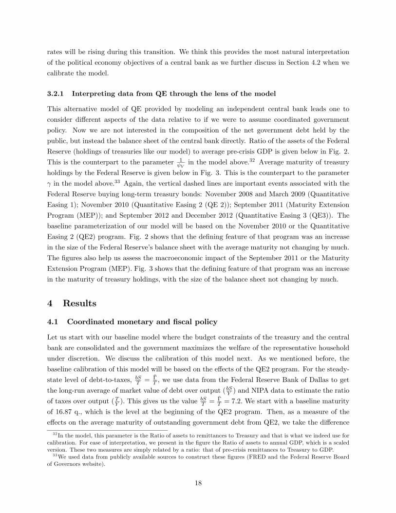
rates will be rising during this transition. We think this provides the most natural interpretation
of the political economy objectives of a central bank as we further discuss in Section 4.2 when we
calibrate the model.
3.2.1 Interpreting data from QE through the lens of the model
This alternative model of QE provided by modeling an independent central bank leads one to
consider different aspects of the data relative to if we were to assume coordinated government
policy. Now we are not interested in the composition of the net government debt held by the
public, but instead the balance sheet of the central bank directly. Ratio of the assets of the Federal
Reserve (holdings of treasuries like our model) to average pre-crisis GDP is given below in Fig. 2.
This is the counterpart to the parameter 1ψV
in the model above.32 Average maturity of treasury
holdings by the Federal Reserve is given below in Fig. 3. This is the counterpart to the parameter
γ in the model above.33 Again, the vertical dashed lines are important events associated with the
Federal Reserve buying long-term treasury bonds: November 2008 and March 2009 (Quantitative
Easing 1); November 2010 (Quantitative Easing 2 (QE 2)); September 2011 (Maturity Extension
Program (MEP)); and September 2012 and December 2012 (Quantitative Easing 3 (QE3)). The
baseline parameterization of our model will be based on the November 2010 or the Quantitative
Easing 2 (QE2) program. Fig. 2 shows that the defining feature of that program was an increase
in the size of the Federal Reserve’s balance sheet with the average maturity not changing by much.
The figures also help us assess the macroeconomic impact of the September 2011 or the Maturity
Extension Program (MEP). Fig. 3 shows that the defining feature of that program was an increase
in the maturity of treasury holdings, with the size of the balance sheet not changing by much.
4 Results
4.1 Coordinated monetary and fiscal policy
Let us start with our baseline model where the budget constraints of the treasury and the central
bank are consolidated and the government maximizes the welfare of the representative household
under discretion. We discuss the calibration of this model next. As we mentioned before, the
baseline calibration of this model will be based on the effects of the QE2 program. For the steady-
state level of debt-to-taxes, bST = ΓT , we use data from the Federal Reserve Bank of Dallas to get
the long-run average of market value of debt over output ( bSY ) and NIPA data to estimate the ratio
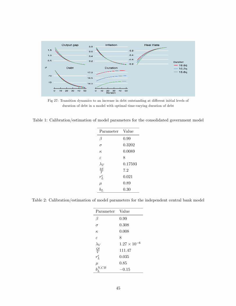
of taxes over output ( TY ). This gives us the valuebST = Γ
T = 7.2. We start with a baseline maturity
of 16.87 q., which is the level at the beginning of the QE2 program. Then, as a measure of the
effects on the average maturity of outstanding government debt from QE2, we take the difference
32 In the model, this parameter is the Ratio of assets to remittances to Treasury and that is what we indeed use forcalibration. For ease of interpretation, we present in the figure the Ratio of assets to annual GDP, which is a scaledversion. These two measures are simply related by a ratio: that of pre-crisis remittances to Treasury to GDP.33We used data from publicly available sources to construct these figures (FRED and the Federal Reserve Board
of Governors website).
18
in Fig. 1 between QE2 and the MEP (the third and fourth dashed vertical lines), which is 0.67 q.
That is, according to our measure, the reduction in maturity was from 16.87 q to 16.2 q, with a
difference of 0.67q.
To model the case of a liquidity trap, we follow Eggertsson and Woodford (2003) and assume
a negative shock to the exogenous effi cient rate of interest, ret , which makes the zero lower bound
binding.34 The process for ret follows a two-state Markov process with an absorbing state: From
period 0 on then ret takes on a negative value of reL. It remains at this value with probability µ in
every period, while with probability 1 − µ, it reverts back to steady-state and stays there foreverafter. This means that the economy will exit the liquidity trap with a constant probability of 1−µevery period and that once it exits, it does not get into the trap again. The appendix contains
details about the computation algorithm.
To parameterize the model we use a mix of calibration/estimation based on the effects of QE2
on inflation and yields calculated by Krishnamurthy and Vissing-Jorgensen (2011) as well as the
expected duration of the zero lower bound episode and its effects on output and inflation. We pick
the quarterly discount factor of β = 0.99 and we fix the elasticity of substitution among varieties
of goods at a standard value of 8. We allow for debt while at the liquidity trap to be 30% above
its steady-state value, which is in line with the Federal Reserve Bank of Dallas data.35
Then, we estimate (σ, λT , κ, reL, µ) by matching five targets. Our first two targets are a
reduction in 8 quarters ahead yield of ∆i∗ (8) = −16 b.p. and an increase in expected cumulative
inflation over 10 years of ∆π∗ (40) = 5b.p. as a result of the QE2 program when the economy is
initially in a ZLB situation. These were the estimates in Krishnamurthy and Vissing-Jorgensen
(2011) of the effects of the QE2 program. Our third target is a 3-year average duration of the ZLB
period (for an average ZLB duration of about 3 years, we target µ∗ = 0.91). Finally, our fourth
and fifth targets are a drop in output of 10% and a 2% percent drop in inflation during the ZLB
episode to make the experiment relevant for the recent “Great Recession” in the United States
(Y ∗ (1) and π∗ (1) of −0.10 and -0.02 respectively).36
Our criterion for estimation is the mean squared weighted relative error given by
L =
√(∆π (40)
∆π∗ (40)− 1
)2
+
(∆i (8)
∆i∗ (8)− 1
)2
+
(Q (µ)
Q (µ∗)− 1
)2
+
(Y (1)
Y ∗ (1)− 1
)2
+
(π (1)
π∗ (1)− 1
)2
where Q (µ) = 11−µ is the expected duration in quarters of the ZLB episode. The values of the
targets for our best match are π (1) = −0.021, Y (1) = −0.091, ∆π (40) = 4.72 b.p., ∆i (8) = −5.87
b.p., and µ = 0.89 (about 2.25 years). Our estimated parameter values are given in Table 1.
34One can think of this here as being driven by a preference shock. For an alternate way of generating a liquiditytrap in monetary models, based on an exogenous drop in the borrowing limit, see Eggertsson and Krugman (2012).35We also adjust the quantity of debt level after QE2 to keep the market value of the debt fixed during the QE2
intervention (it has to be adjusted to 0.297).36One can alternatively impose some priors on the parameters we estimate using Bayesian methods, but we felt
this strategy is more transparent, given that our estimated value for the parameters are relatively reasonable.
19
4.1.1 Solution at positive interest rates
We start by showing the solution at positive interest rates to show how debt maturity changes
the policy incentives of the government. The complication in solving a MPE is that we do not
know the unknown expectation functions πE , Y E , and SE . To solve this, we use the method of
undetermined coeffi cients. All the details of the derivations are provided in the appendix.
Let us first consider the most basic exercise to clarify the logic of the government’s problem.
How do the dynamics of the model look like in the absence of shocks when the only difference from
steady state is that there is some initial value of debt with some fixed value for debt duration?
Fig. 4 shows the dynamics of the endogenous variables in the model for an initial value of debt
that is 30 percent above the steady state. We see that if debt is above steady state, it is paid over
time back to steady state. For our baseline duration of 16.87 quarters (solid line), the half-life of
debt repayment is about 12 quarters. In the transition inflation is about 0.75 percent above steady
state and the real interest rate is below its steady state. As a consequence, output is also above
its steady state value. This result is in contrast to the classic Barro tax smoothing result whereby
debt follows a random walk. The reason is that debt creates an incentive to create inflation for a
discretionary government as further described below. By paying down debt back to steady state,
the government eliminates this incentive and achieves the first best outcome in the model.
The figure illustrates that for a given maturity of government debt, debt is inflationary and
implies a lower future real interest rate until a new steady state is reached. What is the logic for
this result? Perhaps the best way to understand the logic is by inspecting the government budget
constraint (24). Recall that debt issued in nominal terms, although in the budget constraint we
have rewritten it in terms of bt =BtPt−bb. This implies that for a given outstanding debt bt−1, any
actual inflation will reduce the real value of the outstanding debt. Accordingly we have the term
β−1πt term in the budget constraint which reflects this inflation incentive. As the literature has
stressed in the past (see e.g. Calvo and Guidotti (1990 and 1992)), if prices are flexible then this
will reduce actual debt in equilibrium only if the inflation is unanticipated. The reason for this
is that otherwise anticipated inflation will be reflected one-to-one in the interest rate paid on the
debt.
Apart from the incentive to depreciate the real value of the debt via inflation, there is a second
force at work. In our model, the government is not only able to affect the price level, it can also
have an effect on the real interest rate. Hence, we see that in Fig. 4 the real interest rate is below
steady state during the entire transition path back to steady state. This reduces the real interest
rate payments the government needs to pay on debt — in contrast to the classic literature with
flexible prices where the (ex-ante) real interest rate is exogenous. We refer to this as the rollover
incentive of the government.
Intuitively, it may be most straight forward to see the rollover incentive by simplifying the
model down to the case in which ρ = 0 and there is only one period debt. In that case, the budget
20
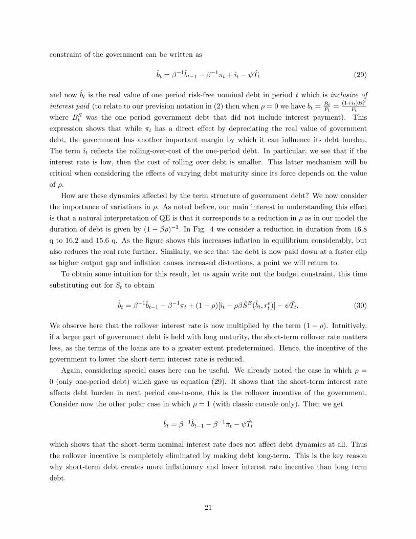
constraint of the government can be written as
bt = β−1bt−1 − β−1πt + ıt − ψTt (29)
and now bt is the real value of one period risk-free nominal debt in period t which is inclusive of
interest paid (to relate to our prevision notation in (2) then when ρ = 0 we have bt = BtPt
=(1+it)BSt
Pt
where BSt was the one period government debt that did not include interest payment). This
expression shows that while πt has a direct effect by depreciating the real value of government
debt, the government has another important margin by which it can influence its debt burden.
The term ıt reflects the rolling-over-cost of the one-period debt. In particular, we see that if the
interest rate is low, then the cost of rolling over debt is smaller. This latter mechanism will be
critical when considering the effects of varying debt maturity since its force depends on the value
of ρ.
How are these dynamics affected by the term structure of government debt? We now consider
the importance of variations in ρ. As noted before, our main interest in understanding this effect
is that a natural interpretation of QE is that it corresponds to a reduction in ρ as in our model the
duration of debt is given by (1 − βρ)−1. In Fig. 4 we consider a reduction in duration from 16.8
q to 16.2 and 15.6 q. As the figure shows this increases inflation in equilibrium considerably, but
also reduces the real rate further. Similarly, we see that the debt is now paid down at a faster clip
as higher output gap and inflation causes increased distortions, a point we will return to.
To obtain some intuition for this result, let us again write out the budget constraint, this time
We observe here that the rollover interest rate is now multiplied by the term (1 − ρ). Intuitively,
if a larger part of government debt is held with long maturity, the short-term rollover rate matters
less, as the terms of the loans are to a greater extent predetermined. Hence, the incentive of the
government to lower the short-term interest rate is reduced.
Again, considering special cases here can be useful. We already noted the case in which ρ =
0 (only one-period debt) which gave us equation (29). It shows that the short-term interest rate
affects debt burden in next period one-to-one, this is the rollover incentive of the government.
Consider now the other polar case in which ρ = 1 (with classic console only). Then we get
bt = β−1bt−1 − β−1πt − ψTt
which shows that the short-term nominal interest rate does not affect debt dynamics at all. Thus
the rollover incentive is completely eliminated by making debt long-term. This is the key reason
why short-term debt creates more inflationary and lower interest rate incentive than long term
debt.
21
Having established intuitively and numerically that at positive interest rates, decreasing the
duration of debt increases the incentives of the government to lower short-term real interest rates,
we now move on to analyzing the case where the nominal interest rate is at the zero lower bound.
At the ZLB, manipulating this incentive can be particularly valuable.
4.1.2 Solution at the ZLB: QE2
Consider the following policy experiment: In the liquidity trap, the level of debt is constant at
bL. When out of the trap, then bL is optimally determined by the government according to the
MPE previously described. Why is this an interesting environment? Now we can ask the following
question: What would be the effect of changing the duration of debt once-and-for-all, while the zero
lower bound is binding? In other words, we are interested in the comparative static of the model as
we vary the duration of debt in the liquidity trap, but at the same time holding aggregate debt, bL,
constant. We think this is an interesting comparative static, because it corresponds so closely to
QE. QE did not involve increasing aggregate government debt, as pointed out in the introduction.
Instead it just involved exchanging long-term government debt with short-term government debt
(money), which we interpret here as a reduction in ρ. In our experiment the steady-state market
value of debt to taxes is always kept fixed. For now, however, a key abstraction is that the value
of ρ is fixed so that once you change ρ (QE), it does not revert back to where it was. We will come
back to this issue in Section 5.
Before exploring the comparative static at the heart of this section, let us review first how the
model behaves in the absence of any intervention, i.e., the evolution of each of the endogenous
variables in the face of the shock we chose in the last section. Figs. 5 and 6 show the response
of inflation and output to a negative shock to the effi cient rate of interest in the benchmark
economy, when the duration of government debt is fixed at 16.87 quarters. We will be interested
in understanding if QE can improve upon the outcome we see in these figures, which feature an
output drop of approximately 10 percent and inflation drop of 2 percent (by construction of our
calibration).
Some comments are in order about the baseline economy in the absence of QE. First note that
the shock here generates a considerable recession and a drop in inflation. This is driven entirely by
the fact that the central bank cannot accommodate the shock via cuts in the nominal interest rate.
This creates a gap between the equilibrium real interest rate, rt, and the effi cient rate of interest ret(i.e. the real interest rate needed for output to remain at the first best steady state). This interest
rate gap is shown in Fig. 7. It is well known from the existing literature (see e.g. Eggertsson and
Woodford (2003)), that this situation can be greatly improved if the central bank could commit
to keeping the nominal interest rate low for some time after the shock is over. This is beneficial
because aggregate demand depends not only on the current interest rate gap but the entire path
of future interest rates.
The optimal commitment analyzed by Eggertsson and Woodford (2003) is not possible in our
environment, however. The reason is that we are considering a MPE, so the government cannot
22
commit to future policy that is dynamically inconsistent (this is the so called “deflationary bias”
of discretionary policy at the ZLB, see Eggertsson (2006)). The optimal commitment involves
promising real interest rate below the effi cient rate of interest rate when the shock is over —but at
that time the government has little incentive to deliver on this promise.
Another point worth stressing in Fig. 5 is that once the shock is over (and each of the thin
lines revert up) then inflation overshoots its long run value in our MPE. This is a feature of our
calibration, as we assumed that there is outstanding government debt of 30 percent above steady
state. Thus the government does already have some incentive to inflate which is reflected in these
numbers. The fact that output drops by about 10 percent in Fig. 6 simply suggests that this
incentive is not strong enough for the government to be able to escape the ZLB. One solution to
this problem, then, would be simply to issue even more nominal debt (this is a solution analyzed
in Eggertsson (2006)), an approach we abstract from here by virtue of bL being constant.37
To motivate this abstraction, i.e. fixed bL, we can think of some political or economic limits on
how much total aggregate government debt can be issued (e.g. a debt limit imposed by Congress
or that too high debt gives rise to perception of default, a consideration we have not included in
our model). Moreover, when we consider the case of the independent central bank, the option of
raising total number of government bonds may not be available. In any case, when the government
has two instruments —the stock of nominal debt and its composition in terms of duration —we want
to understand how both margins work, and our focus is on the latter. This leads us to consider
next the central comparative static of this paper: What happens when you permanently reduce the
duration of government debt in the MPE? Can manipulating the term structure make expansionary
future monetary policy “credible”without further cuts in the current nominal interest rate?
In Figs. 8 and 9 we see what happens if the government reduces the duration of government
debt from 16.87 quarters to 16.2 quarters, this is the number we computed on the basis of the
data from QE2. The figures shows the change in output and inflation as a result of this policy
intervention. The bottom-line is that inflation now increases by 14 basis points (annualized) and
output increases by 30 basis points. We can also ask how large intervention would have been needed
to fully close the output gap. The answer to this question is that the duration would have had to
go down from 16.87 to 8.5 quarters.
What is the key logic? Because government has more short-term debt the central bank keeps
the short-term real interest rates lower in future in order to keep the real interest rate low on the
debt it is rolling over. Thus, QE provides a “signal”about the future conduct of monetary policy.
In particular it generates a credible signal about the future path of short-term interest rates. This
then enables it to have effect on macroeconomic prices and quantities at the zero lower bound. The
change in the response of the real interest rate is given in Fig. 10, where one can see that the real
interest rate is lower throughout the horizon post QE.38
37Note that we keep the market value of debt constant (before and after change in duration) in our numericalexperiments via appropriate adjustments.38This result thus connects our paper with Persson, Persson, and Svensson (1987 and 2006), who show in a flexible
price environment that a manipulation of the maturity structure of both nominal and indexed debt can generate an
23
4.1.3 Capital losses from reneging on optimal policy
We have emphasized so far that the reason why lowering the duration of debt during a liquidity
trap situation is beneficial is that it provides incentives for the government to keep the real interest
rate low in future as it is now rolling over more short-term debt. We have shown these results by
comparing the path of the real interest rate under optimal policy at a baseline and lower duration
of debt.
Another way of framing this is that otherwise it would suffer capital losses on its balance sheet.
These losses then would have to be accounted for by raising costly taxes. One way to illustrate the
mechanism behind this result is to conduct the following thought experiment: suppose that once
the liquidity trap is over, the government reneges on the path for inflation and output dictated by
optimal policy under discretion and instead perfectly stabilizes them at zero. In such a situation,
how large are capital losses, or equivalently, how high do taxes have to rise out of zero lower
bound compared to if the government had continued to follow optimal policy? In particular, is
this increase in taxes more when debt is of shorter duration ? We show in Fig. 11 the change
in taxes (which are scaled as a fraction of output) if the government were to renege on optimal
policy at different durations of debt. The increase in taxes out of zero lower bound are higher at
a shorter duration of outstanding debt. Thus, lowering the duration of government debt provides
the government with more of an incentive to keep the real interest rate low in future in order to
avoid having to raise costly taxes.
4.1.4 Quantitative assessment of MEP/QE3
Given the parameter estimates based on QE2 and its effects on expected inflation and future
short-term interest rates given in Table 1, we now conduct an assessment of the macroeconomic
effects of MEP/QE3. This policy involved a reduction in the duration of outstanding government
debt as well, as can be seen from Fig. 1. Our experiment is based on the difference in duration
between September 2011 and September 2013 (we thus use the entire period following MEP for
this calibration), which is equal to 1.8 q and bigger than the effect from QE2.39 Accordingly, the
macroeconomic effects, as shown below in Figs. 12-13 are larger as well as the drop in the real
interest rate, as shown in Fig. 14 below, is now bigger. The extent of deflation is now reduced by
30 basis points, and output is higher as a consequence on the order of 90 basis points.
4.2 An independent central bank
We now model the effect of QE using the political economy set-up where the central bank directly
cares about transfers to the treasury. To parameterize the model we use quarterly average from
2003-2008 of remittances to Treasury from the Federal Reserve to get the steady state value of V .
Our baseline value of 1ψV
= SγbCB
V = QlV = 111.47 corresponds to the average ratio of holdings of
equivalence between discretion and commitment outcomes.39As noted before, this measure of policy intervention will also include policy changes brought about by QE3.
24
Treasuries by the Federal Reserve to remittances to Treasury over the period of 2003-2008. When
considering QE as an increase in the scale of the balance sheet, we assume V is fixed at the steady
state value while the scale of assets and liabilities (SγbCB = Ql) increases. In Fig. 2 we show the
asset side of the Fed’s balance sheet as a ratio of annual GDP, where we use Treasury holdings of
the Fed as a proxy for the asset side. This gives a baseline ratio of the Fed’s assets over annual
GDP pre-crisis as 5.1%. Then, as a measure of the effects on the size of the Federal Reserve’s
balance sheet from QE2, we take the difference in Fig. 2 between QE2 and the MEP (the third
and fourth dashed vertical lines), which is an increase in the Fed’s balance sheet (ratio of asset
to annual GDP) from 5.1% to 10.6%. Finally, we also pick the value of γ based on the average
maturity of Treasury holdings of the FED during 2003-2008, which is equal to 7.57 q. We model
the liquidity trap in the same way as before.
For the other structural parameters of the model, like before for the consolidated budget con-
straint case, we estimate them using a mean squared relative error criterion. Unlike for the con-
solidated government debt, however, since there is no clear metric on the net asset position of the
Federal Reserve during the crisis (in terms of deviation from steady-state), we choose to estimate
that parameter bN,CBL , along with five others from before.40 The targets in the criterion are the
same as before and the values of the targets for our best match are π (1) = −0.02, Y (1) = −0.10,
which along with (22)-(25) define the equilibrium in the approximated economy. The final step to computing the
solution is then to plug in the conjectured solution and to match coeffi cients on various variables in (22)-(25), (51),
and (52), along with the requirement that expectation are rational, to determine πb, Yb, Sb, ib, bb, and Tb. The details
of this step are in the appendix.
The most important relationships emerging from our analysis are captured by (51) and (52). (51) is the so
called “targeting rule” of our model. That represents the equilibrium (static) relationship among the three target
variables πt, Yt, and Tt that emerges from the optimization problem of the government. (51) thus captures how
target variables are related in equilibrium as governed both by the weights they are assigned in the loss function
(λπ and λT ) as well as the trade-offs among them as given by the private sector equilibrium conditions (κ−1 and
[κ−1 (1− ρ)σ−1 + β−1] 1ψ). Note in particular that κ−1 represents the trade-off between πt and Yt as given by (23)
while [κ−1 (1− ρ)σ−1 +β−1] 1ψrepresents the trade-off between πt and Yt vs. Tt as given by the combination of (22),
(23), and (24).
(52) is another optimality condition characterizing the Markov-perfect equilibrium and represents the “tax-
smoothing objective” of the government. In contrast to similar expressions following the work of Barro (1979),
which would lead to taxes being a martingale, output appears in (52) because of sticky-prices, which makes output
endogenous. Finally, because of the dynamic nature of (52), as opposed to (51), the unknown coeffi cients that are
critical for expectations of variables, πb, Yb, and Sb, appear in (52). As we shall see —and this is again in contrast to
59
the classic tax smoothing result in which debt is a random walk —the government will in general have an incentive
to pay down public debt if it is above steady-state due to strategic reasons.
8.6.1 Polar cases on price rigidities
To clarify what is going on in the model, we first find it helpful to consider two special cases.
a) Fully flexible prices When prices are fully flexible, then as is well-known, monetary policy cannot control
the (ex-ante) real interest rate rt. Then, the only way monetary policy can affect the economy is through surprise
inflation as debt is nominal. In fact there is a well-known literature that addresses the issue of how the duration of
nominal debt in a flexible price environment affects allocations under time consistent optimal monetary policy. For
example, Calvo and Guidotti (1990 and 1992) address optimal maturity of nominal government debt in a flexible
price environment while Sims (2013) explores how the response of inflation to fiscal shocks depends on the maturity of
government debt under optimal monetary policy. We conduct a complementary exercise here and want to characterize
how inflation incentives depend on the duration of debt under optimal monetary and fiscal policy under discretion.
Thus, we are interested in how πb depends on duration of debt.
For this exercise, we can think of this special case of fully flexible prices as κ → ∞. Note however, that fromthe two optimality conditions (51) and (52), while under flexible prices Tb = 0, there is indeterminacy in terms of
inflation and nominal interest rate dynamics.44 This is a well-known result in monetary economics under discretion
in a flexible price environment, and comes about because the government cannot affect output and taxes can be put
to zero with various combinations of inflation and interest rate choices. To show our result on the role of the duration
of debt, we follow the literature such as Calvo and Guidotti (1990 and 1992) and Sims (2013) and include a ( very
small) aggregate social cost of inflation that is independent of the level of price stickiness. Then, the objective of the
government under flexible prices will be given by
Ut = −[λ′ππ
2t + λT T
2t
]where λ
′π parameterizes the cost of inflation that is independent of sticky prices. Using λ
′π = 0.001 and the rest of
the parameter values from Table 1, Fig A1 shows how πb depends on duration of debt (quarters). We see that with
shorter duration, there is more of an incentive to use current inflation. The intuition for this result is that from (24),
we see that everything else the same, when ρ (and thereby, duration) decreases, then there will be a greater period by
period incentive to increase St, that is, keep nominal interest rates low to manage the debt burden. This, however,
will increase current inflation further in equilibrium according to our result. As a consequence —and perhaps a little
counterintuitively — equilibrium nominal interest rate will generally increase as well with lower duration since the
real rate is exogenously given under flexible prices. In particular, observe that ıt = Etπt+1 (since Yt = 0 and there
44Note that λπ = εk.
60
are no shocks) and hence it is increasing one-to-one with expected inflation.
5 10 15 20 25Duration
0.2
0.4
0.6
0.8
1.0b
Fig A1: Inflation response coeffi cients at different duration of debt under flexible prices
b) Fully rigid prices Next we can consider the other extreme case: that of fully rigid prices. In this case,
inflation is zero in equilibrium and hence πb = 0. Then, one can directly consider the effects on the ex-ante real
interest rate by analyzing the effect on the nominal interest rate since rb = ib − πbbb = ib. Thus, we are interested
in how ib depends on the duration of debt. Using the parameters from Table 1, Fig A2 shows how ib depends on
duration of debt (quarters). We see that with shorter duration, there is more of an incentive to keep the nominal
interest rate lower. The intuition for this result is again that from (24), when ρ (and thereby, duration) decreases,
then there will be more of an incentive to increase St, that is keep interest rates low, to manage the debt burden.
61
5 10 15 20 25Duration
1.0
0.8
0.6
0.4
0.2
ib
Fig A2: Nominal interest rate response coeffi cients at different duration of debt under
rigid prices
We now move to discussing in detail properties of the solution for the partially rigid price cases that underlies
our baseline calibration.
8.6.2 Real interest rate incentives and duration of outstanding debt
How does the duration of debt affect the real interest rate incentives of the central bank for the partially rigid cases
that underlies our baseline calibration? The effect on the real interest rate of lower duration is at the heart of the
matter because what influences output is eventually the real interest rate and the aim in a zero lower bound situation
is precisely to be able to decrease the short-term real interest rate (today and in future) even when the current
short-term nominal interest rate is stuck at zero. That is, we are interested in the properties of
rt = ıt − Etπt+1 = (ib − πbbb) bt−1 = rbbt−1
where rt is the short-term real interest rate. This is important because in a liquidity trap situation, as is well-known,
decreasing future real interest rate is key to mitigating negative effects on output, and so, if rb depends negatively
on duration, then we are able to provide a theoretical rationale for quantitative easing actions by the government.
Having established the results in the two special cases above, we now move on to the main mechanism in our
paper in the intermediate and quantitatively relevant case of partially rigid prices. Fig A3 shows how rb depends
on duration of debt (quarters). When the duration of debt in the hands of the public is shorter, it unambiguously
provides an incentive to the government to keep the short-term real interest rate lower in future. The intuition again
is that by doing so, it reduces the cost of rolling over the debt period by period. That is, if the debt is short-term,
then current real short rates will more directly affect the cost of rolling the debt over period by period, while the
cost of rolling over long-term debt is not affected in the same way period by period.
62
5 10 15 20 25Duration
1.0
0.8
0.6
0.4
0.2
rb
Fig A3: Real interest rate response coeffi cients at different duration of debt
8.6.3 Inflation incentives and duration of outstanding debt
While the dependence of real interest rate incentive of the government on the duration of debt is the main mechanism
of our paper, given the attention inflation incentives receive in the literature, we now study how πb varies with the
duration of outstanding government debt?45 Moreover, it helps us emphasize a point that just focusing on inflation
incentives might not be suffi cient to understand the nature of optimal monetary and fiscal policy in a liquidity trap
situation.
While an analytical expression for πb is available in the appendix and it is possible to show that πb > 0 for
all ρ < 1, a full analytical characterization of the comparative statics with respect to the duration of debt is not
available and so we rely on numerical results. Fig A4 below shows how πb depends on duration of debt (quarters) at
different levels of κ. As expected, πb is positive at all durations in the figure.46 More importantly, note that that at
our baseline parameterization of κ = 0.02, πb does decrease with duration over a wide range of maturity.47 At the
same time, however, there is a hump-shaped behavior, with πb increasing when duration is increased at very short
durations.
45For some recent discussion and analysis of how inflation dynamics in sticky-price models could depend on durationof government debt, see Sims (2011).46Again, it is possible to show analytically that for all ρ < 1, πb > 0. In a very similar model but one with no
steady-state debt, Eggertsson (2006) proved that πb > 0 for ρ = 0 (that is, for one period debt).47Some limited analytical results on the properties of πb with respect to ρ are available in the appendix. For
example, it can be shown that πb is positive for all ρ < 1 and that when ρ = 1 + β−1σκ (and thus, ρ > 1), πb = 0. Inthis sense, for a specific case, one can show that πb is declining in ρ by comparing some extreme cases (such asρ = 0 with ρ = 1 + β−1σκ). Please see the appendix for details. Note also here that the upper bound on ρ is β−1. Sothis case of πb = 0 is not necessarily always reached.
63
5 10 15 20 25Duration
0.002
0.004
0.006
0.008
0.010
0.012
0.014
b
Fig A4: Inflation response coeffi cients at different duration of debt
What drives this result? First, note from (24) that everything else the same, when ρ (and thereby, duration)
decreases, then there will be an incentive to decrease St, that is keep interest rates low to manage the debt burden.
This will then increase inflation in equilibrium. At the same time however, the government’s incentives on inflation
are not fully/only captured by this reasoning. This is because what ultimately matters for the cost of debt is the
real interest rate, which because of sticky prices, is endogenous and under the control of the central bank, and which
we have seen before robustly depends negatively on the duration of debt. Therefore, to understand the overall effect
on the government’s inflation incentives, it is critical to analyze the targeting rule, as discussed above and given by
(51). Here, the term [κ−1 (1− ρ)σ−1 + β−1] plays a key role as it captures the trade-off between πt and Yt vs. Tt. Note first that β−1 here simply captures the role of surprise inflation in reducing the debt burden as government
debt is nominal. This term would be present even when prices are completely flexible. The term κ−1 (1− ρ)σ−1
however, appears because of sticky prices. This reflects how the real interest rate is affected by manipulation of the
nominal interest rate and how it in turn affects output.
Thus, in situations where either κ−1, σ−1, or (1− ρ) is high, this term can dominate and it can be the case that
decreasing the duration (or decreasing ρ) actually leads to a lower πb. This means, for example, that when κ−1 is
low (or when prices are more flexible), the hump-shaped behavior of πb gets restricted to very short maturities only
as the channel coming from sticky-prices is not that influential. We in fact showed this above in the case of fully
flexible prices, where inflation response depends negatively throughout on duration of debt.
8.6.4 Debt dynamics and duration of outstanding debt
While the primary focus so far is on properties of rb as it determines the real interest rate incentives of the central bank,
it is also interesting to consider the properties of bb, the parameter governing the persistence of government debt. This
exercise is interesting in its own right, but more importantly, it is also worth exploring because as explained before,
what is critical is the behavior of the real interest rate, and that gets affected by bb as Etπt+1 = πbbt = πbbbbt−1.
Unlike for πb, it is not possible to show a tractable analytical solution (or any property) for bb as it is generally a
root of a fourth-order polynomial equation. We thus rely fully on numerical solutions.
Fig. A5 shows how bb depends on duration of debt. It is clear that the persistence of debt increases monotonically
64
as the duration increases.48 In fact, for a high enough duration, debt dynamics approach that of a random walk
(bb = 1), as in the analysis of Barro (1979). The persistence of debt increases with duration mainly because the
response of the short-term real interest rate decreases, as we discussed above. Some of this effect is reflected in
the response of inflation decreasing as also discussed above. Thus, the existence of long-term nominal debt has an
important impact on the dynamics of debt under optimal policy under discretion.
5 10 15 20 25Duration
0.2
0.4
0.6
0.8
1.0bb
Fig A5: Debt response coeffi cients at different duration of debt
8.7 Computation at ZLB
In our experiment the debt is kept fixed at the zero lower bound at bL . Moreover, at the zero lower bound,
ıt = 1− β−1. Given the specific assumptions on the two-state Markov shock process, the equilibrium is described by
the system of equations
Yt = −σ(−πb(1− µ)bt − ret − µπL + ıt
)+ (1− µ)btYb + µYL,
πt = β(πb(1− µ)bt + µπL
)+ κYt,
ıt = 1− β−1,
bt = bL,
St = −ıt + ρβ ((1− µ)SbbL + µSL) .
48There is thus, no hump-shaped pattern, unlike for inflation. The reason is that what matters directly forpersistence of debt is the real interest rate and there is no hump-shaped pattern there as we show later. Note alsothat for one-period debt, often bb is negative (even here, recall that πb is still positive). A negative bb is not veryinteresting empirically as it implies oscillatory behavior of debt.
65
where variables with a b subscript denote the solution we compute at positive interest rates while variables with a L
subscript denote values at the ZLB. The solution to this system is