Time-dependent Aero-elastic Adjoint-based Aerodynamic Shape Optimization of Helicopter Rotors in Forward Flight Asitav Mishra * Dimitri Mavriplis † Jay Sitaraman ‡ Department of Mechanical Engineering,University of Wyoming, Laramie, WY 82071-3295. A formulation for sensitivity analysis of fully coupled time-dependent aeroelastic problems is given in this paper. This work is an extension of a previously derived formulation to incorporate periodically varying rotor pitch angle as design parameters to perform rotor shape optimization in forward flight conditions. Both for- ward sensitivity and adjoint sensitivity formulations are derived that correspond to analogues of the non-linear aeroelastic analysis problem. Both sensitivity analysis formulations make use of the same iterative disciplinary solution techniques used for analysis, and make use of an analogous coupling strategy. The fully coupled aeroelastic analysis formulation is first verified to effectively perform performance predictions of a four bladed HART2 rotor in forward flight started impulsively from rest. Upon successful verification of the fully cou- pled adjoint formulation, it is used to perform trim and aerodynamic shape design optimization for helicopter rotors in forward flight conditions. I. Introduction Adjoint equations, popular for aerodynamic shape optimization problems using computational fluid dynamics (CFD), 1–9 are a very powerful tool in the sense that they allow the computation of sensitivity derivatives of an objective function to a set of given inputs at a cost which is essentially independent of the number of inputs. While the use of adjoint equations is now fairly well established in steady-state shape optimization, only recently have inroads been made into extending them to unsteady flow problems. Preliminary demonstration of the method’s feasibility in three-dimensional problems was done by Mavriplis. 10 Full implementation in a general sense and application to large scale problems involving helicopter rotors was then carried out by Nielsen et. al. in the NASA FUN3D code 12, 13 and by Mani et. al. 14 Since engineering optimization is an inherently multidisciplinary endeavor, the next logical step involves extending adjoint methods to multidisciplinary simulations and using the obtained sensitivities for driving multidisciplinary optimizations. In the context of fixed and especially rotary wing aircraft, aeroelastic coupling effects can be very important and must be considered in the context of a successful optimization strategy. The coupling of computational fluid dynamics (CFD) and computational structural dynamics (CSD) and the use of sensitivity analysis on such a system has been addressed in the past primarily from a steady-state standpoint. 15, 16 Until now, relatively little work has been done addressing unsteady aeroelastic optimization problems, mainly due to complexities in the linearization of coupled time-dependent systems. In previous work, 17, 18 a time-dependent three-dimensional aeroelastic adjoint formulation for helicopter rotor optimization problems was derived. This work built upon a previously demonstrated time-dependent aerodynamic optimization capability that was applied to helicopter rotors in reference 14 through the addition of a Hodges-Dowell type beam finite-element model to simulate the rotor structure, and the development of the fully coupled discrete adjoint of the resulting aeroelastic system. This work demonstrated the effectiveness of using this approach for performing aeroelastic optimization of a representative rotorcraft configuration in hover conditions. The aim of current work is to extend the formulation to include time-dependent rotor pitch inputs to accommodate forward flight analysis. For shape optimization of rotors in forward flight, pitch inputs not only can feature as design parameters, but also can allow for strong rotor trim constraints by making use of force and moment sensitivities with respect to pitch inputs. * Postdoctoral Research Associate; [email protected]† Professor; [email protected]‡ Associate Professor; [email protected]1 of 21 American Institute of Aeronautics and Astronautics
Transcript
Time-dependent Aero-elastic Adjoint-based AerodynamicShape Optimization of Helicopter Rotors in Forward Flight
Asitav Mishra ∗ Dimitri Mavriplis †
Jay Sitaraman ‡
Department of Mechanical Engineering,University of Wyoming, Laramie, WY 82071-3295.
A formulation for sensitivity analysis of fully coupled time-dependent aeroelastic problems is given in thispaper. This work is an extension of a previously derived formulation to incorporate periodically varying rotorpitch angle as design parameters to perform rotor shape optimization in forward flight conditions. Both for-ward sensitivity and adjoint sensitivity formulations are derived that correspond to analogues of the non-linearaeroelastic analysis problem. Both sensitivity analysis formulations make use of the same iterative disciplinarysolution techniques used for analysis, and make use of an analogous coupling strategy. The fully coupledaeroelastic analysis formulation is first verified to effectively perform performance predictions of a four bladedHART2 rotor in forward flight started impulsively from rest. Upon successful verification of the fully cou-pled adjoint formulation, it is used to perform trim and aerodynamic shape design optimization for helicopterrotors in forward flight conditions.
I. Introduction
Adjoint equations, popular for aerodynamic shape optimization problems using computational fluid dynamics(CFD), 1–9 are a very powerful tool in the sense that they allow the computation of sensitivity derivatives of anobjective function to a set of given inputs at a cost which is essentially independent of the number of inputs. While theuse of adjoint equations is now fairly well established in steady-state shape optimization, only recently have inroadsbeen made into extending them to unsteady flow problems. Preliminary demonstration of the method’s feasibility inthree-dimensional problems was done by Mavriplis.10 Full implementation in a general sense and application to largescale problems involving helicopter rotors was then carried out by Nielsen et. al. in the NASA FUN3D code12, 13 andby Mani et. al.14
Since engineering optimization is an inherently multidisciplinary endeavor, the next logical step involves extendingadjoint methods to multidisciplinary simulations and using the obtained sensitivities for driving multidisciplinaryoptimizations. In the context of fixed and especially rotary wing aircraft, aeroelastic coupling effects can be veryimportant and must be considered in the context of a successful optimization strategy. The coupling of computationalfluid dynamics (CFD) and computational structural dynamics (CSD) and the use of sensitivity analysis on such asystem has been addressed in the past primarily from a steady-state standpoint.15, 16 Until now, relatively little workhas been done addressing unsteady aeroelastic optimization problems, mainly due to complexities in the linearizationof coupled time-dependent systems. In previous work,17, 18 a time-dependent three-dimensional aeroelastic adjointformulation for helicopter rotor optimization problems was derived. This work built upon a previously demonstratedtime-dependent aerodynamic optimization capability that was applied to helicopter rotors in reference14 through theaddition of a Hodges-Dowell type beam finite-element model to simulate the rotor structure, and the development ofthe fully coupled discrete adjoint of the resulting aeroelastic system. This work demonstrated the effectiveness of usingthis approach for performing aeroelastic optimization of a representative rotorcraft configuration in hover conditions.
The aim of current work is to extend the formulation to include time-dependent rotor pitch inputs to accommodateforward flight analysis. For shape optimization of rotors in forward flight, pitch inputs not only can feature as designparameters, but also can allow for strong rotor trim constraints by making use of force and moment sensitivities withrespect to pitch inputs.∗Postdoctoral Research Associate; [email protected]†Professor; [email protected]‡Associate Professor; [email protected]
1 of 21
American Institute of Aeronautics and Astronautics
II. Aerodynamic Analysis and Sensitivity Formulation
II.A. Flow Solver Analysis Formulation
The base flow solver used in this work is the NSU3D unstructured mesh Reynolds-averaged Navier-Stokes solver.NSU3D has been widely validated for steady-state and time-dependent flows and contains a discrete tangent andadjoint sensitivity capability which has been demonstrated previously for optimization of steady-state and time-dependent flow problems. As such, only a concise description of these formulations will be given in this paper,with additional details available in previous references.14, 17, 19, 20 The flow solver is based on the conservative form ofthe Navier-Stokes equations which may be written as:
∂U(x, t)∂t
+∇ ·F(U) = 0 (1)
For moving mesh problems these are written in arbitrary Lagrangian-Eulerian (ALE) form as:
∂V U∂t
+∫
dB(t)[F(U)− xU] ·ndB = 0 (2)
Here V refers to the area of the control volume, x is the vector of mesh face or edge velocities, and n is the unitnormal of the face or edge. The state vector U consists of the conserved variables and the Cartesian flux vectorF = (Fx,Fy,Fz) contains both inviscid and viscous fluxes. The equations are closed with the perfect gas equation ofstate and the Spalart-Allmaras turbulent eddy viscosity model21 for all cases presented in this work.
The solver uses a vertex-centered median dual control volume formulation that is second-order accurate, wherethe inviscid flux integral S around a closed control volume is discretized as:
S =∫
dB(t)[F(U)− xU] ·ndB =
nedge
∑i=1
F⊥ei(Vei ,U,nei)Bei (3)
where Be is the face area, Ve is the normal face velocity, ne is the unit normal of the face, and F⊥e is the normal fluxacross the face. The time derivative term is discretized using a second-order accurate backward-difference formula(BDF2) scheme. Denoting the spatially discretized terms at time level n by the operator Sn(Un), the resulting systemof non-linear equations to be solved for the analysis problem at each time step can be written as:
Rn =32V nUn−2V n−1Un−1− 1
2V n−2Un−2
∆t+Sn(Un) = 0 (4)
which in simplified form exhibiting the functional dependencies on U and x at different time levels is given as:
Rn(Un,Un−1,Un−2,xn,xn−1,xn−2) = 0 (5)
At each time step n, the implicit residual is linearized with respect to the unknown solution vector Un and solved forusing Newton’s method as: [
∂Rk
∂Uk
]δUk =−Rk (6)
Uk+1 = Uk +δUk
δUk→ 0,Un = Uk
The Jacobian matrix is inverted iteratively using a line-implicit agglomeration multigrid scheme that can also be usedas a preconditioner for a GMRES Krylov solver.22
Although the above equation denotes the solution at a single time level n, for the remainder of this paper we willuse the generalized notation:
R(U,x) = 0 (7)
where the vector U denotes the flow values at all time steps, and where each (block) row in this equation correspondsto the solution at a particular time step as given in equation (5). Equation (7) denotes the simultaneous solution of alltime steps and is solved in practice by Newton’s method using forward block substitution (i.e. forward integration intime) since each new time step depends on the previous two time levels.
2 of 21
American Institute of Aeronautics and Astronautics
II.B. Mesh deformation capability
In order to deform the mesh for time-dependent problems a spring analogy and a linear elastic analogy mesh defor-mation approach have been implemented. The linear elasticity approach has proven to be much more robust and isused exclusively in this work. In this approach, the mesh is modeled as a linear elastic solid with a variable modulusof elasticity that can be prescribed either as inversely proportional to cell volume or to the distance of each cell fromthe nearest wall.23, 24 The resulting equations are discretized and solved on the mesh in its original undeformed con-figuration in response to surface displacements using a line-implicit multigrid algorithm analogous to that used for theflow equations. The governing equations for mesh deformation can be written symbolically as:
G(x,D) = 0 (8)
where x denotes the interior mesh coordinates and D denotes shape parameters that define the surface geometry.
III. Aerodynamic Sensitivity Analysis Formulation
The basic sensitivity analysis implementation follows the strategy developed in references.10, 19 Consider an arbi-trary objective function L that is evaluated using the unsteady flow solution set U and unsteady mesh solution set xexpressed as:
L = L(U,x) (9)
Assuming that the state variables (i.e.U,x) are dependent on some input design parameters D, the total sensitivity ofthe objective function L to the set of design inputs can be expressed as the inner product between the vector of statesensitivities to design inputs and the vector of objective sensitivities to the state variables as:
dLdD
=
[∂L∂x
∂L∂U
]∂x∂D
∂U∂D
(10)
The non-linear flow residual operator and the linear elasticity mesh residual operator as described earlier provide theconstraints which can be expressed in general form over the whole space and time domains as:
G(x,D) = 0 (11)R(U,x) = 0 (12)
which when linearized with respect to the design inputs yields:∂G∂x
0
∂R∂x
∂R∂U
∂x∂D
∂U∂D
=
−∂G∂D
0
(13)
These constitute the forward sensitivity or tangent sensitivity equations. The mesh and flow sensitivity vectors canthen be substituted into equation (10) to obtain the complete sensitivity of the objective with respect to the designvariable D.
The forward sensitivity approach requires a new solution of equation (13) for each design parameter D. On theother hand, the adjoint approach can obtain the sensitivities for any number of design inputs D at a cost which isindependent of the number of design variables. The adjoint problem can be obtained by pre-multiplying equation (13)by the inverse of the large coupled matrix and substituting the resulting expression for the sensitivities into equation(10) and defining adjoint variables as the solution of the system:
∂G∂x
T∂R∂x
T
0∂R∂U
T
Λx
ΛU
=
∂L∂x
T
∂L∂U
T
(14)
3 of 21
American Institute of Aeronautics and Astronautics
where ΛU and Λx are the flow and mesh adjoint variables respectively. The final objective sensitivities can be obtainedas:
dLdD
T=
[∂G∂D
T
0
] Λx
Λu
(15)
Recalling that equation (14) applies over the entire time domain, the back-substitution procedure leads to a reverseintegration in time, beginning with the last physical time step and proceeding to the initial time step. A more detaileddescription of the complete formulation is presented in,25 where the procedure has been used to perform aerodynamicshape optimization for a rigid rotor.
IV. Beam model: Analysis and Adjoint Optimization
A non-linear bend-twist beam model is a suitable and widely utilized structural model for slender fixed and ro-tary wing aircraft structures within the context of an aeroelastic problem. A bend-twist beam model, described be-low, has previously been developed and coupled to the NSU3D unstructured mesh Reynolds-averaged Navier-Stokessolver.24, 26
IV.A. Beam Analysis Formulation
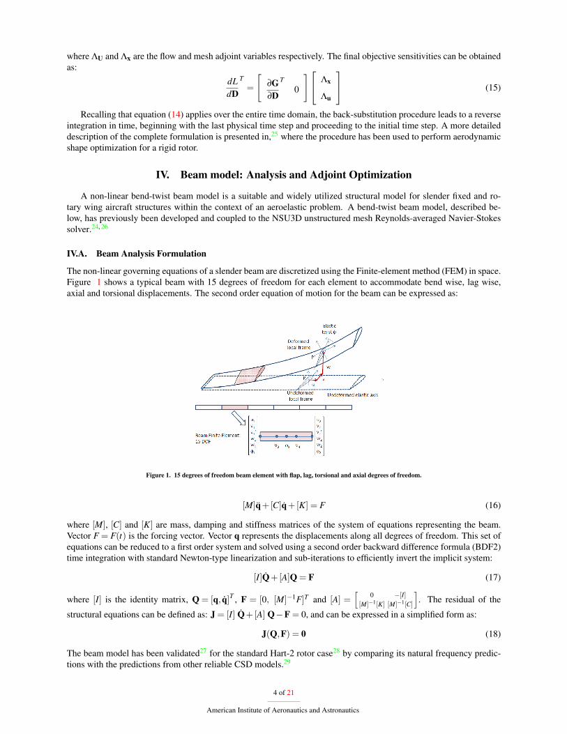
The non-linear governing equations of a slender beam are discretized using the Finite-element method (FEM) in space.Figure 1 shows a typical beam with 15 degrees of freedom for each element to accommodate bend wise, lag wise,axial and torsional displacements. The second order equation of motion for the beam can be expressed as:
Figure 1. 15 degrees of freedom beam element with flap, lag, torsional and axial degrees of freedom.
[M]q+[C]q+[K] = F (16)
where [M], [C] and [K] are mass, damping and stiffness matrices of the system of equations representing the beam.Vector F = F(t) is the forcing vector. Vector q represents the displacements along all degrees of freedom. This set ofequations can be reduced to a first order system and solved using a second order backward difference formula (BDF2)time integration with standard Newton-type linearization and sub-iterations to efficiently invert the implicit system:
[I]Q+[A]Q = F (17)
where [I] is the identity matrix, Q = [q, q]T , F = [0, [M]−1F]T and [A] =[
0 −[I][M]−1[K] [M]−1[C]
]. The residual of the
structural equations can be defined as: J = [I] Q+[A] Q−F = 0, and can be expressed in a simplified form as:
J(Q,F) = 0 (18)
The beam model has been validated27 for the standard Hart-2 rotor case28 by comparing its natural frequency predic-tions with the predictions from other reliable CSD models.29
4 of 21
American Institute of Aeronautics and Astronautics
IV.B. Forward Sensitivity Formulation of Beam Model
The beam tangent (forward sensitivity) linearization is similar to the analysis problem. For a given function, L, itssensitivity with respect to a blade design parameter, D can be written as: dL
dD = ∂L∂D + ∂L
∂Q∂Q∂D . This requires solving for
sensitivity of the beam state (Q), which can be obtained by differentiating Eqn. (18) with respect to the design variableD and rearranging as: [
∂J∂Q
]∂Q∂D
=− ∂J∂F
∂F∂D− ∂J
∂D(19)
The last term on the right hand side is non zero for structural design parameters such as beam element stiffnesses, inwhich case the applied force does not change with the design parameter, making the first term on the right hand sizezero. In the coupled aeroelastic case, using aerodynamic shape parameters that primarily affect the airloads on thestructure, the first term on the right-hand size is non-zero while the second term vanishes. Solving for ∂Q
∂D in Eqn. (19),the forward sensitivity of the objective function dL
dD can be obtained.
IV.C. Adjoint Formulation of Beam Model
The adjoint formulation of the beam model can be derived by approaching the tangent formulation in the reverse(transpose) direction. Taking the transpose of the objective functional sensitivity yields:
dLdD
T=
∂L∂D
T
+∂Q∂D
T∂L∂Q
T
(20)
This requires solving for the transpose sensitivity of the beam state (Q). The solution of ∂Q∂D
Tcan be derived by
transposing Eqn. (19) and substituting into Eqn. (20). This requires solving for an adjoint vector ΛQ defined as:[∂J∂Q
]T
ΛQ =∂L∂Q
T(21)
The above forms the adjoint formulation of the beam model. It is observed here again that the left hand side Jacobianterm of the adjoint step is just the transpose of the Jacobian in the forward linearization. In previous works,17, 27 forwardand adjoint formulations of the beam solver have been implemented and verified for both structural design parameters,and force-based design parameters (as required for the coupled aeroelasticity problem). The beam adjoint formulationwas used to perform time-dependent structural optimizations using the large-scale bound constraint optimization tool(L-BFGS-B)30 as a precursor to their use in fully coupled aero-structural optimization problems.
V. Fully Coupled Fluid-Structure Analysis Formulation
V.A. Fluid-structure interface (FSI)
In addition to the solution of the aerodynamic problem and the structural dynamics problem, the solution of the fullycoupled time-dependent aeroelastic problem requires the exchange of aerodynamic loads from the CFD solver to thebeam structure, which in turn returns surface displacements to the fluid flow solver. The governing equations for theFSI can be written in residual form as:
respectively for the forces transfered to the structural solver and displacements returned to the flow solver. In theseequations, [T ] represents the transfer matrix which projects point-wise CFD surface forces F(x,u) onto the individualbeam elements resulting in the beam forces Fb. The transpose of this matrix is used to obtain the CFD surfacedisplacements xs from the beam degrees of freedom Q. Also note that [T ] is a function of Q since the transfer patternschange with the beam deflection.
V.B. General solution procedure
The aeroelastic problem consists of multiple coupled sets of equations namely, the mesh deformation equations, theflow equations (CFD), the beam model-based structural equations, and the fluid-structure interface transfer equations.
5 of 21
American Institute of Aeronautics and Astronautics
The system of equations to be solved at each time step can be written as:
where S and S′ represent the residuals of the FSI equations, and J represents the residual of the structural analysisproblem. Note that the mesh motion residual now depends also on any surface deflections xs introduced by thestructural model. Within each physical time step, solution of the fully coupled fluid structure problem consists ofperforming multiple coupling iterations on each discipline using the latest available values from the other disciplines.
At the first coupling iteration, xcs = 0 (superscript c denotes the coupling iteration index) and solution of the mesh
deformation equation is trivial, although non zero values of xs are produced at subsequent coupling iterations as thebeam deflects in response to the aero loads. From a disciplinary point of view, the aerodynamic solver producesupdated values of u and x, which are used to compute F(x,u) pointwise surface forces. These surface forces are inputto the FSI/structural model which returns surface displacements xs. These new surface displacements are then fedback into the mesh deformation equations and the entire procedure is repeated until convergence is obtained for thefull coupled aero-structural problem at the given time step.
VI. Sensitivity Analysis for Coupled Aeroelastic Problem
In the formulation of the sensitivity analysis for the coupled aeroelastic problem, it is desirable to mimic as closelyas possible the solution strategies and data structures employed for the analysis problem. Thus, analogous disciplinarysolvers can be reused for each disciplinary sensitivity problem, and the analysis coupling strategy can be extended tothe sensitivity analysis formulation. Furthermore, the data transfered between disciplinary solvers should consist ofvectors of the same dimension for the analysis, tangent and adjoint formulations. Starting with the forward sensitivityproblem, the sensitivity of an objective L can be written as:
dLdD
=
[∂L∂x
∂L∂u
]∂x∂D
∂u∂D
(29)
where the individual disciplinary sensitivities are given as the solution of the coupled system:
∂G∂x
0 0 0 0∂G∂xs
∂R∂x
∂R∂u
0 0 0 0
−∂F∂x
−∂F∂u
I 0 0 0
0 0∂S∂F
∂S∂Fb
∂S∂Q
0
0 0 0∂J
∂Fb
∂J∂Q
0
0 0 0 0∂S′
∂Q∂S′
∂xs
∂x∂D
∂u∂D
∂F∂D
∂Fb
∂D
∂Q∂D
∂xs
∂D
=
−∂G∂D
0
0
0
0
0
The first and second equations correspond to equations for the mesh and flow variable sensitivities, as previouslydescribed for the aerodynamic solver, and the third equation corresponds to the construction of the surface force
6 of 21
American Institute of Aeronautics and Astronautics
sensitivities given these two previous sensitivities. The fourth equation denotes the sensitivity of the FSI transferfrom the fluid to the structural solver, while the fifth equation corresponds to the sensitivity of the structural solver.Finally, the last equation corresponds to the sensitivity of the FSI transfer from the structural solver back to the flowsolver. As can be seen, each disciplinary solution procedure requires the inversion of the same Jacobian matrix asthe corresponding analysis problem, which is done using the same iterative solver. Furthermore, the fluid-structurecoupling requires the transfer of the force sensitivities ∂F
∂D from the flow to the structural solver, and the surface meshsensitivities ∂xs
∂D from the structural solver back to the fluid solver, which are of the same dimension as the force andsurface displacements transfered in the analysis problem, respectively.
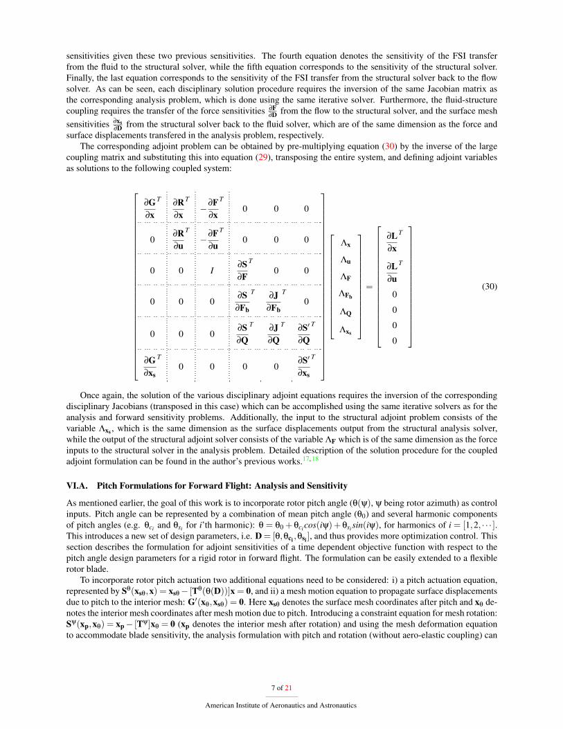
The corresponding adjoint problem can be obtained by pre-multiplying equation (30) by the inverse of the largecoupling matrix and substituting this into equation (29), transposing the entire system, and defining adjoint variablesas solutions to the following coupled system:
∂G∂x
T∂R∂x
T
−∂F∂x
T
0 0 0
0∂R∂u
T
−∂F∂u
T
0 0 0
0 0 I∂S∂F
T
0 0
0 0 0∂S
∂Fb
T∂J
∂Fb
T
0
0 0 0∂S∂Q
T∂J∂Q
T∂S′
∂Q
T
∂G∂xs
T
0 0 0 0∂S′
∂xs
T
Λx
Λu
ΛF
ΛFb
ΛQ
Λxs
=
∂L∂x
T
∂L∂u
T
0
0
0
0
(30)
Once again, the solution of the various disciplinary adjoint equations requires the inversion of the correspondingdisciplinary Jacobians (transposed in this case) which can be accomplished using the same iterative solvers as for theanalysis and forward sensitivity problems. Additionally, the input to the structural adjoint problem consists of thevariable Λxs , which is the same dimension as the surface displacements output from the structural analysis solver,while the output of the structural adjoint solver consists of the variable ΛF which is of the same dimension as the forceinputs to the structural solver in the analysis problem. Detailed description of the solution procedure for the coupledadjoint formulation can be found in the author’s previous works.17, 18
VI.A. Pitch Formulations for Forward Flight: Analysis and Sensitivity
As mentioned earlier, the goal of this work is to incorporate rotor pitch angle (θ(ψ), ψ being rotor azimuth) as controlinputs. Pitch angle can be represented by a combination of mean pitch angle (θ0) and several harmonic componentsof pitch angles (e.g. θci and θsi for i’th harmonic): θ = θ0 +θcicos(iψ)+θsisin(iψ), for harmonics of i = [1,2, · · · ].This introduces a new set of design parameters, i.e. D = [θ,θci ,θsi ], and thus provides more optimization control. Thissection describes the formulation for adjoint sensitivities of a time dependent objective function with respect to thepitch angle design parameters for a rigid rotor in forward flight. The formulation can be easily extended to a flexiblerotor blade.
To incorporate rotor pitch actuation two additional equations need to be considered: i) a pitch actuation equation,represented by Sθ(xsθ,x) = xsθ− [Tθ(θ(D))]x = 0, and ii) a mesh motion equation to propagate surface displacementsdue to pitch to the interior mesh: G′(xθ,xsθ) = 0. Here xsθ denotes the surface mesh coordinates after pitch and xθ de-notes the interior mesh coordinates after mesh motion due to pitch. Introducing a constraint equation for mesh rotation:Sψ(xp,xθ) = xp− [Tψ]xθ = 0 (xp denotes the interior mesh after rotation) and using the mesh deformation equationto accommodate blade sensitivity, the analysis formulation with pitch and rotation (without aero-elastic coupling) can
7 of 21
American Institute of Aeronautics and Astronautics
be represented as:
G(x,D) = 0 (31)Sθ(xsθ,x,D) = 0 (32)
G′(xθ,xsθ) = 0 (33)Sψ(xp,xθ) = 0 (34)
R(xp,u) = 0 (35)
Here [Tθ] and [Tψ] are matrix representations for pitch actuation and rotation, respectively. Although the solid bodymesh rotation constraint is present in all cases, it has been omitted for simplicity in the previous formulation, but isincluded explicitly in this case to differentiate between the two types of prescribed motion (namely blade pitch androtation). The forward sensitivity formulation of the pitching actuation mimics the analysis formulation describedabove and is obtained by linearizing these equations with respect to the design variables, which yields:
∂G∂x
0 0 0 0
∂Sθ
∂x∂Sθ
∂xsθ
0 0 0
0∂G′
∂xsθ
∂G′
∂xθ
0 0
0 0∂Sψ
∂x∂Sψ
∂xp0
0 0 0∂R∂xp
∂R∂u
∂x∂D
∂xsθ
∂D
∂xθ
∂D
∂xp
∂D
∂u∂D
=
−∂G∂D
−∂Sθ
∂D
0
0
0
(36)
From the solution of this equation, now the sensitivity of a time dependent objective function can be obtained as: dLdD =[
∂L∂x
∂L∂xsθ
∂L∂u
][∂x∂D
∂xsθ
∂D∂u∂D
]T
. The corresponding adjoint sensitivity formulation can be obtained by
constructing a transposed Jacobian matrix from Eqn. 36 to solve for corresponding adjoint vectors Λx,Λxsθ, Λxθ
, Λxp ,and Λxu :
∂G∂x
T∂Sθ
∂x
T
0 0 0
0∂Sθ
∂xsθ
T∂G′
∂xsθ
T
0 0
0 0∂G′
∂xθ
T∂Sψ
∂xθ
T
0
0 0 0∂Sψ
∂xp
T∂R∂xp
T
0 0 0 0∂R∂u
T
Λx
Λxsθ
Λxθ
Λxp
Λu
=
∂L∂x
T
∂L∂xsθ
T
0
0
∂L∂u
T
(37)
The final objective sensitivities can be obtained as: dLdD
T=
−∂G∂D
T
−∂Sθ
∂D
T
0 0 0
[ Λx ΛxsθΛxθ
Λxp Λu
]T
Here, Λxsθrefers to adjoint contribution from the pitch sensitivity formulation. For the flexible (aeroelastic) case, the
above forward and adjoint sensitivity systems are augmented by the additional structural and fluid-structure interfacesensitivity/adjoint equations as described previously.
8 of 21
American Institute of Aeronautics and Astronautics
VII. Verification of Coupled Aeroelastic Sensitivity
The forward and adjoint sensitivities for the coupled aeroelastic problem are verified using the complex stepmethod. Any function f (x) operating on a real variable x can be utilized to compute the derivative f ′(x) by redefiningthe input variable x and all intermediate variables used in the discrete evaluation of f (x) as complex variables. Fora complex input, the function when redefined as described produces a complex output. The derivative of the realfunction f (x) can be computed by expanding the complex operator f (x+ ih) as:
f (x+ ih) = f (x)+ ih f ′(x)+ · · · (38)
from which the derivative f ′(x) can be easily determined as:
f ′(x) =Im [ f (x+ ih)]
h(39)
As in the case of finite-differencing, the complex step-based differentiation also requires a step size. However, unlikefinite-differencing the complex step method is insensitive to small step sizes since no differencing is required. In theoryit is possible to verify forward and adjoint-based gradients using the complex step method to machine precision. Withthis in mind, a complex version of the complete coupled aero-structural analysis code has been constructed throughscripting of the original source code to redefine variables from real to complex types and to overload a small numberof functions for use with complex variables.
VIII. RESULTS
VIII.A. Time Dependent Analysis Problem
The chosen test case is a four bladed HART2 rotor in a forward flight condition. The flight condition parameters are:Mach numbers, Mtip = 0.638,M∞ = 0.095, shaft tilt angle towards freestream, αsha f t = 5.4. The corresponding rotorrotational speed is Ω = 1041 RPM. The pitch angle actuation is prescribed as: θ = θ0 +θ1ssin(ψ)+θ1ccos(ψ), withθ0 = 5.0,θ1s = −1.1,θ1c = 2.0. The rotor is impulsively started from rest, in an initially quiescent flow field, androtated with the mesh as a solid body for a fixed number of revolutions. This problem is solved both for a rigid blademodel (using no structural model), as well as for a flexible blade model (using the beam structural model). For thelatter, the flow is solved in tight coupling mode with the beam solver.
The baseline simulation (coarse mesh) makes use of a mixed element mesh made up of prisms, pyramids andtetrahedra consisting of approximately 2.32 million grid points and is shown in Figure (2(a)). The simulations are runfor 5 rotor revolutions using a 2 degree time-step, i.e. for 900 time-steps starting from freestream initialization. Forthe rigid blade simulation, the time-dependent mesh motion is determined by first pitching the blade about the bladeaxis followed by solving the mesh deformation equations and then rotating the entire mesh as a solid body at eachtime step. The unsteady Reynolds-averaged Navier-Stokes equations are solved at each time step in ALE form, usingthe Spalart-Allmaras turbulence model.
The coupled CFD/CSD simulation is run in a similar manner. However, the flow solution (CFD) is coupled withthe beam solver (CSD) at every time step by appropriately exchanging, a) airloads information from the flow domainto the beam and b) blade deformation information from the beam to the flow domain, at the fluid-structure interface(i.e. blade surface). In this coupled simulation, the mesh is moved according to the deformations dictated by the newflexed blade coordinates determined from the structural beam code after the combined kinematics of pitch actuationfollowed by solid body rotation of the entire mesh have been performed. Thus, the flow now sees not only the pitchedand rigidly rotated mesh (observed in rigid blade simulation in forward flight), but also the deformed mesh around theblades due to both pitching and structural deformations. This coupled fluid-structure interaction problem needs to beiterated until satisfactory convergence is achieved on flow, structure and mesh deformation problems within each timestep. This kind of CFD/CSD coupling done within every time step is known as tight coupling.
The simulations were performed on the Yellowstone supercomputer at the NCAR-Wyoming Supercomputing Cen-ter (NWSC), with the analysis problem running in parallel on 1024 cores. Each time step used 6 coupling iterations,and each coupling iteration used 10 non-linear flow iterations with each non-linear iteration consisting of a three-levelline-implicit multigrid cycle. The typical simulation at this level of resolution requires approximately 40 minutes ofwall clock time per rotor revolution. Figure (2(b)) shows the Q-criterion isosurfaces for the flexible rotor after 5 revo-lutions. The figure clearly shows how the wakes from both the root and tip of upstream blades interact with the trailingblades resulting in complex flow features, although these are diffused due to the coarse mesh resolution.
9 of 21
American Institute of Aeronautics and Astronautics
(a) Computational Domain: 2.32 million nodes (b) Q-criterion
Figure 2. Computational polyhedra mesh and Q-criterion for the flexible baseline HART2 rotor in forward flight after 5 revolutions
(a) Rigid Blade (b) Flexible Blade
Figure 3. Flow and turbulence residual convergence at a given time step for rigid and flexible blade analysis
10 of 21
American Institute of Aeronautics and Astronautics
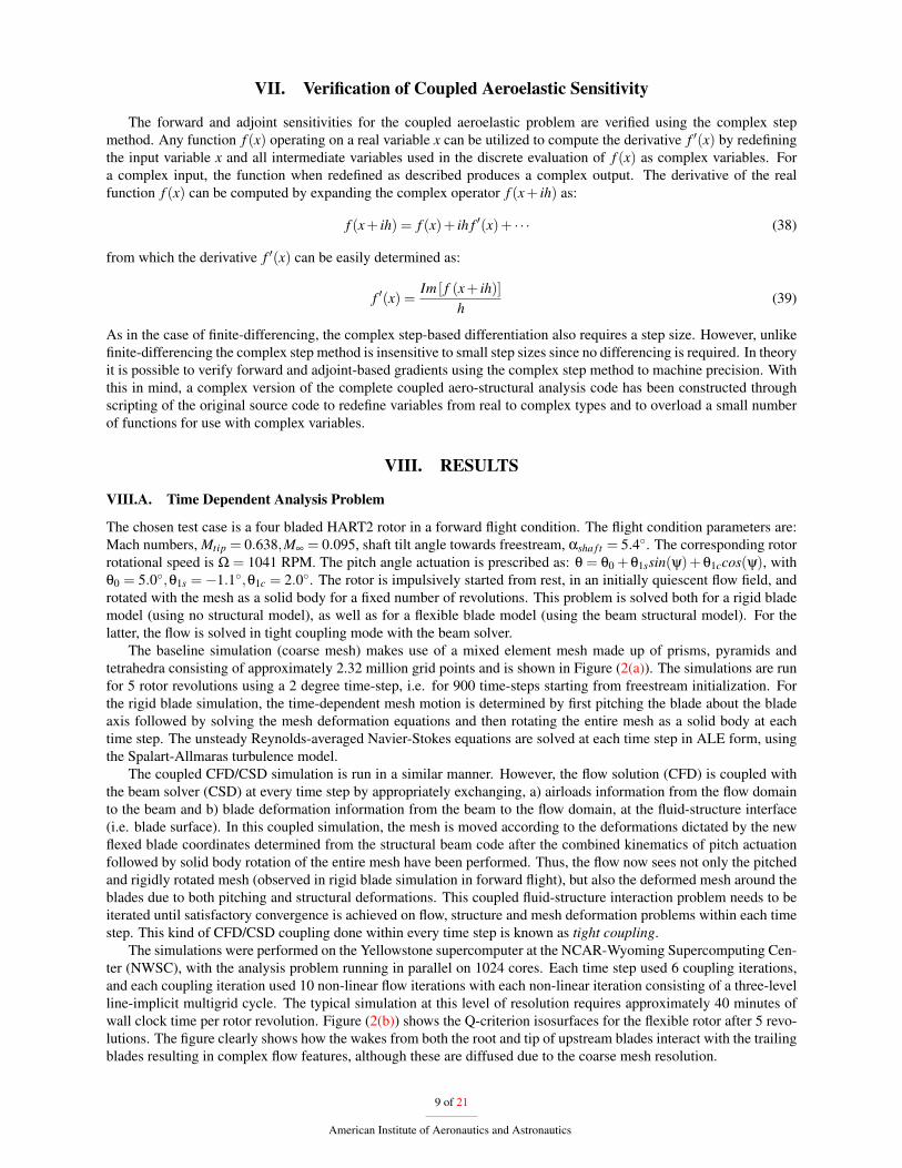
(a) Mesh Convergence per time step for coupled analysis (b) Beam and FSI convergence per coupling iteration
Figure 4. Residual convergence of mesh and beam (overall FSI) in one coupling iteration
Figures 3 and 4 summarize the overall convergence of the rigid and aero-elastic coupling analysis formulations.Figure 3(a) shows the typical flow and turbulence residual convergence within a single time step for the rigid rotorcase (no structural model), while Figure 3(b) depicts convergence of the flow and turbulence residuals at the same timestep for the coupled aeroelastic case. In this case, the jumps in residual values at the start of new coupling iterationsare clearly visible, although these jumps become smaller as the coupling procedure converges. The overall residualhistories closely follow those of the rigid rotor case after the first few coupling iterations. Figure 4(a) depicts theconvergence of the mesh deformation residual for the same time step, also showing jumps in the residual at the startof each new coupling iteration. Solution of the mesh deformation equations terminates when the residuals reach aprescribed tolerance of 1.e− 06, and hence the variable number of iterations per coupling cycle. Most notable is thefact that the initial mesh deformation residual decreases at each new coupling iteration, providing a measure of theconvergence of the entire coupling procedure. The corresponding beam residual drop is observed to be of 15 ordersof magnitude, as shown in Fig. 4(b). Figure 4(b) illustrates the convergence of the coupled beam/FSI residual (i.e.equations (26) and (27)), showing rapid convergence to machine zero in a small number of iterations within a singleCFD/CSD coupling iteration.
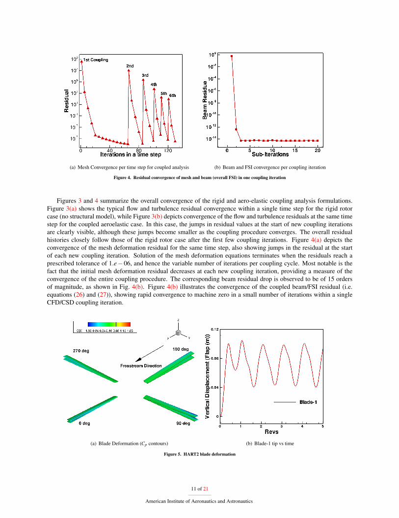
(a) Blade Deformation (Cp contours) (b) Blade-1 tip vs time
Figure 5. HART2 blade deformation
11 of 21
American Institute of Aeronautics and Astronautics
The effect of the CFD/CSD aeroelastic coupling is clearly demonstrated in Figure 5(a), which compares thedeformed blade shape and its corresponding Cp surface contours from the coupled simulation with that from the rigidblade simulation. From the figure it is noted that all four blades show different deformation characteristics due tocorresponding different aerodynamic environment they experience in a forward flight. The blade attains the largestflap displacement at azimuth, ψ = 180 and the smallest flap displacement at azimuth, ψ = 0. For both the flexibleand rigid blades, the pressure contours demonstrate that the advancing side blades experience more compressibilityeffects (larger pressure gradients near the rotor tips) than the retreating side blades. The flexible blade tip verticaldisplacement time history shown in Figure 5(b) demonstrates 1/rev behavior of blade flapping.
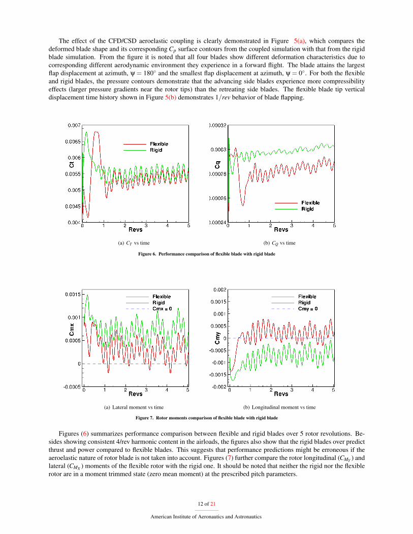
(a) CT vs time (b) CQ vs time
Figure 6. Performance comparison of flexible blade with rigid blade
(a) Lateral moment vs time (b) Longitudinal moment vs time
Figure 7. Rotor moments comparison of flexible blade with rigid blade
Figures (6) summarizes performance comparison between flexible and rigid blades over 5 rotor revolutions. Be-sides showing consistent 4/rev harmonic content in the airloads, the figures also show that the rigid blades over predictthrust and power compared to flexible blades. This suggests that performance predictions might be erroneous if theaeroelastic nature of rotor blade is not taken into account. Figures (7) further compare the rotor longitudinal (CMY ) andlateral (CMX ) moments of the flexible rotor with the rigid one. It should be noted that neither the rigid nor the flexiblerotor are in a moment trimmed state (zero mean moment) at the prescribed pitch parameters.
12 of 21
American Institute of Aeronautics and Astronautics
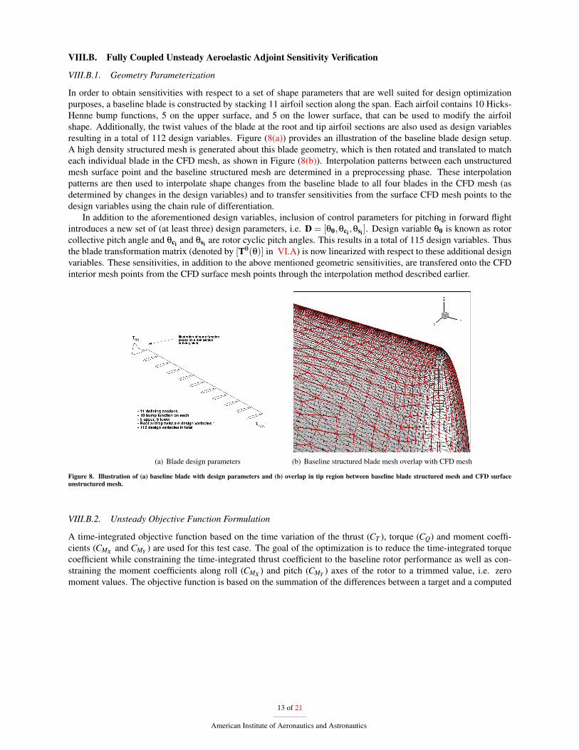
In order to obtain sensitivities with respect to a set of shape parameters that are well suited for design optimizationpurposes, a baseline blade is constructed by stacking 11 airfoil section along the span. Each airfoil contains 10 Hicks-Henne bump functions, 5 on the upper surface, and 5 on the lower surface, that can be used to modify the airfoilshape. Additionally, the twist values of the blade at the root and tip airfoil sections are also used as design variablesresulting in a total of 112 design variables. Figure (8(a)) provides an illustration of the baseline blade design setup.A high density structured mesh is generated about this blade geometry, which is then rotated and translated to matcheach individual blade in the CFD mesh, as shown in Figure (8(b)). Interpolation patterns between each unstructuredmesh surface point and the baseline structured mesh are determined in a preprocessing phase. These interpolationpatterns are then used to interpolate shape changes from the baseline blade to all four blades in the CFD mesh (asdetermined by changes in the design variables) and to transfer sensitivities from the surface CFD mesh points to thedesign variables using the chain rule of differentiation.
In addition to the aforementioned design variables, inclusion of control parameters for pitching in forward flightintroduces a new set of (at least three) design parameters, i.e. D = [θ0,θci ,θsi ]. Design variable θ0 is known as rotorcollective pitch angle and θci and θsi are rotor cyclic pitch angles. This results in a total of 115 design variables. Thusthe blade transformation matrix (denoted by [Tθ(θ)] in VI.A) is now linearized with respect to these additional designvariables. These sensitivities, in addition to the above mentioned geometric sensitivities, are transfered onto the CFDinterior mesh points from the CFD surface mesh points through the interpolation method described earlier.
Figure 8. Illustration of (a) baseline blade with design parameters and (b) overlap in tip region between baseline blade structured mesh and CFD surfaceunstructured mesh.
VIII.B.2. Unsteady Objective Function Formulation
A time-integrated objective function based on the time variation of the thrust (CT ), torque (CQ) and moment coeffi-cients (CMX and CMY ) are used for this test case. The goal of the optimization is to reduce the time-integrated torquecoefficient while constraining the time-integrated thrust coefficient to the baseline rotor performance as well as con-straining the moment coefficients along roll (CMX ) and pitch (CMY ) axes of the rotor to a trimmed value, i.e. zeromoment values. The objective function is based on the summation of the differences between a target and a computed
13 of 21
American Institute of Aeronautics and Astronautics
objective value at each time level n . Mathematically the global objective function is defined as:
Lg = LShape +LTrim (40)
LShape = ω11T
n=N
∑n=1
∆t[δCn
Q]2 (41)
LTrim = ω21T
n=N
∑n=1
∆t [δCnT ]
2 +ω3[δCMX
]2+ω4
[δCMY
]2 (42)
δCnQ = (Cn
Q−CnQtarget) (43)
δCnT = (Cn
T −CT target) (44)
δCMX =1T
n=N
∑n=1
∆t(CnMX−Cn
MX target) (45)
δCMY =1T
n=N
∑n=1
∆t(CnMY−Cn
MY target) (46)
where the mean target thrust coefficient value is specified to the Hart2 baseline mean trim value of CT target = 4.4e−3,and the target torque and moment values are set to zero. The weights (ωi, i = [1,2,3,4]) are included to equalize thedifference in orders-of-magnitude between the thrust, torque and moment coefficients. Use of pitch control param-eters ([θ0,θci ,θsi ]) as design variables and use of moment penalty terms ensure that the optimized rotor shape withoptimized control parameters tend towards a final trimmed state when the rotor design cycles converge. This approachis computationally more efficient than the use of a hard constraint formulation, since this latter approach would re-quire the computation of multiple adjoint problems at each design cycle, as opposed to the single adjoint required inthe current formulation. However, the trim constraint may not be satisfied exactly in this approach.
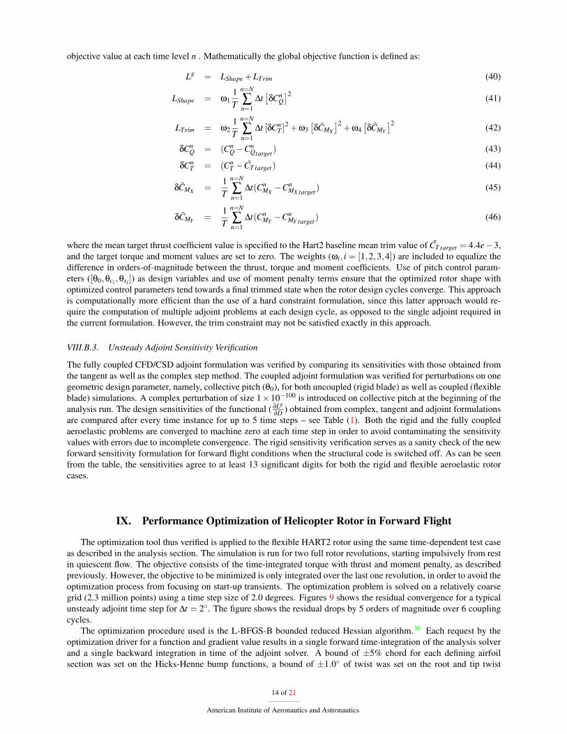
The fully coupled CFD/CSD adjoint formulation was verified by comparing its sensitivities with those obtained fromthe tangent as well as the complex step method. The coupled adjoint formulation was verified for perturbations on onegeometric design parameter, namely, collective pitch (θ0), for both uncoupled (rigid blade) as well as coupled (flexibleblade) simulations. A complex perturbation of size 1×10−100 is introduced on collective pitch at the beginning of theanalysis run. The design sensitivities of the functional ( ∂Lg
∂D ) obtained from complex, tangent and adjoint formulationsare compared after every time instance for up to 5 time steps – see Table (1). Both the rigid and the fully coupledaeroelastic problems are converged to machine zero at each time step in order to avoid contaminating the sensitivityvalues with errors due to incomplete convergence. The rigid sensitivity verification serves as a sanity check of the newforward sensitivity formulation for forward flight conditions when the structural code is switched off. As can be seenfrom the table, the sensitivities agree to at least 13 significant digits for both the rigid and flexible aeroelastic rotorcases.
IX. Performance Optimization of Helicopter Rotor in Forward Flight
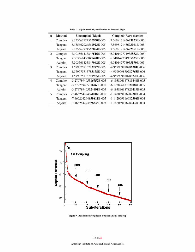
The optimization tool thus verified is applied to the flexible HART2 rotor using the same time-dependent test caseas described in the analysis section. The simulation is run for two full rotor revolutions, starting impulsively from restin quiescent flow. The objective consists of the time-integrated torque with thrust and moment penalty, as describedpreviously. However, the objective to be minimized is only integrated over the last one revolution, in order to avoid theoptimization process from focusing on start-up transients. The optimization problem is solved on a relatively coarsegrid (2.3 million points) using a time step size of 2.0 degrees. Figures 9 shows the residual convergence for a typicalunsteady adjoint time step for ∆t = 2. The figure shows the residual drops by 5 orders of magnitude over 6 couplingcycles.
The optimization procedure used is the L-BFGS-B bounded reduced Hessian algorithm.30 Each request by theoptimization driver for a function and gradient value results in a single forward time-integration of the analysis solverand a single backward integration in time of the adjoint solver. A bound of ±5% chord for each defining airfoilsection was set on the Hicks-Henne bump functions, a bound of ±1.0 of twist was set on the root and tip twist
14 of 21
American Institute of Aeronautics and Astronautics
Table 1. Adjoint sensitivity verification for Forward Flight
n Method Uncoupled (Rigid) Coupled (Aero-elastic)1 Complex 8.135662924562930E-005 7.569817143673123E-005
Figure 9. Residual convergence in a typical adjoint time step
15 of 21
American Institute of Aeronautics and Astronautics
definitions, and a bound of ±5.0 of pitch angle was set on all the pitch parameters (collective and cyclics). Theoptimizations were performed on the Yellowstone supercomputer at the NCAR-Wyoming Supercomputing Center(NWSC) with the simulations (analysis/adjoint) running in parallel on 1024 cores. Each time step in the analysisproblem employed 6 coupling cycles. Each coupling cycle used 10 nonlinear iterations. A typical coupled functionalgradient (analysis/adjoint) computation step requires approximately 70 minutes when run on 1024 cores.
The performance optimization consists of three main stages: i) Trim ii) Shape/performance optimization and, iii)re-trim. The ’Trim’ step involves trimming the rotor to a target wind tunnel rotor thrust value of CT = 4.4e− 3 andzero longitudinal and lateral moments (CMY ,CMX = 0). The objective function used in this step consists only of thethrust and moment terms in Eqn 40 (ω1 = 0) and the objective minimization is performed using only the three pitchparameters, namely, collective and cyclics as design variables.
In the second stage, blade shape optimization is performed by including the performance objective, i.e., CQ terminto the time dependent objective function to be minimized. Appropriate weights (ωi, i= 1,2,3,4) are used to maintainthe rotor trim state through a penalty function while the blade shape is optimized to obtain minimum rotor power.In total 115 design parameters were used in this stage, including 112 blade shape parameters and 3 pitch controlparameters. However, even after optimization convergence in stage two, the exact trim state is not maintained. Thisis because the trim objective components in the objective function were used only as weak constraint terms, i.e. aspenalty terms and not as hard constraints. Therefore, the last stage involves trimming the rotor back to the target thrustand moment values, once again using only the three control pitch parameters as design inputs. This stage is otherwisereferred to as the ’re-trim’ stage in this paper.
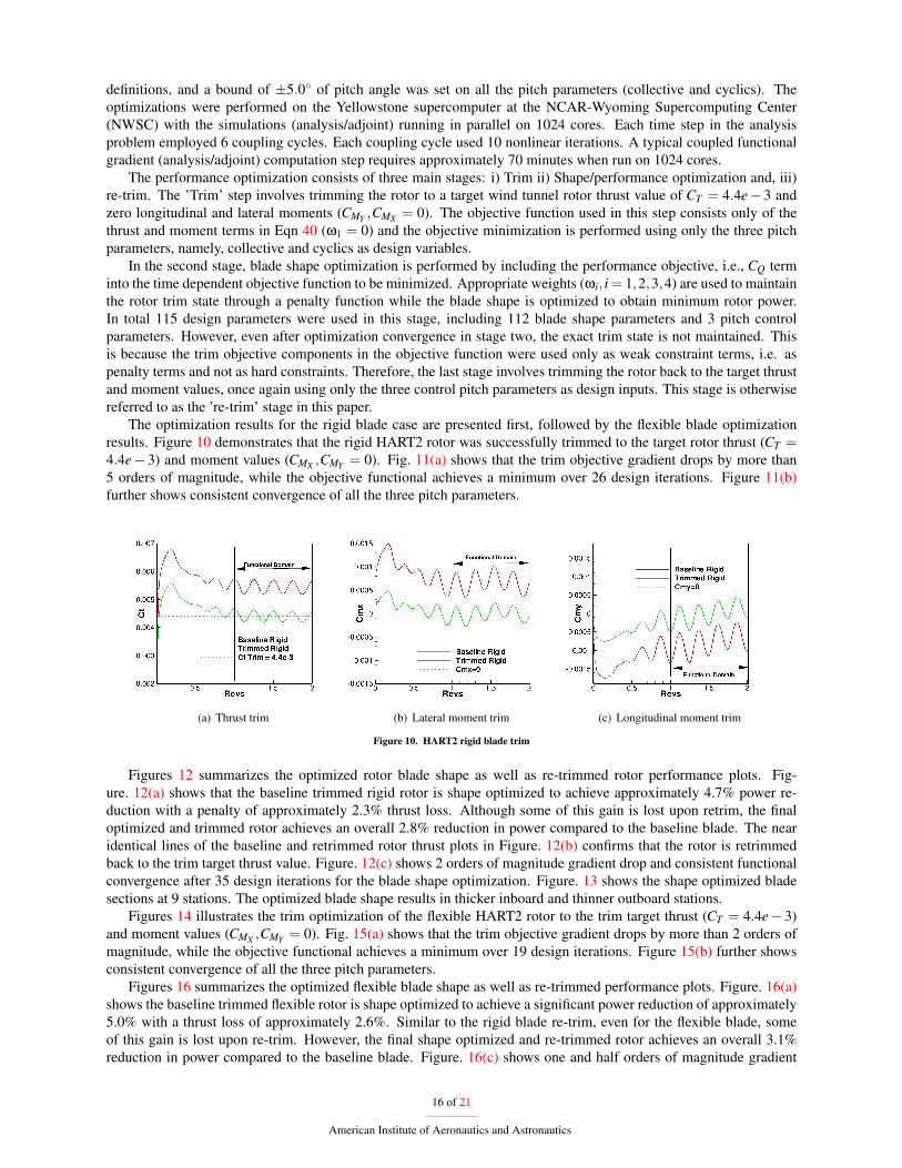
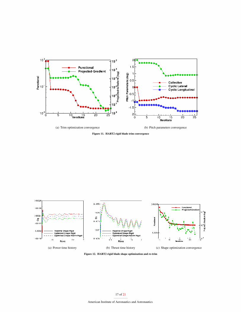
The optimization results for the rigid blade case are presented first, followed by the flexible blade optimizationresults. Figure 10 demonstrates that the rigid HART2 rotor was successfully trimmed to the target rotor thrust (CT =4.4e− 3) and moment values (CMX ,CMY = 0). Fig. 11(a) shows that the trim objective gradient drops by more than5 orders of magnitude, while the objective functional achieves a minimum over 26 design iterations. Figure 11(b)further shows consistent convergence of all the three pitch parameters.
(a) Thrust trim (b) Lateral moment trim (c) Longitudinal moment trim
Figure 10. HART2 rigid blade trim
Figures 12 summarizes the optimized rotor blade shape as well as re-trimmed rotor performance plots. Fig-ure. 12(a) shows that the baseline trimmed rigid rotor is shape optimized to achieve approximately 4.7% power re-duction with a penalty of approximately 2.3% thrust loss. Although some of this gain is lost upon retrim, the finaloptimized and trimmed rotor achieves an overall 2.8% reduction in power compared to the baseline blade. The nearidentical lines of the baseline and retrimmed rotor thrust plots in Figure. 12(b) confirms that the rotor is retrimmedback to the trim target thrust value. Figure. 12(c) shows 2 orders of magnitude gradient drop and consistent functionalconvergence after 35 design iterations for the blade shape optimization. Figure. 13 shows the shape optimized bladesections at 9 stations. The optimized blade shape results in thicker inboard and thinner outboard stations.
Figures 14 illustrates the trim optimization of the flexible HART2 rotor to the trim target thrust (CT = 4.4e− 3)and moment values (CMX ,CMY = 0). Fig. 15(a) shows that the trim objective gradient drops by more than 2 orders ofmagnitude, while the objective functional achieves a minimum over 19 design iterations. Figure 15(b) further showsconsistent convergence of all the three pitch parameters.
Figures 16 summarizes the optimized flexible blade shape as well as re-trimmed performance plots. Figure. 16(a)shows the baseline trimmed flexible rotor is shape optimized to achieve a significant power reduction of approximately5.0% with a thrust loss of approximately 2.6%. Similar to the rigid blade re-trim, even for the flexible blade, someof this gain is lost upon re-trim. However, the final shape optimized and re-trimmed rotor achieves an overall 3.1%reduction in power compared to the baseline blade. Figure. 16(c) shows one and half orders of magnitude gradient
16 of 21
American Institute of Aeronautics and Astronautics
(a) Trim optimization convergence (b) Pitch parameters convergence
Figure 11. HART2 rigid blade trim convergence
(a) Power time history (b) Thrust time history (c) Shape optimization convergence
Figure 12. HART2 rigid blade shape optimization and re-trim
17 of 21
American Institute of Aeronautics and Astronautics
(a) Thrust trim (b) Lateral moment trim (c) Longitudinal moment trim
Figure 14. HART2 flexible blade trim
18 of 21
American Institute of Aeronautics and Astronautics
(a) Trim optimization convergence (b) Pitch parameters convergence
Figure 15. HART2 flexible blade trim convergence
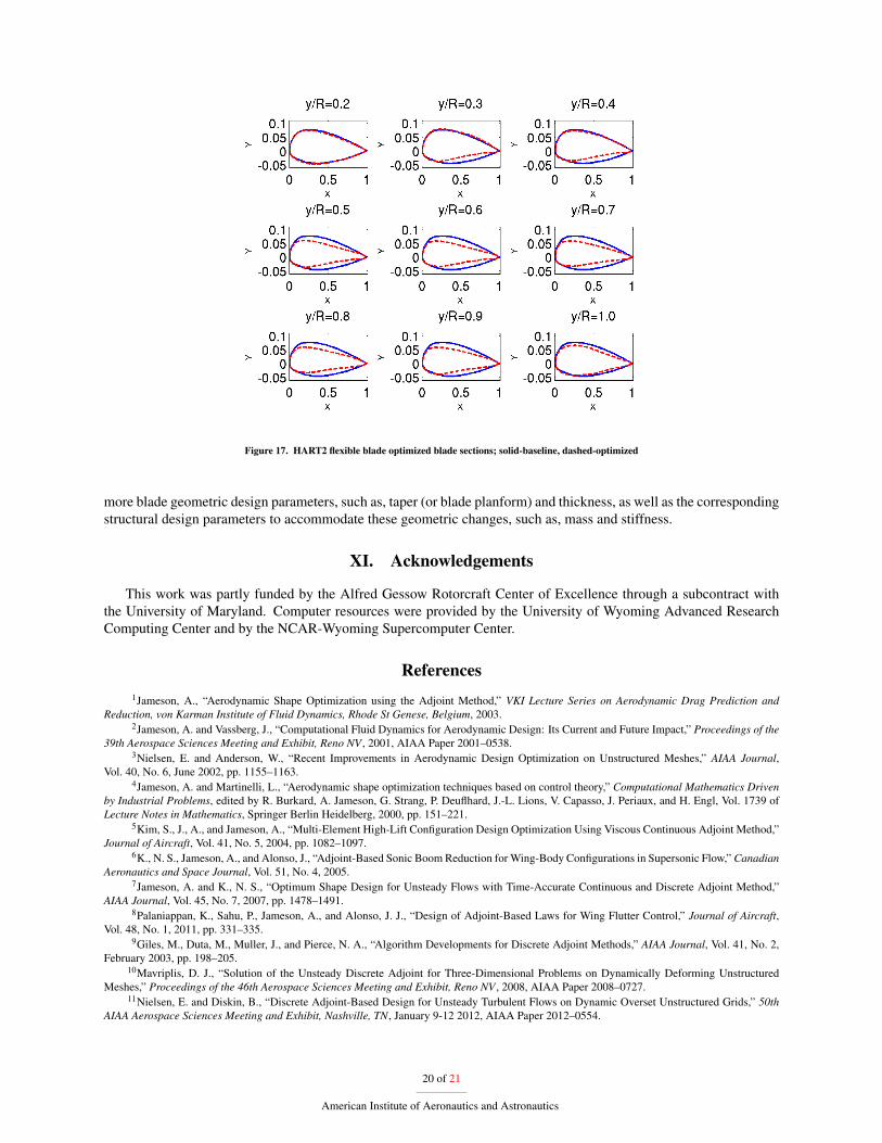
drop and consistent functional convergence even after 21 design iterations for the blade shape optimization stage.Figure. 17 shows the shape optimized blade sections at 9 stations. The optimized blade shapes show similar trend tothose observed in the rigid blade shape optimization, i.e. thicker inboard and thinner outboard stations.
(a) Power time history (b) Thrust time history (c) Shape optimization convergence
Figure 16. HART2 flexible blade shape optimization and re-trim
X. Conclusions and Future Works
In this work, a discrete adjoint formulation for time-dependent tightly coupled aeroelastic three-dimensional prob-lems of flexible rotors in forward flight conditions has been developed. The unsteady adjoint sensitivities of theformulation over several time steps have been verified. The current formulation for rotor problems in forward flightconditions was built upon a previously developed adjoint formulation for rotor problems in hover conditions, by incor-porating a blade cyclic pitch capability in the analysis formulation as well as in tangent and adjoint sensitivity analysisformulations. The formulation is designed to reuse as much as possible the original coupled aeroelastic data-structuresand solution strategies used for the analysis problem, thus simplifying implementation and verification.
After successful verification of the developed adjoint optimization tool, it was effectively used to perform efficientrotor blade shape design targeting minimum rotor torque with the constraint of a prescribed rotor trim state. Theperformance optimization on both rigid as well as flexible blades consistently resulted in approximately 3.0% powerreduction over the baseline blade shape while sustaining a target trim state.
In the future, this work will be extended to carry out multipoint rotor design optimization, for example, for multipleflight conditions such as hover as well as forward flight. In addition, the future rotor design optimizations will include
19 of 21
American Institute of Aeronautics and Astronautics
more blade geometric design parameters, such as, taper (or blade planform) and thickness, as well as the correspondingstructural design parameters to accommodate these geometric changes, such as, mass and stiffness.
XI. Acknowledgements
This work was partly funded by the Alfred Gessow Rotorcraft Center of Excellence through a subcontract withthe University of Maryland. Computer resources were provided by the University of Wyoming Advanced ResearchComputing Center and by the NCAR-Wyoming Supercomputer Center.
References1Jameson, A., “Aerodynamic Shape Optimization using the Adjoint Method,” VKI Lecture Series on Aerodynamic Drag Prediction and
Reduction, von Karman Institute of Fluid Dynamics, Rhode St Genese, Belgium, 2003.2Jameson, A. and Vassberg, J., “Computational Fluid Dynamics for Aerodynamic Design: Its Current and Future Impact,” Proceedings of the
39th Aerospace Sciences Meeting and Exhibit, Reno NV , 2001, AIAA Paper 2001–0538.3Nielsen, E. and Anderson, W., “Recent Improvements in Aerodynamic Design Optimization on Unstructured Meshes,” AIAA Journal,
Vol. 40, No. 6, June 2002, pp. 1155–1163.4Jameson, A. and Martinelli, L., “Aerodynamic shape optimization techniques based on control theory,” Computational Mathematics Driven
by Industrial Problems, edited by R. Burkard, A. Jameson, G. Strang, P. Deuflhard, J.-L. Lions, V. Capasso, J. Periaux, and H. Engl, Vol. 1739 ofLecture Notes in Mathematics, Springer Berlin Heidelberg, 2000, pp. 151–221.
5Kim, S., J., A., and Jameson, A., “Multi-Element High-Lift Configuration Design Optimization Using Viscous Continuous Adjoint Method,”Journal of Aircraft, Vol. 41, No. 5, 2004, pp. 1082–1097.
6K., N. S., Jameson, A., and Alonso, J., “Adjoint-Based Sonic Boom Reduction for Wing-Body Configurations in Supersonic Flow,” CanadianAeronautics and Space Journal, Vol. 51, No. 4, 2005.
7Jameson, A. and K., N. S., “Optimum Shape Design for Unsteady Flows with Time-Accurate Continuous and Discrete Adjoint Method,”AIAA Journal, Vol. 45, No. 7, 2007, pp. 1478–1491.
8Palaniappan, K., Sahu, P., Jameson, A., and Alonso, J. J., “Design of Adjoint-Based Laws for Wing Flutter Control,” Journal of Aircraft,Vol. 48, No. 1, 2011, pp. 331–335.
9Giles, M., Duta, M., Muller, J., and Pierce, N. A., “Algorithm Developments for Discrete Adjoint Methods,” AIAA Journal, Vol. 41, No. 2,February 2003, pp. 198–205.
10Mavriplis, D. J., “Solution of the Unsteady Discrete Adjoint for Three-Dimensional Problems on Dynamically Deforming UnstructuredMeshes,” Proceedings of the 46th Aerospace Sciences Meeting and Exhibit, Reno NV , 2008, AIAA Paper 2008–0727.
11Nielsen, E. and Diskin, B., “Discrete Adjoint-Based Design for Unsteady Turbulent Flows on Dynamic Overset Unstructured Grids,” 50thAIAA Aerospace Sciences Meeting and Exhibit, Nashville, TN, January 9-12 2012, AIAA Paper 2012–0554.
20 of 21
American Institute of Aeronautics and Astronautics
12Nielsen, E. J., Diskin, B., and Yamaleev, N., “Discrete Adjoint-Based Design Optimization of Unsteady Turbulent Flows on DynamicUnstructured Grids,” AIAA Journal, Vol. 48-6, June 2010, pp. 1195–1206.
13Nielsen, E. J., Lee-Rausch, E. M., and Jones, W. T., “Adjoint-Based Design of Rotors in a Noninertial Reference Frame,” Journal of Aircraft,Vol. 47-2, March-April 2010, pp. 638–646.
14Mani, K. and Mavriplis, D. J., “Geometry Optimization in Three-Dimensional Unsteady Flow Problems using the Discrete Adjoint,” 51stAIAA Aerospace Sciences Meeting, Grapevine, TX, January 2013, AIAA Paper 2013-0662.
15Martins, J. R. R. A. and Lambe, A. B., “Multidisciplinary Design Optimization: A Survey of Architectures,” AIAA Journal, Vol. 51, 2013,pp. 2049–2075.
16Kenway, G. K. W., Kennedy, G. J., and Martins, J. R. R. A., “Scalable parallel approach for high-fidelity steady-state aeroelastic analysisand adjoint derivative computations,” AIAA Journal, 2013, (In press).
17Mishra, A., Mani, K., Mavriplis, D. J., and Sitaraman, J., “Time-dependent Adjoint-based Optimization for Coupled Aeroelastic Problems,”21st AIAA CFD Conference, San Diego, CA, June 24–27 2013, AIAA Paper 2013–2906.
18Mishra, A., Mani, K., Mavriplis, D. J., and Sitaraman, J., “Time-dependent Adjoint-based Aerodynamic Shape Optimization Applied toHelicopter Rotors,” 70th American Helicopter Society Annual Forum, Montreal, QC, CA, May 20–22 2014.
19Mavriplis, D. J., “Discrete Adjoint-Based Approach for Optimization Problems on Three-Dimensional Unstructured Meshes,” AIAA Journal,Vol. 45-4, April 2007, pp. 741–750.
20Mavriplis, D. J., “Solution of the Unsteady Discrete Adjoint for Three-Dimensional Problems on Dynamically Deforming UnstructuredMeshes,” Proceedings of the 46th AIAA Aerospace Sciences Meeting, Reno, NV , 2008, AIAA Paper 2008–0727.
21Spalart, P. R. and Allmaras, S. R., “A One-equation Turbulence Model for Aerodynamic Flows,” La Recherche Aerospatiale, Vol. 1, 1994,pp. 5–21.
22Mavriplis, D. J., “Multigrid Strategies for Viscous Flow Solvers on Anisotropic Unstructured Meshes,” Journal of Computational Physics,Vol. 145, No. 1, Sept. 1998, pp. 141–165.
23Yang, Z. and Mavriplis, D. J., “A Mesh Deformation Strategy Optimized by the Adjoint Method on Unstructured Meshes,” AIAA Journal,Vol. 45, No. 12, 2007, pp. 2885–2896.
24Mavriplis, D. J., Yang, Z., and Long, M., “Results using NSU3D for the first Aeroelastic Prediction Workshop,” Proceedings of the 51stAerospace Sciences Meeting and Exhibit, Grapevine TX, 2013, AIAA Paper 2013–0786.
25Mani, K. and Mavriplis, D. J., “Adjoint based sensitivity formulation for fully coupled unsteady aeroelasticity problems,” AIAA Journal,Vol. 47, No. 8, Aug. 2009, pp. 1902–1915.
26Schuster, D. M., Chwalowski, P., Heeg, J., and Wieseman, C. D., “Summary of Data and Findings from the First Aeroelastic PredictionWorkshop,” Seventh International Conference on Computational Fluid Dynamics (ICCFD7), ICCFD, Big Island, HI, July 9-13 2012.
27Mishra, A., Mani, K., Mavriplis, D. J., and Sitaraman, J., “Helicopter Rotor Design using Adjoint-based Optimization in a Coupled CFD-CSD Framework,” 69th American Helicopter Society Annual Forum, Phoenix, AZ, May 21–23 2013.
28Yu, Y. H., Tung, C., van der Wall, B., Pausder, H.-J., Burley, C., Brooks, T., Beaumier, P., Delrieux, Y., Mercker, E., and Pengel, K., “TheHART-II Test: Rotor Wakes and Aeroacoustics with Higher-Harmonic Pitch Control (HHC) Inputs -The Joint German/French/Dutch/US Project-,”58th American Helicopter Society Annual Forum, Montreal, Canada, June 11–13 2002.
29Smith, M. J., Lim, J. W., van der Wall, B. G., Baeder, J. D., Bierdron, R. T., Boyd Jr., D. D., Jayaraman, B., Junk, S. N., and Min, B.-Y.,“Adjoint-based Unsteady Airfoil Design Optimization with application to Dynamic Stall,” 68th American Helicopter Society Annual Forum, FortWorth, TX, May 1–3 2012.
30Zhu, C., Byrd, R. H., Lu, P., and Nocedal, J., “L-BFGS-B - FORTRAN Subroutines for Large-scale Bound Constrained Optimization,” Tech.rep., Department of Electrical Engineering and Computer Science, December 31 1994.
21 of 21
American Institute of Aeronautics and Astronautics