Thirteenth Eurographics Workshop on Rendering (2002) P. Debevec and S. Gibson (Editors) Time Dependent Photon Mapping Mike Cammarano and Henrik Wann Jensen Department of Computer Science, Stanford University Abstract The photon map technique for global illumination does not specifically address animated scenes. In particular, prior work has not considered the problem of temporal sampling (motion blur) while using the photon map. In this paper we examine several approaches for simulating motion blur with the photon map. In particular we show that a distribution of photons in time combined with the standard photon map radiance estimate is incorrect, and we introduce a simple generalization that correctly handles photons distributed in both time and space. Our results demonstrate that this time dependent photon map extension allows fast and correct estimates of motion-blurred illumination including motion-blurred caustics. 1. Introduction Motion blur is generally understood to be important in im- age synthesis for high quality animated scenes. Motion blur arises in traditional photography and film-making because real cameras require finite, nonzero exposure times to ac- quire an image. The resulting images represent the integral of the radiance incident on the image plane over the duration of the exposure. Thus computer graphics systems striving for photorealism — the production of images that appear photo- graphic — must simulate this behavior. While simulating cameras is one reason to model motion blur, even stronger motivation comes from the need to con- form to the limitations of common display devices. Most high quality computer animations are ultimately intended for viewing at 24 or 30 frames per second. However, the human visual system is reported to be sensitive to temporal frequen- cies up to 60Hz 15 . As a result, film and video frame rates are insufficient when each frame represents an instantaneous sample of the temporal domain. In practice, early computer graphics pioneers found that the artifacts introduced by low rates of temporal sampling were unacceptable. However, by incorporating motion blur, each frame represents the image radiance integrated over time, rather than an instantaneous sample. This filtering eliminates the most perceptually ob- jectionable artifacts like temporal strobing, resulting in the illusion of fluid motion even at the limited frame rate of typ- ical display media. The simulation of motion blur is essential to image quality in fast-moving animated scenes. Figure 1: Glass ball moving above a ground plane. The top image shows the strobing effect of a sequence of still frames, while the bottom image shows the smooth motion blur, in- cluding a motion-blurred caustic, obtained by integrating over the exposure interval. c The Eurographics Association 2002.
Transcript
Thirteenth Eurographics Workshop on Rendering (2002)P. Debevec and S. Gibson (Editors)
Time Dependent Photon Mapping
Mike Cammarano and Henrik Wann Jensen
Department of Computer Science, Stanford University
AbstractThe photon map technique for global illumination does not specifically address animated scenes. In particular,prior work has not considered the problem of temporal sampling (motion blur) while using the photon map. In thispaper we examine several approaches for simulating motion blur with the photon map. In particular we show thata distribution of photons in time combined with the standard photon map radiance estimate is incorrect, and weintroduce a simple generalization that correctly handles photons distributed in both time and space. Our resultsdemonstrate that this time dependent photon map extension allows fast and correct estimates of motion-blurredillumination including motion-blurred caustics.
1. Introduction
Motion blur is generally understood to be important in im-age synthesis for high quality animated scenes. Motion blurarises in traditional photography and film-making becausereal cameras require finite, nonzero exposure times to ac-quire an image. The resulting images represent the integralof the radiance incident on the image plane over the durationof the exposure. Thus computer graphics systems striving forphotorealism — the production of images that appear photo-graphic — must simulate this behavior.
While simulating cameras is one reason to model motionblur, even stronger motivation comes from the need to con-form to the limitations of common display devices. Mosthigh quality computer animations are ultimately intended forviewing at 24 or 30 frames per second. However, the humanvisual system is reported to be sensitive to temporal frequen-cies up to 60Hz15. As a result, film and video frame ratesare insufficient when each frame represents an instantaneoussample of the temporal domain. In practice, early computergraphics pioneers found that the artifacts introduced by lowrates of temporal sampling were unacceptable. However, byincorporating motion blur, each frame represents the imageradiance integrated over time, rather than an instantaneoussample. This filtering eliminates the most perceptually ob-jectionable artifacts like temporal strobing, resulting in theillusion of fluid motion even at the limited frame rate of typ-ical display media. The simulation of motion blur is essentialto image quality in fast-moving animated scenes.
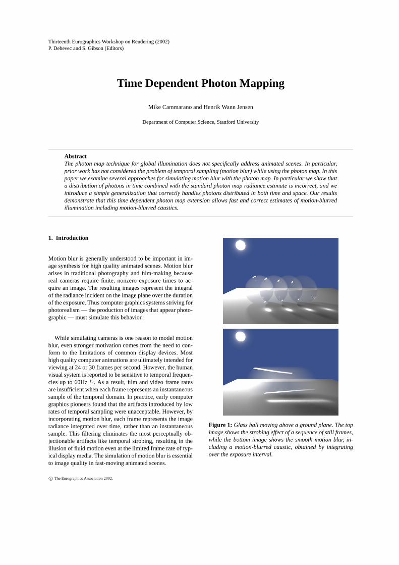
Figure 1: Glass ball moving above a ground plane. The topimage shows the strobing effect of a sequence of still frames,while the bottom image shows the smooth motion blur, in-cluding a motion-blurred caustic, obtained by integratingover the exposure interval.
Cammarano and Jensen / Time Dependent Photon Mapping
Most of the research into motion blur can be classified asone of four basic approaches11:
1. Analytic methods5
2. Temporal supersampling5 3
3. Postprocess blur13
4. Geometric substitution2
1.1. Temporal supersampling
All four of the approaches characterized above have re-mained active research areas, and fostered many interest-ing algorithms. However, only supersampling methods haveshown the generality and robustness to accurately handlecomplicated dynamic scenes. Postprocessing methods haveall relied on approximations of scene motion, while ana-lytic and geometric substitution methods have been limitedin the geometry and motion they can handle. For robust high-quality rendering, and in particular for simulating global illu-mination, temporal supersampling is the only viable method.
We can further classify temporal supersampling tech-niques as belonging to one of two general categories. Accu-mulation buffer methods render a sequence of complete “in-between” frames and average them together5 4, while distri-bution ray tracing techniques evaluate multiple time samplesat each image pixel3.
The simulation of global illumination and motion blur to-gether has received relatively little attention. Cook et al.3
demonstrated that distribution ray tracing could be used tosimulate global illumination effects including motion blur.Besuievsky and Pueyo1 simulated motion blur with the ra-diosity algorithm by computing multiple frames at differ-ent times and averaging those using an accumulation buffer.Myszkowski et al.12 presented an efficient global illumina-tion method for animated scenes in which the result of a pho-ton tracing pass is averaged over several frames. However,their method still computes a solution for a static scene for agiven frame, and they do not consider motion blur within in-dividual frames. The only methods that currently are able tosimultaneously simulate both motion blur and global illumi-nation are based on Monte Carlo ray tracing. In Monte Carloray tracing it is straightforward to simulate motion blur bydistributing paths randomly in time — for example, Lafor-tune10 demonstrated this using bidirectional path tracing.
Unfortunately, the general Monte Carlo ray tracing al-gorithms in which motion blur can be trivially simulatedrequire substantial computation to reduce the noise to anacceptable level. For static scenes, there are several algo-rithms for improving the speed of Monte Carlo ray tracingby caching information about the illumination in the scene.Methods such as irradiance caching16 and photon mapping7
are examples of such caching techniques where illuminationvalues are stored for points on the surfaces in the scene (orinside a scattering medium8). However, these caching tech-niques do not work when the objects move within the shutter
time used for the frame. If different photon or ray-paths havedifferent times, then the cached illumination values will bedistributed in space along the path of moving objects. No-tably, in the case of photon mapping this invalidates the as-sumptions that the photons are located on the surfaces of theobjects.
In this paper we extend the photon mapping method tohandle motion-blurred global illumination in scenes withmoving objects. We derive a time dependent radiance esti-mate that correctly accounts for photons distributed in bothspace and time. Our results indicate that this radiance esti-mate is superior to alternative techniques such as the accu-mulation buffer, and that it correctly renders motion-blurredillumination effects that the standard photon map radianceestimate cannot handle.
2. Time Dependent Global illumination
In global illumination and realistic image synthesis we areconcerned with estimating the radiance through pixels in theimage plane. This can be expressed as
Lp =∫
ts
∫A
L(x′,~ω, t)s(x′,~ω, t)g(x′)dA(x′)dt, (1)
whereLp is the radiance through pixelp, ts is the total shut-ter or frame time,A is the area of the pixel,g(x′) is a filterfunction, the shutters(x′,~ω, t) specifies the exposure timefor each pixel, andL(x′,~ω, t) is the radiance through the lo-cationx′ on the image plane in the direction of the observerat timet. In scenes with only static objects the integral overtime can be ignored, andL(x′,~ω, t) becomesL(x′,~ω). Other-wise, radiance must be integrated in time as well. In the caseof Monte Carlo ray tracing this is typically done by tracingrays at different times through the pixel and averaging theradiance returned by each ray. At the first object intersectedby a ray the radiance in the direction of the observed is com-puted using the rendering equation9:
L(x,~ω, t) = Le(x,~ω, t)+∫
Ωfr (x,~ω′,~ω, t)Li(x,~ω′, t)(~ω′ ·~n)d~ω′.
(2)Here,L(x,~ω, t) is the outgoing radiance at a surface locationx with normal~n in direction~ω at timet, fr is the BRDF,Le
is the emitted radiance, andLi is the incident radiance. Notethat the integration of motion blur only happens at the pixel,and that all rays belonging to the same path have the sametime.
3. Global Illumination Using Photon Maps
Before describing how to solve the rendering equation intime using photon maps let us briefly describe the basicsof the photon mapping algorithm7. Photon mapping is atwo-pass algorithm in which the first pass consists of tracingphotons from the light sources through the scene and storingthese photons in the photon map as they interact with ele-ments in the scene. The second pass is rendering where the
Cammarano and Jensen / Time Dependent Photon Mapping
photon map is used to provide fast estimates of the reflectedradiance,L, of the surfaces in the scene:
L(x,~ω)≈ 1πr2
np
∑p=1
fr (x,~ωp,~ω)Φp(x,~ω′). (3)
This radiance estimate uses thenp nearest photons to the lo-cationx, πr2 is an approximation of the area covered by thephotons, andΦp is the flux carried by photonp. This esti-mate assumes that the photons are located on a locally flatsurface. As a consequence the estimate is invalid if, for ex-ample, the object is moving and the photons are distributedin time along the path of the moving object. Even if the ob-ject is static the time information in the photon map is ig-nored and, as we will show in the following, the standardradiance estimate is incorrect if the path of the incoming raycan intersect one or more moving objects during the time ofthe exposure interval.
4. Methods for Computing Motion Blur with PhotonMaps
As observed in the introduction, we will restrict our atten-tion to supersampling methods. Among such methods, thereremain several choices for how to evaluate motion blur inthe overall rendering pipeline. We will consider how photonmapping fits into each of these in turn.
As a cautionary example, we will show that some seem-ingly reasonable sampling strategies can lead to objection-able errors in the resulting images. Also, we will demon-strate that other simple strategies preserve consistency, butat the cost of performing substantial amounts of redundantcomputation. We will then propose an extension of the pho-ton map radiance estimate into the temporal domain that ad-dresses both problems, maintaining consistency while stillallowing for efficient sampling.
4.1. Accumulation buffer
Perhaps the most straightforward method is the “accumula-tion buffer” approach, which takes the average of a num-ber of in-between frames, each rendered independently at aspecific time4. In this case, we would recompute the pho-ton map for each partial frame. This approach can computemotion blur to an arbitrary degree of accuracy by using asufficiently large number of in-between frames; however,the approach is inefficient. To obtain acceptable results freefrom temporal aliasing in fast-moving areas, a large numberof in-between frames may be needed. Portions of a sceneunaffected by motion (or for which coarser temporal sam-pling would suffice) are still rerendered in these in-betweenframes.
4.2. Distribution ray tracing
A distribution ray tracing renderer can evaluate motion blurby associating a time with each ray. By using adaptive sam-
Figure 2: Sunlight reflected onto the ground from a movingvehicle will appear as a sharp caustic to an observer mov-ing at the same speed - even though both vehicles are mov-ing rapidly relative to the ground beneath. The texture of theroad will be motion blurred, but the caustic should not be.
pling methods, such a renderer can be more efficient thanthe accumulation buffer approach by directing extra tempo-ral samples only at portions of the image affected by motion.There are several ways in which photon mapping might beincorporated into such a renderer.
4.2.1. Do Nothing
The simplest approach is to not worry about temporally dis-tributing the photons at all. We could perform the photontrace at a single time (say, the start of the interval), anduse the corresponding map throughout. The resulting pho-ton map does not represent the correct distribution of pho-tons in time and space during the time interval considered.The direct-lighting contribution to the final image will havecorrect motion blur from the distribution ray tracing, but ef-fects relying on the photon map, such as caustics, will not beevaluated correctly if they are affected by motion.
4.2.2. Distribute photons in time, but ignore their timesin the reconstruction
We can distribute photons in time in the same manner we dis-tribute rays: by associating a time with each photon and trac-ing it through the scene accordingly. This gives us a correctdistribution of photons in space and time. The photons canthen be stored in the standard photon map structure, withoutfurther regard for the associated times. In this approach, thephoton map stores the projection of the correct distributionof photons in space and time (4 dimensions) into a distribu-tion in space (3 dimensions). This might seem reasonable,but it leads to incorrect results in many cases.
The problem is that the standard photon map radiance es-timate at a point in space will give the average intensity ofillumination over the entire time period during which pho-tons were traced. Instead, as we observed in section 2, weshould compute the radiance at the time associated with thesample ray.
As a simple test scene for illustrating inconsistency, wewill consider the scene shown in Figure 2. An observer is
Cammarano and Jensen / Time Dependent Photon Mapping
driving in a car behind a truck. Both vehicles are drivingat the same speed and as a consequence the truck appearsfocused to the observer while other elements of the sceneare motion blurred. Consider a caustic on the road generatedby sunlight reflecting of the back of the truck. This causticwill move along with the truck and it will therefore appearsharp and focused at any given instant in time to the observer.However, if this caustic is simulated simply by distributingphotons in time then the photons will be covering a largerarea of the road corresponding to the distance moved by thetruck within the shutter time. Therefore, the radiance esti-mate will predict a large blurred caustic whereas the correctcaustic should be sharp and focused at all times.
4.2.3. Estimate radiance directly from photonsdistributed in time as well as space
A key element in the photon mapping algorithm is the abil-ity to estimate radiance effectively from an irregular distri-bution of photons. This is done using filtered density esti-mation over the photons in a spatial neighborhood. It is con-sistent with the philosophy of the photon map to extend thisapproach to temporal sampling as well as spatial. The ideais to distribute the photons continuously in time, and retainthis temporal information as an extra dimension in the pho-ton map. In the following sections we will show how thistemporal information can be used to derive a simple exten-sion to the photon map that effectively enables filtering ofphotons in both time and space.
5. Building a Time Dependent Photon Map
For the purpose of estimating density in time as well as spacewe include time information in the photon map by addingan additionalfloat time element to each photon. Thisincreases the photon size from 20 bytes6 to 24 bytes andresults in the following photon representation:
struct photon float x,y,z; // positionfloat time; // photon timechar q[4]; // energy (rgbe)char phi, theta; // incident directionshort flag; // flag used in kdtree
If space is a concern then it would be possible to add the timeto the photon structure presented by Jensen6 by using theavailable bits in the photon flag to represent an 8-bit quan-tized time (this compressed representation of the time wouldbe sufficient except in scenes with extreme motion blur).
To build the time dependent photon map we perform pho-ton tracing in time by associating a random time with eachphoton path. At the light source we pick a uniformly dis-tributed random time in the given shutter interval. This timeis then used for the entire photon path, and the time is stored
with all the photons generated along the path. Otherwise thephoton tracing is exactly the same as for the standard photonmap.
An important difference from standard photon tracing isthat we propagate and store radiant energy instead of radiantflux (the energy is compressed in the same way as the fluxin the standard photon map). The radiant energy,Qe, of eachemitted photon is:
Qe =Φl tsne
, (4)
whereΦl is the power of the light source emitting the pho-ton, ts is the shutter or frame time, andne is the number ofemitted photons.
6. A Time Dependent Radiance Estimate
In this section we will describe how the time dependent pho-ton map enables us to compute radiance for a given surfacelocation at a given time.
The reflected radiance,Lr , from a surface is given by:
Lr (x,~ω, t) =∫
Ωfr (x,~ω′,~ω, t)Li(x,~ω′, t)(~ω′ ·~n)d~ω′. (5)
Here,L(x,~ω, t) is the radiance at surface locationx in direc-tion~ω at timet, fr is the BRDF,Li is the incident radiance,and~n is the surface normal atx (Note thatx depends implic-itly on the time, since the intersection of a ray with a mov-ing object depends on the time associated with the ray). Thestandard photon map radiance estimate applies the photonmap to this equation using the relationship between radianceand flux, and similarly we will use the relationship betweenradiance and radiant energy,Q:
Lr (x,~ω, t) =d3Q(x,~ω, t)
(~n ·~ω)d~ωdAdt. (6)
Substituting this expression in equation 5 we obtain:
Lr (x,~ω, t) =∫
Ωfr (x,~ω′,~ω, t)
d3Q(x,~ω′, t)(~n ·~ω′)d~ω′ dAdt
(~ω′ ·~n)d~ω′
=∫
Ωfr (x,~ω′,~ω, t)
d3Q(x,~ω′, t)dAdt
. (7)
This equation shows that we have to estimate the densityof the radiant energy in both space and time. To use the timedependent photon map, we will make a series of assumptionssimilar to those for the standard photon map. Specifically,we will assume that the nearest photons in the photon mapin space and in time represent the incident flux atx at timet.This assumption enables us to approximate the integral by asum over the radiant energy,Qp, of thenp nearest photons:
Lr (x,~ω, t)≈np
∑p=1
fr (x,~ωp,~ω, t)Qp
∆A∆t. (8)
In the standard photon map it is assumed that the photons are
Cammarano and Jensen / Time Dependent Photon Mapping
located on a locally flat surface, and the area∆A is approx-imated byπr2 wherer is the smallest possible radius of asphere centered atx containing thenp nearest photons. Thisis equivalent to a nearest neighbor density estimate14.
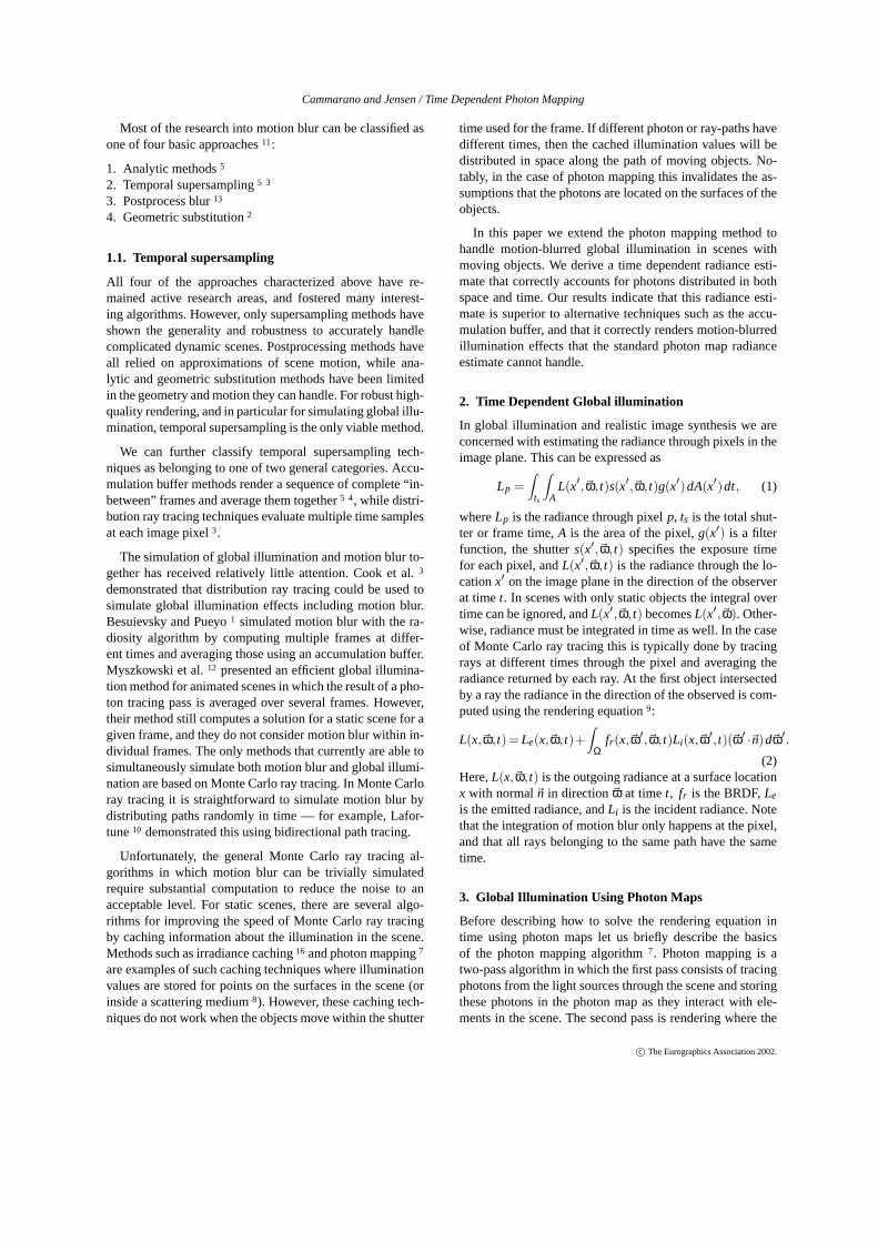
Essentially, we are estimating the incident radiance basedon the photons that hit a small disc-shaped patch of surfacecentered aboutx, as in Figure 3a. For photons distributed intime, we can visualize the space-time distribution of pho-tons by considering a patch of surface extruded into thetime dimension, as in Figure 3b. We are considering a 4-dimensional analogue to a cylinder, in which a sphere in the3 spatial dimensions is extruded through time fromt = 0to t = 1. For a basic visualization, however, it is convenientto omit the spatial dimension orthogonal to the surface andsimply depict the surface patch extruded through time. Thestandard photon map radiance estimate, which ignores tem-poral distribution of photons, can be thought of as implicitlyusing a cylinder with maximum extent in time, as in Figure3b.
Note that this standard estimate blurs illumination overthe entire exposure time of the frame. This is entirely appro-priate if there is no change in visibility along the eye pathduring the exposure time, since the pixel values ultimatelycomputed are integrated over the full exposure time. If thepath from the eye can potentially intersect any moving ob-jects, however, then it is important to determine the incidentillumination at the time associated with the ray, rather thanblurring over the entire exposure time. In practice, our sys-tem tests whether an eye path has intersected the boundingboxes of moving objects. If not, then the standard radianceestimate can be used, ignoring any time information in thephotons. When moving objects are intersected, however, wemust use a revised density estimate that accounts for timedependence by restricting the photons in the estimate to benearby in time as well as space.
This restriction to temporally neighboring photons can berepresented as taking a cylindrical slice of space-time over anarrower range of times, as shown in Figure 3c. Such a cylin-drical slice represents a compact neighborhood of space-time, local in all 4 dimensions. More details on the selectionof neighboring photons will be described in the followingsection.
Let ∆t be the time spanned by the nearest photons and letr be the radius of the smallest sphere centered atx enclosingthenp photons. We can then approximate equation 8 as
Lr (x,~ω, t)≈1
πr2∆t
np
∑p=1
fr (x,~ωp,~ω, t)Qp. (9)
This is equivalent to a nearest neighbor density estimatein both space and time. For slightly better estimates it canbe advantageous to include a smoothing kernel as well. This
x
y
a) Photons in standard radiance estimate at a patch of sur-face.
x
y
t
t=0.0
t=1.0
b) Photons in radiance estimate at a patch of surface, shownextruded through time (t = 0 to t = 1).
x
y
t
t=0.0
t=1.0
t=0.4
t=0.6
c) Photons in time-dependent radiance estimate at a patch ofsurface over a restricted slice of time.
Figure 3: Space-time diagrams illustrating the photons usedin a radiance estimate.
gives
Lr (x,~ω, t)≈1
πr2∆t
np
∑p=1
fr (x,~ωp,~ω, t)K1
(xp−x
r
)
K2
(tp− t
12∆t
)Qp.
(10)
whereK1(y) is the smoothing kernel in space, andK2(y) isthe smoothing kernel in time. The time of photonp is tp,and it is assumed here that the maximum distance in timeto a photon is1
2∆t. See Silverman14 for an overview of dif-ferent smoothing kernels and their respective trade-offs be-tween bias (blur) and variance (noise). Specifically, in timeone might use a uniform kernel,K2(y) = 1, in which case theestimate is equivalent to the nearest neighbor estimate. An-other option is the Epanechnikov kernel,K2(y) = 3
2(1−y2)which gives less blur but slightly more noise. Notice that thekernels are different from the corresponding 2D kernels usedin the space domain.
This time dependent radiance estimate is a consistent es-timator. As the number of photons in the photon map is in-creased to infinity, we can increasenp while ∆t and∆A go to
Cammarano and Jensen / Time Dependent Photon Mapping
zero in the estimates — thus it is possible to get an arbitrar-ily accurate estimate of the radiance at a given time on anylocally flat surface.
Note that the technique in this section could be used to de-rive a time dependent radiance estimate for participating me-dia. This would require changing the volume radiance esti-mate of Jensen and Christensen8 to estimate density in timeas well.
7. Locating nearby photons
The time dependent radiance estimate depends on the nearbyphotons in time and space. In this section we present twostrategies for locating these photons. One is based on a sim-ple two-pass extension of the standard photon map, and thesecond uses a 4D kd-tree.
7.1. A two-pass approach
The implementation of the photon map can be modifiedslightly to take the time dependence into account. As pre-viously stated we need to quickly locate the nearest photonsin both space and time. A natural approach that follows ourderivation of the radiance estimate is to simply use the stan-dard 3D photon map kd-tree to identify the photons nearestin space, and then in a second pass further restrict this set tothe photons nearby in time. For our implementation, we de-termine the spatially nearby photons using the standard kd-tree search, and then use a quicksort partitioning algorithmto efficiently select the nearest of those photons in time. Weuse a randomized quicksort partition to avoid the poor worstcase behavior of quicksort in the presence of nearly sortedelements. This is generally a good algorithmic practice, andit is particularly relevant here since photon times will tend tobe correlated with position in a motion blurred caustic.
The number of photons used in the time density estimateis a user-defined fraction of the photons located in the firstpass (we have found 50% to work well for our test-scenes).This means that we need to locate more photons than thestandard photon map in order to have enough photons to geta smooth density estimate. Note that the maximum time dif-ference should go to zero in the limit in order to make thefinal estimate consistent.
An important detail is that the photons searched over canbe trivially clipped to only those that are within certain maxi-mum allowed distances in space and time. The standard pho-ton map routinely restricts the search fork-nearest neigh-bors to a maximum distance, basing the estimate on fewerthank photons rather than using photons that are unreason-ably far away. This is essential to maintain the quality ofthe estimate in dimly lit regions where photons are sparse,and also speeds the search for nearest neighbors since onlyphotons within this range need be considered. We similarlyrestrict the maximum allowed difference in time for photons
in the time-dependent estimate, thereby obtaining the samebenefits: avoiding errors in the estimate due to sparsely dis-tributed photons, and speeding the search for nearest neigh-bors.
The two-pass approach is straightforward to incorporateinto an existing photon map implementation. Our results in-dicate that the performance is quite good, adding little per-formance penalty to the standard radiance estimate. In ad-dition the method naturally adapts to local variations in thespace and time photon density.
7.2. Locating photons using a 4D kd-tree
An alternative to the two-pass approach is extending thestandard 3d photon map kd-tree into a 4d kd-tree with timeas the extra dimension. The 4d kd-tree is potentially fastersince it makes it possible to directly locate the nearest pho-tons in both space and time.
In order to locate the nearest photons we need to specify adistance metric. In 3d this is trivially given as the distance tothe photon, but in 4d the answer is not as simple since spaceand time do not share common units or a natural distancemetric. Given one photon that is 2 units away in distanceand 1 unit away in time, and a second photon that is 1 unitaway in distance and 2 units away in time, there is no clearanswer to which is the nearer neighbor. We can address thisproblem of specifying a distance metric over space and timeby providing the user with a parameterκ to control the rel-ative weights of spatial versus temporal distance. By simpleextension of the Euclidean distance metric for space, we canthen define a global “space-time distance”:
d =√
∆x2 + ∆y2 + ∆z2 + κ∆t2.
or simply:
d =√
r2 + κ∆t2.
This resolves the immediate problem, but introduces an ex-tra user control with an unintuitive effect on image quality.Also, such an explicitly specified distance metric would ap-ply throughout the scene, whereas our earlier implementa-tion adaptively varies the relative sizes ofr and∆t dependingon the local distribution of photons.
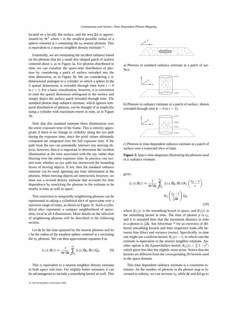
Given the user-specified distance metric, we can locateneighboring photons by expanding a 4D (hyper-)sphere un-til it containsk photons. Figure 4a depicts a sphere that hasbeen expanded until just large enough to contain 15 pho-tons. Since we are no longer using a space-time cylinder tolocate nearest photons, it is no longer appropriate to substi-tuteπr2∆t for ∆A∆t as in equation 9. Instead, we will needto use the volume of the space-time sphere over which wehave located the photons. Since we continue to assume thatwe are at a small patch of a locally flat surface, the volumeunder consideration is that of the 3D sphere inx, y, andt,
Cammarano and Jensen / Time Dependent Photon Mapping
x
y
t
t=0.0
t=1.0
a) The hyper-sphere sphere has been expanded until it is justlarge enough to contain 15 photons.
x
y
t
t=0.0
t=1.0
t=0.4
t=0.6
b) The sphere does not accurately represent the volume oc-cupied by this set of photons. Here, the photons are con-centrated in time, and it is more appropriate to use a sphereclipped by the minimum and maximum time values.
Figure 4: Using a 4D hypersphere to locate photons.
relating temporal and spatial distance). However, no matterwhat value ofκ is chosen to relate spatial and temporal dis-tance, there can still be regions in the scene where photonsare not equally well distributed in space and time. In the ex-amples of Figure 4, the photons are more concentrated intime. Consequently, the 4D bounding sphere does not ac-curately represent the volume occupied by the photons, andusing the volume of the sphere as∆A∆t in the radiance esti-mate introduces an excessive amount of temporal blur. Thisis analogous to the problem with excessive blur near edgediscontinuities in the standard photon map6, but is moreproblematic since it affects every time-dependent radianceestimate. One fairly straightforward fix is to clip the sphereagainst the minimum and maximum times represented by thephotons, as shown in Figure 4b. It is possible to derive a sim-ple closed form expression for the volume of such a clippedsphere, and substituting this volume for∆A∆t in equation 9eliminates the unnecessary temporal blur.
We have tested the 4D kd-tree method, where the near-est photons are located within a 4D sphere according to aspace-time distance metric (based on a user defined parame-ter κ relating spatial and temporal distance). Our implemen-tation of the radiance estimate for this method is using theclipped sphere volume as described above. The implemen-tation yielded results roughly comparable in quality to thoseobtained with the two-pass method described above. Overall,however, we found that the complications associated withthe 4D kd-tree made it considerably less elegant and appeal-ing than the two-pass method. As a consequence we use thetwo-pass method for all the examples presented in this pa-per.
8. Results
We have implemented the time dependent radiance estimatein a Monte Carlo ray tracer that supports both photon map-ping and motion blur. The motion blur is rendered by adap-tively sampling ray paths with different times through eachpixel until the contrast is below a given threshold. All our ex-amples use the two-pass method for locating the nearest pho-tons. The user specified fraction is 50% for all examples, andwe use 50 to 100 photons in the combined time-space den-sity estimate, which means that we have to locate 100-200spatially neighboring photons in the initial kd-tree search.The kd-tree uses the standard Euclidean distance metric tolocate the nearest photons (i.e. the photons are located withina sphere around the point of interest).
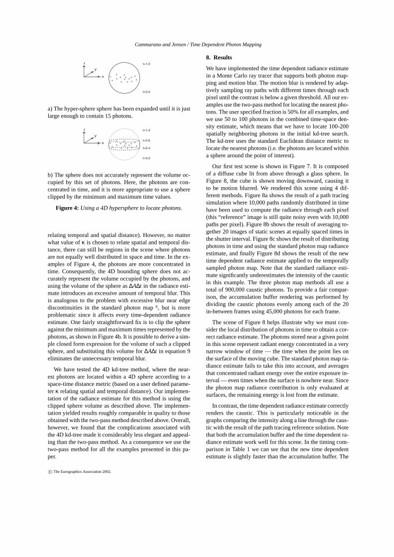
Our first test scene is shown in Figure 7. It is composedof a diffuse cube lit from above through a glass sphere. InFigure 8, the cube is shown moving downward, causing itto be motion blurred. We rendered this scene using 4 dif-ferent methods. Figure 8a shows the result of a path tracingsimulation where 10,000 paths randomly distributed in timehave been used to compute the radiance through each pixel(this “reference” image is still quite noisy even with 10,000paths per pixel). Figure 8b shows the result of averaging to-gether 20 images of static scenes at equally spaced times inthe shutter interval. Figure 8c shows the result of distributingphotons in time and using the standard photon map radianceestimate, and finally Figure 8d shows the result of the newtime dependent radiance estimate applied to the temporallysampled photon map. Note that the standard radiance esti-mate significantly underestimates the intensity of the causticin this example. The three photon map methods all use atotal of 900,000 caustic photons. To provide a fair compar-ison, the accumulation buffer rendering was performed bydividing the caustic photons evenly among each of the 20in-between frames using 45,000 photons for each frame.
The scene of Figure 8 helps illustrate why we must con-sider the local distribution of photons in time to obtain a cor-rect radiance estimate. The photons stored near a given pointin this scene represent radiant energy concentrated in a verynarrow window of time — the time when the point lies onthe surface of the moving cube. The standard photon map ra-diance estimate fails to take this into account, and averagesthat concentrated radiant energy over the entire exposure in-terval — even times when the surface is nowhere near. Sincethe photon map radiance contribution is only evaluated atsurfaces, the remaining energy is lost from the estimate.
In contrast, the time dependent radiance estimate correctlyrenders the caustic. This is particularly noticeable in thegraphs comparing the intensity along a line through the caus-tic with the result of the path tracing reference solution. Notethat both the accumulation buffer and the time dependent ra-diance estimate work well for this scene. In the timing com-parison in Table 1 we can see that the new time dependentestimate is slightly faster than the accumulation buffer. The
Cammarano and Jensen / Time Dependent Photon Mapping
difference is not substantial since this scene is dominated bymotion blur, and as a result the adaptive sampling of motionblur is less beneficial here.
Figure 9 shows a scene in which the spot from a laserpointer (aligned alongside the camera) is reflected off theback of a moving truck. (For added clarity, a still frameof this scene is shown in Figure 5). This causes a motionblurred stripe of laser light to be reflected on the ground.However, in the back of the truck, we can see a reflectionof this spot on the ground. The interesting point about thisscene is that while the laser spot on the ground should beblurred into a stripe by the truck’s motion, its reflection inthe back of the truck should always appear as a sharply fo-cused spot! The diagram in Figure 6 should help make thispoint clear. Notice that the observer is static in this sceneunlike the earlier example illustrated in Figure 2.
All versions of the truck scene were rendered using a to-tal of 40,000 caustic photons. The comparison of renderingtechniques in Figure 9 shows how the accumulation buffermethod (a) correctly captures the sharp spot reflected in theback of the truck, but even with 9 in-between frames, it can-not smoothly reproduce the laser stripe on the ground. Ap-plying the standard radiance estimate to photons distributedin time (b) smoothly renders the blurred laser stripe on theground, but incorrectly blurs the reflection seen in the backof the truck. Our proposed time dependent photon map (c)correctly renders both effects. Furthermore, as the timings inTable 1 show, the proposed method has performance com-parable to that of the standard radiance estimate, and sub-stantially faster than the accumulation buffer method. Thereason for the better timings is that the caustic and mo-tion blur occupy a relatively small portion of an image —this is often the case in rendered images. Consequently, thisscene demonstrates the importance of using efficient, adap-tive sampling techniques, which only do extra work (e.g. forcaustics or motion blur) in the parts of an image that requireit.
9. Conclusions
In this paper we have addressed the problem of using pho-ton mapping in scenes with motion blur. We have derived asimple time dependent radiance estimate. The new insight isthat temporal sampling can be simulated by estimating thephoton density in time as well as space. The time depen-dent radiance estimate provides smooth and visually pleas-ing approximations of radiance in moving scenes, withoutthe distinctive strobing/banding artifacts of the accumulationbuffer. It is consistent, and will converge to an arbitrarily ac-curate solution simply by using a sufficient number of pho-tons in the map. Most importantly, the method is efficient.Its performance is at least as good as accumulation buffermethods, and for typical scenes it can be substantially faster.It imposes a small penalty over the standard photon map ra-
Figure 5: A shiny truck parked by the tower of Pisa. A redlaser aligned with the camera shines a spot on the back ofthe truck, which reflects the spot onto the ground. This spoton the ground can be seen again in the reflection in the backof the truck.
t=2t=1t=0
t=2t=1t=0
Figure 6: Diagram of view along line of sight of a laserpointer shining on a moving planar reflector. The spot caston the ground gets blurred into a stripe by the mirror’s mo-tion, but its reflection in the mirror, as seen along the line ofsight illustrated, is a focused spot.
Method Consistent? Render times†
Fig. 8 Fig. 9
Path tracing Yes 9+ hrs. n/a
Accumulation buffer Yes 47sec 316sec‡
Standard radiance estimate onphotons distributed in time No 37sec 74sec
Time dependentradiance estimate Yes 43sec 72sec
† Render times for photon map techniques include the time for theinitial photon tracing.‡ Note that the accumulation buffer technique would require manymore in-between frames (and consequently longer render time) tocorrectly reproduce the blurred caustic on the ground.
Table 1: Performance comparison of the techniques.
Cammarano and Jensen / Time Dependent Photon Mapping
diance estimate, but has the considerable advantage of givingcorrect results.
We have devoted a significant amount of space in section4 to considering various flawed or inefficient methods forcomputing motion blur in the presence of photon maps. Thisis not without good reason. Both photon mapping and mo-tion blur are widely used techniques, and there are a numberof rendering systems that support both. However, in the ab-sence of any prior published research on how to correctlyevaluate the photon map for time-varying scenes, these ex-isting implementations almost surely use one of these naivemethods by default. Consequently, we have felt it worth-while to examine the shortcomings of these approaches,which can reasonably be expected to underlie any render-ing system that supports both photon maps and motion blurwithout having carefully considered the interrelationship be-tween the two.
One promising opportunity for future work is to extendour technique to take advantage of inter-frame redundancyover an animated sequence, similar to Myszkowski et al.12.
10. Acknowledgements
Thanks to the reviewers and to Maryann Simmons, SteveMarschner, and Pat Hanrahan for helpful comments. Thisresearch was funded in part by the National Science Founda-tion Information Technology Research grant (IIS-0085864).Mike Cammarano is supported by a 3Com Corporation Stan-ford Graduate Fellowship and a National Science Founda-tion Fellowship.
References
1. Gonzalo Besuievsky and Xavier Pueyo. A Motion BlurMethod for Animated Radiosity Environments.WinterSchool of Computer Graphics, 1998. 1998.
3. Robert L. Cook, Thomas Porter, and Loren Carpen-ter. Distributed Ray Tracing.ACM Computer Graphics(Proc. of SIGGRAPH ’84), 18:137–145, 1984.
4. Paul E. Haeberli and Kurt Akeley. The accumulationbuffer: Hardware support for high-quality rendering.Proceedings of SIGGRAPH 1990, 309–318, 1990.
5. Jonathan Korein and Norman Badler. Temporal Anti-Aliasing in Computer Generated Animation.ACMComputer Graphics (Proc. of SIGGRAPH 1983),17:377–388, 1983.
6. Henrik Wann Jensen.Realistic Image Synthesis UsingPhoton Mapping, A K Peters, 2001.
7. Henrik Wann Jensen. Global Illumination Using Pho-ton Maps. InRendering Techniques ’96 (Proceed-ings of the Seventh Eurographics Workshop on Ren-dering), pages 21–30, New York, NY, 1996. Springer-Verlag/Wien.
8. Henrik Wann Jensen and Per H. Christensen. EfficientSimulation of Light Transport in Scenes with Partici-pating Media using Photon Maps.Proceedings of SIG-GRAPH 1998, 311–320, 1998.
9. James T. Kajiya. The Rendering Equation.ACM Com-puter Graphics (Proc. of SIGGRAPH ’86), 20:143–150,1986.
10. Eric P. Lafortune.Mathematical Models and MonteCarlo Algorithms for Physically Based Rendering.Ph.d. thesis, Katholieke University, Leuven, Belgium1996.
11. Ryan Meredith-Jones. Point Sampling Algorithms forSimulating Motion Blur.Master’s Thesis, University ofToronto, 2000.
12. Karol Myszkowski, Takehiro Tawara, HiroyukiAkamine and Hans-Peter Seidel. Perception-GuidedGlobal Illumination Solution for Animation Rendering.Proceedings of SIGGRAPH 2001.
13. Michael Potmesil and Indranil Chakravarty. Mod-eling Motion Blur in Computer Generated Images.ACM Computer Graphics (Proc. of SIGGRAPH 1983),17:389–399, 1983.
14. B. W. Silverman.Density Estimation for Statistics andData Analysis. Monographs on Statistics and AppliedProbability 26. Chapman & Hall/CRC. 1998.
15. Brian A. Wandell.Foundations of Vision, Sinauer As-sociates, 1995.
16. Greg Ward, Francis Rubinstein and Robert Clear. ARay Tracing Solution to Diffuse Interreflection.Pro-ceedings of SIGGRAPH 1988, 85–92, 1988.
Cammarano and Jensen / Time Dependent Photon Mapping
Figure 7: Still frame showing the setup for the cube scene.The arrow indicates the direction the cube will move in Fig-ure 8.
path trace
a) Path tracing w/ 10,000 samples/pixel.
path traceacc. buffer
b) Accumulation buffer.
path tracestandard
c) Standard radiance estimate.
path tracetime dep.
d) Time dependent radiance estimate.
Figure 8: Motion blurred images of the moving cube scenerendered using various techniques. All 4 images were ren-dered at 640x480. To illustrate the variance associated withthe techniques, the graphs show pixel values for each imagealong a horizontal line through the caustic. For comparison,the graph for each photon map method also shows pixel val-ues from the path traced “reference” image - which is stillvery noisy even with 10,000 samples per pixel.
a) Accumulation buffer.
b) Standard radiance estimate.
c) Time dependent radiance estimate.
Figure 9: Moving truck scene, also depicted without mo-tion in Figure 5. The laser spot reflected onto the groundis blurred into a stripe by the truck’s motion. However, thereflection of this spot seen in the back of the truck should notbe blurred, as illustrated in Figure 6.