177
AY4489 Time Domain EMC Emissions Measurement System Final Report May 2004

AY4489
Time Domain EMC Emissions Measurement System
Final Report
May 2004

2/177
RA0603/R/18/079/1
This report was prepared by Multiple Access Communications Ltd for the Office of Communications (Ofcom).
© Copyright 2004. Applications for reproduction should be made to HMSO.
Multiple Access Communications LtdDelta House, Enterprise Road Chilworth Science Park SOUTHAMPTON SO16 7NS, UK Tel: +44 (0)23 8076 7808 Fax: +44 (0)23 8076 0602

3/177
Executive Summary
Time Domain EMC Emissions Measurement System
Final Report
Radiated electromagnetic emissions measurements are currently performed using a
conventional radio frequency (RF) receiver to sweep the frequency band of interest. This
method of spectral analysis works well for continuous signals but has drawbacks in that the
measurement time is long when a wide band of frequencies must be swept using a narrow
bandwidth receiver, which requires a significant measurement or dwell time at each
frequency. In addition, this method is not guaranteed to measure the peak radiated power
when measuring impulsive (ie, non-continuous) emissions, since emissions will only be
present during the dwell time of the receiver at a few frequencies. Currently, the only solution
is to assume that the impulsive emissions are repetitive and to observe them for long enough
using a peak hold detector, so that eventually a measurement is taken at all frequencies of
interest. Whilst this method has served the industry well for many years, recent advances in
ultra high-speed sampling systems now offer an alternative method of measuring radiated
emissions in the time domain that, potentially, overcomes these limitations. By using a high-
speed sampling system that is able to capture the RF signal or the intermediate frequency (IF)
output of a receiver, and by processing the captured signals in the digital domain, it is
possible to measure all frequencies nearly instantaneously within the RF band of the receiver
and thus accurately capture the effects of impulsive emissions. Of course, this assumes that
an impulse occurs at the instant the measurement is made.
Ofcom (formerly the Radiocommunications Agency) commissioned Multiple Access
Communications (MAC) Ltd to perform a study into the potential benefits and drawbacks of
using the time domain method for measuring radiated emissions in electromagnetic
compatibility (EMC) tests. The main objectives of this work are to understand the capabilities
of the time domain approach using current state-of-the-art technology and to investigate the
benefits that a time domain approach could bring to EMC testing of modern products.
We undertook this study in four stages. In Stage 1 we constructed a prototype time domain
EMC emissions measurement system (TDEEMS) based on commercial off-the-shelf

4/177
components to reduce design time and cost. In Stage 2 we calibrated and tested the TDEEMS
using the electromagnetic compatibility test facilities of EMC Projects Ltd, who is a
subcontractor in this project. In Stage 3 we made radiated EMC emissions measurements of
some example equipment under test (EUT) using a conventional EMC test receiver and the
TDEEMS, so that the results and the practical implications of using the two approaches could
be compared. Finally, in Stage 4, the TDEEMS was used to perform in situ1 EMC
measurements from a railway.
An outline diagram of the prototype TDEEMS is shown in Figure A. The TDEEMS was
based around an Agilent Infiniium 54854A digital sampling oscilloscope, which can sample
at up to 20 Gsamples/s and can measure signals over a RF bandwidth from direct current
(DC) to 4 GHz. The external front end (shown in Figure A) was required to reduce the system
noise figure and hence achieve the necessary sensitivity.
1 In situ measurements are those made at an open site of a piece of bulky or heavy equipment under test that cannot be moved to an EMC test house.
Broadbandantenna
Low passfilter
Low noiseamplifier
Data capture device(sampling oscilloscope)
PCFront end
Figure A Block diagram of prototype TDEEMS.

5/177
A single antenna covering the frequency range 30 MHz to 4 GHz was not available to us
during these measurements, so two measurement passes using different antennas were
required. The front end was constructed from off-the-shelf amplifiers and filters. It consisted
of a low pass filter, to reject out-of-band signals, and a low noise amplifier, to amplify the
signal from the measurement antenna, since the oscilloscope was not sufficiently sensitive to
measure this signal directly. As amplifiers covering the desired frequency range from 50 kHz
to 30 MHz as well as that from 30 MHz to 4 GHz were not readily available, we constructed
separate front ends to cover these bands. Because separate antennas were required for these
frequency ranges, this did not increase the number of measurement passes required.
The gain of the pre-amplifier was determined using a power budget analysis, which took into
account the dynamic range and the sensitivity of the oscilloscope and the typical Class B
measurement limits used for measuring electrical equipment. The frequency response and
noise performance of the system components (ie, the antennas, oscilloscope, pre-amplifier
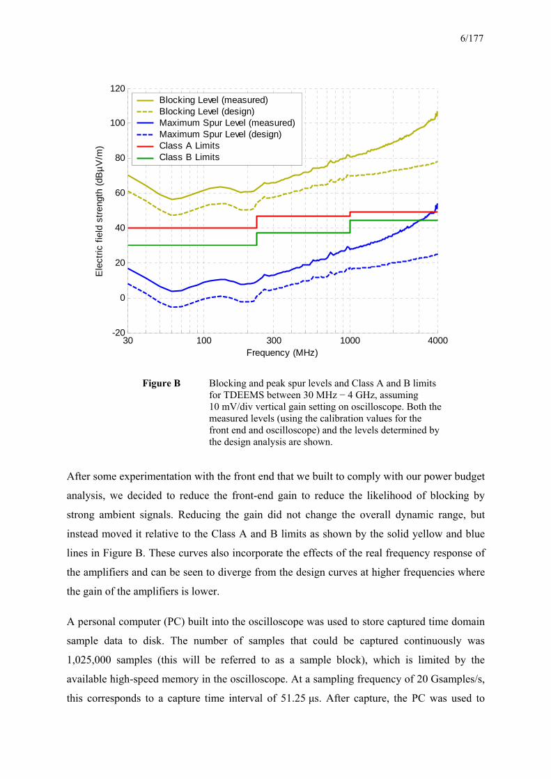
and cables) were also included in this analysis. As shown in Figure B, the front end was
designed to centre the Class B measurement limits (shown by the solid green line) within the
upper and lower limits of the dynamic range of the oscilloscope (shown by the dotted yellow
and blue lines, respectively).
The dynamic range of the TDEEMS is limited by the performance of the analogue-to-digital
converter (ADC) that is used to sample the signal in the oscilloscope. The ADC can only
sample the signal up to a maximum (full-scale) voltage, which is dependent on the vertical
gain setting used. At maximum voltage, the receiver is blocked, and this provides the upper
limit on the dynamic range. There are several factors that provide the lower limit on the
dynamic range, although the dominant factor is due to spurious frequency components (or
spurs) that are generated by imperfections in the ADC. As the amplitude and frequencies of
the spurs are dependent on the input signal, it is not possible to compensate for these;
therefore, they have to be considered as noise. Hence, the dynamic range of the oscilloscope
is equal to the spurious free dynamic range (SFDR), which was measured at 53 dB as a worst
case. This is the difference between the yellow and blue lines shown in Figure B.
6/177
After some experimentation with the front end that we built to comply with our power budget
analysis, we decided to reduce the front-end gain to reduce the likelihood of blocking by
strong ambient signals. Reducing the gain did not change the overall dynamic range, but
instead moved it relative to the Class A and B limits as shown by the solid yellow and blue
lines in Figure B. These curves also incorporate the effects of the real frequency response of
the amplifiers and can be seen to diverge from the design curves at higher frequencies where
the gain of the amplifiers is lower.
A personal computer (PC) built into the oscilloscope was used to store captured time domain
sample data to disk. The number of samples that could be captured continuously was
1,025,000 samples (this will be referred to as a sample block), which is limited by the
available high-speed memory in the oscilloscope. At a sampling frequency of 20 Gsamples/s,
this corresponds to a capture time interval of 51.25 µs. After capture, the PC was used to
30 100 300 1000 4000-20
0
20
40
60
80
100
120
Frequency (MHz)
Ele
ctric
fiel
d st
reng
th (d
BµV
/m)
Blocking Level (measured)Blocking Level (design)Maximum Spur Level (measured)Maximum Spur Level (design)Class A LimitsClass B Limits
Figure B Blocking and peak spur levels and Class A and B limits for TDEEMS between 30 MHz − 4 GHz, assuming 10 mV/div vertical gain setting on oscilloscope. Both the measured levels (using the calibration values for the front end and oscilloscope) and the levels determined by the design analysis are shown.

7/177
process the time domain signal to determine an estimate of the power spectrum of the signal,
using Fast Fourier Transform (FFT)-based algorithms, known as periodograms. Post-
processing rather than on-line processing of time domain sample data permitted
experimentation with different spectral estimation algorithms, and reduced the potential for
software bugs to render the data unusable. The software running on the PC was written using
a combination of C++ and the mathematical modelling language MATLAB.
Before using the TDEEMS to take measurements we calibrated it against a signal generator
whose calibration could be traced back to National Standards. Our calibration method
enabled us to compensate for frequency response variations in the front-end components and
the oscilloscope. Our initial tests of the TDEEMS were performed using test sources that
produced known and constant emissions. The test sources were measured using both a
conventional EMC test receiver and the TDEEMS. The following tests were made.
1. A continuous wave (CW) test. A signal generator was connected to a transmit
antenna and was configured to generate a CW signal of a known amplitude. After
each measurement, the signal frequency was changed to cover a range of spot
frequencies spanning 30 MHz to 4 GHz. The signal from a separate receive antenna
was measured using a conventional EMC test receiver and the TDEEMS.
2. Broadband noise test. Measurements were made of a broadband noise generator, as
used to calibrate an open air test site (OATS).
3. Comb generator. The emissions from a comb generator that radiates at discrete
frequencies spaced 100 MHz apart in the frequency range 80 MHz − 12 GHz were
measured.
4. Low frequency (below 30 MHz) measurements. These were made using a loop
antenna to determine the magnetic emissions from a 110 kHz test source and a PC
monitor.
The results of the test source measurements confirmed that the TDEEMS was able to make
reliable measurements of stationary sources and these measurements agreed closely with
those made using the conventional frequency domain EMC receiver. The CW measurements
were within 1 dB and the comb generator results within 2 dB of the conventional EMC test
receiver measurements at all frequencies up to 2 GHz.

8/177
Having confirmed the correct operation of the TDEEMS, we proceeded with measurements
of five example EUTs, which were chosen because they were likely to be sources of
impulsive emissions. The EUTs were an energy saving light bulb, a fast transient generator
used for conducted emissions tests, a 14" colour portable television, an electric drill with the
suppressor removed and a desktop PC without its case fitted. Measurements were made in a
screened room, at a distance of 1 m between 30 MHz − 1 GHz, and at a distance of 2 m
between 1 GHz − 4 GHz, and on an OATS at a distance of 10 m between 30 MHz − 1 GHz.
Each EUT was measured using both a conventional EMC test receiver and the TDEEMS, and
the measurements were performed twice, a week apart, to allow the repeatability performance
to be examined. Using the TDEEMS it was possible to capture one sample block every
0.75 s, which was the time taken to transfer the data from the oscilloscope to the PC and write
it to disk. To allow the variance between the frequency spectra of each sample block to be
examined, fifty sample blocks were captured during each measurement performed using the
TDEEMS. This also enabled us to average the frequency spectra, or to record the peak power
over a longer time period, hence implementing average and peak detectors as provided in a
conventional EMC test receiver.
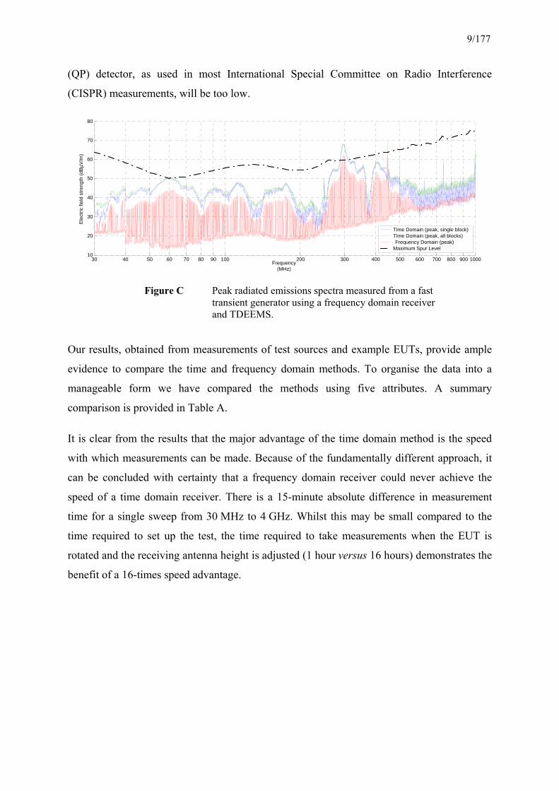
All of the measurement results we obtained during the project are documented in the main
report. As an example, we include here the peak radiated emissions spectrum of the transient
generator measured using the frequency domain receiver and the TDEEMS (Figure C). The
transient generator result is interesting because it reveals the behaviour of both methods when
measuring an emission whose pulse repetition frequency (PRF) is lower than the dwell time
of the frequency domain receiver. The spectrum obtained with the time domain method is
continuous, as we would expect, but the frequency domain receiver has produced a line
spectrum whose envelope closely corresponds to the time domain result. This result
conveniently illustrates the problem of using a swept approach to measure an impulsive
signal. The frequencies at which the frequency domain receiver has not recorded a signal are
due to the absence of an impulse when measuring these frequencies. In contrast, capturing a
single impulse with the TDEEMS is sufficient to determine its spectral characteristics. Whilst
the spectral characteristics of the emission are clear from a visual inspection of the envelope
of the frequency domain result, there is also an amplitude difference between the results of
the two methods. This error is attributed to the response time of the frequency domain
detector. As such this error may not exist in other frequency domain receivers, with different
detectors, but it does highlight the fact that impulsive measurements made with a quasi-peak
9/177
(QP) detector, as used in most International Special Committee on Radio Interference
(CISPR) measurements, will be too low.
Our results, obtained from measurements of test sources and example EUTs, provide ample
evidence to compare the time and frequency domain methods. To organise the data into a
manageable form we have compared the methods using five attributes. A summary
comparison is provided in Table A.
It is clear from the results that the major advantage of the time domain method is the speed
with which measurements can be made. Because of the fundamentally different approach, it
can be concluded with certainty that a frequency domain receiver could never achieve the
speed of a time domain receiver. There is a 15-minute absolute difference in measurement
time for a single sweep from 30 MHz to 4 GHz. Whilst this may be small compared to the
time required to set up the test, the time required to take measurements when the EUT is
rotated and the receiving antenna height is adjusted (1 hour versus 16 hours) demonstrates the
benefit of a 16-times speed advantage.
30 40 50 60 70 80 90 100 200 300 400 500 600 700 800 900 100010
20
30
40
50
60
70
80
Frequency(MHz)
Ele
ctric
fiel
d st
reng
th (d
BµV
/m)
Time Domain (peak, single block)Time Domain (peak, all blocks)Frequency Domain (peak)
Maximum Spur Level
Figure C Peak radiated emissions spectra measured from a fast transient generator using a frequency domain receiver and TDEEMS.

10/177
Attribute Frequency Domain Time Domain
Measurement Accuracy
Stationary signals Excellent. Accuracy is well proven
Excellent. Our results indicate that accuracy is as good as frequency domain method.
Impulsive signals 1. Reasonable for peak measurements when PRF is high.
2. Detector response time is critical.
3. Poor for measurements of low PRF signals.
1. Excellent for peak measurements, provided that the peak is captured.
2. Triggering is critical. 3. Average measurements
are difficult due to problems retaining the time domain information when triggering is used.
Repeatability 1. Results show good repeatability with both stationary and impulsive measurements.
2. The results obtained using the frequency domain receiver were repeatable, but due to the long peak detector time constant are inaccurate in both runs.
1. Results show good repeatability with stationary sources.
2. Variability in the reported results with impulsive sources is attributed to changes in the source that were not captured by the frequency domain method.
Measurement Time
Single sweep 30 MHz to 4 GHz Peak only
16 minutes
1 minute
Peak and average
25 minutes 1 minute
Rotating EUT 64 hours 4.8 hours
Dynamic Range
Sensitivity Good with LNA. Good with LNA. Spurious level > 80 dBc typical ≈ -60 dB Dynamic range 110 dB typical ≈ 60 dB
Use on OATS Able to handle high-level ambient signals by using RF pre-selection filters.
Susceptible to blocking because pre-selection cannot be used and dynamic range is limited.
Table A Summary of the performance comparison between the time and frequency domain methods.

11/177
A second definite advantage of the time domain approach is its ability to measure accurately
the spectral characteristics of short impulses. The test results obtained using the frequency
domain receiver demonstrated that, for impulsive emissions with a high PRF, a frequency
domain receiver is also capable of making a reliable peak measurement, provided that the
response time of the peak detector is sufficient to follow the impulse envelope. However,
when the PRF is low or irregular, the frequency domain method is unable to provide a
reliable measurement. The tests carried out to demonstrate the use of the TDEEMS for in situ
measurements is a particularly extreme example of a situation in which the time domain
method is able to provide a useful measurement that would be impossible with the frequency
domain approach. In this case the source of the emission is travelling at high speed past the
receiver giving a measurement window of only a few seconds. As the prototype TDEEMS
was able to capture sufficient data to analyse the complete spectrum in just 51.25 µs, the
short measurement window was not a problem.
The major disadvantage of the time domain approach is its limited dynamic range and this
fact alone may render the time domain approach unsuitable for use on an OATS. Based on
the measurements made at EMC Projects Ltd, a dynamic range of 100 dB is necessary to
measure emissions at the level of the Class B limits in the presence of ambient broadcast and
cellular radio signals. The dynamic range of 60 dB provided by the prototype TDEEMS is
insufficient to measure signals at either the Class A or Class B limits.
The dynamic range of the prototype system is limited by the spurious frequency components
generated by imperfections in the ADC. Whilst a different implementation may be able to
achieve an improved performance, by using techniques such as dithering to reduce the spur
levels, it is felt unlikely that a 100 dB dynamic range over a 4 GHz bandwidth will be
achievable in the near-term.
If a time domain approach to EMC measurements is to be adopted, further work will be
required to determine suitable parameters for the measurements. This will include an
alternative detector to the CISPR QP detector, since it will not be possible to implement a
detector that can operate continuously in time, due to the high sampling rates employed in the
TDEEMS. These parameters, which are discussed in this report, will have to be determined in
liaison with EMC test equipment manufacturers to determine what is technically feasible. It
will then be necessary to determine reasonable emissions limits by measuring emissions from
a wide range and different classes of equipment, with consideration given to interference to
12/177
radio services at these power levels and PRFs. This is a significant area of further work, since
existing EMC standards will have to be updated.
Another area for potential investigation is the implementation of a measurement receiver that
combines the frequency domain and time domain approaches (a hybrid receiver). In this
architecture the detector in the conventional EMC receiver is replaced with a fast ADC, and
the narrowband IF filter is replaced with a wideband IF filter. The RF band is still swept in
frequency (albeit in larger steps) and the output of the ADC is processed using FFT-based
techniques. Using this approach allows a number of frequencies (N) to be monitored
simultaneously, potentially reducing the measurement time by a factor of N. This approach is
now commonplace in modern spectrum analysers to improve the measurement time.
Overall our conclusions from this work are as follows.
1. The time domain approach provides some capabilities that could never be achieved
using the frequency domain method.
2. The time domain approach is the best method for measuring impulsive emissions in a
screened room environment.
3. There is a role for the time domain approach in reducing the time taken to undertake
EMC tests.
4. The dynamic range limitations are a serious drawback and for the near-term will
restrict the use of the time domain technique to screened room environments, where a
reduced dynamic range is acceptable, or to specific measurements that cannot be
made in any other way.
5. Fundamentally, the frequency domain approach will always be able to achieve a
better dynamic range than the time domain approach and so, in our opinion, will never
be completely replaced by time domain measurements.
Prepared by Multiple Access Communications Ltd
May 2004

13/177
Table of Contents
List of Abbreviations ............................................................................................................... 17
List of Symbols ........................................................................................................................ 19
1 Introduction...................................................................................................................... 21
2 Design .............................................................................................................................. 22
2.1 Sampling Data Method ............................................................................................ 23
2.1.1 Theoretical Dynamic Range ................................................................................ 24
2.1.2 Dynamic Range Due to Imperfections in the ADC ............................................. 26
2.1.3 Measuring the Dynamic Range of the Oscilloscope............................................ 30
2.2 Measurement Antennas............................................................................................ 32
2.3 Measurement Limits ................................................................................................ 35
2.4 Power Budget Analysis............................................................................................ 35
2.5 Noise Figure Analysis.............................................................................................. 38
2.5.1 Noise Performance of the Oscilloscope............................................................... 40
2.6 Blocking and Detection Levels................................................................................ 40
2.7 Low Frequency Measurements ................................................................................ 42
2.7.1 Antennas and Measurement Limits ..................................................................... 42
2.7.2 Power Budget Analysis........................................................................................ 42
2.8 Software Design and Architecture ........................................................................... 43
2.8.1 Data Capture ........................................................................................................ 44
2.8.2 Calibration............................................................................................................ 46
2.8.3 Post-Processing .................................................................................................... 46
2.8.4 Spectrum Data Display ........................................................................................ 47
2.8.5 SDB Viewer ......................................................................................................... 47
2.9 Summary of Design Requirements .......................................................................... 47
3 Implementation ................................................................................................................ 48
3.1 Front-End Implementation....................................................................................... 48

14/177
3.2 Calibration................................................................................................................ 49
3.2.1 Oscilloscope Calibration...................................................................................... 50
3.2.2 30 MHz − 4 GHz Front-End Calibration ............................................................. 51
3.2.3 100 kHz − 30 MHz Front-End Calibration.......................................................... 52
3.3 Updated Power Budget ............................................................................................ 53
4 Spectral Estimation .......................................................................................................... 55
4.1 Periodogram............................................................................................................. 55
4.1.1 Periodogram Parameters ...................................................................................... 57
4.1.2 Windowing Functions.......................................................................................... 58
4.2 Effects of Non-continuous Sampling....................................................................... 61
4.3 Detector Modelling .................................................................................................. 61
4.4 Data Processing Flow Diagram ............................................................................... 62
4.5 Measuring Emissions from Impulsive Sources........................................................ 63
4.5.1 Triggering on Impulsive Emissions ..................................................................... 65
5 Measurements .................................................................................................................. 66
5.1 Measurement of Test Sources.................................................................................. 66
5.1.1 Continuous Wave (CW) Tests ............................................................................. 67
5.1.2 Hopped CW Test.................................................................................................. 69
5.1.3 Broadband Noise Test.......................................................................................... 71
5.1.4 Comb Generator Test........................................................................................... 76
5.1.5 Low Frequency Tests........................................................................................... 80
5.2 Measurements of Example Equipment .................................................................... 82
5.2.1 Measurement Setup.............................................................................................. 82
5.2.2 Energy Saving Light Bulb ................................................................................... 84
5.2.3 Fast Transient Generator...................................................................................... 92
5.2.4 Portable Television .............................................................................................. 97
5.2.5 Electric Drill....................................................................................................... 103

15/177
5.2.6 Desktop PC ........................................................................................................ 111
5.3 Open Air Test Site (OATS) Measurements ........................................................... 116
5.3.1 Ambient Signal Measurement............................................................................ 116
5.3.2 Example Equipment........................................................................................... 118
5.4 In situ Measurements ............................................................................................. 127
5.4.1 Measurement Setup............................................................................................ 127
5.4.2 Results................................................................................................................ 129
5.4.3 Sources of Error in Train Measurements ........................................................... 135
6 Analysis of Results ........................................................................................................ 137
6.1 Measurement Accuracy ......................................................................................... 137
6.1.1 Does the System Architecture Affect Measurement Accuracy?........................ 138
6.1.2 Measurement Accuracy with Time-varying Sources......................................... 140
6.1.3 Peak vs Average Measurements......................................................................... 141
6.2 Repeatability of Measurements.............................................................................. 143
6.3 Measurement Time ................................................................................................ 144
6.3.1 Comparison of Time and Frequency Domain Sweep Times ............................. 145
6.3.2 OATS Measurement Time................................................................................. 146
6.4 Dynamic Range...................................................................................................... 148
6.5 Performance of OATS/in situ Measurements ........................................................ 150
6.6 Summary ................................................................................................................ 152
7 Extending the System .................................................................................................... 154
7.1 Current ADC Technology...................................................................................... 155
7.2 Commercial System Considerations ...................................................................... 156
7.2.1 Minimising the Processing Time ....................................................................... 156
7.2.2 Automatic Gain Control..................................................................................... 158
7.2.3 Reducing the Level of the ADC Spurs .............................................................. 158
7.3 Hybrid Frequency Domain/Time Domain System ................................................ 161

16/177
8 Conclusions and Further Work ...................................................................................... 163
References.............................................................................................................................. 166
Appendix A − Measurement Equipment Used ...................................................................... 169
Appendix B − In situ Measurement Antennas....................................................................... 170
Appendix C − Photographs of EMC Measurements ............................................................. 171

17/177
List of Abbreviations
AC Alternating Current
ADC Analogue-to-Digital Converter
AGC Automatic Gain Control
AM Amplitude Modulation
ASIC Application Specific Integrated Circuit
CGE Comb Generator Emitter
CNE Comparison Noise Emitter
CISPR International Special Committee on Radio Interference
CPU Central Processor Unit
CSV Comma Separated Value
CW Continuous Wave
DAB Digital Audio Broadcasting
DAC Digital-to-Analogue Converter
DC Direct Current
DDR Double Data Rate
DFT Discrete Fourier Transform
DNL Differential Non-Linearity
DSP Digital Signal Processor
EMC Electromagnetic Compatibility
EUT Equipment under Test
FCC Federal Communications Commission
FFT Fast Fourier Transform
FS Full-Scale
GPIB General Purpose Interface Bus
GSM Global System for Mobile communications
GUI Graphical User Interface
18/177
HF High Frequency
IF Intermediate Frequency
INL Integral Non-Linearity
ITT Invitation to Tender
JTFA Joint Time and Frequency Analysis
LNA Low Noise Amplifier
LUT Lookup Table
MAC Ltd Multiple Access Communications Limited
OATS Open Air Test Site
PC Personal Computer
PCN Personal Communication Networks
PRF Pulse Repetition Frequency
PSD Power Spectral Density
QP Quasi-Peak
RA Radiocommunications Agency
RF Radio Frequency
RMS Root-Mean-Square
SDB Sampled Data Block
SDRAM Synchronous Dynamic Random Access Memory
SFDR Spurious Free Dynamic Range
SNR Signal-to-Noise Ratio
STFT Short Time Fourier Transform
TDEEMS Time Domain EMC Emissions Measurement System
VHF Very High Frequency

19/177
List of Symbols
Af Antenna factor (in dB/m)
b Sample block number
B Number of sample blocks being processed
Bbin FFT bin bandwidth
Brx Receiver bandwidth
E Electric field strength (normally in dBµV/m)
Elim Electric field strength limit (normally in dBµV/m)
f Analogue frequency
fs Sampling frequency
fstep Frequency step
F Noise figure (normally in dB)
G Gain (in dB)
Hx(f) Transfer function of component x (in frequency domain)
I lim Current limit (normally in dBµA)
k Boltzmann’s constant (1.38 x 10⁻²³ joules/K)
K dBµA to dBµV conversion factor (34 dB)
L Number of samples to skip between segments (in periodogram)
Lx Loss due to component x (in dB)
m Segment index or number
M Number of segments (in periodogram)
n Sample index
N Number of ADC output bits
NP Number of points or samples (in FFT)
Noccurrences Number of occurrences of an impulse (in FFT)
P[ω] Power spectrum (at discrete frequency ω)
PSS[ω] Single-sided power spectrum (at discrete frequency ω)
20/177
R Window coherent gain factor
SFDR Spurious Free Dynamic Range (in dB)
SNR Signal-to-Noise Ratio (normally in dB)
T Absolute temperature (in Kelvin)
Tdwell Dwell time
TFFT Length of FFT in time (normally in µs)
VFS RMS full-scale voltage of ADC or oscilloscope (normally in dBµV)
Vin Input voltage (to ADC)
Vscope Voltage at input to oscilloscope
Vspur RMS voltage level of peak spurious component (normally in dBµV)
∆v Voltage level represented by each ADC output code
ω Analogue frequency normalised with respect to sampling frequency
w[n] Windowing function value (at sample index n)
x[n] Data sample value (at sample index n)
xs[n] Data sample value within segment of periodogram (at sample index n)
xws[n] Windowed data sample value within segment (at sample index n)
Xs[ω] Amplitude spectrum (at discrete frequency ω)

21/177
1 Introduction
The measurement of radiated radio frequency (RF) emissions from electrical and electronic
devices is currently performed using a swept or stepped frequency receiver. As a
consequence, the receiver can only examine a narrow bandwidth at any instant in time. This
approach is adequate for measurement of continuous emissions, but is severely limited as a
method to measure impulsive emissions. To overcome this limitation the current approach is
to sweep the same RF band many times and to use a peak hold detector to record the
maximum signal strength encountered at each frequency. Whilst this method has served the
industry well for many years, it has a major drawback in that the measurement time is long
and it is still not guaranteed to measure the peak radiated power.
Recent advances in high speed sampling systems now offer an alternative time domain
electromagnetic emissions measurement method, which overcomes many of the limitations of
the swept frequency approach, especially when measuring impulsive emissions. Following
Multiple Access Communications (MAC) Ltd’s formal responses [1], [2] to the
Radiocommunications Agency (RA) Invitation to Tender (ITT), Reference Number AY4489,
MAC Ltd was commissioned to perform a study to investigate the potential benefits and
pitfalls of the time domain measurement method. The study involved designing and building
a prototype time domain EMC emissions measurement system (TDEEMS), when possible
based around commercial off-the-shelf components to minimise design effort and cost. The
prototype TDEEMS was calibrated and tested using the electromagnetic compatibility (EMC)
test facilities of EMC Projects Ltd, who is a subcontractor in this project.
The TDEEMS was used to perform radiated emissions measurements on five
electric/electronic devices, which are likely sources of impulsive emissions. The five items
were also tested using the conventional frequency swept approach so that the results could be
compared with the time domain method. We also used the TDEEMS to perform in situ
measurements. In situ measurements are those made at an open site with a piece of bulky or
heavy equipment that cannot be moved to an EMC test house.
In this report we present the work performed by MAC Ltd in fulfilling these tasks. We
describe the design of the TDEEMS in Section 2. Details of the system component choices
and results from the calibration measurements are given in Section 3. The signal processing
methods used to determine the power spectrum of the time domain sample data are described

22/177
in Section 4. Results from measuring the emissions from the test sources and example
equipment, together with the in situ measurement results are presented in Section 5. We
provide an analysis of the results, together with a comparison with the conventional swept
receiver measurement approach in Section 6. Suggestions for extending the TDEEMS, a
review of current analogue-to-digital converter (ADC) technology and considerations for
implementing a commercial measurement system are provided in Section 7. Finally, a
summary of conclusions is given in Section 8.
2 Design
A block diagram of the TDEEMS that we have implemented is shown in Figure 1. A similar
TDEEMS has been implemented previously by Krug and Russer [3].
The TDEEMS is based around a commercial off-the-shelf digital sampling oscilloscope that
can sample at up to 20 Gsamples/s with an analogue bandwidth of 4 GHz. A pre-amplifier on
the input to the oscilloscope is required as the oscilloscope input stage is not sensitive enough
to detect signals directly from the antenna. A low pass filter on the input to the pre-amplifier
is provided to reject out-of-band signals. A personal computer (PC) is used to control and
store sampled data from the oscilloscope. After capture, the PC can process the time domain
signal to determine the frequency spectrum of the signal.
Broadbandantenna
Low passfilter
Low noiseamplifier
Data capture device(sampling oscilloscope)
PCFront end
Figure 1 Time domain EMC emissions measurement system block diagram.

23/177
The major advantage of using a high speed sampling system that operates at the RF or
intermediate frequency (IF) of a receiver and processing the captured signals in the digital
domain is that it is possible to measure all frequencies simultaneously within the RF band of
the receiver and thus accurately capture the effects of impulsive emissions. The major
disadvantage of being able to measure instantaneously over a wide frequency range is that the
measurement dynamic range is much lower than that possible with a conventional EMC test
receiver. The reasons for the dynamic range limitation will be discussed in Section 2.1, but
the consequence is that the time domain measurement method is susceptible to blocking by
strong signals, such as those from broadcast transmitters and cellular base stations. For
measurements within a screened enclosure this is not an issue; however, it might limit the
applicability of the time domain method for use on open air test sites. We discuss the
blocking performance of the TDEEMS in Section 6.5.
In this section the analysis and design of the TDEEMS is documented. We will start by
determining the dynamic range offered by the oscilloscope, and investigate the factors that
limit the dynamic range. Next, the antenna gains and the typical electric field strength limits
used in EMC measurements are determined. From this, the pre-amplifier gain necessary for
the oscilloscope to detect signals from the antenna can be calculated. We then analyse the
noise performance of the system. Finally, a description of the software running on the PC to
capture, store, process and analyse the measurement data is provided.
2.1 Sampling Data Method
For the purposes of this study we used an Agilent Infiniium 54854A oscilloscope, as the
hardware was readily available and minimal development effort was required. This
oscilloscope can sample at up to 20 Gsamples/s and theoretically permits the analysis of the
RF band from direct current (DC) to 10 GHz at the same time instant. In practice, however,
the RF band that can be measured by such an instrument is limited by other factors, and the
Agilent oscilloscope used in this project is limited to a measurement bandwidth of 4 GHz.
Consideration of extending the TDEEMS to higher frequency ranges will be given in
Section 7.
The first stage in designing the TDEEMS was to determine the dynamic range available from
the oscilloscope. A large dynamic range is desirable so that the measurement system can
handle a wide range of signal powers, and reduce the probability of blocking from strong

24/177
broadcast signals in open air environments. The factors that limit the dynamic range will now
be discussed.
2.1.1 Theoretical Dynamic Range
The Infiniium digital sampling oscilloscope employs an ADC based around a flash ADC
architecture as shown in Figure 2. In this architecture a bank of comparators with different
voltage thresholds is used to determine the amplitude of the input signal. The voltage
thresholds are derived from a known reference voltage using a resistive ladder, and for an
N-bit ADC, 2N voltage levels (and hence 2N resistors) are required. Finally, a decoder on the
outputs of the comparators is used to produce the binary encoded output.
The function of an ADC is to produce a digital output code that is proportional to the voltage
applied to its input. An ADC is designed to measure a voltage up to a maximum limit that is
referred to as the full-scale voltage. Above this input voltage the ADC will produce the same
R
R
R
R
R
R
R
0.5R
1.5R
Encoderand latch
Digitaloutput
N
Strobe
+VREF
Analog input
Figure 2 Simplified block diagram of a 3-bit flash ADC architecture.

25/177
digital output code, therefore, this code no longer provides a representation of the input
voltage waveform. This is called clipping or saturation and provides the upper limit on the
dynamic range.
Due to the digital output of the ADC only a finite number of codes are used to represent the
voltage level of the waveform (this process is known as quantisation). An ideal ADC will use
the output code that represents the voltage level that is closest to the true voltage level of the
input. Therefore, there is an error in the output represented by the digital code, which results
in quantisation noise, as will be demonstrated later in this section. This provides the
theoretical lower limit on the dynamic range.
It can be shown [4] that the signal-to-noise ratio (SNR) (ie, the ratio of the root-mean-square
(RMS) amplitude of a full-scale input sinewave to the RMS amplitude of the quantisation
noise) of an ideal ADC, in decibels (dB) is given by
76.102.6 +⋅= NSNR (1)
where N is the number of bits in each ADC sample. For the Infiniium oscilloscope N = 8
which produces a SNR of approximately 50 dB over the input signal bandwidth.
By capturing a block of samples, a Fast Fourier Transform (FFT) can be performed to convert
the time domain sample data to the frequency domain (see Section 4). As the input waveform
is being decomposed into discrete frequency bands (called bins) by the FFT, the noise power
is shared across all bins. This is analogous to a bank of band-pass filters and hence the noise
floor in each bin is lowered by the processing gain, G, which is given by (in dB)
⎟⎠⎞
⎜⎝⎛⋅=
2log10 PNG (2)
where NP is the number of points, or samples, over which the FFT is calculated. The
Infiniium oscilloscope can capture a block of up to 1,025,000 samples (1025 Ksamples) at the
full sample rate of 20 Gsamples/s that provides a processing gain of approximately 57 dB.
Therefore, the theoretical dynamic range available from the ADC in the oscilloscope is the
sum of the SNR due to quantisation noise and the processing gain of the FFT (107 dB) as
shown in Figure 3. The vertical power scale is in decibels relative to the input power required

26/177
to drive the ADC at full-scale (dBFS), ie, the maximum input power beyond which the ADC
saturates.
2.1.2 Dynamic Range Due to Imperfections in the ADC
In practice, the lower limit of the dynamic range will not be limited by quantisation noise, but
by spurious frequency components generated by imperfections in the ADC. Some of the
imperfections are caused by component mismatches or stray capacitance effects at high
frequencies. For example, it is very difficult to match the values of all the resistors in the
resistive ladder to the same value (see Figure 2). We will now illustrate some of the effects of
these imperfections on the dynamic range of the ADC.
The first two types of imperfection that affect a real ADC are offset and gain errors, which
produce an output code that is scaled or translated with respect to the measured input voltage.
These errors can be corrected easily by calibration of the ADC, which is performed by the
manufacturer of the oscilloscope. However, there are two types of linearity errors that are
more difficult to correct.
The transfer functions for an ideal (imaginary) and a real 3-bit ADC are shown in Figure 4.
From the figure it can be seen that the difference in input voltage (∆v) represented by each
0
-20
-40
-60
-80
-100
-120
SNR
= 5
0 dB
ADC fullscale
RMS quantisation noise level
G =
57
dB
0 B = 4 GHz
FFT noise floor
FFT bin size = fs /NP
Theo
retic
al d
ynam
ic ra
nge
Pow
er (d
BFS
)
Frequency
Figure 3 Theoretical dynamic range available from Agilent Infiniium 54854A oscilloscope with FFT processing of the ADC output sample data.

27/177
output code is the same in the case of the ideal ADC transfer function. This results in a
constant quantisation noise level across the Nyquist bandwidth, assuming that the amplitude
probability density function of the input signal is flat (the SNR is given by Equation 1).
However, in a real ADC the voltage difference required to produce an adjacent digital output
code varies, and therefore the noise level increases due to the increased error. This type of
distortion is known as differential non-linearity (DNL).
Differential non-linearity in the ADC transfer function will produce spurious artefacts (spurs)
at discrete frequencies in the output spectrum measured using the FFT. Most high speed
ADCs are designed to distribute this differential non-linearity across the entire input voltage
range and, as a result, the amplitudes and frequencies of these spurs will vary according to the
amplitude of the input signal. These will also vary according to the frequency content of the
input signal, due to the dynamic or alternating current (AC) performance of the ADC.
However, in general, the frequencies of the spurs due to DNL are not harmonically related to
the input signal.
Out
put c
ode
Vin
∆v
Err
or d
ue to
quan
tisat
ion
Ideal 3-bit ADC transfer function(∆v is constant for each output code)
Real 3-bit ADC transfer function(with differential non-linearity)
Vin
000
001
010
011
100
101
110
111
Out
put c
ode
∆v2
Err
or d
ue to
quan
tisat
ion
and
DN
L
Vin
000
001
010
011
100
101
110
111
ideal (straight line) characteristic
∆v1
0
1/8F
S
1/4F
S
1/2F
S
5/8F
S
3/4F
S
7/8F
S FS Vin
0
1/8F
S
1/4F
S
1/2F
S
5/8F
S
3/4F
S
7/8F
S FS
Vin = analogue input voltage normalised to fullscale (FS)
Figure 4 Ideal 3-bit ADC transfer function and real 3-bit ADC transfer function exhibiting differential non-linearity.
28/177
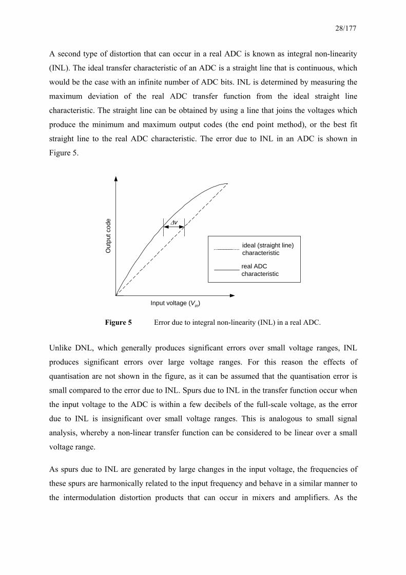
A second type of distortion that can occur in a real ADC is known as integral non-linearity
(INL). The ideal transfer characteristic of an ADC is a straight line that is continuous, which
would be the case with an infinite number of ADC bits. INL is determined by measuring the
maximum deviation of the real ADC transfer function from the ideal straight line
characteristic. The straight line can be obtained by using a line that joins the voltages which
produce the minimum and maximum output codes (the end point method), or the best fit
straight line to the real ADC characteristic. The error due to INL in an ADC is shown in
Figure 5.
Unlike DNL, which generally produces significant errors over small voltage ranges, INL
produces significant errors over large voltage ranges. For this reason the effects of
quantisation are not shown in the figure, as it can be assumed that the quantisation error is
small compared to the error due to INL. Spurs due to INL in the transfer function occur when
the input voltage to the ADC is within a few decibels of the full-scale voltage, as the error
due to INL is insignificant over small voltage ranges. This is analogous to small signal
analysis, whereby a non-linear transfer function can be considered to be linear over a small
voltage range.
As spurs due to INL are generated by large changes in the input voltage, the frequencies of
these spurs are harmonically related to the input frequency and behave in a similar manner to
the intermodulation distortion products that can occur in mixers and amplifiers. As the
Out
put c
ode
Input voltage (Vin)
∆v
ideal (straight line)characteristic
real ADCcharacteristic
Figure 5 Error due to integral non-linearity (INL) in a real ADC.

29/177
amplitudes of the INL errors are higher, the amplitudes of the spurs due to INL are higher
than those due to DNL.
To reduce the level of the spurs due to the non-linearity in the ADC transfer function, the
Infiniium oscilloscope employs a calibration lookup table on the output of the ADC [5],
which is shown in Figure 6. The lookup table is programmed during oscilloscope calibration
by a microprocessor that uses a digital-to-analogue converter (DAC) to generate a ramp
voltage waveform at the input to the ADC. When the 8-bit code at the ADC output changes,
the 16-bit DAC input code that resulted in the change is stored in the lookup table.
During normal operation of the oscilloscope, the lookup table is used to map the 8-bit output
code produced by the ADC to 16-bits. As the 16-bit code can represent 65,536 rather than
256 voltage levels, the lookup table can correct for the non-linear ADC transfer function. The
DAC can run at much lower sample rates than the ADC, and hence will exhibit better
linearity and resolution.
The calibration procedure is a time domain operation (as the oscilloscope is intended for time
domain measurements), and does not compensate for the frequency response of the ADC.
The ramp rise time will be very slow compared to the maximum sampling rate
(20 Gsamples/s) of the ADC, and so the correction for non-linearity may not work so well at
higher input frequencies. The PC must also store twice as much data, as the calibration
lookup table values are not accessible from the programming interface to the oscilloscope.
Vin
16-bitDAC
8-bitADC
8 16calibrationlookup
table (LUT)
16 micro-processor
16
PC
calibration hardware
Figure 6 Infiniium oscilloscope ADC calibration.

30/177
2.1.3 Measuring the Dynamic Range of the Oscilloscope
As the amplitude of the spurs due to distortion in the ADC transfer characteristic is dependent
on the architecture and imperfections in the realisation of the ADC, the amplitudes of the
spurs have to be measured. The universally accepted method for measuring the spurious
performance is to drive the ADC input with a full-scale continuous wave (CW) signal and
process the sample output data using a FFT. From the resulting frequency spectrum the ratio
of the RMS signal amplitude to the RMS value of the peak spurious spectral content can be
determined. This is referred to as the spurious free dynamic range (SFDR), and is an
important specification for an ADC.
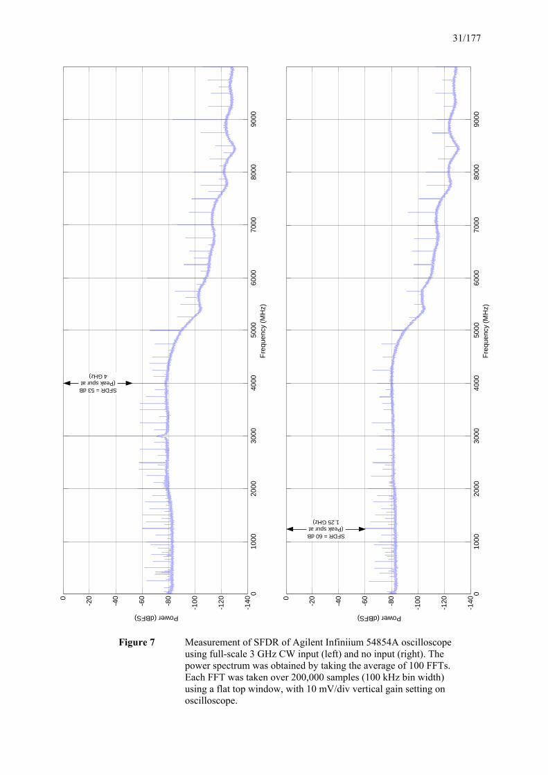
To measure the SFDR of the Infiniium oscilloscope, we used a signal generator to provide a
3 GHz CW input to the oscilloscope. The vertical scale on the scope was set to 10 mV per
division and there are eight divisions vertically. Therefore, to drive the ADC on the scope at
full-scale, the amplitude of the CW input needs to be 80 mV (peak-to-peak).
A FFT was performed over 200,000 samples (this is a nominal FFT length, and is more than
sufficient to measure the SFDR), and the result is shown in the left-hand plot in Figure 7. It
can be seen from the plot that the SFDR is only 53 dB, and therefore the spurs limit the
usable dynamic range of the oscilloscope. The right-hand plot in Figure 7 shows the result of
the FFT with no input signal. In this case the SFDR has increased to 60 dB since the ADC is
not operating over its full voltage range. As a result the spurs generated by integral non-
linearity have been reduced in amplitude.
The level of the spurs generated by the ADC can be expected to lie between the values of the
SFDR with a full-scale input (53 dB) and the SFDR without an input (60 dB) during the
measurements. It is possible that the level of the spurs could be even lower if a wideband
signal is being measured, as this will tend to dither the input signal. Many other factors
influence the performance of an ADC, including timing uncertainties (aperture jitter) and the
architecture of the ADC. Further information regarding performance measurements of ADCs
can be found in [6].
31/177
010
0020
0030
0040
0050
0060
0070
0080
0090
00-1
40
-120
-100-80
-60
-40
-200
Freq
uenc
y (M
Hz)
Power (dBFS)
SFDR = 53 dB(Peak spur at
4 GHz)
010
0020
0030
0040
0050
0060
0070
0080
0090
00-1
40
-120
-100-80
-60
-40
-200
Freq
uenc
y (M
Hz)
Power (dBFS)
SFDR = 60 dB(Peak spur at
1.25 GHz)
Figure 7 Measurement of SFDR of Agilent Infiniium 54854A oscilloscope using full-scale 3 GHz CW input (left) and no input (right). The power spectrum was obtained by taking the average of 100 FFTs. Each FFT was taken over 200,000 samples (100 kHz bin width) using a flat top window, with 10 mV/div vertical gain setting on oscilloscope.
32/177
From Figure 7 it can be seen that the noise level is approximately -80 dBFS up to 4 GHz, if
the spurs are ignored. This is the noise floor due to thermal noise, and is determined by the
noise performance of the ADC front end in the oscilloscope. The noise performance of the
TDEEMS will be considered in Section 2.5.
2.2 Measurement Antennas
Most radiated emissions measurements are made at frequencies above 30 MHz and this sets a
general lower limit for the operating frequency range of broadband EMC measurement
antennas. Below 30 MHz, conducted emissions tend to dominate and high levels of
background noise from the high frequency (HF) band and the size of the antenna makes
measurements problematic. Measurements below 30 MHz are typically performed in a
screened room with a loop antenna to detect magnetic rather than electric fields. However,
the system as it stands will measure emissions in this band if used with a suitable antenna,
since the time domain approach can cover frequencies down to DC. Consideration is given to
low frequency measurements in Section 2.7.
So that a single measurement pass can be made using the TDEEMS, a broadband
measurement antenna covering the frequency range from 30 MHz to 4 GHz is desirable.
Unfortunately, antennas that are calibrated across this entire frequency range are not readily
available. Antennas are available which cover the 30 MHz to 3 GHz frequency range,
including the Schaffner BiLog antenna CBL 6143 [7], which was used for the in situ
measurements (see Section 5.4). However, for the purposes of the design of the TDEEMS
only the measurement antennas available at EMC Projects Ltd were considered. These are
listed in Table 1.
As can be seen from the table, there are no antennas that cover the entire frequency range to
4 GHz. Therefore, when performing measurements, two passes were required with antenna
BA4 used for measurements between 30 MHz and 1 GHz, and antenna DRGFS used for
measurements between 1 GHz and 4 GHz.

33/177
Plant Number Type Manufacturer and Model Frequency
Range (MHz)
BA4 Biconical log/hybrid Chase CBL6111A 30 − 1000
BIC4A Biconical Schwarzbeck VHBB 9133 25 − 300
LP4 Log periodic array Schwarzbeck UHALP 9107 300 − 1000
DRGFS Double ridged guide horn EMCO 3115 1000 − 18000
The function of an antenna is to collect the electromagnetic power over the effective receive
area or aperture of the antenna. The relationship between the voltage seen at the antenna
terminals (Vr), and the electric field strength (E) is given by the antenna factor, Af, which is
defined as
⎟⎟⎠
⎞⎜⎜⎝
⎛⋅=
rf V
EA log20 (3)
where E and Vr are expressed in linear terms. The antenna factor is a measure of the
sensitivity of an antenna, and is normally specified in units of decibels/metre. The antenna
factor is a function of frequency.
The calibrated free space antenna factors for the measurement antennas available at EMC
Projects Ltd are shown in Figure 8. It can be seen that above the resonant frequency the
antenna factor is proportional to the logarithm of frequency. These antenna factors are typical
for EMC measurement antennas, and can be used in the design of the TDEEMS.
Table 1 Measurement antennas used at EMC Projects Ltd.

34/177
As well as performing two measurement passes using different antennas, measurements were
performed using antenna BA4 above 1 GHz, as the antenna still responds to frequencies
above this limit. However, above 1 GHz, the antenna factor increases rapidly and this
compromises the available dynamic range by limiting the measurement sensitivity.
Making measurements above 1 GHz using a single antenna is problematic, because at these
frequencies the dimensions of the equipment under test (EUT) approach the wavelengths
being measured [8]. At these frequencies, the EUT begins to act as an antenna array and a
single receive antenna at a fixed position may not measure the peak radiated emission due to
beam-forming effects. These effects can be mitigated by using movable antennas. However,
it was beyond the scope of this project to study the issues associated with using antennas at
these frequencies.
30 100 300 1000 40000
5
10
15
20
25
30
35
Frequency (MHz)
Ant
enna
fact
or (d
B/m
)BA4DRGFSBIC4ALP4
Figure 8 Free space antenna factors for measurement antennas used during study at EMC Projects Ltd.

35/177
2.3 Measurement Limits
Most of the standards for radiated emissions limits from electrical equipment are based on
limits specified by the International Special Committee on Radio Interference (CISPR). The
CISPR 22 standard [9] specifies radiated emissions limits for frequencies below 1 GHz. The
limits above 1 GHz are still under consideration, so for radiated emissions limits above
1 GHz we used the limits specified by the Federal Communications Commission (FCC)
CFR47 Part 15 standard [10].
The CISPR 22 quasi-peak (QP) Class B (domestic environment) limits below 1 GHz and the
FCC CFR47 limits above 1 GHz will be used to determine the required input sensitivity of
the TDEEMS. The radiated emissions limits at 10 m are listed in Table 2. For reference, the
Class A (industrial and commercial environments) limits are also shown, as it is desirable to
include these limits within the dynamic range of the measurement system. As most
equipment manufacturers will aim to meet the Class B limits, these will be used in
subsequent analyses.
Frequency Range (MHz)
Class A QP emissions limit (dBµV/m)
Class B QP emissions limit (dBµV/m)
30 − 230 40 30
230 − 1000 47 37
1000 − 4000 49.5 44.5
2.4 Power Budget Analysis
Now that the oscilloscope dynamic range, antenna factors and measurement limits are known,
we can determine an approximate system power budget. This will allow the pre-amp gain
needed to drive the oscilloscope to be determined. In the power budget we will estimate the
cable and insertion losses in the system.
A component block diagram of the TDEEMS is shown in Figure 9.
Table 2 Radiated emissions limits used in the design of the TDEEMS.

36/177
Each component of the system has a frequency response or transfer function denoted by
Hx(f). From Figure 9 it can be seen that the system transfer function, Hsys(f), is given by
)()()()()()()()(
)( fHfHfHfHfHfHfEfV
fH scopeinsertampfiltercableafant
scopesys == (4)
The system transfer function relates the electric field strength at the antenna to the voltage
measured on the oscilloscope. Note that the antenna transfer function, Haf(f) has dimensions
of 1/[distance], since it relates the electric field strength at the antenna to the output voltage
of the antenna.
Due to the piecewise emissions limits, a power budget will be performed for each of the three
frequency ranges shown in Table 2. For each frequency range, Equation 4 can be rewritten,
using logarithmic quantities, as
scopeicablefantscope LLGLAEV −−+−−=− (5)
where Eant is the electric field strength at the antenna (in dBµV/m), Vscope is the voltage
measured by the oscilloscope (in dBµV) and Af is the antenna factor (in dB/m). Lcable is the
cable loss, G is the pre-amplifier gain, Li is the insertion loss and Lscope is the loss due to the
oscilloscope frequency response (all in dB).
The design objective is to provide enough pre-amplifier gain to amplify the antenna output
voltage so that an emission on the thresholds of the Class B limits (denoted by Elim) will be
centred within the dynamic range of the oscilloscope, taking into account the antenna factors,
cable loss and insertion losses, hence
limEEant = (6)
Haf(f) Hcable(f) Hfilter(f) Hamp(f) Hscope(f)
Broadbandantenna
Cablelosses
Low-passfilter
Pre-amplifier
Oscilloscope
Hinsert(f)
Insertionlosses
Figure 9 TDEEMS component block diagram.

37/177
and
2
SFDRVV FSscope −= , (7)
where VFS is the peak RMS input voltage amplitude of the oscilloscope and SFDR is the
spurious free dynamic range of the oscilloscope. This peak input voltage to the oscilloscope
is 40 mV peak when the vertical gain is set to 10 mV per division (see Section 2.1.3), or
89 dBµV RMS.
For the purposes of the power budget, it will be assumed that the oscilloscope has unity gain
over all frequencies (ie, Lscope = 0 dB). By rearrangement and substitution into Equation 5,
the required pre-amplifier gain (G) in each frequency range is given by
lim2ESFDRVLLAG FSicablef −−+++= (8)
The average of the highest and lowest antenna factor will be used in each frequency range, ie,
2
(max)(min) fff
AAA
+= (9)
The TDEEMS power budget is shown in Table 3. Note that the voltage at the pre-amplifier
input (Vin) is given by
icablefin LLAEV −−−= lim (10)
It can be seen from Table 3 that the pre-amp gain values required across the three frequency
bands are 49.7, 50.35 and 54.55 dB from 30 − 230 MHz, 230 − 1000 MHz and 1 − 4 GHz,
respectively. Therefore, the average pre-amplifier gain required is 51.5 dB.

38/177
2.5 Noise Figure Analysis
Now that we have determined the pre-amplifier gain required to ensure that emissions on the
threshold of the Class B limits are centred within the dynamic range of the oscilloscope, we
must ensure that the noise floor at the output of the pre-amplifier does not exceed the level of
the spurs, which would limit the dynamic range.
Any practical signal source has a natural noise floor due to thermal noise. The thermal noise
power (in dBm, ie, relative to 1 dB milliwatt) within a bandwidth B (Hz) at a temperature T
(Kelvin) is given by
30)log(10 +⋅= kTBPnoise (11)
where k is Boltzmann’s constant (1.38 x 10⁻²³ joules/K). As we will be using a FFT to
measure the power spectrum of the pre-amplifier output, the bandwidth corresponds to the
FFT bin width or frequency resolution that is given by
Frequency Range (MHz)
Parameter Symbol 30 - 230 230 - 1000 1000 - 4000
Lowest antenna factor (dB/m) Af(min) 5.2 10.1 24
Highest antenna factor (dB/m) Af(max) 19.2 25.6 33.1
Radiated emissions limit (dBµV/m) Elim 30 37 44.5
Average antenna factor (dB/m) Af 12.2 17.85 28.55
Estimated cable loss (dB) Lcable 3 5 6
Insertion losses (dB) Li 2 2 2
Voltage at pre-amp input (dBµV) Vin 12.8 12.15 7.95
Full-scale oscilloscope input (dBµV) VFS 89 89 89
Oscilloscope SFDR (dB) SFDR 53 53 53
Oscilloscope input voltage (dBµV) Vscope 62.5 62.5 62.5
Pre-amplifier gain required (dB) G 49.7 50.35 54.55
Table 3 TDEEMS power budget.

39/177
P
sbin N
fB = (12)
where fs is the sampling frequency and NP is the number of points, or samples, over which the
FFT is calculated. For the FFT plot shown in Figure 7, fs = 20 Gsamples/s and NP = 200,000.
At 25 °C (298 K), the thermal noise power in each FFT bin is -124 dBm. This is the noise
level at the input to the front-end pre-amplifier, and since its input impedance is 50 Ω, this
corresponds to an input RMS voltage of -17 dBµV.
The pre-amplifier will amplify the signal and noise level, as well as adding noise of its own.
The noise added by the pre-amplifier is given by its noise figure (F), which is given by
in
out
SNRSNR
F = (13)
where SNRin and SNRout are the signal-to-noise ratios at the input and output of the pre-
amplifier, respectively. The noise level at the output of the pre-amplifier is given by
FGVV innoiseoutnoise ++= __ (14)
where G is the gain of the pre-amplifier, and Vnoise_in is the noise level at the input to the pre-
amplifier (-17 dBµV). The maximum spur level (Vspur) is given by
SFDRVV FSspur −= (15)
where VFS is the peak oscilloscope input voltage (89 dBµV RMS at a vertical gain setting of
10 mV/div), and SFDR is the spurious free dynamic range of the oscilloscope (measured at
53 dB). Therefore, the maximum spur level is 36 dBµV RMS.
As already stated, the noise level at the output of the pre-amplifier must not exceed the level
of the spurs. By equating Vnoise_out to Vspur and rearranging, we obtain
dBFG 53=+ (16)
Therefore, for a gain of 51.5 dB, the noise figure must not exceed 1.5 dB. Consequently, a
very low noise amplifier (LNA) is required if this gain is to be achieved. The practical
implications of this are discussed in Section 3.1.

40/177
2.5.1 Noise Performance of the Oscilloscope
In Section 2.1.3 the noise floor due to thermal noise and the noise performance of the
oscilloscope front end was measured at -80 dBFS at frequencies up to 4 GHz. From this we
can calculate the noise figure of the oscilloscope. This measurement was made with a full-
scale input voltage of 89 dBµV RMS; therefore the noise floor is 9 dBµV RMS. The
estimated noise figure of the oscilloscope is the difference between the thermal noise floor
determined in Section 2.5 (-17 dBµV) and the measured noise floor, or 26 dB.
The noise figure in linear terms of a cascaded system (Fsystem) is given by
...11
21
3
1
21 +
−+
−+=
GGF
GF
FFsystem (17)
where FN and GN are the noise figure and gain of the Nth stage of the system, both expressed
in linear terms. For two cascaded elements, eg, a low noise amplifier and an oscilloscope, the
overall noise figure will be lower than that of the oscilloscope alone if F1 < F2 and G1 is
sufficiently large.
As the required pre-amplifier gain is 51.5 dB (see Section 2.4), the noise performance of the
system will only be degraded if the noise figure of the pre-amplifier is greater than 26 dB.
Typical practical amplifiers have noise figures that are much less than this value.
2.6 Blocking and Detection Levels
Figure 10 shows the blocking and maximum spur levels for the TDEEMS assuming a pre-
amplifier gain of 51.5 dB. The blocking threshold is the maximum received signal level
beyond which the ADC in the Infiniium oscilloscope will start to saturate. Below the
maximum spur (or detection) level, it is not possible to distinguish between the signal and the
worst-case spurs generated by the ADC. It can be seen that the Class B limits are centred
between the blocking and maximum spur levels, which was the original design objective.
For Figure 10 we have assumed that antenna BA4 will be used for the 30 MHz to 1 GHz
frequency range, and antenna DRGFS will be used for the 1 GHz to 4 GHz range. The cable
losses and insertion losses are constant across each frequency range, as listed in Table 3. In
addition, it is assumed that the frequency response of the low pass filter in the front end and
the frequency response of the oscilloscope are both flat across the frequency range of interest.

41/177
At 900 MHz the blocking field strength is approximately 68 dBµV/m. This corresponds to a
received power of -63 dBm taking into account the antenna factor. These signal levels are not
uncommon in proximity to cellular base stations, and therefore it may not be possible to
measure down to the limits defined in Section 2.3 in open air environments using the
TDEEMS. The severity of this limitation will be discussed in Section 6.5 when we report on
the measurements made during the project.
To prevent blocking, it is desirable to be able to adjust the gain of the TDEEMS so that it can
continue to operate in the presence of strong signals. The vertical gain of the Infiniium
54854A oscilloscope is adjustable over the range 1 mV/div to 1 V/div (although noise
performance degrades considerably below 10 mV/div). This makes it possible to implement
automatic gain control (AGC) so that the oscilloscope can adjust its gain when the ADC
saturates. ADC saturation can be detected by checking for sample values that are close to the
full-scale output value of the ADC.
30 100 300 1000 4000-10
0
10
20
30
40
50
60
70
80
Frequency (MHz)
Ele
ctric
fiel
d st
reng
th (d
BµV
/m)
Blocking LevelMaximum Spur LevelClass A LimitsClass B Limits
Figure 10 TDEEMS blocking and detection thresholds, assuming a front-end pre-amplifier gain of 51.5 dB.

42/177
2.7 Low Frequency Measurements
To evaluate the performance of the TDEEMS for making radiated emissions measurements
below 30 MHz, magnetic emissions measurements were made in a screened room. A brief
design analysis for the low frequency measurements will now be presented.
2.7.1 Antennas and Measurement Limits
Below 30 MHz the CISPR 15 standard [11] for radiated emissions from lighting equipment
was used to determine the required input sensitivity of the TDEEMS. This specifies the limits
for the current flowing in a loop antenna, with the EUT positioned at the centre of the loop.
As the loop antenna current limit, rather than the magnetic field strength limit, is specified,
there are no antenna factors involved. A loop antenna with a 2 m diameter supplied by EMC
Projects Ltd was used to perform the measurements.
The standard covers the frequency range from 9 kHz to 30 MHz, with the highest limit of
88 dBµA (QP) between 9 kHz to 70 kHz (in a 2 m loop antenna), and the lowest limit of
9 dBµA (QP) between 3 MHz to 30 MHz (in a 4 m loop antenna). Between the frequencies of
70 kHz and 3 MHz the limits are in between these values. As the limit of 9 dBµA covers the
largest frequency range, this was used in the design analysis. Note that the difference between
the highest and lowest limit is 79 dB, which exceed the SFDR of the TDEEMS. When
making these measurements, it will be necessary to adjust the gain manually to accommodate
the level of the signal being measured within the dynamic range of the oscilloscope.
2.7.2 Power Budget Analysis
The low frequency power budget for the TDEEMS is shown in Table 4. Note that a vertical
gain setting of 100 mV/div is assumed on the oscilloscope. From Table 4 it can be seen that a
pre-amplifier gain of 44.5 dB will be required to cover the 3 MHz − 30 MHz frequency
range. Note that the conversion factor, K, of 34 dB, was added to the measurement limits to
convert from dBµA to dBµV (this assumes a 50 Ω system, 20 log 50 = 34).

43/177
2.8 Software Design and Architecture
The software to control the oscilloscope, the data capture and data processing functions was
designed to run on a PC under the Windows XP operating system. As a high-end sampling
oscilloscope, the Infiniium 54854A oscilloscope used in this project had a built-in PC running
Windows XP, which was very convenient since a separate PC or laptop was not required for
storing and processing the captured sample data.
The TDEEMS software suite consisted of five programs to allow the capture, storage and
processing of time domain EMC emissions measurement data from the Infiniium
oscilloscope. The programs were written using the mathematical modelling language
MATLAB, with the exception of the data capture software that was written using the Borland
C++ Builder development environment for speed and implementation reasons. As MATLAB
had built-in support for most of the signal processing functions that were required, its use
reduced the software development time, and the potential for software errors. After the
programs were written and thoroughly tested, they were converted to stand-alone executable
applications using the MATLAB compiler.
Parameter Symbol 0.009 - 0.07 3 - 30
Loop antenna current limit (dBµA) I lim 88 9
dBµA to dBµV conversion factor (dB) K 34 34
Estimated cable loss (dB) L cable 3 3
Insertion losses (dB) L i 2 2
Voltage at pre-amp input (dBµV) V in 117 38
Full-scale oscilloscope input (dBµV) V FS 109 109
Oscilloscope SFDR (dB) SFDR 53 53
Oscilloscope input voltage (dBµV) V scope 82.5 82.5
Pre-amplifier gain required (dB) G -34.5 44.5
Frequency Range (MHz)
Table 4 TDEEMS low frequency power budget.
44/177
A block diagram showing the data flow between the TDEEMS software suite programs is
shown in Figure 11. Each of the programs will now be briefly summarised. The TDEEMS
software suite is explained in more detail in [12].
2.8.1 Data Capture
The data capture program allowed sample data to be captured from the oscilloscope and
written to the hard disk drive in the PC. Due to the high sampling rate of the oscilloscope
(20 Gsamples/s), it was not possible for the PC to capture data continuously from the
oscilloscope and so a block-by-block approach was taken. The maximum sample block
length supported by the oscilloscope is 1025 Ksamples, which corresponds to a capture
interval (ie, the time taken to sample the oscilloscope input signal) of 51.25 µs. The sample
block size is limited by the amount of high-speed memory available in the oscilloscope.
The data capture program provides a graphical user interface (GUI) to allow data capture to
be started and stopped. The GUI permitted the number of sample blocks, sample rate and
sample block length to be set. The data capture program wrote the raw sample data to disk in
a binary file format, to minimise the data storage requirements and improve the performance
of the system. Storing the raw time domain sample data to disk directly, rather than
processing the data first, allows different processing algorithms (ie, spectral estimation) to be
used with the same input data. It also considerably reduced the potential for software errors to
render the data unusable.
The data capture program communicates with the oscilloscope via its General Purpose
Interface Bus (GPIB). Software libraries are supplied with the oscilloscope to provide access
to this interface. The files containing the time domain sample block data are called sampled
data block (SDB) files.

45/177
Dat
aca
ptur
epr
ogra
m
sam
pled
data
file
(*.s
db)
Cal
ibra
tion
prog
ram
Sign
al g
ener
ator
front
-end
calib
ratio
nda
ta fi
le(*
.cal
)
Spec
trum
ana
lyse
r
Infin
iium
osc
illosc
ope
Fron
t-end
(pre
-am
plifi
er +
filte
r)
Post
-pr
oces
sing
prog
ram
cabl
e +
ante
nna
calib
ratio
nda
ta fi
les
(*.c
al)
time
dom
ain
sam
ple
data
spec
trum
data
file
(*.s
rm)
Spec
trum
data
dis
play
prog
ram
SDB
vie
wer
prog
ram
CW
sig
nal
(ent
ered
man
ually
by
user
)co
ntro
l
spec
trum
data
Figure 11 Data flow between TDEEMS software suite programs.

46/177
2.8.2 Calibration
The calibration program allowed the individual or combined frequency responses of the
TDEEMS front end (ie, filter and pre-amplifier) and the oscilloscope to be measured. The
results were used to correct the radiated emissions power spectrum measurements to
compensate for the frequency response of the front end.
The calibration program controlled a signal generator via the GPIB that was used to inject a
CW signal into the TDEEMS front end. When calibrating the front end only, the output of the
front end was connected directly to a spectrum analyser. The frequency response of the front
end was measured by sweeping the input frequency over the range of interest using the signal
generator and measuring the amplitude at the signal generator frequency using the spectrum
analyser.
When calibrating the complete measurement system, the Infiniium oscilloscope was used to
capture a block of 262,144 samples. A FFT was performed on the captured data and the peak
amplitude was measured over the frequency range of interest. A FFT window function was
chosen that guarantees to measure the peak amplitude even if the frequency of the CW input
was not aligned with a FFT bin (see Section 4.1.2).
The calibration program GUI allowed the start and stop frequencies and frequency step to be
specified. The measurement instrument (spectrum analyser or oscilloscope) could also be
chosen. The calibration data were written to a file in comma separated value (CSV) format,
which allowed the results to be plotted easily in MATLAB or Excel. Details of the equipment
used during the calibration process are given in Appendix A.
2.8.3 Post-Processing
The post-processing program processed the time domain sample data captured using the data
capture program, calculated the power spectrum using the spectral estimation techniques
described in Section 4 and applied the appropriate calibration factors. The post-processing
program has a modular architecture that allowed different spectral estimation methods to be
used by writing a new spectral estimation module.
The captured data blocks are read from a SDB file and passed into the spectral estimation
module by the post-processing program. The output of the spectral estimation module was
then passed to a module to apply the correction factors from the system calibration file,

47/177
antenna factors and cable loss factors file. The calibrated output spectrum was written to a
file, and optionally, the spectrum data display program could be called directly to display the
output spectrum. The output data were stored in CSV format, for ease of import into Excel,
MATLAB or the spectrum data display program. The use of the MATLAB to perform
spectral analysis of a signal from an oscilloscope is described in [13].
2.8.4 Spectrum Data Display
The spectrum data display program read the power spectrum data files produced by the post-
processing software and plotted the results to the screen or a printer. It allowed the results
from more than one spectrum file to be overlaid on the same plot for comparison purposes.
Measurement results from the conventional EMC test receiver could be imported for
comparison.
2.8.5 SDB Viewer
The SDB viewer program could be used to read a SDB file and plot the time domain sample
waveform to the screen for analysis purposes.
2.9 Summary of Design Requirements
In this section we have identified the following requirements for the implementation of the
TDEEMS front end.
• The gain of the front end above 30 MHz should be 51.5 dB in order to centre the
Class B measurement limits within the dynamic range of the oscilloscope.
• The sum of the gain and the noise figure of the pre-amplifier must not exceed 53 dB;
otherwise, the noise floor will limit the dynamic range instead of the spurs.
• As the analogue bandwidth of the oscilloscope is 4 GHz, the front end should work up
to this frequency. Low pass filtering should be provided above 4 GHz to prevent
aliasing and reduce noise levels.
• The front end should provide a gain of 44.5 dB up to 30 MHz.
• So that the system can also monitor emissions in the HF band and can be used to
make magnetic emissions measurements, it is desirable for the front end to work at
frequencies down to 9 kHz, if possible.
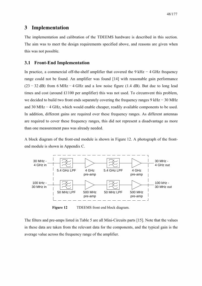
48/177
3 Implementation
The implementation and calibration of the TDEEMS hardware is described in this section.
The aim was to meet the design requirements specified above, and reasons are given when
this was not possible.
3.1 Front-End Implementation
In practice, a commercial off-the-shelf amplifier that covered the 9 kHz − 4 GHz frequency
range could not be found. An amplifier was found [14] with reasonable gain performance
(23 − 32 dB) from 6 MHz − 4 GHz and a low noise figure (1.4 dB). But due to long lead
times and cost (around £1100 per amplifier) this was not used. To circumvent this problem,
we decided to build two front ends separately covering the frequency ranges 9 kHz − 30 MHz
and 30 MHz − 4 GHz, which would enable cheaper, readily available components to be used.
In addition, different gains are required over these frequency ranges. As different antennas
are required to cover these frequency ranges, this did not represent a disadvantage as more
than one measurement pass was already needed.
A block diagram of the front-end module is shown in Figure 12. A photograph of the front-
end module is shown in Appendix C.
The filters and pre-amps listed in Table 5 are all Mini-Circuits parts [15]. Note that the values
in these data are taken from the relevant data for the components, and the typical gain is the
average value across the frequency range of the amplifier.
50 MHz LPF 500 MHzpre-amp
50 MHz LPF 500 MHzpre-amp
5.4 GHz LPF 4 GHzpre-amp
5.4 GHz LPF 4 GHzpre-amp
30 MHz -4 GHz in
100 kHz -30 MHz in
30 MHz -4 GHz out
100 kHz -30 MHz out
Figure 12 TDEEMS front end block diagram.

49/177
Mini-Circuits Part Number Part Notes
SLP-50 50 MHz low pass filter -
VLP-64 5.4 GHz low pass filter -
ZFL-500 500 MHz pre-amplifier Minimum gain = 20 dB Noise figure = 5.3 dB Frequency range = 0.05 − 500 MHz
ZJL-4HG 4 GHz pre-amplifier Minimum, typical gain = 13, 17 dB Noise figure = 4.5 dB Frequency range = 20 − 4000 MHz
From Table 5 it can be seen that the front end provides a typical gain of only 34 dB using two
cascaded amplifiers for the 30 MHz − 4 GHz frequency range, rather than 51.5 dB as
specified by the requirements. Cascading three of these amplifiers would have provided a
typical gain of 51 dB, although the sum of the noise figure and gain would be 55.5 dB. The
level of the noise floor would then exceed the level of the spurs, reducing the dynamic range.
It should also be noted that as these are typical gains, the gain will be even higher at some
frequencies (see Section 3.2.2), reducing the dynamic range even further.
We could have introduced an attenuator to reduce the gain slightly, so that the design
requirements would be met. Using a lower gain than specified by the design requirements
allowed the spurs to be seen in the results. The power budget assumed the worst-case spur
level, and as explained in Section 2.1.3, the typical spur levels are likely to be lower. As this
was a prototype measurement system, it was useful to use the lower gain so that the
behaviour of the spurs could be observed.
For the 9 kHz − 30 MHz frequency range it was not possible to find a readily available
amplifier to cover the range down to 9 kHz, so an amplifier which covered the range from
50 kHz was used instead. This amplifier will work at frequencies below 50 kHz, although its
gain will be reduced. The calibration process will correct this, although the signal-to-noise
ratio will be lower at these frequencies.
3.2 Calibration
Before the TDEEMS could be used to make radiated RF emission measurements, the
frequency response of the oscilloscope and front end must be measured. This will allow the
Table 5 TDEEMS front end components.

50/177
frequency spectra obtained from the TDEEMS to be adjusted to compensate for gain
variations in the oscilloscope and front end. The calibration measurements in this section
were made using the calibration program, which is described in Section 2.8.
Note that the oscilloscope and 30 MHz − 4 GHz front end were calibrated between 10 MHz
and 4 GHz in 10 MHz frequency steps. The oscilloscope and 100 kHz − 30 MHz front end
were calibrated using 100 kHz frequency steps.
3.2.1 Oscilloscope Calibration
The Agilent Infiniium 54854A oscilloscope used in this project is primarily intended for
measuring signals in the time domain. As such, it is calibrated by the manufacturer to ensure
that it measures the correct voltage amplitude using a known DC input voltage that is slowly
ramped from minimum to maximum amplitude (see Section 2.1.2). The manufacturer does
not specify the oscilloscope’s AC performance, and therefore its frequency response had to
be measured.
To measure the frequency response, a signal generator was used to generate a full-scale CW
input signal to the oscilloscope, over the full frequency range from 10 MHz to 4 GHz in
10 MHz intervals. A block of sample data was captured from the oscilloscope at each
frequency, and a FFT was performed by the calibration program. A suitable windowing
function was used to truncate the time domain sample data before they were processed by the
FFT (see Section 4.1.2 for further details). By measuring the amplitude of the frequency
component at the signal generator frequency and comparing this with the known signal
generator amplitude, the frequency response of the oscilloscope was determined. The results
are shown in Figure 13.
From the plot in Figure 13 it can be seen that the frequency response was not monotonic,
especially at frequencies above 2 GHz. This is to be expected, due to the difficulties in
implementing a RF input stage and ADC that can operate over such a wide frequency range.
The measurement of the oscilloscope frequency response was repeatable, with a typical
difference of 0.2 − 0.3 dB between two different measurements. The response also varied,
according to the vertical gain setting, by up to 1 dB, although the typical difference was less
than 0.5 dB (the larger differences generally occurred at frequencies between 2 GHz and
4 GHz). The oscilloscope provided four input channels, all of which provided a similar

51/177
frequency response. The gain varied by up to 1 dB between different channels, although the
typical difference was 0.5 dB.
3.2.2 30 MHz − 4 GHz Front-End Calibration
The frequency response of the front end was measured using the same method that was used
to measure the frequency response of the oscilloscope. The front-end frequency response
(Figure 14) has been determined by measuring the combined response of the front end and
the oscilloscope and then subtracting the frequency response of the oscilloscope and RF lead.
From the plot in Figure 14 it can be seen that a trough that is approximately 200 MHz wide is
present between 2 GHz and 3.5 GHz. After power up the trough is centred at 3.4 GHz, and
drifts downwards in frequency before finally settling at 2.2 GHz. The dip in the frequency
response is probably due to impedance mismatches at particular frequencies as the
temperature of the front-end pre-amplifiers increase.
0 500 1000 1500 2000 2500 3000 3500 4000-7
-6
-5
-4
-3
-2
-1
0
Frequency (MHz)
Am
plitu
de re
spon
se (d
B)
Figure 13 Agilent Infiniium 54854A frequency response with 10 mV/div vertical gain setting. The signal generator and oscilloscope were connected using a short (1 m) RF cable.

52/177
0 500 1000 1500 2000 2500 3000 3500 400022
24
26
28
30
32
34
36
38
40
Frequency (MHz)
Am
plitu
de re
spon
se (d
B)
After power on10 mins after power on1 hour after power on
Figure 14 Front-end frequency response (10 MHz − 4000 MHz). The front-end input was connected to the signal generator using a barrel connector and the output was connected to the oscilloscope using a short (1 m) RF cable.
As commercial off-the-shelf components are being used in the prototype front end, we had
little control over such performance issues and felt that it would be an inefficient use of our
time to expend effort attempting to eliminate the trough. Consequently, the approach we have
taken is to manually adjust the results to compensate for the trough.
The gain of the front end also decreases with frequency and rolled off more quickly than
anticipated in the initial design. The majority of the gain roll-off is due to the pre-amplifiers,
although the filters and insertion and cable losses between the front-end components also
contribute.
3.2.3 100 kHz − 30 MHz Front-End Calibration
The frequency response of the 100 kHz − 30 MHz front end is shown in Figure 15. Its
frequency response was measured in the same way as the 30 − 4000 MHz front end. The
response was measured over the 1 MHz − 100 MHz frequency range to demonstrate the

53/177
response of the low pass filter. From Figure 15 it can be seen that the front end provides a
gain of approximately 47 − 48 dB across the 3 − 30 MHz frequency range, which is slightly
higher than the 44.5 dB suggested by the design analysis.
3.3 Updated Power Budget
Now that the front end and oscilloscope have been calibrated, it is possible to update the
power budget analysis that was performed in Section 2.4 to include the calibrated values.
Figure 16 shows the updated blocking and maximum spur levels for the TDEEMS. The levels
determined by the design analysis in Section 2.6 are indicated by the dotted lines for
comparison. Note that the design levels assume the higher pre-amplifier gain of 51.5 dB and
flat oscilloscope and front-end frequency responses
As a reminder, the blocking threshold is the maximum received signal level across the entire
input bandwidth that can be accommodated before the ADC in the oscilloscope starts to
saturate. The maximum spur level is the level of the worst-case measured spur generated by
0 10 20 30 40 50 60 70 80 90 100-30
-20
-10
0
10
20
30
40
50
Frequency (MHz)
Am
plitu
de re
spon
se (d
B)
Figure 15 Low frequency front-end frequency response (1 MHz − 100 MHz).
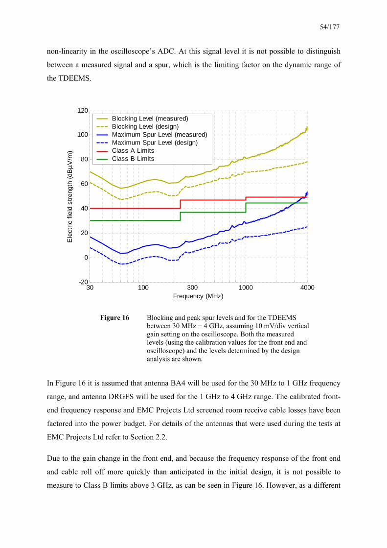
54/177
non-linearity in the oscilloscope’s ADC. At this signal level it is not possible to distinguish
between a measured signal and a spur, which is the limiting factor on the dynamic range of
the TDEEMS.
In Figure 16 it is assumed that antenna BA4 will be used for the 30 MHz to 1 GHz frequency
range, and antenna DRGFS will be used for the 1 GHz to 4 GHz range. The calibrated front-
end frequency response and EMC Projects Ltd screened room receive cable losses have been
factored into the power budget. For details of the antennas that were used during the tests at
EMC Projects Ltd refer to Section 2.2.
Due to the gain change in the front end, and because the frequency response of the front end
and cable roll off more quickly than anticipated in the initial design, it is not possible to
measure to Class B limits above 3 GHz, as can be seen in Figure 16. However, as a different
30 100 300 1000 4000-20
0
20
40
60
80
100
120
Frequency (MHz)
Ele
ctric
fiel
d st
reng
th (d
BµV
/m)
Blocking Level (measured)Blocking Level (design)Maximum Spur Level (measured)Maximum Spur Level (design)Class A LimitsClass B Limits
Figure 16 Blocking and peak spur levels and for the TDEEMS between 30 MHz − 4 GHz, assuming 10 mV/div vertical gain setting on the oscilloscope. Both the measured levels (using the calibration values for the front end and oscilloscope) and the levels determined by the design analysis are shown.

55/177
measurement antenna is required to cover the 1 − 4 GHz range, in a commercial product it
will be possible to insert an additional pre-amplifier when measuring in this frequency range.
4 Spectral Estimation
In this section the spectral estimation algorithm used to obtain the emissions spectra based on
sample data acquired using the TDEEMS will be described in detail. The spectral estimation
algorithm is implemented by the post-processing program described in Section 2.8.3.
All the data captured using the TDEEMS during this study have been processed using FFT-
based algorithms to obtain power spectrum estimates, known as periodograms. We will start
by defining the periodogram mathematically and discuss how it is typically modified to
improve its performance using windowing functions, overlapping FFTs and averaging. We
then discuss the non-continuous sampling behaviour of the TDEEMS and some of the
potential implications, including modelling a detector such as those employed in a
conventional EMC test receiver. A block diagram of the spectral estimation algorithm
implemented by the post-processing program is then provided. Finally, some of the
implications using the spectral estimation algorithm to measure impulsive emissions are
described.
4.1 Periodogram
The periodogram estimate of the power spectrum associated with a finite length sequence of
data samples, denoted by x[n], where n is the sample index, is expressed mathematically as
21
0][1)( ∑
−
=
−=PN
n
jn
P
enxN
P ωω . (18)
where NP is the number of points, or samples, over which the periodogram is calculated, and
ω is the normalised digital frequency given by
sffπω 2
= (19)
where fs is the sampling frequency, and f is the analogue frequency of interest.

56/177
In Equation 18 the summation is recognised as the discrete Fourier transform (DFT) of the
sampled data sequence. The |·| operator denotes taking the magnitude of the complex
spectrum as produced by the DFT. The computationally efficient equivalent of the DFT is the
FFT, which is employed in the post-processing program. It is necessary to square the
magnitude response of the FFT in order to obtain a power spectrum.
When measuring noise sources, the power spectrum measured using the periodogram varies
with time. Bartlett [16] modified the periodogram so as to average the results over a number
of power spectra or segments (M), hence reducing the variance of the measurements. The
Bartlett periodogram is expressed mathematically as
21
0
1
0][1)( ∑ ∑
−
=
−
=
−+=M
m
N
n
jnP
PB
P
enmNxMN
P ωω (20)
The Fourier transform assumes that the signal being analysed is continuous in time, but as the
DFT operates over a finite time interval (or block of samples), then a windowing function
should be applied to the DFT to prevent spectral leakage. Spectral leakage is the result of
discontinuities in the signal at the boundaries of the sample block due to truncation.
Windowing functions are discussed later in this section.
In the Bartlett method, the sample blocks or segments that are used to calculate the
periodogram are contiguous and non-overlapping. If a windowing function is applied to each
sample block, the Bartlett periodogram could lead to loss of spectral information, as shown in
Figure 17. Impulses that are close to the boundaries of the windows are attenuated more than
impulses in the centre of the window. If the attenuated impulses have spectral content that is
different from the non-attenuated impulses, then the spectral content of the attenuated
impulses will be attenuated or lost.
To reduce the attenuation or loss of spectral data on the boundaries of the windowed segment,
the spectra can be averaged over several overlapping segments. This leads to the Welch
periodogram [17], which is given by
21
0
1
0][][1)( ∑ ∑
−
=
−
=
−⋅⋅+=M
m
N
n
jn
PW
P
enwnmLxRMN
P ωω (21)

57/177
where L is number of samples to skip from segment to segment and R is the window coherent
gain factor. For overlapping sample blocks L must be in the range 0 < L < NP. It is typical to
use an overlap factor of approximately 50%. The window coherent gain factor, R, is used to
compensate for the gain of the window function w[n] and is given by
∑−
=
=1
0][
PN
nnwR (22)
4.1.1 Periodogram Parameters
For most of the measurements made in this study, the sampling frequency (fs) used was
20 Gsamples/s. The number of points in the FFT (NP) was chosen to match the bandwidth of
the conventional EMC test receiver to the bandwidth of each FFT bin (the bandwidth of each
FFT bin is given by Equation 12 in Section 2.5). Different parameters were used for the
Welch periodogram, according to the frequency range being measured, as the conventional
EMC test receiver bandwidth was different above and below 1 GHz. These parameters are
listed in Table 6. For comparison, the conventional EMC test receiver measurement
parameters are shown in Table 9 in Section 5.1.3.
w[n
]
n
x[n]
n
x[n]
· w
[n]
n
Original waveform
Window waveform
Original waveformafter windowingimpulses attenuated
due to windowing
segment 1 segment 2 segment 3
Figure 17 Loss of spectral information due to non-overlapping windowing.

58/177
Parameter 30 MHz − 1000 MHz
1000 MHz − 4000 MHz
Sampling frequency fs 20 Gsamples/s 20 Gsamples/s
FFT bin bandwidth Bbin 100 kHz 1 MHz
FFT length NP 200000 20000
Samples between segments L 103125 12562
Number of segments per sample block M 8 80
Approximate overlap factor between segments 48.4 % 37.2 %
In Table 6 it is assumed that the maximum sample block size of 1025 Ksamples is being used
(see Section 2.8.1), which corresponds to a sampling time interval of 51.25 µs. This was the
case for most of the measurements performed during the study so as to maximise the
probability of capturing an impulsive emission within the sampling time interval.
4.1.2 Windowing Functions
Because the periodogram operates over a data sequence of finite length, discontinuities at the
boundaries of the sample blocks result in spectral leakage. These discontinuities produce
frequency components outside the Nyquist bandwidth that are aliased back into the
measurement band, corrupting its frequency spectrum. To mitigate the effects of spectral
leakage, a windowing function can be applied to the time domain sample block to taper the
waveform to zero amplitude at the boundaries of the sample block. Some common window
functions and their corresponding frequency responses are shown in Figure 18.
The effects of using the windowing functions to reduce spectral leakage can be seen by
examining the frequency response plot in Figure 18. In the case of the rectangular window,
ie, no window is applied, a frequency response with high side-lobes is produced. If it is
assumed that only a single frequency is present in the input data sequence, and this frequency
is aligned with the centre frequency of a FFT bin, then no spectral leakage occurs since the
nulls in the frequency response are aligned with the centre of adjacent FFT bins. In this case
an integer number of cycles fit within the sample block and a windowing function is not
necessary.
Table 6 TDEEMS measurement parameters used for processing results above and below 1 GHz, based on a sample block size of 1025 Ksamples.

59/177
0 8 16 24 32-0.2
0
0.2
0.4
0.6
0.8
1
Sample index
Am
plitu
de
Rectangular windowHamming windowFlat Top window
0 1 2 3 4 5 6 7 8 9 10 11 12 13 14 15 16-100
-90
-80
-70
-60
-50
-40
-30
-20
-10
0
Number of FFT bins
Res
pons
e (d
B)
Rectangular windowHamming windowFlat Top window
Figure 18 FFT windowing functions and their corresponding normalised frequency response.

60/177
If the single frequency is not aligned with the centre frequency of a FFT bin, then the sample
block does not contain an integer number of cycles and a discontinuity exists between the end
and beginning of the sample block. This discontinuity results in additional frequency
components at the FFT output that are the result of taking the FFT over a finite time interval.
Applying a windowing function prior to taking the FFT helps to reduce the levels of
unwanted components, but at the expense of frequency resolution, as the main lobe is wider.
It can be seen from Figure 18 that the Hamming and flat top windows have lower side-lobes,
and hence lower spectral leakage at the expense of a wider main lobe. A wide main lobe is
advantageous for measuring narrowband sources, ie, those with bandwidths smaller than the
FFT bin width, as the FFT response will be close to the amplitude of the input signal. For
example, if no windowing function is applied and the input frequency is offset by half the
FFT bin width, the FFT response is 6 dB lower, as the signal power is now divided between
two adjacent FFT bins. This error in the response due to the windowing function is called the
scalloping loss, and is specified when the input frequency is offset by half the FFT bin width
in order to produce the worst-case error. The flat top window, however, is designed to have
0 dB response across an entire FFT bin width (and hence no scalloping loss), so that the peak
signal amplitude is always measured correctly. Hence, this window was used for the
calibration measurements and some of the system test measurements.
A wide main lobe is a disadvantage for measuring wideband sources, ie, those with
bandwidths greater than the FFT bin width, as the FFT response will be artificially higher as
the power in a FFT bin will include some of the power from adjacent FFT bins. The
Hamming window provides a reasonable trade-off between main lobe width and side-lobe
levels in these situations, with a scalloping loss of 2 dB. This window was used for all the
EUTs measured in Section 5.2, although the amplitudes in adjacent frequency bins may be
overestimated due to the width of the main lobe.
The choice of windowing function effectively determines the frequency response of each bin
in the FFT. To emulate the conventional EMC test receiver, a windowing function should be
chosen to match the response of its IF filter. The bandwidths specified by most EMC
standards are defined as being half the offset from the centre frequency at which the
measured power is 6 dB below its value at the centre frequency. By examining Figure 18, this
suggests that no windowing function should be applied. However, this would result in
unacceptably high side-lobe levels, which would reduce the dynamic range of the TDEEMS.

61/177
4.2 Effects of Non-continuous Sampling
During the design of the data capture program (Section 2.8.1) we stated that it is not possible
for the PC to capture data continuously from the oscilloscope and so a block-by-block
approach is taken, due to the high sampling rate of the oscilloscope. It is desirable to capture
more than one sample block using the TDEEMS so that the chances of capturing impulsive
emissions are increased and to allow the variance of the measurements to be reduced, as it is
possible to average the spectra over a greater number of segments using the periodogram.
Processing time and disk space limit the number of sample blocks that can be captured using
the TDEEMS. Each sample block of 1025 Ksamples requires 2 megabytes of disk space as
the ADC samples are 16-bit (see Section 2.1.2). For most of the measurements 50 sample
blocks were captured, ie, 100 megabytes of disk space was required for each measurement.
The typical time interval between consecutive sample blocks (or processing time) is
dependent on many factors, including hard disk performance, data transfer rates on internal
interfaces within the oscilloscope and the extent to which the Agilent Intuilink software
libraries, MATLAB and the TDEEMS software are optimised. When capturing sample
blocks with a length of 1025 Ksamples (which corresponds to a sampling time interval of
51.25 µs) using the TDEEMS, the processing time was found to be approximately 0.75 s (see
Section 6.3). Therefore, the processing time was over four orders of magnitude higher than
the capture interval and, consequently, there is a high probability that impulsive emissions
will be missed. Whilst this might at first appear to be no different from the current frequency
swept approach, it should be remembered that each sample block covers the entire RF
bandwidth. Therefore, as long as one or more sample blocks capture an impulse, it is possible
to determine the emissions at all frequencies within the RF band. It is also possible to use the
trigger on the oscilloscope to detect impulsive emissions, which will be discussed in Section
4.5.1.
4.3 Detector Modelling
In the Bartlett and Welch periodograms, the spectra of each segment are averaged. This
averaging process could be replaced with a different process, such as one that stores the
maximum power value in each FFT bin over the measurement interval, hence providing an
estimate of the peak power spectrum. This is akin to the peak detector in the conventional
EMC test receiver. Peak and average spectra were measured for all of the EUTs in this study
using both the frequency and time domain methods.

62/177
The average and peak processes could also be replaced with processes that attempt to model a
detector with a defined rise and decay time, as suggested in [18]. However, due to the non-
continuous nature of the measurements, it is not possible to provide a detector with a
continuous time response such as the quasi-peak CISPR detector. This detector has charge
and discharge times of 1 ms and 550 ms between 30 MHz and 4 GHz respectively. If the
period between data acquisition intervals was sufficiently short, it would be possible to
provide an approximation to the CISPR detector. However, as the period between the
acquisition of consecutive samples blocks with the TDEEMS is typically 0.75 seconds, and
as the CISPR detector has response times that are much shorter, it is not possible to model the
CISPR detector. It might be possible to reduce the data processing and storage time in a
commercial TDEEMS (see Section 7.2).
The CISPR quasi-peak detector was originally designed to protect amplitude modulation
(AM) radio broadcasts based on perceived audio quality tests. Its applicability to modern
digital radio modulation schemes is debatable, although some form of peak-to-average (crest
factor) power measurement is still relevant to the performance of these schemes. However,
consideration of this is beyond the scope of this study.
4.4 Data Processing Flow Diagram
A block diagram of the TDEEMS spectral estimation as implemented by the post-processing
program is shown in Figure 19. In the figure, B is the total number of sample blocks being
processed (up to 50), and m and b are the current segment and block numbers, respectively.
All other symbols were defined in previous sections.
This spectral estimation algorithm allowed the Welch periodogram to be applied over a single
block of time domain sample data captured by the TDEEMS. It was not possible to apply the
Welch periodogram (ie, overlapping segments) over more than one sample block, due to the
time discontinuity between sample blocks. However, the spectra obtained using the Welch
periodogram from each sample block could be averaged, in a similar fashion to the Bartlett
periodogram. This will allow longer averaging periods and measurements that are
consequently less noisy.
Note that the process of applying calibration factors to the output spectrum is not shown in
Figure 19. As the oscilloscope, front end, cables and antennas are calibrated at discrete
frequencies, the post-processing program calculates calibration factors for the intervening

63/177
frequencies using linear interpolation. Details on oscilloscope and front-end calibration can
be found in Section 3.2.
4.5 Measuring Emissions from Impulsive Sources
The FFT assumes that the signal being analysed is stationary over the period of the FFT (ie,
the statistics of the measured signal do not change over that time period). For this to be true,
the capture interval has to be short compared to the period over which the amplitudes of the
frequency components are varying. If a frequency component is only present for a fraction of
Increment segment number
Process next segmentfrom sample block
last segment(m = M)?
)]1(:[][ −+= ps NmLmLxnx
Apply window to segment
][][][ nxnwnx sws ⋅=
Take FFT of segment
∑−
=
−⋅=1
0
][1][PN
n
jnws
Ps enx
RNX ωω
Calculate single-sidedpower spectrum
Initialisation
⎪⎩
⎪⎨⎧
⋅= 2
2
][2][
][ω
ωω
S
SSS X
XP
Process next sample block(block number b)
][][ nxnx b=
Detector modelling
Peak
Average
0,0,0][ === bmP ω
])[],[max(][ ωωω SSPPP =
MBPPP SS
⋅+=
][][][ ωωω
1+= mm
No
Increment sampleblock number
1+= bb
Yes
last sample block(b = B)?
Take logarithm of spectrum
Yes
No
])[log(10][ ωω PPdB ⋅=
Finish
0=ω
0≠ω
Figure 19 Spectral estimation processing algorithm implemented in TDEEMS (performed by FFT spectral estimation module written in MATLAB).

64/177
this time period, then the peak instantaneous power of the frequency component is reduced
by a factor F (in dB), given by
⎟⎟⎠
⎞⎜⎜⎝
⎛⋅=
FFT
pulse
TT
F log20 (23)
where Tpulse is the duration of time for which the frequency component is present in the FFT,
and TFFT is the period of the FFT, which is given by
sPFFT fNT ⋅= (24)
where Np is the number of points, or samples in the FFT and fs is the sampling frequency.
Note the factor of 20 in Equation 23. Since the oscilloscope is measuring the input voltage,
and the value must be squared to obtain the power when calculating the periodogram.
One method of estimating the peak instantaneous power of the frequency component is to
truncate the length of the FFT to match the time duration of the frequency component (ie,
Tpulse = TFFT), which can be achieved by using a shorter window function. This is referred to
as the short time Fourier transform (STFT). By applying the STFT to a sample block at
multiple time offsets, it is possible to identify the position of the frequency component in
time. We have gained time resolution at the expense of frequency resolution, due to the
uncertainty principle [19]. We will demonstrate the use of the STFT to determine the peak
powers when measuring the some of the example equipment in Section 5.2.
If the duration of the pulse or frequency component is not known, then it is possible to
process the sample data multiple times using different window lengths. This process is
referred to as joint time and frequency analysis (JTFA). This technique has been applied to
time domain EMC simulation data to determine the shielding properties of slots and
enclosures [20].
The implications of this are that the TDEEMS will not measure the true peak power at all
frequencies of an impulsive emission, if the impulse is shorter than the period of the FFT
(10 µs with 200K samples). Depending on the characteristics of the signal (ie, the repetition
frequency), the periodogram processing, which assumes that the signal is stationary over an
entire sample block (51.25 µs) or multiple sample blocks, could make the situation worse.
For this reason the time domain results in this report will be processed over both a single

65/177
sample block and the entire 50 sample blocks, to allow the results to be compared. Some of
the measurements of impulsive sources will also be processed using the STFT to illustrate the
results of joint time and frequency analysis.
However, it should be considered that very short impulses are unlikely to cause significant
interference problems with digital radio modulation schemes. Therefore, it may be an
advantage if short impulses are attenuated in power, as these are likely to have less impact on
any radio system. For future work it could be desirable to determine the maximum
interference pulse length that would have a significant impact on the performance of common
radio standards, although this is beyond the scope of this project.
4.5.1 Triggering on Impulsive Emissions
One powerful feature of the oscilloscope for making time domain measurements is the ability
to trigger data acquisition once the voltage at the input exceeds a user-defined threshold. This
is particularly useful for measuring impulsive emissions, since the oscilloscope will always
trigger on an impulse during every measurement. As the sampling time window is very short,
this feature is essential for capturing emissions with long time periods between impulses.
Most oscilloscopes have several triggering modes, which include ‘automatic’ and ‘triggered’
modes. In ‘automatic’ mode, the Agilent Infiniium oscilloscope will wait for either a 20 ms
time period to elapse, or for a trigger event to occur (whichever happens first) before
acquiring data. In ‘triggered’ mode the oscilloscope does not acquire data unless a trigger
event occurs. The measurements made in this study used the ‘automatic’ triggering mode
unless specified otherwise. Unfortunately, the triggering will not be able to isolate impulses
when they are superimposed on broadband noise, or a continuous emission that exceeds the
amplitude of the impulsive emission.
The triggering action of the oscilloscope will help considerably when it comes to measuring
the peak radiated power, although it will make it more difficult to determine the average
radiated power. This will be discussed in more detail during the measurements in the next
section.
66/177
5 Measurements
In this section the results from the radiated EMC measurements made using conventional
EMC test receivers and the TDEEMS are presented. The results from measuring the test
sources to ensure that the TDEEMS was working and correctly calibrated are presented first.
Next, the results from measuring the example equipment are provided. Finally, we present
some results from using the TDEEMS to perform in situ EMC measurements from a railway.
To perform these tests, the EMC test facilities of EMC Projects Ltd were used (except for the
railway measurements). Details of the measurement equipment used at EMC Projects Ltd are
provided in Appendix A. The plant numbers of the equipment used are given in this section
so that it can be cross-referenced in the Appendix. In the following results, the term
‘frequency domain’ applies to measurements made using the conventional EMC test receiver,
and the term ‘time domain’ applies to measurements made using the TDEEMS.
5.1 Measurement of Test Sources
The purpose of the system tests was to check that with stationary sources the measurements
made using the TDEEMS were similar to those made using a conventional EMC test
receiver. The tests to be performed using both the frequency domain and time domain
methods are as follows.
1. Continuous Wave (CW) Tests. A signal generator and transmit antenna will be used
to produce a narrowband emission at known frequencies.
2. Hopped CW Test. Similar to the CW tests, except the signal generator frequency will
be made to follow a short pre-defined sequence, with a short dwell time at each
frequency.
3. Broadband Noise Test. The emissions from a broadband noise source as used to
calibrate the OATS will be measured.
4. Comb Generator Test. The emissions from a comb generator as used to evaluate the
shielding properties of an enclosure will be measured.
5. Low Frequency Test. The performance of the TDEEMS will be evaluated below
30 MHz, by measuring magnetic emissions.

67/177
5.1.1 Continuous Wave (CW) Tests
A two-port test using transmit and receive antennae in an anechoic lined screened room was
performed, as shown in Figure 20. A signal generator was connected to the transmit antenna
and used to generate CW signals at different frequencies. The voltage at the output of the
receive antenna was measured, using both a conventional EMC test receiver and the
TDEEMS.
Note that antenna factors and cable losses did not need to be considered, since only the
differences in power levels measured at the receiver using the different systems were of
interest. Different signal generators and transmit antennas were used depending on the
frequency range. The receiver voltages measured using the conventional EMC test receiver
(RX6) and the TDEEMS are listed in Table 7.
1.2 m 2 m
1.4 m
Signal generator
TX antenna RX antenna
1.4 m
screened room (depth = 3.6 m)
Conventional EMC test receiveror TDEEMS
5 m
3 m
Figure 20 Two-port test using screened room.

68/177
For frequencies between 30 MHz and 1 GHz, the tracking generator built into the test
receiver (RX6) was used as a signal generator with an output signal level of 90 dBµV.
Between 1 GHz and 4 GHz, an Agilent E4433B signal generator was used with an output
signal level of 77 dBµV.
RX/TX antenna
Frequency (MHz)
Frequency domain measurement
(dBµV)
Time domain measurement
(dBµV)
Difference (dB)
BA4/BIC4 30 56 57 +1
BA4/BIC4 100 70 70 0
BA4/BIC4 150 67 68 +1
BA4/BIC4 200 72 73 +1
BA4/BIC4 250 68 68 0
BA4/BIC4 300 61 61 0
BA4/LP7 300 73 73 0
BA4/LP7 400 70 71 +1
BA4/LP7 500 68 69 +1
BA4/LP7 800 64 65 +1
BA4/LP7 1000 62 62 0
DRG2/DRGFS 1000 50 50 0
DRG2/DRGFS 2000 44 44 0
DRG2/DRGFS 3000 37 39 +2
DRG2/DRGFS 4000 30 34 +4
From Table 7 it can be seen that the difference in voltage measurements between the
conventional EMC test receiver and the TDEEMS increased at frequencies above 2 GHz. The
increased differences at these frequencies are mainly due to the trough in the front-end
frequency response which could not be adequately compensated for during calibration (see
Section 3.2.2).
A second set of tests were performed using the signal generator to sweep over the frequency
range of the antennas, so that the frequency response of the two-port system could be
measured. The TDEEMS calibration software was used for this purpose and the results are
Table 7 Measured receiver voltages using conventional EMC test receiver and TDEEMS with CW waveform at various spot frequencies.

69/177
shown in Figure 21. Different transmit antennas had to be used for frequencies above and
below 300 MHz, hence the change in response at this frequency between the two figures.
There are fewer points on the frequency domain trace in Figure 21 since the conventional
EMC test receiver results were not available in electronic format and had to be entered
manually from a graph. The CW sweep was only performed up to 1 GHz, due to the
frequency range of the EMC measurement receiver and tracking generator.
5.1.2 Hopped CW Test
During the hopped CW test the Agilent E4433B signal generator was configured to generate
a sequence of CW signals at different frequencies, with a dwell time of 10 ms at each
frequency. A spectrum analyser (SA10) was used to measure the received voltage in
maximum hold mode. In this mode the frequency band was continuously swept, and the peak
voltage observed at each frequency over all sweeps was recorded. The spectrum analyser
sweep time was 10 ms and the resolution bandwidth was 5 MHz. It took a few seconds to
measure all frequencies in the sequence using the spectrum analyser. For this test, the
conventional EMC test receiver would not have been suitable, since it only performs a single
sweep across the frequency band with a 20 ms dwell time at each frequency. Therefore, only
two or three of the CW frequencies would have been measured.
The TDEEMS was configured to capture multiple sample blocks, since the capture period for
each sample block was 51.25 µs, and therefore only one transmitted frequency is likely to be
measured during this period. By taking the maximum amplitudes of the frequency spectra
generated for the sample blocks (using the peak detector), a single spectrum was produced
which includes all frequencies in the sequence.
Horn antennas were used both for transmit and receive during the hopped CW test in the
1 − 4 GHz frequency range. Tests were not performed below 1 GHz due to the frequency
range of the antennas. The results are shown in Table 8.

70/177
30 40 50 60 70 80 90100 150 200 250 300-35
-30
-25
-20
-15
-10
Frequency (MHz)
Am
plitu
de re
spon
se (d
B)
Two-port test using antennas BA4(RX) + BIC4(TX)
Time domainFrequency domain
300 400 500 600 700 800 900 1000-30
-28
-26
-24
-22
-20
-18
-16
Frequency (MHz)
Am
plitu
de re
spon
se (d
B)
Two-port test using antennas BA4(RX) + LP7(TX)
Time domainFrequency domain
Figure 21 Two-port frequency response measured using conventional EMC test receiver and the TDEEMS. 30 MHz − 300 MHz response is shown in the top plot and 300 MHz − 1 GHz response is shown in the bottom plot.

71/177
Frequency (MHz) Frequency domain
measurement (dBµV)
Time domain measurement
(dBµV)
Difference (dB)
1100 50.5 48.7 -1.8
1800 46.5 46.6 +0.1
1900 45 45.2 +0.2
2300 44 44.8 +0.8
2750 40 44.4 +4.4
3200 35 37.5 +2.5
3700 33 35.9 +2.9
From Table 8 it can again be seen that the difference in voltage measurements between the
conventional EMC test receiver and TDEEMS increased at frequencies above 2 GHz. This is
mainly due to the trough in the front-end frequency response, which is particularly prominent
at 2750 MHz in this case.
5.1.3 Broadband Noise Test
In the broadband noise test the emissions from a wideband transmitter typically used to
calibrate EMC test facilities were measured. The noise generator used is a York EMC
Services Comparison Noise Emitter (CNE) [21], with a quoted usable frequency range of
150 kHz to 1 GHz, although it also radiates at frequencies outside this range. The CNE was
fitted with its smaller 100 mm diameter top loaded monopole transmit antenna. A diagram of
the test setup is shown in Figure 22.
Table 8 Results of hopped CW tests in the 1 - 4 GHz frequency range using horn antennas DRGFS(RX) and DRG2(TX).

72/177
The measurements in the frequency domain were made using the conventional EMC test
receiver RX14. This receiver was used to perform peak voltage measurements over the
30 MHz to 4 GHz frequency range in half bandwidth frequency steps, with a dwell time of
20 ms at each frequency. Below 1 GHz, the receiver bandwidth was set to 100 kHz, which is
a bandwidth that is typical of conventional EMC measurements performed in this frequency
range. Above 1 GHz, the bandwidth was increased to 1 MHz to reduce the frequency step
size and hence the measurement time. Also, the RX14 receiver does not allow a measurement
2 m
1.4 m
CNE broadbandnoise generator
RX antenna
1.4 m
screened room (depth = 3.6 m)
Conventional EMC test receiver
2 m
30 MHz - 4 GHz front endInfiniium oscilloscope
HP8496B20 dBattenuator
5 m
3 m
Figure 22 Test setup for measuring emissions from CNE broadband noise generator.

73/177
bandwidth which is smaller than this value above 1 GHz. These details are summarised in
Table 9.
Parameter 30 MHz − 1 GHz
Frequency Range
1 GHz − 4 GHz Frequency
Range
Receiver bandwidth Brx 100 kHz 1 MHz
Frequency step fstep 50 kHz 500 kHz
Dwell time Tdwell 20 ms 20 ms
Different receive antennas were used for the frequency domain measurements above and
below 1 GHz, as described in the design of the TDEEMS (see Section 2.2). Between
30 MHz − 1 GHz antenna BA4 was used, and between 1 GHz − 4 GHz antenna DRGFS was
used.
As a result, two measurement passes had to be performed using the TDEEMS with the
different antennas. The sample block size was chosen so that the frequency resolution of the
FFT matched the bandwidth of the conventional EMC test receiver during each measurement
pass (the measurement parameters for the TDEEMS are summarised in Table 6 in Section
4.1.1). As the test sources measured in this section do not exhibit impulsive behaviour, we
captured fifty blocks of 200 Ksamples (instead of 1025 Ksamples) during each measurement
pass so as to reduce storage space. Because of this, the number of segments in each sample
block (M) was reduced from eight to one, and therefore a Bartlett periodogram was used to
process the results rather than a Welch periodogram.
For the broadband noise generator, a Hamming window was applied to the time domain
sample data, as it produces wideband RF emissions. As peak voltage measurements were
made using the conventional EMC test receiver, the peak power, instead of the average
power, was measured in each FFT bin by the TDEEMS. The emissions measured using the
frequency and time domain methods are shown in Figure 23. These results have been
corrected to compensate for the antenna factors and the cable losses. Note that the level of the
maximum spur is marked on the plot (see Section 3.3). Any spikes that appear in the
spectrum below this line may be due to spurs generated by the ADC in the oscilloscope, since
it is not possible to distinguish between the spurs and narrowband emissions.
Table 9 Conventional EMC test receiver measurement parameters.

74/177
1000
1500
2000
2500
3000
3500
4000
5055606570758085
Freq
uenc
y (M
Hz)
Electric field strength (dBµV/m)
Tim
e D
omai
nFr
eque
ncy
Dom
ain
Max
imum
Spu
r Lev
el
100
200
300
400
500
600
700
800
900
1000
30405060708090
Freq
uenc
y (M
Hz)
Electric field strength (dBµV/m)
Tim
e D
omai
nFr
eque
ncy
Dom
ain
Max
imum
Spu
r Lev
el
Figure 23 Peak radiated emissions spectra from York EMC Services CNE broadband noise source at a distance of 2 m in a screened room (30 MHz − 1 GHz, left, and 1 GHz − 4 GHz, right), with corrections for antenna factors and cable loss factors.

75/177
Because the radiated emissions power from the CNE noise generator are significantly above
Class B limits, it was necessary to reduce the gain of the TDEEMS to prevent the ADC in the
oscilloscope from saturating for the measurements below 1 GHz. A 20 dB attenuator (DB10)
was inserted at the input to the front end, and the oscilloscope vertical gain was set to
200 mV/div to achieve the gain reduction. The total peak voltage within the measurement
bandwidth was measured at 134 dBµV RMS (at the input to the oscilloscope), whereas the
normal blocking level is 89 dBµV RMS at 10 mV/div vertical gain and no attenuation (used
for measuring Class B limits). Adding the attenuation and changing the vertical gain resulted
in an effective blocking level of 135 dBµV RMS. For measurements above 1 GHz the
attenuator was not necessary, as the power spectral density (PSD) of the noise source is lower
in this frequency range, and the antenna is not designed to operate below 1 GHz. However, it
was still necessary to reduce the gain of the oscilloscope to 200 mV/div.
From the plots in Figure 23 it can be seen that the variance (or spread) of the time domain
measurements was larger (this is more noticeable below 1 GHz). This is because the period
over which the peak voltage was measured was shorter using the time domain method. The
total measurement period T in the time domain is given by
s
P
fNBT ⋅
= (25)
where B is the number of sample blocks captured, NP is the number of points, or samples,
over which the FFT is calculated, and fs is the sampling frequency. For these measurements
B = 50, NP = 200,000 and fs = 20 Gsamples/s, resulting in a total measurement period of
500 µs. The frequency domain dwell time was 40 times larger than this (20 ms), hence the
lower variance.
The emissions from the noise source are detectable using the conventional EMC test receiver
and the TDEEMS up to approximately 3 GHz, before the emissions fall below the noise
floor. Note that the difference in power measured using the two methods increases with
frequency. This is to be expected as the calibration of both systems will not be as good at
higher frequencies.

76/177
5.1.4 Comb Generator Test
In this test the RF emissions from a York EMC Services CGE01 comb generator [22] were
measured using both methods. This is a device which radiates at discrete frequencies spaced
80 or 100 MHz apart in the frequency range 80 MHz − 12 GHz, with the transmit antenna
integrated within the CGE01 housing. The measurements were made at a distance of 2 m in a
screened anechoic room, as shown in Figure 24. The angle between the comb generator and
receive antenna matches the angle used on the calibration certificate for the comb generator.
The same parameters were used for the frequency and time domain measurements as used for
the broadband noise generator, except a flat top window rather than a Hamming window was
applied to the time domain sample data in this case. This is because the comb generator
produces narrowband RF emissions and a flat top window is better for measuring narrowband
emissions (see Section 4.1.2). An average rather than the peak detector was used by the
TDEEMS.
Again, it was again necessary to reduce the gain of the TDEEMS as the RF emissions from
the comb generator were significantly above Class B limits. A 20 dB attenuator was placed at
the input of the front end and the vertical gain of the oscilloscope was set to 100 mV/div, to
prevent the ADC in the oscilloscope from saturating.
From the plot of the results in Figure 25 it can be seen that the noise floor of the conventional
EMC test receiver exhibits sharp discontinuities at certain frequencies (eg, 450 MHz and
1000 MHz). The 10 dB discontinuity at 1000 MHz is due to a change in receiver IF
bandwidth from 100 kHz to 1 MHz. The other discontinuities are due to the use of different
input stages in the receiver to cover different frequency ranges.
The noise floor of the TDEEMS generally increases in amplitude with frequency due to the
calibration factors that have been applied to correct for the frequency response of the
oscilloscope and front end (see Section 3.2). Additional discrete frequencies are also shown
in the time domain results (eg, 1250 MHz, 2250 MHz and 2750 MHz). These are spurs that
have been introduced by distortion due to non-linearity in the oscilloscope’s ADC. In this
case the spurs can be identified because the frequency spectrum of the comb generator is
known. However, these spurs are approximately 10 dB lower than the worst-case spur
amplitude measured earlier.

77/177
The measured comb amplitudes between 100 and 1000 MHz are shown in Table 10, with
antenna factors and cable loss factors applied using both measurement methods. Also shown,
for comparison, are the comb amplitudes taken from the comb generator’s calibration
certificate. Note that frequencies above 1 GHz are not considered as the measurement
antenna (BA4) is only calibrated up to 1 GHz. For the frequency domain and time domain
measurements, two sets of values are provided because the measurements were repeated
twice, a week apart.
2 m
0.94 m
CGE01 combgenerator
RX antenna
1.4 m
screened room (depth = 3.6 m)
Conventional EMC test receiver
2 m
30 MHz - 4 GHz front endInfiniium oscilloscope
HP8496B20 dBattenuator
5 m
3 m
Figure 24 Test setup for measuring emissions from CGE01 comb generator.

78/177
500
1000
1500
2000
2500
3000
3500
4000
01020304050607080
Freq
uenc
y (M
Hz)
Measured voltage at receiver input (dBµV)
Tim
e D
omai
nFr
eque
ncy
Dom
ain
Max
imum
Spu
r Lev
el
Figure 25 Average measured receiver voltages using antenna BA4 at a distance of 2 m from York EMC Services CGE01 comb generator in a screened room (30 MHz - 4000 MHz).

79/177
From Table 10 it can be seen that measurements made using the conventional EMC test
receiver correspond closely to the measurements made using the TDEEMS. The maximum
difference in measurement Run 1 was 5.9 dB at 600 MHz, and 2 dB at 600 MHz in Run 2.
The time domain measurements in Run 1 are unreliable, because the ADC saturated in some
of the measurements, which could explain the larger difference between the results. This was
only discovered during post-processing of the Run 1 measurements, and therefore the
measurements could not be repeated. In Run 2, a higher gain was used, and therefore the
measurements are not saturated. Above 300 MHz the comb amplitudes measured at EMC
Projects Ltd using both methods correspond closely to the comb amplitudes shown on its
calibration certificate. However, below 300 MHz the difference between the measurements
made at EMC Projects Ltd and the calibration certificate values increase (up to 10 dB at
100 MHz). This could be due to the differences in the screened room used to make the
measurement, different coupling with the different measurement antennas, and a different
measurement distance. The measurement distance at EMC Projects Ltd was 2 m instead of
3 m used during calibration (due to the dimensions of the screened room).
Run 1 measurement (dBµV/m)
Run 2 measurement (dBµV/m) Frequency
(MHz) Frequency domain
Time domain
Frequency domain
Time domain
Calibration measurement
(dBµV/m)
100 60.8 62.9 59.4 61.0 69.5
200 66.4 68.6 65.0 65.5 71.5
300 78.8 78.1 72.4 73.4 79.5
400 82.1 79.8 78.0 79.5 81.5
500 83.1 81.5 81.0 82.9 83.5
600 94.7 88.8 90.4 92.4 91.5
700 101.6 98.1 98.4 99.7 98.5
800 102.6 99.2 99.3 100.6 99.5
900 94.7 93.0 97.0 98.7 96.5
1000 No result 92.3 93.0 94.3 94.5
Table 10 Emissions measured from the CGE01 comb generator using conventional EMC test receiver, TDEEMS and calibration certificate values.

80/177
5.1.5 Low Frequency Tests
To evaluate the performance of the TDEEMS at low frequencies (between
20 kHz − 30 MHz), magnetic emissions were measured from a 110 kHz magnetic test source
and a 14" PC monitor using a 2 m loop antenna in the screened room. The EUT was placed at
the centre of the loop.
The peak voltage measurements in the frequency domain were made using a conventional
EMC test receiver (RX12). The low frequency measurements use a smaller measurement
bandwidth of 10 kHz, hence different measurement parameters were used for the frequency
and time domain measurements than were used previously. These are shown in Table 11.
Frequency Domain Parameters
Receiver bandwidth Brx 10 kHz
Frequency step fstep 5 kHz
Dwell time Tdwell 20 ms
Time Domain Parameters
Sampling frequency fs 5 Gsamples/s
FFT bin bandwidth Bbin 10 kHz
FFT length NP 500000
Number of segments per sample block M 1
Number of sample blocks B 50
The time domain measurements were made using the TDEEMS with the low frequency
(DC − 30 MHz) front end. The vertical gain of the oscilloscope was set to 100 mV/div. A
Hamming window and the peak detector were applied during the periodogram processing.
The currents induced in the loop antenna due to the magnetic emissions from the test source
are shown in the top plot in Figure 26. From the plot it can be seen that the noise floor of the
TDEEMS was lower, and therefore it is possible to see the harmonics from the magnetic test
source using the TDEEMS. Conventional EMC test receivers and spectrum analysers can
have noise figures as high as 30 dB when used without a pre-amplifier, whereas the
TDEEMS has a noise figure of 4.5 dB, and hence the lower noise floor.
Table 11 Frequency and time domain measurement parameters for low frequency tests (20 kHz − 30 MHz).

81/177
0.1 1 10-60
-50
-40
-30
-20
-10
0
10
20
30
Frequency (MHz)
Loop
ant
enna
cur
rent
(dB
µA)
Time DomainFrequency DomainMaximum Spur Level
0.1 1 10-60
-50
-40
-30
-20
-10
0
10
20
30
Frequency (MHz)
Loop
ant
enna
cur
rent
(dB
µA)
Time DomainFrequency DomainMaximum Spur Level
Figure 26 Currents induced in a 2 m loop antenna due to magnetic emissions from a 110 kHz magnetic test source (top plot) and a 14" PC monitor (bottom plot) in a screened room. The frequency range of the measurements was 20 kHz − 30 MHz.

82/177
Magnetic emissions were also measured from a 14" PC monitor using the same measurement
setup. The monitor was not connected to a video signal, although the cathode ray tube was
scanning. The measurement results obtained are shown in the bottom plot in Figure 26. From
the plot it can be seen that the frequency domain and time domain results are closely
correlated. Again, the results show that the noise floor of the conventional EMC test receiver
was higher than the noise floor of the TDEEMS.
5.2 Measurements of Example Equipment
The measurements that have been documented up to this point have been from sources whose
RF emissions exhibit stationary behaviour (ie, the statistics of the measured signal do not
change with time). Because stationary sources have been measured, both measurement
methods provide accurate representations of the power spectrum of the radiated emissions.
This was deliberate to allow the TDEEMS to be calibrated and tested.
In this section the radiated emissions from a range of example equipment measured using the
conventional EMC test receiver and the TDEEMS will be presented. The items tested were
chosen because they were likely to exhibit time-varying and impulsive emissions. As a
consequence, the different measurement methods are likely to produce different results. The
items tested are listed below.
1. An energy saving light bulb.
2. A fast transient generator, as used for conducted immunity EMC tests.
3. A portable television (with a cathode ray tube display).
4. An electric drill, with the suppressor removed.
5. A desktop PC, with and without its case.
5.2.1 Measurement Setup
All items were measured in an anechoic screened room using the conventional EMC test
receiver (RX14 in Appendix A) and the TDEEMS. Each item of equipment was measured
using two separate measurement passes with different antennas to cover different frequency
ranges. Antenna BA4 was used to perform measurements between 30 MHz and 1 GHz (at a
distance of 1 m) and antenna DRGFS was used to perform measurements between 1 GHz and

83/177
4 GHz (at a distance of 2 m). It was necessary to use a shorter distance for the lower
frequency measurements due to the larger size antenna, as a fixed separation of 1 m between
the sides of the screened room and the antenna was maintained. This was not the case for the
test source measurements, as the test sources were physically smaller than the example
equipment. These measurement distances are not adequate for assuming far-field conditions
at low frequencies; however, in this study we are primarily interested in comparing the
performance of the TDEEMS with the conventional EMC test receiver rather than making
accurate EMC measurements. The equipment configuration using antenna BA4 is shown in
Figure 27.
The frequency domain measurement parameters were the same as used for the noise
generator and the comb generator measurements. These are listed in Table 9 in Section 5.1.3.
The time domain measurement parameters used are listed in Table 6 in Section 4.1.1. Unlike
the measurement of the test sources, the sample block size was increased to 1025 Ksamples
to maximise the sampling time interval (51.25 µs), and hence the probability of capturing an
impulse. In many cases, the trigger facilities of the oscilloscope were used as described in
Section 4.5.1 to ensure that impulsive emissions were captured.
Both the peak and average detectors in the conventional EMC test receiver were used during
the measurements. To allow comparison, the time domain measurements were processed
using both the average and peak detectors. Unless otherwise stated, a Hamming window was
applied to the time domain sample data. Each EUT was tested twice using both methods so
that the repeatability of the measurements could be analysed. The measurements were
performed about a week apart with the same equipment, although the positioning of the EUT
and antenna inevitably varied slightly between measurements.
The optional 20 dB attenuator before the TDEEMS front end was used to reduce the signal
power when measuring sources with high radiated emissions, which would otherwise cause
the oscilloscope in the ADC to saturate. The vertical gain of the oscilloscope was also
changed to prevent this occurring. The gain settings will be listed for each measurement that
was performed.

84/177
5.2.2 Energy Saving Light Bulb
The time domain characteristic of the waveform radiated from an energy saving fluorescent
light bulb is shown in Figure 28. It can be seen that the waveform is periodic, and consists of
a burst emission that is approximately 150 ns in length, and has a repetition period of
20.77 µs (48.15 kHz). The burst emission consists of a tone that is amplitude modulated by a
2 m
0.8 m
EquipmentUnder Test
RX antenna
1.4 m
screened room (depth = 3.6 m)
Conventional EMC test receiver
1 m
30 MHz - 4 GHz front endInfiniium oscilloscope
OptionalHP8496B20 dBattenuator
5 m
3 m
Figure 27 Test setup for measuring radiated emissions in screened room using antenna BA4 and conventional EMC test receiver and TDEEMS. The separation distance was increased to 2 m when using antenna DRGFS to make measurements between 1 and 4 GHz.

85/177
Gaussian shaped pulse (as shown in the lower plot in Figure 28, which is an expanded plot of
the pulse at around 25 µs), and each burst emission could vary by up to 6 dB in power. The
measurements were made without the attenuator (see Figure 27) and with the oscilloscope
vertical gain set to 200 mV/div.
The frequency spectrum measured using the conventional EMC test receiver and TDEEMS is
shown in Figure 29. Again, the maximum spur level that could be generated by the
oscilloscope’s ADC has been calculated and is marked on the plot. From the figure it can be
seen that the emission was centred at a frequency of 160 MHz. However, the measured
amplitude using the frequency domain approach was typically 10 dB lower than the time
domain approach (all sample blocks), for both peak and average measurements. This could be
due to the response time of the detector in the conventional EMC test receiver. As observed
when measuring the test sources, the noise floor of the conventional EMC test receiver was
higher than the TDEEMS.
Because the emissions waveform was periodic, the measured spectrum remained relatively
constant between one sample block and the next. Hence, the measurements made over 50
sample blocks exhibit less noise than the measurement made over a single sample block, due
to the averaging process. The frequency of the impulse also varied slightly from one sample
block to another; hence the apparent difference in frequency between the measurements made
over a single sample block and all 50 sample blocks. This can be seen in Figure 30, which
shows the spectra of each sample block captured.
The measurements in the time domain require further explanation. The time domain average
measurement was slightly higher than the true average measurement, as three impulses fit
within the 51.25 µs sampling time window, but the sampling time window is not three times
the repetition period as shown in Figure 28. To obtain a better measurement of the average
power, the sampling time window should be an integer number of periods of the time domain
waveform. In this case, the sampling time window was approximately 2.5 periods in length.
Reprocessing the data with a 41.54 µs (two periods) window produced an average
measurement which was 2.4 dB lower (38.8 dB instead of 41.2 dB at 160.1 MHz).

86/177
0 5 10 15 20 25 30 35 40 45 50
-0.5
-0.4
-0.3
-0.2
-0.1
0
0.1
0.2
0.3
0.4
0.5
Time (µs)
Am
plitu
de (V
)
25.5 25.55 25.6 25.65 25.7 25.75 25.8 25.85 25.9
-0.5
-0.4
-0.3
-0.2
-0.1
0
0.1
0.2
0.3
0.4
0.5
Time (µs)
Am
plitu
de (V
)
Figure 28 Time domain emissions waveform from an energy saving light bulb at a distance of 1 m in a screened room (measured voltage at input to oscilloscope with no correction factors). The lower plot expands the area of the upper plot that centres around 25 µs.

87/177
3040
5060
7080
9010
020
030
040
050
060
070
080
090
010
00-1
00102030405060
Freq
uenc
y (M
Hz)
Electric field strength (dBµV/m)
Tim
e D
omai
n (a
vera
ge, s
ingl
e bl
ock)
Tim
e D
omai
n (a
vera
ge, a
ll bl
ocks
)Fr
eque
ncy
Dom
ain
(ave
rage
)M
axim
um S
pur L
evel
3040
5060
7080
9010
020
030
040
050
060
070
080
090
010
00-1
00102030405060
Freq
uenc
y (M
Hz)
Electric field strength (dBµV/m)
Tim
e D
omai
n (p
eak,
sin
gle
bloc
k)Ti
me
Dom
ain
(pea
k, a
ll bl
ocks
)Fr
eque
ncy
Dom
ain
(pea
k)M
axim
um S
pur L
evel
Figure 29 Peak and average radiated emissions spectra from energy saving light bulb at 1 m distance in screened room (30 MHz − 1 GHz), with corrections for antenna factors and cable loss factors.

88/177
Because the length of the burst emission from the energy saving light bulb (Tpulse = 150 ns) is
much shorter than the length of the sampling window (TFFT = 10 µs), the peak radiated power
measured using the TDEEMS is much lower than the peak instantaneous power (see Section
4.5). Using Equation 23 from this section, the measured peak power is approximately 36.5 dB
lower than the actual peak instantaneous power.
The effect of using a FFT with a length that was matched to the duration of the burst emission
from the light bulb (ie, TFFT = Tpulse) can be seen by examining the plot on the left-hand side
of Figure 31. The length of the FFT was 3000 samples (corresponding to a time period of
150 ns) and was aligned with an impulse in the time domain, ie, the FFT was performed at a
time offset of 25.5 µs (see Figure 28). As a result, the peak power of the impulse has been
correctly measured (ie, was approximately 37 dB higher than the power of the impulse
measured using the full 200 Ksample FFT). The harmonics were now more apparent as the
signal-to-noise ratio has increased, but the frequency resolution has been degraded to
6.66 MHz rather than 100 kHz.
0
5
10
15
20
25
30
35
40
45
50100 110 120 130 140 150 160 170 180 190 200
Frequency (MHz)
Sam
ple
Blo
ck N
umbe
r
-40
-30
-20
-10
0
10
20
30
40
Ele
ctric
fiel
d st
reng
th (d
BµV
/m)
Figure 30 Radiated emissions spectra (between 100 − 200 MHz) of light bulb measured over 50 sample blocks. The variation in the frequency of the impulse from one sample block to another is visible.

89/177
3040
5060
7080
9010
020
030
040
050
060
070
080
090
010
00-4
0
-20020406080
Freq
uenc
y (M
Hz)
Electric field strength (dBµV/m)
Tim
e D
omai
n (p
eak,
sin
gle
200
Ksa
mpl
e FF
T)Ti
me
Dom
ain
(pea
k, s
ingl
e 30
00 s
ampl
e FF
T)M
axim
um S
pur L
evel
Figure 31 Effect of using a FFT with a length that is matched to the duration of the burst emission from the light bulb (left) and using a swept STFT to localise the burst emission in time and frequency (right).

90/177
The three-dimensional plot on the right-hand side of Figure 31 shows the results of applying
a STFT to a single block of 1025 Ksamples (see Section 4.5). The length of the FFT was set
to the length of the impulse (3000 samples or 150 ns), and the FFT was performed at different
time offsets within the sample block. 1,500 FFTs were performed, as shown on the ‘sample
block number’ axis, which is effectively the time axis. Each sample block was spaced
approximately 1,025,000/1,500 = 683 samples apart, which corresponds to a time period of
34 ns. There was a high overlap between each FFT (approximately 77%) to improve the
accuracy of the measured peak radiated power.
The advantage of the swept STFT was that only the duration of the impulse needed to be
known in order to measure the peak amplitude. More processing was required though, as a
FFT had to be calculated for each time offset. As the time emissions waveform from the light
bulb was relatively simple, it would be possible to automate the measurement of the burst
period of the waveform and repetition rate by analysing the waveform in the time domain.
Hence, it would be possible to make better measurements of peak and average power without
having to use multiple FFTs. However, a more complex waveform, which was superimposed
on broadband noise or with multiple sources of impulsive emissions, would be significantly
more difficult to measure. The STFT would perform better in these situations.
Returning to the measured radiated emissions spectra in Figure 29, the spurs from the ADC in
the oscilloscope are clearly visible in the spectra measured using the time domain method.
These are more prominent in the average measurements (due to the lower noise floor) at
frequencies of 250, 400, 500, 625, 750 and 875 MHz. However, the spur levels are well
below the maximum spur level predicted by our initial analysis. There were no emissions that
could be measured from the energy saving light bulb above 1 GHz. Hence, there is no plot of
the spectrum between 1 and 4 GHz.
The repeatability of the light bulb peak radiated spectra measurements is shown by the plots
in Figure 32. It can be seen that the conventional EMC test receiver produced the same peak
measurement of 40 dBµV/m; however the time domain method produced peak results
(calculated over 50 sample blocks) of 48 dBµV/m and 52 dBµV/m for each measurement run.
It was observed that the amplitude of the emissions from the light bulb decreased slightly
depending on the length of time the light bulb had been switched on. However, the
measurements were performed in the same sequence (ie, the frequency domain measurement
was made 20 minutes before the time domain measurement) in both measurement runs. The

91/177
3040
5060
7080
9010
020
030
040
050
060
070
080
090
010
000102030405060
Freq
uenc
y (M
Hz)
Electric field strength (dBµV/m)
Tim
e D
omai
n (r
un 1
, pea
k, a
ll bl
ocks
)Fr
eque
ncy
Dom
ain
(run
1, p
eak)
Max
imum
Spu
r Lev
el
3040
5060
7080
9010
020
030
040
050
060
070
080
090
010
000102030405060
Freq
uenc
y (M
Hz)
Electric field strength (dBµV/m)
Tim
e D
omai
n (r
un 2
, pea
k, a
ll bl
ocks
)Fr
eque
ncy
Dom
ain
(run
2, p
eak)
Max
imum
Spu
r Lev
el
Figure 32 Repeatability of energy saving light bulb measurements using conventional EMC test receiver and TDEEMS. Two different sets of measurements are shown by the left and right plots.

92/177
light bulb had been switched on for the same length of time at the time of each measurement.
It could be that the short measurement interval of the TDEEMS was not sufficient to provide
a stable peak power measurement, even though the measurement was made over 50 sample
blocks. This resulted in a total measurement interval of 2.56 ms (50 * 51.25 µs), although the
frequency domain measurement was made with a significantly longer dwell time of 20 ms.
5.2.3 Fast Transient Generator
A fast transient generator is used during conducted EMC immunity testing for mains powered
appliances. The EUT is plugged into the transient generator, which produces short transients
of up to several kilovolts on the mains power supply to the EUT. The transients consist of a
15 ms burst of exponentially rising and decaying pulses, with a 2 ms spacing. The burst is
repeated every 300 ms. Each pulse has a rise time of approximately 5 ns and a decay time of
approximately 90 ns.
The radiated emissions waveform from the transient generator will have a different shape
from the power supply waveform that it produces, although the transient generator will
radiate at the same time that the discharge on the mains supply occurs. As the minimum pulse
spacing is 15 ms, and the TDEEMS sampling window is 51.25 µs, then only a single pulse
can be captured within the window. The time domain emissions waveform from the transient
generator is shown in Figure 33. The measurements were made with the 20 dB attenuator (see
Figure 27) and a vertical gain setting of 200 mV/div on the oscilloscope.
The frequency spectrum that was measured using the conventional EMC test receiver and
TDEEMS is shown in Figure 34. From the figure it can be seen that the spectrum captured
using the frequency domain approach appears as a comb spectrum. This is because the EMC
test receiver dwell time is only 20 ms, whereas the pulse repetition frequency (PRF) of the
transient generator is 300 ms. Hence, the impulse was only captured at some frequencies,
resulting in measurement of the noise floor at most frequencies.
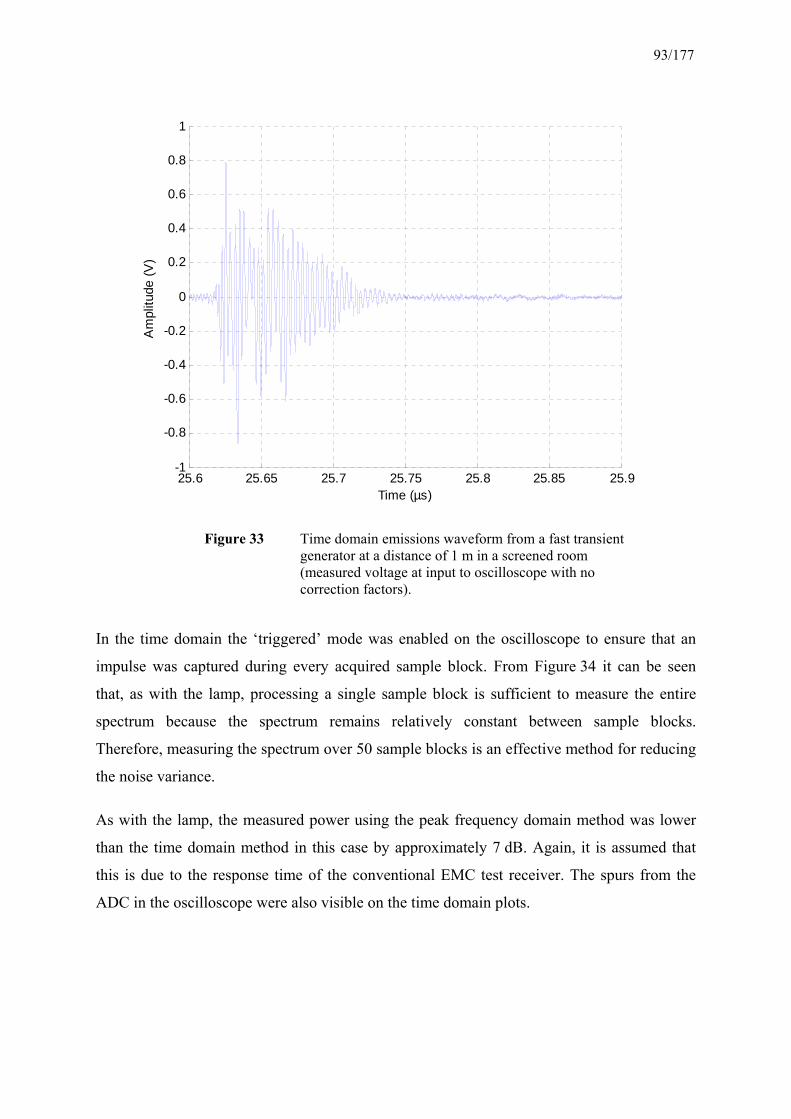
93/177
In the time domain the ‘triggered’ mode was enabled on the oscilloscope to ensure that an
impulse was captured during every acquired sample block. From Figure 34 it can be seen
that, as with the lamp, processing a single sample block is sufficient to measure the entire
spectrum because the spectrum remains relatively constant between sample blocks.
Therefore, measuring the spectrum over 50 sample blocks is an effective method for reducing
the noise variance.
As with the lamp, the measured power using the peak frequency domain method was lower
than the time domain method in this case by approximately 7 dB. Again, it is assumed that
this is due to the response time of the conventional EMC test receiver. The spurs from the
ADC in the oscilloscope were also visible on the time domain plots.
25.6 25.65 25.7 25.75 25.8 25.85 25.9-1
-0.8
-0.6
-0.4
-0.2
0
0.2
0.4
0.6
0.8
1
Time (µs)
Am
plitu
de (V
)
Figure 33 Time domain emissions waveform from a fast transient generator at a distance of 1 m in a screened room (measured voltage at input to oscilloscope with no correction factors).

94/177
3040
5060
7080
9010
020
030
040
050
060
070
080
090
010
001020304050607080
Freq
uenc
y (M
Hz)
Electric field strength (dBµV/m)
Tim
e D
omai
n (p
eak,
sin
gle
bloc
k)Ti
me
Dom
ain
(pea
k, a
ll bl
ocks
)Fr
eque
ncy
Dom
ain
(pea
k)M
axim
um S
pur L
evel
3040
5060
7080
9010
020
030
040
050
060
070
080
090
010
0001020304050607080
Freq
uenc
y (M
Hz)
Electric field strength (dBµV/m)
Tim
e D
omai
n (a
vera
ge, s
ingl
e bl
ock)
Tim
e D
omai
n (a
vera
ge, a
ll bl
ocks
)Fr
eque
ncy
Dom
ain
(ave
rage
)M
axim
um S
pur L
evel
Figure 34 Peak and average radiated emissions spectra from fast transient generator at 1 m distance in screened room (30 MHz − 1 GHz), with corrections for antenna factors and cable loss factors.

95/177
The frequency domain average measurements are very close to the noise floor and as a
consequence are likely to be unreliable. The time domain average measurements were higher
than the true average because the oscilloscope always triggered on the impulse.
Unfortunately, as with most commercial oscilloscopes, it is not possible for the Infiniium
oscilloscope to trigger immediately, which might provide a more accurate average power
measurement. Even if it were possible to do this, it would then be unlikely that the impulse
would be captured due to the short time sampling window.
One possible solution would be to measure the time period between trigger events on the
oscilloscope and to attempt to correct the results assuming no emissions are present between
the trigger events, which is the case with the fast transient generator. Again, the oscilloscope
used does not have this capability, although it could be provided by a commercial
implementation of the system. It may also be possible to reduce the sampling frequency of
the oscilloscope (ie, use a longer timebase setting) to allow the period between impulses to be
measured.
As the characteristics of the fast transient generator waveform are known, it is possible to
apply a correction factor to the average power measurements. Since the impulse occurs seven
times (Noccurrences) within the period of the waveform (Tperiod = 300 ms), the correction factor
F (in dB) is given by
⎟⎟⎠
⎞⎜⎜⎝
⎛ ⋅⋅=
period
FFTsoccurrence
TTN
F log20 (26)
where TFFT is the period of the time sampling window (51.25 µs). This provides a correction
factor of -58.4 dB for the average measurements made using the time domain method.
The repeatability of the fast transient generator peak radiated spectra measurements is shown
by the plots in Figure 35. The measured spectrum was different for each measurement run,
although the envelope of the spectrum produced by the two different methods was almost
identical in each case. Therefore, the different spectrum measured during each measurement
run was probably due to the variation in equipment position and orientation, and hence the
variation in the frequencies of the resonances due to the screened room.

96/177
3040
5060
7080
9010
020
030
040
050
060
070
080
090
010
001020304050607080
Freq
uenc
y (M
Hz)
Electric field strength (dBµV/m)
Tim
e D
omai
n (r
un 2
, pea
k, a
ll bl
ocks
)Fr
eque
ncy
Dom
ain
(run
2, p
eak)
Max
imum
Spu
r Lev
el
3040
5060
7080
9010
020
030
040
050
060
070
080
090
010
001020304050607080
Freq
uenc
y (M
Hz)
Electric field strength (dBµV/m)
Tim
e D
omai
n (r
un 1
, pea
k, a
ll bl
ocks
)Fr
eque
ncy
Dom
ain
(run
1, p
eak)
Max
imum
Spu
r Lev
el
Figure 35 Repeatability of fast transient generator measurements using conventional EMC test receiver and TDEEMS. Two different sets of measurements are shown by the left and right plots.

97/177
5.2.4 Portable Television
The time domain radiated emissions waveform from a portable 14" colour television is shown
in Figure 36. The measurements were made without the attenuator (see Figure 27) with a
vertical gain setting of 50 mV/div and a voltage trigger level of 75 mV on the oscilloscope.
The most significant emissions from the television are due to the electromagnets that are used
to deflect the electron beam inside the cathode ray tube. The peak field strengths are
developed during the horizontal and vertical flyback periods, when the electron beam returns
to the side or top of the picture, respectively.
During the measurements, the television was not connected to a video signal, but the electron
beam was still scanning. Therefore, horizontal and vertical flyback were not synchronised to
a fixed time reference and so the period between horizontal and vertical flyback varied. As no
video signal was present, the control circuitry blanked the picture to black.
The frequency spectrum measured using the conventional EMC test receiver and TDEEMS is
shown in Figure 37. The highest emission from the television is centred at 75 MHz, with
harmonics visible at multiples of this frequency. The peak measurements made using the
frequency domain and time domain methods are similar (46 and 51 dBµV/m, respectively),
but the average measurement in the frequency domain mode does not show the broadband
emission at 75 MHz. This behaviour may be explained by examining Figure 38, which shows
the peak spectra measured using the 75 mV trigger setting and no trigger on the oscilloscope.
In the plot without the trigger the emissions at 75 MHz (and harmonics) are not present. As
these emissions are only being generated during flyback of the electron beam, the time
domain measurement does not capture these non-continuous emissions without the trigger.
Likewise, the frequency domain average measurement will be low as the emission is likely to
have a low duty cycle.
There were no emissions that could be measured from the portable TV above 1 GHz. Hence,
there is no plot of the spectrum between 1 and 4 GHz.

98/177
0 5 10 15 20 25 30 35 40 45 50
-0.1
-0.05
0
0.05
0.1
Time (µs)
Am
plitu
de (V
)
25.2 25.4 25.6 25.8 26 26.2 26.4 26.6 26.8 27
-0.1
-0.05
0
0.05
0.1
Time (µs)
Am
plitu
de (V
)
Figure 36 Time domain emissions waveform from a portable 14" colour television at a distance of 1 m in a screened room (measured voltage at input to oscilloscope with no correction factors).
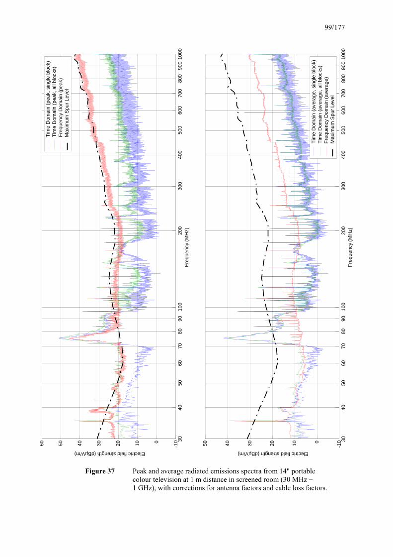
99/177
3040
5060
7080
9010
020
030
040
050
060
070
080
090
010
00-1
00102030405060
Freq
uenc
y (M
Hz)
Electric field strength (dBµV/m)
Tim
e D
omai
n (p
eak,
sin
gle
bloc
k)Ti
me
Dom
ain
(pea
k, a
ll bl
ocks
)Fr
eque
ncy
Dom
ain
(pea
k)M
axim
um S
pur L
evel
3040
5060
7080
9010
020
030
040
050
060
070
080
090
010
00-1
001020304050
Freq
uenc
y (M
Hz)
Electric field strength (dBµV/m)
Tim
e D
omai
n (a
vera
ge, s
ingl
e bl
ock)
Tim
e D
omai
n (a
vera
ge, a
ll bl
ocks
)Fr
eque
ncy
Dom
ain
(ave
rage
)M
axim
um S
pur L
evel
Figure 37 Peak and average radiated emissions spectra from 14" portable colour television at 1 m distance in screened room (30 MHz − 1 GHz), with corrections for antenna factors and cable loss factors.

100/177
3040
5060
7080
9010
020
030
040
050
060
070
080
090
010
000102030405060
Freq
uenc
y (M
Hz)
Electric field strength (dBµV/m)
Tim
e D
omai
n (n
o tri
gger
, pea
k, a
ll bl
ocks
)Ti
me
Dom
ain
(75
mV
trig
ger,
peak
, all
bloc
ks)
Max
imum
Spu
r Lev
el
Figure 38 Peak radiated emissions spectra from 14" portable colour television at 1 m distance in screened room, measured with a 75 mV trigger voltage or no trigger on the oscilloscope. Note the absence of emissions at 75 MHz (and harmonics) on the plot with no trigger.

101/177
The repeatability of the portable TV peak radiated spectra measurements is shown by the
plots in Figure 39. As with the fast transient generator, the measured spectrum was different
for each measurement run, although the variation was similar for both measurement methods.
The powers measured during the second run were generally higher than those measured
during the first run; for example, the peak emission at 75 MHz was approximately 6 dB
higher during the second run (determined using both measurement methods). As before, the
variation could have been due to the differences in the equipment position and orientation, or
the amplitude of the emissions might have depended upon on the length of time for which the
television had been switched on. In the second set of measurements, the television had been
switched on for approximately an hour before the measurements were made, while the first
set of measurements were made shortly after the television had been switched on.

102/177
3040
5060
7080
9010
020
030
040
050
060
070
080
090
010
000102030405060
Freq
uenc
y (M
Hz)
Electric field strength (dBµV/m)
Tim
e D
omai
n (r
un 1
, pea
k, a
ll bl
ocks
)Fr
eque
ncy
Dom
ain
(run
1, p
eak)
Max
imum
Spu
r Lev
el
3040
5060
7080
9010
020
030
040
050
060
070
080
090
010
000102030405060
Freq
uenc
y (M
Hz)
Electric field strength (dBµV/m)
Tim
e D
omai
n (r
un 2
, pea
k, a
ll bl
ocks
)Fr
eque
ncy
Dom
ain
(run
2, p
eak)
Max
imum
Spu
r Lev
el
Figure 39 Repeatability of portable TV measurements using conventional EMC test receiver and TDEEMS. Two different sets of measurements are shown by the left and right plots.

103/177
5.2.5 Electric Drill
The typical time domain emissions waveform from a handheld electric drill is shown in
Figure 40 and Figure 41. The measurements were made with the 20 dB attenuator (see
Figure 27) and a vertical gain setting of 200 mV/div on the oscilloscope.
The suppressor in the electric drill has been removed, and hence, the waveform consists of
sporadic bursts of pulses caused by arcing of the drill commutator. During the measurements
the drill was under no mechanical load (ie, no drill bit was attached and the drill was allowed
to spin freely). The spectrum of each pulse is similar, although the spacing in time between
the impulses varies significantly, as the arcing process occurs randomly.
0 5 10 15 20 25 30 35 40 45 50-0.5
-0.4
-0.3
-0.2
-0.1
0
0.1
0.2
0.3
0.4
0.5
Time (µs)
Am
plitu
de (V
)
Figure 40 Time domain emissions waveform (51.25 µs sampling window) from an electric drill with no suppressor fitted at a distance of 1 m in a screened room (measured voltage at input to oscilloscope with no correction factors).

104/177
25 25.5 26 26.5 27 27.5-0.5
-0.4
-0.3
-0.2
-0.1
0
0.1
0.2
0.3
0.4
0.5
Time (µs)
Am
plitu
de (V
)
25.58 25.6 25.62 25.64 25.66 25.68 25.7 25.72-0.5
-0.4
-0.3
-0.2
-0.1
0
0.1
0.2
0.3
0.4
0.5
Time (µs)
Am
plitu
de (V
)
Figure 41 Time domain emissions waveform over two shorter time windows from an electric drill with no suppressor fitted at a distance of 1 m in a screened room (measured voltage at input to oscilloscope with no correction factors).

105/177
The frequency spectrum measured using the conventional EMC test receiver and TDEEMS is
shown in Figure 42. The emissions from the drill are broadband and extend above 1 GHz, as
shown by the plot in Figure 43. Note that the measurement bandwidth is 1 MHz instead of
100 kHz above 1 GHz, hence the 10 dB transition in power at this frequency.
The peak frequency domain and time domain results were similar. The time domain peak
measurements made over 50 sample blocks are higher than those made over one sample
block, as the amplitudes of the impulses vary and therefore the likelihood of detecting a
larger peak increases when measuring over a longer time interval. By this rationale, the
frequency domain results should be higher, as the conventional EMC test receiver dwell time
was 20 ms and the time domain measurement time was approximately 2.5 ms over 50 sample
blocks. However, this did not appear to be the case as it was with the broadband noise
generator measured in Section 5.1.3. This is likely to be because the response time of the
peak detector in the conventional EMC test receiver is unable to track the rapidly changing
amplitude of the impulsive emission. In the case of the broadband noise generator, the
continuous emission allowed the peak detector to respond correctly.
The time domain average measurements were typically 30 dB higher than the frequency
domain average measurements. As with all the EUTs measured so far, the shape of the
spectra of each impulse appeared to be reasonably constant and averaging over 50 sample
blocks produced a result with a lower noise variance. The triggering action of the
oscilloscope will result in an average measurement that is higher than the true average. In this
case it is not possible to calculate a correction factor, due to the variable time spacing
between impulses. However, as suggested in Section 7.2, it may be possible to use a longer
timebase setting on the oscilloscope to try to estimate the average spacing and calculate the
correction factor from this.

106/177
3040
5060
7080
9010
020
030
040
050
060
070
080
090
010
0001020304050607080
Freq
uenc
y (M
Hz)
Electric field strength (dBµV/m)
Tim
e D
omai
n (a
vera
ge, s
ingl
e bl
ock)
Tim
e D
omai
n (a
vera
ge, a
ll bl
ocks
)Fr
eque
ncy
Dom
ain
(ave
rage
)M
axim
um S
pur L
evel
3040
5060
7080
9010
020
030
040
050
060
070
080
090
010
0020304050607080
Freq
uenc
y (M
Hz)
Electric field strength (dBµV/m)
Tim
e D
omai
n (p
eak,
sin
gle
bloc
k)Ti
me
Dom
ain
(pea
k, a
ll bl
ocks
)Fr
eque
ncy
Dom
ain
(pea
k)M
axim
um S
pur L
evel
Figure 42 Peak and average radiated emissions spectra from electric drill without suppressor at 1 m distance in screened room (30 MHz − 1 GHz), with corrections for antenna factors and cable loss factors.

107/177
1000
1500
2000
2500
3000
3500
4000
50556065707580859095100
Freq
uenc
y (M
Hz)
Electric field strength (dBµV/m)
Dril
l - T
ime
Dom
ain
(pea
k, s
ingl
e bl
ock)
Dril
l - T
ime
Dom
ain
(pea
k, a
ll bl
ocks
)D
rill -
Fre
quen
cy D
omai
n (p
eak)
Max
imum
Spu
r Lev
el
Figure 43 Peak radiated emissions spectra from electric drill (without suppressor fitted) at 2 m distance in screened room (1 GHz - 4 GHz), with corrections for antenna factors and cable loss factors.

108/177
As has been the case with the other test sources, the length of the impulse from the drill
(typically 150 ns) was shorter than the length of the sampling window (10 µs), and therefore
peak radiated power measured using the TDEEMS was much lower than the peak
instantaneous power. However, a variable number of impulses occurred during each capture
interval, which makes it more difficult to calculate a corrected peak power. To provide a
better estimate of the peak power, a STFT has been applied to a single block of
1025 Ksamples, as shown by the plot in Figure 44.
As with the STFT performed on the light bulb measurements, the length of the FFT was set to
the length of the impulse (3000 samples or 150 ns), and a FFT was performed at different
time offsets within the sample block. As before, 1500 FFTs were performed over a
1025 Ksample block so each FFT corresponds to a time period of 34 ns (the ‘sample block
number’ axis corresponds to the FFT number). As can be seen from the time domain
waveform plot of the sample block in Figure 40, most of the impulses were generated
between 24 µs and 28 µs. Therefore, only FFT numbers 700 to 820 are shown in the STFT
plot, which correspond approximately to this time range. The peak instantaneous powers
(over a 66.6 MHz bandwidth) reached 95 dBµV/m, which was almost 20 dB higher than the
peak measured powers over the entire 1025 Ksample block (see Figure 42).
The repeatability of the electric drill peak radiated spectra measurements are shown by the
plots in Figure 45. In the first measurement run the shape of the power spectra measured
using the two methods varied, although this was not the case in the second measurement run.
This may have been due to the length of time between the two different measurements. In
both measurement runs the frequency domain measurements were made shortly after the drill
was switched on. The time domain measurements were made after the drill had been running
for 1½ hours and 20 minutes in the case of the first and second measurement runs,
respectively. As a result, the temperature of the drill could affect the radiated power
spectrum, hence explaining the differences between the frequency domain and time domain
results in the first measurement run, as the time period between the two measurements was
greater.

109/177
Figure 44 Using a STFT to localise the impulses from the drill in time and frequency.
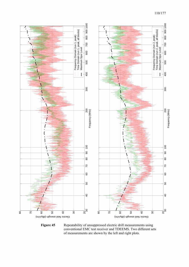
110/177
3040
5060
7080
9010
020
030
040
050
060
070
080
090
010
0020304050607080
Freq
uenc
y (M
Hz)
Electric field strength (dBµV/m)
Freq
uenc
y D
omai
n (r
un 2
, pea
k)Ti
me
Dom
ain
(run
2, p
eak,
all
bloc
ks)
Max
imum
Spu
r Lev
el
3040
5060
7080
9010
020
030
040
050
060
070
080
090
010
0020304050607080
Freq
uenc
y (M
Hz)
Electric field strength (dBµV/m)
Freq
uenc
y D
omai
n (r
un 1
, pea
k)Ti
me
Dom
ain
(run
1, p
eak,
all
bloc
ks)
Max
imum
Spu
r Lev
el
Figure 45 Repeatability of unsuppressed electric drill measurements using conventional EMC test receiver and TDEEMS. Two different sets of measurements are shown by the left and right plots.

111/177
5.2.6 Desktop PC
The time domain radiated emissions waveform from a desktop PC with its cover removed is
shown in Figure 46. The measurements were made without the attenuator (see Figure 27) and
a vertical gain setting of 50 mV/div on the oscilloscope.
From Figure 46 it can be seen that the emissions waveform from the PC is very complex. The
frequency spectrum measured using the conventional EMC test receiver and TDEEMS is
shown in Figure 47. From the spectra it was possible to see line emissions that are likely to be
due to harmonics of the central processor unit (CPU) bus frequency (60 MHz), although the
fundamental frequency was not as prominent. Emissions due to the internal CPU clock
frequency (150 MHz) are not so noticeable but are also present. The other narrowband
emissions are probably due to other clock frequencies used in the PC and their harmonics.
The PC will be a source of many different impulsive emissions as it is a complex switching
digital device. These will manifest themselves as broadband noise, and from Figure 48 it can
0 5 10 15 20 25 30 35 40 45 50
-0.1
-0.05
0
0.05
0.1
Time (µs)
Am
plitu
de (V
)
Figure 46 Time domain emissions waveform from a desktop PC with the cover removed at a distance of 1 m in a screened room (measured voltage at input to oscilloscope with no correction factors).

112/177
be seen that these extend beyond 1 GHz. Note that the noise floor of the conventional EMC
test receiver swamps the measurement of the radiated emissions from the PC above 1 GHz.
As expected, the peak and average emissions measured in both frequency ranges over the
longer time interval (50 sample blocks or approximately 2.5 ms) are higher than those
measured over a single sample block (51.25 µs) using the time domain method. As there are
many continuous and impulsive sources of emissions from the PC, the frequency domain
peak measurement is higher than the time domain measurement, due to the longer 20 ms
measurement interval. In this case, the response time of the peak detector in the conventional
EMC test receiver has less effect, because the emissions from the PC are continuous.
Unlike the other EUTs measured, the average measurements made using the conventional
EMC test receiver were similar rather than lower than the average measurements made using
the TDEEMS. Again, this is probably due to the continuous emissions from the PC for two
reasons. Firstly, the triggering on the oscilloscope will not produce time domain
measurements that are higher than the true average, since the oscilloscope will always trigger
due to the continuous emissions. Secondly, the response time of the average detector in the
conventional EMC test receiver will not have so much of an effect in reducing the frequency
domain measurement.
It was also observed that the frequency domain average measurements are higher at some
frequencies, eg 800 − 900 MHz, than the time domain measurements. This was due to the
higher noise floor of the conventional EMC test receiver, which limited the dynamic range
for the frequency domain measurements. This effect was not as severe over the 300 − 400
MHz frequency range, where the radiated emissions from the PC were generally higher than
the noise floor of the conventional EMC test receiver.
The repeatability of the PC peak radiated spectra measurements is shown by the plots in
Figure 49. The measured radiated power spectra were very similar between the two
measurement runs, with the typical difference in power being only 2 − 3 dB for line
emissions. In both measurement runs the results obtained using both measurement methods
were very similar.

113/177
100
200
300
400
500
600
700
800
900
1000
-100102030405060
Freq
uenc
y (M
Hz)
Electric field strength (dBµV/m)
Tim
e D
omai
n (p
eak,
sin
gle
bloc
k)Ti
me
Dom
ain
(pea
k, a
ll bl
ocks
)Fr
eque
ncy
Dom
ain
(pea
k)M
axim
um S
pur L
evel
100
200
300
400
500
600
700
800
900
1000
-100102030405060
Freq
uenc
y (M
Hz)
Electric field strength (dBµV/m)
Tim
e D
omai
n (a
vera
ge, s
ingl
e bl
ock)
Tim
e D
omai
n (a
vera
ge, a
ll bl
ocks
)Fr
eque
ncy
Dom
ain
(ave
rage
)M
axim
um S
pur L
evel
Figure 47 Peak and average radiated emissions spectra from PC at 1 m distance in screened room (30 MHz - 1 GHz), with corrections for antenna factors and cable loss factors.

114/177
Freq
uenc
y (M
Hz)
1000
1500
2000
2500
3000
3500
4000
20304050607080
Electric field strength (dBµV/m)
PC
with
cas
e re
mov
ed -
Tim
e D
omai
n (p
eak,
sin
gle
bloc
k)P
C w
ith c
ase
rem
oved
- Ti
me
Dom
ain
(pea
k, a
ll bl
ocks
)P
C w
ith c
ase
rem
oved
- Fr
eque
ncy
Dom
ain
(pea
k)M
axim
um S
pur L
evel
Figure 48 Peak radiated emissions spectra from PC (without case fitted) at 2 m distance in screened room (1 GHz - 4 GHz), with corrections for antenna factors and cable loss factors.

115/177
100
200
300
400
500
600
700
800
900
1000
0102030405060
Freq
uenc
y (M
Hz)
Electric field strength (dBµV/m)
Tim
e D
omai
n (r
un 1
, pea
k, a
ll bl
ocks
)Fr
eque
ncy
Dom
ain
(run
1, p
eak)
Max
imum
Spu
r Lev
el
100
200
300
400
500
600
700
800
900
1000
0102030405060
Freq
uenc
y (M
Hz)
Electric field strength (dBµV/m)
Tim
e D
omai
n (r
un 2
, pea
k, a
ll bl
ocks
)Fr
eque
ncy
Dom
ain
(run
2, p
eak)
Max
imum
Spu
r Lev
el
Figure 49 Repeatability of PC (without case fitted) measurements using conventional EMC test receiver and TDEEMS. Two different sets of measurements are shown by the left and right plots.

116/177
5.3 Open Air Test Site (OATS) Measurements
In this section the results obtained from using the TDEEMS on an OATS to measure the
example equipment are documented. In all these tests the measurements were made on EMC
Projects Ltd’s open air test site, OATS2, using antenna BA4 at a height of 1 m above the
ground plane. The antenna was vertically polarised and the distance between the antenna and
the EUT was 10 m. The test setup is shown in Figure 50.
The OATS is intended for measurements from 30 MHz to 1 GHz, as it is only calibrated over
this range and cable losses above 1 GHz are generally too high. All measurements were made
using the conventional EMC test receiver (RX12) and the TDEEMS. The conventional EMC
test receiver bandwidth was set to 100 kHz, and the band from 30 MHz to 1000 MHz was
swept in 50 kHz steps with a 20 ms dwell time at each frequency, as in the screened room
measurements.
5.3.1 Ambient Signal Measurement
The ambient spectrum measured between DC and 1 GHz is shown in the two plots in
Figure 51. Note that antenna correction factors and cable loss factors have been applied to
convert the measured receiver voltages to the electric field strength at the antenna.
From Figure 51 it can be seen that again the noise floor of the frequency domain receiver is
higher than that of the TDEEMS measurement system, by approximately 10 dB. However,
the maximum spur level in the TDEEMS is higher than the conventional EMC test receiver
noise floor, and therefore the time domain system has the lower dynamic range.
10 m
4 m
1 m
RX antenna BA4 onpneumatic mast
EUT on rotatingturntable in shelter
ground plane
Figure 50 Test setup for open air measurements on EMC Projects Ltd’s open air test site OATS2.

117/177
050
100
150
200
250
300
010203040506070
Freq
uenc
y (M
Hz)
Electric field strength (dBµV/m)
Tim
e D
omai
n (p
eak)
Freq
uenc
y D
omai
n (p
eak)
Max
imum
Spu
r Lev
el
300
400
500
600
700
800
900
1000
1020304050607080
Freq
uenc
y (M
Hz)
Electric field strength (dBµV/m)
Tim
e D
omai
n (p
eak)
Freq
uenc
y D
omai
n (p
eak)
Max
imum
Spu
r Lev
el
Figure 51 Ambient electric field strength measurements using antenna BA4 on open air test site OATS2 (DC − 300 MHz frequency range on left plot, and 300 MHz − 1 GHz frequency range on right plot).

118/177
When measuring the ambient emissions using the TDEEMS, it was necessary to decrease the
gain of the oscilloscope from 10 mV/div to 200 mV/div (26 dB) to prevent blocking due to
the ambient signals. The measured peak signal power across the TDEEMS system bandwidth
was typically 107 dBµV, whereas the normal blocking level is 89 dBµV RMS at 10 mV/div
vertical gain. The most powerful ambient signals present are due to broadcast services
including high frequency (HF) and very high frequency (VHF) radio stations, Digital Audio
Broadcasting (DAB), TV broadcasts and cellular signals such as GSM. The consequences of
having to reduce the gain of the oscilloscope and the effect on blocking levels are discussed
in Section 6.4.
5.3.2 Example Equipment
The EUTs were measured on the OATS using the conventional EMC test receiver (RX6) to
perform the frequency domain measurements and the TDEEMS. This receiver is the EMC
test receiver normally used by EMC Projects Ltd for OATS measurements, as it provides a
CISPR QP detector. The receiver was tuned manually to the frequencies of the emissions
from the EUT, which had been identified previously from the measurements performed in the
screened room. The results were not available in electronic format, and therefore do not
appear in the plots of the results in this section.
A problem with measuring impulsive sources on the OATS is capturing an impulse using the
trigger on the oscilloscope in the presence of ambient signals. This is demonstrated by the
time domain waveform captured whilst measuring the emissions from the energy saving light
bulb, which is shown in Figure 52.
No attenuator was present at the input to the TDEEMS in this measurement and the
oscilloscope vertical gain was set to 100 mV/div and a trigger voltage of 400 mV. It can be
seen that the amplitude of the impulse just exceeds the amplitude of the ambient noise and
hence it was possible to trigger on the impulse (which occurs at approximately 25.6 µs in the
plot).

119/177
The radiation emissions spectra of the energy saving light bulb captured using the TDEEMS
on the OATS is shown on the plot on the left in Figure 53. The broadband emission from the
light bulb can be seen centred at a frequency of approximately 160 MHz (refer to Section
5.2.2). The spectral estimation (peak and average) was only performed over a single sample
block, since many more ambient signals are present when measuring over 50 sample blocks.
The peak field strength measured using the conventional EMC test receiver with the CISPR
QP detector was 25.4 dBµV/m at 158 MHz. The field strength measured using the TDEEMS
was 37.7 dBµV/m (peak) and 31.4 dBµV/m (average) and at the same frequency. Again, the
response times of the different detectors will account for the different field strength
measurements.
0 5 10 15 20 25 30 35 40 45 50-0.5
-0.4
-0.3
-0.2
-0.1
0
0.1
0.2
0.3
0.4
0.5
Time (µs)
Am
plitu
de (V
)
Figure 52 Time domain voltage waveform at input to oscilloscope captured when measuring emissions from energy saving light bulb on OATS2 using antenna BA4 at a distance of 10 m (vertical polarisation).

120/177
1020
3040
5060
7080
9010
020
030
040
050
060
070
080
090
0100
0-1
001020304050607080
Freq
uenc
y (M
Hz)
Electric field strength (dBµV/m)
Ligh
t bul
b on
OA
TS2
(pea
k, s
ingl
e bl
ock)
Ligh
t bul
b on
OA
TS2
(ave
rage
, sin
gle
bloc
k)M
axim
um S
pur L
evel
1020
3040
5060
7080
9010
020
030
040
050
060
070
080
090
0100
0-2
0
-10010203040506070
Freq
uenc
y (M
Hz)
Electric field strength (dBµV/m)
Ligh
t bul
b on
OA
TS2
(pea
k, s
ingl
e bl
ock)
Ligh
t bul
b on
OA
TS2
(line
ar s
ubtra
ctio
n of
am
bien
t spe
ctra
)M
axim
um S
pur L
evel
Figure 53 Peak and average radiated emissions spectra of energy saving light bulb measured on OATS2 using antenna BA4 (left). Peak spectra of energy saving light bulb after linear subtraction of spectra of ambient signals measured on OATS2 using antenna BA4 (right).

121/177
In an attempt to remove the ambient signals from the plot, the ambient spectrum was
measured and then subtracted from the spectrum of the light bulb. During this process linear
power spectra were subtracted, before antenna and calibration factors had been applied.
Attempting to cancel the ambient spectrum in this way is imperfect, because the ambient
spectrum is continuously changing and so varies between measurements of the ambient-only
spectrum and the emissions from the EUT. It is possible that large signals may be present
during the ambient spectrum measurement but not during the EUT measurement. Subtracting
the ambient spectrum in this case will result in large troughs in the resulting spectrum. To
prevent such troughs, any frequency components with abnormally low powers in the
subtracted spectrum (ie, significantly below the noise floor) are set to a constant power value.
This power value was chosen to be the median value of all of the powers in the original
spectrum of the light bulb on the OATS. The original and subtracted power spectra are shown
in the plot on the right in Figure 53. It can be seen that many of the ambient emissions have
been reduced in amplitude, especially in the HF band.
Another algorithm was found for removing ambient signals, which appeared to produce
better results, except in the HF band. This worked by calculating the difference in power
between the ambient spectrum and the original spectrum in each power bin. For those bins in
which the power difference was less than 6 dB, the power value in the bin was set to a
constant power value, which again was the median value of all the powers in the original
spectrum. The results of using this algorithm on the original spectrum of the light bulb on the
OATS are shown in Figure 54.
It may be possible to improve the results by performing the measurements of the ambient
power spectra and the light bulb power spectra closer together in time. During our
measurements the time interval between the ambient and the light bulb measurements was
approximately 1 hour. The minimum period between these measurements would be 0.75 s,
due to the TDEEMS acquisition and storage time (although this is much faster than
attempting to use these algorithms with the conventional frequency domain approach). In
practice, however, the time taken to manually switch the EUT on and off will limit this
period.

122/177
1020
3040
5060
7080
9010
020
030
040
050
060
070
080
090
0100
0-1
0010203040506070
Freq
uenc
y (M
Hz)
Electric field strength (dBµV/m)
Ligh
t bul
b on
OA
TS2
(pea
k, s
ingl
e bl
ock)
Ligh
t bul
b on
OA
TS2
(pow
er d
iffer
ence
alg
orith
m)
Max
imum
Spu
r Lev
el
Figure 54 Peak spectra of energy saving light bulb after ambient signals removed using power difference algorithm, measured on OATS2 using antenna BA4.
123/177
We have considered simple algorithms here that may aid the automated processing of power
spectra measured using the TDEEMS on the OATS, since the measurement system could
automatically identify the ambient signals that are present. These algorithms could not be
used to identify the spurs generated by the ADC in the oscilloscope, since the amplitudes and
frequencies of most of the spurs depend on the input signal. There are many other
possibilities for these algorithms, such as using the power spectra measured in the screened
room to identify the frequencies of emissions from the EUT and disregarding any other
frequencies present in the OATS measurement results.
The radiated emissions spectra of the electric drill and the desktop PC measured on the
OATS are shown in Figure 55. Both sets of measurements were made with a vertical gain
setting of 200 mV/div on the oscilloscope. A 400 mV trigger level was used for the
measurements of the drill to ensure that the impulses were captured, and no trigger was used
for the measurements of the PC as its emissions were mainly stationary. The ambient signal
levels are also shown on both plots.
It can be seen from left-hand plot in the figure that the radiated emissions from the electric
drill were broadband, and were larger in amplitude than weak ambient signal levels up to
about 1 GHz. If this had not been the case, it would have been difficult to measure the
emissions from the drill as the oscilloscope would trigger on the ambient signals instead. The
measurements of the electric drill on the OATS were performed twice, a week apart. As was
the case in the screened room, between each measurement run the radiated power spectra
varied. As mentioned previously, this variation is likely to be related to the temperature of the
drill.
The radiated emissions from the PC with the case removed are shown in the right-hand plot
in Figure 55. As the amplitude of the radiated emissions from the PC was relatively low, they
were below the noise floor of the TDEEMS at most frequencies, although some broadband
emissions were visible between 200 − 400 MHz. It is not possible to increase the gain of the
TDEEMS to allow the emissions to be measured without causing the ADC in the oscilloscope
to saturate due to the high ambient signal levels.

124/177
3040
5060
7080
9010
020
030
040
050
060
070
080
090
010
0001020304050607080
Freq
uenc
y (M
Hz)
Electric field strength (dBµV/m)
PC
with
cas
e re
mov
ed o
n O
ATS
2 (p
eak,
all
bloc
ks)
Ambi
ent m
easu
rem
ent (
peak
, all
bloc
ks)
Max
imum
Spu
r Lev
el
3040
5060
7080
9010
020
030
040
050
060
070
080
090
010
0001020304050607080
Freq
uenc
y (M
Hz)
Electric field strength (dBµV/m)
Ele
ctric
dril
l on
OA
TS2
(run
1, p
eak,
all
bloc
ks)
Ele
ctric
dril
l on
OA
TS2
(run
2, p
eak,
all
bloc
ks)
Am
bien
t mea
sure
men
t (pe
ak, a
ll bl
ocks
)M
axim
um S
pur L
evel
Figure 55 Peak spectra of radiated emissions from electric drill without suppressor (left) and PC without case fitted (right) measured on OATS2 using the TDEEMS.

125/177
The radiated emissions from the electric drill and the PC measured on the OATS using the
conventional EMC test receiver and the TDEEMS are shown in Table 12 and Table 13,
respectively. QP measurements were made using the CISPR detector in the conventional
EMC test receiver, and peak measurements were made using the TDEEMS. It can be seen in
Table 12 that the frequency domain measurements are generally 10 − 15 dB lower than the
corresponding time domain measurements. This is due to the response times of the different
detectors used in each system. The time domain PC measurements in Table 13 are typically
only 2 − 3 dB higher than the corresponding frequency domain measurements, which is
consistent with the same measurements in the screened room. The difference between the
time and frequency domain results is less in this case because the emissions from the PC are
mostly continuous.
For the frequency domain drill measurements, the antenna height, polarisation and orientation
of the EUT were varied to determine the maximum emission from the EUT. It was not
possible to do this using the prototype TDEEMS, since the results have to be post-processed,
whereas the effect of varying these parameters can be seen instantly with the conventional
EMC test receiver. In a commercial implementation of the TDEEMS, multiple measurements
can be made whilst varying these parameters (see Section 7.2).
EMC test receiver frequency (MHz)
TDEEMS FFT bin frequency (MHz)
Frequency domain measurement
(dBµV/m)
Time domain measurement
(dBµV/m)
30 30.0 37.90 52.49
50.63 50.6 26.21 37.83
90.18 90.2 22.43 34.46
130.25 130.3 26.89 38.87
205.105 205.1 36.30 40.90
354.16 354.2 41.11 52.61
522.06 522.0 32.54 43.35
690.22 690.2 27.51 43.11
774.25 774.3 39.47 36.11
1000 1000.0 30.90 54.06
Table 12 Radiated emissions from electric drill on OATS2 measured using conventional EMC test receiver RX11 (QP) and TDEEMS (peak) at chosen spot frequencies.

126/177
EMC test receiver frequency (MHz)
TDEEMS FFT bin frequency (MHz)
Frequency domain measurement
(dBµV/m)
Time domain measurement
(dBµV/m)
180.42 180.4 31.60 33.03
203.23 203.2 30.76 32.39
240.5 240.5 34.46 35.30
315.84 315.8 42.63 40.89
360.8 360.8 36.42 44.22
420.9 420.9 36.90 38.64
481.09 481.1 37.43 38.34
516.5 516.5 34.40 29.17
541.23 541.2 37.02 40.00
601.37 601.4 37.90 45.73
676.8 676.8 30.17 31.81
The drill measurements were made at an antenna height of 1 m with vertical polarisation,
except the frequency domain measurements above 100 MHz, which were made with an
antenna height of 4 m and horizontal polarisation. Therefore, the results obtained using the
two methods cannot be compared above this frequency. The orientation of the PC did not
need to be varied to determine the maximum emissions because one side of the case on the
PC was removed, so all measurements using both methods were made with vertical antenna
polarisation with an antenna height of 1 m.
Measurements of the fast transient generator on the OATS were not performed due to the
high radiated emissions produced by this equipment. Radiated emissions measurements of the
portable television were made on the OATS, but no emissions could be measured. This was
because it was not possible to trigger on the emissions as the ambient noise levels on the
OATS were higher than the radiated emissions.
Table 13 Radiated emissions from PC (without case fitted) on OATS2 measured using conventional EMC test receiver RX11 (QP) and TDEEMS (peak) at chosen spot frequencies.

127/177
5.4 In situ Measurements
In this section we present the results of using the TDEEMS to perform in situ measurements
of EMC emissions from a railway. In situ measurements are those made of bulky or heavy
equipment that cannot be moved to a dedicated EMC test location.
5.4.1 Measurement Setup
The measurements were performed from the roof of a van parked in a road lay-by, next to a
railway with 25 kilovolt overhead electric cables. The location of the measurements was the
village of Brandon, approximately six miles east of Coventry, UK, on the main London to
Birmingham railway line (Ordnance Survey grid reference 440800 N, 276100 E). The
measurements were carried out using the measurement facilities of the off-site measurement
group of the Radio Technology and Compatibility Group within Ofcom. A cross-sectional
view of the measurement setup is shown in Figure 56.
The distance from the antenna to the centre of the railway tracks was approximately 10 m, as
shown in Figure 56, and height of the antenna (approximately 4 m) was chosen to line up
1 m
~ 10 m
~ 4 m
SteelFence
5 m R
F cable
Optional HP8495A10 dB attenuator
Centrebetweentracks
Front end
Van
Infiniium oscilloscope
Train
Electrical conductors+ pantograph
Figure 56 Test setup for measuring radiated EMC emissions from railway using TDEEMS.
128/177
with the overhead electrical conductors. Photographs of the railway EMC measurement setup
are shown in Appendix C.
Radiated emissions were measured using a bi-log antenna (serial number 5074) over the
30 MHz to 3 GHz frequency range, and a horn antenna (serial number 9005) over the 1 GHz
to 4 GHz frequency range. As before, measurements were performed using two separate
passes to cover both frequency ranges. Both vertical and horizontal antenna polarisations
were used. Details of these measurement antennas, which were supplied by Ofcom, are given
in Appendix B.
The TDEEMS was set up inside the van using a 5 m RF cable to connect to the antenna on
the roof of the van. In these tests we only made measurements using the TDEEMS and did
not use the conventional EMC test receiver, as the trains were passing at speeds of up to
100 mph (approximately 45 metres per second). As the typical measurement time window
was only 2 or 3 seconds it would have only been possible to monitor a few spot frequencies
using the conventional EMC test receiver. In such cases, the time domain measurement
approach is highly advantageous due to the short capture interval.
Because many of the emissions from the trains exceed the Class B limits, it was necessary (as
before) to add a 10 dB attenuator before the front end and decrease the vertical gain of the
oscilloscope to 200 mV/div to prevent the ADC in the oscilloscope from saturating. This
increased the effective blocking level at the input of the oscilloscope from 89 dBµV RMS to
125 dBµV RMS.
The time domain measurements were processed using both peak and average detectors, using
the periodogram measurement parameters listed in Section 4.1.1 with a Hamming window
applied. Above 1 GHz a 100 kHz FFT resolution was used for the railway measurements
(rather than 1 MHz as used previously), since in this case the TDEEMS results were not
being compared with the conventional EMC test receiver. In all cases the triggering facility
on the oscilloscope was used to capture the impulses (as the level of these exceeded the
ambient noise level). A trigger level was set to at least 95% of the peak voltage due to the
ambient noise level. This was necessary because of software interface issues with the
oscilloscope, which meant that a trigger must occur at least every 2 seconds, otherwise data
capture could fail. By choosing such a voltage level, there was normally a delay before data
capture occurred, during which a transient emission could cause the scope to trigger.

129/177
5.4.2 Results
The typical time domain EMC emissions waveform due to the arcing of the pantograph on
the train is shown in Figure 57. These measurements were made using the bi-log antenna with
a horizontal polarisation and were generated by a local train travelling at approximately
70 mph. The arcing process produces a train of pulses, with each pulse consisting of an
exponentially decaying waveform. The pulse amplitude varied considerably from one train to
the next as the arcing process did not always occur in the same place; hence, the distance
between the arc and the measurement antenna was not constant. The arcing process was
observed to occur every few seconds. The length of each impulse (Tpulse) appeared to remain
relatively constant (approximately 1 µs) across all the measurements.
The radiated emissions spectra obtained from these measurements are shown in Figure 58.
The results have been processed over a single sample block (during which an impulse
occurred) and the entire set of twenty blocks that were captured. Most of these sample blocks
consisted of ambient measurements, as the arcing only occurred in two out of the twenty
blocks captured. For this reason the average measurements (shown by the green traces) are
not particularly relevant; hence, only the peak measurements (shown by the blue traces) will
be considered here. As the single sample block captured an impulse due to arcing, the peak
measurements made over the single sample block were similar to the peak measurements
made over all twenty sample blocks. As a result, it is possible simply to process all results
herein over all the sample blocks for ease of analysis.
From Figure 58 it can be seen that the arcing process produces a very wideband emission that
extends to approximately 750 MHz before dropping below the noise floor of the system. The
emission extended to higher frequencies than this, but because of the reduction in gain at
higher frequencies (mainly due to the front end and antenna), it was not possible for the
TDEEMS to detect the emissions above this frequency. Because of this, only the
measurements up to 1 GHz made using the bi-log antenna are shown, even though the
frequency range of the antenna extended to 3 GHz.

130/177
0 5 10 15 20 25 30 35 40 45 50
-0.8
-0.6
-0.4
-0.2
0
0.2
0.4
0.6
0.8
Time (µs)
Am
plitu
de (V
)
25 26 27 28 29 30 31 32 33 34 35 36
-0.8
-0.6
-0.4
-0.2
0
0.2
0.4
0.6
0.8
Time (µs)
Am
plitu
de (V
)
Figure 57 Time domain emissions waveform from arcing of pantograph on overhead electric railway (measured voltage at input to oscilloscope with no correction factors). The top plot shows the entire 51.25 µs sampling window, and the bottom plot is a section of this window.

131/177
100
200
300
400
500
600
700
800
900
1000
102030405060708090
Freq
uenc
y (M
Hz)
Electric field strength (dBµV/m)
Trai
n m
easu
rem
ent (
peak
ove
r 20
bloc
ks)
Trai
n m
easu
rem
ent (
aver
age
over
20
bloc
ks)
Max
imum
Spu
r Lev
el
100
200
300
400
500
600
700
800
900
1000
102030405060708090
Freq
uenc
y (M
Hz)
Electric field strength (dBµV/m)
Trai
n m
easu
rem
ent (
peak
, sin
gle
bloc
k)Tr
ain
mea
sure
men
t (av
erag
e, s
ingl
e bl
ock)
Max
imum
Spu
r Lev
el
Figure 58 Peak and average measurements of local train measured using bi-log antenna 5074 (horizontal polarisation) over frequency range 10 MHz − 1 GHz.

132/177
Because the length of each impulse (Tpulse = 1 µs) was shorter than the length of the capture
interval (TFFT = 10 µs), the peak radiated power measured was lower than the true peak. By
examining Figure 57, it can be seen that up to five (Noccurrences) impulses could occur in a
10 µs period (between 25 and 35 µs). Using Equation 26 in Section 5.2.3, the true peak
radiated power was calculated as 6 dB above the measured peak.
The peak emissions between 10 MHz − 1 GHz measured using vertical and horizontal
antenna polarisations are shown in Figure 59 by the blue traces. Note that separate
measurements were made using the different antenna polarisations, and so the results cannot
be directly compared. The maximum spur levels that can be generated by the ADC are also
shown on the plots, although only above 30 MHz as the antenna is not calibrated below this
frequency. The peak ambient power spectra that was measured when a train was not passing
is also shown as an orange trace.
From Figure 59 it can be seen that radiated power spectra due to the arcing swamped virtually
all of the ambient signals. Many of the peak powers occurred below 30 MHz in the HF band,
which was outside the calibrated frequency range of the antenna. Between 30 MHz to
50 MHz, peak radiated field strengths were approximately 60 dBµV/m and 78 dBµV/m for
vertical and horizontal measurements, respectively (remember these are measured over a
100 kHz bandwidth).
The peak emissions measured between 1 GHz − 4 GHz using the horn antenna with both
vertical and horizontal polarisation are shown in Figure 60. The peak ambient power spectra
and the maximum spur levels are also shown. As the radiated power in this band was lower
than the 30 MHz − 1 GHz band, the 10 dB attenuator at the input to the TDEEMS was not
required for these measurements.
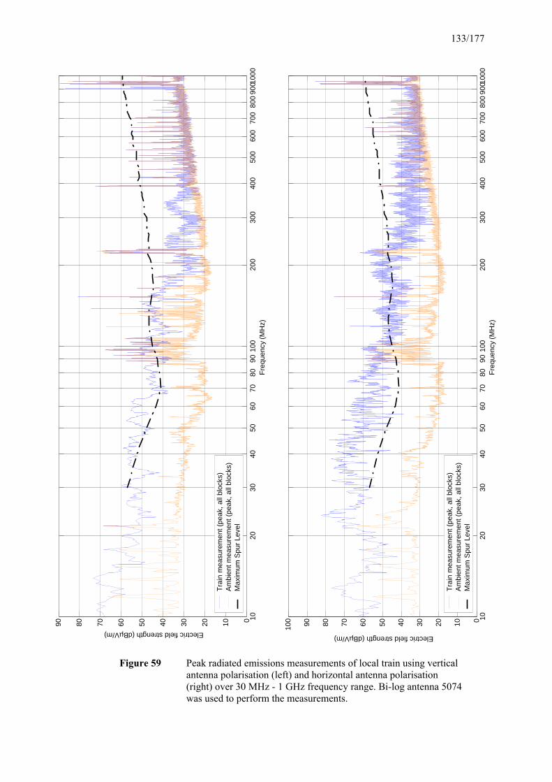
133/177
1020
3040
5060
7080
9010
020
030
040
050
060
070
080
090
0100
00102030405060708090
Freq
uenc
y (M
Hz)
Electric field strength (dBµV/m)
Trai
n m
easu
rem
ent (
peak
, all
bloc
ks)
Am
bien
t mea
sure
men
t (pe
ak, a
ll bl
ocks
)M
axim
um S
pur L
evel
1020
3040
5060
7080
9010
020
030
040
050
060
070
080
090
0100
00102030405060708090100
Freq
uenc
y (M
Hz)
Electric field strength (dBµV/m)
Trai
n m
easu
rem
ent (
peak
, all
bloc
ks)
Am
bien
t mea
sure
men
t (pe
ak, a
ll bl
ocks
)M
axim
um S
pur L
evel
Figure 59 Peak radiated emissions measurements of local train using vertical antenna polarisation (left) and horizontal antenna polarisation (right) over 30 MHz - 1 GHz frequency range. Bi-log antenna 5074 was used to perform the measurements.
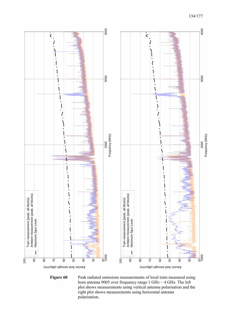
134/177
1000
2000
3000
4000
2030405060708090100
Freq
uenc
y (M
Hz)
Electric field strength (dBµV/m)
Trai
n m
easu
rem
ent (
peak
, all
bloc
ks)
Am
bien
t mea
sure
men
t (pe
ak, a
ll bl
ocks
)M
axim
um S
pur L
evel
1000
2000
3000
4000
2030405060708090100
Freq
uenc
y (M
Hz)
Electric field strength (dBµV/m)
Trai
n m
easu
rem
ent (
peak
, all
bloc
ks)
Am
bien
t mea
sure
men
t (pe
ak, a
ll bl
ocks
)M
axim
um S
pur L
evel
Figure 60 Peak radiated emissions measurements of local train measured using horn antenna 9005 over frequency range 1 GHz − 4 GHz. The left plot shows measurements using vertical antenna polarisation and the right plot shows measurements using horizontal antenna polarisation.

135/177
Figure 60 shows that the radiated power spectra due to arcing dropped below the noise floor
of the system at around 1.7 GHz − 2 GHz. Many discrete frequencies were also present in
both the train and the ambient power spectra (eg, at frequencies of approximately 2 GHz,
2.2 GHz, 2.5 GHz and 3 GHz), that were probably due to spurs in the oscilloscope’s ADC,
although it was not possible to distinguish these from ambient signals. There was also a
wideband emission present in the train power spectra between 2.7 GHz − 2.8 GHz that is not
present in the ambient power spectra. We believe this was due to airport radar that was
operating nearby but was not present in all the measurements. It was not an emission from the
train as it was found to be present in some of the other ambient measurements that were
made.
In the power spectra measurements made of the train using a vertical antenna polarisation, a
very strong narrowband signal can be seen at 1.77 GHz. This is part of the Personal
Communication Networks (PCN) base station receive band, and was due to transmissions
from a GSM mobile phone that was in use on the train at the time of the measurement. Many
of the other train measurements exhibited emissions that were present in the GSM or PCN
mobile transmit bands.
5.4.3 Sources of Error in Train Measurements
As already mentioned, because the trains are passing at high speed and the arcing process
occurs randomly, the measured amplitude of the impulses varied due to the different
distances from the receive antenna. The peak will be measured when the arcing occurs
directly in line with the main beam of the antenna. If this does not occur, the polar response
of the antenna needs to be taken into account. Unfortunately, due to the speed of the trains
and the difficulty in observing the arcing process, it was very difficult to obtain an estimate of
the angle to allow measurement compensation.
As measurement distance was only 10 m (to the centre of the track), and the antenna 3 dB
beam width was 40° at 30 MHz, the arcing needed to occur within a distance of
approximately 25 m. This corresponded to a time interval of approximately half a second at
100 mph. The only method to estimate the peak power was to perform as many
measurements as possible, and record the peak power spectra encountered. During the train
measurements, approximately 33 sets of measurements were performed (although two
different antennas and polarisations were used within these measurements). There were also

136/177
several types of train (including the high-speed Intercity trains, local trains and goods trains),
and probably many different train models.
Another reason for performing many measurements is that the intensity of the arc will vary,
and again this will depend on many factors, including the distance of gap between the
conductors and the pantograph and the power drawn by the train. These types of error will
affect any measurement system, including a conventional EMC test receiver.
Using the TDEEMS to perform these measurements introduces additional difficulties,
including ensuring the oscilloscope triggers on these emissions. Because the processing and
storage time is approximately 0.75 s, the oscilloscope could trigger on a low amplitude
emission (for example, when the train is outside the 25 m measurement distance), and miss a
higher amplitude emission that occurs during the measurement distance. Another difficulty is
choosing a vertical gain setting on the oscilloscope to prevent the ADC from saturating
(blocking). The train measurements were made with a vertical gain setting of 200 mV/div and
a 10 dB attenuator to prevent this; however, ADC saturation still occurred in several of the
measurements.
In most in situ EMC emissions measurements it would be possible to set the oscilloscope
gain in advance to prevent ADC saturation. In this case we chose the vertical gain after
measuring the emissions from several trains at the beginning of the measurements. In
approximately 90% of the subsequent measurements, ADC saturation did not occur. If we
had set a lower gain, the dynamic range for most of these measurements would have been
impaired. One possible method of improving the TDEEMS for making these measurements
would have been to use all four available channels on the Infiniium oscilloscope (each set up
with a different gain) to capture the emissions.
Because there are so many variables in these measurements, it was difficult to obtain a true
peak estimated radiated power due to arcing, let alone identify whether emissions from one
type of train were worse than emissions from a different type of train. These measurements
are not repeatable because it is not possible to control all the variables. By examining the
peak power spectra of a measured impulse when ADC saturation did not occur (see
Figure 59), the peak electric field strength was 78 dBµV/m above 30 MHz. It was even
greater than this in the HF band (at least 82 dBµV/m), although the antenna was not
calibrated in this band and so the actual field strength will be higher. These are the peak field

137/177
strengths encountered during the measurements. The peak radiated powers from the arcing on
the train will be even higher than this, although due to all the factors listed above, we could
not determine the peak field strength.
Railway EMC measurements are notoriously challenging due to all the sources of
uncertainty, and are atypical in that most in situ measurements are made of stationary
equipment. However, the TDEEMS has allowed the approximate shape and (to an extent) the
bandwidth of the interference due to arcing to be determined, which would not be possible
using conventional methods because of the long measurement time. Using the conventional
EMC test receiver it would only be possible to monitor a small number of frequencies (using
either multiple receivers or a fast frequency-hopping receiver). It would be easier, however,
to make peak measurements at single frequencies using the conventional EMC test receiver,
as the dwell time or measurement interval is longer than the TDEEMS, which cannot
measure continuously.
6 Analysis of Results
One of the major aims of this project was to assess the technical and economic strengths and
weaknesses of the time domain measurement method when compared to existing methods.
The results presented in Section 5 provide objective data that can be used to compare the time
domain approach with the currently adopted swept frequency approach and from this to draw
some conclusions about the technical advantages and disadvantages of the time domain
approach. Drawing objective economic conclusions is more difficult, because there are many
non-technical factors that will affect the economic argument.
To compare the time and frequency domain approaches we have analysed the measurement
data collected during this project to investigate the capabilities of both approaches in several
important characteristics. For convenience we present our discussions of each of these
characteristics in the following separate sub-sections.
6.1 Measurement Accuracy
Taking accurate measurements is clearly a fundamental characteristic of any EMC
measurement system. Given the difficulty of ensuring reliable and consistent measurement
results across a wide range of different test laboratories and test environments, it is of
paramount importance that the measurement uncertainty introduced by the test equipment is
138/177
minimised. Measurements based on swept frequency techniques have been used for several
decades and, consequently, have gained global acceptance. Before the time domain method
can be adopted, it must first gain the acceptance of the industry as a whole; thus it is
important to demonstrate that the time domain method is at least as accurate as the existing
approach.
In considering measurement accuracy there are three distinct but related facets we will
address. The first is whether or not the fundamentally different approach taken by the time
domain method introduces any characteristics that render it impossible to achieve the same
level of accuracy as the existing approach. The second is how do the characteristics of
impulsive signals affect the measurement accuracy of each of the measurement methods? The
third is the difference between peak and average measurements. We will consider these three
facets separately.
6.1.1 Does the System Architecture Affect Measurement Accuracy?
Implementing any wideband RF system with a flat frequency response over a frequency
range of several gigahertz is an exacting requirement. Both the time and frequency domain
approaches share this requirement and therefore suffer from the same inaccuracies introduced
by a failure to implement a RF front end with a perfectly flat frequency response. To
compensate for the inevitable frequency response variations a calibration table is used.
Following the RF front end the architectures of the time and frequency domain approaches
diverge. Whereas the frequency domain approach typically employs an analogue IF stage,
containing fixed bandwidth filters, the proposed time domain approach directly digitises the
RF signal and performs all subsequent processing operations numerically. The advantage of
such an approach is that numerical operations are precisely repeatable and do not suffer from
unit-to-unit or temperature variations. Hence, the accuracy of a digital implementation is
governed only by the numerical precision, which can be chosen to render errors insignificant
compared to the errors introduced by other parts of the system. In contrast, an analogue IF
stage will suffer from variations due to component tolerances, leading to additional
measurement uncertainty. In practice, the digitisation process is imperfect, as discussed in
Section 2.1.2, and whilst the impact of this on the measurement of peak power is small, it
nevertheless has an impact on system performance, as we shall show in a later section.
139/177
Our experiments on the test sources, reported in Section 5.1, can be used to gauge the
comparative performance of the time and frequency domain methods. The RF emissions from
all but one of the test sources were time stationary and thus we would expect both methods to
yield the same results. The best indication that this is the case can be seen from the CW
measurement (see Section 5.1.1), in which the reported measurements were in agreement to
less than 1 dB over all frequencies below 2 GHz. Above 2 GHz larger differences were
observed; however, most of this error can be attributed to the frequency response trough in
our prototype RF front end. Similarly, the results obtained from measurements of the comb
generator are in agreement to within 2 dB.
The CW and comb generator measurements are both examples of narrowband measurements;
hence, they are insensitive to the measurement bandwidth. The measurements made using the
broadband noise generator test the equivalence of the two approaches with a signal whose
power measurement will be proportional to the measurement bandwidth. The results from
this test demonstrate the effect of the observation interval when measuring noise-like sources.
As the frequency domain approach had a longer dwell time than the prototype time domain
approach, the measurement variance is greater in the time domain measurements. However,
the results again demonstrate close correlation between the two methods and allow us to
conclude that both methods can be trusted when measuring stationary sources.
The RX14 EMC receiver, as used in many of our tests, has a 6 dB bandwidth of 100 kHz but
an otherwise unspecified frequency response. To reduce measurement errors due to the
response of the IF filter, the frequency was adjusted in increments of half the receiver
bandwidth. With the time domain method and with more modern frequency domain receivers
the channel filter is implemented digitally; consequently, such errors can be much reduced.
The frequency response of any system using a digital IF is determined by the windowing
function used to prevent spectral leakage in the FFT. This was discussed in Section 4.1.2. For
narrowband emissions the power measured using the FFT in the TDEEMS may be lower than
the true power due to the scalloping loss of the windowing function.
During the tests it was possible to choose a window function that was suitable for the source
being measured, ie, a flat top window for narrowband CW measurements and a Hamming
window for wideband sources, such as the noise generator. The Hamming window (or
similar) would probably be used in any proposed time domain measurement system, since it
provides a good trade-off between main lobe width (which produces artificially high
140/177
measurements for broadband emissions) and side-lobe levels. The flat top window should
always be used for calibration purposes as it correctly measures the amplitude of narrowband
signals. It is of no use for measuring wideband signals due to its wide main lobe.
6.1.2 Measurement Accuracy with Time-varying Sources
Measurement of time-varying sources is known to be a problem with the frequency domain
method and so the question we seek to answer is, can the time domain approach provide a
more accurate result?
The problem with the frequency domain approach is that it measures each frequency at a
different time and thus it will only measure the frequency content of an impulsive emission at
the frequencies it happens to be monitoring whilst the impulse is present. The only available
solution to this problem is to use a peak-hold detector and to observe the source for long
enough that the emission is eventually measured at all frequencies of interest. In contrast, the
time domain approach is capable of simultaneously measuring at all frequencies up to its
limit, but, due to the high sampling rates and limited processing bandwidth of the prototype
system, it is incapable of continuous measurement. Consequently, with asynchronous
sampling the probability of the time domain method capturing an impulsive emission is
extremely low. This problem is most acute when the signals to be measured are short
impulses with low pulse repetition frequencies (PRFs). Fortunately, a simple solution to this
problem was found in the prototype TDEEMS by using the triggering features of the
oscilloscope (see Section 4.2). A further benefit of the triggering features is the delayed
trigger mode, which enables the trigger level to be adjusted to a level just below the peak
voltage of the time domain emission waveform and to capture the signal before and after the
trigger event. Hence, even if the impulse length exceeds the capture period, the power spectra
can still be measured at the peak voltage level.
When using the FFT to determine a signal’s spectral characteristics, the assumption is made
that the signal is stationary over the FFT duration. In the measurements of example
equipment all of the example equipment produced impulses that were shorter than the capture
interval (51.25 µs), and hence this assumption is not valid. Thus, even though the time
domain approach can capture an impulse, a FFT performed over the whole capture interval
will result in a peak radiated power measurement that is too low. Analysis of the results from
the light bulb and the electric drill showed that the results were, respectively, 36.5 and 20 dB
too low. In this study we were able to determine the magnitude of the error by analysing the
141/177
time domain characteristics of the captured impulse. However, this approach is unlikely to be
acceptable for a commercial TDEEMS as it requires significant operator interaction and will
negate the time saving advantages of the time domain method. An alternative technique with
which we experimented was to use a short time Fourier transform, whose length was matched
to the impulse duration. Again, since it requires prior knowledge of the signal’s time domain
characteristics, this is not a practical proposition for an unknown emission. However, by
varying the length of the FFT and analysing the same data with each length, it is possible to
determine the maximum emission level without prior knowledge of the emission
characteristics.
We found that for all the example equipment (with the exception of the fast transient
generator) the repetitive nature of the impulsive emissions enabled the conventional EMC test
receiver to also provide a good representation of the shape of the peak radiated power spectra,
provided that the EUT was observed for long enough that an impulse occurred during the
dwell time of the receiver at every frequency.
In the results of our measurements of example equipment we noted that the two measurement
methods produced different peak measurement results and that the magnitude of the
difference was dependent upon the characteristics of the pulsed waveform produced by the
EUT. We observed that when the source emitted short pulses, the time domain approach
produced much larger peak powers and the effect was more pronounced when the PRF was
low. This was due to the response time of the peak detector in the conventional EMC test
receiver, which has long charge and discharge times. The peak spectra of the example
equipment were typically 5 to 10 dB higher when measured using the TDEEMS compared to
the conventional EMC test receiver. The exception to this was the measurements of the PC,
which produced a complex combination of broadband noise and narrowband emissions that
were mostly stationary. Consequently, the peak measurements made using the conventional
EMC test receiver were 2 to 3 dB higher, due to the longer 20 ms measurement interval over
which the peak value was recorded.
6.1.3 Peak vs Average Measurements
Existing EMC standards require both peak and average measurements to be made, and in
most cases a specific detector characteristic is defined to guarantee consistency of results and,
as in the case of the quasi-peak detector, to emulate the behaviour of a receiver in the
presence of the unwanted emission. With stationary signals the frequency domain technique

142/177
is able to perform peak and average measurements equally well. In this section we will
examine the behaviour of both the time and frequency domain methods when making peak
and average measurements on impulsive emissions.
As noted in the previous section both methods are able to make peak measurements on
impulsive signals provided that the PRF is sufficiently high. However, for emissions with low
PRFs the time domain method is clearly able to make peak measurements much more rapidly
and does not suffer from the detector response time distortion that will be a feature of most
frequency domain equipment currently used in EMC test labs.
Making average measurements of impulsive emissions was a problem for both measurement
techniques. In the frequency domain case, the problem is that of observing the signal for long
enough that the periods when the emission both is and is not present are sampled in the
correct proportion. For example, if an impulse has a duty cycle of 1:10 (ie, it is present for
one tenth of the time), then the correct average will only be reported if at least ten samples
are taken with only one recording the time that the impulse was present. The problem for the
frequency domain approach is exacerbated by the response time of the detector, which in the
case of the receiver we used, was too slow to respond to the impulse and hence further
distorted the measurement. The frequency domain average measurements of the light bulb
and the electric drill were 13 and 20 dB lower than the average measurements performed
using the TDEEMS.
Similar problems were encountered when attempting to make average measurements with the
TDEEMS. If the measurements were made without using the oscilloscope trigger, then the
short capture interval and the long data storage time made it unlikely that an impulse would
be observed. At the other extreme, if the measurements were made using the trigger, then
every captured block contained an impulse and, hence, the resulting average values were
artificially high. Some of these problems were a result of the prototype nature of the
TDEEMS and it may be possible to improve the performance of the average measurements in
a commercial implementation (see Section 7.2).
The TDEEMS produced good average measurements when the interval between impulses
was short, ie, less than the length of the capture interval. It also produced a good
approximation to the peak radiated power when the length of the impulse was equal or
greater than the length of the time sampling window. For some of the time domain
143/177
measurements, if the pulse repetition pattern and frequency were known, it was possible to
correct the average results manually to obtain a true average power value. This was
performed in the cases of the light bulb and the fast transient generator. However, the
emissions from the drill and the television were too complex to analyse.
When measuring an emission with a low duty cycle (ie, the emission is only present for a
small fraction of the time), the true average result will be very close to the receiver noise
floor and it is not a meaningful measure of the interfering effect of the emission.
6.2 Repeatability of Measurements
Measurement repeatability refers to the ability of the measurement system to obtain the same
results when the same source is measured at different times. Clearly this is an important
characteristic of any measurement system and any measurement inconsistency would need to
be accounted for in the overall uncertainty of the EMC test result.
For most of the measurements performed during this study, the peak radiated power spectra
were measured twice using both the conventional EMC receiver and the TDEEMS over two
different measurement runs separated by a week. The aim here was to compare the behaviour
of the two methods when making repeat measurements. Due to the variable nature of the
measurements on single impulses, our repeatability comparisons for the time domain
approach are based only on the compound results obtained from observations of 50 impulses.
All frequency domain measurements are in effect compound results and so in this case the
problem does not arise.
From the measurements of both the test sources and example equipment we observed that the
repeatability of the time domain measurements was generally as good as that of the frequency
domain measurements. This was certainly the case for the test sources and the majority of the
example equipment measured. It could be shown that the variation in these measurements
was due to changes in the equipment setup, as the radiated emission spectra measured using
both methods varied in the same manner.
The exception was the measurement of the light bulb, whose spectra differed when measured
using the time domain method but were similar when measured using the frequency domain
method. On the second run the peak light bulb measurement in the time domain was 4 dB
higher and the second harmonic of the emission was 10 dB higher. In the frequency domain
144/177
the measurements were the same. It is impossible to know exactly why this difference
occurred, but, as has been previously documented, the emissions from the light bulb varied
from impulse to impulse and so it is likely that such variations could explain the
measurement difference. Whilst the frequency domain results might appear to negate this
argument, we note that the response time of the peak detector is already assumed to be the
cause of the difference in peak measurements between the two methods and it is conceivable
that this is also masking the change in emissions from the light bulb between the two runs.
From the results of the second run (see Figure 34) it can be seen that the frequency domain
method has not recorded the second harmonic emission at 320 MHz.
In summary, the most reliable tests of repeatability are those taken with a known source
whose characteristics can be trusted to remain stable between measurement runs. The comb
generator results demonstrate that the time domain approach produces repeatable results. The
conclusions we can draw from measurements of the light bulb are that emissions from real
products can vary over a long time period; therefore it may not be possible to obtain a true
peak measurement without a much longer observation period than current EMC practices
would use. Finally, we note that whilst these tests give us no cause to doubt the repeatability
of the time domain method, they only cover a small set of example equipment and more
measurements need to be made to determine the right capture interval.
6.3 Measurement Time
The anticipated reduction in time taken to make EMC measurements is, perhaps, the main
driving factor behind the interest in the time domain measurement method. Reducing the time
required to take the measurements has obvious implications for the cost of the type approval
process. However, it is not the only advantage. Reducing the time taken to make a single
measurement allows more measurements to be made and hence the quality of the
measurements may be improved. With the ever-increasing complexity of modern electronic
equipment, it may be that, in the longer term, the quality improvement is more important than
the time saving. In this section we compare the measurement time of both methods and
consider the impact of using the time domain technique with a rotating table and varying
antenna heights.

145/177
6.3.1 Comparison of Time and Frequency Domain Sweep Times
The theoretical sweep time, ie, the time taken to perform the measurements over the
frequency range of interest using the conventional EMC test receiver (Tsweep) is given by
dwellstep
startstopsweep T
fff
T ⋅⎟⎟⎠
⎞⎜⎜⎝
⎛ −= (27)
where Tdwell is the dwell time at each frequency and fstart, fstop and fstep are the start, stop and
step frequencies, respectively. Between 30 MHz and 1000 MHz, a frequency step (fstep) of
50 kHz was used, with a dwell time (Tdwell) of 20 ms. This gives a theoretical measurement
time of approximately 6.5 minutes. However, this analysis ignores the retuning time of the
receiver and the actual measurement time was almost doubled to approximately 12.5 minutes
(for peak measurements only). The measurements between 1 GHz and 4 GHz with a 0.5 MHz
frequency step took a further 4 minutes (the theoretical time is 2 minutes).
The conventional EMC test receiver (RX14 in Appendix A) is also capable of making peak
and average measurements in a single sweep. However, this almost doubled the measurement
time to approximately 25 minutes for the full sweep between 30 MHz and 4 GHz. However,
processing the frequency domain measurements was fairly quick, as only the calibration
factors for antenna and cable losses needed to be applied, which took several seconds.
The time taken to perform the measurements in the time domain is shown in Table 14. Two
sets of times are shown, one for processing the results using the 1 GHz Pentium-III based PC
built into the Infiniium oscilloscope, and another for processing the results using a 2.6 GHz
Pentium-4 based desktop PC. The desktop PC is four to eight times faster than the PC built
into the oscilloscope, due to the slow performance of the oscilloscope hard disk and the faster
processor in the desktop PC.
Most of the time taken to capture the sample data was due to the time taken to transfer the
data between the internal memory in the oscilloscope and the software running on the internal
PC, and then writing the data to the hard disk. The capture time is approximately four orders
of magnitude greater than the actual sampling window time. The gap between the two PCs
would be narrowed if the raw time domain sample data were not written to the hard disk,
which would be the case in a commercial implementation of the TDEEMS.

146/177
Measured Times 1 GHz Pentium-III
based PC in oscilloscope
2.6 GHz Pentium-4 based desktop PC with fast hard disk
Capture and storage time (single block of 1025 Ksamples)
2 s
Capture and storage time (50 blocks of 1025 Ksamples)
37 s
Processing time (single block) 7 s 1.5 s
Processing time (50 blocks) 184 s 23 s
Total measurement time (single block) 9 s 3.5 s
Total measurement time (50 blocks) 221 s (3 m, 41 s) 60 s (1 m)
The processing time shown in Table 14 is the time taken to process the time domain sample
data using the periodogram measurement parameters listed in Section 4.1.1, for either peak or
average measurements. Note that due to the architecture of the software, it is necessary to
conduct separate runs of FFT processing for each of the peak and average measurements. A
more refined commercial implementation could perform both peak and average
measurements without repeating the FFT, but this would have little impact on the processing
times listed in Table 14.
Reducing the size of the sample block from 1025 Ksamples to 200 Ksamples lowered the
measurement time from 37 s to 12 s, and decreases the processing time for 50 blocks from
184 s to 23 s. These times were measured using the 1 GHz Pentium-III based PC in the
oscilloscope to process the results.
6.3.2 OATS Measurement Time
Many EMC test houses (including EMC Projects Ltd) perform radiated emissions
measurements on the OATS after performing a pre-measurement scan of the EUT in a
screened room. The pre-measurement scan is used to determine the frequencies of the
radiated emissions without ambient signals present. Calibrated measurements are then made
on the OATS.
On the OATS the emissions from the EUT are measured at antenna heights varying from 1 m
to 4 m, with both vertical and horizontal antenna polarisations. The EUT is also rotated on a
Table 14 TDEEMS measurement times using 1 GHz PC in oscilloscope and 2.6 GHz desktop PC.

147/177
turntable in an attempt to determine the peak emission from the EUT. These parameters are
varied whilst the frequency domain receiver is tuned to the frequency of one of the emissions
and the process repeated for all emission frequencies. This process can be very time-
consuming, especially for EUTs that radiate at many frequencies.
OATS measurements are normally performed manually, but this is not as rigorous as an
automated method. For example, the measurements of the light bulb only took 5 − 10 minutes
to perform manually using the conventional EMC test receiver, since the EUT only radiated a
single frequency. On the other hand, the drill, which radiates at many frequencies, took 35 −
40 minutes to measure. These times exclude the pre-measurement scan in the screened room,
although this normally only takes five minutes.
The TDEEMS has the potential to significantly reduce measurement times, for both manual
and automated measurements, as all frequencies can be monitored during each measurement.
However, the architecture of the prototype TDEEMS that has been implemented is not
suitable for this, as the raw time domain sample data were being written to disk and post-
processed manually off-line. This was to allow experimentation with different spectral
estimation algorithms and reduce the potential for implementation errors. A commercial
implementation of the system would not need to do this, and could therefore provide
calibrated measurements across the entire measurement bandwidth by implementing an on-
line spectral estimation and calibration algorithm.
As an estimate based on this study, a good commercial implementation of the TDEEMS may
be able to make peak and average measurements using the Welch periodogram over a single
1025 Ksample block every 1 − 2 seconds using today’s desktop PC technology. This assumes
a 100 kHz measurement bandwidth over a 4 GHz RF band. For example, an automated
system which rotated the EUT in the horizontal (azimuth) plane in 10 degree increments,
with 1 m increments in antenna height (from 1 m up to 4 m) and using both antenna
polarisations would have (360/10) * 4 * 2 = 288 different measurement positions. Assuming
a two second measurement time, the complete scan would take approximately 9.6 minutes.
This estimate excludes the time taken to move the antenna and rotate the EUT, which would
not have a significant effect if the time taken to move the EUT or antenna was approximately
the same as the two second measurement time. This also assumes a front end and broadband
antenna that can operate across this entire 4 GHz frequency range, if it is desired to cover the
entire band. It should be noted that measurements using the time domain approach should be

148/177
made over 50 sample blocks, and this increases the time for each measurement from 2 s to 60
s (see Table 14). Hence, the total measurement time is now 4.8 hours.
The theoretical measurement time with a conventional EMC test receiver would take 794
seconds (approximately 13 minutes) assuming a 100 kHz frequency step between
30 − 4000 MHz with a 20 ms dwell time. This results in an automated measurement time of
64 hours, assuming the parameters above. All the automated measurements made in this
study have used a conventional EMC test receiver with a 20 ms dwell time (with peak and
average detectors). This dwell time is too short for measurements made using the CISPR QP
detector, since the decay time of the detector is of the order of half a second. Strictly
speaking, it is necessary to use a dwell time of at least 15 seconds to obtain accurate
measurements using this detector.
One difficulty with using an automated system on the OATS is finding an automated method
for handling the ambient signals (see Section 5.3.2). Also, the Infiniium oscilloscope used in
this study cannot measure to Class A or B limits on the OATS due to the spurs and having to
adjust the gain of the oscilloscope to prevent receiver blocking. However, if these automated
measurements were performed in a large screened room, then neither of these problems
would exist.
6.4 Dynamic Range
Dynamic range determines the range of signal levels that can be measured simultaneously. In
a conventional receiver, at the small signal end of the range, the dynamic range is limited by
the receiver noise floor and, at the large signal end of the range, by the blocking level.
Furthermore, the noise floor is dependent upon the measurement bandwidth and the blocking
level is usually considered to be the 1 dB compression point. With the time domain method
the dynamic range is limited currently by the capability of the ADC. The upper limit is set by
the maximum signal level that can be handled without saturating the ADC and the lower limit
by the spurs produced by the ADC.
The worst-case SFDR of the oscilloscope used in the TDEEMS was measured as 53 dB by
driving the oscilloscope with a full-scale CW input and measuring the amplitude of the peak
spurious component. This value has been used throughout this report to indicate the
maximum spur level that could be present in the emissions power spectra. Compared to a
conventional EMC receiver, which may have a dynamic range exceeding 100 dB, the time

149/177
domain receiver is extremely limited. However, for measurements in a screened room
environment, in which the aim is to test whether or not a pre-defined limit has been exceeded,
53 dB is more than sufficient dynamic range. For measurements on an OATS, the limited
dynamic range of the TDEEMS is a severe restriction and is discussed separately in Section
6.5.
Frequency domain receivers have a huge advantage over the time domain receiver when
handling inputs with a wide dynamic range. Since a frequency domain receiver only
measures on a narrow band of frequencies at one time, it is always possible to place a pre-
selection filter at its input to remove unwanted out-of-band signals. Since the time domain
technique measures all frequencies simultaneously, it cannot use pre-selection. Measurements
of the CNE noise generator highlight this limitation of using the TDEEMS to measure
wideband emissions. Whereas a conventional EMC test receiver measures the power over
pre-selected bandwidth (typically up to 100 MHz at frequencies below 1 GHz), the time
domain system measures the power over the entire input bandwidth (4 GHz in the case of the
prototype). Therefore, receiver blocking is far more likely to occur, especially when
measuring wideband emissions. Because of the gain changes necessary to prevent this, the
sensitivity of the system is reduced dramatically. However, the CNE is an extreme case, as a
wideband emission covering a bandwidth such as this is unlikely to be typical of normal
measurements.
Due to the narrow dynamic range of the time domain approach, it may not be possible to
measure to Class A or B limits using the TDEEMS across the entire frequency range. If a
single emission is present, then this does not present a problem, as the level of the peak
emission can always be measured. However, if multiple emissions are present at different
amplitudes, then the peak emission could mask the other emissions (as these drop below the
maximum spur level or detection threshold). This could be a problem due to different
measurement limits in different frequency bands. For example, a wideband emission that is
below the limit in the 230 MHz − 1 GHz band could mask an emission above the limit in the
30 − 230 MHz band (as this band has a lower limit). Likewise, antenna factors and the
frequency response of the overall system could also contribute to the masking problem (refer
to Section 3.3). This problem could be exacerbated for standards that specify different limits
for narrowband and wideband emissions, as wideband emissions limits are generally higher
than narrowband limits.

150/177
In practice the spurs did not appear to be visible in most of the measurements performed
below 1 GHz using the TDEEMS. The exceptions to this were the measurements of the comb
generator and the energy saving bulb and, in general, the spurs were more visible with
narrowband inputs. This can be explained by a process known as dithering. Spurs are the
result of periodicity in the quantisation noise, which is more prevalent with narrowband input
signals because the quantisation noise contains frequency components that are harmonically
related to the input signal and the sampling clock frequencies. Wideband inputs (especially
noise sources) result in quantisation noise that is more random and hence does not lead to
such spurs. In Section 7.2 we will discuss how this effect could be used to our advantage in a
commercial TDEEMS.
The worst spur levels encountered were during the measurements of the comb generator, and
during the train measurements between 1 GHz − 4 GHz. The train measurements are
unreliable as a guide to the typical spur level as it is not possible to distinguish an ambient
signal from a spur. From the comb generator results the worst-case spur level was a minimum
of 10 dB below that determined by the measurement of the SFDR. As a result, the usable
dynamic range of the TDEEMS was 63 dB for our measurements. We will discuss in
Section 7 how a commercial implementation of the TDEEMS may be able to improve its spur
level.
6.5 Performance of OATS/in situ Measurements
For the majority of EMC measurements the use of an OATS is the accepted practice. Clearly,
more reliable measurements can be made in a screened room environment, but the difficulty
and cost of building a screened room of sufficient size to make far-field measurements at
30 MHz renders this approach impractical for most test houses. Consequently, if the time
domain method is to be widely accepted as a replacement method, it must be suitable for use
on an OATS. Similarly, in situ measurements are by definition carried out in the open air and,
consequently, place similar demands on equipment performance.
The problem presented by open air measurements is that of differentiating the ambient
signals from the emissions by the EUT. Worse still, the typical received levels of broadcast
signals, such as FM radio, television and cellular radio, can be much higher than the EMC
emission limits. This places requirements on the dynamic range of the measurement receiver

151/177
that are easily achievable for a frequency domain receiver but highly demanding for a time
domain one.
As reported in Section 5.3.1, to prevent blocking due to the ambient signals when measuring
on the OATS, it was necessary to decrease the gain of the oscilloscope from 10 mV/div to
200 mV/div, a gain reduction of 26 dB. The effects of this change in gain are shown in
Figure 61, which identifies the blocking level, maximum spur levels and noise floor for the
OATS test setup accounting for cable losses, antenna factors and the front-end frequency
response.
From Figure 61 the dynamic range limitation of the time domain system is clear. It can be
seen that the peak spur level is above the Class B limits at all frequencies and above the Class
A limits above 400 MHz. Consequently, allowing for the measurement uncertainty on the
OATS, it is impossible to distinguish between a spur and an emission at the Class A or B
limits. This does not completely exclude the use of the TDEEMS on an OATS, as the spurs
30 100 300 1000 40000
20
40
60
80
100
120
140
Frequency (MHz)
Ele
ctric
fiel
d st
reng
th (d
BµV
/m)
Blocking levelPeak spur levelTDEEMS noise floorClass A limitsClass B limits
Figure 61 TDEEMS blocking level, peak spur level and noise floor on OATS assuming a 200 mV/div vertical gain setting on the oscilloscope.

152/177
are similar to ambient signals, and the noise floor (due to thermal noise) of the TDEEMS is
actually lower. The spur can be ignored if the same emission is not present during the pre-
measurement scan in the screened room (on the higher gain setting), or if the emission
remains when the EUT is switched off. If an emission is present at the same frequency as a
spur, then it will not be possible to measure its amplitude unless it exceeds the level of the
spur (but this is also the case with ambient signals). However, it does make the TDEEMS
awkward to use, as more ‘false emissions’ will be present in the measured spectrum.
Figure 61 also demonstrates a further dynamic range limitation of the TDEEMS. Even if the
spurs could be completely eliminated, the dynamic range is only just good enough to make
measurements to the Class A limits below 400 MHz and is not good enough to measure to the
Class B limits. Based on Figure 61 we can conclude that to measure signals to the Class B
limits in the presence of the ambient signal levels we encountered during our tests, the
receiver requires a dynamic range of 100 dB (giving approximately 20 dB signal-to-noise
ratio at 1 GHz). It should be considered for comparison purposes that the location of EMC
Projects Ltd’s OATS was in a semi-rural location, which is relatively “quiet” from an
ambient noise point of view. The TDEEMS is unlikely to be usable in a location that is in
close proximity to a broadcast transmitter or cellular base station. However, most open air
EMC test facilities are unlikely to be located close to high power RF transmitters.
If the dynamic range limitation can be overcome, an advantage of using the TDEEMS for
OATS measurements is that the short capture interval could aid in the identification of
ambient signals. Because measurements of the entire RF bandwidth can be made very close
in time, it is possible to make ambient spectra measurements, switch on the EUT and then
measure the radiated emissions and ambient signals. These measurements could be performed
a few seconds apart, assuming the EUT can enter its normal mode of operation within this
time period. Therefore, the effect of medium- to long-term variations in the ambient signal
power spectra can be removed, using the techniques discussed in Section 5.3. This could be
combined with an algorithm that attempts to identify true emissions from the screened room
measurements.
6.6 Summary
A summary of the main characteristics of the frequency domain and time domain
measurement methods is given in Table 15.

153/177
Attribute Frequency Domain Time Domain
Measurement Accuracy
Stationary signals Excellent. Accuracy is well proven
Excellent. Our results indicate that accuracy is as good as frequency domain method.
Impulsive signals 1. Reasonable for peak measurements when PRF is high.
2. Detector response time is critical.
3. Poor for measurements of low PRF signals.
1. Excellent for peak measurements, provided that the peak is captured.
2. Triggering is critical. 3. Average measurements
are difficult due to problems retaining the time domain information when triggering is used.
Repeatability 1. Results show good repeatability with both stationary and impulsive measurements.
2. The results obtained using the frequency domain receiver were repeatable, but due to the long peak detector time constant are inaccurate in both runs.
1. Results show good repeatability with stationary sources.
2. Variability in the reported results with impulsive sources is attributed to changes in the source that were not captured by the frequency domain method.
Measurement Time
Single sweep 30 MHz to 4 GHz Peak only
16 minutes
1 minute
Peak and average
25 minutes 1 minute
Rotating EUT 64 hours 4.8 hours
Dynamic Range
Sensitivity Good with LNA. Good with LNA. Spurious level > 80 dBc typical ≈ -60 dB Dynamic range 110 dB typical ≈ 60 dB
Use on OATS Able to handle high-level ambient signals by using RF pre-selection filters.
Susceptible to blocking because pre-selection cannot be used and dynamic range is limited.
Table 15 Comparison of frequency domain and time domain measurement approaches.

154/177
7 Extending the System
The TDEEMS has been designed to operate between 30 MHz and 4 GHz. Currently most
EMC measurements are made at frequencies up to 1 GHz. However, in the future it is likely
that measurements will be made at frequencies up to 18 GHz and possibly beyond. In this
section we consider extending the measurement system to higher frequency ranges, and
possible techniques for extending the dynamic range of the measurement system.
To extend the TDEEMS above 4 GHz, a higher bandwidth oscilloscope could be used.
Several manufacturers, including Agilent and Tektronix, now produce digital sampling
oscilloscopes that support bandwidths of 6 GHz (eg, the Agilent Infiniium 84855A).
Ultimately, a dedicated time domain measurement instrument could be built using similar or
better ADC technology than that employed in currently available commercial oscilloscopes.
However, as the market for oscilloscopes is larger, then it is this market that will drive the
advances in ADC technology.
Another method that can be employed to extend the frequency range of the TDEEMS is
shown in Figure 62. In this system the spectrum is divided into several RF bands and a down-
converter is used to convert each of these to baseband. A 1 GHz transition band has been
provided at the top and bottom of the Nyquist zone in each band to allow for the roll-off of
the input filters. A problem with this approach would be obtaining a broadband antenna that
could cover such a broad frequency range. Horn antennas that cover the frequency range 1 −
18 GHz (as used for the 1 - 4 GHz measurements) are readily available, although a separate
antenna would be required for frequencies below 1 GHz.

155/177
4 GHz - 7 GHz
DC - 4 GHz
Broadbandantenna
3.5 GHz
7 GHz - 10 GHz
6.5 GHz
10 GHz - 13 GHz
9.5 GHz
Infiniium oscilloscope
Building the system above will be expensive and was beyond the scope of this project.
However, mixers and RF amplifiers are available which can operate at these frequencies and
such a system is feasible. The filter requirements are challenging because of high operating
frequencies, and because the filters need to provide a minimum attenuation equal to the
SFDR of the oscilloscope.
7.1 Current ADC Technology
The high sampling rate (20 Gsamples/s) ADC employed in the Infiniium oscilloscope is
based around a flash ADC architecture, as described in Section 2.1. The current state-of-the-
art for off-the-shelf 8-bit flash ADC converters provides sampling rates of up to
1.6 Gsamples/s, with full-power bandwidths that can exceed the sampling rate by 1 − 2 times
[23]. In order to achieve a 20 Gsamples/s sampling rate, the Infiniium 54854A oscilloscope
uses an application specific integrated circuit (ASIC) that combines 80 flash ADCs on a
single chip, each running at 250 Msamples/s. By using sophisticated signal timing and
Figure 62 Extending the TDEEMS above 4 GHz.

156/177
buffering techniques, the inputs to the 80 ADCs are all delayed by different time offsets (time
duplexing) to achieve the overall 20 Gsamples/s sampling rate. Due to the high sampling rate,
it is also necessary to place the waveform acquisition memory on the same chip, which is
why the oscilloscope is limited to capturing sample blocks of 1025 Ksamples at the full
sampling rate. This technology is expensive, with the Agilent 54854A Infiniium oscilloscope
used in this project costing approximately £35,000. Similar offerings are also available from
other oscilloscope manufacturers, such as Tektronix [24] and LeCroy [25].
When choosing an ADC, the SFDR must be traded against the sampling rate and hence the
bandwidth that can be digitised. If a lower analysis bandwidth is used, a higher SFDR can be
obtained, since it is more difficult to produce ADCs with good linearity performance at
higher sampling rates. At the time of writing, Analog Devices produces a 14-bit ADC
(AD6645) with a 105 Msamples/s sampling rate, and provides a SFDR of 89 dB [26]. The
Agilent E1437A digitiser module provides a 23-bit ADC, which runs at 20 Msamples/s and
provides a SFDR of 110 dB [27]. This highly sensitive ADC was originally designed for
military use.
As the bandwidths of these ADCs are considerably lower than that of the Agilent 54854A
oscilloscope used in this study, their use in a spectrum analysis application would also require
a down-converter to sweep the frequency band of interest. This combines the frequency and
time domain measurement approaches, and is described in more detail in Section 7.3.
7.2 Commercial System Considerations
In this section we discuss some of issues and propose suggestions for a commercial
implementation of the TDEEMS. It has already been suggested that any commercial
implementation of a TDEEMS is likely to be based around ADC technology developed for
use in fast digital sampling oscilloscopes, as this is the market that currently drives the
development of the fastest ADCs.
7.2.1 Minimising the Processing Time
In Section 6.2 we suggested that it would be necessary to make multiple time domain
measurements of the radiated power spectra of the EUT in order to measure medium to long
term variations. To this end it will be desirable to minimise the processing time required to
obtain the power spectra, so that the measurements can be made close together in time (and
hence minimise the response or display time for the user), and to reduce the overall

157/177
measurement time if a significant number of sample blocks need to be captured. If the
processing time was sufficiently short, it may even be possible to implement an
approximation to a continuous-time detector (see Section 4.3).
The prototype TDEEMS wrote the time domain sample data directly to disk to allow
experimentation with spectral estimation algorithms and to reduce the possibility of software
bugs rendering the data unusable. The downsides to this were the storage requirements (2 MB
for each sample block of 1025 Ksamples), and the time taken to write the data to the disk in
the oscilloscope. A commercial TDEEMS could run the spectral estimation algorithm on-
line, which would significantly reduce storage requirements. A good desktop PC should be
able to process each sample block in 1 − 2 seconds using today’s technology (see Section
6.3). If a dedicated digital signal processor (DSP) architecture was employed, it may be
possible to realise performance gains over a PC architecture, although this would increase the
development costs.
Another possibility is to use a fast memory technology, such as synchronous dynamic random
access memory (SDRAM) to store the sample data prior to the spectral estimation processing.
This technology is inexpensive and 512 megabytes of SDRAM (costing approximately £50)
would allow 256 sample blocks to be stored with the total measurement interval being 13 ms.
Assuming modern double data rate (DDR) memory was used with a 64-bit bus and 200 MHz
clock speed, the peak bus bandwidth would be 3.2 gigabytes per second. It would be possible
to copy a 2 MB sample block from the ADC to the memory in 7 ms (assuming 10%
overhead), with the time taken to capture 256 sample blocks being approximately 1.8 s. If the
sample block size was reduced to 200 Ksamples, the time period could be 1.4 ms, although
the maximum length of impulse that could be captured would be 10 µs. By using this
approach, the interval between measurements can be reduced by three orders of magnitude,
allowing an approximation to a continuous time detector to be implemented. However, the
data would still have to be post-processed, which would take approximately five minutes for
a block size of 1025 Ksamples using a fast PC. This is still fast compared to the frequency
domain approach.
An essential requirement of the TDEEMS is a triggering facility so that accurate peak power
measurements can be made, as described in Section 6.1. One difficulty will be choosing a
trigger threshold without user intervention. One option would be to measure the peak voltage
over a fixed time period (with no trigger) which could then be used to derive a trigger level

158/177
which was 90 − 95% of the peak value. Using a slower time-base setting on the oscilloscope
(lower sampling frequency) would allow a longer measurement period to be examined, so
that impulses were not missed. However, measurements of the frequency spectra cannot be
made at the slower time-base settings due to aliasing. This method of using the slower time-
base setting could also be used to analyse the waveform to obtain a good average power
measurement. For example, with a pulsed waveform, the time between the impulses can be
measured and a correction factor can be applied to the power spectrum of the pulse to obtain
a true average power measurement.
7.2.2 Automatic Gain Control
Another useful feature would be AGC to alter the gain in the presence of strong blocking
signals (as implemented in the prototype TDEEMS), which can be implemented by detecting
sample values that are close to the full-scale value of the ADC in the time domain sample
data. It is also possible to implement AGC inside the ADC itself using an auto-ranging ADC.
7.2.3 Reducing the Level of the ADC Spurs
In Section 6.4 we described how correlation between the input signal and the quantisation
noise generates spurs in the output spectrum of the ADC. The problem is exacerbated if the
input signal consists of frequencies that are sub-multiples of the sampling frequency. By
deliberately superimposing noise on the input signal, the correlation, and hence the level of
the spurs can be reduced. This dithering technique can improve the SFDR obtainable from an
ADC under certain conditions.
The amount of noise that needs to be added to the input signal is dependent upon the
architecture of the ADC. In an ideal ADC (see Section 2.1.2), adding noise which has an
RMS amplitude that is approximately half the voltage represented by each output code (∆v/2)
is sufficient to dither the input signal. In practice, most systems have enough noise
superimposed on the input signal so that adding the additional dither noise is not necessary.
Increasing the noise level above this level will reduce the signal-to-noise ratio of the system.
For a real ADC, the level of the noise added must be high enough to reduce the effects of
non-linearity in the transfer function. If discontinuities occur at certain voltage levels in the
transfer function (differential non-linearity), then the RMS level of the noise added should be
equal to the half the difference in voltage levels between two adjacent discontinuities.
However, the effect that this will have also depends on the amplitude of the discontinuity and

159/177
the amplitude probability distribution of the input waveform. The aim is to randomise the
errors due to DNL across the entire input range of the ADC.
Many flash ADCs are based around multi-stage architectures, called sub-ranging ADCs, to
improve sampling rates and reduce the number of comparators required to digitise the input
signal. A block diagram and the typical transfer function of a sub-ranging ADC is shown in
Figure 63. It is likely that the flash ADCs used in the Infiniium oscilloscope are based around
such an architecture.
In a 6-bit sub-ranging ADC, as shown in Figure 63, a 3-bit ADC (the main-range ADC) is
used to digitise the input, and the output is fed to a 3-bit DAC. The output voltage from the
DAC is subtracted from the input voltage, and is then digitised by another 3-bit ADC (the
outp
ut c
ode
Vin
3-bitADC
Σ+
-
ADCinput 3-bit
DAC
3-bitADC
Data out(bits 5-3)
Data out(bits 2-0)
Figure 63 Block diagram (top) and typical transfer function (bottom) of a 6-bit sub-ranging ADC.

160/177
sub-range ADC), to provide an overall 6-bit resolution. Because of the difficulties in
producing ADCs with zero offset voltages, discontinuities occur in the transfer function as
the output code from the main-range ADC changes between adjacent codes. In this case, the
RMS amplitude of the dithering noise should be at least half the voltage range represented by
the 3-bit sub-range ADC.
In a commercial TDEEMS system a low power signal that was outside the frequency range of
interest during the measurements (ie, below 30 MHz) could be added to the input signal to
provide dithering. This would increase the dynamic range of the system without affecting the
measurements over the wanted frequency range. However, there is a limit to the noise power
of the dithering signal. The saturation level of the ADC is constant, and saturation will occur
when the sum of the signal power and the dithering power exceeds the maximum input level.
Thus, the higher the dithering signal power, the lower the signal power that will cause
saturation. Thus, dithering is only an effective method for increasing dynamic range if it
reduces the spur level by more than it reduces the maximum signal level.
Whilst measuring the dynamic range of the Infiniium oscilloscope in this study (see Section
2.1.3), we introduced broadband noise below 30 MHz at varying power levels to determine
the effect on the SFDR. Unfortunately, this did not appear to have any discernable effect.
This is likely to be due to the architecture of the ADC in the oscilloscope. As there are 80
separate ADCs that are all time-multiplexed in the oscilloscope (see Section 7.1), each of
these will exhibit a different transfer characteristic. This effectively dithers the input, as each
ADC will have different voltage thresholds for a particular output code. Other factors, such as
non-uniform delays in the time-multiplexing and the calibration of the ADC may also explain
why dithering did not appear to have a significant effect in this case.
Other possible methods for reducing the level of the spurs are to use non-uniform sampling
techniques [28]. In classical sampling the sampling period is fixed, which is known as
periodic sampling. If the sampling period varies from one sample to the next, and the time
offset is known to a high accuracy (pseudo-randomised sampling), then signal processing
techniques can be used to measure frequencies than exceed half the mean sampling
frequency. Hence, the Nyquist criterion does not apply and a lower bandwidth ADC could be
used, providing a greater SFDR. Whilst an interesting approach, the complexity of generating
a pseudo-random, high speed clock has, to date, prevented this approach finding widespread

161/177
use, and we could not find a non-uniform sampling system available that provides bandwidth
comparable to our prototype system, and exhibits a better SFDR.
Classical sampling also assumes that the voltage level between quantisation levels is constant
(deterministic quantisation). If a voltage offset is added to each sample, the quantisation level
is randomised from one sample to the next (pseudo-randomised quantisation). This is exactly
equivalent to dithering the input signal. A similar effect can be obtained by using randomised
sampling, in which the sampling period varies from one sample to the next, although in this
case the time offset is not known. Non-uniform sampling techniques have the disadvantage
that the processing algorithms are computationally more intensive than classical spectral
estimation methods.
7.3 Hybrid Frequency Domain/Time Domain System
One possible option for implementation is a hybrid receiver measurement system, which uses
a conventional RF front end to down-convert the input signal to a wideband IF, and then uses
a fast ADC to sample the IF signal and process it in the digital domain. This approach is
becoming increasingly popular in modern spectrum analysers to reduce measurement time,
because the final, digital IF processes many frequencies in parallel and thus allows a faster
sweep without distorting the measurement results [29]. A simplified block diagram of the
hybrid receiver is shown in Figure 64. A real implementation of this system would use a
down-converter with multiple IF stages, which would be required due to the image response
of the mixing process and the wide tuning range required.
Broadbandantenna
Low passfilter
Low noiseamplifier
Hybrid receiver
Down-converter
ADC
HardwareFFT +
detectormodelling
To PC or display
Figure 64 Simplified block diagram of hybrid frequency domain/time domain EMC emissions measurement receiver.

162/177
Assuming a 100 kHz measurement bandwidth, an ADC that can sample at 102.4 Msamples/s
could be employed, such as the Analog Devices AD6645 ADC described in Section 7.1.
Processing the ADC output using a FFT with NP = 1024 points would allow N = 512 carriers
to be measured simultaneously, and the measurement time would be reduced by a factor of N
over a conventional EMC test receiver. In addition, because a much lower ADC sampling
rate can be used compared to a pure time domain approach (102.4 Msamples/s instead of
20 Gsamples/s), an ADC with better resolution (14-bits instead of 8-bits) and SFDR (89 dB
instead of 53 dB) can be achieved. In practice, the number of carriers that can be measured
simultaneously will be lower (possibly 400 instead of 512), to allow for the roll-off of the low
pass anti-alias filter.
ADC blocking is now less likely, due to the increased SFDR and the lower measurement
bandwidth. The length of the FFT required to process the ADC sample data is now much
shorter (say 1024 points instead of 200,000 points). As a result, it may be possible to use
dedicated hardware to perform the FFT, considerably reducing the amount of time required to
process the results between measurements. It may be possible to perform the processing on-
line and in real time, allowing continuous measurements and custom detectors to be
implemented digitally (see Section 4.3).
If we assume that we can capture a 40 MHz bandwidth using the ADC (this is lower than the
Nyquist frequency to allow for roll-off of the anti-alias filter), we would require 100
frequency steps between DC and 4 GHz. Assuming the FFT lengths and sampling
frequencies listed above, each measurement would take 1024/102.4 Msamples/s = 10 µs.
Allowing another 10 µs for retuning the down converter, the total sweep time is
100 * (10 µs + 10 µs) = 2 ms. However, we would want to capture more than one sample
block at each frequency, to reduce the measurement variance and allow a detector to be
implemented. If we were to capture, say, 100 sample blocks at each frequency, this would
take 1 ms, and increase the total measurement time to 101 ms. This excludes the FFT
processing time, although to process 10,000 FFTs each with 1024 points using a modern
desktop PC only takes 2 − 3 seconds. The total processing time is even faster than the time
domain approach due to the much smaller FFT size (NP = 1024 instead of 200,000), as the
processing time required for a FFT is proportional to NP log (NP). However, the downside of
the hybrid approach over the time domain approach is that it still only allows a limited band
of frequencies to be monitored at the same time instant. Therefore, it can still miss impulsive

163/177
emissions, although the chances of this occurring are lower than using a conventional EMC
test receiver. However, assuming that each impulse is the same, it would be possible to
trigger the measurement at each frequency step to build up the complete power spectrum.
8 Conclusions and Further Work
The time domain method for measuring radiated EMC emissions provides some capabilities
that could never be achieved using a conventional EMC test receiver. These capabilities
include the ability to measure the entire RF bandwidth nearly instantaneously, and the ability
to determine accurately the power spectra of short impulses. Results from this study suggest
that the time domain method provides the same level of accuracy as a conventional EMC test
receiver for measuring stationary sources, and provides good measurement repeatability,
although measurements should be made over multiple sample blocks to ensure this.
The major disadvantage with the time domain approach is the relatively low dynamic range
(53 dB in the case of our prototype) due to the spurs generated by an ultra-fast ADC. Because
of the wide measurement bandwidth, it is very easy for the ADC to saturate, resulting in a
distorted output spectrum. This severely limits the use of the time domain approach for
making measurements on an OATS. As was shown in Section 6.4, a dynamic range of almost
100 dB is required for making OATS measurements to Class B limits, with a 20 dB signal-to-
noise ratio at 1 GHz. Even if the spurs were not present, the noise floor of the prototype
TDEEMS limits the dynamic range to 80 dB. It is highly unlikely that ADC technology will
be able to provide dynamic ranges as high as 100 dB at sampling rates above 1 Gsamples/s in
the foreseeable future (ie, within the next 5 − 10 years). Therefore, the use of the time domain
approach is likely to be restricted to screened room environments in the near future.
The prototype TDEEMS constructed for this project was based on off-the-shelf hardware. It
is tempting to believe that a dedicated hardware platform might be capable of improved
performance, particularly with regard to dynamic range. However, we can see no justification
for this belief. Many companies such as Agilent, Tektronix and Analog Devices are investing
considerable effort and money to improve their ADC performance. If such efforts have failed
to achieve the dynamic range that would be needed for a TDEEMS that could operate
effectively on an OATS, then it seems unlikely that this goal is possible with current
semiconductor technology. In some respects a dedicated TDEEMS will be able to improve on

164/177
the prototype system. However, such improvements will be restricted to areas that affect the
ease of use rather than the RF performance.
There is a role for the time domain approach to reduce the measurement time in EMC testing.
As was shown in Section 6.3, the time taken to measure a 4 GHz RF band can be reduced
from 16 minutes using a conventional EMC test receiver, to approximately 1 minute using
the TDEEMS. This assumes a 20 ms dwell time for the conventional EMC test receiver, and
that 50 sample blocks were captured using the TDEEMS and processed using a fast desktop
PC. It should be noted that the frequency domain measurements would take far longer if a
CISPR QP detector were to be employed. The time domain approach could reduce the time
taken to perform automated measurements from 64 hours to 4.8 hours.
If the OATS measurement method is to be retained, and a time domain approach is desired, it
will be necessary to reduce the sampling rate and hence the measurement bandwidth in order
to increase the dynamic range. By reducing the measurement bandwidth, the achievable
dynamic range can be increased. It will still be necessary to reduce the sampling frequency
considerably (ie, to less than 100 Msamples/s) to provide an acceptable dynamic range. As a
result, it will only be possible to measure a bandwidth of 30 − 40 MHz simultaneously and so
the band will need to be swept in frequency. This is a hybrid receiver that combines the
frequency domain and time domain approaches (see Section 7.3).
It is not technically feasible to implement a continuous time detector such as the CISPR QP
detector using the time domain approach, as it is not possible to process the sample data at
such high sample rates. Even if a hybrid approach is chosen, it will still be technically
difficult to implement a continuous time detector unless the sampling rate is considerably
reduced. Therefore, to allow either the time domain or hybrid receiver approach to be
adopted, a new non-continuous (in time) detector will have to be proposed by EMC standards
organisations. It may be that these are simple peak and average detectors. It will be necessary
to specify the windowing function, sampling rates, number of sample blocks, sample block
sizes and time period between the capture of each sample block.
If a time domain approach is adopted using the screened room, then it will also be necessary
to determine a triggering algorithm to allow accurate peak and average power measurements
of impulsive sources (discussed in Sections 6.1 and 7.3). This may also be necessary in a
hybrid receiver, depending on how many sample blocks are captured and the proportion of

165/177
the time that the receiver is actually sampling the emissions. The measurement time using
these approaches would be increased significantly if user intervention was required to set the
trigger level. Further consideration needs to be given to this algorithm. Some suggestions for
AGC and automated time domain waveform analysis have been given in Section 7.3.
From this study, it is clear that currently adopted EMC measurements methods using a QP
detector will underestimate the power of impulsive emissions. However, it was not within the
remit of this project to investigate how severely impulsive emissions interfere with typical
equipment and so we have been unable to determine the implications of this underestimate.
Further work will be required to determine the appropriate detection methods and
measurement limits for impulsive emissions to ensure that the chosen limits provide adequate
protection.
Finally, we conclude that the time domain approach of making EMC measurements shows
great promise, but is currently pushing the boundaries of technology and the limitations that
this imposes would make widespread adoption of this technique a high risk. Consequently,
for the foreseeable future the time domain approach will be restricted to circumstances in
which these limitations can be tolerated or no alternative approach is available. Based on this
conclusion we believe that, for EMC measurement purposes, the currently adopted frequency
domain approach will prevail for some time.
166/177
References 1. Multiple Access Communications Limited, “To propose, implement and analyse a
prototype time domain EMC radiated measurement method”, Response to Tender AY4489 (RA/T/02148), 2 May 2003.
2. Multiple Access Communications Limited, “Amendment to MAC Tender RA/T/02148 relating to RA Project AY4489”, Amended Response to Tender AY4489 (RA/T/18001), 2 June 2003.
3. Krug, F and Russer, P, “Ultra-fast Broadband EMI Measurement In Time-domain Using FFT and Periodogram”, IEEE International Symposium on Electromagnetic Compatibility Digest (2002), pages 577-582, 2002.
4. Ifeachor, F and Jervis, B, Digital Signal Processing − A Practical Approach, Addison-Wesley, 1998.
5. Agilent Technologies, “Agilent 54854A and 54855A Infiniium Oscilloscopes Programmer’s Reference”, Publication Number 54855-97001, www.agilent.com, January 2003.
6. Analog Devices Inc., “Mixed Signal and DSP Design Techniques”, series of application notes, www.analog.com, downloaded August 2003.
7. Schaffner, “X-Wing BiLog Antenna 30MHz − 3GHz CBL 6143 data sheet”, www.schaffner.com, downloaded February 2004.
8. Rowell, A, Welsh D and Papatsoris, A, “Practical Limits for EMC Emission Testing at Frequencies Above 1GHz Final Report (AY3601)”, a report for the Radiocommunications Agency, York EMC Services Ltd, 2000.
9. CISPR 22 − 3rd Edition, “Information technology equipment − Radio disturbance characteristics − Limits and methods of measurement”, International Electrotechnical Commission, 1997.
10. “FCC Rules for Radio Frequency Devices”, Codes of Federal Regulations, CFR Title 47 Part 15, http://wireless.fcc.gov/rules.html, downloaded March 2004.
11. CISPR 15 − 2000-08 Edition, “Limits and methods of measurement of radio disturbance characteristics of electrical lighting and similar equipment”, International Electrotechnical Commission, 2000.
12. Multiple Access Communications Ltd, “TDEEMS Software Suite − User Guide”, RA0603/R/18/092/1, March 2004.
13. Pierre, J and Kubichek, R, “Spectral Analysis: Analyzing a Signal Spectrum”, Tektronix Inc., application note, www.tektronix.com/scopes, downloaded December 2003.

167/177
14. Miteq Inc., “AVG4-00100400-14 variable gain amplifier data sheet”,
http://www.miteq.com/micro/amps/afsamps/c24b/specialampdesignpdf/pg50.html, downloaded March 2004, (UK supplier is UKRF, www.ukrf.com).
15. Mini-Circuits Inc., “Amplifier Selection Guide”, www.minicircuits.com, downloaded August 2003.
16. Bartlett, M, “Smoothing Periodograms from Time Series with Continuous Spectra”, Nature (London), Vol. 161, pages 686-687, 1948.
17. Welch, P, “The Use of Fast Fourier Transform for the Estimation of Power Spectra: A Method Based on Time Averaging Over Short, Modified Periodograms”, IEEE Transactions on Audio and Electroacoustics, Vol. AU-15, No. 2, pages 70-73, 1967.
18. Krug, F, Hermann T and Russer, P, “A Novel EMC Testing Technique based on Time Domain Methods”, The 19th Annual Review of Progress in Applied Computational Electromagnetics, pages 716-723, March 24-28, 2003.
19. Taylor F and Mellott J, Hands-On Digital Signal Processing, First edition, McGraw-Hill, 1998.
20. Johnk, R, Novotny, D and Archambeault, B, “Using joint time-frequency analysis to enhance time-domain numerical EMC simulations”, Interference Technology Magazine, Annual Guide, 2003.
21. York EMC Services Ltd, “CNE Applications Manual”, DOC/94/04 Version D, December 1995.
22. York EMC Services Ltd, “CGE01 Operation Manual”, 1901/DOC/014, July 2001.
23. National Semiconductor Corporation, “ADC081000 8-Bit, 1 GSPS A/D Converter with Internal Reference and Sample-and-Hold Advance Information”, www.national.com, downloaded February 2004.
24. Tektronix Inc., “TDS7000 Series Digital Phosphor Oscilloscopes Data Sheet”, www.tektronix.com/tds7000, downloaded February 2003.
25. LeCroy Corporation, “WaveMaster Series Oscilloscope Data Sheet”, www.lecroy.com, downloaded February 2004.
26. Analog Devices Inc., “AD6645 14-bit, 80/105 MSPS, A/D Converter Data Sheet”, Revision B, July 2003, www.analog.com, downloaded February 2003.
27. Agilent Technologies, “Agilent E1437A 20 MSample/Second ADC with Filter and FIFO Technical Specifications”, Publication Number 5965-9774E, www.agilent.com, May 2004.
28. University of Latvia Institute of Electronics and Computer Science, “Digital Alias-free Signal Processing”, www.edi.lv/dasp-web, downloaded April 2004.

168/177
29. Buxton, B and Miles, D, “Using real-time spectrum analysers to evaluate real-life RF
signals”, Microwave Engineering Europe Magazine, April 2004.

169/177
Appendix A − Measurement Equipment Used
Details of the measurement equipment used at EMC Projects Ltd during this project are listed
in Table A-1.
Plant Number Description Manufacturer Model
DB70 Variable Attenuator Hewlett-Packard HP 8496B
RX6 EMC Test Receiver (20 MHz − 1300 MHz)
Rohde & Schwarz ESVP
RX11 EMC Test Receiver (1 GHz) Chase UHR4000
RX14 EMC Test Receiver (20 Hz − 26.5 GHz) Rohde & Schwarz ESMI
SA10 Spectrum Analyser Marconi 2390A
- Signal Generator Agilent E4433B
- Oscilloscope Agilent Infiniium 54854A
- Broadband Noise Generator York EMC Services CNE
- Comb Generator York EMC Services CGE01
Table A-1 Measurement equipment used at EMC Projects Ltd during the project.
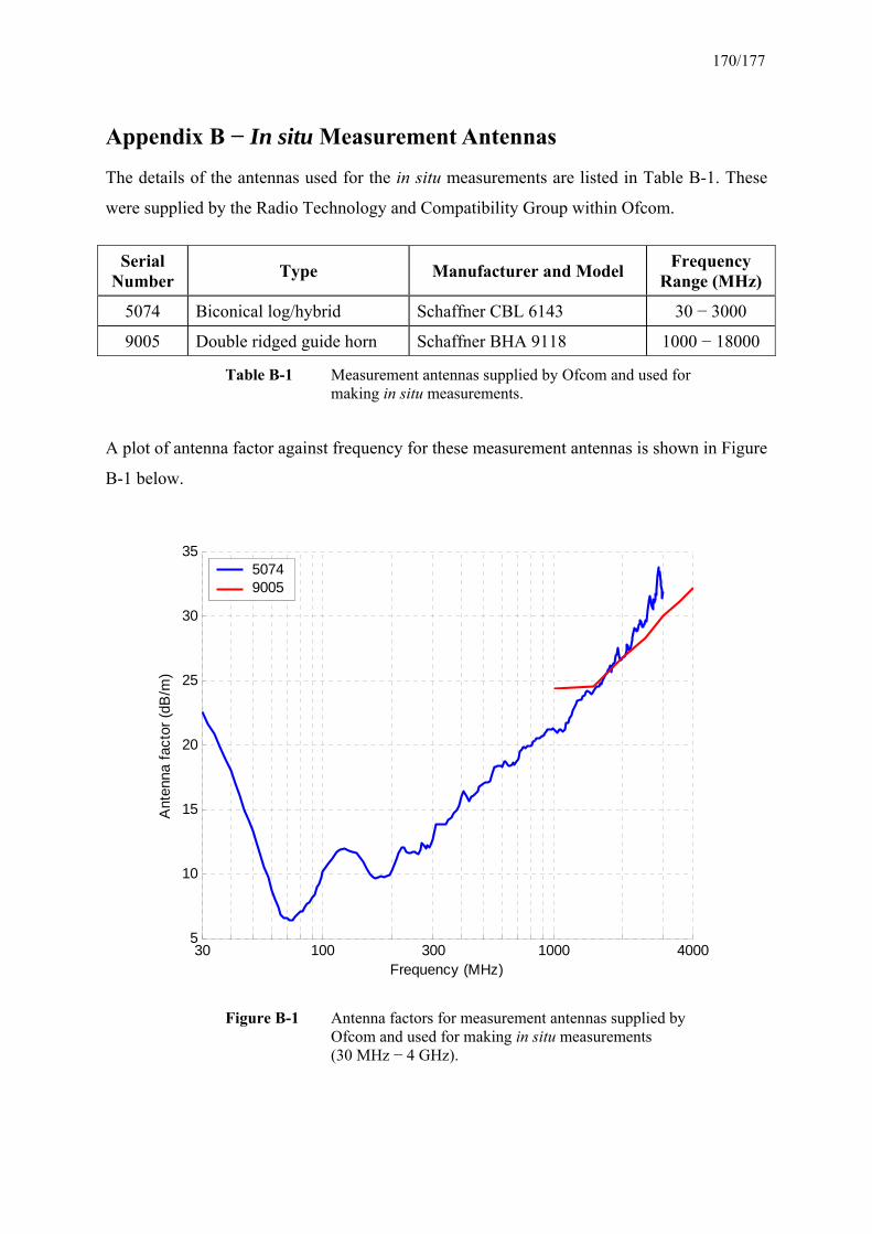
170/177
Appendix B − In situ Measurement Antennas
The details of the antennas used for the in situ measurements are listed in Table B-1. These
were supplied by the Radio Technology and Compatibility Group within Ofcom.
Serial Number Type Manufacturer and Model Frequency
Range (MHz)
5074 Biconical log/hybrid Schaffner CBL 6143 30 − 3000
9005 Double ridged guide horn Schaffner BHA 9118 1000 − 18000
A plot of antenna factor against frequency for these measurement antennas is shown in Figure
B-1 below.
Table B-1 Measurement antennas supplied by Ofcom and used for making in situ measurements.
30 100 300 1000 40005
10
15
20
25
30
35
Frequency (MHz)
Ant
enna
fact
or (d
B/m
)
50749005
Figure B-1 Antenna factors for measurement antennas supplied by Ofcom and used for making in situ measurements (30 MHz − 4 GHz).
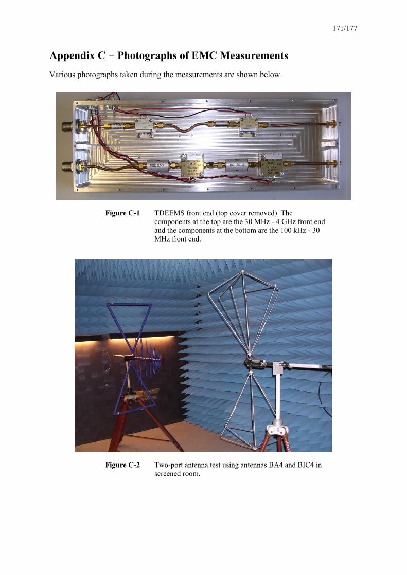
171/177
Appendix C − Photographs of EMC Measurements
Various photographs taken during the measurements are shown below.
Figure C-1 TDEEMS front end (top cover removed). The components at the top are the 30 MHz - 4 GHz front end and the components at the bottom are the 100 kHz - 30 MHz front end.
Figure C-2 Two-port antenna test using antennas BA4 and BIC4 in screened room.

172/177
Figure C-3 Measuring emissions from CGE01 comb generator in screened room using antenna BA4.
Figure C-4 Measurement of magnetic emissions from 110 kHz magnetic test source using 2 m loop antenna.

173/177
Figure C-5 Measurements using antenna BA4 on open air test site OATS2.
Figure C-6 Measuring radiated emissions from energy saving fluorescent light bulb using antenna DRGFS.

174/177
Figure C-7 Measuring radiated emissions from fast transient generator using antenna BA4.
Figure C-8 Measuring radiated emissions from portable 14" colour television using antenna DRGFS.

175/177
Figure C-9 Measuring radiated emissions from electric drill (without suppressor fitted) using antenna BA4.
Figure C-10 Measuring radiation emissions from desktop PC (without case fitted) using antenna BA4.

176/177
Figure C-11 Van with antennas on roof for railway EMC measurements.
Figure C-12 EMC measurements of local train.

177/177
Figure C-13 EMC measurements of local train.
Figure C-14 TDEEMS equipment inside van.


