Page 1
W I S S E N T E C H N I K L E I D E N S C H A F T
www.numerik.math.tugraz.at
Time Fractional DiffusionEquation
Sarah-Lena Bonkhoff
Institut fur Numerische Mathematik
9th Workshop on Analysis and Advanced Numerical Methods forPartial Differential EquationsStrobl, 07 July 2016
Page 2
www.numerik.math.tugraz.at
Table of Contents
1. Time Fractional Diffusion Problem
2. Variational Formulation
3. Fundamental Solution
4. Single Layer Potential
Sarah-Lena Bonkhoff, Institut fur Numerische Mathematik07-07-20162
Page 3
www.numerik.math.tugraz.at
Table of Contents
1. Time Fractional Diffusion Problem
2. Variational Formulation
3. Fundamental Solution
4. Single Layer Potential
Sarah-Lena Bonkhoff, Institut fur Numerische Mathematik07-07-20163
Page 4
www.numerik.math.tugraz.at
Time Fractional Diffusion Equation
Model problem:
0∂αt u(x , t)−∆u(x , t) = f (x , t), in QT := Ω× (0,T ),
u(x , t) = 0, on ΣT := ∂Ω× (0,T ),
u(x ,0) = u0(x), for x ∈ Ω,
where Ω ⊂ Rn is a smooth and bounded domain and0 < α ≤ 1.
→ R0 ∂
αt : Riemann-Liouville derivative
→ C0 ∂
αt : Caputo derivative
Sarah-Lena Bonkhoff, Institut fur Numerische Mathematik07-07-20164
Page 5
www.numerik.math.tugraz.at
Time Fractional Diffusion Equation
Model problem:
0∂αt u(x , t)−∆u(x , t) = f (x , t), in QT := Ω× (0,T ),
u(x , t) = 0, on ΣT := ∂Ω× (0,T ),
u(x ,0) = u0(x), for x ∈ Ω,
where Ω ⊂ Rn is a smooth and bounded domain and0 < α ≤ 1.
→ R0 ∂
αt : Riemann-Liouville derivative
→ C0 ∂
αt : Caputo derivative
Sarah-Lena Bonkhoff, Institut fur Numerische Mathematik07-07-20164
Page 6
www.numerik.math.tugraz.at
Riemann-Liouville Definition
- Left R.-L. fractional derivative of order 0 < α ≤ 1 is defined as
R0 ∂
αt u(x , t) =
1Γ(1− α)
∂
∂t
∫ t
0
u(x , τ)
(t − τ)αdτ,
where Γ(·) denotes Gamma function
Γ(x) =
∫ ∞0
tx−1e−t dt
- Right R.-L. fractional derivative of order 0 < α ≤ 1 is defined as
Rt ∂
αT u(x , t) = − 1
Γ(1− α)
∂
∂t
∫ T
t
u(x , τ)
(τ − t)αdτ
Sarah-Lena Bonkhoff, Institut fur Numerische Mathematik07-07-20165
Page 7
www.numerik.math.tugraz.at
Riemann-Liouville Definition
- Left R.-L. fractional derivative of order 0 < α ≤ 1 is defined as
R0 ∂
αt u(x , t) =
1Γ(1− α)
∂
∂t
∫ t
0
u(x , τ)
(t − τ)αdτ,
where Γ(·) denotes Gamma function
Γ(x) =
∫ ∞0
tx−1e−t dt
- Right R.-L. fractional derivative of order 0 < α ≤ 1 is defined as
Rt ∂
αT u(x , t) = − 1
Γ(1− α)
∂
∂t
∫ T
t
u(x , τ)
(τ − t)αdτ
Sarah-Lena Bonkhoff, Institut fur Numerische Mathematik07-07-20165
Page 8
www.numerik.math.tugraz.at
Riemann-Liouville Definition
→ Laplace transform of the R.-L. derivative (n − 1 ≤ α < n)
LR0 Dα
t f (t); s = sα f (s)−n−1∑k=0
sk [R0 Dα−k−1t f (t)]t=0,
Sarah-Lena Bonkhoff, Institut fur Numerische Mathematik07-07-20166
Page 9
www.numerik.math.tugraz.at
Caputo Definition
- Left Caputo fractional derivative of order 0 < α ≤ 1:
C0 ∂
αt u(x , t) =
1Γ(1− α)
∫ t
0
∂u(x , τ)
∂τ
1(t − τ)α
dτ
- Right Caputo fractional derivative of order 0 < α ≤ 1:
Ct ∂
αT u(x , t) = − 1
Γ(1− α)
∫ T
t
∂u(x , τ)
∂τ
1(τ − t)α
dτ
→ Laplace transform of the Caputo derivative (n − 1 < α ≤ n)
LC0 Dα
t f (t); s = sα f (s)−n−1∑k=0
sα−k−1f (k)(0),
Sarah-Lena Bonkhoff, Institut fur Numerische Mathematik07-07-20167
Page 10
www.numerik.math.tugraz.at
Caputo Definition
- Left Caputo fractional derivative of order 0 < α ≤ 1:
C0 ∂
αt u(x , t) =
1Γ(1− α)
∫ t
0
∂u(x , τ)
∂τ
1(t − τ)α
dτ
- Right Caputo fractional derivative of order 0 < α ≤ 1:
Ct ∂
αT u(x , t) = − 1
Γ(1− α)
∫ T
t
∂u(x , τ)
∂τ
1(τ − t)α
dτ
→ Laplace transform of the Caputo derivative (n − 1 < α ≤ n)
LC0 Dα
t f (t); s = sα f (s)−n−1∑k=0
sα−k−1f (k)(0),
Sarah-Lena Bonkhoff, Institut fur Numerische Mathematik07-07-20167
Page 11
www.numerik.math.tugraz.at
Fractional Derivatives
Relationship between R.-L. and Caputio derivatives for0 < α ≤ 1:
R0 ∂
αt u(x , t) =
u(x ,0)
Γ(1− α)tα+ C
0 ∂αt u(x , t)
- For homogeneous initial condition the R.-L. definition coincideswith the Caputo definition
- R.-L. derivatives for definitions of new function classes
- Caputo derivatives for handling inhomogeneous initial conditions
Sarah-Lena Bonkhoff, Institut fur Numerische Mathematik07-07-20168
Page 12
www.numerik.math.tugraz.at
Fractional Derivatives
Relationship between R.-L. and Caputio derivatives for0 < α ≤ 1:
R0 ∂
αt u(x , t) =
u(x ,0)
Γ(1− α)tα+ C
0 ∂αt u(x , t)
- For homogeneous initial condition the R.-L. definition coincideswith the Caputo definition
- R.-L. derivatives for definitions of new function classes
- Caputo derivatives for handling inhomogeneous initial conditions
Sarah-Lena Bonkhoff, Institut fur Numerische Mathematik07-07-20168
Page 13
www.numerik.math.tugraz.at
Analytical Solution
1D time fractional diffusion equation for 0 < α ≤ 1C0 ∂
αt u(x , t)− ∂2
x u(x , t) = 0, x ∈ (0,1), t ≥ 0u(0, t) = u(1, t) = 0, t ≥ 0
u(x ,0) = u0(x), x ∈ (0,1)
→ separation of variables:
u(x , t) = 2∞∑
k=1
Eα,1(−(kπ)2tα)sin(kπx)
∫ 1
0u0(τ)sin(kπτ) dτ
with Mittag-Leffler function
Eµ,ν(z) :=∞∑
k=0
zk
Γ(µk + ν), z ∈ C.
Sarah-Lena Bonkhoff, Institut fur Numerische Mathematik07-07-20169
Page 14
www.numerik.math.tugraz.at
Analytical Solution
1D time fractional diffusion equation for 0 < α ≤ 1C0 ∂
αt u(x , t)− ∂2
x u(x , t) = 0, x ∈ (0,1), t ≥ 0u(0, t) = u(1, t) = 0, t ≥ 0
u(x ,0) = u0(x), x ∈ (0,1)
→ separation of variables:
u(x , t) = 2∞∑
k=1
Eα,1(−(kπ)2tα)sin(kπx)
∫ 1
0u0(τ)sin(kπτ) dτ
with Mittag-Leffler function
Eµ,ν(z) :=∞∑
k=0
zk
Γ(µk + ν), z ∈ C.
Sarah-Lena Bonkhoff, Institut fur Numerische Mathematik07-07-20169
Page 15
www.numerik.math.tugraz.at
Analytical Solution
1D time fractional diffusion equation for 0 < α ≤ 1C0 ∂
αt u(x , t)− ∂2
x u(x , t) = 0, x ∈ (0,1), t ≥ 0u(0, t) = u(1, t) = 0, t ≥ 0
u(x ,0) = u0(x), x ∈ (0,1)
→ separation of variables:
u(x , t) = 2∞∑
k=1
Eα,1(−(kπ)2tα)sin(kπx)
∫ 1
0u0(τ)sin(kπτ) dτ
with Mittag-Leffler function
Eµ,ν(z) :=∞∑
k=0
zk
Γ(µk + ν), z ∈ C.
Sarah-Lena Bonkhoff, Institut fur Numerische Mathematik07-07-20169
Page 16
www.numerik.math.tugraz.at
Example
u(x , t) = 2∞∑
k=1
Eα,1(−(kπ)2tα)sin(kπx)
∫ 1
0u0(τ)sin(kπτ) dτ
u0(x) = x(1− x), x ∈ (0,1)
0
0.2
0.4
0.6
0.8
1
0
0.5
1
1.5
2
0
0.05
0.1
0.15
0.2
0.25
distance
time
U(x
,t)
solution for α = 1
0
0.2
0.4
0.6
0.8
1
0
0.5
1
1.5
2
0
0.05
0.1
0.15
0.2
0.25
distance
time
U(x
,t)
solution for α = 12
Sarah-Lena Bonkhoff, Institut fur Numerische Mathematik07-07-201610
Page 17
www.numerik.math.tugraz.at
Table of Contents
1. Time Fractional Diffusion Problem
2. Variational Formulation
3. Fundamental Solution
4. Single Layer Potential
Sarah-Lena Bonkhoff, Institut fur Numerische Mathematik07-07-201611
Page 18
www.numerik.math.tugraz.at
Fractional Derivative Spaces [Ervin and Roop (2007)]
For r , s > 0 and I = (0,T ) we consider the anisotropic Sobolevspaces
H r ,s(Ω× I) = L2(I; H r (Ω)) ∩ Hs(I; L2(Ω))
Define Hsl (I) as the closure of C∞0 (I) with respect to the norm
‖v‖Hsl (I) :=
(‖v‖2L2(I) + |v |2Hs
l (I)
) 12, |v |Hs
l (I) := ‖R0 Dst v‖L2(I).
→ analogue we can define the spaces Hsr (I) and Hs
c (I) with
|v |Hsr (I) := ‖Rt Ds
T v‖L2(I)
|v |Hsc (I) := |(R
0 Dst v , R
t DsT v)L2(I)|
12 , s 6= n − 1
2
Sarah-Lena Bonkhoff, Institut fur Numerische Mathematik07-07-201612
Page 19
www.numerik.math.tugraz.at
Fractional Derivative Spaces [Ervin and Roop (2007)]
For r , s > 0 and I = (0,T ) we consider the anisotropic Sobolevspaces
H r ,s(Ω× I) = L2(I; H r (Ω)) ∩ Hs(I; L2(Ω))
Define Hsl (I) as the closure of C∞0 (I) with respect to the norm
‖v‖Hsl (I) :=
(‖v‖2L2(I) + |v |2Hs
l (I)
) 12, |v |Hs
l (I) := ‖R0 Dst v‖L2(I).
→ analogue we can define the spaces Hsr (I) and Hs
c (I) with
|v |Hsr (I) := ‖Rt Ds
T v‖L2(I)
|v |Hsc (I) := |(R
0 Dst v , R
t DsT v)L2(I)|
12 , s 6= n − 1
2
Sarah-Lena Bonkhoff, Institut fur Numerische Mathematik07-07-201612
Page 20
www.numerik.math.tugraz.at
Fractional Derivative Spaces [Ervin and Roop (2007)]
For r , s > 0 and I = (0,T ) we consider the anisotropic Sobolevspaces
H r ,s(Ω× I) = L2(I; H r (Ω)) ∩ Hs(I; L2(Ω))
Define Hsl (I) as the closure of C∞0 (I) with respect to the norm
‖v‖Hsl (I) :=
(‖v‖2L2(I) + |v |2Hs
l (I)
) 12, |v |Hs
l (I) := ‖R0 Dst v‖L2(I).
→ analogue we can define the spaces Hsr (I) and Hs
c (I) with
|v |Hsr (I) := ‖Rt Ds
T v‖L2(I)
|v |Hsc (I) := |(R
0 Dst v , R
t DsT v)L2(I)|
12 , s 6= n − 1
2
Sarah-Lena Bonkhoff, Institut fur Numerische Mathematik07-07-201612
Page 21
www.numerik.math.tugraz.at
Properties
- For s 6= n + 12 the spaces Hs
c (I) and Hs0(I) are equal with
seminorms and norms
- For 0 < α < 1 and w ∈ Hα(I), v ∈ C∞0 (I):(R0 Dα
t w , v)
I=(
w , Rt Dα
T v)
I
- For 0 < α < 1 and w ∈ H1(I),w(0) = 0, v ∈ Hα2 (I)(
R0 Dα
t w , v)
I=(
R0 D
α2
t w , Rt D
α2
T v)
I
Sarah-Lena Bonkhoff, Institut fur Numerische Mathematik07-07-201613
Page 22
www.numerik.math.tugraz.at
Properties
- For s 6= n + 12 the spaces Hs
c (I) and Hs0(I) are equal with
seminorms and norms
- For 0 < α < 1 and w ∈ Hα(I), v ∈ C∞0 (I):(R0 Dα
t w , v)
I=(
w , Rt Dα
T v)
I
- For 0 < α < 1 and w ∈ H1(I),w(0) = 0, v ∈ Hα2 (I)(
R0 Dα
t w , v)
I=(
R0 D
α2
t w , Rt D
α2
T v)
I
Sarah-Lena Bonkhoff, Institut fur Numerische Mathematik07-07-201613
Page 23
www.numerik.math.tugraz.at
Properties
- For s 6= n + 12 the spaces Hs
c (I) and Hs0(I) are equal with
seminorms and norms
- For 0 < α < 1 and w ∈ Hα(I), v ∈ C∞0 (I):(R0 Dα
t w , v)
I=(
w , Rt Dα
T v)
I
- For 0 < α < 1 and w ∈ H1(I),w(0) = 0, v ∈ Hα2 (I)(
R0 Dα
t w , v)
I=(
R0 D
α2
t w , Rt D
α2
T v)
I
Sarah-Lena Bonkhoff, Institut fur Numerische Mathematik07-07-201613
Page 24
www.numerik.math.tugraz.at
Variational Formulation [Li and Xu (2010)]
Find u ∈ H1,α20 (QT ), u(x ,0) = 0:(
R0 ∂
α2
t u, Rt ∂
α2
T v)
QT
+ (∂xu, ∂xv)QT= (f , v)QT
for all v ∈ H1,α20 (QT ), v(x ,0) = 0 and 0 < α < 1.
→ Bilinearform is continuous and coercive
⇒ Existence and uniqueness of the solution by Lax-Milgram
Sarah-Lena Bonkhoff, Institut fur Numerische Mathematik07-07-201614
Page 25
www.numerik.math.tugraz.at
Variational Formulation [Li and Xu (2010)]
Find u ∈ H1,α20 (QT ), u(x ,0) = 0:(
R0 ∂
α2
t u, Rt ∂
α2
T v)
QT
+ (∂xu, ∂xv)QT= (f , v)QT
for all v ∈ H1,α20 (QT ), v(x ,0) = 0 and 0 < α < 1.
→ Bilinearform is continuous and coercive
⇒ Existence and uniqueness of the solution by Lax-Milgram
Sarah-Lena Bonkhoff, Institut fur Numerische Mathematik07-07-201614
Page 26
www.numerik.math.tugraz.at
Table of Contents
1. Time Fractional Diffusion Problem
2. Variational Formulation
3. Fundamental Solution
4. Single Layer Potential
Sarah-Lena Bonkhoff, Institut fur Numerische Mathematik07-07-201615
Page 27
www.numerik.math.tugraz.at
Model Problem
Time fractional diffusion equation with Caputo derivativeC0 ∂
αt u −∆u = 0, in QT = Ω× (0,T ),
u|ΣT= g, on ΣT = Γ× (0,T ),
u(x ,0) = 0, for x ∈ Ω,
0 < α ≤ 1 and Ω open and bounded with smooth boundary.
Consider the fractional diffusion equation
(C0 ∂
αt −∆)G(x , t) = δ(x , t).
→ Fourier-Laplace transform:
(|ξ|2 + sα)ˆG(ξ, s) = 1
⇔ ˆG(ξ, s) =1
|ξ|2 + sα
Sarah-Lena Bonkhoff, Institut fur Numerische Mathematik07-07-201616
Page 28
www.numerik.math.tugraz.at
Model Problem
Time fractional diffusion equation with Caputo derivativeC0 ∂
αt u −∆u = 0, in QT = Ω× (0,T ),
u|ΣT= g, on ΣT = Γ× (0,T ),
u(x ,0) = 0, for x ∈ Ω,
0 < α ≤ 1 and Ω open and bounded with smooth boundary.
Consider the fractional diffusion equation
(C0 ∂
αt −∆)G(x , t) = δ(x , t).
→ Fourier-Laplace transform:
(|ξ|2 + sα)ˆG(ξ, s) = 1
⇔ ˆG(ξ, s) =1
|ξ|2 + sα
Sarah-Lena Bonkhoff, Institut fur Numerische Mathematik07-07-201616
Page 29
www.numerik.math.tugraz.at
Model Problem
Time fractional diffusion equation with Caputo derivativeC0 ∂
αt u −∆u = 0, in QT = Ω× (0,T ),
u|ΣT= g, on ΣT = Γ× (0,T ),
u(x ,0) = 0, for x ∈ Ω,
0 < α ≤ 1 and Ω open and bounded with smooth boundary.
Consider the fractional diffusion equation
(C0 ∂
αt −∆)G(x , t) = δ(x , t).
→ Fourier-Laplace transform:
(|ξ|2 + sα)ˆG(ξ, s) = 1
⇔ ˆG(ξ, s) =1
|ξ|2 + sα
Sarah-Lena Bonkhoff, Institut fur Numerische Mathematik07-07-201616
Page 30
www.numerik.math.tugraz.at
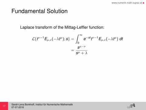
Fundamental Solution
Laplace transform of the Mittag-Leffler function:
Ltν−1Eµ,ν(−λtµ); s =
∫ ∞0
e−st tν−1Eµ,ν(−λtµ) dt
=sµ−ν
sµ + λ
→ Fourier transform of the fundamental solution:
ˆG(ξ, s) =1
|ξ|2 + sα↔ G(ξ, t) = tα−1Eα,α(−|ξ|2tα)
Sarah-Lena Bonkhoff, Institut fur Numerische Mathematik07-07-201617
Page 31
www.numerik.math.tugraz.at
Fundamental Solution
Laplace transform of the Mittag-Leffler function:
Ltν−1Eµ,ν(−λtµ); s =
∫ ∞0
e−st tν−1Eµ,ν(−λtµ) dt
=sµ−ν
sµ + λ
→ Fourier transform of the fundamental solution:
ˆG(ξ, s) =1
|ξ|2 + sα↔ G(ξ, t) = tα−1Eα,α(−|ξ|2tα)
Sarah-Lena Bonkhoff, Institut fur Numerische Mathematik07-07-201617
Page 32
www.numerik.math.tugraz.at
Fundamental Solution
→ invert Fourier transform:
G(x , t) = (2π)−n2
∫Rn
tα−1Eα,α(−|ξ|2tα)eiξx dξ
= π−n2 tα−1|x |−nH(1)
(14|x |2t−α
),
where
H(1)(z) := H2012
[z∣∣∣(α,α)( n
2 ,1),(1,1)
]=
12πi
∫C
Γ( n2 + s)Γ(1 + s)
Γ(α + αs)z−s ds,
is the Mellin-Barnes integral definition of the Fox H-function
Sarah-Lena Bonkhoff, Institut fur Numerische Mathematik07-07-201618
Page 33
www.numerik.math.tugraz.at
Table of Contents
1. Time Fractional Diffusion Problem
2. Variational Formulation
3. Fundamental Solution
4. Single Layer Potential
Sarah-Lena Bonkhoff, Institut fur Numerische Mathematik07-07-201619
Page 34
www.numerik.math.tugraz.at
Single Layer Potential
→ For a given boundary distribution σ(x , t) ∈ C∞(ΣT ) we definethe single layer potential
u(x , t) = Sσ(x , t) =
∫ t
0
∫Γ
σ(y , τ)G(x − y , t − τ) dsy dτ,
for x ∈ Ω, t ∈ (0,T )
→ Boundary integral equation:
Vσ(x , t) := γ(Sσ)(x , t) = γ(u)(x , t) = g(x , t),
for (x , t) ∈ ΣT
→ For 0 < s < 1 the operator
V : H−s,−α2 s(ΣT )→ H1−s,α2 (1−s)(ΣT )
is continuous
Sarah-Lena Bonkhoff, Institut fur Numerische Mathematik07-07-201620
Page 35
www.numerik.math.tugraz.at
Single Layer Potential
→ For a given boundary distribution σ(x , t) ∈ C∞(ΣT ) we definethe single layer potential
u(x , t) = Sσ(x , t) =
∫ t
0
∫Γ
σ(y , τ)G(x − y , t − τ) dsy dτ,
for x ∈ Ω, t ∈ (0,T )
→ Boundary integral equation:
Vσ(x , t) := γ(Sσ)(x , t) = γ(u)(x , t) = g(x , t),
for (x , t) ∈ ΣT
→ For 0 < s < 1 the operator
V : H−s,−α2 s(ΣT )→ H1−s,α2 (1−s)(ΣT )
is continuous
Sarah-Lena Bonkhoff, Institut fur Numerische Mathematik07-07-201620
Page 36
www.numerik.math.tugraz.at
Single Layer Potential
→ For a given boundary distribution σ(x , t) ∈ C∞(ΣT ) we definethe single layer potential
u(x , t) = Sσ(x , t) =
∫ t
0
∫Γ
σ(y , τ)G(x − y , t − τ) dsy dτ,
for x ∈ Ω, t ∈ (0,T )
→ Boundary integral equation:
Vσ(x , t) := γ(Sσ)(x , t) = γ(u)(x , t) = g(x , t),
for (x , t) ∈ ΣT
→ For 0 < s < 1 the operator
V : H−s,−α2 s(ΣT )→ H1−s,α2 (1−s)(ΣT )
is continuous
Sarah-Lena Bonkhoff, Institut fur Numerische Mathematik07-07-201620
Page 37
www.numerik.math.tugraz.at
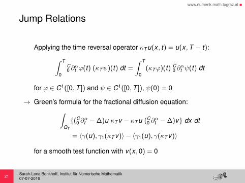
Jump Relations
Applying the time reversal operator κT u(x , t) = u(x ,T − t):∫ T
0
C0 ∂
αt ϕ(t) (κTψ)(t) dt =
∫ T
0(κTϕ)(t) C
0 ∂αt ψ(t) dt
for ϕ ∈ C1([0,T ]) and ψ ∈ C1([0,T ]), ψ(0) = 0
→ Green’s formula for the fractional diffusion equation:∫QT
(C0 ∂
αt −∆)u κT v − κT u (C
0 ∂αt −∆)v dx dt
= 〈γ(u), γ1(κT v)〉 − 〈γ1(u), γ(κT v)〉
for a smooth test function with v(x ,0) = 0
Sarah-Lena Bonkhoff, Institut fur Numerische Mathematik07-07-201621
Page 38
www.numerik.math.tugraz.at
Jump Relations
Applying the time reversal operator κT u(x , t) = u(x ,T − t):∫ T
0
C0 ∂
αt ϕ(t) (κTψ)(t) dt =
∫ T
0(κTϕ)(t) C
0 ∂αt ψ(t) dt
for ϕ ∈ C1([0,T ]) and ψ ∈ C1([0,T ]), ψ(0) = 0
→ Green’s formula for the fractional diffusion equation:∫QT
(C0 ∂
αt −∆)u κT v − κT u (C
0 ∂αt −∆)v dx dt
= 〈γ(u), γ1(κT v)〉 − 〈γ1(u), γ(κT v)〉
for a smooth test function with v(x ,0) = 0
Sarah-Lena Bonkhoff, Institut fur Numerische Mathematik07-07-201621
Page 39
www.numerik.math.tugraz.at
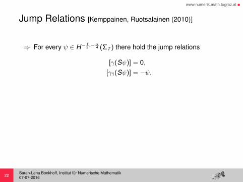
Jump Relations [Kemppainen, Ruotsalainen (2010)]
⇒ For every ψ ∈ H−12 ,−
α4 (ΣT ) there hold the jump relations
[γ(Sψ)] = 0,[γ1(Sψ)] = −ψ.
Sarah-Lena Bonkhoff, Institut fur Numerische Mathematik07-07-201622
Page 40
www.numerik.math.tugraz.at
Coercivity
Theorem (Kemppainen, Routsalainen (2010))
The single layer operator V : H−12 ,−
α4 (ΣT )→ H
12 ,α4 (ΣT ) is an
isomorphism. Futhermore, it is coercive, i.e. there exists a positiveconstant c such that
〈Vσ, σ〉 ≥ c‖σ‖2H− 1
2 ,−α4 (ΣT )
for all σ ∈ H−12 ,−
α4 (ΣT ).
→ TFDE admits a unique solution u(x , t) ∈ H1,α2 (QT )
u(x , t) = Sσ(x , t),
where σ ∈ H−12 ,−
α4 (ΣT ) is the unique solution of
Vσ = g, g ∈ H12 ,
α4 (ΣT )
Sarah-Lena Bonkhoff, Institut fur Numerische Mathematik07-07-201623
Page 41
www.numerik.math.tugraz.at
Coercivity
Theorem (Kemppainen, Routsalainen (2010))
The single layer operator V : H−12 ,−
α4 (ΣT )→ H
12 ,α4 (ΣT ) is an
isomorphism. Futhermore, it is coercive, i.e. there exists a positiveconstant c such that
〈Vσ, σ〉 ≥ c‖σ‖2H− 1
2 ,−α4 (ΣT )
for all σ ∈ H−12 ,−
α4 (ΣT ).
→ TFDE admits a unique solution u(x , t) ∈ H1,α2 (QT )
u(x , t) = Sσ(x , t),
where σ ∈ H−12 ,−
α4 (ΣT ) is the unique solution of
Vσ = g, g ∈ H12 ,
α4 (ΣT )
Sarah-Lena Bonkhoff, Institut fur Numerische Mathematik07-07-201623
Page 42
www.numerik.math.tugraz.at
Outlook
- Investigation of the boundary integral operators
→ apply the theory of boundary integral equation to thefractional diffusion equation
- Behavior of the fundamental solution
- Space time discretizations for the time fractional diffusionequation
Sarah-Lena Bonkhoff, Institut fur Numerische Mathematik07-07-201624
Page 43
www.numerik.math.tugraz.at
[1] DIETHELM, K., AND WEILBEER, M.Initial-boundary value problems for time-fractional diffusion-wave equations andtheir numerical solution.1st IFAC Workshop on Fractional Differentiation and its Applications (2004).
[2] ERVIN, V. J., AND ROOP, J. P.Variational solution of fractional advection dispersion equations on boundeddomains in Rd .Numer. Methods Partial Differential Equations 23, 2 (2007), 256–281.
[3] KEMPPAINEN, J.Properties of the single layer potential for the time fractional diffusion equation.J. Integral Equations Appl. 23, 3 (2011), 437–455.
[4] KEMPPAINEN, J., AND RUOTSALAINEN, K.Boundary integral solution of the time-fractional diffusion equation.In Integral methods in science and engineering. Vol. 2. Birkhauser Boston, 2010.
[5] LI, X., AND XU, C.Existence and uniqueness of the weak solution of the space-time fractionaldiffusion equation and a spectral method approximation.Commun. Comput. Phys. 8, 5 (2010), 1016–1051.
[6] PODLUBNY, I.Fractional differential equations.Mathematics in Science and Engineering. Academic Press, 1999.
Sarah-Lena Bonkhoff, Institut fur Numerische Mathematik07-07-201625
Page 44
www.numerik.math.tugraz.at
Sarah-Lena Bonkhoff, Institut fur Numerische Mathematik07-07-201626
Page 45
www.numerik.math.tugraz.at
Asymptotic Behavior [Kemppainen (2011)]
G(x , t) =
π−
n2 tα−1|x |−nH(1)
( 14 |x |
2t−α), x ∈ Rn, t > 0
0, x ∈ Rn, t > 0
(i) if z := 14 |x |
2t−α ≥ 1, then
|G(x , t)| ≤ Ct−αn2 −1+α exp(−σt−
α2−α |x |
22−α ),
where σ = 41
α−2αα
2−α (2− α)
(ii) if z ≤ 1, then
|G(x , t)| ≤ C
t−1 n = 2t−
α2 −1 n = 3
t−α−1(| log(|x |2t−α)|+ 1) n = 4t−α−1|x |−n+4 n > 4
Sarah-Lena Bonkhoff, Institut fur Numerische Mathematik07-07-201627
Page 46
www.numerik.math.tugraz.at
Asymptotic Behavior [Kemppainen (2011)]
G(x , t) =
π−
n2 tα−1|x |−nH(1)
( 14 |x |
2t−α), x ∈ Rn, t > 0
0, x ∈ Rn, t > 0
(i) if z := 14 |x |
2t−α ≥ 1, then
|G(x , t)| ≤ Ct−αn2 −1+α exp(−σt−
α2−α |x |
22−α ),
where σ = 41
α−2αα
2−α (2− α)
(ii) if z ≤ 1, then
|G(x , t)| ≤ C
t−1 n = 2t−
α2 −1 n = 3
t−α−1(| log(|x |2t−α)|+ 1) n = 4t−α−1|x |−n+4 n > 4
Sarah-Lena Bonkhoff, Institut fur Numerische Mathematik07-07-201627
Page 47
www.numerik.math.tugraz.at
Asymptotic Behavior [Kemppainen (2011)]
G(x , t) =
π−
n2 tα−1|x |−nH(1)
( 14 |x |
2t−α), x ∈ Rn, t > 0
0, x ∈ Rn, t > 0
(i) if z := 14 |x |
2t−α ≥ 1, then
|G(x , t)| ≤ Ct−αn2 −1+α exp(−σt−
α2−α |x |
22−α ),
where σ = 41
α−2αα
2−α (2− α)
(ii) if z ≤ 1, then
|G(x , t)| ≤ C
t−1 n = 2t−
α2 −1 n = 3
t−α−1(| log(|x |2t−α)|+ 1) n = 4t−α−1|x |−n+4 n > 4
Sarah-Lena Bonkhoff, Institut fur Numerische Mathematik07-07-201627
Page 48
www.numerik.math.tugraz.at
Caputo Derivative
For 0 < α < 1 and w ∈ H1(I), v ∈ Hα2 (I) we have(
C0 Dα
t w , v)
I=(
R0 D
α2
t w , Rt D
α2
T v)
I−(
w(0)t−α
Γ(1− α), v)
I.
⇒ Variational Formulation: find u ∈ H1,α20 (QT ):
(R0 ∂
α2
t u, Rt ∂
α2
T v)
QT
+ (∂xu, ∂xv)QT= (f , v)QT +
(u(x ,0)t−α
Γ(1− α), v)
QT
for all v ∈ H1,α20 (QT ).
Sarah-Lena Bonkhoff, Institut fur Numerische Mathematik07-07-201628
Page 49
www.numerik.math.tugraz.at
Caputo Derivative
For 0 < α < 1 and w ∈ H1(I), v ∈ Hα2 (I) we have(
C0 Dα
t w , v)
I=(
R0 D
α2
t w , Rt D
α2
T v)
I−(
w(0)t−α
Γ(1− α), v)
I.
⇒ Variational Formulation: find u ∈ H1,α20 (QT ):
(R0 ∂
α2
t u, Rt ∂
α2
T v)
QT
+ (∂xu, ∂xv)QT= (f , v)QT +
(u(x ,0)t−α
Γ(1− α), v)
QT
for all v ∈ H1,α20 (QT ).
Sarah-Lena Bonkhoff, Institut fur Numerische Mathematik07-07-201628
Page 50
www.numerik.math.tugraz.at
Continuity
Theorem (Kemppainen, Ruotsalainen (2010))Let 0 < s < 1. The operator
V : H−s,−α2 s(ΣT )→ H1−s,α2 (1−s)(ΣT )
is continuous.
- Sφ = G ∗ γ′(φ)
- ψ 7→ G ∗ ψ : H r ,α2 rcomp(Rn × (0,T ))→ H r+2,α2 (r+2)
loc (Rn × (0,T )) iscontinuous
- Trace γ : H r ,s(QT )→ Hλ,µ(ΣT ) is continuous and surjective forλ = r − 1
2 , µ = sr λ and r > 1
2 , s ≥ 0
- γ′ : H−λ,−µ(ΣT )→ H−r ,−scomp (Rn × (0,T ))
Sarah-Lena Bonkhoff, Institut fur Numerische Mathematik07-07-201629
Page 51
www.numerik.math.tugraz.at
Continuity
Theorem (Kemppainen, Ruotsalainen (2010))Let 0 < s < 1. The operator
V : H−s,−α2 s(ΣT )→ H1−s,α2 (1−s)(ΣT )
is continuous.
- Sφ = G ∗ γ′(φ)
- ψ 7→ G ∗ ψ : H r ,α2 rcomp(Rn × (0,T ))→ H r+2,α2 (r+2)
loc (Rn × (0,T )) iscontinuous
- Trace γ : H r ,s(QT )→ Hλ,µ(ΣT ) is continuous and surjective forλ = r − 1
2 , µ = sr λ and r > 1
2 , s ≥ 0
- γ′ : H−λ,−µ(ΣT )→ H−r ,−scomp (Rn × (0,T ))
Sarah-Lena Bonkhoff, Institut fur Numerische Mathematik07-07-201629


![Numerical study of time-fractional hyperbolic partial ... · advection-diffusion equation. Sousa [23] proposed an approximation of the Caputo fractional derivative of order 1 < 6](https://static.documents.pub/doc/80x56/5edbf1b6ad6a402d6666651a/numerical-study-of-time-fractional-hyperbolic-partial-advection-diffusion-equation.jpg)
