TECHNISCHE UNIVERSITÄT MÜNCHEN Lehrstuhl für Systemarchitektur: Betriebssysteme, Kommunikationssysteme, Rechnernetze „Time-of-flight in Wireless Networks as Information Source for Positioning „ Alejandro Ramírez Vollständiger Abdruck der von der Fakultät für Informatik der Technischen Universität München zur Erlangung des akademischen Grades eines Doktors der Naturwissenschaften genehmigten Dissertation. Vorsitzende: Univ.-Prof. G.J. Klinker, Ph.D. Prüfer der Dissertation: 1. Univ.-Prof. Dr. U. Baumgarten 2. Univ.-Prof. Dr. R. Kraemer, Brandenburgische Technische Universität Cottbus Die Dissertation wurde am 29. November 2010 bei der Technischen Universität München eingereicht und durch die Fakultät für Informatik am 06. Juni 2011 angenommen.
Transcript
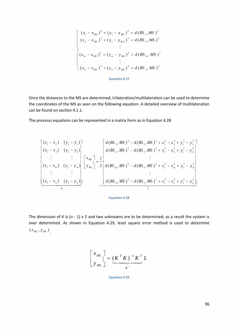
TECHNISCHE UNIVERSITÄT MÜNCHEN
Lehrstuhl für Systemarchitektur: Betriebssysteme, Kommunikationssysteme, Rechnernetze
„Time-of-flight in Wireless Networks as Information Source for Positioning „
Alejandro Ramírez
Vollständiger Abdruck der von der Fakultät für Informatik der Technischen Universität München zur
Erlangung des akademischen Grades eines
Doktors der Naturwissenschaften
genehmigten Dissertation.
Vorsitzende: Univ.-Prof. G.J. Klinker, Ph.D.
Prüfer der Dissertation:
1. Univ.-Prof. Dr. U. Baumgarten
2. Univ.-Prof. Dr. R. Kraemer, Brandenburgische Technische Universität Cottbus
Die Dissertation wurde am 29. November 2010 bei der Technischen Universität München eingereicht
und durch die Fakultät für Informatik am 06. Juni 2011 angenommen.
2
3
Wireless communication is the transfer of information over a distance without the use of electrical
conductors or wires. This form of communication has become ubiquitous today; it can be found in
just about any place including watches, bus tickets and even running shoes.
The mobility achieved by such communications has allowed a whole new set of applications, like
surfing the internet from anywhere in an airport, paying the bus fare with an RFID ticket and talking
on the phone with a wireless headset. However mobility brings a whole new set of problems too.
The long range capabilities of this communication technology make it challenging to find the location
of a user. This presents a problem, for example, when a user is able to use the wireless connection of
a company to access the internet and commit illegal behavior while been located outside of the
premises of this company. This could bring legal actions against the company which will also damage
its reputation.
In the case of finding the location of a wireless user, the current state-of-the-art allows for a very
wide variety of methods to be used. While the most accurate methods require expensive proprietary
hardware, a few others novel approaches use simple information sources to achieve a cheap but
very inexact approximation of the user's position.
The main purpose of this work is to develop a system that uses the round-trip-time of a wireless
signal to calculate the position of a mobile device using only off-the-shelf standard hardware. It is
compatible with all radio hardware without the need to change any internal component.
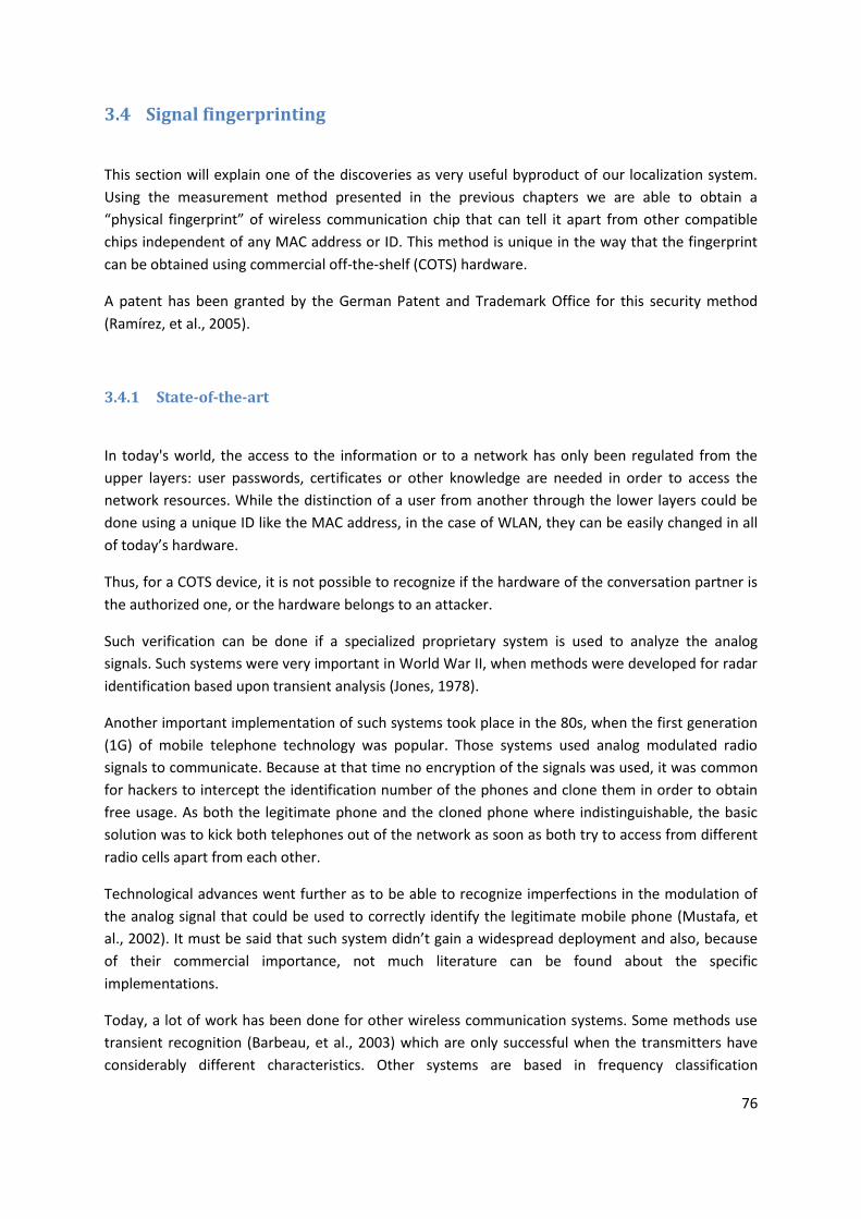
We will show that the system meets or exceeds the performance of commercial location systems
based in standard hardware and RSSI measurements. The system has been deployed in very
different conditions including very demanding industrial environments like a production line in an
automotive factory.
This system has many real world applications, some of which were implemented during the time of
this research. One challenging case that can be solved with the proposed system is including asset
and staff tracking in hospital. Another example is in the automotive branch, where workers and
heavy duty tools can be tracked to legally and officially document the work progress.
4
5
Table of Contents Table of Contents .................................................................................................................................... 5
Abbreviations and acronyms .................................................................................................................. 8
Chapter 1: Problem definition ........................................................................................................ 11
List of Figures ...................................................................................................................................... 152
List of Equations .................................................................................................................................. 157
List of Tables ....................................................................................................................................... 161
8
Abbreviations and acronyms
ACK Acknowledgement
ADC Analog to Digital Converter
ANN Artificial Neural Networks
BB Bound Boxing
BS Base Station
COTS Commercial Off-the-Shelf
DCO Digital Controlled Oscillator
EPO European Patent Office
GNSS Global Navigation Satellite System
GPS Global Positioning System
GPTO German Patent and Trademark Office
GUI Graphical User Interface
HOMEPLANE Home Media Platform and Networks
ISI InterSymbol Interference
LNA Low Noise Amplifier
LOS Line of Sight
LPF Low Pass Filter
LS Least Squares
LSL Least Squares Lateration
MAC Medium Access Control layer
MANET Mobile ad hoc network
MDL Multiditaleration
MS Mobile Station
NLOS Non Line of Sight
ODBC Open Database Connectivity
9
OFDM Orthogonal Frequency Division Multiplexing
PHY Physical layer
PM Pattern Matching
PSD Power Spectral Density
ppm Parts per Million
RFID Radio Frequency Identification
RMS Root Mean Squares
RSSI Received Signal Strength Indicator
RSU RoadSide Unit
RToF Round Trip Time of Flight
RTTDOA Round Trip Time Difference of Arrival
RWP Random WayPoint model
SIFS Shortest InterFrame Space
SNR Signal to Noise Ratio
SS Signal Strength
TDOA Time Difference of Arrival
TI Texas Instruments
TOA Time of Arrival
ToF Time of flight
TSF Timing Synchronization Function
UWB Ultra Wideband
VCO Voltage Controlled Oscillator
WGN White Gaussian Noise
WIPO World Intellectual Property Organization
WLAN Wireless Local Area Network
ZOMOFI ZOne MOnitoring & FInd
10
11
Chapter 1: Problem definition
For localization in outdoor environments, Global Navigation Satellite Systems (GNSS) like the global
positioning system (GPS) already provide a performance which is sufficient for many services,
especially after the deactivation of selective availability (Conley, 2000). To calculate the position
synchronized atomic clocks are required as well as especially designed hardware devices.
In typical indoor-environments, localization with satellite-based solution is practically impossible, as
a position fix takes several hours due to the distinctive NLOS-environment (Eissfeller B., 2005). Thus,
different alternatives have been proposed throughout the literature some of which are already
commercially available.
Indoor-localization solutions can be classified as follows:
Dedicated localization equipment including Ultra-wideband (UWB) (Cassioli, 2001), Ubisense
(Ward, 2007), ultrasound (Holm, 2005), etc.
localization systems based on standard wireless communication hardware
The information sources that these systems can use are:
received signal strength indication (RSSI)
Time-of-Flight (ToF)
Angle-of-Arrival (AoA)
While the best results with respect to accuracy and real-time behavior can be achieved with
dedicated localization systems, the utilization of already existing communication hardware can have
significant economic advantages.
As wireless communication systems are not designed for accurate indoor localization, it can be very
demanding to achieve sufficient localization performance. The main stumbling blocks are inaccurate
timers as well as the demanding environments involved (non line-of-sight, NLOS). While RSSI
information is very easy to extract from existing communication hardware, its fundamental
limitations (Elnahrawy, et al., 2004) make RSSI evaluations inappropriate for most use cases.
Thus, the main challenge to be addressed within this thesis is the extraction and evaluation of signal
time-of-flight information from standard communication hardware to show the enhanced
capabilities as well as limitations of this approach for indoor-localization
12
1.1 Motivation
Today, several systems exist, which task is to determine the location of a wireless device. In the case
of outdoor localization, the most famous one is the Global Positioning System (GPS), in which time
measurements between satellites and a receiver located anywhere on the Earth are done in order to
find the user’s position. However, when GPS is used indoors, the GPS signal is far too weak due to
penetration loss, which, added with the many signal reflections, result in a disappointing
performance. Proprietary pseudolite systems which generate GPS signals indoors also exist.
Unfortunately, their range is limited to about 10 meters and the usage of the GPS frequencies is
illegal in most developed (Eissfeller B., 2005).
To find the position of a device indoors, other systems exist, which have a better performance than
GPS, for example Radio Frequency IDentification (RFID) systems. There are also many systems based
on standard communication systems like WLAN, ZigBee, Bluetooth, GSM, UMTS, WiMAX, etc. Almost
all of these systems work by estimating the distance between a wireless client and a wireless base
station. After the distance to several stations has been calculated, algorithms like multilateration are
used to estimate the 2D/3D position of the client. To estimate this distance, there are two possible
information sources that can be used:
* The signal strength (SS): the amplitude of the signal when it arrives at the receiver
* The time of flight (ToF): The time it took the signal to travel between the transmitter and receiver
The most common method used to approximate the distance between two devices is the use of the
received signal strength indication (RSSI). This uses the physical property of the propagation of
electromagnetic waves, which says that the energy contained in a radio wave will diminish in
proportion to the distance travelled. The ratio between the power of the transmitted signal and the
power of the received signal is computed. The smaller this ratio, the farther one device is located
from the other.
Another method used to calculate the distance between two devices is to use the time it takes for a
signal to travel from one station to another; this time is typically known as Time-of-flight (ToF). Since
electromagnetic waves propagate with a speed very close to the speed of light under typical indoor
scenarios, the distance can easily be calculated based on this time.
When the ToF is used, it must be noted that very accurate timers are required for the receiving
stations. An error of just one microsecond (1 µs) in the delay estimation causes an error of 300 m in
the distance estimation. Additionally, synchronization of these stations might be necessary,
depending on the specific method used to obtain the location.
Literature describes different ways in which the relationship between nodes can be exploited to
obtain the position of the individual nodes. To achieve that, nodes in the network are distinguished
into two groups: beacon nodes which know their own position, and standard nodes, that have to
13
calculate their position through the relationship to other nodes. Furthermore, this document will
make a separation between the methods that can be used to find these positions:
Distance-based methods: In this category, the position of the individual nodes will be
approximated based on a direct distance measurement between all the nodes or between
the standard nodes and the beacon nodes. Examples for this kind of localization can be
found in (Savarese, et al., 2002), (Savvides, et al., 2001), and (Savvides, et al., 2002) among
others. An example in which the position estimation is done using the RSSI of the signals
received from the beacon nodes can be found in (Bergamo, et al., 2002).
Distance-less methods: In this category of methods, the range between the individual
network nodes will be defined by the hop-count, which is the number of nodes that will be
required to forward a data packets for two specific nodes to be able to communicate with
each other. This information will allow the retrieval of a geographic approximation of the
positions based on the network topology. No explicit measurement of the distances takes
place. Examples of such methods can be found in the works of (Niculescu, et al., 2003) as
well as the further developments of (Hsieh, et al., 2006).
1.2 State of the art
This section will explain the various options and methods for measuring these distances. The
problems that arise in such measurements will also be further illuminated.
1.2.1 Possible types of distance measurement
As mentioned before, there are several ways to obtain the distance travelled by a radio signal. The
most common methods of measurement are using either the signal strength of the received signal
or the time of flight.
1.2.2 Measurement of the Received Signal Strength
Received Signal Strength Indication (RSSI) is a measurement of the energy present in a received radio
signal. The rate in which the energy of a radio signal decreases when it is travelling a distance is a
well-known physical property.
The main advantages of this using the RSSI for estimating a distance is that the transmitter and the
receiver do not require any sort of time synchronization between them. Also, the RSSI signal can be
obtained very easily using standard hardware. However, this method is very sensitive to
disturbances in the signal path, for example through attenuation of signal strength or multipath
14
propagation due to intervening obstacles. This means that the signal strength varies even at fixed
stations over time, so the relationship between RSS and distance is very inaccurate (Elnahrawy, et
al., 2004) (see Figure 1.1). It can also be seen on the figure that the further apart the transmitter and
the receiver are from each other, the more difficult it is to tell the distance apart from one another.
One way to reduce these inaccuracies is by calibrating the area and then comparing these offline
measurements with the actual measurements. One example is the RADAR system from Microsoft
Research (Bahl, et al., 2000). Such a calibration takes a lot of time and effort, making such a
deployment quite costly. This calibration must be repeated if important changes in the environment
have been done, like after removing a wall or a big shelve.
In Figure 1.1, the relationship between the signal strength and the distance is presented. These
measurements were obtained every 5 meters outdoors with a direct line-of-sight (LOS). The results
are presented using a logarithmic scale to highlight the linear relationship. The values obtained show
a constantly decreasing curve, with a few exceptions. The position corresponding to 15 meters is not
in line with the other values of the curve, which will generate an error when the position is
calculated. The measurement at 15 meters (highlighted in orange) has an overlap with the value that
would correspond to 7 meters. The next outlier can be seen at 30 meters (highlighted in purple),
which delivers a value corresponding to 15 meters. As distance progresses it is more difficult to tell
the distance apart from each other. For example, the values reported for 45 meters and 50 meters
can easily have an error of 10 meters. Naturally, these specific results are dependent on the specific
environment where the measurements are done, and even in the same scenario the results may
change over time because of reflections.
Figure 1.1: Dependency of the RSSI on the distance to the transmitter.
-60,0
-55,0
-50,0
-45,0
-40,0
-35,0
-30,0
-25,0
-20,0
1,0 10,0 100,0
RSS
I (d
Bm
)
Distance (m)
Distance vs signal strength
15
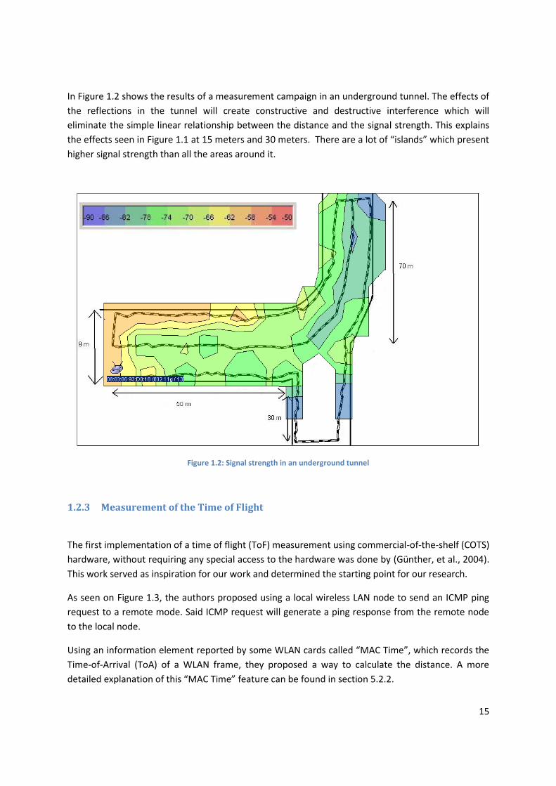
In Figure 1.2 shows the results of a measurement campaign in an underground tunnel. The effects of
the reflections in the tunnel will create constructive and destructive interference which will
eliminate the simple linear relationship between the distance and the signal strength. This explains
the effects seen in Figure 1.1 at 15 meters and 30 meters. There are a lot of “islands” which present
higher signal strength than all the areas around it.
Figure 1.2: Signal strength in an underground tunnel
1.2.3 Measurement of the Time of Flight
The first implementation of a time of flight (ToF) measurement using commercial-of-the-shelf (COTS)
hardware, without requiring any special access to the hardware was done by (Günther, et al., 2004).
This work served as inspiration for our work and determined the starting point for our research.
As seen on Figure 1.3, the authors proposed using a local wireless LAN node to send an ICMP ping
request to a remote mode. Said ICMP request will generate a ping response from the remote node
to the local node.
Using an information element reported by some WLAN cards called “MAC Time”, which records the
Time-of-Arrival (ToA) of a WLAN frame, they proposed a way to calculate the distance. A more
detailed explanation of this “MAC Time” feature can be found in section 5.2.2.
16
Local node Remote node
Re
mo
te d
ela
y
Data frame(eg. ICMP ping request)
Immediate ACK
MAC processing
Lo
ca
l de
lay
Data frame
(eg. ICMP ping response)
Immediate ACK
Local delay on
remote node
Upper layer
processing
Figure 1.3: Sequence diagram of the measurement system proposed by (Günther, et al., 2004)
By setting a monitor device next to a local node, the duration of the remote delay and the local delay
are recorded. The authors then suppose that when using WLAN cards of the same manufacturer and
model the delays of the hardware components are exactly the same. With that assumption, a
subtraction of the remote delay and the local delay will result in the time-of-flight (ToF) of the signal.
An additional contribution of this work is has to do with the usage of low resolution measurements.
As the “MAC Time” has a resolution of 1µs, which represents to a ToF of 300 meters (or 150m on a
round-trip-time, RTT), they proposed to average the results of several measurements to obtain a
higher accuracy. The exact cause of why this averaging works hasn’t been properly clarified in the
literature, even though the validity of the idea has been empirically demonstrated.
n
n
mitteln
xxx
nT
1
211
Equation 1.1
17
The first possible explanation for why this works would be a presumption of Günther and Hoene that
there is Gaussian noise present, originating from thermal noise, multi-path and clock drift. Section
3.2.3 contains simulations and validations about why this source would be too low to account for the
effect seen.
The next proposal by the authors is an influence by the so-called stochastic resonance. Stochastic
resonance can be found in a bistable system (a system with only two states, in which an internal
threshold decides the state of the system) when a small sinusoidal signal is added to a large wide
band noise signal. Both added signals will then be fine-tuned to achieve a resonance and thus find a
hidden signal inside the system, which magnitude is not large enough to trigger the threshold of said
system. The authors propose that the not quantifiable signal is the time-of-flight, which however is
not periodic. There is also no control on the noise sources presented. The authors noticed some
discrepancies with stochastic resonance in their verification model, reason for which they present a
third possible reason for a successful measurement.
The third reason proposed is the beat frequency, which takes into account that two WLAN cards
driven by a built-in crystal oscillator with nearly the same frequency are present in their
measurement system. The subtraction of both frequencies will give a lower order frequency as a
result, which will be the effect of the two interfering waves, known as beat frequency.
During our work, measurements show that two WLAN cards of the same manufacturer and model
do not present the exact internal hardware delay, to a degree that said assumption would cause
great errors in a location system. The different internal hardware delay is actually a feature that can
be used as a ‘fingerprint’, and allows us to identify a user’s hardware independently of who the user
claims to be (Ramírez, et al., 2005). Section 3.4will explain how this works.
Unlike the system presented in (Günther, et al., 2004) our own system is able to locate any mobile
device using WLAN cards of different manufacturers. The reasons the system works are explained in
detail in section 3.1 and section 3.2.
A somewhat similar measurement system has been built by the University of Waikato (Bartels,
2005). They built custom IEEE 802.11 hardware to measure the ToF of a wireless signal. The platform
used was the WAG v2 implementation on an FPGA which grants access to a 44MHz clock, which is 44
times faster than the one used on (Günther, et al., 2004). As clock cycle will represent a distance of
3.4 meters of RTT, the authors made a measurement campaign between 3 and 18 meters with steps
of 3 meters, which shows that the steps could be identified from each other without any overlap.
The resolution of the clock was very high so no additional signal processing algorithms were
required. The noise present in the measurements wasn’t analyzed any further.
In addition to the system of the University of Waikato many other proprietary measurement systems
exist which are able to measure the ToF of a signal. All of these require specialized hardware and are
marginally compatible with standard hardware. A few examples are UbiSense, Aeroscout and Zebra
Enterprise Solutions (previously known as WhereNet).
18
1.2.4 Problems of distance measurement
The two main environment-related problems of distance measurement will now be briefly
addressed.
Signal Attenuation
The signal or energy attenuation is the conversion of electromagnetic energy into another form of
energy. This can happen even, for example, through the penetration of matter such as the Earth's
atmosphere, or reinforced concrete walls. However, when the signal propagates in vacuum,
damping through beam divergence occurs; this is known as “free space loss” as seen on Figure 1.4.
On the figure it can be noticed that the amount of red lines crossing a specific surface ‘A’ decreases
as the beams diverge. The attenuation manifests itself in the decay of a signal, thus reducing the
signal amplitude. As it can be seen in Equation 1.2, the reduction of the energy received is
dependent on the frequency used. The distance is to be given in meters and the frequency in Hertz.
Figure 1.4: An example of beam divergence in free space propagation. Source: Wikicommons.
( ) ((
)
) ( ) ( )
Equation 1.2
It is to be expected that an indoor scenario will have a reduced signal range when compared with an
outdoor scenario, because of the many obstacles that are typically involved.
19
Multipath propagation
Only in very rare cases is there a direct line of sight path between all transmitters and receiver that is
completely free of reflections. Usually there is an innumerable amount of reflections caused either
by topography such as hills, natural vegetation, buildings, or even objects inside a building.
In an indoor scenario this is a particularly strong effect. There are reflections on obstacles such as
house walls and furniture, which affect the propagation path of the waves as well as having an
attenuation effect. Figure 1.5 shows an example where the line-of-sight path is presented in red and
the multipath reflections are presented in blue.
RXTX
Floor
Ceiling
Obstacle
Figure 1.5: Example of multi-path propagation, LOS presented in red, reflections in blue
Multipath propagation typically causes constructive and destructive interference as well as phase
shifting of the signal. Such propagation will cause a delay spread, causing signals similar to the
original to arrive at different times at the destination, coming from multiple paths with different
angles. Figure 1.6 is an example where there is a line-of-sight signal which is received first and has
the highest intensity. The second signal received presents destructive interference causing the signal
to be received with a lower intensity than the LOS signal. The following signals get weaker as they
travel.
Figure 1.6: An example of multipath delay propagation. Source: Wikicommons
20
Multipath propagation gives rise to the problem of the intersymbol interference (ISI) in which one
symbol interferes with subsequent symbols.
1.3 Document description
This document is organized in six chapters. The first chapter includes the motivation of the work as
well as a brief overview of the state-of-the-art of measurement systems for localization.
The second chapter of this document will include a brief explanation of the different methods for
2D/3D localization. It will also give an overview of our proposed system. This will be done right from
the start to make it easier to the reader to understand the rest of the document. An in-depth
explanation of all the concepts used in this section will be done throughout the rest of the
document.
In the third chapter, it will be explained the reasons why the system we used to obtain one
dimensional distance measurements works. This includes a generic model of a radio receiver circuit
as well as the mathematical modeling that shows the mentioned functionality. It will also analyze the
effects of real world conditions like noise, reflections, the frequency used and the reference clocks in
the proposed system. It also incorporates analytic results as well as MATLAB models. The algorithms
for pre-processing, the ones in charge of collecting the raw data into a one-dimensional distance
vector, will also be explained. Some of these algorithms are brand new while others have been taken
from other areas of mathematics and statistics. In the final section of this chapter, we will explain a
very useful side effect of the localization system proposed, which allows us to get a hardware
fingerprint out of every wireless card. This feature could make the spoofing of MAC addresses a
security problem of the past.
In chapter four, the signal post-processing algorithms, which take care of converting the one-
dimensional measurements into a 2D/3D-dimensional position, will be clarified. This includes the
state-of-the-art algorithms and some proposals of our own. Side-by-side comparisons under
simulation scenarios will be used to show the increase in functionality and accuracy that our
algorithms achieve
Chapter five features our implementations along with their corresponding results. Three main
examples will be shown; some of them based on standard off-the-shelf hardware while others use
proprietary hardware implementations. It also contains analytic models, measurements and
simulations of the construction of such a system, analyzing the limitations that real hardware can
achieve. The final section of this chapter includes the results of real world tests in different
environments.
Finally, Chapter six the outlook of the proposed systems will be discussed and the conclusions will be
made. This chapter also proposes several topics that should be researched in order to achieve an
improved performance.
21
During this work a total of 11 German, European and WIPO patent applications were filed. The
detailed ideas contained in each one of them can be found throughout the document. The can also
be found collectively in the Bibliography section.
22
23
Chapter 2: Time-of-flight measurement and our proposed system
This chapter will give explain the basic ways of obtaining a time-of-flight measurement for a
localization system. The basic understanding of the different measurement methods is necessary to
understand how the proposed system works.
First, the concepts of Time-of-Arrival (TOA), Time-Difference-of-Arrival (TDOA) and Round Trip Time
(RTT) are explained in a generic form, without any specifics of the concrete implementation. The
fourth section will present the proposed measurement system in the context of the previous
measurement methods and explain some specific design decisions.
2.1 Measurement by Time of Arrival (TOA)
The time of arrival (TOA) of a radio signal measures the signal propagation time from transmitter to
receiver, to obtain the distance between the two devices. The electromagnetic waves propagate
with the speed of light (when in vacuum), which means that for the distance between stations to be
accurately calculated, very accurate timers are required (see Figure 2.1).
Sender Receiver
T p
rop
ag
t 0
t send
t 0
t recv
Figure 2.1: Distance measurement with TOA
It is crucial for the transmitter and receiver to be synchronized throughout the duration of the
transmission for the measurement to be correct. After the measurement has been done, the
propagation time can be easily calculated using Equation 2.1.
Equation 2.1
24
where tsend is the time when the transmission started and trecv is when the transmission was received.
Both times must be known in order to be able to do this calculation. Thus, the distance will be
calculated by the following equation.
cTdpropag
Equation 2.2
The advantage of using the time-of-flight instead of the RSSI is that when the signal travels through
obstructions such as walls, the time it takes for the signal to travel will be affected only very slightly;
in the case of the RSSI, the effect of such obstructions is far greater. Although the speed of the light
in a solid medium significantly slower than the speed of light in vacuum (25% for water, 33% for
glass, 0,3% for air), a typical in-building scenario will have most of the signal path travelling through
air.
A problem remains with the multipath propagation of a radio signal. When the direct line-of-sight is
completely blocked, a reflected signal will be the only one that can be detected, which will always
have travelled a longer distance.
There are two main difficulties in the implementation of a ToF-based measurement. The first one is
that a very exact synchronization of the stations involved will be necessary in order to achieve the
time measurements. The second difficulty lies in the timer granularity and accuracy. With a timer
resolution of 3 ns (333MHz), each single measurement would have an error of 1 meter. It must be
mentioned that this timer resolution can hardly be found in real world wireless systems. Alternative
methods can be utilized to estimate this time if specialized proprietary hardware is available.
A commercial-off-the-shelf (COTS) system that can use TOA is GSM. The technical specifications
3GPP TS 05.10 and TS 45.010 (3GPP, 2009) defines a value with the name ‘timing advance’ for the
synchronization between a base station and a cell phone. This defines timing steps that allows a
resolution of 550 meters. The granularity of this value makes it useless for indoor location.
2.2 Measurement by Time Difference of Arrival (TDOA)
An extended form of the above measurement method is the time difference of arrival (TDOA). This is
when the signal from one transmitter is registered by multiple receivers.
Through a correlation analysis of the received signals, the location of the transmitting station can be
obtained. This analysis will require the position of the receivers to be known.
25
Sender
t1
Receiver 3
Receiver 2
Receiver 1
t2
t3
Figure 2.2: TDOA with 3 receivers
Several stations can listen to one signal sent by the sender. While this method removes the
synchronization requirement of the sender with the receivers as required with TOA, synchronization
between all the receiving stations is still needed. While some wireless communication systems
already include a synchronized infrastructure, it is too inaccurate to be used for distance
measurements. For example, ZigBee has a synchronization accuracy of 1ms which would correspond
to 300km speed of light, while WLAN has a synchronization of 1µs which corresponds to 300 meters
speed of light.
A localization system that uses TDOA based on COTS hardware can be found on GSM under the
name of Uplink- Time Difference of Arrival. By having the handset send a roaming signal which is
then received by different based stations at different times, the position of the wireless device can
be found within a few hundred meters. Such accuracy is of little use for indoor positioning.
2.3 Round Trip Time of Flight (RTT, RTToF)
The round trip time-of-flight is another method that builds on the TOA. In contrast, the response of
the receiver will also be included in the measurement process. As shown in Figure 2.3, the total time
of 2-way communication between the two will be used and not the one-way communication time.
26
Sender Receiver
T
pro
ce
ss
t1 send
t2 recv
t4 recv
t3 send
T to
tal Receiver
t1 total
Sender 3
Sender 2
Sender 1
t2 total
t3 total
Figure 2.3: Distance measurement with Roundtrip Time of Flight
This measurement method doesn’t require synchronization between the devices, but the devices
measuring a distance do have to communicate the result of this measurement to a central station so
that the calculation of the position can take place.
The distance d between the stations is then calculated as follows:
( )
Equation 2.3
The computation of Tprocess is not always easy to implement. A remaining problem here is that the
resolution of the station timers must be really high in order to achieve an acceptable level of
position accuracy. One disadvantage is that two way communications will be required for each base
station.
To keep the generality of the following explanation, let us take two wireless devices. If WLAN is
used, the first station would represent an access point (AP) and the second station would represent
a client. In RFID systems, the first station would represent an RFID reader and the second station
would represent an RFID tag. On a cellular network, the first station would represent a base station
(BS) and the second station would represent a mobile station (MS).
If the RTT of the signal travelling between the stations could be accurately measured, the basic
relationship between the distance and the measured time is given by Equation 2.4.
27
Equation 2.4
2.4 Our proposed system (Ramirez, et al., 2005) (Ramirez, et al., 2008)
The main system proposed will be based on a generic round-trip-time (RTT) that has just been
presented on section 2.3. But some specific design decisions make it advantageous.
Local node Remote node
Me
asu
red
time
Data frame
Immediate answer
MAC
processing
time
time
tsend
trecv
Figure 2.4: sequence diagram of the proposed measurement system
By using RTT it is advantageous that many communication protocols that include an automatic
immediate answer to a data frame. Such immediate answers, typically called ‘acknowledgement’,
are common in point-to-point wireless communication protocols in which the communication
channel is considered an unreliable medium. Another feature of such automatic responses is that
they are usually generated by hardware, without the involvement of an operating system, which
guarantees us a very stable MAC processing time.
Special attention should be granted to the fact that our time measurement will always start once the
data frame has been completely sent. This will mean that the time measurement will not be affected
by the amount of data sent in the frame. Another advantage of measuring at the end of the wireless
frame is that the measurements can be done at a different layer than the physical layer. For
example, the MAC layer or even the application layer will be able to do the measurements. Yet
another benefit is that when the measurement starts, the channel contention has already finished,
28
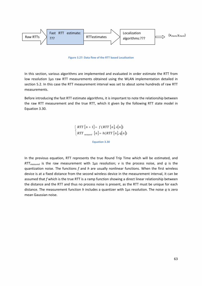
Fast RTT estimator
Localization
algorithms Raw RTTs RTTestimates
estimatreszz54t4t(xclient,yclient)
removing the random time components of the channel access function found in some wireless
protocols (for example IEEE 802.11).
There are a few ways to obtain the time measurements that our method requires. The specific
implementation details can be found in Chapter 5: For example, using the ‘MAC Time’ feature of
some IEEE 802.11 WLAN chipsets as explained on section 5.2. The interrupt that a radio chip
generates when a frame is received can also be used, as shown in section 5.3. Furthermore, internal
register of the WLAN chips can be used, as presented on section 5.4.
The distance will then be proportional to the time measured as seen in Equation 2.5.
( )
Equation 2.5
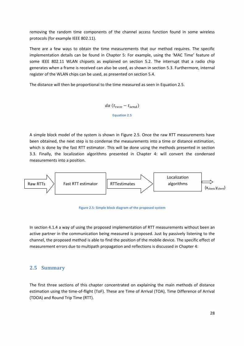
A simple block model of the system is shown in Figure 2.5. Once the raw RTT measurements have
been obtained, the next step is to condense the measurements into a time or distance estimation,
which is done by the fast RTT estimator. This will be done using the methods presented in section
3.3. Finally, the localization algorithms presented in Chapter 4: will convert the condensed
measurements into a position.
Figure 2.5: Simple block diagram of the proposed system
In section 4.1.4 a way of using the proposed implementation of RTT measurements without been an
active partner in the communication being measured is proposed. Just by passively listening to the
channel, the proposed method is able to find the position of the mobile device. The specific effect of
measurement errors due to multipath propagation and reflections is discussed in Chapter 4:
2.5 Summary
The first three sections of this chapter concentrated on explaining the main methods of distance
estimation using the time-of-flight (ToF). These are Time of Arrival (TOA), Time Difference of Arrival
(TDOA) and Round Trip Time (RTT).
29
The fourth section gives a brief description of our positioning system, which is based on the RTT
measurement method. Important features of our method where highlighted as well as the
advantages that those features bring.
30
31
Chapter 3: Physical layer modeling
Throughout the entire document the focus of this work is on an accurate indoor positioning,
especially with standard hardware devices. This chapter will take the task of explaining the basic
principles that make our system work. The first section will concentrate on explaining the internal
functionality of a radio device, and how it will be able to do a Time-of-arrival (ToA) measurement.
The second section will explain the case of a two-way communication, the Round-Trip-Time (RTT)
measurement, which is based on the system model of real RFID hardware. Section three will go into
the details of the methods and algorithms used to convert raw measurements of low granularity into
accurate distance estimations. The fourth section will present a very interesting effect that allows
the positioning system to obtain a ‘hardware fingerprint’ using the measured time of flight (ToF).
3.1 Model description
Usually, to find the position of a wireless device several transceiver devices need to intervene.
However, for sake of simplicity in this section and without loss of generalization, the distance
estimation between two wireless devices will be considered.
In this section a generic model for a round-trip-time based location system is presented. Afterwards,
a deeper view into the model of a radio device is done. Finally, several simulations are made to
achieve a true understanding of the localization accuracy that can be achieved.
Let us start with two wireless devices. The first device will initiate a frame exchange by sending a
message to the second device. As a response to this, the second device will send a message back to
the first device. The first device will be taken to be stationary while the second device will be mobile.
The distance between these two devices will be estimated.
The wireless data exchange will be the one corresponding to Round-Trip-Time (RTT) as presented on
Figure 2.3. Consider the wireless signal sent from the first device at time T1 which arrives at a later
time T2 to the second device will take place. At this point, a certain processing time in the tag will
take place. At time T3 a reply is sent from the second device to the first device. Finally, at time T4, the
second device receives this second signal.
It is a known fact that radio waves propagate at the speed of light when traveling in a vacuum. In a
typical indoor scenario a wireless signal will be moving mostly through air, with a propagation speed
still very close to c. Based on this, if the overall round-trip-time (RTT) could be accurately measured,
the distance between the two devices can be very easily derived, as shown in Equation 3.1.
32
( )
Equation 3.1
Under ideal conditions in which the wireless channel has remained stable from the time the
transmission of the first signal to the transmission of the second signal, the study of the delay
estimation from the first device to the second device (T2 − T1) is equivalent to the study of the delay
estimation from the second device to the first device (T4 − T3). That is why for the rest of this
chapter, only one way will be considered, namely the estimation of the distance propagation delay
from the first device to the second device.
It should also be noticed that the processing time, represented by the delay T3 − T2, will be seen as
being fixed to a known value, as is the case in real life. More information about this fixed time can be
found in section 4.2.1. For a typical indoor scenario, such value is in the order of microseconds, and
the distance propagation delay is in the order of nanoseconds.
To understand the behavior of such a system simulations are presented. In that way it can be
understood how a better resolution than the basic clock frequency can be obtained. First of all a
model of the internal functionality of the radio system is presented. For that, a block diagram
presenting the general signal processing chain is introduced, highlighting each step of the model and
the corresponding naming for each of the parameters. After the complete model has been
presented, each step is described in detail: the mathematical representation of the signal in the time
domain and in the frequency domain is given for each block, and besides, the corresponding signal
shape is displayed all along the process. Finally, the way of determining the time estimate is
explained as a final step.
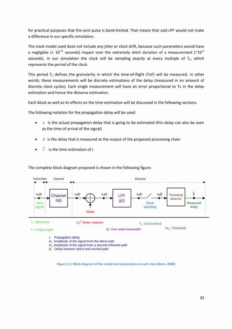
3.1.1 General description
In the block diagram of the model, presented in Figure 3.1, three main domains can be distinguished.
The first section corresponds to the sent signal, followed by the channel and finally the receiver. The
receiver is comprised of an addition of noise, a low pass filter, the clock sampling and threshold
detection. For each step, there are specific parameters that can affect the delay estimation through
the influence of the analog signal. As there are many parameters, they have been color-coded and
listed under the block diagram and will be studied more precisely in the rest of the chapter.
The model proposed involves the main factors that can have an effect in our delay estimation,
allowing us to obtain analytical results. However, it must be mentioned that in this model a couple
aspects have been omitted:
The transmitted signal is not currently band-limited and hence, an additional Low Pass Filter (LPF)
could have been set at the sender. In this model, this aspect has been omitted, since it is assumed
33
for practical purposes that the sent pulse is band-limited. That means that said LPF would not make
a difference in our specific simulation.
The clock model used does not include any jitter or clock drift, because such parameters would have
a negligible (< 10-11 seconds) impact over the extremely short duration of a measurement (~10-6
seconds). In our simulation the clock will be sampling exactly at every multiple of TC, which
represents the period of the clock.
This period TC defines the granularity in which the time-of-flight (ToF) will be measured. In other
words, these measurements will be discrete estimations of the delay (measured in an amount of
discrete clock cycles). Each single measurement will have an error proportional to Tc in the delay
estimation and hence the distance estimation.
Each block as well as its effects on the time estimation will be discussed in the following sections.
The following notation for the propagation delay will be used:
is the actual propagation delay that is going to be estimated (this delay can also be seen
as the time of arrival of the signal)
is the delay that is measured at the output of the proposed processing chain
~ is the time estimation of
The complete block diagram proposed is shown in the following figure:
Figure 3.1: Block diagram of the model and parameters at each step (Stern, 2008)
Transmitter
s1(t)
Sent
signal
Channel
h(t)
s2(t) s3(t) LPF
g(t)
s4(t) s5[i]
Channel Receiver
Noise
Clock
sampling
Threshold
detector
τ
Measured
delay
^
Ts: Slew time
TP: Pulse lenght
τ: Propagation delay
A1: Amplitude of the signal from the direct path
A2: Amplitude of the signal from a second reflected path
Δ: Delay between direct and second path
σn2: Noise variance
Br: One-sided bandwidth
Tc: Clock period
ATh: Threshold
34
3.1.2 Transmitted signal
Signal in the time domain
Different signals can be used for this analysis. A few examples are an isosceles trapezoid, a smoother
trapezoidal pulse (Ho, et al., 1995), a Gaussian pulse (Cramer, et al., 1998). The isosceles trapezoid
has been chosen for this work, as it enables better considerations for the analysis and results. Figure
3.2 shows the chosen form with its corresponding parameters: slew time (TS), pulse length (TP) and
amplitude (A).
Amplitude
Ts: Slew Time
Tp: Pulse Lenght
A : Amplitude
Ts
Tp
Time
A
Figure 3.2: Sent signal
If the slew time is reduced, the rate of change of the signal will increase, causing a larger the
bandwidth for the pulse.
Mathematically speaking, the pulse can be defined as:
( )
{
[ ]
[ ]
( )
[ ]
Equation 3.2
35
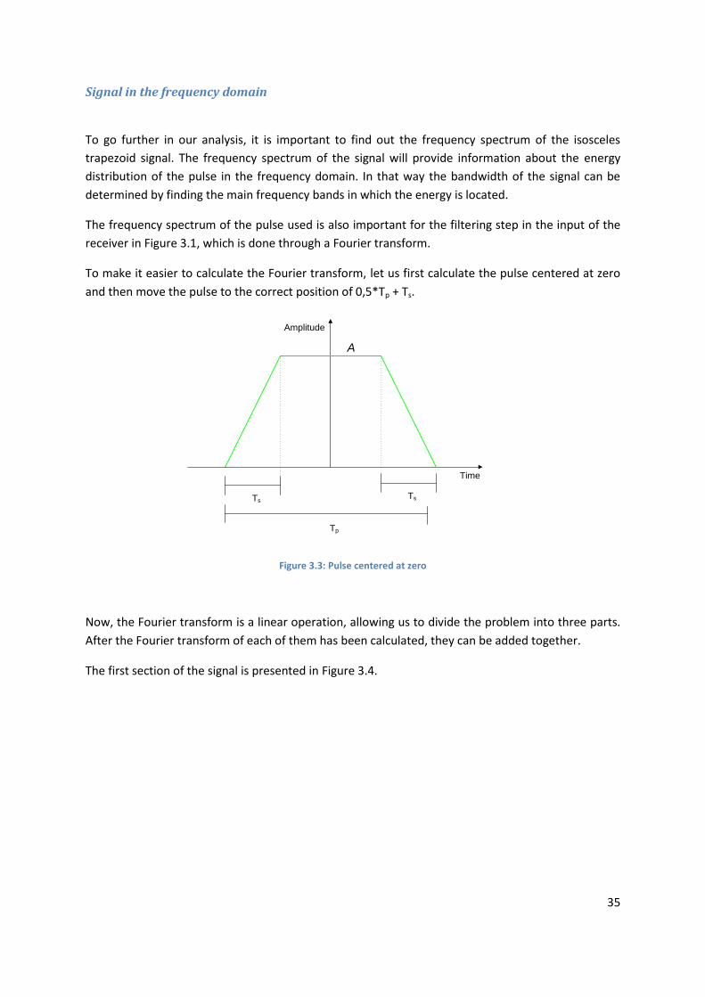
Signal in the frequency domain
To go further in our analysis, it is important to find out the frequency spectrum of the isosceles
trapezoid signal. The frequency spectrum of the signal will provide information about the energy
distribution of the pulse in the frequency domain. In that way the bandwidth of the signal can be
determined by finding the main frequency bands in which the energy is located.
The frequency spectrum of the pulse used is also important for the filtering step in the input of the
receiver in Figure 3.1, which is done through a Fourier transform.
To make it easier to calculate the Fourier transform, let us first calculate the pulse centered at zero
and then move the pulse to the correct position of 0,5*Tp + Ts.
Amplitude
Ts
Tp
Time
Ts
A
Figure 3.3: Pulse centered at zero
Now, the Fourier transform is a linear operation, allowing us to divide the problem into three parts.
After the Fourier transform of each of them has been calculated, they can be added together.
The first section of the signal is presented in Figure 3.4.
36
Amplitude
Ts
Tp
2
Time
A
Figure 3.4: First section of the signal
The following Fourier transform will be the one corresponding to Figure 3.4
( ) ∫
(
)
Equation 3.3
Doing a variable substitution for
Equation 3.4
We obtain
( ) ∫
(
)
( )
∫
Equation 3.5
Which, using the properties of the Fourier transform and undoing the substitution of Equation 3.4
results into
37
( )
(
( ))
( ( ) ( ) ( ))
Equation 3.6
Now, the Fourier transform of the constant section as seen on Figure 3.5 can be calculated.
Amplitude
Ts
Tp
Time
A
Ts
Figure 3.5: Second section of the signal
The Fourier transform will be represented by
( ) ( ) ( ( ))
Equation 3.7
Now for the third part of the signal, as seen on Figure 3.6, the Fourier transform can be calculated.
38
Amplitude
Time
A
Ts
Tp
2
Figure 3.6: Third section of the signal
In a similar fashion to Equation 3.6, this is given by Equation 3.8
( )
(
( ))
( ( ) ( ) ( ))
Equation 3.8
Now that the Fourier transform of all three parts have been calculated, Fourier transform of the
centered signal shown in Figure 3.3 is equivalent to the addition of those three parts.
( ) ( ) ( ) ( )
Equation 3.9
( ) (( ) ( ( )) ( ))
Equation 3.10
Finally, all that is required is to move the signal to the right. As a displacement of
in the time
domain is equivalent to the multiplication by , the following result is obtained.
39
( ) ( ) ( ( )) ( )
Equation 3.11
The power spectral density (PSD) can be easily obtained from Equation 3.11
| ( )| ( ) | ( ( )) ( )|
] [
Equation 3.12
This power spectral density is shown in Figure 3.7. Notice the many side-lobes generated by the
multiplication of sinc with sinc in Equation 3.12.
Figure 3.7: Frequency spectrum of the trapezoidal pulse (Ts=2ns, Tp=24ns, A=1)
3.1.3 Channel
Multipath
Let us take a transmitted pulse as detailed in section 3.1.2 using an amplitude A = 1. The output of
the channel for this given input can be represented by a Finite Impulse Response filter (FIR) as
shown the next equation.
( ) ∑ ( )
Equation 3.13
40
where Ap is the amplitude of the signal after travelling through the pth path and p is the actual
propagation delay of the signal using the same pth path.
As presented on the block diagram presented on Figure 3.1, s1(t) will represent the signal entering
the channel and s2(t) the signal exiting the channel. The resulting s2(t) signal of having the signal s1(t)
go through the FIR filter is shown in Equation 3.14.
( ) ∑ ( )
Equation 3.14
Each single path will introduce a delay and attenuation but will not affect its shape. As there can be
an almost infinite number of paths for the signal to travel, the following calculations will concentrate
in two predominant paths: the line-of-sight path (LOS) and a second path coming from a reflection.
Figure 3.8 shows an example of the two path model used in this section.
Direct path
Second path
Wall
Figure 3.8: Example diagram of the signal propagation with two predominant paths
Applying these two predominant paths presented on Figure 3.8 into s2(t) as represented on Equation
3.14 the following Equation 3.15 is obtained.
( ) ( ) ( ( ))
Equation 3.15
Where A1 corresponds to the amplitude of the signal after propagating through the direct path, A2 is
the amplitude of the signal after propagating through the second path, is the propagation delay
of the signal through the direct path and Δ is the additional propagation time that it takes the signal
to travel the second path in comparison to the direct path. It should be noticed that Δ is always a
positive value, because the second path will always cover more distance than the direct path.
41
Figure 3.9: Simple example of the signal propagation using both paths
As mentioned before, each single path doesn’t change the waveform. However, the addition of
several paths with different delay and attenuation coefficients will generate a new wave as s2(t).
Channel: Noise
Another part of the channel model is the addition of noise. The chosen noise source, n(t), is additive
white Gaussian noise (AWGN), which is a function presenting a Gaussian probability density function
(PDF) which is centered on 0 and set for a variable variance of 2
n . The power spectrum density will
remain constant over the whole frequency range of f +−∞,+∞*.
Noise addition in the time domain
The new signal been generated after the noise addition is presented in Equation 3.16.
( ) ( ) ( )
Equation 3.16
42
Figure 3.10: Example of the resulting signal after adding noise
(A1=1, Tp=1000ns, Ts=100ns, =300ns,2
n =0.01)
Figure 3.10 shows a signal with no reflections added by the channel that has been corrupted by
noise. As this works concentrates on measuring the time of arrival of the signal, the time it takes for
the rising flank to reach a specific threshold is measured. More information about the threshold can
be found in the section Receiver: Threshold detection on page 46. A zoomed version of the previous
figure can be seen in Figure 3.11.
Figure 3.11: Zoomed example of the resulting signal after adding noise
(A1=1, Tp=1000ns, Ts=100ns, =300ns,2
n =0.01)
43
Noise addition in the frequency domain
Equation 3.17 represents the power spectral density of the signal resulting from the noise addition.
| ( )| | ( )|
Equation 3.17
Where
is the constant power spectral density over the whole frequency range of ] [.
3.1.4 Receiver
Receiver: Low pass filter (LPF)
The first part of the receiving front-end shown in Figure 3.1 is a low pass filter used to get rid of most
of the high frequency components present in the s3 signal which has the added AWGN noise.
The time domain signal after the filter is the equivalent of a convolution of the input signal
convolution of A and B the impulse response of the filter g(t) as seen in the following Equation 3.18.
( ) ( ) ( )
Equation 3.18
The filter used is a first-order low pass filter. Seen in the frequency domain, the transfer function of
the filter G(f) is given by the following Equation 3.19.
( )
Equation 3.19
where B is the one-sided bandwidth of the filter.
The resulting equation for s4 in the frequency domain is given by Equation 3.20:
| ( )| | ( )| | ( )|
Equation 3.20
44
Figure 3.12: Example of the signal after a first-order low pass filter
(A1=1, Tp=1000ns, Ts=100ns, =300ns,2
n =0.01,
B =10 MHz)
Figure 3.12 shows an example of the result of the low pass filter. It can be clearly seen on the plot in
red that the effect of the noise has been reduced significantly.
Figure 3.13: Zoomed example of the signal after a first-order low pass filter
(A1=1, Tp=1000ns, Ts=100ns, =300ns,2
n =0.01,
B =10 MHz)
45
Figure 3.13 presents a close up of Figure 3.12 during the rising flank, which is the only part of the
curve that is relevant to our work. It should be noticed that the LPF will generate an additional delay
that is systematic.
Receiver: Clock sampling
This is the main component in the digitalization of an analog signal and it is a mandatory conversion
for the digital signal processing to take place, which allows the extraction of the data being
transmitted. Even though the functionality of this step is very similar to that of an Analog-to-Digital
Converter (ADC), our block model implements only the quantization of the signal in time; a
quantization of the amplitude will not be done to keep the model simple enough at this step.
The simple discretization of the analog signal will be represented by Equation 3.21.
[ ] ( )
Equation 3.21
Figure 3.14: Sampled signal
(A1=1, Tp=1000ns, Ts=100ns, =300ns,2
n =0.01,
B =10 MHz)
46
Receiver: Threshold detection
The last block of the diagram presented in Figure 3.1 is the threshold detection. This threshold
represents the detection threshold present in the adaptive amplifier. The detection will be triggered
if the energy of the signal is larger than a predetermined threshold Ath.
Figure 3.15: Threshold detection
(A1=1, Tp=1000ns, Ts=100ns, =300ns,2
n =0.01,
B =10 MHz)
Figure 3.15 shows an example of an overestimated delay. The signal first arrives at = 300ns, the
measured delay is actually 130ns higher reaching 430ns. Applying d =c t it means that, using the
parameters shown under the figure and the specific noise from Figure 3.13, the measurement would
result in an error of 39m. This includes, of course, a systematic error that can be easily calibrated.
The methods used for converting these measurements into a distance will be explained in detail in
the following chapter.
3.1.5 Further Enhancements
The contents of this section have been presented as a patent application (Ramírez, et al., 2010).
As said before, typical indoor environments have many limitations, in particular because there are
many reflections of the wireless signals. Each reflection causes a distortion of the signal, for example
in amplitude or in phase, which can lead to localization errors.
The problem tackled in this section is to improve the raw accuracy of the system through hardware
enhancements, especially on standard off-the-shelf hardware. One of the major limitations is
imposed by the clock frequency of the system.
47
We will demonstrate that it is sometimes good to add noise to the system in order to obtain a better
location.
Based on the simulator described in this chapter, let us consider the consequences of having a time
estimation based on a 10 MHz clock frequency. Its period, i.e. the duration of a clock cycle, is 100 ns.
Ignoring any noise sources, all the tags located between 0 m and 30 m away from the reader
(corresponding to a time-of-flight between 0 ns and 100 ns) will be detected after one clock cycle,
and thus, no difference in their position can be identified. In the same way, all the tags located 30 m
to 60 m away from the reader (corresponding to a TOF of 100 ns to 200 ns) will be detected after
two clock cycles, and thus, no difference in their position can be identified (see Figure 3.16, for
02
n ).
If some noise is added to the analog input signal coming from the antenna, the situation changes a
little. Supposing that the noise being added is random, it will affect the specific clock cycle in which
the signal will be detected. As an example, when no noise is present, a tag located 29m away from
the reader will always be detected on the first clock cycle reporting a distance of 15m. However,
when noise with 3.02
n is added, the signal will cause the tag to be detected sometimes on the
first clock cycle, and other times on the second clock cycle. Just by averaging several measurements
that include noise, the reported time would be very close to the time corresponding to 30m (100 ns).
Figure 3.16: Distance estimated vs. actual distance (theoretical results with an infinite number of measurements)
48
It must be noted that the small noise variance used in this first example would have only a slight
influence over the time measurement system, which would have a noticeable effect on distances
like 29.9m, but would be unnoticeable at 15m. The reason for this is that the added noise would not
be enough to change the specific clock cycle in which a time-of-flight corresponding to 15m (50ns) is
detected, because it is too far away from the threshold (100ns).
As it can be derived from Figure 3.16, for a special set of parameters, there is an optimal noise
variance in which the localization accuracy is the best. When the noise variance is equal to 0, the
estimated distance function of the actual distance looks like a step function. When the noise
variance gets larger, the step function becomes smoother up to a straight line (in red), which is a
very good estimation. When the noise variance gets even larger, the straight line becomes flatter
and the error in the distance estimation is large again.
For this reason a set of simulations was done with a series of parameters. Taking a 16,7MHz channel
to simulate an IEEE802.11 WLAN communication system we have selected three different clock
frequencies for our time measurement: 10 MHz, 20MHz and 100MHz. Additionally, noise is added
with a variance from 10-2 to 103 to analyze the performance of the location accuracy. The results are
presented on Figure 3.17. For a clock frequency of 10MHz, the optimal variance of the noise is
42
n
, achieving the minimum error for distance estimation. If the noise is increased or
decreased, the error in the distance estimation will always increase.
It must be noted that the optimal noise variance of 4 obtained in this example is hundreds of times
larger than the noise present in a real system, meaning that it is not in any way intuitive that adding
so much noise to a location system would actually increase the systems accuracy. It must also be
noted that increasing noise in a communications system will make the data transmission less reliable
and would reduce the achievable data rate of such communication. Nevertheless, the improvement
in accuracy for a location system through this method ranges from a 10 times to a 100 times
increase. To eliminate the negative effects of the added noise on other wireless transmissions, the
noise can also be added directly within the hardware. Thus, the additional noise is generated
completely within the device and does not result in any distortion of the frequency bands in use.
Based on these results we can calculate the optimal noise to be added to any distance measurement
system. Such noise can be added to any system. In most of the cases, the amount of noise that
already exists in a system will be negligible in comparison to the amount of noise to be added,
according to Figure 3.17.
When signal processing is performed, the elimination or the reduction of noise is often one of the
major tasks. However, in our case, we have shown that noise can have a positive effect, and
moreover, it could be interesting to intentionally add noise in order to achieve a more accurate
estimation of the position of a device.
49
Figure 3.17: Error average vs. noise variance (theoretical error with an infinite number of measurements)
3.2 Modeling of the RTT
In section 3.1 we have explained how our system works in the physical layer when using a
unidirectional communication. This section will be in charge of the next step, which is making use of
the round trip time (RTT) of the signal. Some of the models presented in this section are based on
the research on the ZOMOFI hardware platform of Albis Technologies Ltd (previously Siemens
Switzerland Ltd) presented under the master thesis of (Ben Ghouil, 2008); work done under our
supervision.
ZOMOFI is an active RFID system composed by tags and controllers to find out the presence of
specific devices in a controlled area. Detailed information about the ZOMOFI system architecture
can be found in chapter 5.4
Two models will be proposed for the functionality of the RTT based on the delays inside and
between the devices implicated: The first model will originate from a theoretical analysis of the
measurement process and the noise and delays in the involved components. This is done in order to
visualize the impact of each of the noise sources present in the circuit and the effect that they have
in our RTT measurement.
The second model will be built using real world measurements of each of the system components,
clocks and noise sources to be able to obtain a more accurate representation of the real system.
50
Finally, the results of the analysis will uncover which components have an important effect on the
RTT measurement accuracy, so that their substitution can be studied for a future hardware platform.
It will also reveal which components have little to no effect on the system.
3.2.1 Hardware description
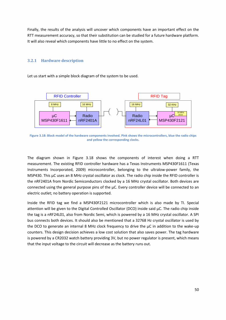
Let us start with a simple block diagram of the system to be used.
µC
MSP430F1611
Radio
nRF2401A
Radio
nRF24L01
µC
MSP430F2121
8 MHz 16 MHz16 MHz
16 MHz
DCO
RFID TagRFID Controller
32 KHz
Figure 3.18: Block model of the hardware components involved. Pink shows the microcontrollers, blue the radio chips and yellow the corresponding clocks.
The diagram shown in Figure 3.18 shows the components of interest when doing a RTT
measurement. The existing RFID controller hardware has a Texas Instruments MSP430F1611 (Texas
Instruments Incorporated, 2009) microcontroller, belonging to the ultralow-power family, the
MSP430. This µC uses an 8 MHz crystal oscillator as clock. The radio chip inside the RFID controller is
the nRF2401A from Nordic Semiconductors clocked by a 16 MHz crystal oscillator. Both devices are
connected using the general purpose pins of the µC. Every controller device will be connected to an
electric outlet; no battery operation is supported.
Inside the RFID tag we find a MSP430F2121 microcontroller which is also made by TI. Special
attention will be given to the Digital Controlled Oscillator (DCO) inside said µC. The radio chip inside
the tag is a nRF24L01, also from Nordic Semi, which is powered by a 16 MHz crystal oscillator. A SPI
bus connects both devices. It should also be mentioned that a 32768 Hz crystal oscillator is used by
the DCO to generate an internal 8 MHz clock frequency to drive the µC in addition to the wake-up
counters. This design decision achieves a low cost solution that also saves power. The tag hardware
is powered by a CR2032 watch battery providing 3V, but no power regulator is present, which means
that the input voltage to the circuit will decrease as the battery runs out.
51
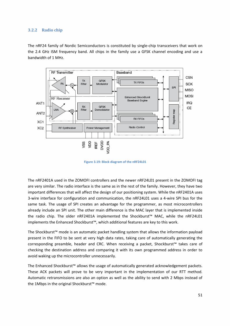
3.2.2 Radio chip
The nRF24 family of Nordic Semiconductors is constituted by single-chip transceivers that work on
the 2.4 GHz ISM frequency band. All chips in the family use a GFSK channel encoding and use a
bandwidth of 1 MHz.
Figure 3.19: Block diagram of the nRF24L01
The nRF2401A used in the ZOMOFI controllers and the newer nRF24L01 present in the ZOMOFI tag
are very similar. The radio interface is the same as in the rest of the family. However, they have two
important differences that will affect the design of our positioning system. While the nRF2401A uses
3-wire interface for configuration and communication, the nRF24L01 uses a 4-wire SPI bus for the
same task. The usage of SPI creates an advantage for the programmer, as most microcontrollers
already include an SPI unit. The other main difference is the MAC layer that is implemented inside
the radio chip. The older nRF2401A implemented the Shockburst™ MAC, while the nRF24L01
implements the Enhanced Shockburst™, which additional features are key to this work.
The Shockburst™ mode is an automatic packet handling system that allows the information payload
present in the FIFO to be sent at very high data rates, taking care of automatically generating the
corresponding preamble, header and CRC. When receiving a packet, Shockburst™ takes care of
checking the destination address and comparing it with its own programmed address in order to
avoid waking up the microcontroller unnecessarily.
The Enhanced Shockburst™ allows the usage of automatically generated acknowledgement packets.
These ACK packets will prove to be very important in the implementation of our RTT method.
Automatic retransmissions are also an option as well as the ability to send with 2 Mbps instead of
the 1Mbps in the original Shockburst™ mode.
52
Both chips inform the microcontroller of the reception of a new packet using the IRQ pin. After the
IRQ has been set, it has to be cleared by software.
3.2.3 Noise sources
Noise is an unwanted signal present in an electrical system that interferes with the main signal to be
processed. Noise can have different sources, and, as it manifests itself differently in different
components, it sometimes receives different names.
Oscillators clocks
Phase noise is the frequency domain representation of rapid, short-term, random fluctuations in the
phase of a waveform, caused by time domain instabilities (National Communications System,
Technology & Standards Division, 1996). Those effects in the time domain are known as jitter, so
both phase noise and jitter are directly linked together. This is present in the oscillator and clocks
that are used in any radio or digital system.
While an ideal oscillator generates a perfect sine wave, responsible for two delta functions
corresponding to the positive and negative conjugates of the oscillator’s frequency, real oscillators
generate sidebands which spread the power of the signal to neighboring frequencies. Noise can also
be found along the whole spectrum to a lesser degree, especially at low frequencies. The frequency
variation is an intrinsic characteristic of every oscillator and can be found in the datasheet of the
device.
Oscillators have different degrees of susceptibility to external conditions. The main factors that
affect their output frequency are temperature, vibration and the supply voltage.
There are many types of oscillators. Crystal oscillators are the most popular oscillators and can be
found in almost all electronic equipment. They are very cheap and offer an acceptable accuracy for
most applications. The most common material for crystal oscillators is quartz. In order set the
frequency of a quartz oscillator laser trimming under a controlled environment is done.
A typical quartz oscillator is very susceptible to changes in the temperature. The overall frequency
tolerance, measured in parts-per-million (ppm) is the allowed frequency deviation from the target
frequency specified for the device. This number takes for granted that the device is performing
under a framework of working conditions including operating temperature range, supply voltage,
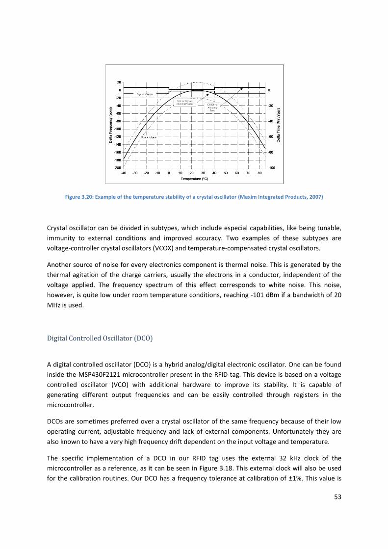
output load and aging. Figure 3.20 shows an example of the temperature stability on a typical 32 KHz
crystal oscillator produced by Maxim Integrated Products. The delta frequency of 0 ppm has been
optimized to be achieved at room temperature. Any changes in temperature will induce a higher
error in the output frequency. It should be noticed that the increase in frequency output error is not
directly dependent on the amount of the temperature change, but also on the current temperature.
53
Figure 3.20: Example of the temperature stability of a crystal oscillator (Maxim Integrated Products, 2007)
Crystal oscillator can be divided in subtypes, which include especial capabilities, like being tunable,
immunity to external conditions and improved accuracy. Two examples of these subtypes are
voltage-controller crystal oscillators (VCOX) and temperature-compensated crystal oscillators.
Another source of noise for every electronics component is thermal noise. This is generated by the
thermal agitation of the charge carriers, usually the electrons in a conductor, independent of the
voltage applied. The frequency spectrum of this effect corresponds to white noise. This noise,
however, is quite low under room temperature conditions, reaching -101 dBm if a bandwidth of 20
MHz is used.
Digital Controlled Oscillator (DCO)
A digital controlled oscillator (DCO) is a hybrid analog/digital electronic oscillator. One can be found
inside the MSP430F2121 microcontroller present in the RFID tag. This device is based on a voltage
controlled oscillator (VCO) with additional hardware to improve its stability. It is capable of
generating different output frequencies and can be easily controlled through registers in the
microcontroller.
DCOs are sometimes preferred over a crystal oscillator of the same frequency because of their low
operating current, adjustable frequency and lack of external components. Unfortunately they are
also known to have a very high frequency drift dependent on the input voltage and temperature.
The specific implementation of a DCO in our RFID tag uses the external 32 kHz clock of the
microcontroller as a reference, as it can be seen in Figure 3.18. This external clock will also be used
for the calibration routines. Our DCO has a frequency tolerance at calibration of ±1%. This value is
54
quite high when compared to the typical frequency tolerance of a crystal oscillator, which is 500
times lower. The frequency tolerance over the operating of temperature of 0°C to 85°C is 3%, which
is 35000 times higher than that of a crystal clock of the same frequency.
To make matters worse, the frequency tolerance over a supply voltage Vcc change from 3.0V to 3.6V
is 3%, which is 50000 times higher than that of a crystal clock. This frequency tolerance is decisive
for our scenario because the RFID tag is battery powered and no power regulator is present. The
effects of the draining battery during one measurement are noticeable and even catastrophic, as will
be shown later in this chapter.
Quantization error
In digital signal processing, a time and energy quantization always occurs. The time domain
quantization is typically done by a clock which has a finite frequency. For an event to be processed
by a digital system it will have to wait for the next clock cycle, which induces an additional time
equivalent to rounding up the time when the event up to the next clock cycle. This results in a
discrete time signal.
In the case of energy, this is typically done by an analog-to-digital converter (ADC) which reduces the
accuracy of the analog voltage measurement to a digital representation limited by the amount of
bits available.
The difference between the original analog value and the corresponding digital representation is
known as quantization error.
In our specific system, there are several clocks involved as seen on Figure 3.18. All our clocks are
relatively fast achieving clock cycles shorter that one millionth of a second. However, the speed of
light is also very fast. Using the fastest clock present in our system, 16 MHz, means that during one
clock cycle our radio signal would have travelled for ~19 meters.
As these clocks have different frequencies, are not synchronized and even have a different amount
of noise, simulations of all of these parameters will be required. They will be presented in section
3.2.4 shown next.
3.2.4 Measurement models
Based on the previously detailed noise sources, several models of our measurement system have
been developed. The reference for all clock frequencies used and the corresponding noise are our
current system, which has an 8 MHz crystal oscillator in the RFID controller and a 16 MHz DCO in the
RFID tag. The radio chips in both sides use a 16MHz crystal oscillator.
55
The first set of simulation models will be based on theoretical noise analysis based on datasheets.
The second set of simulations will be based on real measurements done directly on our hardware
platform. All simulations have been done using MATLAB.
Synchronous clocks
This first model will look at the effects that the distance has over the round trip time (RTT) when
both clocks are perfectly synchronized. Let us take the following diagram:
RFID Tag
RFID Controller
T1 T2 T3
T4
Start Endd
cd
c
Figure 3.21: Simple diagram of a synchronized RTT measurement
Figure 3.21 shows a simple diagram of the timing information of a RTT measurement. The RFID
controller is shown in blue and the RFID tag is shown in red. It can be easily recognized that the clock
inside the RFID Tag has double the speed as the RFID controller. As ideal clocks are used in this
model, there are no fluctuations in the frequency.
Our measurement will be done by the microcontroller inside the RFID controller as seen in Figure
3.18. First of all, a message will be sent by the controller and start the internal counter. Next, we
have the signal propagation delay which is proportional to the distance divided by the speed of light.
As the receiving tag is a digital device working on discrete time intervals, the time it takes for the
next clock cycle to arrive after the reception event has been triggered corresponds to T1. Thus, this
time will always be rounded up to the next full clock cycle.
⌈ ⁄
⌉
Equation 3.22
In Equation 3.22, Ttag represents the period of the clock inside the tag and ⌈ ⌉ is the ceiling function.
The equation shows how T1 will be dependent on the speed of the clock, leading to a systematic
56
error in the measurement. This relationship will be useful during the analysis of the simulations and
implementations later in the document.
T2 represent the time that the receiving device takes to answer the request and is referred to as
‘processing time’ throughout this document. Such time includes the delays added by the low noise
amplifier (LNA), demodulation and storage of the decoded information in an internal register. This is
measured in a non-fractional amount of clock cycles.
T3 represents the amount of time that the tag takes to send the answer message. This includes the
Tsetup, which represents the time a device takes to switch between the receive mode to the transmit
mode as given by their datasheet. It also takes into account Ttransmission, which is the amount of time it
takes to transmit the information over the amount of bytes air at the given data rate.
ratedata
sizepacketT
ontransmissi
Equation 3.23
ontransmissisetupTTT
3
Equation 3.24
Further, the propagation time is defined by the distance divided by the speed of light. And finally T4,
which, in a similar fashion to T1, corresponds to the time it takes for the next clock cycle to arrive to
be able to stop the clock of the controller, and thus including having to be rounded up to the closest
clock cycle.
The result of adding all of these delays is presented in Equation 3.25. The result of the outer ceiling
function is the amount of clock cycles that the controller device will measure. By multiplying it by
Tcontroller the total amount of time measured can be calculated.
⌈
⌈ ⁄
⌉
⌉
Equation 3.25
In order to keep the analysis simple in this section, we are using some abstraction on the
components involved. For example, the interaction between the radio chip and the microcontroller
contained in the tag are kept simple so to be seen as a single element. A fully detailed analysis of
each component and the effect on the system will be done in chapter 5.4. The analysis includes not
only theoretical numbers but also time delay measurements made on real hardware components.
57
Doing a simulation of Equation 3.25 over a distance from 0 to 100 meters using steps of 1 meter, we
obtain Figure 3.22.
Figure 3.22: Simulation of our RTT measurement method using synchronized clocks. Tcontroller = 62,5ns (16 MHz), Ttag = 125ns (8MHz).
The effect that the time discretization has on the time measurements can be clearly seen. The
stepped function is present because of the ceiling function of the equation. This causes, for example,
that all distances between 20 and 35 meters will be measured to have the same amount of clock
cycles.
This stepped function will be maintained independently on the amount of measurements done at
the same position because the model includes synchronized clocks and no noise has been included.
Asynchronous clocks
In the real world, it is not easy to achieve an accurate synchronization of clocks present in different
devices. Complicated algorithms as well as specialized hardware are usually required, involving a
very high effort.
1770
1771
1772
1773
1774
1775
1776
0 10 20 30 40 50 60 70 80 90 100
Clo
ck
cyc
les
Distance (meters)
RTT vs distance
58
Moving in the direction of a more realistic model, we will now suppose that the clocks present in the
model are not synchronized. We will suppose that the clocks started at an unknown random time
leading to a uniformly distributed offset between the RFID controller and the RFID tag.
RFID Tag
RFID Controller
T1 T2 T3
T4
Start Endd
cd
c
Figure 3.23: Diagram of our measurement process using asynchronous clocks
Figure 3.23 shows the different steps in the measurement process. A timer will be started at the
RFID controller when a transmission is sent to the RFID tag. The timer will be stopped when the
response is detected by the RFID controller.
T1 represents the time between the transmission of the message from the RFID controller and the
corresponding notification of the RFID tag. As presented in the previous section which uses
synchronized clocks, this time will be rounded up to the following clock cycle on the RFID tag. This
will be the first discretization error in the scenario.
tag
tag
TT
cdrandT
1
1
Equation 3.26
It should be noticed that a new clock cycle might arrive at the RFID tag while the transmitted signal
was travelling in the air. It should also be noticed that the time-of-flight given by d/c can be greater
than one clock cycle.
Next we have the processing time given by T2, which is a discrete amount of clock cycles, as only
digital components are involved. This processing time involves the amount of instructions required
by the RFID tag to be able to provide the RFID controller with a response.
Time T3 is composed of two parts. The first part involves the time required by the radio chip to
initiate the transmission of the response. This amount of time is usually given by the radio chip
59
manufacturer. The second part is the time-of-flight as given by d/c. The form of T3 can be seen in
Equation 3.23 and Equation 3.24.
At the final time T4 is where the second discretization takes place. When the response arrives to the
RFID controller, it will be required to wait for the following clock cycle to arrive to be able to stop the
timer started at the beginning of T1.
Adding T1, T2, T3 and T4 we obtain the total measured time as seen in the following equation.
controller
controller
tag
tag
totalT
T
TTTT
cdrand
T
321
Equation 3.27
By doing a simulation of Equation 3.27 for distances from 0 to 100 meters we obtain the following
plot.
Figure 3.24: Results for unsynchronized clocks (1 measurement per distance). Tcontroller = 62,5ns (16 MHz), Ttag = 125ns (8MHz).
1771
1772
1773
1774
1775
1776
1777
0 10 20 30 40 50 60 70 80 90 100
Clo
ck
cyc
les
Distance (meters)
RTT vs distance
60
Figure 3.24 shows the interesting effect that the lack of synchronization adds to the measurement
process. It can be seen that when the value gets close to the threshold, the noise introduced
because of the lack of synchronization will make it sometimes leap before.
According to Figure 3.22, the leap from 1772 to 1773 clock cycles is located very close to 20 meters.
Figure 3.24 now shows that as the 20 meters mark gets closer the added noise in the clock
synchronization is able to tip over the measurement value to the next clock cycle. In a similar matter,
said lack of synchronization is able to make a measurement happen on the previous clock cycle.
It should be noticed that there is still an important discretization of the measurements. As our
microcontroller is only able to measure full clock cycles, the granularity of the measurement is still
quite coarse. This causes that sometimes random distances 30 meters of each other report the same
amount of clock cycles (for example, in Figure 3.24 the time measurement corresponding to 15
meters and 39 meters report the same value).
To reduce the discretization effect we will present the result of averaging 10 measurements per
distance.
Figure 3.25: Simulation results for unsynchronized clocks. Averaging of 10 measurements per distance.
Figure 3.25 shows a more smooth result. This has been done by averaging 10 simulated
measurements for each distance. It is now easier to see that the RTT is directly proportional to the
distance as almost no steps can be recognized. The averaging of several measurements has
1771
1772
1773
1774
1775
1776
1777
0 20 40 60 80 100
Clo
ck c
ycle
s
Distance (meters)
RTT vs distance
61
effectively increased our overall resolution for the measured distance. It can now be said that the
reason why our system works is actually the noise present in the system.
A similar effect to the lack of synchronization was presented in section 3.1 of this document, in
which even for a synchronized system, the noise in the signal itself allows us to achieve the
detection threshold at a different time. That noise allows us to also obtain a more linear function
when averaging several measurements.
We will propose additional algorithms to the simple averaging which provide even better results in
section 3.3.
Effect of the clock accuracy
In this section, the effect of the clock accuracy will be analyzed. A typical clock signal has about 20
parts per million (ppm) of error for temperatures between -40°C and 85°C. More accurate clocks can
be easily obtained, but the price can increase 10 times in order to obtain a clock 10 times as
accurate. Section 3.2.3 explains the sources of noise in more detail.
The noise of the clocks included in our model will be given by Equation 3.28.
11_
randppmfftagtagcentralTag
Equation 3.28
The noise distribution used here is a Gaussian noise as given in the following equation.
2
2
2
22
1
x
Gaussexf
Equation 3.29
In Equation 3.29 the mean is represented by µ which in our case will be zero and σ² represents the
variance, corresponding to 20ppm.
Adding this noise model to Equation 3.27 we obtain the following plot.
62
Figure 3.26: Effect of adding 20ppm of noise to the clock accuracy
3.3 Preprocessing algorithms
The preprocessing algorithms refer to the synthesis of many measurements into a higher accuracy
value.
By processing the measured values obtained with the procedure presented in the previous chapters,
an improvement between 14 and 100 times can be achieved through the collection of several
thousand individual measurements. The precision of the single measurements are one of the
limitations to achieving a better accuracy. However, as presented on the previous sections, clock
stability, and even the specific implementation on the silicon of the electronic components used can
affect this accuracy.
In order to predict/estimate the position of a device, the data flow as in Figure 3.27 will be
implemented. The blue block represents the preprocessing algorithms in this section 3.3. The
localization algorithms will be presented on Chapter 4: .
The preprocessing algorithms require many single measurements. To help keep the computational
burden to a minimum during real-time tracking operation, a ring buffer can be implemented. In that
buffer, when a new measurement enters the oldest exit. This would naturally have an adverse effect
if the stations are moving fast after a time of rest. More information about the specific
implementation can be found in Chapter 5:
1771
1772
1773
1774
1775
1776
1777
0 20 40 60 80 100
Clo
ck c
ycle
s
Distance (meters)
RTT vs distance
63
Fast RTT estimate:
???
Localization
algorithms:??? Raw RTTs RTTestimates (xclient,yclient)
Figure 3.27: Data flow of the RTT based Localization
In this section, various algorithms are implemented and evaluated in order estimate the RTT from
low resolution 1µs raw RTT measurements obtained using the WLAN implementation detailed in
section 5.2. In this case the RTT measurement interval was set to about some hundreds of raw RTT
measurements.
Before introducing the fast RTT estimate algorithms, it is important to note the relationship between
the raw RTT measurement and the true RTT, which it given by the following RTT state model in
Equation 3.30.
),(
),(1
nqnRTThnRTT
nvnRTTfnRTT
measured
Equation 3.30
In the previous equation, RTT represents the true Round Trip Time which will be estimated, and
RTTmeasured is the raw measurement with 1µs resolution; v is the process noise, and q is the
quantization noise. The functions f and h are usually nonlinear functions. When the first wireless
device is at a fixed distance from the second wireless device in the measurement interval, it can be
assumed that f which is the true RTT is a ramp function showing a direct linear relationship between
the distance and the RTT and thus no process noise is present, as the RTT must be unique for each
distance. The measurement function h includes a quantizer with 1µs resolution. The noise q is zero
mean Gaussian noise.
64
Figure 3.28: Measured RTT distribution of 1000 measurements
For simplicity, h will be assumed to be Equation 3.31.
[ ] ( [ ] [ ]) [ ] [ ]
Equation 3.31
It is important to note that q’ is not a Gaussian distribution any more, but rather a Quantized
Gaussian Distribution. As the quantizer has a uniform distribution, then q’ is of zero mean which
would imply:
0' qEqE
Equation 3.32
RTTEqERTTEqRTTERTTEmeasured
''
Equation 3.33
1
0
lim
1N
n
measuredNmeasurednRTT
NRTTERTTERTT
Equation 3.34
0
100
200
300
400
500
600
700
800
310 311 312 313 314
Histogram of the raw data
65
This would mean that the cumulative average of a very large sample of measurements would give
the best estimate of the RTT. The RTT state description in the case of a fixed wireless device can be
written as in
{ [ ] [ ]
[ ] [ ] [ ]
Equation 3.35
We will start with the very basic signal processing techniques to the latest and most advanced in an
effort to get a fast estimate of the true RTT while using a relatively small measurement interval;
different algorithms and filter designs were investigated. These algorithms can be classified
according to their nature into the following classes: “Statistics Based” algorithms, “Wavelet based
algorithms, “Estimation Theory” algorithms.
3.3.1 Statistics Based Approach
The Statistics Based algorithms that were implemented consist of Cumulative Average, Moving
Average Filter, and Moving Gaussian Filter with local or global statistics.
Cumulative Average
The Cumulative Average filter produces an updated estimate of the RTT with every measurement,
and is given by the average of all previous raw RTT measurements including the current
measurement. The estimated RTT is given by Equation 3.36:
0,)1(
11
)1(
nnRTTn
nRTTn
nnRTT
Equation 3.36
As previously mentioned, a large number of measurements n are required while the wireless device
is held at a fixed distance; the cumulative average would approach the true RTT. It is important to
note that n is a large value.
66
Moving Average Filter
Due to the low resolution of the raw measurement, our effort is to smooth the data in order to
obtain RTT estimates with higher resolution. The moving average filter is defined by Equation 3.37:
{
[ ]
( ) [ ] [ ]
[ ]
∑ [ ]
Equation 3.37
The advantage of using the moving average filter in treating the measured data is its ability to
quickly update the estimates in case the wireless device has to change its location.
Moving Gaussian Filter (Local Statistics) (Ramirez, et al., 2006)
Rather than uniformly averaging the measured data in a window of fixed length W as in the case of
the Moving Average Filter or even the whole measurement set available up to the Nth sample. We
propose to average the measurements in a weighted manner, where the weights are sampled from
a Gaussian distribution N (µ,σ/γ). The center µ and the standard deviation σ of the distribution are
updated with the new measurements of the RTT as shown in the Equation 3.38 to Equation 3.40.
The scaling factor γ was set to a fixed value (Alvarado, 2006).
1
0
)(
1
0
)(
2
2
W
i
RTTinRTT
W
i
nRTTinRTT
measured
RTT
RTT
measuredmeasured
e
einRTT
nRTT
Equation 3.38
1
0
1W
i
measuredmeasured inRTTW
nRTT
Equation 3.39
2
1
0
2)(
1nRTTinRTT
Wn measured
W
i
measuredRTT
Equation 3.40
67
The importance of this method is that it eliminates ‘outliers’, which are measurements that are not
consistent with the observed measurements in the active window. The elimination takes place by
increasing the weights near the current mean (measurements that make sense), and by decreasing
the weights on measurements that lie away from the average. The factor γ is responsible for how
strong the elimination should be. Large values of γ produces a strong elimination meaning near zero
weights for outliers, for small values of γ, the Gaussian curve would be flatter and thus averaging
would be uniform on the measured data. Due to the sense of locality this approach is called ‘Moving
Gaussian Filter with local Statistics’.
Moving Gaussian Filter (Global Statistics)
Another form of the Moving Gaussian filter will use global statistics rather than with local statistics.
In this case the elimination of ‘outliers’ would take into consideration a larger history of
measurements, and thus the mean and the standard deviation of the Gaussian distribution would
depend on the global set of measurements up till the nth sample, the Equation 3.41 represents the
Moving Gaussian Filter (Global Statistics).
1
0
)(
1
0
)(
2
2
W
i
RTTinRTT
W
i
nRTTinRTT
measured
RTT
RTT
measuredmeasured
e
einRTT
nRTT
Equation 3.41
In this variation of the moving Gaussian filter the average RTT will be updated every time a new
measurement arrives using Equation 3.42.
0,)1(
11
)1(
nnRTT
nnRTT
n
nnRTT
measuredmeasuredmeasured
Equation 3.42
Moreover, the variance required to calculate the Gauss curve will be updated using Equation 3.43
every time a new measurement arrives.
68
(m-1)th level mth level
LP 2
HP 2
LP
HP
2
2
H
L
LL
LH
Input
1
)1)((12
2
n
nRTTnRTTnRTTnRTTnnn
measuredmeasuredmeasuredmeasuredRTT
RTT
measured
measured
Equation 3.43
3.3.2 Wavelet Based Algorithms
After discussing the Statistics Bases algorithms for estimating RTT in the previous section, this
section will make use of wavelets techniques which have proved to be useful in many fields of signal
and image processing. Specifically the wavelets are used to denoise the RTT measurements in order
to estimate the true RTT. Two versions of RTT wavelet denoising were implemented. The first
approach is Fixed Wavelet Denoising; the second approach is Moving Wavelet Denoising.
The wavelet transform is a lossless decomposition of a given signal into high (detail coefficients) and
low frequency components (approximation coefficients). It is High Pass (HP) filtering and down
sampling of an input signal to get the detail coefficients, and Low Pass (LP) filtering and down
sampling to get the approximation coefficients. Wavelet decomposition can do multilevel
decomposition where the Approximation coefficients are repeatedly decomposed to Detail and
Approximation coefficients as shown in Figure 3.29. The low and high pass filters are finite impulse
response (FIR) filters that depend on the type of wavelet being used.
Figure 3.29: Wavelet Decomposition
69
The wavelet transform is a lossless decomposition process due to the fact that the original signal can
be fully reconstructed by applying an inverse wavelet transform. The inverse wavelet transform
upsamples the detail and the approximation coefficients, then filters them through the inverse LP
and HP filters. The process is repeated backwards from one level to another until the original signal
is recovered.
The main purpose behind wavelet denoising is the cancellation of the noise contained in the wavelet
coefficients; this is done by eliminating some wavelet coefficients lying below a certain threshold
Tthresh as shown in Equation 3.44. Wavelet denoising of a signal of length N can be done using a hard
threshold (Equation 3.45) or soft threshold (Equation 3.46), in both approaches the wavelet
coefficients are transformed according to f.
)log(2 NTthresh
Equation 3.44
thresh
thresh
hard
Tcoeffcoeff
Tcoefff
,
,0
Equation 3.45
threshthresh
thresh
soft
TcoeffTcoeff
Tcoefff
),(
,0
Equation 3.46
is defined to be the standard deviation of the detail coefficients, which would be the result from
the HP filtering.
After transforming the wavelet coefficients, the inverse wavelet transform is applied to restore a
‘Denoised Version’ of the original signal.
As previously mentioned, two approaches were used: the fixed wavelet denoising and the moving
wavelet denoising.
Fixed Wavelet RTT Estimation
In order to get an estimate of the real RTT, this approach applies five-level-wavelet decomposition
and denoises the RTT raw measurements available. Wavelet denoising, in general, tries to cancel the
White Gaussian Noise (WGN) that is contained in the wavelet coefficients falling below the threshold
Tthresh. The results of this algorithm are the estimates of the RTT. The advantage of this approach is
that it looks for the noise lying in the set of measurements, finds a threshold and cancels it. The
drawback is that there is no fixed RTT estimate.
70
Moving Wavelet RTT Estimation
This approach Moving Wavelet RTT, would only return one estimate per set of measurements. As in
the fixed wavelet RTT estimation, the wavelet denoising takes place on the five level wavelet
decomposition of the RTT measurements. A moving window of length W runs over the
measurement. Whenever a new sample arrives, the window is shifted by one sample, and wavelet
denoising is applied again. The estimated RTT can be described by the following Equation 3.47.
)0()1:(
WnnRTTwavdennRTT
Equation 3.47
As the wavelet denoising (waveden) would return an array of length W, only the first element in this
array is picked up as an estimate to the RTT.
The plot in Figure 3.30 shows the Moving Wavelet RTT estimate and the Fixed Wavelet RTT estimate
when using ‘symmetric’ 8bins wavelet. When treating 30 seconds (3000 RTT measurements) we
obtain the following:
Figure 3.30: RTT estimation using Fixed Wavelet and Moving Wavelet
0 500 1000 1500 2000 2500 3000 313.55
313.60
313.65
313.70
313.75
313.80
313.85
313.90
313.95
314.00
314.05 Moving Wavelet Fixed wavelet
RTT
(µ
s)
71
3.3.3 Estimation Theory Approach
After applying Statistical Based and Wavelets based algorithms, in an effort to get a good estimate of
the RTT, another class of algorithms is introduced. These algorithms belong to estimation theory.
The first algorithm is the Kalman filter which under certain assumptions proves to be the best
estimator. The second algorithm is Particle Filter which is one of most advanced estimators, that has
the ability to work with nonlinear models. As with the previously introduced algorithms, the filtering
takes place on the RTT measurements to return a best estimate of the RTT. We will start with the
first algorithm in this class, the Kalman filter.
RTT Estimation using Kalman Filter
This algorithm previously introduced by Rudolf Kalman estimates the posteriori distribution of a
state given a measurement. The assumptions are that the state space model is a linear model and
the posteriori density at any given step has a Gaussian distribution. In the case of the RTT state
model, it is linear in transition, but nonlinear in measurement. In case it is to be assumed linear in
measurement then the noise wouldn’t be strictly Gaussian distributed any more, but rather a sort of
1µs-step Quantized Gaussian distribution as in Equation 3.48.
{ [ ] [ ] ( ) [ ] [ ] [ ] ( )
Equation 3.48
Although not all the assumptions of Kalman Filter apply to the RTT model, it is still worth a try to
filter the RTT measurement to get an RTT estimate, therefore it was assumed that q’ has a Gaussian
distribution with mean of zero and variance 2
q .
The advantage of the Kalman Filtering is that it is very practical in online live estimations due to the
fact that it only needs the previous measurement and the current measurement to get an estimate
of the current true RTT, without having to buffer a previous set of RTT measurements. The Kalman
filter has a Prediction stage Equation 3.49, in which the current RTT estimate is predicted using the
previously measured RTT and the state transition equation. After the prediction stage, the predicted
estimate is updated / corrected (Equation 3.51) based on the current measurement via the Kalman
gain Equation 3.50 which minimizes the estimator error.
The following equations were involved in estimating the RTT (Kalman, 1960).
72
1|11|
.1|11|1
nnnn
nnnn
PP
nRTTnRTT
Equation 3.49: Prediction
2
1|
1|
qnn
nn
P
PK
Equation 3.50: Kalman gain
1|||
1|1||
)1(
)(
nnnn
nnmeasurednnnn
PKP
nRTTnRTTKnRTTnRTT
Equation 3.51: Update
nRTTnn
1| represents the predicted RTT based on the previous measurement, nRTT
nn
|denotes
the estimated RTT based on the current measurement. Pn|n-1 is the variance of the posteriori density
of RTT given the previous measurement. Pn|n is the variance of the posteriori density of RTT given
the current measurement.
The performance using real measurements is shown in Figure 3.32 in a direct comparison to particle
filters, which are introduced in the following section.
RTT Estimation using Particle Filter
Another way of estimating the RTT is using an Unscented Particle filter. A Particle filter is a
sequential Bayesian filter based on Monte Carlo Simulations. The name Particle filter is due to the
fact that this filter would estimate the posteriori distribution of the RTT given the measurements by
a random set of samples with corresponding weights, and computes estimates based on these
samples and weights. These samples have the notion of particles due to their randomness and their
associated weights (Van der Merwe, et al., 2001). The Particle filter is more powerful in estimating
non-Gaussian probability distributions when compared to the Kalman filter, which assumes Gaussian
probability distributions in addition to linear RTT state space.
73
Figure 3.31: Particle Filter algorithm
The particle filter has two main steps for its algorithm, both of which can be seen in Figure 3.31. The
first step is the particle selection where particles are chosen based on a certain distribution. Particles
with low weights (small values) are eliminated; this is called the “survival of the fittest”. Also during
this step, heavy weight particles split into smaller particles as seen in Figure 3.31. The second step is
Prediction where the particles are updated based on the state transition Equation 3.51.
As with previous algorithms, 3000 raw RTT samples were filtered by the particle filter with
importance resampling. It is to be noted that the newly estimated RTT only depends on the
previously measured RTT sample. Plots for both Kalman and Particle filter can be seen in the plot in
Figure 3.32.
74
Figure 3.32: RTT estimates using Particle and Kalman filter
3.3.4 Evaluation of the Algorithms
Finally, and after presenting several different algorithms for estimating the RTT, one or two
algorithms are to be chosen in order to be implemented in the RTT estimator which would feed the
estimates into the Prediction / Location estimation block shown in Figure 3.27.
In order to evaluate the performance of the estimation algorithms the following criteria were taken
into consideration:
{ [ ]}: Maximize correlation between estimates and distance. The algorithms
should take into consideration the linear nature between RTT and distance.
{ ( | )}: Minimize the standard deviation between estimates at
different time instances measured at given fixed distance.
25 RTT raw measurement sets corresponding to distances {10m, 20m, 30m, 40m, 50m} are used, five
measurements per distance. The size of each set is 3000 RTT raw measurements. 25 estimates of the
RTT were generated by each algorithm. The different algorithms were compared according to the
criteria presented above and the results can be seen in Table 3.1 below. The column σ represents
the STD that should be minimized. The column R represents the average of the [ ]e, which
should be maximized.
0 500 1000 1500 2000 2500 3000 313.55
313.60
313.65
313.70
313.75
313.80
313.85
313.90
313.95
314.00 Kalman Filter Particle Filter
RTT
est
imat
es
75
Fast RTT estimator:
MOVING GAUSSIAN or
PARTICLE FILTER
Localization
algorithms:??? Raw RTTs RTTestimates
estimatreszz54t4tt(xclient,yclient)
Class Method σ(µs) R
Statistical Based Estimation
Raw RTT 0.3779 0.8944
Cumulative 0.0529 0.9455
Moving 0.0529 0.9455
Moving Gaussian(Local) 0.0246 0.9822
Moving Gaussian(Global) 0.0245 0.9821
Wavelet Based Estimation
Moving Wavelet 0.0533 0.9454
Fixed Wavelet 0.0832 0.9376
Estimation Theory Approach
Kalman Filter 0.1648 0.14
Particle Filter 0.0448 0.9899
Table 3.1: Comparison of the different estimation algorithms
It can be concluded that Gaussian (Local/Global) used with γ = 0.5, and Particle filter gave the best
results, since they gave the best minimum σ and higher R compared to the other algorithms. The
Kalman filter as expected didn’t give good results due to the fact that the RTT state model is
nonlinear in nature, and if assumed that the noise is not Gaussian. This is one of the drawbacks in
Kalman filter, compared to the Particle filter which is able to attack any posteriori distribution of the
RTT| RTTmeasured.
It can be stated that, either Moving Gaussian filter (Global/Local) or Particle filter, are to be used as
RTT estimators as presented in Figure 3.33. The next step is to find a location predictor / estimator
to obtain a 2D/3D position out of the denoised RTT measurements, which can be found in Chapter 4:
Figure 3.33: Flow diagram of the RTT based localization
76
3.4 Signal fingerprinting
This section will explain one of the discoveries as very useful byproduct of our localization system.
Using the measurement method presented in the previous chapters we are able to obtain a
“physical fingerprint” of wireless communication chip that can tell it apart from other compatible
chips independent of any MAC address or ID. This method is unique in the way that the fingerprint
can be obtained using commercial off-the-shelf (COTS) hardware.
A patent has been granted by the German Patent and Trademark Office for this security method
(Ramírez, et al., 2005).
3.4.1 State-of-the-art
In today's world, the access to the information or to a network has only been regulated from the
upper layers: user passwords, certificates or other knowledge are needed in order to access the
network resources. While the distinction of a user from another through the lower layers could be
done using a unique ID like the MAC address, in the case of WLAN, they can be easily changed in all
of today’s hardware.
Thus, for a COTS device, it is not possible to recognize if the hardware of the conversation partner is
the authorized one, or the hardware belongs to an attacker.
Such verification can be done if a specialized proprietary system is used to analyze the analog
signals. Such systems were very important in World War II, when methods were developed for radar
identification based upon transient analysis (Jones, 1978).
Another important implementation of such systems took place in the 80s, when the first generation
(1G) of mobile telephone technology was popular. Those systems used analog modulated radio
signals to communicate. Because at that time no encryption of the signals was used, it was common
for hackers to intercept the identification number of the phones and clone them in order to obtain
free usage. As both the legitimate phone and the cloned phone where indistinguishable, the basic
solution was to kick both telephones out of the network as soon as both try to access from different
radio cells apart from each other.
Technological advances went further as to be able to recognize imperfections in the modulation of
the analog signal that could be used to correctly identify the legitimate mobile phone (Mustafa, et
al., 2002). It must be said that such system didn’t gain a widespread deployment and also, because
of their commercial importance, not much literature can be found about the specific
implementations.
Today, a lot of work has been done for other wireless communication systems. Some methods use
transient recognition (Barbeau, et al., 2003) which are only successful when the transmitters have
considerably different characteristics. Other systems are based in frequency classification
77
(Hippenstiel, et al., 1996) and other general characteristics of the radio waves (Gassend, et al.,
2003).
All of the work mentioned as part of the state-of-the-art uses specialized hardware to be able to
achieve a verification of the sender.
Otherwise, the detection of a user who is spoofing a MAC address or ID using only COTS hardware is,
to the best of our knowledge, an impossible task. A possible exception is the use of plausibility
checks when two devices with the same MAC address are logged-in from spatially separated nodes.
Such a check would recognize that both cannot be trusted nodes, but even then it will not be able to
identify which one it is without the use of encryption and/or authentication keys.
3.4.2 Technical features (Ramirez, et al., 2005)
The proposed method is based on the passive monitoring of the response times. These monitors will
measure the time it takes a node to answer a standard frame, and through this information it will
obtain a fingerprint that will identify the node’s hardware.
The delay measured is, for example, the time it takes a station to answer a Data frame with an Ack
frame. The measurement can be made by one of the parties taking part in the communication or by
a third party. In both cases the time must start when the first frame is in the air (the first or the last
bit, it doesn’t matter, as long as we know which one it was). The receiver station is going to read the
frame, and is going to wait a predefined time (SIFS in the case of IEEE 802.11, i.e. 9µs in 802.11g)
during which it will process the frame in parallel to the waiting. Once the wait is over, the receiver is
going to send an answer to the sender (an ACK frame, for example) which will be received at the
sender side and at the sniffer.
This fingerprint is based on the time-delay variations between different hardware. Nevertheless, this
is not a unique fingerprint for each network card that exists in the world. Different fingerprints can
be seen between different chipset manufacturers, and even between models of the same
manufacturer. However, chips belonging to the same model or model family will have a fingerprint
so similar that the distinction between them cannot be easily made. Eventually, for those cases,
algorithms used for MIMO systems could be useful to separate such devices; however such topics
will not be covered in this work.
78
Figure 3.34: Example of the measured RTT for three WLAN cards
presents the results corresponding to three different wireless LAN cards. All three cards are from
different models of the manufacturer Intel®. If sufficient data is obtained through frame exchanges,
it can be determined which card is using the remote node, independently of the MAC address
reported.
Another factor that will affect this fingerprint is the temperature of the chipset, changing the
properties of the curve enough to identify two chipsets of the same model working at a different
temperature.
3.5 Summary
Chapter 3 of this work has concentrated on obtaining RTT measurements and reducing any noise
present that would lead to inaccuracies in a distance measurement. To achieve this, we have first
concentrated on explaining the internal workings of a radio device and its effects on a one-way
wireless communication. We have analyzed the effects of reflections, and the system clock speed, to
understand the performance of the measurements under different circumstances.
The second section has focused on the two-way wireless communication, which is the base of the
Round-Trip-Time (RTT) used in our system. We presented the effects of having synchronized clocks
and also drifting unsynchronized clocks of different frequencies. All of the presented modeling and
simulation results were verified with measurements on real RFID hardware.
0,00
0,05
0,10
0,15
0,20
0,25
0,306
4,3
6
64
,39
64
,42
64
,45
64
,48
64
,51
64
,54
64
,57
64
,60
64
,63
64
,66
64
,69
64
,72
64
,75
64
,78
64
,81
Pro
bab
ility
(%
)
Time (μs)
Ack Delay
IntelPRO/Wireless2200
IntelPRO/Wireless4965
IntelPRO/Wireless3945
79
The third section is in charge of explaining how raw measurements can be denoised to obtain, in the
case of the RTT, a direct relationship to the real distance. In order to achieve this, several signal
processing algorithms were adapted to our signal source. A comparison of the accuracy obtained by
these algorithms has also been presented. The best results have been obtained by the Gaussian
filter, an algorithm inspired by the image processing world, proposed for the first time as part of this
thesis.
80
81
Fast RTT estimator:
MOVING GAUSSIAN or
PARTICLE FILTER
Localization
algorithms:??? Raw RTTs RTTestimates
estimatreszz54t4tt(xclient,yclient)
Chapter 4: Localization Algorithms
This chapter will explain how the measurement done in the previous chapter can be transformed
into a position. As seen on Figure 4.1, the many raw RTT measurements will be condensed into RTT
estimates. The estimates from different measuring stations will be collected into a centralized device
were the localization algorithms will be executed.
Figure 4.1: Dataflow diagram of the RTT based localization
Some localization algorithms require a distance estimation to be calculated. The method used for
this distance estimation is not important to the localization algorithm. We will start by presenting
some popular algorithms found in the state-of-the-art of localization algorithms. Further we will
propose two new algorithms, which we have decided to call Multidilateration and Round-Trip-Time
Difference of Arrival (RTTDOA). Simulations will be presented to compare the performance of the
presented algorithms under various conditions.
The last section of the chapter will present two new distance-less localization algorithms. The first
algorithm will be based on artificial neural networks and the second is our proposal for an algorithm
that takes advantage of pattern matching (PM) using the time-of-flight (ToF)
4.1 Distance-based methods
This section will give an overview of the functionality of the two main localization algorithms used in
the state-of-the-art, and will also present two of our own.
4.1.1 Multilateration (Bulusu, et al., 2000)
The most used algorithm for finding the location of a device is Trilateration/Multilateration (aka
least squares lateration). It is widely used in many systems including GPS, where the location of a
82
Mobile Station is determined given the relative distance between this Mobile Station and three or
more satellites, using the coordinates of these Base Stations in a common frame of reference.
P1 P2
P3
r3
r1
r2
C
x
y
Figure 4.2: Trilateration a geometric positioning algorithm
As seen in Figure 4.2, multilateration is the problem of finding coordinates (x, y) of a point C, where
distance measurements (r1, r2, r3,…, rn) are available between known reference points and C given
by Pn=(xn, yn). The position of the mobile user can be derived from the equations:
222
2
3
2
3
2
3
2
2
2
2
2
2
2
1
2
1
2
1
nnnryyxx
ryyxx
ryyxx
ryyxx
Equation 4.1
This equation system presented in Equation 4.1 can be regrouped into Equation 4.2. The steps for
this regrouping can be observed in (Bulusu, et al., 2000):
83
2
1
2
1
2222
1
2
1
2
1
2
2
2
2
2
2
2
1
2
1
2
1
2
2
2
2
2
2
2
1
11
1313
1212
2
1
yxyxrr
yxyxrr
yxyxrr
y
x
yyxx
yyxx
yyxx
NNNNN
Equation 4.2
When enough distance measurements are available there are more equations than unknowns,
making Equation 4.2 an overdetermined system. In the ideal case, one solution exists, which could
be found by solving the linearly independent equations. However, in a real case there are errors on
the measurements of the distance. Such error will lead to the simultaneous equations yielding no
solution. In such case, we have an optimization problem in which we are looking for an optimal point
which minimizes the mean square error over the space (x, y)R. To solve this we use the Moore–
Penrose pseudoinverse. More information about the regrouping of the terms to reach this solution
can be found in (Bulusu, et al., 2000).
bAAAbAyxTT
optopt
1
Equation 4.3
Where:
2
1
22222
1
2
1
2
1
2
3
2
3
2
2
2
1
2
1
2
1
2
2
2
2
2
2
2
1
11
2313
1212
2
1
yxyxrr
yxyxrr
yxyxrr
b
yyxx
yyxx
yyxx
A
NNNNNN
Equation 4.4
4.1.2 Multidilateration (Ramírez, et al., 2007) (Müller, 2007)
The multidilateration algorithm is a variation of the multilateration algorithm which uses calculated
distances between wireless nodes. This method has been submitted as a national and international
patent application (Ramírez, et al., 2007).
While in multilateration a solution is looked for looking at all nodes at once, in Multi-Dilateration the
problem is further divided into segments. Each segment will be formed by a pair of nodes, as will be
explained further in this section.
84
For every possible pair of neighbor nodes, the intersection points of the circles depicting the
measured distance will be calculated separately. The main quantity of such intersection points will
be located close to the actual position of the node to be located. Out of this main quantity of
calculated positions, the final position result is obtained.
The intersection points of the distance circles of the neighbor nodes P1 and P2 of a node to be
located M can be found using the equation of a circle
( ) ( )
Equation 4.5
( ) ( )
Equation 4.6
where (xi,yi) represents the positions of the neighbor node Pi, (x, y) represents the coordinates of the
unknown node’s position M and di are the distances between M and its neighbor nodes through
subtraction and regrouping we obtain
2
1
2
2
2
1
2
2
2
2
2
12112222 yyxxddxxxyyy
Equation 4.7
This can be further converted into
12
2
1
2
2
2
1
2
2
2
2
2
1
12
21
2 yy
yyxxdd
yy
xxxy
Equation 4.8
To simplify the solving of the resulting equation we do the substitution of the parameters
12
21
1yy
xxp
Equation 4.9
85
and
12
2
1
2
2
2
1
2
2
2
2
2
1
222 yy
yyxxddp
Equation 4.10
which results in the equation of the line through the intersection nodes
21pxpy
Equation 4.11
Equation 4.5 will be regrouped into
1
2
1
2
1yxxdy
Equation 4.12
And with Equation 4.11 will be equaled to
1
2
1
2
121yxxdypxp
Equation 4.13
After squaring both sides we obtain
0222
11
22
1
2
12121
22
1 xxxxdypypxpxp
Equation 4.14
And again through regrouping
02212
1
2
1
2
121121
2
1
2 xdypxyppxpx
Equation 4.15
86
To make it easier to solve the polynomial equation we do a new substitution through the parameters
2
1
2
1
2
123
11212
2
11
22
1
xdypq
xyppq
pq
Equation 4.16
Will simplify the equation into the polynomial
032
2
1 qxqxq
Equation 4.17
With the solution
1
31
2
22
2,12
4
q
qqqqx
Equation 4.18
Finally, through the evaluation of the parameters p1 and p2 as well as q1, q2 and q3, the amount of
the intersection points of the distance circles of two neighboring nodes can be found. The amount of
possible solutions can be two points, one point or none.
In general, with a total of n neighbors the amount of node pairs is given by
2
11
1
nni
n
i
Equation 4.19
For each neighbor pair there will typically be found 2 intersection points. One of these points usually
lies close to the position been looked for and the other one will be far away from it. In order to
eliminate the intersection points located far away of the position sought, we propose the
introduction of a threshold, after which the points will no longer be used to calculate the result. All
points located within the specified threshold forming a cluster will used to calculate the final result.
The computation of the final result can, for example, be done through averaging of the ‘x’ and ‘y’
components of the positions as if calculating the center of mass.
tser
n
i
i
n
x
x
ercestis
secint
1
int
Equation 4.20
87
tser
n
i
i
n
y
y
ercestis
secint
1
int
Equation 4.21
Figure 4.3 explains illustrates the procedure of this approach to find the position of a node M. In the
figure below, the different nodes representing base stations P1, P2, P3, and P4 do distance
measurements d1, d2, d3 and d4 each of which includes an error derr, as represented by the
corresponding circles. The intersection of the circle pairs are marked by white stars. All points of the
intersection of every neighbor pair will be computed so that the data set for the final result can be
chosen. A cluster finding algorithm is the used in order to locate the concentration of intersection
points, represented by the dark stars on the figure. Soon after, the center of mass of the points
inside the cluster is calculated to obtain the estimated position Mest.
P2
P1
P3
P4
M
Mest
d3 + derr, 3
d4 + derr, 4
d1 + derr, 1
d2 + derr, 2
Figure 4.3: Multi-Dilateration with four neighbors
The main difference to the algorithms described in the state-of-the-art is the division of the
localization problem into individual estimations. This has the advantage, that single strong outliers
can be easily identified and excluded from the position calculation.
The problem of collinearity, in which neighboring nodes are located close to a straight line, can also
be confronted using this method. Figure 4.4 shows that if collinearity is present, the mulitaleration
method will deliver two solutions, one of which will be located far away of the correct solution. In
order to identify the correct solution, it will be required to look for an increase in the density of the
circle intersection points, as this will be close to the correct solution. An exceptional case is when all
neighboring nodes are located in a perfect line, causing both solutions to be just as likely. For such
cases, plausibility checks can help identify the correct solution.
88
d1 +derr, 1
d2 +derr, 2
d3 +derr, 3
Mest, 1
Mest, 2
M
Figure 4.4: Positioning stations located in a collinear fashion
4.1.3 Bound Boxing
Another distance-based method for determining the position of a device is ‘Bound Boxing’ (BB). This
method, originally presented by Savvides et al in 2002 and then further developed by Whitehouse
and Culler in 2006, starts from the suggestion that the probable position of a device will be
contained inside a rectangular area (the minimal bounding box), the searched position being the
middle of this area.
Let us take a node M and try to find its position. There are several neighboring nodes Pi, each of
which calculates a distance di to the node M. Said distance will be then added and subtracted from
the xi and yi components of the position of each neighboring node forming the corners of BB.
(xi ― di, yi ― di)
(xi ― di, yi + di)
(xi + di, yi ― di)
(xi + di, yi + di)
Equation 4.22
The position of the node will be located inside the calculated BB, reason why it is necessary to
calculate the smallest intersection surface. To obtain this, the maximum of the smallest limits as well
as the minimum of the largest limits have to be calculated.
89
(max(xi ― di), max(yi ― di))
(min(xi ― di), min (yi + di))
(max (xi + di), max(yi ― di))
(min (xi + di), min (yi + di))
Equation 4.23
d1
d2
d3
MMest
x3 + d3
x2 - d2 x1 + d1
y3 - d3
y2 + d2
y1 + d1
Figure 4.5: Example of the implementation of the Bounding Box algorithm
The center position of this rectangular surface is the calculated position. An example of a BB
implementation can be found in Figure 4.5 and the resulting area has been highlighted in gray.
The main advantage of this method is the simplicity with which the position can be calculated.
Another advantage is that co-linearity, as shown on Figure 4.4 is no longer a problem, because
through the calculation of the maximum and minimum of all neighboring nodes only one such limit
of each type will be required. Any further error doesn’t have an influence on the final position.
There is, however, one important weakness in this method. While a great accuracy can be obtained
when the node M is located between the neighboring nodes, higher inaccuracies will be obtained if
the node M is located on the perimeter of the area covered by the neighboring nodes.
90
d1
d2
d3
M
Mest
x3 - d3 x2 + d2
y3 - d3
y2 - d2
y1 - d1
y1 + d1
y2 + d2
Figure 4.6: Example of BB when the mobile device is not located between the neighboring nodes
As it can be seen on Figure 4.6, the error obtained in such a boundary position can be important. If
the node M took a position on the corner of the depicted surface, the reported position would be on
the middle of said surface, taking us to a very extreme error.
On the other hand, the best case scenario would be achieved by setting the neighboring nodes on
each of the corners of the positioning surface. For this reason, the application scenario must be
thoroughly analyzed before selecting the localization method.
4.1.4 Round-trip-time difference of arrival (RTTDOA)
This idea has been presented as a patent application (Ramírez, et al., 2008).
Different measurement methods have advantages and disadvantages. One of the advantages of the
TDOA positioning method is that several receiving devices can listen passively to the signal sent by
the device, which position is going to be found. However, TDOA has the disadvantage that all the
receiving devices will require a very accurate synchronization of their internal timers. On the other
hand, the RTT method has the advantage that it requires no synchronization between the measuring
stations, but has the disadvantage that it needs two radio transmissions per each measuring device.
We propose a hybrid method through which we combine RTT and TDOA to remove each other’s
disadvantages. Concretely, we remove the requirement for synchronization of TDOA by using the
RTT method, and we remove the requirement of two radio transmissions per measuring device by
using TDOA. We have decided to call it RTTDOA.
A detailed step by step explanation of the proposed measurement procedure will be detailed in
Figure 4.8. In the current section we will do just a quick overview of the proposed idea.
91
As seen in Figure 4.7, a wireless device AP1 with known position will initiate a communication
sending a packet addressed to the MS; the remaining BSs will each start their local internal timers
upon detecting that a packet was sent. After receiving this packet, the MS replies to the BS with an
ACK packet as seen in the right portion of figure Figure 4.7. This ACK packet sent by the MS is also
seen by the other BSs in range, so that the local timers will be stopped upon the reception of this
ACK signal.
Receive
packet
Send
packet
listen
listen
listen
listen
MS
AP1
Send
ACK
Receive
ACK
listen
listen
listen
listen
AP1
MS
Figure 4.7: One BS sends to the MS (other BSs receive). MS replies by an ACK (other BSs receive)
In other words, we propose an RTT measurement in which the wireless devices not currently
involved in the point-to-point communication will listen to the channel, and measure the time
between the first sent packet and the corresponding sent ACK answer. This measured delay cannot
be directly converted to a distance because of the complex geometrical positions of the stations
involved. We propose two solutions to this: The first is a mathematical solution and the second is an
empirical solution.
92
I II
III IV
V
AP1
AP2
AP3
AP4
AP5
Counter
Enable
PACKET
Counter
Enable
AP1
AP2
AP3
AP4
AP5
Prepare the
ACK
PACKET
AP1
AP2
AP3
AP4
AP5
Counter
Enable PACKET
AP1
AP2
AP3
AP4
AP5
Counter
Enable PACKET
AP1
AP2
AP3
AP4
AP5
Counter
Enable
PACKET
MSMS
MS MS
MS
Figure 4.8: I) AP1 transmits any data packet towards the mobile station (MS) in red. A counter at AP1 is enabled to start counting. It will be stopped when the corresponding answer is received. Because of the broadcasting nature of the wireless medium and the spatial location of the modes in this specific example, AP3 is the first to receive the sent
packet. At this time, AP3 starts its internal counter. II) The same data packet sent by AP1 arrives at the mobile station. The MS prepares an answer to this packet. III) same data packet sent by AP1 arrives at AP2. Here a local counter is
started. IV) same data packet arrives to AP5. The local counter of AP5 starts counting. V) AP4 is the last one to receive the data packet, because it is the farthest away from AP1. The local counter starts.
The elapsed time measured by each wireless station will be related indirectly to the distance
separating it from the first wireless device and the responding wireless device. A generic step-by-
step sequence diagram can be seen in Figure 4.9. The full diagram is presented on Figure 4.10. BSm
represents the first wireless device in direct communication with a mobile wireless device (MS)
which position is to be found. The blue line is the packet been sent from the first device (BSm)
towards the mobile device. The red line represents the ACK packet sent from the mobile device (MS)
to the first device (BSm). Two other wireless devices are listening to the radio channel; BSi is a
wireless device located physically closer to BSm than the MS and BSj is a wireless device farther
apart.
93
BSm BSi MS BSj
SEND
PACKET
time
Arrival
@ BSi PACKET
BSm BSi MS BSj
time
Arrival
@ MS PACKET
BSm BSi MS BSj
time Arrival
@ BSi
PACKET
I II
III IV BSm BSi MS BSj
time
Arrival
@ BSi
ACK
gprocesT
sin
V VI BSm BSi MS BSj
time
Arrival
@ BSm
ACK
gprocesT
sin
BSm BSi MS BSj
time
Arrival
@ BSi
ACK
gprocesT
sin
Figure 4.9: I) BSm initiates the communication towards MS. Since BSi has a lesser distance from BSm than MS, the packet will arrive first to BSi. II) The packet has arrived to the MS. III) The packet arrives to BSj, which represent a BS that is located further away than the MS. IV) The MS has had enough time to prepare an ACK and transmit it. In this specific case BSj is closer to the MS than any other station. V) In this specific case the distance between MS and the BSm is less
than the distance between the MS and BSi, making the arrival of the ACK to BSm the next step in our timing diagram VI) The ACK finally arrives to BSi. Note the different gradient of the red line, which is caused because of the spatial
geometry of the participating stations.
When BSm sends a packet to the MS, the reception of this packet triggers the timers of BSi and BSj.
Because of the different paths travelled by the signal (as seen on Figure 4.7), these two wireless
devices are triggered at different absolute times. An exception would be when the distance d(BSm,
BSi) = d(BSm, BSj), in which case the absolute time in which the local timers are triggered would be
the same.
A processing time is required by the MS before it can send a reply to BSm with an ACK. Typically, this
processing delay (Tprocess) is in the range of hundreds of µs, making it several orders of magnitude
larger than the flight time of the radio signals. When the MS replies, the packets flows through
different paths towards BSi and BSj, as accentuated by the different slopes of the red lines between
MS, BSi and BSj. The elapsed time measured by any BS is given by the Equation 4.24.
94
Figure 4.10: Complete timing diagram indicating the time differences
( ) ( ) ( )
Equation 4.24
( ) : = distance between two stations, a and b.
: = speed of light in the medium
: = internal delay inside the MS between receiving the packet and responding by an ACK.
For the generic case of n BSs available, with the mth BS directly communicating with the MS, the
Equation 4.24 can be arranged in a matrix form as in the following equation:
BSm BSi MS BSj
t
95
e
processmn
processmm
processm
processm
T
BS
BS
BS
BS
MSBSD
n
m
A
cTBSBSd
cTBSBSd
cTBSBSd
cTBSBSd
c
T
T
T
T
MSBSd
MSBSd
MSBSd
MSBSd
c
n
m
),(
),(
),(
),(
1
),(
),(
),(
),(
10100
1
0
2
0
010
00101
1
2
1
),(
2
1
2
1
Equation 4.25
Distance Estimation
A is a full Rank matrix. Under the assumption that clocks possess an infinite resolution, the distance
between the MS and the BS can be computed as in the equation below.
)(
105.000
1
05.0
01
5.00
10
005.001
)(),(1
ecTCTAMSBSDi
Equation 4.26
The relation governing the distances between the BSs and the MS is given in Equation 4.27.
{x1, x2, …, xm, …,xn} & {y1, y2, …, ym, …, yn} represent the corresponding ordinates and abscissas of the
n BSs in an orthonormal reference of frame. (xMS, yMS) are the coordinates of the MS to be
determined.
96
222
222
2
2
2
1
2
2
2
1
2
1
2
1
),()()(
),()()(
),()()(
),()()(
MSBSdyyxx
MSBSdyyxx
MSBSdyyxx
MSBSdyyxx
nMSnMSn
mMSmMSm
SMMS
MSMS
Equation 4.27
Once the distances to the MS are determined, trilateration/multilateration can be used to determine
the coordinates of the MS as seen on the following equation. A detailed overview of multilateration
can be found on section 4.1.1.
The previous equations can be represented in a matrix form as in Equation 4.28
L
nnn
mmmMS
MS
K
nn
mm
yyxxMSBSdMSBSd
yyxxMSBSdMSBSd
yyxxMSBSdMSBSd
yyxxMSBSdMSBSd
y
x
yyxx
yyxx
yyxx
yyxx
22
1
22
1
2
1
2
22
1
22
1
2
1
2
2
3
2
1
2
3
2
1
2
1
2
3
2
2
2
1
2
2
2
1
2
1
2
2
11
11
3131
2121
),(),(
),(),(
),(),(
),(),(
2
1
)()(
)()(
)()(
)()(
Equation 4.28
The dimension of K is (n - 1) x 2 and two unknowns are to be determined; as a result the system is
over determined. As shown in Equation 4.29, least square error method is used to determine
),(MSMS
yx.
LKKKy
x
K
TT
MS
MS
1
)(
Equation 4.29
97
The proposed geometric method will deliver good results when a relatively accurate distance
measurement can be obtained. For the scenarios where no LOS can be guaranteed we propose the
following variation.
A further development: RTTDOA-PM
This extended method has been presented as a patent application to the GPTO (Ramírez, et al.,
2010).
While this new distance-based method, RTTDOA, provides a mathematical way to solve the problem,
the mathematical modeling of a real world system is quite a challenging task. Non-linear frequency
response in electronic components as well as changing conditions in an environment favor a more
empiric and pragmatic approach.
A good way of relieving these modeling complexities is the use of calibration on the intended
environment. For this reason we propose a new distance-less method. We chose to use pattern
recognition, in which data is analyzed and compared to previously recorded patterns of data to find
their similarities.
TOF based location systems are used mainly in outdoor environments, and when they are used
indoors they eliminate the effect of reflections through a large amount of channel bandwidth usage,
for example Ultra Wideband (UWB) utilizes a bandwidth of 500MHz (Ward, 2007). Pattern matching
is not common when using TOF as a signal source (Müller, 2004). In our case, the limited bandwidth
due to the use of standard hardware will not be able to eliminate the effect of the reflections
through the use of a large bandwidth, and as such, pattern matching is a great option. For NLOS
scenarios, our pattern matching variation of RTTDOA is also very good, as this method doesn’t
require a direct distance measurement between a BS and a MS.
Advantages
In a RTT localization system, all base stations must communicate with the MS in order to find the
position. This causes a significant consumption of the time of the channel in addition to packet
collision that might take place in the medium. When dealing with portable device, which is most
likely the case with Mobile stations, energy and battery resources are of great importance.
The RTTDOA method proposed will reduce the total amount of measurement by at least 66% (a
system with three measuring stations will only require one active link instead of three). As an
example of a typical implementation of this system, where five measuring stations are used, the
battery lifetime would be four times longer than a RTT implementation as only 20% of the packets
have to be sent as compared to the RTT (only one link has to be active out of the five). The channel
congestion time will also be reduced, leaving more space for real-time communications like VoIP or
industrial time critical communication.
98
Another important feature is that it also removes the requirement for synchronization needed by
TDOA systems. Another advantage of the RTTDOA is that it can locate MS’s that are not
communicating with every BS’s, allowing for a completely passive location infrastructure that can
remain hidden while still being able to locate the mobile wireless devices.
Even further, the newly proposed RTTDOA-PM no longer requires knowing where the BS’s are
located while still maintaining many of the advantages of the plain RTTDOA. As the proposed pattern
matching doesn’t require the real distance between the nodes, it is especially good for scenarios
where no line-of-sight (LOS) between some BS’s and the MS are present, for example a typical WLAN
indoor scenarios or a typical outdoor cellular network. Since pattern matching reliefs us from the
whole mathematical modeling of the environment, it is also very good where strong reflections are
present, like in the surrounding of large mass of water or in the industrial production environments
where many reflecting metal objects are present.
4.1.5 Performance comparison of distance-based methods (Müller, 2007)
The scenario
In order to understand the capabilities of the proposed multidilateration locating algorithm, we have
devised a series of simulations based on a mobile ad hoc network (MANET), in which we propose a
vehicular communication system scenario. We will have cars and roadside infrastructure (RSU)
devices communicate in a cooperative manner with the purpose of calculating the accurate position
of the cars involved.
Using our proposed method, a distance approximation between all the nodes can be obtained. Such
an approximation can be obtained using the method presented in Chapter 2: in a real world scenario
by using the IEEE 802.11p: Wireless Access in Vehicular Environments (IEEE, 2007) in the same way
that we used other IEEE 802.11 variants in previous chapters to achieve the distance estimation. Of
course, if any other technically feasible methods could achieve a distance approximation, they would
also be compatible with our positioning algorithms.
There is a major distinction between our scenario and the state-of-the-art. Previous authors
(Niculescu, et al., 2003) usually propose two kinds of nodes in a MANET: beacon nodes which know
their current position accurately and normal nodes which have no idea about their current position.
In our case, all nodes will know their GPS position, which is not very accurate. Such local inaccurate
positions will be used cooperatively by other nodes as will be explained later.
We should mention that there is the possibility of having something comparable to the mentioned
beacon nodes in the case of static Roadside Units (RSU), for example traffic lights or traffic cameras.
Even in such scenario we will differ from the state-of-the-art in that, while the typical density of
beacon nodes by other authors is relatively high (between 5% and 10% of the total of the nodes)
(Hsieh, et al., 2006), the density present in a typical vehicular environment can easily be one or two
orders of magnitude lower.
99
The algorithms
For the comparisons we will use three different algorithms:
Multilateration / Least Squares Lateration (LSL) (Bulusu, et al., 2000)
Bounding Box (BB) (Whitehouse, et al., 2006)
Multi-Dilateration (MDL) (Ramírez, et al., 2007)
Least Squares Lateration - Multilateration (LSL) (Bulusu, et al., 2000)
d1
d2
d3
M
d1 + derr,1
d2 + derr,2
d3 + derr,3
MMest
Figure 4.11: Trilateration a) Ideal case. b) Typical case
Figure 4.11a shows an ideal case of multilateration with three nodes (aka trilateration) when the
distance measurement contains no errors. Figure 4.11b shows the typical problems when using
multilateration, which appear when the distance measurements are not perfect, leading to an error
in the calculated position. On this Figure 4.11b it can be clearly seen that the position estimation
‘Mest’ differs from the real position ‘M’. A detailed explanation of multilateration can be found in
section 4.1.1.
100
Bounding Box (BB) (Whitehouse, et al., 2006)
d1
d2
d3
MMest
x3 + d3
x2 - d2 x1 + d1
y3 - d3
y2 + d2
y1 + d1
d1
d2
d3
M
Mest
x3 - d3 x2 + d2
y3 - d3
y2 - d2
y1 - d1
y1 + d1
y2 + d2
Figure 4.12: Bounding Box. a) Simple BB with 3 neighbors. b) Inaccuracies shown at the borders
The Bounding Box algorithm also allows us to find the position of a node in the network as long as
distance measurements can be obtained. Figure 4.12 shows an example of this method when the
measurements a very exact. The example to the right shows the difficulties that the method can
have when the node to be located does not have neighbors in all directions, as it happens when the
user is located at the border of the network. More information about such cases can be found at the
end of section 4.1.3.
Multi-Dilateration (MDL)
P2
P1
P3
P4
M
Mest
d3 + derr, 3
d4 + derr, 4
d1 + derr, 1
d2 + derr, 2
Figure 4.13: Multidilateration with four neighbors.
101
Figure 4.13 shows again how our newly proposed Multi-Dilateration algorithm works. All the
intersections of the distance circles corresponding to the neighbor pairs are calculated and then the
dataset of the final result are chosen. In the case of the simulations in this section, once the dataset
is ready, an average of the chosen points will give the final position result. The details about this new
algorithm can be found in section 4.1.2.
To have a first comparative view of the performance of the algorithms, we simulated an abstract
mobile network model using the Random Waypoint Model (RWP). A finite amount of mobile nodes
will choose a random destination inside a rectangular surface. Each node will move towards the
chosen destination with a constant speed. When a node reaches the planed position, it will choose
another position to go to. The simulation area is set to 600m x 600m and the radio range to 300m.
Figure 4.14: Example of Random Waypoint using the previously defined parameters. The red lines represent the communication links
The amount of nodes will vary to keep up with the amount of neighbors per node as seen on Figure
4.14. As a reference in this and all other simulations, the position reported by GPS will be fixed to an
average error of 12,5m in a random direction, which is a typical GPS accuracy with selective
availability disabled. Each of the results presented in the simulations is an average of 100 iterations.
102
Figure 4.15: Average RMS distance for each algorithm
On Figure 4.15, in addition to the comparison of all three algorithms, the measured RMS distance
(dRMS) of GPS input data is also shown. It can be easily recognized that both Least Squares-
Multilateration (LSL) and Bounding Box-Algorithm (BB) provide a bad position approximation when
few neighbors are available. These huge errors are shown to be out of the scale of the figure.
It can also be notice that only multidilateration (MDL) was able to improve the accuracy of the input
GPS position with only a few neighbors. While LSL achieved an improvement after having about 11
neighbors on average, BB was only able to do it when more than 50 neighbors per node were
present. When the measured distances used by LSL to calculate the position are not very exact, it
will lead to important errors when the position is calculated. Such an effect can be seen mostly when
the mobile node is located at the edge of the network. In the case of BB, the edge of the network
always presents bad performance.
To have a better look at the differences presented by the algorithms at the edge of the network and
at the center, a new simulation is shown in Figure 4.16 using fixed amount of node set to 20. To
identify the nodes close to the center of the network from those at the edge, the following metric
was used: The absolute distance between each node and the center of the simulation surface will be
used to do a ranking. To have a statistically significant simulation, 50 iterations will be used.
It can be seen on Figure 4.16 that BB exhibits a high inaccuracy when the nodes are located close to
the border of the surface. Because of the high amount of neighbors, LSL presents a better
0
5
10
15
20
25
30
35
40
0 5 10 15 20 25 30 35 40 45 50 55 60
dR
MS
(m
)
Mean neighbors per node
RWP - Comparison
GPS dRMS
LSL dRMS
BB dRMS
MDL dRMS
103
performance than BB, but it also presents some degradation in accuracy when located close to the
border.
Figure 4.16: Algorithm comparison according to the amount of neighbors farther from the center
In general, it can be said that MDL works better in this scenario than all the other algorithms.
Requiring just a few neighbors, it reaches good position accuracy, quite better than the input data
that has a 12,5m dRMS error. The MDL method produces good results even in the border of the
network.
Column Simulations
On the next scenario we will concentrate on special use cases for using these algorithms. We
propose the simulation of the movements of cars on a highway. In this case, the following
movement pattern was chosen:
The amount of network nodes inside the simulation area is no longer fixed. They enter the
simulation based on a configurable statistical distribution.
A new incoming node enters at a fixed position at the border of the simulation area. It will
move inside a defined corridor in the X and Y direction towards the opposite side of the
simulation area. The vertical movement will only be allowed in a single direction; going
RWP - Comparison
0
10
20
30
40
50
60
70
80
90
100
0 2 4 6 8 10 12 14 16 18 20
Neighbors farther from center
dR
MS
(m
)
LSL dRM S
M DL dRM S
BB dRM S
104
backwards is not possible. In each simulation step, a sideways movement will be introduced
represented by a constant distribution from -2.5m to 2.5m.
When a node leaves the simulation area, it will be deleted.
Figure 4.17 shows an example of the column scenario.
Figure 4.17: Abstract diagram of the column simulations
As it can be seen in Figure 4.18, the performance of the individual algorithms has changed
considerably when compared to the RWP scenario.
Figure 4.18: Average dRMS for the column scenario
Platoon Column - Algorithm Comparison
0
5
10
15
20
25
30
35
40
45
50
55
60
65
70
0 5 10 15 20 25 30 35 40 45 50
Mean neighbors per node
dR
MS
(m
)
GPS dRM S
LSL dRM S
M DL dRM S
BB dRM S
105
While the BB algorithm showed the worst performance in the RWP scenario, in this test it was able
to take over the LSL algorithm. It can also be noticed that, unlike in the RWP scenario, BB was able to
achieve a better accuracy than plain GPS with a low to moderate amount of neighbors. The same
cannot be said of LSL, which has a huge error, even when a large amount of neighbors are in range.
Even when MDL can achieve the best results, the accuracy achieved is lower than the one in the
RWP scenario. In the RWP scenario, MDL was able to accomplish results better than 5 meters, while
in this case the curve converges around 7 meters. It should also be noticed that for a large amount of
neighbors, the MDL algorithm is only marginally better than the BB algorithm.
The bad performance of LSL is easy to explain, as almost all of the nodes are in spread into a thin
straight line making then collinear, a problem explained in section 4.1.1. Figure 4.19 shows two
screenshot of our simulator to compare the instant performance of the algorithms LSL and MDL. The
left side shows the performance of the LSL algorithm and the huge error that this algorithm causes.
The co-linearity present in the Y-axis is responsible for the large error present in the X-axis, making
this algorithm completely unsuitable for the column scenario. The right side shows the sizable
performance improvements brought by the MDL algorithm proposed in this document.
Figure 4.19: Instant screenshot of a) LSL b) MDL. The black dots represent the real position of the node, blue is the position reported by GPS and red is the calculated position by LSL/MDL. The higher error in LSL is caused by the
collinearity as detailed on section 4.1.2. Simulation area 450m x 450m.
Crossing simulation
While the previous platoon column simulation scenario is a good representation for highways and
rural roads, we will now go to a typical city scenario: the crossing simulation.
106
Basically, this crossing scenario is not much different than the column scenario, as there would be
two orthogonal corridors intersecting each other in the middle of the simulation area. Looking at it
from the network topology, there is the difference that the nodes from both corridors are going to
be able to contact each other as they come into the range of 300m. Figure 4.20 shows a schematic of
said scenario.
Figure 4.20: Schematic of the crossing scenario. The circle represents the radio range of 300m. The simulation area is 450m x 450m.
The following figure shows the average dRMS accuracy of each algorithm for different amounts of
mean neighbors per node.
Figure 4.21: Average dRMS of the crossing simulation scenario
Crossing - Algorithm Comparison
0
5
10
15
20
25
30
35
40
45
50
55
60
65
70
0 5 10 15 20 25 30 35 40 45
Mean neighbors per node
dR
MS
(m
)
GPS dRM S
LSL dRM S
M DL dRM S
BB dRM S
107
The performance of the LSL algorithm has improved because the co-linearity of the nodes is not as
pronounced as on the previous platoon column scenario. It is mainly inside the circle presented in
Figure 4.20 that the nodes will have several non-collinear neighbors. The performance improvement,
however, is not enough to overtake any of the other algorithms, as some co-linearity remains. It
should be noted that the LSL algorithm cannot get a better accuracy than the base GPS input of
12,5m even when having 40 neighbors.
The algorithm showing the best performance is our new MDL algorithm. In this simulation scenario
the performance of MDL even increased a bit from the previous scenario due to the reduced
collinearity. MDL stays as the winner throughout all the simulations for different network densities.
On the other hand, the BB algorithm shows a worsening of its performance when the density of the
nodes is low. In this case, an improvement over the basic GPS accuracy is achieved for the first time
at about an average of 20 neighbors per node, while on the previous scenario this value was reached
at about 11 average neighbors per node. The cause of this is that more nodes are close to the border
of the simulation area in this scenario than on the platoon column scenario. To understand this issue
better, we will show the details of the performance of the different algorithms depending on the
distance to the center of the simulation area. To obtain these results, an averaging of 50 snapshots
has been done.
Figure 4.22: Average accuracy vs. center distance for the crossing scenario
0
2
4
6
8
10
12
14
16
18
20
22
24
26
28
30
32
34
36
0 50 100 150 200 250 300 350 400 450 500
dR
MS
(m
)
Mean distance from center (m)
Crossing - dRMS vs. Center Distance
LSL dRMS
MDL dRMS
BB dRMS
108
It is clear from Figure 4.22 that in direct proximity to the center of the crossing, where the distance is
less than 100m, all algorithms present a good performance. In this region most of the nodes will
have the highest amount of neighbors which will also be present in almost all directions. As the
simulation gets away from the middle, LSL suffers because of the increasing collinearity and BB
suffers because the nodes are getting closer to the border of the simulation area. As soon as the
distance reaches 300m, it means that the nodes can no longer contact other nodes from the
perpendicular corridor causing the error of LSL to increase exponentially. BB can withstand working
under these conditions of collinearity, but it suffers greatly between 400m and 500m when the
border effects of the simulation area are predominant.
The newly proposed MDL still presents the best performance of all the algorithms. Even though
some effects can be seen because of collinearity and proximity to the borders, none of these are as
catastrophic as they have proven to be for LSL and BB.
4.1.6 Simple automatic calibration method for wireless localization systems (Ramirez,
et al., 2009) (Marchenko, 2009)
This interactive calibration phase can save a significant amount of time. In addition, changing
environments can make re-calibrations necessary, resulting in further cost-prone work which usually
has to be performed by localization-specialists manually. Thus, calibration and re-calibration
contribute significantly to the total cost of ownership (TCO) of a location system. We propose a way
to perform calibration and re-calibration automatically.
First of all, it should be explained how “calibration” typically works. In a typical indoor location
system, first the measuring devices (access points) have to be deployed to their corresponding
positions, after that, it is required for a user to carry a client device to a known position. This
position is communicated to the localization system and the measuring process is started. This
process is usually repeated on many different positions. The concrete amount of measurements and
calibration points required depend on the technology used by the system. At a typical density, the
average distance between the calibration points is about 5 meters.
“Automatic calibration” means that this calibration takes place without the interaction of a user.
Manual calibration has always been necessary for indoor location systems based on standard off-
the-shelf hardware, a feature that can be seen in the commercial systems of Ekahau, MagicMap, and
SkyHook. In the research, semi-automatic calibration methods have already been developed by
other authors (Betoni, et al., 2008), but unfortunately the calibration time is in the order of days or
weeks. In case proprietary hardware is used in both the client and the system, some systems use
proprietary measuring methods that can achieve a fast “automatic calibration” with different
degrees of effectiveness, as can be found in the commercial systems from Nanotron and Ubisense.
The idea presented in this section is a new “auto-calibration” method which was inspired by the
calibration of joysticks and analogue game controllers for PC games. Before such a controller can be
109
used for the first time, it must be calibrated such that the software can correctly interpret the signals
sent by the hardware.
The typical calibration procedure is shown in Figure 4.23 and has the following steps:
• Center the joystick.
• Press a button without touching the joystick.
• Next the Wizard asks you to move the joystick in all directions to calibrate the x-axis and y-
axis of the joystick.
• Push a button on the joystick once more.
Through this procedure, the computer can now calibrate the full range of motion for the joystick.
The computer also knows where the center point is.
Figure 4.23: Game device calibration under Windows XP
Using this process, the software application learns the absolute minimum and maximum range of
both the x- and y-axes. The resting point is also important in this case. In addition, a linear
performance is assumed between the center and maximum positions.
The same basic principle can be applied to wireless localization systems. To explain how this
principle can be adapted we start with an example:
Let us consider Figure 4.24 to be an indoor parking lot of 100m x 100m as the environment for our
localization system. The position of each Access Point (AP) is assumed to be known and will be set in
each corner, thus, also the distances between the AP’s are known. The area where the handheld
device will move is limited. This implies that the maximum distance from any AP to the handheld
client can easily be calculated in advance. For practical reasons, the smallest distance is assumed to
be 1-2 m as AP’s are typically installed about 2-3 meter above ground.
110
Figure 4.24: Example environment: 100mx100m indoor parking lot
In the next step, the AP’s will perform time-of-flight measurements based on the round-trip time-of-
flight.
As soon as a client comes into the range of the localization APs, the APs start to collect information
about the amount of time it takes for a client to respond (Round Trip Time, RTT). The values for RTT
represent a monotonous growth function as the time traveled by the signal will always increase with
the distance. This work assumed a linear dependency between the RTT and the distance; a better
modeling of this dependency is recommended for more accurate results. To determine this
relationship in detail, it is required to measure the RTT values of a client in different known distances
to an AP. These measurements are not depending on the environment and could be performed e.g.
within the factory where the device is manufactured. As a result of these measurements, it is
possible to build a graphic like the one shown Figure 4.25.
Figure 4.25: Example of the relationship between distance (x-axis) and RTT (y-axis)
A simpler method to obtain this curve will be proposed next. If all localization AP’s have the same
technical specifications, we can assume that this curve is similar for all of the AP’s involved. If the
111
client is placed at a known position, the real distance from each AP to the client can be calculated by
applying simple geometry. If this known position is not equidistant to all AP’s, which is a reasonable
assumption for any wide area deployment, RTT measurements for a wide range of distances will be
generated automatically. As an example, if the position shown in Figure 4.24 is used, we will receive
RTT reports for the distances of 40m, 70m, 75m and 95m.
An optimal position which provides a possibly wide range of distances to each AP could be
determined in advance.
Knowing the gradient and form of the curve, we have to consider at least three parameters per AP:
smallest reported RTT (minAP), largest reported RTT (maxAP) and the current reported RTT (curAP).
The smallest possible distance corresponds to a distance of 2 meters, as explained before. The
maximum distance is the longest possible distance which can be expected from the geometry of the
deployment as shown in Figure 4.24.
When the client moves to a new, unknown position, all AP’s receive new information. Every AP
compares the current data from the Client (curAP) with minAP and maxAP. If the current data is
smaller than minAP, then minAP takes this new number (new minAP = curAP). If curAP is bigger than
maxAP, then maxAP will be increased to this new value (new maxAP = curAP). As the client changes
to new positions, minAP and maxAP will be constantly updated with minima and maxima of curAP.
To estimate the current position, curAP will be converted to a distance by mapping its current value
on the curve (see horizontal red line in Figure 4.26). Once the intersection between the horizontal
line for curAP and the curve is found, this will be projected on the x-axis, resulting in a distance
estimation in meters (curPosition).
Figure 4.26: Distance estimation
Once a distance estimation has been done for each AP, this data is forwarded to another server
which will finally calculate the 2D/3D position of the client through algorithms like multilateration
and trilateration.
112
l
Figure 4.27: Centralized visualization GUI for the proposed system
In Figure 4.27 the estimated position of the client can be seen, as shown by the triangle in the
middle. The red circles represent the calculated distances to each of the AP’s. The AP’s are shown as
small, blue circles in each corner of the area to be located. On the right hand side, we see maximum,
minimum and current data for each AP, as well as the corresponding projections on the distance vs.
time relationship.
The performance of this simple automatic calibration method is presented in section 5.4.3. For this
method to be used with the RTTDOA measurement method presented in section 4.1.4, the
measured distances have to be converted into distances from each AP.
4.2 Distance-less methods
4.2.1 ToF pattern Matching (PM)
The idea proposed in this section has been filed as a patent application (Ramírez, et al., 2007).
As mentioned in the introductory section of this document, other commercial ToF-based location
systems exist. As said proprietary systems can measure distances very accurately, they use
geometric algorithms in order to estimate the location.
113
The use of pattern matching algorithms is a common method for indoor localization when using RSSI
as a signal source, but it is not used for time-based measurements (Patmanathan, 2006) (Müller,
2004).
The solution we propose is the application of “location fingerprinting” methods to a ToF-based
indoor positioning system. This combination has been implemented in our laboratories and achieved
better real world results than commercial ToF-based radio positioning systems and commercial RSSI-
based radio positioning systems. The same principle can even be extended to ToF- and RSSI-based
“non-radio” positioning systems, like acoustic positioning systems.
The idea consists of collecting ToF measurements taken at randomly selected positions in the
working area and recording these values as a built-in characteristic of the position selected. The
wireless device will take measurements from every wireless device that it can see. The coordinates
of the position where the ToF measurements were made must also be recorded. The idea is to
generate a vector in the form of:
BS1 BS2 … BSn X Y
Table 4.1: Generic calibration vector for a single position
where BSn is the measured RTT between an access point or base station (BS) of index ‘n’ and the
wireless device; X and Y correspond to the coordinates of the position where the measurements
were done. In that way we “fingerprint” the position, indirectly taking into account the effect of the
obstacles that block the LOS signal, as well as the traveled distance of the first identifiable signal.
A series of vectors will be collected covering one or two positions in every room. In case of an
outdoor scenario once every 10m²-20m² are typically be sufficient.
Table 4.2: Example of a calibration matrix for 5 BS
114
After the calibration phase is finished, the wireless device can be set to an unknown position inside
the working area. Measurements on this position will be collected forming a measurement vector of
the form shown in Table 4.3.
BS1 BS2 … BSn
Table 4.3: Example of a generic measurement vector for an unknown position
We compare the measured ToF from the different sources with those previously obtained in known
positions using a Least Squares (LS) approach. The calibration vectors will then be sorted
incrementally according to the difference (or error) between them and the measurement vector.
Even though the position of the calibration vector with the least error will most probably be the one
closest to our real position, a further extrapolation can be done. The position of the second
calibration vector with the least error can also be used as well as the third. For this purpose we use a
weighted function, in which the weights are inversely proportional to the error reported for each
vector. In this way we would be calculating a weighted center of mass of the positions with the least
error.
1
3
2
Pos
Figure 4.28: Example of the position calculation. The circles represent the positions of the calibration vectors. The diameter of the circle is inversely proportional to the error.
Figure 4.28 shows an example of the weighted center of mass calculation to obtain the position of a
wireless device. In this figure only the position of the three calibration vectors with the least error
are shown. Further calibration vectors with a larger error could also be used, but, because of the
115
weighting used, the rest of the calibration vectors offer so little effect to the final position that the
mathematical processing of them is not even worth doing.
It should be noted that the presented method is very similar to the simplest Kohonen neural
network.
At this point in the document is necessary to stop for a moment and clarify the different effects that
reflections will cause on the radio signal in a RSSI-based positioning system, and in our proposed
ToF-based system in a typical indoor environment. A detailed explanation of this can be found in
Chapter 3: .
In the real world, when a radio signal is received, the signal has gone through deformation by the
channel due to reflections, attenuation and other non-linear effects. This channel transfer function,
known in the wireless communications world as H, spreads the energy of the signal in the time
domain, making it necessary for the receiver electronics to reconstruct the signal. This
reconstruction process has three main stages: the adaptive amplifier, the inner receiver and the
outer receiver.
The adaptive amplifier section is constantly sensing the channel, looking for anything that may
resemble a radio signal. As soon as this amplifier receives a signal it considers interesting, it will start
processing the channel in an analog form. From this point forward, in general, the decoding of the
signal will take a predetermined amount of time, independent of how the signal looks like or how
the channel has deformed it. The analog to digital conversion is done by the inner receiver. After this
conversion has been done, the resulting digital values are forwarded to the outer receiver, which is
in charge of finally identifying the data encoded in the radio signal.
Through this explanation it should be noticed that the point in time when the data packet will finally
be recognized is defined by the point in time when the adaptive amplifier detects a signal as
“interesting” plus a constant amount of time specified that takes the inner receiver to sample the
signal, plus another constant amount of time that takes the outer receiver to interpret the digitized
samples and extract the data. Said two time periods are constant because they will always require
the same amount of samples from the channel to operate. This implies that the moment when the
signal will be recognized will then be defined only by the first moment when a radio signal exceeds a
certain threshold and thus is interpreted as something worth taking a look at. This level is known as
“detection threshold”. This threshold, however, will not yet be sufficient to allow the correct
decoding of the signal. The “decoding threshold” is the one in charge of that. Summing up, the
internal method of operation of a wireless device will allow us to obtain the most direct path of the
signal whose energy surpasses the “detection threshold”, even if a reflection of the same signal
reaching the receiver at a later time has a higher SNR.
In a typical RSSI-based positioning system, the value reported as a measurement is the value of the
best SS achieved, which can be coming from a reflection or the direct path. It must also be said that
some systems use an average of the energy received during a predetermined number of symbols. In
the typical case, if a reflection achieves a better SNR than the direct path, the information used by
the positioning system will be that of the reflection, even if the signal in the direct path is still fully
detectable and decodable by the receiver.
116
Detection
threshold
Decoding threshold
Reported SS
Real distance Distance reported by ToF
That means that in the scenarios where the LOS path is obstructed by an obstacle which partly
absorbs the wireless signal, the distance traveled by the signal of the LOS path can still be accurately
measured as long as this direct path has enough SS for the signal to be detected. If the RSSI of the
LOS path is too low to be detected at all, then the first path with enough energy will be measured.
For these reasons, the ToF will always provide a better estimate of the direct LOS path than the RSSI,
but the measured distance will not always be the accurate.
Figure 4.29: Effects of the indoor profile of a wireless signal in the reported SS and the reported ToF
The implementation of “location fingerprinting” as explained before, uses ToF-based radio
positioning in indoor non-LOS scenarios, in a way not found in any other current commercial systems
to the best of our knowledge. The closest algorithm that can be found on the literature is (Kanaan, et
al., 2004), which suggests using LS with TOA. The five main differences from our system to that
proposal are:
We do not use TOA as the information source, we use the RTT
We do not use geometric calculations, mainly because we don’t (and often can’t) convert
ToF into distances
Knowledge about the position of the BS is not required for our system
Unlike the proposal in the mentioned paper, we are able to extrapolate positions between
the calibration points
Our practical accuracy (1.4 meters) using the HOMEPLANE implementation detailed in
section 5.3 exceeds the maximum theoretical accuracy presented by that paper of 2.75
meters
In comparison to a RSSI-based positioning system that uses pattern matching, our system has proven
to have advantages in real world tests too. Having our system deployed in the Siemens campus in
Munich Perlach it has proven to be a particularly difficult environment for all positioning systems.
dBm
ns
117
Because of the metal walls and ceiling, the reflections present are a lot more disruptive than in a
regular cement building. As metal attenuates a lot of the signal, a single wall may only let a very
small part of the energy of the signal go through it. This situation makes almost every one of our test
positions a non-LOS scenario.
Figure 4.30: Example of a hallway in an indoor scenario
In the case of the RSSI-based positioning system installed in this metallic environment, it has a
theoretical advantage because the metal makes every office into an “island” with very clear RSSI
fingerprints. This means that the amount of energy reaching each room is very distinct from the
amount of energy reaching other rooms. This is caused because of the high attenuation caused by
the building materials as explained in the previous paragraph.
However, this advantage is quickly lost, for the reason that as soon as any door is opened, closed or
even moved, the big metal plate in that door will be responsible for very strong reflections,
drastically changing the signal fingerprint of the rooms separated by this door.
In the case of our ToF-based location system, the movement of doors or other reflecting furniture
has less effect on our measurement. As explained before, we do not measure the path taken by the
signal with the best signal strength, but that of the first signal with enough energy to be detected
when it arrived at our receiving station. This means that further reflections that took a longer path
and thus arrived later have no effect. In the case presented on Figure 4.30, the straight line path is
through a metal wall, which attenuated the signal too much as to be detected at the receiver. The
most direct path that can still be detected happened to go through the raised floor as seen on Figure
4.31, explaining why a consistent additional flight time of two meters was measured for any position
with a wall in between. Since the reflections of the doors and walls would usually extend the flight
time of the wireless signal by more than two meters, they were ignored by our ToF-based system.
118
Figure 4.31: Example of raised floor. Our signal found the most direct, still detectable path, through the raised floor.
The system we present here has another very pragmatic advantage. With the advent of the new IEEE
802.11n standard from 2009 (IEEE, 2009), features like beamforming or adaptive transmission power
become common. This makes the usage of RSSI for localization purposes very hard if not impossible.
It should also be said that all commercial 802.11 positioning systems based on unmodified standard
hardware commercial are working with RSSI localization today.
4.2.2 Artificial Neural Networks
Introduction
Intelligent systems can also be used in order to predict or estimate the location of a user. In this
section, the use of Artificial Neural Networks (ANN) is proposed in order to locate the client.
The network topology being used would convert RTT to distance in a non-linear fashion. The inputs
of the Network are estimated RTT from three Base Stations, the output of the network is a 3-
dimensional vector containing an estimated distance based on these RTTs. The estimated distances
would be trilaterated (section 4.1.1: Multilateration) in order to obtain the (x,y) position of the
mobile station.
Artificial Neural Networks, as seen in Figure 4.32, emulate the behavior of Biological Neural
Networks which consists of weighted connections of nodes connected from one layer to another,
each processing a set of signals that are fed at its input and fired to the input of a neighboring node.
ANNs can be trained to classify certain inputs, or to approximate certain functions. The most
commonly known method for training Neural Networks is the Back Propagation. This method
minimizes the Mean Square Error (MSE) between the output of the network and the expected
output given by the training set. The minimization of this error is back propagated using the method
of chain derivatives from the output back into the hidden layers, and is minimized with respect to
the weights of each connection between the nodes in the network. It should be noted that this only
happens in the training phase; once the weights are set they remain fixed for later use. Minimizing
the error on the training set is of great importance, but still the network shouldn’t be allowed to
perfectly memorize patterns, as it wouldn’t be able to generalize. Generalization means that the
Network should give acceptable results when used with newly unseen data. This relies on the
training algorithm being used, and the size and the characteristics of the training set.
Positioning using Artificial Neural Networks
In order to estimate the location of the user, the three RTT estimates (3 inputs) coming from three
access points were fed to the Neural Network, in order to be converted into three corresponding
distances (3 outputs). Then trilateration is later applied on the estimated distances to obtain the two
dimensional position of the client (x, y). Based on this information, the proposed neural network
topology consists of 3 Inputs, 2 Hidden layers, and 3 Outputs.
Input Output
Hidden Layers
120
d1
Hidden Layers
RTT1
RTT2
RTT3
d2
d3
Figure 4.33: The Neural Network being used in the design with Activation Functions
The nodes in the Hidden layer have a hyperbolic tangent as in Equation 4.30 activation function. The
importance of this activation is its probabilistic nature, as it smoothens the inputs. The inputs will be
limited between [-1, 1].
1
1)(
xw
xw
T
T
T
e
exwf
Equation 4.30
The output nodes consist of a ramp activation function because the output doesn’t require being
limited to a fixed interval.
Performance Evaluation
For the performance evaluation we have done a measurement campaign of 25 positions. Out of this,
16 RTT randomized estimate vectors were used to train the Neural Network with a Gradient Descent
Algorithm with momentum. The idea behind including momentum in the training algorithm is to
make sure that the Neural Network weights wouldn’t be stuck in local minima which would reduce
Generalization.
121
Before training is started the data was normalized as in Equation 4.31. Having small values being fed
to the network helps to increase the computational power of the network until convergence.
)(
))((
RTTstd
RTTmeanRTTRTT
normalized
Equation 4.31
After the training the network, the remaining 9 RTT estimate vectors that were not previously seen
by the network were fed to the inputs as a test vector to check the reliability of the network. This
new inputs were normalized using the mean and standard deviations previously used to normalize
the training inputs. The output of the ANN was fed to the multilateration algorithm. The
performance of the Network can be seen in Table 4.4.
Outputs σ (m) µ(m)
1
d 0.39 2.59
2
d 0.72 4.64
3
d 1.03 4.08
clientx
1.10 5.09
clienty
0.89 3.59
Table 4.4: Performance of the Neural Network
The average errors in estimating clientx
and client
y
were 5.09m and 3.59m respectively. The error is
acceptable compared to a RSSI location system. The error can be improved by training the Neural
Network with a slightly larger training set, or trying out different training algorithms other than the
Gradient descent. Also different network topologies with an increased number of hidden layers can
be used, or the activation functioned can be varied.
122
4.3 Summary
In this chapter, the state-of-the-art of positioning algorithms for a 2D/3D positioning system has
been presented. Several new methods have also been introduced. A direct comparison between
location algorithms of similar categories has been done, with some clear winners.
From the distance-based methods, our newly proposed Multidilateration (MDL) has steadily
delivered the best position of all algorithms. The new MDL method has proven to work better than
all others with high and low neighbor density.
On the other hand, out of the distance-less methods which work directly on the measured round trip
time (RTT) without estimating a distance, the best performance has been obtained by the Time-of-
Flight Pattern Matching (ToF-PM). This method works particularly well for indoor NLOS
environments. An honorable mention must be made for our new automatic calibration method,
which, even though it doesn’t achieve the best accuracy, it delivers usable results with very little
effort.
123
Chapter 5: Implementations
This chapter will go into the details of the implementations of the proposed measurement method.
First of all we will introduce the general system architecture used. This allows us to have most of the
measurement collection, the signal processing and the graphical user interface (GUI) independently
of the basic wireless technology used, either be it WLAN, RFID or any proprietary system.
Two implementations were done using WLAN communication; the first used the HOMEPLANE
hardware platform and the second used standard WLAN components based on Atheros, Prism and
Ralink chipsets.
In addition, an implementation using RFID technology will be presented, in which the ZOMOFI
product from Albis Technologies (previously known as Siemens Switzerland) was used.
5.1 Generic architecture
As we have mentioned in the introduction of this chapter, we have different implementations which
used very different radio technologies. As part of this work we have made sure that all of these
implementations can use the same algorithms, with some minor adaptations. After the position has
been calculated, the visualization of the position will be done by the same system.
For these reasons we have developed the system architecture represented in Figure 5.1. Our three
main implementations have been highlighted on the figure using colored blocks, were WLAN
(green), HOMEPLANE (red) and ZOMOFI (yellow), each have their own components. Specific details
about the three blocks can be found in section 5.2, section 5.3 and section 5.4 respectively.
124
9
(x,y
)
Homeplane –
Hardware an
Laptop2
Homeplane –
Hardware an
Laptop1
?t(x,y)
ZOMOFI
Tag
?t
(x,y)
?t
(x,y
)
ZOMOFI
GPS
PASSIVE RFID
WLAN
HOMEPLANE
Devices with
Watson J2SE
Passive
RFID Tag
mySQL - Database
Position request for
specific device
CoordinatesCoordinates
HOLMES - Server
Client-ID
process
Login
Auth
entication
Coord
inate
s
Positio
n r
equest
Ping response
Ping request
ODBC –
Connection
Measured ToF
SSH – initiate
measurement
Access Point
Access Point
Access Point
Reference table for WLAN
calibration
ToF -> Coordinates
Master
Reference table for
HOMEPLANE calibration
ToF -> Coordinates
Reference table for ZOMOFI
calibration
ToF -> Coordinates
Master
ZOMOFI
Controllers
OD
BC
–
Co
nn
ectio
n
Mobile devices
with
Watson J2ME
RFID
Reader
CF
GPS Mouse
To
F m
ea
su
rem
en
t
? t
Figure 5.1: System architecture of the HOLMES system
The database and visualization components shown in the middle of the figure enclosed into a purple
block have been named HOLMES in honor to Sherlock Holmes, the fictional detective character
created by Sir Arthur Conan Doyle. In the same manner, a portable user interface programmed in
Java has been named WATSON, which can be identified on the left and bottom sides of the figure.
From the architecture in Figure 5.1 it can be seen that the HOLMES – Server and the MySQL –
Database, present in the center of the system, will receive the calculated positions by the different
Master computers. Both HOMEPLANE and WLAN share a Master, while ZOMOFI has its own Master.
5.1.1 Master
Meanwhile, the role of the Master can be divided into three tasks. The first task is to control the
infrastructure of wireless communication devices so that they can collect raw measurements and
retrieve the condensed results after said devices used the preprocessing algorithms presented on
section 3.3. In order to avoid the retransmission of hundreds or even thousands of values originating
from raw measurements, we have decided to do the signal preprocessing locally as soon as the
measurements are obtained. The second task is to apply the localization algorithms presented on
125
Chapter 5: on the preprocessed measurements obtained from different wireless measuring stations.
Once the position has been calculated in the second task, the third task can initiate, which is to
update the current position of the mobile device in the database located into HOLMES. This update
is done using Open Database Connectivity (ODBC) which provides a standardized software interface
to access our MySQL database.
5.1.2 HOLMES
The HOLMES Server is the central component of the GUI. In addition to being able to obtain
information from the database, it offers runs a webserver that accepts http requests formatted as
REST requests. We have chosen REST instead of the more common SOAP because the messages are
several times smaller, reducing the battery consumption of a mobile device. The exact numbers are
presented on Table 5.1.
REST SOAP
Request size 0 Bytes 600 Bytes
Response size 127 Bytes 474 Bytes
Total 127 Bytes 1074 Bytes
Table 5.1: Overhead for REST and SOAP
As seen on Figure 5.2, when the mobile device wants to know its position, it will send a HTTP GET
request towards the HOLMES Webserver. The Webserver will then request the information from the
MySQL database. The answer from the database will then be formatted in a XML file and sent to the
mobile device.
The update of the database works in a similar way. The mobile device sends a HTTP POST message
which will contain the new coordinates. The webserver will then do the update on the database. The
database will confirm the update to the webserver and the webserver will then send a REST
compliant response to the mobile device.
It should be noticed that the mobile device that is being located will not be the only device to have
access to the user interface, but also any other device having access to the Webserver. We have
implemented a very simple user authentication system using a username and a password, but due to
practical reasons no SSL connections were used between the mobile device and the webserver.
126
GET /wlan_position?clienteID=3
Request data
Data
XML (Position)
POST /add_wlan_position?posX=400&posY=300
Update data
Response
Response
Mobile device HOLMES Webserver mySQL Database
Figure 5.2: Sequence diagram of the REST communication
5.1.3 WATSON (Ramirez, et al., 2008)
As mentioned before, the WATSON user interface has been programmed in Java. This allows us to
write one application that can run under most operating systems. As seen on Figure 5.3, WATSON
enables the visualization of the mobile user’s position, but it also enables additional features. For
example, the GUI is able to zoom in and out of the map using buttons on the corners of the screen.
The map can also be ‘dragged’ in all four directions by just sliding the finger on the screen. The maps
used can be located locally on the handheld device or can be downloaded from the HOLMES server.
A button labeled “Locate me now!” enables the location of the user to be calculated on-demand.
This can be useful in cases when the user wants the location system to track his position exclusively
when he explicitly requests it. An additional case where this button can be useful is when no wireless
frames are being exchanged with the mobile device, which means that no measurements can be
obtained.
Two additional features seen in Figure 5.1 is the ability for WATSON to forward information obtained
through a local GPS receiver and a passive RFID reader. By reading a passive RFID, as the range of
such radio technology is just a few centimeters it can be used as a trigger to tell HOLMES where the
mobile device is located (Ramirez, et al., 2007).
127
Figure 5.3: The WATSON graphical user interface programmed in Java.
On the bottom of the Figure 5.3 the current building and floor are presented. Additional information
can also be streamed using this space in the GUI, for example, specific information about the office
the user is currently inside, or even a short message meant for the user independently of his
location.
As shown by the blue box and brown boxes on Figure 5.1, WATSON also supports GPS and passive
RFIDs as information source. The lower part of the GUI shows the information about the available
location technologies. In the specific example shown on the Figure 5.3, we have no GPS reception
inside the building. WLAN and Ultra Wideband (UWB) were available at the moment that the
screenshot was taken. WATSON is able to display both positions at the same time using different
colors or symbols, or it can also calculate a position using both methods. We have combined both
positions using a weighted average similar to the one shown in section 4.2.1.
Another feature of the WATSON interface is the ability to show the position of more than one user
on the same map, represented in Figure 5.3 by the blue circle. That is very useful for users who
would like to meet each other or even if the second user represents a static position, like the
location of the nearest printer or the location of a specific office.
WATSON also been built with power saving in mind. If a mobile device were to be constantly polling
for its position, the batteries could run out very quickly. For this reason WATSON implements itself a
webserver in the mobile device. After the user logs into the WATSON user interface, WATSON will
contact HOLMES to verify this login information. After the authentication has finished, HOLMES will
then add the contact information (IP Address, Port, and User ID) to a local table, so that it can “push”
the location updates. In this way, HOLMES will contact WATSON every time the position of the
128
mobile device has changed. Of course, a threshold has been added to avoid updating a position that
has changed very little.
WATSON Web
An additional very simple web-based GUI is also available, which has less features that the WATSON
explained in the previous paragraph. This is a simple webpage that request a picture of the current
map from the server and also contains a very simple script written in JavaScript. This script
constantly polls the current position of the mobile device by sending REST-compliant requests to the
HOLMES Server. The HOLMES Server answers the request with a XML-file that contains the position
of the user with is then parsed by the script running on the mobile device. Once the position is
known by the script, it will draw a circle on the proper coordinates using the maps as a background
picture.
WATSON Web has the advantage that it doesn’t need to be installed at all and that it works on all
the major web browsers. All that is required is for a mobile client to open the correct HTTP address.
It is, of course, a very simplified version of a user interface, so the scrolling of the map, or zooming in
and out has to be done using directly any controls provided by the web browser itself. Currently it
also supports the display of more than one position on the map, which can be coming from different
location technologies or even from different users.
5.2 Implementation: WLAN
5.2.1 Architecture
Our first implementation is based on commercial IEEE 802.11 WLAN hardware. This decision was
taken because of two built-in capabilities into the WLAN protocol as well as into the hardware used,
both of which we will explain.
Due to the unstable nature of a wireless channel, the IEEE 802.11 standard uses frame
acknowledgements in the MAC layer (layer 2 of the OSI model). These frames are produced by a
state machine running inside the WLAN chipset, which will generate the frame exchange presented
in Figure 5.4. The presence of a hardware generated MAC-layer acknowledgement (ACK) will help us
measure the RTT without the intervention of the non-deterministic processing time typically found
in the upper layers which are usually implemented in software. It must be mentioned that the
transmission of the ACK frame will always be preceded by a Short Interframe Space (SIFS), which
means that the WLAN device must wait a predetermined amount of time before sending the frame.
This time is supposed to be predetermined by the standard, but, as explained in section 3.4, the
actual hardware implementations may vary.
129
Moreover, the IEEE 802.11 standard does not allow windowing, a capability commonly found in
other protocols like TCP. This means that when a frame is sent, this frame must be acknowledged
immediately and no other frames are allowed to be sent until then. This also means that every time
an ACK frame is received, it is an acknowledgement to the frame right before it.
Local node Remote node
Me
asu
red
time
Data frame(eg. any IP packet)
Immediate ACK
MAC
processing
time
Figure 5.4: Local/Remote Delay, ACKs being processed at MAC layer
5.2.2 Acquisition of the RTT
For the acquisition of the RTT information any data frame and its corresponding acknowledge can be
used, as seen in Figure 5.4. To achieve the most accurate timing information, the measurements
would have to be done in the lowest possible layer. In the specific case of WLAN devices, we take
advantage of a built-in capability found in some devices.
In some IEEE 802.11 standard hardware, every time a frame arrives to the MAC layer from the PHY
layer, additional information is added to the frame. The information in this additional header is
dependent on the hardware manufacturer and as such received different names. Figure 5.5 shows
the data format in the case of a Prism chip (today part of Conexant Systems Inc.). It usually contains
the signals strength of the frame received, the rate in which the frame has been coded, the channel
in which the frame was received and the time at which the frame arrived to the MAC layer after
being decoded.
130
0 4 12 23
Message
Code
Message
Length Device
Host Time MAC Time
Channel RSSI
Signal Quality Signal
Noise Rate
IsTX Frame Length
Figure 5.5: Format of the Prism monitoring header
This timestamp, added by the local WLAN card is how we will measure. This specific feature receives
different names depending on the manufacturer. To achieve homogeneity throughout the
document, we will call it “MAC time”. Even though the timer used as a reference for this timestamp
is a local timer, the source comes from a coarse network wide synchronization, as we will explain.
In an IEEE 802.11 infrastructure network, an access point sends beacon frames a specific amount of
times per second. This beacon frequency is known as “beacon interval” (IEEE Computer Society,
2007) is adjustable, and has a default value of 10 beacons per second. If the 802.11 is working in ad-
hoc mode, all stations send beacon frames. This beacon frames include a timestamp field, which
represents the value of the timing synchronization function (TSF) timer of the source device (IEEE
Computer Society, 2007). The TSF will make sure that all stations are synchronized to a common
clock. The TSF timer has a resolution of 1µs.
On Figure 5.4, when using the local node, the MAC time will be reported when the ACK frame arrives
to the MAC layer.
In order to measure the RTT of the signal, it is necessary to know when the data frame is sent.
However, no MAC time is reported when sending a frame. In addition, the channel access function in
IEEE 802.11, known as Distributed Coordination Function (DCF), introduces random delays before
sending a data frame.
131
So we have a couple other options to find out this important piece of information. The first option
would be to set a listening device physically close to the sending device so that it receives both
frames seen on Figure 5.4. This option is easy to realize, but will require additional devices. The
second option is to change the firmware of the device so that the sending time is reported. This
second option doesn’t require additional hardware, but mandates access to closed source software.
We chose the first option to achieve the implementation as seen on Figure 5.6.
AP 1
Data
Ack
Ack
Data
ClientAP 2
Figure 5.6: Network topology when using a listening device next to the access point.
This topology involves having a listening device located right next to the access point so that the
measurements can be done. This second device AP 2 will work in monitor mode, which means that
no wireless frames will be sent from it. This allows the access point AP 1 to work without having any
hardware or software changes involved.
The MAC processing time presented on Figure 5.4 includes the SIFS. As the processing time is a
constant, it will have a systematic impact on the RTT measurement that can be compensated
Looking in detail in Figure 5.4, it shows that the time measurement starts after the data frame has
been fully transmitted. Starting the measurement at this moment has the advantage that the length
of the transmitted data frame has no effect on the measured time. For practical reasons, when data
frames are going to be sent with the only purpose of doing a RTT measurement, these frames should
be as short as possible, so that the measurement can be done quickly without using too much time
of the wireless channel.
On the other hand, if the timer is stopped at the end of the frame, the length of the ACK frame will
affect the result of the measurement. Fortunately, these frames always have the same length
independent of the contents of the data frame before it.
A guide of the duration of each component of our frame exchange is presented on Table 5.2.
132
Local node
Data frame Preamble 32 µs
PHY Header 8 µs
Transmission of data frame (30 Bytes) 16 µs
Remote node SIFS 32 µs
ACK frame Preamble 32 µs
PHY Header 8 µs
Transmission of ACK frame 16 µs
Table 5.2: Duration of different elements present in a frame exchange according to IEEE 802.11g
The numbers presented on Table 5.2 correspond to calculations using the IEEE 802.11g amendment
when using a bandwidth of 20 MHz and the OFDM PHY. Only one data frame is sent as well as its
corresponding ACK as represented in Figure 5.4. The frame is 30 bytes long, which correspond to a
data frame without payload. The preamble and PHY header are sent at 1 Mbps while the data frame
is sent at 54 Mbps. The corresponding ACK is sent with 24 Mbps.
When plotting the raw data received using the topology presented, the following results are
obtained.
Figure 5.7: RTT of 1000 frames. The measurements were done by a listening device located next to the sender. This measurements use an IEEE 802.11b WLAN card using an Atheros chipset
310
311
312
313
314
0 200 400 600 800 1000
133
Figure 5.7 shows the results of 1000 consecutive measurements. The corresponding histogram was
presented in Figure 3.28. In this specific case, the raw data present covers only the discrete values of
313µs, 314µs and 315µs. This is so because of the TSF time resolution of 1µs as explained before.
Using a data rate of 11 Mbps, a typical network communication allows between 100 and 1000 frame
exchanges per second to be done.
It should be noticed that the maximum resolution of 1µs corresponds to a distance measurement
error of 300m (or 150m in RTT). Such huge error would automatically make this measurement
method completely unusable for indoor location. However, the algorithms and methods presented
in section 3.3 allow a quantity of measurements to be processed to achieve a far higher resolution.
If we measure several distances, the histogram will “slide” towards the right as the distance
increases. Using the algorithms presented in section 3.3 onto the data obtained, we are able to
calculate obtain the linear curve presented on Figure 5.9.
Figure 5.8: Histogram for different distances
Figure 5.9 shows an example of the measurements been done under very ideal conditions explain
using our IEEE 802.11g equipment based on Atheros chipsets to show the typical relationship
between the ToF the distance. The linearity of the results can be easily seen, presenting a Pearson
correlation coefficient (Spiegel, 1992) of 0.982.
0
2000
4000
6000
8000
10000
12000
120 121 122
10m
20m
50m
134
Figure 5.9: Relation of the ToF to the distance
5.2.3 Performance analysis
To test the performance of the location system presented throughout this document, we have done
a measurement campaign in a very challenging environment. An indoor production facility of the
automobile industry was used in which lots of metal can be found. The surface is 140m x 60m and
contains two cranes able to move car bodies across the hall of the production line. In addition, 13
KUKA industrial robots represent additional moving metallic surfaces as well as forklifts and other
vehicles. Static metal enclosures with a height of 1 meter work as a fence around the robots arms,
and also a few 2,5m metal static and sliding walls can be found.
We have set up 6 WLAN access point pairs distributed among the area hanging on columns at a
height of about 2,5 meters. Each access point is a Linux-based devices manufactured by the
company Meraki. We have changed the internal firmware to run OpenWRT (Kamikaze), the Linux
distribution for embedded devices, so that we can have our own code running in the device. The
device contains an Atheros chipset.
121,05
121,10
121,15
121,20
121,25
121,30
121,35
121,40
121,45
121,50
121,55
0 5 10 15 20 25 30 35 40 45 50
Tim
e-o
f-F
lig
ht
(µs)
Distance (m)
Time of Flight vs. distance
135
Figure 5.10: Example of the location of the access points
The location of an access point pair can be seen on the top of Figure 5.10. The two devices are white
and about the size of a pack of cigarettes. They are connected to each other by a yellow Ethernet
cable. As explained in the previous section, one of the devices will work in monitoring mode and the
other one will have an active connection to the client. We will be using the ad hoc mode of WLAN
instead of the infrastructure mode in order for the client to have a direct connection with each
device without requiring associating to each one of them.
We have installed the system and the calibrated it. For the signal processing, the statistics based
approach presented in section 3.3.1 was used for the denoising of the measurements and the
pattern matching approach presented in section 4.2.1 was used to calculate the position. We have
calibrated the system selecting 20 random positions distributed among the area. The calibration
was done between 6 p.m. and 8 p.m., reason why there was little movement in the area. Once the
calibration phase was finished, we have quickly tested the accuracy to guarantee the functionality of
the system.
The performance of the system was measured by two engineers of the automotive company one
month after the installation. A simple restart of the devices took place just before the measurement
started. No new calibration was done and the measurements were done during normal operation of
the factory. The results are presented in Figure 5.11.
136
Figure 5.11: Results of the measurement campaign
137
Figure 5.11 presents the results of the measurement of 27 positions. The green circles represent the
real position of the device and the red circle represents the position reported by our system. The
error of each of the measurements is highlighted in bold letters. The 6 positions of the access points
are marked by orange boxes.
The results present a median of 2,9 meters and a standard deviation of 1,6 meters. The average
error was 3 meters and the maximum error is of 7 meters. There doesn’t seem to be any systematic
error in any specific direction, so adding all the error vectors including its direction gives a result very
close to zero.
5.3 Implementations: HOMEPLANE
The next implementation was a proof of concept to show the performance of our proposed method
using hardware with a better timer resolution. It was done as part of the project ‘Home Media
Platform and Networks’, HOMEPLANE, which was a project funded by the Federal Ministry of
Economics and Technology (Bundesministerium für Wirtschaft und Technologie, BMWi) in Germany.
The central aim of the project HOMEPLANE is to create a unified platform oriented towards the end
user which can enable the multitude of services in future home networks (HOM10). As part of the
work package: ‘Intelligent and user friendly networks and services,’ we have developed a localization
system for WLAN-based devices in the home. Together with IHP GmbH – Innovations for High
Performance Microelectronics (Leibniz-Institut für Innovative Mikroelektronik), privileged access to a
IEEE 802.11a WLAN chip implemented in an FPGA has allowed us to test the performance of the
measurement method described in this document and obtain an unprecedented accuracy.
5.3.1 Architecture
The HOMEPLANE hardware platform has three components. The first component is a computer with
a PCMCIA slot. The computer will execute the driver that will control the configuration and
functionality of the communication. The second component is a PCMCIA adapter which implements
the MAC layer. The third component is the implementation of the physical layer, which includes a
Xilinx Virtex-II FPGA and a MAX2829 frontend chip from Maxim. The last two components can be
seen in Figure 5.12.
138
Figure 5.12: The HOMEPLANE
5.3.2 Measuring & performance
As part of the HOMEPLANE project, IHP GmbH built the hardware platform and programmed the
software for it. Based on the method proposed in this document, IHP GmbH provided us with
timestamps at very specific times. The first timestamp, T1, takes place as soon as a frame has been
sent. The second timestamp, T2, takes place when the frame has been fully received by the remote
node. The third timestamp, T3, is done when the response frame has been completely sent by the
remote node. The fourth timestamp, T4, is done when the immediate answer was received at the
local node. All four timestamps can be seen on Figure 5.13.
Local node Remote node
Data frame
Immediate answer
time
T1
T4
T2
T3
Figure 5.13: Diagram of the four timestamps provided by the HOMEPLANE platform
139
In the practical implementation, the timestamps T2 and T3 sent in the immediate answer
corresponds to the values measured on the previous frame. However, the method proposed in this
work only requires the time corresponding to T1 and T4.
By subtracting T4 from T1, the time-of-flight of the signal is obtained. Figure 5.14 presents the
histograms of the measured data corresponding to distances between 0 meters and 50 meters, in
steps of 10 meters. The values of the measurements have been normalized by subtracting the time it
takes for the signal processing without including any ToF. For that reason, the middle of the
histogram corresponding to a distance of 0 meters is centered on an RTT of 0.
0m
10m
20m
30m 40m 50m
Figure 5.14: Histogram for different distances using the HOMEPLANE platform
The histograms show the increase in the average of the values as the distance increases. That will
imply a sliding of the histogram towards the right.
A one dimensional measurement campaign was done to test the performance of the platform. As in
the WLAN implementation, the statistics based approach presented in section 3.3.1 was used for the
denoising of the measurements and the pattern matching approach presented in section 4.2.1 was
used to calculate the position. The average accuracy obtained was of 1,4 meters, with a standard
deviation of 0,7 meters when tested in the hallway presented on Figure 4.29 which has a maximum
line-of-sight of 50 meters. This is the best accuracy obtained so far and is due to two very important
factors. The first factor is the higher resolution in this platform in comparison to the WLAN platform.
The 20MHz clock allows for 50ns per measurement, which is 20 times better than the resolution of
140
the WLAN platform. The second factor is a very good programming inside the FPGA for obtaining the
time measurements, producing a very nice looking Gaussian curve.
5.4 Implementation: ZOMOFI (Ramirez, et al., 2010)
This section will detail the implementation and the obtained accuracy using an active RFID hardware
platform. Thanks to a cooperation project with Siemens Switzerland Ltd we were granted full access
to the hardware and firmware specification.
Specific firmware changes were designed to implement the method proposed in this work. The
system architecture was designed and implemented with the purpose of accomplishing a location
system without changing any hardware components.
5.4.1 Architecture
In the last decades, Radio Frequency Identification (RFID) has become a proven technology for
identification and tracking purposes. Thanks to a technology developed by Siemens Switzerland Ltd,
the ZOne MOnitoring & FInd (ZOMOFI) solution permits the zone positioning of mobile objects inside
of buildings. It works by reporting the coarse area in which an RFID tag is located.
The ZOMOFI system has three system components: portable tags, controllers and a computer with
the corresponding management software (known as Edgeware).
The tags are mobile radio transceivers that send beacon messages in programmable intervals. The
battery lifetime from these devices is of several years and is highly dependent on the beacon rate
used. The tags have a transmission range of up to 160 meters in outdoor environments. The active
nature of the RFID tags allows then to operate without problems close to metal structures. Some
tags have additional capabilities including temperature and humidity sensors, motion detection and
information storage.
The controllers are fixed radio transceivers that work as gateways for the RFID radio communication.
Its task is the forwarding of information between the ‘Edgeware’ computer and the RFID tags. They
are connected to a backbone network through an Ethernet, WLAN or serial port connection. Part of
the intelligence of the communication system is built into these controllers, each taking part in the
proprietary anti-collision MAC protocol of ZOMOFI.
The ‘Edgeware’ computer is the brain of the value added services of the ZOMOFI system. It keeps a
list of the RFID tags that are received by each controller and is able to send commands to specific
tags. The zone monitoring software works by reporting the location of the radio coverage area of the
controller that can see each tag.
141
Figure 5.15: A ZOMOFI controller (serial port version) and a ZOMOFI tag
5.4.2 Measuring
In a similar fashion to the WLAN implementation, the ZOMOFI controllers were set up in pairs.
Another important change to the ZOMOFI product was to enable an automatic acknowledgement
feature found in the radio chip contained in the tag. This would allow the radio chip to immediately
answer to an incoming frame without the intervention of the microcontroller. This is actually very
important as the microcontroller is driven by a digital controller oscillator (DCO) which is known to
be very inaccurate.
The ZOMOFI controller first send a configuration frame towards a specific tag so that the automatic
acknowledgement feature can be turned on. The configuration frame will also contain the amount of
measurements that the tag will be request to do in total, so that this especial mode of the radio chip
can be turned off. Afterwards, a very short frame is sent towards the tag, which will trigger the
automatic response.
The radio chip inside the ZOMOFI controller doesn’t generate an interrupt when the frame has been
sent. However, radio chip has a pin available for the power amplifier that is used by the antenna.
This pin will generate 1,8 volts when the antenna receives power, which is enough to trigger a pin of
the microcontroller. The firmware was adapted to use this pin as an interrupt and to reset a counter
when this happens. When the response from the tag is received by the ZOMOFI controller another
interrupt is triggered, which will have the firmware save the value of the timer into an internal
register; this value is the RTT.
5.4.3 Performance
Figure 5.16 presents the results of the distance versus the measured RTT. Like in all the previous
implementations, the order of the distances was chosen in random order. For every distance, five
142
measurements were done. After the algorithms have been applied, the linear increase of the
measurement time can be easily detected.
Figure 5.16: Distance measurement with the ZOMOFI platform
The ZOMOFI hardware platform, in collaboration with our new positioning algorithms, achieved an
average positioning accuracy of 1,6m in an outdoor LOS scenario. The standard deviation is 1 meter.
The maximum error is 3,5 meters.
143
Figure 5.17: Positioning accuracy of the ZOMOFI platform in an outdoor environment
5.5 Summary
This section was in charge of showing the performance of the implementations of the method
proposed in this work. The first section presented the basic system architecture that was used to
obtain the measurements, process the data, calculate the position and show this position using a
GUI.
The three implementations presented use the same algorithms to calculate the position. The best
performance was obtained by the HOMEPLANE platform which, using a 20MHz clock, achieved an
average accuracy of 1,4 meters. Another important result is the WLAN implementation which
achieved an accuracy of 2,9 meters in a very challenging environment, as is the case of an industrial
factory hall. The third implementation was done on an active RFID platform. This platform achieved
an accuracy of 1,6 meters outdoors.
All three implementations prove the viability of the method proposed in this dissertation.
144
145
Chapter 6: Outlook & Conclusions
Today, more than half of the world’s population uses wireless mobile communications. This
development has also opened new business opportunities for location based services. The required
accurate position determination of the wireless communication device is a big technical challenge.
While GPS is a sufficiently accurate system for outdoor areas, there is no generally accepted solution
for indoor areas. The presented dissertation introduces a new method that is particularly useful for
indoor areas. It allows the usage of the time of flight of a wireless signal to determine the position of
a device. A significant advantage of the work presented in this thesis is the high time resolution for
the signal time of flight measurement which is achieved using commercial-off-the-shelf hardware.
This allows for a very accurate location even with simple internal clocks. In addition, the required
novel algorithms for the processing of the measurements as well as for calculating the 2D/3D
position are presented. Moreover, three example implementations on different base technologies
for wireless communications are presented. As a direct result of this work 11 patent applications
have been filed and two publications have been made.
There are a couple of ways of improving the accuracy of our proposed system. For example, the
results of our simulations points toward some minor improvements by increasing the clock quality.
This could be achieved by replacing the crystal oscillator on the circuit for another one with the same
frequency but a higher stability. The same improvement can be obtained by using double sided two-
way ranging methods (Jiang, et al., 2007), which help compensate for any clock offsets.
On the other hand, one of the key components to achieve a higher resolution is the clock resolution.
As confirmed by the simulations and the implementations, increasing the oscillator’s frequency will
cause a mayor improvement on the accuracy of the complete system.
On the level of the signal processing, ways should be studied to use the received signal strength
indicator (RSSI) of the received signals in addition to the time-or-flight. The RSSI information is
usually freely available, but presents a lower quality than the ToF.
For the denoising of the signal, this work presented a performance analysis of the most popular
algorithms applicable to our measurements. As newer algorithms are published, a selection of them
can be done in order to do a new comparison.
Finally, the an implementation done on Siemens Scalance W access points has just been finished,
which will help take the system described through this document be available as a product. This
platform also contains an Atheros chipset, reason for which it is expected to achieve a performance
very similar to the WLAN implementation presented in section 5.2
Figure 4.30: Example of a hallway in an indoor scenario ................................................................... 117
Figure 4.31: Example of raised floor. Our signal found the most direct, still detectable path, through
the raised floor. ................................................................................................................................... 118