35
Time Series Analytics with Spark Simon Ouellette Faimdata
| Date post: | 21-Feb-2017 |
| Category: |
Data & Analytics |
| Upload: | spark-summit |
| View: | 172 times |
| Download: | 3 times |
Time Series Analytics with Spark
Simon OuelletteFaimdata
What is spark-timeseries?
• Open source time series library for Apache Spark 2.0• Sandy Ryza
– Advanced Analytics with Spark: Patterns for Learning from Data at Scale
– Senior Data Scientist at Clover Health• Started in February 2015
https://github.com/sryza/spark-timeseries

Who am I?
• Chief Data Science Officer at Faimdata• Contributor to spark-timeseries since September 2015• Participated in early design discussions (March 2015)• Been an active user for ~2 years
http://faimdata.com
Survey: Who uses time series?

Design Question #1: How do we structure multivariate time series?
Columnar or Row-based?

Vectors Date/Time
Series 1 Series 2
Vector 1 2:30:01 4.56 78.93
Vector 2 2:30:02 4.57 79.92
Vector 3 2:30:03 4.87 79.91
Vector 4 2:30:04 4.48 78.99
RDD[(ZonedDateTime, Vector)]
DateTimeIndex
Vector forSeries 1
Vector forSeries 2
2:30:01 4.56 78.93
2:30:02 4.57 79.92
2:30:03 4.87 79.91
2:30:04 4.48 78.99
TimeSeriesRDD(DateTimeIndex,RDD[Vector]
)
Columnar representation Row-based representation
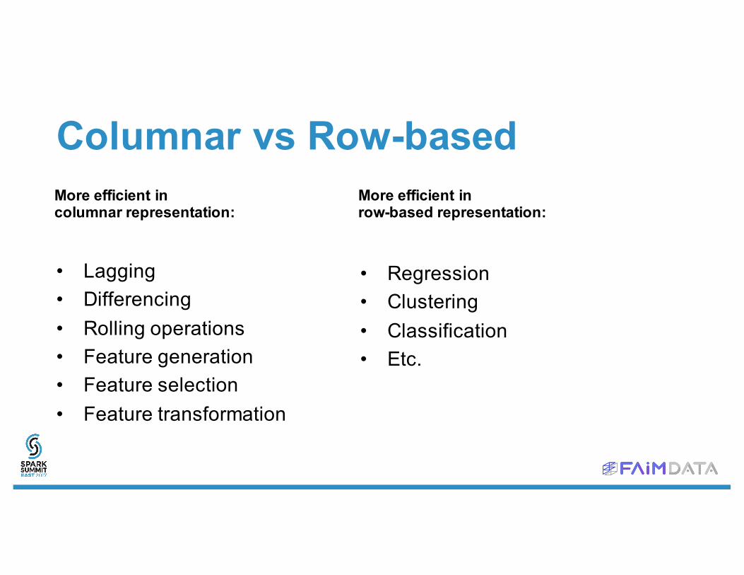
Columnar vs Row-based
• Lagging• Differencing• Rolling operations• Feature generation• Feature selection• Feature transformation
• Regression• Clustering• Classification• Etc.
More efficient incolumnar representation:
More efficient inrow-based representation:

Example: lagging operation
• Time complexity: O(N)(assumes pre-sorted RDD)
• For each row, we need to get values from previous k rows
• Time complexity: O(K)
• For each column to lag, we truncate most recent k values, and truncate the DateTimeIndex’soldest k values.
Columnar representationRow-based representation

Example: regression• We’re estimating:
• The lagged values are typically part of each row, because they are pre-generated as new features.
• Stochastic Gradient Descent: we iterate on examples and estimate error gradient to adjust weights, which means that we care about rows, not columns.
• To avoid shuffling, the partitioning must be done such that all elements of a row are together in the same partition (so the gradient can be computed locally).
Current solution• Core representation is columnar.• Utility functions to go to/from row-based.• Reasoning: spark-timeseries operations are
mostly time-related, i.e. columnar. Row-based operations are about relationships between the variables (ML/statistical), thus external to spark-timeseries.
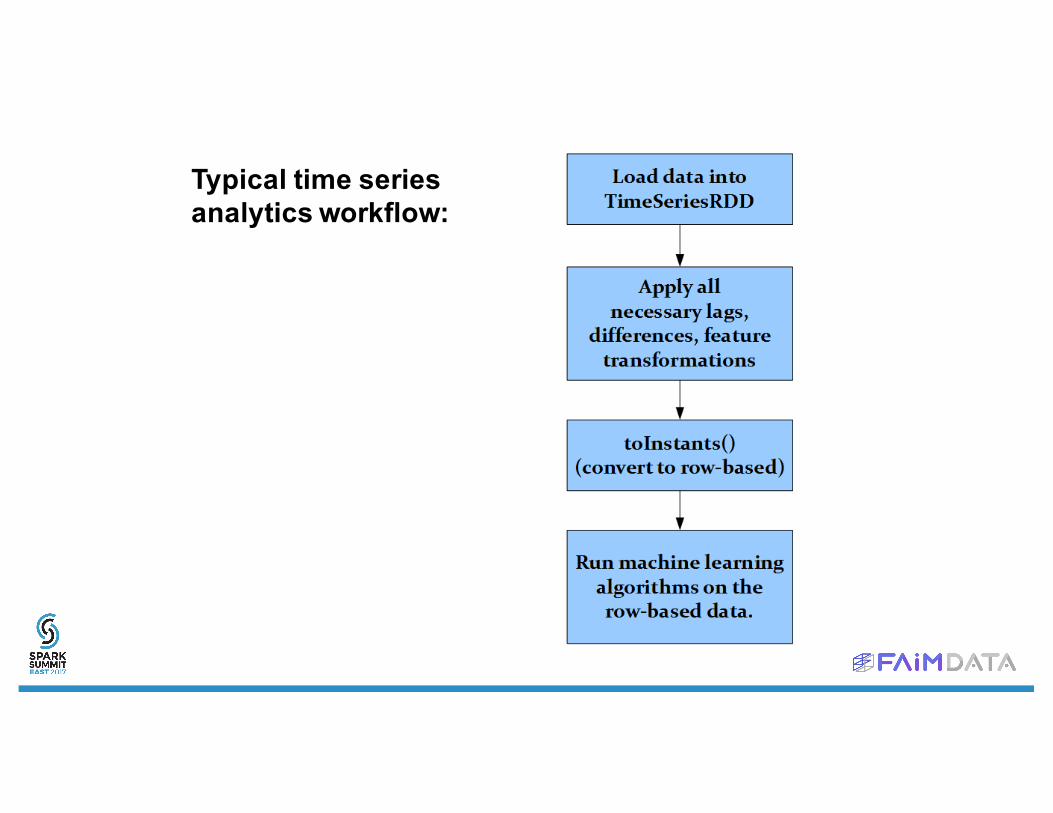
Typical time seriesanalytics workflow:

Survey: Who uses univariate time series that don’t fit inside a single
executor’s memory?
(or multivariate of which a single variable’s time series doesn’t fit)

Design Question #2: How do we partition the multi-variate time series
for distributed processing?
Across features, or across time?

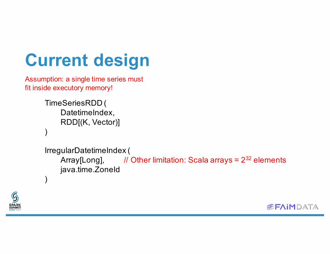
Current designAssumption: a single time series must fit inside executory memory!
Current designAssumption: a single time series must fit inside executory memory!
TimeSeriesRDD (DatetimeIndex,RDD[(K, Vector)]
)
IrregularDatetimeIndex (Array[Long], // Other limitation: Scala arrays = 232 elementsjava.time.ZoneId
)
Future improvements• Creation of a new TimeSeriesRDD-like class that
will be longitudinally (i.e. across time) partitioned rather than horizontally (i.e. across features).
• Keep both types of partitioning, on a case-by-case basis.
Design Question #3: How do we lag, difference, etc.?
Re-sampling, or index-preserving?
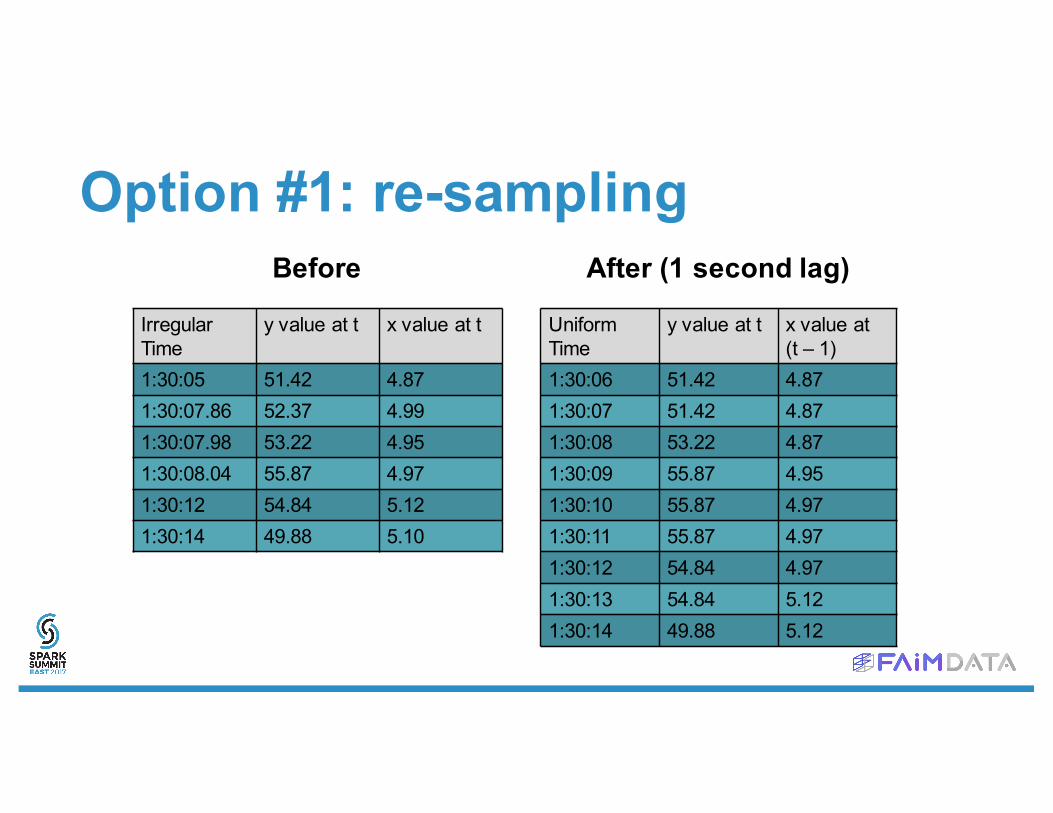
Option #1: re-sampling
Irregular Time
y value at t x value at t
1:30:05 51.42 4.871:30:07.86 52.37 4.991:30:07.98 53.22 4.951:30:08.04 55.87 4.971:30:12 54.84 5.121:30:14 49.88 5.10
Uniform Time
y value at t x value at (t – 1)
1:30:06 51.42 4.871:30:07 51.42 4.871:30:08 53.22 4.871:30:09 55.87 4.951:30:10 55.87 4.971:30:11 55.87 4.971:30:12 54.84 4.971:30:13 54.84 5.121:30:14 49.88 5.12
Before After (1 second lag)

Option #2: index preserving
Irregular Time
y value at t x value at t
1:30:05 51.42 4.871:30:07.86 52.37 4.991:30:07.98 53.22 4.951:30:08.04 55.87 4.971:30:12 54.84 5.121:30:14 49.88 5.10
Irregular Time
y value at t x value at (t – 1)
1:30:05 51.42 N/A1:30:07.86 52.37 4.871:30:07.98 53.22 4.871:30:08.04 55.87 4.871:30:12 54.84 4.971:30:14 49.88 5.12
Before After (1 second lag)
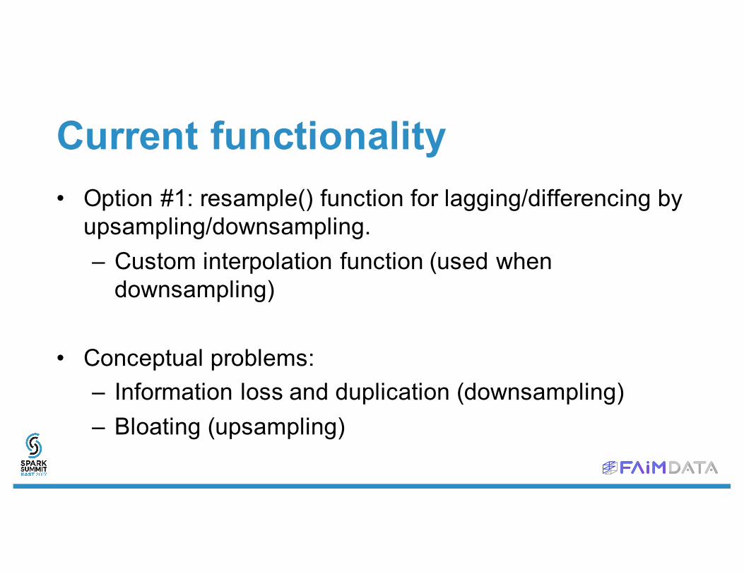
Current functionality• Option #1: resample() function for lagging/differencing by
upsampling/downsampling. – Custom interpolation function (used when
downsampling)
• Conceptual problems:– Information loss and duplication (downsampling)– Bloating (upsampling)
Current functionality• Option #2: functions to lag/difference irregular
time series based on arbitrary time intervals. (preserves index)
• Same thing: custom interpolation function can be passed for when downsampling occurs.

Overview of current API
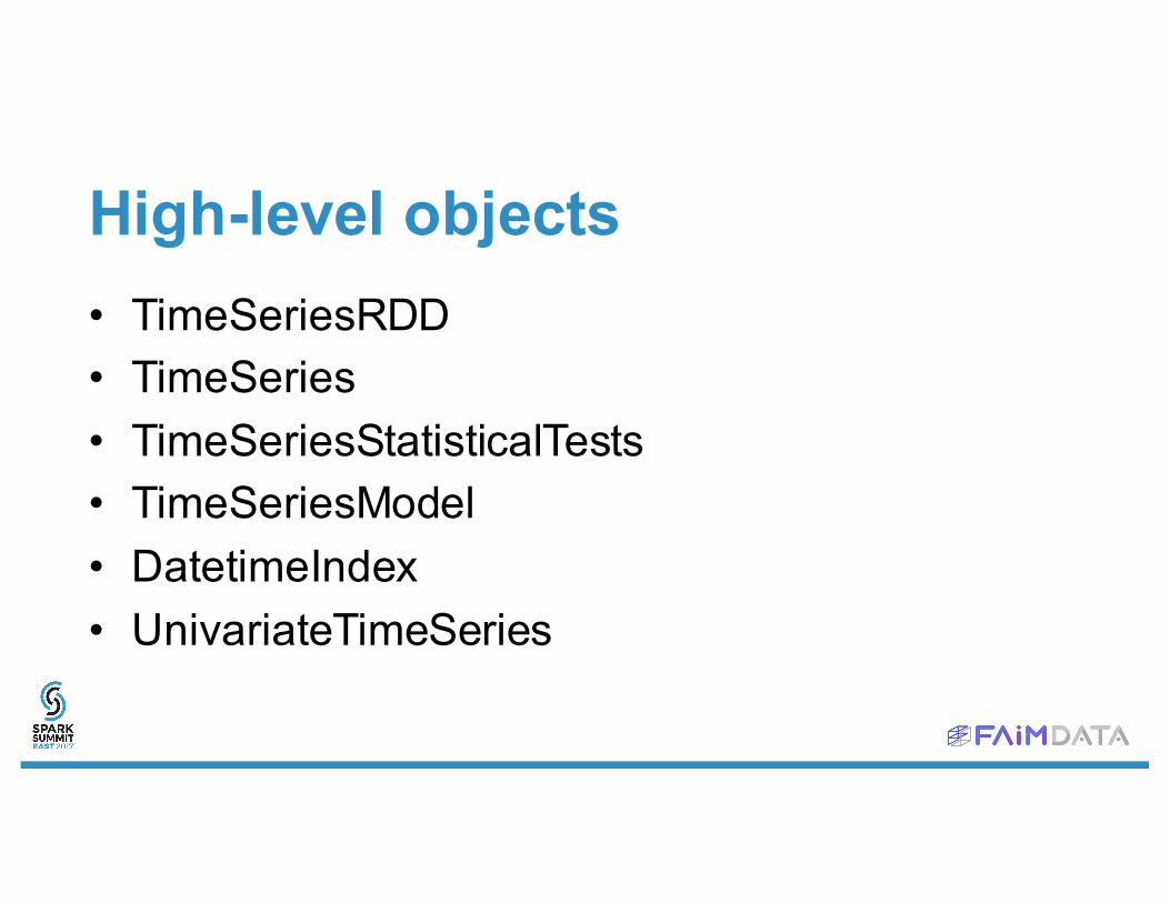
High-level objects• TimeSeriesRDD• TimeSeries• TimeSeriesStatisticalTests• TimeSeriesModel• DatetimeIndex• UnivariateTimeSeries

TimeSeriesRDD• collectAsTimeSeries• filterStartingBefore, filterStartingAfter, slice• filterByInstant• quotients, differences, lags• fill: fills NaNs by specified interpolation method (linear, nearest, next, previous,
spline, zero)• mapSeries• seriesStats: min, max, average, std. deviation• toInstants, toInstantsDataFrame• resample• rollSum, rollMean• saveAsCsv, saveAsParquetDataFrame
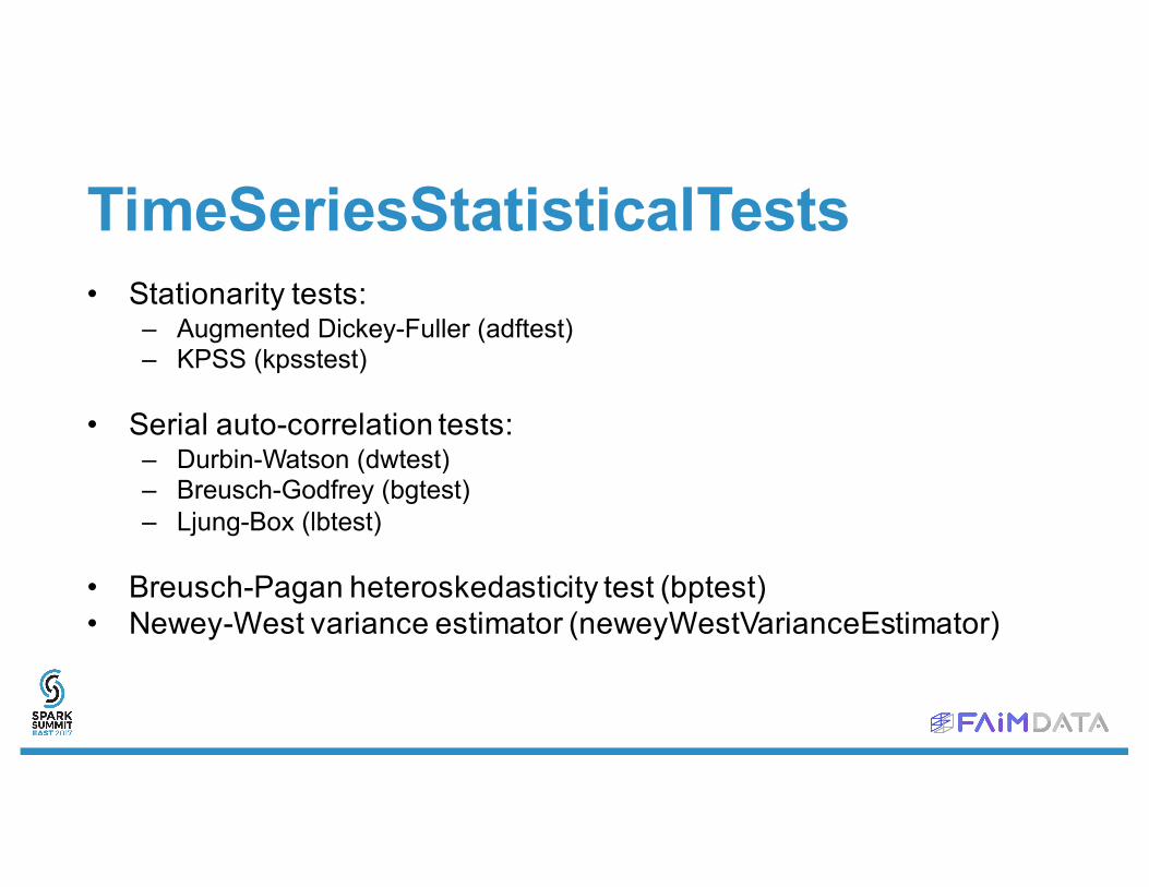
TimeSeriesStatisticalTests• Stationarity tests:
– Augmented Dickey-Fuller (adftest)– KPSS (kpsstest)
• Serial auto-correlation tests:– Durbin-Watson (dwtest)– Breusch-Godfrey (bgtest)– Ljung-Box (lbtest)
• Breusch-Pagan heteroskedasticity test (bptest)• Newey-West variance estimator (neweyWestVarianceEstimator)
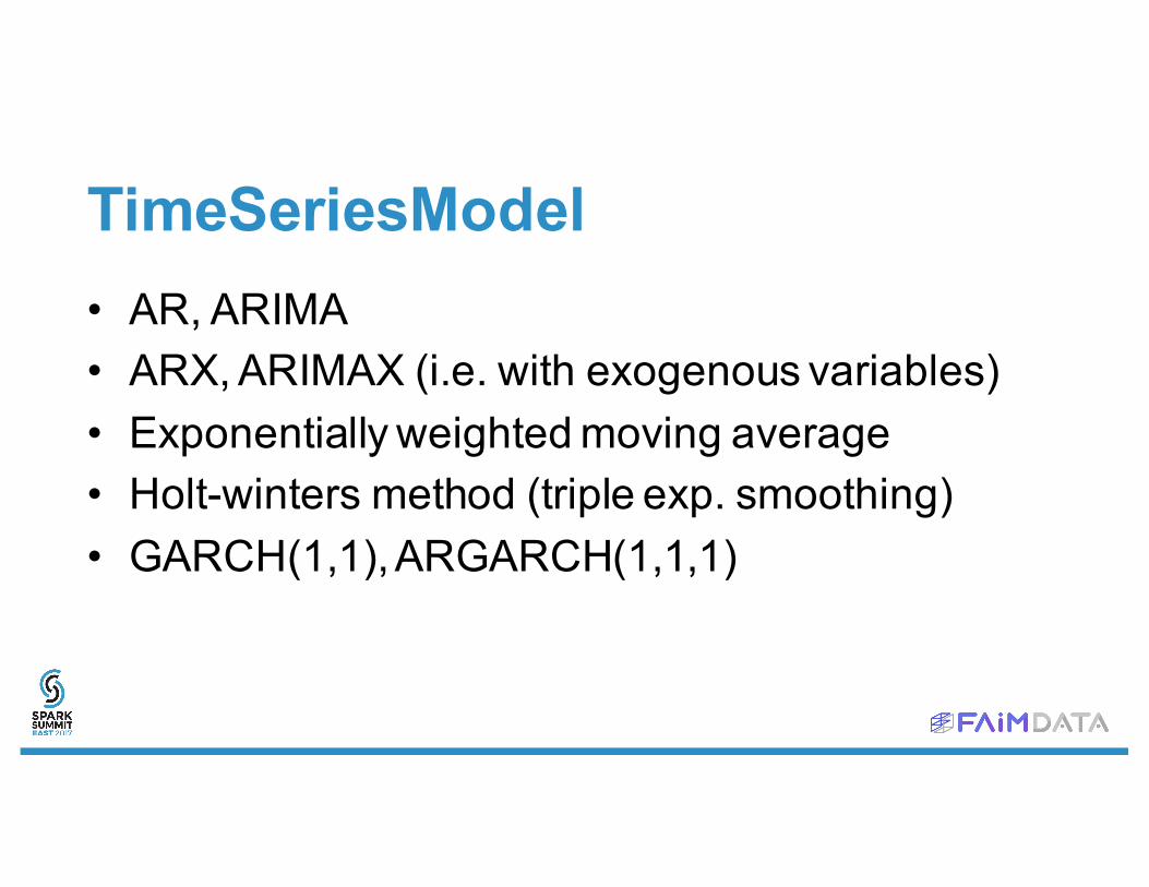
TimeSeriesModel• AR, ARIMA• ARX, ARIMAX (i.e. with exogenous variables)• Exponentially weighted moving average• Holt-winters method (triple exp. smoothing)• GARCH(1,1), ARGARCH(1,1,1)
Others• Java bindings
• Python bindings
• YAHOO financial data parser
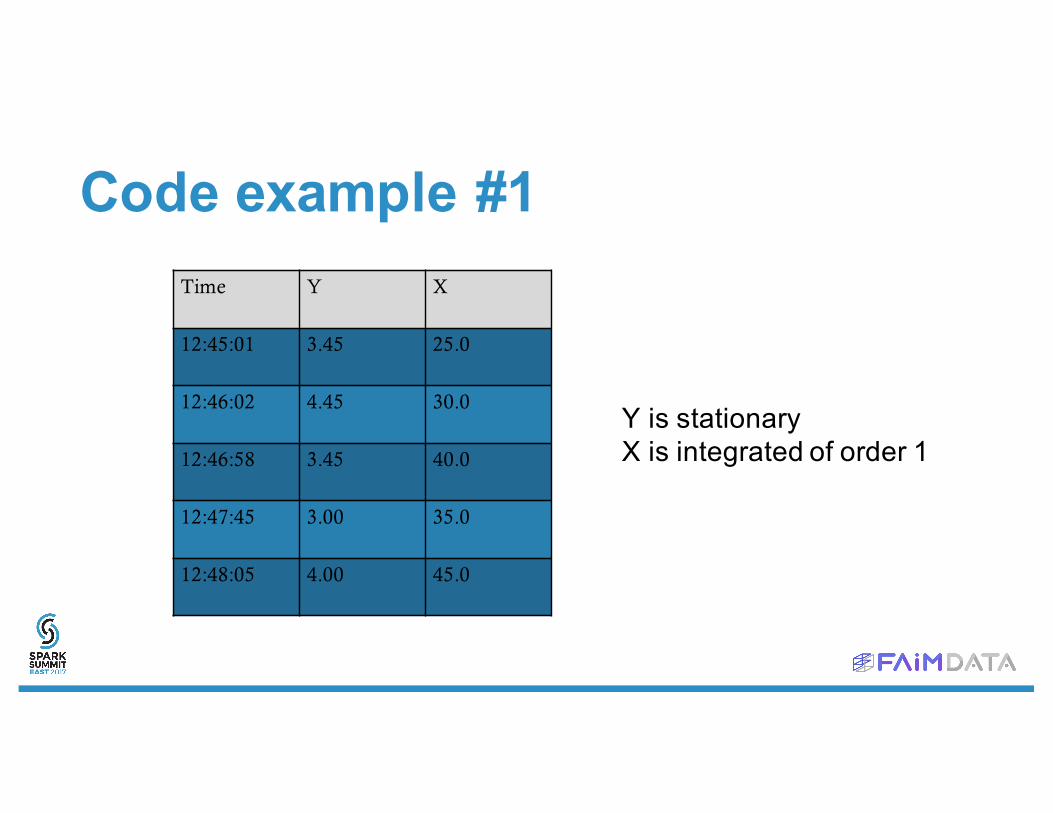
Code example #1Time Y X
12:45:01 3.45 25.0
12:46:02 4.45 30.0
12:46:58 3.45 40.0
12:47:45 3.00 35.0
12:48:05 4.00 45.0
Y is stationaryX is integrated of order 1
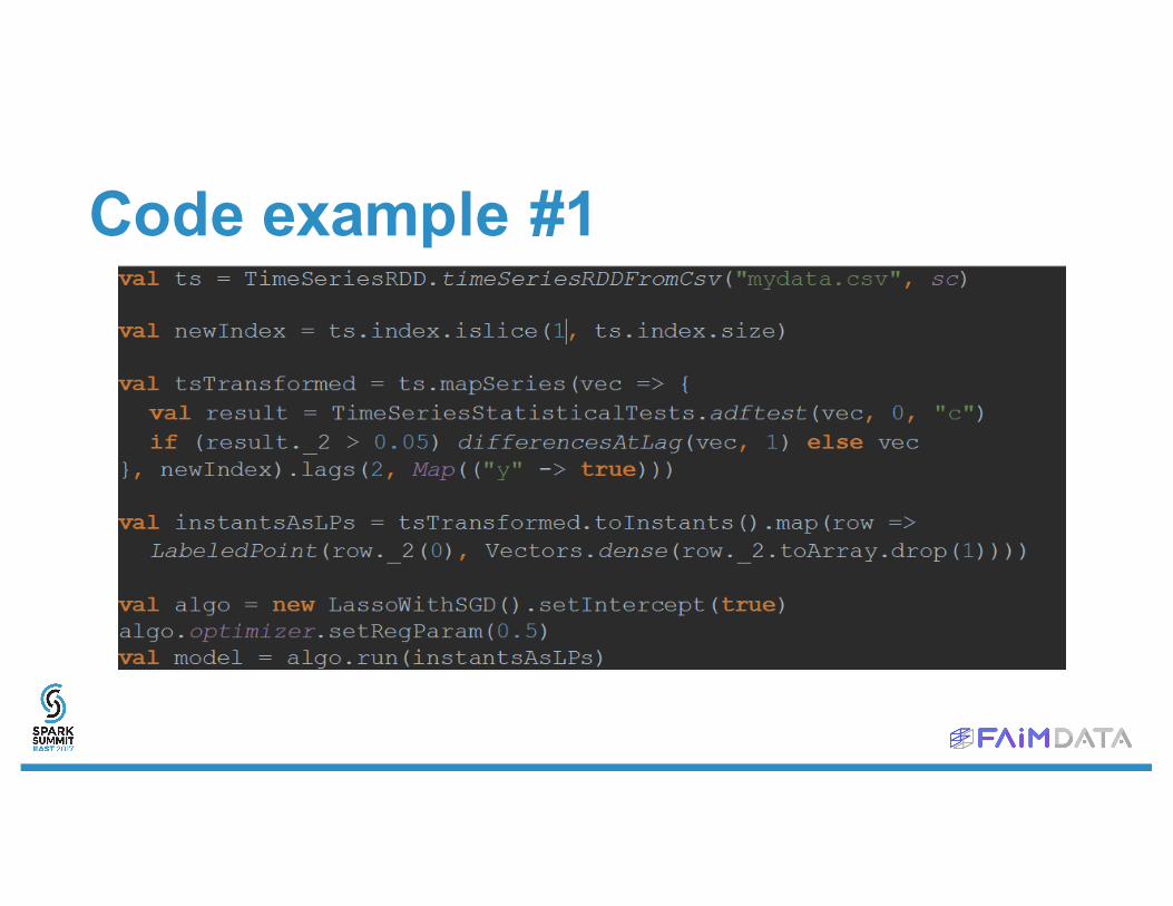
Code example #1

Code example #1Time y d(x) Lag1(y) Lag2(y) Lag1(d(x)) Lag2(d(x))
12:45:01 3.45
12:46:02 4.45 5.0 3.45
12:46:58 3.45 10.0 4.45 3.45 5.0
12:47:45 3.00 -5.0 3.45 4.45 10.0 5.0
12:48:05 4.00 10.0 3.00 3.45 -5.0 10.0
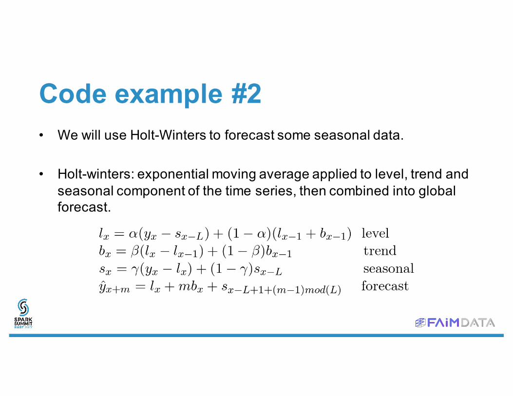
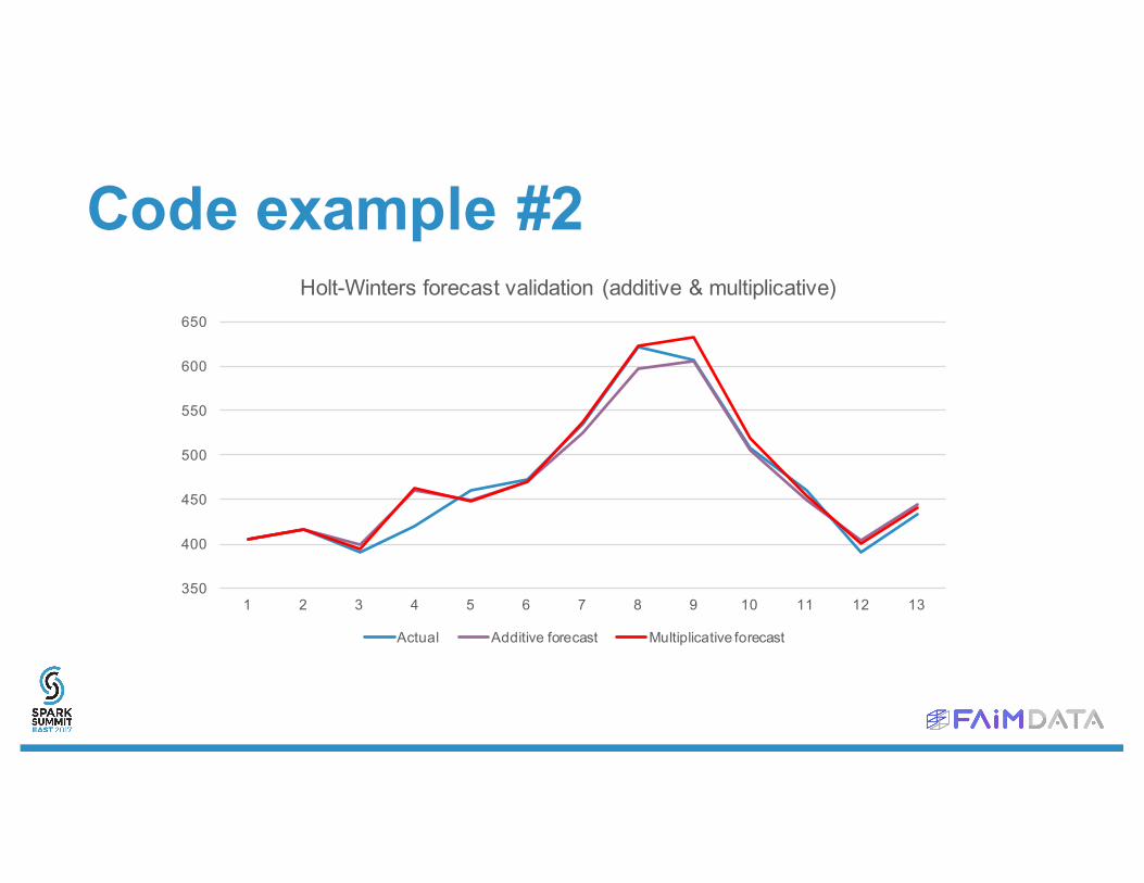
Code example #2• We will use Holt-Winters to forecast some seasonal data.
• Holt-winters: exponential moving average applied to level, trend and seasonal component of the time series, then combined into global forecast.

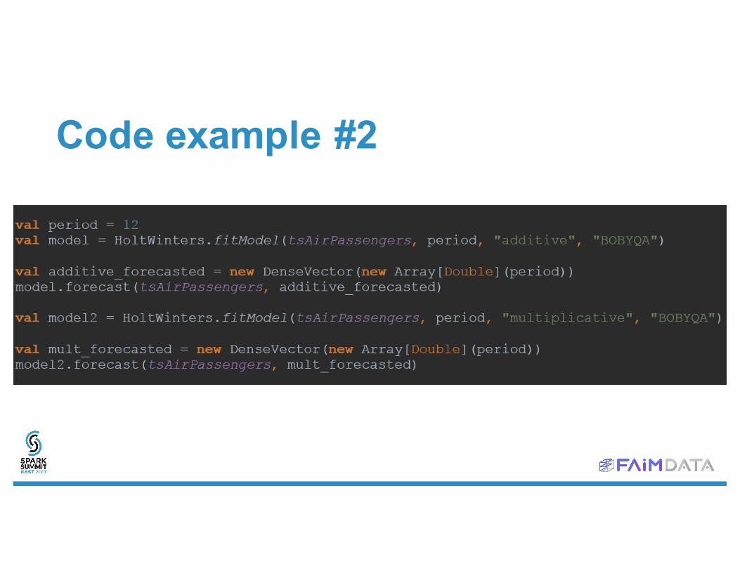
Code example #2
0
100
200
300
400
500
600
700
1 5 9 13 17 21 25 29 33 37 41 45 49 53 57 61 65 69 73 77 81 85 89 93 97 101
105
109
113
117
121
125
129
133
137
141
Passengers
Code example #2
Code example #2
350
400
450
500
550
600
650
1 2 3 4 5 6 7 8 9 10 11 12 13
Holt-Winters forecast validation (additive & multiplicative)
Actual Additive forecast Multiplicative forecast

Thank You.e-mail: [email protected]


