University of Pretoria

Department of Economics Working Paper Series

Time-Varying Risk Aversion and Realized Gold Volatility

Riza Demirer Southern Illinois University Edwardsville

Konstantinos Gkillas University of Patras - University Campus

Rangan Gupta University of Pretoria

Christian Pierdzioch Helmut Schmidt University

Working Paper: 2018-81

December 2018

__________________________________________________________

Department of Economics

University of Pretoria

0002, Pretoria

South Africa

Tel: +27 12 420 2413

Time-varying risk aversion and realized gold volatility

Riza Demirera, Konstantinos Gkillasb, Rangan Guptac, Christian Pierdziochd

December 2018

Abstract

We study the in- and out-of-sample predictive value of time-varying risk aversion for realizedvolatility of gold-price returns via extended heterogeneous autoregressive realized volatility(HAR-RV) models. Our findings suggest that time varying risk aversion possesses predictivevalue for gold volatility both in- and out-of-sample. Risk aversion is found to absorb insample the predictive power of stock-market volatility at a short forecasting horizon. Wealso study the out-of-sample predictive power of risk aversion in the presence of realizedhigher-moments, jumps, gold returns, a leverage effect as well as the aggregate stock-marketvolatility in the forecasting model. Results show that risk aversion adds to predictive value,where the shape of the loss function used to evaluate losses from forecast errors plays aprominent role for the beneficial effects using time-varying risk aversion to forecast realizedvolatility. Specifically, additional tests suggest that the short-run (long-run) out-of-samplepredictive value of risk aversion is beneficial for investors who are more concerned aboutover-predicting (under-predicting) gold market volatility. Overall, our findings show thattime-varying risk aversion captures information useful for out-of-sample predicting realizedvolatility not already contained in the other predictors.

Keywords: Gold-price returns; Realized volatility; Forecasting

a Department of Economics and Finance, Southern Illinois University Edwardsville, Edwardsville,IL 62026-1102, USA; E-mail address: rdemire@siue.edu.

b Department of Business Administration, University of Patras − University Campus, Rio, P.O.Box 1391, 26500 Patras, Greece ; Email address: gillask@upatras.gr.

c Department of Economics, University of Pretoria, Pretoria, 0002, South Africa; E-mail address:rangan.gupta@up.ac.za.

d Corresponding author. Department of Economics, Helmut Schmidt University, Holstenhofweg85, P.O.B. 700822, 22008 Hamburg, Germany; Email address: c.pierdzioch@hsu-hh.de.

1 Introduction

Recent research on global financial markets establishes a link between cycles in capital flows and

the level of risk aversion (e.g. Rey 2018), showing that risk aversion has significant explanatory

power over equity-market comovements (e.g., Xu 2017, Demirer et al. 2018). Clearly, capital

flows across risky and relatively safer assets would be closely linked to the level of risk aversion

in financial markets as utility maximizing investors assume investment positions based on their

willingness to take on risks. To that end, given the role of gold as a traditional safe haven in

which investors seek refuge during periods of uncertainty, one can argue that the role of risk

aversion as a driver of return dynamics in financial markets is not necessarily limited to equities,

but also extends to the market for gold. Interestingly, however, despite the multitude of studies

that explore the role of gold as a potential safe haven (e.g., Baur and Lucey 2010, Lucey and

Li 2015), the influence of time-varying risk aversion on the volatility of gold-price movements

is largely understudied, partially due to the challenges in controlling for the time variation in

macroeconomic uncertainty to estimate the time variation in risk aversion. The main contribution

of this paper is to examine the predictive power of risk aversion over gold volatility by utilizing a

recently developed measure of time-varying risk aversion which distinguishes the time variation

in economic uncertainty from the time variation in risk aversion. By doing so, we provide new

insight to the role of risk aversion in financial markets and volatility modeling in safe-haven

assets.

Clearly, forecasting volatility of gold returns is of interest not only for investors in the pricing of

related derivatives as well as hedging strategies for stock market-fluctuations, but also for policy

makers given the evidence that commodities, in particular gold, possess predictive value over

currency-market fluctuations (e.g., Chen and Rogoff 2003, Cashin et al. 2004, Apergis 2014), an

issue that is particularly important for emerging economies that have high risk exposures with re-

spect to currency fluctuations. Furthermore, given the evidence of significant volatility spillovers

across gold and other commodities, particularly oil (e.g., Ewing and Malik 2013), and that pre-

cious metals served as sources of information transmission during financial crises (Kang et al.

2017), exploring the predictive role of risk aversion over gold volatility can provide valuable in-

1

sight to whether the time-variation in risk aversion is the underlying fundamental factor driving

the spillover effects across asset classes, particularly during periods of high uncertainty. Al-

though the literature offers a limited number of studies relating various uncertainty measures to

gold-return dynamics (e.g., Jones and Sackley 2016, Balcilar et al. 2016, Bouoiyour et al. 2018),

these studies have not specifically examined the effect of the changes in the level of market risk

aversion on safe-haven assets, particularly gold. To that end, the time-varying risk aversion mea-

sure recently developed by Bekaert et al. (2017) offers a valuable opening as it distinguishes the

time variation in economic uncertainty (the amount of risk) from time variation in risk aversion

(the price of risk), providing an unbiased representation for time-varying risk aversion in finan-

cial markets. To the best of our knowledge, ours is the first study to utilize this unbiased measure

of risk aversion in the context of forecasting for safe-haven assets.

In our empirical analysis, we focus on the realized volatility of gold returns that we compute

from intraday data. The use of intraday data allows us to control for higher moments including

the realized skewness and kurtosis that have been shown to have predictive power in forecasting

models in a number of different contexts including gold (Mei et al. 2017, Bonato et al. 2018,

Gkillas et al. 2018). We employ the heterogeneous autoregressive RV (HAR-RV) model devel-

oped by Corsi (2009) to model and forecast the realized volatility of gold returns as this widely-

studied model accounts for several stylized facts such as fat tails and the long-memory property

of financial-market volatility, despite the simplicity offered by the model. To that end, we extend

the HAR-RV model to study the in- and out-of-sample predictive value of risk aversion, after

controlling for various alternative predictors including realized higher-moments, realized jumps,

gold returns, a leverage term as well as stock-market volatility.

Considering that the prices of risky assets drop as investors demand greater compensation for

risk when risk aversion is high, one can argue that the volatility impact on gold would be in the

positive direction, captured by good realized volatility (computed from positive returns), while

the opposite holds during good times. For this reason, we differentiate between “good” and

“bad” realized volatility, allowing us to explore possible asymmetric effects of risk aversion on

gold volatility. Finally, controlling for the aggregate stock-market volatility, measured by the

VIX index, in our models allows us to separately examine the impact of economic uncertainty

2

and changes in risk aversion on realized volatility. This distinction is particularly important as

risk aversion can fluctuate due to changes in wealth, background risk, and emotions that alter

risk appetite (Guiso et al. 2018). To that end, given the unbiased nature of the risk-aversion

measure utilized in our tests, distinguishing the time variation in economic uncertainty from the

time variation in risk aversion, our study provides new insight to the drivers of realized volatility

of gold returns.

Our findings show that time-varying risk aversion possesses predictive value for realized gold

volatility both in- and out-of-sample. While realized skewness and (at a medium and long fore-

casting horizon) stock-market volatility stand out as significant in-sample predictors for realized

volatility, risk aversion is found to absorb the predictive power of stock-market volatility if in-

vestors predict realized volatility at a short forecasting horizon. Out-of-sample results show

that the inclusion of risk aversion in the HAR-RV model yields better results for various model

configurations in terms of forecast accuracy relative to alternative models that include realized

higher-moments, jumps, gold returns, a leverage term and aggregate stock-market volatility. We

systematically document how the relative forecast accuracy of the HAR-RV-cum-risk-aversion

model relates to the length of the rolling-estimation window used to compute out-of-sample fore-

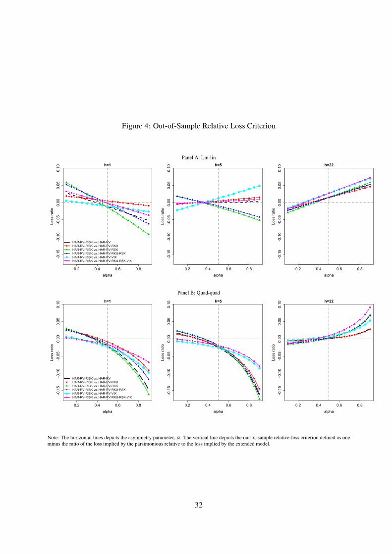
casts, the length of the forecast horizon, and the loss function (absolute versus squared error loss)

used to evaluate forecast errors. We find that the shape of the loss function plays a prominent

role for the beneficial effects of using time-varying risk aversion to forecast realized volatility.

Additional tests show that the short-run predictive value of risk aversion is particularly beneficial

for investors who are more concerned about over-predicting gold market volatility, an important

concern for the accuracy of forecasting models particularly during turbulent periods when in-

vestors shift funds towards safe havens, driving volatility in these assets. Overall, our findings

show that time-varying risk aversion contains information useful for out-of-sample forecasting

of realized volatility over and above the information already embedded in other widely-studied

predictors like higher-order moments, jumps, and stock-market volatility.

We present in Section 2 a brief review of the different strands of studies on gold. We describe in

Section 3 the methods that we use in our empirical analysis. We present our data in Section 4,

summarize our empirical results Section 5, and conclude in Section 6.

3

2 Literature Review

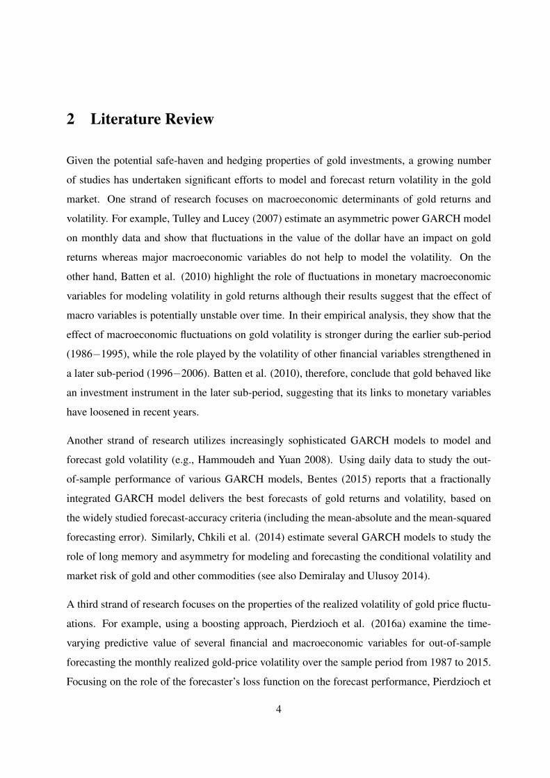
Given the potential safe-haven and hedging properties of gold investments, a growing number

of studies has undertaken significant efforts to model and forecast return volatility in the gold

market. One strand of research focuses on macroeconomic determinants of gold returns and

volatility. For example, Tulley and Lucey (2007) estimate an asymmetric power GARCH model

on monthly data and show that fluctuations in the value of the dollar have an impact on gold

returns whereas major macroeconomic variables do not help to model the volatility. On the

other hand, Batten et al. (2010) highlight the role of fluctuations in monetary macroeconomic

variables for modeling volatility in gold returns although their results suggest that the effect of

macro variables is potentially unstable over time. In their empirical analysis, they show that the

effect of macroeconomic fluctuations on gold volatility is stronger during the earlier sub-period

(1986−1995), while the role played by the volatility of other financial variables strengthened in

a later sub-period (1996−2006). Batten et al. (2010), therefore, conclude that gold behaved like

an investment instrument in the later sub-period, suggesting that its links to monetary variables

have loosened in recent years.

Another strand of research utilizes increasingly sophisticated GARCH models to model and

forecast gold volatility (e.g., Hammoudeh and Yuan 2008). Using daily data to study the out-

of-sample performance of various GARCH models, Bentes (2015) reports that a fractionally

integrated GARCH model delivers the best forecasts of gold returns and volatility, based on

the widely studied forecast-accuracy criteria (including the mean-absolute and the mean-squared

forecasting error). Similarly, Chkili et al. (2014) estimate several GARCH models to study the

role of long memory and asymmetry for modeling and forecasting the conditional volatility and

market risk of gold and other commodities (see also Demiralay and Ulusoy 2014).

A third strand of research focuses on the properties of the realized volatility of gold price fluctu-

ations. For example, using a boosting approach, Pierdzioch et al. (2016a) examine the time-

varying predictive value of several financial and macroeconomic variables for out-of-sample

forecasting the monthly realized gold-price volatility over the sample period from 1987 to 2015.

Focusing on the role of the forecaster’s loss function on the forecast performance, Pierdzioch et

4

al. (2016) find that a forecaster who encounters a larger loss when underestimating rather than

overestimating gold-price volatility benefits from using the forecasts implied by their boosting

approach. In an earlier study, using high-frequency, intra-daily gold data to construct measures of

realized gold-price volatility, Neely (2004) shows that option implied volatility is a biased fore-

cast of the realized volatility and that implied volatility tends to be informationally inefficient

with respect to forecasts computed by means of competing econometric models, while econo-

metric forecasts have no incremental value over implied volatility when a delta hedging tracking

error is used to evaluate out-of-sample volatility forecasts.

The literature on realized gold volatility is directly relevant for our research. Specifically, we use

the HAR-RV model developed by Corsi (2009) to model and forecast realized gold volatility.

Variants of the HAR-RV model have been widely studied in recent research (see, for example,

Haugom et al. 2014, Lyócsa and Molnár 2016) as it accounts for several stylized facts such as

fat tails and the long-memory property of financial-market volatility, despite the simplicity the

model offers. In our empirical analysis, we extend the core HAR-RV model to include measures

of realized higher-moments including realized skewness and kurtosis that have been found to

significantly improve model performance in the case of stock market indexes (Mei et al. 2017).

This is a remarkable finding given that, in the case of gold and silver, evidence suggests that it

is difficult to beat the HAR-RV model in terms of forecasting performance by using versions

of the univariate HAR-RV model extended to include semi-variances and jumps (Lyócsa and

Molnár 2016). Finally, we control for realized jumps, gold returns, and the aggregate stock

market volatility as measured by the VIX index, and examine whether risk aversion possesses

incremental in- and out-of-sample predictive power over gold market volatility beyond that is

captured by a number of predictors that have often been used in the literature.

5

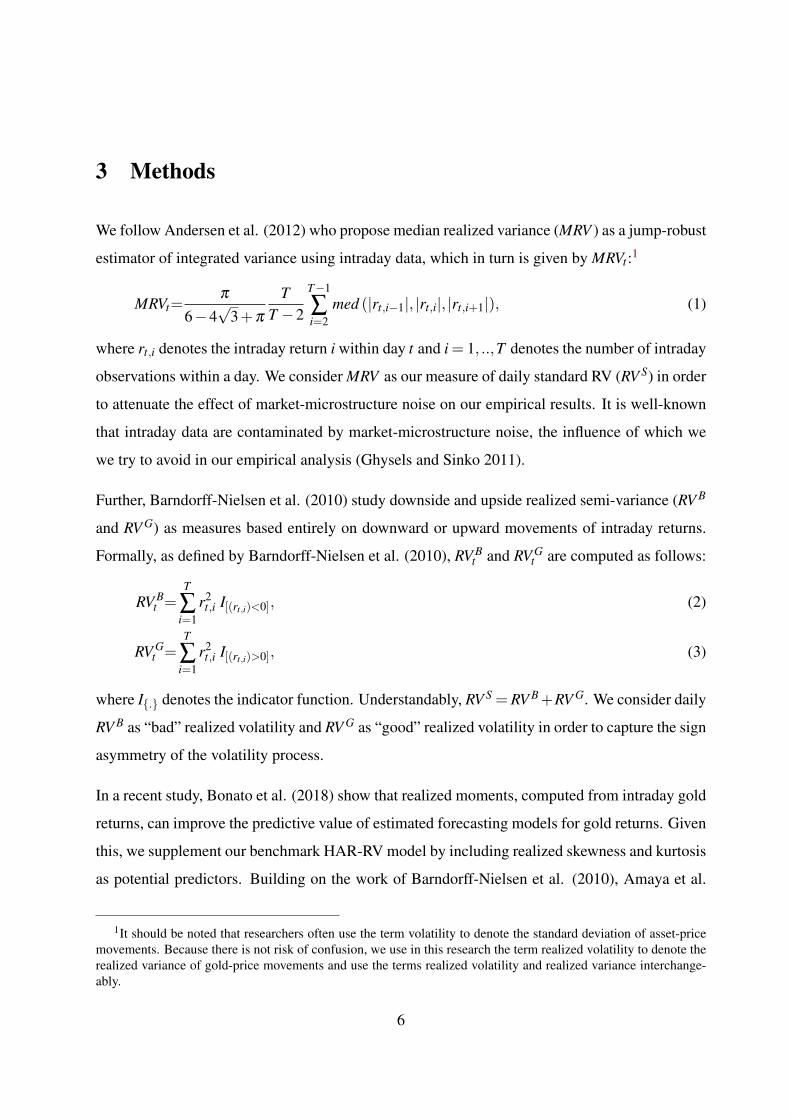
3 Methods

We follow Andersen et al. (2012) who propose median realized variance (MRV ) as a jump-robust

estimator of integrated variance using intraday data, which in turn is given by MRVt :1

MRVt=π

6−4√

3+π

TT −2

T−1

∑i=2

med (|rt,i−1|, |rt,i|, |rt,i+1|), (1)

where rt,i denotes the intraday return i within day t and i = 1, ..,T denotes the number of intraday

observations within a day. We consider MRV as our measure of daily standard RV (RV S) in order

to attenuate the effect of market-microstructure noise on our empirical results. It is well-known

that intraday data are contaminated by market-microstructure noise, the influence of which we

we try to avoid in our empirical analysis (Ghysels and Sinko 2011).

Further, Barndorff-Nielsen et al. (2010) study downside and upside realized semi-variance (RV B

and RV G) as measures based entirely on downward or upward movements of intraday returns.

Formally, as defined by Barndorff-Nielsen et al. (2010), RV Bt and RV G

t are computed as follows:

RV Bt =

T

∑i=1

r2t,i I[(rt,i)<0], (2)

RV Gt =

T

∑i=1

r2t,i I[(rt,i)>0], (3)

where I{.} denotes the indicator function. Understandably, RV S = RV B+RV G. We consider daily

RV B as “bad” realized volatility and RV G as “good” realized volatility in order to capture the sign

asymmetry of the volatility process.

In a recent study, Bonato et al. (2018) show that realized moments, computed from intraday gold

returns, can improve the predictive value of estimated forecasting models for gold returns. Given

this, we supplement our benchmark HAR-RV model by including realized skewness and kurtosis

as potential predictors. Building on the work of Barndorff-Nielsen et al. (2010), Amaya et al.

1It should be noted that researchers often use the term volatility to denote the standard deviation of asset-pricemovements. Because there is not risk of confusion, we use in this research the term realized volatility to denote therealized variance of gold-price movements and use the terms realized volatility and realized variance interchange-ably.

6

(2015) compute higher-moments of realized skewness (RSK) and realized kurtosis (RKU) from

intraday returns. Following Amaya et al. (2015), RSKt and RKUt , standardized by the realized

variance, is defined as follows:

RSKt=

√T ∑

Ti=1 r3

t,i

(∑Ti=1 r2

t,i)3/2

, (4)

RKUt=T ∑

Ti=1 r4

t,i

(∑Ti=1 r2

t,i)2. (5)

We consider daily RSK as a measure of the asymmetry of distribution of the daily returns, while

RKU measures the extremes of the same.

As far as the literature on modelling and forecasting realized volatility is concerned, Corsi (2009)

proposes the HAR-RV model, which in turn has become one of the most popular models in this

strand of research. The HAR-RV model has been shown to capture “stylized facts” of long mem-

ory and multi-scaling behavior associated with volatility of financial markets. The benchmark

HAR-RV model, for h−days-ahead forecasting, can be described as follows:

RV jt+h=β0 +βd RV j

t +βw RV jw,t +βm RV j

m,t + εt+h, (6)

where (to simplify notation) j can be either S, B or G as described earlier. RV jw,t denotes the

average RV j from day t−5 to day t−1, while RV jm,t denotes the average RV j from day t−22 to

day t−1.

We use the standard HAR-RV model as our benchmark model for predicting realized-volatility

and, as in Mei et al. (2017), we add realized skewness, realized kurtosis, or both as additional

predictors to the benchmark model. In addition, based on the question we are aiming to answer,

we first add the widely-utilized stock-market volatility index (VIX) associated with the S&P500

index, and the recently developed measure of time-varying risk aversion (RISK) in order to ex-

plore whether risk aversion captures incremental predictive information. To this end, we consider

7

the following modified HAR-RV models:

RV jt+h=β0 +βd RV j

t +βw RV jw,t +βm RV j

m,t +θ RSKt + εt+h, (7)

RV jt+h=β0 +βd RV j

t +βw RV jw,t +βm RV j

m,t +η RKUt + εt+h, (8)

RV jt+h=β0 +βd RV j

t +βw RV jw,t +βm RV j

m,t +θ RSKt +η RKUt + εt+h, (9)

RV jt+h=β0 +βd RV j

t +βw RV jw,t +βm RV j

m,t +θ RSKt +η RKUt + γ V IXt + εt+h, (10)

RV jt+h=β0 +βd RV j

t +βw RV jw,t +βm RV j

m,t +θ RSKt +η RKUt + γ V IXt +δ RISKt + εt+h.

(11)

4 Data

We use intraday data on gold to construct daily measures of standard realized volatility, the

corresponding good and bad variants, realized skewness, and realized kurtosis. Gold futures are

traded in NYMEX over a 24 hour trading day (pit and electronic). We focus on gold futures

prices, rather than spot prices, due to the low transaction costs associated with futures trading,

which makes the analysis more relevant for practical applications in the context of hedging and/or

safe-haven analyses. Furthermore, one can expect price discovery to take place primarily in the

futures market as the futures price responds to new information faster than the spot price due to

lower transaction costs and ease of short selling associated with the futures contracts (Shrestha

2014). The futures price data, in continuous format, are obtained from www.disktrading.com

and www.kibot.com. Close to expiration of a contract, the position is rolled over to the next

available contract, provided that activity has increased. Daily returns are computed as the end of

day (New York time) price difference (close to close). In the case of intraday returns, 1-minute

prices are obtained via last-tick interpolation (if the price is not available at the 1-minute stamp,

the previously available price is imputed). 5-minute returns are then computed by taking the

log-differences of these prices and are then used to compute the realized moments.

Besides the intraday data, we obtain data on the VIX index compiled by the Chicago Board

Options Exchange (CBOE) from the FRED database of the Federal Reserve Bank of St. Louis,

which is a popular measure of the stock market’s expectation of volatility implied by S&P500

8

index options. In addition, for measuring risk aversion (RISK), we utilize the risk aversion index

of Bekaert et al. (2017), which is available for download from: https://www.nancyxu.net/

risk-aversion-index. These authors develop a new measure of time-varying risk aversion

that ultimately can be calculated from observable financial information at high (daily) frequen-

cies. This measure relies on a set of six financial instruments, namely, the term spread, credit

spread, a detrended dividend yield, realized and risk-neutral equity return variance and realized

corporate bond return variance. As discussed earlier, an important feature of this measure is that

it distinguishes time variation in economic uncertainty (the amount of risk) from time variation

in risk aversion (the price of risk) and, thus, provides an unbiased representation for time-varying

risk aversion based on a utility function in the hyperbolic absolute risk aversion (HARA) class.

− Please include Table 1 about here. −

The sample period runs from December 2, 1997 to December 30, 2016 (reflecting data availabil-

ity of the risk aversion index used as one of the predictors), giving us a total of 4,748 observations.

Table 1 reports some summary statistics of the data. In our forecasting tests, we consider three

forecasting horizons (short, h = 1; medium, h = 5; long h = 22) and construct the data matrix

such that we have exactly the same number of observations (4,704 observations; computing RV

for the long forecast horizon and computing RVm each consumes 22 observations) for all three

forecasting horizons.

5 Empirical Findings

5.1 In-Sample Findings

Table 2 summarizes the estimation results for the standard realized volatility for the full sam-

ple period. Estimation results are computed using the R programming environment (R Core

Team 2017). Newey-West robust standard errors are computed using the R packages “sandwich”

(Zeileis 2004). We estimate, in a first step, the core HAR-RV model. In a second step, we add

risk aversion. In a third step, we estimate other predictors. We observe that the MRV component

9

of the core HAR-RV model has significant predictive power at all forecasting horizons. The

MRVw component is significant at the short forecasting horizon, while the MRVm component is

significant mainly at the medium and long forecasting horizons. The models supplemented by

the realized moments yield evidence partially in line with Mei et. al (2017) in that only realized

skewness is found to have significant in-sample predictive power, across all forecast horizons.

Interestingly, we see that including risk aversion in the model adds predictive value in the case

of the short forecasting horizon, as indicated by the significant estimated coefficients. Adding

aggregate stock-market volatility in the model adds predictive power only in case of the medium

and long forecasting horizon and not for the short forecast horizon. When risk aversion is also

included in the model, we see that risk aversion dominates stock-market volatility in terms of

short-term predictive power, rendering the coefficient of the latter insignificant. In the case of

the medium and long forecast horizons, the estimated coefficients of both stock-market volatility

and risk aversion are found to be significant.

− Please include Table 2 about here. −

Another noteworthy observation is that the sign of the coefficient for risk aversion switches from

positive in the short forecast horizon to negative for the medium and long forecast horizons.

As a higher value for risk aversion is associated with market conditions during which investors

have a greater tendency to move out of risky assets and into safer alternatives, possibly those

classified as safe havens, the finding of a positive risk aversion effect on the short-term volatility

in gold returns is not unexpected. The negative coefficients on risk aversion for longer forecast

horizons, however, may be an indication of a correction effect to the initial, immediate reaction

of the market to unexpected news. In short, our in-sample tests highlight the predictive power of

risk aversion at all forecast horizons, absorbing the predictive power of stock-market volatility

in the case of daily forecasts. Hence, we conclude that time-varying risk aversion has significant

predictive power for realized volatility of gold-price movements over and above the predictive

power that stock-market volatility unfolds.

Tables 3 and 4 summarize the findings for bad and good realized volatility, respectively. The

results for the core HAR-RV are qualitatively similar to the results reported in Table 2. While

10

the coefficient of realized volatility are always significant, the coefficients estimated for weekly

(monthly) realized volatility are only significant at the short (medium and long) forecasting hori-

zon. In the case of the realized moments, we see that realized skewness retains its predictive

power for both the good and bad volatility, whereas the predictive power of realized kurtosis is

limited to the short forecast horizon and mainly to good volatility. Considering that good volatil-

ity in gold corresponds to periods when the gold market is experiencing substantial gains, the

predictive power of realized kurtosis over good volatility could be associated with the informa-

tion content this moment captures following extreme (or crisis) periods.

− Please include Tables 3 and 4 about here. −

More importantly, the estimated coefficients for risk aversion in the HAR-RV model that already

contains realized moments and stock-market volatility are found to be significant, both in the

case of good and bad volatility. Similar to our findings for standard realized volatility, in the

case of the short forecast horizon, risk aversion is again found to absorb the predictive power

of stock-market volatility in both Tables 3 and 4. At the medium and long forecasting horizons,

however, both stock-market volatility and risk aversion have significant in-sample predictive

power (with the evidence for good volatility being somewhat weaker). Overall, our in-sample

tests highlight the predictive power of risk aversion over bad and good gold realized volatility

at all forecast horizons, however, particularly in the short run when the predictive value of risk

aversion dominates the predictive value of stock-market volatility.

5.2 Out-of-Sample Findings

Understandably, in-sample predictive value does not necessarily imply that a predictor also has

out-of-sample predictive value. For our out-of-sample analysis, we use a rolling-estimation win-

dow. To this end, we vary the length of the estimation window between 1000 and 3000 obser-

vations (for example, a rolling window that uses approximately the first ten years of data to start

the estimations has 2227 observations) and then move the rolling-estimation window forward in

time on a daily basis until we reach the end of the sample period. Finally, we the Diebold and

11

Mariano (1995) test to compare forecast accuracy. The test results are derived using the modified

Diebold-Mariano test proposed by Harvey, Leybourne and Newbold (1997), where we report the

p-values for both tests computed using the R package “forecast” (Hyndman 2017, Hyndman and

Khandakar 2008).

− Please include Figure 1 about here. −

Figure 1 presents results for the standard realized volatility and two different loss functions: an

absolute loss function (L1 loss) and squared error loss (L2). We compare the forecasts implied

by the HAR-RV-RISK model with the forecasts implied by the alternative core HAR-RV model

without any additional predictors. The results show that the forecasts computed by means of the

model that features risk aversion are more accurate than the forecasts computed by means of the

core HAR-RV model for the long forecast horizon under the L1 loss function for a broad range

of rolling-window lengths. Under the L2 loss function, the p-values show that the model that

includes time-varying risk aversion fares better than the core HAR-RV model at the long forecast

horizon for relatively short rolling windows. In contrast, for the short forecasting horizon, time-

varying risk aversion adds predictive value when we study a relatively long rolling window.

Hence, the shape of the loss function an investor uses to evaluate losses from forecast errors plays

a prominent role for the beneficial effects of using time-varying risk aversion to forecast realized

volatility. Specifically, the L1 loss function often yields, for various model configurations and

rolling-estimation-window lengths, stronger evidence of superior relative out-of-sample forecast

asccuracy of the HAR-RV-RISK model than the L2 loss function.

− Please include Figure 2 about here. −

Figure 2 depicts results for bad and good realized volatility. We report results for the L1 loss

function and use the core HAR-RV without any additional predictors as the alternative model.

For several intermediate lengths of the rolling-estimation window, the core HAR-RV without any

additional predictors offers significantly better short-term forecasts of bad realized volatility than

the HAR-RV model extended to include time-varying risk aversion. For good realized volatility,

12

the results for the long forecasting horizon strengthen in favor of the HAR-RV-RISK model

for the shorter rolling-estimation windows, while the results for the short forecasting horizon

become stronger when we study a relatively long rolling-estimation window. As compared to the

results for the standard realized volatility summarized in the upper panel of Figure 1, however,

the results for bad and good realized volatility are less strong.

− Please include Figure 3 about here. −

Figure 3 summarizes results of two additional forecast comparisons. In the upper panel, we

use the HAR-RV model extended to include the higher-order moments as the alternative model.

We again focus on the L1 loss function because it is less sensitive to large outliers caused by

sudden bursts of volatility than the L2 loss function and often yields strong and stable results for

a wide range of rolling-estimation windows. The test results are significant or hover around the

10% level of significance for rolling windows of length up to approximately 2500 observations,

while the test results for the short forecasting horizon turn significant for the relatively long

rolling-estimation windows. In the lower panel, we use the HAR-RV model that features stock-

market volatility as an additional predictor as the alternative model. Results show that for the

long forecast horizon the test results are highly significant for a broad range of rolling-estimation

windows. We also observe several significant results for the medium forecasting horizon. The

test results for the short forecasting horizon are insignificant and, in fact, show that the alternative

model yields more accurate forecasts for various lengths of the rolling-estimation window than

the model that features time-varying risk aversion as a predictor of realized volatility

5.3 The Role of the Loss Function

The L1 and L2 loss functions used to set up the Diebold-Mariano test are special cases of a more

general and potentially asymmetric loss function. Depending on the type of positions an investor

holds, an asymmetric loss function arises naturally, for example, if underestimating volatility

is more costly than an overestimation of the same magnitude. We use Figure 4 to illustrate

how the shape of the loss function affects the relative out-of-sample performance of the models.

13

Specifically, the figure displays the following out-of-sample relative-loss criterion (Pierdzioch et

al. 2016b):

R(A,B,α, p) = 1− ∑Tτ {[α +(1−2α)I( f eA < 0]| f eA|p}

∑Tτ {[α +(1−2α)I( f eB < 0]| f eB|p}

, (12)

where f e denotes the forecast error (actual minus forecast) implied by models A and B, α ∈

(0,1), and p ∈ {1,2}, and the summation runs over the out-of-sample periods. The out-of-

sample relative-loss criterion can be interpreted as an out-of-sample R2 criterion that compares

the performance of two models, A and B, for a forecaster who has a potentially asymmetric

loss function. The parameter α governs the asymmetry of the loss function. A symmetric loss

function obtains for α = 0.5, while α > 0.5 ( α < 0.5 ) implies that the loss from under-predicting

(over-predicting) realized volatility exceeds the loss from an over-prediction (under-prediction)

of the same magnitude. For p = 1, the loss function is of the lin-lin type, while p = 2 results in a

quad-quad loss function (see Elliott et al. 2005, 2008). Specifically, the parameter configuration

α = 0.5 and p = 1 (α = 0.5 and p = 2) results in the L1 (L2) loss functions assumed to set up

the Diebold-Mariano test as special cases.

− Please include Figure 4 about here. −

We set model as A = HAR-RV-RISK and use the various other variants of the HAR-RV model as

the alternative model B in order to shed light on the out-of-sample predictive value time-varying

risk aversion adds to the forecasting model. We then plot the resulting out-of-sample relative-loss

criterion for the lin-lin and quad-quad loss functions as a function of the asymmetry parameter.

We use roughly the first ten years of data to start the rolling-estimation-window procedure. To

be precise, the first rolling window comprises data up to and including 12/31/2007, which gives

2227 forecasts.

Results (for standard realized volatility) show that R > 0 (that is, the HAR-RV-RISK model

performs better than the alternative model) for approximately α < 0.5 (α < 0.4 ) in the case of a

lin-lin (quad-quad) loss function when we assume a short forecasting horizon. In this case, using

time-varying risk aversion to replace the other predictors included in the alternative model mainly

benefits an investor who incurs a larger loss from over-predicting (that is, the forecast exceeds the

14

actual realized volatility) realized volatility than from an under-prediction of the same magnitude.

For α close to the symmetric benchmark, the out-of-sample relative-loss criterion takes on values

close to zero, which explains why the Diebold-Mariano tests in Figure 1 are not significant for

rolling-window lengths of 2200−2300 observations.

For the long forecast horizon, in contrast, we observe R > 0 for approximately α > 0.3 for

both loss functions. In other words, (almost) all types of investors benefit from utilizing time-

varying risk aversion for predicting realized volatility at the long forecast horizon, where the

relative benefit increases in the magnitude of the asymmetry parameter. Hence, we conclude

that the short-run (long-run) predictive value of risk aversion is beneficial for investors who are

more concerned about over-predicting (under-predicting) gold volatility. In addition, we observe

that the out-of-sample relative-loss criterion takes on a somewhat larger numerical value for the

symmetric benchmark when we assume a lin-lin rather than a quad-qaud loss function, which

explains why the Diebold-Mariano test in the upper panel of Figure 1 yields significant results

while the test results in the lower panel only scratch the 10% significance level. Finally we

observe the largest benefit of using time-varying risk aversion for forecasting realized volatility

when the alternative model includes„ in addition to the higher-order moments, also stock-market

volatility.

Results for the medium forecast horizon are mixed. The results for the quad-quad loss function

resemble the results for the short forecasting horizon. The results for four out of the six models

under an assumed lin-lin loss function, in contrast, resemble the results for the long forecasting

horizon, where we observe the largest gain in terms of the out-of-sample relative loss criterion

for approximately α > 0.3 when we compare the HAR-RV-RISK model with the HAR-RV-

RKU-RSK-VIX model. Hence, relying on risk aversion rather than on higher-order moments

and market volatility is particularly beneficial for investors who suffer a larger loss from under-

predicting gold volatility than from a comparable over-prediction and who use a lin-lin function

to evaluate losses.

In short, our tests that use alternative functional forms of the loss function suggest that the short-

run predictive value of risk aversion tends to be beneficial for investors who are more concerned

about over-predicting gold volatility. This is an important concern as investors tend to display

15

short-term overreaction to bad news which means that, during crisis periods, investors may show

a tendency to overshoot in their estimations of gold-market fluctuations. To that end, our analy-

sis shows that risk aversion can help improve the accuracy of forecasts, particularly in situations

when the informational efficiency of the market is compromised due to crisis conditions or un-

expected negative events. At the same time, our findings also show that using time-varying risk

aversion as a predictor of realized volatility can help investors who are particularly concerned

about under-predicting realized volatility at a long forecast horizon.

Considering the occurence of a market correction following a severe shock, as experienced dur-

ing the global financial crisis of 2008, the finding of long-run predictive performance of risk

aversion can be used to improve the pricing of related derivatives as under-predicting volatility

would imply under-valuation of derivative securities that can be used to hedge risks. To that end,

the differential findings of the predictive value of risk aversion for the short and long forecast

horizons have significant implications for the pricing of related derivative instruments as well as

the cost of hedging strategies to manage risk exposures.

5.4 Jumps and Other Extensions

In an application to stock-market volatility forecasting, Patton and Sheppard (2015) find that

adding jumps and semi-variance improves the forecasting performance for longer forecast hori-

zons relative to the HAR-RV benchmark. Motivated by this finding, we consider a model that

features realized jumps. Andersen et al. (2010) noted that:

limM→∞

RVt =∫ t

t−1σ

2(s)ds+Nt

∑j=1

κ2t, j, (13)

where Nt is the number of jumps within day t and κt, j is the jump size. Thus RVt is a consis-

tent estimator of the integrated variance∫ t

t−1 σ2(s)ds plus the jump contribution. Moreover, the

results of Barndorff-Nielsen and Shephard (2004) imply that

limM→∞

BVt =∫ t

t−1σ

2(s)ds, (14)

16

where BVt is the realized bipower variation defined as

BVt = µ−11

(N

M−1

) M

∑i=2|rt,i−1||ri,t |=

π

2

M

∑i=2|rt,i−1||ri,t |, (15)

where µa = E(|Z|a), Z ∼ N(0,1), and a > 0. Therefore,

Jt = RVt−BVt (16)

is a consistent estimator of the pure jump contribution and can form the basis of a test for jumps.

For a formal test for jumps, we follow Barndorff-Nielsen and Shephard (2006), such that:

JTt =RVt−BVt

(νbb−νqq)1N T Pt

(17)

where, νbb =(

π

2

)2+π−3, νqq = 2, and T Pt is the Tri-Power Quarticity defined as:

T Pt = Mµ−34/3

(M

M−1

) M

∑i=3|rt,i−2|4/3|rt,i−|4/3|rt,i|4/3 (18)

which converges to

T Pt →∫ t

t−1σ

4(s)ds (19)

even in the presence of jumps. Note, for each t, JTtD∼ N(0,1) as M→ ∞.

The jump contribution to RVt is either positive or null. Therefore, to avoid having negative

empirical contributions, following Zhou and Zhu (2012), we re-define the jump measure as:

Jt = max(RVt−BVt ,0) (20)

We summarize results for a model that features jumps in the upper-left panel of Figure 5. The

results of the Diebold-Mariano test under an assumed L1 loss function show that the forecasts

implied by the HAR-RV-RISK model are significantly more accurate than the forecasts implied

by the HAR-RV model extended to include jumps for several rolling-estimation windows and for

all three forecasting horizons.

− Please include Figure 5 about here. −

17

Next, we consider a model that features bad and good volatility as predictors of standard real-

ized volatility (rather than as left-hand-side variables, as in Sections 5.1 and 5.2). The findings

reported in the upper-right panel of Figure 5 show that the model that features time-varying risk

aversion often produces better forecasts at the short and medium forecasting horizon, and for

some rolling-estimation windows also at the long forecasting horizon. In short, our additional

tests provide further support for the predictive power of risk aversion over realized volatility.

As yet another extension, we consider a model that features gold returns as a predictor (lower-

left panel of Figure 5). The motivation for including gold returns in the list of predictors is

that returns capture the effects on the gold market of other factors not already captured by the

other predictors in the model. Once again, we see that the model that features time-varying risk

aversion as a predictor often fares better in terms of forecast accuracy. We obtain a variant of

the returns model when we consider the possibility that negative returns (that is, leverage) rather

than returns per se affect realized volatility (see, e.g., Corsi and Renò 2012). To this end, we

use min(0,rt) as a predictor (lower-left panel of Figure 5) only to find again that time-varying

risk aversion yields more accurate forecasts than the alternative model for several choices of

the length of the rolling-estimation window. Overall, our findings show that time-varying risk

aversion adds predictive value even when we control for several other widely-studied predictors

of realized volatility including jumps and stock-market volatility.

6 Concluding Remarks

This paper examines the predictive power of risk aversion over gold returns volatility by utilizing

a recently developed measure of time-varying risk aversion, which distinguishes the time vari-

ation in economic uncertainty from the time variation in risk aversion. We employ the popular

heterogeneous autoregressive realized volatility (HAR-RV) model developed by Corsi (2009) to

model and forecast the realized volatility of gold returns as this widely-studied model accounts

for several stylized facts such as fat tails and the long-memory property of financial-market

volatility, despite the simplicity offered by the model. We further extend the HAR-RV model to

18

study the in- and out-of-sample predictive value of risk aversion, after controlling for various al-

ternative predictors including realized skewness, realized kurtosis, realized jumps, gold returns,

a leverage term as well as the aggregate stock-market volatility measured by the VIX index.

Our findings suggest that time-varying risk aversion possesses predictive value for gold realized

volatility both in- and out-of-sample. While realized skewness and the aggregate stock-market

volatility are found to be significant predictors, we find that risk aversion dominates the predictive

power of stock-market volatility, particularly in the short forecasting horizon as far as the in-

sample results are concerned. Out-of-sample results show that the HAR-RV model that features

risk aversion often yields better results in terms of forecast accuracy than reasonable rival models,

where the evidence of superior relative out-of-sample forecast accuracy from using time-varying

risk aversion as a predictor are stronger when an investor uses the absolute loss rather than the

squared error loss as the relevant criterion for evaluating losses from forecast errors. Additional

tests confirm the importance of the shape of the loss function and suggest that the out-of-sample

predictive value of risk aversion is particularly beneficial for investors who are more concerned

about over-predicting (under-predicting) gold realized volatility at a short (medium and long)

forecast horizon. Overall, our findings show that time-varying risk aversion captures information

useful for predicting realized volatility not already contained in the other predictors, and allows

more accurate out-of-sample forecasts to be computed.

19

References

Amaya, D., Christoffersen, P., Jacobs, K., and Vasquez, A. (2015). Does realized skewness pre-

dict the cross-section of equity returns? Journal of Financial Economics 118: 135−167.

Andersen, T.G., Dobrev, D., and Schaumburg, E. (2012). Jump-robust volatility estimation

using nearest neighbor truncation. Journal of Econometrics 169: 75−93.

Andersen, T., Bollerslev, T., and Diebold, F. (2010). Parametric and nonparametric volatility

measurement. Handbook of Financial Econometrics: Tools and Techniques, Chapter 2

Volume 1 in Handbooks in Finance: 67−137.

Apergis, N. (2014). Can gold prices forecast the Australian dollar movements? International

Review of Economics and Finance 29: 75˘82.

Balcilar, M., Gupta, R., and Piedzioch, C. (2016). Does uncertainty move the gold Price? New

evidence from a nonparametric causality-in-quantiles test. Resources Policy 49: 74−80.

Barndorff-Nielsen, O.E. and Shephard, N. (2004). Power and Bipower Variation with Stochas-

tic Volatility and Jumps. Journal of Financial Econometrics 2: 1−37.

Barndorff-Nielsen, O.E. and Shephard, N. (2006). Econometrics of Testing for Jumps in Finan-

cial Economics using Bipower Variation. Journal of Financial Econometrics 4: 1−30.

Barndorff-Nielsen, O.E., Kinnebrouk, S., and Shephard, N. (2010). Measuring downside risk:

realised semivariance. Volatility and Time Series Econometrics: Essays in Honor of

Robert F. Engle, (Edited by T. Bollerslev, J. Russell and M. Watson), 117-136. Oxford

University Press.

Batten, J.A., Ciner, C., and Lucey, B.M. (2010). The macroeconomic determinants of volatility

in precious metal markets. Resoures Policy 35: 65−71.

Baur, D.G., and Lucey, B.M. (2010). Is gold a hedge or a safe haven? An analysis of stocks,

bonds and gold. Financial Review 45: 217−229.

20

Bekaert, G., Engstrom, E. C., Xu, N. R. (2017). The time variation in risk appetite and uncer-

tainty. Columbia Business School Research Paper No. 17-108.

Bekaert, G., Hoerova, M. (2014). The VIX, the variance premium and stock market volatility.

Journal of Econometrics 183: 181−192.

Bentes, S.I. (2015). Forecasting volatility in gold returns under the GARCH, IGARCH and

FIGARCH frameworks: new evidence. Physica A 438: 355−364.

Bonato, M., R. Demirer, R. Gupta, C. Pierdzioch (2018). Gold futures returns and realized

skewness: A forecasting experiment using a quantile-boosting approach. Resources Policy

57: 196−212.

Bouoiyour, J., Selmi, R., and Wohar, M. E. (2018). Measuring the response of gold prices to

uncertainty: An analysis beyond the mean. Economic Modelling 75: 05˘116.

Cashin, P., Céspedes, L. F., and Sahay, R. (2004). Commodity currencies and the real exchange

rate. Journal of Development Economics 75: 239−268.

Chen, Y. C., and Rogoff, K. 2003. Commodity-currencies. Journal of International Economics

60: 133−160.

Chkili, W., Hammoudeh, S., and Nguyen, D.K. (2014). Volatility forecasting and risk man-

agement for commodity markets in the presence of asymmetry and long memory. Energy

Economics 41: 1−18.

Corsi, F. (2009). A simple approximate long-memory model of realized volatility. Journal of

Financial Economics 7: 174−196.

Corsi, F., Pirino, D., Reno, R. (2010). Threshold bipower variation and the impact of jumps on

volatility forecasting. Journal of Econometrics 159: 276−288.

Corsi, F., and Renò, R. (2012). Discrete-time volatility forecasting with persistent leverage

effect and the link with continuous-time volatility modeling. Journal of Business and

Economics Statistics 30: 368−380.

21

Demiralay, S., and Ulusoy, V. (2014). Non-linear volatility dynamics and risk management of

precious metals. North American Journal of Economics and Finance 30: 183−202.

Demirer, R., Omay, T., Yuksel, A., and Yuksel, A. (2018). Global risk aversion and emerging

market return comovements. Economics Letters 173:118−121.

Diebold, F. X., and Mariano, R. S. (1995). Comparing predictive accuracy. Journal of Business

and Economic Statistics 13: 253−263.

Duong, D., Swanson, N. R. (2015). Empirical evidence on the importance of aggregation,

asymmetry, and jumps for volatility prediction. Journal of Econometrics 187: 606−621.

Elliott, G., Komunjer, I., Timmermann, A. (2005) Estimation and testing of forecast rationality

under flexible loss. Review of Economic Studies 72: 1107−1125.

Elliott, G., Komunjer, I., Timmermann, A (2008) Biases in macroeconomic forecasts: Irra-

tionality or asymmetric loss? Journal of the European Economic Association 6: 122−157.

Ewing, B.T., and Malik, F. (2013). Volatility transmission between gold and oil futures under

structural breaks. International Review of Economics and Finance 25: 113−121.

Ghysels, E., and Sinko, A. (2011). Volatility forecasting and microstructure noise. Journal of

Econometrics 160: 257−271.

Gkillas, K., Gupta, R., Pierdzioch, C. (2018). Forecasting (good and bad) realized exchange-

rate variance: Is there a role for realized skewness and kurtosis? Working paper 2018-79.

University of Pretoria.

Guiso, L., Sapienza, P., and Zingales, L. (2018). Time varying risk aversion. Journal of Finan-

cial Economics 128: 403˘421.

Hammoudeh, S., and Yuan, Y. (2008). Metal volatility in presence of oil and interest rate

shocks. Energy Economics 30: 606−620.

Harvey, D., Leybourne, S., and Newbold, P. (1997). Testing the equality of prediction mean

squared errors. International Journal of Forecasting 13: 281−291.

22

Haugom, E., Langeland, H., Molnár, P., and Westgaard, S. (2014). Forecasting volatility of the

U.S. oil market. Journal of Banking and Finance 47: 1−14.

Hyndman, R.J. (2017). forecast: Forecasting functions for time series and linear models. R

package version 8.0, URL: http://github.com/robjhyndman/forecast.

Hyndman, R.J., and Khandakar, Y (2008). Automatic time series forecasting: the forecast

package for R. Journal of Statistical Software 26: 1−22.

Jones, A.T., and Sackley, W.H., (2016). An uncertain suggestion for gold-pricing models: the

effect of economic policy uncertainty on gold prices. Journal of Economics and Finance

40: 367−379.

Kang, S. H., McIver, R., and Yoon, S.-M. (2017). Dynamic spillover effects among crude

oil, precious metal, and agricultural commodity futures markets. Energy Economics 62:

19−32.

Lyócsa, S., and Molnár, P. (2016). Volatility forecasting of strategically linked commodity

ETFs: gold-silver. Quantitative Finance 16: 1809−1822.

Lucey, B.M., and Li, S. (2015). What precious metals act as safe havens, and when? Some US

evidence. Applied Economics Letters 22: 35−45.

Mei, D., Liu, J., Ma, F., and Chen, W. (2017). Forecasting stock market volatility: Do realized

skewness and kurtosis help? Physica A 481: 153−159.

Neely, C.j. (2004). Implied colatility from options on gold futures: Do econometric forecasts

add value or simply paint the lilly? Working Paper 2003-018C, Federal Reserve Bank of

St. Louis.

Patton, A. J. and Sheppard, K. (2015). Good volatility, bad volatility: Signed jumps and the

persistence of volatility. Review of Economics and Statistics 97: 683˘697.

Pierdzioch, C., Risse, M., and Rohloff, S. (2016a). A boosting approach to forecasting the

volatility of gold-price fluctuations under flexible loss. Resources Policy 47: 95−107.

23

Pierdzioch, C., Risse, M., and Rohloff, S. (2016b). Fluctuations of the real exchange rate, real

interest rates, and the dynamics of the price of gold in a small open economy. Empirical

Economics 51: 1481−1499.

R Core Team (2017). R: A language and environment for statistical computing, Vienna, Austria:

R Foundation for Statistical Computing. URL http://www.R-project.org/. R version 3.3.3.

Rey, H. (2018). Dilemma not trilemma: The global financial cycle and monetary policy inde-

pendence. NBER Working Paper: 21162 (Feb. 2018).

Shrestha, K. (2014). Price discovery in energy markets. Energy Economics 45: 229?233.

Tulley, E., and Lucey, B.M. (2007). A power GARCH examination of the gold market. Re-

search in International Business and Finance 21: 316−325.

Xu, N. R. (2017). Global risk aversion and international return comovements. Working paper

(Dec. 11, 2017).

Zeileis, A. (2004). Econometric computing with HC and HAC covariance matrix estimators.

Journal of Statistical Software 11: 1−17.

Zhou, H., and Zhu, J.Q. (2012). An empirical examination of jump risk in asset pricing and

volatility forecasting in China’s equity and bond markets. Pacific-Basin Finance Journal

20: 857−880.

24

Table 1: Summary Statistics

Statistic MRV RKU RSK VIX RISK

Min 0.0117 -10.2952 -9.6646 9.8900 2.2310Mean 0.1342 3.9758 6.4664 20.8974 2.7643Median 0.0907 0.2374 5.0788 19.3400 2.5778Max 4.3766 150.0968 382.7679 80.8600 27.1459

Note: MRV was multiplied by the factor 103.

25

Tabl

e2:

Full

Sam

ple

Est

imat

esfo

rRea

lized

Vola

tility

Pane

lA:F

orec

asth

oriz

onh=

1re

sults

.tabl

eIn

terc

ept

MRV

MRV

wM

RVm

RIS

KR

KU

RSK

VIX

Adj

.R2

HA

R-R

V0.

0001◦ *

**0.

6107

***

0.15

46**

*0.

1351

*–

––

–0.

6035

p-va

lue

0.00

630.

0001◦

0.00

01◦

0.08

11–

––

––

HA

R-R

V-R

ISK

−0.

0001◦ *

*0.

5991

***

0.16

23**

*0.

0950

0.00

01◦ *

**–

––

0.60

57p-

valu

e0.

0395

0.00

01◦

0.00

01◦

0.19

480.

0003◦

––

––

HA

R-R

V-R

ISK

-RK

U−

0.00

01◦

0.59

68**

*0.

1638

*0.

0944

*0.

0001◦ *

**0.

0001◦

––

0.60

57p-

valu

e0.

1044

0.00

01◦

0.07

730.

0911

0.00

130.

7583

––

–H

AR

-RV

-RIS

K-R

SK−

0.00

01◦

0.60

01**

*0.

1606

***

0.09

120.

0001◦ *

**–

−0.

0001◦ *

**–

0.60

62p-

valu

e0.

1274

0.00

01◦

0.00

010.

2051

0.00

02◦

–0.

0001◦

––

HA

R-R

V-R

ISK

-VIX

−0.

0001◦ *

*0.

5992

***

0.16

14**

*0.

0911

0.00

01◦ *

**–

–0.

0001◦

0.60

57p-

valu

e0.

0453

0.00

01◦

0.00

020.

1922

0.00

54–

–0.

3238

–H

AR

-RV

-RIS

K-R

KU

-RSK

-VIX

−0.

0001◦

0.59

90**

*0.

1610

**0.

0890

0.00

01◦ *

**0.

0001◦−

0.00

01◦∗∗∗

0.00

01◦

0.60

61p-

valu

e0.

1781

0.00

01◦

0.03

100.

1076

0.00

790.

8977

0.00

460.

4497

–

Pane

lB:F

orec

asth

oriz

onh=

5re

sults

.tabl

eIn

terc

ept

MRV

MRV

wM

RVm

RIS

KR

KU

RSK

VIX

Adj

.R2

HA

R-R

V0.

0001◦ *

*0.

3326

***

0.05

040.

3694

***

––

––

0.32

20p-

valu

e0.

0188

0.00

800.

7852

0.00

01–

––

––

HA

R-R

V-R

ISK

0.00

01◦ *

0.33

14**

*0.

0512

0.36

51**

*0.

0001◦

––

–0.

3219

p-va

lue

0.06

780.

0055

0.77

020.

0016

0.91

76–

––

–H

AR

-RV

-RIS

K-R

KU

0.00

01◦ *

0.32

78**

*0.

0536

0.36

42**

*0.

0001◦

0.00

01◦

––

0.32

20p-

valu

e0.

0756

0.00

320.

7966

0.01

050.

8910

0.47

89–

––

HA

R-R

V-R

ISK

-RSK

0.00

01◦ *

*0.

3330

***

0.04

840.

3587

***

0.00

01◦

–−

0.00

01◦ *

**–

0.32

35p-

valu

e0.

0266

0.00

510.

7895

0.00

220.

9368

–0.

0010

––

HA

R-R

V-R

ISK

-VIX

0.00

01◦ *

0.33

18**

*0.

0461

0.34

19**

*−

0.00

01◦ *

––

0.00

01◦ *

**0.

3266

p-va

lue

0.07

160.

0028

0.81

960.

0206

0.08

15–

–0.

0062

–H

AR

-RV

-RIS

K-R

KU

-RSK

-VIX

0.00

01◦ *

*0.

3327

***

0.04

460.

3392

***−

0.00

01◦ *

0.00

01◦−

0.00

01◦ *

**0.

0001◦∗∗

0.32

72p-

valu

e0.

0315

0.00

300.

8218

0.00

820.

0693

0.97

750.

0029

0.01

57–

Pane

lC:F

orec

asth

oriz

onh=

22re

sults

.tabl

eIn

terc

ept

MRV

MRV

wM

RVm

RIS

KR

KU

RSK

VIX

Adj

.R2

HA

R-R

V0.

0001◦ *

**0.

1031

***

0.14

160.

2846

**–

––

–0.

1470

p-va

lue

0.00

01◦

0.00

160.

4929

0.04

31–

––

––

HA

R-R

V-R

ISK

0.00

01◦ *

**0.

1128

***

0.13

520.

3181

***−

0.00

01◦

––

–0.

1485

p-va

lue

0.00

01◦

0.00

700.

4899

0.00

710.

4596

––

––

HA

R-R

V-R

ISK

-RK

U0.

0001◦ *

**0.

1109

***

0.13

640.

3176

**−

0.00

01◦

0.00

01◦

––

0.14

83p-

valu

e0.

0001◦

0.00

600.

5479

0.04

030.

3962

0.54

37–

––

HA

R-R

V-R

ISK

-RSK

0.00

01◦ *

**0.

1147

***

0.13

180.

3103

**−

0.00

01◦

–−

0.00

01◦ *

**–

0.15

09p-

valu

e0.

0001◦

0.00

530.

5105

0.01

720.

4016

–0.

0034

––

HA

R-R

V-R

ISK

-VIX

0.00

01◦ *

**0.

1131

***

0.13

000.

2948

**−

0.00

01◦ *

*–

–0.

0001◦ *

**0.

1533

p-va

lue

0.00

01◦

0.00

760.

5013

0.01

360.

0230

––

0.02

03–

HA

R-R

V-R

ISK

-RK

U-R

SK-V

IX0.

0001◦ *

**0.

1169

***

0.12

630.

2912

**−

0.00

01◦ *

*−

0.00

01◦−

0.00

01◦ *

*0.

0001◦ *

*0.

1545

p-va

lue

0.00

01◦

0.00

520.

5388

0.02

930.

0260

0.49

820.

0174

0.03

16–

Not

e:**

*(*

*,*)

deno

tes

sign

ifica

nce

atth

e1%

(5%

,10%

)lev

el.p

-val

ues

are

base

don

New

ey-W

estr

obus

tsta

ndar

der

rors

.◦de

note

sa

valu

esm

alle

rtha

n0.

0001

(in

abso

lute

valu

e).A

dj.R

2=

adju

sted

coef

ficie

ntof

dete

rmin

atio

n.

26

Tabl

e3:

Full

Sam

ple

Est

imat

esfo

rBad

Rea

lized

Vola

tility

Pane

lA:F

orec

asth

oriz

onh=

1re

sults

.tabl

eIn

terc

ept

MRV

MRV

wM

RVm

RIS

KR

KU

RSK

VIX

Adj

.R2

HA

R-R

V0.

0001◦ *

**0.

5020

***

0.22

91**

*0.

1604

**–

––

–0.

5287

p-va

lue

0.00

520.

0001◦

0.00

01◦

0.04

44–

––

––

HA

R-R

V-R

ISK

−0.

0001◦

0.49

16**

*0.

2362

**0.

1171

**0.

0001◦ *

**–

––

0.53

10p-

valu

e0.

2567

0.00

01◦

0.01

370.

0403

0.00

50–

––

–H

AR

-RV

-RIS

K-R

KU

−0.

0001◦

0.48

78**

*0.

2386

***

0.11

66*

0.00

01◦ *

**0.

0001◦ *

**–

–0.

5311

p-va

lue

0.21

470.

0001◦

0.00

01◦

0.06

920.

0051

0.69

32–

––

HA

R-R

V-R

ISK

-RSK

−0.

0001◦

0.49

44**

*0.

2329

***

0.11

38*

0.00

01◦ *

**–

−0.

0001◦ *

**–

0.53

19p-

valu

e0.

4829

0.00

01◦

0.00

01◦

0.09

970.

0063

–0.

0001◦

––

HA

R-R

V-R

ISK

-VIX

−0.

0001◦

0.49

16**

*0.

2347

***

0.11

18*

0.00

01◦ *

––

0.00

01◦

0.53

11p-

valu

e0.

1723

0.00

01◦

0.00

700.

0519

0.09

73–

–0.

1304

–H

AR

-RV

-RIS

K-R

KU

-RSK

-VIX

−0.

0001◦

0.49

21**

*0.

2336

***

0.11

07*

0.00

01◦ *

*0.

0001◦

−0.

0001◦ *

**0.

0001◦

0.53

19p-

valu

e0.

3700

0.00

01◦

0.00

01◦

0.08

290.

0377

0.84

200.

0026

0.31

51–

Pane

lB:F

orec

asth

oriz

onh=

5re

sults

.tabl

eIn

terc

ept

MRV

MRV

wM

RVm

RIS

KR

KU

RSK

VIX

Adj

.R2

HA

R-R

V0.

0001◦ *

**0.

2824

***

0.13

000.

3499

**–

––

–0.

3130

p-va

lue

0.00

160.

0009

0.46

170.

0219

––

––

–H

AR

-RV

-RIS

K0.

0001◦ *

0.28

26**

*0.

1298

0.35

09**

*−

0.00

01◦

––

–0.

3128

p-va

lue

0.05

250.

0016

0.46

510.

0035

0.97

25–

––

–H

AR

-RV

-RIS

K-R

KU

0.00

01◦ *

*0.

2801

***

0.13

140.

3506

***−

0.00

01◦

0.00

01◦

––

0.31

28p-

valu

e0.

0600

0.00

120.

4516

0.00

270.

9677

0.63

46–

––

HA

R-R

V-R

ISK

-RSK

0.00

01◦ *

*0.

2860

***

0.12

580.

3470

***−

0.00

01◦

–−

0.00

01◦ *

**–

0.31

42p-

valu

e0.

0235

0.00

220.

4334

0.00

01◦

0.93

67–

0.00

17–

–H

AR

-RV

-RIS

K-V

IX0.

0001◦ *

*0.

2827

***

0.12

410.

3304

***−

0.00

01◦ *

*–

–0.

0001◦

0.31

70p-

valu

e0.

0292

0.00

170.

4706

0.00

260.

0478

––

0.00

94–

HA

R-R

V-R

ISK

-RK

U-R

SK-V

IX0.

0001◦ *

*0.

2860

***

0.12

110.

3293

***−

0.00

01◦ *

−0.

0001◦−

0.00

01◦ *

**0.

0001◦ *

*0.

3175

p-va

lue

0.01

580.

0012

0.46

650.

0013

0.07

430.

8437

0.00

900.

0158

–

Pane

lC:F

orec

asth

oriz

onh=

22re

sults

.tabl

eIn

terc

ept

MRV

MRV

wM

RVm

RIS

KR

KU

RSK

VIX

Adj

.R2

HA

R-R

V0.

0001◦ *

**0.

1030

***

0.17

740.

2493

**–

––

–0.

1441

p-va

lue

0.00

01◦

0.00

470.

3444

0.04

16–

––

––

HA

R-R

V-R

ISK

0.00

01◦ *

**0.

1130

**0.

1707

0.29

07**

*−

0.00

01◦

––

–0.

1461

p-va

lue

0.00

01◦

0.01

110.

3479

0.00

480.

3835

––

––

HA

R-R

V-R

ISK

-RK

U0.

0001◦ *

**0.

1122

***

0.17

120.

290*

*6−

0.00

01◦

0.00

01◦

––

0.14

59p-

valu

e0.

0001◦

0.00

880.

3729

0.02

420.

3233

0.81

30–

––

HA

R-R

V-R

ISK

-RSK

0.00

01◦ *

**0.

1169

***

0.16

610.

2861

**−

0.00

01◦

–−

0.00

01◦ *

**–

0.14

79p-

valu

e0.

0001◦

0.00

660.

3771

0.02

240.

2989

–0.

0069

––

HA

R-R

V-R

ISK

-VIX

0.00

01◦ *

**0.

1130

**0.

1650

0.27

00**

−0.

0001◦ *

*–

–0.

0001◦ *

*0.

1504

p-va

lue

0.00

01◦

0.01

140.

3589

0.01

030.

0343

––

0.02

73–

HA

R-R

V-R

ISK

-RK

U-R

SK-V

IX0.

0001◦ *

**0.

1192

***

0.15

990.

2684

**−

0.00

01◦

**−

0.00

01◦−

0.00

01◦ *

*0.

0001◦ *

*0.

1512

p-va

lue

0.00

01◦

0.00

710.

3814

0.01

860.

0332

0.38

070.

0377

0.04

52–

Not

e:**

*(*

*,*)

deno

tes

sign

ifica

nce

atth

e1%

(5%

,10%

)lev

el.p

-val

ues

are

base

don

New

ey-W

estr

obus

tsta

ndar

der

rors

.◦de

note

sa

valu

esm

alle

rtha

n0.

0001

(in

abso

lute

valu

e).A

dj.R

2=

adju

sted

coef

ficie

ntof

dete

rmin

atio

n.

27

Tabl

e4:

Full

Sam

ple

Est

imat

esfo

rGoo

dR

ealiz

edVo

latil

ity

Pane

lA:F

orec

asth

oriz

onh=

1re

sults

.tabl

eIn

terc

ept

MRV

MRV

wM

RVm

RIS

KR

KU

RSK

VIX

Adj

.R2

HA

R-R

V0.

0001◦ *

*0.

5697

***

0.16

19**

*0.

1514

**–

––

–0.

5371

p-va

lue

0.01

010.

0001◦

0.00

01◦

0.04

10–

––

––

HA

R-R

V-R

ISK

−0.

0001◦ *

**0.

5582

***

0.16

89**

*0.

1041

0.00

01◦ *

**–

––

0.53

99p-

valu

e0.

0085

0.00

01◦

0.00

01◦

0.18

460.

0003◦

––

––

HA

R-R

V-R

ISK

-RK

U−

0.00

01◦

0.56

45**

*0.

1649

**0.

1048

**0.

0001◦ *

**−

0.00

01◦ *

*–

–0.

5402

p-va

lue

0.19

610.

0001◦

0.03

530.

0196

0.00

05◦

0.02

19–

––

HA

R-R

V-R

ISK

-RSK

−0.

0001◦

0.56

90**

*0.

1587

***

0.09

810.

0001◦ *

**–

−0.

0001◦ *

**–

0.54

38p-

valu

e0.

3065

0.00

01◦

0.00

01◦

0.21

610.

0007◦

–0.

0001◦

––

HA

R-R

V-R

ISK

-VIX

−0.

0001◦ *

*0.

5582

***

0.16

81**

*0.

1000

0.00

01◦ *

**–

–0.

0001◦

0.53

99p-

valu

e0.

0116

0.00

01◦

0.00

01◦

0.15

910.

0041

––

0.33

93–

HA

R-R

V-R

ISK

-RK

U-R

SK-V

IX−

0.00

01◦

0.58

17**

*0.

150*

**0

0.09

750.

0001◦ *

**−

0.00

01◦ *

**−

0.00

01◦ *

**0.

0001◦

0.54

50p-

valu

e0.

8129

0.00

01◦

0.00

010.

1350

0.00

200.

0001◦

0.00

01◦

0.79

21–

Pane

lB:F

orec

asth

oriz

onh=

5re

sults

.tabl

eIn

terc

ept

MRV

MRV

wM

RVm

RIS

KR

KU

RSK

VIX

Adj

.R2

HA

R-R

V0.

0001◦ *

*0.

2987

***

0.06

050.

3746

***

––

––

0.27

57p-

valu

e0.

0221

0.00

030.

6762

0.00

08–

––

––

HA

R-R

V-R

ISK

0.00

01◦

0.29

4***

30.

0631

0.35

66**

*0.

0001◦

––

–0.

2759

p-va

lue

0.15

640.

0002

0.62

760.

0090

0.69

06–

––

–H

AR

-RV

-RIS

K-R

KU

0.00

01◦

0.29

27**

*0.

0642

0.35

65**

0.00

01◦

0.00

01◦

––

0.27

58p-

valu

e0.

2124

0.00

010.

7043

0.01

090.

5925

0.51

59–

––

HA

R-R

V-R

ISK

-RSK

0.00

01◦ *

*0.

3042

***

0.05

390.

3511

***

0.00

01◦

–−

0.00

01◦∗∗∗

–0.

2792

p-va

lue

0.04

880.

0001

0.68

900.

0088

0.72

87–

0.00

02◦

––

HA

R-R

V-R

ISK

-VIX

0.00

01◦

0.29

44**

*0.

0591

0.33

47**

*−

0.00

01◦

––

0.00

01◦ *

*0.

2800

p-va

lue

0.21

870.

0001

0.69

380.

0065

0.23

33–

–0.

0195

–H

AR

-RV

-RIS

K-R

KU

-RSK

-VIX

0.00

01◦

0.30

70**

*0.

0491

0.33

31**

−0.

0001◦−

0.00

01◦−

0.00

01◦ *

**0.

0001◦ *

*0.

2820

p-va

lue

0.10

420.

0001◦

0.76

230.

0146

0.32

360.

1831

0.00

02◦

0.02

18–

Pane

lC:F

orec

asth

oriz

onh=

22re

sults

.tabl

eIn

terc

ept

MRV

MRV

wM

RVm

RIS

KR

KU

RSK

VIX

Adj

.R2

HA

R-R

V0.

0001◦ *

**0.

0688

**0.

1638

0.27

84*

––

––

0.12

32p-

valu

e0.

0001◦

0.02

010.

4524

0.07

37–

––

––

HA

R-R

V-R

ISK

0.00

01◦ *

**0.

0743

**0.

1605

0.30

12**

−0.

0001◦

––

–0.

1237

p-va

lue

0.00

01◦

0.04

720.

4168

0.01

580.

6342

––

––

HA

R-R

V-R

ISK

-RK

U0.

0001◦ *

**0.

0737

**0.

1609

0.30

11*

−0.

0001◦

0.00

01◦

––

0.12

35p-

valu

e0.

0001◦

0.04

200.

4716

0.05

180.

5970

0.86

12–

––

HA

R-R

V-R

ISK

-RSK

0.00

01◦ *

**0.

0824

**0.

1528

0.29

66**

−0.

0001◦

–−

0.00

01◦ *

**–

0.12

59p-

valu

e0.

0001◦

0.03

760.

4436

0.02

830.

5665

–0.

0037

––

HA

R-R

V-R

ISK

-VIX

0.00

01◦ *

**0.

0743

**0.

1564

0.27

90**

−0.

0001◦ *

––

0.00

01◦ *

*0.

1279

p-va

lue

0.00

01◦

0.05

360.

4170

0.01

760.

0586

––

0.02

30–

HA

R-R

V-R

ISK

-RK

U-R

SK-V

IX0.

0001◦ *

**0.

0856

**0.

1475

0.27

76**

−0.

0001◦ *

−0.

0001◦−

0.00

01◦ *

*0.

0001◦ *

*0.

1290

p-va

lue

0.00

01◦

0.03

180.

4584

0.03

190.

0577

0.24

670.

0205

0.03

72–

Not

e:**

*(*

*,*)

deno

tes

sign

ifica

nce

atth

e1%

(5%

,10%

)lev

el.p

-val

ues

are

base

don

New

ey-W

estr

obus

tsta

ndar

der

rors

.◦de

note

sa

valu

esm

alle

rtha

n0.

0001

(in

abso

lute

valu

e).A

dj.R

2=

adju

sted

coef

ficie

ntof

dete

rmin

atio

n.

28

Figure 1: Forecast Comparison (Realized Volatility)

1000 1500 2000 2500 3000

0.0

0.2

0.4

0.6

0.8

1.0 Alternative model: HAR-RV / L1

Rolling-window length

p va

lue

h=1h=5h=22

1000 1500 2000 2500 3000

0.0

0.2

0.4

0.6

0.8

1.0 Alternative model: HAR-RV / L2

Rolling-window length

p va

lue

h=1h=5h=22

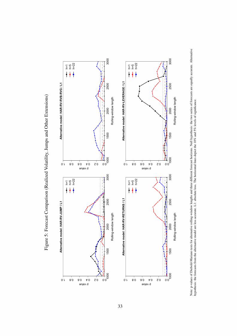
Note: p-values of Diebold-Mariano tests for alternative rolling-window lengths and three different forecast horizons. Null hypothesis: the twoseries of forecasts are equally accurate. Alternative hypothesis: the forecasts from the alternative model are less accurate. The core HAR-RVmodel is the alternative model. L1: absolute loss. L2: quadratic loss. The horizontal lines depict the 10% and 5% levels of significance.

29

Figure 2: Forecast Comparison (Bad and Good Realized Volatility)

1000 1500 2000 2500 3000

0.0

0.2

0.4

0.6

0.8

1.0 Bad RV / Alternative model: HAR-RV / L1

Rolling-window length

p va

lue

h=1h=5h=22

1000 1500 2000 2500 3000

0.0

0.2

0.4

0.6

0.8

1.0 Good RV / Alternative model: HAR-RV / L1

Rolling-window length

p va

lue

h=1h=5h=22

Note: p-values of Diebold-Mariano tests for alternative rolling-window lengths and three different forecast horizons. Null hypothesis: the twoseries of forecasts are equally accurate. Alternative hypothesis: the forecasts from the alternative model are less accurate. The core HAR-RVmodel is the alternative model. Results are based on the L1 loss function (absolute loss). The horizontal lines depict the 10% and 5% levels ofsignificance.

30

Figure 3: Forecast Comparison (Realized Volatility, Extended Models)

1000 1500 2000 2500 3000

0.0

0.2

0.4

0.6

0.8

1.0 Alternative model: HAR-RV-RKU-RSK / L1

Rolling-window length

p va

lue

h=1h=5h=22

1000 1500 2000 2500 3000

0.0

0.2

0.4

0.6

0.8

1.0 Alternative model: HAR-RV-VIX / L1

Rolling-window length

p va

lue

h=1h=5h=22

Note: p-values of Diebold-Mariano tests for alternative rolling-window lengths and three different forecast horizons. Null hypothesis: the twoseries of forecasts are equally accurate. Alternative hypothesis: the forecasts from the alternative model are less accurate. The core HAR-RV-RSK-RKU (upper panel) and the HAR-RV-VIX (lower panel) model are the alternative models. Results aree based on the L1 loss function(absolute loss). The horizontal lines depict the 10% and 5% levels of significance.

31

Figure 4: Out-of-Sample Relative Loss Criterion

Panel A: Lin-lin

0.2 0.4 0.6 0.8

-0.15

-0.10

-0.05

0.00

0.05

0.10 h=1

alpha

Loss

ratio

HAR-RV-RISK vs. HAR-RVHAR-RV-RISK vs. HAR-RV-RKUHAR-RV-RISK vs. HAR-RV-RSKHAR-RV-RISK vs. HAR-RV-RKU-RSKHAR-RV-RISK vs. HAR-RV-VIXHAR-RV-RISK vs. HAR-RV-RKU-RSK-VIX

0.2 0.4 0.6 0.8

-0.15

-0.10

-0.05

0.00

0.05

0.10 h=5

alpha

Loss

ratio

0.2 0.4 0.6 0.8

-0.15

-0.10

-0.05

0.00

0.05

0.10 h=22

alphaLo

ss ra

tio

Panel B: Quad-quad

0.2 0.4 0.6 0.8

-0.15

-0.10

-0.05

0.00

0.05

0.10 h=1

alpha

Loss

ratio

HAR-RV-RISK vs. HAR-RVHAR-RV-RISK vs. HAR-RV-RKUHAR-RV-RISK vs. HAR-RV-RSKHAR-RV-RISK vs. HAR-RV-RKU-RSKHAR-RV-RISK vs. HAR-RV-VIXHAR-RV-RISK vs. HAR-RV-RKU-RSK-VIX

0.2 0.4 0.6 0.8

-0.15

-0.10

-0.05

0.00

0.05

0.10 h=5

alpha

Loss

ratio

0.2 0.4 0.6 0.8

-0.15

-0.10

-0.05

0.00

0.05

0.10 h=22

alpha

Loss

ratio

Note: The horizontal lines depicts the asymmetry parameter, α . The vertical line depicts the out-of-sample relative-loss criterion defined as oneminus the ratio of the loss implied by the parsimonious relative to the loss implied by the extended model.

32

Figu

re5:

Fore

cast

Com

pari

son

(Rea

lized

Vola

tility

,Jum

psan

dO

ther

Ext

ensi

ons)

1000

1500

2000

2500

3000

0.00.20.40.60.81.0

Alte

rnat

ive

mod

el: H

AR

-RV-

JUM

P / L

1

Rol

ling-

win

dow

leng

th

p value

h=1

h=5

h=22

1000

1500

2000

2500

3000

0.00.20.40.60.81.0

Alte

rnat

ive

mod

el: H

AR

-RV-

RVB

-RVG

/ L1

Rol

ling-

win

dow

leng

th

p value

h=1

h=5

h=22

1000

1500

2000

2500

3000

0.00.20.40.60.81.0

Alte

rnat

ive

mod

el: H

AR

-RV-

RET

UR

NS

/ L1

Rol

ling-

win

dow

leng

th

p value

h=1

h=5

h=22

1000

1500

2000

2500

3000

0.00.20.40.60.81.0

Alte

rnat

ive

mod

el: H

AR

-RV-

LEVE

RA

GE

/ L1

Rol

ling-

win

dow

leng

th

p value

h=1

h=5

h=22

Not

e:p-

valu

esof

Die

bold

-Mar

iano

test

sfo

ralte

rnat

ive

rolli

ng-w

indo

wle

ngth

san

dth

ree

diff

eren

tfor

ecas

thor

izon

s.N

ullh

ypot

hesi

s:th

etw

ose

ries

offo

reca

sts

are

equa

llyac

cura

te.A

ltern

ativ

ehy

poth

esis

:the

fore

cast

sfr

omth

eal

tern

ativ

em

odel

are

less

accu

rate

.L1:

abso

lute

loss

.The

hori

zont

allin

esde

pict

the

10%

and

5%le

vels

ofsi

gnifi

canc

e.

33