1 TIMING OR TARGETING: THE ASYMMETRIC MOTIVES OF CAPITAL STRUCTURE DECISIONS Islam Abdeljawad Fauzias Mat Nor Graduate School of Business Universiti Kebangsaan Malaysia Email: [email protected]Abstract This study investigates how the timing behavior and the adjustment towards the target of capital structure interact in the capital structure decisions. Past literature finds that both timing and targeting are significant in determining the leverage ratio which is inconsistent with any standalone framework. This study argues that the coexistence of both timing and targeting is possible. The preference of the firm for timing behavior or targeting behavior depends on the cost of deviation from the target. Since the cost of deviation from the target is likely to be asymmetric between overleveraged and underleveraged firms, the direction of the deviation from the target leverage is expected to alter the preference toward timing or targeting in the capital structure decision. Using GMM-system estimators with the Malaysian data for the period of 1992-2009, this study finds that Malaysian firms, on average, adjust their leverage at a slow speed of 12.7% annually increased to 14.2% when the timing variable is accounted for. Moreover, the speed of adjustment is found to be significantly higher and the timing role is lower for overleveraged firms compared with underleveraged firms. Overleveraged firms seem to find less flexibility to time the market as more pressure is exerted on them to return to the target regardless the timing opportunities because of the higher costs of deviation from the target leverage. Underleveraged firms place lower priority to rebalance toward the target compared with overleveraged firms as the costs of being underleveraged is lower and hence, they have more flexibility to time the market. The findings of this study support that tradeoff theory and timing theory are not mutually exclusive. Firms consider both targeting and timing in their financing decisions but the preference of one motive over the other is conditional on the cost of the deviation from the target. KEYWORDS: Market timing theory, Tradeoff theory, Dynamic capital structure, Speed of adjustment, GMM system 1. INTRODUCTION Equity market timing and tradeoff theories get an increasing interest in the capital structure literature for the entire last decade. Market timing theory (Baker and Wurgler, 2002) suggests that firms can recognize times of mispricing of their own stock and time their issuing (repurchasing) activity accordingly. In this theory, firms are indifferent toward any target leverage and no steady adjustment toward any target should be noticed. Instead, changes in leverage are largely dominated by successive timing activities. On the other hand, the trade-off theory include a family of models, both static and dynamic, in
Transcript
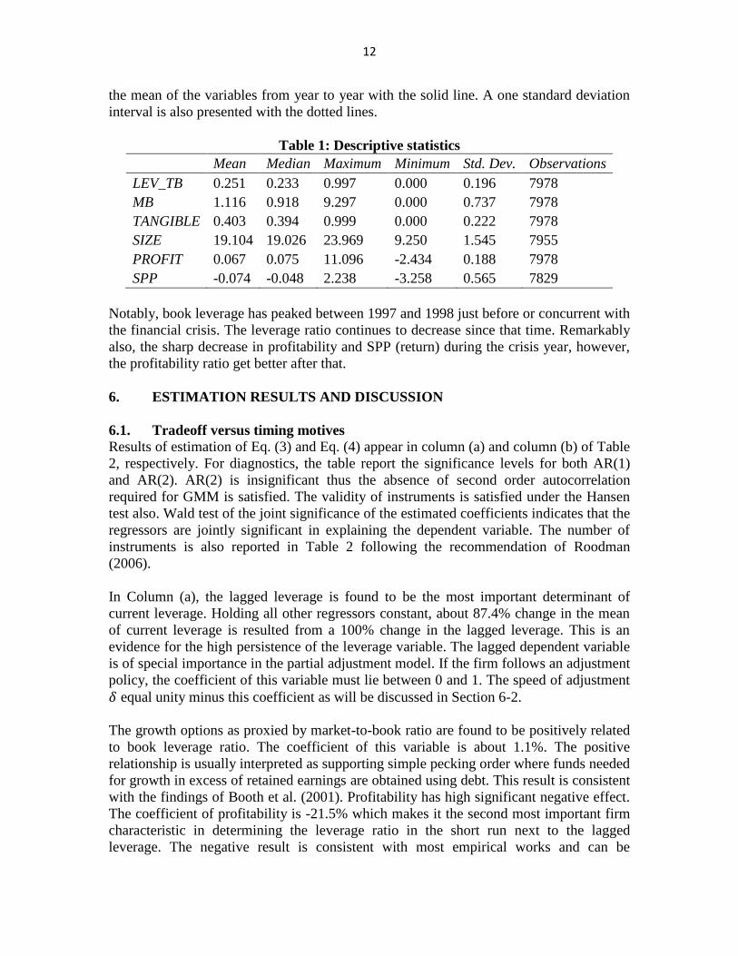
1
TIMING OR TARGETING: THE ASYMMETRIC MOTIVES OF CAPITAL
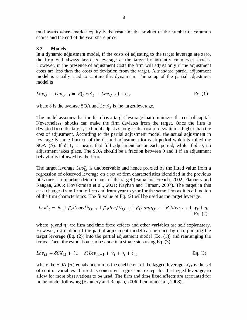
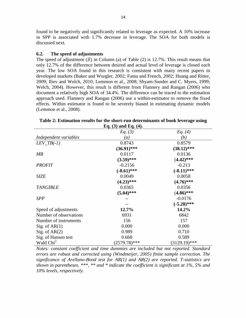
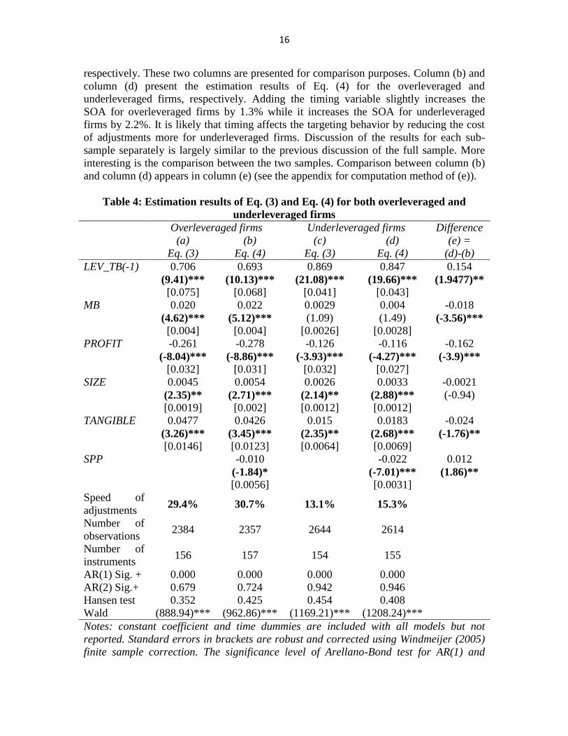
Notes: constant coefficient and time dummies are included with all models but not
reported. Standard errors in brackets are robust and corrected using Windmeijer (2005)
finite sample correction. The significance level of Arellano-Bond test for AR(1) and
17
AR(2) are reported. T-statistics are shown in parentheses. ***, ** and * indicate the
coefficient is significant at 1%, 5% and 10% levels, respectively.
In general, firms are found to be much more sensitive to be overleveraged than to be
underleveraged. The SOA for overleveraged firms is much higher (about 30.7%) than
underleveraged firms (15.3%). The timing coefficient for underleveraged firms is more
than doubled than that of overleveraged firms. For overleveraged firms the coefficient of
timing is 1% and it is significant only at p=10% level while for underleveraged firms the
coefficient is 2.2% and it is significant at p=1% level. It is apparent that underleveraged
firms are more affected by market valuation and less hurry to adjust to the target.
The higher coefficient of SPP for underleveraged firms is not likely to be a result of
growth options. The variable that is supposed to capture growth, market-to-book ratio, is
actually much higher for overleveraged firms than for underleveraged firms in which it is
insignificant. Profitability may signal growth but it is higher for overleveraged firms also.
The tangibility variable is higher for overleveraged firms as it is more important to reduce
the costs of distress for these firms (Harris and Raviv, 1990). All the variables that are
thought to relate with the tradeoff dynamism are higher for the overleveraged firms. SPP
is the only factor that is higher for underleveraged firms.
6.4. New insight to the role of historical timing of Baker and Wurgler (2002) as a
capital structure determinant
In their seminal paper, (Baker and Wurgler, 2002) propose a timing variable that captures
the history of timing activities of the firm and they called it the temporal “external
finance weighted-average market-to-book” ratio (EFWAMB). For a given firm-year, this
variable is defined as
Eq. (5)
where e and d denote net equity and net debt issues, respectively. The sum of e+d is the
external financing raised each year.
is market-to-book ratio. The weight for
each year is the ratio of external financing raised by the firm in that year to the total
external financing raised by the firm in years (0) through (t-1). Negative weights are reset
to zero. This variable takes high values for firms that raise external finance when the MB
ratio is high and low values for firms that raise external finance while the MB ratio is
low. This paper defines (e) as while (d) is
defined as .
Abdeljawad and Mat Nor (2011) find that this variable is significant in determining the
capital structure for Malaysian firms. If firms time the mispricing periods and they do not
rebalance the effect of this timing, timing effect may accumulate over time and hence the
history of timing will continue affecting the current leverage. If the hypothesis about the
asymmetric effect of timing is valid in the short run, it should continue to hold in the long
run. To investigate this possibility, this research will re-run a model similar to that used
by (Abdeljawad and Mat Nor, 2011; Baker and Wurgler, 2002) but with a dummy
variable that captures whether the firm is overleveraged or underleveraged and an
18
interaction term between the EFWAMB and the dummy variable. Using the dummy
variable to differentiate the two possibly different behaviors is more reliable here to
capture the moderating effect (Whisman and McClelland, 2005) since no concern about
the instruments. The model includes the same control variables used previously in this
research but in a static framework. OLS with both firm and year fixed effects are used.
Standards errors are corrected using “panel corrected standard errors”. The setup of the
equation to be estimated is
Eq.(6)
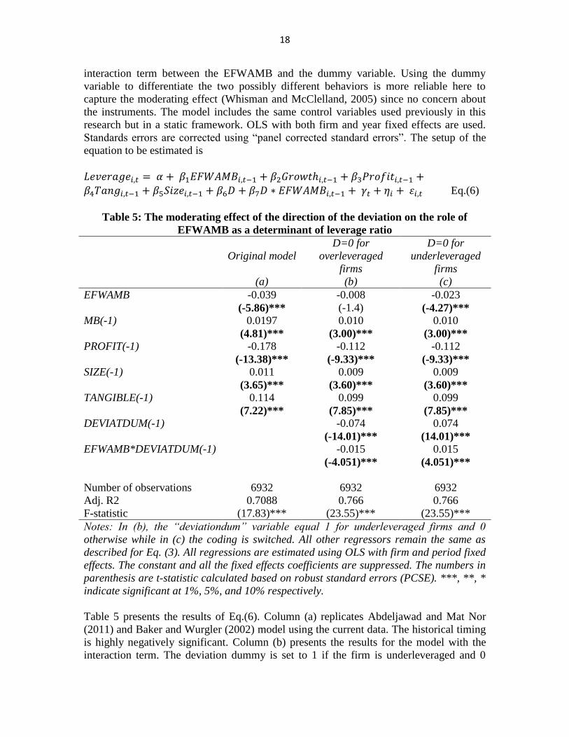
Table 5: The moderating effect of the direction of the deviation on the role of
EFWAMB as a determinant of leverage ratio
Original model
D=0 for
overleveraged
firms
D=0 for
underleveraged
firms
(a) (b) (c)
EFWAMB -0.039 -0.008 -0.023
(-5.86)*** (-1.4) (-4.27)***
MB(-1) 0.0197 0.010 0.010
(4.81)*** (3.00)*** (3.00)***
PROFIT(-1) -0.178 -0.112 -0.112
(-13.38)*** (-9.33)*** (-9.33)***
SIZE(-1) 0.011 0.009 0.009
(3.65)*** (3.60)*** (3.60)***
TANGIBLE(-1) 0.114 0.099 0.099
(7.22)*** (7.85)*** (7.85)***
DEVIATDUM(-1) -0.074 0.074
(-14.01)*** (14.01)***
EFWAMB*DEVIATDUM(-1) -0.015 0.015
(-4.051)*** (4.051)***
Number of observations 6932 6932 6932
Adj. R2 0.7088 0.766 0.766
F-statistic (17.83)*** (23.55)*** (23.55)***
Notes: In (b), the “deviationdum” variable equal 1 for underleveraged firms and 0
otherwise while in (c) the coding is switched. All other regressors remain the same as
described for Eq. (3). All regressions are estimated using OLS with firm and period fixed
effects. The constant and all the fixed effects coefficients are suppressed. The numbers in
parenthesis are t-statistic calculated based on robust standard errors (PCSE). ***, **, *
indicate significant at 1%, 5%, and 10% respectively.
Table 5 presents the results of Eq.(6). Column (a) replicates Abdeljawad and Mat Nor
(2011) and Baker and Wurgler (2002) model using the current data. The historical timing
is highly negatively significant. Column (b) presents the results for the model with the
interaction term. The deviation dummy is set to 1 if the firm is underleveraged and 0
19
otherwise. The interaction term is significant indicating that the direction of the deviation
from the target is able to moderate the relationship between EFWAMB and leverage. A
simple way to find the direct effect of EFWAMB in each subsample is to switch the
coding of the dummy variable and noting the coefficient of EFWAMB (Whisman and
McClelland, 2005). The direct effect of EFWAMB when firms are overleveraged is not
significant in column (b) while it is highly significant for the underleveraged firms as
appear in column (c). It can be concluded that underleveraged firms are more inclined to
exploit mispricing opportunities and the effect of this timing behavior takes longer time
to be rebalanced. This result may add doubt to the generalizability of the timing theory
since the results of Baker and Wurgler (2002) may be driven by underleveraged firms as
the period of their study, the late 1980’s and the 1990’s, are characterized by the low
leverage used by firms (Huang and Ritter, 2009).
7. CONCLUSIONS
Using an estimator that is found to be more efficient for estimating dynamic panel data
with short time dimension, that is system GMM; this study reveals that Malaysian firms
are adjusting their capital structure to the target but at a slow rate. At the same time, firms
consider timing of the market conditions as an important factor when making financial
decisions. This study finds evidence for asymmetric timing behavior as well as targeting
behavior between firms over- and underleveraged. Specifically, overleveraged firms
adjust to the target faster and they are less concern with timing. On the other side,
underleveraged firms adjust slower but they consider timing more seriously. This
behavior is likely to result from taking into account all the costs and benefits of being at
the target, adjustment toward the target and timing opportunities. Deviating from the
target to the upper side is likely to be more costly than deviating below the target because
bankruptcy costs and agency costs of debt will intensify quickly as the firm deviates more
above the target. Hence, overleveraged firms need to adjust faster to reduce these costs
despite the market conditions. Underleveraged firms are less urged to adjust and hence it
is feasible for them to consider market conditions more in their financing decisions.
These results are confirmed in the short run as well as long run modeling.
The finding of this study supports that firms consider both targeting and timing in their
financing decisions. No standalone theory can interpret the full spectrum of empirical
results. This result is consistent with the view of Myers (2003) that capital structure
“theories are conditional not general”.
REFERENCES Abdeljawad, I., Mat Nor, F., 2011. Equity Market Timing and Capital Structure: Evidence from
Malaysia., 13th Malaysian Finance Association, Langkawi, Malaysia. Alti, A., 2006. How Persistent Is the Impact of Market Timing on Capital Structure? The Journal
of Finance 61, 1681-1710. Antoniou, A., Guney, Y., Paudyal, K., 2008. The determinants of capital structure: capital market-
oriented versus bank-oriented institutions. Journal of Financial and Quantitative analysis 43, 59-92.
20
Arellano, M., Bond, S., 1991. Some tests of specification for panel data: Monte Carlo evidence and an application to employment equations. The Review of Economic Studies 58, 277.
Arellano, M., Bover, O., 1995. Another look at the instrumental variable estimation of error-components models* 1. Journal of econometrics 68, 29-51.
Baker, M., Wurgler, J., 2002. Market Timing and Capital Structure. The Journal of Finance 57, 1-32.
Baxter, N.D., 1967. Leverage, risk of ruin and the cost of capital. Journal of Finance 22, 395-403. Blundell, R., Bond, S., 1998. Initial conditions and moment restrictions in dynamic panel data
models. Journal of econometrics 87, 115-143. Bolger, F. & Harvey, N. 1993. Context-Sensitive Heuristics in Statistical Reasoning. The
Quarterly Journal of Experimental Psychology Section A 46(4): 779-811. Booth, L., Aivazian, V., Demirguc-Kunt, A., Maksimovic, V., 2001. Capital structures in developing
countries. Journal of Finance 56, 87-130. Bradley, M., Jarrell, G.A., Kim, E.H., 1984. On the Existence of an Optimal Capital Structure:
Theory and Evidence. The Journal of Finance 39, 857-878. Byoun, S., 2008. How and When Do Firms Adjust Their Capital Structures toward Targets? The
Journal of Finance 63, 3069-3096. Clark, B.J., Francis, B.B., Hasan, I., 2009. Do Firms Adjust Toward Target Capital Structures? Some
International Evidence. SSRN eLibrary. Clogg, C.C., Petkova, E., Haritou, A., 1995. Statistical Methods for Comparing Regression
Coefficients Between Models. American Journal of Sociology 100, 1261-1293. Cohen, A., 1983. Comparing Regression Coefficients Across Subsamples. Sociological Methods &
Research 12, 77-94. Cook, D.O., Tang, T., 2010. Macroeconomic conditions and capital structure adjustment speed.
Journal of Corporate Finance 16, 73-87. De Bie, T., De Haan, L., 2007. Market timing and capital structure: Evidence for Dutch firms.
Economist 155, 183-206. Deangelo, H. & Masulis, R. W. 1980. Optimal Capital Structure under Corporate and Personal
Taxation. Journal of Financial Economics 8(1): 3-29.
de Miguel, A., Pindado, J., 2001. Determinants of capital structure: new evidence from Spanish panel data. Journal of Corporate Finance 7, 77-99.
Deesomsak, R., Paudyal, K., Pescetto, G., 2004. The determinants of capital structure: evidence from the Asia Pacific region. Journal of Multinational Financial Management 14, 387-405.
Drobetz, W., Wanzenried, G., 2006. What determines the speed of adjustment to the target capital structure? Applied Financial Economics 16, 941-958.
Fama, E.F., French, K.R., 2002. Testing Trade-Off and Pecking Order Predictions about Dividends and Debt. The Review of Financial Studies 15, 1-33.
Flannery, M.J., Hankins, K.W., 2007. A theory of capital structure adjustment speed. Unpublished Manuscript, University of Florida.
Flannery, M.J., Rangan, K.P., 2006. Partial adjustment toward target capital structures. Journal of Financial Economics 79, 469-506.
Frank, M.Z., Goyal, V.K., 2007. Trade-Off and Pecking Order Theories of Debt. SSRN eLibrary. Graham, J.R., Harvey, C.R., 2001. The theory and practice of corporate finance: evidence from
the field. Journal of Financial Economics 60, 187-243. Harris, M., Raviv, A., 1990. Capital structure and the informational role of debt. Journal of
Finance 45, 321-349.
21
Homaifar, G., Zietz, J., Benkato, O., 1994. An empirical model of capital structure: some new evidence. Journal of Business Finance & Accounting 21, 1-14.
Hovakimian, A., 2006. Are observed capital structures determined by equity market timing? Journal of Financial and Quantitative analysis 41, 221-243.
Hovakimian, A., Li, G., 2011. In search of conclusive evidence: How to test for adjustment to target capital structure. Journal of Corporate Finance 17, 33-44.
Hovakimian, A., Opler, T., Titman, S., 2001. The Debt-Equity Choice. The Journal of Financial and Quantitative Analysis 36, 1-24.
Huang, R., Ritter, J., 2009. Testing theories of capital structure and estimating the speed of adjustment. Journal of Financial and Quantitative analysis 44, 237-271.
Hussain, M.I., 2005. Determenation of capital structure and prediction of corporate financial distress. Univirsity Putra Malaysia.
Iliev, P., Welch, I., 2010. Reconciling estimates of the speed of adjustment of leverage ratios. SSRN eLibrary.
Jensen, M., 1986. Agency costs of free cash flow, corporate finance, and takeovers. The American Economic Review 76, 323-329.
Jensen, M., Meckling, W., 1976. Theory of the firm: Managerial behavior, agency costs and ownership structure. Journal of Financial Economics 3, 305-360.
Kayhan, A., Titman, S., 2007. Firms' histories and their capital structures. Journal of Financial Economics 83, 1-32.
Kraus, A. & Litzenberger, R. 1973. A State-Preference Model of Optimal Financial Leverage.
Journal of Finance 28(4): 911-922.
Leary, M.T., Roberts, M.R., 2005. Do Firms Rebalance Their Capital Structures? The Journal of Finance 60, 2575-2619.
Lemmon, M.L., Roberts, M.R., Zender, J.F., 2008. Back to the Beginning: Persistence and the Cross Section of Corporate Capital Structure. The Journal of Finance 63, 1575-1608.
Mahajan, A., Tartaroglu, S., 2008. Equity market timing and capital structure: International evidence. Journal of Banking & Finance 32, 754-766.
Myers, S., 1977. Determinants of corporate borrowing. Journal of Financial Economics 5, 147-175.
Myers, S., Majluf, N., 1984. Corporate financing and investment decisions when firms have informationthat investors do not have. Journal of Financial Economics 13, 187-221.
Myers, S.C., 1984. The Capital Structure Puzzle. The Journal of Finance 39, 575-592. Myers, S.C., 2003. Chapter 4 Financing of corporations, in: G.M. Constantinides, M.H., Stulz,
R.M. (Eds.), Handbook of the Economics of Finance. Elsevier, pp. 215-253. Ozkan, A., 2001. Determinants of Capital Structure and Adjustment to Long Run Target:
Evidence From UK Company Panel Data. Journal of Business Finance & Accounting 28, 175-198.
Paternoster, R., Brame, R., Mazerolle, P., Piquero, A., 1998. Using the correct statistical test for the equality of regression coefficients. Criminology 36, 859-866.
Rajan, R., Zingales, L., 1995. What do we know about capital structure? Some evidence from international data. Journal of Finance 50, 1421-1460.
Roodman, D., 2006. How to do xtabond2: An Introduction to" Difference" and" System" GMM in Stata. Center for global development.
Shyam-Sunder, L., C. Myers, S., 1999. Testing static tradeoff against pecking order models of capital structure. Journal of Financial Economics 51, 219-244.
Smith, D.J., Chen, J., Anderson, H.D., 2010. Partial Adjustment Towards Target Capital Structure: Evidence from New Zealand. SSRN eLibrary.
22
Strebulaev, I. & Yang, B. 2007. The Mystery of Zero-Leverage Firms. working paper,
Stanford University.
Titman, S., Wessels, R., 1988. The Determinants of Capital Structure Choice. The Journal of Finance 43, 1-19.
Tversky, A. & Kahneman, D. 1974. Judgment under Uncertainty: Heuristics and Biases. science 185(4157): 1124-1131.
Welch, I., 2004. Capital Structure and Stock Returns. The Journal of Political Economy 112, 106-131.
Whisman, M.A., McClelland, G.H., 2005. Designing, testing, and interpreting interactions and moderator effects in family research. Journal of Family Psychology 19, 111.
Windmeijer, F., 2005. A finite sample correction for the variance of linear efficient two-step GMM estimators. Journal of econometrics 126, 25-51.
APPENDICES
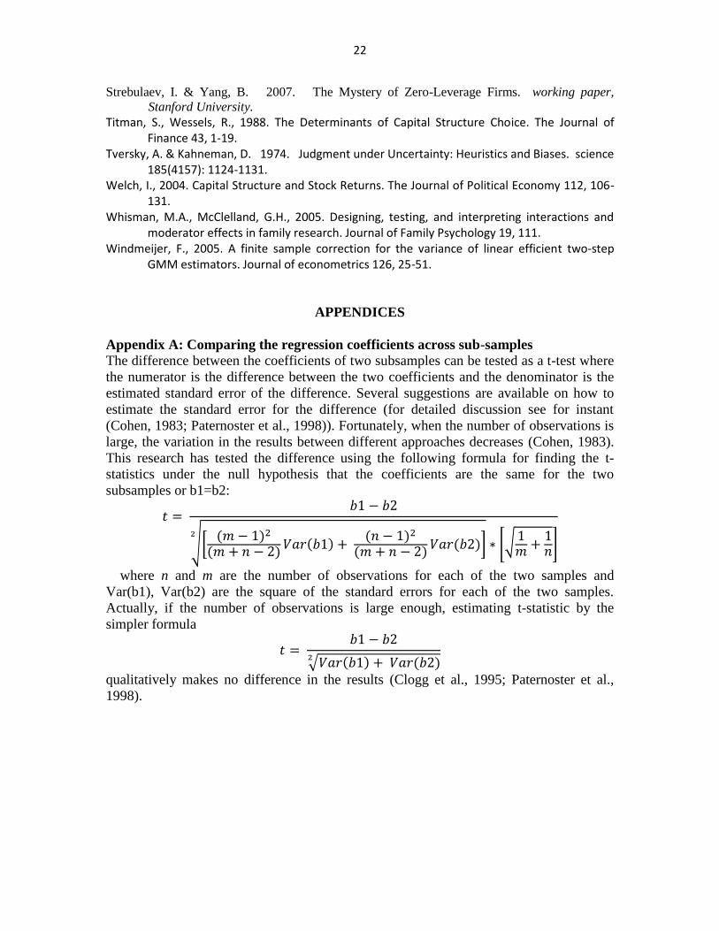
Appendix A: Comparing the regression coefficients across sub-samples
The difference between the coefficients of two subsamples can be tested as a t-test where
the numerator is the difference between the two coefficients and the denominator is the
estimated standard error of the difference. Several suggestions are available on how to
estimate the standard error for the difference (for detailed discussion see for instant
(Cohen, 1983; Paternoster et al., 1998)). Fortunately, when the number of observations is
large, the variation in the results between different approaches decreases (Cohen, 1983).
This research has tested the difference using the following formula for finding the t-
statistics under the null hypothesis that the coefficients are the same for the two
subsamples or b1=b2:
where n and m are the number of observations for each of the two samples and
Var(b1), Var(b2) are the square of the standard errors for each of the two samples.
Actually, if the number of observations is large enough, estimating t-statistic by the
simpler formula
qualitatively makes no difference in the results (Clogg et al., 1995; Paternoster et al.,