Timothy Taylor’s Principles of Economics 3e...ic and they can get a strong foundation from Tim...

Timothy Taylor’s

Principles of Economics 3e Economics and the Economy

Timothy Taylor Managing Editor:

The Journal of Economic Perspectives Macalester College

+ Arguably the most clearly written book on the market + Used by over 200 instructors + 3e: all new design with high resolution graphs + 3e: thorough update of data, discussions, references, and examples + 3e: more attention to:

New tools of monetary policy in the US & the European Union Quantitative easing and "forward guidance," where monetary policy will be

roughly the same for the next few years

And the European Central Bank's role a lender of last resort

More on anti-trust legislation

Differentiators:

Taylor 3e is a mainstream book; it covers all the main topics in a balanced way

Taylor writes about the subject with no ideological axe to grind.

Book is remarkably well written with clear examples; comprehensive, but no fluff.

Focus on helping students solve problems – Taylor walks students through the problem-solving process.

Affordable Student Prices and Options!

For Instructors What's Changed For Students What's Changed

Instructor Manual New to 3e Loose-leaf Option New to 3e

Lecture Slides Overhauled for 3e Color Paperback Option New to 3e

Test Item File Expanded and Updated for 3e Lecture Guide New to 3e

Computerized Test Bank Expanded and Updated for 3e Sapling Web Assignments Updated for 3e

Sapling Web Assignments Updated for 3e Online Quizzes and eFlash Cards Will be updated in 2015

Instructor Resource Folder New to 3e Annual Reader from Tim's Blog Available for Spring Term 2015

Free use of Content/Graphs from Tim’s Blog New to 3e

To Review Online Textbook:

www.textbookmedia.com

To Request Paperback: [email protected]

Chapter 1: The Interconnected Economy Chapter 2: Choice in a World of Scarcity Chapter 3: International Trade Chapter 4: Demand and Supply Chapter 5: Labor and Financial Capital Markets Chapter 6: Globalization and Protectionism Chapter 7: Elasticity Chapter 8: Household Decision Making Chapter 9: Cost and Industry Structure Chapter 10: Perfect Competition Chapter 11: Monopoly Chapter 12: Monopolistic Competition and Oligopoly Chapter 13: Competition and Public Policy Chapter 14: Environmental Protection and Negative Externalities Chapter 15: Technology, Positive Externalities, and Public Goods Chapter 16: Poverty and Economic Inequality Chapter 17: Issues in Labor Markets: Unions, Discrimination, Immigration Chapter 18: Information, Risk and Insurance Chapter 19: Financial Markets Chapter 20: Public Choice Chapter 21: The Macroeconomic Perspective Chapter 22: Economic Growth Chapter 23: Unemployment

Chapter 24: Inflation Chapter 25: The Balance of Trade Chapter 26: The Aggregate Supply-Aggregate Demand Chapter 27: The Keynesian Perspective Chapter 28: The Neoclassical Perspective Chapter 29: Money and Banks Chapter 30: Monetary Policy and Bank Regulation Chapter 31: Exchange Rates and International Capital Flows Chapter 32: Government Budgets and Fiscal Policy Chapter 33: Government Borrowing and National Chapter 34: Macroeconomic Policy around the World Appendix to Chapter 1: Interpreting Graphics Appendix to Chapter 8: Indifference Curves Appendix to Chapter 19: Present Discounted Value Appendix to Chapter 27: An Algebraic Approach to the Expenditure-Output Model

About the author: Tim Taylor’s career has been devoted to making complex economic ideas clear to students, policy makers and other professional econo-mists. Taylor is the founding and only managing editor of the Ameri-can Economic Association’s Journal of Economic Perspectives, which for more than 20 years has been an accessible source for state-of-the art economic thinking. Tim has won numerous teaching awards from his teaching stints at institutions like Stanford, the University of Min-nesota and Macalester College.

“Thank you very much for the opportunity to speak of why I am using the Taylor ‘s Textbooks, supported by Sapling's Home Work service. In a word, VALUE! Spoken three times...Value, Value, Value! Examples to illustrate definitions and concepts are representative of life experienced by limited resource students. They "get" the concepts in a context easily applied to their lives, without having to spend a for-tune! -- Harry Anderson, Luna College “I truly appreciate that the book is cost effective and comprehensive for my students. I can present a top-ic and they can get a strong foundation from Tim Taylor's text, then we can go into in-depth discussions as we relate the text material to the real world and other sources.” --- Shari Lyman, Community College of Southern Nevada

“Tim Taylor’s Principles is an excellent introductory text, with solid content comparable to that of far more expensive texts. Our students find it a most helpful learning aid and also deeply appreciate its rela-tively low cost.” -- William J. Murphy, New England Institute of Technology

“I got the book and, frankly, couldn't put it down. I have listened to all of Tim's' programs for The Teach-ing Company and find him to be an extremely knowledgeable economist, who has the ability to take com-plex issues and make them come alive. His book is really an extension of his rather amazing style.” - Bill Sciacca, Penn State-Scranton

“I'm a huge fan of Prof. Taylor and have listened to all of his recorded courses for The Teaching Company. Thanks for making me aware of Tim’s Blog. This is a great resource!” -- Peter Canellis, Vaughn College

“I found the Macro split to be clearly written, logically organized, and quite a good introduction to the basic macroeconomic canon. Frankly, for the price it can’t be beaten.” -- Michael Kuehlwein, Pomona College

“When I first came across Timothy Taylor's textbook I could hardly believe it - a nice text for a great price. I'm happy I switched. It is a godsend for students on a budget.” --Lester Hadsell, SUNY Oneonta

“Tim is also an award-winning teacher and a highly sought-after editor. The characteristics that have made him successful in these capacities are those I look for in an economic principles textbook — clear organization and sensible, engaging writing, with the content needed to challenge young, smart students. Because of TM’s quality-value package, I am extremely excited about assigning Tim’s textbook this fall.” --John Karl Scholz, UW-Madison “Taylor’s book has a unique approach that builds intuition in a rigorous way, with clear discussion and relevant examples. Other books promise that, but Taylor’s actually achieves it.” --Jeffrey Sundberg, Lake Forest College

Timothy Taylor’s Principles of Economics Economics and the Economy

Timothy Taylor Journal of Economic Perspectives

Macalester College

Third Edition

For instructors: • Instructor’s manual • PowerPoint® slides • Computerized test disk

Free to students: • e-Textbook available as Micro and Macro splits • e-Study Guide • e-Lecture Guide • e-Pamphlet (with video): Using Adobe® Reader for the Maximum e-Book Experience • e-Pamphlet (with audio): Study Tips for the College Student

When ordering this title, use ISBN 1-930789-26-2To order the Micro version, use ISBN 1-930789-42-4To order the Macro version, use ISBN 1-930789-88-2

Timothy Taylor’s Principles of Economics: Economics and the Economy, Edition 3Copyright © 2014, 2011, 2008 Timothy Taylor. Published by Textbook Media.

ISBN 1-930789-26-2

All rights reserved. No part of this publication may be reproduced or transmitted in any form or by any means, electronic or mechanical, including photocopying and recording, or by any information storage or retrieval system without the prior written permission of the author and the publisher.

Printed in the United States of America by Textbook Media

iii

Preface xxvAbout the Author xxvii

PART I THE INTERCONNECTED ECONOMY

1 The Interconnected Economy 1 2 Choice in a World of Scarcity 12 3 International Trade 33

PART II SUPPLY AND DEMAND

4 Demand and Supply 52 5 Labor and Financial Capital Markets 77 6 Globalization and Protectionism 91

PART III THE FUNDAMENTALS OF MICROECONOMIC THEORY

7 Elasticity 112 8 Household Decision Making 131 9 Cost and Industry Structure 150 10 Perfect Competition 166 11 Monopoly 186 12 Monopolistic Competition and Oligopoly 201

PART IV MICROECONOMIC POLICY ISSUES APPLICATIONS

13 Competition and Public Policy 216 14 Environmental Protection and Negative Externalities 231 15 Technology, Positive Externalities, and Public Goods 246 16 Poverty and Economic Inequality 260 17 Issues in Labor Markets: Unions, Discrimination, Immigration 279

Brief Contents

iv Brief Contents

18 Information, Risk, and Insurance 297 19 Financial Markets 311 20 Public Choice 331

PART V THE MACROECONOMIC PERSPECTIVE AND GOALS

21 The Macroeconomic Perspective 340 22 Economic Growth 356 23 Unemployment 371 24 Inflation 388 25 The Balance of Trade 409

PART VI A FRAMEWORK FOR MACROECONOMIC ANALYSIS

26 The Aggregate Supply–Aggregate Demand Model 424 27 The Keynesian Perspective 444 28 The Neoclassical Perspective 472

PART VII MONETARY AND FISCAL POLICY

29 Money and Banks 485 30 Monetary Policy and Bank Regulation 500 31 Exchange Rates and International Capital Flows 523 32 Government Budgets and Fiscal Policy 549 33 Government Borrowing and National Savings 570 34 Macroeconomic Policy around the World 585

APPENDIX CHAPTERS

1 Interpreting Graphs 600 8 Indifference Curves 612 19 Present Discounted Value 626 27 An Algebraic Approach to the Expenditure-Output Model 629

Glossary G-1Index I-1

v

Preface xxvAbout the Author xxvii

PART I THE INTERCONNECTED ECONOMY

1 The Interconnected Economy 1

What Is an Economy? 2Market-Oriented vs. Command Economies 2The Interconnectedness of an Economy 2

The Division of Labor 3Why the Division of Labor Increases Production 4Trade and Markets 4The Rise of Globalization 5

Microeconomics and Macroeconomics 6Microeconomics: The Circular Flow Diagram 7Macroeconomics: Goals, Frameworks, and Tools 9

Studying Economics Doesn’t Mean Worshiping the Economy 9Key Concepts and Summary 10Review Questions 11

2 Choice in a World of Scarcity 12

Choosing What to Consume 13A Consumption Choice Budget Constraint 13How Changes in Income and Prices Affect the Budget Constraint 13Personal Preferences Determine Specific Choices 15From a Model with Two Goods to the Real World of Many Goods 16

Choosing Between Labor and Leisure 16An Example of a Labor-Leisure Budget Constraint 16How a Change in Wages Affects the Labor-Leisure Budget Constraint 17Making a Choice Along the Labor-Leisure Budget Constraint 17

Choosing Between Present and Future Consumption 18Interest Rates: The Price of Intertemporal Choice 19The Power of Compound Interest 20An Example of Intertemporal Choice 21

Contents

vi Contents

Three Implications of Budget Constraints: Opportunity Cost, Marginal Decision-Making, and Sunk Costs 22

Opportunity Cost 22Marginal Decision-Making and Diminishing Marginal Utility 23Sunk Costs 24

The Production Possibilities Frontier and Social Choices 24The Shape of the Production Possibilities Frontier and Diminishing Marginal Returns 25Productive Efficiency and Allocative Efficiency 27Why Society Must Choose 28

Confronting Objections to the Economic Approach 28A First Objection: People, Firms, and Society Don’t Act Like This 29A Second Objection: People, Firms, and Society Shouldn’t Do This 29

Facing Scarcity and Making Trade-offs 31Key Concepts and Summary 31Review Questions 32

3 International Trade 33

Absolute Advantage 35A Numerical Example of Absolute Advantage and Trade 35Trade and Opportunity Cost 38Limitations of the Numerical Example 39

Comparative Advantage 39Identifying Comparative Advantage 40Mutually Beneficial Trade with Comparative Advantage 42How Opportunity Cost Sets the Boundaries of Trade 44Comparative Advantage Goes Camping 45The Power of the Comparative Advantage Example 45

Intra-industry Trade between Similar Economies 45The Prevalence of Intra-industry Trade between Similar Economies 45Gains from Specialization and Learning 46Economies of Scale, Competition, Variety 47Dynamic Comparative Advantage 48

The Size of Benefits from International Trade 49From Interpersonal to International Trade 50Key Concepts and Summary 51Review Questions 51

PART II SUPPLY AND DEMAND

4 Demand and Supply 52

Demand, Supply, and Equilibrium in Markets for Goods and Services 53Demand for Goods and Services 53

Contents vii

Supply of Goods and Services 53Equilibrium—Where Demand and Supply Cross 55

Shifts in Demand and Supply for Goods and Services 57The Ceteris Paribus Assumption 57An Example of a Shifting Demand Curve 57Factors That Shift Demand Curves 58Summing Up Factors That Change Demand 59An Example of a Shift in a Supply Curve 60Factors That Shift Supply Curves 61Summing Up Factors That Change Supply 62

Shifts in Equilibrium Price and Quantity: The Four-Step Process 62Good Weather for Salmon Fishing 63Seal Hunting and New Drugs 64The Interconnections and Speed of Adjustment in Real Markets 65

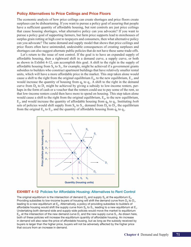
Price Ceilings and Price Floors in Markets for Goods and Services 65Price Ceilings 65Price Floors 68Responses to Price Controls: Many Margins for Action 69Policy Alternatives to Price Ceilings and Price Floors 71

Supply, Demand, and Efficiency 72Consumer Surplus, Producer Surplus, Social Surplus 72Inefficiency of Price Floors and Price Ceilings 73

Demand and Supply as a Social Adjustment Mechanism 75Key Concepts and Summary 75Review Questions 76

5 Labor and Financial Capital Markets 77

Demand and Supply at Work in Labor Markets 77Equilibrium in the Labor Market 78Shifts in Labor Demand 79Shifts in Labor Supply 80Technology and Wage Inequality: The Four-Step Process 80Price Floors in the Labor Market: Living Wages and Minimum Wages 81The Minimum Wage as an Example of a Price Floor 82

Demand and Supply in Financial Capital Markets 83Who Demands and Who Supplies in Financial Capital Markets 84Equilibrium in Financial Capital Markets 85Shifts in Demand and Supply in Financial Capital Markets 85The United States as a Global Borrower: The Four-Step Process 86Price Ceilings in Financial Capital Markets: Usury Laws 87

Don’t Kill the Price Messengers 88Key Concepts and Summary 90Review Questions 90

viii Contents

6 Globalization and Protectionism 91

Protectionism: An Indirect Subsidy from Consumers to Producers 92Demand and Supply Analysis of Protectionism 92Who Benefits and Who Pays? 94

International Trade and Its Effects on Jobs, Wages, and Working Conditions 95

Fewer Jobs? 95Trade and Wages 97Labor Standards 98

The Infant Industry Argument 99The Dumping Argument 100

The Growth of Anti-Dumping Cases 100Why Might Dumping Occur? 101Should Anti-Dumping Cases Be Limited? 101

The Environmental Protection Argument 101The Race to the Bottom Scenario 102Pressuring Low-Income Countries for Higher Environmental Standards 103

The Unsafe Consumer Products Argument 103The National Interest Argument 104How Trade Policy Is Enacted: Global, Regional, and National 106

The World Trade Organization 106Regional Trading Agreements 107Trade Policy at the National Level 108Long-Term Trends in Barriers to Trade 108

The Trade-offs of Trade Policy 109Key Concepts and Summary 110Review Questions 111

PART III THE FUNDAMENTALS OF MICROECONOMIC THEORY

7 Elasticity 112

Price Elasticity of Demand 113Calculating the Elasticity of Demand 114A Possible Confusion, a Clarification, and a Warning 115

Price Elasticity of Supply 116Calculating the Elasticity of Supply 117

Elastic, Inelastic, and Unitary Elasticity 118Applications of Elasticity 120

Does Raising Price Bring in More Revenue? 120Passing on Costs to Consumers? 122Long-Run vs. Short-Run Impact 125

Contents ix

Elasticity as a General Concept 126Income Elasticity of Demand 127Cross-Price Elasticity of Demand 127Elasticity in Labor and Financial Capital Markets 127Stretching the Concept of Elasticity 128

Conclusion 129Key Concepts and Summary 129Review Questions 130

8 Household Decision Making 131

Consumption Choices 131Total Utility and Diminishing Marginal Utility 132Choosing with Marginal Utility 134A Rule for Maximizing Utility 135Measuring Utility with Numbers 135

How Changes in Income and Prices Affect Consumption Choices 135How Changes in Income Affect Consumer Choices 136How Price Changes Affect Consumer Choices 137The Logical Foundations of Demand Curves 138Applications in Business and Government 139

Labor-Leisure Choices 141The Labor-Leisure Budget Constraint 142Applications of Utility Maximizing with the Labor-Leisure Budget Constraint 143

Intertemporal Choices in Financial Capital Markets 144Using Marginal Utility to Make Intertemporal Choices 145Applications of the Model of Intertemporal Choice 147

The Unifying Power of the Utility-Maximizing Budget Set Framework 148Key Concepts and Summary 148Review Questions 149

9 Cost and Industry Structure 150

The Structure of Costs in the Short Run 152Fixed and Variable Costs 152Average Costs, Average Variable Costs, Marginal Costs 153Lessons Taught by Alternative Measures of Costs 155A Variety of Cost Patterns 156

The Structure of Costs in the Long Run 156Choice of Production Technology 157Economies of Scale 158Shapes of Long-Run Average Cost Curves 159The Size and Number of Firms in an Industry 161Shifting Patterns of Long-Run Average Cost 163

x Contents


10 Perfect Competition 166

Quantity Produced by a Perfectly Competitive Firm 167Comparing Total Revenue and Total Cost 167Comparing Marginal Revenue and Marginal Costs 169Marginal Cost and the Supply Curve 170Profits and Losses with the Average Cost Curve 170The Shutdown Point 172Short-Run Outcomes for Perfectly Competitive Firms 174

Entry and Exit in the Long-Run Output 175How Entry and Exit Lead to Zero Profits 175Economic Profit vs. Accounting Profit 176The Economic Function of Profits 177

Factors of Production in Perfectly Competitive Markets 177The Derived Demand for Labor 177The Marginal Revenue Product of Labor 178Are Workers Paid as Much as They Deserve? 180Physical Capital Investment and the Hurdle Rate 180Physical Capital Investment and Long-Run Average Cost 182

Efficiency in Perfectly Competitive Markets 182Conclusion 183Key Concepts and Summary 183Review Questions 184

11 Monopoly 186

Barriers to Entry 187Legal Restrictions 187Control of a Physical Resource 187Technological Superiority 188Natural Monopoly 188Intimidating Potential Competition 190Summing Up Barriers to Entry 190

How a Profit-Maximizing Monopoly Chooses Output and Price 191Demand Curves Perceived by a Perfectly Competitive Firm and by a Monopoly 191Total and Marginal Revenue for a Monopolist 191Marginal Revenue and Marginal Cost for a Monopolist 194Illustrating Monopoly Profits 195The Inefficiency of Monopoly 197

Contents xi


12 Monopolistic Competition and Oligopoly 201

Monopolistic Competition 202Differentiated Products 202Perceived Demand for a Monopolistic Competitor 202How a Monopolistic Competitor Chooses Price and Quantity 203Monopolistic Competitors and Entry 205Monopolistic Competition and Efficiency 207The Benefits of Variety and Product Differentiation 208

Oligopoly 208Why Do Oligopolies Exist? 209Collusion or Competition? 209The Prisoner’s Dilemma 209The Oligopoly Version of the Prisoner’s Dilemma 210How to Enforce Cooperation 212


PART IV MICROECONOMIC POLICY ISSUES APPLICATIONS

13 Competition and Public Policy 216

Corporate Mergers 217Regulations for Approving Mergers 217The Four-Firm Concentration Ratio 218The Herfindahl-Hirschman Index 219New Directions for Antitrust 220

Regulating Anticompetitive Behavior 221When Breaking Up Is Hard to Do: Regulating Natural Monopolies 223

The Choices in Regulating a Natural Monopoly 223Cost-Plus versus Price Cap Regulation 225

The Great Deregulation Experiment 225Doubts about Regulation of Prices and Quantities 225The Effects of Deregulation 226Frontiers of Deregulation 227

Around the World: From Nationalization to Privatization 228Key Concepts and Summary 229Review Questions 229

xii Contents

14 Environmental Protection and Negative Externalities 231

Externalities 233Pollution as a Negative Externality 233Command-and-Control Regulation 234Market-Oriented Environmental Tools 235

Market-Friendly Environmental Tool #1: Pollution Charges 235Market-Friendly Environmental Tool #2: Marketable Permits 236Market-Friendly Environmental Tool #3: Better-Defined Property Rights 238Applying Market-Oriented Environmental Tools 239

The Benefits and Costs of U.S. Environmental Laws 239Benefits and Costs of Clean Air and Clean Water 240Marginal Benefits and Marginal Costs 241The Unrealistic Goal of Zero Pollution 242

International Environmental Issues 242The Trade-off between Economic Output and Environmental Protection 243Key Concepts and Summary 244Review Questions 245

15 Technology, Positive Externalities, and Public Goods 246

The Incentives for Developing New Technology 248Some Grumpy Inventors 248The Positive Externalities of New Technology 249Contrasting Positive Externalities and Negative Externalities 250

How to Raise the Rate of Return for Innovators 251Intellectual Property Rights 251Government Spending on Research and Development 253Tax Breaks for Research and Development 254Cooperative Research and Development 254A Balancing Act 254

Public Goods 255The Definition of a Public Good 255The Free Rider Problem 256The Role of Government in Paying for Public Goods 258

Positive Externalities and Public Goods 258Key Concepts and Summary 259Review Questions 259

Contents xiii

16 Poverty and Economic Inequality 260

Drawing the Poverty Line 261The Poverty Trap 263The Safety Net 265

Temporary Assistance for Needy Families 266Earned Income Credit (EIC) 266Food Stamps 267Medicaid 267Other Safety Net Programs 268

Measuring Income Inequality 268Income Distribution by Quintiles 268Lorenz Curve 269

Causes of Growing Income Inequality 271The Changing Composition of American Households 271A Shift in the Distribution of Wages 271

Government Policies to Reduce Income Inequality 273Redistribution 274The Ladder of Opportunity 274Inheritance Taxes 275

The Trade-off between Incentives and Income Equality 276Key Concepts and Summary 277Review Questions 278

17 Issues in Labor Markets: Unions, Discrimination, Immigration 279

Labor Unions 280Facts about Union Membership and Pay 281Higher Wages for Union Workers 282The Decline in U.S. Union Membership 284Concluding Thoughts about the Economics of Unions 287

Employment Discrimination 287Earnings Gaps by Race and Gender 287Investigating the Female/Male Earnings Gap 289Investigating the Black/White Earnings Gap 289Competitive Markets and Discrimination 291Public Policies to Reduce Discrimination 291An Increasingly Diverse Workforce 292

Immigration 292Historical Patterns of Immigration 293Economic Effects of Immigration 293Proposals for Immigration Reform 294


xiv Contents

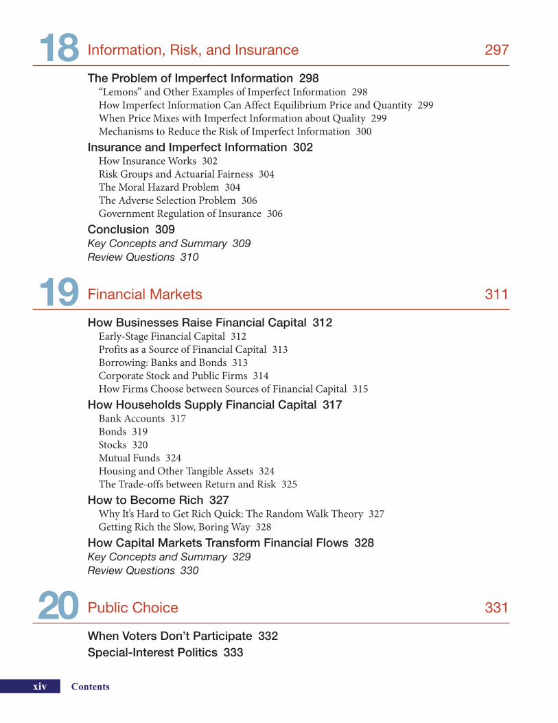
18 Information, Risk, and Insurance 297

The Problem of Imperfect Information 298“Lemons” and Other Examples of Imperfect Information 298How Imperfect Information Can Affect Equilibrium Price and Quantity 299When Price Mixes with Imperfect Information about Quality 299Mechanisms to Reduce the Risk of Imperfect Information 300

Insurance and Imperfect Information 302How Insurance Works 302Risk Groups and Actuarial Fairness 304The Moral Hazard Problem 304The Adverse Selection Problem 306Government Regulation of Insurance 306


19 Financial Markets 311

How Businesses Raise Financial Capital 312Early-Stage Financial Capital 312Profits as a Source of Financial Capital 313Borrowing: Banks and Bonds 313Corporate Stock and Public Firms 314How Firms Choose between Sources of Financial Capital 315

How Households Supply Financial Capital 317Bank Accounts 317Bonds 319Stocks 320Mutual Funds 324Housing and Other Tangible Assets 324The Trade-offs between Return and Risk 325

How to Become Rich 327Why It’s Hard to Get Rich Quick: The Random Walk Theory 327Getting Rich the Slow, Boring Way 328

How Capital Markets Transform Financial Flows 328Key Concepts and Summary 329Review Questions 330

20 Public Choice 331

When Voters Don’t Participate 332Special-Interest Politics 333

Contents xv

Identifiable Winners, Anonymous Losers 334Pork Barrels and Logrolling 334Voting Cycles 336Where Is Government’s Self-Correcting Mechanism? 336A Balanced View of Markets and Government 337Key Concepts and Summary 338Review Questions 339

PART V THE MACROECONOMIC PERSPECTIVE AND GOALS

21 The Macroeconomic Perspective 340

Measuring the Size of the Economy: Gross Domestic Product 342GDP Measured by Components of Demand 342GDP Measured by What Is Produced 345The Problem of Double Counting 345

Comparing GDP among Countries 346Converting Currencies with Exchange Rates 346Converting to Per Capita GDP 349

The Pattern of GDP over Time 350How Well Does GDP Measure the Well-Being of Society? 351

Some Differences between GDP and Standard of Living 351Does a Rise in GDP Overstate or Understate the Rise in the Standard of Living? 354GDP Is Rough, but Useful 354


22 Economic Growth 356

The Relatively Recent Arrival of Economic Growth 357Worker Productivity and Economic Growth 358The Power of Sustained Economic Growth 360The Aggregate Production Function 361

Components of the Aggregate Production Function 361Growth Accounting Studies 364A Healthy Climate for Economic Growth 365

Future Economic Convergence? 365Arguments Favoring Convergence 367Arguments That Convergence Is Neither Inevitable Nor Likely 368The Slowness of Convergence 369

Key Concepts and Summary 370Review Questions 370

xvi Contents

23 Unemployment 371

Unemployment and the Labor Force 372In or Out of the Labor Force? 372Calculating the Unemployment Rate 372Controversies over Measuring Unemployment 373

Patterns of Unemployment 374The Historical U.S. Unemployment Rate 374Unemployment Rates by Group 375International Unemployment Comparisons 376

Why Unemployment Is a Puzzle for Economists 377Looking for Unemployment with Flexible Wages 378Why Wages Might Be Sticky Downward 378

The Short Run: Cyclical Unemployment 379The Long Run: The Natural Rate of Unemployment 380

Frictional Unemployment 381Productivity Shifts and the Natural Rate of Unemployment 382Public Policy and the Natural Rate of Unemployment 383The Natural Rate of Unemployment in Recent Years 384The Natural Rate of Unemployment in Europe 385

A Preview of Policies to Fight Unemployment 386Key Concepts and Summary 386Review Questions 387

24 Inflation 388

Combining Prices to Measure the Inflation Rate 389The Changing Price of a Basket of Goods 389Index Numbers 391Measuring Changes in the Cost of Living 393Practical Solutions for the Substitution and the Quality/New Goods Biases 394Alternative Price Indexes: PPI, GDP Deflator, and More 395

Inflation Experiences 396Historical Inflation in the U.S. Economy 396Inflation around the World 397

Adjusting Nominal Values to Real Values 398Nominal to Real GDP 398Nominal to Real Interest Rates 400

The Dislocations of Inflation 401The Land of Funny Money 401Unintended Redistributions of Purchasing Power 402Blurred Price Signals 404Problems of Long-Term Planning 404Some Benefits of Inflation? 405

Contents xvii

Indexing and Its Limitations 405Indexing in Private Markets 405Indexing in Government Programs 406Might Indexing Reduce Concern Over Inflation? 406

A Preview of Policy Discussions of Inflation 406Key Concepts and Summary 407Review Questions 408

25 The Balance of Trade 409

Measuring Trade Balances 410Components of the U.S. Current Account Balance 410

Trade Balances in Historical and International Context 412The Intimate Connection between Trade Balances and Flows of Financial Capital 413

The Parable of Robinson Crusoe and Friday 413The Balance of Trade as the Balance of Payments 414

The National Saving and Investment Identity 416The National Saving and Investment Identity 416Domestic Savings and Investment Determine the Trade Balance 417Exploring Trade Balances One Factor at a Time 417How Short-Term Movements in the Business Cycle Can Affect the Trade Balance 418

When Are Trade Deficits and Surpluses Beneficial or Harmful? 419The Difference between Level of Trade and the Trade Balance 420Final Thoughts about Trade Balances 422Key Concepts and Summary 422Review Questions 423

PART VI A FRAMEWORK FOR MACROECONOMIC ANALYSIS

26 The Aggregate Supply–Aggregate Demand Model 424

Macroeconomic Perspectives on Demand and Supply 425Say’s Law and the Macroeconomics of Supply 425Keynes’ Law and the Macroeconomics of Demand 426Combining Supply and Demand in Macroeconomics 427

Building a Model of Aggregate Supply and Aggregate Demand 427The Aggregate Supply Curve and Potential GDP 427The Aggregate Demand Curve 429Equilibrium in the Aggregate Supply–Aggregate Demand Model 430AS and AD Are Macro, not Micro 430

Shifts in Aggregate Supply 431How Productivity Growth Shifts the AS Curve 431How Changes in Input Prices Shift the AS Curve 431

xviii Contents

Shifts in Aggregate Demand 432How Changes by Consumers and Firms Can Affect AD 433How Government Macroeconomic Policy Choices Can Shift AD 435

How the AS–AD Model Combines Growth, Unemployment, Inflation, and the Balance of Trade 436

Growth and Recession in the AS–AD Diagram 437Unemployment in the AS–AD Diagram 437Inflationary Pressures in the AS–AD Diagram 437The Balance of Trade and the AS–AD Diagram 439

Keynes’ Law and Say’s Law in the AS–AD Model 440Key Concepts and Summary 441Review Questions 442

27 The Keynesian Perspective 444

The Building Blocks of Keynesian Analysis 445The Importance of Aggregate Demand in Recessions 445Wage and Price Stickiness 446The Two Keynesian Assumptions in the AS–AD Model 447

The Components of Aggregate Demand 448What Causes Consumption to Shift? 448What Causes Investment to Shift? 449What Causes Government Demand to Shift? 450What Causes Exports and Imports to Shift? 450

The Phillips Curve 451The Discovery of the Phillips Curve 451The Instability of the Phillips Curve 453Keynesian Policy for Fighting Unemployment and Inflation 454

The Expenditure-Output Model 455The Axes of the Expenditure-Output Diagram 455The Potential GDP Line and the 45-degree Line 456The Aggregate Expenditure Schedule 457

Building the Aggregate Expenditure Schedule 457Consumption as a Function of National Income 457Investment as a Function of National Income 458Government Spending and Taxes as a Function of National Income 459Exports and Imports as a Function of National Income 460Building the Combined Aggregate Expenditure Function 461

Equilibrium in the Keynesian Cross Model 463Where Equilibrium Occurs 463Recessionary and Inflationary Gaps 464

Contents xix

The Multiplier Effect 465How Does the Multiplier Work? 465Calculating the Multiplier 467Calculating Keynesian Policy Interventions 468Multiplier Trade-offs: Stability vs. the Power of Macroeconomic Policy 469

Is Keynesian Economics Pro-Market or Anti-Market? 469Key Concepts and Summary 470Review Questions 471

28 The Neoclassical Perspective 472

The Building Blocks of Neoclassical Analysis 473The Importance of Potential GDP in the Long Run 473The Role of Flexible Prices 475How Fast Is the Speed of Macroeconomic Adjustment? 477

Policy Implications of the Neoclassical Perspective 478Fighting Recession or Encouraging Long-Term Growth? 478Fighting Unemployment or Inflation? 479The Neoclassical Phillips Curve Trade-Off 481

Macroeconomists Riding Two Horses 482Key Concepts and Summary 483Review Questions 484

PART VII MONETARY AND FISCAL POLICY

29 Money and Banks 485

Defining Money by Its Functions 486Barter and the Double Coincidence of Wants 486Three Functions for Money 487

Measuring Money: Currency, M1, and M2 487How Banks Work 489

Banks as Financial Intermediaries 490A Bank’s Balance Sheet 491How Banks Go Bankrupt 493

How Banks Create Money 494The Story of System Bank 495The Money Multiplier 496Cautions about the Money Multiplier 497


xx Contents

30 Monetary Policy and Bank Regulation 500

Monetary Policy and the Central Bank 501The Federal Reserve 501Other Tasks and Funding of Central Banks 502

How a Central Bank Affects the Money Supply 503Open Market Operations 503Reserve Requirements 506The Discount Rate 506Quantitative Easing 506Forward Guidance 507

Monetary Policy and Economic Outcomes 507The Effect of Monetary Policy on Interest Rates 507The Effect of Monetary Policy on Aggregate Demand 508What the Federal Reserve Has Done 509

Pitfalls for Monetary Policy 511Long and Variable Time Lags 512Excess Reserves 512Unpredictable Movements of Velocity 513Is Unemployment or Inflation More Important? 515Should the Central Bank Tackle Asset Bubbles and Leverage Cycles? 517

Bank Regulation 517Bank Runs 518A Weakened Banking Sector 518Deposit Insurance 519Bank Supervision 519Lender of Last Resort 520Summary 521


31 Exchange Rates and International Capital Flows 523

How the Foreign Exchange Market Works 524The Extraordinary Size of the Foreign Exchange Markets 524Demanders and Suppliers of Currency in Foreign Exchange Markets 524Participants in the Exchange Rate Market 527Strengthening and Weakening Currency 527

Demand and Supply Shifts in Foreign Exchange Markets 530Expectations about Future Exchange Rates 531Differences across Countries in Rates of Return 532Relative Inflation 532Purchasing Power Parity 534

Contents xxi

Macroeconomic Effects of Exchange Rates 534Exchange Rates, Aggregate Demand, and Aggregate Supply 535Fluctuations in Exchange Rates 537Exchange Rates, Trade Balances, and International Capital Flows 538Summing Up Public Policy and Exchange Rates 541

Exchange Rate Policies 541Floating Exchange Rates 541Using Soft Pegs and Hard Pegs 543Trade-offs of Soft Pegs and Hard Pegs 544A Single Currency 546


32 Government Budgets and Fiscal Policy 549

An Overview of Government Spending 550Total U.S. Government Spending 550Keeping Federal Budget Numbers in Perspective 552State and Local Government Spending 552

An Overview of Taxation 553State and Local Taxes 555

Federal Deficits and Debt 557Debt/GDP Ratio 557The Path from Deficits to Surpluses to Deficits 558

Using Fiscal Policy to Affect Recession, Unemployment and Inflation 559Expansionary Fiscal Policy 561Contractionary Fiscal Policy 562

Automatic Stabilizers 563Counterbalancing Recession and Boom 563

Practical Problems with Discretionary Fiscal Policy 564Long and Variable Time Lags 564Temporary and Permanent Fiscal Policy 565Coordinating Fiscal and Monetary Policy 565Structural Economic Change Takes Time 566The Limitations of Potential GDP and the Natural Rate of Unemployment 566Educating Politicians 566Summing Up Discretionary Fiscal Policy 567

Requiring a Balanced Budget? 567Conclusion 568Key Concepts and Summary 568Review Questions 569

xxii Contents

33 Government Borrowing and National Savings 570

How Government Borrowing Affects Investment and the Trade Balance 570The National Saving and Investment Identity 571What about Budget Surpluses and Trade Surpluses? 571

Fiscal Policy, Investment, and Economic Growth 572Crowding Out Physical Capital Investment 572The Interest Rate Connection 573Public Investment in Physical Capital 575Public Investment in Human Capital 575How Fiscal Policy Can Improve Technology 577Summary of Fiscal Policy, Investment, and Economic Growth 577

Will Private Saving Offset Government Borrowing? 578Fiscal Policy and the Trade Balance 579

Twin Deficits? 579Fiscal Policy and Exchange Rates 579From Budget Deficits to International Economic Crisis 581Using Fiscal Policy to Address Trade Imbalances 582


34 Macroeconomic Policy around the World 585

The Diversity of Countries and Economies across the World 586Economic Growth 587

Growth Policies for the Technological Leaders 588Growth Policies for the Converging Economies 588Growth Policies for the Technologically Disconnected 589

Lower Unemployment 591Unemployment from a Recession 591The Natural Rate of Unemployment 592Undeveloped Labor Markets 593

Policies for Lower Inflation 593Policies for a Sustainable Balance of Trade 594

Concerns over International Trade in Goods and Services 595Concerns over International Flows of Capital 595

Final Thoughts on Economics and Market Institutions 597Key Concepts and Summary 599Review Questions 599

Contents xxiii

APPENDIX CHAPTERS

1 Interpreting Graphs 600

Pie Graphs 601Bar Graphs 602Line Graphs 602

Line Graphs with Two Variables 602Time Series 605Slope 605Slope of Straight Lines in Algebraic Terms 606

Comparing Line Graphs with Pie Charts and Bar Graphs 607How Graphs Can Mislead 607

8 Indifference Curves 612

What Is an Indifference Curve? 612The Shape of an Indifference Curve 612The Field of Indifference Curves 614The Individuality of Indifference Curves 614

Utility-Maximizing with Indifference Curves 614Maximizing Utility at the Highest Indifference Curve 615

Changes in Income 616Responses to Price Changes: Substitution and Income Effects 617Indifference Curves with Labor-Leisure and Intertemporal Choices 619

A Labor-Leisure Example 619An Intertemporal Choice Example 621

Conclusion 624

19 Present Discounted Value 626

Applying Present Discounted Value to a Stock 626Applying Present Discounted Value to a Bond 627Other Applications 628

27 An Algebraic Approach to the Expenditure-Output Model 629

Question 631Answer 631

Glossary G-1Index I-1

xxv

When authors describe their reasons for writing an eco-nomics textbook, it seems customary to proclaim lofty goals, like teaching students “to think like economists” so that they can become more informed voters and citi-zens. Paul Samuelson, the author of the most famous in-troductory economics textbook for the second half of the twentieth century, famously said: “I don’t care who writes a nation’s laws—or crafts its advanced treaties—if I can write its economics textbooks.” On my best days, I have sufficient time and energy to lift my eyes to the horizon, strike a statuesque pose, and proclaim exalted goals. But most of the time, I’m just a workaday teacher and my goals are more limited and concrete.

The pedagogical approach of this textbook is rooted in helping students master the tools that they need to solve problems for a course in introductory economics. Indeed, one of the great pleasures of writing the book is having the opportunity to share my teaching toolkit of step-by-step explanations, practical examples, and metaphors that stick in the mind. On quizzes and exams, I do not ask broad or open-ended questions about informed citizen-ship and thinking like an economist. At the most basic level, my goal for an economics class is that students should feel well-prepared for quizzes and exams.

The preparation that students need to perform well in an introductory economics class can be divided into three parts. First, an introductory economics class involves mastering a specialized vocabulary. I sometimes tell stu-dents that learning economics is akin to learning a foreign language—with the added difficulty that terms in eco-nomics like “demand” or “supply” or “money” sound like standard English, and thus learning economics often re-quires that students drop their preconceptions about what certain words mean.

Second, students need to acquire some basic analytical tools. There are four central analytical models in an intro-ductory economics course: budget constraints, supply and demand, cost curves, and aggregate demand–aggregate supply. These four models are used for a very wide vari-ety of applications; still, there are only four of them. There are also a few key formulas and equations to learn with regard to topics like growth rates over time and elasticity.

Third, students must learn to recognize when these terms and tools apply and to practice using them. I often tell students not to bother memorizing particular ques-tions and answers from the textbook or homework, be-cause my quiz and exam questions will ask them to apply what they have learned in contexts they have not seen be-fore. To provide a variety of contexts, this book describes many economic issues and events, drawn from recent times and past history, and also drawn both from U.S. and international experiences. When students see a concept or analytical skill applied in a number of ways, they learn to focus on the underlying and unifying idea. I’ve also found that students do take away knowledge of many economic events and episodes—although different students seem to focus on an unpredictable (to me) array of examples, which is perhaps as it should be in an introductory course.

As a workaday teacher, the goal of helping students master the material so that they can perform well on my quizzes and exams is lofty enough—and tough enough— for me. There’s an old joke that economics is the science of taking what is obvious about human behavior and mak-ing it incomprehensible. Actually, in my experience, the process works in the other direction. Many students spend the opening weeks of an introductory economics course feeling as if the material is difficult, even impossible, but by the middle and the end of the class, what seemed so difficult early in the term has become obvious and straightforward. As a course in introductory economics focuses on one lesson after another and one chapter after another, it’s easy to get tunnel vision. But when you raise your eyes at the end of class, it can be quite astonishing to look back and see how far you have come. As students apply the terms and models they have learned to a se-ries of real and hypothetical examples, they often find to their surprise that they have also imbibed a considerable amount about economic thinking and the real-world econ-omy. Learning always has an aspect of the miraculous.

As always, my family makes a significant contribution to the existence of this book. In the six years since the first edition, the U.S. and world economy has been convulsed by a Great Recession and then by an ungainly process of sluggish and partial recovery. The task of updating figures

Preface

xxvi Preface

and examples for this third edition is inevitably large, but thinking about how to build connections from the con-cepts in the text to the economic events of the last few years made it larger. During the process of preparing this revised edition, my wife has dealt lovingly with a distract-ed husband; my children, with a father who was sleep- deprived or “at the office.” In a very real sense, then, this

book is from my dear ones to the students and instructors who use it. I hope that it serves you well.

Timothy Taylor St. Paul, Minnesota October 1, 2013

xxvii

Timothy T. Taylor Timothy T. Taylor has been the Managing Editor of the Journal of Economic Perspectives, published by the American Economic Association, since the first issue of the journal in 1987. All issues of the journal are freely available online at http://e-jep.org. Taylor holds a B.A de-gree in economics and political science from Haverford College. He holds an M.S. degree in economics from Stanford University, where he focused on public finance, industrial organization, and economic history.

Taylor has taught economics in a variety of contexts. In 2012, his book The Instant Economist: Everything You Need to Know About How the Economy Works, was pub-lished by Penguin Plume. It was named an “Outstanding Academic Title” by Choice magazine of the American Li-brary Assocation and was also listed as one of the Best Books for 2012 in the “Business” category by Library Journal. He has recorded a variety of lecture courses for The Teaching Company, based in Chantilly, Virginia, in-cluding Economics (3rd edition), Unexpected Economics, America and the New Global Economy, Legacies of Great Economists, and History of the U.S. Economy in the 20th Century. In 1992, he won the Outstanding Teacher Award from the Associated Students of Stanford University. In 1996, he was named a Distinguished Instructor for his courses in introductory economics at the University of Minnesota. In 1997, he was voted Teacher of the Year by students at the Humphrey Institute of Public Affairs at the University of Minnesota.

He has published articles on various topics in eco-nomics in publications such as the Milken Institute Re-view, the Cato Journal, Public Interest, and the Journal of Economic Perspectives. He blogs regularly at http:// conversableeconomist.blogspot.com.

About the Author

52

When people talk about prices, the discussion often takes a judgmental tone. A bidder in an auction pays thousands of dollars for a dress once worn by Diana, Princess of Wales. A collector spends thousands of dollars for some drawings by John Lennon of the Beatles. Mouths gape. Surely such purchases are a waste of money? But when economists talk about prices, they are less inter-ested in making judgments than in gaining a practical understanding of what determines prices and why prices change. In 1933, the great British economist Joan Robinson (1903–1983) explained how economists perceive price:

The point may be put like this: You see two men, one of whom is giving a banana to the other, and is taking a penny from him. You ask, How is it that a banana costs a penny rather than any other sum? The most obvious line of attack on this question is to break it up into two fresh questions: How does it happen that the one man will take a penny for a banana? and: How does it happen that the other man will give a penny for a banana? In short, the natu-ral thing is to divide up the problem under two heads: Supply and Demand.

As a contemporary example, consider a price often listed on large signs beside well-traveled roads: the price of a gallon of gasoline. Why was the average price of gasoline in the United States $3.15 per gallon in January 2011? Why did the price for gasoline rise to $3.75 per gallon six months later by June 2011? To explain why prices are at a certain level and why that level changes over time, economic analysis focuses on the determinants of what gasoline buyers are willing to pay and what gasoline sellers are willing to accept. For example, the price of a gallon of gasoline in June of a given year is nearly always higher than the price in January of that year; over recent de-

CHAPTER Demand and Supply 4

Chapter 4 Demand and Supply 53

cades, gasoline prices in midsummer have averaged about 10 cents per gallon more than their midwinter low. The likely reason is that people want to drive more in the summer, and thus they are willing to pay more for gas at that time. However, in 2011, gasoline prices rose by much more than the average winter-to-summer rise, which suggests that other factors related to those who buy gasoline and firms that sell it changed during those six months, too.

This chapter introduces the economic model of demand and supply. The discussion begins by examining how demand and supply determine the price and the quantity sold in markets for goods and services, and how changes in demand and supply lead to changes in prices and quantities. In Chapter 5, the same demand and supply model is applied to markets for labor and financial capital. In Chapter 6, the same supply and demand model is applied to international trade. In situation after situation, in different places around the world, across different cultures, even reaching back into history, the demand and supply model offers a useful framework for thinking about what determines the prices and quan-tities of what is bought and sold.

Demand, Supply, and Equilibrium in Markets for Goods and ServicesMarkets for goods and services include everything from accounting services, air travel, and apples to zinc, zinfandel wine, and zucchini. Let’s first focus on what economists mean by demand, what they mean by supply, and then how demand and supply interact in an economic model of the market.

Demand for Goods and ServicesEconomists use the term demand to refer to a relationship between price and the quantity demanded. Price is what a buyer pays (or the seller receives) for a unit of the specific good or service. Quantity demanded refers to the total number of units that are pur-chased at a given price. A rise in price of a good or service almost always decreases the quantity demanded of that good or service; conversely, a fall in price will increase the quantity demanded. When the price of a gallon of gasoline goes up, for example, people look for ways to reduce their purchases of gasoline by combining several errands, com-muting by carpool or mass transit, or taking weekend or vacation trips by car close to home. Economists refer to the relationship that a higher price leads to a lower quantity demanded as the law of demand.

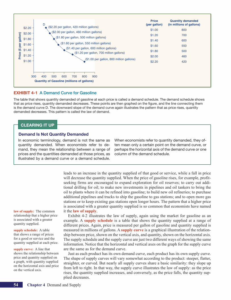
Exhibit 4-1 gives a hypothetical example in the market for gasoline. The table that shows the quantity demanded at each price is called a demand schedule. Price in this case is measured per gallon of gasoline. The quantity demanded is measured in millions of gallons. A demand curve shows the relationship between price and quantity demanded on a graph, with quantity on the horizontal axis and the price per gallon on the vertical axis. The demand schedule shown by the table and the demand curve shown on the graph are two ways of describing the same relationship between price and quantity demanded.

Each individual good or service needs to be graphed on its own demand curve, because it wouldn’t make sense to graph the quantity of apples and the quantity of oranges on the same diagram. Demand curves will appear somewhat different for each product; for example, they may appear relatively steep or flat, or they may be straight or curved. But nearly all demand curves share the fundamental similarity that they slope down from left to right. In this way, demand curves embody the law of demand; as the price increases, the quantity demanded decreases, and conversely, as the price decreases, the quantity demanded increases.

Supply of Goods and ServicesWhen economists talk about supply, they are referring to a relationship between price received for each unit sold and the quantity supplied, which is the total number of units sold in the market at a certain price. A rise in price of a good or service almost always

demand: A relationship between price and the quantity demanded of a certain good or service.

quantity demanded: The total number of units of a good or service purchased at a certain price.

law of demand: The common relationship that a higher price leads to a lower quantity demanded of a certain good or service.

demand schedule: A table that shows a range of prices for a certain good or service and the quantity demanded at each price.

demand curve: A line that shows the relationship between price and quantity demanded of a certain good or service on a graph, with quantity on the horizontal axis and the price on the vertical axis.

supply: A relationship between price and the quantity supplied of a certain good or service.

quantity supplied: The total number of units of a good or service sold at a certain price.

54 Chapter 4 Demand and Supply

leads to an increase in the quantity supplied of that good or service, while a fall in price will decrease the quantity supplied. When the price of gasoline rises, for example, profit- seeking firms are encouraged to expand exploration for oil reserves; to carry out addi-tional drilling for oil; to make new investments in pipelines and oil tankers to bring the oil to plants where it can be refined into gasoline; to build new oil refineries; to purchase additional pipelines and trucks to ship the gasoline to gas stations; and to open more gas stations or to keep existing gas stations open longer hours. The pattern that a higher price is associated with a greater quantity supplied is so common that economists have named it the law of supply.

Exhibit 4-2 illustrates the law of supply, again using the market for gasoline as an example. A supply schedule is a table that shows the quantity supplied at a range of different prices. Again, price is measured per gallon of gasoline and quantity supplied is measured in millions of gallons. A supply curve is a graphical illustration of the relation-ship between price, shown on the vertical axis, and quantity, shown on the horizontal axis. The supply schedule and the supply curve are just two different ways of showing the same information. Notice that the horizontal and vertical axes on the graph for the supply curve are the same as for the demand curve.

Just as each product has its own demand curve, each product has its own supply curve. The shape of supply curves will vary somewhat according to the product: steeper, flatter, straighter, or curved. But nearly all supply curves share a basic similarity: they slope up from left to right. In that way, the supply curve illustrates the law of supply: as the price rises, the quantity supplied increases, and conversely, as the price falls, the quantity sup-plied decreases.

law of supply: The common relationship that a higher price is associated with a greater quantity supplied.

supply schedule: A table that shows a range of prices for a good or service and the quantity supplied at each price.

supply curve: A line that shows the relationship between price and quantity supplied on a graph, with quantity supplied on the horizontal axis and price on the vertical axis.

300 400

($2.20 per gallon, 420 million gallons)D

($2.00 per gallon, 460 million gallons)






500 600 700 800 900

Quantity of Gasoline (millions of gallons)

Pri

ce (

$ p

er g

allo

n)

$2.20

$2.00

$1.80

$1.60

$1.40

$1.20

$1.00

Price (per gallon)

Quantity demanded (in millions of gallons)

$1.00 800$1.20 700$1.40 600$1.60 550$1.80 500$2.00 460$2.20 420

EXHIBIT 4-1 A Demand Curve for Gasoline The table that shows quantity demanded of gasoline at each price is called a demand schedule. The demand schedule shows that as price rises, quantity demanded decreases. These points are then graphed on the figure, and the line connecting them is the demand curve D. The downward slope of the demand curve again illustrates the pattern that as price rises, quantity demanded decreases. This pattern is called the law of demand.

Demand Is Not Quantity Demanded

CLEARING IT UP

In economic terminology, demand is not the same as quantity demanded. When economists refer to de-mand, they mean the relationship between a range of prices and the quantities demanded at those prices, as illustrated by a demand curve or a demand schedule.

When economists refer to quantity demanded, they of-ten mean only a certain point on the demand curve, or perhaps the horizontal axis of the demand curve or one column of the demand schedule.


Equilibrium—Where Demand and Supply CrossBecause the graphs for demand and supply curves both have price on the vertical axis and quantity on the horizontal axis, the demand curve and supply curve for a particular good or service can appear on the same graph. Together, demand and supply determine the price and the quantity that will be bought and sold in a market.

Exhibit 4-3 illustrates the interaction of demand and supply in the market for gasoline. The demand curve D is identical to Exhibit 4-1. The supply curve S is identical to Ex-hibit 4-2. When one curve slopes down, like demand, and another curve slopes up, like supply, the curves intersect at some point.

In every economics course you will ever take, when two lines on a diagram cross, this intersection means something! The point where the supply curve S and the demand curve D cross, designated by point E in Exhibit 4-3, is called the equilibrium. The equilibrium price is defined as the price where quantity demanded is equal to quantity supplied. The equilibrium quantity is the quantity where quantity demanded and quantity supplied are equal at a certain price. In Exhibit 4-3, the equilibrium price is $1.40 per gallon of gasoline and the equilibrium quantity is 600 million gallons. If you had only the demand and supply schedules, and not the graph, it would be easy to find the equilibrium by looking for the price level on the tables where the quantity demanded and the quantity supplied are equal.

The word equilibrium means “balance.” If a market is balanced at its equilibrium price and quantity, then it has no reason to move away from that point. However, if a market is not balanced at equilibrium, then economic pressures arise to move toward the equilibrium price and the equilibrium quantity.

equilibrium price: The price where quantity demanded is equal to quantity supplied.

equilibrium quantity: The quantity at which quantity demanded and quantity supplied are equal at a certain price.

equilibrium: The combination of price and quantity where there is no economic pressure from surpluses or shortages that would cause price or quantity to shift.

Supply Is Not the Same as Quantity Supplied

CLEARING IT UP

In economic terminology, supply is not the same as quantity supplied. When economists refer to supply, they mean the relationship between a range of prices and the quantities supplied at those prices, a relation-ship that can be illustrated with a supply curve or a

supply schedule. When economists refer to quantity supplied, they often mean only a certain point on the supply curve, or sometimes, they are referring to the horizontal axis of the supply curve or one column of the supply schedule.

300 400








500 600 700 800 900


Pri

ce (

$ p

er g

allo

n)

$2.20

$2.00

$1.80

$1.60

$1.40

$1.20

$1.00

Price (per gallon)

Quantity supplied (millions of gallons)

$1.00 500$1.20 550$1.40 600$1.60 640$1.80 680$2.00 700$2.20 720

EXHIBIT 4-2 A Supply Curve for Gasoline The supply schedule is the table that shows quantity supplied of gasoline at each price. As price rises, quantity supplied also increases. The supply curve S is created by graphing the points from the supply schedule and then connecting them. The upward slope of the supply curve illustrates the pattern that a higher price leads to a higher quantity supplied—a pattern that is common enough to be called the law of supply.


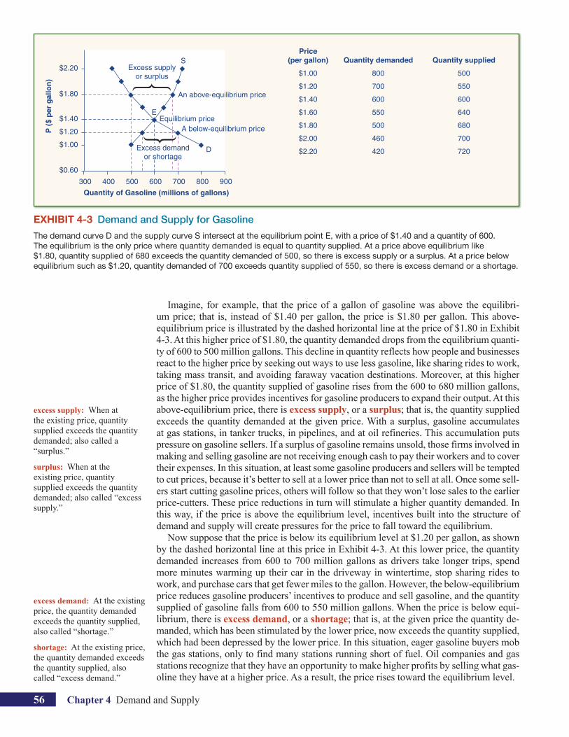
Imagine, for example, that the price of a gallon of gasoline was above the equilibri-um price; that is, instead of $1.40 per gallon, the price is $1.80 per gallon. This above- equilibrium price is illustrated by the dashed horizontal line at the price of $1.80 in Exhibit 4-3. At this higher price of $1.80, the quantity demanded drops from the equilibrium quanti-ty of 600 to 500 million gallons. This decline in quantity reflects how people and businesses react to the higher price by seeking out ways to use less gasoline, like sharing rides to work, taking mass transit, and avoiding faraway vacation destinations. Moreover, at this higher price of $1.80, the quantity supplied of gasoline rises from the 600 to 680 million gallons, as the higher price provides incentives for gasoline producers to expand their output. At this above-equilibrium price, there is excess supply, or a surplus; that is, the quantity supplied exceeds the quantity demanded at the given price. With a surplus, gasoline accumulates at gas stations, in tanker trucks, in pipelines, and at oil refineries. This accumulation puts pressure on gasoline sellers. If a surplus of gasoline remains unsold, those firms involved in making and selling gasoline are not receiving enough cash to pay their workers and to cover their expenses. In this situation, at least some gasoline producers and sellers will be tempted to cut prices, because it’s better to sell at a lower price than not to sell at all. Once some sell-ers start cutting gasoline prices, others will follow so that they won’t lose sales to the earlier price-cutters. These price reductions in turn will stimulate a higher quantity demanded. In this way, if the price is above the equilibrium level, incentives built into the structure of demand and supply will create pressures for the price to fall toward the equilibrium.

Now suppose that the price is below its equilibrium level at $1.20 per gallon, as shown by the dashed horizontal line at this price in Exhibit 4-3. At this lower price, the quantity demanded increases from 600 to 700 million gallons as drivers take longer trips, spend more minutes warming up their car in the driveway in wintertime, stop sharing rides to work, and purchase cars that get fewer miles to the gallon. However, the below- equilibrium price reduces gasoline producers’ incentives to produce and sell gasoline, and the quantity supplied of gasoline falls from 600 to 550 million gallons. When the price is below equi-librium, there is excess demand, or a shortage; that is, at the given price the quantity de-manded, which has been stimulated by the lower price, now exceeds the quantity supplied, which had been depressed by the lower price. In this situation, eager gasoline buyers mob the gas stations, only to find many stations running short of fuel. Oil companies and gas stations recognize that they have an opportunity to make higher profits by selling what gas-oline they have at a higher price. As a result, the price rises toward the equilibrium level.

excess supply: When at the existing price, quantity supplied exceeds the quantity demanded; also called a “surplus.”

surplus: When at the existing price, quantity supplied exceeds the quantity demanded; also called “excess supply.”

excess demand: At the existing price, the quantity demanded exceeds the quantity supplied, also called “shortage.”

shortage: At the existing price, the quantity demanded exceeds the quantity supplied, also called “excess demand.”

Price (per gallon)

Quantity demanded

Quantity supplied

$1.00 800 500$1.20 700 550$1.40 600 600$1.60 550 640$1.80 500 680$2.00 460 700$2.20 420 720

EXHIBIT 4-3 Demand and Supply for Gasoline The demand curve D and the supply curve S intersect at the equilibrium point E, with a price of $1.40 and a quantity of 600. The equilibrium is the only price where quantity demanded is equal to quantity supplied. At a price above equilibrium like $1.80, quantity supplied of 680 exceeds the quantity demanded of 500, so there is excess supply or a surplus. At a price below equilibrium such as $1.20, quantity demanded of 700 exceeds quantity supplied of 550, so there is excess demand or a shortage.

300

S

D

E

900800700600500400

$1.80

$2.20


P (

$ p

er g

allo

n)

$1.40

$1.20

$1.00

$0.60

Excess supplyor surplus

An above-equilibrium price

Equilibrium priceA below-equilibrium price

Excess demandor shortage


Shifts in Demand and Supply for Goods and ServicesA demand curve shows how quantity demanded changes as the price rises or falls. A sup-ply curve shows how quantity supplied changes as the price rises or falls. But what hap-pens when factors other than price influence quantity demanded and quantity supplied? For example, what if demand for, say, vegetarian food becomes popular with more con-sumers? Or what if the supply of, say, diamonds rises not because of any change in price, but because companies discover several new diamond mines? A change in price leads to a different point on a specific demand curve or a supply curve, but a shift in some economic factor other than price can cause the entire demand curve or supply curve to shift.

The Ceteris Paribus AssumptionA demand curve or a supply curve is a relationship between two and only two variables: quantity on the horizontal axis and price on the vertical axis. Thus, the implicit assump-tion behind a demand curve or a supply curve is that no other relevant economic fac-tors are changing. Economists refer to this assumption as ceteris paribus, a Latin phrase meaning “other things being equal.” Any given demand or supply curve is based on the ceteris paribus assumption that all else is held equal. If all else is not held equal, then the demand or supply curve itself can shift.

An Example of a Shifting Demand CurveThe original demand curve D0 in Exhibit 4-4 shows at point Q that at a price of $20,000 per car, the quantity of cars demanded would be 18 million. The original demand curve

ceteris paribus: Other things being equal.

Price Decrease to D2 Original Quantity Demanded D0 Increase to D1

$16,000 17.6 million 22.0 million 24.0 million$18,000 16.0 million 20.0 million 22.0 million$20,000 14.4 million 18.0 million 20.0 million$22,000 13.6 million 17.0 million 19.0 million$24,000 13.2 million 16.5 million 18.5 million$26,000 12.8 million 16.0 million 18.0 million

EXHIBIT 4-4 Shifts in Demand: A Car Example Increased demand means that at every given price, the quantity demanded is higher, so that the demand curve shifts to the right from D0 to D1. Decreased demand means that at every given price, the quantity demand is lower, so that the demand curve shifts to the left from D0 to D2.

8 282320181714.413

$22,000

$24,000

$26,000

$28,000

Quantity

$16,000

$18,000

$20,000

$14,000

$12,000

$10,000

S

R

T Q

D2 D0 D1

Price

p = 20,000q = 14.4 million

p = 20,000q = 20 million

p = 20,000q = 18 million


also shows how the quantity of cars demanded would change as a result of a higher D0 or lower price; for example, if the price of a car rose to $22,000, the quantity demanded would decrease to 17 million, as at point R.

The original demand curve D0, like every demand curve, is based on the ceteris pa-ribus assumption that no other economically relevant factors change. But now imagine that the economy expands in a way that raises the incomes of many people. As a result of the higher income levels, a shift in demand occurs, which means that compared to the original demand curve D0, a different quantity of cars will now be demanded at every price. On the original demand curve, a price of $20,000 means a quantity demanded of 18 million, but after higher incomes cause an increase in demand, a price of $20,000 leads to a quantity demanded of 20 million, at point S. Exhibit 4-4 illustrates the shift in demand as a result of higher income levels with the shift of the original demand curve D0 to the right to the new demand curve D1.

This logic works in reverse, too. Imagine that the economy slows down so that many people lose their jobs or work fewer hours and thus suffer reductions in income. In this case, the shift in demand would lead to a lower quantity of cars demanded at every given price, and the original demand curve D0 would shift left to D2. The shift from D0 to D2 represents a decrease in demand; that is, at any given price level, the quantity demanded is now lower. In this example, a price of $20,000 means 18 million cars sold along the original demand curve, but only 14.4 million cars sold after demand has decreased.

When a demand curve shifts, it does not mean that the quantity demanded by every individual buyer changes by the same amount. In this example, not everyone would have higher or lower income, and not everyone would buy or not buy an additional car. Instead, a shift in a demand captures an overall pattern for the market as a whole.

Factors That Shift Demand CurvesA change in any one of the underlying factors that determine what quantity people are willing to buy at a given price will cause a shift in demand. Graphically, the new demand curve lies either to the right or to the left of the original demand curve. Various factors may cause a demand curve to shift: changes in income, change in population, changes in taste, changes in expectations, and changes in the prices of closely related goods. Let’s consider these factors in turn.

A change in income will often move demand curves. A household with a higher income level will tend to demand a greater quantity of goods at every price than a household with a lower income level. For some luxury goods and services, such as expensive cars, exotic spa vacations, and fine jewelry, the effect of a rise in income can be especially pronounced. However, a few exceptions to this pattern do exist. As incomes rise, many people will buy fewer popsicles and more ice cream, less chicken and more steak; they will be less likely to rent an apartment and more likely to own a home; and so on. Normal goods are defined as those where the quantity demanded rises as income rises, which is the most common case; inferior goods are defined as those where the quantity demanded falls as income rises.

Changes in the composition of the population can also shift demand curves for certain goods and services. The proportion of elderly citizens in the U.S. population is rising, from 9% in 1960, to 13% in 2000, and to a projected (by the U.S. Census Bureau) 20% of the population by 2030. A society with relatively more children, like the United States in the 1960s, will have greater demand for goods and services like tricycles and day care facilities. A society with relatively more elderly persons, as the United States is projected to have by 2030, has a higher demand for nursing homes and hearing aids.

Changing tastes can also shift demand curves. In demand for music, for example, 50% of sound recordings sold in 1990 were in the rock or pop music categories. By 2008, rock and pop had fallen to 41% of the total, while sales of rap/hip-hop, religious, and country categories had increased. Tastes in food and drink have changed, too. From 1970 to 2011, the per person consumption of chicken by Americans rose from 40 pounds per year to 84 pounds per year, and consumption of cheese rose from 11 pounds per year to 33 pounds

shift in demand: When a change in some economic factor related to demand causes a different quantity to be demanded at every price.

normal goods: Goods where the quantity demanded rises as income rises.

inferior goods: Goods where the quantity demanded falls as income rises.


per year. Changes like these are largely due to movements in taste, which change the quantity of a good demanded at every price: that is, they shift the demand curve for that good.

Changes in expectations about future conditions and prices can also shift the demand curve for a good or service. For example, if people hear that a hurricane is coming, they may rush to the store to buy flashlight batteries and bottled water. If people learn that the price of a good like coffee is likely to rise in the future, they may head for the store to stock up on coffee now.

The demand curve for one good or service can be affected by changes in the prices of related goods. Some goods and services are substitutes for others, which means that they can replace the other good to some extent. For example, if the price of cotton rises, driv-ing up the price of clothing, sheets, and other items made from cotton, then some people will shift to comparable goods made from fabrics like wool, silk, linen, and polyester. A higher price for a substitute good shifts the demand curve to the right; for example, a higher price for tea encourages buying more coffee. Conversely, a lower price for a sub-stitute good has the reverse effect.

Other goods are complements for each other, meaning that the goods are often used together, so that consumption of one good tends to increase consumption of the other. Examples include breakfast cereal and milk; golf balls and golf clubs; gasoline and sports utility vehicles; and the five-way combination of bacon, lettuce, tomato, mayonnaise, and bread. If the price of golf clubs rises, demand for a complement good like golf balls decreases. A higher price for skis would shift the demand curve for a complement good like ski resort trips to the left, while a lower price for a complement has the reverse effect.

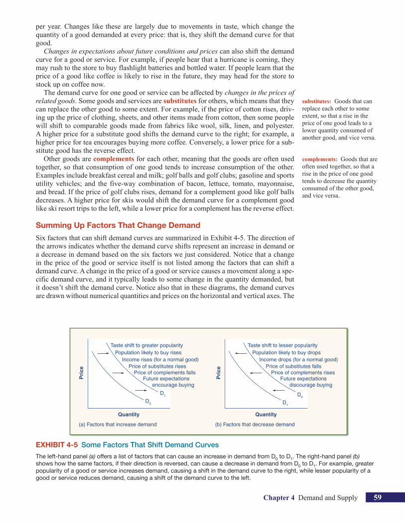
Summing Up Factors That Change DemandSix factors that can shift demand curves are summarized in Exhibit 4-5. The direction of the arrows indicates whether the demand curve shifts represent an increase in demand or a decrease in demand based on the six factors we just considered. Notice that a change in the price of the good or service itself is not listed among the factors that can shift a demand curve. A change in the price of a good or service causes a movement along a spe-cific demand curve, and it typically leads to some change in the quantity demanded, but it doesn’t shift the demand curve. Notice also that in these diagrams, the demand curves are drawn without numerical quantities and prices on the horizontal and vertical axes. The

substitutes: Goods that can replace each other to some extent, so that a rise in the price of one good leads to a lower quantity consumed of another good, and vice versa.

complements: Goods that are often used together, so that a rise in the price of one good tends to decrease the quantity consumed of the other good, and vice versa.

EXHIBIT 4-5 Some Factors That Shift Demand CurvesThe left-hand panel (a) offers a list of factors that can cause an increase in demand from D0 to D1. The right-hand panel (b) shows how the same factors, if their direction is reversed, can cause a decrease in demand from D0 to D1. For example, greater popularity of a good or service increases demand, causing a shift in the demand curve to the right, while lesser popularity of a good or service reduces demand, causing a shift of the demand curve to the left.

Quantity

Taste shift to greater popularityPopulation likely to buy rises

Income rises (for a normal good)Price of substitutes rises

Price of complements fallsFuture expectations encourage buying

(a) Factors that increase demand

D0

D1

Pri

ce

Quantity

Taste shift to lesser popularityPopulation likely to buy drops

Income drops (for a normal good)Price of substitutes falls

Price of complements risesFuture expectations discourage buying

Pri

ce

(b) Factors that decrease demand

D1

D0


demand and supply model can often be a useful conceptual tool even without attaching specific numbers.

When a demand curve shifts, it will then intersect with a given supply curve at a dif-ferent equilibrium price and quantity. But we are getting ahead of our story. Before dis-cussing how changes in demand can affect equilibrium price and quantity, we first need to discuss shifts in supply curves.

An Example of a Shift in a Supply CurveA supply curve shows how quantity supplied will change as the price rises and falls, based on the ceteris paribus assumption that no other economically relevant factors are changing. But if other factors relevant to supply do change, then the entire supply curve can shift. Just as a shift in demand is represented by a change in the quantity demanded at every price, a shift in supply means a change in the quantity supplied at every price. In thinking about the factors that affect supply, remember the basic motivation of firms: to earn profits. If a firm faces lower costs of production, while the prices for the output the firm produces remain unchanged, a firm’s profits will increase. Thus, when costs of production fall, a firm will supply a higher quantity at any given price for its output, and the supply curve will shift to the right. Conversely, if a firm faces an increased cost of production, then it will earn lower profits at any given selling price for its products. As a result, a higher cost of production typically causes a firm to supply a smaller quantity at any given price. In this case, the supply curve shifts to the left.

shift in supply: When a change in some economic factor related to supply causes a different quantity to be supplied at every price.

PriceDecrease

to S1

Original Quantity Supplied S0

Increase to S2

$16,000 10.5 million 12.0 million 13.2 million$18,000 13.5 million 15.0 million 16.5 million$20,000 16.5 million 18.0 million 19.8 million$22,000 18.5 million 20.0 million 22.0 million$24,000 19.5 million 21.0 million 23.1 million$26,000 20.5 million 22.0 million 24.2 million

EXHIBIT 4-6 Shifts in Supply: A Car Example Increased supply means that at every given price, the quantity supplied is higher, so that the supply curve shifts to the right from S0 to S2. Decreased supply means that at every given price, quantity supplied of cars is lower, so that the supply curve shifts to the left from S0 to S1.

8 2319.81816.5

L J MK

S1 S0 S2

13

$22,000

$24,000

$26,000

$28,000

Quantity

$16,000

$18,000

$20,000

$14,000

$12,000

$10,000

Price

p = 20,000q = 19.8 million

p = 20,000q = 18 million

p = 20,000q = 16.5 million


As an example, imagine that supply in the market for cars is represented by S0 in Ex-hibit 4-6. The original supply curve, S0, includes a point with a price of $20,000 and a quantity supplied of 18 million cars, labeled as point J, which represents the current mar-ket equilibrium price and quantity. If the price rises to $22,000 per car, ceteris paribus, the quantity supplied will rise to 20 million cars, as shown by point K on the S0 curve.

Now imagine that the price of steel, an important material input in manufacturing cars, rises, so that producing a car has now become more expensive. At any given price for sell-ing cars, car manufacturers will react by supplying a lower quantity. The shift of supply from S0 to S1 shows that at any given price, the quantity supplied decreases. In this exam-ple, at a price of $20,000, the quantity supplied decreases from 18 million on the original supply curve S0 to 16.5 million on the supply curve S1, which is labeled as point L.

Conversely, imagine that the price of steel decreases, so that producing a car becomes less expensive. At any given price for selling cars, car manufacturers can now expect to earn higher profits and so will supply a higher quantity. The shift of supply to the right from S0 to S2 means that at all prices, the quantity supplied has increased. In this exam-ple, at a price of $20,000, the quantity supplied increases from 18 million on the original supply curve S0 to 19.8 million on the supply curve S2, which is labeled M.

Factors That Shift Supply CurvesA change in any factor that determines what quantity firms are willing to sell at a given price will cause a change in supply. Some factors that can cause a supply curve to shift include: changes in natural conditions, altered prices for inputs to production, new tech-nologies for production, and government policies that affect production costs.

The cost of production for many agricultural products will be affected by changes in natural conditions. For example, the area of northern China that typically grows about 60% of the country’s wheat output experienced its worst drought in at least 50 years in the second half of 2009. The U.S. agricultural sector experienced a severe drought in 2012. A drought decreases the supply of agricultural products, which means that at any given price, a lower quantity will be supplied; conversely, exceptionally good weather would shift the supply curve to the right.

Goods and services are produced using combinations of labor, materials, and machin-ery. When the price of a key input to production changes, the supply curve is affected. For example, a messenger company that delivers packages around a city may find that buying gasoline is one of its main costs. If the price of gasoline falls, then in the market for messenger services, a higher quantity will be supplied at any given price per delivery. Conversely, a higher price for key inputs will cause supply to shift to the left.

When a firm discovers a new technology, so that it can produce at a lower cost, the supply curve will shift as well. For example, in the 1960s a major scientific effort nick-named the Green Revolution focused on breeding improved seeds for basic crops like wheat and rice. By the early 1990s, more than two-thirds of the wheat and rice in low- income countries around the world was grown with these Green Revolution seeds—and the harvest was twice as high per acre. A technological improvement that reduces costs of production will shift supply to the right, so that a greater quantity will be produced at any given price.

Government policies can affect the cost of production and the supply curve through taxes, regulations, and subsidies. For example, the U.S. government imposes a tax on al-coholic beverages that collects about $8 billion per year from producers. There is a wide array of government regulations that require firms to spend money to provide a cleaner environment or a safer workplace. A government subsidy, on the other hand, occurs when the government sends money to a firm directly or when the government reduces the firm’s taxes if the firm carries out certain actions. For example, the U.S. government pays more than $20 billion per year directly to firms to support research and development. From the perspective of a firm, taxes or regulations are an additional cost of production that shifts supply to the left, leading the firm to produce a lower quantity at every given price. How-ever, government subsidies reduce the cost of production and increase supply.


Summing Up Factors That Change SupplyNatural disasters, changes in the cost of inputs, new technologies, and the impact of gov-ernment decisions all affect the cost of production for firms. In turn, these factors affect firms’ willingness to supply at a given price. Exhibit 4-7 summarizes factors that change the supply of goods and services. Notice that a change in the price of the product itself is not among the factors that shift the supply curve. Although a change in price of a good or service typically causes a change in quantity supplied along the supply curve for that specific good or service, it does not cause the supply curve itself to shift.

Shifts in Equilibrium Price and Quantity: The Four-Step ProcessBecause demand and supply curves appear on a two-dimensional diagram with only price and quantity on the axes, an unwary visitor to the land of economics might be fooled into believing that economics is only about four topics: demand, supply, price, and quantity. However, demand and supply are really “umbrella” concepts: demand covers all of the factors that affect demand, and supply covers all of the factors that affect supply. The factors other than price that affect demand and supply are included by using shifts in the demand or the supply curve. In this way, the two-dimensional demand and supply model becomes a powerful tool for analyzing a wide range of economic circumstances.

To understand how this works, let’s begin with a single economic event. It might be an event that affects demand, like a change in income, population, tastes, prices of substi-tutes or complements, or expectations about future prices. It might be an event that affects supply, like a change in natural conditions, input prices, or technology, or government policies that affect production. How does this economic event affect equilibrium price and quantity? We can analyze this question using a four-step process.

Step 1: Think about what the demand and supply curves in this market looked like before the economic change occurred. Sketch the curves.Step 2: Decide whether the economic change being analyzed affects demand or supply.Step 3: Decide whether the effect on demand or supply causes the curve to shift to the right or to the left, and sketch the new demand or supply curve on the diagram.Step 4: Compare the original equilibrium price and quantity to the new equilibrium price and quantity.

To make this process concrete, let’s consider one example that involves a shift in sup-ply and one that involves a shift in demand.

EXHIBIT 4-7 Some Factors That Shift Supply CurvesThe left-hand panel (a) offers a list of factors that can cause an increase in supply from S0 to S1. The right-hand panel (b) shows that the same factors, if their direction is reversed, can cause a decrease in supply from S0 to S1.

Quantity

Favorable natural conditions forproduction

A fall in input prices

Improved technology

S0S1

Lower producttaxes/ less costlyregulations

(a) Factors that increase supply

Pri

ce

Quantity

Poor natural conditions forproductionA rise in input pricesA decline in technology(not common)

S0

S1

Higher product taxes/more costlyregulations

(b) Factors that decrease supply

Pri

ce


Good Weather for Salmon Fishing In summer 2000, weather conditions were excellent for commercial salmon fishing off the California coast. Heavy rains meant higher than normal levels of water in the rivers, which helps the salmon to breed. Slightly cooler ocean temperatures stimulated growth of plankton, the microscopic organisms at the bottom of the ocean food chain, thus pro-viding everything in the ocean with a hearty food supply. The ocean stayed calm during fishing season, so commercial fishing operations didn’t lose many days to bad weather. How did these weather conditions affect the quantity and price of salmon? Exhibit 4-8 uses the four-step approach to work through this problem.

1. Draw a demand and supply diagram to show what the market for salmon looked like before the good weather arrived. The original equilibrium E0 was $3.25 per pound, and the original equilibrium quantity was 250,000 fish. (This price per pound is what commercial buyers pay at the fishing docks; what consumers pay at the grocery is higher.)

2. Did the economic event affect supply or demand? Good weather is a natural condi-tion that affects supply.

3. Was the effect on supply an increase or a decrease? Good weather increases the quantity that will be supplied at any given price. The supply curve shifts to the right from S0 to S1.

4. Compare the new equilibrium price and quantity to the original equilibrium. At the new equilibrium, E1, the equilibrium price fell from $3.25 to $2.50, but the equilib-rium quantity increased from 250,000 to 550,000 salmon. Notice that the equilibri-um quantity demanded increased, even though the demand curve did not move.

Price per Pound

Quantity Supplied in 1999

Quantity Supplied in 2000

Quantity Demanded

$2.00 80 400 840$2.25 120 480 680$2.50 160 550 550$2.75 200 600 450$3.00 230 640 350$3.25 250 670 250$3.50 270 700 200

EXHIBIT 4-8 Good Weather for Salmon Fishing: The Four-Step ProcessStep 1: Draw a demand and supply diagram to illustrate what the market for salmon looked like in the year before the good weather arrived. The demand curve D0 and the supply curve S0 show that the original equilibrium price is $3.25 per pound and the original equilibrium quantity is 250,000 fish.Step 2: Will the change described affect supply or demand? Good weather is an example of a natural condition that affects supply.Step 3: Will the effect on supply be an increase or decrease? Good weather is a change in natural conditions that increases the quantity supplied at any given price. The supply curve shifts to the right, moving from the original supply curve S0 to the new supply curve S1, which is shown in both the schedule and the figure.Step 4: Compare the new equilibrium price and quantity to the original equilibrium. At the new equilibrium E1, the equilibrium price falls from $3.25 to $2.50, but the equilibrium quantity increases from 250,000 to 550,000 salmon.

0 200 400 600 800 1,000$0.00

Quantity (thousands of fish)

Pri

ce (

$ p

er p

ou

nd

)

$1.00

$0.50

$4.00

$3.50

$3.00

$2.50

S0

E0 (p = 3.25, q = 250)

E1 (p = 2.50, q = 550)

D0

S1

$2.00

$1.50


In short, good weather conditions increased supply for the California commercial salmon fishing industry. The result was a higher equilibrium quantity of salmon bought and sold in the market at a lower price.

Seal Hunting and New DrugsIn the late 1990s, about 280,000 Canadian seals were killed each year. In 2000, the number dropped to 90,000 seals. What happened? One major use of seals was that some of their body parts were used as ingredients in traditional medications in China and other Asian nations that promised to treat male impotence. However, pharmaceutical companies—led by Pfizer Inc., which invented the drug Viagra—developed some alternative and medi-cally proven treatments for male impotence. How could the invention of Viagra and other drugs to treat male impotence affect the harvest of seals? Exhibit 4-9 illustrates the four-step analysis.

1. Draw a demand and supply diagram to illustrate what the market for seals looked like in the year before the invention of Viagra. In Exhibit 4-9, the demand curve D0 and the supply curve S0 show the original relationships. In this case, the analysis is performed without specific numbers on the price and quantity axes. (Not surpris-ingly, detailed annual data on quantities and prices of the body parts of seals are not readily available.)

2. Did the change described affect supply or demand? A newly available substitute good, like Viagra, will affect demand for the original product, seal body parts.

EXHIBIT 4-9 The Seal Market: A Four-Step Analysis Step 1: Draw a demand and supply diagram to illustrate what the market for seals looked like in the year before the invention of Viagra. The demand curve D0 and the supply curve S0 show the original relationships.Step 2: Will the change described affect supply or demand? A newly available substitute good, like Viagra, will affect demand for the original product, seals.Step 3: Will the effect on demand be positive or negative? A less expensive substitute product will tend to mean a lower quantity demanded of the original product, seal, at every given price, causing the demand curve for seal to shift to the left from D0 to D1.Step 4: Compare the new equilibrium price and quantity to the original equilibrium price. The new equilibrium E1 occurs at a lower quantity and a lower price than the original equilibrium E0.

q1 q0

Quantity

Pri

ce

p0

p1

S0

E0

E1

D0D1


3. Was the effect on demand an increase or a decrease? An effective substitute product for male impotence means a lower quantity demanded of the original product at ev-ery given price, causing the demand curve for seals to shift left to the new demand curve D1.

4. Compare the new equilibrium price and quantity at E1 to the original equilibrium price and quantity at E0. The new equilibrium E1 occurs at a lower quantity and a lower price than the original equilibrium E0.

The extremely sharp decline in the number of Canadian seals killed in the late 1990s, together with anecdotal evidence that the price of seal body parts dropped sharply at this time, suggests that the invention of drugs to treat male impotence helped reduce the num-ber of seals killed. In fact, some environmentalists are hoping that such drugs may reduce demand for other common ingredients for traditional male potency medicines, including tiger bones and monkey heads.

The Interconnections and Speed of Adjustment in Real MarketsIn the real world, many factors that affect demand and supply can change all at once. For example, the demand for cars might increase because of rising incomes and popu-lation, and it might decrease because of rising gasoline prices (a complementary good). Likewise, the supply of cars might increase because of innovative new technologies that reduce the cost of car production, and it might decrease as a result of new government regulations requiring the installation of costly pollution-control technology. Moreover, rising incomes and population or changes in gasoline prices will affect many markets, not just cars. How can an economist sort out all of these interconnected events? The answer lies in the ceteris paribus assumption. Look at how each economic event affects each market, one event at a time, holding all else constant.

In the four-step analysis of how economic events affect equilibrium price and quantity, the movement from the old to the new equilibrium seems immediate. But as a practical matter, prices and quantities often do not zoom straight to equilibrium. More realistically, when an economic event causes demand or supply to shift, prices and quantities set off in the general direction of equilibrium. Indeed, even as they are moving toward one new equilibrium, prices are often then pushed by another change in demand or supply toward another equilibrium.

Price Ceilings and Price Floors in Markets for Goods and ServicesControversy often surrounds the prices and quantities that are established by demand and supply. After all, every time you buy a gallon of gasoline, pay the rent for your apartment, or pay the interest charges on your credit card, it’s natural to wish that the price had been at least a little lower. Every time a restaurant sells a meal, a department store sells a sweat-er, or a farmer sells a bushel of wheat, it’s natural for the profit-seeking seller to wish that the price had been higher. In some cases, discontent over prices turns into public pressure on politicians, who may then pass legislation to prevent a certain price from climbing “too high” or falling “too low.” The demand and supply model shows how people and firms will react to the incentives provided by these laws to control prices, in ways that will often lead to undesirable costs and consequences. Alternative policy tools can often achieve the desired goals of price control laws, while avoiding at least some of the costs and trade-offs of such laws.

Price CeilingsPrice controls are laws that the government enacts to regulate prices. Price controls come in two flavors. A price ceiling keeps a price from rising above a certain level, while a

price controls: Government laws to regulate prices.

price ceiling: A law that prevents a price from rising above a certain level.


price floor keeps a price from falling below a certain level. This section uses the demand and supply framework to analyze price ceilings; the next section turns to price floors.

In many markets for goods and services, demanders outnumber suppliers. There are more people who buy bread than companies that make bread; more people who rent apart-ments than landlords; more people who purchase prescription drugs than companies that manufacture such drugs; more people who buy gasoline than companies that refine and sell gasoline. Consumers, who are also potential voters, sometimes flex enough political strength to push for a law to hold down the level of a certain price. In some cities, for example, renters have pressed political leaders to pass rent control laws, a form of price ceiling that usually works by stating that rents can only be raised by a certain maximum percentage each year.

Rent control can become a politically hot topic when rents begin to rise rapidly. Rents might rise for many reasons. Perhaps a change in tastes makes a certain suburb or town a more popular place to live. Perhaps locally based businesses expand, bringing higher incomes and more people into the area. Changes of this sort can cause a change in the de-mand for rental housing, as illustrated in Exhibit 4-10. The original equilibrium E0 lies at the intersection of supply curve S0 and demand curve D0, corresponding to an equilibrium price of $500 and an equilibrium quantity of 15,000 units of rental housing. The effect of greater income or a change in tastes is to shift the demand curve for rental housing to the right, as shown by the data in the table and the shift from D0 to D1 on the graph. In this market, at the new equilibrium E1, the price of a rental unit would rise to $600 and the equilibrium quantity would increase to 17,000 units.

price floor: A law that prevents a price from falling below a certain level.

Shifts of Demand or Supply versus Movements along a Demand or Supply Curve

CLEARING IT UP

One common mistake in applying the demand and supply framework is to confuse the shift of a demand or a supply curve with the movement along a demand or supply curve. As an example, consider a problem that asks whether a drought will increase or decrease the equilibrium quantity and equilibrium price of wheat. Lee, a student in an introductory economics class, might reason:

“Well, it’s clear that a drought reduces supply, so I’ll shift back the supply curve, as in the shift from the orig-inal supply curve S0 to S1 shown on the diagram (call this Shift 1). So the equilibrium moves from E0 to E1, the equilibrium quantity is lower and the equilibrium price is higher. Then, a higher price makes farmers more likely to supply the good, so the supply curve shifts right, as shown by the shift from S1 to S2 on the diagram (shown as Shift 2), so that the equilibrium now moves from E1 to E2. But the higher price also reduces demand and so causes demand to shift back, like the shift from the original demand curve D0 to D1 on the diagram (labeled Shift 3), and the equilibrium moves from E2 to E3.”

At about this point, Lee suspects that this answer is headed down the wrong path. Think about what might be wrong with Lee’s logic, and then read the an-swer that follows.

Answer: Lee’s first step is correct: that is, a drought shifts back the supply curve of wheat and leads to a prediction of a lower equilibrium quantity and a higher

equilibrium price. The rest of Lee’s argument is wrong because it mixes up shifts in supply with quantity sup-plied, and shifts in demand with quantity demanded. A higher or lower price never shifts the supply curve, as suggested by the shift in supply from S1 to S2. Instead, a price change leads to a movement along a given supply curve. Similarly, a higher or lower price never shifts a demand curve, as suggested in the shift from D0 to D1. Instead, a price change leads to a movement along a given demand curve. Remember, a change in the price of a good never causes the demand or supply curve for that good to shift.

Quantity

Pri

ce

S1

S2

S0

D0

D1

E0

E2

E1Shift 1

Shift 2

Shift 3


Long-time apartment dwellers will dislike these price increases. They may argue, “Why should our rents rise because a lot of newcomers want to move in?” The current apartment-dwellers are also voters, and they may elect local politicians who pass a price ceiling law that limits how much rents can rise.

What’s a Price Bubble? A Story of Housing Prices

According to data from the Federal Housing Finance Agency, the average price of a U.S. single-family home rose about 1–3% per year in the first half of the 1990s; 3–5% per year in the second half of the 1990s; 7–8% per year in the early 2000s; and more than 10% per year from late 2004 to early 2006.

Although no one seriously expected price increas-es of 10% per year to continue for long, what happened next was still a shock. Although certain metropolitan areas or states had seen declines in housing prices from time to time, there had not been a nationwide de-cline in housing prices since the Great Depression of the 1930s. But housing prices started falling in 2006, and through much of 2008 and 2009, housing prices were falling at a rate of 4–5% per year. Of course, these national averages understate the experience of certain parts of the country where both the boom and the bust were much larger.

Economists refer to this chain of events as a price “bubble.” Remember that one possible reason for de-mand to shift is expectations about the future. If many people expect that housing prices are going to rise in the future, demand for housing will shift to the right—thus helping the prediction of higher prices come true. For a time, a cycle of expecting higher prices, increas-

es in demand, and resulting higher prices can be self- reinforcing. But this process cannot last forever. At some unpredictable time, potential buyers recognize that the expectations of ever-higher future prices are unrealistic, at which point the expectation that future prices will stop rising or start falling causes demand to shift back in the other direction, and the price bubble deflates. Price bubbles are not just observed in hous-ing: they are also seen from time to time in markets for collectible items and in stock markets.

The bursting of the price bubble in housing—which happened in many countries around the world, not just the United States—has caused great economic diffi-culties. Those who owned homes watched the value of this asset decline. Some of those who borrowed mon-ey to buy a house near the peak of the bubble found a few years later, after the bubble had burst, that what they owed to the bank was much more than the house was worth. When many people began to default on their mortgage loans, banks and other financial institu-tions then faced huge losses. The bursting of the price bubble in housing helped to trigger the global econom-ic slowdown that started in 2008 and continued for several years.

PriceOriginal Quantity

SuppliedOriginal Quantity

Demanded

New Quantity

Demanded$400 12,000 18,000 23,000$500 15,000 15,000 19,000$600 17,000 13,000 17,000$700 19,000 11,000 15,000$800 20,000 10,000 14,000

EXHIBIT 4-10 A Price Ceiling Example—Rent ControlThe original intersection of demand and supply occurs at E0. Demand shifts from D0 to D1. The new equilibrium would be at E1—except that a price ceiling prevents the price from rising. Because the price doesn’t change, the quantity supplied remains at 15,000. However, after the change in demand, the quantity demanded rises to 19,000. There is excess demand, also called a shortage.

Quantity (thousands of rental units)

Pri

ce (

do

llars

in m

on

thly

ren

t)

10 11 12 13 14 15 16 17 18 19 20 21 22 23 24

$900

$800

$700

$600

$500

$400

$300

$200

$100

0

S0

E0

E1

D0D1

Excess demandor shortage

from price ceiling

Price ceilingset here


For simplicity, let’s assume that a rent control law is passed to keep the price at the original equilibrium of $500 for a typical apartment. In Exhibit 4-10, the horizontal line at the price of $500 shows the legally fixed maximum price set by the rent control law. However, the underlying forces that shifted the demand curve to the right have not van-ished. At that price ceiling, the quantity demanded exceeds the quantity supplied: that is, at a price of $500 the quantity supplied remains at the same 15,000 rental units, but the quantity demanded is 19,000 rental units. Thus, people who would like to rent in this area are knocking on the doors of landlords, searching for apartments. A situation of excess demand, also called a shortage, results when people are willing to pay the market price but cannot purchase (or in this case rent) what they desire.

Rent control has been especially popular in wartime and during times of high inflation. New York City, the most prominent U.S. city that has imposed rent control laws for a long period, put rent control in place as a “temporary” measure during World War II. Rent control was also especially popular during the 1970s, when all prices in the U.S. economy were rising rapidly as part of an overall process of inflation. By the mid-1980s, more than 200 American cities, with about 20% of the nation’s population, had rent control laws. But in the last two decades, the political pendulum began swinging against rent control. More than 30 states adopted laws or constitutional amendments banning rent control out-right. In many cities that kept some form of rent control, the focus of the law shifted from trying to hold rents below the equilibrium price to offering ways for resolving disputes between tenants and landlords, like disagreements about maintenance, pets, and noise. But in New York City, relatively strict rent controls have persisted into the 2000s.

Although the effect of rent control laws in the United States has faded in recent years, price ceilings are often proposed for other products. For example, price ceilings to limit what producers can charge have been proposed in recent years for prescription drugs, on doctor and hospital fees, the charges made by some automatic teller bank machines, and auto insurance rates. Many low-income countries around the world have also imposed price ceilings on basic items like bread or energy products. In the early 2000s, the gov-ernment of the African country of Zimbabwe tried to help its ordinary citizens by placing ceilings on the prices of ordinary household items like bread, wheat, and cooking oil. But many producers of these items, faced with the low prices, went out of business. More re-cently, Venezuela tried a similar policy with similar results. The goal of the price ceiling had been to keep necessities affordable to all, but the result was that the quantity of the products declined and shortages occurred.

Price ceilings are enacted in an attempt to keep prices low for those who demand the product. But when the market price is not allowed to rise to the equilibrium level, quantity demanded exceeds quantity supplied, and thus a shortage occurs. Those who manage to purchase the product at the lower price given by the price ceiling will benefit, but sellers of the product will suffer, along with those who are not able to purchase the product at all.

Price FloorsPrice floors are enacted when discontented sellers, feeling that prices are too low, appeal to legislators to keep prices from falling. A price floor is the lowest legal price that can be paid in markets for goods and services, labor, and financial capital. Price floors are sometimes called “price supports” because they prevent a price from falling below a certain level.

Around the world, many countries have passed laws to keep farm prices higher than they otherwise would be. In the annual budget of the European Union, roughly half of all spending late in the first decade of the 2000s—about $65 billion per year—was used to keep prices high for Europe’s farmers. Thanks to this policy, the prices received by Euro-pean farmers for such agricultural staples as wheat, barley, rice, milk, and beef have held substantially above the price prevailing in the world market for several decades.

Exhibit 4-11 illustrates the effects of a government program that assures a price above the equilibrium by focusing on the market for wheat in Europe. In the absence of govern-ment intervention, the price would adjust so that the quantity supplied would equal the


quantity demanded at the equilibrium point E0, with price p0 and quantity Q0. However, policies to keep prices high for farmers keeps the price above what would have been the market equilibrium level—the price pf shown by the dashed horizontal line in the diagram. The result is a quantity supplied of QS in excess of the quantity demanded Qd. When quantity supply exceeds quantity demanded, then a situation of excess supply ex-ists, also called a surplus. The high-income countries of the world, including the United States, Europe, and Japan, spend roughly $1 billion per day in supporting their farmers. If the government is willing to purchase the excess supply (or to provide payments for others to purchase it), then farmers will benefit from the price floor, but taxpayers and consumers of food will pay the costs. Numerous proposals have been offered for reducing farm subsidies. But in many countries, political support for subsidies for farmers—and indirectly, for what is viewed as the traditional rural way of life—remains strong.

Responses to Price Controls: Many Margins for ActionAlthough a government can set price floors or price ceilings, such rules often have unin-tended consequences. The focus of the discussion so far has been on reactions that take the form of changes in quantity demanded or quantity supplied, and thus on understand-ing why price ceilings commonly lead to shortages and price floors lead to surpluses. However, buyers and sellers in real-world markets have many other ways in which they

Price Ceilings and Floors Do Not Change Demand or Supply

CLEARING IT UP

Neither price ceilings nor price floors cause demand or supply to change. Remember, changes in price don’t cause demand or supply to change. Price ceilings and price floors can cause a different choice of quantity de-

manded along a demand curve, but they don’t move the demand curve. Price controls can cause a different choice of quantity supplied along a supply curve, but they don’t shift the supply curve.

EXHIBIT 4-11 The European Wheat Prices: A Price Floor ExampleThe intersection of demand D and supply S would be at the equilibrium point E0. However, a price floor set at pf holds the price above E0 and prevents it from falling. The result of the price floor is that the quantity supplied Qs exceeds the quantity demanded Qd. There is excess supply, also called a surplus.

Qd Q0

Quantity

Pri

ce

QS

pf

p0

E0

D

Excess supplyor surplus

Price floor set here

S


can react to price controls. The ability of households and firms to react in a variety of ways to government rules is called the problem of “many margins for action.”

One alternative reaction occurs when buyers and seller decide to break the government rules on prices or sales, which is referred to as a black market. Consider a landlord who owns rent-controlled property. Suppose that although the law dictates the cap on the rent that the landlord can charge, a potential tenant is willing to pay more than the rent control law allows to live in the apartment. If this “extra rent” is paid in cash, then who will know?

A second margin for action is “side payments,” which are additional payments that are made along with the actual price paid. In New York City, with its long history of rent con-trol, landlords have devised innovative charges like a “nonrefundable cleaning deposit” and a “nonrefundable key deposit,” or they may require several months’ rent in advance. These charges can have the effect of making the tenant pay more than the actual rent.

A third margin for action involves quality adjustment. In the case of rent control, a landlord may keep the rent low but put off needed maintenance or the installation of new appliances. The result is a lower-priced apartment—but also a lower-quality apartment.

A fourth margin for action involves shifting who is involved in the transaction. In cities with rent control, it isn’t unusual for a tenant living in a rent-controlled apartment not to move out officially; instead, the tenant sublets the apartment to someone else. In this case, the original tenant pays the rent-controlled rate but charges the market rate to the new renter and pockets the difference.

Those who favor price floors and price ceilings are often quite aware of the actions that can circumvent the underlying purpose of price controls. Thus, supporters of price controls also favor rules that will include penalties for black markets, make side payments illegal, require certain quality levels, and prohibit shifts in who is involved in the transac-tion. However, establishing rules or laws that will limit all of the alternative margins for action is like trying to block a flowing stream with your fingers. Shutting down the many margins for action by which citizens and firms respond to price controls is much easier said than done.

black market: An illegal market that breaks government rules on prices or sales.

Price Controls of 1776

During the American Revolution, a number of states imposed price ceilings on many goods. After Rhode Island passed price control laws in 1776, the city of Providence reported on the effects to the state legis-lature in 1777:

[The effect] is so intricate, variable, and complicat-ed, that it cannot remain any time equitable . . . It was made to cheapen the articles of life, but it has in fact raised their prices, by producing an artificial and in some respects a real scarcity. It was made to unite us in good agreement respecting prices; but hath produced animosity, and ill will between town and country, and between buyers and sell-

ers in general. It was made to bring us up to some equitable standard of honesty . . . but hath pro-duced a sharping set of mushroom peddlers, who adulterate their commodities, and take every ad-vantage to evade the . . . act, by quibbles and lies.

Price control laws are often popular in the short run, because they look like an easy fix, but they be-come less popular over time as shortages occur, social tensions arise, and efforts to evade the laws gain force. The problems noted by the citizens of Providence, Rhode Island, in 1777 apply today as they did more than 200 years ago.

When Floors Are Higher Than Ceilings

CLEARING IT UP

In economics, (price) ceilings often appear graphical-ly lower than (price) floors. The reason is that binding price ceilings are below the equilibrium level, stopping the price from rising, and binding price floors are above

the equilibrium level, stopping the price from falling. Thus, above-equilibrium price floors are higher than below-equilibrium price ceilings.


Policy Alternatives to Price Ceilings and Price FloorsThe economic analysis of how price ceilings can create shortages and price floors create surpluses can be disheartening. If you want to pursue a policy goal of assuring that people have a sufficient quantity of affordable housing, but rent controls are just price ceilings that cause housing shortages, what alternative policy can you advocate? If you want to pursue a policy goal of supporting farmers, but farm price supports lead to storehouses of surplus grain rotting at high cost to taxpayers and consumers, then what alternative policy can you advocate? The same demand and supply model that shows that price ceilings and price floors often have unintended, undesirable consequences of creating surpluses and shortages can also suggest alternate public policies that do not have these same trade-offs.

Let’s return to the issue of rent control. If the goal is to have an expanded supply of affordable housing, then a rightward shift in a demand curve, a supply curve, or both as shown in Exhibit 4-12, can accomplish this goal. A shift to the right in the supply of affordable housing from S0 to S1, for example, might be achieved if a government grants subsidies to builders who construct apartment buildings that have relatively smaller rental units, which will have a more affordable price in the market. This step taken alone would cause a shift to the right from the original equilibrium E0, to the new equilibrium, E1, and would increase the quantity of housing from q0 to q1. A shift to the right in the demand curve from D0 to D1 might be achieved by giving a subsidy to low-income renters, per-haps in the form of cash or a voucher that the renters could use to pay some of the rent, so that low-income renters could then have more to spend on housing. This step taken alone would cause a shift to the right from the original equilibrium, E0, to the new equilibrium, E2, and would increase the quantity of affordable housing from q0 to q2. Instituting both sets of policies would shift supply from S0 to S1, demand from D0 to D1, the equilibrium from the original E0 to E3, and the quantity of affordable housing from q0 to q3.

EXHIBIT 4-12 Policies for Affordable Housing: Alternatives to Rent ControlThe original equilibrium is the intersection of demand D0 and supply S0 at the equilibrium E0. Providing subsidies to low-income buyers of housing will shift the demand curve from D0 to D1, leading to a new equilibrium at E2. Alternatively, a policy of providing subsidies to builders of affordable housing would shift the supply curve from S0 to S1, leading to a new equilibrium at E1. Undertaking both demand-side and supply-side policies would move the market to equilibrium E3, at the intersection of the new demand curve D1 and the new supply curve S1. As drawn here, both of these policies will increase the equilibrium quantity of affordable housing. An increase in demand will also raise the price of affordable housing, but as long as the subsidy received by buyers is larger than the higher price, buyers will not be adversely affected by the higher price that occurs from an increase in demand.

q1 q2

Quantity (housing units)

Pri

ce (

do

llars

per

ho

usi

ng

un

it)

q0 q3

p2

p3

p0

p1

E0

E3

E2

S0

S1

D1

D0

E1


Any combination of these policies is likely to be more useful in expanding affordable housing than rent control because these policies tend to increase the quantity of affordable housing, whereas rent control tends to decrease it. Moreover, these alternative policies sidestep many of the problems that arise when suppliers and demanders react to price controls.

Similarly, there are a number of alternative policies to support farmers or rural areas that do not involve setting price floors for crops. For example, the government could provide income directly to farmers, especially to those with lower incomes. The govern-ment might also assist rural economies in many other ways: establishing new branches of state colleges and universities in agricultural areas, creating parks or nature preserves that might attract tourists, supporting research into new methods of producing and using local crops to help the local farmers stay ahead, helping to build transportation links to rural areas, and subsidizing high-speed Internet cable connections across rural areas or wireless phone service. All of these alternative policies would help rural communities while avoid-ing the problem of price floors because these alternative policies don’t encourage farmers to produce an excess supply of surplus food.

With alternative policies like these readily available, why do governments enact price floors and price ceilings? One reason is that in public policy debates over price controls, people often don’t take into account the unintended but predictable trade-offs. Another reason is that government sometimes views laws about price floors and ceilings as hav-ing zero cost, while giving subsidies to demanders or suppliers requires a government to collect taxes and spend money. The point here is not to endorse every proposal for using targeted subsidies or tax breaks to change demand and supply. Each policy proposal must be evaluated according to its own costs and benefits. But before reaching for the seem-ingly easy policy tool of price controls, with their predictable if undesired consequences and trade-offs, it is wise to consider alternative policies to shift demand and supply so as to achieve the desired new market equilibrium.

Supply, Demand, and EfficiencyIn the market equilibrium, where the quantity demanded equals quantity supplied, noth-ing is wasted. No excess supply sits unsold, gathering dust in warehouses. No shortages exist that cause people to stand in long lines or rely on political connections to acquire goods—alternatives that involve wastes of time and energy. All those who wish to pur-chase or sell goods at the equilibrium market price are able to purchase or sell the quantity that they desire, as movements of the equilibrium price bring quantity demanded and supplied into balance.

The familiar demand and supply diagram holds within it the concept of economic efficiency, which was introduced in Chapter 2. To economists, an efficient outcome is one where it is impossible to improve the situation of one party without imposing a cost on someone else. Conversely, if a situation is inefficient, it becomes possible to benefit at least one party without imposing costs on others. Thus, the definition of productive efficiency in Chapter 2 was that the economy was producing without waste and getting all it could out of its scarce resources, in the sense that it was impossible to get more of good A without a reduction in good B. Efficiency in the demand and supply model has the same basic meaning: the economy is getting as much benefit as possible from its scarce resources, and all the possible gains from trade have been achieved.

Consumer Surplus, Producer Surplus, Social SurplusConsider the example of a market for portable music devices shown in Exhibit 4-13. The equilibrium price is $80, and the equilibrium quantity is 28 million. To see the benefits received by consumers, look at the segment of the demand curve above the equilibrium point and to the left. This portion of the demand curve shows that at least some demanders would have been willing to pay more than $80 for a portable music player. For example, point J shows that if the price was $90, the quantity demanded of the portable music


player would have been 20 million. Those consumers who would have been willing to pay $90 for a portable music player based on the utility they expect to receive from it, but who were able to pay the equilibrium price of $80, clearly received a benefit. Remember, the demand curve traces out the willingness to pay for different quantities. The amount that individuals would have been willing to pay minus the amount that they actually paid is called consumer surplus. Consumer surplus is the area labeled F—that is, the area between the market price and the segment of the demand curve above equilibrium.

The equilibrium price also benefits producers. The supply curve shows the quantity that firms are willing to supply at each price. For example, point K on Exhibit 4-13 illus-trates that at a price of $40, firms would still have been willing to supply a quantity of 14 million. Those producers who would have been willing to supply the portable music players at a price of $40, but who were instead able to charge the equilibrium price of $80, clearly received a benefit. Producer surplus is the amount that a seller is paid for a good minus the seller’s actual cost. In Exhibit 4-13, producer surplus is the area labeled G—that is, the area between the market price and the segment of the supply curve below the equilibrium.

Social surplus is the sum of consumer surplus and producer surplus. In Exhibit 4-13, social surplus would thus be shown as the area F + G. Social surplus is larger at equilib-rium quantity and price than it would be at any other quantity. At the efficient level of output, it is impossible to increase consumer surplus without reducing producer surplus, and it is impossible to increase producer surplus without reducing consumer surplus.

Inefficiency of Price Floors and Price CeilingsThe imposition of a price floor or a price ceiling will prevent a market from adjusting to its equilibrium price and quantity, and thus will create an inefficient outcome. But there

consumer surplus: The benefit consumers receive from buying a good or service, measured by what the individuals would have been willing to pay minus the amount that they actually paid.

producer surplus: The benefit producers receive from selling a good or service, measured by the price the producer actually received minus the price the producer would have been willing to accept.

social surplus: The sum of consumer surplus and producer surplus.

EXHIBIT 4-13 Consumer and Producer Surplus The triangular area labeled by F shows the area of consumer surplus, which shows that the equilibrium price in the market was less than what many of the consumers were willing to pay. For example, point J on the demand curve shows that even at the price of $90, consumers would have been willing to purchase a quantity of 20 million. But those consumers only needed to pay the equilibrium price of $80. The triangular area labeled by G shows the area of producer surplus, which shows that the equilibrium price received in the market was more than what many of the producers were willing to accept for their products. For example, point K on the supply curve shows that at a price of $40, firms would have been willing to supply a quantity of 14 million. However, in this market those firms could receive a price of $80 for their production. The sum of consumer surplus and producer surplus—that is, F + G—is called social surplus.

20

Consumer surplus

Producer surplus

28

Quantity

Pri

ce

10 14

J

E

S

D

K

G

F

30

$120

$80

$90$100

$60

$20

$40


is an additional twist here. Along with creating inefficiency, price floors and ceilings will also transfer some consumer surplus to producers, or some producer surplus to consum-ers. Let’s consider a price ceiling and a price floor in turn.

Imagine that several firms develop a promising but expensive new drug for treating back pain. If this therapy is left to the market, the equilibrium price will be $600 per month, and 20,000 people will use the drug, as shown in Exhibit 4-14a. The original level of consumer surplus is T + U, and producer surplus is V + W + X. However, the govern-ment decides to impose a price ceiling of $400 to make the drug more affordable. At this price ceiling, firms in the market now produce only a quantity of 15,000. As a result, two changes occur. First, an inefficient outcome occurs, and the total social surplus is reduced. Deadweight loss is the name for the loss in social surplus that occurs when the economy produces at an inefficient quantity. In Exhibit 4-14a, the deadweight loss is the area U + W. When deadweight loss exists, it is possible for both consumer and producer surplus to increase, in this case because the price control is blocking some suppliers and demanders from transactions that they would both be willing to make. A second change from the price ceiling is that some of the producer surplus is transferred to consumers. After the price ceiling is imposed, the new consumer surplus is T + V, while the new producer sur-plus is X. In other words, the price ceiling transfers the area of surplus V from producers to consumers.

For the case of a price floor shown in Exhibit 4-14b, envision a situation where a city has several movie theaters that are all losing money. The current equilibrium is a price of $8 per movie, with 1,800 people attending movies. The original consumer surplus is G + H + J, and producer surplus is I + K. The city government is worried that movie theaters will go out of business, thus reducing the entertainment options available to citizens, so it decides to impose a price floor of $12 per ticket. As a result, the quantity demanded of movie tickets falls to 1,400. The new consumer surplus is G, and the new producer sur-plus is H + I. In effect, the price floor causes the area H to be transferred from consumer to producer surplus, but also causes a deadweight loss of J + K.

deadweight loss: The loss in social surplus that occurs when a market produces an inefficient quantity.

FIGURE 4-14 Efficiency and Price Floors and Ceilings(a) The original equilibrium price is $600 with a quantity of 20,000. Consumer surplus is T + U, and producer surplus is V + W + X. A price ceiling is imposed at $400, so firms in the market now produce only a quantity of 15,000. As a result, the new consumer surplus is T + V, while the new producer surplus is X. In effect, the price ceiling transfers the surplus V from producers to consumers, but also causes deadweight loss in social surplus of U + W.(b) The original equilibrium is $8 at a quantity of 1,800. Consumer surplus is G + H + J, and producer surplus is I + K. A price floor is imposed at $12, which means that quantity demanded falls to 1,400. As a result, the new consumer surplus is G, and the new producer surplus is H + I. In effect, the price floor causes the area H to be transferred from consumer to producer surplus, but also causes a deadweight loss in social surplus of J + K.

15,000 20,000

D

S

UT

V W

X

(a) Reduced social surplus from a price ceiling

$400

$600Priceceiling

Q

P

1,400 1,800

D

S

(b) Reduced social surplus from a price floor

$8

$12PricefloorJ

KI

H

G

Q

P


This analysis shows that a price ceiling, like a law establishing rent controls, will trans-fer some producer surplus to consumers—which helps to explain why consumers often favor them. Conversely, a price floor like a guarantee that farmers will receive a certain price for their crops will transfer some consumer surplus to producers, which explains why producers often favor them. However, both price floors and price ceilings block some transactions that buyers and sellers would have been willing to make and create deadweight loss. Removing such barriers so that prices and quantities can adjust to their equilibrium level will increase the economy’s social surplus.

Demand and Supply as a Social Adjustment MechanismThe demand and supply model emphasizes that prices are not set only by demand or only by supply, but by the interaction between the two. In 1890, the famous economist Alfred Marshall wrote that asking whether supply or demand determined a price was like arguing “whether it is the upper or the under blade of a pair of scissors that cuts a piece of paper.” The answer is that both blades of the demand and supply scissors are always involved.

The adjustments of equilibrium price and quantity in a market-oriented economy often occur without much government direction or oversight. If the coffee crop in Brazil suffers a terrible frost, then the supply curve of coffee shifts to the left, and the price of coffee rises. Some people—call them the coffee addicts—continue to drink coffee and pay the higher price. Others switch to tea or soft drinks. No government commission is needed to figure out how to adjust coffee prices, or which companies will be allowed to process the remaining supply, or which supermarkets in which cities will receive a certain quan-tity of coffee to sell, or which consumers will ultimately be allowed to drink the brew. Such adjustments in response to price changes happen all the time in a market economy, often so smoothly and rapidly that we barely notice them. Think for a moment of all the seasonal foods that are available and inexpensive at certain times of the year, like fresh corn in midsummer, but more expensive at other times of the year. People alter their diets and restaurants alter their menus in response to these fluctuations in prices without fuss or fanfare. For both the U.S. economy and the world economy as a whole, demand and supply is the primary social mechanism for answering the basic questions about what is produced, how it is produced, and for whom it is produced.

1. A demand schedule is a table that shows the quanti-ty demanded at different prices in the market. A de-mand curve shows the relationship between quantity demanded and price in a given market on a graph. The law of demand points out that a higher price typically leads to a lower quantity demanded.

2. A supply schedule is a table that shows the quantity supplied at different prices in the market. A supply curve shows the relationship between quantity sup-plied and price on a graph. The law of supply points out that a higher price typically leads to a higher quan-tity supplied.

3. The equilibrium price and equilibrium quantity oc-cur where the supply and demand curves cross. The equilibrium occurs where the quantity demanded is equal to the quantity supplied.

4. If the price is below the equilibrium level, then the quantity demanded will exceed the quantity supplied. Excess demand or a shortage will exist. If the price is

above the equilibrium level, then the quantity supplied will exceed the quantity demanded. Excess supply or a surplus will exist. In either case, economic pres-sures will push the price toward the equilibrium level.

5. Economists often use the ceteris paribus or “other things being equal” assumption, that while examining the economic impact of one event, all other factors remain unchanged for the purpose of the analysis.

6. Factors that can shift the demand curve for goods and services, causing a different quantity to be demanded at any given price, include changes in tastes, popu-lation, income, prices of substitute or complement goods, and expectations about future conditions and prices.

7. Factors that can shift the supply curve for goods and services, causing a different quantity to be supplied at any given price, include natural conditions, input prices, changes in technology, and government taxes, regulations, or subsidies.

Key Concepts and Summary n


1. In the economic view, what determines the level of prices?

2. What does a downward-sloping demand curve mean about how buyers in a market will react to a higher price?

3. Will demand curves have the same exact shape in all markets?

4. What does an upward-sloping supply curve mean about how sellers in a market will react to a higher price?

5. Will supply curves have the same shape in all markets? 6. What is the relationship between quantity demanded

and quantity supplied at equilibrium? 7. How can you locate the equilibrium point on a de-

mand and supply graph? 8. When analyzing a market, how do economists deal

with the problem that many factors that affect the mar-ket are changing at the same time?

9. If the price is above the equilibrium level, would you predict excess supply or excess demand? If the price is below the equilibrium level, would you predict a shortage or a surplus?

10. Explain why a price that is above the equilibrium lev-el will tend to fall toward equilibrium. Explain why a price that is below the equilibrium level will tend to rise toward the equilibrium.

11. Name some factors that can cause a shift in the de-mand curve in markets for goods and services.

12. Does a price ceiling attempt to make a price higher or lower?

13. How does a price ceiling set below the equilibrium level affect quantity demanded and quantity supplied?

14. Does a price floor attempt to make a price higher or lower?

15. How does a price floor set above the equilibrium level affect quantity demanded and quantity supplied?

16. Make a list of ways that buyers and sellers may re-spond to price ceilings and price floors, other than changes in quantity.

17. Why might economists commonly prefer public pol-icies that shift demand and/or supply rather than im-posing price ceilings or price floors?

18. What’s the difference between demand and quantity demanded?

19. Name some factors that can cause a shift in the supply curve in markets for goods and services.

20. Is supply the same thing as quantity supplied? Ex-plain.

21. What is consumer surplus? How is it illustrated on a demand and supply diagram?

22. What is producer surplus? How is it illustrated on a demand and supply diagram?

23. What is total surplus? How is it illustrated on a de-mand and supply diagram?

24. What is the relationship between total surplus and economic efficiency?

25. What is deadweight loss?

Review Questions n

8. When using the supply and demand framework to think about how an event will affect the equilibrium price and quantity, proceed through four steps: (a) sketch a supply and demand diagram to think about what the market looked like before the event; (b) de-cide whether the event will affect supply or demand; (c) decide whether the effect on supply or demand is negative or positive, and draw the appropriate shifted supply or demand curve; (d) compare the new equilib-rium price and quantity to the original ones.

9. Price ceilings prevent a price from rising above a cer-tain level. When a price ceiling is set below the equi-librium price, quantity demanded will exceed quantity supplied, and excess demand or shortages will result. Price floors prevent a price from falling below a cer-tain level. When a price floor is set above the equi-librium price, quantity supplied will exceed quantity demanded, and excess supply or surpluses will result.

10. Price floors and price ceilings often lead to unintended consequences because buyers and sellers have many

margins for action. These margins include black mar-kets, side payments, quality adjustments, and shifts in who is involved in the transaction.

11. Policies that shift supply and demand explicitly, through targeted subsidies or taxes, are often prefer-able to policies that attempt to set prices because they avoid the shortages, surpluses, and other unintended consequences that price ceilings and floors typically produce.

12. Consumer surplus is the gap between the price that consumers are willing to pay, based on their prefer-ences, and the market equilibrium price. Producer surplus is the gap between the price for which produc-ers are willing to sell a product, based on their costs, and the market equilibrium price. Social surplus is the sum of consumer surplus and producer surplus. Total surplus is larger at the equilibrium quantity and price than it will be at any other quantity and price. Deadweight loss is the loss in total surplus that occurs when the economy produces at an inefficient quantity.

Date post:	08-May-2020
Category:	Documents
Upload:	others
View:	3 times
Download:	0 times

Timothy Taylor’s Principles of Economics 3e...ic and they can get a strong foundation from Tim...

Documents