ABSTRACT Title Of Dissertation: HIGH-SPEED PERFORMANCE, POWER AND THERMAL CO-SIMULATION FOR SOC DESIGN Ankush Varma, Doctor of Philosophy, 2007 Dissertation Directed by: Professor Bruce Jacob Department of Electrical and Computer Engineering This dissertation presents a multi-faceted effort at developing standard System Design Language based tools that allow designers to the model power and thermal behavior of SoCs, including heterogeneous SoCs that include non-digital components. The research contributions made in this dissertation include: • SystemC-based power/performance co-simulation for the Intel XScale micro- processor. We performed detailed characterization of the power dissipation pat- terns of a variety of system components and used these results to build detailed power models, including a highly accurate, validated instruction-level power model of the XScale processor. We also proposed a scalable, efficient and vali- dated methodology for incorporating fast, accurate power modeling capabilities into system description languages such as SystemC. This was validated against physical measurements of hardware power dissipation. • Modeling the behavior of non-digital SoC components within standard Sys- tem Design Languages. We presented an approach for modeling the functional- ity, performance, power, and thermal behavior of a complex class of non-digital
Transcript
ABSTRACT
Title Of Dissertation: HIGH-SPEED PERFORMANCE, POWER AND THERMAL CO-SIMULATION FOR SOC DESIGN
Ankush Varma, Doctor of Philosophy, 2007
Dissertation Directed by: Professor Bruce JacobDepartment of Electrical and Computer Engineering
This dissertation presents a multi-faceted effort at developing standard System Design
Language based tools that allow designers to the model power and thermal behavior of
SoCs, including heterogeneous SoCs that include non-digital components. The research
contributions made in this dissertation include:
• SystemC-based power/performance co-simulation for the Intel XScale micro-
processor. We performed detailed characterization of the power dissipation pat-
terns of a variety of system components and used these results to build detailed
power models, including a highly accurate, validated instruction-level power
model of the XScale processor. We also proposed a scalable, efficient and vali-
dated methodology for incorporating fast, accurate power modeling capabilities
into system description languages such as SystemC. This was validated against
physical measurements of hardware power dissipation.
• Modeling the behavior of non-digital SoC components within standard Sys-
tem Design Languages. We presented an approach for modeling the functional-
ity, performance, power, and thermal behavior of a complex class of non-digital
components — MEMS microhotplate-based gas sensors — within a SystemC
design framework. The components modeled include both digital components
(such as microprocessors, busses and memory) and MEMS devices comprising a
gas sensor SoC. The first SystemC models of a MEMS-based SoC and the first
SystemC models of MEMS thermal behavior were described. Techniques for sig-
nificantly improving simulation speed were proposed, and their impact quantified.
• Vertically Integrated Execution-Driven Power, Performance and Thermal
Co-Simulation For SoCs. We adapted the above techniques and used numerical
methods to model the system of differential equations that governs on-chip ther-
mal diffusion. This allows a single high-speed simulation to span performance,
power and thermal modeling of a design. It also allows feedback behaviors, such
as the impact of temperature on power dissipation or performance, to be modeled
seamlessly. We validated the thermal equation-solving engine on test layouts
against detailed low-level tools, and illustrated the power of such a strategy by
demonstrating a series of studies that designers can perform using such tools. We
also assessed how simulation and accuracy are impacted by spatial and temporal
resolution used for thermal modeling.
HIGH-SPEED PERFORMANCE, POWER AND THERMAL CO-SIMULATION FOR SOC DESIGN
by
Ankush Varma
Dissertation submitted to the Faculty of the Graduate School of the
University of Maryland, College Park in partial fulfillment
of the requirements for the degree of
Doctor of Philosophy
2007
Advisory Committee:
Professor Bruce Jacob, ChairProfessor Shuvra BhattacharyyaProfessor Neil GoldsmanProfessor Adam PorterProfessor Gang QuDr. Yaqub M. Afridi
To my loving grandparents
Nana, Nani, Papaji, Dadi and Ammamma
ii
ACKNOWLEDGEMENTS
The completion of dissertation is not the result of my efforts alone. A number of people
are to blame, and I would like to name names. The chief conspirator is, of course, my lov-
ing wife, Brinda. She has been my friend, hiking buddy, colleague, proof-reader, and
accomplice in most of the adventures I’ve had.
My parents were involved in this dissertation by proxy. Whether its my genes or
my upbringing, its their fault either way. In addition, their unconditional, unshakable faith
in me, and their irrational belief that whatever I was doing was really important, were no
help at all when I was procrastinating on writing this document. Yes, they rock.
My advisor, Professor Jacob, provided feedback, insights and guidance, taught me
how to write well and how to present my ideas cogently. He provided unconditional sup-
port and a large helping of patience. He also provided funding, which has been empirically
shown to be very important to large percentage of graduate students.
Yaqub Afridi at NIST has been a friend, a mentor and a teacher. He also provided
very valuable help and guidance on the black magic involved in MEMS systems. Akin
Akturk provided help and guidance on thermal modeling and numerical techniques, and
also bravely volunteered to proof-read papers and (gasp!) even this dissertation. Professor
Goldsman initially suggested the idea of extending my power modeling techniques to
thermal modeling during my Ph.D. proposal examination. This would have been a very
different dissertation without their help.
iii
My Ph.D. committee members, Professor Bhattacharyya, Professor Porter and
Professor Qu, provided encouragement, support and many suggestions for improvement.
Eric Debes, Igor Kozintsev and Nancy Garrison were kind enough to take me
under their wing while I was interning at Intel, and have been friends, mentors and bud-
dies. It was while working with them that many of the ideas presented in this dissertation
were first developed. Those were fun times.
Mainak Sen is implicated in the completion of this dissertation on multiple counts.
He proofread my papers, continually beat me at racketball, and ungrudgingly shared his
stash of lab food. In addition, he graduated before I did, thus setting a bad example and
making me aware of the disconcerting fact that there is life after grad school. Or is there?
List Of TablesTABLE 2.1. Dualities Between Thermal and Electrical Behavior . . . . . . . . . . . . . . . . 50TABLE 3.1. Using the Power Model Interface. . . . . . . . . . . . . . . . . . . . . . . . . . . . . . . 65TABLE 3.2. Observed XScale power dissipation in various low-power modes. . . . . . 67TABLE 3.3. Additional Power Dissipation due to shifts, using stimuli at 403MHz.
These are values averaged over all instruction types.. . . . . . . . . . . . . . . . 71TABLE 3.4. Power dissipation during various stall types, shown here in terms of
additional mW of power dissipated at 403 MHz. . . . . . . . . . . . . . . . . . . . 71TABLE 3.5. Observed SDRAM Power Parameters (at a memory bus speed of 91MHz)
75TABLE 4.1. Techniques for enhancing simulation efficiency, and their impact on
performance. The exact analytical model for the microhotplates is used unless otherwise specified. . . . . . . . . . . . . . . . . . . . . . . . . . . . . . . . . . . . . 99
TABLE 7.2. Physical and Thermal Properties of Some Materials at 350K . . . . . . . . 141
xi
Chapter 1: Introduction1. Motivation
Advances in VLSI technology have allowed exponentially increasing numbers of transis-
tors [9] to be crammed onto a single chip. This has led to the advent of System-on-Chip
(SoC) designs, which implement all major system components on a single chip to achieve
both lower die counts and higher performance. However, the increasing system complexity
can make such larger, faster systems increasingly difficult to design, simulate and verify.
The classic engineering approach to tackling such complexity is to break the design into
sub-modules, so that system design may be tackled in a layered, hierarchical manner, with
extensive design re-use. System Description Languages (SDLs) such as SpecC [6] and
SystemC [5, 7] have now evolved to provide the high levels of abstraction required for
efficient system-level design and high-speed performance modeling, allowing top-level
design space exploration to occur very early in the design flow, before resources are
invested into a particular system implementation.
The modularity of such a top-down approach for SoCs has led to accompanying
changes in the services offered by the EDA (Electronic Design Automation) industry. A
variety of vendors now offer microprocessors, memory modules, timers, peripherals, DSPs
and hardware acceleration units as pre-designed “shrink-wrapped” IP (Intellectual
Property) modules, which system designers can re-use in systems in a standard manner.
SystemC-specific programming, synthesis and verification tools are all currently incorpo-
rated into the product suites of various EDA vendors. Rather than design each component
of a complex system, system designers can now choose components (or cores) from a host
1
of available alternatives, assemble a high-level system model and perform high-speed
performance analysis and design space exploration to create an optimized design.
Power is a primary design constraint for a wide variety of systems, especially where
battery life or thermal dissipation are critical design parameters. While current SDL-based
tools and methodologies provide excellent performance modeling abilities, designers still
have to rely heavily on guesswork, simplified spreadsheets and previous experience to
estimate power. Inaccurate power estimates have real costs: overestimating power
consumption leads to an over-designed, sub-optimal system, while underestimating power
causes power issues to emerge late in the design flow, when major design decisions have
already been made and resources committed to them. The costs of changing the design late
into the design flow can be prohibitively high, and may even cause the entire design to
become infeasible. The high penalties for exceeding power budgets also mean that
designers must design very defensively, and avoid aggressive designs if there is uncertainty
about their power behavior. There is a real need to be able to model and address power
issues early in the design flow, while there is still scope for design modification.
Thermal dissipation is a major design issue for high-performance systems for a
variety of reasons: high costs of chilling server rooms, the rising on-chip heat density, and
the physical limitations of air-based cooling systems. In contrast, embedded systems,
especially mobile embedded systems, have been historically constrained by battery life
(power coming in), rather than heat dissipation (power going out). However, there are a
number of emerging factors that make thermal issues increasingly important for high-end
embedded systems:
2
• A high-end embedded processor for signal or media processing may dissipate as
much as 3W of peak power [1, 2].
• Active cooling solutions and even heat sinks are bulky, heavy and expensive,
making them unsuitable for embedded systems, mobile embedded systems in
particular.
• The infeasibility of cooling solutions means that the junction-to-ambient thermal
resistance for an embedded processor package may be 40 — 60K/W [3], as
opposed to ~0.3K/W for desktop processors [8]. This implies that even the
relatively modest power consumption of an embedded SoC becomes thermally
significant.
• Lastly, embedded systems are often required to operate in harsh and uncontrolled
environments. This may include poor ventilation (such as in a utility closet or
pocket) which translates into a high effective thermal resistance, as well as elevated
environmental temperatures (outdoors operation, locked cars in summer etc.).
These serve to exacerbate any existing thermal issues, and reduce the thermal
design margins. A report by the CDC, studying fatal car trunk entrapment in
children, found that temperatures inside a locked car in summer could reach as high
as 78ºC [4]. As a result of harsh thermal conditions in everyday environments,
embedded system specifications routinely require correct operation at ambient
temperatures as high as 85ºC.
As a result of these considerations, both power and thermal issues have become major
constraints for many embedded systems. The ability to model these issues during system
design phases is central to making optimal design choices.
3
2. Problem Description
This dissertation addresses the issues of estimating the power, performance and thermal
characteristics of SoCs. This involves answering a number of key questions: What are the
power dissipation characteristics of typical embedded systems components? How can
power dissipation be modeled using standard SoC design and performance modeling
methodologies such as SystemC? Can non-digital components with continuous-time
behavior be modeled this way? How can this be extended to modeling chip-level thermal
diffusion? And lastly, what are the trade-offs between accuracy and simulation speed
involved?
These complexity of these issues is exacerbated by feedback behavior in the
system. The relationships between performance, power and temperature are not unilateral.
While a simplistic view would assume that performance characteristics determine power
dissipation, which governs thermal behavior, this is not the complete picture: Temperature,
in turn, affects power (for example, through the temperature-dependence of subthreshold
leakage current), performance (as in the case of Dynamic Thermal Management strategies)
and thermal diffusion itself (through temperature-induced variations in substrate thermal
conductivity).
This dissertation is an attempt to answer the questions raised above, and to make
system-level power and thermal metrics visible to system designers by augmenting the
capabilities of existing SoC performance modeling tools while maintaining the high
simulation speeds required for system-level design.
4
3. Contributions and Significance
This dissertation consists of three major inter-related studies. First, we performed a
detailed study of the power consumption patterns of the Intel XScale embedded micropro-
cessor and built the most detailed instruction-level power model of such a processor to date
[12, 13]. We then showed how an instruction-level power modeling framework can be
overlaid on existing SystemC performance modeling frameworks, allowing both fast
simulation speeds (over 1 Million Instructions Per Second, or MIPS), as well as accurate
power modeling, of the microprocessor, its SIMD co-processor, caches, off-chip bus and
on-board SDRAM. We showed that while high-level system modeling languages do not
currently model power, they can do so. We explored SystemC extensions and software
architectures that enable power modeling and means of obtaining these power models for
IP modules so that accurate simulation-based power estimates can be made available to
system designers as early as possible. The central problem was that low-level system
descriptions can be analyzed for power, but run too slowly to be really useful, while high-
level high-speed system descriptions provide no power modeling capabilities. We
developed a system design methodology that bridges this gap, providing both high
simulation speed and accurate power estimation capabilities.
Secondly, we showed that such a methodology need not be restricted to pure-digital
systems, and we investigated the means to extend it to MEMS devices whose behavior is
governed entirely by continuous-time differential equations, which cannot currently be
handled by SystemC. To do this, we used SystemC to model an heterogeneous SoC that
includes a MEMS microhotplate structure developed at NIST. We demonstrated how
equation solvers may be implemented in SystemC, what some of the trade-offs are, and
5
how high simulation speed may be maintained in the integrated modeling of such devices.
We also showed how the integrated modeling of such devices allows implicit feedback
behaviors to be modeled at design time [10, 11]. Overlooking such feedback phenomena
can frequently lead to suboptimal system designs.
Third, we used the experience gained from the power modeling and mixed-mode
modeling study above to extend our SystemC-based modeling infrastructure to the next
level: solving the system of tens of thousands of differential equations that govern chip-
level thermal behavior. We found that we were able to do so efficiently, while maintaining
high simulation speeds, and reasonably accurate temperate estimates. Further, we showed
how a vertically-integrated unified modeling tool could model various forms of feedback
behavior that is important for accurate thermal modeling, and for estimating the efficacy
and performance cost of thermal management techniques. This approach is illustrated in
Figure 1.1. We used execution-driven simulation (rather than a trace-driven approach) to
enable the modeling of feedback relationships between power, temperature and
performance at runtime.
4. Organization of Dissertation
The rest of this dissertation is organized as follows. Chapter 2 provides detailed
background on the issues involved and discusses related work. Chapter 3 describes a
detailed study of the power consumption patterns of the Intel XScale embedded micropro-
cessor and experimentally-validated techniques for power-performance co-simulation in
SoC design environments. Chapter 4 shows that such a methodology need not be restricted
to pure-digital systems, and explores techniques to extend it to MEMS devices whose
behavior is governed entirely by continuous-time differential equations. Chapter 5
6
SystemC Kernelcomponent
performance model
component performance
model
component performance
modelPerformance ModelingLayer
component power model
component power model
component power model
Power Modeling Layer
Thermal Modeling Layer
Thermal Monitor Thread
Spatial Power
DistributionP(x, y)Floorplan
Spatial Thermal
DistributionT(x, y)
Thermal Grid ODE
Solver
Component- Temperature
mapping
Simulated Temperature
Sensors
high-level activity
information
high-level activity
information
bus performance model
high-level activity
information
Figure 1.1. Overview of the Integrated Power, Performance and Thermal Modeling Approach.Various component performance models run a standard SystemC-based performance simulation(the bottom layer in the above figure). These performance models are modified to provide high-level activity information to power models, whose output is fed to a thermal modelinginfrastructure that uses differential equation solvers to compute the spatial thermal distributionfor the SoC studied. An example of this kind of distribution is shown at the very top. Thesimulation is execution-driven, allowing updated thermal information to be fed back to powermodels (allowing subthreshold leakage effects to be modeled) as well as to simulated temperaturesensor performance models (allowing Dynamic Thermal Management techniques to beevaluated). Details of this approach are discussed in Chapter 5.
The spatial thermal distribution can potentially also be used by a variety of external tools, suchautomated design space explorers, software optimizers, or thermally-aware floorplanning, layoutand routing tools
example spatial thermaldistribution
7
describes the design, validation and use of an integrated performance, power and thermal
co-simulation methodology. Chapter 6 summarizes the findings of these studies, and draws
conclusions based on them. This is followed by appendices and references for each chapter.
8
Chapter 2: Background and Related WorkThis dissertation draws extensively upon a wide variety of previous work in a number of
fields, and builds upon it further. Much of the work presented is based on concepts from the
following fields:
• Performance Simulation: Performance simulation is a well-studied field, and
simulators are used very extensively both for software development and architec-
tural exploration. We build on recent work on System Description Languages
(SDLs) as tools for modeling the performance and functionality of complex
systems in an efficient manner. In particular, we explore how the simulation
infrastructures used for SDL-based performance modeling can be extended to
model power as well.
• Power Modeling: This includes work on modeling the power dissipation character-
istics of microprocessors and peripherals in isolation, as well as system-level power
modeling.
Microprocessor power consumption has been studied for well over ten years
now. Microarchitectural power models use an extremely detailed processor model
and switching activity information to model power. At a higher level, instruction-
level power models assign energy costs to each instruction type to obtain simple but
accurate models of microprocessors. Instruction-level power models have been
used to successfully model a wide variety of embedded microprocessors. Their
main limitation is that they are not known to work for high-performance out-of-
order processors, which employ extensive instruction re-ordering and high degrees
of speculation. We focus on embedded systems, and build further on work done on
9
instruction-level power modeling.
Energy consumption patterns of DRAM, SRAM, buses and peripherals have also
been the subject of research, although not as much as microprocessors. We draw
upon or adapt existing power models of these components where possible.
However, we also study some novel components (such as MEMS gas sensors) that
have not been studied before, and develop new power models for them.
System-level power modeling encompasses techniques to model an entire SoC,
including microprocessors, buses, caches, memory and peripherals. Techniques
used in the industry for modeling SoC power are currently ad hoc, based on
spreadsheets, guesswork and experience, and there have been only a handful of
papers in research that address this issue. This is primarily because methodologies
for system-level (as opposed to microarchitectural) power modeling have been
developed relatively recently. The research done so far by various groups includes
case studies and proposed software architecture solutions to the problem of
integrating power modeling into a performance modeling framework. We draw
upon this to develop a software architecture that is suited to SDL-based power
modeling. However, rather than assume the existence of power models, we address
the issue of how such models are created, calibrated and integrated into the
framework while simultaneously addressing how the computational overheads of
power modeling can be minimized so that high simulation speeds can be
maintained.
• Thermal Issues: These include the characterization and modeling of the impact of
temperature on circuit correctness and power dissipation, including the impact of
10
temperature on subthreshold leakage current, performance characteristics, thermal
conductivity, reliability, signal integrity and power/ground supply integrity. We
also draw upon extensive research on device-level and finite-element modeling of
on-chip thermal behavior, as well as some studies on dynamic thermal management
strategies.
The rest of this chapter is organized as follows. Section 1 discusses the traditional
and SoC design flows, and the differences between the two. Section 2 discusses various
approaches to performance modeling and provides an overview of the SystemC system
description language. Section 3 discusses power dissipation and provides a literature
overview of techniques for estimating the power dissipation of various system
components. Section 4 discusses related work on the system-level modeling of MEMS and
including the impact of temperature on performance and power, thermal and power
management strategies and chip-level thermal modeling techniques.
SI units are used for all quantities discussed in all equations and measurements in
this dissertation, except where specified otherwise.
1. Design Flows
1.1 The Traditional Design Flow
Traditionally, designers start with C or C++ simulators to model the components of
interest, such as processors, caches, memory systems and so forth. Rather than model the
entire system, these typically model the components of interest in detail, and make
simplifying assumptions about the rest of the system.
11
In the design flow, top-level decisions are taken based on simulations using tools
such as the ones mentioned above, and then the design is implemented in RTL (Register
Transfer Level) in a Hardware Description Language (HDL) such as Verilog [31] or VHDL
[50], which can be further synthesized. An intermediate step may be to implement the
design in behavioral HDL first, which is higher level than synthesizable HDL and may
allow some tweaking of the design, since it is more amenable to simulation.
Synthesis tools then operate on the HDL and a technology-specific library of
standard cells to create a gate-level netlist, based on the constraints and operating
conditions specified by the designer and on various technology parameters. This netlist is
then placed-and-routed on a floorplan of the chip, and finally undergoes layout, where the
exact masks of the various layers that will go on silicon is defined. This is then ready for
fabrication into silicon.
At each step of the way, lower-level design decisions are taken, optimizations
made, and verification performed to ensure that the lower-level implementation indeed
conforms to the higher-level specification. The tool flow described above is mature, well-
understood and widely used. There exist tools at the circuit, gate and HDL level to model
designs in terms of both power and performance. However, these can typically run only at
a few thousand instructions per second, making them too slow for system designers to
explore power consumption of realistic workloads.
12
1.2 The SoC Design Flow
Both monolithic and SoC designs may incorporate pre-designed modules, commonly
referred to as IP cores1, which provide parameterizable modules such as processors,
memory and peripherals for re-use. However, heavy use of modular pre-designed IP cores
is the major distinguishing feature of SoC design.
A typical IP core may contain synthesis scripts, documentation and tests, which
allow the user to adapt the IP core to arbitrary process technologies (for soft cores) and test
the correctness of the implementation. IP cores are typically provided by design companies
and other such vendors. In this document, we will use the term “IP core” to refer to any
self-contained design intended primarily for re-use in larger systems, regardless of whether
is developed by a third party or in-house. For our purposes, it is simply the basic block of
design re-use.
IP Cores fall into three broad categories:
• “Hard” IP Cores are provided at the layout level. The SoC designer has little or no
flexibility in terms of their configuration, and they are directly plugged into the
final design in the design flow back end. Their aspect ratio, size and fabrication
technology are fixed.
• “Soft” IP Cores are provided as technology-independent HDL code or netlists.
They are thus extremely flexible and can be synthesized for different technology
libraries. However, they may involve an additional investment of effort from the
SoC designer, who has to perform synthesis and later design steps for these, rather
than just insert the core into a layout. These are the most commonly-available and
1. “IP” standing for “Intellectual Property”.
13
most flexible IP cores. Many vendors provide a users a choice of hard or soft IP
cores, and charge a premium for the soft version.
• “Firm” IP Cores are technology-specific and provide an intermediate degree of
flexibility. They are somewhat configurable but are not provided as high-level
HDL. They typically contain some placement data but allow some degree of
configurability as well.
As the degree of integration increases, the increase in complexity is handled through re-
use, and system designers increasingly use IP cores in designs [91] in order to reduce
design cost and address time-to-market pressures, to the point where IP Cores comprise the
bulk of the chip.
The SoC design flow from HDL onwards falls to the chip designer, and has
remained similar the traditional design flow. However, top-level design decisions about
which cores to use, what the top-level design parameters of each configurable core should
be, and how they should be interconnected are crucial to successful system design, and
have an enormous impact on both performance and cost.
Languages to describe hardware at higher levels than current HDLs have evolved to
address the increasing complexity of system-level design, since RTL is too low a level of
abstraction for efficient design of large multi-million gate systems. These System Descrip-
tion Languages (SDLs) are aimed at extending existing languages to allow high-level
hardware description, often while maintaining a C/C++-like syntax. Examples of these
include SpecC [38], SystemC [44], SystemVerilog [76], HardwareC [66] and Handel-C
[62], among others. A survey of SoC design languages is presented by Habibi and Tahar
14
[47]. Of these, SystemC has rapidly emerged as a standard for high-level system design,
and was approved as IEEE Standard 1666 in December 2005 [51].
Designers first create a very high-level SDL design, make basic design decisions,
and refine it into successively more detailed SDL designs by adding more detail as design
decisions are made. For this purpose, SDLs such as SystemC allow designers to describe
designs at a variety of levels of abstraction [17]. In the final step, a sufficiently detailed and
low-level SDL model can either be directly synthesized (using newly available SoC design
tools) or refined further into an HDL implementation, after which the traditional optimize,
place-and-route and layout steps can be followed.
EDA vendors now provide synthesizable, configurable IP cores with SDL models
along with HDL implementations so that designers can use the SDL description for high-
level design, and plug in the HDL into the final implementation. As system complexity
increases, increasing portions of SoC design get replaced by IP cores, much in the same
way that chip designers use HDL-based IP cores, and software engineers re-use code
libraries. System designers choose, configure and connect IP cores, but typically do not
design the innards of the cores [91].
Despite these vast improvements in performance estimation and design re-use,
there are still few tools for SoC power estimation, and designers frequently have to depend
solely on spreadsheets and previous experience for power estimation until well into the
design flow. Even when RTL, netlists, or circuit-level models for IP cores are available,
their simulation speeds are orders of magnitude lower than those required for SoC design
space exploration, where designers want to simulate many seconds of real time. In
addition, there exist no systematic techniques for modeling and integrating analog or
15
MEMS components into such SDL-based design flows, and these components are often
simply treated as black boxes, limiting the accuracy and scope of the system model.
2. Performance Modeling
Traditionally, processor designers, programmers and researchers have used specialized
processor simulators, typically written in procedural sequential languages such as C and
C++. This approach has been around at least since the IBM/360 [16]. While designers use
these simulators to explore the microarchitectural space and find the optimal processor
designs, programmers use fast, simple instruction-set simulators (also known as functional
simulators) to quickly check that code behaves as expected, and then use more complex
cycle-accurate microarchitectural simulators to analyze performance and optimize code
further.
SimpleScalar [4] is a freely available simulator suite and simulation infrastructure
that focuses on the microprocessor and cache hierarchy, allowing both software
performance exploration and microarchitectural design space exploration. SimpleScalar
simulates a MIPS-like architecture at the instruction level. It provides five different
simulators that focus on different aspects of the architecture, going from high to low levels
of abstraction. At the highest level, Sim-Fast is a functional simulator providing quick
results without detailed statistics or timing information. At the lowest abstraction level,
Sim-Outorder is a detailed low-level cycle-accurate microarchitectural simulator. The
SimpleScalar toolkit provides the basic simulation infrastructure of the type used to
evaluate modern processor architectures and memory subsystems. In addition, it also
allows designers and researchers to evaluate the impact of specific design choices, such as
branch prediction, cache architecture, pipelining etc. SimpleScalar does not directly
16
Figure 2.1. A Juxtaposition of Traditional and SoC Design Flows. In a traditional design flow, the HDL is usually written after the top-level design is finalized, whilethe SoC design flow uses the HDL implementations that are supplied as part of soft IP corecomponents and designers simply connect IP cores and write HDL for “glue logic” that links thecores together. The post-synthesis flow is quite similar in each case. Synthesis, Place&Route andLayout steps all use technology-specific standard-cell library information. Externally-designedsupplied components, such as standard-cell libraries and IP cores, are shown in grey in the abovefigure. The bottom, centre image is a die photograph of an XScale-based SoC.
Veri f
icat
ion
Top-Level Design Space
HDLImplementation
Gate-Level Netlist
Final Chip Design
Synthesis
Placement
Routing
Layout
Traditional Design Flow
C/C++ SimulationDesign Space Exploration
Final Top-Level Design
Top-Level Design Space
HDL for glue logic andcustom components
Gate-Level Netlist
Final Chip Design
Synthesis
Placement
Routing
Layout
SystemC SimulationDesign Space Exploration
Final Top-Level Design
SystemC models of IP Cores
HDL Implementations ofIP Cores
SoC Design Flow Using Soft IP Cores
Verif
i cat
ion
Standard Cell Libraries
17
support power modeling, although there are tools based on it that are used to estimate
power.
SimICS [63] is an instruction level functional simulator developed at the Swedish
Institute of Computer Science. SimICS aims at being fast and memory-efficient, and
achieving a balance between detailed timing simulation and full-featured functional
simulation. It supports complex memory hierarchies, and can simulate multi-processor
systems. SimICS gathers statistics about memory usage, frequency of various events, and
instruction profiling. It allows exploration of the memory hierarchy space, but does not
provide power information.
The SimOS simulator [77] is designed to enable the study of operating systems in
uniprocessor and multiprocessor systems. The SimOS simulator is capable of simulating
the computer hardware in sufficient detail to run a complete operating system. It provides a
flexible trade-off between simulation speed and the level of detail and statistics that are
collected. However, power consumption is not directly modeled.
Specialized proprietary simulators are also used widely in industry to perform these
tasks. Processor manufacturers often have teams aimed specifically at the task of building
simulators for these purposes. These are usually performance simulators only, and power
budgets are typically calculated based on spreadsheets, experience and conservative
design.
As system complexity increases, some drawbacks of ad hoc simulators become
more apparent. These include:
• Simulators written from the ground up are usually cycle-driven. Every subcompo-
nent is triggered on every cycle, even if it does nothing.
18
• Simulators assume that the processor directs (or “drives”) the simulation i.e., it
makes the appropriate calls to other components and no higher-level entity makes
function calls to the processor model. This often creates scalability issues when
going from uniprocessor to multiprocessor scenarios.
• Microarchitectural simulators are written in C, since that is the language most
familiar to microarchitects. However, this choice of language has negative implica-
tions on scalability since it does not discourage use of static and global variables.
This often prevents multiple-instantiation of components in a design.
• There is no formal model for concurrency, and brute-force cycle-driven simulation
is used to ensure synchronicity between components.
• For each new simulator, designers much re-create code for simple functionality
such as arbitrary-precision arithmetic, FIFOs, 4-value logic etc.
Traditional simulators were designed to help explore processor microarchitecture,
and they have been enormously successful at this job. However, the emerging demands of
SoC design demanded that all the problems listed above be solved in a manner that is
relatively transparent to the designer. This was addressed by System Description
Languages (SDLs), which are aimed at extending existing languages to allow high-level
hardware description, often while maintaining a C/C++-like syntax. Examples of these
include SpecC [38], SystemC [44], SystemVerilog [76], HardwareC [66] and Handel-C
[62], among others. A survey of SoC design languages is presented by Habibi and Tahar
[47]. Of these SystemC has rapidly emerged as a standard for high-level system design, and
has recently been accepted as an IEEE standard [51]. The SystemC system description
language is discussed in detail in Section 2.1.
19
Given these tools, the job of the SoC designer revolves around choosing pre-
existing components, connecting them together and configuring the system to find optimal
configurations, and these languages have been very successful as tools for aiding this.
Examples of using high levels of abstraction for system performance analysis include
Conti et. al.’s work on comparing different arbitration schemes for the AMBA AHB on-
chip bus [29] and Pasricha et. al.’s work on exploring communication architectures [71],
among others.
2.1 The SystemC Language
SystemC is an ANSI and IEEE standard C++ class library for system and hardware design.
Its provides a C++-based standard for designers and system architects who need to design
and model complex systems, including systems that are a hybrid between hardware and
software.
SystemC is implemented as a C++ class library, and is thus closely related to C++.
However, the SystemC language imposes some of its own rules and syntax, and it must be
noted that it is possible to create a well-formed C++ program that is legal according to the
C++ programming language standard but that violates the SystemC standard [51].
SystemC provides the following facilities to the user:
• The Core SystemC Language: providing primitives such as modules, interfaces,
ports, inter-module communication channels (known simply as “channels”), events
and so on. At the most fundamental level, a SystemC application consists of a
number of modules having ports through which they are attached to channels that
enable inter-module communication.
20
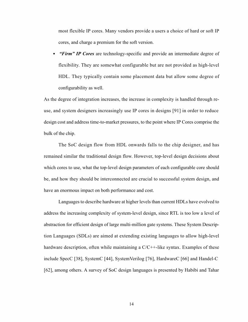
• The SystemC Kernel: an event-driven process scheduler that mimics the passage of
simulated time and allows parallel processes to synchronize and communicate in a
manner that is useful for modeling a system of hardware and software components.
The event-driven, rather than cycle-driven, nature of the simulation kernel allows
high simulation efficiency, since synchronization functions need not be invoked for
every clock cycle. The SystemC scheduler is non-preemptive, and is deterministic
with reference to events occurring and different simulation times. It is not determin-
istic with reference to events that occur at the same simulation time.
• Data Types: most of which are specifically designed to ease the modeling of
commonly used hardware primitives, such as 4-valued logic (0/1/X/Z), bit vectors,
finite-precision integers and fixed point types.
• Predefined Channels: representing the common communication types. These
include clocks, signals, FIFOs, mutexes, semaphores etc.
• Utilities: providing common reporting, tracing and debugging functionality.
• Specialized libraries: Other task-specific libraries built on top of SystemC, such as
the SystemC Verification (SCV) Library, the SystemC Transaction-Level Modeling
(TLM) library, and many bus models.
SystemC provides support for multiple levels of abstraction, going from RTL-like
cycle-accurate simulation to pure functional simulation (i.e. no timing) and a variety of
highly useful intermediate levels of abstraction [17].
21
3. Power
3.1 Power Dissipation
Power Dissipation for CMOS VLSI integrated circuits is dominated by substrate power
dissipation, which is the power dissipated in the active devices, rather than by energy losses
in the interconnect. Total power dissipation consists of dynamic, static and short-circuit
components.
The dynamic power (often also referred to as switching power) is the power
dissipated while charging and discharging the capacitive load at the outputs of each CMOS
logic cell whenever a transition occurs. Historically, the dynamic power has been the
dominant component of power dissipation. It can be expressed as:
(EQ 2.1)
Where
• α is the average number of output transitions in each clock period. α is usually less
than 1, and so is often also defined as the probability of an output transition in a
clock period.
• f is the clock frequency.
• Cl is the load capacitance.
The Static Power dissipation is the power used by on-chip constant-current sources, and
the leakage current, with the latter dominating. The three main components of leakage
current are the subthreshold leakage current, the reverse-biased junction leakage current,
Pdynamic12--- αfVdd
2 Cl⋅=
22
and the gate-direct tunneling leakage, with the subthreshold leakage current being the
largest of these. According to the BSIM3v3.2 MOSFET model [55, 74], off-state (Vds =
VDD, Vgs = 0) subthreshold leakage current can be expressed as:
(EQ 2.2)
where
• ktech is a transistor geometry and CMOS technology dependent parameter
• W and L are the transistor width and length
• VT denotes the device threshold voltage
• S (the subthreshold swing parameter) is the subthreshold voltage decrease required
to increase Isub by a factor of ten.
Here, S is given by:
(EQ 2.3)
where
• n≥1 is a device-dependent parameter
• kB is the Boltzmann’s constant
• T denotes the temperature in Kelvin
• q is the electron charge.
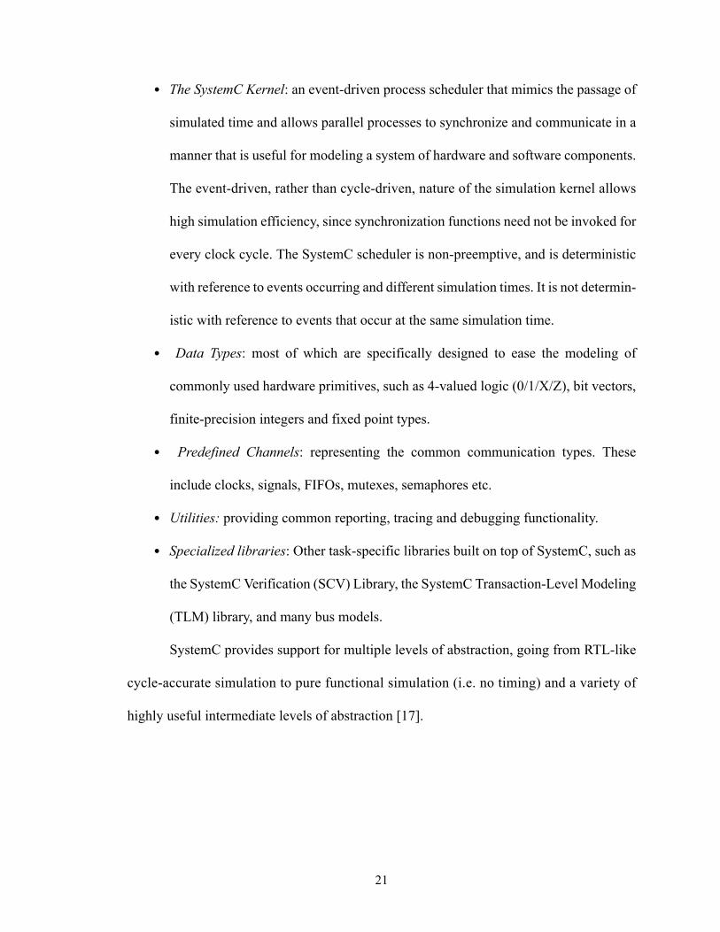
Typical values of S are 70-90mV/decade for bulk CMOS devices. In general, the tempera-
ture sensitivity of Isub is 8-12x/100ºC [74].
Figure 2.2 illustrates these trends in subthreshold leakage and total power as a
function of substrate temperature.
Isub ktechWL-----⎝ ⎠
⎛ ⎞ 10
VT
S------–
=
S 2.3nkbT q⁄=
23
Figure 2.2. Subthreshold Leakage Trends.(a) Subthreshold Leakage Current (Isub(Vgs=0))trends as a function of substrate temperature.(b) Total Die Power as a function of substrate temperature.The above figures were taken from work published by Pedram and Nazarian [74], where theywere published courtesy Vivek De, Intel.
(a)
(b)
24
3.2 Microprocessor Power Estimation
A large amount of research has been done on microarchitectural power analysis, especially
for microprocessors. Wattch [15] is a widely-used tool built on the SimpleScalar [4]
framework that allows power analysis and simulation of microprocessors. It uses
capacitance-based analytical power models of regular structures in the processor such as
arrays, buses, register files and caches to build up a picture of overall power consumption.
XTREM [30] is a microarchitectural power model of the XScale [73] based on Sim-XScale,
which is in part derived from ARM-SimpleScalar. It uses an approach similar to Wattch to
model microarchitectural power. XTREM is not publicly available at the time of writing.
Powell and Chau [75] describe the Power Factor Analysis (PFA) technique, which
assigns a fixed activity factor to each functional unit inside the processor, and assumes that
this does not depend on input signals to the unit. Landman and Rabaey [59, 60, 61] extend
this with more powerful statistical tools and allow the power consumption to be a function
of the incoming data. They aim at empirically creating statistical power models of
functional units, and making power predictions based on certain assumptions about the
statistical properties of the inputs. A similar powerful statistical approach is also proposed
by Marculescu et. al. [65] who use information theory to create short input sequences that
have the same statistical properties as much larger ones, thus allowing for faster analysis.
Although these techniques have been applied in large part to processors and DSPs, they are
applicable to digital hardware in general.
Chen, Irwin and Bajwa [22] describe a methodology for microarchitectural power
estimation and design space exploration based on having a lookup table for each functional
unit that maps input signals transitions to power consumption. They also describe a
25
technique for reducing the size of the ensuing tables, to prevent them from being combina-
torially large. However, the level of detail required for accurate modeling makes this
approach slow, and they do not demonstrate its applicability on large benchmarks.
SimplePower [100], also based on SimpleScalar, allows the power models of functional
units to be either table-lookups (as described by Chen et. al. [22]) or analytical models.
SimplePower models the processor core, instruction and data caches, and the on-chip back-
end bus between the processor and caches. Intel’s Architecture-Level Power Simulator
(ALPS) [45] also takes a microarchitectural activity-based approach to power modeling,
and is also used to provide power data for subsequent thermal modeling.
While microarchitectural power analysis is aimed at optimizing processor configu-
ration for a set of input programs by predicting power, higher-level power models discard
fine-grained microarchitectural information to create a mapping between incoming instruc-
tions and power. Tiwari et. al. [88, 89] show how instruction-level power can be character-
ized from hardware measurements. Sinha et. al. [85] perform energy profiling of ARM
processors and also describe how leakage power can be estimated by plotting processor
power at various frequencies. Brandolese et. al. [14] propose a generic mathematical model
for 32-bit microprocessors which decomposes instructions into functionalities, allowing
for simpler instruction-level characterization and modeling of 32-bit microprocessors.
Chakrabarti and Gaitonde [20] present a simple instruction-level power model based on
dividing instructions into categories, and characterizing only representative instructions
from each category. Julien, Laurent et. al. study similar instruction-level power models for
DSPs [53]. However, they validate their approach only on extremely small programs, not
on realistic workloads. Sinevriotis et. al. study [84] low-power optimizations and instruc-
26
tion-level power models of a 3-stage ARM7 processor as well as a Motorola DSP56100
DSP. Zhang [101] and Baynes et. al. [6] create and use similar instruction-level power
models of the Motorola M-Core processor in order to study the power consumption of real-
time embedded operating systems.
All of these study in-order microprocessor cores, which are typical in embedded
systems because of their simplicity, predictability and high energy efficiency. However,
instruction-level power models of out-of-order, superscalar high-performance cores have
not been widely reported in literature. This is presumably because the added unpredictabil-
ity of the architecture, through the addition of re-order buffers and speculative execution,
decouples microarchitectural energetics from the incoming instruction stream.
Russell and Jacome [78], as well as Sinha and Chandrakasan [85] observe that the
power per instruction in embedded processors is a low-variance distribution, suggesting
that differences between energy consumption by different functional units are drowned out
by the activities common to many instructions. This supports the view that a highly
detailed fine-grained power model is only required if microarchitectural parameters within
the processor itself need to be tuned, or if extremely accurate power estimates are needed.
3.3 Power Estimation for Other Components
Power models for various kinds of DRAM are provided in technical notes by Micron
Technologies [67, 68]. These are de facto standard power models used for detailed power
modeling of commercial DRAM components. The fundamental aspects of RAM power are
discussed by Itoh et. al. [52]. Analytical power models of SRAM and caches are studied by
Kamble and Ghose [54]. The CACTI [82], and eCACTI [64] tools also provide accurate
27
static power estimates of caches and SRAM, and are thus widely used in both industry and
academia. We use CACTI 4.0 as a low-level static analysis tools for estimating the energy
consumption of various cache operations.
Some work has also been done in modeling peripheral power consumption.
Celebician, Rosing and Mooney [19] present simple analytical power models of system
components including an I/O controller, FLASH memory, audio CODEC and audio output.
Cheng and Pedram [23] present power models of a backlit TFT-LCD display, and how
concurrent brightness-contrast scaling (CBCS) can be used to reduce power consumption
while reducing the associated degradation in image quality. Choi et. al. [27] and Gatti et. al.
[39] discuss system-level strategies for power optimization LCD display schemes. Both of
these use simple power models of the display to underpin their work. Givargis, Vahid and
Henkel [41, 43], present an instruction-based method for modeling peripheral cores, on the
lines of that used for instruction-level microprocessor power modeling, but much simpler.
They validate their results for a UART, a DMA controller and JPEG decode accelerator.
Fornaciari et. al. [34] present a microarchitectural approach based on the TOSCA
hardware-software co-design environment can be applied to a variety of embedded system
components, and even to a full control-oriented ASIC.
Bus power has also been studied in some detail. Fornaciari et. al. [35] present an
activity-based bus power model and use it to study the effect of bus encoding and cache
size on address and data bus power dissipation. Bona, Zaccaria and Zafalon [13] represent
one of the first attempts at integrating some power estimation into a SystemC design. They
describe how the Siemens’ STBus component was adapted to model bus power in a
SystemC model of a 4-way ARM multiprocessor system. Caldari, Conti et. al. [18]
28
describe a similar model for the AMBA AHB on-chip bus, as well as thoughts on how this
could be extended to other on-chip components or systems in general. Givargis and Henkel
[42] present generic mathematical cache and bus power models while Zhang, Irwin et. al.
[103, 104, 105] study on-chip interconnect and its power consumption. This field of
research provides the basis for the power models we use.
3.4 System Power Estimation
In contrast, system-level power simulation has been explored in relatively recently.
Simunic, Benini and De Micheli [83] present analytical power models for components of a
SmartBadge-type embedded system. They use a simplified power model of the ARM
processor, which estimates processor power as a simple function of voltage, frequency and
idle state (to take into accounted lower power consumption during cache misses). They
also describe such analytical power models for a DC/DC converter, on-board bus, caches
and memory, and were able to obtain accuracy within 5% of hardware on Dhrystone
benchmarks. Early work by Benini, Hodgson and Siegel [8] is based on modeling
components as simple state machines. Benini and de Micheli [9] also provide an overview
of software and hardware energy minimization approaches typically used by system
designers.
Bergamaschi and Jiang [10] present a technique that can be used to create a power
state machine for a system, provided that the power model for each component is also a
state machine. Bergamaschi et. al.’s SEAS (System for Early Analysis of SoCs) [11]
addresses power, along with floorplan and area estimates to enable designers to estimate
whether a proposed designs violate area or power budgets. They assume spreadsheet-like
or state-machine power models for the core.
29
Lajolo, Raghunandan, Dey and Lavagno [57, 58] argue that the complexity of
model components and software implies that all parts of the system must be simulated
together, and trace-based simulation can introduce inaccuracies. They simulate software
through macro-modeling, where an energy model is created for blocks of software as well
as hardware. High-level instruction set simulators simulate functionality, and low-level
RTL and gate-level simulators are invoked to calculate timing and energy. To speed up the
simulation speed, they use caching and sequence compaction techniques to minimize the
number of times low-level RTL energy estimating simulators have to be called. While they
too aim at simulation-based execution-driven power simulation, they differ from our work
in that they explore ways to tie together different simulators at run-time, while we propose
an integrated SDL-based approach that uses lower-level tools only for characterization.
SoftWatt [46] is a system power estimation tool based on SimOS [77]. It estimates
software power consumption by analyzing SimOS simulation traces and using simple
analytical power models. It can be used to capture the relative power contributions of the
user and kernel code, identify the power-hungry operating system services and characterize
the variance in kernel power profile with respect to workload.
Givargis and Vahid’s Platune [40] is a hardware-software co-design tool targeted at
tuning SoC design parameters by running small configurable kernels on a number of
different configurations to perform automatic design-space exploration. It is suitable for
finding the optimum parameters in a fixed system configuration with parameterizable
components.
30
Orion [93, 94, 95] addresses the issue of power-performance estimation on an
interconnection network to explore architectural trade-offs using Wattch-like microarchi-
tectural power models [15].
More recently, as system power estimation has become a greater issue, approaches
to full-system power estimation have emerged. Beltrame, Palermo, Sciuto, and Silvano [7]
describe a plug-in to the StepNP simulation platform [72] that enables power estimation for
multi-processor systems on a chip, although they do not describe details of simulation
speed or power accuracy achieved.
Talarico, Rosenblit, Malhotra and Stritter [87] present a framework where a
simulator is instrumented to produce traces that may be post-processed for power
estimation. While this approach is faster than gate-level power modeling, we believe that
the huge traces required and the time taken for post-processing limit its scalability and
speed. Our experiences show that trace post-processing is an inherently slow activity, since
it is almost entirely disk-bound. The results they present have runtimes of a few thousand
clock cycles, which is too little to validate full system-level workloads.
31
Another approach is described by Bansal, Lahiri, Raghunanthan and Chakradhar at
NEC Laboratories [5]. They propose a more sophisticated software architecture based on
power monitors, software plug-ins that monitor component activity at runtime to estimate
power. They also allow for different power models for the same component to be swapped
in and out at runtime, to minimize the computational overhead of power modeling. They
simulate a simple sample architecture in order to demonstrate that system power estimation
can be done without significant loss of accuracy. We use a similar software architecture,
albeit with a single power model for each component. However, we extend these power
Figure 2.3. System Power Estimation Framework proposed by Talarico et. al. [87]. The system relies heavily on execution traces of all components being studied.
32
models to account for temperature-dependent power dissipation, and chip-level thermal
behavior.
4. System-Level Modeling of MEMS and Heterogeneous SoCs
There has been relatively little work so far on modeling the behavior of non-digital SoC
components within standard SystemC frameworks. Bjornsen et. al. [12] describe using
SystemC to model the transient behavior of high-speed analog-to-digital converters. They
found SystemC to be an effective modeling tool, with simulation speeds significantly faster
than HDL. Zhang et. al. [102] compared Verilog, VHDL, C/C++ and SystemC as
candidates for modeling liquid flow in a microfluidic chemical handler, and found
SystemC to be the most suitable, since SystemC processes, events and modules are suitable
building blocks for expressing fluid flow in a manner analogous to dataflow.
We have published the first SystemC models of a MEMS-based SoC, the first
SystemC models of MEMS thermal behavior, techniques for improving simulation
efficiency, and a detailed case study of the application of this approach to a real heteroge-
Figure 2.4. Power Modeling System Architecture proposed by Bansal at. al. [5].This strategy is based on runtime power modeling rather than trace analysis.
33
neous SoC. The rest of this section provides background information on related work in
literature.
Attempts at generalized modeling of mixed-signal elements for large-scale
hardware design include VHDL-AMS [33] and Verilog-AMS [37], aimed at extending the
VHDL and Verilog language definitions to include analog and mixed-signal regimes.
These have been moderately successful for mixed-domain component modeling; however,
they are designed for implementation and end-of-design verification late in the design
flow, not for system-level design and verification. Effective system-level design involves
representing entire systems at high levels of abstraction and modeling them at high
simulation speeds. These requirements are not adequately met by HDL frameworks that
primarily target component-level design, creating the need for higher-level techniques and
tools that are more efficient at system-level design.
The SystemC 2.0 standard [51, 69] addresses purely digital simulation. However,
increasing on-chip heterogeneity has led to the demand for modeling both digital and non-
digital components within an integrated framework. Ongoing efforts such as SystemC-
AMS [90] and SEAMS [3] propose extensions to the SystemC language definition and
additions to the SystemC kernel to incorporate analog and mixed-signal devices into the
simulation framework. In contrast, the techniques and models presented in this paper use a
standard, unmodified SystemC kernel and library to model non-digital components, and
represent the first application of SystemC design to a MEMS SoC.
34
5. Thermal Issues
With process technologies reaching the nanometer region, chip power density has scaled
exponentially across process generations [80]. This has led to increasing die temperatures
in modern chips. The exponential dependence of subthreshold leakage power dissipation
on temperature aggravates this problem further, potentially affecting correctness of
operation, timing closure (and hence speed), as well as reducing reliability and operational
lifetime. In addition, the increasing demand for mobile systems has increased the need for
low-power designs.
A system or device reaches steady-state thermal equilibrium when the rate of heat
transfer out of the system equals the system’s net power dissipation. The three key
mechanisms involved in heat transfer are radiation, conduction and convection. Cooling
systems (heat sinks, heat spreaders, fans etc.) all focus on reducing peak temperatures by
increasing the rate of heat transfer. Radiation is the simplest heat transfer mode, involving
just a large exposed surface area for transferring heat to the surroundings, often using fins
on a heat sink to increase this surface area further. Conduction to the ambient surroundings
as well as to cooler nearby components is also achieved by heat sinks, heat spreaders etc.
Figure 2.5 shows a cross-sectional diagram of the mounting of a chip on a printed
circuit board. Heat transfer directly away from the chip is primarily conductive. A high-
conductivity thermal interface material fills surface imperfections to ensure efficient heat
transfer from the chip to the heat sink. Heat transfer away from the heat sink is primarily
radiative or convective, since air has a very low thermal conductivity (about four orders of
magnitude less than that of aluminum). A secondary heat transfer path also exists
downward through the package backing to the PCB. The PCB is in physical contact with
35
the surroundings, and can conduct heat away (for example, to a case). However, the
thermal conductivity along this path is significantly less than that along the primary heat
transfer path to the heat sink [97] because of the comparatively low-conductivity materials
used and the low cross-sectional area presented to lateral heat flow. In embedded systems,
weight/size considerations, as well as the lower dissipated power, neccessitate the use of
simple heat spreader (a simple, fin-less, metal sheet of the appropriate dimensions) to often
be used instead of the more efficient heat sink.
Conductive and radiative heat transfer can be improved through purely passive heat
transfer systems. However, improving convective-mode transfer usually requires an active
cooling solution, of which the CPU cooling solutions of fans and air vents are a common
example.
In the past, increasing system power consumption has been address by the use of
“bigger fans” as a downstream fix, but this solution is not scalable as power densities
increase while components occupy smaller and smaller areas. Further, active cooling
Heat Sink
Thermal Interface Material
Silicon Chip
Chip Pad Bonds
Ceramic Package Backing
Ball Grid Array
Printed Circuit Board
Figure 2.5. Cross-Sectional View of Chip and HeatSink Mounted on a PCB.The figure shows the typical mounting of a silicon chip and heat sink on a printed circuit board.The fins on the heat sink increase total surface area for better heat transfer outward, and athermal interface material (“thermal grease”) ensures a high thermal contact surface area, andthus better thermal conductivity, between the chip and the heat sink.
36
solutions are impractical for use in small form-factor mobile devices, such as smartphones
or GPS units. The cost of effective packaging and cooling also increases, since such
packages and cooling systems must be designed to address worst-case power dissipation
and ambient conditions. Dynamic Thermal Management (DTM) techniques [74], reduce
system performance at runtime before excessively high temperatures are reached, allowing
the system as a whole to be designed with lower worst-case parameters in mind. Such
DTM techniques may include “thermal throttling” (first used on the Pentium 4), where all
execution is stopped if the processor nears a thermally unsafe condition. Alternatively, the
Figure 2.6. A Simplified Equivalent Thermal Circuit For The Chip Mount.
Convection
Convection
Radiation
Radiation
Heat Sink
Conduction
Thermal Interface Material
Chip Junction
Chip Pad Connect and Underfill
Ceramic Package Backing
Ball Grid Array
Primary Heat Transfer Path
Secondary Heat Transfer Path
37
processor speed may simply be slowed down, or specific functional blocks disabled to
prevent overheating.
The rest of this section is organized as follows. Section 5.1 discusses the impact of
temperature on system design and performance parameters, such as leakage current,
performance characteristics, substrate thermal conductivity, reliability, signal integrity and
power/ground supply integrity. Section 5.2 provides an overview of various thermal and
power management techniques. Section 5.3 discusses various chip-level thermal modeling
techniques, such as thermal simulation, electrothermal simulation, and microarchitecture-
level thermal modeling.
5.1 Thermal Impact on Design and Performance Parameters
5.1.1 Impact of Temperature on Subthreshold Leakage Current
The subthreshold leakage power for a CMOS transistor is given by:
(EQ 2.4)
where
• µ is the mobility.
• Cox is the oxide capacitance.
• m is the body effect coefficient, and has a value in the range of 1.1 - 1.4.
• W is the channel width.
• L is the channel length.
• k is the Boltzmann constant.
• T is the temperature (in Kelvin).
• q is the electronic charge.
Isubthreshold µ T( )CoxWL-----⎝ ⎠
⎛ ⎞ m 1–( ) kTq
------⎝ ⎠⎛ ⎞ 2
eq Vg Vt T( )–( ) mkT⁄
1 eqVds– kT⁄
–( )=
38
• Vg is the gate voltage.
• Vt is the threshold voltage.
• Vds is the drain-source voltage.
The mobility and threshold voltage in the above equation are also temperature-dependent,
and their values are given by:
(EQ 2.5)
(EQ 2.6)
here, T0 is room temperature (300K), and κ is the threshold voltage temperature
coefficient, with a value around 0.7mV/K [56].
The decrease in threshold voltage and the increase in kT/q (on both of which the
current has exponential dependence) dominates the slight decrease in mobility with
temperature, and leads to an overall increase in the subthreshold leakage current that is
close to exponential.
As described earlier in the chapter, a more directly usable approximation is described
by Pedram et. al. [55, 74], based on the BSIM3v3.2 MOSFET model. The subthreshold
leakage of a transistor in the “off” state (Vds = VDD, Vgs = 0) can be expressed as:
(EQ 2.7)
where ktech is a transistor geometry and CMOS technology dependent parameter, W and L
are the transistor width and length, VT denotes the device threshold voltage and S (the
subthreshold swing parameter) is the subthreshold voltage decrease required to increase
Isub by a factor of ten. It is S=2.3nkBT/q where n≥1 is a device-dependent parameter, kB is
µ T( ) µ T0( ) TT0-----⎝ ⎠
⎛ ⎞ 1.5–=
Vt T( ) Vt T0( ) κ T T0–( )–=
Isub ktechWL-----⎝ ⎠
⎛ ⎞ 10
VT
S------–
=
39
the Boltzmann’s constant, T denotes the temperature in degrees Kelvin, and q is the
electron charge. Typical values of S are 70-90mV/decade for bulk CMOS devices. In
general, the temperature sensitivity of Isub is 8-12x/100ºC [74].
This gives us
(EQ 2.8)
where s is the temperature sensitivity of subthreshold leakage current mentioned above,
and Tk is temperature rise (not absolute temperature) over which this approximation is
valid. For example, in the above sensitivity values, s is 8-12 and Tk is 100ºC.
5.1.2 Impact of Temperature on Performance Characteristics
MOSFET performance parameters are also dependent on temperature. In particular, both
dynamic power dissipation and gate delay depend on the drain current, which is given by
the alpha-power law:
(EQ 2.9)
here K is a technology-specific constant, vsat is the saturation velocity and α is the velocity
saturation index, with a value of 1.0 – 2.0 in the deep submicron region. It is usually
assumed that the saturation region is in effect for almost the entire duration of a transition
[56]. As temperature increases, the saturation velocity decreases slightly, and is given by
(EQ 2.10)
Psub Psub0 s
T T0–Tk
--------------⋅=
ID KWvsat T( ) Vdd Vt T( )–( )α=
vsat T( ) vsat T0( ) η T T0–( )–=
40
where η is the saturation velocity temperature coefficient (typically around 120ms-1/K at in
a 70nm process). The saturation velocity dominates the temperature-dependence of drain
current at high supply voltages, and drain current drops as temperature increases. However
as the Vdd supply voltage drops closer to Vt, temperature-dependent changes in the (Vdd-
Vt(T))α term increase in significance to the point where they cancel out the saturate velocity
effects, and weaken the negative temperature sensitivity of drain current. At supply
voltages around 1.0 V, the temperature dependence of the drain current may even become
slightly positive [56].
5.1.3 Impact of Temperature on Thermal Conductivity
For detailed modeling, the impact of temperature on thermal conductivity may also be
taken into account. This is given by [2, 32]:
(EQ 2.11)
This nonlinearity is often accounted for by using Kirchoff transformations [2, 32] to find an
equivalent “apparent temperature”, that can then be solved linearly.
5.1.4 Impact of Temperature on Reliability
At high current densities, electromigration occurs in the metal interconnect. This the
gradual transport of material caused by momentum transfer between conducting electrons
and the metal atoms comprising the interconnect. The high current density can be thought
of as an “electron wind”, blowing metal atoms “downwind” to form “hillock” or “whisker”
κ T( )κ T0( )
1 D2.8 19×10---------------------+
------------------------------- TT0-----⎝ ⎠
⎛ ⎞43---–
=
41
structures, and leaving voids in the “upwind” direction. If unchecked, this can cause greatly
reduce circuit reliability by hastening its failure. The Mean Time To Failure (MTTF) is
given by Black’s equation [74]:
(EQ 2.12)
where:
• A is a process and geometry-dependent constant.
• J is the DC (average) current.
• n is 2 under normal conditions.
• Q is the activation energy for grain-boundary diffusion. Its value is ~0.7eV for Cu-
Al.
• k is the Boltzmann constant.
• T is the metal temperature.
The impact of current density and temperature alone on circuit reliability can then be
expressed as [74, 81]:
(EQ 2.13)
where Jmax(Tspec) is the maximum current density at the specification temperature, and
Jmax(Tjunc) is the updated current density based on the actual junction temperature based on
Equation 2.12 (Black’s equation). As temperature rises, the currents that can be safely
handled by the system grow successively smaller. In an SoC, the spatial and temporal local
maximum of the temperature can easily exceed the specification temperature, which
greatly lowers the limits on allowable current. If this is not taken into account, chip lifetime
A full-chip thermal model uses a lower-level power model that generates a power density
map, or power profile, which is a tabulation of the power density at each point on the chip.
For convenience, this map may be generated from, or expressed in terms of, the spatial
location, chip area, and net power consumed by each chip component at a given point of
time.
Several approaches have been proposed to perform thermal analysis. These differ
in the level of detail, the numerical techniques used, the heat sources that are modeled, and
the ability to handle various types of boundary conditions. Thermal modeling techniques
may be roughly classified into two categories [74].
The first set of techniques is based on the discretization of differential operators or
field strength. These techniques use numerical methods to solve the chip heat conduction
equations. The numerical methods used include finite difference methods [25, 32], finite
element methods [21, 99] and boundary-element methods [36]. These methods are highly
i C
R
v0
Figure 2.7. The Electrical Analogue Of A Simple Thermal System. The heat generated is modeled as a current source. The thermal capacity of the system ismodeled as a capacitor, and thermal resistance to the ambient conditions is modeled as anelectrical resistance. The ambient temperature is treated as a voltage source.
51
accurate and can handle a wide range of boundary conditions and heat sources. However,
this accuracy comes from their approach of dividing the system being studied into a very
large number of elements. The resulting thermal circuits are extremely large, resulting in
very slow simulation. Some techniques, such as 3-D thermal ADI [96, 97] and model order
reduction [28, 98] have been designed to overcome this shortcoming and lower the
computational cost of high-accuracy numerical solution.
The second category of thermal modeling techniques is based on Green function
formulation [24, 48, 92], which reduces the 3-D problem to a 2-D problem. These
techniques are less accurate, but are faster and simpler.
Figure 2.8. Full-Chip Thermal Modeling. This involves treating the entire chip as a distributed network of heat sources, capacitances andthermal resistances, formulating the solution as a set of differential equations, and solving fortemperature as a function of time.
52
5.3.2 Electrothermal Simulation
The thermal modeling techniques mentioned above can be extended to electrothermal
simulation, wherein the electrical behavior of the circuit is also modeled, and is used to
derive the power consumption values. Again, there are two major techniques used for
integrated electrothermal simulation.
In the first approach, also known as the direct method, the thermal problem is
directly transformed into the corresponding electrical circuit, and an electrical circuit
solver models both the thermal behavior and the actual electrical behavior. This approach is
used, for example, by Sabry et. al. [79].
The second approach, known as the relaxation method, uses separate electrical and
thermal simulators and iterates repeatedly, updating each simulator with the values from
the other at each iteration. This method is usually preferred, since it allows the use of
existing software packages designed for basic simulations and also allows the thermal and
electrical models for a system to be build independently. Its advantages included its
simplicity, however, it frequently fails to achieve convergence for very strongly coupled
problems, and is also unable to efficiently model changes that occur very rapidly.
The relaxation method and finite difference method are used by Cheng et. al. for
their ILLIADS-T electrothermal timing simulator [25]. Given the chip layout, the
packaging specification, and a periodic input signal pattern, the simulator models each gate
as a heat source to find the on-chip steady-state temperature profile and the resulting circuit
performance and reliability. Digele, Lindenkreuz and Kasper [32] also use this method,
additionally accounting for the temperature-dependence of thermal conductivity.
53
Akturk et. al. [2] propose a method for predicting the temperature profile of
complex ICs at a single-device resolution by mathematically linking full-chip heating with
non-isothermal device operation equations. The technique accounts for the application
specific activity levels by using a using a Monte Carlo methodology. They report the
results for a Pentium III chip, also show how these techniques may be extended to the
modeling of 3-D stacked ICs [1].
5.3.3 Microarchitecture-level Thermal Modeling
The approaches described above are highly accurate, but are not designed for modeling
bidirectional interactions between processor software and on-chip thermal behavior. In
particular, there is a need for designers to be able to predict thermal behavior early in the
design flow, well before layout.
A step in this direction is the increased use of microarchitectural simulators, such as
HotSpot [49]. These use a power dissipation data from microarchitectural power tools such
as Wattch [15] to model heat sources on the granularity of functional unit blocks, with each
functional block assumed to have a uniform power density.
Such simulators use a microarchitectural power modeling framework (such as
Wattch), which inputs power data into a thermal equation solver. Information from the
thermal equation solver can be fed back into the performance model (for example as data
sensed on a simulated temperature sensor). This allows designers to easily evaluate the
impact of Dynamic Temperature Management (DTM) and Dynamic Power Management
(DPM) approaches.
The usefulness of a high-level modeling methodology depends largely on its
simulation speed. Microarchitectural models use low spatial and thermal resolutions,
54
lumped RC networks, and often also use non-uniform grid sizes in order to reduce the
computational complexity thermal equation solving. The underlying premise is that
compact models early in the design flow are a useful tool, even if they have lower accuracy
than detailed device-level models.
Microarchitecture-level thermal modeling is the most closely related to our work
among the approaches discussed in this chapter. However, the microarchitectural power
modeling approach poses a problem for SoCs, since the microarchitecture of third-party IP
cores is often unknown to the system designer, and since even microarchitecture-level
modeling may be too detailed (and thus slow) for simulation of system-level workloads.
We leverage system-level, rather than microarchitectural, power and performance
modeling techniques to allow thermal analysis at higher levels of abstraction, provide high
simulation speeds, and to interoperate with the tools and methodologies that are used for
SoC design. In addition, we also quantify the impact of different spatial and temporal
granularities on accuracy and simulation speed. Further, we model additional effects, such
as the impact of temperature on substrate thermal conductivity, that are not addressed by
current microarchitecture-level tools. To do this, we restrict ourselves to a uniform-grid
thermal analysis of SoCs, since variable-grid analysis introduces complications in the
modeling of temperature-dependent substrate conductivity.
55
Chapter 3: High-Speed Power-Performance Co-Simulation for XScale-Based SoCs
1. Introduction
The XScale microprocessor core is an Intel implementation that is compliant with ARM
version 5TE and is the successor to the Intel StrongARM line of embedded microproces-
sors. The XScale is a 7/8 stage superpipelined 32-bit RISC core, with dynamic voltage and
frequency management, a MAC coprocessor for 16-bit SIMD (Single Instruction Multiple
Data) multiplication and a 40-bit accumulator [8]. Later versions of the XScale also
featured an integrated WMMX (Wireless MultiMedia eXtension) SIMD coprocessor [7].
The PXA series of XScale-based SoCs are application processors, widely used in high-end
mobile embedded devices such as smartphones, PDAs and portable media players. Other
XScale variants are used as IO, network or control plane processors in desktop/server
environments.
The PXA271 (Bulverde) studied in this section is an SoC that features an Intel
XScale Core, instruction and data caches, on-chip memory-mapped SRAM, a WMMX
coprocessor unit and a wide variety of on-chip controllers for various peripherals. Figure
3.1 shows the block diagram corresponding to PXA27X series of XScale-based application
processor SoCs.
Energy consumption, which directly impacts battery life, is a major design
constraint in this class of devices, making power models of such devices a valuable tool for
hardware/software co-design, workload analysis and system optimization. In this section
we experimentally characterize instruction-level power dissipation patterns for an XScale-
based PXA271 SoC, identifying many new effects to build the most detailed instruction-
56
level power models to date of any ARM-based processor, and also characterizing the
power dissipation patterns the WMMX SIMD co-processor, L1 caches, SDRAM and the
on-board address and data buses. We follow this up by building a generic framework for
fast execution-driven power-performance co-simulation within standard SystemC, and
expressing the experimentally obtained power models within this framework. Lastly, we
validate this approach by running large, realistic benchmarks and a commercial operating
system on an XScale-based test platform and comparing physical measurements of power
Figure 3.1. The Intel PXA27x Processor Block Diagram for a Typical System [7]. Note that block sizes do not correspond to actual die area occupied by components.
57
dissipation over realistic lengths of time (a complete Windows CE OS boot and application
run over billions of clock cycles) against those predicted by the SystemC simulation.
To the best of our knowledge, this is the first System Description Language (SDL)-
based approach to validate the accuracy of the power estimates obtained against physical
measurements from a real system. We are also the first to report power-enabled simulation
speeds over 1 million instructions per second (MIPS). The power modeling and character-
ization techniques we use here were applied to a SystemC-based simulation infrastructure
but are applicable to any execution-driven simulation framework. Our results indicate that
the power estimates obtained were accurate within 5% of physical measurements from
hardware, while the simulation speeds achieved consistently exceeded a Million Instruc-
tions Per Second (MIPS).
The contributions of the work presented here include:
• Detailed characterization results and power models of a variety of embedded
system components, including an accurate instruction-level power model of the
XScale processor.
• Realistic validation of a system-level execution-driven power modeling approach
against physical hardware.
• A scalable, efficient and validated methodology for incorporating fast, accurate
power modeling capabilities into system description languages such as SystemC.
Some of the work presented in this chapter has appeared in the proceedings of SPIE
(SPIE’05)[16] and been accepted for publication in the IEEE Transactions on Embedded
Computing Systems (TECS ‘07) [17].
58
2. Methodology
We divide the methodology into three sections: parameter extraction, in which the
components are characterized, performance modeling, in which a SystemC-based
performance simulation infrastructure is set up, and power modeling, where the
performance modeling framework is augmented with power modeling capabilities.
2.1 Stimulus-Based Parameter Extraction
In this section, we describe how system components can be characterized so that the high-
level power models reflect accurate information. We use short assembly programs (stimuli)
to characterize various components. A stimulus sets up the system into a predefined state
and runs a large number of instances of a short instruction sequence in a loop. For example,
the energy cost of a microprocessor instruction can be calculated by running a number of
instances of the instruction in a loop while measuring average power. To study more
complex effects, a sequence of several instructions can be replicated several times and
looped. The loop should be short enough to fit in the instruction cache (unless out-of-cache
effects are being studied) and long enough for the error due to the branch at the end of the
loop to have negligible impact on measurements [15]. Similarly, stimuli running repeated
cache misses or memory accesses can be used to easily measure the energy cost of each bus
transaction type. Stimuli for each component are based on its ISA or external interface, not
on its detailed microarchitecture, and so are fairly straightforward to create.
Using the method described, we ran various stimuli on hardware to obtain the
parameters for the power models. However, it must be stressed this approach is not limited
to post-silicon characterization, but can be used with any lower-level tool (including RTL
and microarchitectural descriptions) that can map an energy value to each stimulus. A wide
59
variety of RTL and micro-architectural power modeling tools exist, and stimuli can be run
on these instead of hardware to extract power model parameters (this approach is taken, for
example, by Givargis et. al. for peripheral cores [5, 6]). It must be noted that such tools are
not completely accurate, and their inaccuracies will be reflected in the final power
estimates when they are used for characterization instead of hardware. We characterize
directly with hardware to quantify how much additional inaccuracy is introduced by our
methodology and we find this to be well within 5%.
2.2 Performance Modeling
The platform we model is based on the XScale [8], a family of Intel microprocessors that
implement the ARM™ ISA, use deep pipelines and microarchitectural optimizations for
high performance, and feature a WMMX (Wireless MMX) SIMD co-processor. We use
Intel’s Xsim, a C-based cycle-count accurate performance simulator for the XScale family.
It models all XScale instructions, the L1 caches and the WMMX coprocessor. The fetch
and retire times of each instruction are computed by tracking dependencies and resource
constraints instead of detailed pipeline modeling. Xsim has been validated to be cycle-
accurate at instruction execution, and accurate within 2% of hardware on memory
accesses. We modified Xsim to enable its re-use as a modular SystemC component.
We use transaction-level SystemC models of SDRAM, SRAM and other system
modules. We create a transaction- level bus model to reflect the off-chip system bus. The
various memories (SDRAM, SRAM and Flash) are bound to identical address ranges on
the simulated platform and on actual hardware.
A complete SystemC-based platform simulation consistently reached execution
speeds between 1 and 1.2 MIPS, allowing us to complete a Windows CE boot and applica-
60
tion run in under 20 minutes. No appreciable slowdown was observed (at a measurement
accuracy of 2%) when power modeling capabilities were added1. This is to be expected,
since the computational overhead of the kind of high-level power modeling performed in
this case is typically very small (a member function invocation and a counter update each
time a component power model is invoked) compared to the computation involved in
decoding and executing a single processor instruction (which involves multiple nested
switch statements, bit manipulation, a variety of function calls, checks for special
conditions, register file and cache updates, checks for stalls and hazards, updating pipeline
state, managing timing information and possibly TLB and branch predictor lookups). The
overall execution speed is thus determined by the performance modeling, and power
modeling, if done at a sufficiently high level of abstraction, is not a bottleneck.
It must be noted that the high accuracy in terms of power consumption is due to the
detailed nature of the power models used, including the most detailed instruction-level
XScale/ARM power model to date. However, the gains in speed result from the high
transaction-level abstraction at which both power and performance were modeled.
1. Measured on a 2.8GHz Pentium 4 HT with 1GB of 400MHz DDR RAM. Disabling power modeling at
compile time changed the average execution time over 10 runs of a 1.25 billion instruction run from 1068 to
1059 seconds (0.8%). The maximum variation of individual runs from the mean (due to random latencies,
background processes etc.) was 21 seconds in each case (1.87%).
61
2.3 Software Architecture for Power Models
At the most fundamental level, the purpose of a component's power model is to monitor
component activity in order to track its energy consumption. We separate out activity
monitoring, which is highly component-specific, from energy accounting and reporting,
which can be standardized across all power models.
While the implementation of this is not complex, we found that the robustness and
re-use achieved through this approach considerably simplified both the creation of power
models and the top-down data gathering required for power analysis. No changes in the
SystemC kernel were required and the power-enabled components fit directly into the
existing framework. In addition, the fact that the power model of each component exposes
a standard interface to the rest of the system simplifies component-independent power
analysis operations (such as sorting all components by average power consumption,
finding components with the maximum variation in power etc.). We outline some of salient
details that illustrate its general applicability.
62
2.3.1 Interfaces
Each performance model uses a component-specific interface (the Component Power
Hooks) to transfer power- specific information to the corresponding power model, which
computes the energy involved based on this information. However, rather than having a
separate energy accounting and reporting scheme for each component, a generic Power
Model Interface provides a standard definition and implementation of these. This is seen in
Figure 3.2.
Component Power Hooks: These are a small set of functions exposed by the
power model and called by the component (the performance model) when it has power-
relevant information (such as information about the current transaction). The XScale
power model exposes functions such as gotInstruction(), gotCacheAccess() etc. The
information needed by the power model is passed as parameters to these functions. For
example, the performance model passes the cache access type and number of bytes
Figure 3.2. Proposed Software Structures for SystemC Power Modeling. The hooks for communication between performance and power models are component-specific, while the Power Model Interface is standardized.
63
accessed as parameters to gotCacheAccess(), which causes the power model to calculate
the incremental energy consumed and update its state accordingly. The component power
hooks are tightly coupled to functionality, and each component can have a different set of
these.
Power Model Interface: This is a common interface implemented by all power
models. We implement this as a generic power model class which defines default
implementations of all functions and data structures required. It provides a set of public
functions to allow system-wide power data gathering and analysis (Table 1). In addition, it
also implements a set of protected functions and fields that maintain internal data structures
and energy accounting information. Power models extend this class, and do not have to
duplicate common functionality, thus creating a unified energy accounting structure and
freeing power models from having to implement individual energy accounting schemes.
2.3.2 Internal Data Structure
The total energy consumed by a component can often be further broken down into various
categories. SDRAM energy, for example, comprises read energy, write energy, activate
energy and power down energy. A single lumped “energy” counter would discard the fine
grained information that a power model can provide.
To address this, we broke down each component's energy consumption into various
contributors. Each contributor in a component was identified by a name, and had its own
energy counter. The data for each component's contributors was kept in an internal hash
table for fast lookup by name. The class that implemented the generic power model
interface performed all housekeeping and energy accounting tasks.
64
In hierarchical systems, sub-components can be mapped as contributors, and their
power models are queried for energy values when needed. This hierarchical structuring
enables system scalability, since it allows a top-level system power analysis or trace
generation scheme to study the system at various levels of granularity without having to be
aware of the details of each modeled component. Thus, low-level modules can be added,
subtracted or substituted without having to rewrite the top-level power data gathering
procedures (which only need to know about top-level modules). This is contrast to schemes
where each power model for each component in the system under study must be considered
separately since there is no hierarchical structure associated with the power models [2].
TABLE 3.1. Using the Power Model Interface. This table illustrates common operations such as obtaining a reference to acomponent’s power model, obtaining the total energy consumed, getting the energyconsumed for particular operations, updating the energy consumed, and manipulat-ing the power models of sub-components, if any.
Get power model of a component. component.getPM()
Get total energy consumed by a component.
component.getPM().getEnergy()
Get read energy consumed by SDRAM.
sdram.getPM().getEnergy(“read”)
Add 32nJ to SDRAM read energy(can only be called by a power model).
sdram.getPM().incrementEnergy(“read”, 32E-9)
Find out if the given contributor is a sub-component.
mem.getPM().isComponent(“sdram1”)
Get the power model of a sub-com-ponent
mem.getPM().getPM(“sdram1”)
65
All of these are implemented in the generic power model class, which manages
these data structures and exposes only simple function calls to the outside world (Table 1).
Note that in a hierarchical system (such as a memory sub-system), a contributor may itself
be a component and have its own power model.
3. Power Models
This section describes the power models used for the XScale microprocessor, its WMMX
SIMD co-processor, off-chip address and data buses, caches, SRAM and SDRAM. The
calibration data is also provided where appropriate.
3.1 The XScale Microprocessor
To model the Xscale processor, we used an instruction/event-based processor power model
based on earlier studies of microprocessor power consumption [12, 14, 15, 16]. Our
stimulus programs characterized the following energy effects:
• Leakage Power and Voltage-Frequency Scaling: The XScale processor provides
a large number of voltage/frequency settings. We ran a given stimulus at a fixed
voltage and varied the frequency, obtaining a linear plot, as shown in Figure 3.3.
Static power dissipation, which is largely leakage power, was estimated by
extending this curve to obtain power consumption at zero frequency [14]. Power
was then given by:
(EQ 3.1)
Where Pstatic and Pdynamic are the static and dynamic power consumption respec-
tively. Istatic is the static current consumed. CL is the load capacitance of the sys-
tem, f is the switching frequency, and Vdd is power supply voltage.
P Pstatic Pdynamic= VIstatic12---CLfVdd
2+ +=
66
• Low-Power States: We also characterized power consumption of the processor in
various low-power modes such as idle, deep idle, standby, sleep and deep sleep [8].
The power corresponding to each mode is shown in Table 3.2.
• Instruction Opcode: Based on functionality, we divided the instructions into 11
different types (add, load etc.), in a manner similar to that used by Sinha et. al. [14].
TABLE 3.2. Observed XScale power dissipation in various low-power modes.
Power Mode Average Power Dissipation (mW)
idle (@416MHz) 130.54
deep idle (@13Mhz) 13.91
standby 3.45
sleep 0.15
deep sleep 0.09
50 100 150 200 250 300 350 400 4500
25
50
75
100
125
150
175
200
225
250
275
300
325
Core Frequency(MHz)
Pow
er D
issi
patio
n (m
W)
Figure 3.3. Finding Static Power Dissipation and Frequency Scaling Factor for the XScale. A large number of “add” instructions were run in a loop at a fixed voltage of 1.3V, and thefrequency was varied linearly to obtain a power-frequency plot. The y intercept (72.36mW)reflects static power dissipation, which is mostly due to leakage power. The slope of the graphwas then used to calculate CL.
Pow
er D
issi
patio
n(m
W)
67
Each energy cost was measured using straightforward stimuli running the same
instruction repeatedly with zero operands. The average power dissipation measured
while running a large number of identical instructions repeatedly in a loop ranged
from 304mW to 402mW, and is shown in Figure 3.4.
• Operand Value: The value of the operands affected the energy consumed to
execute an instruction. Energy was observed to increase roughly linearly with the
operand value and the number of “1”s in the operand [3, 13]. The additional energy
cost at 403MHz was observed to be approximately1mW for each bit set.
• Bypass Paths: A rather interesting pattern of bypass path behavior was observed,
with three different cases:
ADD AND B CMP LDR MOV MUL ORR STR SUB nop0
255075
100125150175200225250275300325350375400425
Instruction Type
Ave
rage
Pow
er D
issi
patio
n (m
W)
Figure 3.4. Relative Base Energy Costs of Various Instructions.These are shown in terms of average power dissipation at 403MHz.
68
(i) The base case is when there are no inter-instruction dependencies and all source
operands are obtained through register file reads.
(ii) When all source registers for an instruction are the destination registers for a
previous instruction, the source operands are obtained from bypass paths and 4%
less energy than the base case is used.
(iii) When both the bypass paths and the register file are used to get source oper-
ands, 5% more energy than the base case is used.
To the best of our knowledge, we are the first to characterize this effect.
• Sign Update and Conditional Flags: Instructions which updated or used the
conditional flags consumed more energy than instructions which did not. This
increase was under 0.5% and so it has not been made part of the power model.
add cmp mov mul orr0
255075
100125150175200225250275300325350375400
0123
Instruction
Pow
er D
issi
patio
n
Figure 3.5. Impact of Register Switching on Average Power Dissipation.Average Power Dissipation observed using stimuli is shown as a function of the number ofregisters switched for the five of the most common instruction types. A monotonic increase inpower dissipation is observed as the number of switched registers increases. All values aremeasured at 403MHz.
69
• Register Switching: When two consecutive instructions use different source or
destination registers, an energy overhead is incurred depending upon the number of
registers switched. As seen in Figure 3.5, this can exceed 10% of the total instruc-
tion energy and can be expected to be incurred often. To the best of our knowledge,
we are the first to characterize this effect.
• Cache Accesses: Caches are modeled as on-chip SRAM. From the instruction-set
point of view, the energy cost of a load or store depends on the number of bytes
accessed. We characterize and model this. The difference between loads and stores
is included in the opcode energy cost mentioned earlier, and change in energy with
data cache access size shown in Figure 3.6 is included in the power model used.
• Shifts: The ARM instruction set allows the last operand of an instruction to be bit-
shifted by an immediate or a register value. This shift causes an additional result
byte half-word word double word0
50
100
150
200
250
300
350
400
450
500
550
loadstore
Cache Access Type
Ave
rage
Pow
er D
issi
patio
n
Figure 3.6. The Average Power Dissipation of Various Types of Data Cache Accesses. Larger accesses, such as double-word accesses, use slightly more energy. The y-axisplots the average power dissipation of a large number of such accesses runcontinuously (in a loop) at 403MHz.
70
latency of one cycle. Incremental energy costs for all shift types were modeled.
These costs, averaged over all instruction types, are summarized in Table 3.3.
• Stalls: Stalls can be divided into instruction stalls, which are due to inter-instruction
data dependencies, event stalls, such as stalls on a double-word load, branch stalls,
or the pipeline flush penalty, and memory stalls on accesses to external memory.
Energy costs of all stall types were characterized and modeled. The observed costs
of various stall types are listed in Table 3.4.
TABLE 3.3. Additional Power Dissipation due to shifts, using stimuli at 403MHz. These are values averaged over all instruction types.
Shift Type Average Additional Power Dissipation (mW)
shift by immediate value 15.82
shift by register value 63.33
Rotate Right Extended (RRX) 43.29
TABLE 3.4. Power dissipation during various stall types, shown here in terms of additional mW of power dissipated at 403 MHz.
Stall Type Power Dissipation (mW)
data dependency 360
event stall 452
branch stall 369
stall on external memory 330
71
3.2 The WMMX Co-Processor
The XScale processor family has an on-die ISA-mapped Wireless MMX coprocessor [11]
for fast SIMD processing. We divided the WMMX instructions into 17 types based on
functionality, in a manner similar to that for the main processor. Base costs for WMMX
instructions were characterized separately and built into the power model. The base costs
for each instruction type are shown in Figure 3.7. Additional effects for WMMX instruc-
tions were not characterized, since most workloads studied did not use a high number of
dynamic WMMX instructions.
3.3 Address and Data Buses
An off-chip system bus connected the processor to Flash ROM, SDRAM and various
peripherals on the platform. We characterized the power requirements of both the address
and data bus by using stimuli to drive specific sequences of values onto them. Bus energy
consumption in the nth bus clock cycle can be expressed as:
wunpckehuwwsubwsllw
wpackwuswor
wmulumwmov
wmaxuwwmaddu
wmacwldrw
wavg2hwandnwaligniwaccu
tmrctmia
0 50 100 150 200 250 300 350 400 450 500
Inst
ruct
ion
Type
Average Power Dissipation (mW)
Figure 3.7. Average Power Dissipation for various WMMX instruction types.The Core Frequency used is 403MHz.
72
(EQ 3.2)
Where C1 is a constant depending on bus capacitance, C0 is the energy cost of turning on
the bus driver I/O circuits, D is the data on the bus (including control bits) and H represents
the Hamming Distance between two binary numbers.
For each type of memory transaction (write, burst write, read line etc.), the exact
sequence of low-level operations involved is defined by the memory protocol and the
memory controller configuration. For example, for an 8-word read from a particular
memory address (a typical cache miss), the exact timings of row address and column
address strobe assertions as well as the row address, column address, activation time etc.
are known. The SystemC bus power model simply calculated these and assigned an energy
consumption to each incoming transaction rather than running a cycle-by-cycle simulation,
which would drastically affect simulation speed.
Note that the bus was driven by multiple power sources: the processor drove both
address and data buses, while the SDRAM consumed I/O power when it drove data onto
the data bus. We accounted for these appropriately.
We observed that the 3.3V (I/O) power supply consumed 62mW as a base cost. In
addition, each bit flipped on the address bus costed 291pJ, and each bit flipped on the data
bus costed 219pJ.
3.4 Caches and SRAM
We used an SRAM power model similar to that used in some previous work [1, 4, 9] to
model caches and on-chip memory-mapped SRAM. Energy consumption was modeled as:
(EQ 3.3)
En C1 H Dn Dn 1–,( )× C0+=
E NreadEread NwriteEwrite NidleEidle+ +=
73
Where N is the number of times each operation was performed and E is the energy cost of
that operation. The cache energy consumption was modeled in the XScale instruction-level
power model, with each kind of cache access (load or store, byte, half-word, word or
double-word) characterized and modeled separately. The cache energy consumption is
illustrated in Figure 3.6.
3.5 SDRAM
SDRAM power consumption can be divided into core power consumption (for the memory
elements) [10], and I/O power consumption (for driving data onto the data bus). We
characterized these using stimuli. We used the data bus power model to calculate SDRAM
I/O power consumption. The main elements of SDRAM core power are:
• Base Power Consumption (Pb): The average power consumed by SDRAM when
not accessed is the sum of the standby and average refresh power.
• Activation Power (Pact): The average power consumed when an SDRAM page is
active.
• Read or Write Power (Prw): The power consumed during each SDRAM read/
write operation. The values of read and write current for SDRAM are equal [10].
The observed values of these are noted in Table 3.5. SDRAM power was modeled in a
manner similar to the bus transactions. The low-level operations in each transaction are
defined by the bus protocol and memory controller. The SDRAM power model simply
used these to calculate the energy cost of each incoming transaction without having to run a
cycle-by-cycle simulation. For a given transaction, energy consumption is given by:
(EQ 3.4)Etransaction PbTb PactTact PrwTrw+ +=
74
Representing the power model at the transaction level, rather than at the cycle level, lowers
the computational overhead of power modeling, and contributes to simulation speedup.
4. Experimental Setup
For validation, we used a reference platform (Figure 3.8) featuring an XScale-based
PXA271 SoC that implemented an XScale processor, its WMMX coprocessor, L1 instruc-
tion and data caches (32KB each) and other system components [8]. The platform had
64MB on-board SDRAM, 32MB synchronous Flash and a variety of peripherals. The main
board was instrumented with 100mΩ resistors in series with the power supply on each
module, which enabled power measurements of individual components at a granularity
similar to that at which power is modeled.
We measured the power consumption over multiple channels simultaneously using
an NI-DaQ data acquisition card, sampling at up to 20KHz with a post-calibration accuracy
of µV. The voltage drop across each resistor was of the order of millivolts to tens of
millivolts. The instrumentation resistors used were 1% accurate. Post-processing of
acquired data was done using LabView virtual instruments.
TABLE 3.5. Observed SDRAM Power Parameters (at a memory bus speed of 91MHz)
Parameter Value (mW)
Pb 20
Pact 82
Prw 53
5±
75
The major contributors to power consumption were the XScale-based PXA271
SoC, the SDRAM memory, and the off-chip buses. The three power domains we measured
for validation are:
• Core Power: The 1.3V main power supply to the XScale- based PXA271 SoC. In
our configuration, it powers the XScale microprocessor core, L1 caches, WMMX
unit, clocks and on-chip interconnect.
• I/O Power: The 3.3V supply to the PXA271. It powers the on-chip memory
controller and I/O pads, including all off-chip buses. It also provides standby power
for on-chip components.
Figure 3.8. The Reference Platform Used for Physical Experiments. The XScale processor, the WMMX unit and the L1 caches are on the PXA271 SoC. The LogicAnalyzer connections allow bus signals and timing to be observed, while an array of powerinstrumentation resistors allows the power supply of each component to be studied separately.
76
• SDRAM Power: The 3.3V power supply common to the SDRAM (both SDRAM
core and I/O pads).
We compared the predicted and measured power for each domain separately. Processor
frequency was varied, while the memory controller ran the off-chip bus at 91MHz.
5. Results
For validation, we measured average power over long benchmark runs and compared it
with the power estimates obtained from simulation. We used Windows CE as the operating
system, and ran identical benchmarks on the hardware and the simulator. The simulator ran
a complete OS boot routine followed by the application. Each benchmark was run in a
loop, with average power measured physically on hardware over a period of one second
and compared with the estimate obtained from the simulator.
To validate our results, we used the following benchmarks:
• Autocorrelation and Huffman Decoding benchmarks from the EEMBC
benchmark suite.
• The Motion Estimation kernel from an h.264 video encoder.
• A video filter (vidsp) from an h.264 video decoder. We evaluated three versions of
this filter: plain C, hand- optimized assembly, and hand-optimized assembly with
(MatMul) benchmarks from SNU-RT benchmark suite from Seoul National
University.
Figure 3.9 (a) shows microprocessor core power consumption. We saw excellent
agreement between the measured and estimated power, with a worst-case error of 3.9% (for
77
vidsp C). As in earlier studies [12, 14], we observed a low variation in processor power at
a constant speed.
The power consumed by the I/O power supply is illustrated in Figure 3.9 (b). The
base power consumption when there was no I/O activity was 62mW. Activity such as bus
transactions consumed additional power. Large benchmarks with frequent memory
accesses, such as Huffman Decoding or FFT, stress the memory hierarchy, leading to
increased bus power consumption. Of the other benchmarks, only MatMul was cache-
bound. However, the large (32KB) cache size ensured that benchmarks with sufficient
cache locality displayed very sporadic bus traffic, hence consuming little bus power. For
example, the Motion Estimation benchmark uses an 800KB data set. However, it performs
significant computation on each block before fetching the next one, thus having low
average bus power dissipation. Figure 3.9(c) shows the power consumed by the on-board
SDRAM. The patterns observed were similar to those observed for XScale I/O, since the
bulk of bus transactions map to an SDRAM access. The SDRAM standby power was
28mW which corresponded closely to the sum of power-down active standby power and
average self-refresh power calculated from the component datasheet (31mW).
It is interesting to note that while physical hardware measurements can only reveal
the total power consumed by each component, detailed power modeling can expose a much
finer degree of detail. For example, Figure 3.10 shows the various components of core
power while running Huffman Decoding and FFT at 403MHz. Direct physical measure-
ments cannot resolve net power into these components.
We also studied power variation with core frequency. Figure 3.11 shows system
power consumption while running Huffman Decoding and FFT at various core speeds,
78
vidsp_wmmx
vidsp_asm
vidsp
motion_est
matmul
jfdct
fft
auto
huffde
0 25 50 75 100 125 150 175
I/O (3.3V) Power
MeasuredEstimated
Power(mW)
vidsp_wmmx
vidsp_asm
vidsp
motion_est
matmul
jfdct
fft
auto
huffde
350 375 400 425 450 475
Core (1.3V) Power
MeasuredEstimated
Power (mW)
Figure 3.9. Power Consumedby Various Power Domains at403 MHz. Note that Huffman Decodingand FFT generate the highestbus activity, thus consumingthe most SDRAM and I/Opower.
(a)
(b)
vidsp_wmmx
vidsp_asm
vidsp
motion_est
matmul
jfdct
fft
auto
huffde
0 25 50 75 100 125 150
SDRAM Power
Measured Estimated
Power(mW)
(c)
79
with bus frequency kept at 91MHz. Note that nonlinearities in I/O and SDRAM power are
correctly tracked (Figure 3.11(a)). These nonlinearities arise because Huffman Decoding
generates a very large amount of memory traffic. At high core speeds, the traffic is so high
that the SDRAM clock on the bus almost always on. As core speed falls, the bus traffic falls
linearly. Below a certain point, the time between transactions is sufficient for the SDRAM
clock on the bus to be turned off for significant amounts of time, leading to the further
lowering of power consumption at 91MHz. FFT (Figure 3.11(b)) does not display such
Figure 3.10. Contributors to Core Power Consumption.The values are for simulation runs of various benchmarks at 403MHz. In contrast to the finedetail visible here, hardware measurements can only measure the total power consumption.
Leakage 23.24%
opcode 14.92%
reg switching 6.13%L1 cache 22.51%
other 0.93%
stall 29.62%
shift/rotate 2.66%
huffde
Leakage 25.30%
opcode 12.36%
reg switching 6.12%L1 cache 23.56%
other 0.89%
stall 28.91%
shift/rotate 2.87%
fft
Leakage 23.43%
opcode 22.32%
reg switching 6.69%
L1 cache 26.78%
other 0.69%
stall 15.62%
shift/rotate 4.46%
jfdct
Leakage 23.19%
opcode 23.41%
reg switching 7.84%
L1 cache 28.16%
other 0.55%
stall 13.79%
shift/rotate 3.07%
matmul
80
high memory traffic, leading to a more linear plot. For other benchmarks, the bus traffic is
low and power consumption is mostly the base power consumption, which does not
decrease significantly as core speed is lowered.
For all benchmarks, the power estimates obtained were in excellent agreement with
physical measurements. While power consumption for each component varied by over a
Figure 3.11. System Power Consumption at Various Core Frequencies. Bus frequency is kept constant at 91MHz. Note that nonlinearities in I/O and SDRAM powerfor Huffman Decoding are correctly modeled.
factor of two over this frequency range, we tracked this accurately and obtained average
errors under 5% and worst-case errors under 10% for each component at all speeds.
6. Conclusion
Modeling at high levels of abstraction enables component re-use, top-down design and
rapid design space exploration. While languages such as SystemC provide valuable and
widely-accepted tools for high-speed high-level system performance modeling, there still
exists no standard strategy for high-speed system power modeling. In this study, we
defined a simulation-based methodology for extending system performance modeling
frameworks to also include power modeling. We demonstrated the use of this methodology
with a case study of a real, complex embedded system, comprising the Intel XScale
embedded microprocessor, its WMMX SIMD co-processor, L1 caches, SDRAM and the
on-board address and data buses. We described detailed power models for each of these
components and validated the system power estimates against physical measurements from
hardware, demonstrating that such frameworks enable designers to model both power and
performance at high speeds without sacrificing accuracy.
The power-enabled system simulator predicted power accurately across a variety of
applications, with the worst-case difference between estimated and measured power being
under 10%, and average error under 5%. Since the power models are implemented at a high
level of abstraction, they are extremely lightweight in terms of computation, and adding
them to existing performance models did appreciably affect simulation speed. The
simulation proceeded at speeds in excess of 1 MIPS, enabling us to run complete applica-
tions on a real-world operating system.
82
Chapter 4: Modeling Heterogeneous SoCs with SystemC:A Digital/MEMS Case Study
1. Introduction
Modern SoCs can incorporate not only digital but also analog and MEMS components on
the same silicon substrate. Extensive research has been done on analog and MEMS fabrica-
tion techniques, with the result that many such components can now be fabricated using
processes compatible with standard digital CMOS process technologies [4]. This gives
designers a new capability but raises a number of important questions. How are these non-
digital components to be modeled in system simulation? How is the software driving
heterogeneous components to be written, tested, debugged and optimized? To exploit the
wide range of components and perform hardware-software co-design and validation, the
high-level models used must accurately represent all SoC components.
In practice, the requirement to model all SoC components faithfully can be relaxed
under certain circumstances — for example, if the communication between a non-digital
and a digital component is predominantly unidirectional or deterministic. During high-
level modeling, components such as pad drivers or clock generators can be abstracted away
conveniently and without significant loss of accuracy because they do not usually impact
high-level system behavior in complex ways.
However, this approach — abstracting away non-digital behavior entirely —
becomes invalid when there is feedback in the system, such as in the case of microproces-
sors running control programs that interact with analog or MEMS sensors and actuators.
Components with complex time-dependent behavior cannot be abstracted away because
the behavior of the digital system can depend on both time and the state of the non-digital
83
component. Unfortunately, current high-level SoC design tools, such as SystemC, are
design to model only digital components.
There is thus a gap between the high-level event-driven simulation methodology
used by the SoC designer and the FEM, SPICE or MATLAB-based differential-equation-
solving approach used for design and analysis of non-digital components. Accurate
modeling of feedback systems containing heterogeneous components requires bridging
this gap. The alternative — waiting for a hardware prototype before performing software
development and verification — is undesirable for reasons of cost, complexity and time-to-
market. Current design flows demand that the complete system be modeled, tested,
debugged and verified well before the expensive fabrication stage, where design modifica-
tion costs become prohibitive.
This chapter presents an approach for modeling the functionality, performance,
power, and thermal behavior of a complex class of non-digital components — MEMS
microhotplate-based gas sensors — within a SystemC design framework. The components
modeled include both the digital components (such as microprocessors, busses and
memory) and the MEMS devices comprising a gas sensor SoC.
The contributions made in this work include the first SystemC models of a MEMS-
based SoC and the first SystemC models of MEMS thermal behavior, as well as techniques
for significantly improving simulation speed. Towards demonstrating the effectiveness of
these techniques, a detailed case study of the application of the proposed approach to a real
heterogeneous SoC is also presented, providing some insights on how device-level design
decisions can have system-level impact, and how such issues can be studied and addressed
through integrated full-system modeling.
84
The rest of this chapter is organized as follows: Section 2 describes the operation
and architecture of the MEMS Gas Sensor SoC, Section 3 discusses the methodology used
for the characterization and modeling of system components, Section 4 illustrates some of
the results and insights that can be obtained using integrated SoC simulation, and section
Section 5 presents conclusions and directions for future work.
Some of the work presented in this chapter was also published in CASES’06 [10].
2. The MEMS Gas Sensor SoC
A microhotplate-based gas sensor exploits temperature-dependent conductivity variations
in certain thin films to facilitate the detection of trace gases in the ambient atmosphere. The
MEMS gas sensor SoC presented here integrates an array of such sensors with on-chip
digital circuitry to enable programmable control and data gathering. This SoC incorporates
a wide range of components: a MEMS microhotplate-based gas sensor array, an 8051
microcontroller, and on-chip interconnect and peripherals. In such a system, one of the
design challenges is posed by the heterogeneity of the components involved: issues
regarding analog, digital and MEMS design all need to be understood and taken into
account. The following sections describe SoC design and operation, with Section 2.1
presenting the structure and operation of microhotplate-based gas sensors, and Section 2.2
describing overall SoC topology and system architecture.
2.1 The MEMS Microhotplate-Based Gas Sensor
The conductance of certain metal oxide films varies with the temperature, concentration,
and type of gas molecules adsorbed into the film. Conductance-type gas microsensors use a
MEMS microhotplate device to vary the temperature of the thin film to facilitate the
85
detection of trace gases in the environment. Monolithic integrated gas sensors have
numerous possible applications such as detecting food product freshness, detecting toxin
leakage in chemical facilities, or identifying hazardous chemical agents in public places.
A microhotplate is a MEMS device used to obtain high temperatures over a
localized area on a silicon chip. Bulk micromachining techniques [4] can physically and
thermally isolate the heating elements from the underlying silicon substrate, allowing
surface temperatures as high as 450ºC to be reached. Such structures feature low power
dissipation, low fabrication cost, and scalability to different process technologies, making
them suitable for use in chemical microsensors [3] or as microscopic infrared sources [8].
Recent advances in MEMS fabrication have allowed these to be scalably
implemented with standard CMOS-compatible foundry processes, enabling designers to
integrate MEMS gas sensors, analog components, and digital components into a single
SoC [3, 4]. The microhotplate’s small size facilitates building the on-chip sensor arrays
needed for gas classification in complex sensing environments.
Structural Components A microhotplate-based gas sensor consists of a central
platform supported at each corner by a cantilever joining it to the substrate, as illustrated in
Figure 4.1(a). The material immediately below and around the platform is etched away in a
single postprocessing step, which physically and thermally isolates it from the substrate.
The central structure of the microhotplate is physically suspended over empty space, with
only the cantilevers at the corners providing mechanical support.
Electrical Components Electrically, a microhotplate-based gas sensor comprises
three major components, shown in Figure (a): a polysilicon heater, a temperature sensor,
and a thin film gas sensor. The cross-section of the microhotplate in Figure 4.1(b)
86
Figure 4.1. The Design of a MEMS Microhotplate based Gas Sensor.(a) Scanning Electron Microscope (SEM) micrograph of a microhotplate, showing it suspendedabove the underlying substrate. Cantilever supports at the corners provide structural support and electrical pathways. The goldelectrodes, between which the thin sensor film is deposited, are also visible. The microhotplate isfabricated with a standard digital CMOS foundry process, followed by an etching step to suspendthe microstructure and chemical vapor deposition of the metal oxide thin film.
(b) Cross-section of the suspended microhotplate. The figure shows the polysilicon heater, the Al temperature sensor, the metal oxide sensing filmand the insulating SiO2 layers. Cantilever supports are not shown.
(b)
(a)
87
illustrates their physical implementation as conductive layers separated by insulating
silicon oxide layers. A description of each component follows:
• Polysilicon Heater: Implemented as a serpentine resistor, this generates heat to
raise microhotplate temperature. The heater current or voltage may be controlled.
Note that the electrical resistance of a polysilicon heater is not constant and changes
linearly with temperature within the range of operation.
• Temperature Sensor: Implemented in an Aluminum or Polysilicon layer with a
known temperature coefficient of resistance (TCR). A small constant current is
passed through this, and the voltage drop across it is used to measure microhotplate
surface temperature.
• Gas Sensor Film: A thin film of tin or titanium oxide (SnO2 or TiO2) is deposited
between two gold electrodes onto the top surface of the microhotplate, exposed to
the external atmosphere. The thin film conductivity changes when specific
molecules are adsorbed into it. The observed conductivity patterns depend on the
temperature, concentration and type of adsorbed molecules, giving molecules a
signature pattern that facilitates chemical detection. Since different thin films
interact differently with gas molecules [4], individual elements in a microhotplate
array may differ in the type of sensor film used to improve sensing ability.
A microsensor array can be encapsulated behind a digital-only interface as illustrated in
Figure (b), facilitating integration into high-level digital SoC designs. A digital-to-analog
converter (DAC) drives the polysilicon heater current and an ADC senses the voltage drop
88
(b)
Figure 4.2. MEMS Microhotplate Gas Sensor Schematics.
(a) Schematic showing the electrical components of the microhotplate-based gas sensor.
(b) Schematic illustrating digital encapsulation of a sensor array using an ADC/DAC array andmultiplexing. A Digital Gain Control (DGC) register may be used to improve accuracy anddynamic range.
(a)
R
egis
ter
Amp 1 DAC nDAC 1
DAC nDAC n Amp n
R
egis
ter
ADC MUX
...
ADC MUX Amp
Register Register Register
DGC
Sensor 1
Sensor n
89
across the temperature sensor. Multiplexing circuitry enables the use of a single ADC, thus
reducing the chip area required for implementation. The ADC and DAC are connected to
registers that can be memory-mapped to a system bus via control circuitry.
2.2 System Architecture
The system topology for the integrated MEMS gas sensor SoC is illustrated in Figure 4.3. It
consists of a microhotplate array, an 8051 microcontroller, and on-chip interconnect. The
8051 supports a single-master on-chip Special Function Register (SFR) bus, to which the
gas sensor array is connected, allowing programs to access the microhotplate array via
memory-mapped I/O.
A high-speed cycle-accurate SystemC model of the microcontroller was created to
facilitate hardware-software development and testing. The HDL implementation of the
Figure 4.3. System Topology For The Integrated Gas Sensor SoC. A gas sensor array is connected to ADC/DAC and multiplexing circuitry, whichcommunicates with the microcontroller over an on-chip bus.
On-chip Processing Element:8051 Micro-controller
RAM
ROM Serial Port
Real-time Timers
MEMS Gas Sensor Array
ADC/DAC blocks
Off-chipMemory
Bus
PeripheralCommunicationBus (SFR bus)
TemperatureGas Sensor ReadingHotplate Current SelectSensor Element Select
90
microcontroller was synthesized from a commercially available 8051 IP core. The primary
functions of the microcontroller software include controlling each microhotplate,
maintaining the appropriate surface temperature, and collecting gas sensor data. A control
algorithm monitors the temperature sensor reading and varies the heater current to
converge rapidly and stabilize at the required surface temperature. Gas sensor conductivity
readings are quickly taken at each temperature. This last activity is simple timed data-
gathering, with no feedback loop involved. The gathered data may be processed on-chip or
transmitted by the SoC to a central location for remote analysis.
3. Methodology
There were many challenges inherent in the integrated modeling of a heterogeneous SoC.
First, microhotplate behavior is dependent not just on electrical parameters but also on the
heating and cooling of the microstructure. This was addressed by setting up a lumped
parameter model that correctly models the coupling between power dissipation, heating,
and the electrical resistance of the heater. Even when this was done, a problem was posed
by the fact that the behavior of analog and MEMS components is best represented by
differential equations, not by the discrete-time event-based state machines used for digital
simulation in SystemC. This was solved by expressing microhotplate behavior in discrete
time, so that numerical methods could be applied, and then integrating this efficiently into
SystemC’s network-of-communicating-processes model of computation. In addition, the
values of the various simulation parameters must be known to enable accurate system
modeling.
There are thus four major issues that need to be addressed: modeling the MEMS
microhotplates, integrating these models with SystemC, improving simulation efficiency,
91
and obtaining the values of various component parameters. The remainder of this section
discusses each of these in detail.
3.1 Electrical And Thermal Modeling Of MEMS Microhotplates
The work presented in this dissertation focuses on modeling the electrothermal aspects of
the microhotplate, not the electrochemical gas-sensing aspects of the metal oxide thin film.
A MEMS microhotplate can be modeled using a lumped analytical model incorporating the
following state variables:
• Polysilicon heater power dissipation (P).
• Microhotplate surface temperature (T), measured using temperature
sensor resistance.
• Ambient temperature (T0).
• Microhotplate thermal resistance (Rth).
• Microhotplate thermal capacitance (Cth)
• Polysilicon heater current (I), controlled by writing to a DAC register.
• Polysilicon heater electrical resistance (Re).
• Polysilicon heater temperature coefficient of resistance (TCR or α).
Of these Rth, Cth and α are treated as constant for a given microhotplate structure. System
behavior can be expressed as a set of differential equations in these variables. Second-order
effects in microhotplate behavior, such as the slight (less than 5%) variation of Rth with
temperature, are not currently modeled.
The thermal equation governing heat flow is:
(EQ 4.1)PT T0–( )
Rth-------------------- Cth
d T T0–( )dt
-----------------------+=
92
Where t represents time. The heater electrical power dissipation can be written simply as:
(EQ 4.2)
And the heater electrical resistance varies with temperature as:
(EQ 4.3)
Taking T' = T - T0, we use the above equations to obtain:
(EQ 4.4)
which is a first-order Ordinary Differential Equation (ODE).
Systems of differential equations are most commonly solved using numerical
methods, which have a wide range of applicability. However, the above equation is simple
enough to have an exact analytical solution. More complex systems, such as a collection of
distributed heat sources on a chip [5, 6], typically require numerical analysis. For this
study, we used the exact solution but, for purposes of completeness, also ran on the model
with the numerical solution to measure the effect on runtime. The two mechanisms produce
equivalent results, with the exact solution requiring less computation. Their impact on
simulation speed is discussed in Section 3.3.
The Euler Forward Method for numerically solving such ODEs involves using a
discrete-time representation of Equation 4.4 being used to derive microhotplate surface
temperature at time-step n+1 from the state variables at time-step n.
This computation can be performed at runtime with the microhotplate implemented as a
SystemC module with the parameters defined at instantiation. A SystemC process
calculates and updates the state variables at each time-step. Since a microhotplate has a
separate SystemC process, its time-step size can be varied independently of the time-step
size used for other system components. In this case, the microcontroller runs on a 10ns
time-step (a 100 MHz core clock frequency), while microhotplate simulation reaches
convergence at a 100µs or smaller time-step. This is because the thermal time constant of
the microhotplate (τ = RthCth) is typically of the order of milliseconds, and time-steps of τ/
10 or smaller tend to converge. Note that the time-step chosen must be sufficiently small to
ensure that the numerical solutions obtained are stable and convergent (the error increases
with the square of the time-step in Euler Forward Iteration), yet not so small that too much
simulation time is spent modeling the MEMS component, impeding system simulation.
An exact analytical solution to Equation 4.4 (in terms of Tn and tn) is given by:
(EQ 4.6)
This computation is performed in a similar manner at runtime. However, since this is an
exact solution, each time-step may be arbitrarily large without significant loss of accuracy.
The rest of this paper uses the exact solution unless otherwise specified.
T′n 1+ T′nea tn 1+ tn–( ) b e
a tn 1+ tn–( )1–( )
a-----------------------------------------
a
+
αIn2Re0 1 Rth⁄–
Cth---------------------------------------- b;
In2Re0Cth
---------------
=
= =
94
3.2 Integration with SystemC
A SystemC simulation consists of a hierarchical network of parallel processes that
exchange messages and concurrently update signal and variable values under the control of
a simulation kernel. Signal assignment statements do not affect the target signals
immediately, and the new values become effective only in the next simulation cycle. As
shown in Figure 4.4, the kernel resumes when all the processes become suspended, either
by executing a wait statement or upon reaching the last process statement. On resuming,
the kernel updates the signals and variables and suspends itself again while scheduled
processes resume execution. If the time of the next scheduled event is the current
simulation time, the processes execute a delta cycle, in which signal and variable values are
updated without incrementing the current time [7].
The microhotplate is modeled as a standard SystemC module. It does not require
any changes to the SystemC kernel or library, and it obeys standard SystemC simulation
semantics, running as a user-defined process. Each time it is invoked, the microhotplate
simulation process calculates the amount of time elapsed since the last update, solves the
system state equations accordingly, updates the state variables to reflect the new device
state and finally suspends execution until it is invoked again by the kernel.
Each microhotplate has standard SystemC port/channel connections to the rest of
the system. It communicates with actual microcontroller C programs compiled and loaded
into the SystemC model of the microcontroller, rather than with mathematical idealizations
of program behavior. In particular, system interrupts, computation time, microcontroller
CPU states, and the busses are all cycle-accurate representations of the hardware being
designed, validated against HDL simulations.
95
3.3 Simulation Efficiency
Effective design-space exploration depends on high simulation speeds, making simulation
efficiency a key design issue. This section explores three avenues for improving simulation
efficiency: using more efficient SystemC processes, reducing SystemC kernel synchroni-
zation overheads, and using exact solutions to reduce the computational overheads
involved in MEMS modeling. These provide a combined speedup of over 70x compared to
simulation done without these techniques.
SystemC provides two kinds of processes: SC_METHODS and SC_THREADS
[7]. The main difference in terms of simulation semantics is that an SC_THREAD’s state is
stored each time it is suspended and is restored each time it resumes, allowing local
Figure 4.4. The Execution Semantics Of Systemc. A number of interacting processes run until they end or execute a wait statement. Once allprocesses have run, the kernel updates all signals and variables before running readyprocesses again. The user can define specific conditions under which simulation should stop.
Simulation Start
Initialization
Process nProcess 1
All Processes Suspended
SystemCKernel
SimulationStopped
...
96
variable values to be preserved. A process resumes from the exact state it left on
suspension. Storing and restoring state across invocations has obvious simulation
overheads. SC_METHODs, on the other hand, are similar to function calls and restart from
the beginning each time they are invoked. No local state is preserved across invocations.
We found that storing required state as class data fields to allow the use of SC_METHODs
instead of SC_THREADs raised simulation speed from 56 KIPS (thousand instructions per
second) to 281 KIPS1.
Code profiling indicated that synchronization of the main CPU process with the
SystemC kernel at each suspend-resume was the performance bottleneck, since the
processor module incremented the elapsed time after each executed instruction in order to
be cycle-accurate. To eliminate this bottleneck, we used free-running simulation, where the
CPU continuously fetches and executes instructions while using an internal counter to keep
track of elapsed cycles. This continues until an event that requires synchronization with the
system occurs; events that trigger synchronization include interrupts, communication with
system components that have separate processes, and reaching a user-defined limit on the
maximum number of free-running cycles. When a synchronization event occurs, the
processor informs the SystemC kernel of the time elapsed since the last synchronization
(based on the internal counter that tracks elapsed cycles), updates any state required to
ensure complete synchronization, resets the internal counter, and continues execution.
1. All measurements of simulation speed were performed with a 1.6GHz Pentium M processor with 2MB of
L2 cache and 768MB of PC2700 DDR SDRAM. Compilation was done using gcc 3.4.4 with
-O2 compile-time flags.
97
A processor usually spends much of its time fetching and executing instructions
rather than communicating with other system components, so free-running simulation
provides an elegant method for reducing overheads while maintaining cycle-accuracy. An
upper bound can be put on the number of consecutive free-running cycles, causing regular
synchronization regardless of other activity. We found that allowing up to 100 free-running
cycles further sped up simulation from 281 KIPS to 2.89 MIPS. Allowing up to 4000 free-
running cycles further boosted simulation speed to 4.17 MIPS, after which further
increases led to no additional speedup. Profiling indicated that, after this optimization, the
simulator was spending time in instruction processing and microhotplate modeling, not in
synchronization.
Lastly, solving the differential equations governing microhotplate behavior also has
a computational overhead. For a microhotplate with nominal time constant of 1ms,
accurate modeling requires a time-step size smaller than 100µs while using the Euler
Forward Method. Other, more sophisticated, numerical methods may be used that allow
larger time-steps. Simulation efficiency is significantly higher when the exact analytic
solution to the system of equations is used, since it allows the use of arbitrarily large time-
steps without significant loss of accuracy. In practical terms, the microhotplate state only
needs to be updated when the processor writes to it to change the DAC input or reads from
it to find out the temperature, leading to lowered computational overheads. In the
simulation framework presented here, system modeling proceeds at 4.17 MIPS using the
exact solution and 3.71MIPS using the numerical solution (See section Section 3.1 for
details on the two approaches).
98
3.4 Component Characterization
For characterization, the 8051 microcontroller IP core was synthesized to TSMC 0.25µm
CMOS technology using Synopsys Design Compiler. Gate-level power simulation, with
SAIF back-annotation [9] of activity was performed using Synopsys Power Compiler.
Layout and back-annotation of delays and capacitance were performed using Tanner L-
Edit. The microcontroller has a simple two-state power model, consuming 4.4mW when
active (at 100MHz) and 0.25mW when idle. This state-machine based power model was
observed to be accurate within 5% of gate-level power simulation for all programs run.
The values of the critical thermal and electrical parameters for the microhotplate —
electrical resistance, temperature coefficient of resistance, thermal resistance and thermal
capacitance — were the nominal design parameters and were verified experimentally on
standalone hotplates fabricated through MOSIS, using the standard techniques described
by Afridi et. al. [2, 3, 4].
TABLE 4.1. Techniques for enhancing simulation efficiency, and their impact on performance. The exact analytical model for the microhotplates is used unless otherwise specified.
TechniqueSimulation speed (MIPS)
SC_THREAD only 0.056
SC_METHOD only 0.281
SC_METHOD with up to 100 free-running cycles 2.89
SC_METHOD with up to 4000 free-running cycles 4.17
SC_METHOD with up to 4000 free-running cycles (Numer-ical model)
3.71
99
4. Results
The ability to model the complete system in detail enables designers to find answers easily
and quickly to questions about overall system behavior. Such questions can range from
how a microhotplate responds to a given input to finding out whether a given piece of code
running on a microcontroller can meet desired performance parameters while controlling
one or more MEMS devices. This section first presents a validation of the SystemC
microhotplate model by comparing expected and observed behavior to a simple input.
Further, this section discusses the observed results when a given temperature controller
program is used to run a microhotplate and illustrates the kind of detailed observations that
can be drawn from this. Lastly, it provides an example of how full-system simulation can
help detect undesirable effects caused by valid low-level decisions that are suboptimal at
the system level.
4.1 Model Validation
Validation of the microhotplate model was performed by using a function generator to apply
a step voltage across a stand-alone microhotplate (implemented through MOSIS) and
comparing the experimental data obtained against the SystemC model of such a device.
Figure 4.5 shows such a comparison, and the high degree of correlation between simulation
and experimental behavior is clearly seen. The simulated peak temperature is about 3%
lower due to a small difference (caused by the slight temperature-dependence of thermal
resistance) between the simulated and observed values of Rth. Figure 4.5 also shows a
thermomicrograph sequence of a MEMS microhotplate heating up, illustrating the high
surface temperatures that can be attained over a localized area.
100
Figure 4.5. A Comparison Between Experimental And Simulated Microhotplate Behavior. A 2V voltage pulse is applied between 4 and 14ms. The observed changes in surface temperatureare compared against those predicted by simulation. The plot on the top is “noisier” and lesssharp simply because of the small, but unavoidable, experimental noise. The bottom strip showsa thermomicrograph sequence of a microhotplate structure heating up [1].
ºC
101
4.2 Simulation With a Controller Program
The above test provides crucial experimental validation for the microhotplate models used;
however, system designers need to know how the system as a whole behaves when
configured with a given topology and loaded with specific software. The results from
SystemC simulation enable total SoC power dissipation and microhotplate behavior to be
modeled in an integrated environment. This enables designers to observe the time-domain
behavior of the entire system when running specific software.
To illustrate this, a test C program implementing a simple proportional controller
was implemented, to control surface temperature in a single-microhotplate system. It was
given a setpoint of 380ºC for 20ms followed by a setpoint of 200ºC for a further 20ms, after
which the program turned the microhotplate off. This simplified program was chosen for
illustration here because it is representative of the control aspects of the software stack used
for microhotplate-based gas sensor applications.
Figure 4.6 illustrates the output of the simulation. The X axis represents system
time in milliseconds, while microhotplate temperature, power, and current, as well as
microcontroller power dissipation, are suitably scaled to be shown on the Y axis. The
results shown here are based on a SystemC simulation incorporating both the cycle-
accurate behavior of the microcontroller and the electrothermal behavior of the microhot-
plate. A discussion of the behavior of the four variables plotted follows.
The microhotplate heater current, directly controlled by the microcontroller,
changes step-wise, since it is incremented in discrete steps through a DAC. The microhot-
plate power dissipation changes step-wise when current changes and smoothly at other
times. It does not change in fixed size steps, since a) It is proportional to the square of the
102
current and b) It depends on the electrical resistance of the polysilicon heater, which
increases linearly with surface temperature. For example, between 3ms and 5ms, heater
current is constant, yet microhotplate power dissipation rises smoothly in a classic
asymptotic exponential curve. This is because the steadily increasing temperature raises
the electrical resistance of the polysilicon heater (Equation 4.3), leading to an increase in
power dissipation at a constant current. Note that the large change in microhotplate power
dissipation around 22ms corresponds to only a small variation in heater current, since they
are quadratically related.
Figure 4.6. An Example Illustrating The Use Of Integrated Functional, Power And ThermalModeling In A Heterogeneous System. The X axis represents system time in milliseconds, while other variables are suitably scaled tobe shown on the Y axis. A feedback loop, in the form of a proportional controller program, isloaded into the SystemC simulator and given a surface temperature setpoint of 380ºC for 20ms,followed by a setpoint of 200ºC for another 20ms, and finally turns the microhotplate off att=40ms.
0
50
100
150
200
250
300
350
400
450
0 5 10 15 20 25 30 35 40 45 50Time (ms)
SystemC Power Modeling of a MEMS Microhotplate-based SoC
Surface Temperature (ºC)
Microhotplate Power (mW) x 10
Microhotplate Current (mA) x 10
CPU Power (mW)) x 10
103
The microhotplate surface temperature changes smoothly, since the thermal
capacitance of the microhotplate causes the temperature to be continuous in time, always
varying smoothly. Around t=5 ms, the surface temperature first overshoots and then
undershoots the setpoint of 380ºC before settling at it. This overshoot-and-stabilize
behavior is typical of the proportional controller algorithm used. The same is true of the
undershoot at t=25 ms. At t=40ms, the controller sets the heater current to 0, immediately
dropping microhotplate power to 0. However, surface temperature follows a decaying
exponential as it cools off, finally stabilizing at 30ºC, since that was set as the ambient
room temperature in the simulation.
The “jagged” nature of the CPU power plot is due to the CPU waking up periodi-
cally in response to a timer interrupt, performing the computation required to run the
controller, sending control signals to the microhotplate DACs, and then going into a low-
power mode. The tiny “blips” in CPU power dissipation after t=40ms are due to interrupts
being processed, but in these instances no feedback control computations are performed,
leading to a much shorter active CPU duty cycle.
4.3 System-Level Effects of Low-Level Design Decisions
At the microhotplate design level, using a controlled-current or a controlled-voltage source
to drive the heater is an implementation detail, with circuit-level concerns typically
deciding the choice of one over the other. However, we found that such decisions could
significantly impact system-level behavior, with integrated SystemC modeling of the
MEMS device helping both to detect such behavior and to ensure optimal design.
In the previous example, a controlled current source was used to drive the
microhotplate heater. However, exploring the design space using SystemC indicated that
104
the behavior would be very different, exhibiting much less overshoot-undershoot behavior,
if the hotplates heaters were driven by a controlled voltage source rather than a controlled
current source. At first glance, this seems counter-intuitive, but it is borne out by the
SystemC simulation (see Figure 4.7).
The reason that this seemingly minor device-level design decision has broader
impact is that heater resistance increases with temperature, so power dissipation increases
with temperature at constant current; but at constant voltage, microhotplate power dissipa-
tion falls with increasing temperature (since P = I2R = V2/R). A current-driven microhot-
plate thus has a small implicit positive feedback effect: higher power dissipation drives
temperature up, which tends to cause a rise in power dissipation. A voltage-driven
microhotplate, on the other hand, has a small implicit negative feedback effect: higher
temperature causes higher heater resistance, which tends to reduce power dissipation.
These loops interact with the overriding feedback loop implemented in software.
Figure 4.7 shows system behavior for the same control program when heater
voltage, and not current, is directly controlled. The negative feedback loop leads to signifi-
cantly more stable behavior, with considerably smaller and fewer overshoots. Also note
that power decreases when voltage is constant and temperature is rising (around 7ms). This
is because the rising temperature raises microhotplate resistance, and the power dissipated
is inversely proportional to this resistance. The increased feedback stability was an easily-
overlooked factor that can now be used to guide system-level, component-level, and
software-level decisions for the SoC presented here. Unanticipated feedback behavior is a
serious issue, since, depending upon severity, it can lead to suboptimal performance or
105
oscillatory behavior and may neccessitate software fixes or even require the system to be
modified and re-fabricated.
Integrated simulation of both digital and MEMS components proved to be an
extremely useful tool in the hardware-software co-design for this SoC:
• Full-system simulation results were among the inputs in the decision to use voltage-
driven, rather than current-driven, microhotplates.
• Integrated simulations were used to assess system robustness while facing process
variations in device parameters.
• Running the software stack under realistic conditions enables more thorough
testing, leading to better defect detection before the system is fabricated.
Figure 4.7. Systemc Power And Thermal Modeling Of A Microhotplate Driven By Controlled-Voltage Source.A controlled-voltage source is used here, rather than a controlled-current source. This introducesa small inherent negative feedback loop, resulting in much more stable behavior, with muchsmaller overshoots and a faster settling time (compare with the overshoot-undershoot behavior inFigure 4.6).
0
50
100
150
200
250
300
350
400
450
0 5 10 15 20 25 30 35 40 45 50Time (ms)
SystemC Power Modeling of a MEMS Microhotplate-based SoC
Surface Temperature (ºC)
Microhotplate Power (mW) x 10
Microhotplate Voltage (V) x 40
CPU Power (mW)) x 10
Smal l e r
10
6
• Interrupt routines, timer settings, operating frequency, I/O and control algorithm
parameters can be better optimized when realistic simulation results are available.
In the absence of these, designers need to allow larger margins of error to account
for the uncertainty in the final performance of the system.
Complex system-level interactions, such as those illustrated above, need to be taken into
account by system, software, and component designers, and integrated modeling of both
microcontroller and MEMS device behavior in SystemC enabled precisely that.
5. Conclusion
This chapter describes an approach for modeling the functionality, power, performance and
thermal behavior of a complex class of MEMS components — MEMS microhotplate-
based gas sensors — within a standard SystemC design framework. The system
components modeled include both standard digital components (microprocessors, busses
and memory) and MEMS devices.
The contributions made in this work include the first SystemC models of a MEMS-
based SoC, the first modeling of MEMS thermal behavior in SystemC, techniques for
attaining significant (over 70x) improvement in simulation speed and a detailed case study
of the application of the proposed models and techniques to a real system. It also provides
insights on how device-level design decisions can have system-level impact, which can be
captured and addressed through accurate modeling of the entire system, including non-
digital components.
Future work will include more detailed hotplate models that include second-order
effects, analytical studies of microhotplate feedback behavior and application of the
presented techniques to other components of heterogeneous SoCs.
107
Chapter 5: Thermal Modeling1. Introduction
In previous chapters, we discussed techniques for modeling power consumption within
SystemC simulation frameworks, and how a differential equation solver could be
implemented within standard SystemC. In this chapter, we apply these techniques on a
much larger scale to solve the harder problem of full-chip thermal analysis for an SoC,
which necessitates the simultaneous solution of the thousands of differential equations that
govern chip-level heat flow. Here again, we make extensive use of numerical methods to
obtain solutions.
In this chapter, we describe a full-chip thermal modeling strategy for IP-core based
SoCs, validate it by comparing its output against lower-level tools and widely-published
datasets, design a large, complex SoC, and apply our integrated performance, power and
thermal modeling strategy to it in order to demonstrate the kind of powerful insights and
analysis such to tool facilitates.
We use an integrated execution-driven approach rather than a trace-driven one for
the following reasons:
• Execution traces generated by performance simulators are large, often many
gigabytes for each second of real time, which tends to make disk I/O and string
processing dominate simulation time, making overall simulation slow. Specialized
techniques are required to mitigate these overheads, such as dumping entire
structures to binary traces to avoid string parsing overheads, and precisely control-
ling the trace output to ensure that no unnecessary information is dumped. Direct
108
execution-driven simulation eliminates these overheads by processing all informa-
tion at runtime.
• Feedback behavior cannot be easily modeled in a trace-based simulation. A
performance or power trace is useless if the operating system is sensing chip
temperature and changing behavior based on the value sensed. In a traditional
trace-driven flow, functional information (CPU speed, cache miss rate etc.),
decides power dissipation, which in turn is an input to the thermal model. This
unidirectional flow of information cannot model feedback behavior, in cases such
as software-based thermal throttling. In execution-driven simulation, on the other
hand, the output of a thermal model can easily be made available to performance
and power models.
The rest of this chapter is organized as follows. Section 2 provides an overview of the
software structure used to facilitate efficient co-simulation. Section 3 describes the grid-
based thermal modeling strategy used. Section 4 presents a limit study on how spatial and
temporal granularity affect simulation speed and accuracy. Section 5 validates the thermal
modeling approach presented against widely-published lower-level thermal modeling
tools. Finally, Section 6 illustrates the power of the approach presented by applying it to an
example SoC, and demonstrating its use to evaluate the power, performance and thermal
impact of various implicit thermal feedback paths.
109
Figure 5.1. Overall Software Structure for Integrated Power, Performance and Thermal Co-Simulation.
SystemC Kernel
component performance
model
component performance
model
component performance
model
Performance ModelingLayer
component power model
component power model
component power model
Power Modeling Layer
Thermal Modeling Layer
Thermal Monitor Thread
Spatial Power
DistributionP(x, y)
Floorplan
Spatial Thermal
DistributionT(x, y)
Thermal Grid ODE
Solver
Component- Temperature
mapping
Simulated Temperature
Sensors
high-level activity
information
high-level activity
information
bus performance model
high-level activity
information
Operating SystemKernel
Applications/Tasks
Dynamic VoltageScaling
Dynamic Thermal
Management
System SoftwareStack
110
2. Software Structure
We used a three-tiered software structure, illustrated in Figure 5.1, to facilitate integrated
power, performance and thermal co-simulation. The first part is a standard SystemC
performance model of the system. This model is binary-compatible with hardware and can
run the entire system software stack and model timing. A traditional simulator is usually
restricted to this type of performance modeling.
We attached a power model to the performance model of each component, monitor-
ing activity and updating statistics on total energy consumed, average power etc., as
described in earlier chapters. The performance models communicate high-level activity
information to the power models, such as number of cache reads and writes, current CPU
frequency, number of stalls etc. These power models collectively form the power modeling
layer, which can be overlaid on top of the existing performance modeling layer, and
receives data unidirectionally from it.
The output of the power models, most notably the average power dissipations of
each component, are collected by a Thermal Monitor that orchestrates the activity of the
Thermal Modeling Layer. The Thermal Monitor is a full-fledged SystemC process, and
thus runs in parallel to the performance and power monitoring activity. It can be run at a
user-defined periodicity. At each invocation, it gathers power modeling information,
matches it against the chip floorplan to create a spatial power distribution (or power
profile) using the average power dissipation over one period, updates the Thermal Grid
ODE Solver with this power distribution, and runs the solver for one period, using a user-
defined timestep. Since lumped power models are used, each component is modeled as a
111
region of constant power density. Similar approaches are also used by lower-level thermal
modeling tools [1, 2, 6, 15, 16].
The Thermal Grid Solver solves the Ordinary Differential Equations (ODEs)
governing chip-level thermal diffusion based on the spatial power distribution, and
generates a spatial temperature distribution, mapping the present temperature of each point
on the grid. It also uses the floorplan to calculate the average temperature of each
component marked on the floorplan.
A major advantage of using a vertically-integrated execution-driven (rather than
trace-driven) approach is that we can now use this information to model the thermal
feedback in the system. There are two principal feedback paths in the system:
• Power Sensitivity to Temperature: The power dissipation characteristics of each
component in the system are assumed to be known in the discussion above.
However, many aspects of the power dissipation, notably leakage power dissipated
in caches, is a function of temperature. This represents a feedback relationship,
with power and temperature directly influencing each other. We model this
feedback path by calculating the temperature of each component, and keeping its
power model updated with this information.
• Temperature-based Changes in Functional Behavior: Dynamic Thermal
Management (DTM) techniques implemented in the system require input from a
on-chip temperature sensors. These may cause the system to drastically change its
behavior if the temperature has crossed some predetermined threshold, or if such a
condition is imminent, in order to prevent the temperature from exceeding the
maximum specified value. Since the spatial distribution of temperature for the
112
entire chip is known at the thermal modeling layer, this information can easily be
fed back to the simulated temperature sensors in the performance modeling layer.
This allows designers to evaluate the efficacy of different DTM strategies, the
impact of temperature sensor placement, and the impact of temperature sensors that
may differ in accuracy, time delay and so forth.
3. Grid-Based Thermal Modeling
For modeling the thermal behavior, we divide the chip into a uniform grid. Each square on
the grid is modeled as a lumped element, with a heat source at its centre and thermal
resistances connecting it to its neighbors, as well as to the top and bottom of the chip, as
shown in Figure .
The resulting circuit can be expressed equivalently as a large set of differential
equations. We use numerical methods similar to those described by Akturk et. al. [1, 2],
Figure 5.2. Using A Uniform Mesh To Define Thermal Grid Elements. The chip is overlaid with a uniform mesh of predefined spatial granularity, which divides the chipinto identical elements. A lumped thermal model of each element is then created, and joined to itsneighbors. The solution to the overall resulting system of ODEs is used to calculate the thermalbehavior, including the temperature of each grid element.
Silicon wafer with grid overlay
Individual grid element with equivalent circuit
113
Wang et. al. [15, 16] and Huang et. al. [6], but adapt them to the higher levels of abstraction
and speed associated with SoC simulation.
Simulation efficiency demands that the number of discrete timesteps taken and the
number of points on the chip considered for numerical analysis be kept as low as possible.
However, standard techniques such as second or forth-order Runge-Kutta methods
(common known as RK2 and RK4) require tight control of the step size, and may diverge if
the step sizes used are too large [12]. To avoid such problems, we trade off accuracy for
stability and use Euler Backward Iteration (EBI) [12], an implicit numerical method for
solving Ordinary Differential Equations (ODEs). While not as accurate as the RK2 or RK4
methods mentioned above at small step sizes, it has the advantage of being unconditionally
stable, and thus converging to the final value even at very large timesteps. In addition, the
specific systems we’re looking tend to exponentially converge to stable steady-state
temperature values except when there are large fluctuations in power dissipation. This
allows numerical errors to be bounded, further adding to the usability of the EBI method.
To implement EBI, we keep track of two temperature matrices (Tt(x, y) and Tt-1(x,
y)). These represent the temperature at each grid point at time steps t and t-1, respectively.
As an initial value boundary condition, all points on Tt-1are set to some predefined
temperature, typically the ambient temperature. At each subsequent timestep t, the value of
the temperature at each grid point at time t can be calculated from the temperatures of the
grid point itself, and of its neighbors, at time t-1, which is known. Additionally, the thermal
resistance between adjacent grid points is also known, as is the heat capacity of any given
grid point. At each timestep t, the updated temperature at each grid point can be expressed
as:
114
(EQ 5.1)
where:
• Tt(x, y) and Tt-1(x, y) are the temperatures in Kelvin at point (x, y) on the grid at time
steps t and t-1 respectively, as mentioned above.
• h is the length of each timestep, in seconds.
• C is the heat capacity of each grid point.
• pt-1(x, y) is the power dissipated by grid point (x, y) at time t-1 (in Watts).
• Tt-1, i is the temperature of the ith neighbor of the grid point (x, y) at time t-1. Each
grid point has six neighbors: four lateral neighbors that at grid points on the chip,
and two vertical neighbors that are the top and bottom chip surfaces.
• Ri,x,y is the thermal resistance between the grid point (x, y) and its ith neighbor.
Note that the temperature-dependence of thermal resistance can be easily taken into
account at runtime, because the substrate thermal conductivity at each grid point can be
easily updated at runtime based on its temperature at that point of time.
4. A Limit Study on Spatial and Temporal Granularity
Decomposing the chip into a uniform two-dimensional grid and incrementing the time in
discrete steps is a necessary step for the kind of numerical analysis mentioned above. The
values chosen for the spatial and temporal granularity (the size of each grid point and the
duration of each time step) can obviously have a large impact on both accuracy and
simulation speed. Rather than arbitrarily pick “acceptable” values, we perform a limit
study of the impact of spatial and temporal granularity on accuracy and speed.
To do this, we modeled a simple 130nm chip consisting of an OpenRISC processor
core and 4-way set-associative L1 instruction and data caches, with a die size of 2mm x
2mm. As the software stack, we ran the µC/OS-II embedded real-time operating system,
and a pair of AES encryption/decryption tasks. The peak frequency was chosen as 400MHz
and Dynamic Voltage Scaling was implemented and enabled in the OS to reduce the power
consumption when the processor was idle. The ambient temperature was taken as 30ºC,
and so was the initial chip temperature. For simplicity, only square grid points (equal x and
y spatial granularity) were used. The spatial granularity was varied from 10µm to 250µm,
and the temporal granularity from 0.5µs to 500µs. For each combination of spatial and
temporal granularity, the peak chip temperature was noted at 100ms (when temperatures
were still rising sharply) and 200ms (when temperatures were getting closer to steady
state), and compared against the corresponding temperature obtained from a highly
detailed simulation run, with spatial and temporal granularities of 1µm and 0.001µs. The
error in the simulation versus the control was thus obtained for every combination of
spatial and temporal granularity.
Figure 5.3 and Figure 5.4 show the errors in peak chip temperature as the spatial
and temporal granularity were varied. As can be seen, the error increases as the temporal
granularity gets larger for any given spatial granularity (the top figures). This is to be
expected: larger timesteps are less precise in any numerical method.
116
Figure 5.3. Error In Peak Temperature Estimated At 100ms At Various Spatial And TemporalGranularities. The top figure shows the errors at each spatial granularity as temporal granularity is varied,while the bottom figure shows the same data, now plotted at different temporal granularities asthe spatial granularity is varied.
0.5 1 2 5 10 20 50 100 200 500-35
-30
-25
-20
-15
-10
-5
0
5Spatial
Granularity (µm)
102050100150200250
Temporal Granularity (µs)
%Er
ror
10 20 50 100 150 200 250-35
-30
-25
-20
-15
-10
-5
0
5Temporal
Granularity (µs)
0.5125102050100200500
Spatial Granularity (µm)
%Er
ror
117
Figure 5.4. Error In Peak Temperature Estimated At 200ms At Various Spatial And TemporalGranularities. The top figure shows the errors at each spatial granularity as temporal granularity is varied,while the bottom figure shows the same data, now plotted at different temporal granularities asthe spatial granularity is varied.
0.5 1 2 5 10 20 50 100 200 500-45
-40
-35
-30
-25
-20
-15
-10
-5
0
5Spatial
Granularity (µm)
102050100150200250
Temporal Granularity (µs)
%Er
ror
10 20 50 100 150 200 250-45
-40
-35
-30
-25
-20
-15
-10
-5
0
5Temporal
Granularity (µs)
0.5125102050100200500
Spatial Granularity (µm)
%Er
ror
118
Another interesting trend is that the opposite behavior is observed with spatial
granularity. As the size the grid points increases grows larger, the error at any given
temporal granularity decreases. At first glance, this is counterintuitive: one would expect
errors to decrease as more and more points on the grid are considered.
The reason for this behavior is that the error depends strongly on h/τ, the ratio of the
temporal granularity to the thermal time constant for each grid element. At very low values
of this ratio, the temporal granularity is effectively infinitesimal compared to the time
constant, leading to low errors. As the time step used grows larger, h/τ is no longer small,
and higher-order effects introduce error. However, τ itself is the product of the effective
thermal resistance connected to the grid element and its heat capacity. The former term is
dominated by a constant, and the latter grows as the square of the size of the grid element.
Thus, larger spatial granularities lead to larger τ for each grid element, which lowers the
error introduced due to larger time steps. Of course, this cannot be taken beyond a point, as
other errors creep in at large spatial granularities. As seen in Figure 5.3, spatial granulari-
ties over 100µm can lead to errors that do not diminish even at very small temporal
granularities. Another factor that must be kept in mind is that large granularities may
converge to the correct value of final temperature eventually, but do not accurately model
the transients when temperature is quickly rising or falling. This can be seen by juxtaposing
Figure 5.3 and Figure 5.4: large granularity values lead to much larger errors at 100ms,
when temperatures are still climbing, than at 200ms, when the system is closer to equilib-
rium. Accurate transients are important, especially for reactive DTM approaches, and
designers must be careful not to use excessively large granularities in order to reduce
computation complexity.
119
It is also interesting to perform a study of the simulation speed at various spatial and
temporal granularities, to see how they affect it. Figure 5.5 shows that simulation speed
increases roughly linearly with temporal granularity, and roughly quadratically with spatial
granularity. This is to be expected: the number of timesteps is the total simulation time
divided by the temporal granularity, and the number of grid points is the total chip area
divided by the square of the spatial granularity. The simulation speed was 1.57MHz when
thermal and power modeling were completely disabled, and this represents the upper limit
of simulation speed at very high granularities, when the computational overheads of
thermal and power modeling are negligible, and performance modeling speed is the main
factor determining simulation speed. These simulation speeds were obtained on a dual-
processor 2.4GHz AMD Opteron system with an 800MHz Front Side Bus and 4GB of
RAM.
5. Validation
5.1 Comparison with Device-Level Thermal Modeling Tools
We also validate the SystemC thermal modeling engine against low-level, high-accuracy
thermal modeling tools to ensure correctness. To do this, we use the power density data for
a chip of dimensions 11.3x14.4 mm, described by Wang and Chen[15, 16], and also
described by Akturk, Goldsman and Metze [1, 2].
Akturk et. al. [1, 2] use the layout used by Wang and Chen [15, 16], but group some
of the functional blocks and assign a single power density of each new block based on the
functional blocks enclosed by it to reproduce the temperature map given for that chip. They
then use the layout, geometry, and power profile illustrated in Figure 5.6 in conjunction
with vertical (including package) and lateral resistances to obtain time-dependant tempera-
120
0.5 1 2 5 10 20 50 100 200 5000
0.2
0.4
0.6
0.8
1
1.2
1.4
1.6Spatial
Granularity (µm)
102050100150200250
Temporal Granularity (µs)
Sim
ulat
ion
Spee
d (M
Hz)
10 20 50 100 150 200 2500
0.2
0.4
0.6
0.8
1
1.2
1.4
1.6Temporal
Granularity (µs)
0.5125102050100200500
Spatial Granularity (µm)
Sim
ulat
ion
Spee
d (M
Hz)
Figure 5.5. Simulation Speed As A Function Of Spatial And Temporal Granularity.Simulation speed was measured in millions of cycles simulated per second. The top figure showsthe speed at each spatial granularity as temporal granularity is varied, while the bottom figureshows the same data, now plotted at different temporal granularities as the spatial granularityis varied. The simulation speed with power and thermal modeling disabled is 1.57MHz.
121
ture maps of the chip surface. The values of these thermal resistances 8E+4 W/m2K and
7E+3 W/m2K respectively. They use their simulator to obtain the temperature map shown
in Figure 5.7(a), using a grid with approximately 55.5 million points to derive the results.
Wang and Chen [15, 16] also independently obtained a similar temperature map from their
power distribution profile.
We use a power density map identical to that used by Akturk et. al., and the same
values of thermal resistance. However, we restrict ourselves to a thermal modeling grid
with a mesh size of 100µm, thus using only 13E+3 points rather than the 55 million points
used by Akturk et. al. The resulting temperature map can be seen in Figure 5.7 (b). The
fewer grid points used lead to some loss of accuracy, with an average deviation of about
7.4ºC, and a worst-case deviation of 12.1ºC from that predicted by the low-level models,
over a total temperature variation of over 120ºC. This small loss of accuracy is expected to
be a reasonable trade-off for the significant reduction in computational complexity, which
allows faster high-level simulation.
5.2 Validation Against Microarchitectural Power Modeling Tools
As additional validation, we run a similar comparison against the output from the
HotSpot microarchitectural thermal modeling tool[13]. Here again, we use the same power
density profile used by HotSpot to model the Alpha 21364 chip, and compare the HotSpot-
generated thermal map with the results obtained with our simulation infrastructure. These
maps are shown in Figure 5.8. Note that even though the spatial granularity was reduced to
speed up simulation, the thermal maps have the same main hotspot location, and its
temperature is correctly calculated to within 5.3ºC (with an average error of 3.7ºC).
122
Power(mW)
Figure 5.6. Layout And Power Map Used In Reference Chip.
Image courtesy A. Akturk.
11.3mm
14.4mm
123
(a)
(b)
Figure 5.7. Comparison With Device-level Thermal Models.
(a) Thermal map obtained from methods used by Akturk et. al. [1, 2].
(b) Thermal map obtained from SystemC-based thermal equation solver.
Note that while the number of grid points has been reduced from 55E+6to 13E+3, the there is onlya slight reduction in the accuracy. The average difference in temperature between the two maps is7.4ºC, and the worst-case difference is 12.1ºC.
Temperature (K)
124
Figure 5.8. Validation Against The Hotspot Microarchitectural Thermal Modeling Tool.(a) The thermal map generated by HotSpot for an Alpha 21364 chip [13].(b) The thermal map generated by using an 80x80 grid using the proposed methods.(c) Die Photo of the 21364 Core.
(a)
(b)
(c)
125
6. Vertically Integrated Modeling of a Example SoC
This section illustrates some possible uses of the integrated power, performance and
thermal modeling. and well as underscores the power of this approach by running some
experimental on detailed SoC designs. We use HDL implementations of freely available IP
cores, characterize their power and performance metrics from HDL, build efficient
SystemC power models for them, integrate these into configurable, parameterizable SoC
models, and simulate the behavior of a wide variety of benchmarks running on these SoCs.
6.1 SoC Components
The components we model are:
• OpenRISC CPU: The OpenRISC microprocessor/DSP is a freely available, open-
source 32-bit RISC CPU design by OpenCores.org. The design is implemented in
the Verilog hardware description language. It has a Harvard microarchitecture, a 5
stage integer pipeline, virtual memory support (MMU) and basic DSP capabilities.
It has been manufactured successfully as an ASIC, and has also been hosted in
FPGA environments. The GNU toolchain has been ported to OpenRISC to support
development in several languages and the Linux, µClinux and µCOS-II operating
systems have been ported to the processor. We created a detailed SystemC power
and performance model of the OpenRISC, and included shared-memory
multiprocessor support.
• L1 Instruction and Data Caches: We build detailed and accurate SystemC
performance models of L1 caches, and use the CACTI 4.2 [14, 10] cache power
estimation tool to obtain the values of the cache leakage power dissipation, read
energy, write energy and die area. CACTI is a static integrated tool for modeling
126
cache timing, power, and area. It is widely used for estimating cache area and
power costs, and allows detailed specification of various cache parameters.
• On-chip SRAM: On-die memory-mapped SRAM is modeled in SystemC, and its
power parameters are obtained from Cacti 4.2, similar to way caches are modeled.
For this, we used Cacti’s “SRAM-only” option, which omits the modeling of cache-
specific chip structures, such as tags, indices, valid bits, tag-matching circuitry etc.
• Peripherals: We used a number of on-die hardware peripherals, based on freely-
available IP cores from OpenCores.org. These include an AES cryptographic
acceleration unit, an RS232 UART, an AC97 audio codec, a simple DRAM
memory controller (for external DRAM accesses) and a DMA controller to speed
up data transfer. Except the DRAM controller, these are assumed to be on idle/
standby except when applications specifically access them. The idle, standby and
running power for each of these, as well as die area used, was characterized by
synthesizing each of these to a gate-level netlist and using activity back-annotation
to get accurate power estimates and taking them through preliminary layout/
floorplanning for an area estimate. The clock speed of each of these is one-fourth of
the top CPU speed for the SoC, unless specified otherwise.
6.2 The Reference SoC
The SystemC integrated power, performance and thermal modeling infrastructure takes a
simple XML file as a configuration specification. This specifies the global parameters such
as chip thickness, chip size and package thermal parameters. In addition, it also specifies
location and size of each IP core (as a set of two x-y coordinates), the configuration of each
core (such as cache size and associativity, SRAM memory size etc.), and the power
127
parameters for each core (leakage power dissipation, power dissipation when fully active
etc.). We design a 90nm 750MHz dual-core OpenRISC-based SoC as a standard platform
for our studies, and use it for our studies where possible. This is the reference SoC used,
except where otherwise specified. The SoC layout is illustrated in Figure 5.9.
6.3 Benchmarks
We use embedded systems benchmarks from the MiBench [5], MediaBench [9], and
MediaBench II video [3] embedded systems benchmark suites. Each of these represents a
suite of relatively portable C-code benchmarks of various types to represent the workloads
typically executed on various classes of embedded systems. MiBench concentrates on as
diverse a set of benchmarks as possible, defining six major categories: Automotive and
Industrial Control, Consumer Devices, Office Automation, Networking, Security, and
Figure 5.9. Layout Of Reference SoC Used. Showing Components And Their Locations On TheChip.This is a dual-core SoC, with two OpenRISC processors with separate 16K/8-way L1 instructionand data caches, 64K on-die, memory-mapped shared SRAM, and various peripheral components.The figure shows an color thermal overlay based on chip temperatures at 3000ms when AESbenchmarks were running on both CPUs. The ambient temperature for this simulation was 60ºC.
Tech:90nmApp :AESDie :2400x2500µm
128
Telecommunications. MediaBench and MediaBench II concentrate on multimedia and
telecommunications applications, since these are frequently the most computation-
intensive tasks run on mobile embedded systems.
The benchmarks we use are:
• mp3: This is a high-quality MPEG Audio Decoder (“mad”) from the MiBench
consumer benchmark suite, based on the libmad mp3 library. It supports MPEG-1
and the MPEG-2 extension to lower sampling frequencies. All three audio layers
(Layer I, Layer II, and Layer III, also known as MP3) are fully implemented. This
benchmark can use small or large MP3s for its data inputs. We use the large inputs
except where specified otherwise.
• h.264: This is an h.264/MPEG 4 part 10/AVC video codec from the MediaBench II
video benchmark suite. The h.264 standard is particularly notable for its high
compression rates, providing good video quality at bit rates that are substantially
lower (typically half or less) than what previous standards, such as MPEG-2,
H.263, or MPEG-4 Part 2, would need.
• AES: The Advanced Encryption Standard (AES), chosen by the National Institute
of Standards and Technology (NIST) and adopted by the US government, is a
symmetric-key block cipher. We use the Rijndael benchmark from MiBench
security suite. The keys and blocks used may be 128, 192, or 256-bits long. It has
been widely analyzed, and is one of the most secure publicly-known symmetric-
key encryption algorithms and has been approved by the US Government for the
encryption of top security information. Unless otherwise specified, an encryption
and a decryption task are run in parallel.
129
• GSM: The Global Standard for Mobile (GSM) communications benchmark is taken
from the MiBench telecommunication benchmark suite. A large speech sample is
taken as input, and we run an encoding and a decoding task in parallel unless
otherwise specified.
• ADPCM: Adaptive Differential Pulse Code Modulation (ADPCM) is a variation of
the well-known standard Pulse Code Modulation (PCM). A common implementa-
tion takes 16-bit linear PCM samples and converts them to 4-bit samples, yielding a
compression rate of 4:1. The input data are large speech samples. This benchmark
is taken from the MiBench telecommunication benchmark suite.
6.4 Modeling the Temperature-Dependence of Leakage Power
The leakage power reported by many standard synthesis/layout tools is often given as a
constant independent of temperature. However, this approach ignores the exponential
dependence of subthreshold leakage power dissipation on the temperature [11]. There is, in
fact, a feedback relationship between temperature and leakage power, with an increase in
one driving increases in the other until an elevated steady-state temperature is reached. The
dynamic integrated co-simulation-based approach presented above readily takes this effect
into account, allowing the impact of elevated temperatures on power dissipation to be taken
into account.
Embedded systems do not usually exhibit high power dissipation, but the high
thermal resistances to embedded-system packages and enclosures, coupled with the high
operating temperature ratings for embedded systems1, mean that thermal issues are
increasing in importance for embedded systems as well. Figure 5.10 shows the peak chip
temperatures observed for various benchmarks at ambient temperatures ranging from 35ºC
130
to 75ºC. The power dissipation and peak temperatures are first calculated by simply taking
the leakage power dissipation predicted by the lower-level tools (Cacti for the caches/
SRAM and Synopsys Design Compiler for other components). Then a second simulation
run is executed, this time with the temperature-dependence of leakage power dissipation
taken into account. As can be seen from the figure, the increased leakage power dissipation
at elevated temperatures plays a significant role: sometimes leading to a potentially
dangerous increase of an additional 10ºC.
6.5 Modeling the Impact of Dynamic Thermal Management Techniques
Packages and cooling systems must be designed to address worst-case power dissipation
and ambient conditions. The worst-case combination of factors rarely occurs, and this
represents an opportunity for cost savings. The constraints on packaging and cooling may
be relaxed somewhat if undesirable thermal behavior is detected and addressed at runtime,
making the system run in a lower thermal envelope. Dynamic Thermal Management
(DTM) techniques [11], reduce system performance at runtime before excessively high
temperatures are reached, allowing the system as a whole to be designed with lower worst-
case parameters in mind. Such DTM techniques may include “thermal throttling” (first
used on the Pentium 4), where all execution is stopped if the processor nears a thermally
unsafe condition. Alternatively, the processor speed may simply be slowed down, or
specific functional blocks disabled to prevent overheating.
1.Desktop processors are usually designed for environmental temperatures under
45ºC[8, 4], while embedded systems may need to operate at temperatures as high as 85ºC
[7]).
131
Figure 5.10. The Effect of including Temperature-Dependent Leakage Power on peak chiptemperature. The figure shows the peak chip temperature on a dual-core OpenRISC-based SoC for thevarious benchmarks, at ambient temperatures ranging from 35ºC to 75ºC. As seen, assuming aconstant leakage power rather than a dynamically-calculated temperature-dependent leakagepower can cause the peak chip temperature to be underestimated by a significant amount,especially at higher ambient temperatures, which make this effect more pronounced. Allobservations correspond to a simulation time of 3000ms. Running longer simulations led tosimilar results because the temperature had stabilized at this point.
35 45 55 65 7550556065707580859095
100105110115120125
aes
Constant LeakageTemperature-dependent Leakage
Ambient Temperature
Chi
p Pe
ak T
empe
ratu
re (C
)
35 45 55 65 7550556065707580859095
100105110115120125
h.264
Constant LeakageTemperature-dependent Leakage
Ambient Temperature
Chi
p Pe
ak T
empe
ratu
re (C
)
35 45 55 65 7550556065707580859095
100105110115120125
gsm
Constant LeakageTemperature-dependent Leakage
Ambient Temperature
Chi
p Pe
ak T
empe
ratu
re (C
)
35 45 55 65 7550556065707580859095
100105110115120125
mp3
Constant LeakageTemperature-dependent Leakage
Ambient Temperature
Chi
p Pe
ak T
empe
ratu
re (C
)
132
Essentially, DTM strategies avert catastrophic system failure at high temperatures
at the cost of possible performance degradation. To ascertain whether a given DTM
strategy is suitable, designers must be able to quantify its impact on performance. This
represents one of the feedback relationships mentioned earlier: the temperature is sensed
through a temperature sensor and directly causes a change in performance (stopping the
cores), which is reflected as a lowering in temperature. An integrated performance, power
and thermal modeling strategy is thus a useful tool in quantifying the impact of DTM
strategies.
To illustrate this usage mode, we modeled the dual-core OpenRISC reference SoC
described in Section 6.2. We placed a simulated temperature sensor at the midpoint of the
boundary between the two OpenRISC cores in the reference layout shown in Section 5.9,
which is close to highest-temperature point in the SoC. We used an interrupt-driven
strategy, where all chip functionality other than on-chip timers was disabled via clock
gating as soon as the sensor detected that a predetermined threshold temperature (105ºC)
has been exceeded. This forced all on-chip components into a low-power mode where
leakage power dissipation was the primary power dissipation mode. Normal execution
resumed as soon as the sensor temperature dropped below 102.5ºC. We assumed that the
temperature sensor had an associated lag time of 100µs, and that it takes an additional
100µs to make the transition to or from the low-power state. These response time values
are similar to those reported for thermal throttling response times in contemporary
microprocessors [4].
Once this was set up, we ran simulations for each benchmark (run symmetrically on
each core) at various values of ambient temperature. As can be seen in Figure 5.11, there
133
was little loss of performance at relatively cool ambient temperatures, but performance
falls off rapidly as ambient temperatures exceed 65ºC since thermal throttling is invoked
much more frequently at higher steady-state chip temperatures.
7. Conclusion
In this chapter, we presented a technique for integrated execution-driven power,
performance and thermal co-simulation. We demonstrated how the use of an execution-
driven (rather than trace-driven) approach allows designers to explore important feedback
relationships that have a very significant impact on system design. Such relationships
Figure 5.11. Evaluating The Degradation Of Performance With Thermal Throttling. The graph shows the normalized performance (against unthrottled execution) of eachbenchmark at various values of ambient temperature. Thermal throttling is used as a DynamicThermal Management (DTM) strategy. A thermal threshold of 105ºC is chosen, and the clock toall on-chip components other than timers is stopped when the temperature at an on-chip sensorexceeds this threshold. Chip functionality is restored when the temperature drops below102.5ºC. Each of these transitions is assumed to take 100µs, with an additional 100µs lagassociated with the temperature sensing process. The temperature sensor used is placed at themidpoint of the boundary between the two OpenRISC cores in the reference layout shown inFigure 5.9.
45 50 55 60 65 70 7575
80
85
90
95
100
adpcmaesgsmh263mp3susan
Ambient Temperature (C)
Nor
mal
ized
Per
form
ance
134
include the impact of temperature on subthreshold leakage power dissipation and the
impact of temperature on chip performance in a thermally-throttled SoC. In addition, we
explored the impact of spatial and temporal granularity chosen for discrete thermal analysis
on the accuracy of the estimates obtained. We also validated the thermal modeling
techniques by giving known inputs to the thermal modeling layer from widely-published
data sets and comparing the output against that from highly detailed lower-level simulation
tools.
135
Chapter 6: ConclusionPower, performance, and thermal issues present a host of inter-related problems to SoC
designers. This dissertation has been an attempt to address these problems in a holistic
manner, and to explore the creation of tools that enable SoC designers to model these issues
in order to address them effectively
This dissertation consists of three major inter-related studies. First, we performed a
detailed study of the power consumption patterns of the Intel XScale embedded micropro-
cessor and built the most detailed instruction-level power model of such a processor to
date. We then showed how an instruction-level power modeling framework can be overlaid
on existing SystemC performance modeling frameworks, allowing both fast simulation
speeds (over 1 Million Instructions Per Second, or MIPS), as well as accurate power
modeling, of the microprocessor, its SIMD co-processor, caches, off-chip bus and on-board
SDRAM. We showed that while high-level system modeling languages do not currently
model power, they can do so. We explored SystemC extensions and software architectures
that enable power modeling and means of obtaining these power models for IP modules so
that accurate simulation-based power estimates can be made available to system designers
as early as possible. The central problem was that low-level system descriptions can be
analyzed for power, but run too slowly to be really useful, while high-level high-speed
system descriptions provide no power modeling capabilities. We developed a system
design methodology that bridges this gap, providing both high simulation speed and
accurate power estimation capabilities. The contributions of this study included:
136
• Detailed characterization results and power models of a variety of embedded
system components, including an accurate instruction-level power model of the
XScale processor.
• Realistic validation of a system-level execution-driven power modeling approach
against physical hardware. The power estimates made were found to be within 5%
on average, and within 10% in the worst case.
• A scalable, efficient and validated methodology for incorporating fast, accurate
power modeling capabilities into system description languages such as SystemC.
In the second study, we showed that such a methodology need not be restricted to pure-
digital systems, and we investigated the means to extend it to devices whose behavior is
governed entirely by continuous-time differential equations, which cannot currently be
handled by SystemC. To do this, we used SystemC to model an heterogeneous SoC that
includes a MEMS microhotplate structure developed at NIST. We demonstrated how
equation solvers may be implemented in SystemC, what some of the trade-offs are, and
how high simulation speeds may be maintained in the integrated modeling of such devices.
We also showed how the integrated modeling of such devices allows implicit feedback
behaviors to be modeled at design time. Overlooking such feedback phenomena can
frequently lead to suboptimal system designs. The contributions made in this study
include:
• The first SystemC models of a MEMS-based SoC and the first SystemC models of
MEMS thermal behavior.
• Techniques for significantly improving simulation speed.
137
• A detailed case study of the application of the proposed approach to a real heteroge-
neous SoC, providing insights on how device-level design decisions can have
system-level impact, and how such issues can be studied and addressed through
integrated full-system modeling.
Third, we used the experience gained from the power modeling and mixed-mode modeling
study above to extend our SystemC-based modeling infrastructure to the next level: solving
the system of tens of thousands of differential equations that govern chip-level thermal
behavior. We found that we were able to do so efficiently, while maintaining high
simulation speeds, and reasonably accurate temperate estimates. Further, we showed how a
vertically-integrated unified modeling tool could model various forms of feedback
behavior that is important for accurate thermal modeling, and for estimating the efficacy
and performance cost of thermal management techniques. The contributions made in this
study include:
• The first SoC-level power, performance and thermal co-simulation techniques.
• A study of the sensitivity of these techniques to the spatial and temporal granularity
chosen.
• A validation of these techniques against widely-published tools and data sets.
• Example studies illustrating how these techniques may be used to answer complex
SoC design questions.
138
Taken together, these studies address many of the major problems current problems in SoC
design and modeling, as well as the inter-relations between these issues. The tools and
techniques presented in this dissertation should enable a variety of useful studies and
design space explorations, and well as lay the foundation for further research in the field on
sophisticated co-simulation of complex, heterogeneous systems.
139
Appendices1. Power and Thermal Characteristics of Contemporary Application
Processors
• Intel PXA26x datasheet gives thermal resistance as TBD (To Be Decided) and
TABLE 7.1. Thermal Characteristics of Certain Common Embedded Application Processors
Processor Package
Max Clock (MHz)
Junction-to-Air Thermal Resistance (ºC/W)
Max Power (mW)
Typical Power (mW)
Pkg. Dimensions (mm)
Atmel AT91 [4]
100-lead TQFP
82 40 68 68 14x14
Analog Devices ADSP-TS201STigerSharc[2],[3]
576-ballBGA_ED
600 19.6 (without heat sink)
3000 2000 25x25
Intel PXA255[6]
256-lead mBGA
400 33 1400 500 17x17
AMCCPower PC 440GR Embedded Processor [1]
E-PBGA 667 20 3200 2500 35x35
FreescaleMCF52223ColdFire [5]
100LQFP, 64QFN
80 53 - 68 (1-layer PCB),24 - 43 (4-layer PCB)
- -(blank in official datasheet)
12x12
140
updates do not specify the exact values.
• Intel PXA270 datasheet has junction-to-case (not air) thermal resistance of 2ºC/W.
• For comparison, the Intel Pentium 4 (in a 775-land package) shows a net thermal
resistance of only 0.29ºC/W [7].
2. Physical and Thermal Properties of Some Materials
TABLE 7.2. Physical and Thermal Properties of Some Materials at 350K
Thermal Conductivity(W/(m.K))
Electrical Conductivity(m.Ω)
Specific Heat (J/Kg.K)
Density (Kg/m3)
Silicon 148 25.2E-3 700 2330
Aluminum 237 37.7E+6 900 2700
Copper 401 59.6E+6 380 8920
Air (dry)
0.024 — 1003 (at con-stant pres-
sure)
1.202
SiO2 (as bulk glass)
~1.4 — (<1E-16)
1000 2200
141
References
Chapter 1
[1] Analog Devices. Thermal Relief Design for ADSP-TS201S TigerSHARCProcessors. Analog Devices, 2004.
[2] Analog Devices. ADSP-TS201S TigerSHARC Embedded ProcessorDatasheet. Analog Devices, 2006.
[3] Atmel. AT91 ARM Thumb Microcontrollers: AT91R40008 Electrical Char-acteristics. Atmel, December 2005.
[4] Centers for Disease control and Prevention (CDC). Fatal car trunk entrap-ment involving children – united states, 1987-1998. Morbidity and Mortal-ity Weekly Report, 47(47):1019 – 1022, December 1998.
[5] A. Fin, F. Fummi, M. Martignano, and M. Signoretto. Systemc: A homoge-nous environment to test embedded systems. In Intl. Conf. on Hardware-Software Codesign (CODES), 2001.
[6] M. Fujita and H. N. Ra. The standard SpecC language. In Intl. Symposiumon System Synthesis (ISSS), 2001.
[7] T. Grötker, S. Liao, G. Martin, and S. Swan. System Design With SystemC.Kluwer Academic Publishers, 2002.
[9] G. E. Moore. Cramming more components onto integrated circuits. Elec-tronics, 38(8):1–4, April 1965.
[10] A. Varma, Y. Afridi, A. Akturk, P. Klein, A. Hefner, and B. Jacob. Model-ing heterogeneous systems with SystemC: A digital/MEMS case study. InIntl. Conf. on Compilers, Architecture and Synthesis for Embedded Systems(CASES), Seoul, Korea, October 2006.
[11] A. Varma, Y. Afridi, A. Akturk, P. Klein, A. Hefner, and B. Jacob. Model-ing heterogeneous systems with SystemC: A digital/MEMS case study.ACM Transactions on Embedded Computing Systems, submitted, 2007.
[12] A. Varma, E. Debes, I. Kozintsev, and B. Jacob. Instruction-level powerdissipation in the Intel XScale embedded microprocessor. In SPIE’s 17thAnnual Symposium on Electronic Imaging Science & Technology, 2005.
142
[13] A. Varma, E. Debes, I. Kozintsev, P. Klein, and B. Jacob. Accurate and fastsystem-level power modeling: An XScale-based case study. ACM Transac-tions on Embedded Computing Systems, to appear, 2007.
Chapter 2
[1] A. Akturk, N. Goldsman, and G. Metze. Self-consistent modeling of heatingand MOSFET performance in 3-d integrated circuits. IEEE TRANSAC-TIONS ON ELECTRON DEVICES, 52(11):2395–2403, November 2005.
[2] A. Akturk, N. Goldsman, L. Parker, and G. Metze. Mixed-mode tempera-ture modeling of full-chip based on individual non-isothermal device oper-ations. Solid-State Electronics (SSE), 49(7):1127 – 1134, 2005.
[3] H. Aljunaid and T. J. Kazmierski. SEAMS - a SystemC environment withanalog and mixed-signal extensions. In International Symposium on Cir-cuits and Systems (ISCAS), 2004.
[4] T. Austin, E. Larson, and D. Ernst. SimpleScalar: An infrastructure forcomputer system modeling. IEEE Computer, 35(2):59–67, Feb. 2002.
[5] N. Bansal, K. Lahiri, A. Raghunathan, and S. T. Chakradhar. Power moni-tors: a framework for system-level power estimation using heterogeneouspower models. In 18th International Conference on VLSI Design, pages579–585, Kolkota, India, January 2005.
[6] K. Baynes, C. Collins, E. Fiterman, B. Ganesh, P. Kohout, C. Smit,T. Zhang, , and B. Jacob. The performance and energy consumption ofembedded real-time operating systems. IEEE Transactions on Computers,52(11):1454–1469, November 2003.
[7] G. Beltrame, G. Palermo, D. Sciuto, and C. Silvano. Plug-in of power mod-els in the StepNP exploration platform: Analysis of power/performancetrade-offs. In Intl. Conf. on Compilers, Architecture and Synthesis forEmbedded Systems (CASES), Washington, D.C., 2004.
[8] L. Benini, R. Hodgson, and P. Siegel. System-level power estimation andoptimization. In Intl. Symp. on Low-Power Electronics and Design(ISLPED), 1998.
[9] L. Benini and G. D. Micheli. System-level power optimization: Techniquesand tools. ACM Transactions on Design Automation of Embedded Systems(TODAES), 5(2):115–192, April 2000.
[10] R. A. Bergamaschi and Y. W. Jiang. State-based power analysis for systems-on-chip. In Design Automation Conference (DAC), 2003.
143
[11] R. A. Bergamaschi, Y. Shin, N. Dhanwada, S. Bhattacharya, W. E. Dough-erty, I. Nair, J. Darringer, and S. Paliwal. SEAS: A system for early analysisof SoCs. In Intl. Symposium on System Synthesis (ISSS), 2003.
[12] J. Bjornsen and T. Ytterdal. Behavioral modeling and simulation of high-speed analog-to-digital converters using SystemC. In International Sympo-sium on Circuits and Systems (ISCAS), 2003.
[13] A. Bona, V. Zaccaria, and R. Zafalon. System level power modeling andsimulation of a high-end industrial Network-on-Chip. In Design Automa-tion and Test in Europe (DATE), 2004.
[14] C. Brandolese, W.Fornaciari, F.Salice, and D.Sciuto. Energy estimation for32bit microprocessors. In Intl. Conf. on Hardware-Software Codesign(CODES), 2000.
[15] D. Brooks, V. Tiwari, and M. Martonosi. Wattch: A framework for architec-ture-level power analysis and optimization. In Intl. Symp. on ComputerArchitecture (ISCA), 2000.
[16] F. P. Brooks. The Mythical Man-Month. Addison-Wesley Professional,1995.
[17] L. Cai and D. Gajski. Transaction Level Modeling: An overview. In Intl.Conf. of Hardware-Software Codesign and System Synthesis(CODES+ISSS), 2003.
[18] M. Caldari, M. Conti, M. Coppola, P. Crippa, S. Orcioni, L. Pieralisi, andC. Turchetti. System-level power analysis methodology applied to theAMBA AHB bus. In Design Automation and Test in Europe (DATE), 2003.
[19] O. Celebican, T. S. Rosing, and V. J. M. III. Energy estimation of peripheraldevices in embedded systems. In Great Lakes Symposium on VLSI, 2004.
[20] C. Chakrabarti and D. Gaitonde. Instruction level power model of micro-controllers. In IEEE International Symposium on Circuits and Systems,1999.
[21] D. Chen, E. Li, E. Rosenbaum, , and S.-M. Kang. Interconnect thermalmodeling for accurate simulation of circuit timing and reliability. IEEETransactions on VLSI Systems (TVLSI), 19(2):197 – 205, 2000.
[22] R. Y. Chen, M. J. Irwin, and R. S. Bajwa. Architecture-level power estima-tion and design experiments. ACM Transactions on Design Automation ofEmbedded Systems (TODAES), 6(1):50 – 66, January 2001.
[23] W.-C. Cheng and M. Pedram. Power minimization in a backlit tft-lcd dis-play by concurrent brightness and contrast scaling. IEEE Transactions onConsumer Electronics, 50(1):25–32, Feb. 2004.
144
[24] Y.-K. Cheng and S.-M. Kang. An efficient method for hot-spot identifica-tion in ULSI circuits. In Intl. Conf. on Computer-Aided Design (ICCAD),1999.
[25] Y.-K. Cheng, P. Raha, C.-C. Teng, E. Rosenbaum, and S.-M. Kang.ILLIADS-T: an electrothermal timing simulator for temperature-sensitivereliability diagnosis of CMOS VLSI chips. IEEE Transactions on Com-puter-Aided Design of Integrated Circuits and Systems (TCAD), 17(8):668–681, 1998.
[26] H. Chiueh, J. Draper, and J. John Choma. A dynamic thermal managementcircuit for system-on-chip designs. Analog Integrated Circuits and SignalProcessing, 36(2):175 – 181, 2003.
[27] I. Choi, H. Shim, and N. Chang. Low-power color tft lcd display for hand-held embedded systems. In Intl. Symp. on Low-Power Electronics andDesign (ISLPED), 2002.
[28] L. Codecasa, D. D’Amore, and P. Maffezzoni. An arnoldi based thermalnetwork reduction method for electro-thermal analysis. IEEE TransactionsOn Components And Packaging Technologies, 26(1):186 – 192, 2003.
[29] M. Conti, M. Caldari, G. B. Vece, S. Orcioni, and C. Turchetti. Performanceanalysis of different arbitration algorithms of the amba ahb bus. In DesignAutomation Conference (DAC), 2004.
[30] G. Contreras, M. Martonosi, J. Peng, R. Ju, and G.-Y. Lueh. XTREM: Apower simulator for the Intel XScale. In Languages, Compilers, and Toolsfor Embedded Systems (LCTES), 2004.
[31] Design Automation Standards Committee of the IEEE Computer Societyand IEEE-SA Standards Board. IEEE standard Verilog hardware descrip-tion language. IEEE Std 1364-2001. IEEE Computer Society Press, 2001.
[32] G. Digele, S. Lindenkreuz, and E. Kasper. Fully coupled dynamic electro-thermal simulation. IEEE Transactions on VLSI Systems (TVLSI), 5(3):250– 257, 1997.
[33] A. Doboli and R. Vemuri. Behavioral modeling for high-level synthesis ofanalog and mixed-signal systems from VHDL-AMS. IEEE Transactions onComputer-Aided Design of Integrated Circuits and Systems (TCAD),22(11):1504 – 1520, November 2003.
[34] W. Fornaciari, P. Gubian, D. Sciuto, and C. Silvano. Power estimation ofembedded systems: A hardware/software codesign approach. IEEE Trans-actions on VLSI Systems (TVLSI), 1997.
145
[35] W. Fornaciari, D. Sciuto, and C. Silvano. Power estimation of system-levelbuses for microprocessor-based architectures: A case study. In Intl. Conf. onComputer design (ICCD), 1999.
[36] J. P. Fradin and B. Desaunettes. Automatic computation of conductive con-ductances intervening in the thermal chain. In International Conference onEnvironmental Systems, 1995.
[37] P. Frey and D. O’Riordan. Verilog-AMS: Mixed-signal simulation andcross domain connect modules. In IEEE/ACM International Workshop onBehavioral Modeling and Simulation, 2000.
[38] M. Fujita and H. N. Ra. The standard SpecC language. In Intl. Symposiumon System Synthesis (ISSS), 2001.
[39] F. Gatti, A. Acquaviva, L. Benini, and B. Ricco. Low power control tech-niques for tft lcd displays. In Intl. Conf. on Compilers, Architecture and Syn-thesis for Embedded Systems (CASES), 2002.
[40] T. Givargis and F. Vahid. Platune: A tuning framework for system-on-a-chip platforms. IEEE Transactions on Computer-Aided Design of Inte-grated Circuits and Systems (TCAD), 21(11):1317–1327, November 2002.
[41] T. Givargis, F. Vahid, and J. Henkel. Instruction-based system-level powerevaluation of SoC peripheral cores. In Intl. Symposium on System Synthesis(ISSS), 2000.
[42] T. D. Givargis and J. Henkel. Fast cache and bus power estimation forparameterized system-on-a-chip design. In Design Automation and Test inEurope (DATE), 2000.
[43] T. D. Givargis, F. Vahid, and J. Henkel. Trace-driven system-level powerevaluation of system-on-a-chip peripheral cores. In Asia South PacificDesign Automation Conference (ASP-DAC), 2001.
[44] T. Grötker, S. Liao, G. Martin, and S. Swan. System Design With SystemC.Kluwer Academic Publishers, 2002.
[45] S. H. Gunther, F. Binns, D. M. Carmean, and J. C. Hall. Managing theimpact of increasing microprocessor power consumption. Intel TechnologyJournal, Q1, 5(1), 2005.
[46] S. Gurumurthi, A. Sivasubramaniam, M. J. Irwin, N. Vijaykrishnan, andM. Kandemir. Using complete machine simulation for software power esti-mation: The SoftWatt approach. In International Symposium on High Per-formance Computer Architecture, 2002.
146
[47] A. Habibi and S. Tahar. A survey on system-on-a-chip design languages. Inthe 3rd IEEE International Workshop on System-on-Chip for Real-TimeApplications, 2003.
[48] A. Haji-Sheikh. Peak temperature in high-power chips. IEEE TransactionsOn Electron Devices, 37(4):902 – 907, 1990.
[49] W. Huang, S. Ghosh, S. Velusamy, K. Sankaranarayanan, K. Skadron, andM. R. StanE. HotSpot: a compact thermal modeling methodology for early-stage vlsi design. IEEE Transactions on VLSI Systems (TVLSI), 14(5):501 –513, 2006.
[50] IEEE Computer Society and IEEE Standards Coordinating Committee.IEEE standard VHDL language reference manual. IEEE Std 1076-1987.IEEE, 1988.
[51] D. A. S. C. IEEE Computer Society. IEEE Std 1666 - 2005 IEEE StandardSystemC Language Reference Manual. IEEE Computer Society, 2005.
[52] K. Itoh, K. Sasaki, and Y. Nakagome. Trends in low-power RAM circuittechnologies. Proceedings of the IEEE, 83(4):524–543, 1995.
[53] N. Julien, J. Laurent, E. Senn, and E. Martin. Power consumption modelingand characterization of the ti c6201. In IEEE Computer IEEE Computer,2003.
[54] M. B. Kamble and K. Ghose. Analytical energy dissipation models for lowpower caches. In Intl. Symp. on Low-Power Electronics and Design(ISLPED), 1997.
[55] P. Ko, J. Huang, Z. Liu, and C. Hu. BSIM3 for analog and digital circuitsimulation. In IEEE Symposium on VLSI Technology CAD, pages 400 – 429,1993.
[56] J. C. Ku, M. Ghoneima, and Y. Ismail. The importance of including thermaleffects in estimating the effectiveness of power reduction techniques. InCustom Integrated Circuits Conference, 2005. Proceedings of the IEEE2005, pages 301–304, 18-21 Sept. 2005.
[57] M. Lajolo, A. Raghunandan, S. Dey, and L. Lavagno. Cosimulation-basedpower estimation for system-on-chip design. IEEE Transactions on VLSISystems (TVLSI), 10(3):253 – 266, June 2002.
[58] M. Lajolo, A. Raghunathan, S. Dey, and L. Lavagno. Efficient power esti-mation techniques for system-on-chip design. In Design Automation andTest in Europe (DATE) [57], pages 253 – 266.
[59] P. Landman. High-level power estimation. In Intl. Symp. on Low-PowerElectronics and Design (ISLPED), 1996.
147
[60] P. E. Landman and J. Rabaey. Activity-sensitive architectural power analy-sis. IEEE Transactions on Computer-Aided Design of Integrated Circuitsand Systems (TCAD), 15(6):571–587, 1996.
[61] P. E. Landman and J. M. Rabaey. Architectural power analysis: The dual bittype method. IEEE Transactions on VLSI Systems (TVLSI), 3(2):173–187,June 1995.
[62] S. M. Loo, B. E. Wells, N. Freije, and J. Kulick. Handel-C for rapid proto-typing of VLSI coprocessors for real time systems. In The Thirty-FourthSoutheastern Symposium on System Theory, 2002.
[63] P. S. Magnusson, M. Christensson, J. Eskilson, D. Forsgren, G. Hallberg,J. Högberg, F. Larsson, A. Moestedt, and B. Werner. SimICS: A full systemsimulation platform. IEEE Computer, 35(2):50–58, Febuary 2002.
[64] M. Mamidipaka and N. Dutt. ecacti: An enhanced power estimation modelfor on-chip caches. Technical report, Center for Embedded Computer Sys-tems (CECS), University of California at Irvine, September 2004.
[65] R. Marculescu, D. Maculescu, and M. Pedram. Sequence compaction forpower estimation: Theory and practice. IEEE Transactions on Computer-Aided Design of Integrated Circuits and Systems (TCAD), 18(7):973 – 993,1999.
[66] G. D. Micheli, D. Ku, F. Mailhot, and T. Truong. The Olympus synthesissystem. IEEE Design and Test of Computers, 7(5):37–53, 1990.
[67] Micron. TN-46-03 Calculating DDR Memory System Power. Micron, 2003.
[68] Micron. TN-47-04:Calculating Memory System Power for DDR2, 2004.
[69] Open SystemC Initiative. SystemC 2.0.1 Language Reference Manual.Open SystemC Initiative, 2003.
[70] M. Ozisik. Boundary Value Problems of Heat Conduction. Oxford Univer-sity Press, 1968.
[71] S. Pasricha, N. Dutt, and M. Ben-Romdhane. Extending the transactionlevel modeling approach for fast communication architecture exploration.In Design Automation Conference (DAC), 2004.
[72] P. G. Paulin, C. Pilkington, and E. Bensoudane. StepNP: a system-levelexploration platform for network processors. IEEE Design and Test of Com-puters, 19(6):19–26, 2002.
[73] N. Paver, B. Aldrich, and M. Khan. Programming with Intel Wireless MMXTechnology: A Developer’s Guide to Mobile Multimedia Applications. IntelPress, 2004.
148
[74] M. Pedram and S. Nazarian. Thermal modeling, analysis, and managementin VLSI circuits: principles and methods. Proceedings of the IEEE,94(8):1487–1501, August 2006.
[75] S. Powell and P. Chau. Estimating power dissipation of VLSI signal pro-cessing chips: the PFA technique. VLSI Signal Processing, 1990.
[76] D. I. Rich. The evolution of SystemVerilog. In Electronics Systems andSoftware, 2004.
[77] M. Rosenblum, S. A. Herrod, E. Witchel, and A. Gupta. Complete com-puter system simulation: the SimOS approach. IEEE parallel and distrib-uted technology: systems and applications, 3(4):34–43, Winter 1995.
[78] J. T. Russell and M. F. Jacome. Software power estimation and optimizationfor high-performance 32-bit embedded processors. In Intl. Conf. on Com-puter design (ICCD), 1998.
[79] M.-N. Sabry, A. Bontemps, V. Aubert, and R. Vahrmann. Realistic and effi-cient simulation of electro-thermal effects in VLSI circuits. IEEE Transac-tions on VLSI Systems (TVLSI), 5(3):283 – 289, September 1997.
[80] K. Sankaranarayanan, S. Velusamy, M. Stan, and K. Skadron. A case forthermal-aware floorplanning at the microarchitectural level. Journal ofInstruction-Level Parallelism, 7:1 – 16, October 2005.
[81] T. Sato, J. Ichimiya, N. Ono, K. Hachiya, and M. Hashimoto. On-chip ther-mal gradient analysis and temperature flattening for SoC design. In AsiaSouth Pacific Design Automation Conference (ASP-DAC), pages 1074 –1077, Shanghai, China, 2005.
[82] P. Shivakumar and N. P. Jouppi. Cacti 3.0: An integrated cache timing,power, and area model. Technical report, Compaq Western Research Labo-ratory, August 2001.
[83] T. Simunic, L. Benini, and G. D. Micheli. Cycle-accurate simulation ofenergy consumption in embedded systems. In Design Automation Confer-ence (DAC), 1999.
[84] G. Sinevriotis, A. Leventis, D. Anastasiadou, C. Stavroulopoulos,T. Papadopoulos, T. Antonakopoulos, and T. Stouraitis. SOFLOPO:Towards systematic software exploitation for low-power designs. In Intl.Symp. on Low-Power Electronics and Design (ISLPED), 2000.
[85] A. Sinha and A. P. Chandrakasan. JouleTrack - a web based tool for soft-ware energy profiling. In Design Automation Conference (DAC), 2001.
149
[86] J. Srinivasan and S. V. Adve. Predictive dynamic thermal management formultimedia applications. In ACM International Conference on Supercom-puting (ICS), pages 109 – 120, 2003.
[87] C. Talarico, J. W. Rozenblit, V. Malhotra, and A. Stritter. A new frameworkfor power estimation of embedded systems. IEEE Computer, 38(2):71–78,Febuary 2005.
[88] V. Tiwari, S. Malik, and A. Wolfe. Power analysis of embedded software: Afirst step towards software power minimization. IEEE Transactions on VLSISystems (TVLSI), 2(4):437 – 445, 1994.
[89] V. Tiwari, S. Malik, A. Wolfe, and M. T.-C. Lee. Instruction-level poweranalysis and optimization of software. In IEEE International Conference onVLSI Design, 1996.
[90] A. Vachoux, C. Grimm, and K. Einwich. SystemC-AMS requirements,design objectives and rationale. In Design Automation and Test in Europe(DATE), 2003.
[91] F. Vahid and T. Givargis. The case for a configure-and-execute paradigm. InIntl. Conf. on Hardware-Software Codesign (CODES), 1999.
[92] B. Wang and P. Mazumder. Fast thermal analysis for VLSI circuits via semi-analytical green’s function in multi-layer materials. In Intl. Conf. on Com-puter-Aided Design (ICCAD), 2004.
[93] H. Wang, L.-S. Peh, and S. Malik. Power-driven design of router microar-chitectures in on-chip networks. In Annual IEEE/ACM International Sym-posium on Microarchitecture (MICRO), 2003.
[94] H.-S. Wang, L.-S. Peh, and S. Malik. A power model for routers: Modelingalpha 21364 and infiniband routers. In IEEE Micro, 2003.
[95] H.-S. Wang, Z. Zhu, L.-S. Peh, and S. Malik. Orion: A power-performancesimulator for interconnection networks. In Annual IEEE/ACM InternationalSymposium on Microarchitecture (MICRO), 2002.
[96] T.-Y. Wang and C. C.-P. Chen. 3-D thermal-ADI: a linear-time chip leveltransient thermal simulator. IEEE Transactions on Computer-Aided Designof Integrated Circuits and Systems (TCAD), 21(2):1434 – 1445, 2002.
[97] T.-Y. Wang and C. C.-P. Chen. 3D Thermal-ADI: An efficient chip-leveltransient thermal simulator. In International Symposium on PhysicalDesign, 2003.
150
[98] T.-Y. Wang and C. C.-P. Chen. SPICE-compatible thermal simulation withlumped circuit modeling for thermal reliability analysis based on modelingorder reduction. In International Symposium on Quality Electronic Design,2004.
[99] S. Wünsche, C. Clauß, and P. Schwarz. Electro-thermal circuit simulationusing simulator coupling. IEEE Transactions on VLSI Systems (TVLSI),5(3):277–282, 1997.
[100] W. Ye, N. Vijaykrishnan, M. Kandemir, and M. J. Irwin. The design and useof SimplePower: A cycle-accurate energy estimation tool. In Design Auto-mation Conference (DAC), 2000.
[101] T. Zhang. RTOS performance and energy consumption analysis based on anembedded system testbed. Master’s thesis, University of Maryland, 2001.
[102] T. Zhang, K. Chakrabarty, and R. Fair. Integrated hierarchical design ofmicroelectrofluidic systems using SystemC. In International Conference onModeling and Simulation of Microsystems, 2002.
[103] Y. Zhang, R. Y. Chen, W. Ye, and M. J. Irwin. System-level interconnectpower modeling. In IEEE International ASIC Conference, 1998.
[104] Y. Zhang and M. J. Irwin. Energy-delay analysis for on-chip interconnect atthe system level. In IEEE Computer Society WorkShop on VLSI, 1999.
[105] Y. Zhang, W. Ye, and M. J. Irwin. An alternative architecture for on-chipglobal interconnect: Segmented bus power modeling. In Asilomar Confer-ence on Signals, Systems and Computers, 1998.
Chapter 3
[1] G. Beltrame, G. Palermo, D. Sciuto, and C. Silvano. Plug-in of power mod-els in the StepNP exploration platform: Analysis of power/performancetrade-offs. In Intl. Conf. on Compilers, Architecture and Synthesis forEmbedded Systems (CASES), Washington, D.C., 2004.
[2] A. Bona, V. Zaccaria, and R. Zafalon. System level power modeling andsimulation of a high-end industrial Network-on-Chip. In Design Automa-tion and Test in Europe (DATE), 2004.
[3] G. Contreras, M. Martonosi, J. Peng, R. Ju, and G.-Y. Lueh. XTREM: Apower simulator for the Intel XScale. In Languages, Compilers, and Toolsfor Embedded Systems (LCTES), 2004.
151
[4] S. L. Coumeri and D. E. Thomas. Memory modeling for system synthesis.In Intl. Symp. on Low-Power Electronics and Design (ISLPED), 1998.
[5] T. Givargis, F. Vahid, and J. Henkel. Instruction-based system-level powerevaluation of SoC peripheral cores. In Intl. Symposium on System Synthesis(ISSS), 2000.
[6] T. D. Givargis, F. Vahid, and J. Henkel. Trace-driven system-level powerevaluation of system-on-a-chip peripheral cores. In Asia South PacificDesign Automation Conference (ASP-DAC), 2001.
[7] Intel. Intel PXA27x Processor Family Developers Manual. Intel, 2004.
[8] Intel. Intel XScale Microarchitecture for the PXA255 Processor: User’sManual. Intel, 2004.
[9] K. Itoh, K. Sasaki, and Y. Nakagome. Trends in low-power RAM circuittechnologies. Proceedings of the IEEE, 83(4):524–543, 1995.
[10] Micron. TN-46-03 Calculating DDR Memory System Power. Micron, 2003.
[11] N. Paver, B. Aldrich, and M. Khan. Programming with Intel Wireless MMXTechnology: A Developer’s Guide to Mobile Multimedia Applications. IntelPress, 2004.
[12] J. T. Russell and M. F. Jacome. Software power estimation and optimizationfor high-performance 32-bit embedded processors. In Intl. Conf. on Com-puter design (ICCD), 1998.
[13] G. Sinevriotis, A. Leventis, D. Anastasiadou, C. Stavroulopoulos,T. Papadopoulos, T. Antonakopoulos, and T. Stouraitis. SOFLOPO:Towards systematic software exploitation for low-power designs. In Intl.Symp. on Low-Power Electronics and Design (ISLPED), 2000.
[14] A. Sinha and A. P. Chandrakasan. JouleTrack - a web based tool for soft-ware energy profiling. In Design Automation Conference (DAC), 2001.
[15] V. Tiwari, S. Malik, A. Wolfe, and M. T.-C. Lee. Instruction-level poweranalysis and optimization of software. In IEEE International Conference onVLSI Design, 1996.
[16] A. Varma, E. Debes, I. Kozintsev, and B. Jacob. Instruction-level powerdissipation in the Intel XScale embedded microprocessor. In SPIE’s 17thAnnual Symposium on Electronic Imaging Science & Technology, 2005.
[17] A. Varma, E. Debes, I. Kozintsev, P. Klein, and B. Jacob. Accurate and fastsystem-level power modeling: An XScale-based case study. ACM Transac-tions on Embedded Computing Systems, to appear, 2007.
152
Chapter 4
[1] M. Afridi, D. Berning, A. Hefner, J. Suehle, M. Zaghloul, E. Kelley,Z. Parrilla, and C. Ellenwood. Transient heating study of microhotplatesusing a high-speed thermal imaging system. In Semiconductor ThermalMeasurement, Modeling, and Management Symposium (SEMI-THERM),San Jose, CA, March 2002.
[2] M. Afridi, A. Hefner, D. Berning, C. Ellenwood, A. Varma, B. Jacob, andS. Semancik. MEMS-based embedded sensor virtual components for SoC.In Proceedings of the International Semiconductor Device Research Sym-posium, 2003.
[3] M. Afridi, A. Hefner, D. Berning, C. Ellenwood, A. Varma, B. Jacob, andS. Semancik. MEMS-based embedded sensor virtual components for Sys-tem-on-a-Chip (SoC). Journal of Solid-State Electronics, 48(10-11):1777–1781, October-November 2004.
[4] M. Y. Afridi, J. S. Suehle, M. E. Zaghloul, D. W. Berning, A. R. Hefner,R. E. Cavicchi, S. Semancik, C. B. Montgomery, and C. J. Taylor. A mono-lithic CMOS microhotplate-based gas sensor system. IEEE Sensors Jour-nal, 2(6):644–655, 2002.
[5] A. Akturk, N. Goldsman, and G. Metze. Self-consistent modeling of heatingand MOSFET performance in 3-d integrated circuits. IEEE TRANSAC-TIONS ON ELECTRON DEVICES, 52(11):2395–2403, November 2005.
[6] A. Akturk, N. Goldsman, L. Parker, and G. Metze. Mixed-mode tempera-ture modeling of full-chip based on individual non-isothermal device oper-ations. Solid-State Electronics (SSE), 49(7):1127 – 1134, 2005.
[7] T. Grötker, S. Liao, G. Martin, and S. Swan. System Design With SystemC.Kluwer Academic Publishers, 2002.
[8] M. Parameswaran, A. M. Robinson, D. L. Blackburn, M. Gaitan, , andJ. Geist. Micromachined thermal radiation emitter from a commercialCMOS process. IEEE Electron Device Letters, 12(2):57–59, 1991.
[9] Synopsys. Power Compiler User Guide. Synopsys Inc., January 2005.
[10] A. Varma, Y. Afridi, A. Akturk, P. Klein, A. Hefner, and B. Jacob. Model-ing heterogeneous systems with SystemC: A digital/MEMS case study. InIntl. Conf. on Compilers, Architecture and Synthesis for Embedded Systems(CASES), Seoul, Korea, October 2006.
Chapter 5
153
[1] A. Akturk, N. Goldsman, and G. Metze. Self-consistent modeling of heatingand MOSFET performance in 3-d integrated circuits. IEEE TRANSAC-TIONS ON ELECTRON DEVICES, 52(11):2395–2403, November 2005.
[2] A. Akturk, N. Goldsman, L. Parker, and G. Metze. Mixed-mode tempera-ture modeling of full-chip based on individual non-isothermal device oper-ations. Solid-State Electronics (SSE), 49(7):1127 – 1134, 2005.
[3] J. E. Fritts, F. W. Steiling, and J. A. Tucek. MediaBench II video: expeditingthe next generation of video systems research. In SPIE Electronic Imaging- Embedded Processors for Multimedia and Communications II, volume5683, pages 79–93, January 2005.
[4] S. H. Gunther, F. Binns, D. M. Carmean, and J. C. Hall. Managing theimpact of increasing microprocessor power consumption. Intel TechnologyJournal, Q1, 5(1), 2005.
[5] M. R. Guthaus, J. S. Ringenberg, D. Ernst, T. M. Austin, T. Mudge, andR. B. Brown. Mibench: A free, commercially representative embeddedbenchmark suite. In IEEE 4th Annual Workshop on Workload Characteriza-tion, Austin, Texas, December 2001.
[6] W. Huang, S. Ghosh, S. Velusamy, K. Sankaranarayanan, K. Skadron, andM. R. StanE. HotSpot: a compact thermal modeling methodology for early-stage vlsi design. IEEE Transactions on VLSI Systems (TVLSI), 14(5):501 –513, 2006.
[9] C. Lee, M. Potkonjak, and W. H. Mangione-Smith. MediaBench: A tool forevaluating and synthesizing multimedia and communications systems. InInternational Symposium on Microarchitecture, pages 330–335, 1997.
[10] M. Mamidipaka and N. Dutt. ecacti: An enhanced power estimation modelfor on-chip caches. Technical report, Center for Embedded Computer Sys-tems (CECS), University of California at Irvine, September 2004.
[11] M. Pedram and S. Nazarian. Thermal modeling, analysis, and managementin VLSI circuits: principles and methods. Proceedings of the IEEE,94(8):1487–1501, August 2006.
[12] W. Press, S. Teukolsky, W. Vetterling, and B. Flannery. Numerical Recipesin C: The Art of Scientific Computing. Cambridge University Press, Cam-bridge, UK, second edition, 2002.
154
[13] K. Sankaranarayanan, S. Velusamy, M. Stan, and K. Skadron. A case forthermal-aware floorplanning at the microarchitectural level. Journal ofInstruction-Level Parallelism, 7:1 – 16, October 2005.
[14] P. Shivakumar and N. P. Jouppi. Cacti 3.0: An integrated cache timing,power, and area model. Technical report, Compaq Western Research Labo-ratory, August 2001.
[15] T.-Y. Wang and C. C.-P. Chen. 3-D thermal-ADI: a linear-time chip leveltransient thermal simulator. IEEE Transactions on Computer-Aided Designof Integrated Circuits and Systems (TCAD), 21(2):1434 – 1445, 2002.
[16] T.-Y. Wang and C. C.-P. Chen. 3D Thermal-ADI: An efficient chip-leveltransient thermal simulator. In International Symposium on PhysicalDesign, 2003.
Chapter 6
[1] AMCC. PowerPC 440GR Embedded Processor: Preliminary Data Sheet.AMCC, 2006.
[2] Analog Devices. Thermal Relief Design for ADSP-TS201S TigerSHARCProcessors. Analog Devices, 2004.
[3] Analog Devices. ADSP-TS201S TigerSHARC Embedded ProcessorDatasheet. Analog Devices, 2006.
[4] Atmel. AT91 ARM Thumb Microcontrollers: AT91R40008 Electrical Char-acteristics. Atmel, December 2005.