1

T itle Page

The effect of duration post-migraine on visual electrophysiology and visual field

performance in people with migraine.

Bao N Nguyen1, Algis J Vingrys1, Allison M McKendrick1

1 Department of Optometry and Vision Sciences, The University of Melbourne,

Australia

Corresponding author: Allison M McKendrick

Address: Department of Optometry and Vision Sciences,

The University of Melbourne, Parkville, Victoria, 3010, Australia

Email: allisonm@unimelb.edu.au

Phone: +61 3 8344 7005

Word count (abstract, excluding subheadings): 200

Word count (main text): 4529

Number of figures: 6

Number of tables: 5

Number of appendices: 2

2

Abstract

Purpose

In between migraines, some people show visual field defects that are worse when

measured closer to the end of a migraine event. In this cohort study, we consider

whether electrophysiological responses correlate with visual field performance at

different times post-migraine, and explore evidence for cortical versus retinal

origin.

Methods

Twenty-six non-headache controls and 17 people with migraine performed three

types of perimetry (static, flicker and blue-on-yellow) to assess different aspects of

visual function at two visits conducted at different durations post-migraine. On the

same days, the pattern electroretinogram (PERG) and visual evoked response

(PVER) were recorded.

Results

Migraine participants showed persistent, interictal, localised visual field loss, with

greater deficits at the visit nearer to migraine offset. Spatial patterns of visual field

defect consistent with retinal and cortical dysfunction were identified. The PERG

was normal, whereas the PVER abnormality found did not change with time post-

migraine and did not correlate with abnormal visual field performance.

Conclusions

3

Dysfunction on clinical tests of vision is common in between migraines; however,

the nature of the defect varies between individuals and can change with time.

People with migraine show markers of both retinal and/or cortical dysfunction.

Abnormal visual field sensitivity does not predict abnormality on

electrophysiological testing.

K eywords

Migraine, contrast, visual fields, visual evoked potential, electroretinogram

Top five key references

1. Drummond P and Anderson M. Visual field loss after attacks of migraine

with aura. Cephalalgia. 1992;12:349-352.

Contact: Peter Drummond Murdoch University, Perth, Australia.

Email: P.Drummond@murdoch.edu.au

2. Ambrosini A, de Noordhout A, Sandor P, et al. Electrophysiological

studies in migraine: A comprehensive review of their interest and

limitations. Cephalalgia. 2003;23:suppl 1:13-21.

Contact: Jean Schoenen University of Liège, Liège, Belgium.

Email: jschoenen@ulg.ac.be

4

3. Shibata K, Osawa M, Iwata M. Simultaneous recording of pattern reversal

electroretinograms and visual evoked potentials in migraine. Cephalalgia.

1997;17:742-747.

Contact: Koichi Shibata

Japan.

Email: kshbtgm@dnh.twmu.ac.jp

4. Sand T, White L, Hagen K et al. Visual evoked potential latency,

amplitude and habituation in migraine: A longitudinal study. Clin

Neurophysiol. 2008;119:1020-1027.

Contact: T rond Sand Norwegian University of Science and Technology,

Trondheim, Norway.

Email: trond.sand@ntnu.no

5. Yenice O, Temel A, Incili B, et al. Short-wavelength automated perimetry

in patients with migraine. Graefes Arch Clin Exp Ophthalmol.

2006;244:589-595.

Contact: Ozlem Y enice Marmara University School of Medicine,

Istanbul, Turkey.

Email: yeniceozlem@yahoo.com

5

Introduction

Migraine is a common neurological disorder involving vision. Many studies have

identified abnormal visual function in between migraines (the interictal period).

These include perceptual measures of cortical visual processing (e.g. (1-4)), as

well as electrophysiology (e.g. (5-14)) and visual field assessment using static (15-

22), flickering (20, 23, 24), and blue-on-yellow perimetry (25, 26).

Previous literature does not suggest a single, common anatomical locus for visual

anomalies in migraine. Brain neuroimaging has demonstrated structural changes in

both primary visual cortex (V1) and extrastriate areas (for a review, see Schwedt

and Dodick (27)). Electrophysiology suggests cortical involvement, as abnormal

cortical evoked potentials occur concurrently with normal retinal responses (6, 8,

14). However, there is also evidence for involvement of the pre-cortical visual

pathways. Case studies demonstrate retinal vascular involvement in some

individuals (e.g. (28)), and reduced retinal nerve fibre layer thickness (29) and

transient retinal vasospasm (30) have been associated with migraine. Several

studies report performance differences on psychophysical tasks that assess pre-

cortical vision (4, 31-35). Furthermore, the spatial pattern of visual field defects

can resemble retinal (e.g. monocular and arcuate (15, 18, 20, 21, 23, 25, 26)) or

cortical (e.g. bilateral and homonymous (17, 19, 22)) dysfunction in different

people. These interictal visual field defects do not only occur in people who

experience visual aura during their migraine attacks.

6

A challenge for experiments considering the anatomical locus of visual

dysfunction in migraine is the fact that migraine is an episodic condition. Visual

function can vary with time both in the lead up to a migraine (10, 36, 37) and

post-migraine (9, 16, 19, 20, 24). The increase (36, 37) and normalisation (10) of

cortical evoked potentials in the pre-attack period are presumed to reflect

physiological changes involved in the build up to a migraine event, such as the

normalisation of cortical excitability (38, 39) or the increase in serotonin

immediately before an attack (37, 40). In contrast, visual field defects are worse

the day after a migraine (24) and gradually improve over time (16, 19, 20), which

suggests that they may be sequelae of migraine.

In this study, we compare visual fields and electrophysiology in the same

individuals, measured on the same day, at different time-points after migraine. To

our knowledge, this is the first study to directly compare visual field assessment

with electrophysiology in the same migraine cohort. We consider the anatomical

locus of abnormalities, as inferred from the spatial pattern and binocularity of

visual field defects, and from comparison of simultaneously recorded pattern

electroretinogram (PERG) and visual evoked response (PVER).

7

Methods

Participants

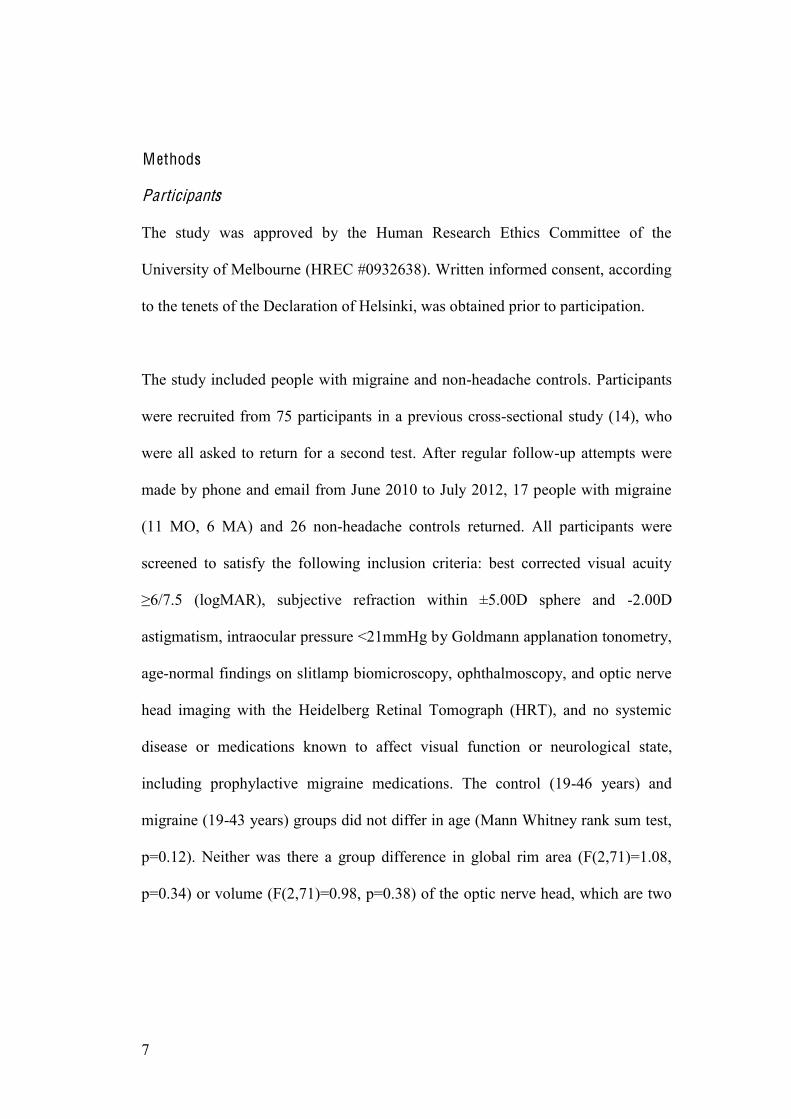
The study was approved by the Human Research Ethics Committee of the

University of Melbourne (HREC #0932638). Written informed consent, according

to the tenets of the Declaration of Helsinki, was obtained prior to participation.

The study included people with migraine and non-headache controls. Participants

were recruited from 75 participants in a previous cross-sectional study (14), who

were all asked to return for a second test. After regular follow-up attempts were

made by phone and email from June 2010 to July 2012, 17 people with migraine

(11 MO, 6 MA) and 26 non-headache controls returned. All participants were

screened to satisfy the following inclusion criteria: best corrected visual acuity

-2.00D

astigmatism, intraocular pressure <21mmHg by Goldmann applanation tonometry,

age-normal findings on slitlamp biomicroscopy, ophthalmoscopy, and optic nerve

head imaging with the Heidelberg Retinal Tomograph (HRT), and no systemic

disease or medications known to affect visual function or neurological state,

including prophylactive migraine medications. The control (19-46 years) and

migraine (19-43 years) groups did not differ in age (Mann Whitney rank sum test,

p=0.12). Neither was there a group difference in global rim area (F(2,71)=1.08,

p=0.34) or volume (F(2,71)=0.98, p=0.38) of the optic nerve head, which are two

8

HRT parameters that correlate with perimetric indices describing generalised and

localised visual field loss in people with glaucoma (41).

Participants completed a clinical interview, headache questionnaire, and the

Migraine Disability Assessment Score (MIDAS) questionnaire (42) to describe

their migraines, where applicable (Table 1). The MIDAS questionnaire score

measures the number of days in the preceding three months where migraines

resulted in reduced productivity in tasks of daily living. Scores are interpreted as

minimal (Grade 1, score 0-5), mild (Grade 2, score 6-10), moderate (Grade 3,

score 11-20), or severe disability (Grade 4, score 21+). Migraine participants

reported symptoms (headache, nausea/vomiting, photophobia, phonophobia) that

fulfilled the International Headache Society criteria (43) for migraine without aura

(MO) and migraine with aura (MA). The MO and MA groups were pooled, as

both groups demonstrate similar visual field losses (16, 18, 20, 21, 23-25). Control

participants had never had a migraine and were free from regular headaches (less

than 4 in the past year).

Timing of the test visits

Each session lasted up to 3 hours. For people with migraine, the first visit was

scheduled at least one week post-migraine. The second visit was scheduled as

close as practicable, but at least one day, after the cessation of migraine symptoms

(maximum 6 days post-migraine). The difference in the number of days post-

9

migraine between the two visits ranged from 3 to 199 days (Figure 1; median 16

days). Control participants completed two sessions at least 1 day apart (median 18

days, range 1-132 days).

F igure 1 Days since last migraine at the two test visits for the migraine

participants. M O participants are shown as filled square symbols, whereas M A

participants are shown as filled diamond symbols. The M O participant who

was tested one day before a migraine is shown as a cross symbol. V isit 1 was

scheduled at least 7 days after a migraine. V isit 2 was scheduled at a time

closer after a migraine (within 6 days).

M O : M igraine without aura; M A : M igraine with aura.

10

Increased PVER amplitude has been reported in the pre-attack period, up to 72

hours before a migraine (37). Prodromal symptoms, including fatigue and

difficulty concentrating, commonly occur up to 48 hours before an attack (44) and

participants

were contacted (by phone or email) after each test session. This follow-up found

that the majority of participants did not have a migraine within 72 hour of each

test session. One of the 17 participants experienced a migraine the day after the

first test session. Data from this participant have been represented as cross

symbols in Figures 1-3. Excluding the data from this individual from statistical

analyses did not change our conclusions.

Visual field tests

Visual field tests were always conducted first because of possible ocular

discomfort following electrode placement for PERG recordings. Three different

visual field tests were included. Standard automated perimetry (SAP) is the

standard perimetric technique and is most commonly encountered in clinical

practice. Participants completed SAP first, as it is well tolerated and generally

easiest for a naïve observer to learn. Temporal modulation perimetry (TMP) and

short-wavelength automated perimetry (SWAP) were conducted next, in random

order, as visual field defects in people with migraine have been identified using

TMP (20, 24) and SWAP (25) that are not measurable on SAP. These different

forms of perimetry test different aspects of visual processing, with flicker

11

perimetry preferentially assessing magnocellular pathways (45) and SWAP

assessing the blue-on-yellow (or koniocellular) system (46). SAP is non-visual

pathway selective (47).

Table 1 Summary of self-reported migraine character istics (median, range).

Independent sample t-tests and M ann Whitney rank sum tests comparing the

migraine character istics between groups are provided.

M ID AS: M igraine Disability Assessment Score; M O: M igraine without aura;

M A : M igraine with aura.

Migraine characteristics

MO MA Statistic p

Days since last migraine at Visit 1 18 (7-150) 25 (7-200) U=26.0 0.51

Days since last migraine at Visit 2 3 (1-5) 2 (1-6) U=24.0 0.38

Age at first migraine (years) 15 (4-17) 12 (10-30) U=21.0 0.24

Years of migraine 13 (3-23) 20 (7-30) t15=0.77 0.45

Migraines in past year 8 (1-50) 5 (1-50) U=17.5 0.39

Weeks between migraines 3 (1-20) 6 (1-24) U=22.0 0.29

Estimated number of lifetime attacks 100 (30-550) 89 (14-1300) U=25.0 0.45

MIDAS questionnaire score (days) 20 (0-49) 3 (1-4) U=7.0 0.010

Headache duration (hours) 12 (2-72) 8 (2-48) U=26.0 0.51

12

SAP and TMP were performed on the Medmont M-700 perimeter (Medmont Pty

Ltd., Camberwell, Victoria, Australia), which has been described elsewhere (48).

In brief, the stimuli ( max = 565 nm, max luminance 320 cd/m2) are 0.43°

(Goldmann size III) light-emitting diodes presented on a background luminance of

3.2 cd/m2 (CIE 1931 x=0.53, y=0.42) and arranged in concentric rings. SAP

thresholds were measured using the Central Threshold test at 103 locations at 1°,

3°, 6°, 10°, 15°, 22° and 30° eccentricities. For TMP, the Auto-Flicker test was

conducted at 73 locations at 1°, 3°, 6°, 10°, 15° and 22°. This test varies the

temporal frequency of the flickering stimuli with retinal eccentricity (18 Hz, 1°-3°;

16 Hz, 6°; 12 Hz, 10°-15°; 9 Hz, 22°). Stimuli were presented for 200ms (SAP)

and 800ms (TMP) durations. SWAP was performed on the Octopus 101 perimeter

(Haag-Streit Inc., Koeniz, Switzerland), a detailed description of which has been

given previously (49). Blue ( max = 440nm) test stimuli of 1.72° (Goldmann size

V) were projected for 200 ms against a yellow background (100 cd/m2), to which

participants adapted for at least 3 minutes before testing. Thresholds were

measured using the Dynamic strategy (50) at 52 locations at 3°, 9°, 15°, and 21°

eccentricity.

Participants had a brief practice before testing. Tests with false-positive or false-

negative rates above 30% were excluded. The automated blind-spot monitor

identified fixation losses exceeding 30% in four control and four migraine

participants. However, continuous monitoring of the limbal position by direct

13

visual inspection (Medmont) or via video camera (Octopus) confirmed steady

fixation.

Visual field analysis

The global indices generated by the perimeter were analysed. The Medmont

perimeter returns Average Defect and Pattern Defect, whereas the Octopus

perimeter returns Mean Defect and Loss Variance. These indices are determined

relative to a proprietary age-matched normative database and describe generalised

and localised visual field loss, respectively.

Global indices provide single summary statistics for visual field performance but

do not illustrate which locations are abnormal across the visual field. To establish

a point-wise assessment of visual field abnormality, we determined two-sided

empirical confidence limits of sensitivity at each visual field location (20), based

on our 26 control participants. We used our controls because people with migraine

are not excluded from the proprietary databases. Locations at and immediately

above and below the blindspot were excluded. As visual field outcomes are non-

parametric (51), locations where sensitivity was lower than the 8th percentile limit

(2nd worst-

nd percentile limit). In the same way, point-wise

confidence limits were determined for the change in sensitivity between the first

and second visits, where a negative change indicated a reduction in sensitivity at

14

the second visit. Assuming that thresholds at individual locations are independent,

visual fields were judged to be abnormally depressed (p<0.05) if there were at

least 8 locations below our control group lower limit (p<0.04 for a single location)

out of a total 101 test points on SAP, 6 of 73 on TMP, and 5 of 50 on SWAP (see

Appendix A1).

The fellow eye was also examined to classify whether the pattern of defect was

homonymous. Two approaches were used: (1) visual inspection, to see if locations

of depressed sensitivity were in the same hemifield in both eyes and respected the

vertical midline; and (2) quadrant analysis (1), where a quadrant was classified as

abnormal (p<0.05) if there were at least 4 SAP, 3 TMP, or 3 SWAP locations that

were depressed within that quadrant (see Appendix A1). When the same quadrant

was classified as abnormal in both eyes, using either criterion, the deficit was

considered homonymous.

Pattern electrophysiology

The PERG reflects retinal ganglion cell activity (52), whereas the PVER measures

V1 function and integrity of the retinocortical pathway (53) and other brain areas

(54). The PERG and PVER were recorded simultaneously to rule out cortical

dysfunction arising

-

15

a migraine when tested with flickering stimuli (TMP) (24). The steady-state

response is presumed to share similar neural substrates as behavioural measures of

temporal processing (flicker) (55).

The protocol for simultaneous PERG and PVER has been described in detail

elsewhere (14). Responses were recorded monocularly according to ISCEV

standards (52, 53) using the Espion (Diagnosys LLC, Cambridge, UK). Electrode

impedance was generally below 5 kOhms and did not exceed 10 kOhms.

Participants fixated on a 0.5° diameter red square in the centre of the screen (Sony

G520 21-inch CRT monitor: frame rate 100 Hz, resolution 1024 x 786 pixels)

positioned 50cm away. The stimulus was a square-wave checkerboard (31° square

field, 52 cd/m2 mean luminance, 96% contrast, 0.8° checks), counter-phased at 1

-

response). Stimuli were presented using an interleaved block design to balance the

effect of fatigue on recordings.

Two hundred signals were amplified, bandpass-filtered (1.25-100 Hz), and

digitised (1000 Hz) to 16-bit resolution. Timing and amplitude measures were

extracted. In compliance with ISCEV standards (52, 53), peak times were

measured for the positive components of the PERG (P50) and PVER (P100).

Peak-to-peak amplitudes were measured for the two neural signals closest in

succession along the visual pathway, representing activity of the retinal ganglion

16

cells (PERG P50-N95 amplitude (56)) and V1 (PVER N75-P100 amplitude (54)).

The different components were identifiable on all transient waveforms collected.

Similarly, the amplitude and phase at the second harmonic (16.7 Hz) of the steady-

state PERG and PVER, reflecting retinal ganglion cell (56) and primary visual

cortical activity (57), respectively, were determined by Discrete Fourier

Transform. Decreased phase values correspond to signal delays in the time

domain. Steady-state responses below noise levels at neighbouring frequencies

(14.6 and 18.8 Hz) (58) were removed from the dataset. PVER interhemispheric

asymmetry (7, 9, 11, 13), which may be related to the laterality of the migraine

headache (11) or aura (7, 9), was defined as the percentage difference in amplitude

between the right and left hemispheres.

Statistical analysis

For control and migraine participants, a worst eye was chosen for analysis based

on the total number of abnormal points across all visual fields. Statistical

comparisons were performed using SPSS version 20.0 (SPSS Inc., Chicago,

Illinois, United States). Data were tested to confirm statistical normality (Shapiro-

Wilk normality test) and homogeneity of

Repeated-measures analyses of variance considered group differences (RM-

ANOVA, =0.05) nested within visit (visit 1, 2) and test (transient, steady-state)

or perimeter (SAP, TMP, SWAP). Where the assumption of sphericity was

violated, the degrees of freedom were amended using a Huynh-Feldt correction.

17

Paired t-tests, or Wilcoxon signed rank tests where the data were non-Gaussian,

were used to test for within-individual changes between visits. The alpha level was

adjusted using a Holm-Bonferroni correction for multiple comparisons (59).

Results

Changes in electrophysiology with time post-migraine

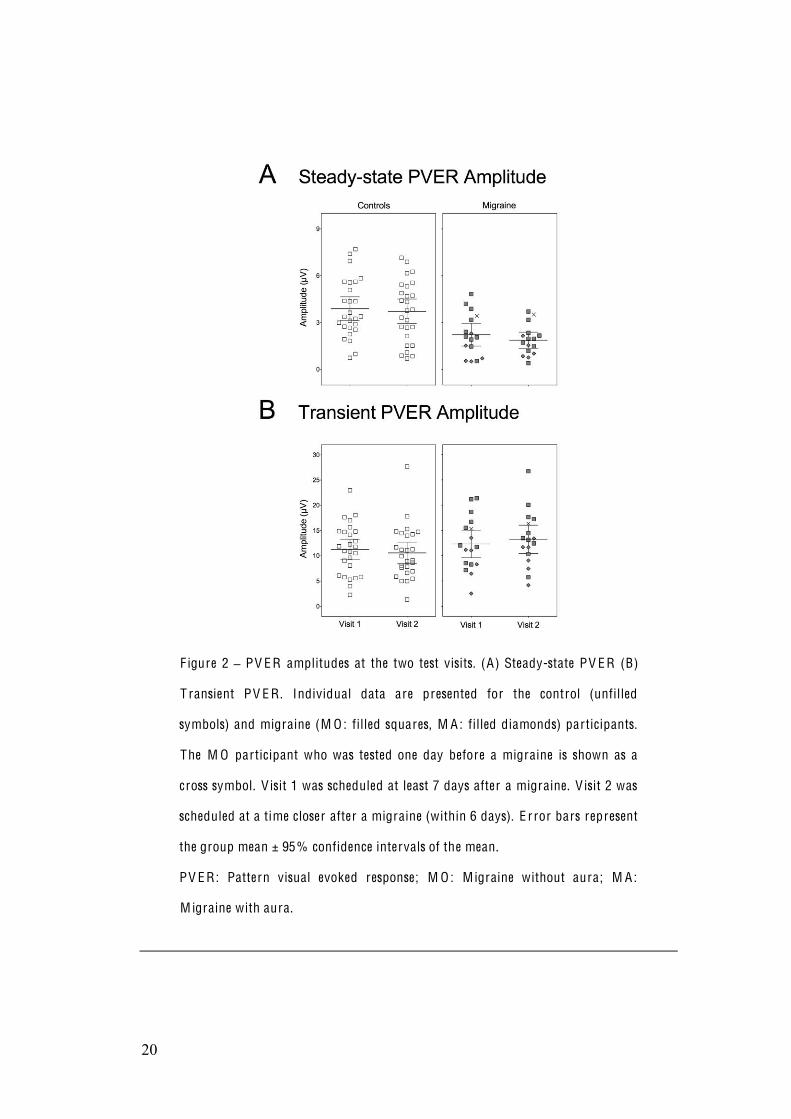
We find differences in PVER amplitude between migraine and control groups

depending on the component analysed (Table 2; group x component interaction:

F(1,40)=7.92, p=0.008). Separate component analyses indicated reduced steady-

state PVER (Figure 2A; F(1,40)=11.4, p=0.002) but normal transient PVER

amplitudes (Figure 2B; F(1,41)=1.37, p=0.25) in the migraine group. Our data

further demonstrate that PVER amplitude did not change at the second visit, i.e.

closer to a migraine. Comparisons between the two visits were performed using

paired t-tests and none was found to be significant (steady-state: controls t25=1.20,

p=0.24, migraine t15=1.88, p=0.079; transient: controls t25=1.63, p=0.12, migraine

t16=1.58, p=0.13). Neither was there a significant change in PVER timing (Table

2; group x visit interaction: F(1,40)=0.95, p=0.34), PVER/PERG ratio (Table 2;

group x visit interaction: F(1,40)=0.05, p=0.82), or interhemispheric amplitude

asymmetry (Table 3; paired Wilcoxon signed rank tests, p>0.05) with time post-

migraine. Although the PERG is normal in between migraine attacks (6, 8, 14),

differences in the PERG may manifest closer to a migraine. We did not find

evidence for such an effect (Table 2; group x visit interactions: p>0.05).

18

Table 2 Summary of retinal (PE R G) and cortical (PV E R) electrophysiological measures (mean ± standard deviation) at the two

test visits. V isit 1 was scheduled at least 7 days after a migraine. V isit 2 was scheduled at a time closer after a migraine (within 6

days). R M-A N O V As comparing the electrophysiological measures between groups are provided. ** denotes significance using

Holm-Bonfer roni correction for multiple comparisons, p<0.01.

PE R G: Pattern electroretinogram; PV E R: Pattern visual evoked response; R M-A N O V A : Repeated-measures analysis of variance.

19

Control Migraine RM-ANOVA group comparisons

Visit 1 Visit 2 Visit 1 Visit 2

PERG amplitude (µV) Group: F(1,41)=1.01, p=0.32 Group x component: F(1,41)=2.76, p=0.10 Group x visit: F(1,41)=1.36, p=0.25

Transient response 10.2 ± 2.63 9.79 ± 2.05 11.6 ± 3.22 10.1 ± 2.21

Steady-state response 3.23 ± 0.52 3.28 ± 0.62 3.19 ± 0.96 3.20 ± 0.61

PERG timing Group: F(1,41)=0.65, p=0.43 Group x component: F(1,41)=0.39, p=0.54 Group x visit: F(1,41)=0.21, p=0.65

Transient peak time (ms) 51 ± 3 51 ± 2 51 ± 2 51 ± 2

Steady-state phase (rads) 6.03 ± 0.22 5.81 ± 0.42 6.01 ± 0.24 5.91 ± 0.30

PVER amplitude (µV) Group: F(1,40)=0.15, p=0.70 Group x component: F(1,40)=7.92, p=0.008 ** Group x visit: F(1,40)=4.04, p=0.051

Transient response 11.3 ± 5.04 10.6 ± 5.30 12.9 ± 4.80 13.8 ± 5.11

Steady-state response 3.89 ± 1.88 3.72 ± 1.95 2.22 ± 1.37 ** 1.87 ± 0.97 **

PVER timing Group: F(1,40)=0.03, p=0.87 Group x component: F(1,40)=0.02, p=0.90 Group x visit: F(1,40)=0.95, p=0.34

Transient peak time (ms) 103 ± 6 102 ± 6 103 ± 6 102 ± 4

Steady-state phase (rads) 7.83 ± 1.11 7.94 ± 1.01 7.78 ± 0.48 7.57 ± 1.19

PVER/PERG ratio Group: F(1,40)=1.95, p=0.17 Group x component: F(1,40)=11.7, p=0.001 ** Group x visit: F(1,40)=0.05, p=0.82

Transient 1.19 ± 0.52 1.12 ± 0.52 1.24 ± 0.60 1.23 ± 0.53

Steady-state 1.25 ± 0.63 1.19 ± 0.67 0.74 ± 0.51 ** 0.60 ± 0.48 **

20

F igure 2 PV E R amplitudes at the two test visits. (A) Steady-state PV E R (B)

T ransient PV E R . Individual data are presented for the control (unfilled

symbols) and migraine (M O : filled squares, M A : filled diamonds) participants.

The M O participant who was tested one day before a migraine is shown as a

cross symbol. V isit 1 was scheduled at least 7 days after a migraine. V isit 2 was

scheduled at a time closer after a migraine (within 6 days). E r ror bars represent

the group mean ± 95% confidence intervals of the mean.

PV E R: Pattern visual evoked response; M O : M igraine without aura; M A:

M igraine with aura.

21

Table 3 Summary of PV E R amplitude interhemispher ic asymmetry (median, range) at the two test visits. V isit 1 was scheduled at

least 7 days after a migraine. V isit 2 was scheduled at a time closer after a migraine (within 6 days). Paired Wilcoxon signed rank

tests comparing the asymmetry measures between visits are provided.

PV E R: Pattern visual evoked response.

Control Migraine

Visit 1 Visit 2 Paired tests Visit 1 Visit 2 Paired tests

Transient PVER asymmetry (%) 17 (1 37) 21 (3 62) Z = -1.18, p=0.24 16 (2- 39) 16 (2 43) Z = -0.40, p=0.69

Steady-state PVER asymmetry (%) 15 (2 41) 20 (3 51) Z = -1.06, p=0.29 22 (3 60) 26 (3- 75) Z = -0.87, p=0.38

22

Visual field changes with time post-migraine

For Average/Mean Defect, there was a significant interaction between group, visit,

and perimeter (Huynh-Feldt =0.83, F(1.66,68.1)=4.02, p=0.029). The change

with time was evident in the control group only an improvement in SAP

Average Defect at the second visit (Table 4; paired t-test: t25=4.80, p<0.001). The

migraine participants tended to show worse generalised sensitivity closer to a

migraine, i.e. decrease in TMP Average Defect and increase in SWAP Mean

Defect at the second visit. These changes, however, did not reach statistical

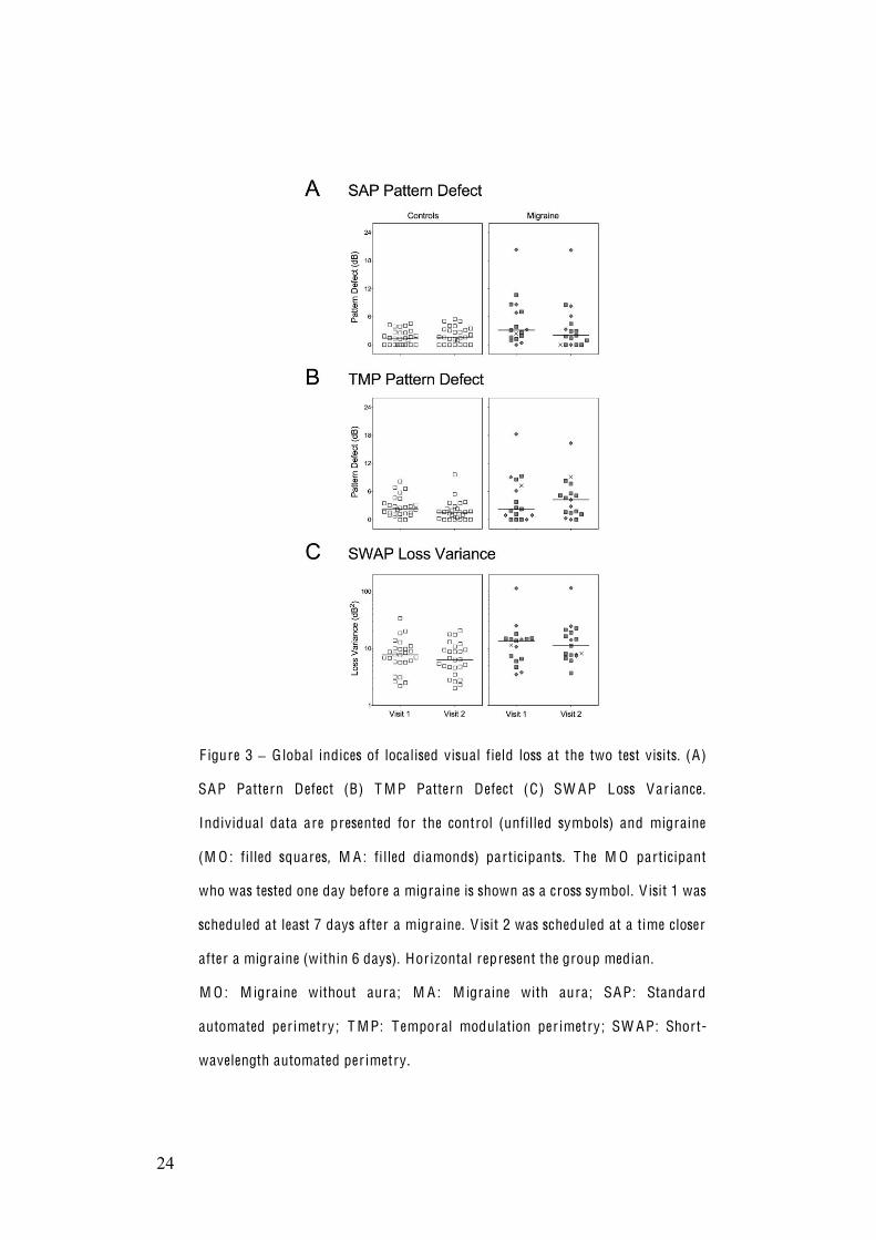
significance (Table 4; paired t-tests: p>0.05). The Pattern Defect/Loss Variance is

shown in Figure 3 and were similar at both visits for all participants (Table 4;

paired Wilcoxon signed rank tests: p>0.05). Thus, overall, perimetric global

indices did not change between visits, although the migraine participants did not

show the same learning benefits as controls.

23

Table 4 Summary of visual field global indices at the two test visits. (A) Average/M ean Defect (mean ± standard deviation) and

(B) Pattern Defect/Loss Variance (median, range). V isit 1 was scheduled at least 7 days after a migraine . V isit 2 was scheduled at a

time closer after a migraine (within 6 days). Paired t-tests and Wilcoxon signed rank tests comparing the global indices between

visits are provided. ** denotes significance using Holm-Bonfer roni correction for multiple comparisons, p<0.004.

SAP: Standard automated per imetry; T M P: Temporal modulation per imetry; SW AP: Short-wavelength automated per imetry.

Control Migraine

Visit 1 Visit 2 Paired tests Visit 1 Visit 2 Paired tests

A. Average/Mean Defect

SAP Average Defect (dB) -0.85 ± 1.14 -0.04 ± 1.26 t25 = 4.80, p<0.001 ** -0.87 ± 1.02 -0.66 ± 1.13 t16 = 1.08, p=0.30

TMP Average Defect (dB) -3.24 ± 1.04 -3.20 ± 1.09 t25 = 0.27, p=0.79 -3.40 ± 1.23 -3.56 ± 1.17 t25 = 0.65, p=0.52

SWAP Mean Defect (dB) 3.08 ± 2.90 2.92 ± 2.98 t25 = 0.77, p=0.45 3.31 ± 2.85 3.94 ± 2.71 t25 = 1.39, p=0.18

B. Pattern Defect/Loss Variance

SAP Pattern Defect (dB) 1.44 (0 4.58) 1.67 (0 5.49) Z = -1.41, p=0.16 3.14 (0 20.4) 2.02 (0 20.3) Z = -1.40, p=0.16

TMP Pattern Defect (dB) 2.30 (0 8.14) 1.57 (0 9.62) Z = -1.56, p=0.12 2.25 (0 18.3) 4.26 (0 16.3) Z = -0.05, p=0.96

SWAP Loss Variance (dB2) 7.75 (2.20 33.8) 6.35 (2.00 20.5) Z = -0.92, p=0.36 13.6 (3.50 113.9) 11.2 (3.70 115.5) Z = -0.26, p=0.80

24

F igure 3 G lobal indices of localised visual field loss at the two test visits. (A)

SAP Pattern Defect (B) T M P Pattern Defect (C) SW AP Loss Variance.

Individual data are presented for the control (unfilled symbols) and migraine

(M O : filled squares, M A : filled diamonds) participants. The M O participant

who was tested one day before a migraine is shown as a cross symbol. V isit 1 was

scheduled at least 7 days after a migraine. V isit 2 was scheduled at a time closer

after a migraine (within 6 days). Horizontal represent the group median.

M O : M igraine without aura; M A : M igraine with aura; SAP: Standard

automated per imetry; T M P: Temporal modulation per imetry; SW AP: Short-

wavelength automated per imetry.

25

When visual fields of migraine individuals were assessed using point-wise

control group performance were depressed, not better (Figure 4, black bars). This

was evident for all visual field tasks, although different people were identified as

abnormal for each test. The total number of depressed points for a given individual

did not change with time post-migraine (Wilcoxon signed rank tests: SAP Z=-

0.05, p=0.96; TMP Z=-0.89, p=0.38; SWAP Z=-0.32, p=0.75). However,

individuals with migraine showed point-wise changes in sensitivity that fell

outside that predicted from control group test-retest variability. The proportion of

migraine participants with a significant number of points across the visual field

where sensitivity was significantly decreased closer to the end of a migraine was

41% for SAP, 24% for TMP, and 47% for SWAP. These proportions were

significantly different from controls (chi-square, SAP p=0.008, TMP p=0.049,

SWAP p=0.003). In contrast, migraine point-wise sensitivity was not significantly

improved at the second visit, when chi-square tests were corrected for multiple

comparisons (SAP p=0.24, TMP p=0.14, SWAP p=0.049). To illustrate this,

Figure 5 shows the sensitivity at the first visit as a function of sensitivity at the

second visit, pooled across the range of visual field locations. Whereas on average

the migraine and control groups showed similar upper limits of test-retest

performance, the lower limits of the migraine group were below that of controls

across most of the sensitivity range. Thus, people with migraine showed a

26

significant number of points with reduced sensitivity to begin with (Figure 4) and

which were associated with larger losses closer to a migraine (Figure 5).

Patterns of visual field loss

Where point-wise comparisons revealed a statistically significant number of

depressed points, we investigated whether the pattern of visual field loss involved

one or both eyes. Data from one migraine participant were excluded from this

analysis due to a false negative rate >30% in one eye. Both monocular and

bilateral visual field defects were observed in our migraine participants, although

the presence of a bilateral defect does not preclude the possibility of two

monocular defects.

Only three people with migraine (19%) showed normal results for every visual

field task at every visit, compared with 77% controls. Five people with migraine

(31%) demonstrated a repeatable bilateral visual field defect (e.g. Figure 6A).

None gave a homonymous pattern respecting the vertical midline. Nevertheless, as

the bilateral visual field loss was diffuse and generalised across the entire field, the

majority of cases (80%) satisfied our less conservative definition for homonymous

deficits, where at least one quadrant was flagged as

the other hand, four different migraine participants (25%) showed monocular

sensitivity loss affecting the same eye at both visits. A further three people (19%)

showed normal fields at the first visit, but developed a monocular field defect

27

closer to a migraine (e.g. Figure 6B). Monocular defects ranged from patchy loss

affecting all four quadrants of a single eye, to an arcuate scotoma that crossed the

vertical midline. We interpret these as being of retinal origin.

F igure 4 Proportion of the total number of visual field locations at the first

visit (at least 7 days after a migraine) that were identified as depressed (black

bars) or better (white bars) relative to the lower 8th percentile and upper 92nd

percentile limits of control group performance, respectively, for each individual

with migraine. The majority of locations identified as abnormal were depressed,

not better . A visual field was considered abnormal if there were at least 8 SAP, 6

T M P, or 5 SW AP locations (horizontal dotted lines) that were identified as

depressed. Participants in the migraine with aura group (participants 12-17) are

shown to the r ight of each panel.

SAP: Standard automated per imetry; T M P: Temporal modulation per imetry;

SW AP: Short-wavelength automated per imetry.

28

F igure 5 V isual field sensitivity at the second visit plotted as a function of

sensitivity at the first visit. The shaded area indicates the 90% confidence

interval of test-retest performance for the control group. The 5th and 95th

confidence limits for the migraine group are shown as individual symbols.

Confidence limits were determined for the range of dB values pooled across all

visual field locations. Only sensitivity values appearing at least 20 times were

included in the analysis in order to obtain a reasonable estimate of the upper

95% and lower 5% confidence limits. For (A) SAP and (C) SW AP, sensitivity

was measured in 1dB steps, whereas for (B) T M P, sensitivity was measured in

3dB steps. Consistent with previous literature (60), both groups showed

increased variability for locations with low sensitivity. However , the migraine

group showed lower limits of visual field sensitivity across the range of

sensitivity values. Upper limits were similar between groups.

SAP: Standard automated per imetry; T M P: Temporal modulation per imetry;

SW AP: Short-wavelength automated per imetry.

29

F igure 6 Example SAP visual field defects based on point-wise comparisons

with control group performance. Shaded squares indicate depressed points, i.e.

locations where the sensitivity fell below the lower 8th percentile of control group

sensitivity. A SAP visual field was considered abnormal if there were at least 8

locations across the visual field that were identified as depressed. (A) Diffuse

visual field loss in both eyes of a 20-year-old female with migraine with aura. (B)

Right eye visual field defect in a 36-year-old female with migraine with aura,

showing monocular infer ior arcuate loss one day after migraine (left-hand side).

H er visual fields were normal at the first visit 56 days after migraine (r ight-hand

side).

SAP: Standard automated per imetry; SW AP: Short-wavelength automated

per imetry.

30

Relationship between abnormal interictal measures of visual function and

migraine characteristics

Of the visual field and electrophysiological measures analysed in this study, the

steady-state PVER amplitude (Figure 2A), Pattern Defect/Loss Variance (Figure

3), and the number of depressed points based on point-wise comparisons (Figure

4) remained consistently abnormal during the post-migraine period. Spearman

rank correlations between these measures, averaged across both visits, were not

significant (Table 5), implying that these abnormalities might be caused by

different mechanisms. To explore the possibility that abnormal interictal measures

on electrophysiological or visual field tests related to a particular feature of

migraine, correlation coefficients were determined between the consistently

abnormal visual functional measures noted above and the migraine characteristics

shown in Table 1. None of the correlations was significant (see Appendix A2).

31

Table 5 Relationship between abnormal measures of electrophysiology and

visual field indices averaged across both visits. Spearman rank correlations were

not significant using a Holm-Bonfer roni correction for multiple comparisons,

p<0.008.

PV E R: Pattern visual evoked response; SAP: Standard automated per imetry;

T M P: Temporal modulation per imetry; SW AP: Short-wavelength automated

per imetry.

Relationship between steady-state PVER amplitude and visual field measures

Rs p

SAP Pattern Defect -0.33 0.19

Depressed points -0.18 0.48

TMP Pattern Defect 0.07 0.80

Depressed points 0.05 0.84

SWAP Loss Variance -0.28 0.27

Depressed points -0.19 0.45

32

Discussion

The results of this study are consistent with both retinal and cortical visual

dysfunction being present in people with migraine. On the one hand, our

electrophysiological results, like others (6, 8, 14), argue for a predominant cortical

anomaly in migraine. Steady-state PVER amplitudes were consistently reduced

(Figure 2A), whereas the PERG was normal, implying no diffuse retinal

dysfunction (Table 2). On the other hand, both binocular and monocular visual

field defects were found (Figure 6). Monocular patterns of visual field loss arise

from pre-chiasmal or retinal dysfunction. The homonymous nature of migraine

visual aura and the nature of some bilateral field loss are supportive of a cortical

origin. Thus, visual field tests suggest the presence of both cortical and retinal

dysfunction in people with migraine. Our findings suggest that the retinal defects

affect small, localised regions, whereas the cortical defects tend to involve larger

and more generalised regions.

A novel component of this study was the measurement of SAP, TMP, and SWAP

visual fields as well as transient and steady-state electrophysiological responses on

the same day, which enables comparison between these approaches for measuring

visual processing in the same individuals. People with migraine show reduced

visual field sensitivity to a range of different stimuli, which is consistent with

other psychophysical evidence that deficits in people with migraine are not neural

pathway-specific (20, 24, 25, 31, 33). On the other hand, the steady-state but not

33

transient response at V1 was abnormal in the migraine group. Faster flickering

stimuli have consistently demonstrated differences in electrophysiological studies

of people with migraine (5, 9, 61). In some cases, as observed here, a clear

separation between migraine and control groups was only measurable in the

steady-state response (14, 61). Flicker is known to induce higher metabolic

demands and increase blood flow in the brain (62). Disrupted neurovascular

coupling in migraine (63) may lead to functional abnormalities that depend on

flicker rate. The stimulation rate used in the present study (~8 Hz) corresponds to

the temporal frequency that produces a maximal change in cerebrovascular

response to a flickering checkerboard pattern as measured by fMRI-BOLD (64).

Alternatively, the reduction in steady-state PVER amplitude may reflect abnormal

visual motion processing, as the major sources of the steady-state PVER are

cortical areas V1 and V5/MT (57). Indeed, there is converging evidence for altered

function in visual motion processing pathways from studies involving transcranial

magnetic stimulation (65), structural brain imaging (66), and behavioural

measures of global motion integration processing (1-3).

Consistent with earlier reports (16, 19, 20, 22, 24), this study demonstrates visual

field changes with time post-migraine. However, in this study, sensitivity changes

were observed with point-wise comparisons and not by comparing the perimetric

global indices. The Pattern Defect/Loss Variance was consistently abnormal, with

some migraine individuals showing markedly abnormal values at both visits

34

(Figure 2). It may be that our participants were not tested close enough to a

migraine to detect a difference with time. Participants in the previous study were

tested the day following migraine offset, with test sessions lasting no more than

one hour (24). Our participants, however, were asked to return within one week of

a migraine, as we anticipated that it would be more difficult for participants to

arrange a second visit of 3 hours duration at short notice. As a result, the average

time post-migraine at the second visit was not 24 hours, but 3 days. The more

demanding nature of the long test session likely biased the timing of the second

visit to a day further away from a headache, and prevented migraine participants

from completing the second session the day after an attack, where performance is

likely to be worse.

A significant number of locations showed a more pronounced reduction in

sensitivity 1-6 days after a migraine. The decrease in sensitivity was not due to

increased variability, as the upper limits of test-retest performance in both groups

indicate a similar number and degree of relatively improving locations (Figure 5),

consistent with a previous report (24). Differences in visual field sensitivity

immediately post-migraine are possibly explained by fatigue or poor concentration

as a result of anti-migraine medications or the symptoms of migraine itself. We

endeavoured to minimise post-migraine effects by scheduling test visits at least 1

day after the offset, and not onset, of all migraine symptoms. Moreover, the

changes in sensitivity were apparent for discrete locations across the visual field,

35

whereas fatigue would be expected to produce an overall reduction in sensitivity.

Differences in Average/Mean Defect in the migraine group did not fall outside the

test-retest variability of control group performance (Table 2). An alternative

reason for reduced sensitivity is aversion to the test stimuli (67). This might also

explain the reduction in steady-state PVER amplitude. We did not formally

measure aversion; however, none of the participants reported discomfort or

voluntarily withdrew from the study during testing. Furthermore, participants with

a strong aversion to visual stimuli are likely to have excluded themselves from

volunteering for a study that explicitly involved extensive visual testing.

Although the mechanism for localised visual field deficits in migraine cannot be

ascertained from this study, it has been suggested that decreased sensitivity might

result from localised vascular events (68). Abnormal peripheral vascular flow and

vasospastic tendencies in people with migraine (69, 70), particularly transient

retinal vasospasms occurring during a migraine attack (30), could cause altered

perfusion and increase the risk of focal ischaemic damage to the optic nerve head

(68, 70) and retina (28). However, the steady-state (flicker) PERG was normal in

our migraine group and did not correlate with localised visual field losses. It is

worth noting that the pattern electrophysiological measures used in this study

involve a large, full-field target and are therefore global responses, which are not

designed to find small localised losses or investigate the spatial extent of visual

dysfunction. Future studies may take advantage of multifocal techniques (71),

36

which have the potential to provide more information about localised visual field

defects. Current multifocal techniques, however, do not have the same spatial

resolution as the visual field tests employed in this study, which identify

sensitivity losses in people with migraine at discrete locations using test stimuli of

0.5° and 1.7°. In contrast, visual field defects have not been found in people with

migraine using targets of similar size to that used routinely in multifocal

electrophysiology (approximately 10° (71)) (72), suggesting that larger targets

may be less useful in detecting the localised visual anomalies in migraine.

We found that an abnormal electrophysiological response did not correlate with

visual field performance measured in the same individuals. The difference

between electrophysiological and visual field tests may be related to the spatial

extent of the test targets, as discussed earlier. In addition, for the most part,

electrophysiological measures obtained at least 7 days post-migraine were not

significantly different from responses obtained, on average, 2-3 days after an

attack, which is consistent with other PVER studies in migraine (10, 37). In

contrast, visual field sensitivity was worse closer to a migraine, as has been

previously reported (16, 19, 20, 24). Without having measured visual function at

multiple times in the migraine cycle (i.e. before, during, and after an attack), our

interpretation of the literature to date is that some visual field defects represent

adverse sequelae of migraine, as they are worst in the days following an attack.

The effects of migraine can extend from the central nervous system to peripheral

37

organs (e.g. to the retina), which may explain individual cases of ocular

involvement in migraine (e.g. (28)) and the development of monocular visual field

loss closer to a migraine (e.g. Figure 6B). Such retinal changes do not manifest as

group differences in the PERG, but are detected by visual field tests that allow

spatial localisation. However, abnormal cortical electrophysiological responses are

generally unchanged after a migraine, but have been reported to differ before and

during an attack (10, 36, 37). This suggests that changes in neural activity

identified using electrophysiology are related to cortical susceptibility to

migraines, given that the pathogenesis of migraine involves the brain (27) and the

symptomatology of migraine is largely cortical.

The test-retest results of this study also have implications for clinical and research

settings where perimetric and electrophysiological techniques are used. Knowing

whether deficits are likely to remain stable over time, or are a temporary

consequence of migraine, is important for interpretation of test results. The

potential for change in visual function after migraine should be considered, as this

will affect the ability to determine abnormality and disease progression in people

with migraine in comparison with normal test-retest variability.

38

Clinical implications

- We show that both cortical and retinal dysfunction can occur in people

who have migraines. In some cases, these appear independent of each

other, with visual field changes that appear retinal in origin being variable

as a function of time post-migraine.

- An abnormal result on an electrophysiological test does not predict

whether visual field performance will also be abnormal in people with

migraine.

Funding

This work was supported by the National Health and Medical Research Council

[grant number 509208] and Australian Research Council [grant number

FT0990930] to author AMM. BN was supported by the Elizabeth and Vernon

Puzey Postgraduate Scholarship from the Faculty of Science at the University of

Melbourne.

Conflict of interest statement

The authors declare that there is no conflict of interest.

39

Supplementary material

Appendix 1 Pointwise analysis of visual fields

A visual field location was deemed abnormally depressed if the sensitivity fell

below the empirical lower 8th percentile limit of our control group (n=26)

performance. Similarly, sensitivity was considered significantly decreased at the

second visit if the change in sensitivity fell outside the confidence limits of control

group test-retest change. We subsequently determined the number of depressed

points required to flag the overall visual field result as abnormal, given the total

number of locations tested. Assuming that the thresholds at individual locations

are independent, the probability (p) that n points, out of a total N, fall below the

lower confidence limit of control group performance is given by:

NCnn (1 )N n (1)

where

NCnN!

n!(N n)! (2)

and is the probability that an individual point will fall below the lower

confidence limits of control group performance ( =0.04). Visual fields were

considered abnormal (p<0.05) if there were at least n number of points that were

40

identified as depressed (p=0.04 for a single point) within a visual field, or portion

of visual field, consisting of N number of test locations (Table A1).

Table A1 The probability (p<0.05) that a visual field consists of at least n

number of statistically abnormal points ( =0.04), given the total number of test

locations (N) (A) across the entire visual field, (B) in the upper quadrants of the

visual field, and (C) in the lower quadrants of the visual field. Locations at,

immediately above, and below the blindspot were not included.

SAP: Standard automated per imetry; T M P: Temporal modulation per imetry;

SW AP: Short-wavelength automated per imetry.

Number of statistically abnormal points across the entire visual field

N n P

SAP 101 8 0.030

TMP 73 6 0.045

SWAP 50 5 0.035

Number of statistically abnormal points across the upper quadrants

N n p

SAP 25 4 0.014

TMP 17 3 0.025

SWAP 12 3 0.010

Number of statistically abnormal points across the lower quadrants

N n p

SAP 24 4 0.012

TMP 16 3 0.021

SWAP 12 3 0.010

41

Table A2 Relationship of abnormal measures of electrophysiology and visual

field indices, averaged across both visits, with migraine character istics.

Spearman rank correlation coefficients are provided.

M ID AS: M igraine Disability Assessment Score; PV E R: Pattern visual evoked

response; SAP: Standard automated per imetry; T M P: Temporal modulation

per imetry; SW AP: Short-wavelength automated per imet ry.

SAP Pattern Defect Depressed points

R p R p

Age at first migraine (years) 0.09 0.75 -0.04 0.89

Years of migraine 0.40 0.11 0.22 0.39

Weeks between migraines 0.07 0.79 0.18 0.49

Migraines in past year -0.09 0.74 -0.27 0.29

Estimated number of lifetime attacks 0.09 0.72 -0.15 0.55

MIDAS questionnaire score (days) -0.26 0.32 -0.47 0.06

Headache duration (hours) 0.05 0.85 -0.03 0.90

TMP Pattern Defect Depressed points

R p R p

Age at first migraine (years) -0.05 0.84 -0.12 0.63

Years of migraine 0.16 0.54 0.19 0.46

Weeks between migraines -0.27 0.29 -0.28 0.28

Migraines in past year 0.20 0.43 0.21 0.43

Estimated number of lifetime attacks 0.27 0.29 0.29 0.26

MIDAS questionnaire score (days) 0.30 0.25 0.16 0.53

42

Headache duration (hours) 0.19 0.46 -0.04 0.89

SWAP Loss Variance Depressed points

R p R p

Age at first migraine (years) 0.24 0.35 0.28 0.28

Years of migraine 0.28 0.28 0.14 0.60

Weeks between migraines -0.07 0.78 -0.05 0.84

Migraines in past year 0.09 0.73 0.04 0.87

Estimated number of lifetime attacks 0.19 0.47 0.07 0.80

MIDAS questionnaire score (days) -0.09 0.72 -0.16 0.54

Headache duration (hours) 0.15 0.55 -0.10 0.70

PVER Steady-state amplitude

R p

Age at first migraine (years) 0.09 0.73

Years of migraine -0.15 0.55

Weeks between migraines -0.15 0.57

Migraines in past year 0.13 0.63

Estimated number of lifetime attacks 0.09 0.73

MIDAS questionnaire score (days) 0.54 0.02

Headache duration (hours) 0.11 0.67

43

References

1. McKendrick AM and Badcock DR. Motion processing deficits in migraine. Cephalalgia 2004; 24: 363-372.

2. Antal A, Temme J, Nitsche MA, et al. Altered motion perception in migraineurs: evidence for interictal cortical hyperexcitability. Cephalalgia 2005; 25: 788-794.

3. Ditchfield JA, McKendrick AM and Badcock DR. Processing of global form and motion in migraineurs. Vision Res 2006; 46: 141-148.

4. Shepherd AJ, Beaumont HM and Hine TJ. Motion processing deficits in migraine are related to contrast sensitivity. Cephalalgia 2012; 32: 554-570.

5. Diener HC, Scholz E, Dichgans J, et al. Central effects of drugs used in migraine prophylaxis evaluated by visual evoked potentials. Ann Neurol 1989; 25: 125-130.

6. Khalil NM. Investigations of visual function in migraine by visual evoked potentials and visual psychophysical tests. PhD Thesis, University of London, UK, 1991.

7. Tagliati M, Sabbadini M, Bernardi G, et al. Multichannel visual evoked potentials in migraine. Electroencephalogr Clin Neurophysiol 1995; 96: 1-5.

8. Shibata K, Osawa M and Iwata M. Simultaneous recording of pattern reversal electroretinograms and visual evoked potentials in migraine. Cephalalgia 1997; 17: 742-747.

9. Shibata K, Osawa M and Iwata M. Pattern reversal visual evoked potentials in migraine with aura and migraine aura without headache. Cephalalgia 1998; 18: 319-323.

10. Judit A, Sandor PS and Schoenen J. Habituation of visual and intensity dependence of auditory evoked cortical potentials tends to normalize just before and during the migraine attack. Cephalalgia 2000; 20: 714-719.

11. Logi F, Bonfiglio L, Orlandi G, et al. Asymmetric scalp distribution of pattern visual evoked potentials during interictal phases in migraine. Acta Neurol Scand 2001; 104: 301-307.

12. Ambrosini A, de Noordhout AM, Sandor PS, et al. Electrophysiological studies in migraine: a comprehensive review of their interest and limitations. Cephalalgia 2003; 23: 13-31.

13. Coppola G, Parisi V, Fiermonte G, et al. Asymmetric distribution of visual evoked potentials in patients with migraine with aura during the interictal phase. Eur J Ophthalmol 2007; 17: 828-835.

14. Nguyen BN, McKendrick AM and Vingrys AJ. Simultaneous retinal and cortical visually evoked electrophysiological responses in between migraine attacks. Cephalalgia 2012; 32: 896-907.

15. Lewis RA, Vijayan N, Watson C, et al. Visual field loss in migraine. Ophthalmology 1989; 96: 321-326.

16. Drummond PD and Anderson M. Visual field loss after attacks of migraine with aura. Cephalalgia 1992; 12: 349-352.

17. Wakakura M and Ichibe Y. Permanent homonymous hemianopias following migraine. J Clin Neuroophthalmol 1992; 12: 198-202.

18. De Natale RD, Polimeni D, Narbone MC, et al. Visual field defects in migraine patients. In: Mills RP (ed) Perimetry Update 1992/93 Proceedings of the Xth

44

International Perimetric Society Meeting Amsterdam/New York: Kugler Publications, 1993: pp 283-284.

19. Sullivan-Mee M and Bowman B. Migraine-related visual-field loss with prolonged recovery. J Am Optom Assoc 1997; 68: 377-388.

20. McKendrick AM, Vingrys AJ, Badcock DR, et al. Visual field losses in subjects with migraine headaches. Invest Ophthalmol Vis Sci 2000; 41: 1239-1247.

21. patients with migraine. J Neurol 2003; 250: 201-206.

22. Goodwin D. Transient complete homonymous hemianopia associated with migraine. Optometry 2011; 82: 298-305.

23. McKendrick AM and Badcock DR. An analysis of the factors associated with visual field deficits measured with flickering stimuli in-between migraine. Cephalalgia 2004; 24: 389-397.

24. McKendrick AM and Badcock DR. Decreased visual field sensitivity measured 1 day, then 1 week, after migraine. Invest Ophthalmol Vis Sci 2004; 45: 1061-1070.

25. McKendrick AM, Cioffi GA and Johnson CA. Short-wavelength sensitivity deficits in patients with migraine. Arch Ophthalmol 2002; 120: 154-161.

26. Yenice O, Temel A, Incili B, et al. Short-wavelength automated perimetry in patients with migraine. Graefes Arch Clin Exp Ophthalmol 2006; 244: 589-595.

27. Schwedt TJ and Dodick DW. Advanced neuroimaging of migraine. Lancet Neurol 2009; 8: 560-568.

28. Gutteridge IF, McDonald RA and Plenderleith JG. Branch retinal artery occlusion during a migraine attack. Clin Exp Optom 2007; 90: 371-375.

29. Martinez A, Proupim N and Sanchez M. Retinal nerve fibre layer thickness measurements using optical coherence tomography in migraine patients. Br J Ophthalmol 2008; 92: 1069-1075.

30. Killer HE, Forrer A and Flammer J. Retinal vasospasm during an attack of migraine. Retina 2003; 23: 253-254.

31. Coleston DM, Chronicle E, Ruddock KH, et al. Precortical dysfunction of spatial and temporal visual processing in migraine. J Neurol Neurosurg Psych 1994; 57: 1208-1211.

32. McKendrick AM, Vingrys AJ, Badcock DR, et al. Visual dysfunction between migraine events. Invest Ophthalmol Vis Sci 2001; 42: 626-633.

33. McKendrick AM and Badcock DR. Contrast-processing dysfunction in both magnocellular and parvocellular pathways in migraineurs with or without aura. Invest Ophthalmol Vis Sci 2003; 44: 442-448.

34. Tibber MS and Shepherd AJ. Transient tritanopia in migraine: evidence for a large-field retinal abnormality in blue-yellow opponent pathways. Invest Ophthalmol Vis Sci 2006; 47: 5125-5131.

35. McKendrick AM and Sampson GP. Low spatial frequency contrast sensitivity deficits in migraine are not visual pathway selective. Cephalalgia 2009; 29: 539-549.

36. Sand T and Vingen JV. Visual, long-latency auditory and brainstem auditory evoked potentials in migraine: relation to pattern size, stimulus intensity, sound and light discomfort thresholds and pre-attack state. Cephalalgia 2000; 20: 804-820.

45

37. Sand T, Zhitniy N, White LR, et al. Visual evoked potential latency, amplitude and habituation in migraine: a longitudinal study. Clin Neurophysiol 2008; 119: 1020-1027.

38. Siniatchkin M, Reich AL, Shepherd AJ, et al. Peri-ictal changes of cortical excitability in children suffering from migraine without aura. Pain 2009; 147: 132-140.

39. Chen WT, Wang SJ, Fuh JL, et al. Peri-ictal normalization of visual cortex excitability in migraine: an MEG study. Cephalalgia 2009; 29: 1202-1211.

40. Sakai Y, Dobson C, Diksic M, et al. Sumatriptan normalizes the migraine attack-related increase in brain serotonin synthesis. Neurology 2008; 70: 431-439.

41. Iester M, Mikelberg FS, Courtright P, et al. Correlation between the visual field indices and Heidelberg retina tomograph parameters. J Glaucoma 1997; 6: 78-82.

42. Lipton RB, Stewart WF, Sawyer J, et al. Clinical utility of an instrument assessing migraine disability: the Migraine Disability Assessment (MIDAS) questionnaire. Headache 2001; 41: 854-861.

43. International Headache Society. The international classification of headache disorders (2nd edition). Cephalalgia 2004; 24: 9-160.

44. Blau JN. Migraine prodromes separated from the aura: complete migraine. BMJ 1980; 281: 658-660.

45. Vingrys A, Demirel S and Kalloniatis M. Multi-dimensional color, flicker and increment perimetry. In: Mills RP and Wall M (eds) Perimetry Update 1994/95 Proceedings of the XIth International Perimetric Society Meeting. Amsterdam/New York: Kugler Publications, 1994: pp 159-166.

46. Demirel S and Johnson CA. Isolation of short-wavelength sensitive mechanisms in normal and glaucomatous visual field regions. J Glaucoma 2000; 9: 63-73.

47. Swanson WH, Sun H, Lee BB, et al. Responses of primate retinal ganglion cells to perimetric stimuli. Invest Ophthalmol Vis Sci 2011; 52: 764-771.

48. Vingrys AJ and Helfrich KA. The Opticom M-600: a new LED automated perimeter. Clin Exp Optom 1990; 73: 3-17.

49. Hermann A, Paetzold J, Vonthein R, et al. Age-dependent normative values for differential luminance sensitivity in automated static perimetry using the Octopus 101. Acta Ophthalmol 2008; 86: 446-455.

50. Weber J and Klimaschka T. Test time and efficiency of the dynamic strategy in glaucoma perimetry. Ger J Ophthalmol 1995; 4: 25-31.

51. Vingrys AJ and Pianta MJ. Developing a clinical probability density function for automated perimetry. Aust N Z J Ophthalmol 1998; 26: S101-103.

52. Bach M, Brigell MG, Hawlina M, et al. ISCEV standard for clinical pattern electroretinography (PERG): 2012 update. Doc Ophthalmol 2013; 126: 1-7.

53. Odom JV, Bach M, Brigell M, et al. ISCEV standard for clinical visual evoked potentials. Doc Ophthalmol 2010; 120: 111-119.

54. Di Russo F, Pitzalis S, Spitoni G, et al. Identification of the neural sources of the pattern-reversal VEP. Neuroimage 2005; 24: 874-886.

55. King-Smith PE and Kulikowski JJ. Pattern and flicker detection analysed by subthreshold summation. J Physiol 1975; 249: 519-548.

56. Luo X and Frishman LJ. Retinal pathway origins of the pattern electroretinogram (PERG). Invest Ophthalmol Vis Sci 2011; 52: 8571-8584.

46

57. Di Russo F, Pitzalis S, Aprile T, et al. Spatiotemporal analysis of the cortical sources of the steady-state visual evoked potential. Hum Brain Mapp 2007; 28: 323-334.

58. Meigen T and Bach M. On the statistical significance of electrophysiological steady-state responses. Doc Ophthalmol 1999; 98: 207-232.

59. Holm S. A simple sequentially rejective multiple test procedure. Scand J Stat 1979; 6: 65-70.

60. Artes PH, Iwase A, Ohno Y, et al. Properties of perimetric threshold estimates from Full Threshold, SITA Standard, and SITA Fast strategies. Invest Ophthalmol Vis Sci 2002; 43: 2654-2659.

61. Marrelli A, Tozzi E, Porto C, et al. Spectral analysis of visual potentials evoked by pattern-reversal checkerboard in juvenile patients with headache. Headache 2001; 41: 792-797.

62. Pastor MA, Artieda J, Arbizu J, et al. Human cerebral activation during steady-state visual-evoked responses. J Neurosci 2003; 23: 11621-11627.

63. Zaletel M, Strucl M, Bajrovic FF, et al. Coupling between visual evoked cerebral blood flow velocity responses and visual evoked potentials in migraneurs. Cephalalgia 2005; 25: 567-574.

64. Singh M, Kim S and Kim TS. Correlation between BOLD-fMRI and EEG signal changes in response to visual stimulus frequency in humans. Magn Reson Med 2003; 49: 108-114.

65. Battelli L, Black KR and Wray SH. Transcranial magnetic stimulation of visual area V5 in migraine. Neurology 2002; 58: 1066-1069.

66. Granziera C, DaSilva AF, Snyder J, et al. Anatomical alterations of the visual motion processing network in migraine with and without aura. PLoS Med 2006; 3: e402.

67. Marcus DA and Soso MJ. Migraine and stripe-induced visual discomfort. Arch Neurol 1989; 46: 1129-1132.

68. Flammer J, Pache M and Resink T. Vasospasm, its role in the pathogenesis of diseases with particular reference to the eye. Prog Retin Eye Res 2001; 20: 319-349.

69. Zahavi I, Chagnac A, Hering R, et al. Prevalence of Raynaud's phenomenon in patients with migraine. Arch Intern Med 1984; 144: 742-744.

70. Gasser P and Meienberg O. Finger microcirculation in classical migraine. A video-microscopic study of nailfold capillaries. Eur Neurol 1991; 31: 168-171.

71. Hood DC, Bach M, Brigell M, et al. ISCEV standard for clinical multifocal electroretinography (mfERG) (2011 edition). Doc Ophthalmol 2012; 124: 1-13.

72. Harle DE and Evans BJ. Frequency doubling technology perimetry and standard automated perimetry in migraine. Ophthalmic Physiol Opt 2005; 25: 233-239.

Minerva Access is the Institutional Repository of The University of Melbourne

Author/s:

Nguyen, BN; Vingrys, AJ; McKendrick, AM

Title:

The effect of duration post-migraine on visual electrophysiology and visual field performance

in people with migraine

Date:

2014-01-01

Citation:

Nguyen, B. N., Vingrys, A. J. & McKendrick, A. M. (2014). The effect of duration post-

migraine on visual electrophysiology and visual field performance in people with migraine.

CEPHALALGIA, 34 (1), pp.42-57. https://doi.org/10.1177/0333102413498939.

Persistent Link:

http://hdl.handle.net/11343/43117