Title stata.com etregress — Linear regression with endogenous treatment effects Description Quick start Menu Syntax Options for maximum likelihood estimates Options for two-step consistent estimates Options for control-function estimates Remarks and examples Stored results Methods and formulas References Also see Description etregress estimates an average treatment effect (ATE) and the other parameters of a linear regression model augmented with an endogenous binary-treatment variable. Estimation is by full maximum likelihood, a two-step consistent estimator, or a control-function estimator. In addition to the ATE, etregress can be used to estimate the average treatment effect on the treated (ATET) when the outcome may not be conditionally independent of the treatment. etreg is a synonym for etregress. Quick start ATE and ATET from a linear regression model of y on x and endogenous binary treatment treat modeled by x and w etregress y x, treat(treat = x w) As above, but use a control-function estimator etregress y x, treat(treat = x w) cfunction With robust standard errors etregress y x, treat(treat = x w) vce(robust) Add the interaction between treat and continuous covariate x using factor variables etregress y x i.treat#c.x, treat(treat = x w) vce(robust) ATE after etregress with the required vce(robust) option and endogenous treatment interaction terms margins r.treat, vce(unconditional) As above, but calculate ATET margins, vce(unconditional) predict(cte) subpop(if treat==1) Menu Statistics > Treatment effects > Endogenous treatment > Maximum likelihood estimator > Continuous outcomes 1
Transcript
Title stata.com
etregress — Linear regression with endogenous treatment effects
Description Quick startMenu SyntaxOptions for maximum likelihood estimates Options for two-step consistent estimatesOptions for control-function estimates Remarks and examplesStored results Methods and formulasReferences Also see
Description
etregress estimates an average treatment effect (ATE) and the other parameters of a linearregression model augmented with an endogenous binary-treatment variable. Estimation is by fullmaximum likelihood, a two-step consistent estimator, or a control-function estimator.
In addition to the ATE, etregress can be used to estimate the average treatment effect on thetreated (ATET) when the outcome may not be conditionally independent of the treatment.
etreg is a synonym for etregress.
Quick startATE and ATET from a linear regression model of y on x and endogenous binary treatment treat
modeled by x and w
etregress y x, treat(treat = x w)
As above, but use a control-function estimatoretregress y x, treat(treat = x w) cfunction
With robust standard errorsetregress y x, treat(treat = x w) vce(robust)
Add the interaction between treat and continuous covariate x using factor variablesetregress y x i.treat#c.x, treat(treat = x w) vce(robust)
ATE after etregress with the required vce(robust) option and endogenous treatment interactionterms
etregress — Linear regression with endogenous treatment effects 3
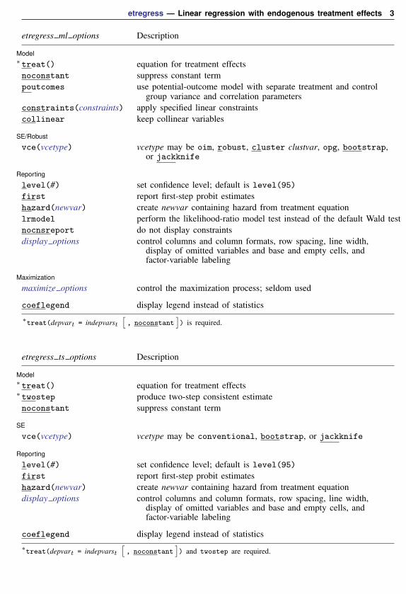
etregress ml options Description
Model∗treat() equation for treatment effectsnoconstant suppress constant termpoutcomes use potential-outcome model with separate treatment and control
group variance and correlation parametersconstraints(constraints) apply specified linear constraintscollinear keep collinear variables
SE/Robust
vce(vcetype) vcetype may be oim, robust, cluster clustvar, opg, bootstrap,or jackknife
Reporting
level(#) set confidence level; default is level(95)
first report first-step probit estimateshazard(newvar) create newvar containing hazard from treatment equationlrmodel perform the likelihood-ratio model test instead of the default Wald testnocnsreport do not display constraintsdisplay options control columns and column formats, row spacing, line width,
display of omitted variables and base and empty cells, andfactor-variable labeling
Maximization
maximize options control the maximization process; seldom used
coeflegend display legend instead of statistics
∗treat(depvart = indepvarst[, noconstant
]) is required.
etregress ts options Description
Model∗treat() equation for treatment effects∗twostep produce two-step consistent estimatenoconstant suppress constant term
SE
vce(vcetype) vcetype may be conventional, bootstrap, or jackknife
Reporting
level(#) set confidence level; default is level(95)
first report first-step probit estimateshazard(newvar) create newvar containing hazard from treatment equationdisplay options control columns and column formats, row spacing, line width,
display of omitted variables and base and empty cells, andfactor-variable labeling
coeflegend display legend instead of statistics∗treat(depvart = indepvarst
4 etregress — Linear regression with endogenous treatment effects
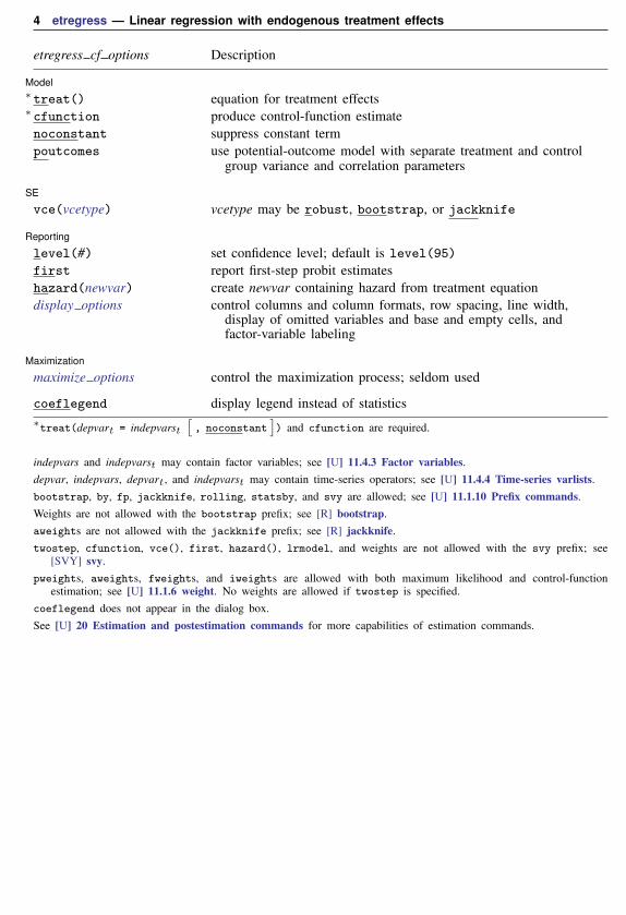
etregress cf options Description
Model∗treat() equation for treatment effects∗cfunction produce control-function estimatenoconstant suppress constant termpoutcomes use potential-outcome model with separate treatment and control
group variance and correlation parameters
SE
vce(vcetype) vcetype may be robust, bootstrap, or jackknife
Reporting
level(#) set confidence level; default is level(95)
first report first-step probit estimateshazard(newvar) create newvar containing hazard from treatment equationdisplay options control columns and column formats, row spacing, line width,
display of omitted variables and base and empty cells, andfactor-variable labeling
Maximization
maximize options control the maximization process; seldom used
coeflegend display legend instead of statistics∗treat(depvart = indepvarst
[, noconstant
]) and cfunction are required.
indepvars and indepvarst may contain factor variables; see [U] 11.4.3 Factor variables.depvar, indepvars, depvart, and indepvarst may contain time-series operators; see [U] 11.4.4 Time-series varlists.bootstrap, by, fp, jackknife, rolling, statsby, and svy are allowed; see [U] 11.1.10 Prefix commands.Weights are not allowed with the bootstrap prefix; see [R] bootstrap.aweights are not allowed with the jackknife prefix; see [R] jackknife.twostep, cfunction, vce(), first, hazard(), lrmodel, and weights are not allowed with the svy prefix; see
[SVY] svy.pweights, aweights, fweights, and iweights are allowed with both maximum likelihood and control-function
estimation; see [U] 11.1.6 weight. No weights are allowed if twostep is specified.coeflegend does not appear in the dialog box.See [U] 20 Estimation and postestimation commands for more capabilities of estimation commands.
etregress — Linear regression with endogenous treatment effects 5
Options for maximum likelihood estimates
� � �Model �
treat(depvart = indepvarst[, noconstant
]) specifies the variables and options for the treatment
equation. It is an integral part of specifying a treatment-effects model and is required.
noconstant; see [R] estimation options.
poutcomes specifies that a potential-outcome model with separate variance and correlation parametersfor each of the treatment and control groups be used.
constraints(constraints), collinear; see [R] estimation options.
� � �SE/Robust �
vce(vcetype) specifies the type of standard error reported, which includes types that are derived fromasymptotic theory (oim, opg), that are robust to some kinds of misspecification (robust), thatallow for intragroup correlation (cluster clustvar), and that use bootstrap or jackknife methods(bootstrap, jackknife); see [R] vce option.
� � �Reporting �
level(#); see [R] estimation options.
first specifies that the first-step probit estimates of the treatment equation be displayed beforeestimation.
hazard(newvar) will create a new variable containing the hazard from the treatment equation. Thehazard is computed from the estimated parameters of the treatment equation.
6 etregress — Linear regression with endogenous treatment effects
Options for two-step consistent estimates
� � �Model �
treat(depvart = indepvarst[, noconstant
]) specifies the variables and options for the treatment
equation. It is an integral part of specifying a treatment-effects model and is required.
twostep specifies that two-step consistent estimates of the parameters, standard errors, and covariancematrix be produced, instead of the default maximum likelihood estimates.
noconstant; see [R] estimation options.
� � �SE �
vce(vcetype) specifies the type of standard error reported, which includes types that are derived fromasymptotic theory (conventional) and that use bootstrap or jackknife methods (bootstrap,jackknife); see [R] vce option.
vce(conventional), the default, uses the conventionally derived variance estimator for thetwo-step estimator of the treatment-effects model.
� � �Reporting �
level(#); see [R] estimation options.
first specifies that the first-step probit estimates of the treatment equation be displayed beforeestimation.
hazard(newvar) will create a new variable containing the hazard from the treatment equation. Thehazard is computed from the estimated parameters of the treatment equation.
The following option is available with etregress but is not shown in the dialog box:
coeflegend; see [R] estimation options.
Options for control-function estimates
� � �Model �
treat(depvart = indepvarst[, noconstant
]) specifies the variables and options for the treatment
equation. It is an integral part of specifying a treatment-effects model and is required.
cfunction specifies that control-function estimates of the parameters, standard errors, and covariancematrix be produced instead of the default maximum likelihood estimates. cfunction is required.
noconstant; see [R] estimation options.
poutcomes specifies that a potential-outcome model with separate variance and correlation parametersfor each of the treatment and control groups be used.
� � �SE �
vce(vcetype) specifies the type of standard error reported, which includes types that are robust tosome kinds of misspecification (robust) and that use bootstrap or jackknife methods (bootstrap,jackknife); see [R] vce option.
etregress — Linear regression with endogenous treatment effects 7
� � �Reporting �
level(#); see [R] estimation options.
first specifies that the first-step probit estimates of the treatment equation be displayed beforeestimation.
hazard(newvar) will create a new variable containing the hazard from the treatment equation. Thehazard is computed from the estimated parameters of the treatment equation.
maximize options: iterate(#),[no]log, and from(init specs); see [R] maximize. These options
are seldom used.
init specs is one of
matname[, skip copy
]#[
# . . .]copy
The following option is available with etregress but is not shown in the dialog box:
coeflegend; see [R] estimation options.
Remarks and examples stata.com
Remarks are presented under the following headings:
OverviewBasic examplesAverage treatment effect (ATE)Average treatment effect on the treated (ATET)
Overview
etregress estimates an ATE and the other parameters of a linear regression model that alsoincludes an endogenous binary-treatment variable. In addition to the ATE, the parameters estimatedby etregress can be used to estimate the ATET when the outcome is not conditionally independentof the treatment.
We call the model fit by etregress an endogenous treatment-regression model, although it isalso known as an endogenous binary-variable model or as an endogenous dummy-variable model.The endogenous treatment-regression model is a specific endogenous treatment-effects model; it usesa linear model for the outcome and a normal distribution to model the deviation from the conditionalindependence assumption imposed by the estimators implemented in teffects; see [TE] teffectsintro. In treatment-effects jargon, the endogenous binary-variable model is a linear potential-outcomemodel that allows for a specific correlation structure between the unobservables that affect the treatmentand the unobservables that affect the potential outcomes. See [TE] etpoisson for an estimator thatallows for a nonlinear outcome model and a similar model for the endogeneity of the treatment.
8 etregress — Linear regression with endogenous treatment effects
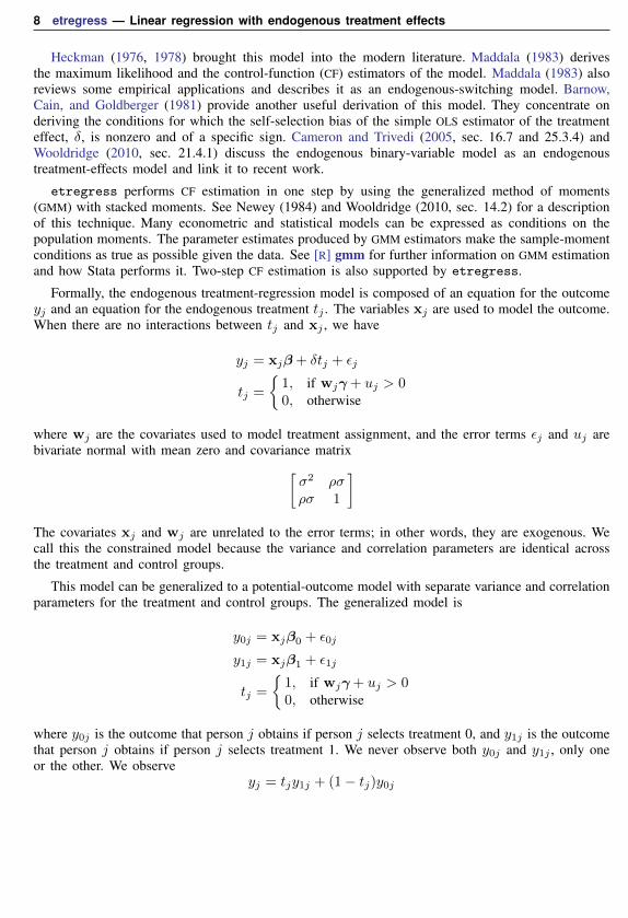
Heckman (1976, 1978) brought this model into the modern literature. Maddala (1983) derivesthe maximum likelihood and the control-function (CF) estimators of the model. Maddala (1983) alsoreviews some empirical applications and describes it as an endogenous-switching model. Barnow,Cain, and Goldberger (1981) provide another useful derivation of this model. They concentrate onderiving the conditions for which the self-selection bias of the simple OLS estimator of the treatmenteffect, δ, is nonzero and of a specific sign. Cameron and Trivedi (2005, sec. 16.7 and 25.3.4) andWooldridge (2010, sec. 21.4.1) discuss the endogenous binary-variable model as an endogenoustreatment-effects model and link it to recent work.
etregress performs CF estimation in one step by using the generalized method of moments(GMM) with stacked moments. See Newey (1984) and Wooldridge (2010, sec. 14.2) for a descriptionof this technique. Many econometric and statistical models can be expressed as conditions on thepopulation moments. The parameter estimates produced by GMM estimators make the sample-momentconditions as true as possible given the data. See [R] gmm for further information on GMM estimationand how Stata performs it. Two-step CF estimation is also supported by etregress.
Formally, the endogenous treatment-regression model is composed of an equation for the outcomeyj and an equation for the endogenous treatment tj . The variables xj are used to model the outcome.When there are no interactions between tj and xj , we have
yj = xjβ + δtj + εj
tj =
{1, if wjγ + uj > 00, otherwise
where wj are the covariates used to model treatment assignment, and the error terms εj and uj arebivariate normal with mean zero and covariance matrix[
σ2 ρσρσ 1
]The covariates xj and wj are unrelated to the error terms; in other words, they are exogenous. Wecall this the constrained model because the variance and correlation parameters are identical acrossthe treatment and control groups.
This model can be generalized to a potential-outcome model with separate variance and correlationparameters for the treatment and control groups. The generalized model is
y0j = xjβ0 + ε0j
y1j = xjβ1 + ε1j
tj =
{1, if wjγ + uj > 00, otherwise
where y0j is the outcome that person j obtains if person j selects treatment 0, and y1j is the outcomethat person j obtains if person j selects treatment 1. We never observe both y0j and y1j , only oneor the other. We observe
etregress — Linear regression with endogenous treatment effects 9
In this unconstrained model, the vector of error terms (ε0j , ε1j , uj)′ comes from a mean zero
trivariate normal distribution with covariance matrix σ20 σ01 σ0ρ0
σ01 σ21 σ1ρ1
σ0ρ0 σ1ρ1 1
The covariance σ01 cannot be identified because we never observe both y1j and y0j . However,
identification of σ01 is not necessary to estimate the other parameters because all covariates and theoutcome are observed in observations from each group. We normalize the treatment error variance tobe 1 because we observe only whether an outcome occurs under treatment. More details are foundin Methods and formulas.
Rather than showing two separate regression equations, etregress reports one outcome equationwith interaction terms between the treatment and outcome covariates. etregress can fit the constrainedand generalized potential-outcome models using either the default maximum likelihood estimator orthe one-step CF estimator obtained with option cfunction. The two-step CF estimator providesconsistent estimates for the constrained model.
Basic examples
When there are no interactions between the treatment variable and the outcome covariates in theconstrained model, etregress directly estimates the ATE and the ATET.
Example 1: Basic example
We estimate the ATE of being a union member on wages of women in 1972 from a nonrepresentativeextract of the National Longitudinal Survey on young women who were ages 14–26 in 1968. We willuse the variables wage (wage), grade (years of schooling completed), smsa (an indicator for living inan SMSA—standard metropolitan statistical area), black (an indicator for being African-American),tenure (tenure at current job), and south (an indicator for living in the South).
10 etregress — Linear regression with endogenous treatment effects
We use etregress to estimate the parameters of the endogenous treatment-regression model.
. use http://www.stata-press.com/data/r15/union3(National Longitudinal Survey. Young Women 14-26 years of age in 1968)
. etregress wage age grade smsa black tenure, treat(union = south black tenure)
Linear regression with endogenous treatment Number of obs = 1,210Estimator: maximum likelihood Wald chi2(6) = 681.89Log likelihood = -3051.575 Prob > chi2 = 0.0000
LR test of indep. eqns. (rho = 0): chi2(1) = 19.84 Prob > chi2 = 0.0000
The likelihood-ratio test in the footer indicates that we can reject the null hypothesis of no correlationbetween the treatment-assignment errors and the outcome errors. The estimated correlation betweenthe treatment-assignment errors and the outcome errors, ρ, is −0.575. The negative relationshipindicates that unobservables that raise observed wages tend to occur with unobservables that lowerunion membership. We discuss some details about this parameter in the technical note below.
The estimated ATE of being a union member is 2.95. The ATET is the same as the ATE in this casebecause the treatment indicator variable has not been interacted with any of the outcome covariates,and the correlation and variance parameters are identical across the control and treatment groups.
etregress — Linear regression with endogenous treatment effects 11
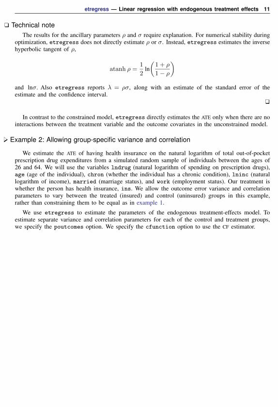
Technical noteThe results for the ancillary parameters ρ and σ require explanation. For numerical stability during
optimization, etregress does not directly estimate ρ or σ. Instead, etregress estimates the inversehyperbolic tangent of ρ,
atanh ρ =1
2ln(
1 + ρ
1− ρ
)and lnσ. Also etregress reports λ = ρσ, along with an estimate of the standard error of theestimate and the confidence interval.
In contrast to the constrained model, etregress directly estimates the ATE only when there are nointeractions between the treatment variable and the outcome covariates in the unconstrained model.
Example 2: Allowing group-specific variance and correlation
We estimate the ATE of having health insurance on the natural logarithm of total out-of-pocketprescription drug expenditures from a simulated random sample of individuals between the ages of26 and 64. We will use the variables lndrug (natural logarithm of spending on prescription drugs),age (age of the individual), chron (whether the individual has a chronic condition), lninc (naturallogarithm of income), married (marriage status), and work (employment status). Our treatment iswhether the person has health insurance, ins. We allow the outcome error variance and correlationparameters to vary between the treated (insured) and control (uninsured) groups in this example,rather than constraining them to be equal as in example 1.
We use etregress to estimate the parameters of the endogenous treatment-effects model. Toestimate separate variance and correlation parameters for each of the control and treatment groups,we specify the poutcomes option. We specify the cfunction option to use the CF estimator.
12 etregress — Linear regression with endogenous treatment effects
. use http://www.stata-press.com/data/r15/drugexp(Prescription drug expenditures)
. etregress lndrug chron age lninc, treat(ins=age married lninc work) poutcomes> cfunction
Wald test of indep. (rho0 = rho1 = 0): chi2(2) = 8.88 Prob > chi2 = 0.0118
The Wald test reported in the footer indicates that we can reject the null hypothesis of no correlationbetween the treatment-assignment errors and the outcome errors for the control and treatment groups.The estimate of the correlation of the treatment-assignment errors for the control group (ρ0) ispositive, indicating that unobservables that increase spending on prescription drugs tend to occur withunobservables that increase health insurance coverage. Because ρ1 is also positive, we make the sameinterpretation for individuals with insurance. The estimate ρ1 is larger than the estimate ρ0, indicatinga stronger relationship between the unobservables and treatment outcomes in the treated group.
The estimated ATE of having health insurance is −0.86. Note that while the ATE and ATET were thesame in example 1, that is not the case here. We show how to calculate the ATET for a potential-outcomemodel in example 6.
The estimate of the outcome error standard-deviation parameter for the control group (σ0) isslightly larger than that of the treatment group parameter (σ1), indicating a greater variability in theunobservables among the untreated group.
etregress — Linear regression with endogenous treatment effects 13
Average treatment effect (ATE)
When there is a treatment variable and outcome covariate interaction, the parameter estimates frometregress can be used by margins to estimate the ATE, the average difference of the treatmentpotential outcomes and the control potential outcomes.
Example 3: Allowing interactions between treatment and outcome covariates, ATE
In example 1, the coefficients on the outcome covariates do not vary by treatment level. Thedifferences in wages between union members and nonmembers are modeled as a level shift capturedby the coefficient on the indicator for union membership. In this example, we use factor-variablenotation to allow some of the coefficients to vary over treatment level and then use margins (see[R] margins) to estimate the ATE. (See [U] 11.4.3 Factor variables for an introduction to factor-variablenotation.)
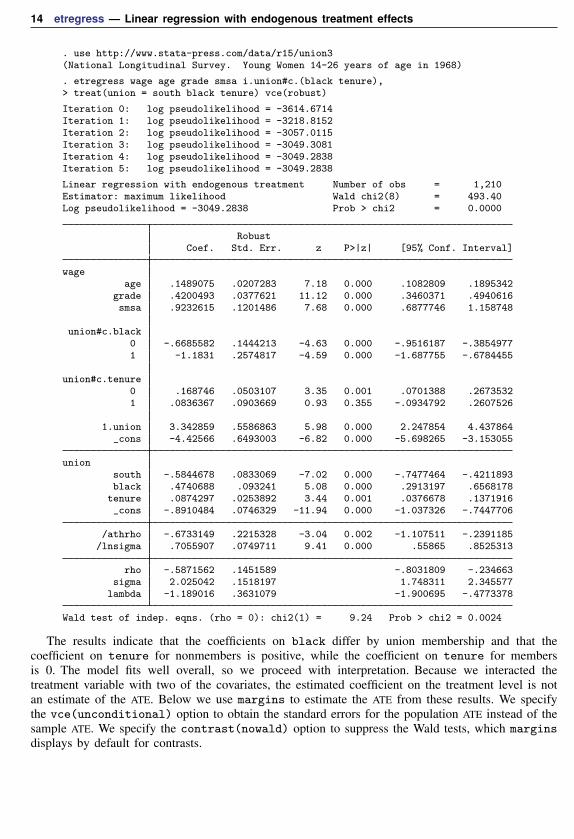
We begin by estimating the parameters of the model in which the coefficients on black andtenure differ for union members and nonmembers. We specify the vce(robust) option becausewe need to specify vce(unconditional) when we use margins below.
Linear regression with endogenous treatment Number of obs = 1,210Estimator: maximum likelihood Wald chi2(8) = 493.40Log pseudolikelihood = -3049.2838 Prob > chi2 = 0.0000
RobustCoef. Std. Err. z P>|z| [95% Conf. Interval]
Wald test of indep. eqns. (rho = 0): chi2(1) = 9.24 Prob > chi2 = 0.0024
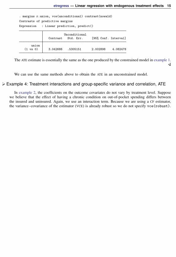
The results indicate that the coefficients on black differ by union membership and that thecoefficient on tenure for nonmembers is positive, while the coefficient on tenure for membersis 0. The model fits well overall, so we proceed with interpretation. Because we interacted thetreatment variable with two of the covariates, the estimated coefficient on the treatment level is notan estimate of the ATE. Below we use margins to estimate the ATE from these results. We specifythe vce(unconditional) option to obtain the standard errors for the population ATE instead of thesample ATE. We specify the contrast(nowald) option to suppress the Wald tests, which marginsdisplays by default for contrasts.
etregress — Linear regression with endogenous treatment effects 15
The ATE estimate is essentially the same as the one produced by the constrained model in example 1.
We can use the same methods above to obtain the ATE in an unconstrained model.
Example 4: Treatment interactions and group-specific variance and correlation, ATE
In example 2, the coefficients on the outcome covariates do not vary by treatment level. Supposewe believe that the effect of having a chronic condition on out-of-pocket spending differs betweenthe insured and uninsured. Again, we use an interaction term. Because we are using a CF estimator,the variance–covariance of the estimator (VCE) is already robust so we do not specify vce(robust).
16 etregress — Linear regression with endogenous treatment effects
. use http://www.stata-press.com/data/r15/drugexp(Prescription drug expenditures)
. etregress lndrug i.ins#i.chron age lninc, treat(ins=age married lninc work)> poutcomes cfunction
Wald test of indep. (rho0 = rho1 = 0): chi2(2) = 8.90 Prob > chi2 = 0.0117
The results indicate that the coefficient on chron differs by whether an individual has insurance.The model fits well overall, so we proceed with interpretation.
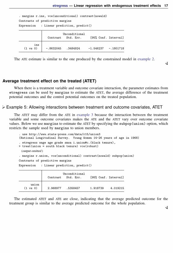
Because we interacted the treatment variable with one of the covariates, the estimated coefficienton the treatment level is not an estimate of the ATE. Below we use margins to estimate the ATEfrom these results. We specify the vce(unconditional) option to obtain the standard errors for thepopulation ATE instead of the sample ATE. We specify the contrast(nowald) option to suppressthe Wald tests.
etregress — Linear regression with endogenous treatment effects 17
ins(1 vs 0) -.8632045 .3484924 -1.546237 -.1801718
The ATE estimate is similar to the one produced by the constrained model in example 2.
Average treatment effect on the treated (ATET)
When there is a treatment variable and outcome covariate interaction, the parameter estimates frometregress can be used by margins to estimate the ATET, the average difference of the treatmentpotential outcomes and the control potential outcomes on the treated population.
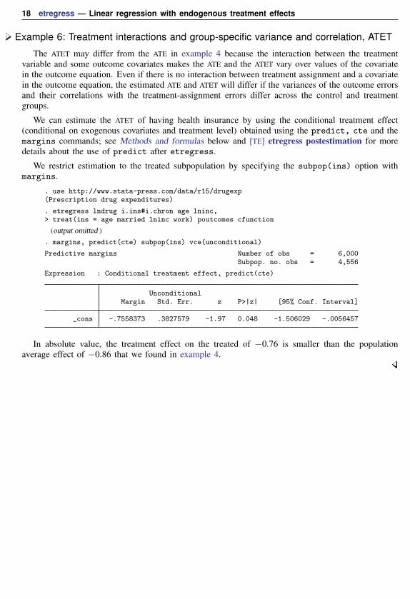
Example 5: Allowing interactions between treatment and outcome covariates, ATET
The ATET may differ from the ATE in example 3 because the interaction between the treatmentvariable and some outcome covariates makes the ATE and the ATET vary over outcome covariatevalues. Below we use margins to estimate the ATET by specifying the subpop(union) option, whichrestricts the sample used by margins to union members.
. use http://www.stata-press.com/data/r15/union3(National Longitudinal Survey. Young Women 14-26 years of age in 1968)
. etregress wage age grade smsa i.union#c.(black tenure),> treat(union = south black tenure) vce(robust)
The estimated ATET and ATE are close, indicating that the average predicted outcome for thetreatment group is similar to the average predicted outcome for the whole population.
18 etregress — Linear regression with endogenous treatment effects
Example 6: Treatment interactions and group-specific variance and correlation, ATET
The ATET may differ from the ATE in example 4 because the interaction between the treatmentvariable and some outcome covariates makes the ATE and the ATET vary over values of the covariatein the outcome equation. Even if there is no interaction between treatment assignment and a covariatein the outcome equation, the estimated ATE and ATET will differ if the variances of the outcome errorsand their correlations with the treatment-assignment errors differ across the control and treatmentgroups.
We can estimate the ATET of having health insurance by using the conditional treatment effect(conditional on exogenous covariates and treatment level) obtained using the predict, cte and themargins commands; see Methods and formulas below and [TE] etregress postestimation for moredetails about the use of predict after etregress.
We restrict estimation to the treated subpopulation by specifying the subpop(ins) option withmargins.
. use http://www.stata-press.com/data/r15/drugexp(Prescription drug expenditures)
. etregress lndrug i.ins#i.chron age lninc,> treat(ins = age married lninc work) poutcomes cfunction
etregress — Linear regression with endogenous treatment effects 19
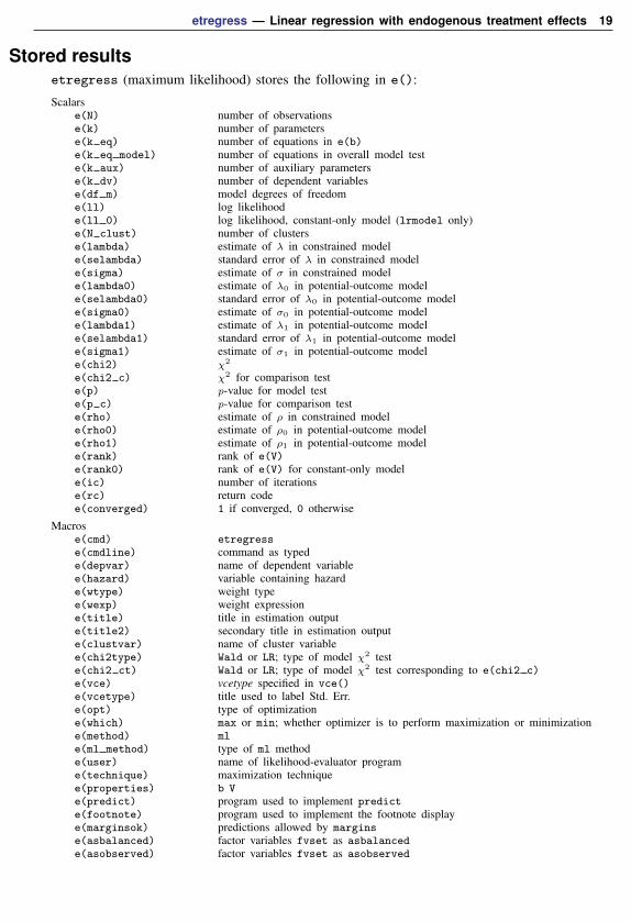
Stored resultsetregress (maximum likelihood) stores the following in e():
Scalarse(N) number of observationse(k) number of parameterse(k eq) number of equations in e(b)e(k eq model) number of equations in overall model teste(k aux) number of auxiliary parameterse(k dv) number of dependent variablese(df m) model degrees of freedome(ll) log likelihoode(ll 0) log likelihood, constant-only model (lrmodel only)e(N clust) number of clusterse(lambda) estimate of λ in constrained modele(selambda) standard error of λ in constrained modele(sigma) estimate of σ in constrained modele(lambda0) estimate of λ0 in potential-outcome modele(selambda0) standard error of λ0 in potential-outcome modele(sigma0) estimate of σ0 in potential-outcome modele(lambda1) estimate of λ1 in potential-outcome modele(selambda1) standard error of λ1 in potential-outcome modele(sigma1) estimate of σ1 in potential-outcome modele(chi2) χ2
e(chi2 c) χ2 for comparison teste(p) p-value for model teste(p c) p-value for comparison teste(rho) estimate of ρ in constrained modele(rho0) estimate of ρ0 in potential-outcome modele(rho1) estimate of ρ1 in potential-outcome modele(rank) rank of e(V)e(rank0) rank of e(V) for constant-only modele(ic) number of iterationse(rc) return codee(converged) 1 if converged, 0 otherwise
Macrose(cmd) etregresse(cmdline) command as typede(depvar) name of dependent variablee(hazard) variable containing hazarde(wtype) weight typee(wexp) weight expressione(title) title in estimation outpute(title2) secondary title in estimation outpute(clustvar) name of cluster variablee(chi2type) Wald or LR; type of model χ2 teste(chi2 ct) Wald or LR; type of model χ2 test corresponding to e(chi2 c)e(vce) vcetype specified in vce()e(vcetype) title used to label Std. Err.e(opt) type of optimizatione(which) max or min; whether optimizer is to perform maximization or minimizatione(method) mle(ml method) type of ml methode(user) name of likelihood-evaluator programe(technique) maximization techniquee(properties) b Ve(predict) program used to implement predicte(footnote) program used to implement the footnote displaye(marginsok) predictions allowed by marginse(asbalanced) factor variables fvset as asbalancede(asobserved) factor variables fvset as asobserved
20 etregress — Linear regression with endogenous treatment effects
Matricese(b) coefficient vectore(Cns) constraints matrixe(ilog) iteration log (up to 20 iterations)e(gradient) gradient vectore(V) variance–covariance matrix of the estimatorse(V modelbased) model-based variance
Functionse(sample) marks estimation sample
etregress (two-step) stores the following in e():
Scalarse(N) number of observationse(df m) model degrees of freedome(lambda) λ
e(selambda) standard error of λe(sigma) estimate of sigmae(chi2) χ2
e(p) p-value for model teste(rho) ρ
e(rank) rank of e(V)
Macrose(cmd) etregresse(cmdline) command as typede(depvar) name of dependent variablee(hazard) variable containing hazarde(title) title in estimation outpute(title2) secondary title in estimation outpute(chi2type) Wald or LR; type of model χ2 teste(vce) vcetype specified in vce()e(method) twostepe(properties) b Ve(predict) program used to implement predicte(footnote) program used to implement the footnote displaye(marginsok) predictions allowed by marginse(marginsnotok) predictions disallowed by marginse(asbalanced) factor variables fvset as asbalancede(asobserved) factor variables fvset as asobserved
Matricese(b) coefficient vectore(V) variance–covariance matrix of the estimators
Functionse(sample) marks estimation sample
etregress — Linear regression with endogenous treatment effects 21
etregress (control-function) stores the following in e():
Scalarse(N) number of observationse(k) number of parameterse(k eq) number of equations in e(b)e(k aux) number of auxiliary parameterse(k dv) number of dependent variablese(lambda) estimate of λ in constrained modele(selambda) standard error of λ in constrained modele(sigma) estimate of σ in constrained modele(lambda0) estimate of λ0 in potential-outcome modele(selambda0) standard error of λ0 in potential-outcome modele(sigma0) estimate of σ0 in potential-outcome modele(lambda1) estimate of λ1 in potential-outcome modele(selambda1) standard error of λ1 in potential-outcome modele(sigma1) estimate of σ1 in potential-outcome modele(chi2 c) χ2 for comparison teste(p c) p-value for comparison teste(rho) estimate of ρ in constrained modele(rho0) estimate of ρ0 in potential-outcome modele(rho1) estimate of ρ1 in potential-outcome modele(rank) rank of e(V)e(converged) 1 if converged, 0 otherwise
Macrose(cmd) etregresse(cmdline) command as typede(depvar) name of dependent variablee(hazard) variable containing hazarde(wtype) weight typee(wexp) weight expressione(title) title in estimation outpute(title2) secondary title in estimation outpute(chi2 ct) Wald; type of model χ2 test corresponding to e(chi2 c)e(vce) vcetype specified in vce()e(vcetype) title used to label Std. Err.e(method) cfunctione(properties) b Ve(predict) program used to implement predicte(footnote) program used to implement the footnote displaye(marginsok) predictions allowed by marginse(asbalanced) factor variables fvset as asbalancede(asobserved) factor variables fvset as asobserved
Matricese(b) coefficient vectore(V) variance–covariance matrix of the estimators
Functionse(sample) marks estimation sample
Methods and formulasMaddala (1983, 117–122 and 223–228) derives both the maximum likelihood and the CF estimators
implemented here. Greene (2012, 890–894) also provides an introduction to the treatment-effects model.Cameron and Trivedi (2005, sections 16.7 and 25.3.4) and Wooldridge (2010, section 21.4.1) discussthe endogenous binary-variable model as an endogenous treatment-effects model and link it to recentwork.
22 etregress — Linear regression with endogenous treatment effects
Methods and formulas are presented under the following headings:
Constrained modelGeneral potential-outcome modelAverage treatment effectAverage treatment effect on the treated
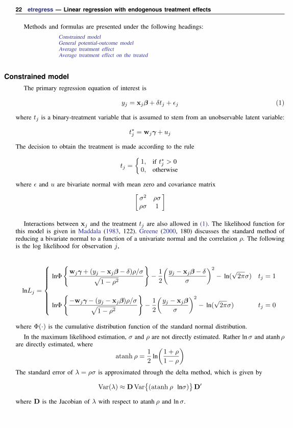
Constrained model
The primary regression equation of interest is
yj = xjβ + δtj + εj (1)
where tj is a binary-treatment variable that is assumed to stem from an unobservable latent variable:
t∗j = wjγ + uj
The decision to obtain the treatment is made according to the rule
tj =
{1, if t∗j > 00, otherwise
where ε and u are bivariate normal with mean zero and covariance matrix[σ2 ρσρσ 1
]Interactions between xj and the treatment tj are also allowed in (1). The likelihood function for
this model is given in Maddala (1983, 122). Greene (2000, 180) discusses the standard method ofreducing a bivariate normal to a function of a univariate normal and the correlation ρ. The followingis the log likelihood for observation j,
lnLj =
lnΦ
{wjγ + (yj − xjβ− δ)ρ/σ√
1− ρ2
}− 1
2
(yj − xjβ− δ
σ
)2
− ln(√
2πσ) tj = 1
lnΦ
{−wjγ− (yj − xjβ)ρ/σ√
1− ρ2
}− 1
2
(yj − xjβ
σ
)2
− ln(√
2πσ) tj = 0
where Φ(·) is the cumulative distribution function of the standard normal distribution.
In the maximum likelihood estimation, σ and ρ are not directly estimated. Rather lnσ and atanh ρare directly estimated, where
atanh ρ =1
2ln(
1 + ρ
1− ρ
)The standard error of λ = ρσ is approximated through the delta method, which is given by
Var(λ) ≈ DVar{
(atanh ρ lnσ)}D′
where D is the Jacobian of λ with respect to atanh ρ and lnσ.
etregress — Linear regression with endogenous treatment effects 23
Maddala (1983, 120–122) also derives the CF estimator as a two-step estimator. This estimatoris implemented here. We will discuss it and then discuss the one-step CF estimator that is alsoimplemented.
For the two-step estimator, probit estimates of the treatment equation
Pr(tj = 1 | wj) = Φ(wjγ)
are obtained in the first stage. From these estimates, the hazard, hj , for each observation j is computedas
hj =
φ(wj γ̂)
/Φ(wj γ̂) tj = 1
−φ(wj γ̂)/{
1− Φ(wj γ̂)}
tj = 0
where φ is the standard normal density function. If
dj = hj(hj + wj γ̂)
thenE (yj | tj ,xj ,wj) = xjβ + δtj + ρσhj
Var (yj | tj ,xj ,wj) = σ2(1− ρ2dj
)The two-step parameter estimates of β and δ are obtained by augmenting the regression equation
with the hazard h. Thus the regressors become [x t h ], and the additional parameter estimate βh isobtained on the variable containing the hazard. A consistent estimate of the regression disturbancevariance is obtained using the residuals from the augmented regression and the parameter estimateon the hazard
σ̂ 2 =e′e + β2
h
∑Nj=1 dj
N
The two-step estimate of ρ is then
ρ̂ =βhσ̂
To understand how the consistent estimates of the coefficient covariance matrix based on theaugmented regression are derived, let A = [x t h ] and D be a square diagonal matrix of size Nwith (1− ρ̂ 2dj) on the diagonal elements. The conventional VCE is
Vtwostep = σ̂ 2(A′A)−1(A′DA + Q)(A′A)−1
whereQ = ρ̂ 2(A′DA)Vp(A′DA)
and Vp is the variance–covariance estimate from the probit estimation of the treatment equation.
The one-step CF estimator is a GMM estimator with stacked moments. See Newey (1984) andWooldridge (2010, sec. 14.2) for a description of this technique. Many econometric and statisticalmodels can be expressed as conditions on the population moments. The parameter estimates producedby GMM estimators make the sample-moment conditions as true as possible given the data.
Under CF estimation, as in maximum likelihood estimation, we directly estimate atanh ρ and lnσrather than ρ and σ, so the parameter vector is
θ = (β′, δ,γ′, atanh ρ, lnσ)′
24 etregress — Linear regression with endogenous treatment effects
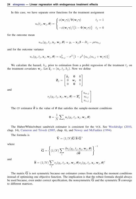
In this case, we have separate error functions for the treatment assignment
]We calculate the hazard, hj , prior to estimation from a probit regression of the treatment tj on
the treatment covariates wj . Let z̃j = (xj , tj , hj). Now we define
Zj =
z̃j 0 00 wj 00 0 1
and
sj(yj , tj ,xj ,wj , θ) = Z′j
um,jut,juv,j
The CF estimator θ̂ is the value of θ that satisfies the sample-moment conditions
0 =1
N
∑isj(yj , tj ,xj ,wj , θ)
The Huber/White/robust sandwich estimator is consistent for the VCE. See Wooldridge (2010,chap. 14), Cameron and Trivedi (2005, chap. 6), and Newey and McFadden (1994).
The formula isV̂ = (1/N)G S G ′
where
G =
{(1/N)
∑i
∂sj(yj , tj ,xj ,wj , θ)
∂θ̂
}−1and
S = (1/N)∑i
sj(yj , tj ,xj ,wj , θ)sj(yj , tj ,xj ,wj , θ)′
The matrix G is not symmetric because our estimator comes from stacking the moment conditionsinstead of optimizing one objective function. The implication is that the robust formula should alwaysbe used because, even under correct specification, the nonsymmetric G and the symmetric S convergeto different matrices.
etregress — Linear regression with endogenous treatment effects 25
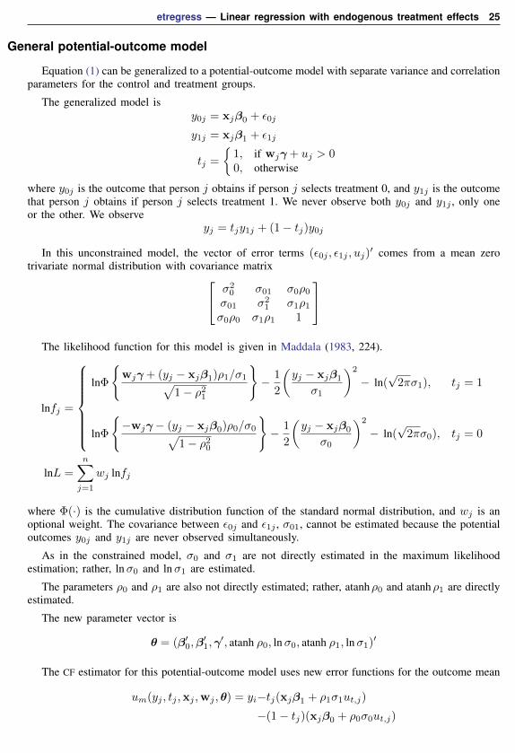
General potential-outcome model
Equation (1) can be generalized to a potential-outcome model with separate variance and correlationparameters for the control and treatment groups.
The generalized model isy0j = xjβ0 + ε0j
y1j = xjβ1 + ε1j
tj =
{1, if wjγ + uj > 00, otherwise
where y0j is the outcome that person j obtains if person j selects treatment 0, and y1j is the outcomethat person j obtains if person j selects treatment 1. We never observe both y0j and y1j , only oneor the other. We observe
yj = tjy1j + (1− tj)y0j
In this unconstrained model, the vector of error terms (ε0j , ε1j , uj)′ comes from a mean zero
trivariate normal distribution with covariance matrix σ20 σ01 σ0ρ0
σ01 σ21 σ1ρ1
σ0ρ0 σ1ρ1 1
The likelihood function for this model is given in Maddala (1983, 224).
lnfj =
lnΦ
{wjγ + (yj − xjβ1)ρ1/σ1√
1− ρ21
}− 1
2
(yj − xjβ1
σ1
)2
− ln(√
2πσ1), tj = 1
lnΦ
{−wjγ− (yj − xjβ0)ρ0/σ0√
1− ρ20
}− 1
2
(yj − xjβ0
σ0
)2
− ln(√
2πσ0), tj = 0
lnL =
n∑j=1
wj lnfj
where Φ(·) is the cumulative distribution function of the standard normal distribution, and wj is anoptional weight. The covariance between ε0j and ε1j , σ01, cannot be estimated because the potentialoutcomes y0j and y1j are never observed simultaneously.
As in the constrained model, σ0 and σ1 are not directly estimated in the maximum likelihoodestimation; rather, lnσ0 and lnσ1 are estimated.
The parameters ρ0 and ρ1 are also not directly estimated; rather, atanhρ0 and atanhρ1 are directlyestimated.
The new parameter vector is
θ = (β′0,β′1,γ′, atanh ρ0, lnσ0, atanh ρ1, lnσ1)′
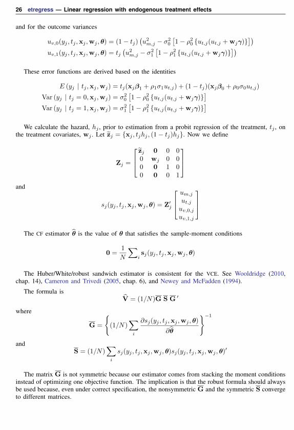
The CF estimator for this potential-outcome model uses new error functions for the outcome mean
]We calculate the hazard, hj , prior to estimation from a probit regression of the treatment, tj , on
the treatment covariates, wj . Let z̃j = {xj , tjhj , (1− tj)hj}. Now we define
Zj =
z̃j 0 0 00 wj 0 00 0 1 00 0 0 1
and
sj(yj , tj ,xj ,wj , θ) = Z′j
um,jut,juv,0,juv,1,j
The CF estimator θ̂ is the value of θ that satisfies the sample-moment conditions
0 =1
N
∑isj(yj , tj ,xj ,wj , θ)
The Huber/White/robust sandwich estimator is consistent for the VCE. See Wooldridge (2010,chap. 14), Cameron and Trivedi (2005, chap. 6), and Newey and McFadden (1994).
The formula isV̂ = (1/N)G S G ′
where
G =
{(1/N)
∑i
∂sj(yj , tj ,xj ,wj , θ)
∂θ̂
}−1and
S = (1/N)∑i
sj(yj , tj ,xj ,wj , θ)sj(yj , tj ,xj ,wj , θ)′
The matrix G is not symmetric because our estimator comes from stacking the moment conditionsinstead of optimizing one objective function. The implication is that the robust formula should alwaysbe used because, even under correct specification, the nonsymmetric G and the symmetric S convergeto different matrices.
etregress — Linear regression with endogenous treatment effects 27
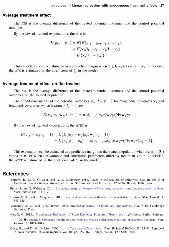
Average treatment effect
The ATE is the average difference of the treated potential outcomes and the control potentialoutcomes.
This expectation can be estimated as a predictive margin when xj(β1−β0) varies in xj . Otherwise,the ATE is estimated as the coefficient of tj in the model.
Average treatment effect on the treated
The ATE is the average difference of the treated potential outcomes and the control potentialoutcomes on the treated population.
The conditional means of the potential outcomes ytj , t ∈ (0, 1) for exogenous covariates xj andtreatment covariates wj at treatment tj = 1 are
This expectation can be estimated as a predictive margin on the treated population when xj(β1−β0)varies in xj or when the variance and correlation parameters differ by treatment group. Otherwise,the ATET is estimated as the coefficient of tj in the model.
ReferencesBarnow, B. S., G. G. Cain, and A. S. Goldberger. 1981. Issues in the analysis of selectivity bias. In Vol. 5 of
Evaluation Studies Review Annual, ed. E. W. Stromsdorfer and G. Farkas, 123–126. Beverly Hills: Sage.
Brave, S., and T. Walstrum. 2014. Estimating marginal treatment effects using parametric and semiparametric methods.Stata Journal 14: 191–217.
Brown, G. K., and T. Mergoupis. 2011. Treatment interactions with nonexperimental data in Stata. Stata Journal 11:545–555.
Cameron, A. C., and P. K. Trivedi. 2005. Microeconometrics: Methods and Applications. New York: CambridgeUniversity Press.
Cerulli, G. 2015a. Econometric Evaluation of Socio-Economic Programs: Theory and Applications. Berlin: Springer.
. 2015b. ctreatreg: Command for fitting dose-response models under exogenous and endogenous treatment. StataJournal 15: 1019–1045.
Cong, R., and D. M. Drukker. 2000. sg141: Treatment effects model. Stata Technical Bulletin 55: 25–33. Reprintedin Stata Technical Bulletin Reprints, vol. 10, pp. 159–169. College Station, TX: Stata Press.
Heckman, J. 1976. The common structure of statistical models of truncation, sample selection and limited dependentvariables and a simple estimator for such models. Annals of Economic and Social Measurement 5: 475–492.
. 1978. Dummy endogenous variables in a simultaneous equation system. Econometrica 46: 931–959.
Maddala, G. S. 1983. Limited-Dependent and Qualitative Variables in Econometrics. Cambridge: Cambridge UniversityPress.
Nannicini, T. 2007. Simulation-based sensitivity analysis for matching estimators. Stata Journal 7: 334–350.
Newey, W. K., and D. L. McFadden. 1994. Large sample estimation and hypothesis testing. In Vol. 4 of Handbookof Econometrics, ed. R. F. Engle and D. L. McFadden, 2111–2245. Amsterdam: Elsevier.
Nichols, A. 2007. Causal inference with observational data. Stata Journal 7: 507–541.
Vella, F., and M. Verbeek. 1998. Whose wages do unions raise? A dynamic model of unionism and wage ratedetermination for young men. Journal of Applied Econometrics 13: 163–183.
Wooldridge, J. M. 2010. Econometric Analysis of Cross Section and Panel Data. 2nd ed. Cambridge, MA: MIT Press.
Also see[TE] etregress postestimation — Postestimation tools for etregress
[TE] etpoisson — Poisson regression with endogenous treatment effects
[ERM] eregress — Extended linear regression
[R] heckman — Heckman selection model
[R] probit — Probit regression
[R] regress — Linear regression
[SVY] svy estimation — Estimation commands for survey data