U niversita degli Studi di Trieste XV CICLO DEL DOTTORATO DI RICERCA IN FISICA Titolo Tesi di Dottorato: DARK MATTER IN EARLY-TYPE GALAXIES WITH X-RAY HALOES. A SPECTROSCOPIC STUDY OF DYNAMICS AND ABUNDANCE INDICES Dottorando Srdj an Samurovié ( 6{, Coordinatore del Collegio dei Docenti Chiar.mo Prof. Gaetano Senatore Universita degli Studi di Trieste Relatore Chiar.mo Prof. John Danziger Osservatorio Astronomico di Trieste Correlatore Chiar.ma Prof. Maria Francesca Matteucci Universita degli Studi di Trieste
Transcript
U niversita degli Studi di Trieste XV CICLO DEL DOTTORATO DI RICERCA IN FISICA
Titolo Tesi di Dottorato:
DARK MATTER IN EARLY-TYPE GALAXIES WITH X-RAY HALOES. A SPECTROSCOPIC STUDY OF DYNAMICS AND ABUNDANCE INDICES
Dottorando Srdj an Samurovié ( 6{,
Coordinatore del Collegio dei Docenti Chiar.mo Prof. Gaetano Senatore
U niversita degli Studi di Trieste
Relatore Chiar.mo Prof. John Danziger
Osservatorio Astronomico di Trieste
Correlatore Chiar.ma Prof. Maria Francesca Matteucci
U niversita degli Studi di Trieste
BIB. GENERALE UN.IS DR 0 63
N . INV . : 066 63
ABSTRACT
In this thesis the existence of dark matter in the early-type galaxies with and without X-ray haloes was explored. I used high quality long-slit spectra obtained from various sources related to the field, binary, group and cluster galaxies from which, after the reduction procedure, fullline-of-sight velocity profiles were extracted. The analyzed spectra extend from the center out to one to three effective (half-light) radii. Some published data from the literature related to the kinematical and photometric parameters were also used.
The velocity profiles were modeled as a truncated Gauss-Hermite series, taking into account velocity, velocity dispersion, and Gauss-Hermite parameters, h3 and h4, that describe asymmetric and symmetric departures from the Gaussian, respectively. Comparison of velocity profiles with the predictions of different dynamical models which were constructed: two-integral Jeans model and three-integral Schwarzschild's numerica! orbital superposition model was done. From the two-integral modeling it is inferred that some galaxies could not be fitted with this approach thus leading to the conclusion that their distribution function depends on three integrals of motion. This kind of modeling, however, provided useful constraints on the mass-to-light ratios in these galaxies.
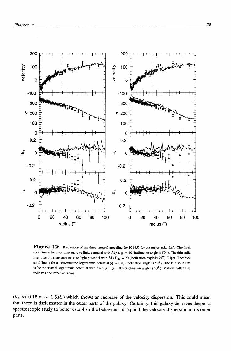
A generai conclusion is that, while some galaxies can be fitted without the inclusion of dark matter in their haloes, one cannot reject its existence, because the models are marginally consistent at larger radii with this assumption. X-ray haloes, when they are present, show the similar trend of increasing mass-to-light ratio as in the case of two-integral modeling. The three-integral mod-els that were constructed permitted me to explore stellar orbits in different potentials: spherical, axisymmetric and flattened triaxial. For each analyzed galaxy a discussion was presented about which potential is the most appropriate and comparison of results with the results obtained with the two-integral modeling technique (where available) was done.
Absorption features present in the integrated stellar spectra of early-type galaxies that pro-vide information on the chemical evolution of these objects were also studied. Using the afore-mentioned long-slit spectra absorption line indices were extracted and compared with the available models of chemical evolution of galaxies.
111
This thesis is dedicated to the Living Memory
ofmy father, Svetozar Samurovié
Dear friend, ali theory is grey, And green the golden tree of life.
Goethe, Faust
ACKNOWLEDGMENTS
I would like to thank my thesis advisors J ohn Danziger an d Francesca Matteucci for their help, encouragement and support. They provided guidance and posed interesting and important problems yet allowing me a large amount of freedom in solving them.
I would like to thank the following colleagues from the Trieste Observatory and the De-partment of Astronomy of the University of Trieste for numerous discussions an d ad vice: Simone Zaggia for the help in obtaining spectra of galaxies from the Fomax sample and the help in the data reduction, Antonio Pipino for calculation of different photo-chemical evolution models, Francesco Calura for stimulating discussions about different aspects of elliptical galaxies, Piercarlo Bonifacio for the help with the data reduction. I thank Fabio Mardirossian for his continuai help while he was the Director of both institutions. I express my gratitude to the late Giuliano Giuricin who helped me in the initial phases of this work.
I thank Eduardo Simonneau for useful discussions regarding different observational aspects of elliptical galaxies.
I would especially like to thank the following two colleagues from the Belgrade Astronomica! Observatory for numerous interesting discussions: Milan M. éirkovié and Slobodan Ninkovié. Big thanks goes to Milan S. Dimitrijevié and Zoran Knezevié in their role as Director of the Belgrade Astronomica! Observatory for their understanding and help. I also thank Luka C. Popovié for his help.
I am grateful to Giuseppe Furlan, the head of the ICTP TRIL (Training an d Research in I tali an Laboratories) program and Elena Dose, the secretary of the ICTP TRIL program for their continuai help during the work on this thesis.
This research has made use of the NASAIIPAC Extragalactic Database (NED) (http: l /nedwww. ipac. c al tec h. edu/) is operated by the Jet Propulsion Laboratory, California Institute ofTechnology, under contract with the National Aeronautics and Space Admin-istration. This research has also made use of the HyperLeda information system (http: l /leda. uni v-lyon1 . fr ). The usage of the ESO archi ve (http: l l archi ve. es o. org/) is al so acknow ledged.
The spectra of severa! galaxies were obtained courtesy of Marcella Carollo and Kenneth C. Freeman. Olivier Hainout kindly provided photometry data for IC3370. Nicola Caon kindly pro-vided Fomax galaxies photometry data in machine readable form. I acknowledge the use of the Gauss-Hermite Fourier Fitting Software developed by R.P. van der Marel and M. Franx and the use of the Two-integral Jeans Modeling Software developed by R.P. van der Mare l an d J.J. Binney.
I would like to thank my parents, Ljiljana and Svetozar, and brother, Rastko, for their help, support and encouragement. To my great sorrow, my father, Svetozar, lawyer and painter, died during the work on this thesis, on June 14, 2001. His keen interest in my work and Science was always of great importance to me. I dedicate this thesis to the living memory of him using his favorite quotation from Goethe's Faust.
I thank my wife, Hana Ovesni, for her patience, understanding and interest for my work. I am grateful to Kristinka Ovesni, Darinka Ovesni and Goran Milicié for their encouragement and help.
vii
CONTENTS
Abstract .............................................................................. iii
Acknowiedgements ................................................................... vii
Introduction .......................................................................... l
Galaxies are large systems that contain stars, gas, dust, planets and, most probably, dark matter. A large galaxy can contain approximately 1011 - 1012 stars. The amount of gas and dust can vary from a few percent of the total stellar mass ( as in lenticular galaxies) to about ten percent for the most gas-rich objects (spirai galaxies). As noted by Binney & Tremaine (1987), in reply to the statement of Sandage made in 1961 that "galaxies are to astronomy what atoms are to physics", some analogy between galaxies and atoms indeed exists: galaxies are relatively isolated systems and they maintain their identity throughout their li ves, except for occasionai collisions and mergers with other galaxies. Also, a galaxy is a dynamical and chemical unit. However, there are some differences: for galaxies the laws from the world of atoms do not ho l d: a huge number of processes in some galaxy may, but not necessarily, be present in some other galaxy. That is why Binney & Tremaine suggested a more appropriate analogy: the relationship between galaxies and astronomy should be regarded as the relationship between ecosystems and biology - this analogy takes into account their complexity, their relative isolation and their ongoing evolution.
Galaxies can be classified according to the Hubble's classification system (see Figure l) into four main types: ellipticals, lenticulars, spirals and irregulars. Early-type (elliptical and lenticular) galaxies belong to the left-hand end of the Hubble's tuning-fork diagram. The originai suggestion of E. Hubble was that galaxies evolve from the left-hand end to the right. This suggestion has now been abandoned.
Elliptical galaxies have the surface brightness that falls off smoothly with radius, and in most cases can be fitted by R 11 4 or de Vaucoulers la w:
where Re is the effective radius, that is the radius of the isophote containing half of the total luminosity and le is the surface brightness at Re· The shape of elliptical galaxies varies in form from round to elongated. One can use the simple formula n= 10[1- (b/a)], where (b/a) denotes the apparent axial ratio, to write the type of these galaxies: En. Therefore, EO are round galaxies, and E6 are highly elongated systems as seen projected on the sky. Research over the last 20 years has brought new knowledge about ellipticals and we now know that these galaxies are much more complex systems that they seemed. The elliptical galaxies contain little or no gas or dust. The old stars that are prevalent are cool, evolved, and therefore of late spectral type. In the middle of the Hubble's diagram there is a class of galaxies designated as type SO, known as lenticular galaxies. They have a smooth centrai brightness condensation similar to an elliptical galaxy that is surrounded by a large region of less steeply declining brightness. They have disks that do not show
2------------------------------ Introduction
• EO
0 .. ~
. :.~ *
. . .. ·'~···· a·:· ~S· .....
Sa Sb I m • ~ @ E3 E6 so
~ @ lSJ ...... tt ':W ·-.... . .
SBa SBb IBm
Figure l: The Hubble tuning-fork diagram. On the left-hand end there are elliptical galaxies, in the middle there are lenticulars (SO) and on the right-hand end there spirals (Sa--tSc) and irregulars. Lower part ofthe right-hand end is occupied by galaxies with bars (letter "B").
any conspicuous structure. Because of their appearance, and also because of their stellar content (e.g., spectral type), they look more like ellipticals rather than spirai galaxies. The problems may arise in the classification of SO galaxies. For example, fora close well-studied galaxy NGC3379 it is not certain whether i t is a bona fide normal elliptical or a face-on lenticular galaxy. The example of IC3370 also presented in this thesis provides another case of a problematic classification (its distance is rv 42 M pc, for the Hubble constant ho rv O. 7). The remark of Gregg et al. (2003) therefore seems appropriate: "If after such detailed investigations, we are unable to discem the morphological type of NGC3379, at a distance of only lO Mpc, then it is practically impossible to establish the true morphology of other early type galaxies at greater distances in clusters such as Coma, let alone at high redshift".
Spirai galaxies (including our own, Milky Way) consist of three main parts: spheroid, thin disk and dark halo. Spirals contain a prominent disk that is composed of Population I stars, gas, and dust. The disk also contains spirai arms, in which are embedded bright O and B stars, gas, and dust - this is a piace in which the stars are currently forming. Hubble divided spirals into a sequence of four classes (types), called Sa, Sb, Se, and Sd. Along this sequence (Sa---* Sd) the relative luminosity of the spheroid (that contains older Population II stars) decreases, the relative mass of the gas increases, and the spirai arms become more loosely wound. The Milky Way is sometimes classified as Sbc, expressing the fact that its Hubble type is between Sb and Se. Rotation curves of spirals are typically ftat, a fact that is of importance for the dark matter studies (see below).
Irregular galaxies are galaxies for which one cannot easily distinguish a particular pattem. The majority of irregulars are low-luminosity gas-rich system such as the Magellanic Clouds (see Fig. l - the letters "I" and "m" refer to irregulars of the type similar to that of the Magellanic Clouds).
l. DARK MATTER PROBLEM IN EARLY-TYPE GALAXIES
The problem of the dark matter in galaxies remains perhaps the most important astrophysical prob-lem in contemporary cosmology and extragalactic astronomy. Although its nature is stili unknown, generai opinion is that it exists and that it is a necessary ingredient of every viable cosmologica! model (see recent overview of the dark matter problem in galaxies in Binney (2003): in this paper
Introduction ------------------------------3
the problems of the cold dark matter (CDM) and MOND theory are presented).1 The existence of the dark matter in spirai galaxies (late-type galaxies ), like our own, Milky Way is rather clear mainly because of existence of cool gas which provides a powerful tool for obtaining rotation curves (that provide dependence of circular speed on radius from the center of the galaxy), that are, for most spirals, nearly flat thus indicating presence of dark mass in their outer parts - dark haloes (see, e.g., Binney & Tremaine 1987). There are problems in the determination of its shape, but observations tend to conclude that the dark halo is flattened (see, e.g., Samurovié, éirkovié & Milosevié-Zdjelar 1999).
However, the problem of dark matter in elliptical galaxies (early-type galaxies) is more com-plicated - it is more difficult to confirm the presence of dark haloes around ellipticals. Since elliptical galaxies contain little or no cool gas usually one cannot use 21-cm observations to trace kinematics of neutra! hydrogen out to large radii, as is possible in the case of spirals. The sup-port against gravitational collapse in ellipticals comes from essentially random motions rather than ordered rotation. In an attempt to check whether ellipticals have dark haloes one can use stel-lar kinematics, but since their outer parts are very faint, it is usually difficult to obtain spectra to constrain kinematics at large radii. An additional problem is related to the fact that one does not a priori know anything about the orbits of stars in ellipticals. Current investigations lead to the conclusion that there is less unambiguous evidence for the dark matter in ellipticals than in the case of spirals. Moreover, there are hints that in ellipticals the dark matter is not needed at ali or, more precisely, not needed in some early-type galaxies, out to a given observed distance from the galactic center.
Recent reviews on the dark matter problem in elliptical galaxies can be found for example in Danziger (1997), Binney & Merrifield (1998) and Bertin (2000). I here briefly present different approaches that can be used in order to determine the presence of the dark haloes around early-type galaxies. As in Danziger (1997) I split the different methodological approaches in three large groups that are then subdivided: gas, test particles and lensing methods.
(a) GAS The gas in the early type-galaxies can be found in the X-ray haloes, this is a hot gas with temperature T "' 107 K. Studi es of X-ray haloes strongly suggest the existence of dark matter out to large distances from the center (review in Mathews & Brighenti 2003). I refer the reader to Chapter 3 where I present relevant calculations and apply them to the galaxies from my samples that posses X-ray haloes. The gas can also be warm, with T "' 104 K. This is ionized hydrogen that includes emission line gas and Ha + [NII] regions (e.g. Buson et al. 1993, Zeilinger et al. 1996). Pizzella et al. (1997) analyzed the velocity fields of ionized gas disks in four ellipticals and derived mass-to-light ratios as a function of radiai distance. Using triaxial mass distribution they found that M l L ratio changes within individuai galaxies, although there is no systematic increase with radius. The mean value for the B-band that was found is "' 5M0 1 LB0 out to one effective radius (note that ho = 0.5 was used). This technique is limited to the inner regions of galaxies. Cold gas has been detected in several early-type galaxies out to large distances (:2:: 10Re). Bertola et al. (1993) found that variation of mass-to-light ratio in the B-band, M0 1 LB8 (in this thesis abbreviated to M l L B), in ellipticals is similar to that of spirai galaxies. They showed that in spirals and ellipticals there exists a radius where the density of the dark matter is equal to that of
1 In this thesis al l the calculations w ere done in the framework of the classica! Newtonian dynamics -no attempts were made to perform calculations within alternative theories (e.g. MOND theory ofMilgrom 1983).
4----------------------------- Introduction
the visible matter. Expressed in units of effective radius, Re, this distance is at 1.2 Re· Morganti et al. (1995) studied the example of elliptical galaxy NGC5266 and found that a disk of neutra! hydrogen extends out to lO Re· They discovered that there was an increase of mass-to-light ratio in the B-band from a value of M/ LB ~ 2- 3 in the inner region to M/ LB ~ 12 at the most distant measured point at ~ 9 Re. Thus they concluded that there is a hint of a dark matter halo. Oosterloo et al. (2002) studied five dust lane elliptical galaxies and found that in the case of NGC3108 the regular distribution and kinematics of the Hl allowed them to derive the mass-to-light ratio: they calculated the value of M/ LB ~ 18 at 6 Re. The very recent result of radio and optical observations of the same galaxy of Jozsa, Oosterloo & Morganti (2003) suggests that the mass-to-light ratio out to 6Re is ~ 15 M0 / Lv0 (in the V-band) (corresponds to M/ LB ~ 22 in the B-band). They reached the conclusion that this galaxy possesses a dark halo similar to that observed in spirals.
(b) TEST PARTICLES Planetary nebulae (PNe) are very a promising tool for dark mat-ter research because they are detectable even in moderately distant galaxies through their strong emission lines. Hui, Freeman & Dopita (1995) found that the mass-to-light ratio in the centrai region of a giant elliptical galaxy NGC5128 is ~ 3.9 and that out to ~ 5 Re it increases to ~ 10 (in the B-band), thus indicating the existence of the dark halo. In an extension of this work, very recently, Peng, Ford & Freeman (2003) presented their results of an imaging and spectroscopic survey for PNe in NGC5128. They detected 1141 PNe, out of which they confirmed 780. They found that PNe exist at distances out to 80 kpc ( ~ 15Re) making this study the largest kinematic study of an elliptic galaxy to date, both in the number of velocity tracers and in radiai extent. They found that the dark matter is necessary to explain the observed stellar kinematics, but their value of M/ LB is much lower than that expected from determinations that use X-ray haloes: within 80 kpc they found the total dynamic mass ~ 5 x 10¹¹ M 0 with M/ LB ~ 13. According to the paper of Bahcall, Lubin & Dorman (1995) that is based on the compilation of the mass-to-light ratios from the literature, at 80 kpc one should expect M/ LB ~ 112 ± 28. lt was already found by Hui et al. (1995) that the dynamical mass that they measured within 25 kpc was systematically lower than that measured by Forman, Jones & Tucker (1985) from ROSAT data who calculated a total mass of 1.2 x 10¹² M0 within 20 kpc. Also, van Gorkom et al. (1990) estimated the dynami-cal mass of NGC5128 using Hl synthesis observations and found that it is much lower than that obtained using X-ray halo: they found that the total mass is 2.5 x 10¹¹ M0 , and the mass within 1.2Re is 1.2 x 10¹¹ M0 . Thus, they found that there exists a constant mass-to-light ratio (that is equal to 3.1) out to at least 8.7 kpc. An interesting example of usage of PNe methodology in dark matter research is that of galaxy NGC3379. Ciardullo, Jacoby & Dejonghe (1993) used 29 PNe (out to 3.8 Re) to draw the conclusion that the mass-to-light ratio M/ LB ~ 7 and that there is no need for the dark matter. Recently, Romanowsky et al. (2003) observed PNe in three galaxies (NGC821, NNGC3379 and NGC4494) and confirmed this conclusion for NGC3379 using much larger sample of 109 PNe (out to ~ 5.5 Re). I analyzed this galaxy in some detail using different available data (photometry, long-slit spectra, X-ray data) in Chapters l and 2 and I reached the same conclusions, although I stress that some doubts stili remain.
Globular clusters can also be used as tracers of dark matter in the early-type galaxies: Mould
et al. (1990) obtained optical multislit spectra of two giant elliptical galaxies M49 and M87 from the Virgo cluster. They found that the velocity dispersion profiles of the cluster systems were flat, thus suggesting the existence of an isothermal halo of dark matter in these elliptical galaxies. Grillmair et al. (1994) studied the radiai velocities of 47 globular clusters in NGC1399 in the Fomax cluster. Under the assumption that the clusters were on purely circular orbits, they gave a lower limit on a globally constant mass-to-light (M/L) ratio of 79 ± 20 in the B-band. Their result suggesting that M/ L is severa! times larger than values of mass-to-light ratio determined from the stellar component closer to the core implies that M/ L must increase substantially with radius. This galaxy has been analyzed in Chapter 2 of this thesis. Coté et al. (2003) studied M49 ( == NGC4472) galaxy and showed that the globular clusters radiai veloci ti es and density profiles provide "unmistakable evidence" for a massive dark halo. Very recently, Bridges et al. (2003) presented their results obtained using Gemini/GMOS spectrograph of severa! early-type galaxies. It is important to note that they have observed 22 globular clusters in the aforementioned galaxy NGC3379 an d found no evidence of the dark matter out to 6 Re: they, in fact, in their preliminary analysis reached the conclusion that the mass-to-light ratio decreases (from ("'V 8 at 2 Re to ("'V 4 at ("'V 6 Re, in the V-band, see Fig. 3 in Chapter 3 that includes this result transformed to the B-band).
A large set of dark matter investigations in early-type galaxies is made of studies of inte-grated stellar light. Since this is one of the main subjects of my thesis in subsequent chapters I will provide more details later. Here I present briefly the history of observations and modeling procedures. Binney, Davies & Illingworth (1990) in their seminai paper established a two-integral axisymmetric modeling based on the photometric observations. They analyzed galaxies NGC720, NGC1052, and NGC4697 and modeled velocities and velocity dispersions out to ("'V l Re· van der Marel et al. (1990) applied this approach to NGC3379 (out to ("'V l Re), NGC4261 (out to ("'V l Re), NGC4278 (out to ("'V l Re) and NGC4472 (out to 0.5 Re). Cinzano & van der Marel (1994) modeled the galaxy NGC2974 out to 0.5 Re introducing a new moment- modeling of the Gauss-Hermite moments (for definitions see Chapter l) defined previously in van der Marel & Franx (1993). Ali these modeling procedures did not take into account dark matter, because they dealt with the regions in which dark matter was not expected to make a significant contribution. In this case they showed that this method can provide a hint on the embedded stellar disk. Bertin, Saglia & Stiavelli (1992) and Saglia, Bertin & Stiavelli (1992) developed self-consistent two-component models of ellipticals. They fitted the models to observed photometric and kinematic profiles of individuai galaxies and found that the amount of dark matter within one effective radius is not too large (it is of similar order to the luminous mass). In the case of NGC4472 (under their physical assumptions) it was found that dark matter must be present.
Saglia et al. (1993) presented a kinematical and line strength profiles of NGC4472, IC4296 and NGC7144 and from their dynamical modeling (quadratic programming) concluded that there is a strong evidence for dark matter in these galaxies. Carollo et al. (1995) observed and modeled a set of elliptical galaxies (NGC2434, NGC2663, NGC3706 and NGC5018). They used two-integral modeling procedure to model the stellar line-of-sight velocity distribution (using velocity dispersion and Gauss-Hermite h4 parameter) out to two effective radii. They concluded that the massi ve dark matter haloes must be present in three of the four galaxies (they were analyzed in this thesis using a three-integral modeling procedure), an d in case of NGC2663 there was no evidence of the dark matter. In 1997 Rix et al. used the Schwarzschild (1979) method for construction of axisymmetric and triaxial models of galaxies in equilibrium without explicit knowledge of the
6 -----------------------------Introduction
integrals of motion. They introduced into the analysis velocity, velocity dispersion and Gauss-Hermite parameters h3 and h4 . They used the galaxy NGC2434 (from Carollo et al. 1995) to perform a detailed dynamical modeling in order to conclude that this galaxy contains a lot of dark matter: they found that about half of the mass within one effective radius is dark.
Statler et al. (1996) studied stellar kinematical fields of the post-merger elliptical galaxy NGC1700 out to four effective radii. In a subsequent paper Statler et al. (1999) found, using two-integral axisymmetric models as well as three-integral quadratic programming models that NGC1700 must have a radially increasing mass-to-light ratio, and that NGC1700 "appears to rep-resent the strongest stellar dynamical evidence to date for dark halos in elliptical galaxies". Unfor-tunately, as noted by Statler et al., this galaxy has not been observed in the X-ray domain. Saglia et al. (2000) modeled the galaxy NGC1399 using two-integral models (major photometric axis only) out to rv 2.5 Re. They marginally detected the infiuence of the dark component that starts from 1.5 Re.
Gerhard et al. (1998) modeled NGC6703 using two-integral approach out to 2.6 Re and found that dark halo must exist and that dark matter contributes about equal mass at 2.6 Re to that from stars. Kronawitter et al. (2000) modeled a large sample of 21 elliptical galaxies out to 1-2 Re: for three of them (NGC2434, NGC7507, NGC7626) they found that models based on luminous matter should be ruled out. De Bruyne et al. (2001) modeled NGC4649 and NGC7097 using a three-integral quadratic programming method and found that in the case of NGC4649 a constant mass-to-light ratio (M/ Lv = 9.5) fit can provide good agreement with the data and that a marginally better fit can be obtained including 10% of dark matter at 1.2 Re. In the case of NGC7097 both kinematic and photometric data can be fitted out to 1.6 Re using a constant mass-to-light ratio rv 7 .2. Cretton et al. (2000) modeled the giant elliptical galaxy NGC2320 using the Schwarzschild orbit superposition method and found that the models with radially constant mass-to-light ratio and logarithmic models with dark matter provide comparably good fits to the data and have similar dynamical structure (but note that the mass-to-light in the V-band is rather large: rv 15 for the mass-follows-light models and rv 17 for the logarithmic models).
The Schwarzschild method can be applied in modeling of the centrai parts of the early-type galaxies, see for example, the paper by van der Marel et al. (1998) in which M32 was analyzed, the Cretton & van der Bosch (1999) paper in which axisymmetric models of NGC4342 were pre-sented, the Gebhardt et al. (2000) paper in which a black hole in the center of NGC3379 was modeled, the Gebhardt et al. (2003) paper with the sample of 12 ellipticals that were analyzed using axisymmetric approach. Finally, I mention the paper of Cappellari et al. (2002) that modeled in detail, using the Schwarzschild formalism, internai parts of one early-type galaxy that is also a subject of this thesis, IC1459.
A new, promising, avenue in studi es of integrated light from the early-type galaxies is usage of new integrai field spectrographs (like, for example, SAURON, cf. Bacon et al. 2001, de Zeeuw et al. 2002) that should provide information on line-of-sight velocity distribution and spectral indices in two dimensions improving the limitations of long-slit spectroscopy that is limited by time to few position angles. Unfortunately, this technique is at the moment limited to the interior parts of the galaxies ( out to rv l Re, Emsellem, 2002, priv. communication). Therefore, long-slit spectroscopy with its long exposures stili remains a necessary tool in dark matter studies.
There are numerous studies of early-type dwarf galaxies in the Local Group that investigate the internai dynamics of dwarf ellipsoidal galaxies. A successful fit to the data is obtained when
Introduction -----------------------------7
one assumes that they are embedded in a dark halo with mass of"' 107 M0 , and a luminous mass component with a mass-to-light ratio in V-band M/ Lv = 2.5 (see, e.g. Mateo 1998).
(c) LENSING METHODS In this group of methods, I include weak gravitationallensing that enables determination of the dependence of the velocity dispersion on the luminosity of the lensing galaxies and is suitable for studies of the dark matter in outer part of galaxies. It was found that a Navarro-Frenk-White (NFW) profile provides a good fitto the data (Kleinheinrich et al. 2003). Strong gravitationallenses can also be used for probing of the galaxy haloes, but only in the inner regions of galaxies (few tens of kiloparsecs) (see, for example, Prada et al. 2003). I also mention the Lenses Structure and Dynamics (LSD) Survey that gathers kinematic data for distant (up to z "' l) early-type galaxies that are gravitationallenses (review in Treu et al. 2003). The results of this survey suggest that extended dark matter haloes are detected in the early-type galaxies and that the dark matter contributes 50-75% to the total mass within the Einstein radius (cases of the lens galaxies MG2016+ 112 in Treu & Koopmans (2002) and 0047-281 in Koopmans & Treu 2003).
2. THE AIM OF THIS THESIS
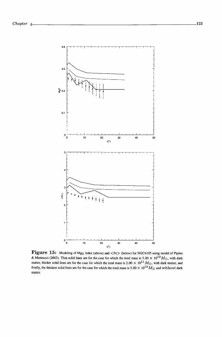
This thesis is dedicated to the detailed study of the kinematics of the early-type galaxies that is extracted from the integrated spectra of their stars. Since the existence of dark matter in the early-type galaxies can be established only in a study that takes into account ali available observational data, the observational data that I had were then used in combination with the photometry data and the X-ray data in cases where galaxies posses X-ray haloes. A substantial part of the thesis is devoted to the construction of realistic dynamical models of the early-type galaxies: a publicly available code for two-integral modeling (van der Marel2003) was used and I built my own pack-age for three-integral dynamical modeling (based on the Schwarzschild (1979) method and Rix et al. (1997) paper) that I describe in detail. A reduction of long-slit spectra of ali of the galaxies that I had at my disposal (except for three galaxies from Carolio et al. (1995) sample for which I took the data from literature) was made. Some photometric data from the literature was al so used. Comparison of my results with the results of other aforementioned techniques in cases where such data existed revealed both agreement and discrepancies. Finaliy, in an attempt at making a link between the dynamics and chemical evolution I calculated abundance indices and compared them with the up-to-date chemical evolution mo~els (Matteucci 2001, Pipino & Matteucci 2003)
REFERENCES
Bacon, R., Copin, Y., Monnet, G., Milier, B. W., Aliington-Smith, J.R., Bureau, M., Carolio, C.M., Davies, R.L., Emseliem, E., Kuntschner, H., Peletier, R.F., Verolme, E.K. & Tim de Zeeuw, P.T.: 2001, MNRAS, 326, 23
Bertin, G.: 2000, Dynamics ofGalaxies, Cambridge University Press Bertin, G., Saglia, R.P. & Stiavelli, M.: 1992, ApJ, 384, 423 Bertela, F., Pizzella, A., Persic, M. & Salucci, P.: 1993, ApJ, 416, L45 Binney, J.J., Davies, R.D. & Illingworth, G.D.: 1990, ApJ,361, 78 Binney, J.J. & Merrifield, M.R.: 1998, Galactic Astronomy, Princeton University Press Binney, J.J. & Tremaine, S.: 1987, Galactic Dynamics, Princeton University Press Binney, J.J.: 2003, to appear in IAU Symposium 220, "Dark Matter in Galaxies", S. Ryder, D.J.
Pisano, M. Walker & K. Freeman (eds.), preprint astro-ph/0310219 Bridges, T., Beasley, M., Faifer, F., Forbes, D., Forte, J., Gebhardt, K., Hanes, D., Sharples, R. &
Zepf, S.: 2003, in press, in "J oint Discussion 6: Extragalactic Globular Clusters an d their Host Galaxies", IAU Generai Assembly, July 2003. T. Bridges and D. Forbes (eds.), preprint astro-ph/0310324
Buson, L.M., Sadler, E.M., Zeilinger, W.W., Bertin, G., Bertela, F., Danzinger, I.J., Dejonghe, H., Saglia, R.P. & de Zeeuw, P. T.: 1993, A&A, 280,409
Cappellari, M., Verolme, E.K., van der Marel, R.P., Verdoes Kleijn, G.A., Illingworth, G.D., Franx, M., Carollo, C.M. & de Zeeuw, P.T.: 2002, ApJ, 578, 787
Carollo, C.M., de Zeeuw, P.T., van der Marel, R.P., Danziger, I.J. & Qian, E.E.: 1995, ApJ, 441, L25
Ciardullo, R., Jakoby, G.H. & Dejonghe, H.G.: 1993, ApJ, 414, 454 Cinzano, P. & van der Marel, R.P.: 1994, MNRAS, 270, 325 Coté P., McLaughlin, D.E., Cohen, J.G. & Blakeslee, J.P.: 2003, 591, 850 Cretton, N. & van der Bosch, F.C: 1999, ApJ, 514, 704. Cretton, N., Rix, H-W. & de Zeeuw, P.T.: 2000, ApJ, 536,319 Danziger I.J.: 1997, Dark and Visible Matter in Galaxies, ASP Conference Series, Vol. 117,
Massimo Persic & Paolo Salucci (eds.), 28 De Bruyne, V., Dejonghe, H., Pizzella, A., Bemardi, M. & Zeilinger, W. W.: 2001, ApJ, 546, 903 de Zeeuw, P.T., Bureau, M., Emsellem, E., Bacon, R., Carollo, C.M., Copin, Y., Davies, R.L.,
Forman, W., Jones, C. & Tucker, W.: 1985, ApJ, 293, 102 Gebhardt, K., Richstone, D., Kormendy, J., Lauer, T.R., Ajhar, E.A., Bender, R., Dressler, A.,
Faber, S.M., Grillmair, C., Magorrian, J. & Tremaine, S.: 2000, AJ, 119, 1157 Gebhardt, K., Richstone, D., Tremaine, S. Lauer, T.R., Bender, R., Bower, G., Dressler, A. Faber,
S.M., Filippenko, A.V., Green, R., Grillmair, C., Ho, L.C., Kormendy, J., Magorrian, J. & Pinkney, J.: 2003, ApJ, 583, 92
Gerhard, 0., Jeske, G., Saglia, R.P. & Bender, R.: 1998, MNRAS, 295, 197 Gregg, M.D, Ferguson, H.C., Minniti, D., Tanvir, N. & Catchpole, R.: 2003, AJ, in press,
preprint astro-ph/0312158 Grillmair, C.J., Freeman, K.C., Bicknell, G.V., Carter, D., Couch, W.J., Sommer-Larsen, J. &
Taylor, K.: 1994, ApJ, 422, L9 Hui, X., Ford, H.C., Freeman, K.C., Dopita, M.A.: 1995, ApJ, 449, 592 Jozsa, G., Oosterloo, T. & Morganti, R.: 2003, in Proceedings of "Dark Matter in Galaxies",
International Astronomica! Union, Symposium no. 220, held 22-25 July, 2003 in Sydney
Introduction ----------------------------9,
Kleinheinrich, M., Schneider, P., Erben, T., Schirmer, M., Rix, H-W., Meisenheimer, K. & Wolf, C.: 2003, to appear in the Proceedings of the Meeting on "Gravitational Lensing: A unique Tool for Cosmology" held in Aussois, France, 5-11 Jan. 2003, preprint astro-ph/0304208
Koopmans, L.V.E. & Treu, T.: 2003, ApJ, 583, 606 Kronawitter, A, Saglia, R.P., Gerhard, O. & Bender, R: 2000, A& AS, 144, 53 Mateo, M.L.: 1998, ARAA, 36, 435 Mathews, W.G. & Brighenti, F.: 2003, ARAA, 41, 191 Matteucci, F.: 2001, Chemical Evolution ofthe Galaxy, Kluwer Academic Publishers, Dordrecht Milgrom, M.: 1983, ApJ, 270, 365 Morganti, R., Pizzella, A., Sadler, E.M. & Bertola, F.: 1995, PASA, 12, 143 Mould, J.R., Oke, J.B., de Zeeuw, P.T. & Nemec, J.M.: 1990, AJ, 99, 1823 Oosterloo, T. A., Morganti, R. Sadler, E. M., Vergani, D. & Caldwell, N.: 2002, AJ, 123,729 Peng, E. W., Ford, H.C. & Freeman, K.C.: 2003, ApJ, in press, preprint astro-ph/0311236 Pipino, A. & Matteucci, F.: 2003, MNRAS, in press, preprint astro-ph/0310251 Pizzella, A., Amico, P., Bertola, F., Buson, L.M., Danziger, I.J., Dejonghe, H., Sadler, E.M., Saglia,
R.P., de Zeeuw, P.T., & Zeilinger, W.W.: 1997, A& A, 323, 349 Prada, F., Vitvitska, M., Klypin, A., Holtzman, J.A., Schlegel, D.J., Grebel, E.K., Rix, H-W.,
Brinkmann, J., McKay, T.A. & Csabai, 1.: 2003, ApJ, in press, astro-ph/0301360 Rix, H.-W., de Zeeuw, P.T., Cretton, N., van der Marel, R.P. & Carollo, C.M.: 1997, ApJ, 488, 702 Romanowsky, A.J., Douglas, N.G., Arnaboldi, M., Kuijken, K., Merrifield, M.R., Napolitano,
N.R., Capaccioli, M. & Freeman, K.C.: 2003, Science, 5640, 1696 Saglia, R.P., Bertin, G. & Stiavelli, M.: 1992, ApJ, 384, 433 Saglia, R. P., Bertin, G., Bertola, F., Danziger, l. J., Dejonghe, H., Sadler, E. M., Stiavelli, M., de
Zeeuw, P. T. & Zeilinger, W. W.: 1993, ApJ, 403, 567 Saglia, R.P., Kronawitter, A., Gerhard, O. & Bender, R.: 2000, AJ, 119, 153 Samurovié, S., éirkovié, M.M. & Milosevié-Zdjelar, V.: 1999, MNRAS, 309,63 Schwarzschild, M.: 1979, ApJ, 232, 236 Statler, T., Smecker-Hane, T. & Cecil, G.: 1996, AJ, 111, 1512 Statler, T., Dejonghe, H., & Smecker-Hane, T.: 1999, ApJ, 117, 126 Treu, T., Koopmans, L.V.E., Sand, D.J., Smith, G.P. & Ellis, R.S: 2003, to appear in the proceed-
ings of IAU Symposium 220 "Dark matter in galaxies", S. Ryder, D.J. Pisano, M. Walker, and K. Freeman (eds.), preprint astro-ph/0311052
Treu, T. & Koopmans, L.V.E.: 2002, ApJ, 575, 87 van der Marel, R.P. & Franx, M.: 1993, ApJ, 407,525 van der Marel, R.P., Binney, J. & Davies, R.L.: 1990, MNRAS, 245, 582 van der Marel, R.P., Cretton, N., de Zeeuw, P.T. & Rix, H-W.: 1998, ApJ, 493, 613 van der Marel, R.P.: 2003, homepage at : http: l /www-int. stsci. edu/- mare l/ van Gorkom, J. H., van der Hulst, J. M., Haschick, A. D. & Tubbs, A. D.: 1990, AJ, 99, 1781 Zeilinger, W.W., Pizzella, A., Amico, P., Bertin, G., Bertola, F., Buson, L. M., Danziger, I.J.,
l THEORETICAL CONCEPTS, OBSERVATIONS AND REDUCTIONS
1.1 STELLAR KINEMATICS: THEORETICAL APPROACH
Stars are moving in a given galaxy under the influence of a potential <I>( x, t). If one wants to give a full description of the state of a collisionless system such as galaxy at any time t, one can use the number of stars f(x, v, t)d3xd3v that have positions in the small volume d3x that is centered on x an d ha ve veloci ti es in the small range d3v that is centered on v. The function f (x, v, t) is called the distribution function (or phase-space density) of the system. This is obviously a non-negative function: f ~ O.
In the case of all extemal galaxies, one cannot obtain data necessary for the reconstruction of the distribution function directly: one can observe line-of-sight velocities and angular coordinates. Since individuai stars cannot be resolved, one has to deal with integrated stellar light that represents the average of the stellar properties of numerous unresolved stars that lie along each line of sight (LOS). Each star will have a slightly different LOS velocity, and therefore its spectral features will be shifted by a different amount: ~u = c~À/ À = VLOS· The final galaxy spectrum will be shifted and broadened, as shown in Fig. l.
The first step in the analysis of the shifts and broadenings is to define the line of sight velocity distribution (LOSVD, also called velocity profile, VP): this is a function F( VLos) that defines the fraction of the stars that contribute to the spectrum that have LOS velocities between VLos and VLos + dvLos and is given as F( VLos)dvLOS· Now, if one assumes that all stars have identica! spectra S( u) (where u is the spectral velocity in the galaxy's spectrum), then the intensity that is received from a star with LOS velocity VLos is S ( u - VLos). When one sums over all stars one gets:
G(u) ex j dvwsF(vws)S(u- vws). (l)
This relation represents the starting point for a study of stellar kinematics in extemal galaxies (cf. Binney & Merrifield 1998, hereafter BM98). The observer gets G ( u) for a LOS through a galaxy by obtaining its spectrum. If the galaxy is made of certain type of stars, one can estimate S( u) using a spectrum of a star from the Milky Way galaxy (see Fig. l, lower part).
The solution of Eq. (l) seems rather simple. 1t would be enough to take its Fourier transform:
F(k) ex: ~(k) S(k)
(2)
12 ------------------Theoretical concepts, observations and reductions
3
Q) 2 :l
Q) x 0::
galaxy IC3370
template KO !Il star (HR2701)
5000 5200 Posttton CPIXELl
5400
Figure l: Reduced centrai spectrum of the galaxy IC3370 (above) and template star (below). Spectra ha ve been wavelength calibrated: x axis is in Angstroems. Note effects of velocity dispersi an and redshift in the case of the galaxy; y axis is in arbitrary units.
w h ere quantities with tilde sign are the Fourier transforms of the originai functions. This is however a very difficult task, since ~(:; will be plagued by large errors that vary from point to point and the simple derivation of F( VLos) will not be easy (for details, see BM98). Therefore, less direct methods have been invented to salve this problem.
First we can define the simplest properties of a LOSVD. Its mean value is given as:
Vws =l dvwsvwsF(vws). (3)
Its dispersion is given as:
alos =l dvws(vws- Vws) 2 F(vws). (4)
One possible solution is to assume that the LOSVD has the Gaussian form. Sargent et al. (1977) invented the method known as Fourier Quotient Method, that has a problem of large errors for the ratio ~(Zj that vary from point to point. The cross-correlation method based on the calcula-tion of the cross-correlati an function between the galaxy and the stellar spectra was pioneered by Simkin (1974) and developed further by Tonry and Davis (1979) and Statler (1995).
The LOSVD can be modeled as truncated Gauss-Hermite (FTaH) series that consists of a Gaussian that is multiplied by a polynomial (van der Marel & Franx 1993, also Gerhard 1993):
(5)
Chapter 1------------------------------13
bere r represents tbe li ne strengtb, w = ( VLos - v) l O", a _ ~ exp (-w2 l 2), w bere v an d O" v27r
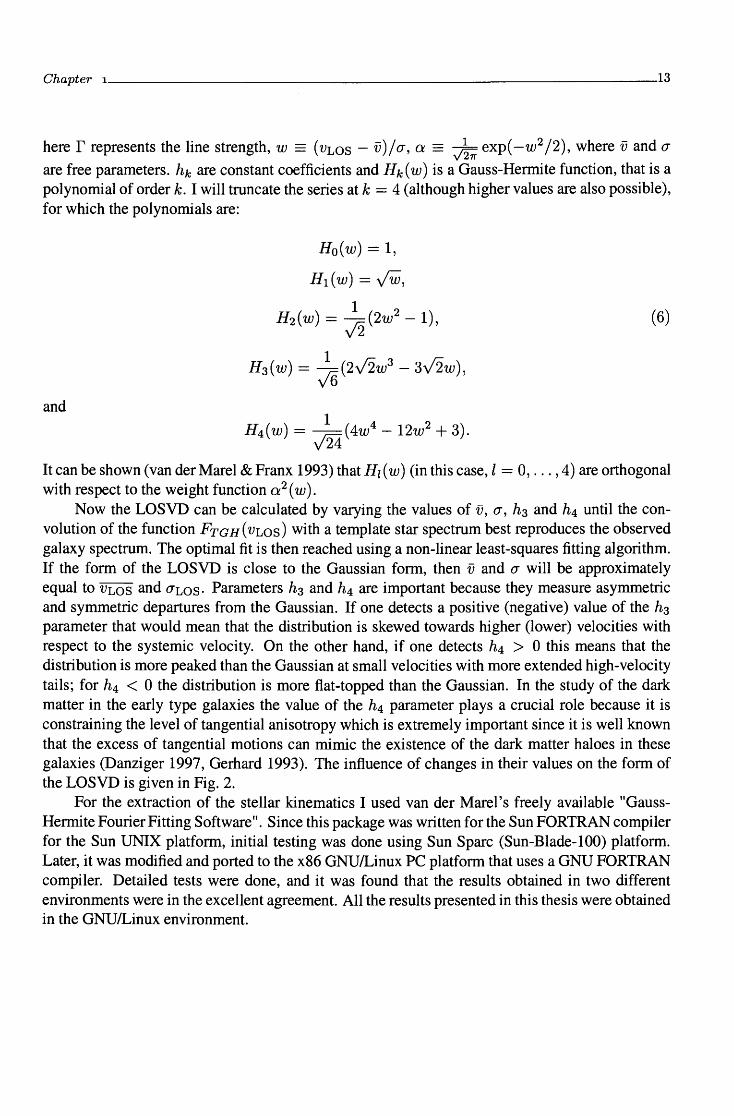
are free parameters. hk are constant coefficients and Hk (w) is a Gauss-Hermite function, tbat is a polynomial of order k. I will troncate tbe series at k = 4 (altbougb bigber values are also possible), for wbicb tbe polynomials are:
an d
Ho(w) =l,
H1(w) = Vw, H2(w) = ~(2w2 - 1),
l H3(w) = J6(2v'2w3
- 3J2w),
l H4(w) = . JOA(4w4 - 12w2 + 3).
v24
(6)
lt can be sbown (van der Marel & Franx 1993) tbat Hz (w) (in tbis case, l = O, ... , 4) are ortbogonal witb respect to tbe weigbt function a 2 (w).
Now tbe LOSVD can be calculated by varying tbe values of v, O", h3 and h4 until tbe con-volution of tbe function Fra H( VLos) witb a template star spectrum best reproduces tbe observed galaxy spectrum. Tbe optimal fit is tben reacbed using a non-linear least-squares fitting algoritbm. If tbe form of tbe LOSVD is close to tbe Gaussian form, tben v and O" will be approximately equal to VLos an d O"Los. Parameters h3 an d h4 are important because tbey measure asymmetric and symmetric departures from tbe Gaussian. If one detects a positive (negative) value of tbe h3 parameter tbat would mean tbat tbe distribution is skewed towards bigber (lower) velocities witb respect to tbe systemic velocity. On tbe otber band, if one detects h4 > O tbis means tbat tbe distribution is more peaked tban tbe Gaussian at small velocities witb more extended bigb-velocity tails; for h4 < O tbe distribution is more fiat-topped tban tbe Gaussian. In tbe study of tbe dark matter in tbe early type galaxies tbe value of tbe h4 parameter plays a crociai role because it is constraining tbe level of tangenti al anisotropy w bi cb is extremely important since i t is well known tbat tbe excess of tangential motions can mimic tbe existence of tbe dark matter baloes in tbese galaxies (Danziger 1997, Gerbard 1993). Tbe infiuence of cbanges in tbeir values on tbe form of tbe LOSVD is given in Fig. 2.
For tbe extraction of tbe stellar kinematics I used van der Marel's freely available "Gauss-Hermite Fourier Fitting Software". Since tbis package was written for tbe Sun FORTRAN compiler for tbe Sun UNIX platform, initial testing was done using Sun Sparc (Sun-Blade-100) platform. Later, i t was modified and ported to tbe x86 GNU/Linux PC platform tbat uses a GNU FORTRAN compiler. Detailed tests were done, and it was found tbat tbe results obtained in two different environments were in tbe excellent agreement. Ali tbe results presented in tbis tbesis were obtained in tbe GNU/Linux environment.
14 ----------------- Theoretical concepts, observations and reductions
1 1 1
0.8 0.8 0.8
0.6 0.6 0.6 0.4 0.4 0.4 0.2 0.2 0.2
o o o -10 -5 o 5 10 -10 -5 o 5 10 -10 -5 o 5
1
~0.8 ~ ..._, 0.6
::c: t)
~0.4
0.2
o -1 o
1
0.8
0.6
0.4
0.2
o -10
1 1
0.8 0.8
0.6 0.6
0.4 0.4
0.2 0.2
o o -5 o 5 10 -1 o -5 o 5 10 -10 -5 o 5
1 1
0.8 0.8
0.6 0.6
0.4 0.4
0.2 0.2
o o -5 o 5 10 -1 o -5 o 5 10 -10 -5 o 5
w
Figure 2: Plots demonstrating various combinations of h3 and h4 on the shape of the function FTGH(W). Pure Gaussian is in the center (both h3 and h4 are equal to zero). h3 parametrizes the skew-ness of the line profile, while h4 measures whether the profile is more or less peaked than a Gaussian. Units of the variable w are arbitrary.
10
10
10
Chapter 1------------------------------15
1.2 OBSERVATIONS
1.2.3 Generai remarks
I have used different long-slit data obtained from different sources that wili be calied Samples hereafter. They are:
Sample l. Observations obtained courtesy of J. Danziger (ESO NTT was used) which include spectra of IC1459 and IC3370.
Sample 2. Observations obtained courtesy of A. Graham and S. Zaggia (Double Beam Spec-trograph attached to the Australi an N ational University 2.3 m telescope at Siding Springs Observatory was used) which include the spectra of the foliowing galaxies: NGC1336, NGC1339, NGC1373, NGC1374, NGC1379, NGC1399, NGC1404 and NGC1419 (from Pornax cluster- see Graham et al. (1998)).
Sample 3. Observations obtained courtesy of M. Carolio and K. Preeman (again Double Beam Spectrograph attached to the Australian National University 2.3 m telescope at Siding Springs Observatory was used) which include NGC3379 and NGC4339. Galaxy NGC4105 was observed using ESO 2.2 m telescope with EPOSC.
Details of the instrumental setup wili be given in detail when each sample wili be analyzed. Here I present the details of the reduction procedures that are common forali the observations. Note that in this thesis I wili also deal with Sample 4 which includes three galaxies taken from the literature: NGC2434, NGC3706 and NGC5018 (Carolio et al. 1995). Por ali galaxies for which I had the observational data I extracted steliar kinematic parameters (velocity, velocity dispersion, h3 an d h4 parameters) an d spectral indices.
Ali the reduction procedures of the long-slit spectra were done using the ESO MIDAS pack-age1. Ali the standard MIDAS commands and the commands from the context long were used, and where necessary small routines were written using MIDAS command language, MCL. Pirst, I com-bined the spectra taken under the same conditions using COMBINE/LONG command. This was a very efficient way to remove the cosmic particle hits from the raw data. The bias, that is composed of a DC offset that is noiseless, and a noise component generated by the process of CCD readout, was subtracted: I have made a combined bias frame out of ali available bias frames. A correction for the dark current was not made. Por fiat-fielding which performs the corrections for variations in pixel sensitivity across the CCD array, I combined available fiat-field frames into a single fiat-field frame which was normalized to unity. Prames of interest (galaxy's and stellar) were then divided by this single frame. Por the purpose ofthe wavelength calibration I used spectra of different lamps (for example Helium-Argon) which were available for each observation. Interactive identification of lines was done using MIDAS commands that were embedded in a small MCL script: typical RMS uncertainty was rv 0.03 A. Sky subtraction was of a crucial importance because the outer parts of the galaxies are very faint, and sky removal had to be done very carefuliy. The command
1 MIDAS is developed and maintained by the European Southem Observatory.
16 -----------------Theoretical concepts, observations and reductions
SKYFIT /LONG was used taking an average of rv 30 rows near the edges of the exposure frames. For the extraction of the kinematical parameters of the galaxies rebinning into a logarithmic scale was done using simple MIDAS commands. Finally, the frames were trimmed by removing the rows and columns near the edges of the frames. In some cases I will present comparisons of my extracted kinematical parameters with those taken from literature (see below). The agreement is typically very good.
I used IRAF 2 for extraction of photometric profiles and for conversion of the MIDAS format into the IRAF format required by the Fourier Fitting package.
1.2.4 Sample l
IC3370
GENERAL INFORMATI ON
IC3370 is a bright galaxy, classified as E2-E3 (elliptical) galaxy, absolute blue magnitude -21.4, heliocentric radiai velocity 2930± 24 kms- 1 (taken from the LEDA database). It covers 2.9 x 2.3 arcmin on the sky (RC3). However, it is a rather unusual elliptical galaxy and according to Jarvis (1987, hereafter referred to as J87) i t should be classified as SOpec (see below). One arcsec in the galaxy corresponds to rv 203.02 pc. The effective radius is 35" (=7.10 kpc).
PHOTOMETRIC OBSERVATIONS
I used frames kindly provided by O. Hainaut using ESO NTT and EMMI in the RILD mode on July 3-4, 2002 in the B-band. The photometry of IC3370 is very interesting and i t is given in detail in J87. I present here some additional elements that are complementary to that study and are of importance for the analysis that I am undertaking.
One should note that J87 took for the major axis the position angle (PA) of 40°, Carollo, Danziger & Buson (1993) took for the same axis P.A. of 51°, while the spectra in this study were taken using P. A. = 60°. The reason for these differences lies in a very particular photometry of this galaxy that has strong isophotal twisting as shown in J87 and in Fig. 3 (see position angle (P.A.) plot). This may be evidence for the fact that this galaxy is triaxial, because the isophotes of an axisymmetric system must always be aligned with one another (see, for example, BM98). Fasano & Bonoli (1989) using a sample of 43 isolated ellipticals found that the twisting observed in these galaxies is intrinsic (triaxiality). Jarvis has taken the mean position angle of isophotes to be equal to 40 ± 2° which is true for the data up to 80". However, at larger radii the PA tends to increase, so the usage of larger value of 60° (and 150° for the minor axis) is justified (see Fig. 3).
In Fig. 3 I present relevant photometric data obtained using IRAF task ellipse: ellipticity, magnitude in the B-band for major axis (filled circles) and minor axis (open circles), a4 parameter (fourth harmonic deviations from ellipse) an d the position angles, as a function of distance. The value of a4 is positive up to one effective radius (for almost ali values of radius ), thus indicating that the isophotes are disky, while beyond one effective radius, the isophotes become boxy since a4
is negative. Since a4 increases rapidly up to rv 5" this can lead to the conclusion of the embedded disk. The existence of the stellar disk was shown in J87. The photometric data in the case of
2 IRAF is distributed by NOAO, which is operated by AURA Inc., under contract with the National Science Foundation.
Figure 3: Photometric profiles for IC3370 (in the B-band). From top to bottom: ellipticity, surface brightness for the B filter in mag asrcsec- 2 (for major axis: full circles; for minor axis: open circles), a4 parameter and position angle.
IC3370, as well as in case of other galaxies that I present bere, will be necessary far the dynamical modeling that will be given in the next Chapter.
18 -----------------Theoretical concepts, observations and reductions
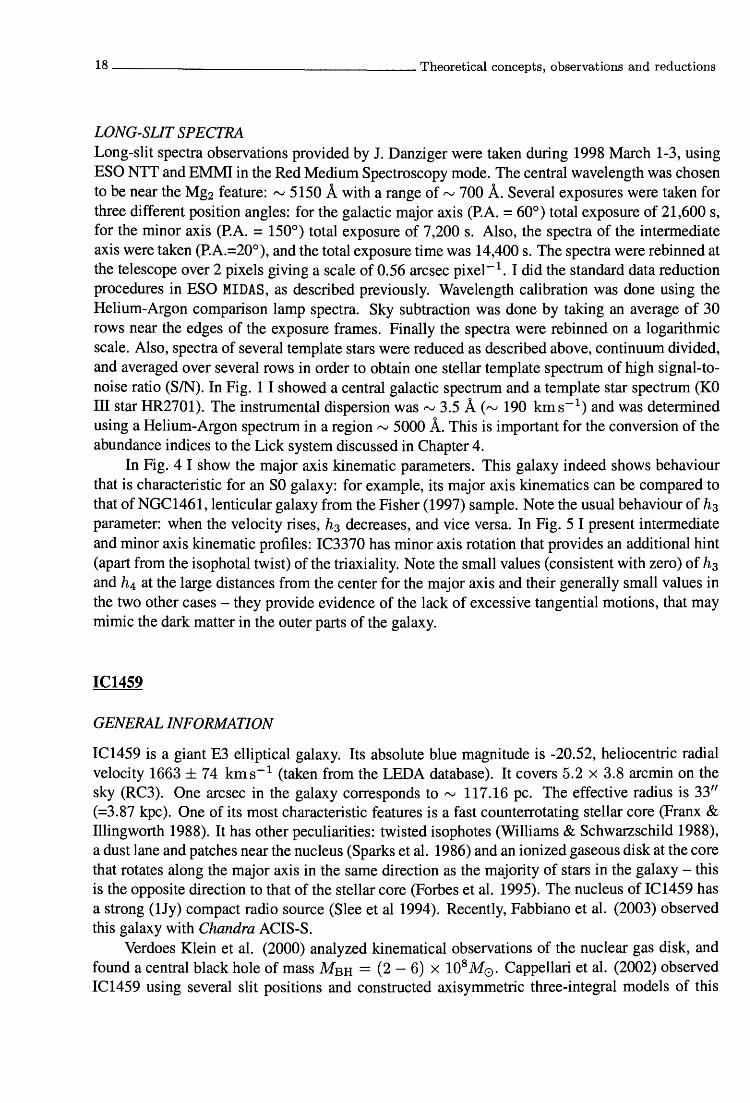
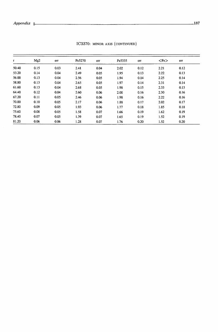
LONG-SLIT SPECTRA Long-slit spectra observations provided by J. Danziger were taken during 1998 March 1-3, using ESO NTT and EMMI in the Red Medium Spectroscopy mode. The centrai wavelength was chosen to be near the Mg2 feature: f'.J 5150 A with a range of f'.J 700 A. Severa! exposures were taken for three different position angles: for the galactic major axis (P.A. = 60°) total exposure of 21,600 s, for the minor axis (P.A. = 150°) total exposure of 7,200 s. Also, the spectra of the intermediate axis were taken (P.A.=20°), and the total exposure time was 14,400 s. The spectra were rebinned at the telescope over 2 pixels giving a scale of 0.56 arcsec pixel- 1 . I did the standard data reduction procedures in ESO MIDAS, as described previously. Wavelength calibration was done using the Helium-Argon comparison lamp spectra. Sky subtraction was done by taking an average of 30 rows near the edges of the exposure frames. Finally the spectra were rebinned on a logarithmic scale. Also, spectra of severa! template stars were reduced as described above, continuum divided, and averaged over severa! rows in order to obtain one stellar template spectrum of high signal-to-noise ratio (SIN). In Fig. l I showed a centrai galactic spectrum and a template star spectrum (KO Ill star HR2701). The instrumental dispersion was f'.J 3.5 A (f'.J 190 kms-1) and was determined using a Helium-Argon spectrum in a region f'.J 5000 A. This is important for the conversion of the abundance indices to the Lick system discussed in Chapter 4.
In Fig. 4 I show the major axis kinematic parameters. This galaxy indeed shows behaviour that is characteristic for an SO galaxy: for example, its major axis kinematics can be compared to that ofNGC1461, lenticular galaxy from the Fisher (1997) sample. Note the usual behaviour of h3 parameter: when the velocity rises, h3 decreases, and vice versa. In Fig. 5 I present intermediate and minor axis kinematic profiles: IC3370 has minor axis rotation that provides an additional hint (apart from the isophotal twist) ofthe triaxiality. Note the small values (consistent with zero) of h3 and h4 at the large distances from the center for the major axis and their generally small values in the two other cases - they provide evidence of the lack of excessive tangential motions, that may mimic the dark matter in the outer parts of the galaxy.
IC1459
GENERAL INFORMATI ON
IC1459 is a giant E3 elliptical galaxy. Its absolute blue magnitude is -20.52, heliocentric radiai velocity 1663 ± 74 kms- 1 (taken from the LEDA database). It covers 5.2 x 3.8 arcmin on the sky (RC3). One arcsec in the galaxy corresponds to f'.J 117.16 pc. The effective radius is 33" (=3.87 kpc). One of its most characteristic features is a fast counterrotating stellar core (Franx & Illingworth 1988). It has other peculiarities: twisted isophotes (Williams & Schwarzschild 1988), a dust lane and patches near the nucleus (Sparks et al. 1986) and an ionized gaseous disk at the core that rotates along the major axis in the same direction as the majority of stars in the galaxy- this is the opposi te direction to that of the stellar core (Forbes et al. 1995). The nucleus of IC1459 has a strong (lJy) compact radio source (Slee et al 1994). Recently, Fabbiano et al. (2003) observed this galaxy with Chandra ACIS-S.
Verdoes Klein et al. (2000) analyzed kinematical observations of the nuclear gas disk, and found a centrai black hole of mass MsH = (2- 6) x 108 M0 . Cappellari et al. (2002) observed IC1459 using severa! slit positions and constructed axisymmetric three-integral models of this
Figure 4: Kinematic profiles for the major axis of IC3370 (P.A.= 60°). From top to bottom: velocity, velocity dispersion, h3 and h4 parameters. One effective radius is plotted using dashed lines.
galaxy using the Schwarzschild orbit superposition method. They found, using stellar and gas kinematics, that MBH = (1.1 ± 0.3) x 109 M0 .
PHOTOMETRIC OBSERVATIONS
Photometric observations made by J. Danziger during 1997 August 28-30 using the ESO NTT and EMMI in the Red Medium Spectroscopy mode in the V-band were used. I present the results ob-
20 ----------------Theoretical concepts, observations and reductions
200
>.. 100 -+--> ·-C) o o .......... Q) >
-100
-200 200 150
b
100 50 o
0.2
M o ..c:
-0.2
0.2
'<l' o ..c:
-0.2
-100 -50 o 50 100 radius (")
100
o
-100
-200 200 150
b
100 50
! !! • ~ t \,~!!! !
' ' ' ' ' ' ' ' ' ' ' '
0 ~~~~~~~~~HHHHHHHH
0.2
o
-0.2
0.2
o
-0.2
-100 -50 o 50 100 radius (")
Figure 5: Kinematic profiles for the intermediate (P.A.= 150°, left) and minor (P.A.= 20°, right) axes of IC3370. From top to bottom: velocity, velocity dispersion, h3 and h4 parameters. One effective radius is plotted using dashed lines.
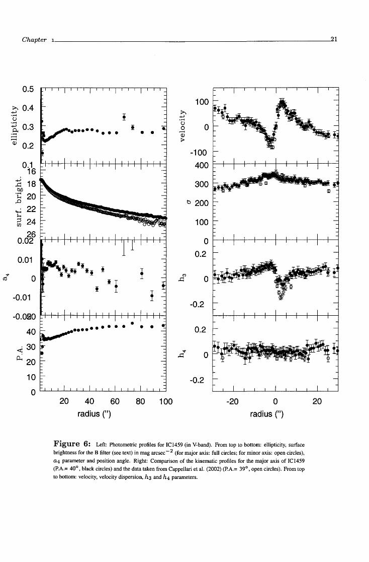
tained using the aforementioned IRAF routine in Fig. 6 where surface brightness was transformed to the B-band using relation B - V = 0.99 taken from the LEDA database. The photometric profile was compared with that of Franx & Illingworth (1988) and i t was found that they were in a good agreement.
Figure 6: Left: Photometric profiles for IC1459 (in V-band). From top to bottom: ellipticity, surface brightness for the B filter (see text) in mag arcsec- 2 (for major axis: full circles; for minor axis: open circles), a4 parameter and position angle. Right: Comparison of the kinematic profiles for the major axis of IC 1459 (P.A.= 40°, black circles) and the data taken from Cappellari et al. (2002) (P.A.= 39°, open circles). From top to bottom: velocity, velocity dispersion, h3 and h4 parameters.
22 -----------------Theoretical concepts, observations and reductions
LONG-SUT SPECTRA
Long-slit spectra observations provided by J. Danziger were done during the same nights using the same telescope and setup as in the case of IC3370. The centrai wavelength was chosen to be near the Mg2 feature: rv 5150 A. The range that was covered was rv 700 A. Severa! exposures were taken for two different position angles: for the galactic major axis (P.A. = 40°) total exposure of 35,100 s, and for the minor axis (P.A. = 130°) total exposure of 3,600 s. Because of the fact that only one exposure was available for the minor axis, the removal of the cosmic ray hits was not successful and I have taken the minor axis stellar kinematics from Cappellari et al. (2002). I compared the results for the major axis and plot the comparison in Fig. 6. Cappellari et al. (2002) used the Cerro Tololo Inter-American Observatory (CTIO). The agreement is good, except for the velocity and h3 parameter near the galactic center where some discrepancy exists. Note, however, that Cappellari et al. (2002) used P.A.=39° and observations that I had were made at P.A.=40°. In the outer parts agreement is excellent for the whole velocity profile. The spectra were rebinned at the telescope over 2 pixels giving a scale of 0.56 arcsec pixel - 1 . I made standard reduction procedures in ESO MIDAS, as described previously. Wavelength calibration was done using a Helium-Argon comparison lamp spectra. Finally the spectra were rebinned on the logarithmic scale. Again, spectra of severa! template stars were reduced as described above, continuum divided, and averaged over severa! rows in order to obtain one stellar template spectrum of high signal-to-noise ratio (SIN). This time the template star HR5852 was used. The instrumental dispersion was rv 3.5 A (rv 190 kms- 1) and was determined using Helium-Argon spectrum in a region rv 5000 A.
In Fig. 7 I show the major and minor axis kinematic parameters. Major axis data show the rapid increase of velocity in the inner rv 3": velocity rises to rv 100 km s-1 (note however a small asymmetry in my determination of velocity). Velocity dispersion is large at the centre: rv 350 kms- 1, and decreases rapidly to rv 240 kms-1 (at rv 40 "). There is a plateau in velocity disper-sion between rv 20" and 30" after which velocity dispersion decreases. The h3 parameter shows a typical behaviour, i.e. it rises (falls) when velocity rapidly increases (decreases). In the outer parts it shows small departures from zero. The h4 parameter shows very small departures from zero in the inner parts, and in the outer parts there is an increase of its value, suggesting existence of the radiai anisotropy. Minor axis data provide evidence of small velocities, and larger centrai velocity dispersion (rv 380 kms- 1). Both h3 and h4 parameters show very small departures from zero throughout the observed parts of the galaxy.
::>-. +) •~'""i
() o
........t Q)
>
t")
~
.q-..c:
Chapter 1--------------------------------23
100 40 ! ::>-. 20 rWtr +) .......
o () o o ........t
! Q)
> -20 -100 -40
400 400
300 300 • • • • !~rl
b 200 t , ! Htq b 200
100 100
o 0.2
o
-0.2
0.2
o
-0.2
-100
t! o
0.2
! !~,.-"" l t") ! ''f.N, ~ o !
! -0.2
0.2
''M,' .q- o ! ! ..c:
-0.2
-50 o 50 100 -20 o radius ('') radius (")
Figure 7: Stellar kinematics of IC1459. Left: major axis data. Right: minor axis data (taken from Cappellari et al. 2002). From top to bottom: velocity, velocity dispersion, h3 and h4 parameters. One effective radius in case of the major axis is plotted using dashed line. Note that in case of the minor axis i t is out of scale.
1.2.5 Sample 2
20
In this subsection I will describe the sample and present the stellar kinematic results for the early-
24 ----------------- Theoretical concepts, observations and reductions
type galaxies in the Fornax cluster obtained courtesy from A. Graham and S. Zaggia. These ob-servations include 13 galaxies (major axes data) and represent a sample of 86% ofFornax galaxies brighter that BT = 15 mag. From the observed galaxies I chose 8 galaxies for which I could extract the full velocity profiles and whose spectra extend to the distances larger than one effective radius (except for NGC1336, see below). A detailed description of the observations is given in Graham et al. (1998) (hereafter G98) and here I provide only some details that will be of importance for the modeling procedures. In TABLE 1-1 I give the basic observational data of Sample 2.
NOTE: Column (l): name, columns (2) and (3) coordinates (R.A. and Dee.), column ( 4 ): morphological type (according to Ferguson ( 1989)),
column (5): heliocentric radiai velocity (fromLEDA database), column (6): total apparent blue magnitude, column (7) effective radius
in arcsecs, column (8) approximate radiai radiai range of the kinematical data (in units of effective radius), column (9) blue surface
brightness at l effective radius given in (maglsq.arcsec.), column (lO) major axis position angle, column (11): total exposure time (in
hours). (*) Note that the effective radius for NGC1399, as in Kronawitter et al. (2000), was taken from Bicknell et al. (1989) (see
Chapter 2).
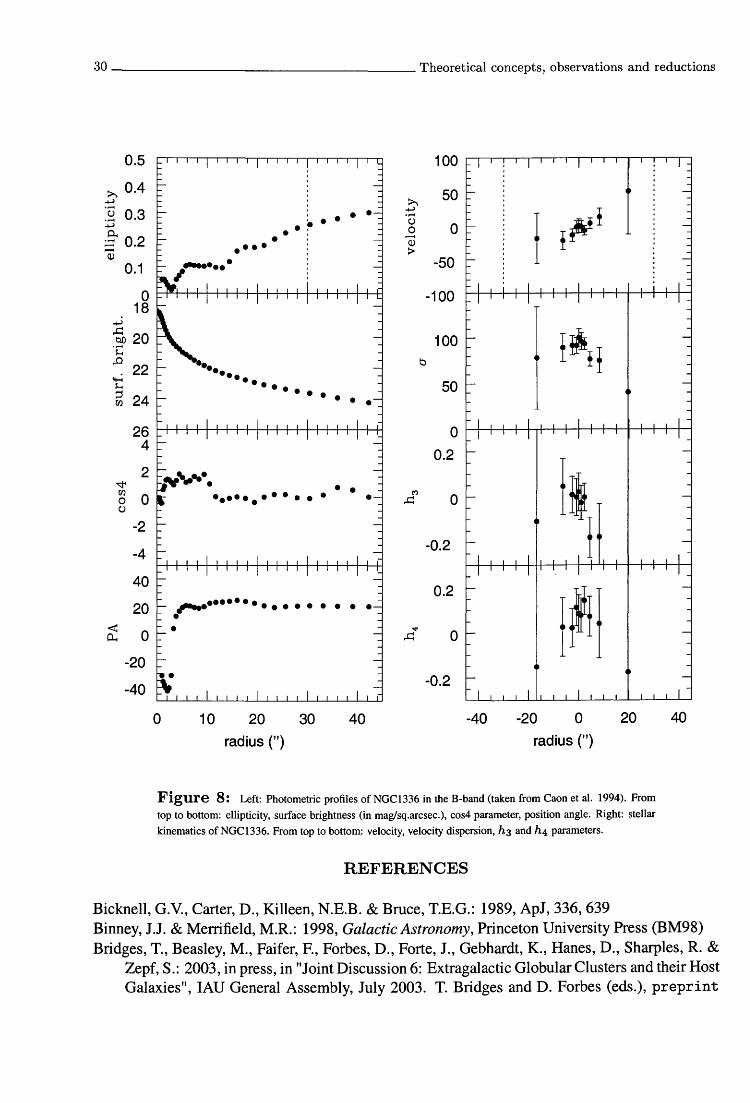
The spectra were obtained during two runs in November and December 1996. The blue arm of the Double Beam Spectrograph was attached to the Australian National University's 2.3 m tele-scope at Siding Spring Observatory. The spatial scale on the chip was 0.91 arcsec pixel- 1 . A spectrograph slit width of 2 arcsec on the sky with a length greater than the spatial extent of the CCD was used. FWHM for the are lines of was found to be equal to 2.7 pixels or 1.50A, giving a resolution of 86 km s- 1 at 5200 A. I did the whole reduction procedure (explained in section 1.2.3 of this Chapter). The Neon-Argon lamp frames were used for the wavelength calibration. The spectra of several template stars were reduced and used for the extraction of the full velocity profiles. The template star HD4128 was used in extracting the stellar kinematics of the following galaxies: NGC1336, NGC1379, NGC1374, NGC1399 and NGC1419. The template star HD4188 was used in case of these galaxies: NGC1339, NGC1373 and NGC1404. Note that in the pre-sentation of the photometric data I used Caon et al. (1994) data that give the cos4 parameter that represents the amplitude of the residua! cos4 coefficient (multiplied by 100) of the isophotal devi-ation from the best fitting ellipse. In ali the plots of this Sample, East (E) side is given with the
Ex p (hr)
l 2 3.5 l 0.75 3 2.5 l
Chapter 1------------------------------25
positive vaiues of the radius (right han d si de), an d the w est si de (W) is given with the negative vaiues of the radius (left han d si de).
NGC1336 (Fig. 8)
One arcsec in this gaiaxy corresponds to f'..J 100 pc. The effective radius is 30" (=3.00 kpc). The veiocity has a siow increase an d does not reach Iarge vaiues (maximum of 50 km s- 1, with Iarge error bars ). Veiocity dispersion pro fii es show a Iack of symmetry an d ha ve a decreasing trend (error bars are Iarge, so this shouid be taken with caution). G98 suggested the existence of a bar -note the Iarge cos4 parameter in the photometetric profiie inside 10", and aiso the small positive vaiues of h4 in this region.
NGC1339 (Fig. 9)
One arcsec in the gaiaxy corresponds to f'..J 93.95 pc and the effective radius is 15" (=1.41 kpc). The data for the rotation curve extend to f'..J 2Re and the veiocity remains constant. The veiocity dispersion falls from the centrai vaiue of f'..J 170 kms- 1 to f'..J 100 kms- 1 (at f'..J 1Re) and then begins to rise: at the Iast measured point a ~ 125 km s-1 . The parameter h3 behaves as usuai when the gaiaxy has such a rotation curve: it rises when veiocity rises, and declines when veiocity deciines. h4 shows signs of an increase: oniy in the very internai part its vaiue is consistent with zero.
NGC1373 (Fig. 10)
One arcsec in the gaiaxy corresponds to f'..J 95.13 pc. The effective radius is 11" (=1.05 kpc). The rotation curve is rather symmetric and with a small degree of rotation. On the contrary, the veiocity dispersion shows ciear signs of asymmetry. Aiso, there is a trend of rising veiocity dispersion vaiues in the outer parts. From h3 and h4 i t is difficult to draw conciusions. There is a hint that h4 has small positive vaiues throughout the observed regions of the gaiaxy.
NGC1374 (Fig. 11)
One arcsec in the gaiaxy corresponds to f'..J 92.22 pc. The effective radius is 26" (=2.40 kpc). The rotation curve is another exampie of the steep increase of the veiocity in the inner parts ( f'..J 5"). As noted by G98, although the overall veiocity profiie is symmetric there are important departures from symmetry, which are aiso visibie in the veiocity dispersion profiies: when the piateau of a f'..J 150 km s-1is reached at f'..J IO" the veiocity dispersion changes behavior beyond one effective radius. h3 and h4 profiies aiso show a Iack of symmetry.
NGC1379 (Fig. 12)
One arcsec in the gaiaxy corresponds to f'..J 94.58 pc. The effective radius is 24" (=2.27 kpc). This gaiaxy has a siow rotation (the vaiue of the maximum veiocity: f'..J 40 km s-1 ). Veiocity profiies show a Iack of symmetry twice: first, near the centrai region and, second, in the outer regions - on the E si de veiocity approaches zero, and on the W si de i t tends to be constant f'..J 30 - 40 km s- 1.
The veiocity dispersion does not show a tendency to decline beyond one effective radius.
26 -----------------Theoretical concepts, observations and reductions
NGC1399 (Fig. 13)
One arcsec in the galaxy corresponds to"' 100.19 pc. The effective radius is 42" (=4.21 kpc); note, however that this value might be problematic: Caon et al.(1994) calculated a value of 127" (=12. 72 kpc) by fitting their extended photometry (see the note related to this galaxy in the next Chapter). This is the largest galaxy in the Fornax cluster and is positioned in the center of the cluster. The rotation curve shows evidence for a kinematically distinct inner component. The velocity reaches (at W side) at"' 20" a value of"' 30 kms- 1which then steadily falls to zero (at"' 50"). At the E side the velocity remains constant at"' 30 km s- 1(starting from 10"). The velocity dispersion is very high at the center"' 320 km s-1and quickly declines to"' 250 km s-1(at 10") and then remains approximately flat. The h3 parameter remains slightly positive throughout the whole observed galaxy. The h4 parameter shows small departures from zero but which can be considered to be consistent with zero throughout the whole observed galaxy.
NGC1404 (Fig. 14)
One arcsec in the galaxy corresponds to"' 134.55 pc. The effective radius is 26" (=3.50 kpc). This galaxy shows a steep gradient of velocity: i t rises to "' 100 km s-1within 10". Note, however, that there is a flattening at the inner "' 2 " (note the different binning used in extracting stellar kinematics for this galaxy with respect to the other galaxies in the Fornax cluster). The velocity remains constant beyond one effective radius, v"' 80 kms- 1and the profile looks symmetric with respect to the center. The velocity dispersion profiles are in generai symmetric, too. There are two local maxima at ±2 11 from the center. Beyond these two points the velocity dispersion decreases at a nearly constant rate until it reaches a plateau at "' 12". Departures from symmetry can be seen in the outer parts of the galaxy ("' 3Re). In these outer regions the velocity dispersi an again becomes a "' 200 km s- 1. The h3 parameter shows the usual behaviour for the case of the galaxy with rapidly increasing velocity (see the note for NGC1339) and is consistent with zero at large distances from the center ("' 3Re). h4 is slightly negative, but within the errar bars i t is consistent with zero throughout the whole observed galaxy.
NGC1419 (Fig. 15)
One arcsec in the galaxy corresponds to"' 114.25 pc, and the effective radius is 9" (=1.03 kpc). As noted by G98 the velocity and dispersion profiles of this galaxy are very similar to those of NGC1336. The velocity is small and is almost consistent with zero in the inner parts. The velocity dispersi an is approximately constant (a "' l 00 km s - 1) within the observed parts of this galaxy. Not much can be said about h3 and h4 : in the outer regions they appear to be consistent with zero.
1.2.6 Sample 3
These are observations of early-type galaxies obtained courtesy of M. Carollo and K. Freeman. Galaxies NGC3379 and NGC4339 were observed using the Double Beam Spectrograph attached to the Australian National's University 2.3 m telescope at Siding Springs Observatory. Galaxy NGC4105 was observed using ESO 2.2 m telescope with EFOSC.
Chapter 1------------------------------27
For NGC4339 the long slit observations of the major axis (P.A.=20°) were taken on March 14, 1997, and the total exposure time was 20,000 s. For NGC3379 the long slit spectra of the major axis (P.A.=70°) were taken on March 13-14, 1997 and the total exposure time was 6,000 s. In both cases: (i) the scale was 0.59 arcsec pixel - 1 , (ii) wavelength calibration was done using Neon-Argon lamp, and (iii) the template star was cpd-43. The instrumental dispersion was rv 2 À(rv 100 km s- 1) and was determined using a Neon-Argon spectrum in a region rv 5000 A. For NGC4339 the photometry data were taken from the paper of Caon et al. (1994) (see Fig. 15). For NGC3379 the surface brightness was taken from the paper of Capaccioli et al. (1990), whereas ellipticity, a4 parameter and position angle as function of radius using images from the ESO archi ve (l band) were extracted using standard IRAF commands (see Fig. 17).
NGC4339 (Fig. 16)
NGC4339 is an EO galaxy, with heliocentric radiai velocity of 1292 km s-1 , and absolute B mag-nitude -19.25. One arcsec in the galaxy corresponds to rv 89.31 pc. The effective radius is 16" (=1.43 kpc). The rotation shows a rapid increase: within inner 5" velocity rises to rv 70 km s- 1and stays approximately constant out to 30 " ( rv 2Re). The velocity dispersion pro file shows flat top in the inner 5" ( of approximately 120 km s- 1) an d then declines rapidly out to 60" (at rv 1Re). Beyond one effective radius there are no signs of further decline of velocity dispersion. h3 and h4 do not show large departures from zero. The h4 parameter remains slightly positive throughout the observed parts of the galaxy.
NGC3379 (Fig. 17, Fig. 18)
NGC3379 is a bright EO galaxy (note however the ellipticity E ~ 0.15 in Fig. 17; there are stili some doubts whether this is a bona fide normal elliptical or a face-on lenticular galaxy, cf. Gregg et al. 2003), with heliocentric radiai velocity of 911 kms- 1 , and absolute B magnitude -20.57. One arcsec in the galaxy corresponds to rv 63.12 pc. The effective radius is 35" (=2.22 kpc).
Since I had only major axis (P.A.=70°) data, I have taken data from Statler & Smecker-Hane (1999) for the major and the minor axis (P.A.=340°). I compared the results for the inner region which I have in common for the major axis and found that they are in an excellent agreement (see Fig. 17 (right)). The data that I had extend out to ~ 30 ",so in the modeling procedures (see next Chapter) I will use Statler & Smecker-Hane (1999) measurements because their data extend to a larger radius (80" that is ~ 2 Re) and are also available for the minor axis.
This galaxy shows steep increase of velocity: i t rises to rv 60 km s- 1in the inner 20". After a plateau between rv 20" and rv 60" the velocity shows a tendency to decrease. The velocity dispersion peaks at rv 230 kms- 1and then decreases rapidly. There is a plateau between rv 20" an d rv 50". One can see that there is an obvious asymmetry at rv 80". However, other observations show that there is a decreasing trend out to 6 Re (see next Chapter). The h3 parameter is small out to rv 50 ", but shows departures from zero at rv 70". h4 remains small throughout the whole observed galaxy, except in the outer parts for which there is a hint of departures from zero, but sin ce error bars are large, it is difficult to draw firm conclusions. Minor axis data suggest that NGC3379 does not show significant rotation on the minor axis. The velocity dispersion profile is similar to
28 -----------------Theoretical concepts, observations and reductions
that of the minor axis. The h3 an d h4 parameters are small throughout the whole observed galaxy on the minor axis (see Fig. 18).
NGC4105 (Fig. 19, Fig. 20)
GENERAL INFORMATI ON
NGC41 05 is an E galaxy, with heliocentric radiai velocity of 1918 km s - 1, an d absolute B mag-nitude -20.72. One arcsec in the galaxy corresponds to rv 134.14 pc. The effective radius is 11" (=1.48 kpc).
PHOTOMETRIC OBSERVATIONS
Photometric data w ere extracted from frames obtained courtesy of M. Carollo & K. Freeman using standard IRAF routines (Fig. 19). Note that the surface brightness is given in the R-band.
LONG-SLIT SPECTRA
Long slit spectra were obtained on March 9-13, 1994 using ESO 2.2 m telescope with EFOSC. The total exposure time for the major axis (P.A.=150°) was 27,900 s. The total exposure time for the minor axis (P.A.=60°) was 14,400 s. The scale was 0.336 arcsec pixel - 1 . The wavelength calibration was done using Helium-Argon lamp. The template star was HR5582. The instrumental dispersion was rv 4.2 À(rv 280 kms- 1) and was determined using Helium-Argon spectrum in a region rv 5ooo A.
On the major axis this galaxy shows a maximum value of the velocity rv 60 kms- 1(see Fig. 20, left). Note that there is a hint of a counterrotating stellar core in the inner 3". In generai, there is a lack of symmetry about the galaxy center. The centrai value of the velocity dispersion is large: rv 320 km s- 1. It declines in the inner rv 5" after which there is a tendency that to remain constant ( out to 2Re). h3 al so shows a hint of the effects of the counterrotating stellar core in the inner 3". A t the larger radii the value of h3 is consistent with zero. The h4 parameter remains small (slightly negative, but consistent with zero) throughout the whole observed galaxy. On the minor axis NGC4105 shows rather complex behaviour and again a lack of symmetry is evident (see (Fig. 20). The velocity dispersion decreases from the centrai value of rv 320 km s- 1to rv 200 km s-1 . Not much can be said about h3 and h4 parameters, except that they show asymmetries.
1.2.7 Sample 4
In this sample I include three galaxies from Carollo et al. (1995) for which these authors found an indication of existence of a dark halo: NGC2434 (a galaxy studied in detail also in Rix et al. 1997, see next chapter), NGC3706 and NGC5018. The details conceming these galaxies are given in the above two papers for each galaxy. Stellar kinematics for ali galaxies are given in Carollo et al. (1995). Here, I give only a brief overview and present kinematical data (see related Figures) which I obtained in electronic form courtesy of M. Carollo:
Chapter 1------------------------------29
NGC2434 (Fig. 21)
This is E0-1 gaiaxy, with heliocentric radiai veiocity v= 1390 ± 27 kms-1(taken from the NED database). Totai apparent corrected B-magnitude is 11.29 (taken from the LEDA database). Detaiis on photometry can be found in Carollo & Danziger (1994a). One arcsec in the gaiaxy corresponds to f'..J 96.31 pc. The effective radius is 24" (=2.31 kpc). This gaiaxy possesses a strong isophotai twisting in the inner f'..J l O". Isophotes are disky in the inner f'..J 3". The veiocity does no t reach Iarge vaiues: at f'..J 2Re it is f'..J 30 kms-1 . The veiocity dispersion peaks at f'..J 260 kms- 1,
and then declines rapidiy. Note that from f'..J 15" outwards i t remains constant. h3 parameters have small vaiues throughout the observed gaiaxy. Note, however, that the veiocity data in combination with the h3 data may indicate the existence of the counterrotating stellar core (a case simiiar to that of NGC4105). Apart from small positive vaiues in the inner region, the h4 parameter is zero in the outer regions thus providing (in combination with the flat veiocity dispersion pro fii e) a strong indication of the existence of the dark hai o.
NGC3706 (Fig. 22)
This is an E gaiaxy (according to the LEDA database), with heliocentric radiai veiocity 3215± 150 km s- 1(taken from NED database). The totai corrected apparent B-magnitude is 12.32 (taken from the LEDA database). Detaiis on photometry can be found in Carollo & Danziger (1994a). One arcsec in the gaiaxy corresponds to f'..J 222.75 pc. The effective radius is 27" (=6.01 kpc). This gaiaxy does not show strong isophotai twisting: the P.A. decreases siowiy from f'..J 80° (at f'..J
2") to f'..J 70°(at f'..J 100"). The rotation curve (and h3 behaviour) is very simiiar to that of gaiaxies NGC1339 and NGC1404. The centrai veiocity dispersion is rather high: 340 kms- 1and declines rapidiy in the inner f'..J 20". At f'..J 2Re i t does show a piateau (aibeit oniy on one side - data on the opposi te si de are unfortunateiy unavailabie ). The h4 parameter has small positive vaiues in the inner region and in the outer regions small negative vaiues (that deviate from zero).
NGC5018 (Fig. 23)
This is an E-SO gaiaxy (according to LEDA database), with heliocentric radiai veiocity 2897 kms- 1. The totai corrected apparent B-magnitude is 11.7 (ali data are from ESO Lauberts & Vaientijn cataiog, as quoted in Carollo & Danziger (1994b). Detaiis of photometry can be found in Carollo & Danziger (1994b). The gaiaxy does not show an isophotal twist. Note the asymmetry in veiocity: maximum on one side f'..J 100 kms-1, and on the other side maximum f'..J 50 kms- 1.
The veiocity dispersion has a doubie peaked maximum vaiues (at f'..J 240 km s- 1 ). There exists a decreasing trend in the veiocity dispersion. The h3 parameter shows compi ex variations ( especially in the region w h ere the veiocity is negative). The h4 parameter remains positive throughout the whoie observed gaiaxy .
Gaiaxies from Sample 4 will be modeied in next Chapter using the Schwarzschiid technique.
30 ------------------- Theoretical concepts, observations and reductions
0.5
~ 0.4 ..p.)
:§ 0.3 ..p.)
E o.2 Q)
..p.)
0.1
o 18
~ 20 ·~ ...0
22 ~ ~
~ 24
26 4
2
-2
-4
40
20
0: o -20
-40
o
• • • •••• , ....... •
••••• ••••••
,.... ........... . •
10 20 radius (")
30 40
50
o
-50
-100
b
100
50
o 0.2
o
-0.2
0.2
-0.2
!~l -40 -20 o 20
radius (")
Figure 8: Left: Photometric profiles of NGC1336 in the B-band (taken from Caon et al. 1994). From top to bottom: ellipticity, surface brightness (in mag/sq.arcsec.), cos4 parameter, position angle. Right: stellar kinematics of NGC1336. From top to bottom: velocity, velocity dispersion, h3 and h4 parameters.
Binney, J.J. & Merrifield, M.R.: 1998, Galactic Astronomy, Princeton University Press (BM98) Bridges, T., Beasley, M., Faifer, F., Forbes, D., Forte, J., Gebhardt, K., Hanes, D., Sharples, R. &
Zepf, S.: 2003, in press, in "Joint Discussion 6: Extragalactic Globular Clusters and their Host Galaxies", IAU Generai Assembly, July 2003. T. Bridges and D. Forbes (eds.), preprint
•••••••••••• ~ • .. : C) • o • ,.. ~ o • ~ l > ! -100 '!··' : :
-200
150 ! ~~~ ! b 100 !! !
• • • ! 50
o 0.2
!' t') o t! I ,.c:
-0.2
[ 1~\/!I I 0.2
-r ,.c: o
-0.2
o 10 20 30 40 50 -40 -20 o 20 radius (") radius (")
Figure 9: Left: Photometric profiles of NGC1339 in the B-band (taken from Caon et al. 1994). From top to bottom: ellipticity, surface brightness (in mag/sq.arcsec.), cos4 parameter, position angle. Right: stellar kinematics of NGC1339. From top to bottom: velocity, velocity dispersion, hg and h4 parameters. Dashed line indicates one effective radius.
astro-ph/0310324 Caon, N., Capaccioli, M. & D'Onofrio, M.: 1994, A& ASS, 106, 199 Capaccioli, M., Held, E. V., Lorenz, H. & Vietri, M.: 1990, AJ, 99, 1813
!
40
Cappellari, M., Verolme, E.K., van der Mare!, R.P., Verdoes Kleijn, G.A., Illingworth, G.D., Franx, M., Carollo, C.M. & de Zeeuw, P.T.: 2002, ApJ, 578, 787
Carollo, C.M., de Zeeuw, P.T., van der Mare!, R.P., Danziger, I.J., & Qian, E.E.: 1995, ApJ, 441,
32 ------------------- Theoretical concepts, observations and reductions
0.5
:>. 0.4 ~
:§ 0.3 ~
0.. ;.:= 0.2 O)
0.1
o 18
_; ..c: 20 l:lll
~ 22 ~ 24 ~ ;:1 m 26
28 4
2 ~ m o o C)
-2
-4
160
<e: 140 ~
120
100
L25
100
50 l :>. ~
!~!l C) o o O) >
-50
-100
150
f b 100 l
!~! ••• • 50
o 0.2
p~ • • C') o ..c:
-0.2
0.2
f l • • • • ""' ..c: o
-0.2
o 10 20 30 40 50 -40 -20 o 20 radius (") radius (")
Figure 10: Left: Photometric profiles of NGC1373 in the B-band (taken from Caon et al. 1994). From top to bottom: ellipticity, surface brightness (in mag/sq.arcsec.), cos4 parameter, position angle. Right: stellar kinematics of NGC1373. From top to bottom: velocity, velocity dispersion, h3 and h4 parameters. Dashed line indicates one effective radius.
o 10 20 30 40 50 -40 -20 o 20 radius (") radius (")
Figure 11: Left: Photometric profiles of NGC1374 in the B-band (taken from Caon et al. 1994). From top to bottom: ellipticity, surface brightness (in mag/sq.arcsec.), cos4 parameter, position angle. Right: stellar kinematics of NGC1374. From top to bottom: velocity, velocity dispersion, h3 and h4 parameters. Dashed line indicates one effective radius.
40
Fabbiano, G., Elvis, M, Markoff, S, Siemiginowska, A., Pellegrini, S., Zezas, A., Nicastro, F., Trinchieri, G. & McDowell, J.: 2003, ApJ, 588, 175
Fasano, G. & Bonoli, C. : 1989, A& ASS, 79, 291 Fisher, D.: 1997, AJ, 113, 950 Forbes, D.A., Reizel, D.B. & Williger, G.M.: 1995, AJ, 109, 1576 Franx, M. & Illingworth, G.D.: 1988, ApJ, 324, L55
34 ------------------- Theoretical concepts, observations and reductions
0.2
:2 0.15 C)
•.-i ...,_.) 0.1 .e-.......... Q) 0.05
o 18
_; ..c= 20 0.0
~ 22 ~ 24 ~ ::J rJl 26
28 4
2 .q< rJl o o C)
-2
-4 80
60
<t: 40 ~
20
o -20
100
:;:.... 50 I!J ;!:::! C) o B p ! Q)
> • -50
-100 150
l ! !f'! l b 100 ••••
50
o
I~! l 0.2
C") o ..c=
-0.2
0.2
!I' l ••• ""' • ..c= o • .... •••• "'. . .. • • -0.2
o 20 40 60 -50 o 50 radius (") radius (")
Figure 12: Left: Photometric profiles of NGC1379 in the B-band (taken from Caon et al. 1994). From top to bottom: ellipticity, surface brightness (in mag/sq.arcsec.), cos4 parameter, position angle. Right: stellar kinematics of NGC1379. From top to bottom: velocity, velocity dispersion, h3 and h4 parameters. Dashed line indicates one effective radius.
Gerhard, 0.: 1993, MNRAS, 265, 213 Graham, A. W, Colless, M.M, Busarello, G., Zaggia, Z. & Longo, G.: 1998, A& ASS, 133, 325. Gregg, M.D, Ferguson, H.C., Minniti, D., Tanvir, N. & Catchpole, R.: 2003, AJ, in press,
preprint astro-ph/0312158 Jarvis, B.: 1987, AJ, 94, 30 (J87) Kronawitter, A., Saglia, R.P., Gerhard, O. & a Bender, R.: 2000, A& ASS, 144, 53
Figure 13: Left: Photometric profiles ofNGC1399 in the B-band (taken from Caon et al. 1994). From top to bottom: ellipticity, surface brightness (in mag/sq.arcsec.), cos4 parameter (note lack of data between 1011 and 3511
), position angle. Right: stellar kinematics of NGC1399. From top to bottom: velocity, velocity dispersion, h3 and h4 parameters. Dashed line indicates one effective radius.
Rix, H.-W., de Zeeuw, P.T., Cretton, N., van der Marel, R.P. & Carollo, C.M.: 1997, ApJ, 488, 702 Sargent, W.L.W., Schechter, P.L., Boksenberg, A. & Shortridge, K. : 1977, AJ, 212, 326 Simkin, S.M.: 1974, A& A, 31, 129 Slee, O. B., Sadler, E. M., Reynolds, J. E. & Ekers, R. D.: 1994, MNRAS, 269, 928 Sparks, W. B., Hough, J. H., Axon, D. J., & Bailey, J.: 1986, MNRAS, 218,429 Statler, T.S.: 1995, AJ, 109, 1371
36 ------------------- Theoretical concepts, observations and reductions
0.5
>. 0.4 +.1
:§ 0.3 +.1 o. ~ 0.2 Q)
0.1
18 ..; 18 ..c: bll
•.-4 20 ~ ..0 ~ 22 ~ ;:l rt.l 24
26 4
2 ...q< rt.l o o C)
-2
-4
160
<X: 140 ~
120
100
100 >.
:"!::! C) o .3 Q)
> -100 300
f! !Hf~it 200 ! b • • •
100
o 0.2
C'l o ..c:
-0.2
0.2
"" o !H ..c:
-0.2
o 10 20 30 40 50 -50 o 50 radius (") radius (")
Figure 14: Left: Photometric profiles ofNGC1404 in the B-band (taken from Caon et al. 1994). From top to bottom: ellipticity, surface brightness (in mag/sq.arcsec.), cos4 parameter, position angle. Right: stellar kinematics of NGC1404. From top to bottom: velocity, velocity dispersion, h3 and h4 parameters. Dashed line indicates one effective radius.
Statler, T., & Smecker-Hane, T.: 1999, ApJ, 117, 839 Tonry, J. & Davis, M.: 1979: AJ, 84, 1511 van der Marel, R.P., & Franx, M.: 1993, ApJ, 407, 525
!
Verdoes Kleijn, G. A., van der Marel, R. P., Carollo, C. M., & de Zeeuw, P. T.: 2000, AJ, 120, 1221
Figure 15: Left: Photometric profiles ofNGC1419 in the B-band (taken from Caon et al. 1994). From top to bottom: ellipticity, surface brightness (in mag/sq.arcsec.), cos4 parameter, position angle. Right: stellar kinematics of NGC1419. From top to bottom: velocity, velocity dispersion, h3 and h4 parameters. Dashed line indicates one effective radius.
38 -------------------- Theoretical concepts, observations and reductions
0.2 100
:>.. 0.15 50 l' ~ :>.. •.-l
~ C) l :0 0.1 • C) o o ~ • • • Q) ,l Q) >
0.05 -50 ! o -100
18 .; 150 ..c: 20 tlD
,~f\, ·c 22 100 .o b ~ ~ 24 ! ! ::J 50 m 26
28 o 4 0.2 2
-.::t< m o ••••• M o o ..c: C)
-2
-4 -0.2 80
60 0.2
f"If < 40 ""' ~ ..c: o
20 • • o -0.2 -20
o 10 20 30 -20 o 20 radius (") radius (")
Figure 16: Left: Photometric profiles of NGC4339 in the B-band (taken from Caon et al. 1994). From top to bottom: ellipticity, surface brightness (in mag/sq.arcsec.), cos4 parameter, position angle. Right: stellar kinematics of NGC4339. From top to bottom: velocity, velocity dispersion, h3 and h4 parameters. Dashed line indicates one effective radius.
Figure l 7: Left: Photometric profiles of NGC3379 in the B-band. From top to bottom: ellipticity, surface brightness from Capaccioli et al. (1990) (in mag/sq.arcsec.) for major (black circles) and minor (open circles) axis, cos4 parameter, position angle. Right: Comparison of stellar kinematics of my extraction (black circles) and Statler & Smecker-Hane (1999). From top to bottom: velocity, velocity dispersion, h3 and h4 parameters. Dashed line indicates one effective radius.
40 ------------------Theoretical concepts, observations and reductions
100 100
50 ,Wti ! ! 50 :;:..... :;:..... ! ~ • ~ ' ' C) • C) ! ' '! o o • o o !~!j_Ar .... ~~ ........ • ........ Q) • Q) > ! ,~..,. >
-50 -50 : :
-100 -100
200 ! ,.A,, 200 ,,'{\.y. ! !
150 150 b ! o ! !
100 100
50 50
o o 0.2 0.2
! httrJn f !.'? o !!!~~!!! !.'? ! ..c: ..c: o ! -0.2 -0.2
0.2 ! 0.2 l 'l' o !I~!Ì I 'l' I !!!,-.'Hl ..c: ..c: o
-0.2 -0.2
-50 o 50 -50 o 50 radius (") radius (")
Figure 18: Stellar kinematics of NGC3379 (taken from Statler & Smecker-Hane (1999)) for major (left) and minor (right) axis. From top to bottom: velocity, velocity dispersion, h3 and h4 parameters. Dashed line indicates one effective radius.
Figure 19: Photometric profiles of NGC4105 in the R-band. From top to bottom: ellipticity, surface brightness (in mag/sq.arcsec.), cos4 parameter, position angle.
42 -----------Theoretical concepts, observations and reductions
2 o o ,-----,----,---.------,,.---,----,------.----.-..,-----,-..,----,
~ 100 ....,_J ·-g o ~
Q)
> -100
]!~rrl -200
300 300
b 200 b 200
100 100
0f---+--.-+--+---if--l--+-----l---l~-+--+----l o 0.2 0.2
-0.2
0.2
.r;:;,-:t' o
-0.2
-20 o radius (")
20 -20 o radius (")
Figure 2 O: Stellar kinematics of NGC41 05 for major (left) and minor (right) axis. From top to bottom: velocity, velocity dispersion, h3 and h4 parameters. Dashed line indicates one effective radius.
Figure 21: Stellar kinematics of NGC2434 for major axis. From top to bottom: velocity, velocity dispersion, h3 and h4 parameters. Dashed line indicates one effective radius. Data taken from Carollo et al. (1995).
44 ------------------- Theoretical concepts, observations and reductions
200
:;:..... 100 ~! . : ~ •1"""'1 • (.) o • o .--1 • <l) • :>
-100
-200
300 ' ..... "-·n_ b 200 ! ! l
100
o 0.1 !
!~\ ! C') o ..c:
H!! )(! -0.1
-0.2
0.1
HH~I '<t o ..c:
-0.1
-0.2 -100 -50 o 50 100
radius (")
Figure 22: Stellar kinematics of NGC3706 for major axis. From top to bottom: velocity, velocity dispersion, h3 and h4 parameters. Dashed line indicates one effective radius. Data taken from Carollo et al. (1995).
Chapter 1 45
200
100 •• ~ l~~ ......., • ·-C) o o
,..~_.\! ........ (l)
> -100
-200
200 ~·"".:.,! b
100
o 0.1
~I t') o ~
H~ 1t -0.1
-0.2
0.1 It\11~ j """ o ~
-0.1
-0.2 -100 -50 o 50 100
radius (")
Figure 23: Stellar kinematics of NGC5018 for major axis. From top to bottom: velocity, velocity dispersion, ha and h4 parameters. Dashed line indicates one effective radius. Data taken from Carollo et al. (1995).
46 ---------------------- Theoretical concepts, observations and reductions
Chapter 2------------------------------47
2 DYNAMICAL MODELING OF EARLY-TYPE GALAXIES: TWO- AND THREE-INTEGRAL APPROACHES
2.1 TWO-INTEGRAL MODELING
2.1.1 THEORETICAL INTRODUCTION
For the two-integral (21) modeling procedures I used the modeling technique developed by Binney, Davies & Illingworth (1990, hereafter BDI), and subsequently used by van der Marel, Binney & Davies (1990) and Cinzano & van der Marel (1994). Only in Cinzano & van der Marel (1994) does the modeling include h3 and h4 parameters. Statler, Dejonghe & Smecker-Hane (1999) used the modified version of this method to analyze mass distribution in NGC1700. Here I brie:fly present the assumptions and the modeling steps.
Two-integral modeling is the first step in understanding of the dynamics of the elliptical galax-ies, because in cases of small departures from triaxiality (which is far more probable, and true in case of IC3370 as has been shown previously), comparison of real systems with the models can provide useful insights. The assumptions of axisymmetry and the fact that the velocity dispersion tensor is everywhere isotropic are the starting points for the procedure that includes the following three steps (cf. BDI): (i) inversion of the luminosity profiles and obtaining three-dimensionallumi-nosity density that provides the mass density (under the assumption of constant mass-to-light ratio ); (ii) evaluation of the potential and derivation of the velocity dispersion and azimuthal streaming (under the assumptions that the form ofthe distribution function is f(E, Lz), where E is the energy and Lz is the angular momentum of the individuai star about the symmetry axis of the galaxy and that the velocity dispersion is isotropic) and (iii) comparison of the projected kinematical quanti ti es from the model with the observed kinematic parameters; optionally, a disk, and/or a dark halo can be included in the modeling procedure (see Fig. 1).
The first step in the modeling procedure involves making a least-squares fit for a :flattened Jaffe model (Jaffe 1983, Eqs. (2) and (3)) or a :flattened modified Hubble model. The brightness distribution in the case of the modified Hubble profile is given as (see Binney & Tremaine 1987, Eq. (2-39)):
2joa I(R) = l+ (R/a)2'
(where j 0 is the centralluminosity density and a is the core radius), and was used in the 2I modeling procedures of the galaxies for which I have sufficient data: photometry, and major and minor axis
48 ------------------Dynamical Modeling of Early-Type Galaxies
long-slit spectra. Because I was mainly interested in the outer parts of galaxies I di d not correct for the effects of seeing that are of importance near the centres of galaxies. Six Lucy iterations were used to get a fit of the surface brightness pro file to the mode l. In cases when the disk was taken into account, the surface brightness of the disk was subtracted assuming that the disk is exponential.
For the evaluation of the dynamical quantities one assumes that the spheroid's mass density p(R, z) == 1 8j(R, z) where 1 8 is some constant mass-to-light ratio, and j(R, z) is a luminosity density along the line of sight. Here, it would be appropriate to present an estimate of the typical mass-to-light ratio in elliptical galaxies. van der Marel (1991) found in his sample of 37 bright ellipticals that the average mass-to-light ratio in the B-band is: M/ LB == (5.95 ± 0.25)h50 .
He also found that the mass-to-light ratio is correlated with the total luminosity: M/ LB == 3.84h5o(LB/ L*,B) 0·35 , where L*,B = 3.3 x l010h50
2 L0 . The gravitational potenti al 4> 8 generated by the spheroid is :
q,,(R, z) =t <Ì>z(R)P21 ( z ) , l=O JR2 + z2
(l)
where Pk is the Legendre polynomial of order k. Six-point Gaussian evaluation is used to solve the integrals on a logarithmic grid of r values (r, z, (} are the usual cylindrical coordinates):
P1(r) = 11
p(r sinO, rcos O)P21(cos O)d(cosO)
and direct evaluation of the integrals for these r values:
- ( ) - [ l rr 2l+2 2l {00
ds ] 4>l r - -47rG r2l+l lo Pl(s)s ds + r lo Pl(s) 82l-l
an d a linear interpolation of cÌ> l versus log r.
(2)
(3)
If one includes the disk, it is assumed that its mass-to-light ratio is 1 d· The disk potential (cf. BDI and references therein) is given as:
4> == _ 27rGl' dld(O) { 00 Jo(kR)e-kz dk. d Rd lo (R:i2 + k2)3/2
(4)
For z = O this integrai can be evaluated analytically. For z =l O, R =l O this integrai must be evaluated numerically.
When one has the potential4> = 4>8 +4>d and the luminosity density j, the velocity dispersion a in the meridional directions, under the assumptions of the distribution function of the form f (E, L z) is given by Satoh formula:
(5)
where the integrai is along aline of constant R. The mean-square azimuthal speed v~ is given as:
Figure l: Flowchart of two-integral modeling procedure. VP stands for velocity profile.
Since I assume, for the moment, in this subsection, that the distribution function is of the form f(E, Lz) the second radiai velocity moment, v1 = a1, and the second vertical velocity moment, v; = a; are everywhere equal and v RVz = O. The Jeans equations are:
(7)
8pvh 8~ P[2 2] _ 8R +p 8R + R vR- ve/> -O. (8)
I solve them searching for unknowns v~ and a1 =a;. Using a free parameter, k, one can, as usual, assign a part of the second azimuthal velocity moment v~ to streaming:
(9)
Then I project the dynamical quantities on to the sky to get predictions.
50------------------Dynamical Modeling of Early-Type Galaxies
2.1.2 MODELING RESULTS
Using the two-integral axisymmetric modeling procedure I analyzed four galaxies for which I had sufficiently good major and minor axis steliar kinematics and photometry. I assume symmetry about the y-axis and therefore I folded ali the observational data taking into account that velocity and h3 are odd functions of the radius, and that velocity dispersion and h4 are even functions of the radius. In ali the foliowing calculations a Hubble constant Ho = 70 km s-1 Mpc- 1 has been assumed.
2.1.2.1 Sample l
IC3370
As might be expected the axisymmetric modeling of IC3370 di d not give a good fitto the observed data given the strong isophotal twisting present in this galaxy. I used the inclination angle of 50° that gave the best (but far from perfect) results. In Fig. 2 and Fig. 3 I present my modeling results for major, minor and intermediate axis.
Major axis (Fig. 2 (left)): For major axis k = 0.6 (dotted lines) can give a good fit in the inner regions ( rv 25 ") for the velocity. A good fit is obtained in the outer regions (> 50") for the velocity dispersion. On the contrary, k = l provides a good fit for the velocity in the outer region (> l Re); the velocity dispersion seems to be fitted weli throughout the whole galaxy with k = l. I experimented with the inclusion of the inner embedded disk of 6" (solid lines), but this does not change much the results - these lines overlap the dashed lines that are plotted for the case when the disk is not present. I made some tests with the inclusion of the dark matter halo. As in Caro li o & Danziger (1994b) I added an isochrone Renon potential (with the core radius of 35 kpc): the results obtained with the dark matter are plotted as a dot-dashed line (k = l in this case). Note that up to rv 2Re one cannot distinguish the velocity dispersion profile with the dark matter from the one without it. At 2Re the model with the dark matter predicts a rapid increase of velocity dispersion, which is not observed in this galaxy. In fact, the decrease of the velocity dispersion foliows almost perfectly the constant mass-to-light prediction (out to rv 3Re). Both h3 and h4 are fitted reasonably in ali the given cases. The mass to-light-ratio found in ali the cases at rv 3Re is rv 5.4.
Minor axis (Fig. 2 (right)): Because of the fact that the axisymmetric modeling predicts zero velocity for the minor axis, a successful fit could not be achieved (the same is true for the h3 parameter). Modeling of the velocity dispersion therefore provided a possibility for severa! interesting tests. One can see that a k = 0.6 fit (dotted line, M/ LB = 4.80, no dark matter, no embedded disk) cannot produce a successful fit for the velocity dispersion. Therefore, in ali other tests in the case of the minor axis I used k = l. Two cases of M/ LB = 6.59, one with the embedded disk (solid line) and the other without (dashed line, but completely overlapped with the soli d line) provided better, but a stili unsatisfactory fit to the data. The same is vali d when one adds the dark matter halo (in this case M/ LB = 6.53) (dot-dashed lines). Therefore, I increased the mass-to-light ratio to 9.68 (case without the dark matter and with the disk represented with the thick dashed line) to achieve a better agreement. Stili better agreement is obtained when one increases further the mass-to-light ratio to 12.65: this is the case without the dark matter and the
Chapter 2------------------------------'51
included disk represented by the thick dot-dashed line. Note, however, the discrepancy in the inner parts of the galaxy.
Intermedia te axis (Fig. 3 ): Severa! tests w ere done using lower values of the constant mass-to-light ratio. Successful fits are obtained for k = l (again the k = 0.6 case can be ruled out). Ali the models with k = l give a good fit in the inner parts of the galaxy ( rv 20 ") and they ali fail in the outer parts. In a similar manner they ali reproduce weli the velocity dispersion profile, except for the case when the dark matter halo is included (dot-dashed line) for which there is a non-existent peak (at rv 60"). h3 and h4 parameters are fitted correctly throughout the whole galaxy (modeled h3 shows departures in the outer region and h4 shows smali departures from the data in the inner part).
Strictly speaking IC3370 should not be modeled using the axisymmetric modeling technique. However, this technique permits the foliowing tentative conclusion. In IC3370 up to rv 3Re the dark matter halo is not needed for the successful modeling: the mass-to-light ratio varies between rv 5 (based upon the major axis data) and rv 13 (based upon the minor axis data). Note however, that M/ L n rv 13 is the upper limit, because it must be stressed that this kind of modeling of the observed minor axis dispersions tends to overestimate the mass-to-light ratio (as given in BDI): this modeling, for a given M/ L n underestimates the minor axis dispersions since the mode l wili be flattened by enhanced v~ which does not contribute to the minor axis profile. The real galaxy is flattened by enhanced v; which contributes on the minor axis.
52----------------------- Dynamical Modeling of Early-Type Galaxies
200
>. 150 -+-> 'C)
100 o Q) >
50
o
200 b
100
o 0.2
C':) o ,.q
-0.2
0.2
.q. o ,.q
-0.2
200
150 >. ~ 100 () .s Q) 50 >
o -50
200 b
100
o 0.2
C':) ,.q o
-0.2
0.2
.q. ,.q o
-0.2
o 50 100 o 50 100 radius (") radius (")
Figure 2: Predictions of the two-integral models for IC3370. Left: major axis predictions. Dotted lines: k = 0.6, M/ LB = 5.42, no dark matter included, no embedded disk. Dashed lines: k = l, M/ LB = 5.42, no dark matter included, no embedded disk (overlapped with solid line). Solid lines: k = l, M/ LB = 5.28, no dark matter included, embedded disk included. Dot-dashed lines: k = l, M/ LB = 5.42, dark matter included, embedded disk included. Right: minor axis predictions. Dotted line: k = 0.6, M/ L B = 4.80, no dark matter included, no embedded disk. Dashed line: k = l, M/ L B = 6.59, no dark matter included, no embedded disk (overlapped with the solid line). Solid line: k = l, M/ LB = 6.59, no dark matter included, embedded disk included. Dot-dashed line: k = l, M/ LB = 6.53, dark matter included, embedded disk included. Thick dashed line: k = l, M/ L B = 9.68, no dark matter, embedded disk. Thick dot-dashed line: k = l, M/ L B = 12.64, no dark matter, embedded disk. Vertical dotted line indicates one effective radius.
Figure 3: Predictions ofthe two-integral models for IC3370. Intermediate axis predictions. Dotted lines: k = 0.6, M/ LB = 3.64, no dark matter included, no embedded disk. Dashed lines: k = l, M/ LB = 5.19, no dark matter included, no embedded disk (overlapped with solid line). Solid lines: k = l, M/ L B = 5.19, no dark matter included, embedded disk included. Dot-dashed lines: k = l, M/ LB = 4.77, dark matter included, embedded disk included. Vertical dotted line indicates one effective radius.
This galaxy has a counterrotating core, and therefore, two-integral axisymmetric modeling based on the photometric profiles will necessarily fail in the inner regions. I used the inclination angle of 65 o in ali the cases because it provided the best fitto the data (although very far from perfect).
Major axis (Fig. 4 (left)): In the case of the major axis I tested k = 0.6 value: first, it gave marginally good fit for the velocity in the outer region of the galaxy (M/ LB = 3.81), and a marginally good fit in the region slightly beyond lRe for the velocity dispersion (dashed line), and, second, a case of larger M/ LB = 6.83 did not fit the velocity, nor the velocity dispersion
54------------------Dynamical Modeling of Early-Type Galaxies
(solid line). In both of these cases no dark matter halo was included, and no embedded disk was assumed. Their inclusion does not alter the fit at ali. If one takes k == l, there are two cases that I decided to present: first, M/ L n == 6.83 (no dark halo, and no embedded disk) (dotted lines) the velocity is extremely large (it declines from rv 350 km s-1 at 20" to rv 220 km s-1 at 100"); the velocity dispersion can be fitted, almost perfectly, throughout the whole observed galaxy, and second, the case when M/ L n == 3.81 (no dark halo, and no embedded disk) (dot-dashed lines) for which the fitted velocity has smalier values (although stili much larger than the observed ones): in a region between 20" and 100" the velocity decreases from 260 kms-1 to 170 kms- 1 ; the velocity dispersion is much lower, and the successful fit is attained only in the outer parts. The h3 parameter, because of the fact that there is a counterrotating core, cannot be fitted. For the h4 parameter this modeling did not give successful fit in the outer parts where there possibly exists a radiai anisotropy (judging from the observed non-zero value of the h4 parameter). The inclusion of dark matter and/or embedded disk does not alter the results. Therefore, one can state that only the test with k == l (M/ L n == 6.83 ± 0.13) can provide a fitto the velocity dispersion. The fact that the predicted velocity is much larger is of a crociai importance and wili be addressed below. I note that the inclusion of a dark halo (Henon potential, tested with different core radii) did not alter the fitting results in this case.
It was argued that the Gauss-Hermite estimates are not the best approximation of the mean line-of-sight velocity and velocity dispersion of the LOSVD (cf. Statler, Smecker-Hane & Cecil 1996, De Rijcke et al. 2003), because their real values depend on the h3 and h4 parameters. Only in the case of IC 1459 ( of ali four galaxies analyzed using 2I technique only in this galaxy are there significant departures in the Gauss-Hermite paramaters from zero fora major axis) I applied the correction for the velocity and velocity dispersion. I used De Rijcke et al. (2003) formulas to get the corrected values that are then compared with the modeling results. The corrected values are, for the velocity:
and for the velocity dispersion:
where the index "GH" is related to the Gauss-Hermite estimates. This correction is done only in the case of the major axis, since in the case of minor axis the departures from zero in h3 and h4 are minima!. After the correction is done one can note two changes with respect to the uncorrected values (see Fig. 5) : (i) the counterrotating core shows lower absolute velocity: about 40 km s-1
(the same effect is seen in NGC1700 by Statler, Smecker-Hane & Cecil 1996), (ii) the velocity dispersion values in the outer part bave increased (h4 is positive), but the generai trend of decline remains. When one now examines the modeling results given in Fig. 5 one can see that better fitto the observations is obtained using k == 0.6, and the constant mass-to-light ratio M/ L n == 5.31 ± 0.10 that is somewhat lower than the value estimated for the best fit in the uncorrected case. This however does not alter the main conclusion: IC1459 can be successfuliy fitted without invoking of dark matter. Note however, that the error bars for h4 are rather large in the outer parts. New observations ofiC1459 made (but stili unpublished) by Bridges et al. (2003) should hopefuliy clarify the kinematics at rv 3Re.
Minor axis (Fig. 4 (right)): In Fig. 4 three k == 0.6 cases are plotted: one for M/ L n == 3.05 ( dashed line) which does not provi de a good fit for the velocity dispersion, an d the other one for
Chapter 2------------------------------55
which M/ L n = 7.33 that provides a better agreement (solid line). Finally, a thick short dashed line gives a prediction of the velocity dispersion for M/ L n = 12.21 and obviously does not provide a good fit (except marginally at"' 15"). A better fit was obtained using k = 1: with the dotted lines I present a case with M/ L B = 8.54 (no dark matter, no embedded disk). However, a fit with k = l, but with a lower value of mass-to-light (M/ L n = 3.05, dot-dashed line) predicts a velocity dispersion that is too low. Finally, if one increases mass-to-light ratio to M/ L n = 14.23 (thick long dashed line) one can get a prediction that seems valid at"' 25 ". Values ofboth velocity and h3 parameter are consistent with zero for the minor axis, and h4 is fitted properly for these cases. In this case, as well as in the case of the major axis, inclusion of the dark matter and the embedded disk did not alter the predictions.
I showed that in the case of the major axis the best fit for the velocity dispersion can be obtained using k = l and M/ L n = 6.83 ± 0.13 (or 5.31 ± 0.10 obtained using corrected values of v and u) . However, with these assumptions the velocity is enormously high. This means that one is faced with the same situation that BDI described in the case of NGC720. Therefore, as in BDI, one can conclude that IC1459 cannot have a distribution function of the form f(E, Lz), and that three-integral modeling is needed.
Because of the counterrotating core there is a strong hint that IC1459 is a result of the merger. That is why I compared the results of Bendo & Barnes (2000) w ho used an N-body code to study the LOSVD of simulated merger remnants with the stellar kinematics that I extracted. A reasonable agreement is seen in Fig. 9 by Bendo & Barnes (2003) which was reproduced bere as Fig. 6 showing the dependence of the Gauss-Hermite parameters as functions of position along the major axis fora typical 3:1 merger (merger between disc galaxies with mass ratios of 3:1). Although in the centrai parts there is a small discrepancy between the observations and the simulation, in the outer parts is there an obvious trend for an increase in the h4 parameter. Ostriker (1980) gave severa! arguments against the merging hypothesis. Here, I quote some which are of importance in the case of IC 1459. The velocity dispersion obtained in the simulation is in almost excellent agreement with the observed values. Note, however, that the scaling in the simulation is arbitrary and that in the case of the simulation (v/u)max ~ l whereas in the case of IC1459 this ratio is (v/u)max ~ 3.5, i.e. the centrai velocity dispersion ofiC1459 is very high (rv 350 kms-1). This would mean that hypothetical gaseous tracers in a galaxy with u ~ 350 km s-1 would show a circular velocity (cf. Binney & Tremaine 1987) of V eire = v"iu ~ 500 km s- 1 which is much more than is seen in any spirai. There is also a problem of metallici ti es in merging (not addressed in this simulation): the most metal-rich ellipticals seem to be far more metal rich than typical spirals.
2.1.2.3 Sample 3
NGC3379
It was already mentioned in the Introduction that NGC3379 is a galaxy for which the evidence for dark matter is scarce (Ciardullo et al. 1993, Romanowsky et al. 2003). I present my results for the two-integral axisymmetric modeling for the major and minor axis in Fig. 7. The inclination angle that I used in ali the cases was 40°.
56----------------------- Dynamical Modeling of Early-Type Galaxies
~ +l 'C) o ~ >
(")
..c:
'<!' ..c:
300 300
200 ~ 200 +l 'C)
100 o ~ 100 > o o
-100 400
300 300
b 200 b 200
100 100
o o 0.2 0.2
o (")
..c: o
-0.2 -0.2
0.2 0.2
o '<!' o ..c:
-0.2 -0.2
o 20 40 60 80 100 o 10 20 radius (") radius (")
Figure 4: Predictions of the two-integral models for IC1459. Left: major axis predictions. Dotted lines: k = l, M/ L n = 6.83, no dark matter included, no embedded disk. Dashed lines: k = 0.6, M/ L n = 3.81, no dark matter included, with embedded disk. Solid lines: k = 0.6, M/ L n = 6.83, no dark matter included, embedded disk included. Do t -dashed lines: k = l, M/ L B = 3. 81, no dark matter included, without embedded disk . Right: minor axis predictions. Dotted line: k = l, M/ L B = 8. 54, no dark matter included, with embedded disk. Dashed line: k = 0.6, M/ L n = 3.05, no dark matter included, with embedded disk. Solid line: k = 0.6, M/ L B = 7 .33, no dark matter included, embedded disk included. Dot-dashed line: k = l, M/ L n = 3.05, no dark matter included, without embedded disk. Thick long dashed line: k = l, M/ L n = 14.23, no dark matter included, with embedded disk. Thick short dashed line: k = 0.6, M/ L n = 12.21, no dark matter included, with embedded disk. Vertical dotted line indicates one effective radius; in case of the minor axis i t is out of scale.
30
Major axis (Fig. 7 (left)): When one takes k = l and does not include either a dark matter
Figure 5: Predictions of the two-integral models for IC1459 for corrected values of the observed velocity and velocity dispersion (see text for details) .. Dotted line: k = l, M/ L B = 9.56, no dark matter included, no embedded disk. Solid line: k = 0.6, M/ LB = 5.31, no dark matter included, embedded disk included.
halo or an internai embedded disk, using M/ LB = 5.44 (dotted lines) one gets an exaggerated value of the velocity but a rather reasonable fit for the velocity dispersion (especialiy in the inner part). In ali other cases for the major axis I wili use k = 0.5 which provides a better fitto the data in the outer part of NGC3379. Again, inclusion of the dark matter halo (Henon potential, tested with different core radii) does not change the modeled values: for example, when one models a rotation curve, a result of a test used with an embedded disk and a dark halo (dot-dashed line) is overlapped with a solid line that represents a test made with the same mass-to-light ratio, M/ LB = 4.75, without an embedded disk and without a dark halo. This combination gives a good fit for the velocity dispersion in the outer regions. Also, a case with M/ LB = 5.44 (dashed line), without embedded disk and without a dark halo gives a good fit in the outer part of the galaxy. Note that the velocity cannot be fitted at ali in the inner region ( < 20") where there is a strong isophotal
58 ------------------- Dynamical Modeling of Early-Type Galaxies
-0.4 -0.2 0.0 0.2 0.4 Pooltlon olang the oxlo
Figure 6: Taken from Bendo & Barnes (2000) (their Fig. 9). Parameters ofthe LOSVD along the major axis for a remnant, a typical 3: l merger.
twist, as shown in the previous Chapter. Both h3 and h4 parameters are fitted similarly in ali the models and the fit is very close to the observed values.
Minor axis (Fig. 7 (right)): Again, in the case of the minor axis I consider various tests related to the velocity dispersion. With a dotted line I present the k = l case with M/ LB = 4.18 without the dark matter, and without a disk: this does not provide a good fit. Neither can the case with k = 0.5 with a dark matter halo and a disk, with M/ LB = 4.18 (dot-dashed line overlapped with a solid line that belongs to the case with the same mass-to-light ratio, but without the dark matter). Thick dot-dashed line represents the test that used M/ LB = 6.69 (k = 0.5, without dark matter, and with embedded disk) and which provides a good fit in the inner region (out to rv 1Re), but fails in the outer regions. On the contrary, a test made with M/ LB = 8.91 and k = 0.5 (thick long dashed line) provides a good fit in the outer regions (beyond rv 1Re).
My conclusion based upon the two-integral modeling that I performed is that in NGC3379 there is no evidence for dark matter out to rv 2.3Re and that this galaxy can be fitted with a constant mass-to-light ratio that is between rv 5 and rv 9. From the minor axis modeling I infer that a small increase of the mass-to-light ratio cannot be ruled out. Here, parenthetically, the remark that was given previously in the case of IC3370 that minor axis modeling overestimates the mass-to-light ratio would be appropriate. These results are in agreement with the papers by other authors. Ciardullo et al. (1993) found that NGC3379 does not possess a dark halo, and that mass-to-light ratio is rv 7 (their observations of PNe extend out to 3.5 Re). Also, Romanowsky et al. (2003) carne to a similar conclusion that little if any dark matter is evident in the halo of this galaxy and they found that M/ LB = 6.4 ± 0.6 (their observations extend to rv 5.5 Re).
NGC4105
Here I present my results for the two-integral axisymmetric modeling for the major and minor axis
Figure 7: Predictions of the two-integral models for NGC3379. Left: major axis predictions. Dotted lines: k = l, M/ L n = 5.44, no dark matter included, no embedded disk. Dashed lines: k = 0.5, M/ L n = 5.44, no dark matter included, without embedded disk. Solid lines: k = 0.5, M/ L n = 4.75, no dark matter included, embedded disk included. Dot-dashed lines: k = l, M/ L n = 4.75, dark matter included, with embedded disk (overlapped with the solid line). Right: minor axis predictions. Dotted line: k = l, M/ L n = 4.18, no dark matter included, without embedded disk. Dashed line: k = 0.5, M/ L n = 4.18, no dark matter included, with embedded disk. Solid line: k = 0.5, M/ L B = 4.18, no dark matter included, embedded disk included. Dot-dashed line: k = 0.5, M/ L B = 4.18, dark matter included, with embedded disk (overlapped with solid line). Thick long dashed line: k = 0.5, M/ L n = 8.91, no dark matter included, without embedded disk. Thick dot-dashed line: k = 0.5, M/ L B = 6.69, no dark matter included, with embedded disk. Vertical dotted line indicates one effective radius.
80
60 ------------------Dynamical Modeling of Early-Type Galaxies
in Fig. 8. Tbe inclination angle tbat I used in ali tbe cases was 50°. Major axis (Fig. 8 (Jeft)): Tbe case of k = 0.5 and M/ LB = 4.50 (no dark matter baio,
no disk included) provided tbe bes t fit to tbe velocity dispersion for tbe distance > 2" ( dotted line). However, tbis case (as weli as ali tbe otbers mentioned below) predicts a grossly excessive velocity. Tbe solid lines sbow tbe predictions of tbe case witb k = l, M/ LB = 4.50 (no dark matter baio, disk included), for wbicb velocity is again exaggerated, and velocity dispersion is lower tban observed (altbougb beyond rv 2" witbin tbe error bars. Finaliy, witb a dot-dasbed line I present tbe case of k = l, M/ LB = 5.94 (no dark matter baio, disk included), tbat predicts an even larger velocity, but a good fit to tbe velocity dispersion. Tbe h3 parameter predictions provi de a ratber good agreement witb tbe observations (apart from tbe region between 10" and 20"). Tbe h4 parameter is fitted properly in ali tbe cases. Note tbat again inclusion of tbe embedded disk and/or tbe dark matter baio (Renon potential, tested witb different core radii) does not cbange tbe predictions of tbe two-integral modeling.
Minor axis (Fig. 8 (right)): Tbe case of k = 0.5 and M/ LB = 5.86 (no dark matter baio, no disk included) did not provide a successful fit to tbe velocity dispersion for a radius < 10" (dotted line). Tbe same conclusion is reacbed for tbe case of k = l and M/ LB = 4.87 (witb a dark matter baio and a disk) presented as tbe dot-dasbed line. Tbe solid line is for tbe case of k = l and M/ LB = 6.42 (witbout dark matter, and witb a disk) and tbis represents tbe best fit in ali cases (note tbat i t overlaps tbe cases witb tbe same mass-to-ligbt ratios, but (i) witb tbe dark matter and a disk and (ii) witbout tbe dark matter and witbout tbe disk). Since h3 and h4 do not sbow large departures from zero, tbey are fitted properly.
My conclusion for NGC4105 is tbat tbis galaxy sbould be modeled using a tbree-integral ap-proacb (tbe modeling results are very similar to tbese obtained in tbe case ofiC1459, and NGC720 from BDI). However, judging by axisymmetric modeling one can see tbat tbe dark matter is not needed (out to rv 2.5 Re) and tbat a successful fit (only for dispersion, for reasons given above) can be obtained fora constant mass to ligbt ratio M/ LB rv 6.
2.2 THREE-INTEGRAL MODELING
2.2.1 THEORETICAL INTRODUCTION
For axisymmetric potentials one can bave orbits tbat bave tbree integrals of motion: E, Lz and 13. Tbere is no generai expression for tbe tbird integrai, 13 . Tbe assumption tbat tbe distribution bas tbe form f = f(E, Lz, 13 ) broadens tbe range of possible axisymmetric motions (see Appendix 3 for details on orbits). Tbree-integral models are used for modeling of triaxial systems. Scbwarzscbild (1979) invented a very powerful metbod tbat can be used for tbe construction of axisymmetric and triaxial models of galaxies in equilibrium witbout explicit knowledge of tbe integrals of motion. Tbe basic steps of tbis approacb are tbe foliowing: one specifies tbe mass mode l p( r), finds its potential and tben constructs a grid of celis in position space. Tben initial conditions are cbosen fora set of orbits and for every orbit one integrates tbe equations of motion for many orbita! periods and measures bow mucb time tbe orbit spends in eacb celi (tbat measures bow mucb mass tbe orbit contributes to tbat celi). Finaliy, one needs to determine tbe non-negative weigbts for eacb orbit sucb tbat tbe summed mass in eacb celi is equal to tbe mass given by tbe originai p( r). For tbe las t step one can use different metbods; for example, Scbwarzscbild (1979) used linear programming.
Figure 8: Predictions of the two-integral models for NGC4105. Left: major axis predictions. Dotted lines: k = 0.5, M/ L B = 4.50, no dark matter included, with embedded disk. Solid lines: k = 1.0, M/ LB = 4.50, no dark matter included, embedded disk included. Dot-dashed lines: k =l, M/ LB = 5.94, without dark matter, with embedded disk. Right: minor axis predictions. Dotted line: k = 0.5, M/ L B = 5.86, no dark matter included, without embedded disk. Dashed line: k = l, M/ L B = 6 .42, no dark matter included, without embedded disk (overlapped by solid line). Solid line: k = l, M/ L B = 6.42, no dark matter included, embedded disk included. Dot-dashed line: k = l, M/ LB = 4.87, dark matter included, with embedded disk. Dashed line: k = l, M/ L B = 6.42, with dark matter, with embedded disk (overlapped by solid line). Vertical dotted line indicates one effective radius.
20
A non-negative least squares (NNLS) method (Lawson & Hanson 1974) was used in this work (see Appendix 2 for details on NNLS).
62 -------------------Dynamical Modeling of Early-Type Galaxies
NNLS
SUPERPOS/T/ON OFORBITS
Observations: Surface Brightness & VPs
Potential - density Mass model
Orbit library
SOM
com onent
Figure 9: Flowchart of three-integral modeling procedure. (SOM stands for self-organizing maps; see Appendix 4 for details on SOMs, NNLS stands for non-negative least squares; see Appendix 2 for details on NNLS).
Schwarzschild's originai idea has recentiy been further deveioped: nameiy, modeis are now made that match the buik kinematics and LOSVD of observed gaiaxies. Rix et al. (1997) used such an approach to search for dark matter in elliptical gaiaxies. Cretton & van der Bosch (1999) used it to confirm the presence of nuciear biack hoies. Recently, Gebhardt et al. (2003) used the orbit superposition method for detection of centrai biack hoies in 12 gaiaxies. These works deai with axisymmetric modeling oniy. I have used the Rix et al. (1997) aigorithm to build a new Schwarzschild modeiing code that uses the so-called seif-organizing maps (SOMs) (Kohonen 1997, Murtagh 1995) to extract veiocity profiies from the Iarge orbit Iibrary. The flowchart is presented in Fig. 9.
Chapter 2------------------------------63
The details of the modeling procedure are given in Rix et al. (1997). I explain here severa! important steps. Note that in the paper of Rix et al. (1997) there are numerous unfortunate (un-corrected) typographical errors that are absent from the preprint version of this paper ( available through LANL as astro-ph/9702126). Namely, in equations (4), (5), (7), (8), (9), (11) and (12) the sign ">" should be omitted. In equation (13) the comma sign (",")in the second term on the right hand side should be omitted and, finally, in equation (14) Ne in a matrix on the left hand side should read Ne, -yNO in the vector on the left hand side should read 'YNo and Ne in the vector on the right hand side should read Ne.
As already mentioned, details of orbit calculations are given in Appendix 3. Here I note that it is important to bave the projected properties of orbits in order to compare them with the observations. As given in Cretton et al. (1999) only three coordinates in the phase space are available for comparison with the observations: the projected positions x', y' (that are chosen to be aligned with the photometric major and minor axis), and the line-of-sight velocity, VJos (_ Vz' ). If the inclination angle is i (for edge-on galaxy i = 90°), these coordinates are related to the cylindrical coordinates (R, z, 4>) as:
x'= Rsin</>,
y' = - R cos i cos 4> + z sin i,
an d VJos = (v R cos 4> - v <P sin 4>) sin i + v z cos i.
(lO)
(l l)
(12)
One can assign to each orbit in the library an index k, with k = l, ... , N 0 , where N 0 is the total number of orbits (in this thesis N 0 = 729). The occupation weight of the orbit k in the storage cube celi that is centered on (x, y, v) is denoted as w~yv· The occupation weights for each orbit are normalized to unit mass:
L w;yv =l, Vk. (13) xyv
After the calculation of the k-th orbit, one can proceed with the modeling with the direct comparison with the observational constraints. These constraints are taken at different constraint positions on the projected face of the galaxy. One can again use the photometric and kinematic data as in the case ofthe 2I modeling. The constraint positions are labeled by l, with l= l, ... , Ne. As in Rix et al. ( 1997) one can denote by f xy ,l the fraction of the area of the storage cube celi centered on the grid point (x, y) that is contained within the constraint area l.
Let Mzk be the fraction of the total mass in orbit k that contributes to constraint area l. This mass fraction is obtained by summing over the storage cube for the given orbit:
Mzk =L /xy,l w;yv· (14) xyv
T o calculate a dynamical mode l one needs to estimate its orbita[ weights 'Yk, which measure the fraction of the total mass of the system that resides in each orbit k. The total mass fraction Mz of the model that contributes to constraint area l is then obtained as a sum over ali orbits:
(15)
64 -------------------Dynamical Modeling of Early-Type Galaxies
Under the assumption that the steliar popuiation has the same mass-to-Iight ratio everywhere in the gaiaxy one can obtain the observed mass fractions M?bs at the constraint positions l from the observed surface brightnesses 1.1/ìbs as:
M obs obs A /L l = 1-ll l tot, (16)
Al is the area of constraint position l, and Ltot is the totai observed Iuminosity. When one wants to fit the predicted mass fractions Ml to the observed mass fractions M?bs one encounters a Iinear superposition probiem for the 'Yk.
For this kind of modeling one must be sure that the contributions of individuai orbits to ali kinematic constraints add up Iineariy. This can be achieved if one chooses the Gauss-Hermite coefficients hm (m= l, ... , M) to describe the shape of the VP. The normalized VP contributed by orbit k to constraint position l is
k l ~ k VPl,v = Mk L.....J /xy,l Wxyv·
l xy (17)
When one performs the sum over ali orbits one obtains the totai normalized VP at the con-straint position l:
l ~ k k VPl,v = M L.....J "'/k Ml VPl,v· l k
(18)
The Gauss-Hermite moment hm,l of order m at constraint position l is defined as an integrai over VP l (v):
hm,l = 2.,fo L: VPz(v) a(wz) Hm(wz) dv. (19)
The function a is a Gaussian weighting function:
a( wl)=-- exp --wl . l [ l 2] ~ 2
(20)
Here, wl is de fin ed as wl - (v - Vi)/ al, w h ere the veiocity Vi an d dispersion az are free parameters. The Hm (wl) are Hermite poiynomiais that were defined previousiy. In a simiiar manner one can define the Gauss-Hermite moment hk l of orbit k and order m for constraint m, position l, as an integrai over VPf (v) ( of which VPf v is the discrete representation). When one chooses the free parameters Vi and alto be the same for each orbit k, i t foliows that
Ml hm,l = L "'/k Mlk h':n,,l. k
(21)
Therefore, fitting the observed Gauss-Hermite moments h~,i through the combination M?bs h~,i is ai so a Iinear superposition probiem for the 'Yk.
In practice one chooses Vi and az equai to the parameters of the best-fitting Gaussian to the observed VP at constraint position l, which are the observationaliy determined quantities. This implies h~~s = h~~s =O for the first- and second-order observed Gauss-Hermite moments. When
' '
Chapter 2-------------------------------'65
one requires that the predicted moments h1,l and h2 ,l should reproduce this, the model VP auto-maticaliy has the correct mean velocity and velocity dispersion (as determined through a Gaussian fit). So these latter quantities need not be fitted separately. As for the errors D.h~~s and D.h~~s that correspond to the observationaliy quoted errors D. V in Vz an d D. a in al, one can ~btain them' using the foliowing equations:
(22)
The question of the zeroth-order moment ho is resolved by not including this quantity in the fit, because it is not accessible observationaliy. 1t determines the unknown difference in the line strength between the galaxy spectrum and the template spectrum. In practice one can safely use the assumption ho= l.
After the calculation of the properties of ali the orbits is finished forali constraint positions one proceeds with the evaluation of the non-negative superposition of orbital weights 'Yk that best matches the observational constraints within the error bars. When the observational errors are normaliy distributed, the quality of the fitto the data is determined by the x2 statistic:
N p ( Mobs _ '\"" Mk) 2
Ne M ( Mobs hobs _ l:'YkMk hk ) 2
2 _ """' l L...J 'Yk l + """' """' l m,l l m,l X = ~ D.Mobs ~ ~ D.(Mobshobs) ·
l=l l l=Np+l m=l l m,l
(23)
Here, Np are photometric constraints and Nk = Ne - Np are kinematic constraints (Ne is the number of constraint positions). I bave chosen the number M of Gauss-Hermite moments that can be extracted from spectroscopic observations to be M = 4, since the kinematic parameters extracted from spectra are v, a, h3 an d h4 • Therefore when higher order moments c an be routinely extracted from spectra i t wili be straightforward to include them in the fitting procedure also.
When one divides ali quantities by their observational uncertainties, e.g., Mfbs --+ Mfbs / D.Mfbs, Mlh}, 1 --+ Mlh}, 1 / D.(Mfbsh~~t), etc., the x2 minimization is converted into a least squares problem:
"'/l
(24)
66 ------------------Dynamical Modeling of Early-Type Galaxies
Here, M denotes mass fractions, "obs" is related to the observed quantities. The total number of orbits is N 0 (l used 729, and Rix et al. used 420 orbits). This least squares problem has to be solved for the occupation vector (/'1, ... ,l'No), with the constraints /'k ~ O, for k = l, ... , N 0 for m = l, 2, 3, 4. I have used, as did Rix et al. (1997), a non-negative least-squares (NNLS) procedure described in Appendix 2. The dimension of the vector on the right hand side of the equation is 500. One hundred points belong to the photometric data and 400 points belong to kinematical data: 200 are zeros related to velocity and velocity dispersion, 100 points are related to h3 parameter and l 00 points are related to h4 parameter. Since the extraction of the kinematical parameters provides smaller number of points (non equidistant), I made a fitto the observational data using Chebishev polynomials to get a hundred equidistant points that are then included in the vector on the right hand side (similarprocedure is also applied on the photometric data). Obviously, the same grid used in this fitting is also used when obtaining data on the left hand side of the equation. Therefore, in the case of 729 orbits and 500 constraints, the dimension of the matrix on the left hand side is 729 x 500, the dimension of the vector on the left hand side is 729, and the dimension of the vector on the right hand side is 500. Since this is an ill-posed problem, the regularization procedure has to be applied (in Appendix l I present the details of the procedure that I used).
The code that I have created was used for testing severa! astrophysically important potentials (details in Appendix 3) for the different samples of galaxies that I had. Results and discussions are given below.
The modeling of IC3370 deserves particular attention because of its strong isophotal twisting. Therefore, I present some details concerning the modeling of galaxies with an isophotal twist.
2.2.2 GALAXIES WITH ISOPHOTAL TWIST
Galaxies with some isophotal twist are very common: in fact, it is very difficult to find a galaxy with perfectly axisymmetric ispohotes. This suggests the existence of triaxiality is frequent in the bulges of spirai galaxies and in ellliptical galaxies. Although some departures from axisymmetry is present in ali the galaxies from my samples, the case of IC3370 is particularly important, be-cause this galaxy shows a large isophotal twist: position angle (PA) changes from rv 20° in the internai parts of the galaxy to rv 80° in the outer parts. The existence of an isophotal twist can be due to different dynamical processes: a differential rotation in the inner regions of the galaxies (cf. Carter 1978, Williams & Schwarzschild 1979), or some sort of tidal interaction of an ovai (bar) distortion (Kormendy 1982), although as noted in Bertola, Vietri & Zeilinger (1988) this ef-fect can be detected in non-barred galaxies. This second explanation is geometrica!: if emitting ellipsoidal surfaces are concentric and coaxial but triaxial (without rotational symmetry) and non homologous (two different axial ratios vary with the distance from the center), their projections on the piane of the observer will be concentric ellipses, that are in generai non-homologous (their ellipticity varies), and non-coaxial (isophote twist). Therefore, the twisting is purely an effect of the projection of non-homologous ellipsoids (Stark 1977). Simonneau, Varela & Mufioz-Tufion (1998) (hereafter SVMT) gave a prescription on how to study the relation between the form and the position of the ellipsoidal structures and the form and the position of their elliptical projections: they analyzed the relative isophotal twisting as a function of the form of the ellipsoidal structures: variation of their axial ratios, position angles (c/J, 'ljJ) and the inclination angle, O.
Chapter 2------------------------------67
I here briefty present the SVMT procedure that I impiemented by writing a FORTRAN code that provides an input for generating orbits in a triaxiai potenti ai when both p and q change aiong the radius (see Appendix 3, Eq. (23)).
First, Iet A, B and C be the semi-axes of an ellipsoid (ellipticai gaiaxy in my case) and Iet {x, y, z} be its own reference system, where the coordinate axes coincide with the symmetry axes of the ellipsoid. The axes x and y define its equatoriai piane, {x, y} and { z} is the poiar axis. In this frame the equation of this ellipsoid given by:
(25)
The object that is observed is aligned aiong the z0-direction, or line of sight of the observer (LSO). This direction allows one to define the observer's reference system {x0 , y0 , z0 }, where the observer piane {x0 , y 0 } is perpendicuiar to the LSO direction, the observer's poiar axis, zo. The equatori ai piane {x, y} of the ellipsoid and the piane of the observer { x 0 , y0 } intersect in the so-called line of nodes (LN). The angie between both pianes which is the angie subtended between z an d z0 , is de fin ed as the inclination () of the observed object. The position of the x an d y axes (on their equatoriai piane), and that of the x 0 and y 0 axes (in the observer's piane) with respect to the Iine of nodes (common to both pianes), is aiso fundamentai in anaiyzing the observations. The angie 'ljJ is subtended between the x0 -axis and the LN, on the {x0 , y 0 } -piane. The angie subtended between the x-axis and the LN on the equatoriai piane {x, y} is </J. One can choose the axis x between the two symmetry axes of the equatoriai piane of the ellipsoid such that <P < 1r /2 (see Fig. 10).
Three Euier angies ((), 1;, 1/J) allow one to transform one reference system to another by means of three rotations: the first, Rz (<P), accounts for a rotation of angie <P aro un d the z-axis, in order to aiign x with the LN; the second, Rn (O), for a rotation of angie () aro un d axis n, to align z with z0 ;
and the third Rzo('l/J), fora rotation of angie 'ljJ around the z0 -axis, to align LN with x 0 . Then, for any point, the coordinates (x0 , y0 , z0 ) in the observer's system are transformed into the coordinates (x, y, z) in the ellipsoidai system, according to the following equations:
( Rxx Rxy Rxz ) Ryx Ryy Ryz Rzx Rzy Rzz
Here, Rjk are the matrix eiements of the totai rotation n that correspond to the three partiai rotations mentioned above:
Rxx = cos <P cos 'ljJ + cos () sin <P sin 'ljJ, Rxy =- cos <P sin 'ljJ + cos ()sin <P cos 1/J, Rxz =-sin() sin 1;, Ryx =-sin <P cos 'ljJ + cos () cos <P sin 1/J, Ryy = sin <P sin 'ljJ + cos () cos <P cos 'ljJ) , Ryz =-sin() cos 1;, Rzx =sin() sin 1/J, Rzy =sin() cos 1/J,
(R)
68 -------------------- Dynamical Modeling of Early-Type Galaxies
Figure l O: Taken from SVMT (their Figure l). Reference systems of the ellipsoid is without subscripts. Observer's reference system is with a subscript "0". (), cp, 1/J are the Euler angles and LN stands for line of nodes.
Rzz =COSO
where Risa unitary matrix. The ellipsoid from the Eq. (25) can now be written in the observer's reference system as:
Now one can proceed with establishing the reiations that connect geometrie properties of the emitting ellipsoids from their projections- isophotes. Eq. (26) for the ellipsoid given in Eq. (25), but referred in the observed piane, can be written as:
E(zo) =l
This ellipsoid projects an ellipse on to the piane of observer {x0 , y 0 } whose equation is obtained by removing z0 in equations:
E(zo)- l= O
an d d
-d [E(zo)] =O. zo
Using Eq. (26) after differentiation one gets:
p2 Po- _l =l,
p2
which after using Eq. (27), Eq. (28), Eq. (29) and Eq. (30) becomes:
l ( 2 2 ) QzzA2 B2C2 QyyXo + QxxYo- 2qxyXoYo '
w h ere
(32)
(33)
Now one has the ellipse on which the ellipsoid is projected and one can continue with evaiuating the semi-axis vaiues and their positions with respect to the reference system {x0 , y 0 }. Let {xe, Ye} be the proper axes of this ellipse for which one can measure the semi axes a and b, respectiveiy.
The ellipse position is defined by the angie 8e that is subtended between the axes Xe and x0 of the observer piane (8e < 1r /2, so the semi-axis a over Xe can be greater or Iess than the semi-axis b over Ye). From Eq. (32) it hoids:
2qxy tan 28e = __ ....;:.....__ Qxx - Qyy
and by taking into account the vaiues of qjk in Eq. (33) one has:
70 ------------------Dynamical Modeling of Early-Type Galaxies
tan 2(8e + 'ljJ) = (B2- A2) cosO sin 2c/> (34) A2(cos2 O sin2 cf>- cos2 cf>)+ B2(cos2 O cos2 cf>- sin2 cf>)+ C2 sin2 O
which allows one to piace the axes of the projected ellipse on to the observer's p lane, as a function of the ellipsoid dimensions (A, B, C) an d of its orientation (O, cf>).
Now from Eq. (32) of the projected ellipse on to the { x 0 , y 0 }-piane, the a and b semi-axis values can be calculated from the following equations:
an d 2 b2 a + = q xx + qyy.
Using the set of equations for the Rjk elements from (R) as functions of the Euler's angles (O, c/>, 'ljJ ), Eq. (31) and Eq. (33) for qxx and qYY' one obtains:
(35)
an d
Using these equations one can calculate the semi-axes a and b of the projected ellipse using the elements (A, B, C) of the ellipsoid an d the corresponding Euler angles between the two reference systems. Eq. (34), Eq. (35) and Eq. (36) fully determine the projected ellipse on to the piane of the observer.
The inverse problem: ellipses vs. ellipsoids.
The inverse problem deals with the estimate of the parameters that characterize an ellipsoid using elements measured on to its projected ellipse. The ellipse is defined by its semi-axis values a an d b, that are measured along its symmetry axes Xe an d Ye, respectively. The relative position of the Xe axis with respect to the line of nodes is defined by the angle 8 (position angle) such as O ~ 8 ~ 1r /2. The steps below describe the process of inverting Eq. (34), Eq. (35) and Eq. (36). The new auxiliary variable K is
(37)
Using Eq. (35) and Eq. (36) one has:
a2b2 - K 2 (a2 + b2 ) = [A2 B 2 - K 2 (A2 - B 2)] cos2 O- K 2 sin2 O (38)
and from equation Eq. (34) one has
tan 28[(a2 + b2)- 2K2)] A2 - B 2 . --------- = - Slll2 cf>
2cos0 2 (39)
Chapter 2: _____________________________ 71
From Eq. (37) and Eq. (39) it is easy to establish the connection between the variable K (which includes three elements of the ellipsoid: A, B and PA cp) and the measured parameters of the projected ellipse: a, b and 8:
(40)
From Eq. (39) follows the equation:
(41)
From Eq. (37) and Eq. (41) it follows:
(42)
an d
B2 = a2
; b2 [l + E ( cos 20 - sin 20 :~~: co~())] , (43)
where E measures the ellipticity:
(44)
Finally, from Eq. (36) i t follows:
= + Sln2u-- - cos u . C2 a2 + b2 [l E ( 2 . À cosO cos2cjJ 2À1 +cosO)]
2 sin2 B sin 2cjJ sin2 O (45)
Thus the problem of finding ellipsoid quantities A, B and C has been solved: they are func-tions of the a, b and 8 ( = 8e + 'ljJ) parameters that are associated with the projected ellipse and of the position angles (0, cp) ofthe ellipsoid with respect to the observer. Briefiy put:
A, B, C= f(a, b, 8e, O, c/J, 'l/J). (46)
These calculations were implemented in a FORTRAN code that fora given galaxy calculates p = B l A, an d q C l A parameters that are then used in generating of the orbit library in a triaxial potential of the form (see Eq. (23) of Appendix 3). The three Euler angles are free parameters: inclination O is chosen from the two-integral (21) modeling procedure (the angle that provides the best 21 fit is taken). The other two angles are then chosen by visual inspection of severa! combinations: the smoothest solutions that do not exceed a value of one for p and q are then taken. Since the Schwarzschild modeling is a CPU intensive procedure and a large disk storage is also required, it was only applied to IC3370 (but in future I pianto test it on severa! other galaxies from my sample).
72 -------------------Dynamical Modeling of Early-Type Galaxies
2.2.3 MODELING RESULTS
Using tbe tbree-integral modeling procedure I analyzed ali galaxies tbat were presented in Cbapter l. I again assume symmetry about tbe y-axis and tberefore I folded ali tbe observational data taking into account tbat velocity and h3 are odd functions of tbe radius, and tbat velocity dispersion and h4 are even functions of tbe radius. Symmetry assumption in tbe case of tbe galaxies tbat belong to tbe Fomax cluster (as sbown in Cbapter l) is bigbly questionable so tbe results bave to be taken witb great caution.
2.2.3.1 Sample l
IC3370
I performed numerous tests witb tbis galaxy: different potentials, different inclinations, different values of tbe parameters tbat figure in tbe different potentials were tested. I present bere only tbe best fits. An inclination of 50° was used everywbere. In Fig. 11 (left) I present two tests: one is for tbe M/ L B = 7 potenti al an d is given as a tbick soli d line, an d tbe otber is a test made witb an axisymmetric logaritbmic potential (q = 0.8). As one migbt expect, given large isopbotal twisting of IC3370, a test made witb an axisymmetric potential does not provide a good fitto tbe data. A mucb better fit is obtained using a constant mass-to-ligbt ratio potential. In Fig. 11 (rigbt) I present results of modeling made in tbe triaxiallogaritbmic potential. Tbe tbin soli d line is for tbe potential for wbicb p= q= 0.8. Tbick lines are for tbe particular modeling (as mentioned earlier applied only in case of IC3370) in a logaritbmic triaxial potential in wbicb p and q vary witb a radius, as described above. Viewing angles tbat were cbosen: () = 80°, cjJ = 20° and 'lj; = 60°. Tbe differences between tbem are not large and tbe generai impression is tbat tbe triaxial potential provides a better fit for tbe h4 parameter and tbe constant mass-to-ligbt ratio provides a better fit for tbe h3 parameter. If one assumes tbat adopting a logaritbmic potential means tbat tbere is a dark matter witbin a given galaxy, tbe case of IC3370 is a difficult one: a conclusion based only on tbe Scbwarzscbild modeling implies tbat to 3Re one cannot exclude constant mass-to-ligbt ratio. Tbe fact tbat logaritbmic potential also fits tbis galaxy means tbat tbere is a bint of tbe existence of tbe dark matter. Tberefore, some firm conclusion cannot be given as was possible in tbe case of tbe two-integral modeling, but tbe overali impression is tbat tbe constant mass-to-ligbt ratio is more adequate at least interior to"' 2Re. In addition tbat I tested different values of mass-to-ligbt ratios, but tbe predicted values of tbe Gauss-Hermite parameters ali seem to be very similar.
IC1459
In Fig. 12 I present severa! examples of tbe modeling of IC1459. Tbey are made witb smali variations in tbe inclination angle, but tbis does not affect tbe conclusions. On tbe left band side I plotted two examples of modeling using a constant mass-to-ligbt ratio: a case witb M/ LB = lO is plotted using a tbick soli d line, an d a case witb a larger M/ L B = 20 is plotted using a tbin solid line. Note tbat in tbe case of tbe lower mass-to-ligbt ratio a ratber good fit for h4 is attained up to"' 2Re· A larger mass-to-ligbt potential produces a discrepancy witb observed data in tbe inner region of IC1459. Tbe h3 parameter cannot be fitted properly in a region between "'40"
Figure 11: Predictions of the three-integral modeling for IC3370 for the major axis. Left: The thick soli d line is for a constant mass-to-light potential with M/ L B = 7. The thin solid line is for the axisymmetric logarithmic potential with q = 0.8. Right. The thick solid line is fora triaxiallogarithmic potential in which p and q vary along the radius. The thin solid line is for the triaxiallogarithmic potential with fixed p = q = 0.8. Vertical dotted line indicates one effective radius.
and rv 70". On the right hand si de of Fig. 12 I present two different tests made using logarithmic potentials: the thick solid line represents an axisymmetric logarithmic potential with q == 0.8, and the thin solid line is for the triaxial logarithmic potential with fixed p == q == 0.8. A constant mass-to-light ratio (M/ L n == 10) provides a better fit in the inner region. Again, in the case of IC1459 it is difficult to draw a conclusion conceming the existence of dark matter: the fact is that a constant mass-to-light ratio (M/ L B rv 10) provides a successful fit up to rv 2Re, so a conservative statement would be that interior to 2Re there is no need for the dark matter in this galaxy. Of
74 ------------------Dynamical Modeling of Early-Type Galaxies
concem here is that M/ L n "-J 10 begins to be high for the stellar population expected in an E galaxy. For the outer regions, the situation is rather complex because none of the models tested (in addition to the tests shown here I performed numerous other tests with different combinations of parameters) could produce significant positive values of h4 that may imply the existence of radiai anisotropies. However, since the observed velocity dispersion steadily decreases one may conclude that the infiuence of the dark halo is very small (if any) interior to 3Re· One may wonder whether radiai velocities could result from the process (coalition of two galaxies) that produced the counterrotating core (see the end of Section 2.1.2.1).
2.2.3.2 Sample 2
NGC1336
In Fig. 13 I present several examples of the modeling of NGC1336. The inclination angle was 50° in ali the cases. On the left hand side I plotted two examples of modeling using a constant mass-to-light ratio: a case with M/ L n = 7 is plotted using the thick solid line, and a case with a smaller M/ L B = 5 is plotted using the thin soli d line. While in both cases h3 c an be fitted, neither of these two tests provided a satisfactory fit to h4 in the inner regions. On the right hand side of Fig. 13 I plotted two different tests made using logarithmic potentials: the thick solid line represents an axisymmetric logarithmic potential with q = 0.8, and the the thin solid line is for the triaxiallogarithmic potential with fixed p = q = 0.8. Both logarithmic potentials provide a better fit to the h4 parameter; note, however, the larger noise in the case of the triaxial potential. Since the observations of NGC1336 extend out to "-J 0.8 Re one cannot say much about the dark matter in this galaxy. I only comment that the constant mass-to-light ratio potential is not adequate in the inner parts (interior to "-J 5") and that in generai logarithmic potentials provide a better fit. Note that this galaxy (Fig. 8 from Chapter l) possesses an axisymmetric profile: the P.A. changes only in a very interior part (;52").
NGC1339
Fig. 14 shows four different examples of the modeling of NGC 1336. The inclination angle was 50° in ali the cases. On the left hand side I plotted two examples of modeling using a constant mass-to-light ratio: a case with M/ L B = 7 is plotted using the thick soli d line, an d a case with a smaller M/ L B = 5 is plotted using the thin soli d line. In both cases h3 can be fitted, except for the las t observed point at "-J 23". The modeled h4 parameter shows departures from the observed one in the inner region; from "-J O" to "-J 5" the fit is poor, and also beyond 15" it is not very good. On the right hand si de of Fig. 14 I plotted two different tests made using logarithmic potentials: the thick solid line represents an axisymmetric logarithmic potential with q = 0.8, and the the thin solid line is for the triaxiallogarithmic potential with fixed p = q = 0.8. The triaxial potential provides a better fit to the h3 parameter in the inner region. lt is difficult to say which of the two provides a better agreement with the observed value of h4 : in the inner region ( < 5") i t is the axisymmetric potential, but between "-J 5" and "-J lO" i t is the triaxial potential. Beyond l Re a successful fit could not be achieved. An axisymmetric potential provides a slightly better fit to h3 (but in generai the fit is not good). NGC1339 is an interesting example of a galaxy with a rather large h4 parameter
o 20 40 60 80 100 o 20 40 60 80 radius (") radius (")
Figure 12: Predictions of the three-integral modeling for IC1459 for the major axis. Left: The thick solid line is for a constant mass-to-light potential with M l L B = 10 (inclination angle is 50° ). The thin solid line is for the a constant mass-to-light potential with M l L B = 20 (inclination angle is 70° ). Right. The thick solid line is fora axisymmetric logarithmic potential (q = 0.8) (inclination angle is 50°). The thin solid line is for the triaxiallogarithmic potential with fixed p = q = 0.8 (inclination angle is 50°). Vertical dotted line indicates one effective radius.
100
(h4 ~ 0.15 at rv 1.5Re) which shows an increase of the velocity dispersion. This could mean that there is dark matter in the outer parts of the galaxy. Certainly, this galaxy deserves deeper a spectroscopic study to better establish the behaviour of h4 and the velocity dispersion in its outer parts.
76 --------------------- Dynamical Modeling of Early-Type Galaxies
100 100
::>.. 50 ::>.. 50 4J 4J '8 '8 o o ~ o > ~ o >
-50 -50 150 150
b 100 b 100
C"l ..c:1
"<l' ..c:1
50 50
o o 0.2 0.2
o C"l o ..c:1
-0.2 -0.2
0.2
o
-0.2
o 5 10 15 20 25 o 5 10 15 20 radius (") radius (")
Figure 13: Predictions ofthe three-integral modeling for NGC1336 for the major axis. Left: The thick solid line is for a constant mass-to-light potential with M l L B = 7 (inclination angle is 50° ). The thin solid line is for the a constant mass-to-light potential with M l L B = 5 (inclination angle is 50° ). Right. The thick solid line is fora axisymmetric logarithmic potential (q = 0.8) (inclination angle is 50°). The thin solid line is for the triaxiallogarithmic potential with fixed p= q = 0.8 (inclination angle is 50°).
NGC1373
25
In Fig. 15 I present severa! examples of the modeling of NGC1373. The inclination angle is 40° in the case of the constant mass-to-light ratio, and 50° in the case of the logarithmic potentials, but this does not affect the conclusions. On the left hand si de I present two examples of modeling using a constant mass-to-light ratio: the case with M/ LB = 6 is plotted using thick solid line, and the case with a larger M/ LB = 15 is plotted using a thin solid line. On the right hand
o 5 10 15 20 25 o 5 10 15 20 radius (") radius (")
Figure 14: Predictions of the three-integral modeling for NGC1339 for the major axis. Left: The thick solid line is fora constant mass-to-light potential with M/ LB = 7 (inclination angle is 50°). The thin solid line is for the a constant mass-to-light potential with M/ L B = 5 (inclination angle is 50° ). Right. The thick solid line is fora axisymmetric logarithmic potential (q = 0.8) (inclination angle is 50°). The thin solid line is for the triaxiallogarithmic potential with fixed p= q = 0.8 (inclination angle is 50°).
25
side of Fig. 15 I plotted two different tests made using logarithmic potentials: the thick solid line represents an axisymmetric logarithmic potential with q = 0.8, and the thin solid line is for the triaxiallogarithmic potential with fixed p = q = 0.8. 1t is very hard to draw any conclusions about the dark matter judging from this kind of modeling. Ali tests produced similar results an d they ali seem to fit the Gauss-Hermite parameters. However, there is a strong hint that there is dark matter in this galaxy, because from l Re the velocity dispersi an has a strong increase. Because of the fact
78 ---------------------- Dynamical Modeling of Early-Type Galaxies
100 100
>-. 50 >-. 50 .,._.) .,._.)
'() '() o o m o > m o >
-50 -50 150 150
b 100 b 100
t'J ..c1
~
..c1
50 50
o o 0.2 0.2
o t'J o ..c1
-0.2 -0.2
0.2
o
-0.2
o 5 10 15 20 25 o 5 10 15 20 radius (") radius (")
Figure 15: Predictions ofthe three-integral modeling for NGC1373 for the major axis. Left: The thick solid line is for a constant mass-to-light potential with M l L B = 6. The thin solid line is for the a constant mass-to-light potential with M l L B = 15. Right. The thick solid line is for a axisymmetric logarithmic potential (q = 0.8). The thin solid line is for the triaxial logarithmic potential with fixed p = q = 0.8. Inclination angle is 40° in the case of the constant mass-to-light ratio potentials and 50° in the case of the logarithmic ones. Vertical dotted line indicates one effective radius.
25
that there are asymmetries in the stellar kinematics and the Gauss-Hermite parameters have large error bars, this represents a case where firm conclusions cannot be given. This galaxy certainly deserves more attention, both observationally and theoretically.
NGC1374
Fig. 16 provides severa! examples of the modeling of NGC1374. The inclination angle is 40° in
Chapter 2------------------------------19
ali cases. On the left hand side I plotted two examples of modeling using a constant mass-to-light ratio: the case with M/ L B = 6 is plotted using a thick soli d line, an d a case with a larger M/ L B = 15 is plotted using a thin soli d li ne. On the right han d si de of Fig. 16 I plotted two different test made using logarithmic potentials: the thick solid line represents an axisymmetric logarithmic potential with q = 0.9, and the thin solid line is for the triaxiallogarithmic potential with fixed p = q = 0.9. Also in this case i t is very difficult to draw any conclusions about the dark matter judging from this kind of modeling. Both logarithmic potentials produced marginaliy better fits for h4 in the inner regions of NGC1374. Beyond one effective radius ali tests produced very similar results. This galaxy does not show a steeply declining velocity- note however that the data extend only to rv 1.2Re. This is another galaxy deserving more attention, both observationaliy and theoreticaliy.
NGC1379
In Fig. 17 I present severa! examples of the modeling of NGC1379. The inclination angle was different for different cases (given in Fig. 17). On the left hand side I plotted two examples of modeling using a constant mass-to-light ratio: the case with M/ LB = 7 is plotted using a thick solid line, and the case with a larger M/ LB = 15 is plotted using thin solid line. On the right hand si de of Fig. 17 I plotted two different test made using logarithmic potentials: thick soli d line represents an axisymmetric logarithmic potential with q = 0.9, and the thin solid line is for the triaxial logarithmic potential with fixed p = q = 0.8. Ali tests produced rather similar results and they ali seem to fit the Gauss-Hermite parameters (logarithmic potentials are insignificantly better). Therefore, it seems inappropriate to draw any conclusions about the dark matter judging from this kind of modeling for NGC1379: observational data extend out to rv 1Re, for which ali tested models fit the observations. This is another good candidate for further observations: i t would be especialiy interesting to see the behaviour of the velocity dispersion (and h4 ) at larger radii.
NGC1399
Fig. 18 presents some examples of the modeling ofNGC1399. The inclination angle was different for different cases (given in Fig. 18). On the left hand side I plotted two examples of modeling using a constant mass-to-light ratio: the case with M/ L B = 7 is plotted using a thick soli d line, and the case with a larger M/ LB = 15 is plotted using thin solid line. On the right hand side of Fig. 18 I plotted two different test made using logarithmic potentials: the thick soli d line represents an axisymmetric logarithmic potential with q = 0.9, and the thin solid line is for the triaxial logarithmic potential with fixed p = q = 0.9. Ali tests produced similar fits and they ali seem to fit the Gauss-Hermite parameters. The axisymmetric logarithmic potential predicts a slightly larger velocity dispersion. It is interesting that constant mass-to-light ratio potentials predict h3 and h4 parameters that are in agreement with the observed values and the velocity dispersion does not show a tendency to decrease. NGC1399 has been the subject of numerous analyses (Saglia et al. 2000 and references therein). Saglia et al. (2000) found that the gravitational potential is dominated by the luminous component out to the last data point in their observations (97"), with a mass-to-light ratio M/ LB = 10. They found that the infiuence of the dark component
80 --------------------- Dynamical Modeling of Early-Type Galaxies
100 100
>. 50 >. 50 ~ ~
'8 '8 o o Q) o Q) > > o
-50 -50 200 200 150 150
b b 100 100 50 50 o o
0.2 0.2
("l o ("l o ..c: ..c:
-0.2 -0.2
~ ..c:
0.2 0.2
o ~ o ..c:
-0.2 -0.2
o 10 20 30 40 o 10 20 30 radius (") radius (")
Figure 16: Predictions ofthe three-integral modeling for NGC1374 for the major axis. Left: The thick solid line is for a constant mass-to-light potential with M l L B = 6. The thin solid line is for the a constant mass-to-light potential with M l L B = 15. Right. The thick solid line is for a axisymmetric logarithmic potential (q = 0.9). The thin solid line is for the triaxial logarithmic potential with fixed p = q = 0.9. Inclination angle is 40° in all the cases. Vertical dotted line indicates one effective radius.
40
is marginally detected starting from rv 60". Recently, Napolitano et al. (2002) using isotropic axisymmetric Jeans equation found a mass-to-light ratio M/ L n = 26 within 400". Using the Schwarzschild modeling approach I found that both potentials give a good fit to the observed Gauss-Hermite parameters. I confirm that even in this simple modeling the discrepancy (for the in the velocity and in the velocity dispersion) emerges at rv 60": one can compare the fitted velocity dispersion in an axisymmetric case and in case of constant mass-to-light ratio. Both agree within
o 5 10 15 20 25 o 5 10 15 20 radius (") radius (")
Figure 17: Predictions ofthe three-integral modeling for NGC1379 for the major axis. Left: The thick solid line is for a constant mass-to-light potential with M l L B = 7 (inclination angle is 40° ). The thin solid line is for the a constant mass-to-light potential with M l L B = 15 (inclination angle is 30° ). Right. The thick solid line is fora axisymmetric logarithmic potential (q = 0.9) (inclination angle is 30°). The thin solid line is for the triaxiallogarithmic potential with fixed p = q = 0.8 (inclination angle is 50°). Vertical dotted line indicates one effective radius.
the error bars, but the axisymmetric modeling predicts larger velocity dispersion.
25
I stress that there exists uncertainty related to NGC1399: the problem of establishing its effective radius. As noted in TABLE 1-1 I used the effective radius of 42" given by Bicknell et al. (1989), but Caon et al.(1994) calculated a value of 127" by fitting their extended photometry. As suggested in Saglia et al. (2000) the value of the effective radius of NGC1399 is highly uncertain, because its light profile is very shallow in the outer regions. Note, however, that this value did
82 ---------------------- Dynamical Modeling of Early-Type Galaxies
100 100
::>-. 50 ::>-. 50 ~ ~
'C) 'C) o o
Q) o > Q) o >
-50 -50
300 300
b 200 b 200
t"l ..c:
~ ..c:
100 100
o o 0.2 0.2
o t"l o ..c:
-0.2 -0.2
0.2 0.2
o ~ o ..c:
-0.2 -0.2
o 20 40 60 80 o 20 40 60 radius (") radius (")
Figure 18: Predictions ofthe three-integral modeling for NGC1399 for the major axis. Left: The thick solid line is fora constant mass-to-light potential with M/ LB = 7 (inclination angle is 40°). The thin solid line is for the a constant mass-to-light potential with M/ L B = 15 (inclination angle is 30°). Right. The thick solid line is fora axisymmetric logarithmic potential (q = 0.9) (inclination angle is 30°). The thin solid line is for the triaxiallogarithmic potential with fixed p = q = 0.8 (inclination angle is 50°). Vertical dotted line indicates one effective radius.
80
not in:fluence the modeling procedure and the final results - it is given in the plot merely as an orientation for the reader.
NGC1404
In Fig. 19 I present severa! examples of the modeling of NGC1404. The inclination angle was
Chapter 2------------------------------'83
different for different cases (given in Fig. 19). On the left hand side I plotted two examples of modeling using a constant mass-to-light ratio: the case with M/ LB = 6 is plotted using a thick solid line, and the case with a larger M/ LB = 15 is plotted using a thin solid line (in both cases the inclination was 40°). On the right hand side ofFig. 19 I plotted the results oftwo different tests made using logarithmic potentials: the thick solid line represents an axisymmetric logarithmic potential with q = 0.8 (inclination was 50°), and the thin solid line is for the triaxiallogarithmic potential with fixed p = q = 0.8 (inclination was 60°). Ali tests produced similar results and they ali seem to fit the Gauss-Hermite parameters. The best fit of the Gauss-Hermite parameters is obtained using constant mass-to-light potential (M/ LB = 6), and this is especialiy true in the outer parts of the galaxy where ali other potentials seem to fail. Note also that this potential produced the lowest amount of noi se in the fit; in the case of the logarithmic potentials there is much noise in the fit of the velocity and velocity dispersion. Therefore, judging from the Schwarzschild modeling, one cay say that NGC1404 can be fitted out to ~ 3Re with the constant mass-to-lightratio potential for which M/ L B = 6, an d that there is no need for dark matter. It may be that the flat dispersion profile from ~ 1.6Re to ~ 3Re is flat owing to strong tangential anisotropies (note the large error bars for h4 ). However, this conclusion is not firm, because as can be seen from the right hand si de of Fig. 19 axisymmetric potentials provi de a rather good fit to h4 . This is another galaxy from the Fomax cluster that deserves further spectroscopic observations at severa! slit positions, so that two-integral modeling can be performed and its results compared with the Schwarzschild modeling.
NGC1419
In Fig. 20 I show several examples of the modeling of NGC1419. The inclination angle was 40° in ali cases. On the left hand side I plotted two examples of modeling using a constant mass-to-light ratio: the case with M/ L B = 6 is plotted using a thick soli d line, an d the case with a larger M/ L B = 15 is plotted using a thin soli d line. On the right han d si de of Fig. 20 I plotted two different tests made using logarithmic potentials: the thick solid line represents an axisymmetric logarithmic potential with q = 0.9, and the thin solid line is for the triaxiallogarithmic potential with fixed p = q = 0.9. Ali tests produced nearly the same result and they ali seem to fit the Gauss-Hermite parameters (partly because of the large error bars). Because of this and the fact that the observations extend only out to ~ 1Re I refrain from drawing a conclusion about the existence of dark matter in NGC1419.
84 ---------------------- Dynamical Modeling of Early-Type Galaxies
150 150
>-. 100 >-. 100 -+-) -+-)
'<) 50
'<) o o 50
Q) Q) > > o o
-50 -50
300 300
b 200 b 200
t'J ..c:
'<!" ..c:
100 100
o o 0.2 0.2
t'J o ..c: o
-0.2 -0.2
0.2 0.2
o '<!" ..c: o
-0.2 -0.2
o 20 40 60 80 o 20 40 60 radius (") radius (")
Figure 19: Predictions of the three-integral modeling for NGC1404 for the major axis. Left: The thick solid line is for a constant mass-to-light potential with M l L B = 7 (inclination angle is 40° ). The thin solid line is for the a constant mass-to-light potential with M l L B = 15 (inclination angle is 30°). Right. The thick solid line is fora axisymmetric logarithmic potential (q = 0.9) (inclination angle is 30°). The thin solid line is for the triaxiallogarithmic potential with fixed p = q = 0.8 (inclination angle is 50°). Vertical dotted line indicates one effective radius.
2.2.3.3 Sample 3
NGC4339
80
In Fig. 21 I show severa! examples of the modeling of NGC4339. The inclination angle was 40° in ali cases. On the left hand side I plotted two examples of modeling using a constant mass-to-
Figure 20: Predictions ofthe three-integral modeling for NGC1419 for the major axis. Left: The thick solid line is for a constant mass-to-light potential with M l L B = 6. The thin solid line is for the a constant mass-to-light potential with M l L B = 15. Right. The thick solid line is for a axisymmetric logarithmic potential (q = 0.9). The thin solid line is for the triaxial logarithmic potential with fixed p = q = 0.8 Inclination angle is 40° in ali the cases. Vertical dotted line indicates one effective radius.
10
ligbt ratio: tbe case witb M/ LB = 6 is plotted using a tbick solid line, and tbe case witb a larger M/ LB = 15 is plotted using a tbin solid line. On tbe rigbt band side of Fig. 21 I plotted two different tests made using logaritbmic potentials: tbe tbick solid line represents an axisymmetric logaritbmic potential witb q = 0.9, and tbe tbin solid line is for tbe triaxiallogaritbmic potential witb fixed p = q = 0.9. Note tbat I bave omitted tbe outer two points outer point in h3 and tbe outer point in h4 because of tbeir large uncertainty. Constant mass-to-ligbt ratio potentials
86 --------------------- Dynamical Modeling of Early-Type Galaxies
100 100 80 80
>. >. -+J 60 -+J 60 'C) 'C) o o
Q) 40 Q) 40 > > 20 20
150 150
100 100 b b
50 50
o o 0.2 0.2
C"J o C"J ...c1 ...c1 o
-0.2 -0.2
"<!' ...c1
0.2 0.2
"<!' o o ...c1
-0.2 -0.2
o 10 20 30 40 o 10 20 30 radius (") radius (")
Figure 21: Predictions of the three-integral modeling for NGC4339 for the major axis. Left: The thick solid line is for a constant mass-to-light potential with M l L B = 6. The thin solid line is for the a constant mass-to-light potential with M l L B = 15. Right. The thick solid line is for a axisymmetric logarithmic potential (q = 0.9). The thin solid line is for the triaxial logarithmic potential with fixed p = q = 0.8 Inclination angle is 40° in all the cases. Vertical dotted line indicates one effective radius.
40
provided better fit interior to l Re· In the outer parts both axisymmetric and constant mass-to-light ratio potentials give similar results. Therefore, in this case also I refrain from drawing a conclusi an about the existence of dark matter in NGC4339.
NGC3379
In Fig. 22 I present severa! examples ofthe modeling ofNGC3379. Again there is a small variation
in the inclination angle (indicated in caption of Fig. 22), but this does not affect the conclusions. On the left hand side I plotted two examples of modeling using a constant mass-to-light ratio: the case with M/ LB = 7 is plotted using a thick solid line, and the case with a larger M/ LB = 10 is plotted using thin solid line. In both cases a good fit for h4 is obtained up to the last observed point ( f'.J 2.3Re). The h3 parameter cannot be fitted properly. Note the larger noise in the case of a slightly larger mass-to-light ratio. On the right hand side of Fig. 22 I plotted two different tests made using logarithmic potentials: the thick solid line represents an axisymmetric logarithmic potential with q = 0.9, and the thin solid line is for the triaxiallogarithmic potential with fixed p = q = 0.9. From these plots one can conclude that the constant mass-to-light ratio between 7 and 9 can previde a good fit for h4 . Note, however, that the h3 parameter cannot be fitted in any of the cases that I present. Both logarithmic and triaxial potentials fail to produce a satisfactory fit in the inner region of the galaxy. In the outer parts the results of modeling that used such a potential do not show large discrepancies with respect to the observed points and look very similar to the results obtained in the case when constant mass-to-light ratio potentials were used in calculating orbits. Overall conclusion is that, as in the two-integral modeling, the constant mass-to-light ratio potential for 7~M/ LB~10 can previde a good description of the observed stellar kinematics in NGC3379 and that there is no need fora dark matter halo interior to f'.J 2.3Re· However, there is a problem of fitting the h3 parameter which cannot be fitted using available potentials.
NGC4105
In Fig. 23 I present severa! examples ofthe modeling ofNGC4105. Again there is a small variation in the inclination angle (indicated in caption of Fig. 23), but this does not affect the conclusions. On the left hand side I plotted two examples of modeling using a constant mass-to-light ratio: the case with M/ LB = 7 is plotted using a thick solid line, and the case with a larger M/ LB = 10 is plotted using thin solid line. Ali tests provided a similar result, and one can only note that the triaxial logarithmic potential provided a marginally better fit to the h4 profile, although, it must also be noted that the noise is larger in the outer region of NGC4105. In both cases a good fit for h4 is obtained up to the last observed point ( f'.J 2.3Re).
2.2.3.4 Sample 4
The photometric and kinematic data for three galaxies, NGC2434, NGC3706 and NGC5018, were taken from the literature (kinematics from Carollo et 1995, and photometry from Carollo & Danziger 1994a,b) in order to compare the modeling results. The results from Carollo et al. (1995) are given in Fig. 24.
NGC2434
In Fig. 25 I present severa! examples of the modeling of NGC2434. The inclination angle is taken to be 50° in the case of the constant mass-to-light ratio potentials and 40° in case of logarithmic potentials. On the left hand side I plotted two examples of modeling using a constant mass-to-light ratio: the case with M/ L B = 5 is plotted using a thick soli d line, an d the case with a larger
88 --------------------- Dynamical Modeling of Early-Type Galaxies
:>-. ~
'C) o
Q) >
(")
..c:
'<l' ..c:
200 200
100 :>-. 100 ~
'C) o
o Q) > o
-100 -100
200 200 b b
100 100
o o 0.2 0.2
o (")
..c: o
-0.2 -0.2
0.2 0.2
o '<l' o ..c:
-0.2 -0.2
o 20 40 60 80 o 20 40 60 80 radius (") radius (")
Figure 2 2: Predictions of the three-integral modeling for NGC3379 for the major axis. Left: The thick solid line is fora constant mass-to-light potential with M/ LB = 7 (inclination angle is 40°). The thin solid line is for the a constant mass-to-light potential with M/ L B = 10 (inclination angle is 50° ). Right. The thick solid line is fora axisymmetric logarithmic potential (q = 0.9) (inclination angle is 40°). The thin solid line is for the triaxiallogarithmic potential with fixed p = q = 0.9 (inclination angle is 40°). Vertical dotted line indicates one effective radius.
M/ L B = l O is plotted using a thin soli d line. On the right han d si de of Fig. 25 I plotted two different test made using logarithmic potentials: the thin solid line represents an axisymmetric logarithmic potential with q = 0.9, and the thick solid line is for the triaxiallogarithmic potential with fixed p = q = 0.9. It is difficult to draw conclusions about the dark matter judging from this kind of modeling. All tests produced similar results and they all seem to fit the Gauss-Hermite parameters. Carollo et al. (1995) and Rix et al. (1997) found evidence for the existence of dark
Figure 23: Predictions ofthe three-integral modeling for NGC4105 for the major axis. Left: The thick so !id line is for a constant mass-to-light potential with M l L B = 7 (inclination angle is 50° ). The thin so !id line is for the a constant mass-to-light potential with M l L B = l O (inclination angle is 50° ). Right. The thick solid line is fora axisymmetric logarithmic potential (q = 0.9) (inclination angle is 50°). The thin solid line is for the triaxial logarithmic potential with fixed p = q = O. 9 (inclination angle is 40° ). Vertical dotted line indicates one effective radius.
30
matter in NGC2434. My simple modeling shows that out to f'.J 2.4Re, although the logarithmic potential is not excluded (especially, the triaxial variant represented with the thin line in Fig. 25 on the right-hand si de), constant mass-to-light ratio potentials provides a similar fit. lt is important to add that in case of the triaxial potenti al the NNLS fit gave solutions for h4 out to f'.J 50".
90 -------------------- Dynamical Modeling of Early-Type Galaxies
bu200 100
NGC2434 NGC2663 NGC3706 NGC5018
o~------~~~~\~~~~~~~~~~~~~~~~~~~~~~~~~~
0.2 0.1
N• 0 -0.1 -0.2 ~~~~~~~~~~~~~~~~~a~~~~~~~-~~~~~~~~
Figure 24: Fig. 2. from Carollo et al. (1995). Modeling results for the sample of Carollo et al. (1995). Note that galaxy NGC2663 is not included in my analysis. Velocity dispersion a e of the best-fitting Gaussian to the even part of the velocity pro file VP e an d the Gauss-Hermite moment Z4 of VP e, as function of projected radius R'. Solid lines are predictions of CTrms. the rms projected line-of-sight velocity, for edge-on models with distribution function j(E, Lz), and no dark halo. The greater are the discrepancies between the observed points and the modeling curve, the larger is certainty that there is a dark halo in a given galaxy. See details in Carollo et al. (1995).
NGC3706
In Fig. 26 I present severa! examples of the modeling of NGC3706. The inclination angle is taken to be 50° in the case of the constant mass-to-light ratio potentials and 40° in the case of logarithmic potentials. On the left hand si de I plotted two examples of modeling using a constant mass-to-light ratio: the case with M/ L B = 5 is plotted using a thick soli d line, an d the case with a larger M/ LB = 10 is plotted using a thin solid line. On the right hand side of Fig. 26 I plotted two different tests made using logarithmic potentials: the thin solid line represents an axisymmetric logarithmic potential with q = 0.9, and the thick solid line is for the triaxiallogarithmic potential with fixed p = q = 0.9. In this case the best fit is obtained using a triaxiallogarithmic potential, and so I can confirm the conclusion of Caro Ilo et al. (1995) that most probably there is a dark matter in this galaxy. This is the case for which the discrepancy between the two-integral models (without dark matter) made by Carollo et al. (1995) and the observations is the largest (see Fig. 24). Note, however, that the h3 parameter cannot be fitted (especially in the internai region of the galaxy). 1t is important to add that in the case of the triaxial potential the NNLS fit gave solutions for h4 out to rv 65".
NGC5018
In Fig. 27 I present severa! examples of the modeling of NGC5018. The inclination angle is taken to be 80° in ali the cases. On the left hand si de I plotted two examples of modeling using a constant
Figure 2 5: Predictions of the three-integral modeling for NGC2434 for the major axis. Left: The thick solid line is for a constant mass-to-light potential with M l L B = 5. The thin solid line is for the a constant mass-to-light potential with M l L B = l O. Right. The thin solid line is fora axisymmetric logarithmic potential (q = 0.9). The thick solid line is for the triaxiallogarithmic potential with fixed p= q = 0.9. Inclination angle is taken to be 50° in case of the constant mass-to-light ratio potentials and 40° in case of logarithmic potentials. Vertical dotted line indicates one effective radius.
60
mass-to-light ratio: the case with M l LB = 5 is plotted using a thick solid line, and the case with a larger M l L B = l O is plotted using a thin soli d line. On the right han d si de of Fig. 27 I plotted two different test made using logarithmic potentials: the thin soli d line represents an axisymmetric logarithmic potential with q = 0.9, and the thick solid line is for the triaxiallogarithmic potential with fixed p = q = 0.9. In this case the best fit is again obtained using triaxial logarithmic potential, so I again confirm the conclusion of Carollo et al. (1995) that most probably there is
92 ---------------------Dynamical Modeling of Early-Type Galaxies
200 200
>. 150 >. 150 -+-l -+-l ·c;
100 o ID >
·c; 100 o
ID > 50 50
400 400
300 300
b 200 b 200
(") ..c:
""' ..c:
100
o 0.2
o
-0.2
0.2
o
-0.2
o 20 40 radius (")
60 80
(") ..c:
""' ..c:
100
o 0.2
o
-0.2
0.2
o
-0.2
o 20 40 radius (")
60 80
Figure 26: Predictions ofthe three-integral modeling for NGC3706 for the major axis. Left: The thick solid line is for a constant mass-to-light potential with M l L B = 5. The thin solid line is for the a constant mass-to-light potential with M l L B = l O. Right. The thin solid line is for a axisymmetric logarithmic potential (q = 0.9). The thick solid line is for the triaxiallogarithmic potential with fixed p= q = 0.9. Inclination angle is 40° in ali the cases. Vertical dotted line indicates one effective radius.
dark matter in this galaxy. It is again important to add that for the triaxial potential the NNLS fit gave solutions for h4 out to rv 40". The case is not so strong as i t is for NGC3706 where the effect is visible also when one compares the two-intergral modeling result with the observations in Fig. 24.
Figure 27: Predictions ofthe three-integral modeling for NGC5018 for the major axis. Left: The thick solid line is for a constant mass-to-light potential with M l L B = 5. The thin solid line is for the a constant mass-to-light potential with M l L B = 10. Right. The thin solid line is fora axisymmetric logarithmic potential (q = 0.9). The thick solid line is for the triaxiallogarithmic potential with fixed p= q = 0.9. Inclination angle is 80° in all the cases. Vertical dotted line indicates one effective radius.
94 -----------------Dynamical Modeling of Early-Type Galaxies
Bridges, T., Beasley, M., Faifer, F., Forbes, D., Forte, J., Gebhardt, K., Hanes, D., Sharples, R. & Zepf, S.: 2003, in press, in "Joint Discussion 6: Extragalactic Globular Clusters and their Host Galaxies", IAU Generai Assembly, July 2003. T. Bridges and D. Forbes (eds.), preprint astro-ph/0310324
Caon, N., Capaccioli, M. & D'Onofrio, M.: 1994, A& ASS, 106, 199 Carollo, C.M., de Zeeuw, P.T., van der Marel, R.P., Danziger, I.J., & Qian, E.E.: 1995, ApJ, 441,
L25 Carollo, C.M., & Danziger, I.J.: 1994a, MNRAS, 270, 523 Carollo, C.M., & Danziger, I.J.: 1994b, MNRAS, 270,743 Ciardullo, R., Jakoby, G.H. & Dejonghe, H.G.: 1993, ApJ, 414, 454 Cinzano, P., & van der Marel, R.P.: 1994, MNRAS, 270, 325 Carter, D.: 1978, MNRAS, 182,797 De Rijcke, S., Dejonghe, H., Zeilinger, W.W. & Hau, G.K.T.: 2003, A& A, 400, 119 Cretton, N. & van der Bosch, F.C: 1999, ApJ, 514, 704. Cretton, N., Rix, H.-W. & de Zeeuw, P.T.: 1999, ApJ, 536,319. Gebhardt, K., Richstone, D., Tremaine, S. Lauer, T.R., Bender, R., Bower, G., Dressler, A. Faber,
S.M., Filippenko, A.V., Green, R., Grillmair, C., Ho, L.C., Kormendy, J., Magorrian, J. & Pinkney, J.: 2003, ApJ, 583, 92
Jaffe, W.: 1983, MNRAS, 202, 995. Kohonen, T.: 1997, Self-Organizing Maps, Springer-Verlag. Kormendy, J.: 1982, in Morphology and dynamics of galaxies; Proceedings of the Twelfth Ad-
vanced Course, Saas-Fee, Switzerland, March 29-April3, 1982, Sauverny, Switzerland, Ob-servatoire de Geneve, 1983, 113.
Lawson, C.L. & Hanson, R.J.:1974, Solving Least Squares Problems, Englewood Cliffs, New Jersey: Prentice-Hall
Murtagh, F.: 1995, Pattern Recognition Letters, 16, 399. Napolitano, N.R., Arnaboldi, M. & Capaccioli, M.: 2002, A& A, 383, 791 Ostriker, J.P.: 1980, Comments on Astrophysics, Vol. 8, No. 6, 177 Rix, H.-W., de Zeeuw, P.T., Cretton, N., van derMarel, R.P. & Carollo, C.M.: 1997, ApJ, 488,702 Romanowsky, A.J., Douglas, N.G., Arnaboldi, M., Kuijken, K., Merrifield, M.R., Napolitano,
N.R., Capaccioli, M. & Freeman, K.C.: 2003, Science, 5640, 1696 Saglia, R.P., Kronawitter, A., Gerhard, O. & Bender, R.: 2000, AJ, 119, 153 Schwarzschild, M.: 1979, ApJ, 232, 236 Simonneau, E., Varela, A.M. & Mufioz-Tufion, C.: 1998, Nuovo Cimento, 113,927 (SVMT) Stark, A.A.: 1977, ApJ, 213, 368 Statler, T., Smecker-Hane, T. & Cecil, G.N: 1996, AJ, 111, 1512 Statler, T., Dejonghe, H., & Smecker-Hane, T.: 1999, AJ, 117, 126 van der Marel, R.P.: 1991, MNRAS, 253, 710 van der Marel, R.P., Binney, J. & Davies, R.L.: 1990, MNRAS, 245, 582 van der Marel, R.P., & Franx, M.: 1993, ApJ, 407, 525 Williams, T.B. & Schwarzschild, M.: 1979, ApJ, 227, 56
Chapter 3,------------------------------95
3 GALAXIES WITH X-RAY HALOES
In the sample of galaxies that I analyzed severa! galaxies are catalogued as X-ray sources: IC1459, NGC1399, NGC1404, NGC4105 and NGC3379. X-rays are important for the early-type galaxies because they can provide independent constraints on the masses and mass-to-light ratios out to large radii (fora review see Danziger 1997, Mathews & Brighenti 2003, hereafter MB03).
The Einstein Observatory detected X-ray haloes around these galaxies, and the mass of the hot gas was estimated to be equal r-v 1010 M0 . Originally, Fabricant, Lecar & Gorenstein (1980) found that the mass of the dark halo of M87 lies between 1.7 x 10¹³ M0 and 4.0 x 10¹³ M0 ,
and that the dark halo extends out to 50' (or 230 kpc). Therefore, an M/ L ratio of 180 can be estimated from these data. The basics for the mass calculations inferred from X-rays were given in this paper, and I here only briefiy present basic assumptions and formulas. One assumes that spherical symmetry holds, and that the condition of hydrostatic equilibrium is vali d:
dPgas _ GM(r)Pgas dr - r2 (l)
w h ere M ( r) is the mass interi orto the radius r, an d the gas obeys the perfect gas la w:
P. _ PgaskTgas gas- ,
J-tffiH (2)
where J-t is the mean molecular weight for full ionization (taken to be 0.61), and m H is the mass of the hydrogen atom. From these two equations one can give the expression for the gravitating mass interior to radius r (e.g. Danziger 1997):
In the parenthesis on the right-hand-side one can adda term related to an additional nonthermal turbulent, magnetic, or cosmic ray pressure Pnt (e.g. MB03), so that the previous formula would read:
M(r) = _ kTgasT (dlnp + dlnTgas + Pnt dlnPnt) . G J-tmp dlnr dlnr P gas dlnr
(4)
Although in early-type galaxies that contain strong radio sources one can estimate the pressure Pnt (MB03) this pressure is usually ignored in mass determinations of these galaxies, so I will neglect i t in this thesis.
96 -------------------------Galaxies with X-ray haloes
Hot gas in early-type galaxies derives from two sources: internai and external. Interna] sources are evolving stars that continuously eject gas at a rate of rv 1.3[LB/(1011 LB,0 )] M 0 yr- 1, where L B is luminosity in B-band. As noted by MB03 i t is generally assumed that gas ejected by orbiting red giant stars passes through shocks and is raised to the stellar kinematic temperature:
(5) where a is the stellar velocity dispersion. Also, type la supernovae can provide some additional heating. For some massive galaxies in my sample large X-ray luminosities of Lx rv 1040 - 1043
ergs s-1 for LB > 3 x 10¹⁰ LB,0 , are detected (see TABLE 3-1). This indicates that most of the internally produced gas is currently trapped in the galactic or group potential. At times when most of the galactic stars were forming, type II supernovae were driving winds of metal-enriched gas into the inter-galactic environment. The gas that was expelled in this way enriched the hot gas in the outer regions of the early-type galaxies. Later, some of this local gas fell back into the centrai galaxy, thus providing an external source of gas. An additional source of external gas was provided by a continued accretion from the ambient cosmologica! flow that was gravitationally bound to the group or cluster (MB03). The diffuse external gas that arrived after having fallen through the deeper potential well of the surrounding group (cluster), was shock-heated to the virial temperature of the galaxy group (cluster). This more distant accreted and shocked gas is hotter than gas virialized to T* deeper in the stellar potential of the early-type galaxy. These two together an outwardly increasing gas temperature that is observed (see Fig. l, right). Fig. l was taken from MB03 and i t shows the dependence p* ex n~ that was found in the early-type galaxies. 1t is obvious
l
that relation ne ex p! holds over a wide range in galactic radius. Here, ne is the electron density of the hot gas. In giant elliptical galaxies i t is typically n(O) rv 0.1 cm-3 at the center and declines with radius as n ex r-1.25±0.25.
The total mass of hot gas in massive elliptical galaxies is roughly several times 1010 M0 (about ;S l percent of the total stellar mass). This number depends on the extent of the given galaxy.
If one wants to calculate the mass and mass-to-light ratio of elliptical galaxy based upon X-ray observations one can use the following approach (which was used in Kim & Fabbiano (1995), hereafter KF95, for NGC507 & NGC499): one assumes circular symmetry and derives a radiai profile ofthe X-ray surface brightness measured in concentric rings centered on the X-ray centroid. In a given range one then fits the analytic King approximation model:
[
2] -3{3+0.5 ~X rv l+(~) (6)
(for details see KF95). Here a is the core radius (the radius where the surface brightness falls to half of its centrai value), and slope {3. If the temperature of the X-ray emitting gas does not change much as a function of radius one can assume isothermality - in ali cases in this thesis this assumption is valid because I have dealt mostly with the internai parts of galaxies (inside at most 3 effective radii). Now using this assumption together with the formula for ne ex r-3.8 (KF95) (see above) one can estimate the total gravitational mass at a given radius r (assuming hydrostatic equilibrium) in a convenient form (Kim & Fabbiano (1995)):
Figure 1: Taken from MB03 (their Figure 2).(Left panel:) The observed and azimuthally averaged electron density profile n(r) in NGC 4472 is shown as a function of radius normalized to the effective radius Re = 8.57 kpc at distance d = 17 Mpc. The observations are from Einstein (Trinchieri, Fabbiano, & Canizares 1986) (filled circles) and ROSAT (lrwin & Sarazin 1996) (open circles); for the inner region MB03 bave Abel-inverted Chandra surface brightness data from Loewenstein et al. (2001) (open squares) and normalized them to previous observations. The solid line is an analytic fitto the observations. The dashed line is the square root of the stellar
density p!/2 (r) normalized ton at r = Re. (Right panel:) Typical temperature profiles for severa! bright E galaxies, taken from Brighenti & Mathews (1997), based on the following sources: NGC 1399: ROSAT PSPC from Jones et al. (1997); NGC 5044: ROSAT PSPC from David et al. (1994); NGC 4636: ROSAT PSPC from Trinchieri et al. (1994); NGC 4472: ROSAT HRI AND PSPC from lrwin & Sarazin (1996). The solid line is an approximate analytic fitto T(r) for NGC 4472. Note that galaxy NGC 1399 is present in my sample and will be analyzed later.
20 25
here the exponent a is related to the temperature (T "' r-a) and is taken to be zero in ali cases below. This formula is valid outside the core region.
The mass-to-light ratio (in the B-band) can be expressed as a function of radius r:
MT _2 ..JL ( T ) ( r ) ( d ) -l -L = 1.16 x 10 102.s (3/3 +a) -k 03 lOM ' B l ev l arcsec pc
(8)
where B is the B magnitude of galaxy inside radius r (Kim & Fabbiano 1995). I present the results for my sample of galaxies with X-ray haloes below, taking f3 = 0.5,
except for the faint X-ray galaxy NGC3379 where f3 = 0.64 (result taken from Brown & Bregman 2001). In TABLE 3-1 I present estimated masses and mass-to-light ratios for the galaxies within the radius for which I had the long-slit spectra. The data sources are given at the bottom of TABLE 3-1.
Using Eq. (3) one can estimate the total integrated mass M(r) within a given radius. Loewen-stein & White (1999) using the relationship between the X-ray temperatures and stellar velocity dispersions (the T-u relation: < T >ex:< u >1.45 , where < ... > denotes mean value) found that minimum values of dark matter core radii scale as rnM > 4(Lv /3L*) 314 h80
1 kpc and that the minimum dark matter mass fraction is ~20% within one optical effective radius reff and is ~39% - 85% within 6 Teff, depending on the stellar density profile and observed value of /3spec· Here,
- /Lffip < u >2
/3spec = k < T > (9)
98 -------------------------Galaxies with X-ray haloes
When dark matter dominates the gravitationai potentiai on Iarge scaies, then < T > is a measure of the dark matter content within the extraction radii (in this case 6 Teff (Loewenstein & White (1999)). The Fundamentai piane (FP) 1 provides a link between the veiocity dispersion and the giobaiiuminosity and therefore f3spec is a good quantity for establishing the dark-to-Iuminous mat-ter ratio within the opticai radius. One can aiso use temperature profiies as an additionai constraint on dark matter; unfortunateiy, these profiies are avaiiabie oniy for gaiaxies that are very bright in X-rays.
Name
IC1459 NGC1399 NGC1404 NGC4105 NGC3379
TABLE 3-1
X-RAY AND MASS PROPERTIES OF GALAXIES WITH X-RAY HALOES
r r r /reff B logLx T D M (~)B (") (kpc) (erg s- 1) (keV) (Mpc) (1011 M0)
NOTE: References: (l) Brown & Bregman (1998), (2) Fabbiano et al. (2003), (3) Davis & White (1996), (4) Brown & Bregman (2001), (5)
Fabbiano, Kim & Trinchieri (1992)
In TABLE 3-1 I give a Iist of galaxies from different samples that posses X-ray haloes. The second and third coiumns give the radius for each gaiaxy out to which Iong-slit spectra extend to (in arcsecs and kiioparsecs, respectiveiy). The fourth coiumn expresses this in units of effective radii. Totai B-magnitudes in the fifth coiumn were taken from the LEDA cataiog. In the sixth coiumn are the data for X-ray Iuminosities that were collected from the literature (see the notes to T AB LE 3-1 ). Temperatures in the seventh coiumn w ere collected from the paper by D avis & White (1996), except in the case of NGC3379 for which the temperature is taken from the Brown & Bregman (2001) paper that deais with emission mechanisms in X-ray faint gaiaxies. In the case of IC1459 there is aiso a recent estimate by Fabbiano et al. (2003) that agrees well with Davis & White (1996). Distances in the eighth coiumn are calcuiated using Ho = 70 km s-1 Mpc- 1 (using heiiocentric radiai veiocities form the NED archi ve). In the ninth coiumn the mass of each gaiaxy in units of 1011 M0 is estimated using Eq. (7) fora radius given in the second coiumn, and finally, in the tenth coiumn the estimate of the mass-to-Iight ratio for each gaiaxy is given using Eq. (8) again for the radius in the second coiumn. It is important to repeat that in the approximation which I have made in ali cases the temperature is taken to be constant in the given region so a parameter from Eq. (7) and Eq. (8) is taken to be zero.
1 Elliptical galaxies popolate a two-dimensional manifold in the space of their observable quantities: effective radius, r eff, effective
surface brightness (mean surface brightness within r eff ), and centrai velocity dispersion a. This manifold was named fundamental p lane
(FP), cf. Djorgovski & Davis (1987), Dressler (1987), see also Binney & Merrifield (1998).
Chapter 3------------------------------99
In Fig. 2 and Fig. 3 are presented graphical estimates of the mass-to-light ratios (in the B-band) for the galaxies from my samples. Shaded regions with indicated lower and upper limits provide estimates obtained using the value of T a for the lower limit and T x == 1.5Ta for the upper limit, because Brown & Bregman (1998) for objects with few counts assumed this latter limit (for example in the cases of NGC1399 and NGC1404). For severa! galaxies they found that T x ~ 2Ta: this relation was used only in the case of NGC3379 (for which they do not provide the estimate of Tx) thus giving a corresponding upper limit. The case for which Tx == 1.5Ta is also plotted as a thick dotted line in Fig. 3. Ta is calculated using Eq. (5) which after insertion of appropriate values becomes:
(lO)
where a is expressed in km s-1 . Estimates from two-integral (2I) (where available) and three-integral (3I) modeling are also included. In the case of NGC3379 I also included available results on the mass-to-light ratio that were obtained using PNe (Ciardullo et al. 1993 (C93), and Ro-manowsky et al. 2003 (R03)) and globular clusters (GCs) (preliminary results by Bridges et al. 2003 originally presented in the V-band were transformed into the B-band using B-V=0.97, taken from the LEDA database). It should be noted however that the methodology of the PNe an d GCs does not provi de measures of h3 and h4 as tests of the models.
A detailed stellar dynamical modeling of these galaxies was given in Chapter 2 of this thesis. Here, I only briefiy note that Figures 2 and 3 show in graphical form how X-rays can be used as an independent tracer of the mass of the early-type galaxy: they show an overlapping (in some cases good, in other cases poor) of X-ray data with the estimates obtained using stellar dynamical models. A careful inspection of Figs. 2 and 3 shows that there is an overlapping of the mass-to-light ratio predictions based on the X-rays calculations and those based using other methods (2I and/or 3I modeling, PNe, GCs). If one leaves out, for the moment, the cases ofNGC1399 and NGC1404 for which only 3I estimates are available, and use 2I estimates, one can see that agreement between 2I modeling and X-ray estimates is: (i) poor (IC1459), (ii) very good (NGC4105) and (iii) excellent (NGC3379). The conclusion that can be drawn from this small sample is that a good agreement between the stellar dynamics estimate and the X-ray halo estimate can be attained in the region between rv l and rv 2 - 3Re in two cases. The results for other two galaxies analyzed using 3I technique only (NGC1399, NGC1404) also seem to support this conclusion. The case of IC1459 (the galaxy with the counterrotating core) is the only one for which there is a strong discrepancy between the X-ray and stellar dynamics estimate. Note, however, that for NGC4105 there is a hint of the counterrotating core and yet there is agreement between the two methods. The reason for a poor agreement in the case of IC 1459 may li e in the temperature determination in the inner parts of the galaxy (inside 3 Re): lower temperature (T rv 0.6 keV, taken from Davis & White 1996) does provide at least a marginai concordance with the 2I modeling; the estimate based on T a (Eq. (lO)) is large which is a consequence of the large centrai velocity dispersion of this galaxy.
What is, however, intriguing is the obvious rising trend in the mass-to-light ratios based on the X-ray estimates: if one again leaves out NGC1399 and NGC1404, where only 3I estimates exist, one can see from Figs. 2 and 3, that the mass-to-light ratio obtained from X-rays beyond 2Re is either too large (IC1459, NGC4105), or consistent with 2I estimates (NGC3379). Using the P~e observations that provi de mass-to-light ratio estimates out to much larger radii, one can see that the conclusions based on the X-rays for NGC3379 are inconsistent with the observations (see Fig. 3) beyond 3Re· (Unexpected behaviour of the mass-to-light ratio in this galaxy based on the GCs is in
agreement with the X-ray estimates.) Using these findings, together with the recent result of Peng et al. (2003) who have recently found that for NGC5128 at 15 Re the mass-to-light ratio is only 13 (in the B-band) (much lower than the value expected from the X-rays analysis: M/ LB rv 112±28, cf. Bahcall, Lubin & Dorman 1995), one can infer that there is a discrepancy between the mass-to-light ratios calculated using X-rays and PNe techniques at the large radii (beyond 3Re) from the center. One possible reason could be that the initial assumptions about the hot gas are not correct. In a very recent review Bosma (2003) writes: "Yet the new Chandra and XMM data show a wealth of detail in the images of the X-ray gas of individuai galaxies, so much that one can question the validity of the hydrostatic equilibrium equation used to evaluate masses". Bosma (2003) also notes that another complication related to the mass determinations based on the X-rays is the contribution to the X-ray flux of low mass X-ray binaries, which presumably occur in globular clusters and in the field. Of course, i t could be that the estimates based on the PNe are erroneous, but one should bear in mind that (for example for NGC5128, out to rv 1.2Re) some estimates for the mass-to-light ratio based on the m synthesis observations are much lower than those expected from the X-ray approach (see Introduction, cf. van Gorkom et al. 1990). However, it should be noted that Sarazin, Irwin & Bregman (2001) studied the X-ray faint elliptical galaxy NGC4697 using high spatial resolution Chandra observations which resolved most of the X-ray counts (61% within one effective radius) into point sources. Recently, Paolillo et al. (2003) have analyzed the X-ray halo of the elliptical galaxy NGC507 in the Pisces cluster, and found that 20% of the sources detected in the NGC507 halo are due to point sources, while the nature of the remaining population is not clear (they could be either accreting binaries hosting a massi ve black ho le or density clumps of the X-ray halo). It is also possible that the extended X-ray emission traces in fact the group or cluster potential rather than the potential of the elliptical galaxy itself (Bosma 2003). lt is worthwhile noting that ali five galaxies given in TABLE 3-1 belong either to some group (IC1459, NGC3379, NGC4105) orto the Fomax cluster (NGC1399, NGC1404). The reason for the large discrepancy between the X-ray based estimates and PNe estimates at large radii is unclear and remains to be sol v ed.
REFERENCES
Bahcall, N.A., Lubin, L.M. & Dorman, V.: 1995, ApJ, 447, L81 Binney, J.J. & Merrifield, M.R.: 1998, Galactic Astronomy, Princeton University Press Bosma, A: 2003, to appear in the proceedings of IAU Symposium 220 "Dark matter in galaxies",
S. Ryder, D.J. Pisano, M. Walker, and K. Freeman (eds.), preprint astro-ph/0312154 Bridges, T., Beasley, M., Faifer, F., Forbes, D., Forte, J., Gebhardt, K., Hanes, D., Sharples, R. &
Zepf, S.: 2003, in press, in "Joint Discussion 6: Extragalactic Globular Clusters and their Host Galaxies", IAU Generai Assembly, July 2003. T. Bridges and D. Forbes (eds.), preprint astro-ph/0310324
100 O 10 20 30 40 50 60 70 BO 90 100 110 120 130 140 150 R["J
o 2 4 R [kpcj 6 10 20~~-r~""-r~,.~-.~,.~-..-,~-..-,
NGC1404
Lower limit: T= 0.40 KeV
..! ':. 10 ::&
NGC4105 Upper limit: T = 0.91 KeV
t R.,,
DW96
Lower llmit: T= 0.61 KeV
0~~~~-LLLLL~~~~LL~~~_LLLLL~~~UU
50 R["J
100 o 10 20 30 40 R["J
50 60
Figure 2: Mass-to-light ratios of four galaxies with X-ray haloes from my sample (part 1): IC1459, NGC1399, NGC4105 and NGC1404 (clockwise). Mass-to-light ratios are given in the B-band. The scale ofthe lower x-axis is given in arcseconds and the upper x-axis is in kiloparsecs. For the problem of the detennination of the effective radius of NGC1399 see Chapter 2. For each galaxy, the effective radius is plotted as a dashed verticalline. Limits on the mass are given using lower and upper limits obtained using Tu (see text for details). Mass dependence on the temperatures from the paper by Davis & White (1996) is denoted as "DW96". Where available I included results from the dynamical modeling: "21" refers to two-integral modeling and "31" refers to three-integral modeling. Stripes in the 21 case provide the limits within which the kinematics can be fitted (see text for details). 31 modeling points with errar bars should be understood as the range within which the 31 modeling procedure provides a reasonable fit to the observed kinematical data.
70 BO
102 ---------------------------- Galaxies with X-ray haloes
2 4 R [kpc] 6
10
8
Lower limit: T = 0.25 KeV
4
2
o~~~--~~--~~--~~--~-L--~~--~~~--~~
o 50 100 150 R["]
Figure 3: Mass-to-light ratios of a galaxy with X-ray baio from my sample (part Il): NGC3379. See caption ofFig. 2 for explanation. Note that in this case three additional points are given in the plot: R03 refers to Romanowsky et al. (2003), C93 to Ciardullo, Jacoby & Dejonghe (1993). B03 refers to Bridges et al. (2003) preliminary result based on the globular clusters (GCs) (see lntroduction and this Chapter for details) and is represented by a thick dot-dashed line. Note also that for NGC3379 Davis & White (1996) do not provide an estimate of temperature. In this case two upper limits are given: one for T x = l. 5T u represented by a thick dotted line, and one for which Tx = 2Tu as a solid line.
David, L.P., Jones, C., Forman, W., Daines, S.: 1994, ApJ, 428, 544 Davis, D.S. & White, R.E.: 1996, ApJ, 470, L35 Djorgovski, G. & Davis, M.: 1987, ApJ, 313, 59 Dressler, A.: 1987, ApJ, 317,1 Fabbiano, G., Elvis, M., Markoff, S., Siemiginowska, A., Pellegrini, S., Zezas, A., Nicastro, F.,
Trinchieri, G. & McDowell. J.: 2003, ApJ, 588, 175 Fabbiano, G., Kim, D.-W. & Trinchieri, G.: 1992, ApJSS, 80, 531 Fabricant, D. & Gorenstein, P.: 1980, ApJ, 241, 560 Fabricant, D. & Gorenstein, P.: 1983, ApJ, 267, 535 Fabricant, D., Lecar, M. & Gorenstein, P.: 1980, 241, 552 lrwin, J.A. & Sarazin, C.L.: 1996, ApJ, 471, 683 Jones, C., Stem, C., Forman, W., Breen, J., David, L., Tucker, W. & Franx, M.: 1997, ApJ, 482,
Capaccioli, M. & Freeman, K.C.: 2003, Science, 5640, 1696 Sarazin, C.L., Irwin, J.A. & Bregman, J. N.: 2001, ApJ, 556, 533 Shigeyama, T.: 1998, ApJ, 497, 587 Trinchieri, G., Fabbiano, G., Canizares, C.R.: 1986, ApJ, 310, 637 Trinchieri, G, Kim, D.-W., Fabbiano, G. & Canizares, C.R.C.: 1994, ApJ, 428, 555 van Gorkom, J. H., van der Hulst, J. M., Haschick, A. D. & Tubbs, A. D.: 1990, AJ, 99, 1781
104 ----------------------------- Galaxies with X-ray haloes
Chapter 4-------------------------------105
4 LINE STRENGTH INDICES
4.1 MEASUREMENTS
S. Faber initiated in 1972 a long-term spectroscopic project that was aimed at the study of the steliar populations in globular clusters and early-type galaxies. Far this purpose the Image Dissector Scanner IDS on the Shane 3m telescope of Lick Observatory was used. Faber an d her coliaborators observed a large number of galaxies, and stars of ali types, field and cluster giants, subgiants and dwarfs in the spectral range from f"'.J 4000 A to f"'.J 6200 A with a f"'.J 8.6 A FWHM resolution. The Lick group defined and measured 21 indices to monitor the strength of spectral features in stars and galaxies (see Gonzalez 1993).
Spectral indices were defined in Faber et al. (1985) and reprinted in Binney & Merrifield (1998)1 . Note, however, that since the early papers of the Lick group the wavelength accuracy has improved and new definitions are now valid. Ali of my calculations were based on the updated versi an of the indices table taken from the WWW si te of G. Worthey 2 .
In arder to define an index one should define a centrai band of width ~o and two si de bands. The "side-band level" 18 is defined to be the mean intensity aver the two side bands, and the intensity of the centrai feature le is the mean intensity in the centrai band. There are two groups of indices: one is measured as an equivalent width (far example iran indices):
and the other is measured in magnitudes (far example Mg2):
w= -2.5log(l- ~: ).
The spectra that I had were centered to be near the Mg2 feature (f"'.J 5150 A). For the compar-ison with the models I will use Mg2 and iron indices and their definitions are given in TABLE 4-1 (fora fulllist of definitions see WWW site of G. Worthey).
1 Note the misprint in the book of Binney & Merrifield, for the Mg2 index the centrai band should read: 515.600--519.725 nm instead
of 515.600--519.750 nm, cf. Faber et al. (1985). 2 http://astro.wsu.edu/worthey/html/index.table.html
Name Mg2 Fe5270 Fe5335
TABLE 4-1
DEFINITIONS OF INDICES USED IN THIS THESIS
Index band 5154.125 5196.625 5245.650 5285.650 5312.125 5352.125
blue continuum 4895.125 5233.150 5304.625
4957.625 5248.150 5315.875
red continuum 5301.125 5285.650 5353.375
5366.125 5318.150 5363.375
NOTE: Units: "mag" refers to the index measured in magnitudes, and "ang" refers to the index measure in Angstroems.
Units mag ang ang
For the purpose of measuring of the line strength indices I have written a set of routines in FORTRAN that I embedded in the MIDAS scripts in arder to extract indices from the long-slit spectra. I relied on the AVINT routine by Davis & Rabinowitz (1984) that was included in the SLATEC library of programs 3• This routine, based on overlapping parabolas, calculates the integrai
l f(x)dx
when f(x) is tabulated in nonequally spaced abscissas- this is the most generai case: in my cal-culations abscissas were equally spaced. I tested the routine using some elementary functions and also some standard spectra obtained from the site of G. Worthey and the agreement was excellent with the elementary functions and very good in the case of the Worthey's spectra.
I performed two tests to verify the accuracy of my spectral indices calculations. The first test is an example (p. 61) from Chapter 2.3 of Davis & Rabinowitz (1984): integrals of four functions given in TABLE 4-2 over [0,1] are calculated using the AVINT algorithm. The functions are calculated at x = 0.00, 0.10, 0.15, 0.20, 0.23, 0.25, 0.30, 0.40, 0.45, 0.48, 0.53, 0.62, 0.78, 0.82, 0.89, 0.92 and 1.00. The agreement with both theoretical and values calculated by Davis & Rabinowitz is extremely good. In the second test I calculated the aforementioned three indices for ali seven IDS stars whose spectra and indices are given on the WWW site of G. Worthey (see TABLE 4-3). The agreement, is typically very good, although I note that in case of a very low Mg2 (HYA VB 95) and a very low Fe5335 (HYA VB 103R) there are some discrepancies. I also note the discrepancy with the Worthey's calculations in the case of HR 6770 (in iron indices). As an additional test I will compare my results with the results of other authors when such data exist for the internai parts of early-type galaxies.
3 http://www.netlib.org/slatec/src.
Chapter 4----------------------------107
TABLE 4-2
COMPARISON OF CALCULATIONS OF INTEGRALS OF ANALYTIC FUNCTIONS
NOTE: Letter "W" refers to the calculations ofWorthey, and letter "S" refers to the results obtained using AVINT routine in this thesis. Note
that in the case of HYA VB l 03 two different spectra were given.
The routines that I have written were used on the deredshifted spectra, and measurements were standardized to a Lick system. Two steps were necessary to transform the spectra into the Lick system (see for exampie Halliday 1998):
l. correction to zero veiocity dispersion, and 2. correction to the Lick IDS spectrai resoiution ( f'J 8.2A at f'J 5200 A ).
The correction for the effects of the veiocity dispersion included the following steps: different stellar spectra were smoothed by Gaussians of various widths that correspond to measurements of a = O - 400 km s-1 in the intervais of 35 km s-1 . The smoothing was done using IRAF task gauss. Then a correction factor is calcuiated by a comparison of the each smoothed spectrum with a measurement for the originai unsmoothed stellar spectrum. In the case of the moiecuiar index Mg2 the correction factor is defined as a difference between the measurement of the originai unbrodened stellar spectrum and that of the spectrum broadened to a particuiar veiocity dispersion:
C(a) = Iorig- la.
For the atomic indices (Fe5270(=Fel), Fe5335(=Fe2)) 4 correction factor is defined as the ratio between the originai an d the smoothed li ne indices:
Because the bands are wide, the corrections for Mg2 are very small, so I do not appiy them. On the contrary, the corrections for the iron indices can be significant, and I present in Fig. l the caicuiated vaiues of the corrections for the iron indices in the case of IC3370.
The second correction is reiated to the different spectrai resoiution of my observations and those of the Lick IDS. The spectra of the calibration Iamps (for exampie Helium-Argon) were inspected to measure the instrumentai resoiution and then the gaiaxy frames were broadened so as to match the Lick spectrai resoiution ( f'J 8.2A at f'J 5200 A ).
Following the paper of Carollo, Danziger & Buson (1993) the estimate of the errors for the indices was calcuiated using:
JoBJ +2 x DK+ (1 +~)x SKY +ron2
Ei = OBJ '
where OBJ is the totai count in the object, SKY is the totai count in the sky, DK is the totai count in dark, and ron is the read-out noise of the CCD. The term t?- comes from a subtraction of a sky averaged on Nrows(=30) rows from the gaiactic spectra. O~~scan now define the error on the line-strength index:
E= coeff x i=c1,c2,b
where cl, c2 and b indicate respectiveiy the two continua and the index band. The coefficient is equai to 1.08(= -2.5log e) for the Mg2 index (and is mentioned here oniy for the sake of
100 u <Cl O 1.2 o • o <D • • o •• 50 1.1 o •••• • •
o ~~~~~~~~~~~~~~ 1 o 20 40 60 80 1 00 120
r(") 1 00 120 140 160 180 200 220
a
Figure l: The corrections for the iron indices for IC3370. Left: Dependence of the velocity dispersion on the radius. Right: Values of the corrections of the iron indices: black circles denote Fe5270 and open circles denote Fe5335.
completeness, because the Mg2 correction was not applied), and to (Ore(; xWeix) for the iron indices con t
( Cteat is the total co un t in the feature, W p ix is the pixel width in A , an d C con t is the average continuum).
In the case of Sample 2 (Fornax galaxies) I had spectra of three template stars: HD4188, HD26846 and HD4128. Since for HD4188 the calculated Mg2 index was negative, for HD26846 Fe5335 was negative and for HD4128 both Mg2 and Fe5335 were negative, no reliable corrections could bave been obtained and therefore for this Sample I do not present result of calculations of indices. The stellar populations of early-type galaxies in the Fornax cluster are given in detail in Kuntschner (2000).
The results which I obtained are in a good agreement with these of Carollo, Danziger & Buson (1993) for IC1459 (Mg2 is in an excellent agreement, Fe5270 that I obtained is somewhat higher r..; 3.8 in the center whereas they obtained r..; 3.4) and IC3370 (Mg2 in an excellent agreement, iron indices for IC3370 are not given in Carollo, Danziger & Buson 1993). For NGC3379 both Mg2 and iron indices that I obtained are in a very good agreement with these obtained by Kuntschner et al. (2001). For NGC4339 I obtained a lower value of Mg2 (r..; 0.20) than that found in Davis et al. (1987) that is 0.26. Finally, for NGC4105 the centrai value for Mg2 that I obtained (r..; 0.26) is a bit lower than that given by Davis et al. (1987) (r..; 0.3). Iron indices were not compared for NGC4339 and NGC4105 because they are not given in Davis et al. (1987).
4.2 MODELING
The modeling of the indices in this thesis was based on the Pipino & Matteucci (2003) paper and the models were calculated by A. Pipino. Here, I briefly present the basics of the model.
This is a multi-zone photo-chemical evolution model for elliptical galaxies that takes into account detailed nucleosynthetic yields, feedback from supernovae and an initial infall episode. Its
basic prediction is that for galaxies with higher mass the infall and the star formation timescales are shorter: the most massi ve objects are older than the less massive ones (the larger galaxies stop forming stars at earlier times). According to this scenario, the galaxies are created outside-in: the outermost regions acerete gas, form stars and develop a galactic wind very quickly, whereas in the centrai core the star formation can last up to rv 1.3 Gyr.
This monolithic collapse model in which ellipticals formed relatively quickly and at high red-shifts is opposed to the hierarchical clustering model according to which ellipticals form over a large redshift interval. An evidence in favour of the monolithic collapse (for a full list see e.g. Calura 2003) is the increase in the strength of the metal metal absorption lines (Mass-Metallicity relation) with the velocity dispersion (see Fig. 10). The sample of five galaxies (especially galax-ies with different peculiarities, such as counterrotating core, isophotal twisting, possible lack of dark matter) is of course too small to draw statistically significant conclusions, but the trend of increasing strength with the velocity dispersion is obvious.
Severa! different models were run with a calibration derived in the Pipino & Matteucci (2003) paper that uses calibration relations ofWorthey (1994). This calibration is derived fora 12 Gyr old simple stellar population (SSP) with solar abundance ratios and [Fe/H]> -0.5 and the relations are:
Mg2 = 0.187 · [Fe/H] + 0.263,
< Fe >= 1.74 · [Fe/H] + 2.97,
where notation [Fe/H] is defined to be:
[Fe/H) - log10 ( :~~]) gaJaxy - log10 ( :~~]) 0
,
w h ere n(Fe )/n(H) is the abundance (by number) of iron relative to hydrogen. There exists a significantly different calibration based on the synthetic indices by Tantalo et
al. (1998). At present the quality of fit with this calibration is not good, especially for the Mg2 index where unphysical results occur. One suspects that this calibration needs to be revised.
Results of different runs are given in Fig. 11-Fig. 15. In severa! runs a dark matter halo was included for which the profile was taken from Bertin et al. (1992). The assumption that was made in this case is that the total mass of the dark component is ten times larger than that of the luminous one. Dark halo has a scale radius of 10 Re. Because of the fact that no significant amount of dark matter was found in this thesis from the dynamical modeling, severa! runs were made without the dark matter component. Physically, the lack of the dark matter means that the galactic wind in a given galaxy stars earlier at a given radiai distance from the center but does not affect the chemical evolution. These runs seem to previde a better agreement with the observed data (see below).
An important conclusion from the paper of Pipino & Matteucci (2003) is that the variations of Mg2 depend on the radiai gradients in [Fe/H] and [Mg/Fe] (see Fig. 7 in their paper), while the predicted <Fe> gradient refiects instead the variation of the real abundance, [Fe/H], as a function of galactic radius (see their Fig. 8). Therefore, one can conclude that the modeling of the iron indices is more reliable in establishing the real variation of the metallicity with the radius.
The results of the modeling are as follows. Two cases for which I had the spectra that extend out to large radiai distances are especially difficult ones: IC1459 (with a counterrotating core) and IC3370 (with the large isophotal twisting). The calibration based on Worthey (1994) provided
various degrees of fitto the observed data. Severa! tests were done for each galaxy, and only the best fits to the observed values were plotted. The masses that were used are given in captions of Fig. 11-Fig. 15. Different input parameters are given in Pipino & Matteucci (2003): the best model "IIb" was used. Por IC3370 (see Fig. 11) the model with dark matter can provide a good fit for the iron index, but fails for Mg2 , whereas the test done without the dark matter provides better agreement for Mg2 throughout the whole galaxy. None of the computed models could provi de a good fit for Mg2 index of IC1459 (see Fig. 12). The mode! which is devoid of dark matter provides better agreement in the outer parts of IC1459 (beyond 1Re)· The observational results for NGC3379 (see Fig. 13) unfortunately do not extend out to a large radiai distance and finn conclusions cannot be drawn. In the case of NGC4339 (see Fig. 14) the model without dark matter provi de a good fit beyond rv 10 " for both indices (the fit for Mg2 is better). Finally, in the case of NGC4105 (see Fig. 15) the models provide an excellent fitto the Mg2 index (again for the test done without the dark matter); none of the models run could fit the iron index.
AsI have shown, the approach of Pipino & Matteucci can provide satisfactory fits in sev-era! difficult cases with the assumption of the absence of the dark halo in the given galaxy. One may argue that the changes of different input parameters to the mode! could improve the fit for a given galaxy without depriving it of its dark matter content. Severa! such tests were run: (i) the efficiency of star formation (v) was vari ed but without a significant improvement of the fit (in the case of IC3370, for example), (ii) the infall timescale (r) was varied but again without a signifi-cant improvement of the fit (again for IC3370). Only the exclusion of the dark matter halo could improve the fitto the data. It is probably premature to draw a conclusion about the dark matter content in early-type galaxies based on this kind of modeling ( certainly, more tests are needed on a larger sample), but this approach in combination with the dynamical analyses could provide some insights into the chemo-dynamical properties and history of these galaxies.
112 ------------------------------- Line Strength lndices
0.5 l l l 5 l l l
0.4 - - 4f- -
0.3 - - 3 ~ -t\l t\l ~.r .. bll
~~ <Il
::il r..
~· '-\-0.2 - 2
0.1 - 1 - -
o o l l l l l l l l l
4 - - 4- -
3 -/· -~ - "3
~~: <Il ·...; " <Il r.. r..
2 - v2
1 - - 1 - -
o l l l o l l l
-100 -50 o 50 100 -100 -50 o 50 100 radius (") radius ("}
Figure 2: Mg2 and iron indices (Fe5270, Fe5335, and <Fe>) for the major axis of IC3370.
-20 -10 o 10 20 -20 -10 o 10 20 radius (") radius (")
Figure 8: Mg2 and iron indices (Fe5270, Fe5335, and <Fe>) for the major axis ofNGC4105.
0.4 l l l 4
3 0.3 r- -
N
c t"'lljll!j N 1••••••11!! bO &2 ! l t ::il
0.2 !! !!Ili 0.1 l l l
l l l
3r ..... . - 3 . .
l 1\ . l
r!:2 ~ .... t G)
t<.2 v
1 r- -
l l l
-20 -10 o 10 20 -20 -10 o 10 20 radius (") radius ('')
Figure 9: Mg2 and iron indices (Fe5270, Fe5335, and <Fe>) for the minor axis ofNGC4105.
00" ....... s c b
m ....... s c b
I IC1459
300 - NGC4105 -
I IC3370
t NGC3379
200 - -
NGC4339
100 L-L-~-L-L~~--L-~~-L~1 ~--L-~~-L_I~-L-L~~
0.2 0.25 0.3 0.35 Mg2
300- l NGC4105
t NGC3379
200 - IC3370
~ NGC4339
0.4
I IC1459
-
-
100L--L--L--L--~~~--~~L--L--L--L1 --~~--~~L-~
2.5 3 3.5 4 <Fe>
Figure 10: Mass-Metallicity relation for the galaxies in my samples. Left: Mg2 index (in magnitudes) vs. velocity dispersion (in km/s). Right: <Fe> index (in Angstroems) vs. velocity dispersion (in km/s).
Figure 11: Modeling of Mg2 index (above) and <Fe> (below) for IC3370 using model ofPipino & Matteucci (2003). Thin solid lines are for the case for which the total mass is 1.15 X 10¹¹ M0, with dark matter, thicker solid lines are for the case for which the total mass is 4.00 X 10¹¹ M0, with dark matter, and finally, the thickest solid lines are for the case far which the total mass is 1.15 x 10¹¹ M0 and without dark matter.
120 ------------------------------- Line Strength Indices
l l l l
0.3
CII ;t 0.2
0.1
1\ Q)
""' v
OL-L-~~~~~~-L-L-L-L~~~~--L-L-~~
o 20 40 60 80 100 r(")
4
3
2
OL-L-~~~~~_L_L_L-L-L~~_J~L_L-~~~
o 20 40 60 80 100 r(")
Figure 12: Modeling of Mg2 index (above) and <Fe> (below) for IC1459 using model of Pipino & Matteucci (2003). Thin solid lines are for the case for which the total mass is 6.00 X 10¹¹ M0, with dark matter, thicker solid lines are for the case for which the total mass is 2.38 X 10¹¹ M0, with dark matter, and finally, the thickest solid lines are for the case for which the total mass is 6.00 X 10¹¹ M0 and without dark matter.
Figure 13: Modeling ofMg2 index (above) and <Fe> (below) for NGC3379 using model ofPipino & Matteucci (2003). Thin solid lines are for the case for which the total mass is 1.00 X 10¹¹ M0, with dark matter, thicker solid lines are for the case for which the total mass is l. 82 x l 011 M 0 , with dark matter, and finally, the thickest solid lines are for the case for which the total mass is 1.00 X 10¹¹ M0 and without dark matter.
0.3
C\1 ~ 0.2
0.1
o~~-L~~~~-L-L~~~~_L~~~~~-L~
o 10 20 30 40 50 r("}
4
3
2
o~~-L~~~~-L-L~~~~_L~~~~~-L~
o 10 20 30 40 50 r("}
Figure 14: Modeling ofMg2 index (above) and <Fe> (below) for NGC4339 using model ofPipino & Matteucci (2003). Thin solid lines are for the case for which the total mass is 7.00 X 10¹⁰ M0, with dark matter, thicker solid lines are for the case for which the total mass is 5.5 x 10¹⁰ M0, with dark matter, and finally, the thickest solid lines are for the case for which the total mass is 7.00 X 10¹⁰ M0 and without dark matter.
Figure 15: Modeling ofMg2 index (above) and <Fe> (below) for NGC4105 using model ofPipino & Matteucci (2003). Thin solid lines are for the case for which the total mass is 5.00 X 10¹⁰ M0, with dark matter, thicker solid lines are for the case for which the total mass is 2.00 X 10¹¹ M0, with dark matter, and finally, the thickest solid lines are for the case for which the total mass is 5.00 X 10¹⁰ M0 and without dark matter.
Chapter 5------------------------------125
5 CONCLUSIONS
It has been shown that the problem of dark matter in the early-type galaxies is not completely resolved, although analyses of the observational data and the modeling presented in this thesis in combination with other methodologies found in the literature can provide some important conclu-sions.
The fìrst conclusion is that the former point of view (cf. Binney & Merrifield 1998, hereafter BM98) is stili valid: it remains very difficult to establish unambiguously the existence of dark haloes in early-type galaxies based on observations alone. Smali values of the lh41 parameter at large radiai distances from the center of a given galaxy can mean that there is no significant orbita! anisotropy an d that a slow decline (or even increase) of the velocity dispersion is due to the existence of a dark halo. However, as I bave shown in the case of the two galaxies, for which the spectra extend to ~ 3Re (IC1459, IC3370), and at least for two other cases which are well studied in literature (NGC5128 out to ~ 15Re and NGC3379 out to ~ 6Re) the velocity dispersion does no t show such a slow decline ( even if the h4 parameter does show a non-zero value at ~ 3Re in the case of IC1459). In principle, it is incorrect to draw conclusions about dark matter in a given galaxy judging only from the behaviour of the velocity dispersion, if the h4 parameter is not known. Therefore, ali statements in literature when there is claim about the existence of dark matter in a given galaxy, but without providing the information about h4 should be taken with caution, and the data should be, if possible, reanalyzed. A question that one naturaliy poses is: "how canone establish whether the decline is 'slow'?", or, more precisely, "what is the criterion for the behaviour of the velocity dispersion in the absence of a dark halo?".
These coupled questions lead to the second conclusion, al so recognized earlier (cf. BM98): for a confirmation of the existence of dark matter in early-type galaxies detailed modeling is needed. As shown in the previous Chapters, one can use two- and three-integral modeling tech-niques. Bach one has its own merits and shortcomings. Two-integral modeling (Binney, Davies, & Illingworth 1990) gives a prediction of the velocity dispersion behaviour and sometimes i t might be enough to perform only this analysis: this would be an ideai case of an axisymmetric galaxy in which there are only two integrals of motion. It is not an easy task to find a priori a galaxy which simultaneously possesses these two features: of the four galaxies studied in this thesis us-ing a two-integral approach (IC1459, IC3370, NGC3379, NGC4105), none of them fulfilied both of these two requirements. It is however interesting to see how they differ with respect to these given requirements: the best fitto the whole observed velocity profile was found in the case of NGC3379; beyond ~ 20" (the region where this galaxy is axisymmetric) the whole velocity pro-file can be fitted for both major and minor axis, thus leading to the conclusion that the dark halo is not necessary. This result is in agreement with the recent study of Romanowsky et al. (2003)
126------------------------------Conclusions
who studied this galaxy using planetary nebulae (PNe). Por IC1459 and NGC4105 the velocity dispersion declines again in an agreement with the no dark matter hypothesis, but since the two-integral modeling cannot provide a simultaneous fit to velocity and velocity dispersion one can conclude that the motion in these two galaxies depends on three integrals of motion. Note also that since IC1459 possesses a stellar counter-rotating core, two-integral modeling based on pho-tometry, fails in the inner regions of this galaxy. The case of IC3370 was particularly difficult to model because this galaxy shows a large isophotal twist, indicating triaxiality. Stili, using the two-integral approach, the fit to the velocity dispersion was obtained without the introduction of a dark halo. Regardless of the fact that the two-integral modeling is not suitable when there are strong departures from axisymmetry and when the motion depends on the third integrai, this method is very convenient for establishing the possible range of the mass-to-light ratio of a given galaxy. Its application gave results that are in agreement with the results obtained using other methods: for example, for IC1459 the estimated mass-to-light ratio (6;5Mj LB;SlO) is in agreement with the value found using X-ray data, while for NGC3379 the obtained mass-to-light ratio (5;5M/ LB;59) is in agreement with the values found using X-ray data, PNe, and globular clusters. It is important to note that a constant mass-to-light ratio does not exclude the presence of a dark halo: if the dark matter has the same profile as the stars, the derived mass-to-light ratio will be constant with radius, but of course, it will be higher than that produced by the stars alone (cf. Ashman 1992). But if the mass-to-light ratio of a given galaxy is not significantly different from the result obtained by van der Marel (1991): M/ LB = (5.95 ± 0.25)h50 , one can claim that no significant amount of the dark matter is present. An additional clue related to the two-integral modeling is that there is a tendency fora slight increase of the mass-to-light ratio in the outer parts of the early-type galaxies which I studied.
The existence of the triaxiality and the existence of the third integrai of motion in the early-type galaxies initiated the development of the three-integral techniques based on the Schwarz-schild's (1979) orbit superposition method. The third conclusion is related to the three-integral modeling in generai: using the three-integral modeling technique one can obtain better fits to the observed galaxy kinematics but the price that one has to pay is rather high. This method is very CPU intensive and requires large disk storage and therefore its application is rather difficult which is the reason why so far only a fairly small number of galaxies has been analyzed in such a way: to date (in fact, until June 2003, see Gebhardt (2003) review) only 17 galaxies were analyzed using three different codes1 for the orbit superpositions (none of them is freely available), and the analyses mainly dealt with the inner parts, i.e. centrai massive black holes. Gebhard (2003) however warns: "With so few groups using orbit-based codes, we must be certain that the immense freedom allowed by these codes does not bias the results due to some feature of an individuai code." Therefore, one may conclude that the interpretation of the results obtained using the orbit superposition method must be taken with the greatest caution and used (wherever possible) in combination with the results obtained using other methods. The "immense freedom" inherent in these models ( choice of orbits, choice of potenti al, features of the potenti al, number of orbits, etc) stili permits some conclusions related to the "features of an individuai code" and the properties of galaxies to be drawn. In my implementation (which makes the second code to be added to the Gebhard's list) orbit superposition method provided hints about the applicability of a given potential. It also gave a possibility to test different features of a given potential (flattening, different
1 Here, I add the code ofRomanowsky & Kochanek 2001 that was applied in the Romanowsky et al. 2003 paper.
Chapter 5------------------------------127
mass-to-light ratios, for example ). Since this method (Rix et al. 1997 implementation) forces the fit of the velocity and the velocity dispersion, one has to study carefully the modeling of the Gauss-Hermite parameters. I found that in the very difficult case of IC3370 the constant mass-to-light ratio potential provides a better fit to h3 and h4 interior to 2Re (see Fig. 11 in Chapter 2) and that inside this region dark matter is not required. Between 2 and 3 effective radii the triaxial logarithmic potential provides a marginally better fit for h4 indicating that there is a hint of the presence of a dark halo in the outer regions. Also, as can be seen from the same Figure, an axisymmetric potential is clearly ruled out, which is in agreement with the fact that this galaxy shows a strong isophotal twisting. Another example, IC1459 (see Fig. 12 from Chapter 2), shows how difficult i t is to discriminate between different potentials using orbit superposition techniques. Clearly, one can easily rule out unrealistically large mass-to-light ratios (r...~ 20 in the B-band) in the inner parts of the galaxy. Beyond r...~ lRe both mass-to-light ratio potentials (for M/ LB r...~ 10 and r...~ 20) seem to provide similar fits. None of the potentials used managed to fit satisfactorily the h4 parameter in the outer parts, therefore making it difficult to draw conclusions about the dark matter in IC1459. This method provides similar fits for different potentials when one is constrained to the galaxy's inner parts: in the Fomax sample, for example, it is very difficult to see differences in the modeling curves which were plotted using different potentials. Also, in the case of the Carollo et al. (1995) sample, of ali four galaxies, my implementation only in the case of NGC3706, the galaxy for which the modeling curve shows the largest departure from the observed data, provides a hint of the dark matter halo (see Figs. 24 and 26 from Chapter 2); ali other galaxies can be reasonably fitted with a constant mass-to-light ratio potential. The overall conclusion is that the three-integral modeling, in my implementation, can only provide a useful hint about applicability of a given potential fora given set of orbits. Given the "immense freedom" of this kind of modeling, this method should (or better, must) be used in combination with other approaches to infer the existence of dark haloes.
The problems that arose in the three-integral method which show that different approaches have to be applied to a given galaxy in order to determine the existence of the dark halo lead to a fourth conclusion: discrepancies between the results of different methodologies have to be studied very carefully because they may indicate that some of the fundamental physical assumptions are not valid and need to be revised and/or some new assumptions should be taken into account. To illustrate the present doubts I compiled the TABLE 5-1 which shows state of art results in dark matter research. In the first column I put the method of research: in some cases I included two different sets of data because they show small differences. For example, Romanowsky et al. (2003) claim that there is no dark matter in the outer parts of their sample, whereas Peng et al. (2003) infer that for NGC5128 the dark halo exists although the estimated mass-to-light ratio is much smaller than expected. In both of these the information about about h3 and h4 is missing. Note, however, that Romanowsky et al. (2003) took into account in their analysis possible orbita! anisotropies, while Peng et al. (2003) assumed orbita! isotropy for which they found confirmation in the recent mass estimates ofNGC5128 obtained with Chandra and XMM and presented in the paper by Kraft et al. (2003). Since the major part of this thesis is dedicated to the study of the integrated stellar spectra I dedicated one row of T ABLE 5-l to my results, an d put together the estimates from the literature in a separate one. The second column is my personal estimate of the "strength" of different methods to predict the existence of dark matter haloes. lt is given in asterisks using the following scale: one means that the method provides no evidence of the dark matter, and five
128------------------------------Conclusions
asterisks means that a given method very strongly suggests existence of dark haloes (intermediate cases are in between). The third column is the radius out to which a given method is being applied (i t is given in units of effective radius ), the fourth column presents the mass-to-light ratio obtained with a given method at the radius given in the third column (note that it is given in the B-band; I converted the data originally given in other bands to the B-band for the sake of comparison). Finally, in the fifth column are the references. One can see that methods based on gas (hot gas from X-ray observations) and cold gas (from neutra! hydrogen observations) give large mass-to-light ratios. lt is of interest to note that especially X-ray analyses strongly suggest very large mass-to-light ratios in the outer parts of early-type galaxies, which has not been confirmed recently using other methods (such as PNe or globular clusters (GCs)). Of course, one should be cautious about these two new techniques when drawing conclusions, because the number of analyzed galaxies is stili very small. However, some of the two basic postulates of this method: (i) the fact that the gas obeys the perfect gas low an d (ii) the fact that the condition of hydrostatic equilibrium obtains, may not be vali d (see the discussion in Chapter 3). In the case of the mass-to-light ratio estimate based on the col d gas the basic assumptions are (cf. Oosterloo et al. 2002): (i) spherical mass distribution and (ii) circular orbits of the gas, which may not be true. Also, since the cold gas is not frequent in the early-type galaxies this method is unsuitable for larger surveys in the future. One may notice that in this thesis strong evidence for dark haloes in the early-type galaxies was not found thereby reducing the "strength" of the integrated spectra method (h ere I assume both observations an d two-and three-integral modeling) from four (found in literature) to two (l put two, an d not one, because of the slight trend of increase of the mass-to-light ratio for galaxies studied using two-integral technique and because in some cases the Schwarzschild modeling suggested the applicability of the logarithmic potential). The reasons for this could be (i): my results are biased because my sample included only galaxies that do not have much dark matter, (ii) the modeling that I used was not suitable for the detection of the dark matter. The first of this statements could be true, but one should bear in mind that I analyzed galaxies that are isolated (field), that belong to some group and that belong to a Fornax cluster. The samples of galaxies included both bright and intermedi ate luminosity galaxies2 • A bigger sample would, of course, be useful, but even the present one should be large enough to provide some conclusions that might be indicative of the existence of dark matter in the early-type galaxies. The second statement could also be true, but again, one should take into account that given the "immense liberty" (at least in the three-integral modeling case) such an outcome was one of the possible ones. Therefore, in order to see the convergence of results for a given galaxy ( observations plus modeling for every given method), a combination of different methodologies is necessary. The lensing technique, another promising new method, can provide useful insights about the dark matter in distant early-type galaxies (z rv l), especially about the evolution of the stellar mass-to-light ratio with redshift. Results obtained so far strongly suggest the existence of large amounts of dark matter (> 50% of the mass inside the Einstein radius) in the early-type galaxies. Probably, the best way to study the dark haloes in the near future would be by using PNe and GCs in combination with the integrated spectra data: stellar spectra should provide reliable estimates of the velocity profiles out to rv 3Re and PNe and/or GCs in the outer parts. For example, Bridges et al. (2003) obtained (but has not published) results for GCs of, among other galaxies, IC1459- it will be if great interest to compare their findings with the results obtained in this thesis.
2 About a possible bias, see also the fifth conclusion below.
Chapter 5-----------------------------129
TABLE 5-1
RESULTS OF DARK MATTER RESEARCH IN EARLY-TYPE GALAXIES USING DIFFERENT METHODOLOGIES
Method DM evidence Radius M/LB Reference
Hot gas ***** 6Re 33.5 Loewenstein & White (1999) Warmgas * l Re 5 Pizze Ila et al. ( 1997) Cold gas **** 6Re 18 Oosterloo et al. (2002) PNe (l) * 6Re 6.4 Romanowsky et al. (2003) PNe (2) ** 15 Re 13 Peng et al. (2003) GCs * 6Re 8 Bridges et al. (2003) Integrated spectra (l) ** 3Re 5-10 this thesis Integrated spectra (2) **** l-3Re 5-20 see Introduction Lensing ***** 5Re 8 Treu & Koopmans (2002)
As a fìfth conclusion I confirm using my samples of galaxies that in galaxies with larger values of the effective radius in physical units there is a hint of dark matter: Bertin et al. (1994) found that for galaxies that have Re > 8 kpc one can argue in favor of dark matter. Note that this value was calculated for ho = 0.5, whereas throughout this thesis I have used ho = O. 7, which after rescaling gives the boundary value of the effective radius ~ 5.7 kpc. I found that indeed, for galaxies which have Re > 5. 7 kpc there is evidence for the existence of a dark halo. Such cases are: IC3370 (Re ~ 7.1 kpc) and NGC3706 (Re ~ 6.01 kpc). The case of NGC1399 for which there is a strong hint of dark matter, is a difficult one because of the problem of the determination of its effective radius: if one adopts Caon et al. (1994) value of 127"(=12.72 kpc) this would put this galaxy in the group of galaxies with large effective radius in kpc. For galaxies which ha ve Re < 5. 7 kpc the modeling di d not provi de much evidence for the existence of dark haloes (except for NGC1339 and NGC1373 for which there is a hint based on the rising velocity dispersion and large h4 at f'..J 1.5Re). As suggested by Bertin et al. (1994): "this might be taken as an indication that dark halos come roughly as objects of the same physical size, so that they would emerge preferentially from the stellar dynamical data only when the luminous galaxy is sufficiently extended". This is an interesting fact which certainly deserves a deeper study (possibly with PNe, an d/or GCs) in the future.
A sixth conclusion should be related to the relationship between the X-ray haloes and dar~ haloes: unfortunately, some finn statement cannot be given at this point. Of the five galaxies which have X-ray haloes (IC1459, NGC1399, NGC1404, NGC4105 and NGC3379) using the stellar dynamics models, only in the case of NGC1399 is there a hint of a dark halo. The results from the observations using the X-ray technique suggest much larger mass-to-light ratios at the large radiai distance from the center than that obtained using PNe technique. For example, for NGC5128 Peng et al. (2003) obtained M/ LB f'..Jl3 which much lower than the value expected from the X-rays analysis: M/ LB f'..J 112 ± 28, (Bahcall, Lubin & Dorman 1995). The reason for such a large discrepancy between these two estimates at large radii is unclear and remains to be solved.
130-----------------------------Conclusions
Given the problems in establishing the very existence of the dark matter haloes in the early-type galaxies the seventh conclusion comes as no surprise: one cannot say much about the nature of the dark matter content of these galaxies, for example, whether i t is baryonic or non-baryonic.
The final, eighth conclusion is related to the modeling of the line strength indices: it was shown that in several cases (most notably of IC1459 and IC3370) a better fitto the observed values is obtained without dark matter.
PROSPECTS FOR THE FUTURE
If we want to establish unambiguously the existence of dark haloes in early-type galaxies we need to perform more accurate studies involving different interconnected branches of astrophysics. To date, different important aspects (for example, stellar dynamics, X-ray haloes and other mass tracers, chemical evolution) have been studied in detail, but much is left to be done, especially observationally, always bearing in mind the theoretical assumptions which have to be constantly questioned. First of ali, i t is absolutely necessary to enlarge the sample of integrated stellar spectra of early-type galaxies observed out to at least three effective radii. Forali the existing observations a criticai reanalysis that takes into account the full line-of-sight velocity distribution is needed (when such data exist). On the basis of the results from this thesis, a good way to proceed would be to choose several early-type galaxies which should be isolated, which should exhibit axisymmetry andare devoid of peculiarities (such as counterrotating core), which should possess an X-ray halo, an d preferably ha ve other possible mass tracers (for example, PNe and/or GCs) in order to perform a detailed stellar kinematic modeling (inside ~ 3Re) and an X-ray study (beyond lRe). This is, of course, an ambitious undertaking - a search for such candidates is already a demanding task. Other mass tracers will have to be studied and the results should be confronted with the previous two analyses. Detailed chemical evolution modeling should also be performed. Only in this way can we expect that the dark matter problem in early-type galaxies will be solved.
REFERENCES
Ashman, K.M.: 1992, PASP, 104, 1109 Bahcall, N.A., Lubin, L.M. & Dorman, V.: 1995, ApJ, 447, L81 Bertin, G., Bertola, F., Buson, L. M., Danzinger, I. J., Dejonghe, H., Sadler, E. M., Saglia, R. P.,
de Zeeuw, P. T. & Zeilinger, W. W.: 1994, A& A, 292, 381 Binney, J.J., Davies, R.D. & Illingworth, G.D.: 1990, ApJ, 361, 78 Binney, J.J. & Merrifield, M.R.: 1998, Galactic Astronomy, Princeton University Press (BM98) Bridges, T., Beasley, M., Faifer, F., Forbes, D., Forte, J., Gebhardt, K., Hanes, D., Sharples, R. &
Zepf, S.: 2003, in press, in "Joint Discussion 6: Extragalactic Globular Clusters and their Host Galaxies", IAU Generai Assembly, July 2003. T. Bridges and D. Forbes (eds.), preprint astro-ph/0310324
Caon, N., Capaccioli, M. & D'Onofrio, M.: 1994, A& ASS, 106, 199 Carollo, C.M., de Zeeuw, P.T., van der Marel, R.P., Danziger, I.J. & Qian, E.E.: 1995, ApJ, 441,
L25 Gebhardt, K.: 2003, to appear in "Camegie Observatories Astrophysics Seri es, Vol. l: Coevolution
ofBlack Holes and Galaxies," ed. L. C. Ho, preprint astro-ph/0306090
Chapter 5----------------------------131
Kraft, R. P., Forman, W. R., Jones, C., Murray, S. S., Hardcastle, M. J. & Worrall, D. M.: 2003, ApJ, 592, 129
Loewenstein, M. & White, R.E.: 1999, ApJ, 518,50 Oosterloo, T. A., Morganti, R. Sadler, E. M., Vergani, D. & Caldwell, N.: 2002, AJ, 123, 729 Peng, E.W., Ford, H.C. & Freeman, K.C.: 2003, ApJ, in press, preprint astro-ph/0311236 Pizzella, A. Amico, P., Bertela, F., Buson, L.M., Danziger, I.J., Dejonghe, H., Sadler, E.M., Saglia,
R.P., de Zeeuw, P.T. & Zeilinger, W.W.: 1997, A & A, 323, 349 Rix, H.-W., de Zeeuw, P.T., Cretton, N., van der Marel, R.P. & Carollo, C.M.: 1997, ApJ, 488,702 Romanowsky, A.J. & Kochanek, C.S.: 2001, ApJ, 553, 722 Romanowsky, A.J., Douglas, N.G., Arnaboldi, M., Kuijken, K., Merrifield, M.R., Napolitano,
N.R., Capaccioli, M. & Freeman, K.C.: 2003, Science, 5640, 1696 Schwarzschild, M.: 1979, ApJ, 232, 236 Treu, T. & Koopmans, L.V.E.: 2002, ApJ, 575,87 van der Marel, R.P.: 1991, MNRAS, 253, 710
The solution of the system of equations given in eqo (14) of Rix et al. (1997) gives the orbita! weights ìko Non-negative least square (NNLS) fit always gives a formally unique solution (more about NNLS in a separate appendix)o However, this solution will in principle be very irregular in phase space which is physically implausibleo Non-negativity is the only physical constraint on the distribution function (DF)o
The study of the extremely simple worked example (from Hansen (200 l)) provides a descrip-tion of the problems that one faces when encountered with an ill-posed problem such as the one mentioned aboveo One can consider the following least-squares problem:
min Il Ax - b ll2 o (l) x
Here, coefficient matrix A and right-hand side (RHS) vector b are given by:
(
Ool6 OolO) A= 0017 0011
2002 lo29 (2)
an d
(0027)
b = 0025 3o33
(3)
In this case the RHS vector bis generated by simply adding a small perturbation to an exact RHS that corresponds to the exact solution
= ( 1.00) x 1.00
( 0°16 0°10) ( 1.00) ( OoOl)
b = Ool7 Ool1 x l 00 + -0003 2002 1.29 o 0002
(4)
The problem with this least-squares problem is that the matrix A is ill-conditionedo Namely, since its condition number1 is equal to 1.0975 x 10³ (using MATLAB cond routine), this means
1 The condition number of a matrix A is a measure of the sensitivity of the solution of a system of linear equations to errors in the data. It also gives an indication of the accuracy of the results from matrix inversion and the linear equation solution. If the condition number of A is large, A is said to be ill-conditioned. A value near l indicates a well-conditioned matrix. The condition number is the ratio of the largest singular value of A to the smallest.
that the computed solution will be very sensi ti veto perturbations of the data. If now one calculates the ordinary least-squares (LSQ) solution by means of QR factorization (using, for example, NAG routine F08AEF) one obtains the solution:
( 7.01)
XLSQ = -8.40 (5)
lt is quite obvious that this solution is worthless. One therefore must try to apply some procedure in order to get a better approximation to the exact solution: x T = (l l).
The very large condition number implies that the columns of the matrix A are nearly linearly dependent. Therefore one could try to replace the ill-conditioned matrix A= (a1 a2) with either (al O) or (O a2 ), both of each are well conditioned. Thus one gets two so-called basic solutions:
l ( 1.65) XB = 0.00 ' x~= ( 0.00)
2.58 (6)
The corresponding residua! norms are both small:
(7)
and these solutions are much less sensitive to perturbations of the data. However, as can be seen these solutions are again not good and they have nothing in common with the exact solution: XT =(l 1).
When one tries to find the ordinary least-squares solution, XLSQ one can encounter a major difficulty that its norm is much greater than the norm of the exact solution. Therefore, one can try to add some side constraint that the solution norm must not exceed a certain value a:
min Il Ax- b ll2 subject to Il x Il~ a. (8) x
Fora set of different a's (a =0.1, 1.0, 1.385, 10) one obtains:
( 0.08)
xo.l = 0.05 ( 0.84)
'x1.o = 0.54 ( 1.17)
'X1.385 = 0.74 ( 6.51)
'X1.385 = -7.60 (9)
lt is obvious that if one sets the value of a properly (for example, in this case, a = 1.385), one can obtain the solution that is rather close to the exact one: xT = (l 1). However, one must take care when choosing a, and the proper choice is not obvious.
The example given above is the a very small one but it provides an idea of problems that one encounters when dealing with large matrices and vectors: in this thesis when I solve the NNLS problems I use 729 orbits and 500 constraints that leads to matrices whose dimensions are 729 x 500. The problems are the following:
• The condition number of the matrix A is large. • Replacement of A by a well-conditioned matrix derived from A does not necessarily lead to
a useful solution. • One must take care when imposing additional constraints.
To overcome these problems numerica! regularization theory is used in arder to provide ef-ficient and numerically stable methods for inclusion of proper side constraints that lead to useful stabilized solutions. These methods also provide robust ways for choosing the optimal weight given to the side constraints such that the regularized solution is a good approximation to the de-sired unknown solution.
A good introduction to the regularization can be found in the book Numerica[ Recipes in Fortran (Press et al. 1994). In my implementation of the regularization I have relied on the functions written in MATLAB by P.C. Hansen (descriptions are given in a manual Regularization Tools. A Matlab Packagefor Analysis and Solution o/Discrete 111-Posed Problems (Hansen 2001)).
A1.2 Discrete 111-Posed Problems
The definition of the ill-posed problem due to J. Hadamard states that the problem is ill-posed if the solution is not unique or if i t is not a continuos function of the data -i.e., if an arbitrarily small perturbation of the data can cause an arbitrarily large perturbati an of the solution. As a side note, Hadamard believed (beginning of the 20th century) that ill-posed problems were "artificial" in that they would not describe physical systems (far applications in astronomy see Craig & Brown 1986).
Certain finite-dimensionai discrete problems have properties that are very similar to those of ill-posed problems 2 (for example, being highly sensitive to high-frequency perturbations), so it is common to associate the term discrete ill-posed problems with these problems. For linear systems of equations:
Ax = b, A E ~mxn (10)
and linear least-squares problems
min Il Ax- b ll2, A E ~mxn, m> n, x
(11)
one can say that these are discrete ill-posed problems if both of these two criteria are met: (i) the singular values of A decay gradually to zero and (ii) the ratio between the largest and the smallest nonzero singular values is large. The first criterion implies that there is no "nearby" problem with a well-conditioned coefficient matrix and with well-determined numerica! rank (see below). The routines used in MATLAB environment require singular value decomposition (SVD) so this will be discussed in more detaillater. The second criterion implies that the matrix A is ill-conditioned.
A1.3 Tikhonov regularization
The most common and most widely used form of regularization is the so-called Tikhonov regu-larization. The basic idea is to de fine a regularized solution x ..x as the minimizer of the following weighted combinati an of the residua! norm and the si de constraint:
x..x = argmin {Il Ax- b Il~ +À2 Il L(x- x*) Il~}, (12)
where the regularization parameter À controls the weight given to minimization of the side con-straint relative to minimization of the residua! norm. Here, x* is an initial estimate of the solution,
2 111-posed problems must be infinite dimensionai (see Hansen 2001).
and L is typically either the identity matrix In or a p x n discrete approximation of the (n- p)-th derivative operator. lt is obvious that a large value of À (large amount of regularization) favors a small solution seminorm at the cost of a large residua! norm, while a small value of À (small amount of regularization) has the opposi te effect. The regularization parameter À thus controls the properties of the regularized solution and should be chosen with care.
One should stress that there are many other regularization methods apart from Tikhonov regularization: (i) direct regularization methods are: least-squares with a quadratic constraint, damped SVD/GSVD (generalized SVD), truncated SVD (TSVD), truncated GSVD (TGSVD), maximum entropy regularization, and (ii) iterative regularization methods are: conjugate gradients and LSQR, bidiagonalization with regularization, v method.
A1.4 SVD and Generalized SVD
Some useful tools in analyses of ill-posed problems are the singular value decomposition (SVD) and its generalization to two matrices, the generalized singular value decomposition (GSVD) of the matrix pair (A, L). Let A E Rmxn be a rectangular matrix with m~ n. Then the SVD of the matrix A is a decomposition of the form:
n
A = uEvT = 2:: UiO'iVr, (13) i= l
where U = (ul, ... ,Un) and V= (vt, ... , Vn) are the matrices with orthonormal co}umns, UTU = vrv = In, and E = diag(O't, ... ,O' n) has non-negative diagonal elements appearing in non-increasing order such that:
(14)
The numbers O' i are the singular values of the matrix A (see the definition of the condition number above ). The vectors ui an d vi are the left an d right singular vectors of A. respectively. According to the definition, the condition number of A is equal to:
O' t cond(A) = -. O' n
(15)
The GSVD of the matrix pair (A, L) is a generalization of the SVD of A in the sense that the generalized singular values of (A, L) are the square roots of the generalized eigenvalues of the matrix pair (AT A, LT L). The dimension of A E Rmxn and L E Rpxn satisfy m~ n~ p (this is always fulfilled in the case of the ill-posed problems). The GSVD is the decomposition of A and L in the form:
x-1 '
L= V(M,O)X- 1, (16)
where the columns of U E Rmxn and V E RPXP are orthonormal, X E Rnxn is nonsingular, and E and M are p x p matrices: E= diag(O't, ... , O' p), M= diag(J.Lt, ... , J,tp)· The diagonal values of E and M are non-negative and ordered in the following manner:
o ~ (}'l ~ ••. (}'p ~ l' l ~ Jll ~ ..• J,tp > o' (17)
Appendix 1-----------------------------137
and are normalized such that:
i= l, .. . ,p.
Now one can define the generalized singular values "/i of (A, L) as the ratios:
A1.5 The L-Curve
Ui "'i=-, i= l, ... ,p. /-li
(18)
(19)
The so-called L-curve is a very convenient graphical tool for analysis of discrete ill-posed prob-lems. 1t is a plot for ali valid regularization parameters of the (semi)norm Il Lxreg ll2 of the regularized solution versus the corresponding residua! norm Il Axreg - b ll2 (see Fig. 1). Thus, the L-curve displays the compromise between the minimization of these quantities (see also Fig. 18.4.1. from Press et al. (1994)). lts name carne from the fact that for discrete ill-posed prob-lems the L-curve (when plotted in log-log scale), almost always has a characteristic L-shaped form (more or less deformed). There is a distinct corner that separates vertical and horizontal parts of the curve.
Fora general-form regularization (L f= In) the following equation holds that gives the ex-pression for error in Xreg:
(20)
Here, Xreg is a regularized solution, the term in parenthesis denotes the perturbation error due to the perturbation e, and the second term is the regularization error that is caused by regularization of the unperturbed component x. Filter factors for the Tikhonov regularization are given as:
(21)
an d 'Y~
li= ("'![ ~ À2 ) for L f= In (22)
When one introduces only little regularization, most of the filter factors fi are approximately one and the error Xreg -x is dominated by the perturbation error. On the contrary, if one introduces plenty of regularization, most filter factors are small (/i << l, an d Xreg - x is dominated by the regularization errors.
In the case of the Tikhonov regularization the L-curve divides the first quadrant into two regions: any regularized solution must lie on or above this curve (see Fig. 1). Thus the solution obtained using the Tikhonov regularization is optimal in the sense that for a given residua! norm there does not exist a solution with smaller seminorm than the Tikhonov solution (the same also
L-curve, Tikh. corner at 4.0346e-OS 106r---~--~~~~~,---~--~~~~~----~--~~~~~
E o t:: § s - 103 g
residua! norm Il A x- b 112
Figure l: L-curve in case of orbits in triaxial logarithmic potential for which p = q= 0.9. Inclination is 40° and box orbits are used.
holds when one interchanges the roles of the norms). When one locates the corner of the L-curve one can compute an approximation to the optimal regularization parameter that leads to a computation of regularized solution with a good balance between two error types. The definition of the L-curve's corner is the point with the maximum curvature in log-log scale.
A1.6 Tikhonov Regularization
Tikhonov regularization is a direct method because the regularized solution x .x ( defined in eq. (Eq. (12))) is the solution to the following least-squares problem:
(23)
This problem is then solved taking into account the non-negativity of the orbita} weights (see Appendix 2 for more details about NNLS).
A1.7 Choice of the Regularization Parameter
The appropriate choice of the regularization parameter means a good balance between the pertur-bation error and the regularization error in the regularized solution. There are two approaches:
Appendix 1-----------------------------139
(l) methods based on knowledge, or a good estimate of Il e 11 2 (the norm of the perturbation of the RHS) and (2) methods that do not require the knowledge of Il e 11 2 , but extract the necessary information from the given RHS. I have used the L-curve criterion that belongs to the second class using Hansen (2001) routines written in MATLAB. Fora continuous regularization parameter À, I compute the curvature ofthe curve (log Il Ax>.- b 11 2 , log Il Lx>. 11 2), where À is curve's parameter and then search for a point with maximum curvature: this point then can be defined as the L-curve corner. In a similar manner, when the regularization parameter is discrete one can approximate the discrete L-curve in log-log scale by a two-dimensional spline curve, compute the point on the spline curve with maximum curvature and define the corner of the discrete L-curve as the point which is closest to the corner of the spline curve.
REFERENCES Craig, I.J.D & Brown, J.C.: 1986, Inverse Problems in Astronomy, Adam Hilger, Bristol. Hansen, P. C.: 2001, Regularization Tools. A Matlab Package for Analysis and Solution of Discrete
Ill-Posed Problems. Software described in this report is published in Numerica! Algorithms, 1994, 6, l.
Press, W.H., Teukolsky, S.A., Vetterling, W.T. & Flannery, B.P.: 1994, Numerica! Recipes in Fortran, Cambridge University Pres.
Rix, H.-W., de Zeeuw, P.T., Cretton, N., van der Marel, R.P. & Carollo, C.M.: 1997, ApJ, 488, 702
140 ------------------------- Ill-Posed Problems and Regularization
Appendix 2------------------------------141
APPENDIX2
NNLS (NON-NEGATIVE LEAST SQUARES) As it is shown in Chapter 2 and in Appendix l, in solving the least-squares problem (Rix et al. 1997, eq. (14)) there is a constraint that for the occupation vector (J'l, ... , J'N0 ), the foliowing relation holds: /'k ~ O, for k = l, ... , N 0 (No is the number of orbits. This is the non-negative least squares (NNLS) problem to be solved after the regularization procedure has been performed:
Minimize Il Ex- f Il subject to x ~ O.
The standard algorithm for this is given by Lawson & Hanson (1974) and the foliowing dis-cussion relies on this book.
Initialiy one takes the matrix E (matrix on the left hand side of eq. (14) from Rix et al). Its dimension is m 2 x n (in my case, m 2 = 500 and n = 729)1 so the dimension is 500 x 729, because I used 500 observational constraints and 729 orbits). The vector that consists of observational points on the right hand side of this equation has the dimension m 2 = 500. Finaliy, the unknown vector x has the dimension n = 729. Auxiliary n-vectors w and z provide a working space. lndex sets P and Z are defined and modified in the course of execution of the algorithm. Variables indexed in the set Z are held at the value zero. Variables indexed in the set P wili be free to take values different from zero. If such a variable takes a non-positive value, the algorithm wili either move the variable to a positive value or else set the variable to zero and move its index from from set P to set Z. The solution vector x is given as an output.
The foliowing steps are contained in the NNLS algorithm:
Step 1 Step 2 Step 3 Step 4 Step 5 Step 6
Step 7
Set P:= NULL, Z := {1, 2, ... , n}, and x:= O. Compute the n-vector w := ET(! - Ex) If the set Z is empty or if Wj ~O forali j E Z, goto Step 12. Find an index t E Z such that Wt = max{ Wj : j E Z}. M o ve the index t from set Z to set P. Let Ep denote the m 2 x n matrix defined by:
C l . f E ·- { column j of E if j E P o umn J o P .- O if j E z
Compute the n-vector z as a solution of the least-squares problem Ep z f'.J f. Onl y the components Zj, j E P are determined by this problem. Define: Zj :=O for j E Z.
If Zj >O forali j E P, set x:= z and goto Step 2.
1 In the batch procedure that I bave written these two numbers are free parameters and can bave whatever positive value, but for the
sak:e of comparison between different potentials and orbits I use one fixed combination: 500 X 729.
142 --------------------NNLS (Non-negative Least Squares)
an d
Step 8
Step 9 Step 10 Step 11
Step 12
Find an index q E P such that xq/(xq- zq) = min{ Xj/(xj - Zj) : Zj ::; O, j E P}.
Seta:= xq/(xq- zq)· Set x : = x + a( z - x). Move from set P to set Z ali indices j E P for which Xj =O. Goto Step 6.
The end of computation.
The solution vector x as a final result of this algorithm satisfies:
Xj > 0, j E p
Xj = 0, j E Z.
REFERENCES
Lawson, C.L. & Hanson, R.J.:1974, Solving Least Squares Problems, Englewood Cliffs, New Jersey: Prentice-Hall
Rix, H.-W., de Zeeuw, P.T., Cretton, N., van derMarel, R.P. & Carollo, C.M.: 1997, ApJ, 488,702
Appendix 3-----------------------------143
APPENDIX3
ORBITS
In this Appendix I will present some necessary details connected with the orbits of individuai stars in a given potential. The fundamental approximation is valid: forces from individuai stars are neglected and only large-scale forces from the overall mass distribution (made up of billions of stars) is considered (cf. Binney & Tremaine 1997, hereafter BT87). Small-scale irregularities due to individuai stars or objects like globular clusters an d molecular clouds are ignored.
A3.1 GRAVITATIONAL POTENTIALS
A3.1.1 Orbits in Spherical Potentials
The gravitational potential, <P(x) for an arbitrary mass density p(x) is given as (see, for example, Bames (2003)):
<P(x) = -G J d3x' p( x') lx- x' l
where G is the gravitational constant and the integrai is taken over ali space. The potential energy of a test mass mis given as:
U = m<P(x).
(l)
(2)
Using Poisson's equation one can establish the relationship between density and potential:
(3)
from which it is obvious that linearity holds: if p1 generates potential <P 1 and p2 generates <P2 then the sum p1 + P2 generates the sum <P 1 + <P 2.
If one considers a spherical shell of mass m, Newton's first and second theorems state:
l. the gravitational force inside a spherical shell of matter vanishes and 2. the gravitational force on a body that lies outside a closed spherical shell of matter is the same
as it would be if ali the shell's matter were concentrated into a point at its center.
The potential of an arbitrary spherical mass distribution is:
<P(r) = -ir dx a(x) = Gir dxM~x), rO rO X
(4)
the mass that is enclosed is given as:
(5)
144-------------------------------Orbits
A3.1.2 Examples Por a point of mass M a Keplerian potential is given as:
M q>(r) =-G-. r
(6)
Orbits in this potential obey the three Kepler's laws. A circular orbit at radius r has velocity: ve(r) = JGM/r. A circular velocity that declines with increasing radius like r! is therefore called Keplerian. Kepler was the first to understand that in the Solar system Ve ex r!.
Por a uniform sphere of mass M and radius a the potential is:
q>(r) = { -27rGp(a2 - r 2 /3), r <a -Gm/r, r >a (7)
where p is the mass density. Por a singular isothermal sphere that has a density profile: p(r) = p0 (r /ro)-2 the potential
is: (8)
The circular velocity is constant with radius: ve = J 47rG p0r5. In case of galaxies with flat rotation curves this potential can be used as a vali d approximation, but some outer cut-off must be imposed to obtain a finite total mass.
A3.1.3 Potential-Density Pairs
Using Poisson's equation one can obtain pairs of functions (potentials and density) characterized by a total mass M and a length scale a. A very short list is given in TABLE A3-l (for a detailed list, see Ciotti 2001):
TABLE A3-1
POTENTIAL DENSITY PAIRS FOR SPHERICAL POTENTIALS
Name q>(r) p(r)
Plummer -G M vfr2+a2
4a_:;;s (l+ (r2 / a2)) -5/2
Hemquist -G M M a r+a 27r r(r+a)3
Jaffe -GMln (_!L) M a a r+a 47r r 2 (r+a) 2
A3.1.4 Example
An example of an orbit generated in the Hemquist spherical potential (initial conditions were: xo = 0.3, Yo = 0.0, z0 = 0.4, Vx = 0.0, vy = 0.4, and Vz = 0.0 is given in Fig. l. Radiai length scale was 0.1. The number oftime steps in this case, as well as in ali other cases that follow, was 16384. Here, Lz = 0.08. From the z-x plot it is obvious that the motion is confined to two dimensions.
Figure l: Example of an orbit in the Hemquist potential. Clockwise from the top left corner: dependence of y coordinate on x coordinate, dependence of V x component of the velocity v on x coordinate, dependence of v z component of the velocity v o n x coordinate and dependence of z coordinate o n x coordinate. See text for details.
0.4
0.4
146------------------------------Orbits
A3.1.5 Constants and integrals of motion
The constants of motion are functions of phase-space coordinates and time which are constant along orbits:
C(r(t), v( t), t)= const. (9)
Here, r (t) an d v (t) = dr/ dt are a solution to the equations of motion. The function C ( r, v, t) must be constant along every orbit (its value depends on the orbit). If the phase-space has 2n dimensions, there are always 2n independent constants of motion.
Integrals of motion are functions of phase-space coordinates alone which are constant along orbits:
I(r(t), v( t))= const. (lO)
1t can be seen that that an integrai of motion cannot depend on time, so ali integrals are constants of motion but the apposite is not valid, not ali constants are integrals of motion. There are two kinds of integrals (cf. classic paper of Renon & Heiles 1964): non-isolating and isolating. Fora non-isolating integrai the corresponding hypersurface consists of an infinity of sheets that fili the phase space densely, so that the equation
(j =l, ... ' 5) (11)
does not give any information and is equivalent to no condition at ali. Therefore, physicaliy, nonisolating integrals do not bave significance (integrals / 4 and / 5 are generally nonisolating). Isolating integrals (usualiy calied simply "integrals") are important and they constrain the shapes of orbits. In a phase-space of 2n dimensions, an isolating integrai defines a hypersurface of 2n - l dimensions. Regular orbits are those that bave N = n isolating integrals. In such cases each orbit is confined to a hypersurface of 2n - N dimensions.
A3.1.6 Axisymmetric potentials
In the case of the axisymmetric potentials one works in a cylindrical coordinate system (R, 4>, z) that is centered on the galactic nucleus. The galaxy's symmetry axis is aligned with the z-axis. In this case the mass distribution is a function of two variables: cylindrical radius, R, and height z. I wili not include potentials related to axisymmetric disks (see Ciotti 2001) because they are important in the context of spirai galaxies. Fora flattened system I list two potential-density pairs:
Appendix 3-----------------------------147
TABLE A3-2
POTENTIAL DENSITY PAIRS FOR FLATTENED POTENTIALS
Name
Miyamoto-Nagai (MN)
Logarithmic
<I>(r)
GM VR2+(a+vb2+z2)2
~v5ln(R~ + R 2 + z2 fq)
p(R, z)
The logarithmic potential is used in this thesis in severa! of its variants. lts importance comes from the fact that it can describe galaxies with approximately ft.at rotation curves: for the z = O piane the circular velocity Ve = v0R/ y'R~ + R2 rises linearly for R <<Re and is approximately constant for large R. As one can see from the potential-density pairs from TABLE A3-2 (density is obtained using Poisson's equation), the density in the case ofthe logarithmic potential is "dimpled" at the poles (see Fig. 2.8 of Binney & Tremaine 1987). Namely, for q2 < ~ the density along the z-axis is negative, which is obviously unphysical.
The stars which bave motion in the equatorial piane in the axisymmetric potential can be reduced to a two-dimensional problem using the conservation of the z-component of angular mo-mentum of any star. If the symmetric potential (symmetric about the piane z = O) is <I>(R, z) the generai equation of motion of the star is:
(12)
In the cylindrical coordinates the following relations hold:
(13)
(where eR and ez are unit vectors, as well as e</>). Now one can write the acceleration in the cylindrical coordinates (cf. BT87, p. 114, and their equation 1B-24):
R - R~2 = - 8<I> 8R
! (R2~) =0 .. 8<I> z=- az
(14)
(15)
(16)
The second of these equations (Eq. (15)) describes the conservation of the component of angular momentum about the z-axis, Lz = R2~, and the remaining two describe t~e coupled oscillations of the star in the R and z-directions. From Eq. (14) one can eliminate cp to obtain equations for the evolution of R and z:
.. 8<I>eff R=---8R
.. 8<I>eff z=---8R
(17)
148 -------------------------------Orbits
where the effective potential has been introduced:
(18)
Therefore the three-dimensional motion of a star in an axisymmetric potenti al q, ( R, z) c an be reduced to the motion of the star in the piane (see Fig. 2). This non-uniformly rotating piane with coordinates (R, z) is often called the meridional piane. Effective potential governs the star's motion in the meridional piane, which rotates about the z-axis with angular velocity L z / R 2 • On the meridional piane the effective potential has a minimum at R > O and z = O and a steep angular momentum barrier as R -+ O (BT87, Figure 3-2). If the motion of a star in this p lane is constrained only by the energy E (see the formula below) a star should travel everywhere inside within a closed contour of constant q,eff· This is, however, not always observed: it can happen that stars launched from rest at different points along a contour of constant q,eff follow distinct trajectories. This is a consequence of the existence of a third integrai, for which, however, generai expression does not exist (as in the case of two classic integrals given in equations for energy E, and a z-component of the angular momentum (Lz = Rv4>)). The existence of the third integrai implies that a star's orbit is a combination of three peri od motions: radiai, azimuthal, and vertical. The orbit can thus be represented as a path on an invariant 3-torus. In the case of some axisymmetric potentials orbits can go everywhere energetically permitted on the meridional piane. These orbits do not permit the description in terms of motion on an invariant 3-torus. These are irregular, or stochastic orbits in an axisymmetric potenti al that respect only two classica} integrals: E an d Jz.
The energy E of a star that is moving in an arbitrary axisymmetric potential q, is given as:
(19)
that is l . 2 ·2 E = 2 ( R + z ) + <I> eff. (20)
One can see that the effective potential <I>eff is the sum of the gravitational potential energy of the orbiting star and the kinetic energy associated with its motion in the 4>-direction. The difference between <I> eff an d E is the kinetic energy of the motion in the ( R, z) piane. Kinetic energy is non-negative, and therefore the orbit is restricted to the area of the meridional piane that satisfies the relation: E 2:: <I>eff· The curve that bounds this area is called the zero-velocity curve, because the orbit can only reach this curve if its velocity is instantaneously zero.
As noted in BT87 (p. 117) eq. (14) cannot be solved analytically, unless the gravitational potential <I> is of some special form. However, one can follow the evolution of R(t) and z(t) by integrating the equations of motion numerically, starting with some initial conditions.
The motion of the representative point is in the four-dimensional phase space (R, z, R, i). This is complicated to visualize, so one c an study orbits in ( R, z) p lane using a simple techique of the surface of section (see Richstone 1982). Because the energy E(R, z, R, i) is conserved, one can plot the motion of the representative point in a three-dimensional space (for example, (R, z, R) and then determine i to within a sign by the known value of E). Further on, one can decide to plot the points by choosing the moment when the representative point of the star
Appendix 3-----------------------------149
crosses some piane (say z =O piane) in the phase space. Therefore, one can plot (R, R) only when z >O to remove the ambiguity due to the sign of .Z: one can plot the values of R and R every time that the star crosses the equator going upward. These plots are called surfaces of section and were first used by Poincaré (see Fig. 3).
If one now supposes that the star's motion in (R, z) piane respects an additional isolating in-tegrai, I, the trajectory of its phase point in the three-dimensional space with coordinates (R, z, R) is restricted by the condition I = const. to a two-dimensional region, which must cut the piane z = O through (R, z, R) space in a curve, called the orbit's invariant curve. Therefore, if I exists for any orbit, the points that are generated by that orbit in the surface of section must lie on a curve. If, however, the only isolating integrai admitted by motion in the (R, R) piane is E, the points generated by each orbit will fili one or more areas in the surface of section (see Fig. 3). In Fig. 5 one can see the example that the points li e on the smooth curve in the ( R, R) surface of section, so i t seems that some isolating integrai, I is respected by this orbit. This is the example of the third integrai.
A3.1.7 Example
An example of an orbit generated in the axisymmetric logarithmic potential (initial conditions were: xo = 0.3, Yo = 0.0, zo = 0.4, Vx = 0.0, Vy = 0.4, and Vz = 0.0 is given in Fig. 2 and Fig. 3. Here, Lz = 0.08. Potential velocity scale was 1.0, the value of the core radius was Re = 0.2, and the flattening of the potential was q = 0.8. From the z-x plot it is again obvious that the motion is confined to two dimensions.
N
150 ----------------------------------- Orbits
0.6
0.4
0.2
o
-0.2
-0.4
-0.6
0.4
0.2
o
-0.2
-0.4
-0.4 -0.2 o 0.2 0.4 -0.4 -0.2 o 0.2 x x
1
0.5
N > o
-0.5
-1
-0.4 -0.2 o 0.2 0.4 -0.4 -0.2 o 0.2 x x
Figure 2: Example of an orbit in the logarithmic axisymmetric potential. Clockwise from the top left corner: dependence of y coordinate on x coordinate, dependence of Vx component of the velocity v on x coordinate, dependence of v z component of the velocity v o n x coordinate and dependence of z coordinate on x coordinate. See text for details.
Figure 3: Example of an orbit in the logarithmic axisymmetric potential (same orbit as in Fig. 2 but using cylindrical coordinates). Clockwise from the top left corner: dependence of y coordinate on x coordinate (same plot as in Fig. 2), dependence of v R component of the velocity v o n R coordinate, dependence of v z component of the velocity v on R coordinate and dependence of z coordinate on R coordinate.
A3.1.8 Triaxial potentials
0.6
0.5
In the construction of the triaxial potentials, the first step is to generalize an infinitely thin spherical shell into an infinitely thin homeoid (a shell bounded by two similar ellipsoids having a constant
152-------------------------------Orbits
ratio of axes) which has constant density between surfaces m 2 an d m 2 + dm2, where:
Y2 z2 2 2 m =x +b2+c2' (21)
The acceleration inside the shell vanishes (in a similar way like in the spherical case). Therefore one can write <I> = const. inside the shell and on its surface. Outside the shell, the potential is stratified on ellipsoidal surfaces that are defined by:
2 x2 y2 z2 m=--+--+--, l+r l+r l+r
(22)
where parameter r > O labels the surface. In two extreme cases: (i) r =O the isopotential surface coincides with the homeoid, and (ii) when r --+ oo the isopotential surfaces become spherical.
Making a superposition of a series of thin homeoids one can obtain a triaxial mass distribution with p = p(m2 ). The acceleration at a given point (x0 , y0 , z0 ) is generated by the mass within m 2 < m5 = x5 + Y5 /b2 + z5 / c2 . This is again similar to the situation that one encounters in the case of a spherical system where the acceleration at distance r is only due to the mass within that radius, r.
Finally, one can write the expression for the logarithmic potential in the triaxial case:
2 2 2 y z l (
2 2) <I>(x, y, z) = 2v0 ln Re+ x + b2 + c2 . (23)
Again, as is in the aforementioned two-dimensional case i t is not guaranteed that the corresponding density will be positive if the potenti al is too strongly :flattened.
A3.1.8.1 Orbits in Non-Axisymmetric Potentials
Non-axisymmetric potentials with <I>= <I>(x, y) or <I>= <I>( x, y, z) admit a richer variety of orbits. In this case, the only classica! integrai of motion in such a potential is the energy given as:
(24)
Some potentials permit other integrals of motion; in such potentials regular orbits may be mapped onto invariant tori. However, not ali regular orbits can be continuously deformed into one an-other. Therefore, orbits can be grouped into topologically distinct orbit families. Each orbit family requires in principle a different invariant torus.
Appendix 3-----------------------------153
A3.1.8.2 Separable Potentials
In case of separable potentials ali orbits are regular and the mapping to the invariant tori can be constructed analytically and ali integrals of motion are known. This is a special case, and real galaxies do not have such a potential, but it has been shown in numerica! experiments that non-axisymmetric galaxy models with finite cores or shallow cusps usually generate potentials that resemble separable potentials.
The orbits in a separable potential can be classified into different families. In two-dimensions there are two types of closed, stable orbits: (l) loop orbits that loop around the center, and (2) box orbits that oscillate back and forth along the major axis (cf. BT87, Chapter 3.3.1). In three dimensions, a separable potential permits four orbit families: (l) box orbits, (2) short-axis tube orbits (loop around the short (minor) axis), (3) inner long-axis tube orbits and (4) outer long-axis tube orbits . Two families of long axis-tube orbits that orbit around the long (major) axis come from different closed stable orbits and explore different regions of space (BT87, Figure 3-20, also Statler (1987)). Schwarzschild (1979) in his seminai paper defined box orbits as orbits for which one may choose a starting point in space but a definite velocity, namely zero. X-tube orbits are defined as orbits for which one may choose as starting conditions arbitrary x and z coordinates an d and arbitrary y velocity component; other three phase-space coordinates are set to zero. There is no intermediate-axis tube because closed orbits that loop around the intermediate axis are unstable.
A3.1.9 Example
An example of an orbit generated in the triaxial logarithmic potential (initial conditions were: x o = 0.5, Yo = 0.3, zo = O. 7, V x = 0.0, Vy = 0.0, and Vz = 0.0) is given in Fig. 4 and Fig. 5. Here Lz = O, flattening of the potential p = q = 0.9 and the core radius Re = 0.3. Note the difference in the z-x plot with respect to Fig. l an d Fig. 2. Also, note the difference in R - v R pio t with respect to Fig. 3. Because the initial velocity v = O, the motion is again in two dimensions.
154 ----------------------------------- Orbits
N
1
1 0.5
o >" o
-0.5 -1
-1 -1 -0.5 o 0.5 1 -1 -0.5 o 0.5
x x
1
1 0.5
o >" o
-0.5 -1
-1 -1 -0.5 o 0.5 1 -1 -0.5 o 0.5
x x
Figure 4: Example of an orbit in tbe logarithmic triaxial potential (p= q= 0.9). Clockwise from the top left corner: dependence of y coordinate on x coordinate, dependence of V x component of tbe velocity v on x coordinate, dependence of v z component of tbe velocity v o n x coordinate and dependence of z coordinate o n x coordinate. See text for details.
A3.2. LEAPFROG INTEGRATOR
1
1
In this thesis I generated orbits using a leapfrog integrator. This scheme is useful when one deals
Figure 5: Example of an orbit in the logarithmic triaxial potential (same orbit as in Fig. 4 but using cylindrical coordinates). Clockwise from the top left corner: dependence of y coordinate on x coordinate (same plot as in Fig. 2), dependence of VR component of the velocity v on R coordinate, dependence of Vz
component of the velocity v on R coordinate and dependence of z coordinate on R coordinate.
1
1
with the second-order problems and Newtonian equations of motion are second-order intime (see for example, Barnes 2003). Both positions an d veloci ti es are needed to specify the dynamical state of the system.
From classical mechanics i t is known that one can obtain the equations of motion in an arbi-trary coordinate system using a function called Lagrangian that depends on the generalized coordi-
156------------------------------Orbits
nates, generalized veloci ti es and possibly the time. The equations of motion can be obtained using the principle of least action. The Lagrangian is:
L(x, ±,t)= T-U= ~m±2 - U(x, t) (25)
where x is the generalized coordinate, and x is the generalized velocity. Using the Euler-Lagrange equation one can find the trajectory x( t):
From these two equations i t follows:
d aL aL_ 0 dt a±- ax- .
d ( .) dU O - mx +-= dt dx
which is in fact the Newton's law of motion usually expressed as:
In a similar manner, one can use the generalized momentum
which is numerically equal to the total energy. Now one can write the equations of motion:
dp aH dx aH dt - ax' dt ap
(31)
which after using the definition of the Hamiltonian becomes:
dp dU dx dt - dx' dt
p (32) m
that are identica! to the familiar form:
dx dv d t = v' m d t = f (x). (33)
Appendix 3----------------------------157
x o xl x 2 l l l ..
y y y H2 312 512
Figure 6: Scherne of leapfrog integration
There are different numerica} integrators for solving a system of coupled ordinary differential equations but not ali respect the symmetric structure in Eq. (25). The time-centered leapfrog integrator does respect this structure. In second-order systems it is useful to define the velocities at the mid-points of the intervals- it is said that the velocities are staggered with respect to the positions x. If x[k] = x(kh) is the position at time t = kh, where k is the step number and h is the time-step. Velocity v[k + 1/2] = v([k + l/2]h) is the velocity a half-step later (see Fig. 6). The leapfrog step is:
where a(x) = -(l/m)8U/dx is the acceleration. In this scheme both x and v are treated sym-metrically: they are both reversible. The leapfrog scheme is time reversible and that is important because it guarantees conservation of energy, angular momentum and any other conserved quan-tity. The problem of the leapfrog integrator is the need to offset the position and velocity variables by half a timestep. One can do the split of the velocity step:
This is equivalent to Eq. (34) and (35). When used as a mapping from time kh to time (k+ l)h eqs. Eqs. (37) and (38) are equivalent to starting Eqs. (36) through (38) with the linear approximation:
v[l/2] = v[O] + (h/2)a(x[O]) + O(h2). (39)
The solutionjump-starts from a phase-space point offset in velocity by O(h2 ) from specified v[O] and similar errors are made in extracting v[k] at later times. The leapfrog method is only second-order accurate, but it is very stable.
158 _____________________________ Qrbits
REFERENCES
Barnes, J.E.: 2003, home page http: l /www. ifa. hawaii. edu/-barnes/ Binney, J. & Tremaine, S.: 1987, Galactic Dynamics, Princeton University Press (BT87). Ciotti, L.: 2001, Lecture Notes on Stellar Dynamics, Scuola Normale di Pisa editore. Renon, M. & Heiles, C.: 1964, AJ, 69, 73. Richstone, D. O.: 1982, ApJ, 252, 496 Schwarzschild, M.: 1979, ApJ, 232, 236. Statler, T. S.: 1987, ApJ, 321, 113.
The self-organizing map (SOM) method invented by T. Kohonen (Kohonen 1997) is a neural net-work method. The Kohonen (1997) definition states: "SOM [is a] result of a nonparametric re-gression process that is mainly used to represent high-dimensionai, nonlinearly related data items in an illustrative, often two-dimensional display, and to perform unsupervised classification and clustering". Thus i t is closely related to cluster analysis (partitioning) and other methods of data analysis (cf. Murtagh & Hernandez-Pajeres 1995).
The SOM method includes a set of iterative procedures for associating a finite number of object vectors (inputs) with a finite number of representational points (that should be viewed as bins or clusters). These representational points should respect the proximity relations between the inputs, and can be arranged, for example, in a planar grid. lt is important to note that the SOM approach is representative of an unsupervised learning approach: cluster properties are estimated or learned without usage of prior information.
The SOM method can be condensed in the following three points (Murtagh 1995):
l. Each item in a multidimensional input data set is assigned to a cluster center. 2. The cluster centers are themselves ordered by their proximities. 3. The cluster centers are arranged in some specific output representational structure, for exam-
ple a regularly spaced grid.
The output representational grid of cluster centers wi (that are initially randomly valued) is structured through the imposing of neighborhood relations (Murtagh 1995, Murtagh & Hernandez-Pajeres 1995):
Step l Step 2
Step 3
Step 4
Set t= O. Consider an input vector x from the set of inputs. Determine the cluster center c = i such that Il x - w i t) Il is minimum over ali i. For ali clusters centers i:
w(t+l) _ { wit) +o;( t) (x- wit)) if i E Nc(t) i - wit) if i f/_ Nc(t)
Increment t. Goto Step l, unless a stopping condition is reached.
An iteration in this algorithm is the assignment (or re-assignment) of an input vector to a cluster center. An epoch is the assignment (or re-assignment) of ali inputs. Murtagh (1995) found that 5 or 6 epochs are enough to attain convergence. After some testing, in the code that I have applied I decided to use l O epochs as a reasonable number that provides a bai ance between the time needed for one orbit SOM extraction and the quality of the extraction. Here, o;( t) is a small fraction that is used for controlling convergence, Ne (t) is the neighborhood of the lattice element c. The weight vector wit) is calculated fora lattice elementi at iteration number t. The neighborhood is made to decrease with iterations, towards the bes t "winner" (de fin ed in Step 2) cluster center.
Note that the initial cluster centers are randomly valued andare of the same dimensionality as the input data vectors.
4.2 Application
I have applied the aforementioned algorithm and wrote a FORTRAN program based on Murtagh & Hernandez-Pajeres (1995) that extracts positions and velocities from the orbit libraries that I had previously generated (for calculation of orbits see Appendix 3). As an input to the SOM routine for every calculated orbit I have a file that includes projected radius (r, through x and y coordinate) an d line-of -sight velocity an d as an output the following is calculated: for a selected number of points on the grid, projected radius (r, through x an d y coordinate), line-of-sight velocity and the occupation weight (using notation of Rix et al. (1997): Wxyv' for which the following normalization is valid Cl:xyv Wxyv = 1)).
In the following several plots I provide examples of calculated orbits and the SOM recon-struction. These examples were done using a tube orbit but similar results are obtained for a box orbit. Fig. 2 gives the tube orbit (presented in Fig. l) projected using inclination angle of 50°. To show the SOM extraction of occupation weights from this plot, I presented in Fig. 3 numbers representing occupation weight at each given point. Note that the total number of points is 15,000. 1t is obvious that the SOM method manages to extract orbita! weights successfully in 10 epochs. Using SOMs the storage of the necessary data is drastically reduced making them easily accessible for further calculations. Needless to say, one orbit library, with appropriate scaling, can be used in multiple cases after a projection procedure fora desired inclination angle.
Figure l: Tube orbit calculated in the axisymmetric logarithmic potential. Initial conditions w ere: x = O. 9, y = 0.0, z = 0.8, Vx = 0.0, Vy = 0.3, and Vz = 0.0. Potential velocity scale was 1.0, the value of the core radius was Re = 0.2, and the ftattening of the potential was q = 0.9. Note that the orbit extends out to larger radius with respect to the orbit plotted in Figure 3 (from Appendix 3), because of different initial conditions. Clockwise from the top left corner: dependence of y coordinate o n x coordinate, dependence of v R component of the velocity v o n R coordinate, dependence of v z component of the velocity v o n R coordinate and dependence of z coordinate on R coordinate. Discontinuities in v R - R plot are due to the fact that values in the plot are taken only in the case when z > O. Without this condition the whole region of surface of section will be filled (see Chapter A3.1.6).
Figure 2: Tube orbit calculated in the axisymmetric Iogarithmic potential. x-axis in now R coordinate and y-axis is the velocity along the line-of-sight (VJos). lnclination is 50° .
1.5
Appendix 4------------------------163
2 l l l l l l l l l l l l l l
1- -
1- -
1- -388
1- 128 126 -144
1 1--
11~59 10Ò97 -
61173 1- 172 12'858 -153183
~145 108 3~25 -51 85 11~ 74 1~§7
1- 75 141 -180 9~7 7979 ~91"8èa
1- 133 127 11~7 -
m 5fu2 153 159 @8 1~5!09 o o - ->- 65 106 79 111:t~"'a 216 L01 56 118 99 40193 -
5. Kinematic profiles for the intermediate and minor axes of IC3370 ........................ 20
6. Photometric profiles for IC1459 (in the V-band). Kinematic profiles for the major axis of IC1459 (comparison) ......................... 21
7. Stellar kinematics of IC1459 (major and minor axis) .................................... 23
8. Photometric profiles of NGC1336 in the B-band. Stellar kinematics of NGC1336 ..................................................... 30
9. Photometric profiles of NGC1339 in the B-band. Stellar kinematics of NGC1339 ..................................................... 31
10. Photometric profiles of NGC1373 in the B-band. Stellar kinematics of NGC1373 ..................................................... 32
11. Photometric profiles of NGC1374 in the B-band. Stellar kinematics of NGC1374 ..................................................... 33
12. Photometric profiles of NGC1379 in the B-band. Stellar kinematics of NGC1379 ..................................................... 34
13. Photometric profiles of NGC1399 in the B-band. Stellar kinematics of NGC1399 ..................................................... 35
14. Photometric profiles ofNGC1404 in the B-band. Stellar kinematics of NGC1404 ..................................................... 36
15. Photometric profiles of NGC1419 in the B-band. Stellar kinematics of NGC1419 ..................................................... 37
16. Photometric profiles of NGC4339 in the B-band. Stellar kinematics of NGC4339 ..................................................... 38
196 -----------------------List of Figures and Tables
17. Photometric profiles of NGC3379 in the B-band. Stellar kinematics of NGC3379 ..................................................... 39
18. Stellar kinematics of NGC3379 (major an d minor axis ). Taken from Statler & Smecker-Hane (1999) ......................................... 40
19. Photometric profiles of NGC4105 in the R-band ....................................... 41
20. Stellar kinematics of NGC4105 (major and minor axis) ................................ 42
21. Stellar kinematics of NGC2434 (major axis). Taken from Carollo et al. (1995) ........... 43
22. Stellar kinematics of NGC3706 (major axis). Taken from Carollo et al. (1995) ........... 44
23. Stellar kinematics of NGC5018 (major axis). Taken from Carollo et al. (1995) ........... 45
CHAPTER 2
l. Flowchart of two-integral modeling procedure .......................................... 49
2. Predictions of the two-integral models for IC3370 (major and minor axis) ................. 52
3. Predictions of the two-integral models for IC3370 (intermediate axis) ..................... 53
4. Predictions of the two-integral models for IC1459 (major and minor axis) ................. 56
5. Predictions of the two-integral models for IC1459 (corrected velocity and velocity dispersion, major axis) ............................... 57
6. Parameters of the LOSVD along the major axis fora remnant, a typical 3: l merger. Taken from Bendo & Barnes (2000) ................................................ 58
7. Predictions of the two-integral models for NGC3379 (major and minor axis) ............... 59
8. Predictions of the two-integral models for NGC4105 (major and minor axis) ............... 61
9. Flowchart of three-integral modeling procedure. . ...................................... 62
10. Reference systems of the ellipsoid and the observer. Taken from Simonneau et al. (1998) ................................................ 68
11. Predictions of the three-integral modeling for IC3370 for the major axis. . ............... 73
12. Predictions of the three-integral modeling for IC1459 for the major axis ................. 75
13. Predictions of the three-integral modeling for NGC1336 for the major axis. . ............ 76
14. Predictions of the three-integral modeling for NGC1339 for the major axis. . ............ 77
15. Predictions of the three-integral modeling for NGC1373 for the major axis. . ............ 78
16. Predictions of the three-integral modeling for NGC1374 for the major axis. . ............ 80
17. Predictions of the three-integral modeling for NGC1379 for the major axis .............. 81
18. Predictions of the three-integral modeling for NGC1399 for the major axis. . ............ 82
19. Predictions of the three-integral modeling for NGC1404 for the major axis .............. 84
List of Figures and Tables ----------------------------------------------197
20. Predictions of the three-integral modeling for NGC1419 for the major axis .............. 85
21. Predictions of the three-integral modeling for NGC4339 for the major axis. . ............ 86
22. Predictions of the three-integral modeling for NGC3379 for the major axis. . ............ 88
23. Predictions of the three-integral modeling for NGC4105 for the major axis. . ............ 89
24. Modeling results for the sample of Carollo et al. (1995). Taken from Carollo et al. (1995) .................................................... 90
25. Predictions of the three-integral modeling for NGC2434 for the major axis. . ............ 91
26. Predictions of the three-integral modeling for NGC3706 for the major axis. . ............ 92
27. Predictions of the three-integral modeling for NGC5018 for the major axis .............. 93
CHAPTER 3
l. The observed and azimuthally averaged electron density profile n(r) in NGC 4472. Typical temperature profiles for severa! bright E galaxies. Taken from Mathews & Brighenti (2003) ............................................ 97
2. Mass-to-light ratios of four galaxies with X-ray haloes from my sample: IC1459, NGC1399, NGC4105 and NGC1404 ...................................... 101
3. Mass-to-light ratios of a galaxy with X-ray halo from my sample: NGC3379 ............. 102
CHAPTER4
l. The corrections for the iron indices for IC3370 ........................................ 109
2. Mg2 and iron indices (Fe5270, Fe5335, and <Fe>) for the major axis of IC3370 .......... 112
3. Mg2 and iron indices (Fe5270, Fe5335, and <Fe>) for the minor axis of IC3370 ......... 112
4 Mg2 and iron indices (Fe5270, Fe5335, and <Fe>) for the intermediate axis of IC3370 .... 113
5. Mg2 and iron indices (Fe5270, Fe5335, and <Fe>) for the major axis of IC1459 .......... 114
6. Mg2 and iron indices (Fe5270, Fe5335, and <Fe>) for the major axis of NGC3379 ....... 115
7. Mg2 and iron indices (Fe5270, Fe5335, and <Fe>) for the major axis of NGC4339 ....... 116
8. Mg2 and iron indices (Fe5270, Fe5335, and <Fe>) for the major axis of NGC4105 ....... 117
9. Mg2 and iron indices (Fe5270, Fe5335, and <Fe>) for the minor axis of NGC4105 ....... 117
10. Mass-Metallicity relation for the galaxies in my samples .............................. 118
11. Modeling ofMg2 index and <Fe> for IC3370 ....................................... 119
12. Modeling of Mg2 index and <Fe> for IC1459 ....................................... 120
13. Modeling of Mg2 index and <Fe> for NGC3379 .................................... 121
14. Modeling ofMg2 index and <Fe> for NGC4339 .................................... 122
198 -----------------------List of Figures and Tables
15. Modeling of Mg2 index and <Fe> for NGC4105 .................................... 123
APPENDIX l
l. L-curve in case of orbits in triaxiallogarithmic potential for which p = q = 0.9 ........... 138
APPENDIX 3
l. Example of an orbit in the Hemquist potential. ........................................ 145
2. Example of an orbit in the logarithmic axisymmetric potential. ......................... 150
3. Example of an orbit in the logarithmic axisymmetric potential using cylindrical coordinates. . ................................................... 151
4. Example of an orbit in the logarithmic triaxial potential (p= q= 0.9) ................... 154
5. Example of an orbit in the logarithmic triaxial potential using cylindrical coordinates ...... 155
6. Scheme of leapfrog integration ...................................................... 157
APPENDIX 4
l. Tube orbit calculated in the axisymmetric logarithmic potential. ........................ 161
2. Tube orbit calculated in the axisymmetric logarithmic potential (line-of-sight velocity vs. R coordinate). . ......................................... 162
3. SOM reconstruction of the orbit from Fig. 2 ........................................... 163
List of Figures and Tables ----------------------------------------------199
LIST OF TABLES CHAPTER l
l. Graham et al. (1998) sample ......................................................... 24
CHAPTER3
l. X-ray and mass properties of galaxies with X-ray haloes ................................. 98
CHAPTER4
l. Definitions of indices used in this thesis .............................................. 106
2. Comparison of calculations of integrals of analytic functions ............................ 107
3. Comparison with the Worthey's calculations .......................................... 107
CHAPTER 5
l. Results of dark matter research in early-type galaxies using different methodologies. . .... 129
APPENDIX 3
l. Potential density pairs for spherical potentials ......................................... 144
2. Potential density pairs for flattened potentials ......................................... 147
APPENDIX 5
l. Stellar kinematics of IC1459 (major axis) ............................................ 165
2. Stellar kinematics of IC3370 (major axis) ............................................ 168
3. Stellar kinematics of IC3370 (minor axis) ............................................ 169
4. Stellar kinematics of IC3370 (intermediate axis) ...................................... 170
5. Stellar kinematics of NGC1336 (major axis) .......................................... 171
6. Stellar kinematics of NGC1339 (major axis) .......................................... 171