UNCLASSIFIED SECURITY CLASJIPK^ATION OF THIS PAtJe REPORT OOCUMENTATiON PAGE la REPORT SECURITY CLASSIFICATION UNCLASSIFIED 2a. SECURITY CLASSIFICATION AUTHORITY 2b. DECLASSIFICATION / DOWNGRADING SCHEDULE 4. PERFORMING ORGANIZATION REPORT NUM8ER(S> TR 87-01 6a. NAME OF PERFORMING ORGANIZATION Naval Environmental Predictior Research Facility 6b OFFICE SYMBOL (If applicable) lb. RESTRICTIVE MARKINGS 3 DISTRIBUTION/AVAILABILITY OF REPORT Approved for public release; distribution is unlimited 5. MONITORING ORGANIZATION REPORT NUMBER(S) 7a. NAME OF MONITORING ORGANIZATION 6c. ADDRESS (Oty, State, and ZIP Code) Monterey, CA 93943-5006 7b. ADDRESS (Oty, State, and ZIP Code) 8a. NAME OF FUNDING/SPONSORING ORGANIZATION Office of Naval Technology 8b. OFFICE SYMBOL (If applicable) Code 22 9. PROCUREMENT INSTRUMENT IDENTIFICATION NUMBER 8c. ADDRESS fOty, State, and ZIP Code) 800 N. Quincy St. Arlington, VA 22217 10. SOURCE OF FUNDING NUMBERS PROGRAM ELEMENT NO. 62435N PROJECT NO. 3582 TASK NO. WORK UNIT ACCESSION NO. DN656769 11 TITLE (Include Security Classification) Meteorological Radar and its Usage in the Navy (U) 12. PERSONAL AUTHOR(S) Hembree, Dr. Louis A., Jr, 13a. TYPE OF REPORT Final 13b. TIME COVERED FROM 1/86 TO. 3/87 14. DATE OF REPORT (Year, Mont/), Day) 1987, July 15. PAGE COUNT 67 16. SUPPLEMENTARY NOTATION 17 COSATI CODES FIELD "or _LL GROUP TJT il2- SUB-GROUP 18 SUBJECT TERMS {Continue on reverse if necessary and identify by block number) Remote sensing Environmental support Battle group Radar 19 ABSTRACT (Continue on reverse if necessary and identify by block number) The basic principles of radar meteorology are presented along with the current capabilities of meteorological radars. Factors that need to be examined when evaluating a radar for meteorological applications are also discussed. The current use of radars for meteorological measurements within the Navy is presented along with possible future_ applications. It is concluded that Doppler meteorological radar data could have a signif- icant impact on Naval operations. It is recommended that the replacement for the FPS-106 have Doppler capability with at least intensity and velocity displays. It is further recommended that the radar have the capacity to apply various application algorithms to the data. The ability to process weather information should be added to suitable afloat tactical radars. 20 DISTRIBUTION/AVAILABILITY OF ABSTRACT E UNCLASSIFIED/UNLIMITED D SAME AS RPT. n OTIC USERS 21 ABSTRACT SECURITY CLASSIFICATION UNCLASSIFIED 22a. NAME OF RESPONSIBLE INDIVIDUAL Dr. Louis A. Hembree, Jr. 22b. TELEPHONE f/nc/ude Area Code) (408) 647-4787 22c. OFFICE SYMBOL NEPRF WU 6.2-35 DD FORM 1473.84 MAR 83 APR edition may be used until exhausted. All other editions are obsolete. SECURITY CLASSIFICATION OF THIS PAGE UNCLASSIFIED
Transcript
UNCLASSIFIED SECURITY CLASJIPK^ATION OF THIS PAtJe
REPORT OOCUMENTATiON PAGE la REPORT SECURITY CLASSIFICATION
6a. NAME OF PERFORMING ORGANIZATION Naval Environmental Predictior
Research Facility
6b OFFICE SYMBOL (If applicable)
lb. RESTRICTIVE MARKINGS
3 DISTRIBUTION/AVAILABILITY OF REPORT
Approved for public release; distribution is unlimited
5. MONITORING ORGANIZATION REPORT NUMBER(S)
7a. NAME OF MONITORING ORGANIZATION
6c. ADDRESS (Oty, State, and ZIP Code)
Monterey, CA 93943-5006
7b. ADDRESS (Oty, State, and ZIP Code)
8a. NAME OF FUNDING/SPONSORING ORGANIZATION
Office of Naval Technology
8b. OFFICE SYMBOL (If applicable)
Code 22
9. PROCUREMENT INSTRUMENT IDENTIFICATION NUMBER
8c. ADDRESS fOty, State, and ZIP Code)
800 N. Quincy St. Arlington, VA 22217
10. SOURCE OF FUNDING NUMBERS
PROGRAM ELEMENT NO.
62435N
PROJECT NO.
3582
TASK NO.
WORK UNIT ACCESSION NO.
DN656769 11 TITLE (Include Security Classification)
Meteorological Radar and its Usage in the Navy (U)
12. PERSONAL AUTHOR(S) Hembree, Dr. Louis A., Jr,
13a. TYPE OF REPORT Final
13b. TIME COVERED FROM 1/86 TO. 3/87
14. DATE OF REPORT (Year, Mont/), Day) 1987, July
15. PAGE COUNT 67
16. SUPPLEMENTARY NOTATION
17 COSATI CODES
FIELD "or _LL
GROUP
TJT il2-
SUB-GROUP
18 SUBJECT TERMS {Continue on reverse if necessary and identify by block number)
Remote sensing Environmental support Battle group Radar
19 ABSTRACT (Continue on reverse if necessary and identify by block number)
The basic principles of radar meteorology are presented along with the current capabilities of meteorological radars. Factors that need to be examined when evaluating a radar for meteorological applications are also discussed. The current use of radars for meteorological measurements within the Navy is presented along with possible future_ applications. It is concluded that Doppler meteorological radar data could have a signif- icant impact on Naval operations. It is recommended that the replacement for the FPS-106 have Doppler capability with at least intensity and velocity displays. It is further recommended that the radar have the capacity to apply various application algorithms to the data. The ability to process weather information should be added to suitable afloat tactical radars.
20 DISTRIBUTION/AVAILABILITY OF ABSTRACT E UNCLASSIFIED/UNLIMITED D SAME AS RPT. n OTIC USERS
21 ABSTRACT SECURITY CLASSIFICATION UNCLASSIFIED
22a. NAME OF RESPONSIBLE INDIVIDUAL Dr. Louis A. Hembree, Jr.
22b. TELEPHONE f/nc/ude Area Code) (408) 647-4787
22c. OFFICE SYMBOL
NEPRF WU 6.2-35 DD FORM 1473.84 MAR 83 APR edition may be used until exhausted.
All other editions are obsolete. SECURITY CLASSIFICATION OF THIS PAGE
UNCLASSIFIED
■11/ ■- 1-i J
L 7!:v9i: >; A C'i 2; C
'....• j. '. ..j; y V U /
CA !.S) NAVAL... £f^- riO(MTEF<t.Y ,.,.. ^
•: (b j ileteoroi TC tb) (Li; DN i.9> r 1 n a i. :'■■ e AU i 1 i>! } Hembres;,, HD (11/ Jui 198 7 PG (12.) 6? , , KS ': 14/ 'r,<: S7 01 PJ (16) 35S2 KG (20) Unc: 1 assi NQ (21) Or 1Qinal
h-M
LA oci cai Kaclar :s usage in cne
D£
l)i.; ID IC
0 !■■■■
:L e iij r s o (j i'" c c on t a 1 n s c o i ^
r S P rod U C 11 u n S W1 1 a. d (5 ia'tesii Ai 1 I) i 1U and a 1 ac i< and i^ti 11 e,
O Y C) ti' *MEn EIQROLDGICAL RADAR, *W£A'TH1: HL..c>UK 1 i Hr)b ^ I) J. 'cir L..AY h:; Y FSHUHR ,
('2zj ) ( 2£! )
A C i a. w H U W i-i 1'" BTEnS, InPACT, NAVAL OPERATiUNS, L n V h. i._ U U i i Y .
HiL DL
(2b) (33)
C;r: (3^1-) \ '■■.'"1 's
(Li) 1 i"ie b as 1 c pr i n c i p 1 es of r ad ar ruet eoroi Dg y 3.r s pr esen t ecl a 1 on g w 11 h t h e c LAr" r" en t c ap ab i 1111 es o-f met eor a 1 CJd i c a 1 radars,, r'actars that, need to be examined when e V a i u a 11 n g a r a d a r -f o r m e t e o r o 1 o g i c ax 1 a p p 1 x c a 11 o n s a r e also discussed. The current use of radars for meteoroi ogi cai measLArements withm the Navy is P r es>e n t e d " a 1 o n g w 11 n p a s s :i. b i e f u t u r e a p p 11 c a 11 o n s, II; IS concluded tliat Doppler meteoroi ogi cai radar data coui d i"iaVe si gni f i cant i iiiPa.ct on .Nava.1 opera11 ons, It IS recommended that the replacement for the FPS-"10,;3 have Dopoier capability with at least intensiity and velocity displays. It is further recommended that the radar na.vB the capacity to apply various application algorithms to the data, 1 he ability to process weather information shcuic Pe added Lo suiLaPle afloat tactical radars, (U) 0 1
Ilaval Environmental Prediction Researcii Facility <^ Aionterey. CA 93943-5006
Technical Report TR-87-01 Jujy 1987
RtSEARCH REPORTS DtViStON N'H'AL POSTGRADUATE SCHOOL
-MONTEREY, CALlFORf«A 33940
METEOROLOGICAL RADAR AND ITS USAGE IN THE NAVY
Dr. Louis A. Hembree, Jr. Naval Environmental Prediction Research Facility
APPROVED FOR PUBLIC RELEASE; DISTRIBUTION IS UNLIMITED
with meteorological radar, or not desiring to read this
background material, should skip Section 2. In Section 3,
criteria for evaluating the applicability of a radar for meteor-
ological applications are discussed. Section 4 presents the
applications of conventional and Doppler meteorological radars.
Section 5 discusses the current utilization of radars for
meteorological applications in the Navy, both ashore and afloat.
Section 6 discusses possible future use of meteorological radars
in the Navy. Section 7 summarizes the conclusions of the report,
and closes with a series of recommendations.
2. RADAR HETtOROLOGY ■;, ■" \
This section contains a brief discussion of radar meteoro-
logy to introduce the reader to concepts and terminology used
in radar meteorology. The discussion is restricted to pulsed
radars. For further information, the reader is referred to Radar-- Observation of the Atmosphere by Louis J. Battan and Doppler
Radar and Weather Observations by Richard J. Doviak and Dusan S. Zrnic ' .
Meteorological radars are active devices; that is, they send
out directional pulses of electromagnetic energy and measure the energy reflected by various targets. They typically operate in
the frequency band between 3 and 30 GHz. This corresponds to wavelengths between 1 and 10 cm. A 10 cm wavelength is preferred because it is attenuated less by intervening precipitation and
atmospheric gases. The shortest wavelength that is normally used for routine meteorological observations is 5 cm. Shorter wave- lengths are used mainly for research.
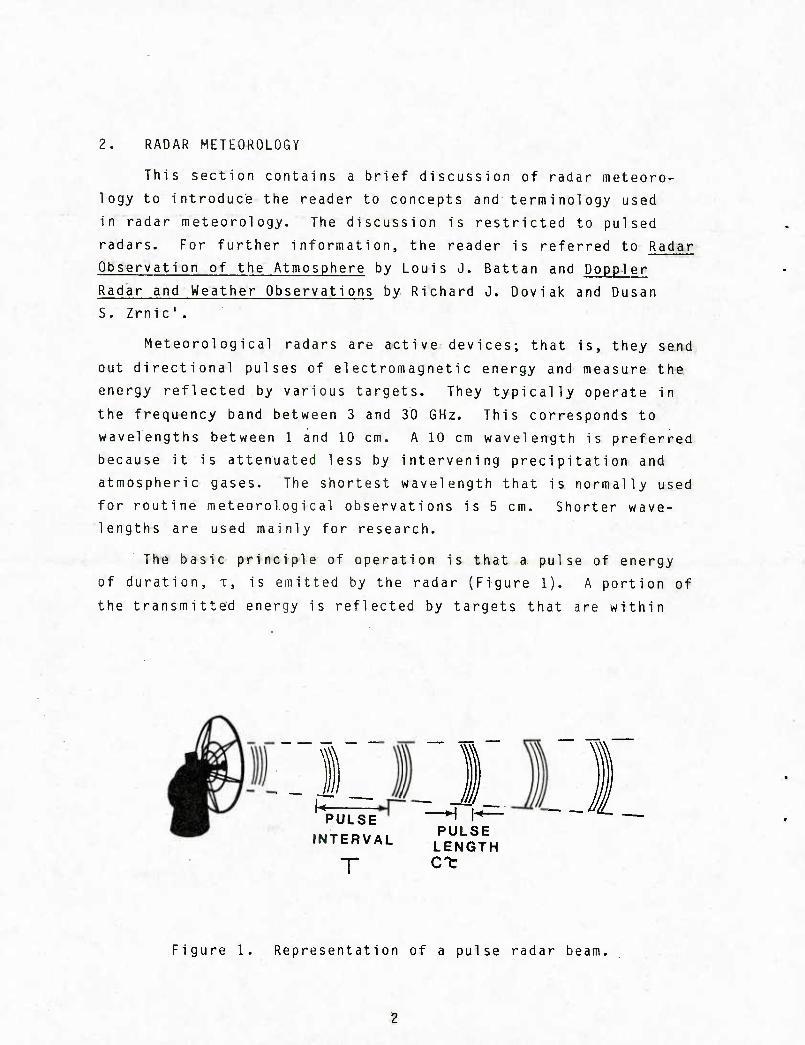
The basic principle of operation is that a pulse of energy of duration, x, is emitted by the radar (Figure 1). A portion of
the transmitted energy is reflected by targets that are within
PULSE INTERVAL
-H
T PULSE
LENGTH
Figure 1. Representation of a pulse radar beam,
I
the beam. During the interval between pulses, the returned
signal is detected and its strength measured. As will be shown
later, the strength of the return can be related to the precipi-
tation intensity. The distance to the target is determined by
the elapsed time between the transmission of the pulse and the
reception of the returned signal and is given by
r=ct/2. (1)
where r is the range, c is the speed of light, and t is the
elapsed time. The radar emits the pulses at a rate called the
pulse repetition frequency, PRF. The pulse repetition period or
pulse interval, T, is the reciprocal of the PRF. There exists a
range beyond which the returned signal has not reached the radar
before the next pulse has been emitted. This range is known as
the maximum unambiguous range and is given by
^max = ^T/2. (2)
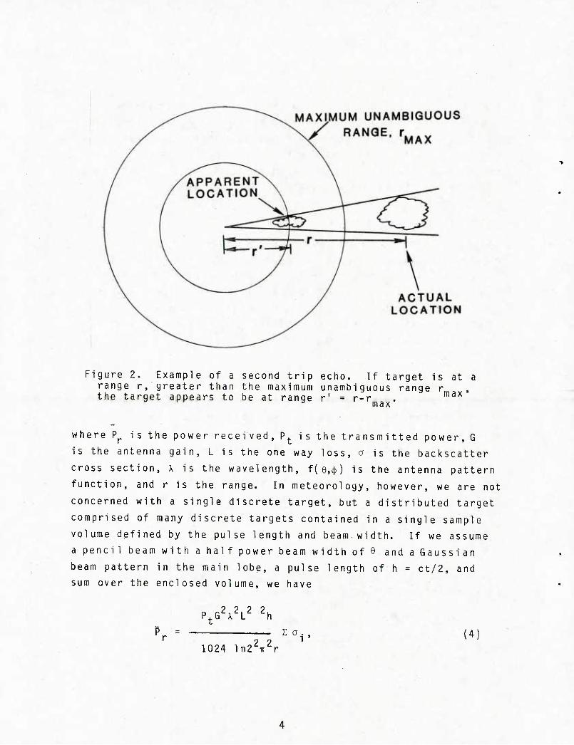
If there is a target at a range greater than r , then max
its return for the nth pulse will be received after the n + 1
pulse has been transmitted (Figure 2). Therefore, the elapsed
time will appear to be t' = t-T and the apparent range will be
r' = ct'/2 = ct/2-r^^^. Since the target will appear to be at
a nearer range than it really is, the range is observed as
ambiguous. To eliminate range ambiguities, all targets must
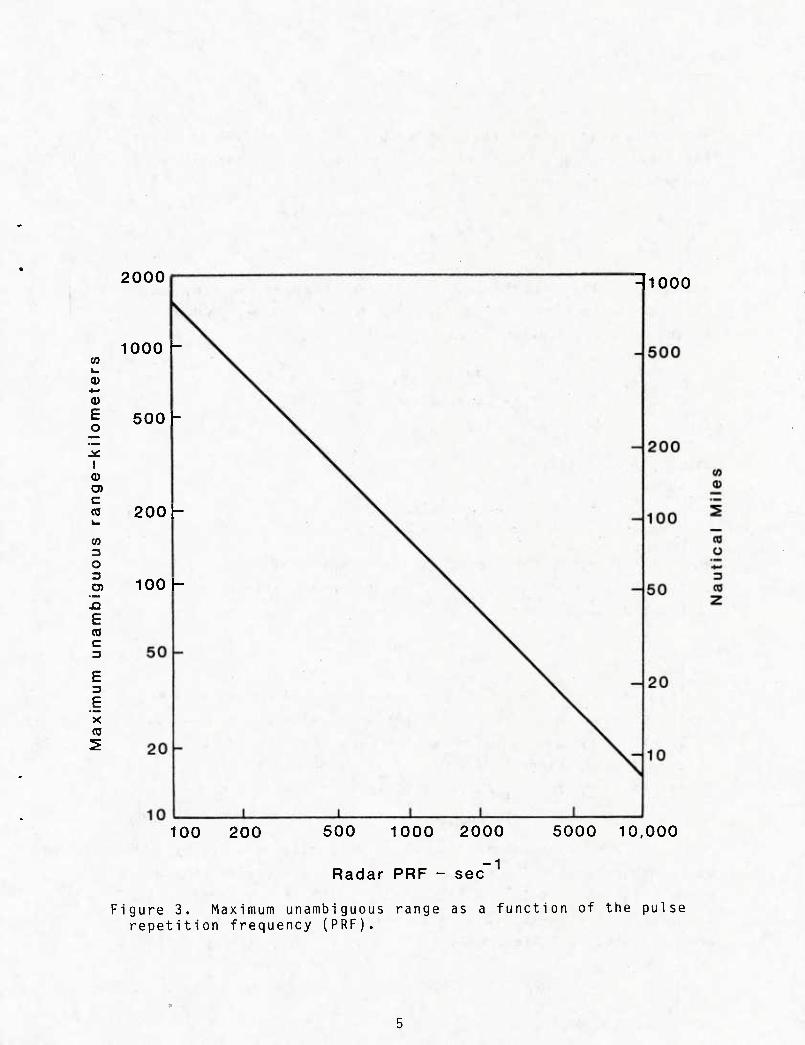
lie within r^^^^. Figure 3 is a plot of unambiguous range as
a functi on of PRF.
2.1 Intensity Considerations
The power returned from the target is given by the radar
equation. For a discrete target the radar equation is
7 7 7 4 P^G^X^L^ f (e,(|))
(4.)3 r^ (3)
Figure 2. Example of a second trip echo. If target is at a range r, greater than the maximum unambiguous range r the target appears to be at range r' = r-r max '
max
where P^ is the power received, P^ is the transmitted power, G
is the antenna gain, L is the one way loss, a is the backscatter
cross section, x is the wavelength, f(e,(()) is the antenna pattern
function, and r is the range. In meteorology, however, we are not
concerned with a single discrete target, but a distributed target
comprised of many discrete targets contained in a single sample
volume defined by the pulse length and beam width. If we assume
a pencil beam with a half power beam width of 9 and a Gaussian
beam pattern in the main lobe, a pulse length of h = ct/2, and
sum over the enclosed volume, we have
P^G^X^L^ ^h
1024 ln2^Tv^r
Za., (4)
(0
o 0) E o
I « a> c OS V.
(O 3 O 3 O)
!o E (0 c 3
(0
2000
1000 -
500 -
- 1000
200 -
100 -
100 200 500 1000 2000 5000 10,000
Radar PRF - sec -1
Figure 3. Maximum unambiguous range as a function of the pulse repetition frequency (PRF).
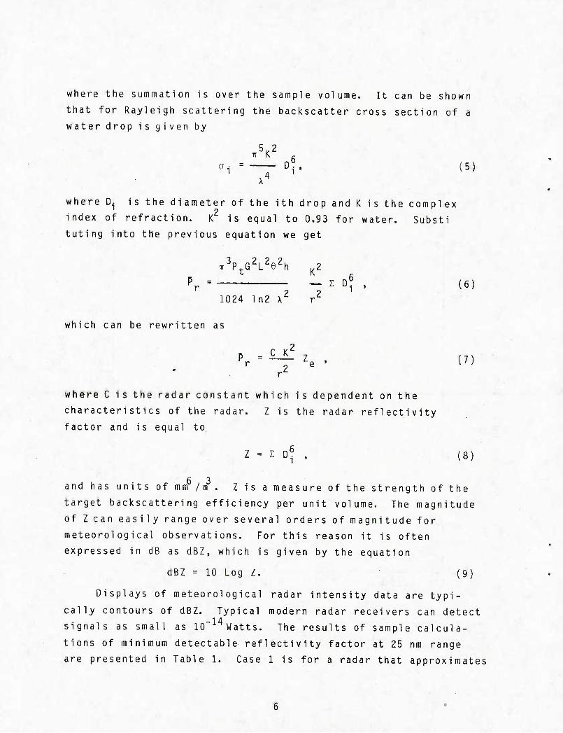
where the summation is over the sample volume. It can be shown
that for Rayleigh scattering the backscatter cross section of a
water drop is given by
.^K^
»?. 5)
where D. is the diameter of the ith drop and K is the complex 2
index of refraction. K is equal to 0.93 for water. Substi
tuting into the previous equation we get
3 2 2 2 ir-'p^G^L^e^h
1024 ln2 X^ r^
E D^ (6)
which can be rewritten as
C K' (7)
where C is the radar constant which is dependent on the
characteristics of the radar. Z is the radar reflectivity
factor and is equal to.
Z = Z D"r (8)
CO-
and has units of mm /m . Z is a measure of the strength of the
target backscattering efficiency per unit volume. The magnitude
of Z can easily range over several orders of magnitude for
meteorological observations. For this reason it is often
expressed in dB as dBZ, which is given by the equation
dBZ = 10 Log Z. (9)
Displays of meteorological radar intensity data are typi-
cally contours of dBZ. Typical modern radar receivers can detect
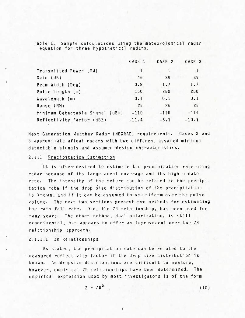
signals as small as 10" Watts. The results of sample calcula-
tions of minimum detectable reflectivity factor at 25 nm range
are presented in Table 1. Case 1 is for a radar that approximates
Table 1. Sample calculations using the meteorological radar equation for three hypothetical radars.
CASE 1
Transmitted Power (MW) 1
Gain (dB) 46
Beam Width (Deg) 0.8
Pulse Length (m) 150
Wavelength (m) 0.1
Range (NM) 25
Minimum Detectable Signal (dBm) -110
Reflectivity Factor (dBZ) -11.4
CASE 2 CASE 3
1 1
39 39
1.7 1.7
250 250
0.1 0.1
25 25
-110 -114
-6.1 -10.1
Next Generation Weather Radar (NEXRAD) requirements. Cases 2 and
3 approximate afloat radars with two different assumed minimum
detectable signals and assumed design characteristics.
2.1.1 Precipitation Estimation
It is often- desired to estimate the precipitation rate using
radar because of its large areal coverage and its high update
rate. The intensity of the return can be related to the precipi-
tation rate if the drop size distribution of the precipitation
is known, and if it can be assumed to be uniform over the pulse
volume. The next two sections present two methods for estimating
the rain fall rate. One, the ZR relationship, has been used for
many years. The other method, dual polarization, is still
experimental, but appears to offer an improvement over the ZR
relationship approach.
2.1.1.1 ZR Relationships
As stated, the precipitation rate can be related to the
measured reflectivity factor if the drop size distribution is
known. As dropsize distributions are difficult to measure,
however, empirical ZR relationships have been determined. The
empirical expression used by most investigators is of the form
.b AR (10)
where R is the rain rate in mm/hr and the reflectivity factor Z
is in mm /m . A and b are empirically determined constants.
Many expressions have been developed over the years. Two of
the most commonly used equations are: , tv-v,^ ,
Stratiform rain
Thunderstorm rain: Z = 486R
(Jones, 1956) .
Z = 200R ^'^ . (11a) . (Marshall and Palmer, 1948),
1.37 , (lib)
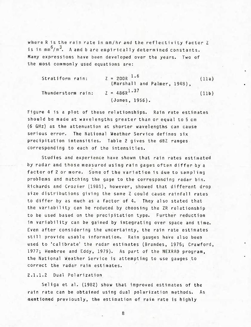
Figure 4 is a plot of these relationships. Rain rate estimates
should be made at wavelengths greater than or equal to 5 cm
(6 GHz) as the attenuation at shorter wavelengths can cause
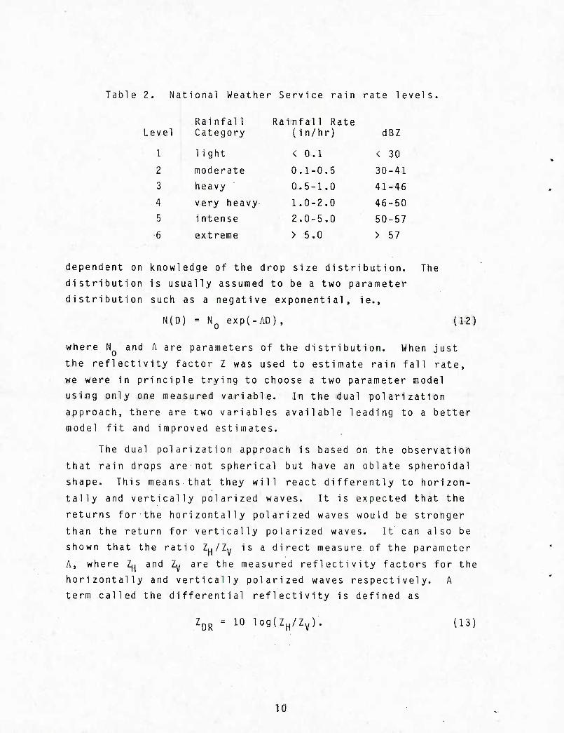
serious error. The National Weather Service defines six
precipitation intensities. Table 2 gives the dBZ ranges
corresponding to each of the intensities.
Studies and experience have shown that rain rates estimated
by radar and those measured using rain gages often differ by a
factor of 2 or more. Some of the variation is due to sampling
problems and matching the gage to the corresponding radar bin.
Richards and Crozier (1981), however, showed that different drop
size distributions giving the same Z could cause rainfall rates
to differ by as much as a factor of 4. They also stated that
the variability can be reduced by choosing the ZR relationship
to be used based on the precipitation type. Further reduction
in variability can be gained by integrating over space and time.
Even after considering the uncertainty, the rain rate estimates
still provide usable information. Rain gauges have also been
used to 'calibrate' the radar estimates (Brandes, 1975; Crawford,
1977; Hembree and Eddy, 1979). As part of the NEXRAD program,
the National Weather Service is attempting to use gauges to
correct the radar rain estimates.
2.1.1.2 Dual Polarization , ?'
Seliga et al. (1982) show that improved estimates of the
rain rate can be obtained using dual polarization methods. As
mentioned previously, the estimation of rain rate is highly
10 =—I—I I 11 Mil—I I I I iiii|—I—I I I iiii|—I—I I I iiii|—1—I M I \n
2 10
E E I
10
10 10
(Marshall-Palmer)-
(Jones)
urnil I I I I mil i i i i mil i i i i mil i I Mill
10 10* 10*
Z-mm^/m^
10* 10'
Figure 4. Plot of two commonly used ZR relationships.
Table 2 lational Weather Service rain rate levels li
Level
.1
2
■ '? ■.
Rainfal1 Category
light
moderate
heavy
very heavy
intense
extreme
Rainfall Rate (in/hr) dBZ
< 0.1 < 30
0.1-0.5 30-41
0.5-1.0 41-46
1.0-2.0 46-50
2.0-5.0 50-57
> 5.0 > 57
dependent on knowledge of the drop size distribution,
distribution is usually assumed to be a two parameter
distribution such as a negative exponential, ie..
The
N(D) NQ exp(-AD), (12)
where N and A are parameters of the distribution When just
the reflectivity factor Z was used to estimate rain fall rate,
we were in principle trying to choose a two parameter model
using only one measured variable. In the dual polarization
approach, there are two variables available leading to a better
model fit and improved estimates.
The dual polarization approach is based on the observation
that rain drops are not spherical but have an oblate spheroidal
shape. This means that they will react differently to horizon-
tally and vertically polarized waves. It is expected that the
returns for the horizontally polarized waves would be stronger
than the return for vertically polarized waves. It can also be
shown that the ratio Zy/Zw is a direct measureof the parameter
A, where Zu and Zw are the measured reflectivity factors for the
horizontally and vertically polarized waves respectively. A
term called the differential reflectivity is defined as
^DR = 1° log(Z^/Zy) (13)
10
The resulting equations for rain rate estimation are typically
in one of the following forms.
or
R = aZj^lO
R = a^H^DR
DR (Exponential Drop Distribution) {14a)
(Gamma Drop Distribution) (14b)
In a single polarization meteorological radar the polarization is
normally horizontal, and therefore Z^ = Z.
Another advantage of dual polarization radar is its ability
to distinguish between the liquid and ice phases of precipitation.
Table 3 (Hall et al., 1980) shows the expected characteristics
of Z and Zr.n at a 10 cm wavelength. Notice the difference in UK
characteristics for rain and dry frozen precipitation.
Table 3. Expected characteristics of Z and Zr.„ at 10-cm wave
length for various hydrometeor types (from Hall et al., 1980).
Hydrometeor Type DR Comments
Rai n
Drizzle, cloud, or fog
Dry snow flakes
Sleet/wet snow
Wet graupel
Wet hail
Dry hail or other high- density ice parti cles
High
Low
High
High
High
Medi um
High
Low
Medium-low Medium-low
High
Negati ve
Vari able
Low
Includes 1arge obi ate drops
Small spherical drops of water and/or small ice particles
Large hori zontally oriented low-density aggregates
Large oblate hori- zontal ly ori ented parti cles
Large conical verti cal1y ori ented particles
Large particles; seldom spheres .
11
Dual polarization approaches are still in the research stage
but are approaching readiness for operational implementation.
Work still needs to be done on defining the empirical rain rate
estimation relations. ^ - . . ...
2.2 Doppler Considerations
Besides measuring the intensity of the return, the newer
generation of meteorological radars include a Doppler capability
which allows them to measure the radial velocity and spectral
width of the targets. This additional information increases the
utility of the meteorological radar.
' ! The total distance traveled by a pulse from the radar to the
target and back is 2r. Measured in wavelengths of the transmit-
ted frequency, it is 2r/x or in radians, 4Trr/x. If the wave
emitted by the radar has a phase of p , the phase at reception
wouldthenbe
P = PQ - 4ur/A . , "
The time rate of change of phase is then
. ■ dp -4TT dr -4Tr V
^■- .'.■ dt X dt X K
The quantity dp/dt is the angular frequency, to,
2iTf. Substitution gives
f = -2V/X
(15)
■■ (16)
and is equal to
. (17)
where f is the Doppler shift frequency, and V is the radial
velocity of the target (also called the Doppler velocity). Note
that only the radial component of the velocity is measured. For
meteorological targets the Doppler shift frequency is always '
in the audio range. Because the Doppler shift is in the audio
range, it represents a very small change in the carrier frequen-
cies used and would be difficult to measure with a single pulse.
Therefore, the phase shift is measured over the longer period of
time from pulse to pulse rather than during the pulse period.
12
From sampling theory it is known that to measure a frequency f, samples must be taken at a frequency of at least 2f. Since
the sampling rate is set at the PRF, the maximum Doppler shift frequency is
f = PRF/2 max
which corresponds to a maximum Doppler velocity of
V = (PRF)x/2.
(18)
(19)
Velocities in the sample volume greater than V fold into the range ±V . This is known as aliasing or velocity folding
and is illustrated in Figure 5. Since the maximum unambiguous
range r„,^ is also a function of the PRF, we have max
V = Xc8r max max (20)
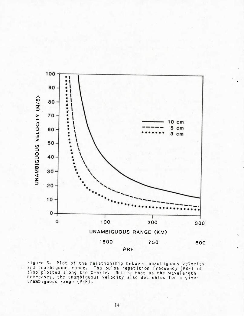
Therefore, r , V , and the PRF are all related. If you want ' max' max' -^ to change one, the other two are affected. Figure 6 is a plot of the relationship between r^,„ and V^,^ for various wavelengths.
in a X m a X
-5V-
-3V-^
-V
. ! 1^ 2ncl Neg Fold
rin^^^ — ;:=-1st Neg Fold
^^—-"""' I ' / +V
1st Positive Fold + 2V +3V
Figure 5. Illustration of aliasing. The unambiguous velocity is +V. Those velocities outside this range appear (fold into within this range). For example a real negative velocity of -3.5V (point a) will appear as a velocity of +0.5V (point b).
13
o o -J
>
CO D O
0
100 200
UNAMBIGUOUS RANGE (KM)
1500 750
300
500 PRF
Figure 6. Plot of the relationship between unambiguous velocity and unambiguous range. The pulse repetition frequency (PRF) is also plotted along the X-axle. Notice that as the wavelength decreases, the unambiguous velocity also decreases for a given unambiguous range (PRF).
14
As discussed before, discrete volumes are being sampled.
Each volume contains targets moving at many velocities (Figure 7).
Therefore the phase shift measured at any one time is a weighted
average of the phase shifts due to all of the targets in the
sampling volume. The weighting is a function of location in the
beam and the strength of their return. In general the stronger
the return, and the closer to the beam center line, the larger
the weighting. Because the resultant phase shift of a mean value
varies, repeated samples are taken to obtain a statistically
significant velocity estimate and to reduce the uncertainty in
the estimate. This distribution is known as the velocity
spectrum (Figure 8). The standard deviation of the spectrum is
known as the spectrum variance or spectrum width and is a measure
of the velocity dispersion.
Several factors can affect the magnitude of the observed
spectrum wi dth:
(1) Systematic wind shear within the sample volume. This
means that one portion of the beam will see a different
velocity than another and the spectral width will be
i ncreased. >■
(2) The spread of terminal velocities of the echoing
targets. The larger the range of effective rain drop
sizes, the larger is the spectrum variance. This effect
is the greatest when the antenna is pointed vertically
and is negligible when pointing horizontally.
(3) The turbulence spectrum of the air. The smaller rain
drops, ice particles, and dust respond faithfully to
rapid changes in air motion and, therefore, reproduce
the air velocities due to turbulence. Hence, the ■
greater the turbulence, the larger the spectrum width.
15
.»i.
(1/2 pulse length)
Figure 7. Target motion within an echo sample volume. The Doppler velocity measured is a weighted mean of the velocities contained in the sample volume. The larger the range of radial velocities in the sample volume, the greater the spectral width.
. , Power '■
■«'
; * v' ■■
Received ,.-,...■ •■■.,'
■ ■■ rS,;'.,- , ■■;
'^max — -^^-T^s. : - ■
/ \..t;k<".. y^ ;■ 1 ;■-. Ny^^^
^^^ **-.
^^^
(Wing) (Wing)
max Frequency
Figure 8. Idealized Doppler spectrum of a precipitation target. The X-axis frequency is the Doppler shift frequency and corresponds to radial velocity.
H
(4) Finite beam width with uniform air motion across the
radar beam. If the wind is perpendicular to the beam
axis, then targets near the edge of the beam will
produce a larger Doppler shift than those near the
center where the Doppler shift would be zero (Figure 9).
(5) Antenna motion. As the antenna rotates, the beam
sweeps through space. Hence the radar does not receive
echoes from identically weighted targets on successive
samples which results in an increased spectrum width.
The spectrum width increases as the antenna rotation
rate increases.
3. CRITERIA FOR RADAR SUITABILITY EVALUATION
Several factors need to be considered when evaluating a
radar for meteorological applications. Many are interrelated,
and an improvement in one may result in a degradation in another.
The relative merits of the factors must be weighed and a
compromise reached. This section discusses these factors and
tradeoffs.
3.1 Beam Width
Most meteorological radars have beam widths between 0.8 and
2.0°, with values near 1.0° preferred. There are four adverse
effects associated with an increase in the beam width: 1) partial
spatial resolution, and 4) increased spectral width.
An assumption implicit in the derivation of the meteorolo-
gical radar equation (Eq. 7) is that the beam is uniformly filled
with scatterers. If the beam is not filled, the estimate of
precipitation intensity is then in error. In Table 4 the
diameters of the beam for different ranges and beam widths are
given. At 25 nm, a 4° beam has a diameter over 3000 meters and
partial beam filling will be a problem. If the beam width is
doubled, the probability that the beam will not be filled is
greatly increased.
17
Component Along Beam
BEAM CENTER LINE
Wind Velocity
4 \ / \ ̂ , Component
Along Beam Zero
Figure 9. Example of spectrum broadening due to a uniforT wind blowing across a beam of finite width. At the center line the radial component is zero. As the angle from tne center line increases, the radial component also increases.
. This leads to a range of velocities being contained in -ie sample volume, hence an increased spectral width.
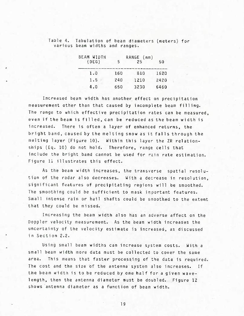
Table 4. Tabulation of beam diameters (meters) for various beam widths and ranges.
BEAM WIDTH (DEG)
1.0
1.5
4.0
RANGE (nm) 5 25 50
160 810 1620
240 1210 2420
650 3230 6460
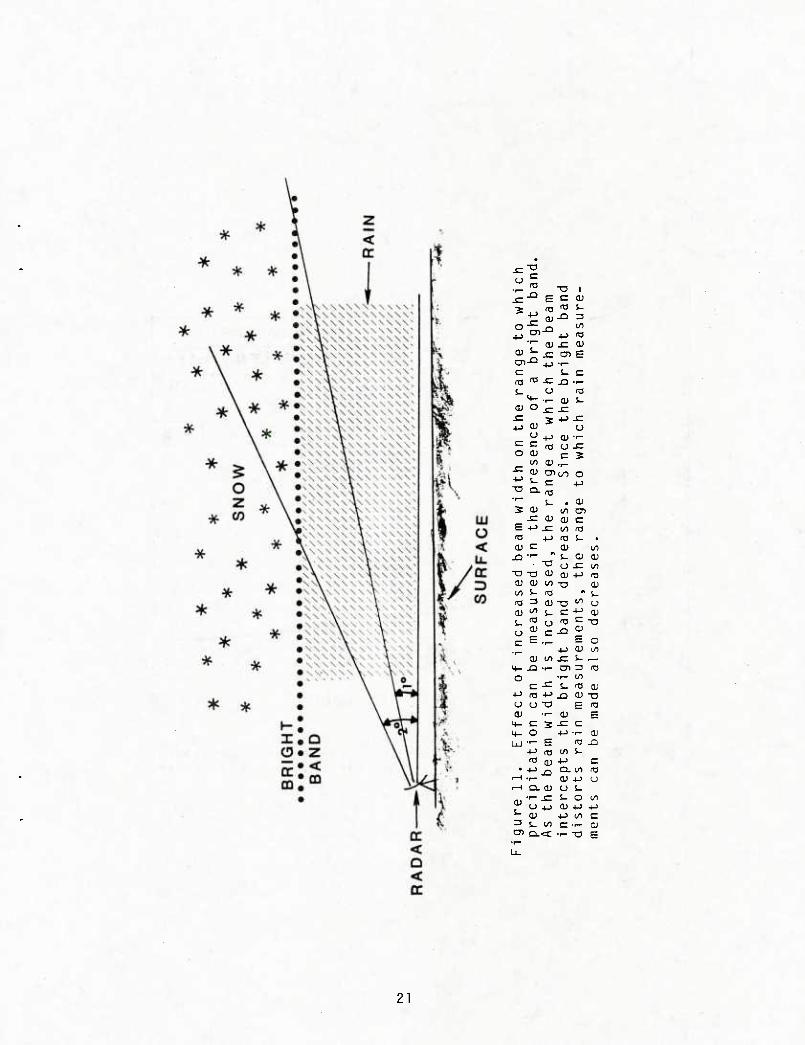
Increased beam width has another effect on precipitation
measurement other than that caused by incomplete beam filling.
The range to which effective precipitation rates can be measured,
even if the beam is filled, can bereduced as the beam width is
increased. There is often a layer of enhanced returns, the
bright band, caused by the melting snow asit falls through the
melting layer (Figure 10). Within this layer the ZR relation-
ships (Eq. 10) do not hold. Therefore, range cells that
include the bright band cannot be used for rain rate estimation.
Figure 11 illustrates this effect.
As the beam width increases, the transverse spatial resolu-
tion of the radar also decreases. With a decrease in resolution,
significant features of precipitating regions will be smoothed.
The smoothing could be sufficient to mask important features.
Small intense rain or hail shafts could be smoothed to the extent
that they could be missed.
Increasing the beam width also has an adverse affect on the
Doppler velocity measurement. As the beam width increases the
uncertainty of the velocity estimate is increased, as discussed
inSection2.2. '
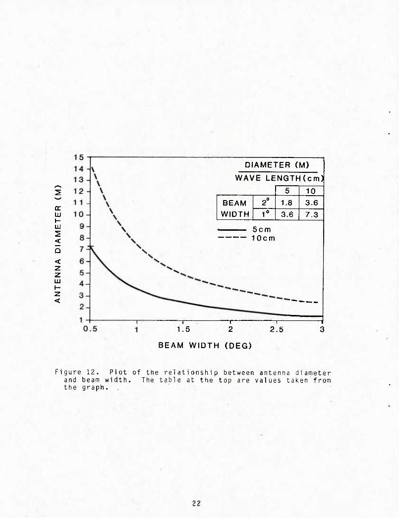
Using small beam widths can increase system costs. With a
small beam width more data must be collected to cover the same
area. This means that faster processing of the data is required.
The cost and the size of the antenna system also increases. If
the beam width is to be reduced by one half for a given wave-
length, then the antenna diameter must be doubled. Figure 12
shows antenna diameter as a function of beam width.
19
■a +J ■ O! -r- o -o
T3 13 *-* O) 03 O 5 ■— +J S-
a--o
-'-' o rt3
OJ 1— «• ID ■— E '—
O ro
. 1— </i
ai 03 CD
C 4J <u r- cu O ^ Q. 5
•r—
O T3 o t/i
•f" o n ■o to o c 1— </l OJ 1. o QJ c: ■a o > o n3
0) O <u tu
<- cr 0)
^' 1—
+-> 0) s- +-> • m Q -a OJ O. O) 3 13 c CO
fc 0) 13
01 O) S- JZ. 0) -C JZ fO -^ 1- -)-> 4-) s u
QJ (/^ c o , ■D
(1) ,_ J-J >-, • +j c- +-> >> X3
ni 5 •/— 4-> rs u o > •'—
-l-> c ■— •r- > s- l/> I/) r— 4-) •<—
3 aj u -(-: 1— 0) u_ OJ O 1— JT: 1— 0.' CLI
•r~ — u- r— **~ .,- ai 4- A-'
+-> V- OJ -C • t/l i- ■^;
cn-tJ to *— C ,,_ u- m 1/1 JT
s- ai +-> r. j-» o 1— 3 ^ ,— re
0) r3 CL'
SI O) ■o «« S_
+J sz n3 ■a A^ s_ .c: 3 c
c fO o o o c ■u X3 — r—
m o
5-
o 4-' 13
c c: O) <JJ T3 .C
ru j-J
S O! ■ CD 4-> CL
5_ , v^ O -C >, >^ O C Oi
13 -O u i_ OJ Q.
. 1/1 OJ o) ro a, •n- ■'-' -t-" J:: r-
. 1' 3 O) +j O 1—I J-J -C .,— >-H 2r oi QJ +-> 1—
aj 13 1. >, S- QJ +-> u to s_ rs -C o a' ai OJ crij-j c JO c >
20
J=-^
o = n3 -a 1 I^ E c QJ
S , % na fO S-
2f J3
J3
+->
:3
dJ i: QJ (U s- .C en E OT-Q 4J •^ c s_ c « "« -C J2 ■^
s_ o fO M- -r- 01 s_
O) o x: J= x: 5 +-> ^ 4j a) o
o -(-> 0) ■1—
c: c fO (J x: O QJ c 3
-^ QJ en
■^ Q. ^
S O) J: O)
E +J jr
-•-.; -O T3 QJ O) O) (/I
00 O
. OJ I/) CT) QJ C (/) re na s_ • QJ in i_ QJ QJ (_) -C </) QJ -t-i n3
T3 QJ
-o '^ C +-'
o QJ
O OJ
OJ (/) M- J3 •.-
°c- ■t-> fO ■!-> O O X3 QJ •.-
4- = 2 M_ O LU T- E
+^ na "J QJ
1—• CL O*
?: o5 >- Q; ^ S_ (/)
•r- cn a:
to O) QJ "O E fa
x: c 4-» -T-
■4->
Q. c/> QJ +J O i~ i- O QJ +J
-4-> l/l C •--
•r- T3
OJ
c 03 U
(/I
c
E
21
cc LJJ H- m
..<
I <
DIAMETER (M)
WAVE LENGTH(cm)
BEAM WIDTH
1.8
3.6
5cm 10cm
10
3.6
7.3
—: 1
1.5 2
BEAM WIDTH (DEG)
2.5
Figure 12. Plot of the relationship between antenna diameter and beam width. The table at the top are values taken from the graph.
tt
3.2 Pulse Length/Range Resolution
The returned power increases as pulse length increases.
This increase in returned power is at the expense of range .•
resolution since pulse length is inversely proportional to the
number of independent range cells per kilometer of range. If
the pulse length is too large, significant features can be
smoothed out and missed just as with increased beam width. What
constitutes a significant feature depends on the application of
the meteorological radar. For non-Doppler data, the pulse
lengths typically are between 0.8 y s (250 m) and 3.3 ys (1 km).
For Doppler applications the pulse length should be less than
2us (600 m). .. , . ,. . •
The variation of radial velocity of the different scatterers
within the pulse volume tends to increase as the pulse length
(and hence pulse volume) is increased. This results in a
broadening of the Doppler spectrum, and therefore increases
uncertainty in the estimate of the mean velocity. ' t ■;■
One disadvantage of short pulse lengths is the increase in
the amount of data that must be processed. For a given maximum
range, halving the pulse length doubles the amount of data.
Another disadvantage is that to maintain the same sensitivity for
a given PRF, as pulse lengths are shortened, the peak transmitted
power must be increased. The increase in transmitted peak power
can be mitigated to some extent by the use of complex wave forms
and pulse coding which increases system complexity and cost.
3.3 Transmitted Power
If other radar design parameters are held constant, then
for a given range, the minimum backscatter cross section that •
can be detected is inversely proportional to the transmitted
power (Eq. 6). If a given receiver can detect a -8 dBZ return
at 50 km with a transmitted power of 1 MW, it would only be able
to detect a -5 dBZ return with a transmitter power of 0.5 MW.
^3
stated another way, if the transmitted power is halved for a given
receiver sensitivity, then the maximum range to which effective
precipitation measurement can be made is reduced by 2 (Eq. 7).
Typical transmitted powers for meteorological radars are 250 KW for 5 cm radars and 1 MW for 10 cm radars.
Two methods for maintaining sensitivity at low transmitter
powers are to increase the sampling time and/or to increase the pulse length. Both have their drawbacks. Sampling time is
increased by averaging over a larger number of pulses. This
means that the radar must look along each radial longer which
causes the antenna to rotate slower and, thus, takes longer to
scan a given area. An increase in pulse width will result in
a decrease in radial resolution as previously discussed. . -'
3.4 Frequency '' ' " ^-■
As previously discussed, meteorological radars typically
operate in the 3 to 30 GHz frequency range. This is because, " ^ above 30 GHz, the attenuation due to water vapor and precipita-
tion is significant and limits range and accuracy. Below 3 GHz the sensitivity to precipitation decreases limiting the radars
usefulness as a meteorological instrument. The physical size
of the antenna also becomes a problem. Most operational meteoro-
logical radars are at either 3 or 6 GHz. 3 GHz is preferred as it is attenuated less by precipitation. 6 GHz is considered the
highest frequency for precipitation measurement. Significant
attenuation can occur even at 6 GHz in ^^v)i heavy precipitation resulting in erroneous measurements. If the detection of clouds in a precipitation free region is of concern, then a frequency
near 30 GHz should be chosen. '■■
The choice of frequency also affects the diameter of the
antenna. If the same beam width is maintained and the frequency
is doubled, then the required antenna diameter decreases by half.
The choice of frequency also affects the unambiguous
velocity. This was discussed in Section 2.2 and illustrated :/ ;•,
in Figure 6. If the frequency is doubled, the unambiguous . velocity is cut in half.
24
3.5 Polari zati on
Radars designed to measure precipitation typically are
horizontally polarized. This is because rain drops tend to be
oblate spheroids and returns for horizontally polarized radars
are larger than for other polarizations. Therefore, preference
should be given to radars that are horizontally polarized.
A dual polarization radar (horizontal and vertical polariza-
tions) might be considered in light of the possible improvement
in precipitation estimation (see Section 2.1.1.2). Even though
still experimental, confidence in this approach is increasing and
could shortly be considered suitable for operational applications
given suitable radars.
4. CURRENT CAPABILITIES
Current meteorological radars employing digital processing
have greatly expanded capabilities over their predecessors
(Bjerkass and Forsyth, 1980). These enhanced capabilities do
however require a well calibrated radar system. Meteorological
radar displays now incorporate color, thereby making their
interpretation easier even though more information may be
included. The following discussion is divided into two sections
according to whether intensity or velocity data is being
addressed.
4.1 Intensi ty Data
As with previous radars the intensity display still contains
much information. With digital processing and color, the display
is no longer limited to six contour levels and the contour levels
can be easily changed. This can be desirable when looking at
winter storms where the intensity range is not as great as with
summer storms. Thus, storm detail could be lost using the same
contouring levels for all cases. The color contour levels are
also easier to read and there is less chance for error. With
contoured displays the structure of the precipitating system is
easier to discern. Regions of high reflectivity (high rainfall
25
rate) can easily be determined and tracked. Figure 13 is an
example of a color-contoured intensity PPI (Plan Position
Indicator) display of an approaching squall line. In the figure,
the red areas indicate regions of extreme rainfall rates and the
possibi1ity of hai1. , . >
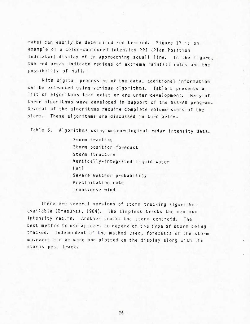
With digital processing of the data, additional information
can be extracted using various algorithms. Table 5 presents a
list of algorithms that exist or are under development. Many of
these algorithms were developed in support of the NEXRAD program.
Several of the algorithms require complete volume scans of the
storm. These algorithms are discussed in turn below.
Table 5. Algorithms using meteorological radar intensity data.
There are several versions of storm tracking algorithms ,, \
available (Brasunas, 1984). The simplest tracks the maximum ■
intensity return. Another tracks the storm centroid. The
best method to use appears to depend on the type of storm being
tracked. Independent of the method used, forecasts of the storm
movement can be made and plotted on the display along with the
storms past track. '•:/ :;_,
11
Figure 13. Example of contoured intensity display. The display is of an intense squall line to the northwest of Nonnan, UK, moving to the southeast. The contouring levels indicate tlie intensity of the return and thereby the precipitation intensity. Photo courtesy of the National Severe Storm Laboratory, Norman, OK.
27
The storm structure algorithm looks at a three-dimensional
region defined as a storm and determines the following
parameters:
* Storm base
* Storm top '
Storm volume *
* Maximum storm reflectivity and its altitude of occurrence
* Storm tilt and its components along horizontal and vertical axes
* Storm overhang
*Overhangorientation
These parameters can then be used as input to other algo-
rithms, such as storm severity, or can be tabulated or plotted
along one side of the display. For example, a plot of the
history of the maximum reflectivity and its altitude would
enable a forecaster to monitor the evolution of the storm.
The vertically-integrated liquid water algorithm converts
meteorological reflectivity data into liquid water content. The
conversion is based on studies of drop size distributions and
empirical studies of the relationship between the reflectivity
factor and liquid water content. Large values of vertically-
integrated liquid water have been correlated to severe thunder-
storms. The output from this algorithm is used by the severe
weather probability algorithm. The liquid water distributions
could also be used to estimate the attenuation field.
The severe weather probability algorithm is used to deter-
mine the probability that a given echo is associated with a
severe storm. A severe storm is defined as one with a tornado
knots or reported wind damage (NEXRAD JSPO, 1985). The results
could then be used to flag storms suspected of being severe.
29
The precipitation rate algorithm converts meteorological
radar reflectivity data to rain rates. The conversion is
performed using empirically determined relationships between
the reflectivity factor and rain rates and studies of drop size
distributions (see Section 2). The output of the algorithm can
be plotted on a display or as input to a higher level algorithm
dependent on rain, such as one to estimate attenuation at mm
wavelengths. . .
The hail algorithm is used to help identify storms likely to
produce hail. The algorithm uses output from the storm tracking
and storm structure algorithms. As currently implemented in
NEXRAD it is used to identify one of the following cases:
* a given storm is producing hail or soon will produce hail
* a given storm is probably producing or will probably produce hail
* a given storm is not currently producing hail
, • * a given storm cannot be analyzed due to lack of suffi ci ent data .
The transverse wind algorithm is used to determine horizon-
tal wind direction and speed. The approach seeks to find similar
patterns in the reflectivity field in successive scans at the
same tilt (Rhinehart, 1979). The similarity is determined by
dividing the initial scan into boxes. Then for each box in the
initial scan, the box in its neighborhood in the second scan that
has the maximum correlation with it is found. The displacement
of the second box from the first is used to define the direction
and speed. The output can be used to supplement the radial winds
determined by Doppler processing. Figure 14 is an example of a
wind field retrieved using this method (Rinehart, 1982).
4.2 Velocity
If a Doppler radar is used then velocity and spectral width
information are also available. Two additional base products and
additional algorithms are now available. Figures 15 and 16 are
examples of the PPIs of the velocity and spectral width corres-
ponding to the intensity PPI of Figure 13. The additional base
products alone add considerable information. In the velocity
30
E
<
<
li- O
X h- o: o z UJ o z
%4^' J
I- "^J* '* -Gift's*
-70
At
140
DISTANCE EAST OF RADAR (km)
Figure 14. PPI of radar reflectivity data and TREC vectors for Hurricane Frederic collected by the Slidell, Louisiana, NWS WSR57 radar at 0331 UT on 12 September 1979 at 0.8 deg elevation. The shaded regions diro. reflectivity contours starting at 15 dBz and increases at 10-dB intervals (from Rinehart, 1982).
31
display of Figure 15, a gust front is seen to be leading the
squall line with a peak velocity towards the radar of 28 m/s.
The shear across the gust front is 40 m/s. The gust front is
in a region of low reflectivity and there is no indication of
its presence in the intensity plot of Figure 13. Some idea
of the vertical wind profile can usually be determined from
the velocity PPI display. The simulated return in Figure 17.
indicates wind veering with height, and the closed contour
indicates a jet blowing from the southwest to the northeast.
Figure 16 is a plot of the spectral width. High values are
associated with turbulence. A region of large spectral widths
is indicated along the gust front as would be expected indicating
increased turbulence. Algorithms that have been or are being
developed that use Doppler meteorological information are listed
in Table 6. The output from the algorithms can be used directly
or input to higher level algorithms or tactical decision aids
(TDAs) .
Table 6. Algorithms that use meteorological Doppler radar data that have been developed or are under development.
*
*
*
*
*
*
*
*
Mesocyclone Detection
Velocity Azimuth Display
Turbulence
Tornado Vortex Signature
Combined Shear
Modified Velocity Volume Processing
Divergence Detection
Sectorized Uniform Wind
Gust Front Detection
The Mesocyclone Detection algorithm is used to detect
mesocyclones. A mesocyclone is a horizontally rotating three-
dimensional region in a storm. Mesocyclones have been associated
with severe weather. The algorithm uses pattern recognition
techniques to search the velocity field for symmetric regions of
large azimuthal shear. The algorithm can also be used to detect
gustfrontsparallel toaradial.
32
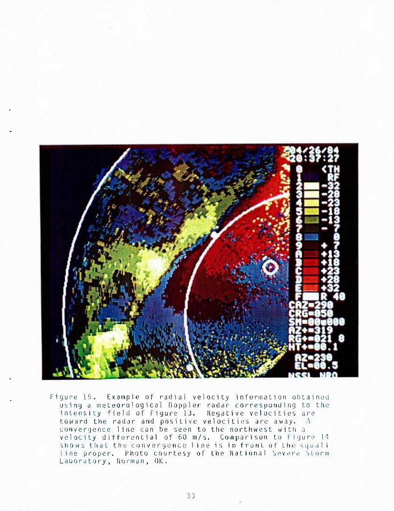
Figure 15. Example of radial velocity information obtained using a meteorological Doppler radar corresponding to the intensity field of Figure 13. Negative velocities are toward the radar and positive velocities am away. A convergence line can be seen to the northwest with a velocity differential of 60 m/s. Comparison to Figure 14 shows that the convergence line is in front of L ii e squall line proper. Photo courtesy of the National Severe SLoi'iii Laboratory, Norman, OK.
33
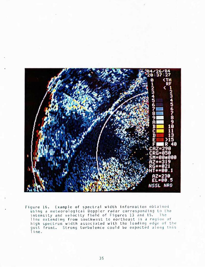
Figure 16. Example of spectral width information obtained using a meteorological Doppler radar corresponding to the intensity and velocity field of Figures 13 and 15. The line extending from southwest to northeast is a region of high spectrum width associated with the leading edge of the gust front. Strong turbulence could be expected along this line.
35
(a)
J i
M r
180 270 OIRCCTION
SPOD —
N
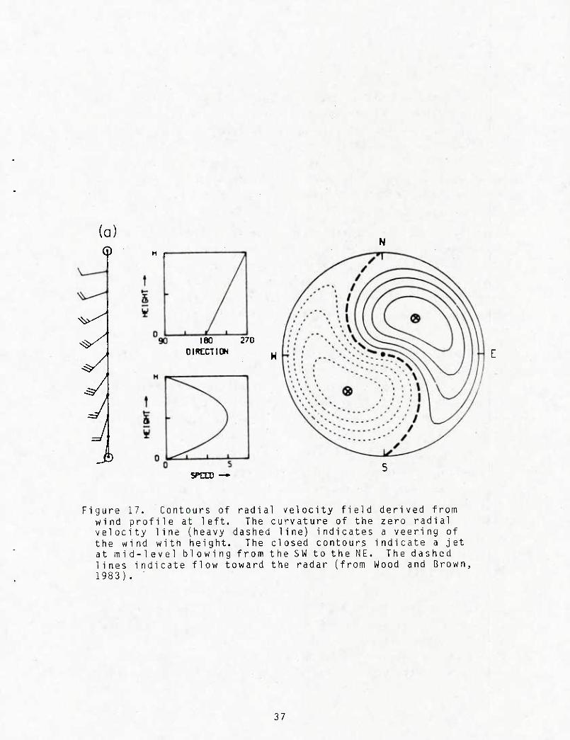
Figure 17. Contours of radial velocity field derived from wind profile at left. The curvature of the zero radial velocity line (heavy dashed line) indicates a veering of the wind with height. The closed contours indicate a jet at mid-level blowing from the SW to the NE. The dashed lines indicate flow toward the radar (from Wood and Brown, 1983).
37
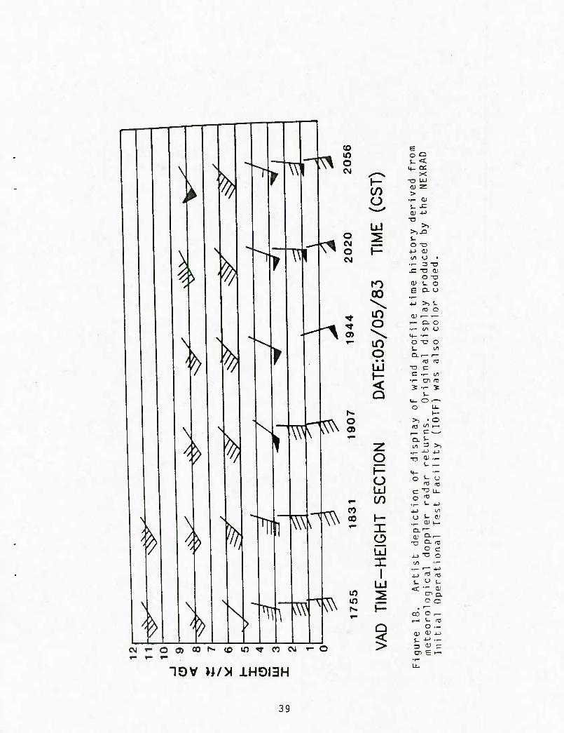
Velocity Azimuth Display (VAD) processing is used to obtain
the vertical profile of mean horizontal wind direction and speed,
divergence, and vertical velocity for the region of the atmos-
phere surrounding the Doppler raddr. A harmonic analysis is
performed on data collected at multiple azimuths as the radar
scans at a constant elevation angle. A sequence of these
vertical profiles can be done to provide a time history of
the wind profile (Figure 18).
The Turbulence algorithm uses Doppler spectrum variance
measurements to estimate the strength of turbulent air motions.
Measurements of the radar reflectivity factor and empirical
limits of the outer scale of the turbulence for a given
meteorological situation are also used. The output is a
parameter indicating the presence of light, moderate, or
severe turbulence.
The Tornado Vortex Signature (TVS) algorithm is used for
the detection of probable tornadic vortices. Tornadic vortices
have a distinctive signature on the velocity PPI; however, when
viewing a full PPI, it can easily be missed due to their small
size. The TVS algorithm is an attempt to automate the detection
of tornadic vortices. The output is a yes/no flag.
The Combined Shear algorithm determines a value that is
related to, but not equivalent to, the total horizontal wind
shear. The value is a combination of the radial and azimuthal
wind shears as determined for each grid point from the velocity
field. The output is a field of shear values that are easily
displayed or input to higher level algorithms. The main
application of this algorithm will be in aviation where wind
shears are important.
The Modified Velocity Volume Processing (VVP) algorithm is
a statistical regression method for calculating the vector wind
field over the radar's survei11ance area. The algorithm assumes
that the wind field varies linearly over the volume being
processed and best fits the kinematic parameters of the linear
wind model to the observed radial wind field. As configured for
3§
CO E
I— CO O
° 5 i- < M_ CC
X
>
LxJ
Tie
hi story de
produced by t
coded .
00 \ If) o
o • • Ld
s
o 1- o of
display of wind profile ti
ar returns. Original display
acility (IOTP) was also color
LiJ CO
1— X o
t depiction
doppler rad
onal Test
F
4 .^ > ^
X 1
bJ
1—
Q
re 18
. Artis
teorolog i ca
l i t
i al Operati
CJ'-OOJfflf^-COifl^COCNJ T-O 3 ll C
"lOV H/'A 1H0I3H
39
NEXRAD, the processing volume is 30 degrees by 30 kilometers by
two elevation scans. The output is the values of seven kinematic
parameters at grid points covered by the processing volume.
The Divergence algorithm is designed to detect divergence in
the top of storms. The magnitude of the divergence at the top of
storms is related to the severity of the storm. The output is a
list of divergence locations and magnitudes.
The Sectorized Uniform Wind algorithm is another method
for estimating the transverse wind component. It does this by
evaluating the azimuthal derivative of the radial component of
the wind. As implemented for NEXRAD the output is composed of
wind vectors at 10 degree azimuthal and 7 kilometer radial
spaci ng.
The Gust Front Detection algorithm is used to detect gust
fronts not parallel to a radial. Pattern recognition techniques
are used to detect the shear lines associated with gust fronts.
The outputs of the algorithm describe the gust front as to
location and strengths. The gust front in Figure 15 would be
detected by this algorithm and the appropriate action initiated,
such as the sending of an alert message.
4.3 Returns In Optically ClearAir ■:.
Up to this point the discussion has been limited to returns
when hydrometeors were present in the sample volume to produce a
return. Returns have also been observed in the optically clear
air by radars operating at frequencies from 10 GHz to 50 MHz.
The source of the returns has been subject to some debate,
especially at frequencies above 3 GHz.
The principle sources of returns in the optically clear
atmosphere are 1) refractive index variation, and 2) insects
and birds. The refractive index variation is tne result of
turbulence at scales of L/2 (L = wavelength). If the L/2 scale
is within the inertial subrange of turbulence, then echoes can be
detected. If the L/2 scale is within the viscous dissipation
range, however, the turbulence is rapidly damped and the radar '
reflectivity decreases.
m'
The returns for radars operating in the 50 MHz to 900 Mhz
range are normally attributed to turbulence induced refractive
index variation. Several radars have been developed in this
frequency range to observe vertical wind profiles mainly above
the boundary layer (Zamora and Shapiro, 1984; Larsen and
Rbttger, 1982; Balsley and Gage 1982). These radars are
known as UHF/VHF profilers. Figure 19 is an example of a wind
profile time history obtained using a wind profiler. Sampling •
rates as high as one profile per minute are obtainable, but
longer averaging times are usually used.
Antenna size is a problem with these systems. At 50 Mhz the
antenna is typically a phased array between 50 and 100 meters on
a side. As the frequency increases the antenna size decreases
and at 900 MHz a 3 m antenna may be sufficient, depending on the
required attitude range. i ;
The height to which observations can be taken consistently
is also influenced by the radar frequency. The lower frequencies
should be able to go to higher altitudes because their critical
turbulence scale is larger than for the higher frequencies.
For meteorological radars operating in the 3 to 6 GHz
frequency range there is considerable debate over whether the
observed clear air returns are due to refractive index turbulence
or to insects and birds, or both. Kropfli (1984) reported X band
returns in the optically clear air and attributed the returns to
particulate scatterers. He said that there was evidence that
they were "not 'strong fliers' if, in fact, they are flying
insects at all." Hennington et al. (1980) presented calculations
and some observations that indicate that a 3 GHz Doppler radar
could at times detect clear air returns. Doviak and Berger \ »
(1980) using dual Doppler methods were able to reconstruct
the spatial structure of planetary boundary layer air motions. 2
They concluded that the refractive index structure constants C n deduced by radar and aircraft were within 1 dB. This would seem
to indicate that the primary source of returns was refractive
index turbulence at least for their daytime conditions.
41
■l^ c. <. k k k k k k k k
1.0
I I I J L I I I
159
J \ L 12 09
19-AU-85
06 J \ L
03 00 TIME
J \ L 21 18 15 12 Z
• . '•• • 18-AU-85
Figure 19. Time-height sector of hourly average profiler winds recorded using the Pennsylvania State University Shanty Town 59 MHz radar. Time periods is from 12 GMT 18 August (RHS) to 12 GMT 19 August (LHS) 1985. Major ordinate divisions are km
. msl. Radar site altitude is approximately 400 m. Isopleths are of wind direction in 20° increments and vertical resolu- tion set to 300 m. The section shows a cold front passage associated with the remnants of Hurricane Danny as the system passed over Pennsylvania.
42
Almost all of the clear a1r measurements for both UHF/VHF
wind profilers and meteorological Doppler radar have been made
over land or along a continental coast. What the results would
be over the open ocean is uncertain. It is believed that there
should be little effect on UHF/VHF profilers; however, with
Doppler radars operating in the 3 to 6 GHz range, there is more
uncertainty. It is not known whether they would be able to
detect clear air returns over the open ocean. And if they can,
what percentage of the time would they be able to, and to what
height These questions can only be resolved by field programs
to collect both UHF/VHF profiler and conventional Doppler
meteorological data at sea.
5. CURRENT METEOROLOGICAL RADAR STATUS IN THE NAVY
Currently the Navy has only one radar designed for meteoro-
logical use (the FPS-106) that is used exclusively at ashore
locations. Many Naval Oceanography Command detachments do not
have a radar unit. A few mobile units are assigned to Marine
Air Corps Squadrons for use by assigned weather personnel. Most
of the remaining detachments in the continental U.S. have a tap
off a nearby National Weather Service Radar using a RADIOS (Radar
information and D^i splay _System) unit.
The RADIOS unit is a remote digital color display. The user
has the capability to dial up any National Weather Service radar
with RADIOS and obtain their current display. The user has no
choice in the scan sequence or the area scanned, or the nature
of the display. The display is contoured with six colors corres-
ponding to the National Weather Service six intensity levels
(see Table 2).
The FPS-106 is a 5 cm (6 GHz) radar with either a 1.5° beam
width (fixed installation) or a 2.0° beam width (mobile installa-
tion). The mobile units are used by weather personnel assigned
43
to Marine Corps Air Squadrons for support. The radar has a
transmitted power of 3000 kw. The receiver is not calibrated
and only relative storm intensities can be obtained. It cannot
be determined, for example, how heavy the precipitation is, only
that one portion of the storm is precipitating more than another
portion. Also the display is not contoured. Contoured displays
have been the practice with most weather radars for many years
and the lack of contouring further reduces the utility of the
radar. A contoured radar display generated using calibrated
data gives a better depiction of the storm structure. This
allows the operator to better monitor storm development and
movement for improving warnings, the directing of aircraft, etc.
Storm motion is determined by plotting storm position on the
screen for successive scans as is done with most meteorological
radars; however, because of the lack of contouring, only the
general storm movement can easily be tracked. The motion of
stronger individual cells embedded within a larger system are
much harder to track. Also, unlike other radars there is no
parallax error correcting feature. This can lead to significant
error in determining storm motion. Parts for the FPS-106 are
also hard to obtain, making maintenance and reliability a concern.
The only meteorological radar information available afloat
is from tactical radar displays or repeaters connected to the
tactical radar displays. A Typical radar used is the AN/SPS-48.
The meteorological user has no control over the scan sequence,
any of the radar parameters, or the data processing. The output
is again uncalibrated and not contoured. Since precipitation
returns are considered to be noise by the tactical radar user,
they often try to eliminate them from the display further
reducing the meteorological usefulness. When tactical radars
aboard ship are available for meteorological use, they are often
considered to be useful even with the above limitations.
44
Both ashore and afloat, the principal meteorological
application of the radar is in support of the forecast office
nowcasting efforts. With the current limitations of the avail-
able meteorological radar data, this consists mainly of
determining storm position, speed, and direction of movement.
Only coarse estimates of storm severity can be made. Some
installations also use meteorological radar information to
route aircraft around storms.
6. IMPLEMENTATION OF RADAR METEOROLOGY IN THE NAVY
6.1 Ashore Installations
In the continental U.S., most Naval Oceanography Command
detachments and Marine Bases with Marine Air Corps Squadrons will
have access to the products discussed in Section 4 through NEXRAD
Principal User Processors (PUP). The PUP is an interactive user
interface to the NEXRAD system which allows the user to request,
display, and store the various products from any NEXRAD radar
site. The PUP unit can also annotate and redistribute the
product. The displays are in full color. Some overseas naval
bases located near air force bases with NEXRAD units will also
have PUPs. The remaining overseas bases and the mobile FPS-106s
do not currently have any replacements scheduled.
Because the FPS-105 is old and parts are hard to obtain, it
is due for replacement. Support radars for overseas sites and
for mobile support of the Marine Corps Air Squadrons are still
needed. Therefore a replacement meteorological radar system will
need to be developed. It should be possible to fill both needs
with different models of the same basic radar system as did the
FPS-106.
The new meteorological radar should incorporate Doppler
radar and advanced digital processing technologies. As these
radars will be providing weather information for flight planning
and safety and base safety, the majority of the NEXRAD type
algorithms would be applicable and should be included. As an
absolute minimum, displays of echo intensity and velocity fields
45
must be included. Without the velocity fields, important
features such as gust fronts, wind shift lines, and wind shears
will be mi ssed.
When choosing a replacement radar, a choice of operating
wavelength must be made. A 10 cm (3 GHz) radar is preferred.
It is attenuated less by precipitation than a 5 cm (6 GHz)
radar, resulting in better rain rate estimates and a reduced
chance of shadowing one storm by another. Reasonable rain rate
estimates can be obtained from a 5 cm radar, except at extreme
rainfall rates. Shadowing is also a major problem only at very
high rain rates.
From Section 2 another advantage of a 10 cm radar is
that, for a given pulse repetition rate (PRF), it has a higher
unambiguous velocity than a 5 cm radar. The disadvantage
of the 5 cm system, however, can be mitigated to some degree
by the use of multiple PRFs to unfold the velocity field.
When it comes to mobility, however, 10 cm radar systems
tend to be less mobile than a 5 cm radar systems. Both the
transmitter and antenna are larger for the 10 cm radar. For a
given beam width, the antenna for a 10 cm system is twice as
large as for a 5 cm system. The smaller size of the 5 cm radar
system components would also be an advantage for a mobile system.
The reduction in antenna size would also reduce its cost.
Anotherquestion that has to be addressed is the choice of
beam width. From previous sections we know that the beam width
is important for several reasons. The choice of beam width
effects the spectral variance, the size of the sample volume, the
resolution, and rain rate estimation. From earlier discussions,
a 1.0° beam width would be best based on these criteria alone.
But if the velocity estimates were to be made within a 70 nm
range, and turbulence and other measurements dependent on spectral
width were confined to within 35 nm, then a 1.5° beam width would
suffice. For a 5 cm radar the difference in antenna size for a
1.0° vs. 1.5° beam width is 12 ft vs. 8 ft. For a 10 cm system
the range is 24 ft to 16 ft.
46
A suitable pulse length also needs to be chosen. Based on
previous sections, a pulse length of 500 m would be recommended
giving a range resolution of 250 m. This is short enough to
obtain good Ooppler information, yet not so small that the
amount of data would present a data processing problem.
Based on the need for a mobile system and cost, a 5 cm
meteorological Doppler radar system would be recommended. It
should have a 1.5° beam width, a 500 m pulse length, a peak
transmitter power of 300 kw minimum, and use multiple PRF's
to extend the unambiguous velocity.
The complete system would require additional items that
would need to be developed. These are antenna controller,
signal processor, data processing system, and display generator.
A detailed discussion of each of these is beyond the scope of
this report; however, a brief discussion follows. The antenna
controller is required to control the antenna, and is probably
the least costly of all the components. The signal processor
takes the signal from the radar receiver and extracts the
intensity and Doppler information from it. The data processing
system takes the output from the signal processor and applies
various algorithms to produce the required output. The complex-
ity of the data processing system depends on the required output.
In its most basic form, it would do error checks on the data and
format it for output to the display generator. In this case, the
only products would be displays of the base variables: intensity,
velocity and spectral width. The display generator would take
the requested output from the data processing system and generate
the di splay.
5.2 Afloat Installations
There are currently no plans to improve or expand the
meteorological radar services afloat. A recent survey of
environmental requirements for the Battle Force Information
Management system (BFIM) (Space and Naval Warfare Systems
Command) summarizes parameters required by a selected subset of
47
BFIM component systems. Figure 20 summarizes those parameters
that can be measured by Doppler radar that are important to the
systems surveyed. Not only can radar measure these parameters,
it can also often give a 2-D or 3-D picture of the parameter. As
the systems surveyed represent only a subset of impacted systems,
it is apparent that meteorological radar information would be of
great benefit to the afloat community. . i ' ,
PROGRAM
ACDS c R R R R AEGIS c C R ASWCS c C M ASWM c M E-2C c EWCM c C C FDDS c c c C c ACS c c c TWCS c c c
C-Critical R-Required M-Marginal
Figure 20. Summary of environmental requirements for each BFIM system included in survey that can be measured using Doppler radar. Extracted from "Report on Environmental Requirements for the Battle Force Information Management System" by Space and Naval Warfare Systems Command.
*l
Many of the products and algorithms described in Section
4 can be of use to the afloat community in their current or
modified form. The output from the algorithms can be used
directly as input to TDAs. The precipitation fields can be
used in the development of a TDA to define areas of good,
marginal, and poor target detection and tracking conditions
for various tracking methods. Storm tracking algorithms can
provide forecasts of storm motion to predict storm position
relative to the fleet. The storm position forecasts can also
be used to forecast the evolution of detection and tracking
conditions. Storm intensity estimates and time histories can
be used in tactical planning and/or for ensuring the safety of
the fleet.
Doppler wind information can be used to determine the local
wind field. Wind shift lines such as fronts and gust fronts can
be identified and approximate strength determined, thereby
allowing appropriate action to be taken. If a carrier is launch-
ing an aircraft, advance notice of a wind shift will reduce
downtime while the ship is repositioned. Wind and precipitation
also affect cruise missile launch and flight performance. This
information obtained from meteorological radar processing can be
incorporated into weapon control systems for pre-launch planning.
Local wind fields might also be used as an input to sea clutter
models allowing for real time updating of the sea clutter model
and resulting thresholds. Derived vertical wind profiles can be
used as input for programs such as ballistic winds, radiation
fallout, etc.
Displays of turbulence fields can be used to increase air
safety by routing aircraft around regions of strong turbulence.
These regions can also affect the launch of cruise missiles and
the missiles can be routed around regions of known strong
turbulence.
If clear air returns in the boundary layer can be detected,
the times when various wind algorithms can be utilized will
be increased. Wind shift lines, wind profiles, turbulence
49
estimates, etc., could then be made in the absence of precipi-
tation. UHF/VHF wind profilers would add the capability to
obtain frequent wind profiles for input to TDAs and numerical ;-
models. The wind profiles would also be of value to single
station forecast models. - /
The meteorological Doppler radar data can be processed and
sent directly to affected BFIM component systems and/or input to
the Tactical Environmental Support System (TESS) where further
process could be performed. Figure 21 is an information flow
diagram for meteorological radar data to the afloat community.
6.2.1 New Radar .. . , , ,
The largest obstacles to the addition of a meteorological
radar aboard ships are space and cost. Both spaces for the
antenna and the transmitter/receiver/signal processor are at
a premium; however, the option should be examined.
The same arguments presented in Section 6.1 in the
discussion on a replacement for the FPS-106 meteorological radar
are applicable here. Size, however, is of even more importance,
making a 5 cm radar system even more attractive. The recommenda-
tion is for the same basic system as for the FPS-106 replacement.
Two benefits of using the same basic system ashore and afloat are
that a common spare parts inventory could be maintained and users
would only need to be familiar with one basic system instead of
two. The antenna controller will be more complex to compensate
for ship motion to maintain antenna stability. Signal and data
processing algorithms will also have to allow for ship motion.
The basic system recommended to replace the FPS-106 called
for a 5-ym Doppler radar with a 1.5° beam width, a peak
transmitter power of 300 kw, a 500 m pulse length, and multiple
PPF's. This would result in an 8-ft diameter dish antenna which
would require a 10-ft diameter dome. The transmitter could be
housed in a single cabinet and the associated control system,
signal processor and analysis system would require another two ,
to four instrument racks. , . ,
If
TESS/BFIM
CONVENTIONAL*' Precipitation location
Precipitation intensity
Stomn movftment
Storm severity
Missile launch
Mission planning
Flight operations
'DOPPLER Horizontal wind distribution
Vertical wind profiles
Turbulence
Wind shear
Safety
Figure 21. Flow diagram for input of meteorological radar data to the afloat community.
51
A UHF/VHF profiler would most likely require a new radar
system as existing UHF/VHF tactical radars do not have the
required beam shape or size. In order to keep the size small, a
frequency in the neighborhood of 900 mHz will have to be chosen.
This will keep the antenna size in the 3-4 meter range. It may
be possible to mount the antenna in a horizontal surface such as
the deck or roof. The electronics associated with the profiler
does not take up much space.
5.2.2 Existing Tactical Radar
By using an existing tactical radar to obtain meteorological
radar information, no new transmitter/receiver and antenna system
is required. Any impact on tactical signal processing can be
minimized by splitting the received signal and having separate
signal and data processors for the tactical and meteorological
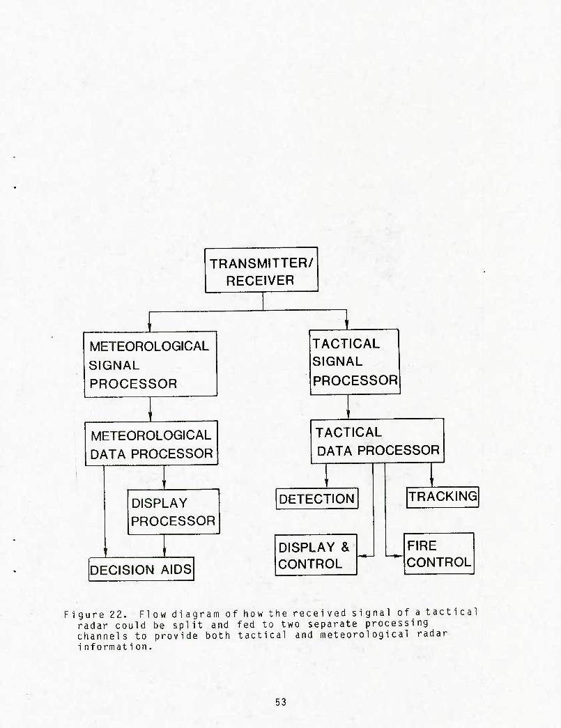
channels (Figure 22). The signal needs to be split because much
of the tactical signal processing removes the information
required for the meteorological processing. -• • '•■
Tactical radars are designed for a different objective than
are meteorological radars. This results in different choices
for the radar design parameters. Fortunately many are somewhat
compatible with meteorological applications. The resulting
parameter choices for a given radar may not be ideal for all
meteorological applications, but at the same time they do not
necessarily rule it out.
The examination of the frequency of existing and planned
tactical radars reveals that there are several which have
frequencies in the 6 and 3 GHz bands. Many of these are elimi-
nated when their beam pattern is examined. A meteorological
radar needs a narrow pencil beam, while many of these radars have
a fan shaped beam (Figure 23). The beam widths of the remaining
radars, while not ideal, would be sufficient if Doppler data
acquisition was limited to less than 50 to 70 nm. The pulse
lengths are also often reasonable for the extraction of meteoro-
logical information. At times they may actually be smaller than
required. "..,■■/:'!'/■ ' '
§2
TRANSMITTER/ RECEIVER
METEOROLOGICAL SIGNAL PROCESSOR
METEOROLOGICAL DATA PROCESSOR
DISPLAY PROCESSOR
TACTICAL SIGNAL
PROCESSOR
TACTICAL DATA PROCESSOR
DETECTION
DECISION AIDS
DISPLAY & CONTROL
TRACKING
FIRE CONTROL
Figure 22. Flow diagram of how the received signal of a tactical radar could be split and fed to two separate processing channels to provide both tactical and meteorological radar i nformati on.
53
(a)
(b)
Figure 23. Example of a fan beam (top) used by 2-D search radars and of a pencil beam (bottom) used in meteorological radars and 3-D search radars. The fan beam often is at a frequency not affected by precipitation or has a precipita- tion canceling circuit.
54
Many of the tactical radars have the capability to produce
a range of pulse repetition frequencies, PRFs. This range often
includes PRFs appropriate to meteorological Doppler measurements.
At times the PRF may be higher than desired for meteorological
measurements, however. The effect of the higher PRFs is to
reduce the unambiguous range. If the unambiguous range is
reduced too much, the extraction of the information becomes
difficult or impossible due to multiple trip echoes (echoes
from ranges greater than the unambiguous range). The range
corresponding to the data is unknown and multiple echoes can
be superimposed upon each other.
The scan rates and dwell times may not be ideal either.
Most meteorological radars have a scan rate between 3 and
5 rpm. At higher rpm the dwell times are usually too short
to give good estimates of the intensities. The spectrum width
is also increased at the higher rpm (see Section 2.2). These
problems might be overcome by the use of complex pulse shapes
and/or pulse encoding.
On many of the radars a parallel signal and data processing
channels could be added to handle the meteorological data proces-
sing with minimal if any impact on the tactical data processing.
The output from the meteorological processing channel could then
be routed to the meteorological station, directed to a BFIM
system, or input to TESS.
Earlierit was stated that a fan beam pattern was not suited
for the extraction of meteorological data. In the strictest
sense this is true; however, MIT Lincoln Labs (Weber, 1985)
analyzed the addition of weather processing to the ASR-9 airport
surveillance radar. This radar has a vertical fan beam antenna
similar to those used on afloat 2-D search radars. The study
showed that weather processing could be added to extract rough
intensity estimates. The output can be used to locate and track
storms. Areas of intense rainfall can also be identified. The
apparent structure of the storms is smoothed compared to conven-
tional meteorological radars using a pencil beam. The approach
outlined could be adapted to some of the 2-D search radars afloat.
55
7. SUMMARY AND RECOMMENDATIONS
Meteorological radar information has proven and continues to
be useful in land based operations. It could also be useful to
the afloat community. The quantitative measurement of precipita-
tion, wind, and turbulence fields could yield useful information
:that is not now available. Features such as wind shift lines,
could be mapped, followed, and projected. Many of the parameters
could be measured as 2-D fields and some as 3-D fields. Some
areas in which meteorological radar data could have an impact are
target detection and tracking, aircraft launch and retrieval,
missile launch, sea clutter modeling, and command and control.
The meteorological Doppler radar data and derived information
could be passed directly to a BFIM system or to TESS for
distribution.
From a meteorological point of view the best implementation
would be a radar dedicated to meteorological data acquisition.
Since this is not likely, the meteorological data acquisition
will have to be piggybacked on an existing or planned tactical
radar. A system could be designed such that the meteorological
signal and data processing is performed concurrently with any
tactical processing. Several existing and planned tactical
radars appear suitable. The AEGIS type radar and derivatives
appear to be the most suitable. How suitable various tactical
radars will prove to be will take additional study.
The following recommendations are made: • ■ '
1. A link between environmental and warfare communj_t_i_e_s should be established to pursue meteorological radar
■ data acquisition and utilization. This effort wouTB" include the screening of tactical radars for meteoro- logical data acquisition suitability. The screening would incorporate radar design parameters, radar operation, and meteorological requirements. How meteorological Doppler radar data could be . ■ incorporated into TDAs would also be investigated.
$S
2 . The use of meteoro 1 o c[ i c a 1_ Doppler radar data to satisfy BF_I_M_and TESS requir'em'e'nts s'hould be examined. Both TESS and BFIM have a need of high resolution data in the vicinity of the battle force for incorporation into TDAs. Meteorological radar is a means of obtaining this data.
3. The FPS-106 radar should be replaced with a Doppler meteorological radar with the capability to measure intensity, velocity, and spectrum width. The capacity to measure velocity is crucial to obtaining optimum utility from a Doppler radar. The additional information obtained with a Doppler radar greatly increases the radar's usefulness.
4. Field programs should be conducted in coordination with ONR to collect meteorological radar data at sea for ^lg.o^i^-'l11_4s7.slopment and testing. To date, meteoro lo- gicaT data processing algorithms have primarily been developed for land based rada^-s. In order to adapt these algorithms and develop new algorithms for afloat applications, data will need to be collected under operational conditions.
5. The addition of a weather processing capability to 2-D search radars shou Id be investigated. While 2-D search radars are not ideal for acquiring meteorological data, information on storm location, movement, and intensity can be obtained from the returns. This information could be use for aircraft routing and planning purposes.
6. The suitability of UHF/VHF wind profilers for deployment within the fleet should be investigated. Wind profilers could give frequent wind profiles for input to various TDAs and numerical models. Low power models specifi- cally designed to minimize detectabi1ity could be developed for probing only the lower atmosphere. This effort would include field programs to investigate the operation of wind profilers in a marine environment.
57
REFERENCES
Battan, L. J.; 1973: Radar Observation of the Atmosphere. University of Chicago Press, Chicago Illinois.
Balsley, B. B. and K. S. Gage, 1982: On the Use of Radars for Operational Wind Profiling. Bull. Am. Meteorol. Soc, 63, No. 9, 1009-1018, Sept. 1982.
Bjerkass, C. J. and D. E. Forsyth, 1980: An Automated Real-Time Storm Analysis and Storm Tracking Program (WEATRK). ATF Force Geophysics Laboratory, Meteorology Division report AFGL-TR-80-0316, October 1980.
Brandes, E., 1975: Optimizing rain fall estimates with the aid of radar. J. Appl. Meteorol.. 14, 1339-1345.
Brasunas, J. C, 1984: A Comparison of Storm Tracking and Extrapolation Algorithms. Lincoln Laboratory MIT Project Report ATC-124, 31 July 1984.
Crawford, K.C., 1977: The Design of a Multivariate Mesoscale Field Experiment. Ph.D. dissertation. University of Ok 1ahoma, 157 pp .
Doviak, R. J. and D. S. Zrnit, 1984: MllllZLRidar_and_Weather Observati ons. AcademicPress, Inc.
Doviak, R. J. and M. Berger, 1980: Turbulence and waves in optic- ally clear planetary boundary layer resolved by dual-Doppler radars. Radio Sci.. 15, No. 2, pp 297-313, March-April 1980.
Hall, M. P. M., S. M. Cherry, J. W. F. Goddard, and G. R. Kennedy, 1980: Raindrop sizes and rainfall rate measured by dual-polarization radar. Nature (London), 285, 195-198.
Hembree, L. and A. Eddy, 1979: "Multivariate Objective Analysis of Convective Complexes," 7th Conference on Inadvertent and Planned Weather Modification, October 8-12, 1979, Bundt, Alberta, Canada.
Hennington, L., R. J. Doviak, D. Sir mans, D. Zrnic, 1976: Measurement of winds in the optically clear air with microwave pulse-Doppler radar. 17th Conf. on Radar Meteor., NBl, 342-348, October, 1976.
Jones, D. M. A., 1956: Rainfall drop-size distribution and radar \ reflectivity. Res. Rept. No. 6. Urbana Meteor. Lab., Illinois State Water survey.
58
Kropfli, R. A., 1984: Turbulence Measurements From Particulate Scatter in thy Clear Unstable Boundary Layer Using Single Doppler Radar. 22nd Conference On Radar Meteorology, 10-13 Sept. 1984, Zurich, Switzerland.
Larsen, M. F. and J. R&ttger, 1982: VHF and UHF Doppler Radars as Tools for Synoptic Research. Bull. Am. Meteorol. Soc, 63, No. 9, 996-1008, Sept. 1982.
Rinehart, R. E., 1979: Internal Storm Motions from a Single Non-Doppler Weather Radar Research report NCAR/TN
Nation Center for Atmospheric 146+STR
, 1980: Transverse Motion Detection and Hail Detection. Proceedings of the NEXRAD Doppler Radar Symposi um/Workshop, P.S. Ray and K. Colbert (eds.), Univ. of Oklahoma, 184-187.
Space and Naval Warfare Systems Command, 1985: Report on Environmental Requirements for the Battle Force Information Management System (Draft). Warfare Systems Architecture a . Engineering Directorate, Space and Naval Warfare Systems • Command,Novemberl986. ;
Seliga, T. A., K. Ayden, and V. N. Bring: 1982: Behavior of the Differential Reflectivity and Circular Depolarization Ratio, Radar Signals and Related Propagation Effects in Rainfall. Proc. URSI Comm. F, Open Symp. Multipie-Parameter Radar Meas., pp. 35-42, Rutherford Appleton Lab. Chilton, Didcot, 0 X f 0 r d s h i r e , U. K.
Wood . V. T. and R. A. Brown, 1983: S i^naie_D o££le r_V eiocitx Signatures: An Atlas of Patterns" in Clear Ai r/W i despread Precipitation and Convective Storms. NOAA Tech. Memo. ERL
Laboratory, Norman, OK., NSSL-95. National November, 1983.
Severe Storms
Zamora, R. J. and M. A. Shapiro, 1984: Diagnostic Divergence and Vorticity Calculations Using a Network of Mesoscale Wind Profilers. 10th Conference on Weather Forecasting a Analysis, June 25-29, 1984, Clearwater Beach, Fla
59
DISTRIBUTION
COMMANDER IN CHIEF U.S. ATLANTIC FLEET ATTN: FLT METEOROLOGIST NORFOLK, VA 23511-6001
COMMANDER IN CHIEF U.S. ATLANTIC FLEET ATTN: NSAP SCIENCE ADVISOR NORFOLK, VA 23511-6001
COMMANDER IN CHIEF U.S. PACIFIC FLEET CODE 02M PEARL HARBOR, HI 96860-7000
COMMANDER IN CHIEF U.S. NAVAL FORCES, EUROPE ATTN: METEOROLOGICAL OFFICER FRO NEW YORK 09510
CINCUSNAVEUR ATTN: NSAP SCIENCE ADVISOR BOX 5 FPO NEW YORK 09510-0151
COMMANDER SECOND FLEET ATTN: METEOROLOGICAL OFFICER FPO NEW YORK 09501-6000
COMSECONDFLT ATTN: NSAP SCIENCE ADVISOR FPO NEW YORK 09501-6000
COMTHIRDFLT ATTN: FLT METEOROLOGIST FPO SAN FRANCISCO 96601-6001
COMSEVENTHFLT ATTN: FLT METEOROLOGIST FPO SAN FRANCISCO 96601-6003
COMTHIRDFLT ATTN: NSAP SCIENCE ADVISOR PEARL HARBOR, HI 96860-7500