TMA521/MMA511 Large Scale Optimization Lecture 8 Cutting plane

TMA521/MMA511

Large Scale OptimizationLecture 8

Cutting plane methods, column generation,

and the Dantzig–Wolfe algorithm

Ann-Brith Stromberg

7 Februari 2013

Ann-Brith Stromberg Cutting planes, column generation, Dantzig–Wolfe

A standard LP problem and its Lagrangian dual

vLP = min cTx,subject to Ax ≤ b,

Dx ≤ d,x ∈ R

n+

◮ We suppose for now that the polyhedronX := { x ∈ R

n+ | Ax ≤ b } is bounded

◮ Let PX := {x1, x2, . . . , xK} be the set of extreme points in X


The Lagrangian dual

◮ The Lagrangian dual of the LP with respect to relaxing theconstraints Dx ≤ d is

vLP = vL := max q(µ),

subject to µ ≥ 0,

◮ The Lagrangian dual function:

q(µ) := minx∈X

{cTx + µT(Dx − d)

}= min

i∈PX

{cTxi + µT(Dxi − d)

}

◮ Solution set: X (µ) := arg minx∈X

{cTx + µT(Dx − d)

}

◮ Equivalent statement:

q(µ) ≤ cTxi + µT(Dxi − d), i ∈ PX , µ ≥ 0


An equivalent formulation

vL := max z ,

subject to z ≤ cTxi + µT(Dxi − d), i ∈ PX ,

µ ≥ 0.

◮ If, at an optimal dual solution µ∗, the solution set X (µ∗) is asingleton, i.e., X (µ∗) = {x∗}, then x∗ is optimal (and unique)— thanks to strong duality

◮ This typically does not happen, unless an optimal solution x∗

happens to be an extreme point of X

◮ But x∗ can always be expressed as a convex combination ofextreme points of X


A cutting plane method for the Lagrangian dual

problem

◮ Suppose only a subset of PX is known, and consider thefollowing relaxation of the Lagrangian dual problem:

max z , (1a)

s.t. z ≤ cTxi + µT(Dxi − d), i = 1, . . . , k, (1b)

µ ≥ 0 (1c)

◮ Let (µk , zk) be the solution to (1)

◮ It holds that zk ≥ vL for k = 1, . . . ,K

◮ How do we determine whether an optimal solution is found?

◮ And what IS the optimal solution when we find it?

◮ If zk ≤ cTxi + (µk)T(Dxi − d) holds for all i ∈ PX , then µk

is optimal in the dual! Why?


Check for optimality—generate new inequality

◮ How check for optimality? Find the most violated constraint

◮ Solve the subproblem

q(µk) := minx∈X

{

cTx + (µk)T(Dx − d)}

(2)

= mini∈PX

{

cTxi + (µk)T(Dxi − d)}

◮ If zk ≤ q(µk) then µk is optimal in the dual

◮ Otherwise, we have identified a constraint of the form

z ≤ cTxk+1 + µT(Dxk+1 − d),

which is violated at (µk , zk) (i.e., it holds thatzk > cTxk+1 + (µk)T(Dxk+1 − d)) f

◮ Add this inequality and re-solve the LP problem!


Cutting plane algorithm

◮ We call this a cutting plane algorithm

◮ It is based on adding constraints to the dual problem in orderto improve the solution, in the process of cutting off theprevious point

◮ Consider the below picture. The thick lines correspond to thesubset of k inequalities known at iteration k

µµ∗

q(µk )

z

zk

µk


Cutting plane algorithm

◮ Obviously, zk ≥ q(µk) must hold, because of the possible lackof constraints.

◮ In this case, zk > q(µk) holds, so in the next step when weevaluate q(µk) we can identify and add the last lackinginequality

◮ The resulting maximization will then yield the optimalsolution µ∗ shown in the picture

◮ How do we generate an optimal primal solution from thisscheme? Let us look at the dual of the problem (1) in thiscutting plane algorithm


Duality relations and the Dantzig–Wolfe algorithm

◮ We rewrite the problem (1)

maximize(z ,µ)

z ,

subject to z − µT(Dxi − d) ≤ cTxi , i = 1, . . . , k,

µ ≥ 0

◮ With LP dual variables λi ≥ 0 we obtain the LP dual:

vk+1 = minimum∑k

i=1(cTxi)λi ,

subject to∑k

i=1 λi = 1,

−∑k

i=1(Dxi − d)λi ≥ 0,

λi ≥ 0, i = 1, . . . , k


The linear programming dual rewritten

◮

vk+1 = minimum cT

(k∑

i=1

λixi

)

, (3)

subject to

k∑

i=1

λi = 1,

λi ≥ 0, i = 1, . . . , k,

D

(k∑

i=1

λixi

)

≤ d

◮ Maximize cTx when x lies in the convex hull of the extremepoints xi found so far and fulfills the constraints that areLagrangian relaxed


An illustration in x-space

x1

x2

x3

x4

x∗

X

Dx ≤ d

λ3 = (0.4, 0.6, 0)


The Dantzig-Wolfe algorithm

◮ The problem (3) is known as the restricted master problem(RMP) in the Dantzig–Wolfe algorithm

◮ In this algorithm, we have at hand a subset {1, . . . , k} ofextreme points of X (and a dual vector µk−1)

◮ Find a feasible solution to the original LP problem by solvingthe restricted master problem (3)

◮ Then generate an optimal dual solution µk to this restrictedproblem problem, corresponding to the constraints Dx ≤ d

◮ If and only if the vector xi generated in the next subproblem(2) was already included, we have found the optimal solutionto the problem


Three algorithms which are “dual” to each other

◮ Cutting plane applied to the Lagrangian dual

⇐⇒

◮ Dantzig–Wolfe applied to the original LP

⇐⇒

◮ Benders decomposition applied to the dual LP.


Column generation

◮ Consider an LP with very many variables:cj , xj ∈ R, aj ,b ∈ R

m, m ≪ n

minimize z =n∑

j=1

cjxj

subject ton∑

j=1

ajxj = b

xj ≥ 0, j = 1, . . . , n

◮ The matrix (a1, . . . , an) is too large to handle.

◮ Assume that m is relatively small =⇒ the basis matrix is nottoo large (m × m)


Basic feasible solutions

◮ B = {m elements from the set {1, . . . , n}} is a basis if thecorresponding matrix B = (aj)j∈B has an inverse, B−1

◮ A basic solution is given by xB = B−1b and xj = 0, j 6∈ B . Itis feasible if xB ≥ 0m

◮ A better basic feasible solution can be found by computingreduced costs: cj = cj − cT

BB−1aj for j 6∈ B

◮ Let cs = minimumj 6∈B

cj

◮ If cs < 0 =⇒ a better solution is received if xs enters the basis

◮ If cs ≥ 0 =⇒ xB is an optimal basic solution


Generating columns

◮ Suppose the columns aj are defined by a setS = {aj | j = 1, . . . , n} being, e.g., solutions to a system ofequations (extreme points, integer points, . . . )

◮ The incoming column is then chosen by solving a subproblemc(a′) = minimum

a∈S

{c − cT

BB−1a}

◮ a′ is a column having the least reduced cost w.r.t. the basis B

◮ If c(a′) < 0 let the column

(c(a′)a′

)

enter the problem


Example: The cutting stock problem

◮ Supply: rolls of e.g. paper of length L

◮ Demand: bi roll pieces of length ℓi < L, i = 1, . . . ,m

◮ Objective: minimize the number of rolls needed for producingthe demanded pieces


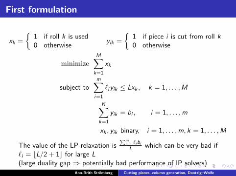
First formulation

xk =

{1 if roll k is used0 otherwise

yik =

{1 if piece i is cut from roll k

0 otherwise

minimize

M∑

k=1

xk

subject to

m∑

i=1

ℓiyik ≤ Lxk , k = 1, . . . ,M

K∑

k=1

yik = bi , i = 1, . . . ,m

xk , yik binary, i = 1, . . . ,m, k = 1, . . . ,M

The value of the LP-relaxation isPm

i=1 ℓibi

Lwhich can be very bad if

ℓi = ⌊L/2 + 1⌋ for large L

(large duality gap ⇒ potentially bad performance of IP solvers)Ann-Brith Stromberg Cutting planes, column generation, Dantzig–Wolfe

Second formulation

◮ Cut pattern: number j contains aij pieces of length ℓi

◮ Feasible pattern if∑m

i=1 ℓiaij ≤ L, where aij ≥ 0, integer

◮ Variables: xj = number of times pattern j is used

minimize

n∑

j=1

xj

subject to

n∑

j=1

aijxj = bi , i = 1, . . . ,m

xj ≥ 0, integer, j = 1, . . . , n

◮ Bad news: n = total number of feasible cut patterns—hugeinteger

◮ Good news: the value of the LP relaxation is often very closeto that of the optimal solution.

⇒ Relax integrality constraints, solve an LP instead of an ILP


Starting solution

Trivial: m unit columns (gives lots of waste) =⇒

minimize

m∑

j=1

xj

subject to xj = bj , j = 1, . . . ,m

xj ≥ 0, j = 1, . . . ,m


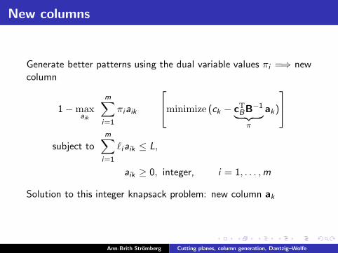
New columns

Generate better patterns using the dual variable values πi =⇒ newcolumn

1 − maxaik

m∑

i=1

πiaik

minimize (ck − cT

BB−1

︸︷︷︸

π

ak)

subject to

m∑

i=1

ℓiaik ≤ L,

aik ≥ 0, integer, i = 1, . . . ,m

Solution to this integer knapsack problem: new column ak


Date post:	28-Feb-2022
Category:	Documents
Upload:	others
View:	1 times
Download:	0 times

TMA521/MMA511 Large Scale Optimization Lecture 8 Cutting plane

Documents