B8.5 Graph Theory Michaelmas Term 2020, 16 lectures Paul Balister Last updated: October 3, 2020 These notes are to accompany the lectures in MT 2020 on graph theory for Part B Mathematics, and are adapted from notes by Oliver Riordan, which in turn were adapted from notes by Alex Scott and Colin McDiarmid. They also owe much to the book Modern Graph Theory, Springer-Verlag, 1998 by B´ ela Bollob´as, and are not for distribution. The notes may possibly be updated as the course proceeds, although no major changes are planned. If you spot any errors, email: [email protected]. Relationship to Part A Graph Theory Part A Graph Theory is recommended but not required as a prerequisite. The course as lectured should be self-contained, though a few key results covered in Part A will be stated as exercises to complete yourself if you did not do Part A. 1 Introduction We need some preliminary definitions and notation (see the separate handout for a sum- mary). We write [n] for the set {1, 2,...,n}. For any set S , we write ( S k ) for the set of subsets of S of size k, that is, ( S k ) = {A ⊆ S : |A| = k} (and has cardinality ( |S| k ) ). Some authors write S (k) instead of ( S k ) . A (simple) graph G is an ordered pair (V,E), where V is a set and E ⊆ ( V 2 ) . In this course V will almost always be finite and non-empty – this is assumed unless stated otherwise. The elements of V are called the vertices of G and the elements of E the edges of G. We often write uv for an edge {u, v} (so uv means the same as vu). We say that u and v are adjacent in G if uv is an edge of G. A vertex v and an edge e are incident if v is one of the endvertices of e, i.e., one of the two vertices in e. Two edges meet if they intersect, i.e., share a vertex. Graphically, we represent vertices as points (or more often blobs) and edges as lines or curves joining pairs of points (blobs); how a graph is drawn is irrelevant as far as the structure of the graph itself is concerned. The reason for using blobs is that it makes clear in the drawing where the vertices are: we may have to draw the lines/curves for two edges so that they cross even though the edges do not share a vertex. a b c d a b c d Figure 1: Two ways of drawing the same graph G =({a, b, c, d}, {ab, ac, ad, bd, cd}). 1
Transcript
B8.5 Graph Theory
Michaelmas Term 2020, 16 lecturesPaul Balister
Last updated: October 3, 2020
These notes are to accompany the lectures in MT 2020 on graph theory for Part BMathematics, and are adapted from notes by Oliver Riordan, which in turn were adaptedfrom notes by Alex Scott and Colin McDiarmid. They also owe much to the book ModernGraph Theory, Springer-Verlag, 1998 by Bela Bollobas, and are not for distribution. Thenotes may possibly be updated as the course proceeds, although no major changes areplanned. If you spot any errors, email: [email protected].
Relationship to Part A Graph Theory
Part A Graph Theory is recommended but not required as a prerequisite. The course aslectured should be self-contained, though a few key results covered in Part A will be statedas exercises to complete yourself if you did not do Part A.
1 Introduction
We need some preliminary definitions and notation (see the separate handout for a sum-mary). We write [n] for the set {1, 2, . . . , n}. For any set S, we write
(
Sk
)
for the set of
subsets of S of size k, that is,(
Sk
)
= {A ⊆ S : |A| = k} (and has cardinality(
|S|k
)
). Some
authors write S(k) instead of(
Sk
)
.
A (simple) graph G is an ordered pair (V,E), where V is a set and E ⊆(
V2
)
. Inthis course V will almost always be finite and non-empty – this is assumed unless statedotherwise. The elements of V are called the vertices of G and the elements of E the edgesof G.
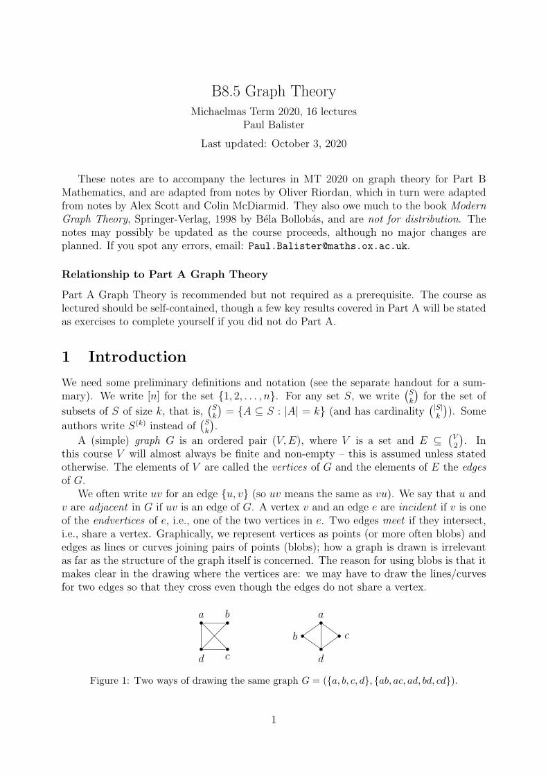
We often write uv for an edge {u, v} (so uv means the same as vu). We say that u andv are adjacent in G if uv is an edge of G. A vertex v and an edge e are incident if v is oneof the endvertices of e, i.e., one of the two vertices in e. Two edges meet if they intersect,i.e., share a vertex. Graphically, we represent vertices as points (or more often blobs) andedges as lines or curves joining pairs of points (blobs); how a graph is drawn is irrelevantas far as the structure of the graph itself is concerned. The reason for using blobs is that itmakes clear in the drawing where the vertices are: we may have to draw the lines/curvesfor two edges so that they cross even though the edges do not share a vertex.
a b
cd
a
b c
d
Figure 1: Two ways of drawing the same graph G = ({a, b, c, d}, {ab, ac, ad, bd, cd}).
1
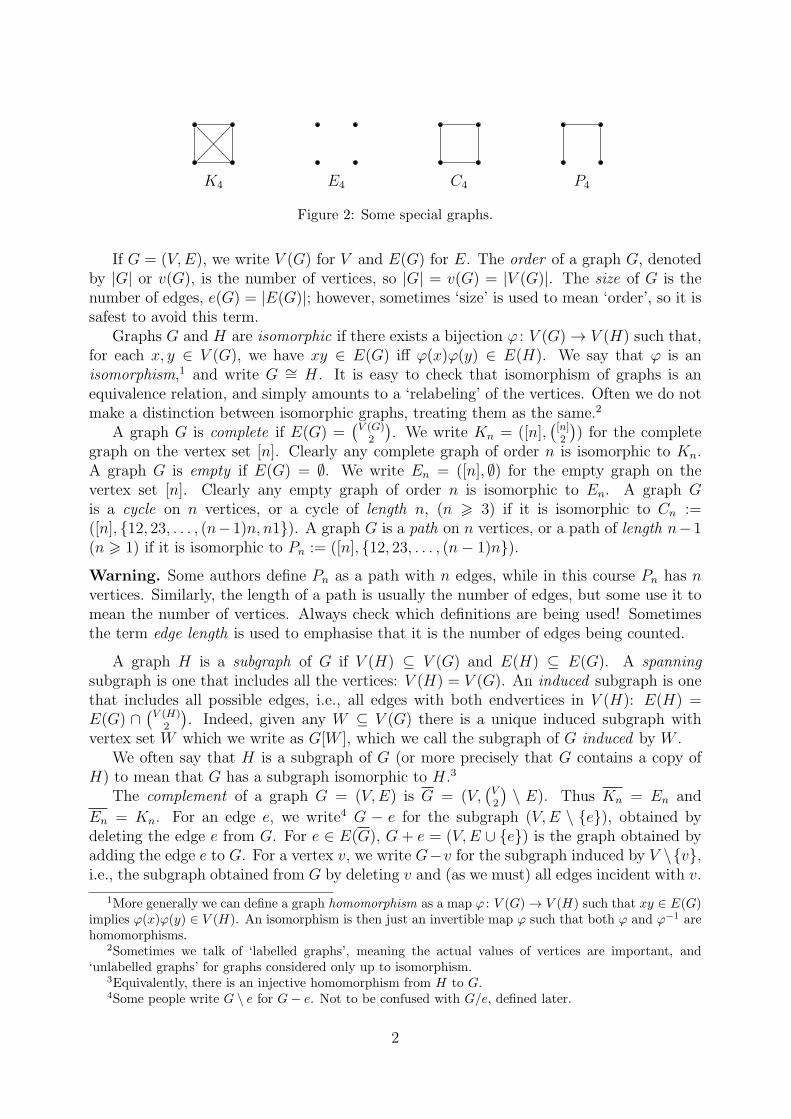
K4 E4 C4 P4
Figure 2: Some special graphs.
If G = (V,E), we write V (G) for V and E(G) for E. The order of a graph G, denotedby |G| or v(G), is the number of vertices, so |G| = v(G) = |V (G)|. The size of G is thenumber of edges, e(G) = |E(G)|; however, sometimes ‘size’ is used to mean ‘order’, so it issafest to avoid this term.
Graphs G and H are isomorphic if there exists a bijection ϕ : V (G) → V (H) such that,for each x, y ∈ V (G), we have xy ∈ E(G) iff ϕ(x)ϕ(y) ∈ E(H). We say that ϕ is anisomorphism,1 and write G ∼= H. It is easy to check that isomorphism of graphs is anequivalence relation, and simply amounts to a ‘relabeling’ of the vertices. Often we do notmake a distinction between isomorphic graphs, treating them as the same.2
A graph G is complete if E(G) =(
V (G)2
)
. We write Kn = ([n],(
[n]2
)
) for the completegraph on the vertex set [n]. Clearly any complete graph of order n is isomorphic to Kn.A graph G is empty if E(G) = ∅. We write En = ([n], ∅) for the empty graph on thevertex set [n]. Clearly any empty graph of order n is isomorphic to En. A graph Gis a cycle on n vertices, or a cycle of length n, (n > 3) if it is isomorphic to Cn :=([n], {12, 23, . . . , (n−1)n, n1}). A graph G is a path on n vertices, or a path of length n−1(n > 1) if it is isomorphic to Pn := ([n], {12, 23, . . . , (n− 1)n}).Warning. Some authors define Pn as a path with n edges, while in this course Pn has nvertices. Similarly, the length of a path is usually the number of edges, but some use it tomean the number of vertices. Always check which definitions are being used! Sometimesthe term edge length is used to emphasise that it is the number of edges being counted.
A graph H is a subgraph of G if V (H) ⊆ V (G) and E(H) ⊆ E(G). A spanningsubgraph is one that includes all the vertices: V (H) = V (G). An induced subgraph is onethat includes all possible edges, i.e., all edges with both endvertices in V (H): E(H) =E(G) ∩
(
V (H)2
)
. Indeed, given any W ⊆ V (G) there is a unique induced subgraph withvertex set W which we write as G[W ], which we call the subgraph of G induced by W .
We often say that H is a subgraph of G (or more precisely that G contains a copy ofH) to mean that G has a subgraph isomorphic to H.3
The complement of a graph G = (V,E) is G = (V,(
V2
)
\ E). Thus Kn = En and
En = Kn. For an edge e, we write4 G − e for the subgraph (V,E \ {e}), obtained bydeleting the edge e from G. For e ∈ E(G), G + e = (V,E ∪ {e}) is the graph obtained byadding the edge e to G. For a vertex v, we write G−v for the subgraph induced by V \{v},i.e., the subgraph obtained from G by deleting v and (as we must) all edges incident with v.
1More generally we can define a graph homomorphism as a map ϕ : V (G) → V (H) such that xy ∈ E(G)implies ϕ(x)ϕ(y) ∈ V (H). An isomorphism is then just an invertible map ϕ such that both ϕ and ϕ−1 arehomomorphisms.
2Sometimes we talk of ‘labelled graphs’, meaning the actual values of vertices are important, and‘unlabelled graphs’ for graphs considered only up to isomorphism.
3Equivalently, there is an injective homomorphism from H to G.4Some people write G \ e for G− e. Not to be confused with G/e, defined later.
2
In much of the following, unless otherwise indicated, the implicitly assumed setting isan arbitrary graph G = (V,E).
Degrees
The degree of a vertex v is the number of incident edges,
d(v) =∣
∣{w ∈ V : vw ∈ E}∣
∣.
We write dG(v) if we want to specify the graph. A vertex w is a neighbour of v if v and w areadjacent, i.e., vw ∈ E. The set N(v) = NG(v) = {w ∈ V : vw ∈ E} is the neighbourhoodof v, so d(v) = |N(v)|. Some authors write Γ(v) instead of N(v).
A graph G is r-regular if every vertex has degree r. If d(v) = 0, v is an isolated vertex.If V = {v1, . . . , vn}, the degree sequence of G is the sequence d(v1), d(v2), . . . , d(vn), oftenarranged in nondecreasing order.
Lemma 1.1 (Handshaking Lemma). For any graph G = (V,E),
∑
v∈V
d(v) = 2e(G).
Proof. Consider the number of pairs (v, e) where v is a vertex of G and e is an edge of Gincident with v. We count them in two different ways. Firstly, each vertex v is in exactlyd(v) such pairs, so there are
∑
v∈V d(v) pairs in total. Secondly, each edge e of G is inexactly two such pairs, so there are 2|E| = 2e(G) pairs.
Corollary 1.2. For any graph G, the number of vertices with odd degree is even.
Paths, cycles and walks in graphs
A path on t vertices in G is a subgraph of G isomorphic to Pt; a cycle of length t in G isa subgraph isomorphic to Ct. We usually just list the vertices to describe a path or cycle.Thus v1v2 · · · vt is a path of length t in G if and only if v1, . . . , vt are distinct vertices ofG and v1v2, . . . , vt−1vt are edges of G.5 Similarly, v1v2 · · · vtv1 is a cycle in G if and onlyif t > 3, v1, . . . , vt are distinct vertices of G, and v1v2, . . . , vt−1vt, vtv1 are edges of G. Agraph is acyclic if it contains no cycles.
We say v0v1 · · · vt is a walk in G if v0, v1, . . . , vt are (not necessarily distinct) vertices ofG such that vivi+1 ∈ E for each i = 0, 1, . . . , t − 1. The length of a walk is the number ofsteps, here t. If x = v0 and y = vt then we speak of a walk from x to y, or an x-y walk; anx-y path is defined similarly. A walk v0v1 · · · vt is closed if vt = v0.
Exercise. Let G be a graph and x, y ∈ V (G). Then G contains an x-y walk if and only ifG contains an x-y path.
5The two definitions of path in G are not quite the same: for existence, they are equivalent, but forcounting paths, they differ by a factor of 2 for t > 2. A similar comment applies to cycles with a differentfactor.
3
In other words, if we want to get from x to y, then allowing ourselves to revisit verticesdoes not help. This simple observation is useful, allowing us to switch back and forthbetween using paths and walks to define connectedness, at any point using whicheverdefinition is easiest to work with. The cleanest proof is to consider a shortest x-y walk andshow that it is a path.
A graph G is connected if for all x, y ∈ V there is at least one x-y path in G. Thecomponents of a general graph G are the maximal connected subgraphs. It is easy to checkthat G is the disjoint union of its components. Indeed, consider the relation ∼ on V (G)defined by “x ∼ y iff there exists an x-y walk”. (Equivalently, there exists an x-y path.)It is easy to check that this is an equivalence relation, and that the components are thesubgraphs induced by the equivalence classes.
We finish this section with a simple lemma giving a condition under which we areguaranteed that G contains a cycle.
Lemma 1.3. Let G be a finite graph in which every vertex has degree at least 2. Then Gcontains a cycle.
Proof. Pick v0 ∈ V (G) and v1 ∈ N(v0). Now for each i > 1 we can successively pick vi+1 ∈N(vi) such that vi+1 6= vi−1 (since |N(vi)| > 2). Thus we have a sequence v0, v1, v2, . . .such that vi−1vi ∈ E(G) for every i, and vi−1, vi and vi+1 are always distinct. Since G hasonly finitely many vertices, some vertex must appear more than once. Pick i < j such thatvi = vj and j is minimal. Then j− i > 3, and by minimality vi, . . . , vj−1 are distinct. Thusvi · · · vj−1vi is a cycle in G.
2 Trees
A tree is simply an acyclic connected graph. A general acyclic graph, or equivalently, agraph in which each component is a tree, is called a forest.
Lemma 2.1. The following are equivalent, where minimality/maximality is with respect todeleting/adding edges.
(i) T is a tree,
(ii) T is a minimal connected graph,
(iii) T is a maximal acyclic graph.
The precise meaning of (ii) is that T = (V,E) is connected, but that for any strictsubset E ′ of E, (V,E ′) is not connected. Equivalently, T is connected, but for any edge eof T , T − e is not connected. Similarly in (iii), T = (V,E) is acyclic, but (V,E ′) containsa cycle for any strict superset E ′ ⊃ E.
Proof. Revision from Part A or exercise, as applicable.
A spanning tree of a graph G is a spanning subgraph of G that is a tree, i.e., a subgraphof G that is a tree containing all the vertices of G.
Corollary 2.2. Every connected graph G has at least one spanning tree.
4
Proof. Remove edges one-by-one, keeping the graph connected, until we can remove nomore. The graph T that remains is a minimal connected graph with vertex set V (G); byLemma 2.1, T is a tree.
A vertex v of any graph G is called a leaf if d(v) = 1. This term is most often used inthe context of trees/forests.
Lemma 2.3. Every tree on n > 2 vertices has at least one leaf.
Proof. T is connected, so it has no isolated vertices (vertices of degree 0). But T has nocycle, so by Lemma 1.3 it must have a vertex of degree less than 2. Therefore it has avertex v with degree 1.
In fact, every tree with at least 2 vertices has at least two leaves; there are many proofsof this fact. One involves modifying the argument above slightly. The significance of leavesis shown by the following simple result.
Lemma 2.4. Let v be a leaf of a graph G. Then G is a tree iff G− v is a tree.
Proof. Revision/Exercise.
Lemma 2.5. If T is a tree on n vertices, then e(T ) = n− 1.
Proof. We use induction on n; the case n = 1 is trivial. Let T be any tree with n > 2vertices. By Lemma 2.3, T has a leaf v. By Lemma 2.4, T ′ = T − v is a tree. Since T ′ hasn− 1 vertices, by induction it has n− 2 edges. Thus T has n− 1 edges.
Combining Lemmas 2.1 and 2.5 gives some further characterisations of trees.
Corollary 2.6. Let G be a graph with n vertices. TFAE (the following are equivalent):(a) G is a tree,
(b) G is connected and e(G) = n− 1,
(c) G is acyclic and e(G) = n− 1.
Proof. (a) implies (b) and (c) by the definition of a tree and Lemma 2.5. Suppose that (b)holds. Then G has a spanning tree T which, by Lemma 2.5, has n − 1 = e(G) edges. Aspanning subgraph includes all the vertices by definition, and since e(T ) = e(G), in thiscase it includes all the edges too. Thus T = G and so G is a tree, completing the proofthat (b) implies (a). Now suppose that (c) holds. Each component Ci of G is a tree. Nowe(Ci) = |Ci| − 1, so e(T ) =
∑
e(Ci) =∑
(|Ci| − 1) = n − c, where c is the number ofcomponents. Thus c = 1 and G is connected.
Counting trees
Let’s start with a simpler question: how many graphs G = (V,E) are there with vertex set[n]? Each of the
(
n2
)
possible edges may or may not be included in E, with all possibilities
allowed, so the answer is 2(n
2). Note that we are not asking how many isomorphism classesthere are: this is a much harder question. (Sometimes, counting graphs on a given vertex
5
set is referred to as ‘counting labelled graphs’; counting isomorphism classes is referred toas ‘counting unlabelled graphs’.)
Counting trees is much harder than counting all graphs. The answer was found (butnot really proved) by Cayley in 1889, though implicitly earlier by Borchardt in 1860; it isnow known as Cayley’s formula.
Theorem 2.7. For any n > 1 there are exactly nn−2 trees T with vertex set [n].
Proof. The result is trivial for n = 1 and 2, so fix n > 3. We shall map each tree on [n] toits Prufer code c = (c1, c2, . . . , cn−2), where 1 6 ci 6 n. (The ci need not be distinct.) Sincethere are nn−2 possible codes, it suffices to show that the map gives a bijection betweentrees on [n] and codes.
Given a tree T on [n] we construct its code as follows:T1 := T has at least one leaf. Find the leaf v1 with the smallest number, remove it,
and write down the number c1 of the (unique) vertex v1 was adjacent to. Repeat untilexactly two vertices remain. Thus, for example, v2 is the smallest leaf of T2 := T − v1,and c2 is the vertex of T2 that v2 is adjacent to. In general vi is the smallest leaf ofTi := T − v1 − · · · − vi−1 and ci is the vertex of Ti it is adjacent to. Note that c1, . . . , cn−2
form the code, not v1, . . . , vn−2.
i leaves of Ti vi ci1 {2, 3, 5, 6} 2 42 {3, 5, 6} 3 43 {4, 5, 6} 4 14 {5, 6} 5 1
Code: 44116
1
5 4
3 2
T = T1
6
1
5 4
3
T2
6
1
5 4
T3
6
1
5
T4
6
1
T5
Figure 3: Example of a Prufer code.
The following observation is key to the proof: a vertex w with degree d in T appearsexactly d−1 times in the code c. Indeed, we write w down in the code each time we deletea neighbour of w, i.e., each time its degree decreases. The final degree of w is always 1:either w is deleted when it is a leaf, or w is left at the end as one of the two final vertices,which are then leaves. More generally, if the degree of w in T − v1 − v2 − · · · − vi−1 is d,then w occurs d− 1 times in ci, . . . , cn−2. It follows from this that
v1 = min{
[n] \ {c1, . . . , cn−2}}
v2 = min{
[n] \ {v1, c2 . . . , cn−2}}
. . .
vi = min{
[n] \ {v1, . . . , vi−1, ci, . . . , cn−2}}
i 6 n− 2. (1)
Let us write vn−1 and vn (with WLOG vn−1 < vn) for the two vertices left at the end whenwe constructed the code, so
{vn−1, vn} = [n] \ {v1, . . . , vn−2}. (2)
6
Then, since we deleted the edge vici at step i, and were left with the edge vn−1vn betweenthe final two vertices,
E(T ) = {v1c1, . . . , vn−2cn−2, vn−1vn}. (3)
The formulae above describe T , the tree that we started with, in terms of its codec = (c1, . . . , cn−2). Does this mean that the proof is complete? No! We started byassuming that T was a tree, with code c, and then showed that given c, we could identifyT (i.e., the map from trees to codes is injective). So for any code coming from a tree, thereis a unique tree with that code. We still need to show that for every code c, there is a treewith code c (i.e., the map from trees to codes is surjective).
The formulae above tell us where to look: if there is a tree with code c, it must be asdescribed above. So let us check.
Formally, let c be any possible code (c1, . . . , cn−2). Then we may use (1) to definev1, . . . , vn−2. (Each time we take the minimum of a non-empty set, which makes sense.)Also, from (1) we see that vi is not equal to any of v1, . . . , vi−1. Thus v1, . . . , vn−2 aredistinct.
Next, we define vn−1 < vn to be the two remaining elements of [n], as in (2), so v1, . . . , vnare distinct; they are 1, 2, . . . , n in some order.
Finally, we let T be the graph with vertex set [n] and edge set given by (3). We needto check that T is indeed a tree, and that it has code c. We do this step-by-step: first notethat from our definition (1) of vi, it is distinct from cj, j > i. Thus cj is distinct from vi,i 6 j, so for each j, cj ∈ {vj+1, . . . , vn}. Let Ti be the graph with
V (Ti) = {vi, . . . , vn} and E(Ti) = {vici, . . . , vn−2cn−2, vn−1vn}.
(This makes sense since the ends of the edges are all vertices.) Then Tn−1 is a tree withtwo vertices. Also, Ti is constructed from Ti+1 by adding a new vertex vi and one edge vici.So, by Lemma 2.4, Ti is a tree for i = n− 2, n− 3, . . . , 2, 1. In particular, T = T1 is a tree.That the code of T is c is an exercise; see Problem Sheet 1.
3 Long circuits, paths and cycles
An Euler circuit (Euler tour)6 in a graph G is a closed walk that contains every edge of Gexactly once. (If |G| = 1 we say that G has a trivial Euler circuit.)
Theorem 3.1. Let G be a connected graph. Then G has an Euler circuit if and only if thedegree of every vertex is even.
Proof. For the (easier) ‘only if’ direction, pick v ∈ V (G). If an Euler circuit enters v ktimes then it leaves v k times, and so it uses 2k edges incident with v. Thus d(v) must beeven.
For the converse, we proceed by induction on e(G), with the result being trivial fore(G) = 0. For the induction step, take any G with e(G) > 0 and assume the result holdsfor all graphs with fewer edges than G. Since G is connected, each vertex has degree at
6A trail in a graph is a walk which does not repeat edges (although it may repeat vertices). A circuit
in a graph is a closed trail, i.e., a closed walk that is a trail. Hence an Euler circuit is just a circuit thatuses every edge of the graph. Warning: some authors use ‘circuit’ to mean ‘cycle’ and vice versa.
7
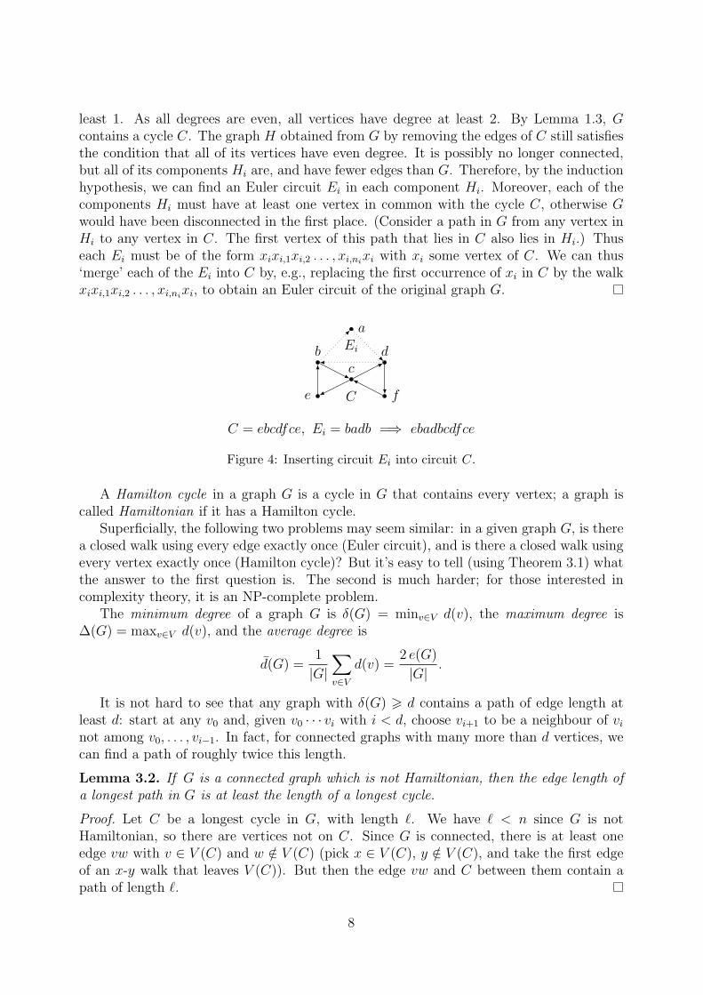
least 1. As all degrees are even, all vertices have degree at least 2. By Lemma 1.3, Gcontains a cycle C. The graph H obtained from G by removing the edges of C still satisfiesthe condition that all of its vertices have even degree. It is possibly no longer connected,but all of its components Hi are, and have fewer edges than G. Therefore, by the inductionhypothesis, we can find an Euler circuit Ei in each component Hi. Moreover, each of thecomponents Hi must have at least one vertex in common with the cycle C, otherwise Gwould have been disconnected in the first place. (Consider a path in G from any vertex inHi to any vertex in C. The first vertex of this path that lies in C also lies in Hi.) Thuseach Ei must be of the form xixi,1xi,2 . . . , xi,ni
xi with xi some vertex of C. We can thus‘merge’ each of the Ei into C by, e.g., replacing the first occurrence of xi in C by the walkxixi,1xi,2 . . . , xi,ni
xi, to obtain an Euler circuit of the original graph G.
a
bc
d
e f
C = ebcdfce, Ei = badb =⇒ ebadbcdfce
Ei
C
Figure 4: Inserting circuit Ei into circuit C.
A Hamilton cycle in a graph G is a cycle in G that contains every vertex; a graph iscalled Hamiltonian if it has a Hamilton cycle.
Superficially, the following two problems may seem similar: in a given graph G, is therea closed walk using every edge exactly once (Euler circuit), and is there a closed walk usingevery vertex exactly once (Hamilton cycle)? But it’s easy to tell (using Theorem 3.1) whatthe answer to the first question is. The second is much harder; for those interested incomplexity theory, it is an NP-complete problem.
The minimum degree of a graph G is δ(G) = minv∈V d(v), the maximum degree is∆(G) = maxv∈V d(v), and the average degree is
d(G) =1
|G|∑
v∈V
d(v) =2 e(G)
|G| .
It is not hard to see that any graph with δ(G) > d contains a path of edge length atleast d: start at any v0 and, given v0 · · · vi with i < d, choose vi+1 to be a neighbour of vinot among v0, . . . , vi−1. In fact, for connected graphs with many more than d vertices, wecan find a path of roughly twice this length.
Lemma 3.2. If G is a connected graph which is not Hamiltonian, then the edge length ofa longest path in G is at least the length of a longest cycle.
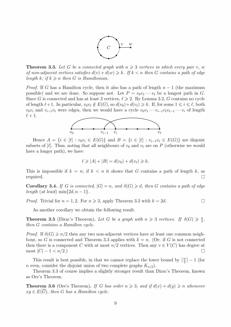
Proof. Let C be a longest cycle in G, with length ℓ. We have ℓ < n since G is notHamiltonian, so there are vertices not on C. Since G is connected, there is at least oneedge vw with v ∈ V (C) and w /∈ V (C) (pick x ∈ V (C), y /∈ V (C), and take the first edgeof an x-y walk that leaves V (C)). But then the edge vw and C between them contain apath of length ℓ.
8
v wC
Theorem 3.3. Let G be a connected graph with n > 3 vertices in which every pair v, wof non-adjacent vertices satisfies d(v) + d(w) > k. If k < n then G contains a path of edgelength k; if k > n then G is Hamiltonian.
Proof. If G has a Hamilton cycle, then it also has a path of length n − 1 (the maximumpossible) and we are done. So suppose not. Let P = v0v1 · · · vℓ be a longest path in G.Since G is connected and has at least 3 vertices, ℓ > 2. By Lemma 3.2, G contains no cycleof length ℓ+1. In particular, v0vℓ /∈ E(G), so d(v0)+d(vℓ) > k. If, for some 1 6 i 6 ℓ, bothv0vi and vi−1vℓ were edges, then we would have a cycle v0v1 · · · vi−1vℓvℓ−1 · · · vi of lengthℓ+ 1.
v0 vi−1 vi vℓ
Hence A = {i ∈ [ℓ] : v0vi ∈ E(G)} and B = {i ∈ [ℓ] : vi−1vℓ ∈ E(G)} are disjointsubsets of [ℓ]. Thus, noting that all neighbours of v0 and vℓ are on P (otherwise we wouldhave a longer path), we have
ℓ > |A|+ |B| = d(v0) + d(vℓ) > k.
This is impossible if k = n; if k < n it shows that G contains a path of length k, asrequired.
Corollary 3.4. If G is connected, |G| = n, and δ(G) > d, then G contains a path of edgelength (at least) min{2d, n− 1}.
Proof. Trivial for n = 1, 2. For n > 3, apply Theorem 3.3 with k = 2d.
As another corollary we obtain the following result.
Theorem 3.5 (Dirac’s Theorem). Let G be a graph with n > 3 vertices. If δ(G) >n2,
then G contains a Hamilton cycle.
Proof. If δ(G) > n/2 then any two non-adjacent vertices have at least one common neigh-bour, so G is connected and Theorem 3.3 applies with k = n. (Or: if G is not connectedthen there is a component C with at most n/2 vertices. Then any v ∈ V (C) has degree atmost |C| − 1 < n/2.)
This result is best possible, in that we cannot replace the lower bound by ⌈n2⌉ − 1 (for
n even, consider the disjoint union of two complete graphs Kn/2).Theorem 3.3 of course implies a slightly stronger result than Dirac’s Theorem, known
as Ore’s Theorem.
Theorem 3.6 (Ore’s Theorem). If G has order n > 3, and if d(x) + d(y) > n wheneverxy ∈ E(G), then G has a Hamilton cycle.
9
Theorem 3.3 also lets us relate the length of the longest path in G to the average degreeof G.
Theorem 3.7. If G is a graph with n vertices containing no path of edge length k, k > 2,then e(G) 6 k−1
2n.
Proof. Induction on n. For n 6 k we have e(G) 6 e(Kn) = n−12n 6
k−12n, so we are
done. Now suppose n > k. We may assume G is connected; otherwise apply the inductionhypothesis to the components (which do not contain Pk+1). Then G is connected with noPk+1 and n > k > 2. So by Theorem 3.3 there are (non-adjacent) vertices v, w of G suchthat d(v) + d(w) 6 k − 1. WLOG d(v) 6 d(w), so d(v) 6
k−12. Since G − v has n − 1
vertices and contains no Pk+1, applying the induction hypothesis to G− v we have
e(G) = d(v) + e(G− v) 6 k−12
+ k−12(n− 1) = k−1
2n,
completing the proof.
The result above can be rephrased to say that if G contains no Pk+1, then d(G) 6 k−1.In other words, if the average degree d(G) is greater than k − 1, then G contains a pathof length k. We do not get the extra factor of 2 we had in Corollary 3.4, but we assumingsomething only about average degree, not about the degree of every vertex.
4 Vertex colourings
A proper vertex colouring (or simply a colouring) of a graph G is an assignment of a colourto each vertex such that adjacent vertices receive different colours. The least numberof colours in such a colouring is the chromatic number χ(G). For example χ(Kn) = n,χ(En) = 1, χ(C4) = 2 and χ(C5) = 3. In fact, any even cycle (cycle of even length) haschromatic number 2, and any odd cycle has chromatic number 3.
Often we use positive integers as the colours: a (proper) k-colouring of G is a functionf : V (G) → {1, . . . , k} so that f(u) 6= f(v) whenever uv ∈ E(G). G is k-colourable if it hasa k-colouring, so χ(G) is the least k for which G is k-colourable.
1 2
34χ(K4) = 4
1 1
11χ(E4) = 1
1 2
12χ(C4) = 2
1
2
3
1
2χ(C5) = 3
Figure 5: Chromatic numbers of some small graphs.
Suppose we have to schedule exams, where each exam takes one period. Construct agraph G with a vertex for each exam and an edge uv whenever one or more students needto take both exams u and v. Then a feasible exam schedule corresponds to a colouringof G, and the least number of periods possible is χ(G).
Certainly, if H is a subgraph of G, then χ(H) 6 χ(G). Clearly, a disconnected graphis k-colourable if and only if its components are, so the chromatic number of G is the
10
maximum of the chromatic numbers of its components. In fact, we can extend this tographs overlapping in certain ways.
The union of two graphs G1 and G2 is the graph with vertex set V (G1) ∪ V (G2) andedge set E(G1) ∪ E(G2).
Lemma 4.1. Let G1 and G2 be graphs with V (G1) ∩ V (G2) = W such that G1[W ] andG2[W ] are complete. Then χ(G1 ∪G2) = max{χ(G1), χ(G2)}.
Proof. As each Gi is a subgraph of G1 ∪ G2, χ(G1 ∪ G2) > max{χ(G1), χ(G2)} is trivial.Now let k = max{χ(G1), χ(G2)} so that both G1 and G2 are k-colourable; we must showthat G1 ∪G2 is also k-colourable. Let ci be a k-colouring of Gi, and let W = {w1, . . . , wr}.Since c1 assigns distinct colours to w1, . . . , wr, we may permute the colours (i.e., keep fixedwhich sets of vertices get the same colour, but assign different colours to these sets) toobtain a new k-colouring c1 of G1 in which w1, . . . , wr get colours 1, 2, . . . , r in this order.Do the same for G2, and then combine the colourings c1 and c2, which agree on W , toobtain a k-colouring of G1 ∪G2.
A cutvertex v in a connected graph G is a vertex such that G − v is disconnected.(In a general graph, it’s a vertex whose deletion disconnects a component of the graph.)Lemma 4.1 may be applied in particular to any graph G with a cutvertex.
A graph G has χ(G) = 1 if and only if G has no edges.A graph G = (V,E) is bipartite if V can be split into disjoint sets X and Y such that
E ⊆ {xy : x ∈ X, y ∈ Y }. (We allow one of X or Y to be empty, so K1 is bipartite.)The complete bipartite graph Km,n has V = {a1, . . . , am, b1, . . . , bn} and E = {aibj : i =1, . . . ,m, j = 1, . . . , n}. The connection to colouring is that χ(G) 6 2 if and only if G isbipartite: consider X = {v : c(v) = 1} and Y = {v : c(v) = 2}.
Deciding whether a (connected) graph is 2-colourable (i.e., bipartite) is very easy: startsomewhere with one colour (it doesn’t matter which) and work outwards from there –having coloured a vertex, the colours of its neighbours are forced, and we either get stuckor we don’t. The next simple lemma gives a criterion.
Lemma 4.2. A graph G is 2-colourable (bipartite) if and only if it contains no odd cycles.
Proof. If G is 2-colourable then, in any 2-colouring, the colours around any cycle C alter-nate, implying that C has even length.
For the reverse implication we use induction on |G|; the base case |G| = 1 is trivial.For the induction step let G be a graph with n > 2 vertices with no odd cycle. We mayassume that G is connected (else colour its components). It follows that there is (at least)one vertex v such that G − v is connected (take v to be a leaf of a spanning tree of G).By induction we may 2-colour G − v. If all neighbours of v have the same colour in thiscolouring, then we may extend the colouring to G by using the opposite colour for v. So wemay suppose that v has neighbours x and y with different colours. Then G− v contains apath P from x to y; along this path the colours alternate, so P has odd length and togetherwith vx and vy forms an odd cycle in G, contradicting our assumption.
In general, finding the chromatic number of a graph is very hard; even the question ‘isχ(G) 6 3’ is hard. However, we can give some general bounds on χ(G).
11
A copy of Kk in a graph G is called a complete subgraph or a clique. The clique numberω(G) of G is the largest k such that G contains a copy of Kk. A set S of vertices is anindependent set in G (or stable set) if G[S] has no edges, i.e., no two vertices of S areadjacent in G. Thus, a (proper) colouring of G corresponds to a partition of V (G) intoindependent sets. The independence number α(G) is the maximum size of an independentset in G. For example, ω(C5) = α(C5) = 2. Note that α(G) = ω(G).
Lemma 4.3. χ(G) > max{ω(G), |G|α(G)
}.
Proof. All vertices in a clique must get different colours in any colouring, so χ(G) > ω(G).Also, since the vertices of each colour form an independent set, each colour is used on atmost α(G) vertices, so we need at least |G|
α(G)colours.
Given an ordering v1, . . . , vn of the vertices of a graph G, the greedy algorithm constructsa (proper) colouring of G with positive integers by colouring the vertices in order: eachvertex receives the least colour not already assigned to one of its neighbours.
Lemma 4.4. χ(G) 6 ∆(G) + 1.
Proof. Take any ordering of the vertices and apply the greedy algorithm: each vertex hasat most ∆(G) forbidden colours, and so will get a colour from {1, 2, . . . ,∆(G) + 1}.
This bound is tight in some cases: in particular if G is complete or an odd cycle. Butusually we can do better; we start with two simple lemmas.
Lemma 4.5. Let G be a connected graph with n vertices and let v ∈ V (G). Then we mayorder the vertices as v1, . . . , vn−1, vn = v so that each vertex other than v has at least oneneighbour coming after it.
Proof. See problem sheet 2.
Lemma 4.6. Let G be a connected graph with ∆(G) 6 d and δ(G) < d. Then χ(G) 6 d.
Proof. Pick a vertex v with d(v) < d, take an ordering as in the last lemma, and apply thegreedy algorithm: each vertex has at most d− 1 forbidden colours.
(We won’t need this lemma in the proof that follows, but it encapsulates one key ideaof that proof.)
Dealing with the d-regular case will be significantly harder, though we now have thetools we need.
Theorem 4.7 (Brooks’ Theorem). Let G be a connected graph. If G is neither an oddcycle nor a complete graph then χ(G) 6 ∆(G).
Proof. For ∆(G) 6 2 the result is easy, so suppose ∆(G) > 3. It is convenient to restate theresult slightly as follows: let d > 3 and let G be any graph with ∆(G) 6 d which does notcontain a copy of Kd+1. Then χ(G) 6 d. Since a connected graph with maximum degreed that contains a copy of Kd+1 must be Kd+1, this restatement (applied with d = ∆(G))implies the theorem. We prove the restated result by induction on n = |G|.
If G is disconnected we are done by induction, so suppose G is connected. If G has acutvertex v, then we may write G = G1 ∪G2 where G1 and G2 overlap precisely in v and
12
|G1|, |G2| < n. By induction χ(G1) 6 d and χ(G2) 6 d, so by Lemma 4.1 χ(G) 6 d. Hencewe may assume G has no cutvertex.
Let v be a vertex of G with degree d. (If there is none, then χ(G) 6 ∆(G) + 1 6 d.)Since G contains no Kd+1, we can find neighbours x and y of v such that xy /∈ E(G).Suppose that G − x − y is connected. Then we may order the vertices of G − x − y as inLemma 4.5, ending at v. Putting x and y at the beginning of this ordering, we obtain anordering of the vertices of G in which each vertex apart from v precedes at least one ofits neighbours. Moreover, the greedy algorithm gives x and y the same colour, so when itcomes to assign a colour to v, at most d − 1 colours are forbidden. Therefore the greedyalgorithm uses at most d colours with this ordering.
Suppose instead that G−x−y is not connected. Then V (G)\{x, y} can be partitionedinto non-empty sets A and B with e(A,B) = 07. Let G1 = G[A ∪ {x, y}] and G2 =G[B ∪ {x, y}], so G consists of its subgraphs G1 and G2 overlapping in the non-adjacentvertices x and y. Both x and y must have neighbours in each of A and B (if say x had noneighbours in A then G− y would be disconnected, so G would have a cutvertex). Hencex and y have degree at most d− 1 in G1 and in G2. Let G
+j = Gj + xy. Then ∆(G+
j ) 6 d.If neither G+
1 nor G+2 contains Kd+1 then by Lemma 4.1 and induction
χ(G) 6 χ(G+ xy) = χ(G+1 ∪G+
2 ) = max{χ(G+1 ), χ(G
+2 )} 6 d.
So suppose that one, say G+1 , contains a copy of Kd+1. Note that this copy must include x
and y, since G1 ⊆ G contains no Kd+1. Since G is connected, in fact G+1 is isomorphic to
Kd+1. Since x and y have degree d − (d − 1) = 1 in G2, we can d-colour G2 with x and yhaving the same colour. Indeed, by induction we can d-colour G[B], and each of x and yhas only one colour ruled out, so since d > 3 we can choose the same colour for both. Butnow we can extend this colouring to all of G.
The chromatic polynomial
Given a graph G, for k = 1, 2, . . . , let PG(k) be the number of (proper) k-colourings of G,i.e., colourings with [k] as the set of available colours (not all colours have to be used). Forexample, PKn
It turns out that with k fixed we can calculate PG(k) inductively, using two operationson graphs.
If e = uv is an edge in a graph G, we let G/e denote the graph obtained by contracting e;that is, G/e is obtained from G by deleting the vertices u and v and adding a new vertexadjacent to each vertex in (N(u) ∪ N(v)) \ {u, v}. (There is a slightly different notion ofcontraction for multigraphs.)
Lemma 4.8. For each edge e of G and positive integer k, PG−e(k) = PG(k) + PG/e(k).
Proof. Suppose that e = uv. Let S be the set of k-colourings of G − e, let S1 = {c ∈ S :c(u) 6= c(v)} and let S2 = {c ∈ S : c(u) = c(v)}. Clearly |S| = |S1|+ |S2|. Also, PG−e(k) =|S|, PG(k) = |S1| (since these are exactly the colourings of G), and PG/e(k) = |S2| (sincethese correspond to the colourings of G/e, taking the common colour of u and v for thenew vertex and vice versa).
7e(A,B) is the number of edges ab of G with a ∈ A and b ∈ B
13
Theorem 4.9. For every graph G there is a unique polynomial pG(x) ∈ Z[x], the chromaticpolynomial of G, such that
pG(k) = PG(k) for each k = 1, 2, . . . . (4)
Moreover, for every edge e of G we have pG(x) = pG−e(x)− pG/e(x).
Proof. Uniqueness is immediate since two polynomials that agree on all positive integersmust be the same. For existence we use induction on e(G). For the base case e(G) = 0,G ∼= En for some n, so PG(k) = kn for every k and the polynomial xn has the requiredproperties.
For the inductive step, pick any edge e of G and note that G − e and G/e have feweredges than G. So by induction there are polynomials pG−e and pG/e satisfying (4) for thecorresponding graphs. Consider pG = pG−e−pG/e; this is a polynomial. By Lemma 4.8, forevery positive integer k we have pG(k) = pG−e(k)− pG/e(k) = PG−e(k)− PG/e(k) = PG(k),as required. The final statement follows immediately: we have shown that there is apolynomial pG satisfying (4), and know that it is unique. We have also shown that for anyedge e, pG−e − pG/e is such a polynomial, so pG−e − pG/e = pG.
From now on we write pG(k) for the number of k-colourings of G, since this number is anevaluation of the chromatic polynomial. In general, identities for numbers of k-colouringsvalid for all k give polynomial identities. As a simple example, if G has componentsG1, . . . , Gj then pG(x) = pG1
(x) · · · pGj(x); this is valid for each x ∈ N (since pH(k) is the
number of k-colourings of H), and both sides are polynomials.
Theorem 4.10. Let G be a graph with n vertices and m edges. Then
pG(x) =n−1∑
i=0
(−1)iaixn−i = a0x
n − a1xn−1 + · · ·+ (−1)n−1an−1x
where a0 = 1, a1 = m and ai > 0 for all i.
Proof. We argue by induction on m. For m = 0 we have G ∼= En, so pG(x) = xn, and weare done. For m > 0, pick an edge e of G. Then |G− e| = n and e(G− e) = m− 1 so bythe induction hypothesis,
pG−e(x) = xn − (m− 1)xn−1 +n−1∑
i=2
(−1)iaixn−i
where each ai > 0. Also |G/e| = n− 1 and e(G/e) 6 m− 1, so
pG/e(x) = xn−1 +n−2∑
j=1
(−1)jbjxn−1−j = xn−1 +
n−1∑
i=2
(−1)i−1bi−1xn−i
where each bj > 0. By the last part of Theorem 4.9,
pG(x) = pG−e(x)− pG/e(x) = xn −mxn−1 +n−1∑
i=2
(−1)i(ai + bi−1)xn−i,
and ai + bi−1 > 0 for each i.
14
5 Edge colourings
A function f : E(G) → [k] is a proper edge-colouring of G if edges that meet (i.e., share anendvertex) always receive distinct colours. The edge-chromatic number χ′(G) (also calledthe chromatic index ) is the smallest k such that G has such an edge-colouring.
Proposition 5.1. If e(G) > 0, then ∆(G) 6 χ′(G) 6 2∆(G)− 1.
Proof. Since the edges incident with a given vertex must get different colours we haveχ′(G) > ∆(G). For the upper bound, list the edges in any order and apply the greedyalgorithm to colour the edges. When we come to colour an edge uv, the number of coloursunavailable is at most d(u)− 1 + d(v)− 1 6 2∆(G)− 2.
Amazingly, given the maximum degree ∆ of a graph, there are only two possible valuesfor the edge-chromatic number, ∆ and ∆ + 1. The proof involves a ‘colour chasing’ argu-ment. (More precisely, the proof combines two simple colour chasing arguments in a cleverway.)
Proof. We need to prove that χ′(G) 6 ∆(G) + 1. We argue by induction on m = e(G).The result is trivial if m is 0 (or 1), so let G be a graph with m > 0 edges, let xy1 beany edge of G, and assume (applying the induction hypothesis to G − xy1) that we havecoloured every edge of G except xy1 with colours 1, . . . ,∆(G)+ 1. Our aim is to show thatwe can recolour so that we can colour the edge xy1 as well.
For any vertex v, since d(v) < ∆(G) + 1, there is at least one colour missing at v, i.e.,not appearing on any edges incident with v. Let t1 be a colour missing at y1. We define asequence y1, y2, . . . , yj of distinct neighbours of x and a sequence t1, t2, . . . , tj of colours asfollows.
If colour t1 is missing at x, colour xy1 with t1 and we are done. If not, there is an edgexy2 with colour t1, and some colour t2 ( 6= t1) is missing at y2. If t2 is missing at x, colourxy2 with t2 and xy1 with t1, and we are done. Otherwise, there is an edge xy3 with colourt2, and there is a colour t3 missing at y3. If t3 is missing at x we can recolour as above;otherwise there is an edge xy with colour t3. This could be a ‘new’ edge, but it couldinstead be xy2.
xmissing tj
y1missing t1
?y2
missing t2t1
y3missing t3t2
...
yjmissing tj
tj−1
=⇒x
y1
t1y2
t2
y3t3
...
yjtj
Figure 6: Recolouring a fan when some tj is missing at x.
15
In general, suppose that we have distinct neighbours y1, . . . , yj of x and distinct colourst1, . . . , tj−1 such that ti is missing at yi for each i = 1, . . . , j−1, the edge xy1 is uncoloured,and xyi has colour ti−1 for each i = 2, . . . , j. We call this a fan of size j. Note that thereis a fan of size 1, consisting of the uncoloured edge xy1. Let tj be a colour missing at yj.
If tj is missing at x, then recolour xyi with ti for each i = 1, . . . , j, and we are done.(There are no conflicts at the yi since ti was missing at yi, and no conflicts at x sincet1, . . . , tj−1 were already present on xy2, . . . , xyj and tj was missing.) Otherwise there is anedge xy with colour tj. Note that y 6= y1 (since xy1 is uncoloured), and y 6= yj , since tj ismissing at yj . If y /∈ {y2, . . . , yj−1} then y is a ‘new’ vertex, so let yj+1 = y – we now havea fan of size j + 1.
The process must terminate (consider a fan of maximal size), and if we are not donethen we have distinct neighbours y1, . . . , yj of x and colours t1, . . . , tj such that (a) ti ismissing at yi for each i = 1, . . . , j, (b) xy1 is uncoloured and xyi has colour ti−1 for eachi = 2, . . . , j, and (c) the colour t := tj appears on xyi for some 2 6 i < j (and so t = ti−1).
xmissing s
y1missing t1
?
...
yi−1
missing t = ti−1ti−2
yimissing titi−1
...
yjmissing t = tj
tj−1
=⇒x
missing s
y1
t1
...
yi−1
t = ti−1
yimissing t
?
...
yjmissing t
tj−1
Figure 7: Recolouring a fan when some t = tj = ti−1.
Let s be a colour missing at x. Note for later that t = ti−1 = tj and ti, . . . , tj−1 appearon distinct edges incident with x, and s is missing at x, so
the colours s, t, ti, . . . , tj−1 are distinct. (5)
For k = 1, . . . , i− 1 we recolour xyk with tk, and we remove the colour from xyi (so now tis missing at yi). We now have:
• t is missing at yj and also at yi (since previously xyi had colour t),
• xyi is the only uncoloured edge,
• for k = i+ 1, . . . , j the edge xyk has colour tk−1,
• for k = i, . . . , j − 1 colour tk is missing at yk, and
• colour s is missing at x.We can of course swap the colours s and t everywhere in the colouring, without causing
any conflicts. But this doesn’t gain anything. Let H be the spanning subgraph of Gconsisting of all edges coloured s or t. Then we can swap s and t within any componentof H without causing conflicts. Since ∆(H) 6 2, H consists of paths and cycles. At eachof x, yi and yj , at least one of s and t is missing, so each of these vertices has degree 6 1
16
in H. Hence the components of H containing x, yi and yj are paths (possibly of length 0),with each of x, yi and yj being an end of one of these paths. Since a path has at most twoends, it cannot be that x, yi and yj are all in the same component of H, so one or both ofthe following cases holds.Case 1: x and yi are in different components of H. Swap s and t in the componentcontaining x. Now t is missing at x, and is still missing at yi, so we can colour xyi with t.Case 2: x and yi are in the same component of H. Then x and yj are in differentcomponents of H. Swap s and t in the component containing x. Now t is missing at x,and is still missing at yj. We can colour xyk with tk for each k = i, i+ 1, . . . , j − 1 (since,recalling (5), swapping s and t did not affect which edges have colours tk, i 6 k < j, orwhich vertices these colours are missing at) and colour xyj with t, and we are done.
Proper edge colourings of any graph G correspond exactly to proper vertex colouringsof the line graph L(G). This is (as it must be for the previous sentence to be true) thegraph with a vertex for each edge of G in which two vertices are adjacent if and onlyif the corresponding edges of G meet. So in a sense, edge colouring is a special case ofvertex colouring, though this viewpoint is not likely to be helpful in proving results suchas Vizing’s Theorem.
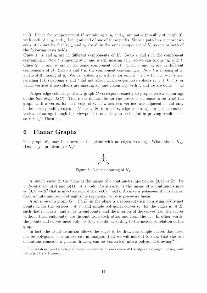
6 Planar Graphs
The graph K4 may be drawn in the plane with no edges crossing. What about K3,3
(Dudeney’s problem), or K5?
Figure 8: A plane drawing of K4.
A simple curve in the plane is the image of a continuous injection φ : [0, 1] → R2. Itsendpoints are φ(0) and φ(1). A simple closed curve is the image of a continuous mapφ : [0, 1] → R2 that is injective except that φ(0) = φ(1). A curve is polygonal if it is formedfrom a finite number of straight-line segments, i.e., φ is piecewise linear.
A drawing of a graph G = (V,E) in the plane is a representation consisting of distinctpoints xv for the vertices v ∈ V , and simple polygonal curves cuv for the edges uv ∈ E,such that cuv has xu and xv as its endpoints, and the interiors of the curves (i.e., the curveswithout their endpoints) are disjoint from each other and from the xv. In other words,the points and curves meet only ‘as they should’ according to the incidence relation of thegraph.
In fact, the usual definition allows the edges to be drawn as simple curves that neednot be polygonal; it is an exercise in analysis (that we will not do) to show that the twodefinitions coincide: a general drawing can be ‘converted’ into a polygonal drawing.8
8In fact drawings of simple graphs can be converted to ones where all the edges are straight line segments– this is Fary’s Theorem.
17
A graph together with a drawing in the plane is often called a plane graph. We tend touse the notation G for a plane graph without explicitly indicating the drawing. A graph isplanar if it has a drawing in the plane.
Given a plane graph, if we omit from the plane the points corresponding to the verticesand edges, what remains falls into open connected components, the faces, exactly oneof which is unbounded. To study plane (and planar) graphs we need surprisingly littletopology. The next lemma may seem obvious, but not all drawings of planar graphs areas simple as one might hope. (E.g., we may have one face inside another, meeting at acutvertex.)
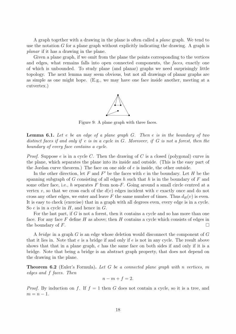
Figure 9: A plane graph with three faces.
Lemma 6.1. Let e be an edge of a plane graph G. Then e is in the boundary of twodistinct faces if and only if e is in a cycle in G. Moreover, if G is not a forest, then theboundary of every face contains a cycle.
Proof. Suppose e is in a cycle C. Then the drawing of C is a closed (polygonal) curve inthe plane, which separates the plane into its inside and outside. (This is the easy part ofthe Jordan curve theorem.) The face on one side of e is inside, the other outside.
In the other direction, let F and F ′ be the faces with e in the boundary. Let H be thespanning subgraph of G consisting of all edges h such that h is in the boundary of F andsome other face, i.e., h separates F from non-F . Going around a small circle centred at avertex v, so that we cross each of the d(v) edges incident with v exactly once and do notcross any other edges, we enter and leave F the same number of times. Thus dH(v) is even.It is easy to check (exercise) that in a graph with all degrees even, every edge is in a cycle.So e is in a cycle in H, and hence in G.
For the last part, if G is not a forest, then it contains a cycle and so has more than oneface. For any face F define H as above; then H contains a cycle which consists of edges inthe boundary of F .
A bridge in a graph G is an edge whose deletion would disconnect the component of Gthat it lies in. Note that e is a bridge if and only if e is not in any cycle. The result aboveshows that that in a plane graph, e has the same face on both sides if and only if it is abridge. Note that being a bridge is an abstract graph property, that does not depend onthe drawing in the plane.
Theorem 6.2 (Euler’s Formula). Let G be a connected plane graph with n vertices, medges and f faces. Then
n−m+ f = 2.
Proof. By induction on f . If f = 1 then G does not contain a cycle, so it is a tree, andm = n− 1.
18
Suppose now that f > 2 and the result holds for smaller values of f . Pick an edge ein the boundary of two faces. By Lemma 6.1, there is a cycle C in G containing e. ThusG− e is connected. When we delete e from the drawing, two faces join up to form a newface, while all other faces remain unchanged. So by induction n − (m − 1) + (f − 1) = 2and hence n−m+ f = 2 as required.
Corollary 6.3. Let G be a planar graph with n > 3 vertices. Then e(G) 6 3n− 6.
Proof. We may assume G is connected (otherwise consider its components) and not atree. Let m = e(G). Consider a drawing of G in the plane, with f faces F1, . . . , Ff . Lete(Fi) be the number of edges in the boundary of Fi counting any bridges twice. Sinceeach non-bridge is in the boundary of two faces and each bridge of only one, we have∑
i e(Fi) = 2m. By the last part of Lemma 6.1, e(Fi) > 3 for every face Fi, so 3f 6 2m.Hence 2 = n−m+ f 6 n−m+ 2m/3 = n−m/3 and the result follows.
We now see that K5 is not planar, since e(K5) = 10 > 9 = 3 × 5 − 6. It is an exerciseto show that any triangle-free planar graph with n > 3 vertices has at most 2n− 4 edges;this shows that K3,3 is not planar.
Dual graphs
Slightly informally, a multigraph consists of a set V of vertices and a set E of edges, whereeach e ∈ E either joins some vertex v to itself (such an edge is called a loop) or joins some(unordered) pair {u, v} of vertices. There may be several edges joining the same pair ofvertices, and there may be several loops at a given vertex v. (Formally, we may definea multigraph as a triple (V,E, φ), where V and E are finite sets, and φ : E →
(
V2
)
∪(
V1
)
encodes the ends (or end for a loop) of an edge e ∈ E.) It is clear how to extend thedefinition of a drawing in the plane to multigraphs; for example, a loop at v is drawn as a(polygonal) simple closed curve from xv to itself meeting the other edges only at xv.
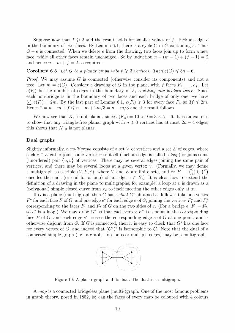
If G is a plane (multi-)graph then G has a dual G∗ obtained as follows: take one vertexF ∗ for each face F of G, and one edge e∗ for each edge e of G, joining the vertices F ∗
1 and F ∗2
corresponding to the faces F1 and F2 of G on the two sides of e. (For a bridge e, F1 = F2,so e∗ is a loop.) We may draw G∗ so that each vertex F ∗ is a point in the correspondingface F of G, and each edge e∗ crosses the corresponding edge e of G at one point, and isotherwise disjoint from G. If G is connected, then it is easy to check that G∗ has one facefor every vertex of G, and indeed that (G∗)∗ is isomorphic to G. Note that the dual of aconnected simple graph (i.e., a graph – no loops or multiple edges) may be a multigraph.
Figure 10: A planar graph and its dual. The dual is a multigraph.
A map is a connected bridgeless plane (multi-)graph. One of the most famous problemsin graph theory, posed in 1852, is: can the faces of every map be coloured with 4 colours
19
so that faces sharing an edge get different colours? Taking duals, it is not hard to checkthat this is equivalent to asking whether every planar (simple) graph G has χ(G) 6 4. Theanswer is yes; the result is known as the ‘Four Colour Theorem’.
If G is planar and has n > 3 vertices, then e(G) 6 3n − 6, so∑
v d(v) = 2e(G) < 6n,and G must have δ(G) 6 5. It follows easily by induction on |G| that every planar graphG has χ(G) 6 6. With not too much work, we can improve this by one, to obtain the ‘FiveColour Theorem’.
Theorem 6.4 (Heawood, 1890). If G is planar then χ(G) 6 5.
Proof. We argue by induction on n = |G|. If n 6 5 then the result is trivial, so suppose Gis planar and has n > 6 vertices, and every planar graph with fewer vertices is 5-colourable.
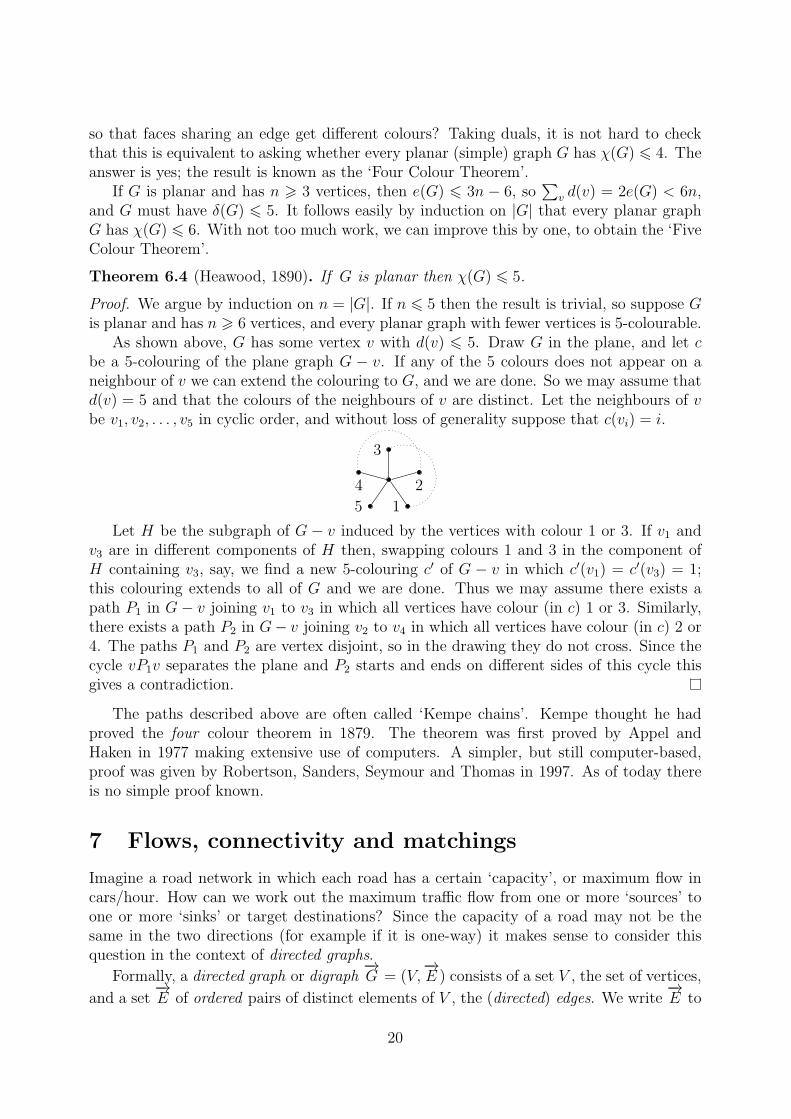
As shown above, G has some vertex v with d(v) 6 5. Draw G in the plane, and let cbe a 5-colouring of the plane graph G − v. If any of the 5 colours does not appear on aneighbour of v we can extend the colouring to G, and we are done. So we may assume thatd(v) = 5 and that the colours of the neighbours of v are distinct. Let the neighbours of vbe v1, v2, . . . , v5 in cyclic order, and without loss of generality suppose that c(vi) = i.
1
2
3
4
5
Let H be the subgraph of G − v induced by the vertices with colour 1 or 3. If v1 andv3 are in different components of H then, swapping colours 1 and 3 in the component ofH containing v3, say, we find a new 5-colouring c′ of G − v in which c′(v1) = c′(v3) = 1;this colouring extends to all of G and we are done. Thus we may assume there exists apath P1 in G− v joining v1 to v3 in which all vertices have colour (in c) 1 or 3. Similarly,there exists a path P2 in G− v joining v2 to v4 in which all vertices have colour (in c) 2 or4. The paths P1 and P2 are vertex disjoint, so in the drawing they do not cross. Since thecycle vP1v separates the plane and P2 starts and ends on different sides of this cycle thisgives a contradiction.
The paths described above are often called ‘Kempe chains’. Kempe thought he hadproved the four colour theorem in 1879. The theorem was first proved by Appel andHaken in 1977 making extensive use of computers. A simpler, but still computer-based,proof was given by Robertson, Sanders, Seymour and Thomas in 1997. As of today thereis no simple proof known.
7 Flows, connectivity and matchings
Imagine a road network in which each road has a certain ‘capacity’, or maximum flow incars/hour. How can we work out the maximum traffic flow from one or more ‘sources’ toone or more ‘sinks’ or target destinations? Since the capacity of a road may not be thesame in the two directions (for example if it is one-way) it makes sense to consider thisquestion in the context of directed graphs.
Formally, a directed graph or digraph−→G = (V,
−→E ) consists of a set V , the set of vertices,
and a set−→E of ordered pairs of distinct elements of V , the (directed) edges. We write
−→E to
20
remind ourselves the graph is directed; often the edge-set is just denoted E. We think of
(x, y) ∈ −→E as an edge from x to y, and write −→xy or simply xy. Note that a directed graph
cannot contain more than one edge from x to y, but can contain both edges xy and yx.We write
N+(x) = {y ∈ V : xy ∈ −→E }
for the out-neighbourhood of x ∈ V , and
N−(x) = {y ∈ V : yx ∈ −→E }
for its in-neighbourhood.
A flow in G with source s and sink t is a function f :−→E → [0,∞) such that for every
x ∈ V \ {s, t} we have∑
y∈N+(x)
f(xy) =∑
y∈N−(x)
f(yx),
i.e., the flow out of x is equal to the flow into x. Here s and t are distinct vertices.
Given any function f :−→E → R, for x ∈ V let
If (x) =∑
y∈N+(x)
f(xy)−∑
y∈N−(x)
f(yx).
We may think of If (x) as the amount of flow that must be injected into the graph at x tomaintain balance; in a flow, If (x) = 0 for x ∈ V \ {s, t}.
For any flow (or, indeed, any function on−→E ),
∑
x∈V
If (x) =∑
x∈V
(
∑
y∈N+(x)
f(xy)−∑
y∈N−(x)
f(yx))
= 0,
since for every uv ∈ −→E , f(uv) appears exactly twice, once with x = u and once with x = v.
For a flow, the terms with x 6= s, t are zero, so If (s) = −If (t), i.e.,
∑
y∈N+(s)
f(sy)−∑
y∈N−(s)
f(ys) =∑
y∈N−(t)
f(yt)−∑
y∈N+(t)
f(ty).
In other words, the net flow leaving s equals the net flow arriving at t. This common valueis called the value of f , and written v(f). (Usually, v(f) = If (s) = −If (t) is positive –otherwise we would regard the flow as having t as source and s as sink.) We can think offlow as being ‘conserved’ at every vertex, but with flow v(f) injected into the graph at sand flow v(f) extracted at t.
A capacity function on a directed graph G = (V,−→E ) is just a function c :
−→E → [0,∞).
A flow f is feasible (w.r.t. c) if f(xy) 6 c(xy) for every xy ∈ −→E . The key question in the
theory of flows is: what is the maximum value of a feasible flow in a given graph with givensource s, sink t and capacity function c? To avoid repeating the definitions, we shall call adirected graph with a given sink, source and capacity function a network. (Of course, theword ‘network’ has many different meanings, depending on the context.) When we say fis a flow in a given network, it is always understood that f is feasible.
21
Given sets S and T of vertices of a directed graph (V,−→E ), let
−→E (S, T ) = {xy ∈ −→
E :x ∈ S, y ∈ T} be the set of edges from S to T .
A cut in a network is a partition of the vertex set into disjoint sets S and T with s ∈ S
and t ∈ T . (Alternatively, we may say that a corresponding set−→E (S, T ) of edges is a cut.)
The capacity of a cut (S, T ) is
c(S, T ) =∑
xy∈−→E (S,T )
c(xy),
i.e., the maximum conceivable flow from S to T (ignoring what happens within S and T ).Clearly, in any feasible flow f , v(f) 6 c(S, T ). Indeed,
v(f) = If (s) =∑
x∈S
If (x) =∑
x∈S
(
∑
y∈N+(x)
f(xy)−∑
y∈N−(x)
f(yx))
=∑
xy∈−→E (S,T )
f(xy)−∑
yx∈−→E (T,S)
f(yx) 6 c(S, T ). (6)
Thus the maximum value of a feasible flow is at most the minimum capacity of a cut. Theremarkable ‘max-flow min-cut’ theorem tells us that we have equality.
Theorem 7.1 (Max-Flow Min-Cut). In any network (−→G, s, t, c) we have
sup{
v(f) : f is a feasible flow}
= min{
c(S, T ) : (S, T ) is a cut}
.
Moreover, the supremum is attained.
The key ingredient of the proof is the notion of an augmenting path, or ‘slack path’. Let
f be a flow in a network. We say that an ordered pair (x, y) is ε-slack if either xy ∈ −→E
and f(xy) 6 c(xy) − ε or yx ∈ −→E and f(yx) > ε (or both). A path x0x1 · · · xr in the
undirected graph associated to−→G is ε-slack if xi−1xi is ε-slack for 1 6 i 6 r, and slack (or
augmenting) if it is slack for some ε > 0.
Lemma 7.2. Let f be a flow in a network. If x0x1 · · · xr is an ε-slack path with x0 = sand xr = t then v(f) is not maximal; in particular, there is a flow f ′ with v(f ′) = v(f)+ε.
Proof. For each i we can either increase the flow along xi−1xi by ε, or decrease the flowalong xixi−1 by ε. Doing either increases If (xi−1) by ε and decreases If (xi) by the sameamount. Making such a change for each i = 1, 2, . . . , r, we see that If (x) is unchangedfor every x 6= s, t (so we still have a flow), and that v(f) = If (s) = −If (t) is increasedby ε.
Proof of Theorem 7.1. First, we show that the supremum is attained. As noted earlier, forany flow f and cut (S, T ) we have v(f) 6 c(S, T ). In particular, v(f) 6
∑
y∈N+(s) c(sy) < ∞so the set {v(f) : f a flow} is bounded. So there are flows fi with v(fi) → M < ∞, where
M is the supremum. Let xy ∈ −→E . Then, passing to a subsequence, we may assume
that fi(xy) converges. Repeating this for each edge, we find a (sub)sequence of flows with
v(fi) → M such that fi(xy) converges for each xy ∈ −→E . But then f(xy) = limi→∞ fi(xy)
defines a flow with value limi→∞ v(fi) = M .
22
Let f be a flow attaining the supremum. It suffices to find a cut with capacity v(f).Let
S = {x ∈ V : there is a slack path from s to x},and let T = V \ S. Clearly s ∈ S (consider a path of length 0). By Lemma 7.2, t /∈ S.Thus (S, T ) is a cut. Suppose x ∈ S and y ∈ T with (x, y) slack. Then taking a slack paths = x0 · · · xr = x and appending xr+1 = y gives a slack path ending at y, contradicting
y /∈ T . Hence, for every xy ∈ −→E (S, T ) we have f(xy) = c(xy), and for every yx ∈ −→
E (T, S)we have f(yx) = 0. I.e., equality holds in (6), so c(S, T ) = v(f).
A maximal flow is one with maximum value. A function (here f or c) is integral if allits values are integers.
Theorem 7.3. Let (−→G, s, t, c) be a network in which the capacity function c is integral.
Then there is a maximal flow f which is integral.
Proof. We have essentially described an algorithm to find such an f ; the key point is thatif the capacity function c and flow f are integral, then any slack path is 1-slack. Start withthe flow with f(xy) = 0 for all edges, and repeat the following: if there is a slack (andhence 1-slack) path from s to t augment the flow along this path by 1 as above, obtaining anew integral flow with larger value; repeat. Otherwise, by the last part of the proof above,there is a cut (S, T ) with v(f) = c(S, T ), so f is maximal.
The algorithm defined above is in fact reasonably efficient: it is easy to check for theexistence of slack paths by (for example) breadth-first search.
A directed path in a directed graph−→G = (V,
−→E ) is a sequence x0x1 · · · xr of distinct
vertices such that x0x1, . . . , xr−1xr ∈ −→E . A set
−→X ⊆ −→
E of edges separates s from t if−→G −−→
X contains no directed path (or, equivalently, no directed walk) from s to t. If (S, T )
is a cut, then−→E (S, T ) separates s from t. Conversely, if
−→X separates s from t then it
contains−→E (S, T ) for some cut (S, T ) – for example, take S to be the set of vertices x such
that−→G −−→
X contains a directed s-x path. Let c(−→X ) =
∑
xy∈−→Xc(xy). Then we see that
min{
c(S, T ) : (S, T ) is a cut}
= min{
c(−→X ) :
−→X separates s from t
}
. (7)
This gives an alternative formulation of the max-flow min-cut theorem. Note, however,that cuts arise in the proof in an essential way, and it is necessary to consider reducing flowalong backwards edges as well as increasing it along forwards ones.
The max-flow min-cut theorem has many variants, some of which we leave as exercises.For example, we may consider several sources s1, . . . , sk and several sinks t1, . . . , tℓ. In thiscontext, a cut (S, T ) is a partition of the vertices with all sources in S and all sinks in T .A flow must satisfy If (x) = 0 for every vertex that is neither a source nor a sink, and its
value is∑k
i=1 If (si). Theorems 7.1 and 7.3 apply mutatis mutandis to this setting.Another important variation allows some edges to have infinite capacity, meaning that
the flow along xy can take any finite value. The results hold in this setting too, with theproviso that if there is no cut with finite capacity, then {v(f)} is unbounded, so of coursethere is no flow with maximum value.
23
One more substantial variant is to impose capacity restrictions on the vertices rather
than edges. Let−→G be a directed graph with source s and sink t, and let c be a (vertex)
capacity function assigning every vertex x 6= s, t a capacity c(x) ∈ [0,∞). A flow in−→G is
feasible if for each vertex x 6= s, t we have
∑
y∈N−(x)
f(yx) =∑
y∈N+(x)
f(xy) 6 c(x),
i.e., the flow through x is at most c(x). (The equality is the definition of a flow; feasibilityis the inequality.)
A vertex-cut is a set S ⊆ V \ {s, t} of vertices such that in−→G − S there is no directed
path from s to t. The capacity of S is∑
x∈S c(x).
Theorem 7.4. Let−→G be a directed graph with source s, sink t and vertex capacity func-
tion c. Then the maximum value of a feasible flow from s to t is the minimum capacity ofany vertex-cut. Furthermore, if c is integral, then there is a flow with maximum value thatis integral.
Proof. Rather than modify the proof of Theorem 7.1, we modify the network so that wecan apply that result.
Form a directed graph−→H with source s and sink t by replacing each vertex x 6= s, t by
two vertices x− and x+ joined by an edge x−x+ with capacity c(x). For each edge of−→G
there is an edge of−→H with infinite (or very large) capacity; edges that start/end at s/t
in−→G do so in
−→H ; every edge of
−→G ending at x 6= s, t now ends at x−, and every edge
starting at x now starts at x+. It is easy to check that feasible flows in−→G are in 1-to-1
correspondence with feasible flows in−→H . In
−→H , a set
−→X of edges with c(
−→X ) finite must be
of the form−→X S = {x−x+ : x ∈ S} for some S ⊆ V \ {s, t}. Moreover,
−→X S is separating if
and only if S is a vertex-cut. The result thus follows from Theorem 7.1 and (7) and, forintegrality, Theorem 7.3.
Connectivity and Menger’s Theorem
Let G be an (undirected) graph and S ⊆ V (G). We say that S separates G if G − S isdisconnected. For vertices x, y of G, S separates x and y if they are in different componentsof G− S.
For a non-negative integer k, a graph G is k-connected if |G| > k + 1 and no set of (atmost) k − 1 vertices separates G. (Every graph is 0-connected. A graph G is 1-connectediff it is connected and |G| > 2. The only k-connected graph with |G| = k + 1 is Kk+1.)
The (vertex) connectivity of a graph G is defined as
κ(G) = max{
k : G is k-connected}
.
Equivalently, κ(G) is the minimum number of vertices that must be deleted to eitherdisconnect G, or reduce it to a single vertex. It follows easily from the definition thatκ(G− x) > κ(G)− 1, and that if H is a spanning subgraph of G then κ(G) > κ(H). It isan exercise to check that if e is an edge of G then κ(G− e) > κ(G)− 1.
24
We now define a ‘local’ version of connectivity. For distinct non-adjacent vertices x andy of G we write
κ(x, y) = κG(x, y) = min{|S| : S separates x and y}.
Note that adjacent vertices can never be separated by deleting other vertices. Also, it iseasy to check that for any non-complete graph G,
κ(G) = minxy∈E(G)
κG(x, y).
Two distinct x-y paths are independent (or internally vertex-disjoint) if the only ver-tices they share are x and y. A set of x-y paths is independent if the paths are pairwiseindependent.
Theorem 7.5 (Menger’s Theorem). Let x and y be distinct non-adjacent vertices of G.Then the maximum size of an independent set of x-y paths is κG(x, y).
Proof. If there are k independent x-y paths then κG(x, y) > k, so we must show that thereare κG(x, y) independent paths.
Turn G into a network with source x and sink y by replacing each edge uv by twodirected edges −→uv and −→vu, and assigning each vertex other than x and y capacity 1. Thena vertex-cut S is simply a set of vertices separating x and y, and its capacity is just |S|.Hence, by Theorem 7.4, there is an integral flow f from x to y with value κG(x, y). Giventhe vertex capacities, f can only take values 0 and 1, so f corresponds to a set of edgesconsisting of independent x-y paths and perhaps some directed cycles. The value of f isthe number of paths, so there are κG(x, y) paths as required.
Corollary 7.6. A graph G is k-connected iff |G| > k + 1 and every pair of non-adjacentvertices is joined by k independent paths.
We can also define edge connectivity, and prove a form of Menger’s Theorem for edge-disjoint paths.
Hall’s Theorem
A matching M in a graph G is a set of pairwise disjoint edges of G; its size |M | is thenumber of edges. Let G be a bipartite graph with vertex classes V1 and V2. A completematching from V1 to V2 is a matching such that every vertex in V1 is incident with someedge in the matching, i.e., a matching of size |V1|.
Given a set S of vertices in a graph G, we write N(S) =⋃
s∈S N(s) for the set of verticeswith at least one neighbour in S.9
Theorem 7.7 (Hall’s Marriage Theorem). Let G be a bipartite graph with bipartition(V1, V2). Then G contains a complete matching from V1 to V2 iff |N(S)| > |S| for eachS ⊆ V1.
9Some authors exclude elements of S from N(S). In the present context, where G is bipartite andS ⊆ V1, it makes no difference.
25
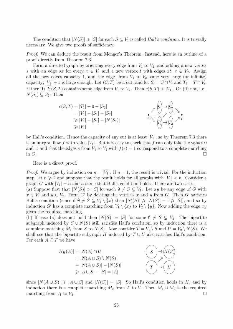
The condition that |N(S)| > |S| for each S ⊆ V1 is called Hall’s condition. It is triviallynecessary. We give two proofs of sufficiency.
Proof. We can deduce the result from Menger’s Theorem. Instead, here is an outline of aproof directly from Theorem 7.3.
Form a directed graph by orienting every edge from V1 to V2, and adding a new vertexs with an edge sx for every x ∈ V1 and a new vertex t with edges xt, x ∈ V2. Assignall the new edges capacity 1, and the edges from V1 to V2 some very large (or infinite)capacity; |V1|+1 is large enough. Let (S, T ) be a cut, and let Si = S ∩ Vi and Ti = T ∩ Vi.
Either (i)−→E (S, T ) contains some edge from V1 to V2. Then c(S, T ) > |V1|. Or (ii) not, i.e.,
by Hall’s condition. Hence the capacity of any cut is at least |V1|, so by Theorem 7.3 thereis an integral flow f with value |V1|. But it is easy to check that f can only take the values 0and 1, and that the edges e from V1 to V2 with f(e) = 1 correspond to a complete matchingin G.
Here is a direct proof.
Proof. We argue by induction on n = |V1|. If n = 1, the result is trivial. For the inductionstep, let n > 2 and suppose that the result holds for all graphs with |V1| < n. Consider agraph G with |V1| = n and assume that Hall’s condition holds. There are two cases.(a) Suppose first that |N(S)| > |S| for each ∅ 6= S ( V1. Let xy be any edge of G withx ∈ V1 and y ∈ V2. Form G′ by deleting the vertices x and y from G. Then G′ satisfiesHall’s condition (since if ∅ 6= S ⊆ V1 \ {x} then |N ′(S)| > |N(S)| − 1 > |S|), and so byinduction G′ has a complete matching from V1 \ {x} to V2 \ {y}. Now adding the edge xygives the required matching.(b) If case (a) does not hold then |N(S)| = |S| for some ∅ 6= S ( V1. The bipartitesubgraph induced by S ∪ N(S) still satisfies Hall’s condition, so by induction there is acomplete matching M1 from S to N(S). Now consider T = V1 \ S and U = V2 \N(S). Weshall see that the bipartite subgraph H induced by T ∪ U also satisfies Hall’s condition.For each A ⊆ T we have
since |N(A ∪ S)| > |A ∪ S| and |N(S)| = |S|. So Hall’s condition holds in H, and byinduction there is a complete matching M2 from T to U . Then M1 ∪ M2 is the requiredmatching from V1 to V2.
26
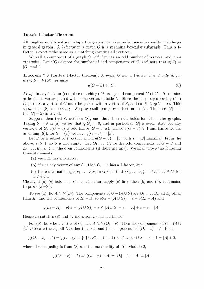
Tutte’s 1-factor Theorem
Although especially natural in bipartite graphs, it makes perfect sense to consider matchingsin general graphs. A k-factor in a graph G is a spanning k-regular subgraph. Thus a 1-factor is exactly the same as a matching covering all vertices.
We call a component of a graph G odd if it has an odd number of vertices, and evenotherwise. Let q(G) denote the number of odd components of G, and note that q(G) ≡|G| mod 2.
Theorem 7.8 (Tutte’s 1-factor theorem). A graph G has a 1-factor if and only if, forevery S ⊆ V (G), we have
q(G− S) 6 |S|. (8)
Proof. In any 1-factor (complete matching) M , every odd component C of G− S containsat least one vertex paired with some vertex outside C. Since the only edges leaving C inG go to S, a vertex of C must be paired with a vertex of S, and so |S| > q(G− S). Thisshows that (8) is necessary. We prove sufficiency by induction on |G|. The case |G| = 1(or |G| = 2) is trivial.
Suppose then that G satisfies (8), and that the result holds for all smaller graphs.Taking S = ∅ in (8) we see that q(G) = 0, and in particular |G| is even. Also, for anyvertex v of G, q(G − v) is odd (since |G − v| is). Hence q(G − v) > 1 and (since we areassuming (8)), for S = {v} we have q(G− S) = |S|.
Let S be a subset of V (G) for which q(G − S) = |S| with s = |S| maximal. From theabove, s > 1, so S is not empty. Let O1, . . . , Os be the odd components of G − S andE1, . . . , Ek, k > 0, the even components (if there are any). We shall prove the followingthree statements.
(a) each Ei has a 1-factor,
(b) if v is any vertex of any Oi, then Oi − v has a 1-factor, and
(c) there is a matching s1v1, . . . , ssvs in G such that {s1, . . . , ss} = S and vi ∈ Oi for1 6 i 6 s.
Clearly, if (a)–(c) hold then G has a 1-factor: apply (c) first, then (b) and (a). It remainsto prove (a)–(c).
To see (a), let A ⊆ V (Ei). The components of G− (A∪ S) are O1, . . . , Os, all Ej otherthan Ei, and the components of Ei − A, so q(G− (A ∪ S)) = s+ q(Ei − A) and
q(Ei − A) = q(G− (A ∪ S))− s 6 |A ∪ S| − s = |A|+ s− s = |A|.
Hence Ei satisfies (8) and by induction Ei has a 1-factor.
For (b), let v be a vertex of Oi. Let A ⊆ V (Oi − v). Then the components of G− (A∪{v} ∪ S) are the Ej, all Oj other than Oi, and the components of (Oi − v)− A. Hence
since Oi is odd. Since x < y+2 and x ≡ y mod 2 imply x 6 y, it follows that q((Oi − v)−A) 6 |A|, so Oi − v satisfies (8), and (b) follows by induction.
Finally, for (c) let H be the bipartite graph with V1 = S and V2 = {o1, . . . , os}, withan edge xoi whenever x ∈ S and there is at least one edge in G from x to Oi. It sufficesto find a complete matching in H, so we check Hall’s condition. Let A ⊆ V1 = S. Ifoi ∈ V2 \ NH(A) then in G there are no edges from A to Oi, so Oi is a component ofG− (S \ A). Hence, q(G− (S \ A)) > |V2 \NH(A)| = s− |NH(A)|. Thus, by (8),
s− |NH(A)| 6 q(G− (S \ A)) 6 |S \ A| = s− |A|.
Hence |NH(A)| > |A|, so Hall’s condition holds in H, and by Hall’s Theorem H has therequired complete matching.
8 Extremal Problems
If G has a subgraph isomorphic to H we say ‘G contains (a copy of) H’ for short, andsometimes write G ⊇ H.10 For a graph H with e(H) > 0 and n > 1 an integer, define
ex(n,H) = max{
e(G) : |G| = n, G contains no copy of H}
andEX(n,H) =
{
G : |G| = n, e(G) = ex(n,H), G contains no copy of H}
.
The graphs in EX(n,H) are called the extremal graphs ; we often describe EX(n,H) bylisting one graph from each isomorphism class. ex(n,H) is the extremal number for H (afunction of n, of course).
For example, if G contains no copy of P3 then all edges must be disjoint. Thusex(n, P3) = ⌊n
2⌋, and EX(n, P3) is {n
2K2} if n is even and {n−1
2K2 ∪ K1} if n is odd,
where mK denotes the disjoint union of m copies of K.What is ex(n,K3)? Good candidate extremal graphs are the complete bipartite graphs
Kk,n−k; to maximize the number k(n − k) of edges we take k = ⌊n/2⌋. More generally,what is ex(n,Kr+1)?
A graph G is r-partite if V (G) is the disjoint union of r sets V1, . . . , Vr (the vertexclasses) with e(G[Vi]) = 0 for each i, i.e., no edges within each Vi. In other words, all edgesgo between parts. This is exactly the same as saying that G is r-colourable. A graph G iscomplete r-partite if in addition every possible edge between parts is present.
Note that empty parts are allowed: the key point is that inside any part with at leasttwo vertices, edges are forbidden. Clearly, any r-partite graph does not contain Kr+1.
Before continuing we make a trivial observation: if a1, . . . , ar are integers with averagea = 1
r
∑
ai then all ai are within 1 of each other (i.e., max ai 6 min ai + 1) if and only ifevery ai is equal to ⌊a⌋ or ⌈a⌉. (There are two cases: all ai = m = a for some integer m, orsome ai = m, some ai = m+1; then m < a < m+1.) Moreover, given r and
∑
ai, there isonly one way (up to reordering) to choose the ai so that these conditions hold. I.e., there
10Perhaps we should not write this, since in other contexts it means that H itself is a subgraph of G, i.e.,that the particular vertices and edges of H are present in G. But usually it is clear from context whetheror not we are considering isomorphic copies.
28
is only one way to divide a given number of (indivisible) objects among r people ‘as fairlyas possible’.
For n, r > 1, the Turan graph Tr(n) is the complete r-partite graph on n vertices withthe vertex class sizes as equal as possible, i.e., each is ⌊n
r⌋ or ⌈n
r⌉. The Turan number tr(n)
is e(Tr(n)). Note that if n 6 r then Tr(n) = Kn.For example, T2(n) is K⌊n/2⌋,⌈n/2⌉. Thus t2(n) is n2
4if n is even, and n2−1
4if n is odd:
t2(n) = ⌊n2
4⌋.
T3(10) has class sizes 3, 3 and 4, and 9+12+12 = 33 edges, so t3(10) = 33. (T1(n) hasno edges.)
Facts about Turan graphs
1. Among all r-partite graphs with n vertices, Tr(n) is the unique (up to isomorphism)one with the largest number of edges. Indeed, only complete r-partite graphs arecandidates, and if two classes differ in size by 2 or more, moving a vertex from thelarger to the smaller gains at least one edge (since it reduces the number of verticesit is not adjacent to).
2. Since each vertex class has size ⌊nr⌋ or ⌈n
r⌉, δ(Tr(n)) = n−⌈n
r⌉ and ∆(Tr(n)) = n−⌊n
r⌋,
so ∆ − δ 6 1. Hence δ(Tr(n)) = ⌊d(Tr(n))⌋ and ∆(Tr(n)) = ⌈d(Tr(n))⌉, whered(G) = 2e(G)/|G| is the average degree of a graph G.
3. To get from Tr(n) to Tr(n− 1) we delete any vertex from a largest vertex class, i.e.,any vertex of minimum degree. So tr(n)− δ(Tr(n)) = tr(n− 1).
Theorem 8.1 (Turan’s Theorem). For all positive integers n and r we have
ex(n,Kr+1) = tr(n) and EX(n,Kr+1) = {Tr(n)}.
Proof. We fix r and use induction on n. If n 6 r then ex(n,Kr+1) =(
n2
)
= tr(n), andEX(n,Kr+1) = {Kn} = {Tr(n)}, as required.
Now let n > r and suppose that the result holds for n − 1. Let G be a graph with nvertices and tr(n) edges containing no copy of Kr+1. We will show that G ∼= Tr(n), fromwhich the result follows. (If H had |H| = n, e(H) > tr(n) and contained no copy of Kr+1,then some spanning subgraph G would have tr(n) edges; so G ∼= Tr(n) and then H wouldcontain a copy of Kr+1 as adding any edge to Tr(n) forms a Kr+1.)
First note that by Fact 2
δ(G) 6 ⌊d(G)⌋ = ⌊d(Tr(n))⌋ = δ(Tr(n)).
Let v ∈ V (G) have degree d(v) = δ(G). Then for H = G− v we have
using Fact 3. But H contains no Kr+1 so by the induction hypothesis, H ∼= Tr(n− 1).Now v cannot have a neighbour in each vertex class of H (or we would get a copy of
Kr+1), so its neighbours must miss some vertex class Vi completely. Adding v to this class,we see that G is r-partite. Now by Fact 1, G ∼= Tr(n).
29
The density of a graph G is e(G)/(
|G|2
)
. For r fixed and n → ∞, Tr(n) has density1− 1
r+ o(1). Thus by Turan’s Theorem, ex(n,Kr+1)/
(
n2
)
= 1− 1r+ o(1). We say that Kr+1
‘appears’ at density 1 − 1r. Thus K3 appears at density 1
2, K4 at density 2
3, K5 at density
34, and so on.What about other graphs? If χ(H) > r + 1, then, since H is not r-partite, Tr(n)
contains no copy of H. Thus for any H, letting r = χ(H)− 1 we have
ex(n,H) > tr(n) = (1− 1r+ o(1))
(
n2
)
.
In particular, H cannot appear before the density 1− 1rat which Kr+1 appears. Are there
‘big’ graphs with a given chromatic number that appear significantly later? Amazingly,the answer turns out to be no.
For s, t > 1 let Ks(t) be the complete s-partite graph with t vertices in each class.For example, K1(t) is the empty graph Et, K2(t) is the complete bipartite graph Kt,t, andKs(1) = Ks. In general Ks(t) = Ts(st).
Theorem 8.2 (Erdos–Stone Theorem). Let r, t > 1 be integers and let ε > 0. There is aconstant n0 = n0(r, t, ε) such that every graph G with n > n0 vertices and
e(G) >(
1− 1r+ ε
)(
n2
)
contains a copy of Kr+1(t).
We prove this theorem in two steps. We first show that any graph with a given densitycontains a subgraph with a relatively large minimum degree.
Lemma 8.3. Let 0 6 α < β 6 1. If G is a graph with |G| = n and e(G) > β(
n2
)
then Ghas an (induced) subgraph H with
δ(H) > α(|H| − 1)
and |H| > √εn, where ε = β − α.
Proof. Define a sequence Gn, Gn−1, . . . of graphs with |Gt| = t as follows. Set Gn = G. Ifδ(Gt) > α(t − 1) then stop. Otherwise, remove a vertex of Gt with minimum degree toget Gt−1. The construction must stop at some point (G1 at the latest); let Gk be the finalgraph, so δ(Gk) > α(|Gk| − 1) by construction. Now
e(Gk) = e(Gn)− δ(Gn)− δ(Gn−1)− · · · − δ(Gk+1)
> β
(
n
2
)
− α(
(n− 1) + (n− 2) + · · ·+ k)
= β
(
n
2
)
− α
(
n
2
)
+ α
(
k
2
)
> ε
(
n
2
)
.
Since e(Gk) 6(
k2
)
it follows that(
k2
)
> ε(
n2
)
. Multiplying by 2k/(k− 1) > 2n/(n− 1) givesk2 > εn2, so k >
√εn.
30
Lemma 8.4. Let r, t > 1 be integers and let ε > 0. There is a constant n1 = n1(r, t, ε)such that every graph G with n > n1 vertices and
δ(G) >(
1− 1r+ ε
)
(n− 1)
contains a copy of Kr+1(t).
Note that Theorem 8.2 will follow easily: apply Lemma 8.3 with β = 1 − 1r+ ε and
α = 1− 1r+ ε
2, and then Lemma 8.4 with ε/2 in place of ε.
Proof. We use induction on r, proving the base case and induction step together. Moreprecisely, for r > 1 let Hr be the statement that for every t > 1 and ε > 0 there is an n1
such that . . . . We shall prove Hr assuming, for r > 2, that Hr−1 holds. Then we will haveshown that H1 holds, and that Hr−1 implies Hr for all r > 2, so by induction Hr holds forall r > 1. A key point is that in proving Hr, r > 2, we must consider all t and all ε > 0;but for a given t we may use the fact that Hr−1 holds for some other, perhaps much largervalue of t.
Let r > 1. To prove Hr, let t > 1 and ε > 0 be given, and let G be a graph with |G| = nand δ(G) > (1− 1
r+ ε)(n− 1). Set
T = ⌈2t/(εr)⌉.
If r > 2 then since
δ(G) > (1− 1r+ ε)(n− 1) > (1− 1
r−1+ ε)(n− 1),
we know by the induction hypothesis Hr−1 that, if n is large enough (depending on r, t, ε),G must contain a copy of Kr(T ). If r = 1 then Kr(T ) is an empty graph with T vertices,so if n is large enough (i.e., n > T ) then G certainly contains a copy of this graph.
In either case, let H be a subgraph of G isomorphic to Kr(T ). Denote its vertex classesby S1, . . . , Sr and let S = V (H) be their union. Let U be the set of vertices in V (G) \ Swhich have at least t neighbours in each class Si; these vertices are the useful ones.
If |U | > (t− 1)(
Tt
)rthen there are at least t vertices in U that have at least t common
neighbours in each Si, giving a Kr+1(t); to see this assign to each u ∈ U an r-tuple(A1, . . . , Ar) where Ai ⊆ Si ∩ N(u) and |Ai| = t. As there are
(
Tt
)rpossible r-tuples, the
average number of times an r-tuple is chosen is |U |/(
Tr
)t> t − 1, and so some r-tuple is
chosen > t times, i.e., we have t vertices in U all joined to the same copy H ′ ⊆ H of Kr(t).So we may suppose that |U | 6 (t − 1)
(
Tt
)r. Let B = V (G) \ (S ∪ U). We count the
number N of edges of G between S and B in two different ways. Firstly, the degree in Gof any vertex v is
n− 1− dG(v) 6 n− 1− δ(G) 6 (n− 1)(
1r− ε
)
6(
1r− ε
)
n,
so counting from S we find that
N 6 |S|(
1r− ε
)
n = rT(
1r− ε
)
n = (T − εrT )n.
31
On the other hand, for each u ∈ B there is a vertex class Si of H such that, in G, thevertex u has at most t−1 6 t neighbours in Si. Then, in G, u has at least T − t neighboursin Si ⊆ S. Hence, counting from B, we see that
N > |B|(T − t).
Since we chose T so that εrT > 2t, it follows that
|B| 6 T − εrT
T − tn 6
T − 2t
T − tn = (1− c)n
for some constant c > 0 (depending on r, t, ε). But now in total there are
n = |S|+ |B|+ |U | 6 rT + (1− c)n+ (t− 1)(
Tt
)r= (1− c)n+O(1)
vertices, a contradiction if n is large enough.
Corollary 8.5. Let H be any graph with e(H) > 0. Then
ex(n,H) =(
1− 1χ(H)−1
+ o(1))(
n2
)
as n → ∞, where χ(H) is the chromatic number of H.
Proof. Let r = χ(H)−1, so H has chromatic number r+1. Since H is not r-partite, Tr(n)does not contain any copies of H, so
ex(n,H) > tr(n) =(
1− 1r+ o(1)
)(
n2
)
.
On the other hand, for large enough t (e.g., t = |H|), the graph Kr+1(t) does contains acopy of H. Therefore
ex(n,H) 6 ex(n,Kr+1(t)) 6(
1− 1r+ o(1)
)(
n2
)
,
where the second inequality is from Theorem 8.2.
Corollary 8.5 answers, at some level, the basic extremal question for any graph H.However, there is a weak point: while for χ(H) > 3 it tells us asymptotically what valueex(n,H) has, for χ(H) = 2 it only tells us that ex(n,H) = o(n2), leaving a wide rangeof possible functions (e.g., roughly n2/ log n, roughly n, roughly n3/2 etc). Can we saysomething more precise in this case?
The Zarankiewicz Problem
Let G be a bipartite graph where the vertex classes have a given size n. How many edgescan G have if it does not contain a copy of some given graph H? This makes sense only ifH is bipartite, and in particular we consider H = K2(t) = Kt,t, i.e., the bipartite analogueof the Turan problem. Formally, let
z(n, t) = max{
e(G) : G ⊆ Kn,n and G contains no Kt,t
}
.
32
Theorem 8.6. If n > t > 2 then
z(n, t) 6 (t− 1)1/tn2−1/t + (t− 1)n
In particular, as n → ∞ with t fixed we have z(n, t) = O(n2−1/t).
Proof. Let G be a maximal bipartite graph with vertex classes X and Y such that |X| =|Y | = n and G contains no Kt,t. Note that by maximality, d(v) > t− 1 for every vertex v.(Otherwise, add a new edge incident with v. The degree of v would still be less than t, sothe new edge cannot be in any Kt,t.)
We say that a vertex v covers a set S of vertices if S ⊆ N(v). A vertex v ∈ X coversexactly
(
d(v)t
)
t-element subsets of Y . On the other hand, a t-element subset of Y is coveredby at most t− 1 vertices in X; otherwise we have a Kt,t. Hence,
∑
v∈X
(
d(v)
t
)
6 (t− 1)
(
n
t
)
.
From here on it is just calculation. Firstly, the polynomial x(x− 1) · · · (x− t+1) is convexon [t− 1,∞), so
(
xt
)
= x(x− 1) · · · (x− t+1)/t! is convex as a function of the real variablex when x > t − 1. Let d = 1
n
∑
v∈X d(v) be the average degree in X. Then, by Jensen’sinequality,
(
d
t
)
61
n
∑
v∈X
(
d(v)
t
)
6t− 1
n
(
n
t
)
. (9)
Hencet− 1
n>
(
d
t
)
/
(
n
t
)
=d(d− 1) · · · (d− t+ 1)
n(n− 1) · · · (n− t+ 1)>
(d− t+ 1
n
)t
.
Rearranging givesd− t+ 1 6 (t− 1)1/tn1−1/t
and soe(G) = dn 6 (t− 1)1/tn2−1/t + (t− 1)n.
Remark. The same method of proof works to show that ex(n,Kt,t) = O(n2−1/t); we countthe number of copies of K1,t in two ways. (As in the proof above, but in the bipartite casewe had the extra restriction that the special vertex of K1,t should be in X.)
The special case t = 2 is the same but with simpler calculations.
Theorem 8.7. For n > 2 we have
z(n, 2) 6n
2(1 +
√4n− 3) ∼ n3/2
as n → ∞.
Proof. We have (9) as before. With t = 2 this becomes d(d− 1) 6 n− 1, rearranging andnoting as before that e(G) = nd gives the result.
33
The bounds just given are only upper bounds. Are they close to the truth? In general,this is an open question. The case t = 2 is particularly nice. Here we have equality if andonly if G is regular, any two vertices in Y have exactly one common neighbour in X, andvice versa. A structure with these properties is called a finite projective plane: think of thevertices in X as points, those in Y as lines, and edges of G as representing incidence.
It turns out that, except for some degenerate cases, for equality we must have n =q2 + q + 1, each point on q + 1 lines and each line having q + 1 points. Is this possible?For q any prime power the answer is yes: take the projective plane over a finite field withq elements. (This is enough to show that in fact z(n, 2) ∼ n3/2). However, for n not of thisform, even the value of z(n, 2) is unknown in general.