8.1.1 Time- and temperature factors ..................................31 8.1.2 NMVOC-speciation ..................................................37
8.2 Biogenic emissions ...................................................................39 8.2.1 NMVOC and NO ......................................................39 8.2.2 Sea salt ......................................................................40
Annex A Reactions and rates of the CBM-IV chemical mechanism Annex B Reactions and rates of the CB99 chemical mechanism Annex C Dry Deposition
TNO-report
TNO-B&O-A − R 2005/297 5 of 57
1. Introduction
The development and application of chemistry transport models has a long tradition in and outside Europe. RIVM and TNO have independently developed models to calculate the dispersion and chemical transformation of air pollutants in the lower troposphere over Europe. The two models are the TNO model LOTOS (Builtjes, 1992; Schaap et al., 2004a) and the RIVM model EUROS (de Leeuw and van Rheineck Leyssius, 1990; van Loon, 1994, 1995; Matthijsen et al., 2002). LOTOS and EUROS were originally developed and used as photo-oxidant models (Builtjes, 1992; Hass et al., 1997; Hammingh et al, 2001, Roemer, 2003). During the last years attention was given to simulate the inorganic secondary aerosols SO4, NH4 and NO3. (Schaap et al., 2004a; Erisman and Schaap, 2004; Matthijsen et al., 2002) and carbonaceous aerosols (Schaap et al., 2004b). The EUROS model also contains the possibility to perform simulations for persistent organic compounds (Jacobs and van Pul, 1996).
The two models have a similar structure and comparable application areas. Hence, based on strategic and practical reasoning, RIVM/MNP and TNO agreed to collaborate on the development of a single chemistry transport model: LOTOS-EUROS. During 2004 the two models were unified which resulted in a LOTOS-EUROS version 1.0 (Schaap et al., 2005). For 2005 a project was defined to: 1. Document the model version 2. Perform validation studies 3. Include several model features such as data assimilation and zooming.
In this report we provide a documentation of the LOTOS-EUROS model. The validation study, new developments and inclusion of several model features will be described in a forthcoming report. The model description in this report is that of version 1.1, the model version operational at October, 1, 2005. This report is not intended to describe a fixed and definite status, because a model such as LOTOS-EUROS is under constant development. Hence, the documentation of the model will be updated continuously and made available through the LOTOS-EUROS website.
TNO-report
6 of 57 TNO-B&O-A − R 2005/297
TNO-report
TNO-B&O-A − R 2005/297 7 of 57
2. Model formulation and domain
2.1 The continuity equation
The main prognostic equation in the LOTOS-EUROS model is the continuity equation that describes the change in time of the concentration of a component as a result of the following processes: – Transport – Chemistry – Dry and wet deposition – Emissions
The equation is given by:
WDQREzCK
zyCK
yxCK
xzCW
yCV
xCU
tC
zhh −−+++
∂∂
∂∂
+
∂∂
∂∂
+
∂∂
∂∂
=∂∂
+∂∂
+∂∂
+∂∂
with C the concentration of a pollutant, U, V and W being the large scale wind components in respectively west-east direction, in south-north direction and in vertical direction. Kh and Kz are the horizontal and vertical turbulent diffusion coefficients. E represents the entrainment or detrainment due to variations in layer height. R gives the amount of material produced or destroyed as a result of chemistry. Q is the contribution by emissions, and D and W are loss terms due to processes of dry and wet deposition respectively.
In the model the equation is solved by means of operator splitting. The time step is split in two halves and concentration changes are calculated for the first half time step in the following order: 1. chemistry 2. diffusion and entrainment 3. dry deposition 4. wet deposition 5. emission 6. advection
Then for the second half time step the order is reversed. Note that if this cycle is repeated, two instances of the chemistry process are taken together with a whole time step. This can be computationally advantageous, because the time integration process does not have to be restarted for the second half time step.
In the following chapters these processes are described in more detail. Furthermore, the input data are described.
TNO-report
8 of 57 TNO-B&O-A − R 2005/297
2.2 Domain
The master domain of LOTOS-EUROS is shown in Figure 2.1. The boundaries of the domain are 35 and 70 North and 10 West and 60 East. The projection is normal longitude-latitude and the standard grid resolution is 0.50° longitude x 0.25° latitude, approximately 25x25 km. By means of a control file the actual domain for a simulation can be set as long as it falls within the master domain as specified above.
Figure 2.1 The domain of the LOTOS-EUROS modelling system. The example shows the average sulphur dioxide concentration (µg/m3) modelled for July, 1997.
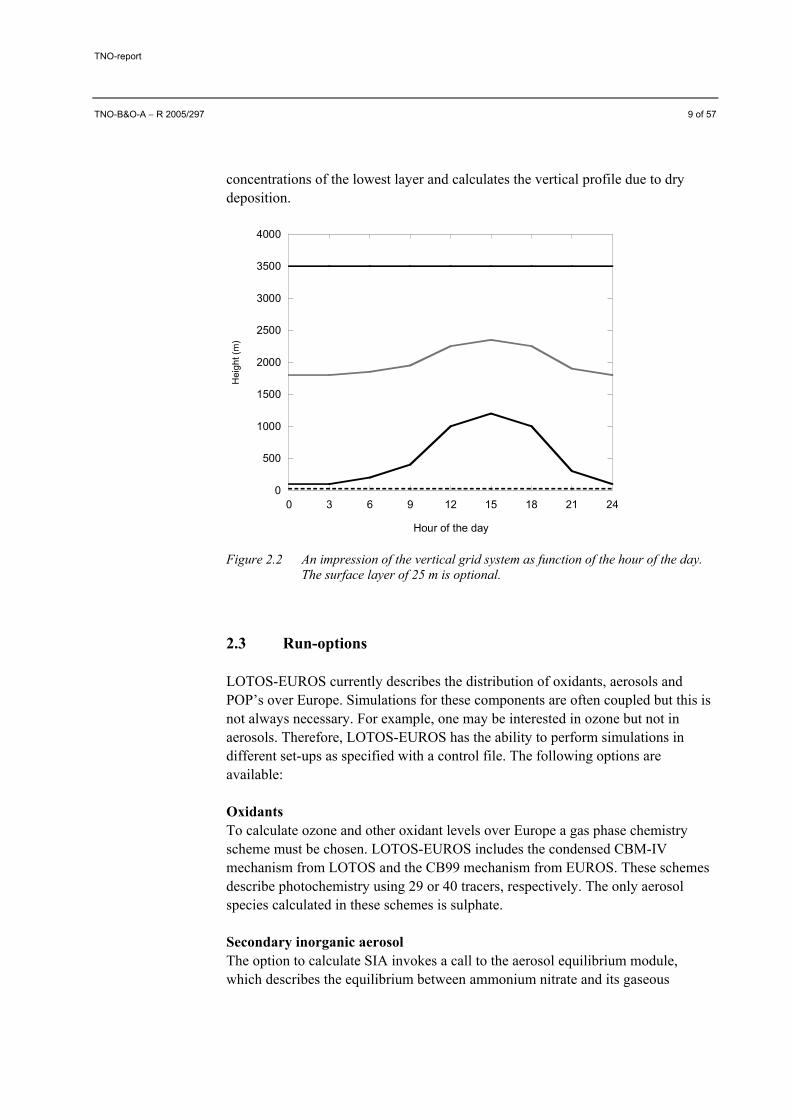
In the vertical there are three dynamic layers and an optional surface layer. The model extends in vertical direction 3.5 km above sea level. The lowest dynamic layer is the mixing layer, followed by two reservoir layers. The height of the mixing layer is derived from meteorological observations and interpolated by the Free University of Berlin or obtained from ECMWF analyses. Mixing layer heights are input into the model every 3 hours. The model uses linear interpolation within the time interval of 3 hours. The height of the reservoir layers is determined by the difference between ceiling (3.5 km) and mixing layer height (See Fig 2.2). Both layers are equally thick with a minimum of 50m. In some cases when the mixing layer extends near or above 3500 m the top of the model exceeds the 3500 m according to the abovementioned description. Optionally, a surface layer with a fixed depth of 25 m can be included in the model. Inclusion of this surface layer is especially useful when concentrations of primary constituents are to be simulated. For output purposes, a diagnostic layer is used to calculate concentrations near the surface (reference height is usually 3.6 m, but it can be changed). It uses the
TNO-report
TNO-B&O-A − R 2005/297 9 of 57
concentrations of the lowest layer and calculates the vertical profile due to dry deposition.
0
500
1000
1500
2000
2500
3000
3500
4000
0 3 6 9 12 15 18 21 24
Hei
ght (
m)
Hour of the day
Figure 2.2 An impression of the vertical grid system as function of the hour of the day. The surface layer of 25 m is optional.
2.3 Run-options
LOTOS-EUROS currently describes the distribution of oxidants, aerosols and POP’s over Europe. Simulations for these components are often coupled but this is not always necessary. For example, one may be interested in ozone but not in aerosols. Therefore, LOTOS-EUROS has the ability to perform simulations in different set-ups as specified with a control file. The following options are available:
Oxidants To calculate ozone and other oxidant levels over Europe a gas phase chemistry scheme must be chosen. LOTOS-EUROS includes the condensed CBM-IV mechanism from LOTOS and the CB99 mechanism from EUROS. These schemes describe photochemistry using 29 or 40 tracers, respectively. The only aerosol species calculated in these schemes is sulphate.
Secondary inorganic aerosol The option to calculate SIA invokes a call to the aerosol equilibrium module, which describes the equilibrium between ammonium nitrate and its gaseous
TNO-report
10 of 57 TNO-B&O-A − R 2005/297
counterparts, ammonia and nitric acid. SIA calculations can only be performed in combination with the full oxidant scheme.
Secondary organic aerosol This option invokes a call to the aerosol equilibrium module, which describes the formation of secondary organic aerosol (SOA). SOA calculations can only be performed in combination with the full oxidant scheme.
Primary aerosol This option enables to switch on/off the calculations for primary aerosol components. At the moment, the primary components include primary PM2.5, PM10-2.5, Black Carbon (BC) and coarse and fine mode sea salt. The calculations for the primary components can be performed stand alone.
Sulphur-only The sulphur-only option performs a simulation for SO2 and SO4 using predefined OH radical concentrations. Hence, the simulation comprises only 2 tracers and is very fast. The sulphur-only option can not be performed together with oxidant calculations as it does not make any sense.
POP’s LOTOS-EUROS also contains a module to perform calculations for PAH’s and POP’s. The description of the model code for these compounds will be reported in a separate document. The code is based on the EUROS-POP module described by Jacobs en van Pul (1996).
TNO-report
TNO-B&O-A − R 2005/297 11 of 57
3. Transport
The transport consists of advection in 3 dimensions, horizontal and vertical diffusion, and entrainment. The advection is driven by meteorological fields (u,v) which are input every 3 hours. The two horizontal wind component u and v are derived from observations according to the Optimal Interpolation method (Kerschbaumer and Reimer, 2003). The wind components are “terrain following”. Terrain following means practically that the ground level wind patterns follow the orography of Europe. The inclusion of the orography is “ensured” in the process of making the meteorological fields. In the LOTOS model the wind components, as well as other meteorological components are input into the model. The vertical wind speed w is calculated by the model as a result of the divergence/convergence of the horizontal wind fields. The recently improved and highly-accurate, monotonic advection scheme developed by Walcek (2000) is used to solve the system. The number of steps within the advection scheme is controlled by the Courant number. The number of steps is chosen such that the Courant restriction is fulfilled everywhere.
Entrainment is caused by the growth of the mixing layer during the day. Each hour the vertical structure of the model is adjusted to the new mixing layer depth. After the new structure is set the pollutant concentrations are redistributed using linear interpolation.
Horizontal and vertical diffusion The horizontal eddy diffusion coefficient Kh is defined as the product of an empirical constant η and a velocity deformation tensor Def .
Kh = η |Def|
∂∂
−∂∂
+
∂∂
+∂∂
=22
|Def|yV
xU
yU
xV
The empirical constant η has a value of 9000 m2 (Liu and Durran, 1977). The Kh value is constraint between 10 m2s-1 and an upper limit of 105 m2s-1.
Vertical diffusion is described using the standard Kz-theory. The Kz values are calculated within the stability parameterisation and are described in the Chapter on meteorology. Vertical exchange is calculated employing the new integral scheme by Yamartino et al. (2005).
TNO-report
12 of 57 TNO-B&O-A − R 2005/297
TNO-report
TNO-B&O-A − R 2005/297 13 of 57
4. Chemistry
Ozone is formed in the atmosphere through chemical reactions between nitrogen oxides (NOx) and volatile organic compounds (VOC). Tens of inorganic and hundreds of organic compounds are known to participate in thousands of photochemical reactions. The explicit treatment of all of these compounds and reactions would be prohibitively complex in an Eulerian-based chemical transport model such as LOTOS-EUROS, especially when such a model is used for long-term (multi-annual) calculations in the framework of regulatory purposes. Since condensation of atmospheric chemistry is required to reach a level of simplification imposed by computational constraints, methods for minimizing the size of a chemical mechanism have been proposed.
A possible way of condensing the inorganic chemistry within photochemical mechanisms is through the lumping of species or the lumping of reactions utilising specific assumptions, e.g. steady state for some radicals. In the lumped structure approach, organic compounds are apportioned to one or more species on the basis of carbon-carbon bond type or on basis of a reactive group (Gery, 1989). For example, propane (CH3-CH2-CH3) is represented by three parafinic groups (PAR) since all three carbon atoms have only single bonds: propene (CH2=CH-CH3) is represented as one olefinic group (OLE) representing the carbon-carbon double bond, and one PAR representing the methyl group.
The most widely applied mechanism using the lumped structure approach for representing urban photochemistry is the Carbon Bond-IV (CB-IV) mechanism. The CB-IV mechanism originally consisted of 81 reactions. It is probably the most widely used mechanism due to its good performance in polluted areas and its relative small number of reactions. In LOTOS-EUROS we use two different versions of CB-IV, called CBM-IV and CB99.
The gas phase mechanisms also describe the photochemical formation of sulphuric acid and nitric acid, which drive the formation of secondary inorganic aerosol. Below we describe the set-up for CBM-IV and CB99 schemes as well as the aerosol chemistry.
4.1 LOTOS chemistry including CBM-IV
The gas phase photochemistry CBM-IV module in LOTOS-EUROS is a modified (condensed) version of the CBM-IV mechanism by Whitten et al. (1980). Characteristic for the Carbon-Bond Mechanism (CBM) are the structure molecules, such as PAR, ETH, FORM, ALD2, MGLY, XO2, XO2N, etc. The structure molecules represent parts of the organic molecules, only ETH has a one-to-one relation with ethane. The full mechanism including the reaction rate
TNO-report
14 of 57 TNO-B&O-A − R 2005/297
parameterisation is shown in Annex A. The scheme includes 28 species and 66 reactions, including 12 photolytic reactions. Compared to the original scheme steady state approximations were used to reduce the number of reactions. In addition, reaction rates have been updated regularly. The mechanism was tested against the results of an intercomparison presented by Poppe et al. (1996) and found to be in good agreement with results presented for other mechanisms. The chemistry scheme further includes gas phase and heterogeneous reactions leading to secondary aerosol formation as presented below. The CBM-IV chemistry is solved using the QSSA method.
Sulphate production It is important to give a good representation of sulphate formation, since sulphate is an important aerosol component. In addition, it competes for the ammonia available to combine with nitric acid. Most models that represent a direct coupling of sulphur chemistry with photochemistry underestimate sulphate levels in winter in Europe. This feature can probably be explained by a lack of model calculated oxidants or missing reactions (Khasibatla et al., 1997). Therefore, in addition to the gas phase reaction of OH with SO2 (in CBM-IV) we represent additional oxidation pathways in clouds with a simple first order reaction constant (Rk), which is calculated as function of relative humidity (%) and cloud cover (ε): Rk = 8.3e-5 * (1 + 2*ε) (s-1), for RH < 90 % Rk = 8.3e-5 * (1 + 2*ε) * [1.0 + 0.1*(RH-90.0)] (s-1), for RH ≥ 90 %
This parameterization is similar to that used by Tarrason and Iversen (1998). It enhances the oxidation rate under cool and humid conditions. With cloud cover and relative humidity of 100 % the associated time scale is approximately two hours. Under humid conditions, the relative humidity in the model is frequently higher than 90 % during the night.
Heterogeneous N2O5 chemistry The reaction of N2O5 on aerosol surfaces has been proposed to play an important role in tropospheric chemistry (Dentener and Crutzen, 1993). This reaction is a source for nitric acid during night time, whereas during the day the NO3 radical is readily photolysed. We parameterised this reaction following Dentener and Crutzen (1993). In this parameterisation a Whitby size distribution is assumed for the dry aerosol. The wet aerosol size distribution is calculated using the aerosol associated water obtained from the aerosol thermodynamics module (see below). The reaction probability of N2O5 on the aerosol surface has been determined for various solutions. Reaction probabilities between 0.01 and 0.2 were found (Jacob, 2000 and references therein). A study by Mentel et al. (1999) indicates values at the lower part of this range. Therefore, we use a probability of γ = 0.05, which is somewhat lower than the generally used recommendation by Jacob (2000). In the polluted lower troposphere of Europe, however, the hydrolysis on the aerosol surfaces is fast, with lifetimes of N2O5 less than an hour (Dentener and Crutzen, 1993). Therefore the exact value of γ does not determine the results strongly. Due
TNO-report
TNO-B&O-A − R 2005/297 15 of 57
to the limited availability of detailed cloud information, we neglect the role of clouds on the hydrolysis of N2O5, which may also contribute to nitric acid formation. However, due to the very fast reaction of N2O5 on aerosol in polluted Europe, the role of clouds on N2O5 hydrolysis is probably less important.
4.2 EUROS chemistry including CB99
The second gas phase chemistry mechanism that is included in LOTOS-EUROS, CB99, is the officially documented and vindicated version by Adelman (1999). CB99 is presented as an updated version of the mechanism and is produced through a critical review of the relevant literature. Kinetic and minor mechanistic updates are applied to the mechanism to make it consistent with the currently best available information. Empirical verification for each major change is presented through modeling Outdoor Chamber and Indoor Teflon smog-chamber experiments. Quantitative and qualitative analyses are presented on the performance of the new mechanism and its predications are compared to those of two older versions of CB-IV. Adelman shows that CB99 exhibits extremely good performance in modelling a wide range of experiments in multiple smog chambers. He recommends the new mechanism for future applications of regulatory air quality simulation models and areas for further improvement are discussed.
CB99 includes 42 species and 95 reactions, including 13 photolytic reactions. Major changes comprise the addition of four reactions with sulphur dioxide, methanol and ethanol, see also Carter (1994), and an updated CB-IV isoprene chemistry mechanism based on the work of Carter (1996). The translation of this updated CB-IV isoprene chemistry mechanism into CB-IV components is given in Whitten et al. (1996). The full chemical mechanism is given in Annex B. The CB99 chemistry is solved using the a Rosenbrock-3 method.
4.3 Aerosol chemistry in LOTOS-EUROS
Semi-volatile aerosol species are species that maintain equilibrium between the aerosol and gas phase. Ammonium nitrate is a well known example but also organic species can be described as semi-volatile components. Below we specify the methods used to calculate the formation of these components in LOTOS-EUROS.
4.3.1 SIA: Ammonium nitrate
Three thermodynamic equilibrium modules can be used to describe the equilibrium between gaseous nitric acid, ammonia and particulate ammonium nitrate and ammonium sulphate and aerosol water. The three modules are ISORROPIA (Nenes
TNO-report
16 of 57 TNO-B&O-A − R 2005/297
et al., 1998), MARS (Binkowski and Shankar, 1995; Schaap, 1999) and EQSAM (Metzger et al., 2004). Equilibrium between the aerosol and gas phase is assumed at all times. For sub-micron aerosol this equilibrium assumption is valid in most cases, but it may not be valid for coarse fraction aerosol (Meng and Seinfeld, 1996). As our model does currently not incorporate the reaction of nitric acid with sea salt the results of our equilibrium calculations over marine and arid regions should be interpreted with care (Zhang et al., 2001).
4.3.2 Secondary organic aerosol
Secondary biogenic aerosol concentrations may contribute significantly to the total aerosol mass, especially in remote regions. There are little to no measurements of these compounds and there is only very limited experimental knowledge on their formation in the atmosphere. Moreover, large parts of the SOA arise from condensed biogenic precursors whose emissions are still not well known. Hence, the model description and its results are very uncertain. Below we describe the module that computes the secondary biogenic aerosol concentrations, which can optionally be turned on during a model run. Secondary organic aerosols are computed in a similar way as their inorganic counterparts, starting with a number of organic precursors, in literature usually called Reactive Organic Gases (ROG). These organic gases react with OH, the NO3 radical and O3 (or with a subset of these species) resulting into a number of products (Schell, 2000), schematically represented by ROG + OH → Σ αi Ci ROG + NO3 → Σ αi Ci ROG + O3 → Σ αi Ci
The products Ci are partitioned between the gas-phase and the aerosol-phase through equilibrium. In order to calculate the equilibrium concentrations, the module SORGAM is used. This module takes into account 8 different degradation products (from the reaction of an ROG with OH, NO3 or O3). Mainly the biogenic precursors (isoprene, α-pinene) lead to degradation products that give contributions to the aerosol-phase. Anthropogenic ROGs hardly result into a significant contribution to the SOA concentrations.
Since we think that the SOA concentrations are small (on average), they are neglected in most LOTOS-EUROS applications, since they require a disproportional amount of extra CPU time. Recall that 16 additional species (8 gas phase and 8 aerosol phase) need to be taken into account.
TNO-report
TNO-B&O-A − R 2005/297 17 of 57
5. Dry deposition
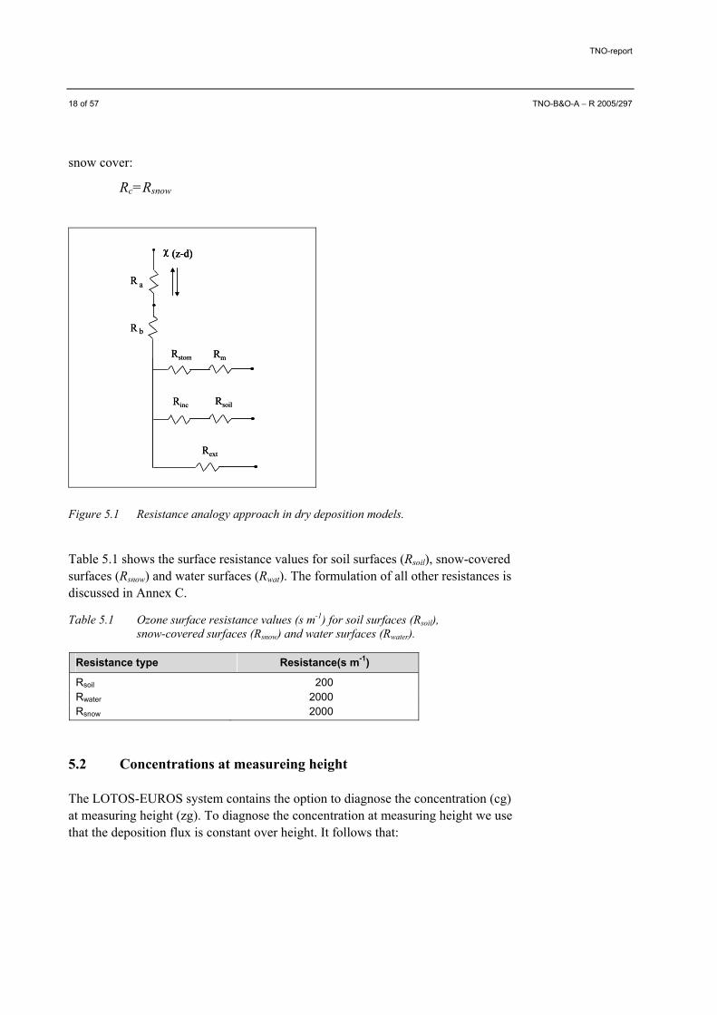
The dry deposition in LOTOS-EUROS is parameterised following the well known resistance approach:
The deposition speed is described as the reciprocal sum of three resistances: the aerodynamic resistance, the viscous sub- layer resistance and the surface resistance. The aerodynamic resistance is dependent on atmospheric stability and is calculated with the stability part of the model. The method used to describe this resistance can be found in Chapter 7 on Meteorology. The viscous sub-layer resistance and the surface resistances for acidifying components and particles are described following the EDACS system developed at ECN. The description of this system is incorporated in Annex C. EDACS includes parameterisations for SO2, NH3, NO, NO2, HNO3 and fine and coarse mode aerosol. The EDACS system does not parameterise surface resistances for ozone deposition, which we describe below. Further, we present how we estimate the concentrations at measuring height.
5.1 Surface resistance of ozone
For the surface resistance of ozone we have adopted the same structure as for the acidifying components in EDACS (see Annex C, and Fig 5.1). Hence the Rc value is parameterised as follows:
vegetative surface: 1
111−
+
++
+=
extsoilincmstomc RRRRR
R
water surfaces:
Rc=Rwat
bare soil:
Rc=Rsoil
TNO-report
18 of 57 TNO-B&O-A − R 2005/297
snow cover:
Rc=Rsnow
χ (z-d)
R a
R b
Rstom Rm
Rinc Rsoil
Rext
χ (z-d)χ (z-d)
R a
R b
Rstom Rm
Rinc Rsoil
Rext
Figure 5.1 Resistance analogy approach in dry deposition models.
Table 5.1 shows the surface resistance values for soil surfaces (Rsoil), snow-covered surfaces (Rsnow) and water surfaces (Rwat). The formulation of all other resistances is discussed in Annex C.
Table 5.1 Ozone surface resistance values (s m-1) for soil surfaces (Rsoil), snow-covered surfaces (Rsnow) and water surfaces (Rwater).
Resistance type Resistance(s m-1)
Rsoil 200 Rwater 2000 Rsnow 2000
5.2 Concentrations at measureing height
The LOTOS-EUROS system contains the option to diagnose the concentration (cg) at measuring height (zg). To diagnose the concentration at measuring height we use that the deposition flux is constant over height. It follows that:
TNO-report
TNO-B&O-A − R 2005/297 19 of 57
)1()1(
1,
11
11
1
zzrefd
tot
zzref
totd
tot
zzreftot
dg
d
dgd
RaVcR
Raccg
RwithV
RRaR
cV
cVcg
cgVcVF
⋅−⋅=−⋅=
=−
⋅=⋅
=
⋅−=⋅−=
The aerodynamic resistance from measuring height (zref) to the height (z) for which the dry deposition speed is calculated in the stability module of LOTOS-EUROS. The abovementioned approach is used for all components except Ozone and NOx. For O3 and NOx we assume a photochemical steady state within the profile. We asess the Ox and NOx concentratrion at measuring height using the Ox and NOx deposition speeds:
[NO2] * k1 = [NO] * [O3] * k3
The reaction rates k1 and k2 are given in Annex A and B. Solving this equation by using NO=NOx-NO2 and O3 = Ox-NO2 gives the equilibriated ground level concentrations.
TNO-report
20 of 57 TNO-B&O-A − R 2005/297
TNO-report
TNO-B&O-A − R 2005/297 21 of 57
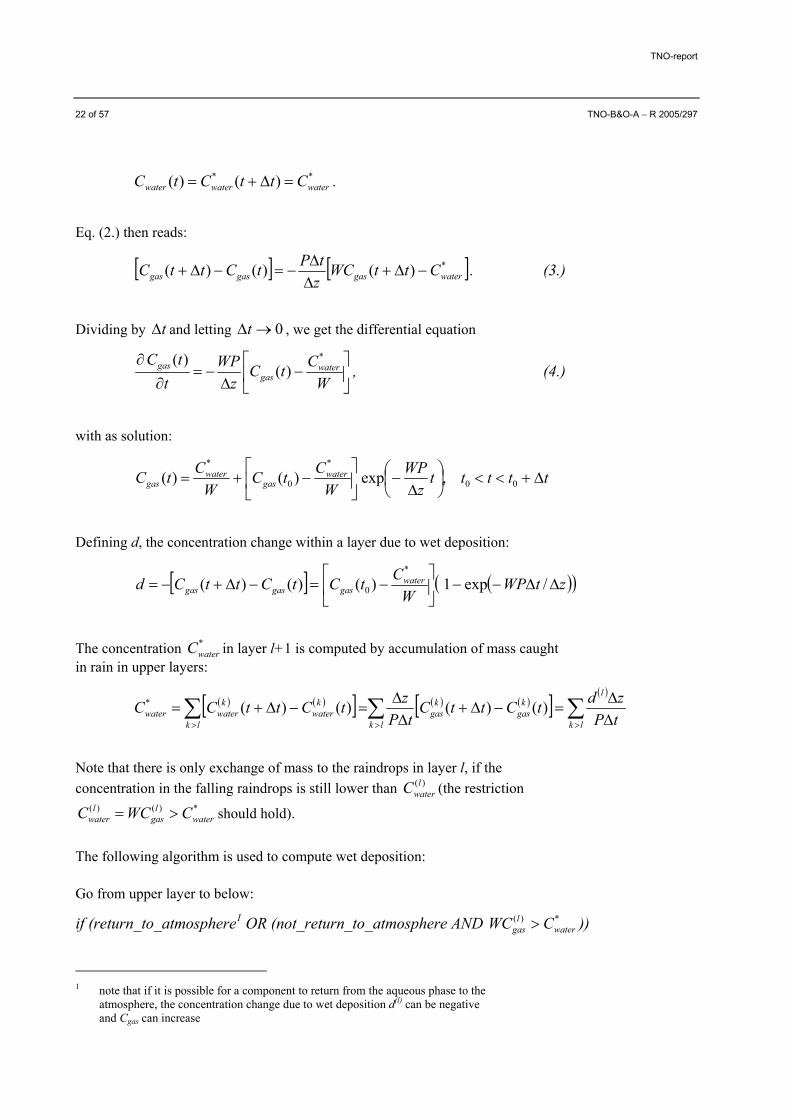
6. Wet Deposition
In LOTOS-EUROS wet deposition is treated in a simplified way. As the meteorological input does not contain detailed information on clouds the in-cloud scavenging of gases and aerosols is neglected. Hence, below we describe the parameterisations for below cloud scavenging only.
6.1 Gases
The standard method to calculate wet deposition for soluble gases is described below.
We define the following parameters: M: mass (µg) Cwater: concentration of component in water (rain), i.e. mass of component per
volume of water (µg/m3) Cgas: concentration of component in gas phase, i.e. mass of component per
volume of air (µg/m3) t: time (h) ∆t: time step (h) V: volume (m3) A: horizontal area (m2) ∆z: layer depth (m) P: precipitation rate (m/h) W: washout ratio, the ratio Cwater/Cgas
Exchange of mass takes place between gas in the air and the raindrops. Conservation of mass says:
We now assume that the process of falling rain from upper layers and mass getting into the raindrops can be split (operator splitting) in the following way: compute the water concentration at the end of the time step in the uppermost layer, then assume that concentration to be the input concentration for the next (lower) layer. Thus proceed to lower layers. Defining *
waterC the water concentration of the layer above the current layer (which has been computed in previous stages and is assumed constant in the current layer), then the operator splitting leads to:
TNO-report
22 of 57 TNO-B&O-A − R 2005/297
** )()( waterwaterwater CttCtC =∆+= .
Eq. (2.) then reads:
[ ] [ ]*)()()( watergasgasgas CttWCztPtCttC −∆+
∆∆
−=−∆+ . (3.)
Dividing by t∆ and letting 0→∆t , we get the differential equation
−
∆−=
∂∂
WCtC
zWP
ttC water
gasgas
*
)()(
, (4.)
with as solution:
tttttz
WPW
CtCW
CtC watergas
watergas ∆+<<
∆−
−+= 00
*
0
*
,exp)()(
Defining d, the concentration change within a layer due to wet deposition:
[ ] ( )( )ztWPW
CtCtCttCd watergasgasgas ∆∆−−
−=−∆+−= /exp1)()()(
*
0
The concentration *waterC in layer l+1 is computed by accumulation of mass caught
in rain in upper layers:
( ) ( )[ ] ( ) ( )[ ]( )
∑ ∑∑> >> ∆
∆=−∆+
∆∆
=−∆+=lk lk
lk
gask
gaslk
kwater
kwaterwater tP
zdtCttCtP
ztCttCC )()()()(*
Note that there is only exchange of mass to the raindrops in layer l, if the concentration in the falling raindrops is still lower than )(l
waterC (the restriction *)()(water
lgas
lwater CWCC >= should hold).
The following algorithm is used to compute wet deposition:
Go from upper layer to below:
if (return_to_atmosphere1 OR (not_return_to_atmosphere AND *)(water
lgas CWC > ))
1 note that if it is possible for a component to return from the aqueous phase to the
atmosphere, the concentration change due to wet deposition d(l) can be negative and Cgas can increase
TNO-report
TNO-B&O-A − R 2005/297 23 of 57
( )( )ztWPW
CtCd watergas
l ∆∆−−
−= /exp1)(
*
0)(
)(0
)(0
)( )()( llgas
lgas dtCttC −=∆+
∑> ∆
∆=
lk
l
water tPzdC
)(*
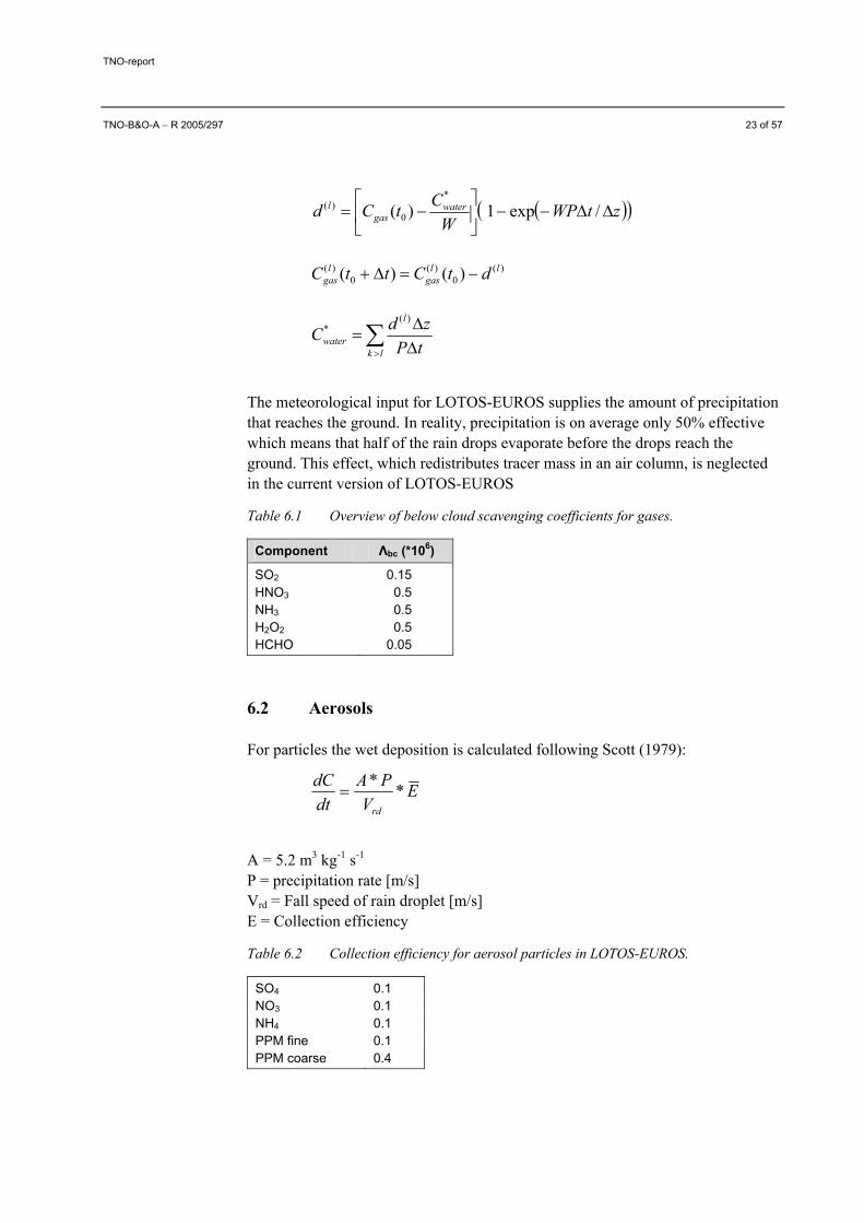
The meteorological input for LOTOS-EUROS supplies the amount of precipitation that reaches the ground. In reality, precipitation is on average only 50% effective which means that half of the rain drops evaporate before the drops reach the ground. This effect, which redistributes tracer mass in an air column, is neglected in the current version of LOTOS-EUROS
Table 6.1 Overview of below cloud scavenging coefficients for gases.
Component Λbc (*106)
SO2 0.15 HNO3 0.5 NH3 0.5 H2O2 0.5 HCHO 0.05
6.2 Aerosols
For particles the wet deposition is calculated following Scott (1979):
EV
PAdtdC
rd
**=
A = 5.2 m3 kg-1 s-1 P = precipitation rate [m/s] Vrd = Fall speed of rain droplet [m/s] E = Collection efficiency
Table 6.2 Collection efficiency for aerosol particles in LOTOS-EUROS.
6.3 Alternative scheme for below cloud scavenging of gases
LOTOS-EUROS also contains an alternative and simple parameterisation to describe the below scavenging of gaseous species. The scavenging of a soluble component C is given by:
The scavenging coefficients (Λbc) were adopted from EMEP (2004; website) and are listed in Table 6.3.
Table 6.3 Overview of below cloud scavenging coefficients for gases.
Component Λbc (*106)
SO2 0.15 HNO3 0.5 NH3 0.5 H2O2 0.5 HCHO 0.05
TNO-report
TNO-B&O-A − R 2005/297 25 of 57
7. Meteorology
The model has an off-line meteorology: the meteorological fields are input every 3-hour. The fields are provided by ECMWF and FUB (see annex for abbreviations). There is a choice to select one of the two data sets. At the moment, ECMWF data sets available to the model cover the meteorological years 1990 till 2004. For the FUB data set, the period 1995-2004 is covered, and in the near future the extension to 1990-1994 will be made.
7.1 FUB data
Meteorological data are obtained from the Free University of Berlin (FUB). The meteorological data are produced at the FUB employing a diagnostic meteoro-logical analysis system based on an optimum interpolation procedure on isentropic surfaces. The system utilizes all available synoptic surface and upper air data (Reimer and Scherer, 1992; Kerschbaumer and Reimer, 2003). The output on the horizontal domain of LOTOS-EUROS of this system is available at TNO. The actual vertical interpolation is performed using a preprocessor at TNO, which enables to specify the vertical resolution, e.g. the vertical extent and the number of layers within and above the mixing layer. The available meteorological input parameters are listed in Table 7.1. Most of the parameters are used in the model. However, the height of the cloud top and base and the stability parameters are not incorporated. Cloud base and top height are excluded because the quality of the data is not good enough. The stability parameters are calculated inside the model for consistency reasons.
TNO-report
26 of 57 TNO-B&O-A − R 2005/297
Table 7.1 The meteorological parameters available in the FUB data.
Parameter
U-wind component [m/s] V-wind component [m/s] Temperature [K] Water vapour [ppm] Density [Kg/m3] Obukov-Monin length* [m] Ustar* [m/s] Precipitation [mm/3h] 10m wind speed [m/s] 2m temperature [K] Cloud cover [] Mixing layer height [m] Surface temperature [K] Surface humidity* [%] Cloud top* [m] Cloud base* [m] Solar radiation [W/m2] Snow fall [mm/3h] Layer heights [m]
A few meteorological parameters are calculated or adjusted inside the model. The relative humidity is calculated from the water vapour concentration using the Claussius-Clapeyron relation. In addition, we neglect rain when the 3-hour accumulated amount of rain is less than 0.3 mm. A limit value was necessary as the rain amounts are very often negligibly small but non zero, which results in a wetted surface. A wet surface has a large impact on the dry deposition speeds for some components, e.g. ozone. Consequently, without the limit value these very small rain amounts would affect the dry deposition fluxes significantly. Finally, stability parameters are calculated online, see below.
7.2 ECMWF data
A meteorological preprocessor has been built to transform meteorological fields derived from ECMWF to input files that LOTOS-EUROS can read. Fields are interpolated from the ECMWF grid (resolution 0.5625° x 0.5625°) to a ½ ° x ¼ ° (longitude x latitude) grid, as used by LOTOS-EUROS.
The meteorological preprocessor comprises the following steps: – read single-layer HDF files with ECMWF meteo fields:
temperature at 2 m cloud cover boundary layer height relative humidity at 2 m wind velocity at 10 m precipitation
TNO-report
TNO-B&O-A − R 2005/297 27 of 57
– interpolate meteo fields in space – set heights of LOTOS-EUROS model layers, using the boundary layer height – read multi-layer HDF files with ECMWF meteo fields
geopotential temperature x-component of wind velocity y-component of wind velocity relative humidity
– interpolate meteo fields in (horizontal) space – interpolate from ECMWF pressure levels to middle of LOTOS layers, using
the geopotential – write meteo fields to binary GRADS format
Most ECMWF meteorological fields are available for each 3 hours; if there are only data available each 6 hours, an extra temporal interpolation step is performed in order to get output each 3 hours.
Wind components in LOTOS-EUROS are “terrain following”. Terrain following means practically that the ground level wind patterns follow the orography of Europe. The inclusion of the orography is “ensured” within the vertical interpolation process of the meteorological fields, because measured horizontal wind speeds are used in the procedure, and these measured wind speeds contain implicitly the terrain features.
A few meteorological parameters are calculated or adjusted inside the model. After the fields are read, the model calculates the corresponding vertical velocity fields (w) according to the mass conservation law of incompressible fluids. Further, the water vapour concentration is calculated using the Claussius-Clapeyron relation. In addition, we neglect rain when the 3-hour accumulated amount of rain is less then 0.3 mm. A limit value was necessary as the rain amounts are very often negligibly small but non zero, which results in a wetted surface. A wet surface has a large impact on the dry deposition speeds for some components, e.g. ozone. Consequently, without the limit value the very small rain amounts would affect the dry deposition fluxes significantly. Finally, stability parameters are calculated online, see below.
Linear interpolation is used to derive the meteorological fields at the interval times between the update times (0h, 3h, etc).
TNO-report
28 of 57 TNO-B&O-A − R 2005/297
7.3 Stability and vertical diffusion coefficient
The vertical diffusion coefficient Kv is determined by:
( )LzU
Kvφκ ∗=
where κ = von Karman constant (0.35) U = friction velocity z = height
L = Monin-Obukov length Φ= function proposed by Businger et al. (1971).
The Monin-Obukov length L is determined as follows:
SEzSaaSL 0)(1 2
21 +=
with a1 and a2 being constants (0.004349 and 0.003724 respectively), z0 the surface roughness length and S and SE given by:
( ))(5.00.35.0 CEabsUS s +−−=
2321 )( SbSabsbbSE ++=
with b1, b2 and b3 being constants (-0.5034, 0.2310 and –0.0325 resp.). Us is the wind speed near the surface (given as input into the model) and CE is an exposure factor depending on cloud cover and solar zenith angle.
For a stable atmosphere (L>0) the expression of the empirical function Φ is:
+=
Lz
Lz
s 7.41φ
For an unstable atmosphere (L<0) the expression is: 25.0
151−
−=
Lz
Lz
uφ
For a neutral atmosphere the function is equal to unity.
TNO-report
TNO-B&O-A − R 2005/297 29 of 57
The friction velocity follows from:
fUU rκ
=∗
with Ur being the wind speed at a reference height (10 m) given as input into the model.
The function f in a stable atmosphere is given by:
−
+
=
Lzz
zz
f rr 0
0
7.4ln
In an unstable atmosphere the function f is:
−
+
+
−
−
+
−
= −−
Lz
Lz
LzLz
LzLz
f
ur
uu
u
ru
ru
0
11
0
0
1tan21tan21
1ln
1
1ln
φφφ
φ
φ
φ
with the empirical function for an unstable atmosphere Φu applied on the reference height zr and on the height of the surface roughness z0.
Aerodynamic resistance From the stability parameters presented above one can easily calculate the aerodynamic resistance:
dzzU
zRah
z∫
∗
=0
)(κφ
It follows that:
*Uf
Ra h
κ=
with fh analogous to function f but instead of reference height the integral is taken to the height to which the aerodynamic resistance is required.
TNO-report
30 of 57 TNO-B&O-A − R 2005/297
TNO-report
TNO-B&O-A − R 2005/297 31 of 57
8. Emissions
8.1 Anthropogenic Emissions
The major driver of the LOTOS-EUROS system is the anthropogenic emission data of VOC, SOx, NOx, NH3, CO, CH4 and PM. In the framework of UBA-project FKZ 202 43270, a European-wide emission data base for the year 2000 has been made on grids of 0.25 x 0.125 latlong, about 15 x 15 km2. The emission sectoral totals have been scaled to conform to the latest country submissions to EMEP for the year 2000, whenever available ( Visschedijk and Denier van der Gon, 2005). The database contains a separation between area and point source information. This database for point sources has been set up already in the 80s and has been updated since, using various sources of information such as national authorities, contacts with (local) experts, industrial interest organisations, various proprietary data bases etc. PM emissions for 2000 are assumed to be the same as those in the CEPMEIP project (derived for 1995). The reasoning is that the uncertainty in the emission estimate is much larger than the trend in the PM emissions. The CEPMEIP database does not specify the composition of the emitted particles. Therefore, black carbon emissions were derived from the primary PM2.5 emissions. The BC emissions are calculated in the model from the estimated BC-fractions per country and source category (Schaap et al., 2004b). We assume 2% of the SO2 emissions to be emitted as particulate sulphate.
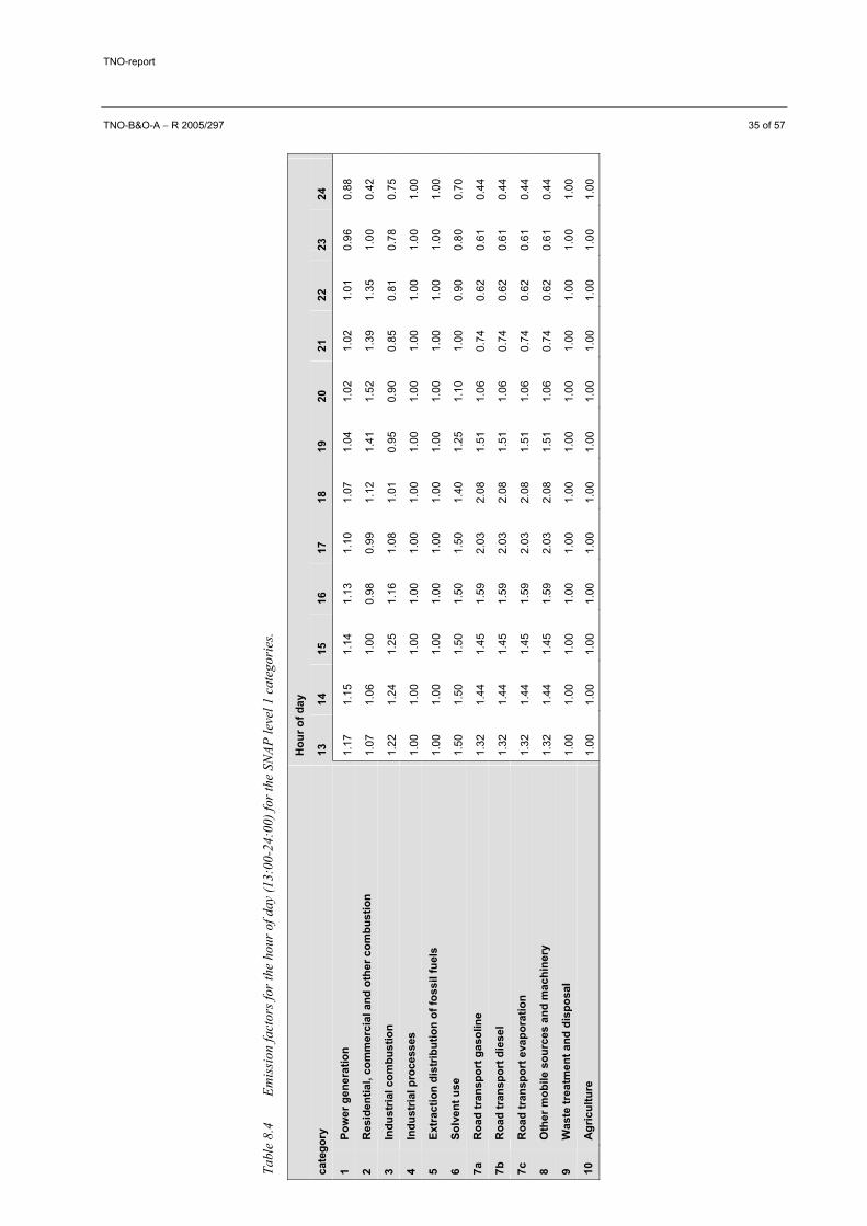
8.1.1 Time- and temperature factors
The basic information, which is also the input data for the chemistry-transport-model (LOTOS-EUROS), is the gridded yearly averaged anthropogenic emission database. However in reality emissions of specific source categories, as for example road transport, fluctuate in time and/or with temperature. The time and temperature factors that are in use LOTOS-EUROS are the result of a critical review of these factors within the TROTREP project (Builtjes et al., 2003). The factors used are specified in the tables below.
Tabl
e 8.
1 M
onth
ly e
mis
sion
s fac
tors
for t
he S
NAP
leve
l 1 c
ateg
orie
s.
Cat
egor
y ja
n fe
b m
ar
apr
may
ju
n ju
l au
g se
p oc
t no
v de
c
1 Po
wer
gen
erat
ion
1.20
1.
15
1.05
1.
00
0.90
0.
85
0.80
0.
87
0.95
1.
00
1.08
1.
15
2 R
esid
entia
l, co
mm
erci
al a
nd o
ther
com
bust
ion
1.70
1.
50
1.30
1.
00
0.70
0.
40
0.20
0.
40
0.70
1.
05
1.40
1.
65
3 In
dust
rial c
ombu
stio
n 1.
10
1.08
1.
05
1.00
0.
95
0.90
0.
93
0.95
0.
97
1.00
1.
02
1.05
4 In
dust
rial p
roce
sses
1.
02
1.02
1.
02
1.02
1.
02
1.02
1.
00
0.84
1.
02
1.02
1.
02
0.90
5 Ex
trac
tion
dist
ribut
ion
of fo
ssil
fuel
s 1.
20
1.20
1.
20
0.80
0.
80
0.80
0.
80
0.80
0.
80
1.20
1.
20
1.20
6 So
lven
t use
0.
95
0.96
1.
02
1.00
1.
01
1.03
1.
03
1.01
1.
04
1.03
1.
01
0.91
7a
Roa
d tr
ansp
ort g
asol
ine
0.88
0.
92
0.98
1.
03
1.05
1.
06
1.01
1.
02
1.06
1.
05
1.01
0.
93
7b
Roa
d tr
ansp
ort d
iese
l 0.
88
0.92
0.
98
1.03
1.
05
1.06
1.
01
1.02
1.
06
1.05
1.
01
0.93
7c
Roa
d tr
ansp
ort e
vapo
ratio
n 0.
88
0.92
0.
98
1.03
1.
05
1.06
1.
01
1.02
1.
06
1.05
1.
01
0.93
8 O
ther
mob
ile s
ourc
es a
nd m
achi
nery
0.
88
0.92
0.
98
1.03
1.
05
1.06
1.
01
1.02
1.
06
1.05
1.
01
0.93
9 W
aste
trea
tmen
t and
dis
posa
l 1.
00
1.00
1.
00
1.00
1.
00
1.00
1.
00
1.00
1.
00
1.00
1.
00
1.00
10
Agr
icul
ture
0.
45
1.30
2.
35
1.70
0.
85
0.85
0.
85
1.00
1.
10
0.65
0.
45
0.45
TNO-report
32 of 57 TNO-B&O-A − R 2005/297
Tabl
e 8.
2 Em
issi
on fa
ctor
s for
the
day
of th
e w
eek
for t
he S
NAP
leve
l 1 c
ateg
orie
s.
Cat
egor
y M
on
Tue
Wed
Th
u Fr
i Sa
t Su
n
1 Po
wer
gen
erat
ion
1.06
1.
06
1.06
1.
06
1.06
0.
85
0.85
2 R
esid
entia
l, co
mm
erci
al a
nd o
ther
com
bust
ion
1.08
1.
08
1.08
1.
08
1.08
0.
8 0.
8
3 In
dust
rial c
ombu
stio
n 1.
08
1.08
1.
08
1.08
1.
08
0.8
0.8
4 In
dust
rial p
roce
sses
1.
02
1.02
1.
02
1.02
1.
02
1.02
1
5 Ex
trac
tion
dist
ribut
ion
of fo
ssil
fuel
s 1
1 1
1 1
1 1
6 So
lven
t use
1.
2 1.
2 1.
2 1.
2 1.
2 0.
5 0.
5
7a
Roa
d tr
ansp
ort g
asol
ine
1.02
1.
06
1.08
1.
1 1.
14
0.81
0.
79
7b
Roa
d tr
ansp
ort d
iese
l 1.
02
1.06
1.
08
1.1
1.14
0.
81
0.79
7c
Roa
d tr
ansp
ort e
vapo
ratio
n 1.
02
1.06
1.
08
1.1
1.14
0.
81
0.79
8 O
ther
mob
ile s
ourc
es a
nd m
achi
nery
1
1 1
1 1
1 1
9 W
aste
trea
tmen
t and
dis
posa
l 1
1 1
1 1
1 1
10
Agr
icul
ture
1
1 1
1 1
1 1
TNO-report
TNO-B&O-A − R 2005/297 33 of 57
Tabl
e 8.
3 Em
issi
on fa
ctor
s for
the
hour
of d
ay (1
:00-
12:0
0) fo
r the
SN
AP le
vel 1
cat
egor
ies.
H
our o
f day
Cat
egor
y 1
2 3
4 5
6 7
8 9
10
11
12
1 Po
wer
gen
erat
ion
0.79
0.
72
0.72
0.
71
0.74
0.
80
0.92
1.
08
1.19
1.
22
1.21
1.
21
2 R
esid
entia
l, co
mm
erci
al a
nd o
ther
com
bust
ion
0.38
0.
36
0.36
0.
36
0.37
0.
50
1.19
1.
53
1.57
1.
56
1.35
1.
16
3 In
dust
rial c
ombu
stio
n 0.
75
0.75
0.
78
0.82
0.
88
0.95
1.
02
1.09
1.
16
1.22
1.
28
1.30
4 In
dust
rial p
roce
sses
1.
00
1.00
1.
00
1.00
1.
00
1.00
1.
00
1.00
1.
00
1.00
1.
00
1.00
5 Ex
trac
tion
dist
ribut
ion
of fo
ssil
fuel
s 1.
00
1.00
1.
00
1.00
1.
00
1.00
1.
00
1.00
1.
00
1.00
1.
00
1.00
6 So
lven
t use
0.
50
0.35
0.
20
0.10
0.
10
0.20
0.
75
1.25
1.
40
1.50
1.
50
1.50
7a
Roa
d tr
ansp
ort g
asol
ine
0.19
0.
09
0.06
0.
05
0.09
0.
22
0.86
1.
84
1.86
1.
41
1.24
1.
20
7b
Roa
d tr
ansp
ort d
iese
l 0.
19
0.09
0.
06
0.05
0.
09
0.22
0.
86
1.84
1.
86
1.41
1.
24
1.20
7c
Roa
d tr
ansp
ort e
vapo
ratio
n 0.
19
0.09
0.
06
0.05
0.
09
0.22
0.
86
1.84
1.
86
1.41
1.
24
1.20
8 O
ther
mob
ile s
ourc
es a
nd m
achi
nery
0.
19
0.09
0.
06
0.05
0.
09
0.22
0.
86
1.84
1.
86
1.41
1.
24
1.20
9 W
aste
trea
tmen
t and
dis
posa
l 1.
00
1.00
1.
00
1.00
1.
00
1.00
1.
00
1.00
1.
00
1.00
1.
00
1.00
10
Agr
icul
ture
1.
00
1.00
1.
00
1.00
1.
00
1.00
1.
00
1.00
1.
00
1.00
1.
00
1.00
TNO-report
34 of 57 TNO-B&O-A − R 2005/297
Tabl
e 8.
4 Em
issi
on fa
ctor
s for
the
hour
of d
ay (1
3:00
-24:
00) f
or th
e SN
AP le
vel 1
cat
egor
ies.
H
our o
f day
cate
gory
13
14
15
16
17
18
19
20
21
22
23
24
1 Po
wer
gen
erat
ion
1.17
1.
15
1.14
1.
13
1.10
1.
07
1.04
1.
02
1.02
1.
01
0.96
0.
88
2 R
esid
entia
l, co
mm
erci
al a
nd o
ther
com
bust
ion
1.07
1.
06
1.00
0.
98
0.99
1.
12
1.41
1.
52
1.39
1.
35
1.00
0.
42
3 In
dust
rial c
ombu
stio
n 1.
22
1.24
1.
25
1.16
1.
08
1.01
0.
95
0.90
0.
85
0.81
0.
78
0.75
4 In
dust
rial p
roce
sses
1.
00
1.00
1.
00
1.00
1.
00
1.00
1.
00
1.00
1.
00
1.00
1.
00
1.00
5 Ex
trac
tion
dist
ribut
ion
of fo
ssil
fuel
s 1.
00
1.00
1.
00
1.00
1.
00
1.00
1.
00
1.00
1.
00
1.00
1.
00
1.00
6 So
lven
t use
1.
50
1.50
1.
50
1.50
1.
50
1.40
1.
25
1.10
1.
00
0.90
0.
80
0.70
7a
Roa
d tr
ansp
ort g
asol
ine
1.32
1.
44
1.45
1.
59
2.03
2.
08
1.51
1.
06
0.74
0.
62
0.61
0.
44
7b
Roa
d tr
ansp
ort d
iese
l 1.
32
1.44
1.
45
1.59
2.
03
2.08
1.
51
1.06
0.
74
0.62
0.
61
0.44
7c
Roa
d tr
ansp
ort e
vapo
ratio
n 1.
32
1.44
1.
45
1.59
2.
03
2.08
1.
51
1.06
0.
74
0.62
0.
61
0.44
8 O
ther
mob
ile s
ourc
es a
nd m
achi
nery
1.
32
1.44
1.
45
1.59
2.
03
2.08
1.
51
1.06
0.
74
0.62
0.
61
0.44
9 W
aste
trea
tmen
t and
dis
posa
l 1.
00
1.00
1.
00
1.00
1.
00
1.00
1.
00
1.00
1.
00
1.00
1.
00
1.00
10
Agr
icul
ture
1.
00
1.00
1.
00
1.00
1.
00
1.00
1.
00
1.00
1.
00
1.00
1.
00
1.00
TNO-report
TNO-B&O-A − R 2005/297 35 of 57
TNO-report
36 of 57 TNO-B&O-A − R 2005/297
The hour of day is local time, hence information over the deviation from GMT is needed for each country. The following time-zones are incorporated:
GMT+0 UK, Ireland, Iceland and Portugal
GMT+1 all other European countries except those listed with GMT+2:
GMT+2 for Finland, Estonia, Latvia, Belarus, Ukrain, Moldavia, Romania, Bulgaria, Greece and Turkey
GMT+3 Azerbaidjan, Armenia, Georgia, Russia untill the Oeral.
Currently it is assumed that all countries have the shift from summer to wintertime and vice versa at the same days, i.e. the last Sunday of October and March, respectively.
In addition to the time factors specified above in Table 8.1 to 8.4, a temperature factor for road transport, categories 7a and 7b, is applied for the emissions of VOC and CO. Their emissions are assumed to decrease linearly with temperature, as shown in Figure 8.1.
0.60.8
11.2
1.41.61.8
-30 -20 -10 0 10 20 30 40temperature (C)
VOC
CO
Figure 8.1 Temperature factors to be applied for VOC and CO from road transport category (71 and 72: gasoline and diesel).
The higher emissions for VOC and CO at lower temperatures are due to the so-called “cold start”.
TNO-report
TNO-B&O-A − R 2005/297 37 of 57
8.1.2 NMVOC-speciation
CBM-IV uses nine primary organic species (i.e., species emitted directly to the atmosphere as opposed to secondary organic species formed by chemical reaction in the atmosphere). Most of the organic species in the mechanism represent carbon-carbon bond types, but ethene (ETH), isoprene (ISOP) and formaldehyde (FORM) are represented explicitly. CB99 includes two additional primary organic species, methanol (MEOH) and ethanol (ETOH). The carbon-bond types include carbon atoms that contain only single bonds (PAR), double-bonded carbon atoms (OLE), 7-carbon ring structures represented by toluene (TOL), 8-carbon ring structures represented by xylene (XYL), the carbonyl group with adjacent carbon atom and higher molecular weight aldehydes represented by acetaldehyde (ALD2), and non-reactive carbon atoms (NR).
Many organic compounds are apportioned to the carbon-bond species based simply on the basis of molecular structure. For example, propane is represented by three PARs since all three carbon atoms have only single bonds, and propene is represented as one OLE (for the one carbon-carbon double bond) and one PAR (for the carbon atom with all single bonds). Some apportionments are based on reactivity considerations, however. For example, olefins with internal double bonds are represented as ALD2s and PARs rather than OLEs and PARs. Further, the reactivity of some compounds may be lowered by apportioning some of the carbon atoms to the non-reactive class NR. For example, the less reactive ethane (C2H6) is represented as 0.4 PAR and 1.6 NR)(EPA, 1999). Apportioning rules have been established for many organic compounds and can be found in e.g. Gery (1989), US EPA (1989) and Carter (1994).
The NMVOC emissions are split into the model species as presented in Table 8.5 and 8.6 for CBM-IV and CB99, respectively. Presently, we use the VOC-splits as used in LOTOS for CBM4 and EUROS for CB99. Hence, the splits are not internally consistent. The split for CB99 is derived from Barrett and Berge (1996) (see also Brouwer, 2005). The split for CBM4 is based on the emission inventory of VOC’s, which are specified in 125 different species or classes. These species are translated to Carbon bond species. The total and lumbed VOC emissions within a SNAP 1 sector are summed to arrive at the total VOC mass and the total moles of the lumbed Carbon Bond species, which were used to determine the average VOC-split for a SNAP 1 category. A newer version of the split for the CBM4 gas phase chemistry scheme is available from the TROTREP project. The major differences between the current used CBM-IV and TROTREP split are the amount of PAR and UNR species. The TROTREP split yields more PAR which is included as UNR (=Unreactive) in the present split. For a detailed comparison of the available VOC-splits we refer to Brouwer (2005). For 2006 an update of the VOC-splits to arrive at harmonisation between the schemes is foreseen.
TNO-report
38 of 57 TNO-B&O-A − R 2005/297
Table 8.5 VOC-speciation used for CBM-IV(mol/ (Kg VOC)).
* PAR also includes the original CBM4 species ACET and KET following PAR = PAR + 3 ACET + 4 KET
The split for CB99 does not contain toluene (TOL). The reason is that in the past all toluene was attributed to xylene (XYL). The actual split between these compounds could not be recovered.
Table 8.6 VOC-speciation used for CB99 (mol/ (Kg VOC)).
In the LOTOS-EUROS the biogenic NMVOC-emissions from forests are given by a method developed by Veldt (1991). Apart from the difference between deciduous, coniferous and mixed forest, the only other parameter was ambient temperature. Extensive studies by Guenther showed that next to ambient temperature also the Photosynthetic Active Radiation (PAR) is important Guenther (1994). These findings by Guenther (1994) have been applied to Europe by Simpson et al. (1995). Although many uncertainties still exist, the method by Simpson is the most suited at the moment. However, this method distinguishes in more detailed forest types as currently available in our current land use database, PELINDA. Hence, we have not updated our scheme yet and still use the method by Veldt (1991). In the UBA-project FKZ 202 43270 a new CORINE/Smiatek land use data base has been made incorporating detailed tree-species information based on Lenz et al. (2001) containing 115 different tree-species on grids of 1 x 1 km2 over Europe. This land use data base will be used in the near future to determine biogenic emissions.
For isoprene the following formula is currently used:
)0.273*(06.05
)0.273*(06.05
*10403.0
*10115.0−−
−−
⋅=
⋅=Tk
decid
Tkconif
eE
eE
Econif/decid Isoprene emission strength (g/m3/hr) Tk Temperature (K)
The emission only occurs during daylight. The emission strength is weighted with the area covered with deciduous and/or coniferous forest.
Monoterpene emissions are included in the calculation for biogenic secondary aerosol concentrations. Monoterpene emissions, a-pinene and d-limoneen, are assumed to occur only from coniferous forest. For both species the following emission strength is calculated:
)0.303*(09.05 **100.4 −−⋅= Tkconif eCE
Econif Emission strength (g/m3/hr) Tk Temperature (K) C Constant, C is 0.23 for d-limonene and 0.21 for a-pinene
TNO-report
40 of 57 TNO-B&O-A − R 2005/297
The emission only occurs during daylight. The emission strength is weighted with the area covered with coniferous forest.
Previous studies indicated only about 4 % of the total NO emissions to be biogenic. For this reason we neglect the biogenic emission of NO at the moment. The formulation by Yienger and Levy, 1995 has also been implemented in test-form and will be used in the near future.
8.2.2 Sea salt
The sea salt emission fluxes in LOTOS-EUROS are currently described using the source formulation by Monahan et al. (1986). This source formulation is an empirical relation between the the whitecap cover, average decay time of a whitecap, the number of drops produced per square meter of whitecap and the resulting droplet flux dF/dr:
)exp(19.105.141.310
10)exp(19.105.1
41.310
6
10
2
2
10)057.01(373.1
65.0)log(38.0
,10)057.01(
53.31084.3
1)(
B
p
pB
p
pp
rUdrdF
rBr
drdE
UW
drdEUW
drdF
−
−
−
⋅+⋅⋅=
−=⋅+=
=⋅⋅=
⋅⋅=
τ
τ
dF/dr source flux of salt particles per increment of drop radius (µm-1m-2s-1) rp wet droplet radius (µm) U10 wind speed at ten meter (m s-1) W(U10) surface fraction covered with whitecap dE/dr droplet flux per increment of drop radius per unit whitecap (µm-1m-2)
The implementation required to translate the particle flux provided by Monahan (1986) into a sea salt mass flux. As sea salt is most probably a wet aerosol after emission we have to account for the fact that the dry radius determines the sea salt mass and that the wet radius determines the atmospheric lifetime. The relation between dry and wet radius varies with relative humidity but for simplicity we assume a constant particle size. At a relative humidity of 80% the particle radius rp and dry particle radius rd are related as follows:
rp = 2.0*rd
TNO-report
TNO-B&O-A − R 2005/297 41 of 57
Such a particle has a salt mass content mp of:
33
61
34
pNaCldNaClp rrm πρπρ ==
With NaClρ the density of salt (2.17 10-6 µg/m3). The salt mass flux is simply given as:
pp
p drdFm
drdM
=
so that the mass flux for the Monahan formulation becomes:
65.0)log(38.0
,10)057.01()(
)(6373.1
)()(
10)exp(19.105.1
41.31010
10
2 pBp
NaCl
pp
rBrrg
UUf
E
rgUfEdrdM
−=⋅+=
=
=
⋅⋅=
−
πρ
The mass flux is obtained by integrating equation x with respect to rp. As the modelling of sea salt is usually performed in several size bins to account for the lifetime differences between particles of different size, the mass flux for each bin n is taken into account. The constant E and function f are independent of rp and can be taken outside the integral:
p
r
rp
p
r
rp
r
rp
p
drrgnI
nIUfEnM
drrgUfEnM
drdrdMnM
n
n
n
n
n
n
∫
∫
∫
−
−
−
=
⋅⋅=
⋅⋅=
=
1
1
1
)()(
)()()(
)()()(
)(
10
10
where rn and rn-1 are the upper and lower limits of each bin. The numeric value of E is 1.56 10-6 and the value for f(U10) is evaluated every hour in the model using the meteorological parameters from the model.
TNO-report
42 of 57 TNO-B&O-A − R 2005/297
The sea salt module consists of two parts. The first part integrates the size dependent part (I) of the emission formulation over the size bins chosen for the simulation. The lowest size bin is integrated starting from 0.14 um as the Monahan function has not been validated for particles smaller than this size. These calculations are only performed at the start of the simulation. The second part of the module contains the actual calculation of the emission strength and is called every hour. The total flux is scaled with the percentage sea in the grid cell.
TNO-report
TNO-B&O-A − R 2005/297 43 of 57
9. Land-use
Land-use describes the type of land that covers the surface. It is important to establish deposition velocities, in particular the uptake rate and the surface roughness. Also it is required to determine the biogenic emission fluxes, such as isoprene and terpene emissions from forests. Land use and land cover are also important for future calculations of NO-soil emissions and wind blown dust and agricultural emissions from ploughing etc
The land-use data set that is used in the model is the so-called PELINDA data-base (de Boer et al., 2000). The NOAA AVHRR NDVI monthly maximum value composites are the main data source for the land cover classification. The 1997 composites have been used. The land cover categories are listed in Table 9.1.
Table 9.1 Land use classes used in Pelinda (de Boer et al., 2000).
urban area arable land irrigated arable land permanent crops pastures natural grassland shrubs and herbs coniferous forest mixed forest deciduous forest bare soil permanent ice and snow wetlands inland water sea
The PELINDA data base has a resolution of approximately 1x1 km. This is converted into a database on the LOTOS-EUROS grid. Each grid is characterised by the fraction of land-use in that particular grid cell. A grid cell is not typified by one land-use category but is often a combination of several categories.
For European Russia a comparison was made with land-use databases from Russian sources and it was decided to use the Russian data base (Stolbovoi and McCallum, 2002)
To apply the EDACS system for dry deposition we have adapted the land use data used by LOTOS-EUROS, since DEPAC only uses a subset of the land use categories. The conversion of these land use classes is not trivial, and it needs further attention. The conversions we made are listed in Table 9.2.
TNO-report
44 of 57 TNO-B&O-A − R 2005/297
Table 9.2 Conversion of Land use categories from Pelinda to DEPAC.
DEPAC Pelinda database
Grass Pastures + natural grassland + shrubs and herbs Arable Arable land + irrigated arable land Permanent crops permanent crops Coniferous forest Coniferous forest + 0.5 Mixed forest Deciduous forest Deciduous forest + 0.5 Mixed forest Water inland water + sea + wetlands + snow or ice Urban Urban area Other Bare soil Desert 0.0
As has been mentioned under biogenic emissions, recently in the UBA project a new land use data base has been made based upon CORINE/Smiatek. Because the CORINE land use data base has an official status, the so-called Corine/Phare land cover data from EEA, this land use data base will be incorporated into the LOTOS-EUROS model in the near future.
TNO-report
TNO-B&O-A − R 2005/297 45 of 57
10. Initial and Boundary Conditions
10.1 Initial conditions
There are two ways to initialise the concentrations at the start of a simulation. The first is to use data from a previous calculation by reading the data from a restart file. The other method is simply an interpolation of the boundary conditions specified for the first hour of the simulation. The boundary conditions used for the latter are described below. Because normally LOTOS-EUROS model runs are performed over a whole year on an hour-by-hour basis, initial conditions have to be specified only on the first hour of January 1. The impact of the initial conditions will gradually disappear, and be no longer important after say 5 days of modelcalculations.
10.2 Boundary conditions
10.2.1 Logan in combination with the EMEP-method for ozone, aerosols and their precursors
Ozone is the gas where specification of accurate boundary conditions is most essential for a good model performance. This is due to the fact that ambient ozone levels in Europe are typically not much greater than the Northern hemispheric background ozone. In LOTOS-EUROS we use the 3-D climatological dataset by Logan (1998), derived from ozone sonde data, or 3-D datasets from global models (e.g TM3/5) for all boundaries (incl. top). By default we use the data set by Logan (1998) as global model results are not available for all years.
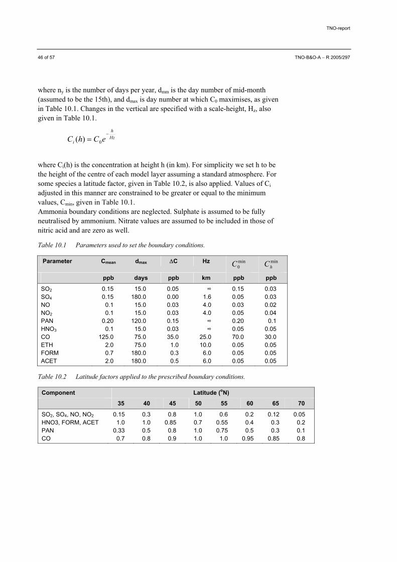
For a number of components, listed in Table 10.1 we follow the EMEP method (Simpson et al., 2003) based on measured data. In this method simple functions have been derived to match the observed distributions. The boundary conditions are adjusted as function of height, latitude and day of the year. The functions are used to set the boundary conditions, both at the lateral boundaries as at the model top. The annual cycle of each species is represented with a cosine-curve, using the annual mean near-surface concentration, C0, the amplitude of the cycle ∆C, and the day of the year at which the maximum value occurs, dmax. Table 10.1 lists these parameters.
We first calculate the seasonal changes in ground-level boundary condition, C0, through:
−⋅∆+=
y
mmmean n
ddCCC
)(2cos max
0 π
TNO-report
46 of 57 TNO-B&O-A − R 2005/297
where ny is the number of days per year, dmm is the day number of mid-month (assumed to be the 15th), and dmax is day number at which C0 maximises, as given in Table 10.1. Changes in the vertical are specified with a scale-height, Hz, also given in Table 10.1.
Hzh
i eChC−
= 0)(
where Ci(h) is the concentration at height h (in km). For simplicity we set h to be the height of the centre of each model layer assuming a standard atmosphere. For some species a latitude factor, given in Table 10.2, is also applied. Values of Ci adjusted in this manner are constrained to be greater or equal to the minimum values, Cmin, given in Table 10.1. Ammonia boundary conditions are neglected. Sulphate is assumed to be fully neutralised by ammonium. Nitrate values are assumed to be included in those of nitric acid and are zero as well.
Table 10.1 Parameters used to set the boundary conditions.
For the meteorological year 1997 there is the option in LOTOS-EUROS to work with boundary conditions provided by the TM3 model. It is anticipated that in the future, boundary conditions for 1997 and for other meteorological years will become available provided by the TM5-model. The exchange between TM3 and LOTOS-EUROS is arranged by updating the boundary concentrations every 6 hours. So, the average concentrations of 28 species in the TM3 model over 6 hours are used. The TM3 model is a global model with a vertical structure in which the height of the layers varies as a function of pressure. Since the vertical structure of LOTOS-EUROS does not match with the vertical structure of TM3 the concentrations of the TM3 species at the different levels must be redistributed over the adjacent levels of LOTOS-EUROS. In order to save time for each of the columns in the TM3 grid the vertical structure is fixed as a monthly average. In other words: the concentrations vary every six hours, but the vertical distribution of the levels varies only month by month.
The TM3 model has a 8°x10° horizontal resolution. The anthropogenic emissions are from the EDGAR/GEIA data base and they represent the emissions of the year 1997.
The methane concentrations in this TM3 model have the tendency to slightly underestimate the measured methane. For instance, comparing to Mace Head the monthly means of methane are about 50 ppb lower as compared with the measured methane in the summer, although the underestimation amounts to just 10-20 ppb in the winter.
For ozone the concentrations (on a monthly basis) compared quite well with the monitoring data at the western edge of the LOTOS-EUROS domain. For the south-eastern corner (Middle-East region) the TM3 model produced quite high ozone values. Due to lack of sufficient monitoring data it is hard to appreciate these values.
TNO-report
48 of 57 TNO-B&O-A − R 2005/297
TNO-report
TNO-B&O-A − R 2005/297 49 of 57
11. Outlook
In this report we have made a model description of LOTOS-EUROS version 1.1, the model version operational at October, 1, 2005. This report gives a snapshot of the model description because a model such as LOTOS-EUROS is under constant development. Hence, the documentation of the model will be updated continuously and made available through the LOTOS-EUROS website (www.lotos-euros.nl).
TNO-report
50 of 57 TNO-B&O-A − R 2005/297
TNO-report
TNO-B&O-A − R 2005/297 51 of 57
12. Bibliography
Adelman, Z.E., 1999. A reevaluation of the Carbon Bond-IV photochemical mechanism. M.Sc. thesis, Department of Environmental Sciences and Engineering, School of Public Health, University of North Carolina, USA.
Asman, W.A.H. (2001), Modelling the atmospheric transport and deposition of ammonia and ammonium: an overview with special reference to Denmark, Atmos. Environ., 35, 1969-1983
Barrett K, Berge E (1996). Transboundary air pollution in Europe; part 1: Estimated dispersion of acidifying agents and of near surface ozone. EMEP/MSC-W, Norwegian Meteorological Institute, Oslo
Binkowski, F. S. and Shankar, U., The Regional Particulate Matter Model, 1. Model description and preliminary results. J. Geophys. Res. 100, D12, 26191-26209 (1995)
Boer M de et al., 2000,Land cover monitoring. An approach towards pan European land cover classification and change detection. NRSP-2, Proj. 4.2/DE-03
Bogaard, A., and Duyzer, J. (1997), Een vergelijking tussen resultaten van metingen en berekeningen van de concentratie van ammoniak in de buienlucht op een schaal kleiner dan5 kilometer, TNO-report, TNO-MEP-R97/423, Apeldoorn, the Netherlands
Brouwer, F.P.E. (2005), Sensitivity of ozone concentrations in the LOTOS-EUROS model, RIVM report 500045 003, RIVM, Bilthoven, the Netherlands
Builtjes PJH, van Loon M, Schaap M, Teeuwisse S, Visschedijnk AJH, Bloos JP (2003).Project on the modelling and verification of ozone reduction strategies: contribution of TNO-MEP. TNO-report, MEP-R2003/166, Apeldoorn, The Netherlands
Carter, W.P.L., 1994. Calculation of reactivity scales using an updated Carbon Bond IV mechanism. Systems Applications International (SAI), San Rafael, CA 94903, USA.
Carter, W.P.L., 1999. Personal communication. E-Mail: [email protected].
Dentener, F.J, and Crutzen, P.J. (1993), Reaction of N2O5 on tropospheric aerosols: Impact on the global distributions of NOx, O3, and OH, J. Geophys. Res., 7149-7163
Dodge, M.C., 1990. Formaldehyde production in photochemical smog as predicted by three state-of-the-science chemical oxidant mechanisms. J.Geophys. Res., 95, pp 3635-3648.
TNO-report
52 of 57 TNO-B&O-A − R 2005/297
Egmond, N.D. van, Kesseboom, H. 1981. Numerieke verspreidingsmodellen voor de interpretatie van de meetresultaten van het nationaal meetnet voor luchtverontreininging. Report 227905048, National Institute of Public Health and Environmental Protection (RIVM), Bilthoven, The Netherlands, In Dutch.
EPA, 1989. Procedures for Applying City-specific EKMA. EPA-450/4-89-012.
EPA, 1991. User's Guide for the Urban Airshed Model, Volume I: User's Manual for UAM (CB4). EPA-450/4-90-007a.
EPA, 1999. Science algoritms of the EPA models-3 community multiscale air quality (CMAQ) modeling system. EPA/600/R-99/030.
Erisman, J.W., van Pul, A., Wyers, P. (1994), Parametrization of surface-resistance for the quantification of atmospheric deposition of acidifying pollutants and ozone, Atmos. Environ., 28, 2595-2607
Erisman, J.W. and Schaap, M. (2004), The need for ammonia abatement with respect to secondary PM reductions in Europe, 129, 159-163
Fraters, D., A.F. Bouwman, T.J.M. Thewessen, 1993. Soil organic matter of Europe. Estimates of soil organic matter content of the top soil of FAO-Unesco soil units, RIVM report 481505004 (in Dutch), National Institute of Public Health and the Environment, Bilthoven, The Netherlands.
Gery, M.W., G.Z. Whitten, J.P. Killius, M.C. Dodge, 1989. A photochemical mechanism for urban and regional scale computer modeling. J.Geophys. Res., 94 (D10), 12925-12956.
Guenther, A., et al. “Natural volatile organic compound emission rate estimates for U.S. Woodland Landscapes” Atm. Env. 28,6,1197-1210, 1994.
Hammingh, P., H. Thè, F. de Leeuw, F. Sauter, A. van Pul and J. Matthijsen, 2001. A Comparison of 3 Simplified Chemical Mechanisms for Tropospheric Ozone Modeling. In: P.M. Midgley, M.J. Reuther and M. Williams (Eds.), Proceedings of EUROTRAC Symposium, 2000, Garmisch-Partenkirchen, Germany.
Jacobs, C.M.J. and W.A.J. van Pul, 1996. Long-range atmospheric transport of persistant Organic Pollutants, I: Description of surface-atmosphere exchange modules and implementation in EUROS. Report 722401013, National Institute of Public Health and Environmental Protection (RIVM), Bilthoven, The Netherlands
Kerschbaumer , A. and E. Reimer ( 2003) Preparation of Meteorological input data for the RCG-model. UBA-Rep. 299 43246, Free Univ. Berlin Inst for Meteorology ( in German)
TNO-report
TNO-B&O-A − R 2005/297 53 of 57
Khasibatla, P., W.L. Chameides, B. Duncan, M. Houyoux, C. Jang, R. Mathur, T. Odman, A. Xiu, 1997. Impact of inert organic nitrate formation on ground-level ozone in a regional air quality modelusing the carbon bond mechanism 4. Geophysical Research Letters, 24, 3205-3208.
Lamb, R.G. 1983. A Regional Scale (1000 km) Model of Photochemical Air Pollution. Part I -Theoretical Formulation. EPA-600/3-83-035, U. S. Environmental Protection Agency, Research Triangle Park, NC.
Lenz R. et al 2001. Species based mapping of biogenic emissionsbin Europe-Case study Italy. Proc. 8 th Eur. Symp on the Physico-Chemical behaviour of the Atmosphere, Turino, Italy
Liu M.K., Durran D. (1977). Development of a regional air pollution model and its application to the Northern Great Plains. US-EPA (EPA-908/1-77-001).
Logan, J. (1998); An analysis of ozonesonde data for the troposphere, recommendations for testing 3-D models and development of a gridded climatology for tropospheric ozone, J. Geophys. Res. 104, 16, 1998
Leeuw, F.A.A.M. de, Rheineck Leyssius, H.J. van, 1990. Modeling study of SOx and NOx during the januari 1985 smog episode. Water, Air and Soil Pollution 51:357-371.
Loon, M. van, 1994. Numerical smog prediction, I: The physical and chemical model. CWI research report, NM-R9411, ISSN 0169-0388, Amsterdam, The Netherlands, http://www.cwi.nl/static/publications/reports/NM-1994.html
Loon, M. van, 1995. Numerical smog prediction II: grid refinement and its application to the Dutch smog prediction model, CWI research report, NM-R9523, ISSN 0169-0388, Amsterdam,The Netherlands, http://www.cwi.nl/static/publications/reports/NM-1995.html
Loon, M. van, 1996. Numerical methods in smog prediction. Ph.D thesis, University of Amsterdam, The Netherlands.
Matthijsen, J., L. Delobbe, F. Sauter and L. de Waal, 2001. Changes of Surface Ozone over Europe upon the Gothenburg Protocol Abatement of 1990 Reference Emissions. In: P.M. Midgley, M.J. Reuther and M. Williams (Eds.), Proceedings of EUROTRAC Symposium, 2000, Garmisch-Partenkirchen, Germany.
Matthijsen, J., F.J. Sauter and E.S. de Waal, 2002. Modelling of particulate matter on a European scale. In: J. Keller and S. Andreani-Aksojoglu (eds.), Proceedings of GLOREAM Symposium, 2001, Wengen, Switserland.
Meng, Z., and Seinfeld, J.H. (1996), Timescales to achieve atmospheric gas-aerosol equilibrium for volatile species, Atmos. Environ., 30, 2889-2900
TNO-report
54 of 57 TNO-B&O-A − R 2005/297
Mentel, T.F., Sohn, M., Wahner, A. (1999), Nitrate effect in the heterogeneous hydrolysis of dinitrogen pentoxide on aqueous aerosols, Phys. Chem. Chem. Phys., 1, 5451-5457.
Metzger, S., Dentener, F.J., Pandis S.N., Lelieveld, J. (2002), Gas/aerosol partitioning: 1. A computationally efficient model, J. Geophys. Res., 107 (D16), 0.1029/2001JD001102
Monahan, E.C., Spiel, D.E., Davidson, K.L. (1986), A model of marine aerosol generation via whitecaps and wave disruption, In Oceanic Whitecaps and their role in in air/sea exchange, edited by Monahan, E.C, and Mac Niocaill, G., pp. 167-174, D. Reidel, Norwell, Mass., USA
Nenes, A., Pilinis, C., and Pandis, S. N., Continued Development and Testing of a New Thermodynamic Aerosol Module for Urban and Regional Air Quality Models, Atmos. Env. 33 (1999), 1553-1560
Poppe, D., Y. Andersson-Sköld, A. Baart, P.J.H. Builtjes, M. Das, F. Fiedler, O. Hov, F. Kirchner, M. Kuhn, P.A. Makar, J.B. Milford, M.G.M. Roemer, R.Ruhnke, D. Simpson, W.R. Stockwell, A. Strand, B. Vogel, H. Vogel, 1996. Gas-phase reactions in atmospheric chemistry and transport models: a model intercomparison. Eurotrac report. ISS, Garmisch-Partenkirchen.
Reimer,E and B. Scherer (1992) An operational meteorological diagnostic system for regional air pollution analysis and long term modelling. Air Poll. Modelling and ist Application IX, Plenum Press
Rheineck Leyssius, H.J. van, F.A.A.M. de Leeuw and B.H. Kessenboom, 1990. A regional scale model for the calculation of episodic concentrations and depositions of acidifying components. Water, Air and Soil Pollution 51:327-344.
SAI, 1993. Systems Guide to the Urban Airshed Model (UAM-V). Systems Applications International, San Rafael, CA.
Schaap, M. (2000), Aerosols in LOTOS (Master thesis), TNO-report TNO-MEP – R 2000/405, TNO-MEP, Apeldoorn, the Netherlands
Schaap, M., van Loon, M., ten Brink, H.M., Dentener, F.D., Builtjes, P.J.H. (2004a), Secondary inorganic aerosol simulations for Europe with special attention to nitrate, Atmos. Phys. Chem., 4, 857-874
Schaap, M., H.A.C. Denier Van Der Gon, F.J. Dentener, A.J.H. Visschedijk, M. Van Loon, H.M. Ten Brink, J-P Putaud, B. Guillaume, C. Liousse and P.J.H. Builtjes (2004b), Anthropogenic Black Carbon and Fine Aerosol Distribution over Europe, J. Geophys. Res., 109, D18201, doi: 10.1029/2003JD004330
Schaap M, Sauter F, Boersen G, Builtjes P (2005). The integration of LOTOS and EUROS: Activities during 2004. TNO-report B&O-A R2005/209, Apeldoorn, The Netherlands (in Dutch)
TNO-report
TNO-B&O-A − R 2005/297 55 of 57
Schell, B., I.J. Ackermann, H. Hass, F.S. Binkowski, A. Ebel: Modeling the formation of secondary organic aerosol within a comprehensive air quality modeling system. J. Geophys. Res., 106, 28275 - 28293.
Simonaitis, R., J.F. Meagher, E.M. Bailey, 1997. Evaluation of the condensed carbon bond (CB-IV) mechanism against smog chamber data at low VOC and NOx concentrations. Atm. Env., 31, 27-43.
Simpson, D., A. Guenther, C.N. Hewitt, R. Steinbrecher: Biogenic emissions in Europe, 1. estimates and uncertainties, Journal of Geophysical Research,vol. 100, No. D11, pp. 22,875-22,890, 1995.
Simpson, D., Fagerli, H., Jonson, J.E., Tsyro, S., Wind, P., and Tuovinen, J-P (2003), Transboundary Acidification, Eutrophication and Ground Level Ozone in Europe, Part 1: Unified EMEP Model Description, EMEP Report 1/2003, Norwegian Meteorological Institute, Oslo, Norway
Stolbovoi V., and I. McCallum, 2002. CD-ROM "Land Resources of Russia", International Institute for Applied Systems Analysis and the Russian Academy of Science, Laxenburg, Austria
Tarrason, L., and Iversen, T. (1998), Modelling intercontinental transport of atmospheric sulphur in the northern hemisphere, Tellus B 50 (4), 331-352
Timin, B., J. Lawrimore, C. Jang, H. Jeffries, 1998. Effect of the updated isoprene chemistry on ozone concentrations in OTAG. Http://envpro.ncsc.org/SMRAQ/papers/isop.htm
US EPA, 1989. User’s manual for OZIPM-4 (Ozone Isopleth Plotting With Optional Mechanisms). Vol. I. EP-450/4-89-001, US Environmental Protection Agency, Research Triangle Park, NC.
Velde, R.J. van der, W.S. Faber, V.F. van Katwijk, J.C.I. Kuylenstierna, H.J. Scholten, T.J.M. Thewessen, M. Verspuij, M. Zevenbergen, 1994. The preparation of a European land use database, RIVM report 712401001, National Institute of Public Health and the Environment, Bilthoven, The Netherlands.
Veldt, C. “The use of biogenic VOC measurements in emission inventories” MT-TNO Rep 91-323, 1991.
Visschedijk, A.J.H. and H.A.C. Denier van der Gon ( 2005) Gridded European anthropogenic emission data for Nox, Sos, NMVOC, NH3, CO, PM 10, PPM 2.5 and CH4 for the year 2000. TNO-Rep B&O-A R 2005/106
Walcek, C.J.; Minor flux adjustment near mixing ratio extremes for simplified yet highly accurate monotonic calculation of tracer advection, J. Geophy. Res., 105, D7 (2000), 9335-9348.
Whitten G., Hogo, H., Killus, J. (1980), The Carbon Bond Mechanism for photochemical smog, Env. Sci. Techn. 14, 14690-700
TNO-report
56 of 57 TNO-B&O-A − R 2005/297
Whitten, G.Z., H.P. Duel, C.S. Burton, J.L. Haney, 1996. Overview of the implementation of an updated isoprene chemistry mechanism in CB/UAM-V. Technical Memorandum of Systems Applications International (SAI), San Rafael, CA 94903, USA, July 22.
Yamartino, R. J., Flemming, J. and Stern, R.M. ADAPTATION OF ANALYTIC DIFFUSIVITY FORMULATIONS TO EULERIAN GRID MODEL LAYERS OF FINITE THICKNESS. 27th ITM on Air Pollution Modelling and its Application. Banff, Canada, October 24-29, 2004
Yarwood, G., C.S. Burton., 1993. An update to the radical-Radical Termination Reactions in the CBM-IV. Technical Memorandum of Systems Applications International (SAI), San Rafael, CA 94903, USA, December 23.
Yienger, J.J and Levy J II m 1995 Empiriocal model of global soil-biohgenic Nox emissions J. Geoph. Res 100, 11447-11464
Zhang Y., Seigneur, C., Seinfeld, J.H.,Jacobson, M., Clegg, S.L., Binkowski, F.S. (2000), A comparative review of inorganic aerosol thermodynamic equilibrium modules: differences, and their likely causes, Atmospheric Environment, 34, 117
TNO-report
TNO-B&O-A − R 2005/297 57 of 57
13. Authentication
Name and address of the principal:
RIVM-MNP
Names and functions of the cooperators:
M. Schaap M. Roemer F. Sauter G. Boersen R. Timmermans P.J.H. Builtjes
Names and establishments to which part of the research was put out to contract:
-
Date upon which, or period in which, the research took place:
July – October 2005
Signature: Approved by:
M. Schaap M.P. Keuken Project Leader Teammanager
TNO-report
TNO-B&O-A − R 2005/297 1 of 3
Bijlage A
Bijlage A Reactions and rates of the CBM-IV chemical mechanism
In this annex we describe the full CBM-IV chemical mechanism of LOTOS-EUROS.
Table A-1 The CBM-IV mechanism used in LOTOS-EUROS. Reaction rates (ppb-x min-1) are to be calculated as k= A*exp(-E/(RT)). Photolysis reactions are indicated with J. ch2o is the water concentration in ppm.
Photolysis reactions For most of the species the clear sky photolysis rates are calculated according to the Roeths flux algorithm (Poppe et al, 1996).
J = A*exp(B(1-1/cosCθ))
with A the photolysis rate at an overhead sun (θ=0) and C a correction factor to account for the bending of solar radiation through scattering in the atmosphere. The constants A,B,C are given in the following table.
TNO-report
TNO-B&O-A − R 2005/297 3 of 3
Bijlage A
The solar zenith angle θ depends on geographical location, i.e. longitude and latitude, local time of day and is calculated with: t = local time of day D = 2π(julian day - 1) / 365 ∆ = 0.006918 - 0.399912 cos(D) + 0.070257 sin(D) - 0.006758 cos(2D) + 0.000907 sin(2D) - 0.002697 cos(3D) + 0.00148 sin(3D) ss = sin(∆)· sin(latitude) cc = cos(∆)·cos(latitude) cos(θ) = ss + cc cos((t - 12.67) (2 π/ 24)).
The photolytic reactions are then corrected with an attenuation factor in case of cloud cover. The amount of clouds in an interval of 3 hours is given in decimals. The attenuation factors are:
Bijlage B Reactions and rates of the CB99 chemical mechanism
The Kinetic PreProcessor (KPP) is used to generate chemistry modules in FORTRAN. To generate a module with KPP, three input files are needed: a file with all equations and reaction rates, a file with all species, and a file with specific instructions. This appendix includes input files with equations and reaction rates for the CBIV_99 mechanism.
Clear sky photolysis rates are calculated according to the Roeths flux algorithm (Poppe et al, 1996):
PHUX(A,B,C) = A*exp(B(1-1/cosCθ))
with A the photolysis rate at an overhead sun (θ=0) and C a correction factor to account for the bending of solar radiation through scattering in the atmosphere. θ is the solar zenith angle (see Annex A).
Troe and Lindemann-Hinshelwood (LMHW) rate constants are used to relate pressure and temperature dependencies exhibited by several of the reactions in CB-IV_99 (Adelman, 1999). The following two boxes show the source code of the Troe and LMHW functions that are called in the following reaction list.
C--- TROE function
DOUBLE PRECISION FUNCTION + TROE(kzero,mzero,kinf,minf,fmulti,MN2,tk) DOUBLE PRECISION kzero,mzero,kinf,minf,fmulti,MN2,tk, + klow,khigh klow = (kzero*(tk/300.D0)**mzero)*MN2 khigh = kinf*(tk/300.D0)**minf TROE = ( klow/(1.D0+(klow/khigh))) * fmulti ** + ((1.D0+(DLOG10(klow/khigh))**2.D0)**(-1.D0)) END RK28 function (LMHW): DOUBLE PRECISION FUNCTION + RK28(k0a,k0ea,k2a,k2ea,k3a,k3ea,MN2,tk) DOUBLE PRECISION k0a,k0ea,k2a,k2ea,k3a,k3ea,MN2,tk RK28 = (k0a*DEXP(k0ea/tk)) + (k3a*DEXP(k3ea/tk)*MN2) / + (1.D0+((k3a*DEXP(k3ea/tk)*MN2)/(k2a*DEXP(k2ea/tk)))) END
TNO-report
2 of 5 TNO-B&O-A − R 2005/297
Bijlage B
EQUATIONS {CB99 mechanism} {NO2 Photolysis}
{ 1.} NO2 + hv = NO + O PHUX(1.07D-2,1.01319D0,0.83330D0) { 2.} O + O2 + M = O3 6.D-34*(TEMP/300.D0)**(-2.3D0) ; { 3.} O3 + NO = NO2 2.D-12*DEXP(-1400.D0/TEMP) ; { 4.} O + NO2 = NO 6.5D-12*DEXP(120.D0/TEMP) ; { 5.} O+NO2=NO3 TROE(9.D-32,-2.D0,
By A.T. Vermeulen (ECN) with small adaptions by M. Schaap (TNO)
Several articles have reviewed the state of the science in evaluating dry deposition (BALDOCCHI, 1993; ERISMAN ET AL., 1994B; ERISMAN & DRAAIJERS, 1995; RUIJGROK ET AL., 1995; WESELY & HICKS, 2000). WESELY AND HICKS (2000) indicated that although models have been improving and can perform well at specific sites under certain conditions, there remain many problems and more research is needed. In spite of these problems, given the necessary meteorological and surface/vegetative data, there are a number of models for estimating deposition velocity (Vd) that have been shown to produce reasonable results using currently available information. Dry deposition processes for gaseous species are generally understood better than for particles. Several dry deposition model formulations have been reported in the literature. These include big-leaf models (HICKS ET AL., 1987; BALDOCCHI ET AL., 1987), multi-layer models (BALDOCCHI, 1988; MEYERS ET AL., 1998) and general dry deposition models (ERISMAN ET AL., 1996). Some of these models have been developed for estimating Vd at specific sites and are used within the framework of monitoring networks (CLARKE ET AL., 1997; MEYERS ET AL., 1991). Computation of the dry deposition rate of a chemical species requires that the concentration c of the substance of interest is known through model computations or measurement. In most modelling schemes, the mass flux density F is found as
( ) ( )zczVF d ⋅−= (5.1)
where c(z) is the concentration at height z and Vd is the dry deposition velocity. Estimates of deposition velocities Vd constitute the primary output of dry deposition models, both for large-scale models and site-specific methods of inferring dry deposition from local observations of concentrations, meteorological conditions, and surface conditions (CHANG ET AL., 1987; VENKATRAM ET AL., 1988; MEYERS ET AL., 1991; GANZEVELD AND LELIEVELD, 1995). z is the reference height above the surface. If the surface is covered with vegetation, a zero-plane displacement is included: z=z-d. d is usually taken as 0.6-0.8 times the vegetation height (THOM, 1975). The absorbing surface is often assumed to have zero surface concentration and the flux is therefore viewed as being linearly dependent on atmospheric concentration. This holds only for depositing gases and not for gases that might be also emitted, such as NH3 and NO. For these gases a nonzero surface concentration, a compensation point cp, might exist, which can be higher than the ambient concentration, in which case the gas is emitted. For these gases the flux is estimated as
])([)( pd czczVF −⋅−= (5.2)
TNO-report
2 of 40 TNO-B&O-A − R 2005/297
Bijlage C
Vd provides a measure of conductivity of the atmosphere-surface combination for the gas and it is widely used to parameterise gas uptake at the ground surface (WESELY & ., 1977; HICKS ET AL., 1989; FOWLER ET AL., 1989). To describe the exchange of a range of gases and particles with very different chemical and physical properties, a common framework is provided, the resistance analogy (THOM, 1975; GARLAND, 1977; WESELY & HICKS, 1977; FOWLER, 1978; BALDOCCHI ET AL., 1987). In this framework, Vd is calculated as the inverse of three resistances:
( ) ( ) cbad RRdzR
zV++−
=1 (5.3)
The three resistances represent bulk properties of the lower atmosphere or surface. Ra, Rb and Rc must be described by parameterisations. Although this approach is practical, it can lead to oversimplification of the physical, chemical, and biological properties of the atmosphere or surface that affect deposition. The term Ra represents the aerodynamic resistance above the surface for the turbulent layer. Ra is governed by micrometeorological parameters and has the same value for all substances. Ra depends mainly on the local atmospheric turbulence intensities. Turbulence may be generated through mechanical forces of friction with the underlying surface (forced convection) or through surface heating (buoyancy or free convection). Unless wind speed is very low, free convection is small compared to mechanical turbulence. The term Rb represents the quasi-laminar resistance to transport through the thin layer of air in contact with surface elements, and is governed by diffusivity of the gaseous species and air viscosity. For surfaces with bluff roughness elements, values of Rb are considerably larger than for relatively permeable, uniform vegetative cover, and the appropriate formulations should be used (TUOVINEN ET AL., 1998). Considerable variation from model to model is associated with the methods used to evaluate the surface or canopy resistance Rc for the receptor itself. Rc represents the capacity for a surface to act as a sink for a particular pollutant, and depends on the primary pathways for uptake such as diffusion through leaf stomata, uptake by the leaf cuticular membrane, and deposition to the soil surface. This makes Rc complicated, because it depends on the nature of the surface and how the sink capacities for specific surfaces vary as a function of the local microclimate. The resistance analogy is not used for particles. For sub-micron particles, the transport through the boundary layer is more or less the same as for gases. However, transport of particles through the quasi-laminar layer can differ. Whereas gases are transported primarily through molecular diffusion, particle transport and deposition basically take place through sedimentation, interception, impaction and/or Brownian diffusion. Sedimentation under the influence of gravity is especially significant for receptor surfaces with horizontally oriented components. Interception occurs if particles moving in the mean air motion pass sufficiently close to an obstacle to collide with it. Like interception, impaction occurs when
TNO-report
TNO-B&O-A − R 2005/297 3 of 40
Bijlage C
there are changes in the direction of airflow, but unlike interception a particle subject to impaction leaves the air streamline and crosses the quasi-laminar boundary layer with inertial energy imparted from the mean airflow. The driving force for Brownian diffusion transport is the random thermal energy of molecules. Transport is a function of atmospheric conditions, characteristics of the depositing contaminant and the magnitude of the concentration gradient over the quasi-laminar layer (DAVIDSON AND WU, 1990). Which type of transport process dominates is largely controlled by the size distribution of the particles (SEHMEL, 1980; SLINN, 1982). For particles with a diameter <0.1µm, deposition is controlled by diffusion, whereas deposition of particles with a diameter >10µm is more controlled by sedimentation. Deposition of particles with a diameter between 0.1 and 1µm is determined by the rates of impaction and interception and depends heavily on the turbulence intensity. To describe particle dry deposition, the terms (Rb+Rc)-1 on the right-hand side of Equation (5.3) must be replaced with a surface deposition velocity or conductance, and gravitational settings must be handled properly. Dry deposition models or modules require several types of inputs from observations or from simulations of atmospheric chemistry, meteorology, and surface conditions. To compute fluxes, the concentrations of the substances must be known. Inputs required from meteorological models are values of friction velocity u*, atmospheric stability via the Monin-Obukhov length scale L, aerodynamic surface roughness z0, and aerodynamic displacement height d. Most dry deposition models also need solar radiation or, preferably, photosynthetically active radiation; ambient air temperature at a specified height; and measures of surface wetness caused by rain and dewfall. All models require a description of surface conditions, but the level of detail depends on the model chosen. Descriptions could include broad land use categories, plant species, leaf area index (LAI), greenness as indicated by the normalised difference vegetation index, various measures of plant structure, amount of bare soil exposed, and soil pH.
1.1.1 Land-use database
From a 1.1 x 1.1 km2 resolution land use database (PELINDA; see Ch. 9) the fraction of surface in each grid cell covered by the land use classes used in DEPAC have been calculated (Nijenhuis and Groten, 1999). For each cell the deposition velocity is calculated weighting the surface fractions of every landuse class. Surface wetness and snow cover have a large effect on the deposition velocities for a number of species, especially SO2. Surface wetness is determined as function of the relative humidity at the surface.
TNO-report
4 of 40 TNO-B&O-A − R 2005/297
Bijlage C
1.1.2 Aerodynamic resistance
The atmospheric resistance to transport of gases across the constant flux layer is assumed to be similar to that of heat (e.g., HICKS ET AL., 1989). The method to estimate the aerodynamic resistance in LOTOS-EUROS is described in the chapter on meteorology. Under the same meteorological conditions, the aerodynamic resistance is the same for all gases and in fact also for aerosols. Only for aerosols with a radius > 5µm does the additional contribution of gravitational settling become significant. When the wind speed increases, the turbulence usually increases as well and consequently Ra becomes smaller.
1.1.3 Quasi laminar layer resistance
The second atmospheric resistance component Rb is associated with transfer through the quasi-laminar layer in contact with the surface. The transport through the quasi-laminar boundary layer takes place for gases by molecular diffusion and for particles by several processes: Brownian diffusion, interception, impaction and by transport under influence of gravitation. None of the processes for particles are as efficient as the molecular diffusion of gas molecules. This is because molecules are much smaller than aerosols and therefore have much higher velocities. For particles with radii <0.1µm Brownian diffusion is the most efficient process, whereas impaction and interception are relatively important for those with radii >1µm. For particles with radii between 0.1 and 1µm the transport through the quasi-laminar boundary layer is slowest (Rb is largest). The quasi- laminar boundary layer resistance is for most surface types more or less constant (forest, at sea for a wind speed < 3 m/s) or decreases with wind speed (low vegetation). Rb quantifies the way in which pollutant or heat transfer differs from momentum transfer in the immediate vicinity of the surface. The quasi-laminar layer resistance Rb can be approximated by the procedure presented by HICKS ET AL. (1987):
3/2
* Pr2
⋅
⋅=
Scu
Rb κ (5.4)
where Sc and Pr are the Schmidt and Prandtl number, respectively. Pr is 0.72 and Sc is defined as iDSc /υ= , with υ being the kinematic viscosity of air (0.15 cm2 s-
1) and Di the molecular diffusivity of pollutant i and thus component specific. The Schmidt and Prandtl number correction in the equation for Rb is listed in Table 5.4 for different gases. Molecular and Brownian diffusivities for a selected range of pollutants, and the deduced values of Schmidt number are listed in Table 5.5. Usually Rb values are smaller than Ra and Rc. Over very rough surfaces such as forest canopies, however, Ra may approach small values and the accuracy of the Rb estimate becomes important. This is especially the case for trace gases with a small or zero surface resistance.
TNO-report
TNO-B&O-A − R 2005/297 5 of 40
Bijlage C
Table 5.4 Schmidt and Prandtl number correction in equation for Rb (HICKS ET AL., 1987) for different gaseous species, and the diffusion coefficient ratio of water to the pollutant i (PERRY, 1950).
Component iOH DD /*2
(Sc/Pr)2/3
SO2 NO NO2 NH3 HNO2 HNO3 HCl PAN H2O O3
1.9 1.5 1.6 1 1.7 1.9 1.5 2.8 1 1.5
1.34 1.14 1.19 0.87 1.24 1.34 1.14 1.73 0.87 1.14
* 1251027.22
−−⋅= smD OH
Table 5.5 Molecular (for gases) and Brownian (for particles) diffusivities (D; cm2 s-1) for a range of pollutants, and the deduced values of Schmidt number (Sc). The viscosity of air is taken to be 0.15 cm2 s-1. From HICKS ET AL. (1987).
Component D Sc
Gaseous species H2 H2O O2 CO2 NO2 O3 HNO3 SO2 Particles (unit density) 0.001 µm radius 0.01 0.1 1 10
0.67 0.22 0.17 0.14 0.14 0.14 0.12 0.12
1.28 10-2 1.35 10-4 2.21 10-6 1.27 10-7 1.38 10-8
0.22 0.68 0.88 1.07 1.07 1.07 1.25 1.25
1.17 101 1.11 103 6.79 104 1.18 106
107
1.1.4 Surface resistance
The surface or canopy resistance Rc is the most difficult of the three resistances to describe, and is often the controlling resistance of deposition flux. The analytical description of Rc has been difficult since it involves physical, chemical and biological interaction of the pollutant with the deposition surface. Over a given area of land, numerous plant, soil, water, and other material surfaces are present, each with a characteristic resistance to uptake of a given pollutant.
TNO-report
6 of 40 TNO-B&O-A − R 2005/297
Bijlage C
Rc values presented in the literature are primarily based on measurements of Vd and on chamber studies. By determining Ra and Rb from the meteorological measurements, Rc can be calculated as the residual resistance. Values of Rc can then be related to surface conditions, time of day, etc., yielding parameterisations. However, measurements using existing techniques are still neither accurate nor complete enough to obtain Rc values under most conditions. Furthermore, Rc is specific for a given combination of pollutants, type of vegetation and surface conditions, and measurements are available only for a limited number of combinations. The surface resistance of gases consists of other resistances (Figure 5.3), either determined by the actual state of the receptor, or by a memory effect. Rc is a function of the canopy stomatal resistance Rstom and mesophyll resistance Rm; the canopy cuticle or external leaf resistance Rext; the soil resistance Rsoil and in-canopy resistance Rinc, and the resistance to surface waters or moorland pools Rwat. In turn, these resistances are affected by leaf area, stomatal physiology, soil and external leaf surface pH, and presence and chemistry of liquid drops and films. Based on values from the literature for the stomatal resistance (WESELY, 1989), and on estimated values for wet (due to rain and to an increase in relative humidity) and snow-covered surfaces, the following parameterisation (with the stomatal resistance, external leaf surface resistance and soil resistance acting in parallel) can be applied for routinely measured components (ERISMAN ET AL., 1994b):
vegetative surface: 1
111−
+
++
+=
extsoilincmstomc RRRRR
R (5.5)
water surfaces:
Rc=Rwat (5.6)
bare soil:
Rc=Rsoil (5.7)
snow cover:
Rc=Rsnow (5.8)
TNO-report
TNO-B&O-A − R 2005/297 7 of 40
Bijlage C
χ (z-d)
R a
R b
Rstom Rm
Rinc Rsoil
Rext
χ (z-d)χ (z-d)
R a
R b
Rstom Rm
Rinc Rsoil
Rext
Figure 5.3 Resistance analogy approach in dry deposition models.
Table 5.6 shows some surface resistance values for soil surfaces (Rsoil), snow-covered surfaces (Rsnow) and water surfaces (Rwat).
Table 5.6 Surface resistance values (s m-1) for soil surfaces (Rsoil), snow-covered surfaces (Rsnow) and water surfaces (Rwat). From ERISMAN ET AL. (1994B).
Gas Soil surfaces, Rsoil Water surfaces, Soil or water
It is not clear whether Rm is relevant at ambient concentrations (ERISMAN ET AL., 1994b). Therefore, they consider the sum of Rstom and Rm to be a new resistance Rst, a stomatally controlled resistance which would equal the true stomatal resistance Rstom if Rm=0. Similarly, they defined a new resistance Rfs=Rinc+Rsoil, a non-stomatal resistance to express that the uptake could be either direct foliage uptake or soil uptake. Thus, Equation (5.6) reduces to
TNO-report
8 of 40 TNO-B&O-A − R 2005/297
Bijlage C
fsst
fsstc RR
RRR
+
⋅= (5.9)
Combining equations (5.3) and (5.10) yields
fsst
fsstba
d RR
RRRR
V +
⋅++=
1 (5.10)
for daytime situations. During the night, when stomata are closed, Rst=∞ is assumed and Equation (5.11) can be reduced to
fsbad
RRRV
++=1 (5.11)
Rcut denotes local leaf cuticular resistance. In BROOK ET AL. (1999):
Rcut(SO2) = Rcut(LUC, season); (5.12)
Rcut(HNO3) = 20 sm-1. (5.13)
LUC denotes land use class. Under wet surface conditions after rainfall or dew Rcut is replaced by Rwcut, which denotes wet cuticle resistance. For SO2, under wet/dew conditions it is assumed a constant value of 50 sm-1 for both dew-covered and rainfall conditions:
Rwcut(SO2) = 50 sm-1 (5.14)
HNO3 uptake is rapid regardless of wetness. Rg denotes ground surface resistance, which varies depending upon whether the surface is soil, water or snow/ice and whether it is wet or dry.
Rg(SO2) = 100 sm-1 (5.15)
Rg(HNO3) = 20 sm-1 (5.16)
For all surface conditions (dry, wet or snow) a small value of 20 sm-1 is used for the ground resistance of HNO3. For wet soil, a constant value of 100 sm-1 is used for SO2. There is little information available for resistance over snow or ice surfaces. From the limited amount of data available (see BROOK ET AL., 1999) a value of 200 s m-1 is set for Rg(SO2) for snow covered surfaces:
Rg(SO2) = 200 sm-1 (5.17)
TNO-report
TNO-B&O-A − R 2005/297 9 of 40
Bijlage C
1.1.4.1 Stomatal (Rstom) and mesophyll (Rm) resistances
Most gases enter plants through stomata. As gas molecules enter the leaf, deposition occurs as molecules react with the moist cells in the sub-stomatal cavity and the mesophyll. Stomatal resistance decreases hyperbolically with increasing light and increases linearly with increasing vapour pressure deficits (JARVIS, 1976). Soil water deficits cause stomata to close after some threshold deficit level is exceeded. Low and high temperatures cause stomatal closure; stomatal opening is optimal at a vegetation-specific temperature. Leaf age, nutrition and adaptation are other factors affecting stomatal resistance (JARVIS, 1976). Elevated exposure to SO2 causes stomata to close, whereas exposure to both O3 and NH3 may increase stomatal opening. Stomatal resistance is different for different types of vegetation. The stomatal resistance for water vapour, Rstom, is a function of the photosynthetically active radiation (PAR), air temperature (T), leaf water potential (ψ), vapour pressure deficit (VPD), and can be calculated using a scheme described by BALDOCCHI ET AL. (1987). This scheme is based on a model presented by JARVIS (1976) for the computation of the stomatal resistance to water vapour transfer of a leaf that is biologically and physically realistic. It is a multiplicative model which is expressed in terms of stomatal conductance (gs), the inverse of Rstom. In this scheme the bulk leaf stomatal conductance is written as:
( ) ( ) ( ) ( )ψfVPDfTfPARfg s ⋅⋅⋅= (5.18)
Values of the functions f(T), f(ψ) and f(VPD) range from 0 to 1. f(PAR) is the influence of photosynthetically active radiation on the stomatal conductance, and depends on the LUC-dependent parameters of the minimum stomatal resistance, Rs(min); the light response constant, brs, equal to the PAR flux density at twice the minimum stomatal resistance; the leaf area index, LAI; and variations in PAR (table 5.7). The response of stomatal resistance to PAR is estimated using a rectangular hyperbola relationship (TURNER AND BEGG, 1974):
( ) ( ) ( ) PARPARbminrPARf
rss /111
+⋅= (5.19)
PAR is estimated as a fraction of the short-wave incoming radiation, Q:
QPAR ⋅= 5.0 (5.20)
Stomatal conductance increases with increasing temperature until a threshold temperature, after which it decreases. This dependence on temperature is the result of energy balance feedbacks between humidity and transpiration of the leaf (SCHULZE AND HALL, 1982) and the influence of temperature on enzymes associated with stomatal operation (JARVIS AND MORISON, 1981). The response of stomatal conductance to temperature (T) is computed using the relationship presented by JARVIS (1976):
TNO-report
10 of 40 TNO-B&O-A − R 2005/297
Bijlage C
( )β
−−
⋅
−−
=optmax
max
minopt
minTT
TTTT
TTTf (5.21)
where, according to JARVIS (1976), and ERISMAN ET AL. (1994b)
( ) ( )minmaxoptmax TTTT −−= /β (5.22)
However, according to BALDOCCHI ET AL. (1987), and BROOK ET AL. (1999)
( ) ( )minoptoptmax TTTT −−= /β (5.23)
Tmin(i), Tmax(i) indicates minimum and maximum temperatures at which stomatal closure occurs, and the optimum temperature Topt(i) indicates the temperature of maximum stomatal opening (Table 5.7).
The influence of vapour pressure deficit on stomatal conductance f(VPD) is represented by
( ) VPDbVPDf vpd ⋅−=1 (5.24)
bvpd is a constant (Table 5.7), while VPD, vapour pressure deficit, is estimated from relative humidity rh(%) by (BELJAARS AND HOLTSLAG, 1990)
( ) esrhVPD ⋅−= 100/1 (5.25)
es is the saturated water vapour pressure (mbar):
+⋅
⋅=T
Tes97.240
502.17exp1365.6 (5.26)
According to MONTEITH (1975), the saturated water vapour pressure es (in kPa) at temperature t (oC) can be calculated using:
54
32
000000003.0000000216.0
000029295.0001398175.0
044383935.0611371893.0
tt
tt
tes
⋅+⋅+
⋅+⋅+
⋅+=
(5.27)
The bulk stomatal resistance is approximated with
sstom gLAI
R⋅
=1 (5.28)
TNO-report
TNO-B&O-A − R 2005/297 11 of 40
Bijlage C
which will lead to an overestimation of Rstom caused by partial shading of leaves (BALDOCCHI ET AL., 1987).
Modelling the stomatal resistance in a detailed manner is only possible if enough information is available. This might be a problem for the water potential and for the leaf area index LAI. For those regions where such data are not available the parameterisation for the stomatal resistance given by WESELY (1989) may be used. This parameterisation is derived from the method by BALDOCCHI ET AL. (1987) and only needs data for global radiation Q (W m-2) and surface temperature Ts (oC):
( )
−⋅⋅
+
+⋅=ss
istom TTQRR
40400
1.02001
2 (5.29)
Values for Ri can be obtained from a look-up table for different land use categories and seasons, as listed in Table 5.8 (from WESELY, 1989).
Table 5.7: Constants used in ERISMAN ET AL. (1994B) to compute Rstom for several vegetation types (adopted from BALDOCCHI ET AL., 1987).
Variable Units Spruce Oak Corn Soybean Rs (min) brs(PAR) Tmin Tmax Topt bvpd ψo
s m-1 W m-2 oC oC oC k Pa-1 M Pa
232 25 -5 35 9 -0.0026 -2.1
145 22 10 45 24-32 0 -2.0
242 66 5 45 22-25 0 -0.8
65 10 5 45 25 0 -1.1
Table 5.8: Internal resistance (Ri) used in ERISMAN ET AL. (1994B) to compute the stomatal resistance for different seasons and land use types. Entities of -999 indicate that there is no air-surface exchange via that resistance pathway (adopted from WESELY, 1989).
Seasonal Category 1 2 4 5 6 7 9 10
Midsummer with lush vegetation Autumn with unharvested cropland Late autumn after frost, no snow Winter, snow on ground and subfreezing Transitional spring with partially green short annuals
-999 -999 -999 -999 -999
60 -999 -999 -999 120
70 -999 -999 -999 140
130 250 250 400 250
100 500 500 800 190
-999 -999 -999 -999 -999
80 -999 -999 -999 160
100 -999 -999 -999 200
(1) Urban land, (2) agricultural land, (4) deciduous forest, (5) coniferous forest, (6) mixed forest including wetland, (7) water, both salt and fresh, (9) non-forested wetland, (10) mixed agricultural and range land
TNO-report
12 of 40 TNO-B&O-A − R 2005/297
Bijlage C
After the passage through the stomatal opening, transfer of pollutant must take place between the gas phase of the stomatal cavity and the apoplast fluids. Parameterisations for Rm usually include a dependency on the Henry constant of the compound (e.g., WESELY, 1989). It was considered independent of land use class and season, and BALDOCCHI ET AL. (1987) estimated that Rm should be between 10 and 50 s m-1. However, many water soluble compounds, such as HNO3 and SO2 are assumed to dissolve easily into the apoplast fluid due to a high or moderate (respectively) Henry coefficient and/or efficient conversion and transport after dissolution. Therefore Rm for HNO3 and SO2 (also for O3) is generally assumed to be negligible (VOLDNER ET AL., 1986; WESELY, 1989, ERISMAN ET AL., 1994B; NOAA, 1997). For NH3, Rm is usually also set to zero. This approximation may be well acceptable for unfertilised vegetation. However, it may be far from realistic if fertilisation causes a high ammonium content in the apoplast, leading to frequent and significant emissions. In that case, it may be necessary to account for Rm, unless the concentration in the stomata is estimated or calculated directly as a compensation point. In general, the mesophyll resistances Rm for all the gases are assumed to be zero, because of insufficient knowledge. This general framework for the water vapour stomatal resistance can be used to describe stomatal uptake for each gas by correcting the Rstom using the ratio of the
diffusion coefficient of the gas involved to that of water vapour ( iDDOH
/2
; Table
5.4) and adding the mesophyll resistance:
mx
OHstomxstom R
DD
RR +⋅= 2, (5.30)
1.1.4.2 External leaf uptake (Rext)
Many studies have shown that the external leaf surface can act as an effective sink, especially for soluble gases at wet surfaces (HICKS ET AL., 1989; FOWLER ET AL., 1991; ERISMAN ET AL., 1993A, 1994A). Under some conditions the external leaf sink can be much larger than the stomatal uptake. When Rext is negligible, Rc also becomes negligible, dominating the other resistances.
1.1.4.2.1 SO2
SO2 dry deposition is enhanced over wet surfaces (Garland & Branson, 1977; Fowler & Unsworth, 1979; Fowler, 1985; Vermetten et al., 1992; Erisman et al., 1993b; Erisman & Wyers, 1993). Erisman et al. (1994b) derived an Rext parameterisation for wet surfaces (due to precipitation and an increase in relative humidity) of heather plants: during or just after precipitation:
Rext = 1 s m-1 (5.31)
TNO-report
TNO-B&O-A − R 2005/297 13 of 40
Bijlage C
in all other cases:
>⋅⋅
≤⋅=
⋅
⋅−
81.3%rh e1058
81.3%rh 25000rh0.278-10
0693.0 rh
exte
R (5.32)
where rh is the relative humidity. The previous equation is applied to air temperatures above -1oC. Below this temperature it is assumed that surface uptake decreases and Rext is set at 200 (-1>T>-5oC), or 500 (T<-5oC) s m-1. Rext will be zero for some hours after precipitation has stopped. This time limit varies with season and depends on environmental conditions. Drying of vegetation is approximated to take 2h during daytime in summer and 4h in winter. During night-time, vegetation is expected to be dry after 4h in summer and after 8h in winter (ERISMAN ET AL., 1993A).
1.1.4.2.2 NH3
While most other gaseous pollutants have a consistently downward flux, NH3 is both emitted from and deposited to land and water surfaces. For semi-natural vegetation, fluxes are usually directed to the surface, whereas fluxes are directed away from the surface over agricultural grassland treated with manure. For arable cropland fluxes may be bi-directional depending on atmospheric conditions and the stage in the cropping cycle (SUTTON, 1990). Nitrogen metabolism has been shown to produce NH3 and as a result there is a compensation point (FARQUHAR ET AL., 1980) at which deposition might change into emission when ambient concentrations fall below the compensation concentration and vice versa. To describe NH3 exchange it is necessary to consider natural and managed vegetation separately. For managed vegetation the compensation point approach seems to be most promising for use in models. However, the current state of knowledge is insufficient to define canopy resistance terms or compensation points reliable over different surface types and under different environmental conditions relevant for model parameterisation (LÖVBLAD ET AL., 1993). Furthermore, the compensation point is expected to be a function of many (undefined) factors and not a constant value. Ammonia generally deposits rapidly to semi-natural (unfertilised) ecosystems and forests. Results show Rc values mostly in the range of 0-50 s m-1 (DUYZER ET AL., 1987, 1992; SUTTON ET AL. 1992; ERISMAN ET AL., 1993B). There is a clear effect of canopy wetness and relative humidity on Rc values (ERISMAN & WYERS, 1993). Under very dry, warm conditions (rh<60%, T>15oC) deposition to the leaf surface may saturate, so that exchange is limited to uptake through stomata, even allowing for the possibility of emission at low ambient concentrations. In this context a larger Rc may be appropriate (~50 s m-1). Table 5.9 shows some values for Rext for NH3, for different land use categories.
TNO-report
14 of 40 TNO-B&O-A − R 2005/297
Bijlage C
Table 5.9: Rext for NH3 (s m-1) over different vegetation categories in Europe. Negative values for Rext denote emission for estimating a net upward flux. From ERISMAN AND DRAAIJERS (1995).
Day Night Land use category
Dry Wet Dry Wet Pasture during grazing: summer winter Crops and ungrazed pasture: summer winter Semi-natural ecosystems and forests
-1000 50
-Rstom -Rstom -500
-1000 20 50
100 0
1000 100 200 300
1000
1000 20 50
100 0
Winter conditions: T>-1 oC, otherwise Rext=200 s m-1 (-1>T>-5 oC) or Rext=500 s m-1 (T<-5 oC)
1.1.4.2.3 NOX
A very small stomatal uptake might be observed for NO at ambient concentrations. Fluxes are, however, very low and uptake is therefore neglected (WESELY ET AL., 1989; LÖVBLAD & ERISMAN, 1992). Uptake of NO2 seems to be under stomatal control with no internal resistance. In EUGSTER AND HESTERBERG (1996) it is addressed that, for deposition of NO2, Rext is assumed to be very large (FOWLER ET AL., 1991) and can be set to infinity. Rext is set at 9999 s m-1.
1.1.4.2.4 HNO3
The difficulty of measuring nitric acid (HNO3) concentrations at ambient levels has limited the number of flux measurements of these gases. Recent investigations, however, consistently show that for vegetative surfaces these gases deposit rapidly, with negligible surface resistances. Deposition of HNO3 seems to be limited by the aerodynamic resistance only. For this gas the external surface resistance is found to be negligible: Rext is set at 1 s m-1.
1.1.4.3 In-canopy transport (Rinc)
Deposition to canopies includes vegetation and soil. Early studies assumed that deposition to soils under vegetation was relatively small (5-10% of the total flux; FOWLER, 1978). Recent work shows that a substantial amount of material can be deposited to the soil below vegetation. This substantial transfer occurs because large-scale intermittent eddies are able to penetrate through the vegetation and transport material to the soil. The in-canopy aerodynamic resistance Rinc for vegetation is modelled according to data from VAN PUL AND JACOBS (1993):
*uhLAIbRinc⋅⋅
= (5.33)
TNO-report
TNO-B&O-A − R 2005/297 15 of 40
Bijlage C
where LAI is the one-sided leaf area index (set to one for a deciduous forest in winter), h the vegetation height and b an empirical constant taken as 14 m-1. The previous equation is only applied to tall vegetation. For low vegetation Rinc is assumed to be negligible. The resistance to uptake at the soil under the canopy Rsoil is modelled similarly to the soil resistance to bare soils. This will probably underestimate uptake to surfaces under forests (partly) covered with vegetation. Parameters used for the calculation of Rinc are summarised in Table 5.10.
Table 5.10 Parameters for the calculation of Rinc, for simple vegetation classes by WILSON AND HENDERSON-SELLERS (1985) to translate OLSON ET AL. (1985).
Vegetation type LAI b h
Desert Tundra Grassland Grassland + shrub cover Grassland + tree cover Deciduous forest Coniferous forest Rain forest Ice Cultivation Bog or marsh Semi-desert Bare soil Water Urban
1.1.4.4 Deposition to soil (Rsoil) and water surfaces (Rwat)
1.1.4.4.1 SO2
Deposition of SO2 to soil decreases at a soil pH below 4 and increases with relative humidity (GARLAND, 1977). In SPRANGER ET AL. (1994) Rsoil dependence on pH and relative humidity is calculated as
pHrhsoil eR ⋅−⋅−= 578.00235.0471.9 (5.34)
When surface temperatures fall below zero or the surface is covered with snow, Rc values increase up to 200-500 s m-1. The deposition of SO2 to snow-covered surfaces depends on pH, snow temperature and probably the amount of SO2 already scavenged by the snow pack. ERISMAN ET AL. (1994B) found the following relations for snow-covered surfaces:
Rsnow=500 s m-1 at T<-1oC
Rsnow=70(2-T) s m-1 at -1<T<1oC (5.35)
TNO-report
16 of 40 TNO-B&O-A − R 2005/297
Bijlage C
1.1.4.4.2 NH3
Deposition of NH3 to soil, snow and water surfaces is similar to that of SO2, only the pH dependence is different. Resistances to unfertilised moist soils will be very small provided that the soil pH is below 7. Fertilised soils, or soils with a high ammonium content, will show emission fluxes, depending on the ambient concentration of NH3. Resistances to water surfaces will be negligible if the water pH is below 7. Resistances to snow will be similar to that of SO2 at pH<7. Resistances will increase rapidly above a pH of 7.
1.1.4.4.3 NOX
For NO at ambient concentrations, emission from soils is observed more frequently than deposition. This emission, the result of microbial activity in the soil, is dependent on soil temperature, water content and ambient concentrations of NO (HICKS ET AL., 1989). Emissions are to be expected at locations with low ambient NO and NO2 concentrations (<5ppb).
The surface resistance for NO2 to soil surfaces is found to be about 1000-2000 sm-1 (WESELY, 1989). If the soil is covered by snow, the resistance will become even higher. Resistances of NO2 to water surfaces are also expected to be high due to the low solubility of this gas.
1.1.4.4.4 HNO3
Resistances to water surfaces (pH>2) and soils for HNO3 are assumed to be negligible. A surface resistance for HNO3 to snow surfaces at temperatures below –5oC is expected. Resistances for HNO2 are assumed to follow those of SO2. Rsoil, Rsnow and Rwat values for different gases are summarised in Table 5.6.
1.1.5 Aerosol dry deposition
The process of dry deposition of particles differs from that of gases in two respects:
Deposition depends on particle size since transfer to the surface involves Brownian diffusion, inertial impaction/interception and sedimentation (all of which are a strong function of particle size).
Presumably the surface resistance for particles less than 10µm diameter (HICKS & GARLAND, 1983) is negligible small to all surfaces.
For submicron particles, the transport through the boundary layer is more or less the same as for gases. However, transport of particles through the quasi-laminar layer can differ. For particles with a diameter <0.1µm, deposition is controlled by
TNO-report
TNO-B&O-A − R 2005/297 17 of 40
Bijlage C
diffusion, whereas deposition of particles with a diameter >10µm is more controlled by sedimentation. Deposition of particles with a diameter between 0.1 and 1µm is determined by the rates of impaction and interception and depends heavily on the turbulence density.
RUIJGROK ET AL. (1997) proposed another parameterisation derived from measurements over a coniferous forest. In this approach, which is simplified from SLINN’s (1982) model, Vd is not only a function of u*, but also of relative humidity (rh) and surface wetness. Inclusion of rh allows to account for particle growth under humid conditions and for reduced particle bounce when the canopy is wet. Dry deposition velocity is expressed as:
dsa
d VR
V11
+= (5.36)
where Ra is the aerodynamic resistance, which is the same as for gaseous species, and Vds is the surface deposition velocity.
For tall canopies Vds is parameterised by RUIJGROK ET AL. (1997) as
hds u
uEV
2*⋅= (5.37)
where uh is the wind speed at the top of the canopy, which is obtained by extrapolating the logarithmic wind profile from ZR to the canopy height h. uh can be expressed as:
+
−⋅
−
−⋅=
Lz
Ldz
zdz
kuu hhh
00
0
0* 1010ln ψψ (5.38)
E is the total efficiency for canopy capture of particles, and is parameterised separately for dry and wet surfaces (RUIJGROK ET AL., 1997).
For dry surfaces, for SO42- particles (BROOK ET AL., 1999):
>
−
⋅+⋅
≤=
80%rh 20
80exp18.01u 005.0
80%rh u 005.0
0.28*
0.28*
rhE (5.39)
For wet surfaces, for SO42- particles (BROOK ET AL., 1999):
>
−
⋅+⋅
≤=
80%rh 20
80exp37.01u 08.0
80%rh u 08.0
0.45*
0.45*
rhE (5.40)
TNO-report
18 of 40 TNO-B&O-A − R 2005/297
Bijlage C
rh (relative humidity) is taken at the reference height.
ERISMAN AND DRAAIJERS (1995) used the following general form for the calculation of Vd:
s
dsa
d V
VR
V ++
= 11 (5.41)
where Vs is the deposition velocity due to sedimentation, to represent deposition of large particles, and Vds can be estimated from Equation (5.38). Relations for E for different components and conditions are given in Table 5.11. These were derived from model calculations and multiple regression analysis (ERISMAN & DRAAIJERS, 1995).
Table 5.11 Parameterisations of E values for different components and conditions. From ERISMAN AND DRAAIJERS (1995).
Wet surface Dry surface
Compound rh ≤ 80% rh > 80♣% rh ≤ 80% rh > 80%
NH4+
41.0
*066.0 u⋅
⋅+⋅⋅
−20
8041.0
* 37.01066.0rh
eu
23.0*05.0 u⋅
⋅+⋅⋅
−20
8023.0
* 18.0105.0rh
eu
SO42- 45.0
*08.0 u⋅
⋅+⋅⋅
−20
8045.0
* 37.0108.0rh
eu 28.0*05.0 u⋅
⋅+⋅⋅
−20
8028.0
* 18.0105.0rh
eu
NO3- 43.0
*10.0 u⋅
⋅+⋅⋅
−20
8043.0
* 37.0110.0rh
eu 25.0*063.0 u⋅
⋅+⋅⋅
−20
8025.0
* 18.01063.0rh
eu
Na+, Ca2+, Mg2+
56.0*679.0 u⋅
⋅+⋅⋅
−20
8056.0
* 37.01679.0rh
eu 12.0*14.0 u⋅
⋅−⋅⋅
−20
8012.0
* 09.0114.0rh
eu
For the large particles (Na+, Ca2+, Mg2+) and for low vegetation (for all particles), the sedimentation velocity has to be added:
80%rh 0067.0
80rh 0067.0
1058.10066.0
1
>⋅⋅=
≤⋅=
−−⋅
−
smeV
smV
rhrh
s
s (5.42)
TNO-report
TNO-B&O-A − R 2005/297 19 of 40
Bijlage C
BIBLIOGRAPHY
Aalst, R.M. van and Diederen, H.S.M.A. (1985). Removal and transformation processes in the atmosphere with respect to SO2 and NOx. In International Air Pollution Modeling (Eds. Zwerver, S. and van Ham, J.), pp. 83-147, Plenum Press, New York.
Aalst, R.M. van, Erisman, J.W. (1991). Atmospheric input. In: Acidification research in the Netherlands (eds. Heij, G.J. and Schneider, T.). Studies in Environmental Science 46, 239-288. Elsevier, Amsterdam.
Adema, E.H., Heeres, P. and Hulskotte, J. (1986). On the dry deposition of NH3, SO2 and NO2 on wet surfaces in a small scale wind tunnel. Proceedings of the Seventh World Clean Air Congress, Sydney, Australia, pp. 1-8.
Andersen, H.V. and Hovmand, M.F. (1995). Ammonia and nitric acid dry deposition and throughfall. Water Air and Soil Pollution 85, 2211-2216.
Aneja, V.P. (1994). Workshop on the intercomparison of methodologies for soil NOx emissions: summary of discussion and research recommendations. Journal of Air and Waste Management Association 44, 977-982.
Aneja, V.P., Holbrook, B.D. and Robarge, W.P. (1997). Nitrogen oxide flux from an agricultural soil during winter fallow in the upper coastal plain of North Carolina, USA. Journal of Air and Waste Management Association 47, 800-805.
Asman, W.A.H. (1992). Ammonia emission in Europe: updated emission and emission variations. Report no. 228471008, RIVM, Bilthoven, The Netherlands.
Asman, W.A.H. and Janssen, A.J. (1987). A long-range transport model for ammonia and ammonium for Europe. Atm. Env. 21, 2099-2119.
Asman, W.A.H. and Jensen, P.K. (1993). Processer for våddeposition (Wet deposition processes, in Danish). Report Danish Sea Research Programme 90, Danish Environmental Protection Agency, Copenhagen, Denmark.
Asman, W.A.H. and Berkowicz, R. (1994). Atmospheric nitrogen deposition to the North Sea. Marina Pollution Bulletin 29, 426-434.
Asman, W.A.H., Sørenson, L., Berkowicz, R., Granby, K., Nielsen, H., Jensen, B., Runge, E.H., Lykkelund, C., Gryning, S.E. and Sempreviva, A.M. (1994). Processer for tørdeposition. Havforskning fra Miljøstyrelsen, nr. 35.
Baker, J.M., Norman, J.M. and Bland, W.L. (1992). Field-scale application of flux measurement by conditional sampling. Agricultural and Forest Meteorology 62, 31-52.
Baldocchi, D.D. (1988). A multi-layer model for estimating sulfur dioxide deposition to a deciduous oak forest canopy. Atmospheric Environment 22, 869-884.
TNO-report
20 of 40 TNO-B&O-A − R 2005/297
Bijlage C
Baldocchi, D.D. (1993). Deposition of gaseous sulfur compounds to vegetation. In Sulfur Nutrition and Assimilation and Higher Plants (eds. Kok, L.J. et al.), pp. 271-293, SGP Academic, The Hauge, Netherlands.
Baldocchi, D.D. and Rao, K.S. (1995). Intra-field variability of scalar flux densities across a transition between a desert and an irrigated potato field. Boundary-Layer Meteorology 76, 109-136.
Baldocchi, D.D., Hicks, B.B. and Camara, P. (1987). A canopy stomatal resistance model for gaseous deposition to vegetated surfaces. Atmospheric Environment 21, 91-101.
Baldocchi, D.D., Hicks, B.B., Meyers, T.P. (1988). Measuring biosphere-atmosphere exchanges of biologically related gases with micrometeorological methods. Ecology 69, 1331-1340.
Beljaars, A.C.M. (1988). The measurement of gustiness at routine wind stations. Contribution to the WMO Technical Conference on Instruments and Methods of Observation, Teco-1988, Leipzig, May-1988.
Beljaars, A.C.M. and Holtslag, A.A.M. (1990). Description of a software library for the calculation of surface fluxes. Environ. Software 5, 60-68.
Beljaars, A.C.M., Holtslag, A.A.M., Westrhenen, R.M. van (1989). Description of a software library for the calculation of surface fluxes. Technical report TR-112, Royal Netherlands Meteorological Institute (KNMI), De Bilt, The Netherlands.
Benkovitz, C.M., Berkowitz, C.M., Easter, R.C., Nemesure, S., Wagner, R. and Schwartz, S.E. (1994). Sulfate over the North Atlantic and adjacent continental regions: evaluation for October and November 1986 using a three-dimensional model driven by observation-derived meteorology. Journal of Geophysical Research 99, 20725-20756.
Böttger, A., Ehhalt, D.H. and Gravenhorst, G. (1980). Atmosphärische Kreisläufe von Stickoxiden und Ammoniak. Kernforschungsanlage Jülichk GmbH, Germany.
Brook, J.R., Di-Giovanni, F., Cakmak, S. and Meyers, T.P. (1997). Estimation of dry deposition velocity using inferential models and site-specific meteorology: uncertainty due to siting of meteorological towers. Atmospheric Environment 31, 3911-3919.
Brook, J.R., Zhang, L., Di-Giovanni, F. and Padro, J. (1999a). Description and evaluation of a model of deposition velocities for routine estimates of air pollutant dry deposition over North America. Part I: model development. Atmospheric Environment 33, 5037-5051.
Brook, J.R., Zhang, L., Li, Y. and Johnson, D. (1999b). Description and evaluation of a model of deposition velocities for routine estimates of air pollutant dry deposition over North America. Part II: review of past measurements and model results. Atmospheric Environment 33, 5053-5070.
Brutsaert, W. (1975). The roughness length for water vapor, sensible heat, and other scalars. J. atmos. Sci. 32, 2028-2031.
TNO-report
TNO-B&O-A − R 2005/297 21 of 40
Bijlage C
Buijsman, E. and Erisman, J.W. (1988). Wet deposition of ammonium in Europe. J. Atm. Chem. 6, 265-280.
Burkhardt, J. and Eiden, R. (1994). Thin water films on coniferous needles. Atmos. Environ. 28A, 2002-2019.
Businger, J.A. (1986). Evaluation of the accuracy with which dry deposition can be measured with current micrometeorological techniques. J. Climate Appl. Meteor. 25, 1100-1124.
Businger, J.A. and Oncley, S.P. (1990). Flux measurement with conditional sampling. Journal of Atmospheric and Oceanic Technology 7, 349-352.
Bussink, D.W., Harper, L.A. and Corré, W.J. (1996). Ammonia transport in a temperate grassland: II. Diurnal fluctuations in response to weather and management conditions. Agronomy Journal 88, 621-626.
Calvert, J.G., Lazrus, A., Kok, G.L., Heikes, B.G., Walega, J.G., Lind, J. and Cantrell, C.A. (1985). Chemical mechanisms of acid generation in the troposphere. Nature 317, 27-35.
Chamberlain, A.C. (1966). Transport of gases from grass and grass-like surfaces. Proc. R. Soc. Lond. A290, 236-265.
Chamberlain, A.C. (1968). Transport of gases to and from surface wigh bluff and wave-like roughness elements. Quarterly Journal of Royal Meteorological Society 94, 318-332.
Chang, J.C., Brost, R.A., Isaksen, I.S.A., Madronich, P., Middleton, P., Stockwell, W.R. and Walcek, C.J. (1987). A three-dimensional Eulerian acid deposition model: physical concepts and formulation. Journal of Geophysical Research 92, 14681-14700.
Clarke, J.F., Edgerton, E.S. and Martin, B.E. (1997). Dry deposition calculations for the clean air status and trends network. Atmospheric Environment 21, 3667-3678.
Coe, H. and Gallagher, M.W. (1992). Measurements of dry deposition of NO2 to a Dutch heathland using the eddy correlation technique. Quarterly Journal of the Royal Meteorological Society 118, 767-786.
Cook, D.R. and Wesely, M.L. (1977). Modification of an ozone sensor to permit eddy-correlation measurements of vertical flux. In ANL-77-65 Part IV, pp. 107-112, Argonne National Laboratory, Argonne, IL.
Dabney, S.M. and Bouldin, D.R. (1990). Apparent deposition velocity and compensation point of ammonia inferred from gradient measurements above and through alfalfa. Atmospheric Environment 24A, 2655-2666.
Davidson, C.I. and Wu, Y.L. (1990). Dry deposition of particles and vapors. In Acidic Precipitation (eds. S.E. Lindberg, A.L. Page and S.A. Norton), vol. 3. Springer-Verlag, New York.
Davidson, E.A., Vitousek, P.M., Matson, P.A., Riley, R., García-Méndez, G. and Maass, J.M. (1991). Soil emissions of nitric oxide in a seasonally dry tropical forest of Mexico. Journal of Geophysical Research 96, 15439-15445.
TNO-report
22 of 40 TNO-B&O-A − R 2005/297
Bijlage C
Davies, T.D. and Mitchell, J.R. (1983). Dry deposition of sulfur dioxide onto grass in rural eastern England. In Precipitation Scavenging, Dry Deposition and Resuspension, vol. 2 (Eds. Pruppacher, H.R., Semonin, R.G. and Slinn, W.G.N.), pp. 795-804.
Delany, A.C. and Davies, T.D. (1983). Dry deposition of NOx to grass in rural East Anglia. Atmospheric Environment 17, 1391-1394.
Delany, A.C., Fitzjarrald, D.R., Lenschow, D.H., Pearson Jr., R., Wendel, G.J. and Woodruff, B. (1986). Direct measurements of nitrogen oxides and ozone fluxes over grassland. Journal of Atmospheric Chemistry 4, 429-444.
Delany, A.C., Semmer, S.R. and Bognar, J. (1997). A cheap, accurate rapid-response ozone sensor for covariance determination of surface deposition flux. In Preprints, 12th Symposium on Boundary Layers and Turbulence, pp. 382-383, American Meteorological Society, Boston, MA.
Denmead, O.T. and Bradley, E.F. (1987). On scalar transport in plant canopies. Irrigation Science 8, 131-149.
Dollard, G.J., Unsworth, M.H., Harvey, M.J. (1983). Pollutant transfer in upland regions by occult precipitation. Nature 302, 241-243.
Dollar, G.J., Atkins, D.H.F., Davies, T.J. and Healy, C. (1987). Concentrations and dry deposition velocities of nitric acid. Nature 326, 481-483.
Dollard, G.J., Jones, B.M.R. and Davies, T.J. (1990). Dry deposition of HNO3 and PAN. A.E.R.E. Report R13780, Harwell, Oxfordshire.
Draaijers, G.P.J. and Erisman, J.W. (1993). Atmospheric sulfur deposition onto forest stands: throughfall estimates compared to estimates from inference. Atmospheric Environment 27A, 43-55.
Draaijers, G.P.J., Van Ek, R. and Beuten, W. (1994). Atmospheric deposition in complex forest landscapes. Boundary-Layer Meteorology 69, 343-366.
Droppo, J.G. Jr. (1985). Concurrent measurements of ozone dry deposition using eddy correlation and profile flux methods. J. Geophys. Res. 90, 2111-2118.
Duyzer, J.H. and Diederen, H.S.M.A. (1989). Measurements of dry deposition velocities of NH3 over heathland and forest. Report P 89/023, TNO, Delft.
Duyzer, J.H., Bouman, A.M.M., Aalst, R.M. van and Diederen, H.S.M.A. (1987). Assessment of dry deposition of NH3 and NH4
+ over natural terrains. In Proceedings of the EURASAP Symposium on Ammonia and Acidification. Bilthoven, The Netherlands, 13-15 April 1987.
Duyzer, J.H. and Bosveld, F.C. (1988). Measurements of dry deposition fluxes of O3, NOx, SO2 and particles over grass/heathland vegetation and the influence of surface inhomogeneity. Report no. R 88/111, TNO, Delft, the Netherlands.
Duyzer, J.H., Verhagen, H.L.M., Westrate, J.H., Bosveld, F.C. and Vermetten, A.W.M. (1992). The dry deposition of ammonia onto a Douglas fir forest in the Netherlands. Environmental Pollution 75, 3-13.
TNO-report
TNO-B&O-A − R 2005/297 23 of 40
Bijlage C
Duyzer, J.H., Weststrate, J.H., Diederen, H.S.M.A., Vermetten, A., Hofschreuder, P., Wyers, P., Bosveld, F.C. and Erisman, J.W. (1994a). The deposition of acidifying compounds and ozone to the Speulderbos derived from gradient measurements in 1988 and 1989. TNO report R94/095, Delft.
Duyzer, J.H., Weststrate, J.H., Beswick, K. and Gallager, M. (1994b). Measurements of the dry deposition flux of sulfate and nitrate aerosols to the Speulderbos using micrometeorological methods. IMW-TNO report R94/255, Delft.
Dyer, A.J. (1974). A review of flux-profile relationships. Boundary Layer Meteorology 7, 363-372.
Dyer, A.J. and Hicks, B.B. (1970). Flux gradient relationships in the constant flux layer. Q. J. Roy. Met. Soc. 96, 715.
Eastman, J.A. and Stedman, D.H. (1977). A fast response sensor for ozone eddy-correlation flux measurements. Atmospheric Environment 11, 1209-1211.
Enders, G., Dlugi, R., Steinbrecher, R., Clement, B., Daiber, R., Eijk, J.V., Gäb, S., Haziza, M., Helas, G., Herrmann, U., Kessel, M., Kesselmeier, J., Kotzias, D., Kourtidis, K., Kurth, H.H., McMillen, R.T., Roider, G., Schürmann, W., Teichmann, U. and Torres, L. (1992). Biosphere- atmosphere interactions: integrated research in a European coniferous forest ecosystem. Atmospheric Environment 26A, 171-189.
Eriksson, E. (1952). Composition of atmospheric precipitation: A. Nitrogen compounds. Tellus 4, 215-232.
Erisman, J.W. (1992). Atmospheric deposition of acidifying compounds in the Netherlands. Ph. D. thesis, University of Utrecht.
Erisman, J.W. (1993). Acid deposition onto nature areas in the Netherlands; Part I. Methods and results. Water Soil Air Pollut. 71, 51-80.
Erisman, J.W. (1994). Evaluation of a surface resistance parameterization of sulfur dioxide. Atmospheric Environment 28, 2583-2594.
Erisman, J.W. and Baldocchi, D. (1994). Modelling dry deposition of SO2. Tellus 46B, 159-171.
Erisman, J.W. and Draaijers, G.P.J. (1995). Atmospheric deposition in relation to acidification and eutrophication. Elsevier, New York.
Erisman, J.W. and Duyzer, J.H. (1991) A micrometeorological investigation of surface exchange parameters. Boundary Layer Meteor. 57, 115-128.
Erisman, J.W. and Wyers, G.P. (1993). On the interaction between deposition of SO2 and NH3. Atmospheric Environment 27A, 1937-1949.
Erisman, J.W., Vermetten, A.W.M., Asman, W.A.H., Slanina, J. and Waijers-IJpelaan, A. (1988). Vertical distribution of gases and aerosols: the behavior of ammonia and related components in the lower atmosphere. Atmospheric Environment 22, 1153-1160.
TNO-report
24 of 40 TNO-B&O-A − R 2005/297
Bijlage C
Erisman, J.W., Elzakker, B.G. van and Mennen, M. (1990). Dry deposition of SO2 over grassland and heather vegetation in the Netherlands. Report no. 723001004, National Institute of Public Health and Environmental Protection, Bilthoven, the Netherlands.
Erisman, J.W., Versluis, A.H., Verplanke, T.A.J.W., Haan, D. de, Anink, D., Elzakker, B.G. van, Mennen, M.G. and Aalst, R.M. van (1993a). Monitoring dry deposition of SO2 in the Netherlands. Atmospheric Environment, 27A, 1153-1161.
Erisman, J.W., Mennen, M., Hogenkamp, J., Kemkers, E., Goedhart, D., Pul, A. and Boermans, J. (1993b). Dry deposition over the Speulder forest. Proceedings of the CEC/BIATEX workshop, Aveiro, Portugal, 4-7 May 1993.
Erisman, J.W., Elzakker, B.G. van, Mennen, M.G., Hogenkamp, J., Zwart, E., Beld, L. van den, Römer, F.G., Bobbink, R., Heil, G., Raessen, M., Duyzer, J.H., Verhage, H., Wyers, G.P., Otjes, R.P. and Möls, J.J. (1994a). The Elspeetsche Veld experiment on surface exchange of trace gases: summary of results. Atmospheric Environment 28, 487-496.
Erisman, J.W., Pul, A. van and Wyers, P. (1994b). Parameterization of surface resistance for the quantification of atmospheric deposition of acidifying pollutants and ozone. Atmospheric Environment 28(16), 2595-2607.
Erisman, J.W., Draaijers, G.J.P., Duyzer, J.H., Hofschreuder, P., Leeuwen, N. van, Römer, F.G., Ruijgrok, W. and Wyersj, G.P. (1994c). Contribution of aerosol deposition to atmospheric deposition and soil loads onto forest. Report No. 722108005, National Institute of Public Health and Environmental Protection, Bilthoven, The Netherlands.
Erisman, J.W., Mennen, M.G., Fowler, D., Flechard, C.R., Spindler, G., Grüner, Duyzer, J.H., Ruigrok, W. and Wyers, G.P. (1996). Towards development of a deposition monitoring network for air pollution of Europe. RIVM Report no. 722108015, National Institute of Public Health and the Environment, Bilthoven, The Netherlands, April 1996.
Erisman, J.W., Mennen, M.G., Fowler, D., Flechard, C.R., Spindler, G., Grüner, A., Duyzer, J.H., Ruigrok, W. and Wyers, G.P. (1997). Deposition monitoring in Europe. Environ. Monit. and Assessment 53, 279-295.
Eugster, W. and Hesterberg, R. (1996). Transfer resistances of NO2 determined from eddy correlation flux measurements over a litter meadow at a rural site on the swiss plateau. Atmospheric Environment 30(8), 1247-1254.
Everett, R.G., Hicks, B.B., Berg, W.W. and Winchester, J.W. (1979). An analysis of particulate sulfur and lead gradient data collected at Argonne National Laboratory. Atmospheric Environment 13, 931-934.
Farquhar, G.D., Firth, P.M., Wetselaar, R. and Wier, B. (1980). On the gaseous exchange of ammonia between leaves and the environment: determination of the ammonia compensation point. Plant Physiol. 66, 710-714.
TNO-report
TNO-B&O-A − R 2005/297 25 of 40
Bijlage C
Fisher, M.J., Charles-Edwards, D.A. and Ludlow, M.M. (1981). An analysis of the effects of repeated short-term soil water deficits on stomatal conductance to carbon dioxide and leaf photosynthesis by the legume, Macroptilium atropurpureum, cv. Siratro. Aust. J. Plant Physiol. 8, 347-357.
Foken, Th., Dlugi, R. and Kramm, G. (1995). On the determination of dry deposition and emission of gaseous compounds at the biosphere-atmosphere interface. Meteorologische Zeitschrift 4, 91-118.
Fowler, D. (1978). Dry deposition of SO2 on agricultural crops. Atmospheric Environment 12, 369-373.
Fowler, D. (1984). Transfer to terrestrial surfaces. Phil. Trans. R. Soc. Lond. B305, 281-297.
Fowler, D. (1985). Dry deposition of SO2 onto plant canopies. In Sulfur dioxide and vegetation (Eds. Winner, W.E., Mooney, H.A. and Goldstein, R.A.), pp. 75-95. Stanford University Press, California.
Fowler, D. and Cape, J.N. (1983). Dry deposition of SO2 onto a Scots pine forest. In Precipitation Scavenging, Dry Deposition, and Resuspension, vol. 2 (Eds. Pruppacher, H.R., Semonin, R.G. and Slinn, W.G.N.), pp. 763-773.
Fowler, D. and Cape, J.N. (1984). The contamination of rain samples by dry deposition on rain collectors. Atmospheric Environment 18, 183-189.
Fowler, D. and Duyzer, J.H. (1990). Micrometeorological techniques for the measurement of trace gas exchange. In: Exchange of trace gases between terrestrial ecosystems and the atmosphere (eds. M.O. Andrae and D.S. Schimel). John Wiley and Sons, pp. 189-207.
Fowler, D. and Unsworth, M.H. (1979). Turbulent transfer of sulfur dioxide to wheat crop. Quarterly Journal of the Royal Meteorological Society 105, 767-784.
Fowler, D., Cape, J.N. and Unsworth, M.H. (1989). Deposition of atmospheric pollutants on forests. Phil. Trans. R. Soc. Lond. B324, 247-265.
Fowler, D., Duyzer, J.H. and Baldocchi, D.D. (1991). Inputs of trace gases, particles and cloud droplets to terrestrial surfaces. Proc. R. Soc. Edinburgh 97B, 35-59.
Fowler, D., Cape, J.N., Sutton, M.A., Mourne, R., Hargreaves, K.J., Duyzer, J.H. and Gallaghar, M.W. (1992). Deposition of acidifying compounds. In Acidification research: evaluation and policy applications (ed. T. Schneider), pp. 553-572. Elsevier, Amsterdam.
Fowler, D., Flechar, C., Storeton-West, R.L., Sutton,M.A., Hargreaves, K.J. and Smith, R.L. (1995). Long term measurements of SO2 dry deposition over vegetation and soil and comparison with models. In Acid Rain Research: Do we have enough answers? (Eds. Heij, G.J. and Erisman, J.W.), pp. 9-19, Elsevier Science, Amsterdam.
Galbally, I. (1979). Sulfur uptake from the atmosphere by forest and farmland. Nature 280, 49-50.
Galbally, I.E. and Roy, C.R. (1980). Destruction of O3 at the earth’s surface. Quarterly Journal of the Royal Meteorological Society 97, 18-29.
TNO-report
26 of 40 TNO-B&O-A − R 2005/297
Bijlage C
Gallagher, M.W., Choularton, T.W., Morse, A.P., Fowler, D. (1988). Measurements of the site dependence of cloud droplet deposition at a hill site. Quart. J. R. Meteor. Soc. 114, 291-303.
Galmarini, S., de Arellano, J., Vilà-Guerau and Duynkerke, P.G. (1997). Scaling the turbulent transport of chemical compounds in the surface layer under neutral and stratified conditions. Quarterly Journal of the Royal Meteorological Society 123, 223-242.
Ganzeveld, L. and Lelieveld, J. (1995). Dry deposition parameterization in a chemistry general circulation model and its influence on the distribution of reactive trace gases. Journal of Geophysical Research 100, 20999-21012.
Gao, W. and Wesely, M.L. (1995). Modeling gaseous dry deposition over regional scales with satellite observations-I Model development. Atmospheric Environment 29, 727-737.
Gao, W., Wesely, M.L., Cook, D.R. and Martin, T.J. (1996). Eddy correlation measurements of NO, NO2, and O3 fluxes. Proceedings of an International Specialty Conference, Measurement of Toxic and Related Air Pollutants. Air Waste Management Association, Pittsburgh, PA, pp. 146-150.
Garland, J.A. (1977). The dry deposition of sulfur dioxide to land and water surfaces. Proc. R. Soc. Lond. A354, 245-268.
Garland, J.A. (1978). Dry and wet removal of sulfur from the atmosphere. Atmospheric Environment 12, 349.
Garland, J.A. and Branson, J.R. (1977). The deposition of sulfur fioxide to pine forest assessed by a radioactive tracer method. Tellus 29, 445-454.
Garland, J.A. and Derwent, R.G. (1979). Destruction at the ground and the diurnal cycle of concentration of ozone and other gases. Quarterly Journal of the Royal Meteorological Society 97, 18-29.
Garland, J.A. and Penkett, S.A. (1976). Absorption of peroxy acetyl nitrate and ozone by natural surfaces. Atmospheric Environment 10, 1127-1131.
Garrat, J.R. and Hicks, B.B. (1973). Momentum, heat and water vapor transfer to and from natural and artificial surfaces. Quarterly Journal of the Royal Meteorological Society 99, 680-687.
Godowitch, J.M. (1990). Vertical ozone fluxes and related deposition parameters over agricultural and forested landscapes. Boundary-Layer Meteorology 50, 375-404.
Granat, L. and Johansson, C. (1983). Dry deposition of SO2 and NOx in winter.
Atmospheric Environment 17, 191-192.
Granat, L. and Richter, A. (1995). Dry deposition to pine of sulfur dioxide and ozone at low concentrations. Atmospheric Environment 29, 1677-1683.
Grantz, D.A., Zhang, X.J., Massman, W.J., den Hartog, G., Neumann, H.H. and Pederson, J.R. (1995). Effects of stomatal conductance and surface wetness on ozone deposition in field-grown grape. Atmospheric Environment 29, 3189-3198.
TNO-report
TNO-B&O-A − R 2005/297 27 of 40
Bijlage C
Gravenhorst, G. and Böttger, A. (1983). Field measurements of NO and NO2 fluxes to and from the ground. In Acid Deposition, Proceedings of the CEC Workshop (eds. Beilke, S. and Elshout, A.J.), pp. 172-184, Reidel, Dordrecht.
Greenhut, G.K. (1983). Resistance of a pine forest to ozone uptake. Boundary-Layer Met. 27, 387-391.
Guenther, A., Baugh, W., Davis, K., Hampton, G., Harley, P., Klinger, L., Vierling, L., Zimmerman, P., Allwine, E., Dilts, S., Lamb, B., Westberg, H., Baldocchi, D., Geron, C. and Pierce, T. (1996). Isoprene fluxes measured by enclosure, relaxed eddy accumulation, surface layer gradient, mixed layer gradient, and mixed layer mass balance techniques. Journal of Geophysical Research 101, 18555-18567.
Guo, Y., Desjardins, R.L., MacPherson, J.I. and Schuepp, P.H. (1995). A simple scheme for partitioning aircraft-measured ozone fluxes into surface-uptake and chemical transformation. Atmospheric Environment 29, 3199-3207.
Güsten, H., Heinrich, G., Schmidt, R.W.H. and Schurath, U. (1992). A novel ozone sensor for direct eddy flux measurements. Journal of Atmospheric Chemistry 14, 73-84.
Güsten, H., Heinrich, G., Monnich, E., Sprung, D., Weppner, J., Ramadan, A. and Ezz El-Din, M. (1996). On-line measurements of ozone surface fluxes: Part II. Surface level ozone fluxes onto the Sahara Desert. Atmospheric Environment 30, 911-918.
Hall, B.D. and Claiborn, C.S. (1997). Measurements of the dry deposition of peroxides to a Canadian boreal forest. Journal of Geophysical Research 102, 29343-29353.
Hall, B.D., Claiborn, C.S. and Baldocchi, D.D. (1999). Measurement and modeling of the dry deposition of peroxides. Atmospheric Environment 33, 577-589.
Hanna, S.R. (1981). Diurnal variation of horizontal wind direction fluctuations in complex terrain at Geysers, Cal. Boundary-Layer Meteor. 21, 207-213.
Hanson, P.J. and Lindberg, S.E. (1991). Dry deposition of reactive nitrogen compounds: a review of leaf, canopy and non-foliar measurements. Atmospheric Environment 25A, 1615-1634.
Hanson, P.J., Rott, K., Taylor, G.E., Gunderson, C.A., Lindberg, S.E. and Ross-Todd, B.M. (1989). NO2 deposition to elements representative of a forest landscape. Atmospheric Environment 23, 1783-1794.
Hargreaves, K.J., Fowler, D., Storeton-West, R.L. and Duyzer, J.H. (1992). The exchange of nitric oxide, nitrogen dioxide and ozone between pasture and the atmosphere. Environmental Pollution 75, 53-60.
Harley, R.A., Russell, A.G., McRae, G.J., Cass, G.R. and Seinfeld, J.H. (1993). Photochemical modeling of the Southern California Air Quality Study. Environmental Science and Technology 27, 378-388.
Harper, L.A., Sharpe, R.R., Langdale, G.W. and Giddens, J.E. (1987). Nitrogen cycling in a wheat crop: soil, plant and aerial nitrogen transport. Agron. 75, 212-218.
TNO-report
28 of 40 TNO-B&O-A − R 2005/297
Bijlage C
Harrison, R.M., Rapsomanikis, S. and Turnbull, A. (1989). Land-surface exchange in a chemically reactive system: surface fluxes of HNO3, HCl and NH3. Atmospheric Environment 23, 1795-1800.
Harrison, R.M., Peak, J.D. and Collins, G.M. (1996). Tropospheric cycle of nitrous acid. Journal of Geophysical Research 101, 14429-14439.
Hartmann, W.R., Santana, M., Hermoso, M., Andreae, M.O. and Sanheuza, E. (1991). Diurnal cycles of formic and acetic acids in the northern part of the Guayana Shield, Venezuela. Journal of Atmospheric Chemistry 13, 63-72.
Hass, H., Jakobs, H.J. and Memmesheimer, M. (1995). Analysis of a regional model (EURAD) near surface gas concentration predictions using observations from networks. Meteorology and Atmospheric Physics 57, 173-200.
Hertel, O., Christensen, J., Runge, R.H., Asman, W.A.H., Berkowicz, R., Hovmand, M.F. and Hov Ø. (1995). Development and testing of a new variable scale air pollution model (ACDEP). Atmospheric Environment 29, 1267-1290.
Hicks, B.B. (1985). Application of forest canopy-atmosphere turbulence exchange information. In The forest-atmosphere interaction (ed. Hutchinson, B.A. and Hicks, B.B.), pp. 631-644. D. Reidel, Dordrecht.
Hicks, B.B. and Garland, J.A. (1983). Overview and suggestions for future research on dry deopsition. Precipitation Scavenging, dry deposition and resuspension (ed. Pruppacher, Semonin and Slinn), pp. 1429-1432. Elsevier, New York.
Hicks, B.B. and Lenschow, D.H. (eds.) (1989). Global Tropospheric Chemistry, Chemical Fluxes in the Global Atmosphere. Report prepared for the National Center for Atmospheric Research Boulder, CO.
Hicks, B.B. and Liss, P.S. (1976). Transfer of SO2 and other reactive gases across the air-sea interface. Tellus 28, 248-254.
Hicks, B.B. and McMillen, R.T. (1984). J. Climate and Appl. Meteorol. 23, 637.
Hicks, B.B. and Meyers, T.P. (1988). Measuring and modeling dry deposition in mountainous areas. In Acid deposition at high elevation sites (eds. Unsworth, M.H. and Fowler, D.), pp. 541-552, Kluwer Academic Publishers, Dordrecht.
Hicks, B.B., Wesely, M.L., Durham, J.L. and Brown, M.A. (1982). Some direct measurements of atmospheric sulfur fluxes over a pine plantation. Atmospheric Environment 16, 2899-2903.
Hicks, B.B., Wesely, M.L., Coulter, R. L., Hart, R.L., Durham, J.L., Speer, R.E. and Stedman, D.H. (1983). An experimental study of sulfur and NOx fluxes over grassland. Boundary-Layer Meteor. 34, 103-121.
Hicks, B.B., Baldocchi, D.D., Meyers, T.P., Hosker Jr, R.P. and Matt, D.R. (1987). A preliminary multiple resistance routine for deriving dry deposition velocities from measured quantities. Water Air Soil Pollut. 36, 311-330.
TNO-report
TNO-B&O-A − R 2005/297 29 of 40
Bijlage C
Hicks, B.B., Matt, D.R., McMillen, R.T. (1989a). A micrometeorological investigation of surface exchange of O3, SO2 and NO2: a case study. Boundary-Layer Meteor. 47, 321-336.
Hicks, B.B., Draxler, R.R., Albritton, D.L., Fehsenfeld, F.C., Hales, J.M., Meyers, T.P., Vong, R.L., Dodge, M., Schwartz, S.E., Tanner, R.L., Davidson, D.I., Lindberg, S.E. and Wesely, M.L. (1989b). Atmospheric processes research and process model development. State of Science/Technology, Report no. 2, National Acid Precipitation Assessment Program.
Hicks, B.B., Matt, D.R., McMillen, R.T., Womack, J.D., Wesely, M.L., Hart, R.L., Cook, D.R., Lindberg, S.E., de Pena, R.G. and Thomson, D.W. (1989c). A field investigation of sulfate fluxes to deciduous forest. Journal of Geophysical Research 94, 13003-13011.
Holtslag, A.A.M. and Bruijn, H.A.R. de (1988). Applied modeling of the nighttime surface energy balance over land. J. Appl. Met. 27, 689-704.
Hove, L.W.A. van (1989). The mechanism of NH3 and SO2 uptake by leaves an its physiological effects. PhD Thesis. Wageningen Agricultural University, The Netherlands.
Hove, L.W.A. van and Adema, E.H. (1996). The effective thickness of water films on leaves. Atmospheric Environment 16, 2933-2936.
Hove, L.W.A. van, Adema, E.H., Vredenberg, W.J. and Pieters, G.A. (1989). A study of the adsorption of NH3 and SO2 on leaf surfaces. Atmos. Environ. 23, 1479-1486.
Huebert, B.J. (1983). Measurement of the dry deposition flux of nitric acid vapor to grassland and forest. In Precipitation Scavenging, Dry Deposition, and Resuspension, vol. 2 (Eds. Pruppacher, H.R., Semonin, R.G. and Slinn, W.G.N.), pp. 785-794.
Huebert, B.J. and Robert, C.H. (1985). The dry deposition of nitric acid to grass. Journal of Geophysical Research 90, 2085-2090.
Huebert, B.J., Luke, W.T., Delany, A.C. and Brost, R.A. (1989). Measurements of concentrations and dry surface fluxes of atmospheric nitrates in the presence of ammonia. Journal of Geophysical Research 93, 7127-7136.
Hutchinson, G.L., Mosier, A.R. and Andre, C.E. (1982). Ammonia and amine emission from a large cattle feedlot. J. Envir. Qual. 11, 288-293.
Jarvis, P.G. (1976). The interpretation of the variation in leaf water potential and stomatal conductance found in canopies in the field. Phil. Trans. R. Soc. London B273, 593-610.
Jarvis, P.G. and Morison, J.I.L. (1981). The control of transpiration and photosynthesis by stomata. In Stomatal Physiology (ed. Jarvis, P.G. and Mansfield, T.A.), pp. 248-279. Cambridge Univ. Press, Cambridge.
Johansson, C. (1987). Pine forest: a negligible sink for atmospheric NOx in rural Sweden. Tellus 39B, 426-438.
Johansson, C., and Granat, L. (1986). An experimental study of the dry deposition of gaseous nitric acid to snow. Atmospheric Environment 20, 1165-1170.
TNO-report
30 of 40 TNO-B&O-A − R 2005/297
Bijlage C
Johansson, C., Richter, A. and Granat, L. (1983). Dry deposition on coniferous forest of SO2 at PPB levels. In Precipitation Scavenging, Dry Deposition, and Resuspension, vol. 2 (Eds. Pruppacher, H.R., Semonin, R.G. and Slinn, W.G.N.), pp. 775-784.
Joslin, J.D. and Wolfe, M.H. (1992). Tests of the use of net throughfall sulfate to estimate dry and occult sulfur deposition. Atmosphere Environment 26A, 63-72.
Kerstiens, G. and Lendzian, K.J. (1989). Interactions between ozone and plant cuticles. New Phytol. 112, 13-19.
Kim, K.H., Lindberg, S.E. and Meyers, T.P. (1995). Micrometeorological measurements of mercury vapor fluxes over background forest soils in eastern Tennessee. Atmospheric Environment 29, 267-282.
Kisser-Priesack, G.M., Scheunert, I. and Gnatz, G. (1987). Uptake of 15NO2 and 15NO by plant cuticles. Naturwissenschaften 74, 550-551.
Langford, A.O., Fehsenfeld, F.C., Zachariassen, J. and Schimel, D.S. (1992). Gaseous ammonia fluxes and background concentrations in terrestrial ecosystems of the United States. Global Biochem. Cycl. 6, 459-483.
Lee, Y. and Schwartz, S.E. (1981). Evaluation of the rate of uptake of nitrogen dioxide by atmospheric and surface liquied waters. J. Geophys. Res. 86, 11971-11983.
Lee, G., Zhuang, L., Huebert, B.J. and Meyers, T.P. (1993). Concentration gradients and dry deposition of nitric acid vapor at the Mauna Loa Observatory, Hawaii. Journal of Geophysical Research 98, 12661-12671.
Lee, D.S., Halliwell, C., Garland, J.A., Dollard, G.J. and Kingdon, R.D. (1998). Exchange of ammonia at the sea surface. A preliminary study. Atmospheric Environment 32(3), 421-439.
Lemon, E. and van Houtte, R. (1980). Ammonia exchange at the land surface. Agron. J. 72, 876-883.
Lenschow, D.J., Pearson Jr., R. and Stankov, B.B. (1982). Measurements of ozone vertical flux to ocean and forest. Journal of Geophysical Research 87, 8833-8837.
Leucken, D.J., Berkowitz, C.M. and Easter, R.C. (1991). Use of a three-dimensional cloud-chemistry model to study the transatlantic transport of soluble sulfur species. Journal of Geophysical Research 96, 22477-22490.
Lindberg, S.E. and Harriss, R.C. (1981). The role of atmospheric deposition in an eastern U.S. deciduous forest. Water Air and Soil Pollution 16, 13-31.
Lindfors, V., Joffre, S.M. and Damski, J. (1991). Determination of the wet and dry deposition of sulfur and nitrogen compounds over the Baltic Sea using actual meteorological data. Finnish Meteorological Institute Contributions no. 4, Helsinki, Finland.
López, A., Fontan, J. and Minga, A. (1993). Analysis of atmospheric ozone measurements over a pine forest. Atmospheric Environment 27A, 555-563.
TNO-report
TNO-B&O-A − R 2005/297 31 of 40
Bijlage C
Loubet, B. (2000). Modélisation du dépôt sec d’ammoniac atmosphérique à proximité des sources. Ph. D. thesis, University Paul Sabatier, France
Lövblad, G. and Erisman, J.W. (1992). Deposition of nitrogen in Europe. In Proc. Critical Loads for Nitrogen, Report no. Nord 1992:41, Lökeberg, Sweden, 6-10 April 1992 (eds. Grennfelt, P. and Thörnelöf, E.), Nordic Council of Ministers, Copenhagen, Denmark.
Lövblad, G., Erisman, J.W. and Fowler, D. (1993). Models and methods for the quantification of atmospheric input to ecosystems. Report no. Nord 1993:573 Göteborg, Sweden, 3-7 November 1992. Nordic Council of Ministers, Copenhagen, Denmark.
Lovett, G.M. (1988). A comparison of methods for estimating cloud water deposition to a New Hampshire (USA) subalpine forests. In: Acid deposition at high elevation sites (Eds. Unsworth, M.H. and Fowler, D.), pp. 309-320. Kluwer, Dordrecht, the Netherlands.
Lovett, G.M. (1994). Atmospheric deposition of nutrients and pollutants in North America: an ecological perspective. Ecological Applications 4, 629-650.
Lovett, G.M. and Lindberg, S.E. (1993). Atmospheric deposition and canopy interactions of nitrogen in forests. Canadian Journal of Forest Research 23, 1603-1616.
Mahrt, L. (1998). Stratified atmospheric boundary layers and breakdown of models. Theoretical and Computational Fluid Dynamics 11, 263-279.
Mahrt, L., Sun, J., Blumen, J., Delany, T. and Oncley, S. (1998). Nocturnal boundary-layer regimes. Boundary-Layer Meteorology 88, 255-278.
Mallant, R.K.A.M. and Kos, G.P.A. (1990). An optical device for the detection of clouds and fog. Aerosol Science and Techn. 13, 196-202.
Massman, W.J., Pederson, J., Delany, A., Grantz, D., den Hartog, G., Neumann, H.H., Oncley, S.P., Pearson Jr., R. and Shaw, R.H. (1994). An evaluation of the regional acid deposition model surface module for ozone uptake at three sites in the San Joaquin Valley of California. Journal of Geophysical Research 99, 8281-8294.
McMahon, T.A. and Denison, P.J. (1979). Empirical atmospheric deposition parameters. A survey. Atmospheric Environment 13, 571-585.
McMillen, R.T., Matt, D.R., Hicks, B.B. and Womack, J.D. (1987). Dry deposition measurements of sulfur dioxide to a Spruce-Fir forest in the Black forest: A data report. NOAA Technical Memorandum ERL ARL-152.
Meyers, T.P. and Baldocchi, D.D. (1988). A comparison of models for deriving dry deposition fluxes of O3 and SO2 to a forest canopy. Tellus 40B, 270-284.
Meyers, T.P. and Baldocchi, D.D. (1993). Trace gas exchange above the floor of a deciduous forest. SO2 and O3 deposition. Journal of Geophysical Research 98, 12631-12638.
Meyers, T.P., Huebert, B.J. and Hicks, B.B. (1989). HNO3 deposition to a deciduous forest. Boundary-Layer Meteorology 49, 395-410.
TNO-report
32 of 40 TNO-B&O-A − R 2005/297
Bijlage C
Meyers, T.P., Hicks, B.B., Hosker, R.P., Womack, J.D. and Satterfield, L.C. (1991). Dry deposition inferential measurement techniques-II. Seasonal and annual deposition rates of sulfur and nitrate. Atmospheric Environment 25A, 2361-2370.
Meyers, T.P., Finklestein, P., Clarke, J., Ellestad, T. and Sims, P.F. (1998). A multi-layer model for inferring dry deposition using standard meteorological measurements. Journal of Geophysical Research 103, 22645-22661.
Monteith, J.L. (1975). Vegetation and the atmosphere. Academic Press, London, England.
Morgan, J.A. and Parton, W.J. (1989). Characteristics of ammonia volatilization from spring wheat. Crop. Sci. 29, 726-731.
Munger, J.W., Wofsy, S.C., Bakwin, P.S., Fan, S.M., Goulden, M.L., Daube, B.C. and Goldstein, A.H. (1996). Atmospheric deposition of reactive nitrogen oxides and ozone in a temperature deciduous forest and a subarctic woodland. 1. Measurements and mechanisms. Journal of Geophysical Research 101, 12639-12657.
Musselman, R.C. and Massman, W.J (1999). Ozone flux to vegetation and its relationship to plant response and ambient air quality standars. Atmospheric Environment 33, 65-73.
Neubert, A., Kley, D. and Wildt, J. (1993). Uptake of NO, NO2 and O3 by sunflower (Helianthus annuus L.) and tobacco plants (Nicotiana tabacum L.): dependence on stomatal conductivity. Atmospheric Environment 27A, 2137-2145.
Neumann, H.H. and Hartog, C.D. (1985). Eddy correlation measurements of atmospheric fluxes of ozone, sulfur, and particles during the campaign intercomparison study. J. Geophys. Res. 90, 2097-2110.
Nicholson, K.W. (1988). The dry deposition of small particles: a review of experimental measurements. Atmospheric Environment 22, 2653-2666.
Nicholson, K.W. and Davies, T.D. (1987). Field Measurements of the dry deposition of particulate sulfate. Atmospheric Environment 21, 1561-1571.
NOAA (1997). NOAA library of input data for ‘Big-leaf’ and ‘Multi-layer’ models. ATDD, NOAA, Oak Ridge, TN.
Oncley, S.P., Lenschow, D.H., Campos, T.L., Davis, K.J. and Mann, J. (1997). Regional-scale surface flux observations across the boreal forest during BOREAS. Journal of Geophysical Research 102, 29147-29154.
Ottley, C.J. and Harrison, R.M. (1992). The spatial distribution and particle size of some inorganic nitrogen, sulfur and chlorine species over the North Sea. Atmospheric Environment 26A, 1689-1699.
Padro, J. (1994). Observed characteristics of the dry deposition velocity of O3 and SO2 above a wet deciduous forest. Science of the Total Environment 146/147, 395-400.
TNO-report
TNO-B&O-A − R 2005/297 33 of 40
Bijlage C
Padro, J. (1996). Summary of ozone dry deposition velocity measurements and model estimates over vineyard, cotton, grass and deciduous forest in summer. Atmospheric Environment 30, 2363-2369.
Padro, J., den Hartog, G. and Neumann, H.H. (1991). An investigation of the ADOM dry deposition module using summertime O3 measurements above a deciduous forest. Atmospheric Environment 25A, 1689-1704.
Padro, J., Neumann, H.H. and den Hartog, G. (1992). Modeled and observed dry deposition velocity of O3 above a deciduous forest in the winter. Atmospheric Environment 26A, 775-784.
Padro, J., Neumann, H.H. and den Hartog, G. (1993). Dry deposition velocity estimates of SO2 from models and measurements over a deciduous forest in winter. Water, Air and Soil Pollution 68, 325-339.
Padro, J., Massman,W.J., Shaw, R.H., Delany, A. and Oncley, S.P. (1994). A comparison of some aerodynamic resistance methods using measurements over cotton and grass from the 1991 California Ozone Deposition Experiment. Boundary Layer Meteorology 71, 327-339.
Panofsky, H.A. and Dutton, J.A. (1984). Atmospheric Turbulence, Models and Methods for Engineering Applications. John Wiley, New York.
Parton, W.J., Morgan, J.A., Altenhofen, J.M. and Harper, L.A. (1988). Ammonia volatilization from spring wheat plants. Agron. J. 80, 857-861.
Pearson Jr., R. and Stedman, D.H. (1980). Instrumentation for fast response ozone measurements from aircraft. In Atmospheric Technology, Vol. 12, pp. 51-55, National Center for Atmospheric Research, Boulder, CO.
Pederson, J.R., Massman, W.J., Mahrt, L., Delany, A., Oncley, S., den Hartog, G., Neumann, H.H., Mickle, R.E., Shaw, R.H., Paw, U.K.T., Grantz, D.A., MacPherson, J.I., Desjardins, R., Schuepp, P.H., Pearson Jr., R. and Arcado, T.E. (1995). California Ozone Deposition Experiment: methods, results, and opportunities. Atmospheric Environment 29, 3115-3132.
Perry, J.H. (ed.) (1950). Chemical Engineers Handbook, 3rd edn. McGraw-Hill, New York.
Peters, L.K. and Bruckner-Schatt, G. (1995). The dry deposition of gases and particulate nitrogen compounds to a spruce stand. Water Air and Soil Pollution 85, 2217-2222.
Peters, L.K., Berkowitz, C.M., Carmichael, G.R., Easter, R.C., Fairweather, G., Ghan, S.J., Hales, J.M., Leung, L.R., Pennell, W.R., Potra, F.A., Saylor, R.D. and Tsang, T.T. (1995). The current status and future direction of Eulerian models in simulating the tropospheric chemistry and transport of trace species: a review. Atmospheric Environment 29, 189-222.
Pilegaard, K. Jensen, N.O. and Hummerlshoj, P. (1995). Deposition of nitrogen oxides and ozone to Danish forest sites. In Acid Rain Research: Do we have enough answers? (Eds. Heij, G.J and Erisman, J.W.), pp. 31-40, Elsevier Science, Amsterdam.
TNO-report
34 of 40 TNO-B&O-A − R 2005/297
Bijlage C
Pio, C.A., Feliciano, M.S., Vermeulen, A.T. and Sousa, E.C. (2000). Seasonal variability of ozone dry deposition under southern European climate conditions, in Portugal. Atmospheric Environment 34, 195-205.
Plantaz, M.A.H.G. (1998). Surface-atmosphere exchange of ammonia over grazed pasture. Ph. D. thesis.
Pleim, J.E., Venkatram, A. and Yamartino, R. (1984). ADOM/TADAP Model Development Program. The Dry Deposition Module, vol. 4. Ontario Ministry of the Environment, Rexdale, Canada.
Pleim, J.E., Xiu, A., Finkelstein, P.L. and Clarke, J.F. (1997). Evaluation of a coupled land-surface and dry deposition model through comparison to field measurements of surface heat, moisture, and ozone fluxes. In Preprints, 12th Symposium on Boundary Layers and Turbulence, pp. 478-479, American Meteorological Society.
Pleim, J.E., Finkelstein, P.L., Clarke, J.F. and Ellestad, T.G. (1999). A technique for estimating dry deposition velocities based on similarity with latent heat flux. Atmospheric Environment 33, 2257-2268.
Quinn, P.K., Charlson, R.J. and Zoller, W.H. (1987). Ammonia, the dominant base in the remote marine troposphere: a review. Tellus 39b, 413-425.
Römer, F.G., Winkel, B.H., Ruigrok, W., Steenkist, R., Wakeren, J.H.A. (1990). The chemical composition of dew and the deposition flux of water vapor: field measurements and modeling. Final report no. 50583-MOC90-3411. KEMA, Arnhem, The Netherlands.
Ruijgrok, W., Davidson, C.I. and Nicholson, K.W. (1995). Dry deposition of particles. Implications and recommendations for mapping of deposition over Europe. Tellus 47B, 587-601.
Ruijgrok, W., Tieben , H. and Eisinga, P. (1997). The dry deposition of particles to a forest canopy: a comparison of model and experimental results. Atmospheric Environment 31, 399-415.
Russell, A.G., Winner, D.A., Harley, R.A., McCue, K.F. and Cass, G.R. (1993). Mathematical modeling and control of the dry deposition flux of nitrogen-containing air pollutants. Environ. Sci. Technol. 27, 2772-2782.
SAI (1996). User’s Guide to the Variable-Grid Urban Airshed Model (UAM-V). SYSAPP-96-95/27r, Systems Applications International, San Rafael, CA.
Sanchez, M.L. and Rodriguez, R. (1997). Ozone dry deposition in a semi-arid Steppe and in a coniferous forest in Southern Europe. Journal of Air and Waste Management Association 47, 792-799.
Sanheuza, E., Santana, M. and Hermoso, M. (1992). Gas- and aqueous-phase formic and acetic acids at a tropical cloud forest site. Atmospheric Environment 26a, 1421-1426.
Schemenauer, R.S., Banic, C.M. and Urquizo, N. (1995). High elevation fog and precipitation chemistry in southern Quebec, Canada. Atmospheric Environment 29, 2235-2252.
TNO-report
TNO-B&O-A − R 2005/297 35 of 40
Bijlage C
Schjørring, J.K. (1991). Ammonia emission from the foliage of growing plants. In Trace gas emissions by plants (Eds. Sharkey, T.d., Mooney, H.A. and Holland, E.A.), pp. 267-292, Academic Press, New York.
Schjørring, J.K. (1995). Long-term quantification of ammonia exchange between agricultural crop land and the atmosphere-I. Evaluation of a new method based on passive flux samplers in gradient configuration. Atmospheric Environment 29, 885-893.
Schjørring, J.K. and Byskov-Nielsen, S. (1991). Ammonia emission from barley plants: field investigations 1989 and 1990. In Nitrogen and phosphorus in soil and air, pp. 249-265. National Agency of Environmental Protection, Ministry of Environment, Denmark.
Schjørring, J.K., Husted, S. and Mattsson, M. (1998). Physiological parameters controlling plant-atmosphere ammonia exchange. Atmos. Environ. 32(3), 491-498.
Schlünzen, K.H. and Pahl, S. (1992). Modification of dry deposition in a developing sea-breeze circulation. A numerical study. Atmospheric Environment 26A(1), 51-61.
Schulze, E.D. and Hall, A.E. (1982). Stomatal responses, water loss and CO2 assimilation rates of plants in contrasting environments. In Encyclopedia of Plant Physiology, vol 12B (ed. Lange, O.L., Nobel, P.S., Osmond, C.B. and Ziegler, H.), pp. 181-230. Springer, Berlin.
Sehmel, G.A. (1980). Particle and gas dry deposition: a review. Atmospheric Environment 14, 983-1011.
Seinfeld, J.H. (1986). Atmospheric chemistry and physics of air pollution. John Wiley and Sons, New York.
Sellers, P.J., Mintz, Y., Sud, Y.C. and Dalcher, A. (1986). A simple biosphere model (SiB) for use within general circulation models. Journal of Atmospheric Science 43, 505-531.
Sheih, C.M., Wesely, M.L. and Hicks, B.B. (1979). Estimated dry deposition velocities of sulfur over the eastern United States and surrounding regions. Atmospheric Environment 13, 1361-1368.
Shepherd, J.G. (1974). Measurements of the direct dry deposition of sulfur dioxide onto grass and water by profile method. Atmospheric Environment 8, 69-74.
Sirois, A. and Barrie, L.A. (1988). An estimate of the importance of dry deposition as a pathway of acidic substances from the atmosphere to the biosphere in eastern Canada. Tellus 40B, 59-80.
Slanina, J., Römer, F.G., Asman, W.A.H. (1982). Investigation of the source regions for acid deposition in the Netherlands. Proc. CEC Workshop on Physic-Chemical behavior of atmospheric pollutants 9 Sept., Berlin.
Slanina, J., Keuken, M.P., Arends, B., Veltkamp, A.C. and Wyers, G.P. (1990). Report on the contribution of ECN to the second phase of the Dutch priority programme on acidification. ECN, Petten, The Netherlands.
TNO-report
36 of 40 TNO-B&O-A − R 2005/297
Bijlage C
Slinn, W.G.N. (1982). Predictions for particle deposition to vegetative surfaces. Atmospheric Environment 16, 1785-1794.
Spranger, T., Hollwurtel, E., Poetzsch-Heffter, F. and Branding, A. (1994). Dry deposition Estimates from Two Different Inferential Models as compared to Net Throughfall Measurements. A contribution to the subproject BIATEX. In Proceedings of EUROTRAC Symposium ’94 (ed. P.M. Borrell et al.), pp. 615-619. SPB Academic Publishing bv, The Hague, The Netherlands.
Stocker, D.W., Zeller, K.F. and Stedman, D.H. (1993a). O3 and NO2 fluxes over snow measured by eddy correlation. Atmospheric Environment 29, 1299-1305.
Stocker, D.W., Stedman, D.H., Zeller, K.F., Massman, W.J. and Fox, D.G. (1993b). Fluxes of nitrogen oxides and ozone measured by Eddy correlation over a short grass prairie. J. Geophys. Res. 98, 12619-12630.
Stull, R.B. (1988). An introduction to Boundary-layer meteorology. Kluwer Academic Publishers, Dordrecht, the Netherlands.
Sutton, M.A. (1990). The surface-atmosphere exchange of ammonia. Ph. D. thesis, University of Ëdinburgh, Scotland.
Sutton, M.A. and Fowler, D. (1993). A model for inferring bi-directional fluxes of ammonia over plant canopies. In Proceedings of the WMO Conference on the Measurement and Modelling of Atmospheric Composition Changes including Pollutant Transport, GAW-91, Sofia, October 1993, pp. 179-182, Geneva.
Sutton, M.A., Fowler, D. and Moncrieff, J.B. (1989). Measurements of atmospheric ammonia and the assessment of its exchange with vegetative surfaces. In Changing composition of the troposphere, Special environmental Report No. 17, WMO, Geneva.
Sutton, M.A., Moncrieff, J.B. and Fowler, D. (1992). Deposition of atmospheric ammonia to moorlands. Environ. Pollut. 75, 15-24.
Sutton, M.A., Fowler, D., Hargreaves, K.J. and Storeton-West, R.L. (1993a). Interactions of NH3 and SO4
2- exchange inferred from simultaneous flux measurements over a wheat canopy. In General assessment of biogenic emissions and deposition of nitrogen compounds, sulfur compounds and oxidants in Europe (eds. J. Slanina, G. Angeletti and S. Beilke). Air Pollut. Res. Rep. 47, CEC, Brussels.
Sutton, M.A., Pitcairn, C.E.R. and Fowler, D. (1993b). The exchange of ammonia between the atmosphere and plant communities. Advances in Ecological Research 24, 301-393.
Sutton, M.A., Fowler, D. and Moncrieff, J.B. (1993c). The exchange of atmospheric ammonia with vegetated surfaces. I. Unfertilized vegetation. Quarterly Journal of the Royal Meteorological Society 119, 1023-1045.
TNO-report
TNO-B&O-A − R 2005/297 37 of 40
Bijlage C
Sutton, M.A., Burkhardt, J.K., Guerin, D. and Fowler, D. (1995a). Measurement and modeling of ammonia exchange over arable surfaces. In Acid rain research: do we have enough answers? (eds. G.J. Heij and J.W. Erisman), Proceedings of a Speciality Conference, ‘s-Hertogenbosh, The Netherlands, 10-12 October 1994. Studies in Environmental Science 64, pp. 71. RIVM, Bilthoven, The Netherlands.
Sutton, M.A., Schjørring, J.K. and Wyers, G.P. (1995b). Plant-atmosphere exchange of ammonia. Phil. Trans. Roy. Soc. London. Series A 351, 261-278.
Sutton, M.A., Lee, D.S., Dollard, G.J. and Fowler, D. (1998a). Introduction atmospheric ammonia: emission, deposition, and environmental impacts. Atmospheric Environment 32, 269-271.
Sutton, M.A., Burkhardt, J.K., Guerin, D., Nemitz, E. and Fowler, D. (1998b). Development of resistance models to describe measurement of bi-directional ammonia surface-atmosphere exchange. Atmospheric Environment 32, 473-480.
Taylor Jr., G.E., Ross-Todd, B.M., Allen, E., Conklin, P., Edmonds, R., Joranger, E., Miller, E., Ragsdale, L., Shepard, J., Silsbee, D. and Swank, W. (1992). Patterns of tropospheric ozone in forested lanscapes of the Integrated Forest Study. In Atmospheric Deposition and Forest Nutrient Cycling: A Synthesis of the Integrated Forest Study (Eds. Johnson, D.W. and Lindberg, S.E.), pp. 50-71, Springer, New York.
Thom, A.S. (1975). Momentum, mass and heat exchange of plant communities. In Vegetation and Atmosphere (ed. Monteith, J.L.), pp. 58-109. Academic Press, London.
Thornton, F.C., Pier, P.A. and Valente, R.J. (1997). NO emissions in the southeastern United States. Journal of Geophysical Research 102, 21189-21195.
TNO (1998). Nieuw Nationaal Model. Verslag van het onderzoek van de projectgroep Revisie Nationaal Model. TNO Milieu, Energie en Procesinnovatie. Apeldoorn.
Trevitt, A.C.F., Freney, J.R., Denmead, O.T., Zhu, Z.-L., Cai, G.-X. and Simpson, J.R. (1988). Water-air transfer resistance for ammonia from flooded rice. Journal of Atmospheric Chemistry 6, 133-147.
Tuovinen, J.P., Aurela, M. and Laurila, T. (1998). Resistances to ozone deposition to flark fen in the northern aapa mire zone. Journal of Geophysical Research 103, 16953-16966.
Turner, N.C. and Begg, J.E. (1974). Stomatal behavior and water status of maize, sorghum and tobacco under field conditions. I: at high soil water potential. Plant Physiol. 51, 31-36.
Unsworth, M.H. and Fowler, D. (eds.) (1988). Acid deposition at high elevation sites. Kluwert, Dordrecht.
Van Pul, W.A.J. and Jacobs, A.F.G. (1993). The conductance of a maize crop and the underlying soil to ozone under various environmental conditions. Boundary Layer Met.
TNO-report
38 of 40 TNO-B&O-A − R 2005/297
Bijlage C
Van Pul, W.A.J., Potma, C.J.M., van Leeuwen, E.P., Draaijers, G.P.J. and Erisman, J.W. (1995). EDACS: European deposition maps of acidifying components on a small scale: model description and preliminary results. National Institute of Public Health and Environmental Protection (RIVM), Report no. 722401005. Bilthoven, the Netherlands, March 1995.
Veltkamp, A.C. and Wyers, G.P. (1997). The contribution of root-derived sulfur to sulfate in throughfall in a Douglas fir forest. Atmospheric Environment 31, 1385-1391.
Venkatram, A., Karamchandi, P.K. and Misra, P.K. (1988). Testing a comprehensive acid deposition model. Atmospheric Environment 22, 737-747.
Vermetten, A.W.M., Hofschreuder, P., Duyzer, J.H., Diederen, H.S.M.A., Bosveld, F.C. and Bouten, W. (1992). Dry deposition of SO2 onto a stand of Douglas fir: the influence of canopy wetness. In Proceedings of the 5th IPSASEP-conference, Richland WA, USA, June 15-19, 1991 (eds. Schwartz, S.E. and Slinn, W.G.N.), pp. 1403-1414. Hemisphere Publishing Corporation, Washington.
Vermeulen, A.T., Wyers, G.P., Römer, F.G., van Leeuwen, N.F.M., Draaijers, G.P.J. and Erisman, J.W. (1997). Fog deposition on a coniferous forest in the Netherlands. Atmospheric Environment 31, 375-386.
Voldner, E.C., Barrie, L.A. and Sirois, A. (1986). A literature review of dry deposition of oxides of sulphur and nitrogen with emphasis on long-range transport modeling in North America. Atmospheric Environment 20, 2101-2123.
Walcek, C.J., Brost, R.A., Chang, J.S. and Wesely, M.L. (1986). SO2, sulfate and HNO3 deposition velocities computed using regional landuse and meteorological data. Atmospheric Environment 20(5), 949-964.
Walmsley, J.L. and Wesely, M.L. (1996). Modification of coded parameterizations of surface resistances to gaseous dry deposition. Atmospheric Environment 30, 1181-1188.
Walton, S., Gallagher, M.W., Choularton, T.W. and Duyzer, J. (1997). Ozone and NO2 exchange to fruit orchards. Atmospheric Environment 31, 2767-2776.
Warren, G.J. and Babcock, G. (1970). Portable ethylene chemiluminiscence ozone monitor. Review of Scientific Instruments 41, 280-282.
Weathers, K.C., Likens, G.E., Bormann, F.H., Eaton, J.S., Bowden, W.B., Anderson, J.L., Cass, D.A., Galloway, J.N., Keene, W.C., Kimball, K.D., Huth, P., Smiley, D. (1986). A regional acidic cloud fog water event in the eastern United States. Nature 319, 657-658.
Weiss, A. and Norman, J.M. (1985). Agric. and For. Meteorol. 34, 205.
TNO-report
TNO-B&O-A − R 2005/297 39 of 40
Bijlage C
Wesely, M.L. (1983). Turbulent transport of ozone to surfaces common in the eastern half of the United States. Atmospheric Constituents: properties, transformation and fates. In Advances in Environmental Science and Technology, vol. 12 (ed. Schwartz, S.E.), pp. 345-370, Wiley, New York.
Wesely, M.L. (1989). Parameterization of surface resistances to gaseous dry deposition in regional-scale numerical models. Atmospheric Environment 23, 1293-1304.
Wesely, M.L. and Hicks, B.B. (1977). Some factors that affect the deposition rates of sulfur dioxide and similar gases on vegetation. J. Air Pollut. Control Assoc. 27, 1110-1116.
Wesely, M.L. and Hicks, B.B. (2000). A review of the current status of knowledge on dry deposition. Atmospheric Environment 34, 2261-2282.
Wesely, M.L., Eastman, J.A. Cook, D.R. and Hicks, B.B. (1978). Daytime variations of ozone eddy fluxes to maize. Boundary-Layer Meteorology 15, 361-373.
Wesely, M.L., Cook, D.R. and Williams, R.M. (1981). Field measurements of small ozone fluxes to ozone, wet bare soil and lake water. Boundary Layer Meteorology 20, 459-471.
Wesely, M.L., Eastman, J.A., Stedman, D.H. and Yalvac, E.D. (1982). An eddy correlation measurement of NO2 flux to vegetation and comparison to O3 flux. Atmospheric Environment 16, 815-820.
Wesely, M.L., Cook, D.R. and Hart, R.L. (1983a). Fluxes of gases and particles above a deciduous forest in wintertime. Boundary-Layer Meteorology 27, 237-255.
Wesely, M.L., Cook, D.R., Hart, R.L., Hicks, B.B., Durham, J.L., Speer, R.E., Stedman, D.H. and Trapp, R.J. (1983b). Eddy correlation measurements of dry deposition of particulate sulfur and submicron particles. In Precipitation Scavenging, Dry Deposition, and Resuspension (Eds. Pruppacher, H.R., Semonin, R.G. and Slinn, W.G.N.), pp. 943-952.
Wesely, M.L., Cook, D.R., Hart, R.L. and Speer, R.E. (1985). Measurements and parameterization of particle sulfur deposition over grass. Journal of Geophysical Research 90, 2131-2143.
Wesely, M.L., Sisteron, D.L., Hart, R.L., Drapapcho, D.L. and Lee, I.Y. (1989). Observations of nitric oxide fluxes over grass. J. atmos. Chem. 9, 447-463.
Wesely, M.L., Sisteron, D.L. and Jastrow, J.D. (1990). Observations of the chemical properties of dew on vegetation that affect the dry deposition of SO2. J. Geophys. Res. 95, 7501-7514.
Whelpdale, D.M. and Shaw, R.W. (1974). Sulfur dioxide removal by turbulent transfer over grass, snow, and other surfaces. Tellus 26, 196-204.
Wilman, B.L.B., Unsworth, M.H., Lindberg, S.E., Bergkvist, B., Jaenicke, R., Hansson, H.C. (1990). Perspectives on aerosol deposition to natural surfaces: interactions between aerosol residence times, removal processes, the biosphere and global environmental change. J. Aerosol. Sci. 21(3), 313-338.
TNO-report
40 of 40 TNO-B&O-A − R 2005/297
Bijlage C
Wyers, G.P. and Duyzer, J.H. (1997). Micrometeorological measurements of the dry deposition flux of sulfate and nitrate aerosols to coniferous forest. Atmospheric Environment 31, 333-343.
Wyers, G.P., Otjes, R.P., Vermeulen, A.T., Wild, P.J. de and Slanina, J. (1992). Measurement of vertical concentration gradients of ammonia by continuous-flow denuders. In Air Pollution Report 39 (eds. G. Angeletti, S. Beilke and J. Slanina). CEC, Brussels.
Wyers, G.P., Otjes, R.P. and Slanina, J. (1993). A continuous-flow denuder for the measurement of ambient concentrations and surface-exchange fluxes of ammonia. Atmos. Environ. 27A(13), 2085-2090.
Wyers, G.P., Veltkamp, A.C., Vermeulen, A.T., Geusebroek, M., Wayers, A. and Mölss, J.J. (1994). Deposition of aerosol to coniferous forest. Report No. ECN-C—94-051, ECN, Petten, The Netherlands.
Yamartino, R.J., Scire, J.S., Carmichael, G.R. and Chang, Y.S. (1992). The CALGRID mesoscale photochemical grid model-I. Model evaluation. Atmospheric Environment 26A, 1493-1512.
Zeller, K.F. and Hehn, T. (1996). Measurements of upward turbulent ozone fluxes above a subalpine spruce-fir forest. Geophysical Research Letters 23, 841-844.
Zeller, K.W., Massman, D., Stocker, D.G., Stedman, D., Hazlett, D. (1989). Initial results from the Pawnee eddy correlation system for dry acidic deposition research. U.S.D.A. Forest Service Research Paper RM-282.
Zhang, L., Padro, J. and Walmsley, J.L. (1996). A multi-layer model vs. single-layer models and observed O3 dry deposition velocities. Atmospheric Environment 30, 339-345.