To Develop a Universal Gamut Mapping Algorithm A thesis submitted in partial fulfilment of the requirements of the University of Derby for the degree of Doctor of Philosophy October 1998 Note: The formatting of this copy of the thesis is different from the formatting of the copies which were officially submitted and is not in accordance with the regulations of the University of Derby. If you refer to specific pages in this edition please include “Condensed format edition” in the reference.
Transcript
To Develop
a Universal
Gamut Mapping
Algorithm
A thesis submitted
in partial fulfilment
of the requirements
of the University of Derby
for the degree of
Doctor of Philosophy
October 1998
Note: The formatting of this copy of the thesis is different fromthe formatting of the copies which were officially submitted and
is not in accordance with the regulations of the University ofDerby. If you refer to specific pages in this edition please include
“Condensed format edition” in the reference.
ii
Abstract
When a colour image from one colour reproduction medium (e.g. nature, a monitor) needs to bereproduced on another (e.g. on a monitor or in print) and these media have different colour ranges(gamuts), it is necessary to have a method for mapping between them. If such a gamut mappingalgorithm can be used under a wide range of conditions, it can also be incorporated in an auto-mated colour reproduction system and considered to be in some sense universal.
In terms of preliminary work, a colour reproduction system was implemented, for which a newprinter characterisation model (including grey–scale correction) was developed. Methods were alsodeveloped for calculating gamut boundary descriptors and for calculating gamut boundaries alonggiven lines from them.
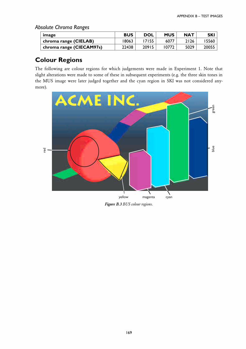
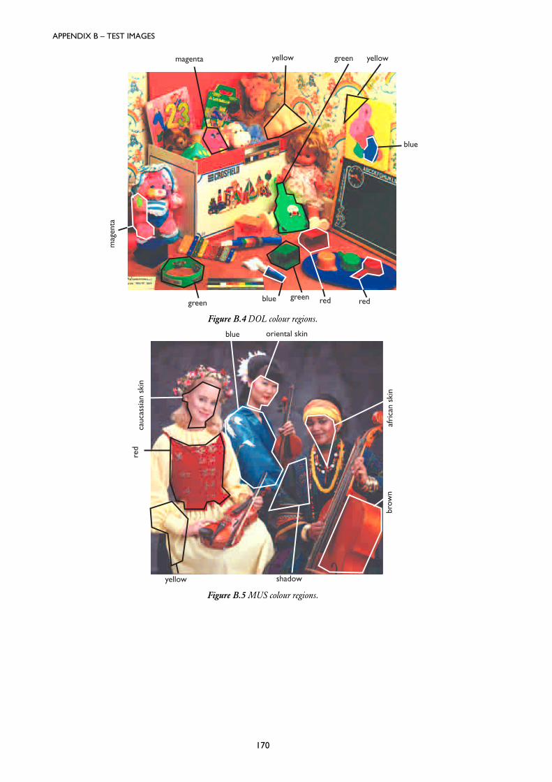
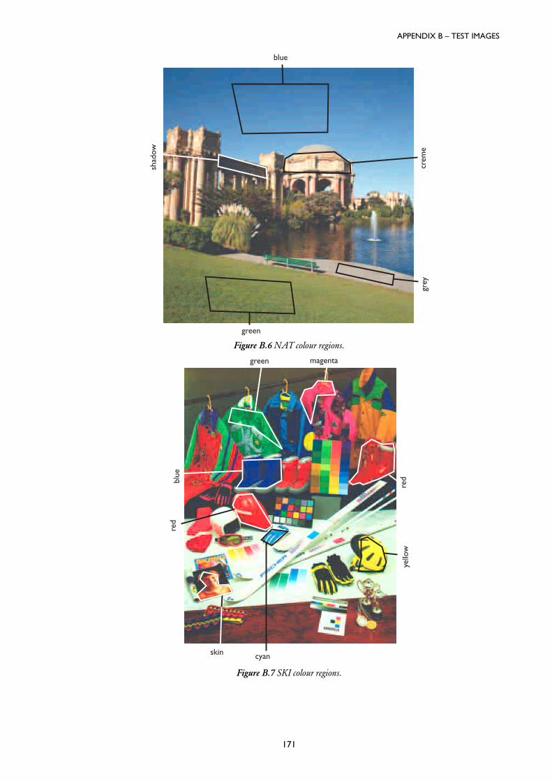
The gamut mapping solution proposed in this thesis is a gamut compression algorithm developedwith the aim of being accurate and universally applicable. It was arrived at by way of an evolution-ary gamut mapping development strategy for the purposes of which five test images were repro-duced between a CRT and printed media obtained using an inkjet printer. Initially, a number ofpreviously published algorithms were chosen and psychophysically evaluated whereby an impor-tant characteristic of this evaluation was that it also considered the performance of algorithms forindividual colour regions within the test images used. New algorithms were then developed on theirbasis, subsequently evaluated and this process was repeated once more. In this series of experimentsthe new GCUSP algorithm, which consists of a chroma–dependent lightness compression followedby a compression towards the lightness of the reproduction cusp on the lightness axis, gave themost accurate and stable performance overall. The results of these experiments were also useful forimproving the understanding of some gamut mapping factors – in particular gamut difference.
In addition to looking at accuracy, the pleasantness of reproductions obtained using various algo-rithms was also looked at and a strong and positive correlation was found between these two prop-erties. It was also shown that the reproductions made with GCUSP were pleasant in isolation,which makes it a very good candidate for a standard universal gamut mapping algorithm.
Errata
Equation 7.2.1 on page 108 is the corrected form of the equation given in the original version ofthe thesis (thanks to Gus Brown (RIT) for pointing out the problem with the original equation).Note that this change does not affect the rest of the thesis as the actual mapping of images usingGCUSP was carried out correctly.
iii
Acknowledgements
Firstly, I would like to express my deepest gratitude to Prof. Ronnier Luo, my Director of Studies.His initial encouragement, continuous support and true friendship were essential to the comingabout of this thesis. I would also like to thank Prof. Tony Johnson for sharing his valuable experi-ence and for his constructive comments during our regular review meetings. Further, I would like tothank Dr. Peter Rhodes for his untiring support in both scientific and linguistic terms. Here Iwould also like to thank my external examiner Prof. Mark Fairchild as well as my internal examinerProf. Lindsay MacDonald for their excellent questions and comments.
Thanks also go to Hewlett Packard for supporting this project in terms of financial and technologi-cal donations alike. Here I would particularly like to thank Mike Stokes of HP Boise and Jay Gon-dek of HP Vancouver.
Next, I would like to thank my colleagues at the Design Research Centre and later the Colour &Imaging Institute as well as all other observers for their patient participation in my psychophysicalexperiments, without which the majority of this work would not have been. More importantly,however, I would like to thank them for their friendship. Disregarding the risk of forgetting some-body, here is an alphabetical list: Ambrosia, Dr. Paula Bourges, Geoff Broadway, Angela Carr,Chun–Di (Vick) Chen, Wen-Lung Chou, Dr. Graham Finlayson, Dr. Shing-Sheng Guan, Dr.Guowei Hong, Steve Hordley, Lu-Yin (Grace) Juan, Hsiao–Pei (Alex) Lee, Robert Liang, Helen Lin,Maryliza Mazijoglou, Gerald Schaefer, Suchitra Sueeprason, Dr. Hong Xu and Peggy Zhu. I wouldalso like to thank Anne Naylor and Suki Atwal for their valuable help.
Thanks also go to everybody from the Focolare and all my friends I didn’t mention by name – Ihope they can forgive this audacity :o). A special thanks also goes to Komerzialrat Eduard Harantfor his magnanimous support throughout my studies.
Unspeakable thanks go to my entire family – first and foremost to my parents, my brother Peterand my sisters Monika and Beatka but also to my grandparents and other members of the family.Finally, I would like to thank God, who is Love.
iv
ContentsList of Tables ix
List of Figures x
1 Introduction 11.1 Background 21.2 Cross–Media Colour Image Reproduction 31.3 Assumptions and Aims 41.4 A Method for Developing GMAs 51.5 Thesis Outline 61.6 Summary 6
2 Literature Survey 72.1 Colorimetry 82.1.1 CIE 1931 XYZ Colour Space 82.1.2 CIE 1976 Uniform Colour Spaces 92.1.2.1 CIELUV 92.1.2.2 CIELAB 112.1.3 Colour Difference Formulæ 112.1.3.1 CMC(l:c) 122.1.3.2 CIE94 122.2 Psychophysics 122.2.1 Pair Comparison 132.2.2 Category Judgement 132.2.3 Magnitude Estimation 132.2.4 Summary 142.3 Colour Appearance 142.3.1 Colour Appearance Phenomena 142.3.2 The Observing Field 152.3.3 RLAB 152.3.4 LLAB 162.3.5 CIECAM97s 182.3.6 Viewing Conditions 202.3.6.1 CRT 202.3.6.2 Print 202.3.7 Summary 202.4 Colour Reproduction Media & Intents 202.4.1 CRT Monitors 212.4.1.1 Chromatic Adaptation to Monitors 212.4.2 Colour Prints 212.4.3 Colour Reproduction Intents 222.5 Characterisation and Calibration 242.5.1 Generic Characterisation Methods 242.5.1.1 Cube Interpolation 242.5.1.2 Polynomial Fitting 252.5.2 CRT Monitor Characterisation & Calibration 262.5.2.1 GOG Model 282.5.2.2 Meyer 1990 Model 292.5.2.3 PLCC Model 292.5.2.4 LIN–LIN2 Model 292.5.2.5 LOG–LOG Model 292.5.2.6 LOG–LOG2 Model 292.5.2.7 LOG–LIN2 Model 29
2.6.4.37 Nakauchi, Imamura & Usui (1996) 582.6.4.38 Ebner & Fairchild (1997) 582.6.4.39 Herzog & Müller (1997) 592.6.4.40 Montag & Fairchild (1997) 602.6.4.41 Motomura, Yamada & Fumoto (1997) 612.6.4.42 Voicu, Myler & Weeks (1997) 612.6.4.43 Wei, Shyu & Sun (1997) 622.6.4.44 Kim, Lee, Kim, Lee & Ha (1998) 622.6.5 Summary of Gamut Mapping Techniques 62
3 Implementation of Colour Reproduction System 653.1 Apparatus 663.1.1 Preliminaries 663.1.2 Viewing Booth 663.1.3 CRT Monitor 673.1.4 Inkjet Printer 673.1.4.1 Temporal Stability 683.1.4.2 Spatial Uniformity 683.1.4.3 Repeatability 693.1.4.4 Difference Between Ink Cartridges 693.1.5 Media Gamuts 693.2 Development of Characterisation Models
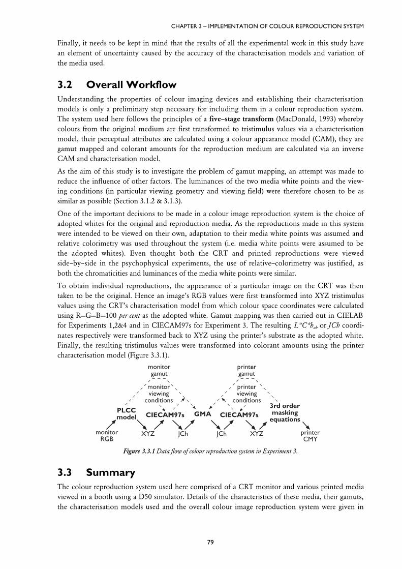
and Investigation of Their Accuracy 723.2.1 CRT Characterisation Model 723.2.2 Printer Characterisation Model Development and Evaluation 723.2.2.1 Distance Weighted Interpolation Model 733.2.2.2 Third Order Masking Equations 733.2.2.3 Fourth Order Masking Equations 743.2.2.4 Four–Sector Model 743.2.2.5 Evaluation of Initial Characterisation Models 753.2.2.6 Grey–Scale–Corrected RGB Printer Characterisation 773.3 Overall Workflow 793.4 Summary 79
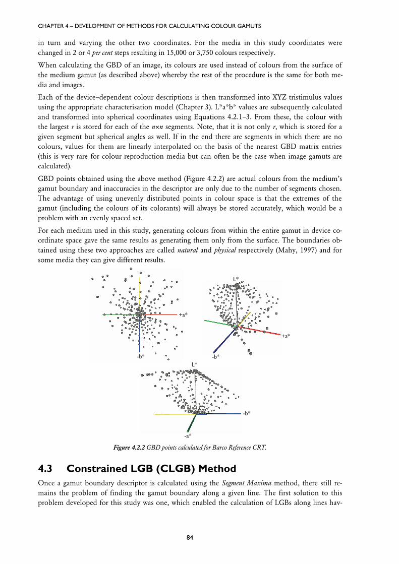
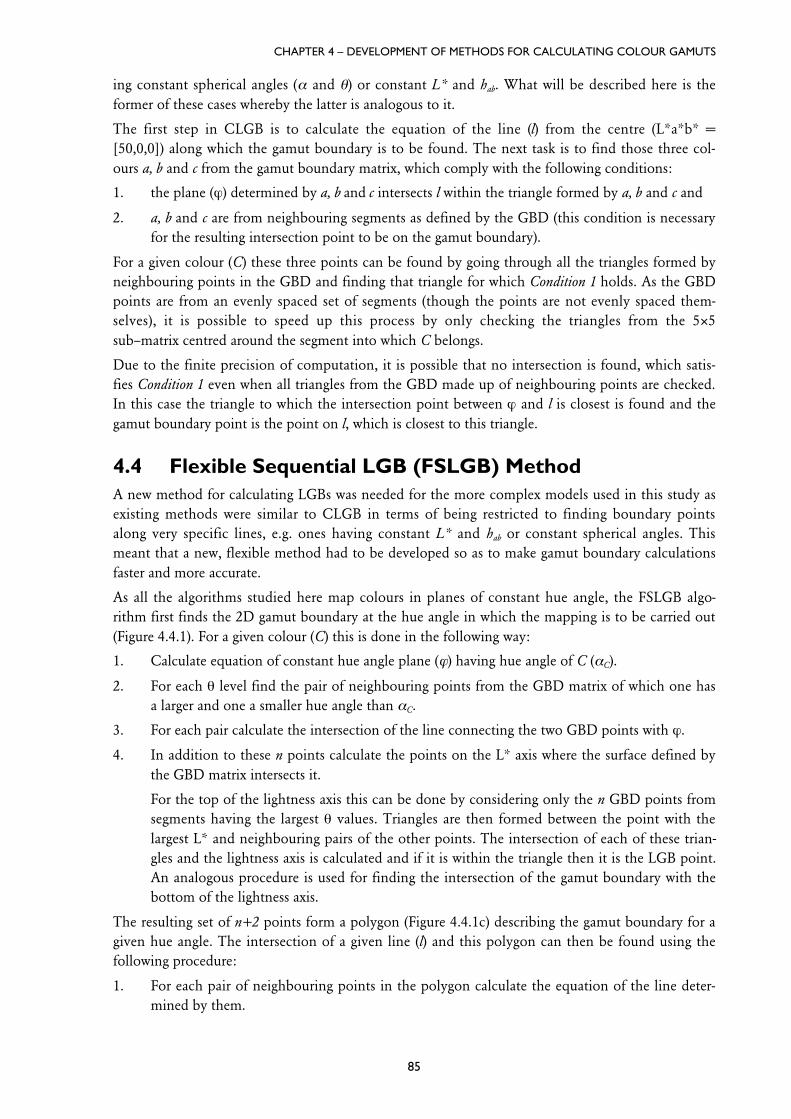
4 Development of Methods for Calculating Colour Gamuts 814.1 Calculating Gamut Boundaries 824.1.1 Basic Geometry 824.2 Segment Maxima GBD (SMGBD) Method 834.3 Constrained LGB (CLGB) Method 844.4 Flexible Sequential LGB (FSLGB) Method 854.5 Summary 86
7 Development of Second Generation GMAs 1077.1 Overview 1087.2 GCUSP 1087.3 CLLIN 1097.4 TRIA 1107.5 CARISMA 1117.6 Summary 112
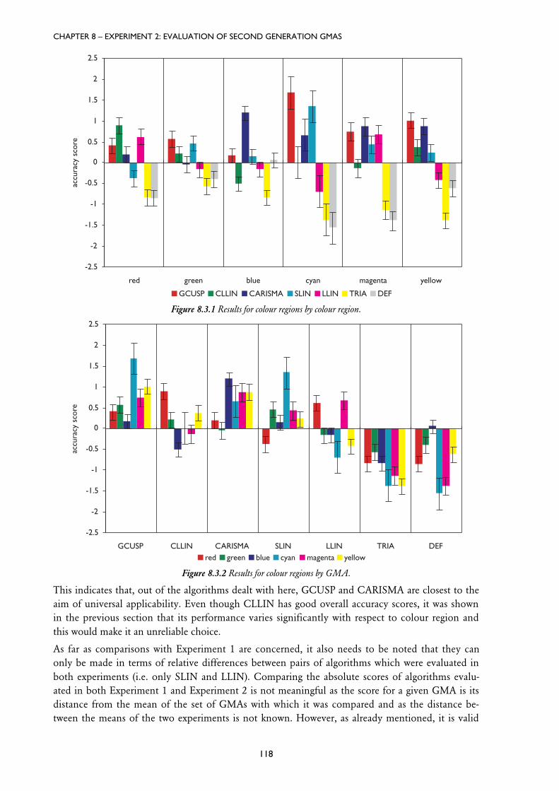
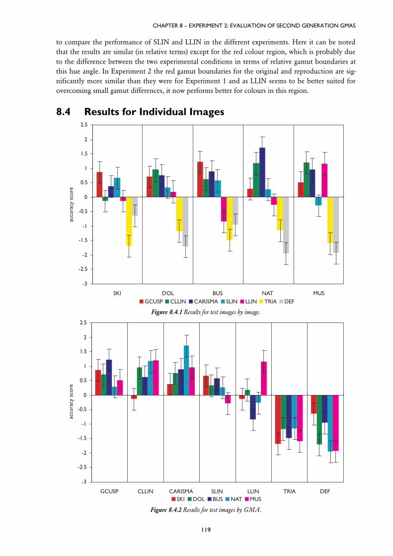
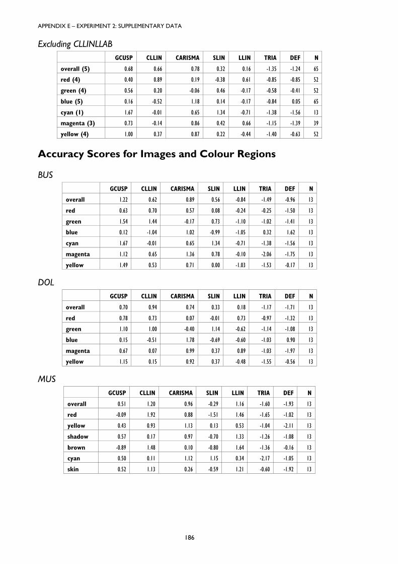
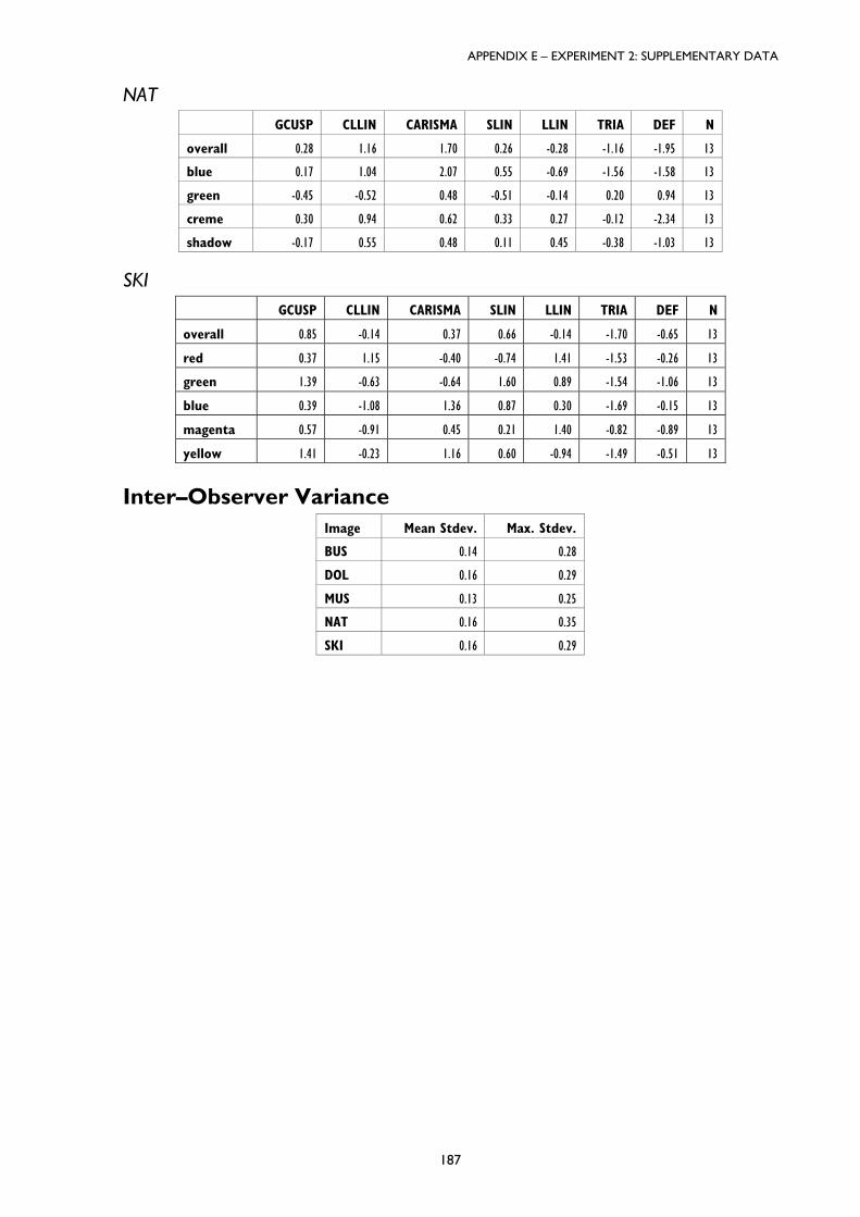
8 Experiment 2: Evaluation of Second Generation GMAs 1138.1 Overview of Experiment 1148.2 Overall Results 1148.3 Results for Colour Regions 1178.4 Results for Individual Images 1198.5 Summary 120
9 Development of Third Generation GMAs 1239.1 GMA Development on the Basis of Colour Region Performance 1249.2 UniGMA 1269.3 LCUSPH 1269.4 Summary 126
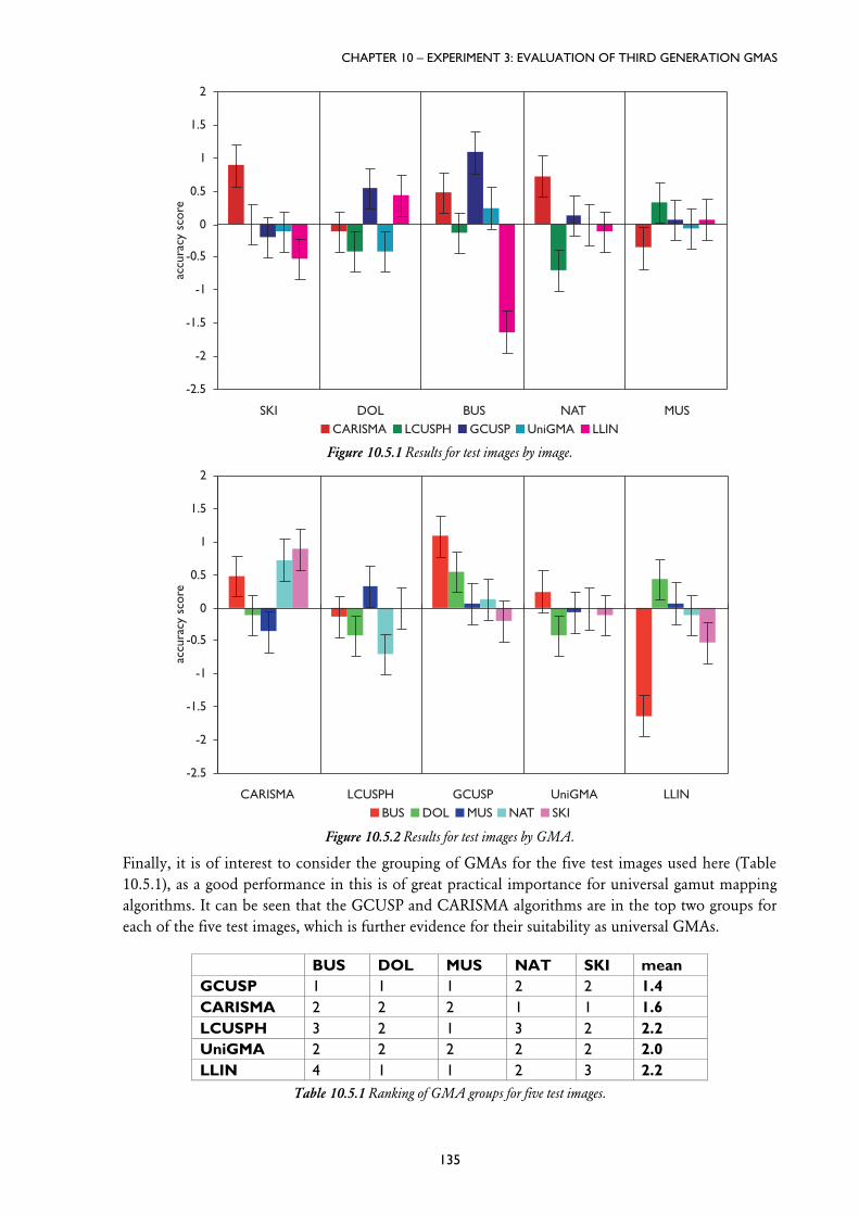
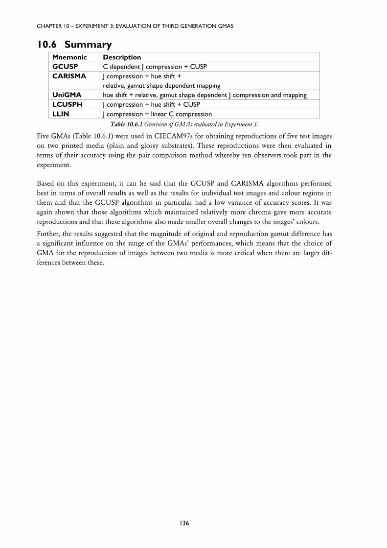
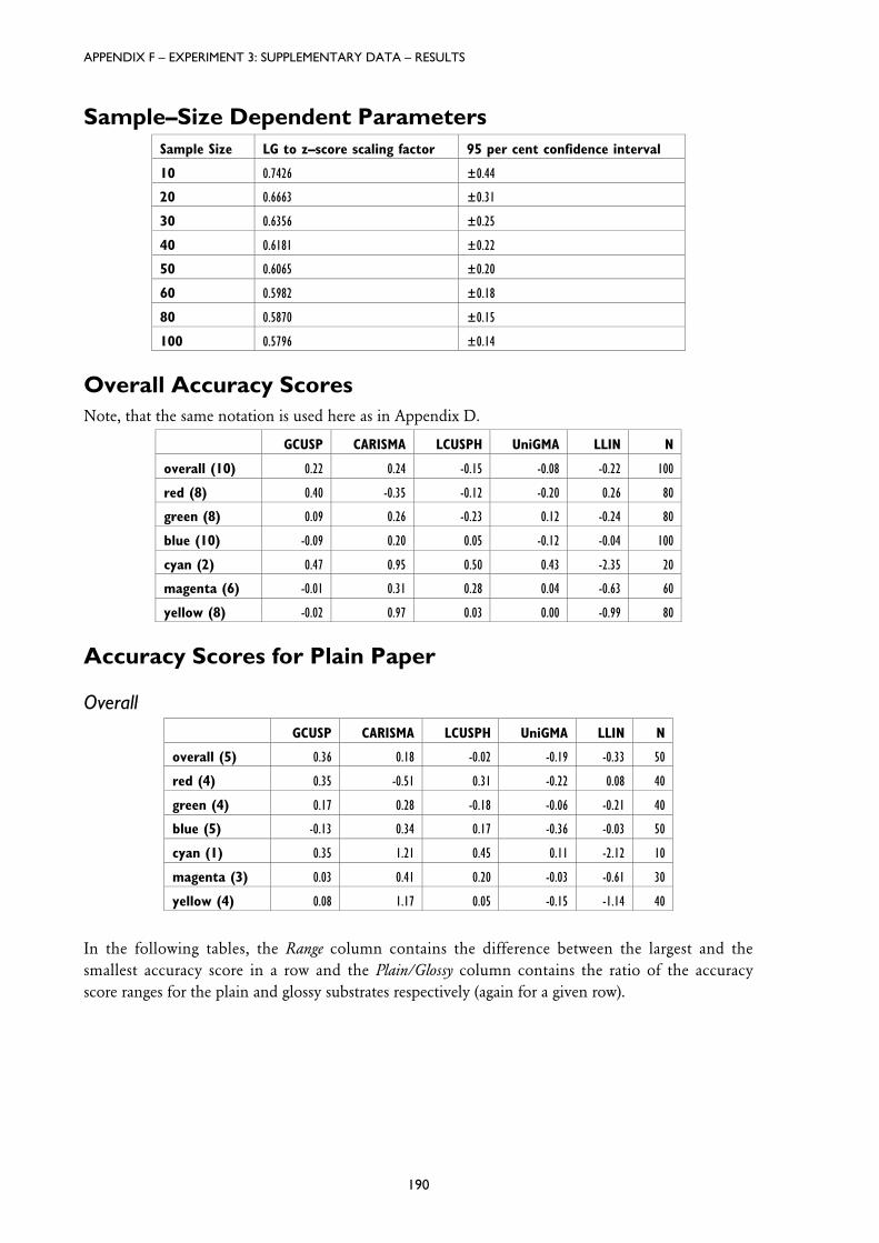
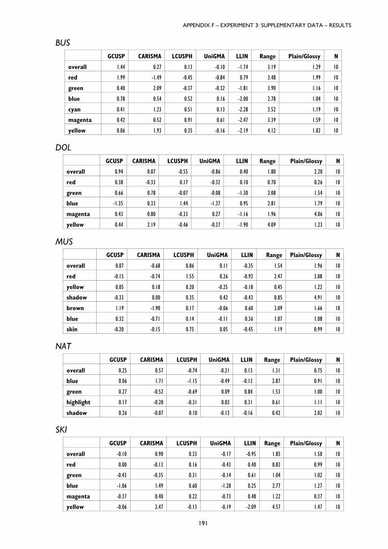
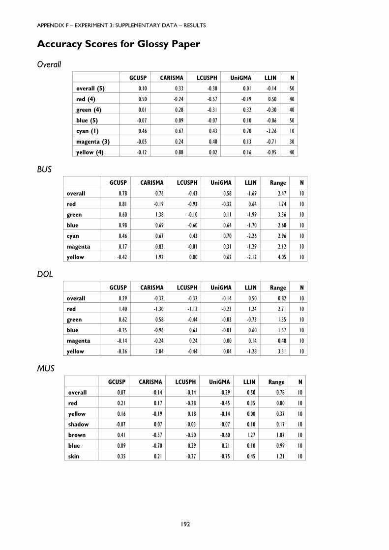
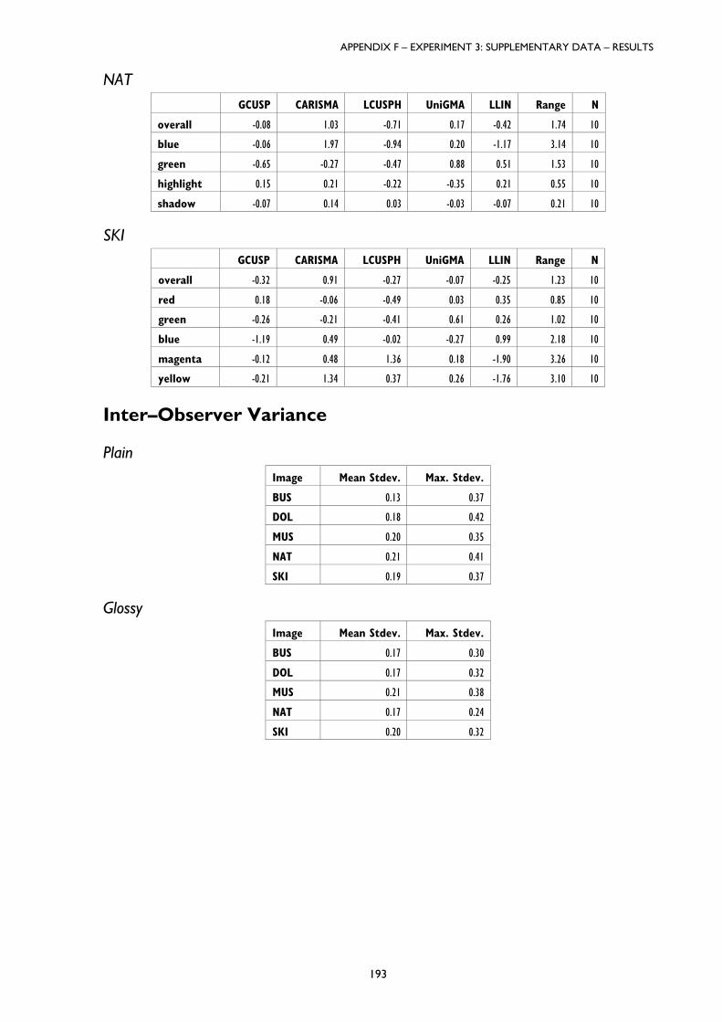
10 Experiment 3: Evaluation of Third Generation GMAs 12710.1 Overview of Experiment 3 12810.1.1 The influence of CIECAM97s on Gamut Mapping 12810.2 Overall Results 13010.3 Overall Results for Plain and Glossy Media 13210.4 Results for Colour Regions 13310.5 Results for Individual Images 13410.6 Summary 136
11 Experiment 4: Investigation of the RelationshipBetween Accuracy and Pleasantness 137
11.1 Introduction 13811.2 Overview of Experiment 13811.3 Pleasantness Results 13911.3.1 Pair Comparison v. Category Judgement 14011.4 Accuracy v. Pleasantness 14111.5 Summary 142
12 Conclusions 14512.1 Overview of Findings 14612.1.1 Colour Reproduction System 14612.1.2 Gamut Boundary Determination 14612.1.3 Experiment 1 – Initial Evaluation 14612.1.4 Experiment 2 – Evaluation of new GMAs 14612.1.5 Experiment 3 – Verification of GMAs 14712.1.6 Experiment 4 – Accuracy versus Pleasantness 14712.2 Summary 14712.3 Future Work 148
CONTENTS
viii
References 151
Appendix A: Device Characterisation 161
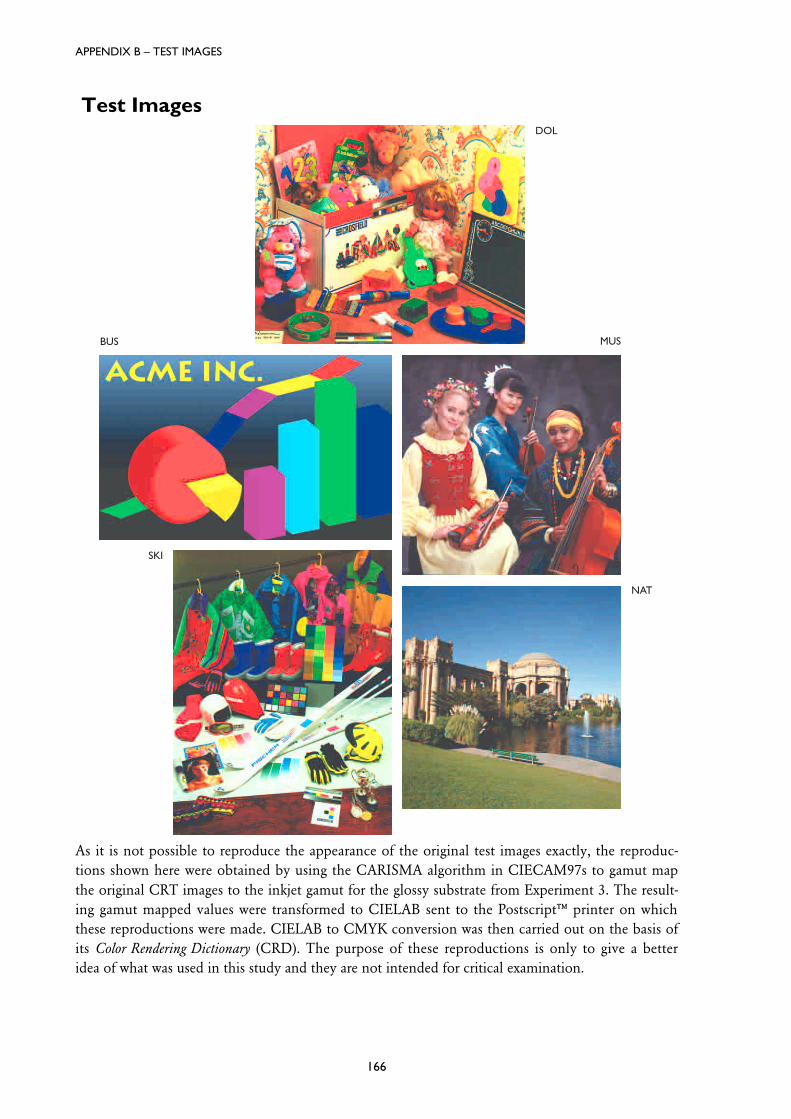
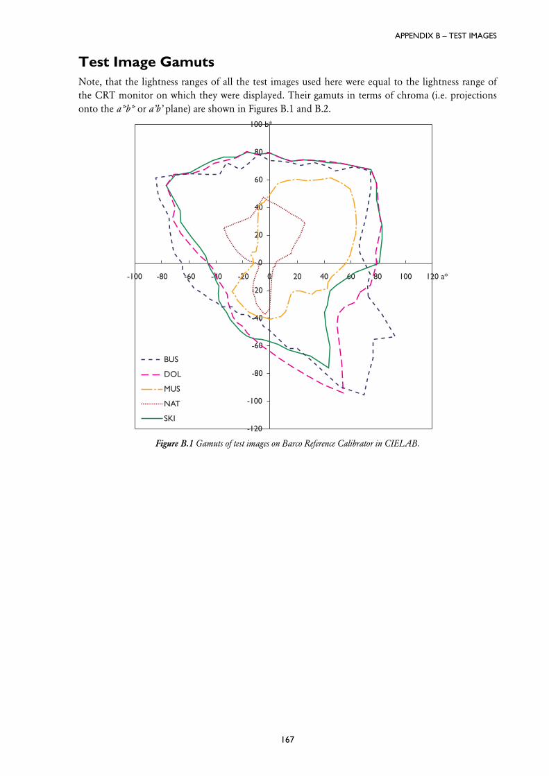
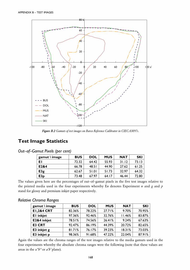
Appendix B: Test Images 165
Appendix C: Data Analysis of Psychophysical Experiments 173
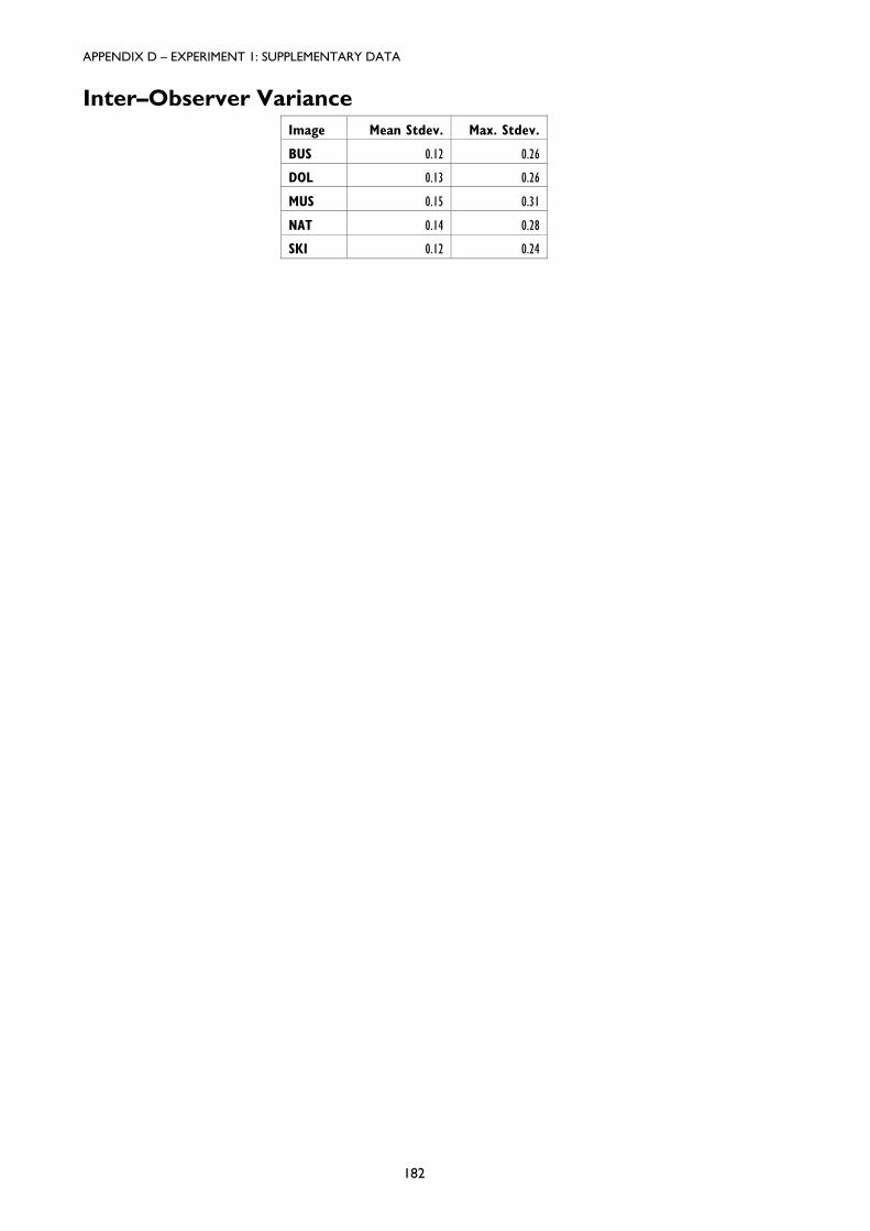
Appendix D: Experiment 1 – Supplementary Data 179
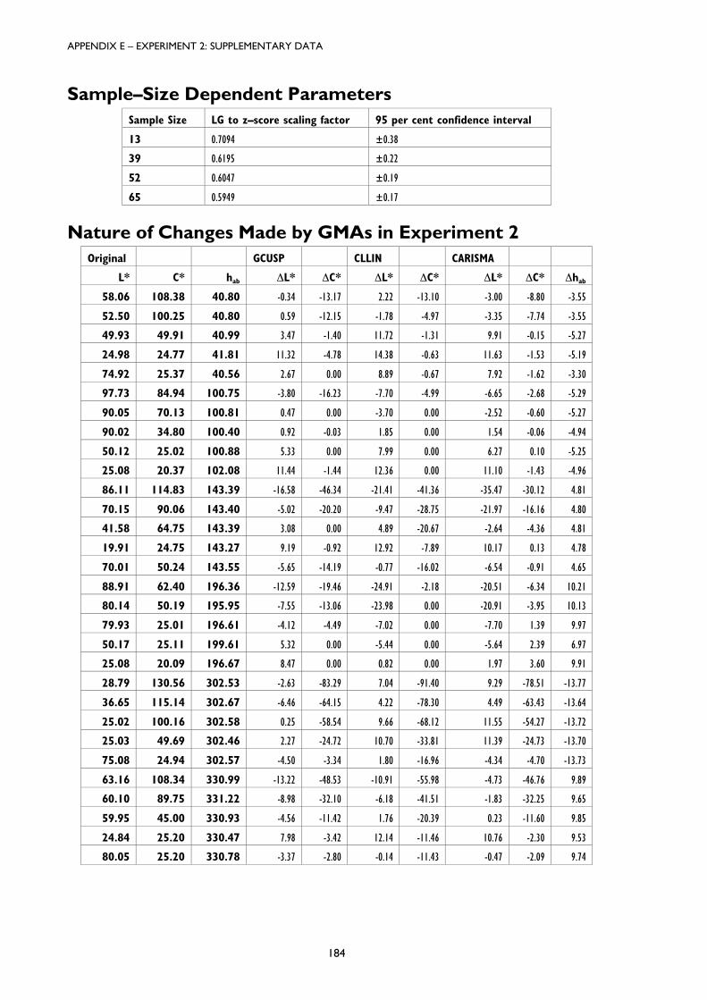
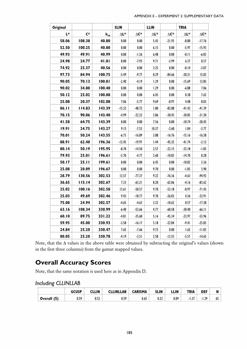
Appendix E: Experiment 2 – Supplementary Data 183
Appendix F: Experiment 3 – Supplementary Data (Results) 189
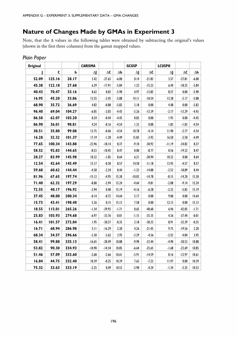
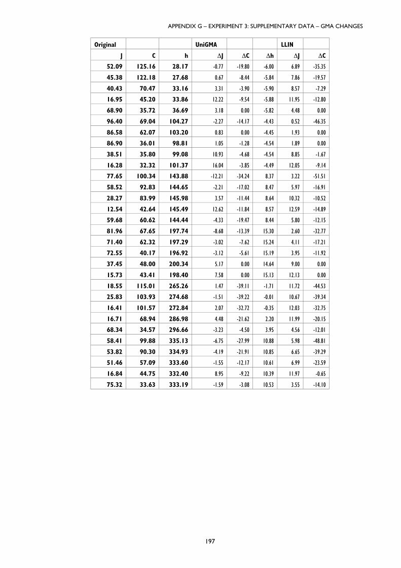
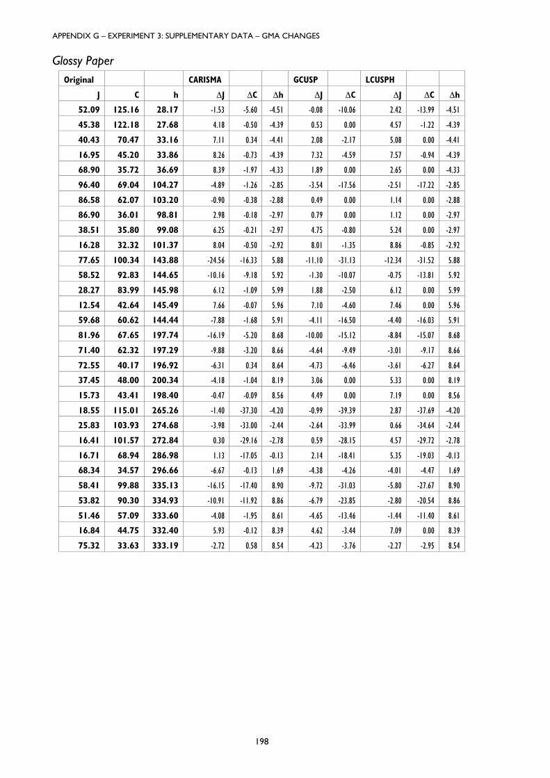
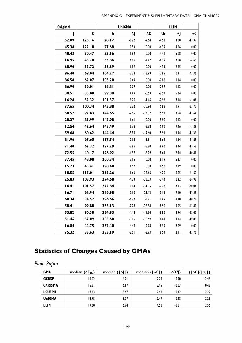
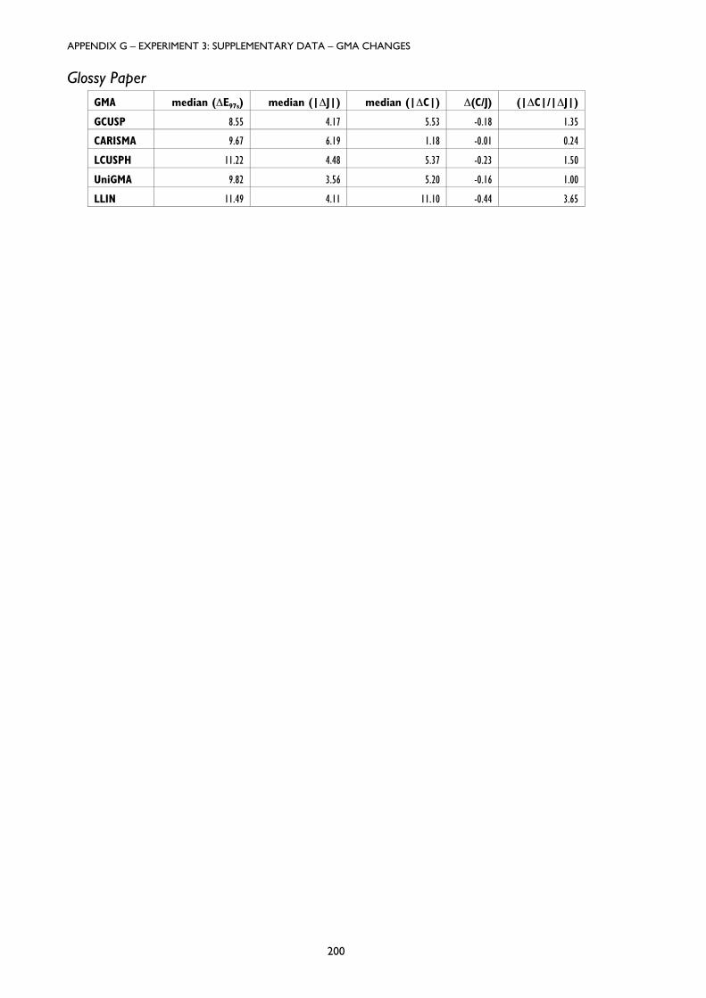
Appendix G: Experiment 3 – Supplementary Data (Changes by GMA) 195
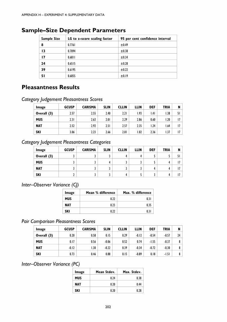
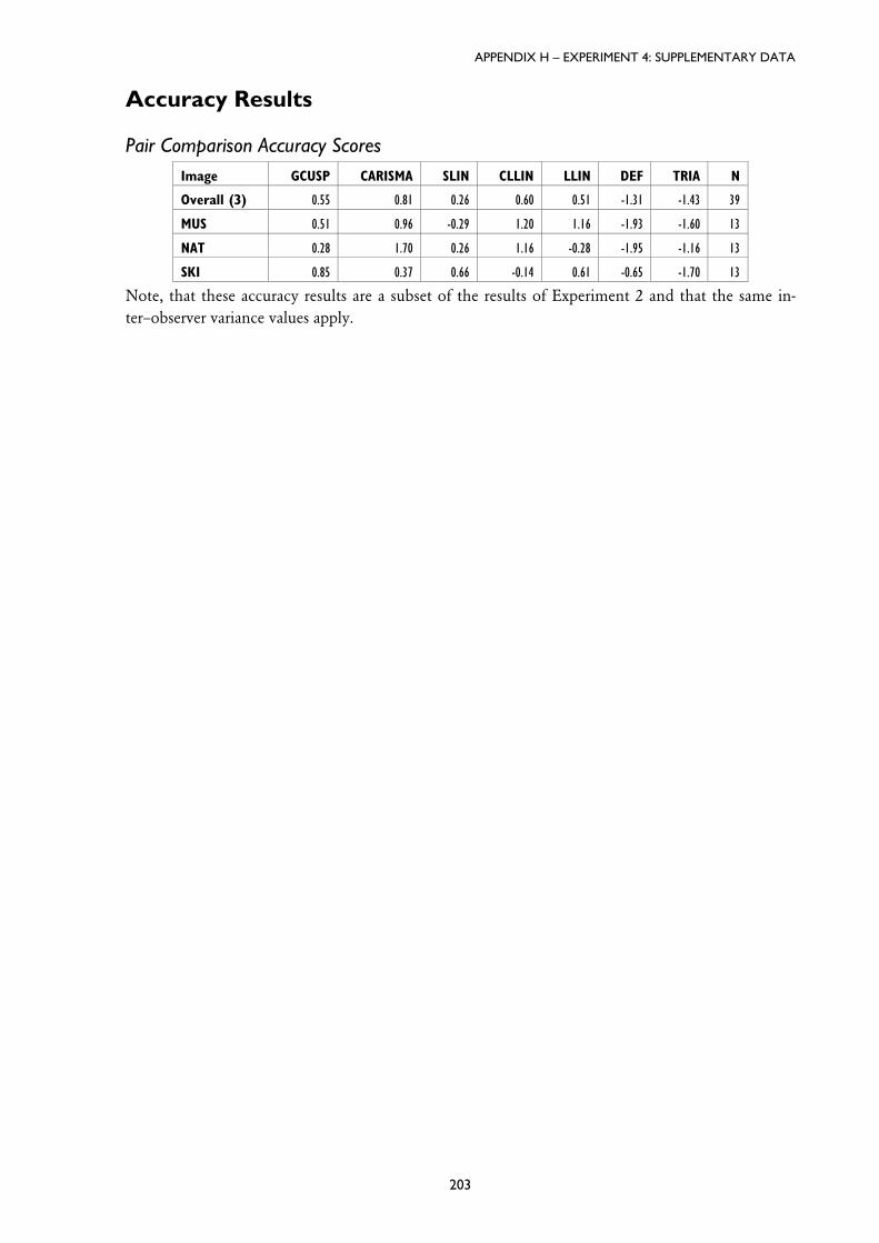
Appendix H: Experiment 4 – Supplementary Data 201
ix
List of Tables
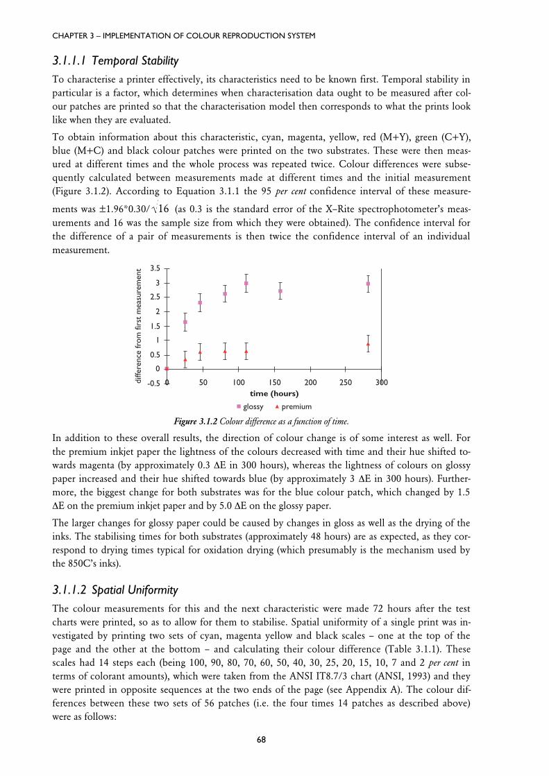
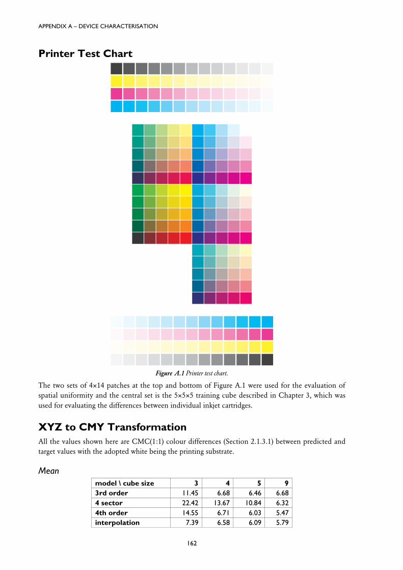
Table 3.1.1 Spatial Uniformity of prints made with HP DeskJet 850C.
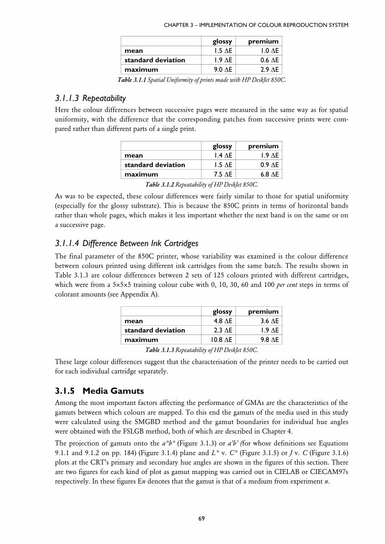
Table 3.1.2 Repeatability of HP DeskJet 850C.
Table 3.1.3 Repeatability of HP DeskJet 850C.
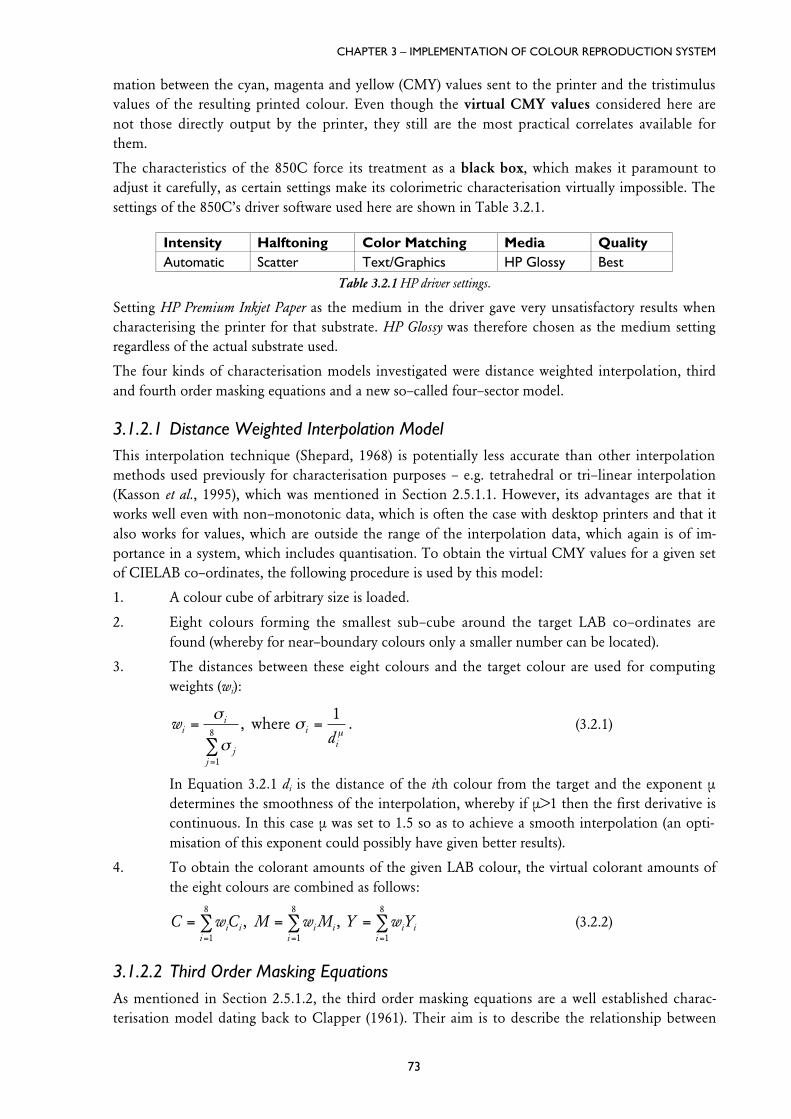
Table 3.2.1 HP driver settings.
Table 3.2.2 Colorant levels used in colour cubes.
Table 3.2.3 Performance of fourth–order masking equations used in Experiment 1 (in terms of DE).
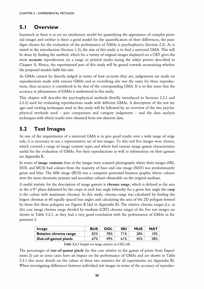
Table 5.2.1: Sample test image statistics in CIELAB.
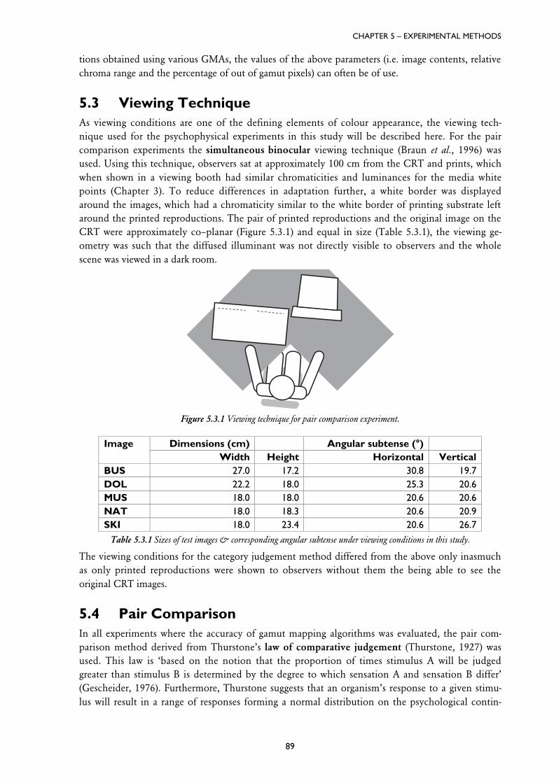
Table 5.3.1 Sizes of test images & corresponding angular subtends under viewing conditions in this study.
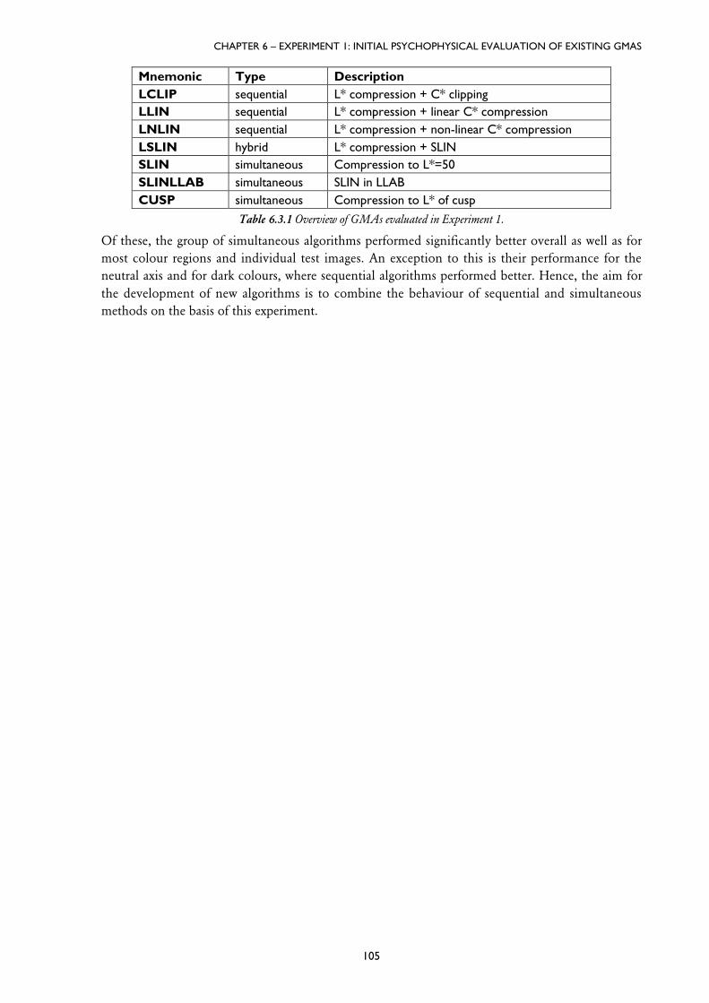
Table 6.3.1 Overview of GMAs evaluated in Experiment 1.
Table 8.2.1 Median changes made by GMAs in Experiment 2.
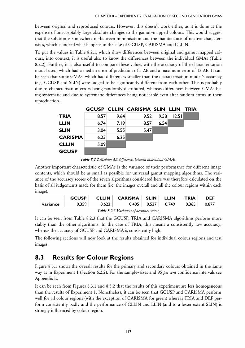
Table 8.2.2 Median DE differences between individual GMAs.
Table 8.2.3 Variances of accuracy scores.
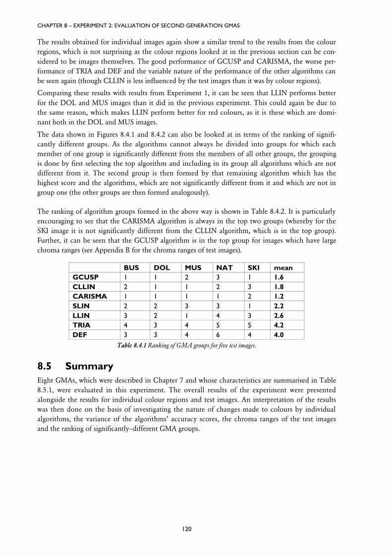
Table 8.4.1 Ranking of GMA groups for five test images.
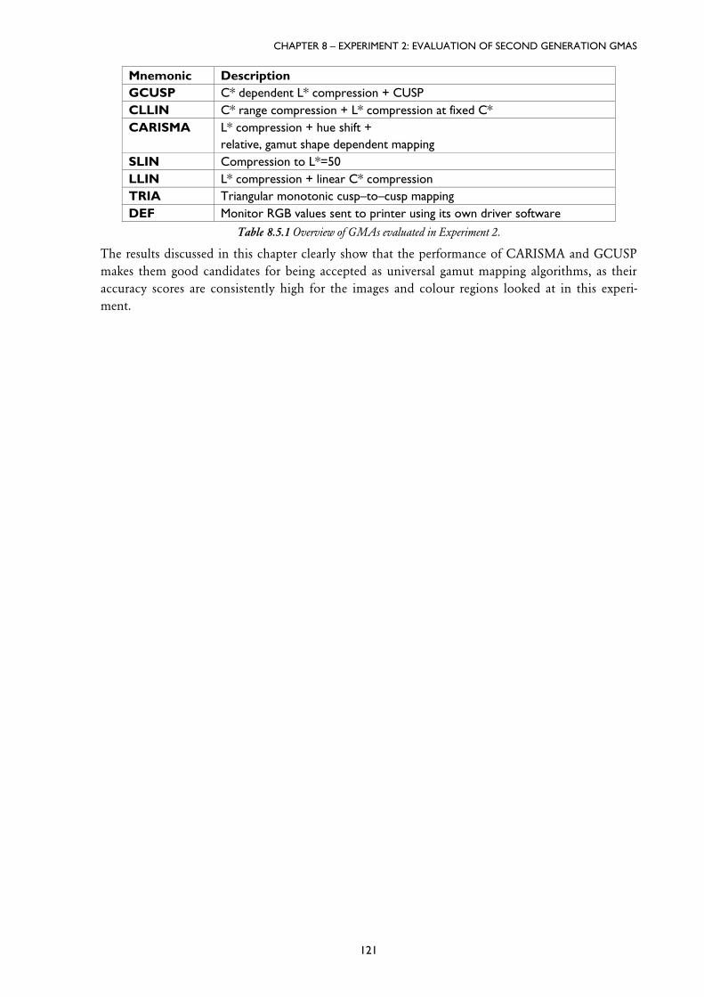
Table 8.5.1 Overview of GMAs evaluated in Experiment 2.
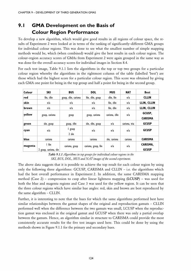
Table 9.1.1 Algorithms in top groups for individual colour regions in the SKI, BUS, DOL, MUS and NAT
images of the second experiment.
Table 10.1.1 Lightness ranges of Experiment 3 media in CIELAB and CIECAM97s.
Table 10.2.1 Variances of GMAs evaluated in Experiment 3.
Table 10.2.2 Statistics of changes made by GMAs to 30 test colours.
Table 10.5.1 Ranking of GMA groups for five test images.
Table 10.6.1 Overview of GMAs evaluated in Experiment 3.
Table 11.3.1 Relationship between category judgement and pair comparison results.
Table 11.4.1 Correlation between accuracy and pleasantness results based on pair comparison experiments.
x
List of Figures
Figure 1.1.1 Cave–wall painting from Lascaux, France.
Figure 1.2.1 Five–stage colour reproduction system (dashed lines represent the data–flow for calculating the
original and reproduction gamuts (Chapter 4)).
Figure 1.2.2 Colour gamuts of a printed medium (solid) and a monitor (transparent).
Figure 1.4.1 Overview of gamut mapping development.
Figure 2.1.1 CIE Standard Colorimetric Observer’s colour matching functions (reproduced from Jackson et
al. (1994)).
Figure 2.1.2 a.) xy and b.) u'v' chromaticity diagrams (line segments represent equal perceptual colour differ-
ences).
Figure 2.1.3 The CIE 1976 L*u*v* colour space.
Figure 2.4.1 Barco Calibrator CRT monitor gamut in CIELAB.
Figure 2.4.2 Halftoning using an amplitude modulated screen.
Figure 2.4.3 Gamut of prints made with HP DeskJet 850C inkjet printer on plain paper (CIELAB).
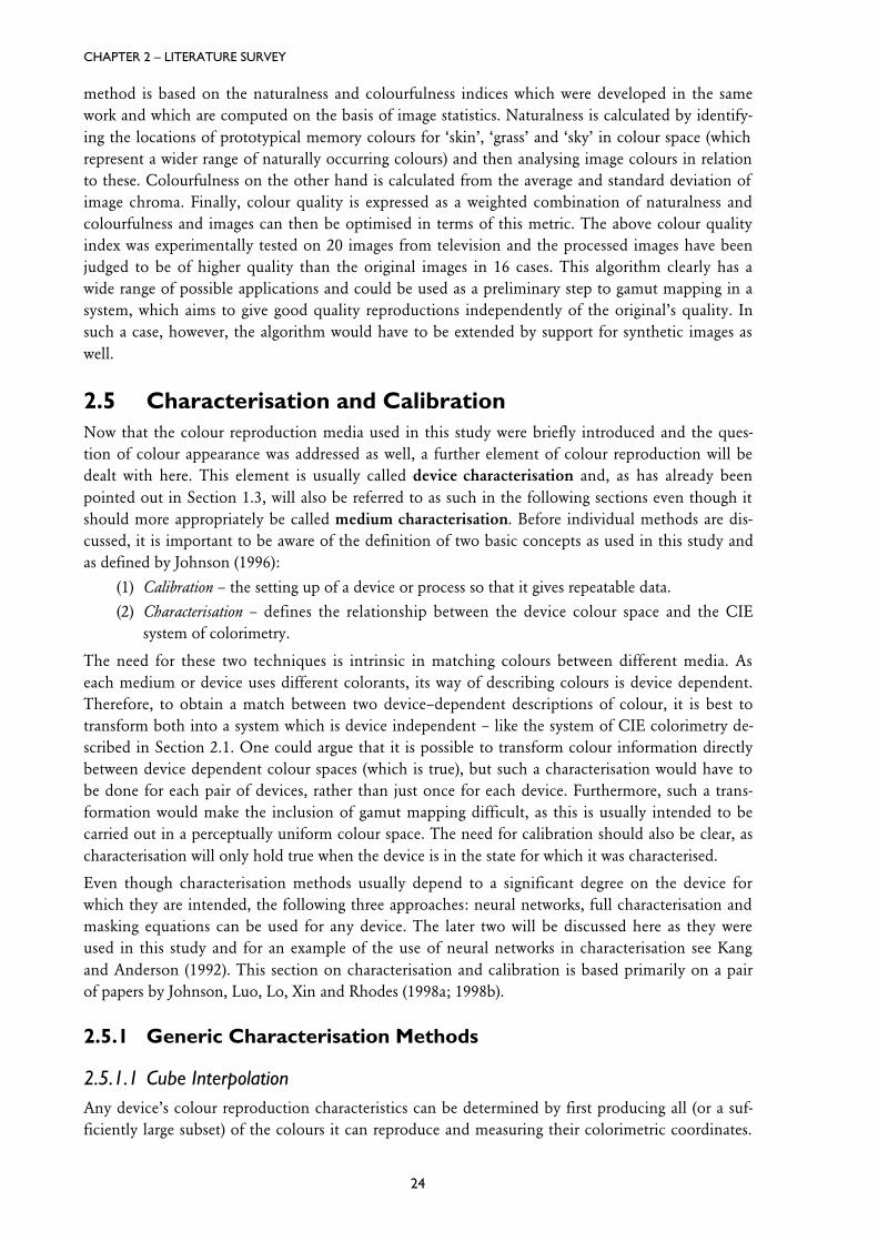
Figure 2.4.4 CRT gamut (solid) and gamut of block dyes representing the gamut of theoretically possible sur-
face colours (mesh), which was obtained by independently varying spectral reflectances at 16 wavelengths
whereby generating spectral reflectance curves, which were then combined with the spectral power distribu-
tion of CIE Standard Illuminant D50.
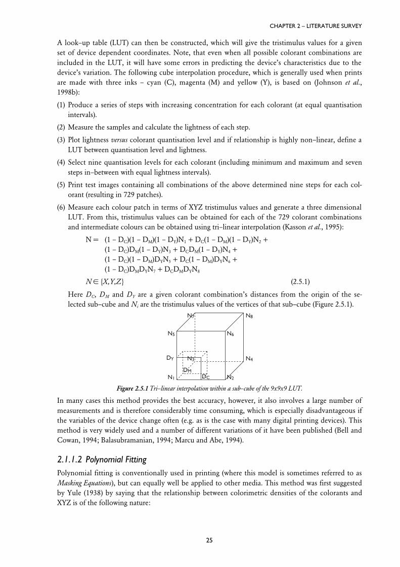
Figure 2.5.1 Tri–linear interpolation within a sub–cube of the 9x9x9 LUT.
Figure 2.5.2 Schematic view of a cathode ray tube (reproduced from (Schläpfer, 1990)).
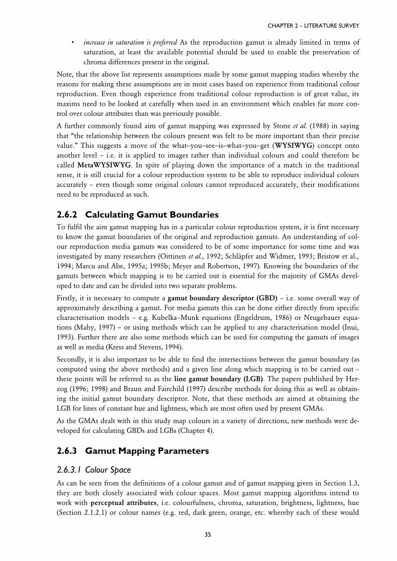
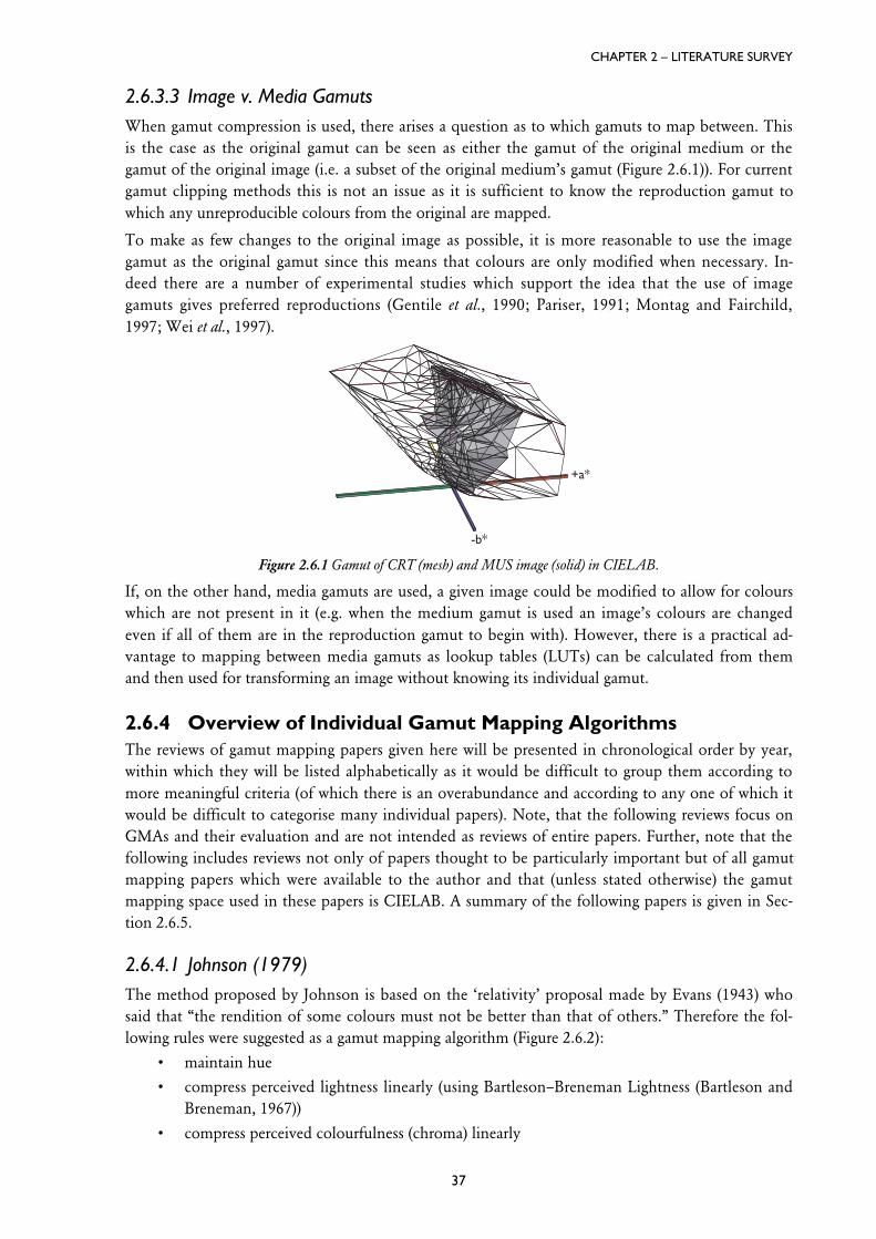
Figure 2.6.1 Gamut of CRT (mesh) and MUS image (solid) in CIELAB.
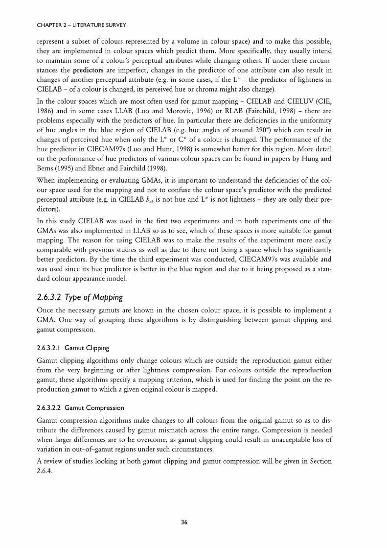
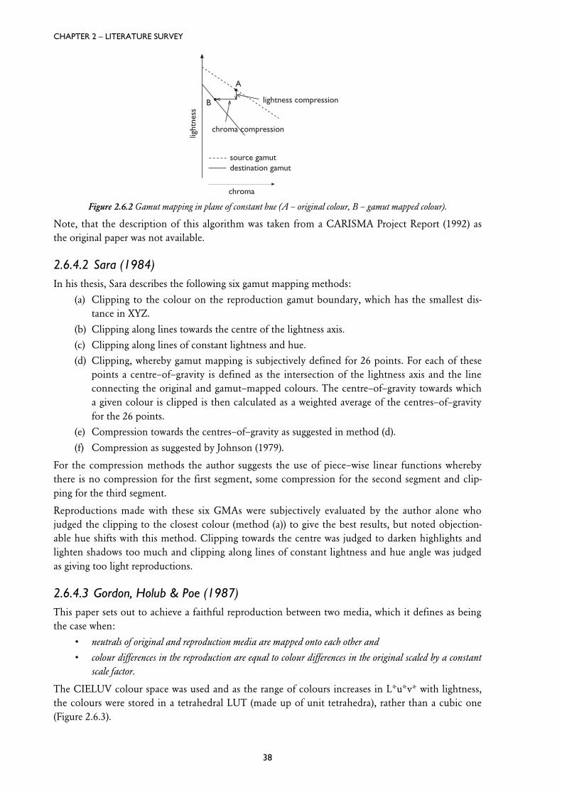
Figure 2.6.2 Gamut mapping in plane of constant hue (A – original colour, B – gamut mapped colour).
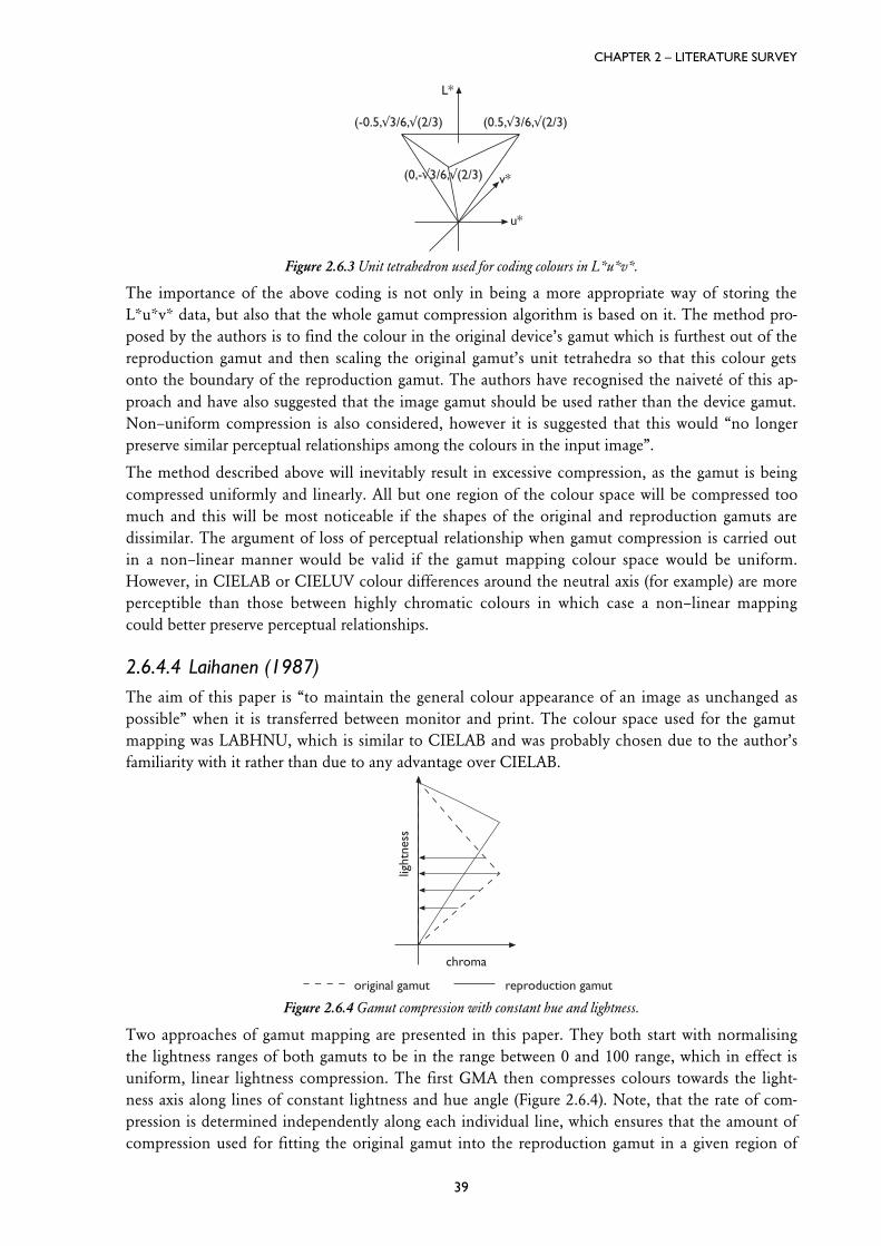
Figure 2.6.3 Unit tetrahedron used for coding colours in L*u*v*.
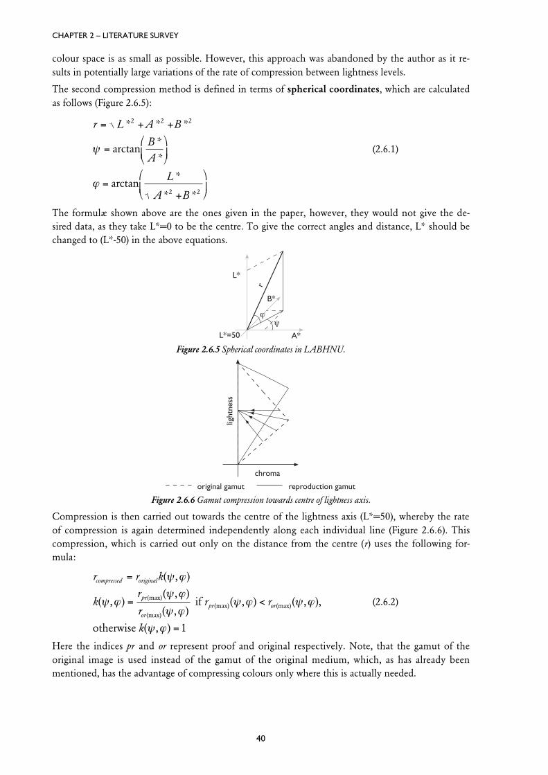
Figure 2.6.4 Gamut compression with constant hue and lightness.
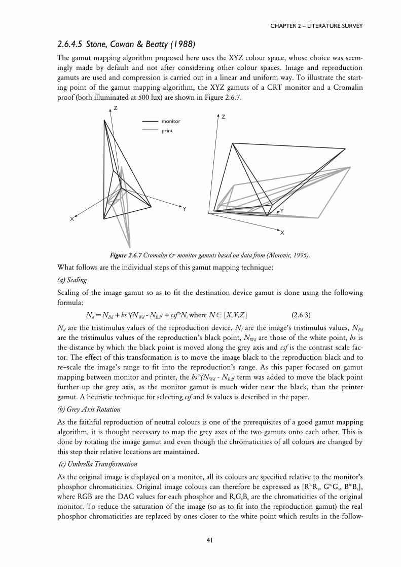
Figure 2.6.5 Spherical coordinates in LABHNU.
Figure 2.6.6 Gamut compression towards centre of lightness axis.
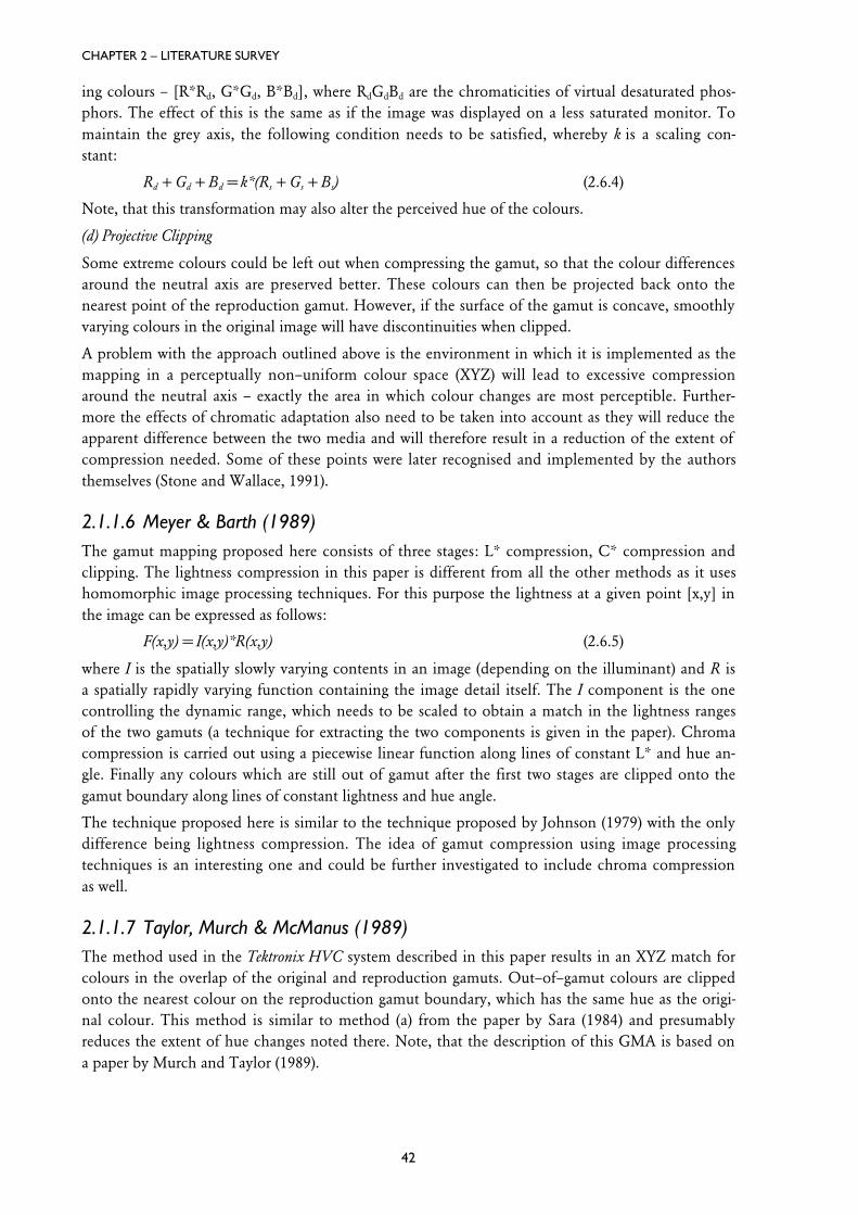
Figure 2.6.7 Cromalin & monitor gamuts based on data from (Morovic, 1995).
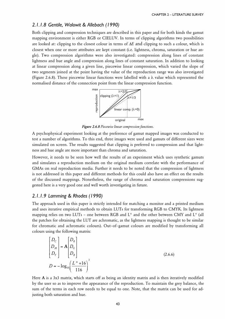
Figure 2.6.8 Piecewise linear compression functions.
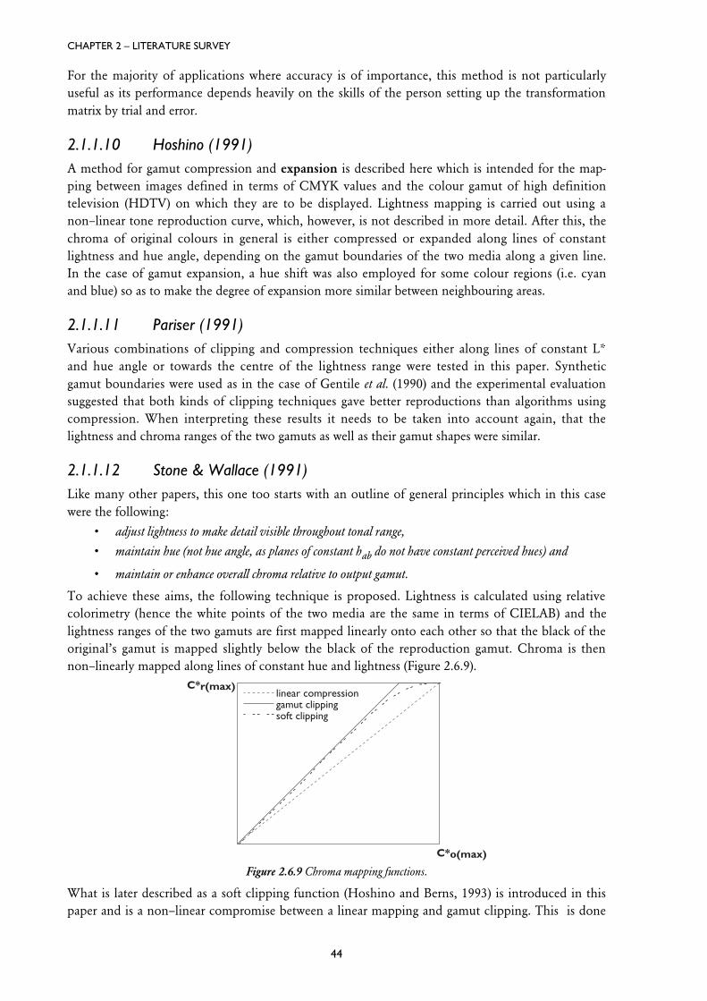
Figure 2.6.9 Chroma mapping functions.
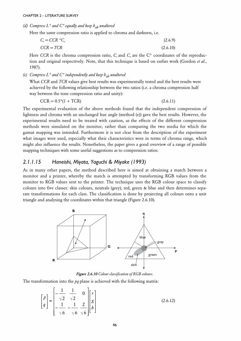
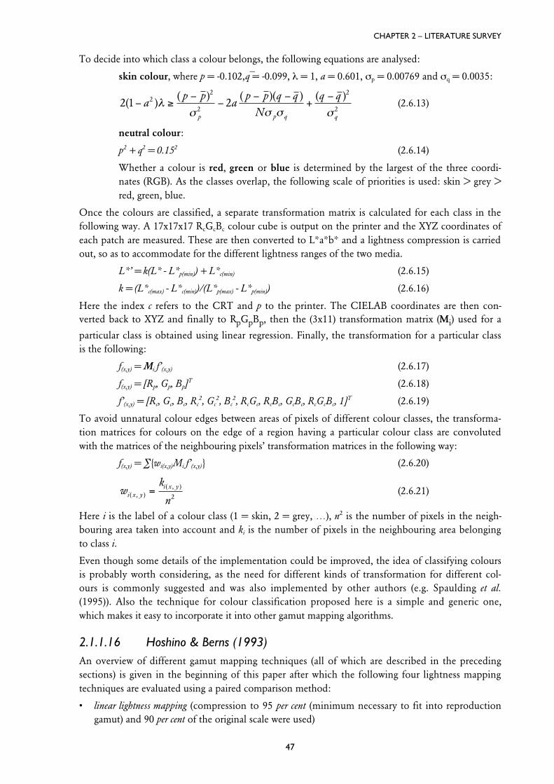
Figure 2.6.10 Colour classification of RGB colours.
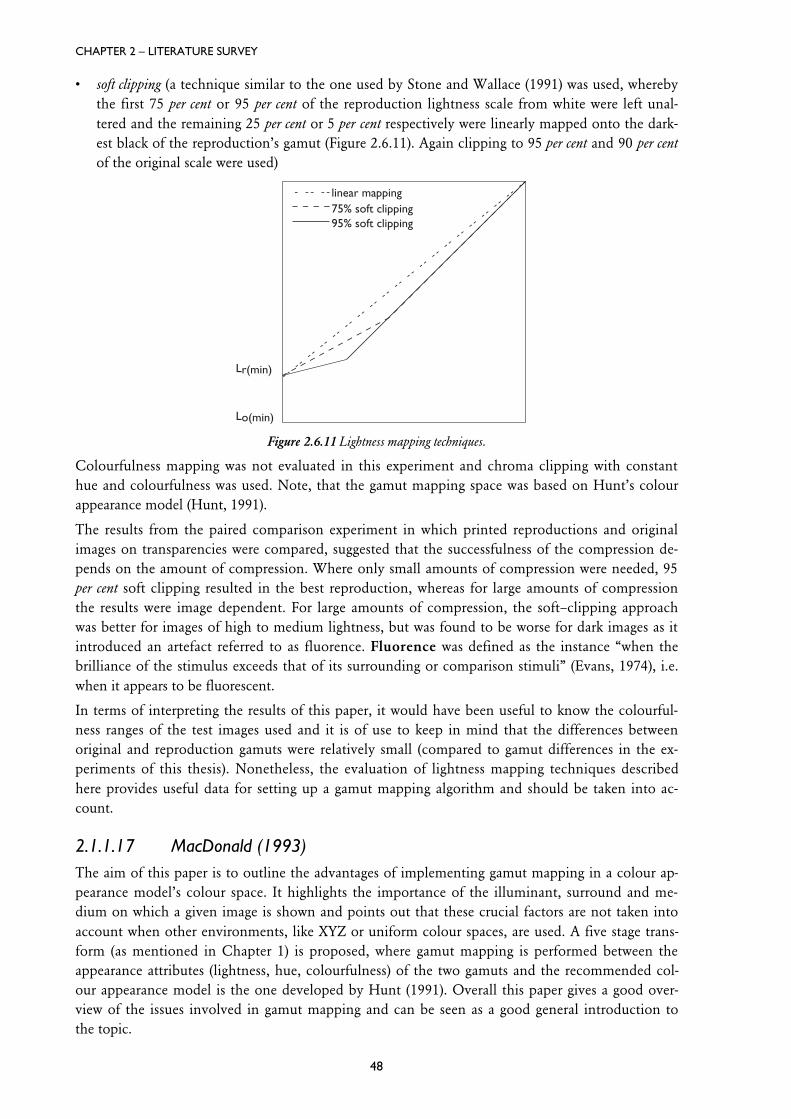
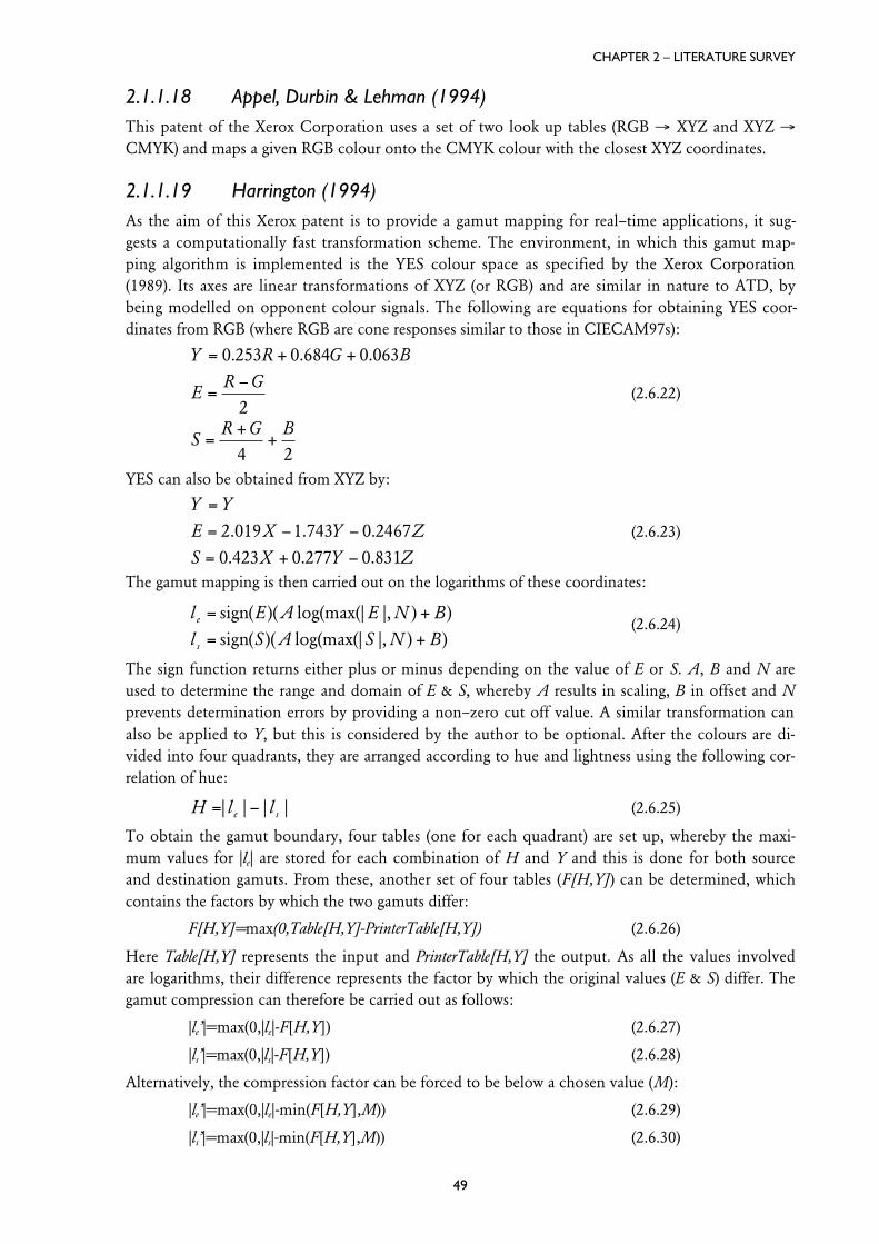
Figure 2.6.11 Lightness mapping techniques.Figure 2.6.12 Linear extrapolation to calculate red coordinate (R’3) for out–of–gamut colour P3 using the
coordinates of two of the closest colours P1 and P2.
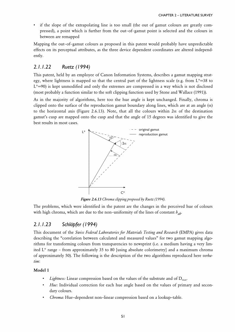
Figure 2.6.13 Chroma clipping proposed by Ruetz (1994).
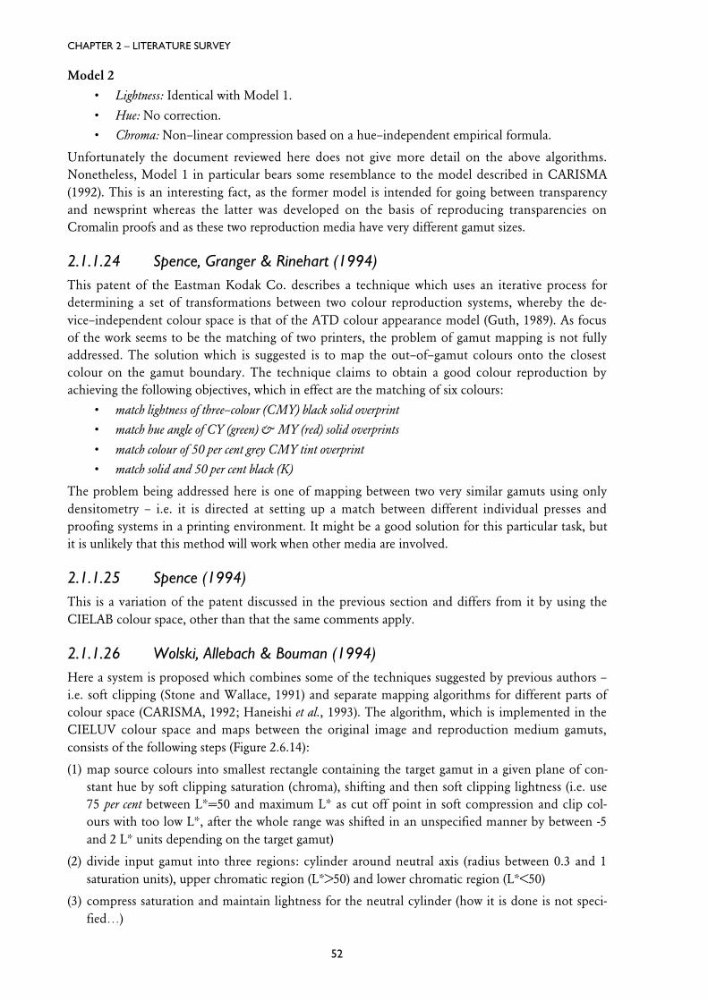
Figure 2.6.14 Visualisation of the gamut mapping algorithm (reproduced from (Wolski et al., 1994)).
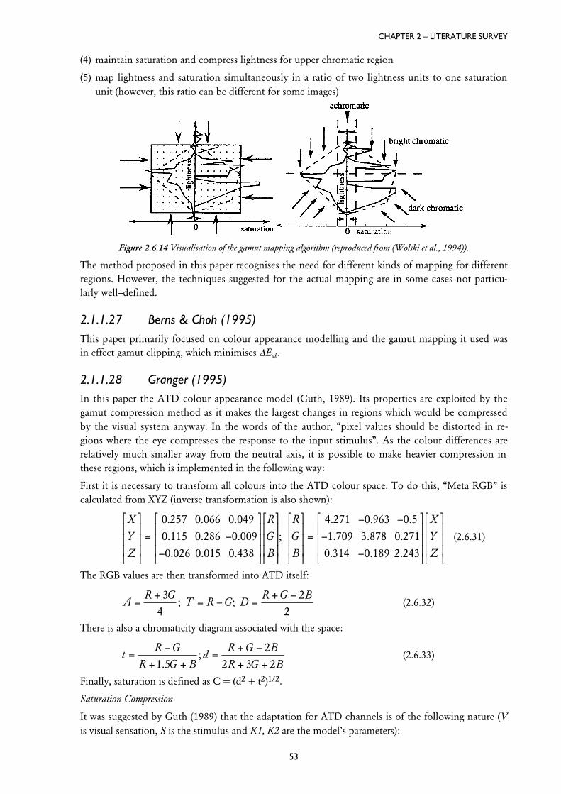
Figure 2.6.15 Adaptive compression of chroma for a particular hue angle (The indices o and r signify original
and reproduction respectively).
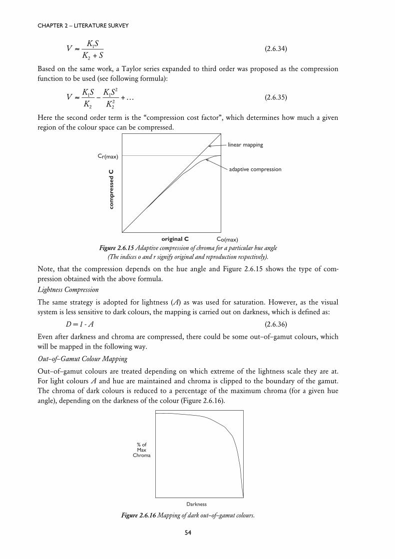
Figure 2.6.16 Mapping of dark out–of–gamut colours.
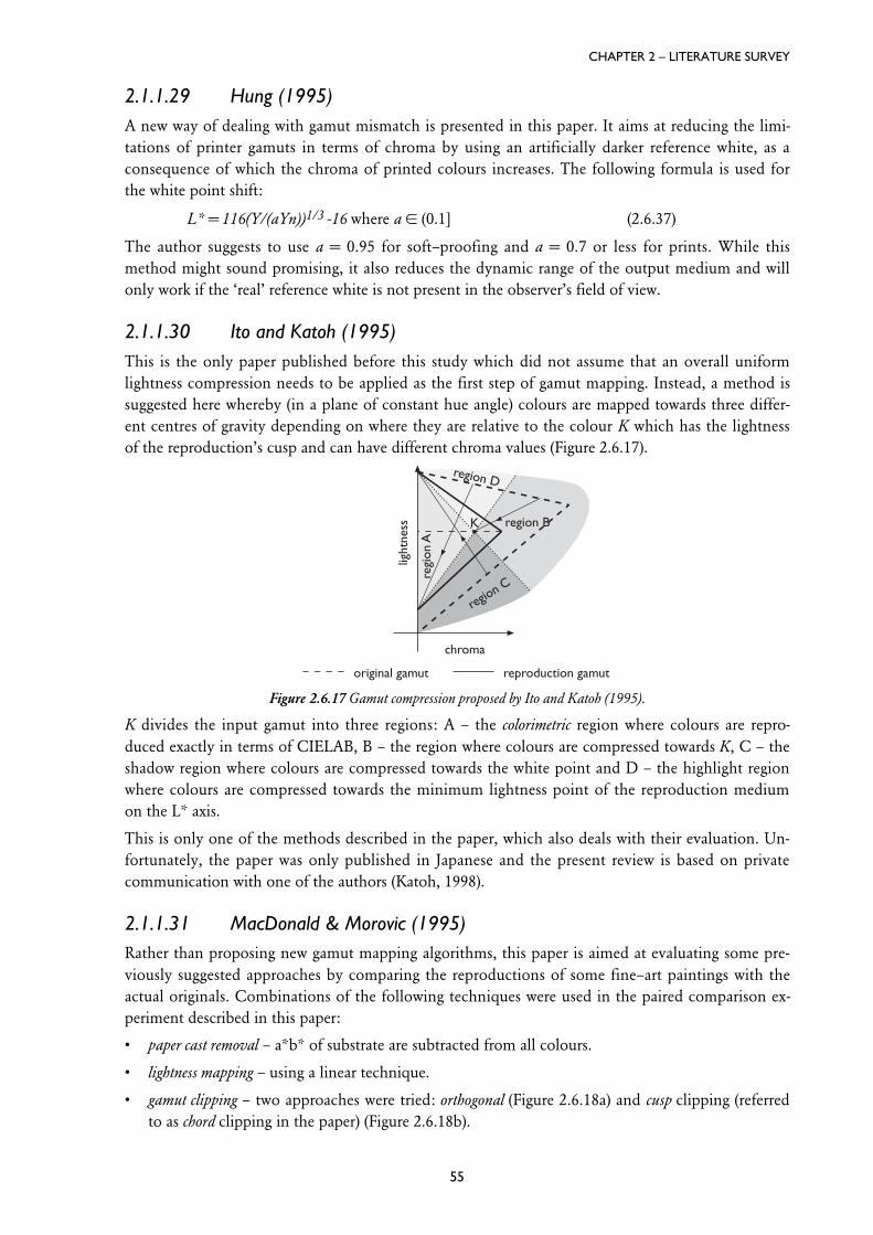
Figure 2.6.17 Gamut compression proposed by Ito and Katoh (1995).
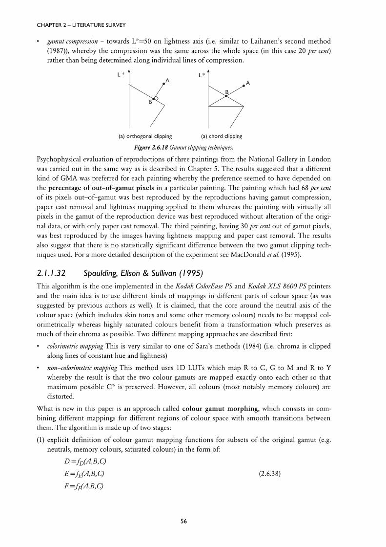
Figure 2.6.18 Gamut clipping techniques.
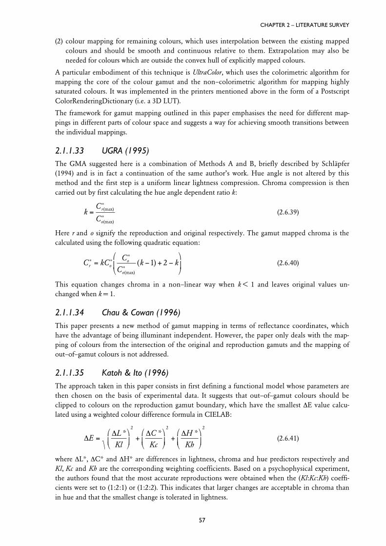
Figure 2.6.19 Gamut clipping algorithm proposed by Marcu and Abe (1996).
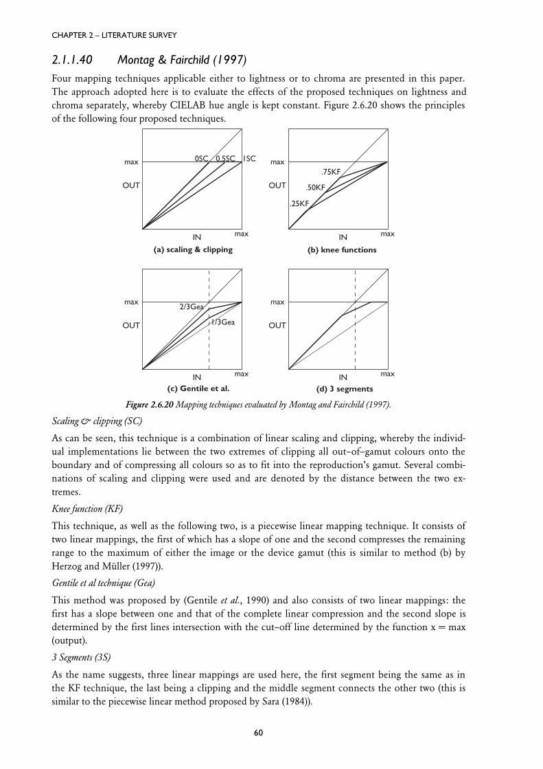
Figure 2.6.20 Mapping techniques evaluated by Montag and Fairchild (1997).
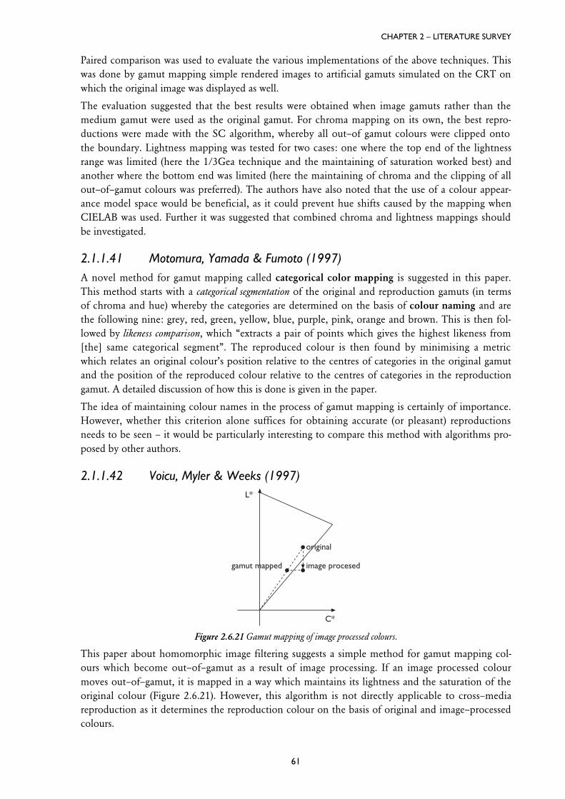
Figure 2.6.21 Gamut mapping of image processed colours.
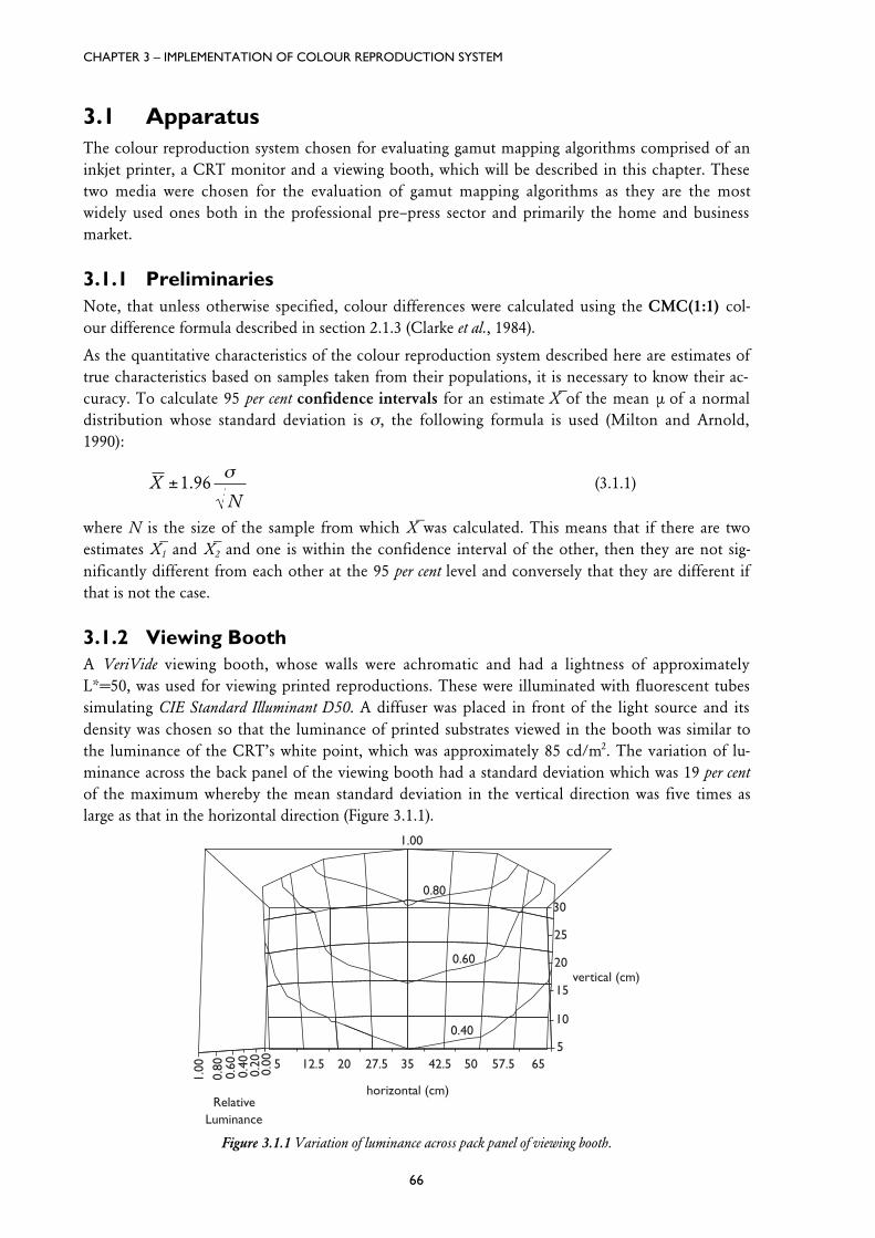
Figure 3.1.1 Variation of luminance across pack panel of viewing booth.
LIST OF FIGURES
xi
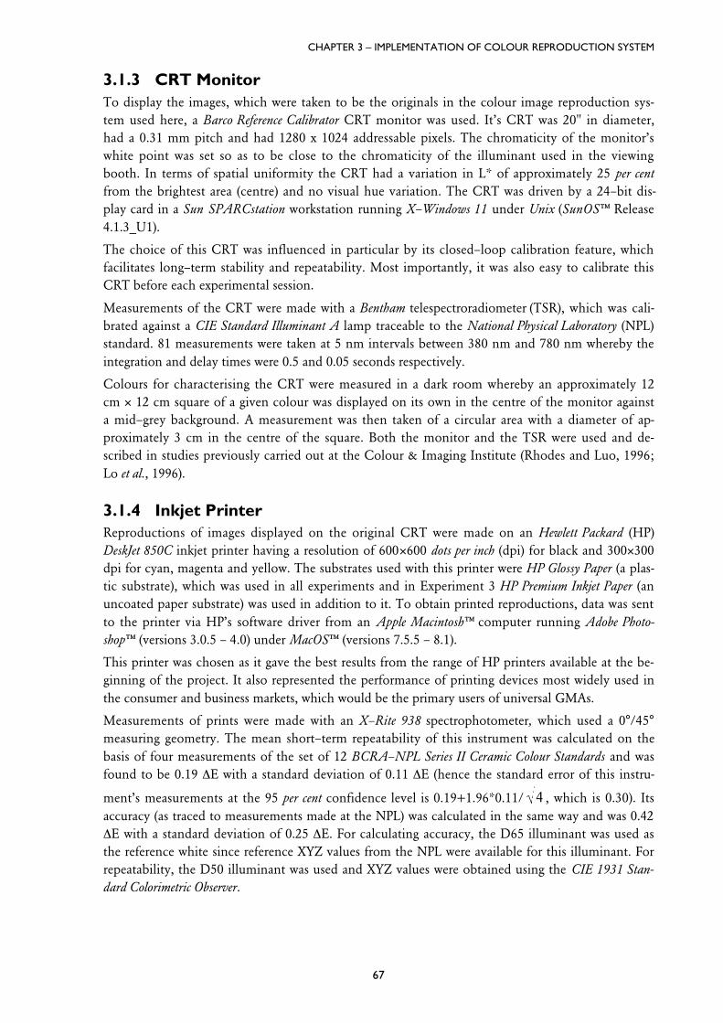
Figure 3.1.2 Colour difference as a function of time.
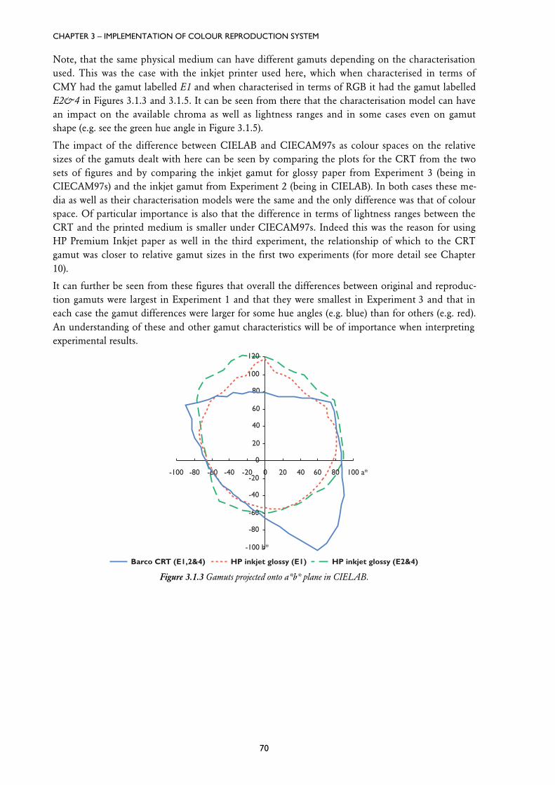
Figure 3.1.3 Gamuts projected onto a*b* plane in CIELAB.
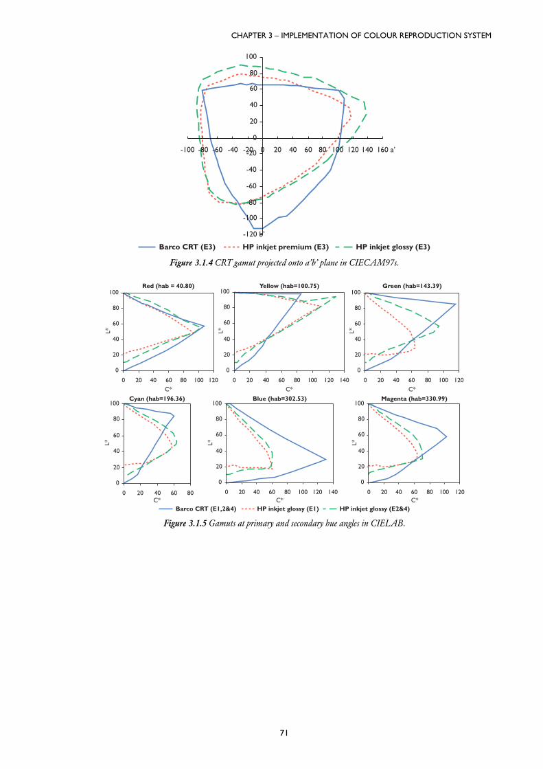
Figure 3.1.4 CRT gamut projected onto a’b’ plane in CIECAM97s.
Figure 3.1.5 Gamuts at primary and secondary hue angles in CIELAB.
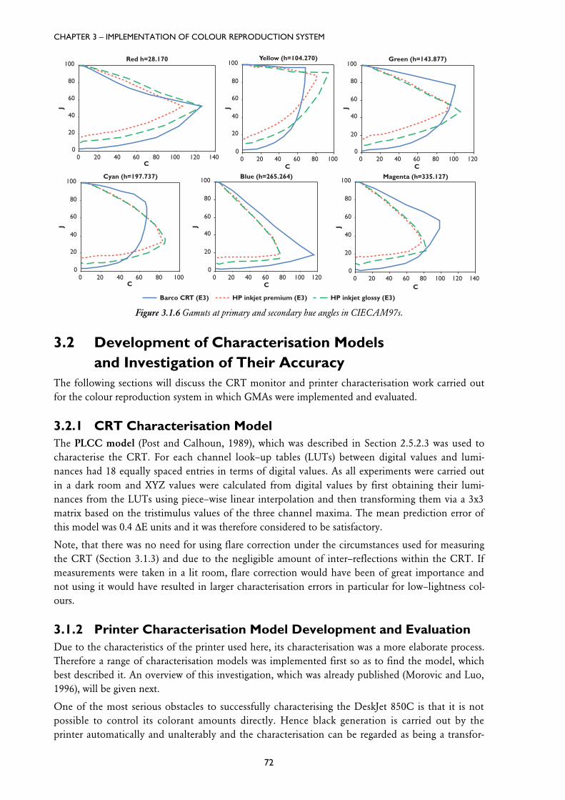
Figure 3.1.6 Gamuts at primary and secondary hue angles in CIECAM97s.
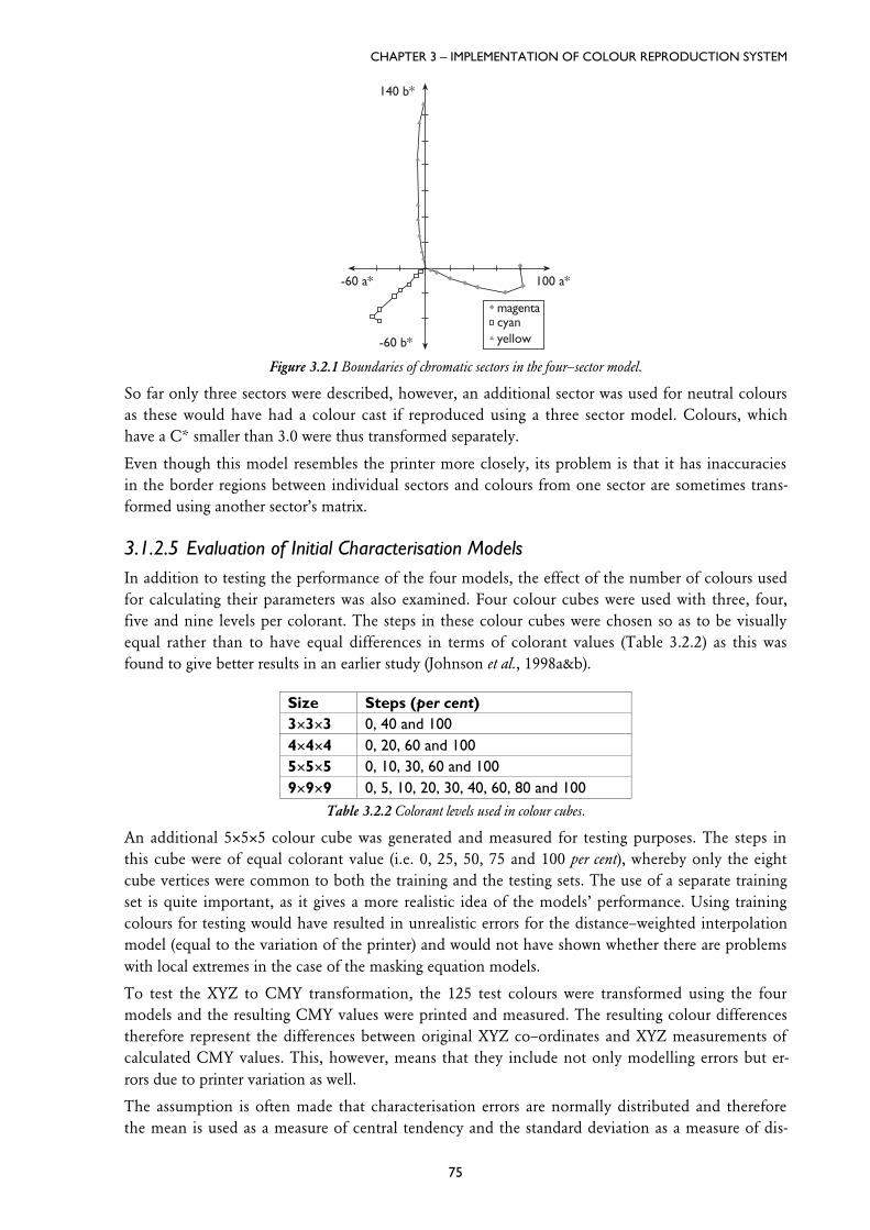
Figure 3.2.1 Boundaries of chromatic sectors in the four–sector model.
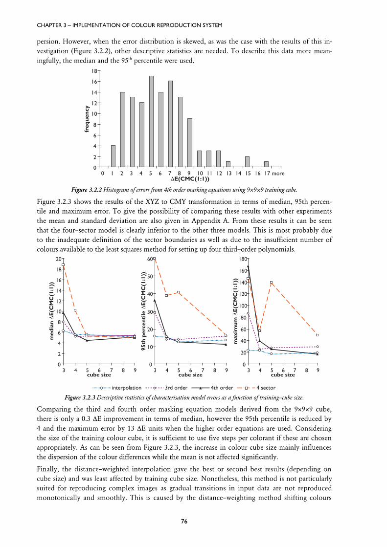
Figure 3.2.2 Histogram of errors from 4th order masking equations using 9´9´9 training cube.
Figure 3.2.3 Descriptive statistics of characterisation model errors as a function of training–cube size.
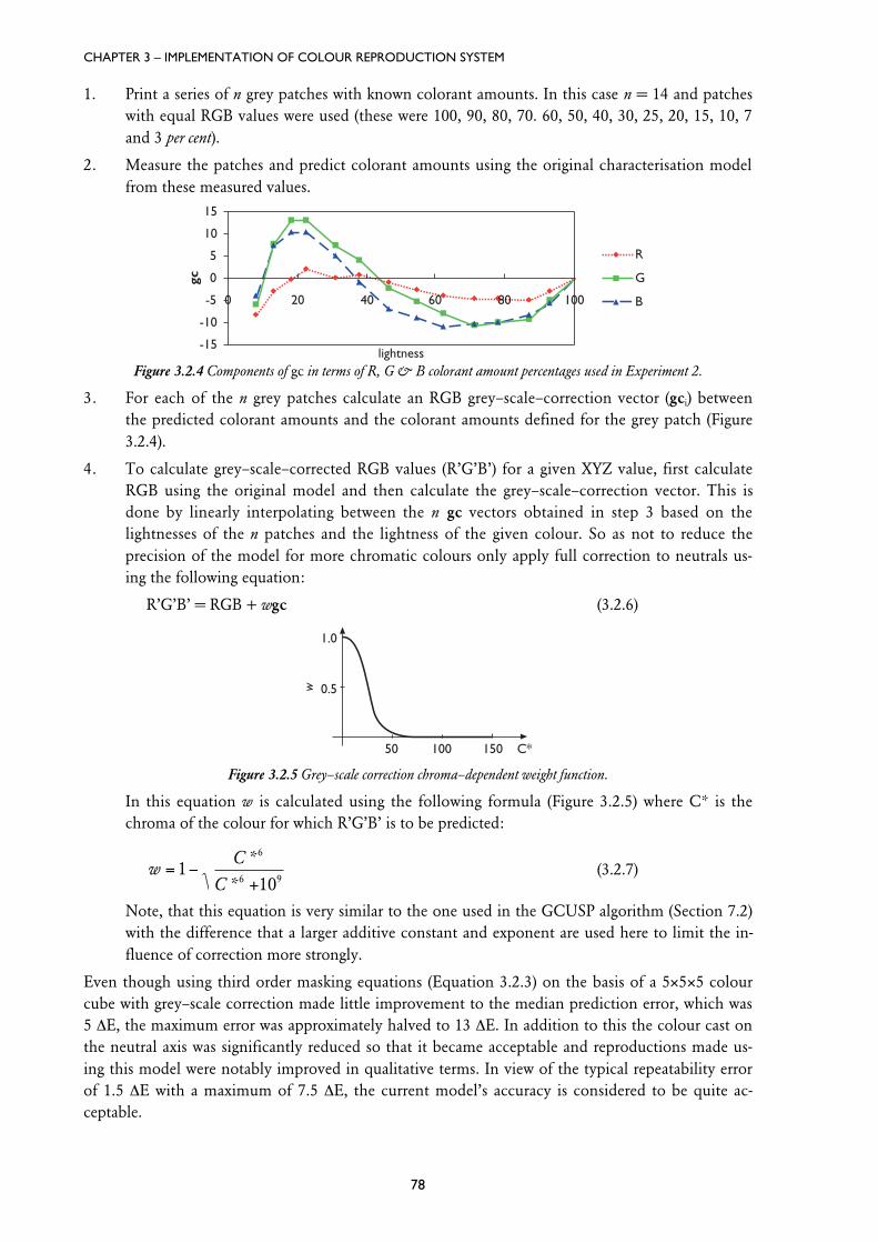
Figure 3.2.4 Components of gc in terms of R, G & B colorant amount percentages used in Experiment 2.
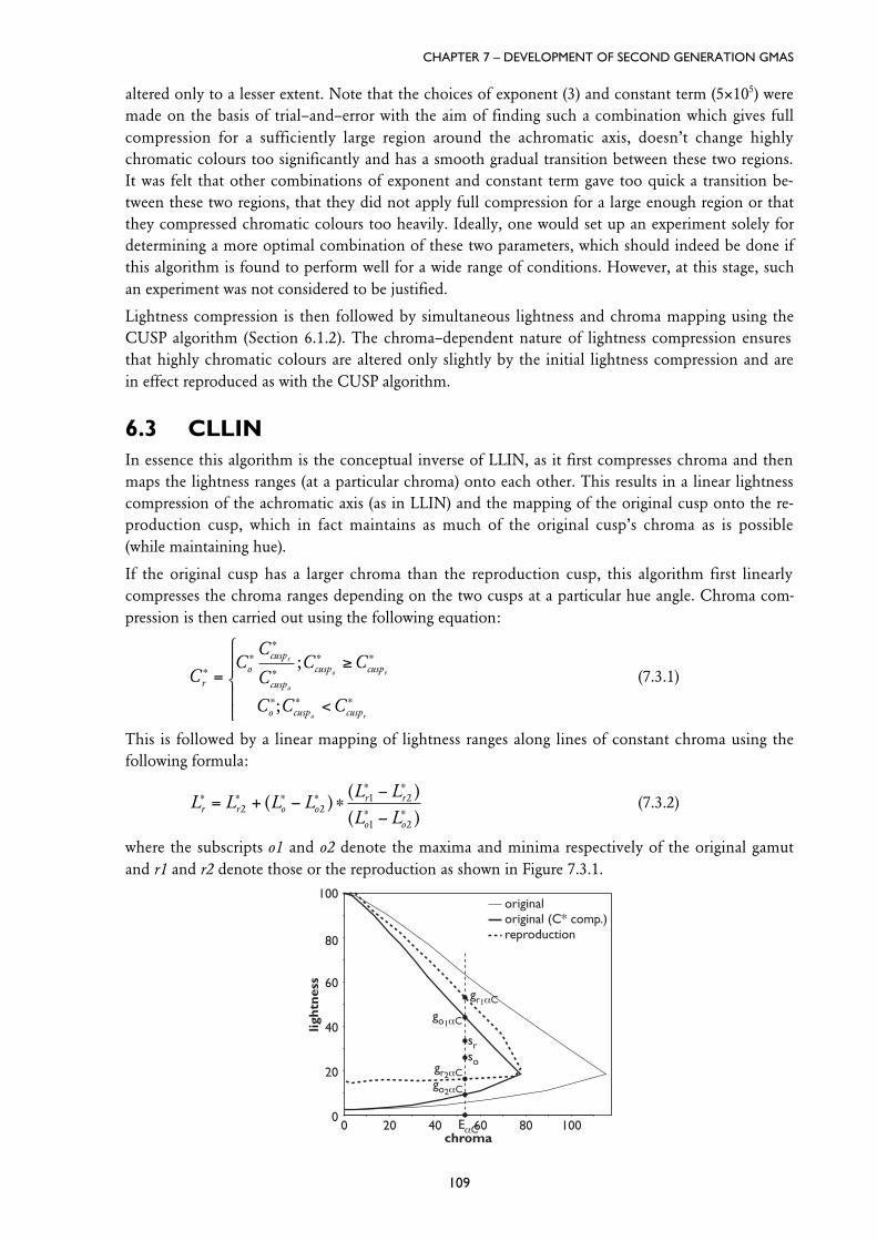
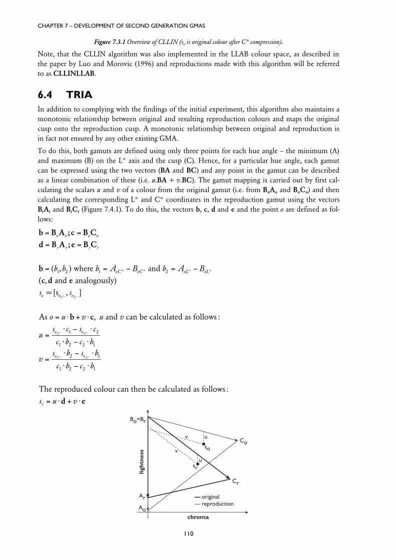
Figure 7.3.1 Overview of CLLIN (so is original colour after C* compression).
Figure 7.4.1 Overview of triangular mapping.
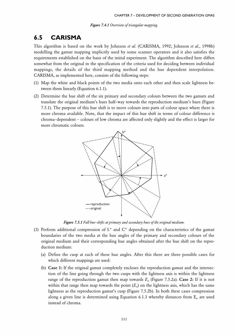
Figure 7.5.1 Full hue–shifts at primary and secondary hues of the original medium.
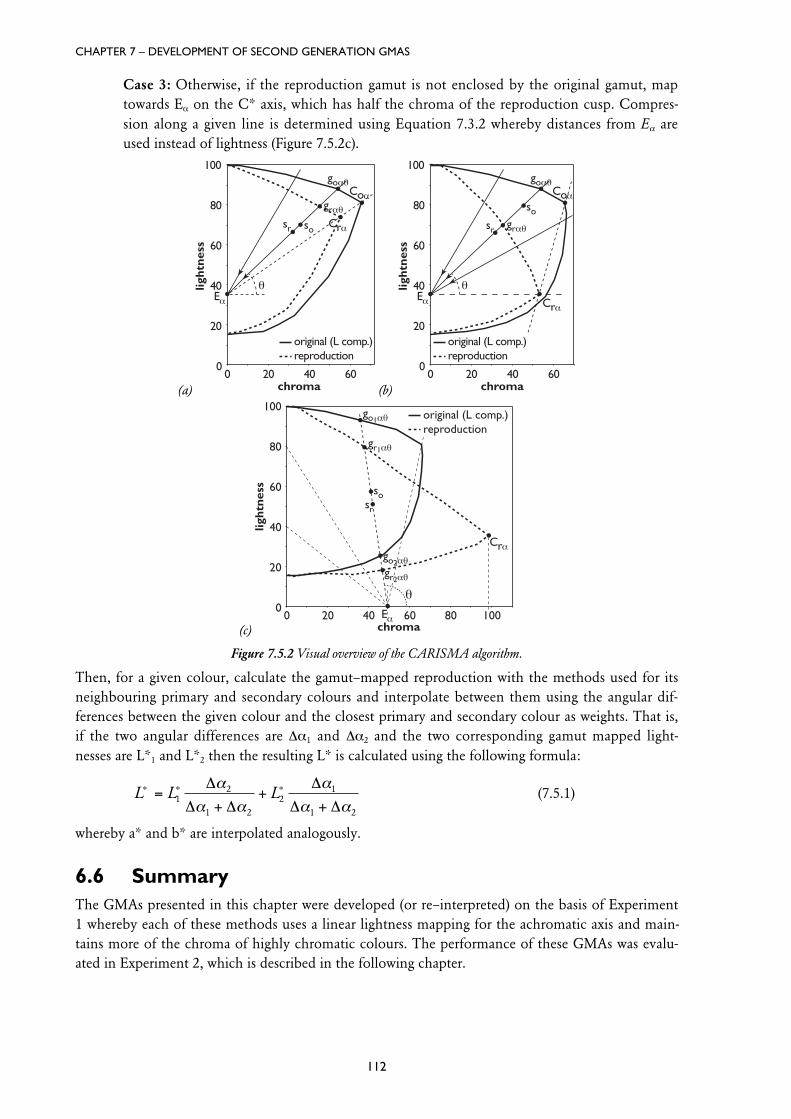
Figure 7.5.2 Visual overview of the CARISMA algorithm.
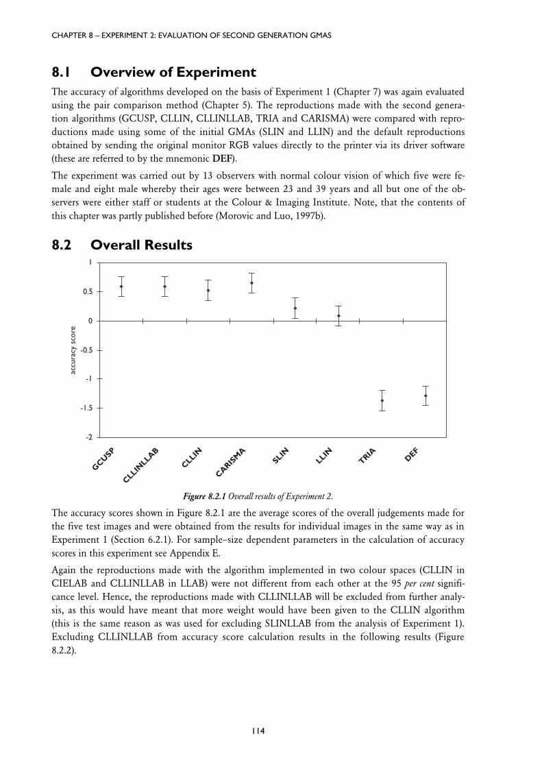
Figure 8.2.1 Overall results of Experiment 2.
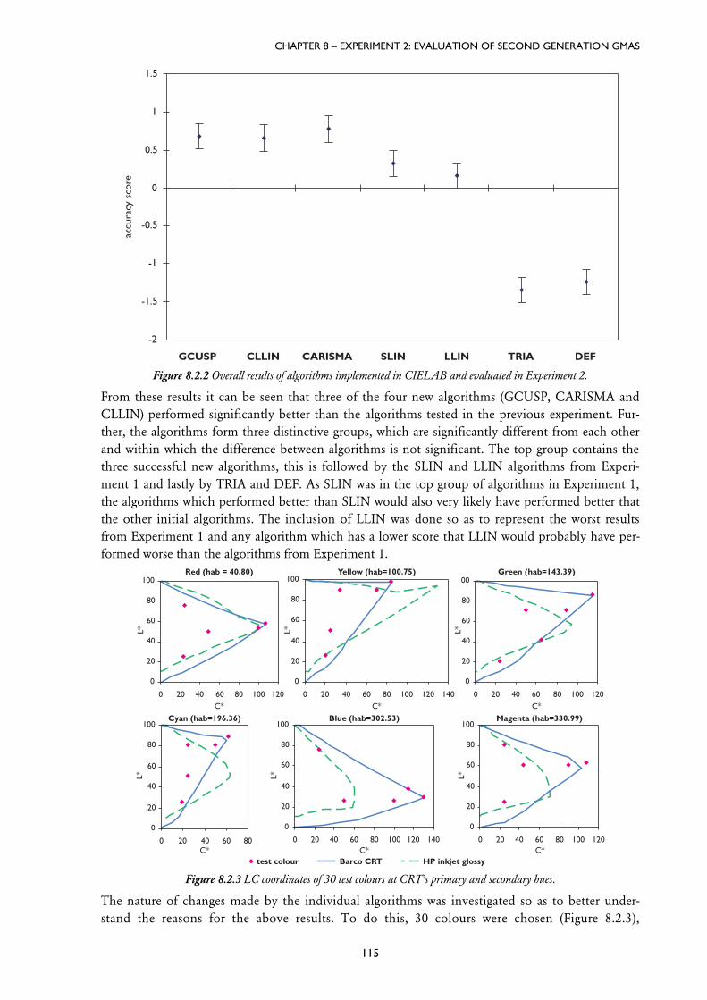
Figure 8.2.2 Overall results of algorithms implemented in CIELAB and evaluated in Experiment 2.
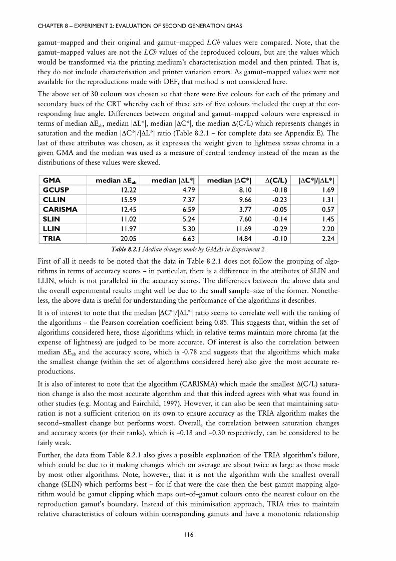
Figure 8.2.3 LC coordinates of 30 test colours at CRT’s primary and secondary hues.
Figure 8.3.1 Results for colour regions by colour region.
Figure 8.3.2 Results for colour regions by GMA.
Figure 8.4.1 Results for test images by image.
Figure 8.4.2 Results for test images by GMA.
LIST OF FIGURES
xii
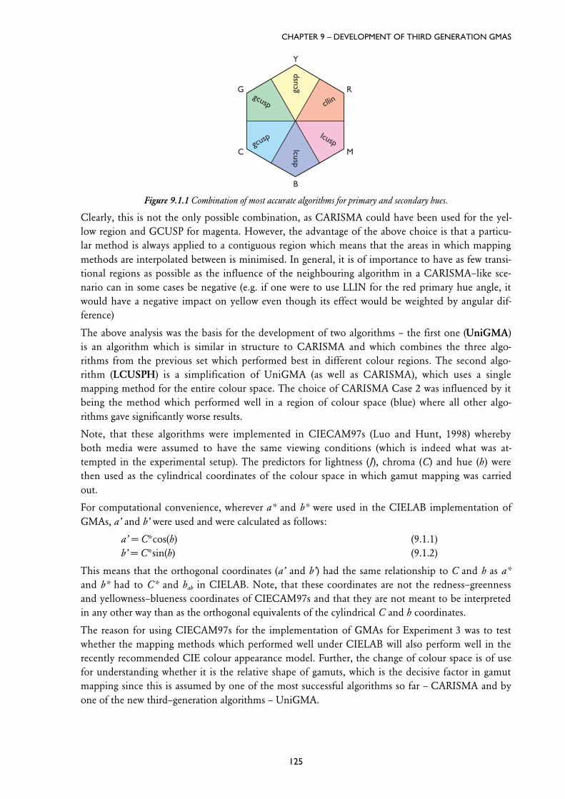
Figure 9.1.1 Combination of most accurate algorithms for primary and secondary hues.
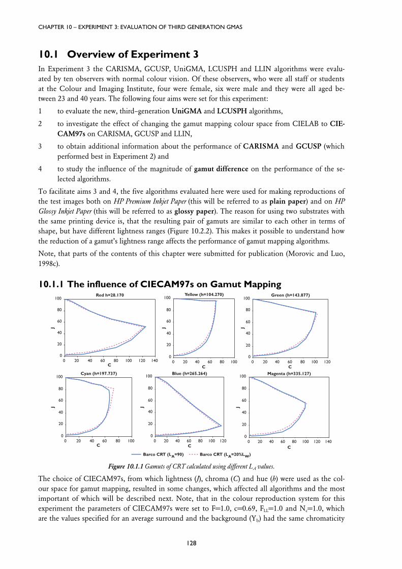
Figure 10.1.1 Gamuts of CRT calculated using different LA values.
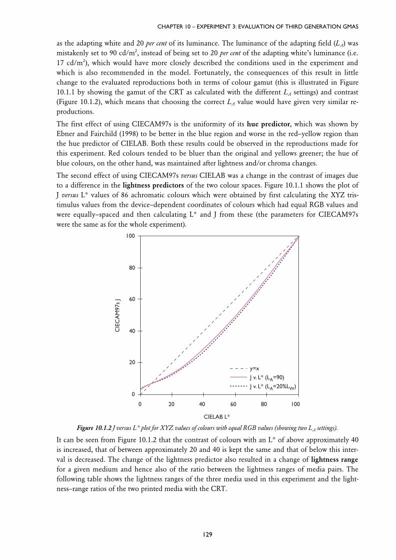
Figure 10.1.2 J versus L* plot for XYZ values of colours with equal RGB values (showing two LA settings).
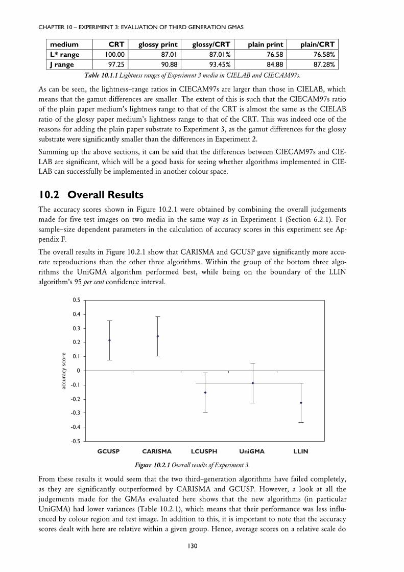
Figure 10.2.1 Overall results of Experiment 3.
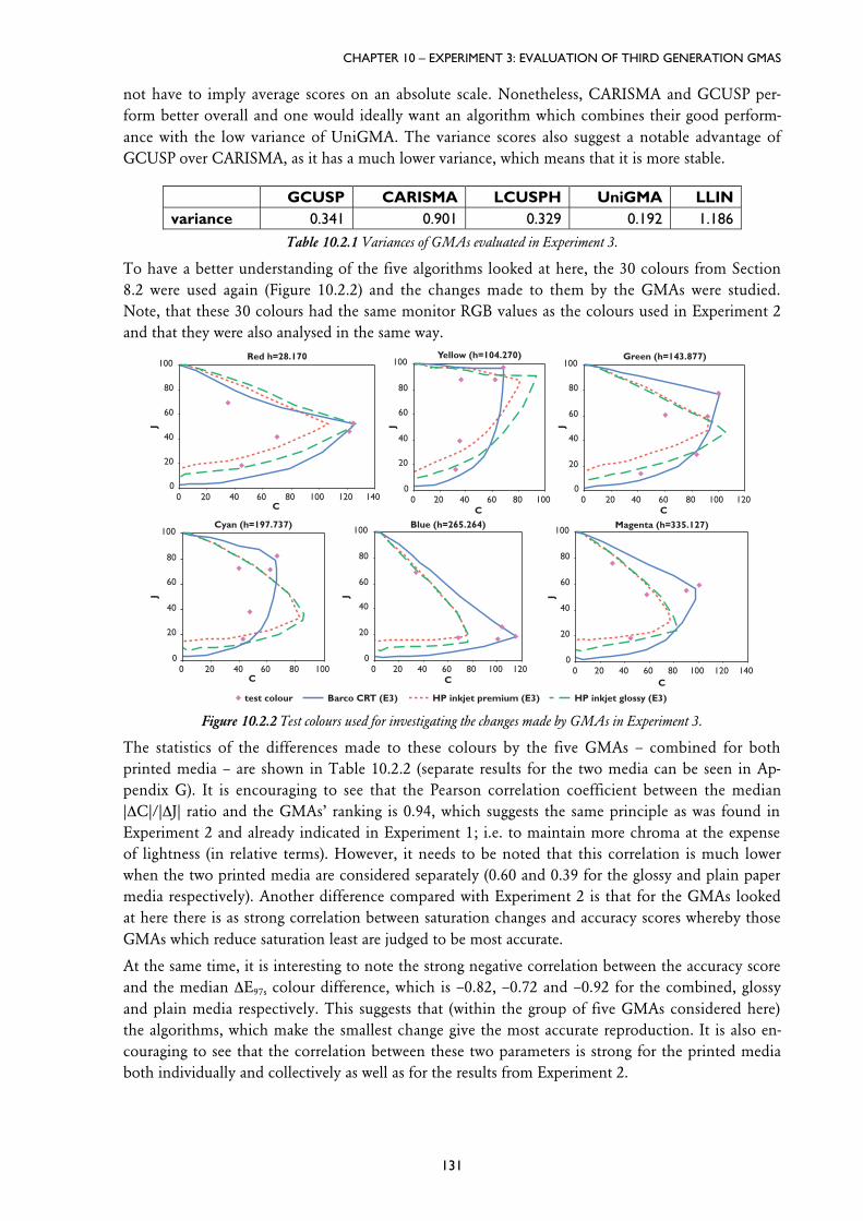
Figure 10.2.2 Test colours used for investigating the changes made by GMAs in Experiment 3.
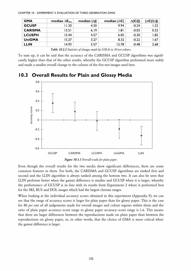
Figure 10.3.1 Overall results for plain paper.
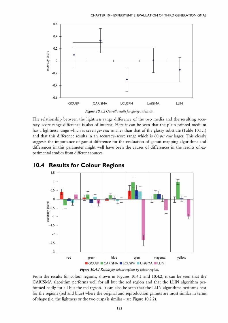
Figure 10.3.2 Overall results for glossy substrate.
Figure 10.4.1 Results for colour regions by colour region.
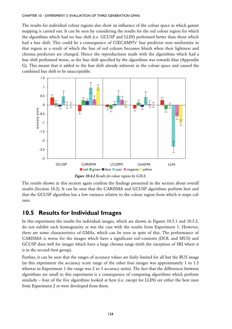
Figure 10.4.2 Results for colour regions by GMA.
Figure 10.5.1 Results for test images by image.
Figure 10.5.2 Results for test images by GMA.
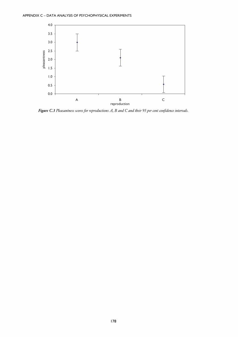
Figure 11.3.1 Overall pleasantness scores obtained using category judgement method.
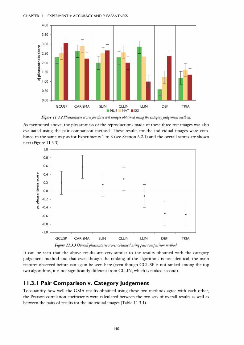
Figure 11.3.2 Pleasantness scores for three test images obtained using category judgement method.
Figure 11.3.3 Overall pleasantness scores obtained using pair comparison method.
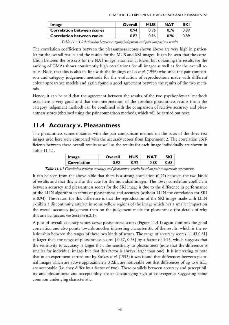
Figure 11.4.1 Overall accuracy scores versus pleasantness scores for the seven GMAs evaluated here.
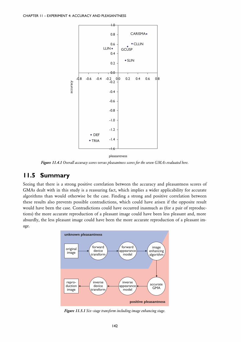
Figure 11.5.1 Six–stage transform including image enhancing stage.
1
Chapter 1
Introduction
Communication of all kinds is like painting –a compromise with impossibilities.
Samuel Butler (II)
CHAPTER 1 – INTRODUCTION
2
1.1 Background
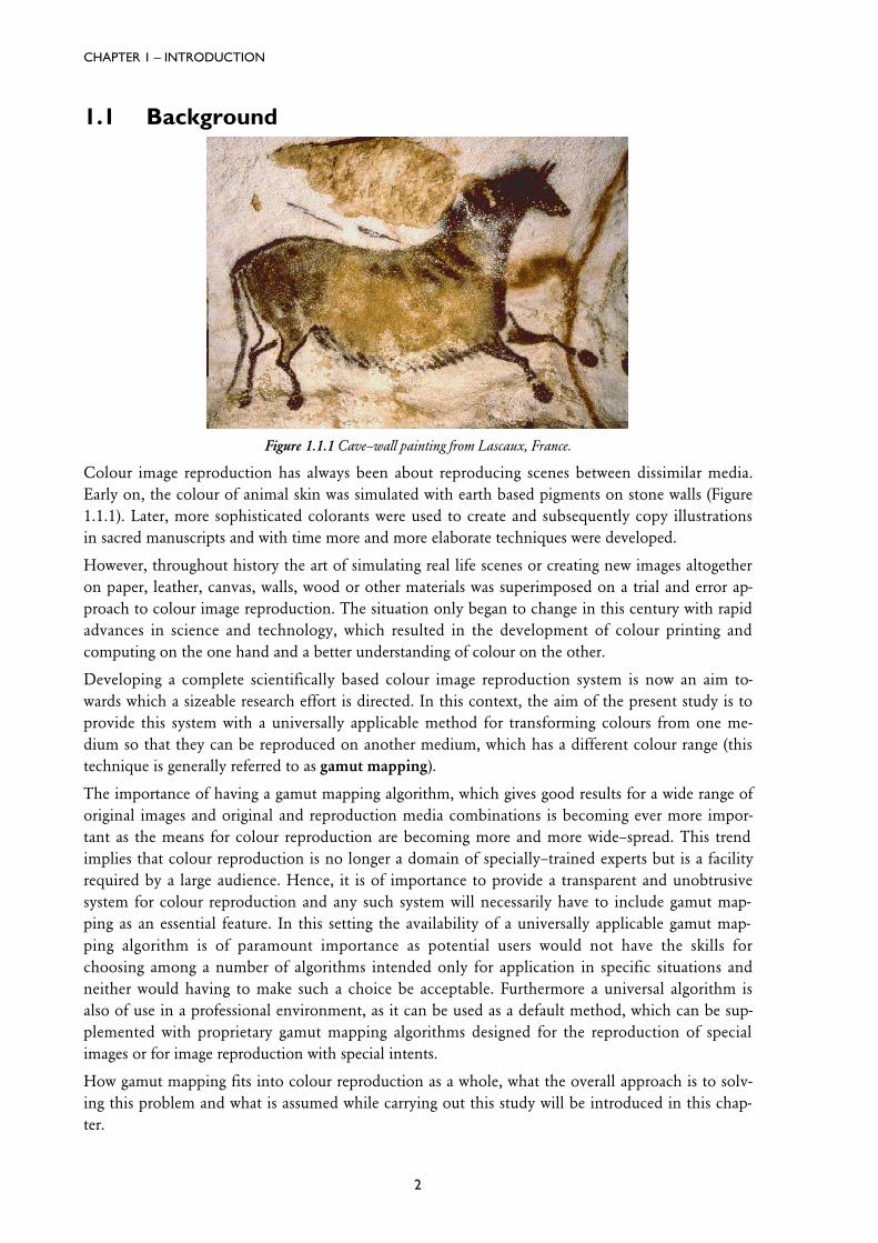
Figure 1.1.1 Cave–wall painting from Lascaux, France.
Colour image reproduction has always been about reproducing scenes between dissimilar media.Early on, the colour of animal skin was simulated with earth based pigments on stone walls (Figure1.1.1). Later, more sophisticated colorants were used to create and subsequently copy illustrationsin sacred manuscripts and with time more and more elaborate techniques were developed.
However, throughout history the art of simulating real life scenes or creating new images altogetheron paper, leather, canvas, walls, wood or other materials was superimposed on a trial and error ap-proach to colour image reproduction. The situation only began to change in this century with rapidadvances in science and technology, which resulted in the development of colour printing andcomputing on the one hand and a better understanding of colour on the other.
Developing a complete scientifically based colour image reproduction system is now an aim to-wards which a sizeable research effort is directed. In this context, the aim of the present study is toprovide this system with a universally applicable method for transforming colours from one me-dium so that they can be reproduced on another medium, which has a different colour range (thistechnique is generally referred to as gamut mapping).
The importance of having a gamut mapping algorithm, which gives good results for a wide range oforiginal images and original and reproduction media combinations is becoming ever more impor-tant as the means for colour reproduction are becoming more and more wide–spread. This trendimplies that colour reproduction is no longer a domain of specially–trained experts but is a facilityrequired by a large audience. Hence, it is of importance to provide a transparent and unobtrusivesystem for colour reproduction and any such system will necessarily have to include gamut map-ping as an essential feature. In this setting the availability of a universally applicable gamut map-ping algorithm is of paramount importance as potential users would not have the skills forchoosing among a number of algorithms intended only for application in specific situations andneither would having to make such a choice be acceptable. Furthermore a universal algorithm isalso of use in a professional environment, as it can be used as a default method, which can be sup-plemented with proprietary gamut mapping algorithms designed for the reproduction of specialimages or for image reproduction with special intents.
How gamut mapping fits into colour reproduction as a whole, what the overall approach is to solv-ing this problem and what is assumed while carrying out this study will be introduced in this chap-ter.
CHAPTER 1 – INTRODUCTION
3
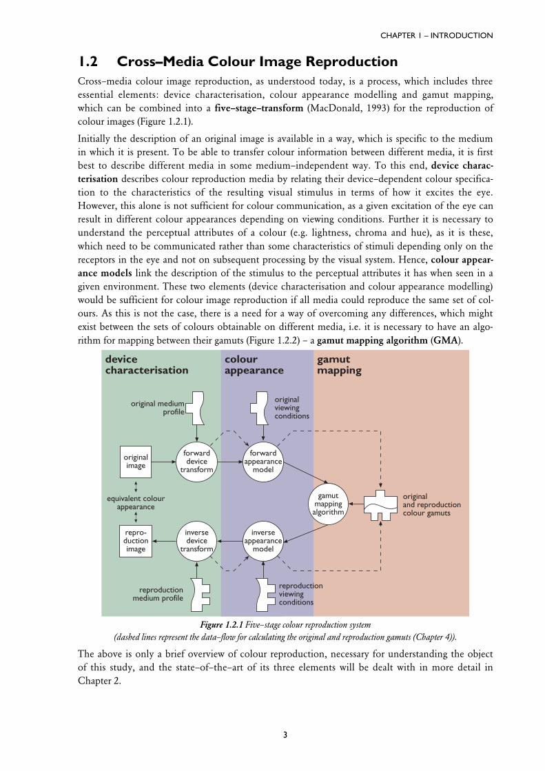
1.2 Cross–Media Colour Image ReproductionCross–media colour image reproduction, as understood today, is a process, which includes threeessential elements: device characterisation, colour appearance modelling and gamut mapping,which can be combined into a five–stage–transform (MacDonald, 1993) for the reproduction ofcolour images (Figure 1.2.1).
Initially the description of an original image is available in a way, which is specific to the mediumin which it is present. To be able to transfer colour information between different media, it is firstbest to describe different media in some medium–independent way. To this end, device charac-terisation describes colour reproduction media by relating their device–dependent colour specifica-tion to the characteristics of the resulting visual stimulus in terms of how it excites the eye.However, this alone is not sufficient for colour communication, as a given excitation of the eye canresult in different colour appearances depending on viewing conditions. Further it is necessary tounderstand the perceptual attributes of a colour (e.g. lightness, chroma and hue), as it is these,which need to be communicated rather than some characteristics of stimuli depending only on thereceptors in the eye and not on subsequent processing by the visual system. Hence, colour appear-ance models link the description of the stimulus to the perceptual attributes it has when seen in agiven environment. These two elements (device characterisation and colour appearance modelling)would be sufficient for colour image reproduction if all media could reproduce the same set of col-ours. As this is not the case, there is a need for a way of overcoming any differences, which mightexist between the sets of colours obtainable on different media, i.e. it is necessary to have an algo-rithm for mapping between their gamuts (Figure 1.2.2) – a gamut mapping algorithm (GMA).
gamutmapping
colourappearance
original mediumprofile
originalimage
repro-ductionimage
equivalent colourappearance
originalviewingconditions
reproductionviewingconditions
reproductionmedium profile
forwarddevice
transform
forwardappearance
model
inverseappearance
model
inversedevice
transform
devicecharacterisation
originaland reproductioncolour gamuts
gamutmappingalgorithm
Figure 1.2.1 Five–stage colour reproduction system(dashed lines represent the data–flow for calculating the original and reproduction gamuts (Chapter 4)).
The above is only a brief overview of colour reproduction, necessary for understanding the objectof this study, and the state–of–the–art of its three elements will be dealt with in more detail inChapter 2.
CHAPTER 1 – INTRODUCTION
4
-a*
-b*
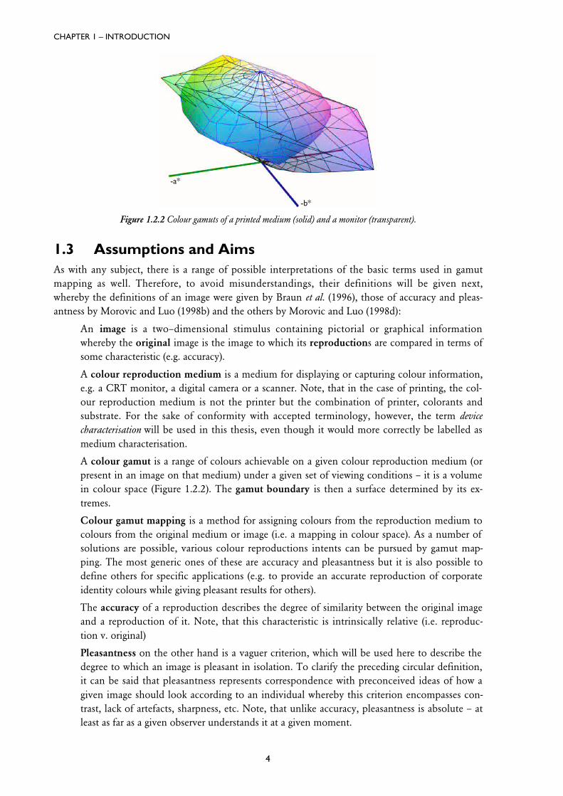
Figure 1.2.2 Colour gamuts of a printed medium (solid) and a monitor (transparent).
1.3 Assumptions and AimsAs with any subject, there is a range of possible interpretations of the basic terms used in gamutmapping as well. Therefore, to avoid misunderstandings, their definitions will be given next,whereby the definitions of an image were given by Braun et al. (1996), those of accuracy and pleas-antness by Morovic and Luo (1998b) and the others by Morovic and Luo (1998d):
An image is a two–dimensional stimulus containing pictorial or graphical informationwhereby the original image is the image to which its reproductions are compared in terms ofsome characteristic (e.g. accuracy).
A colour reproduction medium is a medium for displaying or capturing colour information,e.g. a CRT monitor, a digital camera or a scanner. Note, that in the case of printing, the col-our reproduction medium is not the printer but the combination of printer, colorants andsubstrate. For the sake of conformity with accepted terminology, however, the term devicecharacterisation will be used in this thesis, even though it would more correctly be labelled asmedium characterisation.
A colour gamut is a range of colours achievable on a given colour reproduction medium (orpresent in an image on that medium) under a given set of viewing conditions – it is a volumein colour space (Figure 1.2.2). The gamut boundary is then a surface determined by its ex-tremes.
Colour gamut mapping is a method for assigning colours from the reproduction medium tocolours from the original medium or image (i.e. a mapping in colour space). As a number ofsolutions are possible, various colour reproductions intents can be pursued by gamut map-ping. The most generic ones of these are accuracy and pleasantness but it is also possible todefine others for specific applications (e.g. to provide an accurate reproduction of corporateidentity colours while giving pleasant results for others).
The accuracy of a reproduction describes the degree of similarity between the original imageand a reproduction of it. Note, that this characteristic is intrinsically relative (i.e. reproduc-tion v. original)
Pleasantness on the other hand is a vaguer criterion, which will be used here to describe thedegree to which an image is pleasant in isolation. To clarify the preceding circular definition,it can be said that pleasantness represents correspondence with preconceived ideas of how agiven image should look according to an individual whereby this criterion encompasses con-trast, lack of artefacts, sharpness, etc. Note, that unlike accuracy, pleasantness is absolute – atleast as far as a given observer understands it at a given moment.
CHAPTER 1 – INTRODUCTION
5
In the context of the above definitions, the development of algorithms described in this study as-sumes that the appearance of the original image is what needs to be reproduced and that the origi-nal image has a pleasant appearance. Hence the algorithms aim at an accurate reproduction andhave no image enhancing intents. One could argue that it is often a pleasant reproduction, which isneeded and as this is an important question, the relationship between the pleasantness and accu-racy of reproductions made with GMAs dealt with here was investigated in Experiment 4 and willbe described in Chapter 11.
It further needs to be noted that this study focuses on gamut compression – i.e. gamut mappingfrom a larger to a smaller gamut, as this is most often needed in situations where a universal gamutmapping would be used at present. As the reproduction gamuts in this study were not smaller thanthe original gamuts in all parts of colour space, gamut mapping was only applied in the areas whereit was necessary and no changes were made to original colours when the reproduction gamut waslarger or equal to the original gamut along a given line of compression. In the context of accuratereproduction it was though to be more important to focus on gamut compression. For an investiga-tion of gamut expansion (gamut mapping from a smaller to a larger gamut) refer to Hoshino (1991).
Before going into the details of this study, it is of great importance to clearly understand its aim – auniversal gamut mapping algorithm. Here it will be defined as a gamut mapping algorithm, whichgives consistently good results for a wide range of media combinations and original images. It is notmeant to be a method, which gives the best result for every image under every possible set of con-ditions. Instead, it ought to be seen as a default method, which can be used for the majority of im-ages and media combinations and which can be supplemented by proprietary solutions for use inspecial applications.
Further it needs to be noted that no claims are made about the universality of algorithms devel-oped in this study, as this would require far more extensive testing than is practical in the period oftime available and as this would also require the investigation of gamut expansion and the use of alarger variety of test images. The use of the term “universal” in the title of this thesis denotes its aimrather than a label for its outcomes.
1.4 A Method for Developing GMAsVarious methods have previously been used for developing GMAs whereby in a small number ofcases the starting point was a set of experimental data, which was then modelled. However, in themajority of studies a model was first formulated and then tested experimentally (or the model’s pa-rameters were established on that basis).
The approach taken in this study is a combination of these two styles whereby the starting point isa selection of existing GMAs, which are then experimentally evaluated. The experimental methodused in most experiments of this study has a special feature, which is that in addition to evaluatingthe overall image, individual regions within the image are also evaluated. As in the paper by Mac-Donald and Morovic (1995), these image regions are chosen so as to have characteristic coloursand their evaluation therefore gives information about the performance of GMAs in different partsof colour space. This kind of information is a solid and quantitative basis for making alterations toGMAs.
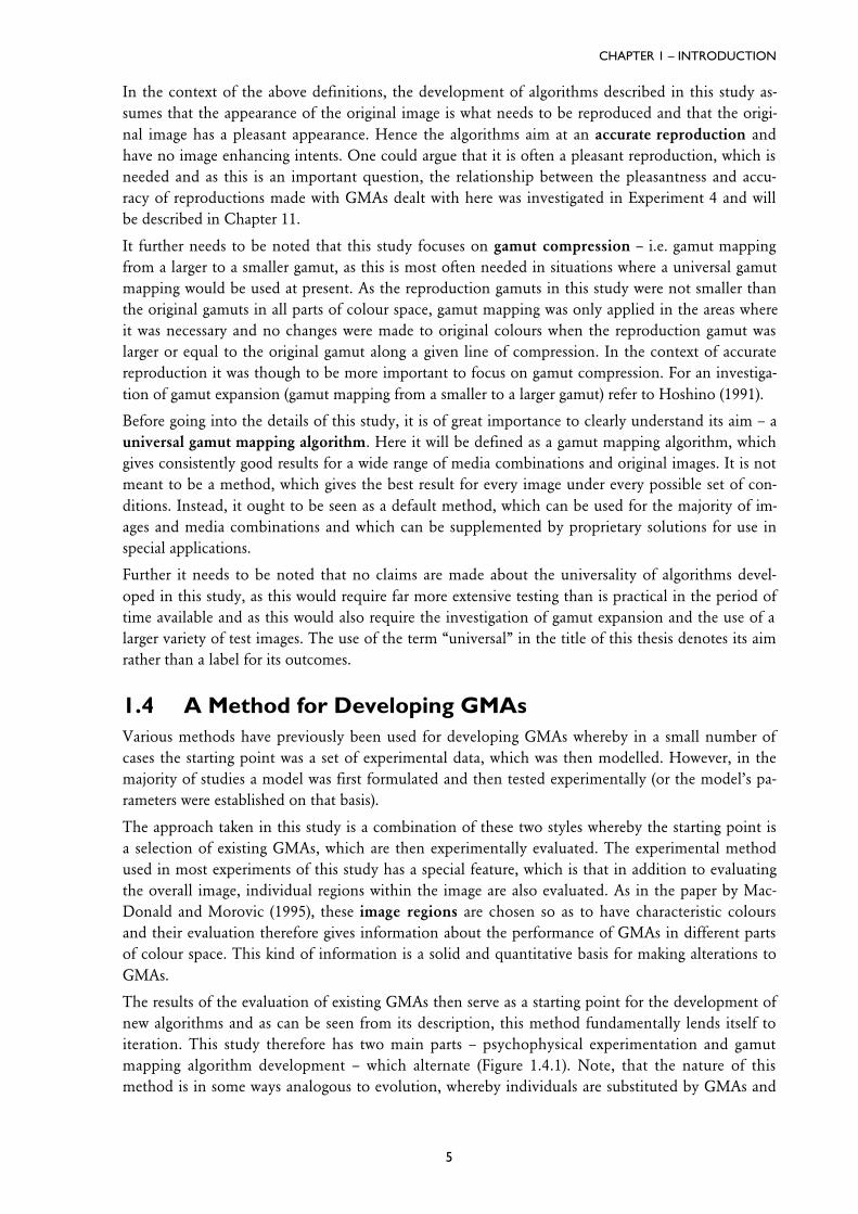
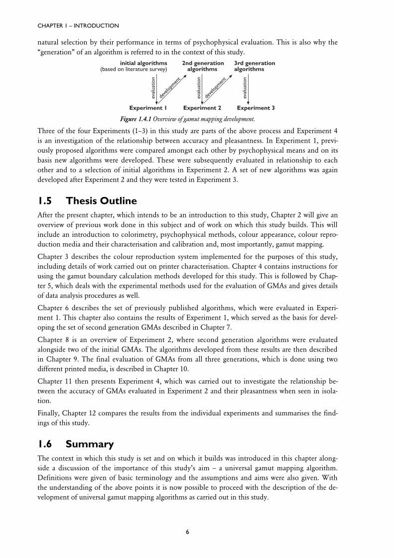
The results of the evaluation of existing GMAs then serve as a starting point for the development ofnew algorithms and as can be seen from its description, this method fundamentally lends itself toiteration. This study therefore has two main parts – psychophysical experimentation and gamutmapping algorithm development – which alternate (Figure 1.4.1). Note, that the nature of thismethod is in some ways analogous to evolution, whereby individuals are substituted by GMAs and
CHAPTER 1 – INTRODUCTION
6
natural selection by their performance in terms of psychophysical evaluation. This is also why the“generation” of an algorithm is referred to in the context of this study.
initial algorithms(based on literature survey)
Experiment 1
eval
uatio
n
2nd generationalgorithms
Experiment 2
deve
lopmen
t
eval
uatio
n
deve
lopmen
t
3rd generationalgorithms
Experiment 3
eval
uatio
n
Figure 1.4.1 Overview of gamut mapping development.
Three of the four Experiments (1–3) in this study are parts of the above process and Experiment 4is an investigation of the relationship between accuracy and pleasantness. In Experiment 1, previ-ously proposed algorithms were compared amongst each other by psychophysical means and on itsbasis new algorithms were developed. These were subsequently evaluated in relationship to eachother and to a selection of initial algorithms in Experiment 2. A set of new algorithms was againdeveloped after Experiment 2 and they were tested in Experiment 3.
1.5 Thesis OutlineAfter the present chapter, which intends to be an introduction to this study, Chapter 2 will give anoverview of previous work done in this subject and of work on which this study builds. This willinclude an introduction to colorimetry, psychophysical methods, colour appearance, colour repro-duction media and their characterisation and calibration and, most importantly, gamut mapping.
Chapter 3 describes the colour reproduction system implemented for the purposes of this study,including details of work carried out on printer characterisation. Chapter 4 contains instructions forusing the gamut boundary calculation methods developed for this study. This is followed by Chap-ter 5, which deals with the experimental methods used for the evaluation of GMAs and gives detailsof data analysis procedures as well.
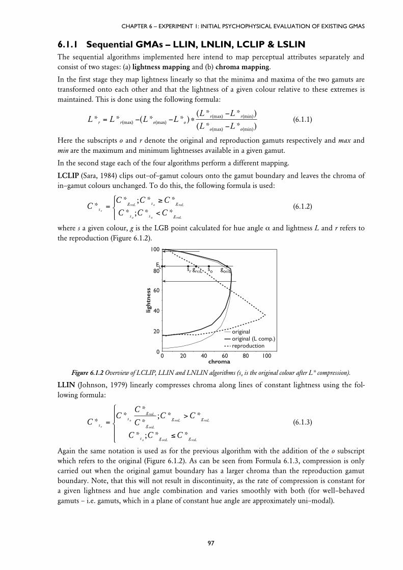
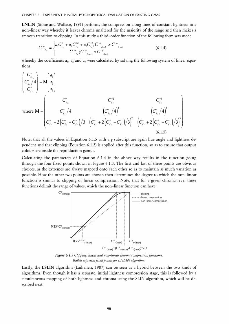
Chapter 6 describes the set of previously published algorithms, which were evaluated in Experi-ment 1. This chapter also contains the results of Experiment 1, which served as the basis for devel-oping the set of second generation GMAs described in Chapter 7.
Chapter 8 is an overview of Experiment 2, where second generation algorithms were evaluatedalongside two of the initial GMAs. The algorithms developed from these results are then describedin Chapter 9. The final evaluation of GMAs from all three generations, which is done using twodifferent printed media, is described in Chapter 10.
Chapter 11 then presents Experiment 4, which was carried out to investigate the relationship be-tween the accuracy of GMAs evaluated in Experiment 2 and their pleasantness when seen in isola-tion.
Finally, Chapter 12 compares the results from the individual experiments and summarises the find-ings of this study.
1.6 SummaryThe context in which this study is set and on which it builds was introduced in this chapter along-side a discussion of the importance of this study’s aim – a universal gamut mapping algorithm.Definitions were given of basic terminology and the assumptions and aims were also given. Withthe understanding of the above points it is now possible to proceed with the description of the de-velopment of universal gamut mapping algorithms as carried out in this study.
7
Chapter 2
Literature Survey
Nature has given to men one tongue,but two ears, that we may hear from others
twice as much as we speak.
Epictetus
CHAPTER 2 – LITERATURE SURVEY
8
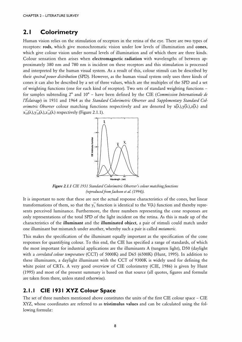
2.1 ColorimetryHuman vision relies on the stimulation of receptors in the retina of the eye. There are two types ofreceptors: rods, which give monochromatic vision under low levels of illumination and cones,which give colour vision under normal levels of illumination and of which there are three kinds.Colour sensation then arises when electromagnetic radiation with wavelengths of between ap-proximately 380 nm and 780 nm is incident on these receptors and this stimulation is processedand interpreted by the human visual system. As a result of this, colour stimuli can be described bytheir spectral power distribution (SPD). However, as the human visual system only uses three kinds ofcones it can also be described by a set of three values, which are the multiples of the SPD and a setof weighting functions (one for each kind of receptor). Two sets of standard weighting functions –for samples subtending 2° and 10° – have been defined by the CIE (Commission Internationale del’Éclairage) in 1931 and 1964 as the Standard Colorimetric Observer and Supplementary Standard Col-orimetric Observer colour matching functions respectively and are denoted by x(l),y(l),z(l) andx10(l),y10(l),z10(l) respectively (Figure 2.1.1).
Figure 2.1.1 CIE 1931 Standard Colorimetric Observer’s colour matching functions(reproduced from Jackson et al. (1994)).
It is important to note that these are not the actual response characteristics of the cones, but lineartransformations of them, so that the yl function is identical to the V(l) function and thereby repre-sents perceived luminance. Furthermore, the three numbers representing the cone responses areonly representations of the total SPD of the light incident on the retina. As this is made up of thecharacteristics of the illuminant and the illuminated object, a pair of stimuli could match underone illuminant but mismatch under another, whereby such a pair is called metameric.
This makes the specification of the illuminant equally important as the specification of the coneresponses for quantifying colour. To this end, the CIE has specified a range of standards, of whichthe most important for industrial applications are the illuminants A (tungsten light), D50 (daylightwith a correlated colour temperature (CCT) of 5000K) and D65 (6500K) (Hunt, 1995). In addition tothese illuminants, a daylight illuminant with the CCT of 9300K is widely used for defining thewhite point of CRTs. A very good overview of CIE colorimetry (CIE, 1986) is given by Hunt(1995) and most of the present summary is based on that source (all quotes, figures and formulæare taken from there, unless stated otherwise).
2.1.1 CIE 1931 XYZ Colour SpaceThe set of three numbers mentioned above constitutes the units of the first CIE colour space – CIEXYZ, whose coordinates are referred to as tristimulus values and can be calculated using the fol-lowing formulæ:
CHAPTER 2 – LITERATURE SURVEY
9
X = k åxlPlDlY = k åylPlDl (2.1.1)Z = k åzlPlDl
Here Pl stands for the power of the stimulus at wavelength l and k is a scaling constant. All otherCIE–defined colour spaces are derived from this one by various transformations.
For plotting the position of individual colours, a two dimensional chromaticity diagram was alsoderived from XYZ and its axes are defined as:
xX
X Y Zy
YX Y Z
=+ +
=+ +
; (2.1.2)
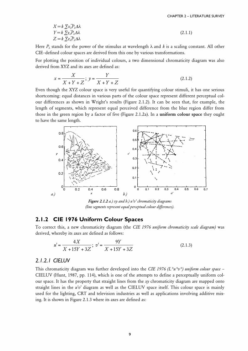
Even though the XYZ colour space is very useful for quantifying colour stimuli, it has one seriousshortcoming: equal distances in various parts of the colour space represent different perceptual col-our differences as shown in Wright’s results (Figure 2.1.2). It can be seen that, for example, thelength of segments, which represent equal perceived difference from the blue region differ fromthose in the green region by a factor of five (Figure 2.1.2a). In a uniform colour space they oughtto have the same length.
a.) b.)
Figure 2.1.2 a.) xy and b.) u’v’ chromaticity diagrams(line segments represent equal perceptual colour differences).
2.1.2 CIE 1976 Uniform Colour SpacesTo correct this, a new chromaticity diagram (the CIE 1976 uniform chromaticity scale diagram) wasderived, whereby its axes are defined as follows:
uX
X Y Zv
YX Y Z
' ; '=+ +
=+ +
415 3
915 3
(2.1.3)
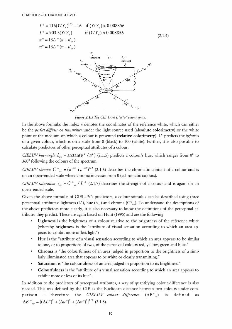
2.1.2.1 CIELUVThis chromaticity diagram was further developed into the CIE 1976 (L*u*v*) uniform colour space –CIELUV (Hunt, 1987, pp. 114), which is one of the attempts to define a perceptually uniform col-our space. It has the property that straight lines from the xy chromaticity diagram are mapped ontostraight lines in the u'v' diagram as well as the CIELUV space itself. This colour space is mainlyused for the lighting, CRT and television industries as well as applications involving additive mix-ing. It is shown in Figure 2.1.3 where its axes are defined as:
CHAPTER 2 – LITERATURE SURVEY
10
L Y Y Y Y
L Y Y Y Y
u L u u
v L v v
n n
n n
n
n
* ( ) ( ) .
* . ( ) ( ) .
* * ( ' ' )
* * ( ' ' )
/= - >
= £
= -
= -
1 / if /
/ if /
16 16 0 008856
903 3 0 008856
13
13
1 3
(2.1.4)
Figure 2.1.3 The CIE 1976 L*u*v* colour space.
In the above formulæ the index n denotes the coordinates of the reference white, which can eitherbe the perfect diffuser or transmitter under the light source used (absolute colorimetry) or the whitepoint of the medium on which a colour is presented (relative colorimetry). L* predicts the lightnessof a given colour, which is on a scale from 0 (black) to 100 (white). Further, it is also possible tocalculate predictors of other perceptual attributes of a colour:
CIELUV hue–angle h v uuv = arctan( * / *) (2.1.5) predicts a colour’s hue, which ranges from 0° to360° following the colours of the spectrum.
CIELUV chroma C u vuv* ( * * ) /= +2 2 1 2 (2.1.6) describes the chromatic content of a colour and ison an open–ended scale where chroma increases from 0 (achromatic colours).
CIELUV saturation s C Luv uv= * / * (2.1.7) describes the strength of a colour and is again on anopen–ended scale.
Given the above formulæ of CIELUV’s predictors, a colour stimulus can be described using threeperceptual attributes: lightness (L*), hue (huv) and chroma (C*uv). To understand the descriptions ofthe above predictors more clearly, it is also necessary to know the definitions of the perceptual at-tributes they predict. These are again based on Hunt (1995) and are the following:
• Lightness is the brightness of a colour relative to the brightness of the reference white(whereby brightness is the “attribute of visual sensation according to which an area ap-pears to exhibit more or less light”)
• Hue is the “attribute of a visual sensation according to which an area appears to be similarto one, or to proportions of two, of the perceived colours red, yellow, green and blue.”
• Chroma is “the colourfulness of an area judged in proportion to the brightness of a simi-larly illuminated area that appears to be white or clearly transmitting.”
• Saturation is “the colourfulness of an area judged in proportion to its brightness.”
• Colourfulness is the “attribute of a visual sensation according to which an area appears toexhibit more or less of its hue”.
In addition to the predictors of perceptual attributes, a way of quantifying colour difference is alsoneeded. This was defined by the CIE as the Euclidean distance between two colours under com-parison – therefore the CIELUV colour difference (DE*uv) is defined as
D = D + D + DE L u vuv* [( *) ( *) ( *) ] /2 2 2 1 2 (2.1.8).
CHAPTER 2 – LITERATURE SURVEY
11
2.1.1.2 CIELABAn additional colour space was defined by the CIE at the same time as CIELUV and for the samepurpose of uniformity – CIE 1976 (L*a*b*) uniform colour space – CIELAB. It is currently used bythe colorant and graphic arts industries as well as for other applications of subtractive mixing (e.g.surface colour industries) and its coordinates are defined by the following transformation of XYZ:
XnYnZn represent the reference white, hab, C*ab and DE*ab can be calculated from formulas (2.1.5),
(2.1.6) and (2.1.8) respectively by substituting a* for u* and b* for v*. There is no chromaticity dia-gram associated with this colour space and saturation is not defined in CIELAB either, due to thenon–linear nature of the a* and b* formulæ.
In literature, the CIE colour spaces are referred to as device independent as they do not depend onany particular input or output device, i.e. scanner, camera, monitor, printer or transparency. Thecharacteristic of what are referred to as device dependent colour spaces is, that they are intrinsi-cally linked to a particular device. These colour spaces are at least three dimensional, limited by themaximum amounts of the device’s colorants and device gamuts are cubes (or hyper–cubes) inthem.
Both the CIELAB and CIELUV colour spaces are imperfect attempts to define a perceptually uni-form colour space as they each have different deficiencies and neither of them is generally consid-ered as superior to the other. Nonetheless, they both offer significant improvements over using theXYZ tristimulus colour space for gamut mapping.
2.1.3 Colour Difference Formulæ
Determining the difference between two stimuli is of significant importance in colorimetry and themain objective for designing colour difference formulæ is to make their results as close to humanjudgements as possible. The simplest forms of colour difference (DE*ab and DE*uv), which were al-ready presented consider the distance between the coordinates of two stimuli in a given colourspace to be their colour difference. However, due to the non–uniformity of colour spaces, ad-vanced colour difference formulæ were developed, which more accurately predict human judge-ments. There are many different formulæ which have been developed to this end and work is stillbeing carried out to improve them (Luo, 1995).
In addition to the two advanced colour difference formulae, which will be presented next, it is use-ful to be aware of the development of models for the calculation of colour differences betweencomplex images which take into account their spatial characteristics. An example of such a modelis S–CIELAB (Zhang and Wandell, 1996) where images are first transformed into an opponent colourspace (whose dimensions are luminance, redness–greenness and yellowness–blueness) where each of thethree channels is blurred in a way which corresponds to the spatial sensitivity of the human visualsystem to the given channel (i.e. the luminance channel is blurred least and the yellow-ness–blueness channel is blurred most). Finally, CIELAB coordinates are computed for each pixelof the filtered images and colour difference, which now takes into account spatial characteristics, is
CHAPTER 2 – LITERATURE SURVEY
12
calculated as in CIELAB. Even though this model is an advance compared to colour differenceformulae, which are designed for uniform colour patches, it still needs to be improved significantlybefore it can reliably predict the results of psychophysical experiments.
2.1.1.1 CMC(l:c)Among the most widely used advanced colour difference formulæ is the CMC(l:c) colour differ-ence formula which apart form improving accuracy also provides a means for changing the relativeimportance of lightness and chroma. The DECMC(l:c) colour difference can be calculated using thefollowing formulæ (Clarke et al., 1984):
D =Dæ
èç
ö
ø÷ +
Dæ
èç
ö
ø÷ +
Dæ
èç
ö
ø÷E
LlS
CcS
HS
CMC l cL C H
( : )
* * *2 2 2
where SL = 0.040975L*1/(1+ 0.01765L*1)unless L*1<16 then SL=0.511SC = 0.0638C*1/(1+0.0131C*1) + 0.638SH = SC(Tf + 1 - f) (2.1.10)
fC
C=
+
*
*1
4
14 1900
T = 0.36 + |0.4cos(h1 + 35)|unless h1 (the hue angle of the first colour) is between 164° and 345°, when:T = 0.56 + |0.2cos(h1 + 168)|
Here L*1, C*1 and h1 represent the standard from which the colour difference is determined andDL*, DC* and DH* are calculated as in CIELAB. When the l:c ratio is set to 1:1, the DE values aremeant to represent the perceptibility of colour difference whereas if set to 2:1 they stand for ac-ceptability.
2.1.1.2 CIE94Another colour difference formula currently used is the CIE94 colour difference formula shown inEquation 2.1.11.
D = D +D
+
æ
èç
ö
ø÷ +
D
+
æ
èç
ö
ø÷
**
*
*
*E L
C
C
H
C2
1
2
1
2
1 0 045 1 0 015. .(2.1.11)
However, the CMC formula described above will be used in this study.
2.2 PsychophysicsAs was pointed out above, colour is a phenomenon, which arises when electromagnetic radiationinteracts with the human visual system. In this context, the previous section focused on quantifyingthe stimulus in terms directly related to its physical properties. However, it also described methodsfor predicting some perceptual attributes (e.g. lightness, chroma and hue) of these physical quanti-ties. This was done on the basis of psychophysics, which according to Fairchild (1998, pp. 43) “isthe scientific study of the relationships between the physical measurements of stimuli and the sen-sations and perceptions that those stimuli evoke.”
The importance of understanding psychophysics follows already from this and is further strength-ened as it is a tool for verifying the accuracy of previous modelling and for assessing such propertieswhich have not been modelled at all or which have not been modelled satisfactorily. For the pur-
CHAPTER 2 – LITERATURE SURVEY
13
poses of the present study, psychophysics was used to determine the accuracy and pleasantness ofreproductions made using different gamut mapping algorithms and the present overview of psy-chophysics is done with this in mind and is not intended as an overview of the entire field.
Most of modern experimental psychology has its origins in the work of Weber (whose law statesthat the ratio of DI/I is constant, whereby I is stimulus intensity and DI is the change in stimulusintensity needed for achieving a just noticeable difference) and Fechner (whose law states that therelationship between the magnitudes of physical stimuli and resulting perceptions is logarithmic) inthe nineteenth century and Stevens (whose law states that this relationship is exponential) in thepresent century.
For the purposes of the present study the most relevant part of psychophysics are the methods usedfor scaling perceptual characteristics of stimuli, three of which are introduced next. However, it isfirst necessary to have an understanding of the kinds of scales, which can result from these meth-ods. They are presented in ascending order of how much they say about what they describe andeach of these scales also has the properties of the preceding scales in the list. The simplest scale isthe nominal scale, which results in a naming or labelling of what it is applied to. In the case of anordinal scale, its members are either in ascending or descending order in terms of the characteristicscaled, but it does not provide information about the magnitude of differences between individualscale values. With an interval scale, the differences between scale values represent equal differencesin terms of the scaled characteristic and a ratio scale also has a meaningful zero–point.
2.1.1 Pair ComparisonThe most important psychophysical method for this study is the pair comparison technique, whichwill be dealt with in detail in Chapter 5. Here it suffices to note that it can be used for quantifyingproperties of stimuli on an interval scale. These scale values are obtained on an experimental basiswhereby each pair combination of a set of stimuli is shown to observers in isolation or alongside areference stimulus. Observers are then asked to chose the stimulus which exhibits more of theproperty being evaluated and when the experiment is not forced–choice, observers are also allowedto judge both of a pair of stimuli to be equal. With the help of Thurstone’s Law of ComparativeJudgement (Thurstone, 1927), data collected in this way can then be transformed into interval scaledata where scores represent the distance of a given stimulus from the mean score of the set of stim-uli being evaluated.
2.1.2 Category JudgementCategory judgement, which will also be dealt with in more detail in Chapter 5, is a method where aproperty’s possible magnitudes are represented by an equi–interval scale of categories and observersare asked to judge into which category a particular stimulus belongs. Based on the Law of Cate-gorical Judgement (Torgerson, 1954) this data can then be transformed into an interval scale wherescores are based on the relative position of stimuli with respect to category boundaries rather thanwith respect to one another (Bartleson, 1984).
2.1.3 Magnitude EstimationIn this method observers are asked to judge the extent to which a stimulus exhibits a given propertyand can directly result in a ratio scale.
For more details on psychophysics in general and these methods in particular see the work ofThurstone (1927), Torgerson (1954), Stevens (1975), Gescheider (1976), Bartleson (1984), Kavsek(1993) and Fairchild (1998).
CHAPTER 2 – LITERATURE SURVEY
14
2.1.4 SummaryThe three scaling methods described above can all be used to evaluate properties of visual stimuli,including the accuracy and pleasantness of reproductions investigated in this study. Note, that theabove methods were presented in order of complexity for the observer (the first method involvesonly a relative binary or ternary choice, the second involves an absolute choice from a fixed set ofpossibilities and the third requires a direct quantification of a given property) and hence also in or-der of reliability. However, reliability comes at the expense of time as the pair comparison experi-ment requires significantly longer to carry out than category judgement or magnitude estimation.In spite of this, it is the method chosen for most of the experimental work in this study as it re-quires the least amount of training (which could also introduce bias to the results) and is also thesimplest.
2.3 Colour AppearanceThe appearance of a given stimulus (as specified in terms of XYZ tristimulus values) depends on thecontext in which it is seen. This is of particular importance for colour reproduction, where in mostpractical situations the aim is to reproduce the appearance of colours or colour images and notsome physical properties of stimuli (more on this in Section 2.4.3). As the CIE XYZ system onlydeals with quantities derived from physical properties of stimuli and not their appearance and as itonly deals with individual stimuli, it is necessary to have some way of deriving their perceptual at-tributes and take into account the influence of the environment in which they are seen. The list ofphenomena not taken into account in the XYZ system is fairly extensive, hence only phenomenawhich are most relevant to complex images will be discussed next. Note, that this overview is basedprimarily on the work of Hunt (1995) and Fairchild (1998) and will be followed by an overview ofthree of the colour appearance models most relevant to colour image reproduction in general andto this study in particular.
2.3.1 Colour Appearance PhenomenaAs far as the global conditions under which a colour is viewed are concerned, there are a number offactors affecting its appearance. Firstly, the level of illumination has an effect on apparent colour-fulness and contrast, whereby an increase in luminance level results in an increase in colourfulness– Hunt effect (Hunt, 1987) – as well as contrast – Stevens effect. Secondly, changes in the lightsource’s chromaticity do not always result in corresponding changes of a stimulus’ perceptual at-tributes – this is referred to as chromatic adaptation and is due to sensory as well as cognitive fac-tors (Fairchild, 1992). When the chromaticity of the illuminant is similar to the locus of Planckianradiators, the colour of the illuminant is significantly discounted and non–selective samples (i.e.ones where spectral reflectance or transmittance is wavelength–independent) appear neutral. How-ever, if it is different, these samples are tinged with the hue of the light source when they are lightand dark colours have a bias towards the complementary hue – Helson–Judd effect. While consid-ering these phenomena, it ought to be kept in mind that the extent of their effect is also influencedby the kind of object considered. For example, the colours of some objects like skin, grass and thesky, which are called memory colours (Hering, 1920) are less susceptible to change than other col-ours.
As for the effect of a colour’s local surroundings, the simultaneous contrast phenomenon is mostprominent. It is used for describing the situation whereby a colour appears lighter when seenagainst a dark background and vice versa. The hue and saturation of the observing field also have asimilar effect by changing the central colour in the direction complementary to the surround’s at-tribute (however, the opposite happens when the central colour is below approximately 1/3° of an-gular subtense in which case assimilation – also known as spreading – occurs). Another similar
CHAPTER 2 – LITERATURE SURVEY
15
phenomenon is crispening whereby the difference between similar colours increases when seenagainst a background similar to them. The lightness of the surround also influences image contrast,which is smaller when it is dim or dark, and colourfulness, which is larger against a dim or dark sur-round (Bartleson and Breneman, 1967; MacDonald et al., 1990).
Finally, it is important to note, that even if all of the above phenomena were modelled perfectly,such a model would only make predictions, which would apply to a theoretical observer and anindividual’s perception of a colour stimulus would most probably differ from it at a given moment,just as it would differ from the perception the same stimulus evokes in another observer. On theone hand this can be seen as a problem, however, on the other this also means that a model can beconsidered to be of use if it does not differ from a group of observers more than individual observ-ers differ from each other. Under such conditions its predictions can be considered to be as reliableas the predictions of an individual observer.
2.3.2 The Observing FieldAs could be seen from the above section, the environment in which a colour is seen has an effecton how it appears. However, different parts of this environment – the observing field affect thecentral colour to different degrees. This is also taken into account in the following colour appear-ance models whereby it is useful to consider the following classification of the observing field givenby Hunt (1995):
• Colour Element – central area of the observing field typically subtending 2° of angular sub-tense.
• Proximal Field – immediate environment of the colour element extending typically forabout 2° from the edge of the colour element in all or most directions.
• Background – environment of the colour element extending typically for about 10° fromthe edge of the proximal field. When the proximal field has the same colour as the back-ground, the latter is taken as extending from the edge of the colour element.
• Surround – field outside the background.
• Adapting Field – total environment of the colour element – including proximal field, back-ground and surround and extending to the limit of vision in all directions.
It can be seen that this classification is primarily intended for the modelling of uniform colourpatches, but it is also of use in modelling the appearance of individual colours in complex imagesas it includes some of the most important factors affecting colour appearance.
2.3.3 RLABThis colour appearance model (Fairchild and Berns, 1993; Fairchild, 1994; Fairchild, 1998) is aimedat applications where the speed of transformation is important and where complex images are con-sidered instead of simple colour patches. The model consists of two stages: first the tristimulus co-ordinates of a colour are transformed into a set of reference viewing conditions (D65, 2° observer,318 cd/m2 illumination and hard copy medium) using a chromatic adaptation transform which canallow for incomplete adaptation when visual display units (VDUs) are viewed. Then, appearanceattributes are calculated from the adapted cone responses and to obtain tristimulus values for an-other set of viewing conditions, the model is analytically reversed. To predict the appearance at-tributes of a colour, the following parameters are required:
• adopted white under source viewing conditions XWYWZW
• absolute luminance of adopted white Yn
• sample under source viewing conditions XYZ• information about the medium and the nature of the surround
CHAPTER 2 – LITERATURE SURVEY
16
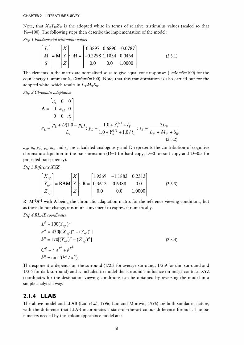
Note, that XWYWZW is the adopted white in terms of relative tristimulus values (scaled so thatYW=100). The following steps then describe the implementation of the model:
Step 1 Fundamental tristimulus values
L
M
S
X
Y
Z
M
é
ë
êêê
ù
û
úúú
=
é
ë
êêê
ù
û
úúú
=
-
-
é
ë
êêê
ù
û
úúú
M ;
. . .
. . .
. . .
0 3897 0 6890 0 0787
0 2298 1 1834 0 0464
0 0 0 0 1 0000
(2.3.1)
The elements in the matrix are normalised so as to give equal cone responses (L=M=S=100) for theequi–energy illuminant SE (X=Y=Z=100). Note, that this transformation is also carried out for theadopted white, which results in LWMWSW.
Step 2 Chromatic adaptation
A =
é
ë
êêê
ù
û
úúú
=+ -
=+ +
+ +=
+ +
a
a
a
ap D p
Lp
Y l
Y ll
LL M S
L
M
S
LL L
nL
n E
n E
EW
W W W
0 0
0 0
0 0
1 0 1 0
1 0 1 0
31 3
1 3
( . );
.
. . /;
/
/
(2.3.2)
aM, aS, pM, pS, mE and sE are calculated analogously and D represents the contribution of cognitivechromatic adaptation to the transformation (D=1 for hard copy, D=0 for soft copy and D=0.5 forprojected transparency).
Step 3 Reference XYZ
X
Y
Z
X
Y
Z
ref
ref
ref
é
ë
êêê
ù
û
úúú
=
é
ë
êêê
ù
û
úúú
=
-é
ë
êêê
ù
û
úúú
RAM R;
. . .
. . .
. . .
1 9569 1 1882 0 2313
0 3612 0 6388 0 0
0 0 0 0 1 0000
(2.3.3)
R=M-1A-1 with A being the chromatic adaptation matrix for the reference viewing conditions, butas these do not change, it is more convenient to express it numerically.
Step 4 RLAB coordinates
L Y
a X Y
b Y Z
C a b
h b a
Rref
Rref ref
Rref ref
R R R
R R R
=
= -
= -
= +
= -
100
430
1702 2
1
( )
[( ) ( ) ]
[( ) ( ) ]
tan ( / )
s
s s
s s (2.3.4)
The exponent s depends on the surround (1/2.3 for average surround, 1/2.9 for dim surround and1/3.5 for dark surround) and is included to model the surround’s influence on image contrast. XYZcoordinates for the destination viewing conditions can be obtained by reversing the model in asimple analytical way.
2.1.4 LLABThe above model and LLAB (Luo et al., 1996; Luo and Morovic, 1996) are both similar in nature,with the difference that LLAB incorporates a state–of–the–art colour difference formula. The pa-rameters needed by this colour appearance model are:
CHAPTER 2 – LITERATURE SURVEY
17
• adopted white under source viewing conditions XWYWZW
• luminance of adopted white under source viewing conditions LS
• Y value of background under source adapting field Yb
• sample under source viewing conditions XYZ• information about the medium and the nature of the surround
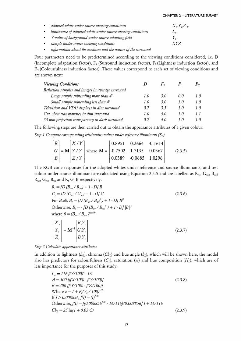
Four parameters need to be predetermined according to the viewing conditions considered, i.e. D(Incomplete adaptation factor), FS (Surround induction factor), FL (Lightness induction factor), andFC (Colourfulness induction factor). These values correspond to each set of viewing conditions andare shown next:
Viewing Conditions D FS Fl FC
Reflection samples and images in average surroundLarge sample subtending more than 4o 1.0 3.0 0.0 1.0Small sample subtending less than 4o 1.0 3.0 1.0 1.0
Television and VDU displays in dim surround 0.7 3.5 1.0 1.0Cut–sheet transparency in dim surround 1.0 5.0 1.0 1.135 mm projection transparency in dark surround 0.7 4.0 1.0 1.0
The following steps are then carried out to obtain the appearance attributes of a given colour:
Step 1 Compute corresponding tristimulus values under reference illuminant (SE)
R
G
B
X Y
Y Y
Z Y
é
ë
êêê
ù
û
úúú
=
é
ë
êêê
ù
û
úúú
M
/
/
/
where M =
é
ë
êêê
ù
û
úúú
0.8951 0.2664 -0.1614
-0.7502 1.7135 0.0367
0.0389 -0.0685 1.0296
(2.3.5)
The RGB cone responses for the adopted whites under reference and source illuminants, and testcolour under source illuminant are calculated using Equation 2.3.5 and are labelled as Rwr, Gwr, Bwr;Rws, Gws, Bws and R, G, B respectively.
Rr = [D (Rwr / Rws) + 1 - D] R
Gr = [D (Gwr / Gws) + 1 - D] G (2.3.6)
For B ³0, Br = [D (Bwr / Bwsb ) + 1 - D] Bb
Otherwise, Br = - [D (Bwr / Bwsb ) + 1 - D] |B| b
where b = (Bws / Bwr )0.0834
X
Y
Z
R Y
G Y
B Y
r
r
r
r s
r s
r s
é
ë
êêê
ù
û
úúú
=
é
ë
êêê
ù
û
úúú
-M 1 (2.3.7)
Step 2 Calculate appearance attributes
In addition to lightness (LL), chroma (ChL) and hue angle (hL), which will be shown here, the modelalso has predictors for colourfulness (CL), saturation (sL) and hue composition (HL), which are ofless importance for the purposes of this study.
Otherwise, f(I) = [(0.0088561/Fs - 16/116)/0.008856] I + 16/116
ChL = 25 ln(1 + 0.05 C) (2.3.9)
CHAPTER 2 – LITERATURE SURVEY
18
where C = (A 2+ B2)1/2
hL = tan-1(B/A) (2.3.10)
2.1.5 CIECAM97sThe CIE 1997 Colour Appearance Model – CIECAM97s is based on the work of many differentinvestigators, including Hunt (Hunt, 1982; 1991; 1994; Hunt and Luo, 1994), Nayatani (Nayataniet al., 1986; 1987; 1990; Nayatani, 1995) and the authors of the RLAB and LLAB models. Whatfollows are instructions for the implementation of this model as given by Luo and Hunt (1998) andas used in this study for Experiment 4. The input parameters of CIECAM97s are:
• adopted white under test viewing conditions XWYWZW
• background under test viewing conditions Xb Yb Zb
• sample under test viewing conditions XYZ• luminance of the test adapting field (cd/m2) LA
LA is normally taken to be 1/5 of the luminance of the adopted white under source conditions• information about the medium and the nature of the surround.
Based on the surround, the following parameters need to be chosen:
Surround F c FLL NC
AverageLarge sample subtending more than 4o 1.0 0.69 0.0 1.0Small sample subtending less than 4o 1.0 0.69 1.0 1.0
Calculate RGB values for sample (as shown in Equation 2.3.11), adopted white and backgroundunder test conditions, the adopted white under reference conditions XWR YWR ZWR = [100,100,100]and the degree of chromatic adaptation D.
D = F – F/[1 + 2(LA1/4) + (LA
2/300)] (2.3.12)
Calculate RGB values after chromatic adaptation whereby the adapted values of RGB are RCGCBC
and those of RWGWBW and RbGbBb are RWCGWCBWC and RbCGbCBbC.
p) + 1 – D]|B|p (2.3.13)whereby BC must be made negative when B is negative andp = (BW/BWR)0.0834
FL = 0.2k4(5LA) + 0.1(1 - k4)2(5LA)1/3 where k = 1/(5LA +1)
CHAPTER 2 – LITERATURE SURVEY
19
Step 2 Calculate cone responses and apply dynamic response function
R
G
B
R Y
G Y
B Y
R
G
B
R Y
G Y
B Y
C
C
C
W
W
W
WC W
WC W
WC W
'
'
'
'
'
'
. . .
. . .
é
ë
êêê
ù
û
úúú
=
é
ë
êêê
ù
û
úúú
é
ë
êêê
ù
û
úúú
=
é
ë
êêê
ù
û
úúú
=
-
- -
-
M M M M
M
H BFD1
H BFD1
BFD1
0 98699 0 14705 0 15996
0 43231 0 51836 0 04929
00 00853 0 04004 0 96849
0 38971 0 68898 0 07868
0 22981 1 18340 0 04641
0 00000 0 00000 1 00000
. . .
. . .
. . .
. . .
é
ë
êêê
ù
û
úúú
=
-
-
é
ë
êêê
ù
û
úúú
MH
(2.3.14)
YbC = (0.43231RbC + 0.51836GbC + 0.04929BbC)Yb
YWC = (0.43231RWC + 0.51836GWC + 0.04929BWC)YW
n = YbC/YWC, Nbb = 0.725(1/n)0.2 and Ncb = 0.725(1/n)0.2
Apply the dynamic response function R'G'B' and RW'GW'BW' which then become Ra'Ga'Ba' andRaW'GaW'BaW' respectively.
Ra' = 40(FLR'/100)0.73/[(FLR'/100)0.73 + 2] + 1 (2.3.15)
if R' < 0 then Ra' = -40(-FLR'/100)0.73/[(-FLR'/100)0.73 + 2] + 1
Ga', Ba', RaW', GaW' and BaW' are calculated similarly.
Step 3 Calculate Appearance Attributes
In addition to brightness (Q), lightness (J), chroma (C), saturation (s) and hue angle (h), which willbe shown here, the model also has predictors for colourfulness (M) and hue composition (H),which are less relevant for imaging applications.
First, redness–greenness (a) and yellowness–blueness (b) are calculated:
a = Ra' – 12Ga'/11 + Ba'/11 (2.3.16)
b = (Ra' + Ga' – 2Ba')/9
This is followed by a calculation of hue:
h = arctan(b/a) (2.3.17)
The eccentricity factor (e) is then calculated using the following unique hue data:
Red Yellow Green Blueh 20.14 90.00 164.25 237.53e 0.8 0.7 1.0 1.2
e = e1 + (e2 - e1)(h – h1)/(h2 – h1) (2.3.18)
where e1 and h1 are the values of e and h for the unique hue having the nearest lower value of h ande2 and h2 are the values having the nearest higher value of h. Next, the value of the achromatic signalis calculated for both the sample and the adopted white:
A = [2Ra' + Ga' + (1/20)Ba' – 2.05]Nbb
AW = [2RaW' + GaW' + (1/20)BaW' – 2.05]Nbb (2.3.19)
Finally, lightness, saturation and chroma can be obtained as follows:
J = 100(A/AW)cz where z = 1 + FLLn1/2 (2.3.20)
CHAPTER 2 – LITERATURE SURVEY
20
se N N a b
R G Bc cb
a a a
=+
+ +
+100 10 13 5021 20
2 2( / )' ' ( / ) '
(2.3.21)
C = 2.44s0.69(J/100)0.67n(1.64 – 0.29n) (2.3.22)
For instructions on how to calculate the reverse model see Luo and Hunt (1998).
2.1.6 Viewing ConditionsSections 2.3.1 and 2.3.2 already highlighted the importance of the environment in which a colouris seen. Here it is of importance to consider several elements including the chromaticity and inten-sity of the light source used, the colour of the background against which a colour or colour image isviewed and the viewing geometry, which includes viewing distance and viewing angle. What will bepresented next is an overview of recommended viewing conditions for CRT monitors and printedreproduction based on a Working Draft of the ISO 3664 standard (1997).
2.1.6.1 CRTThe draft standard for viewing colour images on CRTs is intended for situations when these areseen in isolation and not when they are compared with prints. For such conditions it is recom-mended that the white point of the monitor is set to chromaticities similar to CIE standard illumi-nant D65, that it should have a luminance level of at least 75 cd/m2 and preferably 100 cd/m2 andthat the level of ambient illumination should be below 32 lux. The surround should be neutral andthere should be no strongly coloured areas in the field of view or in places from where they couldbe reflected on the monitor. Further, sources of glare should also be avoided – light sources shouldnot be reflected from the CRT or be in the field of view.
2.1.6.2 PrintThe above draft standard for viewing prints recommends the use of light sources which approxi-mate CIE standard illuminant D50 with a maximum illuminance at the viewing surface of 500 lux±125 lux. To determine how well a given light source approximates the standard illuminant, themethod suggested by the CIE is to be used (CIE, 1981). Prints should be viewed against a neutral,matt surround which should have a luminous reflectance of less that 20 per cent and extend aroundit by at least one third of their dimensions. Further, the backing of these prints should have a lumi-nous reflectance of two to four per cent. Note, that the above are the recommendations for “practi-cal appraisal” of prints, i.e. for conditions which are similar to those under which prints aretypically viewed. The standard also makes another set of recommendations for the “critical ap-praisal” of prints, which differs from the above primarily by the illuminance at the viewing surfacebeing 2000 lux ±500 lux.
2.1.7 SummaryThe importance of colour appearance issues is undeniable in any colour reproduction study for atleast the following reason – to attempt to reduce the effects of phenomena which are not being in-vestigated. Due to this, the viewing conditions for both media dealt with here (CRT and prints)were set so as to prevent any appearance phenomena resulting from differences in luminance level,white point or surround (Chapter 3).
2.4 Colour Reproduction Media & IntentsAn understanding of the basic characteristics of the colour reproduction media used in this study –CRT monitor and colour prints – is essential for their appropriate use and will be discussed in the
CHAPTER 2 – LITERATURE SURVEY
21
following sections. In addition to this, the question of colour reproduction intents will also be dealtwith.
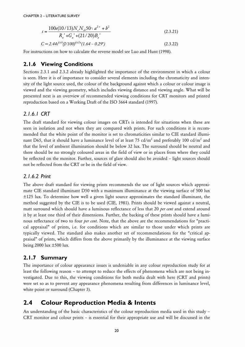
2.4.1 CRT MonitorsCathode–ray tube (CRT) monitors use additive colour reproduction to obtain the colours withintheir gamut. This is done by having three types of phosphors – red green and blue – distributedacross the face of the monitor’s tube. These phosphors can emit light of varying intensities, de-pending on the energy of the electrons fired at them (Sluyterman, 1995). Note, that the size of thephosphors is such that it is below the resolving power of the human visual system, when viewed ata distance of at least approximately 70 cm and the light emitted by an individual phosphor ismerged with the light coming from its neighbours. Due to the phosphors having high chroma, thegamut of a typical computer monitor is quite large in terms of relative colorimetry (Figure 2.4.1).
100 b*
-100 a*
-100 b*
L*L*
100 a*
Figure 2.4.1 Barco Calibrator CRT monitor gamut in CIELAB.
2.4.1.1 Chromatic Adaptation to MonitorsAs monitors are light emitting devices themselves, they are not considered as illuminated objects(i.e. the cognitive component of chromatic adaptation is not active), whereby chromatic adaptationdoes not completely compensate for the illumination in the room where the monitor is viewed(Fairchild, 1992). Incomplete chromatic adaptation also means that users do not adapt to the whiteon the monitor and will perceive it as having a colour cast even after a long period of time. Somemore recent work suggests that the visual system is 60 per cent adapted to the monitor’s white pointand 40 per cent to the ambient illumination’s white point (Katoh, 1994). This is a further reason forsetting the white points of both the monitor and the illuminated print in this study to the samechromaticity.
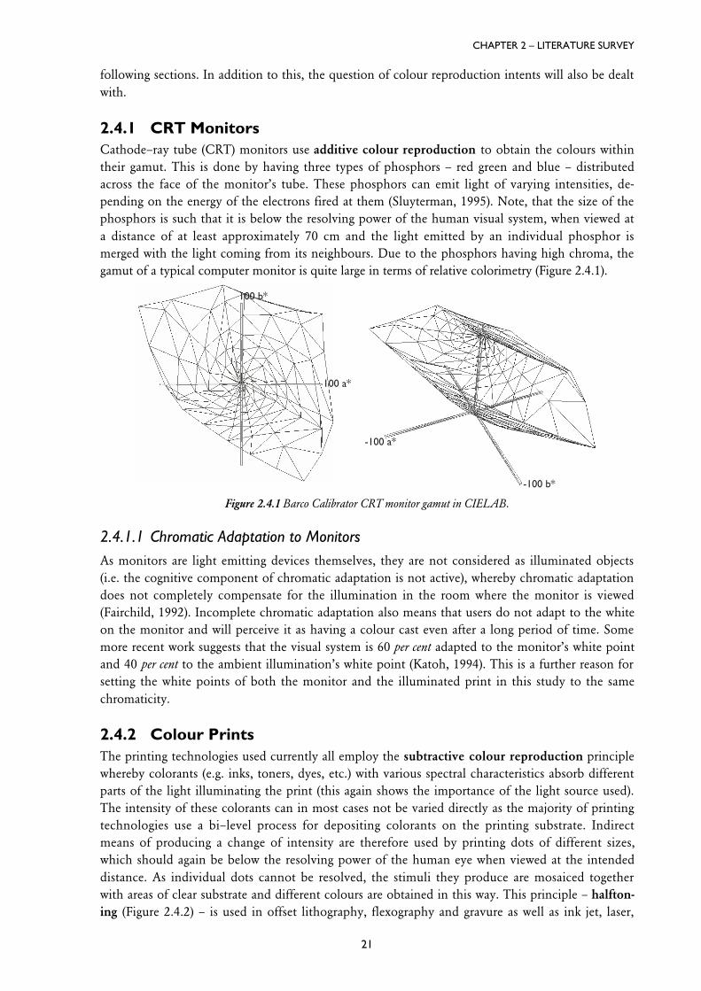
2.4.2 Colour PrintsThe printing technologies used currently all employ the subtractive colour reproduction principlewhereby colorants (e.g. inks, toners, dyes, etc.) with various spectral characteristics absorb differentparts of the light illuminating the print (this again shows the importance of the light source used).The intensity of these colorants can in most cases not be varied directly as the majority of printingtechnologies use a bi–level process for depositing colorants on the printing substrate. Indirectmeans of producing a change of intensity are therefore used by printing dots of different sizes,which should again be below the resolving power of the human eye when viewed at the intendeddistance. As individual dots cannot be resolved, the stimuli they produce are mosaiced togetherwith areas of clear substrate and different colours are obtained in this way. This principle – halfton-ing (Figure 2.4.2) – is used in offset lithography, flexography and gravure as well as ink jet, laser,
CHAPTER 2 – LITERATURE SURVEY
22
thermal wax and phase change printers. In dye diffusion printers, however, the optical density ofthe colorant can be varied directly and halftoning is therefore not needed.
Figure 2.4.2 Halftoning using an amplitude modulated screen.
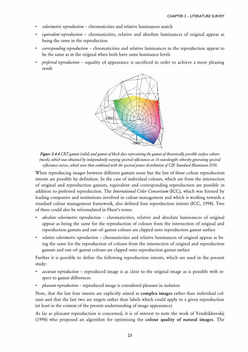
The extremes of print gamuts are the colour coordinates of the usually three chromatic colorantsused (cyan, magenta and yellow), the overprints of pairs of them, the black colorant (or overprint ofall colorants) and the clear substrate. From this it is clear that the size of the gamut for a particularmedium depends on the properties of both colorants and substrate in addition to the characteristicsof the light source used. However, it is not only the colour of these components, but also theirphysical properties (including surface and absorption properties of paper; viscosity, trapping andcolour fastness of colorants) which influence the gamut of a print (Figure 2.4.3).
-100 a*-100 b*
100 L*100 b*
100 a*
Figure 2.4.3 Gamut of prints made with HP DeskJet 850C inkjet printer on plain paper (CIELAB).
An additional constraint to the gamut of both colour reproduction media dealt with here (CRTand print) and indeed any digital medium is quantisation, as a consequence of which only colorantamounts of certain values can be addressed, thereby also making the colour gamut discontinuous.
2.4.3 Colour Reproduction IntentsThe aim of the preceding sections was to illustrate the basic principles and differences of the mediaused in this study. In addition to the CRT used here, the whole visual gamut can serve as the origi-nal gamut when the aim is to reproduce natural scenes (Figure 2.4.4). In spite of this, images onmonitors are often assumed to be the originals as the real scene might not be available or existanymore at the time of reproducing it or because changes were made after the scene was capturedand displayed on the monitor.
Due to the differences between original and reproduction gamuts, different kinds of reproductionrequirements have been defined previously whereby the following list was given by Hunt (1987, pp.178) and is in order of decreasing stringency. Note, that reproduction intents in general can be seenas aims for a colour reproduction system and due to the nature of its other elements these intentscan be interpreted as aims for gamut mapping:
• spectral reproduction – spectral power distributions of original and reproduction are identical
• exact reproduction – relative luminances, chromaticities and absolute luminances are identical
CHAPTER 2 – LITERATURE SURVEY
23
• colorimetric reproduction – chromaticities and relative luminances match
• equivalent reproduction – chromaticities, relative and absolute luminances of original appear asbeing the same in the reproduction
• corresponding reproduction – chromaticities and relative luminances in the reproduction appear tobe the same as in the original when both have same luminance levels
• preferred reproduction – equality of appearance is sacrificed in order to achieve a more pleasingresult
-100a*
-100b*
Figure 2.4.4 CRT gamut (solid) and gamut of block dyes representing the gamut of theoretically possible surface colours(mesh), which was obtained by independently varying spectral reflectances at 16 wavelengths whereby generating spectral
reflectance curves, which were then combined with the spectral power distribution of CIE Standard Illuminant D50.
When reproducing images between different gamuts none but the last of these colour reproductionintents are possible by definition. In the case of individual colours, which are from the intersectionof original and reproduction gamuts, equivalent and corresponding reproduction are possible inaddition to preferred reproduction. The International Color Consortium (ICC), which was formed byleading companies and institutions involved in colour management and which is working towards astandard colour management framework, also defined four reproduction intents (ICC, 1998). Twoof these could also be reformulated in Hunt’s terms:
• absolute colorimetric reproduction – chromaticities, relative and absolute luminances of originalappear as being the same for the reproduction of colours from the intersection of original andreproduction gamuts and out–of–gamut colours are clipped onto reproduction gamut surface
• relative colorimetric reproduction – chromaticities and relative luminances of original appear as be-ing the same for the reproduction of colours from the intersection of original and reproductiongamuts and out–of–gamut colours are clipped onto reproduction gamut surface
Further it is possible to define the following reproduction intents, which are used in the presentstudy:
• accurate reproduction – reproduced image is as close to the original image as is possible with re-spect to gamut differences
• pleasant reproduction – reproduced image is considered pleasant in isolation
Note, that the last four intents are explicitly aimed at complex images rather than individual col-ours and that the last two are targets rather than labels which could apply to a given reproduction(at least in the context of the present understanding of image appearance).
As far as pleasant reproduction is concerned, it is of interest to note the work of Yendrikhovskij(1998) who proposed an algorithm for optimising the colour quality of natural images. The
CHAPTER 2 – LITERATURE SURVEY
24
method is based on the naturalness and colourfulness indices which were developed in the samework and which are computed on the basis of image statistics. Naturalness is calculated by identify-ing the locations of prototypical memory colours for ‘skin’, ‘grass’ and ‘sky’ in colour space (whichrepresent a wider range of naturally occurring colours) and then analysing image colours in relationto these. Colourfulness on the other hand is calculated from the average and standard deviation ofimage chroma. Finally, colour quality is expressed as a weighted combination of naturalness andcolourfulness and images can then be optimised in terms of this metric. The above colour qualityindex was experimentally tested on 20 images from television and the processed images have beenjudged to be of higher quality than the original images in 16 cases. This algorithm clearly has awide range of possible applications and could be used as a preliminary step to gamut mapping in asystem, which aims to give good quality reproductions independently of the original’s quality. Insuch a case, however, the algorithm would have to be extended by support for synthetic images aswell.
2.5 Characterisation and CalibrationNow that the colour reproduction media used in this study were briefly introduced and the ques-tion of colour appearance was addressed as well, a further element of colour reproduction will bedealt with here. This element is usually called device characterisation and, as has already beenpointed out in Section 1.3, will also be referred to as such in the following sections even though itshould more appropriately be called medium characterisation. Before individual methods are dis-cussed, it is important to be aware of the definition of two basic concepts as used in this study andas defined by Johnson (1996):
(1) Calibration – the setting up of a device or process so that it gives repeatable data.
(2) Characterisation – defines the relationship between the device colour space and the CIEsystem of colorimetry.
The need for these two techniques is intrinsic in matching colours between different media. Aseach medium or device uses different colorants, its way of describing colours is device dependent.Therefore, to obtain a match between two device–dependent descriptions of colour, it is best totransform both into a system which is device independent – like the system of CIE colorimetry de-scribed in Section 2.1. One could argue that it is possible to transform colour information directlybetween device dependent colour spaces (which is true), but such a characterisation would have tobe done for each pair of devices, rather than just once for each device. Furthermore, such a trans-formation would make the inclusion of gamut mapping difficult, as this is usually intended to becarried out in a perceptually uniform colour space. The need for calibration should also be clear, ascharacterisation will only hold true when the device is in the state for which it was characterised.
Even though characterisation methods usually depend to a significant degree on the device forwhich they are intended, the following three approaches: neural networks, full characterisation andmasking equations can be used for any device. The later two will be discussed here as they wereused in this study and for an example of the use of neural networks in characterisation see Kangand Anderson (1992). This section on characterisation and calibration is based primarily on a pairof papers by Johnson, Luo, Lo, Xin and Rhodes (1998a; 1998b).
2.5.1 Generic Characterisation Methods
2.5.1.1 Cube InterpolationAny device’s colour reproduction characteristics can be determined by first producing all (or a suf-ficiently large subset) of the colours it can reproduce and measuring their colorimetric coordinates.
CHAPTER 2 – LITERATURE SURVEY
25
A look–up table (LUT) can then be constructed, which will give the tristimulus values for a givenset of device dependent coordinates. Note, that even when all possible colorant combinations areincluded in the LUT, it will have some errors in predicting the device’s characteristics due to thedevice’s variation. The following cube interpolation procedure, which is generally used when printsare made with three inks – cyan (C), magenta (M) and yellow (Y), is based on (Johnson et al.,1998b):
(1) Produce a series of steps with increasing concentration for each colorant (at equal quantisationintervals).
(2) Measure the samples and calculate the lightness of each step.
(3) Plot lightness versus colorant quantisation level and if relationship is highly non–linear, define aLUT between quantisation level and lightness.
(4) Select nine quantisation levels for each colorant (including minimum and maximum and sevensteps in–between with equal lightness intervals).
(5) Print test images containing all combinations of the above determined nine steps for each col-orant (resulting in 729 patches).
(6) Measure each colour patch in terms of XYZ tristimulus values and generate a three dimensionalLUT. From this, tristimulus values can be obtained for each of the 729 colorant combinationsand intermediate colours can be obtained using tri–linear interpolation (Kasson et al., 1995):
Here DC, DM and DY are a given colorant combination’s distances from the origin of the se-lected sub–cube and Ni are the tristimulus values of the vertices of that sub–cube (Figure 2.5.1).
N1 N2
N4N3
N5 N6
N8N7
DC
DM
DY
Figure 2.5.1 Tri–linear interpolation within a sub–cube of the 9x9x9 LUT.
In many cases this method provides the best accuracy, however, it also involves a large number ofmeasurements and is therefore considerably time consuming, which is especially disadvantageous ifthe variables of the device change often (e.g. as is the case with many digital printing devices). Thismethod is very widely used and a number of different variations of it have been published (Bell andCowan, 1994; Balasubramanian, 1994; Marcu and Abe, 1994).
2.1.1.2 Polynomial FittingPolynomial fitting is conventionally used in printing (where this model is sometimes referred to asMasking Equations), but can equally well be applied to other media. This method was first suggestedby Yule (1938) by saying that the relationship between colorimetric densities of the colorants andXYZ is of the following nature:
CHAPTER 2 – LITERATURE SURVEY
26
D
D
D
D
D
D
r
g
b
r c
g m
b y
é
ë
êêê
ù
û
úúú
=
é
ë
êêê
ù
û
úúú
A( )
( )
( )
(2.5.2)
Here Dn with n Î{r,g,b} are the colorimetric densities of the colour resulting from a given CMYcolorant combination and are calculated as:
Dr = log(X0/X), Dg = log(Y0/Y), Db = log(Z0/Z) (2.5.3)
(X0,Y0,Z0) is the white point, A is a 3x3 matrix determined using the least squares method (Miltonand Arnold, 1990, pp. 352) and (Dr(c),Dg(m),Db(y)) are the colorimetric densities of the device’s color-ants for the combination of which the XYZ coordinates are to be calculated. This simple linearmethod does not give good results for many devices, as the assumption of additivity and propor-tionality of colorant densities does not hold for them. However, if higher order and cross–productterms are introduced, as was later suggested by Clapper (1961) and Yule (1967), the precision of thismethod becomes comparable to full characterisation. The following equation shows a third orderpolynomial model with cross products used for printer characterisation:
D
D
D
c m y c m y cm cy my c m y c m c y m c m y y c y m
r
g
b
T
é
ë
êêê
ù
û
úúú
=
= [ ]
BC
C 2 2 2 3 3 3 2 2 2 2 2 2
(2.5.4)
Here B is a 3x18 matrix again obtained using the least squares method and(c,m,y)=(Dr(c),Dg(m),Db(y)). The precision of this method depends on the number of colours used for
obtaining the coefficients of B and it was found that for many printing devices there is little benefitin using more than 64 colours for characterising them (Johnson et al., 1998b). However, this num-ber will depend on the device and on how well the colours are chosen (same considerations applyas for full characterisation). A potential problem with using higher order masking equations is thepossibility, that local minima and maxima present in the equations do not correspond with themodelled relationship and will create artefacts in some parts of colour space. Before any transfor-mations are carried out, it is useful to normalise and scale the data in both colour spaces (the devicedependent and the device independent) using the coordinates of black and white achievable by thedevice which is being characterised.
Other device specific techniques for characterising and calibrating the devices used in this studywill be described in the following sections.
2.1.2 CRT Monitor Characterisation & CalibrationAs the majority of electronic displays used currently are CRTs (Figure 2.5.2) and as this is the tech-nology used by the medium for displaying original images in this study, only CRT calibration andcharacterisation will be described here. An overview of alternative display technologies can befound in (Jackson et al., 1994; Budin, 1995) of which the most important are probably liquid crystaldisplays (LCDs) – for their characterisation see (Selhuber and Parker, 1995). The characteristics ofCRTs which determine their colour reproduction capabilities include:
• chromaticities and maximum luminances of phosphors
• gain and offset settings of electron guns’ voltage (this is done via the contrast and brightness settingsand via adjusting white balance)
• gamma of electron guns relating voltage to light output
CHAPTER 2 – LITERATURE SURVEY
27
• relationship between digital values sent to display and resulting voltages
• amount of ambient flare off CRT
• inter–reflections from neighbouring pixels within the CRT
Figure 2.5.2 Schematic view of a cathode ray tube (reproduced from (Schläpfer, 1990)).
Even if cross–media matching was not an issue, characterisation and calibration of CRTs would stillbe of importance as the variation in colour between different monitors can be as high as 18 DE*ab
(for the same white point, but using different phosphor sets) (Engeldrum and Ingraham, 1990). ForCRT characterisation to be feasible, the following assumptions are usually made (Brill, 1992):
• spatial independence Output at a particular location depends only on that location’s input(i.e. neighbouring pixels do not affect each other).
• gun independence Output of a phosphor is independent from the input to the other guns.
• approximate homogeneity Spatial variation is negligible (i.e. whole CRT can be calibratedfrom average of a few pixels).
• phosphor constancy Relative SPD is independent of digital–to–analog converter (DAC) valueapplied to electron gun (this implies constant chromaticity of phosphors).
Given these assumptions, the tristimulus values for a given pixel can be computed from the follow-ing equation, if the luminances and chromaticities of the three phosphors are known (Johnson etal., 1998a):
X
Y
Z
x
y
x
y
x
y
z
y
z
y
z
y
T
T
T
r
r
g
g
b
b
r
r
g
g
b
b
r
g
b
é
ë
êêê
ù
û
úúú
=
é
ë
êêêêêêê
ù
û
úúúúúúú
é
ë
êêê
ù
û
úúú
1 1 1 (2.5.5)
Here Ti (i Î {r,g,b}) are the luminances of the phosphors, xi, yi and zi are their chromaticities andXYZ are the resulting tristimulus values. Note, that it is important to use the actual chromaticitiesmeasured for the CRT being characterised, rather than values published by the manufacturer asthese are for a whole range of monitors and can be considerably different from an individual one.This part of CRT characterisation is the same for all methods, which make the assumption ofphosphor constancy. However, before this transformation can be carried out, the luminances of thethree phosphors need to be established and there are at least seven methods for doing this:
CHAPTER 2 – LITERATURE SURVEY
28
2.1.1.1 GOG ModelThe GOG model, devised by Berns (1996), takes as its variables the gain, offset and gamma of themonitor to relate digital input to phosphor luminance. This model is based on a previous compre-hensive study by the author and his co–workers (Berns et al., 1993a; 1993b). The following equationshows the calculation of spectral radiance from digital values:
L L kLUT d
k kLUT d
k
L
r r g rr r
n o r g rr r
n o r
r
r r
l l
g g
l
, , (max) , , , ,
,
=-
æ
èç
ö
ø÷ +
æ
èç
ö
ø÷
-
æ
èç
ö
ø÷ +
æ
èç
ö
ø÷ ³
=
2 1 2 10
0
if
otherwise
(2.5.6)
Here Ll,r is the spectral radiance of the red channel, Ll,r(max) is the maximum spectral radiance of thered phosphor, kg,r is the red channel’s gain, ko,r is its offset, LUTr is the video LUT relating digitalvalues to voltage, dr is the red digital value, n is the number of bits per channel used by the DACand gr is the gamma of the red gun. Analogous equations can be set up for the other two channels.Note, that this is already a simplified relationship, as the gain and offset used here relate to thewhole system rather than only to the electronics of the CRT. The whole equation can also be re-written as:
L RL
R kLUT d
k R
r r
g rr r
n o r
r
l l
g
, , (max)
, ,
=
=-
æ
èç
ö
ø÷ +
æ
èç
ö
ø÷ ³where if 0, otherwise =
2 10
(2.5.7)
Here R is a scalar representing a percentage of maximum luminance and therefore the luminance Tr
= RLr(max) (Lr(max) is the maximum luminance of the red channel). Ambient flare and inter–reflectionflare (due to failure of spatial independence) can also be allowed for:
X
Y
Z
X
Y
Z
X
Y
Z
T
T
Tambientflare
erreflectionflare
r
g
b
é
ë
êêê
ù
û
úúú
=
é
ë
êêê
ù
û
úúú
+
é
ë
êêê
ù
û
úúú
+
é
ë
êêê
ù
û
úúúint –
A (2.5.8)
Here A is the (3x3) matrix from equation 2.5.5.
Apart from describing the above model, the author also provided a useful characterisation proce-dure:
(1) Set–up display visually. Turn brightness and contrast controls to minimum, turn off ambi-ent light and display black image (dr=dg=db=0). Adjust offset to just above the settingwhere light is perceptible. Display text image and adjust gain to maximum luminancewithout loss of sharpness.
(2) Measure peak output from R, G, B, the white point and the darkest neutral, which can bemeasured with good precision and accuracy and an intermediate neutral between it andthe white.
(3) Calculate tristimulus matrix (matrix A in Equation 2.5.8) and its inverse. Estimate scalarsfor the neutrals, calculate gain, offset and gamma for each channel (from the three neu-trals).
(4) Change background to neutral with 20 per cent luminance of peak white (use the model tocalculate the neutral’s digital values). Remeasure darkest neutral to determine in-ter–reflection flare.
CHAPTER 2 – LITERATURE SURVEY
29
(5) Measure a series of neutrals (approximately 5–10) to build the LUTs, then subtract in-ter–reflection flare and normalise the scalars.
2.1.1.2 Meyer 1990 ModelThe model proposed by Meyer (1990) is expressed by the following equation:
T k o gV
k K y d
= +
» ò( )g
l
l
l l (2.5.9)
Here T is the luminance, o and g are the offset and gain of the electron gun (not the whole systemas in GOG), Kl is the relative SPD of the CRT and k is a constant which corresponds to the lumi-nance (Y) of the monitor. To extend this relationship to the one between DAC values and lumi-nance, it is necessary to include a transformation between DAC values and voltage. This was foundto be of the nature of V = O + Gd (Berns et al., 1993a), where O and G are the offset and gain of thevideo circuitry and d is the digital value sent to it (this is represented by a video LUT in the GOGmodel).
2.1.1.3 PLCC ModelThe following six models, including this one, are based on work of Post and Calhoun (1989), whichwas later evaluated by Johnson et al. (1998a). This particular model uses piecewise linear interpola-tion assuming constant chromaticity coordinates (hence PLCC), i.e. it uses separate LUTs for eachchannel and assumes that the relationship of T and DAC values is linear between the points in theLUT. The choice of values in the LUT is critical, and more data should be available for the lowluminance end of the range.
2.1.1.4 LIN–LIN2 ModelAssumes the following relationship, where ci (i Î {1,2,3}) are obtained using the least squaresmethod and D represents normalised DAC values:
T c c D c D= + ++1 2 32 (2.5.10)
2.1.1.5 LOG–LOG ModelThis is the original gamma correction, which disregards the influence of gain and offset:
log logT c D= (2.5.11)
2.1.1.6 LOG–LOG2 ModelAn attempt to correct the problems of the LOG–LOG model at low luminances:
log log (log )T c c D c D= + +1 2 32 (2.5.12)
2.1.1.7 LOG–LIN2 ModelThe last of the models which assume constant chromaticity coordinates:
log T c c D c D= + +1 2 32 (2.5.13)
CHAPTER 2 – LITERATURE SURVEY
30
2.1.1.8 PLVC ModelAs can be seen from the name, this model is related to PLCC, with the difference being, that itdoes not assume constant chromaticity with changes in luminance. Therefore instead of three 1DLUTs, a 3D LUT is used, just like in the case of cube interpolation described in Section 2.5.1.1.
The analysis carried out by Johnson et al. (1998a) has shown that the PLCC model gave the bestresults, with the GOG and LOG–LOG2 models being slightly less accurate (however, all threemodels had average DECMC(1:1) errors of only around 0.40).
2.1.1.9 CRT CalibrationThe techniques discussed so far were all concerned with the characterisation of CRTs. However, forcharacterisation to be valid, the device also needs to be calibrated, which is done by setting thevariables of the system to the state in which they were when the device was characterised.
Calibration can also be used to make a given CRT behave like a reference CRT or to make it fitgiven specifications of system gamma and white point. A technique for altering digital values tofulfil these criteria was described by Berns (1996) and has as its inputs the data from the characteri-sation of the CRT and the target values to be emulated. Digital values are then transformed usingthe following equation:
d R
dk
kr
nwhite
r original
n o r
g r
r original
r
( )
( ),
,
int ( )
( )
( )
target
target
= --
æ
èç
ö
ø÷ -
æ
è
ççççççç
ö
ø
÷÷÷÷÷÷÷
é
ë
êêêêêêêê
ù
û
úúúúúúúú
2 12 1
1
g
g
(2.5.14)
Here the variables use the same notation as in the GOG model and Rwhite is the scalar which wouldgive the target white point under original conditions (analogous equations apply for green andblue). Note, that the software simulation of a white point will inevitably result in a lower maximumluminance, which thereby reduces the available tonal range (e.g. when D50 was simulated on a par-ticular monitor with a 9300K CCT white point, the resulting luminance range reduced to 58.6 percent of the original range) (Jennings and Thompson Pearce, 1993). To preserve as much as possibleof the monitors luminance, one of the scalars is usually set to 100 per cent.
2.1.3 Printer Characterisation & CalibrationUnfortunately there is no simple linear relationship between colorants and tristimulus values, asthere is for phosphor luminances. Neither is there a simple additive relationship between the stimu-lations caused by the individual colorants, which makes the whole process of characterising a print-ing device more problematic. As the colour in most prints is achieved by partially superimposinghalftone dots, there arise some problems (Johnson, 1998b) including trapping (the second color-ant’s density will differ from that of the first colorant as they are printed onto different substrates –the first one is printed onto paper, whereas the second one onto a colorant), back transfer and thepartial opacity of colorant. Further problems are caused by multiple internal reflections, first sur-face reflections and the sideways scattering of light. Other factors, which also influence the rela-tionship between colorant amounts and tristimulus values are the halftone structure of the printeddots (i.e. screen ruling and frequency of amplitude modulated halftone screens or the pixel size andnature of frequency modulated screens) and the spectral absorption characteristics of the color-ants.
CHAPTER 2 – LITERATURE SURVEY
31
When colour printers use more than three colorants (e.g. cyan, magenta yellow and black), there isno longer only a single possible solution for obtaining a given colour (except for colours, whichwould be reproduced by only up to two colorants in a three chromatic–colorant system (e.g.CMY)) and this necessitates an algorithm for determining what colorant combination is to be usedfor a particular colour (e.g. see (Lo, 1995) for an example of CMYK determination). However, asthe printer used in this study can only be controlled in terms of three colorants, only models forobtaining CMY values for a given set of XYZ values (and vice versa) will be discussed next.
The majority of models for performing this task can be divided into four groups: cube interpola-tion, polynomial equations, neural networks and Neugebauer equations. The first three have al-ready been dealt with in Section 2.5.1, which leaves only the Neugebauer equations to be discussedhere. For other printer characterisation models and their evaluation see (Herzog, 1997; Herzog andRoger, 1998)
2.1.3.1 Classical Neugebauer EquationsThis model was originally proposed by Neugebauer (1937) and many modifications to it have beendevised since. It is based on the assumption that the colour of a unit area is determined by the ad-dition of the tristimulus values of the different combinations of colorants present in that area. For athree colour system, there are eight possible combinations, whose fractional dot areas can be ex-pressed as:
f1 = (1 - p)(1 - q)(1 - r) (clear substrate)
f2 = p(1 - q)(1 - r) (colorant p)
f3 = q(1 - p)(1 - r) (colorant q)
f4 = r(1 - p)(1 - q) (colorant r)
f5 = qr(1 - p) (overprint of q & r) (2.5.15)
f6 = pr(1 - q) (overprint of p & r)
f7 = pq(1 - r) (overprint of p & q)
f8 = pqr (overprint of p, q & r)
Here p, q and r are the percentage dot areas of the three colorants (p, q & r have been used on pur-pose, as the model can be applied to any set of colorants and using CMY could be confusing). Thedot area (m) can be calculated from density using the Murray–Davies equation (Murray, 1936),where the subscripts t and s represent a tint (for which the dot area is calculated) and the solid re-spectively:
mD
D
t
s
=-( )-( )
-
-
1 10
1 10(2.5.16)
Each of these fractional dot areas has got a set of tristimulus values associated with it, which is ob-tained by measuring the colorant combination it represents (e.g. X4Y4Z4 are the tristimulus values ofa solid patch printed with colorant r – see Equation 2.5.15). The Neugebauer equations can now beexpressed as:
X
Y
Z
f
X
Y
Zi
i
i
ii
é
ë
êêê
ù
û
úúú
=
é
ë
êêê
ù
û
úúú
æ
è
ççç
ö
ø
÷÷÷=
å1
8
(2.5.17)
CHAPTER 2 – LITERATURE SURVEY
32
Note, that the above equation is identical with the tri–linear interpolation equation used for fullcharacterisation (Equation 2.5.1), which makes the Neugebauer equations a 2x2x2 LUT withtri–linear interpolation.
2.1.3.2 N–Modified Neugebauer EquationsSome of the inaccuracies in the Neugebauer Equations’ predictions can be attributed to theMurray–Davies equation not giving an accurate prediction of the percentage dot area (mainly dueto light scatter within the substrate). This was remedied by Yule and Nielsen (1951), who proposedthe following modified version, where n is a medium–dependent parameter determined heuristi-cally (Note, that this problem can also be corrected by using a LUT between the digital values andmeasured density, in which case the classical Neugebauer equations can be used with better accu-racy):
m
D
n
D
n
t
s
=
-æ
èç
ö
ø÷
-æ
èç
ö
ø÷
-
-
1 10
1 10
(2.5.18)
An analogous modification was also incorporated into the Neugebauer equations by Yule and Colt(1951), which are now of the following form:
X
Y
Z
f
X
Y
Z
n
n
n
i
in
in
in
i
x
y
z
x
y
z
1
1
1
1
1
11
8
é
ë
êêêêêêê
ù
û
úúúúúúú
=
é
ë
êêêêêêê
ù
û
úúúúúúú
æ
è
ççççççç
ö
ø
÷÷÷÷÷÷÷
=
å (2.5.19)
2.1.3.3 Modern Neugebauer EquationsThis model was devised by Laihanen (1987) and tries to take into account the shape of the halftonedot. Rather than being based on a unit area containing one halftone dot, this model takes as its in-puts three binary pixmaps – one for each colorant. The XYZ coordinates for a given pixel with thespatial coordinates (u,v) are then calculated in the following way:
X(u,v) = X1 if p(u,v) = q(u,v) = r(u,v) = 0X2 if p(u,v) = 1, q(u,v) = r(u,v) = 0X3 if q(u,v) = 1, p(u,v) = r(u,v) = 0X4 if r(u,v) = 1, p(u,v) = q(u,v) = 0X5 if q(u,v) = r(u,v) = 1, p(u,v) = 0 (2.5.20)X6 if p(u,v) = r(u,v) = 1, q(u,v) = 0X7 if p(u,v) = q(u,v) = 1, r(u,v) = 0X8 if p(u,v) = q(u,v) = r(u,v) = 1
Similar equations apply to Y(u,v) and Z(u,v). The three resulting arrays containing XYZ values forevery halftone pixel can then be integrated over a suitable area (depending on the nature of thedigital halftone screen) so as to give XYZ coordinates for individual image pixels. This can beachieved in two ways, either by a three stage process involving empirically optimised filters beforeand after integration (Laihanen, 1987, pp. 22–23) or by direct integration over a chosen area (A):
CHAPTER 2 – LITERATURE SURVEY
33
XA
X u v du dvA
= òò1
( , ) (2.5.21)
Analogous relationships apply for Y and Z.
2.1.3.4 Vector–Corrected Neugebauer EquationsAgain this model was devised by Laihanen (1987) and is based on first generating a LUT withL*a*b* values calculated for each combination of percentage dot area of the colorants (65 quantisa-tion levels were assumed by the author). The L*a*b* values were obtained using the Neugebauer orN–Modified Neugebauer equations. Once the LUT is set up, additional colours with known per-centage dot areas are measured and their L*a*b* coordinates are calculated. These measured col-ours are then directly inserted into the LUT and all the other entries are modified in the followingway:
L
a
b
L
a
bd
d
L
a
b
L
a
bnew old
ii
kii
k
m ni i
*
*
*
*
*
*
*
*
*
*
*
*
é
ë
êêê
ù
û
úúú
=
é
ë
êêê
ù
û
úúú
+
é
ë
êêê
ù
û
úúú
-
é
ë
êêê
ù
û
úúú
æ
è
ççç
ö
ø
÷÷÷
=
=åå
11
1
1
1
(2.5.22)
Here k is the number of nearest measured L*a*b* vectors taken into account, di is the distance be-
tween the old vector and vector i, m denotes one of the k closest measured vectors and n denotesthe calculated vector having the same percentage dot area as the measured vector m. This methodcan be used for improving the Neugebauer model’s accuracy in critical regions of colour space (e.g.the achromatic axis).
2.1.3.5 Cellular Neugebauer EquationsA further modification of the Neugebauer model was proposed by Heuberger et al. (1992; 1993)and is based on a similar concept as the Vector–Corrected Neugebauer equations. The main idea isto split the cube formed by the 8 colours of the classical equations into 8 cells and then measurethe XYZ coordinates of the 19 new cell vertices (i.e. these are colours formed by 50 per cent halftonedots of the colorants and all their combinations). The Neugebauer equations are then appliedwithin these cells (i.e. taking the vertices of a given sub–cell as the 8 colours in the classical Neuge-bauer equations), whereby the accuracy of the model is improved.
The Neugebauer model was most recently again studied by Mahy (Mahy and Delabastita, 1996;Mahy, 1997; 1998) whereby the analytical calculation of gamut boundaries, the calculation of themodel’s inverse and a method similar to the Cellular Neugebauer model were proposed.
So far the models have only dealt with obtaining XYZ coordinates from colorant amounts, how-ever, in practice there is a need also for the reverse of this transformation. The reverse of the aboveprinter characterisation models can be obtained either analytically, by reversing the terms of themodel (e.g. for masking equations) or by using iterative numerical methods.
2.1.3.6 Printer CalibrationFor the vast majority of digital printers, calibration is not applicable as it is not possible to alter thevariables influencing colour reproduction. Therefore, characterisation needs to be carried out whenany of these variables change (e.g. colorant, substrate or software), which makes it particularly im-portant for this characterisation to require a small number of measurements. Related to printercalibration are also techniques for updating characterisation models when printer parameterschange. A good example for this is the method described in a paper by Balasubramanian and Maltz(1996) which allows the modification of the characterisation model on the basis of measuring a
CHAPTER 2 – LITERATURE SURVEY
34
small number of colours for which correction vectors are calculated. All predicted colours are thencorrected by these vectors in a distance–weighted way. Note, that this paper is not only intendedfor the purpose given here but can also be used for improving the performance of characterisationmodels in critical areas (just like the Vector–Corrected Neugebauer equations).
True printer calibration is primarily applicable to conventional printing – e.g. offset lithographywhere the user has control over parameters like printing speed, viscosity of inks and pressure be-tween blanket and impression cylinders and where it is possible to set target values for solid densityand dot gain to which the system needs to be calibrated.
2.1.4 SummaryThe aim of this section was to give an overview of the characteristics of CRT monitors and printingdevices in general and to describe a number of various characterisation models and calibrationtechniques for them. In the case of CRT characterisation the PLCC was chosen for this study dueto its good performance and ease of implementation. For characterising the inkjet printer used inthis study, some experimental and developmental work was done before arriving at a suitable char-acterisation model which is described in Chapter 3.
2.6 Gamut MappingNow that all other parts of a colour reproduction system – colour appearance and device charac-terisation – were covered, the actual focus of this study – gamut mapping – can be looked at. Tothis end, the aims of gamut mapping, methods for finding gamut boundaries and parameters influ-encing the performance of gamut mapping algorithms will be discussed first. This will be followedby brief reviews of individual gamut mapping papers and finally by a summary of gamut mappingas carried out before the beginning of this study and by other workers in the course of its duration.
2.6.1 Gamut Mapping AimsFirst of all, it is useful to reconsider the aims of gamut mapping, which have already been touchedon in Section 2.4.3. On the highest level, the aim of gamut mapping is to ensure a good corre-spondence of overall colour appearance between the original and the reproduction by compen-sating for the mismatch in the size, shape and location between the original and reproductiongamuts. As a number of colours are physically not reproducible, it is more advisable to aim for areproduction of the image’s appearance rather than the appearance of individual colours in the im-age, since the latter can be impossible for some original colours.
One of the difficulties with implementing this aim is that there is as yet no model for quantifyingthe appearance of complex images and neither is there one for quantifying the difference betweenthem (though S–CIELAB (Zhang and Wandell, 1996) is a step in this direction). In the absence ofsuch a model, a number of objectives were heuristically arrived at in the past and the followingaims were identified by MacDonald (1993) to be common to the majority of gamut mapping stud-ies:
• preserve grey axis of the image & aim for maximum luminance contrast This means a mapping ofthe original image’s white and black points onto the reproduction’s white and black pointsrespectively.
• reduce the number of out–of–gamut colours Ideally all the image’s colours should be broughtwithin the reproduction’s gamut, however, the exclusion of some extremes is sometimesthough to improve the overall appearance match.
• minimise hue shifts It is often thought that when colours are reproduced the hue of coloursneeds to be left unmodified.
CHAPTER 2 – LITERATURE SURVEY
35
• increase in saturation is preferred As the reproduction gamut is already limited in terms ofsaturation, at least the available potential should be used to enable the preservation ofchroma differences present in the original.
Note, that the above list represents assumptions made by some gamut mapping studies whereby thereasons for making these assumptions are in most cases based on experience from traditional colourreproduction. Even though experience from traditional colour reproduction is of great value, itsmaxims need to be looked at carefully when used in an environment which enables far more con-trol over colour attributes than was previously possible.
A further commonly found aim of gamut mapping was expressed by Stone et al. (1988) in sayingthat “the relationship between the colours present was felt to be more important than their precisevalue.” This suggests a move of the what–you–see–is–what–you–get (WYSIWYG) concept ontoanother level – i.e. it is applied to images rather than individual colours and could therefore becalled MetaWYSIWYG. In spite of playing down the importance of a match in the traditionalsense, it is still crucial for a colour reproduction system to be able to reproduce individual coloursaccurately – even though some original colours cannot reproduced accurately, their modificationsneed to be reproduced as such.
2.6.2 Calculating Gamut BoundariesTo fulfil the aim gamut mapping has in a particular colour reproduction system, it is first necessaryto know the gamut boundaries of the original and reproduction gamuts. An understanding of col-our reproduction media gamuts was considered to be of some importance for some time and wasinvestigated by many researchers (Oittinen et al., 1992; Schläpfer and Widmer, 1993; Bristow et al.,1994; Marcu and Abe, 1995a; 1995b; Meyer and Robertson, 1997). Knowing the boundaries of thegamuts between which mapping is to be carried out is essential for the majority of GMAs devel-oped to date and can be divided into two separate problems.
Firstly, it is necessary to compute a gamut boundary descriptor (GBD) – i.e. some overall way ofapproximately describing a gamut. For media gamuts this can be done either directly from specificcharacterisation models – e.g. Kubelka–Munk equations (Engeldrum, 1986) or Neugebauer equa-tions (Mahy, 1997) – or using methods which can be applied to any characterisation model (Inui,1993). Further there are also some methods which can be used for computing the gamuts of imagesas well as media (Kress and Stevens, 1994).
Secondly, it is also important to be able to find the intersections between the gamut boundary (ascomputed using the above methods) and a given line along which mapping is to be carried out –these points will be referred to as the line gamut boundary (LGB). The papers published by Her-zog (1996; 1998) and Braun and Fairchild (1997) describe methods for doing this as well as obtain-ing the initial gamut boundary descriptor. Note, that these methods are aimed at obtaining theLGB for lines of constant hue and lightness, which are most often used by present GMAs.
As the GMAs dealt with in this study map colours in a variety of directions, new methods were de-veloped for calculating GBDs and LGBs (Chapter 4).
2.6.3 Gamut Mapping Parameters
2.6.3.1 Colour SpaceAs can be seen from the definitions of a colour gamut and of gamut mapping given in Section 1.3,they are both closely associated with colour spaces. Most gamut mapping algorithms intend towork with perceptual attributes, i.e. colourfulness, chroma, saturation, brightness, lightness, hue(Section 2.1.2.1) or colour names (e.g. red, dark green, orange, etc. whereby each of these would
CHAPTER 2 – LITERATURE SURVEY
36
represent a subset of colours represented by a volume in colour space) and to make this possible,they are implemented in colour spaces which predict them. More specifically, they usually intendto maintain some of a colour’s perceptual attributes while changing others. If under these circum-stances the predictors are imperfect, changes in the predictor of one attribute can also result inchanges of another perceptual attribute (e.g. in some cases, if the L* – the predictor of lightness inCIELAB – of a colour is changed, its perceived hue or chroma might also change).
In the colour spaces which are most often used for gamut mapping – CIELAB and CIELUV (CIE,1986) and in some cases LLAB (Luo and Morovic, 1996) or RLAB (Fairchild, 1998) – there areproblems especially with the predictors of hue. In particular there are deficiencies in the uniformityof hue angles in the blue region of CIELAB (e.g. hue angles of around 290°) which can result inchanges of perceived hue when only the L* or C* of a colour is changed. The performance of thehue predictor in CIECAM97s (Luo and Hunt, 1998) is somewhat better for this region. More detailon the performance of hue predictors of various colour spaces can be found in papers by Hung andBerns (1995) and Ebner and Fairchild (1998).
When implementing or evaluating GMAs, it is important to understand the deficiencies of the col-our space used for the mapping and not to confuse the colour space’s predictor with the predictedperceptual attribute (e.g. in CIELAB hab is not hue and L* is not lightness – they are only their pre-dictors).
In this study CIELAB was used in the first two experiments and in both experiments one of theGMAs was also implemented in LLAB so as to see, which of these spaces is more suitable for gamutmapping. The reason for using CIELAB was to make the results of the experiment more easilycomparable with previous studies as well as due to there not being a space which has significantlybetter predictors. By the time the third experiment was conducted, CIECAM97s was available andwas used since its hue predictor is better in the blue region and due to it being proposed as a stan-dard colour appearance model.
2.6.3.2 Type of MappingOnce the necessary gamuts are known in the chosen colour space, it is possible to implement aGMA. One way of grouping these algorithms is by distinguishing between gamut clipping andgamut compression.
2.6.3.2.1 Gamut Clipping
Gamut clipping algorithms only change colours which are outside the reproduction gamut eitherfrom the very beginning or after lightness compression. For colours outside the reproductiongamut, these algorithms specify a mapping criterion, which is used for finding the point on the re-production gamut to which a given original colour is mapped.
2.6.3.2.2 Gamut Compression
Gamut compression algorithms make changes to all colours from the original gamut so as to dis-tribute the differences caused by gamut mismatch across the entire range. Compression is neededwhen larger differences are to be overcome, as gamut clipping could result in unacceptable loss ofvariation in out–of–gamut regions under such circumstances.
A review of studies looking at both gamut clipping and gamut compression will be given in Section2.6.4.
CHAPTER 2 – LITERATURE SURVEY
37
2.6.3.3 Image v. Media GamutsWhen gamut compression is used, there arises a question as to which gamuts to map between. Thisis the case as the original gamut can be seen as either the gamut of the original medium or thegamut of the original image (i.e. a subset of the original medium’s gamut (Figure 2.6.1)). For currentgamut clipping methods this is not an issue as it is sufficient to know the reproduction gamut towhich any unreproducible colours from the original are mapped.
To make as few changes to the original image as possible, it is more reasonable to use the imagegamut as the original gamut since this means that colours are only modified when necessary. In-deed there are a number of experimental studies which support the idea that the use of imagegamuts gives preferred reproductions (Gentile et al., 1990; Pariser, 1991; Montag and Fairchild,1997; Wei et al., 1997).
-b*
+a*
Figure 2.6.1 Gamut of CRT (mesh) and MUS image (solid) in CIELAB.
If, on the other hand, media gamuts are used, a given image could be modified to allow for colourswhich are not present in it (e.g. when the medium gamut is used an image’s colours are changedeven if all of them are in the reproduction gamut to begin with). However, there is a practical ad-vantage to mapping between media gamuts as lookup tables (LUTs) can be calculated from themand then used for transforming an image without knowing its individual gamut.
2.6.4 Overview of Individual Gamut Mapping AlgorithmsThe reviews of gamut mapping papers given here will be presented in chronological order by year,within which they will be listed alphabetically as it would be difficult to group them according tomore meaningful criteria (of which there is an overabundance and according to any one of which itwould be difficult to categorise many individual papers). Note, that the following reviews focus onGMAs and their evaluation and are not intended as reviews of entire papers. Further, note that thefollowing includes reviews not only of papers thought to be particularly important but of all gamutmapping papers which were available to the author and that (unless stated otherwise) the gamutmapping space used in these papers is CIELAB. A summary of the following papers is given in Sec-tion 2.6.5.
2.6.4.1 Johnson (1979)The method proposed by Johnson is based on the ‘relativity’ proposal made by Evans (1943) whosaid that “the rendition of some colours must not be better than that of others.” Therefore the fol-lowing rules were suggested as a gamut mapping algorithm (Figure 2.6.2):
Figure 2.6.2 Gamut mapping in plane of constant hue (A – original colour, B – gamut mapped colour).
Note, that the description of this algorithm was taken from a CARISMA Project Report (1992) asthe original paper was not available.
2.6.4.2 Sara (1984)In his thesis, Sara describes the following six gamut mapping methods:
(a) Clipping to the colour on the reproduction gamut boundary, which has the smallest dis-tance in XYZ.
(b) Clipping along lines towards the centre of the lightness axis.
(c) Clipping along lines of constant lightness and hue.
(d) Clipping, whereby gamut mapping is subjectively defined for 26 points. For each of thesepoints a centre–of–gravity is defined as the intersection of the lightness axis and the lineconnecting the original and gamut–mapped colours. The centre–of–gravity towards whicha given colour is clipped is then calculated as a weighted average of the centres–of–gravityfor the 26 points.
(e) Compression towards the centres–of–gravity as suggested in method (d).
(f) Compression as suggested by Johnson (1979).
For the compression methods the author suggests the use of piece–wise linear functions wherebythere is no compression for the first segment, some compression for the second segment and clip-ping for the third segment.
Reproductions made with these six GMAs were subjectively evaluated by the author alone whojudged the clipping to the closest colour (method (a)) to give the best results, but noted objection-able hue shifts with this method. Clipping towards the centre was judged to darken highlights andlighten shadows too much and clipping along lines of constant lightness and hue angle was judgedas giving too light reproductions.
2.6.4.3 Gordon, Holub & Poe (1987)This paper sets out to achieve a faithful reproduction between two media, which it defines as beingthe case when:
• neutrals of original and reproduction media are mapped onto each other and
• colour differences in the reproduction are equal to colour differences in the original scaled by a constantscale factor.
The CIELUV colour space was used and as the range of colours increases in L*u*v* with lightness,the colours were stored in a tetrahedral LUT (made up of unit tetrahedra), rather than a cubic one(Figure 2.6.3).
CHAPTER 2 – LITERATURE SURVEY
39
v*
(-0.5,Ö3/6,Ö(2/3) (0.5,Ö3/6,Ö(2/3)
(0,-Ö3/6,Ö(2/3)
u*
L*
Figure 2.6.3 Unit tetrahedron used for coding colours in L*u*v*.
The importance of the above coding is not only in being a more appropriate way of storing theL*u*v* data, but also that the whole gamut compression algorithm is based on it. The method pro-posed by the authors is to find the colour in the original device’s gamut which is furthest out of thereproduction gamut and then scaling the original gamut’s unit tetrahedra so that this colour getsonto the boundary of the reproduction gamut. The authors have recognised the naiveté of this ap-proach and have also suggested that the image gamut should be used rather than the device gamut.Non–uniform compression is also considered, however it is suggested that this would “no longerpreserve similar perceptual relationships among the colours in the input image”.
The method described above will inevitably result in excessive compression, as the gamut is beingcompressed uniformly and linearly. All but one region of the colour space will be compressed toomuch and this will be most noticeable if the shapes of the original and reproduction gamuts aredissimilar. The argument of loss of perceptual relationship when gamut compression is carried outin a non–linear manner would be valid if the gamut mapping colour space would be uniform.However, in CIELAB or CIELUV colour differences around the neutral axis (for example) are moreperceptible than those between highly chromatic colours in which case a non–linear mappingcould better preserve perceptual relationships.
2.6.4.4 Laihanen (1987)The aim of this paper is “to maintain the general colour appearance of an image as unchanged aspossible” when it is transferred between monitor and print. The colour space used for the gamutmapping was LABHNU, which is similar to CIELAB and was probably chosen due to the author’sfamiliarity with it rather than due to any advantage over CIELAB.
chroma
light
ness
original gamut reproduction gamut
Figure 2.6.4 Gamut compression with constant hue and lightness.
Two approaches of gamut mapping are presented in this paper. They both start with normalisingthe lightness ranges of both gamuts to be in the range between 0 and 100 range, which in effect isuniform, linear lightness compression. The first GMA then compresses colours towards the light-ness axis along lines of constant lightness and hue angle (Figure 2.6.4). Note, that the rate of com-pression is determined independently along each individual line, which ensures that the amount ofcompression used for fitting the original gamut into the reproduction gamut in a given region of
CHAPTER 2 – LITERATURE SURVEY
40
colour space is as small as possible. However, this approach was abandoned by the author as it re-sults in potentially large variations of the rate of compression between lightness levels.
The second compression method is defined in terms of spherical coordinates, which are calculatedas follows (Figure 2.6.5):
r L A B
BA
L
A B
= + +
=æ
èç
ö
ø÷
=+
æ
èç
ö
ø÷
* * *
arctan**
arctan*
* *
2 2 2
2 2
y
j
(2.6.1)
The formulæ shown above are the ones given in the paper, however, they would not give the de-sired data, as they take L*=0 to be the centre. To give the correct angles and distance, L* should bechanged to (L*-50) in the above equations.
L*=50 A*
B*
L*
r
yj
Figure 2.6.5 Spherical coordinates in LABHNU.
chroma
light
ness
original gamut reproduction gamut
Figure 2.6.6 Gamut compression towards centre of lightness axis.
Compression is then carried out towards the centre of the lightness axis (L*=50), whereby the rateof compression is again determined independently along each individual line (Figure 2.6.6). Thiscompression, which is carried out only on the distance from the centre (r) uses the following for-mula:
r r k
kr
rr r
k
compressed original
pr
orpr or
=
= <
=
( , )
( , )( , )
( , )( , ) ( , ),
( , )
(max)
(max)(max) (max)
y j
y jy j
y jy j y j
y j
if
otherwise 1
(2.6.2)
Here the indices pr and or represent proof and original respectively. Note, that the gamut of theoriginal image is used instead of the gamut of the original medium, which, as has already beenmentioned, has the advantage of compressing colours only where this is actually needed.
CHAPTER 2 – LITERATURE SURVEY
41
2.6.4.5 Stone, Cowan & Beatty (1988)The gamut mapping algorithm proposed here uses the XYZ colour space, whose choice was seem-ingly made by default and not after considering other colour spaces. Image and reproductiongamuts are used and compression is carried out in a linear and uniform way. To illustrate the start-ing point of the gamut mapping algorithm, the XYZ gamuts of a CRT monitor and a Cromalinproof (both illuminated at 500 lux) are shown in Figure 2.6.7.
X
Y
Z
monitor
print
X
Y
Z
Figure 2.6.7 Cromalin & monitor gamuts based on data from (Morovic, 1995).
What follows are the individual steps of this gamut mapping technique:
(a) Scaling
Scaling of the image gamut so as to fit the destination device gamut is done using the followingformula:
Nd = NBd + bs*(NWd - NBd) + csf*Ni where N Î {X,Y,Z} (2.6.3)
Nd are the tristimulus values of the reproduction device, Ni are the image’s tristimulus values, NBd
are the tristimulus values of the reproduction’s black point, NWd are those of the white point, bs isthe distance by which the black point is moved along the grey axis and csf is the contrast scale fac-tor. The effect of this transformation is to move the image black to the reproduction black and tore–scale the image’s range to fit into the reproduction’s range. As this paper focused on gamutmapping between monitor and printer, the bs*(NWd - NBd) term was added to move the black pointfurther up the grey axis, as the monitor gamut is much wider near the black, than the printergamut. A heuristic technique for selecting csf and bs values is described in the paper.
(b) Grey Axis Rotation
As the faithful reproduction of neutral colours is one of the prerequisites of a good gamut mappingalgorithm, it is thought necessary to map the grey axes of the two gamuts onto each other. This isdone by rotating the image gamut and even though the chromaticities of all colours are changed bythis step their relative locations are maintained.
(c) Umbrella Transformation
As the original image is displayed on a monitor, all its colours are specified relative to the monitor’sphosphor chromaticities. Original image colours can therefore be expressed as [R*Rs, G*Gs, B*Bs],where RGB are the DAC values for each phosphor and RsGsBs are the chromaticities of the originalmonitor. To reduce the saturation of the image (so as to fit into the reproduction gamut) the realphosphor chromaticities are replaced by ones closer to the white point which results in the follow-
CHAPTER 2 – LITERATURE SURVEY
42
ing colours – [R*Rd, G*Gd, B*Bd], where RdGdBd are the chromaticities of virtual desaturated phos-phors. The effect of this is the same as if the image was displayed on a less saturated monitor. Tomaintain the grey axis, the following condition needs to be satisfied, whereby k is a scaling con-stant:
Rd + Gd + Bd = k*(Rs + Gs + Bs) (2.6.4)
Note, that this transformation may also alter the perceived hue of the colours.
(d) Projective Clipping
Some extreme colours could be left out when compressing the gamut, so that the colour differencesaround the neutral axis are preserved better. These colours can then be projected back onto thenearest point of the reproduction gamut. However, if the surface of the gamut is concave, smoothlyvarying colours in the original image will have discontinuities when clipped.
A problem with the approach outlined above is the environment in which it is implemented as themapping in a perceptually non–uniform colour space (XYZ) will lead to excessive compressionaround the neutral axis – exactly the area in which colour changes are most perceptible. Further-more the effects of chromatic adaptation also need to be taken into account as they will reduce theapparent difference between the two media and will therefore result in a reduction of the extent ofcompression needed. Some of these points were later recognised and implemented by the authorsthemselves (Stone and Wallace, 1991).
2.1.1.6 Meyer & Barth (1989)The gamut mapping proposed here consists of three stages: L* compression, C* compression andclipping. The lightness compression in this paper is different from all the other methods as it useshomomorphic image processing techniques. For this purpose the lightness at a given point [x,y] inthe image can be expressed as follows:
F(x,y) = I(x,y)*R(x,y) (2.6.5)
where I is the spatially slowly varying contents in an image (depending on the illuminant) and R isa spatially rapidly varying function containing the image detail itself. The I component is the onecontrolling the dynamic range, which needs to be scaled to obtain a match in the lightness rangesof the two gamuts (a technique for extracting the two components is given in the paper). Chromacompression is carried out using a piecewise linear function along lines of constant L* and hue an-gle. Finally any colours which are still out of gamut after the first two stages are clipped onto thegamut boundary along lines of constant lightness and hue angle.
The technique proposed here is similar to the technique proposed by Johnson (1979) with the onlydifference being lightness compression. The idea of gamut compression using image processingtechniques is an interesting one and could be further investigated to include chroma compressionas well.
2.1.1.7 Taylor, Murch & McManus (1989)The method used in the Tektronix HVC system described in this paper results in an XYZ match forcolours in the overlap of the original and reproduction gamuts. Out–of–gamut colours are clippedonto the nearest colour on the reproduction gamut boundary, which has the same hue as the origi-nal colour. This method is similar to method (a) from the paper by Sara (1984) and presumablyreduces the extent of hue changes noted there. Note, that the description of this GMA is based ona paper by Murch and Taylor (1989).
CHAPTER 2 – LITERATURE SURVEY
43
2.1.1.8 Gentile, Walowit & Allebach (1990)Both clipping and compression techniques are described in this paper and for both kinds the gamutmapping environment is either RGB or CIELUV. In terms of clipping algorithms two possibilitiesare looked at: clipping to the closest colour in terms of DE and clipping to such a colour, which isclosest when one or more attributes are kept constant (i.e. lightness, chroma, saturation or hue an-gle). Two compression algorithms were also investigated: compression along lines of constantlightness and hue angle and compression along lines of constant saturation. In addition to lookingat linear compression along a given line, piecewise linear compression, which varied the slope oftwo segments joined at the point having the value of the reproduction range was also investigated(Figure 2.6.8). These piecewise linear functions were labelled with a l value which represented thenormalised distance of the connection point from the linear compression function.
max
max
original
repr
oduc
tion
l=1/3
l=2/3
linear comp. (l=0)
clipping (l=1)
Figure 2.6.8 Piecewise linear compression functions.
A psychophysical experiment looking at the preference of gamut mapped images was conducted totest a number of algorithms. To this end, three images were used and gamuts of different sizes weresimulated on screen. The results suggested that clipping is preferred to compression and that light-ness and hue angle are more important than chroma and saturation.
However, it needs to be seen how well the results of an experiment which uses synthetic gamutsand simulates a reproduction medium on the original medium correlate with the performance ofGMAs on real reproduction media. Further it needs to be noted that the compression of lightnessis not addressed in this paper and different methods for this could also have an effect on the resultsof the discussed mappings. Nonetheless, the range of chroma and saturation compressions sug-gested here is a very good one and well worth investigating in future.
2.1.1.9 Lamming & Rhodes (1990)The approach used in this paper is strictly intended for matching a monitor and a printed mediumand uses iterative empirical methods to obtain LUTs for transforming RGB to CMYK. Its lightnessmapping relies on two LUTs – one between RGB and L* and the other between CMY and L* (allthe patches for obtaining the LUT are achromatic, as the lightness mapping is thought to be similarfor chromatic and achromatic colours). Out–of–gamut colours are modified by transforming allcolours using the following matrix:
D
D
D
D
D
D
DL
C
M
Y
R
G
B
é
ë
êêê
ù
û
úúú
=
é
ë
êêê
ù
û
úúú
= -+æ
èç
ö
ø÷
A
log*
10
316
116
(2.6.6)
Here A is a 3x3 matrix, which starts off as being an identity matrix and is then iteratively modifiedby the user so as to improve the appearance of the reproduction. To maintain the grey balance, thesum of the terms in each row needs to be equal to one. Note, that the matrix can be used for ad-justing both saturation and hue.
CHAPTER 2 – LITERATURE SURVEY
44
For the majority of applications where accuracy is of importance, this method is not particularlyuseful as its performance depends heavily on the skills of the person setting up the transformationmatrix by trial and error.
2.1.1.10 Hoshino (1991)A method for gamut compression and expansion is described here which is intended for the map-ping between images defined in terms of CMYK values and the colour gamut of high definitiontelevision (HDTV) on which they are to be displayed. Lightness mapping is carried out using anon–linear tone reproduction curve, which, however, is not described in more detail. After this, thechroma of original colours in general is either compressed or expanded along lines of constantlightness and hue angle, depending on the gamut boundaries of the two media along a given line.In the case of gamut expansion, a hue shift was also employed for some colour regions (i.e. cyanand blue) so as to make the degree of expansion more similar between neighbouring areas.
2.1.1.11 Pariser (1991)Various combinations of clipping and compression techniques either along lines of constant L*and hue angle or towards the centre of the lightness range were tested in this paper. Syntheticgamut boundaries were used as in the case of Gentile et al. (1990) and the experimental evaluationsuggested that both kinds of clipping techniques gave better reproductions than algorithms usingcompression. When interpreting these results it needs to be taken into account again, that thelightness and chroma ranges of the two gamuts as well as their gamut shapes were similar.
2.1.1.12 Stone & Wallace (1991)Like many other papers, this one too starts with an outline of general principles which in this casewere the following:
• adjust lightness to make detail visible throughout tonal range,
• maintain hue (not hue angle, as planes of constant hab do not have constant perceived hues) and
• maintain or enhance overall chroma relative to output gamut.
To achieve these aims, the following technique is proposed. Lightness is calculated using relativecolorimetry (hence the white points of the two media are the same in terms of CIELAB) and thelightness ranges of the two gamuts are first mapped linearly onto each other so that the black of theoriginal’s gamut is mapped slightly below the black of the reproduction gamut. Chroma is thennon–linearly mapped along lines of constant hue and lightness (Figure 2.6.9).
C*o(max)
C*r(max)
soft clippinggamut clippinglinear compression
Figure 2.6.9 Chroma mapping functions.
What is later described as a soft clipping function (Hoshino and Berns, 1993) is introduced in thispaper and is a non–linear compromise between a linear mapping and gamut clipping. This is done
CHAPTER 2 – LITERATURE SURVEY
45
with a higher order function which is tangent to the y=x function near the grey axis and then di-verges from it near the maximum reproduction chroma. The authors also point out that the softclipping function could be made to be tangent to a function whose slope is greater than 1, so as toincrease overall chroma, which can help to obtain more pleasing results in some cases.
A problem, which was identified by the authors is that the lines along which the compression iscarried out are not lines of constant hue, which reduces the effectiveness of this approach.
2.1.1.13 CARISMA (1992)This report describes the gamut mapping work carried out by Johnson, Luo, Rhodes and theirco–workers as part of a project entitled Colour Appearance Research for Interactive System Managementand Application (CARISMA). Their approach to investigating gamut mapping was to “get experi-enced [scanner] operators to reproduce images and see what they do to them”. To do this, a KodakQ60 Ektachrome transparency – on which the IT8.7/1 chart (ANSI, 1993) is based – was given tofive colour reproduction companies in the UK and the USA. Scanner operators were then asked toscan the transparency both with their “standard” setup and also to edit the setup to give a betterreproduction if they felt it was necessary and a gamut mapping algorithm (which will be describedin detail in Section 7.5) was then developed on the basis of the resulting reproductions.
The interesting characteristics of this algorithm are that it suggests changes to hue and that it usesdifferent mapping methods for different hues depending on the relative shapes of the original andreproduction gamuts. Apart from the main gamut mapping algorithm, the report also shows thatthere was substantial agreement between the different scanner operators (using different equipmentand being in different countries).
2.1.1.14 Viggiano & Wang (1992)The aim set out in this paper was to compare various lightness mapping techniques both in XYZand in CIELAB, which was done by looking at the following methods:
(a) Compress Y and keep X and Z constantThis was rejected as it resulted in a shift towards yellowish green.
(b) Compress Y and keep x and y constantEven though hue and grey balance were maintained, chroma was increased and this was foundto be particularly unacceptable for dark colours – therefore this method was also rejected.
(c) Compress L* and keep C* and hab constant
The compression suggested for L* is a linear compression in Bartleson and Breneman’s Dark-ness (V) (Bartleson and Breneman, 1967). The compression is carried out using the followingformulæ:
Vr = TCR * Vo (2.6.7)
V = 1.16 - 0.175*[100*(Y/Yn) + 0.6]0.41 (dim surround) (2.6.8)
Vr and Vo are the darkness values for the reproduction and original respectively and TCR is thetone compression ratio (which should be the ratio of the darkness range of the reproductionand the original). Formulæ for calculating darkness values for other backgrounds are also givenin the paper.
Even though this approach results in a reduction of saturation, it yields good results, as the con-stancy of chroma has already been identified by some earlier work (Pobboravsky et al., 1971) asan important condition for good colour reproduction.
CHAPTER 2 – LITERATURE SURVEY
46
(d) Compress L* and C* equally and keep hab unaltered
Here the same compression ratio is applied to chroma and darkness, i.e.
Cr = CCR *Co (2.6.9)
CCR = TCR (2.6.10)
Here CCR is the chroma compression ratio, Cr and Co are the C* coordinates of the reproduc-tion and original respectively. Note, that this technique is based on earlier work (Gordon et al.,1987).
(e) Compress L* and C* independently and keep hab unaltered
What CCR and TCR values give best results was experimentally tested and the best results wereachieved by the following relationship between the two ratios (i.e. a chroma compression halfway between the tone compression ratio and unity):
CCR = 0.5*(1 + TCR) (2.6.11)
The experimental evaluation of the above methods found that the independent compression oflightness and chroma with an unchanged hue angle (method (e)) gave the best results. However, theexperimental results need to be treated with caution, as the effects of the different compressionmethods were simulated on the monitor, rather than comparing the two media for which thegamut mapping was intended. Furthermore it is not clear from the description of the experimentwhat images were used, especially what their characteristics were in terms of chroma range, whichmight also influence the results. Nonetheless, the paper gives a good overview of a range of possiblemapping techniques with some useful suggestions as to compression ratios.
2.1.1.15 Haneishi, Miyata, Yaguchi & Miyake (1993)As in many other papers, the method described here is aimed at obtaining a match between amonitor and a printer, whereby the match is attempted by transforming RGB values from themonitor to RGB values sent to the printer. The technique uses the RGB colour space to classifycolours into five classes: skin colours, neutrals (grey), red, green & blue and then determines sepa-rate transformations for each class. The classification is done by projecting all colours onto a unittriangle and analysing the coordinates within that triangle (Figure 2.6.10).
G
R
B
p
q
blue
red green
skin
grey
Figure 2.6.10 Colour classification of RGB colours.
The transformation into the pq plane is achieved with the following matrix:
p
q
r
g
b
é
ëêê
ù
ûúú
=
-
- -
é
ë
êêêêê
ù
û
úúúúú
é
ë
êêê
ù
û
úúú
1
2
1
20
1
6
1
6
2
6
(2.6.12)
CHAPTER 2 – LITERATURE SURVEY
47
To decide into which class a colour belongs, the following equations are analysed:
skin colour, where p = -0.102, q = -0.099, l = 1, a = 0.601, sp = 0.00769 and sq = 0.0035:
2 1 222
2
2
2( )
( ) ( )( ) ( )- ³
--
- -+
-a
p pa
p p q qN
q q
p p q q
ls s s s
(2.6.13)
neutral colour:
p2 + q2 = 0.152 (2.6.14)
Whether a colour is red, green or blue is determined by the largest of the three coordi-nates (RGB). As the classes overlap, the following scale of priorities is used: skin > grey >red, green, blue.
Once the colours are classified, a separate transformation matrix is calculated for each class in thefollowing way. A 17x17x17 RcGcBc colour cube is output on the printer and the XYZ coordinates ofeach patch are measured. These are then converted to L*a*b* and a lightness compression is carriedout, so as to accommodate for the different lightness ranges of the two media.
L*’ = k(L* - L*p(min)) + L*c(min) (2.6.15)
k = (L*c(max) - L*c(min))/(L*p(max) - L*p(min)) (2.6.16)
Here the index c refers to the CRT and p to the printer. The CIELAB coordinates are then con-verted back to XYZ and finally to RpGpBp, then the (3x11) transformation matrix (Mi) used for a
particular class is obtained using linear regression. Finally, the transformation for a particular classis the following:
f(x,y) = Mi f’(x,y) (2.6.17)
f(x,y) = [Rp, Gp, Bp]T (2.6.18)
f’(x,y) = [Rc, Gc, Bc, Rc2, Gc
2, Bc2, RcGc, RcBc, GcBc, RcGcBc, 1]T (2.6.19)
To avoid unnatural colour edges between areas of pixels of different colour classes, the transforma-tion matrices for colours on the edge of a region having a particular colour class are convolutedwith the matrices of the neighbouring pixels’ transformation matrices in the following way:
f(x,y) = å{wi(x,y)Mi f’(x,y)} (2.6.20)
wk
ni x y
i x y( , )
( , )=2
(2.6.21)
Here i is the label of a colour class (1 = skin, 2 = grey, …), n2 is the number of pixels in the neigh-bouring area taken into account and ki is the number of pixels in the neighbouring area belongingto class i.
Even though some details of the implementation could be improved, the idea of classifying coloursis probably worth considering, as the need for different kinds of transformation for different col-ours is commonly suggested and was also implemented by other authors (e.g. Spaulding et al.(1995)). Also the technique for colour classification proposed here is a simple and generic one,which makes it easy to incorporate it into other gamut mapping algorithms.
2.1.1.16 Hoshino & Berns (1993)An overview of different gamut mapping techniques (all of which are described in the precedingsections) is given in the beginning of this paper after which the following four lightness mappingtechniques are evaluated using a paired comparison method:
• linear lightness mapping (compression to 95 per cent (minimum necessary to fit into reproductiongamut) and 90 per cent of the original scale were used)
CHAPTER 2 – LITERATURE SURVEY
48
• soft clipping (a technique similar to the one used by Stone and Wallace (1991) was used, wherebythe first 75 per cent or 95 per cent of the reproduction lightness scale from white were left unal-tered and the remaining 25 per cent or 5 per cent respectively were linearly mapped onto the dark-est black of the reproduction’s gamut (Figure 2.6.11). Again clipping to 95 per cent and 90 per centof the original scale were used)
Lo(min)
Lr(min)
linear mapping75% soft clipping95% soft clipping
Figure 2.6.11 Lightness mapping techniques.
Colourfulness mapping was not evaluated in this experiment and chroma clipping with constanthue and colourfulness was used. Note, that the gamut mapping space was based on Hunt’s colourappearance model (Hunt, 1991).
The results from the paired comparison experiment in which printed reproductions and originalimages on transparencies were compared, suggested that the successfulness of the compression de-pends on the amount of compression. Where only small amounts of compression were needed, 95per cent soft clipping resulted in the best reproduction, whereas for large amounts of compressionthe results were image dependent. For large amounts of compression, the soft–clipping approachwas better for images of high to medium lightness, but was found to be worse for dark images as itintroduced an artefact referred to as fluorence. Fluorence was defined as the instance “when thebrilliance of the stimulus exceeds that of its surrounding or comparison stimuli” (Evans, 1974), i.e.when it appears to be fluorescent.
In terms of interpreting the results of this paper, it would have been useful to know the colourful-ness ranges of the test images used and it is of use to keep in mind that the differences betweenoriginal and reproduction gamuts were relatively small (compared to gamut differences in the ex-periments of this thesis). Nonetheless, the evaluation of lightness mapping techniques describedhere provides useful data for setting up a gamut mapping algorithm and should be taken into ac-count.
2.1.1.17 MacDonald (1993)The aim of this paper is to outline the advantages of implementing gamut mapping in a colour ap-pearance model’s colour space. It highlights the importance of the illuminant, surround and me-dium on which a given image is shown and points out that these crucial factors are not taken intoaccount when other environments, like XYZ or uniform colour spaces, are used. A five stage trans-form (as mentioned in Chapter 1) is proposed, where gamut mapping is performed between theappearance attributes (lightness, hue, colourfulness) of the two gamuts and the recommended col-our appearance model is the one developed by Hunt (1991). Overall this paper gives a good over-view of the issues involved in gamut mapping and can be seen as a good general introduction tothe topic.
CHAPTER 2 – LITERATURE SURVEY
49
2.1.1.18 Appel, Durbin & Lehman (1994)This patent of the Xerox Corporation uses a set of two look up tables (RGB ® XYZ and XYZ ®CMYK) and maps a given RGB colour onto the CMYK colour with the closest XYZ coordinates.
2.1.1.19 Harrington (1994)As the aim of this Xerox patent is to provide a gamut mapping for real–time applications, it sug-gests a computationally fast transformation scheme. The environment, in which this gamut map-ping algorithm is implemented is the YES colour space as specified by the Xerox Corporation(1989). Its axes are linear transformations of XYZ (or RGB) and are similar in nature to ATD, bybeing modelled on opponent colour signals. The following are equations for obtaining YES coor-dinates from RGB (where RGB are cone responses similar to those in CIECAM97s):
Y R G B
ER G
SR G B
= + +
=-
=+
+
0 253 0 684 0 063
2
4 2
. . .
(2.6.22)
YES can also be obtained from XYZ by:
Y Y
E X Y Z
S X Y Z
=
= - -
= + -
2 019 1 743 0 2467
0 423 0 277 0 831
. . .
. . .
(2.6.23)
The gamut mapping is then carried out on the logarithms of these coordinates:
l E A E N B
l S A S N Be
s
= +
= +
sign
sign
( )( log(max(| |, ) )
( )( log(max(| |, ) )(2.6.24)
The sign function returns either plus or minus depending on the value of E or S. A, B and N areused to determine the range and domain of E & S, whereby A results in scaling, B in offset and Nprevents determination errors by providing a non–zero cut off value. A similar transformation canalso be applied to Y, but this is considered by the author to be optional. After the colours are di-vided into four quadrants, they are arranged according to hue and lightness using the following cor-relation of hue:
H l le s= -| | | | (2.6.25)
To obtain the gamut boundary, four tables (one for each quadrant) are set up, whereby the maxi-mum values for |le| are stored for each combination of H and Y and this is done for both sourceand destination gamuts. From these, another set of four tables (F[H,Y]) can be determined, whichcontains the factors by which the two gamuts differ:
Here Table[H,Y] represents the input and PrinterTable[H,Y] the output. As all the values involvedare logarithms, their difference represents the factor by which the original values (E & S) differ. Thegamut compression can therefore be carried out as follows:
|le’|=max(0,|le|-F[H,Y]) (2.6.27)
|ls’|=max(0,|ls|-F[H,Y]) (2.6.28)
Alternatively, the compression factor can be forced to be below a chosen value (M):
|le’|=max(0,|le|-min(F[H,Y],M)) (2.6.29)
|ls’|=max(0,|ls|-min(F[H,Y],M)) (2.6.30)
CHAPTER 2 – LITERATURE SURVEY
50
As can be seen, a non–uniform compression technique is used, since the compression factors aredetermined depending on the hue angle and lightness. After the compression, the |le’| & |ls’| valuesare converted back to le & ls (their sign will be determined by their source quadrant) and then to E &S. The method described above uses a cylindrical method of compression i.e. hue and lightness areconstant and compression is only applied to chroma. The patent also discusses a spherical imple-mentation of the linear compression described above, which is analogous.
This is certainly one of the more useful patents as it describes a computationally effective way ofimplementing linear chroma compression, or linear compression towards the centre. However, interms of actual gamut mapping approaches it does not propose any new solutions.
2.1.1.20 Hoshino (1994)This patent deals with gamut expansion so as to extend the gamut of a printed image to be dis-played on a CRT. The algorithm described here can be either implemented in CIELAB or CIELUVand is based on first extending L*, depending on the ratio of lightness ranges of the two gamuts,and then C*, again depending on the ratio of maximum chromas along a given line of constantlightness and hue angle. After this, further compensation is carried out to maintain the appearanceof the image, e.g. the lightness of colours is also increased when their chroma was increased (i.e. tomaintain their saturation).
2.1.1.21 Liang (1994)The aim of this DuPont patent is to match the responses of two different printers to RGB data. Toachieve this, a number of patches with known RGB values are first printed on both printers. Theseare then measured using a colorimeter and LUTs are generated to relate input values to measuredvalues. Colours from the overlap of the two gamuts are mapped by finding the RGB value from thesecond printer’s LUT, which has the CIELAB coordinates of the RGB value chosen from the firstprinter’s LUT. The technique chosen for mapping colours from the first gamut, which are outsideof the second gamut is the following:
• find the two (or more) colours closest to the out of gamut colour, which have a correspondingcolour in the output gamut. Find a colour in the output gamut for the out–of–gamut colour byextrapolating using the two (or more) colours inside the gamut. The extrapolation is carried outin the target printer’s device gamut (it is carried out for R, G and B separately) and it can be lin-ear or of a higher order if necessary. The linear extrapolation is shown graphically in Figure2.6.12.
R1 R2
R’1
R’2
R’3
R3
P1
P2
P3
Figure 2.6.12 Linear extrapolation to calculate red coordinate (R’3) for out–of–gamut colour P3using the coordinates of two of the closest colours P1 and P2.
• if the extrapolated value exceeds 255, it is set to 255
CHAPTER 2 – LITERATURE SURVEY
51
• if the slope of the extrapolating line is too small (the out of gamut colours are greatly com-pressed), a point which is further from the out–of–gamut point is selected and the colours inbetween are remapped
Mapping the out–of–gamut colours as proposed in this patent would probably have unpredictableeffects on its perceptual attributes, as the three device dependent coordinates are altered independ-ently.
2.1.1.22 Ruetz (1994)This patent, held by an employee of Canon Information Systems, describes a gamut mapping strat-egy, where lightness is mapped so that the central part of the lightness scale (e.g. from L*=38 toL*=90) is kept unmodified and only the extremes are compressed in a way which is not disclosed(most probably a function similar to the soft clipping function used by Stone and Wallace (1991)).
As in the majority of algorithms, here too the hue angle is kept unchanged. Finally, chroma isclipped onto the surface of the reproduction gamut boundary along lines, which are at an angle (a)to the horizontal axis (Figure 2.6.13). Note, that all the colours within 2a of the destinationgamut’s cusp are mapped onto the cusp and that the angle of 15 degrees was identified to give thebest results in most cases.
original gamutreproduction gamut
C*
L*
a
2a
a
Figure 2.6.13 Chroma clipping proposed by Ruetz (1994).
The problems, which were identified in the patent are the changes in the perceived hue of colourswith high chroma, which are due to the non–uniformity of the lines of constant hab.
2.1.1.23 Schläpfer (1994)This document of the Swiss Federal Laboratories for Materials Testing and Research (EMPA) gives datadescribing the “correlation between calculated and measured values” for two gamut mapping algo-rithms for transforming colours from transparencies to newsprint (i.e. a medium having a very lim-ited L* range – from approximately 35 to 80 [using absolute colorimetry] and a maximum chromaof approximately 50). The following is the description of the two algorithms reproduced here verba-tim:
Model 1
• Lightness: Linear compression based on the values of the substrate and of Dmax.
• Hue: Individual correction for each hue angle based on the values of primary and secon-dary colours.
• Chroma: Hue–dependent non–linear compression based on a lookup–table.
CHAPTER 2 – LITERATURE SURVEY
52
Model 2
• Lightness: Identical with Model 1.
• Hue: No correction.
• Chroma: Non–linear compression based on a hue–independent empirical formula.
Unfortunately the document reviewed here does not give more detail on the above algorithms.Nonetheless, Model 1 in particular bears some resemblance to the model described in CARISMA(1992). This is an interesting fact, as the former model is intended for going between transparencyand newsprint whereas the latter was developed on the basis of reproducing transparencies onCromalin proofs and as these two reproduction media have very different gamut sizes.
2.1.1.24 Spence, Granger & Rinehart (1994)This patent of the Eastman Kodak Co. describes a technique which uses an iterative process fordetermining a set of transformations between two colour reproduction systems, whereby the de-vice–independent colour space is that of the ATD colour appearance model (Guth, 1989). As focusof the work seems to be the matching of two printers, the problem of gamut mapping is not fullyaddressed. The solution which is suggested is to map the out–of–gamut colours onto the closestcolour on the gamut boundary. The technique claims to obtain a good colour reproduction byachieving the following objectives, which in effect are the matching of six colours:
• match lightness of three–colour (CMY) black solid overprint
• match hue angle of CY (green) & MY (red) solid overprints
• match colour of 50 per cent grey CMY tint overprint
• match solid and 50 per cent black (K)
The problem being addressed here is one of mapping between two very similar gamuts using onlydensitometry – i.e. it is directed at setting up a match between different individual presses andproofing systems in a printing environment. It might be a good solution for this particular task, butit is unlikely that this method will work when other media are involved.
2.1.1.25 Spence (1994)This is a variation of the patent discussed in the previous section and differs from it by using theCIELAB colour space, other than that the same comments apply.
2.1.1.26 Wolski, Allebach & Bouman (1994)Here a system is proposed which combines some of the techniques suggested by previous authors –i.e. soft clipping (Stone and Wallace, 1991) and separate mapping algorithms for different parts ofcolour space (CARISMA, 1992; Haneishi et al., 1993). The algorithm, which is implemented in theCIELUV colour space and maps between the original image and reproduction medium gamuts,consists of the following steps (Figure 2.6.14):
(1) map source colours into smallest rectangle containing the target gamut in a given plane of con-stant hue by soft clipping saturation (chroma), shifting and then soft clipping lightness (i.e. use75 per cent between L*=50 and maximum L* as cut off point in soft compression and clip col-ours with too low L*, after the whole range was shifted in an unspecified manner by between -5and 2 L* units depending on the target gamut)
(2) divide input gamut into three regions: cylinder around neutral axis (radius between 0.3 and 1saturation units), upper chromatic region (L*>50) and lower chromatic region (L*<50)
(3) compress saturation and maintain lightness for the neutral cylinder (how it is done is not speci-fied…)
CHAPTER 2 – LITERATURE SURVEY
53
(4) maintain saturation and compress lightness for upper chromatic region
(5) map lightness and saturation simultaneously in a ratio of two lightness units to one saturationunit (however, this ratio can be different for some images)
Figure 2.6.14 Visualisation of the gamut mapping algorithm (reproduced from (Wolski et al., 1994)).
The method proposed in this paper recognises the need for different kinds of mapping for differentregions. However, the techniques suggested for the actual mapping are in some cases not particu-larly well–defined.
2.1.1.27 Berns & Choh (1995)This paper primarily focused on colour appearance modelling and the gamut mapping it used wasin effect gamut clipping, which minimises DEab.
2.1.1.28 Granger (1995)In this paper the ATD colour appearance model (Guth, 1989). Its properties are exploited by thegamut compression method as it makes the largest changes in regions which would be compressedby the visual system anyway. In the words of the author, “pixel values should be distorted in re-gions where the eye compresses the response to the input stimulus”. As the colour differences arerelatively much smaller away from the neutral axis, it is possible to make heavier compression inthese regions, which is implemented in the following way:
First it is necessary to transform all colours into the ATD colour space. To do this, “Meta RGB” iscalculated from XYZ (inverse transformation is also shown):
X
Y
Z
R
G
B
R
G
B
é
ë
êêê
ù
û
úúú
= -
-
é
ë
êêê
ù
û
úúú
é
ë
êêê
ù
û
úúú
é
ë
êêê
ù
û
úúú
=
- -
-
-
é
ë
0 257 0 066 0 049
0 115 0 286 0 009
0 026 0 015 0 438
4 271 0 963 0 5
1 709 3 878 0 271
0 314 0 189 2 243
. . .
. . .
. . .
;
. . .
. . .
. . .
êêêê
ù
û
úúú
é
ë
êêê
ù
û
úúú
X
Y
Z
(2.6.31)
The RGB values are then transformed into ATD itself:
AR G
T R G DR G B
=+
= - =+ -3
42
2; ; (2.6.32)
There is also a chromaticity diagram associated with the space:
tR G
R G Bd
R G BR G B
=-
+ +=
+ -
+ +1 52
2 3 2.; (2.6.33)
Finally, saturation is defined as C = (d2 + t2)1/2.
Saturation Compression
It was suggested by Guth (1989) that the adaptation for ATD channels is of the following nature (Vis visual sensation, S is the stimulus and K1, K2 are the model’s parameters):
CHAPTER 2 – LITERATURE SURVEY
54
VK S
K S»
+1
2
(2.6.34)
Based on the same work, a Taylor series expanded to third order was proposed as the compressionfunction to be used (see following formula):
VK SK
K S
K» - + ¼1
2
12
22
(2.6.35)
Here the second order term is the “compression cost factor”, which determines how much a givenregion of the colour space can be compressed.
original C
com
pres
sed
C
linear mapping
adaptive compression
Cr(max)
Co(max)Figure 2.6.15 Adaptive compression of chroma for a particular hue angle
(The indices o and r signify original and reproduction respectively).
Note, that the compression depends on the hue angle and Figure 2.6.15 shows the type of com-pression obtained with the above formula.
Lightness Compression
The same strategy is adopted for lightness (A) as was used for saturation. However, as the visualsystem is less sensitive to dark colours, the mapping is carried out on darkness, which is defined as:
D = 1 - A (2.6.36)
Even after darkness and chroma are compressed, there could be some out–of–gamut colours, whichwill be mapped in the following way.
Out–of–Gamut Colour Mapping
Out–of–gamut colours are treated depending on which extreme of the lightness scale they are at.For light colours A and hue are maintained and chroma is clipped to the boundary of the gamut.The chroma of dark colours is reduced to a percentage of the maximum chroma (for a given hueangle), depending on the darkness of the colour (Figure 2.6.16).
Darkness
% ofMax
Chroma
Figure 2.6.16 Mapping of dark out–of–gamut colours.
CHAPTER 2 – LITERATURE SURVEY
55
2.1.1.29 Hung (1995)A new way of dealing with gamut mismatch is presented in this paper. It aims at reducing the limi-tations of printer gamuts in terms of chroma by using an artificially darker reference white, as aconsequence of which the chroma of printed colours increases. The following formula is used forthe white point shift:
L* = 116(Y/(aYn))1/3 -16 where a Î (0.1] (2.6.37)
The author suggests to use a = 0.95 for soft–proofing and a = 0.7 or less for prints. While thismethod might sound promising, it also reduces the dynamic range of the output medium and willonly work if the ‘real’ reference white is not present in the observer’s field of view.
2.1.1.30 Ito and Katoh (1995)This is the only paper published before this study which did not assume that an overall uniformlightness compression needs to be applied as the first step of gamut mapping. Instead, a method issuggested here whereby (in a plane of constant hue angle) colours are mapped towards three differ-ent centres of gravity depending on where they are relative to the colour K which has the lightnessof the reproduction’s cusp and can have different chroma values (Figure 2.6.17).
chroma
light
ness
original gamut reproduction gamut
K
regi
on A
region B
region D
region C
Figure 2.6.17 Gamut compression proposed by Ito and Katoh (1995).
K divides the input gamut into three regions: A – the colorimetric region where colours are repro-duced exactly in terms of CIELAB, B – the region where colours are compressed towards K, C – theshadow region where colours are compressed towards the white point and D – the highlight regionwhere colours are compressed towards the minimum lightness point of the reproduction mediumon the L* axis.
This is only one of the methods described in the paper, which also deals with their evaluation. Un-fortunately, the paper was only published in Japanese and the present review is based on privatecommunication with one of the authors (Katoh, 1998).
2.1.1.31 MacDonald & Morovic (1995)Rather than proposing new gamut mapping algorithms, this paper is aimed at evaluating some pre-viously suggested approaches by comparing the reproductions of some fine–art paintings with theactual originals. Combinations of the following techniques were used in the paired comparison ex-periment described in this paper:
• paper cast removal – a*b* of substrate are subtracted from all colours.
• lightness mapping – using a linear technique.
• gamut clipping – two approaches were tried: orthogonal (Figure 2.6.18a) and cusp clipping (referredto as chord clipping in the paper) (Figure 2.6.18b).
CHAPTER 2 – LITERATURE SURVEY
56
• gamut compression – towards L*=50 on lightness axis (i.e. similar to Laihanen’s second method(1987)), whereby the compression was the same across the whole space (in this case 20 per cent)rather than being determined along individual lines of compression.
A
B
A
B
L * L *
(a) orthogonal clipping (a) chord clipping
Figure 2.6.18 Gamut clipping techniques.
Psychophysical evaluation of reproductions of three paintings from the National Gallery in Londonwas carried out in the same way as is described in Chapter 5. The results suggested that a differentkind of GMA was preferred for each painting whereby the preference seemed to have depended onthe percentage of out–of–gamut pixels in a particular painting. The painting which had 68 per centof its pixels out–of–gamut was best reproduced by the reproductions having gamut compression,paper cast removal and lightness mapping applied to them whereas the painting with virtually allpixels in the gamut of the reproduction device was best reproduced without alteration of the origi-nal data, or with only paper cast removal. The third painting, having 30 per cent out of gamut pixels,was best reproduced by the images having lightness mapping and paper cast removal. The resultsalso suggest that there is no statistically significant difference between the two gamut clipping tech-niques used. For a more detailed description of the experiment see MacDonald et al. (1995).
2.1.1.32 Spaulding, Ellson & Sullivan (1995)This algorithm is the one implemented in the Kodak ColorEase PS and Kodak XLS 8600 PS printersand the main idea is to use different kinds of mappings in different parts of colour space (as wassuggested by previous authors as well). It is claimed, that the core around the neutral axis of thecolour space (which includes skin tones and some other memory colours) needs to be mapped col-orimetrically whereas highly saturated colours benefit from a transformation which preserves asmuch of their chroma as possible. Two different mapping approaches are described first:
• colorimetric mapping This is very similar to one of Sara’s methods (1984) (i.e. chroma is clippedalong lines of constant hue and lightness)
• non–colorimetric mapping This method uses 1D LUTs which map R to C, G to M and R to Ywhereby the result is that the two colour gamuts are mapped exactly onto each other so thatmaximum possible C* is preserved. However, all colours (most notably memory colours) aredistorted.
What is new in this paper is an approach called colour gamut morphing, which consists in com-bining different mappings for different regions of colour space with smooth transitions betweenthem. The algorithm is made up of two stages:
(1) explicit definition of colour gamut mapping functions for subsets of the original gamut (e.g.neutrals, memory colours, saturated colours) in the form of:
D = fD(A,B,C)
E = fE(A,B,C) (2.6.38)
F = fF(A,B,C)
CHAPTER 2 – LITERATURE SURVEY
57
(2) colour mapping for remaining colours, which uses interpolation between the existing mappedcolours and should be smooth and continuous relative to them. Extrapolation may also beneeded for colours which are outside the convex hull of explicitly mapped colours.
A particular embodiment of this technique is UltraColor, which uses the colorimetric algorithm formapping the core of the colour gamut and the non–colorimetric algorithm for mapping highlysaturated colours. It was implemented in the printers mentioned above in the form of a PostscriptColorRenderingDictionary (i.e. a 3D LUT).
The framework for gamut mapping outlined in this paper emphasises the need for different map-pings in different parts of colour space and suggests a way for achieving smooth transitions betweenthe individual mappings.
2.1.1.33 UGRA (1995)The GMA suggested here is a combination of Methods A and B, briefly described by Schläpfer(1994) and is in fact a continuation of the same author’s work. Hue angle is not altered by thismethod and the first step is a uniform linear lightness compression. Chroma compression is thencarried out by first calculating the hue angle dependent ratio k:
kC
Cr
o
=*
*
(max)
(max)
(2.6.39)
Here r and o signify the reproduction and original respectively. The gamut mapped chroma is thecalculated using the following quadratic equation:
C kCC
Ck kr o
o
o
* **
*= - + -
æ
èç
ö
ø÷
(max)
( )1 2 (2.6.40)
This equation changes chroma in a non–linear way when k < 1 and leaves original values un-changed when k = 1.
2.1.1.34 Chau & Cowan (1996)This paper presents a new method of gamut mapping in terms of reflectance coordinates, whichhave the advantage of being illuminant independent. However, the paper only deals with the map-ping of colours from the intersection of the original and reproduction gamuts and the mapping ofout–of–gamut colours is not addressed.
2.1.1.35 Katoh & Ito (1996)The approach taken in this paper consists in first defining a functional model whose parameters arethen chosen on the basis of experimental data. It suggests that out–of–gamut colours should beclipped to colours on the reproduction gamut boundary, which have the smallest DE value calcu-lated using a weighted colour difference formula in CIELAB:
D =Dæ
èç
ö
ø÷ +
Dæ
èç
ö
ø÷ +
Dæ
èç
ö
ø÷E
LKl
CKc
HKh
* * *2 2 2
(2.6.41)
where DL*, DC* and DH* are differences in lightness, chroma and hue predictors respectively andKl, Kc and Kh are the corresponding weighting coefficients. Based on a psychophysical experiment,the authors found that the most accurate reproductions were obtained when the (Kl:Kc:Kh) coeffi-cients were set to (1:2:1) or (1:2:2). This indicates that larger changes are acceptable in chroma thanin hue and that the smallest change is tolerated in lightness.
CHAPTER 2 – LITERATURE SURVEY
58
2.1.1.36 Marcu & Abe (1996)In addition to overviewing a number of previously published techniques, this paper also proposes anew algorithm, where colours are clipped towards a centre on the lightness axis. This centre is de-termined for each colour individually depending on its lightness relative to the gamut’s extremes(Figure 2.6.19).
original gamut reproduction gamut
C*
L*
ine1
e2
C*
L*
in
e'1
e'2
-15%
15%
out
e1/e2=e'1/e'2
Figure 2.6.19 Gamut clipping algorithm proposed by Marcu and Abe (1996).
In addition to clipping, a white shift technique like the one described in Hung (1995) is used. Thispaper also contains a description of some very useful gamut visualisation techniques developed byits authors.
2.1.1.37 Nakauchi, Imamura & Usui (1996)The solution proposed in this paper is quite novel as it defines gamut mapping as an optimisationproblem of finding an image such that:
(a) it is perceptually closest to the original and
(b) all it’s pixels are within the reproduction gamut
The perceptual difference between reproduction and original – PD(r,o) – is then defined by apply-ing band–pass filters to the images and then obtaining their difference using the following formula,which takes into account human contrast sensitivity:
PD r o h o x y r x y( , ) [ ( , ) ( , )]= * -2
(2.6.42)
Here h is the impulse response of an observation filter, r(x,y) and o(x,y) are the CIELAB coordinatesof the reproduction and original at the point (x,y) in the image and * represents convolution.
A method for calculating an image which satisfies the two criteria stated above is given in the paperand this method has the advantage of taking into account image detail rather than beingpixel–based like almost all the other algorithms reviewed here. However, the accuracy of the differ-ence metric being minimised is a potential problem with this method, which is otherwise a verygood one.
2.1.1.38 Ebner & Fairchild (1997)The study described in this paper is of particular importance, as it results in experimental data onwhich gamut clipping can be based. It consisted of a psychophysical experiment designed to “findthe perceptually smallest distance from a point in color space to a closed surface of color (gamutboundary)”. This was done by having as the originals three kinds of images (abstract [a uniformly
CHAPTER 2 – LITERATURE SURVEY
59
coloured square with or without a border], data [a uniformly coloured chart] and figurative [a uni-formly coloured cartoon car]) which were coloured with 25 colours from the surface of the originalCRT gamut. Observers were then asked to “adjust the color of the image on the left–hand side ofthe screen to make it look as close as possible to the image on the right–hand side of the screen”,whereby the original image was on the right and the left–hand image could only have colours fromthe simulated reproduction gamut. The reproduction gamut was the gamut obtained by intersectingthe gamut of a colour laser printer with that of the CRT. Even though this meant that the gamutshapes of the two media were different, it seems from the figures in this paper that the lightnessranges were made to be equal. As there was no significant difference between the results for the dif-ferent image types, they were all pooled together for further analysis.
For a given out–of–gamut colour, the experimental results were then modelled by a weighted com-bination of the following three vectors: (a) constant L* vector, (b) centroid vector (towards L*=50on the lightness axis) and (c) minimum distance to gamut surface vector at the original colour’s hueangle. The experimental results were also compared with the work of Katoh and Ito (1996) and avery good agreement with the (1:2:2) coefficient model was shown. These results indicate some ma-turity in the understanding of gamut clipping and the above model seems to be a good choice forsituations where it is sufficient to overcome gamut differences by clipping.
2.1.1.39 Herzog & Müller (1997)The gamut mapping algorithms proposed here were evaluated by mapping between media with thesame lightness ranges. No lightness compression was therefore necessary, the hue angle of colourswas kept unchanged and the following chroma mapping methods were evaluated:
(a) Piecewise linear compression along lines of constant lightness and hue angle as proposedby Gentile et al. (1990).
(b) Piecewise linear compression along the same lines, which leaves part of the range (betweenzero and a chosen chroma) unchanged and compresses the rest of the range more heavily.
(c) Non–linear compression along the lines of soft–clipping proposed by Stone and Wallace(1991) using the following formula:
C C C C C C Cr o o o* * * * * * *= -( ) + +
æ
èç
ö
ø÷ - -( ) -
æ
èç
ö
ø÷ + + - -
æ
èç
ö
ø÷
12
112
1 12
4 11
1 11
2
max max maxl l l
(2.6.43)
Here r and o represent the reproduction and original respectively, l is a parameter,whereby the function results in clipping when l = 1 and linear compression when l = 0and C*max = C*r(max)/C*o(max).
(d) Compression towards L*=50 on lightness axis.
(e) Mapping whereby colours with a lightness larger than L*0 were compressed towards L*0 onthe lightness axis and colours with a smaller lightness were compressed along lines of con-stant lightness or vice versa, whereby L*0 was either 50 or the lightness of the reproductioncusp.
(f) Two–step mapping where a colour’s chroma is first compressed to a certain value afterwhich the colour is mapped towards L*=50 on the lightness axis.
These methods were experimentally studied using the pair comparison technique by evaluating re-productions made by mapping between two printed media. It was found that clipping along linesof constant lightness and hue angle gave the best results. Indeed this is in line with a number ofprevious studies carried out under similar circumstances (e.g. Gentile et al., 1990; Pariser, 1991)
CHAPTER 2 – LITERATURE SURVEY
60
2.1.1.40 Montag & Fairchild (1997)Four mapping techniques applicable either to lightness or to chroma are presented in this paper.The approach adopted here is to evaluate the effects of the proposed techniques on lightness andchroma separately, whereby CIELAB hue angle is kept constant. Figure 2.6.20 shows the principlesof the following four proposed techniques.
0SC
max
max
IN
OUT
0.5SC 1SC
.25KF
max
max
IN
OUT .50KF
.75KF
max
max
IN
OUT 1/3Gea
2/3Gea
max
max
IN
OUT
(a) scaling & clipping (b) knee functions
(c) Gentile et al. (d) 3 segments
Figure 2.6.20 Mapping techniques evaluated by Montag and Fairchild (1997).
Scaling & clipping (SC)
As can be seen, this technique is a combination of linear scaling and clipping, whereby the individ-ual implementations lie between the two extremes of clipping all out–of–gamut colours onto theboundary and of compressing all colours so as to fit into the reproduction’s gamut. Several combi-nations of scaling and clipping were used and are denoted by the distance between the two ex-tremes.
Knee function (KF)
This technique, as well as the following two, is a piecewise linear mapping technique. It consists oftwo linear mappings, the first of which has a slope of one and the second compresses the remainingrange to the maximum of either the image or the device gamut (this is similar to method (b) byHerzog and Müller (1997)).
Gentile et al technique (Gea)
This method was proposed by (Gentile et al., 1990) and also consists of two linear mappings: thefirst has a slope between one and that of the complete linear compression and the second slope isdetermined by the first lines intersection with the cut–off line determined by the function x = max(output).
3 Segments (3S)
As the name suggests, three linear mappings are used here, the first segment being the same as inthe KF technique, the last being a clipping and the middle segment connects the other two (this issimilar to the piecewise linear method proposed by Sara (1984)).
CHAPTER 2 – LITERATURE SURVEY
61
Paired comparison was used to evaluate the various implementations of the above techniques. Thiswas done by gamut mapping simple rendered images to artificial gamuts simulated on the CRT onwhich the original image was displayed as well.
The evaluation suggested that the best results were obtained when image gamuts rather than themedium gamut were used as the original gamut. For chroma mapping on its own, the best repro-ductions were made with the SC algorithm, whereby all out–of gamut colours were clipped ontothe boundary. Lightness mapping was tested for two cases: one where the top end of the lightnessrange was limited (here the 1/3Gea technique and the maintaining of saturation worked best) andanother where the bottom end was limited (here the maintaining of chroma and the clipping of allout–of–gamut colours was preferred). The authors have also noted that the use of a colour appear-ance model space would be beneficial, as it could prevent hue shifts caused by the mapping whenCIELAB was used. Further it was suggested that combined chroma and lightness mappings shouldbe investigated.
2.1.1.41 Motomura, Yamada & Fumoto (1997)A novel method for gamut mapping called categorical color mapping is suggested in this paper.This method starts with a categorical segmentation of the original and reproduction gamuts (in termsof chroma and hue) whereby the categories are determined on the basis of colour naming and arethe following nine: grey, red, green, yellow, blue, purple, pink, orange and brown. This is then fol-lowed by likeness comparison, which “extracts a pair of points which gives the highest likeness from[the] same categorical segment”. The reproduced colour is then found by minimising a metricwhich relates an original colour’s position relative to the centres of categories in the original gamutand the position of the reproduced colour relative to the centres of categories in the reproductiongamut. A detailed discussion of how this is done is given in the paper.
The idea of maintaining colour names in the process of gamut mapping is certainly of importance.However, whether this criterion alone suffices for obtaining accurate (or pleasant) reproductionsneeds to be seen – it would be particularly interesting to compare this method with algorithms pro-posed by other authors.
2.1.1.42 Voicu, Myler & Weeks (1997)
C*
L*
original
image procesedgamut mapped
Figure 2.6.21 Gamut mapping of image processed colours.
This paper about homomorphic image filtering suggests a simple method for gamut mapping col-ours which become out–of–gamut as a result of image processing. If an image processed colourmoves out–of–gamut, it is mapped in a way which maintains its lightness and the saturation of theoriginal colour (Figure 2.6.21). However, this algorithm is not directly applicable to cross–mediareproduction as it determines the reproduction colour on the basis of original and image–processedcolours.
CHAPTER 2 – LITERATURE SURVEY
62
2.1.1.43 Wei, Shyu & Sun (1997)A method altering all three perceptual attributes (like the method in CARISMA (1992)) is proposedin this paper. Both the use of image and medium gamuts is considered. Lightness compression,which is the first step of this model, is carried out using a function which is the combination of asoft–clipping and an S–shaped tone reproduction curve traditionally used in the Graphic Arts forincreasing the contrast of images. This seems to suggest that one of the aims of this gamut mappingalgorithm is to enhance the appearance of reproductions. The second step of the algorithm is com-pression towards P – the colour having the lightness of the reproduction medium’s cusp on thelightness axis (at a given hue angle), whereby compression along a given line is carried out using thefollowing non–linear function:
R
G aOG
OG
aa
GG G
ro o
a
o
o r
=
-æ
èç
ö
ø÷
æ
èçç
ö
ø÷÷
-=
-1 where (2.6.44)
Here the capital letters represent distances from P whereby O and R stand for original and reproduc-tion colour and Go and Gr are the gamut boundaries for the original and reproduction respectively.Gamut mapped colours are calculated in the above way for a number of hue angles around theoriginal’s hue angle and that colour is chosen as the final reproduction colour, which has the small-est DD colour difference calculated as follows:
D = D + D + D+D l L c C h H( ) ( ) ( )2 2 2 (2.6.45)
Note, that (l:c:h) = (3:1:2) is suggested to be the best choice by a previous study of the same authorsand this is indeed in–line with the findings of Katoh and Ito (1996). In addition to this method, asecond algorithm was also proposed where lightness was compressed via a soft–clipping functionand chroma was compressed overall in the way suggested by Viggiano and Wang (1992). This wasagain followed by finding the gamut mapped colour with the minimum DD which again had thesame parameters as above.
These two models were used for mapping between a dye sublimation and an inkjet printer and theresulting reproductions were evaluated using the pair comparison method. The experimental resultssuggested that the first model using image gamuts performed better than both the first and secondmodels using media gamuts.
2.1.1.44 Kim, Lee, Kim, Lee & Ha (1998)Here a gamut mapping algorithm is proposed which is based on the misinterpreted CARISMA(1992) method published by Morovic and Luo (1997a). A different method for finding the cen-tre–of–gravity towards which colours are mapped is suggested and clipping along lines of constantlightness below L*=50 and compression towards the centre–of–gravity above it are used. Reproduc-tions made using this technique are only subjectively assessed by the authors who consider the newmethod to perform better than the algorithm described by Luo and Morovic (1997a).
2.1.5 Summary of Gamut Mapping TechniquesIt could be seen from the above reviews that a wide variety of gamut mapping strategies have beenproposed and in some cases also evaluated in the past. What will be attempted here is an identifica-tion of the more prevalent approaches and those which seem to be particularly promising or induc-tive of future work.
CHAPTER 2 – LITERATURE SURVEY
63
Firstly, one of the most noticeable trends in the reviewed gamut mapping work is the agreementamong different studies that image–dependent methods are preferred over medium–dependentmethods, which is in some sense supported by all of the following sources (Gentile et al., 1990; Pa-riser, 1991; Hoshino and Berns, 1993; MacDonald and Morovic, 1995; Nakauchi et al., 1996; Mon-tag and Fairchild, 1997; Wei et al., 1997).
Secondly, there is significant number of studies where clipping is given preference over compres-sion whereby this is done implicitly in some cases. This is the case in (Sara, 1984; Meyer and Barth,1989; Taylor et al., 1989; Gentile, 1990; Pariser, 1991; Berns and Choh, 1995; Katoh and Ito, 1996;Marcu and Abe, 1996; Ebner and Fairchild, 1997; Herzog and Müller, 1997; Montag and Fairchild,1997). In some of these papers minimum DE clipping is used by default and in others clipping al-gorithms are proposed without reference to compression. In addition, there is a also good numberof papers among the above which have arrived at the preference of clipping by means ofwell–designed psychophysical experiments (e.g. Gentile, 1990; Pariser, 1991; Ebner and Fairchild,1997; Herzog and Müller, 1997; Montag and Fairchild, 1997). However, in all these cases the rela-tionship between original and reproduction gamuts was either artificial, relatively small (whencompared with gamut differences between the media used in this study) or there was no lightnessdifference between them. It was therefore decided to include both clipping and compression algo-rithms in Experiment 1 of this study (Chapter 6) to see whether clipping is still preferred whengamut differences are large and when there is a significant lightness–range difference between thegamuts used.
Thirdly, the vast majority of algorithms (with the exception of Ito and Katoh (1995)) start withlightness compression. Whether this is the best thing to do in the context of this study will also belooked at in Experiment 1.
Fourthly, the preservation of hue (or hue angle) is also a point which occurs in all but the follow-ing papers (CARISMA, 1992; Schläpfer, 1994; Wei et al., 1997) and the papers where minimum DEclipping is used.
Fifthly, there are a good number of papers which suggest the use of different mapping methodsfor different parts of colour space (CARISMA, 1992; Haneishi et al., 1993; Schläpfer, 1994; Wol-ski et al., 1994; Granger, 1995; Ito and Katoh, 1995; Spaulding et al., 1995; Herzog and Müller,1997; Wei et al., 1997; Kim et al., 1998) and this is an idea which will also be looked at in this study.
In terms of gamut clipping, the method proposed by Katoh and Ito (1996) seems to be a good solu-tion, not least because of its simplicity and good correlation with the results of the experimentalstudy of Ebner and Fairchild (1997). In addition the relative importance of L > h > C used in thismodel is also confirmed by Wei et al. (1997).
In terms of compression algorithms, there is a degree of inhomogeneity between the various pro-posals, whereby the CARISMA (1992) paper seems to be a good reference in this area due to it con-taining experimental data about gamut compression used by experienced scanner operators.
Finally, there are some papers describing interesting approaches, which have either not been testedin comparison to other methods (e.g. (Motomura et al., 1997)) or which rely on a more satisfactorysolution of other problems before they can become effective (e.g. (Nakauchi, 1996)).
Most of the techniques reviewed here were closely related to CRT and printed media. In this con-text, other methods were also tried to reduce the gamut mismatch problem by using more thanfour inks, in which case the gamut of the printed medium is increased. However, it was suggestedthat some of these systems do not actually provide significant improvements (MacDonald et al.,1994) and therefore do not diminish the need for gamut mapping. Attempts have also been madeto obtain exact colour matches (i.e. relative luminances, CIE chromaticities and absolute lumi-
CHAPTER 2 – LITERATURE SURVEY
64
nances are identical) between CRT and print (Laihanen, 1994), however, this means that only col-ours from the overlap of the two gamuts can be used.
Gamut mapping is also of importance in other fields and, as an example, proprietary solutions havebeen devised for the ray tracing of prisms and rainbows (Musgrave, 1989) and for the joining to-gether of several images (e.g. for panoramic pictures) (Pham and Pringle, 1995).
65
Chapter 3
Implementation ofColour Reproduction System
To be uncertain is to be uncomfortable,but to be certain is to be ridiculous.
Chinese Proverb
CHAPTER 3 – IMPLEMENTATION OF COLOUR REPRODUCTION SYSTEM
66
3.1 ApparatusThe colour reproduction system chosen for evaluating gamut mapping algorithms comprised of aninkjet printer, a CRT monitor and a viewing booth, which will be described in this chapter. Thesetwo media were chosen for the evaluation of gamut mapping algorithms as they are the mostwidely used ones both in the professional pre–press sector and primarily the home and businessmarket.
3.1.1 PreliminariesNote, that unless otherwise specified, colour differences were calculated using the CMC(1:1) col-our difference formula described in section 2.1.3 (Clarke et al., 1984).
As the quantitative characteristics of the colour reproduction system described here are estimates oftrue characteristics based on samples taken from their populations, it is necessary to know their ac-curacy. To calculate 95 per cent confidence intervals for an estimate X of the mean µ of a normaldistribution whose standard deviation is s, the following formula is used (Milton and Arnold,1990):
XN
±1 96.s
(3.1.1)
where N is the size of the sample from which X was calculated. This means that if there are twoestimates X1 and X2 and one is within the confidence interval of the other, then they are not sig-nificantly different from each other at the 95 per cent level and conversely that they are different ifthat is not the case.
3.1.2 Viewing BoothA VeriVide viewing booth, whose walls were achromatic and had a lightness of approximatelyL*=50, was used for viewing printed reproductions. These were illuminated with fluorescent tubessimulating CIE Standard Illuminant D50. A diffuser was placed in front of the light source and itsdensity was chosen so that the luminance of printed substrates viewed in the booth was similar tothe luminance of the CRT’s white point, which was approximately 85 cd/m2. The variation of lu-minance across the back panel of the viewing booth had a standard deviation which was 19 per centof the maximum whereby the mean standard deviation in the vertical direction was five times aslarge as that in the horizontal direction (Figure 3.1.1).
6557.55042.53527.52012.55
30
25
20
15
10
5
RelativeLuminance
horizontal (cm)
vertical (cm)
1.00
0.80
0.60
0.40
0.20
0.00
1.00
0.80
0.60
0.40
Figure 3.1.1 Variation of luminance across pack panel of viewing booth.
CHAPTER 3 – IMPLEMENTATION OF COLOUR REPRODUCTION SYSTEM
67
3.1.3 CRT MonitorTo display the images, which were taken to be the originals in the colour image reproduction sys-tem used here, a Barco Reference Calibrator CRT monitor was used. It’s CRT was 20" in diameter,had a 0.31 mm pitch and had 1280 x 1024 addressable pixels. The chromaticity of the monitor’swhite point was set so as to be close to the chromaticity of the illuminant used in the viewingbooth. In terms of spatial uniformity the CRT had a variation in L* of approximately 25 per centfrom the brightest area (centre) and no visual hue variation. The CRT was driven by a 24–bit dis-play card in a Sun SPARCstation workstation running X–Windows 11 under Unix (SunOS™ Release4.1.3_U1).
The choice of this CRT was influenced in particular by its closed–loop calibration feature, whichfacilitates long–term stability and repeatability. Most importantly, it was also easy to calibrate thisCRT before each experimental session.
Measurements of the CRT were made with a Bentham telespectroradiometer (TSR), which was cali-brated against a CIE Standard Illuminant A lamp traceable to the National Physical Laboratory (NPL)standard. 81 measurements were taken at 5 nm intervals between 380 nm and 780 nm whereby theintegration and delay times were 0.5 and 0.05 seconds respectively.
Colours for characterising the CRT were measured in a dark room whereby an approximately 12cm ´ 12 cm square of a given colour was displayed on its own in the centre of the monitor againsta mid–grey background. A measurement was then taken of a circular area with a diameter of ap-proximately 3 cm in the centre of the square. Both the monitor and the TSR were used and de-scribed in studies previously carried out at the Colour & Imaging Institute (Rhodes and Luo, 1996;Lo et al., 1996).
3.1.4 Inkjet PrinterReproductions of images displayed on the original CRT were made on an Hewlett Packard (HP)DeskJet 850C inkjet printer having a resolution of 600´600 dots per inch (dpi) for black and 300´300dpi for cyan, magenta and yellow. The substrates used with this printer were HP Glossy Paper (a plas-tic substrate), which was used in all experiments and in Experiment 3 HP Premium Inkjet Paper (anuncoated paper substrate) was used in addition to it. To obtain printed reproductions, data was sentto the printer via HP’s software driver from an Apple Macintosh™ computer running Adobe Photo-shop™ (versions 3.0.5 – 4.0) under MacOS™ (versions 7.5.5 – 8.1).
This printer was chosen as it gave the best results from the range of HP printers available at the be-ginning of the project. It also represented the performance of printing devices most widely used inthe consumer and business markets, which would be the primary users of universal GMAs.
Measurements of prints were made with an X–Rite 938 spectrophotometer, which used a 0°/45°measuring geometry. The mean short–term repeatability of this instrument was calculated on thebasis of four measurements of the set of 12 BCRA–NPL Series II Ceramic Colour Standards and wasfound to be 0.19 DE with a standard deviation of 0.11 DE (hence the standard error of this instru-
ment’s measurements at the 95 per cent confidence level is 0.19+1.96*0.11/ 4 , which is 0.30). Itsaccuracy (as traced to measurements made at the NPL) was calculated in the same way and was 0.42DE with a standard deviation of 0.25 DE. For calculating accuracy, the D65 illuminant was used asthe reference white since reference XYZ values from the NPL were available for this illuminant. Forrepeatability, the D50 illuminant was used and XYZ values were obtained using the CIE 1931 Stan-dard Colorimetric Observer.
CHAPTER 3 – IMPLEMENTATION OF COLOUR REPRODUCTION SYSTEM
68
3.1.1.1 Temporal StabilityTo characterise a printer effectively, its characteristics need to be known first. Temporal stability inparticular is a factor, which determines when characterisation data ought to be measured after col-our patches are printed so that the characterisation model then corresponds to what the prints looklike when they are evaluated.
To obtain information about this characteristic, cyan, magenta, yellow, red (M+Y), green (C+Y),blue (M+C) and black colour patches were printed on the two substrates. These were then meas-ured at different times and the whole process was repeated twice. Colour differences were subse-quently calculated between measurements made at different times and the initial measurement(Figure 3.1.2). According to Equation 3.1.1 the 95 per cent confidence interval of these measure-
ments was ±1.96*0.30/ 16 (as 0.3 is the standard error of the X–Rite spectrophotometer’s meas-urements and 16 was the sample size from which they were obtained). The confidence interval forthe difference of a pair of measurements is then twice the confidence interval of an individualmeasurement.
-0.5
0
0.5
1
1.5
2
2.5
3
3.5
0 50 100 150 200 250 300time (hours)
diffe
renc
e fr
om fi
rst
mea
sure
men
t
premiumglossy
Figure 3.1.2 Colour difference as a function of time.
In addition to these overall results, the direction of colour change is of some interest as well. Forthe premium inkjet paper the lightness of the colours decreased with time and their hue shifted to-wards magenta (by approximately 0.3 DE in 300 hours), whereas the lightness of colours on glossypaper increased and their hue shifted towards blue (by approximately 3 DE in 300 hours). Further-more, the biggest change for both substrates was for the blue colour patch, which changed by 1.5DE on the premium inkjet paper and by 5.0 DE on the glossy paper.
The larger changes for glossy paper could be caused by changes in gloss as well as the drying of theinks. The stabilising times for both substrates (approximately 48 hours) are as expected, as they cor-respond to drying times typical for oxidation drying (which presumably is the mechanism used bythe 850C’s inks).
3.1.1.2 Spatial UniformityThe colour measurements for this and the next characteristic were made 72 hours after the testcharts were printed, so as to allow for them to stabilise. Spatial uniformity of a single print was in-vestigated by printing two sets of cyan, magenta yellow and black scales – one at the top of thepage and the other at the bottom – and calculating their colour difference (Table 3.1.1). Thesescales had 14 steps each (being 100, 90, 80, 70, 60, 50, 40, 30, 25, 20, 15, 10, 7 and 2 per cent interms of colorant amounts), which were taken from the ANSI IT8.7/3 chart (ANSI, 1993) and theywere printed in opposite sequences at the two ends of the page (see Appendix A). The colour dif-ferences between these two sets of 56 patches (i.e. the four times 14 patches as described above)were as follows:
CHAPTER 3 – IMPLEMENTATION OF COLOUR REPRODUCTION SYSTEM
69
glossy premiummean 1.5 DE 1.0 DEstandard deviation 1.9 DE 0.6 DEmaximum 9.0 DE 2.9 DE
Table 3.1.1 Spatial Uniformity of prints made with HP DeskJet 850C.
3.1.1.3 RepeatabilityHere the colour differences between successive pages were measured in the same way as for spatialuniformity, with the difference that the corresponding patches from successive prints were com-pared rather than different parts of a single print.
glossy premiummean 1.4 DE 1.9 DEstandard deviation 1.5 DE 0.9 DEmaximum 7.5 DE 6.8 DE
Table 3.1.2 Repeatability of HP DeskJet 850C.
As was to be expected, these colour differences were fairly similar to those for spatial uniformity(especially for the glossy substrate). This is because the 850C prints in terms of horizontal bandsrather than whole pages, which makes it less important whether the next band is on the same or ona successive page.
3.1.1.4 Difference Between Ink CartridgesThe final parameter of the 850C printer, whose variability was examined is the colour differencebetween colours printed using different ink cartridges from the same batch. The results shown inTable 3.1.3 are colour differences between 2 sets of 125 colours printed with different cartridges,which were from a 5´5´5 training colour cube with 0, 10, 30, 60 and 100 per cent steps in terms ofcolorant amounts (see Appendix A).
glossy premiummean 4.8 DE 3.6 DEstandard deviation 2.3 DE 1.9 DEmaximum 10.8 DE 9.8 DE
Table 3.1.3 Repeatability of HP DeskJet 850C.
These large colour differences suggest that the characterisation of the printer needs to be carried outfor each individual cartridge separately.
3.1.5 Media GamutsAmong the most important factors affecting the performance of GMAs are the characteristics of thegamuts between which colours are mapped. To this end the gamuts of the media used in this studywere calculated using the SMGBD method and the gamut boundaries for individual hue angleswere obtained with the FSLGB method, both of which are described in Chapter 4.
The projection of gamuts onto the a*b* (Figure 3.1.3) or a’b’ (for whose definitions see Equations9.1.1 and 9.1.2 on pp. 184) (Figure 3.1.4) plane and L* v. C* (Figure 3.1.5) or J v. C (Figure 3.1.6)plots at the CRT’s primary and secondary hue angles are shown in the figures of this section. Thereare two figures for each kind of plot as gamut mapping was carried out in CIELAB or CIECAM97srespectively. In these figures En denotes that the gamut is that of a medium from experiment n.
CHAPTER 3 – IMPLEMENTATION OF COLOUR REPRODUCTION SYSTEM
70
Note, that the same physical medium can have different gamuts depending on the characterisationused. This was the case with the inkjet printer used here, which when characterised in terms ofCMY had the gamut labelled E1 and when characterised in terms of RGB it had the gamut labelledE2&4 in Figures 3.1.3 and 3.1.5. It can be seen from there that the characterisation model can havean impact on the available chroma as well as lightness ranges and in some cases even on gamutshape (e.g. see the green hue angle in Figure 3.1.5).
The impact of the difference between CIELAB and CIECAM97s as colour spaces on the relativesizes of the gamuts dealt with here can be seen by comparing the plots for the CRT from the twosets of figures and by comparing the inkjet gamut for glossy paper from Experiment 3 (being inCIECAM97s) and the inkjet gamut from Experiment 2 (being in CIELAB). In both cases these me-dia as well as their characterisation models were the same and the only difference was that of colourspace. Of particular importance is also that the difference in terms of lightness ranges between theCRT and the printed medium is smaller under CIECAM97s. Indeed this was the reason for usingHP Premium Inkjet paper as well in the third experiment, the relationship of which to the CRTgamut was closer to relative gamut sizes in the first two experiments (for more detail see Chapter10).
It can further be seen from these figures that overall the differences between original and reproduc-tion gamuts were largest in Experiment 1 and that they were smallest in Experiment 3 and that ineach case the gamut differences were larger for some hue angles (e.g. blue) than for others (e.g. red).An understanding of these and other gamut characteristics will be of importance when interpretingexperimental results.
-100 b*
-80
-60
-40
-20
0
20
40
60
80
100
120
-100 -80 -60 -40 -20 0 20 40 60 80 100 a*
Barco CRT (E1,2&4) HP inkjet glossy (E1) HP inkjet glossy (E2&4)
Figure 3.1.3 Gamuts projected onto a*b* plane in CIELAB.
CHAPTER 3 – IMPLEMENTATION OF COLOUR REPRODUCTION SYSTEM
71
Barco CRT (E3) HP inkjet premium (E3) HP inkjet glossy (E3)
Figure 3.1.4 CRT gamut projected onto a’b’ plane in CIECAM97s.
Magenta (hab=330.99)
0
20
40
60
80
100
0 20 40 60 80 100 120C*
L*
Blue (hab=302.53)
0
20
40
60
80
100
0 20 40 60 80 100 120 140C*
L*
Cyan (hab=196.36)
0
20
40
60
80
100
0 20 40 60 80C*
L*
Red (hab = 40.80)
0
20
40
60
80
100
0 20 40 60 80 100 120C*
L*
Yellow (hab=100.75)
0
20
40
60
80
100
0 20 40 60 80 100 120 140C*
L*
Green (hab=143.39)
0
20
40
60
80
100
0 20 40 60 80 100 120C*
L*
Barco CRT (E1,2&4) HP inkjet glossy (E1) HP inkjet glossy (E2&4)
Figure 3.1.5 Gamuts at primary and secondary hue angles in CIELAB.
CHAPTER 3 – IMPLEMENTATION OF COLOUR REPRODUCTION SYSTEM
72
Red h=28.170
0
20
40
60
80
100
0 20 40 60 80 100 120 140C
Yellow (h=104.270)
0
20
40
60
80
100
0 20 40 60 80 100C
Green (h=143.877)
0
20
40
60
80
100
0 20 40 60 80 100 120C
J J J
Barco CRT (E3) HP inkjet premium (E3) HP inkjet glossy (E3)
Cyan (h=197.737)
0
20
40
60
80
100
0 20 40 60 80 100C
Blue (h=265.264)
0
20
40
60
80
100
0 20 40 60 80 100 120C
JJ
Magenta (h=335.127)
0
20
40
60
80
100
0 20 40 60 80 100 120 140C
J
Figure 3.1.6 Gamuts at primary and secondary hue angles in CIECAM97s.
3.2 Development of Characterisation Modelsand Investigation of Their Accuracy
The following sections will discuss the CRT monitor and printer characterisation work carried outfor the colour reproduction system in which GMAs were implemented and evaluated.
3.2.1 CRT Characterisation ModelThe PLCC model (Post and Calhoun, 1989), which was described in Section 2.5.2.3 was used tocharacterise the CRT. For each channel look–up tables (LUTs) between digital values and lumi-nances had 18 equally spaced entries in terms of digital values. As all experiments were carried outin a dark room and XYZ values were calculated from digital values by first obtaining their lumi-nances from the LUTs using piece–wise linear interpolation and then transforming them via a 3x3matrix based on the tristimulus values of the three channel maxima. The mean prediction error ofthis model was 0.4 DE units and it was therefore considered to be satisfactory.
Note, that there was no need for using flare correction under the circumstances used for measuringthe CRT (Section 3.1.3) and due to the negligible amount of inter–reflections within the CRT. Ifmeasurements were taken in a lit room, flare correction would have been of great importance andnot using it would have resulted in larger characterisation errors in particular for low–lightness col-ours.
3.1.2 Printer Characterisation Model Development and EvaluationDue to the characteristics of the printer used here, its characterisation was a more elaborate process.Therefore a range of characterisation models was implemented first so as to find the model, whichbest described it. An overview of this investigation, which was already published (Morovic and Luo,1996), will be given next.
One of the most serious obstacles to successfully characterising the DeskJet 850C is that it is notpossible to control its colorant amounts directly. Hence black generation is carried out by theprinter automatically and unalterably and the characterisation can be regarded as being a transfor-
CHAPTER 3 – IMPLEMENTATION OF COLOUR REPRODUCTION SYSTEM
73
mation between the cyan, magenta and yellow (CMY) values sent to the printer and the tristimulusvalues of the resulting printed colour. Even though the virtual CMY values considered here arenot those directly output by the printer, they still are the most practical correlates available forthem.
The characteristics of the 850C force its treatment as a black box, which makes it paramount toadjust it carefully, as certain settings make its colorimetric characterisation virtually impossible. Thesettings of the 850C’s driver software used here are shown in Table 3.2.1.
Intensity Halftoning Color Matching Media QualityAutomatic Scatter Text/Graphics HP Glossy Best
Table 3.2.1 HP driver settings.
Setting HP Premium Inkjet Paper as the medium in the driver gave very unsatisfactory results whencharacterising the printer for that substrate. HP Glossy was therefore chosen as the medium settingregardless of the actual substrate used.
The four kinds of characterisation models investigated were distance weighted interpolation, thirdand fourth order masking equations and a new so–called four–sector model.
3.1.2.1 Distance Weighted Interpolation ModelThis interpolation technique (Shepard, 1968) is potentially less accurate than other interpolationmethods used previously for characterisation purposes – e.g. tetrahedral or tri–linear interpolation(Kasson et al., 1995), which was mentioned in Section 2.5.1.1. However, its advantages are that itworks well even with non–monotonic data, which is often the case with desktop printers and that italso works for values, which are outside the range of the interpolation data, which again is of im-portance in a system, which includes quantisation. To obtain the virtual CMY values for a given setof CIELAB co–ordinates, the following procedure is used by this model:
1. A colour cube of arbitrary size is loaded.
2. Eight colours forming the smallest sub–cube around the target LAB co–ordinates arefound (whereby for near–boundary colours only a smaller number can be located).
3. The distances between these eight colours and the target colour are used for computingweights (wi):
wd
ii
jj
i
i
= =
=å
s
ss
m
1
8
1, . where (3.2.1)
In Equation 3.2.1 di is the distance of the ith colour from the target and the exponent µdetermines the smoothness of the interpolation, whereby if µ>1 then the first derivative iscontinuous. In this case µ was set to 1.5 so as to achieve a smooth interpolation (an opti-misation of this exponent could possibly have given better results).
4. To obtain the colorant amounts of the given LAB colour, the virtual colorant amounts ofthe eight colours are combined as follows:
C wC M w M Y wYi ii
i ii
i ii
= = == = =å å å, ,
1
8
1
8
1
8
(3.2.2)
3.1.2.2 Third Order Masking EquationsAs mentioned in Section 2.5.1.2, the third order masking equations are a well established charac-terisation model dating back to Clapper (1961). Their aim is to describe the relationship between
CHAPTER 3 – IMPLEMENTATION OF COLOUR REPRODUCTION SYSTEM
74
tristimulus values and colorant amounts using a set of three third order equations, whereby the fol-lowing polynomial was used in this investigation:
C = a11Dr + a12Dg + a13Db +a14Dr
2 + a15Dg2 + a16Db
2 +a17DrDg + a18DrDb + a19DgDb +a110Dr
3 + a111Dg3 + a112Db
3 +a113Dr
2Dg + a114Dr2Db + a115Dg
2Dr +a116Dg
2Db + a117Db2Dr + a118Db
2Dg (3.2.3)
Here C is the virtual amount of cyan and Dr, Dg and Db are the corresponding colorimetric densities,which can be obtained from measured tristimulus values using Equation 2.5.3 from Section 2.5.1.2,which is again given here:
Dr = log(X0/X), Dg = log(Y0/Y) and Db = log(Z0/Z) (3.2.4)
Here X0Y0Z0 is the reference white (i.e. in this case the printing substrate). Analogous equationsapply for the two other virtual colorants – magenta and yellow.
The 3´18 coefficients in these equations are calculated using the least–squares method, wherebythe error is minimised for colours from a colour cube of arbitrary size.
3.1.2.3 Fourth Order Masking EquationsThese are an extension of the previous model where nine new terms were added to the 18 from thethird–order model (again using the same notation):
C = a11Dr + a12Dg + a13Db +a14Dr
2 + a15Dg2 + a16Db
2 +a17DrDg + a18DrDb + a19DgDb +a110Dr
3 + a111Dg3 + a112Db
3 +a113Dr
2Dg + a114Dr2Db + a115Dg
2Dr +a116Dg
2Db + a117Db2Dr + a118Db
2Dg +a119Dr
2Dg2 + a120Dr
2Db2 + a121Dg
2Db2 +
a122Dr3Dg + a123Dr
3Db + a124Dg3Dr +
a125Dg3Db + a126Db
3Dr + a127Db3Dr (3.2.5)
3.1.2.4 Four–Sector ModelThe four–sector model is an extension of the third order masking equations, which tries to resem-ble the actual workings of the printer more closely. As the 850C seems to use black generation simi-lar to 100 per cent grey component replacement (GCR), only three different colorant combinationsare possible: CMK, CYK and MYK. This model therefore consists of three separate transformationmatrices for each of these three sectors.
When transformation matrices are calculated from colour cube data, the smallest of the CMY col-orant amounts determines into which sector a particular colour belongs. When the actual XYZ toCMY transformation is carried out, the CIE LAB hue angle calculated from the XYZ tristimulusvalues determines, which sector’s transformation matrix to use. Even though the boundary is de-fined using a piece–wise linear function (Figure 3.2.1), there are some problems as the boundariesbetween the sectors are not lightness–independent.
CHAPTER 3 – IMPLEMENTATION OF COLOUR REPRODUCTION SYSTEM
75
-60 b*
140 b*
-60 a* 100 a*
magentacyanyellow
Figure 3.2.1 Boundaries of chromatic sectors in the four–sector model.
So far only three sectors were described, however, an additional sector was used for neutral coloursas these would have had a colour cast if reproduced using a three sector model. Colours, whichhave a C* smaller than 3.0 were thus transformed separately.
Even though this model resembles the printer more closely, its problem is that it has inaccuraciesin the border regions between individual sectors and colours from one sector are sometimes trans-formed using another sector’s matrix.
3.1.2.5 Evaluation of Initial Characterisation ModelsIn addition to testing the performance of the four models, the effect of the number of colours usedfor calculating their parameters was also examined. Four colour cubes were used with three, four,five and nine levels per colorant. The steps in these colour cubes were chosen so as to be visuallyequal rather than to have equal differences in terms of colorant values (Table 3.2.2) as this wasfound to give better results in an earlier study (Johnson et al., 1998a&b).
Size Steps (per cent)3´3´3 0, 40 and 1004´4´4 0, 20, 60 and 1005´5´5 0, 10, 30, 60 and 1009´9´9 0, 5, 10, 20, 30, 40, 60, 80 and 100
Table 3.2.2 Colorant levels used in colour cubes.
An additional 5´5´5 colour cube was generated and measured for testing purposes. The steps inthis cube were of equal colorant value (i.e. 0, 25, 50, 75 and 100 per cent), whereby only the eightcube vertices were common to both the training and the testing sets. The use of a separate trainingset is quite important, as it gives a more realistic idea of the models’ performance. Using trainingcolours for testing would have resulted in unrealistic errors for the distance–weighted interpolationmodel (equal to the variation of the printer) and would not have shown whether there are problemswith local extremes in the case of the masking equation models.
To test the XYZ to CMY transformation, the 125 test colours were transformed using the fourmodels and the resulting CMY values were printed and measured. The resulting colour differencestherefore represent the differences between original XYZ co–ordinates and XYZ measurements ofcalculated CMY values. This, however, means that they include not only modelling errors but er-rors due to printer variation as well.
The assumption is often made that characterisation errors are normally distributed and thereforethe mean is used as a measure of central tendency and the standard deviation as a measure of dis-
CHAPTER 3 – IMPLEMENTATION OF COLOUR REPRODUCTION SYSTEM
76
persion. However, when the error distribution is skewed, as was the case with the results of this in-vestigation (Figure 3.2.2), other descriptive statistics are needed. To describe this data more mean-ingfully, the median and the 95th percentile were used.
Figure 3.2.2 Histogram of errors from 4th order masking equations using 9´9´9 training cube.
Figure 3.2.3 shows the results of the XYZ to CMY transformation in terms of median, 95th percen-tile and maximum error. To give the possibility of comparing these results with other experimentsthe mean and standard deviation are also given in Appendix A. From these results it can be seenthat the four–sector model is clearly inferior to the other three models. This is most probably dueto the inadequate definition of the sector boundaries as well as due to the insufficient number ofcolours available to the least squares method for setting up four third–order polynomials.
0
2
4
6
8
10
12
14
16
18
20
3 4 5 6 7 8 9cube size
med
ian
DE
(CM
C(1
:1))
0
10
20
30
40
50
60
3 4 5 6 7 8 9cube size
95th
per
cent
ile D
E(C
MC
(1:1
))
0
20
40
60
80
100
120
140
160
180
3 4 5 6 7 8 9cube size
max
imum
DE
(CM
C(1
:1))
3rd order 4 sector4th orderinterpolation
Figure 3.2.3 Descriptive statistics of characterisation model errors as a function of training–cube size.
Comparing the third and fourth order masking equation models derived from the 9´9´9 cube,there is only a 0.3 DE improvement in terms of median, however the 95th percentile is reduced by4 and the maximum error by 13 DE units when the higher order equations are used. Consideringthe size of the training colour cube, it is sufficient to use five steps per colorant if these are chosenappropriately. As can be seen from Figure 3.2.3, the increase in colour cube size mainly influencesthe dispersion of the colour differences while the mean is not affected significantly.
Finally, the distance–weighted interpolation gave the best or second best results (depending oncube size) and was least affected by training cube size. Nonetheless, this method is not particularlysuited for reproducing complex images as gradual transitions in input data are not reproducedmonotonically and smoothly. This is caused by the distance–weighting method shifting colours
CHAPTER 3 – IMPLEMENTATION OF COLOUR REPRODUCTION SYSTEM
77
towards the centre of the sub–cube within which it interpolates whereby causing problems for col-ours, which are close to sub–cube boundaries. However, this method gives the best results, whenonly a small number of colours are available for setting up the characterisation model.
The above models (with the exception of the four–sector model) can also be used for transformingCMY values to XYZ, which is done simply by reversing the terms in Equations 3.2.1–3 and 3.2.5.As this cannot be done in a straight–forward way for the four–sector model and as this model didnot perform well for the XYZ to CMY transformation, its inverse was not derived for the CMY toXYZ direction.
Evaluating this transformation is a more straightforward task as it can be done by simply calculatingXYZ values from the CMY values of the test cube and then obtaining colour differences betweenthe results and the original XYZ data. Overall the performance of the three models used for thistransformation was worse than their performance for the XYZ to CMY direction (see Appendix A),which can also be seen from Table 3.2.3 and is even more marked for other models and trainingcube sizes.
As a result of this investigation, the fourth–order masking equations and the 5´5´5 training cubewere chosen for the colour reproduction system used in Experiment 1 and its prediction error sta-tistics are summarised in Table 3.2.3. In terms of the quality of resulting reproductions made withthis model, there was a particular problem with the achromatic axis, which was reproduced with abrownish colour cast. The 5´5´5 training set was chosen instead of the larger 9´9´9 as calculatingthe model on the basis of the larger set did not produce qualitatively better results (including thecolour cast for neutrals) and as the printer needed to be characterised every time the print cartridgewas changed.
Median 95th perc. Max. Mean Std. dev.XYZ to CMY 4.51 12.67 25.88 6.03 4.63CMY to XYZ 5.86 12.35 21.10 6.40 3.80
Table 3.2.3 Performance of fourth–order masking equations used in Experiment 1 (in terms of DE).
3.1.2.6 Grey–Scale–Corrected RGB Printer CharacterisationAs it was felt that improvements were needed to the performance of the printer characterisationmodel used in Experiment 1 further work was carried out after the first experiment’s completion. Inparticular the reduction of maximum errors and the correction of the colour cast with which theneutral scale was reproduced were priorities at this stage. The first step towards improving the char-acterisation was the use of RGB instead of CMY for driving the printer as this was suggested by JayGondek of HP Vancouver (Gondek, 1996). To have visually equally spaced training data, the stepsin the 5´5´5 colour cube were the 0, 25, 43, 59 and 100 per cent colorant amounts.
This change alone resulted in a larger gamut as can be seen from Figures 3.1.2 and 3.1.4 where themain difference between the printed medium gamut boundaries from Experiments 1 and 2 is in thekind of device dependent data used. An additional effect of using RGB was that third order mask-ing equations gave better results than before and were therefore used from Experiment 2 onwards.
It is always advantageous to use lower–order equations in least–squares based characterisation mod-els as the higher the order of an equation the more local extremes it can have, which might not cor-respond to the relationship being modelled.
As even the use of RGB for controlling the printer did not sufficiently improve the performance ofthe characterisation model for the achromatic axis, a new method was developed for correcting thisshortcoming. It was briefly introduced in a previous paper (Morovic and Luo, 1997b) and consistsof the following steps:
CHAPTER 3 – IMPLEMENTATION OF COLOUR REPRODUCTION SYSTEM
78
1. Print a series of n grey patches with known colorant amounts. In this case n = 14 and patcheswith equal RGB values were used (these were 100, 90, 80, 70. 60, 50, 40, 30, 25, 20, 15, 10, 7and 3 per cent).
2. Measure the patches and predict colorant amounts using the original characterisation modelfrom these measured values.
-15
-10
-5
0
5
10
15
0 20 40 60 80 100
lightness
R
G
B
gc
Figure 3.2.4 Components of gc in terms of R, G & B colorant amount percentages used in Experiment 2.
3. For each of the n grey patches calculate an RGB grey–scale–correction vector (gci) betweenthe predicted colorant amounts and the colorant amounts defined for the grey patch (Figure3.2.4).
4. To calculate grey–scale–corrected RGB values (R’G’B’) for a given XYZ value, first calculateRGB using the original model and then calculate the grey–scale–correction vector. This isdone by linearly interpolating between the n gc vectors obtained in step 3 based on thelightnesses of the n patches and the lightness of the given colour. So as not to reduce theprecision of the model for more chromatic colours only apply full correction to neutrals us-ing the following equation:
In this equation w is calculated using the following formula (Figure 3.2.5) where C* is thechroma of the colour for which R’G’B’ is to be predicted:
wC
C= -
+1
10
6
6 9
*
*(3.2.7)
Note, that this equation is very similar to the one used in the GCUSP algorithm (Section 7.2)with the difference that a larger additive constant and exponent are used here to limit the in-fluence of correction more strongly.
Even though using third order masking equations (Equation 3.2.3) on the basis of a 5´5´5 colourcube with grey–scale correction made little improvement to the median prediction error, which was5 DE, the maximum error was approximately halved to 13 DE. In addition to this the colour cast onthe neutral axis was significantly reduced so that it became acceptable and reproductions made us-ing this model were notably improved in qualitative terms. In view of the typical repeatability errorof 1.5 DE with a maximum of 7.5 DE, the current model’s accuracy is considered to be quite ac-ceptable.
CHAPTER 3 – IMPLEMENTATION OF COLOUR REPRODUCTION SYSTEM
79
Finally, it needs to be kept in mind that the results of all the experimental work in this study havean element of uncertainty caused by the accuracy of the characterisation models and variation ofthe media used.
3.2 Overall WorkflowUnderstanding the properties of colour imaging devices and establishing their characterisationmodels is only a preliminary step necessary for including them in a colour reproduction system.The system used here follows the principles of a five–stage transform (MacDonald, 1993) wherebycolours from the original medium are first transformed to tristimulus values via a characterisationmodel, their perceptual attributes are calculated using a colour appearance model (CAM), they aregamut mapped and colorant amounts for the reproduction medium are calculated via an inverseCAM and characterisation model.
As the aim of this study is to investigate the problem of gamut mapping, an attempt was made toreduce the influence of other factors. The luminances of the two media white points and the view-ing conditions (in particular viewing geometry and viewing field) were therefore chosen to be assimilar as possible (Section 3.1.2 & 3.1.3).
One of the important decisions to be made in a colour image reproduction system is the choice ofadopted whites for the original and reproduction media. As the reproductions made in this systemwere intended to be viewed on their own, adaptation to their media white points was assumed andrelative colorimetry was used throughout the system (i.e. media white points were assumed to bethe adopted whites). Even thought both the CRT and printed reproductions were viewedside–by–side in the psychophysical experiments, the use of relative–colorimetry was justified, asboth the chromaticities and luminances of the media white points were similar.
To obtain individual reproductions, the appearance of a particular image on the CRT was thentaken to be the original. Hence an image’s RGB values were first transformed into XYZ tristimulusvalues using the CRT’s characterisation model from which colour space coordinates were calculatedusing R=G=B=100 per cent as the adopted white. Gamut mapping was then carried out in CIELABfor Experiments 1,2&4 and in CIECAM97s for Experiment 3. The resulting L*C*hab or JCh coordi-nates respectively were transformed back to XYZ using the printer’s substrate as the adopted white.Finally, the resulting tristimulus values were transformed into colorant amounts using the printercharacterisation model (Figure 3.3.1).
monitorRGB
GMA
XYZ printerCMY
3rd ordermasking
equationsPLCCmodel
JCh
CIECAM97s CIECAM97s
JCh XYZ
monitorviewing
conditions
printerviewing
conditions
monitorgamut
printergamut
Figure 3.3.1 Data flow of colour reproduction system in Experiment 3.
3.3 SummaryThe colour reproduction system used here comprised of a CRT monitor and various printed mediaviewed in a booth using a D50 simulator. Details of the characteristics of these media, their gamuts,the characterisation models used and the overall colour image reproduction system were given in
CHAPTER 3 – IMPLEMENTATION OF COLOUR REPRODUCTION SYSTEM
80
this section. An understanding of these parameters will be necessary for a meaningful interpretationof experimental results described in chapters to come.
81
Chapter 4
Development of Methods forCalculating Colour Gamuts
The changing of bodies into light, and light into bodies,is very comfortable to the course of Nature,
which seems delighted with transmutations.
Sir Isaac Newton (Opticks)
CHAPTER 4 – DEVELOPMENT OF METHODS FOR CALCULATING COLOUR GAMUTS
82
4.1 Calculating Gamut BoundariesKnowing the boundaries of the gamuts between which mapping is to be carried out is essential forthe GMAs used in this project and, as is pointed out in Section 2.6.2, it can be divided into twoseparate problems.
Firstly, it is necessary to compute a gamut boundary descriptor (GBD) – i.e. some overall way ofapproximately describing a gamut. To do this, the Segment Maxima GBD method was developedand then used throughout this study. It was first published in a paper (Morovic and Luo, 1997b)and then discussed in more detail in a book chapter (Morovic and Luo, 1998d).
Secondly, it is also important to be able to find the intersections between the gamut boundary (ascharacterised by the GBD) and a given line along which mapping is to be carried out wherebypoints in which these intersections occur will be referred to as the line gamut boundary (LGB).Two methods have been developed to this end whereby the Constrained LGB method is limited tofinding the gamut boundary along lines of constant spherical angles or constant L* and hab
(Morovic and Luo, 1997b). The Flexible Sequential LGB method (Morovic and Luo, 1998d), on theother hand, was designed so as to efficiently calculate the intersections between the gamut bound-ary and any line having a constant hue angle.
Note, that even though these models will be described in terms of CIELAB, they can easily be usedin any other uniform colour space or colour space associated with a colour appearance model.
4.1.1 Basic GeometryThe basics of 2D and 3D geometry, which are most important for the calculation of gamutboundaries will be briefly introduced in this section. They are by no means comprehensive and areonly intended as a sample of the techniques used for dealing with the present problem.
LinesFor each point (P) of a given line, the following equation describes the coordinates of its points inn–dimensions:
P = A + t*u (4.1.1)
whereby each point on the line has a different value of t and fixed values of A and u. If a line isdetermined by two different points J = [j1,j2,…,jn] and K = [k1,k2,…,kn] then A = J and the vector u= [k1 - j1, k2 – j2, …, kn – jn].
PlanesFor each point (Q) of a given plane, the following equation describes the coordinates of its pointsin n–dimensions:
Q = B + r*v + s*w (4.1.2)
whereby each point on the line has a different set of r and s values and fixed Q, v and w values. If aplane is determined by three points J = [j1,j2,…,jn], K = [k1,k2,…,kn] and L = [l1,l2,…,ln] (whichmust not be collinear) then B = J and the vectors v = [k1 - j1, k2 – j2, …, kn – jn] and w = [l1 - j1, l2 –j2, …, ln – jn].
CHAPTER 4 – DEVELOPMENT OF METHODS FOR CALCULATING COLOUR GAMUTS
83
Intersecting a Line with a Plane in 3DUsing the above notation this can be done on the basis of equations 4.1.1 and 4.1.2, which whencombined result in the following system of three linear equations from which t can be calculated.The value of t then gives the position of the intersection point on the line:
A + t*u = B + r*v + s*w (4.1.3)
Determining Whether Point is in TriangleTo establish whether point P is in the triangle determined by points A, B and C (whereby all fourpoints are co–planar), it is necessary to calculate the area of triangle ABC and the see whether theareas of triangles PBC, APC and ABP add–up to the same value. The area of triangle ABC is halfthe length of the vector obtained by multiplying any two of its vectors, e.g. AB and AC:
AB AC´
2(4.1.4)
4.2 Segment Maxima GBD (SMGBD) MethodUsing this method, the gamut boundary of a colour reproduction medium (or an image from it) isdescribed by a matrix containing the most extreme colours for a given segment of colour space. Inthis study colour space was segmented either in terms of L*, C* and hab or spherical coordinateswhereby spherical coordinates were calculated from CIELAB using the following formulæ:
r = [(L*-L*E)2 + (a*-a*E)
2 + (b*-b*E)2]1/2 (4.2.1)
a = tan-1((b*-b*E)/(a*-a*E)) (4.2.2)
q = tan-1[(L*-L*E)/((a*-a*E)2 + (b*-b*E)
2)1/2] (4.2.3)
where the centre (E) is defined as the point having L*a*b* coordinates of [50,0,0], r is the distanceof a colour from the centre, a is the hue angle having a range of 360° and q is the angle in a planeof constant a having a range of 180° (Figure 4.2.1a).
(a) E a*
b*
L*
r
aq
(b)
b*
a*
E
L*
Figure 4.2.1 Overview of Segment Maxima GBD in CIELAB: (a) spherical coordinates, (b) sphere segmented in terms ofa and q (only 6´6 segments – of which one is highlighted – are shown for the sake of clarity).
The GBD matrix is calculated by first dividing colour space into n´n segments (whereby n=16 forthis study) according to either a and q (Figure 4.2.1b) or L* and hab. Hence, the data is stored ineach segment either in terms of a, q and r or hab, L* and C* respectively.
The following procedure assumes spherical angle segmentation and to calculate the matrix for L*and hab segmentation, q is replaced by L*, a by hab and r by C* in the following description.
For colour reproduction media, colours are generated on the surface of the device coordinategamut. This is done by setting one of the device coordinates to 0 or 100 per cent for each coordinate
CHAPTER 4 – DEVELOPMENT OF METHODS FOR CALCULATING COLOUR GAMUTS
84
in turn and varying the other two coordinates. For the media in this study coordinates werechanged in 2 or 4 per cent steps resulting in 15,000 or 3,750 colours respectively.
When calculating the GBD of an image, its colours are used instead of colours from the surface ofthe medium gamut (as described above) whereby the rest of the procedure is the same for both me-dia and images.
Each of the device–dependent colour descriptions is then transformed into XYZ tristimulus valuesusing the appropriate characterisation model (Chapter 3). L*a*b* values are subsequently calculatedand transformed into spherical coordinates using Equations 4.2.1–3. From these, the colour withthe largest r is stored for each of the n´n segments. Note, that it is not only r, which is stored for agiven segment but spherical angles as well. If in the end there are segments in which there are nocolours, values for them are linearly interpolated on the basis of the nearest GBD matrix entries(this is very rare for colour reproduction media but can often be the case when image gamuts arecalculated).
GBD points obtained using the above method (Figure 4.2.2) are actual colours from the medium’sgamut boundary and inaccuracies in the descriptor are only due to the number of segments chosen.The advantage of using unevenly distributed points in colour space is that the extremes of thegamut (including the colours of its colorants) will always be stored accurately, which would be aproblem with an evenly spaced set.
For each medium used in this study, generating colours from within the entire gamut in device co-ordinate space gave the same results as generating them only from the surface. The boundaries ob-tained using these two approaches are called natural and physical respectively (Mahy, 1997) and forsome media they can give different results.
+a*
-b*
+a*
-b*
L*
-b*
-a*
L*
Figure 4.2.2 GBD points calculated for Barco Reference CRT.
4.3 Constrained LGB (CLGB) MethodOnce a gamut boundary descriptor is calculated using the Segment Maxima method, there still re-mains the problem of finding the gamut boundary along a given line. The first solution to thisproblem developed for this study was one, which enabled the calculation of LGBs along lines hav-
CHAPTER 4 – DEVELOPMENT OF METHODS FOR CALCULATING COLOUR GAMUTS
85
ing constant spherical angles (a and q) or constant L* and hab. What will be described here is theformer of these cases whereby the latter is analogous to it.
The first step in CLGB is to calculate the equation of the line (l) from the centre (L*a*b* =[50,0,0]) along which the gamut boundary is to be found. The next task is to find those three col-ours a, b and c from the gamut boundary matrix, which comply with the following conditions:
1. the plane (j) determined by a, b and c intersects l within the triangle formed by a, b and c and
2. a, b and c are from neighbouring segments as defined by the GBD (this condition is necessaryfor the resulting intersection point to be on the gamut boundary).
For a given colour (C) these three points can be found by going through all the triangles formed byneighbouring points in the GBD and finding that triangle for which Condition 1 holds. As the GBDpoints are from an evenly spaced set of segments (though the points are not evenly spaced them-selves), it is possible to speed up this process by only checking the triangles from the 5´5sub–matrix centred around the segment into which C belongs.
Due to the finite precision of computation, it is possible that no intersection is found, which satis-fies Condition 1 even when all triangles from the GBD made up of neighbouring points are checked.In this case the triangle to which the intersection point between j and l is closest is found and thegamut boundary point is the point on l, which is closest to this triangle.
4.4 Flexible Sequential LGB (FSLGB) MethodA new method for calculating LGBs was needed for the more complex models used in this study asexisting methods were similar to CLGB in terms of being restricted to finding boundary pointsalong very specific lines, e.g. ones having constant L* and hab or constant spherical angles. Thismeant that a new, flexible method had to be developed so as to make gamut boundary calculationsfaster and more accurate.
As all the algorithms studied here map colours in planes of constant hue angle, the FSLGB algo-rithm first finds the 2D gamut boundary at the hue angle in which the mapping is to be carried out(Figure 4.4.1). For a given colour (C) this is done in the following way:
1. Calculate equation of constant hue angle plane (j) having hue angle of C (aC).
2. For each q level find the pair of neighbouring points from the GBD matrix of which one hasa larger and one a smaller hue angle than aC.
3. For each pair calculate the intersection of the line connecting the two GBD points with j.
4. In addition to these n points calculate the points on the L* axis where the surface defined bythe GBD matrix intersects it.
For the top of the lightness axis this can be done by considering only the n GBD points fromsegments having the largest q values. Triangles are then formed between the point with thelargest L* and neighbouring pairs of the other points. The intersection of each of these trian-gles and the lightness axis is calculated and if it is within the triangle then it is the LGB point.An analogous procedure is used for finding the intersection of the gamut boundary with thebottom of the lightness axis.
The resulting set of n+2 points form a polygon (Figure 4.4.1c) describing the gamut boundary for agiven hue angle. The intersection of a given line (l) and this polygon can then be found using thefollowing procedure:
1. For each pair of neighbouring points in the polygon calculate the equation of the line deter-mined by them.
CHAPTER 4 – DEVELOPMENT OF METHODS FOR CALCULATING COLOUR GAMUTS
86
2. For each of these lines calculate their intersection with l and if it lies between the two pointsfrom the polygon then it is an LGB point.
Depending on the shape of the gamut boundary, this procedure can result in varying numbers ofLGB points for a given line. For the gamuts and gamut mapping lines dealt with in this study thealgorithm always calculated at most two points, giving the maximum and minimum along a givenline (e.g. points b1 and b2 from Figure 4.4.1c).
(a) (b)
(c)0
20
40
60
80
100
0 20 40 60 80 100C*
L*
j
b1
l
b2
+b*
+a*
j
+a*-b*
j
2D gamut boundary pointpolygon–line intersection
2D gamut boundarypolygon at aC
Figure 4.4.1 Overview of Sequential LGB algorithm in CIELAB: (a & b) gamut boundary of Barco Reference Calibra-tor CRT obtained using Segment Maxima method and j (a plane of constant hue angle), (c) their intersection and the
intersection of the resulting 2D boundary polygon with lines for which boundary points are to be determined.
4.5 SummaryThe methods described in this chapter were used in this study for calculating overall gamut bound-ary descriptors (Segment Maxima GBD method), for obtaining the gamut boundary along a givenline of constant L* and hab or constant spherical angles (Constrained LGB method) or for doing thisalong any line of constant hab (Flexible Sequential LGB method).
87
Chapter 5
Experimental Methods
All the mighty worldOf eye and ear, both what they half–create,
And what perceive.
William Wordsworth (Lines composed … above Tintern Abbey)
CHAPTER 5 – EXPERIMENTAL METHODS
88
5.1 OverviewInasmuch as there is as yet no satisfactory model for quantifying the appearance of complex picto-rial images and neither is there a good model for the quantification of their differences, the para-digm chosen for the evaluation of the performance of GMAs is psychophysics (Section 2.2). As isstated in the introduction (Section 1.3), the aim of this study is to find a universal GMA. This willbe done by finding the method, which for a variety of original images displayed on a CRT gives themost accurate reproduction on a range or printed media (using the inkjet printer described inChapter 3). Hence, the experimental part of this study will be geared towards ascertaining whetherthe proposed models fulfil this aim.
As GMAs cannot be directly judged in terms of how accurate they are, judgements are made onreproductions made with various GMAs and as everything else was the same for these reproduc-tions, their accuracy is considered to be that of the corresponding GMA. It is in this sense that theaccuracy or pleasantness of GMAs is understood in this study.
This chapter will describe the psychophysical methods (briefly introduced in Sections 2.2.1 and2.2.2) used for evaluating reproductions made with different GMAs. A description of the test im-ages and viewing techniques used in this study will be followed by an overview of the two psycho-physical methods used – pair comparison and category judgement – and the data analysistechniques with which results were obtained from raw observer data.
5.2 Test ImagesAs one of the requirements of a universal GMA is to give good results over a wide range of origi-nals, it is necessary to use a representative set of test images. To this end five images were chosen,which covered a range of image content types and which had various image gamut characteristicsuseful for the evaluation of GMAs. For their reproductions as well as information on their gamutssee Appendix B.
In terms of image contents four of the images were scanned photographs where three images (SKI,DOL and MUS) had colours from the majority of hues and one image (NAT) was predominantlygreen and blue. The fifth image (BUS) was a computer generated business graphic whose colourswere the most chromatic primary and secondary colours obtainable on the original medium.
A useful statistic for the description of image gamuts is chroma range, which is defined as the areain the a*b* plane delimited by the cusps at each hue angle (whereby for a given hue angle the cuspis the colour with maximum chroma). In this study, chroma range was calculated by finding thelargest chromas at 60 equally spaced hue angles and calculating the area of the 2D polygon formedby them (for these polygons see Figures B.1&2 in Appendix B). The relative chroma ranges (i.e. inthis case image chroma range divided by medium (CRT) chroma range) of the five test images areshown in Table 5.2.1, as they had a very good correlation with the performance of GMAs in Ex-periment 2.
Image BUS DOL SKI MUS NATRelative chroma range 82% 78% 71% 28% 10%Out–of–gamut pixels 67% 49% 61% 45% 28%
Table 5.2.1 Sample test image statistics in CIELAB.
The percentages of out–of–gamut pixels (in this case relative to the gamut of prints from Experi-ment 2) can in some cases have an impact on the performance of GMAs and are shown in Table5.2.1 (for more details on the values of these two statistics for all experiments see Appendix B).When investigating differences between individual test images in terms of the accuracy of reproduc-
CHAPTER 5 – EXPERIMENTAL METHODS
89
tions obtained using various GMAs, the values of the above parameters (i.e. image contents, relativechroma range and the percentage of out of gamut pixels) can often be of use.
5.3 Viewing TechniqueAs viewing conditions are one of the defining elements of colour appearance, the viewing tech-nique used for the psychophysical experiments in this study will be described here. For the paircomparison experiments the simultaneous binocular viewing technique (Braun et al., 1996) wasused. Using this technique, observers sat at approximately 100 cm from the CRT and prints, whichwhen shown in a viewing booth had similar chromaticities and luminances for the media whitepoints (Chapter 3). To reduce differences in adaptation further, a white border was displayedaround the images, which had a chromaticity similar to the white border of printing substrate leftaround the printed reproductions. The pair of printed reproductions and the original image on theCRT were approximately co–planar (Figure 5.3.1) and equal in size (Table 5.3.1), the viewing ge-ometry was such that the diffused illuminant was not directly visible to observers and the wholescene was viewed in a dark room.
Figure 5.3.1 Viewing technique for pair comparison experiment.
Table 5.3.1 Sizes of test images & corresponding angular subtense under viewing conditions in this study.
The viewing conditions for the category judgement method differed from the above only inasmuchas only printed reproductions were shown to observers without them the being able to see theoriginal CRT images.
5.4 Pair ComparisonIn all experiments where the accuracy of gamut mapping algorithms was evaluated, the pair com-parison method derived from Thurstone’s law of comparative judgement (Thurstone, 1927) wasused. This law is ‘based on the notion that the proportion of times stimulus A will be judgedgreater than stimulus B is determined by the degree to which sensation A and sensation B differ’(Gescheider, 1976). Furthermore, Thurstone suggests that an organism’s response to a given stimu-lus will result in a range of responses forming a normal distribution on the psychological contin-
CHAPTER 5 – EXPERIMENTAL METHODS
90
uum. Therefore, to determine the difference between two stimuli, it is necessary to determine thedistance between the means of their response distributions, which can be expressed as follows:
y y s s s sy y y y y yB A BAz rA B A B B A
- = + -2 2 2 (5.4.1)
Here yA and yB are the means of response distributions to stimuli A and B respectively, r is thecorrelation coefficient between the two distributions, s is the standard deviation and z is thez–score of B compared to A. As the populations dealt with in this experiment can be assumed tohave the same standard deviations and no correlation, the z–score represents the difference between
the two stimuli on a scale where the unit is s 2 and 0 represents the mean (in Thurstone’s paperthis set of assumptions is referred to as case 5).
A disadvantage of this method is that it gives results, which are relative to the set of GMAs beingevaluated in a given experiment, which is a problem particularly when the results of different ex-periments are compared. Further the time it takes to conduct a pair comparison experiment is sig-nificantly longer than for the category judgement method and this technique is not practicable inits basic form for the comparison of large numbers of stimuli. However, its advantage, which makesit one of the most trustworthy techniques, is that it requires the least amount of subjective inputfrom observers and is therefore a simple task.
5.1.1 Experimental ProcedureTo obtain the differences between n chosen GMAs, observers were shown all pair combinations ofreproductions made with them under the viewing conditions described above. Note, that to eachobserver pairs of reproductions were shown in a different and random order. Given the number ofGMAs to be compared, the number of pairs in an experiment can be calculated using the followingformula:
Number of pairs = n(n-1)/2 (5.4.2)
For each pair, observers were then asked to make a judgement as to which reproduction was closerto the original shown on the CRT in terms of appearance. In addition to making judgements aboutoverall accuracy, observers were asked to make that judgement for individual regions within theimages whereby each region had a characteristic colour (see Appendix B). The evaluation of suchregions in colour images was previously used by MacDonald and Morovic (1995) and provides asolid, quantitative basis for understanding the performance of GMAs in different parts of colourspace.
Note, that observers were not forced to make a choice in these experiments and therefore had theoption to say that both reproductions were equally close to the original.
5.1.2 Data AnalysisFor a given pair, the reproduction chosen by an observer was given a score of 1, the other of a pairof reproductions a score of 0 and when both were judged to be equally accurate they both receiveda score of 0.5. For each observer this data was stored in an n´n raw data matrix where the value incolumn i and row j was the score given to GMA i as compared with GMA j.
The following procedure was then used to obtain accuracy scores from the raw data obtained fromobserver judgements (for a worked example see Appendix C):
1. An n´n frequency matrix was calculated from the responses recorded for each observer fol-lowed by the calculation of a corresponding percentage matrix. For each pair combinationof GMAs these matrices showed how often one GMA was preferred over another.
CHAPTER 5 – EXPERIMENTAL METHODS
91
2. An n´n z–score matrix was then calculated from the percentage matrix as a percentage is thearea under the normal distribution curve on the interval (–¥,z] where 0 is the mean and s isthe unit. As discussed above, these values represent the difference between pairs of GMAs.For extreme values (i.e. 0 per cent and 100 per cent) in the percentage matrix, z–scores – thelimit of which approaches -¥ and ¥ respectively – were obtained by first calculating their lo-gistic function values using the following formula (Bartleson, 1984, pp. 463):
LGf c
N f c=
+- +
æèç
öø÷ln (5.4.3)
where f is the value from the frequency matrix, N is the number of observations and c is anarbitrary additive constant (0.5 was suggested by Bartleson (1984) and has also been used inthis study). These LG values were then transformed to z–scores by using a simple scaling inthe form of z = LG*0.64 where the scaling coefficient was calculated using linear regressionbetween z–scores and corresponding LG values (as LG values depend on the number of ob-servations this scaling coefficient varied between experiments since their sample sizes weresimilar but not identical).
3. To obtain the final accuracy score (A) for each GMA, the values in its corresponding col-umn of the z–scores matrix were averaged. The resulting scores are on an interval scale where0 represents the mean accuracy of the n GMAs being evaluated.
4. A is an estimate of µ – the true accuracy score of a GMA (which is the mean of a normallydistributed population), therefore it is also necessary to calculate its precision. As A is basedon a random sample of size N from a normal distribution with mean µ and variance s2, its95 per cent confidence interval is calculated using the following formula, which has alreadybeen introduced in Chapter 3 (Equation 3.1.1):
AN
±1 96.s
(5.4.4)
The mean of the population (µ) of which A is an estimate will then lie in this interval at the95 per cent confidence level (i.e. at this level a GMA is significantly different from anotheronly if its score is outside the confidence interval of the other GMA). As the scale of A has
units which equal s 2 , s = 1/ 2 . Hence, if the sample size is 13 (as was the case for indi-
vidual images in Experiment 2) then the confidence interval is ± 1.96*(1/ 2 )/ 13 , which isapproximately ±0.38.
Finally, inter–observer variance will be quantified by first calculating the mean values of all col-umns for each individual raw data matrix. Next, for each of these columns the standard deviationsbetween the column means for each observer will be calculated. Overall, inter–observer variancewill be reported in terms of the mean and maximum standard deviations for each individual testimage. When interpreting these values, it is important to understand that they represent the stan-dard deviation of the means for the columns in the percentage matrix and not directly the standarddeviations of accuracy scores.
5.5 Category JudgementThe category judgement technique was used to evaluate the pleasantness of reproductions madewith different GMAs in Experiment 4. It is based on the law of categorical judgement (Torgerson,1954), which is an extension of Thurstone’s law of comparative judgement. The difference betweenthe two is that the law of categorical judgement relates to the relative position of stimuli with re-spect to category boundaries on the psychological continuum rather than with respect to one an-
CHAPTER 5 – EXPERIMENTAL METHODS
92
other (Bartleson, 1984). Using this technique observers are asked to locate an attribute on a prede-termined equi–interval scale.
Compared with the pair comparison method this approach has the advantage that results are on anabsolute scale. On the other hand, its disadvantages include the fact that observers are asked tomake a judgement requiring more subjective input than pair comparison. This makes the resultsmore dependent on training as well as on the characteristics of individual observers themselves.
5.5.1 Experimental ProcedureIn the case of this experiment, each observer was shown reproductions made with a number ofGMAs one at a time. Note, that this was done in a different and random order for each observerwho was then asked to make a judgement for each reproduction in terms of how pleasant it was onan integer scale of 1 – 7. To aid consistency, they were read the following instructions:
For each of the images you will be shown we would like you to tell us how pleasant youthink it is. Please give your opinion on a scale of numbers from one to seven where one rep-resents the most pleasant image and seven represents the least pleasant image you can thinkof. Use numbers between one and seven to represent equal intervals of pleasantness so thatthe difference between any neighbouring categories be the same.
Furthermore, before carrying out the actual experiment, observers were shown two images wherebyeach of these two images was considered to be in the highest and lowest categories respectively bythe majority of observers. Note, that observers were not told how to categorise these images – theyonly served the purpose of helping observers with imagining images close to the extremes of thecategory scale.
5.5.2 Data AnalysisTo obtain the ranking of n reproductions made for each image, the following steps were carried out(Bartleson, 1984; Lo, 1995):
1. An n´n frequency matrix was calculated from raw experimental data where each columncontained the frequency of each GMA being judged as being in the corresponding category.
2. As the law of categorical judgement is concerned with the percentages of times that a givenstimulus (in this case image) is assigned to a position below a given category, an n´(n-1) cu-mulative percentage matrix was calculated.
3. The matrix from step 2 was transformed into a z–score matrix where the same method wasused to deal with extreme percentages as in the pair comparison method.
4. An n´(n-2) difference matrix between adjacent columns was then calculated followed by ob-taining the mean for each column.
5. Next, boundary estimates between the seven categories were determined by setting the ori-gin (which is between category 7 and 6) to zero and adding adjacent mean values from thedifference matrix (from step 4).
6. Scale values in an a n´(n-1) matrix indicating image pleasantness were calculated by subtract-ing z–scores (step 3) from boundary estimates (step 5). This was done as the z–scores repre-sent the distance from each of the category boundaries. For each reproduction the meanscale value was then computed, the ranking of which corresponds to the ranking of theGMAs being evaluated. Note, that the most pleasant reproduction will have a rank of oneand the least pleasant reproduction will rank seventh and that confidence intervals of thesepleasantness scores are calculated in the same way as for the pair comparison method (Equa-tion 5.4.4).
CHAPTER 5 – EXPERIMENTAL METHODS
93
Inter–observer variance will be quantified by calculating the mean category value (c) for each row inthe raw data matrices of each observer using the following equation:
cr i
r
ii
ii
= =
=
å
å1
7
1
7(5.5.1)
where ri are the frequencies in the row of the raw data matrix for which c is to be calculated. Meancategory values are also calculated for each row of the frequency matrix and differences are calculatedbetween individual c values and the corresponding c values from the frequency matrix. Finally, thesedifferences are expressed as percentages of the original c values and their mean is calculated for eachof the test images.
5.6 SummaryThe pair comparison and category judgement techniques presented in this chapter were used forevaluating the accuracy or pleasantness of reproductions made with a variety of GMAs. The ex-perimental results then served as a basis for the improvement of these or the development of newalgorithms, which will be described in the following chapters.
6.1 Choice of Initial AlgorithmsNow that the preliminary work – colour reproduction (Chapter 3), gamut boundary calculation(Chapter 4) and experimental methods (Chapter 5) – was introduced, the first stage of the devel-opment of gamut mapping algorithms can be dealt with. Note, that the work covered here waspartly published before (Morovic and Luo, 1997a).
As indicated in the introduction (Section 1.4), the first stage of the approach taken here consists ofa literature survey of gamut mapping algorithms (Section 2.6) on the basis of which some are cho-sen, implemented and psychophysically evaluated. The majority of the surveyed GMAs have stages,which can be categorised as being either sequential or simultaneous in their compression of light-ness and chroma. Sequential mappings treat these two attributes separately, whereas simultaneousmethods map them together.
A number of algorithms using both kinds of mappings were chosen to represent previously pro-posed solutions to the gamut mapping problem. All the algorithms discussed here kept hue un-changed and only made changes to lightness and chroma. Note, that the descriptions of GMAsoften refer to changing perceptual attributes, however, this is always implemented in terms of theirpredictors in a colour space (for the implications of this see Section 2.6.3.1).
In addition to the six algorithms described in sections 6.1.1 and 6.1.2, another GMA was evaluatedin this experiment. It was meant to be an implementation of the gamut mapping algorithm pro-posed by Johnson et al. (CARISMA, 1992; Johnson et al., 1998b), however, it will not be discussedhere, as it turned out to be an incorrect interpretation and as it did not perform well. Its details canbe found in Morovic and Luo (1997a) where it was labelled JOHNSON.
Throughout the following descriptions of gamut mapping algorithms it is useful to keep in mindthe key characteristics of gamut boundaries in planes of constant hue angle (Figure 6.1.1). These arethe maximum and minimum lightness and the cusp, whereby the cusp is the colour with maxi-mum chroma in a plane of constant hue (as has already been said in Section 5.2). It is primarilythese values, which determine the effect of individual GMAs on the colours of a given hue.
L*r(min)
L*o(min)
L*o(max) = L*r(max) = 100
C*r(max)a
C*o(max)a
reproductionoriginal
chroma
light
ness
Figure 6.1.1 Key characteristics of original and reproduction gamut boundaries in a plane of constant hue.
The following algorithms will be described in terms of CIELAB as that is the colour space in whichthey were originally proposed and also in which they were implemented in this study.
6.1.1 Sequential GMAs – LLIN, LNLIN, LCLIP & LSLINThe sequential algorithms implemented here intend to map perceptual attributes separately andconsist of two stages: (a) lightness mapping and (b) chroma mapping.
In the first stage they map lightness linearly so that the minima and maxima of the two gamuts aretransformed onto each other and that the lightness of a given colour relative to these extremes ismaintained. This is done using the following formula:
L L L LL L
L Lr r o o
r r
o o
* * ( * * )( * * )
( * * )(max) (max)
(max) (min)
(max) (min)
= - - *-
-(6.1.1)
Here the subscripts o and r denote the original and reproduction gamuts respectively and max andmin are the maximum and minimum lightnesses available in a given gamut.
In the second stage each of the four algorithms perform a different mapping.
LCLIP (Sara, 1984) clips out–of–gamut colours onto the gamut boundary and leaves the chroma ofin–gamut colours unchanged. To do this, the following formula is used:
CC C C
C C Csg s g
s s gr
r L o r L
o o r L
** ; * *
* ; * *=
³
<
ìíï
îïa a
a
(6.1.2)
where s a given colour, g is the LGB point calculated for hue angle a and lightness L and r refers tothe reproduction (Figure 6.1.2).
chroma
0
20
40
60
80
100
0 20 40 60 80 100
goaLgraL
light
ness
sosrEL
originaloriginal (L comp.)reproduction
Figure 6.1.2 Overview of LCLIP, LLIN and LNLIN algorithms (so is the original colour after L* compression).
LLIN (Johnson, 1979) linearly compresses chroma along lines of constant lightness using the fol-lowing formula:
CC
C
CC C
C C Cs
sg
gg g
s g g
r
o
r L
o L
o L r L
o o L r L
**
*
*; * *
* ; * *
=>
£
ì
íï
îï
a
a
a a
a a
(6.1.3)
Again the same notation is used as for the previous algorithm with the addition of the o subscriptwhich refers to the original (Figure 6.1.2). As can be seen from Formula 6.1.3, compression is onlycarried out when the original gamut boundary has a larger chroma than the reproduction gamutboundary. Note, that this will not result in discontinuity, as the rate of compression is constant fora given lightness and hue angle combination and varies smoothly with both (for well–behavedgamuts – i.e. gamuts, which in a plane of constant hue angle are approximately uni–modal).
LNLIN (Stone and Wallace, 1991) performs the compression along lines of constant lightness in anon–linear way whereby it leaves chroma unaltered for the majority of the range and then makes asmooth transition to clipping. In this study a third–order function of the following form was used:
Ca C a C a C C C
C C Css s s g g
s g gr
o o o o L r L
o o L r L
*; * *
* ; * *=
+ + >
£
ìíï
îï
* * *1 2
23
3a a
a a
(6.1.4)
whereby the coefficients a1, a2 and a3 were calculated by solving the following system of linear equa-tions:
C
C
C
a
a
a
C C C
C C C
C C C C C C
g
g
g
g g g
g g g
g g g g g g
r
r
r
o o o
r r r
r o r r o r
*
*
*
* * *
* * *
* * * * * *
æ
è
ççç
ö
ø
÷÷÷=
æ
è
ççç
ö
ø
÷÷÷
= ( ) ( )+ -( ) + -( )( )
4
4 4 4
2 3 2 3
1
2
3
2 3
2 3
M
Mwhere 22 3
2 3C C Cg g gr o r
* * *+ -( )( )
æ
è
çççççç
ö
ø
÷÷÷÷÷÷
(6.1.5)
Note, that all the values in Equation 6.1.5 with a g subscript are again hue angle and lightness de-pendent and that clipping (Equation 6.1.2) is applied after this function, so as to ensure that outputcolours are inside the reproduction gamut.
Calculating the parameters of Equation 6.1.4 in the above way results in the function goingthrough the four fixed points shown in Figure 6.1.3. The first and last of these points are obviouschoices, as the extremes are always mapped onto each other so as to maintain as much variation aspossible. How the other two points are chosen then determines the degree to which the non–linearfunction is similar to clipping or linear compression. Note, that for a given chroma level thesefunctions delimit the range of values, which the non–linear function can have.
clippinglinear compressionnon–linear compression
C*r(max)
C*o(max)C*r(max)0.25*C*r(max)
0.25*C*r(max)
C*r(max)+(C*o(max)-C*r(max))*2/3
Figure 6.1.3 Clipping, linear and non–linear chroma compression functions.Bullets represent fixed points for LNLIN algorithm.
Lastly, the LSLIN algorithm (Laihanen, 1987) can be seen as a hybrid between the two kinds ofalgorithms. Even though it has a separate, initial lightness compression stage, this is followed by asimultaneous mapping of both lightness and chroma using the SLIN algorithm, which will be de-scribed next.
Algorithms in this group transform colours so that their lightness and chroma are changed simulta-neously. This is achieved by mapping colours towards a particular point in colour space (i.e. a “cen-tre–of–gravity”).
For SLIN this centre is the point on the lightness axis for which L*=50 (labelled E in Figure 6.1.4)and for the CUSP algorithm the centre–of–gravity is the point on the lightness axis which has thesame lightness as the gamut’s cusp (Ea in Figure 6.1.5). The compression along a given line is thendone linearly using Equation 6.1.3 with the difference that instead of using chroma, distances fromE (or Ea) are used. Note, that an algorithm similar to CUSP has previously been proposed by Itoand Katoh (1995).
The SLIN algorithm was also implemented in the colour space of the LLAB colour appearancemodel as described by Luo et al. (1996) – reproductions made with this algorithm were labelledSLINLLAB.
0
20
40
60
80
100
0 20 40 60 80 100
reproductionoriginal
chroma
goaq
light
ness
graq
Ea
so
sr
Cra
q
Figure 6.1.5 Overview of CUSP algorithm.
As can be seen, the algorithms in this group do not have an initial lightness compression. This wasdone to test the correctness of the (sometimes implicit) assumption, made by all previous studies –except for Ito and Katoh (1995) – that an overall lightness mapping needs to be the first step of aGMA. This assumption arises from the results of investigations where colour reproduction couldonly be controlled via tone–reproduction curves. Under such conditions, it is indeed linear com-pression of lightness, which gives the best results, as has also been shown in a study carried out byJohnson and Birkenshaw (1978). Whether this still holds when individual attributes of a colour can
be controlled independently of each other and of the attributes of other colours is a hypothesiswhich can by no means be declared a priori correct.
6.2 Experimental EvaluationReproductions of the five test images (Section 5.2) were made using the above seven algorithms inthe colour reproduction system described in Chapter 3. These reproductions were evaluated by 12observers with normal colour vision of which five were female and seven male. The observers, whowere all either staff or students at the Colour & Imaging Institute, were aged between 22 and 38years. The pair comparison technique was then used in the way described in Chapter 5 with theoutcome being the following results.
6.2.1 Overall Results
-1.5
-1
-0.5
0
0.5
1
1.5
CUSP SLIN SLINLLAB LSLIN LLIN LNLIN LCLIP
gamut mapping algorithm
accu
racy
sco
re
Figure 6.2.1 Results of initial experiment based on the judgements madefor the overall accuracy of five test images (including 95 per cent confidence intervals).
The results shown in this section were obtained by averaging the percentage matrices obtained forthe overall judgements made for the five test images. The remainder of the data analysis follows theprocedure from Section 5.4.2 whereby the LG to z–score scaling coefficient and the 95 per centconfidence interval were those for sample–size 60 (i.e. 12 observers for five images) and can befound in Appendix D.
The results shown in Figure 6.2.1 represent the overall results of this experiment. However, the fol-lowing analysis and interpretation of experimental results will exclude the reproductions made withSLINLLAB. This is done, as SLIN and SLINLLAB both represent the same algorithm (their differ-ence being only the colour space in which they are implemented) and as the inclusion of bothwould in effect give SLIN a larger weighting. This would be contrary to the aim of this study, whichis the investigation of GMAs and not that of colour spaces. Nonetheless, Figure 6.2.1 is included soas to show the very similar performance of the two SLIN variations.
Excluding SLINLLAB results in the accuracy scores shown in Figure 6.2.2 which will serve as thebasis for drawing conclusions from Experiment 1. These accuracy scores were obtained in the sameway as for Figure 6.2.1 with the difference that the values from SLINLLAB’s row in the z–score ma-trix were excluded.
From the overall results we can clearly see that the simultaneous algorithms (CUSP and SLIN) per-formed significantly better than the sequential algorithms. This suggests that the use of an overalllightness compression as the first step does not give optimal results and it indicates that maintain-ing chroma is of greater importance than was previously thought. Hence, the light-ness–compression hypothesis discussed at the end of Section 6.1.2 does not hold for the present setof algorithms.
-1.5
-1
-0.5
0
0.5
1
1.5
CUSP SLIN LSLIN LLIN LNLIN LCLIP
gamut mapping algorithm
accu
racy
sco
re
Figure 6.2.2 Results of initial experiment based on the judgements madefor the overall accuracy of five test images reproduced by algorithms implemented in CIELAB
(including 95 per cent confidence intervals).
The reason for the failure of overall lightness compression can be found in the shapes of the origi-nal and reproduction gamuts which, in planes of constant hue angle, usually resemble triangles (thevertices being L*min, L*max and the cusp – see Figure 6.1.1) and in the lightnesses of the originalgamut’s cusps being higher than those of the reproduction. Therefore, compressing lightness line-arly (i.e. increasing the lightness of all colours) moves many – especially highly chromatic – coloursinto a region where the maximum achievable chroma is significantly lower than at the original col-our’s lightness (Figure 6.2.3a). This had a particularly marked effect on the reproduction of highlychromatic yellow colours which were reproduced as virtually achromatic using the LLIN, LCLIPand LNLIN algorithms – resulting in obvious artefacts.
Having established that simultaneous algorithms (which give more importance to chroma) performbetter, it is important to note their main shortcoming, which is that they give worse results for thereproduction of dark colours and the achromatic axis than algorithms which have overall lightnesscompression. This was also confirmed by the results obtained for individual colour regions (i.e. the“shadow” region in MUS and the “grey” region in NAT – see Appendix D) . The reason for theworse performance of SLIN and CUSP in these regions is that they in effect use a piece–wise linearlightness compression, which more heavily compresses colours below the centre–of–gravity anddoes not compress those above it at all (Figure 6.2.3b). Clearly this results in a loss of detail for darkcolours.
The following two sections look at the results obtained for individual test images and colour re-gions.
Figure 6.2.3 Effect of using initial lightness compression demonstrated by comparing SLIN, LSLIN and LLIN:(a) chroma of gamut mapped colours, (b) effective lightness compression for achromatic axis.
6.2.2 Results for Colour Regions
-2
-1.5
-1
-0.5
0
0.5
1
1.5
2
2.5
red green blue cyan magenta yellow
accu
racy
sco
re
CUSP SLIN LSLIN LLIN LNLIN LCLIP
Figure 6.2.4 Results for colour regions by colour region.
The results presented here for the primary and secondary colours were obtained by combining thepercentage matrices for regions from different test images having the same characteristic colour. Asthe number of images from which a colour region’s overall score was obtained varied, the 95 percent confidence intervals were also different. The blue region’s results were obtained on the basis ofall five images (N=60), those for red, green and yellow on the basis of four (N=48), those for ma-genta on the basis of three (N=36) and those of cyan on the basis of two images (N=24). Theirsample–size dependent parameters can be found in Appendix D.
As can be seen from Figure 6.2.4, the results for individual algorithms are not significantly influ-enced by the colour region of colours transformed with them. However, it can be seen that therange of accuracy scores does depend on colour region, whereby the ranges for red, blue and ma-genta are significantly larger than those for green, cyan and yellow. This means that there are largerdifferences between the algorithms in the first set of regions than in the second and that the choice
of algorithm is therefore more critical for the former rather than the later set. One of the differ-ences between these two sets is that the lightnesses of the original cusps in the first set are lowerthan those in the second set (see Figure 3.1.4) and are therefore more influenced by lightness com-pression (or its absence). In other words, the criterion which divides these two sets of colour regionsis relative gamut shape.
-2
-1.5
-1
-0.5
0
0.5
1
1.5
2
2.5
CUSP SLIN LSLIN LLIN LNLIN LCLIP
accu
racy
sco
re
red green blue cyan magenta yellow
Figure 6.2.5 Results for colour regions by GMA.
Further, it is also useful to see the data from Figure 6.2.4 grouped by GMA, as this shows how vari-able a given algorithm is (Figure 6.2.5). It can again be seen that the performance of algorithmsevaluated here is not influenced by colour region. Further, this view more clearly shows that thehybrid algorithm LSLIN is an exception to this whereby it performs well in some regions wheresequential algorithms perform badly (e.g. yellow) and badly where simultaneous algorithms performwell (e.g. blue). For the results for individual colour regions for each test image see Appendix D.
6.2.3 Results for Individual ImagesThe results obtained for the performance of GMAs for individual images can be viewed in the sameway as the pooled results for colour regions shown in the previous section. Note, that these are theresults of judgements made for the overall accuracy of reproductions and that each of the accuracyscores dealt with here is based on a sample of 12 (for corresponding parameter values see AppendixD).
Overall, the results in Figure 6.2.6 show a strong correlation between the accuracy scores of GMAsfor SKI, DOL and BUS, whereas the other two images have different overall patterns. This group-ing is very similar to that of the images’ chroma ranges (i.e. the areas of polygons determined bygamuts’ cusps at a number of hue angles – for details see Section 5.2), which are in the region of15,000 to 18,000 units for SKI, DOL and BUS and 6,000 and 2,000 for MUS and NAT respectively(for details see Appendix B). This indicates a link between the size of an image’s gamut and the per-formance of GMAs in terms of its reproduction. However, it is of importance to note that somealgorithms (in particular CUSP and SLIN) perform well for all of the five test images and also forthe colour regions discussed in the previous section. The above data can also be grouped by GMA(Figure 6.2.7) and the resulting overall pattern is again similar to that for colour regions (with theexception of the NAT image).
Mnemonic Type DescriptionLCLIP sequential L* compression + C* clippingLLIN sequential L* compression + linear C* compressionLNLIN sequential L* compression + non-linear C* compressionLSLIN hybrid L* compression + SLINSLIN simultaneous Compression to L*=50SLINLLAB simultaneous SLIN in LLABCUSP simultaneous Compression to L* of cusp
Table 6.3.1 Overview of GMAs evaluated in Experiment 1.
Of these, the group of simultaneous algorithms performed significantly better overall as well as formost colour regions and individual test images. An exception to this is their performance for theneutral axis and for dark colours, where sequential algorithms performed better. Hence, the aim forthe development of new algorithms is to combine the behaviour of sequential and simultaneousmethods on the basis of this experiment.
Development of Second GenerationGamut Mapping Algorithms
We operate with nothing but things which do not exist,with lines, planes, bodies, atoms, divisible time, divisible space –
how should explanation even be possible when we first make everything into an image, into our own image!
Friedrich Nietzsche
CHAPTER 7 – DEVELOPMENT OF SECOND GENERATION GMAS
108
6.1 OverviewThe results of evaluating the initial GMAs in Experiment 1 showed that algorithms like SLIN andCUSP performed well for all but the dark and achromatic regions of colour space. Hence, the aimof the algorithms described in this chapter is to combine the behaviour of sequential algorithms forthe neutral axis with the behaviour of simultaneous algorithms for the remainder of colour space.In other words:
the lightness of achromatic colours ought to be mapped linearly while the chroma of highly chromaticcolours ought to be maintained to a greater extent than was the case with sequential algorithms.
Three new algorithms (GCUSP, CLLIN and TRIA) were developed to this end. Further, a fourthGMA will also be described here (CARISMA), which is the second attempt of implementing theGMA proposed by Johnson et al. (CARISMA, 1992; Johnson et al., 1998b). CARISMA, as describedhere, is in line with the original authors’ intentions as well as being in line with the findings of Ex-periment 1.
Note, that all algorithms (except for CLLINLLAB) were again implemented in CIELAB and thattheir descriptions were previously published (Morovic and Luo, 1997b; Morovic and Luo, 1998a).Note also that all the following algorithms (except for CARISMA) keep hue unchanged.
6.2 GCUSPThe first algorithm developed on the basis of Experiment 1 (GCUSP) is intended as a direct im-plementation of its results – i.e. it gives more importance to chroma and compresses lightness line-arly for achromatic colours.
GCUSP does this by first compressing the lightness of a colour in a chroma–dependent way usingthe following equation:
L p L p L L LL L
L Lr C o C r o o
r r
o o
* ( ) * * ( * * )( * * )
( * * )(max) (max)
(max) (min)
(max) (min)
= - + - --
-
æ
èç
ö
ø÷1 (7.2.1)
where the subscripts o and r denote the original and reproduction gamuts respectively, max and minare the maximum and minimum lightnesses available in a given gamut and pC is thechroma–dependent weighting coefficient. This coefficient is calculated using the following formula,which resembles the Gaussian distribution (Figure 7.2.1):
pC
CC = -
+ ´1
5 10
3
3 5
*
*(7.2.2)
where C* is the chroma of the colour for which lightness is to be compressed.
The use of Equation 7.2.1 for lightness compression means that full linear compression (as in Equa-tion 6.1.1) is applied only to achromatic colours and that the lightness of high–chroma colours is
CHAPTER 7 – DEVELOPMENT OF SECOND GENERATION GMAS
109
altered only to a lesser extent. Note that the choices of exponent (3) and constant term (5´105) weremade on the basis of trial–and–error with the aim of finding such a combination which gives fullcompression for a sufficiently large region around the achromatic axis, doesn’t change highlychromatic colours too significantly and has a smooth gradual transition between these two regions.It was felt that other combinations of exponent and constant term gave too quick a transition be-tween these two regions, that they did not apply full compression for a large enough region or thatthey compressed chromatic colours too heavily. Ideally, one would set up an experiment solely fordetermining a more optimal combination of these two parameters, which should indeed be done ifthis algorithm is found to perform well for a wide range of conditions. However, at this stage, suchan experiment was not considered to be justified.
Lightness compression is then followed by simultaneous lightness and chroma mapping using theCUSP algorithm (Section 6.1.2). The chroma–dependent nature of lightness compression ensuresthat highly chromatic colours are altered only slightly by the initial lightness compression and arein effect reproduced as with the CUSP algorithm.
6.3 CLLINIn essence this algorithm is the conceptual inverse of LLIN, as it first compresses chroma and thenmaps the lightness ranges (at a particular chroma) onto each other. This results in a linear lightnesscompression of the achromatic axis (as in LLIN) and the mapping of the original cusp onto the re-production cusp, which in fact maintains as much of the original cusp’s chroma as is possible(while maintaining hue).
If the original cusp has a larger chroma than the reproduction cusp, this algorithm first linearlycompresses the chroma ranges depending on the two cusps at a particular hue angle. Chroma com-pression is then carried out using the following equation:
CC
C
CC C
C C Cr
ocusp
cusp
cusp cusp
o cusp cusp
r
o
o r
o r
**
*
*
* *
* * *
=³
<
ì
íï
îï
;
;
(7.3.1)
This is followed by a linear mapping of lightness ranges along lines of constant chroma using thefollowing formula:
L L L LL L
L Lr r o o
r r
o o
* * * ** *
* *= + - *
-
-2 2
1 2
1 2
( )( )
( )(7.3.2)
where the subscripts o1 and o2 denote the maxima and minima respectively of the original gamutand r1 and r2 denote those or the reproduction as shown in Figure 7.3.1.
chroma
0
20
40
60
80
100
0 20 40 60 80 100
gr1aC
light
ness
EaC
originaloriginal (C* comp.)reproduction
go1aC
gr2aCgo2aC
so
sr
CHAPTER 7 – DEVELOPMENT OF SECOND GENERATION GMAS
110
Figure 7.3.1 Overview of CLLIN (so is original colour after C* compression).
Note, that the CLLIN algorithm was also implemented in the LLAB colour space, as described inthe paper by Luo and Morovic (1996) and reproductions made with this algorithm will be referredto as CLLINLLAB.
6.4 TRIAIn addition to complying with the findings of the initial experiment, this algorithm also maintains amonotonic relationship between original and resulting reproduction colours and maps the originalcusp onto the reproduction cusp. A monotonic relationship between original and reproduction isin fact not ensured by any other existing GMA.
To do this, both gamuts are defined using only three points for each hue angle – the minimum (A)and maximum (B) on the L* axis and the cusp (C). Hence, for a particular hue angle, each gamutcan be expressed using the two vectors (BA and BC) and any point in the gamut can be describedas a linear combination of these (i.e. u.BA + v.BC). The gamut mapping is carried out by first cal-culating the scalars u and v of a colour from the original gamut (i.e. from BoAo and BoCo) and thencalculating the corresponding L* and C* coordinates in the reproduction gamut using the vectorsBrAr and BrCr (Figure 7.4.1). To do this, the vectors b, c, d and e and the point o are defined as fol-lows:
b B A ;c B C
d B A ;e B C
b
c d e
b c
= =
= =
= = - = -
= × + ×
=× - ×
o o o o
r r r r
oC oC oL oL
o o o
o o
b b b A B b A B
s s
o u v u v
us c s c
c
C L
L C
( , )
(
, ]
* * * *
*
* *
1 2 1 2
1 2
1
where and
, and analogously)
= [s
As , and can be calculated as follows :
*
×× - ×
=× - ×
× - ×
= × + ×
b c b
vs b s b
c b c b
s u v
o o
r
C L
2 2 1
2 1
1 2 2 1
* *
The reproduced colour can then be calculated as follows:
d e
uv
so
sru
v
Ar
Ao
Bo=Br
Co
Cr
chroma
light
ness
originalreproduction
CHAPTER 7 – DEVELOPMENT OF SECOND GENERATION GMAS
111
Figure 7.4.1 Overview of triangular mapping.
6.5 CARISMAThis algorithm is based on the work by Johnson et al. (CARISMA, 1992; Johnson et al., 1998b)modelling the gamut mapping implicitly used by some scanner operators and it also satisfies therequirements established on the basis of the initial experiment. The algorithm described here differssomewhat from the original in the specification of the criteria used for deciding between individualmappings, the details of the third mapping method and the hue dependent interpolation.CARISMA, as implemented here, consists of the following steps:
(1) Map the white and black points of the two media onto each other and then scale lightness be-tween them linearly (Equation 6.1.1).
(2) Determine the hue shift of the six primary and secondary colours between the two gamuts andtranslate the original medium’s hues half–way towards the reproduction medium’s hues (Figure7.5.1). The purpose of this hue shift is to move colours into parts of colour space where there ismore chroma available. Note, that the impact of this hue shift in terms of colour difference ischroma–dependent – colours of low chroma are affected only slightly and the effect is larger formore chromatic colours.
originalreproduction
a*
b*
Figure 7.5.1 Full hue–shifts at primary and secondary hues of the original medium.
(3) Perform additional compression of L* and C* depending on the characteristics of the gamutboundaries of the two media at the hue angles of the primary and secondary colours of theoriginal medium and their corresponding hue angles obtained after the hue shift on the repro-duction medium:
(a) Define the cusp at each of these hue angles. After this there are three possible cases forwhich different mappings are used:
(b) Case 1: If the original gamut completely encloses the reproduction gamut and the intersec-tion of the line going through the two cusps with the lightness axis is within the lightnessrange of the reproduction gamut then map towards Ea (Figure 7.5.2a). Case 2: If it is notwithin that range then map towards the point (Ea) on the lightness axis, which has the samelightness as the reproduction gamut’s cusp (Figure 7.5.2b). In both these cases compressionalong a given line is determined using Equation 6.1.3 whereby distances from Ea are usedinstead of chroma.
CHAPTER 7 – DEVELOPMENT OF SECOND GENERATION GMAS
112
Case 3: Otherwise, if the reproduction gamut is not enclosed by the original gamut, maptowards Ea on the C* axis, which has half the chroma of the reproduction cusp. Compres-sion along a given line is determined using Equation 7.3.2 whereby distances from Ea areused instead of lightness (Figure 7.5.2c).
(a)
0
20
40
60
80
100
0 20 40 60chroma
goaq
light
ness
graq
Ea
sosr Cra
q
original (L comp.)reproduction
Coa
(b)
0
20
40
60
80
100
0 20 40 60chroma
goaq
light
ness
graq
Ea
so
sr
Cra
q
original (L comp.)reproduction
Coa
(c) chroma
0
20
40
60
80
100
0 20 40 60 80 100
light
ness
Ea
reproductionoriginal (L comp.)
gr1aq
go1aq
gr2aq
go2aq
sosr
Cra
q
Figure 7.5.2 Visual overview of the CARISMA algorithm.
Then, for a given colour, calculate the gamut–mapped reproduction with the methods used for itsneighbouring primary and secondary colours and interpolate between them using the angular dif-ferences between the given colour and the closest primary and secondary colour as weights. That is,if the two angular differences are Da1 and Da2 and the two corresponding gamut mapped light-nesses are L*1 and L*2 then the resulting L* is calculated using the following formula:
L L L* * *=D
D + D+
D
D + D1
2
1 22
1
1 2
a
a a
a
a a(7.5.1)
whereby a* and b* are interpolated analogously.
6.6 SummaryThe GMAs presented in this chapter were developed (or re–interpreted) on the basis of Experiment1 whereby each of these methods uses a linear lightness mapping for the achromatic axis and main-tains more of the chroma of highly chromatic colours. The performance of these GMAs was evalu-ated in Experiment 2, which is described in the following chapter.
113
Chapter 8
Experiment 2: Evaluation of Second Generation
Gamut Mapping Algorithms
Statistics are no substitute for judgement.
Henry Clay
CHAPTER 8 – EXPERIMENT 2: EVALUATION OF SECOND GENERATION GMAS
114
8.1 Overview of ExperimentThe accuracy of algorithms developed on the basis of Experiment 1 (Chapter 7) was again evaluatedusing the pair comparison method (Chapter 5). The reproductions made with the second genera-tion algorithms (GCUSP, CLLIN, CLLINLLAB, TRIA and CARISMA) were compared with repro-ductions made using some of the initial GMAs (SLIN and LLIN) and the default reproductionsobtained by sending the original monitor RGB values directly to the printer via its driver software(these are referred to by the mnemonic DEF).
The experiment was carried out by 13 observers with normal colour vision of which five were fe-male and eight male whereby their ages were between 23 and 39 years and all but one of the ob-servers were either staff or students at the Colour & Imaging Institute. Note, that the contents ofthis chapter was partly published before (Morovic and Luo, 1997b).
8.2 Overall Results
-2
-1.5
-1
-0.5
0
0.5
1
GCUSP
CLLINLLAB
CLLIN
CARISM
ASLIN
LLINTRIA
DEF
accu
racy
sco
re
Figure 8.2.1 Overall results of Experiment 2.
The accuracy scores shown in Figure 8.2.1 are the average scores of the overall judgements made forthe five test images and were obtained from the results for individual images in the same way as inExperiment 1 (Section 6.2.1). For sample–size dependent parameters in the calculation of accuracyscores in this experiment see Appendix E.
Again the reproductions made with the algorithm implemented in two colour spaces (CLLIN inCIELAB and CLLINLLAB in LLAB) were not different from each other at the 95 per cent signifi-cance level. Hence, the reproductions made with CLLINLLAB will be excluded from further analy-sis, as this would have meant that more weight would have been given to the CLLIN algorithm(this is the same reason as was used for excluding SLINLLAB from the analysis of Experiment 1).Excluding CLLINLLAB from accuracy score calculation results in the following results (Figure8.2.2).
CHAPTER 8 – EXPERIMENT 2: EVALUATION OF SECOND GENERATION GMAS
115
-2
-1.5
-1
-0.5
0
0.5
1
1.5
GCUSP CLLIN CARISMA SLIN LLIN TRIA DEF
accu
racy
sco
re
Figure 8.2.2 Overall results of algorithms implemented in CIELAB and evaluated in Experiment 2.
From these results it can be seen that three of the four new algorithms (GCUSP, CARISMA andCLLIN) performed significantly better than the algorithms tested in the previous experiment. Fur-ther, the algorithms form three distinctive groups, which are significantly different from each otherand within which the difference between algorithms is not significant. The top group contains thethree successful new algorithms, this is followed by the SLIN and LLIN algorithms from Experi-ment 1 and lastly by TRIA and DEF. As SLIN was in the top group of algorithms in Experiment 1,the algorithms which performed better than SLIN would also very likely have performed better thatthe other initial algorithms. The inclusion of LLIN was done so as to represent the worst resultsfrom Experiment 1 and any algorithm which has a lower score that LLIN would probably have per-formed worse than the algorithms from Experiment 1.
Magenta (hab=330.99)
0
20
40
60
80
100
0 20 40 60 80 100 120C*
L*
Blue (hab=302.53)
0
20
40
60
80
100
0 20 40 60 80 100 120 140C*
L*
Cyan (hab=196.36)
0
20
40
60
80
100
0 20 40 60 80C*
L*
Red (hab = 40.80)
0
20
40
60
80
100
0 20 40 60 80 100 120C*
L*
Yellow (hab=100.75)
0
20
40
60
80
100
0 20 40 60 80 100 120 140C*
L*
Green (hab=143.39)
0
20
40
60
80
100
0 20 40 60 80 100 120C*
L*
Barco CRT HP inkjet glossytest colour
Figure 8.2.3 LC coordinates of 30 test colours at CRT’s primary and secondary hues.
The nature of changes made by the individual algorithms was investigated so as to better under-stand the reasons for the above results. To do this, 30 colours were chosen (Figure 8.2.3),
CHAPTER 8 – EXPERIMENT 2: EVALUATION OF SECOND GENERATION GMAS
116
gamut–mapped and their original and gamut–mapped LCh values were compared. Note, that thegamut–mapped values are not the LCh values of the reproduced colours, but are the values whichwould be transformed via the printing medium’s characterisation model and then printed. That is,they do not include characterisation and printer variation errors. As gamut–mapped values were notavailable for the reproductions made with DEF, that method is not considered here.
The above set of 30 colours was chosen so that there were five colours for each of the primary andsecondary hues of the CRT whereby each of these sets of five colours included the cusp at the cor-responding hue angle. Differences between original and gamut–mapped colours were expressed interms of median DEab, median |DL*|, median |DC*|, the median D(C/L) which represents changes insaturation and the median |DC*|/|DL*| ratio (Table 8.2.1 – for complete data see Appendix E). Thelast of these attributes was chosen, as it expresses the weight given to lightness versus chroma in agiven GMA and the median was used as a measure of central tendency instead of the mean as thedistributions of these values were skewed.
Table 8.2.1 Median changes made by GMAs in Experiment 2.
First of all it needs to be noted that the data in Table 8.2.1 does not follow the grouping of algo-rithms in terms of accuracy scores – in particular, there is a difference in the attributes of SLIN andLLIN, which is not paralleled in the accuracy scores. The differences between the above data andthe overall experimental results might well be due to the small sample–size of the former. Nonethe-less, the above data is useful for understanding the performance of the algorithms it describes.
It is of interest to note that the median |DC*|/|DL*| ratio seems to correlate well with the ranking ofthe algorithms – the Pearson correlation coefficient being 0.85. This suggests that, within the set ofalgorithms considered here, those algorithms which in relative terms maintain more chroma (at theexpense of lightness) are judged to be more accurate. Of interest is also the correlation betweenmedian DEab and the accuracy score, which is -0.78 and suggests that the algorithms which makethe smallest change (within the set of algorithms considered here) also give the most accurate re-productions.
It is also of interest to note that the algorithm (CARISMA) which made the smallest D(C/L) satura-tion change is also the most accurate algorithm and that this indeed agrees with what was found inother studies (e.g. Montag and Fairchild, 1997). However, it can also be seen that maintaining satu-ration is not a sufficient criterion on its own to ensure accuracy as the TRIA algorithm makes thesecond–smallest change but performs worst. Overall, the correlation between saturation changesand accuracy scores (or their ranks), which is –0.18 and –0.30 respectively, can be considered to befairly weak.
Further, the data from Table 8.2.1 also gives a possible explanation of the TRIA algorithm’s failure,which could be due to it making changes which on average are about twice as large as those madeby most other algorithms. Note, however, that it is not the algorithm with the smallest overallchange (SLIN) which performs best – for if that were the case then the best gamut mapping algo-rithm would be gamut clipping which maps out–of–gamut colours onto the nearest colour on thereproduction gamut’s boundary. Instead of this minimisation approach, TRIA tries to maintainrelative characteristics of colours within corresponding gamuts and have a monotonic relationship
CHAPTER 8 – EXPERIMENT 2: EVALUATION OF SECOND GENERATION GMAS
117
between original and reproduced colours. However, this doesn’t work either, as it is done at theexpense of unacceptably large absolute changes to the gamut–mapped colours. This would suggestthat the solution is somewhere in–between minimisation and the maintenance of relative character-istics, which is indeed what happens in the case of GCUSP, CARISMA and CLLIN.
To put the values in Table 8.2.1, which show differences between original and gamut mapped col-ours, into context, it is useful also to know the differences between the individual GMAs (Table8.2.2). Further, it is also useful to compare these values with the accuracy of the characterisationmodel used, which had a median error of prediction of 5 DE and a maximum error of 13 DE. It canbe seen that some GMAs, which had differences smaller than the characterisation model’s accuracy(e.g. GCUSP and SLIN) were judged to be significantly different from each other. This is probablydue to characterisation errors being randomly distributed, whereas differences between GMAs be-ing systematic and due to systematic differences being noticeable even after random errors in theirreproduction.
Table 8.2.2 Median DE differences between individual GMAs.
Another important characteristic of GMAs is the variance of their performance for different imagecontents, which should be as small as possible for universal gamut mapping algorithms. The vari-ance of the accuracy scores of the seven algorithms considered here was therefore calculated on thebasis of all judgements made for them (i.e. the images overall and all the colour regions within eachimage).
It can be seen from Table 8.2.3 that the GCUSP, TRIA and CARISMA algorithms perform morestably than the other algorithms. In the case of TRIA, this means a consistently low accuracy,whereas the accuracy of GCUSP and CARISMA is consistently high.
The following sections will now look at the results obtained for individual colour regions and testimages.
8.3 Results for Colour RegionsFigure 8.3.1 shows the overall results for the primary and secondary colours obtained in the sameway as in Experiment 1 (Section 6.2.2). For the sample–sizes and 95 per cent confidence intervals seeAppendix E.
It can be seen from Figures 8.3.1 and 8.3.2 that the results of this experiment are less homogeneousthan the results of Experiment 1. Nonetheless, it can be seen that GCUSP and CARISMA performwell for all colour regions (with the exception of CARISMA for green) whereas TRIA and DEF per-form consistently badly and the performance of CLLIN and LLIN (and to a lesser extent SLIN) isstrongly influenced by colour region.
CHAPTER 8 – EXPERIMENT 2: EVALUATION OF SECOND GENERATION GMAS
118
-2.5
-2
-1.5
-1
-0.5
0
0.5
1
1.5
2
2.5
red green blue cyan magenta yellow
accu
racy
sco
re
GCUSP CLLIN CARISMA SLIN LLIN TRIA DEF
Figure 8.3.1 Results for colour regions by colour region.
-2.5
-2
-1.5
-1
-0.5
0
0.5
1
1.5
2
2.5
GCUSP CLLIN CARISMA SLIN LLIN TRIA DEF
accu
racy
sco
re
red green blue cyan magenta yellow
Figure 8.3.2 Results for colour regions by GMA.
This indicates that, out of the algorithms dealt with here, GCUSP and CARISMA are closest to theaim of universal applicability. Even though CLLIN has good overall accuracy scores, it was shownin the previous section that its performance varies significantly with respect to colour region andthis would make it an unreliable choice.
As far as comparisons with Experiment 1 are concerned, it also needs to be noted that they canonly be made in terms of relative differences between pairs of algorithms which were evaluated inboth experiments (i.e. only SLIN and LLIN). Comparing the absolute scores of algorithms evalu-ated in both Experiment 1 and Experiment 2 is not meaningful as the score for a given GMA is itsdistance from the mean of the set of GMAs with which it was compared and as the distance be-tween the means of the two experiments is not known. However, as already mentioned, it is valid
CHAPTER 8 – EXPERIMENT 2: EVALUATION OF SECOND GENERATION GMAS
119
to compare the performance of SLIN and LLIN in the different experiments. Here it can be notedthat the results are similar (in relative terms) except for the red colour region, which is probably dueto the difference between the two experimental conditions in terms of relative gamut boundaries atthis hue angle. In Experiment 2 the red gamut boundaries for the original and reproduction are sig-nificantly more similar than they were for Experiment 1 and as LLIN seems to be better suited forovercoming small gamut differences, it now performs better for colours in this region.
8.4 Results for Individual Images
-3
-2.5
-2
-1.5
-1
-0.5
0
0.5
1
1.5
2
2.5
SKI DOL BUS NAT MUS
accu
racy
sco
re
GCUSP CLLIN CARISMA SLIN LLIN TRIA DEF
Figure 8.4.1 Results for test images by image.
-3
-2.5
-2
-1.5
-1
-0.5
0
0.5
1
1.5
2
2.5
GCUSP CLLIN CARISMA SLIN LLIN TRIA DEF
accu
racy
sco
re
SKI DOL BUS NAT MUS
Figure 8.4.2 Results for test images by GMA.
CHAPTER 8 – EXPERIMENT 2: EVALUATION OF SECOND GENERATION GMAS
120
The results obtained for individual images again show a similar trend to the results from the colourregions, which is not surprising as the colour regions looked at in the previous section can be con-sidered to be images themselves. The good performance of GCUSP and CARISMA, the worse per-formance of TRIA and DEF and the variable nature of the performance of the other algorithms canbe seen again (though CLLIN is less influenced by the test images than it was by colour regions).
Comparing these results with results from Experiment 1, it can be seen that LLIN performs betterfor the DOL and MUS images than it did in the previous experiment. This could again be due tothe same reason, which makes LLIN perform better for red colours, as it is these which are domi-nant both in the DOL and MUS images.
The data shown in Figures 8.4.1 and 8.4.2 can also be looked at in terms of the ranking of signifi-cantly different groups. As the algorithms cannot always be divided into groups for which eachmember of one group is significantly different from the members of all other groups, the groupingis done by first selecting the top algorithm and including in its group all algorithms which are notdifferent from it. The second group is then formed by that remaining algorithm which has thehighest score and the algorithms, which are not significantly different from it and which are not ingroup one (the other groups are then formed analogously).
The ranking of algorithm groups formed in the above way is shown in Table 8.4.2. It is particularlyencouraging to see that the CARISMA algorithm is always in the top two groups (whereby for theSKI image it is not significantly different from the CLLIN algorithm, which is in the top group).Further, it can be seen that the GCUSP algorithm is in the top group for images which have largechroma ranges (see Appendix B for the chroma ranges of test images).
Table 8.4.1 Ranking of GMA groups for five test images.
8.5 SummaryEight GMAs, which were described in Chapter 7 and whose characteristics are summarised in Table8.5.1, were evaluated in this experiment. The overall results of the experiment were presentedalongside the results for individual colour regions and test images. An interpretation of the resultswas then done on the basis of investigating the nature of changes made to colours by individualalgorithms, the variance of the algorithms’ accuracy scores, the chroma ranges of the test imagesand the ranking of significantly–different GMA groups.
CHAPTER 8 – EXPERIMENT 2: EVALUATION OF SECOND GENERATION GMAS
relative, gamut shape dependent mappingSLIN Compression to L*=50LLIN L* compression + linear C* compressionTRIA Triangular monotonic cusp–to–cusp mappingDEF Monitor RGB values sent to printer using its own driver software
Table 8.5.1 Overview of GMAs evaluated in Experiment 2.
The results discussed in this chapter clearly show that the performance of CARISMA and GCUSPmakes them good candidates for being accepted as universal gamut mapping algorithms, as theiraccuracy scores are consistently high for the images and colour regions looked at in this experi-ment.
CHAPTER 8 – EXPERIMENT 2: EVALUATION OF SECOND GENERATION GMAS
122
123
Chapter 9
Development of Third Generation Gamut Mapping Algorithms
“Would you tell me, please, which way I ought to go from here?”“That depends a good deal on where you want to get to,” said the Cat.
Lewis Carroll (Alice in Wonderland)
CHAPTER 9 – DEVELOPMENT OF THIRD GENERATION GMAS
124
9.1 GMA Development on the Basis ofColour Region Performance
To develop a new algorithm, which would give good results in all regions of colour space, the re-sults of Experiment 2 were looked at in terms of the ranking of significantly–different GMA groupsfor individual colour regions. This was done to see what the smallest number of simple mappingmethods would be, which (when combined) would give the best results in each colour region. Thecolour–region accuracy scores of GMAs from Experiment 2 were again grouped in the same way aswas done for the overall accuracy scores for individual images in Section 8.4.
For each test image, Table 9.1.1 lists the algorithms in the top or top two groups for a particularcolour region whereby the algorithms in the rightmost column of the table (labelled ‘best’) arethose which had the highest score for a particular colour region. This score was obtained by givingeach GMA one point for being in the top group and half a point for being in the second group.
Table 9.1.1 Algorithms in top groups for individual colour regions in theSKI, BUS, DOL, MUS and NAT images of the second experiment.
The above data suggests that it is possible to achieve the top result for each colour region by usingonly the following three algorithms: GCUSP, CARISMA and CLLIN – i.e. the algorithms whichhad the best overall performance in Experiment 2. In addition, the same CARISMA mappingmethod (Case 2) – compression to cusp after linear lightness mapping (LCUSP) – was used forboth the blue and magenta regions and Case 3 was used for the yellow region. It can be seen thatthe three colour regions which have similar hue angles: red, skin and brown are best reproduced bythe same algorithm – CLLIN.
Further, it is interesting to note that the hues for which the same algorithms performed best havesimilar relationships between the gamut shapes of the original and reproduction gamuts – CLLINperformed well when the difference between the two gamuts was small, LCUSP when the reproduc-tion gamut was enclosed in the original gamut and GCUSP when there was only a partial overlapbetween the gamuts. Hence, an algorithm similar in structure to CARISMA could provide the mostconsistently accurate results for the five test images used here. This could be done by using themethods shown in Figure 9.1.1 for the primary and secondary hues.
CHAPTER 9 – DEVELOPMENT OF THIRD GENERATION GMAS
125
Y
R
M
G
C
B
cllin
lcusp
gcus
p
gcusp
gcusp
lcusp
Figure 9.1.1 Combination of most accurate algorithms for primary and secondary hues.
Clearly, this is not the only possible combination, as CARISMA could have been used for the yel-low region and GCUSP for magenta. However, the advantage of the above choice is that a particu-lar method is always applied to a contiguous region which means that the areas in which mappingmethods are interpolated between is minimised. In general, it is of importance to have as few transi-tional regions as possible as the influence of the neighbouring algorithm in a CARISMA–like sce-nario can in some cases be negative (e.g. if one were to use LLIN for the red primary hue angle, itwould have a negative impact on yellow even though its effect would be weighted by angular dif-ference)
The above analysis was the basis for the development of two algorithms – the first one (UniGMA)is an algorithm which is similar in structure to CARISMA and which combines the three algo-rithms from the previous set which performed best in different colour regions. The second algo-rithm (LCUSPH) is a simplification of UniGMA (as well as CARISMA), which uses a singlemapping method for the entire colour space. The choice of CARISMA Case 2 was influenced by itbeing the method which performed well in a region of colour space (blue) where all other algo-rithms gave significantly worse results.
Note, that these algorithms were implemented in CIECAM97s (Luo and Hunt, 1998) wherebyboth media were assumed to have the same viewing conditions (which is indeed what was at-tempted in the experimental setup). The predictors for lightness (J), chroma (C) and hue (h) werethen used as the cylindrical coordinates of the colour space in which gamut mapping was carriedout.
For computational convenience, wherever a* and b* were used in the CIELAB implementation ofGMAs, a’ and b’ were used and were calculated as follows:
a’ = C*cos(h) (9.1.1)b’ = C*sin(h) (9.1.2)
This means that the orthogonal coordinates (a’ and b’) had the same relationship to C and h as a*and b* had to C* and hab in CIELAB. Note, that these coordinates are not the redness–greennessand yellowness–blueness coordinates of CIECAM97s and that they are not meant to be interpretedin any other way than as the orthogonal equivalents of the cylindrical C and h coordinates.
The reason for using CIECAM97s for the implementation of GMAs for Experiment 3 was to testwhether the mapping methods which performed well under CIELAB will also perform well in therecently recommended CIE colour appearance model. Further, the change of colour space is of usefor understanding whether it is the relative shape of gamuts, which is the decisive factor in gamutmapping since this is assumed by one of the most successful algorithms so far – CARISMA and byone of the new third–generation algorithms – UniGMA.
CHAPTER 9 – DEVELOPMENT OF THIRD GENERATION GMAS
126
9.2 UniGMAThis algorithm is a direct implementation of the analysis described in the previous section and asits structure is similar to that of CARISMA, only the differences will be described here. First of all,there is no overall lightness compression. Secondly, the mappings for the primary and secondaryhues are different and are decided using the following rules:
1 If the cusps of the two gamuts are similar (e.g. if their difference is less than 12 DE), use theCLLIN algorithm (Section 7.3). Note, that the value of 12 DE was chosen heuristically andthat a better way of deciding whether the two gamuts are similar for the purposes of this al-gorithm might need to be devised.
Further note, that as there is no colour difference formula defined for CIECAM97s, theEuclidean distance of two colours was used as their colour difference (just as is the case forDEab in CIELAB). Hence, colour difference in CIECAM97s (DE97s) was calculated as fol-lows:
D = D + D +DE J a bs972 2 2’ ’ (9.2.1)
Note again, that there is no experimental justification for this colour difference formula andthat it was defined only for want of any colour difference formula being available in CIE-CAM97s.
2 Else if the original gamut completely encloses the reproduction gamut, then use uniformlinear lightness compression followed by compression towards the lightness of the cusp onthe lightness axis.
3 Otherwise use the GCUSP algorithm.
The mapping for a given colour is then determined in the same way as in CARISMA and the samehue shift is used as well.
9.3 LCUSPHAs already mentioned, this is a simplified version of both UniGMA and CARISMA which uses thesame mapping throughout colour space. It first compresses lightness linearly and then maps colourstowards the lightness of the cusp on the lightness axis. Finally, this algorithm also has the same hueshift as CARISMA. LCUSPH was chosen for evaluation in Experiment 3, as it performed particu-larly well where other algorithms failed and as it is significantly simpler than the two complex algo-rithms which use it as one of their mapping methods.
9.4 SummaryThe results for individual colour regions in Experiment 2 were used for specifying an algorithm,which for each colour region uses that algorithm which performed best for it. This demonstrates away of effectively utilising the information obtained from the experimental method used in thisstudy. How successful these methods are in comparison to previous algorithms will be investigatedin Experiment 3, which will be described in the following chapter.
127
Chapter 10
Experiment 3: Evaluation of Third Generation
Gamut Mapping Algorithms
‘Where shall I begin, please your Majesty?’ he asked.‘Begin at the beginning,’ the King said, gravely‘and go on till you come to the end: then stop.’
Lewis Carroll (Alice in Wonderland)
CHAPTER 10 – EXPERIMENT 3: EVALUATION OF THIRD GENERATION GMAS
128
10.1 Overview of Experiment 3In Experiment 3 the CARISMA, GCUSP, UniGMA, LCUSPH and LLIN algorithms were evalu-ated by ten observers with normal colour vision. Of these observers, who were all staff or studentsat the Colour and Imaging Institute, four were female, six were male and they were all aged be-tween 23 and 40 years. The following four aims were set for this experiment:
1 to evaluate the new, third–generation UniGMA and LCUSPH algorithms,
2 to investigate the effect of changing the gamut mapping colour space from CIELAB to CIE-CAM97s on CARISMA, GCUSP and LLIN,
3 to obtain additional information about the performance of CARISMA and GCUSP (whichperformed best in Experiment 2) and
4 to study the influence of the magnitude of gamut difference on the performance of the se-lected algorithms.
To facilitate aims 3 and 4, the five algorithms evaluated here were used for making reproductions ofthe test images both on HP Premium Inkjet Paper (this will be referred to as plain paper) and on HPGlossy Inkjet Paper (this will be referred to as glossy paper). The reason for using two substrates withthe same printing device is, that the resulting pair of gamuts are similar to each other in terms ofshape, but have different lightness ranges (Figure 10.2.2). This makes it possible to understand howthe reduction of a gamut’s lightness range affects the performance of gamut mapping algorithms.
Note, that parts of the contents of this chapter were submitted for publication (Morovic and Luo,1998c).
10.1.1 The influence of CIECAM97s on Gamut Mapping
Barco CRT (LA=90) Barco CRT (LA=20%LW)
Red h=28.170
0
20
40
60
80
100
0 20 40 60 80 100 120 140C
Yellow (h=104.270)
0
20
40
60
80
100
0 20 40 60 80 100C
Green (h=143.877)
0
20
40
60
80
100
0 20 40 60 80 100 120C
J J J
Cyan (h=197.737)
0
20
40
60
80
100
0 20 40 60 80 100C
Blue (h=265.264)
0
20
40
60
80
100
0 20 40 60 80 100 120C
JJ
Magenta (h=335.127)
0
20
40
60
80
100
0 20 40 60 80 100 120 140C
J
Figure 10.1.1 Gamuts of CRT calculated using different LA values.
The choice of CIECAM97s, from which lightness (J), chroma (C) and hue (h) were used as the col-our space for gamut mapping, resulted in some changes, which affected all algorithms and the mostimportant of which will be described next. Note, that in the colour reproduction system for thisexperiment the parameters of CIECAM97s were set to F=1.0, c=0.69, FLL=1.0 and Nc=1.0, whichare the values specified for an average surround and the background (Yb) had the same chromaticity
CHAPTER 10 – EXPERIMENT 3: EVALUATION OF THIRD GENERATION GMAS
129
as the adapting white and 20 per cent of its luminance. The luminance of the adapting field (LA) wasmistakenly set to 90 cd/m2, instead of being set to 20 per cent of the adapting white’s luminance (i.e.17 cd/m2), which would have more closely described the conditions used in the experiment andwhich is also recommended in the model. Fortunately, the consequences of this result in littlechange to the evaluated reproductions both in terms of colour gamut (this is illustrated in Figure10.1.1 by showing the gamut of the CRT as calculated with the different LA settings) and contrast(Figure 10.1.2), which means that choosing the correct LA value would have given very similar re-productions.
The first effect of using CIECAM97s is the uniformity of its hue predictor, which was shown byEbner and Fairchild (1998) to be better in the blue region and worse in the red–yellow region thanthe hue predictor of CIELAB. Both these results could be observed in the reproductions made forthis experiment. Red colours tended to be bluer than the original and yellows greener; the hue ofblue colours, on the other hand, was maintained after lightness and/or chroma changes.
The second effect of using CIECAM97s versus CIELAB was a change in the contrast of images dueto a difference in the lightness predictors of the two colour spaces. Figure 10.1.1 shows the plot ofJ versus L* values of 86 achromatic colours which were obtained by first calculating the XYZ tris-timulus values from the device–dependent coordinates of colours which had equal RGB values andwere equally–spaced and then calculating L* and J from these (the parameters for CIECAM97swere the same as for the whole experiment).
0
20
40
60
80
100
0 20 40 60 80 100
CIELAB L*
CIE
CA
M97
s J
y=x
J v. L* (LA=90)
J v. L* (LA=20%LW)
Figure 10.1.2 J versus L* plot for XYZ values of colours with equal RGB values (showing two LA settings).
It can be seen from Figure 10.1.2 that the contrast of colours with an L* of above approximately 40is increased, that of between approximately 20 and 40 is kept the same and that of below this inter-val is decreased. The change of the lightness predictor also resulted in a change of lightness rangefor a given medium and hence also of the ratio between the lightness ranges of media pairs. Thefollowing table shows the lightness ranges of the three media used in this experiment and the light-ness–range ratios of the two printed media with the CRT.
CHAPTER 10 – EXPERIMENT 3: EVALUATION OF THIRD GENERATION GMAS
130
medium CRT glossy print glossy/CRT plain print plain/CRTL* range 100.00 87.01 87.01% 76.58 76.58%J range 97.25 90.88 93.45% 84.88 87.28%
Table 10.1.1 Lightness ranges of Experiment 3 media in CIELAB and CIECAM97s.
As can be seen, the lightness–range ratios in CIECAM97s are larger than those in CIELAB, whichmeans that the gamut differences are smaller. The extent of this is such that the CIECAM97s ratioof the plain paper medium’s lightness range to that of the CRT is almost the same as the CIELABratio of the glossy paper medium’s lightness range to that of the CRT. This was indeed one of thereasons for adding the plain paper substrate to Experiment 3, as the gamut differences for the glossysubstrate were significantly smaller than the differences in Experiment 2.
Summing up the above sections, it can be said that the differences between CIECAM97s and CIE-LAB are significant, which will be a good basis for seeing whether algorithms implemented in CIE-LAB can successfully be implemented in another colour space.
10.2 Overall ResultsThe accuracy scores shown in Figure 10.2.1 were obtained by combining the overall judgementsmade for five test images on two media in the same way as in Experiment 1 (Section 6.2.1). Forsample–size dependent parameters in the calculation of accuracy scores in this experiment see Ap-pendix F.
The overall results in Figure 10.2.1 show that CARISMA and GCUSP gave significantly more accu-rate reproductions than the other three algorithms. Within the group of the bottom three algo-rithms the UniGMA algorithm performed best, while being on the boundary of the LLINalgorithm’s 95 per cent confidence interval.
-0.5
-0.4
-0.3
-0.2
-0.1
0
0.1
0.2
0.3
0.4
0.5
GCUSP CARISMA LCUSPH UniGMA LLIN
accu
racy
sco
re
Figure 10.2.1 Overall results of Experiment 3.
From these results it would seem that the two third–generation algorithms have failed completely,as they are significantly outperformed by CARISMA and GCUSP. However, a look at all thejudgements made for the GMAs evaluated here shows that the new algorithms (in particularUniGMA) had lower variances (Table 10.2.1), which means that their performance was less influ-enced by colour region and test image. In addition to this, it is important to note that the accuracyscores dealt with here are relative within a given group. Hence, average scores on a relative scale do
CHAPTER 10 – EXPERIMENT 3: EVALUATION OF THIRD GENERATION GMAS
131
not have to imply average scores on an absolute scale. Nonetheless, CARISMA and GCUSP per-form better overall and one would ideally want an algorithm which combines their good perform-ance with the low variance of UniGMA. The variance scores also suggest a notable advantage ofGCUSP over CARISMA, as it has a much lower variance, which means that it is more stable.
Table 10.2.1 Variances of GMAs evaluated in Experiment 3.
To have a better understanding of the five algorithms looked at here, the 30 colours from Section8.2 were used again (Figure 10.2.2) and the changes made to them by the GMAs were studied.Note, that these 30 colours had the same monitor RGB values as the colours used in Experiment 2and that they were also analysed in the same way.
Red h=28.170
0
20
40
60
80
100
0 20 40 60 80 100 120 140C
Yellow (h=104.270)
0
20
40
60
80
100
0 20 40 60 80 100C
Green (h=143.877)
0
20
40
60
80
100
0 20 40 60 80 100 120C
J J J
Cyan (h=197.737)
0
20
40
60
80
100
0 20 40 60 80 100C
Blue (h=265.264)
0
20
40
60
80
100
0 20 40 60 80 100 120C
JJ
Magenta (h=335.127)
0
20
40
60
80
100
0 20 40 60 80 100 120 140C
J
Barco CRT (E3) HP inkjet premium (E3) HP inkjet glossy (E3)test colour
Figure 10.2.2 Test colours used for investigating the changes made by GMAs in Experiment 3.
The statistics of the differences made to these colours by the five GMAs – combined for bothprinted media – are shown in Table 10.2.2 (separate results for the two media can be seen in Ap-pendix G). It is encouraging to see that the Pearson correlation coefficient between the median|DC|/|DJ| ratio and the GMAs’ ranking is 0.94, which suggests the same principle as was found inExperiment 2 and already indicated in Experiment 1; i.e. to maintain more chroma at the expenseof lightness (in relative terms). However, it needs to be noted that this correlation is much lowerwhen the two printed media are considered separately (0.60 and 0.39 for the glossy and plain papermedia respectively). Another difference compared with Experiment 2 is that for the GMAs lookedat here there is as strong correlation between saturation changes and accuracy scores whereby thoseGMAs which reduce saturation least are judged to be most accurate.
At the same time, it is interesting to note the strong negative correlation between the accuracy scoreand the median DE97s colour difference, which is –0.82, –0.72 and –0.92 for the combined, glossyand plain media respectively. This suggests that (within the group of five GMAs considered here)the algorithms, which make the smallest change give the most accurate reproduction. It is also en-couraging to see that the correlation between these two parameters is strong for the printed mediaboth individually and collectively as well as for the results from Experiment 2.
CHAPTER 10 – EXPERIMENT 3: EVALUATION OF THIRD GENERATION GMAS
Table 10.2.2 Statistics of changes made by GMAs to 30 test colours.
To sum up, it can be said that the accuracy of the CARISMA and GCUSP algorithms was signifi-cantly higher than that of the other results, whereby the GCUSP algorithm performed more stablyand made a smaller overall change to the colours of the five test images used here.
10.3 Overall Results for Plain and Glossy Media
-0.6
-0.4
-0.2
0
0.2
0.4
0.6
0.8
GCUSP CARISMA LCUSPH UniGMA LLIN
accu
racy
sco
re
Figure 10.3.1 Overall results for plain paper.
Even though the overall results for the two media show significant differences, there are somecommon features in them. For both, the CARISMA and GCUSP algorithms are ranked first andsecond and the LLIN algorithm is always ranked among the bottom two. It can also be seen thatLLIN performs better when the gamut difference is smaller and GCUSP when it is larger, wherebythe performance of GCUSP is in–line with its results from Experiment 2 where it performed bestfor the SKI, BUS and DOL images which had the largest chroma ranges.
When looking at the individual accuracy scores obtained in this experiment (Appendix F), we cansee that the range of accuracy scores is larger for plain paper than for glossy paper. This is the casefor 80 per cent of all judgements made for overall images and colour regions within them and theratio of plain paper accuracy–score range to glossy paper accuracy–score range is 1.6. This meansthat there are larger differences between the reproductions made on plain paper than between thereproductions on glossy paper, or, in other words, that the choice of GMA is more critical whenthe gamut difference is larger.
CHAPTER 10 – EXPERIMENT 3: EVALUATION OF THIRD GENERATION GMAS
133
-0.6
-0.4
-0.2
0
0.2
0.4
0.6
GCUSP CARISMA LCUSPH UniGMA LLIN
accu
racy
sco
re
Figure 10.3.2 Overall results for glossy substrate.
The relationship between the lightness range difference of the two media and the resulting accu-racy–score range difference is also of interest. Here it can be seen that the plain printed mediumhas a lightness range which is seven per cent smaller than that of the glossy substrate (Table 10.1.1)and that this difference results in an accuracy–score range which is 60 per cent larger. This clearlysuggests the importance of gamut difference for the evaluation of gamut mapping algorithms anddifferences in this parameter might well have been the causes of differences in the results of ex-perimental studies from different sources.
10.4 Results for Colour Regions
-3
-2.5
-2
-1.5
-1
-0.5
0
0.5
1
1.5
red green blue cyan magenta yellow
accu
racy
sco
re
GCUSP CARISMA LCUSPH UniGMA LLIN
Figure 10.4.1 Results for colour regions by colour region.
From the results for colour regions, shown in Figures 10.4.1 and 10.4.2, it can be seen that theCARISMA algorithm performs well for all but the red region and that the LLIN algorithm per-formed badly for all but the red region. It can also be seen that the LLIN algorithms performs bestfor the regions (red and blue) where the original and reproduction gamuts are most similar in termsof shape (i.e. the lightness or the two cusps is similar – see Figure 10.2.2).
CHAPTER 10 – EXPERIMENT 3: EVALUATION OF THIRD GENERATION GMAS
134
The results for individual colour regions also show an influence of the colour space in which gamutmapping is carried out. It can be seen by considering the results for the red colour region for whichthe algorithms which had no hue shift (i.e. GCUSP and LLIN) performed better than those whichhad a hue shift. This could be a consequence of CIECAM97s’ hue predictor non–uniformity inthat region as a result of which the hue of red colours becomes bluish when their lightness andchroma predictors are changed. Hence the reproductions made with the algorithms which had ahue shift performed worse, as the hue shift specified by the algorithms was towards blue (AppendixG). This meant that it added to the hue shift already inherent in the colour space and caused thecombined hue shift to be unacceptable.
-3
-2.5
-2
-1.5
-1
-0.5
0
0.5
1
1.5
GCUSP CARISMA LCUSPH UniGMA LLIN
accu
racy
sco
re
red green blue cyan magenta yellow
Figure 10.4.2 Results for colour regions by GMA.
The results shown in this section again confirm the findings presented in the section about overallresults (Section 10.2). It can be seen that the CARISMA and GCUSP algorithms perform best andthat the GCUSP algorithm has a low variance relative to the colour region from which it maps col-ours.
10.5 Results for Individual ImagesIn this experiment the results for individual images, which are shown in Figures 10.5.1 and 10.5.2,do not exhibit such homogeneity as was the case with the results from Experiment 1. However,there are some characteristics of GMAs, which can be seen in spite of this. The performance ofCARISMA is worse for the images which have a significant red–contents (DOL and MUS) andGCUSP does well for images which have a large chroma range (with the exception of SKI where itis in the second–best group).
Further, it can be seen that the ranges of accuracy values are fairly limited for all but the BUS image(in this experiment the accuracy score range of the other four images was approximately 1 to 1.5whereas in Experiment 1 the range was 2 to 3 accuracy units). The fact that the differences betweenalgorithms are small in this experiment is a consequence of comparing algorithms which performsimilarly – four of the five algorithms looked at here (i.e. except for LLIN) are either the best onesfrom Experiment 2 or were developed from them.
CHAPTER 10 – EXPERIMENT 3: EVALUATION OF THIRD GENERATION GMAS
135
-2.5
-2
-1.5
-1
-0.5
0
0.5
1
1.5
2
accu
racy
sco
re
CARISMA LCUSPH GCUSP UniGMA LLINSKI NAT MUSDOL BUS
Figure 10.5.1 Results for test images by image.
-2.5
-2
-1.5
-1
-0.5
0
0.5
1
1.5
2
CARISMA LCUSPH GCUSP UniGMA LLIN
accu
racy
sco
re
BUS DOL MUS NAT SKI
Figure 10.5.2 Results for test images by GMA.
Finally, it is of interest to consider the grouping of GMAs for the five test images used here (Table10.5.1), as a good performance in this is of great practical importance for universal gamut mappingalgorithms. It can be seen that the GCUSP and CARISMA algorithms are in the top two groups foreach of the five test images, which is further evidence for their suitability as universal GMAs.
relative, gamut shape dependent mappingUniGMA hue shift + relative, gamut shape dependent J compression and mappingLCUSPH J compression + hue shift + CUSPLLIN J compression + linear C compression
Table 10.6.1 Overview of GMAs evaluated in Experiment 3.
Five GMAs (Table 10.6.1) were used in CIECAM97s for obtaining reproductions of five test imageson two printed media (plain and glossy substrates). These reproductions were then evaluated interms of their accuracy using the pair comparison method whereby ten observers took part in theexperiment.
Based on this experiment, it can be said that the GCUSP and CARISMA algorithms performedbest in terms of overall results as well as the results for individual test images and colour regions inthem and that the GCUSP algorithms in particular had a low variance of accuracy scores. It wasagain shown that those algorithms which maintained relatively more chroma gave more accuratereproductions and that these algorithms also made smaller overall changes to the images’ colours.
Further, the results suggested that the magnitude of original and reproduction gamut difference hasa significant influence on the range of the GMAs’ performances, which means that the choice ofGMA for the reproduction of images between two media is more critical when there are larger dif-ferences between these.
137
Chapter 11
Experiment 4: Investigation of the Relationship
Between Accuracy and Pleasantness
If we do not find anything pleasant,at least we shall find something new.
Voltaire (Candide)
CHAPTER 11 – EXPERIMENT 4: ACCURACY AND PLEASANTNESS
138
11.1 IntroductionUnlike the first three experiments of this study, which were part of an iterative process of develop-ing and evaluating gamut mapping algorithms, Experiment 4 is aimed at investigating the relation-ship between two of the characteristics of reproductions made with the GMAs dealt with here –pleasantness and accuracy (for their definitions see Section 1.3).
The primary reason for conducting the present study – i.e. that the reproduction of images acrossdifferent media does not permit the exact matching of all original colours – also necessitates thechoice of a criterion or colour reproduction intent according to which colours are gamut–mapped(Section 2.4.3). The existence of different criteria could be seen as implying the need for differentgamut mapping algorithms to fulfil their requirements. Whether this is the case for the accuracyand pleasantness criteria within the framework of this study was therefore investigated in the pre-sent experiment.
As is stated in the introduction (Section 1.3), “the development of algorithms described in thisstudy assumes that the appearance of the original image is what needs to be reproduced [i.e. theaim is accuracy] and that the original image has a pleasant appearance.” It is important to be awareof two issues, which arise in conjunction with this statement. Firstly, that the decision of focusingon accuracy was not taken out of disregard for the pleasantness of reproductions obtained using theinvestigated algorithms, but because the accuracy of a reproduction was considered to be a feature,which is less influenced by individual observers’ characteristics and can therefore be assessed moreobjectively. Secondly, that when interpreting the results of this experiment, it is important to keepin mind that the original images were considered to be pleasant.
Hence, the aim of this experiment is to see whether the accuracy of a reproduction is positively cor-related with its pleasantness when the original image is pleasant and not whether there is this corre-lation also for original images which could themselves be considered unpleasant. The importanceof understanding this lies in it determining whether one needs to develop separate GMAs whichwill give either accurate or pleasant reproductions.
Note, that the results of this experiment were partly published before (Morovic and Luo, 1998b).
11.2 Overview of ExperimentEight observers (four female and four male) with normal colour vision, who were all staff or stu-dents at the Colour & Imaging Institute and aged between 22 and 39 years, took part in this ex-periment. Unlike the previous experiments, only the overall characteristics of reproductions wereconsidered here, without looking at individual colour regions. As was already said in Chapter 5, theviewing conditions were also different for this experiment, since observers evaluated reproductionsin isolation – i.e. without seeing the original image. The seven algorithms evaluated in the presentexperiment are the same ones as in Experiment 2 (whereby CLLINLLAB was excluded altogether)and the pleasantness results will be compared with accuracy scores from that experiment. Note,however, that only the MUS, NAT and SKI test images were used here, as the performance of theGMAs in Experiment 2 for BUS and DOL were similar to their performance for SKI.
Another difference between this experiment and the previous ones is that it uses two different psy-chophysical methods – category judgement (cj) and pair comparison (pc) – both of which are de-scribed in Chapter 5. Category judgement was used because it gives data on an absolute scale,which is more appropriate for pleasantness as it can be considered to be an absolute attribute (withthe qualifications given in Section 1.3). The reason for using pair comparison as well was that itwould be difficult to compare the results from the category judgement experiment with the accu-racy results from Experiment 2, which were obtained using the pair comparison method.
CHAPTER 11 – EXPERIMENT 4: ACCURACY AND PLEASANTNESS
139
The relationship between the results obtained using these two methods will also provide useful in-formation about how much the pleasantness scores depend on the technique used for obtainingthem and therefore also how trustworthy these techniques are within the context of evaluatingcomplex images.
11.3 Pleasantness ResultsThe overall results (Figure 11.3.1) obtained using the category judgement method were calculatedby summing up the frequency matrices from the three individual test images and calculating pleas-antness scores from these (for the data analysis procedure see Section 5.5.2). Note, that the sam-ple–size dependent parameters as well as the numerical results for this experiment can be found inAppendix H.
0
0.5
1
1.5
2
2.5
3
GCUSP CARISMA SLIN CLLIN LLIN DEF TRIA
cj p
leas
antn
ess
sco
re
category 3
category 4
category 5
Figure 11.3.1 Overall pleasantness scores obtained using category judgement method.
The above results clearly show the good performance of CGUSP and CARISMA, which have thetop two ranks (while not being significantly different from SLIN) as well as the bad performance ofreproductions made with DEF and TRIA. The results of the category judgement experiment alsoallow an analysis of the absolute pleasantness of the GMAs looked at here. In these terms it can beseen that CLLIN and LLIN are judged to be in category four, which is the category into which im-ages are placed when they are considered to be half–way between the most and the least pleasantimage an observer can imagine. Hence this category can be considered to be neutral or indetermin-able in terms of pleasantness and any category above it is pleasant and any category below it un-pleasant. Looked at the results in this way, the GCUSP and CARISMA algorithms are consideredto give pleasant reproductions as they are in category three at the 95 per cent confidence level. Atthis level the SLIN algorithm could be either in category three or four and DEF and TRIA are con-sidered unpleasant, as they fall into category five.
It is encouraging to see the close similarity between the results of Experiment 2 (where GCUSP andCARISMA did best and DEF and TRIA worst) and the above scores. The results for individual im-ages again exhibit some of the features of the results of Experiment 2 – in particular the degree towhich GMAs are influenced by individual images (Figure 11.3.2). We can again see the low vari-ance of GCUSP and CARISMA and the high variance of LLIN.
CHAPTER 11 – EXPERIMENT 4: ACCURACY AND PLEASANTNESS
140
0.00
0.50
1.00
1.50
2.00
2.50
3.00
3.50
4.00
GCUSP CARISMA SLIN CLLIN LLIN DEF TRIAMUS NAT SKI
cj p
leas
antn
ess
sco
re
Figure 11.3.2 Pleasantness scores for three test images obtained using the category judgement method.
As mentioned above, the pleasantness of the reproductions made of these three test images was alsoevaluated using the pair comparison method. These results for the individual images were com-bined in the same way as for Experiments 1 to 3 (see Section 6.2.1) and the overall scores are shownnext (Figure 11.3.3).
-1.0
-0.8
-0.6
-0.4
-0.2
0.0
0.2
0.4
0.6
0.8
1.0
GCUSP CARISMA SLIN CLLIN LLIN DEF TRIA
pc p
leas
antn
ess
sco
re
Figure 11.3.3 Overall pleasantness scores obtained using pair comparison method.
It can be seen that the above results are very similar to the results obtained with the categoryjudgement method and that even though the ranking of the algorithms is not identical, the mainfeatures observed before can again be seen here (even though GCUSP is not ranked among the toptwo algorithms, it is not significantly different from CLLIN, which is ranked second).
11.3.1 Pair Comparison v. Category JudgementTo quantify how well the GMA results obtained using these two methods agree with each other,the Pearson correlation coefficients were calculated between the two sets of overall results as well asbetween the pairs of results for the individual images (Table 11.3.1).
CHAPTER 11 – EXPERIMENT 4: ACCURACY AND PLEASANTNESS
141
Image Overall MUS NAT SKICorrelation between scores 0.94 0.96 0.76 0.89Correlation between ranks 0.82 0.96 0.96 0.89
Table 11.3.1 Relationship between category judgement and pair comparison results.
The correlation coefficients between the pleasantness scores shown above are very high in particu-lar for the overall results and the results for the MUS and SKI images. It can be seen that the corre-lation between the two sets for the NAT image is somewhat lower, but obtaining the results for theranking of GMAs shows consistently high correlations for all images as well as for the overall re-sults. Note, that this is also in–line with the findings of Lo et al. (1996) who used the pair compari-son and category judgement methods for the evaluation of reproductions made with differentcolour appearance models and again found a good agreement between the results of the two meth-ods.
Hence, it can be said that the agreement between the results of the two psychophysical methodsused here is very good and that the interpretation of the absolute pleasantness results (from thecategory judgement method) can be combined with the comparison of relative accuracy and pleas-antness scores (obtained using the pair comparison method), which will be carried out next.
11.4 Accuracy v. PleasantnessThe pleasantness scores obtained with the pair comparison method on the basis of the three testimages used here were compared with the accuracy scores from Experiment 2. The correlation coef-ficients between these overall results as well as the results for each image individually are shown inTable 11.4.1.
Table 11.4.1 Correlation between accuracy and pleasantness results based on pair comparison experiments.
It can be seen from the above table that there is a strong correlation (0.92) between the two kindsof results and that this is also the case for the individual images. The lower correlation coefficientbetween accuracy and pleasantness scores for the SKI image is due to the difference in performanceof the LLIN algorithm in terms of pleasantness and accuracy (without LLIN the correlation for SKIis 0.94). The reason for this difference is that the reproduction of the SKI image made with LLINexhibits a discontinuity artefact in some yellow regions of the image which has a smaller impact onthe overall accuracy judgement than on the judgement made for pleasantness (for details of whythis artefact occurs see Section 6.2.1).
A plot of overall accuracy scores versus pleasantness scores (Figure 11.4.1) again confirms the goodcorrelation and also points towards another interesting characteristic of the results, which is the re-lationship between the ranges of these two kinds of scores. The range of accuracy scores [-1.43,0.81]is larger than the range of pleasantness scores [-0.57, 0.58] by a factor of 1.95, which suggests thatthe sensitivity to accuracy is larger than the sensitivity to pleasantness (note that the difference issmaller for individual images but that this factor is always larger than one). It is interesting to notethat in an experiment carried out by Stokes et al. (1992) it was found that differences between picto-rial images which are above approximately 3 DEab are noticeable but that differences of up to 6 DEab
are acceptable (i.e. they differ by a factor of two). These parallels between accuracy and perceptibil-ity and pleasantness and acceptability are an encouraging sign of convergence suggesting somecommon underlying characteristic.
CHAPTER 11 – EXPERIMENT 4: ACCURACY AND PLEASANTNESS
142
TRIA
DEF
LLIN
SLIN
GCUSP
CLLIN
CARISMA
-1.6
-1.4
-1.2
-1.0
-0.8
-0.6
-0.4
-0.2
0.0
0.2
0.4
0.6
0.8
1.0
-0.8 -0.6 -0.4 -0.2 0.0 0.2 0.4 0.6 0.8
pleasantness
accu
racy
Figure 11.4.1 Overall accuracy scores versus pleasantness scores for the seven GMAs evaluated here.
11.5 SummarySeeing that there is a strong positive correlation between the accuracy and pleasantness scores ofGMAs dealt with in this study is a reassuring fact, which implies a wider applicability for accuratealgorithms than would otherwise be the case. Finding a strong and positive correlation betweenthese results also prevents possible contradictions, which could have arisen if the opposite resultwould have been the case. Contradictions could have occurred inasmuch as (for a pair of reproduc-tions) the more accurate reproduction of a pleasant image could have been less pleasant and, moreabsurdly, the less pleasant image could have been the more accurate reproduction of a pleasant im-age.
originalimage
repro-ductionimage
forwarddevice
transform
forwardappearance
model
inverseappearance
model
inversedevice
transformaccurate
GMA
imageenhancingalgorithm
unknown pleasantness
positive pleasantness
Figure 11.5.1 Six–stage transform including image enhancing stage.
CHAPTER 11 – EXPERIMENT 4: ACCURACY AND PLEASANTNESS
143
A positive correlation also means that the algorithms, which perform well in terms of accuracy canbe used in a system, which modifies images so that they become more pleasant. A system like thatcould be implemented as a six–stage transform (Figure 11.5.1) along the lines of the five–stagetransform by MacDonald (1993) discussed in Chapter 1.
An example of such an image enhancing algorithm could be the “algorithm for optimising colorquality of natural images” given by Yendrikhovskij (1998) and briefly discussed in Section 2.4.3.
CHAPTER 11 – EXPERIMENT 4: ACCURACY AND PLEASANTNESS
144
145
Chapter 12
Conclusions
It is not knowledge,but the act of learning,
not possession,but the act of getting there,
which grants the greatest enjoyment.
Karl Friedrich Gauss (Letter to Bolyai, 1808)
CHAPTER 12 – CONCLUSIONS
146
12.1 Overview of FindingsThe aim of this thesis is to give account of work carried out towards the development of universalcolour gamut mapping algorithms. This was done by starting with a literature survey (Chapter 2),then implementing a colour reproduction system (Chapter 3), developing methods for determininggamut boundaries (Chapter 4) and designing and conducting a series of psychophysical experi-ments evaluating accuracy, which alternated with the development of gamut mapping algorithmson their basis (Chapters 5 – 10). In addition to this, the relationship between the accuracy andpleasantness of reproductions made with various algorithms was also investigated (Chapter 11). Amore detailed summary of the most important of these points will be given in the following sec-tions.
12.1.1 Colour Reproduction SystemThe colour reproduction system used in this study was described in Chapter 3 and consisted of aCRT monitor and various printed media obtained using an inkjet printer and viewed under a D50simulator. In this system, special attention was paid to printer characterisation, as this has proven tobe particularly problematic. A satisfactory solution was finally found by the use of third–ordermasking equations combined with a new grey–scale correction method developed for the purposesof this study.
12.1.2 Gamut Boundary DeterminationKnowing the gamut boundaries of the media used in a colour reproduction system is a prerequisiteto mapping colours between them. To this end, new methods were developed for calculating over-all gamut boundary descriptors (Segment Maxima GBD method), for obtaining the gamut boundaryalong a given line of constant L* and hab or constant spherical angles (Constrained Line GamutBoundary (LGB) method) or for doing this along any line of constant hab (Flexible Sequential LGBmethod) (Chapter 4). Having a colour reproduction system and knowing the gamut boundaries ofits media then enabled the investigation of gamut mapping.
12.1.3 Experiment 1 – Initial EvaluationThe first in a series of experiments aimed at the development of universal algorithms was one wherea selection of previously proposed algorithms were evaluated (Chapter 6). These initial algorithmsbelonged into two groups: sequential algorithms, which map individual colour attributes (e.g.lightness and hue) separately and simultaneous algorithms, which map them at the same time. Theresults showed that the group of simultaneous (CUSP and SLIN) algorithms performed signifi-cantly better overall as well as for most colour regions and individual test images. An exception tothis was their performance for the neutral axis and for dark colours, where sequential algorithmsperformed better. Hence, the aim for the development of new, second–generation algorithms wasto combine the behaviour of sequential and simultaneous methods on the basis of the experimen-tal results.
12.1.4 Experiment 2 – Evaluation of new GMAsThe new algorithms (Chapter 7) developed on the basis of Experiment 1 were again evaluated incomparison with two of the initial GMAs. The results of this experiment (Chapter 8) clearlyshowed that two of the new algorithms – CARISMA and GCUSP – had consistently high accuracyscores for the images and colour regions considered, which makes them good candidates for beinguniversal gamut mapping algorithms. Further, the results also showed that it is algorithms which
CHAPTER 12 – CONCLUSIONS
147
maintain more chroma and make smaller overall changes to the gamut–mapped colours, which per-form best. The variance of accuracy scores for all the judgements made for the five test images andcolour regions within them was also calculated and found to be smallest for the GCUSP algorithm.Finally, the algorithms were looked at in terms of the ranking of significantly different groups forthe overall judgements made for each test image. Here, the CARISMA algorithm gave the best re-sults, followed by GCUSP.
12.1.5 Experiment 3 – Verification of GMAsThe aims of Experiment 3 (Chapter 10) included the following: to evaluate the new,third–generation UniGMA and LCUSPH algorithms (Chapter 9) developed on the basis of Ex-periment 2, to verify the performance of CARISMA and GCUSP and to study the influence of themagnitude of gamut difference on the performance of selected algorithms by evaluating reproduc-tions made on two different printing substrates.
Experiment 3 showed that the GCUSP and CARISMA algorithms performed best in terms of over-all results as well as the results for individual test images and colour regions in them and that theGCUSP algorithm’s accuracy scores had a particularly low variance. It was again shown that thosealgorithms which maintained relatively more chroma gave more accurate reproductions and thatthese algorithms also made smaller overall changes to the images’ colours. Further, the results sug-gested that the magnitude of original and reproduction gamut difference has a significant influenceon the range of the GMAs’ performances, which means that the choice of GMA is more criticalwhen there are larger differences between the original and reproduction gamuts.
12.1.6 Experiment 4 – Accuracy versus PleasantnessThe pleasantness of each reproduction made for Experiment 2 was evaluated in isolation usingboth the pair comparison and category judgement methods and the resulting pleasantness scoreswere then compared with corresponding accuracy scores from Experiment 2. Firstly, these resultsshowed a very good agreement between the data obtained using the two psychophysical methods.Secondly, a strong positive correlation was found between the accuracy and pleasantness scores,which implies a wider applicability of algorithms which are successful in terms of accuracy thanwould otherwise be the case. Thirdly, the data from the category judgement method showed thatreproductions made with the CARISMA and GCUSP algorithms were pleasant in absolute terms.
12.2 SummaryDeveloping a universal gamut mapping algorithm first lead to the implementation of a colour re-production system for the printer characterisation of which a new grey–sclae correction method wasdeveloped. This was followed by the development of new methods for the determination of gamutboundaries and the choice of an overall developmental philosophy. It was decided to start with thechoice of a group of existing algorithms and to develop new ones from them in an evolutionaryway. A particularly important decision at this point was to evaluate colour regions within test im-ages in addition to the evaluation of their overall performance, which resulted in more detailed anduseful data than would otherwise have been the case.
The evolutionary approach to developing gamut mapping algorithms used in this study has clearlyresulted in a new algorithm (GCUSP) which significantly and consistently outperforms the initialmethods on which it is based. GCUSP achieved high accuracy scores for the vast majority ofjudgements made both in Experiment 2 (where it was first evaluated) and Experiment 3 (where itwas verified). In addition to the good overall performance, the variance of its accuracy scores wasalso very small (it was lowest in Experiment 2 and lower than that of CARISMA in Experiment 3),
CHAPTER 12 – CONCLUSIONS
148
which indicates a stable performance across the range of images used. Further, it was shown thatthis method performs well both in CIELAB and CIECAM97s, which is of particular practical inter-est and in Experiment 4 it was also shown that the reproductions made with this GMA are pleasant.All these features make GCUSP an excellent candidate for being a universal gamut mapping algo-rithm.
The current study led to nine publications including seven scientific papers (Luo and Morovic,1996; Morovic and Luo, 1996; 1997a; 1997b; 1998a; 1998b; 1998c) and two book chapters(Morovic, 1998; Morovic and Luo, 1998d). In addition, the author is now the Chairman of a CIETechnical Committee (TC) on Gamut Mapping of the newly–formed Division 8 on Imaging Tech-nology. This also demonstrates the significance of the present study.
12.3 Future WorkEven though the field of gamut mapping has made a great advance since the beginning of thisproject, many of gamut mapping’s parameters (e.g. gamut shape & difference, image characteristics,etc.) have been studied only partially and there might still be some which have not even been iden-tified. Clearly, the work described in the present thesis (unlike other studies) has not contributed tothis field by the systematic investigation of individual parameters, but has instead aimed at the de-velopment of a method which could be universally used. In addition to being of use for this end, itis also of use in the systematic study of gamut mapping, since it can serve as a reference when indi-vidual parameters are systematically studied.
As for future work, many of the observations made about the results of individual experiments inthis study lend themselves to systematic investigation. Perhaps, the effect of gamut difference is ofmost practical importance both from the point of view of end–users and from the point of view ofthose studying gamut mapping, as it might well be a cause for differences between the findings ofdifferent studies.
The results also suggest that the algorithms which make smaller changes perform better. Hence, itwould be of interest to compare various clipping algorithms with GCUSP to see whether this prin-ciple holds in the extreme. These clipping algorithms should include the clipping, which minimisesDE (as this has, by definition, the smallest possible colour difference on a pixel–by–pixel basis) andthe algorithm proposed by Katoh and Ito (1996) (as its results are also in–line with the experimentalgamut clipping study by Ebner and Fairchild (1997)).
A number of choices in this study were made by trial and error (most notably, the function deter-mining the percentage of lightness compression in GCUSP) and it would be of interest to deter-mine them on a systematic basis. A further area of future work would be to incorporate some ideasinto GCUSP which were published after GCUSP was developed. An example of this are the resultsof the investigation of lightness compression done by Montag and Fairchild (1997) or some of themapping methods proposed by Herzog and Müller (1997).
Another area of future work could be to focus on issues, which were not investigated at all in thisstudy, e.g. the use of image gamuts versus media gamuts, how well results from actual versus simu-lated colour gamuts correlate, how the spatial characteristics of images could be utilised whengamut mapping them, how well image difference metrics (like S–CIELAB (Zhang and Wandell,1996)) predict the experimental results of this study and how they could be used for gamut map-ping etc. Further, the influence of image contents on gamut mapping is of particular interest. Hereit would be useful to see whether images with similar image statistics (e.g. image gamut, colour his-togram, etc.) but different image contents perform differently when gamut mapped.
The work of the above mentioned CIE TC on Gamut Mapping also follows on from the presentstudy and (as is said in its Terms of Reference) has as its aim:
CHAPTER 12 – CONCLUSIONS
149
To recommend a standard solution to the gamut mapping problem, which could be applied to the areas ofcolour reproduction in general and colour imaging in particular. This solution would consist of (a) a stan-dard way for calculating colour gamuts and (b) a gamut mapping algorithm or a set of gamut mappingalgorithms and rules for deciding when each of them is to be used.
To achieve this aim, the TC has the following work programme:
1. Review current gamut mapping algorithms and algorithms for calculating gamut boundaries.2. Provide guidelines for the evaluation of gamut mapping algorithms.3. Review results of gamut mapping algorithm evaluation done according to guidelines.4. Recommend a standard gamut mapping algorithm or a small number of algorithms and rules for de-
ciding when each of them is to be used.
The arrival at such a standardised, universal algorithm is of great practical importance as it will en-able a consistent quality of image reproduction to be obtained from a variety of computer plat-forms and across a variety of media.
Clearly, the potential for future work in this field is vast and varied.
CHAPTER 12 – CONCLUSIONS
150
151
References
All things were made by him;and without him was not any thing made
that was made.
John (1:3)
REFERENCES
152
ANSI (1993) ANSI IT8.7/1 Color Transmission Target for Input Scanner Calibration, ANSI
Appel J. J., Durbin J. A. and Lehman R. F. (1994) Methods for Matching Color Prints to Color Images ona Monitor Screen, Xerox Corporation, US Patent 5,313,291
Balasubramanian R. (1994) Color Transformations for Printer Color Correction, Proceedings of 2nd
IS&T/SID Color Imaging Conference
Balasubramanian R. and Maltz M. S. (1996) Refinement of printer transformations using weightedregression, SPIE Proceedings, 2658:334–340
Bartleson C. J. (1984) Optical Radiation Measurement. Vol. 5 – Visual Measurements, Bartleson C. J.and Grum F. (eds.), Academic Press Inc.
Bartleson C. J. and Breneman E. J. (1967) Brightness Perception in Complex Fields, Journal of theOptical Society of America, 57/7:953–957
Bell I. E. and Cowan W. (1994) Device Characterisation Using Spline Smoothing and SequentialLinear Interpolation, Proceedings of 2nd IS&T/SID Color Imaging Conference
Berns R. S. (1996) Methods for Characterising CRT displays, Displays. Special Issue: ‘To AchieveWYSIWYG Colour’, 173–182
Berns R. S. and Choh H. K. (1995) Cathode–Ray–Tube to Reflection–Print Matching Under MixedChromatic Adaptation Using RLAB, Journal of Electronic Imaging, 4/4:347–359
Berns R. S., Motta R. J. and Grozynski M. E. (1993a) CRT Colorimetry. Part I: Theory and Prac-tice, Color Research and Application, 18/5:299–314
Berns R. S., Grozynski M. E. and Motta R. J. (1993b) CRT Colorimetry. Part II: Metrology, ColorResearch and Application, 18/5:315–325
Braun G. J. and Fairchild M. D. (1997) Techniques for Gamut Surface Definition and Visualiza-tion, Proceedings of 5th IS&T/SID Color Imaging Conference, 147–152
Braun K. M., Fairchild M. D. and Alessi P. J. (1996) Viewing Techniques for Cross–Media ImageComparisons, Color Research and Application, 21:6–17
Brill M. H. (1992) Tradeoffs in VDU Monitor Calibration and in Color Correction, TAGA Proceed-ings, 903–916
Bristow J. A., Klaman M. and Hoc M. (1994) The Comparison of Colour Gamuts, IARAIGAIConference Proceedings. Advances in Printing Science and Technology, 24:311–332
Budin J. P. (1995) Emissive Displays: the Relative Merits of ACTFEL, Plasma and FEDs, Getting TheBest from State–of–the–Art Display Systems. SID Conference Proceedings, London
CARISMA (1992) Colour Appearance Research for Interactive System Management and Applica-tion – CARISMA, Work Package 2 – Device Characterisation, Report WP2–19 Colour Gamut Com-pression
Chau W. W. K and Cowan W. B. (1996) Gamut Mapping Based on the Fundamental Componentsof Reflective Image Specifications, Proceedings of 4th IS&T/SID Color Imaging Conference, 67–70
CIE (1986) CIE Publication 15.2, Colorimetry, Second Edition
CIE (1981) CIE Publication 51, A Method for Assessing the Quality of Daylight Simulators for Colorime-try
Clapper F. R. (1961) An Empirical Determination of Half–tone Colour Reproduction Require-ments, TAGA Proceedings, 31–41
Clarke F. J. J., MacDonald R. and Rigg B. (1984) Modification of the JPC79 Colour–DifferenceFormula, Journal of the Society of Dyers and Colourists, 100:117
REFERENCES
153
Ebner F. and Fairchild M. D. (1997) Gamut Mapping from Below: Finding the Minimum Percep-tual Distances for Colors Outside the Gamut Volume, Color Research and Application, 22:402–413
Ebner F. and Fairchild M. D. (1998) Finding Constant Hue Surfaces in Color Space, SPIE Proceed-ings, 3300:107–117
Engeldrum P. G. (1986) Computing Color Gamuts of Ink–jet Printing Systems, SID Proceedings,27:25–30
Engeldrum P. G. and Ingraham J. L. (1990) Analysis of White Point and Phosphor Set Differencesof CRT Displays, Color Research and Application, 15:151–155
Evans R. M. (1943) Visual Processes and Color Photography, Journal of the Optical Society of America,33/11:579
Evans R. M. (1974) The Perception of Color, Wiley–Interscience, New York, 97 & 205
Fairchild M. D. (1992) Chromatic Adaptation to Image Displays, TAGA/ISCC Proceedings, 2
Fairchild M. D. (1994) Visual Evaluation and Evolution of the RLAB Color Space, Proceedings of 2nd
IS&T/SID Color Imaging Conference, 9–13
Fairchild M. D. (1998) Color Appearance Models, Addison–Wesley
Fairchild M. D. and Berns R. S. (1993) Image Color – Appearance Specification Through Extensionof CIE LAB, Color Research and Application, 18/3:178–190
Gentile R. S., Walowitt E. and Allebach J. P. (1990) A comparison of techniques for color gamutmismatch compensation, Journal of Imaging Technology, 16:176–181
Gescheider G. A. (1976) Psychophysics, Method and Theory, Lawrence Erlbaum Associates, 84–102
Gondek, J. (1996) Private communication, November 1996
Gordon J., Holub R. and Poe R. (1987) On the Rendition of Unprintable Colors, TAGA Proceed-ings, 186–195
Granger E. M. (1995) Gamut Mapping for Hard Copy Using the ATD Color Space, SPIE Proceed-ings, 2414:27–35
Guth S. L. (1989) Unified Model for Human Color Perception and Visual Adaptation, SPIE Pro-ceedings, 1077:370
Haneishi H., Miyata K., Yaguchi H. and Miyake Y. (1993) A New Method for Color Correction inHardcopy from CRT Images, Journal of Imaging Technology, 37/1:30–36
Harrington S. J. (1994) Methods and Apparatus for Performing Real Time Color Gamut Compressions,Xerox Corporation, U.S. Patent 5,319,473
Hering E. (1920) Outlines of a Theory of the Light Sense, Harvard University Press, Cambridge (Transla-tion Hurvich L. M. and Jameson D. (1964))
Herzog P. G. (1996) Analytical Color Gamut Representations, Journal of the IS&T, 40:516–521
Herzog P. G. (1997) A New Approach to Printer Calibration Based on Nested Gamut Shells, Pro-ceedings of 5th IS&T/SID Color Imaging Conference, 245–249
Herzog P. G. (1998) Further Development of the Analytical Color Gamut Representations, SPIEProceedings, 3300:118–128
Herzog P. G. and Müller M. (1997) Gamut Mapping Using an Analytical Color Gamut Representa-tion, SPIE Proceedings, 3018:117–128
Herzog P. G. and Roger T. (1998) Comparing Different Methods for Printer Characterisation, ICPSConference Proceedings, 2:23–30
REFERENCES
154
Heuberger K. J. and Jing Z. M. (1991) Colour Transformations from RGB to CMY, IARAIGAIConference Proceedings. Advances in Printing Science and Technology, 21:76-90
Heuberger K. J., Jing Z. M. and Persiev S. (1992) Color Transformations from Lookup Tables,TAGA Proceedings
Hoshino T. (1991) A Preferred Color Reproduction Method for the HDTV Digital Still Image Sys-tem, IS&T Proceedings: Symposium on Electronic Photography, 27–32
Hoshino T. (1994) Color Estimation Method for Expanding a Color Image for Reproduction in a DifferentColor Gamut, U.S. Patent 5,317,426
Hoshino T. and Berns R. S. (1993) Color Gamut Mapping Techniques for Color Hard Copy Im-ages, SPIE Proceedings, 1909:152–164
Hung P. C. (1995) Gamut Mapping Using Lightness Adaptation, Electronic Imaging, SPIE, July 1995
Hung P. C. and Berns R. S. (1995) Determination of Constant Hue Loci for a CRT Gamut andTheir Predictions Using Color Appearance Spaces, Color Research and Application, 20:285–295
Hunt R. W. G. (1982) A Model of Colour Vision for Predicting Colour Appearance, Color Researchand Application, 7:95–112
Hunt R. W. G. (1987) The Reproduction of Colour in Photography, Printing & Television, Fourth Edi-tion, Fountain Press, England
Hunt R. W. G. (1991) Revised Colour Appearance Model for Related and Unrelated Colours, ColorResearch and Application, 16:146–165
Hunt R. W. G. (1994) An Improved Predictor of Colourfulness in a Model of Colour Vision, ColorResearch and Application, 19:23–26
Hunt R. W. G. (1995) Measuring Colour, Second Edition, Ellis Horwood
Hunt R. W. G. and Luo M. R. (1994) Evaluation of a Model of Colour Vision by Magnitude Scal-ings: Discussion of Collected Results, Color Research and Application, 19:27–33
ICC (1998) ICC Profile Format Specification, http://www.color.org
Inui M. (1993) Fast Algorithm for Computing Color Gamuts, Color Research and Application,18:341–348
ISO (1997) ISO 3664: Viewing Conditions for Graphic Technology and Photography, Working Draft of3/3/1997
Ito M. and Katoh N. (1995) Gamut Compression for Computer Generated Images, Extended Ab-stracts of SPSTJ 70th Anniversary Symposium on Fine Imaging, 85–88
Jackson R., MacDonald L. W. and Freeman K. (1994) Computer Generated Colour, John Wiley &Sons, New York
Jennings E. and Thompson Pearce B. (1993) Monitor Color Gamut Changes under White PointSimulation, TAGA Proceedings, 85–97
Johnson A. J. (1979) Perceptual Requirements of Digital Picture Processing, Paper presented at IARAIGAIsymposium and printed in part in Printing World 6 February 1980
Johnson A. J. (1996) Methods for Characterising Colour Scanners and Digital Cameras, DisplaysSpecial Issue: ‘To Achieve WYSIWYG Colours’, 183–192
Johnson A. J. and Birkenshaw J. W. (1978) The Influence of Viewing Conditions on Colour Re-production Objectives, IARAIGAI Conference Proceedings – Advances in Printing Science and Technol-ogy, 14:48–72
REFERENCES
155
Johnson A. J., Luo M. R., Lo M. C., Xin J. H., Rhodes P. A. (1998a) Aspects of Colour Manage-ment. Part I – Characterisation of Three–Colour Imaging Devices, Color Research and Application,23:000–000
Johnson A. J., Luo M. R., Lo M. C., Xin J. H., Rhodes P. A. (1998b) Aspects of Colour Manage-ment, Part II Characterisation of Four–Colour Imaging Devices and Colour Gamut Compression,Color Research and Application, 23:000–000
Kang H. R. and Anderson P. G. (1992) Neural Network Applications to the Color Scanner andPrinter Calibrations, Journal of Electronic Imaging.
Kasson J. M., Nin S. I., Plouffe W., Hafner J. L., (1995) Performing Color Space Conversions withThree–Dimensional Linear Interpolation, Journal of Electronic Imaging, 4/3:226–250
Katoh N. (1994) Practical Method for Appearance Match Between Soft Copy and Hard Copy, SPIEProceedings, 2170:170–181
Katoh, N. (1998) Private Communication, March 1998
Katoh N. and Ito M. (1996) Gamut Mapping for Computer Generated Images (II), Proceedings of 4th
IS&T/SID Color Imaging Conference, 126–129
Kavsek M. J. (1993) Methoden psychophysikalischer Messung im Überblick: I. Direkte Skalierver-fahern, Die Farbe, 38:127–139
Kim S. D., Lee C. H., Kim K. M., Lee C. S. and Ha Y. H. (1998) Image Dependent Gamut Map-ping Using a Variable Anchor Point, SPIE Proceedings, 3300:129–137
Kress W. and Stevens M. (1994) Derivation of 3–Dimensional Gamut Descriptors for Graphic ArtsOutput Devices, TAGA Proceedings, 199–214
Laihanen P. (1987) Colour Reproduction Theory based on the Principles of Colour Science,IARAIGAI Conference Proceedings – Advances in Printing Science and Technology, 19:1–36
Laihanen P. (1994) Exact Soft Proofing, Journal of the IS&T, 38/5:432–440
Lamming M. G. and Rhodes W. L. (1990) A Simple Method for Improved Color Printing of Moni-tor Images, ACM Transactions on Graphics, 9/4:345–375
Liang Z. (1994) Method for Reproducing Color Images Having One Color Gamut With a Device Having aDifferent Color Gamut, U.S. Patent 5,323,249
Lo M. C. (1995) The LLAB Model for Quantifying Colour Appearance, PhD. Thesis, University ofLoughborough
Lo M. C., Luo M. R. and Rhodes P. A. (1996) Evaluating Colour Models’ Performance BetweenMonitor and Print Images, Color Research and Application, 21/4:277–291
Luo M. R. (1995) A Review of Colour–Difference Formulæ, Colour Control for Surface Industries,Autumn School ’95, Derby
Luo M. R. and Hunt R. W. G. (1998) The Structure of the CIE 1997 Colour Appearance Model(CIECAM97s), Color Research and Application., 23:138–146
Luo M. R., Lo M. C. and Kuo W. G. (1996) The LLAB(l:c) Colour Model, Color Research and Appli-cation, 21:412–429
Luo M. R. and Morovic J. (1996) Two Unsolved Issues in Colour Management – Colour Appear-ance and Gamut Mapping, Proc. 5th International Conference on High Technology: Imaging Science andTechnology – Evolution & Promise, Chiba, Japan, 136:147
MacDonald L. W. (1993) Gamut Mapping in Perceptual Colour Space, Proceedings of 1st IS&T/SIDColor Imaging Conference, 193–196
REFERENCES
156
MacDonald L. W., Luo M. R. and Scrivener S. A. R. (1990) Factors Affecting the Appearance ofColoured Images on a Video Display Monitor, Journal of Photographic Science, 38:177–186
MacDonald L. W. and Morovic J. (1995) Assessing the Effects of Gamut Compression in the Re-production of Fine Art Paintings, Proceedings of 3rd IS&T/SID Color Imaging Conference
MacDonald L. W., Morovic J. and Saunders D. (1995) Evaluation of Colour Fidelity for Reproduc-tions of Fine Art Paintings, Journal of Museum Management and Development
MacDonald L. W., Deane J. M. and Rughani D. N. (1994) Extending the Colour Gamut of PrintedImages, Proceedings of AIC/RPS Symposium ‘Images in Colour’, Cambridge
Mahy M. (1997) Calculation of Color Gamuts Based on the Neugebauer Model, Color Research andApplication, 22:365–374
Mahy M. (1998) Insight Into the Solutions of the Neugebauer Equations, SPIE Proceedings, 3300
Mahy M. and Delabastita P. (1996) Inversion of the Neugebauer Equations, Color Research and Ap-plication, 21/6
Marcu G. and Abe S. (1994) CRT and Ink Jet Models for Device Independent Color Reproductionin Image Transmission, Proceedings of 2nd IS&T/SID Color Imaging Conference
Marcu G. and Abe S. (1995a) Ink Jet Printer Gamut Visualisation, Proceedings of 11th IS&T Interna-tional Congress on Advanced Non–Impact Printing Technology, 459–462
Marcu G. and Abe S. (1995b) Three–Dimensional Histogram Visualisation in Different ColorSpaces and Applications, Journal of Electronic Imaging, 4:330–346
Marcu G. and Abe S. (1996) Gamut Mapping for Color Simulation on CRT Devices, Electronic Im-aging ’96 Color Hard Copy and Graphic Arts, San Jose
Meyer G. (1990) The Importance of Gun Balancing in Monitor Calibration, SPIE Proceedings,1250:69–79
Meyer G. W. and Robertson C. A. (1997) A Data Flow Approach to Color Gamut Visualization,Proceedings of 5th IS&T/SID Color Imaging Conference, 209–214
Meyer J. and Barth B. (1989) Color Gamut Matching for Hard Copy, SID 89 Digest, 86–89
Milton J. S. and Arnold J. C. (1990) Introduction to Probability and Statistics, McGraw–Hill PublishingCompany, Second Edition, 204–221
Montag E. D. and Fairchild M. D. (1997) Psychophysical Evaluation of Gamut Mapping Tech-niques Using Simple Rendered Images and Artificial Gamut Boundaries, IEEE Trans. Image Proc.,6:977–989
Morovic J. (1995) Soft Proofing – The Influence of Viewing Conditions on Colour Appearance, B. A.(Hons.) Dissertation, London College of Printing
Morovic J. (1998) Colour Management for the Graphic Arts, Colour Image Processing Handbook,Sangwine S. J. and Horne R. E. N. (eds.), Chapman & Hall, 332–357
Morovic J. and Luo M. R. (1996); Characterising Desktop Colour Printers Without Full ControlOver All Colorants, Proceedings of 4th IS&T/SID Color Imaging Conference, 70–74
Morovic J. and Luo M. R. (1997a) Cross–media Psychophysical Evaluation of Gamut Mapping Al-gorithms, Proc. AIC Color 97 Kyoto, 2:594–597
Morovic J. and Luo M. R. (1997b) Gamut Mapping Algorithms Based on Psychophysical Experi-ment, Proceedings of the 5th IS&T/SID Color Imaging Conference, 44–49
Morovic J. and Luo M. R. (1998a) A Universal Algorithm for Colour Gamut Mapping, Proceedingsof CIM ’98 Conference
REFERENCES
157
Morovic J. and Luo M. R. (1998b) The Pleasantness and Accuracy of Gamut Mapping Algorithms,ICPS Conference Proceedings, 2:39–43
Morovic J. and Luo M. R. (1998c) Verification Of Gamut Mapping Algorithms In CIECAM97sUsing Various Printed Media, Proceedings of the 6th IS&T/SID Color Imaging Conference
Morovic J. and Luo M. R. (1998d) Developing Algorithms for Universal Colour Gamut Mapping,Colour Engineering: Vision and Technology, MacDonald L. W. (ed.), John Wiley & Sons
Motomura H., Yamada O. and Fumoto T. (1997) Categorical Color Mapping for Gamut Mapping,Proceedings of the 5th IS&T/SID Color Imaging Conference, 50–55
Murch G. M. and Taylor J. M. (1989) Color in Computer Graphics: Manipulating and MatchingColor, Eurographics Seminar: Advances in Computer Graphics V, Springer Verlag, 41–47
Murray A. (1936) Monochrome Reproduction in Photoengraving, Journal of the Franklin Institute,221:721–744
Musgrave F. K. (1989) Prisms and Rainbows: A Dispersion Model for Computer Graphics, GraphicsInterface ’89, 227–234
Nakauchi S., Imamura M. and Usui S. (1996) Color Gamut Mapping by Optimizing PerceptualImage Quality, Proceedings of the 4th IS&T/SID Color Imaging Conference, 63–67
Nayatani Y., Takahama K. and Sobagaki H. (1986) Prediction of Color Appearance under VariousAdapting Conditions, Color Research and Application, 11:62–71
Nayatani Y., Hashimoto K., Takahama K. and Sobagaki H. (1987) A Nonlinear Color AppearanceModel using Estévez–Hunt–Pointer Primaries, Color Research and Application, 12:231–242
Nayatani Y., Takahama K., Sobagaki H. and Hashimoto K. (1990) Color–Appearance Model andChromatic–Adaptation Transform, Color Research and Application, 15:210–221
Nayatani Y. (1995) Revision of the Chroma and Hue Scales of a Nonlinear Color–AppearanceModel, Color Research and Application, 20:143–155
Neugebauer H. (1937) Die theoretischen Grundlagen des Mehrfarbenbuchdrucks, Zeitschrift für wis-senschaftliche Photographie, Photophysik und Photochemie, 36/4: 73–89
Oittinen P., Autio H. and Saarelma H. (1992) Color Gamut in Halftone Printing, Journal of theIS&T, 36:496–501
Pariser E. G. (1991) An Investigation of Color Gamut Reduction Techniques, IS&T’s 2nd Symposiumon Electronic Publishing, 105–107
Pham B. and Pringle G. (1995) Color Correction for an Image Sequence, IEEE Computer Graphicsand Applications, May 1995, 38–42
Pobboravsky I., Pearson M. and Yule J. A. C. (1971) The Relationship Between PhotomechanicalColor Reproductions and the Original Copy, Inter–Society Color Council Proceedings, 186–195
Post D. L. and Calhoun C. S. (1989) An Evaluation of Methods for Producing Desired Colors onCRT Monitors, Color Research and Application., 14:172–186
Rhodes P. A. and Luo M. R. (1996) A System for WYSIWYG Colour Communication, DisplaysSpecial Issue: To Achieve WYSIWYG Colour, 16/4:213–221
Ruetz B. (1994) Color Printing Method and Apparatus Using an Out–of–Gamut Color Table, Canon In-formation Systems, U.S. Patent 5,299,291
Sara J. J. (1984) The Automated Reproduction of Pictures with Nonreproducible Colors, PhD. Thesis, Mas-sachusetts Institute of Technology (MIT)
REFERENCES
158
Schläpfer K. (1990) How to Test Colour Monitors, IARAIGAI Conference Proceedings. Advances inPrinting Science and Technology, 20:118–130
Schläpfer K. (1994) Color Gamut Compression – Correlations Between Calculated and Measured Values,IFRA Project, EMPA, 8 August 1994
Schläpfer K. and Widmer E. (1993) Which Color Gamut Can Be Achieved in Multicolor Printingand in Television?, TAGA Proceedings, 41–49
Selhuber L. and Parker A. (1995) Optical Characterisation of Colour LCDs: Pitfalls and Solutions,Getting The Best from State–of–the–Art Display Systems. SID Conference Proceedings, London
Shepard D. (1968) A two–dimensional interpolation function for irregularly spaced data, Proceedingsof 23rd National Conference of the ACM, ACM Press, 517–524
Sluyterman S. A. A. (1995) The CRT as the Display of the Future, Getting The Best fromState–of–the–Art Display Systems, SID Conference Proceedings, London
Spaulding K. E., Ellson R. N. and Sullivan J. R. (1995) UltraColor: A New Gamut Mapping Strat-egy, SPIE Proceedings, 2414:61–68
Spence J. P., Granger E. M. and Rinehart C. E. (1994) Technique for Use in Conjunction with an Imag-ing System for Providing an Appearance Match Between Two Images and for Calibrating the System Thereto,Eastman Kodak Company, US Patent 5,317,425
Spence J. P. (1994) Technique for Use in Conjunction with an Imaging System for Providing an AppearanceMatch Between Two Images and for Calibrating the System Thereto, Eastman Kodak Company, US Pat-ent 5,333,069
Stevens S. S. (1975) Psychophysics, John Wiley & Sons, New York
Stokes M., Fairchild M. D. and Berns R. S. (1992) Colorimetrically Quantified Visual Tolerancesfor Pictorial Images, TAGA/ISCC Proceedings, 2:757–777
Stone M. C., Cowan W. B. and Beatty J. C. (1988) Color Gamut Mapping and the Printing ofDigital Color Images, ACM Transactions on Graphics, 7:249–292
Stone M. C. and Wallace W. E. (1991) Gamut Mapping Computer Generated Imagery, GraphicsInterface ’91, 32–39
Taylor J. M., Murch G. M. and McManus (1989) Tektronix HVC: A Uniform Perceptual ColorSystem, SID Digest of Technical Papers
Thurstone L. L. (1927) A Law of Comparative Judgment, Psychological Review, 34:273–286
Torgerson W. S. (1954) A Law of Categorical Judgment, Consumer Behaviour, Clark L. H. (ed.), NewYork University Press, New York, 92–93
UGRA (1995) UGRA GAMCOM Version 1.1 – Program for the Color Gamut Compression and for thecomparison of calculated and measured values, UGRA, St. Gallen, 17 July 1995
Viggiano J. A. S. and Wang J. (1992) A Comparison of Algorithms for Mapping Color BetweenMedia of Differing Luminance Ranges, TAGA Proceedings, 2:959–974
Voicu L. I., Myler H. R. and Weeks A. R. (1997) Practical considerations on color image enhance-ment using homomorphic filtering, Journal of Electronic Imaging, 6/1:108–113
Wei R. Y. C., Shyu M. J. and Sun P. L. (1997) A New Gamut Mapping Approach Involving Light-ness, Chroma and Hue Adjustment, TAGA Proceedings, 685–702
Wolski M., Allebach J. P. and Bouman C. A. (1994) Gamut Mapping. Squeezing the Most out ofYour Color System, Proceedings of the 2nd IS&T/SID Color Imaging Conference, 89–92
Xerox Corporation (1989) Xerox Color Encoding Standard XNSS 288811, Xerox Corporation
REFERENCES
159
Yendrikhovskij S. N. (1998) Color Reproduction and the Naturalness Constraint, PhD. Thesis, Tech-nische Universiteit Eindhoven, The Netherlands, 109–111
Yule J. A. C. (1938) The Theory of Subtractive Colour Photography. I. The Conditions for PerfectColour Rendering, Journal of the Optical Society of America, 28:419–430
Yule J. A. C. (1967) Principles of Colour Reproduction, John Wiley & Sons Inc., 205–232
Yule J. A. C. and Colt R. S. (1951) Colorimetric Investigations in Multi–Colour Printing, TAGAProceedings, 77–82
Yule J. A. C. and Nielsen W. J. (1951) The Penetration of Light into Paper and its Effect on Half-tone Reproduction, TAGA Proceedings, 65–76
Zhang X. M. and Wandell B. A. (1996) A spatial extension to CIELAB for digital color image re-production, Proceedings of the SID Symposiums
REFERENCES
160
161
Appendix A
Device Characterisation
Time flies like the wind, fruit flies like the banana.
Groucho Marx
APPENDIX A – DEVICE CHARACTERISATION
162
Printer Test Chart
Figure A.1 Printer test chart.
The two sets of 4´14 patches at the top and bottom of Figure A.1 were used for the evaluation ofspatial uniformity and the central set is the 5´5´5 training cube described in Chapter 3, which wasused for evaluating the differences between individual inkjet cartridges.
XYZ to CMY TransformationAll the values shown here are CMC(1:1) colour differences (Section 2.1.3.1) between predicted andtarget values with the adopted white being the printing substrate.
As it is not possible to reproduce the appearance of the original test images exactly, the reproduc-tions shown here were obtained by using the CARISMA algorithm in CIECAM97s to gamut mapthe original CRT images to the inkjet gamut for the glossy substrate from Experiment 3. The result-ing gamut mapped values were transformed to CIELAB sent to the Postscript™ printer on whichthese reproductions were made. CIELAB to CMYK conversion was then carried out on the basis ofits Color Rendering Dictionary (CRD). The purpose of these reproductions is only to give a betteridea of what was used in this study and they are not intended for critical examination.
APPENDIX B – TEST IMAGES
167
Test Image GamutsNote, that the lightness ranges of all the test images used here were equal to the lightness range ofthe CRT monitor on which they were displayed. Their gamuts in terms of chroma (i.e. projectionsonto the a*b* or a’b’ plane) are shown in Figures B.1 and B.2.
-120
-100
-80
-60
-40
-20
0
20
40
60
80
100 b*
-100 -80 -60 -40 -20 0 20 40 60 80 100 120 a*
BUS
DOL
MUS
NAT
SKI
Figure B.1 Gamuts of test images on Barco Reference Calibrator in CIELAB.
APPENDIX B – TEST IMAGES
168
-120
-100
-80
-60
-40
-20
0
20
40
60
80 b’
-100 -80 -60 -40 -20 0 20 40 60 80 100 120 a’
BUS
DOL
MUS
NAT
SKI
Figure B.2 Gamuts of test images on Barco Reference Calibrator in CIECAM97s.
The values given here are the percentages of out–of–gamut pixels in the five test images relative tothe printed media used in the four experiments whereby En denotes Experiment n and g and pstand for glossy and premium inkjet paper respectively.
Again the values are the chroma ranges of the test images relative to the media gamuts used in thefour experiments whereby the absolute chroma ranges were the following (note that these values areareas in the a*b* or a’b’ plane).
APPENDIX B – TEST IMAGES
169
Absolute Chroma Rangesimage BUS DOL MUS NAT SKIchroma range (CIELAB) 18063 17155 6077 2126 15560chroma range (CIECAM97s) 22438 20915 10772 5029 20055
Colour RegionsThe following are colour regions for which judgements were made in Experiment 1. Note thatslight alterations were made to some of these in subsequent experiments (e.g. the three skin tones inthe MUS image were later judged together and the cyan region in SKI was not considered any-more).
gree
nbl
ue
red
yellow magenta cyan
Figure B.3 BUS colour regions.
APPENDIX B – TEST IMAGES
170
magenta
mag
enta
yellow yellowgreen
greengreen blue redred
blue
Figure B.4 DOL colour regions.
blue
cauc
assi
an s
kin
afri
can
skin
brow
n
red
yellow shadow
oriental skin
Figure B.5 MUS colour regions.
APPENDIX B – TEST IMAGES
171
blue
green
crem
egr
ey
shad
ow
Figure B.6 NAT colour regions.
green magenta
cyanskin
yello
wre
d
red
blue
Figure B.7 SKI colour regions.
APPENDIX B – TEST IMAGES
172
173
Appendix C
Data Analysis ofPsychophysical Experiments
A man at the dinner table dipped his hands in the mayonnaiseand then ran them through his hair.
When his neighbour looked astonished, the man apologised:“I’m so sorry. I thought it was spinach.”
Siegmund Freud
APPENDIX C – DATA ANALYSIS OF PSYCHOPHYSICAL EXPERIMENTS
174
Worked Example of Pair Comparison Data AnalysisThe following is an example of the data analysis of an experiment in which four observers judge theaccuracy of three reproductions. Note that the values used here are arbitrary and only serve thepurpose of demonstrating the data analysis procedure described in Chapter 5.
Observer 1 (O1) Observer 2 (O2)A B C A B C
A 0 0 A 0 0.5B 1 0 B 1 0C 1 1 C 0.5 1
Average 1 0.5 0 Average 0.75 0.5 0.25Observer 3 (O3) Observer 4 (O4)
A B C A B CA 0.5 0.5 A 0 0.5B 0.5 0 B 1 0C 0.5 1 C 0.5 1
Average 0.5 0.75 0.25 Average 0.75 0.5 0.25
Frequency Matrix (FM) FM=O1+O2+O3+O4A B C
A 0.5 1.5B 3.5 0C 2.5 4
Percentage Matrix (PM) PM=FM/4A B C
A 0.125 0.375B 0.875 0C 0.625 1
Average 0.75 0.563 0.188Stdev 0.204 0.125 0.125
LG Matrix (LGM) LGM=LN((FM+0.5)/(4-FM+0.5))A B C
A -1.386 -0.405B 1.386 -2.197C 0.405 2.197
APPENDIX C – DATA ANALYSIS OF PSYCHOPHYSICAL EXPERIMENTS
175
z–score Matrix (zM) zM=LGM*0.9244A B C
A -1.281 -0.375B 1.281 -2.031C 0.375 2.031
mean 0.828 0.375 -1.20395% interv. 0.693 =1.96*(1/SQRT(2))/SQRT(4)
Figure C.1 Accuracy scores for reproductions A, B and C and their 95 per cent confidence intervals.
The 0.9244 parameter in the LG to z–score transformation is obtained by calculating an equationto fit the z–score v. LG data (Figure C.2). For the present example, 41 percentages (0.005, 0.995 and39 percentages at equal intervals between 0.025 and 0.975) were chosen for which the correspond-ing LG and z–score values were calculated. Percentages are converted to LG values using Equation5.4.3 and to z–scores using the inverse of the standard normal cumulative distribution (this is avail-able in Microsoft Excel™ as the NORMSINV() function which takes a percentage as its input andreturns the corresponding z–score for a normal distribution with a mean of zero and a standarddeviation of one).
APPENDIX C – DATA ANALYSIS OF PSYCHOPHYSICAL EXPERIMENTS
176
z = 0.92443062LGR2 = 0.97795900
-3
-2
-1
0
1
2
3z
-3 -2 -1 0 1 2 3LG
Figure C.2 Z–score v. LG plot including least–squares fit line.
Worked Example of Category Judgement Data AnalysisThe following is an example of data analysis of an experiment where four observers made judge-ments on the pleasantness of three reproductions in terms of seven categories (the experiment wasrepeated twice, i.e. eight observations were made for each image). For details of how to calculate theindividual steps see Chapter 5 and note that the data in this example is again arbitrary.
Note, that the LG to z–score conversion uses 0.7761 as the scaling parameter since the sample sizeis eight (rather than four as in the pair comparison example) and the confidence interval of these
scores is smaller (by a factor of 2 ) than that of the pair comparison example also due to the largersample size.
APPENDIX C – DATA ANALYSIS OF PSYCHOPHYSICAL EXPERIMENTS
178
0.0
0.5
1.0
1.5
2.0
2.5
3.0
3.5
4.0
A B Creproduction
plea
sant
ness
Figure C.3 Pleasantness scores for reproductions A, B and C and their 95 per cent confidence intervals.
179
Appendix D
Experiment 1:Supplementary Data
If you wish to study a granfalloonjust remove the skin of a toy balloon.
Kurt Vonnegut (Cat’s Cradle)
APPENDIX D – EXPERIMENT 1: SUPPLEMENTARY DATA
180
Sample–Size Dependent ParametersSample Size LG to z–score scaling factor 95 per cent confidence interval
12 0.7189 ±0.40
24 0.6515 ±0.28
36 0.6241 ±0.23
48 0.6085 ±0.20
60 0.5982 ±0.18
Overall Accuracy ScoresNote that in the following tables N represents the sample size on which a given row of values isbased and that in the first column the number in brackets is the numbers of images from whichresults are pooled together.
Including SLINLLABCUSP SLIN SLINLLAB LSLIN LLIN LNLIN LCLIP N
Note, that the D values in the above table were obtained by subtracting the original’s values (shownin the first three columns) from the gamut mapped values.
Overall Accuracy ScoresNote, that the same notation is used here as in Appendix D.
Including CLLINLLABGCUSP CLLIN CLLINLLAB CARISMA SLIN LLIN TRIA DEF N
Inter–Observer VarianceImage Mean Stdev. Max. Stdev.
BUS 0.14 0.28
DOL 0.16 0.29
MUS 0.13 0.25
NAT 0.16 0.35
SKI 0.16 0.29
APPENDIX E – EXPERIMENT 2: SUPPLEMENTARY DATA
188
189
Appendix F
Experiment 3:Supplementary Data – Results
Science without religion is lame,religion without science is blind.
Albert Einstein (Science, Philosophy and Religion)
APPENDIX F – EXPERIMENT 3: SUPPLEMENTARY DATA – RESULTS
190
Sample–Size Dependent ParametersSample Size LG to z–score scaling factor 95 per cent confidence interval
10 0.7426 ±0.44
20 0.6663 ±0.31
30 0.6356 ±0.25
40 0.6181 ±0.22
50 0.6065 ±0.20
60 0.5982 ±0.18
80 0.5870 ±0.15
100 0.5796 ±0.14
Overall Accuracy ScoresNote, that the same notation is used here as in Appendix D.
GCUSP CARISMA LCUSPH UniGMA LLIN N
overall (10) 0.22 0.24 -0.15 -0.08 -0.22 100
red (8) 0.40 -0.35 -0.12 -0.20 0.26 80
green (8) 0.09 0.26 -0.23 0.12 -0.24 80
blue (10) -0.09 0.20 0.05 -0.12 -0.04 100
cyan (2) 0.47 0.95 0.50 0.43 -2.35 20
magenta (6) -0.01 0.31 0.28 0.04 -0.63 60
yellow (8) -0.02 0.97 0.03 0.00 -0.99 80
Accuracy Scores for Plain Paper
OverallGCUSP CARISMA LCUSPH UniGMA LLIN N
overall (5) 0.36 0.18 -0.02 -0.19 -0.33 50
red (4) 0.35 -0.51 0.31 -0.22 0.08 40
green (4) 0.17 0.28 -0.18 -0.06 -0.21 40
blue (5) -0.13 0.34 0.17 -0.36 -0.03 50
cyan (1) 0.35 1.21 0.45 0.11 -2.12 10
magenta (3) 0.03 0.41 0.20 -0.03 -0.61 30
yellow (4) 0.08 1.17 0.05 -0.15 -1.14 40
In the following tables, the Range column contains the difference between the largest and thesmallest accuracy score in a row and the Plain/Glossy column contains the ratio of the accuracyscore ranges for the plain and glossy substrates respectively (again for a given row).
APPENDIX F – EXPERIMENT 3: SUPPLEMENTARY DATA – RESULTS
191
BUSGCUSP CARISMA LCUSPH UniGMA LLIN Range Plain/Glossy N
overall 1.44 0.27 0.13 -0.10 -1.74 3.19 1.29 10
red 1.99 -1.49 -0.45 -0.84 0.79 3.48 1.99 10
green 0.40 2.09 -0.37 -0.32 -1.81 3.90 1.16 10
blue 0.78 0.54 0.52 0.16 -2.00 2.78 1.04 10
cyan 0.41 1.23 0.51 0.13 -2.28 3.52 1.19 10
magenta 0.42 0.52 0.91 0.61 -2.47 3.39 1.59 10
yellow 0.06 1.93 0.35 -0.16 -2.19 4.12 1.02 10
DOLGCUSP CARISMA LCUSPH UniGMA LLIN Range Plain/Glossy N
overall 0.94 0.07 -0.55 -0.86 0.40 1.80 2.20 10
red 0.38 -0.33 0.17 -0.32 0.10 0.70 0.26 10
green 0.66 0.78 -0.07 -0.08 -1.30 2.08 1.54 10
blue -1.35 0.33 1.44 -1.37 0.95 2.81 1.79 10
magenta 0.43 0.80 -0.33 0.27 -1.16 1.96 4.06 10
yellow 0.44 2.19 -0.46 -0.27 -1.90 4.09 1.23 10
MUSGCUSP CARISMA LCUSPH UniGMA LLIN Range Plain/Glossy N
overall 0.07 -0.68 0.86 0.11 -0.35 1.54 1.96 10
red -0.15 -0.74 1.55 0.26 -0.92 2.47 3.08 10
yellow 0.05 0.18 0.20 -0.25 -0.18 0.45 1.22 10
shadow -0.33 0.00 0.35 0.42 -0.43 0.85 4.91 10
brown 1.19 -1.90 0.17 -0.06 0.60 3.09 1.66 10
blue 0.32 -0.71 0.14 -0.11 0.36 1.07 1.08 10
skin -0.20 -0.15 0.75 0.05 -0.45 1.19 0.99 10
NATGCUSP CARISMA LCUSPH UniGMA LLIN Range Plain/Glossy N
overall 0.25 0.57 -0.74 -0.21 0.13 1.31 0.75 10
blue 0.06 1.71 -1.15 -0.49 -0.13 2.87 0.91 10
green 0.27 -0.52 -0.69 0.09 0.84 1.53 1.00 10
highlight 0.17 -0.20 -0.31 0.03 0.31 0.61 1.11 10
shadow 0.26 -0.07 0.10 -0.13 -0.16 0.42 2.02 10
SKIGCUSP CARISMA LCUSPH UniGMA LLIN Range Plain/Glossy N
overall -0.10 0.90 0.33 -0.17 -0.95 1.85 1.50 10
red 0.00 -0.13 0.16 -0.43 0.40 0.83 0.99 10
green -0.43 -0.35 0.31 -0.14 0.61 1.04 1.02 10
blue -1.06 1.49 0.60 -1.28 0.25 2.77 1.27 10
magenta -0.37 0.40 0.22 -0.73 0.48 1.22 0.37 10
yellow -0.06 2.47 -0.13 -0.19 -2.09 4.57 1.47 10
APPENDIX F – EXPERIMENT 3: SUPPLEMENTARY DATA – RESULTS
192
Accuracy Scores for Glossy Paper
OverallGCUSP CARISMA LCUSPH UniGMA LLIN N
overall (5) 0.10 0.33 -0.30 0.01 -0.14 50
red (4) 0.50 -0.24 -0.57 -0.19 0.50 40
green (4) 0.01 0.28 -0.31 0.32 -0.30 40
blue (5) -0.07 0.09 -0.07 0.10 -0.06 50
cyan (1) 0.46 0.67 0.43 0.70 -2.26 10
magenta (3) -0.05 0.24 0.40 0.13 -0.71 30
yellow (4) -0.12 0.88 0.02 0.16 -0.95 40
BUSGCUSP CARISMA LCUSPH UniGMA LLIN Range N
overall 0.78 0.76 -0.43 0.58 -1.69 2.47 10
red 0.81 -0.19 -0.93 -0.32 0.64 1.74 10
green 0.60 1.38 -0.10 0.11 -1.99 3.36 10
blue 0.98 0.69 -0.60 0.64 -1.70 2.68 10
cyan 0.46 0.67 0.43 0.70 -2.26 2.96 10
magenta 0.17 0.83 -0.01 0.31 -1.29 2.12 10
yellow -0.42 1.92 0.00 0.62 -2.12 4.05 10
DOLGCUSP CARISMA LCUSPH UniGMA LLIN Range N
overall 0.29 -0.32 -0.32 -0.14 0.50 0.82 10
red 1.40 -1.30 -1.12 -0.23 1.24 2.71 10
green 0.62 0.58 -0.44 -0.03 -0.73 1.35 10
blue -0.25 -0.96 0.61 -0.01 0.60 1.57 10
magenta -0.14 -0.24 0.24 0.00 0.14 0.48 10
yellow -0.36 2.04 -0.44 0.04 -1.28 3.31 10
MUSGCUSP CARISMA LCUSPH UniGMA LLIN Range N
overall 0.07 -0.14 -0.14 -0.29 0.50 0.78 10
red 0.21 0.17 -0.28 -0.45 0.35 0.80 10
yellow 0.16 -0.19 0.18 -0.14 0.00 0.37 10
shadow -0.07 0.07 -0.03 -0.07 0.10 0.17 10
brown 0.41 -0.57 -0.50 -0.60 1.27 1.87 10
blue 0.09 -0.70 0.29 0.21 0.10 0.99 10
skin 0.35 0.21 -0.27 -0.75 0.45 1.21 10
APPENDIX F – EXPERIMENT 3: SUPPLEMENTARY DATA – RESULTS
193
NATGCUSP CARISMA LCUSPH UniGMA LLIN Range N
overall -0.08 1.03 -0.71 0.17 -0.42 1.74 10
blue -0.06 1.97 -0.94 0.20 -1.17 3.14 10
green -0.65 -0.27 -0.47 0.88 0.51 1.53 10
highlight 0.15 0.21 -0.22 -0.35 0.21 0.55 10
shadow -0.07 0.14 0.03 -0.03 -0.07 0.21 10
SKIGCUSP CARISMA LCUSPH UniGMA LLIN Range N
overall -0.32 0.91 -0.27 -0.07 -0.25 1.23 10
red 0.18 -0.06 -0.49 0.03 0.35 0.85 10
green -0.26 -0.21 -0.41 0.61 0.26 1.02 10
blue -1.19 0.49 -0.02 -0.27 0.99 2.18 10
magenta -0.12 0.48 1.36 0.18 -1.90 3.26 10
yellow -0.21 1.34 0.37 0.26 -1.76 3.10 10
Inter–Observer Variance
PlainImage Mean Stdev. Max. Stdev.
BUS 0.13 0.37
DOL 0.18 0.42
MUS 0.20 0.35
NAT 0.21 0.41
SKI 0.19 0.37
GlossyImage Mean Stdev. Max. Stdev.
BUS 0.17 0.30
DOL 0.17 0.32
MUS 0.21 0.38
NAT 0.17 0.24
SKI 0.20 0.32
APPENDIX F – EXPERIMENT 3: SUPPLEMENTARY DATA – RESULTS
194
195
Appendix G
Experiment 3:Supplementary Data –
Changes Caused by GMAs
The word ‘good’ has many meanings.For example, if a man were to shoot his grandmother
at a range of five hundred yards, I should call him a good shot,but not necessarily a good man.
G. K. Chesterton
APPENDIX G – EXPERIMENT 3: SUPPLEMENTARY DATA – GMA CHANGES
196
Nature of Changes Made by GMAs in Experiment 3Note, that the D values in the following tables were obtained by subtracting the original’s values(shown in the first three columns) from the gamut mapped values.