To My Parents - Engineering Faculty...

EXPERIMENTAL ANALYSIS OF FABRICS USED IN FAN BLADE OUT

CONTAINMENT IN AIRCRAFT ENGINES

by

Dnyanesh Naik

A Thesis Presented in Partial Fulfillment of the Requirements for the Degree

Master of Science

ARIZONA STATE UNIVERSITY

August 2005

EXPERIMENTAL ANALYSIS OF FABRICS USED IN FAN BLADE OUT

CONTAINMENT IN AIRCRAFT ENGINES

by

Dnyanesh Naik

has been approved

August 2005

APPROVED: , Chair

Supervisory Committee

ACCEPTED: Department Chair

Dean, Division of Graduate Studies

v

….To My Parents

vi

ACKNOWLEDGEMENTS

I express my sincere gratitude to my advisor and committee chair, Dr. Barzin

Mobasher, for his constant guidance, support and help throughout the course of the my

MS studies. I would also like to extend sincere gratitude to Dr. Subramaniam D. Rajan

who inspired me to learn FEM and other programming tools which are extremely

invaluable. Thanks also to Dr. Apostolos Fafitis for his encouragement throughout my

MS degree and for being on my committee. I greatly appreciate the help provided by Dr.

Dallas Kingsbury, Peter Goguen and Jeff Long in day to day laboratory work. Without

them my task would have been very difficult. Thanks are also extended to my laboratory

mate, Satish Sankaran for helping me in research. I am very glad to have moral boosting

friends like Saurabh Saksena, Mayur Jain, Sunil Wagh, Janine, Himanshu Joshi, who

have always been there at the time of my need. I am grateful to Jitendra and Nora who

helped me gel into the MS program and research work with ease. Finally, I would like to

acknowledge all my friends, especially Chote and Li Shen for their constant support. I

would also like to express my gratitude to all the CEE administrative staffs and folks at

International Student Office for their kind help and support. Last and the most important

I would like to thank my mother, Manali Naik and father Santosh Naik whose blessings

and sacrifice have brought me to this place along with the love from my younger sister

Shivangi.

Chapter 1: Introduction

1.1 Introduction

Aircrafts are the mode of travel in the 21st century. Nowadays, most of the

airplanes are driven with multi jet propulsion engines. One of the many challenges facing

the jet engine designer is to contain a failed fan blade within the engine, so that it

threatens neither the passengers nor the airframe. Conventional containment systems are

designed using titanium or other high strength metals and alloys to prevent engine

fragments from damaging other crucial systems such as the fuselage, fuel lines etc. These

metal cases are heavy and require intricate design changes in the aircraft aerodynamics

coupled with substantial increase in production costs. This kind of system is known as the

hardwall fan case and is designed to reflect the blade back into the engine. Another

containment approach being employed recently is the softwall fan case, features a casing

of aluminum, over-wound with dry aramid fibers. It is designed to permit a broken blade

to pass through its aluminum component, where it is stopped and contained within the

external aramid fiber wrap. The key material properties that are to be considered in both

types of fan cases are the ductility of the metal cases and, particularly in the case of the

softwall system, the energy absorbing capabilities of the aramid fibers and their high

strength per unit weight. Also, these fabric wraps are comparatively inexpensive

(comparison done on weight basis with metals used in the hardwall case type) and

thereby effectively reduce overall aircraft construction expenditure.

2 Kevlar fabrics are popular wraps that are commonly used in the fan housing of an

aircraft engine. Kevlar, golden brown in color, is a synthetic fiber made by EI du Pont de

Nemours & Co., Inc. Kevlar is a very large molecule (polymer) formed by combining a

large number of smaller molecules, called monomers, in a regular pattern. Kevlar is

synthesized from the monomers 1,4-phenyl-diamine (para-phenylenediamine) and

terephthaloyl chloride. The result is a polymeric aromatic amide (aramid) with alternating

benzene rings and amide groups. When they are produced, these polymer strands are

aligned randomly. To make Kevlar, these strands are dissolved and spun, causing the

polymer chains to orient in the direction of the fiber. Its chemical name and formula is

poly-paraphenylene terephthalamide and C14H10N2O2 respectively. The chemical

structure of Kevlar is shown in figure 1.1.

Figure 1.1: Chemical Structure of Kevlar.

Kevlar is about five times stronger than steel on an equal weight basis, yet, at the

same time, is lightweight, flexible and comfortable

3 Kevlar has been used for a variety of purposes as summarized below

• Ropes that secured the airbags in the landing apparatus of the Mars

Pathfinder.

• Shrapnel-resistant shielding in jet aircraft engines to protect the passengers

if there was an explosion.

• Run-flat tires that allow for greater safety because they won't destroy the

wheels.

• Gloves that protect hands and fingers against cuts and slashes.

• Kayaks that provide better impact resistance without the extra weight.

• Skis and helmets that are stronger and lighter in weight to help prevent

fatigue.

• Bullet proof vests used by the police and the army.

Zylon is another fabric that could be developed as a potential aircraft engine

housing component. In this FAA (Federal Aviation Authority) sponsored research two

types of Zylon materials were studied, namely Zylon 500D and Zylon 1500D. Denier

(D) is the unit of linear density equal to the mass in grams per 9000 m of fiber, yarn, or

other textile strand. Zylon is a trademarked name for a range of thermoset polyurethane

materials manufactured by TOBOYO. It consists of rigid-rod chain molecules of poly

phenylene-benzobisoxazole (PBO). Figure 1.2 shows the chemical structure of Zylon.

4

Figure 1.2: Chemical structure of Zylon

Like Kevlar, Zylon is also used in a variety of applications ranging from

protective clothing to sporting goods, industrial applications to aerospace needs. Zylon is

currently being studied as a potential fragment barrier within the walls of the aircraft

fuselage to provide resistance to any ballistic impact. The areal properties of all the three

fabrics that form a part of this study are discussed in the following section.

Area Properties

The total cross sectional area for each ply was calculated using the values of the

linear density and bulk density of the material. Initially, the cross-section area of each

yarn was calculated by taking into account the linear density of the yarn (material) and

dividing it by its bulk density. The total cross-section (c/s) area of the specimen was

defined as the cross-sectional area per yarn multiplied by the number of yarns per inch of

fabric times the total width of the fabric. The dimensions and other properties of the

specimens are provided in Table 1.1. In the table, AS stands for As Spun.

5 Table 1.1: Basic Material Properties

Material Ply Count

Bulk density

(lb/in3) Linear density

(lb/in) c/s area per

ply (in2)

Specimen Size (in)

Kevlar AS-49 17 x 17 0.00530516 9.457(10-7) 1.78(10-4) 2.5 x 12

Zylon AS-500 35 x 35 0.00567358 3.175(10-7) 5.59(10-5) 2.5 x 12

Zylon AS-1500 17 x 17 0.00567358 9.134(10-7) 1.61(10-4) 2.5 x 12

1.2 Literature Review

There is a growing interest in the use of dry aramid fabrics such as Kevlar and

Zylon for use in the softwall fan case. Several researchers like NASA are conducting

ballistic tests under contract to FAA to design fan housing barriers to protect critical

aircraft components against debris from fan blade out events. Impact tests were

conducted by NASA on dry Kevlar 29® and Zylon AS® fabric specimens in a test

configuration designed to simulate its application in a jet engine fan containment system.

For the NASA test setup, high speed 304L stainless steel projectiles (accelerated by a gas

gun) were allowed to pass over the leading edge of the test configuration (a steel ring)

and impact the fabric wound over the ring through a slot from the general direction of the

center of the ring. The projectile impacted the specimen edge on. Impact and residual

energy and fabric deformation for a number of different test conditions were reported.

The energy absorbed was calculated from the change in velocity of the projectile. The

test results demonstrated that aramids Kevlar and Zylon absorb 5 times more kinetic

energy per weight than aluminum fuselage skin. These results also show that Zylon is

6 able to absorb almost three times more energy than Kevlar when compared on an overall

weight basis.

Pereira, Roberts and Revilock conducted similar ballistic tests on Poly phenylene

benzobizoxazole (PBO) and Kevlar 29 fabrics. T6 aluminum cylinders were used as

projectiles that were accelerated using a compressed helium gas gun. These tests were

conducted at elevated temperatures using quartz lamps as heat sources and simulated the

impact of engine fragments in supersonic jet engines. The study concluded that unaged

PBO had excellent energy absorption characteristics. At 260 °C (500 °F) it was able to

absorb approximately 70 percent of the energy that the room temperature fabric could

absorb. However, both at room temperature and at 260 °C (500 °F), it was significantly

better than a similar weight Kevlar fabric.

In another related study, SRI International carried out yarn tensile tests and

transverse load tests, to characterize the deformation and failure of individual fabric

yarns. . The transverse loader tests show the effect of sharp penetrators and blunt

cylindrical penetrators upon impact with the weave fabric. These tests showed that the

two different penetrators result in rupture of yarns at the place of impact and in remote

failure of the yarns respectively.

Softwall engine housings in aircrafts consist of number of fabric layers wound

around an aluminum casing. Briscoe and Motamedi (1992) studied the ballistic impact

characteristics of aramid fabrics considering the influence of interface friction between

the fabric layers. The study showed that the interface frictional work dissipated at the

filament--filament and yarn--yarn junctions is a critical factor in determining the static

tensile yarn and (transverse) fabric stiffness. The changes in these static parameters are

7 considered to be the origin of the subtle changes observed in the ballistic performance of

the corresponding fabrics.

The shear modulus of fabrics is an important variable in the finite element

modeling of ballistic tests on dry aramid fabrics. A shear frame to study the shear

response of fabrics was developed by Chen, Lussier, Cao and Peng (2002). Along with

Liu (2002), they also conducted experimental and numerical analysis on normalization of

picture frame tests (shear frame) for various composite materials.

1.3 Thesis Objective

The primary aim of this thesis is to experimentally obtain the independent material

constants that have a large influence in the development of a robust finite element model

simulating a softwall fan containment system. In this research, the main focus is on the

following areas.

1) The modulus of elasticity, E, Poisson’s Ratio, ν and shear modulus G of any

material are directionally dependent. Because of symmetry, there are a total of

nine independent material constants - E1, E2, E3, G12, G23, G13, ν12, ν23, and ν13.

The objective of this task is to perform the static tests (uniaxial tension tests) on

fabric wraps to obtain the values of confirmed sensitive material constants of

Kevlar and Zylon materials and thereby provide the data necessary for modeling

woven Kevlar and Zylon warps.

2) Perform the experimental static testing (ring tests) of containment wraps subjected

to loads through a blunt nose impactor (penetrator). A wide variation in the

8 location, orientation and geometry of the blunt nose impactor-to-fabric is to be

implemented to assess the robustness of the material models and methodologies

used in the FE quasi static simulations.

3) Perform experiments to determine the frictional coefficients between the

individual fabric layers and understand the importance of the interlayer friction.

4) Investigate, develop and perform methodologies to measure in-plane shear

response. Properties of primary interest from these tests include the mode of load

transfer through reorientation, yarn slip, and shear locking in addition to the mode

of failure under biaxial loading.

The details and the results of the standard tensile tests are explained in Chapter 2.

Chapter three specifically deals with the static ring tests simulating the fan housing of an

engine containment system. Chapter 4 discusses the friction tests and develops a material

mechanics approach in predicting the load deflection curves of multi-ply static ring tests

using the determined coefficients of friction. Details of the various shear tests conducted

are explained in Chapter 5 and conclusions are outlined in Chapter 6.

Chapter 2: Simple Tension Tests

2.1 Introduction to the Tension Tests

The simple tension tests were conducted to evaluate the material constants for a

particular type of fabric. Accordingly, these tests were performed on various fabric

specimens of known dimensions. The obtained data were used in creating the stress-strain

curves for the different fabrics. These curves can then be used as a basis for a material

model suitable for use in a finite element analysis.

2.1.1 Objectives

The primary aim of these simple tension tests was to construct the stress-strain

diagram up to ultimate failure in the warp and fill material directions for the Kevlar AS-

49, Zylon AS-500 and Zylon AS-1500 fabrics. These diagrams were used to determine

the Young’s Modulii and Poisson’s ratios for the fabrics.

2.1.2 Specimen Preparation Procedure

The specimens were custom made with their sides stitched or sides glued using

the sergene greige method. The side stitched specimens and the sides glued specimens are

represented as S1 and S2 respectively. The specimens using the two different methods for

side stitching are shown in figures 2.1 and 2.2.

10

Figure 2.1: Kevlar Specimens (S1) Figure 2.2: Kevlar Specimens (S2)

End Plates

In order to ensure that slipping of the specimens (from the grips) did not influence

the deflection values, a different gripping fixture was used. Each fabric was tested with a

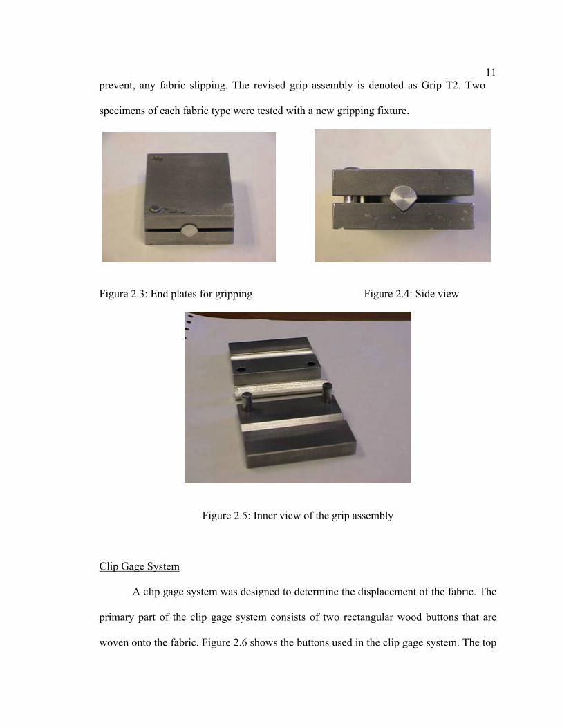
new gripping fixture that is shown in figures 2.3 to 2.7. Flat steel plates 2.5” wide, 2”

long, 0.25” thick are used to grip the specimen at both ends. At each end, one of the two

pieces has a curved groove at the center of the plate throughout its width, which is half

the thickness of the plate. The other plate has a V-notch cut in the same position about

half the thickness of the plate. A round aluminum rod is cut along the length to the shape

of the groove to match the existing grooves in the steel plate. Two shoulder pins are

assembled at the top of the plates to keep the assembly intact and prevent any wobble of

the plates with respect to each other about the aluminum piece. The fabric was held

between the V-notch and the aluminum piece so that the notch pinches against the fabric

and prevents from slipping with respect to the end plates. The two plates were pressed

with hydraulic grips thereby ensuring uniform pressure application to minimize, if not

11prevent, any fabric slipping. The revised grip assembly is denoted as Grip T2. Two

specimens of each fabric type were tested with a new gripping fixture.

Figure 2.3: End plates for gripping Figure 2.4: Side view

Figure 2.5: Inner view of the grip assembly

Clip Gage System

A clip gage system was designed to determine the displacement of the fabric. The

primary part of the clip gage system consists of two rectangular wood buttons that are

woven onto the fabric. Figure 2.6 shows the buttons used in the clip gage system. The top

12button is fixed while the bottom button is allowed to move along the length of the

aluminum rod. A calibrated extensometer fitted on the “button” measures the strain of the

fabric for a particular extensometer gage length. Gage lengths varying from 1.2” to 3.2”

can be adopted using this arrangement. The mass of the button apparatus along with the

extensometer is 0.065 kg. The button is attached to the fabric using a high strength

thread. Figure 2.7(a) illustrates the connection between the button and the fabric. Figure

2.7(b) shows the bond between the fabric and the button after the completion of a tension

tests. The bond between the button apparatus and the fabric is strong enough for proper

load transfer to take place. The experimental setup for a typical tension test using the clip

gage system is shown in figure 2.8.

Figure 2.6: Button part of the clip gage system

Aluminum Rod

Bottom Button

Top Button

13

Figure 2.7: Button apparatus attached to the fabric (a) before testing and (b) after

testing

Figure 2.8: Experimental Setup using the clip gage system

142.1.3 Specimen Test Procedure

The tests were performed according to the Standard ASTM procedure –

ASTM D 3039 “Standard Test Method for Tensile Properties of Fiber-Resin

Composites”. Tests were conducted in a 22 Kips servo-hydraulic test frame operated

under closed-loop control.

The test procedure included a displacement control test with the rate of

displacement of actuator (stroke) set at 0.1”/min. Digital data acquisition was used to

collect data at every 0.5 second. The test was continued until complete failure of the

specimen was achieved. The load-deformation results were used to calculate the stress-

strain response. The overall deformation of the specimen was measured by the stroke

movement of the actuator.

Figure 2.9: Test setup with specimen

152.2 Test Procedure Validations

The tension tests provide the stress-strain curves for the various fabrics. Woven

fabrics inherently have crimp (or waviness) and slack. In the initial stages of testing, the

applied load essentially straightens the yarns of these fabrics by removing the crimp.

Also, two different types of specimens namely S1 and S2 and various different gage

lengths of the actuator and extensometer were used to plot these curves. A number of

different tests were run in order to ascertain the effect of these parameters on the obtained

results

2.2.1 Varying Gage Lengths

A number of tests were run to analyze the affect of different extensometer and

actuator gage lengths on the tension tests results. Table 2.1 provides the details of various

samples tested.

The following notations are used for the gage lengths of the actuator and

extensometer.

L1 = Center-to-center distance between the two V-notches of the grip

L2 = Center-to-center distance between the centers of the button holes in the top

portion of the two buttons.

16Table 2.1: Test Details

Sample Name Sample Type A1 9" Actuator Gage Length; 1.2" Extensometer Gage Length A2 9" Actuator Gage Length; 2.0" Extensometer Gage Length A3 9" Actuator Gage Length; 3.2" Extensometer Gage Length B1 12" Actuator Gage Length; 1.2" Extensometer Gage Length B2 12" Actuator Gage Length; 2.0" Extensometer Gage Length B3 12" Actuator Gage Length; 3.2" Extensometer Gage Length C1 12” Actuator Gage Length (Pre-Loaded Sample); No extensometer C2 9” Actuator Gage Length (Pre-Loaded Sample); 2.0"

Extensometer Gage Length

A typical load–displacement plot (Figure 2.10) shows that actuator displacement

measured is much greater than the extensometer displacement measured. Figure 2.11

shows a typical stress-strain curve.

0 0.05 0.1 0.15 0.2 0.25Displacement, in

0

0.4

0.8

1.2

1.6

Load

, kip

s

Kevlar Sample A29" Actuator Gage Length2" Extensometer Gage Length

Figure 2.10: Load–displacement plot (Sample A2) using actuator stroke & extensometer

reading

17

0 0.01 0.02 0.03 0.04Strain, in/in

0

50

100

150

200

250

Stre

ss, k

si

Kevlar Sample B212 " Actuator Gage Length2" Extensometer Gage Length

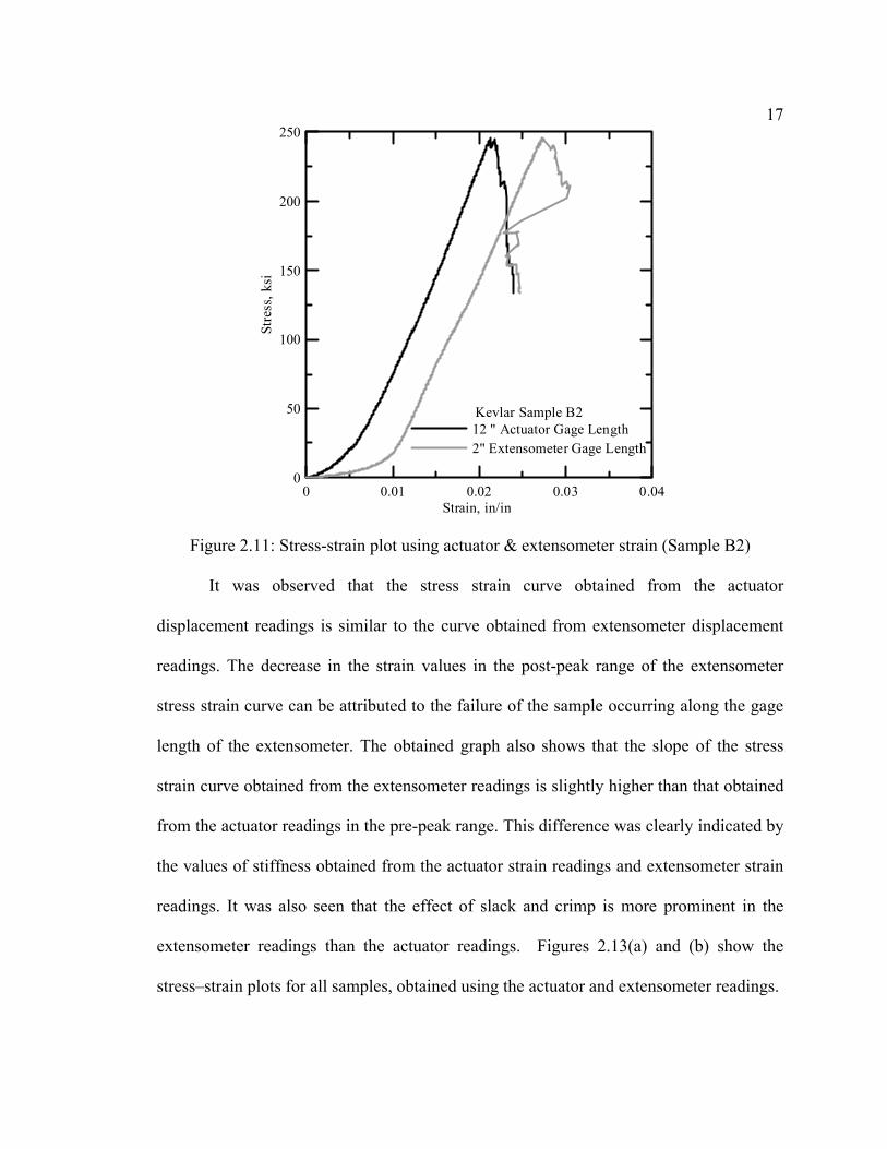
Figure 2.11: Stress-strain plot using actuator & extensometer strain (Sample B2)

It was observed that the stress strain curve obtained from the actuator

displacement readings is similar to the curve obtained from extensometer displacement

readings. The decrease in the strain values in the post-peak range of the extensometer

stress strain curve can be attributed to the failure of the sample occurring along the gage

length of the extensometer. The obtained graph also shows that the slope of the stress

strain curve obtained from the extensometer readings is slightly higher than that obtained

from the actuator readings in the pre-peak range. This difference was clearly indicated by

the values of stiffness obtained from the actuator strain readings and extensometer strain

readings. It was also seen that the effect of slack and crimp is more prominent in the

extensometer readings than the actuator readings. Figures 2.13(a) and (b) show the

stress–strain plots for all samples, obtained using the actuator and extensometer readings.

18

0 0.01 0.02 0.03Strain, in/in

0

100

200

300

Stre

ss, k

si

KevlarActuator Readings

A1A2A3B1B2B3

Figure 2.13(a): Stress-Strain Response with Actuator Readings

0 0.02 0.04 0.06Strain, in/in

0

100

200

300

Stre

ss, k

si

KevlarExtensometer Readings

A1A2A3B1B2B3

Figure 2.13(b): Stress-Strain Response with Extensometer Readings

19Some of the differences in the initial part of the stress strain curves for the

different samples (A & B) with different extensometer gage lengths (1.2”, 2” and 3.2”)

can be attributed to the different levels of slack and crimp in each sample. The results are

summarized in Table 2.2.

Table 2.2: Kevlar Test Results

Actuator Readings

Stiffness, E

ksi

Sample Type

Maximum Stress (ksi)

Maximum Ult. Strain

(in/in)

Toughness

(ksi) Extensometer

Actuator

A1

240.41 0.0178 2.92 14942.11 13412.77

A2

247.22 0.0174 2.89 15287.93 13172.24

A3

263.04 0.0185 3.00 14100.61 13071.31

Average 250.22 0.0179 2.94 14776.9 13218.8

Std. Dev

11.61 0.0006 0.05 610.7 175.4

B1

233.38 0.0168 2.41 14926.76 12961.50

B2

247.09 0.0171 2.55 14426.71 13132.65

B3

245.42 0.0170 2.47 14715.12 12800.05

Average

241.96 0.0170 2.48 14689.5 12964.7

Std. Dev

7.48 0.0002 0.07 251.0 166.3

202.2.2 Cyclic Load Tests

The phenomenon of pre-loading the test specimen was used to study the effect of

the slack and crimp. The specimen was subjected to cyclic loading between 0-0.1 kips

applied at 100 cycles with a frequency of 1 Hz. This loading was applied to the specimen

before the specimen is subjected to the actual loading. Figure 2.14 shows the effect of

this cyclic preloading. The control sample was not preloaded and shows the presence of

slack and crimp visible at the initial portion of the graph (Control Sample Original B1).

By computing the largest slope (corresponding to the largest stiffness of the specimen),

one can slide the graph so that the largest slope passes through the origin. This graph was

denoted as Control Sample Linearized. The same procedure was applied to the sample

that is preloaded (Sample C1). The amount of sliding that was required is greatly reduced

indicating that very little slack and crimp was present in the specimen.

0 0.01 0.02 0.03 0.04Strain, in/in

0

50

100

150

200

250

Stre

ss, k

si

KevlarControl Sample OriginalControl Sample LinearizedPre-Loaded Sample OriginalPre-Loaded Sample Linearized

Pre-Load: Cyclic Load ( 0-13 ksi) 100 cycles @ 1 Hz

Figure 2.14: Stress–strain plots with (Sample C1) and without pre-loading (Sample B1)

21Samples C1 and B1 were tested without the extensometer assembly attached to

the sample. A cyclic load test performed on Kevlar sample C2 of size 9” actuator gage

length and 2” extensometer gage length is shown in the figure 2.15 below.

0 0.005 0.01 0.015 0.02 0.025Strain, in/in

0

50

100

150

200

250

Stre

ss, k

si

Kevlar Sample C29" Actuator Gage Length2.0" Extensometer Gage Length

Figure 2.15: Stress–Strain plots with pre-loading (Sample C2)

The stiffness obtained for the above sample is compared to a similar sample A2

(without pre-loading) in Table 2.3.

Table 2.3: Stiffness and Ultimate Strains With and Without Preloading

Stiffness, E, ksi Max Ult. Strain (in/in)

Extensometer

Actuator

Extensometer

Actuator

Without Preloading (Sample A2) 15288 13172 0.031 0.021

With Preloading (Sample C2) 15109 13232 0.016 0.017

22 The values of the stiffness obtained for a sample with and without preloading

are similar to each other. Thus, pre-loading of the sample only eliminates the slack and

crimp present in the initial portion of the stress strain curve. However, there is a

significant difference in the ultimate strain values for the extensometer readings. Hence,

the cyclic load test may be employed for samples that require an accurate calculation of

the ultimate strain values.

2.2.3 Stitched and Glued Samples

Stitched and glued samples were used in the test program. Figures 2.16 and 2.17

show the tension tests results for stitched and glued samples for Kevlar and Zylon AS-

500. Table 2.4 depicts the comparison of the values of the Young’s modulii obtained

using the stitched and glued samples for the two fabrics. Table 2.4 indicates that there is

no significant difference in the Young’s Modulii E11 for the two fabrics using the stitched

and glued samples. Hence, both samples S1 and S2 can be used to the determine the

material constants for the fabrics

23

0 0.01 0.02 0.03Strain, in/in

0

100

200

300

Stre

ss, k

si

KevlarStiched SampleGlued Sample

Figure 2.16 Stress–Strain Comparisons for Stitched and Glued Samples for Kevlar

0 0.02 0.04 0.06 0.08Strain, in/in

0

100

200

300

400

500

Stre

ss, k

si

Zylon AS-500Stiched SampleGlued Sample

Figure 2.17: Stress–Strain Comparisons for Stitched & Glued Samples for Zylon AS-500

24Table 2.4: Young’s Modulus Comparison for Stitched and Glued Samples for Different

Fabrics

Young's Modulus E11, MPa Fabric

Stitched Glued

Kevlar 13232 13326

Zylon AS-500 19319 19421

2.3 Tension Test Results

Simple tension tests were run on the three types of fabrics using the 22 Kips

servo-hydraulic test frame operated under closed-loop control. The clip gage system was

attached perpendicular to the direction of the actuator displacement for measuring the

Poisson’s ratio for the fabric. For each type of fabric, a total of ten samples were tested,

five in the fill direction and five in the warp direction. The Poisson’s ratio was calculated

for three different ranges as the ratio of lateral stiffness to longitudinal stiffness.

2.3.1 Kevlar Tension Tests

The following are the results of the tension tests carried out on Kevlar samples for

determining Young’s Modulus E11. Figure 2.18 shows the stress-strain response of five

Kevlar samples. Table 2.5 summarizes these results.

25

0 0.01 0.02 0.03 0.04 0.05Strain, in/in

0

50

100

150

200

250

Stre

ss, k

si

KevlarYoung's Modulus E11

Sample 1Sample 2Sample 3Sample 4Sample 5

Figure 2.18: Stress-Strain Curves for the Kevlar Samples for E11

Table 2.5: Tension Test Results From Kevlar Samples for E11

Sample Type

Maximum Stress

ksi

Maximum Ult. Strain

in/in

Toughness ksi

Stiffness, E ksi

1 241.99 0.0274 3.52 13608.58 2 223.93 0.0287 3.27 13187.96 3 235.96 0.0295 4.01 13525.44 4 244.32 0.0365 4.24 13154.00 5 227.41 0.0319 3.73 13380.51

Average 234.72 0.03 3.75 13371.30 8.90 0.00 0.39 200.61 Std. Dev

The Poisson’s Ratio ν12 for Kevlar was obtained from the tension tests using the

clip gauge system. The following graphs (Figures 2.19 and 2.20) show the axial stress

versus lateral strain for these samples.

26

-0.06 -0.04 -0.02 0 0.02Lateral Strain, in/in

0

50

100

150

200

250

Stre

ss, k

si

KevlarSample 1Sample 2Sample 3Sample 4Sample 5

Figure 2.19: Axial Stress Versus Lateral Strains for Kevlar Samples for ν 12

-0.06 -0.04 -0.02 0 0.02 0.04 0.06Strain, in/in

0

100

200

300

Stre

ss ,

ksi

Sample 4Range ( 29 - 87 ksi )Range ( 87 - 145 ksi )Range ( 145 - 203 ksi )

Axial StrainLateral Strain

Figure 2.20: Axial Stress Versus Axial Strain and Lateral Strain for Sample 4 for ν12

27The Poisson’s Ratio ν12 was calculated for three different ranges of stresses and

the results are summarized in table 2.6.

Table 2.6: Poisson’s ratio ν12 for the Kevlar Samples

Poisson's Ratio Stress Range Sample

1 Sample

2 Sample

3 Sample

4 Sample

5 Average Std. Dev

29-87 ksi 1.945 1.746 1.921 1.842 1.764 1.844 0.090 87-145 ksi 0.797 0.680 0.746 0.685 0.615 0.705 0.069 145-203 ksi 0.738 0.524 0.618 0.578 0.631 0.618 0.079

The results obtained from five tension tests run on Kevlar AS-49 for Young’s Modulus

E22 are shown in the figure 2.21 and table 2.7.

0 0.01 0.02 0.03Strain, in/in

0

100

200

300

Stre

ss, k

si

KevlarYoung's Modulus E22


Figure 2.21: Stress-Strain Curves for the Kevlar As-49 Samples for E22

28Table 2.7: Tension Test Results From Kevlar Samples for E22

Sample Type

Maximum Stress

ksi

Maximum Ult. Strain

in/in

Toughness ksi

Stiffness, E ksi

1 245.82 0.0238 3.11 15136.68 2 261.73 0.0228 3.15 15013.68 3 233.39 0.0228 3.01 15378.25 4 206.35 0.0203 2.68 15154.16 5 245.95 0.0185 3.04 15736.76

Average

238.65 0.02 3.00 15283.91 20.67 0.00 0.19 285.27 Std. Dev

The Poisson’s Ratio ν21 for Kevlar AS-49 was obtained from the tension tests using the



-0.06 -0.04 -0.02 0Lateral Strain, in/in

0

400

800

1200

1600

2000

Stre

ss, k

si

KevlarSample 1Sample 2Sample 3Sample 4Sample 5

Figure 2.22: Axial Stress Versus Lateral Strains for Kevlar AS-49 Samples for ν21

29

-0.04 -0.02 0 0.02 0.04Strain, in/in

0

100

200

300

Stre

ss ,

ksi




The Poisson’s Ratio ν21 was calculated for three different ranges of stresses and

the results are summarized in Table 2.8

Table 2.8: Poisson’s Ratio ν21 For the Kevlar AS-49 Samples

Poisson’s Ratio Stress Range Sample

1 Sample

2 Sample

3 Sample

4 Sample

5 Average Std. Dev

58-116 ksi 0.828 0.802 0.290 0.350 0.786 0.611 0.267 116-174 ksi 0.302 0.345 -0.110 0.182 0.391 0.222 0.201 174-217 ksi 0.211 0.256 -0.261 0.000 0.231 0.087 0.220

2.3.2 Zylon AS-500 Tension Tests

The results obtained from five tension tests run on Zylon AS-500 for Young’s Modulus


30

0 0.01 0.02 0.03 0.04 0.05Strain, in/in

0

100

200

300

400

500

Stre

ss, k

si

Zylon AS-500Young's Modulus E11


Figure 2.24: Stress-Strain Curves for the Zylon As-500 Samples for E11

Table 2.9: Tension Test Results Zylon AS-500 Samples for E11

Sample Type

Maximum Stress

ksi

Maximum Ult. Strain

in/in

Toughness ksi

Stiffness, E ksi

1 423.21 0.0337 6.49 19672.93 2 445.82 0.0365 6.92 19930.00 3 400.70 0.0368 5.80 18613.02 4 425.37 0.0356 6.70 19217.05 5 435.37 0.0384 6.99 19115.51

Average

426.09 0.04 6.58 19309.70 16.80 0.00 0.48 511.95 Std. Dev

31The Poisson’s Ratio ν12 for Zylon AS-500 was obtained from the tension tests

using the clip gauge system. The following graphs (Figures 2.25 and 2.26) show the axial

stress versus lateral strain for these samples.

-0.08 -0.06 -0.04 -0.02 0Lateral Strain, in/in

0

100

200

300

400

500St

ress

, ksi

Zylon AS-500Sample 1Sample 2Sample 3Sample 4Sample 5

Figure 2.25: Axial Stress Versus Lateral Strains for Zylon AS-500 Samples for ν12

32

-0.06 -0.04 -0.02 0 0.02 0.04 0.06Strain, in/in

0

100

200

300

400

500

Stre

ss ,

ksi






Table 2.10: Poisson’s Ratio ν12 For the Zylon AS-500 Samples


1 Sample

2 Sample

3 Sample

4 Sample

5 Average Std. Dev

73-174 ksi 0.822 0.793 0.486 0.718 0.560 0.676 0.147 174-290 ksi 0.147 0.186 0.130 0.173 0.122 0.152 0.027 290-363 ksi 0.033 0.044 0.056 0.070 0.056 0.052 0.014

The results obtained from five tension tests run on Zylon AS-500 for Young’s Modulus


33

0 0.01 0.02 0.03 0.04Strain, in/in

0

100

200

300

400

500

Stre

ss, M

Pa



Figure 2.27: Stress-Strain Curves for the Zylon As-500 Samples for E22


Sample Type

Maximum Stress

ksi

Maximum Ult. Strain

in/in

Toughness ksi

Stiffness, E ksi

1 420.69 0.0241 7.37 19730.82 2 410.31 0.0294 8.47 18910.97 3 368.40 0.0263 6.49 19174.01 4 413.91 0.0262 6.93 19717.47 5 378.15 0.0260 6.90 19274.66

Average

398.29 0.0264 7.23 19361.59 23.40 0.0019 0.76 356.65 Std. Dev

34The Poisson’s Ratio ν21 for Zylon AS-500 was obtained from the tension tests



-0.05 -0.04 -0.03 -0.02 -0.01 0Lateral Strain, in/in

0

100

200

300

400

500St

ress

, ksi

Zylon-500Sample 1Sample 2Sample 3Sample 4Sample 5

Figure 2.28: Axial Stress Versus Lateral Strains for Zylon AS-500 Samples for ν21

35

-0.04 -0.02 0 0.02 0.04Strain, in/in

0

100

200

300

400

500

Stre

ss ,

ksi








1 Sample

2 Sample

3 Sample

4 Sample

5 Average Std. Dev

73-174 ksi 1.434 1.280 1.295 1.357 1.101 1.293 0.124 174-290 ksi 0.724 0.613 0.711 0.961 0.801 0.762 0.130 290-363 ksi 0.482 0.564 1.583 0.785 0.671 0.817 0.443

2.3.3 Zylon AS-1500 Tension Tests

Figure 2.30 shows the stress-strain response of five Zylon AS-1500 samples for a

loading rate of 0.2 inches per minute. Table 2.13 summarizes these results.

36

0 0.01 0.02 0.03 0.04 0.05Strain, in/in

0

100

200

300

400

500

Stre

ss, k

si



Figure 2.30: Stress-Strain Curves for the Zylon AS-1500 Samples for E11


Sample Type

Maximum Stress

ksi

Maximum Ult. Strain

in/in

Toughness ksi

Stiffness, E ksi

1 476.49 0.0337 8.45 21477.55 2 494.80 0.0365 9.09 22062.84 3 477.20 0.0368 8.80 21895.82 4 447.86 0.0356 10.11 21111.46 5 453.51 0.0384 8.02 21534.49

Average

469.97 0.04 8.89 21616.43 19.18 0.00 0.79 373.61 Std. Dev

The Poisson’s Ratio ν21 for Zylon AS - 1500 was obtained from the tension tests



37

-0.04 -0.03 -0.02 -0.01 0Lateral Strain, in/in

0

100

200

300

400

500

Stre

ss, k

si

Zylon AS -1500 Sample 1Sample 2Sample 3Sample 4Sample 5

Figure 2.31: Axial Stress Versus Lateral Strains for Zylon As-1500 Samples for ν12

-0.04 -0.02 0 0.02 0.04 0.06Strain, in/in

0

200

400

600

Stre

ss ,

ksi




38The Poisson’s Ratio ν12 was calculated for three different ranges of stresses and


Table 2.14: Poisson’s Ratio ν12 For the Zylon As-1500 Samples


1 Sample

2 Sample

3 Sample

4 Sample

5 Average Std. Dev

73-174 ksi 0.467 0.552 0.720 0.309 0.469 0.503 0.150 174-290 ksi 0.261 0.466 0.159 -0.053 0.244 0.215 0.188 290-363 ksi 0.014 0.384 0.041 -0.280 0.260 0.084 0.255

The results obtained from five tension tests run on Zylon AS-1500 for Young’s

Modulus E22 are shown in the figure 2.33 and table 2.15.

0 0.01 0.02 0.03 0.04 0.05Strain, in/in

0

100

200

300

400

500

Stre

ss, k

si



Figure 2.33: Stress-Strain Curves for the Zylon AS-500 Samples for E22

39Table 2.15: Tension Test Results Zylon AS-1500 Samples for E22

Sample Type

Maximum Stress

ksi

Maximum Ult. Strain

in/in

Toughness ksi

Stiffness, E ksi

1 434.65 0.0303 8.53 20944.24 2 418.19 0.0281 9.32 21136.55 3 460.32 0.0293 8.96 21451.08 4 462.63 0.0311 8.77 21595.03 5 443.91 0.0291 9.28 21403.10

Average

443.94 0.0296 8.97 21306.00 18.48 0.0012 0.34 261.53 Std. Dev

The Poisson’s Ratio ν21 for Zylon AS-1500 was obtained from the tension tests using the



-0.03 -0.02 -0.01 0Lateral Strain, in/in

0

100

200

300

400

500

Stre

ss, k

si

Zylon AS -1500 Sample 1Sample 2Sample 3Sample 4Sample 5

Figure 2.34 Axial Stress Versus Lateral Strains for Zylon AS-1500 Samples for ν21

40

-0.04 -0.02 0 0.02 0.04 0.06Strain, in/in

0

200

400

600

Stre

ss ,

ksi








1 Sample

2 Sample

3 Sample

4 Sample

5 Average Std. Dev

73-174 ksi 0.526 0.539 0.700 0.356 0.501 0.525 0.122 174-290 ksi 0.095 0.079 0.315 0.090 0.156 0.147 0.098 290-363 ksi 0.076 0.035 0.231 0.057 0.064 0.093 0.079

412.4 Comparison of All Fabrics

A comprehensive graph showing all the stress-strain curves for all the fabrics

tested in this phase of the research is presented in figure 2.36. The samples used in the

graph are the samples for E11 tests for all fabrics.

0 0.02 0.04 0.06 0.08Strain, in/in

K-1K-2K-3K-4K-5Z1-1Z1-2Z1-3Z1-4Z1-5

K - KevlarZ1 - Zylon AS-500Z2 - Zylon AS-1500

Z2-1Z2-2Z2-3Z2-4Z2-5

0

200

400

600

Stre

ss, k

si

Figure 2.36: Stress-Strain Curves for All Three Fabrics (E11)

The initial portion of the load-deflection graph shows a large increase in

displacement (actuator stroke) for a very small increase in load. The slack and crimp is

predominant in Zylon AS-500 while it is almost similar for Zylon AS-1500 and Kevlar

AS-49. As the load increases, the yarns stiffen as shown by the increase of the slope of

the load-deflection graph. The failure of all the specimens is sudden (brittle behavior).

42Table 2.17 and 2.18 shows the comparison of the results obtained from the simple

tension tests run on all the three fabric types.

Table 2.17: Tension Tests Results – E11 Results

For E11 Fabric Max. Max. Toughness Stiffness Type Stress Ult. ksi ksi ksi Strain in/in Average 234.63 0.0291 3.52 13468.47 Std. Dev

Kevlar AS-49 8.99 0.0048 0.67 299.49

Average 426.09 0.0362 6.58 19309.70 Std. Dev

Zylon AS-500 16.80 0.0017 0.48 511.95

Average 469.97 0.0336 8.89 21616.43 Std. Dev

Zylon AS-1500 19.18 0.0015 0.79 373.61

Table 2.18: Tension Tests Results – E22 Results

For E22 Fabric Max. Max. Toughness Stiffness Type Stress Ult. ksi ksi ksi Strain in/in Average 238.65 0.0217 3.00 15283.91 Std. Dev

Kevlar AS-49 20.67 0.0022 0.19 285.27

Average 398.29 0.0264 7.23 19361.59 Std. Dev

Zylon AS-500 23.40 0.0019 0.76 356.65

Average 443.94 0.0296 8.97 21306.00 Std. Dev

Zylon AS-1500 18.48 0.0012 0.34 261.53

43The stiffness values obtained from the E11 and E22 tests for the Zylon fabrics

are almost similar. The values differ by about 15% percent for the Kevlar fabrics. This

difference can be attributed to different manufacturing batches used for the specimen

testing. The standard deviation for the (Kevlar) peak strain values of five tests is 0.48%

and 0.22% for the Young’s Modulus in the warp and fills direction respectively. In the

case of Zylon, the peak strain values obtained using Zylon AS-500 are less than those

obtained from Zylon AS-500. The standard deviation of the peak strain for the five tests

for E11 is 0.17% and 0.15%. The ultimate tensile strain is obtained by dividing the

elongation at peak load by the specimen gage length. Gage length used for the grip is L1.

The modulus of elasticity was measured as the maximum slope within the linear range of

the ascending portion of the stress strain curve. The toughness of each specimen is

calculated as the area under the stress strain curve. This included the initial nonlinear

ascending portion of the curve and nonlinear post peak response of the curve.

The average Poisson’s ratios for the three fabric types are represented in the table

2.19. It is observed that the Poisson’s ratio gradually decreases as the specimen

approaches its failure. The higher values of standard deviation for the final stress range

are due to the failure of some yarns in the vicinity of the clip gage system. This failure is

more prominent in the E22 specimens that measure the Poisson’s ratio ν21. There is a

significant decrease in Poisson’s ratio ν21 as compared to the Poisson’s ratio ν12 for the

Kevlar fabric and an increase for Zylon AS-500 fabric. Both the Poisson’s ratios are

almost the same for Zylon AS-1500.

44Table 2.19: Tension Tests Results – Poisson’s Ratios

Poisson’s ratio ν12 Poisson’s ratio ν21

Fabric Stress Range Average Std. Dev Stress Range Average Std.

Dev

29-87 ksi 1.844 0.090 58-116 ksi 0.611 0.267 87-145 ksi 0.705 0.069 116-174 ksi 0.222 0.201

Kevlar AS-49

145-203 ksi 0.618 0.079 174-217 ksi 0.087 0.220

73-174 ksi 0.676 0.147 73-174 ksi 1.293 0.124 174-290 ksi 0.152 0.027 174-290 ksi 0.762 0.130

Zylon AS-500 290-363 ksi 0.052 0.014 290-363 ksi 0.817 0.443

73-174 ksi 0.503 0.150 73-174 ksi 0.525 0.122 174-290 ksi 0.215 0.188 174-290 ksi 0.147 0.098

Zylon AS-1500 290-363 ksi 0.084 0.255 290-363 ksi 0.093 0.079

Some of the failure modes using the grips are shown in Figure 2.37 through 2.42.

The failure (broken yarns) occurred at the middle of the specimen for the Kevlar

specimen while the failure occurred near the grips for the Zylon specimen. For the E22

specimens, there is a localized failure in most of the specimens.

Figure 2.37: Kevlar specimen Figure 2.38: Failure at center

45

Figure 2.39: Zylon AS-500 specimen Figure 2.40: Failure at the edge

Figure 2.41: Zylon AS-1500 specimen Figure 2.42: Localized Failure

Chapter 3: Static Ring Tests

3.1 Introduction to the Static Ring Tests

A series of static ring tests were conducted on the two types of fabric: Kevlar AS-

49 and Zylon AS-500. These tests were conducted using a steel ring to simulate the

engine housing of an aircraft in case of fan blade out event. A total of 21 tests on Kevlar

AS-49 and 21 tests on Zylon AS-500 were conducted. These tests were carried out for 1,

4 and 8 layer fabric wraps.

3.1.1 Objectives

The primary objective of static tests is to simulate the penetration of the blunt

object through the engine containment system assembly. A steel cylinder is used to

simulate the engine housing, and the composite fabric is wrapped around this cylinder.

The tests were conducted by applying the load in a quasi-static manner until failure,

defined as full penetration of the blunt nose through the single or multi-layer fabric. The

load and deformation history were collected throughout the test and energy absorption

capacity of the structure was calculated from this response. This test may ultimately be

used as one of the key parameters in the determination of properties and design of the

containment chamber.


The proposed plan for testing required determination of the load-deformation

response of single and multi-layer specimens for both Kevlar and Zylon wraps. The

specimens were subjected to outward penetration motion of a blunt nose assembly at

various orientations and positions of the two different blunt noses. The blunt nose

assembly was initially set up inside the steel ring. The specimen dimensions were 32” in

diameter, 4” wide and consisted of 1, 4, and 8 layers wrapped around the outside of the

steel cylinder. A small window was machined in the ring to allow for the penetration of

the blunt nose.

For the single layer specimens, a 6” length of fabric overlap was used to glue the

fabric onto itself. For multi layer fabrics, the first layer was directly mounted onto the

ring and temporary fixed onto it by means of a standard cello tape. The last layer was

glued to the previous layer using 5-minute® epoxy. Overlap length for all specimens was

6”. The specimens were covered with opaque plastic sheeting to minimize the degrading

effects of moisture and ultraviolet light.

3.1.3 Test Setup

A test fixture was manufactured by rolling a section of A36 mild steel to

the inner diameter dimensions of the test setup. The ring dimensions are as follows: Outer

Diameter (OD) of 32”, Internal Diameter (ID) of 30”, width of 6”, and a thickness of 1”.

This ring was the main component of the loading fixture and was fabricated at Karlson

Machinery, Phoenix, AZ. The complete loading fixture was made up of four major parts.

The ring was assembled in two parts - as a large, and a small arc. The other components

48include the two side support plates and end plate to connect the two ring components.

A detailed view of the cylinder with side plates is shown in Figure 3.1. The small arc that

was cut out from the ring was connected at the bottom of the ring assembly and did not

alter the geometry of the test set up. The size of the small arc corresponds to a 38° angle.

Use of the ring as two parts allowed for easy installation of the specimen in the loading

fixture. The specimens were first wrapped on an aluminum mandrel (Figure 3.2).

Removal of the small arc during the sample mounting stage facilitated the transfer of the

test specimen from the transfer mandrel (Figure 3.3). The cylinder was attached to two

side plates using 15-3/4” diameter high strength bolts connected along the ring’s

perimeter. These side plates were connected to the base-plate; hence the ring had a

clearance of 3” from the base plate.

Figure 3.1: Test setup

49

Figure 3.2: Mandrel for specimen preparation

Figure 3.3: Specimen transfer ring

50Two different blunt noses were used as the penetrators for the tests in this

program. The dimensions of steel noses are as described in the table 3.1. Figures 3.4 and

3.5 illustrate the two different blunt noses.

Table 3.1 Dimensions of the Various Blunt Noses

Type of Blunt Nose

Width

Thickness

Radius

Thicker Penetrator

{ Type A }

2”

0.3125”

0.1563”

Thinner Penetrator

{Type B}

1.5”

0.2370”

0.1185”

Figure 3.4: Top View Comparison of the Two Blunt Noses

51

Figure 3.5: Side View Comparison of the Two Blunt Noses

Another important parameter was the effect of fixity of the blunt nose loading

mechanism with respect to the specimen, especially with large displacements expected

throughout the test. It was expected that if the side loads were not removed through the

use of hinges, a stiff system would be created which would result in side loads.

Alternatively, any rotation of the test assembly could result in loss of contact of the full

length of the blunt nose with the fabric, thus increasing the contact pressure and

premature failure of the specimen. Measurement of such second order effects would be

difficult if not impossible. Thereby, it was found necessary to fix the end conditions at

the top of the blunt nose housing by fixing the load cell bearings that were placed

orthogonal to the nose bearings as shown in Figure 3.6. In order to avoid side loads and

thereby the titling of the blunt nose, the fixed-fixed condition for the blunt nose assembly

as shown in figure 3.7 was used for all the forty-two tests conducted.

52

Figure 3.6: Top plate with bearings orthogonal to nose bearings (Fixed end condition at

top)

Figure 3.7: Blunt nose housing design (fixed-fixed conditions)

53In order to avoid transferring the entire load to the end joint C-Clamps were

used at points remote from the blunt head contact. The tests were conducted with the

clamps in place for both Kevlar and Zylon specimens. These clamps were placed at the

same height on both sides of the ring to maintain symmetry and uniformity – clamps are

placed at the height of 13.75” from the top of the base plate or at the height of 10.75”

from the bottom of the cylinder OD. The figure 3.8 illustrates the attachment of the C-

Clamps to the steel ring.

Figure 3.8: Attachment of C-clamps to the specimen

It was furthermore observed through the preliminary tests that significant slack

existed for the multi-ply Zylon samples. This can be verified through the analysis of the

54raw test data, which indicated up to 2” of stroke travel under an insignificant amount of

load (e.g. up to 250 lbs). In order to relieve the slack, the specimens were pre-tensioned

using an outward pressure applied at the bottom portion of the ring. The pressure was

applied by placing two steel spacer blocks between the small arc of the ring and the

spacer plate, and pushing the spacer plate outward by tightening the screws. Schematic

diagrams of this set up are shown in figures 3.9 and 3.10. This ensured some of the slack

recovery.

Data acq . System

Command signal generator

Feedback Signal

Error Signal

DIGITAL CONTROLLER

Personal Computer

Data AcquisitionSystem

Servo-Control valve

CommandSignal

Feedbacksignal

specimen

load cell

Figure 3.9: Schematic diagram of the test setup

55

Steel Ring Fabric

Spacer plate

C-Clamp

Small arc

C-Clamp

Figure 3.10: Schematic of test setup with clamps and hinges to remove spurious loads

Additionally, a threaded rod in between the blunt nose and the support plate was

used in order to increase the length of the nose. This also facilitated the rotation of the

blunt nose for various angles as proposed in the test plan. For testing the fabrics for the

off center orientation, a new set of base blocks were designed. These base blocks when

fixed onto the base plate align the edge of the penetrator at a distance of 0.15” from the

edge of the machined window.

3.1.4 Test procedure

Each sample was transferred from the wrapping mandrel to the test rig and the

side plates were then attached. An MTS servo-hydraulic test machine with Digital

Teststar2 controller software was used for all the specimens. All the tests were conducted

under actuator control using a constant rate of travel of 0.4”/min. The test was conducted

in a manner such that the load cell housing the blunt nose remained stationary throughout

56the test, while the actuator and, hence the ring, moved downward thus loading the

fabric against a stationary blunt nose. The data were collected using a digital data

acquisition system at a rate of 2 Hz.

For certain specimens, the test was run in a single step and continued until failure

occurred. For multi-ply specimens (4, 8 ply Kevlar and all Zylon) tests were performed in

two steps. Since the maximum actuator travel length was limited to 4 inches, a

readjustment of the position of the sample was necessary to extend the total displacement

beyond 4” expected in the multi ply and Zylon tests. During the first stage, the sample

was loaded to 250 lbs and the test was placed on hold. At this point the actuator was

brought back to the zero position, while the cross head was moved up to maintain the

preload of the sample at the 250 lbs. At this point, the test was resumed, and

displacement was imposed until the failure of specimen. The adjustment of the cross

head was necessary to ensure enough travel was available for the sample to fail without

causing any impact on the quality of the data obtained.

3.2 Static Ring Test Results

The load deflection curves for various multi ply specimens of Kevlar AS-49 and

Zylon AS-500 were obtained from the data generated through the static ring test. It was

observed that in the initial region of the load deflection curve there was a gradual

increase in the deflection with minimal increase in the load carrying capacity. This was

attributed to the slack due to the sliding and loss of gripping at the clamps. The amount

of slack in all tested specimens was significant to the level of up to 3” of travel distance.

57The latter part of the load deflection curve is considered to be dominated by slack

recovery (there is some deformation because of the straightening of the yarns) and

gradual loading of the specimen to reach the stiffness of the fabric being loaded in

tension on the static ring.

Finally, the ultimate load is reached in these samples in an abrupt manner after

several yarns fracture. The fracture of the yarns before the peak load is observed as the

sudden jump in the load response. The load carried by the fractured yarns is being

transferred to unbroken yarns. It is expected that the load redistribution after the fracture

of a few yarns results in excess load on the surviving yarns. This excess load is sufficient

to push the average stress on the yarns beyond the average ultimate tensile strength. A

maximum level as high as 60% post peak strength was observed in some samples.

0 1 2 3Deflection, Inches

0

2000

4000

6000

Load

, lbf

Kevlar 4 Layer0 Degrees Orientation

Thinner (Type B) PenetratorExperimental

Figure 3.11: Typical Load Deflection Response

58 The figures 3.12 and 3.13 show a four layer Kevlar AS-49 specimen tested with

the thinner penetrator. Figure 3.12 shows the fabric during the beginning of the test while

figure 3.13 shows the fabric towards the end of the test approaching failure. The figure

3.13 shows that a number of yarns fractured yarns at that state of loading. Figure 3.12

was taken when the load was 4.5 lbs; figure 3.13 was taken at the load of 4617 lbs while

the failure load was 5131.5 lbs. The failure of the specimen near the blunt nose area is

shown in figure 3.14.

Figure 3:12: Kevlar Sample at Start of Loading.

59

Figure 3:13: Kevlar Sample at End of a Static Ring Test.

Figure 3:14: Failure of Kevlar Sample at the Blunt Nose.

603.2.1 Kevlar Test Results

Multi-Ply, Multi-Orientation & Same Blunt Nose Comparison

The following section deals with the comparison of the results of the static ring

test for Kevlar for different number of layers ( 1, 4 and 8) and orientations using the same

kind of blunt nose.

Thicker Penetrator

The plot 3.15 hereafter shows the load deflection curves for 1, 4, and 8 layer

Kevlar specimens for 45 degrees orientation for the thicker penetrator.


0

4000

8000

12000

Load

, lbf

Phase II FAAKevlar

45 Degrees OrientationThicker Penetrator

Experimental (1 Layer)Experimental (4 Layer)Experimental (8 Layer)

Figure 3.15: Load Deflection response of Kevlar for same orientation of thicker blunt

nose for multi-layer specimens

61The peak loads for 45 degrees orientation with the thicker blunt nose were

1573, 6363 and 11796 lbs for 1, 4 and 8 layers Kevlar fabric respectively. These peak

loads seem to scale proportionally according to the number of layers of the Kevlar fabric

tested.

The figure 3.16 below shows the load deflection response of one layer Kevlar

fabric for different orientations of the thicker blunt nose.

0 1 2 3 4Deflection, Inches

0

400

800

1200

1600

2000

Load

, lbf

Phase II FAAKevlar

1 Layer FabricThicker Penetrator

0 Degrees45 Degrees90 DegreesOff-Center

Figure 3.16: Load Deflection for various orientations of thicker blunt nose with

one Layer Kevlar

Examination of figure 3.16 indicates that maximum loads at failure differ for

various orientations of blunt nose for the same number of layers. The load is maximum at

zero degrees orientation of the blunt nose and minimum at the 90 degrees orientation.

62The figure also shows that stiffness of Kevlar (lb/in) remains fairly constant up to the

fracture of the first yarn of the fabric. A drop in stiffness is observed from the 0 degrees

to 45 degrees orientation of the blunt nose with the 90 degrees orientation having the

least stiffness. Table 3.2 shows the stiffness values for multi layered Kevlar specimens

for various orientations of the thicker penetrator. The maximum load for the off-center

orientation of the blunt nose lies closer to the maximum load of the 45 degrees

orientation with deviations of 69,161 and 829 lbs for 1, 4 and 8 layer respectively. The

stiffness for the off-center orientation lies between the 45 and 90 degree orientation

stiffness.

Table 3.2: Maximum Load & Stiffness for Kevlar for Thicker Penetrator

Layers Orientation Maximum Load Stiffness, lb/in

1 0 1858 1715

1 45 1573 1418

1 90 1228 1080

1 Off 1642 1307

4 0 6625 5909

4 45 6363 5271

4 90 4925 4790

4 Off 6202 5079

8 0 13231 11025

8 45 11796 10618

8 90 9110 8340

8 Off 10967 9770

63

The responses for 4 and 8 layers of Kevlar fabric using the thicker penetrator are

plotted in figures 3.17 and 3.18 respectively. These responses are similar to the one layer

results for Kevlar.

0 1 2 3 4 5Deflection, Inches

0

2000

4000

6000

8000

Load

, lbf

Phase II FAAKevlar



Figure 3.17: Various Orientations of thicker blunt nose - 4 Layer Kevlar Fabric

64


0

4000

8000

12000

16000

Load

, lbf

Phase II FAAKevlar



Figure 3.18: Various Orientations of thicker blunt nose - 8 Layer Kevlar Fabric

The figures 3.19 and 3.20 are the energy absorbed/areal density and normalized

energy absorbed/areal density graphs for Kevlar samples tested using the thicker

penetrator. The energy-absorbed graphs predict the fabric capacities as near linear in

nature but the normalized energy absorbed capacity show that there is no consistency in

the energy absorption capacity of the fabrics. Figure 3.21 represents the peak load vs.

number of plies for Kevlar using the Type A Penetrator and Figure 3.22 represents the

peak load normalized by areal density for the same. Figure 3.23 represents the stiffness

vs. number of plies as well as linearly extrapolated stiffness values for Kevlar samples

using the thicker blunt nose. Figure 3.24 shows the same with the stiffness value

normalized with the areal density for Kevlar.

65

0 2 4 6 8 10Number of Plies

0.0E+000

1.0E+008

2.0E+008

3.0E+008

4.0E+008

Ener

gy A

bsor

bed

(lb-in

)/Are

al D

ensit

y pe

r ply

(lbs

/in2 )

Kevlar AS-49Thicker Penetrator

0 Degrees Orientation45 Degrees Orientation90 Degrees OrientationOff-Center Orientation

Figure 3.19: Energy absorbed/areal density graphs of 1, 4 and 8 ply Kevlar for thicker

penetrator


0.0E+000

1.0E+007

2.0E+007

3.0E+007

4.0E+007

Ener

gy A

bsor

bed

(lb-in

)/Are

al D

ensit

y pe

r ply

(lbs

/in2 )



Figure 3.20: Energy absorbed/areal density graphs of 1, 4 and 8 ply Kevlar samples

normalized by no of plies for thicker penetrator

66


0

4000

8000

12000

16000

Peak

Loa

d (lb

s)

Thicker Penetrator0 Degrees Orientation45 Degrees Orientation90 Degrees OrientationOff-Center Orientation

Kevlar AS-49

Figure 3.21: Number of plies vs. peak load for Kevlar using thicker penetrator


0.0E+000

1.0E+008

2.0E+008

3.0E+008

4.0E+008

5.0E+008

Peak

Loa

d (lb

s)/A

real

Den

sity

per

ply

(lbs/

in2)



Figure 3.22: Number of plies vs. normalized peak load for Kevlar using thicker

penetrator

67


0

4000

8000

12000

16000

Stiff

ness

(lbs

/in)


--- Linear Extrapolations

Kevlar AS-49

Figure 3.23: No. of plies vs. stiffness for Kevlar using thicker penetrator (actual and

linearly extrapolated)


0.0E+000

1.0E+008

2.0E+008

3.0E+008

4.0E+008

5.0E+008

Stiff

ness

(lbs

/in)/A

real

Den

sity

per

ply

(lbs/

in2 ) Thicker Penetrator


--- Linear ExtrapolationsKevlar AS-49

Figure 3.24: No. of plies vs. normalized stiffness for Kevlar using thicker penetrator

(actual and linearly extrapolated)

68Thinner Penetrator

The load deflection curves for 1, 4, and 8 layer Kevlar specimens for 45 degrees

orientation using the thinner penetrator are shown in figure 3.25.


0

2000

4000

6000

8000

10000Lo

ad, l

bf

Phase II FAAKevlar

45 Degrees OrientationThinner Penetrator


Figure 3.25: Load Deflection response of Kevlar for same orientation of thinner blunt

nose for multi-layer specimens

The peak loads with the thinner penetrator were 1104, 4552 and 8257 lbs for 1, 4

and 8 layers respectively. The following plots show the response of multi-layered Kevlar

fabric with the thinner penetrator. The figure 3.26 shows load-deflection plot for various

orientations of thinner blunt nose with one layer of Kevlar.

69


0

400

800

1200

1600

Load

, lbf

Phase II FAAKevlar

1 Layer FabricThinner Penetrator


Figure 3.26: Load Deflection for various orientations of thinner blunt nose with one

Layer Kevlar

The above plot shows that for the thinner penetrator, the maximum load at failure

occurs at the 90 degree orientation. The stiffness (lb/in) is maximum for the zero degree

orientation of the blunt nose and minimum at 90 degrees orientation. The 45 degree

orientation stiffness lies midway between the other two stiffness values. Similar results

for the stiffness were obtained for multi-layered Kevlar fabrics using the thinner

penetrator. These plots for the multi-layered Kevlar fabric for different orientations are

shown in figures 3.27 and 3.28. Table 3.3 shows the values of the maximum loads and

stiffness for the thinner penetrator.

70Table 3.3: Maximum Load & Stiffness for Kevlar for Thinner Penetrator


1 0 1211 1037

1 45 1104 1031

1 90 1198 951

1 Off 1154 980

4 0 5169 4605

4 45 4552 4468

4 90 4511 4093

4 Off 5181 4285

8 0 9095 8391

8 45 8257 8266

8 90 9575 7671

8 Off 8796 8154

71


0

2000

4000

6000

Load

, lbf

Phase II FAAKevlar

4 Layer FabricType B Penetrator


Figure 3.27: Various Orientations of thinner blunt nose - 4 Layer Kevlar Fabric


0

2000

4000

6000

8000

10000

Load

, lbf

Phase II FAAKevlar

8 Layer FabricType B Penetrator


Figure 3.28: Various Orientations of thinner blunt nose - 8 Layer Kevlar Fabric

72The energy absorbed/areal density and normalized energy absorbed/areal

density graphs for Kevlar samples using the thinner penetrator are plotted in figures 3.29

and 3.30. Although, the energy-absorbed graphs predict the fabric capacities as near

linear in nature but there is a significant variation in the normalized energy absorbed

capacity for the different orientations. The graph of the peak load versus number of plies

for Kevlar using the Type B Penetrator is shown in figure 3.31. The figure indicates that

the peak loads for 90 degree orientations are significantly higher as compared to the other

orientations. These can be attributed to the inverted V shape of the blunt nose and

comparatively lower contact area of the blunt nose. Figure 3.32 represents the peak load

normalized by areal density for the tested Kevlar samples. Figure 3.33 represents the

stiffness versus number of plies as well as linearly extrapolated stiffness values for

Kevlar samples using the thinner blunt nose. Figure 3.34 shows stiffness versus number

of plies as well as linearly extrapolated stiffness values for Kevlar samples using the

thinner blunt nose with the stiffness value normalized with the areal density for Kevlar.

The figures 3.33 and 3.34 indicate that the linear extrapolation of stiffness gives a fair

value of the actual stiffness as obtained from the tests.

73


0.0E+000

5.0E+007

1.0E+008

1.5E+008

2.0E+008

2.5E+008

Ener

gy A

bsor

bed

(lb-in

)/Are

al D

ensit

y pe

r ply

(lbs

/in2 )

Thinner Penetrator0 Degrees Orientation45 Degrees Orientation90 Degrees OrientationOff-Center Orientation

Kevlar AS-49

Figure 3.29: Energy absorbed/areal density graphs of 1, 4 and 8 ply Kevlar for thinner

penetrator


0.0E+000

1.0E+007

2.0E+007

3.0E+007

4.0E+007

Ener

gy A

bsor

bed

(lb-in

)/Are

al D

ensit

y pe

r ply

(lbs

/in2 )



Figure 3.30: Energy absorbed/areal density graphs of 1, 4 and 8 ply Kevlar samples

normalized by no of plies for thinner penetrator

74


0.0E+000

5.0E+007

1.0E+008

1.5E+008

2.0E+008

2.5E+008

Ener

gy A

bsor

bed

(lb-in

)/Are

al D

ensit

y pe

r ply

(lbs

/in2 )


Kevlar AS-49

Figure 3.31: Number of plies vs. peak load for Kevlar using thinner penetrator


0.0E+000

1.0E+007

2.0E+007

3.0E+007

Ener

gy A

bsor

bed

(lb-in

)/Are

al D

ensit

y pe

r ply

(lbs

/in2 )


Figure 3.32: Number of plies vs. normalized peak load for Kevlar using thinner

penetrator

75


0

2000

4000

6000

8000

10000

Stiff

ness

(lbs

/in)



Kevlar AS-49

Figure 3.33: Number of plies vs. stiffness for Kevlar using thinner penetrator (actual and



0.0E+000

1.0E+008

2.0E+008

3.0E+008

Stiff

ness

(lbs

/in)/A

real

Den

sity

per

ply

(lbs/

in2 ) Thinner Penetrator



Kevlar AS-49

Figure 3.34: Number of plies vs. normalized stiffness for Kevlar using thinner penetrator


76Penetrator (Blunt Nose) Comparison Slack Adjustment

The figures 3.35 and 3.36 show the typical load defection curve obtained for a

Kevlar AS-49 sample tested at 45 degrees orientation using the thicker(Type A) and

thinner(Type B) penetrator.


0

2000

4000

6000

Load

, lbf


Thicker PenetratorWith SlackWithout Slack

Figure 3.35: Load-deformation response of four layer Kevlar specimen with and without

slack adjustment with thicker penetrator.

The slack adjustment was achieved by shifting the raw data load deflection curves

along the x-axis so that the curve obtained would coincide with initial portion of the load

deflection curve obtained from finite element analysis models prepared as simulations for

the static ring tests for various orientations of the blunt nose. For the particular

specimens shown above the slack adjustment was of 0.239 inches and 0.479 inches

77respectively. It was observed that a higher slack adjustment was to be applied using the

thicker penetrator for a better comparison with the simulations.


0

1000

2000

3000

4000

5000

Load

, lbf


Thinner PenetratorWith SlackWithout Slack

Figure 3.36: Load-deformation response of four layer Kevlar specimen with and without

slack adjustment with thinner penetrator

Load Deflection Responses

The load deflection curves using the two different penetrators are plotted below

show the comparison of the results for the same number of layers with the same

orientation using the two different penetrators.

78


0

400

800

1200

1600

Load

, lbf


Type A PenetratorType B Penetrator

Figure 3.37: One Layer Kevlar – 45 Degrees Orientation – Both Penetrators


0

2000

4000

6000

8000

Load

, lbf


Type A PenetratorType B Penetrator

Figure 3.38: Four Layer Kevlar – 0 Degrees Orientation – Both Penetrators

79


0

4000

8000

12000

Load

, lbf

Kevlar 8 LayerOff Center Orientation

Thicker PenetratorThinner Penetrator

Figure 3.39: Eight Layer Kevlar – Off Center Orientation – Both Penetrators


0

2000

4000

6000

8000

10000

Load

, lbf


Thicker Penetrator Thinner Penetrator

Figure 3.40: Eight Layer Kevlar – 90 Degrees Orientation – Both Penetrators

80The figures 3.37, 3.38 and 3.39 shows that the maximum load obtained for the

thinner penetrator is less than the maximum load obtained for the thicker penetrator.

Similarly, the stiffness of the Kevlar with the thicker penetrator is higher than the

stiffness with the thinner penetrator. It was obtained that the peak loads and highest

stiffness for Kevlar samples using the thicker (Type A) penetrator was generally higher

than that obtained for the thinner (Type B) penetrator specimens. A difference in this

trend was observed in the 90 orientation as shown in figure 3.40. The maximum loads

obtained with both the penetrators differ marginally for the 90 degree orientation. This

may be attributed to the shear loading of the Kevlar specimens in the 90 degrees

orientation as well as the inverted V Shape configuration of the blunt nose.

3.2.2 Kevlar Static Tests Result Summary

The table 3.4 the results of static ring tests conducted on Kevlar AS-49 for various

orientations of the blunt nose using the thicker penetrator for different number of layers

(1, 4 and 8). Table 3.5 summarizes the results for the thinner penetrator. The tables

clearly indicate that the 90 degree orientation have the least apparent load at first failure.

The tables also show that as the number of layers increase for a constant orientation, the

post peak response gradually increases. Tables 3.4 and 3.5 also indicate that the strokes at

peak loads become fairly constant as the number of layers increases for the same

orientation

813.4: Kevlar Static Ring Test Results for Thicker (Type A) Penetrator

Area under the curve

(lb/in) Blunt Nose Orientation

No of layers

Load at First Failure

(lb)

Stroke at First Failure

(lb)

Peak Load (lb)

Stroke at

Peak Load (in)

Stiffness (lb/in)

Pre Peak

Post Peak

0 1 1755 2.79 1858 2.90 1715 1293 219 0 4 6333 3.18 6625 3.23 5909 4503 889 0 8 8269 3.11 13231 3.62 11025 9907 103645 1 1439 2.61 1573 2.76 1418 1056 334 45 4 4181 2.58 6363 2.99 5271 4363 115645 8 5271 2.78 11796 2.99 10618 7461 239890 1 663 2.12 1228 2.73 1080 880 328 90 4 2693 2.33 4925 3.05 4790 3867 479 90 8 2895 2.24 9110 3.35 8340 7657 1484Off 1 1335 2.11 1642 2.38 1307 1171 244 Off 4 4532 2.27 6202 2.61 5079 4587 622 Off 8 9810 2.56 10967 2.68 9770 7093 940

For all the twenty one tests, the blunt nose end conditions were fixed-fixed and

clamps were used during testing for all cases.

823.5: Kevlar Static Ring Test Results for Thinner (Type B) Penetrator



No of layers


(lb)


(lb)

Peak Load (lb)

Stroke at

Peak Load (in)

Stiffness (lb/in)

Pre Peak

Post Peak

0 1 425 1.86 1211 2.64 1037 814 252 0 4 2285 2.25 5169 2.92 4605 3567 346 0 8 4789 2.36 9095 2.89 8391 5987 604 45 1 993 2.52 1104 2.72 1031 772 265 45 4 2553 2.51 4552 2.97 4468 2844 132945 8 5697 2.38 8257 2.72 8266 5091 270890 1 351 1.88 1198 3.00 951 956 79 90 4 1325 2.04 4511 3.01 4093 3170 149590 8 3281 2.13 9575 3.17 7671 7506 1649Off 1 1006 2.35 1154 2.35 980 750 211 Off 4 4148 2.44 5181 2.66 4285 3373 407 Off 8 6354 2.35 8796 2.67 8154 5759 643

833.2.3 Zylon AS-500 Test Results

Multi-Ply, Multi-Orientation & Same Blunt Nose Comparison

The following section deals with the comparison of the results of the static ring

test for Zylon AS-500 for different number of layers (1, 4 and 8) and orientations using

the same kind of penetrator.

Thicker Penetrator

The plot 3.41 hereafter shows the load deflection curves for 1, 4, and 8 layer

Zylon AS-500 specimens for off center orientation for the thicker penetrator.


0

4000

8000

12000

16000

Load

, lbf

Phase II FAAZylon AS-500

Off Center OrientationThicker Penetrator


Figure 3.41: Load Deflection response of Zylon AS-500 for same orientation of thicker

blunt nose for multi-layer specimens

84The peak loads for off center degrees orientation with the thicker blunt nose

were 1716, 7276 and 13349 lbs for 1, 4 and 8 layers Zylon AS-500 fabric respectively.

These peak loads seem to increase non-linearly according to the number of layers of the

Zylon fabric tested.

The figure 3.42 below shows the load deflection response of one layer Zylon

fabric for different orientations of the thicker blunt nose.


0

500

1000

1500

2000

2500

Load

, lbf

Phase II FAAZylon AS-5001 Layer Fabric

Type A Penetrator0 Degrees45 Degrees90 DegreesOff-Center

Figure 3.42: Load Deflection for various orientations of thicker blunt nose with

one Layer Zylon AS-500

Examination of figure 3.42 indicates that maximum loads at failure differ for

various orientations of blunt nose for the same number of layers. The load is maximum at

90 degrees orientation of the blunt nose and is fairly constant at all the other orientations.

85However, the 90 degree orientation has the least stiffness value while the 45 degree

orientation has the maximum stiffness value. The figure also shows that stiffness of

Zylon (lb/in) remains fairly constant up to the fracture of the first yarn of the fabric.

Table 3.6 shows the stiffness values for multi layered Zylon specimens for various

orientations of the thicker penetrator. The maximum load for the off-center orientation of

the blunt nose lies closer to the maximum load of the 0 degrees orientation with

deviations of 14, 87 and 59 lbs for 1, 4 and 8 layer respectively. The stiffness for the off-

center orientation lies between the 45 and 90 degree orientation stiffness.

Table 3.6: Maximum Load & Stiffness for Zylon AS-500 for Thicker Penetrator


1 0 1730 1609

1 45 1577 1740

1 90 2324 975

1 Off 1716 1459

4 0 7363 5692

4 45 6279 7349

4 90 8957 5669

4 Off 7276 6647

8 0 13290 11382

8 45 9952 12436

8 90 15669 10025

8 Off 13349 11645

86The responses for 4 and 8 layers of Zylon AS-500 fabric using the thicker

penetrator are plotted in figures 3.43 and 3.44 respectively. These responses are similar to

the one layer results for Zylon.


0

2000

4000

6000

8000

10000Lo

ad, l

bfPhase II FAAZylon AS-5004 Layer Fabric

Thicker Penetrator0 Degrees45 Degrees90 DegreesOff-Center

Figure 3.43: Various Orientations of thicker blunt nose - 4 Layer Zylon Fabric

87


0

4000

8000

12000

16000

Load

, lbf


Thicker Penetrator0 Degrees45 Degrees90 DegreesOff-Center

Figure 3.44: Various Orientations of thicker blunt nose - 8 Layer Zylon Fabric

The figures 3.45 and 3.46 show that for the energy absorbed/areal density and normalized

energy absorbed/areal density graphs for Zylon AS-500 samples tested using the type A

penetrator, the 90 degree orientation is most predominant while the off center orientation

is fairly similar to the 0 degree orientation. The 45 degree orientation shows the least

energy absorption. Figure 3.47 and 3.48 indicate the peak load versus number of plies

and peak load normalized by areal density versus the number of plies respectively. This

trend is similar to the energy absorption capacity discussed above. Figure 3.49 and 3.50

show the stiffness versus number of plies as well as linearly extrapolated stiffness values

specific stiffness versus the number of plies respectively. The linear extrapolations agree

significantly with the experimental values except for the 90 degree orientation.

88


0.0E+000

2.0E+008

4.0E+008

6.0E+008

8.0E+008

Ener

gy A

bsor

bed

(lb-in

)/Are

al D

ensit

y pe

r ply

(lbs

/in2 )


Zylon AS-500

Figure 3.45: Energy absorbed/areal density graphs of 1, 4 and 8 ply Zylon for thicker

penetrator


0.0E+000

4.0E+007

8.0E+007

1.2E+008

1.6E+008

Ener

gy A

bsor

bed

(lb-in

)/Are

al D

ensit

y pe

r ply

(lbs

/in2 )


Zylon AS-500

Figure 3.46: Energy absorbed/areal density graphs of 1, 4 and 8 ply Zylon samples

normalized by no of plies for thicker penetrator

89


0

4000

8000

12000

16000

Peak

Loa

d (lb

s)


Zylon AS-500

Figure 3.47: Number of plies vs. peak load for Zylon using thicker penetrator


0.0E+000

2.0E+008

4.0E+008

6.0E+008

8.0E+008

Peak

Loa

d (lb

s)/A

real

Den

sity

per

ply

(lbs/

in2)


Zylon AS-500

Figure 3.48: Number of plies vs. normalized peak load for Zylon using thicker penetrator

90


0

4000

8000

12000

16000

Stiff

ness

(lbs

/in)



Zylon AS-500

Figure 3.49: Number of plies vs. stiffness for Zylon using thicker penetrator (actual and



0.0E+000

2.0E+008

4.0E+008

6.0E+008

8.0E+008

Stiff

ness

(lbs

/in)/A

real

Den

sity

per

ply

(lbs/

in2 ) Thicker Penetrator



Zylon AS-500

Figure 3.50: Number of plies vs. normalized stiffness for Zylon using thicker penetrator


91Thinner Penetrator

The load deflection curves for 1, 4, and 8 layer Zylon AS-500 specimens for the

off center orientation using the thinner penetrator are shown in figure 3.51.


0

2000

4000

6000

8000

10000Lo

ad, l

bf

Phase II FAAZylon AS-500

Off Center OrientationThinner Penetrator


Figure 3.51: Load Deflection response of Zylon As-500 for same orientation of thinner

blunt nose for multi-layer specimens

837, 4916 and 9000 lbs are the peak loads with the thinner penetrator were for 1,

4 and 8 layers respectively. The figure 3.52 shows load-deflection plot for various

orientations of thinner blunt nose with one layer of Zylon AS-500.

92


0

500

1000

1500

2000

2500

Load

, lbf


Thinner Penetrator0 Degrees45 Degrees90 DegreesOff-Center

Figure 3.52: Load Deflection for various orientations of thinner blunt nose with one

Layer Zylon AS-500

The above plot shows that for the thinner penetrator, the maximum load at failure

occurs at the 90 degree orientation. Maximum stiffness occurs for the 90 degree

orientation of the blunt nose and is minimum at the off center orientation. The 90 degree

orientation peak load is about 2.5 times higher than the minimum peak load. For multi-

layered Zylon AS-500 fabrics using the thinner penetrator, similar results as the one layer

were obtained. These plots for the multi-layered Zylon AS-500 fabric for different

orientations are shown in figures 3.53 and 3.54. Table 3.7 shows the values of the

maximum loads and stiffness for the thinner penetrator.

93Table 3.6: Maximum Load & Stiffness for Zylon AS-500 for Thinner Penetrator


1 0 1138 1013

1 45 1100 1034

1 90 2278 1148

1 Off 837 755

4 0 5173 5096

4 45 7380 5151

4 90 8729 5499

4 Off 4916 4658

8 0 9446 10149

8 45 12948 8820

8 90 16649 13525

8 Off 9000 8394

94


0

2000

4000

6000

8000

10000

Load

, lbf



Figure 3.55: Various Orientations of thinner blunt nose - 4 Layer Zylon AS-500 Fabric


0

4000

8000

12000

16000

20000

Load

, lbf



Figure 3.56: Various Orientations of thinner blunt nose - 8 Layer Zylon AS-500 Fabric

95The energy absorbed/areal density and normalized energy absorbed/areal

density graphs for Zylon AS-500 samples using the thinner penetrator are plotted in

figures 3.57 and 3.58. The off center orientation shows the least energy absorption

capacity while the angled orientations (45 and 90) show the greatest energy absorption

capacity. There is a significant non linearity in normalized specific energy. The graph of

the peak load versus number of plies for Zylon AS-500 using the Type B Penetrator

shown in figure 3.59 indicate linear increase in the peak load with increase in the number

of layers. The figure indicates that the peak loads for 90 degree orientations are

significantly higher as compared to the other orientations. Figure 3.60 represents the peak

load normalized by areal density for the tested Zylon AS-500 samples. Figure 3.61

represents the stiffness versus number of plies as well as linearly extrapolated stiffness

values for Zylon AS-500 samples using the thinner blunt nose. Figure 3.62 shows

stiffness versus number of plies as well as linearly extrapolated stiffness values for Zylon

AS-500 samples using the thinner blunt nose with the stiffness value normalized with the

areal density for Zylon AS-500. The figures 3.61 and 3.62 indicate that the linear

extrapolation of stiffness grossly under predicts the actual stiffness for the 90 degree

orientation and the off center orientation.

96


0.0E+000

2.0E+008

4.0E+008

6.0E+008

8.0E+008

Ener

gy A

bsor

bed

(lb-in

)/Are

al D

ensit

y pe

r ply

(lbs

/in2 )


Zylon AS-500

Figure 3.57: Energy absorbed/areal density graphs of 1, 4 and 8 ply Zylon for thinner

penetrator.


0.0E+000

4.0E+007

8.0E+007

1.2E+008

Ener

gy A

bsor

bed

(lb-in

)/Are

al D

ensit

y pe

r ply

(lbs

/in2 )


Zylon AS-500

Figure 3.58: Energy absorbed/areal density graphs of 1, 4 and 8 ply Zylon samples

normalized by Number of plies for thinner penetrator

97


0

4000

8000

12000

16000

20000

Peak

Loa

d (lb

s)


Zylon AS-500

Figure 3.59: Number of plies vs. peak load for Zylon using thinner penetrator


0.0E+000

2.0E+008

4.0E+008

6.0E+008

8.0E+008

Peak

Loa

d (lb

s)/A

real

Den

sity

per

ply

(lbs/

in2) Thinner Penetrator


Zylon AS-500

Figure 3.60: Number of plies vs. normalized peak load for Zylon using thinner penetrator

98


0

4000

8000

12000

16000

Stiff

ness

(lbs

/in)


--- Linear ExtrapolationsZylon AS-500

Figure 3.61: Number of plies vs. stiffness for Zylon using thinner penetrator (actual and



0.0E+000

2.0E+008

4.0E+008

6.0E+008

Stiff

ness

(lbs

/in)/A

real

Den

sity

per

ply

(lbs/

in2 ) Thinner Penetrator


--- Linear ExtrapolationsZylon AS-500

Figure 3.62: Number of plies vs. normalized stiffness for Zylon using thinner penetrator


99Penetrator (Blunt Nose) Comparison Slack Adjustment

The figures 3.63 and 3.64 show the typical load defection curve obtained for a

Zylon AS-500 sample tested at 45 degrees orientation using the thicker(Type A) and

thinner(Type B) penetrator.


0

2000

4000

6000

8000

10000

Load

, lbf

Zylon AS-500 8 Layer45 Degrees Orientation

Thicker PenetratorWith SlackWithout Slack

Figure 3.63: Load-deformation response of eight layer Zylon AS-500 specimen with and

without slack adjustment with thicker penetrator.

The slack adjustment was achieved by shifting the raw data load deflection curves

along the x-axis so that the curve obtained would coincide with initial portion of the load

deflection curve obtained from finite element analysis models prepared as simulations for

the static ring tests for various orientations of the blunt nose. Both these curves have

100been slack shifted by 1.1397 and 0.6061 inches respectively to match the

displacements obtained through the finite element model.


0

4000

8000

12000

16000

Load

, lbf

Zylon AS-500 8 Layer45 Degrees Orientation

Thinner PenetratorWith SlackWithout Slack

Figure 3.64: Load-deformation response of eight layer Zylon AS-500 specimen with and

without slack adjustment with thinner penetrator

Load Deflection Responses

The load deflection responses using the two different penetrators are plotted in the

following section. They show the comparison of the results for the same number of layers

with the same orientation using different penetrators.

101


0

400

800

1200

1600

Load

, lbf

Zylon 1 Layer45 Degrees Orientation


Figure 3.65: One Layer Zylon – 45 Degrees Orientation – Both Penetrators


0

2000

4000

6000

8000

Load

, lbf



Figure 3.66: Four Layer Zylon – 0 Degrees Orientation – Both Penetrators

102


0

400

800

1200

1600

2000

Load

, lbf

Zylon 1 LayerOff Center Orientation


Figure 3.67: One Layer Zylon – Off Center Orientation – Both Penetrators


0

4000

8000

12000

16000

20000

Load

, lbf



Figure 3.68: Eight Layer Zylon – 90 Degrees Orientation – Both Penetrators

103The figures 3.65, 3.66 and 3.67 shows that the maximum load obtained for the

thinner penetrator is less than the maximum load obtained for the thicker penetrator.

Similarly, the stiffness of the Zylon AS-500 with the thicker penetrator is higher than the

stiffness with the thinner penetrator. It was obtained that the peak loads and highest

stiffness for Zylon AS-500 samples using the thicker (Type A) penetrator was generally

higher than that obtained for the thinner (Type B) penetrator specimens. A difference in

this trend was observed in the 90 orientation as shown in figure 3.68. The maximum

loads obtained with both the penetrators differ marginally for the 90 degree orientation.

This may be attributed to the shear loading of the Zylon AS-500 specimens in the 90

degrees orientation as well as the inverted V Shape configuration of the blunt nose.

3.2.4 Zylon AS-500 Static Tests Result Summary

The table 3.8 the results of static ring tests conducted on Kevlar AS-49 for various

orientations of the blunt nose using the thicker penetrator for different number of layers

(1, 4 and 8). Table 3.9 summarizes the results for the thinner penetrator. The tables

clearly indicate that the 90 degree orientation have the least apparent load at first failure.

The tables also show that as the number of layers increase for a constant orientation, the

post peak response gradually increases. Tables 3.4 and 3.5 also indicate that the strokes at

peak loads become fairly constant as the number of layers increases for the same

orientation

1043.8: Zylon AS-500 Static Ring Test Results for Thicker (Type A) Penetrator



No of layers


(lb)


(lb)

Peak Load (lb)

Stroke at

Peak Load (in)

Stiffness (lb/in)

Pre Peak

Post Peak

0 1 1730 4.69 1730 4.69 1609 1323 162 0 4 7363 4.39 7363 4.39 5692 6105 56 0 8 13290 4.69 13290 4.69 11382 9499 410 45 1 1397 4.47 1577 4.57 1740 1274 86 45 4 6216 4.80 6279 4.81 7349 4003 191 45 8 9877 4.53 9952 4.55 11645 7414 875 90 1 1917 4.28 2324 4.64 975 2853 117990 4 7143 4.71 8957 5.12 5669 9745 577890 8 11289 4.64 15669 5.15 10025 16629 7480Off 1 984 3.03 1716 3.58 1459 1159 353 Off 4 6750 4.44 7276 4.52 6647 6469 465 Off 8 13243 4.67 13349 4.69 12436 9192 735

For all the twenty one tests, the blunt nose end conditions were fixed-fixed and

clamps were used during testing for all cases. A preload of 250 lbs was applied in case of

all the samples to account for the 3” limit to the actuator movement.

1053.9: Zylon AS-500 Static Ring Test Results for Thicker (Type B) Penetrator



No of layers


(lb)


(lb)

Peak Load (lb)

Stroke at

Peak Load (in)

Stiffness (lb/in)

Pre Peak

Post Peak

0 1 973 3.31 1138 3.62 1013 869 265 0 4 5048 4.58 5173 4.57 5096 4694 514 0 8 9386 4.52 9446 4.52 10149 7441 40 45 1 977 3.56 1100 3.92 1034 940 76 45 4 4750 4.51 7380 5.19 5151 8651 173145 8 7708 5.05 12948 5.83 8820 14225 187990 1 2268 4.68 2278 4.70 1148 2543 118 90 4 7523 5.14 8729 5.37 5499 9003 180290 8 9140 4.65 16649 5.37 13525 16744 7900Off 1 807 3.71 837 4.04 755 1033 126 Off 4 4788 4.49 4916 4.52 4658 3700 175 Off 8 8868 4.45 9000 4.47 8394 6490 768

3.3 Static Ring Test Observations

The following inferences can be drawn from the static ring tests

1) The initial portion of the graphs represents the force required to overcome the

crimp in the fabric. The “knee” in the Static Test results represents the slippage

that occurs in the Static Test. This phenomenon is more prominent in Zylon AS-

500 as compared to Kevlar AS-49.

1062) Zylon AS-500 results show more energy absorption capacity than the

corresponding Kevlar AS-49 specimens.

3) The effect of the inverted V shape configuration of the blunt nose is predominant

to a greater extent in Zylon AS-500.

4) Zylon AS-500 samples show more slack and crimp as compared to the Kevlar

AS-49 specimens.

5) The 90 degree orientations of the blunt nose show results that deviate from

possible accepted results.

6) The peak loads and stiffness are higher for the thicker (Type A) penetrator.

Chapter 4: Friction Tests

4.1 Introduction to the Friction Tests

Static ring tests were run on Kevlar AS-49 and Zylon AS-500 specimens for

various orientations of the blunt nose and for various number of fabric layers. The figure

4.1 shows the load deflection response of 1, 2, 4, 8 and 24 ply Kevlar samples that were

tested with the thicker penetrator for the zero degrees orientation.

0.00 1.00 2.00 3.00 4.00Actuator Stroke, in

0

5000

10000

15000

20000

25000

30000

35000

Loa

d, lb

s

1 Layer2 Layers4 Layers8 Layers24 Layers

Figure 4.1: Load-deformation response of 1, 2, 4, 8 and 24 ply Kevlar samples

Although the peak load seems to scale proportional to the number of plies (up to

eight plies), these responses may be viewed as highly nonlinear due to the progressive

mechanism of failure that is operational in these specimens. It is observed that the two-

108ply specimen deviates from the one ply curve at about 1000 lbs, approximately 65 %

of the ultimate strength of a single ply. The four-ply specimen deviates from the two-ply

at about 1400 lbs, and the eight ply deviates from four plies at about 2000 lbs. This

indicates that the contribution of outer plies to the stiffness of the overall assembly does

not directly start at the start of the loading cycle. Significant displacement of the inner

plies must take place before the outer plies are able to carry the load. This also indicates

the importance of parameters such as the coefficient of friction between the plies, which

is responsible for the mechanical interlock and thus the transfer of load from one ply onto

the other one.

In addition, a number of finite element simulations were run to simulate the

experimental static ring tests. These models were on commercial finite element package

ABAQUS/Standard. Most of the finite element models were consistent with their

experimental counterparts. However, some of the simulations, mainly those run with the

90 degree and 45 degree orientation specimens deviated from the experimental results.

This can be attributed to some extent to the contribution of coefficient of friction that

exists between the multi-ply specimens.

A series of friction tests were therefore run to compute the coefficient of friction

for the three fabrics.

4.1.1 Objectives

The primary objective of static tests is to compute the coefficients of static and

dynamic friction between two layers of the same fabric. These tests were conducted by

109pulling a sample fabric sandwiched between two fabrics of the same type at a

constant rate and at a constant normal load.


All the three fabrics: Kevlar AS-49, Zylon AS-500 and Zylon AS-1500 were

tested to determine the coefficient of friction. Two fabric specimens were required for

testing the coefficient of friction. The sample to be tested had dimensions of 2.5” by 30”.

The other fabric specimen was used 2.5” wide and 60” in length. A wood block 2.75”

wide, 5.5” in length and 1.5” in height was used to apply the normal load uniformly over

the test area.

4.1.3 Test Procedure

Tests were conducted with help of two test machines namely a 22 Kips and 55

Kips servo-hydraulic test frames operated under closed-loop control. The test procedure

was a displacement control test with the rate of displacement of actuator (stroke) set at

2”/min and 6”/min. Digital data acquisition was used to collect data at every 0.5 second

from both the actuators. The test was continued until the horizontal actuator traveled its

full possible length of 6”. The load-deformation results were used to calculate the

coefficients of frictions. The schematic setup for the test is shown in figure 4.2.

110

55 Kip Actuator

22 KipActuator

Wood Plate

Linear roller Bearings

Figure 4.2: Schematic Setup for Friction test

The grip assembly consisted of two steel plates that interlaid the test specimen.

The test specimen was held in the assembly through mechanical pressure that was

obtained by tightening four threaded rods on the steel plates as shown in the figure 4.3.

To avoid damage to the test specimen, the steel plates were covered with rubber so that in

the actual experiment, the test specimen was interlaid between two rubber pieces that in

turn were fixed on the steel plates.

111

Figure 4.3: Friction Test Gripping Assembly

The testing setup is shown in figure 4.4. The normal loads were applied through

another actuator mounted vertically on an I beam resting on to channel sections

connected to the four columns as shown in figure 4.4. The second layer of fabric was

allowed to move using zinc ball joint rod ends that were fixed to another I beam .This

beam was attached to two column sections as seen in the same figure. The fabric was

placed on a wooden frame. The wooden frame was allowed to move horizontal along two

linear roller bearings that were fixed to the ground.

For the particular experiment, a layer of Kevlar AS-49 fabric was pulled using a

55 kip horizontal actuator and a normal load of 800 pounds was applied throughout the

period of the experiment.

112

Figure 4.4: The Testing Apparatus

The coefficient of friction was computed by applying these series of normal loads

at loading rates of 2.0 in/min and 6.0 in/min. The coefficient of static friction was

computed by plotting the maximum pull for each normal load against the respective

normal loads. The coefficient of dynamic friction was computed by plotting the average

pull for each normal load against the respective normal loads. A typical output from a

friction test is shown in figure 4.5

113

Slip

Forc

e

Friction TestsStatic ( Bond ) FrictionDynamic Friction

Figure 4.4: A Typical Friction Test Output

4.2 Friction Test Results

The friction tests were run on all three fabrics by varying the displacement rate or

pull from 2”/min. to 6”/min. The normal loads applied were 150 lbs, 300 lbs, 500 lbs and

800 lbs for the displacement rates. These normal loads were applied on a contact area of

13.75 square inches. A total number of eight representative tests were run for each fabric

with additional six preliminary tests on Kevlar AS-49 and Zylon AS-500 at very low

normal loads (15 to 80 lbs).

4.2.1 Kevlar AS-49 Friction Test Results

The following are the results of the friction tests carried out on Kevlar. Figure 4.5

shows the force displacement response of 10 Kevlar samples at 2”/min displacement rate.

114

0 2 4 6Slip, in

0

100

200

300

400Fo

rce,

lbf

Kevlar Friction TestChange in Normal Load ( 2 in/min )Contact Area = ( 5.5 x 2.5 ) sq. in

Applied Pressure = 2.99 psiApplied Pressure = 4.48 psiApplied Pressure = 6.07 psiApplied Pressure = 7.64 psiApplied Pressure = 9.22 psiApplied Pressure = 10.69 psiApplied Pressure = 25.02 psiApplied Pressure = 34.11 psiApplied Pressure = 61.60 psi

Figure 4.5: Kevlar Friction Tests for Loading Rate of 2.0 in/min.

The following graph shows the coefficient of the friction for samples tested with a

loading rate of 2.0 inches per minute. The coefficients of static and dynamic friction are

computed taking into account the peak load in the initial part of the test and a constant

load towards the end of the test. The friction coefficients are calculated as the slopes of

the lines obtained by plotting the average pull loads (both peak and constant) against the

normal loads applied.

115

0 200 400 600 800 1000Normal Load

0

200

400

600

Ave

rage

Pul

l

Coefficient of friction ( Static ) = 0.23Coefficient of friction ( Dynamic ) = 0.23Loading Rate = 2.0 in/min

Kevlar Friction TestStaticDynamic

Figure 4.6: Coefficient Of Friction for Kevlar for Loading Rate of 2.0 in/min.

The figure 4.7 shows the results for Kevlar friction test for a loading rate of 6.0

in/min.

0 2 4 6Slip, in

0

100

200

300

400

Forc

e, lb

f

Kevlar Friction TestChange in Normal Load ( 6 in/min )Contact Area = ( 5.5 x 2.5 ) sq. in


Figure 4.7: Kevlar Friction Tests for Loading Rate of 6.0 in/min.

116The coefficients of friction for a loading rate of 6.0 inches per minute are

plotted in figure 4.8.

0 200 400 600 800 1000Normal Load

0

100

200

300

400

Ave

rage

Pul

l


Kevlar Friction TestDynamicStatic

Figure 4.8: Coefficient Of Friction for Kevlar for Loading Rate of 6.0 in/min

The figure 4.9 and 4.10 show the comparison of the static and dynamic coefficient

of friction obtained through the Kevlar friction tests for the two different loading rates.

The table 4.1 shows the coefficients of friction for the different loading rates

Table 4.1: Comparison of Friction Coefficients for Kevlar AS-49.

Loading Rate Coefficient of Static Friction Coefficient of Dynamic Friction 2.0 0.233 0.228 6.0 0.221 0.213

117

0 200 400 600 800 10000

100

200

300

400

Different Loading RatesCoefficient of friction = 0.23Coefficient of friction = 0.22

Kevlar Static FrictionLoading Rate = 2.0 in/minLoading Rate = 6.0 in/min

Figure 4.9: Coefficient of Static Friction for Kevlar

0 200 400 600 800 10000

100

200

300

400


Kevlar Dynamic FrictionLoading Rate = 2.0 in/minLoading Rate = 6.0 in/min

Figure 4.10: Coefficient of Dynamic Friction for Kevlar

1184.2.2 Zylon AS-500 Friction Test Results

The following are the results of the friction tests carried out on Zylon AS-500.

Figure 4.11 shows the force displacement response of ten Zylon samples.

0 2 4 6Slip, in

0

100

200

300

400

Forc

e, lb

f

Zylon AS-500 Friction TestChange in Normal Load ( 2 in/min )Contact Area = ( 5.5 x 2.5 ) sq. in


Figure 4.11: Zylon AS-500 Friction Tests for Loading Rate of 2.0 in/min.

The graph 4.12 shows the coefficient of the friction for Zylon AS-500 tested with

a loading rate of 2.0 inches per minute. The figure 4.13 shows the results for Zylon AS-

500 friction test for a loading rate of 6.0 in/min.

119

0 200 400 600 800Normal Load

0

100

200

300

400

Ave

rage

Pul

l


Zylon AS 500StaticDynamic

Figure 4.12: Coefficient of friction for Zylon AS-500 for Loading Rate of 2.0 in/min

0 2 4 6Slip, in

0

100

200

300

400

Forc

e, lb

f


Applied Pressure = 2.99 psiApplied Pressure = 4.48 psiApplied Pressure = 6.07 psiApplied Pressure = 7.64 psiApplied Pressure = 9.22 psiApplied Pressure = 13.46 psiApplied Pressure = 23.06 psiApplied Pressure = 59.64 psi


120The coefficients of friction for a loading rate of 6.0 inches per minute are

plotted in figure 4.14.

0 200 400 600 800 1000Normal Load

0

100

200

300

400

Ave

rage

Pul

lCoefficient of friction ( Static ) = 0.19Coefficient of friction ( Dynamic ) = 0.17Loading Rate = 6.0 in/min

Zylon AS - 500DynamicStatic

Figure 4.14: Coefficient of Friction for Zylon AS-500 for Loading Rate of 6.0 in/min.

The figure 4.15 and 4.16 show the comparison of the static and dynamic

coefficient of friction obtained through the Zylon friction tests for the two different

loading rates.

121

0 200 400 600 800 10000

100

200

300

400


Zylon AS -500 Static FrictionLoading Rate = 2.0 in/minLoading Rate = 6.0 in/min

Figure 4.15: Coefficient of Static Friction for Zylon AS-500

0 200 400 600 800 10000

100

200

300

400


Zylon AS-500 Dynamic FrictionLoading Rate = 2.0 in/minLoading Rate = 6.0 in/min

Figure 4.16: Coefficient of Dynamic Friction for Zylon AS-500

122The table 4.2 shows the coefficients of static and dynamic friction for the

different loading rates for Zylon AS-500.

Table 4.2: Comparison of Friction Coefficients for Zylon AS-500


4.2.3 Zylon AS-1500 Friction Test Results

The following are the results of the friction tests carried out on Zylon AS-1500.

Figure 4.17 shows the force displacement response of five Zylon AS-1500 samples.

0 2 4 6Slip, in

0

100

200

300

400

Forc

e, lb

f


Applied Pressure = 8.07 psiApplied Pressure = 14.26 psiApplied Pressure = 25.16 psiApplied Pressure = 39.41 psiApplied Pressure = 58.18 psi


123The following graph 4.18 shows the coefficient of the friction for Zylon AS-

1500 tested with a loading rate of 2.0 inches per minute.

0 200 400 600 800Normal Load

0

200

400

600

Ave

rage

Pul

l


Zylon AS - 1500 Friction TestStaticDynamic

Figure 4.18: Coefficient Of Friction for Zylon AS-1500 for Loading Rate of 2.0 in/min.

The figure 4.19 shows the results for Zylon AS-1500 friction test for a loading

rate of 6.0 in/min. The coefficients of friction for a loading rate of 6.0 inches per minute

are plotted in figure 4.20. The figures 4.21 and 4.22 show the comparison of the static

and dynamic coefficient of friction obtained through the Zylon AS-1500 friction tests for

different loading rates.

124

0 2 4 6Slip, in

0

100

200

300

Forc

e, lb

fZylon AS-1500 Friction Test

Change in Normal Load ( 2 in/min )Contact Area = ( 5.5 x 2.5 ) sq. in

Applied Pressure = 8.73 psiApplied Pressure = 13.96 psiApplied Pressure = 24.44 psiApplied Pressure = 39.86 psiApplied Pressure = 61.09 psi


0 200 400 600 800 1000Normal Load

0

100

200

300

400

500

Ave

rage

Pul

l


Zylon AS-1500 Friction TestStaticDynamic

Figure 4.20: Coefficient of Friction for Zylon AS-1500 for Loading Rate of 6.0 in/min.

125

0 200 400 600 800 10000

100

200

300

400


Zylon AS-1500 Static FrictionLoading Rate = 2.0 in/minLoading Rate = 6.0 in/min

Figure 4.21: Coefficient of Static Friction for Zylon AS-1500.

0 200 400 600 800 10000

100

200

300

400


Kevlar Dynamic FrictionLoading Rate = 2.0 in/minLoading Rate = 6.0 in/min

Figure 4.22: Coefficient of Dynamic Friction for Zylon AS-1500.

126The table 4.3 shows the coefficients of friction for the different loading rates.

The table indicates that the coefficients of friction are constant at a particular loading rate

and increase with increase in the loading rate.

Table 4.3: Comparison of Friction Coefficients for Zylon AS-1500


4.3 Mechanics of Material (MM) approach

The coefficients of friction for Kevlar AS-49 and Zylon AS-500 fabrics were

determined through the friction test discussed in the preceding sections. The purpose of

this formulation is to develop a mechanics of materials approach which would allow for

the prediction of load-deformation response of multi- layer Static Ring Tests conducted

as per chapter 2.considering the effects of layer-to-layer friction. The free body diagram

of a multi-layer fabric system is used. A general constitutive response is introduced to

accommodate for the friction between two fabric layers. This friction is a coulomb type

friction measure and its magnitude is dependent on the amount of load transferred

between the two layers. In the absence of friction, all the layers would participate equally

in carrying the load. In the presence of friction, it is expected that outer layers would be

carrying a smaller magnitude of force. Using this information, it is possible to predict the

response of multi-layer fabric systems and compare the experimental data with simulated

response. Figure 4.23 shows the various forces acting on a one layer fabric test.

127

Figure 4.23: Static Ring apparatus with one layer of fabric

The various assumptions made to facilitate the computations of the load deflection

responses for the static ring tests.

1) The primary mode of load transfer is friction between the blunt nose-fabric,

fabric-fabric, and finally, fabric-steel ring. This results in load transfer from the

blunt nose to the fabric layers and back to the ring.

2) The angle θ is same for all layers of the fabric during the test.

3) The angle θ can be related to the displacement of the blunt nose using basic

geometrical relationships. It changes as a function of δ during a test.

4) The axial load is transferred from one layer to the other in the form of a

concentrated point load.

R = 16”

Ө

displacement (δ)

Resultant Force (F)

Membrane force P1

Ө

Membrane force P1

1285) The stress concentrations at the vicinity of the blunt nose and shear

deformations are ignored.

6) The friction coefficient between each layer is the same. The friction force is a

function of the normal load transmitted between each two layers.

The various notations that were used in this section are as follows.

n Layer number, n starts from the bottom (the first layer that is in contact with the

blunt nose at the beginning of the test)

nP Membrane force in layer n .

ik Ratio of membrane force in layer 1i + to layer i .

nF Contact force between layer n and 1n + , e.g. 2F – Force between layer two and

layer three.

iα Ratio of contact force in layer 1i + to layer i

μ Coefficient of friction between any two layers

Analysis of Test Results Based on a No-Friction Condition

Under this assumption that there is no friction between the layers and the response

of all the layers can be adjusted by the response of a single layer multiplied by the

number of layer, one would obtain a single layer approach. The relationship between the

angle θ and the blunt nose displacement δ, as shown in figure 4.23 is

cos RR

θδ

=+

(1)

Using equilibrium of forces in the x-direction, the membrane force in a layer is

129

1 2sinFP

θ= (2)

It is furthermore assumed that the entire length of the fabric material is subjected to

uniform stretching. The initial length 0L and final length L are calculated from geometrical

considerations. If θ is in radians then

0 2L Rπ= (3)

[ ]2 tanL R π θ θ= − + (4)

Therefore, the (engineering) strain can be computed as

tanθ θεπ

−= (5)

The relation between the applied forces and the deformation can be normalized in

the context of a “derived” stress-strain response. The blunt nose force is converted to the

in-plane fabric force and considering the effective thickness of the layer, it is represented

as the stress in the layer. The displacement of the blunt nose is converted to the strain in

the lamina as well. The net stress-strain response obtained from the Static Ring test is

calculated for several multi layer composites.

The graph in figure 4.24 shows the normalized stress-strain plots for 1, 4 and 8

layer Kevlar Static Ring test for the thinner (thickness = 0.235 in, Type B) penetrator.

The complete width of the fabric (4”) has been considered in determining the cross

sectional area, which results in significant underestimation of the strength. A better

approach is to use the contact width (1.5”) of the blunt nose as the effective width of the

specimen. The results from this assumption are shown in figure 1-3. However, the

procedure over predicts the value of the maximum stress indicating that additional

130material beyond the width of the blunt nose is active in carrying the force. Note that

when the data from 4 and 8 layer fabrics are normalized using this procedure, the strain

value computed is significantly higher than the tensile strain measurements. This

indicates that the stiffness offered by a fabric with n layers is less than the value of n

multiplied by the stiffness of a single layer.

0 0.02 0.04 0.06Strain , mm/mm

0

1000

2000

3000

Stre

ss, M

Pa

KevlarStatic Ring - 1 Lyr - 0 Deg. -Type BStatic Ring - 4 Lyr - 0 Deg. -Type BStatic Ring - 8 Lyr - 0 Deg. -Type BTension Test

Figure 4.24: Normalized Stress-Strain Plots For Static Ring Tests Compared With the

Experimental Tension Test (Effective Width = Fabric Width)

131

0 0.02 0.04 0.06Strain , mm/mm

0

1000

2000

3000

Stre

ss, M

Pa

KevlarStatic Ring - 1 Lyr - 0 Deg. -Type BStatic Ring - 4 Lyr - 0 Deg. -Type BStatic Ring - 8 Lyr - 0 Deg. -Type BTension Test

Figure 4.25: Normalized Stress-Strain Plots For Static Ring Tests Compared With the

Experimental Tension Test (Effective Width = Width of the Blunt Nose)

Figure 4.25 shows the load-deformation curves for the Zylon AS-500 fabric and

different number of layers. It should be noted that the peak deflection for the varying

samples is in a narrow range indicating that the stiffness of the samples varies much more

with the number of layers but not the overall ductility. A similar result has been obtained

for Kevlar AS-49 as shown in figure 4.1.

132

0.00 1.00 2.00 3.00 4.00 5.00Actuator Stroke, in

0

5000

10000

15000

20000

25000

30000

35000

Loa

d, lb

s

1 Layer2 Layers4 Layers8 Layers24 Layers

Figure 4.25: Load-deformation response of 1, 2, 4, 8 and 24 layer Zylon AS-500 samples

Two-Layer Static Ring Tests

Figure 4.26 shows the free body diagram for two layers of fabric. Assuming that

the two layers act independent of one another, the two membrane forces are different. All

the other assumptions stated previously are in effect. It is furthermore assumed that the

mode of load transfer between the two layers is by means of the frictional force between

the two layers. This friction force reduces the magnitude of the force that is transferred

from one layer of fabric to the next directly at the vicinity of the blunt nose.

133

P1

P1

P2

P2

F

γ γ

Figure 4.26: FBD for two-layer fabric system (External Equilibrium)

Considering equilibrium in the y–direction (Figure 2-1) and noting

that 90γ θ= − , we have

( )1 22sinF P Pθ= + (6)

Figures 4.27 through 4.28 show the free body diagram for the internal

equilibrium, the various forces in layer two and layer one, respectively.

P

1

P1

P2 P

2

F

γ γ

Fτ τ

1

τ τ

γ γ

Figure 4.27: FBD for two-layer fabric system (Internal Equilibrium)

134

1P2 P

2Fτ τγ γ

Figure 4.28: FBD for two-layer fabric system (Second Layer)

Considering the second layer of fabric and defining the friction as

1Fτ μ= (7)

The equilibrium in the y-direction can be written as

1 2 12 sin 2 sinF P Fθ μ θ= + (8)

P P1

F

γ γ

1

τ τ

F1

Figure 4.29: FBD for two-layer fabric system (First Layer)

Similarly, considering the equilibrium in the y-direction for the first layer of fabric

1 1 12 sin 2 sinF F P Fθ μ θ− = − (9)

If we denote the fraction of the load transferred at the contact point as a variable α such

that

135 1 1F Fα=

(10)

The forces in the two layers can be represented as

( )11

1 2 sin2sin

FP

α μ θθ

− += (11)

( )12

1 2 sin2sin

FP

α μ θθ

−= (12)

Note that by designating 1 0.5α = , one would have the same membrane force in

each layer (equal load sharing rule). We can now compute the ratio of the two membrane

forces as

( )11

1 1

2 sin 11 2 sin

kα μ θ

α μα θ−

=− +

(13)

For various values of coefficient of friction, μ and 1α , and the results obtained from

the one-layer Static Ring Test and the Tension Tests, we can now calculate the

(simulated) response for the 2-layer Static Ring Test as follows.

(1) Assume a value for the coefficient of friction, μ .

(2) Assume a value for 1α .

(3) Loop through the load increments for the one-layer Static Ring test starting

with 0F = .

(4) For the current load value, F (from the 1-layer test result) determine its

correspondingδ . Compute θ using Equation (1).

(5) Calculate 1P using Equation (2).

(6) Compute 1k using Equation (13).

136(7) Now compute the actual net force, F in the 2-layer system using Equation (6)

with 2 1 1P k P= .

(8) End load increment loop.

(9) Plot the load (from Step 7) versus the deflection (from Step 4).

This procedure is repeated for a number of combinations of μ (0 0.3)μ≤ ≤ and

( )1 10.4 0.8α α≤ ≤ , the best fit (matching the max. stiffness of the simulated curve with

the test result) is selected. The figures 4.30 and 4.31 show two typical results from this

analysis.

0 2 4 6Deflection, in

0

1000

2000

3000

4000

Forc

e, lb

s

Zylon 2 LayersUsing Static Ring Test Results

Static Ring CurveObtained Curve μ = 0.000

Figure 4.30: Zylon AS-500 2-Layer Static Ring Test simulation with 0.0μ = and

1 0.49α =

137

0 1 2 3 4Deflection, in

0

1000

2000

3000

4000

Forc

e, lb

s

Kevlar 2 LayersUsing Static Ring Test Results


Figure 4.31: Kevlar 2-Layer Static Ring Test simulation with 0.213μ = and 1 0.610α =

When the tension test results (Chapter 2) are used in Step 5 (instead of Static Ring

Test results – Chapter 3), the simulated curves predict the peak load relatively well but

not the stiffness. Two samples results are shown in figures 4.32 and 4.33.

138


0

2000

4000

6000

Forc

e, lb

s

Kevlar 2 LayersUsing Tension Test Results


Figure 4.32: Kevlar AS-49 2-Layer Static Ring Test simulation with 0.25μ = and

1 0.45α = using Tension Test results

0 1 2 3 4 5Deflection, in

0

2000

4000

6000

Forc

e, lb

s

Zylon 2 LayersUsing Tension Test Results


Figure 4.33: Zylon AS-500 2-Layer Static Ring Test simulation with 0.3μ = and

1 0.34α = using Tension Test results

139The “best fit” graphs are shown in table 4.4 and table 4.5 for Kevlar AS-49

and Zylon AS-500 respectively using the max. 1k values.

Table 4.4: Best Fit Results for Kevlar AS-49

Coefficient

of Friction

Using Static

Ring Results

Using Tension

Test Results

μ 1α 1k 1α 1k

0.000 0.460 0.852 0.300 0.465

0.213 0.610 0.853 0.420 0.461

0.250 0.660 0.854 0.450 0.465

0.300 0.720 0.855 0.500 0.464

Table 4.5: Best Fit Results for Zylon AS-500

Coefficient

of Friction

Using Static

Ring Results

Using Tension

Test Results

μ 1α 1k 1α 1k

0.000 0.490 0.961 0.190 0.265

0.171 0.630 0.985 0.230 0.271

0.200 0.660 0.984 0.250 0.269

0.300 0.790 0.982 0.340 0.273

140Tables 4.4 and 4.5 indicate that for a fairly constant value of the ratio 1k with

increase in the coefficient of friction, the contact force transferred from layer one to layer

two for the both fabrics increases. A larger contact force is transferred if the results from

the Static Ring Tests are considered as compared to the uniaxial Tension Tests.

Four-Layer Static Ring Tests

The derivation is similar to the two-layer case. Figure 4.34 shows the free body

diagram for four layers of fabric.

P1

P1

P2

F

γ γP3

P4

P2

P3

P4

Figure 4.34: FBD for four-layer fabric system (External Equilibrium)

Considering only external forces

( )1 2 3 42sinF P P P Pθ= + + + (14)

141

P

3

P3

P4 P

4

F

γ γ

Fτ τ

3

τ τ

γ γ

2

3 3

3 3

P

1

P1

P2 P

2

F

γ γ

Fτ τ

1

τ τ

γ γ

1 1

1 1

F2

τ2 τ2

τ2τ2

Figure 4.35: FBD for four-layer fabric system (Internal Equilibrium)

3P4 P

4Fτ τγ γ

3 3

Figure 4.36: FBD of fourth layer of four-layer fabric system

Considering the equilibrium of the fourth layer of fabric, we have

( )3 3 42sinF F Pθ μ= + (15)

142

P

3

P3

F

γ γ

F

3

τ τ

2

3 3

τ2 τ2

Figure 4.37: FBD of third layer of four-layer fabric system

Similarly, considering the equilibrium of the third layer of fabric, we have

( )2 3 3 3 22sinF F P F Fθ μ μ− = − + (16)

1P2 P

2Fτ τγ γ

1 1

F2

τ2τ2

Figure 4.38: FBD of second layer of four-layer fabric system

Considering the equilibrium of the second layer of fabric, we have

( )1 2 2 2 12sinF F P F Fθ μ μ− = − + (17)

143

P

1

P1

F

γ γ

F

1

τ τ1 1

Figure 4.39: FBD of first layer of four-layer fabric system

Finally for the first layer of fabric

( )1 1 12sinF F P Fθ μ− = − (18)

Solving the above equations, we have the following conditions.

1 11

2 sin2sin

F F FP μ θθ

− += (19)

( )1 2 2 12

2 sin2sin

F F F FP

μ θθ

− + −= (20)

( )2 3 3 23

2 sin2sin

F F F FP

μ θθ

− + −= (21)

( )34

2 sin 12sin

FP

μ θθ

−= (22)

If the relation between the contact forces is assumed as follows

1 1F Fα= (23)

2 2 1F Fα= (24)

3 3 2F Fα= (25)

144The membrane forces for each layer can be calculated as shown below.

( )1 11

1 2 sin2sin

FP

α α μ θθ

− += (26)

( )1 2 22

1 2 sin 2 sin2sin

FP

α α α μ θ μ θθ

− + −= (27)

( )1 2 3 33

1 2 sin 2 sin2sin

FP

α α α α μ θ μ θθ

− + −= (28)

( )1 2 34

1 2 sin2sin

FP

α α α μ θθ

−= (29)

We can now represent the ratios of the membrane forces as we did with the two-layer

case.

( )1 2 21

1 1

1 2 sin 2 sin1 2 sin

kα α μα θ μ θ

α μα θ− + −

=− +

(30)

( )2 32

2

11

kα α

α−

=−

(31)

33

3 1k α

α=

− (32)

For various values of coefficient of friction, μ and the set ( )1 2 3, ,α α α , and the results

obtained from the one-layer Static Ring Test, we can now calculate the (simulated)

response for the 4-layer Static Ring test as follows.

(1) Assume a value for the coefficient of friction, μ .

(2) Assume values for the components of the set ( )1 2 3, ,α α α .

145(3) Loop through the load increments for the one-layer Static Ring test starting

with 0F = .

(4) For the current load value, F (from the 1-layer test result) determine its

correspondingδ . Compute θ using Equation (1).

(5) Compute , 2,3,4iP i = using Equation (27-29).

(6) Compute ik using Equation (30-32).

(7) Now compute the actual net force, F in the 4-layer system using Equation (14).

(8) End load increment loop.

(9) Plot the load (from Step 7) versus the deflection (from Step 4).

This procedure is repeated for a number of combinations of μ (0 0.3)μ≤ ≤ and iα ,

the best fit (matching the max. stiffness of the simulated curve with the test result) is

selected. Note that the physical constraint on each of these constants is that they cannot

exceed the value one. Also, the constant 3α cannot have value greater than 0.5.

Table 4.6: Best Fit Results for Zylon AS-500

Coefficient of Friction Fitted Values

α α1 α2 1k 2k 3k μ = 0.000 0.500 0.600 0.400 0.400 0.900 0.667 Another good fit 0.480 0.600 0.400 0.369 0.900 0.667 μ = 0.171 0.600 0.500 0.500 0.456 0.500 1.000 Another good fit 0.600 0.500 0.400 0.456 0.600 0.667 μ = 0.270 0.700 0.500 0.500 0.447 0.500 1.000 Another good fit 0.700 0.600 0.500 0.358 0.750 1.000

The figures 4.40 and 4.41 show the graphs for Zylon AS-500 and Kevlar AS-49

for the four-layer analysis with the “best fit” values.

146

0 2 4 6Deflection, in

0

2000

4000

6000

Forc

e, lb

s

Zylon 4 LayersUsing Static Ring Test Results


Figure 4.40: Zylon 4-Layer Static Ring Test simulation with 0.171μ =


0

2000

4000

6000

Forc

e, lb

s

Kevlar 4 LayersUsing Static Ring Test Results


Figure 4.41: Kevlar 4-Layer Static Ring Test simulation with 0.213μ =

147A similar approach can be followed to determine the various coefficients in an

eight layer static ring setup. It is seen that by using the mechanics of materials approach

and incorporating the experimental friction values, it is possible to predict the load

deflection response using the one layer static ring test results. This procedure can be

optimized to predict optimum values of these defined coefficients and get a clearer

perspective of the importance of the coefficient of friction in the static ring tests.

Chapter 5: Shear Tests

5.1 Introduction to Shear Tests

One of the important material properties required for the finite element models of

Kevlar AS-49 and Zylon AS-500 for the static ring tests was the response of these fabrics

to shear deformations. It was also observed that the 45 and 90 degree penetrator

orientation, the photographs taken during the interval of a static ring test suggested the

involvement of shear deformations. Thus, the determination of the shear properties of the

fabrics was necessitated.

5.1.1 Objectives

The primary objective of shear tests is to determine the response of the three

fabrics to shear deformations. These tested were conducting by running uniaxial tension

tests on various kinds of specimens (different dimensions) and using modifications to the

simple tension tests grips.


Tests were run using three different kinds of specimens for three different kinds

of tests. The three different test methods adopted were the off-axis tension tests, “cut”

sample tests and the picture frame tests. For the off-axis, standard static ring specimens of

4”” width and varying lengths were used. Standard tension tests specimens of 2.5” width

149and varying lengths were utilized for the “cut” sample tests. For the picture frame

tests, specimens of 10” by 10” size were tested.

5.1.3 Test Procedure

All the different tests were conducted in a 22 Kips servo-hydraulic test frame

operated under closed-loop control.

The test procedure was a displacement control test with the rate of displacement

of actuator (stroke) set at 0.1”/min. Digital data acquisition was used to collect data at

every 0.5 second. The test was continued until complete failure of the specimen was

achieved. The load-deformation results were used to calculate the stress-strain response.

The overall deformation of the specimen was measured by the stroke movement of the

actuator.

5.2 Off-Axis Tension Tests

The off-axis tests were done only with Kevlar AS-49 and Zylon AS-500 fabrics.

These tests were conducted with the principal directions of fabrics at 5, 10 and 15 degrees

to the vertical.

5.2.1 Off-Axis Tests Specimens

The 4” width static ring samples were cut inclined at 85, 80 and 75 degrees to the

horizontal and used for off-axis tests. An example of a sample cut at 80 degrees is

illustrated in figure 5.1.These tests were continued until complete failure of the specimen

150was achieved. The load-deformation results were used to calculate the stress-strain

response.

Figure 5.1: Off-Axis Test Specimen

5.2.2 Shear Modulus Determination

The shear modulus can be related to the axial modulus of elasticity, axial

Poisson’s ratio and lateral modulus of elasticity by determining the modulus of elasticity

in the particular loading direction. An expression relating all these constants was

suggested by Jones (1975). The off-axis tension test stress strain response can be used to

determine the “inclined” modulus of elasticity. Using the stress strain response from

2”2”

Cut and glued using sergene griege

Cut and glued using sergene griege

80

151these tests, the shear modulus G12 of Kevlar was calculated using the following

orthotropic transformation equation

⎟⎟⎠

⎞⎜⎜⎝

⎛+−−= θθνθθ

θθ22

1

12

2

4

1

4

2212

cos*sin2sincos1cos*sin

11EEEEG

(1)

The following are the various notations used in equation (1).

G12 – Shear Modulus

E1 – Stiffness in the Axial Direction

E2 – Stiffness in the Lateral Direction

ν12 – Poisson’s Ratio in the Axial Direction

E – Stiffness in the Load Direction

θ – Angle made by the load direction to the principal direction

All the known constants used in the above equation were taken from tables 2.17

to 2.19. A typical stress strain response of an off-axis test sample and a regular tension

test is compared in figure 5.2. The off-axis sample is orientated at 80 degrees to the

horizontal.

152

0 0.01 0.02 0.03 0.04Strain , in/in

Kevlar AS - 49Tension TestsOff-Axis Tests

0

100

200

300

Stre

ss, k

si

Figure 5.2: Comparison of Regular Tension Tests to Off Axis Tension Tests

5.2.3 Off-Axis Tests Results

Kevlar AS-49

The figure 5.3 and the table 5.1 shows the results of various off-axis tension tests

run on Kevlar AS-49. All tested Kevlar and Zylon AS-500 samples had a band type of

formation occurring in the middle of the sample as shown figure 5.4. The yarns in this

band seemed to be interlocked very closely as compared to the original fabric. It was also

observed that the slope of the stress strain curve obtained decreased with increase in the

angle of orientation of the principal yarns to the vertical.

153

0 0.01 0.02 0.03 0.04Strain , in/in

Kevlar AS - 49 0 Deg. Orientation ( Tension Tests ) 5 Deg. Orientation10 Deg. Orientation15 Deg. Orientation

0

100

200

300

Stre

ss, k

si

Figure 5.3: Kevlar AS-49 Off-Axis Tension Tests

Table 5.1: Kevlar AS-49 Off-Axis Tension Tests Results.

E11 Results for ν12 G12 ,ksi

Stress Range Average Poisson’s

Ratio E11,ksi E22,ksi

5 Degrees

Off-Axis

10 Degrees

Off-Axis

15 Degrees

Off-Axis

29-87 ksi 1.844 13468 15284 174 210 76 87-145 ksi 0.705 13468 15284 178 218 77 145-203 ksi 0.618 13468 15284 178 218 77

154

Figure 5.4: Band Type Formation

Zylon AS-500

The figure 5.5 shows the results of the off-axis tension tests for Zylon AS-500 for

the three orientations of the principal axis of the fabric

0 0.02 0.04 0.06 0.08Strain , in/in

Zylon AS - 500 0 Deg. Orientation ( Tension Tests ) 5 Deg. Orientation10 Deg. Orientation15 Deg. Orientation

0

100

200

300

400

Stre

ss, k

si

Figure 5.4: Zylon AS-500 Off-Axis Tension Tests

155 There is variation in the results obtained for Zylon AS-500 in the stress-strain

graphs. For higher orientations (10 and 15 degrees), the stress strain graphs seem to

converge and have the same peak load. The results obtained from these tests are tabulated

in table 5.2

Table 5.2: Zylon AS-500 Off-Axis Tension Tests Results.

E11 Results for ν12 G12 ,ksi

Stress Range Average Poisson’s

Ratio E11,ksi E22,ksi

5 Degrees

Off-Axis

10 Degrees

Off-Axis

15 Degrees

Off-Axis

73-174 ksi 0.676 19310 19362 212 128 212 174-290 ksi 0.152 19310 19362 215 129 214 290-363 ksi 0.052 19310 19362 215 129 215

A band formation similar to Kevlar AS-49 was also observed in Zylon AS-500.

5.2.4 Off-Axis Tests Conclusions

The off-axis tests result report different values for the shear modulus G12 under

different orientations of the principal axis to the horizontal. Also, all the yarns are not

simultaneously held on either side of the tension grips. Hence, the value of the Young’s

Modulus obtained in the loaded direction (orientation) is not representative of its value in

the same direction. Hence, the results obtained from the off-axis tension tests are unable

to accurately predict the shear deformations of the fabrics under the various loads.

1565.3 “Cut” Sample Tests

The “Cut” sample tests were done by cutting standard tension test samples along

the width at certain defined positions. These tests required the development of an imaging

program that could compute the displacements of various selected points on the sample

as the test progressed. The displacement data obtained by the image analysis program

was then used to compare to the displacement fields obtained for a similar finite element

model using different shear modulus values.

5.3.1 “Cut” Tests Specimens

Standard tension test specimens of 2.5” width and 12.5” length were reduced to

1.75” width using a standard fabric cutter. The boundaries of the new developed sample

were then glued using sergene griege. A grid of 1.5” width and 6” length (in general) was

marked using a fine point black marker. The grid was drawn such that it lay midway,

along the length of the sample. The size of the inner grid cells drawn was of 0.75” by

0.75”. It was observed that during the course of the test that there were sizeable out of

plane displacements. Hence, the tension grips as described in chapter 2 were modified.

Two aluminum plates were attached along the sides of the grips as shown in figure with

the help of tightened black adhesive tape as shown in the figure 5.5. The aluminum plate

used has two long grooves as shown in figure 5.6. These grooves allow two transparent

Para glass pieces to slide into. These two glass pieces are separated by a distance of 3 mm

and thereby prevent considerable out of plane movement of the test sample. The samples

were then cut at two ends of the grid as shown in figure 5.7

157

Figure 5.5: Aluminum plate with groves

Figure 5.6: Para Glass Sheet

Figure 5.7: Position of Cuts on the Sample

Cut Cut

1585.3.2 Image Analysis Program

An image analysis program was developed using the MATLAB digital processing

tool box to predict the 2-D full displacement fields of structural woven fabrics. In order to

capture the images for the program, a digital frame grabber was used. A monochromatic

light source was used to illuminate the specimen while the images were captured at 1 to

15 second intervals.

The program computed the displacements of the 27 points on the 1.5” by 6” grid

drawn on the sample. The captured images were processed to quantitatively measure the

displacements of these points as a function of the applied strain. These images could be

analyzed at various time intervals and magnifications. The image jump and the image

resize factor were two variables used that considered varying time intervals and

magnifications respectively. The algorithm for the program is as follows

Input the Number of Images, Image Resize Factor and Image Jump.

For each image select the area of interest. This area is the same for all analyzed

images and is selected by considering three fixed points (no movement along

these points during the course of the test). These points form three corners of a

rectangle.

For the cropped image select a datum point (fixed point on the machine or

aluminum plates).

Resize the cropped image using the Image Resize Factor.

Select points on predefined grid (1.5 by 6 inches). Each pt forms a corner of 0.75

inch square.

159 Store the values of pixel coordinates of each grid point for each point for each

image.

Compute the position of each point relative to the fixed datum point

Compute the displacement of each point in every each image relative to its

position in the first image.

Displacement Calibrations

The coordinates of the grid points per image obtained from the program are in

terms of pixel coordinates. These need to be converted into standard units (inches or

mm.) Figure 5.8 shows a photograph taken for calibration purposes. One can trace an

exact known length along this using the pixval command of MATLAB. A small sub

routine within the main program is employed to compute the calibration factor that needs

to be used to convert the pixel values into known units. Table 5.3 summarizes a sample

calibration done by using two fixed points on the aluminum plates with a known distance

between them.

Figure 5.8: Photograph used for calibration

160Table 5.3: Sample Calibration

Point 1 Pixel Coordinates X- Direction

Point 2 Pixel Coordinates X- Direction

Difference in Pixel

Coordinates

Actual Distance Inches

Calibration Factor

539 339 200 1.3125 152.381

Procedure Validations

The image analysis program was used on an “uncut” sample (Simple tension test

sample as discussed in Chapter 2) and its results were compared to the load displacement

collected by the MTS system. This comparison was done to verify the feasibility and

accuracy of the program in predicting the displacements.

The figure 5.9 shows the naming of grid points on “uncut” sample and the

position of the x and y axes for the specimen.

Figure 5.9: Grid on an “uncut” sample

161For verification purposes, a Kevlar AS-49 specimen was used on the 22 Kips

MTS system. The displacement was applied at the rate of 0.1 in/min. The images were

captured every one second. The program was run using an image jump of one second and

also by employing an image jump that would vary along the course of the analysis.

Figure 5.10 shows the first image used for analysis purpose.

Figure 5.10: First Image Analyzed

In figure 5.11 shows the last image processed. The movement of the actuator

during the period of the test is towards the left of the image and hence the final

displacements of points 1, 10 and 19 should be relatively less than points 9, 18 and 27.

Table 5.4 shows the relative displacements of the aforementioned points at the end of the

test calculated using the program. Therefore, the program verifies itself on this account.

162

Figure 5.11: Last Image Analyzed

Table 5.4: Relative Displacements of End Points

Point Final Displacements

in Pixels Point

Final Displacements

in Pixels

1 16 9 38

10 19 18 40

19 15 27 36

The displacements obtained by the program are outputted for every image that

was analyzed. The process of recording photographs is initialized as soon as the test is

begun. Hence, the displacements generated by the program can be related to the time the

photograph was taken and in turn to the loading at that point using the MTS machine

generated load time data. Therefore, stress strain curves obtained using experimental data

163can be compared to the stress strain data that can be obtained from image analysis. A

small grid of 1.5” by 1.5” was used for such a comparison. Figure 5.12 shows the grid

analyzed (marked with ‘x’).

Figure 5.12: Grid Analyzed for Stress-Strain Comparison

Image Analysis was done using Image Jump equal to one and also for a variable

image jump. The stress strain plots were drawn for both the cases for the two end points

on the smaller grid on the middlemost line. These two plots are compared with the

experimental data in figure 5.13 and 5.14 respectively. It was observed that the

displacements between 2 points on a line were found to be equal in many cases if image

jump is set equal to 1. Hence, a variable image was employed to obtain a better stress

strain curve.

164

0 0.01 0.02 0.03Strain, in/in

Kevlar "Uncut" Sample Image Jump = 1

Experimental ResultImage Analysis Result

0

100

200

300

Stre

ss, k

si

Figure 5.13: Stress Strain Curves using Image Jump = One

0 0.01 0.02 0.03Strain, in/in

Kevlar "Uncut" SampleVariable Image Jump

Experimental ResultImage Analysis Result

0

100

200

300

Stre

ss, k

si

Figure 5.14: Stress Strain Curves using Variable Image Jump

165The figure 5.14 shows that the stress strain curve obtained from the variable

jump data is comparable to actual stress strain curve obtained for the whole specimen

using the experimental data. Hence, it can be concluded that the image analysis program

can provide displacement data of various points on a predefined grid with considerable

accuracy.

5.3.3 “Cut” Tests Specimens Results

The “cut” sample tests were run on different types of fabrics. The experimental

displacement field obtained was matched with the prediction from FE model. The

Response Surface Methodology (RSM) was used to carry out the inverse analysis

procedure.

Kevlar AS-49

A Kevlar specimen of size 12.5 by 2.25 inches was used to measure the

displacement field. A grid of 6.75” by 1.5” was marked on the sample with 30 different

points. Points on grid for the cut edge were chosen such that they lied within the two cuts.

Figure 5.15 shows the experimental setup. The figure 5.16 shows the first image analyzed

and the figure 5.17 shows the final image analyzed. For this particular experiment the

image jump used was 6. The figure 5.18 compares the load deflection data from an uncut

sample with “cut” sample.

166

Figure 5.15: Kevlar AS-49 “cut” sample experimental setup

Figure 5.16: Kevlar AS-49 “cut” sample first image analyzed

167

Figure 5.17: Kevlar AS-49 “cut” sample final image analyzed

0 0.2 0.4 0.6Displacement, in

0

400

800

1200

1600

2000

Load

, lbf

Kevlar AS-49"Cut" Sample"Uncut" Sample

Figure 5.18: Comparison of “Cut” and “Uncut” Kevlar Sample

It can be concluded from figure 5.18 that the “cut” Kevlar sample fails at a much

lower load than an “uncut” Kevlar specimen (approximately of the same size). However,

the “uncut” sample undergoes more displacement than a uniaxial tensile test sample.

168 The table 5.5 shows the displacements of the points in pixels on the grid as the

test progresses in the direction of loading.

Table 5.5: Relative Displacements of “Cut” Kevlar Sample

Image No 0 6 12 18 24 30 36 42 48 54 60

Time seconds 0 60 120 180 240 300 360 420 480 540 600

Relative Displacements Point

1 0 6 13 19 25 31 40 47 52 58 68 2 0 6 12 18 25 30 39 46 52 57 66 3 0 4 8 17 22 29 36 43 50 53 63 4 0 5 10 18 24 29 38 43 50 55 65 5 0 5 9 17 23 28 38 43 48 54 64 6 0 5 9 16 21 27 35 41 46 52 62 7 0 6 10 15 20 26 33 39 45 49 59 8 0 5 6 15 20 25 32 38 43 48 58 9 0 2 6 13 17 23 30 34 38 45 54 10 0 6 10 16 20 25 31 37 42 48 55 11 0 5 5 11 14 12 20 20 20 20 24 12 0 6 7 11 13 14 20 21 23 27 32 13 0 4 6 11 11 16 20 22 24 27 34 14 0 3 6 11 12 14 20 21 23 26 33 15 0 4 7 11 12 15 19 22 24 25 34 16 0 4 6 10 12 15 20 22 24 27 35 17 0 3 6 10 12 14 20 22 26 29 38 18 0 4 5 9 12 13 18 21 25 28 36 19 0 2 3 7 9 11 18 18 22 25 34 20 0 2 4 8 11 13 19 22 25 31 39 21 0 3 3 6 5 6 8 7 7 4 7 22 0 4 5 7 6 5 7 7 7 5 7 23 0 3 4 5 5 3 7 5 4 4 6 24 0 3 5 6 5 5 6 4 4 2 7 25 0 3 5 6 5 3 6 2 3 1 5 26 0 4 3 6 5 3 4 2 2 1 4 27 0 3 4 6 4 2 3 2 -1 0 2 28 0 4 4 5 3 1 4 1 -2 -1 2 29 0 3 4 5 6 4 3 5 -6 -4 5 30 0 5 9 15 19 23 31 35 39 46 54

169The following observations can be made from the displacements generated by

the image analysis program.

• X displacements of points in the topmost line of the grid maximum

• Relatively smaller displacements of points in the middlemost line.

• Displacements least on points on bottom most grid line. (Point near the grip

shows displacement comparable to topmost line).

• Negative Displacements tend to occur on points on the bottom most point

inside the cut.

Finite Element Analysis

The basic procedure for the finite element analysis is as follows (please refer to

1. A computer program was written using regression analysis to model the behavior

of the fabric for the “cut” sample.

2. The ABAQUS/Standard analysis is run with the obtained regression coefficients

varying the shear modulus parameter of the material model. The shear modulus is

assumed to be a piece-wise approximation with 4 linear curves.

3. The program is rerun with different values of shear modulus until the objective

function, which is based on the normalization of the differences between the

displacements, is minimized and the displacements through the FE and Image

Analysis match.

The experimental setup was modeled with the same FE material model used for

the static ring tests except that the shear modulus value was varied using response surface

170method (not assumed to be a certain fraction of the modulus of elasticity). The

analysis was a displacement controlled static analysis that involved non-linear stress

strain behavior for the fabric with loading and unloading in both E11 and E22 direction.

The finite element analysis was run using solid elements (8-noded hexagonal elements),

plane stress elements (4-noded quadrilateral elements) and shell elements. The results of

the FE analysis are shown in figure 5.19. The images represent the final result at the last

load step (for the last image analyzed). The first image represents the results using the

solid elements; the second image shows the plane stress elements while the last image

shows the shell elements.

171

Figure 5.19: FE Analysis Results for “Cut” Kevlar Sample

The figure 5.20 shows the results of the shell elements juxtaposed with the final

image analyzed. It can be seen that the shell elements provide a better representation of

the final deformed state.

172

Figure 5.20: Comparison of FE Analysis and Experiment for “Cut” Kevlar Sample

However, the results of the program vary to a great extent. The program has

unresolved issues with it. Choosing the lower and upper limits for the shear modulus has

a big impact on the final result. The response surface method can only predict the local

maximum or minimum. Since the finite element analysis of the fabric is highly non-

linear, the program is unable to predict an acceptable value for the shear modulus.

1735.4 Picture Frame Tests

A typical shear (or trellis) fixture was developed according to a shear frame

developed by Chen, Lussier, Cao and Peng (2002). The figure 5-1 shows the frame

developed by ASU. All the three fabrics Kevlar AS-49, Zylon AS-500 and Zylon AS-

1500 were tested using this frame.

Figure 5.21: Picture Frame Tests

1745.4.1 Shear Frame Apparatus

A schematic of the shear (trellis) frame is shown in figure 5.22. The material used

for fabricating the frame was steel. The frame consists of five basic parts namely

frictionless bearings (7 in number), clamping plates (4 in number), multiplier links, a long

plate with a 3.5” slot and two connecting fixtures (for connecting to the top and bottom

actuators).

Figure 5.22: Schematic Setup of Shear Frame

175Frictionless Bearings

Frictionless bearings of diameter 0.25” each were used for the experiment.

Clamping Plate

The schematic of one of the clamping plates is shown in figure 5.23. The

clamping plate has maximum thickness of 0.75” and a minimum thickness of 0.25”. The

rectangular slot in the plate is of size 5” by 1.71”. A rectangular plate (figure 5.24) is

fixed into this slot and lies on top of the fabric to be tested.

Figure 5.23: Schematic Setup for a Clamping Plate

The material (fabric) is held onto the frame by gripping mechanism similar to the

tension tests V-notch grips. The figure 5.24 shows the gripping mechanism used for the

shear frame.

176

Figure 5.24: Gripping Mechanism for the Claming Plate

The fabric is wound over the circular rod (figure 5.24) and placed in the circular

slot in the top part of the clamping plate. The rectangular part of the clamping plate is

then fixed onto the top with the help of three set screws. The tightened set screws at the

top of the plates keep the assembly intact and prevent the fabric slipping through the

application of uniform mechanical pressure.

177Multiplier Links

The multiplier links increase testing rates roughly two and half times the

crosshead speed. Slight tension variations due to this procedure did not significantly

affect the results. The center to center distance between the bearings on a single

multiplier link is 2.75”. Before the start of the test the multiplier links are at 90° to each

other.

Slotted Steel Plate

The long steel plate used behind the shear frame holds the shear frame in its

original position (fabric is held at 45° direction to the loading direction). The slot in the

plate facilitates the movement of the shear frame in the loading direction.

Connecting Fixtures

The connecting fixtures are used to mount the frame into the hydraulic grips of

the 22 Kips MTS system. The top cross head mount remains stationary while the bottom

cross head mount moves at the rate of 0.1”/min.

5.4.2 Shear Parameters Calculations

Shear Angle Calculations

The shear angle is may be defined as the angle through which the fabric has

sheared. The multiplier link movement induces upward movement of the clamping plates

in the machined slot. Initially, in the stationary position, the links are at 90° to each other.

During the testing of a fabric, downward movement of the actuator results in increase in

the distance between the vertical opposite bearings connecting the multiplier links (top

178bearing is connected the two bottom clamping plates and bottom bearing is connected

to the lowermost multiplier links and the assembly that clamps into the bottom hydraulic

grips of the 22 kips MTS system. Figure 5.25 shows the multiplier links.

δ

Figure 5.25: Movement of Multiplier Links

Let L be the center to center distance between the bearings attached on the

multiplier links along the links as shown in figure 5.25. This distance remains constant

throughout the period of the experiment. In the initial position (before the start of the

experiment), the diagonal distance between the bearings is √2L (diagonal of a square).

After a time t during the course of the experiment let the displacement be δ. Then, the

179vertical diagonal would be √2L+ δ. The cosine rule can be used to obtain the obtuse

shear angle between the multiplier links. This angle θ in degrees is given by equation (2).

90)/2/)22((cos 221 −−−= − LL δδθ (2)

Since, the triangles formed by multiplier links and the clamping plates are similar

to each other, the angle θ can be considered as the shear angle for the test fabric.

Typically, θ starts at 0° and increases as the trellis frame deforms.

Shear Stress Calculations

The figure 5.26 shows the free body diagram of the trellis frame. The shear load

per unit length of the test fabric in the clamping plate can be related to the load recorded

by the machine. Let this shear load per unit length be τ and the actuator load P. The shear

load in each clamping plate is F. If the length of the fabric in the clamping is S, then

P

P

θ

Figure 5.26: Free Body Diagram for Picture Frame

180SF *τ= (3)

Using the free body diagram

)2/cos(**2 θFP = (4)

Hence,

)2/cos(/1*/*2/1 θτ SP= (5)

The shear stress can be computed by normalizing τ with the thickness for each fabric.

5.4.3 Shear Frame Results

The picture frame tests can be used to plot actuator load versus actuator

displacement and actuator load versus the fabric shear angle. The typical shear response

shows an initial region with large increase in shear angle with minimal increase in the

actuator load. During this initial phase, the yarns begin to rotate offering a small

resistance to the applied shear loading. After this phase, the fabric load tends to increase

rapidly. In this phase, it can be assumed that the yarns to compress each other laterally at

the crossover points. Finally, the ending part of load-shear angle curve shows there is a

rapid increase in load with minimal increase in the displacement. During this ending

stage, the trellis frame itself is being tested and the experiment is stopped.

Kevlar AS-49

A Kevlar AS-49 sample of size 10” by 10” was cut such that the total fabric area

minus the corner cut outs was 75 square inches while the test fabric area was 5” by 5”.

The tested Kevlar fabric is shown in figure 5.27.

181

Figure 5.27: Kevlar Test Fabric for Picture Frame Tests

The load deformation plot of the Kevlar sample is shown in figure 5.28. The

sample was tested twice by shifting the tested fabric by 90° in the shear frame. Shear

stress strain plot is shown in figure 5.29. It can be seen that for the Kevlar Fabric, during

the second tests there is comparatively less loading in the initial phase as compared to the

original fresh fabric tested.

182

0 0.4 0.8 1.2 1.6Displacement,in

0

400

800

1200

1600

2000

Load

, lbf

Kevlar AS-49Original SampleOrientation changed by 90°

Figure 5.27: Load Deformation Plot for Kevlar Test Fabric for Picture Frame Tests

0 0.4 0.8 1.2 1.6Shear Strain, radians

0

20

40

60

Shea

r Stre

ss, k

si

Kevlar AS-49Original SampleOrientation changed by 90°

Figure 5.28: Shear Stress Strain Plot for Kevlar Test Fabric for Picture Frame Tests

183 The figure 5.30 shows the Kevlar test in the initial stage of loading while

figure 5.31 shows the sample in the final stage of loading.

Figure 5.30: Kevlar Test Fabric for Picture Frame Tests in Initial Stage of Loading

Figure 5.31: Kevlar Test Fabric for Picture Frame Tests in Final Stage of Loading

184The figure 5.31 indicates that compression buckling occurs in Kevlar during

the final stages of loading.

Zylon AS-500

A Zylon AS-500 sample of size 10” by 10” was cut such that the total fabric area

minus the corner cut outs was 75 square inches while the test fabric area was 5” by 5”.

The load deformation plot of the Zylon AS-500 sample is shown in figure 5.32.

The sample was tested twice by shifting the tested fabric by 45° in the shear frame. The

stress strain plot is shown in figure 5.33. It can be seen that for the Zylon Fabric, the

same plot is obtained for in both the cases. Also, there is a steep rise in the load during

the final phase of the testing.


0

500

1000

1500

2000

2500

Load

, lbf

Zylon AS-500Original SampleOrientation changed by 90°

Figure 5.32: Load Deformation Plot for Zylon AS-500 Test Fabrics

185

0 0.4 0.8 1.2 1.6Shear Strain, Radians

0

40

80

120

Shea

r Stre

ss, k

si


Figure 5.33: Shear Stress Strain Plot for Zylon AS-500 Test Fabrics

Zylon AS-1500

A Zylon AS-1500 sample similar to the Kevlar AS-49 and Zylon AS-500 samples

was cut and tested in the trellis frame with similar configurations of the orientation of the

fabric.

The load deformation plot and load shear angle plot for the 1500D Zylon are

shown in figures 5.34 and 5.35 respectively. It is seen that the orientation shifted sample

is slightly weaker than the originally tested sample.

186


0

500

1000

1500

2000

2500

Load

, lbf


Figure 5.34: Load Deformation Plot for Zylon AS-1500 Test Fabrics

0 0.4 0.8 1.2 1.6Shear Strain, Radians

0

20

40

60

80

100

Shea

r Stre

ss, k

si


Figure 5.35: Load Shear Angle Plot for Zylon AS-1500 Test Fabrics

1875.4.4 Finite Element Simulation

The shear modulus for the fabrics can be computed by creating a model that

mimics the deformations obtained through the picture frame tests. The shear parameters

for the model can be modified until a similar shear stress strain response is obtained. An

FE Approach similar to the one established by Gorezyea, Sherwood, Lussier & Chen for

7th International LS-DYNA users conference can be used.

Date post:	06-Jul-2018
Category:	Documents
Upload:	duongminh
View:	214 times
Download:	0 times

To My Parents - Engineering Faculty...

Documents