Introduction Switching (Phase) Transitions in Distribution Grid An Optimization Approach to Design of Transmission Grids Distance to Failure in Power Networks Conclusions and Path Forward Optimization and Control Theory for Smart Grids Michael Chertkov Center for Nonlinear Studies & Theory Division, Los Alamos National Laboratory April 21, 2010, MIT/LIDS Michael Chertkov – [email protected]http://cnls.lanl.gov/∼chertkov/SmarterGrids/
Transcript
IntroductionSwitching (Phase) Transitions in Distribution Grid
An Optimization Approach to Design of Transmission GridsDistance to Failure in Power Networks
Conclusions and Path Forward
Optimization and Control Theory for Smart Grids
Michael Chertkov
Center for Nonlinear Studies & Theory Division,Los Alamos National Laboratory
April 21, 2010, MIT/LIDS
Michael Chertkov – [email protected] http://cnls.lanl.gov/∼chertkov/SmarterGrids/
IntroductionSwitching (Phase) Transitions in Distribution Grid
An Optimization Approach to Design of Transmission GridsDistance to Failure in Power Networks
Conclusions and Path Forward
Outline
1 Introduction
2 Switching (Phase) Transitions in Distribution GridRedundancy & SwitchingSAT/UNSAT Transition & Message Passing
3 An Optimization Approach to Design of Transmission GridsIntro (II): Power Flow & DC approximationNetwork Optimization
4 Distance to Failure in Power NetworksModel of Load SheddingError Surface & Instantons
5 Conclusions and Path Forward
Michael Chertkov – [email protected] http://cnls.lanl.gov/∼chertkov/SmarterGrids/
IntroductionSwitching (Phase) Transitions in Distribution Grid
An Optimization Approach to Design of Transmission GridsDistance to Failure in Power Networks
Conclusions and Path Forward
Optimization and Control Theory
for Smart Grids
• So what? Impact.
- savings: (a) 30b$ annually is the cost of power losses,
10% efficiency improvement=> 3b$ savings,
(b) cost of 2003 blackout is 7-10b$, 80b$ is the
total cost of blackouts annually in US
- further challenges (more vulnerable, cost of not
doing planning, control, mitigation)
• Grid is being redesigned [stimulus]
The research is timely.
-2T$ in 20 years (at least)
Michael Chertkov – [email protected] http://cnls.lanl.gov/∼chertkov/SmarterGrids/
IntroductionSwitching (Phase) Transitions in Distribution Grid
An Optimization Approach to Design of Transmission GridsDistance to Failure in Power Networks
Conclusions and Path Forward
The greatest Engineering
Achievement ofthe 20th century
will require smart revolution
in the 21st century
US powergrid
Michael Chertkov – [email protected] http://cnls.lanl.gov/∼chertkov/SmarterGrids/
IntroductionSwitching (Phase) Transitions in Distribution Grid
An Optimization Approach to Design of Transmission GridsDistance to Failure in Power Networks
Conclusions and Path Forward
Preliminary Remarks
The power grid operates according to the laws of electrodynamics
Transmission Grid (high voltage) vs Distribution Grid (lowvoltage)
Alternating Current (AC) flows ... but DC flow is often a validapproximation
No waiting period ⇒ power constraints should be satisfiedimmediately. Adiabaticity.
Loads and Generators are players of two types (distributedrenewable will change the paradigm)
At least some generators are adjustable - to guarantee that ateach moment of time the total generation meets the total load
The grid is a graph ... but constraints are (graph-) global
Michael Chertkov – [email protected] http://cnls.lanl.gov/∼chertkov/SmarterGrids/
IntroductionSwitching (Phase) Transitions in Distribution Grid
An Optimization Approach to Design of Transmission GridsDistance to Failure in Power Networks
Conclusions and Path Forward
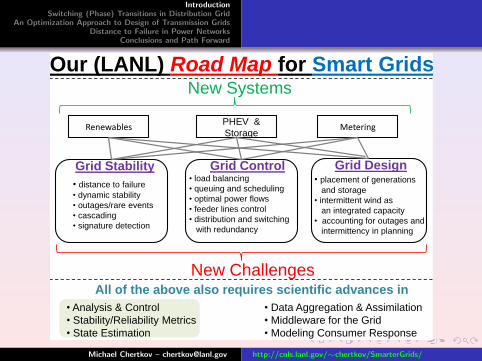
New Systems
RenewablesPHEV &
StorageMetering
New Challenges
Grid Stability
• distance to failure
• dynamic stability
• outages/rare events
• cascading
• signature detection
Grid Control• load balancing
• queuing and scheduling
• optimal power flows
• feeder lines control
• distribution and switching
with redundancy
Grid Design• placement of generations
and storage
• intermittent wind as
an integrated capacity
• accounting for outages and
intermittency in planning
• Analysis & Control
• Stability/Reliability Metrics
• State Estimation
• Data Aggregation & Assimilation
• Middleware for the Grid
• Modeling Consumer Response
All of the above also requires scientific advances in
Our (LANL) Road Map for Smart Grids
Michael Chertkov – [email protected] http://cnls.lanl.gov/∼chertkov/SmarterGrids/
IntroductionSwitching (Phase) Transitions in Distribution Grid
An Optimization Approach to Design of Transmission GridsDistance to Failure in Power Networks
Conclusions and Path Forward
M. Chertkov
E. Ben-Naim
J. Johnson
K. Turitsyn
L. Zdeborova
R. Gupta
R. Bent
F. Pan
L. Toole
A. Berscheid
D. Izraelevitz
S. Backhaus
M. Anghel
N. Santhi
N. Sinitsyn
T-d
ivis
ion
D-d
ivis
ion
MPA
CC
Soptimization & control
theory
statistics statistical physics
information theory
graph theory & algorithms
network analysis
operation research
rare events analysis
power engineering
energy hardware
energy planning & policy http:/cnls.lanl.gov/~chertkov/SmarterGrids/
Michael Chertkov – [email protected] http://cnls.lanl.gov/∼chertkov/SmarterGrids/
IntroductionSwitching (Phase) Transitions in Distribution Grid
An Optimization Approach to Design of Transmission GridsDistance to Failure in Power Networks
Approach A: Take a realistic power grid model and runsimulations. Time Consuming ... and need a new settingwhen details change
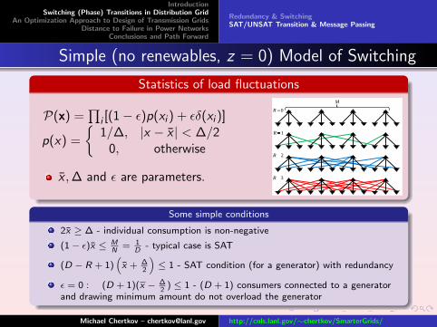
Approach B (probabilistic + physicist/applied.math way):Study behavior of simple abstract models that facilitate theanalysis, and look for universal features. Model choice criteria(in physics): The simpler but richer the better.
Michael Chertkov – [email protected] http://cnls.lanl.gov/∼chertkov/SmarterGrids/
IntroductionSwitching (Phase) Transitions in Distribution Grid
An Optimization Approach to Design of Transmission GridsDistance to Failure in Power Networks
To analyze the SAT-UNSAT transition we solved CavityEquations with Population Dynamics Algorithm. Theapproach allows(a) to compute the probability that the given switch is off/on(b) to estimate number of valid (not overloading)configurations.
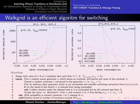
We also developed Belief Propagation and WalkGrid (greedystochastic search, younger brother of WalkSum for K-SAT)algorithms which find SAT-switching efficiently.
Michael Chertkov – [email protected] http://cnls.lanl.gov/∼chertkov/SmarterGrids/
IntroductionSwitching (Phase) Transitions in Distribution Grid
An Optimization Approach to Design of Transmission GridsDistance to Failure in Power Networks
1 Assign each value of σ 0 or 1 randomly (but such that ∀i ∈ G :∑α∈∂i σiα = 1);
2 repeat Pick a random power generator α which shows an overload, and denote the value of the overload, δ;3 Choose a random consumer i connected to the generator α, i.e. σiα = 1;4 Pick an arbitrary other generator which is not overloaded and consider switching connection from (iα) to (iβ).5 if (in the result of this switch α is relieved from being overloaded6 and β either remains under the allowed load or it is overloaded but by the amount less than δ)7 Accept the move, i.e. disconnect i from α and connect it to β thus setting σiβ = 1, σiα = 0.8 else With probability p connect consumer i to β instead of α;9 until Solution found or number of iterations exceeds MTmax.
Michael Chertkov – [email protected] http://cnls.lanl.gov/∼chertkov/SmarterGrids/
IntroductionSwitching (Phase) Transitions in Distribution Grid
An Optimization Approach to Design of Transmission GridsDistance to Failure in Power Networks
Application of the approach to more realistic distribution grids
Extending the story beyond “the commodity flow” approachtowards accounting for AC/DC specifics of the power flows
Switching vs Contingency. Off-line games. ControlAlgorithms.
Bibliography
L. Zdeborova, A. Decelle, M. Chertkov, Phys. Rev. E 90,046112 (2009).
L. Zdeborova, S. Backhaus, M. Chertkov, in proceedings ofHICSS 43 (Jan 2010).
Michael Chertkov – [email protected] http://cnls.lanl.gov/∼chertkov/SmarterGrids/
IntroductionSwitching (Phase) Transitions in Distribution Grid
An Optimization Approach to Design of Transmission GridsDistance to Failure in Power Networks
Conclusions and Path Forward
Intro (II): Power Flow & DC approximationNetwork Optimization
Outline
1 Introduction
2 Switching (Phase) Transitions in Distribution GridRedundancy & SwitchingSAT/UNSAT Transition & Message Passing
3 An Optimization Approach to Design of Transmission GridsIntro (II): Power Flow & DC approximationNetwork Optimization
4 Distance to Failure in Power NetworksModel of Load SheddingError Surface & Instantons
5 Conclusions and Path Forward
Michael Chertkov – [email protected] http://cnls.lanl.gov/∼chertkov/SmarterGrids/
IntroductionSwitching (Phase) Transitions in Distribution Grid
An Optimization Approach to Design of Transmission GridsDistance to Failure in Power Networks
Conclusions and Path Forward
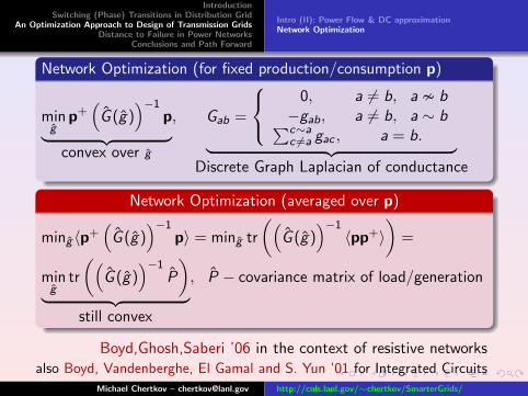
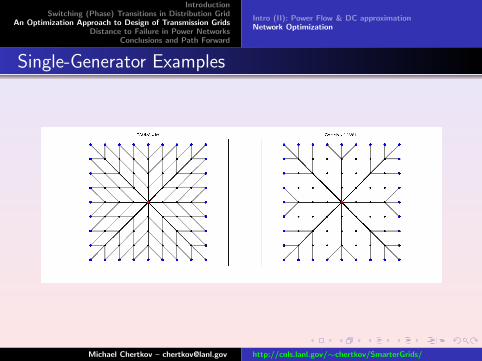
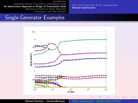
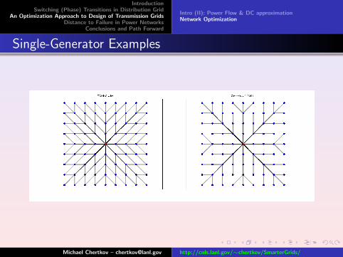
Intro (II): Power Flow & DC approximationNetwork Optimization
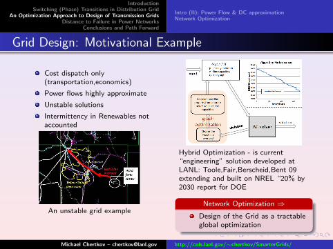
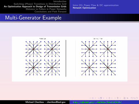
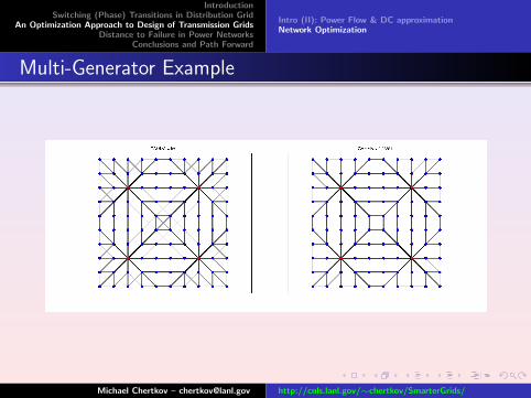
Grid Design: Motivational Example
Cost dispatch only(transportation,economics)
Power flows highly approximate
Unstable solutions
Intermittency in Renewables notaccounted
An unstable grid example
Hybrid Optimization - is current“engineering” solution developed atLANL: Toole,Fair,Berscheid,Bent 09extending and built on NREL “20% by2030 report for DOE
Network Optimization ⇒Design of the Grid as a tractableglobal optimization
Michael Chertkov – [email protected] http://cnls.lanl.gov/∼chertkov/SmarterGrids/
IntroductionSwitching (Phase) Transitions in Distribution Grid
An Optimization Approach to Design of Transmission GridsDistance to Failure in Power Networks
Conclusions and Path Forward
Intro (II): Power Flow & DC approximationNetwork Optimization
The Kirchhoff Laws. Loss Function. Power flows.
The Kirchhoff Laws
∀a ∈ G0 :∑
b∼a Jab = Ja for currents∀(a, b) ∈ G1 : Jabzab = Ua − Ub for potentials
Loss Function
Q(G )=∑{a,b}∈G1
<(
1zab
)|Ua − Ub|2 = J+(G ′)−1J∗ = U+GU∗
U = (G ′)−1J, G ′ = G + 11+, G = (Gab|a, b ∈ G0)
Gab =
0, a 6= b, a � b−gab, a 6= b, a ∼ b∑c∼ac 6=a gac , a = b.
, (zab)−1︸ ︷︷ ︸admittance
= gab︸︷︷︸conductance
+i βab︸︷︷︸susceptance
Complex Power Flow [balance of power]
∀a : Pa = UaJ∗a = J∗a
∑b(G ′)−1
ab Jb = Ua
∑b∼a J∗ab = Ua
∑b∼a
U∗a −U∗bz∗ab
∀a : Ua = ua exp(iϕa), Pa = pa + iqa
Michael Chertkov – [email protected] http://cnls.lanl.gov/∼chertkov/SmarterGrids/
IntroductionSwitching (Phase) Transitions in Distribution Grid
An Optimization Approach to Design of Transmission GridsDistance to Failure in Power Networks
Conclusions and Path Forward
Intro (II): Power Flow & DC approximationNetwork Optimization
DC flow approximation
(0) The amplitude of the complex potentials are all fixed to the same number(unity, after trivial re-scaling): ∀a : ua = 1.
(1) ∀{a, b} : |ϕa − ϕb| � 1 - phase variation between any two neighbors on thegraph is small
(2) ∀{a, b} : rab � xab - resistive (real) part of the impedance is much smallerthan its reactive (imaginary) part. Typical values for the r/x is in the1/27÷ 1/2 range.
(3) ∀a : pa � qa - the consumed and generated powers are mainly real, i.e.reactive components of the power are much smaller than their real counterparts
It leads to
Linear relation between powers and phases (at the nodes): Bϕ = p and∑a pa = 0
Losses (in the leading order): Q = p+(B′)−1G(B′)−1p, B′ = B + 11+
If all lines are of the same grade: B = G/α and Q = α2p+(G ′)−1p , i.e. the
system is equivalent to “resistive network”, where B/α2, p and ϕ play the rolesof the resistivity matrix, vector of currents and vector of voltages
Michael Chertkov – [email protected] http://cnls.lanl.gov/∼chertkov/SmarterGrids/
IntroductionSwitching (Phase) Transitions in Distribution Grid
An Optimization Approach to Design of Transmission GridsDistance to Failure in Power Networks
Conclusions and Path Forward
Intro (II): Power Flow & DC approximationNetwork Optimization
The instantons are well localized (but stillnot sparse)
The troubled nodes and structures arerepetitive in multiple-instantons
Instanton structure is not sensitive tosmall changes in D and statistics ofdemands
Michael Chertkov – [email protected] http://cnls.lanl.gov/∼chertkov/SmarterGrids/
IntroductionSwitching (Phase) Transitions in Distribution Grid
An Optimization Approach to Design of Transmission GridsDistance to Failure in Power Networks
Conclusions and Path Forward
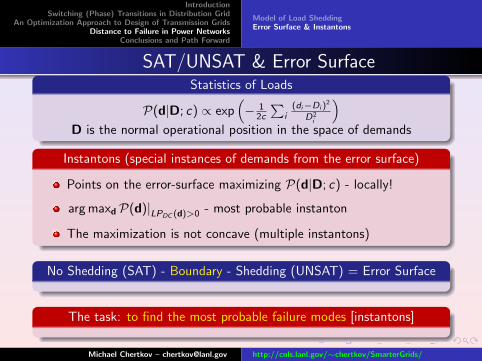
Model of Load SheddingError Surface & Instantons
Concusions and Path Forward (for the distance to failure)Conclusions
Formulated Load Shedding (SAT/UNSAT condition) as an LPDC
Posed the problem of the Error-Surface and Instantons descriptionin the power-grid setting
Instanton-amoeba algorithm was suggested and tested on examples
Path Forward
The instanton-amoeba allows upgrade to other (than LPDC )network stability testers, e.g. for AC flows and transients
Instanton-search can be accelerated, utilizing LP-structure of thetester (in the spirit of [MC,MS ’08])
This is an important first step towards exploration of “next level”problems in power grid, e.g. on interdiction [Bienstock et. al ’09],optimal switching [Oren et al ’08], cascading outages [Dobson et al’06], and control of the extreme [outages] [Ilic et al ’05]
Michael Chertkov – [email protected] http://cnls.lanl.gov/∼chertkov/SmarterGrids/
IntroductionSwitching (Phase) Transitions in Distribution Grid
An Optimization Approach to Design of Transmission GridsDistance to Failure in Power Networks
Conclusions and Path Forward
Bottom Line
A lot of interesting power grid settings for CS/IT, Physics analysis
The research is timely (blackouts, renewables, stimulus)
Stay tuned ... the field is growing explosively
Other Problems under investigation by the team
Control of Reactive Power Flow in a radial circuit [K. Turtisyn, P.Sulc, S. Backhaus, MC ’09 = arXiv:0912.3281 + selected for SuperSession of IEEE/PES Gen Mtg 2010]
Efficient PHEV charging via queuing/scheduling with and withoutcommunications and delays [S. Backhaus, MC, K. Turitsyn, N.Sinitsyn]


![*0.5in @let@token thebibliography[1]![1][]== A Security ...](https://static.documents.pub/doc/80x56/619132e3774ac107566a5c72/05in-lettoken-thebibliography11-a-security-.jpg)


