Tomographic Reconstructions and Predictions of Radial Void ...

TOMOGRAPHIC RECONSTRUCTIONS AND PREDICTIONS OF RADIAL VOID DISTRIBUTION IN BWR FUEL BUNDLE WITH PART-

LENGTH RODS

M. Ahnesjö*, P. Andersson Department of Physics and Astronomy

Uppsala University, 75120, Uppsala, Sweden [email protected]; [email protected]

J.-M. Le Corre and S. Andersson Westinghouse Electric Sweden AB

72163, Västerås, Sweden [email protected]; [email protected]

ABSTRACT

The Westinghouse FRIGG facility, in Västerås/Sweden, is dedicated to the measurement of critical power, stability and pressure drop in fuel rod bundles under BWR operating conditions (steady-state and transient). Capability to measure cross-sectional void and radial void distributions during steady-state operation was already considered when the facility was built in the late 1960s, using gamma transmission measurements. In the 1990s, redesigned equipment was installed to allow for full 2D tomography and some test campaigns were successfully run where the void was measured in the Westinghouse SVEA-96 fuel bundle geometry with and without part-length rods. In this paper, the tomographic raw data from the SVEA-96 void measurement campaigns are revisited using various tomographic reconstruction techniques. This includes an algebraic method and a filtered back-projection method. Challenges, for example due to artifacts created by high difference in gamma absorption, or to accurately identify the location of the bundle structure, are resolved. The resulting detailed void distributions are then averaged over entire sub-channels or within the steam core only, for comparison against sub-channel simulations. The resulting void distributions are compared against sub-channel void predictions using the VIPRE-W/MEFISTO code. The region downstream the part-length rods are of particular interest to investigate how the void in the steam core is redistributed within the open region of the bundle. The comparison shows a reasonable agreement between the measurements and the predictions.

KEYWORDS Tomography, annular two-phase flow, rod bundle, BWR, void fraction

��*�Currently:�SSM�–�Swedish�Radiation�Safety�Authority,�Solna�Strandväg�96,�17116�Stockholm,�Sweden�

829NURETH-16, Chicago, IL, August 30-September 4, 2015 829NURETH-16, Chicago, IL, August 30-September 4, 2015

��

1 INTRODUCTION �Due to the difficulties of measuring void and other thermal hydraulic properties in a BWR fuel bundle during operation, test loops with electrically heated mockup fuel are used instead to give an environment suitable for experiments. The FRIGG loop in Västerås, Sweden owned by Westinghouse is one such testing facility used among other things to find critical power levels for different rod lattices in BWR fuel geometries. In the 1990s, tomographic measurements were performed in order to determine the void distribution and develop void correlations of common BWR fuel geometries [1]. At that time, the main focus was on mean void measurements, but detailed void measurements were also performed although only some of the detailed void measurement data were analyzed by Windecker and Anglart [2] with focus on the void distribution in the lower levels of the fuel bundle close to beginning of heated length. In this work, measurements on part-length rod geometries are analyzed to obtain detailed void distributions with a particular focus on the free volume downstream the end of the part length rods under annular flow conditions. 2 MEASUREMENTS

2.1 Object under Study �The focus of this report is on the detailed void measurements done for fuel geometry with part length rods at two axial elevations downstream the end of the part length rods, labelled �= 1146 mm and 909 mm. This corresponds to 833 mm and 1070 mm from the end of heated length (EHL). The beginning of heated length (BHL) is at 3740 mm from EHL. The two-phase flow measurements were done for two different radial power distributions: uniform power distribution and optimal power distribution both having an annular flow. For each of the elevations, five types of detailed tomographic measurements were performed (see Table I). Flat field intensities, i.e., the unattenuated intensities when no object is present, commonly used for reconstruction were not measured. Instead, reference measurements were performed on the same lattices but under single phase conditions with liquid water and with air. Also, standard transmission measurements of a tungsten slab were done before and after each measurement, to allow for monitoring of drifts in detector response. Table I.�Five different types of measurement was done for each elevation of interest (Z = 1146 mm and 909 mm). The air and cold water measurements were done with no power or pressure. The air

measurement had cold water between the pressure vessel and the fuel bundle.

Measurement Operation conditions Two-phase measurement uniform power Flow: 3 kg/s , power:1511 kW, pressure:70 bar Two-phase measurement optimal power Flow: 3 kg/s , power:1511 kW, pressure:70 bar Reference measurement (warm water) Flow: 4 kg/s, Temperature: 260°C, pressure: 70 bar Air measurement Flow: 0 kg/s, Temperature: 20°C, pressure: 1 bar Cold water measurement Flow: 0 kg/s, Temperature: 20°C, pressure: 1 bar

2.2 Tomography Instrumentation �The tomographic setup used at the FRIGG test loop used a collimated source of 137Cs, emitting 662 keV gamma. The detector setup contains 16 individual sensor elements, consisting of collimated BGO-scintillators. Both the detector, source and their respective collimators were attached to a board, which was lifted and rotated around the object under investigation, which is the heated test section of the FRIGG


��

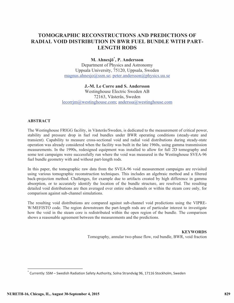
test loop. An overview of the setup is seen in Figure 1. The data acquisition system counts the number of events in the full energy peak of each detector element at each position interrogated.

Figure 1. Schematics of the detector board. The gamma source (fan beam center) is located at

position 1, the rotation center of the object in position 2 and the robot arm is attached at point 3. The tomography board (Figure 1) was rotated around a center point in steps of �� for 153 projections. For each projection seven part-projections were done so that the detector elements are combined to 112 equidistant sensor positions (Figure 2), with detector element one corresponding to sensor position nr 1-7, sensor position nr 55 corresponding to the center beam. The fan-beam did not completely cover the pressure vessel or the isolation. In addition it did not cover the fuel bundle completely in some of the 153 projections. The distance from the center of rotation to the gamma source was 250 mm. In Table II a list of the number of projections and data measurement points is summarized. The exposure time for each part-projection was one second.


��

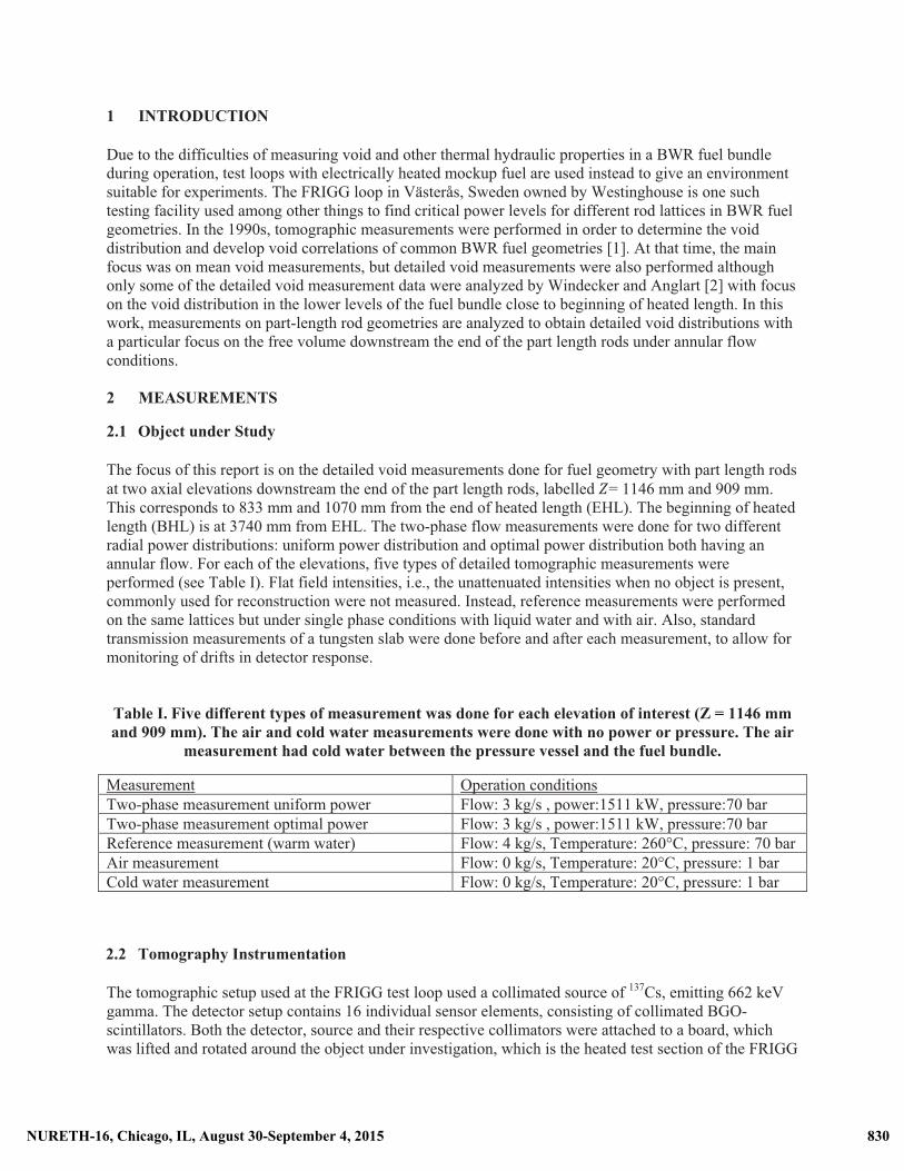
Figure 2. The fan-coverage by the sensor positions per projection. Image courtesy of Westinghouse

It can be noted that, as usual in computed tomography, the damping of each line of sight is obtained by dividing the penetrating intensity with a flat-field intensity, which is the transmitted intensity when no object is present. After this, the attenuation distribution is solved by applying tomographic reconstruction techniques. However, in this case the fan-beam does not cover the entire object for all projections, and only the parts completely covered may be accurately reconstructed using traditional techniques. To address this, reference measurements of the identical fuel elements under single-phase conditions have been used to substitute the flat-field measurement. Thereby, the introduction of void in the fuel mock-up appears as a negative attenuation in the measurement. The exterior parts of the objects, i.e. outside the circle described by the rotating fan-beam cover, as well as the fuel mock-up structures, are the same for the reference measurements as during the examinations of the void distributions of interest.

Table II Numbers of projection, part projections and sensors. The sensor position angular step is equal to the part-projection angular interval.

Detector elements: � 16 Number of part-projections: � 7 Number of projections: 153 Number of sensor positions: � � � � � 112 Total number of projections: � � � � 1071 Total number of data points: � � � � 17136 Sensor position angular step: �� Projection angular step: ��

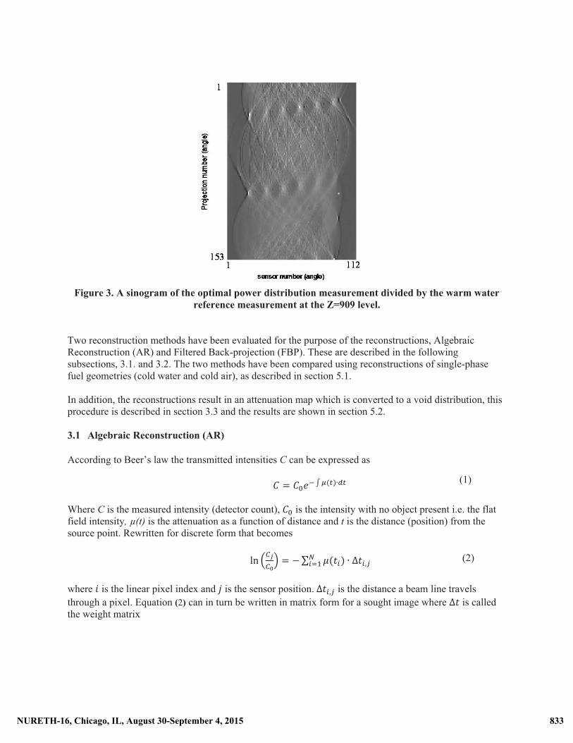
3 RECONSTRUCTION ALGORITHMS �The result of the gamma counting measurements in 153 projections, each consisting of 112 sensor positions can be organized in a sinogram, as seen in Figure 3, where each row is a single radiographic projection. Such sinograms are the input to the tomographic reconstruction, where the pixel attenuation map of the object is calculated.


��

Figure 3. A sinogram of the optimal power distribution measurement divided by the warm water

reference measurement at the Z=909 level. Two reconstruction methods have been evaluated for the purpose of the reconstructions, Algebraic Reconstruction (AR) and Filtered Back-projection (FBP). These are described in the following subsections, 3.1. and 3.2. The two methods have been compared using reconstructions of single-phase fuel geometries (cold water and cold air), as described in section 5.1. In addition, the reconstructions result in an attenuation map which is converted to a void distribution, this procedure is described in section 3.3 and the results are shown in section 5.2. 3.1 Algebraic Reconstruction (AR) �According to Beer’s law the transmitted intensities C can be expressed as � � ��

Where C is the measured intensity (detector count), �� is the intensity with no object present i.e. the flat field intensity, μ(t) is the attenuation as a function of distance and t is the distance (position) from the source point. Rewritten for discrete form that becomes ! "#$#%& � ' ( )�*+�,+-. � �*+/0

where 1 is the linear pixel index and 2 is the sensor position.3�*+/0 is the distance a beam line travels through a pixel. Equation (2) can in turn be written in matrix form for a sought image where �* is called the weight matrix

(1)

(2)


��

4556 ! "�. ��7 &

! "�8 ��7 &9 ! "�: ��7 &;<<= � 3 ' >�*.. ? 3�*.,39 @ 9�*:. ? �*:,

A >).9),A

M is the numbers of sensor positions in all projections, in this case M=17136. N is the total number of pixels used to describe the area of interest. The weight-matrix describes the length each beam has to travel through each pixel and is calculated by a custom-made weight-matrix algorithm developed by the authors of [3]. μ is the sought attenuation for each pixel in the region of interest and can be calculated from matrix division. In this work μ is solved by QR factorization [4]. 3.2 Filtered Back-projection �Filtered back-projection (FBP) is a reconstruction method based on the inverse Radon transform. This is implemented in the MATLAB function iradon [4], which has been used for this work. In the reconstructions used here a Ramp-filter has been applied. In addition to this, a two-dimensional interpolation has been performed to convert the data from fan beam type, to parallel beam, which is the input for the iradon function. Similar to the case in the AR reconstruction described in the previous section, the two-phase transmission data is divided by transmission through a single-phase liquid-reference object. Thereby, the attenuation difference to the reference object is obtained. 3.3 Conversion of the Attenuation Map to a Void Distribution �The pixel void fraction is calculated from the attenuation maps from the tomographic reconstructions. Due to the usage of the reference objects, the attenuation map describes the difference between the two-phase measurement and a reference measurement, which is water close to boiling point. This difference is mostly caused by the introduction of steam in the test section, where the attenuation of 662 keV gamma of steam at 70 bar3)B is much lower than the attention of liquid water at boiling point3)CDE. In addition, some the difference in the attenuation of the liquid water in the two-phase object compared to water at the boiling point needs to be considered. This is because the reference measurement is performed at a slightly lower temperature, and the density is lower due to thermal expansion. The attenuation difference from the algebraic reconstruction (3) or from the iradon function (subsection 3.2) is used in (4) to calculate the void according to FG � �HIJK ��LMJK ��NOP��QLM��R��NOP � ��JK ��NOP��QLM��R��NOP

�Where �)GS is the calculated attenuation difference between the two-phase measurement and the reference measurement for each pixel n, )TUV is the estimated attenuation of the water outside the pressure vessel for the reference measurement, )WXGS and )UVGS are the attenuations that can be calculated for each pixel n in the two-phase measurement and the reference measurement respectively. ��

�

(3)

(4)


��

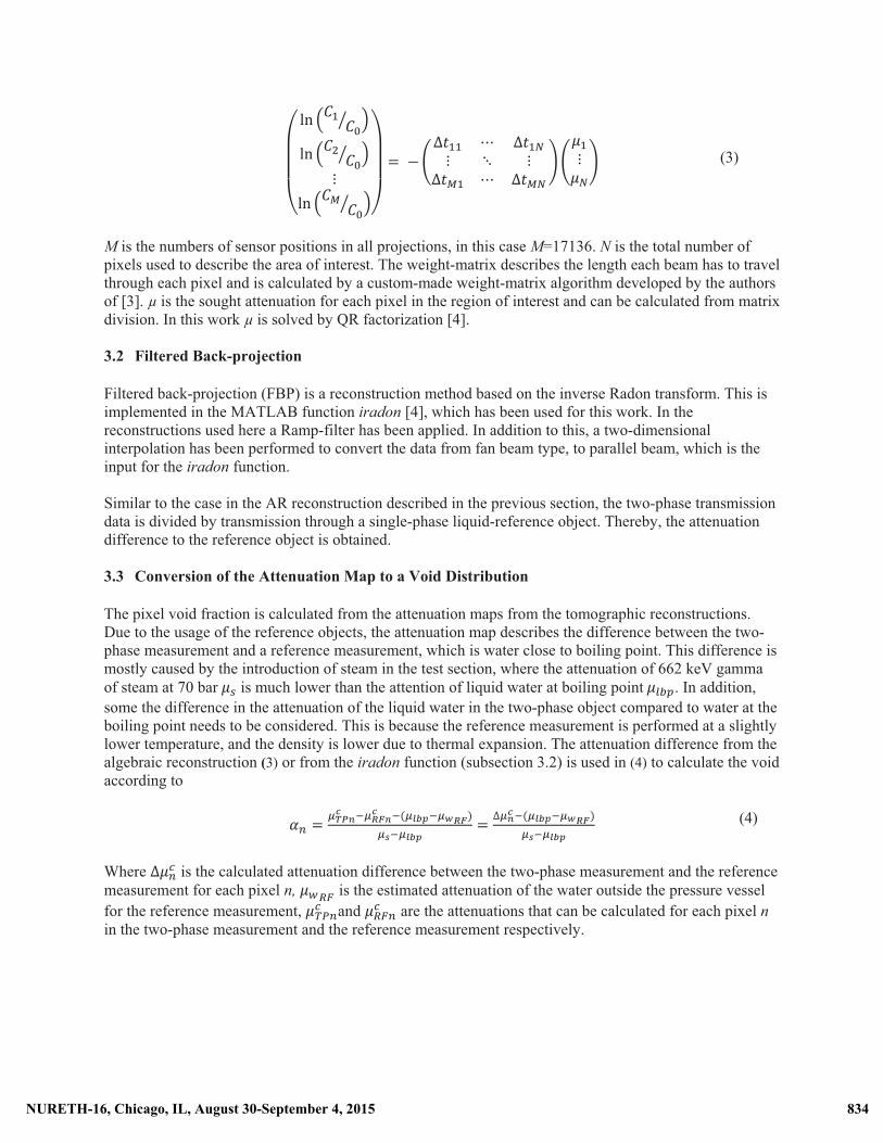
4 SUBCHANNEL AVERAGE VOID CALCULATIONS �For the purpose of subchannel thermal hydraulic code validation, the subchannel void distribution has been calculated by averaging of the void pixels in each subchannel. Normally, the subchannel boundaries are defined by the closest distances between the rod centers, as seen in Figure 4 and Figure 5. Two challenges occur when implementing this to the current data:

1) It is difficult to exactly determine the centers of the rods in the reconstructed image. 2) Due to the discretization of the reconstruction in pixels, which do not align perfectly with the

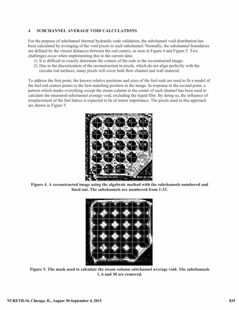
circular rod surfaces, many pixels will cover both flow channel and wall material. To address the first point, the known relative positions and sizes of the fuel rods are used to fit a model of the fuel rod centers points to the best matching position in the image. In response to the second point, a pattern which masks everything except the steam column in the center of each channel has been used to calculate the measured subchannel average void, excluding the liquid film. By doing so, the influence of misplacement of the fuel lattice is expected to be of minor importance. The pixels used in this approach are shown in Figure 5.

Figure 4. A reconstructed image using the algebraic method with the subchannels numbered and

lined out. The subchannels are numbered from 1-33.

Figure 5. The mask used to calculate the steam column subchannel average void. The subchannels

1, 6 and 30 are removed.


��

It can be noted that the noise of the reconstructed pixels propagates to an error of the subchannel and steam column average void. However, this is smaller in the subchannel 29, where the part-length rod is missing, thereby increasing the number of pixels used for the averaging. 5 RESULTS

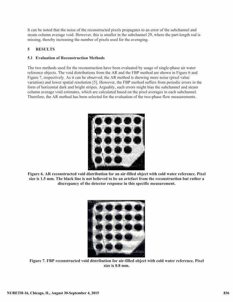
5.1 Evaluation of Reconstruction Methods �The two methods used for the reconstruction have been evaluated by usage of single-phase air water reference objects. The void distributions from the AR and the FBP method are shown in Figure 6 and Figure 7, respectively. As it can be observed, the AR method is showing more noise (pixel value variation) and lower spatial resolution [5]. However, the FBP method suffers from periodic errors in the form of horizontal dark and bright stripes. Arguably, such errors might bias the subchannel and steam column average void estimates, which are calculated based on the pixel averages in each subchannel. Therefore, the AR method has been selected for the evaluation of the two-phase flow measurements.

Figure 6. AR reconstructed void distribution for an air-filled object with cold water reference. Pixel size is 1.5 mm. The black line is not believed to be an artefact from the reconstruction but rather a

discrepancy of the detector response in this specific measurement.

Figure 7. FBP reconstructed void distribution for air-filled object with cold water reference. Pixel

size is 0.8 mm.


��

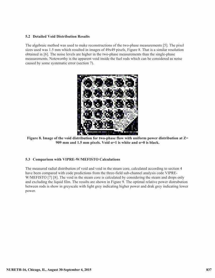
5.2 Detailed Void Distribution Results The algebraic method was used to make reconstructions of the two-phase measurements [5]. The pixel sizes used was 1.5 mm which resulted in images of 49x49 pixels, Figure 8. That is a similar resolution obtained in [6]. The noise levels are higher in the two-phase measurements than the single-phase measurements. Noteworthy is the apparent void inside the fuel rods which can be considered as noise caused by some systematic error (section 7).

Figure 8. Image of the void distribution for two-phase flow with uniform power distribution at Z=

909 mm and 1.5 mm pixels. Void �=1 is white and �=0 is black.

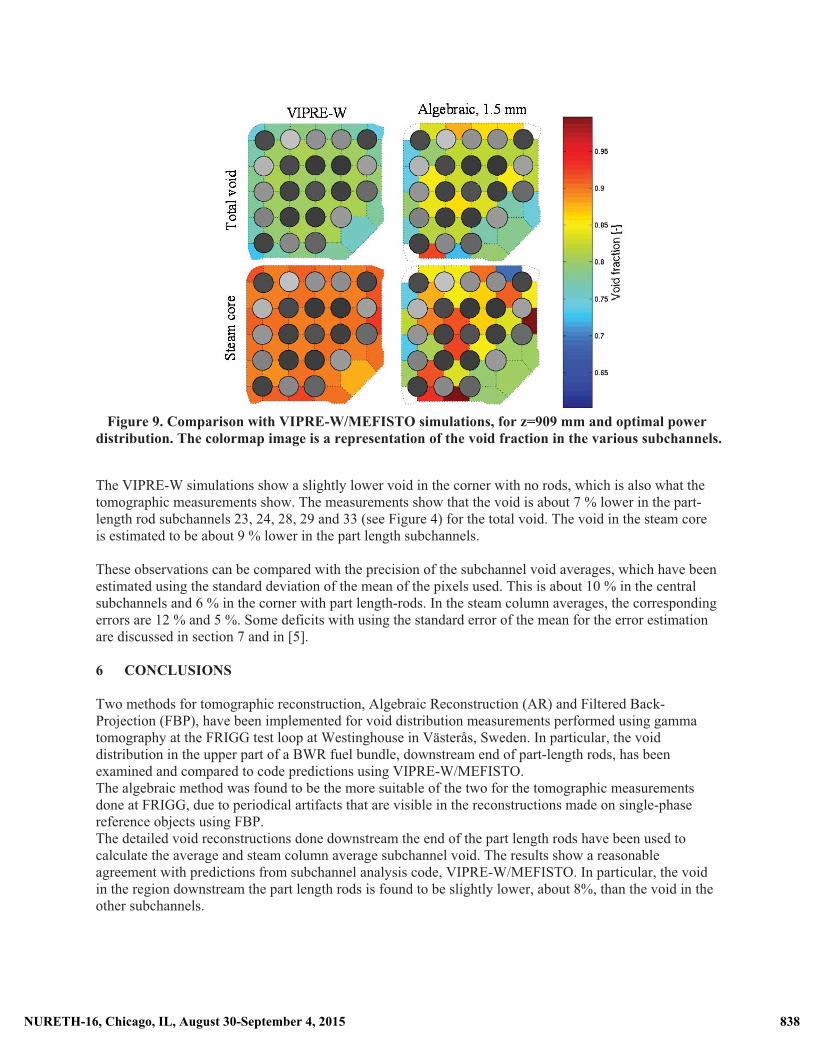
5.3 Comparison with VIPRE-W/MEFISTO Calculations �The measured radial distribution of void and void in the steam core, calculated according to section 4 have been compared with code predictions from the three-field sub-channel analysis code VIPRE-W/MEFISTO [7] [8]. The void in the steam core is calculated by considering the steam and drops only and excluding the liquid film. The results are shown in Figure 9. The optimal relative power distrubution between rods is show in greyscale with light grey indicating higher power and drak grey indicating lower power.


��

Figure 9. Comparison with VIPRE-W/MEFISTO simulations, for z=909 mm and optimal power

distribution. The colormap image is a representation of the void fraction in the various subchannels.

The VIPRE-W simulations show a slightly lower void in the corner with no rods, which is also what the tomographic measurements show. The measurements show that the void is about 7 % lower in the part-length rod subchannels 23, 24, 28, 29 and 33 (see Figure 4) for the total void. The void in the steam core is estimated to be about 9 % lower in the part length subchannels. These observations can be compared with the precision of the subchannel void averages, which have been estimated using the standard deviation of the mean of the pixels used. This is about 10 % in the central subchannels and 6 % in the corner with part length-rods. In the steam column averages, the corresponding errors are 12 % and 5 %. Some deficits with using the standard error of the mean for the error estimation are discussed in section 7 and in [5]. 6 CONCLUSIONS Two methods for tomographic reconstruction, Algebraic Reconstruction (AR) and Filtered Back-Projection (FBP), have been implemented for void distribution measurements performed using gamma tomography at the FRIGG test loop at Westinghouse in Västerås, Sweden. In particular, the void distribution in the upper part of a BWR fuel bundle, downstream end of part-length rods, has been examined and compared to code predictions using VIPRE-W/MEFISTO. The algebraic method was found to be the more suitable of the two for the tomographic measurements done at FRIGG, due to periodical artifacts that are visible in the reconstructions made on single-phase reference objects using FBP. The detailed void reconstructions done downstream the end of the part length rods have been used to calculate the average and steam column average subchannel void. The results show a reasonable agreement with predictions from subchannel analysis code, VIPRE-W/MEFISTO. In particular, the void in the region downstream the part length rods is found to be slightly lower, about 8%, than the void in the other subchannels.


��

7 DISCUSSION AND OUTLOOK �In order to estimate the noise level and the accuracy of the method, the standard error of the mean (SEM) was calculated for each subchannel. However, some assumptions necessary for this might not be satisfied. Firstly, SEM requires that the values are uncorrelated, which is not the case for the pixels calculated in the tomographic reconstructions. Furthermore, the standard error of the mean is based on the assumption that the pixel values are sampled stochastic variables of the same population. This is likewise not true, since large variations of the void are to be expected within the subchannels. For example, at high axial locations in the fuel, such as above the part-length rods, the flow type is predominantly annular flow, where the void fraction is very low close to the fuel rod, where a liquid film is present, and the void fraction is much higher near the center of the subchannels. Therefore, the usage the standard error of the mean is at best a rough estimate of the uncertainty of the measurement results [5]. �The tomographic reconstructions produced in this work are quite coarse and suffer from a high level of noise. Some possible future improvements include:

� A more precise mathematical description of beam paths through the pixels could be implemented, by modelling the finite width beams from source to detector elements. In the current work, only an ideal line was considered for each sensor position.

� More complex iterative solving algorithms, that could be less noise sensitive at higher resolution, are a possibility for improving the result. This might be achieved by adding physical constraints to the reconstructed values of attenuation or by using a better parameterization of the solution than the square pixels, such as pixels with borders matching the fuel and box walls, or even pixels representing the subchannels.

� Image alignment techniques could be used to address the potential movement of the investigated object relative to the position in the reference measurement. However, this requires the separate reconstruction of the reference object and the investigated object, which in principle doubles the time consumption of the reconstruction. Considering the few measured data sets that are available for reconstruction, this seems acceptable.

� The exposure time for each measurement with a detector was one second which might not have been long enough to accurately form an average over the changing two-phase flow. The exposure time should be long enough so that the expected fluctuations in the attenuation due to shifting void are on the level of the statistical error of the detector, which is about 0.15 %. The effects of two-phase fluctuations can be simulated and with time discrete transmission data for a sight line a suitable measurement time for the projections can be found. The measurement time should be so that both the statistical error in the detectors and the two-phase fluctuations converge [9].

� In addition, systematic errors might occur due to vibrations in the rods during operation. Possibly, a damping system could be considered if renewed measurements are made.

8 REFERENCES �[1]�O.�Nylund,�Upgrade�of�the�FRIGG�test�loop�for�BWR�fuel�assemblies,�Västerås:�ABB�Atom�AB,�1997.��[2]�G.�Windecker�and�H.�Anglart,�"Phase�distribution�in�BWR�fuel�assembly�and�evaluation�of�

multidimensional�multi�field�model,"�Nucl.�Technol.�,�no.�134,�pp.�49�61,�2001.��[3]�P.�Andersson,�S.�Jacobsson�Svärd,�E.�Andersson�Sundén�and�H.�Sjöstrand,�"Neutron�tomography�of�

axially�symmetric�objects�using�14�MeV�neutrons�from�a�portable�neutron�generator,"�REVIEW�OF�SCIENTIFIC�INSTRUMENTS,�vol.�85,�2014.��


��

[4]�The�MathWorks,�Inc.,�"Matlab�Documentation,"�2014.�[Online].�Available:�http://se.mathworks.com/help/.�

[5]�M.�Ahnesjö,�"Tomographic�reconstruction�of�subchannel�void�measurements�of�nuclear�fuel�geometries,"�Uppsala�Universitet,�Uppsala,�2015.�

[6]�K.�Holmquist,�"Tomograpic�reconstruction�of�the�void�distribution�in�the�nuclear�fuel�test�loop�FRIGG,"�Uppsala�Univetsity,�Uppsala,�2006.�

[7]�J.�M.�Le�Corre,�C.�Adamsson�and�Brynjell�Rahkola,�"Validation�of�VIPRE�W�Sub�channel�Void�Predictions,"�in�NURETH�13,�N13P1080,�Kanazawa,�2009.��

[8]�C.�Adamsson�and�J.�M.�Le�Corre,�"Modeling�and�validation�of�a�mechanistic�tool�(MEFISTO)�for�the�prediction�of�critical�power�in�BWR�fuel�assemblies,"�Nucl.�Eng.�Des.,�vol.�241,�pp.�2843�2858,�2011.��

[9]�P.�Andersson,�E.�Andersson�Sundén,�S.�Jacobsson�Svärd�and�H.�Sjöstrand,�"Correction�for�dynamic�bias�error�in�transmission�measurements,"�REVIEW�OF�SCIENTIFIC�INSTRUMENTS,�no.�83,�2012.��

�


Date post:	18-Dec-2021
Category:	Documents
Upload:	others
View:	1 times
Download:	0 times

Tomographic Reconstructions and Predictions of Radial Void ...

Documents