Too Much Connection May be Hazardous to Your Health: Political

Connections and Firm Value

Presented by Carl R. Chen

Carl Chena, Danglun Luob, and Ting Zhanga

a. University of Dayton, USAb. Sun Yat-Sen University, China

I. Introduction

We study the relationship between Political connections and firm value. Chinese data is used because where a relationship-based economy dominates. Guanxi (networks) is a power force in Chinese culture.

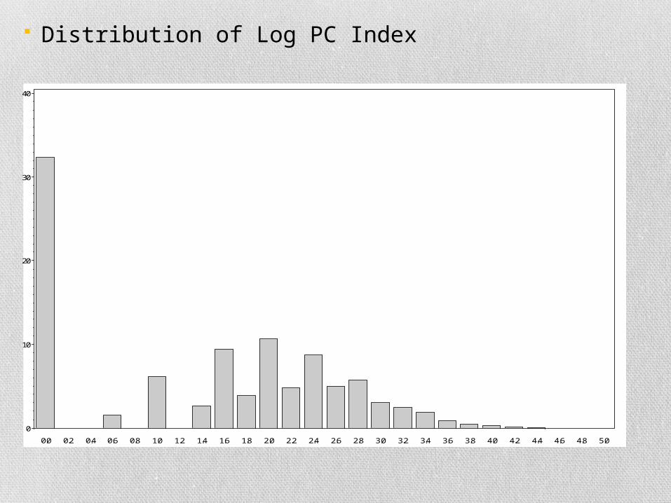
A unique political connection index is constructed to capture variations in the strength of firm political relations in China. Prior studies use binary variable.

“Businessmen should not get too far with the government; but they should not get too close with the government, either.”–by Wenrong Shen, Steel King of China, CEO and Chairman of Jiangsu Shagang Group

Benefits of Political Connections

Political connections with the government help firms to obtain benefits including easier access to debt financing, lighter taxation, stronger market power, and relaxed regulatory oversight.

Costs of Political Connection

Such connections can jeopardize firm value if the government and bureaucrats exert political pressure to engage in Rent-Seeking

A Chinese Example• Zijin Mining Group ( 紫金礦業 ) is the largest

company in China involved in the exploration, mining, and sale of gold and other nonferrous metals. It has developed strong connections with the government.

• In 2008, the firm was among the first accredited by the Fujian provincial government as a high-tech firm, although it adopted traditional, low-tech mining processes.

• Benefit: The firm’s high-tech status afforded it a favorable tax rate of 15% (versus 25% for non-high-tech firms).

• Cost: More than 20 current or retired local/provincial government officials hold senior or mid-level management positions in the firm, receiving an estimated compensation of RMB20 million per year, among others.

Research Questions:

(1) Is Political Connection Good or Bad? (2) When is Connection Good? When is

Bad? (3) Is the benefit-cost affected by the

economic and/or legal environment?

Summary of Major Findings A nonlinear, hump-shaped relation exists

between political connections and Tobin’s q and stock returns.

The Good:Firm Tobin’s q and the cross-sectional stock returns first increase at a lower level of connections, but …

The Bad: …q and stock returns decrease at a higher level of connection.

Our results reconcile previous conflicting findings, and better explain the benefit of political connections and the cost of rent-seeking for politically connected firms.

The Ugly: The positive effect of political connections on firm value is enhanced for firms headquartered in regions with strong government intervention, an under- developed legal system, and a planned economy.

Chairman of

board

CEO

Other senior officers (CFO,

Board Secretary, Vice CEO)

Directors

Central level officers or

bureaucrats

Local/city level officers

or bureaucrats

Provincial level officers

or bureaucrats

Local/city level officers

or bureaucrats

Provincial level officers

or bureaucrats

Central level officers or

bureaucrats

Channels of Political Connections for Chinese FirmsGovernment Firms NPC,

and CPPCC

Construction of political index: Numerical Example

Index score depends on both the political rank and the level of connections

Political position Political rank Political rank score

Government system

Deputy minister and above 1 7

TING 2 6

Deputy TING 3 5

CHU 4 4

Deputy CHU 5 3

KE 6 2

Deputy KE and below 7 1 Level of political connections

Connection at a central level 2

Connection at a provincial level 1

Connection at a local or city level 0 Level of political connections

NPC system and CPPCC system

Connection at a central level 6

Connection at a provincial level 4

Connection at a local or city level 2

NPC: National People’s CongressCPPCC: Chinese people’s Political Consultative Conference

Example of index construction:• Zhongjin’s CEO, board chair, directors and other senior officers connection

(1) (2) (3) (4) (5) (6) (7) (8) (9) (10) (11) (12)

(13) =(9) +

(10)+(11)+(12)

Stock ID Year Senior Officer

ID

Position Indicator (1 =

CEO; 2 = Board chair; 3 = Director; 4

= Other officer)

Connection with

Government Level Indicator

(1 Central, 2 Province, 3 local, 0 no

connection)

Connection with NPC

Level Indicator (1 Central, 2 Province, 3 local, 0 no

connection)

Connection with CPPCC

Level Indicator (1 Central, 2 Province, 3 local, 0 no

connection)

Govern-ment

Political Rank (See Table A1)

NPC Score (See Table A1)

CPPCC Score (See Table A1)

Government Political Rank

Score (See Table A1)

Government Political

Connection Level Score

(2 = Central; 1 = Provincial; 0

= Local)

PC Score for Each Senior Officer

600489 2005 1 1, 3 1 0 0 7 0 0 1 2 3

600489 2005 2 2, 3 1 0 0 4 0 0 4 2 6

600489 2005 3 3 3 0 0 7 0 0 1 0 1

600489 2005 4 3 1 0 0 4 0 0 4 2 6

600489 2005 5 3 1 0 0 4 0 0 4 2 6

600489 2005 6 3 2 0 0 4 0 0 4 1 5

600489 2005 7 3 2 0 0 5 0 0 3 1 4

600489 2005 8 3 2 0 0 7 0 0 1 1 2

• Firm level political connection index

(1) (2)

(3) = Sum of PC scores in Column (13) of Panel

A

(4) (5) (6) (7) (8)

= LN(1+(3))

Stock ID Year Simple PC Index Simple CEO PC

Index Simple Chairman

PC Index Simple Director PC Index

Simple Other Officer PC Index

LN(PC Index)

600489 2005 33 3 6 24 0 3.526

Distribution of Simple PC Index

0

10

20

30

40

0 2 4 6 8 10 12 14 16 18 20 22 24 26 28 30 32 34 36 38 40 42 44 46 48 50 52 54 56 58 60 62 64 66 68 70 72 74 76 78 80

Distribution of Log PC Index

0

10

20

30

40

0.0 0.2 0.4 0.6 0.8 1.0 1.2 1.4 1.6 1.8 2.0 2.2 2.4 2.6 2.8 3.0 3.2 3.4 3.6 3.8 4.0 4.2 4.4 4.6 4.8 5.0

IV. Empirical Results: Tobin’s q1. Tobin’s q and PC Index: Portfolio Sorting

Panel A: Univariate portfolio sorts of firm value in year t based on LN(PC Index) in year t

Panel A1: Univariate sorts of firm industry-adjusted Tobin’s Q based on LN(PC Index)

Panel A2: Univariate sorts of firm Tobin’s

Q based on LN(PC Index)

Portfolio Mean Median Mean Median

D0 (No PC) 0.232 0.008 1.607 1.375 D1 (Lowest PC) 0.184 0.020 1.553 1.380 D2 0.172 -0.042 1.550 1.319 D3 0.274 0.037 1.645 1.397 D4 0.247 -0.019 1.608 1.331 D5 0.194 -0.016 1.573 1.354 D6 0.209 0.049 1.599 1.441 D7 0.197 0.012 1.569 1.394 D8 0.147 -0.032 1.516 1.343 D9 0.133 -0.006 1.495 1.331 D10(Highest PC) -0.022 -0.109 1.308 1.186 D10 – D0 (Highest – No PC)

-0.254*** (-4.07)

-0.117***

(-3.19)

-0.299*** (-3.33)

-0.188** (-2.49)

D10 – D1 (Highest – Lowest PC)

-0.206*** (-4.59)

-0.129***

(-3.69)

-0.245*** (-3.32)

-0.193** (-2.54)

Panel B: Kernel regression of industry-adjusted Tobin’s Q and LN(PC Index)

• Kernel regression estimation is performed on pooled data using the Epanechnikov kernel method (Härdle, 1990), with the error bounds of 95% confidence intervals. The bandwidth of 0.1 is validated using a cross-validation algorithm that minimizes the sum of squared residuals.

2. Tobin’s q and PC Index: Multivariate Regressions

Regression Models

Firm Value = α + β1 LN(PC Index) + +ε. (1)

Firm Value = α + β1 LN(PC Index) + β2 (LN PC Index) 2+ +ε. (2)

Firm Value = α + β1 LN(PC Index<1.6) + β2 LN(PC Index≥1.6) + +ε. (3)

ControlN

ii

2

ControlN

ii

3

ControlN

ii

3

where

LN(PC Index <1.6) 6.1)()(6.1)(6.1

IndexPCLNifIndexPCLN

IndexPCLNif

LN(PC Index ≥1.6) 6.1)(06.1)(6.1)(

IndexPCLNif

IndexPCLNifIndexPCLN

All regressions are estimated with generalized method of moments (GMM) Variance inflation factor (VIF) does not indicate multicollinearity a problem

Panel A: Regression analysis of industry-adjusted Tobin’s Q on LN(PC Index) Dep. var.: Industry-adjusted

Tobin’s Q

Linear regression

Quadratic regression

Piecewise regression

Quadratic regression

(1) (2) (3) (4) LN(PC Index) -0.035* 0.169* 0.2051*

(-1.74) (1.70) (1.79) (LN PC Index) 2 -0.046**

(-2.13) -0.057**

(-2.22)

LN(PC Index) < 1.6 0.110* (1.74)

LN(PC Index) ≥ 1.6 -0.068*** (-3.09)

Asset growth -0.202*** -0.205*** -0.204*** -0.270*** (-5.42) (-5.48) (-5.46) (-5.61) Operating margin 0.099 0.106 0.103* 0.152 (0.93) (0.98) (1.82) (1.29) LN(post-IPO age) 0.066** 0.064* 0.064** -0.079* (1.98) (1.90) (2.26) (-1.79) % of independent directors -0.659* -0.634* -0.631*** -1.011** (-1.75) (-1.68) (-2.65) (-2.31) CEO/Chairman duality 0.103** 0.102** 0.104*** 0.091 (2.14) (2.10) (3.03) (1.63) SOE -0.291*** -0.290*** -0.290***

(-7.70) (-7.60) (-8.49) State ownership -1.043 (-7.55)*** LN(board size) -0.357*** -0.343*** -0.348*** -0.420*** (-4.88) (-4.63) (-5.78) (-4.84) LN(market value) 0.116*** 0.116*** 0.116*** (5.21) (5.17) (9.74) LN(total asset) 0.124***

(3.66) Insider holding 0.443 0.429 0.415 0.006 (0.96) (0.95) (1.24) (0.10) Adj. R2 0.07 0.07 0.07 0.03 N 4,344 4,344 4,344 4,344

Panel C: Quadratic regression of industry-adjusted Tobin’s Q and LN(PC Index)

Firm LN(PC Index)

0.00

0.05

0.10

0.15

0.20

0.25

0.30

0.35

0.40

0.45

0 1 2 3 4 5

Firm

Indu

stry

-Adj

uste

d To

bin’

s Q

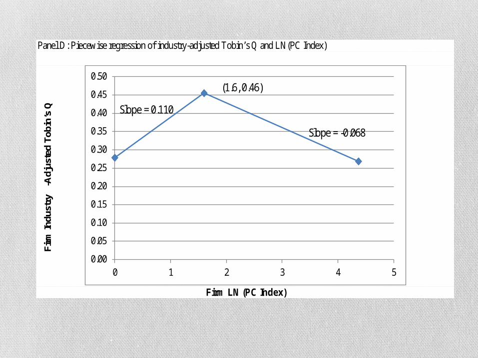
Panel D: Piecewise regression of industry-adjusted Tobin’s Q and LN(PC Index)

Firm LN (PC Index)

0.00

0.05

0.10

0.15

0.20

0.25

0.30

0.35

0.40

0.45

0.50

0 1 2 3 4 5

Firm

Indu

stry

-Adj

uste

d To

bin’

s Q

Slope = 0.110

Slope = -0.068

(1.6, 0.46)

Why hump-shaped?

1. According to the argument of “strength in numbers” (Murphy, Shleifer, and Vishny, 1993), if only a few people seek rent, they will get caught; but if many do so, the probability of any one of them getting caught is much lower, hence the returns to stealing or looting are higher. As more resources are allocated to rent-seeking, according to Murphy et al., returns to production fall.

2. “Power tends to corrupt, and absolute power corrupts absolutely. Great men are almost always bad men” (Lord Acton, 1887)

V. Empirical Results: Cross-Sectional Stock Returns1. Cross-sectional stock returns and political index: Portfolio sorting (1) (2)

Portfolio Raw stock returns Three-factor alpha D0 (No PC) 0.0288 0.0026 D1 (Lowest PC) 0.0315 0.0051 D2 0.0264 -0.0005 D3 0.0322 0.0057 D4 0.0246 -0.0006 D5 0.0284 0.0032 D6 0.0292 0.0039 D7 0.0308 0.0051 D8 0.0294 0.0014 D9 0.0260 -0.0009 D10 (Highest PC) 0.0222 -0.0041 D10 – D0 (Highest – No PC)

-0.0066* (-1.90)

-0.0068***

(-3.32) D10 – D1 (Highest – Lowest PC)

-0.0092** (-2.32)

-0.0092***

(-3.31)

2. Fama-MacBeth regressions of stock returns and 3-factor Alphas

Dependent variable Raw monthly stock returns Three-factor alpha (1) (2)

LN(PC Index) 0.0034*** 0.0035*** (2.97) (4.24) LN(PC Index) 2 -0.0017***

(-6.74) -0.0017***

(-7.29) LN (market value) 0.0038** (2.03) Book-to-market 0.0007***

(2.97)

Excess market return 1.0031*** (Market return - risk free rate) (3.70) Momentum -0.0227**

(-2.12) -0.0313***

(-4.80) Asset growth 0.0165*** 0.0173*** (6.46) (5.94) Operating margin 0.0174*** 0.0188*** (2.73) (2.81) Leverage 0.0038

(0.86) 0.0025

(0.64) SOE -0.0020

(-1.43) -0.0013

(-0.61) LN(firm age) 0.0045 0.0038 (1.04) (0.88) % of independent directors -0.0126*** -0.0129** (-3.24) (-1.94) Average Adj. R2 0.38 0.02 N 31,714 33,674

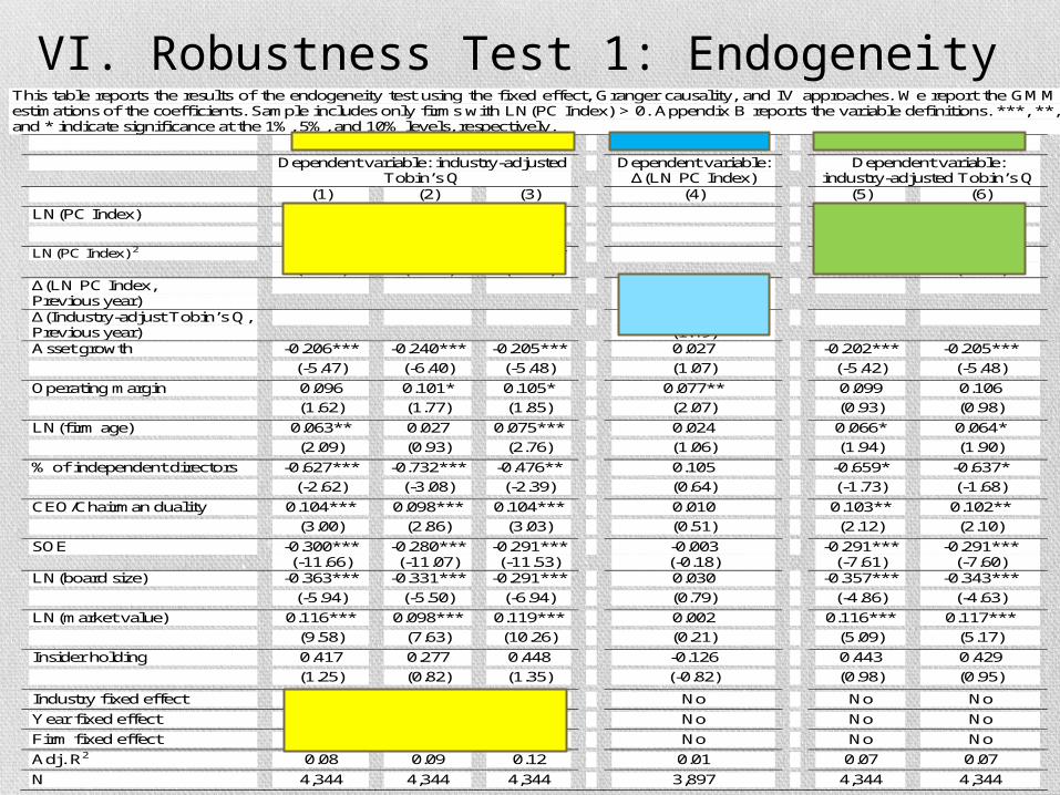
VI. Robustness Test 1: EndogeneityThis table reports the results of the endogeneity test using the fixed effect, Granger causality, and IV approaches. We report the GMM estimations of the coefficients. Sample includes only firms with LN(PC Index) > 0. Appendix B reports the variable definitions. ***, **, and * indicate significance at the 1%, 5%, and 10% levels, respectively.

Fixed effect Granger causality IV

Dependent variable: industry-adjusted Tobin’s Q

Dependent variable: ∆(LN PC Index)

Dependent variable: industry-adjusted Tobin’s Q

(1) (2) (3) (4) (5) (6)

LN(PC Index) 0.176** 0.164** 0.214*** -0.035* 0.169*

(2.08) (1.98) (2.86) (-1.71) (1.70)

LN(PC Index) 2 -0.048** (-2.54)

-0.044** (-2.40)

-0.056*** (-3.42)

-0.046** (-2.13)

∆(LN PC Index, Previous year)

-0.074*** (-4.10)

∆(Industry-adjust Tobin’s Q, Previous year)

0.029 (1.49)

Asset growth -0.206*** -0.240*** -0.205*** 0.027 -0.202*** -0.205***

(-5.47) (-6.40) (-5.48) (1.07) (-5.42) (-5.48)

Operating margin 0.096 0.101* 0.105* 0.077** 0.099 0.106

(1.62) (1.77) (1.85) (2.07) (0.93) (0.98)

LN(firm age) 0.063** 0.027 0.075*** 0.024 0.066* 0.064*

(2.09) (0.93) (2.76) (1.06) (1.94) (1.90)

% of independent directors -0.627*** -0.732*** -0.476** 0.105 -0.659* -0.637*

(-2.62) (-3.08) (-2.39) (0.64) (-1.73) (-1.68)

CEO/Chairman duality 0.104*** 0.098*** 0.104*** 0.010 0.103** 0.102**

(3.00) (2.86) (3.03) (0.51) (2.12) (2.10)

SOE -0.300*** (-11.66)

-0.280*** (-11.07)

-0.291*** (-11.53)

-0.003 (-0.18)

-0.291*** (-7.61)

-0.291*** (-7.60)

LN(board size) -0.363*** -0.331*** -0.291*** 0.030 -0.357*** -0.343***

(-5.94) (-5.50) (-6.94) (0.79) (-4.86) (-4.63)

LN(market value) 0.116*** 0.098*** 0.119*** 0.002 0.116*** 0.117***

(9.58) (7.63) (10.26) (0.21) (5.09) (5.17)

Insider holding 0.417 0.277 0.448 -0.126 0.443 0.429

(1.25) (0.82) (1.35) (-0.82) (0.98) (0.95)

Industry fixed effect Yes No No No No No

Year fixed effect No Yes No No No No

Firm fixed effect No No Yes No No No

Adj. R2 0.08 0.09 0.12 0.01 0.07 0.07

N 4,344 4,344 4,344 3,897 4,344 4,344

Robustness Tests 2: Different Measures of Tobin’s Q Dep. var.: Industry-adjusted Tobin’s Q

(alternative measures) Tobin’s Q2 Tobin’s Q3 (5) (6)

LN(PC Index) 0.358** 0.3408* (2.06) (1.84)

(LN PC Index) 2 -0.093** (-2.38)

-0.085** (-2.02)

Asset growth -0.187** -0.198** (-2.22) (-2.17) Operating margin 0.361* 0.350 (1.72) (1.54) LN(post-IPO age) -0.306*** -0.275*** (-4.22) (-3.55) % of independent directors -1.702** -1.916** (-2.26) (-2.40) CEO/Chairman duality 0.167* 0.172* (1.82) (1.70) State ownership -1.484 -1.580 (-6.67)*** (-6.67)*** LN(board size) -0.634*** -0.656*** (-4.77) (-4.61) LN(total asset) 0.067 0.054 (1.16) (0.89) Insider holding 0.917 0.858 (1.08) (0.96) Adj. R2 0.07 0.03 N 4,344 4,344

Robustness Tests 3: PC Index Sensitivity 1. We assign different values for political ranks. Results remain the same, albeit a little weaker.

2. We decompose into rank index and level index. Neither has significant impact. The effect exists only both are considered suggesting that political connection is multi-dimensional.

3. We construct a headcount PC index by simply counting the number of total officers in a firm that are politically connected. Therefore, we treat different government levels equally, and the results remain, albeit a little weaker.

VII. Conclusions

Prior studies use binary variable to measure political connections. Such indicators lack important information and fail to capture variations in the strength of a firm’s political ties with the government. Our index, in contrast, is able to capture such variations and reflect the dynamic nature of firms’ decisions to pursue political connections through various channels.

For the first time in the literature, we report a nonlinear, hump-shaped relation between Tobin’s Q/stock returns and political connections, a finding that remains robust to controls for the potential endogeneity issues and sensitivity of the index constructions.

The hump-shaped relation between political connections and firm value better explains the benefits and the costs of such connections. Firms benefit from political connections when the PC index is below a threshold, but firm value decreases when the index is higher than the threshold, suggesting that rent-seeking may outweigh the benefits.

The positive effect of political connections on firm value is enhanced for firms headquartered in regions with strong government intervention, an underdeveloped legal system, and a planned economy.

An investment strategy that involves buying a portfolio of stocks with the lowest degree of political connections and simultaneously shorting that with the highest would earn a three-factor alpha of 92 basis points per month.