Tool for the simulation and optimization of the operation of a fossil fuel fired power plant.

G. Tzolakisa, P. Papanikolaoua, D. Kolokotronisa, N. Samarasb, A. Tourlidakisa, A.

Tomboulidesa dkolokotronis@uowm.gr

a Department of Mechanical Engineering, University of Western Macedonia, 50100 Kozani, Greece

b Department of Applied Informatics, University of Macedonia, 156 Egnatia Str., 54006 Thessaloniki, Greece

ABSTRACT As electricity generation from nuclear power, is treated with skepticism and the cost of producing energy from renewable sources is still high, fossil fuels will remain a dominant source of energy production worldwide. Taking into account new policies for environmental protection with stricter emissions limits, the need for more efficient use of fossil fuels is imminent. In this research work, mathematical programming algorithms were applied for the simulation and optimization of the coupled steam/water circuit and flue gases circuit of an existing lignite-fired power plant in Kozani, Greece (KARDIA IV). The optimization of the plant’s overall thermal efficiency was conducted using as control variables the mass flow rates of the steam turbine extractions and the fuel consumption. The simulation software used was gPROMS. All the mathematical models of the power plant components were introduced in the software by the authors and validated through comparisons with the control room data of the power plant. The results showed that further increase in the overall thermal efficiency of the plant is possible (0.55% absolute increase) through the regulation of the turbines’ extractions mass flow rates and the parallel reduction of the fuel consumption by 2.05% which also results to an equivalent reduction of the greenhouse gases, keeping the power production constant. The setup of the mathematical model and the flexibility of gPROMS, render this software applicable to various power plants offering to the user the capability to utilise many parameters as control variables, depending on the operational interventions of the power plant that can be conducted.

KeyWords: gProms, Power Plant Operation Simulation, Optimization

1. Introduction

Developments in the energy field indicate a change in the global energy map. The energy demand of developing countries (e.g. India, China) will continue to increase whereas there will be small increase in developed countries which already showed a preference towards renewables and natural gas and a more skeptical approach towards nuclear energy. The geography as well as the size of those developing countries result to the preference of fossil fuels as the primary source of energy, despite them being the most environmentally harmful. Recent reports showed that fossil fuels remain the main source of energy production worldwide supported by subsidies of $523 billion in 2011, an increase of almost 30% since 2010 and six times more than the subsidies for renewable sources [1]. All those energy sources with the usually contradictory advantages and disadvantages, create an increasingly complex problem when energy security, environmental protection and economic objectives are taken into account. Nowadays, energy efficiency is widely considered to be one of the key steps towards the solution of the aforementioned problem. In that direction, the International Energy Agency (IEA) recommended the adoption of energy efficiency measures known as the

“IEA 25 energy efficiency policy recommendations” [2]. Measures have also been announced by other large energy-consuming countries such as China (through the “China – U.S. Energy Efficiency Alliance”) as well as by the E.U. [3] and the United States [4]. Electric energy production is one of the main fields that all of these Directives must be taken into account. There are a lot of examples concerning the optimization of power plants in the literature. These examples include optimization of Combined Cycle Gas Turbine (CCGT) power plants [5], nuclear power plants [6] and of course coal-fired power plants which is the subject of the present work with examples such as the optimization of the thermal efficiency and gross power generation of a super-critical coal-fired power plant through the numerical optimization of the high-pressure turbine and two high pressure feed water heaters of a modified thermal cycle [7]. Other examples include the thermoeconomic optimization of a coal-fired power plant’s annual cost with the boiler’s thermodynamic efficiency and the isentropic efficiencies of the rest of the components as the decision variables [8] and various projects on the optimization of coal-fired power plants with Carbon Capture Systems CCS [9], [10], [11]. Use of CCS as retrofitting methods is considered as a high cost alternative method for reducing the environmental impact of existing power plants. Taking into account the financial crisis and difficulties that arise in many countries to resort to such methods, operational optimization is a low-cost alternative, which is examined in this work. Technics which can be used for optimization include on-line monitoring [12], [13] of the plants’ operation through continuous data collection, mathematical programing algorithms [14], [15], [16] which are suitable for large scale non-linear problems and are used in this work, artificial neural networks (ANN) [17], [18] which are usually combined with on-line monitoring technics [19], and genetic algorithms [20], [21] which are suitable for global optimization and multi-objective optimization problems and are also used in combination with (ANN) in power plants [22]. In the present work, emphasis is given to the flexibility of the simulation and optimization software gPROMS and of the mathematical models of power plant components which were imported to the software and validated by the control room data of Unit IV of the existing lignite-fired power plant of KARDIA in Greece. The main objective was to optimize the overall thermal efficiency of the unit using as control variables the steam extraction mass flow rates from various stream turbine stages as well as the fuel consumption by maintaining the net electric power output constant. The flexibility of setting up a power plant model from its individual components was tested in order to be able to achieve optimization through the use of various different optimization variables, depending on the specific needs of each plant. Therefore, the methodology of the modeling process is presented through a brief description of the software and the mathematical model of each individual component, as well as of their characteristic equations and the libraries for thermodynamic and heat transfer properties. Next, an implementation of the described components for the simulation and optimization of an actual power plant is studied in order to validate the simulation results and afterwards to verify if optimization is possible, within realistic boundaries of computational time and results. The paper ends with the conclusions section where the most important results are summarized as well as the possible uses of the program and the models in power plants of all kinds.

2. Methods and Analysis

2.1. g-Proms Software and Algorithms Used

For the simulation and optimization of the power plant operation the commercial gProms software was selected due to its flexibility to solve large, sparse, non-linear problems, dynamic or steady-state and its user-friendly interface. The use of a Newton-type method solver without decomposition, which can be set for variable speed and accuracy of calculations through the parameterization of its convergence tolerance and the Jacobian matrix’s recalculation frequency, reduces the simulation and the optimization time without losses in the accuracy. However, since a Newton-type method is used, initialization of the variables is necessary. Its ability to handle reversible symmetric discontinuities (IF statements) and general discontinuities like the change of state of the water, are qualities that are needed to increase the flexibility of the modeling process. The easiness of use of gPROMS lies to the availability of a “topology” interface where the user can create a power plant or any other set-up by “drag and drop” the suitable components models, either from the program’s libraries or the ones constructed from the user in the software syntax which is the case of this work. The connection between the respective inlets and outlets of each component should be set by the user. The software provides a variety of components’ models in its libraries, but since it is a software that was initially designed for chemical processes, power plants components’ mathematical models are not included. What makes it attractive is the freedom that it offers to the user to create user-defined models, being subroutines that can be used inside the models or libraries, as long as they are coded into the software’s internal java-based language as projects with a discrete structure. However, the real flexibility of the software program lies in the involved optimization algorithms. To optimize any objective function and with any control variable, the user just needs to indicate which variable or parameter is the objective function and if it is a max or min problem and then indicate the control variables, among the variables or parameters of the initial problem without any changes to the construction of the power plant’s mathematical model, provided that the choice of the independent variables does not violate the continuity and energy equations that have been set between the connections of the different components. That gives the freedom to run multiple cases of various objective functions with various different control variables. For the general optimization problem, gPROMS makes use of the Control Vector Parameterization approach, either with Single or Multi-shooting algorithms [23]. In our case, single-shooting was used because of its suitability for steady-state problems. The optimization code employs a mixed integer non-linear programming code implementing a reduced sequential quadratic programming algorithm (SQP) [24]. Details on which solvers have been used for the simulation and optimization runs can be found in our previous work [25]. Another important issue was the way of performing the calculations of gas or steam properties which if applied inside the components’ models would dramatically increase the number of equations and variables of the overall problem since they need to be recalculated for each component’s input and output for every iteration leading to the need of high computational power and time. Use of gPROMS’ Foreign Objects (FO) function helped to reduce the equations as well as the number of variables. A FO is an external piece of software which provides a gPROMS simulation or optimization case with computational services during run time. Therefore, all the properties (thermodynamic and heat transfer) of either the water or the flue gases have been implemented into various Foreign Objects so that they can be calculated through them and thus exclude those equations and variables from the overall problem. Use of

FOs, in this work’s case model, reduced the number of variables to 10906 from 375630, the number of equations from 333983 to 10667 and the number of the parameters of the model (in which constants from the polynomial calculations of the properties are included) to 3615 from 588215. As a result, through the use of a desktop computer with an Intel Pentium D CPU at 3.40GHz, 2.00 GB RAM with Microsoft Windows XP Professional Service Pack 3 32-bit and gPROMS v.3.1.2, the run time of a simulation was reduced to 8 seconds from the initial 2100 seconds. That way, depending on which properties are required, based on the available equation set for each component, the respective FO can be called to provide the requested information, without changes to the initial models setup.

2.2. Modeling of libraries

2.2.1. Thermodynamic and heat transfer properties

The libraries which have been imported to the program are those for the calculation of the thermodynamic and heat transfer properties of the fluids in the flue gases stream and the water/steam stream which are required for the detailed boiler system. The heat transfer properties equations are based on the libraries of the D.N.A. (Dynamic Network Analysis) power plant simulation software [26]. D.N.A. is an open-source Fortran 77 and C code software for the simulation of fossil fuel power plants and therefore it contains the necessary libraries of properties for water/steam additionally to the fuels and flue gases properties of such power plants. Those libraries produced satisfactory results and due to the open source nature of D.N.A., the conversion into gPROMS modeling format is possible. For the water/steam thermodynamic properties the IAPWS-IF97 regulation [27] has been implemented. For the flue gas stream, the gases are considered to be ideal gases and due to their complexity, all calculations are based on polynomial approximations. Due to the high temperature of the flue gases exiting the burner, heat transfer through radiation from the waterwalls to the water cannot be ignored and in this case only gas phase water and CO2 are the participating substances in the heat transfer process. That explains the importance of their molar fraction in the flue gases. A grey body assumption for the flame which emits heat to the inner surface of a furnace chamber is used in our case due to the use of solid fuel which produces soot during the combustion. In order to avoid violations of the thermodynamic laws, assurance of no-cross of temperature profile, cooling of the hot flow as well as pressure drop has been assured through the use of appropriate boundary conditions equations. Detailed description of the equations which have been used can be found in our previous work [28].

2.2.2. Modeling of components

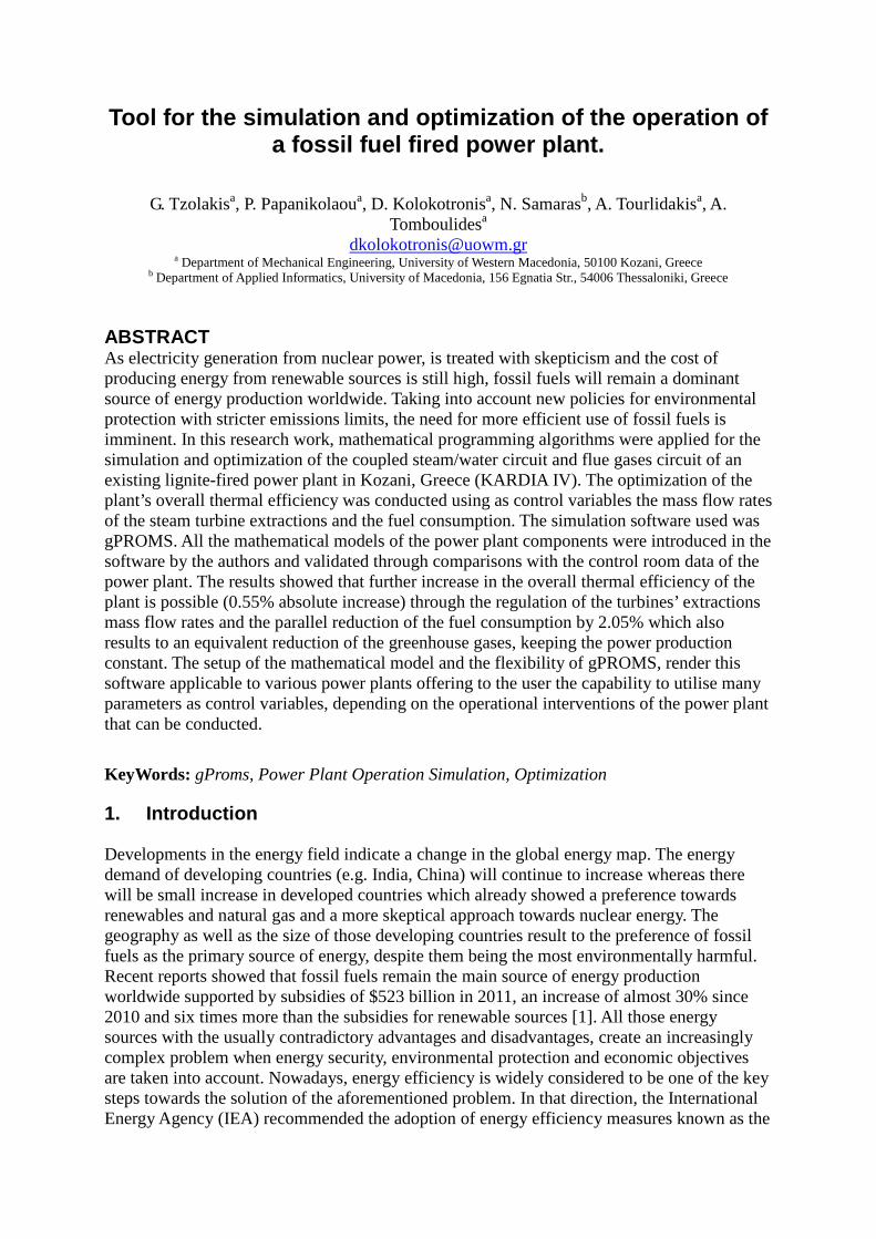
Τhe power plant which has been modeled was that of KARDIA’s Unit IV in Greece. The process flow diagram of the plant as it has been modeled in gPROMS and its topology interface is presented in Figure 1. Mass and energy balance equations, thermodynamic properties calculations and boundary conditions equations, as mentioned above, were used for all the components. Heat transfer properties were used in the flue gases circuit where more detailed models were implemented.

Figure 1. Process flow diagram of Kardia’s 300 MWel Unit IV power plant. (GEN=Generator, GEN_Elec=Generator’s electric energy production, GEN_Heat=Generator’s heat losses, HP, IP, LP=High, Intermediate, Low pressure steam turbine, EX=Steam splitter, EXT=Water extraction, Cond=Condenser, Cond_Heat=Condenser’s heat losses, C_Pump=Pump after the condenser, D_Pump =Main flow pump, Elec_x_Pump=Respective pump’s electrical power usage, V=Throttle, R=Preheater, A=Attemperator, ATMP_VALVE=Attemperator’s valve, DEAE=Deaerator, BURN=Burner, MIXER=Furnace’s water mixer, FURNACE=Furnace, SH=Superheater, F_SH=Waterwall parallel to the respective superheater, RH=Reheater, F_RH=Waterwall parallel to the respective reheater, DRUM=Steam separator, ECO=Economizer)[28].

This is a 300 MWel gross power output plant with steam superheat (SH 1a, SH 1b, SH 2, SH3) reheat (RH1a, RH1b, RH2) and 7 water reheaters (R1-R6, DEAE) heated from the equivalent stream extractions (EX1-EX7) from the steam turbines (HP, IP1-IP4, LP1-LP3). The steam turbines are connected to the generators (GEN1-GEN8) which produce the electrical power. For superheaters and reheaters. the most important equation is the heat transfer from the flue gases to the water through the pipes which is calculated as:

ltc TAUFhmhmQ ∆=+= 4433 &&& [W] (1) where 3m& and 4m& are the respective input and output mass flow rates of the steam of the

above components in kg/s and hi the respective specific enthalpies in kJ/kg. They are expressed as a sum because of the negative value that is given to all the outlet mass flow rates. Ut is the overall heat transfer coefficient based on the overall inner surface area and is calculated as:

instin

out

watoutgas

it

rar

r

rar

U

⋅⋅+⋅

⋅+

⋅⋅

⋅=

9.0

1ln

75.0

1

5.0

111

λ

[kW/m2K] (2)

where ri and rout are the internal and external radii of the water pipes in m, agas and ast are the heat transfer coefficients of the flue gases and steam in kW/m2K and λw is the thermal conductivity of the steam pipes in kW/mK. ∆Τl is the mean logarithmic temperature in K, A is the overall heat transfer surface in m2 and the Fc factor is used so that the whole temperature space can be covered. In addition, the pressure drop for the two fluids can be calculated from

( )υ⋅

+−

⋅=∆ −

R

L

T

T

g N

gSdS

Swf

p2

0

220

5 210 [bar] for flue gases (3)

where SL is the parallel to the flow distance of the centres of two consecutive pipes in m, ST the normal to the flow distance of the centres of two consecutive pipes in m, f0 is the friction factor as calculated in Elmegaard [26], do the outer diameter of the pipes in m and NR the number of pipe rows in the superheater or the reheater, υ is the mean specific volume of the fluid in m3/kg, w is the speed of the fluid in m/s and g is the gravitational acceleration in m/s2.

∆+⋅=∆ −2

225

210

υυ

υw

d

flwp

iw [bar] for steam (4)

where f is the friction coefficient, di is the pipe internal diameter in m, l is the pipe length in m and υ is the specific volume in m3/kg. The turbines’ characteristic equation is the polytropic efficiency’s ηpol which is defined from:

γγη 1

1

2

1

2

−

=

pol

P

P

T

T (5)

and connects the output pressure (P2) with the input pressure (P1), temperature (T1) and γ, the specific heat ratio of the steam. Steam from the turbines is condensed (Cond.) and then

pumped (C_Pump) to the first four water reheaters and then is driven to the Deaerator (DEAE) for separation of the steam and have its pressure risen (D_Pump). Fraction of the water’s flow is directed to the steam reheaters’ attemperator (A3) through a splitter (EXT_1). Further water reheating occurs in the last two water reheaters, after which the extractions (EXT_2, EXT_3) for the superheaters’ attemperators (A1, A2) are located. The attemperators are used to regulate the steam temperature when exiting a superheater or a reheater, with the water from the extractions, and the flow rate is calculated based on the steam’s inlet temperature to the attemperator and the requested temperature at its exit. After the reheaters, the water is further heated in the economizer (ECO), a gas-liquid heat exchanger. That water mixes (MIXER) with the separated water from the water-steam separator (DRUM) by taking into account the partial pressure equation. The furnace chamber’s waterwalls (FURNACE) and the waterwalls of the secondary chamber (F_SH1a, F_SH1b, F_SH2, F_SH3, F_RH1a, F_RH1b, F_RH2) are responsible for the water evaporation before entering the HP and IP1 turbines. Similar equations to those used for superheaters and reheaters were implemented for the furnace chamber and the waterwalls. The burner (BURN) converts the chemical energy of the fuel to heat through the stoichiometric combustion model equations, taking into account the excess air factor λ equation:

fuel

air

mAF

m

&

&

min

=λ (6)

where AFmin is the stoichiometric air to fuel ratio which depends on the fuel composition,

fuelm& the fuel mass flow rate in kg/s and airm& the air mass flow rate in kg/s. The pressure ratio

PR:

PRP

P

air

fg = (7)

where Pfg is the pressure of the exiting flue gases from the burner and Pair is the pressure of the input air in the burner, both in [bar], is used for the calculation of the flue gases pressure. The flue gases, as combustion products, flow through the furnace chamber and the secondary chamber where the waterwalls, the superheaters and reheaters are located. Details on the equations for the components of the flue gas circuit can be found in our previous work [28]. Concerning the rest of the components, additional equations which were implemented include pressure drop for the heat exchangers (R1-R6, Cond, DEAE). In addition, the overall efficiency for the pumps is given by the equation:

( ) 212113 10⋅−= PPumEnp & (8)

where np is the overall pump efficiency, E3 the input electric power in kW, P2 and P1 the output and input pressures respectively in kPa,1m& and u1 the input water mass flow rate and internal energy in kg/s and kJ/kg respectively. An overall efficiency equation for the generators is also used. The valves (V1-V6, ATMP_VALVE1- ATMP_VALVE3) were employed as regulatory components in order to accomplish corrected pressure and temperature. The attemperators and the economizer are the connection points between the two circuits. Details on the equations of the water-steam circuit can be found in our previous work [25] were that circuit is examined in full detail. After the set-up of the plant as shown in Figure 1, the overall efficiency of the plant, which is the objective function of the optimization problem, is calculated as the product of the boiler’s efficiency η-thermal [28] and the water-steam circuit’s efficiency η [25]:

η-total = η-thermal x η (9)

Therefore, optimization of the objective function requires combined optimization for the two circuits.

3. Components validation through simulation.

Detailed validation studies of the components’ mathematical models for each circuit separately were performed in our previous works [25], [28]. The results of the complete plant’s simulation compared to the measured data from the control room are illustrated in Table 1 and Table 2.

In Table 1 a comparison between the control room’s measured data and the complete plant’s simulated results from the water - steam circuit are presented. The compared values are those of the output mechanical power of the turbine stages, the input and output heat exchange rates as well as the thermal efficiency of the cycle.

Table 1. Comparison of the water steam circuit’s values between the control room’s data and the complete plant’s simulation results with their relative differences.

Components Measured Data gPROMS Relative

Difference [%] Generators Electric Power Production [kW] GEN1 -81428 -79900 -1.88

GEN2 -30873 -30172 -2.27

GEN3 -30505 -30799 0.96

GEN4 -23849 -24213 1.53

GEN5 -40035 -39539 -1.24

GEN6 -29468 -29613 0.49

GEN7 -32259 -33424 3.61

GEN8 -21390 -22400 4.72

Total -289807 -290060 0.09

Heaters Heat Consumption [kW] S/H 603600 598992 -0.76

R/H 105350 106734 1.31

Condencer Heat Losses [kJ/s] Cond. -421640 -422138 0.12

Unit Thermal Efficiency [-] η 0.4004 0.4 -0.10

Superheating (S/H) includes the heat transfer taking place to the waterwalls of the main and secondary chamber, the superheaters and the economizer. Reheating (R/H) takes into account the reheaters. As it can be observed, the results are satisfactory with the exception of the last two generators and the corresponding turbine stages. That occurs due to their slightly different behavior due to the fact that the stream is a mix of gas and liquid water. However, the total produced electric power remains almost unchanged. Those results prove that the behavior of the water-steam cycle remains the same after the implementation of the more advanced and

detailed model of the boiler. Table 2 presents the results of the input and output temperatures of the steam and flue gases streams flowing through the superheaters and the reheaters. The control room data and the complete plant’s simulation results are compared. The initial conditions which were utilised for the flue gas circuit can be found in our previous work [28].

Table 2. Comparison of the inlet and outlet temperatures of the steam and flue gas streams in the flue gas circuit between the control room data and the complete plant’s model simulated results.

Components Measured Data Complete Plant Relative Difference [%]

Inlet Temp. [oC]

Outlet Temp. [oC]

Inlet Temp. [oC]

Outlet Temp. [oC]

Inlet Temp. [oC]

Outlet Temp. [oC]

Steam Values

FURNACE 332.11 361 335.06 364.44 0.89 0.95 SH1a 361 364.44 371.75 0.95 SH1b 428 371.75 427.78 -0.05 SH2 408 512 422 500.8 3.43 -2.19 SH3 494 535 496 535.4 0.40 0.07

RH1a 339 338.39 368.65 -0.18

RH1b 444 368.65 435.13 -2.00 RH2 414 535 431 535.28 4.11 0.05

Flue Gases Values

FURNACE 1197.11 965 1205.98 974.69 0.74 1.00

SH1a 428 426 -0.47

SH1b 548 546.49 -0.28

SH2 830 838.78 1.06

SH3 780 766.98 -1.67

RH1a 405 398.12 -1.70

RH1b 492 491.16 -0.17

RH2 682 674.46 -1.11

The results in all cases showed satisfactory agreement and the discrepancy between the measured data and the calculations were below 2.2% at all points. Thus, the good behavior of the model of the complete plant is proven.

4. Optimization results

Since the simulation results were satisfactory, the optimization algorithm, as presented in the “Methods and Analysis” section and in reference [28], was applied to the power plant’s model. As mentioned above, any user-defined operational parameters which are not related to the constructional characteristics of a component could be used as an optimization variable.

In this case, for the optimization process, the mass flow rates of the steam extractions from the turbines to the water reheaters and the mass flow rate of the fuel in the burner were used as control variables. The fuel mass flow rate is the main dependency of the overall efficiency of the plant since it provides the chemical energy which is transformed to heat through the combustion process. The fuel consumption is related to the greenhouse gases emissions and a first measure to reduce them is through the reduction of this quantity by maintaining the electric power production, something which can be achieved through optimization of the overall efficiency.

Prior to any optimization attempt, boundary conditions need to be defined for the problem. The boundary conditions that have been set are presented in Table 3:

Table 3. Boundary conditions for the optimization problem.

Component Variable Condition Value Accepted Deviation

HP Inlet Steam

Temp. Equal 535

oC +/- 2

oC

HP Inlet Steam

Pres. Equal 170 bar +/- 0.2 bar

HP Inlet Steam

Mass flow rate Equal 246.9 kg/s +/- 0.2 kg/s

IP1 Inlet Steam

Temp. Equal 535

oC +/- 2

oC

Plant Net Elec.

Energy Prod. Equal 281 MW +/- 0.2 MW

Additional conditions are all the natural boundary conditions of the fluids, e.g. positive temperature, pressure, specific volume, entropy. The temperature boundaries were specified in order to protect the metallic parts of the turbines from excessive temperatures which would lead to faster aging. The steam mass flow and the net electric power production are the main variables which guarantee stability at the specific load of the plant since the goal is to achieve improved efficiency through the decrease of the fuel consumption and not the increase of the produced electric power since this is not possible without modifications to the structural characteristics of the plant. Deviations indicated in Table 3 are acceptable due to their minimal effect to the plant because of the small percentage change and are also necessary for the flexibility of the optimization problem. Τhe characteristic parameters of the optimization problem are illustrated in Table 4:

Table 4. Optimization Problem Characteristics.

Parameter Equality

Equations

Inequality

Equations

Decision

Variables

Independent

Variables

Optimization

Accuracy

Initial Search

Step

Value 10667 10 9 239 10-6

0.5

Another parameterisation which can be applied to the control variables is the form of the scaling [29]. Scaling is necessary when the control variables vary significantly in magnitude. The scaling performed is of the general form:

j

jjj d

cqq

−=~ (10)

where qj is the jth original control variable and jq~ is the corresponding scaled control

variable. In this case, where the scaling has been set to 1, the values of cj and dj are respectively:

( )minmax

2

1jjj qqc += (11)

( )minmax

2

1jjj qqd −= (12)

so that the scaled variables will be between -1 and 1. It should be noted that the use of local optimization algorithms for the solution of the Non Linear Programming does not guarantee a global optimum solution. This is a common drawback in optimization-based design methods which can be solved with global optimization techniques.

4.1. Comparison between optimization and simulation results.

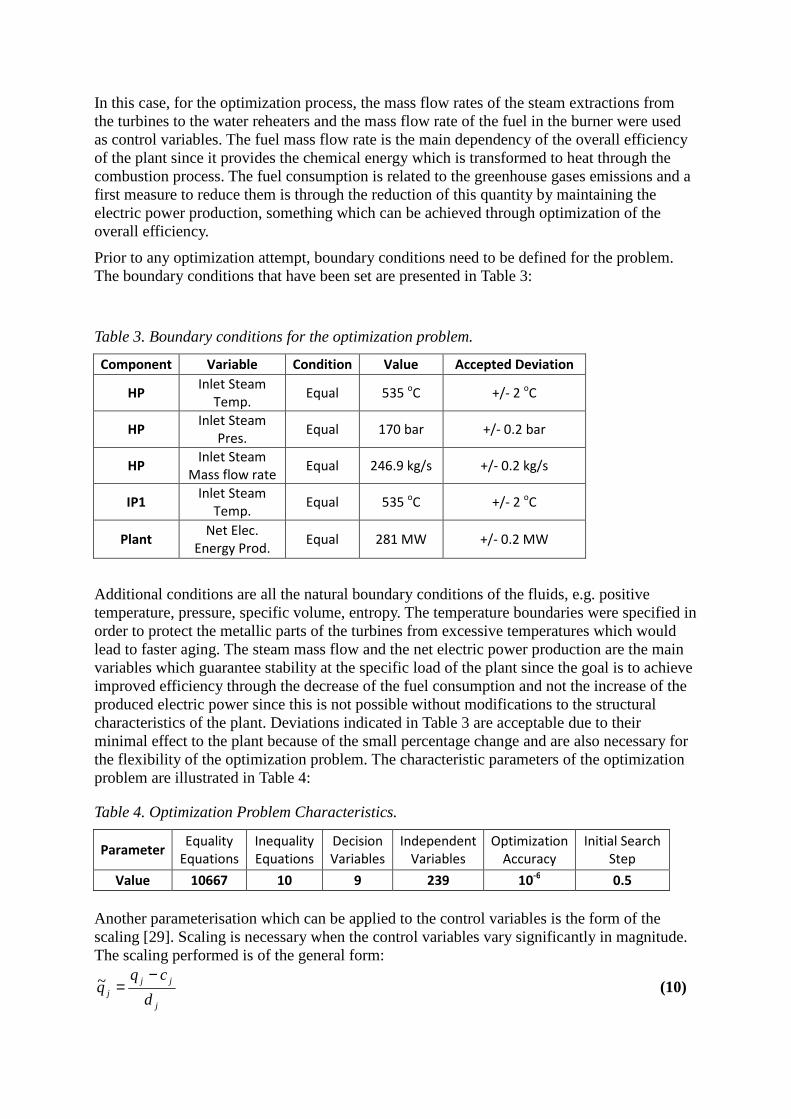
Initially, the changes to the control variables are presented in order to demonstrate the trend that they follow while optimizing the overall efficiency of the plant. In Figure 2 the simulated and optimized values of the extractions mass flow rates are presented, as well as their absolute differences. The negative values indicate an outlet flow. A decrease in the extractions mass flow rate of the first two turbine stages with parallel increase of the later was observed. This way, more energy is given to the high pressure turbine stages (HP and IP1) and less to the lower pressure ones, as a result of the constant electric power production, which derives from the energy of the superheated steam, which should remain constant. That way, the reheated water receives more energy from the first four reheaters where the extracted steam is further exploited as it returns to the condenser through the previous reheaters as shown in Figure 1. Therefore, reheated water with higher energy content than previously the optimization passes through the last two reheaters where less steam is used. As a result water with higher energy content enters the furnace waterwalls. The small absolute increase of the last extraction’s mass flow rate translates to a high relative increase (14.89%), because of the already small value of that turbine’s stage extraction. Similar results have been recorded with the state-of-the-art technologies which promote the complete cancelation of the HP steam extraction through increase of the rest [30].

The aforementioned behaviour resulted to reduced fuel requirement. According to the boundary conditions, the steam production should remain the same which means that the output from the boiler is the same as well. However, the inlet water to the furnace walls has higher energy content; therefore less heat is required to reach the same output conditions which can be achieved with less fuel.The optimization shows a relative decrease by 2.05% to the fuel’s mass flow rate. That percentage corresponds to a 3.18 kg/s reduction which is considered important for a power plant, taking into account the non-stop operation of those units. The fuel reduction is also directly related to a flue gases reduction. Since the fuel-to-air ratio is considered to be constant, so is the composition of the flue gases. With that assumption, a simplified estimation of the CO2 reduction can be calculated. Since the composition of the flue gases was calculated from the combustion simulation to be 11.24% per kg of flue gas therefore the absolute reduction of CO2 equals to: (572.4-560.6) x 3600 x 0.112447 = 4.776 t/h CO2 (or -2.06%) As expected the percentage of the reduction is the same and this is also an important hourly reduction of the most common greenhouse gas.

In Table 5 the heat transfer rates (inlets and outlets) taking place in specific components of the plant as well as the electric power production from the respective turbine stages along with the efficiencies of the two different circuits (flue gases and steam/water circuits) are presented and compared with the simulated ones.

Figure 2. Absolute change of the mass flow rates of the steam turbine extractions (control variables) (HP: -3,88%, IP1: -2,1%, IP2: 16%, IP3: 8,74%, IP4: 28,55%, LP1: 19,15%, LP2: 14,89%).

Table 5. Comparison of the simulated and optimized values of fuel mass flow rate, electric energy production, heat exchange rates and efficiencies.

Components Simulation Optimization Relative Difference [%] Burner Fuel mass flow rate [kg/s] BURN 155 151.82 -2.05

Generators Electric Energy Production [kW] GEN1 -79900 -79691 -0.26

GEN2 -30172 -30536 1.21

GEN3 -30799 -31726 3.01

GEN4 -24213 -25067 3.53

GEN5 -39539 -39537 -0.01

GEN6 -29613 -29463 -0.51

GEN7 -33424 -32437 -2.95

GEN8 -22400 -21768 -2.82

Heat Exchangers Heat Exchange Rate [kJ/s] S/H 598992 587953 -1.84

R/H 106734 104213 -2.36

Cond. -422138 -409147 -3.08

Thermal efficiency of water steam circuit [-] η 0.4 0.406 1.50

Boiler thermal efficiency [-] η-thermal 0.8227 0.8242 0.18

Unit overall thermal efficiency [-] η-total 0.3291 0.334733 1.71

As it can be observed, the heat transfer requirements for steam superheating and reheating have been reduced, as mentioned above. Reduction can be also noticed to the condenser heat losses. That is to be expected since less steam enters the condenser and higher percentage of the high energy steam of the first two stages is exploited for the electric energy production, resulting in lower energy steam at the exit of the turbines and combined with the constant thermodynamic properties of the water at the exit, the heat extraction that is required during condensing is less than that of the simulated conditions. The stability of the electric power production can be also verified. Although there are some small changes in the power production of the individual generators, the overall production is constant. More specifically, the first generators show an increase while the latter show a decrease in power generation. That can be justified through the increases and decreases of the steam turbines extractions. More steam through the turbines means more mechanical power production. It should be mentioned that the same constant efficiency value has been used for all generators therefore the percentage of mechanical power which is converted to electrical is the same for all stages. Finally, the optimized values of the overall efficiency, as well as of the individual efficiencies of the two circuits, on which the overall efficiency depends, are compared to their simulated values. The results of the optimization showed an absolute increase of 0.6% (1.5% relative) in the water-steam circuit and 0.15% (0.18% relative) in the flue gases circuit, which led to a 0.55% absolute increase of the overall thermal efficiency of the power plant. The above results indicate that optimization is possible and within realistic limits. The

resulting increase of the plant’s efficiency might be considered very small and within computational error margin. However, in power plants, as in this case, it has been shown that such changes have a considerable impact on the behavior of the power plant leading to major changes, such as fuel consumption and CO2 emissions reductions, which were reported previously. The reason that operational optimization is necessary lies to the fact that distortions and changes to the original operating conditions as well as to the components of a power plant have occurred through time, leading to altered operation values. Especially in the cases of coal-fired power plants, a change to the coal’s composition due to the fuel quality of different locations and depths, in addition to the aging of the equipment and the superheaters, reheaters and waterwalls fouling can alter the operational parameters of the power plant [31].

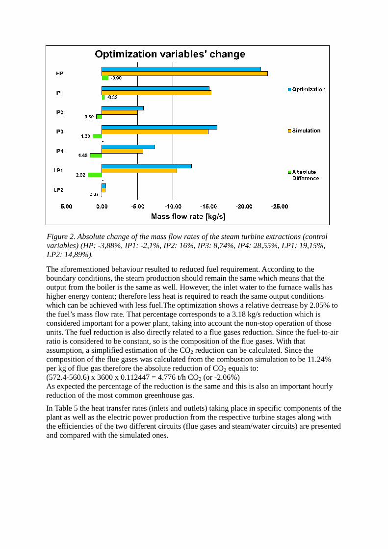
4.2. Sensitivity Analysis The effect of each control variable’s per-unit-increase from its original simulation value to the objective function is presented in Figure 3.

Figure 3. Effect of the control variables’ modular change to the objective function and their absolute change.

The negative values to the objective function’s change indicate that increase of the control variable by one unit will result to an decrease of the objective function and vice versa. Therefore, in this case, decrease of the control variables is necessary for the increase of the objective function, since this is a maximization problem. However, because of the general rule which indicates that output flows obtain a negative value, such as the turbine extractions, the need for lower values (decrease) translates into an even larger negative number, meaning that the extractions mass flow rate need to increase. On the other hand, the mass flow rate of the fuel is an input value to the burner therefore the above rule applies as is.

Therefore, based on the above explanation, the results showed that, increase of the plant’s efficiency is possible through increase of the mass flow rate of any turbine extraction or from the decrease of the fuel’s mass flow rate to the burner. If they were to be optimised individually, that increase would vary between 0.18% and 0.27% in absolute percentage value

Optimization variables and objective function change

of the efficiency. From all extractions, those of the HP and IP1 turbines had the smallest positive effect. Taking into account the various constrains that are imposed to a power plant as well as the non-linearity of the problem and the dependencies of the other variables, optimization takes into account the above values and sacrifices the HP and IP1 extractions by decreasing their values, for the increase of the rest of the extractions mass flow rate values to be possible since they affect more the efficiency of the plant. Subsequently these changes result to the reduction of fuel consumption and this also leads to the increase of plant’s efficiency.

5. Conclusions

The main objective of this work was to present a flexible tool for simulating and optimizing fossil fueled power plants. The flexibility of the simulation and optimization software gPROMS towards that goal was firstly explained. Subsequently, the power plant model of an existing 300MW lignite-fired power plant in Kozani, Greece (KARDIA Unit IV) which was created in gPROMS was described together with the main characteristic equations used in the components’ mathematical models. In order to reduce the computational time of simulations and optimizations processes, the creation of modules in gPROMS Foreign Objects (FO) for the calculations of the thermodynamic and heat transfer properties of the fluids was necessary. By implementing these modules in this work’s case model, the number of variables was reduced to 10906 from 375630, the number of equations from 333983 to 10667 and the number of the parameters of the model (in which constants from the polynomial calculations of the properties are included) to 3615 from 588215. The above reductions resulted to the dramatic reduction of the simulation computational time from 2100 to 8 seconds. This reduction has a great impact on the optimization time taking into account that optimization occurs through a number of continuous simulations. The complete plant’s model gave satisfactory simulation results with the error within the 2.5% region compared to the measured data of the control room with only 2 cases above that value but below the accepted 5% region. Since the validation was satisfactory, an operational optimization scenario was considered using the overall plant efficiency as the objective function. The mass flow rates of the turbine extractions and the fuel mass flow rate were the optimization (or control) variables. The result was an increase of 0.55% to the overall efficiency derived from a 2.06% reduction of the fuel’s consumption with parallel reduction of the first two steam extractions and increase of the rest. The electric power production remained unchanged. Due to the size of the particular type of power plants and their daily, non-stop operation, such a percentage increase is considered important due to the resulting benefits from the fuel economy since 2.06% fuel reduction translates to 11.5 t/h less lignite and an equivalent 2.06% reduction of the flue-gas emissions which translates to 4.8 t/h less CO2 emissions therefore lower penalty fees.

The gPROMS software together with the components mathematical models that were created as well as the Foreign Object modules, can be potentially used as a decision and optimization tool in the control room. One of the main advantages of gPROMS is its ability to treat a problem as a steady-state one while all the variables are time differentiable, by considering them constant and this specific attribute makes easier the transition from a steady-state problem to a dynamic one. Concerning real-time problems, gPROMS has the ability to interact with external software through the use of Foreign Process Interface (FPI) feature and to communicate with them with the Output Channel Interface (OCI) feature. More details about the available solvers in gPROMS and the FO, FPI and OCI features can be found in the gPROMS manuals [29], [32], [33]. Its fast simulation and optimization processing times as well as its ability to communicate and interact with external software, can render it an

attractive software environment that can be successfully used by the engineer in charge for instant decisions for the optimized operation of the plant through adjustments to specific control variables.

6. References

[1] International Energy Agency – ΙΕΑ, World Energy Outlook 2012 Executive Summary, IEA PUBLICATIONS, Paris, November 2012.

[2] International Energy Agency – IEA, 25 Energy Efficiency Policy Recommendations: 2011 Update, IEA PUBLICATIONS, Paris, 2008.

[3] The European Parliament and the Council of the European Un ion Directive, 2012/27/EU of the European Parliament and of the Council of 25 October 2012, Official Journal of the European Union, 14.11.2012

[4] Environmental Protection Agency and National Highway Traffic Safety Administration, 2017 and Later Model Year Light-Duty Vehicle Greenhouse Gas Emissions and Corporate Average Fuel Economy Standards, Federal Register / Vol. 77, No. 199 / October 2012.

[5] E. T. Bonataki, K.C. Giannakoglou, Preliminary design of optimal combined cycle power plants through evolutionary algorithms, Evolutionary and Deterministic Methods for Design Optimization and Control with Applications to Industrial and Societal Problems, EUROGEN (2005), 2005

[6] H. Eliasi, M.B. Menhaj, H. Davilu, Robust nonlinear model predictive control for a PWR nuclear power plant, Progress in Nuclear Energy, Volume 54, Issue 1, January 2012, Pages 177-185.

[7] W. Elsner, Ł. Kowalczyk, M. Marek, Numerical thermodynamic optimization of supercritical coal fired power plant with support of IPSEpro software, Archives of Thermodynamic, Vol. 33 (2012), No. 3, 101-110.

[8] J. Xiong, H. Zhao, C Zhang, C Zheng, P. B. Luh, Thermoeconomic operation optimization of a coal-fired power plant, Energy, Vol. 42, Issue 1, (2012), P. 486-496.

[9] T. Harkin, A. Hoadley, B. Hooper, Using multi-objective optimisation in the design of CO2 capture systems for retrofit to coal power stations, Energy, Vol. 41, Issue 1, (2012), P. 228-235.

[10] J. C. Eslick, D. C. Miller, A multi-objective analysis for the retrofit of a pulverized coal power plant with a CO2 capture and compression process, Computers & Chemical Engineering, Vol. 35, Issue 8, (2011), P. 1488-1500.

[11] J. Cristóbal, G. Guillén-Gosálbez, L. Jiménez, A. Irabien, Multi-objective optimization of coal-fired electricity production with CO2 capture, Applied Energy, Vol. 98, (2012), P. 266-272.

[12] H.M. Hashemian, On-line monitoring applications in nuclear power plants, Progress in Nuclear Energy, Vol. 53, Issue 2, (2011), P. 167-181.

[13] S. Munukutla, R. Craven, Coal-fired power plant performance monitoring in real-time, Centre for Energy Systems Research, Tennessee Tech University, 2006.

[14] N.Shabani, T. Sowlati, A mixed integer non-linear programming model for tactical value chain optimization of a wood biomass power plant, Applied Energy, Vol. 104, (2013), P. 353-361.

[15] V. Marano, G. Rizzo, F. A. Tiano, Application of dynamic programming to the optimal management of a hybrid power plant with wind turbines, photovoltaic panels and compressed air energy storage, Applied Energy, Vol. 97, (2012), P. 849-859.

[16] J. I. Manassaldi, S. F. Mussati, N. J. Scenna, Optimal synthesis and design of Heat Recovery Steam Generation (HRSG) via mathematical programming, Energy, Vol. 36, Issue 1, (2011), P. 475-485.

[17] E. Ayaz, Component-wide and plant-wide monitoring by neural networks for Borssele nuclear power plant, Energy Conversion and Management, Vol. 49, Issue 12, (2008), P. 3721-3728.

[18] T. Bekat, M. Erdogan, F. Inal, A. Genc, Prediction of the bottom ash formed in a coal-fired power plant using artificial neural networks, Energy, Vol. 45, Issue 1, (2012), P. 882-887.

[19] M. Fast, T. Palmé, Application of artificial neural networks to the condition monitoring and diagnosis of a combined heat and power plant, Energy, Vol. 35, Issue 2, (2010), P. 1114-1120.

[20] A. G. Kaviri, M. Nazri, M. Jaafar, T. M. Lazim, Modeling and multi-objective exergy based optimization of a combined cycle power plant using a genetic algorithm, Energy Conversion and Management, Vol. 58, (2012), P. 94-103.

[21] P. Ahmadi, I. Dincer, Exergoenvironmental analysis and optimization of a cogeneration plant system using Multimodal Genetic Algorithm (MGA), Energy, Vol. 35, Issue 12, (2010), P. 5161-5172.

[22] M.V.J.J. Suresh, K.S. Reddy, A. K. Kolar, ANN-GA based optimization of a high ash coal-fired supercritical power plant, Applied Energy, Vol. 88, Issue 12, (2011), P. 4867-4873.

[23] I. Spangelo, Trajectory Optimization for Vehicles Using Control Vector Parameterization and Nonlinear Programming, Report 94-111-W, (1994), Dept. of Engineering Cybernetics, The Norwegian Institute of Technology, Norway

[24] S. S. Rao, Engineering Optimization: Theory and Practice, 3rd Edition, 1996, John Wiley & Sons Inc., ISBN 0-471-55034-5

[25] G. Tzolakis, P. Papanikolaou, D. Kolokotronis, N. Samaras, A. Tourlidakis, A. Tomboulides, Emissions’ reduction of a coal-fired power plant via reduction of consumption through simulation and optimization of its mathematical model, Operational Research Journal (Special Issue): Optimization Models in Environmental and Sustainable Development, 2009.

[26] B. Elmegaard, Simulation of Boiler Dynamics – Development, Evaluation and Application of a General Energy System Simulation Tool, Ph.D. Thesis: Report Number ET–PhD 99–02. Department of Energy Engineering, Technical University of Denmark, (1999).

[27] International Association for the Properties of Water and Steam, Revised Release on the IAPWS Industrial Formulation 1997 for the Thermodynamic Properties of Water and Steam, Lucerne, Switzerland, 2007.

[28] G. Tzolakis, P. Papanikolaou, D. Kolokotronis, N. Samaras, A. Tourlidakis, A. Tomboulides, Simulation of a coal-fired power plant using mathematical programming algorithms in order to optimize its efficiency, Applied Thermal Engineering, Vol. 48, (2012), P. 256-267.

[29] Process Systems Enterprise, gPROMS Introductory User Guide, (2004).

[30] A . Chaibakhsh, A. Ghaffari, Steam turbine model, Simulation Modeling Practice and Theory 16 (2008) 1145-1162.

[31] P. Papanikolaou, Assessment and simulation of impact of ash deposits in solid fuel boiler, Diploma Thesis, Dept. of Engineering and Management of Energy Resources, University of Western Macedonia, Kozani, Greece, (2008).

[32] Process Systems Enterprise, gPROMS Advanced User Guide, (2004).

[33] Process Systems Enterprise, gPROMS System Programmer Guide, (2004).

7. Acknowledgements

We would like to acknowledge the Public Power Corporation of Greece for its financial and technical support.