Page 1
Toolpath and Cutter Orientation Optimization in 5-Axis CNC Machining of Free-form
Surfaces Using Flat-end Mills
by
Shan Luo
BSc, Jianghan University, 2008
MSc, Wuhan University of Technology, 2011
A Dissertation Submitted in Partial Fulfillment
of the Requirements for the Degree of
DOCTOR OF PHILOSOPHY
in the Department of Mechanical Engineering
Shan Luo, 2015
University of Victoria
All rights reserved. This dissertation may not be reproduced in whole or in part, by
photocopy or other means, without the permission of the author.
Page 2
ii
Supervisory Committee
Toolpath and Cutter Orientation Optimization in 5-Axis CNC Machining of Free-form
Surfaces Using Flat-end Mills
by
Shan Luo
BSc, Jianghan University, 2008
MSc, Wuhan University of Technology, 2011
Supervisory Committee
Dr. Zuomin Dong, (Department of Mechanical Engineering) Supervisor
Dr. Martin Byung-Guk Jun, (Department of Mechanical Engineering) Co-supervisor
Dr. Keivan Ahmadi, (Department of Mechanical Engineering) Departmental Member
Dr. Sue Whitesides, (Department of Computer Science) Outside Member
Page 3
iii
Abstract
Supervisory Committee
Dr. Zuomin Dong, (Department of Mechanical Engineering) Supervisor
Dr. Martin Byung-Guk Jun, (Department of Mechanical Engineering) Co-supervisor
Dr. Keivan Ahmadi, (Department of Mechanical Engineering) Departmental Member
Dr. Sue Whitesides, (Department of Computer Science)
Outside Member
Planning of optimal toolpath, cutter orientation, and feed rate for 5-axis Computer
Numerical Control (CNC) machining of curved surfaces using a flat-end mill is a
challenging task, although the approach has a great potential for much improved
machining efficiency and surface quality of the finished part. This research combines and
introduces several key enabling techniques for curved surface machining using 5-axis
milling and a flat end cutter to achieve maximum machining efficiency and best surface
quality, and to overcome some of the key drawbacks of 5-axis milling machine and flat
end cutter use. First, this work proposes an optimal toolpath generation method by
machining the curved surface patch-by-patch, considering surface normal variations
using a fuzzy clustering technique. This method allows faster CNC machining with
reduced slow angular motion of tool rotational axes and reduces sharp cutter orientation
changes. The optimal number of surface patches or surface point clusters is determined
by minimizing the two rotation motions and simplifying the toolpaths. Secondly, an
optimal tool orientation generation method based on the combination of the surface
normal method for convex curved surfaces and Euler-Meusnier Sphere (EMS) method
for concave curved surfaces without surface gouge in machining has been introduced to
achieve the maximum machining efficiency and surface quality. The surface normal
based cutter orientation planning method is used to obtain the closest curvature match
and longest cutting edge; and the EMS method is applied to obtain the closest curvature
match and to avoid local gouging by matching the largest cutter Euler-Meusnier sphere
with the smallest Euler-Meusnier sphere of the machined surface at each cutter contact
Page 4
iv
(CC) point. For surfaces with saddle shapes, selection of one of these two tool orientation
determination methods is based on the direction of the CNC toolpath relative to the
change of surface curvature. A Non-uniform rational basis spline (NURBS) surface with
concave, convex, and saddle features is used to demonstrate these newly introduced
methods. Thirdly, the tool based and the Tri-dexel workpiece based methods of chip
volume and cutting force predictions for flat-end mills in 5-axis CNC machining have
been explored for feed rate optimization to achieve the maximum material removal rate.
A new approach called local parallel slice method which extends the Alpha Shape
method - only for chip geometry and removal volume prediction has been introduced to
predict instant cutting forces for dynamic feed rate optimization. The Tri-dexel workpiece
model is created to get undeformed chip geometry, chip volume, and cutting forces by
determining the intersections of the tool envelope and continuously updating the
workpiece during machining. The comparison of these two approaches is made and
several machining experiments are conducted to verify the simulation results. At last, the
chip ploughing effects that become a more serious problem in micro-machining due to
chip thickness not always being larger than the tool edge radius are also considered. It is
a challenging task to avoid ploughing effects in micro-milling. A new model of 3D chip
geometry is thus developed to calculate chip thickness and ploughing volume in micro 5-
axis flat-end milling by considering the minimum chip thickness effects. The research
forms the foundation of optimal toolpath, cutter orientation, cutting forces/volume
calculations, and ploughing effects in 5-axis CNC machining of curved surfaces using a
flat-end mill for further research and direct manufacturing applications.
Page 5
v
Table of Contents
Supervisory Committee ...................................................................................................... ii
Abstract .............................................................................................................................. iii
Table of Contents ................................................................................................................ v
List of Tables ................................................................................................................... viii
List of Figures .................................................................................................................... ix
Acknowledgments............................................................................................................. xv
Introduction ................................................................................................. 1 Chapter 1:
1.1 Background and Motivation ............................................................................... 1
1.1.1 Toolpath and Orientations............................................................................... 1
1.1.2 Machine Dynamics ......................................................................................... 4
1.2 Research Contributions ....................................................................................... 6
1.3 Dissertation Outline .......................................................................................... 11
Literature Review...................................................................................... 15 Chapter 2:
2.1 Toolpath Planning ............................................................................................. 15
2.1.1 Surface Division Machining Toolpath .......................................................... 17
2.1.2 Steepest-directed and Iso-cusped (SDIC) Method ........................................ 18
2.1.3 Accessibility-map (A-map) Method ............................................................. 19
2.2 Tool Orientation ................................................................................................ 20
2.2.1 Principal Axis Method (PAM) ...................................................................... 21
2.2.2 Euler-Meusnier Sphere (EMS) Curvature Match ......................................... 22
2.2.3 C-space Based Tool Orientation Methods .................................................... 23
2.3 Machine Dynamics ........................................................................................... 24
2.3.1 Toolpath and Tool Orientation Optimization by Dynamic Constraints........ 24
2.3.2 Chip Volume in 5-axis CNC Machine .......................................................... 25
2.3.3 Cutting Force in 5-axis CNC Machine ......................................................... 28
Optimization of 5-Axis CNC Toolpath and Cutter Orientation for Chapter 3:
Machining Free-form Surfaces ......................................................................................... 31
3.1 Machining Surfaces Patch by Patch Using the Fuzzy Cluster Method ............ 32
3.1.1 Fuzzy C-means Clustering Method .............................................................. 33
3.1.2 Generation of Surface Patches by Surface Normal Vector Distances .......... 35
3.2 Optimization of the Number of Surface Patches .............................................. 37
3.3 Optimal Toolpath Generation ........................................................................... 45
3.3.1 Surface Patch Boundary Definition by Alpha Shape .................................... 45
3.3.2 Toolpath Generation ..................................................................................... 46
3.4 Conclusions ....................................................................................................... 47
Optimal Tool Orientation Generation ....................................................... 48 Chapter 4:
Page 6
vi
4.1 The Euler-Meusnier Sphere (EMS) Method for Tool Orientation in a Concave
Surface .......................................................................................................................... 48
4.1.1 Principal Curvature Calculation for a NURBS Surface ................................ 50
4.1.2 Two rotation Angles Identification ............................................................... 52
4.2 Optimal Tool Orientation .................................................................................. 55
4.3 Conclusions ....................................................................................................... 58
Chip Volume and Cutting Force Calculations in 5-axis CNC Machining of Chapter 5:
Free-form Surfaces Using Flat-end Mills ......................................................................... 59
5.1 Formulation of Swivel Head 5-axis CNC Tool Motion ................................... 61
5.2 Chip Volume Calculation ................................................................................. 62
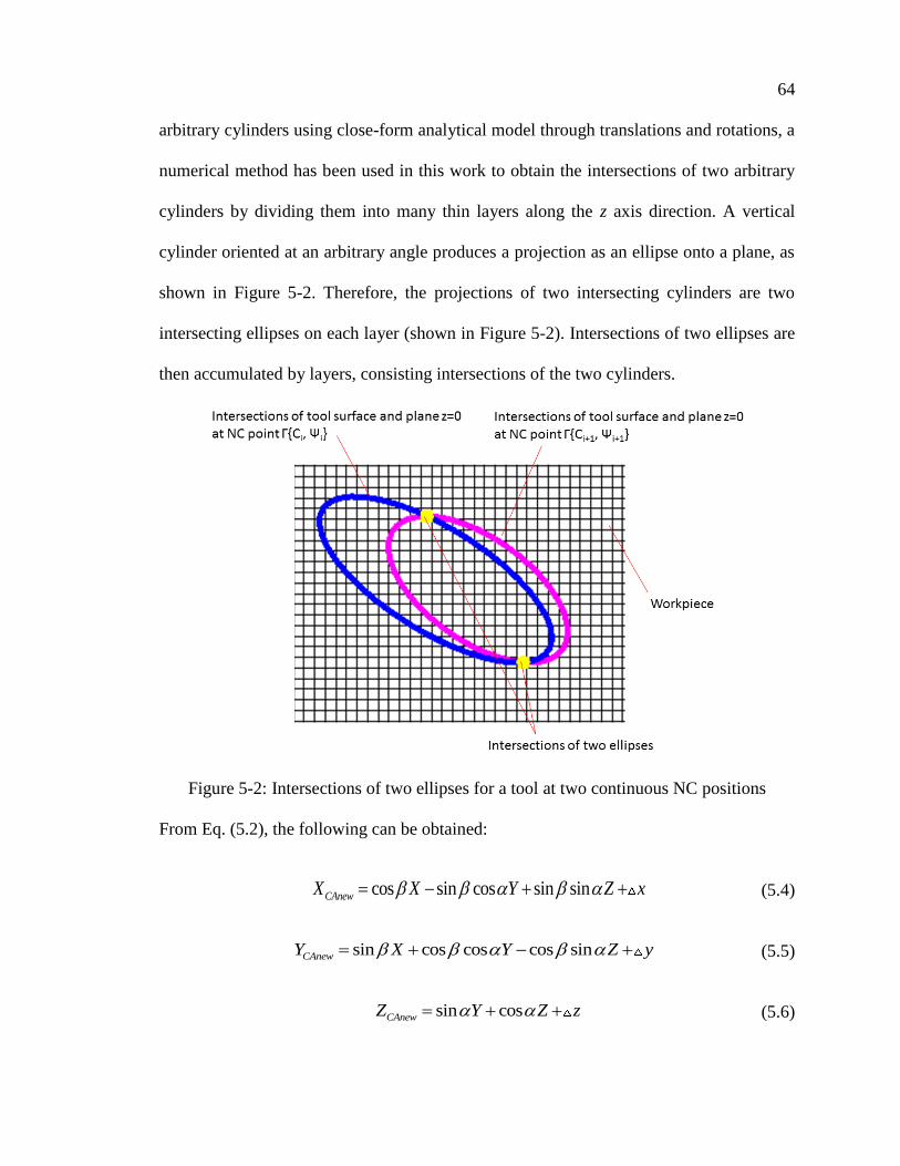
5.2.1 The Alpha Shape Method ............................................................................. 63
5.2.1.1 Intersections of two ellipses .................................................................. 63
5.2.1.2 Volume calculation by the Alpha Shape method .................................. 66
5.2.1.3 The algorithm of chip volume calculation ............................................ 67
5.2.2 Local Parallel Sliced Method ........................................................................ 75
5.2.2.1 Chip load model .................................................................................... 75
5.2.2.2 Chip volume by local parallel sliced method ........................................ 77
5.2.2.3 Cutter-workpiece engagement maps ..................................................... 79
5.3 Cutting Force Model ......................................................................................... 82
5.4 Case Studies and Results .................................................................................. 84
5.4.1 Examples of Chip Volume Simulation by the Alpha Shape Method ........... 84
5.4.2 Simulation Results of Chip Volume and Cutting Forces by Local Parallel
Sliced Method ........................................................................................................... 90
5.5 Experiment Verification.................................................................................... 94
5.6 Conclusions ....................................................................................................... 96
The Tri-dexel Method of Chip Volume and Cutting Forces Calculation Chapter 6:
and Simulation for Free-form Surfaces in 5-axis CNC Machining with Flat-end Mills .. 97
6.1 Tri-dexel Method for Chip Volume and Cutting Force Calculation ................. 98
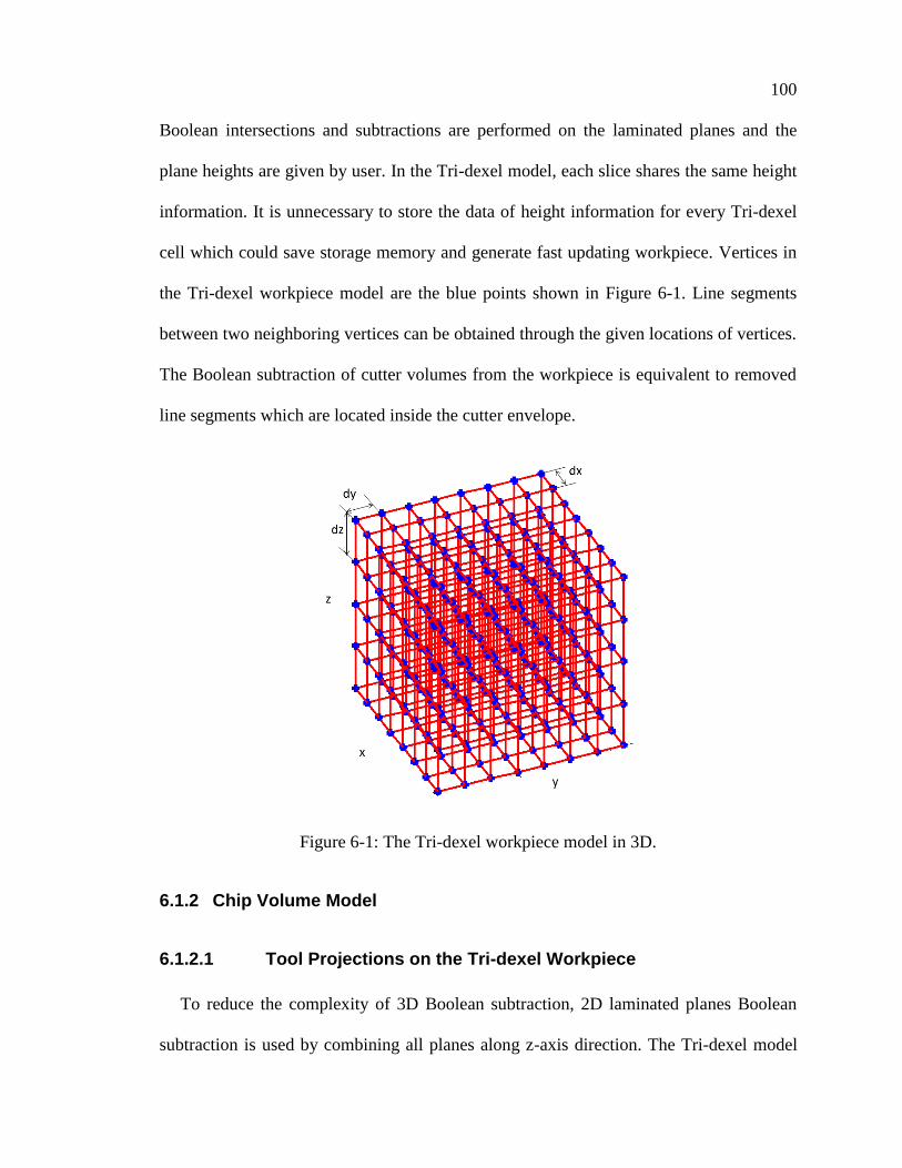
6.1.1 Tri-dexel Workpiece ..................................................................................... 98
6.1.2 Chip Volume Model ................................................................................... 100
6.1.2.1 Tool Projections on the Tri-dexel Workpiece ..................................... 100
6.1.2.2 Boolean operation and chip thickness generation ............................... 101
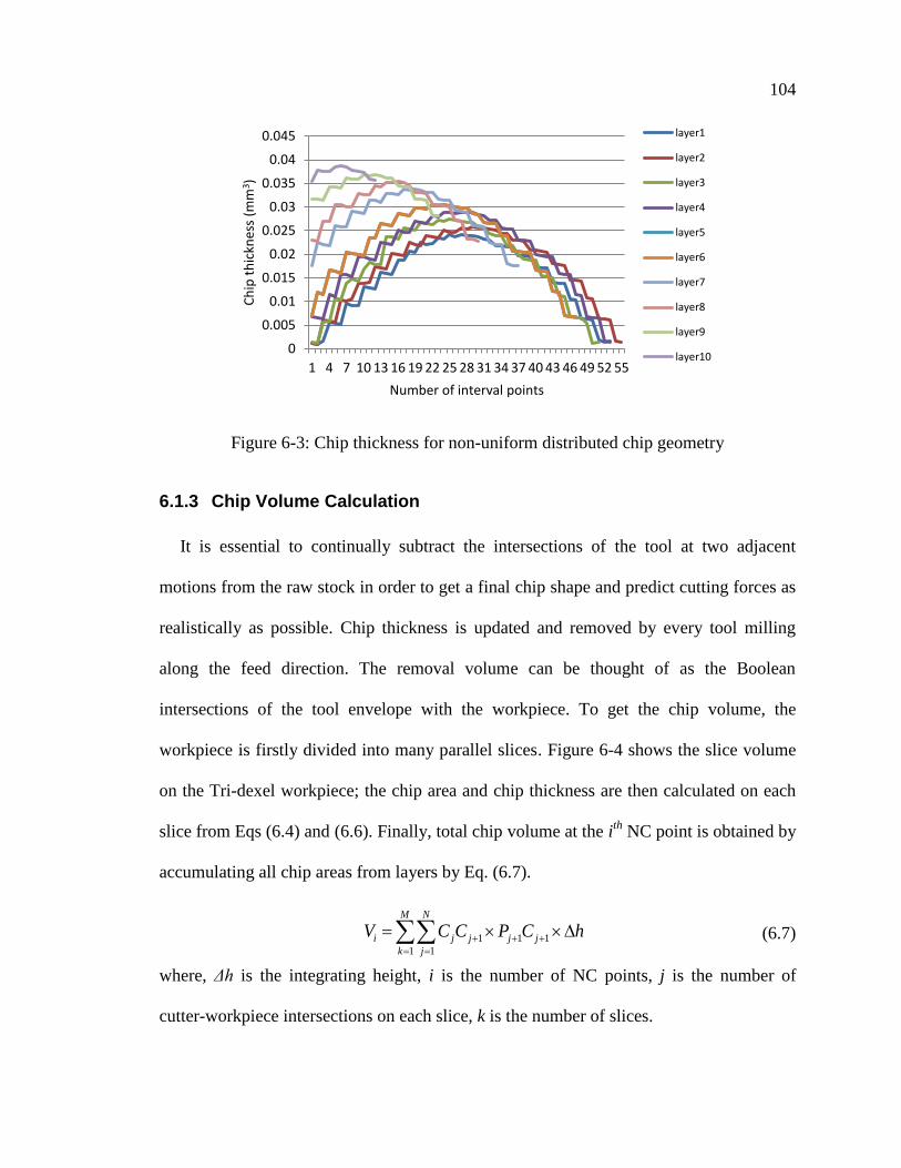
6.1.3 Chip Volume Calculation ........................................................................... 104
6.2 Cutting Forces Prediction ............................................................................... 111
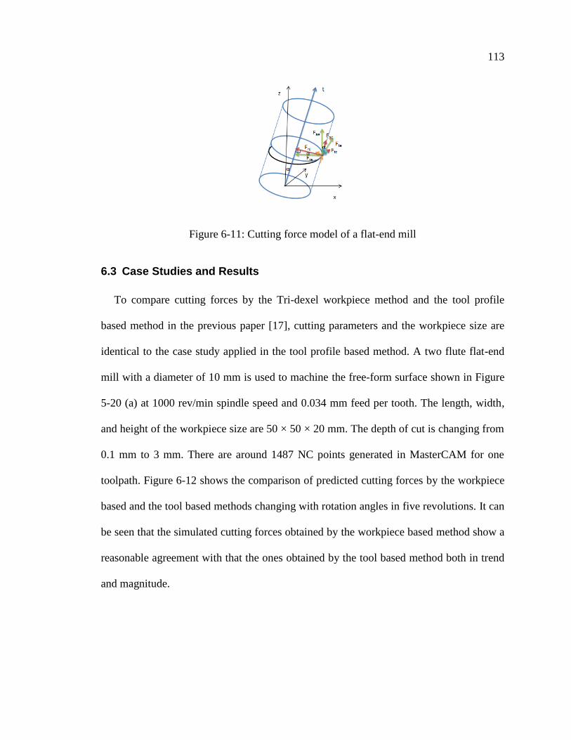
6.3 Case Studies and Results ................................................................................ 113
6.4 Experimental Verification ............................................................................... 117
6.5 Conclusions ..................................................................................................... 120
Conclusions and Future Work ................................................................ 122 Chapter 7:
7.1 Conclusions ..................................................................................................... 122
7.2 Future Work .................................................................................................... 126
Page 7
vii
Bibliography ................................................................................................................... 130
Appendix1 ....................................................................................................................... 140
Appendix2 ....................................................................................................................... 145
Appendix3 ....................................................................................................................... 148
Appendix4 ....................................................................................................................... 153
A4.1 Introduction ........................................................................................................ 154
A4.2 Ploughing effects in 5-axis Micro Flat-end Milling........................................... 156
A4.2.1 Chip Geometry of a 5-axis Micro Flat-end Mill ......................................... 156
A4.2.2 Chip ploughing area/volume by local parallel sliced method ..................... 158
A4.2.3 Case Studies and Results ............................................................................ 160
A4.3 Ploughing Effects in 3-axis Micro Ball-end Milling ......................................... 162
A4.3.1 Chip Geometry in Micro Ball-end Milling ................................................. 162
A4.3.2 Ploughing Volume Calculation for Ball-end Milling ................................. 164
A4.3.3 Chip Thickness Calculation Considering Runout Effects........................... 168
A4.3.4 Ploughing Volume Calculation Algorithm Ignoring Runout Effects ......... 170
A4.3.5 Ploughing Volume Simulation .................................................................... 173
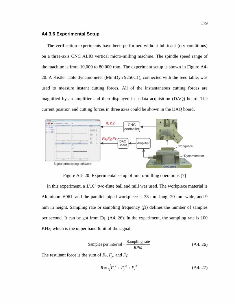
A4.3.6 Experimental Setup ..................................................................................... 179
A4.3.7 Experimental Result .................................................................................... 180
A4.4 Conclusion ......................................................................................................... 185
Page 8
viii
List of Tables
Table 1: The relation of optimal cluster numbers and termination criterion ε for a NURBS
surface ................................................................................................................ 42
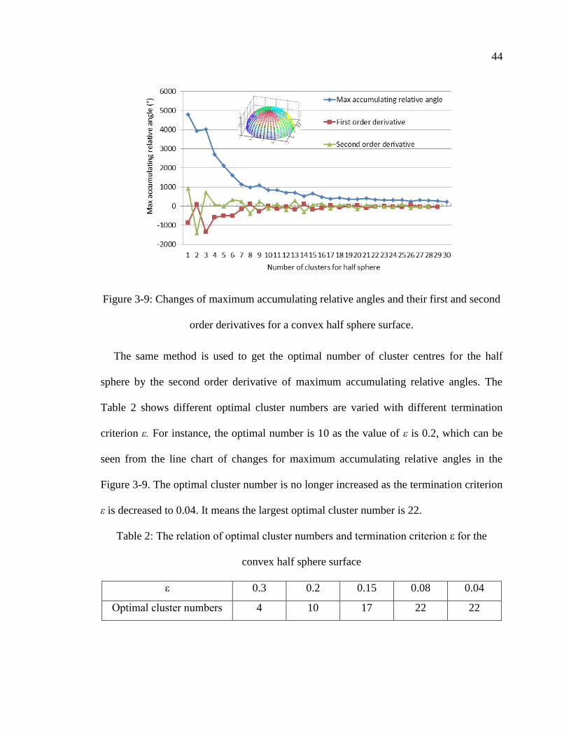
Table 2: The relation of optimal cluster numbers and termination criterion ε for the
convex half sphere surface ................................................................................. 44
Table 3: Relationship of surface features, curvatures, gouging and the tool orientation
methods .............................................................................................................. 56
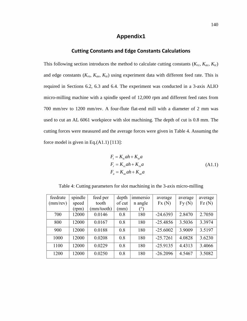
Table 4: Cutting parameters for slot machining in the 3-axis micro-milling ................. 140
Table 5: The parameters for four groups’ experiments .................................................. 181
Page 9
ix
List of Figures
Figure 1-1: The research roadmap ...................................................................................... 6
Figure 2-1: Iso-parametric toolpath for NURBS surface .................................................. 16
Figure 2-2: Iso-planar toolpath for curved surface ........................................................... 16
Figure 2-3: Surface patches by cluster centers [11] ......................................................... 18
Figure 2-4: The A-map for tool orientation [32] .............................................................. 20
Figure 2-5: Coordinate systems and lead-tilt angles [13] ................................................. 21
Figure 2-6: Triad formed by principal curvature directions and the surface normal [34] 22
Figure 2-7: Euler- Meusnier sphere [39] .......................................................................... 22
Figure 2-8: Gouge-free condition [39] .............................................................................. 23
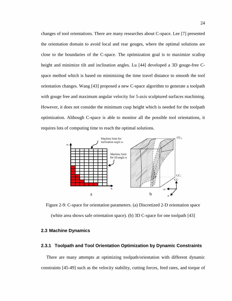
Figure 2-9: C-space for orientation parameters. (a) Discretized 2-D orientation space
(white area shows safe orientation space). (b) 3D C-space for one toolpath
[43] ................................................................................................................ 24
Figure 2-10: Accessibility cones on the CC point mesh [52] ........................................... 25
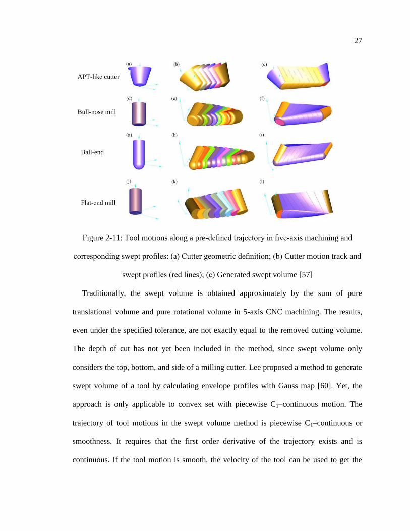
Figure 2-11: Tool motions along a pre-defined trajectory in five-axis machining and
corresponding swept profiles: (a) Cutter geometric definition; (b) Cutter
motion track and swept profiles (red lines); (c) Generated swept volume [57]
....................................................................................................................... 27
Figure 2-12: Tool engagement regions and decomposed motion [67] ............................. 29
Figure 2-13: Distribution of chip thickness (a) Horizontal feed; (b) Vertical feed [68]... 29
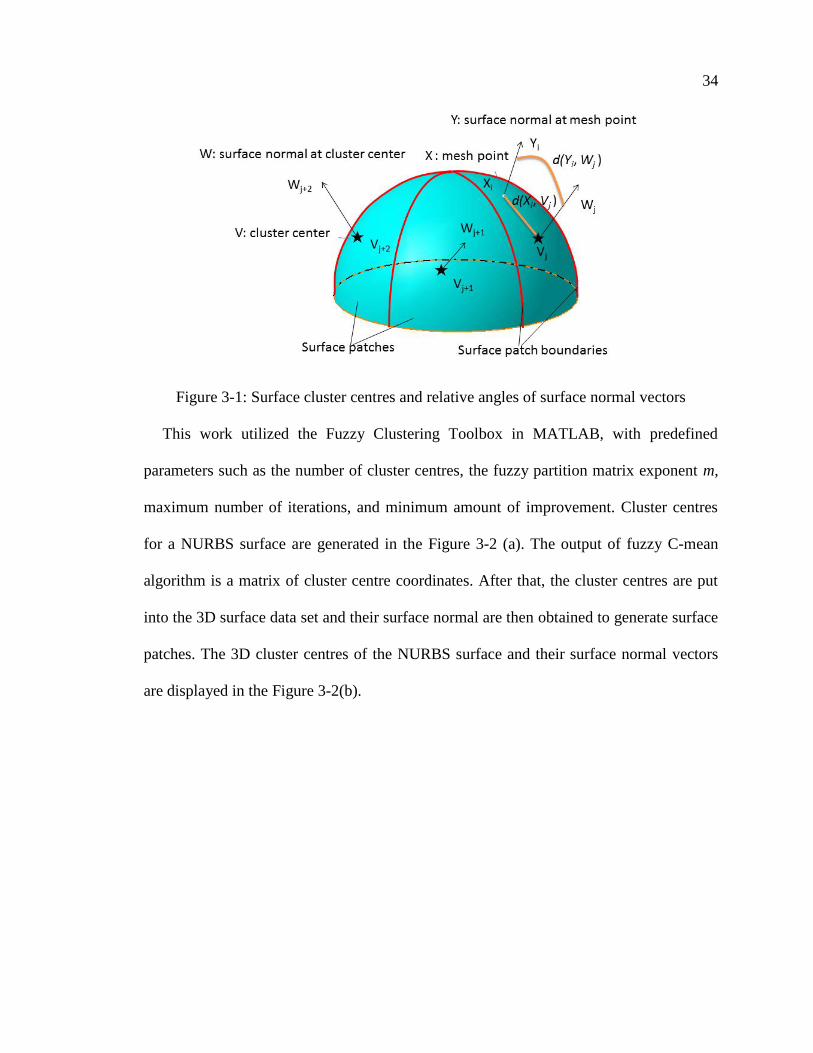
Figure 3-1: Surface cluster centres and relative angles of surface normal vectors ........... 34
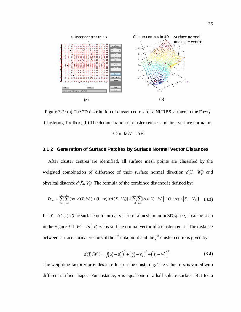
Figure 3-2: (a) The 2D distribution of cluster centres for a NURBS surface in the Fuzzy
Clustering Toolbox; (b) The demonstration of cluster centres and their
surface normal in 3D in MATLAB ............................................................... 35
Figure 3-3: Surface divisions with tool orientations for a NURBS surface from 1 cluster
to 10 clusters .................................................................................................. 37
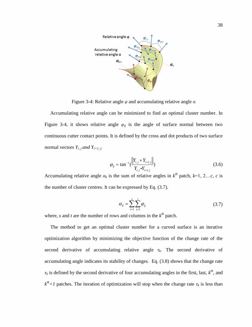
Figure 3-4: Relative angle φ and accumulating relative angle α ...................................... 38
Figure 3-5: Changes of accumulating relative angles with different numbers of cluster
centres and ith
cluster for a NURBS surface in 3D bar chart. ........................ 40
Figure 3-6: Changes of maximum accumulating relative angles and their first and second
order derivatives for a NURBS surface ......................................................... 41
Figure 3-7: Surface divisions with tool orientations for a convex half sphere surface from
1 cluster to 10 clusters. .................................................................................. 42
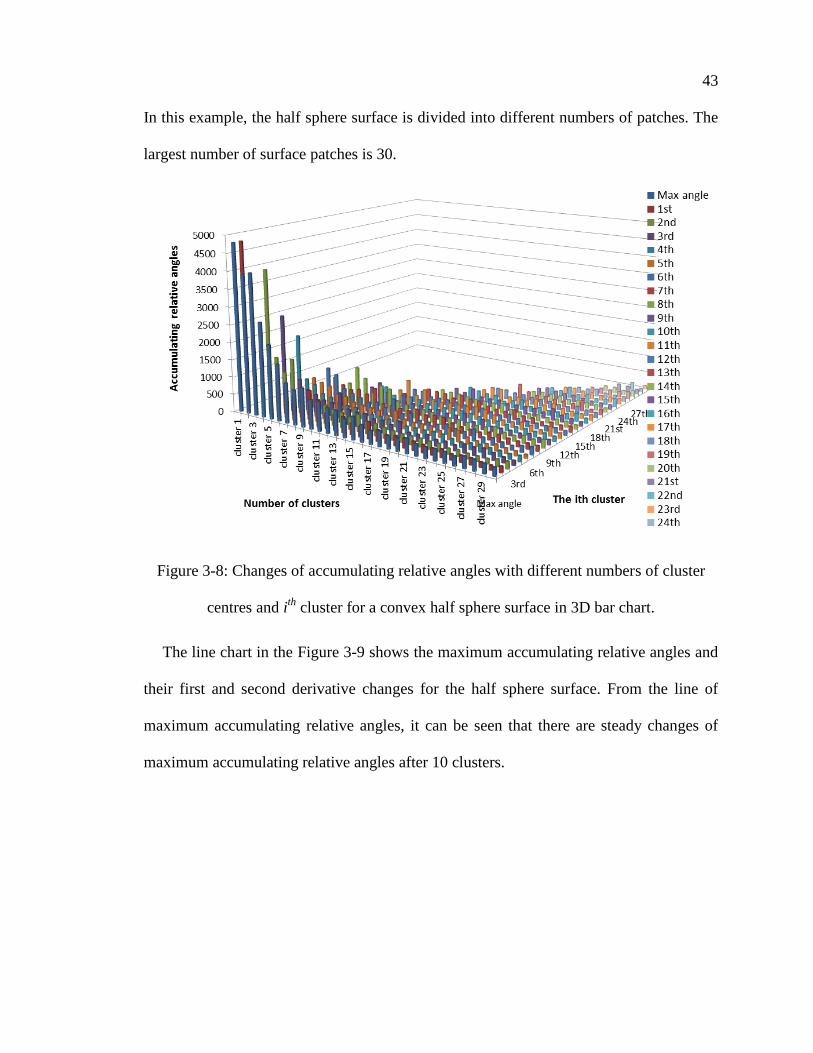
Figure 3-8: Changes of accumulating relative angles with different numbers of cluster
centres and ith
cluster for a convex half sphere surface in 3D bar chart. ....... 43
Page 10
x
Figure 3-9: Changes of maximum accumulating relative angles and their first and second
order derivatives for a convex half sphere surface. ....................................... 44
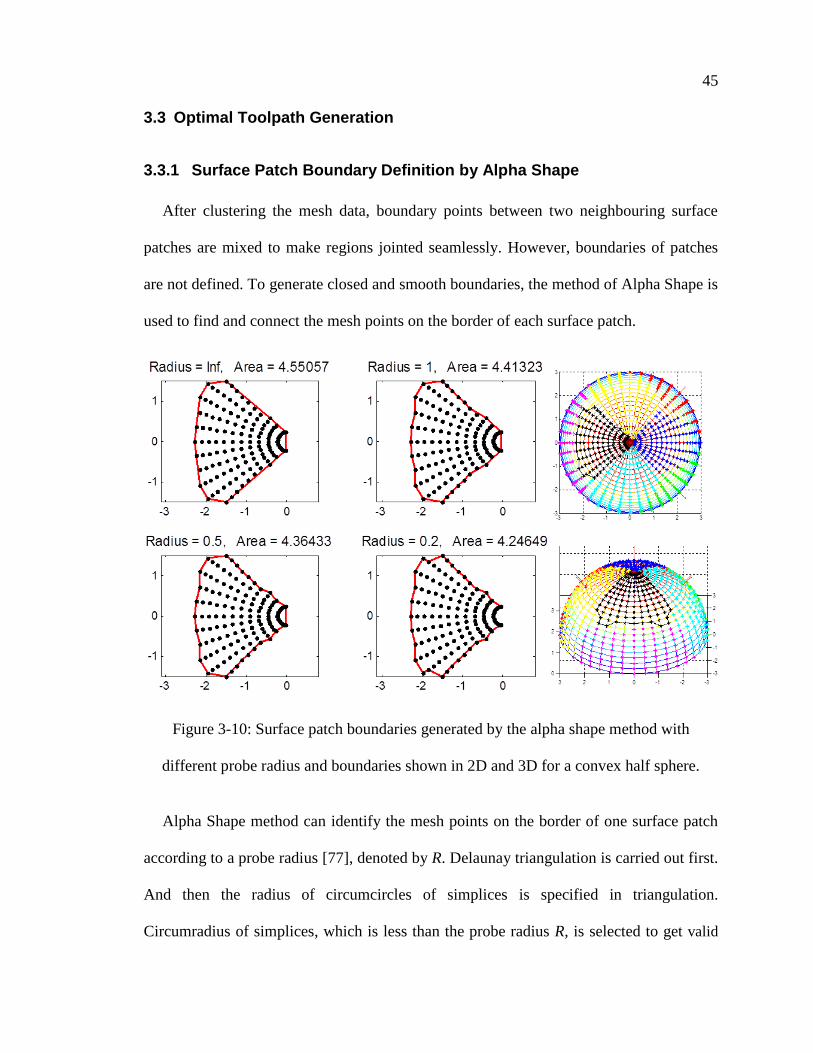
Figure 3-10: Surface patch boundaries generated by the alpha shape method with
different probe radius and boundaries shown in 2D and 3D for a convex half
sphere. ............................................................................................................ 45
Figure 3-11: (a) 5 cluster centres of a convex half sphere generated by the clustering
toolbox; (b) Toolpath generation for one surface patch ................................ 47
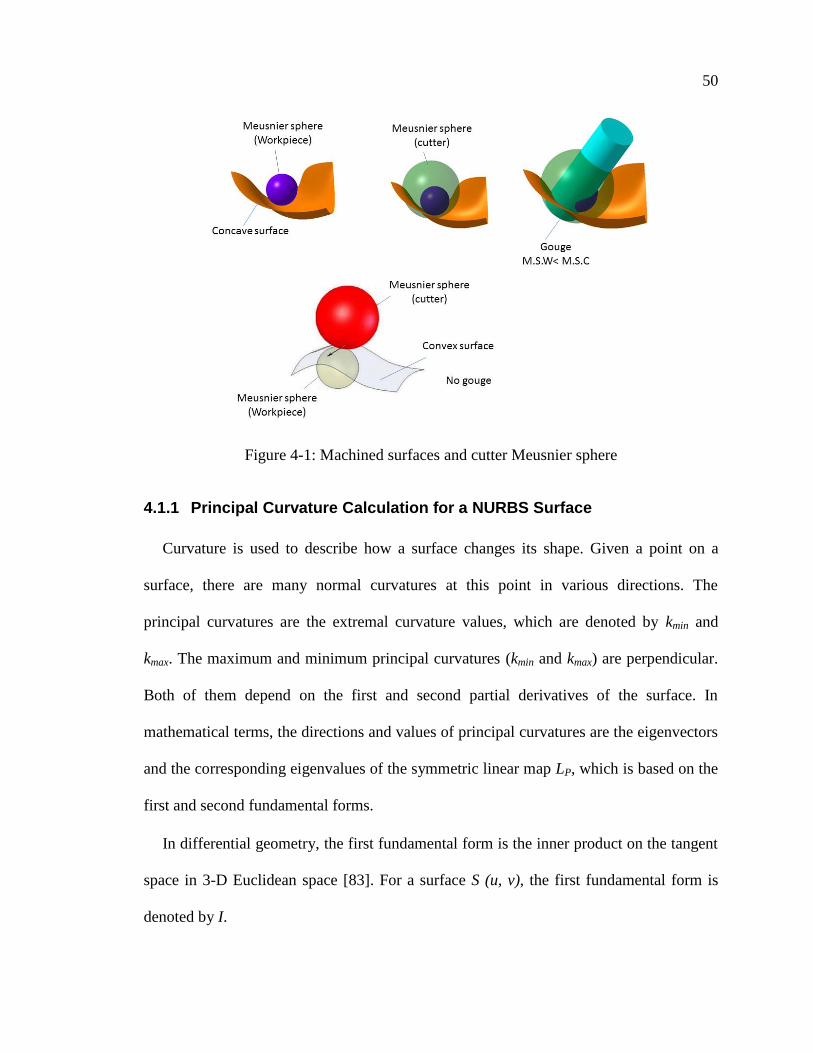
Figure 4-1: Machined surfaces and cutter Meusnier sphere ............................................. 50
Figure 4-2: Inclination angle α confirmation .................................................................... 53
Figure 4-3: Tool orientation in the Meusnier sphere method ........................................... 54
Figure 4-4: The relation of tool axis with the surface normal and the smallest principal
curvature direction. ........................................................................................ 54
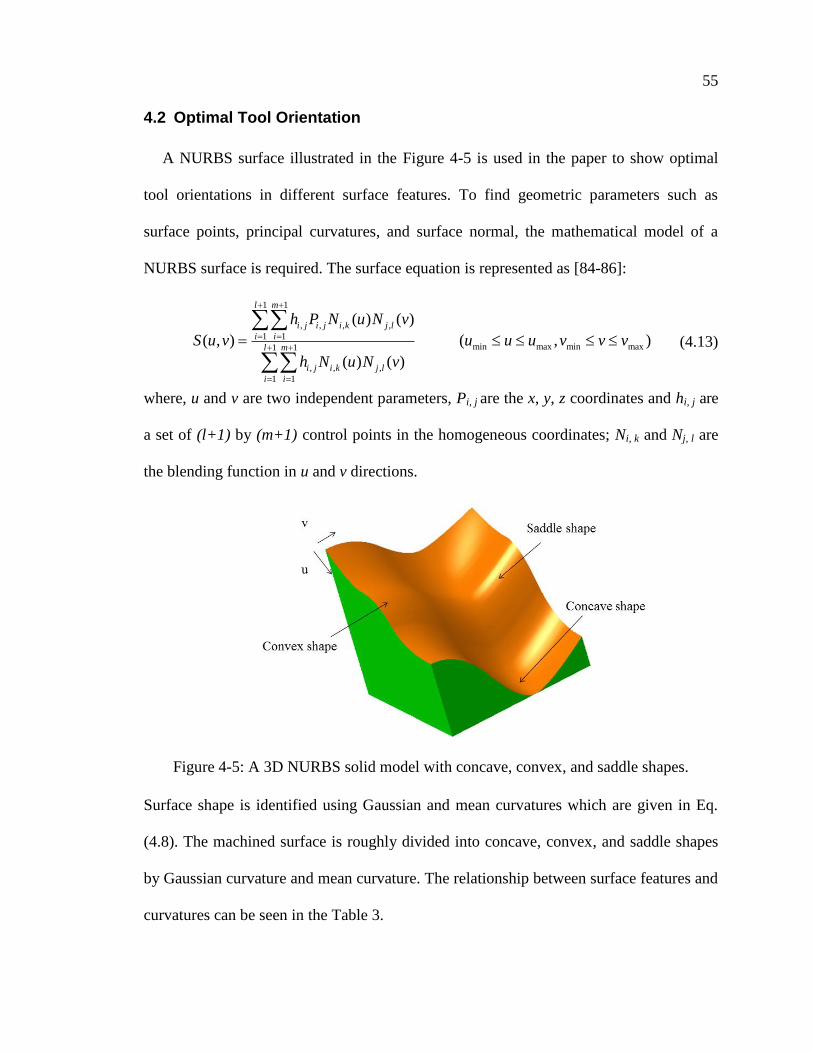
Figure 4-5: A 3D NURBS solid model with concave, convex, and saddle shapes. ......... 55
Figure 4-6: (a) Divisions on grid points of the NURBS surface in 3D; (b) Surface features
in 2D .............................................................................................................. 56
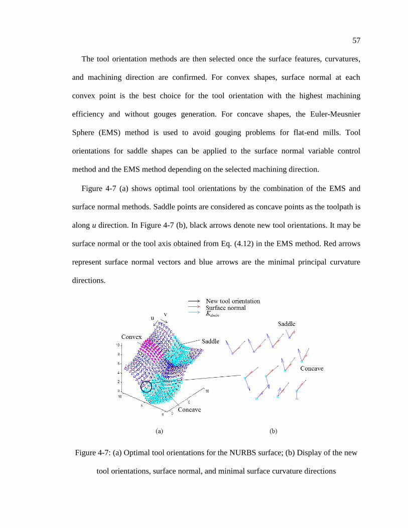
Figure 4-7: (a) Optimal tool orientations for the NURBS surface; (b) Display of the new
tool orientations, surface normal, and minimal surface curvature directions 57
Figure 5-1: The tool motion in the local coordinate system and illustration of rotation
angles. ............................................................................................................ 62
Figure 5-2: Intersections of two ellipses for a tool at two continuous NC positions ........ 64
Figure 5-3: Tetrahedron in a parallelepiped...................................................................... 66
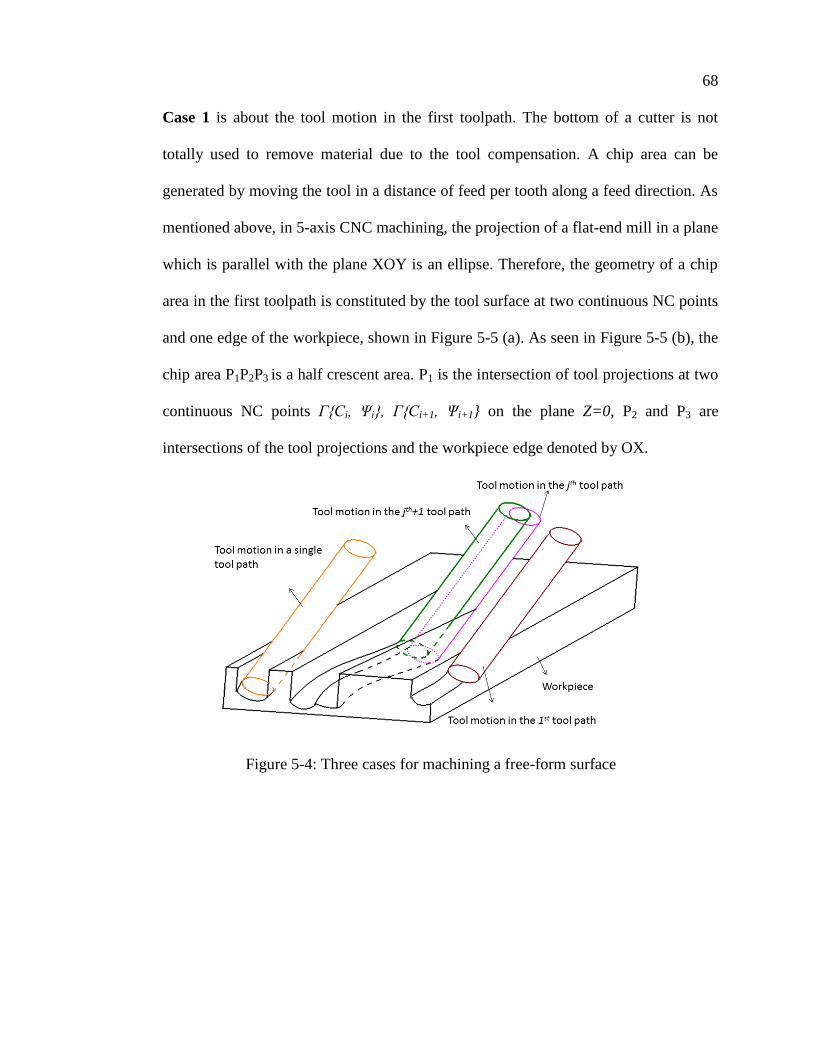
Figure 5-4: Three cases for machining a free-form surface .............................................. 68
Figure 5-5: (a) Tool simulation in Case 1 of the first toolpath machining; (b) The chip
area for the first toolpath on the plane z=0 .................................................... 69
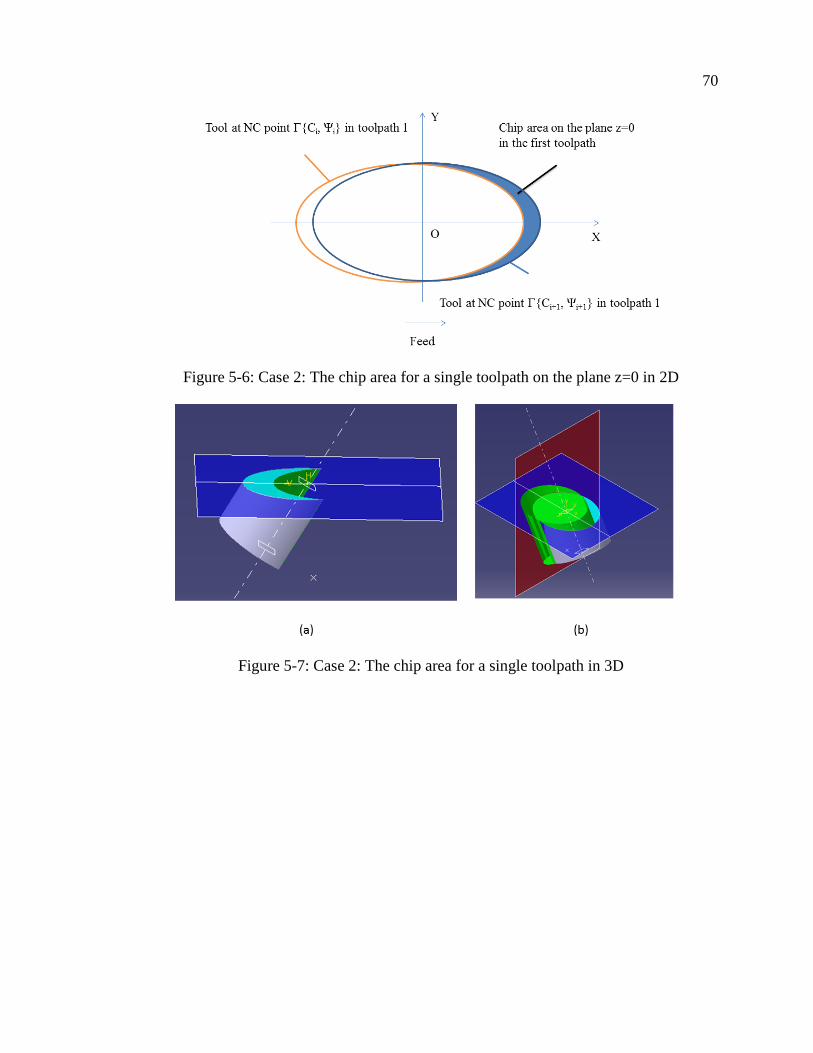
Figure 5-6: Case 2: The chip area for a single toolpath on the plane z=0 in 2D .............. 70
Figure 5-7: Case 2: The chip area for a single toolpath in 3D .......................................... 70
Figure 5-8: Case 2: Valid chip outline by layers in a single toolpath ............................... 71
Figure 5-9: Case 3: (a) Tool motion in the second toolpath; (b) Removed chip in two
adjacent NC points ........................................................................................ 71
Figure 5-10: The chip area for one toolpath considering its neighboring toolpath on the
plane z=0 in case 3 ........................................................................................ 72
Figure 5-11: (a) The valid chip outline generation in two continuous toolpaths (b) Valid
chip outline points; (c) Solid chip shape by the Alpha Shape method .......... 73
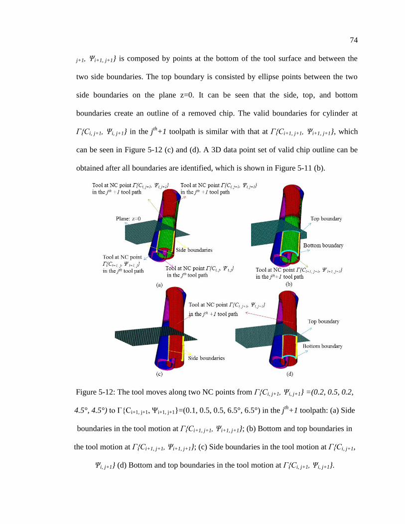
Figure 5-12: The tool moves along two NC points from Γ{Ci, j+1, Ψi, j+1} =(0.2, 0.5, 0.2,
4.5°, 4.5°) to Γ{Ci+1, j+1, Ψi+1, j+1}=(0.1, 0.5, 0.5, 6.5°, 6.5°) in the jth
+1
toolpath: (a) Side boundaries in the tool motion at Γ{Ci+1, j+1, Ψi+1, j+1}; (b)
Bottom and top boundaries in the tool motion at Γ{Ci+1, j+1, Ψi+1, j+1}; (c) Side
boundaries in the tool motion at Γ{Ci, j+1, Ψi, j+1} (d) Bottom and top
boundaries in the tool motion at Γ{Ci, j+1, Ψi, j+1}. ......................................... 74
Page 11
xi
Figure 5-13: Determination of instantaneous chip thickness: (a) Tool motions at two
adjacent NC points; (b) Tool projections on A-A section ............................. 76
Figure 5-14: (a) Chip shape outline points; (b) Sliced chip area for layers; (c) Chip
volume consists of sliced parallelepipeds ..................................................... 78
Figure 5-15: Chip thickness on different layers ................................................................ 79
Figure 5-16: Cutter-workpiece engagement domain in 2D .............................................. 80
Figure 5-17: Cutter-workpiece engagement domain from a removed chip volume: (a) 9
slices with 60 interval points; (b) 15 slices with 100 interval points ............ 81
Figure 5-18: (a)-(c) Displays how the sliced volume is gradually removed in the free-
form surface machining ................................................................................. 82
Figure 5-19: Cutting geometry of a flat-end mill.............................................................. 84
Figure 5-20: (a) Simulation of machining a 3D curve on a free form surface, workpiece
size: 50×50×20 mm3, tool diameter: 10 mm; (b) The simulation of tool
motions in MATLAB. ................................................................................... 85
Figure 5-21: Chip volume simulation for the first toolpath .............................................. 86
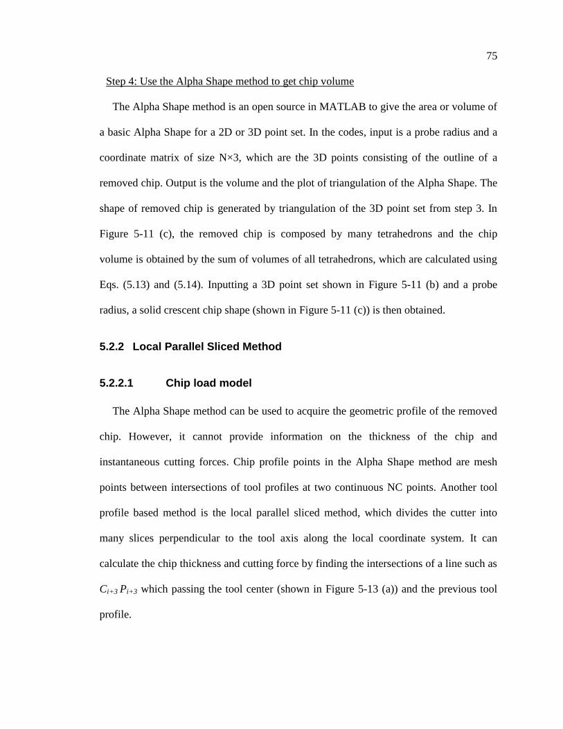
Figure 5-22: Chip volume simulation for the second toolpath ......................................... 87
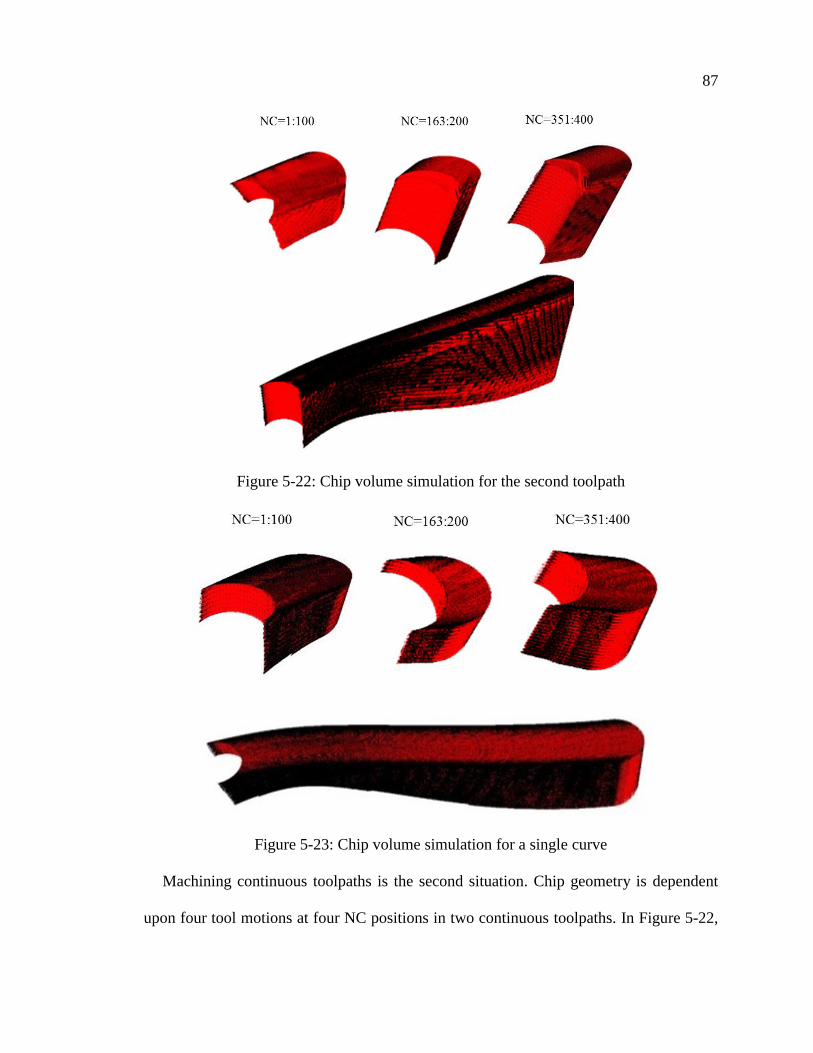
Figure 5-23: Chip volume simulation for a single curve .................................................. 87
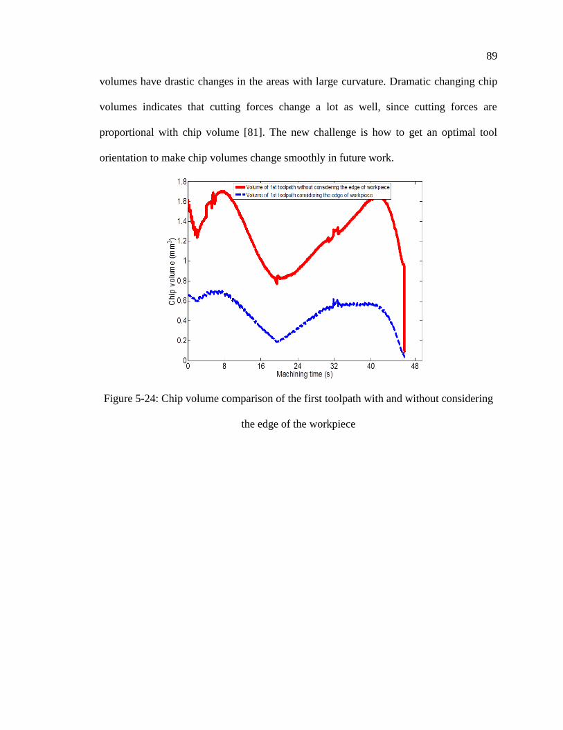
Figure 5-24: Chip volume comparison of the first toolpath with and without considering
the edge of the workpiece .............................................................................. 89
Figure 5-25: Volume comparison of the second toolpath with and without considering the
first toolpath. ................................................................................................. 90
Figure 5-26: Simulated cutting forces in X, Y and Z directions for the whole toolpath .. 91
Figure 5-27: Predicted X, Y and Z forces for five revolutions in 5-axis CNC machining
with a flat-end mill ........................................................................................ 91
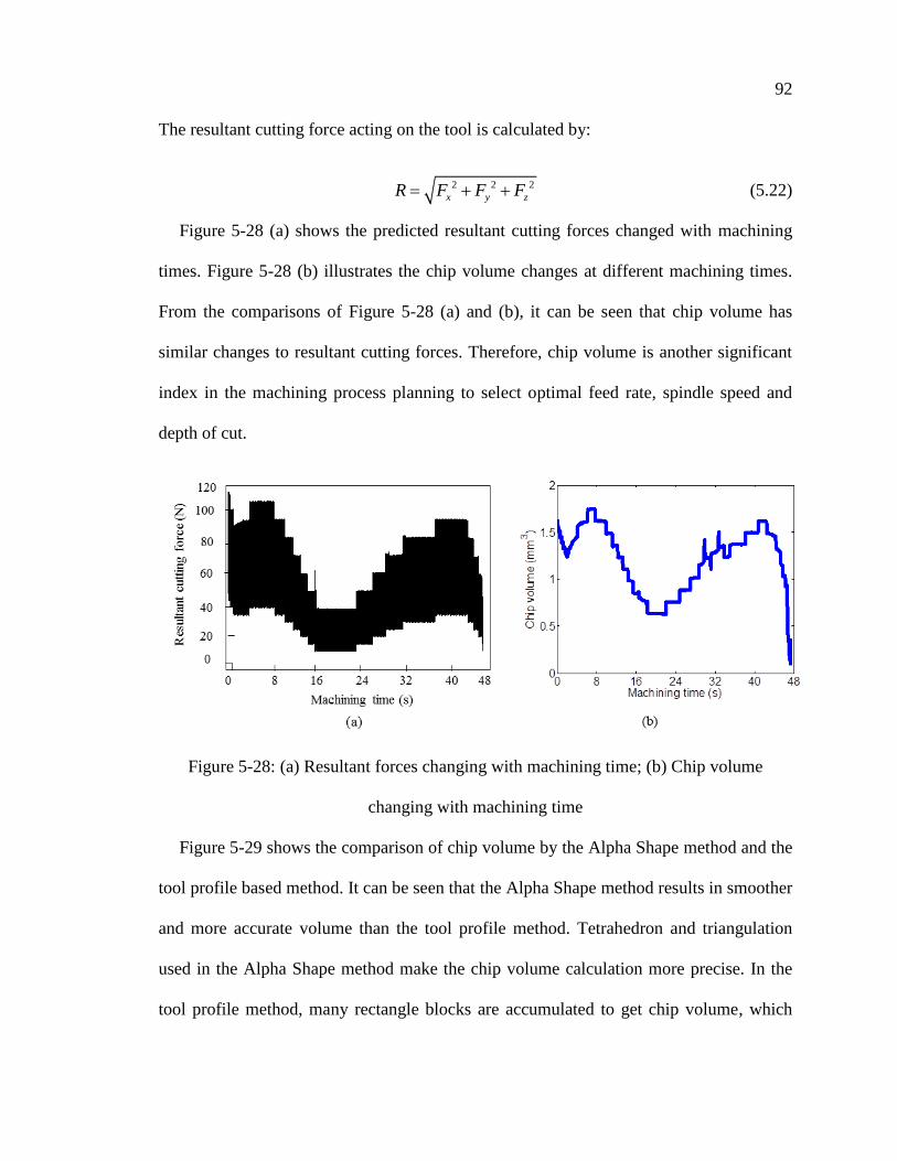
Figure 5-28: (a) Resultant forces changing with machining time; (b) Chip volume
changing with machining time ...................................................................... 92
Figure 5-29: Comparison of chip volume by the Alpha Shape method and the tool profile
based method ................................................................................................. 93
Figure 5-30: Comparison of NC points got by MasterCAM and the uniform interpolation
method ........................................................................................................... 94
Figure 5-31: Measured and predicted cutting forces changing with rotation angles in three
revolutions. .................................................................................................... 95
Figure 6-1: The Tri-dexel workpiece model in 3D. ........................................................ 100
Figure 6-2: Boolean subtraction and chip thickness generation ..................................... 102
Figure 6-3: Chip thickness for non-uniform distributed chip geometry ......................... 104
Figure 6-4: Chip thickness on the Tri-dexel workpiece.................................................. 105
Figure 6-5: The non-uniform distributed chip shape ...................................................... 106
Figure 6-6: The uniform distributed chip shape and redefined chip thickness ............... 108
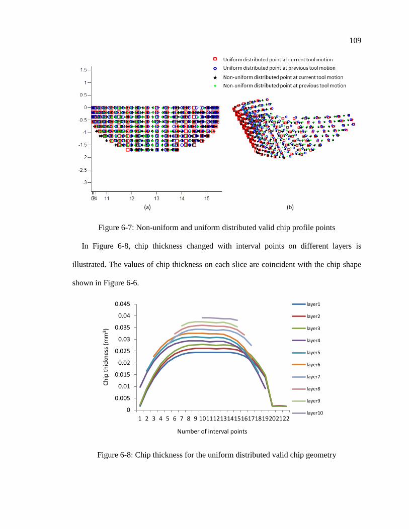
Figure 6-7: Non-uniform and uniform distributed valid chip profile points .................. 109
Figure 6-8: Chip thickness for the uniform distributed valid chip geometry ................. 109
Page 12
xii
Figure 6-9: Cutting simulation of tool removing in the Tri-dexel workpiece ................ 110
Figure 6-10: Varied depth of cut in the workpiece method ............................................ 111
Figure 6-11: Cutting force model of a flat-end mill ....................................................... 113
Figure 6-12: Comparison of simulated cutting forces by the workpiece and the tool based
methods ....................................................................................................... 114
Figure 6-13: (a)-(c) Simulated cutting forces by the Tri-dexel workpiece method; (b) (e)-
(g) Simulated cutting forces by the tool based method ............................... 115
Figure 6-14: Resultant cutting forces by the workpiece method .................................... 116
Figure 6-15: Comparison of chip volume by the tool based method and the workpiece
method ......................................................................................................... 116
Figure 6-16: The pocket toolpath .................................................................................... 118
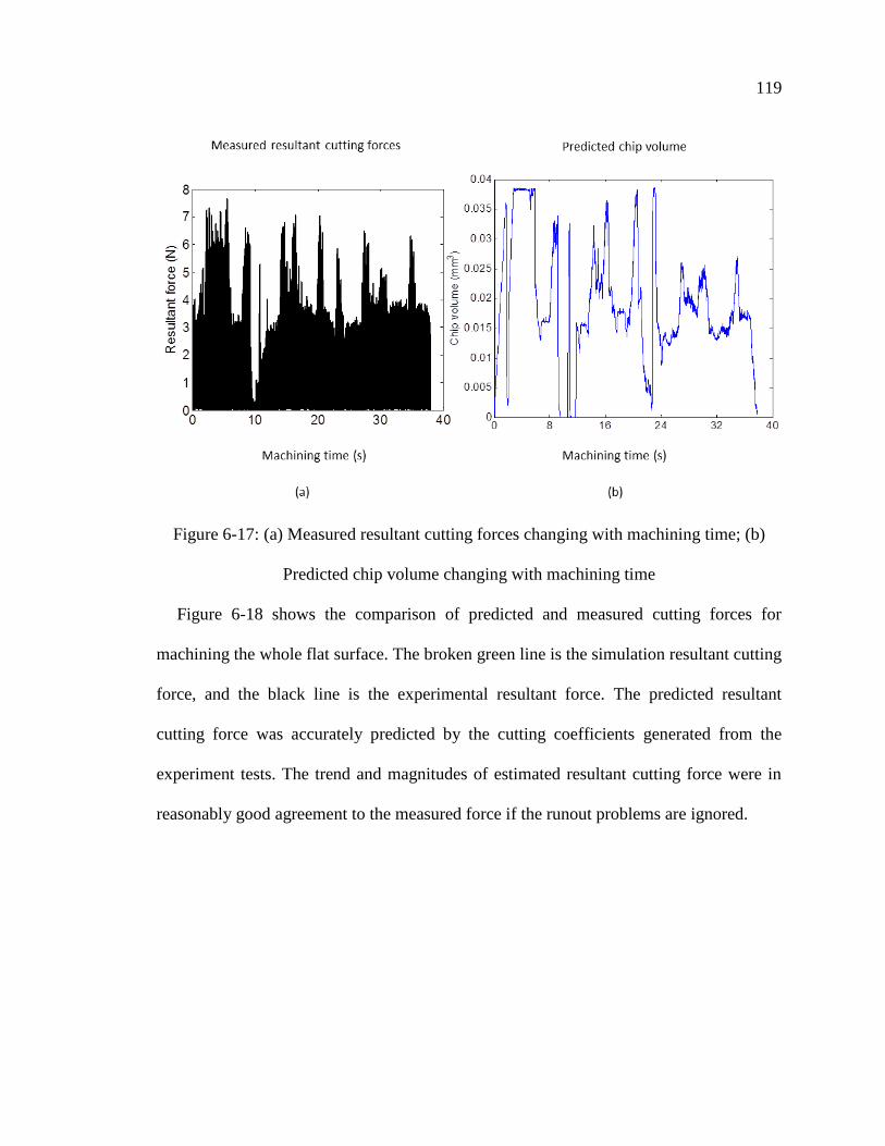
Figure 6-17: (a) Measured resultant cutting forces changing with machining time; (b)
Predicted chip volume changing with machining time ............................... 119
Figure 6-18: Comparison of simulation and experimental resultant forces in 3-axis
milling ......................................................................................................... 120
Figure 7-1: A CFRP 3D chip model ............................................................................... 128
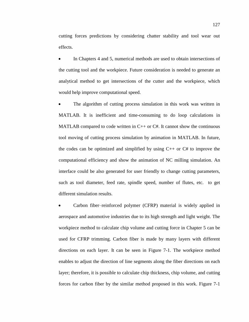
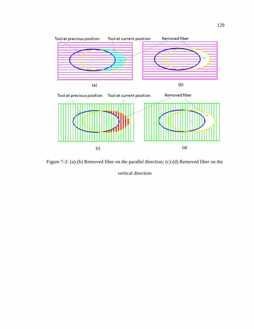
Figure 7-2: (a)-(b) Removed fiber on the parallel direction; (c)-(d) Removed fiber on the
vertical direction .......................................................................................... 129
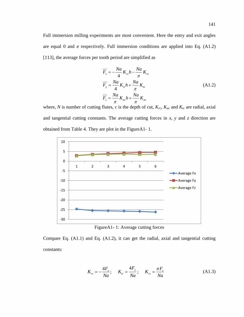
FigureA1- 1: Average cutting forces .............................................................................. 141
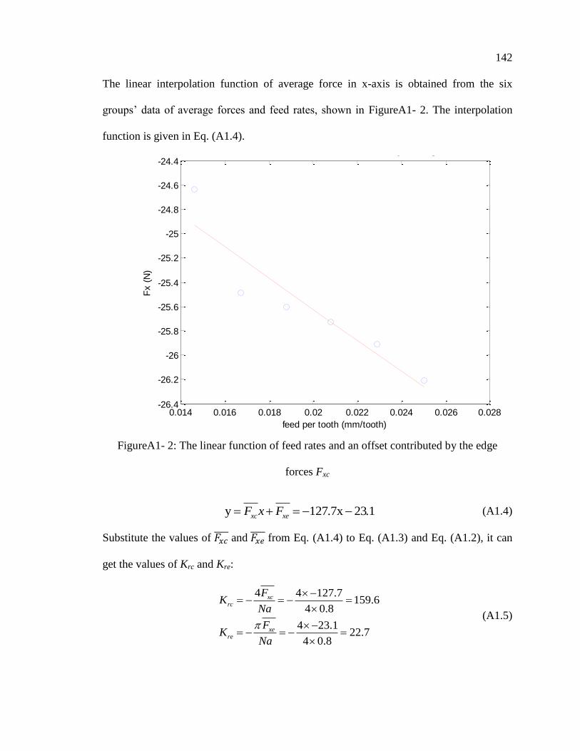
FigureA1- 2: The linear function of feed rates and an offset contributed by the edge
forces Fxc ..................................................................................................... 142
FigureA1- 3: The linear function of feed rates and an offset contributed by the edge
forces Fyc ..................................................................................................... 143
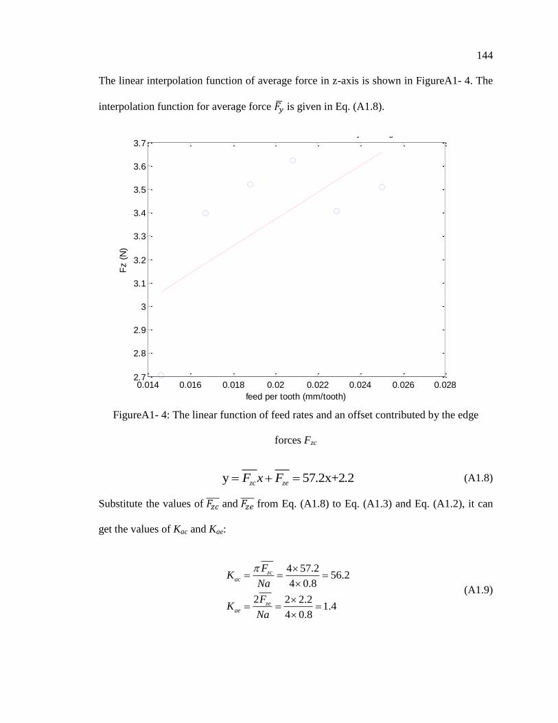
FigureA1- 4: The linear function of feed rates and an offset contributed by the edge
forces Fzc ...................................................................................................... 144
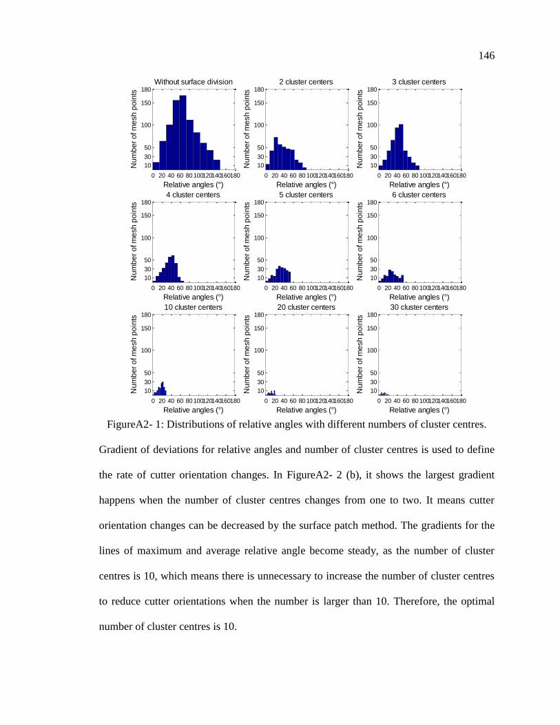
FigureA2- 1: Distributions of relative angles with different numbers of cluster centres.
......................................................................................................................................... 146
FigureA2- 2: (a) Relation of cluster centre numbers and the maximum and average
relative angles; (b) the change rates of cluster centre numbers and maximum and average
relative angles. ................................................................................................................ 147
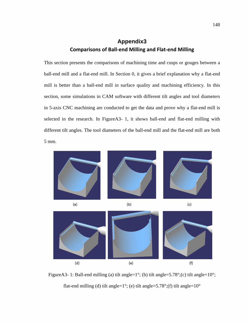
FigureA3- 1: Ball-end milling (a) tilt angle=1°; (b) tilt angle=5.78°;(c) tilt angle=10°;
flat-end milling (d) tilt angle=1°; (e) tilt angle=5.78°;(f) tilt angle=10° ..... 148
FigureA3- 2: (a) comparison of machining time with different tilt angles between ball-
end milling and flat-end milling .................................................................. 149
FigureA3- 3: (a) ball-end milling in several toolpaths, D=5mm, tilt angle=5.78°; (b) flat-
end milling in several toolpaths, D=5mm, tilt angle=5.78°;(c) ball-end
milling in one toolpath, D=50mm, tilt angle=0°; (d) flat-end milling in one
toolpath, D=50mm, tilt angle=90°............................................................... 150
FigureA3- 4: (a) comparison of machining time with different tool diameters between
ball-end milling and flat-end milling ........................................................... 151
Page 13
xiii
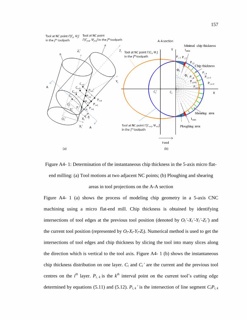
Figure A4- 1: Determination of the instantaneous chip thickness in the 5-axis micro flat-
end milling: (a) Tool motions at two adjacent NC points; (b) Ploughing and
shearing areas in tool projections on the A-A section ................................. 157
Figure A4- 2: (a) Ploughing and shearing volume; (b) Ploughing and shear areas on
layers ........................................................................................................... 160
Figure A4- 3: A free-form surface in micro-milling with a flat-end mill ....................... 161
Figure A4- 4: The interpolated toolpath ......................................................................... 161
Figure A4- 5: Comparison of the total, ploughing and shearing volume ....................... 162
Figure A4- 6: A 3D chip geometry of a micro ball-end mill feed in the horizontal
direction ....................................................................................................... 163
Figure A4- 7: The projection in the slice plane when the angle ϕ is zero ...................... 164
Figure A4- 8: Coordinate rotation for upward direction machining ............................... 167
Figure A4- 9: Small segments of a curve in cubes ......................................................... 168
Figure A4- 10: A 3D curve machining ........................................................................... 168
Figure A4- 11: Process faults with parallel offset runout ............................................... 169
Figure A4- 12: The ploughing and shearing volume calculation flowchart ................... 172
Figure A4- 13: Two different toolpaths: a) Straight lines and down-ramping, b) A straight
line ............................................................................................................... 173
Figure A4- 14: The changes of shearing and ploughing volumes with the height of kth
slice z(k)for slot machining ......................................................................... 174
Figure A4- 15: The Voxel and Boolean method: Chip volume simulation for (a) Slot
machining; (b) Straight lines and down-ramping machining ...................... 175
Figure A4- 16: Slot machining: Chip volume simulations changing with the number of
samples. Spindle speed=40,000 rpm, depth of cut=0.1mm, ft =0.75 µm/tooth
..................................................................................................................... 176
Figure A4- 17: Straight line and down-ramping machining: chip volume simulations
changing with rotation angle θ. Spindle speed=20,000 rpm, depth of cut=0.2-
0.7mm, ft =1.5 µm/tooth .............................................................................. 177
Figure A4- 18: Slot machining: Chip volume simulations changing with rotation angle θ
ignoring runout. Spindle speed=40,000 rpm, depth of cut=0.1mm, ft =0.75
µm/tooth ...................................................................................................... 178
Figure A4- 19: Slot machining: Chip volume simulations changing with rotation angle θ
considering runout, ε=0.01µm, spindle speed=40,000 rpm, depth of
cut=0.1mm, ft =0.75 µm/tooth ..................................................................... 178
Figure A4- 20: Experimental setup of micro-milling operations [7] .............................. 179
Figure A4- 21: Measured resultant cutting forces with machining times ....................... 181
Figure A4- 22: Measured resultant cutting forces for the slot machining. Spindle
speed=40,000 rpm, depth of cut=0.1mm, ft =0.75 µm/tooth ....................... 183
Page 14
xiv
Figure A4- 23: The surfaces generated by the ball end milling processes: (a) Depth of cut
dc=100 µm, ft =0.75 µm/tooth; (b) dc=200 µm, ft =0.75 µm/tooth; (c) dc=150-
600 µm, ft =1.5 µm/tooth; (c) dc=200-700 µm, ft =1.5 µm/tooth ................. 184
Figure A4- 24: Topography of the machined surfaces in a 3D surface measurement
machine ....................................................................................................... 185
Page 15
xv
Acknowledgments
I am grateful to my supervisors, Professor Zuomin Dong and Professor Martin B.G. Jun,
for their generous support, encouragement, kindness, understanding, and awesome
supervision. I thank them for revealing to me the fascinating world of tool-part geometry
and dynamics of 5-axis CNC machining.
I would also like to acknowledge my friends and colleagues in the Advanced
Manufacturing Research Laboratory at the University of Victoria: Yanqiao Zhang,
Abdolreza Bayesteh, Salah Erfurjani, Farid Ahmed, Max Rukosuyev, and Junghyuk Ko
from whom I learned a lot over the past four years.
Finally, I would like to thank my family, Yanchang Luo, Guilin Cheng, Kai Luo, and
Jinrong Cheng for their love and support throughout the lengthy process of my PhD work,
and for their patience and guidance at the difficult moments during my life.
Page 16
1
Introduction Chapter 1:
1.1 Background and Motivation
1.1.1 Toolpath and Orientations
Compared with traditional 3-axis CNC machining, 5-axis CNC milling provides better
tool accessibility, thus increasing material removal rate, reducing machine setup time,
and producing better surface quality for sculptured surfaces. The CNC
toolpath/orientation planning involving the identification of optimal tool orientation for
5-axis CNC machining is much more complicated than the traditional CNC toolpath
planning for 3-axis machining. 5-axis CNC machining matters more than ever before to
many industries from automobile industries, aerospace, energy to mould industries [1].
Dramatic tool orientation changes as machining a surface with large curvature have
become a significant issue, due to slow rotational axis movements and the less rigid
machine-cutter-part system. A 5-axis CNC machine is less rigid than the corresponding
three-axis counterpart, due to the two additional rotational axes. 5-axis CNC machining
uses five synchronized motions to reach different portions of the machined surface.
However, these 5 axes of motion are not created as equal. The first three axes are
normally accomplished by the conventional linear motions of a conventional 3-axis CNC
machine with higher stiffness and response time due to the rigid machine tool structure
and the larger electric drives. The last two axes of rotation are commonly accomplished
by two smaller drives on the mill head. These less rigid axes of rotation motions also
present slower rate of change and response time. Furthermore, drastic changes in cutter
Page 17
2
orientation lead to undesirable surface problems such as overcutting, overlap, and
changing cutting forces.
Good rigidity and high precision can satisfy high accuracy demand during machining.
The shorter tool length in 5-axis CNC machine inherently reduces the rigidity and
feedrate compared with 3-axis CNC machines. The increased rigidity of CNC machine
provides better cutting capability and performance and retains accuracy and repeatability
at the highest levels. Yet, the rigidity is based on the machine body and rotational heads.
It is difficult to change the rigidity after CNC machines are designed. Therefore, it is
better to consider other approaches to improve the cutting performance.
For each tool location in a toolpath, there are numerous choices for the selection of a
cutter inclination. Most existing methods for tool orientations are relative to the surface
normal vector at every cutter contact (CC) point [7]. However, there is a drawback for the
surface normal accessibility. For a machined surface area with large curvature, the tool
orientation tends to suffer drastic changes that lead to larger velocity, acceleration, and
jerk on the rotational axes of the machine. Drastic changes in cutter orientation lead to
undesirable surface problems such as overcutting and overlap and unsmooth cutting force
[8, 9]. Therefore, smooth tool motions are necessary. Tool orientation variation and the
change from one CC point to the next should be minimized. To avoid dramatic tool
orientation changes, it is beneficial to generate a fast execution toolpath and small
changes of tool postures by machining surfaces patch-by-patch with similar surface
orientation, identified by the fuzzy clustering method and similar surface normal
variations. Chapter 3 will give more details about toolpaths generated by the fuzzy
clustering technique and the surface normal method.
Page 18
3
Today, to avoid cutter-part surface interference/gouge at large curvature areas and to
simplify toolpath/orientation planning, a small diameter ball-end mill is commonly used
during machining [2]. This leads to low machining efficiency and large cusps for areas of
the surface with small curvature. Large diameter end cutters present a more rigid and
capable tool with a varying cutter curvature from the radius of the cutter to infinity (in
principle) to support better cutter-part curvature match, leading to much improved
machining efficiency and surface quality [3]. Therefore, it is more sensible to select flat-
end mills for sculptured surface machining. However, flat-end mills cannot easily avoid
curvature gouging problems. It is still challenging to tool orientations using a flat-end
cutter for sculptured surfaces without gouging generation in 5-axis CNC machining. The
control and planning of the tilt angles of the rotational cutter are much more challenging
due to the complex cutter and part surface interaction in 5-axis machining, particularly
when a flat-end mill is used. To improve machining efficiency and the surface quality of
the finished part, the flat-end mill will be focused on in this research, and new methods
will be introduced for gouge avoidance in concave surface milling and for complicated
chip volume and cutting forces calculations.
Currently, commercial Computer Aided Manufacturing (CAM) software can generate
toolpaths automatically. However, the software still has some problems generating
optimal and flexible tool orientations for sculptured surfaces. To avoid gouges, CAM
software tends to select a small diameter ball-end mill for machining which causes low
machining efficiency. Furthermore, CAM system requires the user to select a tool
orientation following a trial and error approach [4-6]. Firstly, cutter orientations are
created by a user-defined strategy like “surface-normal machining” and “tilted through
Page 19
4
curve”; the toolpath has to be simulated and modified if gouges occur. The traditional
trial and error approach to avoid gouges is inconvenient; therefore, a new approach
should be generated to avoid gouging automatically. In this work, an optimal tool
orientation based on the combination of the Euler-Meusnier Sphere (EMS) method and
the surface normal method to avoid gouges and improve machining efficiency will be
discussed in Chapter 4 to avoid gouges and improve machining efficiency.
1.1.2 Machine Dynamics
Researches of machining dynamic play a significant role when high efficiency is required
[10-12]. The kinematics of tool motions is the most investigated aspect when smooth tool
orientation changes are needed. The tilt and lead angles affect mechanics and dynamics
of the machining process in terms of cutting forces, cutting forces coefficients, torque,
chip thickness, stability, and tool breakage [13]. In this research, instant cutting forces
and cutting volume predictions are mainly considered to optimize the last remaining
planning variable feed rate to achieve high machining efficiency and surface quality in 5-
axis CNC machining using flat-end mills.
Most of the previous research on 5-axis machining has focused on the geometric
aspects such as toolpath/tool orientation generation and machine dynamics aspects
separately [14]. But not too much previous research considers the combination of
geometry and dynamics. Cutter-part surface geometry is linked to dynamics through chip
volume for sculptured surfaces in 5-axis CNC machining. However, there are many new
problems generated when geometry and dynamics are considered together. For dynamics,
it is better to select a toolpath that has maximum cutting force/volume while the height of
cusps remains within the specified tolerance zone. For 5-axis CNC machining, cutting
Page 20
5
forces are predicted with respect to inclination and lead angles. Cutting forces are
changed with varied tool orientations even if the cutting parameters such as feed rate,
depth of cut, and spindle speed are the same. There is an existing conflict: two rotation
angles for the maximum cutting forces may not be same with rotation angles obtained by
the geometry method for gouging avoidance. Therefore, optimal toolpath and tool
orientation should be selected to obtain the maximum cutting force and removed material
volume while the height of cusps is under the given machining tolerance.
In Vericut, cutting conditions are shown in the status display and available when
stepping through the program using NC Program Review. The feature shows detailed
information about the cutter’s engagement with material, including: axial depth, radial
width, volume removal rate, chip thickness, maximum surface speed, and contact area.
Lots of studies about ball-end mill cutting forces have been done in recently; however,
few studies have been done for flat-end mills in 5-axis CNC machining.
5-axis CNC machining is widely used to produce various components with complex
geometry while potentially providing better tool accessibility to complex surfaces,
producing more accurate curved surfaces, increasing material removal rate, and reducing
machine setup time [15]. For 3-axis CNC machining using a flat-end mill, chip thickness
is constant along the axial direction, and chip volume calculation is relatively simple by
discretizing the tool along the axial direction. However, in 5-axis CNC machining using a
flat-end mill, the contact area between the cutter and machined surface changes all the
time due to the inclination and rotation angles. The varying contact area causes
challenges with calculating chip volume and engagement zone. Knowing values of
removed chip volume can help choose optimal cutting parameters. Therefore, chip
Page 21
6
thickness and chip volume calculation using flat-end mills in 5-axis CNC machining
should be studied to offer another approach to select optimal cutting parameters.
Predicting cutting forces is significant in the planning process. Cutting force estimates
are useful when choosing optimal cutting parameters such as feedrate, depth of cut to
improve the machining efficiency, and surface quality. The cutting force calculations can
also be used for cutter deflection, tool breakage detection, and process planning. In this
work, two numerical methods will be developed to calculate chip volume and cutting
forces in Chapters 5 and 6.
1.2 Research Contributions
This research aims at introducing new enabling techniques for the combined optimal
toolpath, cutter orientation, and chip volume/cutting force calculations for optimal feed
rates to maximize machining efficiency and obtain better surface quality in 5-axis CNC
machining of curved surfaces using flat-end mills.
Figure 1-1: The research roadmap
Page 22
7
Figure 1-1is the research roadmap that summarizes how research contributions fit into
the overall effort to obtain high machining efficiency and good surface quality. The
research firstly considers slow responses and weakness of machine tool rotation axes to
generate optimal tool path by machining surfaces into patches, ensuring machining
efficiency and machine-cutter-part system stiffness. It also explores the largest cutting
edge and best curvature match for optimal tool orientation to obtain maximum removal
material with no gouge generation. Lastly, it covers to chip volume and cutting force
modeling and calculations using machining dynamics models to optimize the last
remaining planning variable, feed rate, to accomplish high machining efficiency and
surface quality for 5-axis machining of curved surfaces using a flat-end mill. The
following is a list of contributions toward methods of optimal toolpath/orientation
generation and chip volume/cutting force prediction in 5-axis CNC milling using a flat-
end mill that have been made over this work:
Optimal toolpath generation: To avoid sharp cutter orientation changes by
machining surfaces patch-by-patch with similar surface orientation, an optimal
toolpath identified by fuzzy clustering technique and surface normal variations
control method was proposed to generate fast CNC machining (see Section 3.1 of
Chapter 3). The optimal number of surface patches or surface point clusters is
identified by minimizing accumulating changes of relative angles, discussed in
Section 3.2. To generate closed and smooth boundaries, the computational geometry
method of Alpha Shape is used to find and connect the mesh points on the border of
each surface patch. This work was presented at the 2014 Virtual Machining Process
Technology Conference [16].
Page 23
8
Optimal tool orientation generation: An optimal and flexible tool orientation
method based on the combination of Euler-Meusnier spheres (EMS) method and
surface normal variations control method is developed in Section 4.1 of Chapter 4.
Better cutter-surface curvature matches and gouge avoidance at the cutter contact
point (CCP) are obtained by applying the EMS principle to determine the optimal
cutter orientation at each cutter contact point on the toolpath for concave surfaces;
the surface normal variation control method is used for convex surfaces due to its
higher efficiency and no gouging issue; selection of one of these methods in tool
orientation determination for saddle shapes is based on the direction of the CNC
toolpath relative to the surface curvature change.
In 5-axis CNC machining, maximum feed rates can achieve the highest machining
efficiency. However, feed rates are always changed, as the synchronized lineal and
rotational movements of rotation axes, and the complicated cutter-part contact geometry.
It becomes complicated to select optimal feed rates for free-form surface machining in 5-
axis CNC machines using flat-end mills. In this work, chip volume and cutting force
predictions will be proposed for the feedrate optimization. Compared to ball-end mill
machining, the chip volume and cutting force prediction in 5-axis CNC machining with
flat-end mills are much more challenging due to the complexity of cutter-part surface
geometry interaction. A ball-end mill has constant curvature so the cutter location is
easier to be determined, while the curvature for a flat-end mill at each CC point varies
with different tilt and lead angle in 5-axis CNC machines; therefore, the discrete method
for chip volume and cutting force calculation with flat-end mills is much more
complicated than ball-end mills. To overcome these challenges, this author developed
Page 24
9
two numerical approaches to generate chip model and calculate chip volume and cutting
forces. These developments induce several more contributions to the field:
Chip volume calculation by Alpha Shape method: A computational geometry-
based Alpha Shape method is applied to model the volume and shape of the removed
chip during 5-axis milling (see section 5.2.1 of Chapter 5). The 3D chip modeling
requires identifying the chip boundary that defined by a valid tool geometric outline
at two continuous NC points. Since it is difficult to calculate the intersections of two
arbitrary cylinders using closed-form analytical model through translations and
rotations, a numerical method has been used in this work to obtain the intersections
of two arbitrary cylinders by dividing them into many thin layers along the z axis
direction. Three cases of toolpaths are considered to obtain the chip volume and
simulate the real tool motions. The Alpha Shape method provides an efficient and
robust way to calculate chip volume for arbitrary tool orientations because a series of
complicated trigonometric equations, to get intersections of tool motions at two
arbitrary positions, are replaced by a numerical method in ALGORITHM (see
Section 5.2.1.3 of Chapter 5). This work was presented at the 2015 Virtual
Machining Process Technology Conference [17].
Chip volume/cutting force calculations by the tool based method: Alpha Shape
method can display solid chip shape and calculate chip volume with a fast computing
time; however, chip thickness and cutting forces cannot be calculated by this method.
A new approach— the local parallel sliced method (see Section 5.2.2) is then
presented to obtain cutter-workpiece engagement domains, where the depth of cut
and cutting flutes entering/exiting the workpiece are required to predict instant
Page 25
10
cutting forces. Local parallel sliced method divides the cutter into many slices
perpendicular to the tool axis along the local coordinate system. On each layer, the
removal chip area is a polygon shape generated by connecting two neighbouring
edge points on the current and previous tool edges. The total chip volume is obtained
by adding all polygon areas along axial direction.
The tool profile based method can save computing time to calculate chip volume and
cutting forces. However, it cannot be used in the pocket toolpath. That is why another
approach—the workpiece based method is proposed.
Chip volume/cutting force calculations by Tri-dexel workpiece method: The Tri-
dexel workpiece method (presented in Section 6.1 of Chapter 6) is robust for use with
any kinds of toolpaths to predict chip volume and cutting forces; it gets chip volume
and cutting forces through the intersection of the tool envelope and continuously
updated the workpiece rather than from the tool intersections at four continuous
positions in two neighboring toolpaths. The removed volume is obtained by subtracting
the cutter-workpiece engagement zone. To reduce the complexity of 3D Boolean
subtraction, the Tri-dexel workpiece is sliced into many 2D laminated layers along z-
axis direction in Section 6.1.2. Chip volume can be obtained from the non-uniform
distributed chip model by the intersections of the tool envelope and the workpiece, but
cutting force calculations cannot be applied by this model. Extending the non-uniform
distributed chip model that can only predict chip volume, a uniform distributed chip
model has been added to calculate cutting forces by finding the same column index of a
flat-end mill. The workpiece method is robust for use with to any toolpath to predict
cutting forces; however, the computing time is much longer than the tool profiled
Page 26
11
method since the workpiece is updated with many line segment operations such as
intersection and subtraction at every tool motion in the whole toolpath.
Chip ploughing volume prediction: It is a challenging task to avoid ploughing
problems in micro-machining. When the cutter crosses the minimum chip thickness
boundary, it enters into the ploughing zone with no material removed. Therefore, it is
important to know the ploughing effects in micro-milling. Chip ploughing volume
prediction for 5-axis micro flat-end milling is presented in Section A4.2. The tool
based model proposed in Section 5.2.2 is used to calculate chip thickness and
ploughing volume. Ploughing zone is the area where the chip thickness is less than
the minimum chip thickness; while in the shearing zone, the chip thickness is larger
than the minimum chip thickness. Chip geometry and chip ploughing volume for a
micro ball-end mill are discussed in Section A4.3. Different cutting conditions, such
as feed rate, spindle, and depth of cut, are tested in a 3-axis micro CNC machine with
a ball-end mill to better understand the ploughing effects in micro machining and to
increase cutting efficiency. Two different CNC toolpaths are used to simulate the
machining process and to obtain the relation between chip ploughing volume and
rotation angle.
1.3 Dissertation Outline
This dissertation presents work in improving current toolpath and orientation methods
and exploring the combination of cutter-workpiece geometry and machine dynamics in 5-
axis CNC machining using flat-end mills. This research emphasizes optimal
toolpath/orientation generation and the development and implementation of numerical
Page 27
12
approaches to calculate chip volume and cutting forces for feed rate optimization by a
flat-end mill in 5-axis CNC machining.
Chapter 2 is the literature reviews for three aspects: toolpath planning, tool orientation
methods, and machine dynamics.
Chapter 3 starts with presenting an optimal toolpath by machining a surface patch-by-
patch using fuzzy clustering techniques and similar surface normal variations control.
This reduces the range of the rotational axes’ motions and helps to avoid sharp cutter
orientation changes. This chapter also gives a discussion on optimal number of surface
patches establishment by minimizing accumulating relative angle. At the end of this
chapter, the computational geometry method of Alpha Shape is discussed to generate
closed and smooth boundaries of surface patches.
Chapter 4 presents an optimal tool orientation based on the combination of the EMS
method and the surface normal variable control method. The EMS method considers the
best curvature match to achieve maximum removal material with no gouge generation.
The surface normal variable control method can also obtain the highest machining
efficiency by the largest cutting edge. A NURBS with three surface features such as
concave, convex, and saddle is selected to give a detailed explanation of the optimal
toolpath approach. Typically, the EMS method is applied to concave parts to avoid local
gouges. The highest efficient tool orientation for a convex surface is along surface normal
directions. For a saddle surface, the EMS method or surface normal method is selected by
machining directions.
Optimal feed rate can be determined by chip volume and cutting forces. However, it is
complicated to calculate chip volume and cutting forces as machining free-form surfaces
Page 28
13
using flat-end mills in 5-axis CNC machining due to the two rotational angles and
flexible changes of tool curvature. It is also challenging to apply the analytical method to
get intersections of two flat-end mills at arbitrary directions. To overcome these
problems, Chapter 5 presents a completely new numerical tool based approach to predict
chip volume and cutting forces. Extending the Alpha Shape method, which can only
predict cutting chip geometry, a parallel slice local volume modeling approach has been
added to predict cutting forces. An experiment for the research of cutting volume and
cutting forces in 3-axis micro CNC machine was conducted. The simulation results for 5-
axis machining were verified by machining experiments through specifying the two
rotation angles to zeros. The simulated and measured forces are shown in reasonably
good agreement in both the trend and magnitudes if the runout effects are ignored.
Chapter 6 improves the chip volume and cutting force predictions in any kinds of
toolpaths by demonstrating a Tri-dexel workpiece method. The tool based method
presented in Chapter 5 can provide fast computing time, but it has limitations in the
application of pocket toolpath. The comparisons of these two numerical approaches are
made by a same case study. Extending the non-uniform distributed chip model that can
only predict chip volume, a uniform distributed chip model has been presented to
calculate cutting forces by finding the same column index of a flat-end mill.
Appendix4 is a relative study of chip ploughing volume in Micro-milling. It is a
challenging task to avoid ploughing problems in micro-machining. When the cutter
crosses the minimum chip thickness boundary, the tool would enter into the ploughing
zone with no material removed. The model proposed in Section 5.2.2 for macro 5-axis
flat end milling works in micro-milling to calculate chip thickness and ploughing volume.
Page 29
14
The ploughing effects for 3-axis micro ball-end milling are also introduced in this
chapter. Two algorithms in this work are demonstrated to get the ploughing volume. To
better understand the ploughing volume problem in micro machining and to increase
cutting efficiency, an experiment testing different axial depths of cut and feed rates was
conducted.
Finally, conclusions and recommendations for future work are discussed in Chapter 7.
Page 30
15
Literature Review Chapter 2:
Toolpath/orientation generation and machine dynamics in 5-axis CNC machining is an
established field and many researchers have already made significant contributions to this
area. The literature summarized in Section 2.1 that several traditional toolpath generation
methods and some new toolpath generation techniques have been developed to improve
machining efficiency and surface quality. Section 2.2 discusses tool orientation
methodologies along with optimization methods that would overcome some limitations.
There are many researches have studied ball-end mill cutting forces in recent years;
Section 2.3 discusses these contributions. One challenge of adopting ball-end mill
machining is time consumption and poor surface quality. Flat-end mills with flexible
curvature changes can help engineers overcome these limitations, but very limited studies
on 5-axis CNC machining using flat-end mills have been carried out due to the
complexity of cutter-part surface geometry interaction.
2.1 Toolpath Planning
Studies on toolpath generation for CNC machine have been conducted for many years.
Traditionally, there are several toolpath generation approaches, such as the iso-planar
[18], iso-parametric [19], and iso-scallop [20].
The iso-parametric approach is widely applied in freeform surfaces [19, 21-23]. There
are two variables to define freeform surfaces along toolpath and toolpath interval
directions. During toolpath planning, one parameter is changed while the other is fixed.
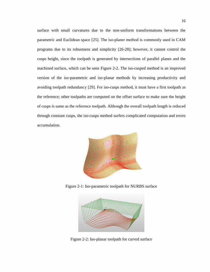
This method has short computing time but long machining time [24]. From Figure 2-1, it
can be seen that iso-parametric toolpaths are commonly much denser in areas of the
Page 31
16
surface with small curvatures due to the non-uniform transformations between the
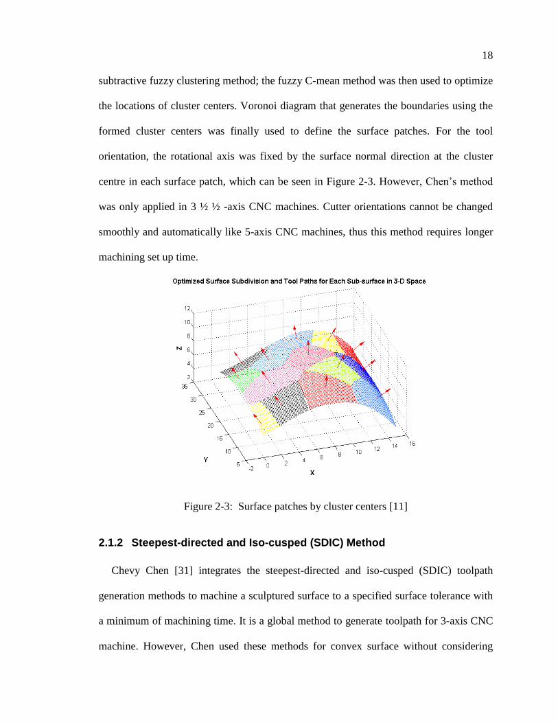
parametric and Euclidean space [25]. The iso-planer method is commonly used in CAM
programs due to its robustness and simplicity [26-28]; however, it cannot control the
cusps height, since the toolpath is generated by intersections of parallel planes and the
machined surface, which can be seen Figure 2-2. The iso-cusped method is an improved
version of the iso-parametric and iso-planar methods by increasing productivity and
avoiding toolpath redundancy [29]. For iso-cusps method, it must have a first toolpath as
the reference; other toolpaths are computed on the offset surface to make sure the height
of cusps is same as the reference toolpath. Although the overall toolpath length is reduced
through constant cusps, the iso-cusps method surfers complicated computation and errors
accumulation.
Figure 2-1: Iso-parametric toolpath for NURBS surface
Figure 2-2: Iso-planar toolpath for curved surface
Page 32
17
Some new toolpath generation techniques have been developed to improve machining
efficiency and surface quality.
2.1.1 Surface Division Machining Toolpath
Machining a surface patch-by-patch is based on dividing the surface into regions by
specified features, and machining each region separately [1]. There are some studies
about toolpath generation based on regions. Ding [26] used the isophote method to
partition a surface into different areas by the angle between the surface normal and that of
the intersecting planes to reduce redundant tool paths. This method makes the toolpath
side steps to be adaptive to the surface geometry features, reducing the total toolpath
length and increasing machining efficiency. However, it was a challenge to connect the
toolpaths of two neighbouring regions to obtain a much smoother surface. Lee [5]
classified a freeform surface according to principal surface curvatures to find optimal tool
orientations. The surface points were sorted into four different types such as convex,
concave, hyperbolic, and parabolic. A flat-end mill was used to machine convex and flat
regions; a ball-end mill was selected to machine small curvature regions. However, tool
changes should be minimized, due to the non-profit added operations. Chevy Chen
proposed a toolpath method based on fuzzy cluster points and the Voronoi diagram [30].
This toolpath was applied to divide the sculptured surface into surface patches. All the
points in each patch have similar surface features such as surface shape and
machinability. The sculptured surface was first classified into convex, concave, and
saddle shapes according to Gaussian/mean curvatures of the surface. After the rough
subdivision, two fuzzy pattern clustering methods were used for the fine surface
subdivision. Cluster centers in a particular surface shape region were first identified by
Page 33
18
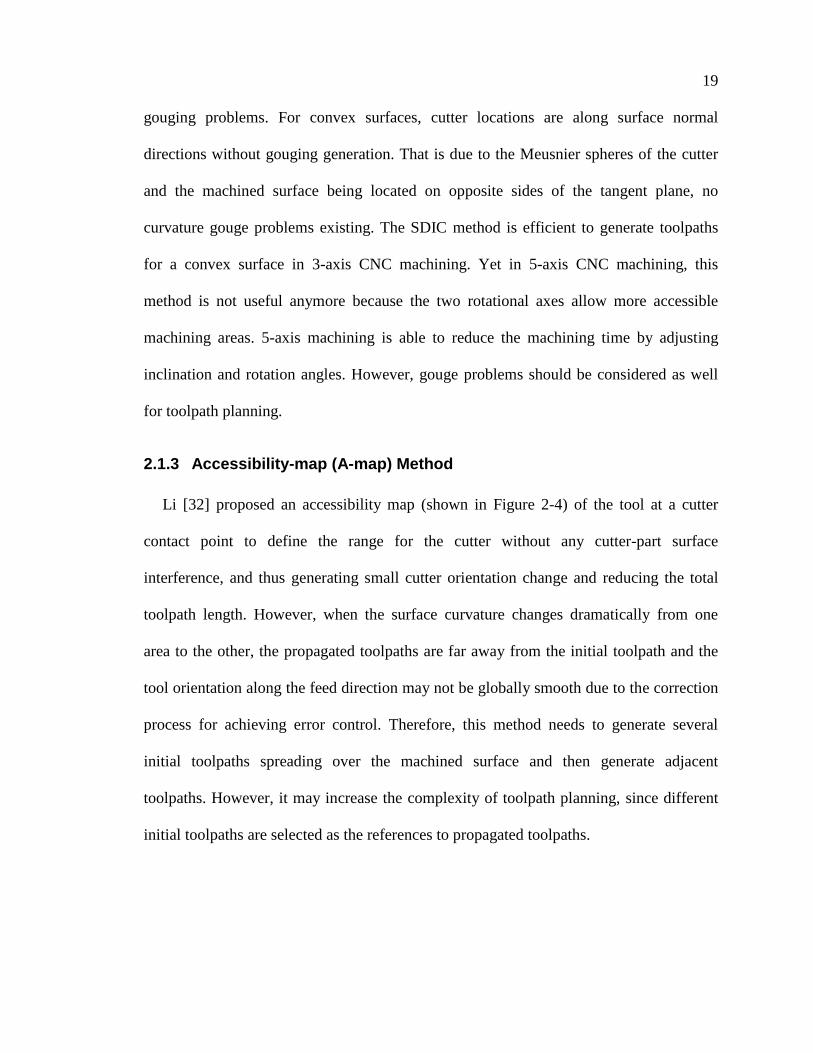
subtractive fuzzy clustering method; the fuzzy C-mean method was then used to optimize
the locations of cluster centers. Voronoi diagram that generates the boundaries using the
formed cluster centers was finally used to define the surface patches. For the tool
orientation, the rotational axis was fixed by the surface normal direction at the cluster
centre in each surface patch, which can be seen in Figure 2-3. However, Chen’s method
was only applied in 3 ½ ½ -axis CNC machines. Cutter orientations cannot be changed
smoothly and automatically like 5-axis CNC machines, thus this method requires longer
machining set up time.
Figure 2-3: Surface patches by cluster centers [11]
2.1.2 Steepest-directed and Iso-cusped (SDIC) Method
Chevy Chen [31] integrates the steepest-directed and iso-cusped (SDIC) toolpath
generation methods to machine a sculptured surface to a specified surface tolerance with
a minimum of machining time. It is a global method to generate toolpath for 3-axis CNC
machine. However, Chen used these methods for convex surface without considering
Page 34
19
gouging problems. For convex surfaces, cutter locations are along surface normal
directions without gouging generation. That is due to the Meusnier spheres of the cutter
and the machined surface being located on opposite sides of the tangent plane, no
curvature gouge problems existing. The SDIC method is efficient to generate toolpaths
for a convex surface in 3-axis CNC machining. Yet in 5-axis CNC machining, this
method is not useful anymore because the two rotational axes allow more accessible
machining areas. 5-axis machining is able to reduce the machining time by adjusting
inclination and rotation angles. However, gouge problems should be considered as well
for toolpath planning.
2.1.3 Accessibility-map (A-map) Method
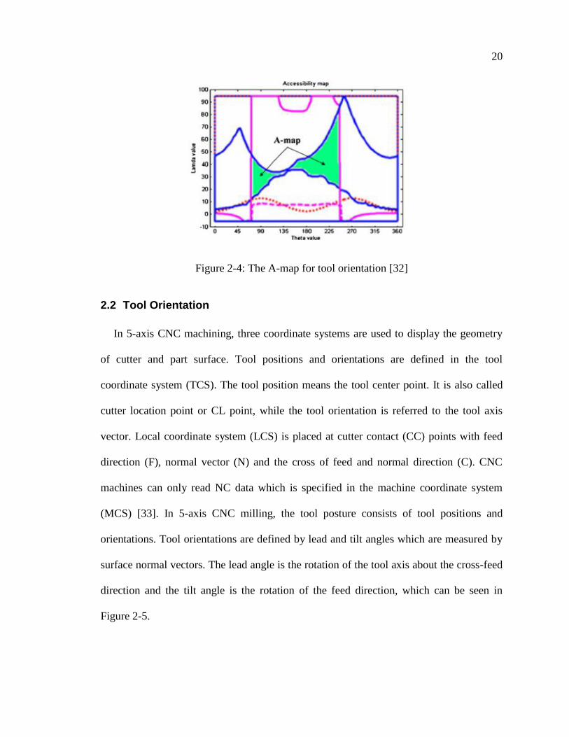
Li [32] proposed an accessibility map (shown in Figure 2-4) of the tool at a cutter
contact point to define the range for the cutter without any cutter-part surface
interference, and thus generating small cutter orientation change and reducing the total
toolpath length. However, when the surface curvature changes dramatically from one
area to the other, the propagated toolpaths are far away from the initial toolpath and the
tool orientation along the feed direction may not be globally smooth due to the correction
process for achieving error control. Therefore, this method needs to generate several
initial toolpaths spreading over the machined surface and then generate adjacent
toolpaths. However, it may increase the complexity of toolpath planning, since different
initial toolpaths are selected as the references to propagated toolpaths.
Page 35
20
Figure 2-4: The A-map for tool orientation [32]
2.2 Tool Orientation
In 5-axis CNC machining, three coordinate systems are used to display the geometry
of cutter and part surface. Tool positions and orientations are defined in the tool
coordinate system (TCS). The tool position means the tool center point. It is also called
cutter location point or CL point, while the tool orientation is referred to the tool axis
vector. Local coordinate system (LCS) is placed at cutter contact (CC) points with feed
direction (F), normal vector (N) and the cross of feed and normal direction (C). CNC
machines can only read NC data which is specified in the machine coordinate system
(MCS) [33]. In 5-axis CNC milling, the tool posture consists of tool positions and
orientations. Tool orientations are defined by lead and tilt angles which are measured by
surface normal vectors. The lead angle is the rotation of the tool axis about the cross-feed
direction and the tilt angle is the rotation of the feed direction, which can be seen in
Figure 2-5.
Page 36
21
Figure 2-5: Coordinate systems and lead-tilt angles [13]
2.2.1 Principal Axis Method (PAM)
Principal Axis Method (PAM) is based on a surface-cutter curvature match at cutter
contact points [34-36]. When the tool is tilted along the feed direction, the minimum tool
curvature is matched to the maximum surface curvature at the CC point. An osculating
plane (shown in Figure 2-6) is a plane that contains the CC point and its surface normal
vector. The curvature is changed from maximum principal curvature to minimum as the
osculating plane is rotated around the normal axis. In Figure 2-6, the two principal
directions and surface normal vector are orthogonal with each other. However, PAM only
considers the cutter contact point; the cutting edge of the tool may penetrate the design
surface and then cause gouges. To remove rear gouging, the tool is tilted until gouging is
eliminated or reduced to a specified tolerance zone, and thus it is suitable for open face
freeform surface [37]. It results in curvatures that are no longer matched and the
effectiveness of the PAM is reduced at the CC point.
Page 37
22
Figure 2-6: Triad formed by principal curvature directions and the surface normal [34]
2.2.2 Euler-Meusnier Sphere (EMS) Curvature Match
Wang [38] presented a 3D model which is based on the new Euler-Meusnier Sphere
(EMS) concept (shown in Figure 2-7) from a generic mathematical and geometric model
of the cutter and surface geometry to avoid gouging for concave surfaces. Given a point
on a surface, there are many normal curvatures at this point in various directions.
Meusnier spheres at this point are determined by these curvatures. The largest and
smallest Meusnier spheres are obtained by the minimum and maximum principle
curvatures.
Figure 2-7: Euler- Meusnier sphere [39]
Page 38
23
The total elimination of curvature gouges can only be accomplished by ensuring that
there is no overlap between the volumes defined by the largest and smallest Meusnier
spheres of the cutter and the machined surface.
Figure 2-8: Gouge-free condition [39]
The EMS curvature match method is a good way for tool orientations to avoid
gouging; however, it may not be optimal for a non-uniform curvature surface and
sometimes this may not be able to iso-cusps machining. The feed direction in iso-cusps
machining cannot always follow the same direction of minimum principal curvature of
the surface. For concave surfaces, curvature match becomes much more difficult from the
bottom to top.
2.2.3 C-space Based Tool Orientation Methods
The machining configuration space (C-space) is used to find optimal tool orientations
by different machining constraints [9, 40, 41]. This method considers local, rear, and
global gouges in machining[42]. The C-space (shown in Figure 2-9) is the tool tilting and
inclination parameter areas without gouging generation [43]. After construction of the C-
space, there is an optimization process to select smaller tilt angles and the minimum
Page 39
24
changes of tool orientations. There are many researches about C-space. Lee [7] presented
the orientation domain to avoid local and rear gouges, where the optimal solutions are
close to the boundaries of the C-space. The optimization goal is to maximize scallop
height and minimize tilt and inclination angles. Lu [44] developed a 3D gouge-free C-
space method which is based on minimizing the time travel distance to smooth the tool
orientation changes. Wang [43] proposed a new C-space algorithm to generate a toolpath
with gouge free and maximum angular velocity for 5-axis sculptured surfaces machining.
However, it does not consider the minimum cusp height which is needed for the toolpath
optimization. Although C-space is able to monitor all the possible tool orientations, it
requires lots of computing time to reach the optimal solutions.
Figure 2-9: C-space for orientation parameters. (a) Discretized 2-D orientation space
(white area shows safe orientation space). (b) 3D C-space for one toolpath [43]
2.3 Machine Dynamics
2.3.1 Toolpath and Tool Orientation Optimization by Dynamic Constraints
There are many attempts at optimizing toolpath/orientation with different dynamic
constraints [45-49] such as the velocity stability, cutting forces, feed rates, and torque of
Page 40
25
a 5-axis machine tool. Farouki [50] proposed an approach to calculate toolpath feed rate
by considering the maximal torque and power of the tool. López de Lacalle [51] used the
prediction of deflection forces as a criterion for the best choice of toolpaths. It provides
the possibility of selecting tool orientations with low deflection forces for geometrical
requirements. Bi introduced an accessibility cone to optimize cutter orientation along
both feed and cross-feed directions [52]. The accessibility cone (shown in Figure 2-10) is
a set of tool orientations from which the cutter contact point is accessed by the cutter
without gouging. This optimization method considers stability of feed velocities and the
smoothness of cutting force at mesh points and only the accessibility cones are needed to
compute, and thus increasing computation efficiency.
Figure 2-10: Accessibility cones on the CC point mesh [52]
2.3.2 Chip Volume in 5-axis CNC Machine
Computing an actual shape of removed material is still challenging [53-56]. There are
some new methods applied to resolve this problem. Sweep volume based on solid method
was introduced by Leuven [57]. Undeformed chip shape can be constructed from the
boundaries of instantaneous engagement domain between a flat-end mill and the
Page 41
26
workpiece [58]. There are two main approaches to calculate the removed chip volume
[57]: (a) computation of swept volume by the tool profile along NC trajectory and (b)
implementation of the Boolean intersection and subtraction of the tool envelope with the
workpiece. The workpiece based methods to calculate removed material in 5-axis
machining is still challenging due to the non-robust 3D Boolean subtraction operation
and complicated process of updating the workpiece [59]. Sweep volume is a tool
representation method introduced by Weinert [53] using solid modelling technique. A
moving frame in 5-axis tool motions was introduced for the solid sweep volume. Swept
profiles were first generated along the NC trajectory. After moving the profiles, a closed-
form envelope surface was created. It can be seen in Figure 2-11. This solid-based
method can obtain a much more precise cutting volume than the discrete method.
However, the swept profiles are complicated to obtain as the cutter has both translational
and rotational motions.
Page 42
27
Figure 2-11: Tool motions along a pre-defined trajectory in five-axis machining and
corresponding swept profiles: (a) Cutter geometric definition; (b) Cutter motion track and
swept profiles (red lines); (c) Generated swept volume [57]
Traditionally, the swept volume is obtained approximately by the sum of pure
translational volume and pure rotational volume in 5-axis CNC machining. The results,
even under the specified tolerance, are not exactly equal to the removed cutting volume.
The depth of cut has not yet been included in the method, since swept volume only
considers the top, bottom, and side of a milling cutter. Lee proposed a method to generate
swept volume of a tool by calculating envelope profiles with Gauss map [60]. Yet, the
approach is only applicable to convex set with piecewise C1–continuous motion. The
trajectory of tool motions in the swept volume method is piecewise C1–continuous or
smoothness. It requires that the first order derivative of the trajectory exists and is
continuous. If the tool motion is smooth, the velocity of the tool can be used to get the
Ball-end
Flat-end mill
APT-like cutter
Bull-nose mill
Page 43
28
swept profile. Otherwise, the swept profile cannot be found. The swept volume method
displays the shape of removed material and can be used for NC verification. However, it
cannot produce the value of chip volume and chip thickness at each NC point to calculate
cutting forces and select optimal cutting parameters. On the other hand, Ferry [61]
generated a swept volume by collecting solid models of the tool together at various NC
points along the tool trajectory. The swept volume was subtracted from the workpiece to
get the finished part. The Parallel Slicing Method (PSM) was used by Ferry to create
cutter-workpiece engagement maps for 5-axis flank machining, with the information of
engagement angles and depth of cut, which is the requirement for predicting cutting
forces. The PSM can obtain the removed volume; however, it is a computationally
inefficient approach to do Boolean operations for achieving the solid model of cutter-
workpiece engagement.
2.3.3 Cutting Force in 5-axis CNC Machine
Predicting the cutting force is significant in the process planning process [11, 33, 49,
62-64]. Cutting volume is the total chip volume of each CC point. Chip thickness is an
important factor to get chip volume and cutting forces. The most popular analytical
method to calculate chip thickness in ball-end milling is the sine product assumption [65]
in which the chip thickness t is simplified as t=f×sinϕ×sink, f is the feed per tooth, ϕ is
the immersion angle, k is the rotation angle along the tool axis. However, this method
causes model errors in axial and tangential directions, especially for small depth of cut
within 10% of cutter radius [66].
Tao Huang [67] proposed that the chip thickness can be calculated by the sum of two
individual cutting conditions with only tilt or lead angle, seen in Figure 2-12.
Page 44
29
Figure 2-12: Tool engagement regions and decomposed motion [67]
Ferry and Altintas [68] presented a method to compute the chip thickness in 5-axis
flank milling by distributing the chip thickness into horizontal and vertical feed
components, which can be seen in Figure 2-13. B. Ozturk [69] mentioned the boundaries
of engagement regions of the ball-end mill and the workpiece to predict cutting forces
more accurately. However, those methods do not calculate the chip thickness considering
both tilt and lead angles.
Figure 2-13: Distribution of chip thickness (a) Horizontal feed; (b) Vertical feed [68]
Page 45
30
For 5-axis CNC machine, cutting forces and cutting volume depend on two rotational
angles, feedrate, depth of cut, toolpath, chip thickness, cutting coefficients, and entry and
exit angles. Chip thickness and cutting forces prediction for 5-axis CNC ball-end milling
has been studied by many researchers [70]. Harshad [71] proposed an analytical method
to predict an uncut chip geometry including chip thickness, length, and width by
instantaneous shear angle in a ball-end milling process. Cutting forces were predicted
considering strain and temperature and shear strength by the Johnson-Cook material
model [71]. Bouzakis [72] developed an algorithm to consider the machining surface
topography, the chip formation, cutting forces, and the corresponding cutting tool
deflection with ball-end mills. Various cutting parameters as surface roughness, feedrate,
radial depth of cut, and tool axis inclination angle were investigated to get chip geometry
and cutting forces. Zhang [73] used the Dexel approach to get cutter-workpiece
engagement for chip thickness and cutting force calculation by finding start and exit
angles of discs through the spherical part of the tool. However, very limited studies on 5-
axis CNC machining using flat-end mills have been carried out [74], due to the
complexity of cutter-part surface geometry interaction. A ball-end mill has constant
curvature, therefore chip geometry is easier to obtain, while the curvature for a flat-end
mill at each cutter contact (CC) point varies with different tilt and lead angles during 5-
axis machining. Thus, the discrete method for chip volume calculation with a flat-end
mill is much more complicated.
Page 46
31
Optimization of 5-Axis CNC Toolpath and Cutter Chapter 3:
Orientation for Machining Free-form Surfaces
An early version of the work proposed in this chapter was presented at the 2014 Virtual
Machining Process Technology conference:
Shan Luo, Zuomin Dong, and Martin B. Jun. Optimization of 5-axis CNC toolpath and
cutter orientation for machining curved surfaces. In Virtual Machining Process
Technology Conference, 2014 [16].
The work presented in this chapter has improved the method further by adding the
process to optimize the number of surface patches.
The original intent of this research was to generate a new 5-axis CNC toolpath and
cutter orientation planning method using fuzzy clustering technique to reduce the range
of the rotational axes’ motions and to avoid sharp cutter orientation changes. A generic
curved surface with half spherical shape and a free-form surface were divided into
patches using the combination of fuzzy cluster method and surface normal variation
control method, discussed in Section 3.1. Fuzzy cluster method is used to get the number
of cluster centres or surface patches; it is discussed in Section 3.1.1. Surface patch
generation is discussed in Section 3.1.2 by selecting surface grid points with similar
surface normal vector distances and creating an accessibility cone area with a set of
surface normal vectors. The optimal number of surface patches or surface point clusters is
identified and discussed in great detail in Section 3.2. Surface patch boundaries using
computational geometry method is introduced in Section 3.3.
Page 47
32
In this research, a method to reduce the range of the two axes of rotation motions is
adopted. 5-axis CNC toolpaths are generated for different portions of the machine
surface, in which the efficient tool orientation has limited variation. This is generated by
dividing the surface into multiple patches in which all machined points share similar
surface normal directions. The method is accomplished through the application of the
fuzzy clustering method. In earlier research, Chen has used the fuzzy clustering method
to generate 3 ½ ½ axis CNC toolpath [75], where the surface is divided into some easy-
to-machine surface patches by cluster points. For each surface patch, the rotational axes
are set up and fixed by the surface normal direction at cluster point. So it is easy if each
surface patch has the same tool orientation. Once the rotational axes are fixed, the static
and dynamic stiffness are increased as a rigid body without the bearing connection.
Fuzzy clustering method used in 3 ½ ½ -axis CNC machine can be improved in 5- axis
CNC machines. Although the machine stiffness is stronger and the cost is cheaper, it is
time-consuming in 3 ½ ½ -axis machining, due to setups of the rotation axis for different
surface patches machining. To increase machine efficiency, 5-axis CNC machines can be
used in the idea of surface patches division. In 5-axis CNC machining, surface patches
are not only generated according cluster points but also similar surface normal vectors at
all machined points in one surface patch.
3.1 Machining Surfaces Patch by Patch Using the Fuzzy Cluster Method
In this work, a mesh of discrete grid points is used to represent a curved surface
through a half sphere surface example. The grid points are clustered into an adequate
number of regions by the fuzzy clustering method. The fuzzy “similarity” of two surface
points is defined by the weighted combination of a difference of their surface normal
Page 48
33
direction and their physical distance or Euclidean distance. The new method divides the
machined surface into patches with limited surface normal variation through three steps:
a) finding cluster centres using Fuzzy C-means clustering (FCM) method; b) identifying
the most similar cluster centre for all surface grid points to form the surface point cluster;
and c) mixing boundary points between two neighbouring surface patches.
3.1.1 Fuzzy C-means Clustering Method
Fuzzy C-means clustering (FCM) is an iterative optimization algorithm to minimize
the objective cost function of J [76]:
2
2
1 1 1 1
( , ) ( ) ( , ) ( )n c n c
m m
ij i j ij i j
i j i j
J u V u d X V u X V
(3.1)
where n and c are the number of data points and cluster centres, respectively; uij
represents the membership of ith
data to jth
cluster centre; m is the fuzzy partition matrix
exponent index; Vj is the jth
cluster centre as shown in Figure 3-1; d (Xi, Vj) is the
Euclidean distance between the ith
data point and jth
cluster centre. X =(x, y, z) represents
the location of a data point in Cartesian coordinates, and V = (u, v, w) represents the
location of a cluster centre. The distance between a data point at ith
data point and
the jth
cluster centre in 3D is defined by:
2 2 2
( , )i j i j i j i jd X V x u y v z w
(3.2)
Page 49
34
Figure 3-1: Surface cluster centres and relative angles of surface normal vectors
This work utilized the Fuzzy Clustering Toolbox in MATLAB, with predefined
parameters such as the number of cluster centres, the fuzzy partition matrix exponent m,
maximum number of iterations, and minimum amount of improvement. Cluster centres
for a NURBS surface are generated in the Figure 3-2 (a). The output of fuzzy C-mean
algorithm is a matrix of cluster centre coordinates. After that, the cluster centres are put
into the 3D surface data set and their surface normal are then obtained to generate surface
patches. The 3D cluster centres of the NURBS surface and their surface normal vectors
are displayed in the Figure 3-2(b).
Page 50
35
Figure 3-2: (a) The 2D distribution of cluster centres for a NURBS surface in the Fuzzy
Clustering Toolbox; (b) The demonstration of cluster centres and their surface normal in
3D in MATLAB
3.1.2 Generation of Surface Patches by Surface Normal Vector Distances
After cluster centres are identified, all surface mesh points are classified by the
weighted combination of difference of their surface normal direction d(Yi, Wj) and
physical distance d(Xi, Vj). The formula of the combined distance is defined by:
1 1 1 1
[ ( , ) (1 ) ( , )] [ (1 ) ]n c n c
n c i j i j i j i j
i j i j
D d Y W d X V Y W X V
(3.3)
Let Y= (x′, y′, z′) be surface unit normal vector of a mesh point in 3D space, it can be seen
in the Figure 3-1. W = (u′, v′, w′) is surface normal vector of a cluster centre. The distance
between surface normal vectors at the ith
data point and the jth
cluster centre is given by:
2 2 2
( , )i j i j i j i jd Y W x u y v z w
(3.4)
The weighting factor α provides an effect on the clustering. The value of α is varied with
different surface shapes. For instance, α is equal one in a half sphere surface. But for a
Page 51
36
curved surface with parallel surface normal, the physical distance is considered as well,
as surface normal distance does not work very well for the clustering.
In the combined distance matrix Dn×c, entries in the ith
row are distances of surface
normal vectors between a mesh point and the jth
cluster centre. The minimal distance in
the ith
row is found first by Eq. (3.5) and its index represents the cluster centre which is
closest to the ith
data point. According to this method, all data points can get their own
closest cluster centre. In other words, each cluster centre has its data points obtained by
the shortest combined distance.
1
min( )n
ic
i
c D
(3.5)
where, Dic is the ith
row of the distance matrix Dn×c; c represents the distance between one
data point and its closest cluster centre. In Figure 3-1, the ith
mesh point Xi is in the jth
surface patch where the cluster centre is Vj. All mesh points will find their closest cluster
centre by minimizing the surface normal vector distance. Different surface patches are
created by adding points that have similar surface normal vector distances. The number
of surface patches or the number of cluster centres need to be given. Figure 3-3 shows the
surface divisions with tool orientations for NURBS surface from 1 cluster to 10 clusters.
Different colors represent different surface patches.
Page 52
37
Figure 3-3: Surface divisions with tool orientations for a NURBS surface from 1 cluster
to 10 clusters
3.2 Optimization of the Number of Surface Patches
Patch-by-patch machining is used to minimize the motions of the two rotational axes,
avoiding dramatic cutter orientation changes during the 5-axis CNC machining. The more
the surface patches we have, the fewer cutter orientation changes there should be.
However, when there are too many surface patches, the effect of surface patches to cutter
orientation changes is not obvious. Toolpath generation would also become much more
complicated when the number of surface patches is increased. It is thus beneficial to find
an optimal number of surface patches to minimize rotation motions and simplify toolpath
generation.
Page 53
38
Figure 3-4: Relative angle φ and accumulating relative angle α
Accumulating relative angle can be minimized to find an optimal cluster number. In
Figure 3-4, it shows relative angle φij is the angle of surface normal between two
continuous cutter contact points. It is defined by the cross and dot products of two surface
normal vectors Yi, j and Yi+1, j:
, 1,1
, 1,
tan ( )i j i j
ij
i j i j
Y Y
Y Y
(3.6)
Accumulating relative angle αk is the sum of relative angles in kth
patch, k=1, 2…c, c is
the number of cluster centres. It can be expressed by Eq. (3.7).
1 1
s t
k ij
i j
(3.7)
where, s and t are the number of rows and columns in the kth
patch.
The method to get an optimal cluster number for a curved surface is an iterative
optimization algorithm by minimizing the objective function of the change rate of the
second derivative of accumulating relative angle τk. The second derivative of
accumulating angle indicates its stability of changes. Eq. (3.8) shows that the change rate
τk is defined by the second derivative of four accumulating angles in the first, last, kth
, and
kth
+1 patches. The iteration of optimization will stop when the change rate τk is less than
Page 54
39
a termination criterion ε which is between 0 and 1. The value of ε is given by the user.
The optimal number of clusters is obtained when the change of accumulating relative
angles is largest and stable. The criterion of stable change is that there are three
consecutive τ under the termination criterion ε.
1
1
k kk
c
(3.8)
Changes of accumulating relative angles with different number of cluster centres and
ith
cluster for NURBS surface are shown in the 3D bar chart in Figure 3-5, using three
variables: accumulating relative angles, the number of cluster centres, and the ith
cluster.
The first row along the axis of number of clusters is the maximum accumulating relative
angles from 1 cluster to 10 clusters. The ith
cluster axis shows the distributions of
accumulating relative angle in each surface patch. When machining the entire surface in
one patch, the maximum accumulating relative angle is around 2300°, whereas the
smallest maximum accumulating relative angle about 400° appears when 10 patches are
applied. The larger the maximum accumulating relative angle we have, the more tool
orientation changes there should be. Compared with the changes of maximum
accumulating relative angle from 6 to 10 cluster centres, it can be seen that there are not
too many changes for the changes of maximum accumulating relative angle as the
number of cluster centres is increased. However, when the number of cluster centres is
less than 6, the maximum accumulating relative angle has a fairly large decrease from
2400° to 400°, while the number of cluster centre increases from 1 to 5.
Figure 3-5 shows the relation of cutter orientation changes and cluster centres from the
changes of accumulating relative angles. However, the optimal number of clusters is not
obvious in the bar chart. The line chart in Figure 3-6 shows 40 maximum accumulating
Page 55
40
relative angles and their first order and second order derivative change with different
number of clusters. In the blue line with rhombus, the accumulating relative angles
decrease with the increase of number of clusters. But it reduces very slowly after 5
clusters. It has similar results with the 3D bar diagrams: maximum accumulating relative
angles have a sharp reduction as the number of cluster centres increases from 1 to 5.
After 5, the relative angles are changed very slowly.
Figure 3-5: Changes of accumulating relative angles with different numbers of cluster
centres and ith
cluster for a NURBS surface in 3D bar chart.
The first order derivative can show the change of accumulating relative angles. In
Figure 3-6, the red line with rectangles is the first order derivative of accumulating
relative angles and it shows the largest first order derivative happens as the number of
cluster centres changes from one to two. That means cutter orientation changes can be
decreased by the surface patch method. However, the first order derivative cannot
Page 56
41
indicate how fast the change could be. Therefore, the second order derivative is used to
define the speed and stability of changes to accumulating relative angles.
Figure 3-6: Changes of maximum accumulating relative angles and their first and second
order derivatives for a NURBS surface
The green line with triangles in Figure 3-6 is the second derivative of accumulating
relative angles. The change rate τk is then obtained by the second derivative of
accumulating relative angles through Eq. (3.8) to find the optimal number of cluster
centres. The optimal number of cluster centres is depended on the termination criterion ε
specified by user. The Table 1 shows the optimal cluster numbers of the NURBS surface
are changed with different termination criterion ε. It can be seen that optimal cluster
number rises as ε decreases. However, after ε reduces to 0.08, the optimal cluster number
remains at 12, which means that it is unnecessary to reduce the termination criterion ε to
get more surface patches, reducing tool orientation changes, when the number is larger
than 12. Therefore, the largest optimal number of cluster centres is 12.
Page 57
42
Table 1: The relation of optimal cluster numbers and termination criterion ε for a NURBS
surface
ε 1 0.25 0.2 0.15 0.14 0.08 0.05 0.03
Optimal cluster
numbers 1 2 5 5 7 12 12 12
The convex half sphere is another example to verify the surface patch method. Figure
3-7 shows the surface is divided into different patches from 1 to 10. The surface divisions
are almost same for 2 and 3 clusters. It is due to the surface normal at the tip of the half
sphere is zero, causing the number of surface patches is one less than the number of
clusters as it is larger than 2.
Figure 3-7: Surface divisions with tool orientations for a convex half sphere surface from
1 cluster to 10 clusters.
A 3D bar chart in Figure 3-8 is made to show the changes of accumulating relative
angles with different number of cluster centres and ith
cluster for the convex half sphere.
Page 58
43
In this example, the half sphere surface is divided into different numbers of patches. The
largest number of surface patches is 30.
Figure 3-8: Changes of accumulating relative angles with different numbers of cluster
centres and ith
cluster for a convex half sphere surface in 3D bar chart.
The line chart in the Figure 3-9 shows the maximum accumulating relative angles and
their first and second derivative changes for the half sphere surface. From the line of
maximum accumulating relative angles, it can be seen that there are steady changes of
maximum accumulating relative angles after 10 clusters.
Page 59
44
Figure 3-9: Changes of maximum accumulating relative angles and their first and second
order derivatives for a convex half sphere surface.
The same method is used to get the optimal number of cluster centres for the half
sphere by the second order derivative of maximum accumulating relative angles. The
Table 2 shows different optimal cluster numbers are varied with different termination
criterion ε. For instance, the optimal number is 10 as the value of ε is 0.2, which can be
seen from the line chart of changes for maximum accumulating relative angles in the
Figure 3-9. The optimal cluster number is no longer increased as the termination criterion
ε is decreased to 0.04. It means the largest optimal cluster number is 22.
Table 2: The relation of optimal cluster numbers and termination criterion ε for the
convex half sphere surface
ε 0.3 0.2 0.15 0.08 0.04
Optimal cluster numbers 4 10 17 22 22
Page 60
45
3.3 Optimal Toolpath Generation
3.3.1 Surface Patch Boundary Definition by Alpha Shape
After clustering the mesh data, boundary points between two neighbouring surface
patches are mixed to make regions jointed seamlessly. However, boundaries of patches
are not defined. To generate closed and smooth boundaries, the method of Alpha Shape is
used to find and connect the mesh points on the border of each surface patch.
Figure 3-10: Surface patch boundaries generated by the alpha shape method with
different probe radius and boundaries shown in 2D and 3D for a convex half sphere.
Alpha Shape method can identify the mesh points on the border of one surface patch
according to a probe radius [77], denoted by R. Delaunay triangulation is carried out first.
And then the radius of circumcircles of simplices is specified in triangulation.
Circumradius of simplices, which is less than the probe radius R, is selected to get valid
Page 61
46
vertices of free boundary facets that are inside the probe radius. After that, free boundary is
used to get the coordinates of boundary points which are the vertices of the free boundary
facets. Finally, an arc over the surface of a sphere between two points is adopted to
connect boundary points and create boundary lines.
The value of the probe radius R is found by trial-and-error method. When R is infinite,
the basic Alpha Shape is a convex hull, which can be seen in Figure 3-10. The smaller the
probe radius the more precise the boundary should be. But the value of R cannot be too
small, or it cannot include all grid points for the surface patch.
3.3.2 Toolpath Generation
The surface normal vectors at cluster centres are calculated and shown with arrows in
the Figure 3-11 (b). There are five cluster centres to create four surface patches due to the
surface normal at the top of the sphere being zero; therefore, no surface patch is created
for the cluster centre at the top of the sphere. After surface divisions, the iso-parametric
toolpath is generated for each surface patch. Tool orientations are decided by surface
normal at each mesh point. In this convex surface example, the surface curvature and the
tool curvature are opposite, no gouging would be generated, and the most efficient cutter
orientation is along the surface normal direction. Figure 3-11 (b) shows the iso-
parametric toolpath for one surface patch. Toolpaths for other patches can be generated
similarly.
Page 62
47
Figure 3-11: (a) 5 cluster centres of a convex half sphere generated by the clustering
toolbox; (b) Toolpath generation for one surface patch
3.4 Conclusions
An optimal toolpath by machining a surface patch-by-patch with points of similar
surface normal orientations is presented to reduce the range of rotation motion and avoid
sharp cutter orientation changes. This method is based on the fuzzy clustering technique
and the similar surface normal variation control method. The optimal number of surface
patches is identified considering both changes of accumulating relative angles to
minimize the two rotation motions and simplify toolpath generation. Two types of
surfaces are demonstrated for surface divisions and the identification of optimal number
of surface patches. Furthermore, Alpha Shape method based on the probe radius is used
to define patch boundaries. The Iso-parametric CNC toolpath is generated due to its
simplicity and surface normal vectors are the most efficient cutter orientations for convex
surfaces.
Page 63
48
Optimal Tool Orientation Generation Chapter 4:
This chapter presents an optimal and flexible tool orientation methodology based on the
combination of Euler-Meusnier spheres (EMS) method and surface normal in 5-axis
CNC free-form surface machining using a flat-end mill in Sections 4.1 and 4.2. The
largest cutting edge and best curvature match are considered to achieve maximum
removal material and better surface quality. Tool orientations generated by the EMS
method depend on surface principal curvatures. The motivation of principal curvature
calculations, discussed in Section 4.1.1, is to get the two cutter rotational angles
illustrated in Section 4.1.2. A NURBS surface with concave, convex, and saddle features
is applied in Section 4.2 to show how proper tool orientation methods are selected to
avoid gouges and improve machining efficiency. Typically, EMS is a method for concave
surfaces to avoid local gouging by matching the largest cutter Euler-Meusnier sphere
with the smallest Euler-Meusnier sphere of the surface at each cutter contact (CC) point.
Surface normal is the most efficient tool orientation approach for convex surfaces, due to
the largest Euler-Meusnier sphere is generated at the surface normal direction without
generating gouges. Selection of one of these methods in tool orientation determination for
saddle shapes is based on the direction of the CNC toolpath in relative to the surface
curvature change.
4.1 The Euler-Meusnier Sphere (EMS) Method for Tool Orientation in a
Concave Surface
The EMS method provides a generic local solution for gouge detection and
elimination in sculptured surface machining. In Figure 4-1, it can be seen that if the
Page 64
49
Meusnier sphere of cutter is larger than that of the workpiece, gouge would be generated.
The criterion of gouge free is that match the largest Euler-Meusnier Sphere of the cutter
into the smallest Euler-Meusnier Sphere. Wang [82] used this method to avoid local
gouging only for concave surfaces. In this research, a new toolpath would be generated
based on the combination of the EMS method and surface normal for both concave and
convex surface shapes. To avoid gouging, the EMS method would be used for tool
orientations. In a surface patch, the iso-parametric toolpath is then generated due to
simple approach.
For convex shapes, the surface curvature and the tool curvature are opposite (shown in
Figure 4-1), therefore no gouging is generated, and the most efficient cutter orientation is
along the surface normal direction. This is due to the cutter Meusnier sphere being the
biggest along the surface normal direction, producing more removal material. For
concave surfaces, if the Meusnier sphere of the cutter is larger than that of the workpiece,
there is gouge generated.
The EMS method is applied to get ideal cutter orientations for concave surfaces. The
surface normal variable control method is used to cutter orientations due to its high
efficiency for convex surfaces.
Page 65
50
Figure 4-1: Machined surfaces and cutter Meusnier sphere
4.1.1 Principal Curvature Calculation for a NURBS Surface
Curvature is used to describe how a surface changes its shape. Given a point on a
surface, there are many normal curvatures at this point in various directions. The
principal curvatures are the extremal curvature values, which are denoted by kmin and
kmax. The maximum and minimum principal curvatures (kmin and kmax) are perpendicular.
Both of them depend on the first and second partial derivatives of the surface. In
mathematical terms, the directions and values of principal curvatures are the eigenvectors
and the corresponding eigenvalues of the symmetric linear map LP, which is based on the
first and second fundamental forms.
In differential geometry, the first fundamental form is the inner product on the tangent
space in 3-D Euclidean space [83]. For a surface S (u, v), the first fundamental form is
denoted by I.
Page 66
51
2 2I 2Edx Fdxdy Gdy (4.1)
2
2
,
, ,
,
u u u
u v v u
v v v
E S S S
F S S S S
G S S S
(4.2)
Su and Sv are two tangent vectors on tangent space.
,u v
S SS S
u v
(4.3)
The surface unit normal vector n is:
u v
u v
S Sn
S S
(4.4)
The coefficients of second fundament form at a given point are obtained by projections of
second partial derivatives of S onto the normal line. They can be expressed by:
L = Suu ∙ n,M = Suv ∙ n, N = Svv ∙ n
(4.5)
The matrixes of first and second fundamental form in the basis (Su, Sv) of the tangent
plane are I and II, respectively.
I= , II=E F L M
F G M N
(4.6)
A new matrix LP called shape operator is formed to get the principal curvatures.
1I IIPL
(4.7)
where, I-1
is the inverse matrix of I. The directions and values of principle curvatures are
the eigenvectors and eigenvalues of the shape operator LP.
Gaussian curvature and mean curvature are denoted by K and H, given by the following
equations:
2
2 2
2,
2( )
LN M EN GL FMK H
EG F EG F
(4.8)
Page 67
52
The maximum and minimal principal curvature Kmax and Kmin are obtained from Gaussian
curvature and mean curvature:
2
max
2
min
K H H K
K H H K
(4.9)
The principal directions for maximum and minimal principal curvature are Kdmax and
Kdmin, which expressed by:
max min
max min
d d
d d
EN GLK K
FN GM
EM FLK K
FN GM
(4.10)
4.1.2 Two rotation Angles Identification
The criterion of the EMS method to avoid gouges is to match the largest cutter
Meusnier sphere with the smallest Meusnier sphere of the surface at each CC point. In
Figure 4-2, P is the CC point, O is the centre of smallest Meusnier sphere of the
machined surface, A is the bottom centre of the flat-end mill; n is the surface normal
vector; 𝐭 is the axis direction of the tool; OP is the radius of the smallest Meusnier Sphere
of the workpiece, which is the reciprocal of the largest surface curvature at the CC point
P, denoted by R; AP is the radius of the cutter, which is given as r. From the geometry of
cutter and Meusnier sphere, the inclinational angle α can be obtained from the following
equation:
1sin ( )
r
R
(4.11)
The radius of the smallest Meusnier sphere R is determined by the maximum surface
curvature. Therefore, the surface maximum principle curvatures are required to get the
Page 68
53
inclination angle α. Radius of curvature is the reciprocal of the surface curvature at each
cutter contact point. The principal curvatures are eigenvalues of the shape operator LP
(given in the Eq. (4.7)). From Eq. (4.9), it can be seen that the maximal and minimal
principal curvatures can be also calculated by Gaussian and mean curvatures.
Figure 4-2: Inclination angle α confirmation
The lead angle α has been determined by the largest surface curvature. On the other hand,
for better curvature match and machining efficiency, the tool axis should be in the plane
A which is defined by the smallest principal curvature direction of the surface and the
surface normal at the cutter contact point O, shown in Figure 4-3.
Page 69
54
Figure 4-3: Tool orientation in the Meusnier sphere method
From the relation of the tool axis and surface normal and smallest principal curvature
direction shown in the Figure 4-4, it can be seen that the tool axis direction can be
obtained once the minimal principal curvature direction and surface normal at cutter
contact point O are confirmed. In the Figure 4-4, OC is the surface normal, denoted by n,
OD is the minimal principal curvature direction at the point O, denoted by Kdmin, OE is
the tool axis expressed by t. t is obtained by the Eq. (4.12).
min( ) ( )dOE OC CE OC OD OC n K n
(4.12)
Figure 4-4: The relation of tool axis with the surface normal and the smallest principal
curvature direction.
Page 70
55
4.2 Optimal Tool Orientation
A NURBS surface illustrated in the Figure 4-5 is used in the paper to show optimal
tool orientations in different surface features. To find geometric parameters such as
surface points, principal curvatures, and surface normal, the mathematical model of a
NURBS surface is required. The surface equation is represented as [84-86]:
1 1
, , , ,
1 1min max min max1 1
, , ,
1 1
( ) ( )
( , ) ( , )
( ) ( )
l m
i j i j i k j l
i i
l m
i j i k j l
i i
h P N u N v
S u v u u u v v v
h N u N v
(4.13)
where, u and v are two independent parameters, Pi, j are the x, y, z coordinates and hi, j are
a set of (l+1) by (m+1) control points in the homogeneous coordinates; Ni, k and Nj, l are
the blending function in u and v directions.
Figure 4-5: A 3D NURBS solid model with concave, convex, and saddle shapes.
Surface shape is identified using Gaussian and mean curvatures which are given in Eq.
(4.8). The machined surface is roughly divided into concave, convex, and saddle shapes
by Gaussian curvature and mean curvature. The relationship between surface features and
curvatures can be seen in the Table 3.
Page 71
56
For a concave shape, Gaussian curvature is positive and mean curvature is negative;
for a convex shape, both Gaussian and mean curvatures are positive. A saddle shape is
special with curves up in one direction, and curves down in a different direction. It means
saddle points can become concave points and convex points by different machining
directions. For instance, in Figure 4-6, a NURBS surface consists of three surface
features: concave (cyan squares), convex (pink stars), and saddle (blue circles). It can be
seen that saddle points in Figure 4-6 (a) are concave points if machining the surface along
u direction and they are convex ones if machining along v direction.
Table 3: Relationship of surface features, curvatures, gouging and the tool orientation
methods
Surface
features
Gaussian
curvature
CGaussian
Mean curvature
Cmean
Gouging
possibility
Tool orientation
methods
Concave CGaussian>0 Cmean<0 Certain EMS
Convex CGaussian>0 Cmean>0 Impossible Surface normal
Saddle CGaussian<0 Cmean<0/Cmean>0 Uncertain EMS/Surface
normal
Figure 4-6: (a) Divisions on grid points of the NURBS surface in 3D; (b) Surface features
in 2D
Page 72
57
The tool orientation methods are then selected once the surface features, curvatures,
and machining direction are confirmed. For convex shapes, surface normal at each
convex point is the best choice for the tool orientation with the highest machining
efficiency and without gouges generation. For concave shapes, the Euler-Meusnier
Sphere (EMS) method is used to avoid gouging problems for flat-end mills. Tool
orientations for saddle shapes can be applied to the surface normal variable control
method and the EMS method depending on the selected machining direction.
Figure 4-7 (a) shows optimal tool orientations by the combination of the EMS and
surface normal methods. Saddle points are considered as concave points as the toolpath is
along u direction. In Figure 4-7 (b), black arrows denote new tool orientations. It may be
surface normal or the tool axis obtained from Eq. (4.12) in the EMS method. Red arrows
represent surface normal vectors and blue arrows are the minimal principal curvature
directions.
Figure 4-7: (a) Optimal tool orientations for the NURBS surface; (b) Display of the new
tool orientations, surface normal, and minimal surface curvature directions
Page 73
58
4.3 Conclusions
This chapter presents an optimal tool orientation method in a 5-axis CNC machine
using a flat-end mill. The optimal tool orientation is obtained by the combination of the
Euler-Meusnier Sphere (EMS) method and the surface normal variable control method to
avoid gouges and improve machining efficiency. The EMS method is applied to concave
parts to avoid local gouges by matching the largest Euler-Meusnier Sphere of the cutter to
the smallest Euler-Meusnier Sphere of the machined surface. The highest efficient tool
orientations for a convex surface are along surface normal directions. For saddle surfaces,
the EMS method or the surface normal variable control method is selected by the selected
machining direction.
Page 74
59
Chip Volume and Cutting Force Calculations in 5-axis Chapter 5:
CNC Machining of Free-form Surfaces Using Flat-end Mills
An early version of the work proposed in this chapter was presented at the 2015 Virtual
Machining Process Technology Conference:
Shan Luo, Zuomin Dong, and Martin B. Jun. Chip volume calculation and simulation in
5-axis CNC machining with flat-end mills. In Virtual Machining Process
Technology Conference, 2015 [17].
The work presented in this chapter has improved the technology further by exploring a
new approach to calculate cutting forces.
Optimal feed rate enables to maximize removed material. Chip volume and cutting
force predictions will be introduced in this chapter to optimize the last remaining
planning variable feed rate. This chapter starts by describing formulation of a swivel head
5-axis CNC tool motion in section 5.1. Section 5.2 presents two convergence studies to
show how chip volume is calculated. A computational geometry-based Alpha Shape
method is applied to resolve the 3D cutter-workpiece intersection problems, solid chip
shape, and calculate chip volume, which were discussed in Section 5.2.1. Extending the
Alpha shape method that can only predict cutting chip geometry, a parallel slice local
volume modeling approach has been added to predict cutting forces as well. It is
discussed in Section 5.2.2. The method is introduced to obtain the chip thickness and
cutting forces within the cutter-workpiece engagement zone, discussed in Section 5.2.2.2.
The modeled cutting chip introduced in Section 5.2.2.1 is sliced into a number of parallel
planes which are perpendicular to the tool axis. The intersections of the cutter and the
Page 75
60
workpiece are obtained by accumulating intersections of two ellipses on each of these
slices, which are discussed in Section 5.2.2.3. In Section 5.3, the cutting flutes entering
and exiting to the workpiece and the depth of cut are obtained to predict the cutting
forces. The method can be applied to various machine configurations, thus providing an
efficient and robust method for calculating chip volume and cutting forces for arbitrary
tool orientations. The new approach also considers depth of cut and scallop height
between two adjacent toolpaths.
To demonstrate the validity and capability of these new methods, simulation of the
cutting and chip forming process of 5-axis CNC machining on a free-form surface has
been carried out, shown in Section 5.4. Cutting force predictions are made for Al 6061
with a two-flute carbide flat-end cutter. In Section 5.5, physical validation experiment in
controlled conditions has been carried out on a 3-axis micro CNC machine with the two
cutter rotation angles set to be zero. The predicted and measured cutting forces are in
reasonably good agreement both in trend and magnitude. Uniform interpolation was
applied at two continuous NC points by a distance of feed per tooth to reduce modeling
error and get more precise cutting forces. The presented chip volume and cutting force
method can be used to perform cutting force estimations for generating optimal toolpath
and orientation during 5-axis milling. These approaches are applicable in arbitrary tool
orientations and consider depth of cut. Compared to the analytical swept volume method,
they are not restricted to be applied only in piecewise C1–continuous motions. The local
parallel sliced method requires longer computational time than traditional analytical
methods, but it supports the ultimate goal of chip modeling and chip volume calculation,
which results in accurate dynamics cutting force prediction.
Page 76
61
5.1 Formulation of Swivel Head 5-axis CNC Tool Motion
For 5-axis CNC machines, there are different kinematic configurations, such as swivel
head and rotary table [78]. The swivel head consists of two types of structures C-A and
C-B (A, B, and C are the rotational axes about the x, y, and z axes, respectively). In this
work, a swivel head 5-axis CNC machine is considered to study tool motions and chip
volume generations. As the kinematic transformation usually varies with different
machine configurations, a 5-axis CNC machine with a swivel head configuration, where
the C-axis is primary and the A-axis is secondary, is considered. As shown in Figure 5-1,
the local coordinate system (Ol, Xl, Yl, Zl) is at the cutter contact CC point Ol. The
normalized projection of cutter feed direction is denoted by Xl, Zl is the unit normal
vector of the surface, Yl is cross-feed, and Yl= Xl × Zl. The trajectory of the tool moving
along two NC points PCAM and PCAL in the machine coordinate system (MCS) and local
coordinate system (LCS) can be transformed using homogeneous translation and rotation
matrix multiplication as in Eq. (5.1):
( , , ) ( , ) ( , )CAM CAL
P Trans x y z Rot z Rot x P
(5.1)
The homogeneous transformation for the translation by Δx, Δy, Δz in the x, y, z direction
is denoted by Trans(Δx, Δy, Δz) and the rotation about z and x axes are denoted by Rot(z,
β), Rot(x, α), respectively. Replacing PCAM, PCAL, Trans(Δx, Δy, Δz), Rot(z, β) and Rot(x,
α) with their elements allows Eq. (5.2) to be expressed as:
1 0 0 cos sin 0 0 1 0 0 0
0 1 0 sin cos 0 0 0 cos sin 0
0 0 1 0 0 1 0 0 sin cos 0
1 0 0 0 1 0 0 0 1 0 0 0 1 1
CAnew
CAnew
CAnew
X x X
Y y Y
Z z Z
(5.2)
For a flat-end mill, the cutter geometry is a cylinder, which can be represented as follows:
Page 77
62
cos
sin
X r
T Y r
Z z
(5.3)
where, r is the tool radius, θ is the tool rotation angle about z axis, θ ∈ [0, 2π], z ∈ [h1,
h2], and the length of the tool is defined by h1 and h2.
Figure 5-1: The tool motion in the local coordinate system and illustration of rotation
angles.
5.2 Chip Volume Calculation
Maximum chip volume is a goal in machining planning processes, since the larger
chip volume is removed, the higher efficiency would be generated. Total chip volume is
calculated by local and global methods. Locally, the chip model should be generated by
the tool geometry, depth of cut, and feed rates. Chip thickness is an important parameter
to get chip volume. Globally, for each CC point, the entry and exit angles are varied in a
Page 78
63
sculptured surface. For a flat-end mill, the chip thickness is constant along axis direction
in three-axis CNC machining. It becomes much more difficult in 5-axis CNC machining.
Due to the inclination and ration angles, the contact area between the cutter and part
surface changes all the time, causing challenges to get the chip thickness and engagement
area in cutting process. In this chapter, two approaches, the Alpha Shape method and the
local parallel sliced method, are presented to calculate chip volume.
5.2.1 The Alpha Shape Method
An Alpha Shape defined in computational geometry is a family of piecewise linear
simple curves in the Euclidean plane associated with the shape of a finite set of points
[79]. The Alpha Shape associated with a set of points is a generalization of the concept of
the convex hull. The Alpha Shape method is a well-established technique in
computational geometry for triangulation, boundary and area/volume of an Alpha Shape
[77]. In this work, the 3D Alpha Shape method is used to model a chip shape and
calculate the chip volume during the 5-axis milling. The model requires the chip
boundary defined by a valid tool geometric outline at two continuous NC points.
5.2.1.1 Intersections of two ellipses
In defining the Alpha Shape chip profile, the geometric outline of the cutting tool is
formed by the intersections of the tool at two adjacent cutter-contact (CC) positions along
the feed direction. Assuming the flat-end mill can be modeled as a cylinder, the chip
geometry in 5-axis CNC machining can thus be modeled through the intersection of two
cylinders at two continuous cutter-contact points, and the volume of the two intersected
cylinders can be obtained. Since it is difficult to calculate the intersections of two
Page 79
64
arbitrary cylinders using close-form analytical model through translations and rotations, a
numerical method has been used in this work to obtain the intersections of two arbitrary
cylinders by dividing them into many thin layers along the z axis direction. A vertical
cylinder oriented at an arbitrary angle produces a projection as an ellipse onto a plane, as
shown in Figure 5-2. Therefore, the projections of two intersecting cylinders are two
intersecting ellipses on each layer (shown in Figure 5-2). Intersections of two ellipses are
then accumulated by layers, consisting intersections of the two cylinders.
Figure 5-2: Intersections of two ellipses for a tool at two continuous NC positions
From Eq. (5.2), the following can be obtained:
cos sin cos sin sinCAnewX X Y Z x
(5.4)
sin cos cos cos sinCAnewY X Y Z y
(5.5)
sin cosCAnewZ Y Z z
(5.6)
Page 80
65
Assuming the plane z=0 is the top of the workpiece, the plane z= h1 is the bottom of the
tool at a NC point. After transformation, the projection of a cylinder is ellipse on the
plane Z=h (h∈ [h1, 0]). For the ellipse, all z values are given as h. Substitute ZCAnew=h
into Eq. (5.6), it can be obtained that:
sin
cos
h Y zZ
(5.7)
From Eqs. (5.4), (5.5) and (5.7), the x and y values of points on the ellipse are derived as:
sin
cos sin cos sin sincos
ellipse
h Y zX X Y x
(5.8)
sinsin cos cos cos sin
cosellipse
h Y zY X Y y
(5.9)
For the ith
and ith
+1 NC points, they are denoted by (xi, yi, zi, αi, βi) and (xi+1, yi+1, zi+1,
αi+1, βi+1), respectively. Therefore translation steps Δxi, Δyi, Δzi can be formulated as:
Δxi= xi+1 - xi, Δyi= yi+1 - yi, Δzi= zi+1 - zi
(5.10)
Substituting Eq. (5.3) into Eqs. (5.8) and (5.9), it can get the ellipse function at the ith
NC
point,
sin sin
cos cos sin sin cos sin sincos
i i
iellipse i i i i i i
i
ih r zX r r x
(5.11)
sin sincos sin sin cos cos cos sin
cos
i i
iellipse i i i i i i
i
ih r zY r r y
(5.12)
Using Eqs. (5.11) and (5.12), an ellipse on the plane z=hi during any tool motion can be
formed. Between two continuous tool motion points, the removed chip area is the
intersect area of two ellipses along moving direction. As shown in Figure 5-2, the ellipse
on the left is the intersections of the tool surface and plane z=0 at the ith
NC point, and
the ellipse on the right is the ith
+1 ellipse.
Page 81
66
5.2.1.2 Volume calculation by the Alpha Shape method
The Alpha Shape method defines the volume of a basic Alpha Shape for a set of 3D
points by Delaunay triangulation, according to a probe radius, denoted by α. More
specifically, Delaunay triangulation is carried out first to a 3D point set, and then the
radius of circumcircles of simplices in triangulation is identified. If the radius of
circumcircles is less than the probe radius, valid vertices of free boundary facets are
found. Finally, the volume of Alpha Shape can be calculated from valid vertices. Solid
Alpha shapes created by Delaunay triangulation are composed by many tetrahedrons. The
volume of an Alpha shape is obtained by accumulating volumes of all tetrahedrons which
are part of the parallelepipeds. The volume of a tetrahedron can be obtained by the
volume of a parallelepiped.
Figure 5-3: Tetrahedron in a parallelepiped
In the Figure 5-3, the volume of a 3D parallelepiped has been given by the scalar triple
product of three vectors defined by four vertices A, B, C, D as follows:
( )parallelepipedV AD AB AC
(5.13)
The volume of a tetrahedron (consisted by orange lines in the Figure 5-3) is:
Page 82
67
6
parallelepiped
tetrahedron
VV
(5.14)
5.2.1.3 The algorithm of chip volume calculation
ALGORITHM (Generation of chip volume between four NC points in two continuous
toolpaths)
Input:
Γ{Ci, j, Ψi, j}, Γ{Ci+1, j, Ψi+1, j}, Γ{Ci, j+1, Ψi, j+1}, Γ{Ci+1, j+1, Ψi+1, j+1}: four NC points in
two continuous toolpaths from NC-data. In the jth
toolpath, Ci, j and Ci+1, j are the ith
and ith
+1 cutter contact (CC) points; Ψi, j and Ψi+1, j are their corresponding rotational
angles. Ci, j+1 and Ci+1, j+1 are the ith
and ith
+1 CC points in the jth
+1 toolpath; Ψi, j+1
and Ψi+1, j+1 are their corresponding rotational angles.
R: the tool radius
h1: the tool height
α: the probe radius
Output:
Chip volume and all profile points for the Alpha Shape method to create the shape of a
removed chip.
Step 1: Define coordinate frames
Generate a cylinder with an arbitrary axis from Eq. (5.3).
Step 2: Divide four intersecting cylinders by layers to get their intersections
Three cases are considered for calculating chip volume from machining a complex
surface, as shown in Figure 5-4.
Page 83
68
Case 1 is about the tool motion in the first toolpath. The bottom of a cutter is not
totally used to remove material due to the tool compensation. A chip area can be
generated by moving the tool in a distance of feed per tooth along a feed direction. As
mentioned above, in 5-axis CNC machining, the projection of a flat-end mill in a plane
which is parallel with the plane XOY is an ellipse. Therefore, the geometry of a chip
area in the first toolpath is constituted by the tool surface at two continuous NC points
and one edge of the workpiece, shown in Figure 5-5 (a). As seen in Figure 5-5 (b), the
chip area P1P2P3 is a half crescent area. P1 is the intersection of tool projections at two
continuous NC points Γ{Ci, Ψi}, Γ{Ci+1, Ψi+1} on the plane Z=0, P2 and P3 are
intersections of the tool projections and the workpiece edge denoted by OX.
Figure 5-4: Three cases for machining a free-form surface
Page 84
69
Figure 5-5: (a) Tool simulation in Case 1 of the first toolpath machining; (b) The chip
area for the first toolpath on the plane z=0
Case 2 is a curve machining or a single toolpath machining (shown in Figure 5-4).
Removed chip is only created by the tool surface at two continuous NC points. To
calculate chip volume, two intersecting tool surfaces are firstly divided by layers to get
their intersections (shown in Figure 5-6); two intersecting ellipses which can be
obtained from Eqs. (5.11) and (5.12) are then used to generate a crescent shape chip
area shown in the Figure 5-6 on each layer. Figure 5-7 illustrates the chip area in a 3D
chip shape. Finally, intersections on all layers are collected to get the valid chip
outline shown in Figure 5-8 (a).
Page 85
70
Figure 5-6: Case 2: The chip area for a single toolpath on the plane z=0 in 2D
Figure 5-7: Case 2: The chip area for a single toolpath in 3D
Page 86
71
Figure 5-8: Case 2: Valid chip outline by layers in a single toolpath
Figure 5-9: Case 3: (a) Tool motion in the second toolpath; (b) Removed chip in two
adjacent NC points
Page 87
72
Figure 5-10: The chip area for one toolpath considering its neighboring toolpath on the
plane z=0 in case 3
Case 3 is about the tool motion in two continuous toolpaths shown in Figure 5-9. In
real free-form surface machining, there is a scallop height between two continuous
toolpaths due to the machining tolerance and tool compensation. This can be seen in
Figure 5-10, where removed chips in the jth
+1 toolpath are less than that in a single
toolpath in Case 2 since part of material in the jth
+1 toolpath is already removed by
the tool in the jth
toolpath. The Figure 5-10 shows how chip geometry is generated.
More specifically, the intersection of tool outlines at two continuous NC points Γ{Ci, j,
Ψi, j} and Γ{Ci+1, j, Ψi+1, j} represents removed material in the jth
toolpath, denoted by a
crescent area P5P3P4. P4 and P5 are intersections of tool projections at NC points Γ{Ci,
j, Ψi, j} and Γ{Ci+1, j, Ψi+1, j}. In the jth
+1 toolpath, as the tool moves from point Γ{Ci,
j+1, Ψi, j+1} to Γ{Ci+1, j+1, Ψi+1, j+1}, the removed chip area is P1P2P3. P1 is the
intersection of tool projections on the plane Z=0 at two NC points Γ{Ci, j+1, Ψi, j+1} to
Γ{Ci+1, j+1, Ψi+1, j+1}; P2 and P3 are intersections of tool projections at Γ{Ci, j+1, Ψi, j+1}
Page 88
73
and Γ{Ci+1, j+1, Ψi+1, j+1} in the jth
+1 toolpath, and the tool projection at Γ{Ci+1, j, Ψi+1,
j} in the jth
toolpath. Intersections on all layers are collected to get the valid chip
outline shown in Figure 5-11 (a). A 3D point set of valid chip in Figure 5-11 (b) is
obtained to get the solid chip shape and volume by the Alpha Shape method illustrated
in Figure 5-11 (c).
Figure 5-11: (a) The valid chip outline generation in two continuous toolpaths (b) Valid
chip outline points; (c) Solid chip shape by the Alpha Shape method
Step 3: Determine the valid boundaries for a valid chip profile
From step 2, it is known that side boundaries for tool at Γ{Ci+1, j+1, Ψi+1, j+1}, and Γ{Ci,
j+1, Ψi, j+1} in the jth
+1 toolpath are the accumulating intersection of tool at Γ{Ci, j+1, Ψi,
j+1}, Γ{Ci+1, j+1, Ψi+1, j+1}, and tool at Γ{Ci+1, j, Ψi+1, j}. Side boundaries are shown in
Figure 5-12 (a) and (c). In Figure 5-12 (b), the bottom boundary for the tool at Γ{Ci+1,
Page 89
74
j+1, Ψi+1, j+1} is composed by points at the bottom of the tool surface and between the
two side boundaries. The top boundary is consisted by ellipse points between the two
side boundaries on the plane z=0. It can be seen that the side, top, and bottom
boundaries create an outline of a removed chip. The valid boundaries for cylinder at
Γ{Ci, j+1, Ψi, j+1} in the jth
+1 toolpath is similar with that at Γ{Ci+1, j+1, Ψi+1, j+1}, which
can be seen in Figure 5-12 (c) and (d). A 3D data point set of valid chip outline can be
obtained after all boundaries are identified, which is shown in Figure 5-11 (b).
Figure 5-12: The tool moves along two NC points from Γ{Ci, j+1, Ψi, j+1} =(0.2, 0.5, 0.2,
4.5°, 4.5°) to Γ{Ci+1, j+1, Ψi+1, j+1}=(0.1, 0.5, 0.5, 6.5°, 6.5°) in the jth
+1 toolpath: (a) Side
boundaries in the tool motion at Γ{Ci+1, j+1, Ψi+1, j+1}; (b) Bottom and top boundaries in
the tool motion at Γ{Ci+1, j+1, Ψi+1, j+1}; (c) Side boundaries in the tool motion at Γ{Ci, j+1,
Ψi, j+1} (d) Bottom and top boundaries in the tool motion at Γ{Ci, j+1, Ψi, j+1}.
Page 90
75
Step 4: Use the Alpha Shape method to get chip volume
The Alpha Shape method is an open source in MATLAB to give the area or volume of
a basic Alpha Shape for a 2D or 3D point set. In the codes, input is a probe radius and a
coordinate matrix of size N×3, which are the 3D points consisting of the outline of a
removed chip. Output is the volume and the plot of triangulation of the Alpha Shape. The
shape of removed chip is generated by triangulation of the 3D point set from step 3. In
Figure 5-11 (c), the removed chip is composed by many tetrahedrons and the chip
volume is obtained by the sum of volumes of all tetrahedrons, which are calculated using
Eqs. (5.13) and (5.14). Inputting a 3D point set shown in Figure 5-11 (b) and a probe
radius, a solid crescent chip shape (shown in Figure 5-11 (c)) is then obtained.
5.2.2 Local Parallel Sliced Method
5.2.2.1 Chip load model
The Alpha Shape method can be used to acquire the geometric profile of the removed
chip. However, it cannot provide information on the thickness of the chip and
instantaneous cutting forces. Chip profile points in the Alpha Shape method are mesh
points between intersections of tool profiles at two continuous NC points. Another tool
profile based method is the local parallel sliced method, which divides the cutter into
many slices perpendicular to the tool axis along the local coordinate system. It can
calculate the chip thickness and cutting force by finding the intersections of a line such as
Ci+3 Pi+3 which passing the tool center (shown in Figure 5-13 (a)) and the previous tool
profile.
Page 91
76
Figure 5-13: Determination of instantaneous chip thickness: (a) Tool motions at two
adjacent NC points; (b) Tool projections on A-A section
Figure 5-13 (a) illustrates the calculation of chip thickness in a 5-axis CNC machining
using a flat-end mill. The tool is divided into many slices to get the chip volume by
accumulating small parallelepipeds along the axial depth of cut and engagement angle.
Let Ol’-Xl’-Yl’-Zl’ be the previous tool position and orientation, Ol-Xl-Yl-Zl represent the
current tool position and orientation after a distance of feed per tooth. Figure 5-13 (b)
shows the instantaneous chip thickness distribution on the ith
layer. Pi1 and Pi2 are
intersections of current and previous tool edges. Ci and Ci’ are the current and previous
tool centres on the ith
layer. Pi, k is the point on the current tool’s cutting edge determined
by equations (5.11) and (5.12); CiPi, k is a vector line runs from the current tool centre to
the tool edge. Pi, k’ is the intersection of line vector CiPi, k and the previous tool edge on
Page 92
77
the ith
layer. Chip thickness for the kth
interval point can be defined as the distance
between Pi, k and Pi, k’, denoted by:
( , , ) ( , , ) '( , , )ct z k P z k P z k
(5.15)
where, z is the height along the tool axis at the point P, ϕ is the engagement angle or
immersion angle.
5.2.2.2 Chip volume by local parallel sliced method
On each slice, a polygon area is created by connecting the current and the previous
tool edge points between the two intersections Pi1 and Pi2 along the feed direction (shown
in Figure 5-13 (b)). In Figure 5-14 (a), red points are cutter-workpiece intersections at
current position; green circles are corresponding intersections at previous position.
Figure 5-14 (b) shows the removal volume is divided into 9 layers along the direction
which is perpendicular to the current tool axis. On each layer, the removal chip area is a
polygon shape generated by connecting two neighbouring edge points on the current and
previous tool edges. In Figure 5-14 (c), it can be seen that a chip shape is composed by
many parallelepipeds. The total chip volume is obtained by adding the volume of all
parallelepipeds along axial direction. The equation of total chip volume is defined by:
1 1
, , 1 , ,
1 1
M N
total i k i k i k i k
k i
V P P P P z
(5.16)
where, M is the number of interval points on each layer, N is the number of slices; Δz is
the integrating height along the current tool axis.
Page 93
78
Figure 5-14: (a) Chip shape outline points; (b) Sliced chip area for layers; (c) Chip
volume consists of sliced parallelepipeds
Figure 5-15 shows how the chip thickness changes with the number of interval points on
different layers. From the Eq. (5.15), it can be seen chip thickness is relative to the axial
depth of cut and engagement angle.
Page 94
79
Figure 5-15: Chip thickness on different layers
5.2.2.3 Cutter-workpiece engagement maps
A cutting force model requires getting engagement areas by discretizing the cutter into
slices in the tool coordinate system. The immersion angle is measured clockwise from the
y-axis in local coordinate system. In Figure 5-13 (b), the engagement or immersion angle
ϕi, k at the point Pi, k is the angle between two vectors Ci Pi, k and Ci Pi1. It can be
determined by the following equation:
, 11
,
, 1
cosi i k i i
i k
i i k i i
C P C P
C P C P
(5.17)
The cutter-workpiece engagement maps [61] are generated by transforming a removal
chip shape at a particular tool motion from global coordinate system to local coordinate
system. The 3D chip shape, as illustrated in Figure 5-14, is projected to the plane YlZl,
Page 95
80
which goes through the current tool axis. The boundaries of the engagement domain are
the intersections of the tool envelopes at two continuous tool motions. The engagement
domain consists of many pieces of rectangles (shown in Figure 5-16), which are
convenient to predict cutting forces. Each rectangle represents an immersion angle at a
specified height along the tool axis. It is given by four parameters: ϕst, ϕex, dz, Z. ϕst and
ϕex are entry and exit angles; dz is the integrating height or the height of a rectangle and Z
is the distance from the tool tip to the bottom of rectangles. Entry and exit angles are
required for calculating cutting forces. They can be obtained from Eq. (5.17).
Figure 5-16: Cutter-workpiece engagement domain in 2D
Figure 5-17 shows the engagement domain at the 300th
NC point in a single toolpath
machining. The number of layers and rectangles depend on the resolution defined by user.
This figure illustrates the difference in the engagement domain resolution achieved by
various numbers of slice planes and interval points on each slice. Figure 5-17 (a) shows
the removal volume is generated by 9 slice planes with a 0.33 mm separation between
planes, whereas Figure 5-17 (b) shows the engagement domain is divided into 15 slices.
In this case, the distance between planes is 0.2 mm. The higher number of slices, the
Page 96
81
more accurate the chip shape boundary is. The edge of engagement domain with high
resolution is more smoothly and less “blocky” than with lower number of slices.
However, a high resolution case requires more significant computing time. It took
approximately 4 minutes to calculate chip volume/cutting forces and determine the
engagement domain for around 1500 NC points using a removal volume of 9 slice planes.
By increasing the number of slices to 15, the computing time was expanded to 8 minutes.
The algorithm was written in MATLAB. MATLAB is inefficient in doing loop
calculations compared to code written in C++ or C#. It is one reason why this method is
time-consuming.
Figure 5-17: Cutter-workpiece engagement domain from a removed chip volume: (a) 9
slices with 60 interval points; (b) 15 slices with 100 interval points
Figure 5-18 shows how the sliced volume is gradually removed in the free-form
surface machining. There are three NC points are demonstrated to the removed volume.
The number of slices is different due to the varying depth of cut.
Page 97
82
Figure 5-18: (a)-(c) Displays how the sliced volume is gradually removed in the free-
form surface machining
5.3 Cutting Force Model
Accurate modeling of cutting force is the focus of machine dynamics research. It is
also the foundation for predicting cutting force to determine the optimal cutting
parameters, such as feed rate and depth of cut, to improve the machining efficiency while
satisfying surface quality requirements. The cutting force is normally modeled as three
components, radial (Fr), axial (Fa), and tangential (Fr), (as shown in Figure 5-19) for the
thin layer of cutting under consideration, dz, expressed as [47-49]:
( , , )
( , , )
( , , )
r rc c re
a ac c ae
t tc c te
dF K t z k dz K dz
dF K t z k dz K dz
dF K t z k dz K dz
(5.18)
Page 98
83
where, Krc, Kac, and Ktc are the radial, axial and tangential cutting force coefficients,
respectively; and Kre, Kae, and Kte are the edge force coefficients, dz is the integrating
height, tc (z, θ, k) is the instantaneous undeformed chip thickness at a NC point (x, y, z,
α,β), represented by Eq. (5.15).
In local coordinate system (LCS), the deferential forces in x, y and z direction are
obtained by the following:
, ,
, ,
cos sin
sin cos
xl t i k r i k
yl t i k r i k
zl a
dF dF dF
dF dF dF
dF dF
(5.19)
where, φ is immersion angle defined by Eq. (5.17). Forces in the local coordinate system
are then transformed into world coordinate system (WCS) to compare forces measured by
dynamometer.
1 1( , ) ( , )
xw xl
yw yl
zw zl
dF dF
dF Rot x Rot z dF
dF dF
(5.20)
Rot(z, β) and Rot(x, α) are rotation matrixes got from Eq. (5.2). Differential cutting forces
for discretized engagement cutting edge elements are then summed by integrating the
differential forces along the immersion angle and axial depth of cut to obtain the total
forces for each given toolpath segment.
Page 99
84
Figure 5-19: Cutting geometry of a flat-end mill
5.4 Case Studies and Results
5.4.1 Examples of Chip Volume Simulation by the Alpha Shape Method
In the previous section, the Alpha Shape method to generate chip shape and calculate
chip volume is proposed. In this section, a 5-axis CNC machine with swivel head
configuration (AC type) is used to simulate tool motions. Tool motions along a pre-
defined trajectory can be calculated from Eq.(5.2). To display removed chips and get
precise chip volume simulation, a free form surface shown in Figure 5-20 (a) is machined
by a two flutes flat-end mill, with a tool diameter of 10 millimeters. The workpiece size is
with a length and width of 50 millimeters respectively, and a height of 20 millimeters.
The depth cut varying from 0.1 mm to 3 mm. In the milling process, the cutting
parameters are selected by the workpiece material and tool size. The spindle speed is
Page 100
85
selected as 1000 rpm. For each revolution, the feed per tooth can be calculated by the
following expression [80]:
t
ff
S N
(5.21)
where, f is the feed rate, S is the spindle speed; N is the number of flutes.
The test NC program used in this paper is generated by commercial CAM software.
The toolpath generation method is followed by iso-cusps method. Tool orientations are
surface normal directions.
Figure 5-20: (a) Simulation of machining a 3D curve on a free form surface, workpiece
size: 50×50×20 mm3, tool diameter: 10 mm; (b) The simulation of tool motions in
MATLAB.
The number of NC points is respected with the feed per tooth and the length of a
toolpath. NC points with cutter location and orientation are input in ALGORITHM; the
probe radius is 4 mm. The output of the algorithm is chip volume and chip shape. Figure
Page 101
86
5-20 (b) shows the tool motions with various orientation angles in a pre-defined
trajectory in MATLAB. The tool profiles are divided into two parts by a plane z=0.
Assuming the workpiece is under the plane z=0. Depth of cut is the height from the
centre of the tool’s bottom to the top of the workpiece.
Removed chips are the part of the tool’s swept volume below the plane z=0. It can be
seen in the Figure 5-11 (c), the shape of a removed chip is a 3D solid crescent, consisted
by many tetrahedrons. The simulation of all chips in a toolpath is then generated by
accumulating a crescent shape at each NC point.
Overall, there are two different situations for a free-form surface machining. For the
first and last toolpaths, chip geometry is generated by tool projections at two continuous
NC points and the edge of the workpiece. The chip volume simulation for the first
toolpath is indicated in the Figure 5-21. In different NC points, chip shapes are various
due to changed tool orientations and depth of cut.
Figure 5-21: Chip volume simulation for the first toolpath
Page 102
87
Figure 5-22: Chip volume simulation for the second toolpath
Figure 5-23: Chip volume simulation for a single curve
Machining continuous toolpaths is the second situation. Chip geometry is dependent
upon four tool motions at four NC positions in two continuous toolpaths. In Figure 5-22,
Page 103
88
chip volume simulation in the second toolpath of a free-form surface is shown. Chip
geometry at a NC point is a part of a crescent.
A single toolpath machining or curve machining is different with surface machining.
For a single toolpath machining, a chip shape is only respective with the intersections of
two tool motions at two continuous NC points. Therefore, the chip shape at any NC
points is a crescent. In surface machining, the case of a single toolpath machining is an
ideal situation. In Figure 5-23, it shows that chip volumes from the 163rd
NC point to the
200th
obtained from the single toolpath machining method are larger than that got by two
continuous toolpaths machining approach in Figure 5-22. However, it cannot be achieved
due to the machining tolerance and the tool compensation in the real CNC machining.
In Figure 5-24, a comparison is made between chip volume of the first toolpath with
and without considering the edge of the workpiece. It is a single toolpath machining
situation as the first toolpath without considering the edge of the workpiece. The values
of chip volume obtained from the single toolpath machining method are bigger than that
achieved by the first toolpath machining method. At the beginning of the machining
process, the volume got from the two different methods is not changed too much due to
the small depth of cut. Large depth of cut causes big gap of chip volume obtained by the
two approaches during the middle and the end of the machining process.
Chip volume computed from the single toolpath machining method for the second
toolpath of the surface is still more than that obtained by the method considering two
continuous toolpaths. The comparison result can be seen in the Figure 5-25. From the
graph, it can be seen that chip volume changes smoothly in this case due to the smooth
surface curvature changes. Tool orientations depend on surface normal; sometimes chip
Page 104
89
volumes have drastic changes in the areas with large curvature. Dramatic changing chip
volumes indicates that cutting forces change a lot as well, since cutting forces are
proportional with chip volume [81]. The new challenge is how to get an optimal tool
orientation to make chip volumes change smoothly in future work.
Figure 5-24: Chip volume comparison of the first toolpath with and without considering
the edge of the workpiece
Page 105
90
Figure 5-25: Volume comparison of the second toolpath with and without considering the
first toolpath.
5.4.2 Simulation Results of Chip Volume and Cutting Forces by Local
Parallel Sliced Method
A simulated test is performed for the same free-form surface shown in Figure 5-20.
The toolpaths for the whole surface were generated in MasterCAM software with 15,430
NC points. For each toolpath, there are approximately 1478 NC points employing one-
way toolpath with lifts. The workpiece size and cutting parameters to get chip volume
remain the same with the case study for the Alpha Shape method. The spindle speed is
selected as 1000 rpm. The feed rate can be calculated from Eq. (5.21). Its value is 0.034
mm per tooth. For each revolution, there are around 80 sampling points selected to
calculate cutting forces. Figure 5-26 illustrates simulated cutting forces in X, Y and Z
Page 106
91
directions for one toolpath. Figure 5-27 shows the simulation results of the instantaneous
cutting forces changed with the rotation angles in five revolutions.
Figure 5-26: Simulated cutting forces in X, Y and Z directions for the whole toolpath
Figure 5-27: Predicted X, Y and Z forces for five revolutions in 5-axis CNC machining
with a flat-end mill
Page 107
92
The resultant cutting force acting on the tool is calculated by:
2 2 2
x y zR F F F
(5.22)
Figure 5-28 (a) shows the predicted resultant cutting forces changed with machining
times. Figure 5-28 (b) illustrates the chip volume changes at different machining times.
From the comparisons of Figure 5-28 (a) and (b), it can be seen that chip volume has
similar changes to resultant cutting forces. Therefore, chip volume is another significant
index in the machining process planning to select optimal feed rate, spindle speed and
depth of cut.
Figure 5-28: (a) Resultant forces changing with machining time; (b) Chip volume
changing with machining time
Figure 5-29 shows the comparison of chip volume by the Alpha Shape method and the
tool profile based method. It can be seen that the Alpha Shape method results in smoother
and more accurate volume than the tool profile method. Tetrahedron and triangulation
used in the Alpha Shape method make the chip volume calculation more precise. In the
tool profile method, many rectangle blocks are accumulated to get chip volume, which
Page 108
93
makes the volume and cutting forces obtained from the tool profile method look very
“blocky”.
Figure 5-29: Comparison of chip volume by the Alpha Shape method and the tool profile
based method
To calculate cutting forces, the distance between two NC points should be the value of
feed per tooth or feed per revolution. However, G-code generated by commercial
software is not uniform due to the machine tolerance and tool compensation and it is not
distributed by feed rate. In Figure 5-30, it shows that the diamond points are NC points
generated by MasterCAM. Some of them are closely spaced at large curvature areas,
others are not so close. An interpolation method called “interparc” is used to interpolate a
set of 2D or 3D points at fixed distance. Interparc is an open source in MATLAB using
Page 109
94
an ODE solver. The new interpolated NC points—tool positions are distributed uniformly
along the toolpath. Tool orientations can be interpolated using the same approach.
Figure 5-30: Comparison of NC points got by MasterCAM and the uniform interpolation
method
5.5 Experiment Verification
For the validation of the proposed chip volume and cutting force modeling
approaches, an experiment has been conducted on a free-form surface by using a flat-end
mill. Due to the lack of a 5-axis CNC machine, a 3-axis CNC ALIO vertical micro-
milling machine was used instead to verify the predicted cutting forces by enabling two
rotational angles to be zeros. A Kistler table dynamometer (MiniDyn 9256C1) was used
for measuring instantaneous cutting forces. The Al 6061 workpiece was cut without
lubricant by a 4-flute carbide flat-end mill with a diameter of 1/8″. The experiment was
carried out with varying axial depth of cut (0.1-1.2 mm) at 10,000 rev/min spindle speed
and 0.02 mm feed per tooth. The sampling rate was 100 kHz, which is the maximum
capacity of the DAQ board.
Page 110
95
Figure 5-31 shows the comparison of measured and simulated cutting forces in three
revolutions. It can be seen that the magnitudes of the predicted cutting forces in x, y and z
directions are in reasonably good agreement to the experimental ones if the runout effects
are not considered. Cutting force calculations are based on the instantaneous chip
thickness. The accuracy of predicted chip thickness can be guaranteed after the validation
of simulated cutting forces. The discretized chip volume is obtained by the scalar triple
product of chip thickness, integrating axial depth of cut, and radial edge contact length
between two continuous interval points on each layer. Therefore, chip volume validation
can be evaluated by measured cutting forces.
Figure 5-31: Measured and predicted cutting forces changing with rotation angles in three
revolutions.
Page 111
96
5.6 Conclusions
A new numerical tool-based method to calculate chip volume and predict cutting
forces in a 5-axis CNC machining with a flat-end mill has been presented in this work.
The Alpha Shape method is only used to calculate chip volume; therefore, the local
parallel sliced method is added to predict cutting forces by identifying cutter-workpiece
engagement domain where the cutting flutes enter and exit the workpiece and depth of
cut are required to cutting force calculation. These approaches have widely applications
and are not restrict to continuous C1 toolpath.
An experiment was conducted to verify the simulation results of cutting volume and
cutting forces in 3-axis micro CNC machine through specifying the two rotation angles to
be zeros. Measured forces are shown in reasonably good agreement with simulated ones
if the runout effects are ignored.
The local parallel sliced method offers a new way to obtain cutter-workpiece
engagement domain and cutting forces for a given NC file in 5-axis machining with a
flat-end mill. There are also some improvements for further research:
Optimal tool orientation should be found to get smooth changing volumes.
Analytical method to get intersections of the cutter and the workpiece could
improve computational speed.
Page 112
97
The Tri-dexel Method of Chip Volume and Cutting Chapter 6:
Forces Calculation and Simulation for Free-form Surfaces in 5-
axis CNC Machining with Flat-end Mills
The tool based method presented in Chapter 5 limits in some tool paths, such as the
pocket tool path to calculate chip volume and cutting forces for feed rate optimization. To
generate a method to predict chip volume and cutting forces for any tool path, a Tri-dexel
workpiece method is created by establishing intersections of the tool envelope and the
workpiece at every tool motion in this chapter. To decrease the complexity of 3D
Boolean subtraction, 2D Boolean subtraction is used alternatively by dividing the Tri-
dexel workpiece into many layers along z-axis direction in Section 6.1.2. The workpiece
is always updated for the next tool operation. In Section 6.1.3, the non-uniform and
uniform distributions of a chip shape were discussed. The chip shape generated by the
Tri-dexel workpiece method is non-uniform distributed. It does not affect the chip
volume calculation; however, cutting force prediction requires a chip shape to be
distributed uniformly. Therefore, chip profile points are redefined by finding same
column index of the cylinder tool to get a uniform distributed chip shape.
In Section 6.2, cutting force model for the workpiece based method was discussed.
Section 6.3 is one example same with Section 5.4 in Chapter 5 but using different method
to predict chip volume and cutting forces for a free-form surface in 5-axis CNC milling
with a flat-end mill. This simulation was conducted on the AL 6061 workpiece material
to demonstrate the validity of the proposed method. A benchmark experiment test in a 3-
axis micro-milling machine is used to verify the predicted chip volume and cutting forces
Page 113
98
on a flat surface using a constant depth of cut and the pocket toolpath in Section 6.4.
Force predictions are in good agreement with the measured data both in magnitude and
trend if the runout effects are ignored.
6.1 Tri-dexel Method for Chip Volume and Cutting Force Calculation
6.1.1 Tri-dexel Workpiece
There are several models to represent volumetric models in the NC simulation process,
such as the voxel model and dexel model [87]. The dexel model represents an object with
a grid of long columns compacted together extending along z-axis direction, while the
voxel model consists of many small cubes in a regular lattice [88]. The difference
between dexel and voxel model is the object of z-axis. In voxel model, the height of
model is divided into many small pieces. For dexel model shown in Figure 6-1, the
volume along z-axis is continuous without separating into pieces. voxel representation
has advantages in the Boolean operation over the dexel model because Boolean
operations are conducted at the level of primitive volumetric element; but it is time
consuming, since it requires data on every solid cubes. The dexel model enables higher
efficiency computation than the voxel model, as it does not require data on every section
of model in z-axis direction which the voxel model has to consider [59].
There are many studies about the applications of dexel and voxel representations.
Benouamer [89] presented multi-dexel model to do NC milling simulation. Every dexel
includes values of entry and exit angles and the material property. But the multiple usage
of the single-dexel model caused topological inconsistencies and ignored small objects if
the size of dexel is too large. Hook [90] proposed a dexel data structure to simulate free-
Page 114
99
form. Each dexel is defined by ray intersection. However, in Hook’s data, structure was
limited to the viewing direction. The view cannot be changed once the dexel data
structure has been built. Huang [91] improved Hook’s approach by developing a Tri-
dexel model to support dynamic viewing transformations and an assessment of dimension
errors.
The voxel model is robust and can apply to many CAD and NC simulation software
[92]. Karunakaran [93] used octree solid representation which is an adaptive version of
the voxel model to do the volumetric NC simulation. The voxel model was divided into
eight parts recursively to simulate cutting process and optimize the cutting parameters to
satisfy the cutting force constraints. Wastra [94] developed a 3D voxel structure to obtain
removed volume from the raw stock in the prototyping system. The voxel representation
used simple data structure to generate fast updating the workpiece. However, a huge
memory space was required to storing the model data, if the accuracy of the model was
improved by large size of voxels.
In this work, an improved Tri-dexel model (shown in Figure 6-1) is applied as a
workpiece model defined by many rectangles extending along the z-axis. Tri-dexel
locations are confirmed by a 2D grid in the xy-plane and physically extend the z-axis of
the Tri-dexel coordinate system. Grid points are uniformly distributed along x, y and z
axes by distances dx, dy, and dz respectively. The size of each Tri-dexel cube dx, dy, and
dz are determined by a user specified tolerance. The higher the tolerance, the more
accurate calculation of chip volume and cutting forces there will be. However, high
tolerance causes long computing time. To resolve this problem, the regular Tri-dexel
mode is improved by slicing the Tri-dexel workpiece into many 2D laminated planes. All
Page 115
100
Boolean intersections and subtractions are performed on the laminated planes and the
plane heights are given by user. In the Tri-dexel model, each slice shares the same height
information. It is unnecessary to store the data of height information for every Tri-dexel
cell which could save storage memory and generate fast updating workpiece. Vertices in
the Tri-dexel workpiece model are the blue points shown in Figure 6-1. Line segments
between two neighboring vertices can be obtained through the given locations of vertices.
The Boolean subtraction of cutter volumes from the workpiece is equivalent to removed
line segments which are located inside the cutter envelope.
Figure 6-1: The Tri-dexel workpiece model in 3D.
6.1.2 Chip Volume Model
6.1.2.1 Tool Projections on the Tri-dexel Workpiece
To reduce the complexity of 3D Boolean subtraction, 2D laminated planes Boolean
subtraction is used by combining all planes along z-axis direction. The Tri-dexel model
Page 116
101
of the workpiece is divided into many layers. The number of layers depends on the depth
of cut and the resolution defined by user. On each layer, it consists of m by n grid points.
The number of layers is depended on the tolerance defined by user. Chip volume and
cutting forces are relative to chip thickness, obtained by moving the tool along a distance
of feed per tooth. To simulate the machining process and find chip thickness, a layer of
the workpiece is used to display the generation of chip thickness and the Boolean
subtraction. The projection of a flat-end mill on a plane is an ellipse. The ellipse is
relative to two neighbouring NC points, which are denoted by (xi-1, yi-1, zi-1, αi-1, βi-1) and
(xi, yi, zi, αi, βi). x, y, z are coordinates of the tool, α and β are two rotational angles. The
equations of the ellipse at the ith
NC point can be obtained from [17]:
sin sin
cos cos sin sin cos sin sincos
i i
iellipse i i i i i i
i
ih r zX r r x
(6.1)
sin sin
cos sin sin cos cos cos sincos
i i
iellipse i i i i i i
i
ih r zY r r y
(6.2)
min( 0)iellipse i iZ h Z h
(6.3)
where, r is the tool radius, θ is the immersion angle, αi is lead angle, βi is tilt angle, hi is
height of the plane, Δxi and Δyi are translation steps along x and y axes at the ith
NC point.
6.1.2.2 Boolean operation and chip thickness generation
The simulation of cutting process is equivalent to the Boolean subtraction of tool
volumes from the machined workpiece. Figure 6-2 shows chip thickness generation and
the 2D Boolean subtraction. As the tool moves from the previous position P0 to current
position P1, new intersections of the Tri-dexel workpiece and current tool’s boundary are
found and stored in the current list. They are denoted by C1, C2 ... Cj, j is the number of
Page 117
102
intersections. Line segments which run from the current tool centre to the points from
current list are connected to get the intersections with the previous tool edge. These
intersections are stored in the previous list, denoted by P1, P2…Pj. From here, a polyline
arc-shape along the tool edge is generated by connecting intersections in the previous and
current lists. The polyline arc-shape is regarded as the chip area on each slice. It can be
calculated by adding all areas of small polygons, such as the polygon C1 C2 P2 P1 show in
Figure 6-2. As the polygons are very small, they can be considered as rectangles to
calculate the area.
On the kth
removal chip slice, the chip area Ak is obtained by the accumulating of many
small polygons Cj Cj+1 Pj+1 Pj, j is the number of intersections in the current list. The chip
area Ak can be got from the following equation:
1 1 1
1
( )N
k j j j j
j
A C C P C
(6.4)
where, CjCj+1 is the integrated tool edge length, Pj+1Cj+1 is the chip thickness tj+1.
Figure 6-2: Boolean subtraction and chip thickness generation
Page 118
103
The material in the polyline arc-shape is removed. From the geometry of the tool and
the workpiece, it can be seen that workpiece line segments which are inside the current
tool projection are trimmed. Therefore, the problem becomes finding entities that are
inside an ellipse and then deleting line segments composed by these entities. Points inside
an ellipse can be obtained by the following inequality:
2 2
2 21
x y
a b
(6.5)
where, a and b are the semi-major axis and semi-minor axis of an ellipse of the current
tool projection.
Lines connected by points from current and previous lists are chip thickness, denoted
by CjPj in Figure 6-2. Chip thickness can be obtained once the intersections of the
workpiece and current and previous tool edges are confirmed. Let (xcj, ycj, zcj) be the
coordinates at the current tool projection point Ci; (xpj, ypj, zpj) represents the coordinates
of the previous tool projection point Pj. The chip thickness tj in the 3D Euclidean space
is:
2 2 2( ) ( ) ( )j cj pj cj pj cj pjt x x y y z z
(6.6)
The same method can be used to get chip thickness on different layers of a chip shape.
Figure 6-3 illustrates how chip thickness changes with the points in the current list on
various layers.
Page 119
104
Figure 6-3: Chip thickness for non-uniform distributed chip geometry
6.1.3 Chip Volume Calculation
It is essential to continually subtract the intersections of the tool at two adjacent
motions from the raw stock in order to get a final chip shape and predict cutting forces as
realistically as possible. Chip thickness is updated and removed by every tool milling
along the feed direction. The removal volume can be thought of as the Boolean
intersections of the tool envelope with the workpiece. To get the chip volume, the
workpiece is firstly divided into many parallel slices. Figure 6-4 shows the slice volume
on the Tri-dexel workpiece; the chip area and chip thickness are then calculated on each
slice from Eqs (6.4) and (6.6). Finally, total chip volume at the ith
NC point is obtained by
accumulating all chip areas from layers by Eq. (6.7).
1 1 1
1 1
M N
i j j j j
k j
V C C P C h
(6.7)
where, Δh is the integrating height, i is the number of NC points, j is the number of
cutter-workpiece intersections on each slice, k is the number of slices.
0
0.005
0.01
0.015
0.02
0.025
0.03
0.035
0.04
0.045
1 4 7 10 13 16 19 22 25 28 31 34 37 40 43 46 49 52 55
Ch
ip t
hic
knes
s (m
m3 )
Number of interval points
layer1
layer2
layer3
layer4
layer5
layer6
layer7
layer8
layer9
layer10
Page 120
105
In 5-axis CNC machining using a flat-end mill, the machined workpiece on each slice
is different, due to the two rotational angles. The data on each layer, such as unremoved
and removed workpiece line segments, cutter-workpiece intersections, and chip thickness
are stored separately. The Tri-dexel workpiece is updated for every milling operation. NC
points are generated according feed per tooth. For surface machining, there are several
cases for the last layer of the workpiece slices between two continuous NC points
depending on the depth of cut. If the depth of cut between two tool motions changes too
much, causing the numbers of slices at position (xi-1, yi-1, zi-1, αi-1, βi-1) and (xi, yi, zi, αi, βi)
to be different, the workpiece should be divided into two types. The fewer number of the
workpiece slices between the two tool positions is found as a reference to divide the
workpiece. The first type is to keep all workpiece data from the previous tool position if
workpiece slices are less than or equal with the fewer number of workpiece slices. For
others, their workpiece data are from the beginning where no line segments are removed.
Figure 6-4: Chip thickness on the Tri-dexel workpiece
Figure 6-5 (a) shows cutter-workpiece engagement by layers; Figure 6-5 (b) illustrates
that the chip shape consists of many non-uniform distributed polygons. This is due to line
Page 121
106
segments from P1 to the current tool edge (shown in Figure 6-2) not being uniformly
distributed, causing non-uniform distributed immersion angles. It is good enough to
obtain chip volume from these non-uniform distributed polygons; however, it cannot
obtain accurate cutting forces since cutting force are calculated by accumulating
differential radial, axial, and tangential forces along the immersion angle and axial depth
of cut. If immersion angles are not distributed uniformly, the integrating forces from
layers are hard to calculate.
Figure 6-5: The non-uniform distributed chip shape
To resolve this problem, new cutter-workpiece intersections are obtained by finding
boundaries of a chip shape. Firstly, uniformly distributed current tool profile points which
are under the first slice plane or the plane Z=0 are founded. These points are not
Page 122
107
composed of the real removed chip shape, since some of them have already been
removed by the tool at previous position. Therefore, it is better to get the boundaries of
the valid chip shape by finding intersections of the tool at the current and previous
positions. The method to find the boundaries of the tool at two continuous NC points has
been proposed in the Section 5.2.1. The points under the plane Z=0 are stored in the
under points list by column index. Points in the same column of the cylinder tool share
the same column index. Column indexes of two intersections lines composed by the
current and previous tool intersections are obtained as the boundary conditions to get
valid chip profile points. The index of valid under points shown in the Figure 6-6 (a)
should be between the two column indexes of the two intersection lines. Finally, the valid
current tool profile points (red squares in Figure 6-6 (b)) can be obtained by indexes of
the valid under points. The same approach can be used to get the valid previous tool
profile points (blue squares in Figure 6-6 (b)). From Figure 6-6 (b), it can be seen that a
chip shape consists of valid previous and current tool profile points that are uniformly
distributed. On each slice, immersion angles, which are between the line segments
intruding from each ellipse centre to valid tool profile points, are distributed uniformly as
well. The chip thickness is redefined by connecting valid current and previous tool profile
points.
Page 123
108
Figure 6-6: The uniform distributed chip shape and redefined chip thickness
Figure 6-7 shows the non-uniform and uniform distributed valid chip profile points.
Green star points and black dot points are the current and previous valid chip profile
points, respectively. Red squares are the uniform distributed new current valid chip
profile points. Different kinds of methods to get distributed chip profile do not affect the
total chip volume, but cutting forces would be affected due to the distribution of
immersion angles.
Page 124
109
Figure 6-7: Non-uniform and uniform distributed valid chip profile points
In Figure 6-8, chip thickness changed with interval points on different layers is
illustrated. The values of chip thickness on each slice are coincident with the chip shape
shown in Figure 6-6.
Figure 6-8: Chip thickness for the uniform distributed valid chip geometry
0
0.005
0.01
0.015
0.02
0.025
0.03
0.035
0.04
0.045
1 2 3 4 5 6 7 8 9 10111213141516171819202122
Ch
ip t
hic
knes
s (m
m3)
Number of interval points
layer1
layer2
layer3
layer4
layer5
layer6
layer7
layer8
layer9
layer10
Page 125
110
Figure 6-9 shows the simulation of the tool is removing material from the workpiece.
It can be seen that the density of the removed workpiece is different which is due to the
depth of cut changing for the whole toolpath.
Figure 6-9: Cutting simulation of tool removing in the Tri-dexel workpiece
An example of cutter profiles at some tool motions illustrates the changed depth of
cut, shown in the Figure 6-10. There are three cases for depth of cut affecting number of
layers of the workpiece. Firstly, if the depth of cut increases, a new layer of the
workpiece without any subtraction operation is added to the workpiece at the forward
tool motion. Subtraction would be operated in the new layer of the workpiece, and
information of line segments are saved for the next tool operation. If the depth of cut does
not change too much, the numbers of workpiece layers are the same as the last tool
motion. Finally, if the depth of cut decreases, only part of the workpiece would
participate in Boolean intersecting and subtracting operations; line segments in the
participated workpiece are updated after every Boolean operation. The other layers of the
workpiece at the previous tool motion, whose heights are larger than the maximum height
Page 126
111
of the tool at current position, would not perform the Boolean operation until the depth of
cut is bigger than its maximum height.
Figure 6-10: Varied depth of cut in the workpiece method
6.2 Cutting Forces Prediction
Predicting cutting force accurately is significant to the machine dynamics research and
it is the foundation to determine optimal cutting parameters. The cutting force prediction
mainly consists of the instantaneous undeformed chip thickness calculation and cutter-
workpiece engagement feature extraction such as entry/exit angles. A numerical
technique is used to slice the cutter into many discs and sum the differential cutting
forces along the immersion angle and axial depth of cut for each tool motion along a
toolpath.
For 5-axis CNC machine, cutting forces are relative to chip thickness, cutting
coefficient, feed rate, and two rotation angles. Chip thickness is also a significant
parameter for chip volume. The following steps demonstrate the chip volume calculation:
1) Model the removed chip geometry and calculate chip thickness
Page 127
112
2) Obtain the engagement area to calculate immersion angle or start and exit
angles
3) Calculate cutting forces in tangential, radial, and axial directions with cutting
coefficients in local coordinate system (LCS)
4) Transform cutting forces from local coordinate system (LCS) to world
coordinate system (WCS)
For a given NC point on the flat-end milling, the three differential cutting forces radial
(Fr), axial (Fa) and tangential (Fr) are given by the following equation [47-49]:
( )
( )
( )
r rc j re
a ac j ae
t tc j te
dF K t K dz
dF K t K dz
dF K t K dz
(6.8)
where, Krc, Kac, and Ktc are the radial, axial, and tangential cutting force coefficients, and
Kre, Kae, and Kte are the edge force coefficients, determined by experimental tests and the
workpiece material properties. tj is the instantaneous undeformed chip thickness given in
Eq. (6.6); dz is the integrating height along z-axis.
In the feed coordinate system, cutting forces are obtained by transforming the
differential radial, axial, and tangential forces using the immersion angle ϕ:
, ,
, ,
cos sin
sin cos
x t i k r i k
y t i k r i k
z a
dF dF dF
dF dF dF
dF dF
(6.9)
Finally, differential forces in the feed coordinate system are summed for all layers in a
toolpath segment.
Page 128
113
Figure 6-11: Cutting force model of a flat-end mill
6.3 Case Studies and Results
To compare cutting forces by the Tri-dexel workpiece method and the tool profile
based method in the previous paper [17], cutting parameters and the workpiece size are
identical to the case study applied in the tool profile based method. A two flute flat-end
mill with a diameter of 10 mm is used to machine the free-form surface shown in Figure
5-20 (a) at 1000 rev/min spindle speed and 0.034 mm feed per tooth. The length, width,
and height of the workpiece size are 50 × 50 × 20 mm. The depth of cut is changing from
0.1 mm to 3 mm. There are around 1487 NC points generated in MasterCAM for one
toolpath. Figure 6-12 shows the comparison of predicted cutting forces by the workpiece
based and the tool based methods changing with rotation angles in five revolutions. It can
be seen that the simulated cutting forces obtained by the workpiece based method show a
reasonable agreement with that the ones obtained by the tool based method both in trend
and magnitude.
Page 129
114
Figure 6-12: Comparison of simulated cutting forces by the workpiece and the tool based
methods
The predicted cutting forces by two approaches along x, y, and z directions in the
whole toolpath are also compared in Figure 6-13. From the comparison of cutting forces
obtained by the workpiece method and the tool profile method, it can be seen that the
results are very similar. For the workpiece method, the tool is sliced into layers by planes
which are perpendicular with z-axis, while in the tool profile based method, the planes
selected to slice the tool are perpendicular with the tool axis at different cutter locations.
Therefore, the ways to divide the tool into many layers do not affect the cutting forces
calculation.
Page 130
115
Figure 6-13: (a)-(c) Simulated cutting forces by the Tri-dexel workpiece method; (b) (e)-
(g) Simulated cutting forces by the tool based method
The resultant cutting force acting on the tool can be obtained from (5.20). Figure 6-14
shows the resultant cutting forces changed with machining times for the whole toolpath
by Tri-dexel workpiece method. In Figure 6-15, it compares the chip volume obtained by
two different methods. It seems that chip volume obtained by the workpiece method has
more smooth changes than the tool based method since the intersections of the tool and
the workpiece obtained by the workpiece method are much more precise if the resolution
of workpiece grids is high, additionally with longer computing time. From Figure 6-14
and Figure 6-15, it can be seen that simulated chip volume has similar changes to
resultant cutting forces. Therefore, chip volume can be regarded as another important
parameter in the machining process planning to select optimal feed rate, spindle speed,
and depth of cut.
Page 131
116
Figure 6-14: Resultant cutting forces by the workpiece method
Figure 6-15: Comparison of chip volume by the tool based method and the workpiece
method
0 5 10 15 20 25 30 35 40 450
20
40
60
80
100
120
Machining time (s)
Re
su
lta
nt cu
ttin
g fo
rce
(N
)
0 8 16 24 32 40 480
0.1
0.2
0.3
0.4
0.5
0.6
0.7
0.8
0.9
Machining time (a)
Ch
ip v
olu
me
(m
m3)
Volume by tool based method
Volume by workpiece method
Page 132
117
The computing time used in the workpiece method is much longer than in the tool
profiled method since the workpiece updates with many line segments operations, such as
intersection and subtraction. This must be considered at each tool motion in the
workpiece method. However, the tool profile based method cannot be used in the pocket
toolpath because it requires the same number of NC points in two neighboring toolpaths
to get intersections of tool motions at four positions. Pocket milling cannot guarantee
generation of the same number of NC points in two continuous toolpaths, since the tool
cuts the material inside of the workpiece along an arbitrarily closed boundary. The range
of the closed boundary is gradually increased, causing the number of NC points in the
outside toolpath to be larger than that in the inside toolpath. Zig-zag and one way
toolpaths do not have these kinds of problems. They are linear toolpaths and can generate
same number of NC points in two neighboring toolpaths. The workpiece method is robust
for use with any kind of toolpaths. It gets chip volume and cutting forces through the
intersection of the tool envelope and the workpiece rather than from the tool intersections
at four continuous positions in two neighboring toolpaths.
6.4 Experimental Verification
A benchmark experiment [95] has been used to verify the simulation cutting force and
chip volume modeling methods on a flat surface with the pocket toolpath (shown in
Figure 6-16). The depth of cut is 0.2 mm. The experiment was conducted in a 3-axis
ALIO micro-milling machine with a spindle speed of 30,000 rpm and a feed rate of 1
μm/tooth. A four-flute flat-end mill with a diameter of 2 mm was used to cut an AL 6061
workpiece in the air without lubricant. The size of the workpiece is 10 × 15 × 5 mm as
the width, length, and height, respectively. The benchmark data is collected by a 3-axis
Page 133
118
Kistler table dynamometer (MiniDyn 9256C1).The 5-axis cutting forces modeling
method based on the Tri-dexel workpiece can also work in 3-axis milling with the two
rotational angles set to be zero.
Figure 6-16: The pocket toolpath
Resultant cutting force acting on the tool is obtained by:
2 2 2
x y zR F F F
(6.10)
Figure 6-17 (a) illustrates the measured resultant force changed with machining time,
while Figure 6-17 (b) shows the chip volume changed with machining time. From the
comparison, it can be seen that the trend of chip volume was similar to the experimental
resultant cutting force. The calculation of chip volume is faster and easier than cutting
force. Therefore, chip volume is another good index to choose optimal cutting parameters
such as feed rate, depth of cut, and spindle speed in the machining process planning.
Page 134
119
Figure 6-17: (a) Measured resultant cutting forces changing with machining time; (b)
Predicted chip volume changing with machining time
Figure 6-18 shows the comparison of predicted and measured cutting forces for
machining the whole flat surface. The broken green line is the simulation resultant cutting
force, and the black line is the experimental resultant force. The predicted resultant
cutting force was accurately predicted by the cutting coefficients generated from the
experiment tests. The trend and magnitudes of estimated resultant cutting force were in
reasonably good agreement to the measured force if the runout problems are ignored.
Page 135
120
Figure 6-18: Comparison of simulation and experimental resultant forces in 3-axis
milling
6.5 Conclusions
This chapter presents an improved Tri-dexel workpiece method of chip volume and
cutting force predictions to overcome the limit application of the pocket toolpath by the
tool based approach proposed in Chapter 5. A Tri-dexel workpiece model is generated to
for the predict removal material volume and cutting forces by updating the machined
workpiece and subtracting the cutter-workpiece engagement zone. The 3D Tri-dexel
workpiece is sliced into many 2D laminated layers to reduce the complexity of 3D
Boolean operations. On each slice, the instantaneous chip thickness is determined by the
intersections of the tool cutting edge and the workpiece line segments. A uniform
distributed chip model has been proposed to calculate cutting forces by finding same
0 5 10 15 20 25 30 35 400
1
2
3
4
5
6
7
8
Machining time (S)
Resultant
forc
e (
N)
Cutting forces change with machining time
Simulation resultant force
Experimental resultant force
Page 136
121
column index of the flat-end mill. The comparison of the tool profile based method and
the workpiece based method to calculate chip volume and cutting forces are discussed by
a same case study presented in Section 5.4.2 of Chapter 5. Simulations of cutting forces
and chip volume for 5-axis have been carried out by the Tri-dexel workpiece method. A
benchmark validation experiment in controlled cutting conditions has been used on a 3-
axis micro CNC machine. The simulation results for 5-axis CNC machining were verified
by 3-axis machining experiments through setting the two cutter rotation angles at zero.
The simulated results were in reasonably good agreement with the experiment cutting
forces.
Page 137
122
Conclusions and Future Work Chapter 7:
7.1 Conclusions
This research focuses on the new methods for determining optimal toolpath, cutter
orientation, and feed rate planning based on calculated chip volume and cutting forces in
5-axis CNC machining using a flat-end mill. The research considers cutter-part surface
geometry, chip volume and cutting force predictions. Chapter 3 presents an optimal
toolpath generation by dividing a machining surface patch-by-patch using the fuzzy
clustering technique and similar surface normal variables control to avoid dramatic tool
orientation changes. Chapter 4 proposes an optimal tool orientation method based on the
EMS and the surface normal method to avoid gouges and obtain highest machining by
the largest cutting edge and best curvature match. Chapters 5 and 6 develop two
approaches to calculate chip volume and cutting forces for feed rate optimization.
Machining experiments are conducted to verify the simulation results.
In Chapter 3, machining surface patch-by-patch with points of similar surface normal
orientation is adopted to reduce the range of rotation motion and avoid sharp cutter
orientation changes. This method is based on the fuzzy clustering technique. The
optimized distance is the weighted combination of 3D Euclidean distance of surface
normal vectors and physical distance between mesh points and cluster centres. The value
of weighting factor α is varied with different shapes of the surface. An optimal number of
surface patches are identified considering both changes of accumulating relative angles to
minimize the two rotation motions and simplify toolpath generation. Furthermore, the
Alpha Shape method based on the probe radius is used to define patch boundaries. The
Page 138
123
Iso-parametric CNC toolpath is generated due to its simplicity and surface normal vectors
are the most efficient cutter orientations for convex surfaces. The proposed method in this
chapter provides an alternative to generate 5-axis CNC toolpaths and cutter orientation
for convex curved surfaces.
Chapter 4 develops an optimal tool orientation in a 5-axis CNC machining. The
flexible combination of the EMS method and the surface normal variable control method
has been used to obtain optimal tool orientations to avoid gouges and improve machining
efficiency. The mathematical model of a NURBS surface is provided to get surface
features including concave, convex, and saddle points, principal curvatures, and surface
normal direction. The relationship of surface features, curvatures, gouges, and tool
orientation methods is presented. The EMS method is applied to concave parts to avoid
local gouges. The tilt rotational angle is decided by matching the largest cutter Euler-
Meusnier sphere with the smallest Euler-Meusnier sphere of the surface at each cutter
contact (CC) point, and the lead angle is relied on the surface smallest principal curvature
direction. The highest efficient tool orientation for a convex surface is along the surface
normal direction. The tool orientation for saddle surfaces can be applied to the EMS
method or the surface normal method depending on the selected machining direction.
A general discussion for predicting chip volume and cutting forces to optimize feed
rate in a 5-axis CNC free-form surface machining with a flat-end mill has been presented
in Chapter 5. The Alpha Shape method and the local parallel sliced method have been
used to obtain removed chip volume. The Alpha Shape method provides an efficient and
robust calculation of chip volume for arbitrary tool orientations because a series of
complicated trigonometric equations, to get intersections of tool motions at two arbitrary
Page 139
124
positions, are replaced by a numerical method in ALGORITHM. Although the Alpha
Shape method is able to calculate chip volume and display solid chip shapes with a fast
computing time, it cannot be used to get chip thickness and predict cutting forces. The
local parallel sliced method can obtain the cutter-workpiece engagement domain where
the cutting flutes enter and exit the workpiece and depth of cut are required to calculate
cutting forces. These approaches have wide applications and do not restrict to continuous
C1 toolpath. To verify the proposed Alpha Shape method and get precise chip volume
simulation, NC programs for machining a free-form surface is developed to demonstrate
cutting volumes. Three cases to calculate chip volume are considered. The first two cases
are about machining the surface for the first toolpath and one of two continuous
toolpaths. The third one is a single toolpath machining or curve machining. Comparisons
between these three cases are conducted.
The presented cutting force model can predict the 5-axis flat-end milling process
accurately based on the chip thickness obtained by the local parallel sliced method. An
experiment for the research of cutting volume and cutting forces in 3-axis micro CNC
machine was conducted. The simulation results for 5-axis machining were verified by
machining experiments through specifying the two rotation angles to be zeros. Measured
forces are shown in reasonably good agreement with simulated ones if the runout effects
are ignored. Uniform interpolation was applied at two continuous NC points by a distance
of feed per tooth to reduce the modeling error and get more precise cutting forces. Chip
volume is a significant parameter in the machining process, due to the similar changes
that occur with resultant cutting forces.
Page 140
125
The local parallel sliced method offers a new way to obtain cutter-workpiece
engagement domain and cutting forces for a given NC file in 5-axis machining with a
flat-end mill. This approach is robust because it can be applied to/used for various types
of cutters and sculptured surfaces without additional analysis. It also gives user a degree
of flexibility to choose between computational speed, accuracy, and a combination of
both by different resolutions.
In Chapter 5, the tool based method to calculate chip volume and cutting forces is
limited in the application of the pocket toolpath. Therefore, an improved method for
modeling chip geometry and numerically calculating chip volume and cutting forces with
a flat-end mill is proposed in Chapter 6. This work demonstrates the feasibility of
generating a Tri-dexel workpiece model for the purpose of predicting removal material
volume and cutting forces by updating the machined workpiece and subtracting the
cutter-workpiece engagement zone. The 3D voxel workpiece is sliced into many 2D
laminated layers to reduce the complexity of 3D Boolean operations. On each slice, the
instantaneous chip thickness is determined by the intersections of the tool cutting edge
and the workpiece line segments. Extending the non-uniform distributed chip model that
can only predict chip volume, a uniformly distributed chip model has been added to
calculate cutting forces by finding same column index of the flat-end mill. The
comparison of the tool profile based method and the workpiece based method to calculate
chip volume and cutting forces are also introduced by a same case study in the paper
[17]. 5-axis simulation of cutting forces and chip volume has been carried out for milling
cases that tool orientations and depth of cut change continuously by the voxel workpiece
method. A physical benchmark validation experiment in controlled cutting conditions has
Page 141
126
been used on a 3-axis micro CNC machine. The simulation results for 5-axis CNC
machining were verified by 3-axis machining experiments through setting the two cutter
rotation angles to zero. The simulation and experiment results illustrate that the voxel
workpiece model is capable of prediction since the predicted results were in reasonably
good agreements with the experiment cutting forces.
7.2 Future Work
There is lots of work that could be further conducted in this research area, as follows:
In this dissertation, two approaches are introduced to calculate chip
volume and cutting forces in Chapter 4 and Chapter 5 without considering runout
effects. In the future, further considerations are required to predicting more
precise chip volume and cutting forces by considering the effects of machine
vibration and tool wear-out problems. Calculating cutting force is the first step for
the research of machining dynamics. Another important consideration is the
analysis and modeling of relative static and dynamic deformations for the cutting
tool. The tool chatter vibrations affect the accuracy of chip thickness generation
during machining operations.
There are many researches about the feed rate optimization for the ball-
end mill, but very limit studies in the 5-axis CNC machining using flat-end mills
due to the complicated cutter-workpiece contact geometry. In this work, chip
thickness, chip volume, and cutting force calculations for flat-end mills in 5-axis
CNC machining are presented by numerical methods. It would be easy in the
future to develop a feed rate optimization algorithm based on chip volume and
Page 142
127
cutting forces predictions by considering chatter stability and tool wear out
effects.
In Chapters 4 and 5, numerical methods are used to obtain intersections of
the cutting tool and the workpiece. Future consideration is needed to generate an
analytical method to get intersections of the cutter and the workpiece, which
would help improve computational speed.
The algorithm of cutting process simulation in this work was written in
MATLAB. It is inefficient and time-consuming to do loop calculations in
MATLAB compared to code written in C++ or C#. It cannot show the continuous
tool moving of cutting process simulation by animation in MATLAB. In future,
the codes can be optimized and simplified by using C++ or C# to improve the
computational efficiency and show the animation of NC milling simulation. An
interface could be also generated for user friendly to change cutting parameters,
such as tool diameter, feed rate, spindle speed, number of flutes, etc. to get
different simulation results.
Carbon fiber–reinforced polymer (CFRP) material is widely applied in
aerospace and automotive industries due to its high strength and light weight. The
workpiece method to calculate chip volume and cutting force in Chapter 5 can be
used for CFRP trimming. Carbon fiber is made by many layers with different
directions on each layer. It can be seen in Figure 7-1. The workpiece method
enables to adjust the direction of line segments along the fiber directions on each
layer; therefore, it is possible to calculate chip thickness, chip volume, and cutting
forces for carbon fiber by the similar method proposed in this work. Figure 7-1
Page 143
128
shows a 3D chip model of CFRP in different layers. Figure 7-2 illustrates
removed chips on the parallel and vertical directions. Chip thickness is obtained
by removing the tool a distance of feed per tooth. The angle between fiber
direction and the tool moved direction is called relative angle. Exploring the
relation between relative angle and machining efficiency and surface quality
would be an interesting area to explore. It is useful to select an optimal direction
to cut carbon fiber for better surface quality and high machining efficiency. The
workpiece approach can also calculate the length of fiber which is removed by
layers, shown in Figure 7-2.
Figure 7-1: A CFRP 3D chip model
Page 144
129
Figure 7-2: (a)-(b) Removed fiber on the parallel direction; (c)-(d) Removed fiber on the
vertical direction
Page 145
130
Bibliography
1. Lasemi, A., D.Y. Xue, and P.H. Gu, Recent development in CNC machining of
freeform surfaces: A state-of-the-art review. Computer-Aided Design, 2010. 42(7):
pp. 641-654.
2. Wang, Y.J., Curvature Gouge Detection and Prevention in 5-axis CNC Machining
2007.
3. Fard, M.J.B. and H.Y. Feng, Effect of tool tilt angle on machining strip width in five-
axis flat-end milling of free-form surfaces. International Journal of Advanced
Manufacturing Technology, 2009. 44(3-4): pp. 211-222.
4. Rao, A. and R. Sarma, On local gouging in five-axis sculptured surface machining
using flat-end tools. Computer aided design, 2000. 32(2000): pp. 409–420.
5. Lee, Y.S. and H. Ji, Surface interrogation and machining strip evaluation for 5-axis
CNC die and mold machining. International Journal of Production Research, 1997.
35(1): pp. 225-252.
6. Kim, C.B., S. Park, and M.Y. Yang, Verification of NC toolpath and manual and
automatic editing of NC code. International Journal of Production Research, 1995.
33(3): pp. 659-673.
7. Lee, Y.-S., Admissible tool orientation control of gouging avoidance for 5-axis
complex surface machining. Computer aided design, 1997. 29(7): pp. 507-521.
8. Choi, B.K. and R.B. Jerard, Sculptured surface machining: theory and applications.
1998, Dordrecht; London Kluwer Academic.
9. Li, S.X. and R.B. Jerard, 5-axis machining of sculptured surfaces with a flat-end
cutter. Computer-Aided Design, 1994. 26(3): pp. 165-178.
10. Erdim, H., I. Lazoglu, and B. Ozturk, Feedrate scheduling strategies for free-form
surfaces. International Journal of Machine Tools & Manufacture, 2006. 46(7-8): pp.
747-757.
11. Ozturk, E. and E. Budak, Modeling of 5-axis milling processes. Taylor & Francis
Group, 2007. 11: pp. 287–311.
12. Erdim, H., I. Lazoglu, and M. Kaymakci, free-form surface machining and
comparing feedrate scheduling strategies. Machining Science and Technology, 2007.
11(1): pp. 117-133.
Page 146
131
13. Ozturk, E., L.T. Tunc, and E. Budak, Investigation of lead and tilt angle effects in 5-
axis ball-end milling processes. International Journal of Machine Tools &
Manufacture, 2009. 49(14): pp. 1053-1062.
14. Boz, Y., H. Erdim, and I. Lazoglu, Modeling Cutting Forces for Five Axis Milling of
Sculptured Surfaces. Advanced materials research: pp. 701-712.
15. Lin, T., J.W. Lee, and E.L.J. Bohez, A new accurate curvature matching and optimal
tool based five-axis machining algorithm. Journal of Mechanical Science and
Technology, 2009. 23(10): pp. 2624-2634.
16. Shan Luo, Zuomin Dong, and M.B.G. Jun. Optimization of 5-axis CNC toolpath and
cutter orientation for machining curved surfaces. in Virtual Machining Process
Technology conference. 2014.
17. Shan Luo, Zuomin Dong, and M.B.G. Jun. Chip volume calculation and simulation
in 5-axis CNC machining with flat-end mill. in Virtual Machining Process
Technology conference. 2015.
18. Han, Z. and D.C.H. Yang, Iso-phote Based Tool-path Generation for Machining
Free-form Surfaces. Journal of manufacturing science and engineering, 1999.
121(4): pp. 656-664.
19. Loney, G.C. and T.M. Ozsoy, NC machining of free form surfaces. Computer aided
design, 1987. 19(2): pp. 85-90.
20. Suresh, K. and D.C.H. Yang, Constant Scallop-height Machining of Free-form
Surfaces. Journal of engineering for industry, 1994. 116(2): pp. 253-259.
21. Feng, H.-Y. and H. Li, Constant scallop-height toolpath generation for three-axis
sculptured surface machining. Computer-Aided Design, 2002. 34(9): pp. 647-654.
22. Yi, X.Z., et al., Toolpath generation of 5-axis CNC whirlwind milling model for
freeform surfaces. 2005 IEEE International Conference on Mechatronics and
Automations, Vols 1-4, Conference Proceedings, ed. J. Gu and P.X. Liu. 2005, 4.5.
537-540.
23. Yuwen, S., et al., Iso-parametric toolpath generation from triangular meshes for free-
form surface machining. Adv Manuf Technol, 2006. 28(2006): pp. 721-726.
24. Sarma, R. and D. Dutta, The Geometry and Generation of NC Toolpaths. Journal of
mechanical design (1990), 1997. 119(2): pp. 253-258.
25. Jee, S. and T. Koo. Tool-path generation for nurbs surface machining in Proceedings of
the American Control Conference. 2003.
Page 147
132
26. Ding, S., et al., Adaptive iso-planar toolpath generation for machining of free-form
surfaces. Computer-Aided Design, 2003. 35(2): pp. 141-153.
27. Tam, H.y., H. Xu, and Z. Zhou, Iso-planar interpolation for the machining of implicit
surfaces. computer aided design, 2002. 34(2002): pp. 125-136.
28. Ren, F., Y.W. Sun, and D.M. Guo, Combined reparameterization-based spiral
toolpath generation for five-axis sculptured surface machining. International Journal
of Advanced Manufacturing Technology, 2009. 40(7-8): pp. 760-768.
29. Lo, C.C., A new approach to CNC toolpath generation. Computer aided design,
1998. 30(8): pp. 649-655.
30. Chen, Z.C., Z.M. Dong, and G.W. Vickers, Automated surface subdivision and
toolpath generation for -axis CNC machining of sculptured parts. Computers in
Industry, 2003. 50(3): pp. 319-331.
31. Chen, Z.C., Optimal and Intelligent Multi-Axis CNC Toolpath Generation for
Sculptured Part Machining. 2004, university of victoria. p. 4.5.
32. Li, L.L., et al., Generating tool-path with smooth posture change for five-axis
sculptured surface machining based on cutter accessibility map. International
Journal of Advanced Manufacturing Technology, 2011. 53(5-8): pp. 699-709.
33. Plakhotnik, D. and B. Lauwers, Computing of the actual shape of removed material
for five-axis flat-end milling. Computer aided design. 44(11): pp. 1103-1114.
34. RAO, N., F. ISMAIL, and S. BEDI, Tool path planning for five-axis machining
using the principal axis method. Int. J. Mach. Tools Manufact, 1997. 37(7): pp.
1025-1040.
35. P.Gray, S.Bedi, and F.Ismail, rolling ball method for 5-axis surface machining.
Computer aided design, 2003. 35(2003): pp. 347-357.
36. Rao, N., F. Ismail, and S. Bedi, Toolpath planning for five-axis machining using the
principal axis method. International Journal of Machine Tools & Manufacture,
1997. 37(7): pp. 1025-1040.
37. Hosseinkhani, Y., J. Akbari, and A. Vafaeesefat, Penetration-limination method for
five-axis CNC machining of sculptured surfaces. International Journal of Machine
Tools & Manufacture, 2007. 47(10): pp. 1625-1635.
38. Wang, Y.J., Z. Dong, and G.W. Vickers, Euler-Meusnier Sphere Based Milling
Cutter Model for Curvature Gouge Avoidance in Curved Surface Machining. Society
of Manufacturing Engineers, 2008: pp. 1-9.
Page 148
133
39. Wang, Y.J., Z.M. Dong, and G.W. Vickers, A 3D curvature gouge detection and
elimination method for 5-axis CNC milling of curved surfaces. International Journal
of Advanced Manufacturing Technology, 2007. 33(3-4): pp. 368-378.
40. Olling, G., et al., Five-axis Control Sculptured Surface Machining Using Conicoid
End Mill, in Machining Impossible Shapes. 1999, Springer US. pp. 366-375.
41. Chiou, C.J. and Y.S. Lee, A shape-generating approach for multi-axis machining G-
buffer models. Computer-Aided Design, 1999. 31(12): pp. 761-776.
42. Jun, C.S., K. Cha, and Y.S. Lee, Optimizing tool orientations for 5-axis machining
by configuration-space search method. Computer-Aided Design, 2003. 35(6): pp.
549-566.
43. Wang, N. and K. Tang, Automatic generation of gouge-free and angular-velocity-
compliant five-axis toolpath. Computer-Aided Design, 2007. 39(10): pp. 841-852.
44. Lu, J., et al., A three-dimensional configuration-space method for 5-axis tessellated
surface machining. International journal of computer integrated manufacturing,
2008. 21(5): pp. 550-568.
45. Yoon, J.-H., H. Pottmann, and Y.-S. Lee, Locally optimal cutting positions for 5-axis
sculptured surface machining. Computer-Aided Design, 2003. 35(1): pp. 69-81.
46. Ho, M.-C., Y.-R. Hwang, and C.-H. Hu, Five-axis tool orientation smoothing using
quaternion interpolation algorithm. International Journal of Machine Tools and
Manufacture, 2003. 43(12): pp. 1259-1267.
47. Makhanov, S.S. and W. Anotaipaiboon, Advanced Numerical Methods to Optimize
Cutting Operations of Five-Axis Milling Machines, 5, Editor. 2007, Springer Series
in Advanced Manufacturing.
48. Ozturk, E. and E. Budak, Modelling of 5-axis milling process. Machining Science
and Technology, 2007. 11(3): pp. 287-311.
49. Budak, E., E. Ozturk, and L.T. Tunc, Modeling and simulation of 5-axis milling
processes. CIRP annals, 2009. 58(1): pp. 347-350.
50. Farouki, R.T., Y.F. Tsai, and C.S. Wilson, Physical constraints on feedrates and feed
accelerations along curved toolpaths. Computer Aided Geometric Design, 2000.
17(4): pp. 337-359.
51. Lacalle, L.N.L.p.d., et al., Toolpath selection based on the minimum deflection
cutting forces in the programming of complex surfaces milling. Computer aided
design, 2007. 47(2007): pp. 388–400.
Page 149
134
52. Bi, Q.Z., et al., Wholly smoothing cutter orientations for five-axis NC machining
based on cutter contact point mesh. Science China-Technological Sciences, 2010.
53(5): pp. 1294-1303.
53. Weinert, K., et al., Swept volume generation for the simulation of machining
processes. International Journal of Machine Tools and Manufacture, 2004. 44(6):
pp. 617-628.
54. Blackmore, D., M.C. Leu, and L.P. Wang, The sweep-envelope differential equation
algorithm and its application to NC machining verification. Computer-Aided Design,
1997. 29(9): pp. 629-637.
55. Martin, R.R. and P.C. Stephenson, Sweeping of three-dimensional objects.
Computer-Aided Design, 1990. 22(4): pp. 223-234.
56. Abdel-Malek, K. and H.-J. Yeh, Geometric representation of the swept volume using
Jacobian rank-deficiency conditions. Computer-Aided Design, 1997. 29(6): pp. 457-
468.
57. Du, S., et al., Formulating swept profiles for five-axis tool motions. International
Journal of Machine Tools & Manufacture, 2005. 45(7-8): pp. 849-861.
58. Ozturk, B. and I. Lazoglu, Machining of free-form surfaces. Part I: Analytical chip
load. International Journal of Machine Tools and Manufacture, 2006. 46(78): pp.
728-735.
59. Lee, S. and A. Nestler, Virtual workpiece: workpiece representation for material
removal process. The International Journal of Advanced Manufacturing Technology,
2012. 58(5-8): pp. 443-463.
60. Lee, S.W. and A. Nestler, Complete swept volume generation, Part I: Swept volume
of a piecewise C1-continuous cutter at five-axis milling via Gauss map. Computer-
Aided Design. 43(4): pp. 427-441.
61. Ferry, W. and D. Yip-Hoi, Cutter-Workpiece Engagement Calculations by Parallel
Slicing for Five-Axis Flank Milling of Jet Engine Impellers. Journal of
manufacturing science and engineering, 2008. 130(5): pp. 51011.
62. Boz, Y., H. Erdim, and I. Lazoglu. Modeling Cutting Forces for Five Axis Milling of
Sculptured Surfaces. 2011: TRANS TECH PUBLICATIONS LTD.
63. Fussell, B.K., R.B. Jerard, and J.G. Hemmett, Modeling of cutting geometry and
forces for 5-axis sculptured surface machining. Computer aided design, 2003. 35(4):
pp. 333-346.
64. Altintas, Y., Manufacturing automation: metal cutting mechanics, machine tool
vibrations, and CNC design 2012, Cambridge ; New York
Page 150
135
65. Engin, S. and Y. Altintas, Mechanics and dynamics of general milling cutters.: Part I:
helical end mills. International Journal of Machine Tools and Manufacture, 2001.
41(15): pp. 2195-2212.
66. Liang, X.-G. and Z.-Q. Yao, An accuracy algorithm for chip thickness modeling in
5-axis ball-end finish milling. Computer-Aided Design, 2011. 43(8): pp. 971-978.
67. Huang, T., X. Zhang, and H. Ding, Decoupled chip thickness calculation model for
cutting force prediction in five-axis ball-end milling. Int J Adv Manuf Technol, 2013.
2013.
68. Ferry, W.B. and Y. Altintas, Virtual five-axis flank milling of jet engine impellers -
Part I: Mechanics of five-axis flank milling. Journal of manufacturing science and
engineering, 2008. 130(1).
69. Ozturk, B. and I. Lazoglu, Machining of free-form surfaces. Part I: Analytical chip
load. International Journal of Machine Tools & Manufacture, 2006. 46(7-8): pp.
728-735.
70. Lamikiz, A., et al., Cutting force estimation in sculptured surface milling.
International Journal of Machine Tools & Manufacture, 2004. 44(14): pp. 1511-
1526.
71. Sonawane, H.A. and S.S. Joshi, Analytical modeling of chip geometry and cutting
forces in helical ball end milling of superalloy Inconel 718. CIRP Journal of
Manufacturing Science and Technology, 2010. 3(3): pp. 204-217.
72. Bouzakis, K.D., P. Aichouh, and K. Efstathiou, Determination of the chip geometry,
cutting force and roughness in free form surfaces finishing milling, with ball end
tools. International Journal of Machine Tools and Manufacture, 2003. 43(5): pp.
499-514.
73. Zhang, L., Process modeling and toolpath optimization for five-axis ball-end milling
based on tool motion analysis. The International Journal of Advanced
Manufacturing Technology, 2011. 57(9-12): pp. 905-916.
74. Wang, Y., Z. Dong, and G. Vickers, A 3D curvature gouge detection and elimination
method for 5-axis CNC milling of curved surfaces. The International Journal of
Advanced Manufacturing Technology, 2007. 33(3-4): pp. 368-378.
75. Chen, Z.Z.C., Z.M. Dong, and G.W. Vickers, Automated surface subdivision and
toolpath generation for 3 1/2 1/2-axis CNC machining of sculptured parts.
Computers in Industry, 2003. 50(3): pp. 319-331.
76. Collazo-Cuevas, J.I., et al. Comparison between Fuzzy C-means clustering and
Fuzzy Clustering Subtractive in urban air pollution. in Electronics, Communications
and Computer (CONIELECOMP). 2010.
Page 151
136
77. Edelsbrunner, H. and E.P. M, Three-dimensional alpha shapes. ACM Trans. Graph.,
1994. 13(1): pp. 43-72.
78. Chiou, C.J. and Y.S. Lee, Swept surface determination for five-axis numerical
control machining. International Journal of Machine Tools and Manufacture, 2002.
42(14): pp. 1497-1507.
79. Edelsbrunner, H., D. Kirkpatrick, and R. Seidel, On the shape of a set of points in the
plane. Information Theory, IEEE Transactions on, 1983. 29(4): pp. 551-559.
80. Mayor, J.R. and A.A. Sodemann, Intelligent Tool-Path Segmentation for Improved
Stability and Reduced Machining Time in Micromilling. Journal of manufacturing
science and engineering, 2008. 130(3): pp. 31121.
81. Shan Luo, et al., Chip Ploughing Volume Calculation and Simulation in Micro Ball-
End Mill Machining, in 8th International Conference on Micromanufacturing. 2013:
Victoria, Canada.
82. Wang, Y.J., Z. Dong, and G.W. Vickers, A 3D curvature gouge detection and
elimination method for 5-axis CNC milling of curved surfaces. International Journal
of Advanced Manufacturing Technology, 2007. 33(3-4): pp. 368-378.
83. Li, X., Curvature analysis and geometric description of landforms using MATLAB,
in Environmental Science and Information Application Technology (ESIAT). 2010:
Wuhan. p. 712 - 715.
84. Chiou, J.C.J. and Y.-S. Lee, Five-Axis High Speed Machining of Sculptured
Surfaces by Surface-Based NURBS Path Interpolation Computer-Aided Design &
Applications, 2007. 4(5): pp. 639-648
85. Liang, H.B. and X. Li, A 5-axis Milling System Based on a New G code for NURBS
Surface. 2009 Ieee International Conference on Intelligent Computing and Intelligent
Systems, Proceedings, Vol 2, ed. W. Chen, S.Z. Li, and Y.L. Wang. 2009, 5. 600-
606.
86. Yangtao Li Arc-Length Parameterized NURBS Toolpath Generation and Velocity
Profile Planning for Accurate 3-Axis Curve Milling in Mechanical Engineering.
2012, Concordia University Montreal. p. 86.
87. Ren, Y., S.K. Lai-Yuen, and Y.-S. Lee, Virtual prototyping and manufacturing
planning by using tri-dexel models and haptic force feedback. Virtual and Physical
Prototyping, 2006. 1(1): pp. 3-18.
88. Zhu, W. and Y.-S. Lee, Dexel-based force-torque rendering and volume updating for
5-DOF haptic product prototyping and virtual sculpting. Computers in Industry,
2004. 55(2): pp. 125-145.
Page 152
137
89. Benouamer, M.O. and D. Michelucci, Bridging the gap between CSG and Brep via a
triple ray representation, in Proceedings of the fourth ACM symposium on Solid
modeling and applications. 1997, ACM: Atlanta, Georgia, USA.
90. Hook, T.V., Real-time shaded NC milling display. SIGGRAPH Comput. Graph.,
1986. 20(4): pp. 15-20.
91. Huang, Y. and J.H. Oliver, NC milling error assessment and toolpath correction, in
Proceedings of the 21st annual conference on Computer graphics and interactive
techniques. 1994, ACM.
92. Muller, H., et al., Online sculpting and visualization of multi-dexel volumes, in
Proceedings of the eighth ACM symposium on Solid modeling and applications.
2003, ACM: Seattle, Washington, USA.
93. Karunakaran, K.P. and R. Shringi, A solid model-based off-line adaptive controller
for feed rate scheduling for milling process. Journal of Materials Processing
Technology, 2008. 204(1): pp. 384-396.
94. Walstra, W.H., W.F. Bronsvoort, and J.S.M. Vergeest, Interactive simulation of
robot milling for rapid shape prototyping. Computers & Graphics, 1994. 18(6): pp.
861-871.
95. Bayesteh, A. and M.B.-G. Jun, Feed rate optimization issues in micro-milling, in
Proceedings of NAMRI/SME. 2013. p. 1-8.
96. Cheng, X., et al., Design and development of a micro polycrystalline diamond ball
end mill for micro/nano freeform machining of hard and brittle materials. Journal of
micromechanics and microengineering, 2009. 19(11): pp. 115022.
97. Chen, M.J., et al., Research on the Influence Factors for the Deflection of Micro-
ball-end Cutter in Micro-end-milling Process, in Advances in Materials
Manufacturing Science and Technology Xiv, T. Huang, et al., Editors. 2012, Trans
Tech Publications Ltd: Stafa-Zurich. pp. 84-87.
98. Wang, J.-J.J. and C.M. Zheng, Identification of shearing and ploughing cutting
constants from average forces in ball-end milling. International Journal of Machine
Tools & Manufacture, 2002. 42(6): pp. 695-705.
99. Liu, X., et al., A Geometrical Simulation System of Ball End Finish Milling Process
and Its Application for the Prediction of Surface Micro Features. Journal of
manufacturing science and engineering, 2006. 128(1): pp. 74-85.
100. Bono, M. and J. Ni. Experimental analysis of chip formation in micro-milling. 2002:
SOC MANUFACTURING ENGINEERS.
Page 153
138
101. Rahman, M., W.Y. San, and L. Kui, Micro-Ball Endmilling of Tungsten Carbide for
Micro-Molding and Prototyping Applications. Key engineering materials, 2012: pp.
591-594.
102. Ikawa, N., S. Shimada, and H. Tanaka, Minimum thickness of cut in
micromachining. Nanotechnology, 1992. 3(1): pp. 6.
103. Weule, H., V. Huntrup, and H. Tritschler, Micro-Cutting of Steel to Meet New
Requirements in Miniaturization. CIRP Annals - Manufacturing Technology, 2001.
50(1): pp. 61-64.
104. Vogler, M.P., R.E. DeVor, and S.G. Kapoor, On the Modeling and Analysis of
Machining Performance in Micro-Endmilling, Part I: Surface Generation. Journal of
manufacturing science and engineering, 2005. 126(4): pp. 685-694.
105. Ramos, A.C., et al., Characterization of the transition from ploughing to cutting in
micro machining and evaluation of the minimum thickness of cut. Journal of
Materials Processing Technology, 2012. 212(3): pp. 594-600.
106. Jun, M.B.G., et al., Investigation of the Dynamics of Microend Milling---Part I:
Model Development. Journal of manufacturing science and engineering, 2006.
128(4): pp. 893-900.
107. Bayesteh, A., D. Gym, and M.B.G. Jun. 2-Dimensional Ploughing Simulation Model
Development in Micro Flat End Milling. in International Conference on
Micromanufacturing. 2013.
108. Liu, X., R.E. DeVor, and S.G. Kapoor, An Analytical Model for the Prediction of
Minimum Chip Thickness in Micromachining. Journal of manufacturing science and
engineering, 2005. 128(2): pp. 474-481.
109. Lim, E.M., et al., the prediction of dimensional error for sculptured surface
productions using the ball-end milling process .1. Chip geometry analysis and cutting
force prediction. International Journal of Machine Tools & Manufacture, 1995.
35(8): pp. 1149-1169.
110. Tsai, C.-L. and Y.-S. Liao, Prediction of cutting forces in ball-end milling by means
of geometric analysis. Journal of Materials Processing Technology, 2008. 205(1-3):
pp. 24-33.
111. Kline, W.A. and R.E. Devor, The effect of runout on cutting geometry and forces in
end milling. Int.J.Mach. Tool Des. Res, 1983. 23(2/3): pp. 123-140.
112. Brissaud, D., et al., Influence of the ploughing effect on the dynamic behaviour of
the self-vibratory drilling head. CIRP annals, 2008. 57(1): pp. 385-388.
Page 154
139
113. Altintas, Y., Manufacturing Automation: Metal Cutting Mechanics, Machine Tool
Vibrations, and CNC Design. 2nd ed. 2012, Cambridge ; New York Cambridge
University Press. xii, 366 p.
Page 155
140
Appendix1
Cutting Constants and Edge Constants Calculations
This following section introduces the method to calculate cutting constants (Krc, Kac, Ktc)
and edge constants (Kre, Kae, Kte) using experiment data with different feed rate. This is
required in Sections 6.2, 6.3 and 6.4. The experiment was conducted in a 3-axis ALIO
micro-milling machine with a spindle speed of 12,000 rpm and different feed rates from
700 mm/rev to 1200 mm/rev. A four-flute flat-end mill with a diameter of 2 mm was
used to cut an AL 6061 workpiece with slot machining. The depth of cut is 0.8 mm. The
cutting forces were measured and the average forces were given in Table 4. Assuming the
force model is given in Eq.(A1.1) [113]:
t tc te
r rc re
a ac ae
F K ah K a
F K ah K a
F K ah K a
(A1.1)
Table 4: Cutting parameters for slot machining in the 3-axis micro-milling
feedrate
(mm/rev)
spindle
speed
(rpm)
feed per
tooth
(mm/tooth)
depth
of cut
(mm)
immersio
n angle
(°)
average
Fx (N)
average
Fy (N)
average
Fz (N)
700 12000 0.0146 0.8 180 -24.6393 2.8470 2.7050
800 12000 0.0167 0.8 180 -25.4856 3.5036 3.3974
900 12000 0.0188 0.8 180 -25.6002 3.9009 3.5197
1000 12000 0.0208 0.8 180 -25.7261 4.0828 3.6230
1100 12000 0.0229 0.8 180 -25.9135 4.4313 3.4066
1200 12000 0.0250 0.8 180 -26.2096 4.5467 3.5082
Page 156
141
Full immersion milling experiments are most convenient. Here the entry and exit angles
are equal 0 and π respectively. Full immersion conditions are applied into Eq. (A1.2)
[113], the average forces per tooth period are simplified as
4
4
x rc re
y tc te
z ac ae
Na NaF K h K
Na NaF K h K
Na NaF K h K
(A1.2)
where, N is number of cutting flutes, c is the depth of cut, Krc, Kac and Ktc are radial, axial
and tangential cutting constants. The average cutting forces in x, y and z direction are
obtained from Table 4. They are plot in the FigureA1- 1.
FigureA1- 1: Average cutting forces
Compare Eq. (A1.1) and Eq. (A1.2), it can get the radial, axial and tangential cutting
constants:
44
; ;yx z
rc tc rc
FF FK K K
Na Na Na
(A1.3)
-30
-25
-20
-15
-10
-5
0
5
10
1 2 3 4 5 6
Average Fx
Average Fy
Average Fz
Page 157
142
The linear interpolation function of average force in x-axis is obtained from the six
groups’ data of average forces and feed rates, shown in FigureA1- 2. The interpolation
function is given in Eq. (A1.4).
FigureA1- 2: The linear function of feed rates and an offset contributed by the edge
forces Fxc
y 127.7x 23.1xc xeF x F
(A1.4)
Substitute the values of 𝐹𝑥𝑐 and 𝐹𝑥𝑒
from Eq. (A1.4) to Eq. (A1.3) and Eq. (A1.2), it can
get the values of Krc and Kre:
4 4 127.7159.6
4 0.8
4 23.122.7
4 0.8
xcrc
xere
FK
Na
FK
Na
(A1.5)
0.014 0.016 0.018 0.02 0.022 0.024 0.026 0.028-26.4
-26.2
-26
-25.8
-25.6
-25.4
-25.2
-25
-24.8
-24.6
-24.4linear function of feed rate and an offset contributed by the edge forces Fxc
feed per tooth (mm/tooth)
Fx (
N)
Page 158
143
The linear interpolation function of average force in y-axis is shown in FigureA3- 3. The
interpolation function for average force 𝐹�� is given in Eq. (A1.6).
FigureA1- 3: The linear function of feed rates and an offset contributed by the edge
forces Fyc
y =157.98x+0.76yc yeF x F
(A1.6)
Substitute the values of 𝐹𝑦𝑐 and 𝐹𝑦𝑒
from Eq. (A1.6) to Eq. (A1.3) and Eq. (A1.2), it can
get the values of Ktc and Kte:
4 4 157.98197.5
4 0.8
4 0.760.75
4 0.8
yc
tc
ye
te
FK
Na
FK
Na
(A1.7)
0.014 0.016 0.018 0.02 0.022 0.024 0.026 0.0282.5
3
3.5
4
4.5
5linear function of feed rate and an offset contributed by the edge forces Fyc
feed per tooth (mm/tooth)
Fy (
N)
Page 159
144
The linear interpolation function of average force in z-axis is shown in FigureA1- 4. The
interpolation function for average force 𝐹�� is given in Eq. (A1.8).
FigureA1- 4: The linear function of feed rates and an offset contributed by the edge
forces Fzc
y 57.2x+2.2zc zeF x F
(A1.8)
Substitute the values of 𝐹𝑧𝑐 and 𝐹𝑧𝑒 from Eq. (A1.8) to Eq. (A1.3) and Eq. (A1.2), it can
get the values of Kac and Kae:
4 57.256.2
4 0.8
2 2 2.21.4
4 0.8
zcac
zeae
FK
Na
FK
Na
(A1.9)
0.014 0.016 0.018 0.02 0.022 0.024 0.026 0.0282.7
2.8
2.9
3
3.1
3.2
3.3
3.4
3.5
3.6
3.7linear function of feed rate and an offset contributed by the edge forces Fzc
feed per tooth (mm/tooth)
Fz (
N)
Page 160
145
Appendix2
Another Method to Identify Optimal Number of Surface Patches
Section 3.2 presents an optimization method to find optimal number of surface patches by
minimizing the objective function of the change rate of second derivative of
accumulating relative angle. An algorithm was developed to give the mathematic method
to identify optimal number of surface patches. Before this approach was proposed,
another abstract method using the distributions of relative angles defined by the angle
surface normal at cluster centre and grid points in every surface patch.
Relative angle d(Yi, Wj) (shown in Figure 3-1) is used to find optimal number of surface
patches, which is defined by the cross and dot products of surface normal vectors Yi at the
ith
grid point and Wj at the jth
cluster centre:
1( , ) tan ( )
i j
i j
i j
Y Wd Y W
Y W
(A2.1)
In FigureA2- 1, distributions of the relative angles with different number of cluster
centres are shown using two variables, relative angles and number of mesh points for a
convex half sphere with 30 surface patches. When machining the entire surface in one
patch, the largest relative angle is around 150°, whereas the smallest relative angle
appears when 30 patches are used. The larger the relative angle the more tool orientation
changes it has. Compared graphs with 20 and 30 cluster centres, it can be seen that there
are not too many changes for the distributions of relative angles as the number of cluster
centre is increased dramatically. However, when the cluster centres is less than 10, the
relative angle has a fairly large decrease from 150° to 30°, while the number of cluster
centre increases from 1 to 10.
Page 161
146
FigureA2- 1: Distributions of relative angles with different numbers of cluster centres.
Gradient of deviations for relative angles and number of cluster centres is used to define
the rate of cutter orientation changes. In FigureA2- 2 (b), it shows the largest gradient
happens when the number of cluster centres changes from one to two. It means cutter
orientation changes can be decreased by the surface patch method. The gradients for the
lines of maximum and average relative angle become steady, as the number of cluster
centres is 10, which means there is unnecessary to increase the number of cluster centres
to reduce cutter orientations when the number is larger than 10. Therefore, the optimal
number of cluster centres is 10.
0 20 40 60 80100120140160180
10
30
50
100
150
180
Relative angles (°)
Nu
mb
er
of m
esh
po
ints
Without surface division
0 20 40 60 80100120140160180
10
30
50
100
150
180
Relative angles (°)
Nu
mb
er
of m
esh
po
ints
2 cluster centers
0 20 40 60 80100120140160180
10
30
50
100
150
180
Relative angles (°)
Nu
mb
er
of m
esh
po
ints
3 cluster centers
0 20 40 60 80100120140160180
10
30
50
100
150
180
Relative angles (°)
Nu
mb
er
of m
esh
po
ints
4 cluster centers
0 20 40 60 80100120140160180
10
30
50
100
150
180
Relative angles (°)
Nu
mb
er
of m
esh
po
ints
5 cluster centers
0 20 40 60 80100120140160180
10
30
50
100
150
180
Relative angles (°)
Nu
mb
er
of m
esh
po
ints
6 cluster centers
0 20 40 60 80100120140160180
10
30
50
100
150
180
Relative angles (°)
Nu
mb
er
of m
esh
po
ints
10 cluster centers
0 20 40 60 80100120140160180
10
30
50
100
150
180
Relative angles (°)
Nu
mb
er
of m
esh
po
ints
20 cluster centers
0 20 40 60 80100120140160180
10
30
50
100
150
180
Relative angles (°)
Nu
mb
er
of m
esh
po
ints
30 cluster centers
Page 162
147
FigureA2- 2: (a) Relation of cluster centre numbers and the maximum and average
relative angles; (b) the change rates of cluster centre numbers and maximum and average
relative angles.
The optimal number of surface patches obtained by this method is same with the one got
by the approach proposed in Section 3.2 as the termination criterion ε is 0.2. Extending
the method introduced in this section that only can give one optimal number of surface
patches by identifying the largest gradient of deviations for relative angles and number of
cluster centres, the approach proposed in Section 3.2 gives user a degree of flexibility to
choose the optimal cluster numbers of NURBS surface by different termination criterion
ε. Anyway, the method introduced in this section is a good try and pre-study to get better
way demonstrated in Section 3.2 to find optimal number of surface patches.
Page 163
148
Appendix3
Comparisons of Ball-end Milling and Flat-end Milling
This section presents the comparisons of machining time and cusps or gouges between a
ball-end mill and a flat-end mill. In Section 0, it gives a brief explanation why a flat-end
mill is better than a ball-end mill in surface quality and machining efficiency. In this
section, some simulations in CAM software with different tilt angles and tool diameters
in 5-axis CNC machining are conducted to get the data and prove why a flat-end mill is
selected in the research. In FigureA3- 1, it shows ball-end and flat-end milling with
different tilt angles. The tool diameters of the ball-end mill and the flat-end mill are both
5 mm.
FigureA3- 1: Ball-end milling (a) tilt angle=1°; (b) tilt angle=5.78°;(c) tilt angle=10°;
flat-end milling (d) tilt angle=1°; (e) tilt angle=5.78°;(f) tilt angle=10°
Page 164
149
An optimal tilt angle got by the EMS method from Section 4.1.2 is used to avoid gouges,
which is 5.78°. From FigureA3- 2 (a), it can be seen that a flat-end mill has shorter
machining time than a ball-end mill when the tool diameter and tilt angle are the same. It
also demonstrates that machining time is rising as tilt angle increased. FigureA3- 2 (b)
shows the comparison of gouges or cusps generated by ball-end and flat-end mills with
different tilt angles. Traditionally, to avoid gouges, a small diameter ball-end mill which
is smaller than the minimal curvature of the machined surface is selected. However, it
causes low machining efficiency and large cusps. Cusps generated by a ball-end mill is
independent with tilt angles, keeping constant no matter how tilt angle changes. In
FigureA3- 2 (b), it shows there are no gouges generated when the tilt angle is the optimal
angle of 5.78° obtained by the EMS method. If a tilt angle is larger than the optimal
angle, gouge would be generated; while the tilt angle is smaller than the optimal angle, it
leads to cusps with a flat-end mill.
FigureA3- 2: (a) comparison of machining time with different tilt angles between ball-
end milling and flat-end milling
Page 165
150
Overall, a ball-end mill always causes constant cusps, due to the constant curvature; a
flat-end mill can eliminate cusps and gouges when the tilt angle is optimal based on
curvature match.
Tool diameter is another significant parameter to control cusps and gouges. FigureA3- 3
shows the 5-axis machining and toolpaths with various tool diameters and tilt angles.
Two different sizes of machining tools are used to compare the machining time. The
diameter of the concave half cylinder is 50 mm. A large diameter tool of 50 mm which
matches the curvature of the concave half cylinder is used as the extreme condition to
achieve the most fast machining time with proper tool rotational angles.
FigureA3- 3: (a) ball-end milling in several toolpaths, D=5mm, tilt angle=5.78°; (b) flat-
end milling in several toolpaths, D=5mm, tilt angle=5.78°;(c) ball-end milling in one
toolpath, D=50mm, tilt angle=0°; (d) flat-end milling in one toolpath, D=50mm, tilt
angle=90°
Page 166
151
FigureA3- 4: (a) comparison of machining time with different tool diameters between
ball-end milling and flat-end milling
In FigureA3- 3 (a) and (b), the tool diameter is 5 mm and the tilt angle is the optimal
angle for the flat-end mill to avoid gouges. (c) and (d) show large diameter of ball-end
and flat-end milling with one toolpath to get fast CNC machining, no gouges or cusps
generated. To get the highest machining efficiency, the tilt angle for the ball-end mill is
0° and for the flat-end mill is 90° as the tool diameter is matching with the concave half
cylinder surface. The concave half cylinder surface is a special surface for ball-end
milling without gouges or cusps generation as the tool diamater matches surface
curvature. For other surfaces, cusps problems always exist in the ball-end mill machining.
From FigureA3- 2 and FigureA3- 4, it can be seen that a flat-end mill can eliminate
gouges by changing tilt angles or tool diameters, but for a ball-end mill, cusps cannot be
avoided expect the tool diameter is same with a concave half cylinder surface. To avoid
surface gouges at large curvature areas, and to simplify the toolpath/orientation planning,
a small diameter ball-end mill is commonly used during machining, this leads to low
machining efficiency, less rigid machine-cutter-part system, and large cusp for areas of
Page 167
152
the surface with small curvature. Therefore, a flat-end mill is selected in 5-axis CNC
machining due to its flexibility and high efficiency.
Page 168
153
Appendix4
Numerical Simulation of Chip Ploughing Volume in Micro Milling
The majority of this chapter is devoted to model 3D chip geometry used to accurately
calculate the chip ploughing volume to support needed toolpath adjustments for ensured
accuracy of the finished part.
This chapter starts by giving a short introduction of ploughing effects in micro milling
in Section A4.1. Chip ploughing becomes a more serious problem in micro-machining
due to its relatively large size with respect to the finished part, negatively impacting on
the accuracy of the finished surface. In Section A4.2, the chip model proposed in Chapter
5 is used to predict chip ploughing and shearing volume in 5-axis CNC micro milling
with flat-end mills. Section A4.3 discusses the ploughing effects in 3-axis micro ball-end
milling. A 3D model is presented in Section A4.3.1. In Section A4.3.2, a new method is
developed to compute the chip ploughing volume by dividing the modeled chip into
many discrete pieces over a ploughing dominated region and a shearing dominated
region. Chip thickness calculation considering runout effects was discussed in Section
A4.3.3. Section A4.3.4 presented an algorithm for ploughing volume calculation. The
study in Section A4.3.5 discussed two simulation methods, analytical method and Dexel
method, to calculate chip ploughing volume in the two given toolpaths. Different axial
depths of cut, spindle speed, and feed rate are tested to study the ploughing effects, which
were discussed in Section A4.3.6. Experiments of cutting force measurement are also
compared with the simulation results in Section A4.3.7.
Page 169
154
A4.1 Introduction
With the advantages of higher accuracy and reduced costs, micro-milling is able to
produce various miniature components with complex geometry. Mechanical micro-
machining plays more roles to many industries than ever before from biomedical,
electronics, automotive industry, and aerospace applications [96-101].
Certain macro cutting mechanisms are no longer applicable to micro-milling anymore
due to the much smaller feed per tooth than the tool’s cutting edge radius. The minimum
chip thickness has not been considered in the macro machining process. Furthermore, the
small micro tools leads to low cutter stiffness, elevated tool wear, and breakage in
machining a hardened workpiece with improper machining parameters [100].
It is a challenging task to avoid ploughing problems in the micro-milling process due
to the shape of micro-mills, such as flat-end mills and ball-end mills. When the cutter
crosses the minimum chip thickness boundary, the tool enters into the ploughing zone
with no material removal. The uncut chip volume varies with the cutting edge and the
depth of cut in the axial direction. The variation results in an increase of the ploughing
area, which can cause increased thrust force. It is vital to better understand the relations
between ploughing and minimum chip thickness in micro-milling to improve the
machining efficiency and obtain a better finish surface.
A couple of studies have been conducted to investigate the effects of minimum chip
thickness and ploughing effects with micro end mills in 3-axis milling. It is difficult to
avoid ploughing effects in micro-milling with low feed rate and small uncut chip
thickness. Unlike traditional macro-milling, chip thickness is not always larger than the
cutting edge radius in micro-machining. Ikawa [102] defined the minimum chip thickness
Page 170
155
as the minimum undeformed chip thickness at a cutting edge under perfect performance
of the machine tool without system deflection and tool wear out. Ploughing domain or
zone is the area in which the chip thickness is less than the minimum chip thickness. In
micro-milling, the minimum chip thickness is relative with cutting edge radius. The
influence of minimum chip thickness is significant if the cutting tool enters into a
ploughing zone, since no material would be removed in ploughing zone [103]. The
effects of minimum chip thickness have been studied by many researchers. Vogler [104]
discussed the effects of minimum chip thickness by cutting experiments. It was
discovered that chip formation occurs only as the chip thickness is larger than the
minimum chip thickness and no chip is formed if the feed rate is low and the minimum
chip thickness is not exceeded. Ramos [105] investigated that ploughing effects influence
the chip formation process, burr formation, surface roughness, and residual stress. The
minimum chip thickness is decreased while the cutting velocities are enlarged and it is
increased with a higher cutting tool edge radius. Wang analyzed the dual effects of
shearing and ploughing effects in terms of axial depth of cut and tool radius through a set
of slot machining tests, while the shearing and ploughing areas remained constant due to
the straight toolpath [98]. Jun reported that chip formation mechanism has changed in
micro-end milling, due to the change of relative size of the cutting edge radius to the chip
thickness. The effects of minimum chip thickness and ploughing to cutting dynamics by a
chip thickness model were investigated and the elastic recovery and elastic-plastic in the
ploughing process was considered [106]. However, the volume of uncut chip has not
been studied. Bayesteh [107] developed a dual-dexel model to calculate ploughing area
Page 171
156
and volume by considering the minimum chip thickness in 3-axis CNC micro milling
with flat-end mills.
There are many researches about ploughing effects in 3-axis micro-milling but very
limited studies in 5-axis flat-end micro machining due to the complexity of cutter-
workpiece contact geometry. The object of this work is to develop a new 3D chip model
with micro flat-end mills to accurately calculate the chip ploughing volume and cutting
forces. Chip volume prediction for a micro ball-end mill is also considered in this work.
To better understand the chip ploughing behavior under different cutting conditions and
to obtain a generic solution to improve machining accuracy and efficiency, different axial
depths of cut and feed rates are tested to control the ploughing area. Toolpaths are
generated to simulate the machining process and determine the relationship between chip
ploughing volume and machining time.
A4.2 Ploughing effects in 5-axis Micro Flat-end Milling
A4.2.1 Chip Geometry of a 5-axis Micro Flat-end Mill
Chip thickness and volume calculation for macro 5-axis flat-end milling by local parallel
sliced method is presented in the Section 5.2.2 of Chapter 5. This method can also be
used in micro 5-axis flat-end milling.
Page 172
157
Figure A4- 1: Determination of the instantaneous chip thickness in the 5-axis micro flat-
end milling: (a) Tool motions at two adjacent NC points; (b) Ploughing and shearing
areas in tool projections on the A-A section
Figure A4- 1 (a) shows the process of modeling chip geometry in a 5-axis CNC
machining using a micro flat-end mill. Chip thickness is obtained by identifying
intersections of tool edges at the previous tool position (denoted by Ol’-Xl’-Yl’-Zl’) and
the current tool position (represented by Ol-Xl-Yl-Zl). Numerical method is used to get the
intersections of tool edges and chip thickness by slicing the tool into many slices along
the direction which is vertical to the tool axis. Figure A4- 1 (b) shows the instantaneous
chip thickness distribution on one layer. Ci and Ci’ are the current and the previous tool
centres on the ith
layer. Pi, k is the kth
interval point on the current tool’s cutting edge
determined by equations (5.11) and (5.12). Pi, k’ is the intersection of line segment CiPi, k
Page 173
158
and tool edge at previous position. Chip thickness tc for the kth
interval point can be
obtained as the distance between Pi, k and Pi, k’ by Eq. (5.15).
Ploughing zone happens as chip thickness is less than the minimum chip thickness. In
Figure A4- 1 (b), the ploughing area is shown in the blue shade domain. In the shearing
area, chip thickness is larger than the minimum chip thickness. The minimum chip
thickness denoted by tcmin is related to the tool edge radius re [108]:
min 0.3c e
ft r
S N
(A4.1)
where, f is the feed rate, S is the spindle speed, N is the number of flutes.
A4.2.2 Chip ploughing area/volume by local parallel sliced method
Figure A4- 2 (b) illustrates a chip shape that is divided many layers along the direction
which is perpendicular to the current tool axis. From Figure A4- 1 (b), it can be seen that
on each layer, the removal chip area is a polygon shape generated by connecting two
neighbouring edge points, Pi, k and Pi, k’, on the current and previous tool edges. The
ploughing area is obtained by connecting edge points which chip thickness is less than
the minimum chip thickness tcmin. It is expressed in the following equation:
1
, , 1 , , , , 1 , ,
1
s M
ploughing i k i k i k i k i k i k i k i k
k k t
A P P P P P P P P
(A4. 2)
where, M is the number of interval points on each layer; t and s are the index of edge
points which chip thickness starts and exits to be less than the minimum chip thickness.
The shearing area shown in Figure A4- 1 (b) is the area where chip thickness is larger
than the minimum chip thickness.
1
, , 1 , ,
1
t
shearing i k i k i k i k
k s
A P P P P
(A4. 3)
Page 174
159
From the Section 5.2.2 of Chapter 5, it is already known a chip shape is composed by
many parallelepipeds. Total chip volume is obtained by adding the volume of all
parallelepipeds along an/the axial direction. Total ploughing volume is integrated by
adding all parallelepipeds which the length along radial direction is smaller than the
minimal chip thickness. The equation of total chip ploughing volume is defined by:
1 1 1
, , 1 , , , , 1 , ,
1 1 1
s N M N
ploughing i k i k i k i k i k i k i k i k
k i k t i
V P P P P z P P P P z
(A4. 4)
where, M is the number of interval points on each layer, N is the number of slices; Δz is
the integrating height along the current tool axis.
The shearing volume can be obtained by adding all parallelepipeds which the length
along radial direction is larger than the minimal chip thickness.
1 1
, , 1 , ,
1 1
t N
shearing i k i k i k i k
k s i
V P P P P z
(A4. 5)
The total volume is the sum of ploughing volume and shearing volume:
total ploughing shearingV V V
(A4. 6)
Page 175
160
Figure A4- 2: (a) Ploughing and shearing volume; (b) Ploughing and shear areas on
layers
A4.2.3 Case Studies and Results
In this section, a 5-axis micro CNC machine is used to simulate chip ploughing volume
and ploughing cutting forces. A free form surface shown in Figure A4- 3 is machined by
a two-flute flat-end mill, with a tool diameter of 1/32″. The length, width and height of
the workpiece size are 5 × 5 × 3 mm. The depth cut varying from 0.1 mm to 2 mm. The
spindle speed is selected as 30,000 rpm, and the feed rate is 0.004 mm/tooth, the
minimum chip thickness is 0.0012 mm.
Page 176
161
Figure A4- 3: A free-form surface in micro-milling with a flat-end mill
The one-way toolpaths for the free-form surface are generated in CAM software with
surface normal as the tool orientation method. NC points got by CAM software are
required to be interpolated with uniform distance of feed per tooth to calculate cutting
forces and chip volume. A toolpath with interpolated NC points is shown in Figure A4- 4.
There are around 3000 NC points generated in this toolpath.
Figure A4- 4: The interpolated toolpath
0
5
10
15
20
1
2
3
4-1.4
-1.2
-1
-0.8
-0.6
Page 177
162
Ploughing and shearing volume are obtained from Eqs. (A4. 4) and (A4. 5). Total volume
is the sum of ploughing and shearing volume. Figure A4- 5 shows the total ploughing and
shearing volume changes with machining time for the whole toolpath.
Figure A4- 5: Comparison of the total, ploughing and shearing volume
A4.3 Ploughing Effects in 3-axis Micro Ball-end Milling
A4.3.1 Chip Geometry in Micro Ball-end Milling
The ball-end milling process is widely used in machining dies and molds for
automotive, medical, and aerospace components with sculptured surfaces. Due to the
constant radius between the cutter contact point and the center of the cutter, it is relatively
easy to generate the toolpath and to calculate the cutting forces and material remove rate
(MRR) for a ball–end mill. Lim [109] presented a 2D chip model to analyze the chip
0 0.5 1 1.5 2 2.5 30
0.0005
0.001
0.0015
0.002
0.0025
0.003
Machining time (s)
Volu
me (
mm
3)
Volume changed with machining time
Ploughing volume
Shearing volume
Total volume
Page 178
163
engagement surface and calculate the undeformed radial chip thickness with ball-end
mill. This model was further extended to a new 3D geometry model related to the rank
angle, shear plane area, chip thickness presented by Tsai [110]. An extended 3D chip
geometry model with ploughing and shearing areas has been developed as shown in
Figure A4- 6. The slice plane is along the radial plane rather than horizontal direction.
The study on chip geometry involves the undeformed radial chip thickness in the cutting
plane, the rotation angle and inclination angle, the surface generated by previous tooth
path and the present machined surface. In order to calculate the volume of the chip in
micro ball–end milling, a single horizontal cut with an axial depth of cut equal to the
cutter radius has been proposed.
Figure A4- 6: A 3D chip geometry of a micro ball-end mill feed in the horizontal
direction
Page 179
164
A4.3.2 Ploughing Volume Calculation for Ball-end Milling
In Figure A4- 6, the chip is divided into many slices along radial direction. When the
inclination angle ϕ is 0º, we can get the projection of the chip as shown in Figure A4- 7.
Each layer of the chip has a shearing dominated area and a ploughing dominated area. As
the chip thickness is less than minimum chip thickness, the tool is in the ploughing area.
In : The projection in the slice plane when the angle ϕ is zero, O1A is the radius of the
cutter, denoted by R. OO1 is the feed per tooth ft, which can be obtained from:
t
ff
RPM N
(A4. 7)
where, f is the feed rate in mm/sec. N is the number of flutes. OE is denoted by r (θ (i, j,
k)). The immersion angle at rotational angle θi for flute j and the kth
slice element θ (i, j,
k) is measured by clockwise from y axis. We can get the unknown side from two given
length of sides and the angle between the two known sides:
2 2 2( ( , , ))+2r( ( sin, , )) ( ( , , ))t tR f r i j k i j k f i j k
(A4. 8)
Figure A4- 7: The projection in the slice plane when the angle ϕ is zero
Page 180
165
In Figure A4- 7, EF or tc is the undeformed radial chip thickness. From the geometry, it
can be known that:
( ( , , )) ( ( , , ))ct i j k R r i j k
(A4. 9)
In the slice plane, the chip thickness is related to the angle ϕ (ϕ is the angle down the ball
that locates the ith
disc), as
( , ) co( s, , ) ( ( , , ))c ct i j k t i j k
(A4. 10)
Substitute Eq. (A4. 8) to (A4. 10), we can get:
2 2 2 2( , , ) ( sin ( , , )( , ) sin ( , , s))coc t t tt i j k R R f i j k f f i j k
(A4. 11)
Because of the helix flutes of the micro ball-end mill, a point on the axis of the cutting
edge will be lagging behind the end point of the tool. Thus, it requires considering the lag
angle. If the helix angle on the tool is β, the new immersion angle should be:
2 ( )
( , , ) ( 1) tani
z ki j k j
N R
(A4. 12)
where, N is the number of flutes, R is radius of the kth
slice, z(k) is height of the kth
slice
from bottom of the cutter, which can be determined as follows:
( ) (1 cos( 0.5) )z k R k
(A4. 13)
where, Δϕ is the incremental inclination angle.
The chip model divides the chip into many small pieces of cuboid shape. When chip
thickness tc(θ, ϕ) is less than minimum chip thickness tmin, the ploughing volume Vp for a
tooth is calculated using the volume sum of the cuboids.
2
2
0
( , , )( , ) θex
st
P cV A L t i j k R
(A4. 14)
Page 181
166
where, the entry and exit angles are θst =0 and θex =π respectively, Δθ is the incremental
rotation angle.
When the feed direction is not horizontal, but upwards as shown in Figure A4- 8, the
chip geometry is different. The local coordinate system xyz is rotated by the x axis, which
makes y′ axis parallel with the feed direction; z′ axis is perpendicular with the feed
direction. In Figure A4- 8, from the geometry analysis, it can be known that the rotation
angle α from z to z′ is the inclination angle of the machined surface. P is a point on the
cutting edge; its coordinate is expressed as following:
cos cos
sin cos
sin
x
y
z
P R
P R
P R
(A4. 15)
P in the local coordinate is transformed to P′ in the new coordinate as:
1 0 0 cos cos
0 cos sin sin cos
0 sin cos sin
x
y
z
P R
P R
RP
(A4. 16)
In the x′ y′ z′ coordinate system, assuming P′ is:
P ′= (Rcosθ′cosϕ′, Rsinθ′cosϕ′, -Rsinϕ′)
(A4. 17)
From Eq. (A4. 16), we can calculate that
cos cos Rcos cos
sin cos cos sin sin Rsin cos
sin cos sin sin cos sin
x
y
z
P R
P R R
R R RP
(A4. 18)
Therefore, θ′ and ϕ′ can be obtained from (12):
1
1
sin (sin cos sin sin cos )
cos coscos ( )
cos
(A4. 19)
Then, the chip thickness tc in Eq. (A4. 11) is modified as:
Page 182
167
2 2 2 2( , , ) ( sin ( , , ) sin ( , , ))( , ) cosc t t tt i j k R R f i j k f f i j k
(A4. 20)
Figure A4- 8: Coordinate rotation for upward direction machining
When the cutter moves upwards or downwards with a tilt angle, the chip thickness
calculation is similar with the slot machining. Yet, the new immersion angle θ′ and
inclination ϕ′ should be obtained by the coordinate rotation. As a 3D curve machining,
the curve is divided by many small pieces of segments. Each segment can be regarded as
a linear line if the curved segment is small enough. The two vertices of each segment are
distributed into the furthest two vertices of a cube. For instance, as shown in Figure A4-
9, curve AC is divided into two segments AB and BC. In coordinate XYZ system,
assume the coordinate for A is (xi, yi, zi); the coordinate for B is (xi+1, yi+1, zi+1). For
triangular geometry calculation, the tilt angle α can be obtained:
11
2 2 2
1 1 1
sin( ) ( ) ( )
i i
i i i i i i
z z
x x y y z z
(A4. 21)
Page 183
168
Figure A4- 9: Small segments of a curve in cubes
Substitute α into Eqs. (A4. 19) and (A4. 20), the chip thickness for 3D curve machining
can be obtained, and ploughing and shearing volume can be obtained from Eq. (A4. 14).
Figure A4- 10 shows the 3D curve machining. When inclination angle α is less than
π/2, the tool moves upwards direction; and vice versa, as α is more than π/2, the feed
direction is downwards.
Figure A4- 10: A 3D curve machining
A4.3.3 Chip Thickness Calculation Considering Runout Effects
When process faults are considered, the radius of a particular tooth such as jth
tooth at the
ith
axial disk is R (i, j) due to process faults. R(i, j) is given by [111],
tan 2
( , ) ( ) cos[ ( ) ( 1) ]R i j r k z k jR N
(A4. 22)
Page 184
169
where, ε is the parallel offset runout, shown in Figure A4- 11; r(k) is radius of the kth
slice, which can be determined as follows:
( ) (1 sin( 0.5) )r k R k
(A4. 23)
z(k)tanβ/R is the angle measured back from tooth 1 to the jth
tooth, λ is the angle between
the direction of the offset and the nearest tooth. λ is not easy to obtain, therefore in the
paper, we assume λ is zero. (j-1)*2π/N is the angle measured back as the tooth
engagement wraps up the helix.
Figure A4- 11: Process faults with parallel offset runout
The chip thickness with runout is:
(( , ) ( , ), ) 1, ( , )cnew ct i j k R i j jt R i
(A4. 24)
If j=1, then
( , 1) ( , )R i j R i N
(A4. 25)
When the runout is larger than the feed per tooth, only the high side of the tool would be
cut [111].
Page 185
170
A4.3.4 Ploughing Volume Calculation Algorithm Ignoring Runout Effects
There are two methods for calculating the chip volume. One is based on the combination
of Tri-dexel and solid Boolean operation. The other is by getting the entry and exit angles
from the Tri-dexel method, then having the volume integration along the sliced
differential elements from the bottom of the tool toward the final axial depth of cut at
each incremental rotation and inclination. Although both methods can calculate the chip
volume, the former cannot be used to obtain the ploughing and shearing volume due to its
long calculation time and memory leak problem.
In this work, a two-step method is used for the calculation of the ploughing volume: a)
calculate the reference immersion angle based on entry angle and exit angle for each
cutting contact (CC) point; and b) from the local view, calculate the ploughing volume
and shearing volume according to the axial depth of cut, feed per tooth, start angle and
end angle.
A general procedure of the ploughing volume simulation program is given in the
flowchart as shown in Figure A4- 12. For step a), a Tri-dexel model of the workpiece was
created, and the input variables set by the user are workpiece width, height and thickness,
chip thickness calculation scale factor, G-code program, axial depth of cut, the number of
teeth, feed rate, spindle speed, cutter diameter.
The toolpath was divided by many segments after the input of G-code. All of the
segments were read and saved in the memory. Then, the tool was moved to the position
of cutter contact points and Boolean subtraction and intersection were used to calculate
the chip total volume [95]. Finally, in the axial depth of cut plane, define a start point,
Page 186
171
connect the central point and the start point as the exit angle and then use the
computational geometry method to find the largest angle to get the exit angle.
For step b), the depth of cut, feed per tooth, exit and entry angle, obtained in step a),
and the helix angle are used to calculate the chip thickness. Present immersion angle is
defined by exit and entry angle. When the present immersion angle is between zero and
the reference immersion angle, the tool works and chips can be generated; otherwise, the
cutting flute does not contact the workpiece. If the chip thickness is less than minimum
chip thickness, calculate the ploughing volume, in this case, the shearing volume is zero.
Vice versa, when the chip thickness is larger than minimum chip thickness, it just
requires calculating the shearing volume.
Page 187
172
Figure A4- 12: The ploughing and shearing volume calculation flowchart
Page 188
173
A4.3.5 Ploughing Volume Simulation
Two CNC toolpaths were generated using MasterCAM to simulate the chip ploughing
volume. It can be seen in Figure A4- 13. In machining slots, the relation between the
depth of cut and shearing/ploughing volume are shown in Figure A4- 14. The workpiece
material is aluminum 6061 alloy. The workpiece is machined by a two-flute micro ball-
end mill with a tool diameter of 1/16″. The edge radius re of the tool is about 2 μm. The
minimum chip thickness tmin is related to the tool edge radius re, which can be got from
Eq. (A4.1).
The minimum chip thickness in the case study is 0.6 μm; the feed per tooth is 0.75μm;
and the depth of cut is 200 μm. The simulation reveals that the shearing volume decreases
with the increased depth of cut r(k); reversely, the ploughing volume grows as r(k)
increases. Thus, the maximum ploughing area appears at the bottom of the cutter.
Figure A4- 13: Two different toolpaths: a) Straight lines and down-ramping, b) A straight
line
Page 189
174
Figure A4- 14: The changes of shearing and ploughing volumes with the height of kth
slice z(k)for slot machining
The total chip volume was simulated by two different methods. Figure A4- 15 (a) and
(b) show the simulation results to calculate the chip volume by Tri-dexel and Boolean
operation method for slot machining and straight lines and down-ramping machining.
The left area in the Figure A4- 15 (a) and (b) displays the changes of G-code. The middle
area shows the 3D simulation of machining. This software can get the 3-axis online chip
volume, which is shown at the bottom.
0 0.05 0.1 0.15 0.20
2
4
6
8x 10
-7
Depth of cut z(k) [mm]
Plo
ughin
g v
olu
me [m
m3]
Plot of ploughing volumes with depth of cut in one revolution
0 0.05 0.1 0.15 0.20
0.5
1
1.5x 10
-5
Depth of cut z(k) [mm]
Shearing v
olu
me [m
m3]
Plot of shearing volumes with depth of cut in one revolution
Page 190
175
Figure A4- 15: The Voxel and Boolean method: Chip volume simulation for (a) Slot
machining; (b) Straight lines and down-ramping machining
When/while machining slots, the total chip volume is constant due to the constant
depth of cut. As shown in Figure A4- 15 (a) and Figure A4- 16, both simulation methods,
the Voxel combined with Boolean and the Voxel combined with integration, have
generated similar results. For the first method, the chip volume is multiplied by a scale
factor of 50 to reduce the number of subsegments of the toolpath and to save the
calculation time. Therefore, the total chip volume obtained by the Voxel and Boolean
operation is approximately 6×10⁻⁴
mm3. The results presented here correspond to the
results generated by Voxel using the integration method, which is about 6×10⁻⁴
mm3
as
well.
Page 191
176
Figure A4- 16: Slot machining: Chip volume simulations changing with the number of
samples. Spindle speed=40,000 rpm, depth of cut=0.1mm, ft =0.75 µm/tooth
For the toolpath of straight line and down-ramping, constant volume is generated
during the straight line section. For the down-cutting section, the total chip volume is
supposed to increase lineally. However, the depth of cut is varied. It is calculated by the
positions of current and previous cutter contact points in the Voxel and Boolean method.
Some deviations exist in CAD model and could cause errors in the Voxel and Boolean
method. There are many deviations as obtaining the entry and exit angles from the Voxel
and Boolean method. Therefore, some deviations exist in the Voxel and integration
method and that is the reason why the chip volume for down-cut was not linearly
increased in the second method.
The phenomenon of ploughing leads to material deformation and side edges
generation. It is important to investigate the ploughing volume and then predict cutting
0 20 40 60 80 100 120 140 1600
0.5
1x 10
-4
Number of Samples
Plo
ughin
g V
olu
me [
mm
3]
0 20 40 60 80 100 120 140 1600
2
4
6x 10
-4
Number of Samples
shearing V
olu
me [
mm
3]
0 20 40 60 80 100 120 140 1600
2
4
6x 10
-4
Number of Samples
Tota
l C
hip
Volu
me [
mm
3]
Page 192
177
process to improve machining reliability and accuracy. Figure A4- 16 and Figure A4- 17
show that ploughing volume is proportional to the shearing volume with similar changes.
The relation between chip volume and the rotation angle θ in ten revolutions is illustrated
in Figure A4- 18 and Figure A4- 19.
Eq. (A4. 22) shows that the radius of a particular tooth is relative to the Z axis of the
tool rather than the rotation angle of the cutter. Therefore, as different teeth of the cutter
are engaged in the machining, the rotation angle does not affect the run out on chip load
[111]. When parallel offset runout is discussed, the ploughing and shearing volume is
different at each flute cutting for a two-flute tool. In Figure A4- 19, it can be seen the
shearing volume cut by a tooth is larger than that by another tooth.
Figure A4- 17: Straight line and down-ramping machining: chip volume simulations
changing with rotation angle θ. Spindle speed=20,000 rpm, depth of cut=0.2-0.7mm, ft
=1.5 µm/tooth
0 100 200 300 400 5000
2
4x 10
-5
Number of Samples
Plo
ughin
g V
olu
me [
mm
3]
0 100 200 300 400 5000
0.5
1
1.5x 10
-3
Number of Samples
shearing V
olu
me [
mm
3]
0 100 200 300 400 5000
0.5
1
1.5x 10
-3
Number of Samples
Tota
l C
hip
Volu
me [
mm
3]
Page 193
178
Figure A4- 18: Slot machining: Chip volume simulations changing with rotation angle θ
ignoring runout. Spindle speed=40,000 rpm, depth of cut=0.1mm, ft =0.75 µm/tooth
Figure A4- 19: Slot machining: Chip volume simulations changing with rotation angle θ
considering runout, ε=0.01µm, spindle speed=40,000 rpm, depth of cut=0.1mm, ft =0.75
µm/tooth
0 10 20 30 40 50 60 700
1
2x 10
-7
Rotation angle (rad)
Vo
lum
e (
mm
3)
Plot of total ploughing volumes with rotation angle
0 10 20 30 40 50 60 700
0.5
1x 10
-5
Rotation angle (rad)
Vo
lum
e (
mm
3)
Plot of total shearing volumes with rotation angle
0 10 20 30 40 50 60 700
1
2x 10
-5
Rotation angle (rad)
Vo
lum
e (
mm
3)
Plot of total shearing and ploughing volumes with rotation angle
0 10 20 30 40 50 60 700
1
2x 10
-7
Rotation angle (rad)
Vo
lum
e (
mm
3)
Plot of total ploughing volumes with rotation angle
0 10 20 30 40 50 60 700
1
2x 10
-6
Rotation angle (rad)
Vo
lum
e (
mm
3)
Plot of total shearing volumes with rotation angle
0 10 20 30 40 50 60 700
2
4x 10
-6
Rotation angle (rad)
Vo
lum
e (
mm
3)
Plot of total shearing and ploughing volumes with rotation angle
Page 194
179
A4.3.6 Experimental Setup
The verification experiments have been performed without lubricant (dry conditions)
on a three-axis CNC ALIO vertical micro-milling machine. The spindle speed range of
the machine is from 10,000 to 80,000 rpm. The experiment setup is shown in Figure A4-
20. A Kistler table dynamometer (MiniDyn 9256C1), connected with the feed table, was
used to measure instant cutting forces. All of the instantaneous cutting forces are
magnified by an amplifier and then displayed in a data acquisition (DAQ) board. The
current position and cutting forces in three axes could be shown in the DAQ board.
Figure A4- 20: Experimental setup of micro-milling operations [7]
In this experiment, a 1/16″ two-flute ball end mill was used. The workpiece material is
Aluminum 6061, and the parallelepiped workpiece is 38 mm long, 20 mm wide, and 9
mm in height. Sampling rate or sampling frequency (fs) defines the number of samples
per second. It can be got from Eq. (A4. 26). In the experiment, the sampling rate is 100
KHz, which is the upper band limit of the signal.
Sampling rate
Samples per intervalRPM
(A4. 26)
The resultant force is the sum of Fx, Fy, and Fz:
222
zyx FFFR
(A4. 27)
Page 195
180
Two different toolpaths, shown in Figure A4- 13, were machined at different cutting
parameters such as depth of cut, spindle speed, and feed rate. The first toolpath was
consisted of two segments of straight lines and a down-ramping. The second was just a
slot cut. The experiments were divided into four groups with two different spindle
speeds: 20,000 and 40,000 rpm, and two different feed rates: 0.75 and 1.5µm/tooth.
The depth of cut for group a) and b) were constant: 0.1 and 0.2 mm respectively. The
depth of cut was changed from 0.15 to 0.6 mm for group d) and from 0.2 to 0.7 mm for
group d).
A4.3.7 Experimental Result
Figure A4- 21 shows the measured resultant cutting forces. The parameter settings
were illustrated in Table 5. Comparing the simulated total chip volume (shown in Figure
A4- 18) and the resultant cutting force, their changes seem to be similar. When
kinematics and certain properties of the milling process were considered, for the slot
tests, the experiment data of the resultant cutting force were not constant due to vibration,
but with some fluctuation within reasonable range. The signal from the dynamometer was
multiplied by a scale factor of ten. In Figure A4- 21 (a), when the depth of cut was 0.1
mm, with spindle speed of 40,000 rpm and feed rate of 0.75 feed per tooth, the average
resultant cutting force was approximately 2.5 N. Compared with group b), the other
cutting parameters were the same, except the axial depth of cut increased to 0.2 mm, the
average resultant cutting force was about 3N. Therefore, the cutting force is linearly
changed with changes of depth of cut, when slots are machined. However, if the toolpath
is a curve, this assumption is not followed any more. For instance, in Figure A4- 21 (c)
and (d), the resultant cutting forces were approximately 4N as the depth of cut was
Page 196
181
0.15mm and 0.2 mm respectively. The forces were not constant as machining the second
straight line sections, due to the vibrations and the side burrs formed by the ploughing
effect. The generation of chip thickness during machining process causes tool chatter
vibrations. The excessive vibrations accelerate tool wear and increase cutting forces and
lead to poor finish surface.
Table 5: The parameters for four groups’ experiments
Group
number Toolpath
Depth of
cut (mm)
Spindle
speed (rpm)
Feed per
tooth (μm)
Feed rate
(rev/sec)
a Straight line 0.1 40,000 0.75 1
b Straight line 0.2 40,000 0.75 1
c Straight line 0.2 40,000 2 2.6
d Straight-down line 0.15-0.6 20,000 1.5 1
e Straight-down line 0.2-0.7 20,000 1.5 1
Figure A4- 21: Measured resultant cutting forces with machining times
Page 197
182
An accurate prediction of total chip volume for a micro-ball end mill is necessary to
predict the cutting forces in process planning, and to study the interaction between the
tool and the milling process and errors left on the finish surface.
The ploughing and shearing volumes depend on the rotation angle θ and the depth of
cut. The differential ploughing and shearing volume are integrated along the in-cut
portion of the tool from rotation and inclination directions to get the total chip volume
generated by flutes.
Figure A4- 18 and Figure A4- 22 illustrate simulated chip volumes and the measured
resultant cutting force for ten revolutions of the slot machining. It can be observed that
the total chip volume shown in Figure A4- 18 is the absolute value of sinusoidal variation
with the rotation angle. The simulation did not consider the tool wear and vibrations. The
shape of the curves of measured resultant force and simulated chip volume is similar. The
mechanistic model also assumes that the ploughing forces are proportional to the
ploughed volume of the material. However, Figure A4- 22 shows that the magnitudes of
resultant cutting force between two flutes of the tool are different. This is due to one
tooth having more in-cut portion with the workpiece than the other and therefore more
cutting force is generated. Comparing Figure A4- 19 and Figure A4- 23, as the process
faults are considered, the shapes of shearing and total volume are similar with resultant
force.
Page 198
183
Figure A4- 22: Measured resultant cutting forces for the slot machining. Spindle
speed=40,000 rpm, depth of cut=0.1mm, ft =0.75 µm/tooth
The surfaces generated in the micro ball-end milling are inspected by a microscope.
Ploughing is related to moderate wear, cutting process damping, and tool stability. The
ploughing effect happens when the flank face of the tool contacts with the machined
surface[112]. It leads to rough surface and burr formation. A significant number of side
burr generation is associated with the heavy ploughing resulting from the large edges.
Figure A4- 23 (a) shows that the surface produced by a milling operation, with a 100 µm
depth of cut and feed rate of 0.75 µm per flute, has less burrs and ploughing effects than
the surface with the same feed rate but larger depth of cut (shown in Figure A4- 23 (b)).
It demonstrates that the ploughing effect is subject to the depth of cut: a larger depth of
cut is associated with a significant ploughing effect. Furthermore, at a high feed rate, the
ploughing effects are less observable. Comparing the surface results in Figure A4- 23 (a)
and (b) with that in Figure A4- 23 (c) and (d), it can be seen that smaller depth of cut and
higher spindle speed obtains a better finish surface and less burrs occur. The parameters
in Figure A4- 23 (a) and (b) are from groups a) and b) in Table 5. The parameters in
Figure A4- 23 (c) and (d) are from groups d) and e) in Table 5.
0 10 20 30 40 50 60 700
0.05
0.1
0.15
0.2
0.25
Resultant
Forc
e [
N]
[rad]
Experiment resultant force in ten revolutions
Page 199
184
Figure A4- 23: The surfaces generated by the ball end milling processes: (a) Depth of cut
dc=100 µm, ft =0.75 µm/tooth; (b) dc=200 µm, ft =0.75 µm/tooth; (c) dc=150-600 µm, ft
=1.5 µm/tooth; (c) dc=200-700 µm, ft =1.5 µm/tooth
Overall, the ploughing phenomenon is expected to decrease as the feed rate is
increased. In micro-ball end milling, the ploughing effects are easier seen due to the tool
geometry. The burrs are more significantly seen in one side of the machined surface. That
is because the ploughing effects are more obvious at cutting entry than at exit.
The surface roughness is obtained by a 3D surface measurement machine. Sq is the
root mean square height. It is calculated by the standard deviation for the amplitudes of
the surface.
The surface quality of side wall in Figure A4- 24 (c) is better than that in Figure A4-
24 (b) due to the high feed rate. Comparing the side walls with good surface quality, the
ploughing effect of group c is less obvious than group b. When comparing Figure A4- 24
Page 200
185
(a) and (b), it can be known that the depth of cut also affects the side wall roughness.
Larger depth of cut leads to higher surface roughness and poor surface quality.
Figure A4- 24: Topography of the machined surfaces in a 3D surface measurement
machine
A4.4 Conclusion
The tool based method of chip thickness and volume calculations proposed in Section
5.2.2 is used to calculate chip ploughing volume in micro 5-axis flat-end milling in this
work. A 3D geometry model and a discrete chip volume calculation method for the
ploughing volume using a micro ball-end mill are also introduced in this chapter. To
better understand the ploughing volume problem in micro-machining and to increase
cutting efficiency, different axial depths of cut and feed rates in a 3-axis micro CNC
machine were tested to reduce the ploughing area. There are two different CNC toolpaths
used to simulate the machining process and to obtain the relation between chip ploughing
volume and rotation angle.
Page 201
186
The simulation results were verified by machining experiments. The cutting tests on
Aluminum 6061 parts led to the following conclusions:
Resultant cutting force was proportional to the removed chip volume.
High feed rate can diminish ploughing.
A larger tool edge radius is associated with a significant ploughing effect.
This approach supports the generation of more efficient and accurate toolp
aths for micro-milling.