1 Chemical Engineering & Technology Topical issue MMPE Manuscript ceat.201500089R1 Numerical Simulation of Wetting Phenomena with a Phase-field Method using OpenFOAM Xuan Cai 1 , Holger Marschall 2 , Martin Wörner 1,* , Olaf Deutschmann 1,3 1 Karlsruhe Institute of Technology, Institute of Catalysis Research and Technology, Hermann-von-Helmholtz-Platz 1, 76344 Eggenstein-Leopoldshafen, Germany 2 Technische Universität Darmstadt, Center of Smart Interfaces, 64287 Darmstadt, Germany 3 Karlsruhe Institute of Technology, Institute for Chemical Technology and Polymer Chemistry, Engesserstr. 20, 76131 Karlsruhe, Germany * Corresponding author: Dr. M. Wörner, E-mail: [email protected], Phone +49 721 608 47426, Fax: +49 721 608 44805
Transcript
1
Chemical Engineering & Technology
Topical issue MMPE
Manuscript ceat.201500089R1
Numerical Simulation of Wetting Phenomena with a Phase-field Method
using OpenFOAM
Xuan Cai1, Holger Marschall2, Martin Wörner1,*, Olaf Deutschmann1,3
1Karlsruhe Institute of Technology, Institute of Catalysis Research and Technology,
The wetting of a liquid on solid surfaces is a crucial process in many applications in chemical
industry such as coating, painting, and reactive gas-liquid flows in chemical sponge reactors. The
technological improvement of these processes requires precise knowledge of wetting dynamics.
Computational fluid dynamics (CFD) can be a valuable tool to gain these insights [1]. For reliable CFD
simulations, it is vital to model accurately the motion of the contact line, where the moving gas-liquid
interface is in contact with the solid surface. In this context, conventional sharp-interface
hydrodynamic models suffer from a paradox between the moving contact line and no-slip boundary
condition at the solid wall [2], which leads to a non-integrable viscous stress singularity at the moving
contact line. Various methods have been proposed such as the precursor film model [3] and the slip
model [4] to resolve this problem. A recent detailed overview on numerical simulations of flows with
moving contact lines is provided in the review by Sui et al. [5].
Among the various methods for interfacial simulations of two-phase flows [6], the phase-field
method is one of the most promising approaches for handling moving contact lines. It relies on a
diffuse interface model [7] that treats the interface between two immiscible fluids as a transition region
of small but finite width, endowed with surface tension [8]. Based on fluid free energy, the method can
be traced back to van der Waals a century ago [9]. In recent years, the phase-field method has
become popular not only for numerical simulation of moving contact lines [10] and related wetting
phenomena [11] but also for capillary two-phase flows in general [7]. In our study, the most significant
feature of this method is that it allows motion of the contact line in combination with a no-slip boundary
condition at a solid wall via a diffusive mechanism induced by a chemical potential gradient [12].
In this paper, we shortly present the phase-field method developed and implemented by the
authors using the free open source library for computational continuum mechanics OpenFOAM. The
method is novel in two respects. Namely, it is the first finite volume method based implementation of
phase-field method for two-phase wetting processes with three-dimensional adaptive mesh refinement
near the interface. Second, it is the first application of the phase-field method for wetting processes
4
using real air-water density and viscosity ratios. The aim of this paper is, first, to validate the method
for some fundamental wetting phenomena and, second, to demonstrate its capabilities concerning
physically more complex wetting dynamics. In Section 2, we introduce the mathematical formulation
and the numerical method. Section 3 presents simulations on capillary rise and droplet spreading on a
flat surface, and highlights the method’s capability regarding adaptive mesh refinement and wetting on
chemically heterogeneous substrates.
2 Mathematical formulation
In OpenFOAM, the governing equations are solved in dimensional form. In this paper, we
present all simulation results in non-dimensional terms, based on suitable dimensionless physical or
geometrical groups. For consistency, we present the governing equations in non-dimensional form as
well. Similar to [13, 14], we base our normalization on a reference length scale, refL , and a reference
velocity scale, refU , which are chosen problem-dependent.
2.1 Phase-field approach for interface evolution
In the phase-field method, the phase distribution of two phases A and B is described by an order
parameter, C . Here we take C as the difference in volumetric phase fractions of both phases, i.e.
A BC . Thus, C takes distinct values A 1C and B 1C in the bulk phases and varies rapidly
but smoothly in a thin transition layer (the diffuse interface). In equilibrium, the variation 0.9 0.9C
occurs over a distance of 4.164 [8], where is an interfacial thickness parameter which we denote
here as interfacial width.
The interface dynamics is governed by an evolution equation for C , the convective Cahn-Hilliard
equation, which reads in non-dimensional form
21
C
CC
Pe
u (1)
Here, ref ref/t U L denotes the non-dimensional time, is the non-dimensional Nabla operator, u
the non-dimensional velocity field, and
3 2 2C C Cn C (2)
5
is the non-dimensional chemical potential [14]. The term on the right-hand-side of Eq. (1) provides a
diffusive mechanism for motion of the contact line at a no-slip wall. Based on the wall free energy
formulation at local equilibrium, one can derive the following boundary condition to account for the
wettability of the solid substrate [15]
2es
cos2ˆ (1 )
2C C
Cnn (3)
Here, e is the equilibrium (static) contact angle and sn̂ is the unit vector normal to the solid surface.
In the above equations, two phase-field method specific non-dimensional parameters appear.
ref ref8 / 9 /CPe L U is a “Peclet number” for the order parameter, where is the mobility and
the interfacial energy. CPe is a measure for the ratio between the advective and diffusive transport of
C and quantifies the diffusion process that governs the motion of the contact line. The Cahn number
/ refCn L relates the interfacial width to the macroscopic length scale. We consider CPe and Cn
as numerical parameters of our phase-field method for interface capturing, which can be varied via
and . The choice of Cn is influenced, at least, by numerical accuracy, efficiency, and stability [15].
The value of CPe affects the temporal evolution of the simulation but has – when chosen in an
appropriate range [8] – no influence on the steady results.
2.2 Equations governing the fluid flow
In this paper, we consider two immiscible, incompressible, isothermal Newtonian fluids. Hence, we
can describe the two-phase flow by the following non-dimensional single-field formulation of the
Navier-Stokes equations
0u (4)
T
st bC CRe P
uu u u +( u) +f f (5)
The density and viscosity fields depend on the order parameter as
B
A
1( 1) ( 1)
2C C C , B
A
1( 1) ( 1)
2C C C (6)
6
where A/B and A/B are the density and viscosity of the pure phases. In Eq. (5), 1
ref ref/ AP p U L
denotes the non-dimensional pressure field. The surface tension force and buoyancy force in Eq. (5)
are
st
1( )C C
Ca Cnf , b
1ˆ( 1)
2z
EoC
Caf e (7)
There are three dimensionless physical groups in the above equations: the Reynolds number
A ref ref A/Re L U , the capillary number A ref8 / 9 /Ca U , and the Eötvös number
2
A B ref( ) /Eo gL , where g is the gravitational acceleration. Eqs. (6) and (7) couple the Navier-
Stokes Eq. (5) with the Cahn-Hilliard Eq. (1). The latter depends in return on the velocity field u , which
is obtained from solution of the Navier-Stokes equation. Finally, we remark that the Cahn number
enters in the definition of the surface tension force while the Peclet number CPe is absent in the
Navier-Stokes equations.
2.3 Numerical aspects
We implemented the above system of equations in OpenFOAM® in order to solve it numerically
with a finite-volume method. Spatial derivatives are approximated by a high-resolution scheme (Gauss
Gamma) and time integration is performed by a second-order two time-level backward scheme
(Gear’s method). The time step is chosen such that the maximum Courant number is 0.1 . For further
details we refer to [16] and [17]. In [16], we also verified and validated the code for several test
problems and studied the influence of CPe , Cn and the grid resolution. The latter showed a good
compromise between accuracy and computational cost if the interface is resolved by 4-8 mesh cells
and 0.01Cn . In [17] we detail on a robust treatment of large density and viscosity ratios as well as
the enforcement of boundedness and conservation properties, e.g. by means of a second-order
implicit block-coupled solution strategy, in which the 4th order Cahn-Hilliard phase-field equation is split
into two Helmholtz-type equations and then solved simultaneously within one linear solver sweep.
Similar to [18], we implemented a relative density flux in the momentum equation due to diffusion of
the two-phase components to achieve volume conservation for two-phase flows with large density
ratios.
7
3 Results and discussion
In this section, we apply the code to two phenomena with moving contact lines: capillary rise and
spreading of a partially wetting droplet on a flat surface. For validation, we start with static-mesh
simulations for planar and axisymmetric problems, where analytical solutions or experimental data are
available for comparison. In order to demonstrate the potential of the method for problems of
increasing computational and physical complexity, we perform three-dimensional (3D) simulations with
adaptive mesh refinement and consider the spreading on a chemically patterned surface. Concerning
the initial conditions, we start all simulations with both phases at rest and a smooth hyperbolic tangent
equilibrium distribution of C in the interfacial region according to the respective value of Cn . For
analyzing the results, we take 0C as position of the interface.
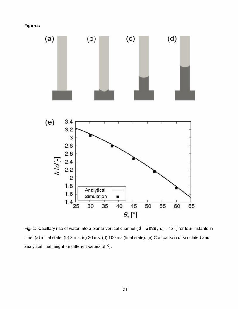
3.1 Equilibrium height of capillary rise
In this test case, we reproduce the capillary rise of a fluid A in the gap between two vertical
parallel plates where it displaces fluid B. The ratio between the final height, h , of the column and the
distance of the plates, d , is
e
2
A
2 cos( )h
d gd (8)
The fluids in our simulations are water (3
A 998kg m ,3
A 10 Pa s ) and air
(3
B 1.2kg m ,5
B 1.81 10 Pa s , 20.072 J m ). The channel width is ref 2mmd L and
29.81msg . The values of the Cahn and Peclet numbers are 0.025Cn and 327Pe ,
respectively. We use a uniform isotropic static mesh and resolve the plate distance d by 40 mesh
cells. This corresponds to approximately four mesh cells for the region 0.9 0.9C . In this paper,
all flows evolve to static state. Thus, there is no characteristic velocity and we define refU indirectly by
setting 1Re .
Fig. 1 a-d illustrates the time dependent simulation results for 45e . Initially, the channel is
filled with air while the water is in the container and the interface is flat (Fig. 1 a). When the simulation
starts, the wall adhesion force causes the water to creep up along the wall, to meet the prescribed
8
equilibrium contact angle (Fig. 1 b). Then a pressure jump arises across the curved interface, which
drives the water further upward (Fig. 1 c). This continues until the capillary force is in balance with the
gravity force (Fig. 1 d). In this study, we performed simulations for five different values of e in the
range 30 60e . For all cases, the computed steady column height (evaluated midway between
the channel centerline and the right plate) is in good agreement with the analytical solution in Eq. (8)
as shown in Fig. 1 e.
(Figure 1)
3.2 Equilibrium shape of a planar droplet
We now consider the spreading of a droplet on a flat homogeneous surface and compare
characteristic dimensions of the computed equilibrium droplet shape with analytical solutions. We start
from a planar semi-circular droplet with initial radius 0 0 / 2R D and initial contact angle 0 90 (Fig.
2 a). We quantify the numerical results for a given value of e by the equilibrium droplet height H and
base length L (Fig. 2 b). In our 2D simulations, the size of the computational domain is 0 03D D and
we resolve 0D by 50 mesh cells. Furthermore, we use ref 0L D , 0.01Cn and 1000CPe .
We first consider the case when gravity forces are negligible ( 0Eo ) so that capillarity is the only
driving force. In this case, the droplet is spreading for e 0 and is dewetting for e 0 . In both
cases, the equilibrium shape is a circular cap. By geometrical constraints it follows
0 0 e
e e e
2 sin2( sin cos )
L R (9)
0 0 e
e e e
(1 cos )2( sin cos )
H R (10)
Here, we performed numerical simulations for seven distinct values of e in the range e45 135 .
In Fig. 2 c we compare the computed values for 0/H R and 0/L R with the analytical solutions from
Eq. (9) and (10). The agreement is very good, both for hydrophilic and hydrophobic situations.
(Figure 2)
9
In the case 0Eo , the droplet spreads on the solid surface due to the combined effect of capillary
and gravitational forces. In the final stage, gravity tends to spread out the droplet further while the
capillary force tends to maintain a circular cap. For 1Eo , the gravity force dominates and the
droplet forms a puddle. Also in the limit Eo the equilibrium height of the droplet is known
analytically [19] and given by
0 e2sin
2
RH
Eo (11)
Similar to numerical studies for other methods [20, 21], we performed simulations for one specific
value of the equilibrium contact angle ( e 60 ) and seven distinct values of the Eötvös number in the
range 0.01 10Eo . In Fig. 3 we plot the final droplet height, H , normalized by 0H from Eq. (10) as
a function of Eo . For 0.1Eo the simulation results agree with the asymptotic solutions given by Eq.
(10), while for 5Eo they agree with the asymptotic solution given by Eq. (11). At 1Eo there is a
transition between both regimes. The inset graphics in Fig. 3 show the equilibrium droplet shape for
0.1Eo (a circular cap), 1Eo (an elongated circular cap) and 10Eo (a puddle).
(Figure 3)
3.3 Spreading dynamics on a homogeneous surface
We now turn to the spreading dynamics of a partially wetting droplet on a flat surface. In a
preliminary study, we neglect gravity ( 0Eo ) so that spreading is driven by capillary forces only. We
further assume that the velocities are so small that inertial forces are negligible, too, and set the
density ratio between the ambient fluid and the droplet to unity. As reference length we choose
ref 0L D , where 0D is the initial drop diameter. For presentation of the transient simulation results, we
scale time by the capillary time scale cap A 0 /t D .
10
3.3.1 Axisymmetric simulations
To investigate the dynamic wetting process, we turn from planar to axisymmetric geometry and
compare the results with experimental data of Zosel [22]. He studied the spreading of droplets of fluids
with different viscosity on a flat surface and recorded the instantaneous droplet base radius. The
droplet diameters were in the range 2.4 3 mm so that gravitational effects are small. The drops were
released with almost spherical shape and low kinetic energy.
For comparison, we selected one specific experiment with an equilibrium contact angle e 58
where a very viscous drop of polyisobutylene ( 0 2.6mmD , A 25Pa s , 3
A 920kg m ,
20.0426 J m ) spreads on a polymer surface (PTFE). The viscosity ratio between the ambient air
and the droplet is 6
B A/ 10 . In our simulations, we set 0.05 in order to save
computational effort. A sensitivity study on showed that a further decrease does not affect the
results significantly. In our axisymmetric simulations, the size of the computational domain is
0 02 1.5D D . We resolve 0D by 100 mesh cells and start from 0 170 . The Cahn number is
0.01Cn and we compare simulations for two values of the Peclet number, 200CPe and 1000 .
In Fig. 4 we compare the time evolution of the computed base radius of the drop with the
experimental data [22]. Good agreement is achieved, especially at the later spreading stage. As CPe
decreases, the base radius changes faster, and the result gets slightly closer to the experimental data.
This is reasonable since in the phase-field method the contact line moves by diffusion. Thus, a
stronger diffusion (i.e. a smaller value of CPe ) leads to a faster spreading.
We also investigated the influence of a dynamic contact angle on the spreading dynamics.
Following [12, 23], we included in Eq. (3) for this purpose a time-dependent term /C t multiplied by
an phenomenological parameter. However, the effect of the dynamic contact model on the spreading
dynamics turned out to be negligible, a results that can be attributed to the high drop viscosity [23].
(Figure 4)
11
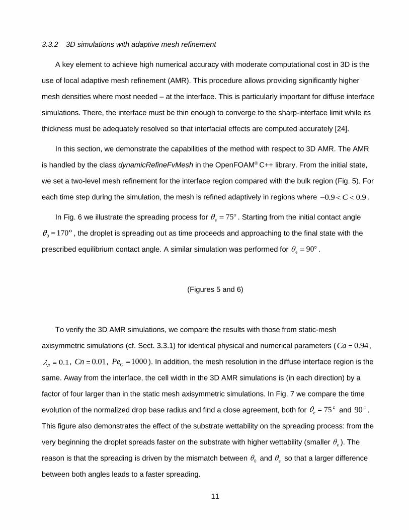
3.3.2 3D simulations with adaptive mesh refinement
A key element to achieve high numerical accuracy with moderate computational cost in 3D is the
use of local adaptive mesh refinement (AMR). This procedure allows providing significantly higher
mesh densities where most needed – at the interface. This is particularly important for diffuse interface
simulations. There, the interface must be thin enough to converge to the sharp-interface limit while its
thickness must be adequately resolved so that interfacial effects are computed accurately [24].
In this section, we demonstrate the capabilities of the method with respect to 3D AMR. The AMR
is handled by the class dynamicRefineFvMesh in the OpenFOAM® C++ library. From the initial state,
we set a two-level mesh refinement for the interface region compared with the bulk region (Fig. 5). For
each time step during the simulation, the mesh is refined adaptively in regions where 0.9 0.9C .
In Fig. 6 we illustrate the spreading process for e 75 . Starting from the initial contact angle
0 170 , the droplet is spreading out as time proceeds and approaching to the final state with the
prescribed equilibrium contact angle. A similar simulation was performed for e 90 .
(Figures 5 and 6)
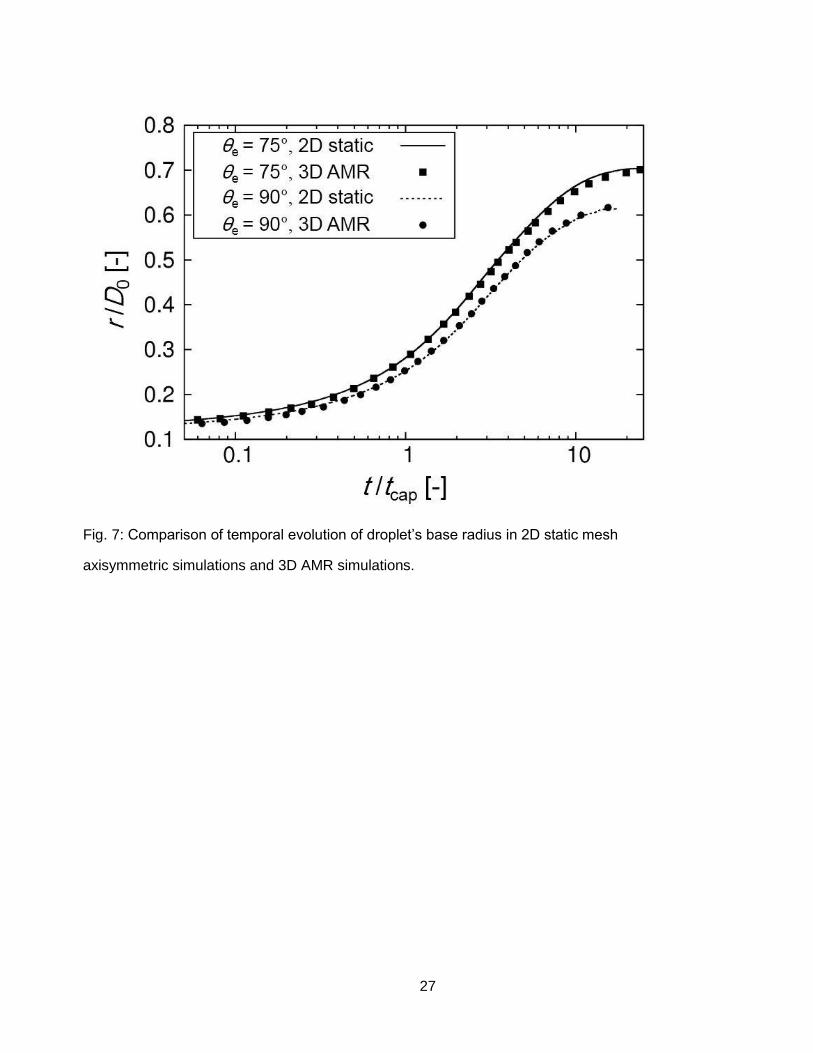
To verify the 3D AMR simulations, we compare the results with those from static-mesh
axisymmetric simulations (cf. Sect. 3.3.1) for identical physical and numerical parameters ( 0.94Ca ,
0.1, 0.01Cn , 1000CPe ). In addition, the mesh resolution in the diffuse interface region is the
same. Away from the interface, the cell width in the 3D AMR simulations is (in each direction) by a
factor of four larger than in the static mesh axisymmetric simulations. In Fig. 7 we compare the time
evolution of the normalized drop base radius and find a close agreement, both for e 75 and 90 .
This figure also demonstrates the effect of the substrate wettability on the spreading process: from the
very beginning the droplet spreads faster on the substrate with higher wettability (smaller e ). The
reason is that the spreading is driven by the mismatch between 0 and e so that a larger difference
between both angles leads to a faster spreading.
12
(Figure 7)
3.4 Droplet spreading on a chemically patterned surface
So far, we considered the spreading on a chemically homogeneous substrate where e is uniform.
We now extend the study to a chemically heterogeneous substrate, patterned with alternating
hydrophilic and hydrophobic stripes. The purpose for considering this test case is to demonstrate that
the method is able to reproduce characteristic phenomena such as anisotropic spreading and stick-
slip motion.
To allow for a qualitative comparison with literature, we consider a similar scenario as Jansen et
al. [25] who used the lattice Boltzmann method (LB). The base surface is made up of hydrophilic SiO2
stripes ( e 40 ) and hydrophobic perfluordecyltrichlorosilane (PFDTS) stripes ( 110e ). The
stripe width ratio is 2PFDTS SiO/ 0.5w w and we use four mesh cells for each SiO2 stripe and two for
each PFDTS stripe. We set 0.94Ca , 1000CPe , 0.02Cn , 0.1.
Initially, the 3 microliter polyisobutylene droplet just touches the surface (Fig. 8 a). Subsequently, it
wets the substrate (Fig. 8 b) but in a manner different from that for a homogeneous surface: due to the
stripe pattern, the droplet spreads preferentially along the stripes while its motion in direction
perpendicular to them is hindered (Fig. 8 c). Finally, the droplet adopts an elongated equilibrium shape
with the larger axis in direction of the stripes (Fig. 8 d).
(Figure 8)
13
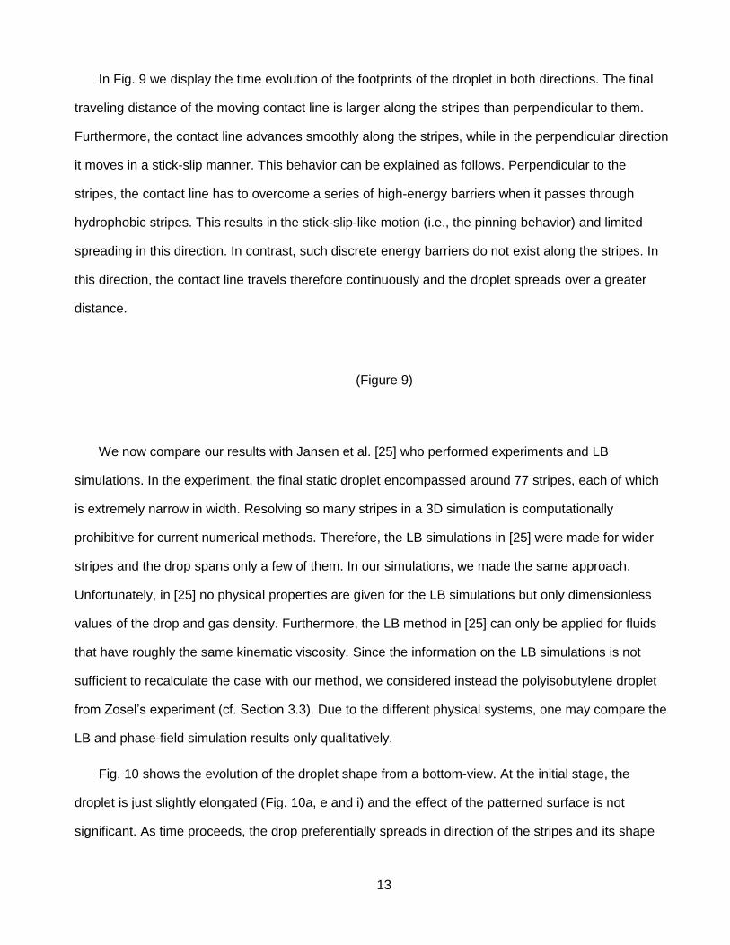
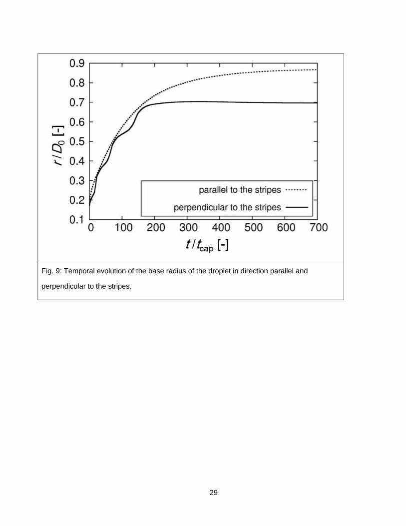
In Fig. 9 we display the time evolution of the footprints of the droplet in both directions. The final
traveling distance of the moving contact line is larger along the stripes than perpendicular to them.
Furthermore, the contact line advances smoothly along the stripes, while in the perpendicular direction
it moves in a stick-slip manner. This behavior can be explained as follows. Perpendicular to the
stripes, the contact line has to overcome a series of high-energy barriers when it passes through
hydrophobic stripes. This results in the stick-slip-like motion (i.e., the pinning behavior) and limited
spreading in this direction. In contrast, such discrete energy barriers do not exist along the stripes. In
this direction, the contact line travels therefore continuously and the droplet spreads over a greater
distance.
(Figure 9)
We now compare our results with Jansen et al. [25] who performed experiments and LB
simulations. In the experiment, the final static droplet encompassed around 77 stripes, each of which
is extremely narrow in width. Resolving so many stripes in a 3D simulation is computationally
prohibitive for current numerical methods. Therefore, the LB simulations in [25] were made for wider
stripes and the drop spans only a few of them. In our simulations, we made the same approach.
Unfortunately, in [25] no physical properties are given for the LB simulations but only dimensionless
values of the drop and gas density. Furthermore, the LB method in [25] can only be applied for fluids
that have roughly the same kinematic viscosity. Since the information on the LB simulations is not
sufficient to recalculate the case with our method, we considered instead the polyisobutylene droplet
from Zosel’s experiment (cf. Section 3.3). Due to the different physical systems, one may compare the
LB and phase-field simulation results only qualitatively.
Fig. 10 shows the evolution of the droplet shape from a bottom-view. At the initial stage, the
droplet is just slightly elongated (Fig. 10a, e and i) and the effect of the patterned surface is not
significant. As time proceeds, the drop preferentially spreads in direction of the stripes and its shape
14
further elongates toward its final state (Fig. 10d, h and l). The results of our phase-field simulations are
in good qualitative agreement with the LB results.
The contact line profile at the longer ends of the droplet is different in the experiment (where it is
smooth) and in the simulations (where it is corrugated and wave like). This relates to the different
number of stripes covered by the droplet. Such corrugation patterns of the contact line were also
observed in other numerical studies where the droplet spans a small number of stripes [26].
(Figure 10)
4 Summary and outlook
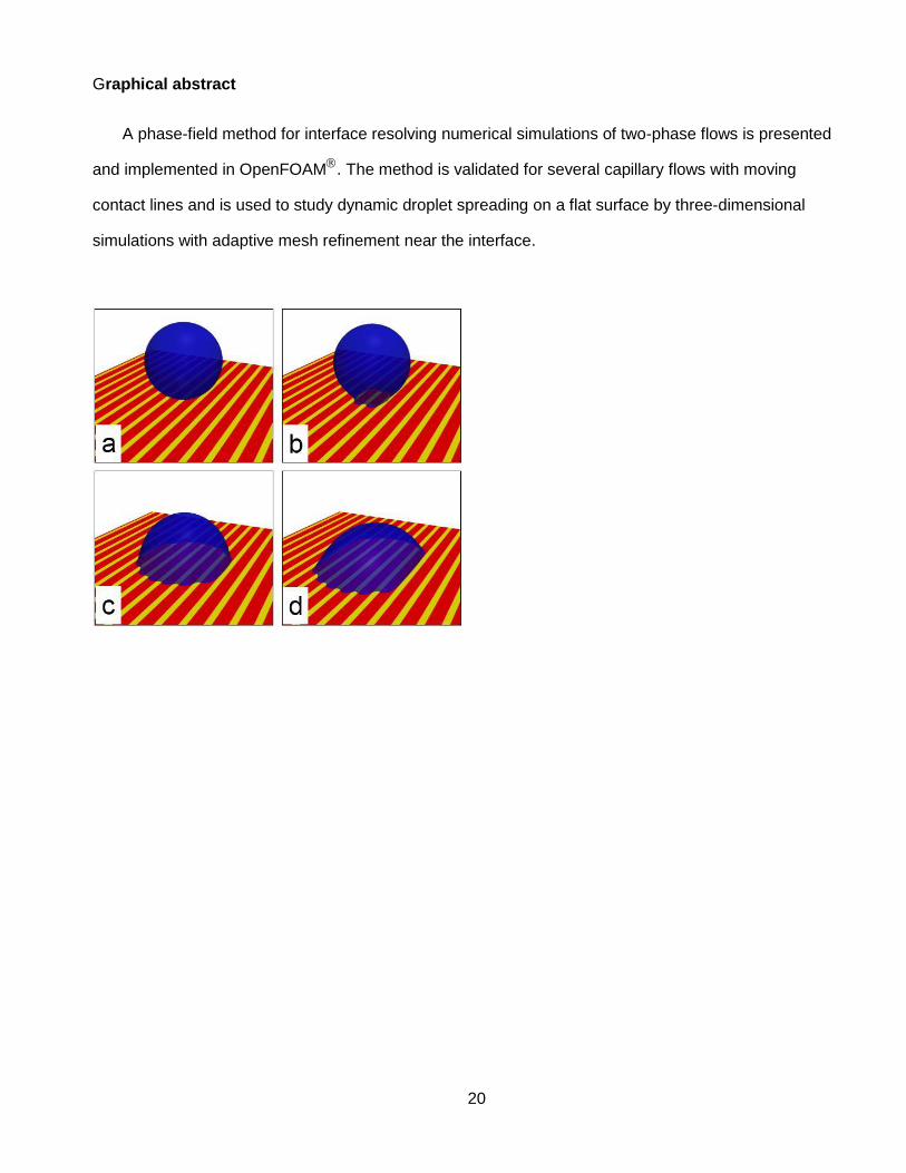
In this paper, we have presented a phase-field method for interface resolving numerical
simulations of two-phase flows with OpenFOAM and applied it to representative capillary flows with
moving contact lines. For both, the capillary rise between parallel plates and droplet wetting on a flat
surface the computed equilibrium shape of the interface agrees well with analytical solutions.
Concerning droplet-spreading dynamics, our time dependent simulation results are in good agreement
with literature data, both for a chemically homogeneous and a chemically patterned surface. We also
demonstrated the use of adaptive mesh refinement at the interface. This altogether shows that the
presented phase-field method is a reliable and promising numerical method for general capillary two-
phase flows involving moving contact lines.
We now advance the method in OpenFOAM towards a volume-conservative and bounded
phase-field framework incorporating both Cahn-Hilliard and Allen-Cahn equations [17]. Next, we will
validate the code with respect to a wall energy relaxation model for dynamic contact angles in rapid
wetting processes and extend our method to contact angle hysteresis.
15
Acknowledgement
We gratefully acknowledge the funding by Helmholtz Energy Alliance “Energy-efficient chemical
multiphase processes” (HA-E-0004). The first and the third author would like to thank Prof. Hocine Alla
and Dipl.-Math. Marouen Ben Said for stimulating discussions.
Symbols used
Ca [-] Capillary number
Cn [-] Cahn number
d [m] distance between parallel vertical plates
0D [m] initial drop diameter
ˆze [-] unit normal vector in vertical direction
Eo [-] Eötvös number
H [m] droplet height
0H [m] equilibrium droplet height for 0Eo
H [m] equilibrium droplet height for Eo
L [m] droplet base length
refL [m] reference length scale
sn̂ [-] unit normal vector to the solid surface
P [-] non-dimensional pressure
CPe [-] Peclet number in Cahn-Hilliard equation
0R [m] initial drop radius
Re [-] Reynolds number
t [s] time
capt [s] capillary time scale, cap A 0 /t D
refU [m s-1] reference velocity scale
u [-] velocity field normalized by refU
16
Greek symbols
[-] volume fraction
[J m-2] interfacial energy
[m] interfacial width
[m3 s kg-1] mobility
[-] viscosity ratio
[Pa s] dynamic viscosity
[-] non-dimensional chemical potential
[kg m-3] density
[] contact angle
[-] non-dimensional time
Subscripts
A phase A
B phase B
e equilibrium
ref reference value
17
References
[1] H. Alla, S. Freifer, T. Roques-Carmes, Colloids and Surfaces A: Physicochemical and Engineering Aspects 2011, 386 (1-3), 107-115. [2] C. Huh, L. E. Scriven, J Colloid Interf Sci 1971, 35 (1), 85-101. [3] P. G. de Gennes, Rev Mod Phys 1985, 57 (3), 827-863. [4] M. Renardy, Y. Renardy, J. Li, J Comput Phys 2001, 171 (1), 243-263. [5] Y. Sui, H. Ding, P. D. M. Spelt, Annu Rev Fluid Mech 2014, 46 (1), 97-119. [6] M. Wörner, Microfluid Nanofluid 2012, 12 (6), 841-886. [7] D. M. Anderson, G. B. McFadden, A. A. Wheeler, Annu Rev Fluid Mech 1998, 30, 139-165. [8] D. Jacqmin, J Comput Phys 1999, 155 (1), 96-127. [9] J. D. v. d. Waals, Verhandel/Konink Akad Weten 1879, 1, 8. [10] P. T. Yue, C. F. Zhou, J. J. Feng, J Fluid Mech 2010, 645, 279-294. [11] M. Ben Said et al., Langmuir 2014, 30 (14), 4033-4039. [12] D. Jacqmin, J Fluid Mech 2000, 402, 57-88. [13] V. V. Khatavkar, P. D. Anderson, H. E. H. Meijer, J Fluid Mech 2007, 572, 367-387. [14] A. Carlson, M. Do-Quang, G. Amberg, Int J Multiph Flow 2010, 36 (5), 397-405. [15] W. Villanueva, G. Amberg, Int J Multiph Flow 2006, 32 (9), 1072-1086. [16] X. Cai, M. Wörner, O. Deutschmann, in 7th Open Source CFD Int Conf (available online at http://www.opensourcecfd.com/conference2013/proceedings-day-2) Hamburg, Germany 2013. [17] H. Marschall, X. Cai, M. Wörner, O. Deutschmann, 2015, Conservative finite volume discretization of the two-phase Navier-Stokes Cahn-Hilliard and Allen-Cahn equations on general grids with applications to dynamic wetting, in preparation. [18] H. Ding, P. D. M. Spelt, C. Shu, J Comput Phys 2007, 226 (2), 2078-2095. [19] P. G. de Gennes, F. Brochard-Wyart, D. Quéré, Capillarity and wetting phenomena: drops, bubbles, pearls, waves. Springer, New York, 2004. [20] Y. M. Chen, R. Mertz, R. Kulenovic, Int J Multiph Flow 2009, 35 (1), 66-77. [21] J. B. Dupont, D. Legendre, A. M. Morgante, J Fuel Cell Sci Tech 2011, 8 (4), 041008-1 - 041008-7. [22] A. Zosel, Colloid Polym Sci 1993, 271 (7), 680-687. [23] A. Carlson, M. Do-Quang, G. Amberg, Phys Fluids 2009, 21 (12), 121701-1- 121701-4. [24] C. Zhou et al., J Comput Phys 2010, 229 (2), 498-511. [25] H. P. Jansen et al., Phys Rev E 2013, 88 (1), 013008. [26] F. J. M. Ruiz-Cabello et al., Langmuir 2009, 25 (14), 8357-8361.