50
| Date post: | 17-Dec-2015 |
| Category: |
Documents |
| Upload: | gyles-dennis |
| View: | 220 times |
| Download: | 1 times |

Topics Covered Introduction and Background
Data Flow and Problem Setup
Convex Hull Calculation
Hardware Acceleration of Integral Relative Electron Density Calculation
Calculating Entry and Exit Points
The Most Likely Path Formalism Optimization
Reconstructions
Conclusions

Introduction and Background
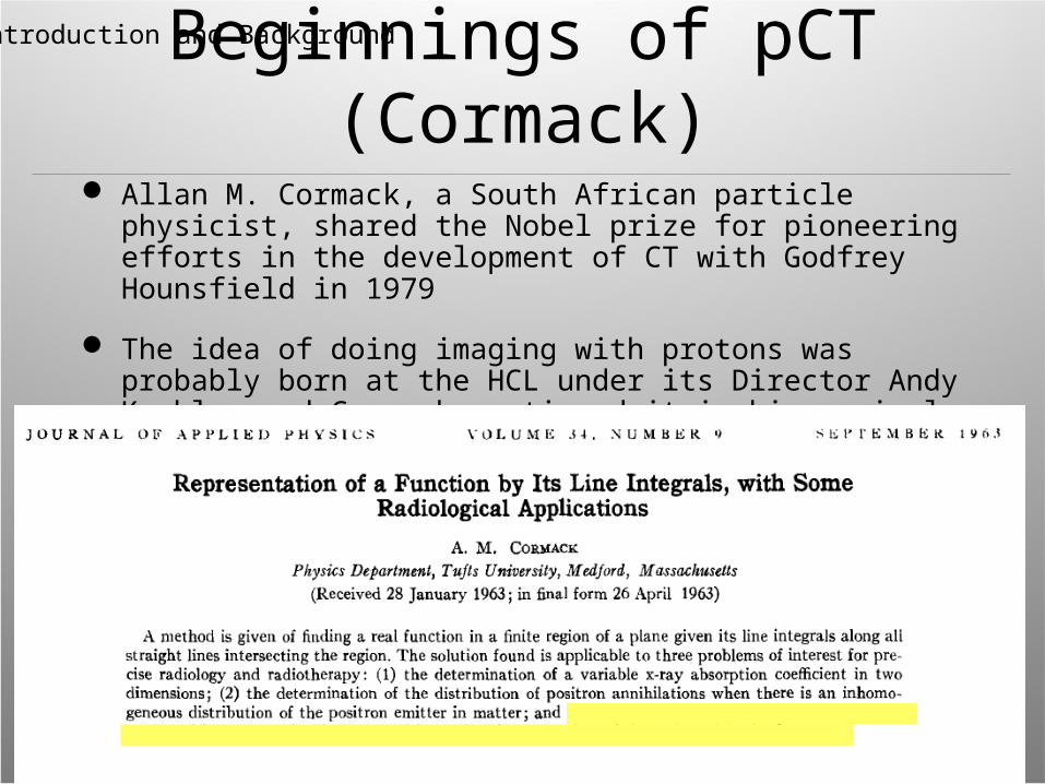
Beginnings of pCT (Cormack)
Allan M. Cormack, a South African particle physicist, shared the Nobel prize for pioneering efforts in the development of CT with Godfrey Hounsfield in 1979
The idea of doing imaging with protons was probably born at the HCL under its Director Andy Koehler and Cormack mentioned it in his seminal paper 1963 paper (J. Appl. Phys. 34, 2722-2727)
Introduction and Background

Beginnings of pCT (Hanson)
In the late 1970s, Ken Hanson, a Los Alamos physicist, experimentally explored the advantages of pCT
Hanson pointed to the dose reduction with pCT and the problem of limited spatial resolution due to proton scattering
Feasibility of pCT system demonstrated
Introduction and Background

Beginnings of pCT In the late 1990s Piotr
Zygmanski, a PhD student, uses the Harvard Cyclotron to test a cone beam CT system with protons
Introduction and Background
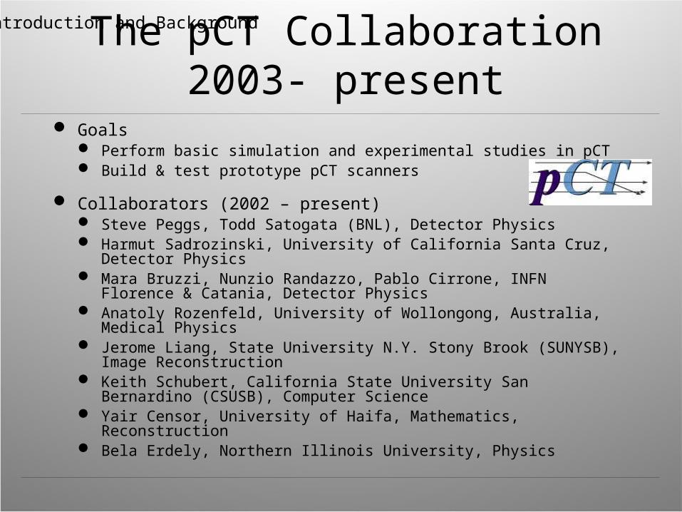
The pCT Collaboration 2003- present
Goals Perform basic simulation and experimental studies in pCT Build & test prototype pCT scanners
Collaborators (2002 – present) Steve Peggs, Todd Satogata (BNL), Detector Physics Harmut Sadrozinski, University of California Santa Cruz,
Detector Physics Mara Bruzzi, Nunzio Randazzo, Pablo Cirrone, INFN Florence &
Catania, Detector Physics Anatoly Rozenfeld, University of Wollongong, Australia, Medical
Physics Jerome Liang, State University N.Y. Stony Brook (SUNYSB),
Image Reconstruction Keith Schubert, California State University San Bernardino
(CSUSB), Computer Science Yair Censor, University of Haifa, Mathematics, Reconstruction Bela Erdely, Northern Illinois University, Physics
Introduction and Background
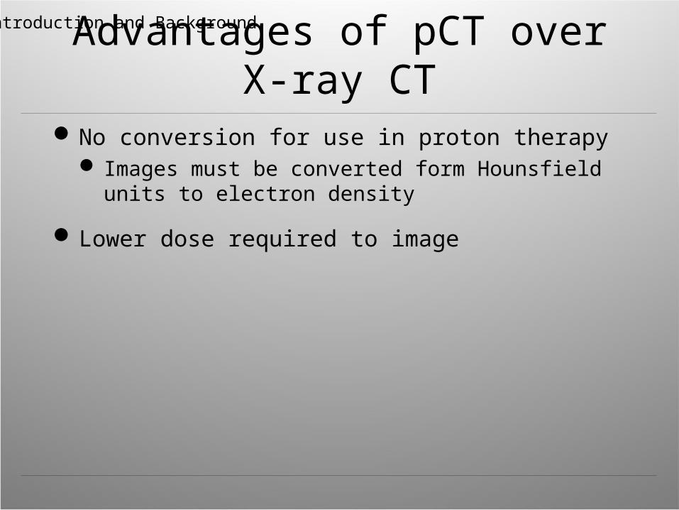
Advantages of pCT over X-ray CT
No conversion for use in proton therapy Images must be converted form Hounsfield units
to electron density
Lower dose required to image
Introduction and Background

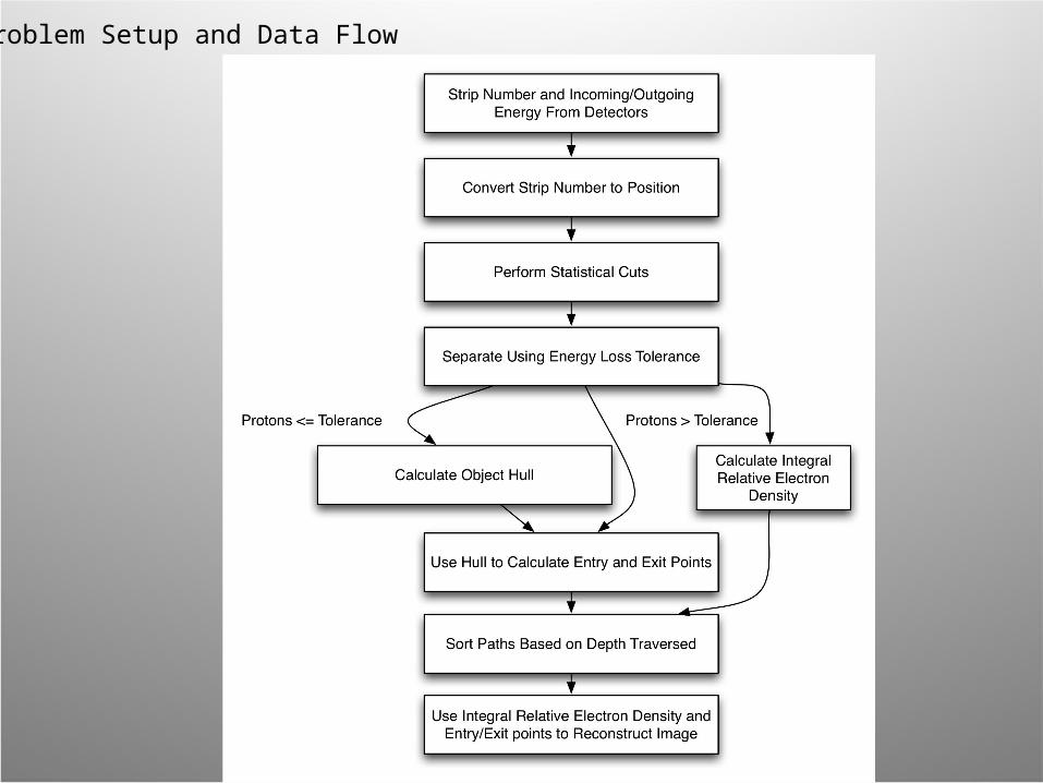
Problem Setup and Data Flow
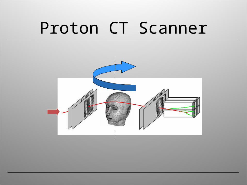
Proton CT Scanner

Problem Setup and Data Flow
System Geometry

Problem Setup and Data Flow
Problem Size106 proton histories, 106 image voxels in this
example
108 proton histories, 107 image voxels expected
Ax = b A is the vectorized proton path matrix b is the integral relative electron density x is the vectorized image to be reconstructed

Problem Setup and Data Flow
Individual Proton Path

Problem Setup and Data Flow
Vectorized Path2-D matrix representation replaced by 1-D row
000000000000000011000000000000000111111000000000…

Problem Setup and Data FlowLinear System and Solution
A is very large and sparse and the system is inconsistent
Solution must me approximated with an iterative projection method like the algebraic reconstruction technique
Problem Setup and Data Flow

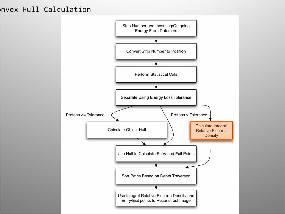
Convex Hull Calculation

Convex Hull Calculation

Convex Hull Calculation
Descretized Area
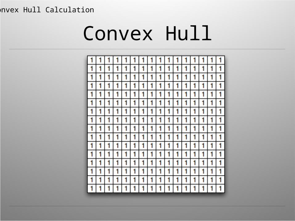
Convex Hull Calculation
Convex Hull

Convex Hull Calculation
Convex Hull

Convex Hull Calculation
Convex Hull

Convex Hull Calculation
Convex Hull

Convex Hull Calculation
Convex Hull

Convex Hull Calculation
Convex Hull
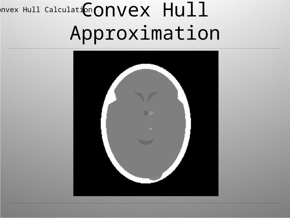
Convex Hull CalculationConvex Hull Approximation

Convex Hull CalculationConvex Hull Approximation

Hardware Acceleration of
Integral Relative Electron Density
Calculation
Convex Hull Calculation

Hardware Acceleration of Integral Relative Electron Density CalculationThe Bethe-Bloch Equation
Simplifies to:

Hardware Acceleration of Integral Relative Electron Density Calculation

Calculating Entry and Exit Points

Calculating Entry and Exit Points

Calculating Entry and Exit Points

Calculating Entry and Exit Points

Calculating Entry and Exit Points
Data Distribution

Most Likely Path Formalism
Optimization

Most Likely Path Formalism Optimization
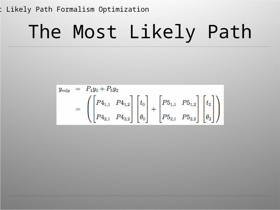
The Most Likely Path

Most Likely Path Formalism Optimization
The Most Likely Path
ymlp has 79 floating point operations per step with matrix multiplication
Sigma/R matrices are calculated every 0.5 mm For 20.0 cm object there are 400 different
combinations
400 different combinations for 106 histories means there are many redundant calculations

Most Likely Path Formalism OptimizationSeparate Sigma and R From y
Distribute P1

Most Likely Path Formalism OptimizationSeparate Sigma and R From y
Most Likely Path Formalism Optimization
The Most Likely Path

Most Likely Path Formalism Optimization
The Most Likely Path
Yt now has only 7 floating point operations per step

Reconstructions

Reconstructions

Reconstructions
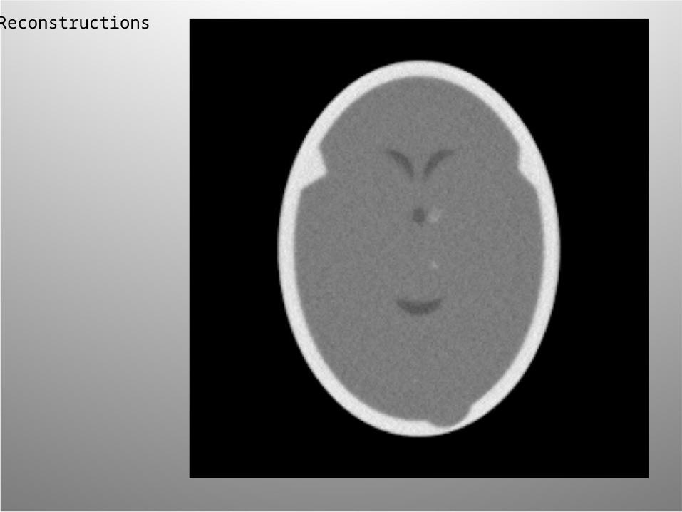
Reconstructions

Conclusions
Conclusions
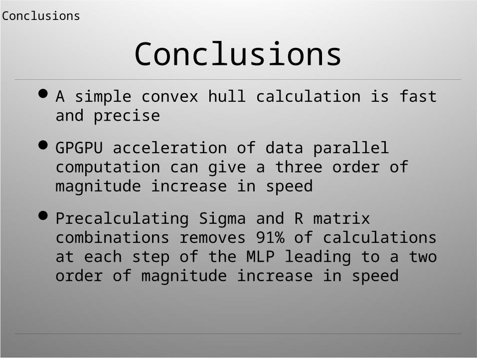
ConclusionsA simple convex hull calculation is fast and
precise
GPGPU acceleration of data parallel computation can give a three order of magnitude increase in speed
Precalculating Sigma and R matrix combinations removes 91% of calculations at each step of the MLP leading to a two order of magnitude increase in speed

Conclusions
Future WorkMigrate all data parallel pCT code to GPGPU
hardware
Improve accuracy of reconstruction
GPGPU cluster research


