228 D. Rivas et al. / Dynamics of Atmospheres and Oceans 39 (2005) 227–249
1. Introduction
Gravity currents are important phenomena in the coastal-zone ecosystem. They estab-lish the fresh water, heat and nutrient exchange between the coast and the sea. There arenumerous examples of these currents; like the East Greenland Current, which carries lessdense polar water southward along the coast of Greenland; the Norwegian Coastal Current,which flows northward along the west coast of Norway; the discharges of the Amazon River,which provide an important amount of fresh water into the Atlantic Ocean, etc. (Griffithsand Linden, 1982).
Coastal gravity currents have motivated various theoretical and experimental studies; inparticular, the stability properties of currents flowing along a vertical wall either straight orcylindrical have been determined (e.g.,Griffiths and Linden, 1981, 1982; Chabert d’Hiereset al., 1991). Laboratory experiments of a surface current generated by continuous injectionthrough a point source show stable currents for 0.5 <Bu < 0.82 (whereBu = R2
0/L20 is the
Burger number;R0 is the deformation radius andL0 is the reference current width), andunstable for 0.15 <Bu < 0.5 (Chabert d’Hieres et al., 1991). Unstable conditions imply thatdisturbances of the mean flow grow in width and depth. In contrast with the point-sourcecurrents, surface currents generated by continuous injection through a line source at theedge of a circular vertical wall show meanders that grow until they separate as anticycloniceddies (Griffiths and Linden, 1981; hereafter referred to as GL81). The experimental valueof the Froude numberF0 = B−1
u for which the disturbances start being evident is alwayssignificantly larger than the theoretical critical value obtained with a baroclinic two-layermodel (in an infinite channel and including Ekman pumping at the interface between thetwo layers). The wavelength and phase speed of the meanders observed in the experimentsare consistent in most cases with those computed with the analytical model, so that GL81conclude that the nature of the disturbances is mostly baroclinic, that is to say, the energysource for the instability is the available potential energy of the basic flow. Similarly, currentsgenerated by a gravitational collapse of a fixed volume of buoyant fluid at the edge of acircular vertical wall over flat bottom are always unstable (Griffiths and Linden, 1982;hereafter referred to as GL82). The characteristics of the disturbances are, in most cases,consistent with those predicted by GL81’s model, so that GL82 conclude that when the initialFroude numberF0 ≥ 4 the disturbances are primarily baroclinic, and whenF0 < 1 they areprimarily barotropic, that is to say, the energy source of the instability is the horizontal shearof the basic current. Also, the experimental series show that the behaviour of the currentsis identical to that of an isolated vortex (like that analysed byChia et al., 1982), thereforethe rigid boundary has no important dynamical influence upon the stability of the currents(GL82).
Since the condition of a vertical coast is seldom met, it is important to study more realisticsituations, like currents flowing over an inclined topography. Experimental currents flowingalong a vertical wall as generated by GL81, but using different bottom topographies thatsimulate both a continental ridge and a continental slope, show a second instability whenthe topography is introduced (Cenedese and Linden, 2002). In the case of continental ridgethe disturbances grow with formation of eddies, while in the case of gentle continentalslope the disturbances reduce their growth rate and eventually damp, then the stable cur-rent re-establishes (Cenedese and Linden, 2002). Moreover, experimental surface currents
D. Rivas et al. / Dynamics of Atmospheres and Oceans 39 (2005) 227–249 229
generated from a continuous point source on a uniform sloping bottom have shown differ-ent behaviour depending on the inclination angle of the topographyα and the parameterΠ = q1/5
0 Ω/g′3/5, whereq0 is the volume flux of fluid discharged from the source,Ω is theangular velocity of the system, andg′ is the reduced gravity (Thomas and Linden, 1998).The current head flows either attached or detached to the topography.
In this paper we present an experimental study of the effects of the bottom slope on theevolution of the surface gravity currents. We deal with the collapse of a lighter wedge andthe continuous-injection of lighter fluid at the edge of a sloping conical bottom. In contrastwith Thomas and Linden (1998), the gravity currents generated here have no starting or endpoint, due to the azimuthal symmetry. This is critical in removing unwanted end effects.These currents flow on a bottom sloping from the free surface, so that the interfacial frontis always over the sloping bottom. In contrast,Cenedese and Linden’s (2002)experimentsalso have azimuthal symmetry of the bottom, but it starts with a flat shelf followed by acontinental slope (i.e. the injection of lighter fluid is over flat bottom, adjacent to a verticalwall).
A remarkable theoretical result of geostrophic adjustment of a buoyant volume patchin the absence of friction and diffusion is that, for a large variety of initial conditions atrest, one third of the potential energy released is converted into kinetic energy of the finalgeostrophic state (van Heijst, 1985; van Heijst and Smeed, 1986). The other two thirds arelost in the wave field. Here we show that the presence of the sloping topography diminishesthis energy conversion ratio: less than one third of the potential energy released during theadjustment process appears in the geostrophic kinetic energy.
The rest of the paper is organised as follows. Section2 describes the experimental set-upand the techniques used to generate the currents, as well as the parameters that determinethe flow. Section3 shows the experimental results and in particular the velocity field isdiscussed. Section4 solves the collapse generated currents by geostrophic adjustment for aconfined wedge initially at rest; solutions of the resulting geostrophic currents and energybudgets are shown. Section5 discusses the experimental and analytical results. In Section6 the conclusions are presented.
2. Experimental methods
The experiments were carried out in a 96.5 cm diameter, circular tank mounted on arotating table. A truncated cone was placed in the centre of the tank, to provide an inclinedbottom (the slope angle isα), as shown inFig. 1a. A bottomless cylinder was placed overthe truncated cone; the cone, the cylinder and the tank were concentric with the rotation axisof the turntable. The tank was filled to a prescribed depth (usually 20 cm) with a salt-watersolution of densityρ2. Then, the turntable was initiated to spin counterclockwise.
In the collapse experiments, once the fluid in the tank was in solid body rotation, freshwater of densityρ1 was carefully injected at the free surface, into the space between the coneand the cylinder; this water contained fluorescein for visualisation purposes (Fig. 1a). Therewas no appreciable mixing between the two fluids during the injection. The experimentstarted by lifting gently and vertically the cylinder that separated the two fluids, allowingthem to move and interact under the influence of gravity and Coriolis forces (Fig. 1b).
230 D. Rivas et al. / Dynamics of Atmospheres and Oceans 39 (2005) 227–249
Fig. 1. Generation of a gravity current by gravitational collapse. (a) The light and heavy fluids are at rest andseparated by a bottomless cylinder. (b) The bottomless cylinder is removed and both fluids adjust geostrophically.
The continuous injection experiments were carried out in a similar set-up as the collapseexperiments, but the fresh water was released from a set of sources evenly distributed at thecircular wedge of the salty water (Fig. 2). The salty wedge was a 20 or 27 cm diameter cir-cumference, and a ring tube sitting over the cone at the height of the wedge delivered the freshwater throughout small holes. Fluorescein in the fresh water was used to visualise the current.
From these experiments information about the current’s width and depth (denoted byL andh, respectively, inFigs. 1b and 2), and the number of the disturbances around thecurrent was obtained. Small and almost neutrally buoyant paper particles were seeded andilluminated on the surface of the fluid. Given the particle characteristics it is justified toassume that their motion follows the fluid surrounding flow and thus allows to measure thevelocity field. Each experiment was recorded by a colour CCD video camera mounted on therotating table superstructure. Digital images were captured in a computer and analysed toextract the velocity field using Particle Tracking Velocimetry (PTV) techniques. For detailson PTV see for example,Dalziel (1993)andvan der Plas (1995).
Fig. 2. . Generation of a gravity current by continuous injection of fluid. There is a ring source where the lighterfluid is released gradually and constantly.
D. Rivas et al. / Dynamics of Atmospheres and Oceans 39 (2005) 227–249 231
In both experimental settings it is assumed that the free surface and the current’s curvaturehave little dynamical effect (i.e. an infinite straight current under a rigid lid is assumed tobe a close analog to the experiments, see e.g. GL81). With this assumptions, the parametersthat determine the flow in the collapse experiments are the reduced gravityg′ = g(ρ2 − ρ1)ρ1(whereg is the gravity), the Coriolis parameterf, the initial maximum values of the freshwater wedge thicknessh0 and widthL0, and the angleα between the bottom and the hori-zontal plane. Notice, however, that tanα= h0/L0 (seeFig. 1a). Dimensional analysis showsthat two dimensionless numbers govern the evolution; we chose the bottom inclinationα
and the Froude number, defined as
F0 ≡ L20
R20
, (1)
whereR0 = √g′h0/f is the internal deformation radius. In the experiments reported
in this paper the experimental parameters had the following values:L0 = 4.6, 5.0 cm,1≤ g′ ≤ 5 cm s−2, f = 1.68 s−1, α= 30, 45, 60. Fig. 3a shows each experiment in theparameter space (α, F0). Notice that the values used here are in the range used by GL82 forthe vertical-wall case, so comparisons can be made.
Similarly, the parameters that determine the flow in the continuous injection experiments,are the reduced gravityg′, the Coriolis parameterf, the rateQat which fresh water is injectedper unit length into the system and the angleα between the bottom and the horizontal plane.Dimensional analysis shows that two dimensionless numbers govern the evolution; we chosethe bottom inclinationα andΠ0, defined as
Π0 = g′2
f 3Q. (2)
The experimental parameters had the following values 1≤ g′ ≤ 5 cm s−2, f = 1.68 s−1,α= 30, 45, 60, 75, Q1 = 0.06 cm2/s for the cases withα= 30, 45, 60, andQ2 = 0.04 cm2/s for the case withα= 75. The rateQj , with j = 1 or 2, is then the rate of flow
Fig. 3. Experimental initial conditions. Circles indicate values used in the present work, whereas asterisks indicatevalues used by GL82 (for the collapse experiments) and GL81 (for the continuous injection experiments).
232 D. Rivas et al. / Dynamics of Atmospheres and Oceans 39 (2005) 227–249
volume supplied to the annular source divided by its perimeter 2πrj , wherer1 = 10.0 cmandr2 = 13.5 cm. The two different values of flow rate and ring-source radius (r1, r2) wereset by experimental limitations.Fig. 3b shows each experiment in the parameter space (α,Π0). As before, the parameter range used here coincides with that used for the vertical-wallcase reported by GL81. Needless to say, in currents generated by continuous-injection theinitial values of depth and width of the current are zero, so that it is not possible to definean initial Froude number.
3. Experimental results
3.1. Collapse experiments
A current can be produced by the gravitational collapse of a volume of light fluid, initiallycontained between the sloping bottom and a vertical wall that separates it from the heavierfluid. The two fluids start with the same surface level. Once the containing vertical wall isremoved, both the upper layer (fresh water) and the lower layer (salty water) adjust under theinfluence of buoyancy and Coriolis forces. The buoyancy causes the lighter fluid to spreadoutwards on the surface, moving away from the inclined boundary. In absence of viscousdissipation, as the layer thickness varies the fluid acquires velocity in order to conservepotential vorticity. Eventually, the flow reaches an approximately geostrophic balance.
It is expected that after the collapse, the width of the current increases about one defor-mation radius in a time on the order of one inertial period, that is to say
L = L0 + cR0, (3)
wherec is a constant of order one. The results show that Eq.(3) matches approximately. Anestimate of the evolution ofL with time is possible. The first measurement ofL after the wallwas lifted was done atτ = t/T= 4, wheret is time andT= 7.5 s is the rotation period of thesystem. At earlier times it was not possible to get meaningful measurements, because thecollapse is occurring and the interface between the current and the environmental fluid is notclear.Fig. 4shows the time evolution ofc; the value ofc was fitted to the data according tothe least squares criteria. The measurements are significantly scattered around the straightline (Fig. 4a), because meanders difficult the definition of the current’s width.Fig. 4a showsthe deformation radiusR0 against the current’s widthL (minus its initial valueL0) for τ = 8.A least square regression producesc= 3.3.Fig. 4b shows the time evolution ofc. Despite thedata scatter,Fig. 4b provides information about the approximate spreading of the current,whose values increase continuously forτ < 50. The width increase at lateτ’s (i.e.τ > 10) isprobably because friction breaks the balance between the Coriolis and the pressure gradientforces. The current then tends to the condition of a stably stratified fluid. It is important totake into account that these measurements have a significant error, which is estimated to be±10%.
In each experiment the boundary of the axially symmetric flow became distorted by thepresence of meanders which showed negligible downstream propagation. Depending onthe value ofα, these meanders grew or became inhibited.Fig. 3a is divided into two parts,
D. Rivas et al. / Dynamics of Atmospheres and Oceans 39 (2005) 227–249 233
Fig. 4. Left: (a) Current’s spreading [L − L0] vs. number of deformation radii in 45 collapse experiments withα= 30 (triangles), 45 (asterisks), 60 (squares) forτ = t/T= 8, whereT= 7.5 s is the rotation period. Notice thatthe deformation radii are given in cm, with different value in each experiment. A straight line was fitted to thedata, with a correlation coefficient of 0.80 and a standard error of estimation of±1.5 cm. Dashed straight linesindicate the 95% confidence interval, where the estimated error in the fitted line slope isδc=±0.33. Right: (b)Non-dimensional current’s spreading [(L − L0)/R0 = c] as a function ofτ; error bars represent the 95% confidenceinterval. Correlation coefficients are about 0.83, standard errors of estimation are about 1.6 cm, and errors in thefitting (δc) are about±0.34.
the right side belongs to cases in which disturbances developed (forα= 60, 90). Currentsflowing adjacent to a vertical boundary (α= 90) are always unstable and the boundary hasno important influence on the dynamics of the current (GL82). However, when the currentflows on a sloping bottom its behaviour is different. Shortly after the collapse, some non-axisymmetric disturbances form in the front; whenα= 60 some of these meanders growand reach large amplitudes, but whenα is small (α= 45 or 30) these disturbances disappearand the current is said to be stable. For comparison,Fig. 5shows the evolution of a stablecurrent (withα= 30 and F0 = 9.4) and an unstable current (withα= 60 and F0 = 8.6).Shortly after the collapse (τ = 4), some meandering structures form (in both values ofα),but later (τ = 20) forα= 30 the current stabilises and the structures diminish in amplitude.The stable behaviour persists later on, we observe it untilτ = 36. Withα= 60 the bottomeffect is weaker and the current is unstable, the meanders persist, increase their amplitudeand anti-cyclonic eddies form. In the unstable current ofFig. 5, atτ = 4 there are meandersin the front, and as time elapses some of these form eddies whereas near the edge theflow stabilises. Atτ = 36 three eddies adjacent to the main flow away from the edge areobserved.
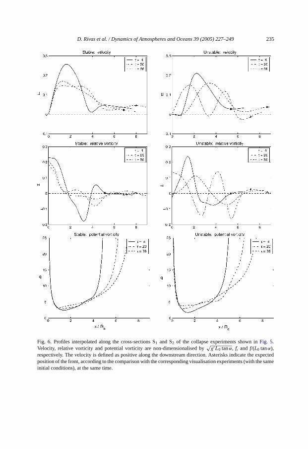
Fig. 6 shows profiles of velocity (U) and relative vorticity (ω) interpolated along thecross-sectionsS1 andS2 shown inFig. 5. In the stable case ofFig. 6 (left), for τ = 4 thevelocity profile shows a maximum which decreases in intensity and the profile smoothensas time elapses. The relative vorticity smoothens as well, decreasing and remaining closeto zero. In the unstable case (right) the velocity profile atτ = 4 is similar to that of thestable case, however, byτ = 20 it has changed and shows two maxima. The relative vorticityprofile shows a positive peak in the region where it was negative whenτ = 4; at this momentthe meanders are increasing their amplitude and eddies are forming. Later (atτ = 36) thevelocity profile shows a maximum like that observed atτ = 4, but its magnitude is smaller,
234 D. Rivas et al. / Dynamics of Atmospheres and Oceans 39 (2005) 227–249
Fig. 5. Evolution of the flow in a stable experiment (α= 30, F0 = 9.4,g′ = 3 cm/s2) and in an unstable experiment(α= 60, F0 = 8.6, g′ = 1 cm/s2). Crosses denote saddle points, whereas circles denote spiral or centres. Somerepresentative streamlines are also plotted, S1 and S2 indicate cross-sections where velocity and relative vorticitywere interpolated; these profiles are shown inFig. 6.
and the relative vorticity profile is smoother; at this moment the current is stable and theeddies are adjacent to it.
Estimates of the profiles of potential vorticityq= (ω + f)/h, whereh is the current’s thick-ness, are also plotted inFig. 6. However in these experiments there is no information abouth, a simple linear thickness profile was used to estimate the potential vorticity. Correspond-ing visualisation experiments, having the same initial conditions, allowed by side views ofthe thickness profile. Linear fits of depthh versus radial distance (width)L to such profilesallowed the potential vorticity estimates. Other types of thickness profiles were also tested(a quadratic one, and the one resulting from the analytical model described in Section4) andthe potential vorticity showed no sensitivity to these changes. Stable and unstable profilesof potential vorticity go to +∞ in the vicinity of the vanishing thickness edge atx= L. Inthe vicinity of the edge formed by the inclined bottom and the surface (close tox= 0 in
D. Rivas et al. / Dynamics of Atmospheres and Oceans 39 (2005) 227–249 235
Fig. 6. Profiles interpolated along the cross-sections S1 and S2 of the collapse experiments shown inFig. 5.Velocity, relative vorticity and potential vorticity are non-dimensionalised by
√g′L0 tanα, f, and f/(L0 tanα),
respectively. The velocity is defined as positive along the downstream direction. Asterisks indicate the expectedposition of the front, according to the comparison with the corresponding visualisation experiments (with the sameinitial conditions), at the same time.
236 D. Rivas et al. / Dynamics of Atmospheres and Oceans 39 (2005) 227–249
Fig. 6), the potential vorticity goes to +∞ as well. Then, the potential vorticity profiles have“U” shapes, so that the values are maxima at the ends and the radial gradient changes signwithin the cross-section of the current. As time elapses, these profiles maintain their shapealmost unchanged, simply spreading as the current width increases. The peak observed inthe unstable relative vorticity profile is not significant in the potential vorticity, since it is avery smooth local extremum.
Fig. 7 shows the wavelength of the meanders (normalised byR0) plotted as a functionof F0. The wavelength is determined by
λ = 2πr0n, (4)
wherer0 is the radius of the bottomless cylinder used for confining the current on its initialcondition (seeFig. 1a), andn is the number of waves (meanders) counted around the currentat times up toτ = 4. The constant quantityr0 is approximately the mean radial position ofthe density interface (the front). As can be observed,λ is greater asF0 increases. The valuesof λ are consistent with those reported for the vertical wall case (GL82) but, as mentionedabove, only for the case withα= 60 these disturbances grow in amplitude, whereas forα< 60 the disturbances appear (τ≤ 4) but eventually diminish (τ≥ 20) and disappear.
3.2. Continuous injection experiments
A current can also be produced by the slow continuous injection of a buoyant fluid on thesurface of a heavier fluid. As the fluid is injected, it moves radially outward by buoyancy and,neglecting viscous dissipation, an azimuthal flow must be established in order to conservepotential vorticity. The Coriolis force due to this azimuthal flow opposes the radial buoyancyand an approximately geostrophic balance is reached.
Fig. 7. Wavelengthλ (normalised by the deformation radiusR0) of the meanders plotted as a function of theFroude numberF0 in 45 collapse experiments withα= 30 (crosses), 45 (circles), 60 (squares); black dotsindicate values representative of the case withα= 90 (vertical wall) reported by GL82.
D. Rivas et al. / Dynamics of Atmospheres and Oceans 39 (2005) 227–249 237
Once the injection of fluid starts, the current increases in widthL and depthh as timeelapses. InFig. 8the non-dimensional current’s width and depth,L* = f2L/g′ andh* = f2h/g′,respectively, are plotted as functions of the non-dimensional timet* = Qjf4t/g′2; subscriptj is 1 or 2, depending on the case:Q1 = 0.06 cm2/s for experiments withα= 30, 45, 60,andQ2 = 0.04 cm2/s for α= 75. The current’s widthL* is approximately proportional tot0.4∗ , whereas the depthh* is proportional tot0.6∗ . These values are similar to those reportedfor currents with a vertical wall (α= 90), whose width and depth increase proportionallyto t0.5∗ approximately (GL81). Sinceh* ∝ t0.6∗ andL* ∝ t0.4∗ then the cross-sectional area ofthe current increases proportionally tot* , as expected for constantQ.
The velocity and vorticity profiles in the continuous injection currents are similar to thoseof the collapse currents atτ = 4, but do not change significantly as time elapses. In this casesuch profiles simply widen, maintaining their maximum magnitude almost constant (Fig. 9).As before, a linear depth profile fitted tohandL observed in the corresponding visualisationexperiment was used to estimate the potential vorticity. Once the current has grown enoughand the destabilising process starts (att* ∼ 45, in this case), the velocity profile presents asmooth deflection also observed in the relative vorticity profile by a change in sign. But thisdeflection is not strong enough to be observed in the potential vorticity profile (Fig. 9c),which is similar to that observed in the collapse currents, but smoother.
Currents were unstable to wave-like disturbances in all experiments. The axially sym-metric flow becomes disturbed, meanders form, which slowly propagate downstream andseverely distort the front as they grow. The phase speeds of the meanders were∼0.3 cm/s(greater than those of the disturbances in the collapse experiments, but so small that mean-ders can be considered as stationary). Apparently, the meanders formed in the currents arequite similar to those reported forα= 90 (GL81): waves with cyclonic regions at the rearof each crest, “giving the appearance of breaking backwards relative to the direction of thecurrent”.
Fig. 10 (left) shows the critical Froude numberFc = L2c/R
2c (whereRc =
√g′hc/f is
the “critical” deformation radius,Lc andhc are the values ofL andh when the current
Fig. 8. Non-dimensional current’s widthL* (left panel) and depthh* (right panel) as functions of non-dimensionaltime t* , in 11 experiments withα= 60 andΠ0 = 3.5 (squares), 14.0 (dots), 31.5 (asterisks), 55.9 (crosses), 87.4(circles). In each case a straight line was fitted; the slope of this line forL* was 0.4 approximately, whereas forh*
was 0.6.
238 D. Rivas et al. / Dynamics of Atmospheres and Oceans 39 (2005) 227–249
D. Rivas et al. / Dynamics of Atmospheres and Oceans 39 (2005) 227–249 239
Fig. 10. Left: Critical Froude numberFc against the corresponding non-dimensional timet* . Results of 11 contin-uous injection experiments withα= 75 (squares), 60 (circles), 45 (asterisks). Right: Dimesionless wavelengthλ/Lc againstFc. Markers are classified as at left panel; black dots indicate values representative of the case withα= 90 (vertical wall) reported by GL81.
became unstable) versus its corresponding non-dimensional time;Fc is therefore calcu-lated immediately prior to the destabilisation of the current (i.e., immediately prior to theappearance of the meanders). Instability first appeared as small wave-like irregularities onthe otherwise axially symmetric current. It can be observed that the values ofFc andt* aregreater than those reported for the case with a vertical wall (Fc ∼ 60 andt* ∼ 3). The greatervalues correspond toα= 45, whereas the smaller values correspond toα= 75. From thisit can be argued that asα is smaller, the current has to spread more so that the lower layerincreases its thickness sufficiently to make the influence of bottom friction negligible, andthus the current is able to destabilise. Also, currents with largerΠ0 show larger criticalwidth.
The number of meanders that form in the flow varies withα andΠ0. From this value thewavelength of the meanders is calculated as
λ = 2πr
n(5)
with r = rj + Lc/2, and wheren is the number of meanders observed around the current,andrj is the radius of the ring source (seeFig. 2). Fig. 10(right) shows the wavelength,normalised byLc, as a function ofFc. As can be observed, forα= 45, 60, λ≈ Lc ≈ 12Rc,whereas forα= 75, λ≈ 2.2Lc ≈ 22Rc. In the latter case,λ is similar to that obtained byGL81, butFc is larger.
Fig. 9. Profiles in a continuous injection experiment withα= 45,Π0 = 31.5,g′ = 3 cm/s2. Velocity, relative vor-ticity, and potential vorticity are non-dimensionalised byg′/f, f, andg′/f3, respectively. The velocity is definedas positive along the downstream direction. Asterisks indicate the expected position of the front, according tothe comparison with the corresponding visualisation experiment (with the same initial conditions), at the sametime.
240 D. Rivas et al. / Dynamics of Atmospheres and Oceans 39 (2005) 227–249
4. Theoretical model of collapse generated currents
4.1. The geostrophic adjustment of a buoyant wedge
The initial conditions of the experiment are set-up with the help of a bottomless cylin-drical wall centred on top of a cone (seeFig. 1). Fresh water with densityρ1 fills the inside,whereas salty (slightly heavier) water with densityρ2 fills the outside; both volumes are atrest (in solid rotation with the rotating tank) and filling up to the same level. The subindex 1 isused for the lighter fluid (upper layer), and the subindex 2 for the heavier fluid (lower layer).Once the cylinder is vertically removed, the process of adjustment starts. An idealised modelof two-dimensional fluid columns that, in the absence of diffusion and viscosity, spread outon the upper layer and contracted in the lower layer is arguably the final steady state. Theend result, once transient motions (waves) radiate away, should then conserve potential vor-ticity. As in Csanady (1971), Hsueh and Cushman-Roisin (1983)and others, a variable thatspecifies the horizontal displacement helps to formulate the geostrophic adjustment. But inthis geometry the expected final condition is in cyclostrophic balance. LetD = D(r) be thedisplacement function, such that a column with final position inr was initially atr − D(r).A ring betweenra andrb in the final state, was originally fromra− D(ra) to ra− D(rb), andby volume conservation
∫ rb−D(rb)
ra−D(ra)2πrH(r) dr =
∫ rb
ra
2πrh(r) dr, (6)
whereH = H(r) andh= h(r) are the initial and final thicknesses, respectively. A restrictionthat in differential form reads:
(r −D)H(r −D)(1 −D′) = rh(r), (7)
whereD′ ≡ dD/dr, a conventional notation that will follow throughout. The same equation,with respective thickness and displacement, applies in each layer.
The conservation of potential vorticity reads
v′ + v/r + fh
= f
H(r −D), (8)
wherev = v(r) is the azimuthal velocity. The argument ofH = H(r) is explicitly specifiedonly when it is the initial column position. It then follows that
v′ + v/r + ff
= (r −D)(1 −D′)r
. (9)
Its integration, under the condition thatv = 0, whereD = 0 (i.e. no motion of columns withnull displacement), produces
v = −fD+ fD2
2r, (10)
a result in agreement with the conservation of global angular momentum (Egger, 2003).The difference in velocity from the layer above to the layer below is dictated by the slope
D. Rivas et al. / Dynamics of Atmospheres and Oceans 39 (2005) 227–249 241
of the interface. In the final steady state the cyclostrophic balance is given by
ρv2
r+ ρfv = p′, (11)
wherep is the pressure, which must be in hydrostatic balance. Therefore, denoting with thesymbol∆ the property from the layer above minus the same property below
∆
(ρv2
r+ ρfv
)= −g∆ρh′
1, (12)
whereh1 = h1(r) is, under the rigid lid approximation, the depth of the interface between thedifferent density fluids.Stommel and Veronis (1980)show that for a uniform depth scenariothe rigid lid approximation is valid. An approximation that we assume also valid, henceH = H1 + H2 = h1 + h2. With Eq. (10), to use the displacement variable instead of velocity,Eqs.(7) and (12)form a closed system.
Since only a qualitative agreement might be expected (i.e. many approximations havebeen made in the model), it is equally illustrative the use of its simplified limit away from thecone’s centre. The cyclostrophic balance reduces to the geostrophic balance, and the conicalbottom becomes a uniform sloping plane. The equations in non-dimensional form are then:
D′1 = 1 − h1
x−D1, (13.1)
mh′1 = µ(D2 −D1), (13.2)
D′2 = 1 − x− h1
x−D2, (13.3)
with the two independent parametersm= h0/L0 andµ= f2L0/g′, and where all derivativesare respectx, the distance from the water’s edge, normalised by the original horizontal ex-tension of the fresh water,L0. The initial thicknesses are embedded in Eqs.(13.1) and (13.2).As in Section3, dimensional analysis show that two dimensionless numbers govern thegeostrophic adjustment:mandµ, in this case. But if Eq.(13.2)is divided bym, it turns outthat the system (13) depends only on the parameterµ/m= L0/R0 =
√F0, which is a compar-
ison of the initial widthL0 to the Rossby deformation radius defined byR0 = √g′mL0/f .
Eq.(13.2)is the thermal wind equation, in non-dimensional notation. Once the displace-ments are established, the velocity follows from the corresponding limit of Eq.(10), i.e.from v=−fD.
Recall thatx= 1 is the non-dimensional position of the original vertical boundary betweenboth fluids, thus if the lighter fluid spreads out starting from someX< 1, with all fluid atx< X remaining in their initial position and at rest, one boundary condition isD1(X) = 0.Under such assumption, another boundary condition isD2(X) = X− 1, since the salty fluidhas swept under the lighter, by that distance. Also, the thickness of the fresh water atX is unchanged from initial conditions, therefore another boundary condition ish1(X) = X[H1(x) = x for x< 1 is the non-dimensional expression for the initial thickness]. The problem
242 D. Rivas et al. / Dynamics of Atmospheres and Oceans 39 (2005) 227–249
Fig. 11. Cross-stream section of the gravitational collapse of a fixed volume of buoyant fluidρ1 <ρ2. The initialstate of the current is at rest (above), and the final state is in geostrophic balance (below). The interface positionbelow corresponds to a solution of the system (13) withF0 = 3.57. The shaded region in both states symbolizesthe cross-sectional area of the same differential column of fluid displacedD1(x).
of finding the appropriateX is solved by conditioning the lighter fluid to extend as much aspossible, ending in a wedge (i.e. withh1 = 0). The initial volume fromx= X to 1 has to beconserved in the final state, and the latter should not end in a column of finite thickness; itshould end at an edge. An iterative procedure on successive tries ofX produces the solution,as depicted inFig. 11.
The theoretical profiles (Fig. 12) are qualitative and quantitatively different to the exper-imental ones shown inFig. 6; the theoretical velocity (and hence the vorticity) is zero in
Fig. 12. Cross-stream profiles of the example ofFig. 11; the solid lines correspond to the upper layer, whereasthe dashed lines correspond to the lower layer. Velocity, relative vorticity, and potential vorticity are non-dimensionalised by
√g′mL0, f, andf/mL0, respectively. The velocity is defined as positive along the downstream
direction.
D. Rivas et al. / Dynamics of Atmospheres and Oceans 39 (2005) 227–249 243
244 D. Rivas et al. / Dynamics of Atmospheres and Oceans 39 (2005) 227–249
the one-layer region (fluid adjacent to the sloping bottom withx< X). As conservation ofpotential vorticity forces the fluid columns to increase their velocity as they move off theirinitial position (spreading and thinning of the light fluid), the theoretical velocity increasesmonotonically in contrast with the experimental velocity, whose maximum is apparently inthe two-layer region of maximum thickness variation, close to where the light fluid occu-pies the whole column (i.e. the limit of what we call the one-layer region, orx= X in theanalytical model). Also, the theoretical maxima of velocity and relative vorticity are greaterthan twice the experimental ones. The theoretical profile of potential vorticity is differentto the experimental profiles (Fig. 6c), although in the one-layer region the experimentalpotential vorticity is close to the theoretical valuef/H. Then, the large difference betweenthe experimental and the theoretical profiles suggests that frictional effects are of paramountimportance.
Additionally, Fig. 13shows the spreading [(L − L0)/R0] of the upper layer as a functionof the Froude numberF0. As can be observed, except for smallF0 (F0 < 0.1) the spreadingof the buoyant fluid is greater than 0.6R0, or say, “about one deformation radius”. Thisanalytical value of 0.6 is about five times smaller than thec= 3.3 of the experimental resultsin Section3.1.
4.2. Energetics
After the containing barrier has been removed, a portion of the available potential energypresent in the initial state is converted into kinetic energy. A finite amount of the potentialenergy released sets the kinetic energy associated with the geostrophically adjusted state,the other fraction is assumed to be converted into energy radiated away by gravity waves.This finite amount is only one-third for quite general initial rest states of different flowgeometries (van Heijst, 1985; van Heijst and Smeed, 1986). This is consistent with thatfound in the classical Rossby adjustment problem described byGill (1982, pp. 194–195).Nevertheless, when a “weak” continuous stratification is used instead of an interfacial
Fig. 13. Spreading of the buoyant fluid (solid line, left axis), and energy conversion ratioγ (dashed line, rightaxis) as functions of the Froude numberF0.
D. Rivas et al. / Dynamics of Atmospheres and Oceans 39 (2005) 227–249 245
discontinuity between the two layers of a front over a constant depth, so that the fluidremains smoothly stratified in the adjusted state, the fraction of converted energy is not1/3 as the case without stratification (van Heijst, 1985;van Heijst and Smeed, 1986), butexactly 1/2 (Ou, 1984, 1986).
The question here is then what portion of the potential energy deficit is converted intokinetic energy of the geostrophically balanced flow for the present model. At any time, thepotential and kinetic energy per unit length are defined as
PE=∫x1
∫z1
ρ1gzdzdx+∫x2
∫z2
ρ1gzdzdx, (14)
KE = 1
2
∫x1
∫z1
ρ1v21 dzdx+ 1
2
∫x2
∫z2
ρ2v22 dzdx. (15)
The change of potential energy (PE) per unit length is
$PE= PEf − PEi, (16)
where PEf and PEi are the amount of the potential energy per unit length in the final andthe initial states, respectively, and which are calculated as
PEi = 16(m2g)[ρ1(L3
0 −X3) + ρ2(L3 − L30)], (17)
PEf = g
2
∫ L
X
[ρ1h21 + ρ2(H2 − h2
1)] dx. (18)
The amount of kinetic energy (KE) per unit length found in the final equilibrium state isgiven by
$KE = 1
2
∫ L
X
[ρ1h1v21 + ρ2h2v
22] dx, (19)
since the initial kinetic energy is null by the given initial conditions. The energy conversionratio is then
γ = $KE
$PE. (20)
Fig. 13shows the ratioγ as a function ofF0; as can be observed, the energy conversionratioγ shows a dependence on how wide the buoyant fluid is in the initial state; as the initialwidth L0 increases (respect toR0), more of the potential energy released is transferredto the geostrophic flow and approaches 1/3, asL0 diminishes so doesγ. The results fordifferent geometries reported byvan Heijst and Smeed (1986)show such dependence whena solid wall is at a short distance from the barrier’s initial position. The values of the energyconversion ratio vary from 0 to 1/3 when the initial width ranges from 0 to 3 times thedeformation radius; for values greater than three deformation radii the conversion ratiomaintains its value of 1/3. In the present work, when the initial width is three deformationradii (F0 = 9, seeFig. 13) γ ∼ 0.29 and increases asymptotically to 1/3, that is, in the limitF0 → ∞, the effect of the edge formed by the inclined bottom and the surface is null,
246 D. Rivas et al. / Dynamics of Atmospheres and Oceans 39 (2005) 227–249
thenγ = 1/3. Notice that the spreading of the buoyant fluid (Fig. 13) andγ have similarbehaviours.
From the experimental profiles shown inFig. 6it is possible to calculate the approximateenergy conversion ratio taking into account the upper layer only, relative to the correspondingtheoretical value (upper layer as well). Forτ = 4, the current contains about 33% of the kineticenergy present in the theoretical geostrophic state; forτ = 36 this amount has decreased toapproximately 10%.
5. Discussion
In the absence of friction and diffusion, the dimensional analysis of the free parametersinvolved indicates that two parameters define the solution phase space. In the case of thecollapse problem the governing equations show that only one parameter defines the solu-tions. The at most two parameters that the dimensional analysis offers, end up as a ratioof them for the solution of the steady geostrophic final state. This final state is indepen-dent of the transients which should depend on the two parameters and are essential for theredistribution of mass and momentum in the system to reach a final steady state.
Currents generated by collapse were characterised by the bottom inclinationα and theFroude numberF0, in the ranges 30 ≤α≤ 60 and 1.7≤ F0 ≤ 28.3. From the experimentalseries it can be concluded that the topography has a stabilising effect on the currents, sothat the bottom inclinationα is the parameter that determines the development and growthof disturbances in the flows, andF0 being a parameter that modifies the wavelength of themeanders (or eddies, if these exist).
Once the experiment starts and the gravitational collapse occurs, the lighter fluid spreadsradially and adjusts under the influence of the buoyancy force (which causes the lighterfluid to spread outwards) and the Coriolis force, reaching an approximately geostrophicbalance. According to the theoretical model, the buoyant fluid spreads more than 0.6R0for F0 > 0.1 (seeFig. 13), which is assumed to occur in a time on the order of one inertialperiod. By then, less than one-third of the potential energy released during the adjustmentprocess is converted into kinetic energy of the geostrophic balance (the rest is radiated awayby gravity waves). The experimental results show that, shortly after the geostrophic balanceis reached, the spreading of the buoyant fluid continues increasing from approximately twodeformation radii atτ = t/T= 4 to values greater than five deformation radii forτ≥ 40 (seeFig. 4). This suggests that the geostrophic balance is broken due to friction which opposesthe motion and hence diminishes the motion and the Coriolis force; the fluid tends to thecondition of a stably stratified fluid. Analytical results show that a quasi-steady alongshelffront in a two-layer fluid overlying a step shelf tends to spread seaward under the influenceof bottom and interfacial stress, and the interface consequently slowly flattens over time(Wright, 1989).
After the collapse, and while the current is widening, non-axisymmetric meanders form inthe density front. These meanders show negligible downstream propagation and can growand reach large amplitudes (and then form closed anticyclonic eddies) when the bottominclination is large (α≥ 60). This behaviour is similar to that observed in the experimentswith a vertical wall (GL82). As reported by GL82, all the currents flowing adjacent to a
D. Rivas et al. / Dynamics of Atmospheres and Oceans 39 (2005) 227–249 247
vertical wall are unstable. They show characteristics of the disturbances (wavelength andalso phase speed close to zero) mostly consistent with those predicted by GL81’s baroclinictwo-layer model (in an infinite channel including Ekman pumping at the interface betweenthe two layers). WhenF0 < 1 the disturbances are primarily barotropic and whenF0 ≥ 4they are primarily baroclinic. The unstable currents shown in the present work (those withα= 60) satisfy GL82’s criteria: stationary meanders whose wavelengths are consistent withtheir results (seeFig. 7); suggesting that for “small” values ofF0 the nature of the instabilityis barotropic, and for “large” values ofF0 it is baroclinic.
GL82 also conclude that the behaviour of the current is identical to that of an isolatedvortex, therefore the vertical rigid boundary has no important dynamical influence upon thestability of the currents. As shown in the present work, when the rigid boundary is not verticalbut inclined, it does have important effects on the currents: for small values of the bottominclination (α< 60) the growth of the meanders is inhibited and they disappear completely.This result differs from those ofFlagg and Beardsley (1978), who studied the baroclinicstability of a front over steep topography (sloping bottom included), andCondie (1993),who worked on the barotropic stability of a shelf break front; they found that an increasein bottom slope tends to stabilise the flows completely. But, in contrast with laboratoryexperiments, their models do not include any frictional effect, so the differences show thatfriction is of major importance in the behaviour of the flows. Indeed, experimental resultson flows with geometries similar to those used byFlagg and Beardsley (1978)andCondie(1993)are consistent with the results presented in this paper. Currents flowing over steptopography present disturbances growing to large amplitude with formation of eddies, whilecurrents flowing over a shelf slope present disturbances that stop growing and eventuallydamp, resulting in stable flows (Cenedese and Linden, 2002).
In the continuous-injection experiments, once the injection of the fluid starts, a flow isestablished which is considered to evolve as a quasi-geostrophic flow forced by volumesupply and friction. All currents were unstable to wave-like disturbances. The differencebetween the experiments is the critical current size at which the destabilising process starts,and the time to reach this size. The non-dimensional current widthL* increases proportionalto t0.4∗ approximately, whereas the non-dimensional depthh* proportional tot0.6∗ ; thus thecross-sectional area and the Froude number increase proportional to timet* . These smoothincreases occur until a critical size is reached and the meanders start to be evident (seeFig. 10a). The critical Froude numberFc and its corresponding timet* are greater for smallvalues ofα, and hence they are significantly greater than the values for the case with notopography (α= 90), reported by GL81, except in the experiments withα= 75 (whosevalues are similar). Therefore, as the bottom inclination is smaller, the time taken by thecurrent to spread and thus destabilise is larger, suggesting that the lower layer has increasedits thickness sufficiently to make the influence of bottom friction negligible. This confirmsthe result found in the collapse-generated experiments, in which the bottom has a stabilisingeffect on the currents, most probably due to friction.
GL81 reported that the phase speed and wavelength of the meanders of their experimentswere mostly consistent with their analytical baroclinic two-layer model, so that the natureof the instability is primarily baroclinic. The phase speed (∼0.3 cm/s) and the wavelength(seeFig. 10b) of the meanders in the present work are consistent with those results, sug-gesting that the instability is primarily baroclinic as well. As the meanders have similar
248 D. Rivas et al. / Dynamics of Atmospheres and Oceans 39 (2005) 227–249
characteristics of those of GL81, when the currents have widened and destabilised, theybehave as flowing without topography.
In all experiments, the velocity profiles show a maximum close to the density-interfacialregion adjacent to the topography (which coincides with the two-layer region of maximumvariation of the current’s thickness), whereas the potential vorticity has a “U” shape, goingto +∞ in each edge (seeFig. 6). These characteristic shapes are modified during unstableconditions (when eddies are forming). When the current destabilises a peak forms in therelative vorticity profile which manifests itself in the potential vorticity profile as a verysmooth local extremum. Nevertheless, the theoretical profiles show quite different shapes,and their maximum values are about three times larger than the experimental ones. Thisdifference demonstrates that the analytical model does not represent properly the dynamicsobserved in the laboratory. Probably the main difference in the analytical and real flows isthe lack of friction in the former. It can be argued that friction is of major importance andcannot be neglected.
6. Conclusions
Experimental observations on the influence of the bottom topography on the behaviourof surface gravity currents in a rotating system were described and discussed. The re-sults show that the topography stabilises the currents, so that the collapse-generated cur-rents are stable when the bottom inclination is small (α< 60), but for large inclina-tions (α≥ 60) the currents are unstable to non-axisymmetric disturbances, developingeddies that separate from the topography. The continuous-injection currents are unsta-ble to wave-like disturbances for any value of the bottom inclination, although the timetaken by the front to destabilise increases with decreasing bottom inclinations. This sug-gests that the front becomes unstable once the thickness of the lower layer has becomesufficiently large so that the bottom-frictional influence on the current is negligible. Thewavelength of the meanders observed in the collapse-generated currents as well as in thecontinuous-injection currents is similar to those observed in currents flowing adjacent toa vertical wall (GL81, GL82), which suggests that the nature of the instability is mostlybaroclinic.
The stabilising effect is most probably due to bottom friction. Interestingly, analysesof stability of inviscid fronts over steep topography show opposite results (Flagg andBeardsley, 1978; Condie, 1993): for large bottom inclinations the flows are stable, whereasfor small ones they are unstable. Nonetheless, experimental results on fronts over similarsteep topography are indeed consistent to the results presented in this paper: instabilityis allowed by step topography, while it is inhibited by shelf slope (Cenedese and Linden,2002).
On the other hand, an inviscid model of collapse-generated currents shows that lessthan one-third of the potential energy released during the geostrophic adjustment process isconverted into kinetic energy of the geostrophic flow. Also, the inviscid model overestimatesthe velocity and potential vorticity, which suggests that the friction is an important factorin the dynamics of the experimental laboratory currents.
D. Rivas et al. / Dynamics of Atmospheres and Oceans 39 (2005) 227–249 249
Acknowledgements
We are thankful to two anonymous reviewers for their comments and suggestions toan earlier version of this manuscript. The experimental measurements were done duringa visit of one of us (DR) to Eindhoven University of Technology; the hospitality of Prof.GertJan van Heijst and the financial support of NUFFIC (The Netherlands) are thankfullyacknowledged. This research was supported by CONACYT (Mexico) through Grant No.2837-T and a postgraduate scholarship to DR.
References
Cenedese, C., Linden, P.F., 2002. Stability of a buoyancy-driven coastal current at the shelf break. J. Fluid Mech.452, 97–121.
Chabert d’Hieres, G., Didelle, H., Obaton, D., 1991. A laboratory study of surface boundary currents: applicationto the Algerian current. J. Geophys. Res. 96 (C7), 12539–12548.
Chia, F., Griffiths, R., Linden, P., 1982. Laboratory experiments on fronts. Part II. The formation of cyclonic eddiesat upwelling fronts. J. Geophys. Astrophys. Fluid Dynam. 19, 189–206.
Condie, S.A., 1993. Formation and stability of shelf break fronts. J. Geophys. Res. 98 (C7), 12405–12416.Csanady, G.T., 1971. On the equilibrium shape of the thermocline in a shore zone. J. Phys. Oceanogr. 1, 263–270.Dalziel, S.B., 1993. Rayleigh–Taylor instability: experiments with image analysis. Dyn. Atmos. Oceans 20,
127–153.Egger, J., 2003. Gravity wave drag and global angular momentum: geostrophic adjustment processes. Tellus 55A,
419–425.Flagg, C.N., Beardsley, R.C., 1978. On the stability of the shelf water/slope water front south of New England. J.
Geophys. Res. 83 (C9), 4623–4631.Gill, A.E., 1982. Atmosphere–Ocean Dynamics. Academic Press, New York, 662 pp.Griffiths, R., Linden, P., 1981. The stability of buoyancy-driven coastal currents. Dyn. Atmos. Oceans 5, 281–306.Griffiths, R., Linden, P., 1982. Laboratory experiments on fronts. Part I. Density-driven boundary currents. Geo-
phys. Astrophys. Fluid Dynam. 19, 159–187.Hsueh, Y., Cushman-Roisin, B., 1983. On the formation of surface to bottom fronts over steep topography. J.
Geophys. Res. 88 (C1), 743–750.Ou, H.W., 1984. Geostrophic adjustment: a mechanism for frontogenesis. J. Phys. Oceanogr. 14, 994–1000.Ou, H.W., 1986. On the energy conversion during geostrophic adjustment. J. Phys. Oceanogr. 16, 2203–2204.Stommel, H., Veronis, G., 1980. Barotropic response to cooling. J. Geophys. Res. 85 (C11), 6661–6666.Thomas, P., Linden, P., 1998. A bi-modal structure imposed on gravity driven boundary currents in rotating systems
by effects of the bottom topography. Exp. Fluids 25, 388–391.van der Plas, G.A.J., 1995. Introduction Manual for Particle Tracking with Diglmage. Internal Report R-1323-D,
Eindhoven University of Technology, The Netherlands.van Heijst, G.J.F., 1985. A geostrophic adjustment model of a tidal mixing front. J. Phys. Oceanogr. 15, 1182–1190.van Heijst, G.J.F., Smeed, D., 1986. On the energetics of adjustment problems in stratified rotating fluids. Ocean
Modell. 68, 1–6.Wright, D.G., 1989. On the alongshelf evolution of an idealized density front. J. Phys. Oceanogr. 19, 532–541.