Topography and volume measurements of theoptic nerve using en-face optical coherence
tomography
John A. Rogers, Adrian Gh. Podoleanu, George M. Dobre, David A. JacksonApplied Optics Group, School of Physical Sciences, University of Kent, Canterbury, CT2 7NR, UK
Abstract: A special imaging instrument was developed which can acquireoptical coherence tomography (OCT) en-face images from the eye fundus,and simultaneously a confocal image. Using this instrument we illustrate forthe first time the application of en-face OCT imaging to produce topographyand perform area and volume measurements of the optic nerve. Theprocedure is compared with the topography, area and volume measurementsusing a confocal scanning laser ophthalmoscope.
References and Links1. R. H. Webb, G. W. Hughes and F. C. Delori,, “Confocal scanning laser ophthalmoscope,” Applied Optics,
26, 1492-1499 (1987).2. W. H. Woon, F. W. Fitzke, A. C. Bird and J. Marshall, "Confocal imaging of the fundus using a scanning
laser ophthalmoscope," British J. Ophthalmology, 76, 470-474, (1992).3. A. E. Elsner, S. A. Burns, J. J. Weiter, and F. C. Delori, “Infrared imaging of sub-retinal structures in the
human ocular fundus,” Vision Research, 36, 191-205 (1996).4. B. R. Masters, “Three-dimensional confocal microscopy of the human optic nerve in vivo,” Opt. Express,
3, 356-359 (1998), http://epubs.osa.org/oearchive/source/6295.htm5. Heidelberg Retina Tomograph, Operation Manual, (Heidelberg Engineering GmbH, Heidelberg, 1997).6. A. W. Dreher, P. C. Tso and R. N. Weinreb, "Reproducibility of topographic measurements of the normal
and glaucomatous optic nerve head with the laser tomographic scanner," American J. Ophthalmology, 111,221-229 (1994).
7. F. S. Mikelberg, C. M. Parfitt, N. V. Swindale, S. L. Graham, S. M. Drance and R. Gosine, "Ability of theHeidelberg Retina Tomograph to detect early glaucomatous visual field loss," J. Glaucoma, 4, 242-247(1995).
8. D. U. Bartsch, W.R. Freeman, “Axial intensity distribution analysis of the human retina with a confocalscanning laser tomograph,” Exp. Eye Res., 58, 161-173 (1994).
9. K. U. Bartz-Schmidt, A. Sengersdorf, P. Esser, P. Walter, R-D. Hilgers and G. K. Kriegsltein, "Thecumulative normalised rim/disc area ratio curve," Graefe's Arch Clin Exp. Ophthalmol. 234 227-231(1996).
10. D. Huang, E.A. Swanson, C. P. Lin, J. S. Schuman, W. G. Stinson, W. Chang, M. R. Hee, T. Flotte, K.Gregory, C. A. Puliafito and J. G. Fujimoto, “Optical Coherence tomography,” Science 254, 1178-1181(1991).
11. J. A. Izaat, M. R. Hee, G. M. Owen, E. A. Swanson and J. G. Fujimoto, “Optical coherence microscopy inscattering media,” Opt. Lett., 19, 590-592 (1994).
12. C. Puliafito, Optical coherence tomography of ocular diseases, (Thorofare, NJ, SLACK Inc., 1996).13. Data sheets of Humphrey Instruments, Optical Coherence Tomography, Humphrey Instruments, (2992
Alvarado St., San Leandro CA 94577, 1996).14. J. S. Schuman, T. Pedut-Kloizman, E. Hertzmark, M. R. Hee, J. R. Walkins, J. G. Cooker, C. A. Puliafito,
J. G. Fujimoto, E. A. Swanson, “Reproducibility of Nerve Fiber Layer Thickness Measurements UsingOptical Coherence tomography,” Ophthalmology, 103, 1889-1898 (1996).
(C) 2001 OSA 5 November 2001 / Vol. 9, No. 10 / OPTICS EXPRESS 533#34986 - $15.00 US Received August 14, 2001; Revised November 05, 2001
15. A. Gh. Podoleanu, M. Seeger, G. M. Dobre, D. J. Webb, D. A. Jackson and F. Fitzke “Transversal andlongitudinal images from the retina of the living eye using low coherence reflectometry,” J. Biomed Optics,3, 12-20 (1998).
16. A. Gh. Podoleanu and D. A. Jackson, “Noise Analysis of a combined optical coherence tomography andconfocal scanning ophthalmoscope,” Appl. Opt., 38, 2116-2127 (1999).
17. A. Gh. Podoleanu, J. A. Rogers, D. A. Jackson, S. Dunne, “Three dimensional OCT images from retina andskin,” Opt. Express, 7, 292-298, (2000), http://www.opticsexpress.org/framestocv7n9.htm
18. R. N. Weinreb, Lusky, D-U Bartsch and D. Morsman, "Effect of repetitive imaging on topographicmeasurements of the optic nerve head,", Arch Ophthalmol., 111, 636-638 (1993).
19. W. Drexler, U. Morgner, R. K. Ghanta, F. X. Kartner, J. S. Schuman, J. G. Fujimoto, “Ultrahigh-resolutionophthalmic optical coherence tomography,” Nature Medicine, 7, 502-507, (2001).
20. D.S.Chauhan and J. Marshall, “The Interpretation of Optical Coherence Tomography Images of theRetina,” Investigative Ophthalmology, 40, 2332-2342 (1999).
21. C. K. Hitzenberger, A. Baumgartner, A. F. Fercher, “Dispersion induced multiple signal peaksplitting in partial coherence interferometry,” Opt. Commun., 154, 179-185, 1998.
22. R. H. Webb, “Scanning laser ophthalmoscope”, in Noninvasive diagnostic techniques in ophthalmology, B.R. Masters ed, (Springer-Verlag, New York, 1990), pp. 438-450.
23. American National Standard for the Safe Use of Lasers: ANSI Z 136.1, (Laser Institute of America, NewYork, NY, 1993).
24. A. Gh.Podoleanu, J. A. Rogers, D. A. Jackson, “OCT En-face Images from the retina with adjustable depthresolution in real time,” IEEE Journal of Selected Topics in Quantum Electron., 5, 1176-1184 (1999).
25. F. C. Delori and K. P. Pflibsen, ‘Spectral reflectance of the human ocular fundus,” Appl. Opt., 28, 1061-1077 (1989),.
26. J. van de Kraats,. T.T.J.M.Berendschot, D. van Norren, D, “The pathways of light measured in fundusreflectometry,” Vision Res, 35, 2229-2247 (1996).
27. Elsner AE, Moraes L, Beausencourt E, et al., “Scanning laser reflectometry of retinal and subretinaltissues,” Opt. Express, 6, 243-250 ( 2000) http://www.opticsexpress.org/oearchive/source/21766.htm
28. A.E. Elsner, M. Miura, S.A. Burns, E. Beausencourt, C. Kunze, L.M. Kelley, , J.P. Walker, G.L. Wing,P.A. Raskauskas, , D.C. Fletcher, Q. Zhou and A.W. Dreher, "Multiply scattered light tomography andconfocal imaging: detecting neovascularization in age-related macular degeneration," Opt. Express, 7, 95-106 (2001) http://www.opticsexpress.org/oearchive/source/22805.htm
29. E. Beausencourt, A. E. Elsner, M. E. Hartnett, C. L. Trempe, “Quantitative analysis of macular holes withscanning laser tomography,” Ophthalmology, 104, 2018-2029 ( 1997).
30. C. Hudson, S. J. Charles, J. G. Flanagan, A. K. Brahma, G. S. Turner and D. McLeod, “Objectivemorphological assessment of macular hole surgery by scanning laser tomography,” British KJ. Ophthalmol.81, 107-116 (1997).
Quantitative imaging of the optic nerve head in the living human eye is becoming increasinglyimportant as a means of characterising its three dimensional structure with elevatedintraocular pressure in glaucoma. Detecting abnormalities and change in the structure isimportant in finding damage and progression of damage. Among the challenges ofcharacterising its structure are limitations in precision and accuracy of the measurementswhich are partly determined by the depth resolution of the imaging system. In addition thecomplex tissue structure with non-planar reflecting surfaces and semi-transparent overlyingneural tissue makes it a difficult task.
High resolution imaging and tomographic assessments in the eye fundus are largelyachieved using a confocal scanning laser ophthalmoscope1 (CSLO). The influence of scatteredlight from outside the focus point within the target is suppressed by a pinhole in front of thephotodetector and conjugate to the focal plane2,3. 3D imaging4 is performed by acquiring en-face images at different positions of the focusing element, each position corresponding to adifferent depth. For instance, a CSLO such as the Heidelberg Retinal Tomograph (HRT)5
collects a stack of 32 en-face consecutive images at equidistant and different depths fromwithin 0.5-4 mm depth in the retina. The HRT has also been developed to provide topographyimages6 and topographic parameters7 of the optic nerve by processing the stack of en-faceimages. For each pixel (x,y) in the transversal section, the reflectance intensity is determinedas a function of scan depth8, z. The depth position of the peak in the axial intensitydistribution versus depth is then used to build a topography map. As a quantitative imagingtool, CSLO can be used to provide 1D, 2D and 3D measurements7 such as: retina thickness,areas of the disk, cup, rim, the ratio of the cup and disk areas and volumes of the cup and the
(C) 2001 OSA 5 November 2001 / Vol. 9, No. 10 / OPTICS EXPRESS 534#34986 - $15.00 US Received August 14, 2001; Revised November 05, 2001
rim, etc9. Computation and analysis of these parameters as well as topographic differenceimages are useful in the description of an optic nerve head, for glaucoma diagnosis and for thefollow-up of the glaucomatous eye. Due to the intrinsic aberrations of the ocular components,the depth resolution2,5,8 of the CSLO is ~ 300 µm.
A method of higher resolution imaging of the retina is optical coherence tomography(OCT)10. In OCT, the depth exploration is obtained by scanning the optical path difference(OPD) between the object path and reference path in an interferometer illuminated by a lowcoherence source. Maximum interference signal is obtained for OPD=0. For an OPD largerthan the coherence length of the source used, the interference signal diminishes considerably,which explains the selection in depth of the OCT11. Generally, using superluminiscent diodes,instrumental depth resolution better than 20 µm is achievable with OCT.
OCT has largely been applied to the fundus to create longitudinal images12 (analogous toultrasound B-scan) that are in-depth measurements through the retina. Practically, a B-scanimage is constructed from many A-scans, which are reflectivity profiles versus depth (Figure1). A commercial OCT instrument13 exists which can produce a longitudinal image of theretina in ~ 1 second.
However, using conventional longitudinal OCT, topography of the fundus is difficult toperform, unless many longitudinal images are collected for different en-face positions andorientations to cover a significant en-face area of the fundus. This may be performed in thesame way as the retinal nerve fiber thickness is measured with OCT, by repeating a number ofcircular cuts around the nerve14. However, such a procedure as well as any other longitudinalOCT procedure is cumbersome as it requires interpolation in the en-face plane. Obviously, itis more natural to construct the topography (which refers to an en-face image) from collecteden-face images. Therefore we looked into ways to overcome this drawback by building anOCT system capable of producing en-face images15 of the fundus. Using this new instrument,topography can be performed with the instrumental depth resolution of the OCT technology,which is much better than that achievable with a CSLO.
A demonstration of en-face OCT based topography, area and volume measurements ismade on the eye of one of the authors (AP). The results are compared with those obtainedusing a state of the art HRT. This is only for illustration purposes to demonstrate thecapability of our dual system and not to compare the accuracy of two different technologies(OCT and CSLO) nor of the accuracy of our instrument with that of a commercial instrument(HRT).
2. System
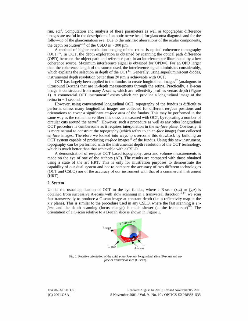
Unlike the usual application of OCT to the eye fundus, where a B-scan (x,z) or (y,z) isobtained from successive A-scans with slow scanning in a transversal direction10-14, we scanfast transversally to produce a C-scan image at constant depth (i.e. a reflectivity map in thex,y plane). This is similar to the procedure used in any CSLO, where the fast scanning is en-face and the depth scanning (focus change) is much slower (at the frame rate)1-9. Theorientation of a C-scan relative to a B-scan slice is shown in Figure 1.
B-scan
C-scan A-scans
Fig. 1: Relative orientation of the axial scan (A-scan), longitudinal slice (B-scan) and en-face or transversal slice (C-scan).
(C) 2001 OSA 5 November 2001 / Vol. 9, No. 10 / OPTICS EXPRESS 535#34986 - $15.00 US Received August 14, 2001; Revised November 05, 2001
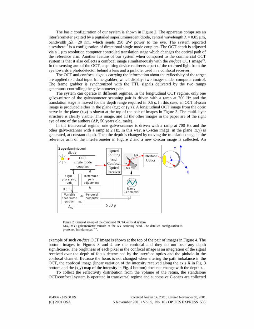
The basic configuration of our system is shown in Figure 2. The apparatus comprises aninterferometer excited by a pigtailed superluminescent diode, central wavelength λ = 0.85 µm,bandwidth ∆λ = 20 nm, which sends 250 µW power to the eye. The system reportedelsewhere15 is a configuration of directional single mode couplers. The OCT depth is adjustedvia a 1 µm resolution computer controlled translation stage which changes the optical path ofthe reference arm. Another feature of our system when compared to the commercial OCTsystem is that it also collects a confocal image simultaneously with the en-face OCT image16.In the sensing arm of the OCT, a splitting device redirects a part of the returned light from theeye towards a photodetector behind a lens and a pinhole, used in a confocal receiver.
The OCT and confocal signals carrying the information about the reflectivity of the targetare applied to a dual input frame grabber, which displays two images under computer control.The frame grabber is synchronized with the TTL signals delivered by the two rampsgenerators controlling the galvanometer pair.
The system can operate in different regimes. In the longitudinal OCT regime, only onegalvo-mirror of the galvanometer scanning pair is driven with a ramp at 700 Hz and thetranslation stage is moved for the depth range required in 0.5 s. In this case, an OCT B-scanimage is produced either in the plane (x,z) or (y,z). A longitudinal OCT image from the opticnerve in the plane (x,z) is shown at the top of the pair of images in Figure 3. The multi-layerstructure is clearly visible. This image, and all the other images in the paper are of the righteye of one of the authors (AP, 50 years old, male).
In the transversal regime, one galvo-scanner is driven with a ramp at 700 Hz and theother galvo-scanner with a ramp at 2 Hz. In this way, a C-scan image, in the plane (x,y) isgenerated, at constant depth. Then the depth is changed by moving the translation stage in thereference arm of the interferometer in Figure 2 and a new C-scan image is collected. An
example of such en-face OCT image is shown at the top of the pair of images in Figure 4. Thebottom images in Figures 3 and 4 are the confocal and they do not bear any depthsignificance. The brightness of each pixel in the confocal image is an integration of the signalreceived over the depth of focus determined by the interface optics and the pinhole in theconfocal channel. Because the focus is not changed when altering the path imbalance in theOCT, the confocal image (linear variation of the intensity received along the axis X in Fig. 3bottom and the (x,y) map of the intensity in Fig. 4 bottom) does not change with the depth z.
To collect the reflectivity distribution from the volume of the retina, the standaloneOCT/confocal system is operated in transversal regime and successive C-scans are collected
OpticalSplitting
andConfocalOptical
Receiver
OCTSingle mode
couplers
RampGenerators
MX
MY
InterfaceOptics
Signalprocessing
unit
Referencepath
adjustment
Personalcomputer
Variablescan frame
grabberSLO
OCT
Superluminiscentdiode
Y
X
Z
Figure 2. General set-up of the combined OCT/Confocal system.MX, MY: galvanometer mirrors of the XY scanning head. The detailed configuration ispresented in references15,16.
(C) 2001 OSA 5 November 2001 / Vol. 9, No. 10 / OPTICS EXPRESS 536#34986 - $15.00 US Received August 14, 2001; Revised November 05, 2001
at different depths17. Ideally, the depth interval between successive frames should be muchsmaller than the system resolution in depth and the depth change applied only after the entireC-scan image was collected. However, in practice, to speed up the acquisition, the translationstage was moved continuously. The movie in Figure 4 is constructed from a stack of 60images collected while moving the stage at 40 µm/s. For the 2Hz frame rate this means 20µm between the frames. In this way, 60 frame-pairs from a volume in depth of 1.18 mm in airare acquired in 30 s. In the movie in Fig. 4, only 50 frames were retained. The first 6 framesdid not show any features and 4 other frames have been discarded due to blinks andmovement effects.
The design is such that there is a strict pixel to pixel correspondence between the two en-face images (OCT and confocal). This helps in two respects: for small movements, theconfocal image can be used to track the eye movements between frames and subsequently totransversally align the OCT images in relation to each other; for large movements and blinks,the confocal image gives a clear indication of the OCT frames which need to be eliminatedaltogether from the collection.
After the stack of pairs of OCT and confocal images has been collected, the confocalimages are used to transversally align the pairs and hence the OCT images. Due to thealignment procedure, the transversal size of the images in the final set of aligned images isreduced from 300 x 300 to 210 x 210 pixels. As a reference for the aligning procedure, thefirst confocal image in the set is used.
CC
Opticdisc
RNFL
RPEPL
RPEandCC
RNFL
Laminacribrosa
Fig. 3. Pair of images from the optic nerveacquired with the standalone OCT/confocal systemin longitudinal regime at y = 0.Top image: OCT; Bottom: confocal; Each imagehas 300x300 pixels.Horizontal: ∆x ~ 3 mm in both images; ∆z (onlythe OCT image) ~ 2 mm depth (vertical axis,measured in air). RNFL (bright): retinal nerve fiberlayer; PL (dark): photoreceptor layer; RPE(bright): retinal pigment epithelium; CC (bright):choriocapillaris.
Fig. 4. ( 1 MB) Movie showing the pair of images fromthe optic nerve acquired with the standaloneOCT/confocal system in transversal regime.Top image: OCT; Bottom: confocal. Each image has300x300 pixels.Horizontal: ∆x ~3 mm, Vertical: ∆y ~ 3 mm in bothimages. The volume is explored from the retinal nervefiber layer to the retinal pigment epithelium, along theoptic axis. The OCT image displayed is at the depthshown by the double arrow in Figure 3 top.
(C) 2001 OSA 5 November 2001 / Vol. 9, No. 10 / OPTICS EXPRESS 537#34986 - $15.00 US Received August 14, 2001; Revised November 05, 2001
Based on the confocal principle, the instrumental depth resolution of a CSLO is limited to afull width half-maximum IDRC = 300 µm (due to the combined limited aperture of the eyeand aberrations2,5,8). Therefore the accuracy in depth location of different scattering featuresand in measuring surface topography and volume is limited. However, interpolationprocedures coupled with peak location software can lead to a much better reproducibility inthe estimation of the peak position in depth. (Topographic reproducibility8 is the ability todetermine the axial location of the centerline of the axial intensity distribution under theassumption of a single interface layer). For instance, the HRT instrument is quoted as givinga reproducibility5,18, RC ~ 20 µm. Considering the instrumental depth resolution this means animprovement factor IF =IDRC/RC = 15 achieved by software processing means, based oninterpolation and peak finding algorithms.
In OCT, the depth resolution is governed by the spectral properties of the low coherencesource, and theoretically, the full width half maximum of the depth sampling profile should behalf of the coherence length of the source, which can easily be much smaller than theachievable depth resolution of a CSLO. Obviously, the same software procedures as used forthe topography based CSLO can be used for an OCT implementation. Considering therecently reported19 instrumental depth resolution of OCT in measuring the retina thickness,IDROCT = 3 µm, and the same value for the improvement factor extended to the OCT case, IF=IDROCT/ROCT, a depth reproducibility ROCT ~ 0.2 µm would seem achievable. This shows thetremendous potential of OCT in providing high depth resolution. However, improvement inthe instrumental depth resolution of OCT does not necessarily attract the same improvementin the final resolution when measuring tissue, as pointed out by comparisons between OCTimages and histology20 and due to the inherent movements of the retina. Variations in theindices of refraction of the intermediate layers up to the depth of interest, from an averagevalue considered in OCT measurement, along with polarization effects due to birefringence ofthe optic nerve justify discrepancies between OCT and histology. Therefore, micronresolutions in tissue, although attractive, have to be considered with caution.
To assess the resolution performances of our system, we used a mirror which was movedaxially through the focus of the interface optics. The FWHM of the signal profile was 16 µmin the OCT channel and ~ 0.9 mm in the confocal channel. All the depth values are measuredin air. Thickness in the retina can be found dividing the axial distances by the index ofrefraction19, n ~ 1.36. The depth resolution of the confocal channel can in principle beimproved to 0.3 mm by using a high NA interface optics and a sufficiently small pinhole.However, as long as much better depth resolution is achievable in the OCT channel, a lowdepth resolution in the confocal channel, sufficient to eliminate the reflections from thecornea, is acceptable. This allows a sufficient good quality CSLO image to be generated basedon a small percentage of the signal reflected by the retina with the majority of the signalremaining in the OCT channel.
For simplicity, in what follows we will approximate the OCT depth resolution as 20 µm(in air) throughout the depth range, although for superficial layers, this may be close to theinstrumental depth resolution, of 16 µm (as measured in air), while for deeper layers, largervalues are expected due to scattering and uncompensated dispersion in the OCT system21.
Due to an 1/e2 beam diameter to the eye of 2.5 mm, the transversal resolution is expectedto be ~ 15 µm, the same in both channels as reported elsewhere when using either confocal8
instruments or OCT14. Using this value as an approximation for the lateral pixel size, we canevaluate the maximum exposure time, according to the same procedure presented inreference22. For a line of 3 mm covering the retina (as a minimum to scan the optic disk), thisgives 200 pixels. Taking into account the line rate of 700 Hz and the frame rate of 2 Hz,investigation with 250 µW is allowed for many hours23 at 850 nm. Seen from a different
(C) 2001 OSA 5 November 2001 / Vol. 9, No. 10 / OPTICS EXPRESS 538#34986 - $15.00 US Received August 14, 2001; Revised November 05, 2001
perspective, the power in our system is 4 times less than the power used in the commercialOCT instrument13 which should allow 4 times longer exposure.
4. Method
4.1. A’-scans
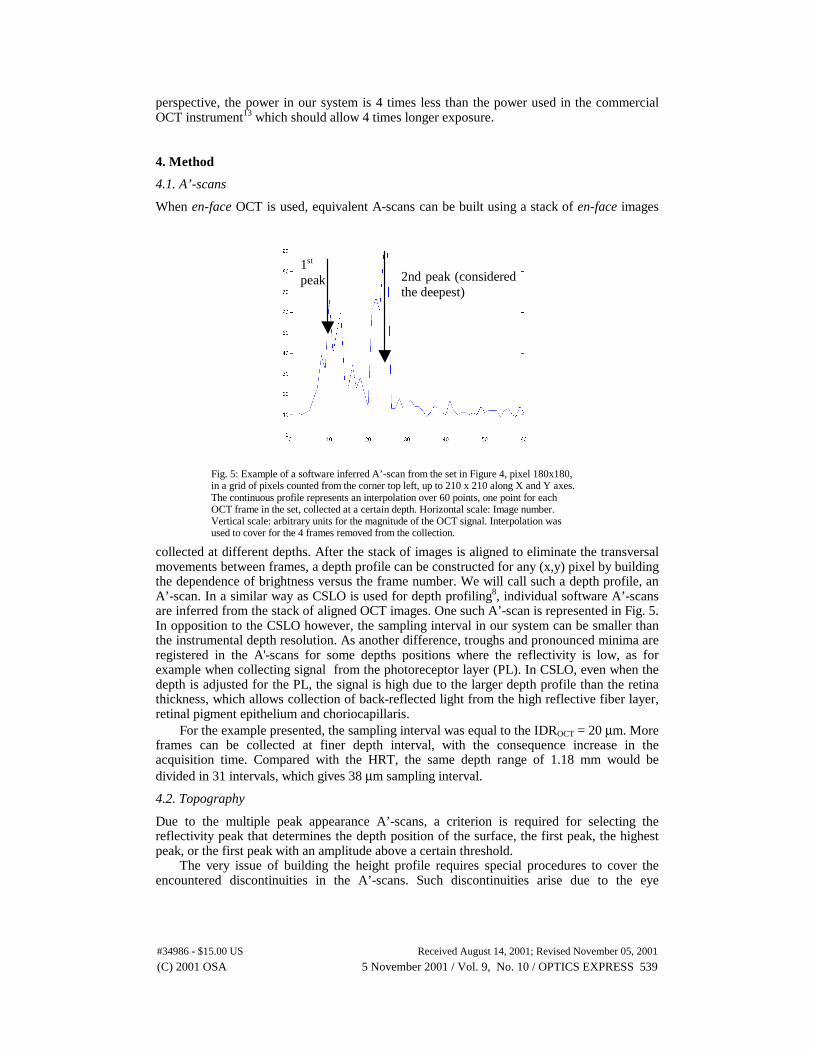
When en-face OCT is used, equivalent A-scans can be built using a stack of en-face images
collected at different depths. After the stack of images is aligned to eliminate the transversalmovements between frames, a depth profile can be constructed for any (x,y) pixel by buildingthe dependence of brightness versus the frame number. We will call such a depth profile, anA’-scan. In a similar way as CSLO is used for depth profiling8, individual software A’-scansare inferred from the stack of aligned OCT images. One such A’-scan is represented in Fig. 5.In opposition to the CSLO however, the sampling interval in our system can be smaller thanthe instrumental depth resolution. As another difference, troughs and pronounced minima areregistered in the A'-scans for some depths positions where the reflectivity is low, as forexample when collecting signal from the photoreceptor layer (PL). In CSLO, even when thedepth is adjusted for the PL, the signal is high due to the larger depth profile than the retinathickness, which allows collection of back-reflected light from the high reflective fiber layer,retinal pigment epithelium and choriocapillaris.
For the example presented, the sampling interval was equal to the IDROCT = 20 µm. Moreframes can be collected at finer depth interval, with the consequence increase in theacquisition time. Compared with the HRT, the same depth range of 1.18 mm would bedivided in 31 intervals, which gives 38 µm sampling interval.
4.2. Topography
Due to the multiple peak appearance A’-scans, a criterion is required for selecting thereflectivity peak that determines the depth position of the surface, the first peak, the highestpeak, or the first peak with an amplitude above a certain threshold.
The very issue of building the height profile requires special procedures to cover theencountered discontinuities in the A’-scans. Such discontinuities arise due to the eye
2nd peak (consideredthe deepest)
1st
peak
Fig. 5: Example of a software inferred A’-scan from the set in Figure 4, pixel 180x180,in a grid of pixels counted from the corner top left, up to 210 x 210 along X and Y axes.The continuous profile represents an interpolation over 60 points, one point for eachOCT frame in the set, collected at a certain depth. Horizontal scale: Image number.Vertical scale: arbitrary units for the magnitude of the OCT signal. Interpolation wasused to cover for the 4 frames removed from the collection.
(C) 2001 OSA 5 November 2001 / Vol. 9, No. 10 / OPTICS EXPRESS 539#34986 - $15.00 US Received August 14, 2001; Revised November 05, 2001
movement, micro-saccades and due to the pulse that displaces tissue near the optic nervehead. The narrower the instrumental depth sampling interval, the more susceptible thetopography method becomes to errors, due to movements or discontinuities in the reflectanceprofile.
For an image of 210x210 pixels there are 2102 A’ scans to be evaluated. We reduced thenumber of samples by superposing A’-scans obtained from 6x6 adjacent transversal positions.This provided an averaging over both transversal and axial directions. Transversally, thisresults in an increase in the lateral pixel size while axially this leads to a smoothing of the A’-scans which provide an average A'-scan more tolerant to discontinuities due to artifacts. Forcomparison, the topography is provided by the HRT in a matrix of 16 x 16 elements. For anangular scan of 100, the HRT element would have a size of ~ 0.2 mm x 0.2 mm. 6 x 6 adjacentpixels leads to a matrix of 36 x 36 elements out of the area of 210 x 210 pixels of the alignedimages in our case. This results in an element size of 60 µm x 60 µm. An optimum in thenumber of pixels to be averaged can be found only by imaging a large number of eyes. For theparticular eye imaged here, 6 pixels seemed a good compromise between the required averageand smoothing of the interpolation procedure and the deterioration of the transversalresolution.
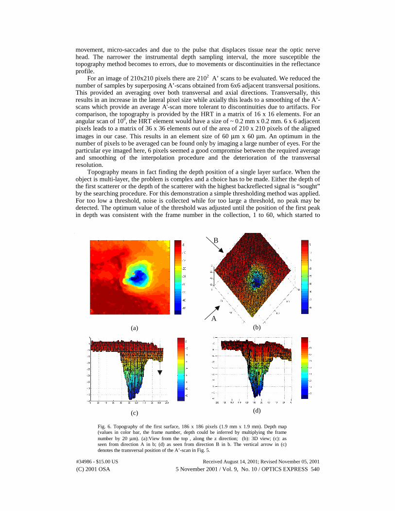
Topography means in fact finding the depth position of a single layer surface. When theobject is multi-layer, the problem is complex and a choice has to be made. Either the depth ofthe first scatterer or the depth of the scatterer with the highest backreflected signal is “sought”by the searching procedure. For this demonstration a simple thresholding method was applied.For too low a threshold, noise is collected while for too large a threshold, no peak may bedetected. The optimum value of the threshold was adjusted until the position of the first peakin depth was consistent with the frame number in the collection, 1 to 60, which started to
(a)
A
B
(b)
(c) (d)
Fig. 6. Topography of the first surface, 186 x 186 pixels (1.9 mm x 1.9 mm). Depth map(values in color bar, the frame number, depth could be inferred by multiplying the framenumber by 20 µm). (a):View from the top , along the z direction; (b): 3D view; (c): asseen from direction A in b; (d) as seen from direction B in b. The vertical arrow in (c)denotes the transversal position of the A’-scan in Fig. 5.
(C) 2001 OSA 5 November 2001 / Vol. 9, No. 10 / OPTICS EXPRESS 540#34986 - $15.00 US Received August 14, 2001; Revised November 05, 2001
show a bright pixel. The topography of the first surface is represented in Fig. 6(a) and 3Dviews in Fig. 6(b-d). 14 more pixels have been removed from each side to avoid the edgeeffects, so the en-face image size is only 186 x 186 pixels.
It is also possible to produce a surface topography of deeper layers. This would be likeeffectively “looking” under the first surface “seeking” for features below the layercorresponding to the first peak. This can also be repeated for a third and so on, highersequence peaks in depth.
To build the topography of the deepest layer, we searched for the first peak starting fromthe end of the A’-scans. We obtain similar representations as in Fig. 6 and represent bothsurfaces in Figure 7. Due to the high depth resolution of the OCT, the two surfaces are clearlydiscernible. We can approximate these two surfaces as corresponding to the retinal fiber layerand the choriocapillaris (please see Fig. 3 top, and Fig. 2 in reference19). The first peak in Fig.5 contributes to the surface as shown by the arrow in Fig. 6c and to the top surface as shownby the arrow in Fig. 7c. The second peak in Fig. 5 contributes to the deepest surface as shownby the arrow in Fig. 7c.
(a) (b)
(c)
A
(d)
Fig. 7. Topography of the deepest surface, 186 x 186 pixels transversal (1.9 mm x 1.9 mm).Depth map (values in color bar, the frame number, depth could be inferred by multiplying theframe number by 20 µm; the color map is different than that in Fig. 6.); (a): as seen from the top;(b): 3D view; (c): first and the deepest surfaces seen from the direction A in (d); (d): 3D views ofthe first and the deepest surfaces (Fig. 6(b) and 7(b) superposed).
(C) 2001 OSA 5 November 2001 / Vol. 9, No. 10 / OPTICS EXPRESS 541#34986 - $15.00 US Received August 14, 2001; Revised November 05, 2001
4.3. Measurements:
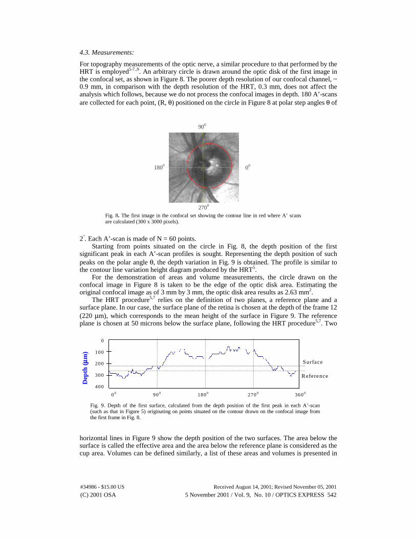
For topography measurements of the optic nerve, a similar procedure to that performed by theHRT is employed5-7.,9. An arbitrary circle is drawn around the optic disk of the first image inthe confocal set, as shown in Figure 8. The poorer depth resolution of our confocal channel, ~0.9 mm, in comparison with the depth resolution of the HRT, 0.3 mm, does not affect theanalysis which follows, because we do not process the confocal images in depth. 180 A’-scansare collected for each point, (R, θ) positioned on the circle in Figure 8 at polar step angles θ of
2°. Each A’-scan is made of N = 60 points.Starting from points situated on the circle in Fig. 8, the depth position of the first
significant peak in each A’-scan profiles is sought. Representing the depth position of suchpeaks on the polar angle θ, the depth variation in Fig. 9 is obtained. The profile is similar tothe contour line variation height diagram produced by the HRT5.
For the demonstration of areas and volume measurements, the circle drawn on theconfocal image in Figure 8 is taken to be the edge of the optic disk area. Estimating theoriginal confocal image as of 3 mm by 3 mm, the optic disk area results as 2.63 mm2.
The HRT procedure5,7 relies on the definition of two planes, a reference plane and asurface plane. In our case, the surface plane of the retina is chosen at the depth of the frame 12(220 µm), which corresponds to the mean height of the surface in Figure 9. The referenceplane is chosen at 50 microns below the surface plane, following the HRT procedure5,7. Two
horizontal lines in Figure 9 show the depth position of the two surfaces. The area below thesurface is called the effective area and the area below the reference plane is considered as thecup area. Volumes can be defined similarly, a list of these areas and volumes is presented in
Dep
th(µµ µµ
m)
0
100
200
300
400
0 0 90 0 180 0 270 0 360 0
Surface
R eference
Fig. 9. Depth of the first surface, calculated from the depth position of the first peak in each A’-scan(such as that in Figure 5) originating on points situated on the contour drawn on the confocal image fromthe first frame in Fig. 8.
1800 00
2700
900
Fig. 8. The first image in the confocal set showing the contour line in red where A’ scansare calculated (300 x 3000 pixels).
(C) 2001 OSA 5 November 2001 / Vol. 9, No. 10 / OPTICS EXPRESS 542#34986 - $15.00 US Received August 14, 2001; Revised November 05, 2001
reference7. It is hoped that these measurements can help an automated classification of theoptic nerve shapes as belonging to the category of normal or glaucomatous eyes.
The results of the measurements are shown in Figure 10 left. The volunteer has had hiseye assessed with the HRT. As far as possible the disk areas were adjusted to be the same.These areas are the starting point of the topographic measurements. Errors could not be totallyavoided, as the two instruments are at different sites. Differences are noticed between theresults obtained with the en-face OCT and with the HRT. A Cup/Disk area ratio of 0.44results in comparison with the 0.329 value returned by the HRT. The value of othermeasurements in Fig. 10 can be compared with the HRT results presented in the Table 1.
4.4. Simulated Longer Resolution Lengths:
To eliminate the discontinuities in the A’-profiles, 6x6 pixels have been put together asmentioned before. It is possible to perform a similar averaging procedure in depth. This isequivalent to sampling the tissue in depth with a coarser depth resolution, in the same way assuggested by us in a previous publication where we discussed en-face OCT imaging withadjustable depth resolution24. Depending on the number of frames from adjacent layers whichare added together to produce one frame, the equivalent depth resolution is increased over theinstrumental depth resolution, IDROCT. Such a procedure results in a smoothing of the A'-scans. In this way, we can “fabricate” a set of images with the instrumental depth resolution ofthe HRT and evaluate the effect on the measurements. To achieve this goal, we superposedeach 15 adjacent OCT images in the set of aligned en-face OCT images to generate imageswith an equivalent of 300 µm sampling interval (this is an approximation, considering theresulting depth sampling interval as 15 x instrumental depth resolution approximated as 20µm). The 300 µm value is specifically targeted as this is usually considered as the CSLO limitof depth resolution in the eye, and similar to that of the HRT. The results of measurementsperformed on the software fabricated set, are shown in Figure 10 right and Table 1. The resultfor the cup area is now smaller, closer to the value obtained with the HRT.
The depth resolution decreases with the number of adjacent en-face images which are
superposed. Therefore, further studies are necessary to find the optimum number of frames tobe superposed, as a compromise between the ease in locating the peaks in the A’-scans andthe error magnitude in area and volume measurements.
Differences are noticed between the quantitative measurements of the optic nerve takenwith the commercial confocal retinal tomograph (HRT) and with our en-face OCT basedretinal tomograph. Different sources of errors are possible. First, the two instruments are attwo different sites and a perfect match of the areas imaged was not possible. Second,instrumental differences may play an important role. The different wavelength may beresponsible for some of the differences observed, 675 nm (HRT) and 850 nm (OCT).Reflectivity and penetration depth of radiation of different wavelengths from visible up to
Fig. 10. Colored map topography of the first surface. The colored areascorrespond to: green, the area above the surface, blue, the area between thesurface and the reference plane and red the area below the reference plane.Values for areas are given in the Table 1.Left: data were processed using the OCT depth resolution;Right: data from the fabricated set of 300 µm depth resolution.
(C) 2001 OSA 5 November 2001 / Vol. 9, No. 10 / OPTICS EXPRESS 543#34986 - $15.00 US Received August 14, 2001; Revised November 05, 2001
infrared was quantified in different reports, which show that longer wavelengths penetratedeeper3,25-27. However, it is difficult to quantitatively assess, taking into account thecomplicated shape of the optic nerve, how the penetration depth influences the measurements.CSLO at longer wavelengths have been reported3,27,28, however the authors are not aware ofany comparative study of how the volumes and areas values measured with CSLO depend onwavelength.
Table 1. Comparative results for the areas and volumes in the optic nerve measured with en-face OCT and with HRT.
Parameter\System used OCT20 µm
OCT300 µm
HRT300 µm
Disk Area (user defined-whole disk)Effective Area (RED&BLUE)Rim Area (BLUE&GREEN)Cup Area (RED)Volume Below Reference (Cup Vol.-RED)Cup/Disk Area Ratio
2.63 mm2
1.613 mm2
1.63 mm2
1.16 mm2
0.241 mm3
0.44
2.63 mm2
1.492 mm2
1.669 mm2
0.949 mm2
0.234 mm3
0.36
2.607 mm2
1.462 mm2
1.748 mm2
0.859 mm2
0.250 mm3
0.329
It is interesting to notice that the coarser depth resolution set, obtained by putting together15 adjacent en-face OCT images, provides measurement values closer to the HRTmeasurements. This may indicate that the depth resolution may play a role in explaining thedifferences noted. It is however too early to speculate based on only one eye investigated thatcoarser depth resolution results in smaller cup areas and larger rim areas. Given theimportance of statistical relevant topography measurements for the follow-up of theglaucomatous eye, such a study may be worth pursuing on a large number of patients.
4.5. Utility of the confocal channel
To perform topography in the way illustrated in the paper, the confocal channel is notabsolutely necessary. The topography was performed using the en-face OCT images.However, the dual representation unique for our system has helped in two respects:(i) The relative movements of the confocal images is easier to track than the movements in theen-face OCT images. The OCT image may not show anything or be so fragmented that itcannot be processed. For instance, any alignment procedure would need to track relevantfeatures in the stack of images. The chosen feature may or may not appear in the displayedimage, depending on the retina inclination and the depth. This is in contrast to the confocalimage, which looks more continuous even when largely out of focus.(ii) The depth profile is evaluated along a contour drawn around the optic disk. This contourcan be for instance drawn over an image resulting from the superposition of all the OCTimages in the stack. Such an image would correspond to an image with a larger depthsampling interval, practically equal to the exploration interval. However, we believe that sucha procedure would deprive the image of its transversal quality, and therefore, the confocalimage is better suited for drawing the contour.
5. Conclusions
The paper demonstrates that the OCT technology, performed en-face, could be a potentialcandidate for topography as well as for area and volume measurements of the optic nerve. Thepaper presents for the first time such topography and measurements, obtained using en-faceOCT. The en-face OCT addresses the incompatibility in the aspect of current CSLO and OCTtechnologies, images acquired with the two technologies could now be easily compared. Thecompatibility in aspect of the images produced by CSLO and en-face OCT allows theapplication of all procedures initially developed around CSLO technology to be extended tothe en-face OCT technology. This paper is a first demonstration of such a possible extension.The same procedures developed for CSLO topography have been extended to the en-faceOCT.
(C) 2001 OSA 5 November 2001 / Vol. 9, No. 10 / OPTICS EXPRESS 544#34986 - $15.00 US Received August 14, 2001; Revised November 05, 2001
The en-face OCT imaging seems more suitable to perform topography than thelongitudinal OCT imaging. If the object is a surface oriented perpendicular to the optic axis,the en-face OCT can provide the topography in one single frame, while longitudinal OCTrequires interpolation of many A-scans. In practice however, the object is more complicated.The same single surface if oriented obliquely to the optic axis also requires interpolation ofthe points in the axial direction from en-face slice to the next en-face slice progressing indepth. The en-face OCT based topography provides continuous surfaces, rectangular to theoptic axis and requires interpolation in depth. The longitudinal OCT based topographyprovides continuous profiles in depth and requires lateral interpolation. For the same data rate,sampling intervals and number of pixels the two methods may be very similar. However, theen-face OCT imaging may allow a quicker inference of the approximate topography profile.The approximate topography may be visible in the very process of frame acquisition (as seenin the movie in Figure 4), which is not possible to grasp when performing longitudinal OCT.In longitudinal OCT, all the volume data needs to be acquired and software processed beforeany surface with orientation rectangular to that of scanning direction could be generated.
The major source of measurement variation from successive examinations is patientrealignment and instrument adjustment. The possibility of working en-face allowed us torealize how critical for the OCT images is the orientation of the eye, which may not be soobvious in longitudinal OCT. In the longitudinal OCT, when the retina surface is inclined, thefinal image shows layers oriented along diagonal directions deviating from horizontal(considering an x,z or an y,z image). The tilt has a different effect in the en-face OCT image,visible in the fragmentation and asymmetry of the en-face image. A horizontal tilt will lead tomore fragments either left or right while vertical tilt will result in more fragments either up ordown in the image. The vertical tilt (inclination in respect to axis y) is not visible inlongitudinal OCT performed horizontally (i.e. in the x,z images) and the horizontal tilt(inclination in respect to axis x) is not visible in the longitudinal OCT performed vertically(i.e. in the y,z images). However, the en-face OCT shows the surface tilt in a single image.This can be noticed in the movie in figure 4. The transversal distribution of fragments indicatethe tilt orientation directly. Longitudinal OCT performed at many radial orientations aroundthe center of the image can show the spatial orientation of the retina surface, but this isobtained only after full collection of data is performed. This may require the investigation tobe repeated if the tilt was too high and some of the slopes in the surface to be constructedcould not be detected.
Due to the high depth resolution, OCT allows better differentiation of layers than CSLOand additionally, topography of deep layers. An illustration was presented in providing thetopography of the choriocapilaris layer, along with the topography of the retinal nerve fibrelayer. If topography of deep layers can be performed accurately and reproductively, newinformation can be provided to the ophthalmologist, in addition to the information currentlycollected using the CSLO technology. It is hoped that further refinements of the technique andsoftware procedure may allow the standalone OCT/confocal system to be successfully appliedto topography of the macula29,30.
This paper describes measurements collected with the HRT and the en-face OCTinstrument from only one eye. The intention was to demonstrate the viability of en-face OCTbased topography and not to make a thorough statistical analysis of the measurementsprovided by en-face OCT nor to compare the reproducibility of OCT with that of CSLO.Large number of eyes need to be imaged to prove the validity of the method for diagnosticpurposes. Such a study, if performed, may suggest new procedures for better area and volumemeasurements. For instance, the high depth resolution may allow a better definition of thereference plane or a complete change in the measurement strategy, where strong localisedreflections can be used as reference (for instance the RPE or the choriocapillaris layer).
AcknowledgementsThe authors acknowledge the support of the UK Engineering and Physical Sciences ResearchCouncil and of the Ophthalmic Technologies Inc. of Toronto, Canada.
(C) 2001 OSA 5 November 2001 / Vol. 9, No. 10 / OPTICS EXPRESS 545#34986 - $15.00 US Received August 14, 2001; Revised November 05, 2001