98
AN INVITATION TO TOPOLOGY Lecture notes by R˘ azvan Gelca
| Date post: | 25-Feb-2018 |
| Category: |
Documents |
| Upload: | ali-al-asadi |
| View: | 215 times |
| Download: | 0 times |

7/25/2019 TOPOLOG8Y
http://slidepdf.com/reader/full/topolog8y 1/98
AN INVITATION TO TOPOLOGY
Lecture notes by Razvan Gelca

7/25/2019 TOPOLOG8Y
http://slidepdf.com/reader/full/topolog8y 2/98
2

7/25/2019 TOPOLOG8Y
http://slidepdf.com/reader/full/topolog8y 3/98
Contents
I General Topology 5
1 Topological Spaces and Continuous Functions 71.1 The topology of the real line . . . . . . . . . . . . . . . . . . . . . . . . . . . . . . . . 7
1.2 The definitions of topological spaces and continuous maps . . . . . . . . . . . . . . . 8
1.3 Procedures for constructing topological spaces . . . . . . . . . . . . . . . . . . . . . . 10
1.3.1 Basis for a topology . . . . . . . . . . . . . . . . . . . . . . . . . . . . . . . . 10
1.3.2 Subspaces of a topological space . . . . . . . . . . . . . . . . . . . . . . . . . 11
1.3.3 The product of two topological spaces . . . . . . . . . . . . . . . . . . . . . . 12
1.3.4 The product of an arbitrary number of topological spaces . . . . . . . . . . . 13
1.3.5 The disjoint union of two topological spaces. . . . . . . . . . . . . . . . . . . 13
1.3.6 Metric spaces as topological spaces . . . . . . . . . . . . . . . . . . . . . . . . 141.3.7 Quotient spaces . . . . . . . . . . . . . . . . . . . . . . . . . . . . . . . . . . . 16
1.3.8 Manifolds . . . . . . . . . . . . . . . . . . . . . . . . . . . . . . . . . . . . . . 17
2 Closed sets, connected and compact spaces 192.1 Closed sets and related notions . . . . . . . . . . . . . . . . . . . . . . . . . . . . . . 19
2.1.1 Closed sets . . . . . . . . . . . . . . . . . . . . . . . . . . . . . . . . . . . . . 19
2.1.2 Closure and interior of a set . . . . . . . . . . . . . . . . . . . . . . . . . . . . 21
2.1.3 Limit points . . . . . . . . . . . . . . . . . . . . . . . . . . . . . . . . . . . . . 22
2.2 Hausdorff spaces . . . . . . . . . . . . . . . . . . . . . . . . . . . . . . . . . . . . . . 24
2.3 Connected spaces . . . . . . . . . . . . . . . . . . . . . . . . . . . . . . . . . . . . . . 25
2.3.1 The definition of a connected space and properties . . . . . . . . . . . . . . . 252.3.2 Connected sets in R and applications . . . . . . . . . . . . . . . . . . . . . . . 27
2.3.3 Path connected spaces . . . . . . . . . . . . . . . . . . . . . . . . . . . . . . . 28
2.4 Compact spaces . . . . . . . . . . . . . . . . . . . . . . . . . . . . . . . . . . . . . . . 30
2.4.1 The definition of compact spaces and examples . . . . . . . . . . . . . . . . . 30
2.4.2 Properties of compact spaces . . . . . . . . . . . . . . . . . . . . . . . . . . . 31
2.4.3 Compactness of product spaces . . . . . . . . . . . . . . . . . . . . . . . . . . 35
2.4.4 Compactness in metric spaces and limit point compactness . . . . . . . . . . 37
2.4.5 Alexandroff compactification . . . . . . . . . . . . . . . . . . . . . . . . . . . 38
3 Separation Axioms 41
3.1 The countability axioms . . . . . . . . . . . . . . . . . . . . . . . . . . . . . . . . . . 413.2 Regular spaces . . . . . . . . . . . . . . . . . . . . . . . . . . . . . . . . . . . . . . . 41
3.3 Normal spaces . . . . . . . . . . . . . . . . . . . . . . . . . . . . . . . . . . . . . . . 42
3.3.1 Properties of normal spaces . . . . . . . . . . . . . . . . . . . . . . . . . . . . 42
3.3.2 Urysohn’s lemma . . . . . . . . . . . . . . . . . . . . . . . . . . . . . . . . . . 43
3

7/25/2019 TOPOLOG8Y
http://slidepdf.com/reader/full/topolog8y 4/98
4 CONTENTS
3.3.3 The Tietze extension theorem . . . . . . . . . . . . . . . . . . . . . . . . . . . 44
II Algebraic topology 45
4 Homotopy theory 474.1 Homotopy . . . . . . . . . . . . . . . . . . . . . . . . . . . . . . . . . . . . . . . . . . 474.2 The fundamental group . . . . . . . . . . . . . . . . . . . . . . . . . . . . . . . . . . 49
4.2.1 The definition and properties of the fundamental group . . . . . . . . . . . . 494.2.2 The behavior of the fundamental group under continuous transformations . . 51
4.3 The fundamental group of the circle . . . . . . . . . . . . . . . . . . . . . . . . . . . 524.3.1 Covering spaces and the fundamental group . . . . . . . . . . . . . . . . . . . 524.3.2 The computation of the fundamental group of the circle . . . . . . . . . . . . 554.3.3 Applications of the fundamental group of the circle . . . . . . . . . . . . . . . 55
4.4 The structure of covering spaces . . . . . . . . . . . . . . . . . . . . . . . . . . . . . 574.4.1 Existence of covering spaces . . . . . . . . . . . . . . . . . . . . . . . . . . . . 574.4.2 Equivalence of covering spaces . . . . . . . . . . . . . . . . . . . . . . . . . . 604.4.3 Deck transformations . . . . . . . . . . . . . . . . . . . . . . . . . . . . . . . 62
4.5 The Seifert-van Kampen theorem . . . . . . . . . . . . . . . . . . . . . . . . . . . . . 654.5.1 A review of some facts in group theory . . . . . . . . . . . . . . . . . . . . . . 654.5.2 The statement and proof of the Seifert-van Kampen theorem . . . . . . . . . 67
4.5.3 Fundamental groups computed using the Seifert-van Kampen theorem . . . . 704.5.4 The construction of compact surfaces and the computation of their funda-mental groups . . . . . . . . . . . . . . . . . . . . . . . . . . . . . . . . . . . . 71
5 Homology 755.1 Simplicial homology . . . . . . . . . . . . . . . . . . . . . . . . . . . . . . . . . . . . 75
5.1.1 ∆-complexes . . . . . . . . . . . . . . . . . . . . . . . . . . . . . . . . . . . . 755.1.2 The definition of simplicial homology . . . . . . . . . . . . . . . . . . . . . . . 775.1.3 Some facts about abelian groups . . . . . . . . . . . . . . . . . . . . . . . . . 785.1.4 The computation of the homology groups for various spaces . . . . . . . . . . 785.1.5 Homology with real coefficients and the Euler characteristic . . . . . . . . . . 84
5.2 Continuous maps between ∆-complexes . . . . . . . . . . . . . . . . . . . . . . . . . 875.2.1 ∆-maps . . . . . . . . . . . . . . . . . . . . . . . . . . . . . . . . . . . . . . . 875.2.2 Simplicial complexes, simplicial maps, barycentric subdivision. . . . . . . . . 895.2.3 The simplicial approximation theorem . . . . . . . . . . . . . . . . . . . . . . 945.2.4 The independence of homology groups on the geometric realization of the
space as a ∆-complex . . . . . . . . . . . . . . . . . . . . . . . . . . . . . . . 965.3 Applications of homology . . . . . . . . . . . . . . . . . . . . . . . . . . . . . . . . . 97

7/25/2019 TOPOLOG8Y
http://slidepdf.com/reader/full/topolog8y 5/98
Part I
General Topology
5

7/25/2019 TOPOLOG8Y
http://slidepdf.com/reader/full/topolog8y 6/98

7/25/2019 TOPOLOG8Y
http://slidepdf.com/reader/full/topolog8y 7/98
Chapter 1
Topological Spaces and Continuous
Functions
Topology studies properties that are invariant under continuous transformations (homeomorphisms).As such, it can be thought of as rubber-sheet geometry. It is interested in how things are connected,but not in shape and size. The fundamental objects of topology are topological spaces and contin-uous functions.
1.1 The topology of the real lineThe Weierstrass ǫ − δ definition for the continuity of a function on the real axis
Definition. A function f : R → R is continuous if and only if for every x0 ∈ R and every ǫ > 0there is δ > 0 such that for all x ∈ R with |x − x0| < δ , one has |f (x) − f (x0)| < ǫ
can be rephrased by the more elegant
Definition. A function f : R → R is continuous if and only if the preimage of each open intervalis a union of open intervals
or even by the most elegant
Definition. A functions f : R→ R is continuous if and only if the preimage of each union of openintervals is a union of open intervals.
For simplicity, a union of open intervals will be called an open set . And because the complementof an open interval consists of one or two closed intervals, we will call the complements of open setsclosed sets . Our topological space is R, and the topology on R is defined by the open sets.
Let us examine the properties of open sets. First, notice that the union of an arbitrary familyof open sets is open. This is not true for the intersection though, since for example the intersectionof all open sets centered at 0 is just {0}. However the intersection of finitely many open sets isopen, provided that the sets intersect nontrivially. Add the empty set to the topology so that theintersection of finitely many open sets is always open. Notice also that R is open since it is theunion of all its open subintervals.
Open intervals are the building blocks of the topology. For that reason, they are said to forma basis . If we just restrict ourselves to bounded open intervals, they form a basis as well. Eachbounded open interval is of the form (x0 − δ, x0 + δ ), and as such it consists of all points that areat distance less than δ from x0. So the distance function (metric) on R can be used for defining atopology.
7

7/25/2019 TOPOLOG8Y
http://slidepdf.com/reader/full/topolog8y 8/98
8 CHAPTER 1. TOPOLOGICAL SPACES AND CONTINUOUS FUNCTIONS
1.2 The definitions of topological spaces and continuous maps
We will define the notions of topological space and continuous maps to cover Rn with continuousfunctions on it (real analysis), spaces of functions with continuous functionals on them (functionalanalysis, differential equations, mathematical physics), manifolds with continuous maps, algebraicsets (zeros of polynomials) and regular (polynomial) maps (algebraic geometry).
Definition. A topology on a set X is a collection T of subsets of X with the following properties
(1) ∅ and X are in T ,
(2) The union of arbitrarily many sets from T is in T ,(3) The intersection of finitely many sets from T is in T .
The sets in T are called open , their complements are called closed . Let us point out that closedsets have the following properties: (1) X and ∅ are closed, (2) the union of finitely many closedsets is closed, (3) the intersection of an arbitrary number of closed sets is closed.
Example 1. On Rn we define the open sets to consist of the whole space, the empty set and theunions of open balls Bx0,δ = {x ∈ Rn | dist(x, x0) < δ }. This is the standard topology on Rn.
Example 2. Let C [a, b] be the set of real-valued continuous functions on the interval [a, b] can be en-dowed with the distance function dist(f, g) = supx |f (x) −g(x)|. Then C [a, b] is a topological space
with the open sets being the unions of ”open balls” of the form Bf,δ = {g ∈ C [a, b] | dist(f, g) < δ }.Example 3. The Lebesgue space L2(R) of integrable functions f on R such that
|f (x)2|dx < ∞,with open sets being the unions of ”open balls” of the form Bf,δ = {g ∈ L2(R) | |f (x)−g(x)|2dx <δ }.
Example 4. In Cn, let the closed sets be intersections of zeros of polynomials. That is, closed setsare of the form
V = {z ∈ Cn | f (z) = 0 for f ∈ S }
where S is a set of n-variable polynomials. The open sets are their complements. This is called theZariski topology .
A particular case is that of n = 1. In that case every polynomial has finitely many zeros (maybeno zeros at all for constant polynomials), except for the zero polynomial whose zeros are the entirecomplex plane. Moreover, any finite set is the set of zeros of some polynomial. So the closed setsare the finite sets together with C and ∅. The open sets are C, ∅, and the complements of finitesets.
Example 5. Inspired by the Zariski topology on C, given an arbitrary infinite set X we can let T cbe the collection of all subsets U of X such that X \U is either countable or it is all of X .
Example 6. We can cook up examples of exotic topologies, such as X = {1, 2, 3, 4}, T ={∅, X, {1}, {2, 3}, {1, 2, 3}, {2, 3, 4}}.
Example 7. There are two silly examples of topologies of a set X . One is the discrete topology,in which every subset of X is open and the other is the trivial topology, whose only open sets are∅ and X .
Example 8. Here is a fascinating topological proof given in 1955 by H. Furstenberg to Euclid’stheorem.

7/25/2019 TOPOLOG8Y
http://slidepdf.com/reader/full/topolog8y 9/98
1.2. THE DEFINITIONS OF TOPOLOGICAL SPACES AND CONTINUOUS MAPS 9
Theorem 1.2.1. (Euclid) There are infinitely many prime numbers.
Proof. Introduce a topology on Z, namely the smallest topology in which any set consisting of allterms of a nonconstant arithmetic progression is open. As an example, in this topology both theset of odd integers and the set of even integers are open. Because the intersection of two arithmeticprogressions is an arithmetic progression, the open sets of T are precisely the unions of arithmeticprogressions. In particular, any open set is either infinite or void.
If we denote
Aa,d = {. . . , a − 2d, a − d,a,a + d, a + 2d , . . .}, a ∈ Z, d > 0,
then Aa,d is open by hypothesis, but it is also closed because it is the complement of the open setAa+1,d ∪ Aa+2,d ∪ . . . ∪ Aa+d−1,d. Hence Z\Aa,d is open.Now let us assume that only finitely many primes exist, say p1, p2, . . . , pn. Then
A0,p1 ∪ A0,p2 ∪ . . . ∪ A0,pn = Z\{−1, 1}.
This union is the complement of the open set
(Z\A0,p1) ∩ (Z\A0,p2) ∩ · · · ∩ (Z\A0,pn),
hence it is closed. The complement of this closed set, which is the set {−1, 1}, must thereforebe open. We reached a contradiction because this set is neither empty nor infinite. Hence ourassumption was false, and so there are infinitely many primes.
Given two topologies T and T ′ such that T ′ ⊂ T , one says that T is finer than T ′, or that T ′is coarser then T .Definition. Given a point x, if a set V contains an open set U such that x ∈ U then V is called aneighborhood of x.
Let X and Y be topological spaces.
Definition. A map f : X → Y is continuous if for every open set U ∈ Y , the set f −1(U ) is openis X .
Example 1. This definition covers the case of continuous maps f : Rm → Rn encountered in
multivariable calculus.Example 2. Let X = C [a, b], the topological space of continuous functions from Example 2 above,
and let Y = R. The functional φ : C [a, b] → R, φ(f ) = ba f (x)dx is continuous.
Example 3. Let X = L p(R), Y = R and φ : X → Y , φ(f ) = ( p |f (x)| pdx)1/p.
Remark 1.2.1. An alternative way of phrasing the defintion is to say that for every neighborhoodW of f (x) there is a neighborhood V of x such that f (V ) ⊂ W .
Proposition 1.2.1. The composition of continuous maps is continuous.
Proof. Let f : X → Y and g : Y → Z be continuous, and let us show that g ◦ f is continuous. If U
⊂ is open, then g−1(U ) is open, so f −1(g−1(U )) is open. Done.
Definition. If f : X → Y is a one-to-one and onto map between topological spaces such that bothf and f −1 are continuous, then f is called a homeomorphism.
If there is a homeomorphism between the topological spaces X and Y then they from thetopological point of view they are indistinguishable.

7/25/2019 TOPOLOG8Y
http://slidepdf.com/reader/full/topolog8y 10/98
10 CHAPTER 1. TOPOLOGICAL SPACES AND CONTINUOUS FUNCTIONS
1.3 Procedures for constructing topological spaces
1.3.1 Basis for a topology
Rather than specifying all open sets, we can exhibit a family of open sets from which all others canbe recovered. In general, basis elements mimic the role of open intervals in the topology of the realline.
Definition. Given a set X , a basis for a topology on X is a collection B of subsets of X such that
(1) For each x
∈ X , there is at least one basis element B containing x,
(2) If x ∈ B1 ∩ B2 with B1, B2 basis elements, then there is a basis element B3 such thatx ∈ B3 ⊂ B1 ∩ B2.
Proposition 1.3.1. Let T be the collection of all subsets U of X with the property that for everyx ∈ U , there is Bx ∈ B such that x ∈ Bx ⊂ U . Then T is a topology.
Proof. (1) X and ∅ are in T trivially.
(2) If U α ∈ T for all α, let us show that U = ∪αU α ∈ T . Given x ∈ U , there is U α such thatx ∈ U α. By hypothesis there is Bα ∈ B such that x ∈ Bα ⊂ U α, and hence x ∈ Bα ⊂ U .
(3) Let us show that the intersection of two elements U 1 and U 2 from T is in T . For x ∈ U 1∪U 2there are basis elements B1, B2 such that x
∈ Bi
⊂ U i, i = 1, 2. Then there is a basis element B3
such that x ∈ B3 ⊂ B1 ∩ B2 ⊂ U 1 ∩ U 2, and so U 1 ∩ U 2 ∈ T . The general case of the intersectionof n sets follows by induction.
Proposition 1.3.2. Let X be a topological space with topology T . If B is a basis for T , then T equals the collection of all unions of elements in B .
Proof. The definition of T implies that the elements of T are unions of elements in B . Moreprecisely, U = ∪x∈U Bx. On the other hand, all unions of elements in B are unions of elements inT , therefore are in T .
Example 1. The collection of all disks in the plane is a basis for the standard topology of theplane.
Example 2. The collection of all rectangular regions in the plane that have sides parallel to theaxes of coordinates is a basis for the standard topology.
Example 3. The basis consisting of all intervals of the form (a, b] with a < b and a, b ∈ R generatesa topology called the upper limit topology. This topology is different from the standard topology,since for example (a, b] is not open in the standard topology. Since (a, b) = ∪n(a, b − 1/n], we seethat the standard topology is coarser than the upper limit topology.
Similarly, the sets [a, b) with a < b and a, b ∈ R form a basis for the lower limit topology.
Taking into account both unions and finite intersections, one can simplify further the generating
family for a topology. A subbasis S for a topology on X is a collection of subsets of X whose unionequals X .
Proposition 1.3.3. The set T consisting of all unions of finite intersections of elements of S andthe empty set is a topology on X .
7/25/2019 TOPOLOG8Y
http://slidepdf.com/reader/full/topolog8y 11/98
1.3. PROCEDURES FOR CONSTRUCTING TOPOLOGICAL SPACES 11
Proof. (1) ∅, X ∈ T by hypothesis.(2) The union of unions of finite intersections of elements in S is a union of finite intersections
of elements in S .(3) It suffices to show that the set B of all finite intersections of elements in S is a basis
for a topology. And indeed, if B1 = S 1 ∩ S 2 ∩ ·· · ∩ S m and B2 = S ′1 ∩ S ′2 ∩ ·· · ∩ S ′n, thenB1 ∩ B2 = S 1 ∩ S 2 ∩ · · · ∩ S ′1 ∩ S ′2 ∩ · ∩ S ′n which is again in B . Done.
Here is a criterion that allows us to recognize at first glance bases for topologies.
Proposition 1.3.4. Let X be a topological space with topology T . Suppose that C is a collectionof open sets of X such that for each open set U
⊂ X and each x
∈ U , there is C
∈ C such that
x ∈ C ⊂ U . Then C is a basis for T .Proof. First, we show that C is a basis. Since for every x ∈ X , there is C ∈ C such that x ∈ C ⊂ X ,it follows that X is the union of the elements of C. For the second condition, let C 1, C 2 ∈ C, andx ∈ C 1∩C 2. Since C 1∩C 2 is open (both C 1 and C 2 are), there is C 3 ∈ C such that x ∈ C 3 ⊂ C 1∩C 2.
Let us show now that C is a basis for the topology T . First, given U ∈ T , for each x ∈ U , thereis C x ∈ C such that x ∈ C x ⊂ U . Then U = ∪x∈U C x. Thus all open sets belong to the topologygenerated by C. On the other hand, every union of elements of C is a union of open sets in T , thusis in T . Hence the conclusion.
Working with a basis simplifies the task of comparing topologies.
Proposition 1.3.5. Let B and B ′ be bases for the topologies T respectively T ′ on X . Then T ′ isfiner than T if and only if for each x ∈ X and each B ∈ B that contains x, there is B′ ∈ B ′ suchthat x ∈ B ′ ⊂ B .
Proof. If T ′ is finer than T , then every B ∈ B is in T ′. Hence for every x ∈ B, there is B′ ∈ B ′such that x ∈ B ′ ⊂ B.
For the converse, let us show that every U ∈ T is also in T ′. For every x ∈ U , there is Bx ∈ B such that x ∈ Bx ⊂ U , and hence there is B ′
x ∈ B ′ such that x ∈ B ′x ⊂ Bx ⊂ U . Then U = ∪x∈U B
′x,
showing that U ∈ T ′.Example. The collection of all disks in the plane and the collection of all squares in the planegenerate the same topology. Indeed, for every disk, and every point in the disk there is a square
centered at that point included in the disk, and for every square and every point in the squarethere is a disk centered at the point included in the square.
Using a basis makes it easier to check continuity.
Proposition 1.3.6. Let X and Y be topological spaces. Than f : X → Y is continuous if andonly if for every basis element of the topology on Y , f −1(B) is open in X .
1.3.2 Subspaces of a topological space
One studies continuous functions on subsets of the real axis, as well, such as continuous functionson open and closed intervals. Continuity is then rephrased by restricting open intervals to the
domain of the function, that is by intersecting open sets with the domain.Definition. Let X be a topological space with topology T . If Y is a subset of X , then Y itself isa topological space with the subspace topology
T Y = {Y ∩ U | U ∈ T }.

7/25/2019 TOPOLOG8Y
http://slidepdf.com/reader/full/topolog8y 12/98
12 CHAPTER 1. TOPOLOGICAL SPACES AND CONTINUOUS FUNCTIONS
Proposition 1.3.7. The set T Y is a topology on Y . If B is a basis of T , then
B Y = {B ∩ Y | B ∈ B}is a basis for T Y .Proof. (1) Y = X ∩ Y and ∅ = ∅ ∩ Y are in T Y .
(2) and (3) follow from
(U 1 ∩ Y ) ∩ · · · ∩ (U n ∩ Y ) = (U 1 ∩ U 2 · · · ∩ U n) ∩ Y
∪α(U α ∩ Y ) = (∪αU α) ∩ Y.
For the second part, let U be open in X and y ∈ U ∩ Y . Choose B ∈ B such that y ∈ B ⊂ U .Then y ∈ B ∩ Y ⊂ U ∩ Y , and the conclusion follows.
Example 1. For [0, 1] ⊂ R, then a basis for the subspace topology consists of all the sets of theform (a, b), [0, b), (a, 1] with a, b ∈ (0, 1).
Example 2. For Z ⊂ R, then the subset topology is the discrete topology.
Example 3. For (0, 1) ∪ {2}, then the open sets of the subset topology are all sets of either theform U or U ∪ {2}, where U is a union of open intervals in (0, 1).
Proposition 1.3.8. If f : X
→ Z is a continuous map between topological spaces and if Y
⊂ X
is a topological subspace, then the restriction f |Y : Y → Z is a continuous map.
Proof. Let U ⊂ Z be open. Then f −1(U ) is open in X . But f |−1Y (U ) = f −1(U ) ∩ Y , which is openin Y . Hence f is continuous.
1.3.3 The product of two topological spaces
By examining how the standard topology on R2 = R× R compares to the one on R, we can makethe following generalization
Definition. Let X and Y be topological spaces. The product topology on X × Y is the topologyhaving as basis the collection B of all the sets of the form U × V , where U is an open set of X and
V is an open set of Y .
Of course, for this to work we need the following
Proposition 1.3.9. The collection B defined this way is a basis.
Proof. The first condition for the basis just states that X × Y is in B , which is obvious. For thesecond condition, note that if U 1 × V 1 and U 2 × V 2 are basis elements, then
(U 1 × V 1) ∩ (U 2 × V 2) = (U 1 ∩ U 2) × (V 1 ∩ V 2),
and the latter is a basis element because U 1 ∩ U 2 and V 1 ∩ V 2 are open.
Proposition 1.3.10. If B X is a basis for the topology on X and B Y is a basis for the topology onY , then
B = {B1 × B2 | B1 ∈ B X , B2 ∈ B Y }is a basis for the topology of X × Y .
7/25/2019 TOPOLOG8Y
http://slidepdf.com/reader/full/topolog8y 13/98
1.3. PROCEDURES FOR CONSTRUCTING TOPOLOGICAL SPACES 13
Proof. We will apply the criterion from Proposition 1.3.4. Given an open set W ⊂ X × Y and(x, y) ∈ W , by the definition of the product topology there is a basis element of the form U × V such that (x, y) ∈ U × V ⊂ W . Then, there are B1 ∈ B X such that x ∈ B1 ⊂ U and B2 ∈ B Y , suchthat y ∈ B2 ⊂ V . Then (x, y) ⊂ B1 × B2 ⊂ U ×V . It follows that B meets the requirements of thecriterion, so B is a basis for X × Y .
Using an inductive construction we can extend the definition of product topology to a cartesianproduct of finitely many topological spaces.
1.3.4 The product of an arbitrary number of topological spaces
There are two ways in which the definition of product topology can be extended to an infiniteproduct of topological spaces, the box topology and what we will call the product topology. LetX α, α ∈ A be a family of topological spaces.
Definition. The box topology is the topology on
α X α with basis all sets of the form
α U α withU α open in X α, for all α ∈ A.
Definition. The product topology is the topology on
α X α with basis all sets of the form
α U α,with U α open in X α and U α = X α for all but finitely many α ∈ A.
Notice that the second topology is coarser than the first. At first glance, the box topology seemsto be the right choice, but unfortunately it is to fine to be of any use in applications. In the case
of normed spaces, the second topology becomes the weak topology, which is quite useful (e.g. inthe theory of differential equations). In fact, the next result is a good reason for picking this as theright topology on the product space.
Proposition 1.3.11. Let X α, α ∈ A and Y be topological spaces. Then f : Y → α X α iscontinuous if and only if the coordinate functions f α : Y → Y α are all continuous.
Proof. Assume first that for each α, f α is continuous. Let B be a basis element for the topology of X , say B =
α∈A0
U α×α∈A0X α, where A0 is finite and U α are open. Then f −1(B) = ∩αf −1α (U α).
All but finitely many U α’s, say U α1, U α2, . . . , U αn, equal to whole space. It follows that
f −1(B) =
∩ni=1f −1αi
(U αi)
which is open, being an intersection of finitely many open sets.For the converse, notice that the projection maps πα :
α X α are continuous because of the way
the topology was defined, and that f α = πα ◦ f . By Proposition 1.2.1, f α is continuous. QED.
1.3.5 The disjoint union of two topological spaces.
Definition. Given a family X α of topological spaces, α ∈ A, the topological space ∐αX α is thedisjoint union of the spaces X α endowed with the topology in which U is open if and only if U ∩X αis open for all α.
Example 1. If X is any topological space, then ∐x∈X {x} equals X as a set, but it is now endowedwith the discrete topology.
Proposition 1.3.12. If X α, α ∈ A, Y are topological spaces then f : ∐αX α → Y is continuous if and only if f |X α is continuous for each α.

7/25/2019 TOPOLOG8Y
http://slidepdf.com/reader/full/topolog8y 14/98
14 CHAPTER 1. TOPOLOGICAL SPACES AND CONTINUOUS FUNCTIONS
1.3.6 Metric spaces as topological spaces
Metric spaces are examples of topological spaces that are widely used in areas such as geometry,real analysis, or functional analysis.
Definition. A metric (distance) on a set X is a function
d : X × X → R
satisfying the following properties
(1) d(x, y) ≥
0 for all x, y ∈
X , with equality if and only if x = y.
(2) d(x, y) = d(y, x) for all x, y ∈ X .
(3) d(x, y) + d(y, z) ≥ d(x, z) for all x,y , z ∈ X .
For ǫ > 0, set
B(x, ǫ) = {y | d(x, y) < ǫ}.
This is called the ǫ-ball centered at x.
Proposition 1.3.13. If d is a metric on a set X , then the collection of all balls B(x, ǫ) for x
∈ X
and ǫ > 0 is a basis for a topology on X .
Proof. The first condition for a basis is trivial, since each point lies in a ball centered at that point.For the second condition, let B(x1, ǫ1) and B(x2, ǫ2) be balls that intersect, and let x be a point intheir intersection. Choose
ǫ < min(ǫ1 − d(x, x1), ǫ2 − d(x, x2)).
Then the triangle inequality implies that if y ∈ B(x, ǫ), then
d(y, xi) < d(y, x) + d(x, xi) < ǫi − d(x, xi) + d(x, xi) < ǫi, i = 1, 2.
Hence y lies in both balls. This shows that B(x, ǫ) ⊂ B(x1, ǫ1) ∩ B(x2, ǫ2), and the condition issatisfied.
Definition. The topology with basis all balls in X is called the metric topology .
Remark 1.3.1. Every open set U is of the form ∪x∈U B(x, ǫx).
Example 1. If X is a metric space with distance function d and A ⊂ X , then A is a metric spacewith the same distance.
Example 2. The standard topology of Rn induced by the Euclidean metric.
Example 3. Given a set X , define
d(x, y) = 1, if x = y
d(x, y) = 0, if x = y.
Then d is a metric which induces the discrete topology.

7/25/2019 TOPOLOG8Y
http://slidepdf.com/reader/full/topolog8y 15/98
1.3. PROCEDURES FOR CONSTRUCTING TOPOLOGICAL SPACES 15
Example 4. On Rn define the metric
ρ(x, y) = max(|x1 − y1|, |x2 − y2|, . . . , |xn − yn|)
Then this is a metric that induces the standard topology on Rn.
The fact that ρ is a metric is easy to check. Just the triangle inequality poses some difficulty,and here is the proof:
|xi − zi| ≤ |xi − yi| + |yi − zi|, for all i.
Thus
|xi − zi| ≤ ρ(x, y) + ρ(y, z).
Taking the maximum over all i on the left yields the triangle inequality.
The fact that the metric ρ defined above induces the same metric is a corollary of the followingresult.
Lemma 1.3.1. Let d and d′ be two metrics on X inducing the topologies T respectively T ′. ThenT ′ is finer than T if and only if for each x ∈ X and each ǫ > 0 there is δ > 0 such that
Bd′(x, δ ) ⊂ Bd(x, ǫ).
Proof. Indeed, if T ′ is finer than T , then any ball in T is the union of balls in T ′, and, by eventuallyshrinking the radius, we can make sure that such a ball is centered at any desired point.
Conversely, suppose the ǫ − δ condition holds. Let U be open in T and x ∈ U . ChooseBd(x, ǫ) ⊂ U . Then there is Bd′(x, δ ) ⊂ Bd(x, ǫ) ⊂ U . This shows that U is open in T ′, asdesired.
Example 5. Let A be an index set and consider X =
a∈AR. Define the metric
ρ(x, y) = supα∈A(|xα, yα|).
This is called the uniform metric on X . Note that X is in fact the set of all functions on A. If A = [a, b], then C [a, b], the space of all continuous functions on [a, b], is a subset of the set of allfunctions, hence it is a metric space with the uniform metric.
Definition. Let X be a metric space with metric d. A subset A of X is said to be bounded if thereis some x ∈ X and M > 0 such that A ⊂ B(x, M ).
An equivalent way of saying this is that the distances between points in A are bounded.
Proposition 1.3.14. Let X be a metric space with metric d. Define d : X × X → R by
d(x, y) = min(d(x, y), 1).
Then d is a metric that induces the same topology as d.

7/25/2019 TOPOLOG8Y
http://slidepdf.com/reader/full/topolog8y 16/98
16 CHAPTER 1. TOPOLOGICAL SPACES AND CONTINUOUS FUNCTIONS
Proof. The first two conditions for a metric are trivially satisfied. For the triangle inequality,
d(x, z) ≤ d(x, y) + d(y, z),
note that if any of the distances on the right are 1 the inequality is obvious since d(x, y) ≤ 1. If allthree distances are less than 1, then the inequality follows from that for d. If only the distance onthe left is 1, then we have
d(x, z) ≤ d(x, z) ≤ d(x, y) + d(y, z) = d(x, y) + d(y, z).
To show that the two metrics generate the same topology, note that open sets can be defined using
only small balls, namely balls of radius less than 1.
Theorem 1.3.1. Let X and Y be metric spaces with metrics dX and dY . Then f : X → Y iscontinuous if and only if for every x0 ∈ X and every ǫ > 0 there is δ > 0 such that dX (x0, x) < δ implies dY (f (x0), f (x)) < ǫ.
Proof. An open set in Y is a unions of balls B(y, ǫ) over all y ∈ Y . The condition from the statementis equivalent to the fact that the preimage of any open set is a union of balls in X , which is thesame as saying that the preimage of any open set is open.
Lemma 1.3.2. The addition, subtraction, and multiplication operations are continuous functionsfrom R×R into R; and the quotient operation is continuous from R× (R\{0}) into R.
Proposition 1.3.15. If X is a topological space and f, g : X → R are continuous functions, thenf + g, f − g and f · g are continuous. If g(x) = 0 for all x, then f /g is continuous.
Proof. Let µ : R × R → R be one of the (continuous) operations from Lemma 1.3.2. The functionφ : X → R×R, φ(x) = (f (x), g(x)) is continuous by Proposition 1.3.11. The conclusion follows bytaking the composition µ ◦ φ.
For metric spaces there is a stronger notion of continuity.
Definition. Given the metric spaces X and Y , a function f : X → Y is uniformly continuous if forevery ǫ > 0 there is δ > 0 such that if x1, x2 ∈ X with dX (x1, x2) < δ then dY (f (x1), f (x2)) < ǫ.
1.3.7 Quotient spaces
Definition. Let X be a topological space and p : X → Y be a surjective map. The quotient topology on Y is defined by the condition that U in Y is open if and only if p−1(U ) is open in X .
Proposition 1.3.16. The above definition gives rise to a topology on Y .
Proof. (1) ∅ and Y are clearly open.(2) If U α are open sets in Y , then
p−1(∪U α) = ∪ p−1(U α)
which is open in X .(3) If U 1, U 2, . . . , U n are open in Y then
p−1(U 1 ∩ U 2 ∩ . . . ∩ U n) = p−1(U 1) ∩ p−1(U 2) ∩ . . . ∩ p−1(U n)
which is open in X .

7/25/2019 TOPOLOG8Y
http://slidepdf.com/reader/full/topolog8y 17/98
1.3. PROCEDURES FOR CONSTRUCTING TOPOLOGICAL SPACES 17
Definition. Let X be a topological space, and let X ∗ be a partition of X into disjoint subsetswhose union is X . Let p : X → X ∗ be the surjective map that carries each of the points of X tothe element of X ∗ containing it. In the quotient topology induced by p, the space X ∗ is called thequotient space of X .
Example 1. The circle.
Let f : R→ C, f (x) = exp(2πix). The image of f is the circle
S 1 = {z ∈ C | |z| = 1}.
The quotient topology makes S 1 into a topological space.
Example 2. The 2-dimensional torus.Consider the square [0, 1] × [0, 1] with the subspace topology, and define on it the equivalence
relation
(x1, 0) ∼ (x1, 1)
(0, x2) ∼ (1, x2).
The quotient space is the 2-dimensional torus. This space is homeomorphic to S 1 × S 1.
Example 3. The 2-dimensional projective plane.In projective geometry there is a viewpoint O in the space and all planes not passing through
O are identified by the rays that pass through O . In coordinates,
RP 2 = (R3\{0})/ ∼
where x ∼ y if there is λ = 0 such that x = λy.Equivalently, RP 2 is the quotient of the sphere
S 2 = {(x,y ,z) ∈ R3 | x2 + y2 + z2 = 1}
obtained by identifying antipodes ((x,y ,z) ∼ (−x, −y, −z)). Even simpler, it is the quotient of theupper hemisphere
S 2+ = {(x,y ,z) ∈ R3 | x2 + y2 + z2 = 1, z ≥ 0}
obtained by identifying diametrically opposite points on the circle z = 0 (this circle is the line atinfinity).
Example 4. On [0, 1] ∪ [2, 3] introduce the equivalence relation 0 ∼ 1 ∼ 2 ∼ 3. The quotient spaceis the figure eight.
1.3.8 Manifolds
The first three examples from the previous section are particular cases of manifolds. Manifolds area special type of quotient spaces.
Definition. A topological space M is an n-dimensional real manifold if there is a family of subsetsU α, α ∈ A, of Rn and a quotient map f : ∐αU α → M such that f |U α is a homeomorphism ontothe image and for all α.

7/25/2019 TOPOLOG8Y
http://slidepdf.com/reader/full/topolog8y 18/98
18 CHAPTER 1. TOPOLOGICAL SPACES AND CONTINUOUS FUNCTIONS
The n-dimensional manifolds over complex numbers are defined in the same way by replacingRn by Cn. It is customary to denote the maps f |U α by f α. By requiring the maps f −1β ◦ f α (wherethey are defined) to be smooth or analytical, one obtains the notions of smooth manifolds or of analytical manifolds. If the maps are complex analytical (i.e. holomorphic) then the manifold iscalled complex.
Example 1. The circle.Let U 1 = (0, 2π), U 2 = (−π, π), U 1, U 2 ⊂ R. The quotient map
f : U 1 ∐ U 2 → S 1,
f (x) = exp(ix) determines a 1-dimensional real manifold structure on S 1.
Example 2. The 2-dimensional torus.Consider the family of (a, a + 1) × (b, b + 1), a, b ∈ 1
2Z. The map
f : R2 → S 1 × S 1,
f (x1, x2) = (exp(ix1), exp(ix2)) induces a manifold structure on the torus.
Example 3. The real projective space
RP n = Rn+1/ ∼
where x ∼ y if there is a real number λ = 0 such that x = λy.
Example 4. The complex projective space
CP n = Cn+1/ ∼
where z ∼ w if there is a complex number λ = 0 such that z = λw.
Example 5. If M 1 and M 2 are manifolds of dimension n1 and n2, then M 1 × M 2 is a manifoldof dimension n1 + n2. If f 1 : ∐αU α → M 1 and f 2 : ∐βV β → M 2 are the maps that define M 1respectively M 2, then f : ∐αU α × ∐βU β → M 1 × M 2, f (x, y) = (f 1(x), f 2(y)) is the map thatdefines the manifold structure on the product.
As such, the n-dimensional torus (S 1
)n
is an n-dimensional manifold.Example 6. The figure eight is not a manifold. This is not easy to prove, the proof requiresexamining the number of connected components obtained by removing the ”crossing point” froma small open set containing it.
7/25/2019 TOPOLOG8Y
http://slidepdf.com/reader/full/topolog8y 19/98
Chapter 2
Closed sets, connected and compact
spaces
2.1 Closed sets and related notions
2.1.1 Closed sets
The natural generalization of a closed interval is that of a closed set.
Definition. A subset A of a topological space X is said to be closed if the set X \A is open.
Example 1. In the standard topology on R, each singleton {x}, x ∈ R is closed.
Example 2. The Cantor set.
C = [0, 1]\ ∪∞n=1 ∪3n−1−1k=0
3k + 1
3n ,
3k + 2
3n
.
Alternatively, the Cantor set consists of all numbers in [0, 1] that allow a ternary expansion withonly the digits 0 and 2 (note that 1 = .2222..., so it is in the Cantor set.)
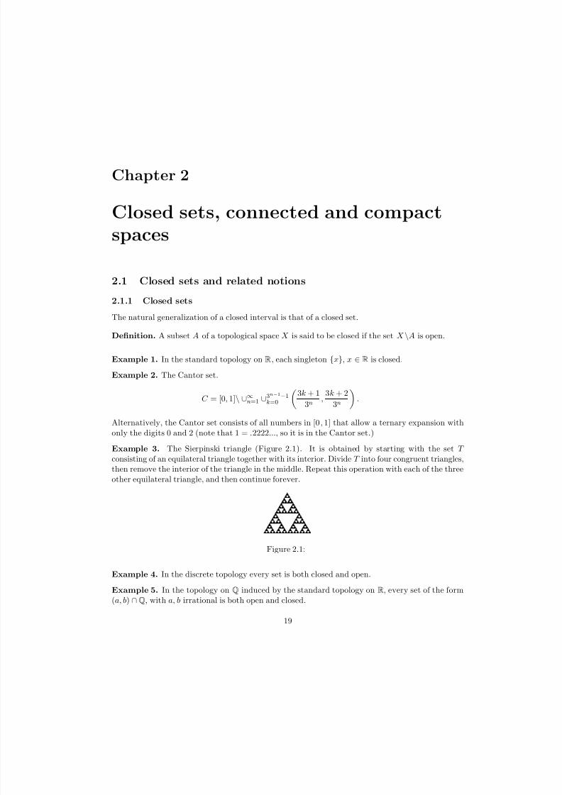
Example 3. The Sierpinski triangle (Figure 2.1). It is obtained by starting with the set T consisting of an equilateral triangle together with its interior. Divide T into four congruent triangles,then remove the interior of the triangle in the middle. Repeat this operation with each of the threeother equilateral triangle, and then continue forever.
Figure 2.1:
Example 4. In the discrete topology every set is both closed and open.
Example 5. In the topology on Q induced by the standard topology on R, every set of the form(a, b) ∩Q, with a, b irrational is both open and closed.
19

7/25/2019 TOPOLOG8Y
http://slidepdf.com/reader/full/topolog8y 20/98
20 CHAPTER 2. CLOSED SETS, CONNECTED AND COMPACT SPACES
Example 6. In the standard topology on Rn, each set of the form
B(x, ǫ) = {y ∈ R | d(x, y) ≤ ǫ}
is closed.
As a corollary of de Morgan’s laws, we obtain the following result.
Proposition 2.1.1. In a topological space X , the following are true:
(1) X and ∅ are closed.
(2) Arbitrary intersections of closed sets are closed.
(3) Finite unions of closed sets are closed.
The notion of a closed set is well behaved with respect to taking subspaces and products of topological spaces.
Proposition 2.1.2. (1) If Y is a subspace of X then A ⊂ Y is closed if and only if A = B ∩ Y with B a closed subset of X .(2) Let Y be a subspace of X . If A is closed in Y and Y is closed in X , then A is closed in X .(3) If A is closed in X and B is closed in Y , then A
×B is closed in X
×Y .
Proof. (1) If B is closed in X , then X \B is open. Thus A = B ∩ Y is the complement of the openset (X \B) ∩ Y , and hence is closed.
For the converse, if A is closed then Y \A is open, thus there is an open set U in X such thatU ∩ Y = Y \A. Then B = X \U is closed and A = B ∩ Y , as desired.
(2) If A is closed in Y , then Y \A is open in Y , so there is an open U ⊂ X such that Y \A = Y ∩U .Then
X \A = U ∪ (X \Y )
which is a union of open sets, so it is open. Consequently A is closed in X .
(3) This follows from
(X × Y )\(A × B) = X × (Y \B) ∪ (X \A) × Y.
Also, we have the following ”alternative definition” of continuity.
Proposition 2.1.3. Let X and Y be topological spaces. Then f : X → Y is continuous if andonly if the preimage of every closed set is closed.
Proof. Since
f −1(Y \A) = X \f −1(A)
the condition from the statement is equivalent to the fact that the preimage of every open set isopen.

7/25/2019 TOPOLOG8Y
http://slidepdf.com/reader/full/topolog8y 21/98
2.1. CLOSED SETS AND RELATED NOTIONS 21
2.1.2 Closure and interior of a set
Definition. Given a subset A of a topological space X , the interior of A, denoted by Int(A), isthe union of all open sets contained in A and the closure of A, denoted by A, is the intersectionof all closed sets containing A.
Because arbitrary unions of open sets are open, the interior of a set is open; it is the largestopen set contained in the set. Also, because arbitrary intersections of closed sets are closed, theclosure of a set is closed; it is the smallest closed set containing the given set. We have
Int(A) ⊂ A ⊂ A.
Note also that A is closed if and only if A = A and A is open if and only if Int(A) = A.
Lemma 2.1.1.
X \A = X \Int(A).
Example 1. For Q ⊂ R with the subset topology we have Int(Q) = ∅ and Q = R.
Definition. A subset A of a topological space X is called dense if A = X .
Theorem 2.1.1. Let A be a subset of a topological space X . Then x is in A if and only if every
open set U containing x intersects A. Moreover, it suffices for the condition to be verified only forbasis elements containing x.
Proof. Note that indeed, the two conditions are equivalent because for every open set U containingx, there is a basis element B such that x ∈ B ⊂ U .
For the converse we will use Lemma 2.1.1. Let x ∈ X and assume there is U ⊂ X \A open, suchthat x ∈ U . Then U ⊂ Int(X \A), which shows that x ∈ Int(X \A). This imples that x ∈ X \A.
Conversely, assume that every open set that contains x intersects A. Then Int(X \A) does notcontain x, so x ∈ X \Int(X \A) = A.
So x is in A if and only if every neighborhood of x intersects A. Let us see now how the closurebehaves under passing to a subspace and under products.
Proposition 2.1.4. (1) Let Y be a subspace of X and A a subset of Y . Let AX denote the closureof A in X . Then the closure of A in Y equals AX ∩ Y .(2) Let Y be a closed subspace of X , and A a subset of Y . Then the closure of A in X and Y isthe same.(3) Let (X α), α ∈ A, be a family of topological spaces, and let Aα ⊂ X α, α ∈ A. If we endow
X α with either the product or the box topology, thenAα =
Aα.
Proof. (1) Let AY be the closure of A in Y . The set A is closed in X , so A
∩Y is closed in Y .
This means that A ∩ Y contains A. On the other hand, every point x ∈ A ∩ Y has the propertythat every open set U ⊂ X intersects A. It follows that U ∩ Y intersects A as well, so x ∈ AY byTheorem 2.1.1.
(2) Again it is clear that AY ⊂ AX . Also, AY is closed in X by Proposition 2.1.2. HenceAY ⊃ AX . Consequently AX = AY .

7/25/2019 TOPOLOG8Y
http://slidepdf.com/reader/full/topolog8y 22/98
22 CHAPTER 2. CLOSED SETS, CONNECTED AND COMPACT SPACES
(3) We prove the equality by double inclusion. Let x = (xα) be a point in
Aα. Let U =
U αbe a basis element in either topology that contains x. Then U α ∩ Aα is nonempty (when we havethe product topology all but finitely many of the U α’s coincide with X α’s. If yα, α ∈ A are pointsin the intersections, then U ∩Aα contains (yα). By Theorem 2.1.1, x ∈ Aα.
Conversely, let x = (xα) be a point in
Aα. For a given Aα0, and an open set U α0 containingxα, the set
U = U α0 ×α=α0
X α
intersects Aα. Then U α0 must intersect Aα0 , so xα0 ∈ Aα0. This proves the other inclusion.
Regarding the properties of the interior, it is not true that if Y is a subspace of X and A ⊂ Y then the interior of A in Y is the intersection with Y of the interior of A in X ; the interior of Ain Y might be larger. Nor is it true that, for infinitely many spaces, the product of the interiors isthe interior of the product in the product topology. We only have
Proposition 2.1.5. If X α, α ∈ A are topological spaces and Aα ⊂ X α, then
Int(Aα) equals theinterior of
Aα in the product topology.
Proof. Since
Int(Aα) is open in the box topology, it is included in Int(
α Aα). If x ∈ Int(Aα),for each α there is U α such that xα ∈ U α and U α ∩ (X α\Aα) = ∅. Consequently, the open set
U α
contains x, and so by Theorem 2.1.1, x ∈ X α\Aα. Hence x ∈ Int(Aα).
As a corollary, for finitely many spaces, the product of the interiors is the interior of the productin the product topology.
There is a characterization of continuity using closures of sets.
Proposition 2.1.6. Let X, Y be topological spaces. Then f : X → Y is continuous if and only if for every subset A of X , one has
f (A) ⊂ f (A).
Proof. Assume that f is continuous and let A be a subset of X . Let also x ∈ A. For an open set U in Y containing f (x), f −1(U ) is open in X , so by Theorem 2.1.1 it intersects A. Hence U intersectsf (A), showing that f (x) ∈ f (A).
Conversely, let us assume that f (A) ⊂ f (A) for all subsets A of X , and show that f is continuous.We will use Proposition 2.1.3. Let B be closed in Y and A = f −1(B). We wish to prove that A isclosed in X , namely that A = A. We have
f (A) ⊂ f (A) = B = B = f (A).
Hence the conclusion.
2.1.3 Limit points
Definition. Let X be a topological space, A a subset, and x ∈ X . Then x is said to be a limit point (or accumulation point) of A if every open set containing x intersects A in some point otherthan x itself.

7/25/2019 TOPOLOG8Y
http://slidepdf.com/reader/full/topolog8y 23/98
2.1. CLOSED SETS AND RELATED NOTIONS 23
This means that x is a limit point of A if and only if every neighborhood of x contains a pointin A which is not x. Said differently, x is a limit point of A if it belongs to the closure of A\{x}.The set of all limit points of a set A is denoted by A′.
Example 1. If A = {1/n | n = 1, 2, 3, . . .}, then A′ = {0}.
Example 2. If A = (0, 1) ⊂ R, in the standard topology, then A′ = [0, 1].
Example 3. If C is the Cantor set (see §2.1.1) then C ′ = C (prove it).
Example 4. For Z ⊂ R, Z′ = ∅.
Proposition 2.1.7. Let A be a subset of a topological space X . Then
A = A ∪ A′.
Proof. A point x is in A if and only if every open set U containing x intersects A. If for some xthat intersection is x itself, then x ∈ A. Otherwise x ∈ A′ by definition.
Corollary 2.1.1. A subset of a topological space is closed if and only if it contains all its limitpoints.
For metric spaces, limit points can be characterized using convergent sequences.
Definition. In an arbitrary topological space, one says that a sequence (xn)n of points in X converges to a point x ∈ X provided that, corresponding to each neighborhood V of x, there is apositive integer N such that xn ∈ V for all n ≥ N . The point x is called the limit of xn.
The notion of convergence can be badly behaved in arbitrary topological spaces, for example inthe trivial topology any sequence converges to all points in the space. In the Zariski topology onC, all sequences that do not contain constant subsequences converge to all points in C. In metricspaces however, we have the following result.
Proposition 2.1.8. Given a metric space X with metric d, if a sequence (xn)n converges, then itslimit is unique.
Proof. Assume that (xn
)n
converges to both x and y, x = y. Then for every ǫ, all terms of the
sequence but finitely many lie in both B(x, ǫ) and B(y, ǫ). But for ǫ < d(x, y)/2, this is impossible,since the balls do not intersect. Hence (xn)n can have at most one limit.
In metric spaces the closure and the limit points of a set can be described in terms of convergentsequences.
Lemma 2.1.2. (The sequence lemma) Let X be a metric space and A a subset of X .
(1) A point x is in A if and only if there is a sequence of points in A that converges to x.
(2) A point x is in A′ if and only if there is a sequence of points in A converging to x that doesnot eventually become constant.
Proof. Using Proposition 2.1.7 we see that (2) implies (1) since if x ∈ A we can use the constantsequence xn = x, n ≥ 1.
To prove (2), assume first that x ∈ A′. Then for every ǫ, there is a point y = x in A such thaty ∈ B(x, ǫ). Start with ǫ = 1 and let x1 be such a point. Consider the ball B(x, d(x, x1)/2) and let
7/25/2019 TOPOLOG8Y
http://slidepdf.com/reader/full/topolog8y 24/98
24 CHAPTER 2. CLOSED SETS, CONNECTED AND COMPACT SPACES
x2 = x be a point of A that lies in this ball. Choose x3 ∈ B(x, d(x, x2)/2) in the same fashion, andrepeat to obtain the sequence x1, x2, . . . , xn, . . ., whose terms are all distinct.
Because d(x, xn) → 0, and because for every neighborhood V of x there is an ǫ such thatB(x, ǫ) ⊂ V , it follows that all but finitely many terms of the sequence are in V . Hence (xn)n is asequence of points in A converging to x that does not eventually become constant.
Conversely, assume that there is a sequence (xn)n of points in A convering to x that does noteventually become constant. Given an arbitrary neighborhood V of x, there are infinitely manyterms of the sequence in that neighborhood, and infinitely many of those must be different from x.So x ∈ A′ by definition.
In fact one of the implications in (2) is true in topological spaces, namely if there is a sequence(xn)n of points in A that converges to x then x ∈ A. Indeed, by the definition of convergence, everyneighborhood of x contains infinitely many points of the sequence, hence it contains points in A.By Theorem 2.1.1, x ∈ A.
For metric spaces continuity can also be characterized in terms of convergent sequences.
Theorem 2.1.2. Let X be a metric space and Y a topological space. Then f : X → Y is continuousif and only if for every x ∈ X and every sequence (xn)n in X that converges to x, f (xn) convergesto f (x).
Proof. Assume that f is continuous and that xn → x. If V is a neighborhood of f (x), then f −1(V )is a neighborhood of x, which contains therefore all but finitely many terms of the sequence. Hence
all but finitely many terms of (f (xn))n are in V . This proves that f (xn) → f (x).For the converse we will use Proposition 2.1.6. Let A be a subset of X and x ∈ A. Then by
Lemma 2.1.2, there is a sequence (xn)n of points in A such that xn → x. Then f (xn) → f (x) so bythe same lemma, f (x) ∈ f (A). It follows that f (A) ⊂ f (A), which proves that f is continuous.
2.2 Hausdorff spaces
Topologies in which sequences converge to more than one point are are counterintuitive and theyseldom show up in other branches of mathematics, the Zariski topology being a rare example. Wewill therefore introduce a large class of ”nice” topological spaces in which this bizarre phenomenondoes not occur.
Definition. A topological space X is called a Hausdorff space if for each pair x1, x2 of distinctpoints of X , there exist neighborhoods U 1 and U 2 of x1 respectively x2 that are disjoint.
Example 1. Every metric space is a Hausdorff space.
Example 2. The product space ∞
n=1R is Hausdorff but is not a metric space. To see that it isHausdorff, choose two points x = y. Then there is some n such that xn = yn. Choose neighborhoodU and V of xn and yn in R such that U ∩ V = ∅. Then
n−1
i=1 R×U ×
∞
i=n+1R andn−1
i=1 R×V ×
∞
i=n+1Rare disjoint neighborhoods of x and y in
∞n=1R.
Example 3. Cn endowed with the Zariski topology is not Hausdorff.

7/25/2019 TOPOLOG8Y
http://slidepdf.com/reader/full/topolog8y 25/98
2.3. CONNECTED SPACES 25
Proposition 2.2.1. If X is a Hausdorff space and x ∈ X , then {x} is a closed set.
Proof. For y ∈ X \{x} there is an open neighborhood V of y such that x ∈ V . Hence V ⊂ X \{x},so X \{x} is open. Hence {x} is closed.
As a corollary, finite subsets of a Hausdorff space are closed.
Proposition 2.2.2. (1) A subspace of a Hausdorff space is Hausdorff.(2) The product of Hausdorff spaces is a Hausdorff space in both the product and the box topology.
Remark 2.2.1. In a Hausdorff space a convergent sequence has exactly one limit. Indeed, if x = y
were limits of the sequence, and U and V are disjoint neighborhoods of x respectively y, then bothU and V should contain all but finitely many terms of the sequence, which is impossible.
2.3 Connected spaces
2.3.1 The definition of a connected space and properties
Definition. Let X be a topological space. Then X is called connected if there are no disjointnonempty open sets U and V such that X = U ∪ V .
If such U and V exist then they are said to form a separation of X . Thus X is not connectedif it has a separation. Another way of formulating the definition is to say that the only subspaces
of X that are both open and closed are X and the empty set.Connectedness is difficult to verify. It is much easier to disprove it.
Example 1. The real line is connected. (We will prove this later).
Example 2. The set of rational numbers Q with the topology induced by the standard topologyon R is not connected. Indeed, the open sets (−∞,
√ 2) ∩Q and (
√ 2, ∞) ∩Q are a separation of Q.
In fact for every two points a and b of Q, there is a separation Q = U ∪ V with a ∈ U and b ∈ V .We say that Q is totally disconnected .
Proposition 2.3.1. (1) If A and B are two disjoint nonempty subsets of a topological space X such that X = A
∪B and neither of the two subsets contains a limit point of the other, then A and
B form a separation of X .(2) If U and V form a separation of X and if Y is a connected subspace of X , then Y lies entirelywithin either U or V .
Proof. (1) Since A ⊂ X \B, it follows that A = A. Similarly, B = B . So A and B are closed, whichmeans that their complements, which are again A and B , are open. So A and B form a separationof X .
(2) If this were not true, then Y ∩ U and Y ∩ V were a separation of Y .
Theorem 2.3.1. The image under a continuous map of a connected space is connected.
Proof. This is a powerful result with a trivial proof. If f : X
→ Y is continuous and f (X ) is not
connected, and if U and V are a separation of f (X ), then f −1(U ) and f −1(V ) are a separation of X .
Corollary 2.3.1. If X and Y are homeomorphic, then there is a bijective correspondence betweentheir connected components.

7/25/2019 TOPOLOG8Y
http://slidepdf.com/reader/full/topolog8y 26/98
26 CHAPTER 2. CLOSED SETS, CONNECTED AND COMPACT SPACES
Proposition 2.3.2. (1) The union of a collection of connected spaces that have a common pointis connected.(2) Let A be a connected subspace of a topological space X . If A ⊂ B ⊂ A, then B is alsoconnected. Consequently, if A is connected and dense in X , then X is connected.(3) The product of connected spaces is connected in the product topology.
Proof. (1) Let X = ∪αX α and a be a common point of the X α’s. Assume that U ∪V is a separationof X . Then by Proposition 2.3.1 (1), each X α is included in either U or V . In fact, each is includedin that of the two sets which contains a, say U . But then V is empty, a contradiction. Theconclusion follows.
(2) Suppose there is a separation U ∪ V of B. Then by Proposition 2.3.1 (2) A lies entirelyinside either U or V . Since U is closed in B , A ∩ B ⊂ U . But A ∩ B = B, and this contradicts thefact that U ∪ V is a separation of B . Hence the conclusion.
(3) Let us prove first that the product of two connected spaces X 1 and X 2 is connected. Fixxi ∈ X i, i = 1, 2. By part (1),
({x1} × X 2) ∪ (X 1 × {x2})
is connected being the union of two connected sets that share ( x1, x2). Now vary x2 and take theunion of all such sets. This union is the entire space X 1 × X 2, and each of the spaces contains{x1} × X 2. Again from (1) it follows that X 1 × X 2 is connected.
An inductive argument shows that the product of finitely many connected sets is connected.
Now let us consider a product X = α X α α ∈ A of connected spaces endowed with the producttopology. For each α, fix a point aα ∈ X α. Then each set of the form
Aα1,α2,...,αn = X α1 × X α2 × · · · × X αn ×α=αi
{aα}
are connected, being finite products of connected spaces, and hence their union is also connectedbecause these sets have the common point (aα). Let us show that
A = ∪∞n=1 ∪α1,α2,...,αn∈A Aα1,α2,...,αn
is dense in X . Indeed, if (xα)
∈ X and
B = U α1 × U α2 × · · · × U αn ×α=αi
X α
is a basis element containing x, then
{xα1} × {xα2} × · · · × {xαn} ×α=αi
{aα} ∈ B ∩ Aα1,α2,...,αn.
This shows that A = X , hence X is connected.
Remark 2.3.1. The product of infinitely many connected spaces in the box topology is not nec-
essarily connected. For example a separation of RN
in the box topology consists of the set of allbounded sequences and the set of all unbounded sequences.
Definition. A maximal connected subset of a topological space is called a connected component .
Theorem 2.3.2. Every topological space can be partitioned into connected components.

7/25/2019 TOPOLOG8Y
http://slidepdf.com/reader/full/topolog8y 27/98
2.3. CONNECTED SPACES 27
Proof. Each singleton {x} of a topological space X is connected. The union of all connected setsthat contain x is connected by Proposition 2.3.2 (1). This union is a maximal connected set thatcontains x, hence it is a connected component. Varying x we partition the set into connectedcomponets.
Definition. A space X is said to be locally connected if for every neighborhood U of x there is aconnected neighborhood V of x such that V ⊂ U .
Proposition 2.3.3. A space is locally connected if and only if the connected components of anyopen set are open.
Proof. Let us assume that the topological space X is locally connected, and let U be an open set.If x is a point in U , then there is a connected open neighborhood of x, V , which is contained inU . But then V must lie in a connected component of U (Proposition 2.3.1 (2)). So the connectedcomponents of U are unions of open sets, so they are open.
Conversely, suppose that the connected components of open sets are open. Then the neighbor-hood V from the definition can be taken to be just one such connected component.
Example 3. The comb space defined as
({0} × [0, 1]) ∪ ([0, 1] × {0}) ∪ ∪∞n=1
1
n
× [0, 1]
is connected but not locally connected.
2.3.2 Connected sets in R and applications
Theorem 2.3.3. The only connected subsets of the real line in the standard topology are theintervals and R.
Proof. Let A be a subset of R. If there are a, b ∈ A a < b such that [a, b] is not a subset of A,that is there is c, a < c < b and c ∈ A, then (−∞, c) ∩ A and (c, ∞) ∩ A form a separation of A.So in this case A is not connected. Hence if α = inf A and β = sup A, α, β ∈ R ∪ {±∞}, then(α, β ) ⊂ A ⊂ [α, β ], which shows that A is an interval or the whole space.
Conversely, let us show that R and all intervals are connected. If U
∩V is a separation of an
interval I (or of R), let a, b ∈ I with a ∈ U and b ∈ V . Consider c = sup{x | x < b, x ∈ U }. Thenc ∈ U on the one hand, and because c = inf {x | x ∈ V }, c ∈ V . But this is impossible. It followsthat I (and for the same reason R) does not admit a separation.
Theorem 2.3.1 becomes the well known
Theorem 2.3.4. (The intermediate value theorem) Let f : R→ R be a continuous function. Thenf maps intervals to intervals.
Let us see some applications.
Theorem 2.3.5. Let f : [a, b] → [a, b] be a continuous map. Then f has a fixed point, meaningthat there is x
∈ [a, b] such that f (x) = x.
Proof. Assume f has no fixed points. Consider the function g : [a, b] → R, g (x) = f (x) − x. Theng([a, b]) is an interval. We have f (a) > a and f (b) < b (because f has no fixed points), so g([a, b])is an interval that contains both positive and negative numbers, so it must contain 0. This is acontradiction, which proves that f has a fixed point.

7/25/2019 TOPOLOG8Y
http://slidepdf.com/reader/full/topolog8y 28/98
28 CHAPTER 2. CLOSED SETS, CONNECTED AND COMPACT SPACES
Theorem 2.3.6. (The one-dimensional Borsuk-Ulam theorem) Given a continuous map of a circleinto a line, there is a pair of diametrically opposite points that are mapped to the same point.
Proof. First let us notice that S 1 is connected, because it is the image of R through the continuousmap f (x) = eix. Let f : S 1 → R be the continuous map. For a point z ∈ S 1, the diametricallyopposite point is −z. Define g : S 1 → R, g(z) = f (z) − f (−z). If for some z , g (z) = 0, then z hasthe desired property. If for some z, g(z) > 0, then g(−z) < 0, and because g(S 1) is connected, itmust contain 0. The conclusion follows.
Theorem 2.3.7. Let A and B be two polygonal regions in the plane. Then there is a line thatdivides each of the regions in two (not necessarily connected) parts of equal areas.
Proof. For each given line l there is one and only one line parallel to l that divides A into tworegions of equal areas, and one and only one line parallel to l that divides B into two parts of equalareas.
Now fix a line l0 in the plane, a point 0, a positive direction and a unit of length of l0. Considerthe lines perpendicular to l0 that cut A respectively B into equal areas, and let xA and xB be thecoordinates of their intersections with l0. Now rotate l0 keeping 0 fixed, and let xA(θ) and xB(θ)be now the same coordinates on l0 depending on the angle of rotation.
Define g : [0, 2π] → R, g (θ) = xA(θ) − xB(θ). Then g(0) = −g(π) (in fact g(x) = −g(x + π) forall x). The function g is continuous, and g([0, 2π]) must be an interval. This interval must containboth nonpositive and nonnegative numbers, hence it contains 0. Thus there is an angle θ such that
xA(θ) = xB(θ). In this case the two lines perpendicular to l0 coincide, they form a line that cutsboth A and B in parts of equal area.
2.3.3 Path connected spaces
There is a property that is much easier to verify in particular applications, and which guaranteesthat a space is connected. This is the property of being path connected.
Definition. Given a topological space X and x, y ∈ X , a path from x to y is a continuous mapφ : [0, 1] → X such that f (0) = x and f (1) = y.
In fact any continuous map φ : [a, b]
→ X , φ(a) = x, φ(b) = y defines a path, since we can
rescale it to ψ(t) = φ((b − a)t + a).
Proposition 2.3.4. The relation on X defined by x ∼ y if there is a path from x to y is anequivalence relation.
Proof. Clearly x ∼ x by using the constant path. Also, if φ : [0, 1] → X is a path from x to y, thenψ(t) = φ(1 − t) is a path from y to x. Hence if x ∼ y then y ∼ x.
Finally, if x ∼ y and y ∼ z, that is if there are paths φ1, φ2 : [0, 1] → X from x to y and from yto z , then
ψ(t) =
φ1(2t) if 0 ≤ t ≤ 1/2φ2(2t
−1) if 1/2
≤ t
≤ 1
is a path from x to z .
Definition. The equivalence classes of ∼ are called the path components of X .
Note that ∼, being an equivalence relation, partitions X into its path components.

7/25/2019 TOPOLOG8Y
http://slidepdf.com/reader/full/topolog8y 29/98
2.3. CONNECTED SPACES 29
Definition. If the space X consists of only one path component, it is called path connected .
Proposition 2.3.5. Each path component of a topological space X is included in a connectedcomponent. Consequently, a path connected space is connected.
Proof. Each path is connected, being the image of a connected set through a continuous map, so byProposition 2.3.1 its image is included in a connected component of X . This means that if x ∼ y,then x and y belong to the same connected component of X . Hence the conclusion.
The property of a space to be path connected is well-behaved under continuous maps.
Theorem 2.3.8. Let f : X
→ Y be a continous map from the path-connected topological space
X to the topological space Y . Then f (X ) is path connected.
Proof. If φ is a path from x to y , then f ◦ φ is a path from f (x) to f (y).
Corollary 2.3.2. If X and Y are homeomorphic, then there is a bijective correspondence betweentheir path components.
Example 1. Every convex set in an R-vector space is path connected. Indeed, a set A is convexif for every x, y ∈ A, the segment {tx + (1 − t)y | t ∈ [0, 1]} is in A. This segment is the path.
In particular every R-vector space, such as Rn, C [a, b], L p(R), is path connected.
Example 2. If n
≥ 2 and x
∈Rn, then Rn
\{x
} is path connected.
Indeed, given y and z in Rn\{x}, consider a circle of diameter yz. Then one of the semicirclesdoes not contain x, and a parametrization of this semicircle defines a path from y to z.
Example 3. If x ∈ R, the space R\{x} has two path components, which are also its connectedcomponents, namely (−∞, x) and (x, ∞).
Here are some applications.
Theorem 2.3.9. If n ≥ 2, the spaces R and Rn are not homeomorphic.
Proof. Arguing by contradiction, let us assume that there is a homeomorphism f : Rn → R. Choosex ∈ Rn. Then f : Rn\{x} → R\{f (x)} is still a homeomorphism (it is one-to-one and onto, thepreimage of each open set is open, and the image of each open set is open). But Rn
\{x
} is path
connected, while its image through the continuous map f is not. This is a contradiction, whichproves that the two spaces are not homeomorphic.
Example 4. The figure eight from §1.3.7 is not a manifold.To prove this, recall that the figure eight is obtained by factoring [0, 1] ∪ [2, 3] by 0 ∼ 1 ∼ 2 ∼ 3.
Let us denote this space by X . Let 0 be the equivalence class of 0. If X were an n-dimensionalmanifold, then there would be a neighborhood U of 0 homeomorphic to an open disk D ⊂ Rn; letf be this homeomorphism. This neighborhood can be chosen small enough as to be included in[0, 1/3) ∪ (2/3, 1] ∪ [2, 7/3) ∪ (8/3, 3]. Then U \{0} is homeomorphic with D\{f (0}. But U \{0} hasat least four path components, while D\{f (0)} has either one path component, if n ≥ 2, or twopath components, if n = 1. This is a contradiction. Hence the figure eight is not a manifold.
Note that a similar argument shows that a 1-dimensional manifold cannot be an n-dimensionalmanifold for n ≥ 2.
Definition. A topological space X is called locally path connected if for every x ∈ X , and open setU containing x, there is a path connected neighborhood V of x such that V ⊂ U .

7/25/2019 TOPOLOG8Y
http://slidepdf.com/reader/full/topolog8y 30/98
30 CHAPTER 2. CLOSED SETS, CONNECTED AND COMPACT SPACES
Example 5. If we remove from R2 a finite set of lines, the remaining set (with the inducedtopology) is locally path connected, but not connected.
Proposition 2.3.6. (1) A topological space X is locally path connected if and only if for everyopen set U of X , each path component of U is open in X .(2) If X is locally path connected, then the components and the path components are the same.
Proof. The proof of (1) is the same as for Proposition 2.3.3.For (2), note that the path components are open, hence they form a partition of X into open
sets. This means that they must also be the connected components of X (recall that the path
components are connected).
And now some pathological examples.
Example 1. The topologists sine curve
T =
x, sin
1
x
| x ∈ (0, 1]
∪ {(0, 0)}
with the topology induced by the standard topology of R2.This space is connected. Indeed, the graph of sin 1
x is connected, because it is the image inthe plane of the connected interval (0, 1] through the continuous map h(x) = (x, sin 1
x). Thus any
separation of T must separate the origin from this graph. But any neighborhood of the origincontains a part of this graph. This proves connectivity.The topologists sine curve is not locally connected, because any neighborhood of (0, 0) contained
in B ((0, 0), 1/2) ∩ T is not connected (it consists of the origin and several disjoint arcs).The topologists sine curve is not path connected. This is equivalent to the fact that f (x) = sin 1
xcannot be extended continuously to [0, 1]. Any path φ : [0, 1] → T would have as limit points whent → 0 the entire interval {0} × [−1, 1], and so it could not be continuous.
Example 2. The comb space defined in §2.3.1 is path connected by not locally path connected.
Example 3. The deleted comb, which is a subspace of the comb defined as
D = (
{0
} × {0, 1
})
∪ ∪∞n=1
1
n×[0, 1] ∪
([0, 1]
× {0
}).
This space is connected but not path connected, since there is no path from (0, 1) to (1, 0) (Proveit!).
2.4 Compact spaces
2.4.1 The definition of compact spaces and examples
Definition. A collection U is called an open cover of a topological space X if the elements of U are open subsets of X and the union of all elements in U is X .
Remark 2.4.1. In general, if A is a subset of a topological space X , an open cover of A is a collectionof open sets in X whose intersections with A is an open cover of A in the subspace topology.
Definition. A space X is said to be compact if every open cover of X contains a finite subcover(i.e. a finite family that also covers X ).
7/25/2019 TOPOLOG8Y
http://slidepdf.com/reader/full/topolog8y 31/98
2.4. COMPACT SPACES 31
Remark 2.4.2. Some mathematicians are unhappy with this very general definition, and require thespace to be Hausdorff, too.
Example 1. Any topological space that has finitely many points is compact.
Example 2. R with the standard topology is not compact because the family U = {(−n, n) |, n ≥ 1}is an open cover that does not have a finite subcover.
As you can see, it is much easier to prove that a space is not compact, then to prove that it iscompact.
The next result will show that there are many (nontrivial) compact spaces.
Theorem 2.4.1. (The Heine-Borel Theorem) A subspace of Rn is compact if and only if it is closedand bounded (in the Euclidean metric).
Proof. Let us first prove that a compact set K ⊂ Rn is closed and bounded. If K were not bounded,then the collection of open balls
B(0, k) = {x ∈ Rn | d(x, 0) < k}, k = 1, 2, 3, . . . ,
would be an open cover of K that does not have a finite subcover. If K were not closed, andx ∈ K ′\K , then the open sets which are complements of the closed balls
B(x, 1/k) = {
y ∈Rn
|d(x, y)
≤ 1/k
}, k = 1, 2, 3, . . . ,
would be an open cover of K with no finite subcover.For the converse, let us assume that K is closed and bounded in Rn but has an open cover U
with no finite subcover. Add to U the complement of K , so that now we have a cover of the wholespace.
Place K in an n-dimensional cube, which by a translation and rescaling, can be made [0 , 1]n.Cut the cube into 2n equal cubes. Each of these cubes is covered by some sets in U , and because theopen cover of K does not have a finite subcover, there is some cube which is covered by infinitelymany elements in U , and which furthermore cannot be covered by finitely many elements in U . Cutthis cube into 2n equal cubes, and again there would be one that cannot be covered by just finitelymany open sets in
U . And this would go on forever.
Note that at kth step, the choice of the cube specifies the kth digits of the binary expansionsof the coordinates of the points inside that cube. Repeating the process for all n and choosing thecorresponding kth digits in the binary expansion, we define a point x ∈ Rn which belongs to allcubes that were chosen. This point is in the closure of K (just because every of the cubes mustcontain points of K or else it is covered by the complement of K ). And x must belong to someopen set U in U .
Because U is open, there is some open ball B(x, ǫ) contained in U . Note that the kth cube inthe process has diameter equal to
√ n/2k, so, for k sufficiently large, it will be contained in B(x, ǫ)
and hence in U . This is a contradiction because that cube does not have a finite subcover. Itfollows that our assumption was false, and consequently K is compact.
2.4.2 Properties of compact spaces
Proposition 2.4.1. A topological space X is compact if and only if for any collection C of closedsubsets of X , with the property that the intersection any finitely many of them is nonempty, theintersection of all elements of C is nonempty.

7/25/2019 TOPOLOG8Y
http://slidepdf.com/reader/full/topolog8y 32/98
32 CHAPTER 2. CLOSED SETS, CONNECTED AND COMPACT SPACES
Proof. By looking at the complements of the elements in C and applying de Morgan’s law thecondition from the statement turns into the definition of compactness.
Definition. The collection C as in the statement of this result is said to have the finite intersection property .
Proposition 2.4.2. (1) Given a subspace Y of X , Y is compact if and only if every cover by opensets in X has a finite subcollection that covers Y .(2) Every closed subspace of a compact space is compact.(3) Every compact subspace of a Hausdorff space is closed.
(4) If Y is a compact subspace of a Hausdorff space X and if x is not in Y , then there are disjointopen sets U and V of X such that Y ⊂ U and x ∈ V .(5) (The tube lemma) Consider the product space X × Y , where Y is compact. If x0 is in X andN is an open set of X × Y containing {x0} × Y , then N contains a set of the form W × Y with W a neighborhood of x0 in X .
Proof. (1) This follows from the fact that the open sets in Y are those of the form Y ∩ U with U open in X .
(2) Given Y ⊂ X with X compact and Y closed, any open cover U of Y by open sets of X canbe extended to an open cover of X by adding the open set X \Y . This will have a finite subcoverof X , which is a finite cover of Y as well. We can remove the set X \Y from this collection and still
have a finite subcover of Y . Using (1) we conclude that Y is compact.(3) If Y is a compact subspace of the Hausdorff space X , then for every y ∈ Y and x ∈ X \Y ,
there are disjoint open sets U x,y and V x,y in X such that x ∈ U x,y and y ∈ V x,y. Fix x. The setsV x,y form an open cover of Y , from which we can extract a finite subcover V x,y1 , V x,y2 , . . . , V x,yn .The open set U x,y1 ∩ U x,y2 ∩ · · · ∩ U x,yn contains x and is disjoint from Y . It follows that X \Y isopen so Y is closed.
(4) This is just a corollary of the proof of (3).
(5) Choose an open cover of this set by basis elements of the form U × V that are includedin N . Since {x0} × Y is compact, there is a subcover U 1 × V 1, U 2 × V 2, . . . , U n × V n. If we setW = U 1 ∩ U 2 ∩ . . . ∩ U n, then {x0} × Y ⊂ W × Y ⊂ N and we are done.
The most important property of compact spaces is the following result:
Theorem 2.4.2. The image of a compact space through a continuous function is compact.
Proof. Let f : X → Y be continuous with X compact. Let U be an open cover of f (X ). Thecollection of open sets
{f −1(U ) | U ∈ U}
is an open cover of X , which has a finite subcover because X is compact. The image through f of that subcover is a finite subcover of f (X ).
We list two useful corollaries of this theorem.
Theorem 2.4.3. Let f : X → Y be a bijective continuous function. If X is compact and Y isHausdorff, then f is a homeomorphism.

7/25/2019 TOPOLOG8Y
http://slidepdf.com/reader/full/topolog8y 33/98
2.4. COMPACT SPACES 33
Proof. The only thing that we have to show is that f −1 is continuous. We use the definition of con-tinuity based on closed sets from Proposition 2.1.3 (2). Let C be closed in X . By Proposition 2.4.2,C is compact in X , so (f −1)−1(C ) = f (C ) is compact in Y . The space Y being Hausdorff, f (C )is closed by Proposition 2.1.3 (3). Hence the preimage under f −1 of every closed set C ⊂ X is aclosed subset of Y . Therefore f −1 is continuous.
Theorem 2.4.4. If f : X → R is continuous and X is compact, then f has an absolute maximumand minimum.
Proof. The set f (X ) is compact in R, so by the Heine-Borel Theorem it is closed and bounded.The maximum and minimum of this set are the maximum and the minimum of f .
This theorem is very useful, and we list below several applications.
Theorem 2.4.5. (The Lebesgue number theorem) Let U be an open covering of the compactmetric space X . Then there is δ > 0, called the Lebesgue number , such that for each subset of X having diameter less than δ , there is an element of U containing it.
Proof. If X belongs to U , we are done. Otherwise, choose a finite subcover U 1, U 2, . . . , U n, andconsider the closed sets C i = X \U i, i = 1, 2, . . . , n.
Recall that the diameter of a set A is
diam(A) = sup{d(a1, a2) | a1, a2 ∈ A},
where d is the distance function on X . Additionally, for a point x ∈ X and a set A ⊂ X , define
d(x, A) = inf {d(x, a) | a ∈ A}.
Define f : X → R,
f (x) = 1
n
ni=1
d(x, C i).
Let us show that f is continuous, which amounts to showing that d(x, C i) is a continuous functionin x.
Lemma 2.4.1. If A is a subset of the metric space X , then d(x, A) is a continuous function of x.
Proof. We will show that if xn → x, then d(xn, A) → d(x, A). Indeed, if d(xn, x) ≤ ǫ, then by thetriangle inequality |d(xn, a) − d(x, a)| ≤ d(x, y) < ǫ. If we choose a such that d(x, a) − d(x, A) < ǫ,the d(xn, a) < d(x, A) + 2ǫ. Hence d(xn, A) < d(x, A) + 2ǫ. Also, if we choose a such thatd(xn, a) − d(xn, A) < ǫ, then d(x, a) < d(xn, A) + 2ǫ, and so d(x, A) < d(xn, A) + 2ǫ. Thus|d(x, A) − d(xn, A)| < 2ǫ, and the lemma is proved.
By Theorem 2.4.4, f has a minimum. If x ∈ X is a minimum of f and U i contains x, thenthere is a ball B (x, ǫ) contained in U i. So d(x, C i) > 0 and consequently the minimal value of f isstrictly positive.
Let us show that we can choose the Lebesgue number δ to be the minimum of f . If A is a set
of diameter let than δ , and x0 ∈ A, then A ⊂ B(x0, δ ). Let us show that B(x0, δ ) lies in one of thesets U i. If this is not the case, then d(x0, C i) < δ , and hence
f (x0) = 1
n
ni=1
d(x0, C i) < 1
nnδ = δ.

7/25/2019 TOPOLOG8Y
http://slidepdf.com/reader/full/topolog8y 34/98
34 CHAPTER 2. CLOSED SETS, CONNECTED AND COMPACT SPACES
This is impossible, since f (x0) has to be at least δ . Therefore B(x0, δ ) lies in some U i and we aredone.
Corollary 2.4.1. Let f : X → Y be a continuous function from the compact metric space X tothe metric space Y . Then f is uniformly continuous.
Proof. Let ǫ > 0. Then for every x0 ∈ X there is δ x0 > 0 such that if dX (x, x0) < δ x0, thendY (f (x), f (x0)) < ǫ/2.
The balls B(x0, δ x0), x0 ∈ X cover X . If δ is their Lebesgue number, then every set of diameterδ lies inside some B(x0, δ x0). If x1, x2 have the property that dX (x1, x2) < δ , and if x0 is such thatx1, x2
∈ B(x0, δ x0), then
dY (f (x1), f (x2)) ≤ dY (f (x1), f (x0)) + d(f (x0), f (x2)) < ǫ/2 + ǫ/2 = ǫ.
This proves that f is uniformly continuous.
Theorem 2.4.6. Among all n-gons that are inscribed in the unit circle, the regular n-gon has thelargest area.
Proof. Let us define f : (S 1)n → [0, ∞) by f (z1, z2, . . . , zn) equal to the area of the convex n-gonwith vertices at z1, z2, . . . , zn) (in some order). The function f is continuous, and the set (S 1)n isclosed and bounded in R2n. Hence f has a maximum.
Let us show that an arbitrary n-gon which is not regular does not maximize f . Indeed, suchan n-gon would have two adjacent sides AB and BC such that AB < BC . If we choose B′ the
midpoint of the arc⌢
ABC , then the area of ABC is strictly smaller than the area of AB ′C (becausethe altitude from B ′ is greater than the altitude from B). Hence if we replace vertex B by B ′, thenwe obtain a polygon with strictly larger area. This proves our claim. It follows that the regularn-gon is the (unique) maximum.
Example 1. (1984 Balkan Mathematical Olympiad) Let α1, α2, · · · , αn be positive real numbers,n ≥ 2, such that α1 + α2 + · · · + αn = 1. Prove that
α1
1 + α2
+· · ·
+ αn
+ α2
1 + α1
+· · ·
+ αn
+ · · · + αn
1 + α1
+· · ·
+ αn−1
≥ n
2n−
1.
Solution: Rewrite the inequality as
α1
2 − α1+
α2
2 − α2+ · · · +
αn
2 − αn≥ n
2n − 1,
then define the function
f (α1, α2, . . . , αn) = α1
2 − α1+
α2
2 − α2+ · · · +
αn
2 − αn.
As said in the statement, this function is defined on the subset of Rn consisting of points whosecoordinates are positive and add up to 1. We would like to show that on this set f is greater than
or equal to n2n−1 .
Does f have a minimum? The domain of f is bounded but is not closed, being the interior of a tetrahedron. We can enlarge it, though, adding the boundary, to the set
M = {(α1, α2, . . . , αn) | α1 + α2 + · · · + αn = 1, αi ≥ 0, i = 1, 2, . . . , n}.
7/25/2019 TOPOLOG8Y
http://slidepdf.com/reader/full/topolog8y 35/98
2.4. COMPACT SPACES 35
We now know that f has a minimum on M .A look at the original inequality suggests that the minimum is attained when all αi’s are equal.
So let us choose a point (α1, α2, . . . , αn) for which αi = α j for some indices i, j. Assume that αi < α jand let us see what happens if we substitute αi + x for αi and α j − x for α j, with 0 < x < α j − αi.In the defining expression of f , only the ith and j th terms change. Moreover
αi
2 − αi+
α j2 − α j
− αi + x
2 − αi − x − α j − x
2 − α j + x
= 2x(α j − αi − x)(4 − αi − α j)
(2 − αi)(2 − α j)(2 − αi − x)(2 − α j − x) > 0,
so when moving the numbers closer, the value of f decreases. It follows that the point that wepicked was not a minimum. Hence the only possible minimum is
1n , 1n , . . . , 1n
in which case the
value of f is n2n−1 . This proves the inequality.
Example 2. The proof of the arithmetic mean - geometric mean inequality (AM-GM):
x1 + x2 + · · · + xn ≥ n n√
x1x2 · · · xn,
which holds for any nonnegative numbers x1, x2, . . . , xn.For the proof, notice that the inequality is homogeneous, meaning that it does not change if we
multiply each of the numbers x1, x2, . . . , xn by the same positive constant. Hence it suffices to prove
the inequality for the case where x1 + x2 + · · · + xn = 1. Consider f (x1, x2, . . . , xn) = n
√ x1x2 · · · xndefined on the thetrahedron x1 + x2 + · · · + xn = 1, which is a compact set being closed andbounded. Then f has a maximum. If the xi are not all equal, say xi < x j for some i and j , chooseǫ < x j −xi and replace xi by xi + ǫ and x j by x j − ǫ. We are still in the domain of f , and because(xi + ǫ)(x j − ǫ) = xix j + ǫ(x j − xi − ǫ) > xix j. Hence the maximum is not attained at points wherethe xi are not all equal. Consequently, the maximum is attained at x1 = x2 = · · · = xn = 1
n , whenf equals 1n . In this case we have equality in AM-GM, and the inequality is proved.
2.4.3 Compactness of product spaces
Theorem 2.4.7. The product of finitely many compact spaces.
Proof. It suffices to check that the product of two compact spaces is compact. Let X and Y bethese spaces. Let U be an open covering of X × Y . Given x ∈ X , the slice {x} × Y is compact,and can be covered by finitely many elements U 1, U 2, . . . , U n of U . Their union is an open set N x of X × Y , which by Proposition 2.4.2 (5) contains a tube W x × Y . The open sets W x, x ∈ X cover X ,and since X is compact, there are x1, x2, . . . , xn such that W x1, W x2, . . . , W xn cover X . It followsthat N x1, N x2, . . . , N xn cover X × Y , and consequently the open sets in U that comprise them forma finite cover of X × Y .
Theorem 2.4.8. (The Tychonoff theorem) The product of an arbitrary number of compact spacesis compact in the product topology.
Proof. This case is significantly harder, and makes use of the Axiom of Choice in the guise of Zorn’sLemma.
Lemma 2.4.2. If C is a collection of subsets of a set A having the finite intersection property, thenthere exists a maximal collection M of subsets of A that has the finite intersection property andcontains C.

7/25/2019 TOPOLOG8Y
http://slidepdf.com/reader/full/topolog8y 36/98
36 CHAPTER 2. CLOSED SETS, CONNECTED AND COMPACT SPACES
Proof. We will apply Zorn’s lemma to the set S whose elements are collections of subsets of A withthe finite intersection property that contain C.
We will show that if S ′ is a subset of S that is (totally) ordered under inclusion then S ′ hasa maximal element. We will show that the union U of all collections in S ′ is an element of S .If C 1, C 2, . . . , C n are finitely many elements of U , then each of them belongs to some S i ∈ S ′,i = 1, 2, . . . , n. Hence all of them belong the the largest of the S i, and because this one has thefinite intersection property, the sets C 1, C 2, . . . , C n have nonempty intersection. Consequently U has the finite intersection property. This proves the lemma.
Lemma 2.4.3. Let M be a collection of subsets of a set A that is maximal with respect to the
finite intersection property. Then(1) Any finite intersection of elements in M is in M.(2) If B is a subset of A that intersects every element of M, then A is an element of M.
Proof. (1) If we add to M the finite intersections of elements in M we still get a collection of setsthat has the finite intersection property. Because of maximality, this collection is M.
(2) Let M′ = M ∪ {B}. Then M′ still has the finite intersection property. Indeed, if M 1, M 2, . . . , M n are in M′, then either none of them is B, in which case their intersection isnonempty, or one of them, say M n is B . Then
M 1 ∩ M 2 ∩ · · · ∩ M n = (M 1 ∩ M 2 ∩ · · · ∩ M n−1) ∩ B.
By part (a), M 1 ∩ M 2 ∩ · · · ∩ M n−1 ∈ M, and so by the hypothesis, its intersection with B is notempty. This shows that M 1, M 2, . . . , M n have nonempty intersection, and consequently that M′
has the finite intersection property. Because of maximality, M′ = M. Done.
Let us now proceed with the proof of the theorem. Let
X =α∈A
X α,
where each X α is compact. Let C be a collection of closed subsets with the finite intersectionproperty. We will show that
∩C ∈CC
is nonempty, which will imply that X is compact by Proposition 2.4.1. Choose M be a maximalfamily that contains C and has the finite intersection property. It suffices to show that
∩M ∈MM
is nonempty. Let πα : X → X α, α ∈ A be the projection. Consider the collections
Mα = {πα(M ) | M ∈ M}
of subsets of X α. This collection has finite intersection property because
M does. By the compact-
ness of X α and Proposition 2.4.1, the intersection of the sets πα(M ), M ∈ M is nonempty. Let xα
be a point in the intersection. We let x = (xα)α∈A and show that x ∈ ∩M ∈MM .To this end, we show that every open set containing x intersects the closure of every set in
M. First we verify this for an open set of the form π−1α (U α), where U α is open in X α. Indeed, U αintersects πα(M ) and πβ(π−1α (U α) = X β for α = β . Hence this is true for such a set. In particular,

7/25/2019 TOPOLOG8Y
http://slidepdf.com/reader/full/topolog8y 37/98
2.4. COMPACT SPACES 37
by Lemma 2.4.3 (2), each set of the form π−1α (U α) is in M. By Lemma 2.4.3 (1), intersections of such sets are in M as well, and these intersections form the basis for the product topology of X .The finite intersection property of M implies that every basis element that contains x intersects allM , M ∈ M. Hence x ∈ ∩M ∈MM , which shows that this intersection is non-empty. The theoremis proved.
2.4.4 Compactness in metric spaces and limit point compactness
There are two other definitions for compactness, which historically precede the one given above.
Definition. A space is said to be limit point compact if every infinite subset has a limit point.
Definition. A space is said to be sequentially compact if every sequence has a convergent subse-quence.
Proposition 2.4.3. Every compact space is limit point compact.
Proof. We argue by contradiction. Let X be a compact subspace that has an infinite subspace Y such that Y ′ = ∅. Because Y = Y ∪ Y ′, it follows that Y is closed, and consequently compact byProposition 2.4.2 (2). The fact that Y ′ = ∅ implies that every point in Y is contained in some openset that does not contain other points of Y . These open sets form an open cover of Y with no finitesubcover (because Y is infinite). This is a contradiction which proves that the original assumptionwas false. Hence X is limit point compact.
Example. Let X = {0, 1} × Z, where {0, 1} is given the trivial topology and Z the discretetopology. In X , every set has a limit point, since in every neighborhood of a point {t, n} you canfind the point {1 − t, n}. On the other hand, the cover of the space by the open sets {0, 1} × {n},n ∈ Z has no finite subcover.
The three notions of compactness coincide for metric spaces.
Theorem 2.4.9. Let X be a metric space. The following are equivalent:(1) X is compact.
(2) X is limit point compact.(3) X is sequentially compact.
Proof. We have shown above that (1) implies (2).
To see why (2) implies (3), let (xn)n≥1 be a sequence and let A = {xn | n ≥ 1}. If A is finite,we are done, because there is a constant subsequence. If A is infinite, then it has a limit point, andthere is a subsequence that converges to that point.
Let us prove that (3) implies (1). For this we will use the notion of an ǫ-net. By definition, andǫ-net is a set N ǫ of points in X such that any point in X is at distance less than ǫ from N ǫ.
Lemma 2.4.4. If X is sequentially compact then for every ǫ there is a finite ǫ-net.
Proof. Assume that for some ǫ, X does not have a finite ǫ-net. If we start with a point x1 thenthere must exist x2 ∈ X \B(x1, ǫ), x3 ∈ X \(B(x1, ǫ) ∪ B(x2, ǫ)), etc. The sequence (xn)n≥1 doesnot have a convergent subsequence, because the distance between any two terms is at least ǫ. Thiscontradicts the hypothesis, absurd. Hence the conclusion.

7/25/2019 TOPOLOG8Y
http://slidepdf.com/reader/full/topolog8y 38/98
38 CHAPTER 2. CLOSED SETS, CONNECTED AND COMPACT SPACES
Returning to the theorem, we mimic the proof of the Heine-Borel theorem in a more generalsetting. Assume that X is not compact and let U be an open cover of X with no finite subcover.Consider a finite 1/2-net, N 1/2. The balls B(x, 1/2) cover X , so one of them, say B(x1, 1/2) isnot covered by finitely many elements of U . Now consider a finite 1/4-net, N 1/4. Among theballs B(x, 1/4) that intersect B(x1, 1/2) one must not admit a finite cover by elements of U , orelse B(x1, 1/2) would have a finite cover. Let B(x2, 1/4) be this ball. Continue the constructionto obtain a sequence x1, x2, . . . , xn, . . . such that B(xn, 1/2n) intersects B(xn+1, 1/2n+1) and suchthat none of the balls B(xn, 1/2n) is covered by finitely many elements of U . This sequence has aconvergent subsequence; let l be its limit. Because
d(xn, xn+1) < 1
2n + 1
2n+1 = 3
2n+1 ,
and therefore
d(xn, xn+k) < 3
1
2n+1 +
1
2n+2 + · · · +
1
2n+k
<
3
2n,
it follows that d(xn, xm) → 0 as m, n → ∞. This implies that xn → 0, as n → ∞. Note that bypassing to the limit as k → ∞ in the inequality d(xn, xn+k) < 3/2n we obtain d(xn, l) ≤ 3/2n.
Let U be an element of U that contains l. Then there is a ball B(l, ǫ) ⊂ U . If we choose nsuch that 1/2n−2 < ǫ, then B(xn, 1/2n) ⊂ B(l, ǫ). Indeed, if x ∈ B(xn, 1/2n) then by the triangleinequality
d(x, l) ≤ d(x, xn) + d(xn, l) < 1
2n +
3
2n =
1
2n−2 < ǫ.
Hence B(xn, 1/2n) is covered by just one element of U , namely U , a contradiction. We concludethat our initial assumption was false, and therefore X is compact.
2.4.5 Alexandroff compactification
A compactification of a space X is a compact space Y in which X is dense. The Alexandroff compactification is obtained by adding one point to X , and can be performed on locally compactHausdorff spaces.
Definition. A space X is said to be locally compact if every point has a compact neighborhood.
Example 1. Rn is locally compact, but clearly not compact.
Theorem 2.4.10. Let X be a locally compact Hausdorff space. Then there exists a compact spaceY containing X such that Y \X consists of one point. Moreover, if Y ′ is a space with the sameproperties, then Y and Y ′ are homeomorphic.
Proof. We can let Y = X ∪ {∞}. We let the open sets of Y be the open sets of X together withthe sets of the form {∞} ∪ (X \K ) = Y \K , where K is compact in X . Let us check that this isindeed a topology on Y .
First, Y and ∅ are clearly open sets (the emptyset in X is compact). Let us check that anarbitrary union of open sets in X and sets of the form Y \K is open in Y . Let U be the unionof the open sets in X . Because the intersection of compact sets is compact, the union of the setsthat are complements of compact sets is the complement of a compact set. Hence the set we aresupposed to check is open is of the form U ∈ X (if no complements of compact sets are taken), or
7/25/2019 TOPOLOG8Y
http://slidepdf.com/reader/full/topolog8y 39/98
2.4. COMPACT SPACES 39
Y \K (if no open sets in X are taken), or U ∪ Y \K ). The first two types are clearly open. Let uscheck that the third type is open.
Indeed,
U ∪ (Y \K )) = Y \(K \U )
which is of the desired form since K \U is closed in K and therefore compact.For the intersection of two open sets in Y we have the following possibilities
U 1 ∩ U 2
(Y \K 1) ∩ (Y \K 2) = Y \(K 1 ∪ K 2)U ∩ (Y \K ) = U ∩ (X \K ).
All these are open. By induction, the intersection of finitely many open sets is open.We need to check that Y is compact. Consider an open cover of Y . One of the open sets covers
{∞}, hence is of the form Y \K . The other open sets must cover K , and because K is compact,there is a finite subcover. Add to this the open set that covers {∞} to obtain a finite subcover of Y .
Let us show that X is a subspace of Y (in the sense that the topology on X is induced by thetopology on Y ). Indeed, for every open subset U of X , U ∩ X = U is open in X . Also, if K iscompact in X , then (Y \K ) ∩ X = X \K , and since K is closed, this is open in X .
Let us prove that Y is Hausdorff. We only have to check that any point x ∈ X can be separatedfrom ∞. Choose a compact neighborhood K of X . Then V 1 = Int(K ) and V 2 = X \K are disjointopen sets such that x ∈ V 1 and ∞ ∈ V 2.
Finally, we check uniqueness. If Y ′ = X ∪{∞′} is another space with the same property, defineh : Y → Y ′, h(x) = x if x ∈ X and h(∞) = ∞′.
Then h is bijective. By Theorem 2.4.3, it suffices to check that h is continuous. Let U be anopen set in Y ′. If U ⊂ X , then h−1(U ) = U , open. If ∞′ ∈ U , then U = U 0 ∪ {∞′} where U 0 isopen in X . Note that because Y ′ is compact, the complement of U 0 in X , which is the same as thecomplement of U in Y , is compact. We thus have h−1(U ) = U 0 ∪{∞}, which is of the form Y \K ,with K compact in X . This set is open, and hence h is continuous. The theorem is proved.
Definition. The space Y defined by this theorem is called the Alexandroff (or one-point) compact-ification of X .
It is important to note that X = Y only when X is not already compact.
Example 2. The one point compactification of the plane R2 is the sphere S 2. We stress out thatthere are other possible compactifications (compacs spaces in which the original space is dense),for example the projective plane is a compactification of R2 as well.

7/25/2019 TOPOLOG8Y
http://slidepdf.com/reader/full/topolog8y 40/98
40 CHAPTER 2. CLOSED SETS, CONNECTED AND COMPACT SPACES

7/25/2019 TOPOLOG8Y
http://slidepdf.com/reader/full/topolog8y 41/98
Chapter 3
Separation Axioms
3.1 The countability axioms
Definition. A space is called separable if it contains a countable subset that is dense.
Example 1. R is separable because Q is dense in R.
Definition. A space is called first countable if each point has a countable system of neighborhoods.
Definition. A space is called second countable if its topology has a countable basis.
Example 2. R is second countable because (a, b), a, b ∈ Q is a countable basis for the standardtopology.
Example 3. If we endow R with the topology defined by the basis [a, b), a, b ∈ R, then it is notsecond countable. Indeed, if we write [a, b) as a union of basis elements, then one of these basiselements has its minimum equal to a. Thus there are at least as many basis elements as there arereal numbers (the function B → inf B is onto), and hence there is no countable basis.
Example 4. The disjoint union of an uncountable family of copies of R with the standard topologyis first countable but not second countable.
Proposition 3.1.1. If X is second countable then it is separable and first countable.
Proof. Choose one point in each basis element (different basis elements may have the same chosenpoint). The set containing these points is countable and dense.
The system of neighborhoods consisting of all basis elements that contain the given point iscountable.
3.2 Regular spaces
Definition. A topological space X is said to be regular if for every point x and every closed set C there are disjoint open set U and V such that x
∈ U and C
⊂ V .
Proposition 3.2.1. (i) A space X is regular if and only if given a point x and a neighborhood U of x, there is a neighborhood V of x such that V ⊂ U .(ii) A subspace of a regular space is regular.(iii) A product of regular spaces is regular.
41

7/25/2019 TOPOLOG8Y
http://slidepdf.com/reader/full/topolog8y 42/98
42 CHAPTER 3. SEPARATION AXIOMS
Proof. (i) If the space is regular, let x be the point and C the closed set which is the complementof U . Then there are open sets V and W such that x ∈ V , C ⊂ W . Then x ∈ V ⊂ V ⊂ U , asdesired.
Conversely, let x be a point and C a closed set that does not contain x. Then for U = X \C there is an open neighborhood V of x such that V ⊂ U . The sets V and W = X \V satisfy thecondition from the definition of a regular space.
(ii) Let Y be a subspace of a regular space X , x ∈ Y and C a closed subset of Y which doesnot contain x. We know that C = C ′ ∩ Y , where C ′ is closed in X . Clearly C ′ does not contain x.So there are disjoint open subsets of X , U and V , such that x ∈ U , C ′ ⊂ V . The open subsets of Y U
∩Y and V
∩Y separate x from C .
(iii) Let X α, α ∈ A be a family of regular spaces. We use (i) to check the regularity of α X αin the product topology. Let x = (xα)α∈A and U an open neighborhood of this point. Withoutloss of generality we may assume U =
U α (or else we pass to a smaller neighborhood). For every
α choose an open neighborhood V α of xα such that V α ⊂ U α, with the condition that we chooseV α = X α whenever U α = X α. Then V =
V α is a neighborhood of x. Since by Proposition 2.1.4
(3) V =
V α, it follows that V ⊂ U , and we are done.
3.3 Normal spaces
3.3.1 Properties of normal spaces
Definition. A topological space X is said to be normal if for every disjoint closed sets C 1 and C 2there are disjoint open sets U 1 and U 2 such that C 1 ⊂ U 1 and C 2 ⊂ U 2.
Proposition 3.3.1. (i) A space X is normal if and only if given a closed set C and an open set U containing C , there is an open set V containing C such that V ⊂ U .(ii) A compact Hausdorff space is normal.
Proof. (i) Suppose X is normal. Let C ′ = X \U , which is a closed set. By hypothesis there aredisjoint open sets V and V ′ containing C respectively C ′. Then V is disjoint from C ′ (since C ′ liesin an open set disjoint from V ) and therefore V ⊂ U = X \C ′, as desired.
For the converse, let C 1 and C 2 be disjoint closed sets. Let U = X
\C 1, and consider the open
set V such that C 1 ⊂ V ⊂ V ⊂ U . The disjoint open sets V and X \V separate C 1 and C 2.(ii) Let C 1 and C 2 be disjoint closed sets in X , which are therefore compact. For every pair
of points x and y in C 1 respectively C 2, there are disjoint open sets U x,y respectively V x,y suchthat x ∈ U x,y and y ∈ V x,y. For a fixed y, the open sets U x,y, x ∈ C 1 cover C 1, and because C 1is compact there is a finite cover U x1,y, U x2,y, . . . , U xn,y. Define U y = U x1,y ∪ U x2,y ∪ · · · U xn,y andV y = V x1,y ∩ V x2,y ∩ · · · V xn,y. Then the open sets U y and V y are disjoint and separate C 1 fromy. If we vary y, the sets V y cover C 2. There is a therefore a finite cover V y1, V y2, . . . V yn . DefineU = U y1 ∩ U y2 ∩ · · · U yn and V = V y1 ∪ V y2 ∪ · · · ∪ V yn . Then U and V are disjoint and separate C 1and C 2. This completes the proof.
Proposition 3.3.2. Every regular space with countable basis is normal.
Proof. Let X be the space and let C 1 and C 2 be two disjoint closed sets. By regularity, each x ∈ C 1has a neighborhood U that does not intersect C 2. Choose an open neighborhood V of x such thatV ⊂ U (which exists by Proposition 3.2.1). There exists a basis element B such that B ⊂ V andhence B ⊂ U and in particular B does not intersect C 2.

7/25/2019 TOPOLOG8Y
http://slidepdf.com/reader/full/topolog8y 43/98
3.3. NORMAL SPACES 43
Since the basis is countable, there basis elements B1, B2, B3, . . . that cover C 1 and whose closuresdo not intersect C 2. Similarly choose basis elements B′
1, B′2, B′
3, . . . that cover C 2 and whose closuresdo not intersect C 1. Naively we can try U = ∪Bn and U ′ = ∪B′
n, but these need not be disjoint.Instead let
V n = Bn\ ∪ni=1 B ′
i, V ′n = B ′n\ ∪n
i=1 Bi.
Note that V m and V ′n are disjoint for every m and n. Hence V = ∪V n and V ′ = ∪V ′n are disjointas well. These two sets separate C 1 from C 2, and we are done.
3.3.2 Urysohn’s lemma
Theorem 3.3.1. (Urysohn’s lemma) Given a normal space X and disjoint closed subsets C 0 andC 1, there is a continuous function f : X → [0, 1] such that f (C 0) = {0} and f (C 1) = {1}.
Proof. For every dyadic number r ∈ [0, 1] (meaning that r is of the form m/2n with m, n ∈ Z+) wewill construct an open set U r such that(i) U r contains C 0 and is disjoint from C 1,(ii) if r < s then U r ⊂ U s. Define the function f : X → [0, 1], f (x) = inf {r | x ∈ U r}. Let us proveit is continuous.It suffices to show that for every a, b ∈ (0, 1), f −1([0, b)) and f −1((a, 1]) are open,because these sets form a subbasis of the standard topology.
We have
f −1
([0, b)) = {x | x ∈ U rfor some r < b} = ∪r<bU r
and this is open. Also,
f −1((a, 1]) = {x | there is s > a such that x ∈ U s}.
Because numbers of the form m/2n are dense, and because of the way the sets U s were constructed,this is the same as
{x | there is r > a such that x ∈ U r} = ∪r>a(X \U r)
which is open, being the union of open sets. This proves continuity.To show the existence of the sets U r, we prove a stronger fact, namely that for every r there are
disjoint open sets U r and V r that satisfy the following nesting conditions: (a) C 0 ⊂ U r, C 1 ⊂ V r(b) for r < s, V s is contained in the complement of U r(c) for r < s the complement of V r is contained in U s.
We proceed by induction on n. The disjoint open sets U 1/2 and V 1/2 such that C 1 ∈ U 1/2,C 2 ∈ V 1/2 exist because X is normal. Now assume that the sets U m/2k and V m/2k were chosen for
k ≤ n and m = 1, . . . , 2k−1. We want to construct U m/2n+1 and V m/2n+1 for m = 0, 1, . . . , 2n+1−1.This was already done for m even, since 2l/2n+1 = l/2n+1. Thus we have to do it for m odd, saym = 2l + 1.
If l = 0 or l = 2n− 1, then, because the space is normal, we can find disjoint open sets U and V that separate the complement of V l/2n from the complement of U (l+1)/2n . Let these be U (2l+1)/2n+1and V (2l+1)/2n+1. Then V l/2n ⊂ U (2l+1)/2n+1 and V (2l+1)/2n+1 ⊂ U (l+1)/2n , which shows that the new
sets satisfy the required nesting conditions with their neighbours. Because all other sets satisfy thenesting conditions (b) and (c) they will satisfy these with the newly constructed sets.
If l = 0, we replace in this construction the complement of V l/2n by C 0, and if l = 2n − 1, wereplace in this construction U 2l+1/2n by C 1. Again, the nesting conditions are satisfied. The setsU r constructed this way satisfy the desired properties, and the result is proved.

7/25/2019 TOPOLOG8Y
http://slidepdf.com/reader/full/topolog8y 44/98
44 CHAPTER 3. SEPARATION AXIOMS
3.3.3 The Tietze extension theorem
As a corollary of Urysohn’s lemma we have the following result.
Theorem 3.3.2. (Tietze extension theorem) Let C be a closed subspace of a normal space X .Then any continuous map f : C → [−1, 1] can be extended to a continuous map f : X → [−1, 1].
Proof. We start by proving the following
Lemma 3.3.1. If X is normal and C is closed in X , then for any continuous function f : C →[−1, 1], there is a continuous function g : X → [−1/3, 1/3] such that |f (x) − g(x)| ≤ 2/3 for allx
∈ C .
Proof. The sets C 1 = f −1(−∞, −1/3]) and C 2 = f −1([1/3, ∞)) are disjoint and closed in A. ByUrysohn’s lemma, there is a continuous function g : X → [−1/3, 1/3] such that g|C 1 = −1/3and g|C 2 = 1/3. So on C ∩ (C 1 ∪ C 2), |f (x) − g(x)| ≤ 1 − 1/3 = 2/3, and on C \(C 1 ∪ C 2),|f (x) − g(x)| ≤ |f (x)| + |g(x)| ≤ 1/3 + 1/3 = 2/3.
Let us return to the proof of the theorem. We will construct a sequence of continuous functionsthat approximate f on C . To this end we use the lemma to construct g0 : X → [−1/3, 1/3], so that|f (x)−g0(x)| ≤ 2/3 for x ∈ C . Now we apply the lemma to the function (f −g0) : C → [−2/3, 2/3].By rescaling, we conclude that there is g1 : C → [−2/9, 2/9] such that |f (x) − g0(x) − g1(x)| ≤4/9. Repeating we obtain a sequence of continuous functions g0, g1, g2, . . . , with the property that
|gn(x)| ≤ 2
n
/3
n+1
and
|f (x) − g0(x) − g1(x) − · · · gn(x)| ≤ 2n+1/3n+1 for x ∈ C.
The series of functions
n gn converges absolutely and uniformly to a function f : X → [−1, 1],and this function has the property that f (x) = f (x) for all x ∈ C . The theorem is proved.
Here is an application of Tietze’s theorem.
Theorem 3.3.3. (Peano) There is a continuous map f : [0, 1] → [0, 1] × [0, 1] that is onto.
Proof. Let C be the Cantor set defined in §2.1.1. Define the function f : C → [0, 1] × [0, 1], asfollows. A number x
∈ C has a unique ternary representation using only 0 and 2 as 0.a1a2a3 . . ..
Let bn = an/2; as such bn = 0 or 1. We let f (x) = (0.b1b3b5 . . . , 0.b2b4b6 . . .), where the expansionsare considered in base 2. It is easy to check that convergence in C implies convergence digit-by-digit, so f is continuous. The function f is also onto, because we can construct the number x fromthe digits b1, b2, b3,... by doubling them and then reading in base 3. By Tietze’s theorem f can beextended to the entire interval [0, 1] and we are done.

7/25/2019 TOPOLOG8Y
http://slidepdf.com/reader/full/topolog8y 45/98
Part II
Algebraic topology
45

7/25/2019 TOPOLOG8Y
http://slidepdf.com/reader/full/topolog8y 46/98

7/25/2019 TOPOLOG8Y
http://slidepdf.com/reader/full/topolog8y 47/98
Chapter 4
Homotopy theory
4.1 Homotopy
The idea of homotopy is to find a way of identifying topological spaces. Throughout this chapterwe will work with locally path-connected spaces.
Examples. Domains in Rn.
Recall the way path components are defined. We say that x ∼ y in X if there is a pathf : [0, 1]
→ X such that f (0) = x and f (1) = y.
Here is a different way to state this, which is generalizable to other types of “connectivity”.The point x can be thought of as a function f x : {0} → X . The fact that x ∼ y means that thereis a function F : {0} × [0, 1] → X such that F |(0, 0) = f x and F |(0, 1) = f y. The set of equivalenceclasses, i.e. the set of path components is usually denoted by π0(X ).
Now let us assume that X is path-connected . We want to look at other types of connectivity,which record holes in the space. Here are some examples that lead to such topological constructs.
Example 1. Consider the differential equation
udx + vdy = 0.
To solve this equation by integration, the differential form on the left should satisfy
∂u∂y
= ∂v∂x
.
If this condition holds, then we can find a function f such that df = udx + vdy, and the equationhas the implicit solution f =constant. Well, not quite. The function f exists if the domain of definition of the form has no “holes”, but otherwise f might not exist.
For example, for
− y
x2 + y2dx +
x
x2 + y2dy = 0,
we can ideed find f = arctan yx , but... there is a problem when we cross the y-axis. There, f
becomes discontinuous.
Example 2. If f (z) is a holomorphic function on a domain D in the plane, and the loop Γ can beshrunk to a point (in the domain), then
Γf (z)dz = 0.
47
7/25/2019 TOPOLOG8Y
http://slidepdf.com/reader/full/topolog8y 48/98
48 CHAPTER 4. HOMOTOPY THEORY
However, this is not necessarily true if Γ cannot be shrunk to a point. For example S 1
1
zdz = 2πi
for the function 1/z which is defined in C\{0}.
Definition. Two continuous maps f , g : X → Y are called homotopic if there is a continuous mapH : X × [0, 1] → Y such that H |X × {0} = f and H |X × {1} = g.
Notation: f
∼ g.
Definition. Two topological spaces X and Y are called homotopically equivalent if there are mapsf : X → Y and g : Y → X such that g ◦ f is homotopic to idX and f ◦ g is homotopic to idY .
Definition. Let A be a subset of the topological space X and let f , g : X → Y be two continuousmaps such that f = g on A. We say that f and g are homotopic relative to A if there is a continuousmap H : X × [0, 1] → Y such that H |X × {0} = f , H |X × {1} = g and H |A × [0, 1] = f |A = g|A.
Notation: f ∼A g. If X = [0, 1], that is if f and g are paths, we denote the homotopicequivalence of f and g relative to the endpoints by f ∼ p g .
Proposition 4.1.1. The relations
∼ and
∼ p are equivalence relations.
Proof. Let us show that ∼ is an equivalence relation. We have f ∼ f since H (x, s) = f (x) is ahomotopy between f and f . Also, if H (x, s) is a homotopy between f and g, then H ′(x, s) =H (x, 1 − s) is a homotopy between g and f . Hence f ∼ g implies g ∼ f . Finally, if f ∼ g andg ∼ h, with homotopies H (x, s) and H ′(x, s), then
H ′′(x, s) =
H (x, 2s), s ∈ [0, 1/2]H ′(x, 2s − 1) s ∈ [1/2, 1]
is a homotopy between f and h, so f ∼ h.
Notation: We denote by [f ] the equivalence class of f .
Definition. Let f be a path from x0 to x1 and g a path from x1 to x2. Then the product of f andg is
f ∗ g =
f (2t), t ∈ [0, 1/2]g(2t − 1), t ∈ [1/2, 1].
Proposition 4.1.2. The product of paths factors to a product of homotopy equivalence classes of paths relative to the endpoints.
Proof. It suffices to notice that if f ∼ p f ′ and g ∼ p g′, with homotopies relative to the endpointsH (t, s) respectively H ′(t, s), then
H ′′(t, s) =
H (2t, s), t ∈ [0, 1/2]H ′(2t − 1, s) t ∈ [1/2, 1]
is a homotopy between f ∗ g and f ′ ∗ g′.

7/25/2019 TOPOLOG8Y
http://slidepdf.com/reader/full/topolog8y 49/98
4.2. THE FUNDAMENTAL GROUP 49
Theorem 4.1.1. The operation ∗ on equivalence classes of paths relative to the endpoints has thefollowing properties: (1) (associativity) if f (1) = g(0) and g(1) = h(0) then
[f ] ∗ ([g] ∗ [h]) = ([f ] ∗ [g]) ∗ [h].
(2) (left and right identities) Given x ∈ X , define ex : I → X , ex(t) = x. Then
[f ] ∗ [ef (1)] = [f ] = [ef (0)] ∗ [f ].
(3) Given [f ] there is a path [ f ] such that
[f ]
∗[ f ] = [ef (0)], and [ f ]
∗[f ] = [ef (1)].
Proof. (1) A homotopy between f ∗ (g ∗ h) and (f ∗ g) ∗ h is given by
H (t, s) =
f 4s+1t
t ∈ [0, 14s + 1
4 ]
g
4t − s+12
t ∈ [ 14s + 1
4 , 14s + 12 ]
h 42−st − 2+s
2−s
t ∈ [ 14s + 1
2 , 1]
(2) A homotopy between f and ef (0) ∗ f is given by
H (t, s) =
f (0) t ∈ [0, 12s]
f
22−s t − s
2−s t ∈ [ 12s, 1]
(3) A homotopy between f ∗ f and ef (0) is given by
H (t, s) =
f (2st) t ∈ [0, 12 ]f (2s(1 − t)) t ∈ [ 12 , 1]
4.2 The fundamental group
4.2.1 The definition and properties of the fundamental group
Definition. A path whose endpoints coincide is called a loop. More precisely, if f : [0, 1] → X hasthe property that f (0) = f (1) = x0, then f is called a loop based at x0.
Alternatively, a loop based at x0 can be identified with a map f : S 1 → X , with f (1) = x0.As such it is a relative map (S 1, 1) → (X, x0). As a corollary of Theorem 4.1.1 we obtain thatthe set of homotopy equivalence classes relative to the endpoints of loops based at x0, denoted byπ1(X, x0), is a group.
Definition. The group π1(X, x0) is called the fundamental group (or the first homotopy group) of X at x0.
Remark 4.2.1. In the same way one can define the higher homotopy groups. One considers relativemaps f : (S n, p)
→ (X, x0), where p = (1, 0, 0, . . . , 0), which can be thought of as f : [0, 1]n
→ X
with the property that f (∂ [0, 1]n) = x0. The composition is defined by the gluing two [0, 1]nto obtain something that is homeomorphic to [0, 1]n. One considers again homotopy equivalenceclasses relative to ∂ [0, 1]n, and the result of the factorization of all maps by this relation is a groupdenoted by πn(X, x0); this is the nth homotopy group. It is important to know that the computationof all homotopy groups of spheres is one of the hardest problems in today’s mathematics.

7/25/2019 TOPOLOG8Y
http://slidepdf.com/reader/full/topolog8y 50/98
50 CHAPTER 4. HOMOTOPY THEORY
Theorem 4.2.1. Let X be a path connected space and x0 and x1 two points in X . Then π1(X, x0)is isomorphic to π1(X, x1).
Proof. Let γ be a path from x0 to x1. Then the isomorphism between π1(X, x0) and π1(X, x1) isgiven by
[f ] → [γ ] ∗ [f ] ∗ [γ ].
The fact that this is a group homomorphism follows from
γ ∗ f ∗ γ ∗ γ ∗ g ∗ γ ∼ p γ ∗ f ∗ ex0 ∗ g ∗ γ ∼ p γ ∗ f ∗ g ∗ γ.
It is invertible, with the inverse given by [f ] → [γ ] ∗ [f ] ∗ [γ ].
Definition. A path connected space is called simply connected if its fundamental group is trivial.
Definition. The loops in the equivalence class of ex0 are called null-homotopic .
So a space is simply connected if and only if all loops are null-homotopic.
Example 1. Any convex set in Rn
is simply connected. In particular Rn
is simply connected.
Theorem 4.2.2. S n is simply connected for n ≥ 2.
Proof. We will do the proof only in the case n = 2, where it is easier to phrase. The other casesare analogous.
Let f : (S 1, 1) → (S 2, x0) be a loop based at x0. We want to shrink the loop to a point bypushing it away from a point that does not belong to it. In view of Theorem 3.3.3, f could passthrough every single point of S 2. To fix this problem, we approximate it by a piece-wise linear loophomotopic to it.
To construct this piece-wise linear loop, we use the fact that S 1
is compact, which implies, byCorollary 2.4.1, that f is uniformly continuous. So for every ǫ there is a positive integer n such thatthe image of any interval of length 1/n lies inside a ball of radius ǫ. Choose ǫ < 1/4, divide [0, 1]into n intervals of length 1/n and define a loop g : [0, 1] → S 2 such that g |[ kn , k+1n ] is the (shortest)
arc of a great circle connecting f ( kn) with f (k+1n ). Because ǫ was chosen small enough, for each tthere is a unique arc of a great circle from f (t) to g(t). Parametrize this arc by its arc-length, thenrescale, to make it φt : [0, 1] → S 2.
Define H : [0, 1] × [0, 1] → S 2, H (t, s) = φt(s). It is not hard to check that H is continuous,because close-by points yield close-by arcs of great circles. Then H is a homotopy from f to g . Sothe loop g is homotopic to f relative to the endpoint.
Now we will show that g is null homotopic. Let N ∈ S 2 be a point that does not belong to
the image of g. Then g : (S 1, 1) → (S 2\N, x0). We know that S 2\N is homeomorphic to R2; leth be the homeomorphism. The loop h ◦ g : (S 1, 1) → (R2, h(x0)) is null homotopic because R issimply connected. Let H be the homotopy relative to the endpoints from h ◦ g and eh(x0). ThenH ′(t, s) = h−1(H (t, s)) is a homotopy relative to the endpoints from g to ex0. Hence g is nullhomotopic, and so is f .

7/25/2019 TOPOLOG8Y
http://slidepdf.com/reader/full/topolog8y 51/98
4.2. THE FUNDAMENTAL GROUP 51
4.2.2 The behavior of the fundamental group under continuous transformations
Definition. Let g : (X, x0) → (Y, y0) be a continuous map. Define g∗ : π1(X, x0) → π1(Y, y0) byg∗([f ]) = [g ◦ f ].
Proposition 4.2.1. The map g∗ is well defined. Moreover, if g : (X, x0) → (Y, y0) and h : (Y, y0) →(Z, z0) are continuous, then (h ◦ g)∗ = h∗ ◦ g∗.
Proof. The fact that g∗ is well defined follows from the fact that if H is a homotopy relative tothe base point between the loops f and f ′ based at x0, then g ◦ H is a homotopy relative to thebasepoint between the loops g ◦ f and g ◦ f ′.
For the second part, we have (h ◦ g) ◦ f = h ◦ (g ◦ f ) so
(h ◦ g)∗([f ]) = h∗([g ◦ f ]) = (h∗ ◦ g∗)([f ]).
Proposition 4.2.2. If g, g′ : (X, x0) → (Y, y0) are homotopic (relative to x0), then g∗ = g ′∗.
Proof. This follows from the fact that for every loop f based at x0, g ◦ f and g ′ ◦ f are homotopicrelative to the basepoint.
Theorem 4.2.3. If X and Y are homotopy equivalent, then π1(X ) is isomorphic to π1(Y ), with
the isomorphism of the fundamental groups induced by the homotopy equivalence between the twospaces.
Proof. Let g : X → Y and h : Y → X be such that h ◦ g ∼ 1X and g ◦ h ∼ 1Y . We will show thatg∗ is an isomorphism. We will apply the following
Lemma 4.2.1. Let g : (X, x0) → (X, x1) be a map homotopic to the identity. Then g∗ :π1(X, x0) → (X, x1) is a group isomorphism.
Proof. Let H : X × [0, 1] → X be the homotopy between 1X and g . Then for a loop f based at x0
H ′(t, s) = H (f (t), s) is a homotopy between f and g ◦ f , but they are not homotopic relative to thebase point (they don’t even have the same base point). To fix this problem, let γ (s) = H (x0, s) be
the path from x0 to x1 traveled by x0 during the homotopy. We will show that g ◦ f ∼ p γ ∗ f ∗ γ .The homotopy is
H ′′(t, s) =
γ (3t) t ∈ 0, s3
f
31−2st − s
1−2s
t ∈ s3 , 1−s3
γ 3s+2t + s−1
s+2
t ∈ 1−s3 , 1
.
Using the lemma we obtain that g∗ ◦ h∗ and h∗ ◦ g∗ are group isomorphisms. Hence g∗ is bothone-to-one and onto, which implies that it is an isomorphism. This proves the theorem.
Corollary 4.2.1. The spaces Rn\{0}, n ≥ 3 are simply connected.
Proof. We will show that Rn\{0} is homotopy equivalent to S n−1 for all n ≥ 1.To this end, consider the inclusion of S n−1 in Rn\{0}, and the map r : Rn\{0} → S n−1,
rx = x/x. Then r ◦ i = 1S n−1 and i ◦ r ∼ 1Rn\{0}, with homotopy H (x, s) = x/xs.

7/25/2019 TOPOLOG8Y
http://slidepdf.com/reader/full/topolog8y 52/98
52 CHAPTER 4. HOMOTOPY THEORY
In view of the proof of this result, we make the following definition.
Definition. If A ⊂ X , a retraction of X onto A is a continuous map r : X → A such that r|A = 1A.In this case A is called a retract of X .
Proposition 4.2.3. If A is a retract of X , and i : A → X is the inclusion, then i∗ : π1(A) → π1(X )is a monomorphism and r∗ : π1(X ) → π1(A) is an epimorphism.
Proof. We have r ◦ i = 1A, thus r∗ ◦ i∗ = 1π1(A). This implies that i∗ is one-to-one, as well as thatr∗ is onto.
There is a related notion.
Definition. Let A be a subspace of X . We say that A is a deformation retract of X if 1X ishomotopic to a map that carries all X into A, such that each point of A remains fixed during thehomotopy. The homotopy is called deformation retraction .
Example 1. The circle is a deformation retract of C\{0}. The deformation retraction is H (z, s) =z/|z|s.
Example 2. The figure eight is a deformation retract of the plane without two points, C\{− 12 , 12}.
Another deformation retract of the plane without two points is S 1 ∪ ({0} × [−1, 1]).
Proposition 4.2.4. Let A be a deformation retract of X . Then the inclusion map i : (A, x0
)
→(X, x0) induces an isomorphism at the level of fundamental groups.
Proof. Let H : X × [0, 1] → X be the deformation retraction. Define r : X → A, r(x) = H (x, 1).Then r ◦ i = 1A. On the other hand i ◦ r is homotopic to 1X , the homotopy being H itself. Theconclusion follows from Theorem 4.2.3.
4.3 The fundamental group of the circle
4.3.1 Covering spaces and the fundamental group
We will introduce now a useful tool for computing and studying the fundamental group of a space.
Definition. A continuous surjective map p : E → B is called a covering map if every point b ∈ Bhas an open neighborhood U in B such that p−1(U ) is a disjoint union of open sets in E and therestriction of p to each of these open sets is a homeomorphism onto U . E is said to be a covering space of B . This open neighborhood U is said to be evenly covered by p. The disjoint open sets in
p−1(U ) are called slices .
Example 1. The map p : R→ S 1, p(x) = e2πix is a covering map.
Example 2. Define the space
X = R ⊔ (S 1 × Z)/ ∼where k ∼ (1, k). This is the real axis with a tangent circle at each integer. Let Y be the Figure 8space defined in §1.3.7, which can be thought of as S 1⊔S 1/1 ∼ 1. The map p : X → Y , p(x) = e2πix
for all x ∈ R, where the image lies in the first S 1, and p(z, k) = z for all z ∈ S 1, k ∈ Z, where theimage lies in the second S 1 is a covering map.

7/25/2019 TOPOLOG8Y
http://slidepdf.com/reader/full/topolog8y 53/98
4.3. THE FUNDAMENTAL GROUP OF THE CIRCLE 53
Proposition 4.3.1. (1) Let p : E → B be a covering map. If B0 is a subspace of B and E 0 = p−1(B0) then p|E 0 : E 0 → B0 is a covering map.(2) Let p : E → B and p′ : E ′ → B ′ be covering maps. Then
p′′ : E × E ′ → B × B′
where p′′(e, e′) = ( p(e), p′(e′)) is a covering map.
Proof. (1) If b0 ∈ B0, there is an open set U in B such that p−1(U ) is the disjoint union of opensets U α, α ∈ A such that p|U α : U α → U is a homeomorphism for each α. The sets U α ∩ E 0, α ∈ Aare open and disjoint in E 0, and each of them is homeomorphic to U
∩B0. This proves the first
part.(2) For the second part, if p−1(U ) = ∪αU α with U α disjoint and each of them covers U and is
homeomorphic to it via p, and p−1(U ′) = ∪βU β, where U β are disjoint and each of them covers U ′
and is homeomorphic to U ′ via p′, then ( p, p′)−1 = ∪α,βU α × U ′β, and the products U α × U ′β aredisjoint and each covers U × U ′ and is homeomorphic to it via ( p, p′).
Example 3. The map
p : R2 → S 1 × S 1,
p(x, y) = (e2πix, e2πiy) is a covering map.
Definition. Let p : E → B be a continuous surjective map, and let X be a topological space. If f : X → B is continuous, then a lifting of f is a map f : X → E such that p ◦ f = f .
Theorem 4.3.1. (The path lifting lemma) Let p : (E, e0) → (B, b0) be a covering map. Then anypath f : [0, 1] → B beginning at b0 has a unique lifting to a path f : [0, 1] → E beginning at e0.
Proof. Cover the path by open sets U that are evenly covered by p. Because [0, 1] is compact, sois f ([0, 1]), and by the Lebesgue number theorem (Theorem 2.4.5), there is n ≥ 1 such that thepartition of [0, 1] into n equal intervals has the image of each of this intervals lie inside an open setevenly covered by p. Consider the first interval, [0, 1n ], and let U 1 be an open set that contains itand is evenly covered by p. Then the lift of f restricted to this interval must lie in the slice V 1 thatcontains e0. Because p : V 1 → U 1 is a homeomorphism, f |[0, 1n ] must equal p−1 ◦ f |[0, 1n ]. Thus therestriction of f to this interval has a unique lifting that starts at e0.
Let us pass to the next interval. The lifting of f |[ 1n , 2n ] must start at f ( 1n). Let [ 1n , 2n ] ⊂ U 2with U 2 evenly covered by V 2. Then the lift of f |[ 1n , 2n ] must lie in the slice V 2 that covers U 2 and
contains f ( 1n). We obtain again f |[ 1n , 2n ] = p−1 ◦ f |[ 1n , 2n ].
Repeating the procedure constructs f , and the construction is unique.
Theorem 4.3.2. (Homotopy lifting lemma) Let p : (E, e0) → (B, b0) be a covering map. LetH : [0, 1] × [0, 1] → B be a homotopy of the paths f and g with f (0) = g(0) = b0, relative to theendpoints. Then there is a unique lifting of H to H : [0, 1]× [0, 1] → E which is a homotopy relativeto the endpoints of the liftings of f and g that start at e0. Consequently f (1) = g(1).
Proof. The proof parallels that of Theorem 4.3.1. Using the fact that [0, 1] × [0, 1] and henceH ([0, 1] × [0, 1]) are compact, using the Lebesgue number theorem we can find n ≥ 1 such thatafter dividing [0, 1]× [0, 1] into equal squares, the image of each square lies inside an open set evenlycovered by p.

7/25/2019 TOPOLOG8Y
http://slidepdf.com/reader/full/topolog8y 54/98
54 CHAPTER 4. HOMOTOPY THEORY
We start with the square [0, 1n ] × [0, 1n ]. There is an open set U 1 evenly covered by p such thatH ([0, 1n ] × [0, 1n ]) ⊂ U 1. Then the lift of H restricted to this square must lie in the slice V 1 that
contains e0. Moreover, H |[0, 1n ]×[0, 1n ] must coincide with p−1◦H |[0, 1n ]× [0, 1n ] because p : V 1 → U 1is an isomorphism. Hence the H restricted to this square has a lifting and this is unique.
Next we pass to [0, 1n ] × [ 1n , 2n ]. As above there is a unique lift H of H restricted to this square
such that H (0, 1n) is as specified by the definition of H on [0, 1n ] × [0, 1n ]. Because of Theorem 4.3.1,the two lifts of H |[0, 1n ] × { 1
n} that come from the two neighboring squares must coincide. So
H |[0, 1n ] × [0, 2n ] has a unique lifting to an H such that H (0, 0) = e0.
If we travel through all the squares in lexicographical order, we obtain the lift H in an inductivemanner.
Because H is continuous, and because the sets p−1(b0) and p−1(f (1)) are discrete, it followsthat H |{0} × [0, 1] and H |{1} × [0, 1] are constant, and hence H is a homotopy relative to theendpoints.
Definition. Let p : (E, e0) → (B, b0) be a covering map. Given f a loop in B based at b0, let f be its lifting to E starting at e0. The lifting correspondence is the map Φe0 : π1(B, b0) → p−1(b0),Φe0([f ]) = f (1).
In view of Theorem 4.3.2, this map is well defined.
Theorem 4.3.3. Let p : (E, e0) → (B, b0) be a covering map. The lifting correspondence Φe0 issurjective. If E is simply connected then Φe0 is a bijection.
Proof. Let e1 be a point in Φe0. Consider a path f : [0, 1] → E , such that f (0) = e0 and f (1) = e1.Then f : [0, 1] → B, f = p◦ f is a loop in B with f (0) = b0, whose lift to E is f . Then Φe0([f ]) = e1,which proves surjectivity.
Assume now that E is simply connected. Let f and g be loops and B with liftings f andg starting at e0, such that f (1) = g(1). Because E is simply connected, f ∼ g. Let H be thehomotopy relative to the end points. Then H = p ◦ H is a homotopy relative to the base pointbetween f and g . This proves injectivity.
Example 4. Let us use this result to compute the fundamental group of the the Lie group S O(3)of rotations in the three-dimensional space.
Note that a rotation is determined by a pair (v, ψ), where v is a unit vector and ψ is the rotationangle (between 0 and 2π). However, (v, ψ) and (−v, −ψ) determine the same rotation, so the mapF : S 2 × [0, 2π) → SO(3), (v, ψ) → rotation of angle ψ about v is 2 − 1. Moreover, if ψ = 0, thenthe vector v is ambiguous.
Consider now the space S 3 = R3 ∪{∞}. Define the map p : S 3 → S O(3), by p(v)= counter-
clockwise rotation about v by the angle 4 arcsin v1+v . When v = 0 or ∞, then the axis of rotation
is ambiguous, but the rotation angle is 0, respectively 2π, and so this does not matter, in bothcases the rotation is the identity map.
The map p is 2 − 1, 0 and ∞ go to the identity map, and if v = 0, ∞, then v determines thesame rotation with the vector w which is of opposite orientation, and whose length is such that
arcsin v1 + v
+ arcsin v1 + v
= π
2.
It is not hard to check that p is continuous. Because S 3 is simply connected, Theorem 4.3.3 impliesthat π1(SO(3)) has two elements. The only group with 2-elements is Z2. We conclude that
π1(SO(3)) = Z2.

7/25/2019 TOPOLOG8Y
http://slidepdf.com/reader/full/topolog8y 55/98
4.3. THE FUNDAMENTAL GROUP OF THE CIRCLE 55
The fact that SO(3) is not simply connected is responsible for the existence of the spin inquantum mechanics. One of the elements of Z2 is spin up, the other is spin down.
Example 5. Because the map S n → RP n which identifies the antipodes is 2 − 1, and because S n
is simply connected if n ≥ 2, it follows that
π1(RP n) = Z2, n ≥ 2.
4.3.2 The computation of the fundamental group of the circle
Theorem 4.3.4. The fundamental group of S 1 is isomorphic to the additive group of integers.
Proof. Consider the covering map p : (R, 0) → (S 1, 1), p(x) = e2πix. From Theorem 4.3.3 it followsthat the lifting correspondence is bijective, and we see that p−1(1) = Z. In particular, the the loopsf : (S 1, 1) → (S 1, 1), f n(z) = zn, n ∈ Z given all equivalence classes in π1(S 1, 1). Because S 1 isa group (the group U (1) of rotations of the plane about the origin), it follows from Problem 4 inHomework 5 that [zm][zn] = [zm+n] is the multiplication rule in π1(S 1, 1). Hence the map Φ1 is agroup isomorphism.
Corollary 4.3.1. The manifolds S 1 and S 2 are not homeomorphic.
This result can be used to compute the fundamental groups of other spaces.
Example. π1(C\{
0
}) = Z.
This follows from the fact that C\{0} ∼ S 1 (see the proof to Corollary 4.2.1).
Corollary 4.3.2. The manifolds R2 and R3 are not homeomorphic.
Proof. Suppose that h : R2 → R3 is a homeomorphism. Then h : R2\{0} → R3\{h(0)} is ahomeomorphism as well. But
π1(R2\{0}) = Z and π1(R3\{0}) = {0},
by Theorem 4.3.4 and Corollary 4.2.1, so the two spaces cannot be homeomorphic.
4.3.3 Applications of the fundamental group of the circle
Lemma 4.3.1. Let f : S 1 → S 1 be a continuous map. The following are equivalent:(1) f is null homotopic;(2) there is a continuous map F : B2 → S 1 such that F |S 1 = f ;(3) f ∗ : π1(S 1, 1) → π1(S 1, f (1)) is the zero map.
Proof. (1) implies (2). Let H : S 1 × [0, 1] → S 1 be the homotopy between f and the trivial loopg(e2πit) = 1 for all t. Define F (re2πit) = H (e2πit, r).
(2) implies (3). The composition of F and the inclusion i
(S 1, 1) i
−→ ( B2, 1)
F
−→ (S 1, f (1))
is just f . Hence f ∗ = F ∗ ◦ i∗, by Proposition 4.2.1. But F ∗ is the zero map since the fundamentalgroup of B2 is the trivial group.
(3) implies (1). The loop defined by the map 1S 1 is mapped by f to a null homotopic loop.This means that f ◦ 1S 1 = f is null homotopic.
7/25/2019 TOPOLOG8Y
http://slidepdf.com/reader/full/topolog8y 56/98
56 CHAPTER 4. HOMOTOPY THEORY
Theorem 4.3.5. Given a non-vanishing continuous vector field on B2, there is a point of S 1 wherethe vector field points directly inwards and a point of S 1 where it points directly outwards.
Proof. Let v(z) be the vector field. Normalize it to a unit vector field by taking v(z)/v(z). Thiscan be interpreted as a continuous function F : B2 → S 1. By Lemma 4.3.1 the function f = F |S 1
induces the trivial homomorphism at the level of the fundamental group.Consider the standard covering map p : R → S 1, view f as a map from [0, 1] to S 1 and take
the unique lifting f : [0, 1] → R such that f (0) ∈ [0, 1] (which exists by Theorem 4.3.1). ByTheorem 4.3.3, f (1) = f (0). The function g(t) = f (t) − t has the property that g(0) ≥ 0, g(1) ≤ 0;by the Intermediate Value Theorem there is t ∈ [0, 1] such that g(t) = 0. Then f (t) = t, showingthat p(t) is a fixed point for f . At this fixed point the vector field points directly outwards.
To find a point where the vector field points inwards, replace the vector field by its negativeand apply this result.
Theorem 4.3.6. (The 2-dimensional Brouwer fixed-point theorem) If f : B2 → B2 is continuous,then there is z ∈ B2 such that f (z) = z.
Proof. We will argue by contradiction. Assume that f has no fixed point. Then we can define acontinuous vector field by assigning to each z ∈ B2 the vector from z to f (z). By Theorem 4.3.5there is z ∈ S 1 where the vector field points directly outwards. But this is impossible since it wouldmean that f (z) lies outside of the disk. Hence the conclusion.
Here is a physical application to Theorem 4.3.5. Consider a flat elastic patch that is a convex
region placed on top of a plane. If we stretch this patch and then release, there is a point thatdoes not move. Indeed, the force field of tensions in the rubber patch points inwards at each pointof the boundary, so there must be a point where this vector field is zero. In fact this is the fixedpoint of Brower’s theorem, since as the patch shrinks it ends up inside the region it covered whenextended, but we see that moreover this point does not move during the contraction.
Proposition 4.3.2. Let A be a 3 ×3 matrix with positive entries. Then A has an eigenvector withpositive entries.
Proof. The set D = [0, ∞)3 ∩ S 2 is topologically a closed 2-dimensional disk. Define f : D → D ,f (v) = Av/Av. By Brouwer’s fixed point theorem f has a fixed point v0. Then Av0 = Av0v0,thus v0 is the desired eigenvector.
Remark 4.3.1. The Perron-Frobenius theorem in Rn states that any square matrix with positiveentries has a unique eigenvector with positive entries (up to a multiplication by a positive constant),and the corresponding eigenvalue has multiplicity one and is strictly greater than the absolute valueof any other eigenvalue.
Theorem 4.3.7. (The Gauss-d’Alembert fundamental theorem of algebra) Every non-constantpolynomial with complex coefficients has at least one complex zero.
Proof. Let f (z) = zn + an−1zn−1 + · · · + a1z + a0 by the polynomial. By rescaling the variable wemay assume that |a0| + |a1| + · · · + |an−1| < 1. We will show that f ( B2) contains 0.
Arguing by contradiction we assume that 0 ∈ f ( B2). Then we can define the continuous
function G : B2
→ S 1
, G(z) = f (z)/|f (z)|. By Lemma 4.3.1, g = G|S 1
induces the trivial map atthe level of the fundamental group.
On the other hand
H (z, s) = zn + san−1zn−1 + · · · + sa1z + sa0|zn + san−1zn−1 + · · · + sa1z + sa0|
7/25/2019 TOPOLOG8Y
http://slidepdf.com/reader/full/topolog8y 57/98
4.4. THE STRUCTURE OF COVERING SPACES 57
is a homotopy between g and zn. But zn is not null homotopic because it induces the map k → nkat the level of the fundamental group. This is a contradiction, which proves that 0 ∈ f ( B2). Weare done.
Theorem 4.3.8. (The Borsuk-Ulam theorem) Every continuous map from the 2-dimensionalsphere to the plane maps some pair of antipodal points to the same point.
Proof. Let us assume that this is not true, namely that there is a map f : S 2 → R2 such thatf (x) = f (−x) for all x ∈ S 2. Then we can define the map G : S 2 → S 1 as the unit vector parallelto the vector from f (x) to f (−x). Intersecting S 2 by R2 × {0} gives a circle, and by restriction weobtain a map g : S 1
→ S 1 with g(
−z) =
−g(z). Because g extends to the upper hemisphere, which
is a disk, g is null-homotopic. We will show that this is not possible. We will use the followingresult.
Lemma 4.3.2. Let φ : [0, 1] → R be a continuous function such that φ(0) = φ(1). Then there arex, y ∈ [0, 1] such that |x − y| = 1
2 and φ(x) = φ(y).
Proof. Extend φ periodically to a function defined on R, denoted also by φ and let ψ(x) = φ(x− 12).
Then the maxima of ψ lie above the graph of φ and the minima of ψ lie below the graph of φ. Sothe continuous function φ − ψ takes both positive and negative values. By the Intermediate ValueTheorem this function becomes zero at some point x. Because of the periodicity we may assumethat x ∈ [0, 1]. If x ≥ 1
2 choose y = x − 12 , if x < 1
2 , choose y = x + 12 . The lemma is proved.
Returning to the theorem, think of g as a map from [0, 1] to S 1 and lift it to a map g : [0, 1] → R.Because g is null homotopic, g(0) = g(1). By the lemma, there are x and y at distance 1
2 for whichg takes the same value. It follows that
g
e2πix
= g
e2πiy
= g−e2πix
,
which contradicts g(−z) = −g(z). Hence our initial assumption is false. The conclusion follows.
4.4 The structure of covering spaces
In what follows all topological spaces will be assumed path connected, unless otherwise specified.
4.4.1 Existence of covering spaces
In this section we will introduce a method for constructing covering spaces which works for alltopological spaces of interest to us. However, one should keep in mind that there are pathologicaltopological spaces for which the construction fails. The required condition is the following:
Definition. A space B is called semilocally simply connected if for each b ∈ B, there is a neigh-borhood U of b such that the homomorphism
i∗ : π1(U, b) →
π1(B, b)
induced by inclusion is trivial.
Example All manifolds have this property.
7/25/2019 TOPOLOG8Y
http://slidepdf.com/reader/full/topolog8y 58/98
58 CHAPTER 4. HOMOTOPY THEORY
Theorem 4.4.1. Let B be path connected, locally path connected, and semilocally simply con-nected. Let b0 ∈ B . Given a subgroup H of π1(B, b0), there exists a path connected, locally pathconnected space E with a covering map p : E → B, and a point e0 ∈ p−1(b0) such that
p∗(π1(E, e0)) = H.
Proof. • Construction of E
The construction is inspired by the procedure used in complex analysis for constructing Riemannsurfaces by analytic continuation along a path.
On the set of all paths in B beginning at b0 we define an equivalence by
α ∼ β if and only if α(1) = β (1) and [α ∗ β ] ∈ H.
We denote the equivalence class of α by α. We define E to be the set of equivalence classes, ande0 the equivalence class of the constant path eb0. The covering map p : E → B is defined by theequation
p(α) = α(1).
Since B is path connected, p is onto.
From the fact that H contains the identity element it follows that this equivalence relation is
coarser than homotopy relative to the endpoints.Also, if α ∼ β then α ∗ δ ∼ β ∗ δ for any path δ for which this makes sense.
Now we give E a topology. A basis for this topology consists of
B(U, α) = { α ∗ δ | δ is a path in U beginning at α(1)}.
Let us prove that this is indeed a basis for a topology.
(1) First note that α ∈ B(U, α), since we can choose δ to be the trivial path. By varying α, wefind that the sets B (U, α) cover E , hence the first condition is satisfied.
Let us now show that if β ∈ B(U 1, α1) ∩ B(U 2, α2) then there is B (U 3, α3) such that
β ∈ B(U 3, α3) ⊂ B(U 1, α1) ∩ B(U 2, α2).
Note that β (1) belongs to the intersection of U 1 and U 2. We choose U 3 = U 1 ∩ U 2 and α3 = β . Wetrivially have
B(U 3, β ) ⊂ B(U 1, β ) ∩ B(U 2, β ),
and the conclusion would follow if we showed that B(U i, β ) ⊂ B(U i, αi), i = 1, 2. In fact muchmore is true, as the following lemma shows.
Lemma 4.4.1. If β ∈ B(U, α) then B (U, α) = B(U, β ).
Proof. Write β = α ∗ δ and note that α = β ∗ δ . Thus α ∈ B(U, β ).
On the other hand, if γ ∈ B(U, β ), then γ = β ∗ δ ′, and since β = α ∗ δ , then γ = α ∗ δ ∗ δ ′. ThusγinB(U, α). Thus B (U, β ) ⊂ B(U, α). The first part of the proof implies the reverse inclusion andwe are done.

7/25/2019 TOPOLOG8Y
http://slidepdf.com/reader/full/topolog8y 59/98
4.4. THE STRUCTURE OF COVERING SPACES 59
• p : E → B is a covering map
We first check that p is continuous and maps open sets to open sets.
Indeed, let U be an open set in B and α a point in p−1(U ). We will show that α has aneighborhood that maps inside U . Let V be a path connected neighborhood such that p(α) ∈ V ⊂U . Then B(V, α) is a neighborhood of α that is mapped inside U . This proves continuity. As forthe rest, note that p(B(U, α)) = V .
Now let us show that every point b ∈ B has an open neighborhood that is evenly covered by p.Here is where we use the fact that B is semilocally simply connected . Choose the open neighborhoodof U such that the homomorphism π1(U, b) → π1(B, b) induced by inclusion is trivial.
We will show that the set p−1(U ) is the union of all sets of the form B(U, α), where α ranges
over all paths in B from b0 to b. As we saw, p maps B(U, α) to U , so the preimage contains allthese sets. On the other hand, if β is in p−1(U ), then β (1) ∈ U . Let α = β ∗ δ , where δ is a pathin U from b to β (1). Then β ∈ B(U, α). This proves the converse inclusion.
If β ∈ B (U, α1) ∩ B(U, α2) then B(U, α1) = B(U, α2) = B(U, β ) by Lemma 4.4.1. So the setsB(U, α) either coincide or are disjoint.
We now show that p : B (U, α) → U is a homeomorphism. We know that the map is onto, solet us check that it is one-to-one. If
p( α ∗ δ ) = p( α ∗ δ ′)
then δ (1) = δ ′(1), and the loop δ
∗δ ′ is null homotopic (in B ), because it lies in U . Then [α
∗δ ] =
[α ∗ δ ′], and the same is true for the coarser equivalence relation: α ∗ δ = α ∗ δ ′. Using also the factthat p maps open sets to open sets, we conclude that its restriction to B(U, α) is a homeomorphism.
• E is path connected
Let α be a point in E . Define f : [0, 1] → E , f (s) = αs, where αs(t) = α(st). Then f is apath from e0 = eb0 to α, which proves that E is path connected. But we need to check that f isa continuous function. So let us check that for any open set of the form B(U, β ), f −1(B(U, β )) isopen in [0, 1]. If s0 is a point in the preimage, then αs0 is in the same equivalence class as someβ ∗ δ with δ a path in U . Because β ∗ δ and αs0 have the same endpoint, it follows that αs0(1) ∈ U .Because U is open, αs(1) = α(s) ∈ U for s in an open interval containing s0. Augmenting to β ∗ δ the path from α(s0) to αs (running along α), we deduce that αs
∈ B(U, β ) for all these s. This
shows that p−1(B(U, β )) contains an entire open interval around s0, and since s0 was arbitrary,this set is open. This proves continuity.
• p∗(π1(E, e0)) = H .
Consider a loop α in B based at b0. Then we can lift it to a path α in E by considering thepaths obtained by travelling partially around α. Note that the lift is unique. Explicitly, α(s) = αs
for s ∈ [0, 1], where αs(t) = α(st).
α ∈ p∗(π1(E, e0)) can be rephrased by saying that α is a loop. The fact that α is a loop isequivalent to the fact that α(0) = α(1), i.e. eb0 = α. This is equivalent, by definition, to α ∈ H .Hence the conclusion.
The next result shows that additional requirement that B be semilocally simply connected isnecessary, at least in the case H = {e}.
Proposition 4.4.1. Assume that there is a covering map p : E → B with E simply connected.Then B is semilocally simply connected.
7/25/2019 TOPOLOG8Y
http://slidepdf.com/reader/full/topolog8y 60/98
60 CHAPTER 4. HOMOTOPY THEORY
Proof. Choose U and open set that is evenly covered by p. Then U has the desired property.Indeed, if α is a loop in U , its lift to one of the slices is null-homotopic in E . Projecting thehomotopy to B we obtain a homotopy in B between α and the trivial loop. Thus i∗(α) = 0, asdesired.
4.4.2 Equivalence of covering spaces
The main result in the previous section allows us to construct many covering spaces, but some of these constructions are equivalent.
Definition. Two covering maps p : E
→ B and p′ : E ′
→ B are called equivalent if there is a
homeomorphism h : E → E ′ that makes the following diagram commute:
E h−→ E ′
p
ց p′
ւB
Equivalence is the analogue of group isomorphism; the spaces are the same, they are onlydenoted differently. In order to adress the equivalence problem for the covering spaces of a givenspace, we need the following result.
Theorem 4.4.2. (The general lifting lemma) Let p : (E, e0)
→ (B, b0) be a covering map, and
f : (Y, y0) → (B, b0) be a continuous map, with Y path connected and locally path connected. Themap f can be lifted to f : (Y, y0) → (E, e0) if and only if
f ∗(π1(Y, y0)) ⊂ p∗(π1(E, e0)).
Furthermore, if such lifting exists, it is unique.
Proof. The condition is necessary since p ◦ f = f implies
f ∗(π1(Y, y0)) = p∗( f ∗(π1(Y, y0)) ⊂ p∗(π1(E, e0)).
To show that the condition is sufficient, recall the path lifting theorem 4.3.1, which is the
particular case of this result when Y is an interval. Since Y is path connected, we can cover itwith a ”star” of paths starting at y0, lift f restricted to each path individually, then check that theresult yields the desired lifting of f on the whole Y .
For the rigorous construction, let y ∈ Y and α a path from y0 to y . Then f ◦ α is a path fromf (y0) = b0 to f (y). Lift this to a path β from e0 to some z ∈ E , and define f (y) = z. Note that bythe uniqueness of the path lifting, we are obliged to define the lift of f this way, which proves theuniqueness of f .
We have to show that f is well defined and continuous. Let us assume that a different path α′
produces the same y. Then f ◦ α′ is a different path from b0 to f (y), which lifts to some path β ′
from e0 to some z ′ ∈ E . For f to be well defined, we need that z = z ′. Note that (f ◦ α) ∗ (f ◦ α′)is a loop in f ∗(π1(Y, y0)), hence in p∗(π1(E, e0)). Thus we can lift it to a loop in E . For this loop
to ”close up”, we need z = z ′, as desired.Let us check continuity. Given a point y ∈ Y , let b = f (y), U an open neighborhood of b evenly
covered by p, and V the slice containing f (y). The set f −1(U ) is an open neighborhood of y , andon this set f = ( p|V )−1 ◦ f which is continuous being a composition of continuous functions. Thetheorem is proved.

7/25/2019 TOPOLOG8Y
http://slidepdf.com/reader/full/topolog8y 61/98
4.4. THE STRUCTURE OF COVERING SPACES 61
Theorem 4.4.3. Let p : (E, e0) → (B, b0) and p′ : (E ′, e′0) → (B, b0) be covering maps. Thenthere is an equivalence relation h : E → E ′ such that h(e0) = e′0 if and only if the groups
H = p∗(π1(E, e0)) and H ′ = p′∗(π1(E ′, e′0))
are equal. If h exists, it is unique.
Proof. If h exists, then
p′∗(π1(E ′, e′0)) = p′∗(h∗(π1(E, e0)) = p((π1(E, e0))
so H = H ′.For the converse, we apply the Generalized Lifting Lemma 4.4.2. The trick is to turn on one
side the diagram defining equivalence:
E ′
hր ↓ p′
E p−→ B
As such, for Y = E , f = p and the covering map p′ : E ′ → B. Let h : (E, e0) → (E ′, e′0) be thelift of p obtained this way. We claim that it is the desired homeomorphism.
To prove that this is a homeomorphism, let h′ : (E ′, e′
0) →
(E, e0) be the map obtained byswitching the roles of E and E ′. Note that the map h′ ◦h satisfies the conditions of the GeneralizedLifting theorem for Y = E , f = p and p : E → B . So does the map 1E . By uniqueness h′ ◦ h = 1E .Similarly h ◦ h′ = 1E ′ .
Finally, the uniqueness of h is guaranteed by Theorem 4.4.2, since the fact that the diagram iscommutative is a way of saying that h is a lifting of p.
In fact we can do better than this, we can prove a result which does not involve base points.
Theorem 4.4.4. Let p : (E, e0) → (B, b0) and p′ : (E ′, e′0) → (B, b0) be covering maps. Thenthere is an equivalence relation h : E
→ E ′ if and only if the groups
H = p∗(π1(E, e0)) and H ′ = p′∗(π1(E ′, e′0))
are conjugate in π1(B, b0).
Recall that two subgroups H 1 and H 2 of a group G are called conjugate if there is α ∈ G suchthat H 2 = αH 1α−1.
Proof. As in the case of the previous result, let us prove first the necessity. If e ′1 = h(e0), then byTheorem 4.4.3 p∗(π1(E, e0)) = p′∗(π1(E ′, e′1)). If β is a path from e′1 to e′0 in E ′, then, because e0, e′0and e′1 sit above the same point in B , α = p ◦ β is a loop, and p′∗(π1(E ′, e′1)) = αp′∗(π1(E ′, e′0))α−1.
To do the converse, we do this construction in reverse. If H ′ = αHα−1 let β be the lift of α
starting at e′0, and set e′1 = β (1). Then p′∗(π1(E ′, e′1)) = α−1π′∗(π1(E ′, e′0))α = π∗(π1(E, e0)), so weare in the conditions of Theorem 4.4.3, and the conclusion follows.
Thus, the covering spaces of a given space are in one-to-one correspondence with the conjugacyclasses of subgroups of its fundamental group.

7/25/2019 TOPOLOG8Y
http://slidepdf.com/reader/full/topolog8y 62/98
62 CHAPTER 4. HOMOTOPY THEORY
Example 1. The projective space RP n has the fundamental group equal to Z2, so it has only twocovering spaces, the projective space itself and the sphere S n.
Example 2. The covering spaces of the plane C\{0} are in one-to-one correspondence with thesubgroups of Z. These subgroups are of the form mZ, m ≥ 0. The corresponding covering spacesare the Riemann surfaces of the function z → m
√ z if m > 0, and the Riemann surface of the
function z → ln z if m = 0.
Example 3. The fundamental group of the torus S 1×S 1 is Z⊕Z, which is abelian, so its coveringspaces are in 1 − 1 correspondence with the subgroups of this group, namely with mZ ⊕ nZ,m, n = 0, 1, 2, 3, . . .. These covering spaces are tori, if m, n > 0, cylinders, if m = 0 or n = 0 but
not both, or R2 if m = n = 0.
The subgroups of the fundamental group form a lattice under inclusion. To this lattice corre-sponds a lattice of covering spaces , as the next result shows.
Proposition 4.4.2. Let H, H ′ be subgroups of π1(B, b0) such that H ′ is a subgroup of H . Letalso p : (E, e0) → (B, b0) and p′ : (E ′, e′0) → (B, b0) be the coverings associated to H respectiveH ′. Then there is a unique covering map p′′ : (E ′, e′0) → (E, e0), that makes the following diagramcommutative:
E ′ p′′−→ E
p′
ց p
ւB
Proof. The existence and uniqueness of the map p′′ follow from the General Lifting Theorem 4.4.2applied to f = p′, Y = E ′ and the covering map p : E → B .
To show that p′′ is a covering map, choose e ∈ E . Let U be an open subset of B that is evenlycovered by E and contains p(e) and V the slice of E that lies above it containg e. Let U ′ be anopen set of B containing p(e) that is evenly covered by p′. Taking U ∩ U ′ for both U and U ′, wemay assume that U = U ′. In that case for each slice W of E ′ that lies above U and maps through
p′′ to V the map p′′−1 : V → W is defined as p′′−1 = p′−1 ◦ p.
At the very top of the lattice of covering spaces sits the covering space corresponding to thetrivial subgroup of the fundamental group, which is simply connected. It is also the unique simplyconnected covering space up to equivalence.
Definition. The unique simply connected covering space of a path connected, locally path con-nected, semilocally simply connected space B is called the universal covering space of B .
Remark 4.4.1. All covering spaces in the lattice of a given space B have the same universal coveringspace, namely the covering space of B . It is in this sense that the covering is universal.
4.4.3 Deck transformations
We assume again that all spaces are path connected and locally path connected . This section isabout the symmetries of a covering space.
Definition. Given a covering map p : E → B, a deck transformation (or covering transformation)is a homeomorphism h : E → E such that p ◦ h = p.

7/25/2019 TOPOLOG8Y
http://slidepdf.com/reader/full/topolog8y 63/98
4.4. THE STRUCTURE OF COVERING SPACES 63
Another way to say this is that a deck transformation is an equivalence of a covering with itself.Deck transformations form a group, the deck transformation group, which we denote by Aut( p).
A deck transformation induces a permutation of the elements of each fiber p−1(b). Thus thegroup of deck transformation acts on the fibers. Because of the uniqueness of path lifting, if h isnot the identity map, then the action of h has no fixed points. For the same reason, the actionis free (i.e. the only map that acts as identity on a fiber is h = 1E ). If the action is transitive inone fiber (meaning that for every e, e′ ∈ p−1(b) there is h ∈ Aut( p) such that h(e) = e′), then it istransitive in all fibers.
Definition. A covering for which the group of deck transformations acts transitively in each fiber
is called regular .
Example 1. The universal covering of the circle p : R → S 1, p(x) = e2πix is regular. The groupof deck transformations is the group of integer translations in R, which is Z. In fact we have usedthe group of deck transformations of this cover in the computation of the fundamental group of thecircle in §4.3.2.
Given a covering map p : (E, e0) → (B, b0), recall the lifting correspondence Φe0 : π1(B, b0) → p−1(b0) defined in §4.3.1.
Lemma 4.4.2. Let H = p∗(π1(E, e0)). The lifting correspondence induces a bijective map
Φe0 : π1(B, b0)/H → p
−1
(b0)
where π1(B, b0)/H is the collection of the right cosets of the group H .
Proof. Assume that Φe0(f ) = Φe0(g) for some loops f and g based at b0. Then f ∗ g is a loopbased at b0 that lifts to a loop in E based at e0. Thus [f ∗ g] ∈ H , and [f ] = [f ∗ g][g] implies[f ] ∈ H [g].
Working with f ∗ g instead, we obtain the same conclusion with righ cosets replaced by leftcosets.
The group of deck transformations defines a map Ψe0 : Aut( p) → p−1(b0), by Ψe0(h) = h(e0).Since h is uniquely determined once its value at e0 is known, Ψe0 is injective.
Lemma 4.4.3. The image of Ψe0 is equal to Φe0(N (H )/H ), where N (H ) is the normalizer of H ,namely the group of all deck transformations h for which hH h−1 = H .
Proof. Recall that Φe0([α]) = α(1), where α is the lift of α starting at e0. Hence we have to showthat there is h ∈ Aut( p) such that h(e0) = α(1) if and only if α ∈ N (H ).
By Theorem 4.4.3, h exists if and only if H = p∗(π1(E, h(e0)). But, as in the proof of Theo-rem 4.4.4, H = [α] ∗ p∗(π1(E, e0)) ∗ [α]−1. Thus h exists if and only if H = [α] ∗ H ∗ [α]−1, i.e.α ∈ N (H ).
Note that although π1(B, b0)/H does not have a group structure, N (H )/H does. This is becauseH is normal in N (H ).
Theorem 4.4.5. The bijection
Φ−1e0 ◦ Ψe0 : Aut( p) → N (H )/H
is a group isomorphism.
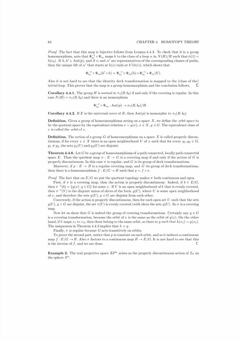
7/25/2019 TOPOLOG8Y
http://slidepdf.com/reader/full/topolog8y 64/98
64 CHAPTER 4. HOMOTOPY THEORY
Proof. The fact that this map is bijective follows from Lemma 4.4.3. To check that it is a grouphomomorphism, note that Φ−1
e0 ◦ Ψe0 maps h to the class of a loop α in N (H )/H such that α(1) =h(e0). If h, h′ ∈ Aut( p), and if α and α′ are representatives of the corresponding classes of paths,then the unique lift of α′ that starts at h(e) ends at h′(h(e)), which shows that
Φ−1e0 ◦ Ψe0(h′ ◦ h) = Φ−1
e0 ◦ Ψe0(h) ∗ Φ−1e0 ∗ Ψe0(h′).
Also it is not hard to see that the identity deck transformation is mapped to the (class of the)trivial loop. This proves that the map is a group homomorphism and the conclusion follows.
Corollary 4.4.1. The group H is normal in π1(B, b0) if and only if the covering is regular. In thiscase N (H ) = π1(B, b0) and there is an isomorphism
Φ−1e0 ◦ Ψe0 : Aut( p) → π1(B, b0)/H.
Corollary 4.4.2. If E is the universal cover of B , then Aut( p) is isomorphic to π1(B, b0).
Definition. Given a group of homeomorphisms acting on a space X , we define the orbit space tobe the quotient space by the equivalence relation x ∼ g(x), x ∈ X , g ∈ G. The equivalence class of x is called the orbit of x.
Definition. The action of a group G of homeomorphisms on a space X is called properly discon-tinuous, if for every x
∈ X there is an open neighborhood U of x such that for every g1, g2
∈ G,
g1 = g2, the sets g1(U ) and g2(U ) are disjoint.
Theorem 4.4.6. Let G be a group of homeomorphisms of a path connected, locally path connectedspace E . Then the quotient map π : E → G is a covering map if and only if the action of G isproperly discontinuous. In this case π is regular, and G is its group of deck transformations.
Moreover, if p : E → B is a regular covering map, and G its group of deck transformations,then there is a homeomorphism f : E/G → B such that p = f ◦ π.
Proof. The fact that on E /G we put the quotient topology makes π both continuous and open.First, if π is a covering map, then the action is properly discontinuous. Indeed, if b ∈ E/G,
then π−1(b) = {g(x) | g ∈ G} for some x. If V is an open neighborhood of b that is evenly covered,
then π−1
(V ) is the disjoint union of slices of the form g(U ), where U is some open neighborhoodof x, and therefore the sets g (U ), g ∈ G are disjoint from each other.
Conversely, if the action is properly discontinuous, then for each open set U such that the setsg(U ), g ∈ G are disjoint, the set π(U ) is evenly covered (with slices the sets g(U ). So π is a coveringmap.
Now let us show that G is indeed the group of covering transformations. Certainly any g ∈ Gis a covering transformation, because the orbit of x is the same as the orbit of g(x). On the otherhand, if h maps x1 to x2, then these belong to the same orbit, so there is g such that h(x1) = g(x1).The uniqueness in Theorem 4.4.3 implies that h = g.
Finally, π is regular because G acts transitively on orbits.To prove the second part, notice that p is constant on each orbit, and so it induces a continuous
map f : E/G → B . Also π factors to a continuous map B → E /G. It is not hard to see that thisis the inverse of f , and we are done.
Example 2. The real projective space RP n arises as the properly discontinuous action of Z2 onthe sphere S n.

7/25/2019 TOPOLOG8Y
http://slidepdf.com/reader/full/topolog8y 65/98
4.5. THE SEIFERT-VAN KAMPEN THEOREM 65
Example 3. A family of topological spaces that arise as quotients of a space by a group actionthat is properly discontinuous are the lens spaces . They arise as quotients of S 3 by a finite cyclicgroup. Specifically, let n, k be positive integers, and consider
S 3 = {(z1, z2) | |z1|2 + |z2|2 = 1} ⊂C3}with the Zn-action given by
m(z1, z2) =
e2πim/nz1, e2πimk/nz2
, m ∈ Zn.
This action is properly discontinuous, because one of z1 or z2 has the absolute value at least√
2/2,
and when you rotate it in the plane you move it at some distance from itself.The quotient is a 3-dimensional manifold L(n, k), called lens space. Note that L(2, 1) is the
3-dimensional real projective space RP 3.By Corollary 4.4.2, π1(L(n, k)) = Zn. In particular, if n = n′ then L(n, k) is not homeomorphic
to L(n′, k′). We thus deduce the existence of infinitely many 3-dimensional manifolds that are nothomeomorphic to each other.
Example 4. The computation of the fundamental group of the figure eight.
Example 5. The computation of the fundamental group of a closed compact orientable surface.
4.5 The Seifert-van Kampen theorem
4.5.1 A review of some facts in group theory
Given a family of groups {Gα}α∈A, consider all words whose ”letters” are elements of these groups.Next we reduce these words by the following two operations:
(1) identify all identity elements.(2) any consecutive letters belonging to the same group should be replaced by their product.
As such we obtain reduced words, in which consecutive letters belong to different groups. Twowords are multiplied by juxtaposition followed by reduction. The common identity element acts asidentity for this multiplication.
Definition. The free product of the groups Gα, α ∈ A, denoted by ∗α∈AGα, is the group of reducedwords with the multiplication defined above.
Note that the group Gα embeds naturally in the free product as the set of all words consistingof one letter which letter is in Gα.
Proposition 4.5.1. Let G = ∗αGα. Given group homomorphisms hα : Gα → H , where H is somegroup, there is a unique group homomorphism h : G → H such that h|Gα
= hα. Conversely, if Gcontains all Gα and this property holds for any group H , then G is the free product.
Definition. The free product of several copies of Z is called a free group.
Free groups are universal in the following sense. Let G be an arbitrary group, and
{gα
} a set
of generators (which could be all elements of G). Then for each generator there is a group homo-morphism hα : Z → G, hα(k) = gkα. By the previous proposition there is a group homomorphismh : ∗αZ→ G. If N is the kernel of h, then
∗αZ/N ≃ G.

7/25/2019 TOPOLOG8Y
http://slidepdf.com/reader/full/topolog8y 66/98
66 CHAPTER 4. HOMOTOPY THEORY
Definition. The description of a group G as the quotient of a free group by a normal subgroup iscalled a presentation of G. The generators of the normal subgroup are called relators .
If the normal subgroup has finitely many elements, the presentation is called finite . A groupthat is finitely generated and finitely presented is usually written as
G = g1, g2, . . . , gm | β 1, β 2, . . . , β n
where the gi’s are the generators, and the β i’s are the relators. Note that the β i’s are words in thegi’s.
Example 1.
Z = g | Zn = g | gnZ2 =
g1, g2 | g1g2g−11 g−12
K =
a,b,c | a2, b2, c2,abc1,bca−1,cab−1
.
where K is the Klein 4-group, i.e. the group of symmetries of a rectangle.
As we will see below, the computation of the fundamental group yields a group presentation.There is a downside to this, there does not exist an algorithm that decides if two presentations give
the same group. This is a theorem!The groups that make up the free product do not intersect. But what if these groups overlap?
We consider only the case of two groups, and make the following definition.
Definition. Given the groups G1, G2 and H , and the group homomorphisms φ1 : H → G1,φ2 : H → G2, we define the free product with amalgamation to be
G1 ∗H G2 = (G1 ∗ G2)/N
where N is the smallest normal subgroup of G1 ∗ G2 containing all elements φ1(h)φ2(h)−1, h ∈ H .
Note that Gk → G1 ∗ G2 → G1 ∗H G2 defines a natural map jk : Gk → G1 ∗H G2, k = 1, 2.
One usually thinks of H as being a common subgroup of G1 and G2, and φ1, φ2 as being theinclusion homomorphisms.
Example 2. If
G1 = u1, . . . , uk | α1, . . . , αlG2 = v1, . . . , vm | β 1, . . . , β nH = w1, . . . , w p | γ 1, . . . , γ q
then the amalgamated product is
G1 ∗H G2 = u1, . . . , uk, v1, . . . , vm | α1, . . . , αl, β 1, . . . , β n, i1∗(w1)(i2∗(w1)−1, . . . , i1∗(w p)(i2∗(w p)−1The free product with amalgamation also has a universality property, stated in the following
proposition.

7/25/2019 TOPOLOG8Y
http://slidepdf.com/reader/full/topolog8y 67/98
4.5. THE SEIFERT-VAN KAMPEN THEOREM 67
Proposition 4.5.2. Given the groups G1, G2 and H , and the group homomorphisms φk : H → Gk,k = 1, 2, consider G1 ∗H G2. Given a group G and group homomorphisms ψk : Gk → G, k = 1, 2,such that ψ1 ◦ φ1 = ψ2 ◦ φ2, there is a unique group homomorphism Φ : G1 ∗H G2 → G such thatΦ ◦ jk = ψk, k = 1, 2. Moreover, G′ is a group for which this property holds for every group G, theG′ = G1 ∗H G2.
Proof. Here is the proof. yada yadaFor the second part, we know that there is a unique Φ : G1 ∗H G2 → G′ that satisfies the
conditions from the statement, and conversely there is a unique Φ ′ : G′ → G, that makes thecorresponding diagram commutative. Composing, we obtain that Φ′ ◦ Φ : G1 ∗H G2 → G1 ∗H G2
satisfies the same property with G = G1∗H
G2
. But the identity isomorphism satisfies this propertytoo. By uniqueness, Φ′ ◦ Φ = 1G1∗H G2
. Similarly Φ ◦ Φ′ = 1G′ , and we are done.
4.5.2 The statement and proof of the Seifert-van Kampen theorem
Theorem 4.5.1. (Seifert-van Kampen theorem, modern version) Let X = U 1 ∪ U 2 where U 1and U 2 are open in X , such that U 1, U 2, U 1 ∩ U 2 are path connected, and let x0 ∈ U 1 ∩ U 2.Consider the homomorphisms ik∗ : π1(U 1 ∩ U 2, x0) → π1(U k, x0) and jk∗ : π1(U k, x0) → π1(X, x0)induced by the inclusion maps, k = 1, 2. If G is a group and φk : π1(U k, x0) → G, k = 1, 2,are group homomorphisms such that φ1 ◦ i1∗ = φ2 ◦ i2∗, then there is a unique homomorphismΦ : π1(X, x0) → G such that Φ ◦ j1∗ = φ1 and Φ ◦ j2∗ = φ2.
The result states that if φ1 and φ2 coincide on U 1 ∩ U 2 then they induce a homomorphism fromπ1(X, x0) to G.
Proof. First let us prove the following result.
Lemma 4.5.1. Suppose X = U 1 ∪ U 2 where U 1 and U 2 are open subsets of X such that U 1 ∩ U 2is path connected. Consider x0 ∈ U 1 ∩ U 2. If ik : U k → X , k = 1, 2 are the inclusion maps theni1∗(π1(U 1, x0)) and i2∗(π1(U 2, x0)) generate π1(X, x0).
Proof. Let f be a loop in X . Using the Lebesgue number theorem 2.4.5, we can find a subdivisiona0 = 0 < a1 < . . . < an = 1 of [0, 1] such that f ([al, al+1]) lies entirely in one of the sets U k.By joining consecutive intervals whose images lie in the same U k, we may assume that for each l,f ([a
l, a
l+1]) and f ([a
l−1, a
l]) lie in different U
k’s. It follows that f (a
l) ∈
U 1∩
U 2
for l = 1, 2, . . . , n−
1.Also f (a0) = f (an) = x0. Consider paths γ l, l = 0, 1, 2, . . . , n from x0 to f (al) (γ 0 = γ n = ex0).Then If we denote f l = γ l ∗ f |[al,al+1] ∗ γ l+1, then
[f ] = [f 1] ∗ [f 2] ∗ · · · ∗ [f n−1].
Of course, [f l] is either in U 1 or U 2, which proves the lemma.
Because of Lemma 4.5.1, Φ is completely determined if we know where it maps loops that lieentirely in U 1 or U 2. This proves uniqueness.
Let us prove existence. To avoid ambiguities, we use indices for homotopy equivalence classes,to specify in which space the homotopy equivalence takes place. So for a path f , [f ]X stands for
the homotopy class rel endpoints of f in X , while [f ]U 1 stands for the homotopy class rel endpointsof f in U 1.
1. We define first a map ρ from the set of loops that lie entirely in one of the U k to G by
ρ(f ) =
φ1([f ]U 1) if f lies in U 1φ2([f ]U 2) if f lies in U 2.

7/25/2019 TOPOLOG8Y
http://slidepdf.com/reader/full/topolog8y 68/98
68 CHAPTER 4. HOMOTOPY THEORY
The map ρ is well defined since if f lies in U 1 ∩ U 2, then
φk([f ]U k) = φkik∗([f ]U 1∩U 2)
and we know that φ1i1∗ = φ2i2∗. The map ρ satisfies the conditions(1) If [f ]U k = [g]U k for some k, then ρ(f ) = ρ(g).(2) If both f and g lie in the same U k, then ρ(f ∗ g) = ρ(f ) · ρ(g).
This second condition holds because φk, k = 1, 2 are homomorphisms.2. Next, we extend ρ to the set of paths that lie entirely in U 1 or U 2. First consider for each
x ∈ X a path from x0 to x (if x0 = x take the constant path). For a path f from x to y define
ρ(f ) = ρ(αx ∗ f ∗ αy).
The conditions (1) and (2) are again satisfied. Indeed, if [f ]U k = [g]U k , then [αx∗f ∗αy] = [αx∗g∗αy],with the homotopy being constant on αx and αy. For (2), notice that if f runs from x to y andg from y to z, then αx ∗ f ∗ αy ∗ αy ∗ g ∗ αz is homotopic relative to the endpoints (in U k) toαx ∗ f ∗ g ∗ αz.
3. We extend ρ further to arbitrary paths in X . Removing the constraints about U 1 and U 2we have the new conditions for the extended map
(1) [f ] = [g] implies ρ(f ) = ρ(g).(2) ρ(f ∗ g) = ρ(f ) ∗ ρ(g) wherever f ∗ g is defined.
The trick is the same as in the lemma. Consider a subdivision of the interval [0, 1] such that each
interval of the subdivision is mapped entirely to one of the two sets U 1 or U 2. Using this subdivision,break f as f 1 ∗ f 2 ∗ · · · f n (f j is the restriction of f to the j -th subinterval). Define
ρ(f ) = ρ(f 1)ρ(f 2) · · · ρ(f n).
But, is this independent of the subdivision? Any subdivision with the given property can betransformed into any other by adding or subtracting points. So it is sufficient to show that ρ(f )does not change if we add one point to the subdivision. The path f j in the middle of whom thepoint was added now breaks into the paths f j,1 and f j,2. These paths belong to the same U k, so wealready know that ρ(f k) = ρ(f k,1) ∗ ρ(f k,2). And that’s all we need. So the map is well defined. Itis an extension of the old ρ because if the path lies entirely in one of the U k’s we can use the trivial
partition.Let us now check condition (1). Consider a homotopy F : [0, 1] × [0, 1] → X between f and g (relative to the endpoints). Consider the subdivisions 0 = a0 < a1 < . . . < am = 1,b0 = 0 < b1 < . . . < bn = 1 of the interval [0, 1] such that for each ( p, q ), f ([a p, a p+1] × [bq, bq+1])lies entirely in one of U k.
Take one of the slices [0, 1] × [bq, bq+1], and let f ′ = F |[0,1]×{bq}, g′ = F |[0,1]×{bq+1}. If we showthat ρ(f ′) = ρ(g′), then by going slice-by-slice we obtain that ρ(f ) = ρ(g).
Write f ′ = f ′1∗f ′2∗·· ·∗f ′m and g′ = g ′1∗g′2∗·· ·∗g′m using the subdivision. For each j = 0, 1, . . . , m,consider the path γ j = F |{aj}×[bq ,bq+1]. Then f ′ j is homotopic rel to the endpoints to γ j ∗ g′ j ∗ γ j+1and the homotopy lies entirely inside one of U 1 or U 2. It follows that
ρ(f ′ j
) = ρ(γ j
)ρ(g′ j
)ρ(γ j
)
(here we used both (1) and (2) in the particular case). Consequently, using the definition of ρ, wehave
ρ(f ′1)ρ(f ′2) · · · ρ(f ′m) = ρ(γ 0)ρ(g′1)ρ(γ 1) · · · ρ(γ m−1)ρ(g′m)ρ(γ m).

7/25/2019 TOPOLOG8Y
http://slidepdf.com/reader/full/topolog8y 69/98
4.5. THE SEIFERT-VAN KAMPEN THEOREM 69
Also, because each γ j lies inside one of U 1 or U 2, by the particular case of (2),
ρ(γ j)ρ(γ j) = ρ(γ j ∗ γ j) = ρ(constant) = identity.
Note also that ρ(γ 0) = ρ(γ m) =identity, because these paths are constant. It follows that
ρ(f ′1)ρ(f ′2) · · · ρ(f ′m) = ρ(g′1)ρ(g′2) · · · ρ(g′m),
and hence ρ(f ′) = ρ(g′), as desired.Finally, let us check condition (2). For f ∗ g we can consider a subdivision that contains the
endpoint of f and the starting point of g . Then
f ∗ g = f 1 ∗ f 2 ∗ · · · ∗ f m ∗ g1 ∗ g2 ∗ · · · ∗ gn
and using the definition we obtain that ρ(f ∗ g) = ρ(f ) · ρ(g).
4. We now define for each loop in X based at x0,
Φ([f ]) = ρ(f ).
Conditions (1) and (2) show that Φ is well defined and is a group homomorphism. Let us now showthat Φ ◦ jk∗ = φk, k = 1, 2. If f is a loop in U k, then
Φ( jk∗([f ]U k)) = Φ([f ]) = ρ(f ) = φk([f ]U k).
by definition. And we are done.
Proposition 4.5.2 implies the following classical version of this theorem.
Theorem 4.5.2. (Seifert-van Kampen Theorem, classical version) If X = U 1∩U 2 with U 1, U 2 openand U 1, U 2, U 1 ∩ U 2 path connected, and if x0 ∈ U 1 ∩ U 2 then
π1(X, x0) = π1(U 1, x0) ∗π1(U 1∩U 2,x0) π1(U 2, x0),
where the amalgamation is defined via the maps induced by inclusions.
Corollary 4.5.1. Given the open subsets U 1, U 2 of X such that U 1, U 2, U 1∩U 2 are path connected,if
π1(U 1, x0) =
u1, . . . , uk
|α1, . . . , αl
π1(U 2, x0) = v1, . . . , vm | β 1, . . . , β nπ1(U 1 ∩ U 2, x0) = w1, . . . , w p | γ 1, . . . , γ q
then
π1(X, x0) =
u1, . . . , uk, v1, . . . , vm | α1, . . . , αl, β 1, . . . , β n, i1∗(w1)(i2∗(w1)−1, . . . , i1∗(w p)(i2∗(w p)−1
Corollary 4.5.2. Given the open subsets U 1, U 2 of X such that U 1, U 2, U 1∩U 2 are path connected,if U 1 ∩ U 2 is simply connected then
π1(X, x0) = π1(U 1, x0) ∗ π1(U 2, x0).
Corollary 4.5.3. Given the open subsets U 1
, U 2
of X such that U 1
, U 2
, U 1∩
U 2
are path connected,if U 2 is simply connected then
π1(X, x0) = π1(U 1, x0)/N
where N is the smallest normal subgroup of π1(U 1, x0) containing the image of i1∗ : π1(U 1∩U 2, x0) →π1(U 1, x0).

7/25/2019 TOPOLOG8Y
http://slidepdf.com/reader/full/topolog8y 70/98
70 CHAPTER 4. HOMOTOPY THEORY
4.5.3 Fundamental groups computed using the Seifert-van Kampen theorem
In the following we will be using Proposition 4.2.4, which asserts that if one space is a deformationretract of another, then the two spaces have isomorphic fundamental groups.
Example 1. The fundamental group of a wedge of circles. The wedge of n circles is obtained bytaking the quotient of their disjoint union by the map that identifies the points of coordinate 1from each of these circles. The standard notation is
ni=1 S 1.
Let us first consider the case n = 2. Take as U 1 and U 2 open subsets of S 1
S 1 such that U kcontains the kth circle, k = 1, 2, and this circle is a deformation retract of it. Then U 1 ∩ U 2 is acontractible space. Applying the Seifert-van Kampen theorem we conclude that
π1(S 1S 1) = π1(S 1) ∗ π1(S 1) = Z ∗ Z.
Proceeding by induction, and taking the set U 1 to be an open neighborhood of n−1
i=1 S 1 and U 2an open neighborhood of the last circle, which are both deformation retract of the correspondingsubsets, we deduce that
π1
ni=1
S 1
= ∗ni=1Z.
Example 2. The fundamental group of the complement in S 3 (or R3) of the trefoil knot.
S 3 = {(z1, z2) | |z1|2 + |z2|2 = 1} ⊂C2.
The trefoil knot K 2,3 can be thought of as the curve
φ(t) =
1√
2e4πit,
1√ 2
e6πit
.
This curve lies on the torus
S 1 × S 1 =
1√
2e2πit,
1√ 2
e2πis
| t, s ∈ [0, 1]
.
The torus separates the solid tori T 1 = {(z1, z2) | |z1| ≥ |z2|} and T 2 = {(z1, z2) | |z1| ≤ |z2|}.Consider two open sets U 1 and U 2 such that T k\K 3,2 is a deformation retract of U k, k = 1, 2. Notethat the annulus (S 1 × S 1)\K 3,2 is a deformation retract of U 1 ∩ U 2.
We have
π1(U k) = π1(T k\K 3,2) = π1(T k) = π1(S 1) = Z, k = 1, 2,
π1(U 1 ∩ U 2) = π1((S 1 × S 1)\K 3,2) = π1(annulus) = Z.
Note also that the inclusion U 1 ∩ U 2 in U 1 induces at the level of the fundamental group the mapZ → Z, m → 3m (this is because the generator of the fundamental group of the annulus ”wraps”three times around the torus in the direction of the generator of the fundamental group of T 1).
Similarly the inclusion U 1 ∩ U 2 → U 2 induces at the level of the fundamental groups the mapZ→ Z, m → 2m.
We obtain for the fundamental group of the complement of the trefoil knot the presentation
π1(S 3\K 3,2) =
x, y | x3 = y2

7/25/2019 TOPOLOG8Y
http://slidepdf.com/reader/full/topolog8y 71/98
4.5. THE SEIFERT-VAN KAMPEN THEOREM 71
Note that the complement of the unknot has a circle as a deformation retract. Consequently,its fundamental group is Z. Let us check that π1(S 3\K 3,2) = Z. Indeed, if we consider the group Gof symmetries of a regular hexagon generated by the rotation ρ about the center by 120◦ and thereflection σ about one main diagonal, then because ρ3 = σ2 =identity there is a group epimorphismof π1(S 3\K 3,2) onto G. But G is non-commutative, hence so is π1(S 3\K 3,2), showing that this groupis not Z. This proves that the trefoil knot is knotted.
Proposition 4.5.3. (The addition of a disk) Let X be a space, and g : S 1 → X a continuous map.Consider the space X ∪g B2 obtained by factoring the disjoint union of X with the unit disk by
the equivalence relation e2πit
∼ g(e2πit). Then the map i∗ : π1(X, x0)
→ π1(X
∪g B2, x0) induced
by inclusion is surjective and its kernel is the normal subgroup of π1(X, x0) containing the imageof g∗|S 1.
Proof. The fact that i∗ is surjective follows from the fact that every loop is homotopic to one thatdoes not intersect the disk. The proof of this fact follows the idea from the proof of Theorem 4.2.2.One approximates loop by a piecewise linear one, which is homotopic to it and misses at least onepoint p of the disk, then one pushes the loop away from p until it leaves the disk.
Let U be the open set X ∪g (B2\{0} and V = 12B2. Then U and V are path connected, and
U ∩ V = 12B2\{0} is also path connected. Moreover, X is a deformation retract of U (just push
the punctured disk towards the unit circle), V is simply connected, and U ∩ V is homotopicallyequivalent to a circle. By the Seifert-van Kampen theorem we have
π1(X ∪g B2, x0) = π1(U, x0) ∗π1(U ∩V,x0) π1(B2, x0)
= π1(X, x0) ∗ π1(S 1, x0){0}.
The amalgamation is defined by the relations g∗([f ]) = 0 for all [f ] ∈ π1(S 1, x0) because [f ] ismapped to 0 by the inclusion of the circle into the disk.
Example 3. Given a group presentation with finitely many relators and finitely many generators,there is a topological space that has this as its fundamental group.
Here is how to construct this space. Let
G =
g1, g2, . . . , gm|
β 1, β 2, . . . , β n
.
Consider the wedge of n circles, and identify the generator of the jth circle with g j, j = 1, 2, . . . , m.Now for each relator β k, consider a loop f k in the wedge of circles that represents it. For each k,take a closed unit disk and glue it to the wedge of circles by the equivalence relation e2πit = f k(t).As a corollary of Proposition 4.5.3, the result of all these operations is a topological space whosefundamental group is G.
4.5.4 The construction of compact surfaces and the computation of their fun-
damental groups
We will consider just the case of the surfaces shown in Figure 4.1, which, as will be seen later,
are all closed compact orientable surfaces. These are the sphere with zero, one, two, three, etc.handles.
The first two, the sphere and the torus, are well understood. For all the others the sameprocedure will be applied: They will be obtained by adding a disk to a wedge of circles. We will dothis in detail for the third surface on the list, the sphere with two handles, the others being similar.
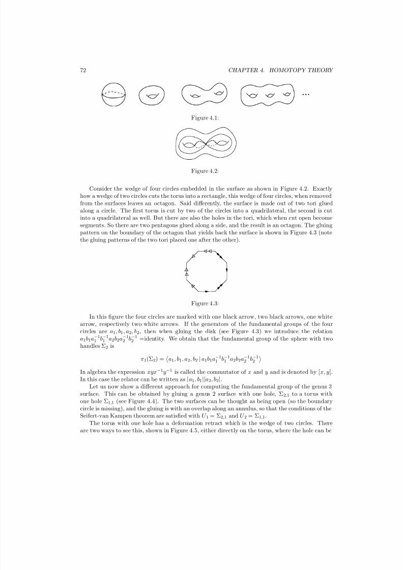
7/25/2019 TOPOLOG8Y
http://slidepdf.com/reader/full/topolog8y 72/98
72 CHAPTER 4. HOMOTOPY THEORY
...
Figure 4.1:
Figure 4.2:
Consider the wedge of four circles embedded in the surface as shown in Figure 4.2. Exactlyhow a wedge of two circles cuts the torus into a rectangle, this wedge of four circles, when removedfrom the surfaces leaves an octagon. Said differently, the surface is made out of two tori gluedalong a circle. The first torus is cut by two of the circles into a quadrilateral, the second is cutinto a quadrilateral as well. But there are also the holes in the tori, which when cut open becomesegments. So there are two pentagons glued along a side, and the result is an octagon. The gluingpattern on the boundary of the octagon that yields back the surface is shown in Figure 4.3 (note
the gluing patterns of the two tori placed one after the other).
Figure 4.3:
In this figure the four circles are marked with one black arrow, two black arrows, one whitearrow, respectively two white arrows. If the generators of the fundamental groups of the fourcircles are a1, b1, a2, b2, then when gluing the disk (see Figure 4.3) we introduce the relationa1b1a−11 b−11 a2b2a−12 b−12 =identity. We obtain that the fundamental group of the sphere with twohandles Σ2 is
π1(Σ2) =
a1, b1, a2, b2 | a1b1a−11 b−11 a2b2a−12 b−12
In algebra the expression xyx−1y−1 is called the commutator of x and y and is denoted by [x, y].In this case the relator can be written as [a1, b1][a2, b2].
Let us now show a different approach for computing the fundamental group of the genus 3surface. This can be obtained by gluing a genus 2 surface with one hole, Σ2,1 to a torus with
one hole Σ1,1 (see Figure 4.4). The two surfaces can be thought as being open (so the boundarycircle is missing), and the gluing is with an overlap along an annulus, so that the conditions of theSeifert-van Kampen theorem are satisfied with U 1 = Σ2,1 and U 2 = Σ1,1.
The torus with one hole has a deformation retract which is the wedge of two circles. Thereare two ways to see this, shown in Figure 4.5, either directly on the torus, where the hole can be

7/25/2019 TOPOLOG8Y
http://slidepdf.com/reader/full/topolog8y 73/98
4.5. THE SEIFERT-VAN KAMPEN THEOREM 73
Figure 4.4:
“inflated” to the point where the result is a regular neighborhood of the union of the meridian andthe longitude, or by looking at the planar representation of the torus with a hole in the middle.
Figure 4.5:
For a genus 2 surface the deformation retract consists of the wedge of four circles shown inFigure 4.6. A way to see this is to recall Figure 4.3, this time with a hole in the middle, and toincrease continuously the size of the hole until only the boundary remains.
Figure 4.6:
Now we are in position to apply the Seifert-van Kampen theorem. Since U 1 ∩ U 2 is an annulus,its fundamental group is Z. In view of Example 1 in § 4.5.3, the fundamental group of the genus 3surface Σ3 is
π1(Σ3) = (Z ∗ Z) ∗Z (Z ∗ Z ∗ Z ∗ Z).
Let the generators of these Z’s be respectively a1, b1, a2, b2, a3, b3.Now let us understand how the amalgamation takes place. The generator of the fundamental
group of the annulus becomes the boundary of the square in the first case, and the boundary of the octagon in the second. By choosing appropriately a1 and b1, we can make the boundary of the square to correspond to the element b1a1b−11 a−11 in the wedge of two circles. Similarly theboundary of the octagon can be made to correspond to the element a2b2a−12 b−12 a3b3a−13 b−13 , and theSeifert-van Kampen theorem sets these equal. As a result we obtain
π1(Σ3) = a1, b1, a2, b2, a3, b3 | [a1, b1][a2, b2][a3, b3] .
In fact, the genus g surface Σg, obtained by adding g handles to the sphere, can also be obtained
by a pairwise gluing of the sides of a 4g-gon, and hence by adding a disk to a wedge of 2g circles.As a result, we obtain
π1(Σg) = a1, b1, a2, b2, . . . , ag, bg | [a1, b1][a2, b2] · · · [ag, bg]

7/25/2019 TOPOLOG8Y
http://slidepdf.com/reader/full/topolog8y 74/98
74 CHAPTER 4. HOMOTOPY THEORY
7/25/2019 TOPOLOG8Y
http://slidepdf.com/reader/full/topolog8y 75/98
Chapter 5
Homology
The homotopy groups, namely the fundamental group and its higher dimensional generalizationsdefined in the previous chapter, have the downsides that they are difficult to compute (as is thecase of the higher dimensional homotopy groups) or they are hard to distinguish from each other(as is the case for the fundamental group obtained as a group presentation). The way aroundthese problems is to introduce a different family of groups, which are much easier to compute andmoreover which are abelian, thus very easily distinguishable. The idea behind this constructiongoes back to H. Poincare. While in the case of homotopy theory the objects where loops (i.e.images of circles) or images of higher dimensional spheres inside the topological space and the
equivalence between them was defined by homotopy, in the new situation the objects are cycles,which are images of manifolds of same dimension inside the same topological space, two cyclesbeing equivalent if between them runs the image of a manifold one dimension higher.
5.1 Simplicial homology
The above idea for constructing a homology theory can be formalized easily in a combinatorialsetting if we triangulate the topological space and all cycles. We follow the point of view of AllenHatcher’s book on Algebraic Topology and construct the simplicial homology based on ∆-complexes(originally called semisimplicial complexes by their inventors Eilenberg and Zilber), mainly due to
the fact that for the classical simplicial complexes the computations are almost impossible.In this chapter all spaces are assumed to be compact.
5.1.1 ∆-complexes
At the heart of homology theory lies the notion of a simplex.
Definition. Let v0, v1, . . . , vn be points in RN , N > n that do not lie in an affine subspace of dimension n or less. The n-simplex with vertices v0, v1, . . . , vn is the set
σn = v0, v1, . . . , vn = {t0v0 + t1v1 + · · · + tnvn ∈ RN | ti ≥ 0, t0 + t1 + · · · + tn = 1}.
In other words an n-simplex is the convex hull of n + 1 points that do not lie in a hyperplane.The list of coefficients (t0, t1, . . . , tn) of a point t0v0 + t1v1 + · · · + tnvn in the simplex are calledbarycentric coordinates .
Example 1. A 1-simplex is a line segment, a 2-simples is a triangle (together with its interior), athree simplex is a solid tetrahedron.
75

7/25/2019 TOPOLOG8Y
http://slidepdf.com/reader/full/topolog8y 76/98
76 CHAPTER 5. HOMOLOGY
We convene that the ordering of the vertices of the simplex defines an orientation, with twoorientations being the same if one gets from one to the other by an even permutation of the vertices,and two orderings are of opposite orientations otherwise.
Example 2. v0, v1, v2 = v1, v2, v0 = − v0, v2, v1.
If we remove several vertices of a simplex, the remaining vertices determine a simplex of smallerdimension, which we will call a sub-simplex of the original simplex. When removing one vertex, theremaining n vertices determine an sub-simplex called face . The union of the faces is the boundaryof the simplex. More precisely, we make the following definition.
Definition. Given an n-simplex σn =
v0, v1, . . . , vn, its boundary is the formal sum
∂σn =n
j=0
(−1) j v0, v1, . . . , v j, . . . , vn
where the hat means that the respective vertex is removed.
Example 3. ∂ v0, v1 = v1 − v0.
The points of σn with all barycentric coordinates positive form the interior of σn, denotedInt(σn). When one coordinate is zero, the point is on a face.
Definition. A ∆-complex K consists of a topological space X and a finite collection of mapsφα : σnα → X of continuous maps from various simplices to X with the following properties:(1) The restriction φα|σnα is one-to-one, and each point of X is the image of exactly one suchrestriction.(2) Each restriction of a map φα to a face is another map φβ.(3) A set U is open in X if and only if φ−1(U ) is open for each α.
An alternative way of saying this is that X is the quotient of the disjoint union of severalsimplices, with the equivalence relation defined by gluing maps that identify one simplex to another.We can assume, for convenience, that these maps are linear isometries (by choosing simplices of the right size).
Given a ∆-complex K , the space X from the definition is usually denoted by
|K
| and is called
the realization of K . Conversely K is called a ∆-complex structure on X . Note that a topologicalspace can have many different ∆-complex structures.
Remark 5.1.1. The realization |K | of a ∆-complex is a metric space with the distance between twopoints being the shortest length of a piece-wise linear path that connects the points.
In practice, one usually identifies the image of the map φα with the simplex σnα. This means thata ∆-complex is a topological space obtained by gluing finitely many simplices by homeomorphismsbetween some of their subsimplices. By contrast, in the older notion of a simplicial complex twosimplices can share at most one sub-simplex. As such, a ∆-structure on a topological space requiresfewer simplices than a simplicial structure, and consequently this concept is more useful for explicitcomputations.
Example 4. The realization of the 2-dimensional torus, the projective plane, and the Klein bottleas ∆-complexes are shown in Figure 5.1.
Example 4. An n-dimensional sphere can be realized as a ∆-complex by gluing two n-simplicesby a (orientation reversing) homeomorphism between their boundaries.

7/25/2019 TOPOLOG8Y
http://slidepdf.com/reader/full/topolog8y 77/98
5.1. SIMPLICIAL HOMOLOGY 77
E
E
F
F
E 2 E 2
1
1V
V V
V
1
2
V V
V 1
1
V 2
2 V V
V V
E 3
E
E
E
E E
E
E
E
E E
1
1
1
1
2 2 2 23 3
F
F F
F 1 1
22
Figure 5.1:
5.1.2 The definition of simplicial homology
For a ∆-complex X , let C n(X ) be the free abelian group with basis the n-dimensional simplices of X . The elements of C n(X ) are called n-chains. For each simplex consider the boundary map,
∂ v0, v1, . . . , vn =n
j=0
(−1) j v0, v1, . . . , v j, . . . , vn .
Extend this map to a group homomorphism δ n : C n(X ) → C n−1(X ), for each n ≥ 1. One obtainswhat is called a chain complex
· · · ∂ n+1
−→ C n(X )
∂ n
−→ C n−1(X )
∂ n−1
−→ · · · ∂ 2
−→ C 1(X )
∂ 1
−→ C 0(X )
→ 0.
Proposition 5.1.1. For each n, ∂ n−1∂n = 0.
Proof. We have
∂ n−1∂ n v0, v1, . . . , vn =n
j=1
∂ n−1 v0, v1, . . . , v j, . . . vn
=i<j
(−1) j(−1)i v0, v1, . . . , vi, . . . , v j, . . . , vn +i>j
(−1) j(−1)i−1 v0, v1, . . . , v j, . . . , vi, . . . , vn .
Note that when exchanging i and j in the second sum, we obtain the negative of the first sum.Hence the result is zero, as desired.
As a corollary, we have what is called a chain complex
· · · ∂ n+1−→ C n(X ) ∂ n−→ C n−1(X )
∂ n−1−→ · · · ∂ 2−→ C 1(X ) ∂ 1−→ C 0(X ) → 0,
in which Im ∂ n ⊂ Ker ∂ n−1 for all n.
Definition. We let Bn(X ) = Im ∂ n+1 and Z n(X ) = Ker ∂ n. The elements of Bn(X ) are calledboundaries , the elements of Z n(X ) are called cycles. The group H n(X ) = Z n(X )/Bn(X ) is calledthe n-th simplicial homology group of X . The cosets of Bn(X ) are called homology classes.
For finite ∆-complexes the chain groups C n(X ) are finitely generated free abelian groups, andconsequently Bn(X ) and Z n(X ) are finitely generated free abelian groups. It follows that H n(X )
is a finitely generated abelian group; in fact the generators of Z n(X ) yield generators for H n(X ),and the generators of Bn(X ) yield the relators of H n(X ). Thus in computations we are led again,as for the fundamental group, to a presentation of H n(X ), but in this case to the presentation of anabelian group. A little linear algebra allows us to compute this group precisely, as we will explainin the next section.
7/25/2019 TOPOLOG8Y
http://slidepdf.com/reader/full/topolog8y 78/98
78 CHAPTER 5. HOMOLOGY
5.1.3 Some facts about abelian groups
The fundamental theorem of finitely generated abelian groups can be stated in two equivalent forms
Version A: Every finitely generated abelian group is of the form
G = Zn ⊕ Z pn11
⊕ Z pn22
⊕ · · · ⊕ Z pnkk
,
where n, k ≥ 0, n1, n2, . . . , nk ≥ 1 and p1, p2, . . . , pk are prime numbers, these numbers are uniquelydefined (up to reordering) by G.
Version B: Every finitely generated abelian group is of the form
G = Zn ⊕ Zm1 ⊕Zm2
⊕ · · · ⊕ Zmk
where n, k ≥ 0, m1 divides m2, m2 divides m3, ..., mk−1 divides mk, and these numbers are uniquelydefined by G.
Note that a finitely generated abelian group is the sum of a free abelian group and a finiteabelian group. The later is called the torsion. The number of copies of Z in the free part is calledthe rank.
In what follows we will be interested in abelian groups that arise as kernels and images of homomorphisms between free abelian groups and as quotients of such groups. The kernels, images,and quotients can be computed as in the case of vector spaces, using row operations on matrices.These operations are:
1. A row is multiplied by −1.
2. Two rows are exchanged.
3. A row is added to or subtracted from another row.
5.1.4 The computation of the homology groups for various spaces
In this section we will call zero-dimensional simplices vertices, one-dimensional simplices edges,two-dimensional simplices faces, and 3-dimensional simplices (solid) tetrahedra. All computations
will be performed for a certain realization of the given space as a ∆-complex; we will prove in§ 5.2.4 that the homology groups are independent of this realization.
Example 1. The circle. We can realize the circle as a ∆-complex by considering the circle itself to be an edge E with the two endpoints at the vertex V = 1. The corresponding chain complex is
0 −→ ZE ∂ −→ ZV −→ 0,
with δ 1E = V − V = 0. Hence
H 1(S 1) = Z 1(S 1) = Z
and
H 0(S 1) = Z 0(S 1)/B0(S 1) = ZV /{0} = Z.
Example 2. The projective plane. RP 2 can be obtained from the upper hemisphere of S 2 bygluing its boundary S 1 by the antipodal map. Using this we can realize RP 2 as a ∆-complex asshown in Figure 5.2.

7/25/2019 TOPOLOG8Y
http://slidepdf.com/reader/full/topolog8y 79/98
5.1. SIMPLICIAL HOMOLOGY 79
V V
V V
F
F
E
E E
E
E 11
1
1
1
2
2
2
2
2
3
Figure 5.2:
The chain complex is
0 −→ ZF 1 ⊕ ZF 2∂ −→ ZE 1 ⊕ ZE 2 ⊕ ZE 3
∂ −→ ZV 1 ⊕ ZV 2 −→ 0.
with the (nontrivial) boundary maps given by
∂ 2F 1 = E 1 + E 2 + E 3, ∂ 2F 2 = E 1 + E 2 − E 3
and
∂ 1E 1 = V 1 − V 2, ∂ 1E 2 = V 2 − V 1, ∂ 1E 3 = V 2 − V 2 = 0.
Computation of H 0(RP 2). The kernel of the zero map ∂ 0 is Z 0(RP 2) = ZV 1 ⊕ ZV 2, with basisV 1, V 2. The image of ∂ 1 is B0(RP 2) = Z(V 1 − V 2), with basis V 1 − V 2. The coordinates of the basisvectors of B0(RP 2) in the basis of Z 0(RP 2) form a matrix which should be brought in reducedrow-echelon form with operations over the integers. This matrix is the row matrix [1, −1], whichis already in row-echelon form. The structure of H 0(RP 2) = Z 0(RP 2)/B0(RP 2) is read in thismatrix. The leading 1 in this matrix says that one of the two Z in Z 0(RP 2) = Z ⊕ Z is factoredout. Hence
H 0(RP 2) = Z.
Computation of H 1(RP 2). A little linear algebra shows that the kernel of ∂ 1, Z 1(RP 2), is a free
abelian group with basis consisting of w1 = E 1 + E 2 and w2 = E 3. On the other hand the imageof ∂ 2 is generated by E 1 + E 2 + E 3 and E 1 + E 2 − E 3. In the basis w1, w2, these generators arew1 + w2 and w1 − w2. The coefficient matrix is
1 11 −1
.
In reduced row-echelon form this is 1 10 2
.
Thus from Z 1(RP 2
) = Z ⊕ Z, the first Z is factored out, while the second is factored by a 2Z.Hence
H 1(RP 2) = (Z/Z) ⊕ (Z/2Z) = Z2.
Note that H 1(RP 2) = π1(RP 2)!

7/25/2019 TOPOLOG8Y
http://slidepdf.com/reader/full/topolog8y 80/98
80 CHAPTER 5. HOMOLOGY
Computation of H 2(RP 2). To find Z 2(RP 2) we need to determine which linear combinations withinteger coefficients of F 1 and F 2 are mapped to zero by ∂ 2. This means that we should have
n1(E 1 + E 2 + E 3) + n2(E 1 + E 2 − E 3) = 0 ∈ ZE 1 ⊕ ZE 2 ⊕ ZE 3.
This can be rewritten as
(n1 + n2)E 1 + (n1 + n2)E 2 + (n1 − n2)E 3 = 0.
For this to happen, n1 + n2 and n1 − n2 should both be zero, hence n1 = n2 = 0. Thus Z 2(RP 2) =
{0
}, and consequently
H 2(RP 2) = {0}.
Example 3. The torus. A realization of the torus as a ∆-complex is shown in Figure 5.3.
V V
V V
F
F E E
E
E
E
1
1
22
1
2
3
Figure 5.3:
We have the chain complex
0 −→ ZF 1 ⊕ ZF 2∂ 2−→ ZE 1 ⊕ ZE 2 ⊕ ZE 3
∂ 1−→ ZV −→ 0.
The boundary maps are
∂ 2F 1 = E 1 + E 2 + E 3, ∂ 2F 2 = −E 1 − E 2 − E 3,
∂ 1E 1 = ∂ 1E 2 = ∂ 1E 3 = V − V = 0.
Computation of H 0(S 1 × S 1). We have B0(S 1 × S 1) = Im ∂ 1 = {0} and Z 0(S 1 × S 1) = ZV .Hence
H 0(S 1 × S 1) = Z
Computation of H 1(S 1 × S 1). We have
B0(S 1 × S 1) = Im ∂ 2 = Z(E 1 + E 2 + E 3).
Also
Z 0(S 1
× S 1
) = Ker ∂ 1 = ZE 1 ⊕ ZE 2 ⊕ ZE 3.The matrix [1, 1, 1] is already in reduced row-echelon form, with leading term 1. Hence one of
the Z’s in Z ⊕ Z⊕ Z is factored out. We thus obtain
H 1(S 1 × S 1) = Z⊕ Z

7/25/2019 TOPOLOG8Y
http://slidepdf.com/reader/full/topolog8y 81/98
5.1. SIMPLICIAL HOMOLOGY 81
Note again that H 1(S 1 × S 1) = π1(S 1 × S 1).Computation of H 2(S 1 × S 1). If we write ∂ 2(n1F 1 + n2F 2) = 0 we obtain
(n1 − n2)(E 1 + E 2 + E 3) = 0.
Hence n1 = n2. We obtain
H 2(S 1 × S 1) = Z 2(S 1 × S 1) = Z(F 1 + F 2) ≃ Z.
In conclusion
H n(S 1 × S 1) = Z if n = 0, 2Z⊕ Z if n = 10 if n > 2.
Example 4. The 3-dimensional sphere. Like the 2-dimensional sphere can be obtainedby gluing together two disks along their boundaries, the 3-dimensional sphere can be obtained bygluing two balls along their boundaries. The balls can be realized as two tetrahedra T 1 and T 2.Thus S 3 can be realized as a ∆-complex with two 3-dimensional simplices T 1 and T 2 that have thesame vertices, edges, and faces. Since a tetrahedron has four faces, six edges, and four vertices, wehave a chain complex
0 −→ ZT 1 ⊕ ZT 2 ∂ 3−→ ZF 1 ⊕ ZF 2 ⊕ F3 ⊕ ZF 4 ∂ 2−→ ZE 1 ⊕ ZE 2 ⊕ ZE 3 ⊕ ZE 4 ⊕ ZE 5 ⊕ ZE 6∂ 1−→ ZV 1 ⊕ ZV 2 ⊕ ZV 3 ⊕ ZV 4 −→ 0.
To exhibit the boundary maps we have to be a little bit more precise. As such we set
T 1 = V 1, V 2, V 3, V 4 , T 2 = V 1, V 3, V 2, V 4, F 1 = V 2, V 3, V 4 , F 2 = V 1, V 3, V 4 , F 3 = V 1, V 2, V 4 , F 4 = V 1, V 2, V 3E 1 = V 1, V 2 , E 2 = V 1, V 3 , E 3 = V 2, V 3 , E 4 = V 3, V 4 , E 5 = V 2, V 4 , E 6 = V 1, V 4 .
The boundary maps are
∂ 3T 1 = ∂ 3 V 1, V 2, V 3, V 4 = V 2, V 3, V 4 − V 1, V 3, V 4 + V 1, V 2, V 4 − V 1, V 2, V 3= F 1 − F 2 + F 3 − F 4
∂ 3T 2 = ∂ 3 V 1, V 3, V 2, V 4 = V 3, V 2, V 4 − V 1, V 2, V 4 + V 1, V 3, V 4 − V 1, V 3, V 2= −F 1 − F 3 + F 2 + F 4,
∂ 2F 1 = ∂ 2 V 2, V 3, V 4 = V 3, V 4 − V 2, V 4 + V 2, V 3 = E 4 − E 5 + E 3
∂ 2F 2 = ∂ 3 V 1, V 3, V 4 = V 3, V 4 − V 1, V 4 + V 1, V 3 = E 4 − E 6 + E 2
∂ 2F 3 = ∂ 3 V 1, V 2, V 4 = V 2, V 4 − V 1, V 4 + V 1, V 2 = E 5 − E 6 + E 1
∂ 2F 4 = ∂ 3
V 1, V 2, V 3
=
V 2, V 3
− V 1, V 3
+
V 1, V 2
= E 3
−E 2 + E 1,
and
∂ 1E 1 = V 2 − V 1, ∂ 1E 2 = V 3 − V 1, ∂ 1E 3 = V 3 − V 2,
∂ 1E 4 = V 4 − V 3, ∂ 1E 5 = V 4 − V 2, ∂ 1E 6 = V 4 − V 1.

7/25/2019 TOPOLOG8Y
http://slidepdf.com/reader/full/topolog8y 82/98
82 CHAPTER 5. HOMOLOGY
The computation of H 0(S 3). It is clear that Z 0(S 3) = ZV 1 ⊕ ZV 2 ⊕ ZV 3 ⊕ ZV 4.
To find B0(S 3), we arrange the coefficients of the images of E 1, E 2,...,E 6 through ∂ 1 in a matrix,then we bring this matrix in row-echelon form. This is the same as the transpose of the matrix of ∂ 1, namely
−1 1 0 0−1 0 1 0
0 −1 1 00 0 −1 10 −1 0 1
−1 0 0 1
.
By performing row operations we obtain successively
−1 1 0 00 −1 1 00 −1 1 00 0 −1 10 0 −1 10 −1 0 1
→
−1 1 0 00 −1 1 00 0 0 00 0 −1 10 −1 0 00 0 −1 1
→
−1 1 0 00 −1 1 00 0 −1 10 0 −1 10 0 0 00 0 0 1
→
1 −1 0 00 1 −1 00 0 1 −10 0 0 00 0 0 00 0 0 0
.
This means that B0(S
3
) = Z
3
, and that when factoring Z 0(S
3
) by B0(S
3
) three of the Z are factoredout of Z4. We thus have
H 0(S 3) = Z.
The computation of H 1(S 3). Let us find the kernel of ∂ 1. The matrix of this transformation is1 −1 1 0 0 01 0 0 0 1 −10 1 0 1 0 −10 0 1 1 −1 0
,
which after performing a number of row operations becomes1 0 −1 0 −1 00 1 1 0 1 10 0 0 1 1 10 0 0 0 0 0
.
The kernel of this matrix is a free abelian group with basis [1 , −1, 1, 0, 0, 0], [1, −1, 0, −1, 1, 0], and[0, 1, 0, 1, 0, −1], that is E 1 − E 2 + E 3, E 1 − E 2 − E 4 + E 5, and E 2 + E 4 − E 6.
On the other hand, the image of ∂ 2 is generated by E 3 + E 4 − E 5, E 2 + E 4 − E 6, E 1 + E 5 − E 6,and E 1
−E 2 + E 3. Of course the standard approach is to write this in the basis of Z 1(S 3) = ker∂ 1,
and then decide what subspace they span. But we can see right away that the first and the lastbasis elements appear in this list, while E 1 − E 2 − E 4 + E 5 = (E 1 − E 2 + E 3) − (E 3 + E 4 − E 5).Hence B1(S 3) = Z 1(S 3), and hence
H 1(S 3) = {0}.
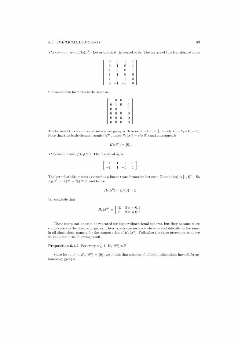
7/25/2019 TOPOLOG8Y
http://slidepdf.com/reader/full/topolog8y 83/98
5.1. SIMPLICIAL HOMOLOGY 83
The computation of H 2(S 3). Let us find first the kernel of ∂ 2. The matrix of this transformation is
0 0 1 10 1 0 −11 0 0 11 1 0 0
−1 0 1 00 −1 −1 0
.
In row-echelon form this is the same as
1 0 0 10 1 0 −10 0 1 10 0 0 00 0 0 00 0 0 0
.
The kernel of this homomorphism is a free group with basis [1, −1, 1, −1], namely F 1−F 2+ F 3−F 4.Note that this basis element equals ∂ 3T 1, hence Z 2(S 3) = B2(S 3) and consequently
H 2(S 3) = {0}.
The computation of H 3(S 3). The matrix of ∂ 3 is 1 −1 1 −1−1 1 −1 1
.
The kernel of this matrix (viewed as a linear transformation between Z-modules) is [1, 1]T . SoZ 3(S 3) = Z(T 1 + T 2) ∼= Z, and hence
H 3(S 3) = Z/{
0}
= Z.
We conclude that
H n(S 3) =
Z if n = 0, 30 if n = 0, 3.
These computations can be repeated for higher dimensional spheres, but they become morecomplicated as the dimension grows. There is only one instance where level of dificulty in the samein all dimensions, namely for the computation of H n(S n). Following the same procedure as abovewe can obtain the following result.
Proposition 5.1.2. For every n ≥ 1, H n(S n) = Z.
Since for m > n, H m(S n) = {0}, we obtain that spheres of different dimensions have differenthomology groups.
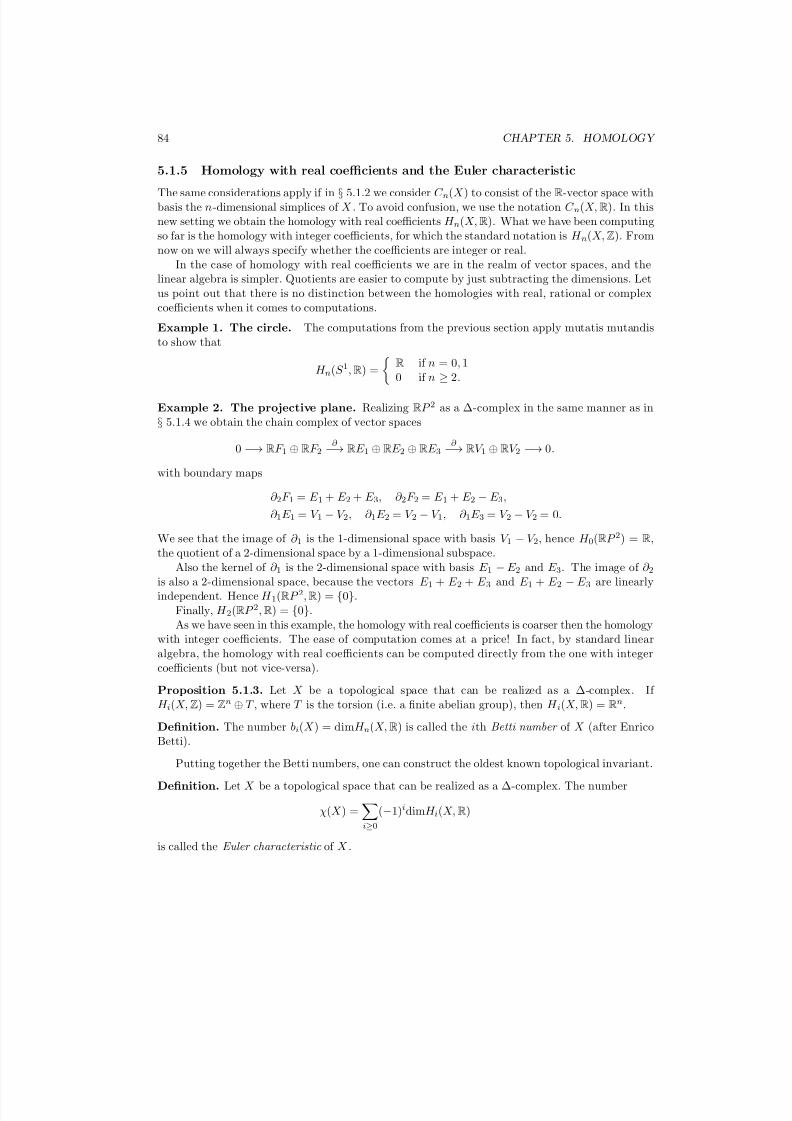
7/25/2019 TOPOLOG8Y
http://slidepdf.com/reader/full/topolog8y 84/98
84 CHAPTER 5. HOMOLOGY
5.1.5 Homology with real coefficients and the Euler characteristic
The same considerations apply if in § 5.1.2 we consider C n(X ) to consist of the R-vector space withbasis the n-dimensional simplices of X . To avoid confusion, we use the notation C n(X,R). In thisnew setting we obtain the homology with real coefficients H n(X,R). What we have been computingso far is the homology with integer coefficients, for which the standard notation is H n(X,Z). Fromnow on we will always specify whether the coefficients are integer or real.
In the case of homology with real coefficients we are in the realm of vector spaces, and thelinear algebra is simpler. Quotients are easier to compute by just subtracting the dimensions. Letus point out that there is no distinction between the homologies with real, rational or complexcoefficients when it comes to computations.
Example 1. The circle. The computations from the previous section apply mutatis mutandisto show that
H n(S 1,R) =
R if n = 0, 10 if n ≥ 2.
Example 2. The projective plane. Realizing RP 2 as a ∆-complex in the same manner as in§ 5.1.4 we obtain the chain complex of vector spaces
0 −→ RF 1 ⊕ RF 2∂ −→ RE 1 ⊕ RE 2 ⊕RE 3
∂ −→ RV 1 ⊕ RV 2 −→ 0.
with boundary maps
∂ 2F 1 = E 1 + E 2 + E 3, ∂ 2F 2 = E 1 + E 2 − E 3,
∂ 1E 1 = V 1 − V 2, ∂ 1E 2 = V 2 − V 1, ∂ 1E 3 = V 2 − V 2 = 0.
We see that the image of ∂ 1 is the 1-dimensional space with basis V 1 − V 2, hence H 0(RP 2) = R,the quotient of a 2-dimensional space by a 1-dimensional subspace.
Also the kernel of ∂ 1 is the 2-dimensional space with basis E 1 − E 2 and E 3. The image of ∂ 2is also a 2-dimensional space, because the vectors E 1 + E 2 + E 3 and E 1 + E 2 − E 3 are linearlyindependent. Hence H 1(RP 2,R) = {0}.
Finally, H 2(RP 2,R) = {0}.
As we have seen in this example, the homology with real coefficients is coarser then the homologywith integer coefficients. The ease of computation comes at a price! In fact, by standard linearalgebra, the homology with real coefficients can be computed directly from the one with integercoefficients (but not vice-versa).
Proposition 5.1.3. Let X be a topological space that can be realized as a ∆-complex. If H i(X,Z) = Zn ⊕ T , where T is the torsion (i.e. a finite abelian group), then H i(X,R) = Rn.
Definition. The number bi(X ) = dimH n(X,R) is called the ith Betti number of X (after EnricoBetti).
Putting together the Betti numbers, one can construct the oldest known topological invariant.
Definition. Let X be a topological space that can be realized as a ∆-complex. The number
χ(X ) =i≥0
(−1)idimH i(X,R)
is called the Euler characteristic of X .

7/25/2019 TOPOLOG8Y
http://slidepdf.com/reader/full/topolog8y 85/98
5.1. SIMPLICIAL HOMOLOGY 85
Theorem 5.1.1. (Poincare) Let X be a topological space that can be realized as a ∆-complex.Then
χ(X ) =i≥0
(−1)idimC p(X,R).
Proof. Note that by the first isomorphism theorem, if f : V → W is a linear map between vectorspaces, then V /Kerf ∼= Imf , and so V ∼= Kerf ⊕ Imf . If V is finite dimensional, then
dimV = dim Kerf + dim Imf.
Using this fact we obtaini≥0
(−1)iβ i(X ) = n≥0
(−1)i(dimZ i(X ) − dimBi(X )) = i≥0
(−1)i(dimZ i(X ) + dimBi−1(X ))
=i≥0
C i(X ),
and we are done.
As a corollary we obtain
Theorem 5.1.2. (Euler) Given a connected planar graph, denote by v the number of vertices,by e the number of edges, and by f the number of faces (including the face containing the point atinfinity). Then
v − e + f = 2.
Proof. By Problem 1 in Homework 3 of this semester and Proposition 5.1.3,
H i(S 2,R) =
R if i = 0, 20 otherwise
.
It follows that χ(S 2) = 1 − 0 + 1 = 2.Place the planar graph on S 2. The faces might not be triangles, nevertheless we can triangulate
them. Adding an edge increases the number of edges by 1 and the number of faces by 1, and sothe sum v − f + s does not change. Once we reach a triangulation, we have a ∆-complex, and then
Theorem 5.1.1 applies. Hence the conclusion.
Example 1. As an application of Euler’s formula, let us determine the platonic solids. Recallthat a platonic solid (i.e. a regular polyhedron) is a polyhedron whose faces are congruent regularpolygons and such that each vertex belongs to the same number of edges.
Let m be the number of edges that meet at a vertex and let n be the number of edges of a face.With the usual notations, when counting vertices by edges we obtain 2e = mv. When countingfaces by edges we obtain 2e = nf . Euler’s formula becomes
2
me − e +
2
ne = 2,
or
e = 1
m +
1
n − 1
−1.
The right-hand side must be a positive integer positive. In particular 1m + 1
n > 1. The onlypossibilities are:

7/25/2019 TOPOLOG8Y
http://slidepdf.com/reader/full/topolog8y 86/98
86 CHAPTER 5. HOMOLOGY
1. m = 3, n = 3, in which case e = 6, v = 4, f = 4; this is the regular tetrahedron.
2. m = 3, n = 4, in which case e = 12, v = 8, f = 6; this is the cube.
3. m = 3, n = 5, in which case e = 30, v = 20, f = 12; this is the regular dodecahedron.
4. m = 4, n = 3, in which case e = 12, v = 6, f = 8; this is the regular octahedron.
5. m = 5, n = 3, in which case e = 30, v = 12, f = 20; this is the regular icosahedron.
We proved the well known fact that there are five platonic solids.
A second example is the piecewise-linear version of the Gauss-Bonnet theorem.
Example 2. Let Σg be a sphere with g handles realized as a polyhedron. At a point x ∈ Σg thatis not a vertex, Σg is locally isometric to the plane, so we say that the curvature at that point isK x = 0. If x is a vertex, then the (sectional) curvature K x is 2π minus the sum of the angles thatmeet at that vertex (this measures how far the vertex is from being flat).
Theorem 5.1.3. (PL Gauss-Bonnet theorem)
x∈Σg
K x = 2πχ(Σg).
First, a convenient realization of Σg as a ∆-complex shows that χ(Σg) = 2 − 2g. If we denoteby v the number of vertices, by e the number of edges, and by f the number of faces, then as inthe proof of Euler’s formula,
v − e + f = χ(Σg).
Multiply this relation by 2π to obtain
2πv
−2πe + 2πf = 2πχ(Σg).
If nk, k ≥ 3, denotes the number of faces which are k-gons, then f = n3 + n4 + n5 + · · · . Also,counting edges by the faces, and using the fact that each edge belongs to two faces, we have2e = 3n3 + 4n4 + 5n5 + · · · . The relation becomes
2πv − π(n3 + 2n4 + 3n5 + · · · ) = 2πχ(Σg).
Because the sum of the angles of a k-gon is (k − 2)π, the sum in the above relation is equal to thesum of all angles of faces. The conclusion follows.
Remark. In the setting of differential geometry, the Gauss-Bonnet theorem is expressed as
S
KdA = 2πχ(S ),
or, in words, the integral of the Gaussian curvature over a closed surface S is equal to the Eulercharacteristic of the surface multiplied by 2π.

7/25/2019 TOPOLOG8Y
http://slidepdf.com/reader/full/topolog8y 87/98
5.2. CONTINUOUS MAPS BETWEEN ∆-COMPLEXES 87
5.2 Continuous maps between ∆-complexes
5.2.1 ∆-maps
So far we talked about topological spaces that can be realized as ∆-complexes. What aboutcontinuous functions between these spaces. It turns out that the appropriate continuous maps inthis situation are the simplicial maps, namely those that map simplices to simplices. Moreover,we will show that any continuous map between topological spaces that are ∆-complexes can beapproximated by a simplicial map.
Definition. A ∆-map f : K →
L is a continuous map |
K | → |
L| which lifts to a map from the
disjoint union of the simplices that comprise K to the disjoint union of the simplices that compriseL such that its restriction to each simplex is a linear map onto a simplex.
Example 1. The inclusion of the Mobius band in the Klein bottle, as a ∆-map is shown inFigure 5.4.
f
f
Figure 5.4:
Example 2. A ∆-map that projects the torus onto a circle is shown in Figure 5.5.
f f
Figure 5.5:
The following result is obvious.
Proposition 5.2.1. The composition of two ∆-maps is a ∆-map.
Definition. Two ∆-complexes are called isomorphic if there are ∆-maps f : K → L, g : L → K such that f ◦ g = 1L, g ◦ f = 1K .

7/25/2019 TOPOLOG8Y
http://slidepdf.com/reader/full/topolog8y 88/98
88 CHAPTER 5. HOMOLOGY
Given a ∆-map f : K → L, it induces a group homomorphism (f #)n : C n(K,Z) → C n(L,Z)defined on generators by (f #)n(σn) = f (σn) if the dimension of f (σn) is n and zero otherwise. Notethat there is one such map in each dimension. The maps ( f #)n satisfy
(f #)n∂ n = ∂ n(f #)n+1.
Definition. A mapping φ∗ = (φn)n between chain complexes
· · · −−−−→ C n+1(K ) ∂ n+1−−−−→ C n(K )
∂ n−−−−→ C n−1(K ) −−−−→ · · ·φn+1 φn φn−1· · · −−−−→ C n+1(L)
∂ n+1−−−−→ C n(L) ∂ n−−−−→ C n−1(L) −−−−→ · · ·
is called a chain map if for all n, ∂ nφn = φn−1∂ n.
Theorem 5.2.1. Any chain map induces a sequence of homomorphisms
(φ∗)n : H n(K ) → H n(L).
Proof. If ∂ nz = 0 then ∂ nφn(z) = φn−1(∂ nz) = 0. If z = ∂ n+1w then φnz = φn(∂w) = ∂ n+1φn(w).Hence we can define
(φ∗)n(γ + ∂ n+1C n+1(K,Z) = φn(γ ) + ∂ n+1(L,Z).
In particular, because f # is a chain map, for each n, (f #)n induces a map (f ∗)n : H n(K,Z) →H n(L,Z).
A short-hand writing is f ∗ : H ∗(K,Z) → H ∗(L,Z) understanding that there is such a map ineach dimension.
Proposition 5.2.2. (a) If f : K → K is the identity map, then (f ∗)n : H n(K,Z) → H n(K,Z) isthe identity isomorphism for each n.(b) If f : K
→ L and g : L
→ M are ∆-maps between ∆-complexes, then ((g
◦f )∗)n = (g∗)n(f ∗)n,
for all n.
Proof. The proof is easy and is left as an exercise.
Example 3. Consider the projection of the torus onto a circle from Example 2 above. Clearly(f ∗)2 = 0, so we only need to be concerned with ( f ∗)0 and (f ∗)1. The map (f #)0 maps the uniquevertex V of the torus, to the unique vertex V ′ of the circle. Since
H 0(S 1 × S 1,Z) = Z 0(S 1 × S 1,Z) = ZV
and
H 0(S
1
,Z
) = Z 0(S
1
,Z
) =Z
V
′
,the map (f ∗)0 : ZV → ZV ′ is an isomorphism.
In dimension 1 the torus has three edges, say E 1, E 2, E 3, and the circle has just one edge, E . Itis not hard to see that (f #)1(E 1) = (f #)1(E 3) = E and (f #)1(E 2) = 0 (the vertical edge is mappedto V ′ by the ∆-map).

7/25/2019 TOPOLOG8Y
http://slidepdf.com/reader/full/topolog8y 89/98
5.2. CONTINUOUS MAPS BETWEEN ∆-COMPLEXES 89
By the computations in § 5.1.4,
H 1(S 1 × S 1,Z) = Z(E 1 + B1(S 1 × S 1,Z)) ⊕ Z(E 2 + B1(S 1 × S 1,Z)) ∼= ZE 1 ⊕ ZE 2
and
H 1(S 1,Z) = Z 1(S 1,Z) = ZE.
Hence (f ∗)1 : Z⊕ Z→ Z is just the projection onto the first coordinate.
Example 4. Let us consider the map f : S 1 → S 1, f (z) = z2. For this to be a ∆-map, one canrealize the first circle as a ∆-complex with two vertices V 1, V 2 and two edges E 1, E 2 as shown in
Figure 5.6. The second circle as a ∆-complex with one edge E and one vertex V , as in § 5.1.4. Letus examine the homology of the first ∆-complex.
0 0
0 0
1 1
1 1
0 0
0 0
1 1
1 1
0 01 1
0 01 1
E
E
V V 1 2
1
2
Figure 5.6:
The chain complex is
0 → ZE 1 ⊕ ZE 2∂ 1−→ ZV 1 ⊕ ZV 2 → 0,
where ∂ 1(E 1) = −∂ 1(E 2) = V 2 − V 1.
Since
ZV 1 ⊕ ZV 2 = ZV 1 ⊕ Z(V 2 − V 1),
it follows that H 0(S 1,Z) is one-dimensional with basis (the equivalence class of) V 1. And sincef #(V 1) = V , we obtain that (f ∗)0 : Z→ Z is the identity map.
In dimension one, an easy computation shows that
H 1(S 1,Z) = Z 1(S 1,Z) = Z(E 1 + E 2).
Because f (#)1(E 1 + E 2) = 2E , we obtain that (f ∗)1 : Z→ Z is multiplication by 2.
5.2.2 Simplicial complexes, simplicial maps, barycentric subdivision.
We will now focus on a more restrictive notion than that of a ∆-complex.
Definition. A ∆-complex K for which every simplex is embedded in |K | is called a simplicial complex . A ∆-map between simplicial complexes is called a simplicial map.
Example 1. In Figure 5.7 we see how the torus can be realized as a simplicial complex. It has 40-dimensional simplices, 12 1-dimensional simplices, and 8 2-dimensional simplices.
Definition. The barycenter of a simplex σk = v0, v1, . . . , vk is the point
σk = 1
k + 1v0 +
1
k + 1v1 + · · · +
1
k + 1vk.

7/25/2019 TOPOLOG8Y
http://slidepdf.com/reader/full/topolog8y 90/98
90 CHAPTER 5. HOMOLOGY
Figure 5.7:
Definition. The barycentric subdivision of a symplex v0, v1, · · · , vk is the collection of the (k +1)!simplices σπ(0), σπ(1), . . . , σπ(k)
where π is a permutation of {0, 1, 2, . . . , k} and for each i = 0, 1, 2, . . . , k, σπ(i) =
vπ(0), vπ(1), . . . , vπ(i)
.
Example 2. The barycentric subdivisions for the one- and two-dimensional simplices are shownin Figure 5.8
Figure 5.8:
Proposition 5.2.3. If K is a ∆-complex, then K (1) is a simplicial complex.
The nth barycentric subdivision is obtained by applying this operation n times to each simplexof a ∆-complex. The mth barycentric subdivision of a ∆-complex K is again a ∆-complex, denotedby K (m).
Each vertex v induces a map v : C n(K ) → C n+1(K ), by v v0, v1, . . . , vn = v, v0, v1, . . . , vnwhen this makes sense, and 0 otherwise.
Lemma 5.2.1. For any vertex v and n-chain c such that vc = 0, one has
∂ n+1(vc) = c − v∂ nc.
Proof. It suffices to check the equality on simplices. For c = v0, v1, . . . , vn, we have
∂ n+1v v0, v1, . . . , vn = ∂ n+1 v, v0, v1, . . . , vn= v0, v1, . . . , vn − v, v1, v2, . . . , vn + v, v0, v2, . . . , vn · · ·= c − v(v1, v2, . . . , vn − v0, v2, . . . , vn + · · · )
and this equals c
−v∂ nc, as desired.
Definition. The first chain derivation is defined inductively on the dimension of chains by
φ0(v) = v
φn(σn) = σnφn−1(∂σn).

7/25/2019 TOPOLOG8Y
http://slidepdf.com/reader/full/topolog8y 91/98
5.2. CONTINUOUS MAPS BETWEEN ∆-COMPLEXES 91
0 01 10 01 1 0 01 1 0 01 101
0
0
0
0
0
0
0
0
0
0
0
0
0
0
0
00000
1
1
1
1
1
1
1
1
1
1
1
1
1
1
1
11111
0 0 0 0 0 0 0 0 0 0
0 0 0 0 0 0 0 0 0 0
0 0 0 0 0 0 0 0 0 0
0 0 0 0 0 0 0 0 0 0
0 0 0 0 0 0 0 0 0 0
0 0 0 0 0 0 0 0 0 0
0 0 0 0 0 0 0 0 0 0
0 0 0 0 0 0 0 0 0 0
0 0 0 0 0 0 0 0 0 0
0 0 0 0 0 0 0 0 0 0
1 1 1 1 1 1 1 1 1 1
1 1 1 1 1 1 1 1 1 1
1 1 1 1 1 1 1 1 1 1
1 1 1 1 1 1 1 1 1 1
1 1 1 1 1 1 1 1 1 1
1 1 1 1 1 1 1 1 1 1
1 1 1 1 1 1 1 1 1 1
1 1 1 1 1 1 1 1 1 1
1 1 1 1 1 1 1 1 1 1
1 1 1 1 1 1 1 1 1 1
0 0 0 0 0 0 0 0 0
0 0 0 0 0 0 0 0 0
0 0 0 0 0 0 0 0 0
0 0 0 0 0 0 0 0 0
0 0 0 0 0 0 0 0 0
0 0 0 0 0 0 0 0 0
0 0 0 0 0 0 0 0 0
0 0 0 0 0 0 0 0 0
0 0 0 0 0 0 0 0 0
0 0 0 0 0 0 0 0 0
0 0 0 0 0 0 0 0 0
1 1 1 1 1 1 1 1 1
1 1 1 1 1 1 1 1 1
1 1 1 1 1 1 1 1 1
1 1 1 1 1 1 1 1 1
1 1 1 1 1 1 1 1 1
1 1 1 1 1 1 1 1 1
1 1 1 1 1 1 1 1 1
1 1 1 1 1 1 1 1 1
1 1 1 1 1 1 1 1 1
1 1 1 1 1 1 1 1 1
1 1 1 1 1 1 1 1 1
Figure 5.9:
Example 3. Figure 5.9 shows the first chain derivations of a 1-simplex and a 2-simplex, where ineach case, the chain derivation of the simplex on the left is the sum of the simplices on the right
with specified orientations.
One can think of the chain derivation as replacing each simplex with the union of the piecesobtained after applying a barycentric subdivision. By iterating this procedure m times we obtainwhat is called the mth chain derivation .
Theorem 5.2.2. Each chain derivation is a chain mapping.
Proof. We argue on the following commutative diagram
· · · ∂ n+1−−−−→ C n(K ) ∂ n−−−−→ C n−1(K )
∂ n−1−−−−→ · · ·φn φn−1
· · · ∂ n+1−−−−→ C n(K (1)) ∂ n−−−−→ C n−1(K (1))
∂ n−1−−−−→ · · ·
We induct on n. For n = 0 there is nothing to check. When n = 1 it is easy to check by hand that∂ 1φ1 = φ0∂ 1.
Assuming that ∂ n−1φn−1 = φn−2∂ n−1 we can write
∂ nφn(σn) = ∂ n(σnφn−1∂ nσn) = φn−1∂ nσn − σn∂ n−1φn−1∂ nσn
= φn−1∂ nσn − σnφn−1∂ n−1∂ nσn = φn−1∂ nσn.
Proposition 5.2.4. Let K be a ∆-complex with first chain derivation φ = (φn)n≥0. Then thereexists a chain mapping
ψ = {ψn : C n(K (1)) → C n(K )}
such that ψn ◦ φn is the identity map on C n(K ), for all n ≥ 0.
Proof. Let f : K (1) → K be a ∆-map defined as follows. First we define f on vertices, by settingf (v) = v if v is a vertex of K and f (σn) is a vertex of the simplex σn of which σn is the barycenter.Extend the construction linearly over each simplex.
Let ψ be the chain map induced by f . Let us show that ψ has the desired property.
Definition. Two chain maps (φn)n≥0 and (ψn)n≥0 are called chain homotopic if there exist linearhomomorphisms Dn : C n(K ) → C n+1(L), n ≥ 0 (with D−1 = 0) such that
∂ n+1Dn + Dn−1∂ n = φn − ψn, for all n ≥ 0.

7/25/2019 TOPOLOG8Y
http://slidepdf.com/reader/full/topolog8y 92/98
92 CHAPTER 5. HOMOLOGY
On a diagram this looks like
C n+1(L) C n(L)∂ n+1
C n+1(K )
C n+1(L)
φn+1−ψn+1
C n+1(K ) C n(K )∂ n+1
C n(K )
C n(L)
φn−ψn
C n(L) C n−1(L)∂ n
C n(K )
C n(L)
C n(K ) C n−1(K )∂ n
C n−1(K )
C n−1(L)
φn−1−ψn−1
C n(K )
C n+1(L)
Dn
C n−1(K )
C n(L)
Dn−1
The idea behind this definition comes from actual homotopies. If a homotopy H : σn×[0, 1] → L
is also a ∆-map, then its image is a prism. The map Dn associates to σn this prism, written as thesum of the simplices that compose it. The 1- and 2-dimensional cases are shown in Figure 5.10.
Figure 5.10:
Theorem 5.2.3. If (φn)n≥0 and (ψn)n≥0 are chain homotopic, then for each n, (φ∗)n = (ψ∗)n,where φ∗ and ψ∗ are the maps induced on homology.
Proof. For a cycle zn ∈ C n(K ) we have
(φ∗)n([zn]) − (ψ∗)n([zn]) = ((φ∗)n − (ψ∗)n)([zn]) = [(φn − ψn)(zn)]
= [∂ n+1Dn(zn) + Dn−1(∂ nzn)] = [∂ n+1Dn(zn)],
and this is zero because it is a boundary.
Definition. Two ∆-complexes K and L are called chain equivalent if there exist chain mappings
φ = {φn : C n(K ) → C n(L)}n≥0 and ψ = {ψn : C n(L) → C n(K )}n≥0 such that φ ◦ ψ is chainhomotopic to the identity map of C ∗(K ) and ψ ◦φ is chain homotopic to the identity map of C ∗(L).
Corollary 5.2.1. Chain equivalent ∆-complexes have isomorphic homology groups in all dimen-sions.
Proof. If φn : C n(K ) → C n(L) and ψn : C n(L) → C n(K ) are chain equivalences, then φn ◦ ψn ischain homotopic to the identity on C n(L) and ψn ◦φn is chain homotopic to the identity on C n(K ).By Theorem 5.2.3, (φ∗)n ◦ (ψ∗)n = 1H n(L) and (ψ∗)n ◦ (φ∗)n = 1H n(K ).
As a corollary, we compute the homology of a simplex.
Proposition 5.2.5. Let σm be an m-dimensional simplex. Then
H n(σm) =
Z if n = 00 otherwise.

7/25/2019 TOPOLOG8Y
http://slidepdf.com/reader/full/topolog8y 93/98
5.2. CONTINUOUS MAPS BETWEEN ∆-COMPLEXES 93
Proof. Pick a vertex v of σm and define Dn : C n(σm) → C n+1(σm) by
Dn(sn) =
vsn if v does not belong to sn
0 otherwise.
One can check that for n ≥ 1,
idn = ∂ n+1Dn + Dn−1∂ n.
This means that idn : H n(σm) → H n(σm) is the zero map, and this can only happen if H n(σm) = 0for n ≥ 1.
On the other hand H 0(σm) = Z, because σm is path connected so any two points are homologous.We are now in position to make the first advance towards the proof that homology groups are
topological invariants.
Theorem 5.2.4. The homology groups of a ∆-complex and its first barycentric subdivision areisomorphic.
Proof. In view of Corollary 5.2.1, it suffices to show that the ∆-complex and its first barycentricsubdivision are chain equivalent.
Let the ∆-complex be K , with the first barycentric subdivision K (1). Let φ = (φn)n≥0 be thefirst chain derivation of K and let ψ = (ψn)n≥0 be the chain map defined in Proposition 5.2.4. Wealready know that ψ
◦φ is chain homotopic to the identity map of C ∗(K ), because it is the identity.
We need to show that ψ ◦ φ is chain homotopic to the identity map of C ∗(K (1)).For a simplex σn v0, v1, . . . , vn ∈ K (1) define
Dn(v0, v1, . . . , vn) = v0, ψ(v0), ψ(v1), . . . , ψ(vn) − v0, v1, ψ(v1), . . . , ψ(vn) + · · ·± v0, v1, . . . , vn, ψ(vn) .
In this sum the convention is that degenerate simplices are equal to 0, while the other simplicesshould be divided by barycenters into actual simplices of the barycentric subdivision.
A little algebra shows that
∂ n+1Dn(σn) + Dn−1∂ n(σn) = φnψn(σn) − σn,
and hence Dn, n ≥ 0 is a chain homotopy between φ ◦ ψ and the identity map. This completes theproof.
It is important to notice that the homology groups are isomorphic in a canonical way, theisomorphism being defined by the first chain derivation. As such a cycle in K gives the same cyclein K (1) but with its simplices subdivided.
Theorem 5.2.5. If f : K → L is a ∆-map then f : K (1) → L(1) is a simplicial map, and thefollowing diagram commutes
H n(K ) (f ∗)n−−−−→ H n(L)
∼= ∼=H n(K (1))
(f ∗)n−−−−→ H n(L(1))
Proof. The corresponding diagram for f # at the level of chains is commutative. The conclusionfollows.
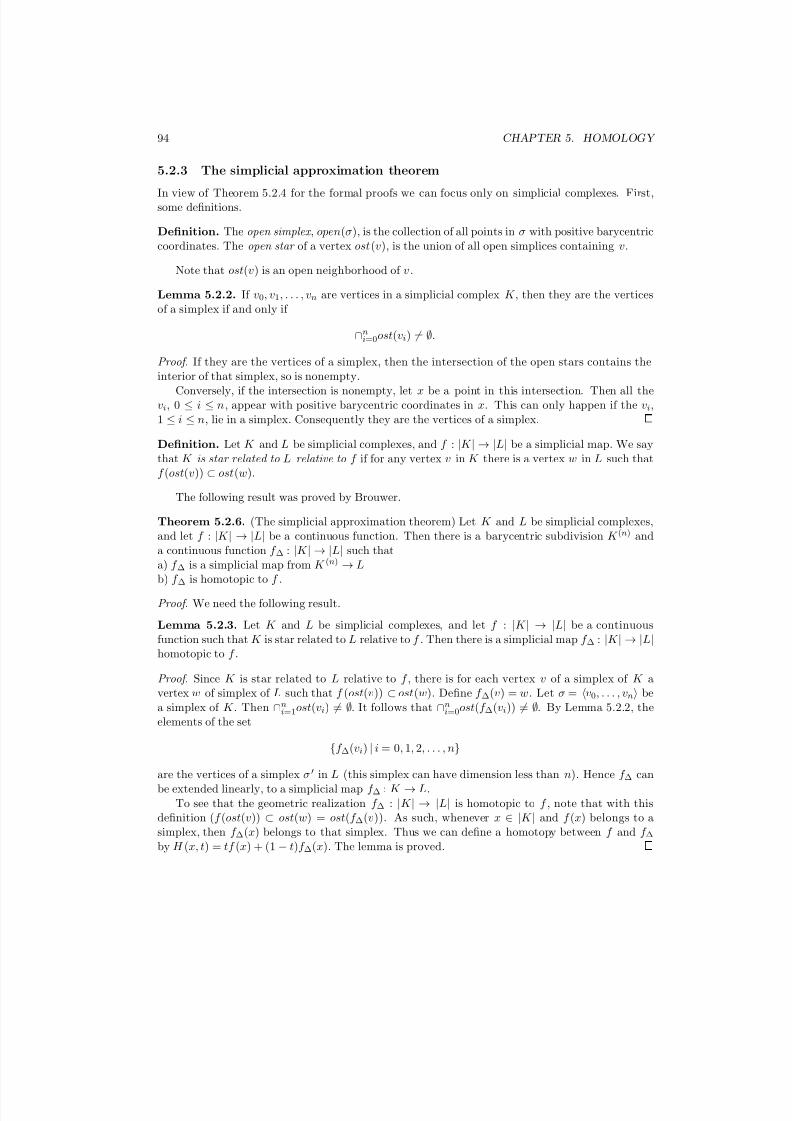
7/25/2019 TOPOLOG8Y
http://slidepdf.com/reader/full/topolog8y 94/98
94 CHAPTER 5. HOMOLOGY
5.2.3 The simplicial approximation theorem
In view of Theorem 5.2.4 for the formal proofs we can focus only on simplicial complexes. First,some definitions.
Definition. The open simplex , open(σ), is the collection of all points in σ with positive barycentriccoordinates. The open star of a vertex ost(v), is the union of all open simplices containing v.
Note that ost(v) is an open neighborhood of v .
Lemma 5.2.2. If v0, v1, . . . , vn are vertices in a simplicial complex K , then they are the vertices
of a simplex if and only if
∩ni=0ost(vi) = ∅.
Proof. If they are the vertices of a simplex, then the intersection of the open stars contains theinterior of that simplex, so is nonempty.
Conversely, if the intersection is nonempty, let x be a point in this intersection. Then all thevi, 0 ≤ i ≤ n, appear with positive barycentric coordinates in x. This can only happen if the vi,1 ≤ i ≤ n, lie in a simplex. Consequently they are the vertices of a simplex.
Definition. Let K and L be simplicial complexes, and f : |K | → |L| be a simplicial map. We saythat K is star related to L relative to f if for any vertex v in K there is a vertex w in L such that
f (ost(v)) ⊂ ost(w).
The following result was proved by Brouwer.
Theorem 5.2.6. (The simplicial approximation theorem) Let K and L be simplicial complexes,and let f : |K | → |L| be a continuous function. Then there is a barycentric subdivision K (n) anda continuous function f ∆ : |K | → |L| such thata) f ∆ is a simplicial map from K (n) → Lb) f ∆ is homotopic to f .
Proof. We need the following result.
Lemma 5.2.3. Let K and L be simplicial complexes, and let f : |K | → |L| be a continuousfunction such that K is star related to L relative to f . Then there is a simplicial map f ∆ : |K | → |L|homotopic to f .
Proof. Since K is star related to L relative to f , there is for each vertex v of a simplex of K avertex w of simplex of L such that f (ost(v)) ⊂ ost(w). Define f ∆(v) = w. Let σ = v0, . . . , vn bea simplex of K . Then ∩n
i=1ost(vi) = ∅. It follows that ∩ni=0ost(f ∆(vi)) = ∅. By Lemma 5.2.2, the
elements of the set
{f ∆(vi) | i = 0, 1, 2, . . . , n}
are the vertices of a simplex σ ′ in L (this simplex can have dimension less than n). Hence f ∆ can
be extended linearly, to a simplicial map f ∆ : K → L.To see that the geometric realization f ∆ : |K | → |L| is homotopic to f , note that with this
definition (f (ost(v)) ⊂ ost(w) = ost(f ∆(v)). As such, whenever x ∈ |K | and f (x) belongs to asimplex, then f ∆(x) belongs to that simplex. Thus we can define a homotopy between f and f ∆by H (x, t) = tf (x) + (1 − t)f ∆(x). The lemma is proved.

7/25/2019 TOPOLOG8Y
http://slidepdf.com/reader/full/topolog8y 95/98
5.2. CONTINUOUS MAPS BETWEEN ∆-COMPLEXES 95
Let us return to the theorem. The space |L| is compact and as explained in Remark 5.1.1, itis also a metric space. The open cover {ost(v), v a vertex of L} has a Lebesgue number η > 0,meaning that every ball of radius η in |L| is inside the open star of some vertex.
The function f is uniformly continuous so there is a δ such that for every x, f (B(x, δ )) subsetB(f (x), η). Consider a sufficiently small barycentric subdivision of K such that the open star of each vertex lies inside a ball of radius δ . Then the image of this every open star lies inside theopen star of a vertex in L, and so K is star related to L relative to f . The conclusion follows byapplying Lemma 5.2.3.
Definition. A map f ∆ satisfying the properties from the statement of the theorem is called a
simplicial approximation of f .
Definition. Two simplicial maps f, g : K → L are said to be contiguous if for every simplex σ ∈ K ,the vertices of f (σ) together with the vertices of g (σ) form a simplex in L.
Proposition 5.2.6. Suppose f : |K | → |L| is a continuous function that has simplicial approxi-mations f ∆ and f ′∆. Then f ∆ and f ′∆ are contiguous.
Proof. Suppose σ = v0, v1, . . . , vn ∈ K . Then for x ∈ open(σ),
f (x) ∈ f (∩iost(vi)) ⊂ ∩if (ost(vi)) ⊂ ∩iost(f ∆(vi)) ∩ ost(f ′∆(vi)).
Since this intersection is not empty, by Lemma 5.2.2 the vertices of f ∆(σ) together with those of f ′∆(σ) are the vertices of a simplex in L.
Theorem 5.2.7. (a) Contiguous simplicial maps have homotopic realizations.(b) Conversely, if K and L are simplicial complexes and f, g : |K | → |L| are homotopic mapswith simplicial approximations f ∆, g∆ : K (m) → L, then there is m > n and simplicial maps mapsf 0 = f ∆, f 1, . . . , f m = g∆ from K (n) to L such that for each 0 ≤ i < n, f i is contiguous to f i+1.
Proof. (a) If f and g are contiguous, then H : |K | → |L|, H (x, t) = (1−t)f (x)+tg(x) is a homotopybetween f and g. Here the line segment (1 − t)f (x) + tg(x) is taken in the simplex to which both
f (x) and g(x) belong by the condition of f and g to be contiguous.(b) Let H : |K | × [0, 1] → |L| be a homotopy with H (·, 0) = f , H (·, 1) = g. Consider the opencover of |K | given by
{H −1(ost(w)) | w vertex in L}.
Using the Lebesgue number lemma, we deduce that there is a partition of [0, 1], 0 = t1 < t2 < . . . <tk−1 = 1 such that for any x ∈ |K | and i < m, H (x, ti) and H (x, ti+1) lie in the same ost(w) forsome w ∈ L. Define the functions hi : |K | → |L| by hi(x) = H (x, ti). Consider the (finitely many)open sets h−1i (ost(w)) ∪ h−1i+1(ost(w)), w a vertex in L, 1 ≤ i ≤ k − 2. Subdivide K enough times
such that each of the simplices of K (n) lies entirely in one of these open sets. Let f i : K (n) → L
be a simplicial map such that hi(ost(v)) ∪ hi+1(ost(v)) ⊂ ost(f i(v)) for each vertex v of K (n). Bydefinition, f i is a simplicial approximation to both hi and hi+1. Hence f i and f i+1 are contiguous.Since h0 = f and hn = g, f 1 and f k−1 are simplicial approximations to f respectively g. ByProposition 5.2.6, f 1 is contiguous to f 0 = f ∆ and f k−1 is contiguous to f k = g∆. The theorem isproved.

7/25/2019 TOPOLOG8Y
http://slidepdf.com/reader/full/topolog8y 96/98
96 CHAPTER 5. HOMOLOGY
5.2.4 The independence of homology groups on the geometric realization of the
space as a ∆-complex
Lemma 5.2.4. Contiguous simplicial maps induce the same homomorphisms at the level of ho-mology groups.
Proof. We will show that the simplicial maps are chain homotopic. Let φ, ψ : K → L be contiguoussimplicial maps. Define Dn : C n(K ) → C n+1(L) by
Dn(v0, v1, . . . , vn =n
i=0(−1)i φ(v0), . . . , φ(vi), ψ(vi), . . . , ψ(vn)).
Here again we use the convention that degenerate simplices are mapped to zero. This map is welldefined, namely each summand is a simplex, precisely because φ and ψ are contiguous.
We compute
∂ n+1Dn(v0, v1, . . . , vn) = ∂ n+1
ni=0
(−1)i φ(v0), . . . , φ(vi), ψ(vi), . . . , ψ(vn)
= j≤i
(−1)i+ j
φ(v0), . . . , φ(v j), . . . , φ(vi), ψ(vi), . . . , ψ(vn)
+i≤ j (
−1)i+ j+1 φ(v0), . . . . . . , φ(vi), ψ(vi), . . . , ψ(v j), . . . , ψ(vn) .
Also
Dn−1∂ n(v0, v1, . . . , vn) = Dn−1
n j=0
(−1) j v0, . . . , v j, . . . , vn
= j<i
(−1)i+ j−1
φ(v0), . . . , φ(v j), . . . , φ(vi), ψ(vi), . . . , ψ(vn)
+ j>i
(−1)i+ j
φ(v0), . . . , φ(vi), ψ(vi), . . . , ψ(v j), . . . , ψ(vn)
.
When adding the two everything with i = j cancels, and we only have the i = j terms from thefirst expression. Each of these appears twice, with opposite signs, except for i = 0 and i = n, oneof which appears with plus, and the other with minus. Hence
(∂ n+1Dn + Dn−1∂ n)(v0, v1, . . . , vn) = φ(v0), φ(v1), . . . , φ(vn) − ψ(v0), ψ(v1), . . . , ψ(vn) ,
showing that Dn, n ≥ 0, is a chain homotopy between φ and ψ . The conclusion follows.
This result combined with Theorem 5.2.6 allows us to define, for each continuous map betweenspaces that can be realized as simplicial complexes, a homomorphism between homology groups.
Definition. Let K and L be ∆-complexes and f :
|K
| → |L
| a continuous map with simplicial
approximation f ∆. Define (f ∗)n : H n(K ) → H n(L) by (f ∗) = (f ∆∗)n.
Theorem 5.2.8. Let K and L be ∆-complexes and f , g : |K | → |L| be continuous maps that arehomotopic. Then (f ∗)n = (g∗)n, n ≥ 0. Consequently, if the underlying topological spaces of two∆-complexes are homotopically equivalent, then their homology groups are isomorphic.

7/25/2019 TOPOLOG8Y
http://slidepdf.com/reader/full/topolog8y 97/98
5.3. APPLICATIONS OF HOMOLOGY 97
Proof. This is a corollary of Lemma 5.2.4 and Theorem 5.2.7.
Corollary 5.2.2. If two spaces are homeomorphic, then their homology groups are isomorphic.
Definition. A space is called contractible if it is homotopy equivalent to a point. An alternativeway to say this is that the identity map is null-homotopic.
Corollary 5.2.3. If X is a contractible topological space that can be realized as a ∆-complex,then
H n(X ) =
Z if n = 00 otherwise.
Proof. If the space is contractible, it has the homology of a point. We realize the point as a∆-complex with one 0-dimensional simplex. The corresponding simplicial complex is
· · · 0 → 0 → ·· · → 0 → Z→ 0.
Hence the conclusion.
5.3 Applications of homology
Theorem 5.3.1. If m and n are positive integers and m = n, then Rm and Rn are not homeomor-
phic.Proof. Assume that for some m < n, there is a homeomorphism h : Rm → Rn. Consider therestriction
h : Rm\{0} →Rn\{h(0)},
which is still a homeomorphism. Thus h should induce isomorphism at the level of homologygroups. If m = 1 this is impossible since the second space is connected, while the first is not.
For m > 1, Rm\{0} and Rn\{h(0)} are homotopically equivalent to S m−1 respectively S n−1. Itfollows that (h∗)n−1 is an isomorphism.
On the other hand, by Proposition 5.1.2, H n−1(S n−1) = Z, while H n−1(S m−1) = 0 because
S m−1
can be realized as a ∆-complex with no n − 1-dimensional simplex. The two groups cannotbe isomorphic, a contradiction. Hence our assumption was false, and the conclusion follows.
The following generalizes Theorem 4.3.6.
Theorem 5.3.2. (Brouwer fixed point theorem) Every continuous function from a closed ball of Rn to itself has a fixed point.
Proof. This proof mimics that for the 2-dimensional situation given in § 4.3.3. Assume to thecontrary that there is f : B
n → Bn
which is continuous with no fixed points. For x ∈ Bn
, defineg(x) as the point where the ray from f (x) to x meets the boundary S n−1 of the ball. The functiong : Bn → S n−1 is continuous (prove it!). Furthermore, if i is the inclusion of S n−1 into B
n, then
g◦
i is the identity map. Looking at the composition of isomorphisms
H n−1(S n−1) i∗−→ H n(B
n) g∗−→ H n−1(S n−1),
we notice that it must be equal to zero, because the homology group in the middle is the trivialgroup, by Corollary 5.2.3. But (g ◦ i)∗ = 1Z. This is a contradiction. The conclusion follows.

7/25/2019 TOPOLOG8Y
http://slidepdf.com/reader/full/topolog8y 98/98
98 CHAPTER 5. HOMOLOGY
The proof of Proposition 4.3.2 applies mutatis mutandis to the following general situation.
Proposition 5.3.1. Every square matrix with positive entries has an eigenvector with positiveentries.
Here is another application to game theory. First some terminology. Consider a game in whichtwo players, 1 and 2, have m respectively n strategies. Let A and B be the be the payoff matrices,meaning that if player 1 chooses strategy i and player 2 strategy j then the payoffs of the two playersare Aij respectively Bij . A mixed strategy is a pair of points (x, y) ∈ Rn × Rm with nonnegativeentries, such that
ni=1 xi =
m j=1 y j = 1. As such they represent probability distributions for
the strategies of the two players. Consequently, the expectation values of the payoffs for the two
players are respectively xT Ay and xT By.A Nash equilibrium (after John Nash) is a mixed strategy (x, y) such that for all x′, y′,
x′T Ay ≤ xT Ay and xT By′ ≤ xT By.
This means that if one of the players plays according to the Nash equilibrium, the other is obligedto play according the the Nash equilibrium in order to maximize the payoff.
Theorem 5.3.3. (Nash) For all payoff matrices A and B there is a Nash equilibrium.
Proof. Assume that there are payoff matrices A and B for which this does not hold. Considerthe space of all mixed strategies. It is the product of an n − 1-dimensional simplex σn−1 with an
m − 1-dimensional simplex σm−1
, hence it is homeomorphic to a closed m + n − 2-dimensional ballBn
. Because of the fact that there are no Nash equlibria, the vector ((∇φ)x, (∇ψ)y) is never zero.Define the function f : σn−1 × σm−1 → ∂ (σn−1 × σm−1) by associating to each point (x, y) thepoint at which the ray from (x, y) of direction ((∇φ)x, (∇ψ)y) intersects the boundary of the spaceof all mixed strategies.
By Brouwer’s fixed point theorem, f has a fixed point. But this is impossible, since the raypoints away from (x, y). The contradiction proves that our assumption was false, and the conclusionfollows.
Remark 5.3.1. There is no known algorithm for finding the Nash equilibrium in polynomial time.