Topological Data AnalysisCBMS Lecture 4

Vin de SilvaPomona College

Point-cloud topology

Point-cloud topology

Data sampled from an unknown topological space Y.Estimate Betti numbers of Y from the sample.

b1 = 3

b1 = 5

b1 = 1

The standard pipeline

hidden/unknownspace X

finite sampleY⊂X

simplicial complexS = S(Y)homology

invariants of S b1 = 1b0 = 1

b2 = 0

The standard pipeline

hidden/unknownspace X

finite sampleY⊂X

simplicial complexS = S(Y)homology

invariants of S b1 = 1b0 = 1

b2 = 0

Simplicial reconstructions‣ Given a collection of points X in Euclidean space:

‣ Proximity graph

‣ Vietoris–Rips complex

‣ Čech complex

‣ Alpha shape (Edelsbrunner, Kirkpatrick, Seidel 1983)

‣ Desire theorems of the form:

E.g. Niyogi–Smale–Weinberger (2004) for the Cech complex

{simplices [x0, x1, . . . , xk] whose vertices are contained in an (r/2)-ball}

{simplices [x0, x1, . . . , xk] for which every kxi � xjk r}

{all vertices [x]} [ {edges [x, y] such that kx� yk r}

⇢simplices [x0, x1, . . . , xk] whose vertices are contained in

an (r/2)-ball whose interior meets no other points of X

�

If Y is well-sampled from X then S(Y) ≈ X

Proximity Graph

(picture credit: Elizabeth Meckes)

Vietoris–Rips complex

(picture credit: Elizabeth Meckes)

Čech complex

(picture credit: Elizabeth Meckes)

Properties‣ Each complex depends on a scale parameter r

‣ r=0

‣ discrete collection of vertices

‣ r=∞‣ graph complex = the complete graph on X

‣ Vietoris–Rips = the complete simplex on X

‣ Čech = the complete simplex on X

‣ Alpha = Delaunay triangulation of convex hull of X

‣ Seek interesting topology in the range 0 < r < ∞

trivial topology

Persistence

Instability

‣ Betti numbers are discrete

‣ Topological spaces‣ topological spaces are continuous

‣ the space of topological spaces is discrete

‣ Finite point-clouds‣ point-clouds are discrete

‣ the space of point-clouds is continuous

‣ Therefore, raw Betti numbers are‣ ✔ suitable for topological spaces

‣ ✘ dangerous for point-clouds

Instability

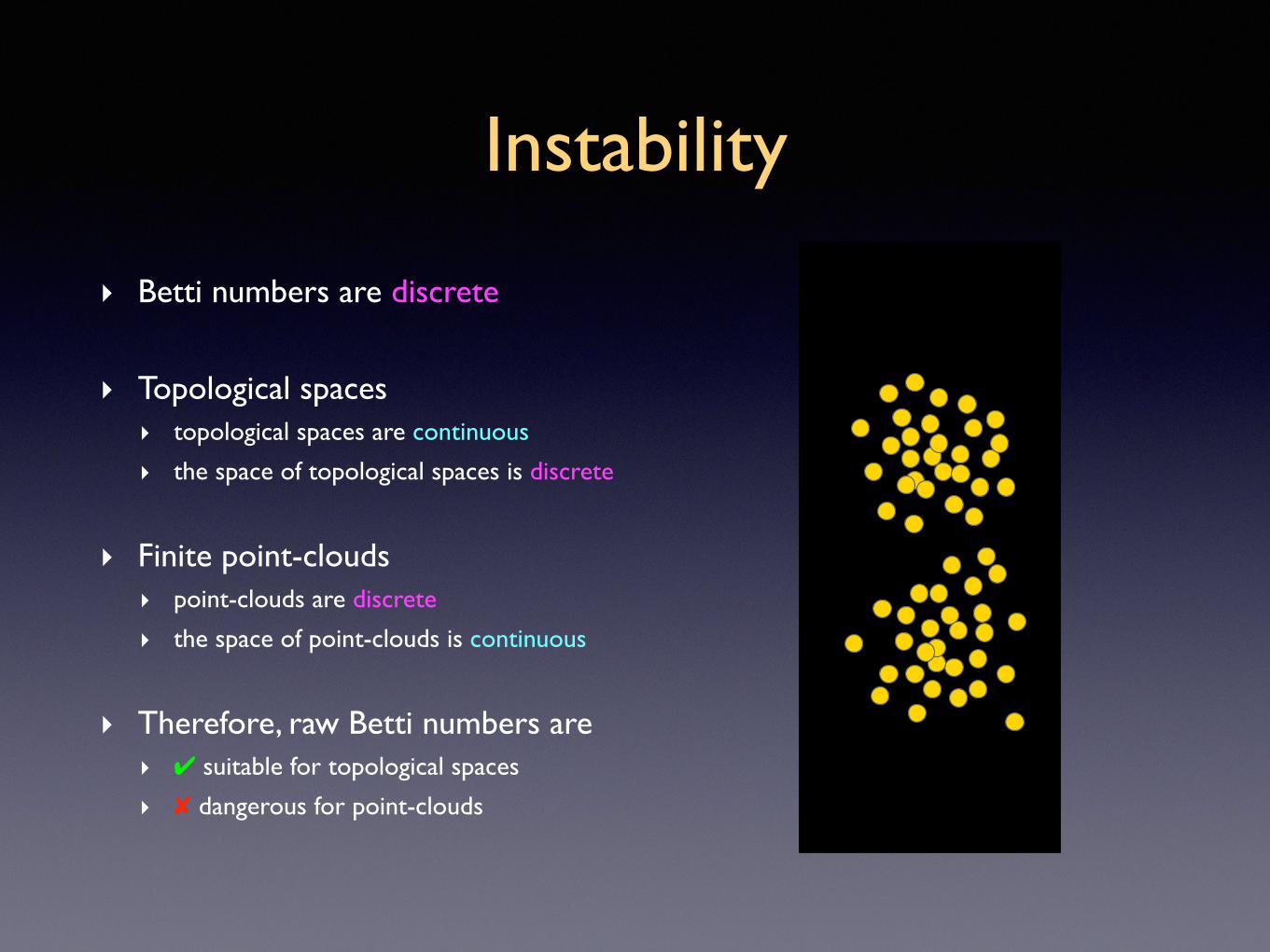
‣ Betti numbers are discrete

‣ Topological spaces‣ topological spaces are continuous

‣ the space of topological spaces is discrete

‣ Finite point-clouds‣ point-clouds are discrete

‣ the space of point-clouds is continuous

‣ Therefore, raw Betti numbers are‣ ✔ suitable for topological spaces

‣ ✘ dangerous for point-clouds

Instability

‣ Betti numbers are discrete

‣ Topological spaces‣ topological spaces are continuous

‣ the space of topological spaces is discrete

‣ Finite point-clouds‣ point-clouds are discrete

‣ the space of point-clouds is continuous

‣ Therefore, raw Betti numbers are‣ ✔ suitable for topological spaces

‣ ✘ dangerous for point-clouds

The standard pipeline (first attempt)

hidden/unknownspace Y

finite sampleX⊂Y

simplicial complexS = S(X)homology

invariants of S b1 = 1b0 = 1

b2 = 0

The standard pipeline (second attempt)

hidden/unknownspace Y

finite sampleX⊂Y

filtered complexS(r) = S(X,r)

persistent homology of S(r)

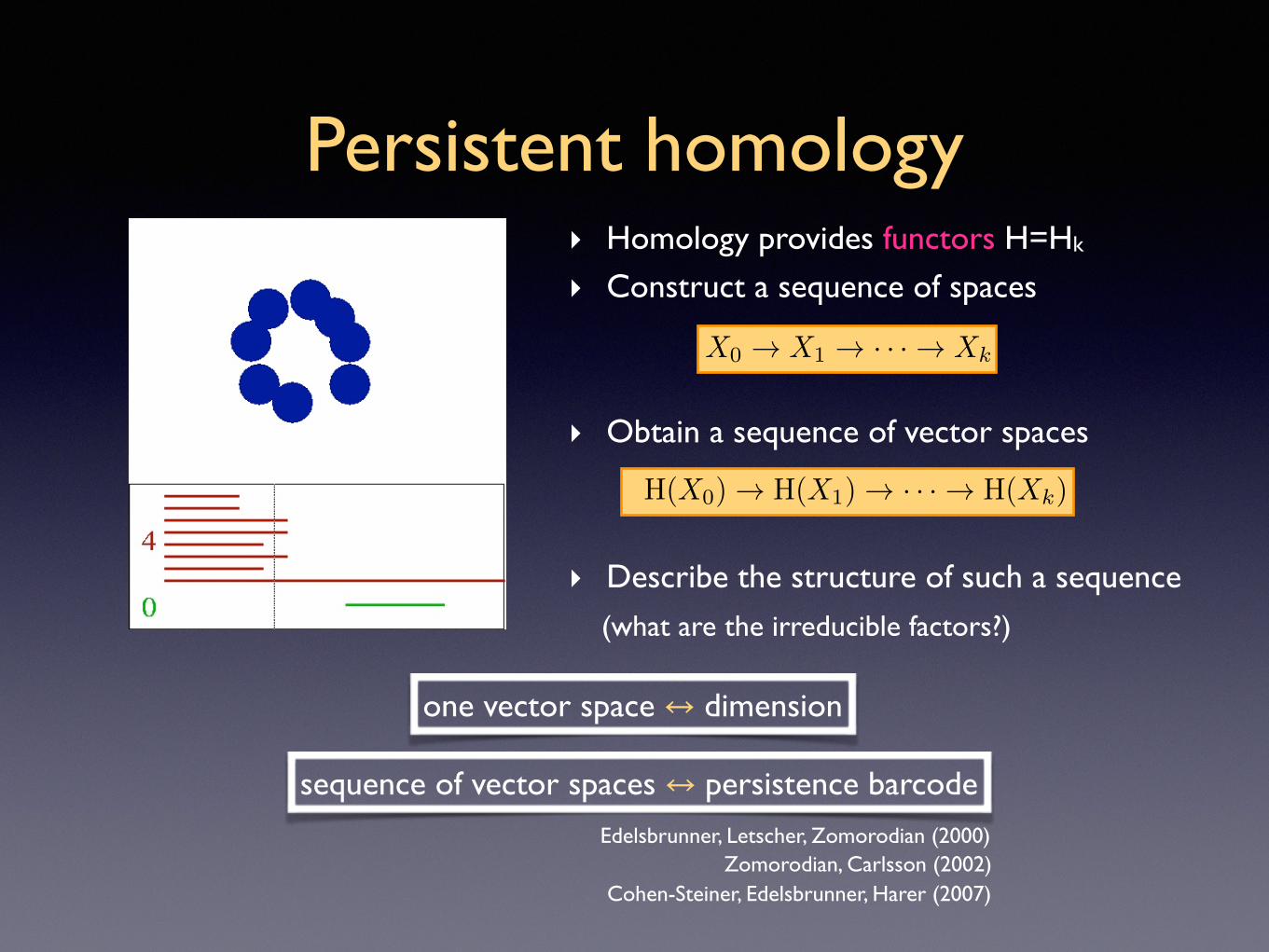
Persistent homology‣ Homology provides functors H=Hk

‣ Construct a sequence of spaces

‣ Obtain a sequence of vector spaces

‣ Describe the structure of such a sequence (what are the irreducible factors?)

X0 ! X1 ! · · · ! Xk

H(X0) ! H(X1) ! · · · ! H(Xk)

one vector space ↔ dimension

sequence of vector spaces ↔ persistence barcodeEdelsbrunner, Letscher, Zomorodian (2000)

Zomorodian, Carlsson (2002)Cohen-Steiner, Edelsbrunner, Harer (2007)

Persistence‣ Algorithm (Edelsbrunner, Letscher, Zomorodian ’00)

‣ barcode: finite collection of half-open intervals

‣ [b,d) indicates feature lifetime: born at time b, dies at time d

‣ Stability theorem (Cohen-Steiner, Edelsbrunner, Harer ’07)

‣ barcode depends continuously on the underlying data

‣ interleaved systems have similar barcode (Chazal, Cohen-Steiner, Glisse, Guibas, Oudot ’09)

‣ continuous measurements (interval length) & discrete information (number of intervals)

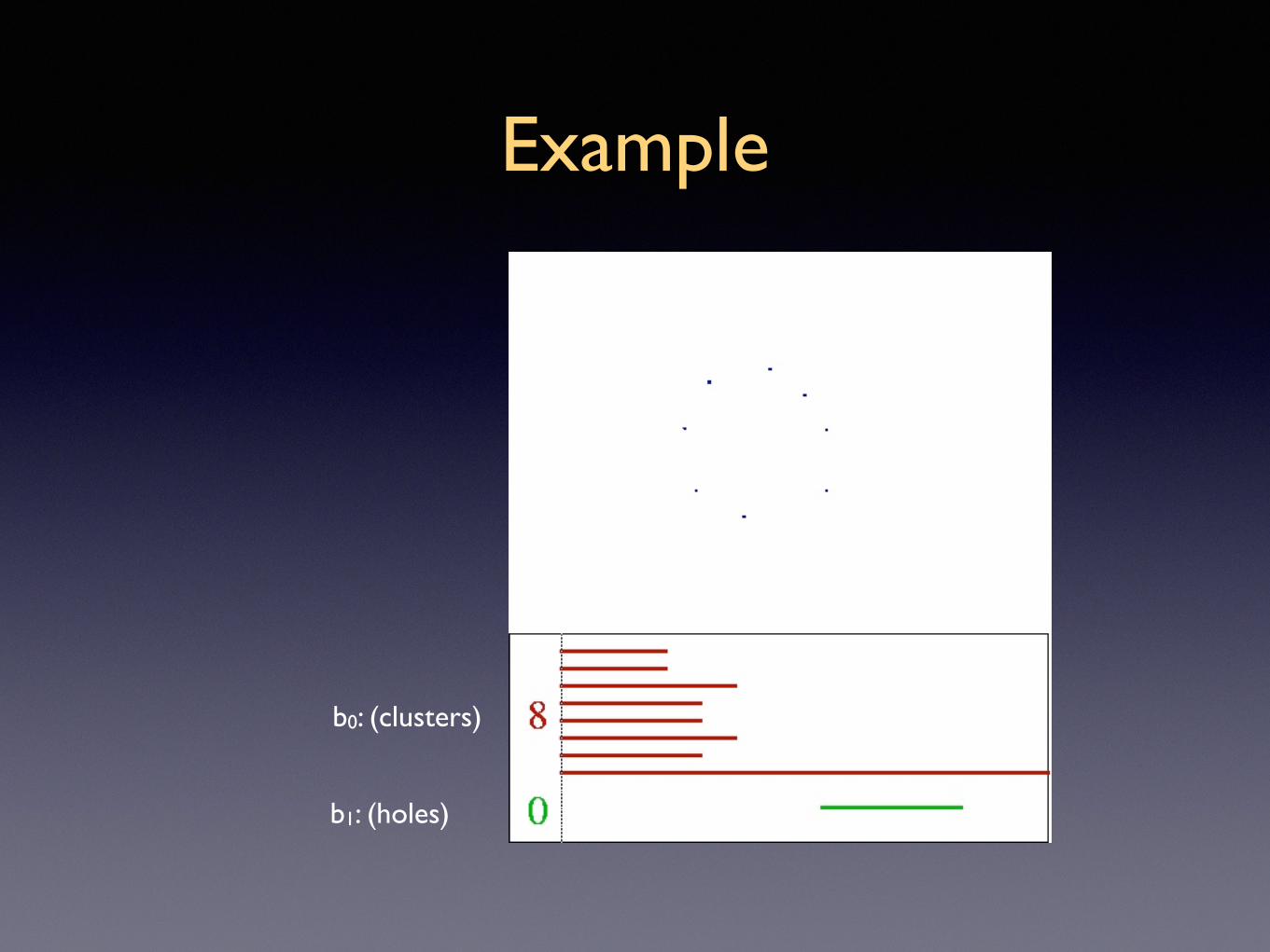
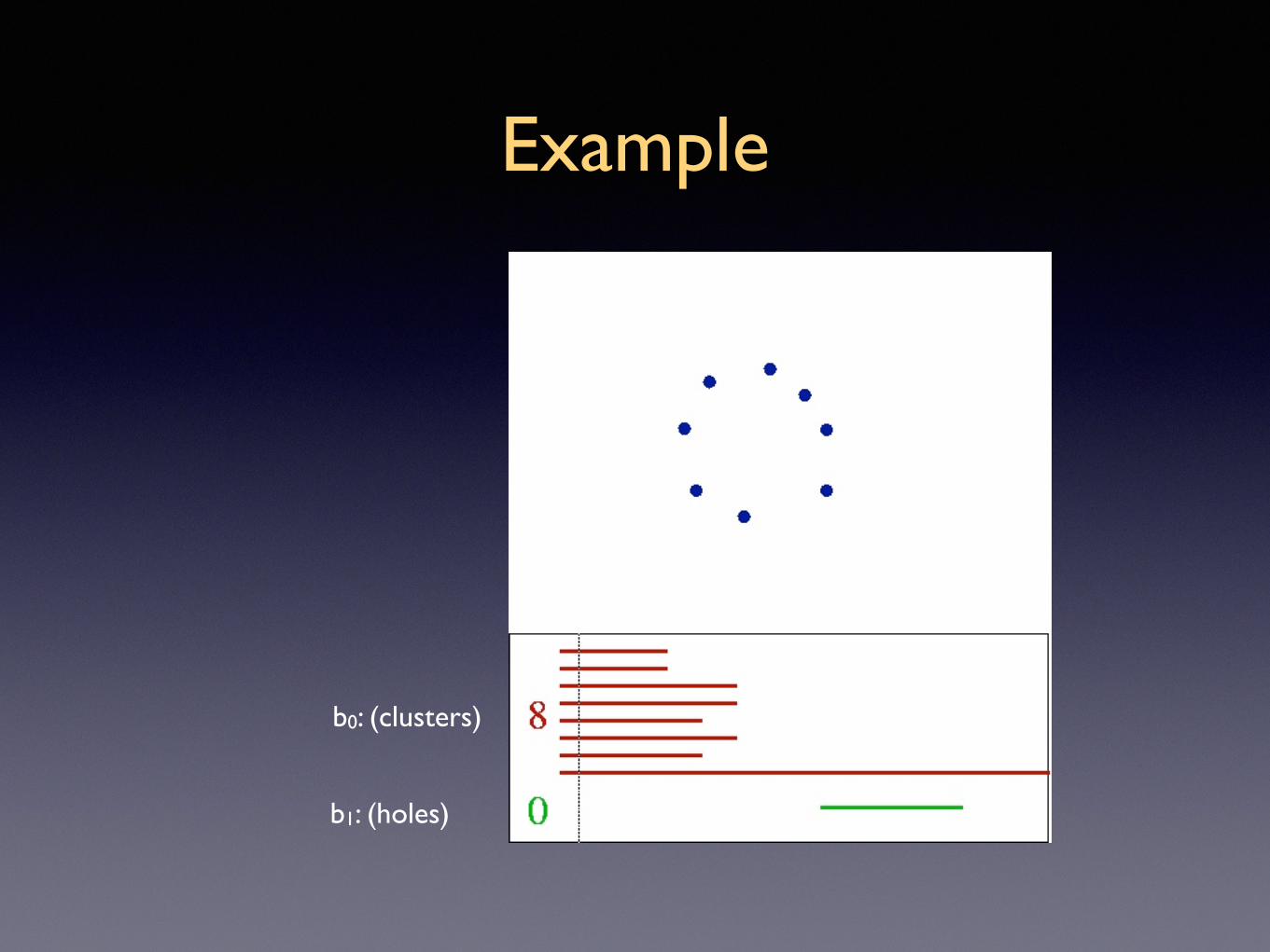
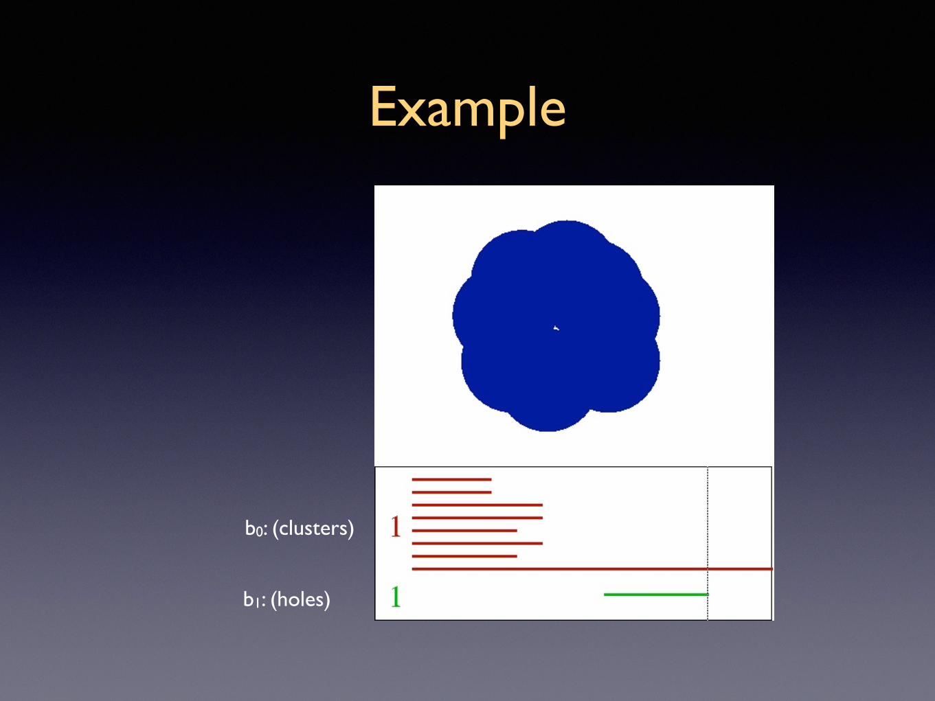
Example

b0: (clusters)

b1: (holes)

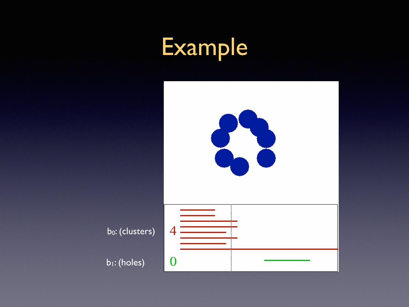
Example

b0: (clusters)

b1: (holes)

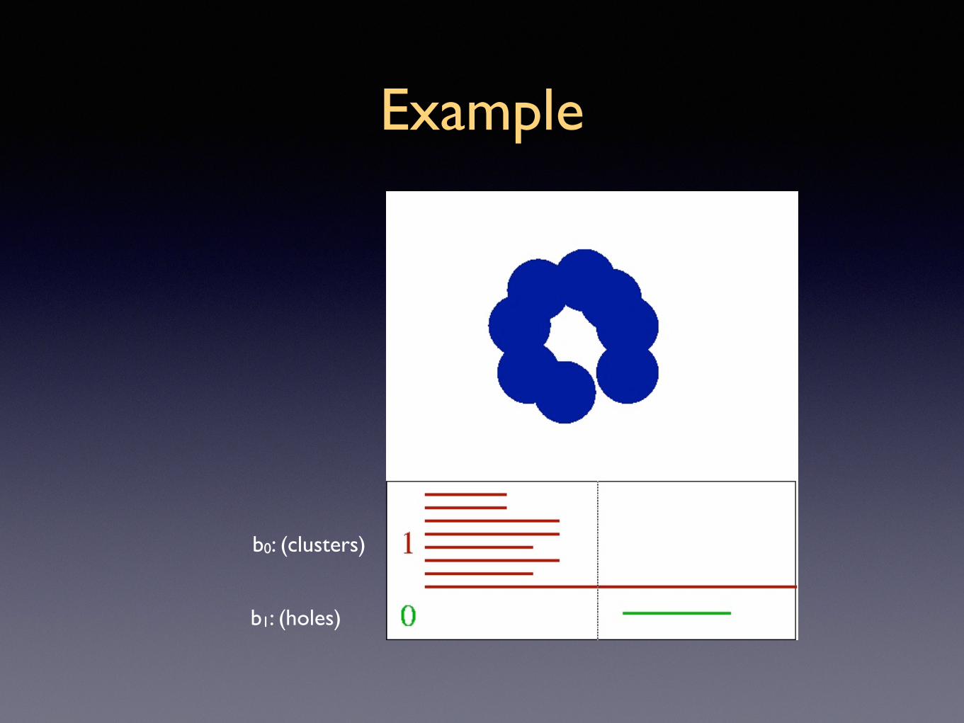
Example

b0: (clusters)

b1: (holes)

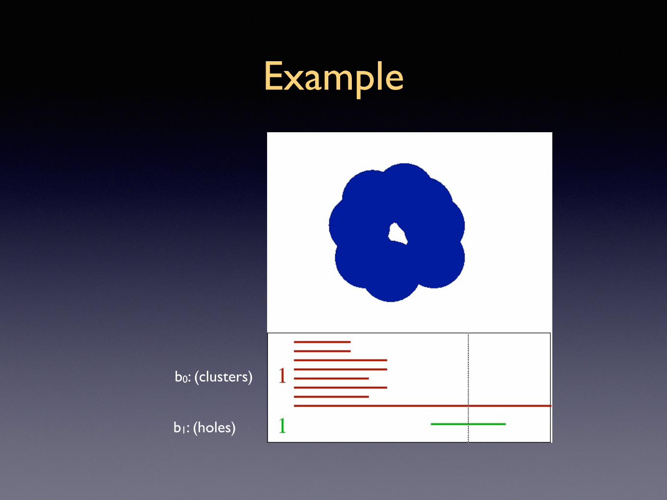
Example

b0: (clusters)

b1: (holes)

Example

b0: (clusters)

b1: (holes)

Example

b0: (clusters)

b1: (holes)

Example

b0: (clusters)

b1: (holes)

Example

b0: (clusters)

b1: (holes)

Example

b0: (clusters)

b1: (holes)

Example

b0: (clusters)

b1: (holes)

Example

b0: (clusters)

b1: (holes)

Example

b0: (clusters)

b1: (holes)

Example

b0: (clusters)

b1: (holes)

Example

b0: (clusters)

b1: (holes)

Example

b0: (clusters)

b1: (holes)

Example

b0: (clusters)

b1: (holes)

Persistence diagram

Persistence diagram

smallscale

largescale

Barcode

Persistence diagram

smallscale

largescale

Barcode0 0.5 10

0.5

1

small scale

large scale

Persistence diagramintervals [b,d)points (b,d)

Persistence diagram

smallscale

largescale

Barcode0 0.5 10

0.5

1

small scale

large scale

Persistence diagramintervals [b,d)points (b,d)

And the Oscar goes to...

Visual Image Patches

‣ Lee, Pedersen, Mumford (2003) studied the local statistical properties of natural images (from Van Hateren’s database)

‣ 3-by-3 pixel patches with high contrast between pixels: are some patches more likely than others?

‣ Carlsson, VdS, Ishkhanov, Zomorodian (2004/8): topological properties of high-density regions in pixel-patch space

Visual image patches

The space of image patches

‣ ~4.2 million high-contrast 3-by-3 patches selected randomly from images in database.

‣ Normalise each patch twice: subtract mean intensity, then rescale to unit norm.

‣ Normalised patches live on a unit 7-sphere in 8-dimensional space with the following basis:

High-density regions

‣ LPM2003 found that the distribution of patches is dense in the 7-sphere.

‣ There are high-density regions:‣ edge features

‣ Can we describe the structure of the high-density regions?‣ threshold by k-nearest-neighbour density estimator

Defining “high-density”

‣ How do we define “high density”?

‣ Select a positive integer k.

‣ rk(x) = distance between x and its k-th nearest neighbour.

‣ x is a high-density point ⇔ rk(x) is small.

‣ Select “cuts” by thresholding on rk(x).‣ k small ⇔ fine structure

‣ k large ⇔ coarse structure

Straining a data soup

Topology in the 21st Century

January 26–27, 2009

Vin de Silva

http://pages.pomona.edu/~vds04747/

Straining a data soup

40Tuesday, January 27, 2009

Varying the density parameter(toy example)

Varying the density parameter(toy example)

A small platter of cuts

10% 20% 30%

K=15

K=100

K=300

A small platter of cuts

Topology in the 21st Century

January 26–27, 2009

Vin de Silva

http://pages.pomona.edu/~vds04747/

A small platter of cuts

10% 20% 30%

K=15

K=100

K=300

44Tuesday, January 27, 2009

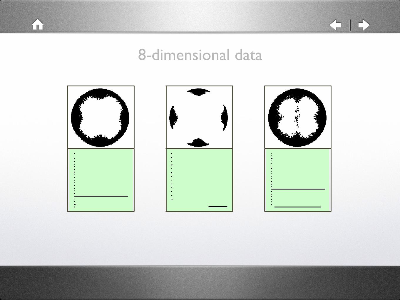
8-dimensional data

Topology in the 21st Century

January 26–27, 2009

Vin de Silva

http://pages.pomona.edu/~vds04747/

(8-dimensional data)

45Tuesday, January 27, 2009

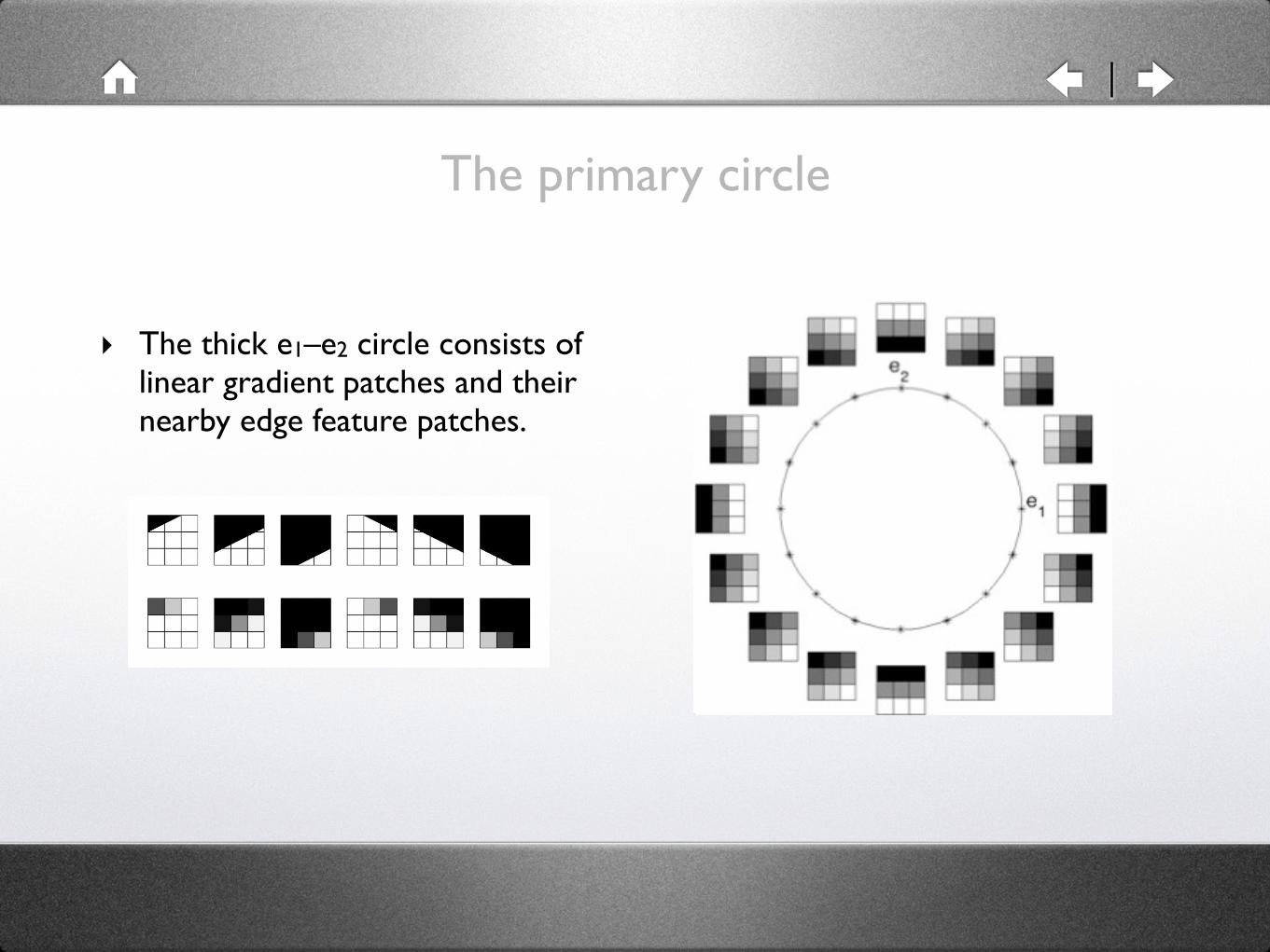
The primary circle

‣ The thick e1–e2 circle consists of linear gradient patches and their nearby edge feature patches.

8-dimensional data

Topology in the 21st Century

January 26–27, 2009

Vin de Silva

http://pages.pomona.edu/~vds04747/

(8-dimensional data)

46Tuesday, January 27, 2009

3-circles model

3-circles model

1 2 3

4

5

1

3

2

54

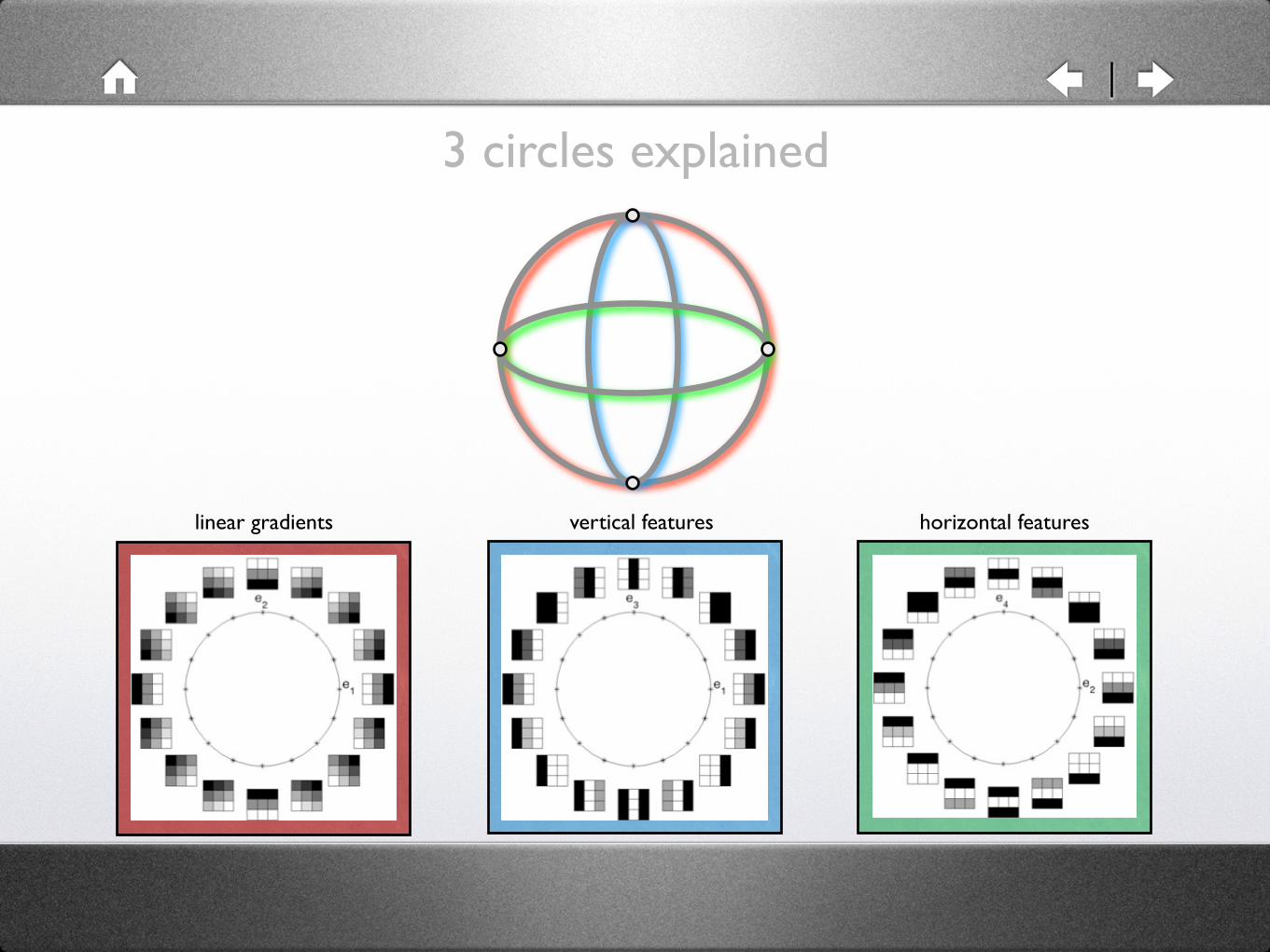
3 circles explained

linear gradients vertical features horizontal features

The secondary circles

vertical features horizontal features

Why is there a predominance of vertical/horizontal local features?Artefact of the square patch shape?Artefact of the natural world?

Tilting the camera

orthogonal images diagonal images

?

Tilting the camera

−1 −0.8 −0.6 −0.4 −0.2 0 0.2 0.4 0.6 0.8 1−1

−0.8

−0.6

−0.4

−0.2

0

0.2

0.4

0.6

0.8

1

orthogonal images diagonal images

?

Tilting the camera

−1 −0.8 −0.6 −0.4 −0.2 0 0.2 0.4 0.6 0.8 1−1

−0.8

−0.6

−0.4

−0.2

0

0.2

0.4

0.6

0.8

1

−1 −0.8 −0.6 −0.4 −0.2 0 0.2 0.4 0.6 0.8 1−1

−0.8

−0.6

−0.4

−0.2

0

0.2

0.4

0.6

0.8

1

orthogonal images diagonal images

Homogenizing over all tilt angles

‣ e1-e2 circle: arbitrary linear functions ax+by in the image plane.

‣ e1-e3 circle: quadratic functions of x.

‣ e3-e4 circle: quadratic functions of y.

‣ What about quadratic functions of arbitrary linear functions ax+by?

The Klein bottle14 ROBERT GHRIST

Figure 9. A Klein bottle embeds naturally in the parameter spaceas a completion of the 3-circle model. In the unfolded identifica-tion space shown, the primary circle wraps around the horizontalaxis twice. The two secondary circles each wrap around the ver-tical axis once (note: the circle on the extreme left and right areglued together with opposite orientation). Each secondary circleintersects the primary circle twice.

[5] G. Carlsson, A. Zomorodian, A. Collins, and L. Guibas, “Persistence barcodes for shapes,”Intl. J. Shape Modeling, 11 (2005), 149-187.

[6] F. Chazal and A. Lieutier, “Weak feature size and persistent homology: computing homologyof solids in R

n

from noisy data samples,” in Proc. 21st Sympos. Comput. Geom. (2005).[7] D. Cohen-Steiner, H. Edelsbrunner and J. Harer, “Stability of persistence diagrams,” in Proc.

21st Sympos. Comput. Geom. (2005), 263–271.[8] V. de Silva, “A weak definition of Delaunay triangulation,” preprint (2003).[9] V. de Silva and G. Carlsson. “Topological estimation using witness complexes,” in SPBG04

Symposium on Point-Based Graphics (2004), 157-166.[10] V. de Silva and R. Ghrist, “Coverage in sensor networks via persistent homology,” to appear,

Alg. & Geom. Topology (2006).[11] V. de Silva and P. Perry, PLEX home page, http://math.stanford.edu/comptop/programs/plex/